Useful estimation procedures for critical gaps

Useful estimation procedures for critical gaps

Werner Brilona,*, Ralph Koenig a, Rod J. Troutbeckb

aInstitute for Transportation and Tra�c Engineering, Ruhr-University, D-44788 Bochum, GermanybQueensland University of Technology, Brisbane, Australia

Abstract

Many di�erent methods for the estimation of critical gaps at unsignalized intersections have been pub-lished in the international literature. This paper gives an overview of some of the more important methods.These methods are described by their characteristic properties. For comparison purposes a set of qualitycriteria has been formulated by which the usefulness of the di�erent methods can be assessed. Among theseone aspect seems to be of primary importance. This is the objective that the results of the estimation pro-cess should not depend on the tra�c volume on the major street during the time of observation. Only if thiscondition is ful®lled, can the estimation be applied under all undersaturated tra�c conditions at unsigna-lized intersections. To test the quali®cation of some of the estimation methods under this criterion, a seriesof comprehensive simulations has been performed. As a result, the maximum likelihood procedure (as ithas been described by Troutbeck) and the method developed by Hewitt can be recommended for practicalapplication. # 1999 Elsevier Science Ltd. All rights reserved.

1. Introduction

The estimation of critical gaps from observed tra�c ¯ow patterns is one of the most di�culttasks in empirical tra�c engineering science. Miller (1972), in his classic paper, could refer to ninedi�erent estimation methods, which did not cover the whole range of possible procedures to beobtained from international literature at that time. Today it would be easy to ®nd more than 20or 30 methods published around the world for the estimation of critical gaps. All of these meth-ods produce di�erent results. Therefore, the important question is: which of these proceduresbeing recommended by di�erent authors reveals a correct estimation? And the other question is:how can we ®nd out if an estimation is valid or not?Before we can answer these questions we should ®rst discuss the fundamental de®nitions. Here

we concentrate on the most simple case of an unsignalized intersection. This is a crossroad of two

0965-8564/99/$Ðsee front matter # 1999 Elsevier Science Ltd. All rights reserved.

PII: S0965-8564(98)00048-2

TRANSPORTATION

RESEARCH

PART A

Transportation Research Part A 33 (1999) 161±186

* Corresponding author. Tel.: +49-234-700-5936; fax: +49-234-700-5936; e-mail: [email protected]

one-way streets (Fig. 1). Here two movements are allowed: one major stream (the prioritymovement) of volume qp, and one minor stream of volume qn.According to tra�c rules, each major stream vehicle can pass the intersection without any

delay. A minor street vehicle, however, can only enter the con¯ict area if the next major vehicle isfar enough away to allow the minor vehicle safe passage of the whole con¯ict area. ``Far enough''is de®ned as: The next major street vehicle will arrive at the intersection at an instant that willhappen tc seconds after the previous major stream vehicle or tc seconds after the minor vehicle'sarrival. This value tc is called the critical gap, which is the minimum time gap in the prioritystream that a minor street driver is ready to accept for crossing or entering the major streamcon¯ict zone.Another limiting factor for the minor street vehicles is the fact that they cannot enter the con-

¯ict area during a short while after the previous minor street vehicle has entered, owing to thephysical length of the vehicles and the necessary safe headways. Thus, as the second variable forthe characterization of minor street driver's behavior we use the follow-up time, tf, where is thetime gap between two successive vehicles from the minor street while entering the con¯ict area ofthe intersection during the same major street gap.It is obvious that tc and tf di�er from driver to driver, from time to time, and between inter-

sections, types of movements, and tra�c situations. Due to this variability, there is no doubt thatthe gap acceptance process is of a stochastic nature. Thus tc and tf can be regarded as randomvariables. Moreover, the parameters of the distribution functions for these variables may besubject to di�erent external in¯uences. Consequently, it is necessary to de®ne some type ofrepresentative characteristics to model the usual behavior of drivers. Therefore, the estimation ofcritical gaps and follow-up times tries to ®nd out values for the variables tc and tf, as well as forthe parameters of their distributions, which represent typical driver behavior at the investigatedintersection during the period of observation. For this paper we concentrate our derivations onthe critical gap, tc.

Fig. 1. Illustration of the basic queuing system.

162 W. Brilon et al./Transportation Research Part A 33 (1999) 161±186

In unsignalized intersection theory, it is generally assumed that drivers are both consistent andhomogeneous. Consistent drivers are expected to behave the same way every time in all similarsituations. This means a driver with a speci®c tc value will never accept a gap of less than tc andhe will accept each major stream gap larger than tc. However, within a population of severaldrivers, each of who behaves consistently, di�erent drivers could have their own tc values. Thesetc values are then treated as a random variable with a special statistical density function fc(t) anda cumulative distribution function Fc(t). The population of drivers is homogeneous if each sub-group of drivers out of the population has the same functions fc(t) and Fc(t).It is clear that in reality drivers are neither completely consistent nor homogenous. A com-

pletely inconsistent driver would apply a new tc value for each gap. Further, the applied tc valuethat is compared with one major street gap is completely independent of the tc used for the pre-vious major stream gap by the same driver some seconds before in the same queuing situation.This, however, is not expected to be the case in reality. Instead it is assumed that a rather carefuldriver will always demand a rather large gap or that a risky driver will always be prepared toaccept rather narrow gaps. Therefore, we assume that real driver behavior is closer to consistencythan to completely inconsistent behavior.For the estimation of critical gaps, tc, from observations, a long series of methods has been

proposed. An overview of the English language literature in the late 1960s was given by Miller(1972). Meanwhile, many more proposals have been made. For the preparation of this paper aselection of candidate procedures has been made, which does not represent by far everything thatis published. The selection has been made on the basis that these procedures have been used orrecommended by authors other than the original sources. In the ®rst part of this paper thesemethods are described. The second part describes criteria for evaluating the di�erent techniques.Finally, a simulation model is used in the evaluation and choice of recommended models.

2. Estimation technique for saturated conditions: Siegloch's method

Siegloch (1973) proposed a consistent framework for the theory of capacities at unsignalizedintersections. This framework is mentioned here to emphasize how the critical gaps are usedwithin subsequent mathematical modeling. Let g(t) be the number of minor street vehicles thatcan enter the con¯ict area during one minor stream gap of size t. The expected number of gaps ofsize t within the major stream is qp h(t) where h(t) is the statistical density function of all gaps (orheadways) in the major stream. Thus, the amount of capacity that is provided by gaps of size tduring an hour is qp h(t) g(t). To get the total capacity c, we have to integrate over the wholerange of possible major stream gaps t. Thus we get

c � qp:

�1t�0

h t� �:g t� �dt �1�

This equation for the capacity of unsignalized intersections forms the foundation of the wholegap-acceptance theory. Almost all of the di�erent analytical capacity estimation formulae foundin the international literature are based on this concept, even in cases where the original authorswhere not aware of this method.

W. Brilon et al./Transportation Research Part A 33 (1999) 161±186 163

The consequence of this equation is that, for capacity calculations, we need to know the majorstream headway distribution h(t) and the function g(t). Siegloch, as a consequence of this theory,proposes a regression technique for the derivation of g(t) from ®eld observations. For this esti-mation technique we need to observe saturated conditions, i.e. continuous queuing on the minorstreet. Only under these conditions can we observe realizations g for the function g(t) by countingthe number of minor street vehicles that enter major street gaps of size t. Of course, the realiza-tions g are always integer numbers. The observation results can be plotted into a graph, as shownin Fig. 2. In almost all cases investigated by the authors (and that is quite a large number), theobservation points are arranged in such a way that a linear approximation for the representationof measurement points is justi®ed. Therefore, a linear regression function is used to represent theobservation data where t is the dependent variable and g is the independent variable:

t � a� b:g s� � �2�where the parameters a and b are the outcome of the regression analysis.It is useful to calculate the average tg (from the observed t values) for each observed g value

before starting the regression. Thus, for every g value within the sample, only one t value (=tg) isused. Otherwise, the more numerous observations for the smaller g would govern the wholeresult. Experience shows that, in almost every case, the average tg values show only small devia-tions from a straight line. The straight line for t=function (g) would be exactly correct, if tc and tfwere constant values. In that case Eq. (2) could be written as

g t� � � 0 for t < t0tÿt0tf

for t 5t0

��3�

Fig. 2. Illustration of Siegloch's method. The points illustrate the observed values for g. The circles represent theaverage t values for each g. The line indicates the regression equation: t � 4:8� 2:9:g from which we can obtain theestimations tc=6.25 s tf=2.9 s).


where

t0 � tc ÿ tf2

s� �Therefore, tc and tf can be evaluated from the regression technique directly. Some authors have

classi®ed this technique for critical gap estimation as deterministic, which is not correct. Instead,this technique fully considers the stochastic nature of gap acceptance.The combination of Eqs. (1) and (3) together with the assumption that h(t) can be described by

the exponential distribution leads to the well-known Siegloch formula for the capacity of anunsignalized intersection of the simple type shown in Fig. 1:

c � 3600

tf:eÿp:t0 �4�

The advantage of Siegloch's procedure for the estimation of tc and tf is its close relation to thesubsequent capacity theory. The drawback for practical application is the fact that this methodcan only be applied for saturated conditions, which are di�cult to ®nd in many practical cases.

3. Estimation techniques for undersaturated conditions

3.1. The lag method

It is more complicated to estimate the critical gap, tc, from tra�c observations with under-saturated conditions. One simple method could be based on lags. A lag is the time from thearrival of the minor vehicle until the arrival of the next major vehicle. We assume the followingconditions: consistent drivers, and independence of the minor street vehicle arrival time and thetra�c situation on the major street.Then the proportion pa, lag (t) of drivers who accept a lag of size t is identical to the probability

that a driver has a tc value smaller than t. Thus we can state

Pa; lag � Fc t� � �5�

From this consideration we could derive the ®rst method of critical gap estimation for undersaturated conditions.All lags should be measured using tra�c observations at an unsignalized intersection. Whether

a lag has been accepted or rejected should also be noted. Then the time scale is divided into Wsegments of size �t, e.g., �t=1 s. For each interval i we look at

Ni = number of all observed lags within interval iAi = number of accepted lags within interval iai = Ai/Ni

If ti is the time at the center of interval i, then

Fc ti� � � ai �6�


which is an approximation of the cumulative distribution function of critical gaps. The meancritical gap then is

tc �XWi�1

ti: Fc ti� � ÿ Fc tiÿ1� �� 7�

where W=number of intervals size �t. Similarly, the standard deviation for the distribution Fc(t)could be estimated.For practical application this method has some drawbacks. For the method, in each interval, i,

a su�ciently large sample should be available. This demands very long observation periodsbecause with low major street tra�c ¯ow it takes a while to observe enough smaller lags, and withlarge major street volumes most minor street vehicles have to queue before they can enter thecon¯ict zone. Consequently, although a large number of drivers' decisions have been observed,there will be very few lags that can be used for this estimation procedure.An estimation procedure is needed that makes use of observed rejected and accepted gaps (i.e.

not only lags) because they also contain information about the size of the critical gap for thedrivers who have been observed. Another disadvantage of this method is that it only addressesrather relaxed situations where no queuing occurs. An additional problem could be that the cri-tical value for the lags might be systematically di�erent from that for the gaps. As a result of allof these problematic aspects, the lag method is not used in practice. It provides us only someinsight from a theoretical point of view.

3.2. Fundamental considerations for further methods

Given the reasons mentioned before, what is really needed for critical gap evaluations of undersaturated conditions is a procedure that also extracts information from those drivers who accepta gap after queuing. The proportion of accepted lags and gaps, pa; lag�gap t� �, is no longer the dis-tribution of tc. The reason is that a driver who accepts a gap has selected among several gaps thatwere provided to him. In this case, the distribution of all major stream gaps a�ects the distribu-tion of accepted gaps. Moreover, among the rejected gaps those drivers with large tc are overrepresented, since they reject many more gaps than drivers who apply small tc values. Given thisbehavior, more considerations are necessary.If we observe a driver on the minor street and his gap acceptance/rejection decisions, we can state

that his tc is greater than the maximum rejected gap and tc is smaller than the gap he accepts. This istrue if the driver behaves consistently (see above). If we observe a series of accepted gaps, ta, then theseaccepted gaps may be described by an empirical statistical distribution function, Fa(t) (see Fig. 3).On the other hand, we can observe the distribution [Fr(t)] of rejected gaps. Here it is, however, a

question of which types of rejected gaps are included in this distribution. Two di�erent de®nitionsare employed here. First, only the largest rejected gaps are included in this distribution. If a minorstreet driver was able to accept the ®rst lag, he has not rejected any gap. In this case, this drivercould be withdrawn from the sample (Case A1) and his accepted lag would not be evaluated for theestimation procedure, or the rejected gap for this driver could be de®ned as 0 (Case A2). Second,all observed rejected gaps are taken into account. In this case, if one individual minor street driverwas waiting for a while, a longer series of rejected gaps would be included. The distinctions used


in Case A must also be made here:

Case B1: Drivers accepting a lag are omitted.Case B2: For drivers accepting a lag, the largest rejected gap is de®ned as 0.

Regardless of the de®nition being used, we know that this distribution Fr(t), illustrated in Fig. 3,must be to the left of the desired distribution Fc(t). On the other hand, the function Fa(t) ofaccepted gaps must be to the right of the Fc(t) distribution. This is a result of the fact that foreach individual consistent driver: tr < tc < ta.Because the distribution function Fc(t) cannot be observed directly, it is the purpose of all of

the following procedures to estimate the function Fc(t) as validly as possible or to estimate at leastits typical parameters, such as the expectation, median, or variance.

3.3. Ra�'s method

The earliest method for estimating critical gaps seems to be that of Ra� and Hart (1950). Hisde®nition translated into our terminology means that tc is that value of t at which the functions

1ÿ Fr t� � and Fa t� �intercept. Miller (1972) gave some additional mathematical interpretations for this method. Healso points out that the results of this tc estimation are sensitive to the tra�c volumes under whichthey have been evaluated. Ra�'s method was used previously in many countries for example,Retzko's work introduced this procedure to Germany (Retzko, 1961).

3.4. Ashworth's method

Under the assumption of exponentially distributed major stream gaps with statistical indepen-dence between consecutive gaps and normal distributions for ta and tc, Ashworth (1968, 1970,

Fig. 3. The distribution function Fc(t) of the critical gaps must be situated between the distribution functions ofrejected gaps Fr(t) (here Case A2; lags are treated as tr=0) and the distribution function Fa(t) for accepted gaps.


1979) found that the average critical gap tc can be estimated from �a (the mean of the acceptedgaps ta; in s) and �a (the standard deviation of accepted gaps) by

tc � �a ÿ p:�2a �8�with p=major stream tra�c volume (vps). If ta is not normally distributed, the solution mightbecome more complicated. However, for a gamma distribution or a log-normal distribution of taand tc, Eq. (4) is still a close approximation. Miller (1972) provides another correction method forthe special case that the tc are gamma distributed. Then the two equations apply

tc � �a ÿ p:�2c

�c � �a: tc�a

s� � �9�

from which tc and �c are to be obtained by substitution.For our evaluations we used Eq. (8).

3.5. Harders' method

Harders (1968) has developed a method for tc estimation that has become rather popular inGermany. The whole practice for unsignalized intersections in Germany is still based on tc and tfvalues, which were evaluated using this technique. The method only makes use of gaps (i.e. as inCase B1 above). The method is similar to the lag method discussed in an earlier section (the LagMethod). However, for Harders' procedure (1968), lags should not be used in the sample. Thetime scale is divided into intervals of constant duration, e.g. �t=0.5 s. The center of each intervali is denoted by ti. For each vehicle queuing on the minor street, we have to observe all majorstream gaps that are presented to the driver and, in addition, the accepted gap. From theseobservations we have to calculate the following frequencies and relative values:

Ni � number of all gaps of size i; that are provided to minor vehicles

Ai � number of accepted gaps of size i

ai � Ai=Ni

�10�

Now these ai values can be plotted over the ti. The curve generated by doing this has the form of acumulative distribution function. It is treated as the function Fc(t). However, nobody has pro-vided any conclusive mathematical concept that this function ai=function (ti) has real propertiesof Fc(t). Instead the approach might be a misunderstanding of the lag method.Part of the method is that each gap t<1s is assumed to be rejected and that each gap t>21 s is

assumed to be accepted. For practical application, it is not guaranteed that ai=function (ti) issteadily increasing over the ti, which should be the case for Fc(t). Therefore, the ai values arecorrected by a ¯oating average procedure, where each ai is also weighted with the Ai values.Finally, the estimation of tc is given by the expectation of the thus formed Fc(t) distributionfunction. From the descriptions, this method appears to be a more pragmatic solution without astrong mathematical background.


3.6. Logit procedures

A couple of methods have been proposed that can be summarized as logit models, as theyprovide similarities to the classical logit models of transportation planning (see Cassidy et al.,1995; Ben-Akiva and Lerman, 1987). In each case the models lead to a function of the logit type.One typical formulation for this family of models follows.Each minor street driver waiting for a su�cient gap has to judge between the two alternatives

i = accept the gap for the crossing or merging manoeuvre;j = reject the gap.

A driver, in his decision situation, d, will expect a speci®c utility from his decision. This utility canbe regarded as a combination of safety on one side and low delays on the other side. We regardthe total utility Uid as an additive combination of a deterministic term Vid and a random term "id:

Uid � Vid � "idUjd � Vjd � "jd

�11�

We assume that the deterministic component Vid can be computed from attributes that can beevaluated by objective measurement techniques. Here we use as one possible solution a linearutility function.

Vid � �� 1:xid1 � �2:xid2 � . . .� �k:xidKVjd � �� 1:xjdt1 � �2:xjd2 � . . .� �k:xjdtK

�12�

where�; �1,�2,..,�K = parameters;xidk = value of the k-th attribute in situation d in case of acceptance;xjdk = value of the k-th attribute in situation d in case of rejection;K = number of attributes.

The random component "id includes all in¯uencing factors that cannot be evaluated preciselyor that are a result of really random elements of the decision process.We do, however, assume that the drivers, on average, make rational decisions; that is, they

make those decisions that provide the highest utility for them. Thus the probability pi(t) ofacceptance of a gap by a driver is

pi t� � � p�Uid > Ujd�pi t� � � p "jd ÿ "id4Vid ÿ Vjd

ÿ � �13�

For the random component "id we assume a Gumbel distribution. (See Ben-Akiva and Lerman,1987). Then the di�erence "d � "jd ÿ "id has a logistic distribution, i.e.:

F"d x� � �1

1� eÿ�:x�14�


f"d x� � ��:ex

1� eÿ�:x� �2 �15�

where � is a parameter of the distribution. Therefore, Eqs. (13) and (14) can be written as

pi t� � � F"d Vid ÿ Vjd

ÿ � � 1

1� eÿ�: VidÿVjd� � �16�

Within the product �.(VidÿVjd) the factor � can be included into the parameters � and �i [seeEq. (12)]. For the special case that only one attribute is observed (K=1) we get

pi t� � � 1

1� eÿ� xidÿxjd� � �17�

As attributes we can use the size of the presented gap, time that the minor street driver has spentin the queue, speed of the major street vehicle, driving direction of the next arriving major vehiclein case of a two-way street, etc.So far the model formulation is much the same as within the classical logit models of trans-

portation planning. If, however, we analyze Eq. (16), we see that the xid and xjd (which could bethe gap until the next arriving major street vehicle) are the same if the gap is accepted (i) orrejected (j).Therefore, the di�erence of attributes is not used within the equation. Instead the attribute

itself is introduced into Eqs. (14) and (16). Thus Eq. (16) becomes:

pi t� � � 1

1� e��1xd1��2xd2�...��K:xdK �18�

Eq. (17) (for k=1 and attribute xd=major stream gap t) takes the form

pi t� � � 1

1� e��t�19�

Now, to derive the critical gap tc, we understand pi(t)=function (gap size t) (=probability that adriver in situation d accepts a gap of size t) as a statistical density function for a random variableT. Then the critical gap is de®ned as the median of this random variable T, that is, tc is the valueof T, for which:�tc

0

pi t� �dt � 0:5 �20�

Finally the parameters �; �1; �1 . . .�K are estimated by a maximum likelihood technique. As anexample Pant and Balakrishnan (1994) have used this kind of logit model with � � 0 and K � 11for di�erent attributes. To solve this model we have to determine the log-likelihood function. Forthe model formulation of Eq. (19), this is given by:

L �; �� Xnd�1

ln1

1� e��td

� �� :yd � �:td ÿ �:yd:td

� ��21�


where:yd = 1 if a driver in situation d accepted a gap and 0 if a driver in situation d rejected a gapn = number of observed decisions;td = gap size o�ered to a minor street driver in situation d (s).

The maximum of L(�; �) can be determined by forming the derivatives and setting both aszero:

�L

��Xni�1

lne��td

1� e��td

� �� 1ÿ yd

� �� 0 �22�

�L

��Xni�1

lne��td

1� e��td

� �� td ÿ td:yd

� �� 0 �23�

These two equations could be solved iteratively. Also, Eq. (21) could be maximized using aspreadsheet maximizing technique. This (using Quattro Pro, version 5) is the method that hasbeen employed for the following analyses.The maximization of L (�; �) reveals values for � and � in Eq. (19). Since this is the distribution

function of a logistic distribution, Eq. (20) can be solved for tc as the mean of this distribution,which is

tc � ��

�24�

The variance of the critical gap thus can be estimated as

�2tc ��2

3�2�25�

Finally, it should once again be noted that this family of models allows the evaluation of otherexternal e�ects on the critical gap by using Eq. (18) instead of Eq. (19). Then the log-likelihoodfunction [see Eq. (21)] must be formed for this more complex model. As attributes we then haveto include other external in¯uencing parameters in addition to the major stream gap [see textbelow Eq. (27)].For an a example of this type of logit estimation, see Fig. 4, which illustrates an evaluation

using the simulations mentioned below for Case B1, i.e. situations in which the driver couldaccept the ®rst lag were omitted.

3.7. Probit procedures

Probit techniques for the estimation of critical gaps have been used since the 1960s. (See Sol-berg and Oppenlander, 1966; Miller, 1972). The formulation for this type of models is quitesimilar to the logit concept. In their original form, however, these models do not use the utility


term. Instead, the size of the critical gap, tc, is directly randomized by an additive term, ". Thuswe formulate for a consistent driver d:

tc;d � �tc � "d �26�

wheretc;d = critical gap for driver d (s)�tc = average critical gap for the whole population of drivers (s);"d = deviation of the critical gap for driver d from �tc (s).

The probability that a driver will accept a major street gap of size t is

pa t� � � p t4tc;dÿ � � p t5 �tc � "d� � �27�

For the probit model it is assumed that the random component "d is normal distributed withmean 0 and standard deviation �". Then Eq. (27) can be further developed into

pa t� � � N tj�tc; �"� � �28�

where:N(t/�tc,se) = cumulative distribution function of a normal distribution with mean �tc and

standard deviation �"

Using the standardized form for the normal distribution, this equation can be written as

pa t� � � �tÿ �tc�"

� ��29�

Fig. 4. Example for the logit estimation. Obtained from the simulation runs for qp=800 vph and qn=200 vph. Theresulting values are: �=6.61, �=ÿ1.01, tc=6.54 s).


where �(z) is the value for the standardized cumulative normal distribution function atpoint z.The terms �tc and �" are parameters of the model. They can be evaluated by regression techni-

ques for the probit if the proportion of accepted lags is used as an estimate for pa(t). (See Miller,1972). With this technique, the method is nearly identical to the lag method. If gaps were alsoincluded, the technique has all the problems mentioned previously for the lag method. Therefore,Hewitt (1983, 1985) proposed a correction strategy to the basic probit method to account for thebias caused by multiple rejection of gaps by drivers applying a large tc value. This technique isdiscussed in the following section.Another important contribution to probit estimation techniques has been given by Daganzo

(1981). Here a theory has been proposed that estimates tc based on the whole history of rejectedgaps and the accepted gap for each individual minor street driver. A normal distribution isapplied for the tc and its variance over the whole population of drivers as well as for the randomterm "d [see Eq. (26)]. The model can only be solved by special software for multi-nominal probitestimation techniques. However, it may not be certain that a solution for the parameters will befound. Therefore, this approach seems to be too complicated for practical application.Mahmassani and She� (1981) propose a probit model that accounts for the in¯uence of wait-

ing time at the stop line on the gap acceptance behavior of drivers. The number of gaps that adriver has rejected before he accepts a gap is one parameter of the model. Here also a log-like-lihood function is given that allows a maximum-likelihood estimation based on probit theory.The estimation leads to a solution in which the critical gap depends on the number of rejectedgaps. This type of solution could be useful as input for simulation models if the concept proves tobe realistic, based on ample empirical research. The solution containing the number of rejectedgaps is, however, not useful for application in guidelines or other analytical capacity calcula-tions. Here the theories allow only for one typical ®xed value of tc to be introduced into furthercalculations.One problem with all probit approaches is that the normal distribution may not be adequate to

be applied for critical gaps since a signi®cant skewness of the tc distribution must be expected.The concept of probit estimations has been included in our analyses via Hewitt's solution.

3.8. Hewitt's method

Hewitt (1983, 1985, 1988, 1993) has published a series of papers on the estimation of criticalgaps. For full explanation of the details of the di�erent procedures, the reader is referred to theoriginal sources. However, a short characterization of the method is given here.Again the time scale is divided into intervals of constant duration, e.g. �t=1s. The center of

each interval i is denoted as ti. The method uses an iterative procedure. As a ®rst approach for thegap acceptance function Fc(t), the lag method is used. However, for the purpose of analyticaltractability, Fc(t) in the ®rst step is estimated according to the probit method. This leads to valuesfor the probability that tc is inside the interval i, which is denoted as ci,0, where the index 0 standsfor the 0th step of iteration.Subsequent theoretical derivations lead to formulae for the expected number of accepted

and rejected lags and gaps, which are given in the following table which corresponds toEq. (30):


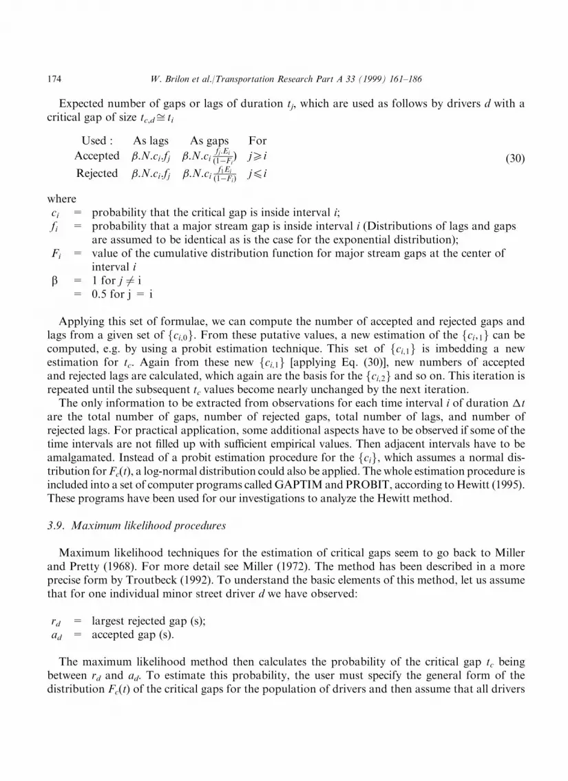
Expected number of gaps or lags of duration tj, which are used as follows by drivers d with acritical gap of size tc,d� ti

Used : As lags As gaps For

Accepted �:N:ci:fj �:N:cifj:Ei

�1ÿFi� j5i

Rejected �:N:ci:fj �:N:cif1Ei

1ÿFi� � j4i

�30�

whereci = probability that the critical gap is inside interval i;fi = probability that a major stream gap is inside interval i (Distributions of lags and gaps

are assumed to be identical as is the case for the exponential distribution);Fi = value of the cumulative distribution function for major stream gaps at the center of

interval ib = 1 for j 6� i

= 0.5 for j = i

Applying this set of formulae, we can compute the number of accepted and rejected gaps andlags from a given set of ci;0f g. From these putative values, a new estimation of the ci;1f g can becomputed, e.g. by using a probit estimation technique. This set of ci;1f g is imbedding a newestimation for tc. Again from these new ci;1f g [applying Eq. (30)], new numbers of acceptedand rejected lags are calculated, which again are the basis for the ci;2f g and so on. This iteration isrepeated until the subsequent tc values become nearly unchanged by the next iteration.The only information to be extracted from observations for each time interval i of duration �t

are the total number of gaps, number of rejected gaps, total number of lags, and number ofrejected lags. For practical application, some additional aspects have to be observed if some of thetime intervals are not ®lled up with su�cient empirical values. Then adjacent intervals have to beamalgamated. Instead of a probit estimation procedure for the cif g, which assumes a normal dis-tribution forFc(t), a log-normal distribution could also be applied. Thewhole estimation procedure isincluded into a set of computer programs calledGAPTIMand PROBIT, according toHewitt (1995).These programs have been used for our investigations to analyze the Hewitt method.

3.9. Maximum likelihood procedures

Maximum likelihood techniques for the estimation of critical gaps seem to go back to Millerand Pretty (1968). For more detail see Miller (1972). The method has been described in a moreprecise form by Troutbeck (1992). To understand the basic elements of this method, let us assumethat for one individual minor street driver d we have observed:

rd = largest rejected gap (s);ad = accepted gap (s).

The maximum likelihood method then calculates the probability of the critical gap tc beingbetween rd and ad. To estimate this probability, the user must specify the general form of thedistribution Fc(t) of the critical gaps for the population of drivers and then assume that all drivers


are consistent. The likelihood that the driver's critical gap will be between rd and ad is given byFa(ad)-Fr(rd). The likelihood L* within a sample of n observed minor street drivers that the twovectors of the rdf g and adf g have been obtained is given by the product:

L� �Ynd�1

Fa ad� � ÿ Fr rd� �� 31�

The logarithm L of the likelihood L* is given by

L �Xnd�1

ln Fa ad� � ÿ Fr rd� �� 32�

In practice, the log-normal distribution is often used as the distribution of the critical gaps tc. Themean critical gap within this distribution has been found to be an acceptable quantity for therepresentation of average driver behavior (see Miller, 1972; Troutbeck, 1992).The likelihood L* is also maximized when the logarithm L of the likelihood is maximized.

Appropriate values for the critical gap distribution parameters (the mean and the variance) arefound by setting the partial derivatives of L with respect to these parameters to zero. This leads toa set of two equations depending on the vectors of the observed rdf g and adf g. These two equa-tions have to be solved by iterative numerical solution techniques. Troutbeck (1992) describes aprocedure for estimating the critical gap parameters using this maximum likelihood technique inmore detail. This numerical method has been used to estimate tc values for the investigationsdescribed in this paper.

4. Criteria for the classi®cation of estimation methods

Before we can compare the di�erent estimation procedures, we have to de®ne the requirementsfor a useful procedure to estimate critical gaps. These requirements cannot be derived usingmathematics. Instead we propose the following set of criteria.

4.1. Distribution

The critical gap tc is not a constant value. Instead it is a variable term where a variation has tobe expected between di�erent drivers and for each individual driver over time. Therefore, thecritical gaps that drivers apply for their decision-making process at unsignalized intersections aredistributed like a random variable. The distribution is characterized by the following:

(a) A minimum value as the lower threshold, which is 50.(b) An expectation �c (average critical gap or mean critical gap; which often is also denoted as

``the critical gap'').(c) A standard deviation �.(d) A skewness factor, which is expected to be positive, i.e. having a longer tail on the right side.


This distribution or its parameters cannot be directly estimated because the critical gap cannotbe observed in an individual driving situation. Only the rejected and accepted gaps can be mea-sured. Therefore, procedures have to be established that try to estimate the distribution or itsparameters as closely as possible. Normally the accepted and/or rejected gaps are used as a basisfor this estimation.

4.2. Consistency

An estimation procedure should be consistent. This means that, if the minor street driverswithin a speci®c composition of tra�c streams have a given distribution of critical gaps, then theprocedure should be able to reproduce this distribution rather closely. The procedure should atleast reproduce the average critical gap quite reliably.These reproduction qualities should not depend on other parameters such as tra�c volumes on

the major or minor street, delay experienced by the drivers, or other external in¯uences. Only ifthis consistency has been proven for a special procedure can the method then be used to studyin¯uences of the external parameters on the critical gap. Otherwise, the in¯uences being found byempirical studies might be due to the inconsistency of the estimation procedure and those in¯u-ences may not really be related to the external parameters being investigated.For most of the well-known estimation procedures for critical gaps, this consistency has not

been proven. There is a strong feeling that a great deal (if not the majority) of all relationshipsbetween critical gaps and other parameters (such as tra�c volumes, time in queue, delays at thestop line as service times of the imbedded queuing system, and geometric characteristics ofintersections, which normally are studied at di�erent sites under di�erent tra�c volumes) foundin the literature might not exist in reality because the di�erences may just be a result of thisinconsistency.

4.3. Robustness of the method

This aspect, as it is already mentioned by Miller (1972), has been emphasized by Hewitt (1995) indiscussing the experiences described in this paper. It means that the results of estimation proceduresshould not be too sensitive to the assumptions being made, such as assumptions about the dis-tributions of critical gaps or of major stream headways.Another factor that deserves mention is the size of the standard error of the mean critical gap.

It is possible that a method that produces a slight bias but a small standard error might be pre-ferable to an unbiased method with a large standard error (Hewitt, 1995).

4.4. Capacity model compatibility

The estimation of critical gaps is not an end in itself. Critical gaps are used in models forcapacity computation at unsignalized intersections. Critical gaps estimated by di�erent proce-dures could have di�erent in¯uences on the model's capacity output. It should be guaranteed thatthe estimated critical gap, in conjunction with the follow-up times tf (and their estimation proce-dure), gives a reliable and realistic estimate of the capacity independent of the external para-meters, especially the major street volume.


In no case is it sensible to use a capacity computation model with critical gaps estimated in away that is not related to the model. In other words, the estimation procedure for critical gapsand the capacity model (as well as the consecutive delay model) must form one integrated unit.It has to be stated that this capacity model compatibility is only given for the Siegloch method,

as shown above. For each of the other estimation procedures, the method of critical gap estima-tion and the capacity (as well as delay) calculation methods have no theoretical connections.Some methods, however, produce results that cannot be handled by the usual theoretical conceptsfor capacity calculations, for example, some of the probit results (see above).

5. Simulation studies

5.1. Description of the simulation concept

These qualities of an estimation procedure, especially consistency, can only be checked for by asimulation model, since an analytical approach is not available. To this end, an extended simu-lation study for testing di�erent tc estimation procedures for consistency has been performed. Thetwo tra�c streams (see Fig. 1) have been generated by randomized procedures. For each simula-tion run, a combination of constant tra�c volumes qp and qn has been given. qp was variedbetween 100 and 900 vph. qn was varied between 0 and the capacity c, which depends on qp. Eachsuch simulation run has been performed for constant tra�c volumes over 10 h. Thus, 46 di�erentcombinations of qp and qn (where qn < capacity) have been performed for two di�erent cases,which are combinations of tc and tf values. The ®rst case may represent minor street right turnerbehavior, whereas the second case could stand for driver behavior of left turners from the minorstreet.

Case ``5.8'' Case ``7.2''Critical gap tc 5.8 7.2 sMinimum tc value 2.0 2.2 sk value for the Erlang distribution 5 5 ÐMaximum tc value 12.5 15.5 sFollow-up time tf 2.6 3.6 sMinimum tf value 1.2 1.6 sk value for the Erlang distribution 2 2 ÐMaximum tf value 7.2 10

The critical gaps, tc, and the follow-up times, tf, for each simulated driver have been generatedaccording to a shifted Erlang distribution using the parameters mentioned before. Each driver isassumed to be consistent, that is, he maintains his generated tc value until his departure. Gener-ated tc values and tf values outside the margins of minimum and maximum values indicatedabove have been replaced by these given extreme values.Moreover, to achieve a realistic pattern of headways, the so-called hyper-Erlang distribution

(see Dawson, 1969; Grossmann, 1991) has been applied to the major stream tra�c ¯ow genera-tion where tra�c on one single lane has been assumed. Also, the arrivals of minor stream vehicles


have been generated according to this type of distribution. These complicated distributions gen-erate tra�c situations of great variability, which are similar to realistic conditions.Within each simulation run the critical gaps, tc, have been estimated out of the simulated ¯ow

patterns according to the above-mentioned estimation methods. A series of 46 estimations for tchas been obtained for each method.

5.2. Results for the critical gap analysis

Fig. 5 illustrates the results of the critical gap analysis. It presents all the tc estimated byHewitt's method for di�erent qp values. Here they are plotted over the major stream tra�cvolume qp, which was generated by the simulation. This type of relation, after some comparisons,turned out to be the most sensible as results in relation to minor street ¯ows qn showed much lessvariation. Each cross represents one tc value. The crosses plotted one above the other were pro-duced for di�erent qn. For both tra�c ¯ows the simulated volumes (not the predetermined valuesfor the generation of headways) were used in the following graphs.We see that the outcome of the Hewitt estimation process reveals tc values between 5.63 and

5.98 s for a correct value of 5.8 s and between 7.08 and 7.52 s for a correct value of 7.2 s. Thus, arather large variation of the results must be stated. For the tc values, a regression analysisregarding their relation to qp has been performed. In this case the regression line was rather hor-izontal and it was close to the correct tc value in both cases. That means that the Hewitt methodon average reproduces the correct tc value very well and its results do not depend on major streetvolumes. Thus, this method ful®lls our most important quality criterion, consistency, with arather high performance. We shall see that this is not the case with most of the other methods.From all the other methods studied, only the maximum likelihood method (Fig. 6 denoted as

the Troutbeck method) comes up to the same performance as the Hewitt method. Here again theregression line shows no relation to major street volumes and the correct tc values are on averageclose to the estimation results. Again, a rather large variation of the results obtained for di�erentminor street volumes can be recognized from the plots. Nevertheless, these two methods ful®ll therequirements formulated above, especially the most important, consistency.Similar plots for the illustration of simulation results have also been produced for the other

methods studied. For the logit method (Fig. 7) we see that the results become very di�erent if we

Fig. 5. Results from the simulation runs for the Hewitt method for two tc-values.


either use gaps and lags or only gaps. In our example (only tc=5.8 s has been evaluated) only theexclusive use of gaps (no lags have been used in the second sample) reproduces on average thecorrect tc. The inclusion of lags into the estimation process leads to a remarkable underestimationof the critical gap. However, in each of the approaches, the results show a signi®cant dependencyon the major street tra�c volume. Thus the logit procedure fails the consistency criterion, andconsequently cannot be recommended as a useful estimation procedure in the form as it isdescribed above. It could be that a correction to the procedure might become available.

Fig. 6. Results from the simulation runs for Troutbeck's Maximum Likelihood Method and for two tc values.

Fig. 7. Results from the simulation runs for the logit method and Ashworth's method. For logit only, the case fortc=5.8 s has been evaluated.


For the Ashworth method (Fig. 7) we see that most of the estimation results are smaller thanthe correct values. Again, as the results do not seem to be correct, this procedure [at least in itsuncorrected version as shown in Eq. (5)] is not recommended for application.A rather disastrous result has evolved from the simulations both for the Ra� and the Harders

procedures (Fig. 8). The Ra� method meets the correct values only for median major street tra�cvolumes, whereas Harders' method leads to a tremendous overestimation of critical gaps. Only ifHarders' method includes the lags in the evaluation process are some improvements for theaverage size of the resulting tc values obtained. The even more important problem is, however,that the results coming out of both types of procedures have a strong relationship to the major

Fig. 8. Results from the simulation runs for the Ra� and Harders methods and for two tc values.


street tra�c volumes, a feature that should be avoided. Therefore, neither method should be usedfor reliable critical gap estimation.For the estimation method according to Siegloch we ®nd better performance (Fig. 9). As with

the Hewitt and Troutbeck methods, both example values of tc are on average a correct replicationof the true tc values. In addition, the regression lines are not much related to major street tra�cvolumes; that is, the major street ¯ow does not systematically in¯uence the estimation results.Therefore, the Siegloch method seems to be a useful estimation technique.The simulation for the Siegloch method allows us to evaluate the capacity with the pre-

determined tc and tf values because a continuous queue has to be generated for the simulation. Asa result, the number of minor street vehicles able to pass the con¯ict zone is exactly the capacityof the intersection. The results from a series of 10 h simulation runs have been noted. They weredescribed by a regression function (see Fig. 10 ):

c � A:eÿB:p �33�which is of the same type as Siegloch's capacity function [Eq. (4)]. The values for A and B havebeen estimated according to the principle of least squares using a spreadsheet technique withoutprior linear transformation. This type of function allows another type of estimation of tc and tf :

Fig. 9. Results from the simulation runs for Siegloch's method.

Fig. 10. Simulated capacities compared with results calculated from Siegloch's formula [Eq. (4)] (using the givencritical gap and follow-up time).


tf � 3600

Atc � B� tf

2s� � �34�

The simulated capacity results and the regression function (``simulated'') are represented inFig. 10. The regression has an extremely high r value, which indicates a very good correlation.However, the tc and tf value obtained from the regression line are di�erent from the true values.The relation between capacity and major ¯ow, as it would be calculated from Siegloch's originalformula with the true values for tc and tf, is also indicated in the graph of Fig. 10 (``calculated'').Both curves for the capacity show signi®cant di�erences. Therefore, the robustness criterion isnot ful®lled. The reason is that the Siegloch formula [Eq. (4)] is only exactly valid for constant tcand tf values and Poisson major street tra�c ¯ows, whereas the simulation has been performedfor more realistic circumstances, especially with non-Poisson major stream arrival patterns. Theseresults indicate that the Siegloch estimation technique is sensitive to the major street headwaydistribution (compare with the robustness criterion).Fig. 11 gives an overview of all the regression lines shown in Figs 5±9. Some procedures could

be improved with additional correction terms. This could be the focus of future research.

5.3. Results for the variance of estimated critical gaps

The simulated 10 h of constant ¯ows do not represent a sample that could be observed in rea-lity. Under practical circumstances, measurements can only be taken for 1 or 2 h. Therefore, wealso studied the convergence behavior of some of the methods. Here the results for the maximumlikelihood method are mentioned. Fig. 12 shows the range of minimum and maximum tc valuesobtained from observation intervals of di�erent durations. We see that for 1 h (and longer)intervals, the variability is less then 0.2 s.

Fig. 11. Comparison of the regression lines for the relation between major street tra�c ¯ow and estimated tc values fortc=5.8 s (a) and tc=7.2 s (b).


The tra�c volume should also be regarded as an additional in¯uencing factor. Fig. 13 showsthe standard deviation in relation to the true value as a function of the number of minor streetvehicles simulated. On the horizontal axis a logarithmic scale has been used. Above a sample sizeof 100 minor street vehicles, the standard deviation is less than 0.3 s. The relation shown in Fig. 13seems to be more generally valid than that shown in Fig. 12.

Fig. 12. Minimum and maximum estimates for the critical gap in relation to the duration of the observation period

(for the maximum likelihood method and a given tc=5.8 s).

Fig. 13. Standard deviation of the estimated critical gaps tc in relation to the sample size of minor street vehicles (for

the maximum likelihood method and a given tc=5.8 s).


6. Conclusion

A review of publications about estimation of critical gaps reveals many di�erent proposedsolutions. It is di�cult to understand which procedure is reliable and which is not. From thesample of methods tested for this paper, the maximum likelihood procedure and Hewitt's methodgave the best results. Both were valid for the two cases studied. This explains the selection of themaximum likelihood method for the evaluation of critical gaps for the next edition of the HCM,Chapter 10. (SeeKyte et al., 1996).The investigation of the di�erent theoretical concepts shows that principles of the various

methods could also be combined. In the future, even more estimation techniques for critical gapsmight be proposed.

Appendix

De®nition of variables:

Ai = number of accepted gaps of size i (Harders method) or the number of accepted lags ofsize i (lag method)

ai = Ai/Ni=rate of acceptance for gaps of size ti (Harders method)ai = Ai/Ni=rate of acceptance for lags of size ti (lag method)c = capacity=maximum number of minor street vehicles, which can cross the major stream

during one hour (vph)�t = length of time interval for the lag method or Harders methodfa(t) = statistical density function for the accepted gapsFa(t) = cumulative distribution function for the accepted gapsfc(t) = statistical density function for the critical gapsFc(t) = cumulative distribution function for the critical gapsfr(t) = statistical density function for the rejected gapsFr(t) = cumulative distribution function for the rejected gapsg = observed value for g(t)g(t) = number of minor street vehicles, which can enter into a major street gap of size th(t) = statistical density function for gaps (headways) between vehicles in the major streamL = Log-likelihood functionL* = Likelihood function�a = mean of the accepted gaps ta (s)�c = average critical gap or the expectation within the distribution function Fc(t) (s)n = number of observed minor street driversNi = number of all gaps of size i, which are provided to minor vehicles (Harders method) or

the number of all lags of size i, which are provided to minor vehicles (lag method)p = major (= ``priority'') street tra�c volume = qp/3600 (veh/s)qn = minor street tra�c volume (vph)qp = major (= ``priority'') street tra�c volume (vph)�a = standard deviation of accepted gaps ta (s)�c = standard derivation of critical gaps


= standard derivation within the distribution function Fc(t) (s)t = time index for drivers or decision situations (logit method) (s)ta = accepted gap (s)tc = critical gap (s)tf = follow-up time (s)tg = average t-value for each g (Siegloch method) (s)ti = center of the i-th time interval for Harders method (s)tr = rejected gap (s)W = number of time intervals (lag method)

References

Ashworth, R., 1968. A note on the selection of gap acceptance criteria for tra�c simulation studies. TransportationResearch 2(2), 171±175.

Ashworth, R., 1970. The analysis and interpretation of gap acceptance data. Transportation Science 4, 270±280.Ashworth, R., 1979. The analysis and interpretation of gap acceptance data. Transportation Research, pp. 270±280.Ben-Akiva, M., Lerman, S. R., 1987. Discrete choice analysis. Mass. Institute of Technology Press: Cambridge, MA.

Cassidy, M. J., Madanat, S. M., Wang, Mu-Han, and Yang, Fan., 1995. Unsignalized intersection capacity and level ofservice: revisiting critical gap. Preprint 950138, Transportation Research Board, annual meeting.

Daganzo, C., 1981. Estimation of gap acceptance parameters within and across the population from direct roadside

observation. Transportation Research 15B, 1±15.Dawson, R. F., 1969. The hypererlang probability distribution Ð a generalized tra�c headway model. In: Proceedingsof the International Symposium on the Theory of Tra�c Flow and Transportation. Karlsruhe, Series Strassenbau

und Strassenverkehrstechnik. No. 86.Grossmann, M., 1991. Methoden zur Berechnung und Beurteilung von Leistungsfaehigkeit und Verkehrsqualitaet anKnotenpunkten ohne Lichtsignalanlagen (Methods for the Calculation and Assessment of Capacity and Tra�cQuality at Unsignalized Intersections) (in German). Ruhr-University Bochum, Institute for Tra�c Engineering, No. 9.

Harders, J., 1968. Die LeistungsfaÈ higkeit nicht signalgeregelter staedtischer Verkehrsknotenpunkte. (Capacity ofUrban Unsignalized Intersections) (in German). Series Strassenbau und Strassenverkehrstechnik, No. 76.

Hewitt, R. H., 1983. Measuring critical gap. Transportation Science 17(1), 87±109.

Hewitt, R. H., 1985. A comparison between some methods of measuring critical gap. Tra�c Engineering and Control26(1), 13±22.

Hewitt, R. H., 1988. Analysis of critical gaps using probit analysis. Paper presented at the Second International

Workshop on Unsignalized Intersections in Bochum. (The English version of the paper is unpublished, a copy isavailable from the authors of this paper on request; a German version has been published: Hewitt, 1993)

Hewitt, R. H., 1993. Analyse von Grenzzeitluecken durch Probit-Analyse (Analysis of Critical Gaps by Probit Analy-sis) (in German). Strassenverkehrstechnik, Germany, pp. 142±148.

Hewitt, R. H., 1995. Personal correspondence with Werner Brilon.Kyte, M., Tian, Z., Mir, Z., Hameedmansoor, Z., Kittelson, W., Vandehey, M., Robinson, B., Brilon, W., Bondzio L.,Wu, N. and Troutbeck, R., 1996. Capacity and level of service at unsignalized intersections, ®nal report: volume 1±

two-way stop-controlled intersections. National Cooperative Highway Research Program, Project 3-46.Mahmassani, H., She�, Y., 1981. Using gap sequences to estimate gap acceptance functions. Transportation Research15B, 143±148.

Miller, A. J., 1972. Nine estimators for gap-acceptance parameters. In: Newell, G. (Ed.), Proceedings of the InternationalSymposium on the Theory of Tra�c Flow and Transportation. Berkeley, California June, 1971. Elsevier Amsterdam.

Miller, A. J., Pretty, R. L., 1968. Overtaking on two-lane rural roads. Proc. Aust. Rd. Res. Board 4(1), 582±591.

Pant, P. D. and Balakrishnan, P., 1994. Neural networks for gap acceptance at stop-controlled intersections. ASCEJournal, pp. 433±446.


Ra�, M. S. and Hart, J. W., 1950. A volume warrant for urban stop signs. Eno foundation for highway tra�c control:

Saugatuck, Connecticut.Retzko, H. G., 1961. Vergleichende Bewertung verschiedener Arten der Verkehrsregelung an staedtischenStraûenverkehrsknotenpunkten (Comparative Evaluation of Di�erent Kinds of Tra�c Control at Urban Intersec-

tions) (in German). Series Strassenbau und Strassenverkehrstechnik, No. 12.Siegloch, W., 1973. Die Leistungsermittlung an Knotenpunkten ohne Lichtsignalanlagen (Capacity Calculations atUnsignalized Intersections) (in German), Series Strassenbau und Strassenverkehrstechnik, No. 154.

Solberg, P. and Oppenlander, J., 1966. Lag and gap acceptance at stop-controlled intersections. Highway Capacity

Record, No. 118. 1966, pp. 48±67.Troutbeck, R. J., 1992. Estimating the critical acceptance gap from tra�c movements. Physical infrastructure centre,Queensland University of Technology. Research Report 92±5.


Documents

Useful estimation procedures for critical gaps