Embed Size (px)
Citation preview
Use of Proficiency Levels
135
9
PISA DATA ANALYSIS MANUAL: SAS® SECOND EDITION – ISBN 978-92-64-05624-4 – © OECD 2009
Introduction ..................................................................................................................................................... 136
Generation of the proficiency levels............................................................................................... 136
Other analyses with proficiency levels ......................................................................................... 141
Conclusion ....................................................................................................................................................... 143

9USE OF PROFICIENCY LEVELS
136PISA DATA ANALYSIS MANUAL: SAS® SECOND EDITION – ISBN 978-92-64-05624-4 – © OECD 2009
INTRODUCTION
The values for student performance in reading, mathematics, and science literacy are usually consideredas continuous latent variables. In order to facilitate the interpretation of the scores assigned to students,the reading, mathematics and science scales were designed to have an average score of 500 points and astandard deviation of 100 across OECD countries. This means that about two-thirds of the OECD membercountry students perform between 400 and 600 points.
In order to render PISA results more accessible to policy makers and educators, proficiency scales havebeen developed for the assessment domains. Since these scales are divided according to levels of difficultyand performance, both a ranking of student performance and a description of the skill associated with thatproficiency level can be obtained. Each successive level is associated with tasks of increased difficulty.
In PISA 2000, five levels of reading proficiency were defined and reported in the PISA 2000 initial reportKnowledge and Skills for Life: First Results from PISA 2000 (OECD, 2001). In PISA 2003, six levels ofmathematics proficiency levels were also defined and reported in the PISA 2003 initial report Learningfor Tomorrow’s World – First Results from PISA 2003 (OECD, 2004a). In PISA 2006, six levels of scienceproficiency were defined and reported in the PISA 2006 initial report Science Competencies for Tomorrow’sWorld (OECD, 2007a).
This chapter will show how to derive the proficiency levels from the PISA databases and how to use them.
GENERATION OF THE PROFICIENCY LEVELS
Proficiency levels are not included in the PISA databases, but they can be derived from the plausible values(PVs).
In PISA 2006, the cutpoints that frame the proficiency levels in science are 334.94, 409.54, 484.14,558.73, 633.33 and 709.93.1 While some researchers might understand that different possible scores canbe assigned to a student, it is more difficult to understand that different levels can be assigned to a singlestudent. Therefore, they might be tempted to compute the average of the five plausible values and thenassign each student a proficiency level based on this average.
As discussed in Chapter 6 and Chapter 8, such a procedure is similar to assigning each student anexpected a posteriori (EAP) score; the biases of such estimators are now well known. Since using EAPscores underestimates the standard deviation, the estimation of the percentages of students at each levelof proficiency will consequently underestimate the percentages at the lowest and highest levels, andoverestimate the percentages at the central levels.
As already stated, international education surveys do not aim to estimate the performance of particularstudents, but rather, they aim to describe population characteristics. Therefore, particular students can beallocated different proficiency levels for different plausible values. Thus, five plausible proficiency levelswill be assigned to each student respectively according to their five plausible values. The SAS® syntax forthe generation of the plausible proficiency levels in science is provided in Box 9.1.
The statement “array” allows the definition of a variable vector. In Box 9.1, two vectors are defined. The first,labelled SCIE, includes the five plausible values for the science combined scale (PV1SCIE to PV5SCIE) andthe three science subscales (PV1EPS to PV5EPS, PV1ISI to PV5ISI, and PV1USE to PV5USE). The second,labelled LEVELSCIE, will create 20 new variables, labelled SCIELEV1 to SCIELEV5 for the science combinedscale; EPSLEV1 to EPSLEV5 for the science/explaining phenomena scientifically subscale; ISILEV1 to ISILEV5for the science/identifying scientific issues subscale; USELEV1 to USELEV1 to the science/use of scientificevidence subscale.
9USE OF PROFICIENCY LEVELS
137PISA DATA ANALYSIS MANUAL: SAS® SECOND EDITION – ISBN 978-92-64-05624-4 – © OECD 2009
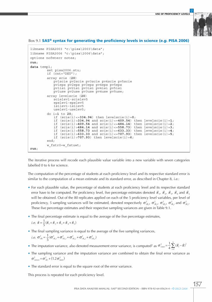
The iterative process will recode each plausible value variable into a new variable with seven categorieslabelled 0 to 6 for science.
The computation of the percentage of students at each proficiency level and its respective standard error issimilar to the computation of a mean estimate and its standard error, as described in Chapter 8, i.e.:
• For each plausible value, the percentage of students at each proficiency level and its respective standarderror have to be computed. Per proficiency level, five percentage estimates denoted ˆ 1, ˆ 2, ˆ 3, ˆ 4 and ˆ 5
will be obtained. Out of the 80 replicates applied on each of the 5 proficiency level variables, per level ofproficiency, 5 sampling variances will be estimated, denoted respectively 2
)( 1ˆ , 2)( 2ˆ , 2
)( 3ˆ , 2)( 4ˆ and 2
)( 5ˆ .These five percentage estimates and their respective sampling variances are given in Table 9.1.
• The final percentage estimate is equal to the average of the five percentage estimates,
i.e. 1( )54321 ˆˆˆˆˆ5
ˆ ++++=
• The final sampling variance is equal to the average of the five sampling variances,
i.e. )(51 2
)ˆ(2
)ˆ(2
)ˆ(2
)ˆ(2
)ˆ(2
)ˆ( 54321++++=
• The imputation variance, also denoted measurement error variance, is computed2 as=
−=5
1
22)( )ˆˆ(
41
iitest
• The sampling variance and the imputation variance are combined to obtain the final error variance as
ˆ ( )2)(
2)(
2)( 2.1 testerror +=
• The standard error is equal to the square root of the error variance.
This process is repeated for each proficiency level.
Box 9.1 SAS® syntax for generating the proficiency levels in science (e.g. PISA 2006)
libname PISA2003 “c:\pisa\2003\data”;
libname PISA2006 “c:\pisa\2006\data”;
options nofmterr notes;
run;
data temp1;set pisa2006.stu;if (cnt=“DEU”);
array scie (20)pv1scie pv2scie pv3scie pv4scie pv5sciepv1eps pv2eps pv3eps pv4eps pv5epspv1isi pv2isi pv3isi pv4isi pv5isipv1use pv2use pv3use pv4use pv5use;
array levelscie (20)scielev1-scielev5epslev1-epslev5isilev1-isilev5uselev1-uselev5;
do i=1 to 20;if (scie(i)<=334.94) then levelscie(i)=0;if (scie(i)>334.94 and scie(i)<=409.54) then levelscie(i)=1;if (scie(i)>409.54 and scie(i)<=484.14) then levelscie(i)=2;if (scie(i)>484.14 and scie(i)<=558.73) then levelscie(i)=3;if (scie(i)>558.73 and scie(i)<=633.33) then levelscie(i)=4;if (scie(i)>633.33 and scie(i)<=707.93) then levelscie(i)=5;if (scie(i)>707.93) then levelscie(i)=6;
end;
w_fstr0=w_fstuwt;run;
9USE OF PROFICIENCY LEVELS
138PISA DATA ANALYSIS MANUAL: SAS® SECOND EDITION – ISBN 978-92-64-05624-4 – © OECD 2009
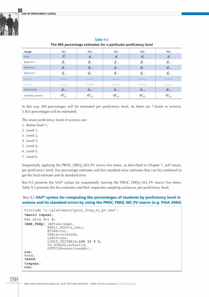
In this way 405 percentages will be estimated per proficiency level. As there are 7 levels in science,2 835 percentages will be estimated.
The seven proficiency levels in science are:
1. Below level 1,
2. Level 1,
3. Level 2,
4. Level 3,
5. Level 4,
6. Level 5,
7. Level 6.
Sequentially applying the PROC_FREQ_NO_PV macro five times, as described in Chapter 7, will return,per proficiency level, five percentage estimates and five standard error estimates that can be combined toget the final estimate and its standard error.
Box 9.2 presents the SAS® syntax for sequentially running the PROC_FREQ_NO_PV macro five times.Table 9.2 presents the five estimates and their respective sampling variances, per proficiency level.
Box 9.2 SAS® syntax for computing the percentages of students by proficiency level inscience and its standard errors by using the PROC_FREQ_NO_PV macro (e.g. PISA 2006)
%include “c:\pisa\macro\proc_freq_no_pv.sas”;%macro repeat;%do kk=1 %to 5;%BRR_FREQ( INFILE=temp1,
REPLI_ROOT=w_fstr,BYVAR=cnt,VAR=scielev&kk,LIMIT=yes,LIMIT_CRITERIA=100 10 5 1,ID_SCHOOL=schoolid,OUTFILE=exercise&kk);
run;%end;%mend;%repeat;run;
Table 9.1The 405 percentage estimates for a particular proficiency level
Weight PV1 PV2 PV3 PV4 PV5
Final ˆ1 ˆ2 ˆ3 ˆ4 ˆ5
Replicate 1 ˆ1_1 ˆ2_1 ˆ3_1 ˆ4_1 ˆ5_1
Replicate 2 ˆ1_2 ˆ2_2 ˆ3_2 ˆ4_2 ˆ5_2
Replicate 3 ˆ1_3 ˆ2_3 ˆ3_3 ˆ4_3 ˆ5_3
………. ………. ………. ………. ………. ……….
………. ………. ………. ………. ………. ……….
Replicate 80 ˆ1_80 ˆ2_80 ˆ3_80 ˆ4_80 ˆ5_80
Sampling variance2
)( 1ˆ2
)( 2ˆ2
)( 3ˆ2
)( 4ˆ2
)( 5ˆ

9USE OF PROFICIENCY LEVELS
139PISA DATA ANALYSIS MANUAL: SAS® SECOND EDITION – ISBN 978-92-64-05624-4 – © OECD 2009
To combine the results:
• Per proficiency level, the five percentage estimates are averaged.
• Per proficiency level, the five sampling variances are averaged.
• By comparing the final estimate and the five PV estimates, the imputation variance is computed.
• The final sampling variance and the imputation variance are combined as usual to get the final errorvariance.
• The standard error is obtained by taking the square root of the error variance.
Table 9.2Estimates and sampling variances per proficiency level in science for Germany (PISA 2006)
Level PV1 PV2 PV3 PV4 PV5
Below Level 1ˆ
i 4.12 3.82 4.25 4.03 4.13
2
)( iˆ (0.60)² (0.59)² (0.72)² (0.67)² (0.71)²
Level 1ˆ
i 11.93 11.8 11.03 11.09 10.70
2
)( iˆ (0.86)² (0.81)² (0.72)² (0.73)² (0.71)²
Level 2ˆ
i 20.26 21.59 21.87 21.16 21.91
2
)( iˆ (0.73)² (0.71)² (0.73)² (0.80)² (0.76)²
Level 3ˆ
i 28.70 27.46 27.33 27.92 27.93
2
)( iˆ (1.00)² (0.94)² (0.69)² (0.91)² (0.92)²
Level 4ˆ
i 23.39 23.45 23.57 23.66 23.77
2
)( iˆ (0.91)² (0.93)² (0.92)² (0.92)² (0.96)²
Level 5ˆ
i 9.82 10.07 10.14 10.24 9.69
2
)( iˆ (0.61)² (0.53)² (0.53)² (0.64)² (0.49)²
Level 6ˆ
i 1.79 1.81 1.82 1.89 1.87
2
)( iˆ (0.25)² (0.28)² (0.23)² (0.20)² (0.21)²
The final results are presented in Table 9.3.
Table 9.3Final estimates of the percentage of students, per proficiency level,
in science and its standard errors for Germany (PISA 2006)
Proficiency level % S.E.
Below Level 1 4.07 0.68
Level 1 11.31 0.96
Level 2 21.36 1.06
Level 3 27.87 1.07
Level 4 23.57 0.95
Level 5 9.99 0.62
Level 6 1.84 0.24
A SAS® macro has been developed for computing the percentage of students at each proficiency level aswell as its respective standard error in one run. Box 9.3 presents the SAS® syntax for running the macro andTable 9.4 presents the structure of the output data file.

9USE OF PROFICIENCY LEVELS
140PISA DATA ANALYSIS MANUAL: SAS® SECOND EDITION – ISBN 978-92-64-05624-4 – © OECD 2009
Box 9.3 SAS® syntax for computing the percentage of students by proficiency levelin science and its standard errors by using the PROC_FREQ_PV macro (e.g. PISA 2006)
%include “c:\pisa\macro\proc_freq_pv.sas”;
%BRR_FREQ_PV( INFILE=temp1,REPLI_ROOT=w_fstr,BYVAR=cnt,PV_ROOT=scielev,LIMIT=yes,LIMIT_CRITERIA=100 10 5 1,ID_SCHOOL=schoolid,OUTFILE=exercise6);
run;
This macro has eight arguments. Besides the usual arguments, the root of the proficiency level variablenames has to be specified. For the science scale, as specified in the data statement of Box 9.1, this will beset as SCIELEV. As indicated in Table 9.4, the number of cases at Level 6 is less than 100.
Table 9.4Output data file exercise6 from Box 9.3
CNT SCIELEV STAT SESTAT STUD_FLAG SCH_FLAG PCT_FLAGDEU 0 4.07 0.68 0 0 1DEU 1 11.31 0.96 0 0 0DEU 2 21.36 1.06 0 0 0DEU 3 27.87 1.07 0 0 0DEU 4 23.57 0.95 0 0 0DEU 5 9.99 0.62 0 0 0DEU 6 1.84 0.24 1 0 1
As before, several breakdown variables can be used. For instance, the distribution of students acrossproficiency levels per gender can be obtained, as in Box 9.4.
Box 9.4 SAS® syntax for computing the percentage of studentsby proficiency level and its standard errors by gender (e.g. PISA 2006)
%BRR_FREQ_PV( INFILE=temp1, REPLI_ROOT=w_fstr,BYVAR=cnt st04q01,PV_ROOT=scielev,LIMIT=yes,LIMIT_CRITERIA=100 10 5 1,ID_SCHOOL=schoolid,OUTFILE=exercise7);
run;
In this case, the sum of the percentages will be equal to 100 per country and per gender, as shown inTable 9.5.
Table 9.5Output data file exercise7 from Box 9.4
CNT ST04Q01 SCIELEV STAT SESTAT STUD_FLAG SCH_FLAG PCT_FLAGDEU 1 0 3.73 0.67 1 0 1DEU 1 1 12.12 1.19 0 0 0DEU 1 2 21.08 1.26 0 0 0DEU 1 3 29.94 1.47 0 0 0DEU 1 4 23.29 1.07 0 0 0DEU 1 5 8.42 0.73 0 0 1DEU 1 6 1.42 0.38 1 0 1DEU 2 0 4.39 0.84 0 0 1DEU 2 1 10.55 1.09 0 0 0DEU 2 2 21.62 1.23 0 0 0DEU 2 3 25.93 1.21 0 0 0DEU 2 4 23.83 1.35 0 0 0DEU 2 5 11.46 1.03 0 0 0DEU 2 6 2.22 0.37 1 0 1
9USE OF PROFICIENCY LEVELS
141PISA DATA ANALYSIS MANUAL: SAS® SECOND EDITION – ISBN 978-92-64-05624-4 – © OECD 2009
As shown in Table 9.5, the percentage of males at Level 5 and 6 is higher than the percentage of females atLevel 5 and 6.
The statistical significance of these differences cannot be evaluated with this procedure, however. Moredetails on this issue will be provided in Chapter 11.
OTHER ANALYSES WITH PROFICIENCY LEVELS
Proficiency levels constitute a powerful tool for communicating the results on the cognitive test. Researchersand/or policy makers might therefore be interested in estimating the influence of some variables (such as thesocial background or self-confidence measures) on the proficiency levels.
PISA 2003, for instance, constructed an index of mathematics self-efficacy, denoted MATHEFF.
Analysing the relationship between proficiency levels and mathematics self-efficacy is relevant, as there isprobably a reciprocal relationship between these two concepts. Better self-perception in mathematics is thoughtto increase a student’s proficiency in mathematics, but an increase in the latter might in return affect the former.
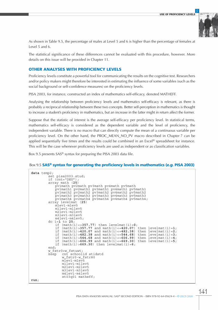
Suppose that the statistic of interest is the average self-efficacy per proficiency level. In statistical terms,mathematics self-efficacy is considered as the dependent variable and the level of proficiency, theindependent variable. There is no macro that can directly compute the mean of a continuous variable perproficiency level. On the other hand, the PROC_MEAN_NO_PV macro described in Chapter 7 can beapplied sequentially five times and the results could be combined in an Excel® spreadsheet for instance.This will be the case whenever proficiency levels are used as independent or as classification variables.
Box 9.5 presents SAS® syntax for preparing the PISA 2003 data file.
Box 9.5 SAS® syntax for generating the proficiency levels in mathematics (e.g. PISA 2003)
data temp2;set pisa2003.stud;if (cnt=“DEU”);array math (25)
pv1math pv2math pv3math pv4math pv5mathpv1math1 pv2math1 pv3math1 pv4math1 pv5math1pv1math2 pv2math2 pv3math2 pv4math2 pv5math2pv1math3 pv2math3 pv3math3 pv4math3 pv5math3pv1math4 pv2math4 pv3math4 pv4math4 pv5math4;
array levelmat (25)mlev1-mlev5m1lev1-m1lev5m2lev1-m2lev5m3lev1-m3lev5m4lev1-m4lev5;
do i=1 to 25;if (math(i)<=357.77) then levelmat(i)=0;if (math(i)>357.77 and math(i)<=420.07) then levelmat(i)=1;if (math(i)>420.07 and math(i)<=482.38) then levelmat(i)=2;if (math(i)>482.38 and math(i)<=544.68) then levelmat(i)=3;if (math(i)>544.68 and math(i)<=606.99) then levelmat(i)=4;if (math(i)>606.99 and math(i)<=669.30) then levelmat(i)=5;if (math(i)>669.30) then levelmat(i)=6;
end;w_fstr0=w_fstuwt;keep cnt schoolid stidstd
w_fstr0-w_fstr80mlev1-mlev5m1lev1-m1lev5m2lev1-m2lev5m3lev1-m3lev5m4lev1-m4lev5st03q01 matheff;
run;

9USE OF PROFICIENCY LEVELS
142PISA DATA ANALYSIS MANUAL: SAS® SECOND EDITION – ISBN 978-92-64-05624-4 – © OECD 2009
Box 9.6 presents SAS® syntax for computing the mean of student self-efficacy per proficiency level.
Box 9.6 SAS® syntax for computing the mean of self-efficacy in mathematicsand its standard errors by proficiency level (e.g. PISA 2003)
%include “c:\pisa\macro\proc_means_no_pv.sas”;
%macro repeat;
%do kk=1 %to 5;
%BRR_PROCMEAN(INFILE=temp2, REPLI_ROOT=w_fstr, BYVAR=cnt mlev&kk, VAR=matheff, STAT=mean,LIMIT=no,LIMIT_CRITERIA=,ID_SCHOOL=,
OUTFILE=exercise&kk);run;
data exercise&kk;set exercise&kk;stat&kk=stat;sestat&kk=sestat;mlev=mlev&kk;keep cnt mlev stat&kk sestat&kk;
run;
%end;data exercise8;
merge exercise1 exercise2 exercise3 exercise4 exercise5;by cnt mlev;stat=(stat1+stat2+stat3+stat4+stat5)/5;samp= ((sestat1**2)+(sestat2**2)+(sestat3**2)+(sestat4**2)+
(sestat5**2))/5;
mesvar=(((stat1-stat)**2)+((stat2-stat)**2)+((stat3-stat)**2)+ ((stat4-stat)**2)+((stat5-stat)**2))/4;
sestat=(samp+(1.2*mesvar))**0.5;keep cnt mlev stat sestet stud_flag sch_flag pct_flag;
run;
%mend repeat;
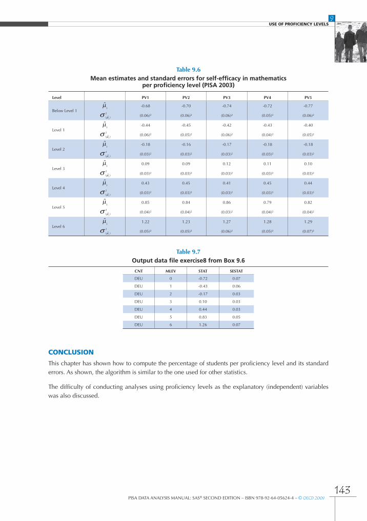
Table 9.6 presents the mean estimates and standard errors for self-efficacy in mathematics per proficiencylevel.
To combine the results:
• Per proficiency level, the five mean estimates are averaged.
• Per proficiency level, the five sampling variances are averaged.
• By comparing the final estimate and the five PV estimates, the imputation variance is computed.
• The final sampling variance and the imputation variance are combined as usual to get the final errorvariance.
• The standard error is obtained by taking the square root of the error variance.
Final results are presented in Table 9.7. It shows that high self-efficacy in mathematics (STAT) is associatedwith higher proficiency levels (MLEV).
9USE OF PROFICIENCY LEVELS
143PISA DATA ANALYSIS MANUAL: SAS® SECOND EDITION – ISBN 978-92-64-05624-4 – © OECD 2009
Table 9.6Mean estimates and standard errors for self-efficacy in mathematics
per proficiency level (PISA 2003)
Level PV1 PV2 PV3 PV4 PV5
Below Level 1µ̂i -0.68 -0.70 -0.74 -0.72 -0.77
2
)ˆ( i(0.06)² (0.06)² (0.06)² (0.05)² (0.06)²
Level 1µ̂i -0.44 -0.45 -0.42 -0.43 -0.40
2
)ˆ( i(0.06)² (0.05)² (0.06)² (0.04)² (0.05)²
Level 2µ̂i -0.18 -0.16 -0.17 -0.18 -0.18
2
)ˆ( i(0.03)² (0.03)² (0.03)² (0.03)² (0.03)²
Level 3µ̂i 0.09 0.09 0.12 0.11 0.10
2
)ˆ( i(0.03)² (0.03)² (0.03)² (0.03)² (0.03)²
Level 4µ̂i 0.43 0.45 0.41 0.45 0.44
2
)ˆ( i(0.03)² (0.03)² (0.03)² (0.03)² (0.03)²
Level 5µ̂i 0.85 0.84 0.86 0.79 0.82
2
)ˆ( i(0.04)² (0.04)² (0.03)² (0.04)² (0.04)²
Level 6µ̂i 1.22 1.23 1.27 1.28 1.29
2
)ˆ( i(0.05)² (0.05)² (0.06)² (0.05)² (0.07)²
CONCLUSION
This chapter has shown how to compute the percentage of students per proficiency level and its standarderrors. As shown, the algorithm is similar to the one used for other statistics.
The difficulty of conducting analyses using proficiency levels as the explanatory (independent) variableswas also discussed.
Table 9.7Output data file exercise8 from Box 9.6
CNT MLEV STAT SESTAT
DEU 0 -0.72 0.07
DEU 1 -0.43 0.06
DEU 2 -0.17 0.03
DEU 3 0.10 0.03
DEU 4 0.44 0.03
DEU 5 0.83 0.05
DEU 6 1.26 0.07

9USE OF PROFICIENCY LEVELS
144PISA DATA ANALYSIS MANUAL: SAS® SECOND EDITION – ISBN 978-92-64-05624-4 – © OECD 2009
Notes
1. In PISA 2000, the cutpoints that frame the proficiency levels in reading are: 334.75, 407.47, 480.18, 552.89 and 625.61. InPISA 2003, the cutpoints that frame the proficiency levels in mathematics are: 357.77, 420.07, 482.38, 544.68, 606.99 and 669.3.
2. This formula is a simplification of the general formula provided in Chapter 5. M, denoting the number of plausible values, hasbeen replaced by 5.

313PISA DATA ANALYSIS MANUAL: SAS® SECOND EDITION – ISBN 978-92-64-05624-4 – © OECD 2009
References
Beaton, A.E. (1987), The NAEP 1983-1984 Technical Report, Educational Testing Service, Princeton.
Beaton, A.E., et al. (1996), Mathematics Achievement in the Middle School Years, IEA’s Third International Mathematics and Science Study,Boston College, Chestnut Hill, MA.
Bloom, B.S. (1979), Caractéristiques individuelles et apprentissage scolaire, Éditions Labor, Brussels.
Bressoux, P. (2008), Modélisation statistique appliquée aux sciences sociales, De Boek, Brussels.
Bryk, A.S. and S.W. Raudenbush (1992), Hierarchical Linear Models for Social and Behavioural Research: Applications and Data AnalysisMethods, Sage Publications, Newbury Park, CA.
Buchmann, C. (2000), Family structure, parental perceptions and child labor in Kenya: What factors determine who is enrolled in school?aSoc. Forces, No. 78, pp. 1349-79.
Cochran, W.G. (1977), Sampling Techniques, J. Wiley and Sons, Inc., New York.
Dunn, O.J. (1961), “Multilple Comparisons among Menas”, Journal of the American Statistical Association, Vol. 56, American StatisticalAssociation, Alexandria, pp. 52-64.
Kish, L. (1995), Survey Sampling, J. Wiley and Sons, Inc., New York.
Knighton, T. and P. Bussière (2006), “Educational Outcomes at Age 19 Associated with Reading Ability at Age 15”, Statistics Canada,Ottawa.
Gonzalez, E. and A. Kennedy (2003), PIRLS 2001 User Guide for the International Database, Boston College, Chestnut Hill, MA.
Ganzeboom, H.B.G., P.M. De Graaf and D.J. Treiman (1992), “A Standard International Socio-economic Index of Occupation Status”,Social Science Research 21(1), Elsevier Ltd, pp 1-56.
Goldstein, H. (1995), Multilevel Statistical Models, 2nd Edition, Edward Arnold, London.
Goldstein, H. (1997), “Methods in School Effectiveness Research”, School Effectiveness and School Improvement 8, Swets and Zeitlinger,Lisse, Netherlands, pp. 369-395.
Hubin, J.P. (ed.) (2007), Les indicateurs de l’enseignement, 2nd Edition, Ministère de la Communauté française, Brussels.
Husen, T. (1967), International Study of Achievement in Mathematics: A Comparison of Twelve Countries, Almqvist and Wiksells,Uppsala.
International Labour Organisation (ILO) (1990), International Standard Classification of Occupations: ISCO-88. Geneva: InternationalLabour Office.
Lafontaine, D. and C. Monseur (forthcoming), “Impact of Test Characteristics on Gender Equity Indicators in the Assessment of ReadingComprehension”, European Educational Research Journal, Special Issue on PISA and Gender.
Lietz, P. (2006), “A Meta-Analysis of Gender Differences in Reading Achievement at the Secondary Level”, Studies in EducationalEvaluation 32, pp. 317-344.
Monseur, C. and M. Crahay (forthcoming), “Composition académique et sociale des établissements, efficacité et inégalités scolaires : unecomparaison internationale – Analyse secondaire des données PISA 2006”, Revue française de pédagogie.
OECD (1998), Education at a Glance – OECD Indicators, OECD, Paris.
OECD (1999a), Measuring Student Knowledge and Skills – A New Framework for Assessment, OECD, Paris.
OECD (1999b), Classifying Educational Programmes – Manual for ISCED-97 Implementation in OECD Countries, OECD, Paris.
OECD (2001), Knowledge and Skills for Life – First Results from PISA 2000, OECD, Paris.
OECD (2002a), Programme for International Student Assessment – Manual for the PISA 2000 Database, OECD, Paris.
314PISA DATA ANALYSIS MANUAL: SAS® SECOND EDITION – ISBN 978-92-64-05624-4 – © OECD 2009
REFERENCES
OECD (2002b), Sample Tasks from the PISA 2000 Assessment – Reading, Mathematical and Scientific Literacy, OECD, Paris.
OECD (2002c), Programme for International Student Assessment – PISA 2000 Technical Report, OECD, Paris.
OECD (2002d), Reading for Change: Performance and Engagement across Countries – Results from PISA 2000, OECD, Paris.
OECD (2003a), Literacy Skills for the World of Tomorrow – Further Results from PISA 2000, OECD, Paris.
OECD (2003b), The PISA 2003 Assessment Framework – Mathematics, Reading, Science and Problem Solving Knowledge and Skills,OECD, Paris.
OECD (2004a), Learning for Tomorrow’s World – First Results from PISA 2003, OECD, Paris.
OECD (2004b), Problem Solving for Tomorrow’s World – First Measures of Cross-Curricular Competencies from PISA 2003, OECD, Paris.
OECD (2005a), PISA 2003 Technical Report, OECD, Paris.
OECD (2005b), PISA 2003 Data Analysis Manual, OECD, Paris.
OECD (2006), Assessing Scientific, Reading and Mathematical Literacy: A Framework for PISA 2006, OECD, Paris.
OECD (2007), PISA 2006: Science Competencies for Tomorrow’s World, OECD, Paris.
OECD (2009), PISA 2006 Technical Report, OECD, Paris.
Peaker, G.F. (1975), An Empirical Study of Education in Twenty-One Countries: A Technical report. International Studies in Evaluation VIII,Wiley, New York and Almqvist and Wiksell, Stockholm.
Rust, K.F. and J.N.K. Rao (1996), “Variance Estimation for Complex Surveys Using Replication Techniques”, Statistical Methods in MedicalResearch, Vol. 5, Hodder Arnold, London, pp. 283-310.
Rutter, M., et al. (2004), “Gender Differences in Reading Difficulties: Findings from Four Epidemiology Studies”, Journal of the AmericanMedical Association 291, pp. 2007-2012.
Schulz, W. (2006), Measuring the socio-economic background of students and its effect on achievement in PISA 2000 and PISA 2003,Paper presented at the Annual Meetings of the American Educational Research Association (AERA) in San Francisco, 7-11 April.
Wagemaker, H. (1996), Are Girls Better Readers. Gender Differences in Reading Literacy in 32 Countries, IEA, The Hague.
Warm, T.A. (1989), “Weighted Likelihood Estimation of Ability in Item Response Theory”, Psychometrika, Vol. 54(3), Psychometric Society,Williamsburg, VA., pp. 427-450.
Wright, B.D. and M.H. Stone (1979), Best Test Design: Rasch Measurement, MESA Press, Chicago.

5PISA DATA ANALYSIS MANUAL: SAS® SECOND EDITION – ISBN 978-92-64-05624-4 – © OECD 2009
Table of contents
FOREWORD ....................................................................................................................................................................................................................3
USER’S GUIDE ............................................................................................................................................................................................................17
CHAPTER 1 THE USEFULNESS OF PISA DATA FOR POLICY MAKERS, RESEARCHERS AND EXPERTSON METHODOLOGY...........................................................................................................................................................................................19
PISA – an overview ..................................................................................................................................................................................................20• The PISA surveys .............................................................................................................................................................................................20
How can PISA contribute to educational policy, practice and research? .........................................................................22• Key results from PISA 2000, PISA 2003 and PISA 2006......................................................................................................23
Further analyses of PISA datasets ..................................................................................................................................................................25• Contextual framework of PISA 2006.................................................................................................................................................28• Influence of the methodology on outcomes ................................................................................................................................31
CHAPTER 2 EXPLORATORY ANALYSIS PROCEDURES.................................................................................................................35
Introduction ..................................................................................................................................................................................................................36
Weights.............................................................................................................................................................................................................................36
Replicates for computing the standard error ........................................................................................................................................39
Plausible values...........................................................................................................................................................................................................43
Conclusion .....................................................................................................................................................................................................................46
CHAPTER 3 SAMPLE WEIGHTS ......................................................................................................................................................................49
Introduction ..................................................................................................................................................................................................................50
Weights for simple random samples ............................................................................................................................................................51
Sampling designs for education surveys....................................................................................................................................................53
Why do the PISA weights vary? .....................................................................................................................................................................57
Conclusion .....................................................................................................................................................................................................................58
CHAPTER 4 REPLICATE WEIGHTS ...............................................................................................................................................................59
Introduction ..................................................................................................................................................................................................................60
Sampling variance for simple random sampling .................................................................................................................................60
Sampling variance for two-stage sampling..............................................................................................................................................65
Replication methods for simple random samples ..............................................................................................................................70
Replication methods for two-stage samples...........................................................................................................................................72• The Jackknife for unstratified two-stage sample designs ......................................................................................................72• The Jackknife for stratified two-stage sample designs ............................................................................................................73• The Balanced Repeated Replication method...............................................................................................................................74
Other procedures for accounting for clustered samples ..............................................................................................................76
Conclusion .....................................................................................................................................................................................................................76
6PISA DATA ANALYSIS MANUAL: SAS® SECOND EDITION – ISBN 978-92-64-05624-4 – © OECD 2009
TABLE OF CONTENTS
CHAPTER 5 THE RASCH MODEL..................................................................................................................................................................79
Introduction ..................................................................................................................................................................................................................80
How can the information be summarised?.............................................................................................................................................80
The Rasch Model for dichotomous items .................................................................................................................................................81• Introduction to the Rasch Model .........................................................................................................................................................81• Item calibration................................................................................................................................................................................................85• Computation of a student’s score ........................................................................................................................................................87• Computation of a student’s score for incomplete designs ..................................................................................................91• Optimal conditions for linking items ................................................................................................................................................92• Extension of the Rasch Model................................................................................................................................................................93
Other item response theory models ............................................................................................................................................................94
Conclusion .....................................................................................................................................................................................................................94
CHAPTER 6 PLAUSIBLE VALUES ....................................................................................................................................................................95
Individual estimates versus population estimates ..............................................................................................................................96
The meaning of plausible values (PVs) .......................................................................................................................................................96
Comparison of the efficiency of WLEs, EAP estimates and PVs for the estimationof some population statistics ............................................................................................................................................................................99
How to perform analyses with plausible values ...............................................................................................................................102
Conclusion ..................................................................................................................................................................................................................103
CHAPTER 7 COMPUTATION OF STANDARD ERRORS ............................................................................................................105
Introduction ...............................................................................................................................................................................................................106
The standard error on univariate statistics for numerical variables ...................................................................................106
The SAS® macro for computing the standard error on a mean .............................................................................................109
The standard error on percentages............................................................................................................................................................112
The standard error on regression coefficients ...................................................................................................................................115
The standard error on correlation coefficients .................................................................................................................................117
Conclusion ..................................................................................................................................................................................................................117
CHAPTER 8 ANALYSES WITH PLAUSIBLE VALUES .......................................................................................................................119
Introduction ...............................................................................................................................................................................................................120
Univariate statistics on plausible values ................................................................................................................................................120
The standard error on percentages with PVs......................................................................................................................................123
The standard error on regression coefficients with PVs .............................................................................................................123
The standard error on correlation coefficients with PVs ...........................................................................................................126
Correlation between two sets of plausible values...........................................................................................................................126
A fatal error shortcut...........................................................................................................................................................................................130
An unbiased shortcut ..........................................................................................................................................................................................131
Conclusion ..................................................................................................................................................................................................................133
CHAPTER 9 USE OF PROFICIENCY LEVELS.......................................................................................................................................135
Introduction ...............................................................................................................................................................................................................136
Generation of the proficiency levels ........................................................................................................................................................136
Other analyses with proficiency levels ...................................................................................................................................................141
Conclusion ..................................................................................................................................................................................................................143
7PISA DATA ANALYSIS MANUAL: SAS® SECOND EDITION – ISBN 978-92-64-05624-4 – © OECD 2009
TABLE OF CONTENTS
CHAPTER 10 ANALYSES WITH SCHOOL-LEVEL VARIABLES ................................................................................................145
Introduction ...............................................................................................................................................................................................................146
Limits of the PISA school samples ..............................................................................................................................................................147
Merging the school and student data files ...........................................................................................................................................148
Analyses of the school variables ..................................................................................................................................................................148
Conclusion ..................................................................................................................................................................................................................150
CHAPTER 11 STANDARD ERROR ON A DIFFERENCE ................................................................................................................151
Introduction ...............................................................................................................................................................................................................152
Statistical issues and computing standard errors on differences..........................................................................................152
The standard error on a difference without plausible values..................................................................................................154
The standard error on a difference with plausible values .........................................................................................................159
Multiple comparisons..........................................................................................................................................................................................163
Conclusion ..................................................................................................................................................................................................................164
CHAPTER 12 OECD TOTAL AND OECD AVERAGE .......................................................................................................................167
Introduction ...............................................................................................................................................................................................................168
Recoding of the database to estimate the pooled OECD total and the pooled OECD average .....................170
Duplication of the data to avoid running the procedure three times ...............................................................................172
Comparisons between the pooled OECD total or pooled OECD average estimatesand a country estimate......................................................................................................................................................................................... 173
Comparisons between the arithmetic OECD total or arithmetic OECD average estimatesand a country estimate.......................................................................................................................................................................................175
Conclusion ..................................................................................................................................................................................................................175
CHAPTER 13 TRENDS ..........................................................................................................................................................................................177
Introduction ...............................................................................................................................................................................................................178
The computation of the standard error for trend indicators on variables other than performance ...........179
The computation of the standard error for trend indicators on performance variables .....................................181
Conclusion ..................................................................................................................................................................................................................185
CHAPTER 14 STUDYING THE RELATIONSHIP BETWEEN STUDENT PERFORMANCE AND INDICESDERIVED FROM CONTEXTUAL QUESTIONNAIRES ..................................................................................................................187
Introduction ...............................................................................................................................................................................................................188
Analyses by quarters ............................................................................................................................................................................................188
The concept of relative risk.............................................................................................................................................................................190• Instability of the relative risk................................................................................................................................................................191• Computation of the relative risk ........................................................................................................................................................192
Effect size.....................................................................................................................................................................................................................195
Linear regression and residual analysis...................................................................................................................................................197• Independence of errors ...........................................................................................................................................................................197
Statistical procedure ............................................................................................................................................................................................200
Conclusion ..................................................................................................................................................................................................................201
8PISA DATA ANALYSIS MANUAL: SAS® SECOND EDITION – ISBN 978-92-64-05624-4 – © OECD 2009
TABLE OF CONTENTS
CHAPTER 15 MULTILEVEL ANALYSES.....................................................................................................................................................203
Introduction ...............................................................................................................................................................................................................204
Two-level modelling with SAS® ....................................................................................................................................................................206• Decomposition of the variance in the empty model...........................................................................................................206• Models with only random intercepts .............................................................................................................................................209• Shrinkage factor............................................................................................................................................................................................213• Models with random intercepts and fixed slopes..................................................................................................................213• Models with random intercepts and random slopes ...........................................................................................................215• Models with Level 2 independent variables .............................................................................................................................220• Computation of final estimates and their respective standard errors...............................................................................223
Three-level modelling..........................................................................................................................................................................................225
Limitations of the multilevel model in the PISA context............................................................................................................227
Conclusion ..................................................................................................................................................................................................................228
CHAPTER 16 PISA AND POLICY RELEVANCE – THREE EXAMPLES OF ANALYSES................................................231
Introduction ...............................................................................................................................................................................................................232
Example 1: Gender differences in performance...............................................................................................................................232
Example 2: Promoting socio-economic diversity within school? .........................................................................................236
Example 3: The influence of an educational system on the expected occupational statusof students at age 30............................................................................................................................................................................................242
Conclusion ..................................................................................................................................................................................................................246
CHAPTER 17 SAS® MACRO.............................................................................................................................................................................247
Introduction ...............................................................................................................................................................................................................248
Structure of the SAS® Macro..........................................................................................................................................................................248
REFERENCES ..............................................................................................................................................................................................................313
APPENDICES .............................................................................................................................................................................................................315
Appendix 1 Three-level regression analysis ....................................................................................................................................316
Appendix 2 PISA 2006 International database .............................................................................................................................324
Appendix 3 PISA 2006 Student questionnaire ..............................................................................................................................333
Appendix 4 PISA 2006 Information communication technology (ICT) Questionnaire .....................................342
Appendix 5 PISA 2006 School questionnaire................................................................................................................................344
Appendix 6 PISA 2006 Parent questionnaire..................................................................................................................................351
Appendix 7 Codebook for PISA 2006 student questionnaire data file..........................................................................355
Appendix 8 Codebook for PISA 2006 non-scored cognitive and embedded attitude items..........................399
Appendix 9 Codebook for PISA 2006 scored cognitive and embedded attitude items.....................................419
Appendix 10 Codebook for PISA 2006 school questionnaire data file ...........................................................................431
Appendix 11 Codebook for PISA 2006 parents questionnaire data file..........................................................................442
Appendix 12 PISA 2006 questionnaire indices ...............................................................................................................................448

9PISA DATA ANALYSIS MANUAL: SAS® SECOND EDITION – ISBN 978-92-64-05624-4 – © OECD 2009
TABLE OF CONTENTS
LIST OF BOXES
Box 2.1 WEIGHT statement in the proc means procedure ..............................................................................................37
Box 7.1 SAS® syntax for computing 81 means (e.g. PISA 2003)..................................................................................................106
Box 7.2 SAS® syntax for computing the mean of HISEI and its standard error (e.g. PISA 2003)....................................109
Box 7.3 SAS® syntax for computing the standard deviation of HISEI and its standard error by gender(e.g. PISA 2003)................................................................................................................................................................................112
Box 7.4 SAS® syntax for computing the percentages and their standard errors for gender (e.g. PISA 2003) ...........112
Box 7.5 SAS® syntax for computing the percentages and its standard errors for grades by gender(e.g. PISA 2003)................................................................................................................................................................................114
Box 7.6 SAS® syntax for computing regression coefficients, R2 and its respective standard errors: Model 1(e.g. PISA 2003)................................................................................................................................................................................115
Box 7.7 SAS® syntax for computing regression coefficients, R2 and its respective standard errors: Model 2(e.g. PISA 2003)................................................................................................................................................................................116
Box 7.8 SAS® syntax for computing correlation coefficients and its standard errors (e.g. PISA 2003)........................117
Box 8.1 SAS® syntax for computing the mean on the science scale by using the PROC_MEANS_NO_PV macro(e.g. PISA 2006)................................................................................................................................................................................121
Box 8.2 SAS® syntax for computing the mean and its standard error on PVs (e.g. PISA 2006)......................................122
Box 8.3 SAS® syntax for computing the standard deviation and its standard error on PVs by gender(e.g. PISA 2006)................................................................................................................................................................................123
Box 8.4 SAS® syntax for computing regression coefficients and their standard errors on PVsby using the PROC_REG_NO_PV macro (e.g. PISA 2006)...........................................................................................124
Box 8.5 SAS® syntax for running the simple linear regression macro with PVs (e.g. PISA 2006) .................................125
Box 8.6 SAS® syntax for running the correlation macro with PVs (e.g. PISA 2006)............................................................126
Box 8.7 SAS® syntax for the computation of the correlation between mathematics/quantity and mathematics/space and shape by using the PROC_CORR_NO_PV macro (e.g. PISA 2003) ...................................................129
Box 9.1 SAS® syntax for generating the proficiency levels in science (e.g. PISA 2006) ....................................................137
Box 9.2 SAS® syntax for computing the percentages of students by proficiency level in science andits standard errors by using the PROC_FREQ_NO_PV macro (e.g. PISA 2006) ..................................................138
Box 9.3 SAS® syntax for computing the percentage of students by proficiency level in science andits standard errors by using the PROC_FREQ_PV macro (e.g. PISA 2006).............................................................140
Box 9.4 SAS® syntax for computing the percentage of students by proficiency level andits standard errors by gender (e.g. PISA 2006) ...................................................................................................................140
Box 9.5 SAS® syntax for generating the proficiency levels in mathematics (e.g. PISA 2003)..........................................141
Box 9.6 SAS® syntax for computing the mean of self-efficacy in mathematics and its standard errorsby proficiency level (e.g. PISA 2003)......................................................................................................................................142
Box 10.1 SAS® syntax for merging the student and school data files (e.g. PISA 2006).........................................................148
Box 10.2 Question on school location in PISA 2006..........................................................................................................................149
Box 10.3 SAS® syntax for computing the percentage of students and the average performance in science,by school location (e.g. PISA 2006) ........................................................................................................................................149
Box 11.1 SAS® syntax for computing the mean of job expectations by gender (e.g. PISA 2003) ....................................154
Box 11.2 SAS® macro for computing standard errors on differences (e.g. PISA 2003).........................................................157
10PISA DATA ANALYSIS MANUAL: SAS® SECOND EDITION – ISBN 978-92-64-05624-4 – © OECD 2009
TABLE OF CONTENTS
Box 11.3 Alternative SAS® macro for computing the standard error on a difference for a dichotomous variable(e.g. PISA 2003)................................................................................................................................................................................158
Box 11.4 SAS® syntax for computing standard errors on differences which involve PVs(e.g. PISA 2003)................................................................................................................................................................................160
Box 11.5 SAS® syntax for computing standard errors on differences that involve PVs(e.g. PISA 2006)................................................................................................................................................................................162
Box 12.1 SAS® syntax for computing the pooled OECD total for the mathematics performance by gender(e.g. PISA 2003)................................................................................................................................................................................170
Box 12.2 SAS® syntax for the pooled OECD average for the mathematics performance by gender(e.g. PISA 2003)................................................................................................................................................................................171
Box 12.3 SAS® syntax for the creation of a larger dataset that will allow the computation of the pooledOECD total and the pooled OECD average in one run (e.g. PISA 2003)................................................................172
Box 14.1 SAS® syntax for the quarter analysis (e.g. PISA 2006) .....................................................................................................189
Box 14.2 SAS® syntax for computing the relative risk with five antecedent variables and five outcome variables(e.g. PISA 2006)................................................................................................................................................................................193
Box 14.3 SAS® syntax for computing the relative risk with one antecedent variable and one outcome variable(e.g. PISA 2006)................................................................................................................................................................................194
Box 14.4 SAS® syntax for computing the relative risk with one antecedent variable and five outcome variables(e.g. PISA 2006)................................................................................................................................................................................194
Box 14.5 SAS® syntax for computing effect size (e.g. PISA 2006) .................................................................................................196
Box 14.6 SAS® syntax for residual analyses (e.g. PISA 2003) ..........................................................................................................200
Box 15.1 Normalisation of the final student weights (e.g. PISA 2006) ........................................................................................207
Box 15.2 SAS® syntax for the decomposition of the variance in student performance in science(e.g. PISA 2006)................................................................................................................................................................................208
Box 15.3 SAS® syntax for normalising PISA 2006 final student weights with deletion of cases with missingvalues and syntax for variance decomposition (e.g. PISA 2006) ................................................................................211
Box 15.4 SAS® syntax for a multilevel regression model with random intercepts and fixed slopes(e.g. PISA 2006)................................................................................................................................................................................214
Box 15.5 SAS® output for the multilevel model in Box 15.4 ...........................................................................................................214
Box 15.6 SAS® syntax for a multilevel regression model (e.g. PISA 2006) ................................................................................216
Box 15.7 SAS® output for the multilevel model in Box 15.6 ...........................................................................................................217
Box 15.8 SAS® output for the multilevel model with covariance between random parameters ......................................218
Box 15.9 Interpretation of the within-school regression coefficient .............................................................................................220
Box 15.10 SAS® syntax for a multilevel regression model with a school-level variable (e.g. PISA 2006) ......................221
Box 15.11 SAS® syntax for a multilevel regression model with interaction (e.g. PISA 2006)...............................................222
Box 15.12 SAS® output for the multilevel model in Box 15.11.........................................................................................................222
Box 15.13 SAS® syntax for using the multilevel regression macro (e.g. PISA 2006) ................................................................224
Box 15.14 SAS® syntax for normalising the weights for a three-level model (e.g. PISA 2006)............................................226
Box 16.1 SAS® syntax for testing the gender difference in standard deviations of reading performance(e.g. PISA 2000)................................................................................................................................................................................233
Box 16.2 SAS® syntax for testing the gender difference in the 5th percentile of the reading performance(e.g. PISA 2006)................................................................................................................................................................................235
Box 16.3 SAS® syntax for preparing a data file for the multilevel analysis ................................................................................238

11PISA DATA ANALYSIS MANUAL: SAS® SECOND EDITION – ISBN 978-92-64-05624-4 – © OECD 2009
TABLE OF CONTENTS
Box 16.4 SAS® syntax for running a preliminary multilevel analysis with one PV ...............................................................239
Box 16.5 SAS® output for fixed parameters in the multilevel model............................................................................................239
Box 16.6 SAS® syntax for running multilevel models with the PROC_MIXED_PV macro .................................................242
Box 17.1 SAS® macro of PROC_MEANS_NO_PV.sas.........................................................................................................................250
Box 17.2 SAS® macro of PROC_MEANS_PV.sas...................................................................................................................................253
Box 17.3 SAS® macro of PROC_FREQ_NO_PV.sas.............................................................................................................................256
Box 17.4 SAS® macro of PROC_FREQ_PV.sas .......................................................................................................................................259
Box 17.5 SAS® macro of PROC_REG_NO_PV.sas................................................................................................................................263
Box 17.6 SAS® macro of PROC_REG_PV.sas..........................................................................................................................................266
Box 17.7 SAS® macro of PROC_CORR_NO_PV.sas............................................................................................................................270
Box 17.8 SAS® macro of PROC_CORR_PV.sas......................................................................................................................................273
Box 17.9 SAS® macro of PROC_DIF_NO_PV.sas .................................................................................................................................276
Box 17.10 SAS® macro of PROC_DIF_PV.sas ...........................................................................................................................................279
Box 17.11 SAS® macro of QUARTILE_PV.sas ...........................................................................................................................................282
Box 17.12 SAS® macro of RELATIVE_RISK_NO_PV.sas........................................................................................................................288
Box 17.13 SAS® macro of RELATIVE_RISK_PV.sas..................................................................................................................................291
Box 17.14 SAS® macro of EFFECT_SIZE_NO_PV.sas.............................................................................................................................296
Box 17.15 SAS® macro of EFFECT_SIZE_PV.sas .......................................................................................................................................298
Box 17.16 SAS® macro of PROC_MIXED_NO_PV.sas ..........................................................................................................................301
Box 17.17 SAS® macro of PROC_MIXED_PV.sas ....................................................................................................................................306
Box A1.1 Descriptive statistics of background and explanatory variables..................................................................................318
Box A1.2 Background model for student performance.......................................................................................................................319
Box A1.3 Final net combined model for student performance........................................................................................................320
Box A1.4 Background model for the impact of socio-economic background..........................................................................321
Box A1.5 Model of the impact of socio-economic background: “school resources” module ...........................................322
Box A1.6 Model of the impact of socio-economic background: “accountability practices” module ............................323
Box A1.7 Final combined model for the impact of socio-economic background...................................................................323
LIST OF FIGURES
Figure 1.1 Relationship between social and academic segregations.................................................................................................27
Figure 1.2 Relationship between social segregation and the correlation between science performanceand student HISEI ...............................................................................................................................................................................27
Figure 1.3 Conceptual grid of variable types................................................................................................................................................29
Figure 1.4 Two-dimensional matrix with examples of variables collected or available from other sources ....................30
Figure 2.1 Science mean performance in OECD countries (PISA 2006)..........................................................................................38
Figure 2.2 Gender differences in reading in OECD countries (PISA 2000).....................................................................................38
Figure 2.3 Regression coefficient of ESCS on mathematic performance in OECD countries (PISA 2003) ........................39
Figure 2.4 Design effect on the country mean estimates for science performance and for ESCSin OECD countries (PISA 2006) ...................................................................................................................................................42
Figure 2.5 Simple random sample and unbiased standard errors of ESCS on science performance in OECD countries(PISA 2006) ...........................................................................................................................................................................................43

12PISA DATA ANALYSIS MANUAL: SAS® SECOND EDITION – ISBN 978-92-64-05624-4 – © OECD 2009
TABLE OF CONTENTS
Figure 4.1 Distribution of the results of 36 students..................................................................................................................................60
Figure 4.2 Sampling variance distribution of the mean...........................................................................................................................62
Figure 5.1 Probability of success for two high jumpers by height (dichotomous)........................................................................82
Figure 5.2 Probability of success for two high jumpers by height (continuous)............................................................................83
Figure 5.3 Probability of success to an item of difficulty zero as a function of student ability ..............................................83
Figure 5.4 Student score and item difficulty distributions on a Rasch continuum.......................................................................86
Figure 5.5 Response pattern probabilities for the response pattern (1, 1, 0, 0) .............................................................................88
Figure 5.6 Response pattern probabilities for a raw score of 1 ............................................................................................................89
Figure 5.7 Response pattern probabilities for a raw score of 2 ............................................................................................................90
Figure 5.8 Response pattern probabilities for a raw score of 3 ............................................................................................................90
Figure 5.9 Response pattern likelihood for an easy test and a difficult test ....................................................................................91
Figure 5.10 Rasch item anchoring .......................................................................................................................................................................92
Figure 6.1 Living room length expressed in integers.................................................................................................................................96
Figure 6.2 Real length per reported length....................................................................................................................................................97
Figure 6.3 A posterior distribution on a test of six items.........................................................................................................................98
Figure 6.4 EAP estimators .....................................................................................................................................................................................99
Figure 8.1 A two-dimensional distribution.................................................................................................................................................127
Figure 8.2 Axes for two-dimensional normal distributions .................................................................................................................127
Figure 13.1 Trend indicators in PISA 2000, PISA 2003 and PISA 2006...........................................................................................179
Figure 14.1 Percentage of schools by three school groups (PISA 2003)...........................................................................................198
Figure 15.1 Simple linear regression analysis versus multilevel regression analysis ..................................................................205
Figure 15.2 Graphical representation of the between-school variance reduction.......................................................................215
Figure 15.3 A random multilevel model ........................................................................................................................................................216
Figure 15.4 Change in the between-school residual variance for a fixed and a random model...........................................218
Figure 16.1 Relationship between the segregation index of students’ expected occupational statusand the segregation index of student performance in reading (PISA 2000)...........................................................244
Figure 16.2 Relationship between the segregation index of students’ expected occupational statusand the correlation between HISEI and students’ expected occulational status..................................................245
LIST OF TABLES
Table 1.1 Participating countries/economies in PISA 2000, PISA 2003, PISA 2006 and PISA 2009 .................................21
Table 1.2 Assessment domains covered by PISA 2000, PISA 2003 and PISA 2006..................................................................22
Table 1.3 Correlation between social inequities and segregations at schools for OECD countries....................................28
Table 1.4 Distribution of students per grade and per ISCED level in OECD countries (PISA 2006)...................................31
Table 2.1 Design effect and type I errors......................................................................................................................................................41
Table 2.2 Mean estimates and standard errors...........................................................................................................................................45
13PISA DATA ANALYSIS MANUAL: SAS® SECOND EDITION – ISBN 978-92-64-05624-4 – © OECD 2009
TABLE OF CONTENTS
Table 2.3 Standard deviation estimates and standard errors................................................................................................................45
Table 2.4 Correlation estimates and standard errors ...............................................................................................................................45
Table 2.5 ESCS regression coefficient estimates and standard errors...............................................................................................46
Table 3.1 Height and weight of ten persons ...............................................................................................................................................52
Table 3.2 Weighted and unweighted standard deviation estimate ...................................................................................................52
Table 3.3 School, within-school, and final probability of selection and corresponding weights for a two-stage,simple random sample with the first-stage units being schools of equal size..........................................................54
Table 3.4 School, within-school, and final probability of selection and corresponding weights for a two-stage,simple random sample with the first-stage units being schools of unequal size ....................................................54
Table 3.5 School, within-school, and final probability of selection and corresponding weights for a simpleand random sample of schools of unequal size (smaller schools) ...............................................................................55
Table 3.6 School, within-school, and final probability of selection and corresponding weights for a simpleand random sample of schools of unequal size (larger schools) ...................................................................................55
Table 3.7 School, within-school, and final probability of selection and corresponding weights for PPS sampleof schools of unequal size ..............................................................................................................................................................56
Table 3.8 Selection of schools according to a PPS and systematic procedure.............................................................................57
Table 4.1 Description of the 630 possible samples of 2 students selected from 36 students, according to their mean...... 61
Table 4.2 Distribution of all possible samples with a mean between 8.32 and 11.68.............................................................63
Table 4.3 Distribution of the mean of all possible samples of 4 students out of a population of 36 students ...............64
Table 4.4 Between-school and within-school variances on the mathematics scale in PISA 2003......................................67
Table 4.5 Current status of sampling errors .................................................................................................................................................67
Table 4.6 Between-school and within-school variances, number of participating schools and studentsin Denmark and Germany in PISA 2003 .................................................................................................................................68
Table 4.7 The Jackknifes replicates and sample means..........................................................................................................................70
Table 4.8 Values on variables X and Y for a sample of ten students.................................................................................................71
Table 4.9 Regression coefficients for each replicate sample................................................................................................................71
Table 4.10 The Jackknife replicates for unstratified two-stage sample designs...............................................................................72
Table 4.11 The Jackknife replicates for stratified two-stage sample designs....................................................................................73
Table 4.12 Replicates with the Balanced Repeated Replication method..........................................................................................74
Table 4.13 The Fay replicates...............................................................................................................................................................................75
Table 5.1 Probability of success when student ability equals item difficulty................................................................................84
Table 5.2 Probability of success when student ability is less than the item difficulty by 1 unit ...........................................84
Table 5.3 Probability of success when student ability is greater than the item difficulty by 1 unit ....................................84
Table 5.4 Probability of success when student ability is less than the item difficulty by 2 units .........................................85
Table 5.5 Probability of success when student ability is greater than the item difficulty by 2 units...................................85
Table 5.6 Possible response pattern for a test of four items..................................................................................................................87
Table 5.7 Probability for the response pattern (1, 1, 0, 0) for three student abilities.................................................................87
Table 5.8 Probability for the response pattern (1, 0) for two students of different ability inan incomplete test design ...............................................................................................................................................................91
Table 5.9 PISA 2003 test design .......................................................................................................................................................................93
14PISA DATA ANALYSIS MANUAL: SAS® SECOND EDITION – ISBN 978-92-64-05624-4 – © OECD 2009
TABLE OF CONTENTS
Table 6.1 Structure of the simulated data..................................................................................................................................................100
Table 6.2 Means and variances for the latent variables and the different student ability estimators...............................100
Table 6.3 Percentiles for the latent variables and the different student ability estimators....................................................101
Table 6.4 Correlation between HISEI, gender and the latent variable, the different student ability estimators..........101
Table 6.5 Between- and within-school variances..................................................................................................................................102
Table 7.1 HISEI mean estimates ....................................................................................................................................................................107
Table 7.2 Squared differences between replicate estimates and the final estimate ................................................................108
Table 7.3 Output data file exercise1 from Box 7.2 ...............................................................................................................................111
Table 7.4 Available statistics with the PROC_MEANS_NO_PV macro........................................................................................111
Table 7.5 Output data file exercise2 from Box 7.3 ...............................................................................................................................112
Table 7.6 Output data file exercise3 from Box 7.4 ...............................................................................................................................112
Table 7.7 Percentage of girls for the final and replicate weights and squared differences ..................................................113
Table 7.8 Output data file exercise4 from Box 7.5 ...............................................................................................................................114
Table 7.9 Output data file exercise5 from Box 7.6 ...............................................................................................................................115
Table 7.10 Output data file exercise6 from Box 7.7 ...............................................................................................................................116
Table 7.11 Output data file exercise6_criteria from Box 7.7 ..............................................................................................................117
Table 7.12 Output data file exercise7 from Box 7.8 ...............................................................................................................................117
Table 8.1 The 405 mean estimates...............................................................................................................................................................120
Table 8.2 Mean estimates and their respective sampling variances on the science scale for Belgium (PISA 2006)..........121
Table 8.3 Output data file exercise6 from Box 8.2 ...............................................................................................................................123
Table 8.4 Output data file exercise7 from Box 8.3 ...............................................................................................................................123
Table 8.5 The 450 regression coefficient estimates...............................................................................................................................125
Table 8.6 HISEI regression coefficient estimates and their respective sampling variance on the science scalein Belgium after accounting for gender (PISA 2006)........................................................................................................125
Table 8.7 Output data file exercise8 from Box 8.5 ...............................................................................................................................125
Table 8.8 Output data file exercise9 from Box 8.6 ...............................................................................................................................126
Table 8.9 Correlation between the five plausible values for each domain, mathematics/quantityand mathematics/space and shape..........................................................................................................................................128
Table 8.10 The five correlation estimates between mathematics/quantity and mathematics/space and shapeand their respective sampling variance..................................................................................................................................129
Table 8.11 Standard deviations for mathematics scale using the correct method (plausible values)and by averaging the plausible values at the student level (pseudo-EAP) (PISA 2003).....................................131
Table 8.12 Unbiased shortcut for a population estimate and its standard error .........................................................................132
Table 8.13 Standard errors from the full and shortcut computation (PISA 2006).......................................................................132
Table 9.1 The 405 percentage estimates for a particular proficiency level ................................................................................138
Table 9.2 Estimates and sampling variances per proficiency level in science for Germany (PISA 2006) .....................139
Table 9.3 Final estimates of the percentage of students, per proficiency level, in science and its standard errorsfor Germany (PISA 2006) .............................................................................................................................................................139
Table 9.4 Output data file exercise6 from Box 9.3 ...............................................................................................................................140
Table 9.5 Output data file exercise7 from Box 9.4 ...............................................................................................................................140
Table 9.6 Mean estimates and standard errors for self-efficacy in mathematics per proficiency level (PISA 2003)...........143
Table 9.7 Output data file exercise8 from Box 9.6 ...............................................................................................................................143

15PISA DATA ANALYSIS MANUAL: SAS® SECOND EDITION – ISBN 978-92-64-05624-4 – © OECD 2009
TABLE OF CONTENTS
Table 10.1 Percentage of students per grade and ISCED level, by country (PISA 2006) .........................................................146
Table 10.2 Output data file exercise1 from Box 10.3 ............................................................................................................................150
Table 10.3 Output data file exercise2 from Box 10.3 ............................................................................................................................150
Table 11.1 Output data file exercise1 from Box 11.1 ............................................................................................................................155
Table 11.2 Mean estimates for the final and 80 replicate weights by gender (PISA 2003) ....................................................155
Table 11.3 Difference in estimates for the final weight and 80 replicate weights between females and males(PISA 2003) ........................................................................................................................................................................................157
Table 11.4 Output data file exercise2 from Box 11.2 ............................................................................................................................158
Table 11.5 Output data file exercise3 from Box 11.3 ............................................................................................................................159
Table 11.6 Gender difference estimates and their respective sampling variances on the mathematics scale(PISA 2003) ........................................................................................................................................................................................159
Table 11.7 Output data file exercise4 from Box 11.4 ............................................................................................................................160
Table 11.8 Gender differences on the mathematics scale, unbiased standard errors and biased standard errors(PISA 2003) ........................................................................................................................................................................................161
Table 11.9 Gender differences in mean science performance and in standard deviation for science performance(PISA 2006) ........................................................................................................................................................................................161
Table 11.10 Regression coefficient of HISEI on the science performance for different models (PISA 2006)....................163
Table 11.11 Cross tabulation of the different probabilities.....................................................................................................................163
Table 12.1 Regression coefficients of the index of instrumental motivation in mathematicson mathematic performance in OECD countries (PISA 2003) ...................................................................................169
Table 12.2 Output data file exercise1 from Box 12.1 ............................................................................................................................170
Table 12.3 Output data file exercise2 from Box 12.2 ............................................................................................................................171
Table 12.4 Difference between the country mean scores in mathematics and the OECD total and average(PISA 2003) ........................................................................................................................................................................................174
Table 13.1 Trend indicators between PISA 2000 and PISA 2003 for HISEI, by country .........................................................180
Table 13.2 Linking error estimates ..................................................................................................................................................................182
Table 13.3 Mean performance in reading by gender in Germany....................................................................................................184
Table 14.1 Distribution of the questionnaire index of cultural possession at home in Luxembourg (PISA 2006) .......188
Table 14.2 Output data file exercise1 from Box 14.1 ............................................................................................................................190
Table 14.3 Labels used in a two-way table .................................................................................................................................................190
Table 14.4 Distribution of 100 students by parents’ marital status and grade repetition........................................................191
Table 14.5 Probabilities by parents’ marital status and grade repetition........................................................................................191
Table 14.6 Relative risk for different cutpoints ..........................................................................................................................................191
Table 14.7 Output data file exercise2 from Box 14.2 ............................................................................................................................193
Table 14.8 Mean and standard deviation for the student performance in reading by gender, gender differenceand effect size (PISA 2006) .........................................................................................................................................................195
Table 14.9 Output data file exercise4 from Box 14.5 ............................................................................................................................197
Table 14.10 Output data file exercise5 from Box 14.5 ............................................................................................................................197
Table 14.11 Mean of the residuals in mathematics performance for the bottom and top quarters of the PISA indexof economic, social and cultural status, by school group (PISA 2003)....................................................................199
16PISA DATA ANALYSIS MANUAL: SAS® SECOND EDITION – ISBN 978-92-64-05624-4 – © OECD 2009
TABLE OF CONTENTS
Table 15.1 Between- and within-school variance estimates and intraclass correlation (PISA 2006).................................209
Table 15.2 Output data file “ranparm1” from Box 15.3........................................................................................................................212
Table 15.3 Output data file “fixparm3” from Box 15.6 .........................................................................................................................217
Table 15.4 Output data file “ranparm3” from Box 15.6........................................................................................................................217
Table 15.5 Variance/covariance estimates before and after centering ............................................................................................219
Table 15.6 Output data file of the fixed parameters file .......................................................................................................................221
Table 15.7 Average performance and percentage of students by student immigrant status and by type of school..........223
Table 15.8 Variables for the four groups of students...............................................................................................................................223
Table 15.9 Comparison of the regression coefficient estimates and their standard errors in Belgium (PISA 2006).........224
Table 15.10 Comparison of the variance estimates and their respective standard errors in Belgium (PISA 2006) ........225
Table 15.11 Three-level regression analyses.................................................................................................................................................226
Table 16.1 Differences between males and females in the standard deviation of student performance (PISA 2000).........234
Table 16.2 Distribution of the gender differences (males – females) in the standard deviationof the student performance .........................................................................................................................................................234
Table 16.3 Gender difference on the PISA combined reading scale for the 5th, 10th, 90th and 95th percentiles(PISA 2000) ........................................................................................................................................................................................235
Table 16.4 Gender difference in the standard deviation for the two different item format scales in reading(PISA 2000) ........................................................................................................................................................................................236
Table 16.5 Random and fixed parameters in the multilevel model with student and school socio-economicbackground ........................................................................................................................................................................................237
Table 16.6 Random and fixed parameters in the multilevel model with socio-economic background and graderetention at the student and school levels ............................................................................................................................241
Table 16.7 Segregation indices and correlation coefficients by country (PISA 2000) ..............................................................243
Table 16.8 Segregation indices and correlation coefficients by country (PISA 2006) ..............................................................244
Table 16.9 Country correlations (PISA 2000).............................................................................................................................................245
Table 16.10 Country correlations (PISA 2006).............................................................................................................................................246
Table 17.1 Synthesis of the 17 SAS® macros..............................................................................................................................................249
Table A2.1 Cluster rotation design used to form test booklets for PISA 2006 ..............................................................................324
Table A12.1 Mapping of ISCED to accumulated years of education ..................................................................................................449
Table A12.2 ISCO major group white-collar/blue-collar classification .............................................................................................451
Table A12.3 ISCO occupation categories classified as science-related occupations ..................................................................451
Table A12.4 Household possessions and home background indices .................................................................................................455
Table A12.5 Factor loadings and internal consistency of ESCS 2006 in OECD countries.........................................................465
Table A12.6 Factor loadings and internal consistency of ESCS 2006 in partner countries/economies................................466
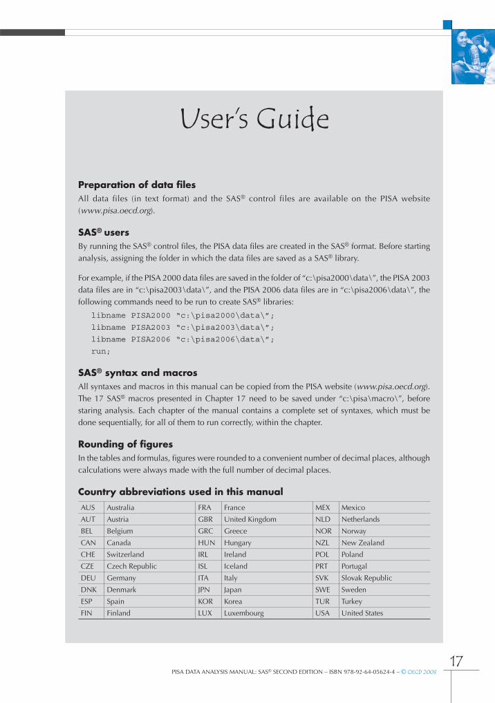
17PISA DATA ANALYSIS MANUAL: SAS® SECOND EDITION – ISBN 978-92-64-05624-4 – © OECD 2009
User’s Guide
Preparation of data filesAll data files (in text format) and the SAS® control files are available on the PISA website(www.pisa.oecd.org).
SAS® usersBy running the SAS® control files, the PISA data files are created in the SAS® format. Before startinganalysis, assigning the folder in which the data files are saved as a SAS® library.
For example, if the PISA 2000 data files are saved in the folder of “c:\pisa2000\data\”, the PISA 2003data files are in “c:\pisa2003\data\”, and the PISA 2006 data files are in “c:\pisa2006\data\”, thefollowing commands need to be run to create SAS® libraries:
libname PISA2000 “c:\pisa2000\data\”;
libname PISA2003 “c:\pisa2003\data\”;
libname PISA2006 “c:\pisa2006\data\”;
run;
SAS® syntax and macrosAll syntaxes and macros in this manual can be copied from the PISA website (www.pisa.oecd.org).The 17 SAS® macros presented in Chapter 17 need to be saved under “c:\pisa\macro\”, beforestaring analysis. Each chapter of the manual contains a complete set of syntaxes, which must bedone sequentially, for all of them to run correctly, within the chapter.
Rounding of figuresIn the tables and formulas, figures were rounded to a convenient number of decimal places, althoughcalculations were always made with the full number of decimal places.
Country abbreviations used in this manualAUS Australia FRA France MEX Mexico
AUT Austria GBR United Kingdom NLD Netherlands
BEL Belgium GRC Greece NOR Norway
CAN Canada HUN Hungary NZL New Zealand
CHE Switzerland IRL Ireland POL Poland
CZE Czech Republic ISL Iceland PRT Portugal
DEU Germany ITA Italy SVK Slovak Republic
DNK Denmark JPN Japan SWE Sweden
ESP Spain KOR Korea TUR Turkey
FIN Finland LUX Luxembourg USA United States
From:PISA Data Analysis Manual: SAS, Second Edition
Access the complete publication at:https://doi.org/10.1787/9789264056251-en
Please cite this chapter as:
OECD (2009), “Use of Proficiency Levels”, in PISA Data Analysis Manual: SAS, Second Edition, OECDPublishing, Paris.
DOI: https://doi.org/10.1787/9789264056251-10-en
This work is published under the responsibility of the Secretary-General of the OECD. The opinions expressed and argumentsemployed herein do not necessarily reflect the official views of OECD member countries.
This document and any map included herein are without prejudice to the status of or sovereignty over any territory, to thedelimitation of international frontiers and boundaries and to the name of any territory, city or area.
You can copy, download or print OECD content for your own use, and you can include excerpts from OECD publications,databases and multimedia products in your own documents, presentations, blogs, websites and teaching materials, providedthat suitable acknowledgment of OECD as source and copyright owner is given. All requests for public or commercial use andtranslation rights should be submitted to [email protected]. Requests for permission to photocopy portions of this material forpublic or commercial use shall be addressed directly to the Copyright Clearance Center (CCC) at [email protected] or theCentre français d’exploitation du droit de copie (CFC) at [email protected].


![STCQE=UWX[]U: - OECD iLibrary](https://img.dokumen.tips/doc/110x75/6319bb481e5d335f8d0b47fd/stcqeuwxu-oecd-ilibrary.jpg)


