Embed Size (px)
Citation preview

Copyright* ©* and* Moral* Rights* for* this* thesis* and,* where* applicable,* any* accompanying* data* are*retained*by*the*author*and/or*other*copyright*owners.**A*copy*can*be*downloaded*for*personal*non>commercial*research*or*study,*without*prior*permission*or*charge.**This*thesis*and*the*accompanying*data*cannot*be*reproduced*or*quoted*extensively*from*without*first*obtaining*permission* in*writing*from* the* copyright* holder/s.* * The* content* of* the* thesis* and* accompanying* research* data* (where*applicable)*must*not*be*changed*in*any*way*or*sold*commercially* in*any*format*or*medium*without*the*formal*permission*of*the*copyright*holder/s.*
When*referring*to*this*thesis*and*any*accompanying*data,*full*bibliographic*details*must*be*given:*
Thesis:* Marina* Costa* Rillo* (2019)* “Unravelling* macroecological* patterns* in* extant* planktonic*Foraminifera”,*University*of*Southampton,*Ocean*and*Earth*Science,*PhD*Thesis,*pages*1>146.**
UNIVERSITY OF SOUTHAMPTON
Faculty of Natural and Environmental Sciences
Ocean and Earth Science
Unravelling macroecological patterns inextant planktonic Foraminifera
by
Marina Costa Rillo
ORCID ID 0000-0002-2471-0002
A thesis submitted for the degree ofDoctor of Philosophy
July 2019
SupervisorThomas H. G. Ezard
Co-supervisorsC. Giles MillerAndy PurvisMichal Kučera
The research presented in this thesis was carried out at the Natural History Museum in London, theNational Oceanography Centre in Southampton (NOCS) and the Center for Marine EnvironmentalSciences (MARUM) in Bremen. This research was financed by the Graduate School of NOCS, Universityof Southampton (3 years) and the German Academic Exchange Service (DAAD) grant number 2016/1757210260 (10 months).
Ao meu pai, Marcio Rillo (in memoriam)


Nature, it seems, is more like a jazz ensemble than a symphony orchestra.(Oswald J. Schmitz, 2018)

UNIVERSITY OF SOUTHAMPTON
ABSTRACT
FACULTY OF NATURAL AND ENVIRONMENTAL SCIENCESOCEAN AND EARTH SCIENCE
Doctor of Philosophy
UNRAVELLING MACROECOLOGICAL PATTERNS IN EXTANT PLANKTONIC FORAMINIFERA
Marina Costa Rillo
Present-day ecological communities and the deep-time fossil record both inform us about the processesthat give rise to, and maintain, diversity of life on Earth. However, these two domains differ in temporal,spatial and taxonomic scales. Integrating these scales remains amajor challenge in biodiversity research,mainly because the fossil record gives us an incomplete picture of the extinct communities. PlanktonicForaminifera provide an excellent model system to integrate present and past changes in biodiversity.They are single-celled marine zooplankton that produce calcite shells, yielding a remarkably completefossil record across millions of years, and are alive today enabling genetic and ecological studies. Theirfossil record has been widely used in the fields of stratigraphy and palaeoclimate. However, we havelimited knowledge about their ecology, preventing us from fully understanding the evolutionary pro-cesses that shaped their diversity through time. The primary objective of this thesis is to improve ourunderstanding of community ecology of extant planktonic Foraminifera species, to enable us to morecomprehensively study their fossil record. I created a large image dataset of over 16,000 individualsfrom a historical museum collection (Chapter 2) and assessed its potential biases (Chapter 3). Using thedata gathered from the collection, I investigated the extent to which individuals of the same species varyin shell size (Chapter 4). Size relates to many physiological and ecological characteristics of an organism,thus understanding how it varies within species and across space gives us insights about the function ofthe species in the ecosystem. Planktonic Foraminifera species greatly differ in howmuch size variation isexplained by environmental (temperature and productivity) and/or ecological (local relative abundance)conditions, suggesting that the known pattern of large size at favourable conditions is not widespread inthe group. Next, I explored how planktonic Foraminifera species interact with each other in ecologicalcommunities (Chapter 5). Their fossil record suggests that competition among species is an importantecological interaction limiting the number of species that can emerge within the group. I tested whetherspecies are competing today in the oceans, and found no evidence for negative interactions. This resultsuggests that either the ecological processes acting on communities today are different than the onesdriving planktonic Foraminifera evolution, or that competition among species did not shape the patternswe observe in their fossil record. Together, these discoveries extend our current understanding of plank-tonic Foraminifera biology and highlight the complexity of ecological dynamics. Future work using theplanktonic Foraminifera fossil record to understand marine biodiversity changes will require scientificresearch across different scales as well as considering other interacting plankton groups.

Contents
List of Figures xi
List of Tables xiii
Declaration of Authorship xv
Acknowledgements xvii
1 Introduction 11.1 Macroecology . . . . . . . . . . . . . . . . . . . . . . . . . . . . . . . . . . . . . . . . 2
1.1.1 Community ecology . . . . . . . . . . . . . . . . . . . . . . . . . . . . . . . . 31.1.2 Macroevolution . . . . . . . . . . . . . . . . . . . . . . . . . . . . . . . . . . . 41.1.3 The bridge between community ecology and macroevolution . . . . . . . . . . 4
1.2 Planktonic Foraminifera . . . . . . . . . . . . . . . . . . . . . . . . . . . . . . . . . . . 51.2.1 Origin and Taxonomy . . . . . . . . . . . . . . . . . . . . . . . . . . . . . . . . 51.2.2 Diversity . . . . . . . . . . . . . . . . . . . . . . . . . . . . . . . . . . . . . . . 61.2.3 Physiology and Ecology . . . . . . . . . . . . . . . . . . . . . . . . . . . . . . . 71.2.4 Macroecological patterns . . . . . . . . . . . . . . . . . . . . . . . . . . . . . . 81.2.5 Macroevolutionary patterns . . . . . . . . . . . . . . . . . . . . . . . . . . . . 10
1.3 The importance of natural history collections . . . . . . . . . . . . . . . . . . . . . . . 131.4 A narrative overview of this thesis . . . . . . . . . . . . . . . . . . . . . . . . . . . . . 14
2 The unknown planktonic foraminiferal pioneer Henry A. Buckley and his collection at The Nat-ural History Museum, London 172.1 Historical Background . . . . . . . . . . . . . . . . . . . . . . . . . . . . . . . . . . . . 192.2 The Henry Buckley Collection of Planktonic Foraminifera . . . . . . . . . . . . . . . . . 21
2.2.1 Slide Collection . . . . . . . . . . . . . . . . . . . . . . . . . . . . . . . . . . . 212.2.2 Scanning Electron Microscope Photomicrographs . . . . . . . . . . . . . . . . . 232.2.3 Digitisation of the Buckley Slide Collection . . . . . . . . . . . . . . . . . . . . . 23
2.3 Future Use of the Collection . . . . . . . . . . . . . . . . . . . . . . . . . . . . . . . . 24
3 Surface sediment samples from early age of seafloor exploration can provide a late 19th cen-tury baseline of the marine environment 273.1 Introduction . . . . . . . . . . . . . . . . . . . . . . . . . . . . . . . . . . . . . . . . . 293.2 Material and Methods . . . . . . . . . . . . . . . . . . . . . . . . . . . . . . . . . . . 30
3.2.1 Historical samples . . . . . . . . . . . . . . . . . . . . . . . . . . . . . . . . . 303.2.2 Holocene and Last Glacial Maximum data . . . . . . . . . . . . . . . . . . . . . 313.2.3 Compositional similarity . . . . . . . . . . . . . . . . . . . . . . . . . . . . . . 33
3.3 Results and Discussion . . . . . . . . . . . . . . . . . . . . . . . . . . . . . . . . . . . 343.4 Conclusion . . . . . . . . . . . . . . . . . . . . . . . . . . . . . . . . . . . . . . . . . . 37
ix
x CONTENTS
4 Biogeographical patterns of intraspecific size variation in extant planktonic Foraminifera 394.1 Introduction . . . . . . . . . . . . . . . . . . . . . . . . . . . . . . . . . . . . . . . . . 414.2 Material and Methods . . . . . . . . . . . . . . . . . . . . . . . . . . . . . . . . . . . 44
4.2.1 Study sites and samples . . . . . . . . . . . . . . . . . . . . . . . . . . . . . . 444.2.2 Shell size data . . . . . . . . . . . . . . . . . . . . . . . . . . . . . . . . . . . . 454.2.3 Sea-surface temperature data . . . . . . . . . . . . . . . . . . . . . . . . . . . 484.2.4 Net-primary productivity data . . . . . . . . . . . . . . . . . . . . . . . . . . . 494.2.5 Relative abundance data . . . . . . . . . . . . . . . . . . . . . . . . . . . . . . 494.2.6 Statistical analysis . . . . . . . . . . . . . . . . . . . . . . . . . . . . . . . . . . 50
4.3 Results . . . . . . . . . . . . . . . . . . . . . . . . . . . . . . . . . . . . . . . . . . . . 514.4 Discussion . . . . . . . . . . . . . . . . . . . . . . . . . . . . . . . . . . . . . . . . . . 56
4.4.1 Limitations . . . . . . . . . . . . . . . . . . . . . . . . . . . . . . . . . . . . . 574.5 Conclusion . . . . . . . . . . . . . . . . . . . . . . . . . . . . . . . . . . . . . . . . . . 59
5 On themismatch in the strength of competition among fossil andmodern species of planktonicForaminifera 615.1 Introduction . . . . . . . . . . . . . . . . . . . . . . . . . . . . . . . . . . . . . . . . . 635.2 Material and Methods . . . . . . . . . . . . . . . . . . . . . . . . . . . . . . . . . . . 66
5.2.1 Spatial data . . . . . . . . . . . . . . . . . . . . . . . . . . . . . . . . . . . . . 665.2.2 Temporal data . . . . . . . . . . . . . . . . . . . . . . . . . . . . . . . . . . . 685.2.3 Ecological similarity data . . . . . . . . . . . . . . . . . . . . . . . . . . . . . . 685.2.4 Community phylogenetics analysis (spatial data) . . . . . . . . . . . . . . . . . 705.2.5 Time series analysis (temporal data) . . . . . . . . . . . . . . . . . . . . . . . . 72
5.3 Results . . . . . . . . . . . . . . . . . . . . . . . . . . . . . . . . . . . . . . . . . . . . 735.3.1 Community phylogenetics (spatial data) . . . . . . . . . . . . . . . . . . . . . . 735.3.2 Time series (temporal data) . . . . . . . . . . . . . . . . . . . . . . . . . . . . 75
5.4 Discussion . . . . . . . . . . . . . . . . . . . . . . . . . . . . . . . . . . . . . . . . . . 765.4.1 Spatial patterns . . . . . . . . . . . . . . . . . . . . . . . . . . . . . . . . . . . 765.4.2 Temporal patterns . . . . . . . . . . . . . . . . . . . . . . . . . . . . . . . . . 785.4.3 Mismatch between macroevolutionary and community dynamics . . . . . . . . 80
6 Conclusion 856.1 Synthesis . . . . . . . . . . . . . . . . . . . . . . . . . . . . . . . . . . . . . . . . . . 856.2 Future directions . . . . . . . . . . . . . . . . . . . . . . . . . . . . . . . . . . . . . . 866.3 Concluding remarks . . . . . . . . . . . . . . . . . . . . . . . . . . . . . . . . . . . . . 87
A Supplement to Chapter 3 89
B Supplement to Chapter 4 93
C Supplement to Chapter 5 105
References 117
Curriculum Vitae 147
List of Figures
1.1 Physical, chemical, physiological and ecological factors affecting the fitness of a single-celled zooplankton . . . . . . . . . . . . . . . . . . . . . . . . . . . . . . . . . . . . . 2
1.2 Global diversity patterns of extant planktonic Foraminifera . . . . . . . . . . . . . . . . 9
2.1 Example of the contents of the Henry Buckley Collection . . . . . . . . . . . . . . . . . 202.2 Map with the sample sites of the Henry Buckley Collection . . . . . . . . . . . . . . . . 232.3 Henry Alexander Buckley . . . . . . . . . . . . . . . . . . . . . . . . . . . . . . . . . . 252.4 Scanning electron microscope Cambridge Stereoscan Mk II . . . . . . . . . . . . . . . . 25
3.1 Map and sea surface temperature annual mean of historical sample sites and corre-sponding neighbouring sites of the Holocene and Last Glacial Maximum data . . . . . . 32
3.2 (A) Compositional similarity between planktonic Foraminifera assemblages of historical,Holocene and Last Glacial Maximum (LGM) samples. (B) Global compositional similarity(temporal turnover) between Holocene and LGM . . . . . . . . . . . . . . . . . . . . . 35
3.3 Compositional similarity (Holocene to LGM temporal turnover) plotted against local es-timates of open-ocean sedimentation rates . . . . . . . . . . . . . . . . . . . . . . . . 36
3.4 Ocean-floor sediment sample collected by HMS Challenger . . . . . . . . . . . . . . . . 38
4.1 (A) Map of shell size data of modern planktonic Foraminifera species(B) A representative specimen from each species analysed . . . . . . . . . . . . . . . . 44
4.2 Shell size histograms for each species of planktonic Foraminifera present in the morpho-metric dataset . . . . . . . . . . . . . . . . . . . . . . . . . . . . . . . . . . . . . . . . 47
4.3 Bias analysis: difference in shell size distributions between populations of the samplesre-sampled by us and of the samples from the Buckley Collection . . . . . . . . . . . . . 48
4.4 Boxplots of individual shell area measurements for each sample for each planktonicForaminifera species . . . . . . . . . . . . . . . . . . . . . . . . . . . . . . . . . . . . 52
4.5 Planktonic Foraminifera shell size plotted against (a) sea surface temperature, (b) netprimary productivity and (c) species’ relative abundance . . . . . . . . . . . . . . . . . 53
4.6 Relationship between annual mean sea-surface temperature and net-primary productivity 554.7 (A) Sea surface temperatures where planktonic Foraminifera species reach maximum
shell size and maximum relative abundance in the sediment(B) Relationship between maximum shell size (logarithmic scale) and maximum relativeabundance of each species. . . . . . . . . . . . . . . . . . . . . . . . . . . . . . . . . . 55
4.8 Washed ocean-floor sediment sample collected by HMS Challenger . . . . . . . . . . . 60
5.1 Number of species of planktonic Foraminifera through time and the diversification rateper million year time bin . . . . . . . . . . . . . . . . . . . . . . . . . . . . . . . . . . 67
5.2 (A) Map of modern planktonic Foraminifera abundance data (sediment traps and ocean-floor core samples). (B) Latitudinal richness gradient of planktonic Foraminifera basedon the coretop samples . . . . . . . . . . . . . . . . . . . . . . . . . . . . . . . . . . . 67
5.3 Schematic figure showing the two different types of data used in the analyses: sedimenttraps and ocean-floor core samples . . . . . . . . . . . . . . . . . . . . . . . . . . . . . 69
xi
xii LIST OF FIGURES
5.4 Spatial data: net relatedness index and nearest taxon index calculated for 3,053 plank-tonic Foraminifera coretop assemblages based on 100 runs of the null model ‘richness’,plotted against annual mean sea-surface temperature at each site . . . . . . . . . . . . 74
5.5 Temporal data: pairwise time-series correlations of planktonic Foraminifera abundancesplotted by sediment trap. Values show the standardised size effect of the correlationbased on the null seasonality model . . . . . . . . . . . . . . . . . . . . . . . . . . . . 76
5.6 Temporal data: pairwise time-series correlations of planktonic Foraminifera abundancesplotted (a) against phylogenetic distance between species in million of years, (b) againstshell size difference between species, and (c) by the photosymbiotic ecological strategyof the species pair. Values show the standardised size effect of the correlation based onthe null seasonality model . . . . . . . . . . . . . . . . . . . . . . . . . . . . . . . . . 77
5.7 Positive significant relationship between speciation and extinction rates of planktonic-Foraminifera Cenozoic macroperforate species . . . . . . . . . . . . . . . . . . . . . . . 81
B.1 Residual plots of linear models per species . . . . . . . . . . . . . . . . . . . . . . . . . 103
C.1 Phylogeny of extant planktonic Foraminifera macroperforate species . . . . . . . . . . . 105C.2 Boxplots of individual shell diameter measurements for each planktonic Foraminifera
species . . . . . . . . . . . . . . . . . . . . . . . . . . . . . . . . . . . . . . . . . . . . 108C.3 Spatial data: net relatedness index and nearest taxon index calculated for 3,053 plank-
tonic Foraminifera coretop assemblages based on 100 runs of the null model ‘taxa’,plotted against sea surface temperature annual mean at each site . . . . . . . . . . . . 109
C.4 Spatial data: net relatedness index and nearest taxon index calculated for 3,053 plank-tonic Foraminifera coretop assemblages based on 100 runs of the null model ‘richness’,plotted against species richness in each assemblage . . . . . . . . . . . . . . . . . . . . 110
C.5 Spatial data: net relatedness index and nearest taxon index calculated for 3,053 plank-tonic Foraminifera coretop assemblages based on 100 runs of the null model ‘richness’,plotted against abundance-weighted community size . . . . . . . . . . . . . . . . . . . 111
C.6 Spatial data: net nearest taxon index calculated for 3,053 planktonic Foraminifera core-top assemblages based on 100 runs of the null model ‘richness’, plotted against the rel-ative abundance of the large species Globorotalia menardii . . . . . . . . . . . . . . . . 111
C.7 Temporal data, first differences: pairwise correlations between the differentiated time-series of planktonic Foraminifera abundances . . . . . . . . . . . . . . . . . . . . . . . 112
C.8 Temporal data: schematic explanation of the time-series analysis. . . . . . . . . . . . . 114C.9 Temporal data: correlation between the observed time-series and its spline-series for
each species in each sediment trap, representing species’ local seasonality . . . . . . . 115C.10 Temporal data, interannual variation: length (in years) of sediment trap sampling as a
function of mean correlation among the species’ residual-series (i.e., original time-seriesminus its spline-series) . . . . . . . . . . . . . . . . . . . . . . . . . . . . . . . . . . . 115
List of Tables
2.1 Overview of the slide contents of the Henry Buckley Collection . . . . . . . . . . . . . . 222.2 Modern specimens of the Henry Buckley Collection. The table shows the species’ name
(original and revised), ordered by the number of mounted specimens in the slide collec-tion, and the number of geographical sites from which these specimens came. . . . . . 22
3.1 Information about the historical sediment samples from the Ocean BottomDeposits Col-lection . . . . . . . . . . . . . . . . . . . . . . . . . . . . . . . . . . . . . . . . . . . . 31
3.2 Historical surface sediments collections . . . . . . . . . . . . . . . . . . . . . . . . . . 37
4.1 Overview of the morphometric dataset extracted from the Henry Buckley Collection . . 464.2 Model selection of the linear and quadratic models testing the relationship between
planktonic Foraminifera shell size, sea surface temperature, net primary productivity andspecies’ relative abundance . . . . . . . . . . . . . . . . . . . . . . . . . . . . . . . . . 54
A.1 Planktonic Foraminifera species counts in the nine historical samples . . . . . . . . . . . 89A.2 Relative abundance of planktonic Foraminifera species in the historical, Holocene and
Last Glacial Maximum samples, part 1 . . . . . . . . . . . . . . . . . . . . . . . . . . . 90A.3 Relative abundance of planktonic Foraminifera species in the historical, Holocene and
Last Glacial Maximum samples, part 2 . . . . . . . . . . . . . . . . . . . . . . . . . . . 91A.4 Relative abundance of planktonic Foraminifera species in the historical, Holocene and
Last Glacial Maximum samples, part 3 . . . . . . . . . . . . . . . . . . . . . . . . . . . 92
B.1 Bias analysis: samples re-sampled from the Ocean-Bottom Deposits Collection at usedin the bias analysis . . . . . . . . . . . . . . . . . . . . . . . . . . . . . . . . . . . . . 94
B.2 Bias analysis: linear mixed-effects model (LMER) testing for a relationship between sizevariation and relative abundance of species . . . . . . . . . . . . . . . . . . . . . . . . 94
B.3 Samples from the Henry Buckley Collection . . . . . . . . . . . . . . . . . . . . . . . . 95B.4 Analysis considering ForCenS samples within a 300 km distance: model selection of the
linear and quadratic models testing the relationship between planktonic Foraminiferashell size, sea surface temperature, net primary productivity and species’ relative abun-dance . . . . . . . . . . . . . . . . . . . . . . . . . . . . . . . . . . . . . . . . . . . . 96
B.5 Analysis excluding historical samples collected by dredging the ocean floor. Model se-lection of the linear and quadratic models testing the relationship between planktonicForaminifera shell size, sea surface temperature, net primary productivity and species’relative abundance . . . . . . . . . . . . . . . . . . . . . . . . . . . . . . . . . . . . . 97
B.6 List of all modern species present in the sediment samples of the Buckley Collection . . 98B.7 Dissolution analysis: linearmixed-effectsmodel (LMER) testing if dissolution affected our
results . . . . . . . . . . . . . . . . . . . . . . . . . . . . . . . . . . . . . . . . . . . . 98
C.1 Average size of planktonic Foraminifera species . . . . . . . . . . . . . . . . . . . . . . 107C.2 Temporal data: meta-data of the sediment traps used in the study . . . . . . . . . . . . 113
xiii

Declaration of Authorship
I, Marina Costa Rillo, declare that this thesis entitled Unravelling macroecological patterns in extantplanktonic Foraminifera and the work presented in it are my own and has been generated by me asthe result of my own original research.
I confirm that:
1. This work was done wholly or mainly while in candidature for a research degree at this University;
2. Where any part of this thesis has previously been submitted for a degree or any other qualificationat this University or any other institution, this has been clearly stated;
3. Where I have consulted the published work of others, this is always clearly attributed;
4. Where I have quoted from the work of others, the source is always given. With the exception ofsuch quotations, this thesis is entirely my own work;
5. I have acknowledged all main sources of help;
6. Where the thesis is based on work done by myself jointly with others, I have made clear exactlywhat was done by others and what I have contributed myself;
7. Either none of this work has been published before submission, or parts of this work have beenpublished as: Rillo et al. 2016; Rillo et al. 2019.
Signed:
Date:
xv

Acknowledgements
The doctoral research is a long journey, in which you know the starting point but seldom know the final destination.This journey is not only academic, but also very personal. Thus, the inspiration and encouragement to pursue a PhDhave come from many sources, which I would like to acknowledge here.
My PhD supervisors: Tom,whoprovidedme the freedom to intellectuallywander the fields of ecology and evolution,and to become a ’foram’ person! Giles, who taught me to love museums and was always so present and supportive.Andy, who inspired me in the early years of my PhD with his biological knowledge and excitement about forams.And Michal, who taught me almost everything I know about planktonic Foraminifera with such a genuine passion -thank you for welcoming me in Bremen!
I will always be grateful to Isabel for all the insightful discussions, great suggestions, late-night proofreadings and forthe friendship - hopefully we will still go to Dartmoor together! And to Anieke, for all her support, friendship andpatience (especially with my Image-Pro Premier skills!) - thank you, it truly made a difference during my PhD.
During these four years I lived in four cities: London, Southampton, Bremen andGroningen. Imade friends in each ofthem, who undoubtedly made my PhD journey more enjoyable. Isabel and Susy were my macroevolution buddiesback at the NHM, and of course lunches with Steve were always amusing! In Southampton, I lived with the besthousemates I could have ever dreamt of - especially Anieke, Helen and Jesse - I had so much fun! Amy and Loretomade the office at NOCS feel very homey. At MARUM, it was lovely to share the office with Christiane, and to meetRaph, Lukas and Siccha. Dharma and Diana brought me some latin warmth during the rainy days in Bremen. InGroningen, life was a bit more secluded, as the writing up stage begun, but at the same time I finally felt homeagain, six years after having left Brazil - thank you family Ekkers for all the gezelligheid!
My friends from the MEME masters, Sergio, Miya, Lore and Bere, it is comforting to know we are all still ‘on thesame boat’, far away from home, trying to make a living out of our passion for science. Hopefully we will have moretime to see each other in our new post-PhD lives!
My friends from the Univesity of São Paulo, Toshiba, obrigada por todos os cafés 23h/8h, todo o otimismo “tu já tápronta!” e pelo paper dos bróders! Gê, minha BBF que escutou feliz todos os meus monólogos de 20 min duranteesses 4 anos. Mica, SV, Yoshi, Joseph e Samurai, que a leitura de Darwin dure pro resto de nossas vidas! Marinis,Drika, Piru, Nescau, Gabi, Xurrus e Laura amo cada um de vocês, o Zubileide me trouxe (e traz!) muito amor eenergia! Kate, não sei como teria sido esse doutorado sem poder reclamar com você - obrigada por compartilhartodas as minhas frustações. E Paulo Inácio, orientador da vida, obrigada pelo apoio e todos os conselhos.
My parents, Anna Helena and Marcio, are the main reason why I chose to become a scientist. Both scientists them-selves, their critical thinking and curiosity shaped who I am. Obrigada, mãe, por toda a torcida, apoio e amor! Epai, te tenho sempre no coração. My sister, Regina, for being by my side in all the happy and sad moments wehad together - irmãzinha do coração, obrigada por existir (e também por resolver todos meus IRs nesses anos dedoutorado). E obrigada pro choconhado por sempre nos receber tão bem em São Paulo!
My life and PhD-crises partner, David, thank you for believing in me and in my work invariably. Your love and opti-mism were my safe-place during these four years. I would not have made it without you.
xvii

Chapter 1
Introduction
There is a mind-blowing variety of life on Earth. Recent estimates predict that 8.7 million (± 1.3 million)eukaryotic species inhabit the Earth today (Mora et al., 2011), and this estimate does not even includethe much older and more diverse Archaea and Bacteria domains of life (Hug et al., 2016). It remains achallenge to understand the ecological and evolutionary processes that give rise to andmaintain this richbiodiversity. Scientific research is often inclined to seek simple and general explanations for observedpatterns (Kinnison et al., 2015). However, ecology and evolution are characterised by complexmultilevelprocesses, and finding general and predictive rules to explain biodiversity has proven difficult (Evanset al., 2012).
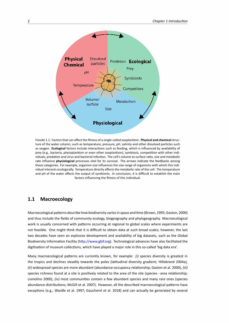
Biological systems are subject to many dynamical factors, with each of the factors affecting and some-times driving the observed patterns. Therefore, one has to consider multiple variables rather than focuson a single onewhen studying these patterns. This principle, which prevents the development of generalrules applicable to different biological systems, was pointed out by Brian McGill as ‘multicausality’ in hisblog post on “Why ecology is hard (and fun)”1. To understand what multicausality means in ecology,McGill proposes a simple exercise: try to sketch all the factors affecting the life of an organism. Let usfocus on a single-celled calcareous zooplankton in the middle of the ocean. Which factors are affectingthe fitness of this individual? These factors can be divided into three broad categories: physical/chem-ical, physiological and ecological (Fig. 1.1). The “hard (and fun)” part of ecology is to try to calculatethe relative contribution of each of these factors to the fitness of this individual, considering that theenvironmental conditions and the strength of ecological interactions are dynamic, so the relative impactof each varies through time. We definitely do not have a short list of the major causes affecting thisindividual’s life.
Instead of abandoning all hope and claiming nothing generalises beyond an individual system, we can tryto deal with this complexity by zooming out of the individual level and looking at biodiversity patternsat large spatial and temporal scales. Macroecology comes as a large-scale pattern-oriented approachto seek generality in ecology and unveil the mechanisms underlying the structure and functioning ofcommunities and ecosystems (Marquet, 2009). By statistically describing macro-biodiversity patterns,we can build the empirical foundations from which deductive and prediction-rich ecological and evolu-tionary hypotheses emerge.
1Weblink (accessed in July 2018): https://dynamicecology.wordpress.com
1
2 Chapter 1 Introduction
FIGURE 1.1: Factors that can affect the fitness of a single-celled zooplankton. Physical and chemical struc-ture of the water column, such as temperature, pressure, pH, salinity and other dissolved particles suchas oxygen. Ecological factors include interactions such as feeding, which is influenced by availability ofprey (e.g., bacteria, phytoplankton or even other zooplankton), symbiosis, competition with other indi-viduals, predation and virus and bacterial infection. The cell’s volume to surface ratio, size and metabolicrate influence physiological processes vital for its survival. The arrows indicate the feedbacks amongthese categories. For example, organism size influences the size range of organisms with which this indi-vidual interacts ecologically. Temperature directly affects the metabolic rate of the cell. The temperatureand pH of the water affects the output of symbionts. In conclusion, it is difficult to establish the main
factors influencing the fitness of this individual.
1.1 Macroecology
Macroecological patterns describe howbiodiversity varies in space andtime (Brown, 1995; Gaston, 2000)and thus include the fields of community ecology, biogeography and phylogeography. Macroecologicalwork is usually concerned with patterns occurring at regional to global scales where experiments arenot feasible. One might think that it is difficult to obtain data at such broad scales; however, the lasttwo decades have seen an explosive development and availability of big datasets, such as the GlobalBiodiversity Information Facility (http://www.gbif.org). Technological advances have also facilitated thedigitisation of museum collections, which have played a major role in this so-called ‘big data era’.
Many macroecological patterns are currently known, for example: (i) species diversity is greatest inthe tropics and declines steadily towards the poles (latitudinal diversity gradient; Hillebrand 2004a),(ii) widespread species are more abundant (abundance-occupancy relationship; Gaston et al. 2000), (iii)species richness found at a site is positively related to the area of the site (species�area relationship;Lomolino 2000), (iv) most communities contain a few abundant species and many rare ones (speciesabundance distributions; McGill et al. 2007). However, all the described macroecological patterns haveexceptions (e.g., Wardle et al. 1997; Gaucherel et al. 2018) and can actually be generated by several
Chapter 1 Introduction 3
different causal pathways (Levins and Lewontin, 1980). Progress in understanding can be advanced bydetermining the conditions under which a given pattern occurs or not (Vellend, 2016).
Most macroecological patterns have been described on the terrestrial biota, making marine macroecol-ogy a relatively new quantitative science (Witman and Roy, 2009; Webb, 2012). Interest in quantifyingand understanding large-scale marine diversity patterns has been rapidly increasing over the last twodecades, following technological innovations in the fields of engineering and molecular biology (e.g.,Danovaro et al. 2014; De Vargas et al. 2015). Macroecological patterns in the oceans can differ to theones described on land (Webb, 2012). For example, the latitudinal diversity gradient in the oceans showshigher diversity at mid-latitudinal bands instead of in the tropics (Tittensor et al. 2010; Sunagawa et al.2015), but this pattern may vary depending on the studied group (Roy et al., 2000; Hillebrand, 2004b;Tittensor et al., 2010). Moreover, a longitudinal diversity gradient is observed, where coastal speciesshowmaximumdiversity in theWestern Pacific (Indo-Australian Archipelago; Renema et al. 2008; Titten-sor et al. 2010).
The great advantage of studying ecology on such broad scales, is that it emphasises the role of evolu-tionary and historical processes in shaping present-day biodiversity patterns (Marquet, 2009; Vellend,2016). By acknowledging that the processes of natural selection, drift, dispersal, and speciation are cen-tral in the dynamics of ecological communities (Vellend, 2010; Fritz et al., 2013), macroecology providesa framework to bridge the fields of community ecology and macroevolution. These fields have longdiffered in temporal, spatial and taxonomic scales (Vellend, 2010; Weber et al., 2017), but together seekto understand the processes generating and maintaining biodiversity.
1.1.1 Community ecology
Community ecology focuses on local and regional processes affecting patterns in the diversity, abun-dance, and composition of species in ecological communities (Vellend, 2010). Communities can be stud-ied at many different spatial scales and, consequently, be defined in many ways (Vellend, 2016). There-fore, the field of community ecology can include the fields of biogeography, macroecology2 and paleoe-cology. Here, I use the definition that an ecological community includes species that directly or indirectlyinteract, and thus the populations of these species should overlap in space and time (see Vellend 2016).When studied at the macroecological scale, population level processes underlie species level patterns,such as geographic range, population size and density, which, in turn, are known to affect species di-versification in deep time (i.e., macroevolution; reviewed in Jablonski 2008b). Therefore, macroecol-ogy expands the spatial and temporal scale of community ecology and brings it closer to the field ofmacroevolution.
2I chose to use ‘macroecological patterns’ instead of ‘community ecology patterns’ in the title of my thesis because I studiedthe biogeography of organism size, and community ecology traditionally focuses on number of individuals and abundance insteadof morphology.
4 Chapter 1 Introduction
1.1.2 Macroevolution
Macroevolution focuses on the processes of speciation and extinction acting over long time spans, whichcreated the biodiversity we observe, assembled into ecological communities (Schluter, 2013). In contrastto evolutionary biology fields that focus on genetic changes in populations from one generation to thenext (i.e., microevolution), macroevolution zooms out to the tree of life, investigating the diversity atand above the species level, focusing on entire clades (i.e., lineages that share a common ancestry). Thetemporal scale of macroevolutionary processes is geological time (i.e., millions of years). The spatialscale of macroevolution can be continental (terrestrial; e.g. Pires et al. 2015), provincial (marine; e.g.Renema et al. 2008) or global (e.g., Benson et al. 2014; Rabosky et al. 2018). Finer temporal and spatialscales are usually unattainable. Nevertheless, macroevolution and macroecology share a similar spatialscale, and the processes underlying macroecological patterns are directly linked to macroevolutionaryprocesses (Mittelbach et al., 2007; Schluter and Pennell, 2017; Rabosky et al., 2018).
Macroevolution can be studied using molecular phylogenies of extant species (neontological approach)or the fossil record (palaeontological approach). Molecular phylogenies allow an explicit test of the evo-lutionary relationships among lineages, whereas the fossil record enables a more direct assessment ofhow diversity changed through time (i.e., diversity trajectories; Quental and Marshall 2010) and estima-tion of extinction and speciation rates (Foote, 2000). Integrating both the palaeontological and neonto-logical approaches is the best way to study the dynamics of biodiversity (Quental and Marshall, 2010;Fritz et al., 2013). However, molecular studies on extinct taxa are usually not feasible, and only sometraits of certain organisms are preserved in the fossil record. It has been estimated that probably lessthan 10% of the biota is represented in the fossil record (Forey et al., 2004).
1.1.3 The bridge between community ecology and macroevolution
The coarser temporal and spatial scale of macroevolution and the lack of longer temporal perspectivein community ecology have prevented the integration of these two fields (Fritz et al., 2013; Yasuharaet al., 2015). However, ecological interactions, which happen at the community scale, are known toshape species’ population dynamics, alter natural selection, and impact trait evolution and lineage di-versification (Jablonski, 2008b). Species evolution and diversification, in turn, influence how speciesinteract with the environment and with each other, affecting the dynamics of ecological communities(Fussmann et al., 2007; Schoener, 2011). Thus, eco-evolutionary feedbacks are at the core of the mech-anisms generating and maintaining biodiversity, making the disconnection between community ecologyand macroevolution artificial.
Besides the different temporal and spatial scales, different taxonomic scales also challenge the integra-tion of macroevolution and community ecology. Community ecology focuses on the population level,studying abundances of interacting species that can belong to distantly related clades. Macroevolution,in turn, focuses on patterns above the species level, studying diversification of species, genera or families,that are usually phylogenetically related. The preservational bias of the fossil record makes the directanalysis of community dynamics in deep time unfeasible for the majority of taxonomic groups (Marshalland Quental, 2016), and thus the connection of population-level ecological processes to macroevolu-tionary processes impossible.
Chapter 1 Introduction 5
Few taxonomic groups have palaeontological data at population level and enough temporal and spatialresolution to connect the mechanisms acting on the community to the macroevolutionary scale. Someexamples includemarine invertebrates (Foote and Sepkoski, 1999) such as ostracodes (Hunt et al., 2017)and bryozoans (Liow et al., 2016), as well as protists such as diatoms, radiolaria, coccolithophores, di-noflagellates and foraminifers (microfossils; reviewed in Yasuhara et al. 2015). Planktonic Foraminiferahave the most complete and abundant fossil record currently known (Kucera, 2007; Ezard et al., 2011)and are, therefore, the most promising model system to integrate community ecology and macroevolu-tion (Yasuhara et al., 2015).
1.2 Planktonic Foraminifera
Planktonic Foraminifera are single-celled eukaryotes (protists) that live as zooplankton throughout theworld’s oceans and produce a calcium carbonate test (or shell; Kucera 2007) around their cells. Upondeath, these shells sink to the ocean floor, accumulating in great numbers and building up an excep-tionally complete fossil record. Planktonic Foraminifera species have at least an 81% chance of beingdetected per million year interval (Ezard et al., 2011), making their species-level fossil record at leastas complete as the best-preserved genus-level records of marine invertebrates (Foote and Sepkoski,1999). Such complete information on the diversity trajectory of a clade is rare and, therefore, plank-tonic Foraminifera are unique for macroevolutionary studies (Ezard et al., 2011; Marshall and Quental,2016). At the sametime, extant species enable genetic and ecological studies, which gives us informationof how these organisms live in the modern oceans, and facilitates the connection between communitiesliving today and millions of years ago. However, there is currently insufficient knowledge of planktonicForaminifera ecology and community dynamics (Yasuhara et al., 2015). It is odd that we know moreabout the fossil record of dead planktonic Foraminifera than we do of the biology of living ones.
The evolutionary history of planktonic Foraminifera can be traced back in high temporal resolution byusing the world wide archive of deep-sea sediment cores, drilled by the Deep Sea Drilling Project (DSDP)and its successors the Ocean Drilling Program (ODP), the Integrated Ocean Drilling Program and theInternational Ocean Discovery Program (IODP). Not surprisingly, planktonic Foraminifera have wide ap-plications in biostratigraphy, because of their abundant and widely distributed fossil record as well asmorphologically distinct, diverse and rapidly-evolving lineages (Wade et al., 2011). Moreover, the cal-cium carbonate of their shells preserves stable isotopes of sea water molecules, which can be used toreconstruct past ocean surface properties and climatic conditions on Earth (i.e., palaeoceanography andpalaeoclimate; Kucera 2007).
1.2.1 Origin and Taxonomy
Foraminifera are an ancient group of protists that first appeared in the fossil record during the Early Cam-brian (Culver, 1991), although genetic data suggest that Foraminiferawere already part of the Proterozoicbiota (Pawlowski et al., 2003). They first appeared in the benthos and expanded into the plankton in theEarly Jurassic (Toarcian; Hart et al. 2003).
Planktonic Foraminifera belong to the eukaryotic supergroup Rhizaria, phylum Foraminifera, classGlobothalamea, order Rotaliida, and the suborder Globigerinida, following the classification of
6 Chapter 1 Introduction
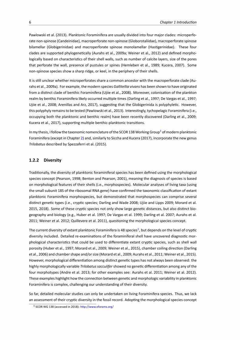
Pawlowski et al. (2013). Planktonic Foraminifera are usually divided into four major clades: microperfo-rate non-spinose (Candeinidae), macroperforate non-spinose (Globorotaliidae), macroperforate spinosebilamellar (Globigerinidae) and macroperforate spinose monolamellar (Hastigerinidae). These fourclades are supported phylogenetically (Aurahs et al., 2009a; Weiner et al., 2012) and defined morpho-logically based on characteristics of their shell walls, such as number of calcite layers, size of the poresthat perforate the wall, presence of pustules or spines (Hemleben et al., 1989; Kucera, 2007). Somenon-spinose species show a sharp ridge, or keel, in the periphery of their shells.
It is still unclear whether microperforates share a common ancestor with the macroperforate clade (Au-rahs et al., 2009a). For example, themodern speciesGallitellia vivans has been shown to have originatedfrom a distinct clade of benthic Foraminifera (Ujiie et al., 2008). Moreover, colonisation of the planktonrealm by benthic Foraminifera likely occurred multiple times (Darling et al., 1997; De Vargas et al., 1997;Ujiie et al., 2008; Arenillas and Arz, 2017), suggesting that the Globigerinida is polyphyletic. However,this polyphyly remains to be tested (Pawlowski et al., 2013). Interestingly, tychopelagic Foraminifera (i.e.,occupying both the planktonic and benthic realm) have been recently discovered (Darling et al., 2009;Kucera et al., 2017), supporting multiple benthic-planktonic transitions.
Inmy thesis, I follow the taxonomic nomenclature of the SCOR138WorkingGroup3 ofmodern planktonicForaminifera (except in Chapter 2) and, similarly to Siccha and Kucera (2017), incorporate the new genusTrilobatus described by Spezzaferri et al. (2015).
1.2.2 Diversity
Traditionally, the diversity of planktonic foraminiferal species has been defined using the morphologicalspecies concept (Pearson, 1998; Benton and Pearson, 2001), meaning the diagnosis of species is basedon morphological features of their shells (i.e., morphospecies). Molecular analyses of living taxa (usingthe small subunit 18S of the ribosomal RNA gene) have confirmed the taxonomic classification of extantplanktonic Foraminifera morphospecies, but demonstrated that morphospecies can comprise severaldistinct genetic types (i.e., cryptic species; Darling and Wade 2008; Ujiie and Lipps 2009; Morard et al.2015, 2018). Some of these cryptic species not only show large genetic distances, but also distinct bio-geography and biology (e.g., Huber et al. 1997; De Vargas et al. 1999; Darling et al. 2007; Aurahs et al.2011; Weiner et al. 2012; Quillevere et al. 2011), questioning the morphological species concept.
The current diversity of extant planktonic Foraminifera is 48 species3, but depends on the level of crypticdiversity included. Detailed re-examinations of the foraminiferal shell have uncovered diagnostic mor-phological characteristics that could be used to differentiate extant cryptic species, such as shell wallporosity (Huber et al., 1997; Morard et al., 2009; Weiner et al., 2015), chamber coiling direction (Darlinget al., 2006) and chamber shape and/or size (Morard et al., 2009; Aurahs et al., 2011;Weiner et al., 2015).However, morphological differentiation among distinct genetic types has not always been observed: thehighly morphologically variable Trilobatus sacculifer showed no genetic differentiation among any of thefour morphotypes (Andre et al. 2013; for other examples see: Aurahs et al. 2011; Weiner et al. 2012).These examples highlight how the connection between genetic andmorphologic variability in planktonicForaminifera is complex, challenging our understanding of their diversity.
So far, detailed molecular studies can only be undertaken on living Foraminifera species. Thus, we lackan assessment of their cryptic diversity in the fossil record. Adopting the morphological species concept
3 SCOR WG 138 (accessed in 2018): http://www.eforams.org/
Chapter 1 Introduction 7
to estimate diversity in the fossil record can be problematic, because morphological change can occurwithin a single evolving lineage without a corresponding change in diversity (i.e., anagenesis; Simpson1951). The importance of planktonic Foraminifera in biostratigraphy means that morphological change,even when anagenetic, has been subject to fine-scale splitting to achieve high stratigraphical resolution(Aze et al., 2011). As a consequence, species diversity can be largely overestimated in the fossil record.Recently, the fossil record of Cenozoic macroperforate planktonic Foraminifera has been revised usingfine stratigraphic resolution and an underlying ancestor-descendant evolutionary hypothesis (Aze et al.,2011). Morphospecies that were seen to intergrade through time were assigned into a single evolv-ing lineage in the phylogeny, being defined as evolutionary species (Simpson, 1951; Pearson, 1998). Thisevolutionary lineage phylogeny resulted in a Cenozoic diversity of 210 planktonic Foraminiferamacroper-forate species (Aze et al., 2011; Ezard and Purvis, 2016), although the relative contribution of anageneticchange to the clade’s diversity has been questioned (Strotz and Allen, 2013) and sampling biases in thefossil record were not considered (Lloyd et al., 2012). Cenozoic species occurrence directly extractedfrom the Neptune Sandbox Berlin database (Lazarus, 1994) have resulted in a diversity estimate of 572species including macro- and microperforates (Hannisdal et al., 2017).
1.2.3 Physiology and Ecology
Our knowledge about cell biology and ecology of planktonic Foraminifera is remarkably limited. This lackof biological knowledge is due to the fact that they are difficult to cultivate and have never generated asecond generation under laboratory conditions (Schiebel and Hemleben, 2017). Thus, in order to studylive individuals, it is necessary to sample them from the surfacewaters in the open ocean either by SCUBAdiving and hand-collecting themwith a glass jar (e.g., LeKieffre et al. 2018) or using plankton net sampling(e.g., Takagi et al. 2018). The diving method is preferred over collection with a net because it minimisescell damage or death due to contact with the net (Huber et al., 1996). Planktonic Foraminifera occur inlow densities (in the order of tenths of individuals per m3; Schiebel and Hemleben 2005; Meilland et al.2019). When compared to other eukaryotic groups, planktonic Foraminifera represent less than 0.1% ofthe plankton abundance in the sunlit ocean (Keeling and del Campo, 2017). This low abundance in thewater column complicates their sampling. More generally, no Rhizaria parasite of humans is currentlyknown, so there is little economical importance to sequence Foraminifera genomes (Burki and Keeling,2014), further hindering our understanding of their biology.
Although we have never observed a full life cycle of planktonic Foraminifera, we know from laboratorystudies that they grow by sequential addition of chambers until reproduction, when the gametes arereleased (gametogenesis) and the cell dies (Be, 1976; Brummer et al., 1986; Hemleben et al., 1989). Theycan experience drasticmorphological changes throughout their ontogeny (Brummer et al., 1986), such asgametogenesis calcification which includes shedding of spines and/or thickening of the shell (Hemlebenet al., 1989). Because of their chamber-by-chamber growth, an adult individual retains the its entireontogenetic history within its shell. Documenting this ontogenetic history using x-ray microscopy hasthe potential to elucidate the role of developmental constraints in species diversification (Schmidt et al.,2013).
The life of a planktonic foraminifer possibly spans from a few weeks to months and is characterisedby a single reproductive episode before death (i.e., semelparity; Hemleben et al. 1989). PlanktonicForaminifera are currently thought to only reproduce sexually, as opposed to the alternating sexual andassexual life cycle of benthic Foraminifera (Parfrey et al., 2008). Therefore, planktonic Foraminifera rely
8 Chapter 1 Introduction
on very precise spatial and temporal synchrony with each other for the release, encounter and fusion oftheir gametes in the three-dimensional oceanic pelagic zone. Some species appear to synchronise theirreproductive cycle with lunar periodicity (Bijma et al., 1990; Bijma and Hemleben, 1994; Jonkers et al.,2015; Venancio et al., 2016), possibly to maximise chances of fertilisation.
Planktonic Foraminifera are heterotrophic and passively feed using their large reticulate networks of cy-toplasm (i.e., rhizopods) to phagocytise their prey. They are omnivorous and prey on other planktonincluding diatoms, dinoflagellates, ciliates and copepods (Anderson et al., 1979; Spindler et al., 1984;Schiebel and Hemleben, 2017). It has been suggested that spinose species have amore carnivorous diet,whereas non-spinose species tend to bemore herbivorous (Schiebel andHemleben, 2017). Some speciesof planktonic Foraminifera are photosymbiotic with eukaryotic algae (Schiebel and Hemleben, 2017) orcyanobacteria (Bird et al., 2017). These photosymbiotic species usually occur in tropical-subtropical olig-otrophic waters, suggesting photosymbiosis is an ecological strategy to survive in nutrient-limited envi-ronments (Be and Hutson, 1977). However, experiments have shown that photosymbiotic species stillrely on prey phagocytosis to grow and achieve reproductive maturation, indicating that photosymbiosiscan not be the only form of daily nutrition (Takagi et al., 2018).
Because planktonic Foraminifera are difficult to observe in their natural habitat and no population dy-namics experiment can be accomplished without reproduction in culture, our knowledge about eco-logical interactions within and among planktonic Foraminifera species is scant. As a consequence, wecurrently do not know about selective predators of living planktonic Foraminifera, nor about intra- orinterspecific competition. Mathematical models have helped to fill in this knowledge gap (e.g., Lombardet al. 2011; Grigoratou et al. 2019). However, there is enough observational data on species relativeabundance on the seafloor (coretops) as well as data on population dynamics through time (sedimenttraps) that, when analysed under a community ecology framework, can give us insights about the ecolog-ical processes regulating planktonic Foraminifera abundance, distribution and community composition.I explore this framework in the next sections as well as throughout my thesis.
1.2.4 Macroecological patterns
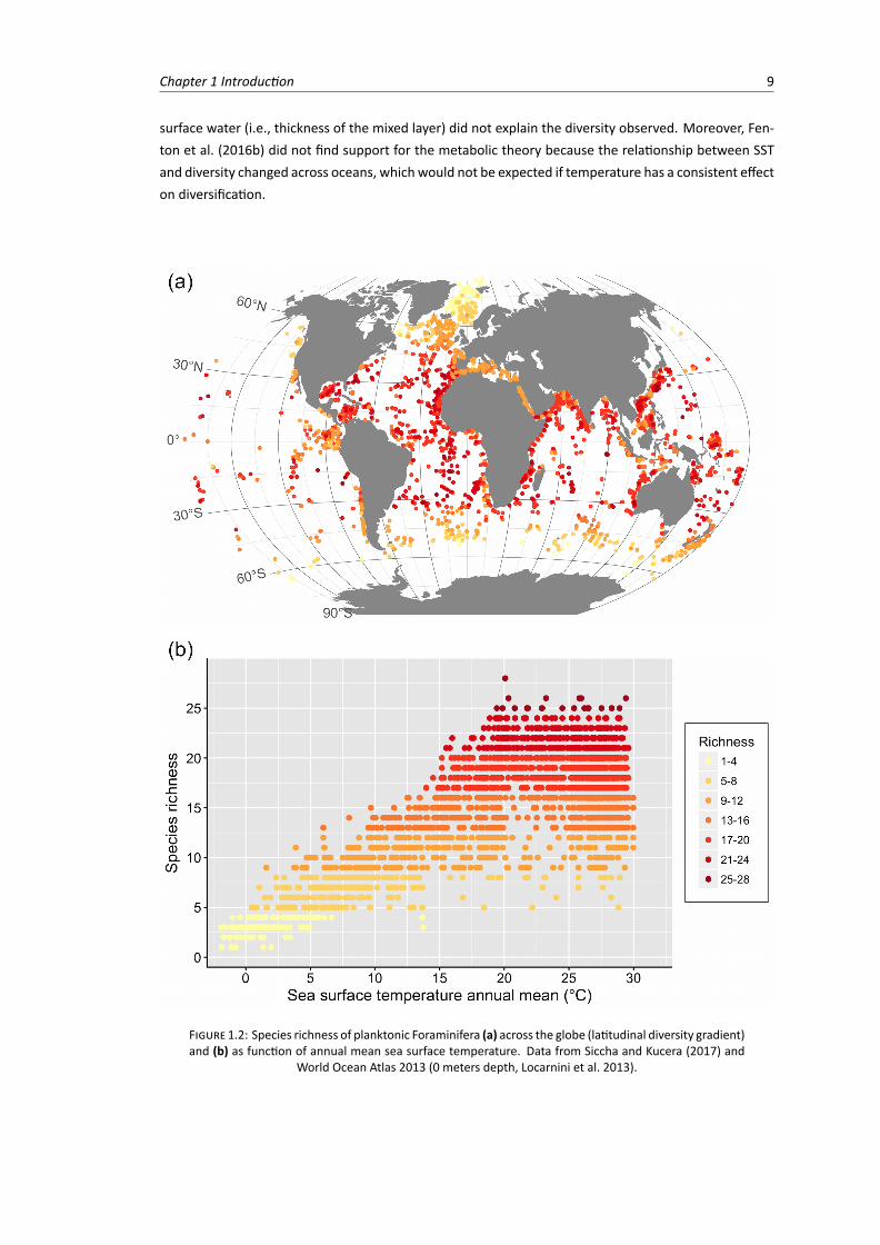
Global diversity patterns of planktonic Foraminifera have been widely studied in relation to environmen-tal variables, especially sea surface temperature (SST) (Fig. 1.2). Rutherford et al. (1999) showed thatthe number of modern planktonic Foraminifera species peaks at intermediate latitudes in all oceans. SSTexplained nearly 90% of the geographic variation of species richness, and Rutherford et al. (1999) sug-gested that the underlying mechanism explaining this pattern was vertical niche partitioning dictated bythe thermal structure of the water column. The strong relationship between SST and diversity was fur-ther confirmed by Tittensor et al. (2010), who studied 13marine taxa, including planktonic Foraminifera.Tittensor et al. (2010) suggested that higher temperatures increase metabolic rates promoting higherspeciation rates, which lead to greater diversity in lower latitudes (metabolic theory of ecology; Brownet al. 2004; Allen et al. 2006). In fact, speciation rates of planktonic Foraminifera calculated over thepast 30 million years increase towards the tropics, supporting the metabolic theory hypothesis (Allenet al. 2006; Allen and Gillooly 2006; but seeWei and Kennett 1986). More recently, Fenton et al. (2016b)explored different diversity measures of planktonic Foraminifera assemblages (including species rela-tive abundance and functional diversity) and how these measures relate globally to ten environmentalvariables. SST was still the variable with the most explanatory power and the vertical structure of the
Chapter 1 Introduction 9
surface water (i.e., thickness of the mixed layer) did not explain the diversity observed. Moreover, Fen-ton et al. (2016b) did not find support for the metabolic theory because the relationship between SSTand diversity changed across oceans, which would not be expected if temperature has a consistent effecton diversification.
FIGURE 1.2: Species richness of planktonic Foraminifera (a) across the globe (latitudinal diversity gradient)and (b) as function of annual mean sea surface temperature. Data from Siccha and Kucera (2017) and
World Ocean Atlas 2013 (0 meters depth, Locarnini et al. 2013).
10 Chapter 1 Introduction
Planktonic Foraminifera assemblages show a latitudinal morphological pattern of larger average shellsizes towards the tropics, only interruptedbypolar and subtropical fronts and in upwelling areas (Schmidtet al., 2004a). The global two-fold increase in assemblage size from the poles to the tropics correlateswith SST and the thermal stratification of the surface water (Schmidt et al., 2004a). The mechanismsgenerating this morphological pattern could be related to food availability, cell physiology (as higher SSTaffects metabolic and growth rates) and/or ecology, as larger sizes could be adapted to vertical nichescreated by the increased stratification of the surface water (Schmidt et al., 2004a). Interestingly, themodern oceans host the largest planktonic Foraminifera of all time (Schmidt et al., 2004b).
Most of these works explored the relationship between planktonic Foraminifera diversity and primaryproductivity, which concerns the ecological interaction of herbivory (predation). However, to date noresearch has investigated competitive interactions among planktonic Foraminifera. We currently do notknow if they compete, although ecological models developed to aid palaeoceanographic reconstruc-tions generally assume they do (e.g., Kretschmer et al. 2018). It is prohibitively difficult to observe directecological interactions among planktonic Foraminifera in the open ocean, but the outcomes of ecolog-ical interactions can yield informative evidence that they have occurred. Thus, instead of studying howplanktonic Foraminifera abundances change in relation to environmental variables, one can investigatehow the changes in their abundances relate to each other. For example, if species occur together in highabundances and are ecologically similar, they are probably adapted to similar environmental conditions,and are not competitively excluding one another. In this way, unravelling community ecology patternscan help us elucidate the role of ecological interactions among planktonic Foraminifera species. I explorethese ideas in Chapter 5.
1.2.5 Macroevolutionary patterns
During the approximately 170 million years of evolution, planktonic Foraminifera species diversityhad three major peaks (Upper Cretaceous, Eocene, Miocene-Pliocene) and two minima (Cretaceous-Paleogene and Eocene-Oligocene transitions), with several fluctuationswithin thesemajor events (Cifelli,1969; Norris, 1991; Fraass et al., 2015). Their diversity never exceeded 100 species (Fraass et al. 2015;or 150 species, using a sub-sampling correction; Lloyd et al. 2012). This noticeable low diversity, es-pecially when compared to the extant diversity of 4000 benthic Foraminifera species (Murray, 2007),is an interesting macroevolutionary pattern, and raises the question of why the Foraminifera tree is sounbalanced?
Many non-exclusive hypotheses can be put forward to explain this macroevolutionary pattern. BenthicForaminifera lineages are older than planktonic ones and, therefore, have had more time to speciateand accumulate species. Also, the plankton was more severely harmed by the asteroid impact at theCretaceous-Paleogene (K-Pg) boundary than the benthic realm (Culver, 2003; Thomas, 2007), and plank-tonic Foraminifera suffered their most extreme extinction event at this boundary (Fraass et al., 2015).Moreover, most of the observed speciation processes involve populations that are in allopatry (i.e., non-overlapping distributions; Coyne and Orr 2004). Geo- or hydrographic barriers block gene flow betweenpopulations, which, over time, become reproductively isolated due to random mutations and/or localadaptation. The apparent lack of barriers to gene flow in marine pelagic ecosystems might prevent al-lopatric divergence of plankton populations (the ‘ubiquity hypothesis’; Finlay 2002) and maintain lowspecies diversity. Indeed, benthic Foraminifera species usually have restricted biogeographical ranges
Chapter 1 Introduction 11
suggesting allopatric processes, whereas planktonic Foraminifera species, which are non-motile and pas-sive dispersers, have extremely broad and overlapping biogeographical distributions (Be and Tolderlund,1971; Norris, 2000; Kucera, 2007). The planktonic Foraminifera fossil record also support the ubiquityhypothesis, in which their high dispersal capability favours sympatric (i.e., co-occurring populations) overallopatric diversification processes (e.g., Lazarus et al. 1995; Pearson et al. 1997; Sexton andNorris 2008).Sympatric diversification of planktonic Foraminifera probably occurs via shifts in the timing of reproduc-tion (seasonal sympatry) or in the depth habitat of co-occurring populations (depth parapatry; Norris2000). The surface water stratification can create different depth habitats in the water column, allowingniche partitioning between populations and subsequently speciation by depth parapatry (Norris, 2000).
Present day molecular analyses at macroecological scales can help us elucidate planktonic Foraminiferaspeciationmodes. For example,Weiner et al. (2012) confirmed that genetic types of the speciesHastige-rina pelagicawere consistently separated by depth throughout their global range, supporting the depthparapatry hypothesis. Moreover, three species of planktonic Foraminifera exhibit genetic mixing be-tween Arctic and Antarctic populations (Darling et al., 2000), supporting the high inter-oceanic disper-sal potential observed in the fossil record (Sexton and Norris, 2008). Transoceanic distributions of ge-netic types were also found by Ujiie and Lipps (2009). However, at the same time, other global phy-logeographical studies have shown that many planktonic Foraminifera species comprise genetic typeswith different geographical distributions (e.g. De Vargas et al. 1999; Darling et al. 2007; Aurahs et al.2009b; Weiner et al. 2014; Ujiie and Ishitani 2016), supporting allopatric processes and opposing theubiquitous dispersal hypothesis. In particular, Darling et al. (2004) combined molecular, biogeographic,fossil, and paleoceanographic data to reconstruct the possible mechanisms driving Neogloboquadrinapachyderma diversification. They showed that the onset of the Northern Hemisphere glaciation createdoceanographic barriers to the gene flow of the Atlantic Arctic and Antarctic populations (Darling et al.,2004). Thus, allopatric processes driven by ocean circulation can play an important role in planktonicForaminifera diversification. More generally, Darling et al. (2004) emphasise how palaeontological dataare crucial to the understanding of present-day marine biogeographical patterns, and vice versa.
The planktonic Foraminifera fossil record allows a precise estimation of diversification rates in deep timeand has been used to understand the relative contribution of biotic and abiotic factors drivingmacroevo-lutionary patterns. Traditionally, there is the idea that competition, predation, and other ecological in-teractions (i.e., biotic factors) shape ecosystems locally and over short time spans, whereas extrinsic,abiotic factors such as climate, oceanographic and tectonic events shape larger-scale patterns regionallyand globally across long time scales (Benton, 2009). Planktonic Foraminifera diversification has beenshown to be shaped by changes in ocean circulation and climate (e.g., Cifelli 1969; Lipps 1970; Leckieet al. 2002; Peters et al. 2013; Fraass et al. 2015). However, Ezard et al. (2011) showed that the inter-play between species ecology (biotic) and climate (abiotic) drives planktonic Foraminifera diversificationacross the Cenozoic. More specifically, speciation rate was more strongly shaped by standing speciesdiversity than by climate change, whereas the reverse was true for extinction (Ezard et al., 2011).
The relationship between diversification rate and standing diversity (per million year time bin) ob-served across planktonic Foraminifera macroevolution is negative, supporting a known macroevolution-ary pattern termed negative diversity-dependent diversification (DDD; Rabosky 2013). DDD theory seesglobal diversity increasing up to an equilibrium point, dictated by a limited number of niches available(i.e., macroevolutionary carrying capacity), which regulates species richness (for a recent discussion see:Rabosky et al. 2015; Harmon and Harrison 2015). This DDD pattern is usually thought to reflect com-petition among species and the filling of niche space (Rabosky 2013, but see Moen and Morlon 2014).
12 Chapter 1 Introduction
Thus, competition among species seems to play a major role in planktonic Foraminifera diversification(Ezard et al., 2011; Etienne et al., 2011), and their high-resolution fossil record has even enable the test ofdifferent competition hypotheses (Ezard and Purvis, 2016). Explicitly testing for competition in the fossilrecord is difficult, usually because of low taxonomic resolution and small sample sizes. Until today, onlyone study has investigated species-level competitive interactions directly observable in the fossil record(bryozoans; Liow et al. 2016). The planktonic foraminiferal fossil record does not face the problem ofresolution nor sample size; however, there is not enough ecological knowledge to derive hypothesesthat would explicitly test for competition in their fossil record. Therefore, studying ecological dynamicsof modern planktonic Foraminifera can certainly help us unlock the full ecological potential of their fossilrecord (Chapter 5).
Besides taxonomic diversification, macroevolutionary patterns can also be described based on morpho-logical evolution. Cope’s rule (Cope, 1887; Stanley, 1973), for example, describes an increase in averageorganism size over time and has been observed in many groups (e.g., Alroy 1998; Hone et al. 2005;Hunt and Roy 2006; Novack-Gottshall and Lanier 2008; Heim et al. 2015). Explanations for average sizeincrease over time usually assume microevolutionary adaptive causes: larger body sizes are under se-lective advantages because of better resistance to predation, better food exploitation and higher repro-ductive success (Kingsolver and Pfennig, 2004; Schmidt et al., 2004c; Van Valkenburgh et al., 2004; Honeand Benton, 2005).
Planktonic Foraminifera lineages display the macroevolutionary trend towards increased size (Arnoldet al., 1995;Webster and Purvis, 2002). However, speciation events do not occurmore often in larger lin-eages, so it is not clear whether there are selective advantage for large-sized species (Arnold et al., 1995).Planktonic Foraminifera also increased in average assemblage size across the Cenozoic, and this sizeincrease correlates positively with increases in latitudinal and vertical temperature gradients (Schmidtet al., 2004b,c). This correlation indicates an abiotic forcing of the macroevolutionary size increase, pos-sibly related to adaptation to new niches that became available due to increased thermal stratificationof the surface water (Schmidt et al., 2004c). Moreover, there is evidence that planktonic Foraminiferaspecies decrease in size before they go extinct (Cordey et al., 1970;Wade and Olsson, 2009; Brombacheret al., 2017a), which suggests that smaller sizes are related to sub-optimal and stressful conditions (butsee Weinkauf et al. 2014). On the other hand, the survivors of both the K-Pg and the Eocene-Oligoceneextinction events were small sized (and unkeeled) planktonic Foraminifera species (Norris, 1991; Kellerand Abramovich, 2009). This demise of large species during mass extinctions suggests that smaller sizedspecies have a selective advantage of reduced extinction rates, possibly because of higher populationdensities (McKinney, 1997).
Macroecological patterns can help us elucidate whether there are selective advantages for larger (orsmaller) sizes in planktonic Foraminifera. If there are selective advantages for larger sizes, the signa-tures of this mechanism should be evident not only among species, but also among populations withina species. Within a species’ range, larger average sizes should be related to optimal conditions whereassmaller average sizes would be found in sub-optimal conditions. This macroecological pattern was ob-served in modern planktonic Foraminifera species (e.g., Hecht 1976; Schmidt et al. 2004a). In Chapter4, I further explore within-species size variation in a global scope, which was possible because of themacroecological scope of natural history collections.
Chapter 1 Introduction 13
1.3 The importance of natural history collections
Natural history collections (NHCs) provide a rich source of data and can contribute to awide rangeof stud-ies at taxonomic, population and community levels (Lister and Climate Change Research Group, 2011;Ward, 2012; De La Sancha et al., 2017; Marshall et al., 2018). Conserved in museums and other institu-tions, NHCs contain the specimens as primary data curated with associatedmetadata (Schilthuizen et al.,2015). NHCs enable researchers to re-examine the primary data, which is especially important in groupswhere the taxonomy is in flux (Balke et al., 2013; Schilthuizen et al., 2015). NHCs have become widelyused in macroecological and palaeontological studies because of their extensive spatial and temporalcoverage, that cannot be replicated by new surveys (Balke et al., 2013; Marshall et al., 2018).
NHCs are particularly important in the assessment of the extent to which humans have impacted theEarth’s biota and reshaped biodiversity patterns (Lister and Climate Change Research Group, 2011; John-son et al., 2011). NHCs samples extend back into previous centuries (i.e., historical samples), which isfundamental for the establishment of a pre-anthropogenic baseline of the state of the Earth’s biota (e.g.,Roemmich et al. 2012; Ward 2012; Gardner et al. 2014; Penn et al. 2018). NHCs have been used, for ex-ample, to assess species biogeographical range shifts (Boakes et al., 2010; Hoeksema et al., 2011) andphenological changes (e.g. flowering time; Robbirt et al. 2011) during the past centuries. Although NHCslikely contain sampling biases, these biases can often be estimated (e.g., Boakes et al. 2010; Ward 2012;Guerin et al. 2018; Chapter 3) and taken into consideration when analysing NHC generated data. At atime when conserving biodiversity is a global priority, NHCs are a window into the natural world beforehuman pressures approached their current intensity and are, therefore, essential to understand currentand future biodiversity trends (Johnson et al., 2011).
Despite their importance, NHCs are significantly under-used due to the difficulty of obtaining andanalysing data within and across collections (Smith and Blagoderov, 2012; Balke et al., 2013). Digitisationandmobilisation of specimens and associatedmetadata removes this barrier, makingNHCsmore accessi-ble for research (Balke et al., 2013). However, digitisation requires considerable work, presenting majortechnical and organisational challenges when performed on such large scales (Smith and Blagoderov,2012). In addition, with dwindling resources being made available for the management of museumcollections, it is becoming more difficult to obtain funds for routine collection maintenance, let alonedigitisation projects (Suarez and Tsutsui, 2004; Gardner et al., 2014; Kemp, 2015; De La Sancha et al.,2017). A recent and rather extreme example of the funding difficulties that natural history museumsface was the fire that consumed the Museu Nacional in Rio de Janeiro in September 2018. Despite be-ing the biggest natural history museum in Latin America, the Museu Nacional had no adequate supportfrom the Brazilian government to preserve and digitise its collection. Sadly, much of its archive is nowdestroyed by the fire and its data permanently lost. It is therefore extremely important for collectionmanagers and researchers to work together, providing new opportunities for funding and collaborationto increase the public and governmental awareness of the relevance and value of NHCs, as well as inten-sify its digitisation efforts (Ward et al., 2015).
Technological advances and innovative workflows are allowing natural history museums to enter a newage of mass digitisation of NHCs (e.g., Blagoderov et al. 2012; Heerlien et al. 2015; Hudson et al. 2015;Blagoderov et al. 2017). Modern imaging technologies also enable scientists to extract new data fromthe same specimens (e.g., Schmidt et al. 2013; Cunningham et al. 2014). As digitisation gets faster andcheaper, more governments and institutions are investing in it (Rogers, 2016). NHCs are becoming evermore available online through open-access data portals (Graham et al., 2004), which provide easy access
14 Chapter 1 Introduction
to NHCs for scientists, students and the public worldwide (Balke et al., 2013). Natural history museumsare not only important scientific research institutions, but also one of the most popular, competent, andsuccessful institutions for the transfer of scientific knowledge to the public (Ohl et al., 2014). Throughtheir NHCs and exhibitions, natural history museums all over the world communicate how scientistsexplore and understand the natural world to the public. Thus, by connecting people to biodiversityresearch and discovery, natural history museums play a crucial role in inspiring people to protect andconserve the amazing diversity of life that exists on Earth.
1.4 A narrative overview of this thesis
I started my doctoral studies working at the Natural History Museum in London (NHM), to re-discoverthe forgotten Henry Buckley Collection of Planktonic Foraminifera (Chapter 2). This work was very ex-citing because I was part of the NHM efforts to digitise NHCs, using their new imaging technologies andinnovative workflows. I imaged every slide of the collection and it is fulfilling to realise that anyonefrom anywhere in the world can now see these specimens online at the NHM Data Portal (https://-doi.org/10.5519/0035055). I also had the chance to participate on public engagement events at theNHM, such as the Science Uncovered and Nature Live.
The Buckley Collection has mainly modern specimens with a wide geographical scope and high intraspe-cific resolution (i.e., many specimens per species per sample) (Chapter 2). However, little informationwas available about the methodology used to sample the seafloor sediments and the foraminifers fromthese sediments. These seafloor sediments were sampled by pioneering marine expeditions such asHMS Challenger, when seafloor sampling techniques were elementary. To assess whether these histori-cal samples are representative of surface sediments, I re-sampled untouched bulk sediments that werestill in their original glass jars (Fig. 3.4). I compared the species composition of the randomly sampledhistorical data with the composition extracted from openly available datasets of the Holocene and LastGlacial Maximum, to assess the degree of sediment mixture in the historical samples (Chapter 3).
Buckley amassed his collection rather secretly, because the museum in the 1970s and 80s did not en-courage him to study microfossils (Chapter 2). Despite the lack of support, Buckley picked and mountedalmost 24,000 specimens, certainly out of passion, with the aim of producing an Atlas of modern plank-tonic Foraminifera. I used the Buckley Collection to explore how species vary in shell size across theirranges, and also estimated the shell size biases in the collection (Chapter 4). I tested the hypothesis thatspecies are largest where they are most abundant, with this correlation indicating the species’ ecologi-cal optimum (Hecht, 1976; Schmidt et al., 2004a). This hypothesis is very interesting because shell sizeis readily measurable in the fossil record, and could potentially inform us about ecological optimum ofextinct species and adaptive evolution in deep time. Size could also inform us about the species’ crypticgenetic diversity: if two populations of the same species are adapting to different environmental condi-tions (i.e., adaptive divergence), we could expect to see these populations increasing in size at differentenvironmental optima. Thus, within the biogeographical range of the species, more than one peak inmaximum shell size could indicate the beginning of a speciation process that would also be evident whenanalysing the species’ cryptic genetic diversity (Schmidt et al., 2004a). With this idea in mind, I wrote aproposal to work in Bremen for one year with Prof. Michal Kucera and was awarded the Research Grantfor Doctoral Candidates from the German Academic Exchange Service (DAAD) to do so.
Chapter 1 Introduction 15
During my doctoral studies I discovered that, although we communicate science in an objective and lin-ear way (i.e., question, data to answer the question, answer), the process of doing science is actually‘branchy’ and cloudy4. We often have to re-evaluate our questions, hypotheses and expectations. Thiswas the case of my Chapter 4: shell size and abundance did not show the positive relationship that I ex-pected based on the literature. Thus, the project I wrote for the DAAD grant could not be accomplished.However, in Bremen, I had the amazing chance to participate on the FORAMFLUX expedition (RVMeteorM140) in August�September 2017 and experience how to sample the plankton with nets and sedimenttraps. Knowing about available data on species relative abundance in seafloor sediments (coretops) andspecies population dynamics in the water column (sediment traps), I had the idea that we could testhow species’ occurrence patterns and dynamics relate to each other. From the fossil record, it seemsthat competition among species is an important mechanism driving planktonic Foraminifera diversifica-tion (Ezard et al., 2011; Ezard and Purvis, 2016), thus I tested in Chapter 5 whether competition is alsostructuring communities in the modern oceans.
In summary, my thesis examines ecological patterns within and interactions among extant planktonicForaminifera species. Because of the global scale of the population- and community-level patterns Iinvestigate in this thesis, my work contributes to the field of macroecology. I begin by describing theNHM Henry Buckley Collection of Planktonic Foraminifera with the aim of encouraging the use of NHCs(Chapter 2). I then study historical ocean-floor surface sediments to assess their age biases, i.e., de-gree of mixing between modern and glacial material (Chapter 3). These historical sediment sampleswere used by Buckley to create his collection, but could also be used as a pre-1900s reference base-line of the ocean floor environment. The global scope and high intraspecific resolution of the BuckleyCollection allowed me to investigate the biogeography of population shell size of nine modern plank-tonic Foraminifera species (Chapter 4). I then investigate ecological interactions among modern speciesusing a community ecology approach with data from coretop and sediment trap samples (Chapter 5).By deepening our understanding of modern planktonic Foraminifera ecology, we can unlock the uniquepopulation-level macroevolutionary dynamics their fossil record provides. I conclude by summarisingthe implications of my discoveries, discussing their limitations, and suggesting future areas of research(Chapter 6).
4Inspired by the TED talk from Uri Alon named “Why Science Demands a Leap into the Unknown”

Chapter 2
The unknown planktonic foraminiferalpioneer Henry A. Buckley and hiscollection at The Natural HistoryMuseum, London
Marina C. Rillo1,2, John Whittaker1, Thomas H. G. Ezard2,3, AndyPurvis4,5, Andrew S. Henderson1,6, Stephen Stukins1 & C. Giles Miller1⇤
1Department of Earth Sciences, The Natural History Museum, Cromwell Road, London SW7 5BD, UK2Ocean and Earth Science, National Oceanography Centre Southampton, University of SouthamptonWaterfront Campus, Southampton SO143ZH, UK3Centre for Biological Sciences, University of Southampton Highfield, Southampton SO171BJ, UK4Department of Life Sciences, The Natural History Museum, Cromwell Road, London SW7 5BD, UK5Department of Life Sciences, Imperial College London, Silwood Park Campus, Ascot SL5 7PY, UK6Saudi Arabian Oil Company, Saudi Aramco P.O. Box 5000, Dhahran 31311, Saudi Arabia*Correspondence: [email protected]
17
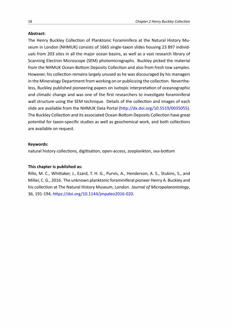
18 Chapter 2 Henry Buckley Collection
Abstract:The Henry Buckley Collection of Planktonic Foraminifera at the Natural History Mu-seum in London (NHMUK) consists of 1665 single-taxon slides housing 23 897 individ-uals from 203 sites in all the major ocean basins, as well as a vast research library ofScanning Electron Microscope (SEM) photomicrographs. Buckley picked the materialfrom the NHMUK Ocean-Bottom Deposits Collection and also from fresh tow samples.However, his collection remains largely unused as he was discouraged by his managersin theMineralogy Department fromworking on or publicizing the collection. Neverthe-less, Buckley published pioneering papers on isotopic interpretation of oceanographicand climatic change and was one of the first researchers to investigate foraminiferalwall structure using the SEM technique. Details of the collection and images of eachslide are available from the NHMUK Data Portal (http://dx.doi.org/10.5519/0035055).The Buckley Collection and its associated Ocean-BottomDeposits Collection have greatpotential for taxon-specific studies as well as geochemical work, and both collectionsare available on request.
Keywords:natural history collections, digitisation, open-access, zooplankton, sea-bottom
This chapter is published as:Rillo, M. C., Whittaker, J., Ezard, T. H. G., Purvis, A., Henderson, A. S., Stukins, S., andMiller, C. G., 2016. The unknown planktonic foraminiferal pioneer Henry A. Buckley andhis collection at The Natural History Museum, London. Journal of Micropalaeontology,36, 191-194, https://doi.org/10.1144/jmpaleo2016-020.
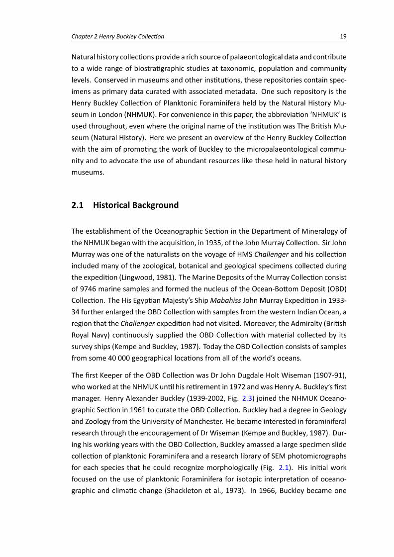
Chapter 2 Henry Buckley Collection 19
Natural history collections provide a rich source of palaeontological data and contributeto a wide range of biostratigraphic studies at taxonomic, population and communitylevels. Conserved in museums and other institutions, these repositories contain spec-imens as primary data curated with associated metadata. One such repository is theHenry Buckley Collection of Planktonic Foraminifera held by the Natural History Mu-seum in London (NHMUK). For convenience in this paper, the abbreviation ‘NHMUK’ isused throughout, even where the original name of the institution was The British Mu-seum (Natural History). Here we present an overview of the Henry Buckley Collectionwith the aim of promoting the work of Buckley to the micropalaeontological commu-nity and to advocate the use of abundant resources like these held in natural historymuseums.
2.1 Historical Background
The establishment of the Oceanographic Section in the Department of Mineralogy ofthe NHMUK beganwith the acquisition, in 1935, of the JohnMurray Collection. Sir JohnMurray was one of the naturalists on the voyage of HMS Challenger and his collectionincluded many of the zoological, botanical and geological specimens collected duringthe expedition (Lingwood, 1981). TheMarine Deposits of theMurray Collection consistof 9746 marine samples and formed the nucleus of the Ocean-Bottom Deposit (OBD)Collection. The His Egyptian Majesty’s ShipMabahiss John Murray Expedition in 1933-34 further enlarged the OBD Collection with samples from the western Indian Ocean, aregion that the Challenger expedition had not visited. Moreover, the Admiralty (BritishRoyal Navy) continuously supplied the OBD Collection with material collected by itssurvey ships (Kempe and Buckley, 1987). Today the OBD Collection consists of samplesfrom some 40 000 geographical locations from all of the world’s oceans.
The first Keeper of the OBD Collection was Dr John Dugdale Holt Wiseman (1907-91),whoworked at the NHMUK until his retirement in 1972 andwas Henry A. Buckley’s firstmanager. Henry Alexander Buckley (1939-2002, Fig. 2.3) joined the NHMUK Oceano-graphic Section in 1961 to curate the OBD Collection. Buckley had a degree in Geologyand Zoology from the University of Manchester. He became interested in foraminiferalresearch through the encouragement of Dr Wiseman (Kempe and Buckley, 1987). Dur-ing his working years with the OBD Collection, Buckley amassed a large specimen slidecollection of planktonic Foraminifera and a research library of SEM photomicrographsfor each species that he could recognize morphologically (Fig. 2.1). His initial workfocused on the use of planktonic Foraminifera for isotopic interpretation of oceano-graphic and climatic change (Shackleton et al., 1973). In 1966, Buckley became one
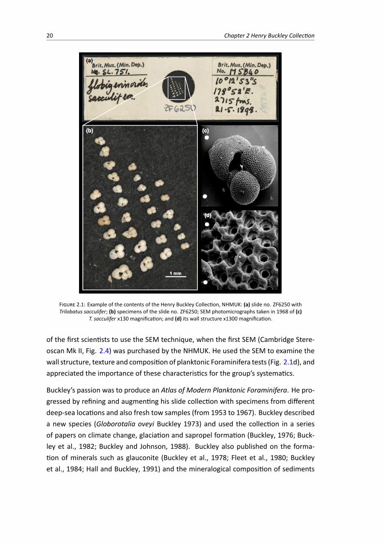
20 Chapter 2 Henry Buckley Collection
FIGURE 2.1: Example of the contents of the Henry Buckley Collection, NHMUK: (a) slide no. ZF6250 withTrilobatus sacculifer; (b) specimens of the slide no. ZF6250; SEM photomicrographs taken in 1968 of (c)
T. sacculifer x130 magnification; and (d) its wall structure x1300 magnification.
of the first scientists to use the SEM technique, when the first SEM (Cambridge Stere-oscan Mk II, Fig. 2.4) was purchased by the NHMUK. He used the SEM to examine thewall structure, texture and composition of planktonic Foraminifera tests (Fig. 2.1d), andappreciated the importance of these characteristics for the group’s systematics.
Buckley’s passion was to produce an Atlas of Modern Planktonic Foraminifera. He pro-gressed by refining and augmenting his slide collection with specimens from differentdeep-sea locations and also fresh tow samples (from 1953 to 1967). Buckley describeda new species (Globorotalia oveyi Buckley 1973) and used the collection in a seriesof papers on climate change, glaciation and sapropel formation (Buckley, 1976; Buck-ley et al., 1982; Buckley and Johnson, 1988). Buckley also published on the forma-tion of minerals such as glauconite (Buckley et al., 1978; Fleet et al., 1980; Buckleyet al., 1984; Hall and Buckley, 1991) and the mineralogical composition of sediments
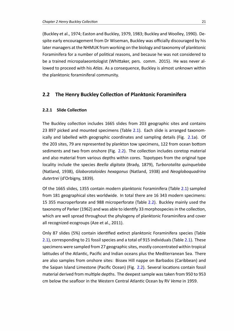
Chapter 2 Henry Buckley Collection 21
(Buckley et al., 1974; Easton and Buckley, 1979, 1983; Buckley andWoolley, 1990). De-spite early encouragement from Dr Wiseman, Buckley was officially discouraged by hislatermanagers at the NHMUK fromworking on the biology and taxonomy of planktonicForaminifera for a number of political reasons, and because he was not considered tobe a trained micropalaeontologist (Whittaker, pers. comm. 2015). He was never al-lowed to proceed with his Atlas. As a consequence, Buckley is almost unknown withinthe planktonic foraminiferal community.
2.2 The Henry Buckley Collection of Planktonic Foraminifera
2.2.1 Slide Collection
The Buckley collection includes 1665 slides from 203 geographic sites and contains23 897 picked and mounted specimens (Table 2.1). Each slide is arranged taxonom-ically and labelled with geographic coordinates and sampling details (Fig. 2.1a). Ofthe 203 sites, 79 are represented by plankton tow specimens, 122 from ocean bottomsediments and two from onshore (Fig. 2.2). The collection includes coretop materialand also material from various depths within cores. Topotypes from the original typelocality include the species Beella digitata (Brady, 1879), Turborotalita quinqueloba(Natland, 1938), Globorotaloides hexagonus (Natland, 1938) and Neogloboquadrinadutertrei (d’Orbigny, 1839).
Of the 1665 slides, 1355 contain modern planktonic Foraminifera (Table 2.1) sampledfrom 181 geographical sites worldwide. In total there are 16 343 modern specimens:15 355 macroperforate and 988 microperforate (Table 2.2). Buckley mainly used thetaxonomy of Parker (1962) and was able to identify 33morphospecies in the collection,which are well spread throughout the phylogeny of planktonic Foraminifera and coverall recognized ecogroups (Aze et al., 2011).
Only 87 slides (5%) contain identified extinct planktonic Foraminifera species (Table2.1), corresponding to 21 fossil species and a total of 915 individuals (Table 2.1). Thesespecimenswere sampled from 27 geographic sites, mostly concentratedwithin tropicallatitudes of the Atlantic, Pacific and Indian oceans plus the Mediterranean Sea. Thereare also samples from onshore sites: Bissex Hill nappe on Barbados (Caribbean) andthe Saipan Island Limestone (Pacific Ocean) (Fig. 2.2). Several locations contain fossilmaterial derived frommultiple depths. The deepest sample was taken from 950 to 953cm below the seafloor in the Western Central Atlantic Ocean by RV Vema in 1959.
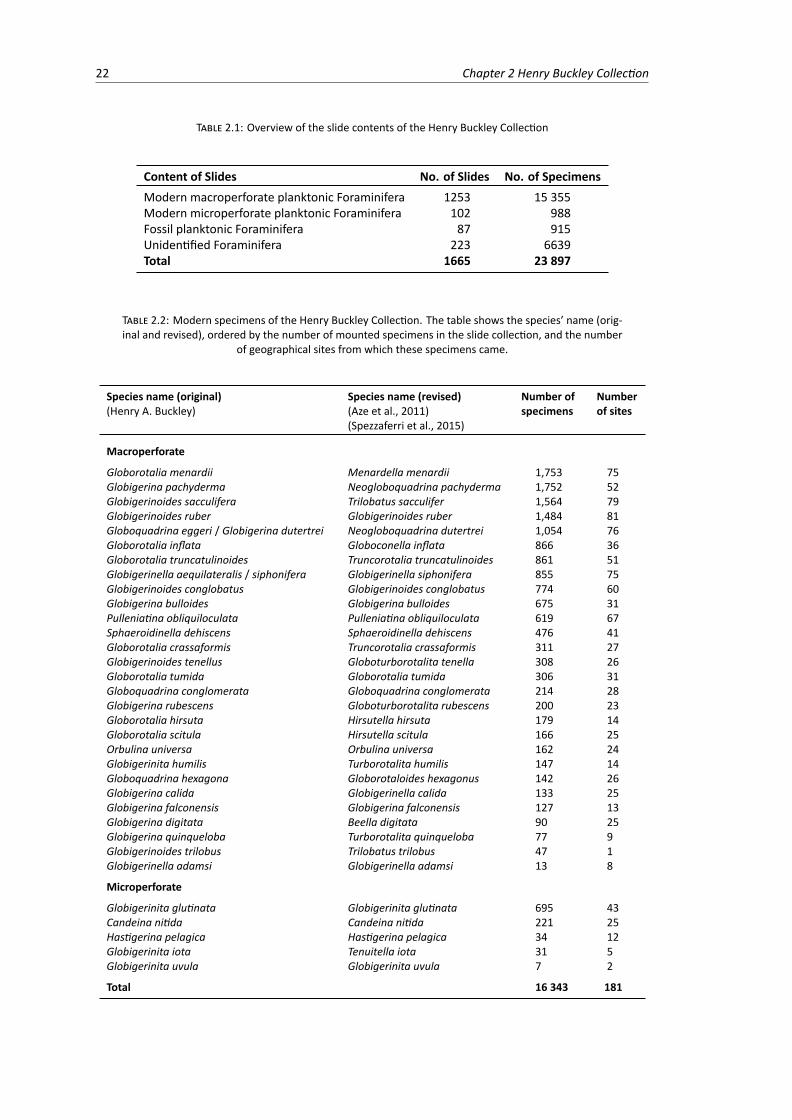
22 Chapter 2 Henry Buckley Collection
TABLE 2.1: Overview of the slide contents of the Henry Buckley Collection
Content of Slides No. of Slides No. of SpecimensModern macroperforate planktonic Foraminifera 1253 15 355Modern microperforate planktonic Foraminifera 102 988Fossil planktonic Foraminifera 87 915Unidentified Foraminifera 223 6639Total 1665 23 897
TABLE 2.2: Modern specimens of the Henry Buckley Collection. The table shows the species’ name (orig-inal and revised), ordered by the number of mounted specimens in the slide collection, and the number
of geographical sites from which these specimens came.
Species name (original)(Henry A. Buckley)
Species name (revised)(Aze et al., 2011)(Spezzaferri et al., 2015)
Number ofspecimens
Numberof sites
Macroperforate
Globorotalia menardii Menardella menardii 1,753 75Globigerina pachyderma Neogloboquadrina pachyderma 1,752 52Globigerinoides sacculifera Trilobatus sacculifer 1,564 79Globigerinoides ruber Globigerinoides ruber 1,484 81Globoquadrina eggeri / Globigerina dutertrei Neogloboquadrina dutertrei 1,054 76Globorotalia inflata Globoconella inflata 866 36Globorotalia truncatulinoides Truncorotalia truncatulinoides 861 51Globigerinella aequilateralis / siphonifera Globigerinella siphonifera 855 75Globigerinoides conglobatus Globigerinoides conglobatus 774 60Globigerina bulloides Globigerina bulloides 675 31Pulleniatina obliquiloculata Pulleniatina obliquiloculata 619 67Sphaeroidinella dehiscens Sphaeroidinella dehiscens 476 41Globorotalia crassaformis Truncorotalia crassaformis 311 27Globigerinoides tenellus Globoturborotalita tenella 308 26Globorotalia tumida Globorotalia tumida 306 31Globoquadrina conglomerata Globoquadrina conglomerata 214 28Globigerina rubescens Globoturborotalita rubescens 200 23Globorotalia hirsuta Hirsutella hirsuta 179 14Globorotalia scitula Hirsutella scitula 166 25Orbulina universa Orbulina universa 162 24Globigerinita humilis Turborotalita humilis 147 14Globoquadrina hexagona Globorotaloides hexagonus 142 26Globigerina calida Globigerinella calida 133 25Globigerina falconensis Globigerina falconensis 127 13Globigerina digitata Beella digitata 90 25Globigerina quinqueloba Turborotalita quinqueloba 77 9Globigerinoides trilobus Trilobatus trilobus 47 1Globigerinella adamsi Globigerinella adamsi 13 8
Microperforate
Globigerinita glutinata Globigerinita glutinata 695 43Candeina nitida Candeina nitida 221 25Hastigerina pelagica Hastigerina pelagica 34 12Globigerinita iota Tenuitella iota 31 5Globigerinita uvula Globigerinita uvula 7 2
Total 16 343 181
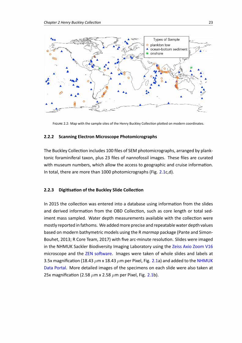
Chapter 2 Henry Buckley Collection 23
FIGURE 2.2: Map with the sample sites of the Henry Buckley Collection plotted on modern coordinates.
2.2.2 Scanning Electron Microscope Photomicrographs
The Buckley Collection includes 100 files of SEM photomicrographs, arranged by plank-tonic foraminiferal taxon, plus 23 files of nannofossil images. These files are curatedwith museum numbers, which allow the access to geographic and cruise information.In total, there are more than 1000 photomicrographs (Fig. 2.1c,d).
2.2.3 Digitisation of the Buckley Slide Collection
In 2015 the collection was entered into a database using information from the slidesand derived information from the OBD Collection, such as core length or total sed-iment mass sampled. Water depth measurements available with the collection weremostly reported in fathoms. Weaddedmore precise and repeatablewater depth valuesbased on modern bathymetric models using the Rmarmap package (Pante and Simon-Bouhet, 2013; R Core Team, 2017) with five arc-minute resolution. Slides were imagedin the NHMUK Sackler Biodiversity Imaging Laboratory using the Zeiss Axio Zoom V16microscope and the ZEN software. Images were taken of whole slides and labels at3.5x magnification (18.43 µm x 18.43 µmper Pixel, Fig. 2.1a) and added to the NHMUKData Portal. More detailed images of the specimens on each slide were also taken at25x magnification (2.58 µm x 2.58 µm per Pixel, Fig. 2.1b).
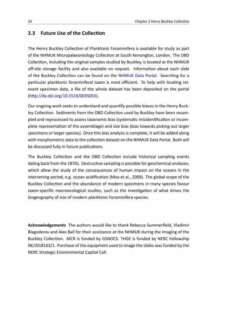
24 Chapter 2 Henry Buckley Collection
2.3 Future Use of the Collection
The Henry Buckley Collection of Planktonic Foraminifera is available for study as partof the NHMUK Micropalaeontology Collection at South Kensington, London. The OBDCollection, including the original samples studied by Buckley, is located at the NHMUKoff-site storage facility and also available on request. Information about each slideof the Buckley Collection can be found on the NHMUK Data Portal. Searching for aparticular planktonic foraminiferal taxon is most efficient. To help with locating rel-evant specimen data, a file of the whole dataset has been deposited on the portal(http://dx.doi.org/10.5519/0035055).
Our ongoing work seeks to understand and quantify possible biases in the Henry Buck-ley Collection. Sediments from the OBD Collection used by Buckley have been resam-pled and reprocessed to assess taxonomic bias (systematic misidentification or incom-plete representation of the assemblage) and size bias (bias towards picking out largerspecimens or larger species). Once this bias analysis is complete, it will be added alongwith morphometric data to the collection dataset on the NHMUK Data Portal. Both willbe discussed fully in future publications.
The Buckley Collection and the OBD Collection include historical sampling eventsdating back from the 1870s. Destructive sampling is possible for geochemical analyses,which allow the study of the consequences of human impact on the oceans in theintervening period, e.g. ocean acidification (Moy et al., 2009). The global scope of theBuckley Collection and the abundance of modern specimens in many species favourtaxon-specific macroecological studies, such as the investigation of what drives thebiogeography of size of modern planktonic Foraminifera species.
Acknowledgements The authors would like to thank Rebecca Summerfield, VladimirBlagoderov and Alex Ball for their assistance at the NHMUK during the imaging of theBuckley Collection. MCR is funded by GSNOCS. THGE is funded by NERC FellowshipNE/J018163/1. Purchase of the equipment used to image the slides was funded by theNERC Strategic Environmental Capital Call.
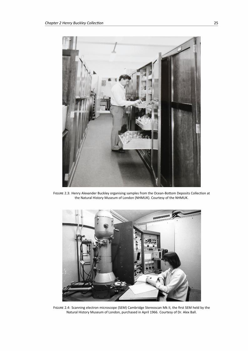
Chapter 2 Henry Buckley Collection 25
FIGURE 2.3: Henry Alexander Buckley organising samples from the Ocean-Bottom Deposits Collection atthe Natural History Museum of London (NHMUK). Courtesy of the NHMUK.
FIGURE 2.4: Scanning electron microscope (SEM) Cambridge Stereoscan Mk II, the first SEM held by theNatural History Museum of London, purchased in April 1966. Courtesy of Dr. Alex Ball.

Chapter 3
Surface sediment samples from earlyage of seafloor exploration can providea late 19th century baseline of themarine environment
Marina C. Rillo1,2,3⇤, Michal Kučera3, Thomas H. G. Ezard1 &C. Giles Miller2
1Ocean and Earth Science, National Oceanography Centre Southampton, University of SouthamptonWaterfront Campus, Southampton SO143ZH, UK2Department of Earth Sciences, Natural History Museum, Cromwell Road, London SW7 5BD, UK3MARUM, University of Bremen, Leobener Strasse, Bremen 28359, Germany*Correspondence: [email protected]
27
28 Chapter 3 Historical seafloor sediments
Abstract:Ocean-floor sediment samples collected up to 150 years ago represent an importanthistorical archive to benchmark global changes in the seafloor environment, such asspecies’ range shifts and invasions and pollution trends. Such benchmarking requiresthat the historical sediment samples represent the state of the environment at, orshortly before, the time of collection. However, early oceanographic expeditions sam-pled the ocean floor using devices like the sounding tube or a dredge, which poten-tially disturb the sediment surface and recover a mix of Holocene (surface) and deeper,Pleistocene sediments. Here we use climate-sensitive microfossils as a fast biometricmethod to assess if historical seafloor samples contain a mixture of modern and glacialsediments. Our assessment is based on comparing the composition of planktonicForaminifera (PF) assemblages in historical samples with Holocene and Last GlacialMaximum (LGM) global reference datasets. We show that eight out of the nine his-torical samples contain PF assemblages more similar to the Holocene than to the LGMassemblages, but the comparisons are only significant in two sites where there is highlocal species’ temporal turnover (from the LGM to the Holocene). When analysing tem-poral turnover globally, we show that upwelling and temperate regions had greatestspecies turnover, which are areaswhere our newmethodologywould bemost diagnos-tic. Our results suggest that sediment samples from historical collections can provide abaseline of the state of marine ecosystems in the late nineteenth century, and thus beused to assess ocean global change trends.
Keywords:natural history collection (NHC), historical collections, pre-industrial, pre-anthropogenic, beta-diversity, species turnover, global change
This chapter is published as:Rillo, M. C., Kucera, M., Ezard, T. H. G., Miller, C. G., 2019. Surface Sediment SamplesFrom Early Age of Seafloor Exploration Can Provide a Late 19th Century Baseline of theMarine Environment. Frontiers in Marine Science, 5, 517, https://doi.org/10.3389/f-mars.2018.00517.
Chapter 3 Historical seafloor sediments 29
3.1 Introduction
Late nineteenth and early twentieth century oceanographic expeditions set out to ex-plore the vast and then widely unknown deep ocean. The voyage of HMS Challengeris a notable example. As she sailed around the globe between 1872�76, researchersmapped for the first time the shape of the ocean basins and described over 4,500 newspecies of marine life (Manten, 1972). These early expeditions have important histor-ical significance, as they mark the beginning of modern oceanography and stimulatedfurther ocean exploration (Wust, 1964).
Froma scientific perspective, the observations andmaterial acquired by these historicalexpeditions have great potential for global change research (Lister and Climate ChangeResearch Group, 2011; Johnson et al., 2011), as they provide a pre-1900 baseline ofthe marine environment (e.g., Roemmich et al. 2012; Gleckler et al. 2016). Yet his-torical seafloor sediment samples remain largely underutilised, because early seafloorsampling techniques involved collecting surficial sediments with instruments like thesounding tube, dredge or even the anchor (Thomson and Murray, 1891). All these in-struments can penetrate below the surface and disturb the top layer of the sediment.As a result, such historical sediment samples might contain surface (Holocene) sedi-ments mixed with deeper, glacial material (Hayward and Kawagata, 2005), potentiallyhindering their use as a historical baseline of the modern marine environment. Coringtechniques provide more accurate sediment chronology (e.g., Rohl et al. 2000); how-ever, historical samples represent the seafloor environment as much as 50 years beforethe earliest core samples collected (Wust, 1964) and, thus, contain sediments withoutany objects deposited after 1900. These uncontaminated historical samples can beuseful for chemical analyses of the seafloor (e.g., pollution trends; Dekov et al. 2010),single-specimen analysis (e.g., Reichart et al. 2003; Wit et al. 2010) and investigationsof species range shifts and invasions in the past century (e.g., Hoeksema et al. 2011).Therefore, it is important to assess the degree to which historical sediment samplesrepresent Holocene or mixed-Pleistocene sediments.
One way to assess the degree of glacial mixing in the historical material is to deter-mine its absolute age using the radiocarbon dating technique or glacial material proxies(e.g., Mg/Ca, oxygen isotopes). However, in cases where the extent of mixing is small,the exponentially decaying nature of the radiocarbon analysis can cause an ambiguousdating, and the isotopic analysis would require a large enough number of specimensto correctly represent the extent of the glacial mixing. Here we propose a complimen-tary method that uses planktonic Foraminifera assemblage composition as a climate-sensitive fingerprint of the sediment age. Planktonic Foraminifera (PF) are single-celledzooplankton that produce calcium carbonate shells and, upon death, accumulate in
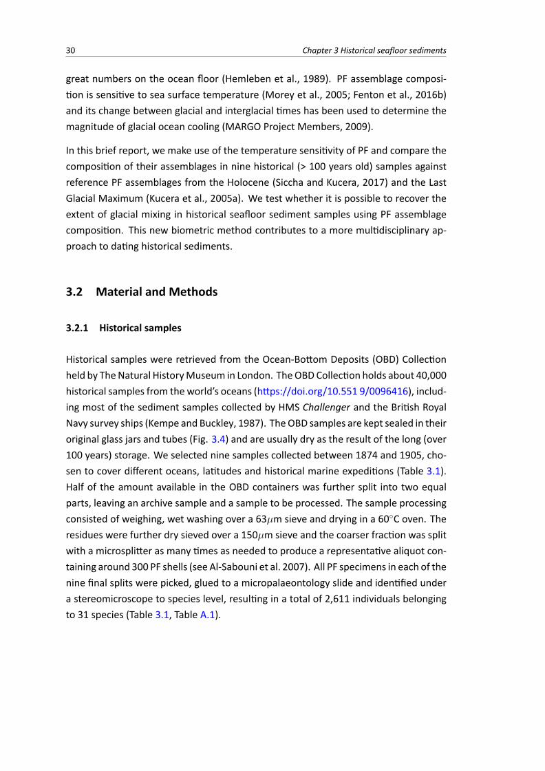
30 Chapter 3 Historical seafloor sediments
great numbers on the ocean floor (Hemleben et al., 1989). PF assemblage composi-tion is sensitive to sea surface temperature (Morey et al., 2005; Fenton et al., 2016b)and its change between glacial and interglacial times has been used to determine themagnitude of glacial ocean cooling (MARGO Project Members, 2009).
In this brief report, we make use of the temperature sensitivity of PF and compare thecomposition of their assemblages in nine historical (> 100 years old) samples againstreference PF assemblages from the Holocene (Siccha and Kucera, 2017) and the LastGlacial Maximum (Kucera et al., 2005a). We test whether it is possible to recover theextent of glacial mixing in historical seafloor sediment samples using PF assemblagecomposition. This new biometric method contributes to a more multidisciplinary ap-proach to dating historical sediments.
3.2 Material and Methods
3.2.1 Historical samples
Historical samples were retrieved from the Ocean-Bottom Deposits (OBD) Collectionheld by TheNatural HistoryMuseum in London. TheOBDCollection holds about 40,000historical samples from the world’s oceans (https://doi.org/10.551 9/0096416), includ-ing most of the sediment samples collected by HMS Challenger and the British RoyalNavy survey ships (Kempe and Buckley, 1987). TheOBD samples are kept sealed in theiroriginal glass jars and tubes (Fig. 3.4) and are usually dry as the result of the long (over100 years) storage. We selected nine samples collected between 1874 and 1905, cho-sen to cover different oceans, latitudes and historical marine expeditions (Table 3.1).Half of the amount available in the OBD containers was further split into two equalparts, leaving an archive sample and a sample to be processed. The sample processingconsisted of weighing, wet washing over a 63µm sieve and drying in a 60�C oven. Theresidues were further dry sieved over a 150µm sieve and the coarser fraction was splitwith a microsplitter as many times as needed to produce a representative aliquot con-taining around 300 PF shells (see Al-Sabouni et al. 2007). All PF specimens in each of thenine final splits were picked, glued to a micropalaeontology slide and identified undera stereomicroscope to species level, resulting in a total of 2,611 individuals belongingto 31 species (Table 3.1, Table A.1).
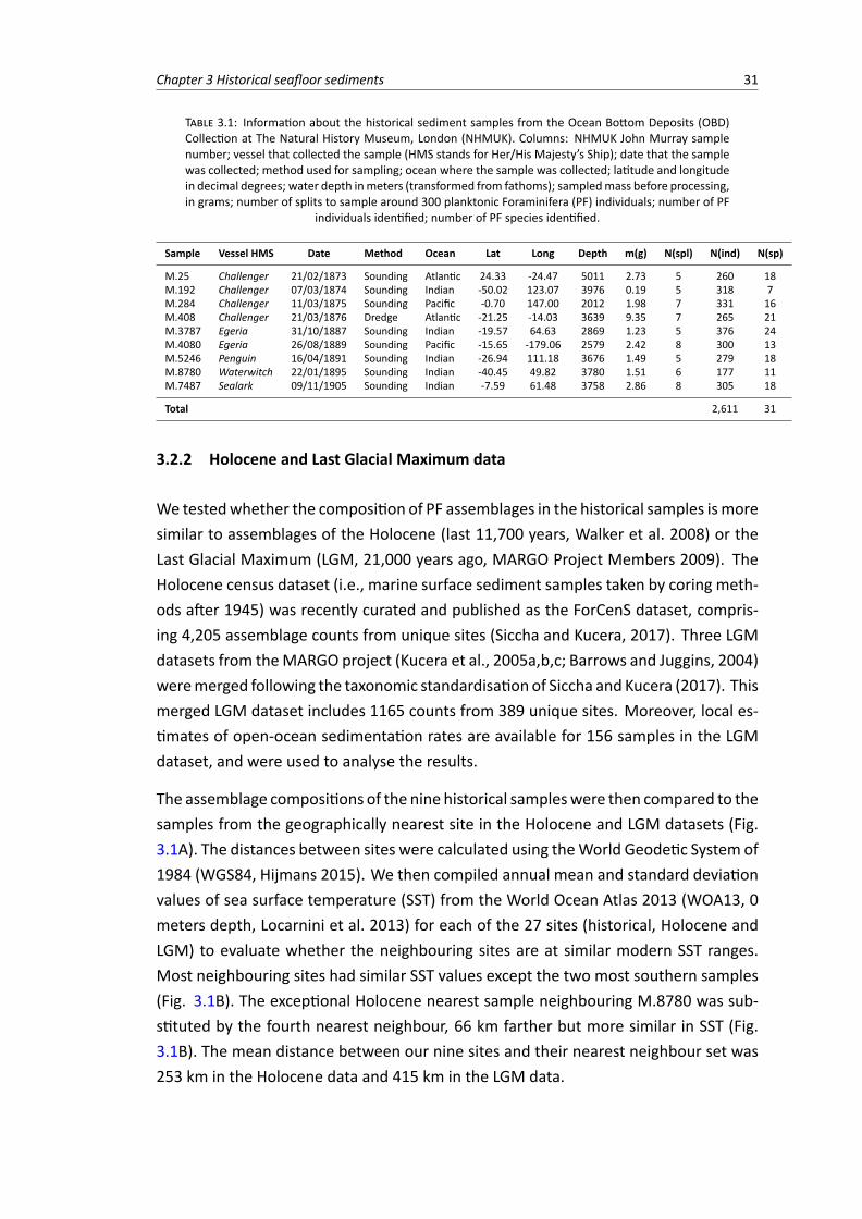
Chapter 3 Historical seafloor sediments 31
TABLE 3.1: Information about the historical sediment samples from the Ocean Bottom Deposits (OBD)Collection at The Natural History Museum, London (NHMUK). Columns: NHMUK John Murray samplenumber; vessel that collected the sample (HMS stands for Her/His Majesty’s Ship); date that the samplewas collected; method used for sampling; ocean where the sample was collected; latitude and longitudein decimal degrees; water depth inmeters (transformed from fathoms); sampledmass before processing,in grams; number of splits to sample around 300 planktonic Foraminifera (PF) individuals; number of PF
individuals identified; number of PF species identified.
Sample Vessel HMS Date Method Ocean Lat Long Depth m(g) N(spl) N(ind) N(sp)
M.25 Challenger 21/02/1873 Sounding Atlantic 24.33 -24.47 5011 2.73 5 260 18M.192 Challenger 07/03/1874 Sounding Indian -50.02 123.07 3976 0.19 5 318 7M.284 Challenger 11/03/1875 Sounding Pacific -0.70 147.00 2012 1.98 7 331 16M.408 Challenger 21/03/1876 Dredge Atlantic -21.25 -14.03 3639 9.35 7 265 21M.3787 Egeria 31/10/1887 Sounding Indian -19.57 64.63 2869 1.23 5 376 24M.4080 Egeria 26/08/1889 Sounding Pacific -15.65 -179.06 2579 2.42 8 300 13M.5246 Penguin 16/04/1891 Sounding Indian -26.94 111.18 3676 1.49 5 279 18M.8780 Waterwitch 22/01/1895 Sounding Indian -40.45 49.82 3780 1.51 6 177 11M.7487 Sealark 09/11/1905 Sounding Indian -7.59 61.48 3758 2.86 8 305 18
Total 2,611 31
3.2.2 Holocene and Last Glacial Maximum data
We testedwhether the composition of PF assemblages in the historical samples ismoresimilar to assemblages of the Holocene (last 11,700 years, Walker et al. 2008) or theLast Glacial Maximum (LGM, 21,000 years ago, MARGO Project Members 2009). TheHolocene census dataset (i.e., marine surface sediment samples taken by coring meth-ods after 1945) was recently curated and published as the ForCenS dataset, compris-ing 4,205 assemblage counts from unique sites (Siccha and Kucera, 2017). Three LGMdatasets from theMARGO project (Kucera et al., 2005a,b,c; Barrows and Juggins, 2004)weremerged following the taxonomic standardisation of Siccha and Kucera (2017). Thismerged LGM dataset includes 1165 counts from 389 unique sites. Moreover, local es-timates of open-ocean sedimentation rates are available for 156 samples in the LGMdataset, and were used to analyse the results.
The assemblage compositions of the nine historical sampleswere then compared to thesamples from the geographically nearest site in the Holocene and LGM datasets (Fig.3.1A). The distances between sites were calculated using theWorld Geodetic System of1984 (WGS84, Hijmans 2015). We then compiled annual mean and standard deviationvalues of sea surface temperature (SST) from the World Ocean Atlas 2013 (WOA13, 0meters depth, Locarnini et al. 2013) for each of the 27 sites (historical, Holocene andLGM) to evaluate whether the neighbouring sites are at similar modern SST ranges.Most neighbouring sites had similar SST values except the two most southern samples(Fig. 3.1B). The exceptional Holocene nearest sample neighbouring M.8780 was sub-stituted by the fourth nearest neighbour, 66 km farther but more similar in SST (Fig.3.1B). The mean distance between our nine sites and their nearest neighbour set was253 km in the Holocene data and 415 km in the LGM data.
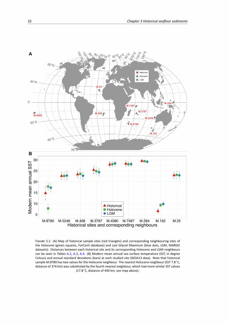
32 Chapter 3 Historical seafloor sediments
FIGURE 3.1: (A) Map of historical sample sites (red triangles) and corresponding neighbouring sites ofthe Holocene (green squares, ForCenS database) and Last Glacial Maximum (blue dots, LGM, MARGOdatasets). Distances between each historical site and its corresponding Holocene and LGM neighbourscan be seen in Tables A.2, A.3, A.4. (B) Modern mean annual sea surface temperature (SST, in degreeCelsius) and annual standard deviations (bars) at each studied site (WOA13 data). Note that historicalsample M.8780 has two values for the Holocene neighbour. The nearest Holocene neighbour (SST 7.8�C,distance of 374 km) was substituted by the fourth nearest neighbour, which had more similar SST values
(17.8�C, distance of 440 km, see map above).
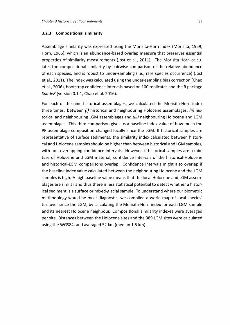
Chapter 3 Historical seafloor sediments 33
3.2.3 Compositional similarity
Assemblage similarity was expressed using the Morisita-Horn index (Morisita, 1959;Horn, 1966), which is an abundance-based overlap measure that preserves essentialproperties of similarity measurements (Jost et al., 2011). The Morisita-Horn calcu-lates the compositional similarity by pairwise comparison of the relative abundanceof each species, and is robust to under-sampling (i.e., rare species occurrence) (Jostet al., 2011). The index was calculated using the under-sampling bias correction (Chaoet al., 2006), bootstrap confidence intervals based on 100 replicates and the R packageSpadeR (version 0.1.1, Chao et al. 2016).
For each of the nine historical assemblages, we calculated the Morisita-Horn indexthree times: between (i) historical and neighbouring Holocene assemblages, (ii) his-torical and neighbouring LGM assemblages and (iii) neighbouring Holocene and LGMassemblages. This third comparison gives us a baseline index value of how much thePF assemblage composition changed locally since the LGM. If historical samples arerepresentative of surface sediments, the similarity index calculated between histori-cal and Holocene samples should be higher than between historical and LGM samples,with non-overlapping confidence intervals. However, if historical samples are a mix-ture of Holocene and LGM material, confidence intervals of the historical-Holoceneand historical-LGM comparisons overlap. Confidence intervals might also overlap ifthe baseline index value calculated between the neighbouring Holocene and the LGMsamples is high. A high baseline value means that the local Holocene and LGM assem-blages are similar and thus there is less statistical potential to detect whether a histor-ical sediment is a surface or mixed-glacial sample. To understand where our biometricmethodology would be most diagnostic, we compiled a world map of local species’turnover since the LGM, by calculating the Morisita-Horn index for each LGM sampleand its nearest Holocene neighbour. Compositional similarity indexes were averagedper site. Distances between the Holocene sites and the 389 LGM sites were calculatedusing the WGS84, and averaged 52 km (median 1.5 km).
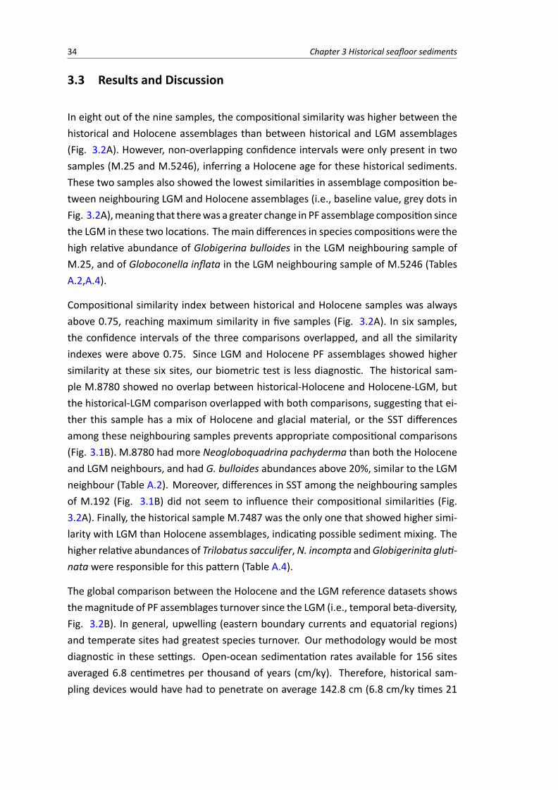
34 Chapter 3 Historical seafloor sediments
3.3 Results and Discussion
In eight out of the nine samples, the compositional similarity was higher between thehistorical and Holocene assemblages than between historical and LGM assemblages(Fig. 3.2A). However, non-overlapping confidence intervals were only present in twosamples (M.25 and M.5246), inferring a Holocene age for these historical sediments.These two samples also showed the lowest similarities in assemblage composition be-tween neighbouring LGM and Holocene assemblages (i.e., baseline value, grey dots inFig. 3.2A),meaning that therewas a greater change in PF assemblage composition sincethe LGM in these two locations. Themain differences in species compositions were thehigh relative abundance of Globigerina bulloides in the LGM neighbouring sample ofM.25, and of Globoconella inflata in the LGM neighbouring sample of M.5246 (TablesA.2,A.4).
Compositional similarity index between historical and Holocene samples was alwaysabove 0.75, reaching maximum similarity in five samples (Fig. 3.2A). In six samples,the confidence intervals of the three comparisons overlapped, and all the similarityindexes were above 0.75. Since LGM and Holocene PF assemblages showed highersimilarity at these six sites, our biometric test is less diagnostic. The historical sam-ple M.8780 showed no overlap between historical-Holocene and Holocene-LGM, butthe historical-LGM comparison overlapped with both comparisons, suggesting that ei-ther this sample has a mix of Holocene and glacial material, or the SST differencesamong these neighbouring samples prevents appropriate compositional comparisons(Fig. 3.1B). M.8780 had more Neogloboquadrina pachyderma than both the Holoceneand LGM neighbours, and had G. bulloides abundances above 20%, similar to the LGMneighbour (Table A.2). Moreover, differences in SST among the neighbouring samplesof M.192 (Fig. 3.1B) did not seem to influence their compositional similarities (Fig.3.2A). Finally, the historical sample M.7487 was the only one that showed higher simi-larity with LGM than Holocene assemblages, indicating possible sediment mixing. Thehigher relative abundances of Trilobatus sacculifer,N. incompta andGlobigerinita gluti-nata were responsible for this pattern (Table A.4).
The global comparison between the Holocene and the LGM reference datasets showsthemagnitude of PF assemblages turnover since the LGM (i.e., temporal beta-diversity,Fig. 3.2B). In general, upwelling (eastern boundary currents and equatorial regions)and temperate sites had greatest species turnover. Our methodology would be mostdiagnostic in these settings. Open-ocean sedimentation rates available for 156 sitesaveraged 6.8 centimetres per thousand of years (cm/ky). Therefore, historical sam-pling devices would have had to penetrate on average 142.8 cm (6.8 cm/ky times 21
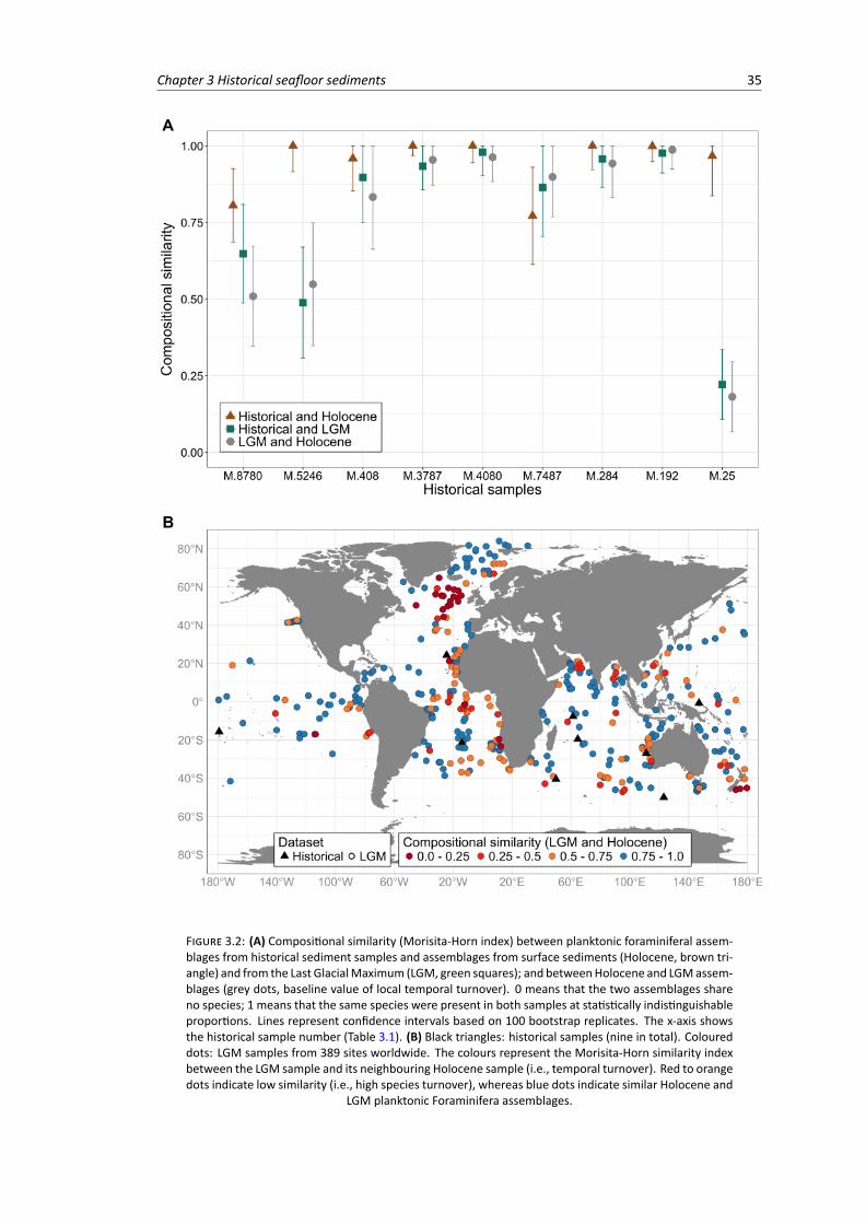
Chapter 3 Historical seafloor sediments 35
FIGURE 3.2: (A) Compositional similarity (Morisita-Horn index) between planktonic foraminiferal assem-blages from historical sediment samples and assemblages from surface sediments (Holocene, brown tri-angle) and from the Last GlacialMaximum (LGM, green squares); and betweenHolocene and LGMassem-blages (grey dots, baseline value of local temporal turnover). 0 means that the two assemblages shareno species; 1 means that the same species were present in both samples at statistically indistinguishableproportions. Lines represent confidence intervals based on 100 bootstrap replicates. The x-axis showsthe historical sample number (Table 3.1). (B) Black triangles: historical samples (nine in total). Coloureddots: LGM samples from 389 sites worldwide. The colours represent the Morisita-Horn similarity indexbetween the LGM sample and its neighbouring Holocene sample (i.e., temporal turnover). Red to orangedots indicate low similarity (i.e., high species turnover), whereas blue dots indicate similar Holocene and
LGM planktonic Foraminifera assemblages.
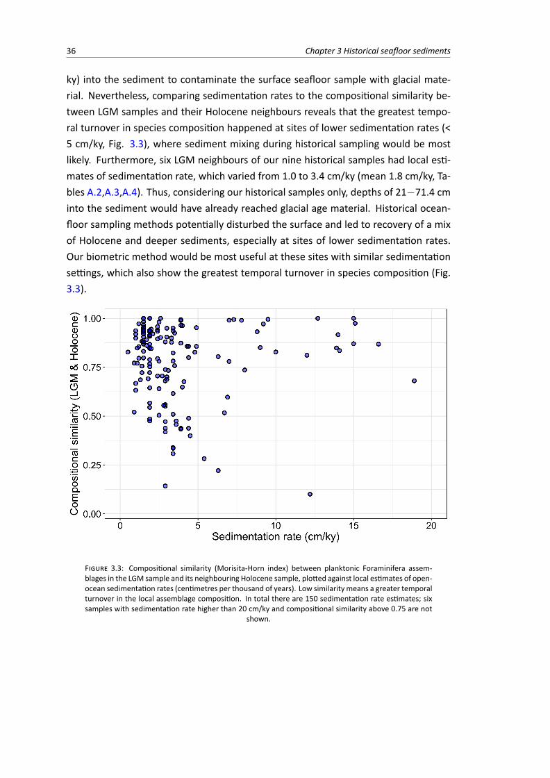
36 Chapter 3 Historical seafloor sediments
ky) into the sediment to contaminate the surface seafloor sample with glacial mate-rial. Nevertheless, comparing sedimentation rates to the compositional similarity be-tween LGM samples and their Holocene neighbours reveals that the greatest tempo-ral turnover in species composition happened at sites of lower sedimentation rates (<5 cm/ky, Fig. 3.3), where sediment mixing during historical sampling would be mostlikely. Furthermore, six LGM neighbours of our nine historical samples had local esti-mates of sedimentation rate, which varied from 1.0 to 3.4 cm/ky (mean 1.8 cm/ky, Ta-bles A.2,A.3,A.4). Thus, considering our historical samples only, depths of 21�71.4 cminto the sediment would have already reached glacial age material. Historical ocean-floor sampling methods potentially disturbed the surface and led to recovery of a mixof Holocene and deeper sediments, especially at sites of lower sedimentation rates.Our biometric method would be most useful at these sites with similar sedimentationsettings, which also show the greatest temporal turnover in species composition (Fig.3.3).
FIGURE 3.3: Compositional similarity (Morisita-Horn index) between planktonic Foraminifera assem-blages in the LGM sample and its neighbouring Holocene sample, plotted against local estimates of open-ocean sedimentation rates (centimetres per thousand of years). Low similarity means a greater temporalturnover in the local assemblage composition. In total there are 150 sedimentation rate estimates; sixsamples with sedimentation rate higher than 20 cm/ky and compositional similarity above 0.75 are not
shown.
Chapter 3 Historical seafloor sediments 37
3.4 Conclusion
Our results indicate that historical ocean-floor sediment samples (collected more than100 years ago) can represent surface (Holocene) sediments, despite the use of technol-ogy not designed to recover undisturbed sediments. Our biometric method relies onthe temporal turnover in species occurrence since the LGM.We show that this turnovervaries in space making our method particularly suitable for upwelling and temperateareas with low sedimentation rates. The new method allows a non-destructive pre-liminary assessment of glacial contamination of historical samples. Independent proxyrecords (e.g., Mg/Ca) and/or radiocarbon dating would be valuable to validate the suc-cess of our technique. Ideally, the biometric approach would compliment chemical-based techniques to date historical sediments, aiming for more robust results as mul-tiple alternative lines of evidence are presented. Our results highlight the scientificpotential of historical seafloor sediment collections (Table 3.2). As human activitiesincreasingly modify the marine environment, these historical collections contain im-portant information on the pre-1900 state of marine ecosystems.
TABLE 3.2: Historical surface sediments collections
Museum Expedition Spatial coverage Period
Natural History Museum in London Challenger1 Atlantic, Antarctic, 1872�76South Indian, Pacific
Muséum National d’histoire Naturelle in Paris Travailleur, Talisman2 Atlantic, Mediterranean 1880�83Museum für Naturkunde in Berlin German Deep-Sea3 Atlantic, Antarctic, 1898�99
(Valdivia) Indian, Mediterranean
1 https://www.hmschallenger.net/2https://gallica.bnf.fr/ark:/12148/bpt6k65190274
3 Keltie (1898); Sandeman (1900)
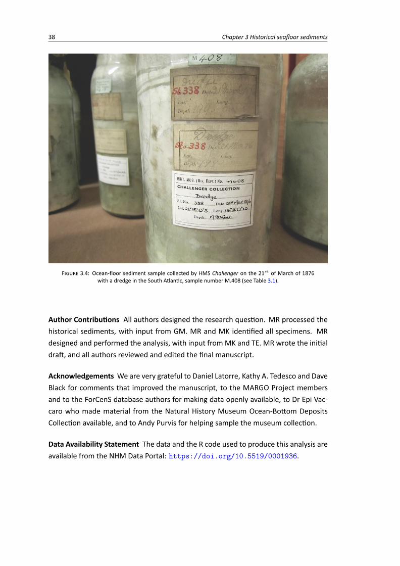
38 Chapter 3 Historical seafloor sediments
FIGURE 3.4: Ocean-floor sediment sample collected by HMS Challenger on the 21st of March of 1876with a dredge in the South Atlantic, sample number M.408 (see Table 3.1).
Author Contributions All authors designed the research question. MR processed thehistorical sediments, with input from GM. MR and MK identified all specimens. MRdesigned and performed the analysis, with input fromMK and TE. MR wrote the initialdraft, and all authors reviewed and edited the final manuscript.
Acknowledgements We are very grateful to Daniel Latorre, Kathy A. Tedesco and DaveBlack for comments that improved the manuscript, to the MARGO Project membersand to the ForCenS database authors for making data openly available, to Dr Epi Vac-caro who made material from the Natural History Museum Ocean-Bottom DepositsCollection available, and to Andy Purvis for helping sample the museum collection.
Data Availability Statement The data and the R code used to produce this analysis areavailable from the NHM Data Portal: .
Chapter 4
Biogeographical patterns of intraspecificsize variation in extant planktonicForaminifera
Marina C. Rillo1,2,3⇤, C. Giles Miller2, Michal Kučera3 &Thomas H. G. Ezard1
1Ocean and Earth Science, National Oceanography Centre Southampton, University of SouthamptonWaterfront Campus, Southampton SO143ZH, UK2Department of Earth Sciences, Natural History Museum, Cromwell Road, London SW7 5BD, UK3MARUM, University of Bremen, Leobener Strasse, Bremen 28359, Germany*Correspondence: [email protected]
39

40 Chapter 4 Intraspecific size variation
Abstract:How plankton organism size varies within species across biogeographical scales is stillpoorly documented, although evidence has accumulated that intraspecific trait vari-ation affects plankton functions in marine ecosystems. Here, we investigate for thefirst time at high intraspecific resolution how planktonic Foraminifera species, a ubiq-uitous zooplankton group, vary in size across the tropical and subtropical oceans of theworld. We measured 3817 individuals of nine species in 53 surface sediments and ob-tained corresponding local values of annual mean sea-surface temperature (SST) andnet primary productivity (NPP), as well as local relative abundance of the species. Givenformer studies, we expected populations to reach largest sizes under optimal environ-mental conditions, where populations reach highest relative abundances. However,we found that species greatly differ in how much size variation is explained by SST,NPP and/or relative abundance. While some species showed a high predictability ofsize variation given one single variable (SST for Trilobatus sacculifer and Pulleniatinaobliquiloculata), other species showed either no (Globigerinoides ruber, Neoglobo-quadrina dutertrei) or weak (Globoconella inflata, Globorotalia menardii) relationshipsbetween size and the studied variables. SST and NPP combined explained most of thesize variation observed in Globigerinella siphonifera, Globorotalia truncatulinoides andGlobigerinoides conglobatus. Moreover, the relationship between size and local abun-dancewasweak, contradicting the idea that planktonic Foraminifera species are largestat their environmental optima. By incorporating intraspecific variation and samplingbroader geographical ranges compared to previous studies, we conclude that the re-lationship between planktonic Foraminifera size and SST, NPP and abundance differsamong species and is, in general, weaker than previously reported.
Keywords:biogeography of traits, intraspecific variation, macroecology, size trends, morphomet-rics, natural history collections (NHC), museum collections
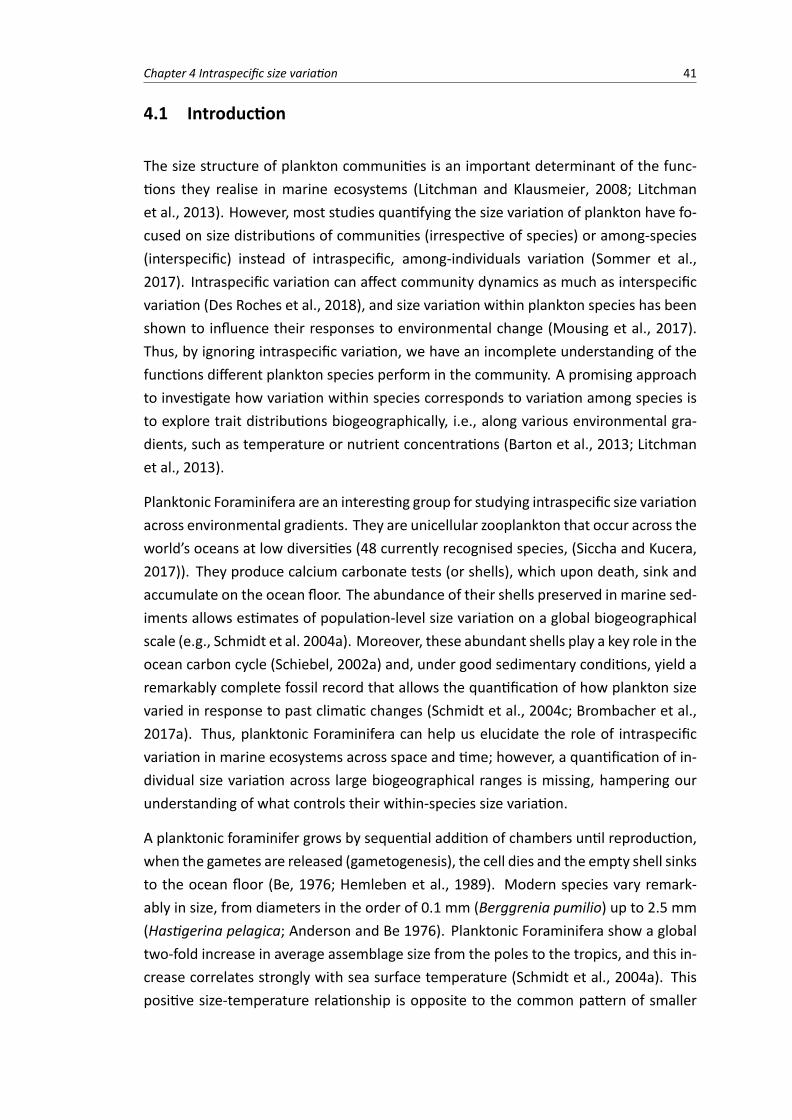
Chapter 4 Intraspecific size variation 41
4.1 Introduction
The size structure of plankton communities is an important determinant of the func-tions they realise in marine ecosystems (Litchman and Klausmeier, 2008; Litchmanet al., 2013). However, most studies quantifying the size variation of plankton have fo-cused on size distributions of communities (irrespective of species) or among-species(interspecific) instead of intraspecific, among-individuals variation (Sommer et al.,2017). Intraspecific variation can affect community dynamics as much as interspecificvariation (Des Roches et al., 2018), and size variation within plankton species has beenshown to influence their responses to environmental change (Mousing et al., 2017).Thus, by ignoring intraspecific variation, we have an incomplete understanding of thefunctions different plankton species perform in the community. A promising approachto investigate how variation within species corresponds to variation among species isto explore trait distributions biogeographically, i.e., along various environmental gra-dients, such as temperature or nutrient concentrations (Barton et al., 2013; Litchmanet al., 2013).
Planktonic Foraminifera are an interesting group for studying intraspecific size variationacross environmental gradients. They are unicellular zooplankton that occur across theworld’s oceans at low diversities (48 currently recognised species, (Siccha and Kucera,2017)). They produce calcium carbonate tests (or shells), which upon death, sink andaccumulate on the ocean floor. The abundance of their shells preserved in marine sed-iments allows estimates of population-level size variation on a global biogeographicalscale (e.g., Schmidt et al. 2004a). Moreover, these abundant shells play a key role in theocean carbon cycle (Schiebel, 2002a) and, under good sedimentary conditions, yield aremarkably complete fossil record that allows the quantification of how plankton sizevaried in response to past climatic changes (Schmidt et al., 2004c; Brombacher et al.,2017a). Thus, planktonic Foraminifera can help us elucidate the role of intraspecificvariation in marine ecosystems across space and time; however, a quantification of in-dividual size variation across large biogeographical ranges is missing, hampering ourunderstanding of what controls their within-species size variation.
A planktonic foraminifer grows by sequential addition of chambers until reproduction,when the gametes are released (gametogenesis), the cell dies and the empty shell sinksto the ocean floor (Be, 1976; Hemleben et al., 1989). Modern species vary remark-ably in size, from diameters in the order of 0.1 mm (Berggrenia pumilio) up to 2.5 mm(Hastigerina pelagica; Anderson and Be 1976). Planktonic Foraminifera show a globaltwo-fold increase in average assemblage size from the poles to the tropics, and this in-crease correlates strongly with sea surface temperature (Schmidt et al., 2004a). Thispositive size-temperature relationship is opposite to the common pattern of smaller

42 Chapter 4 Intraspecific size variation
sizes at higher temperatures observed in other plankton groups (Atkinson et al., 2003;Barton et al., 2013; Sommer et al., 2017). Higher temperatures are known to affectmetabolic rates positively, resulting in smaller organisms and faster generation times(Brown et al., 2004; Savage et al., 2004). Planktonic Foraminifera assemblages, how-ever, do not follow this rule (Schmidt et al., 2004a) and the reason might be related totheir reproductive strategy. As far as we know, they reproduce only sexually (Hemlebenet al., 1989) and thus rely on precise spatial and temporal synchrony with each otherto maximise chances of fertilisation in the pelagic environment. Indeed, there appearsto be a lunar periodicity to the reproductive cycle of some species (Bijma et al., 1990;Bijma and Hemleben, 1994; Jonkers et al., 2015; Venancio et al., 2016), suggesting thatplanktonic Foraminifera generation and development time is constrained by their syn-chronic reproduction. Unfortunately, planktonic Foraminifera have never reproducedin laboratory conditions, thus we have limited knowledge of their reproductive cycle,ecology and population dynamics.
Previous studies have looked at the biogeographical size distribution of planktonicForaminifera and found that maximum shell size often coincides with maximum rela-tive abundance, and occurs at specific optimum temperatures (optimum-size hypothe-sis; Kennett 1976; Hecht 1976; Malmgren and Kennett 1976, 1977; Kahn 1981; Schmidtet al. 2004a; Moller et al. 2013; see Be et al. 1973 for an exception). The local abun-dance of planktonic Foraminifera species is usually estimated by counting dead assem-blages from ocean floor sediments (Siccha and Kucera, 2017). Although this method-ology often yields species’ relative abundances (relative to the co-occurring species inthe sample) instead of absolute abundances, relative abundances estimated from ma-rine sediments have the advantage of averaging out short-term fluctuations that mightblur macroecological patterns (Fenton et al., 2016b). Most of the studies supportingthe optimum-size hypothesis focused on a single oceanic basin, and thus a limited partof each species’ biogeographical range (Be et al., 1973; Kennett, 1976; Hecht, 1976;Malmgren and Kennett, 1976, 1977; Kahn, 1981; Moller et al., 2013). The exception isthe global study of Schmidt et al. (2004a), who analysed 69 Holocene samples world-wide. Although Schmidt et al. (2004a) were concerned with size variation of wholeassemblages instead of within-species variation, they showed that the temperaturesat which a species reaches largest size and highest relative abundance coincide, sup-porting the idea that planktonic Foraminifera species reach largest shell sizes at theirenvironmental (thermal) optima. However, Schmidt et al. (2004a) only taxonomicallyidentified a fraction of their measured individuals, thus a test of the optimum-size hy-pothesis at high intraspecific resolution and large biogeographical scale is still missing.
Nutrient availability can mediate the temperature-size relationships observed in the
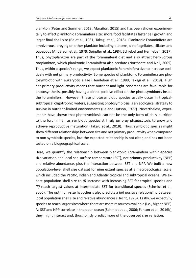
Chapter 4 Intraspecific size variation 43
plankton (Peter and Sommer, 2013; Marañón, 2015) and has been shown experimen-tally to affect planktonic Foraminifera size: more food facilitates faster cell growth andlarger final shell size (Be et al., 1981; Takagi et al., 2018). Planktonic Foraminifera areomnivorous, preying on other plankton including diatoms, dinoflagellates, ciliates andcopepods (Anderson et al., 1979; Spindler et al., 1984; Schiebel and Hemleben, 2017).Thus, phytoplankton are part of the foraminiferal diet and also attract herbivorouszooplankton, which planktonic Foraminifera also predate (Northcote and Neil, 2005).Thus, within a species’s range, we expect planktonic Foraminifera size to increase posi-tively with net primary productivity. Some species of planktonic Foraminifera are pho-tosymbiotic with eukaryotic algae (Hemleben et al., 1989; Takagi et al., 2019). Highnet primary productivity means that nutrient and light conditions are favourable forphotosynthesis, possibly having a direct positive effect on the photosymbionts insidethe foraminifers. However, these photosymbiotic species usually occur in tropical-subtropical oligotrophic waters, suggesting photosymbiosis is an ecological strategy tosurvive in nutrient-limited environments (Be and Hutson, 1977). Nevertheless, exper-iments have shown that photosymbiosis can not be the only form of daily nutritionto the foraminifer, as symbiotic species still rely on prey phagocytosis to grow andachieve reproductive maturation (Takagi et al., 2018). Thus, symbiotic species mightshowdifferent relationships between size andnet primary productivitywhen comparedto non-symbiotic species, but the expected relationship is not clear, and has not beentested on a biogeographical scale.
Here, we quantify the relationship between planktonic Foraminifera within-speciessize variation and local sea surface temperature (SST), net primary productivity (NPP)and relative abundance, plus the interaction between SST and NPP. We built a newpopulation-level shell size dataset for nine extant species at a macroecological scale,which included the Pacific, Indian and Atlantic tropical and subtropical oceans. We ex-pect population shell size to (i) increase with increasing SST for tropical species and(ii) reach largest values at intermediate SST for transitional species (Schmidt et al.,2006). The optimum-size hypothesis also predicts a (iii) positive relationship betweenlocal population shell size and relative abundances (Hecht, 1976). Lastly, we expect (iv)species to reach larger sizeswhere there aremore resources available (i.e., higher NPP).As SST and NPP correlate in the open ocean (Schmidt et al., 2006; Fenton et al., 2016b),they might interact and, thus, jointly predict more of the observed size variation.
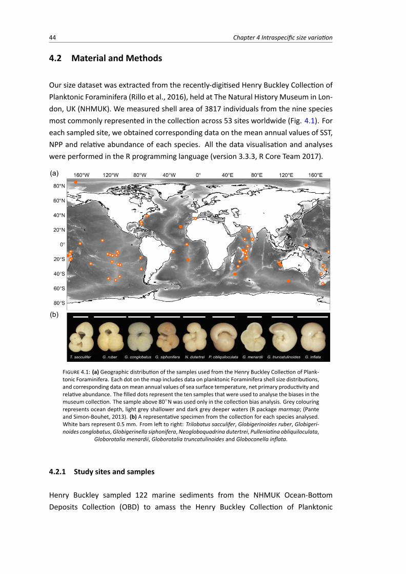
44 Chapter 4 Intraspecific size variation
4.2 Material and Methods
Our size dataset was extracted from the recently-digitised Henry Buckley Collection ofPlanktonic Foraminifera (Rillo et al., 2016), held at The Natural History Museum in Lon-don, UK (NHMUK). We measured shell area of 3817 individuals from the nine speciesmost commonly represented in the collection across 53 sites worldwide (Fig. 4.1). Foreach sampled site, we obtained corresponding data on the mean annual values of SST,NPP and relative abundance of each species. All the data visualisation and analyseswere performed in the R programming language (version 3.3.3, R Core Team 2017).
FIGURE 4.1: (a) Geographic distribution of the samples used from the Henry Buckley Collection of Plank-tonic Foraminifera. Each dot on themap includes data on planktonic Foraminifera shell size distributions,and corresponding data onmean annual values of sea surface temperature, net primary productivity andrelative abundance. The filled dots represent the ten samples that were used to analyse the biases in themuseum collection. The sample above 80�Nwas used only in the collection bias analysis. Grey colouringrepresents ocean depth, light grey shallower and dark grey deeper waters (R package marmap; (Panteand Simon-Bouhet, 2013). (b) A representative specimen from the collection for each species analysed.White bars represent 0.5 mm. From left to right: Trilobatus sacculifer, Globigerinoides ruber, Globigeri-noides conglobatus,Globigerinella siphonifera,Neogloboquadrina dutertrei, Pulleniatina obliquiloculata,
Globorotalia menardii, Globorotalia truncatulinoides and Globoconella inflata.
4.2.1 Study sites and samples
Henry Buckley sampled 122 marine sediments from the NHMUK Ocean-BottomDeposits Collection (OBD) to amass the Henry Buckley Collection of Planktonic
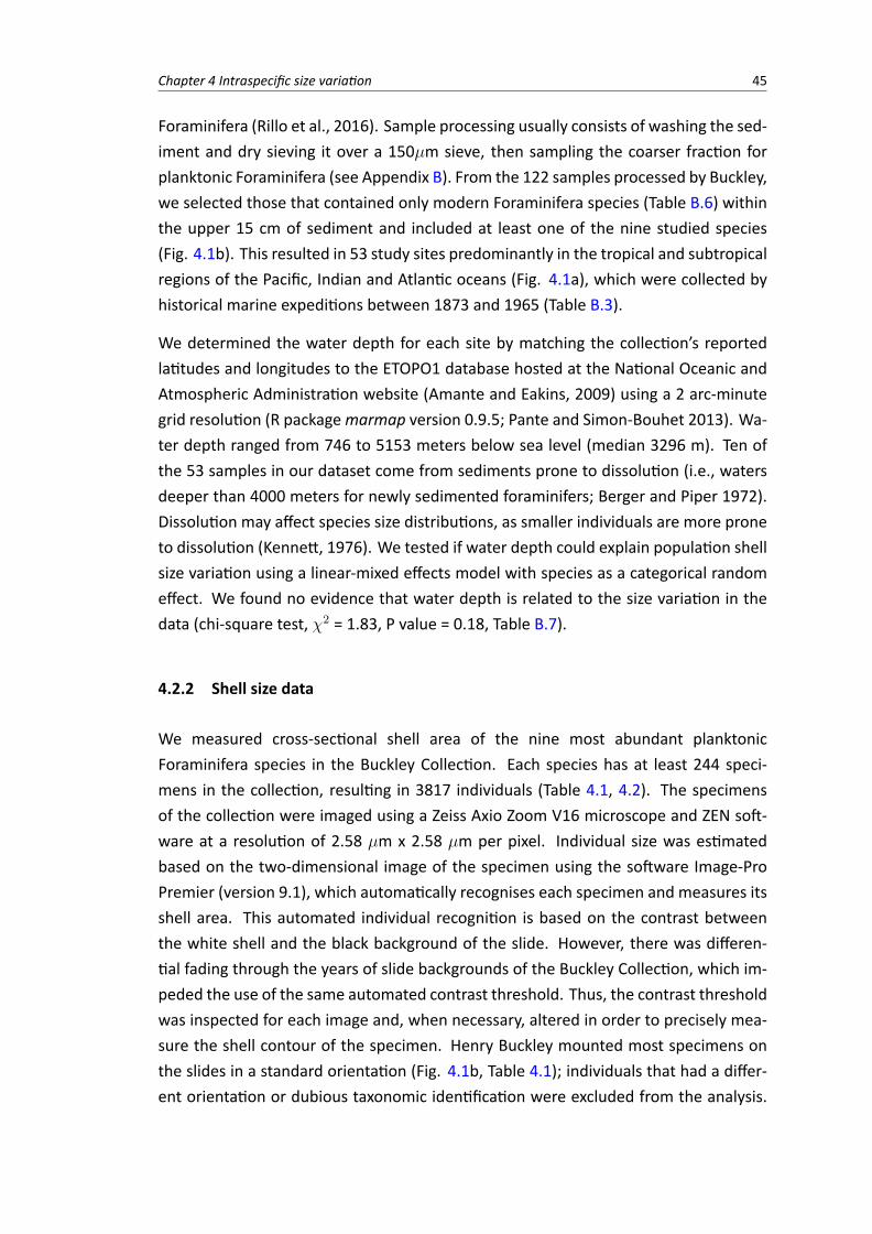
Chapter 4 Intraspecific size variation 45
Foraminifera (Rillo et al., 2016). Sample processing usually consists of washing the sed-iment and dry sieving it over a 150µm sieve, then sampling the coarser fraction forplanktonic Foraminifera (see Appendix B). From the 122 samples processed by Buckley,we selected those that contained only modern Foraminifera species (Table B.6) withinthe upper 15 cm of sediment and included at least one of the nine studied species(Fig. 4.1b). This resulted in 53 study sites predominantly in the tropical and subtropicalregions of the Pacific, Indian and Atlantic oceans (Fig. 4.1a), which were collected byhistorical marine expeditions between 1873 and 1965 (Table B.3).
We determined the water depth for each site by matching the collection’s reportedlatitudes and longitudes to the ETOPO1 database hosted at the National Oceanic andAtmospheric Administration website (Amante and Eakins, 2009) using a 2 arc-minutegrid resolution (R packagemarmap version 0.9.5; Pante and Simon-Bouhet 2013). Wa-ter depth ranged from 746 to 5153 meters below sea level (median 3296 m). Ten ofthe 53 samples in our dataset come from sediments prone to dissolution (i.e., watersdeeper than 4000 meters for newly sedimented foraminifers; Berger and Piper 1972).Dissolution may affect species size distributions, as smaller individuals are more proneto dissolution (Kennett, 1976). We tested if water depth could explain population shellsize variation using a linear-mixed effects model with species as a categorical randomeffect. We found no evidence that water depth is related to the size variation in thedata (chi-square test, �2 = 1.83, P value = 0.18, Table B.7).
4.2.2 Shell size data
We measured cross-sectional shell area of the nine most abundant planktonicForaminifera species in the Buckley Collection. Each species has at least 244 speci-mens in the collection, resulting in 3817 individuals (Table 4.1, 4.2). The specimensof the collection were imaged using a Zeiss Axio Zoom V16 microscope and ZEN soft-ware at a resolution of 2.58 µm x 2.58 µm per pixel. Individual size was estimatedbased on the two-dimensional image of the specimen using the software Image-ProPremier (version 9.1), which automatically recognises each specimen and measures itsshell area. This automated individual recognition is based on the contrast betweenthe white shell and the black background of the slide. However, there was differen-tial fading through the years of slide backgrounds of the Buckley Collection, which im-peded the use of the same automated contrast threshold. Thus, the contrast thresholdwas inspected for each image and, when necessary, altered in order to precisely mea-sure the shell contour of the specimen. Henry Buckley mounted most specimens onthe slides in a standard orientation (Fig. 4.1b, Table 4.1); individuals that had a differ-ent orientation or dubious taxonomic identification were excluded from the analysis.
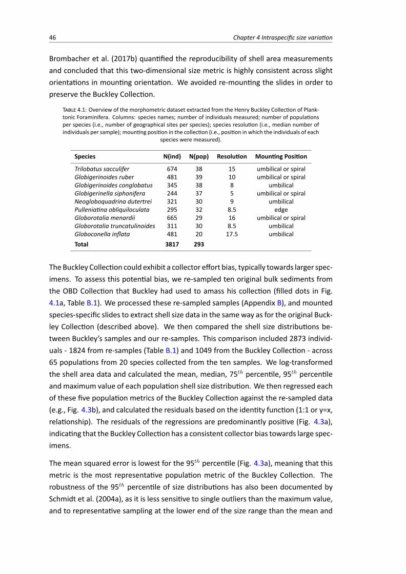
46 Chapter 4 Intraspecific size variation
Brombacher et al. (2017b) quantified the reproducibility of shell area measurementsand concluded that this two-dimensional size metric is highly consistent across slightorientations in mounting orientation. We avoided re-mounting the slides in order topreserve the Buckley Collection.
TABLE 4.1: Overview of the morphometric dataset extracted from the Henry Buckley Collection of Plank-tonic Foraminifera. Columns: species names; number of individuals measured; number of populationsper species (i.e., number of geographical sites per species); species resolution (i.e., median number ofindividuals per sample); mounting position in the collection (i.e., position in which the individuals of each
species were measured).
Species N(ind) N(pop) Resolution Mounting Position
Trilobatus sacculifer 674 38 15 umbilical or spiralGlobigerinoides ruber 481 39 10 umbilical or spiralGlobigerinoides conglobatus 345 38 8 umbilicalGlobigerinella siphonifera 244 37 5 umbilical or spiralNeogloboquadrina dutertrei 321 30 9 umbilicalPulleniatina obliquiloculata 295 32 8.5 edgeGloborotalia menardii 665 29 16 umbilical or spiralGloborotalia truncatulinoides 311 30 8.5 umbilicalGloboconella inflata 481 20 17.5 umbilicalTotal 3817 293
TheBuckley Collection could exhibit a collector effort bias, typically towards larger spec-imens. To assess this potential bias, we re-sampled ten original bulk sediments fromthe OBD Collection that Buckley had used to amass his collection (filled dots in Fig.4.1a, Table B.1). We processed these re-sampled samples (Appendix B), and mountedspecies-specific slides to extract shell size data in the sameway as for the original Buck-ley Collection (described above). We then compared the shell size distributions be-tween Buckley’s samples and our re-samples. This comparison included 2873 individ-uals - 1824 from re-samples (Table B.1) and 1049 from the Buckley Collection - across65 populations from 20 species collected from the ten samples. We log-transformedthe shell area data and calculated the mean, median, 75th percentile, 95th percentileandmaximum value of each population shell size distribution. We then regressed eachof these five population metrics of the Buckley Collection against the re-sampled data(e.g., Fig. 4.3b), and calculated the residuals based on the identity function (1:1 or y=x,relationship). The residuals of the regressions are predominantly positive (Fig. 4.3a),indicating that the Buckley Collection has a consistent collector bias towards large spec-imens.
The mean squared error is lowest for the 95th percentile (Fig. 4.3a), meaning that thismetric is the most representative population metric of the Buckley Collection. Therobustness of the 95th percentile of size distributions has also been documented bySchmidt et al. (2004a), as it is less sensitive to single outliers than the maximum value,and to representative sampling at the lower end of the size range than the mean and
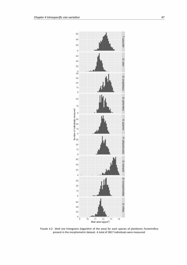
Chapter 4 Intraspecific size variation 47
FIGURE 4.2: Shell size histograms (logarithm of the area) for each species of planktonic Foraminiferapresent in the morphometric dataset. A total of 3817 individuals were measured.
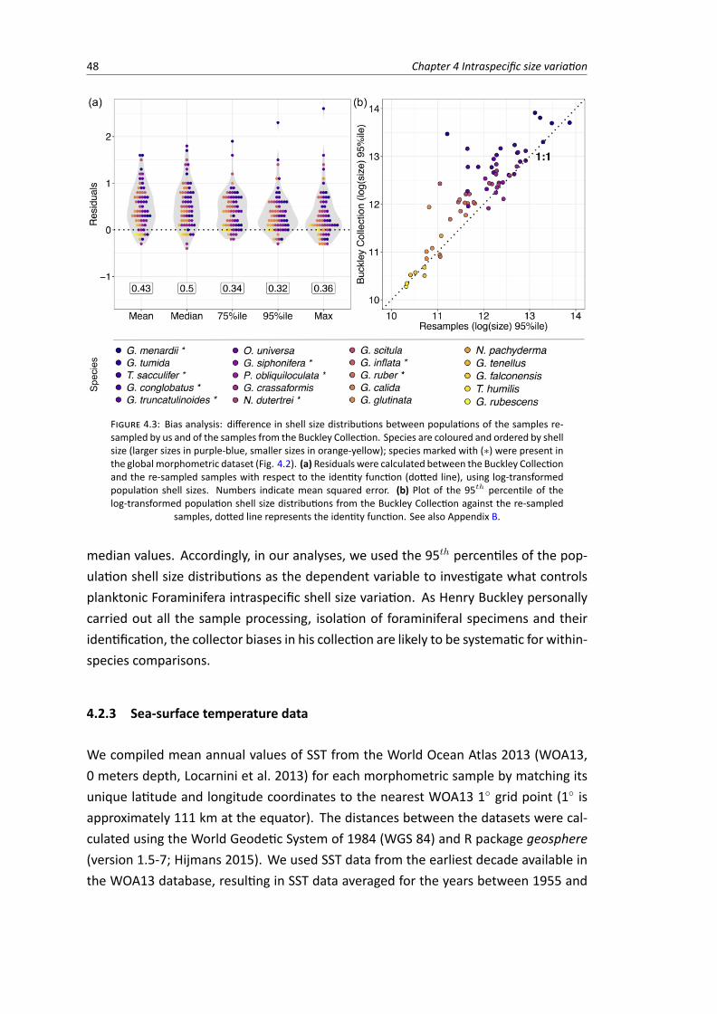
48 Chapter 4 Intraspecific size variation
FIGURE 4.3: Bias analysis: difference in shell size distributions between populations of the samples re-sampled by us and of the samples from the Buckley Collection. Species are coloured and ordered by shellsize (larger sizes in purple-blue, smaller sizes in orange-yellow); species marked with (⇤) were present inthe global morphometric dataset (Fig. 4.2). (a) Residuals were calculated between the Buckley Collectionand the re-sampled samples with respect to the identity function (dotted line), using log-transformedpopulation shell sizes. Numbers indicate mean squared error. (b) Plot of the 95th percentile of thelog-transformed population shell size distributions from the Buckley Collection against the re-sampled
samples, dotted line represents the identity function. See also Appendix B.
median values. Accordingly, in our analyses, we used the 95th percentiles of the pop-ulation shell size distributions as the dependent variable to investigate what controlsplanktonic Foraminifera intraspecific shell size variation. As Henry Buckley personallycarried out all the sample processing, isolation of foraminiferal specimens and theiridentification, the collector biases in his collection are likely to be systematic for within-species comparisons.
4.2.3 Sea-surface temperature data
We compiled mean annual values of SST from the World Ocean Atlas 2013 (WOA13,0 meters depth, Locarnini et al. 2013) for each morphometric sample by matching itsunique latitude and longitude coordinates to the nearest WOA13 1� grid point (1� isapproximately 111 km at the equator). The distances between the datasets were cal-culated using the World Geodetic System of 1984 (WGS 84) and R package geosphere(version 1.5-7; Hijmans 2015). We used SST data from the earliest decade available inthe WOA13 database, resulting in SST data averaged for the years between 1955 and
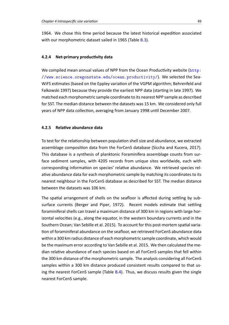
Chapter 4 Intraspecific size variation 49
1964. We chose this time period because the latest historical expedition associatedwith our morphometric dataset sailed in 1965 (Table B.3).
4.2.4 Net-primary productivity data
We compiled mean annual values of NPP from the Ocean Productivity website (). We selected the Sea-
WiFS estimates (based on the Eppley variation of the VGPM algorithm; Behrenfeld andFalkowski 1997) because they provide the earliest NPP data (starting in late 1997). Wematched eachmorphometric sample coordinate to its nearest NPP sample as describedfor SST. The median distance between the datasets was 15 km. We considered only fullyears of NPP data collection, averaging from January 1998 until December 2007.
4.2.5 Relative abundance data
To test for the relationship between population shell size and abundance, we extractedassemblage composition data from the ForCenS database (Siccha and Kucera, 2017).This database is a synthesis of planktonic Foraminifera assemblage counts from sur-face sediment samples, with 4205 records from unique sites worldwide, each withcorresponding information on species’ relative abundance. We retrieved species rel-ative abundance data for each morphometric sample by matching its coordinates to itsnearest neighbour in the ForCenS database as described for SST. The median distancebetween the datasets was 106 km.
The spatial arrangement of shells on the seafloor is affected during settling by sub-surface currents (Berger and Piper, 1972). Recent models estimate that settlingforaminiferal shells can travel a maximum distance of 300 km in regions with large hor-izontal velocities (e.g., along the equator, in the western boundary currents and in theSouthern Ocean; Van Sebille et al. 2015). To account for this post-mortem spatial varia-tion of foraminiferal abundance on the seafloor, we retrieved ForCenS abundance datawithin a 300 km radius distance of eachmorphometric sample coordinate, whichwouldbe themaximum error according to Van Sebille et al. 2015. We then calculated theme-dian relative abundance of each species based on all ForCenS samples that fell withinthe 300 km distance of themorphometric sample. The analysis considering all ForCenSsamples within a 300 km distance produced consistent results compared to that us-ing the nearest ForCenS sample (Table B.4). Thus, we discuss results given the singlenearest ForCenS sample.
50 Chapter 4 Intraspecific size variation
4.2.6 Statistical analysis
Effects of SST, NPP and species relative abundance on planktonic Foraminifera size dis-tributions were assessed using linear and quadratic models and a hierarchical modelselection framework. For each species, the dependent response variable was the log-transformed size distribution (95th percentile) whereas the independent explanatoryvariables were the local mean annual SST, NPP and local relative abundances. Linearand quadratic relationships were considered between shell size and SST and NPP, aswell as the interaction between SST and NPP. We compared the models through a hi-erarchical model selection framework: we started all analyses with a null model thatincluded the population shell size as the dependent variable and the regression param-eter constant (sample mean). We then added the predictor variable(s) to this modelincrementally to see whether the model was improved. Model fit was assessed usingAkaike information criterion corrected for small sample size (AICc); models within adifference of two AICc units (i.e.,�AICc< 2) are equally plausible. Adjusted R squared(R2
adj) were calculated for each model using the R package rsq (version 1.0.1; (Zhang,2017)). Visual inspection of the residual plots did not reveal any obvious deviationsfrom homoscedasticity, except for G. inflata (Fig. B.1).
We used the observations in the 53 samples to investigate two species-level patterns:(i) the SST at which each species reaches its largest size (95th percentile of the pop-ulation) and the SST at which each species is most abundant and (ii) the relationshipbetween species’ maximum size against its maximum relative abundance. These rela-tionships were tested using a standard linear model. We expected to see a tight posi-tive relationship between SST at largest size and SST at highest abundance, as found bySchmidt et al. (2004a).
Chapter 4 Intraspecific size variation 51
4.3 Results
Size variation of planktonic Foraminifera is high within- (Fig. 4.4) and among popula-tions (Fig. 4.5). Among adults within the same species, size variation can range overone order ofmagnitude (e.g., from150µmto 1500µmGloborotaliamenardii, Fig. 4.2).This high intraspecific variation is differentially explained by SST, NPP and relative abun-dance across species. When tested alone, SST shows a significant relationship with sizein four out of nine species. T. sacculifer, G. siphonifera and P. obliquiloculata increasein size significantly with linear increase of SST, and G. truncatulinoides size variationis significantly explained by a quadratic function of SST (Fig. 4.5a). Shell sizes in theother five species do not co-vary significantly with SST. NPP and size variation show asignificant positive relationship only in G. siphonifera (adjusted R2 of 24%; Fig. 4.5b).Although not significant, NPP explains a relatively high proportion of the size variationobserved within G. truncatulinoides (11%, negative relationship) and G. inflata (15%,weak positive relationship). Local relative abundance explains less size variation thanSST and NPP for all species except G. menardii (Fig. 4.5c). T. sacculifer also shows apositive relationship between shell size and relative abundance, but weaker than withSST. Note that due to the low relative abundances (below 10%) of G. conglobatus, G.siphonifera and G. truncatulinoides, we do not infer a relationship between size andrelative abundance for these species.
SST and NPP correlate (Fig. 4.6), thus their isolated effect on size (Fig. 4.5a,b) might beconfounding. For this reason, we considered all variables together in a model selectionframework, including the interaction between SST and NPP. The explanatory power ofthe variables SST, NPP and relative abundance still varies greatly among species (Table4.2). SST explains 25% and 21% of the intraspecific size variation of T. sacculifer and P.obliquiloculata, respectively. SST and NPP together reach the highest predictability ofsize variation: 33% in G. siphonifera and 32% in G. truncatulinoides. When consideringthe interaction between SST and NPP, 34% of the size variation in G. truncatulinoidesand 19% in G. conglobatus is explained. NPP alone explains 15% of the size variationof G. inflata, although the null model is equally plausible (�AICc< 2). G. menardii sizevariation can be predicted by 15% given the additive effect of SST and relative abun-dance, but the null model is also plausible. Surprisingly, G. ruber and N. dutertrei sizevariations are poorly predicted by any of the three variables (see also Fig. 4.5), beingbest explained by the null model.
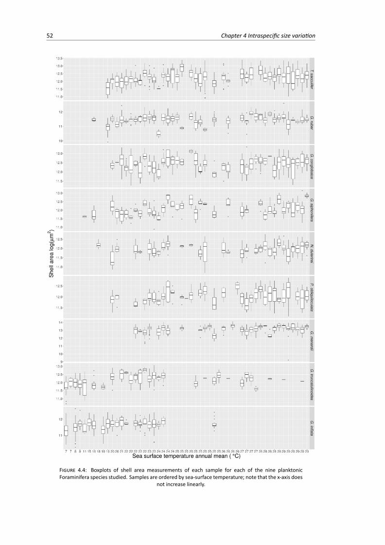
52 Chapter 4 Intraspecific size variation
FIGURE 4.4: Boxplots of shell area measurements of each sample for each of the nine planktonicForaminifera species studied. Samples are ordered by sea-surface temperature; note that the x-axis does
not increase linearly.
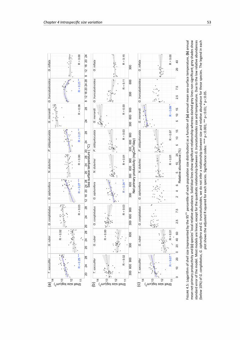
Chapter 4 Intraspecific size variation 53
FIGU
RE4.5:
Logarithm
ofshellsize
(rep
resented
bythe95
thpe
rcen
tileof
each
popu
latio
nsiz
edistrib
ution
)asa
functio
nof
(a)a
nnua
lmeansea-surfa
cetempe
rature,(b)
annu
almeanne
t-prim
aryprod
uctiv
ityan
d(c)spe
cies’localrelativ
eab
unda
nce.
Solid
blue
lines
show
significan
trelati
onshipwhe
reas
dashed
grey
lines
non-sig
nifican
t;grey
shad
esshow
stan
dard
erroro
fthe
mod
el.M
ostm
odelsa
relinear,except
forthe
quad
ratic
relatio
nshipbe
twee
nG.
trun
catulinoide
ssize
andtempe
rature.D
ueto
thelowrelativ
eab
unda
nces
(below
10%)o
fG.con
glob
atus,G
.sipho
nifera
andG.
trun
catulinoide
s,wedo
notinfer
arelatio
nshipbe
twee
nsiz
ean
drelativ
eab
unda
nceforthe
sespecies.
Thelegend
ineach
plot
show
sthe
adjusted
Rsqua
redfore
achspecies.Sign
ificancecode
s:**
*p<
0.00
1;**
p<0.01
;*p<
0.05
.
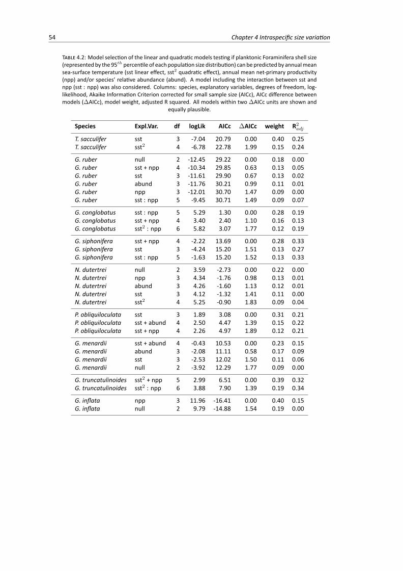
54 Chapter 4 Intraspecific size variation
TABLE 4.2: Model selection of the linear and quadratic models testing if planktonic Foraminifera shell size(represented by the 95th percentile of each population size distribution) can be predicted by annualmeansea-surface temperature (sst linear effect, sst2 quadratic effect), annual mean net-primary productivity(npp) and/or species’ relative abundance (abund). A model including the interaction between sst andnpp (sst : npp) was also considered. Columns: species, explanatory variables, degrees of freedom, log-likelihood, Akaike Information Criterion corrected for small sample size (AICc), AICc difference betweenmodels (�AICc), model weight, adjusted R squared. All models within two �AICc units are shown and
equally plausible.
Species Expl.Var. df logLik AICc �AICc weight R2adj
T. sacculifer sst 3 -7.04 20.79 0.00 0.40 0.25T. sacculifer sst2 4 -6.78 22.78 1.99 0.15 0.24
G. ruber null 2 -12.45 29.22 0.00 0.18 0.00G. ruber sst + npp 4 -10.34 29.85 0.63 0.13 0.05G. ruber sst 3 -11.61 29.90 0.67 0.13 0.02G. ruber abund 3 -11.76 30.21 0.99 0.11 0.01G. ruber npp 3 -12.01 30.70 1.47 0.09 0.00G. ruber sst : npp 5 -9.45 30.71 1.49 0.09 0.07
G. conglobatus sst : npp 5 5.29 1.30 0.00 0.28 0.19G. conglobatus sst + npp 4 3.40 2.40 1.10 0.16 0.13G. conglobatus sst2 : npp 6 5.82 3.07 1.77 0.12 0.19
G. siphonifera sst + npp 4 -2.22 13.69 0.00 0.28 0.33G. siphonifera sst 3 -4.24 15.20 1.51 0.13 0.27G. siphonifera sst : npp 5 -1.63 15.20 1.52 0.13 0.33
N. dutertrei null 2 3.59 -2.73 0.00 0.22 0.00N. dutertrei npp 3 4.34 -1.76 0.98 0.13 0.01N. dutertrei abund 3 4.26 -1.60 1.13 0.12 0.01N. dutertrei sst 3 4.12 -1.32 1.41 0.11 0.00N. dutertrei sst2 4 5.25 -0.90 1.83 0.09 0.04
P. obliquiloculata sst 3 1.89 3.08 0.00 0.31 0.21P. obliquiloculata sst + abund 4 2.50 4.47 1.39 0.15 0.22P. obliquiloculata sst + npp 4 2.26 4.97 1.89 0.12 0.21
G. menardii sst + abund 4 -0.43 10.53 0.00 0.23 0.15G. menardii abund 3 -2.08 11.11 0.58 0.17 0.09G. menardii sst 3 -2.53 12.02 1.50 0.11 0.06G. menardii null 2 -3.92 12.29 1.77 0.09 0.00
G. truncatulinoides sst2 + npp 5 2.99 6.51 0.00 0.39 0.32G. truncatulinoides sst2 : npp 6 3.88 7.90 1.39 0.19 0.34
G. inflata npp 3 11.96 -16.41 0.00 0.40 0.15G. inflata null 2 9.79 -14.88 1.54 0.19 0.00
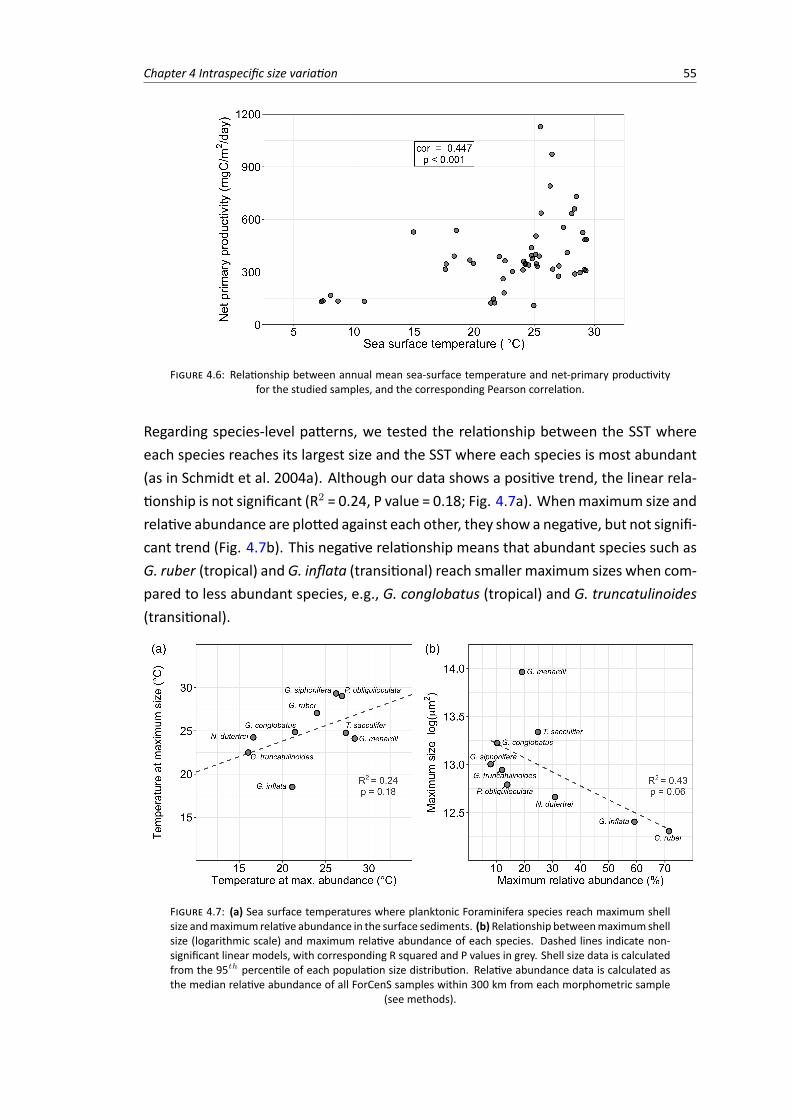
Chapter 4 Intraspecific size variation 55
FIGURE 4.6: Relationship between annual mean sea-surface temperature and net-primary productivityfor the studied samples, and the corresponding Pearson correlation.
Regarding species-level patterns, we tested the relationship between the SST whereeach species reaches its largest size and the SST where each species is most abundant(as in Schmidt et al. 2004a). Although our data shows a positive trend, the linear rela-tionship is not significant (R2 = 0.24, P value = 0.18; Fig. 4.7a). Whenmaximum size andrelative abundance are plotted against each other, they show a negative, but not signifi-cant trend (Fig. 4.7b). This negative relationship means that abundant species such asG. ruber (tropical) and G. inflata (transitional) reach smaller maximum sizes when com-pared to less abundant species, e.g., G. conglobatus (tropical) and G. truncatulinoides(transitional).
FIGURE 4.7: (a) Sea surface temperatures where planktonic Foraminifera species reach maximum shellsize andmaximum relative abundance in the surface sediments. (b)Relationship betweenmaximumshellsize (logarithmic scale) and maximum relative abundance of each species. Dashed lines indicate non-significant linear models, with corresponding R squared and P values in grey. Shell size data is calculatedfrom the 95th percentile of each population size distribution. Relative abundance data is calculated asthe median relative abundance of all ForCenS samples within 300 km from each morphometric sample
(see methods).

56 Chapter 4 Intraspecific size variation
4.4 Discussion
Our new morphometric dataset of species-resolved planktonic Foraminifera allowedus to explore the correlates of intraspecific shell size variation at a macroecologicalscale. We expected planktonic Foraminifera species to be larger at their environmentaloptima, identified here using sea surface temperature, net primary productivity andspecies’ relative abundances. However, we found that species greatly differed in howmuch size variation is explained by these variables (Table 4.2). While some speciesshowed a high predictability of size variation in one variable (e.g., SST for T. sacculiferand P. obliquiloculata), others showed no relationship between size variation and thestudied variables (e.g., G. ruber and N. dutertrei). SST and NPP combined explainedmost of the size variation observed in our study, predicting more than 30% of the vari-ation within G. truncatulinoides and G. siphonifera.
When tested alone, SST explained most of the shell size variation within planktonicForaminifera species; however, only four of the nine studied species showed a signifi-cant relationship between size and SST (Fig. 4.5a). The tropical species T. sacculifer, G.siphonifera and P. obliquiloculata showed the expected positive linear relationship be-tween SST and shell size, while the transitional G. truncatulinoides showed a quadraticrelationship between shell size and SST (Fig. 4.5a). Results for these four species sup-port previous observations that that planktonic Foraminifera species are largest at theirthermal optima (Schmidt et al., 2004a). The remaining five species (namely G. ruber,G. conglobatus, G. menardii, N. dutertrei and G. inflata) showed neither a linear norquadratic relationship between shell size and SST, indicating that the optimum-size hy-pothesis does not apply to all planktonic Foraminifera species. Moreover, the localrelative abundance of a species was in general a poor predictor of its size variation (Ta-ble 4.2, Fig. 4.5c), contrary to the common perception that planktonic Foraminiferaspecies are largest where they are most common (Hecht, 1976).
Six of the nine species studied are obligatory (persistent) photosymbiotic species,namely G. siphonifera, T. sacculifer, G. ruber, G. conglobatus, N. dutertrei and G.menardii (Hemleben et al., 1989; Takagi et al., 2019). Of these, only G. siphonifera andG. conglobatus size variationwas best explained by amodel that includes NPP (and SST,Table 4.2), but the relationship between size and NPP differed in sign and significancefor these two species: significant positive and non-significant negative, respectively(Fig. 4.5b). Photosymbiosis is an important ecological strategy in nutrient-limited envi-ronments (Be and Hutson, 1977; Takagi et al., 2018), but we foundweak and conflictingevidence for links between shell size of symbiotic species and open-ocean NPP. The fac-ultative symbiotic species P. obliquiloculata and G. inflata (Takagi et al., 2019) showednon-significant relationships between size and NPP. And G. truncatulinoides, the only
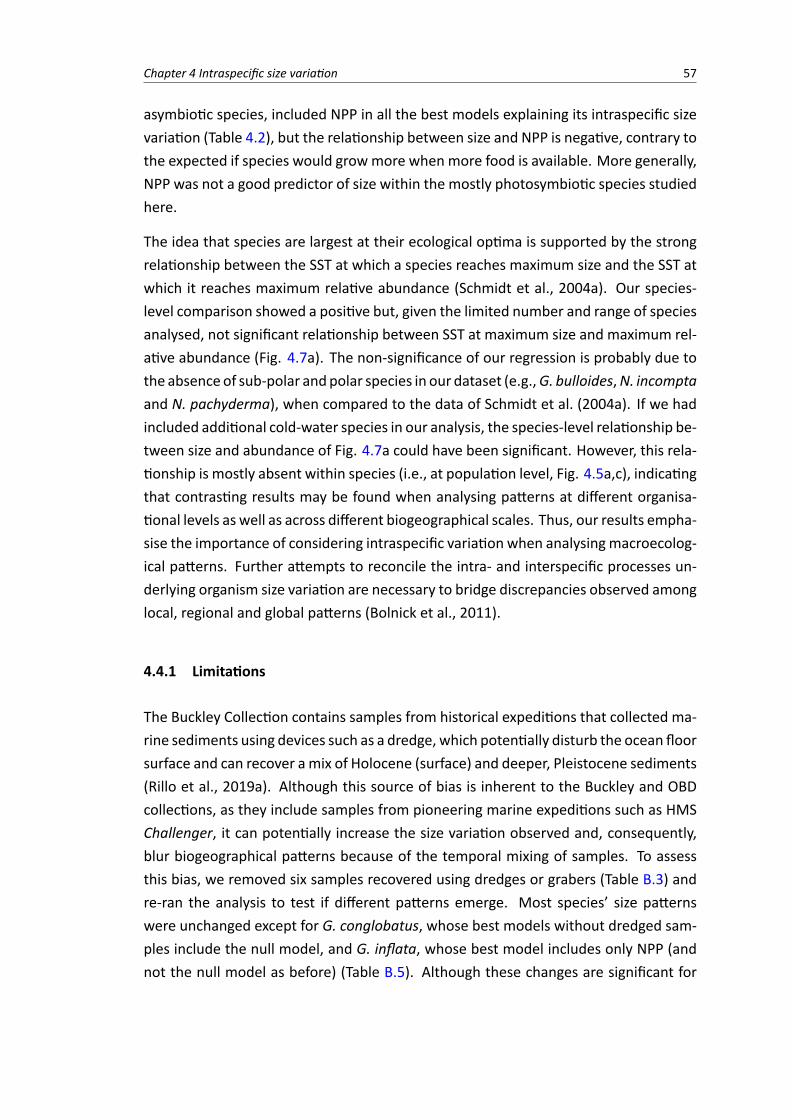
Chapter 4 Intraspecific size variation 57
asymbiotic species, included NPP in all the best models explaining its intraspecific sizevariation (Table 4.2), but the relationship between size and NPP is negative, contrary tothe expected if species would growmore when more food is available. More generally,NPP was not a good predictor of size within the mostly photosymbiotic species studiedhere.
The idea that species are largest at their ecological optima is supported by the strongrelationship between the SST at which a species reaches maximum size and the SST atwhich it reaches maximum relative abundance (Schmidt et al., 2004a). Our species-level comparison showed a positive but, given the limited number and range of speciesanalysed, not significant relationship between SST at maximum size and maximum rel-ative abundance (Fig. 4.7a). The non-significance of our regression is probably due tothe absenceof sub-polar andpolar species in our dataset (e.g.,G. bulloides,N. incomptaand N. pachyderma), when compared to the data of Schmidt et al. (2004a). If we hadincluded additional cold-water species in our analysis, the species-level relationship be-tween size and abundance of Fig. 4.7a could have been significant. However, this rela-tionship is mostly absent within species (i.e., at population level, Fig. 4.5a,c), indicatingthat contrasting results may be found when analysing patterns at different organisa-tional levels as well as across different biogeographical scales. Thus, our results empha-sise the importance of considering intraspecific variation when analysingmacroecolog-ical patterns. Further attempts to reconcile the intra- and interspecific processes un-derlying organism size variation are necessary to bridge discrepancies observed amonglocal, regional and global patterns (Bolnick et al., 2011).
4.4.1 Limitations
The Buckley Collection contains samples from historical expeditions that collected ma-rine sediments using devices such as a dredge, which potentially disturb the ocean floorsurface and can recover amix of Holocene (surface) and deeper, Pleistocene sediments(Rillo et al., 2019a). Although this source of bias is inherent to the Buckley and OBDcollections, as they include samples from pioneering marine expeditions such as HMSChallenger, it can potentially increase the size variation observed and, consequently,blur biogeographical patterns because of the temporal mixing of samples. To assessthis bias, we removed six samples recovered using dredges or grabers (Table B.3) andre-ran the analysis to test if different patterns emerge. Most species’ size patternswere unchanged except for G. conglobatus, whose best models without dredged sam-ples include the null model, and G. inflata, whose best model includes only NPP (andnot the null model as before) (Table B.5). Although these changes are significant for
58 Chapter 4 Intraspecific size variation
these two species, the general pattern remains: intraspecific size variation in plank-tonic Foraminifera cannot be explained consistently for all species.
The presence of cryptic genetic diversity could also have contributed to the high in-traspecific variation found in our study. Some planktonic Foraminifera species are infact complexes of lineages, which are genetically independent butmorphologically sim-ilar (Morard et al., 2015). Cryptic species have been shown to occupy different nichesand to be endemic to particular ocean basins (De Vargas et al., 1999; Darling andWade,2008; Weiner et al., 2014). So, the macroecological scale of our study likely includescryptic diversitywithin ourmorphologically-defined species. T. sacculifer andG. conglo-batus are the only genetically homogeneous species in our study (Aurahs et al., 2011;Seears et al., 2012; Andre et al., 2013). The other species have been shown to comprisesome level of cryptic diversity (De Vargas et al., 1999; Darling andWade, 2008; Morardet al., 2011; Aurahs et al., 2011; Ujiie et al., 2012; Quillevere et al., 2011; Weiner et al.,2014, 2015), except for G. menardii, whose genetic diversity has not yet been deter-mined (Seears et al., 2012). The predictability of size variation in our study does notseem to relate directly to the cryptic diversity of the species: species with strong rela-tionships between size and SST and/or NPP include not only the genetically homoge-neous T. sacculifer andG. conglobatus, but also the genetically diverseG. siphonifera, P.obliquiloculata and G. truncatulinoides. This result suggests that shell growth of thesedifferent genetic types likely respond to SST and/or NPP in similar ways.
The weak relationship between size and local relative abundance found in our studycould be due to the fact that we used relative abundance data from a different source(the ForCenS database; Siccha and Kucera 2017). We assessed the robustness of ourresults by testing the optimum-size hypothesis on amore uniform, but smaller, dataset:the ten re-sampled bulk samples used for the bias analysis (Fig. 4.1a; Table B.1). Wemeasured shell sizes and calculated species’ relative abundances for each of the tenassemblages, so that the same specimens were used to extract abundance and sizedata. 65 populations of 20 species were then used to test if population shell size couldbe predicted by relative abundance using a linear-mixed effect model with species asrandom effects. The results showed no significant relationship between size variationand relative abundance (chi-square test,�2 = 2.18, P value = 0.14, Table B.2), supportingour previous findings using the Buckley Collection data (Table 4.2, Fig. 4.5c).
Potentially the most significant source of uncertainty in the evaluation of the exis-tence of a relationship between size and optimum environmental conditions is theuse of relative abundance as an indicator of planktonic Foraminifera ecological (Hecht,1976) and thermal (Kucera, 2007) optima. Preferably the environmental optimum ofa species would be determined by comparing absolute abundances of populations of
Chapter 4 Intraspecific size variation 59
the same species independently of the abundances of the other species in the assem-blage. When a species is less abundant (or longer-lived) than other species in the localplankton community, its relative abundance in the sediment will be strongly influencedby the more abundant (or shorter-lived) co-occurring species. Moreover, a species canreach high relative abundance because it is better able to tolerate stress than otherspecies. As a result of stress, the abundances of all species will be low, but the mosttolerant specieswill reach high relative abundances. The high relative abundances ofG.ruber together with the lack of a relationship between shell size and SST, NPP and/orrelative abundance (Table 4.2, Fig. 4.5) suggests that this species is able to toleratestress and, therefore, reach high relative abundance in sub-optimal conditions (Be andTolderlund, 1971; Schmuker and Schiebel, 2002). Thus, further investigation on the re-lationship between size and optimal environmental conditionswithin species should fo-cus on absolute abundances estimates derived from plankton tows and sediment traps(e.g., Beer et al. 2010; Aldridge et al. 2012; Weinkauf et al. 2016), instead of relativeabundances in the sediment.
4.5 Conclusion
We tested the hypothesis that planktonic Foraminifera species are largest under op-timal environmental conditions (Hecht, 1976; Schmidt et al., 2004a), identified usinglocal SST, NPP and relative abundance of the species. We found that species vary in thepredictability of their intraspecific size variation. While T. sacculifer, G. conglobatus, G.siphonifera, P. obliquiloculata and G. truncatulinoides reach larger sizes at specific en-vironmental conditions, G. ruber, N. dutertrei, G. menardii and G. inflata do not showsignificant relationships between size and the studied environmental and ecologicalvariables. Our results suggest that the prediction of growing bigger at optimal condi-tions is simplistic to apply to all species. More standardised individual-level studies arenecessary to disentangle the mechanisms underlying planktonic Foraminifera biogeo-graphical size distributions.
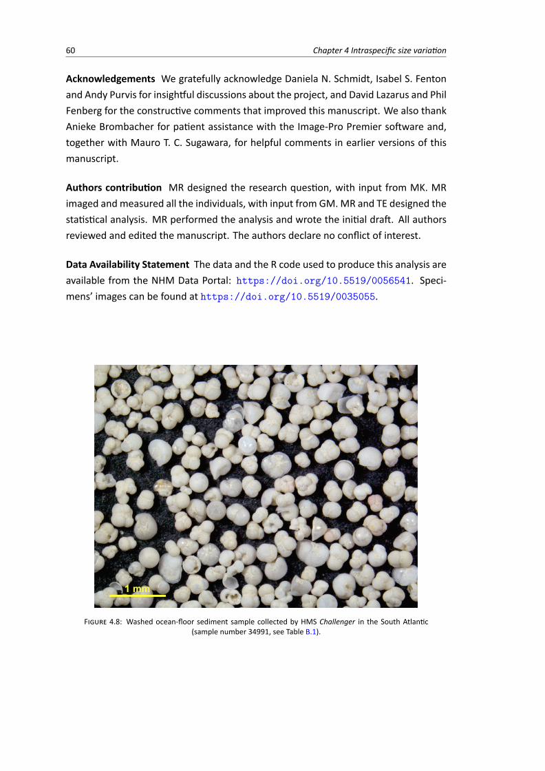
60 Chapter 4 Intraspecific size variation
Acknowledgements We gratefully acknowledge Daniela N. Schmidt, Isabel S. Fentonand Andy Purvis for insightful discussions about the project, and David Lazarus and PhilFenberg for the constructive comments that improved this manuscript. We also thankAnieke Brombacher for patient assistance with the Image-Pro Premier software and,together with Mauro T. C. Sugawara, for helpful comments in earlier versions of thismanuscript.
Authors contribution MR designed the research question, with input from MK. MRimaged andmeasured all the individuals, with input from GM.MR and TE designed thestatistical analysis. MR performed the analysis and wrote the initial draft. All authorsreviewed and edited the manuscript. The authors declare no conflict of interest.
Data Availability Statement The data and the R code used to produce this analysis areavailable from the NHM Data Portal: . Speci-mens’ images can be found at .
FIGURE 4.8: Washed ocean-floor sediment sample collected by HMS Challenger in the South Atlantic(sample number 34991, see Table B.1).
Chapter 5
On the mismatch in the strength ofcompetition among fossil and modernspecies of planktonic Foraminifera
Marina C. Rillo1,2⇤, Mauro T. C. Sugawara3, Brenno Cabella4,Lukas Jonkers2, Michal Kučera2 & Thomas H. G. Ezard1
1Ocean and Earth Science, National Oceanography Centre Southampton, University of SouthamptonWaterfront Campus, Southampton SO143ZH, UK2MARUM, University of Bremen, Leobener Strasse, Bremen 28359, Germany3 Department of Zoology, University of British Columbia, Vancouver V6T 1Z4, Canada4Institute of Theoretical Physics, UNESP Sao Paulo State University, Sao Paulo 01140-070, Brazil
*Correspondence: [email protected]
61
62 Chapter 5 Competition among modern species
AbstractAim: Many clades display the macroevolutionary pattern of a negative relationshipbetween standing diversity and diversification rates. Competition among species hasbeen proposed as the main mechanism that explains this pattern. However, we cur-rently lack empirical insight into how the effects of individual-level ecological interac-tions scale up to affect species diversification. Here, we investigate a clade that showsevidence for negative diversity-dependent diversification in the fossil record and testwhether the clade’s modern communities show a corresponding signal of interspecificcompetition.Location: World’s oceansTime period: HoloceneMajor taxa studied: planktonic Foraminifera (Rhizaria)Methods: We explore spatial and temporal ecological patterns expected under inter-specific competition. Firstly, we use a community phylogenetics approach to test forsigns of local spatial competitive exclusion among ecologically similar species (definedas closely related or of similar shell sizes) by combining species relative abundancesin seafloor sediments. Secondly, we analyse whether population abundances of co-occurring species co-vary negatively throughtimeusing sediment-traptime series span-ning one to 12 years.Results: The great majority of the assemblages are indistinguishable from randomlyassembled communities, showing no significant spatial co-occurrence patterns regard-ing size similarity or phylogeny. Through time, most species pairs correlated positively,indicating synchronous rather than compensatory population dynamics.Main conclusions: We found no detectable evidence for interspecific competitionstructuring extant planktonic Foraminifera communities. Species co-occurrences andpopulation dynamics are likely regulated by the abiotic environment and/or distantlyrelated species, rather than intra-clade density dependent processes. This interpre-tation contradicts the idea that competition drives the clade’s macroevolutionary dy-namics. One way to bring community ecology and macroevolution closer together isto consider that diversification dynamics are influenced by groups that interact ecolog-ically even when distantly related.
Keywords:community ecology, diversity dependent diversification, interspecific competition,macroevolution, microfossils, time series analysis, zooplankton
This chapter is under review at the journal Global Ecology & Biogeography.
Chapter 5 Competition among modern species 63
5.1 Introduction
Ecological interactions play an important role in shaping the diversity of life acrossspace and time. By interacting with each other, individuals change the dynamics oftheir populations and communities. Population dynamics, in turn, influence species’abundances and geographical ranges, which affect species’ diversification rates (i.e.,the balance between speciation and extinction rates) (Harnik, 2011; Jablonski, 2017).However, the resulting net effect of ecological interactions on species’ diversificationmight not correspond to the fitness effects at the individual level. Positive interactionscan have a negative effect on diversification, and negative interactions can enhancediversification (Jablonski, 2008a; Yoder and Nuismer, 2010). For example, predationcan actually promote speciation of the prey due to adaptation to divergent predatorregimes (Langerhans et al., 2007; Meyer and Kassen, 2007); and mutualism can some-times lead to increased extinction rate because of the interdependence of the inter-acting species (Sachs and Simms, 2006). How individual-level interactions scale up toaffect species’ diversification remains a topic that has received scant attention (Jablon-ski, 2017), and we currently lack understanding of how congruent or discordant theseeffects are across ecological and geological time scales (Weber et al., 2017).
Competition among species has, by definition, a negative effect on the fitness of theinteracting individuals. Yet, interspecific competition can affect species’ diversifica-tion positively, by promoting niche partitioning and character displacement (Meyerand Kassen, 2007; Bailey et al., 2013) or negatively by driving species to extinctiondue to niche overlap (Bengtsson, 1989). Within macroevolutionary research, interspe-cific competition has often been proposed to have a consistent negative effect acrossecological and geological time scales, generating the pattern of a negative relation-ship between species diversity and diversification rates (Rabosky, 2013). This negativediversity-dependent diversification (DDD) pattern is thought to reflect that increases inspecies number suppress diversification rates due to increased extinction or becauseopportunities for speciation become reduced once niches are filled, whereas decreasesin species number promote diversification because of weaker competitive interactions(Rabosky, 2013).
Many clades have been shown to display the negative DDD pattern, including birds(Phillimore and Price, 2008; Rabosky and Lovette, 2008), mammals (Alroy, 1996), in-cluding carnivores (Pires et al., 2017), marine metazoans (Sepkoski, 1978; Alroy, 2008)and marine protists Ezard et al. (2011). Although most of these studies evoke interspe-cific competition to explain the observed macroevolutionary pattern (Rabosky, 2013),they do not explicitly test for it. Such an explicit test is difficult to perform, as it requiresnot only a sufficiently well-preserved fossil record to assess the deep-time individual-
64 Chapter 5 Competition among modern species
or population-level fitness responses to ecological interactions, but also an actual fos-silised interaction proxy, both ofwhich are rare (but see Liowet al. 2016). An alternativeapproach to test whether the negativeDDDpattern is a result of upward causation fromcompetition among individuals, is to contrast macroevolutionary and present-day com-munity ecology dynamics (Voje et al., 2015;Weber et al., 2017). This approach involvesinvestigating whether the ecological interactions among most (if not all) extant speciesof a clade (i.e., clade-wide) support interspecific competition, and are thus consistentwith the clade’s observed DDD pattern. To our knowledge, none of the clades that haveshown the negative DDD pattern have been studied in a clade-wide community ecologyframework.
Planktonic Foraminifera represent a useful model system for integrating macroevolu-tion and community ecology (Yasuhara et al., 2015). They are unicellular eukaryotesthat live as zooplankton in the marine pelagic environment and produce calcium car-bonate shells. Upon death, these shells accumulate on the ocean floor building up aremarkably complete fossil record (under adequate sedimentation conditions; Schiebel2002b; Kucera 2007; Ezard et al. 2011). The planktonic Foraminifera fossil record ofthe last 66 million years shows a negative DDD pattern (Fig. 5.1) either by analysingphylogenetic tree structure (Etienne et al., 2011), or considering biotic and abiotic cor-relates of diversification (Ezard et al., 2011), or using non-linear ecological models ofalternative modes of competition (Ezard and Purvis, 2016). Using a model selectionframework, Ezard and Purvis (2016) show that although abiotic factors affect the dy-namics of planktonic Foraminifera diversification, species richness in deep time ex-hibits strong evidence for regulation by interspecific competition. More specifically,their diversification appears to be driven by compensatory contest competition (Ezardand Purvis, 2016), which is analogous to populational logistic growth where resourceavailability is limited and only successful individuals get the amount of resource theyrequire (Brannstrom and Sumpter, 2005). At macroevolutionary scales, compensatorycontest competition results in species with higher average fitness eventually excludingthe lower fitness ones (Ezard and Purvis, 2016). Newly available niches would be filledby species already in similar niches (i.e., incumbency; Ezard and Purvis 2016), invokingniche partitioning and niche conservatism (Wiens et al., 2010).
While competition among planktonic Foraminifera species likely affected the Cenozoicdiversification of the group (Ezard et al., 2011; Etienne et al., 2011; Ezard and Purvis,2016), we currently do not know if (or how) species compete today in the oceans.Planktonic Foraminifera are difficult to cultivate and do not reproduce under labora-tory conditions (Hemleben et al., 1989), hindering our understanding of their popula-tion dynamics and ecological interactions. Assessing if extant planktonic Foraminiferaspecies compete is valuable not only to bridgemacroevolution and community ecology,
Chapter 5 Competition among modern species 65
but also to improve ecological models used in palaeoceanographic reconstructions, asthese models generally assume that planktonic Foraminifera compete without explic-itly testing for it (e.g., Fraile et al. 2008; Lombard et al. 2011; Kretschmer et al. 2018).Globally, there are 47 extant planktonic Foraminifera species (Siccha and Kucera, 2017),occurring in low densities (in the order of tenths of individuals per m3; Schiebel andHemleben 2005; Meilland et al. 2019). When compared to other eukaryotic groups,planktonic Foraminifera represent less than 0.1% of the plankton abundance in thesunlit ocean (Keeling and del Campo, 2017). Planktonic Foraminifera prey on otherplankton groups including phytoplankton, ciliates and copepods (Anderson et al., 1979;Spindler et al., 1984; Hemleben et al., 1989), and several species host photosymbionts(Hemleben et al., 1989; Takagi et al., 2019). Previous works have used observationaldata to explore the relationship between environmental variables and current diver-sity patterns of planktonic Foraminifera spatially (Rutherford et al., 1999; Morey et al.,2005; Tittensor et al., 2010; Fenton et al., 2016b) and temporally (Zaric et al., 2005;Jonkers and Kucera, 2015; Weinkauf et al., 2016). These studies suggest that mean an-nual sea surface temperature (SST) explains the largest portion of the geographical andtemporal variation of planktonic Foraminifera extant diversity. However, to our knowl-edge, no study has explored the role of ecological interactions in shaping their presentdiversity patterns.
Here, we test if extant planktonic Foraminifera species compete by investigating abun-dance patterns globally in space and through time (Fig. 5.2a). The temporal scale westudied ranges from weeks (sediment trap data) to centuries (coretop data). We ex-plore two community-level patterns expected under interspecific competition: (i) lo-cal competitive exclusion (spatial pattern) and (ii) compensatory dynamics (temporalpattern). In terms of the former, when resources are limiting ecologically similar species(e.g., similar size or diet) are expected to compete more intensely, and ultimately ex-clude one another from the local community (Webb et al., 2002). Thus, we expectcompetitive exclusion to lead to the spatial segregation of ecologically similar species,resulting in overdispersed local communities (i.e., local coexistence of less-ecologicallysimilar species given a random assembly process; Webb et al. 2002; Pearse et al. 2014).The underlying assumption is that the ecological similarity measured among speciesin a community reflects the biogeographic and ecological processes structuring it (i.e.,community assembly processes). On the other hand, if competing species coexist, pop-ulation sizes are predicted to change as a function of the abundances of co-occurringcompetitors (e.g., TerHorst 2011; Alzate et al. 2017). Through time, changes in theabundance of one species should be accompanied by compensatory changes in theabundances of other species (i.e., compensatory dynamics; Houlahan et al. 2007).
66 Chapter 5 Competition among modern species
Thus, we expect that, depending on the strength of the interspecific competition, eco-logically similar species will either show complete local competitive exclusion, or pop-ulation abundances will covary negatively through time. If ecological interactions havea consistent effect across geological and current ecological time scales, we expect com-petition among planktonic Foraminifera species to play a key role in structuring theirmodern communities.
5.2 Material and Methods
We used two types of observational data: spatial data from 3,053 coretop samples andtemporal data from 35 sediment traps (370 time series of population abundances in to-tal) (Fig. 5.2, 5.3). We performed two distinct and independent analyses for each datatype: spatial data were analysed using a community phylogenetics approach, consider-ing randomassembly nullmodels. Temporal datawere analysed by pairwise correlationof time series, considering a nullmodel of species’ annual seasonality. All analyseswereconducted using R (version 3.3.3, R Core Team 2017).
5.2.1 Spatial data
Ocean-floor sediment samples are recovered using core sampling (Fig. 5.3); the coretoprepresents the most recent (surface) sediment. Because there is no precise estimateof local sedimentation rate in most sampled sites, core samples typically hold informa-tion on species relative abundances (i.e., relative to the sampled assemblage, as all in-dividuals are identified) rather than absolute abundances. Coretop samples representtime-averaged assemblages on the order of hundreds to thousands of years depend-ing on local sedimentation and bioturbation (Rigual-Hernandez et al., 2012; Jonkerset al., 2019). Such time-averaged assemblages prevent analyses on finer time resolu-tion and might accommodate evolutionary change; however, they have the advantageof averaging out seasonal and inter-annual fluctuations in abundance that might blurmacroecological patterns (Fenton et al., 2016b).
We used relative abundance data from the ForCenS database, which is a curateddatabase, taxonomically harmonised and treated for sampling inconsistencies (Sicchaand Kucera, 2017). Sites deeper than 3,500 meters in the Pacific and Indian oceansand 4,500 meters elsewhere were excluded to minimise the effects of calcium car-bonate dissolution on assemblage composition (Tittensor et al., 2010). We also re-moved samples that only contained one species and those that did not differentiatebetween the species Globorotalia menardii and G. tumida; Globigerinoides ruber pink
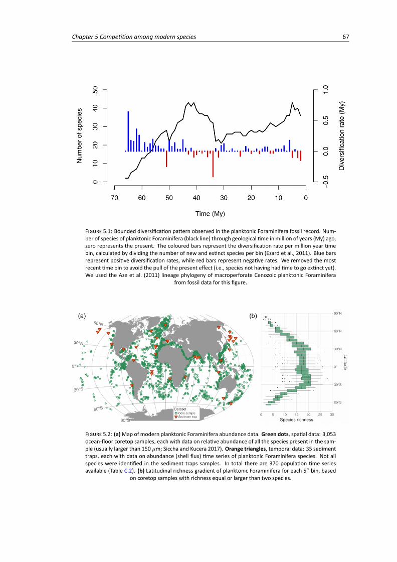
Chapter 5 Competition among modern species 67
FIGURE 5.1: Bounded diversification pattern observed in the planktonic Foraminifera fossil record. Num-ber of species of planktonic Foraminifera (black line) through geological time in million of years (My) ago,zero represents the present. The coloured bars represent the diversification rate per million year timebin, calculated by dividing the number of new and extinct species per bin (Ezard et al., 2011). Blue barsrepresent positive diversification rates, while red bars represent negative rates. We removed the mostrecent time bin to avoid the pull of the present effect (i.e., species not having had time to go extinct yet).We used the Aze et al. (2011) lineage phylogeny of macroperforate Cenozoic planktonic Foraminifera
from fossil data for this figure.
FIGURE 5.2: (a)Map of modern planktonic Foraminifera abundance data. Green dots, spatial data: 3,053ocean-floor coretop samples, each with data on relative abundance of all the species present in the sam-ple (usually larger than 150 µm; Siccha and Kucera 2017). Orange triangles, temporal data: 35 sedimenttraps, each with data on abundance (shell flux) time series of planktonic Foraminifera species. Not allspecies were identified in the sediment traps samples. In total there are 370 population time seriesavailable (Table C.2). (b) Latitudinal richness gradient of planktonic Foraminifera for each 5� bin, based
on coretop samples with richness equal or larger than two species.
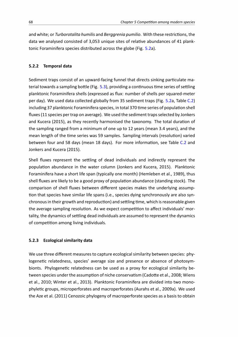
68 Chapter 5 Competition among modern species
andwhite; or Turborotalita humilis and Berggrenia pumilio. With these restrictions, thedata we analysed consisted of 3,053 unique sites of relative abundances of 41 plank-tonic Foraminifera species distributed across the globe (Fig. 5.2a).
5.2.2 Temporal data
Sediment traps consist of an upward-facing funnel that directs sinking particulate ma-terial towards a sampling bottle (Fig. 5.3), providing a continuous time series of settlingplanktonic Foraminifera shells (expressed as flux: number of shells per squared-meterper day). We used data collected globally from 35 sediment traps (Fig. 5.2a, Table C.2)including 37 planktonic Foraminifera species, in total 370 time series of population shellfluxes (11 species per trap on average). We used the sediment traps selected by Jonkersand Kucera (2015), as they recently harmonised the taxonomy. The total duration ofthe sampling ranged from a minimum of one up to 12 years (mean 3.4 years), and themean length of the time series was 59 samples. Sampling intervals (resolution) variedbetween four and 58 days (mean 18 days). For more information, see Table C.2 andJonkers and Kucera (2015).
Shell fluxes represent the settling of dead individuals and indirectly represent thepopulation abundance in the water column (Jonkers and Kucera, 2015). PlanktonicForaminifera have a short life span (typically one month) (Hemleben et al., 1989), thusshell fluxes are likely to be a good proxy of population abundance (standing stock). Thecomparison of shell fluxes between different species makes the underlying assump-tion that species have similar life spans (i.e., species dying synchronously are also syn-chronous in their growth and reproduction) and settling time, which is reasonable giventhe average sampling resolution. As we expect competition to affect individuals’ mor-tality, the dynamics of settling dead individuals are assumed to represent the dynamicsof competition among living individuals.
5.2.3 Ecological similarity data
We use three different measures to capture ecological similarity between species: phy-logenetic relatedness, species’ average size and presence or absence of photosym-bionts. Phylogenetic relatedness can be used as a proxy for ecological similarity be-tween species under the assumption of niche conservatism (Cadotte et al., 2008;Wienset al., 2010; Winter et al., 2013). Planktonic Foraminifera are divided into two mono-phyletic groups, microperforates and macroperforates (Aurahs et al., 2009a). We usedthe Aze et al. (2011) Cenozoic phylogeny of macroperforate species as a basis to obtain
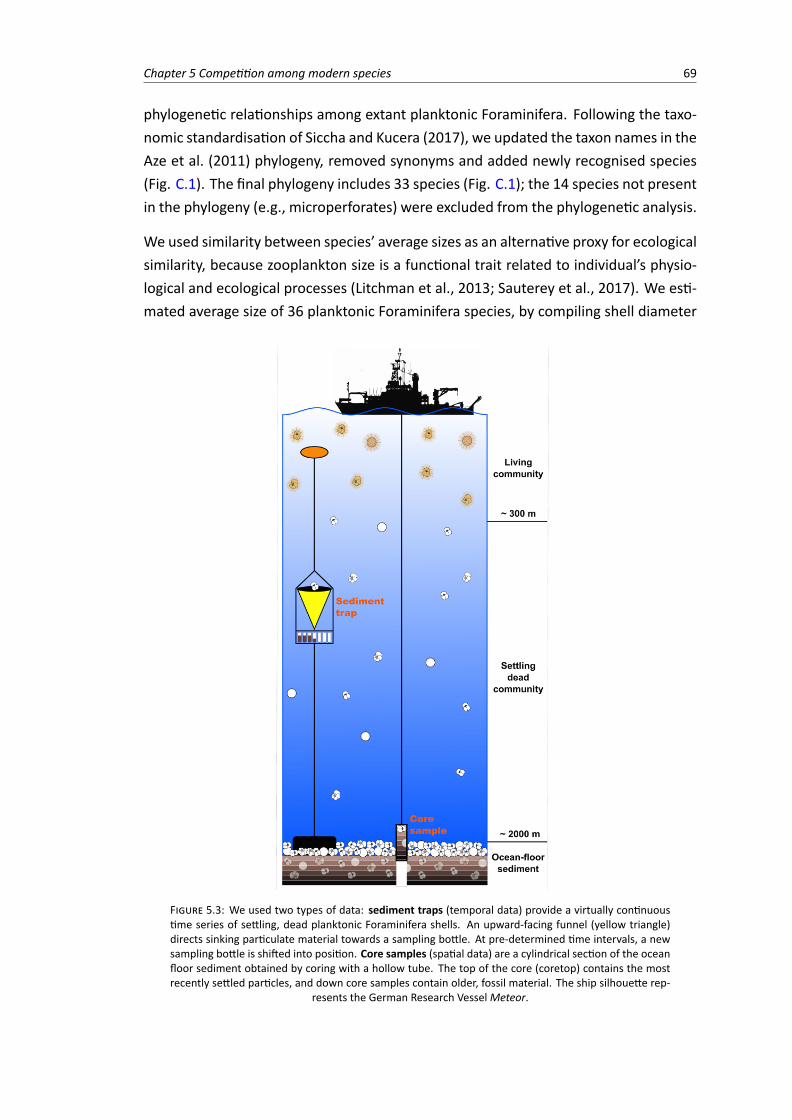
Chapter 5 Competition among modern species 69
phylogenetic relationships among extant planktonic Foraminifera. Following the taxo-nomic standardisation of Siccha and Kucera (2017), we updated the taxon names in theAze et al. (2011) phylogeny, removed synonyms and added newly recognised species(Fig. C.1). The final phylogeny includes 33 species (Fig. C.1); the 14 species not presentin the phylogeny (e.g., microperforates) were excluded from the phylogenetic analysis.
We used similarity between species’ average sizes as an alternative proxy for ecologicalsimilarity, because zooplankton size is a functional trait related to individual’s physio-logical and ecological processes (Litchman et al., 2013; Sauterey et al., 2017). We esti-mated average size of 36 planktonic Foraminifera species, by compiling shell diameter
FIGURE 5.3: We used two types of data: sediment traps (temporal data) provide a virtually continuoustime series of settling, dead planktonic Foraminifera shells. An upward-facing funnel (yellow triangle)directs sinking particulate material towards a sampling bottle. At pre-determined time intervals, a newsampling bottle is shifted into position. Core samples (spatial data) are a cylindrical section of the oceanfloor sediment obtained by coring with a hollow tube. The top of the core (coretop) contains the mostrecently settled particles, and down core samples contain older, fossil material. The ship silhouette rep-
resents the German Research VesselMeteor.
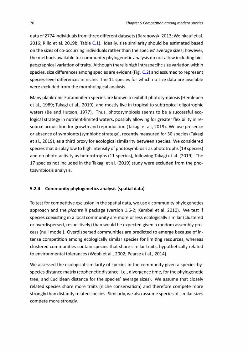
70 Chapter 5 Competition among modern species
data of 2774 individuals from three different datasets (Baranowski 2013;Weinkauf et al.2016; Rillo et al. 2019b; Table C.1). Ideally, size similarity should be estimated basedon the sizes of co-occurring individuals rather than the species’ average sizes; however,the methods available for community phylogenetic analysis do not allow including bio-geographical variation of traits. Although there is high intraspecific size variationwithinspecies, size differences among species are evident (Fig. C.2) and assumed to representspecies-level differences in niche. The 11 species for which no size data are availablewere excluded from the morphological analysis.
Many planktonic Foraminifera species are known to exhibit photosymbiosis (Hemlebenet al., 1989; Takagi et al., 2019), and mostly live in tropical to subtropical oligotrophicwaters (Be and Hutson, 1977). Thus, photosymbiosis seems to be a successful eco-logical strategy in nutrient-limited waters, possibly allowing for greater flexibility in re-source acquisition for growth and reproduction (Takagi et al., 2019). We use presenceor absence of symbionts (symbiotic strategy), recently measured for 30 species (Takagiet al., 2019), as a third proxy for ecological similarity between species. We consideredspecies that display low to high intensity of photosymbiosis as phototrophs (19 species)and no photo-activity as heterotrophs (11 species), following Takagi et al. (2019). The17 species not included in the Takagi et al. (2019) study were excluded from the pho-tosymbiosis analysis.
5.2.4 Community phylogenetics analysis (spatial data)
To test for competitive exclusion in the spatial data, we use a community phylogeneticsapproach and the picante R package (version 1.6-2; Kembel et al. 2010). We test ifspecies coexisting in a local community are more or less ecologically similar (clusteredor overdispersed, respectively) than would be expected given a random assembly pro-cess (null model). Overdispersed communities are predicted to emerge because of in-tense competition among ecologically similar species for limiting resources, whereasclustered communities contain species that share similar traits, hypothetically relatedto environmental tolerances (Webb et al., 2002; Pearse et al., 2014).
We assessed the ecological similarity of species in the community given a species-by-species distancematrix (cophenetic distance, i.e., divergence time, for the phylogenetictree, and Euclidean distance for the species’ average sizes). We assume that closelyrelated species share more traits (niche conservatism) and therefore compete morestrongly than distantly related species. Similarly, we also assume species of similar sizescompete more strongly.
Chapter 5 Competition among modern species 71
For each of the 3,053 planktonic Foraminifera assemblages in the spatial data (Fig.5.2a), we calculated two community dispersion metrics: the mean pairwise distance(MPD) and the mean nearest (taxon) distance (MNTD), both weighted by the abun-dance of each species in the local community. MPD is the average distance betweenall species in the assemblage and thus takes into account clade-wide patterns. MNTDis the average distance between each species and its nearest neighbour in the distancematrix, representing local patterns in the phylogeny or trait space.
To test if the observed MPD and MNTD values differ significantly from the values thatwould be expected under a random assembly process, we generated null models ofcommunity assembly. If species are equivalent (neutral dynamics), we expect commu-nities to be composed of a random subset of species capable of colonising the localcommunity (i.e., the source pool; Webb et al. 2002; Pearse et al. 2014). Our sourcepool includes all extant planktonic Foraminifera species, because the ranges of all buttwo species cover every ocean basin (Be and Tolderlund, 1971). Thus, we assume inthe null models that species can reach all oceanographic regions in the world. If thereare local community assembly processes (i.e., competitive exclusion and environmentaltolerances), the species’ local establishment will be different than the random subset,because the local fitness of species differ (i.e., species are not equivalent).
We tested two random assembly models: ‘taxa’, which shuffles the species-by-speciesdistancematrix, and tests if the observed communities show phylogenetic or size struc-ture; ‘richness’, which shuffles the species abundances in the sample (holding the rich-ness constant), and tests if community structure could have been generated by ran-domly drawing species from the source pool (Kembel et al., 2010). We ran each nullmodel 100 times, then standardised the observed MPD and MNTD values with respectto the expected values and standard deviations of the null distributions (standardisedeffect size), generating the net relatedness index (NRI) and the nearest taxon index(NTI), respectively. Positive values of NRI and NTI indicate clustered assemblages (en-vironmental filters); whereas negative values of NRI and NTI indicate overdispersed as-semblages (competitive exclusion). The difference between NRI and NTI is that theformer accounts for the average (net) distance among all co-occurring species in theassemblage, and the latter accounts for the smallest (nearest) distance between co-occurring species. We used a statistical significance level of 1% to avoid false positivesgiven the large number of samples (3,053 assemblages). Additionally, we retrieved an-nual mean sea-surface temperature (SST) for each of the 3,053 assemblages from theWorld Ocean Atlas 2013 (Locarnini et al., 2013) to assess the relationship between SSTand community patterns.
72 Chapter 5 Competition among modern species
5.2.5 Time series analysis (temporal data)
If two species compete in the local community, we expect that increases in the abun-dance of one species should have a negative impact on the abundance of the otherspecies, generating a negative correlation of abundances through time. To test for suchcompensatory dynamics in the temporal data, we calculated the correlation betweenthe differentiated time-series (i.e., first differences) of co-occurring species pairs (sam-pled in the same sediment trap). We used the non-parametric Kendall rank correlation,whichmakes no assumption on the underlying pairwise distribution. In total, 2,303 cor-relations were calculated and analysed regarding ecological similarity between speciespairs (i.e., phylogenetic relatedness, average sizes or symbiotic strategy).
Planktonic Foraminifera species’ abundances (fluxes) vary seasonally in response to SSTand primary productivity (Jonkers and Kucera, 2015). When correlating these abun-dance time series, similar seasonal cycles can yield strong positive correlations even ifspecies compete within their seasonal peaks. In order to correct for this bias, we built anull model assuming a seasonal cycle with a one year period, but allowing each speciesto have any number of abundance peaks within the year. This flexibility of species sea-sonality is consistent with observations that the same species can display unimodal orbimodal yearly abundance patterns depending on the regional oceanographic setting(Jonkers and Kucera, 2015). Thus, for each observed time series (i.e., each speciesin each sediment trap) we obtained a smoothing spline, which calculates the averageabundance of the species for each day of the year, resulting in an yearly-averaged se-ries (spline series; Fig. C.8), without having to enforce an a priori fixed annual season-ality. The smoothing spline parameter (�) was estimated using the generalised cross-validation method (GCV; Craven and Wahba 1978), which finds the optimum � valueby minimising the mean squared error of the fitting (also used in generalised additivemodels).
To generate the seasonality null model, we calculated the residuals between the ob-served time series and its spline series (Fig. C.8). We then randomised these residualsand added them to the spline series. This procedure was repeated 100 times, to pro-duce a set of surrogate time series with the same seasonality as the observed timeseries, but with random departures from it. For each species pair, we calculated theKendall-rank correlation coefficient between their surrogate series, resulting in a nulldistribution of 100 correlations for each co-occurring species pair (Fig. C.8). We reportthe standardised effect size (SES), which is the observed correlation standardised withrespect to the null distribution. We compared the observed correlation with its nulldistribution for significance, and used a statistical significance level of 1% because ofthe large number of comparisons.
Chapter 5 Competition among modern species 73
The residuals between the observed series and the spline series quantify the deviationof the observed abundances from the average annual abundance pattern. Thus, tocalculate inter-annual variation in abundances, we correlated the residual series of allco-occurring species pairs within sediments traps that were sampled for longer thantwo years (21 traps in total, Table C.2). A positive average correlation of residuals withinthe sediment trap indicates synchronous inter-annual variation in species abundances.We also quantified the intra-annual variability of each species is in each sediment trap,by correlating its observed time series with its spline series (Fig. C.8). High positivecorrelation coefficients indicate that the species has a consistent intra-annual variability(or seasonality) within the given sediment trap.
5.3 Results
5.3.1 Community phylogenetics (spatial data)
Out of the 3,053 planktonic Foraminifera assemblages studied, only two differ signifi-cantly from random assembly processes (Fig. 5.4), i.e., a negligible proportion of thestudied assemblages. Themajority of NRI andNTI values are positive, indicating a trendtowards phylogenetic and size clustering in the seafloor assemblages. As there is noqualitative difference between the results of the ‘richness’ and ‘taxa’ null models (Fig.C.3), we discuss only the former. If we consider a significance level of 5%, 190 assem-blages show significant size structure (of which 182 are clustered), and 12 assemblagesshow significant phylogenetic structure (of which 10 are clustered), supporting an en-vironmental filtering scenario.
Using phylogeny as an ecological proxy, NRI values never reach below two standarddeviations of the null distributions (i.e., the value of -2, Fig. 5.4a), not supporting com-petitive exclusion of close relatives. NTI values, however, show a trend towards nega-tive values in assemblages between 5�C and 12�C, reaching values below -2 (Fig. 5.4c).These assemblages have, on average, seven species and are dominated by Globige-rina bulloides andNeogloboquadrina incompta orN. pachyderma. These species comefrom two distantly-related planktonic Foraminifera subclades, so the phylogenetic dis-tance between coexisting individuals in the community is mostly high (overdispersed).The opposite is observed for the polar assemblages (0�C), which are dominated by N.pachyderma (average relative abundance of 97%) and show a non-significant tendencyfor positive NTI values (environmental filters; Fig. 5.4c).
Dispersion metrics based on species’ size differences show either none or one overdis-persed assemblages (Fig. 5.4b,d, respectively). This single overdispersed assemblage
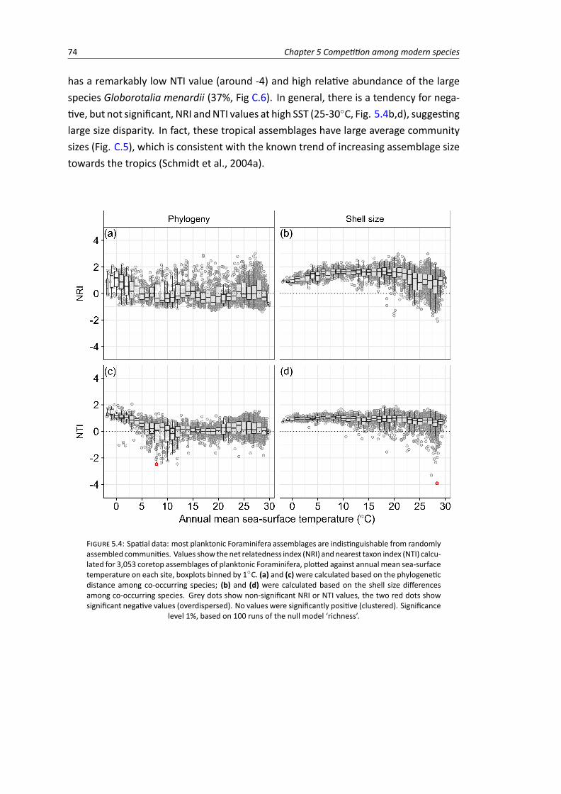
74 Chapter 5 Competition among modern species
has a remarkably low NTI value (around -4) and high relative abundance of the largespecies Globorotalia menardii (37%, Fig C.6). In general, there is a tendency for nega-tive, but not significant, NRI andNTI values at high SST (25-30�C, Fig. 5.4b,d), suggestinglarge size disparity. In fact, these tropical assemblages have large average communitysizes (Fig. C.5), which is consistent with the known trend of increasing assemblage sizetowards the tropics (Schmidt et al., 2004a).
FIGURE 5.4: Spatial data: most planktonic Foraminifera assemblages are indistinguishable from randomlyassembled communities. Values show thenet relatedness index (NRI) and nearest taxon index (NTI) calcu-lated for 3,053 coretop assemblages of planktonic Foraminifera, plotted against annual mean sea-surfacetemperature on each site, boxplots binned by 1�C. (a) and (c)were calculated based on the phylogeneticdistance among co-occurring species; (b) and (d) were calculated based on the shell size differencesamong co-occurring species. Grey dots show non-significant NRI or NTI values, the two red dots showsignificant negative values (overdispersed). No values were significantly positive (clustered). Significance
level 1%, based on 100 runs of the null model ‘richness’.
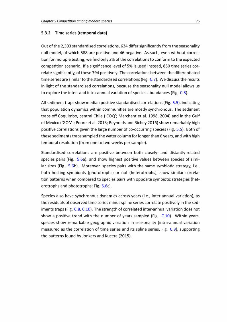
Chapter 5 Competition among modern species 75
5.3.2 Time series (temporal data)
Out of the 2,303 standardised correlations, 634 differ significantly from the seasonalitynull model, of which 588 are positive and 46 negative. As such, even without correc-tion formultiple testing, we find only 2% of the correlations to conform to the expectedcompetition scenario. If a significance level of 5% is used instead, 850 time series cor-relate significantly, of these 794 positively. The correlations between the differentiatedtime series are similar to the standardised correlations (Fig. C.7). We discuss the resultsin light of the standardised correlations, because the seasonality null model allows usto explore the inter- and intra-annual variation of species abundances (Fig. C.8).
All sediment traps showmedian positive standardised correlations (Fig. 5.5), indicatingthat population dynamics within communities are mostly synchronous. The sedimenttraps off Coquimbo, central Chile (‘COQ’; Marchant et al. 1998, 2004) and in the Gulfof Mexico (‘GOM’; Poore et al. 2013; Reynolds and Richey 2016) show remarkably highpositive correlations given the large number of co-occurring species (Fig. 5.5). Both ofthese sediments traps sampled the water column for longer than 6 years, andwith hightemporal resolution (from one to two weeks per sample).
Standardised correlations are positive between both closely- and distantly-relatedspecies pairs (Fig. 5.6a), and show highest positive values between species of simi-lar sizes (Fig. 5.6b). Moreover, species pairs with the same symbiotic strategy, i.e.,both hosting symbionts (phototrophs) or not (heterotrophs), show similar correla-tion patterns when compared to species pairs with opposite symbiotic strategies (het-erotrophs and phototrophs; Fig. 5.6c).
Species also have synchronous dynamics across years (i.e., inter-annual variation), asthe residuals of observed time series minus spline series correlate positively in the sed-iments traps (Fig. C.8, C.10). The strength of correlated inter-annual variation does notshow a positive trend with the number of years sampled (Fig. C.10). Within years,species show remarkable geographic variation in seasonality (intra-annual variationmeasured as the correlation of time series and its spline series, Fig. C.9), supportingthe patterns found by Jonkers and Kucera (2015).
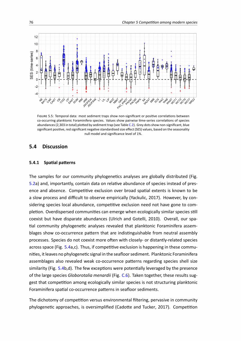
76 Chapter 5 Competition among modern species
FIGURE 5.5: Temporal data: most sediment traps show non-significant or positive correlations betweenco-occurring planktonic Foraminifera species. Values show pairwise time-series correlations of speciesabundances (2,303 in total) plotted by sediment trap (see Table C.2). Grey dots shownon-significant, bluesignificant positive, red significant negative standardised size effect (SES) values, based on the seasonality
null model and significance level of 1%.
5.4 Discussion
5.4.1 Spatial patterns
The samples for our community phylogenetics analyses are globally distributed (Fig.5.2a) and, importantly, contain data on relative abundance of species instead of pres-ence and absence. Competitive exclusion over broad spatial extents is known to bea slow process and difficult to observe empirically (Yackulic, 2017). However, by con-sidering species local abundance, competitive exclusion need not have gone to com-pletion. Overdispersed communities can emerge when ecologically similar species stillcoexist but have disparate abundances (Ulrich and Gotelli, 2010). Overall, our spa-tial community phylogenetic analyses revealed that planktonic Foraminifera assem-blages show co-occurrence pattern that are indistinguishable from neutral assemblyprocesses. Species do not coexist more often with closely- or distantly-related speciesacross space (Fig. 5.4a,c). Thus, if competitive exclusion is happening in these commu-nities, it leaves no phylogenetic signal in the seafloor sediment. Planktonic Foraminiferaassemblages also revealed weak co-occurrence patterns regarding species shell sizesimilarity (Fig. 5.4b,d). The few exceptions were potentially leveraged by the presenceof the large species Globorotalia menardii (Fig. C.6). Taken together, these results sug-gest that competition among ecologically similar species is not structuring planktonicForaminifera spatial co-occurrence patterns in seafloor sediments.
The dichotomy of competition versus environmental filtering, pervasive in communityphylogenetic approaches, is oversimplified (Cadotte and Tucker, 2017). Competition
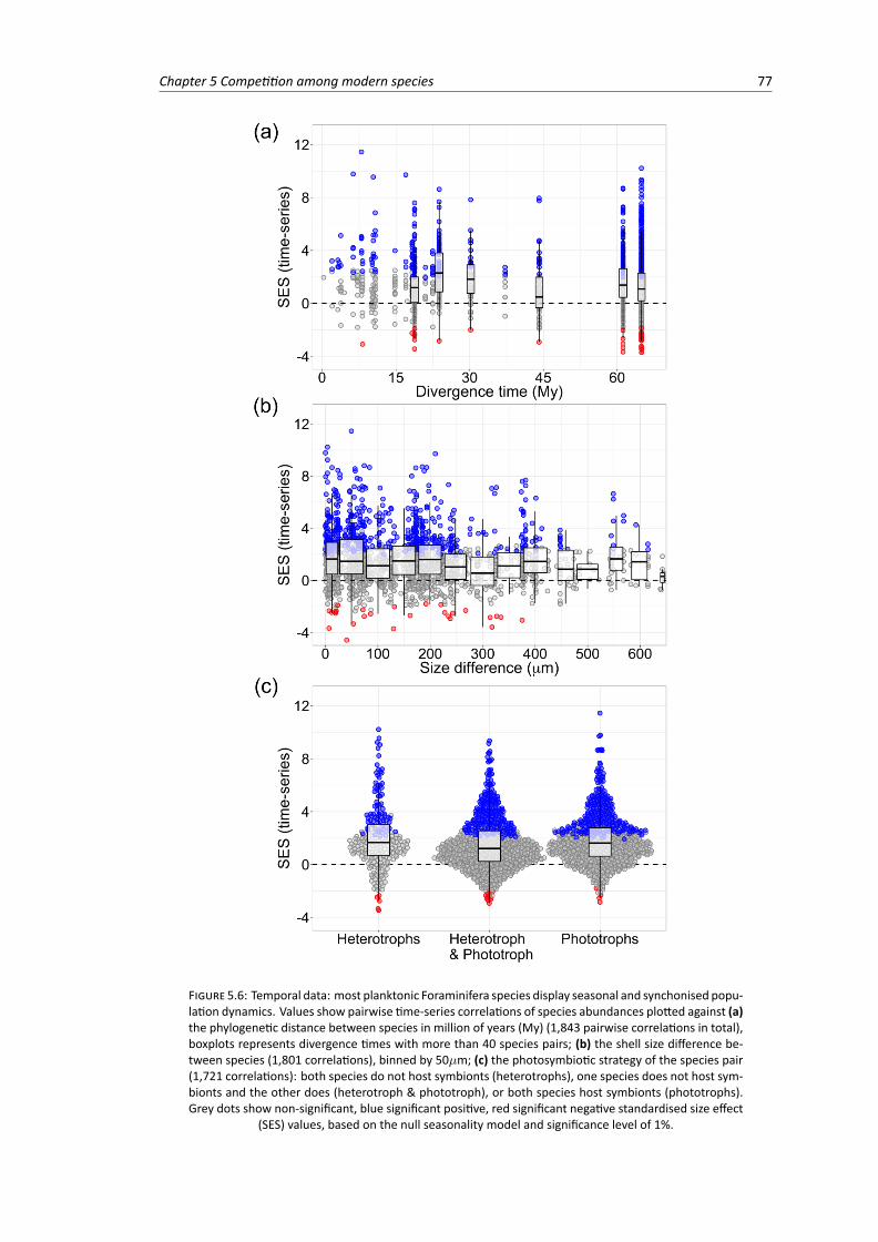
Chapter 5 Competition among modern species 77
FIGURE 5.6: Temporal data: most planktonic Foraminifera species display seasonal and synchonised popu-lation dynamics. Values show pairwise time-series correlations of species abundances plotted against (a)the phylogenetic distance between species in million of years (My) (1,843 pairwise correlations in total),boxplots represents divergence times with more than 40 species pairs; (b) the shell size difference be-tween species (1,801 correlations), binned by 50µm; (c) the photosymbiotic strategy of the species pair(1,721 correlations): both species do not host symbionts (heterotrophs), one species does not host sym-bionts and the other does (heterotroph & phototroph), or both species host symbionts (phototrophs).Grey dots show non-significant, blue significant positive, red significant negative standardised size effect
(SES) values, based on the null seasonality model and significance level of 1%.
78 Chapter 5 Competition among modern species
can instead reinforce co-occurrence of ecologically similar species, giving rise to clus-tered communities identical to those expected under environmental filtering (Mayfieldand Levine, 2010). However, the fact that we observed no significant patterns sug-gests that these plankton communities are influenced by neutral processes, such asdispersal and stochastic extinction (Hubbell, 2001; Rosindell et al., 2011; Matthewsand Whittaker, 2014). Indeed, dispersal–assembly mechanisms have been shown toprevail over niche-assembly mechanisms for the past 30 million years of planktonicForaminifera evolution (Allen and Gillooly, 2006; Allen and Savage, 2007), and re-cent work have shown that plankton biogeography can emerge simply by consider-ing body size, spatial heterogeneity and neutral dispersal given oceanographic currents(Sauterey et al., 2017). However, the lack of support for competition found in our studydoes not necessarily indicate that PF dynamics are neutral. Other non-neutral mech-anisms such as symbiosis, predation and competition with other groups can drive PFcommunity assembly and need to be further investigated.
5.4.2 Temporal patterns
Previous individual sediment-trap studies have shown that planktonic Foraminiferaabundances (measured as shell flux) change synchronously through time largely in re-sponse to changes in temperature and food availability (Marchant et al., 1998; Tedescoand Thunell, 2003; Marchant et al., 2004; Northcote and Neil, 2005; Wan et al., 2010;Rigual-Hernandez et al., 2012; Poore et al., 2013; Jonkers and Kucera, 2015). However,other studies have shown that although seasonal abundances are related to oceano-graphic conditions, species abundance peaks can occur sequentially (Deuser and Ross,1989; Jonkers et al., 2010, 2013) or be inversely related (Kincaid et al., 2000; Kuroy-anagi et al., 2002; Mohiuddin et al., 2002; Rigual-Hernandez et al., 2012), suggestingthat species have different ecological preferences. Species with opposite abundancepatterns during the year are expected to exhibit low correlation values, whereas specieswith sequential abundance peaks (compensatory dynamics) should correlate nega-tively through time. Here, we analysed sediment trap data globally, and show thatthe dynamics of planktonic Foraminifera abundances are largely explained by annualseasonality: 72% of the pairwise correlations did not differ significantly from our sea-sonality null model. The remaining significant correlations were predominantly posi-tive (93%), indicating synchronous population dynamics. This pattern was consistentacross sediment traps with different sampling durations (Fig. 5.5, Table C.2) and acrossyears (Fig. C.10). Therefore, planktonic Foraminifera population dynamics seems tobe influenced by external factors such as the abiotic environment and/or abundanceof other distantly-related plankton groups, rather than intra-clade density-dependentprocesses.
Chapter 5 Competition among modern species 79
Species with similar ecologies (phylogenetically closely related, with similar sizes orsame symbiotic strategies) did not correlate more negatively than other species pairs(Fig. 5.6), as would be expected if they were partitioning the resource through time.Purely heterotrophic species correlated largely positively through time (Fig. 5.6c),showing no temporal niche partitioning. Former research has concluded that phyto-plankton blooms play an important role in planktonic Foraminifera population dynam-ics, both directly as part of their diet and symbiosis, and indirectly as it attracts herbiv-orous zooplankton which are also preyed upon by them (Marchant et al., 1998, 2004;Northcote and Neil, 2005). Our null model accounted for the annual seasonality inspecies abundances and tested if planktonic Foraminifera species could negatively in-fluence each other within their seasonal abundance peaks. We found no such com-pensatory dynamics, even in sediment traps with high temporal resolution in terms ofdays between samples and total number of samples (e.g., ‘COQ’ and ‘GOM’ in Fig. 5.5,Table C.2).
Planktonic Foraminifera species might have different vertical niches and thus live inparapatry in the water column (Fairbanks et al., 1982; Hemleben et al., 1989; Rebotimet al., 2017), yet they would still fall within the same the sample of the sediment trapor the coretop, and thus be observed as co-occurring species in our analyses. Species’vertical niches have been shown to cover a wide range of depths and to overlap consid-erably (Rebotim et al., 2017), making it difficult to define consistent depth habitats ofspecies for all samples analysed here. Nevertheless, symbiont-bearing species are lim-ited to the surface euphotic zone for the optimummaintenance of their photosyntheticalgae (Be et al., 1982; Takagi et al., 2019). Assuming that photosymbiosis is a reasonableproxy for depth habitat, symbiont-bearing species did not show stronger compensatorydynamics (Fig. 5.6c), supporting our results at an admittedly coarse depth habitat clas-sification.
Planktonic Foraminifera species also showed synchronous dynamics across years (Fig.C.10), indicating that inter-annual variation plays a key role in their population dynam-ics. Inter-annual variation in assemblage composition and abundance can be partiallyexplained by changes in SST, such as the El Niño (Kincaid et al., 2000; Tedesco andThunell, 2003; Marchant et al., 2004; Rigual-Hernandez et al., 2012) or the Loop Cur-rent in the Gulf of Mexico (Poore et al., 2013) (producing the high positive correlationin the sediment traps ‘COQ’ and ‘GOM’). However, in other cases inter-annual varia-tion is not predicted by SST, and planktonic Foraminifera abundances respond to thedynamics of phytoplankton (Sautter and Thunell, 1989; Sautter and Sancetta, 1992;Rigual-Hernandez et al., 2012) and/or wind forcing (Wan et al., 2010).
80 Chapter 5 Competition among modern species
5.4.3 Mismatch between macroevolutionary and community dynamics
The fossil record suggests that the diversification dynamics of planktonic Foraminiferaare strongly regulated by competition among species (Ezard et al., 2011; Ezard andPurvis, 2016). However, we found no evidence of interspecific competition shapingspatial and temporal diversity patterns of extant planktonic Foraminifera. The globaland clade-wide scales of our community ecology analysis are comparable in scope tomacroevolutionary analysis, yet these analyses differ markedly in temporal and taxo-nomic scales. The planktonic Foraminifera fossil record showed evidence for competi-tion when analysed at the species level (taxon counts) over millions of years (Ezard andPurvis, 2016). Here, we tested for competition among species at the population leveland in shorter time scales, ranging from weeks up to few thousands of years. Whileplanktonic Foraminifera population dynamics could potentially show different emer-gent patterns when analysed over million-year time spans, interspecific competitionoperates at the individual level and requires population overlap in space and time,also as a diversity-dependent diversification process (Marshall and Quental, 2016).Moreover, the nested hierarchy of organisational levels (i.e., individuals, populations,species) implies that dynamics at higher levels should always propagate downwards(Jablonski, 2008b). Thus, if a clade’s diversification is limited by competition amongspecies, this mechanism should be observable at the population level and ecologicaltime scales.
It could be that interspecific competition limited planktonic Foraminifera diversifica-tion throughout the Cenozoic (Ezard and Purvis, 2016), but species are not competingat present because they are below the clade’s carrying capacity (Rabosky, 2013). Infact, a total of seven planktonic Foraminifera species went extinct in the past five mil-lion years, and the clade is currently in a negative diversification phase (Fig. 5.1; Azeet al. 2011). If the niche spacewas saturated, then the extinctionof these specieswouldhave released the competitive pressure bymaking niche space available. Nevertheless,we would still expect extant species to show niche partitioning and evidence for inter-specific competition across space and/or ecological time, which we did not observein our competition proxies. The macroevolutionary compensatory dynamics proposedby Ezard and Purvis (2016) leads to the hypothesis that empty niche space is filled byspecies occupying similar niches (i.e., incumbency advantages). Thus, we could expectthat species that are ecologically similar to the recently extinct species expanded theirniche by increasing in abundance and/or biogeographical range, compensating for theextinction of their competitors. This hypothesis remains to be tested in the planktonicForaminifera fossil record.
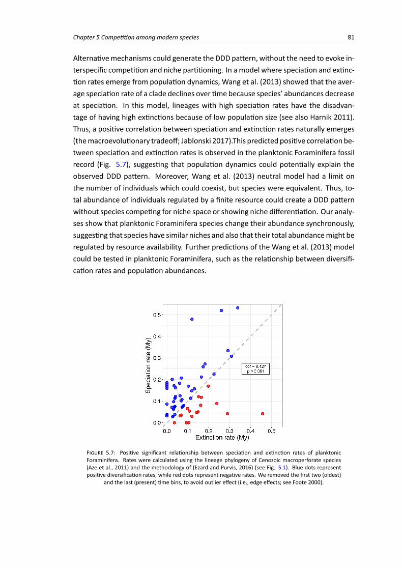
Chapter 5 Competition among modern species 81
Alternativemechanisms could generate the DDD pattern, without the need to evoke in-terspecific competition and niche partitioning. In amodel where speciation and extinc-tion rates emerge from population dynamics, Wang et al. (2013) showed that the aver-age speciation rate of a clade declines over time because species’ abundances decreaseat speciation. In this model, lineages with high speciation rates have the disadvan-tage of having high extinctions because of low population size (see also Harnik 2011).Thus, a positive correlation between speciation and extinction rates naturally emerges(themacroevolutionary tradeoff; Jablonski 2017).This predicted positive correlationbe-tween speciation and extinction rates is observed in the planktonic Foraminifera fossilrecord (Fig. 5.7), suggesting that population dynamics could potentially explain theobserved DDD pattern. Moreover, Wang et al. (2013) neutral model had a limit onthe number of individuals which could coexist, but species were equivalent. Thus, to-tal abundance of individuals regulated by a finite resource could create a DDD patternwithout species competing for niche space or showing niche differentiation. Our analy-ses show that planktonic Foraminifera species change their abundance synchronously,suggesting that species have similar niches and also that their total abundancemight beregulated by resource availability. Further predictions of the Wang et al. (2013) modelcould be tested in planktonic Foraminifera, such as the relationship between diversifi-cation rates and population abundances.
FIGURE 5.7: Positive significant relationship between speciation and extinction rates of planktonicForaminifera. Rates were calculated using the lineage phylogeny of Cenozoic macroperforate species(Aze et al., 2011) and the methodology of (Ezard and Purvis, 2016) (see Fig. 5.1). Blue dots representpositive diversification rates, while red dots represent negative rates. We removed the first two (oldest)
and the last (present) time bins, to avoid outlier effect (i.e., edge effects; see Foote 2000).
82 Chapter 5 Competition among modern species
The geography of diversification might also play a crucial role in the emergence of DDDpatterns (Moen andMorlon, 2014). Allopatric speciation, for example, occurs alongsidethe splitting of the lineage’s distribution in space. In this case, cladogenesis not onlyreduces species’ abundances but also species’ biogeographical ranges. Larger rangesare more likely to experience the emergence of geographic or oceanographic barriers.Thus, as diversification proceeds, ranges are subdivided and per-species rates of specia-tion declines, generating the DDD pattern without niche differentiation among species(Pigot et al., 2010; Moen and Morlon, 2014). Planktonic Foraminifera have the abilityto disperse long distances, evidenced by fossil and genetic data (Darling et al., 2000;Sexton and Norris, 2008). This high dispersal suggests that it may be difficult to geo-graphically isolate pelagic populations for extended periods of time, a key componentin allopatric speciation models. Planktonic Foraminifera fossil record has shown casesof sympatric speciation (Lazarus et al., 1995; Pearson et al., 1997), preventing the useof purely allopatric speciation models. Nevertheless, planktonic Foraminifera geneticstudies revealed phylogeographic patterns of allopatry (De Vargas et al., 1999; Dar-ling et al., 2007; Weiner et al., 2014), suggesting that ocean circulation and directionalflow create dynamical barriers to populations. Moreover, species’ abundances and ge-ographical ranges might interact in a negative way, and rare but widespread species(e.g., globorotaliids) might experience oceanographic gene-flow barriers more oftenthan abundant species. Genetic data provide new perspectives for speciation modesin the plankton, and can shed light on planktonic Foraminifera ecological interactions(e.g., Alizon et al. 2008; Aurahs et al. 2011) and the relationships among species’ abun-dances, geographical ranges, genetic diversity and diversification.
Overall, our results suggest that planktonic Foraminifera species are not competingin the modern oceans, which is consistent with the known low densities of plank-tonic Foraminifera in the water column (Schiebel and Hemleben, 2005; Keeling and delCampo, 2017). Abiotic factors such as SST have been shown to affect current diversitypatterns of planktonic Foraminifera in space (Fenton et al., 2016b) and time (Jonkersand Kucera, 2015), as well as their diversification dynamics (Ezard et al., 2011; Ezardand Purvis, 2016). However, phytoplankton abundance also plays an important rolein planktonic Foraminifera population dynamics (Jonkers and Kucera, 2015), but theireffect on planktonic Foraminifera diversification has not been explored. To further un-derstand the processes governing biodiversity dynamics, we need to include speciesthat are coupled ecologically, even when belonging to distantly related clades (Mar-shall and Quental, 2016). By defining the species pool of macroevolutionary dynamicsecologically rather than only phylogenetically, we can potentially solve the mismatchfound in our study.
Chapter 5 Competition among modern species 83
Acknowledgements We thank all the researchers who have made their data openlyavailable; Isabel S. Fenton, Daniela Schmidt and Phillip Fenberg for insightful commentson themanuscript; James Rosindel, Rampal Etienne, Rachel Germain andMathias Piresfor helpful discussions about the project.
Data accessibility The data that support the findings of this study are openly availableand previously published: refer to Siccha and Kucera (2017) for coretop abundancedata; Table C.2 for time series data; Aze et al. (2011) for phylogeny; Baranowski (2013);Weinkauf et al. (2016); Rillo et al. (2019b) for shell size data; Takagi et al. (2019) forsymbiosis data. The R code used to produce the analyses and figures is available at
.
Authors contribution M.R. designed the research, performed the analyses, wrote themanuscript and led the revisions. B.C. participated in the time series analysis. U.B. pro-vided shell size data. M.K. participated in the design of the research and interpretationof the results. M.S., L.J. and T.E. participated in the interpretation of the results andcritically reviewed themanuscript. All authors read and approved the final manuscript.

Chapter 6
Conclusion
6.1 Synthesis
Planktonic Foraminifera are an important model system for the empirical integrationof spatial and temporal biodiversity dynamics (Yasuhara et al. 2015; Chapter 1). Theirremarkably complete fossil record and mature taxonomy allow in-depth investigationof climatic forcing and evolutionary change across geological time scales (Brombacheret al., 2017a), providing awindow into community dynamics in deep time (Fenton et al.,2016a) and improving predictions of plankton community responses to future climaticchange. However, our basic ecological understanding of the planktonic Foraminiferaremains limited and studies addressing ecological questions are still rare, preventing usfrom fully leveraging the potential of their high-resolution fossil record to elucidate theprocesses that regulate biodiversity dynamics across geological time. In this thesis, Ihave contributed to our understanding of modern planktonic Foraminifera ecology bycombining a global, macroecological approach with natural history collections (NHCs).
The ecological patterns I described and analysed differed from those expected givenour former knowledge of planktonic Foraminifera. Species did not all reach largersizes under optimal environmental conditions (Chapter 4), suggesting the optimum-size hypothesis (Hecht, 1976; Schmidt et al., 2004a) might be overly simplistic. Instead,different physiological and ecological mechanisms are likely to affect growth patternsin different species. Moreover, we found no evidence for competition among modernplanktonic Foraminifera species (Chapter 5), contrary to what has been inferred fromtheir deep time dynamics in the Cenozoic fossil record (Ezard et al., 2011; Ezard andPurvis, 2016). Instead, it seems more likely that planktonic Foraminifera populationdynamics, and consequently evolutionary dynamics, are influenced by availability ofresources (i.e., phytoplankton abundance), but this hypothesis remains to be tested.The questions posed by the two “negative” results presented in this thesis highlight
85

86 Chapter 6 Conclusion
the need of more hypothesis-driven research on planktonic Foraminifera biology andecology.
The use of NHCs to describe ecological patterns can be challenging, as historical sam-ples were not necessarily collected following currentmethodological expectations. Theuse of non-uniform sampling protocols has the potential to increase measurementerrors, which need to be accounted for (Chapter 4). Nevertheless, museum collec-tions provide repositories of major surveys (Lister and Climate Change Research Group,2011) usually not achievable within the time frame of a Ph.D. project or researchgrants. The digitised Buckley Collection (Chapter 2), for example, is now part of thelargest public database of modern planktonic Foraminifera images and IDs, availableat and recently published in a collaboration withPincelli Hull, Allison Yi Hsiang and the Yale PeabodyMuseum of Natural History (Hsianget al., 2019). This database will be an important resource for those looking to learnmodern planktonic foraminiferal taxonomy and to automate the recognition of speciesusing a machine learning approach (Hsiang et al., 2019). Thus, the aggregation of indi-vidual collections into uniformly curated databases facilitates evidence-based investi-gation of ecological hypotheses (e.g., Salguero-Gómez et al. 2016; Dornelas et al. 2018),allowing the different datasets, each with their own advantages and disadvantages, tobecome more than the sum of their parts.
6.2 Future directions
There is still much to explore and understand about planktonic Foraminifera ecologyand evolution. High-resolution time series coupled with local biotic and abiotic vari-ables can give us further insights into what drives the ecological dynamics in this modelsystem. By understanding which other groups of organisms are ecologically relevant toplanktonic Foraminifera communities today, we will then be able to incorporate theminto studies using the foraminiferal fossil record. Ecological interactions among species,however, are highly nonlinear in nature (Deyle et al., 2016). Thus, relationships amongspecies temporal dynamics likely vary in intensity and sign through time (Ushio et al.,2018). Recently, a new method has been developed to investigate nonlinear ecolog-ical interactions among species using time series data and a dynamical systems ap-proach (Sugihara et al., 2012; Ye et al., 2015; DeAngelis and Yurek, 2015). In the fu-ture, this method could be applied to the highest-resolution time series of planktonicForaminifera to investigate the dynamics of their ecological interactions. Applying suchmethods to observational data on planktonic Foraminifera will certainly further ourecological knowledge. These methods are likely to provide an important source of
Chapter 6 Conclusion 87
information in this group particularly, where laboratory based experiments are oftenimpractical.
Planktonic foraminifera thermal niches (i.e., thermal tolerances) have been largely es-timated based on their relative abundances in the sediment (Kucera, 2007). Species’relative abundances in the local assemblage provide ecological information about thespecies-rank abundance distribution and species dominance in the local community.However, the interpretation of this relative abundance is complicated by the time-averaged nature of such sediments, meaning it potentially provides little informationabout the population density of the given species and, consequently, about its niche.As discussed in Chapter 4, a species might reach high relative abundances in the sedi-ment because it is better able to tolerate stress or because it has a shorter life cycle thanother species in the community, without necessarily being highly abundant while livingin the plankton. Thus, in the future, the estimation of the niche of a species should ide-ally be determined using absolute abundances of species (e.g., sediment trap data andplankton tow data), instead of relative abundances in the sediment. Where this is notpossible, reliable estimates of sedimentation rates and of reworking within sediments(e.g., Chapter 3) are critical for reducing uncertainty in age models and thus producingmore accurate estimations of absolute abundances from sediment data.
6.3 Concluding remarks
The planktonic Foraminifera fossil record provides a unique window into how marinebiodiversity changed across millions of years, and this evolutionary history is shaped byecology. Thus understanding the patterns observed in the fossil record requires us tounderstand the generating ecological processes. Ecological and evolutionary dynamicsare complex, because they are influenced by processes occurring at multiple organi-sational, temporal and spatial scales, challenging our ability to determine which pro-cesses are the main drivers of the observed dynamics. In this thesis, I used a macroe-cological approach to unravel morphological and ecological patterns observed withinextant planktonic Foraminifera species operating at scales from weeks to hundreds ofyears. I focused on a global spatial scale but explored different temporal scales to studytheir community ecology. Fully comprehending planktonic Foraminifera ecology, andthus unlocking their evolutionary history, will involve scientific research across multi-ple spatio-temporal scales. Whilst there is already abundant data available on modernplanktonic Foraminifera, facilitating such efforts, there are many discoveries yet to bemade.

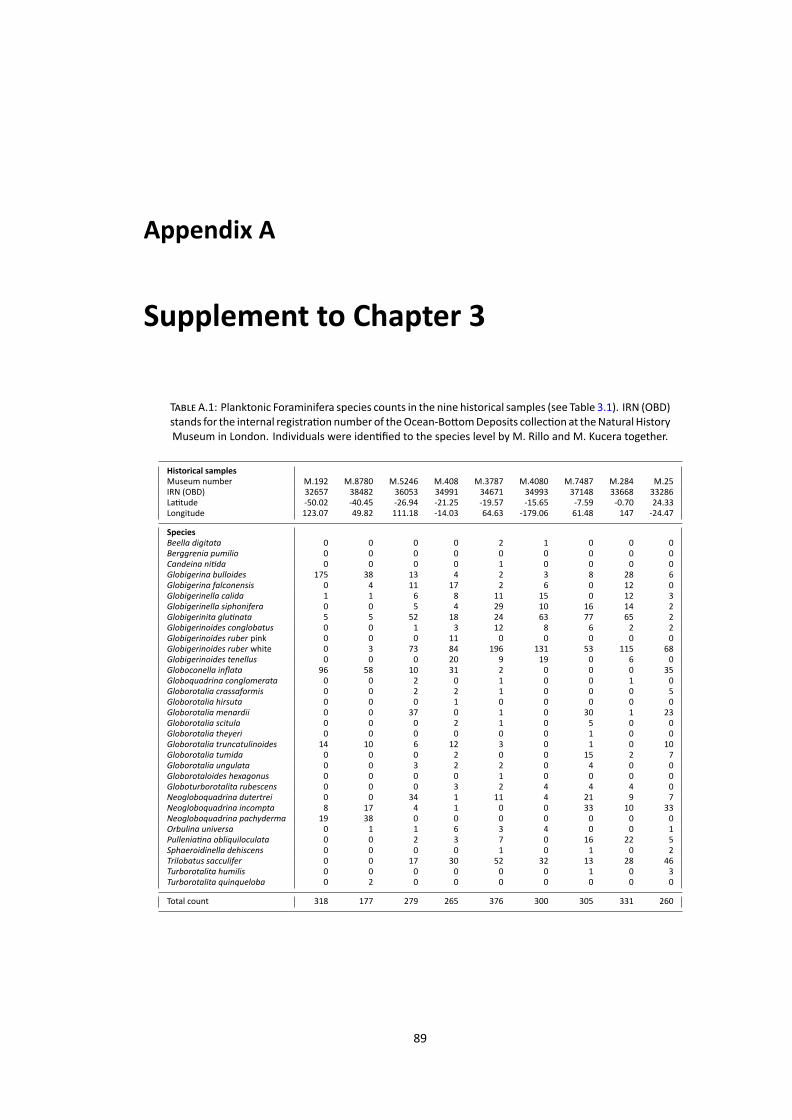
Appendix A
Supplement to Chapter 3
TABLE A.1: Planktonic Foraminifera species counts in the nine historical samples (see Table 3.1). IRN (OBD)stands for the internal registrationnumber of theOcean-BottomDeposits collection at theNatural HistoryMuseum in London. Individuals were identified to the species level by M. Rillo and M. Kucera together.
Historical samplesMuseum number M.192 M.8780 M.5246 M.408 M.3787 M.4080 M.7487 M.284 M.25IRN (OBD) 32657 38482 36053 34991 34671 34993 37148 33668 33286Latitude -50.02 -40.45 -26.94 -21.25 -19.57 -15.65 -7.59 -0.70 24.33Longitude 123.07 49.82 111.18 -14.03 64.63 -179.06 61.48 147 -24.47
SpeciesBeella digitata 0 0 0 0 2 1 0 0 0Berggrenia pumilio 0 0 0 0 0 0 0 0 0Candeina nitida 0 0 0 0 1 0 0 0 0Globigerina bulloides 175 38 13 4 2 3 8 28 6Globigerina falconensis 0 4 11 17 2 6 0 12 0Globigerinella calida 1 1 6 8 11 15 0 12 3Globigerinella siphonifera 0 0 5 4 29 10 16 14 2Globigerinita glutinata 5 5 52 18 24 63 77 65 2Globigerinoides conglobatus 0 0 1 3 12 8 6 2 2Globigerinoides ruber pink 0 0 0 11 0 0 0 0 0Globigerinoides ruber white 0 3 73 84 196 131 53 115 68Globigerinoides tenellus 0 0 0 20 9 19 0 6 0Globoconella inflata 96 58 10 31 2 0 0 0 35Globoquadrina conglomerata 0 0 2 0 1 0 0 1 0Globorotalia crassaformis 0 0 2 2 1 0 0 0 5Globorotalia hirsuta 0 0 0 1 0 0 0 0 0Globorotalia menardii 0 0 37 0 1 0 30 1 23Globorotalia scitula 0 0 0 2 1 0 5 0 0Globorotalia theyeri 0 0 0 0 0 0 1 0 0Globorotalia truncatulinoides 14 10 6 12 3 0 1 0 10Globorotalia tumida 0 0 0 2 0 0 15 2 7Globorotalia ungulata 0 0 3 2 2 0 4 0 0Globorotaloides hexagonus 0 0 0 0 1 0 0 0 0Globoturborotalita rubescens 0 0 0 3 2 4 4 4 0Neogloboquadrina dutertrei 0 0 34 1 11 4 21 9 7Neogloboquadrina incompta 8 17 4 1 0 0 33 10 33Neogloboquadrina pachyderma 19 38 0 0 0 0 0 0 0Orbulina universa 0 1 1 6 3 4 0 0 1Pulleniatina obliquiloculata 0 0 2 3 7 0 16 22 5Sphaeroidinella dehiscens 0 0 0 0 1 0 1 0 2Trilobatus sacculifer 0 0 17 30 52 32 13 28 46Turborotalita humilis 0 0 0 0 0 0 1 0 3Turborotalita quinqueloba 0 2 0 0 0 0 0 0 0
Total count 318 177 279 265 376 300 305 331 260
89
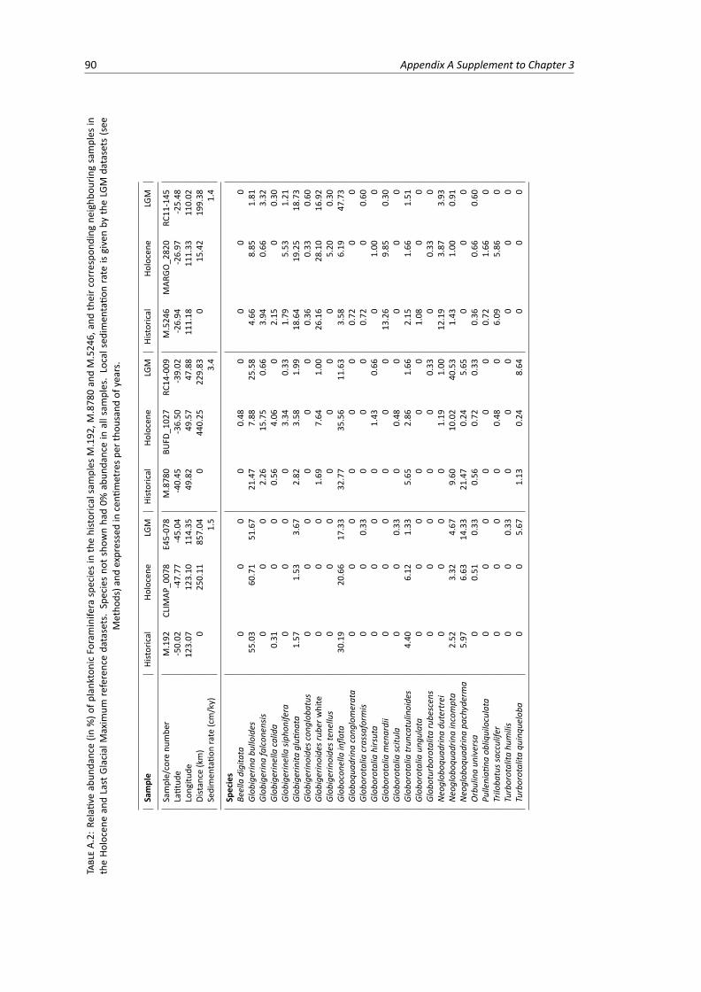
90 Appendix A Supplement to Chapter 3
TABLEA.2:
Relativ
eab
unda
nce(in
%)o
fplanktonicForaminife
raspeciesin
thehistoricalsamples
M.192
,M.878
0an
dM.524
6,an
dtheirc
orrespon
ding
neighb
ourin
gsamples
intheHo
locene
andLast
GlacialM
axim
umreferenceda
tasets.Speciesno
tsho
wnha
d0%
abun
dancein
allsam
ples.Localsed
imen
tatio
nrate
isgivenby
theLG
Mda
tasets
(see
Metho
ds)a
ndexpressedincenti
metresp
erthou
sand
ofyears.
Sample
Historical
Holocene
LGM
Historical
Holocene
LGM
Historical
Holocene
LGM
Sample/core
numbe
rM.192
CLIM
AP_0
078
E45-07
8M.878
0BU
FD_1
027
RC14
-009
M.524
6MAR
GO_2
820
RC11
-145
Latitud
e-50.02
-47.77
-45.04
-40.45
-36.50
-39.02
-26.94
-26.97
-25.48
Long
itude
123.07
123.10
114.35
49.82
49.57
47.88
111.18
111.33
110.02
Distan
ce(km)
025
0.11
857.04
044
0.25
229.83
015
.42
199.38
Sedimen
tatio
nrate
(cm/ky)
1.5
3.4
1.4
Species
Beelladigitata
00
00
0.48
00
00
Glob
igerinabu
lloides
55.03
60.71
51.67
21.47
7.88
25.58
4.66
8.85
1.81
Glob
igerinafalco
nensis
00
02.26
15.75
0.66
3.94
0.66
3.32
Glob
igerinellacalida
0.31
00
0.56
4.06
02.15
00.30
Glob
igerinellasip
honifera
00
00
3.34
0.33
1.79
5.53
1.21
Glob
igerinita
gluti
nata
1.57
1.53
3.67
2.82
3.58
1.99
18.64
19.25
18.73
Glob
igerinoide
scon
glob
atus
00
00
00
0.36
0.33
0.60
Glob
igerinoide
srub
erwhite
00
01.69
7.64
1.00
26.16
28.10
16.92
Glob
igerinoide
sten
ellus
00
00
00
05.20
0.30
Glob
ocon
ellainfla
ta30
.19
20.66
17.33
32.77
35.56
11.63
3.58
6.19
47.73
Glob
oqua
drinacong
lomerata
00
00
00
0.72
00
Glob
orotaliacrassaform
is0
00.33
00
00.72
00.60
Glob
orotaliahirsuta
00
00
1.43
0.66
01.00
0Glob
orotaliamen
ardii
00
00
00
13.26
9.85
0.30
Glob
orotaliascitu
la0
00.33
00.48
00
00
Glob
orotaliatrun
catulinoide
s4.40
6.12
1.33
5.65
2.86
1.66
2.15
1.66
1.51
Glob
orotaliaun
gulata
00
00
00
1.08
00
Glob
oturbo
rotalitarube
scen
s0
00
00
0.33
00.33
0Neo
glob
oqua
drinadu
tertrei
00
00
1.19
1.00
12.19
3.87
3.93
Neo
glob
oqua
drinaincompta
2.52
3.32
4.67
9.60
10.02
40.53
1.43
1.00
0.91
Neo
glob
oqua
drinapa
chyderma
5.97
6.63
14.33
21.47
0.24
5.65
00
0Orbulinaun
iversa
00.51
0.33
0.56
0.72
0.33
0.36
0.66
0.60
Pulleniati
naob
liquiloculata
00
00
00
0.72
1.66
0Triloba
tuss
acculifer
00
00
0.48
06.09
5.86
0Turborotalita
humilis
00
0.33
00
00
00
Turborotalita
quinqu
elob
a0
05.67
1.13
0.24
8.64
00
0
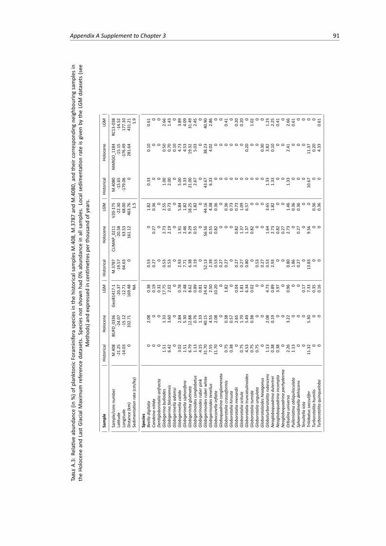
Appendix A Supplement to Chapter 3 91
TABLEA.3:
Relativ
eab
unda
nce(in
%)o
fplanktonicForaminife
raspeciesin
thehistoricalsamples
M.408
,M.378
7an
dM.408
0,an
dtheirc
orrespon
ding
neighb
ourin
gsamples
intheHo
locene
andLast
GlacialM
axim
umreferenceda
tasets.Speciesno
tsho
wnha
d0%
abun
dancein
allsam
ples.Localsed
imen
tatio
nrate
isgivenby
theLG
Mda
tasets
(see
Metho
ds)a
ndexpressedincenti
metresp
erthou
sand
ofyears.
Sample
Historical
Holocene
LGM
Historical
Holocene
LGM
Historical
Holocene
LGM
Sample/core
numbe
rM.408
BUFD
_033
6Ge
oB14
17-1
M.378
7CLIM
AP_0
211
V20-17
5M.408
0MAR
GO_1
184
RC13
-038
Latitud
e-21.25
-24.07
-20.37
-19.57
-20.58
-22.30
-15.65
-15.15
-14.52
Long
itude
-14.03
-15.12
-12.71
64.63
63.53
68.00
-179
.06
-176
.49
177.10
Distan
ce(km)
033
2.71
169.48
016
1.12
463.76
028
1.64
431.21
Sedimen
tatio
nrate
(cm/ky)
NA
1.5
1.9
Species
Beelladigitata
02.08
0.38
0.53
01.82
0.33
0.10
0.61
Cand
eina
nitid
a0
00.19
0.27
0.27
0.36
00
0De
ntiglob
orotaliaan
fracta
00
0.32
00
00
00
Glob
igerinabu
lloides
1.51
1.33
17.75
0.53
2.73
2.55
1.00
0.50
2.66
Glob
igerinafalco
nensis
6.42
3.60
2.02
0.53
2.19
0.73
2.00
0.70
1.43
Glob
igerinellaad
amsi
00
00
00
00.10
0Glob
igerinellacalida
3.02
2.84
0.78
2.93
1.91
5.84
5.00
4.73
3.89
Glob
igerinellasip
honifera
1.51
5.30
2.48
7.71
2.46
1.82
3.33
4.53
4.09
Glob
igerinita
gluti
nata
6.79
12.88
8.62
6.38
9.29
18.25
21.00
19.32
31.49
Glob
igerinoide
scon
glob
atus
1.13
0.76
0.89
3.19
0.55
1.82
2.67
5.03
2.45
Glob
igerinoide
srub
erpink
4.15
1.33
0.81
00
00
00
Glob
igerinoide
srub
erwhite
31.70
40.15
24.42
52.13
56.56
44.16
43.67
38.23
40.90
Glob
igerinoide
sten
ellus
7.55
4.55
2.50
2.39
0.55
4.38
6.33
4.02
2.86
Glob
ocon
ellainfla
ta11
.70
2.08
10.20
0.53
0.82
0.36
00
0Glob
oqua
drinacong
lomerata
00
00.27
00
00
0Glob
orotaliacrassaform
is0.75
0.38
1.82
0.27
00.36
00
0.41
Glob
orotaliahirsuta
0.38
0.57
00
00.73
00
0Glob
orotaliamen
ardii
02.65
0.04
0.27
0.82
0.73
00
0.20
Glob
orotaliascitu
la0.75
1.70
1.81
0.27
1.37
1.09
00
0.20
Glob
orotaliatrun
catulinoide
s4.53
5.49
6.34
0.80
1.37
6.57
00.20
0Glob
orotaliatumida
0.75
0.38
0.02
00.82
00
01.02
Glob
orotaliaun
gulata
0.75
00
0.53
00
00
0Glob
orotaloide
shexag
onus
00
00.27
00
00.30
0Glob
oturbo
rotalitarube
scen
s1.13
2.08
4.73
0.53
1.64
3.65
1.33
3.82
1.23
Neo
glob
oqua
drinadu
tertrei
0.38
0.19
0.89
2.93
2.73
1.82
1.33
0.10
2.25
Neo
glob
oqua
drinaincompta
0.38
03.97
00.82
00
00.41
Neo
glob
oqua
drinapa
chyderma
00
00
0.27
00
00
Orbulinaun
iversa
2.26
3.22
0.96
0.80
2.73
1.46
1.33
2.41
2.66
Pulleniati
naob
liquiloculata
1.13
00
1.86
00.36
00
0.61
Spha
eroidine
llade
hiscen
s0
00
0.27
0.27
0.36
00
0Tenu
itella
iota
00
0.17
00
00
00
Triloba
tuss
acculifer
11.32
5.30
7.33
13.83
9.56
010
.67
11.37
0Turborotalita
humilis
00
0.35
00
0.36
00.20
0Turborotalita
quinqu
elob
a0
00.16
00
0.36
04.33
0.61
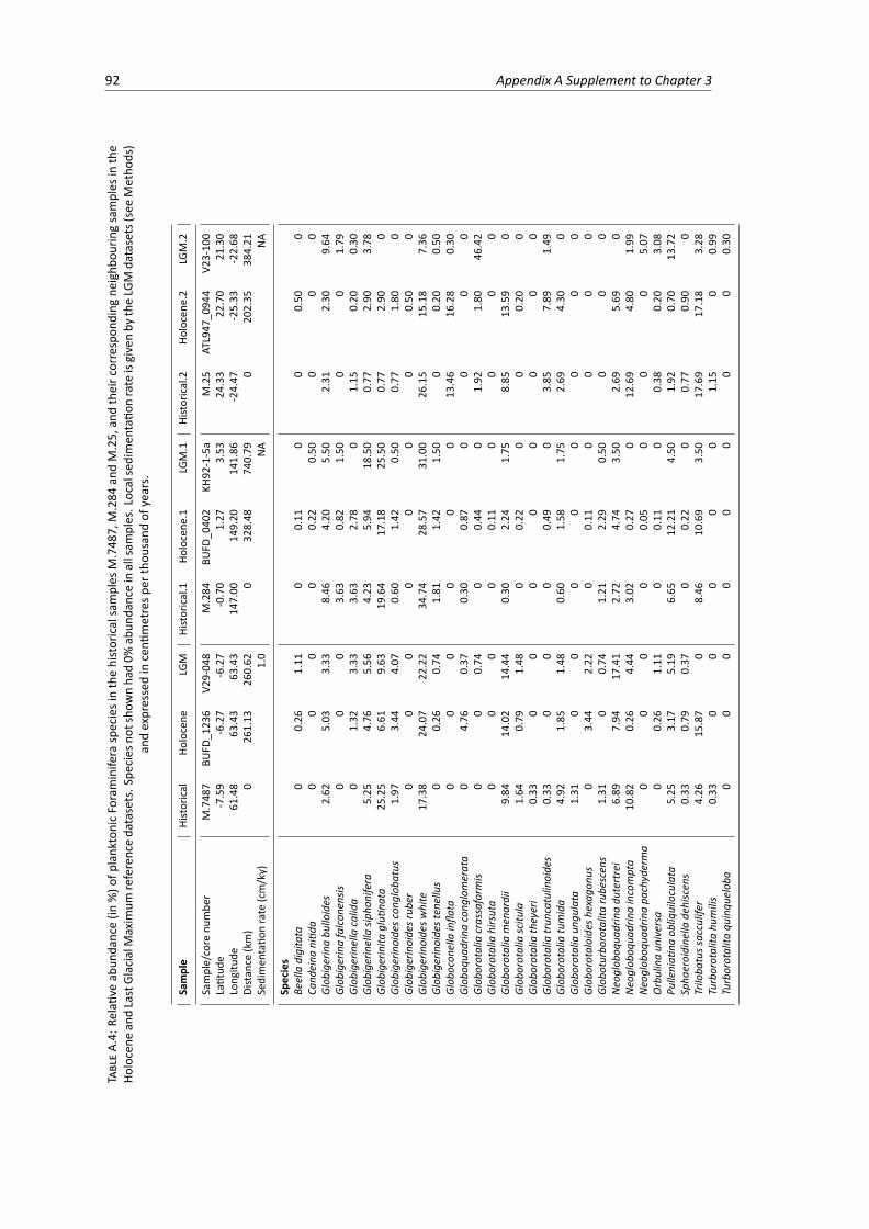
92 Appendix A Supplement to Chapter 3
TABLEA.4:
Relativ
eab
unda
nce(in
%)o
fplanktonicForaminife
raspeciesinthehistoricalsamples
M.748
7,M.284
andM.25,
andtheirc
orrespon
ding
neighb
ourin
gsamples
inthe
Holocene
andLastGlacialM
axim
umreferenceda
tasets.S
pecies
notsho
wnha
d0%
abun
danceinallsam
ples.Localsedimen
tatio
nrate
isgivenby
theLG
Mda
tasets(see
Metho
ds)
andexpressedincenti
metresp
erthou
sand
ofyears.
Sample
Historical
Holocene
LGM
Historical.1
Holocene
.1LG
M.1
Historical.2
Holocene
.2LG
M.2
Sample/core
numbe
rM.748
7BU
FD_1
236
V29-04
8M.284
BUFD
_040
2KH
92-1-5a
M.25
ATL947
_094
4V2
3-10
0Latitud
e-7.59
-6.27
-6.27
-0.70
1.27
3.53
24.33
22.70
21.30
Long
itude
61.48
63.43
63.43
147.00
149.20
141.86
-24.47
-25.33
-22.68
Distan
ce(km)
026
1.13
260.62
032
8.48
740.79
020
2.35
384.21
Sedimen
tatio
nrate
(cm/ky)
1.0
NA
NA
Species
Beelladigitata
00.26
1.11
00.11
00
0.50
0Ca
ndeina
nitid
a0
00
00.22
0.50
00
0Glob
igerinabu
lloides
2.62
5.03
3.33
8.46
4.20
5.50
2.31
2.30
9.64
Glob
igerinafalco
nensis
00
03.63
0.82
1.50
00
1.79
Glob
igerinellacalida
01.32
3.33
3.63
2.78
01.15
0.20
0.30
Glob
igerinellasip
honifera
5.25
4.76
5.56
4.23
5.94
18.50
0.77
2.90
3.78
Glob
igerinita
gluti
nata
25.25
6.61
9.63
19.64
17.18
25.50
0.77
2.90
0Glob
igerinoide
scon
glob
atus
1.97
3.44
4.07
0.60
1.42
0.50
0.77
1.80
0Glob
igerinoide
srub
er0
00
00
00
0.50
0Glob
igerinoide
swhite
17.38
24.07
22.22
34.74
28.57
31.00
26.15
15.18
7.36
Glob
igerinoide
sten
ellus
00.26
0.74
1.81
1.42
1.50
00.20
0.50
Glob
ocon
ellainfla
ta0
00
00
013
.46
16.28
0.30
Glob
oqua
drinacong
lomerata
04.76
0.37
0.30
0.87
00
00
Glob
orotaliacrassaform
is0
00.74
00.44
01.92
1.80
46.42
Glob
orotaliahirsuta
00
00
0.11
00
00
Glob
orotaliamen
ardii
9.84
14.02
14.44
0.30
2.24
1.75
8.85
13.59
0Glob
orotaliascitu
la1.64
0.79
1.48
00.22
00
0.20
0Glob
orotaliatheyeri
0.33
00
00
00
00
Glob
orotaliatrun
catulinoide
s0.33
00
00.49
03.85
7.89
1.49
Glob
orotaliatumida
4.92
1.85
1.48
0.60
1.58
1.75
2.69
4.30
0Glob
orotaliaun
gulata
1.31
00
00
00
00
Glob
orotaloide
shexag
onus
03.44
2.22
00.11
00
00
Glob
oturbo
rotalitarube
scen
s1.31
00.74
1.21
2.29
0.50
00
0Neo
glob
oqua
drinadu
tertrei
6.89
7.94
17.41
2.72
4.74
3.50
2.69
5.69
0Neo
glob
oqua
drinaincompta
10.82
0.26
4.44
3.02
0.27
012
.69
4.80
1.99
Neo
glob
oqua
drinapa
chyderma
00
00
0.05
00
05.07
Orbulinaun
iversa
00.26
1.11
00.11
00.38
0.20
3.08
Pulleniati
naob
liquiloculata
5.25
3.17
5.19
6.65
12.21
4.50
1.92
0.70
13.72
Spha
eroidine
llade
hiscen
s0.33
0.79
0.37
00.22
00.77
0.90
0Triloba
tuss
acculifer
4.26
15.87
08.46
10.69
3.50
17.69
17.18
3.28
Turborotalita
humilis
0.33
00
00
01.15
00.99
Turborotalita
quinqu
elob
a0
00
00
00
00.30
Appendix B
Supplement to Chapter 4
Museum collection shell size bias analysis
To assess the size bias in the Buckley Collection, we re-sampled ten bulk sediments ofthe NHMUK Ocean-Bottom Deposits Collection (OBD) Collection, fromwhich the Buck-ley Collection was created (Fig. 4.1a, Table B.1). Samples were chosen to encompassdifferent oceans, latitudes and marine expeditions; however, the final choice also de-pended on the availability of bulk sediment samples in the OBD Collection. Half of theamount available in the OBD containers was further split into two equal parts, leavingan archive sample and a sample to be processed. The sample processing consisted ofweighing, wet washing over a 63µm sieve and drying in a 60�C oven. The residues werefurther dry sieved over a 150µm sieve and the coarser fraction was split with a micros-plitter as many times as needed to produce a representative aliquot containing around300 planktonic Foraminifera specimens (see Al-Sabouni et al. 2007). All specimens ineach of the nine final splits were identified by MCR and MK under a stereomicroscopeto species level, resulting in a total of 2,611 individuals belonging to 31 species (see alsoRillo et al. 2019a). We mounted species-specific slides from the re-sampled samples,calculated the relative abundance of each species in each sample, and then extractedshell size data in the sameway as for the slides of the Buckley Collection. Only the sizesof species also present in the Buckley Collection samples were measured, resulting in1824 specimens’ shell sizes from 20 species (Table B.1). See section 4.2.2 in the maintext for further information.
93
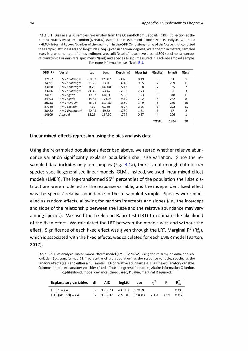
94 Appendix B Supplement to Chapter 4
TABLE B.1: Bias analysis: samples re-sampled from the Ocean-Bottom Deposits (OBD) Collection at theNatural History Museum, London (NHMUK) used in the museum collection size bias analysis. Columns:NHMUK Internal Record Number of the sediment in theOBD Collection; name of the Vessel that collectedthe sample; latitude (Lat) and longitude (Long) given in decimal degrees; water depth in meters; sampledmass in grams; number of times sediment was split N(splits) to achieve around 300 specimens; numberof planktonic Foraminifera specimens N(ind) and species N(ssp) measured in each re-sampled sample.
For more information, see Table B.3.
OBD IRN Vessel Lat Long Depth (m) Mass (g) N(splits) N(ind) N(ssp)
32657 HMS Challenger -50.02 123.07 -3976 0.19 5 14 134991 HMS Challenger -21.25 -14.03 -3740 9.35 7 239 1133668 HMS Challenger -0.70 147.00 -2213 1.98 7 185 733286 HMS Challenger 24.33 -24.47 -5153 2.73 5 31 334671 HMS Egeria -19.57 64.63 -2708 1.23 5 348 1134993 HMS Egeria -15.65 -179.06 -2519 2.42 8 262 836053 HMS Penguin -26.94 111.18 -3350 1.49 5 230 1037148 HMS Sealark -7.59 61.48 -3507 2.86 8 222 1138482 HMSWaterwitch -40.45 49.82 -3780 1.51 6 67 214609 Alpha 6 85.25 -167.90 -1774 0.57 4 226 1
TOTAL 1824 20
Linear mixed-effects regression using the bias analysis data
Using the re-sampled populations described above, we tested whether relative abun-dance variation significantly explains population shell size variation. Since the re-sampled data includes only ten samples (Fig. 4.1a), there is not enough data to runspecies-specific generalised linear models (GLM). Instead, we used linear mixed-effectmodels (LMER). The log-transformed 95th percentiles of the population shell size dis-tributions were modelled as the response variable, and the independent fixed effectwas the species’ relative abundance in the re-sampled sample. Species were mod-elled as random effects, allowing for random intercepts and slopes (i.e., the interceptand slope of the relationship between shell size and the relative abundance may varyamong species). We used the Likelihood Ratio Test (LRT) to compare the likelihoodof the fixed effect. We calculated the LRT between the models with and without theeffect. Significance of each fixed effect was given through the LRT. Marginal R2 (R2
m),which is associated with the fixed effects, was calculated for each LMERmodel (Barton,2017).
TABLE B.2: Bias analysis: linear mixed-effects model (LMER, ANOVA) using the re-sampled data, and sizevariation (log-transformed 95th percentile of the population) as the response variable, species as therandom effects (r.e.) and either a null model (H0) or relative abundance (H1) as the explanatory variable.Columns: model explanatory variables (fixed effects), degrees of freedom, Akaike Information Criterion,
log-likelihood, model deviance, chi-squared, P value, marginal R squared.
Explanatory variables df AIC logLik dev �2 P R2m
H0: 1 + r.e. 5 130.20 -60.10 120.20 0.00H1: (abund) + r.e. 6 130.02 -59.01 118.02 2.18 0.14 0.07

Appendix B Supplement to Chapter 4 95
TABLE B.3: Samples from the Henry Buckley Collection of Planktonic Foraminifera at The Natural His-tory Museum, London (NHMUK) used in the morphometric analysis. Columns: NHMUK Internal RecordNumber of the sediment in the Ocean-Bottom Deposits Collection (OBD IRN); name of the vessel thatcollected the sample; year the sample was collected; latitude (Lat) and longitude (Long) given in deci-mal degrees; sea surface temperature (SST) in Celsius degrees; water depth in meters; sampling methodused in the historical expedition; depth below the seafloor (Dbsf) sampled in centimetres; number of
planktonic Foraminifera specimens N(ind) and species N(ssp) measured at each site.
OBD IRN Vessel Year Lat Long SST Depth(m) Sampling Dbsf(cm) N(ind) N(ssp)
31945 CS Britannia 1899 39.21 -70.24 19.25 -2731 Sounding surface 65 134297 CS Buccaneer 1886 -0.03 -15.94 26.30 -3226 Sounding surface 57 130724 HEMSMabahiss 1934 7.19 63.04 28.38 -4346 Core 4-5.5 53 735818 HMIMS Investigator 1906 20.44 68.84 27.24 -2680 Sounding surface 56 517229 HMNZS Lachlan 1955 -33.88 173.83 17.80 -2464 Worsel sampler surface 106 817262 HMNZS Pukaki 1957 -53.63 169.87 7.95 -746 Dietz grab surface 52 233286 HMS Challenger 1873 24.33 -24.47 23.16 -5153 Sounding surface 46 132657 HMS Challenger 1874 -50.02 123.07 9.32 -3976 Sounding surface 11 133668 HMS Challenger 1875 -0.70 147.00 29.40 -2213 Sounding surface 95 734607 HMS Challenger 1875 -33.70 -78.30 16.79 -3798 Sounding surface 8 134991 HMS Challenger 1876 -21.25 -14.03 23.61 -3740 Dredge surface 181 834671 HMS Egeria 1887 -19.57 64.63 24.83 -2708 Sounding surface 66 834676 HMS Egeria 1887 -23.23 56.30 25.14 -4646 Sounding surface 73 934678 HMS Egeria 1887 -29.93 54.10 21.13 -4211 Sounding surface 63 834993 HMS Egeria 1889 -15.65 -179.06 28.05 -2519 Sounding surface 124 835238 HMS Egeria 1894 7.08 73.80 28.57 -2658 Sounding surface 66 716621 HMS Enterprise 1962 30.90 -78.68 26.63 -821 Dredge surface 35 136043 HMS Penguin 1891 -28.01 112.46 21.94 -1206 Sounding surface 189 936053 HMS Penguin 1891 -26.94 111.18 22.66 -3350 Sounding surface 203 936057 HMS Penguin 1891 -24.89 110.39 22.83 -3829 Sounding surface 193 936361 HMS Penguin 1896 -10.21 178.01 28.91 -4844 Sounding surface 123 836515 HMS Penguin 1897 -9.68 -174.62 28.05 -4057 Sounding surface 71 636683 HMS Penguin 1897 1.21 -161.84 27.32 -4634 Sounding surface 47 836704 HMS Penguin 1897 -13.17 -175.69 28.05 -3952 Sounding surface 111 737130 HMS Sealark 1905 -8.42 65.63 28.35 -3694 Sounding surface 78 737148 HMS Sealark 1905 -7.59 61.48 28.06 -3507 Sounding surface 87 837149 HMS Sealark 1905 -2.70 67.38 28.95 -3594 Sounding surface 119 737190 HMS Sealark 1905 -12.12 64.12 27.16 -3322 Sounding surface 72 737299 HMS Serpent 1868 18.63 69.17 27.85 -3261 Sounding surface 9 138482 HMSWaterwitch 1895 -40.45 49.82 7.78 -3780 Sounding surface 39 217031 RNZFA Tui 1956 -39.77 167.75 16.04 -1137 Dietz grab surface 71 417240 RNZFA Tui 1956 -28.88 170.00 22.18 -3021 Dietz grab surface 165 817273 RNZFA Tui 1958 -20.95 -175.23 25.66 -869 Cone dredge surface 40 616657 RV Argo 1960 -16.42 66.03 26.20 -2810 Core 4-9 60 816365 RV Horizon 1953 -19.48 -173.73 25.66 -4347 Gravity core 5-10 43 416640 RV Horizon 1953 -13.09 -124.28 26.67 -3456 Gravity core 4-8 58 716641 RV Horizon 1953 -14.27 -120.68 25.97 -3617 Gravity core 4-8 41 616642 RV Horizon 1953 -15.22 -117.51 25.97 -3641 Gravity core 1-4 32 516656 RV Horizon 1958 -23.61 -118.22 23.98 -3362 Gravity core 7-11 48 5
(1971,O87) RVMaria Paolina G 1970 35.68 -4.08 18.17 -1500 Sphincter core 0-5 40 316645 RV Spencer F. Baird 1957 5.43 -131.32 27.65 -3415 Gravity core 7-10 51 616646 RV Spencer F. Baird 1957 -26.32 -147.12 21.85 -2312 Gravity core 3-7 54 616647 RV Spencer F. Baird 1957 -46.75 -123.00 9.91 -4030 Gravity core 6-11 53 216648 RV Spencer F. Baird 1957 -48.48 -113.28 8.06 -2677 Gravity core 0-8 41 216649 RV Spencer F. Baird 1957 -43.72 -107.60 10.99 -3141 Gravity core 3-7 17 316370 RV Spencer F. Baird 1958 -11.70 -109.72 25.27 -3296 Gravity core 0-3 1 116650 RV Spencer F. Baird 1958 -18.33 -79.34 20.07 -3157 Gravity core 8-12 49 716651 RV Spencer F. Baird 1958 -27.93 -106.92 21.45 -3039 Gravity core 8-15 67 616652 RV Spencer F. Baird 1958 -27.15 -109.83 21.45 -2819 Gravity core 10-14 51 516653 RV Spencer F. Baird 1958 -14.73 -112.10 24.90 -3034 Gravity core 12-15 69 716654 RV Spencer F. Baird 1958 -9.88 -110.68 25.26 -2712 Gravity core 5-9 46 717162 RV Vema 1959 28.40 -77.93 24.89 -1004 Piston core 0-2 136 817359 RV Vema 1959 -9.75 -34.40 27.14 -4123 Piston core 5-6 86 6
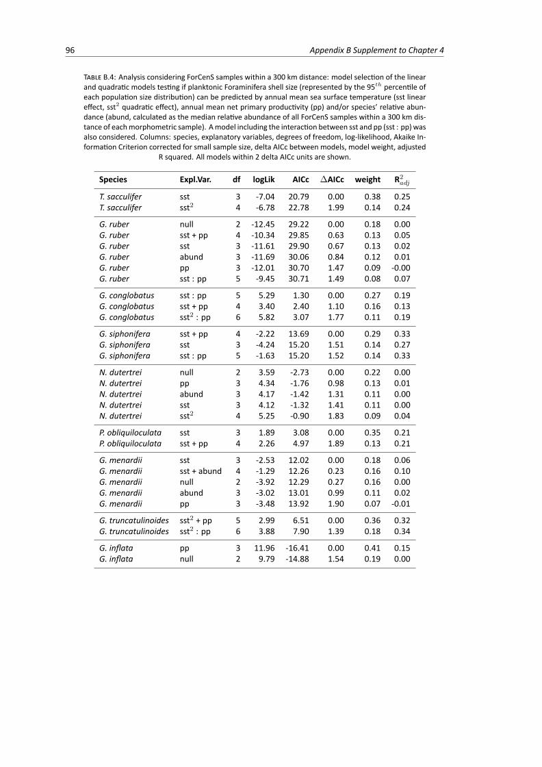
96 Appendix B Supplement to Chapter 4
TABLE B.4: Analysis considering ForCenS samples within a 300 km distance: model selection of the linearand quadratic models testing if planktonic Foraminifera shell size (represented by the 95th percentile ofeach population size distribution) can be predicted by annual mean sea surface temperature (sst lineareffect, sst2 quadratic effect), annual mean net primary productivity (pp) and/or species’ relative abun-dance (abund, calculated as the median relative abundance of all ForCenS samples within a 300 km dis-tance of eachmorphometric sample). Amodel including the interaction between sst and pp (sst : pp) wasalso considered. Columns: species, explanatory variables, degrees of freedom, log-likelihood, Akaike In-formation Criterion corrected for small sample size, delta AICc between models, model weight, adjusted
R squared. All models within 2 delta AICc units are shown.
Species Expl.Var. df logLik AICc �AICc weight R2adj
T. sacculifer sst 3 -7.04 20.79 0.00 0.38 0.25T. sacculifer sst2 4 -6.78 22.78 1.99 0.14 0.24
G. ruber null 2 -12.45 29.22 0.00 0.18 0.00G. ruber sst + pp 4 -10.34 29.85 0.63 0.13 0.05G. ruber sst 3 -11.61 29.90 0.67 0.13 0.02G. ruber abund 3 -11.69 30.06 0.84 0.12 0.01G. ruber pp 3 -12.01 30.70 1.47 0.09 -0.00G. ruber sst : pp 5 -9.45 30.71 1.49 0.08 0.07
G. conglobatus sst : pp 5 5.29 1.30 0.00 0.27 0.19G. conglobatus sst + pp 4 3.40 2.40 1.10 0.16 0.13G. conglobatus sst2 : pp 6 5.82 3.07 1.77 0.11 0.19
G. siphonifera sst + pp 4 -2.22 13.69 0.00 0.29 0.33G. siphonifera sst 3 -4.24 15.20 1.51 0.14 0.27G. siphonifera sst : pp 5 -1.63 15.20 1.52 0.14 0.33
N. dutertrei null 2 3.59 -2.73 0.00 0.22 0.00N. dutertrei pp 3 4.34 -1.76 0.98 0.13 0.01N. dutertrei abund 3 4.17 -1.42 1.31 0.11 0.00N. dutertrei sst 3 4.12 -1.32 1.41 0.11 0.00N. dutertrei sst2 4 5.25 -0.90 1.83 0.09 0.04
P. obliquiloculata sst 3 1.89 3.08 0.00 0.35 0.21P. obliquiloculata sst + pp 4 2.26 4.97 1.89 0.13 0.21
G. menardii sst 3 -2.53 12.02 0.00 0.18 0.06G. menardii sst + abund 4 -1.29 12.26 0.23 0.16 0.10G. menardii null 2 -3.92 12.29 0.27 0.16 0.00G. menardii abund 3 -3.02 13.01 0.99 0.11 0.02G. menardii pp 3 -3.48 13.92 1.90 0.07 -0.01
G. truncatulinoides sst2 + pp 5 2.99 6.51 0.00 0.36 0.32G. truncatulinoides sst2 : pp 6 3.88 7.90 1.39 0.18 0.34
G. inflata pp 3 11.96 -16.41 0.00 0.41 0.15G. inflata null 2 9.79 -14.88 1.54 0.19 0.00
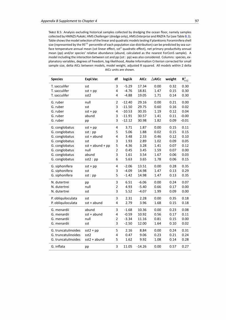
Appendix B Supplement to Chapter 4 97
TABLE B.5: Analysis excluding historical samples collected by dredging the ocean floor, namely samplescollected by HMNZS Pukaki, HMS Challenger (dredge only), HMS Enterprise and RNZFA Tui (see Table B.3).Table shows themodel selectionof the linear andquadraticmodels testing if planktonic Foraminifera shellsize (represented by the 95th percentile of each population size distribution) can be predicted by sea sur-face temperature annual mean (sst linear effect, sst2 quadratic effect), net primary productivity annualmean (pp) and/or species’ relative abundance (abund, calculated as the nearest ForCenS sample). Amodel including the interaction between sst and pp (sst : pp) was also considered. Columns: species, ex-planatory variables, degrees of freedom, log-likelihood, Akaike Information Criterion corrected for smallsample size, delta AICc between models, model weight, adjusted R squared. All models within 2 delta
AICc units are shown.
Species Expl.Var. df logLik AICc �AICc weight R2adj
T. sacculifer sst 3 -5.29 17.34 0.00 0.32 0.30T. sacculifer sst + pp 4 -4.76 18.81 1.47 0.15 0.30T. sacculifer sst2 4 -4.88 19.05 1.71 0.14 0.30
G. ruber null 2 -12.40 29.16 0.00 0.21 0.00G. ruber sst 3 -11.50 29.75 0.60 0.16 0.02G. ruber sst + pp 4 -10.53 30.35 1.19 0.12 0.04G. ruber abund 3 -11.91 30.57 1.41 0.11 -0.00G. ruber pp 3 -12.12 30.98 1.82 0.09 -0.01
G. conglobatus sst + pp 4 3.71 1.87 0.00 0.15 0.11G. conglobatus sst : pp 5 5.06 1.88 0.02 0.15 0.15G. conglobatus sst + abund 4 3.48 2.33 0.46 0.12 0.10G. conglobatus sst 3 1.93 2.89 1.02 0.09 0.05G. conglobatus sst + abund + pp 5 4.36 3.28 1.41 0.07 0.12G. conglobatus null 2 0.45 3.45 1.59 0.07 0.00G. conglobatus abund 3 1.61 3.54 1.67 0.06 0.03G. conglobatus sst2 : pp 6 5.63 3.65 1.78 0.06 0.15
G. siphonifera sst + pp 4 -2.06 13.51 0.00 0.28 0.35G. siphonifera sst 3 -4.09 14.98 1.47 0.13 0.29G. siphonifera sst : pp 5 -1.42 14.98 1.47 0.13 0.35
N. dutertrei pp 3 6.51 -6.06 0.00 0.24 0.07N. dutertrei null 2 4.93 -5.40 0.66 0.17 0.00N. dutertrei sst 3 5.52 -4.07 1.99 0.09 0.00
P. obliquiloculata sst 3 2.31 2.28 0.00 0.35 0.18P. obliquiloculata sst + abund 4 2.79 3.96 1.68 0.15 0.18
G. menardii abund 3 -1.68 10.36 0.00 0.23 0.08G. menardii sst + abund 4 -0.59 10.92 0.56 0.17 0.11G. menardii null 2 -3.34 11.16 0.81 0.15 0.00G. menardii sst 3 -2.50 12.00 1.64 0.10 0.02
G. truncatulinoides sst2 + pp 5 2.16 8.84 0.00 0.24 0.31G. truncatulinoides sst2 4 0.47 9.06 0.23 0.21 0.24G. truncatulinoides sst2 + abund 5 1.62 9.92 1.08 0.14 0.28
G. inflata pp 3 11.05 -14.26 0.00 0.57 0.27
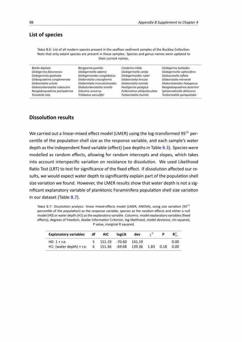
98 Appendix B Supplement to Chapter 4
List of species
TABLE B.6: List of all modern species present in the seafloor sediment samples of the Buckley Collection.Note that only extant species are present in these samples. Species and genus names were updated to
their current names.
Beella digitata Berggrenia pumilio Candeina nitida Globigerina bulloidesGlobigerina falconensis Globigerinella adamsi Globigerinella calida Globigerinella siphoniferaGlobigerinita glutinata Globigerinoides conglobatus Globigerinoides ruber Globoconella inflataGloboquadrina conglomerata Globorotalia crassaformis Globorotalia hirsuta Globorotalia menardiiGloborotalia scitula Globorotalia truncatulinoides Globorotalia tumida Globorotaloides hexagonusGloboturborotalita rubescens Globoturborotalita tenella Hastigerina pelagica Neogloboquadrina dutertreiNeogloboquadrina pachyderma Orbulina universa Pulleniatina obliquiloculata Sphaeroidinella dehiscensTenuitella iota Trilobatus sacculifer Turborotalita humilis Turborotalita quinqueloba
Dissolution results
We carried out a linear-mixed effect model (LMER) using the log-transformed 95th per-centile of the population shell size as the response variable, and each sample’s waterdepth as the independent fixed variable (effect) (see depths in Table B.3). Species weremodelled as random effects, allowing for random intercepts and slopes, which takesinto account interspecific variation on resistance to dissolution. We used LikelihoodRatio Test (LRT) to test for significance of the fixed effect. If dissolution affected our re-sults, we would expect water depth to significantly explain part of the population shellsize variation we found. However, the LMER results show that water depth is not a sig-nificant explanatory variable of planktonic Foraminifera population shell size variationin our dataset (Table B.7).
TABLE B.7: Dissolution analysis: linear mixed-effects model (LMER, ANOVA), using size variation (95th
percentile of the population) as the response variable, species as the random effects and either a nullmodel (H0) or water depth (H1) as the explanatory variable. Columns: model explanatory variables (fixedeffects), degrees of freedom, Akaike Information Criterion, log-likelihood, model deviance, chi-squared,
P value, marginal R squared.
Explanatory variables df AIC logLik dev �2 P R2m
H0: 1 + r.e. 5 151.19 -70.60 141.19 0.00H1: (water depth) + r.e. 6 151.36 -69.68 139.36 1.83 0.18 0.00
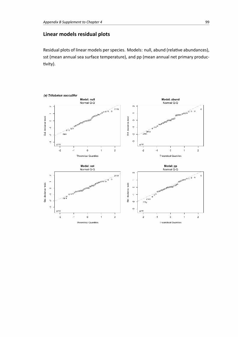
Appendix B Supplement to Chapter 4 99
Linear models residual plots
Residual plots of linear models per species. Models: null, abund (relative abundances),sst (mean annual sea surface temperature), and pp (mean annual net primary produc-tivity).
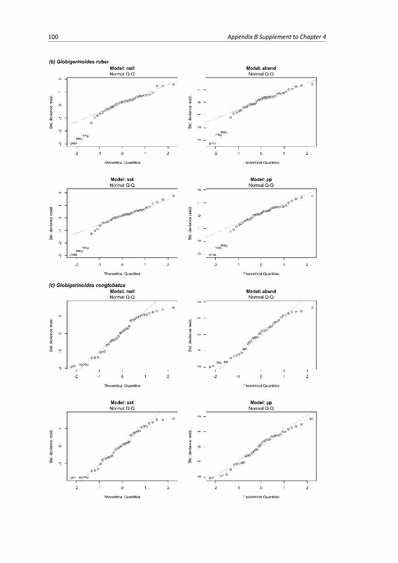
100 Appendix B Supplement to Chapter 4
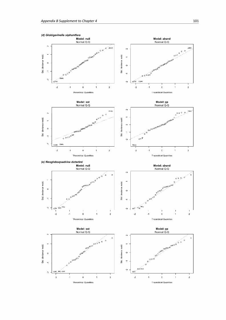
Appendix B Supplement to Chapter 4 101

102 Appendix B Supplement to Chapter 4
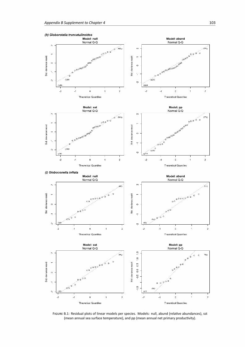
Appendix B Supplement to Chapter 4 103
FIGURE B.1: Residual plots of linear models per species. Models: null, abund (relative abundances), sst(mean annual sea surface temperature), and pp (mean annual net primary productivity).

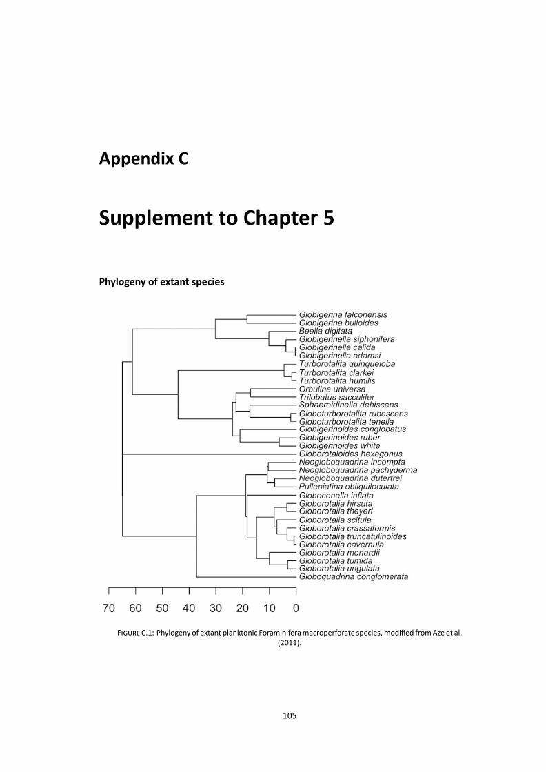
Appendix C
Supplement to Chapter 5
Phylogeny of extant species
FIGURE C.1: Phylogeny of extant planktonic Foraminiferamacroperforate species, modified fromAze et al.(2011).
105
106 Appendix C Supplement to Chapter 5
We modified the Aze et al. (2011) Cenozoic phylogeny of macroperforate planktonicForaminifera (PF) species, following the taxonomic standardisation of Siccha and Kucera(2017) (Fig. C.1) . More specifically, we split the species Globigerinoides ruber into G.ruber (pink pigmented) and G. white (not pigmented) at 6.3 million years ago (Ma)(Aurahs et al., 2011). We also split the species Neogloboquadrina pachyderma intoN. pachyderma and N. incompta at 10.4 Ma (Darling et al., 2006). The main reasonfor adding these species to the Aze et al. (2011) phylogeny is that they are currentlyrecognised species, with clear morphological differences and population-level coretopand sediment trap data.
Shell size estimates of extant species
In order to build a clade-wide species-level size dataset of extant PF, we useddata on 2774 individual shell measurements of 36 species (Table C.1). We ex-tracted data from three different datasets on shell size: [1] Rillo et al. (2019b) (20species, 1824 individuals), [2] Weinkauf et al. (2016) (2 species, 831 individuals)and [3] Baranowski (2013) (35 species, 118 individuals). These three datasets areopenly available online, respectively, at: [1] ,[2] and [3]
. Specimens were collected from seafloor and/or sedimenttrap samples, and we used shell diameter to represent shell size. The species Glo-bigerinoides ruber (white), G. ruber (pink) and G. elongatus were analysed together asG. ruber. For more information about the sampling and the method of measurement,see corresponding references of each dataset.
Shell diameter was measured as the longest shell-axis through the proloculus by Rilloet al. (2019b) and Weinkauf et al. (2016) and from the middle of the last chamberthrough the proloculus to the opposite side of the test by Baranowski (2013). These twoways of measuring the shell diameter would only differ if the last chamber is smallerthan the penultimate chamber, which was not the case formost of the individuals mea-sured by Baranowski (2013).
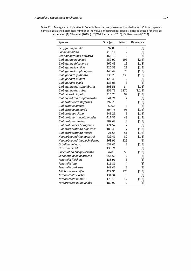
Appendix C Supplement to Chapter 5 107
TABLE C.1: Average size of planktonic Foraminifera species (square-root of shell area). Column: speciesnames; size as shell diameter; number of individuals measured per species; dataset(s) used for the size
estimates: [1] Rillo et al. (2019b), [2] Weinkauf et al. (2016), [3] Baranowski (2013).
Species Size (µm) N(ind) Reference
Berggrenia pumilio 92.08 9 [3]Candeina nitida 418.11 2 [3]Dentigloborotalia anfracta 166.19 2 [3]Globigerina bulloides 259.92 193 [2;3]Globigerina falconensis 262.49 19 [1;3]Globigerinella calida 320.33 22 [1;3]Globigerinella siphonifera 440.47 75 [1;3]Globigerinita glutinata 236.29 233 [1;3]Globigerinita minuta 129.45 2 [3]Globigerinita uvula 133.05 3 [3]Globigerinoides conglobatus 503.56 34 [1;3]Globigerinoides ruber 255.76 1270 [1;2;3]Globoconella inflata 314.74 99 [1;3]Globoquadrina conglomerata 644.71 2 [3]Globorotalia crassaformis 392.28 9 [1;3]Globorotalia hirsuta 590.5 3 [3]Globorotalia menardii 804.75 96 [1;3]Globorotalia scitula 243.25 9 [1;3]Globorotalia truncatulinoides 417.32 48 [1;3]Globorotalia tumida 902.49 8 [1;3]Globorotaloides hexagonus 424.52 2 [3]Globoturborotalita rubescens 189.46 7 [1;3]Globoturborotalita tenella 212.8 51 [1;3]Neogloboquadrina dutertrei 429.41 80 [1;3]Neogloboquadrina pachyderma 263.91 226 [1]Orbulina universa 637.46 8 [1;3]Orcardia riedeli 130.71 5 [3]Pulleniatina obliquiloculata 478.9 53 [1;3]Sphaeroidinella dehiscens 654.56 2 [3]Tenuitella fleisheri 135.91 3 [3]Tenuitella iota 111.81 4 [3]Tenuitella parkerae 149.42 3 [3]Trilobatus sacculifer 427.96 170 [1;3]Turborotalita clarkei 131.34 8 [3]Turborotalita humilis 173.18 12 [1;3]Turborotalita quinqueloba 189.92 2 [3]
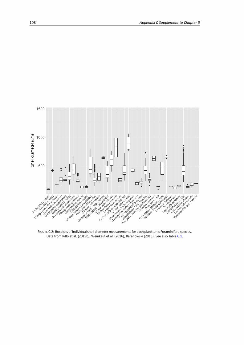
108 Appendix C Supplement to Chapter 5
FIGURE C.2: Boxplots of individual shell diametermeasurements for each planktonic Foraminifera species.Data from Rillo et al. (2019b); Weinkauf et al. (2016); Baranowski (2013). See also Table C.1.
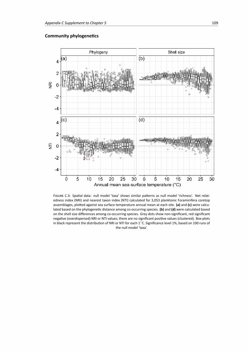
Appendix C Supplement to Chapter 5 109
Community phylogenetics
FIGURE C.3: Spatial data: null model ‘taxa’ shows similar patterns as null model ‘richness’. Net relat-edness index (NRI) and nearest taxon index (NTI) calculated for 3,053 planktonic Foraminifera coretopassemblages, plotted against sea surface temperature annual mean at each site. (a) and (c) were calcu-lated based on the phylogenetic distance among co-occurring species. (b) and (d)were calculated basedon the shell size differences among co-occurring species. Grey dots show non-significant, red significantnegative (overdispersed) NRI or NTI values; there are no significant positive values (clustered). Box-plotsin black represent the distribution of NRI or NTI for each 1�C. Significance level 1%, based on 100 runs of
the null model ‘taxa’.
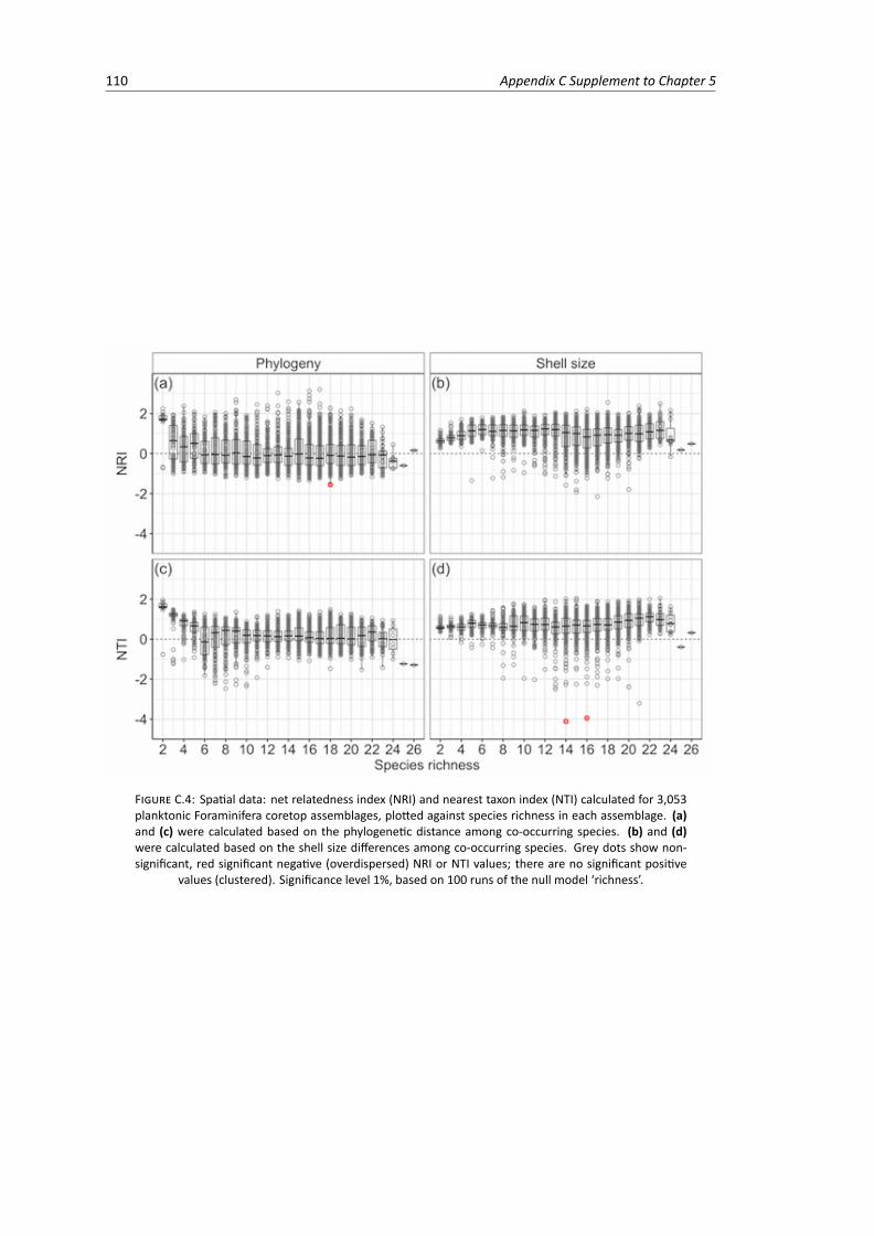
110 Appendix C Supplement to Chapter 5
FIGURE C.4: Spatial data: net relatedness index (NRI) and nearest taxon index (NTI) calculated for 3,053planktonic Foraminifera coretop assemblages, plotted against species richness in each assemblage. (a)and (c) were calculated based on the phylogenetic distance among co-occurring species. (b) and (d)were calculated based on the shell size differences among co-occurring species. Grey dots show non-significant, red significant negative (overdispersed) NRI or NTI values; there are no significant positive
values (clustered). Significance level 1%, based on 100 runs of the null model ‘richness’.
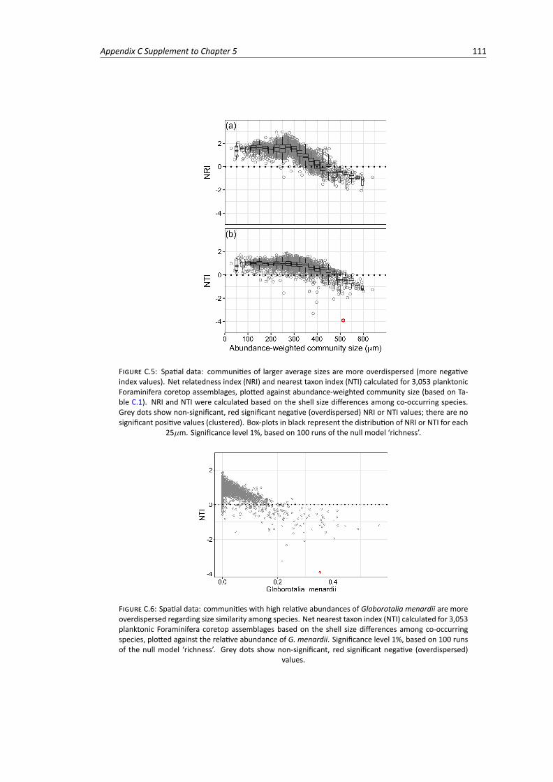
Appendix C Supplement to Chapter 5 111
FIGURE C.5: Spatial data: communities of larger average sizes are more overdispersed (more negativeindex values). Net relatedness index (NRI) and nearest taxon index (NTI) calculated for 3,053 planktonicForaminifera coretop assemblages, plotted against abundance-weighted community size (based on Ta-ble C.1). NRI and NTI were calculated based on the shell size differences among co-occurring species.Grey dots show non-significant, red significant negative (overdispersed) NRI or NTI values; there are nosignificant positive values (clustered). Box-plots in black represent the distribution of NRI or NTI for each
25µm. Significance level 1%, based on 100 runs of the null model ‘richness’.
FIGURE C.6: Spatial data: communities with high relative abundances of Globorotalia menardii are moreoverdispersed regarding size similarity among species. Net nearest taxon index (NTI) calculated for 3,053planktonic Foraminifera coretop assemblages based on the shell size differences among co-occurringspecies, plotted against the relative abundance of G. menardii. Significance level 1%, based on 100 runsof the null model ‘richness’. Grey dots show non-significant, red significant negative (overdispersed)
values.

112 Appendix C Supplement to Chapter 5
Time series analysis
The first differences of the time series calculate the change in species abundances fromonetime step to the next, and reduces the time-series autocorrelation. First differenceswere not calculated for consecutive samples between which there was a sampling gapof more than ten days. The reason is that if the sediment trap did not sample for a spe-cific period (e.g., a collecting bottle was lost), there was no recording of the abundanceflux for that period, and thus the first difference of the two adjacent samples does notrecord the true change in abundance from one time step to the next.
FIGURE C.7: Temporal data, first differences: pairwise Kendall rank correlations of the differentiated time-series of planktonic Foraminifera abundances (2,303 in total) plotted by sediment trap (see Table C.2).Grey dots show non-significant, blue significant positive, red significant negative values; significance level
of 1%.
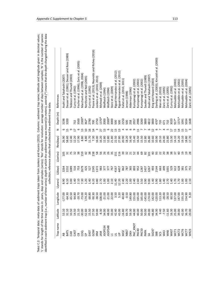
Appendix C Supplement to Chapter 5 113
TABLEC.2:
Tempo
rald
ata:
meta-da
taof
sedimen
ttraps
takenfrom
Jonkersan
dKu
cera
(201
5).Co
lumns:sedimen
ttrapna
me;
latitud
ean
dlong
itude
givenin
decimal
values;
‘L’stan
dsforlen
gthof
thetim
eserie
sin:years,days
andsamples
(series);‘Re
s’stan
dsforresoluti
on:averagenu
mbe
rofd
aysbe
twee
nsamples;‘N’isthenu
mbe
rofspe
cies
iden
tified
ineach
sedimen
ttrap(i.e.,num
bero
ftimeserie
s);d
epth
inwhich
thesedimen
ttrapwas
moo
red(in
meters),asterisk
(*)m
eans
that
thede
pthchan
geddu
ringtheda
tacollection
;referen
cestud
iestha
tcollected
thesedimen
ttrapda
ta.
Trap
name
Latitud
eLong
itude
L(years)
L(days)
L(serie
s)Re
s(days)
NDe
pth(m
)Re
ferences
AB53
.10
-177
.00
8.90
3264
105
26.90
631
98Asah
iand
Takaha
shi(20
07)
BATS
32.10
-64.30
6.10
2232
3158
.60
1532
00De
user
etal.(19
81);De
user
andRo
ss(198
9)CA
R10
.50
-65.50
3.00
1089
7512
.40
9Tede
scoan
dTh
unell(20
03)
CAST
14.50
64.80
1.40
516
3212
.20
1773
2Cu
rryet
al.(19
92)
CB21
.10
-20.70
2.10
753
3817
.90
635
00Fische
reta
l.(199
6);Zaricet
al.(20
05)
COQ
-30.00
-73.00
7.30
2679
159
8.80
1323
00*
Marchan
teta
l.(199
8,20
04)
CP-52.60
174.20
1.20
425
428.80
1036
2*Northcote
andNeil(20
05)
EAST
15.50
68.80
1.40
527
3811
.70
1627
90Cu
rryet
al.(19
92)
GOM
27.50
-90.30
6.20
2245
238
7.30
1470
0Po
oreet
al.(20
13);Re
ynolds
andRichey
(201
6)IRM
59.00
-38.50
3.80
1372
5816
.00
327
50Jonkerse
tal.(201
0,20
13)
JAM
-8.30
108.00
2.70
983
5616
.20
2713
70*
Moh
tadiet
al.(20
09)
JGOFS34
34.00
-21.00
1.00
377
2612
.80
1320
00Wolfte
ich(199
4)JGOFS48
48.00
-21.00
1.00
377
2612
.80
620
00*
Wolfte
ich(199
4)L1
33.00
-22.00
2.10
767
3521
.80
2230
00Storze
tal.(200
9)LIL
42.40
3.50
11.40
4167
151
22.50
1350
0Rigu
al-Herna
ndez
etal.(20
12)
LIP
43.00
5.20
12.20
4457
116
27.80
1350
0Rigu
al-Herna
ndez
etal.(20
12)
MOZ
-16.80
40.80
2.40
862
3920
.90
422
50Fallete
tal.(201
0,20
11)
NB6
769
.70
-0.50
2.20
787
3218
.20
650
0Jensen
(199
8)OKH
59.30
149.80
1.00
365
2116
.40
625
8Alde
rman
(199
6)PA
C_KN
OT
44.00
155.00
2.40
893
5215
.40
929
57Ku
royana
giet
al.(20
02)
PAC4
040
.00
165.00
2.60
952
4416
.50
1129
86Ku
royana
giet
al.(20
02)
PAC5
050
.00
165.00
3.50
1287
6915
.50
732
60Ku
royana
giet
al.(20
02)
PAPA
50.00
-145
.00
3.90
1437
8212
.80
738
00Sautt
eran
dTh
unell(19
89)
SA49
.00
-174
.00
9.00
3267
101
26.80
648
12Asah
iand
Takaha
shi(20
07)
SAZ47
-46.80
142.00
1.40
493
4010
.60
1238
00King
andHo
ward(200
3)SB
B34
.30
-120
.00
5.90
2144
9310
.90
647
0*Da
rling
etal.(20
03);Kincaidet
al.(20
00)
SCS
9.40
113.20
1.80
663
2229
.10
772
0Wan
etal.(20
10)
WA3
-7.50
-28.00
1.40
499
2024
.00
467
1Zaric
etal.(20
05)
WAB
-11.60
-28.50
2.70
1001
3823
.80
571
0Zaric
etal.(20
05)
WAS
T16
.30
60.50
1.40
529
3813
.30
1730
20Cu
rryet
al.(19
92)
WCT
125
.00
137.00
1.70
612
3714
.10
1191
7*Moh
iudd
inet
al.(20
02)
WCT
239
.00
147.00
1.70
628
4014
.20
1413
71*
Moh
iudd
inet
al.(20
02)
WCT
642
.00
155.20
1.00
381
1919
.10
1510
91Moh
iudd
inet
al.(20
05)
WCT
736
.70
154.90
1.00
375
1918
.80
1750
34Moh
iudd
inet
al.(20
04)
WR2
3-20.00
9.20
2.10
751
2817
.70
316
48Zaric
etal.(20
05)
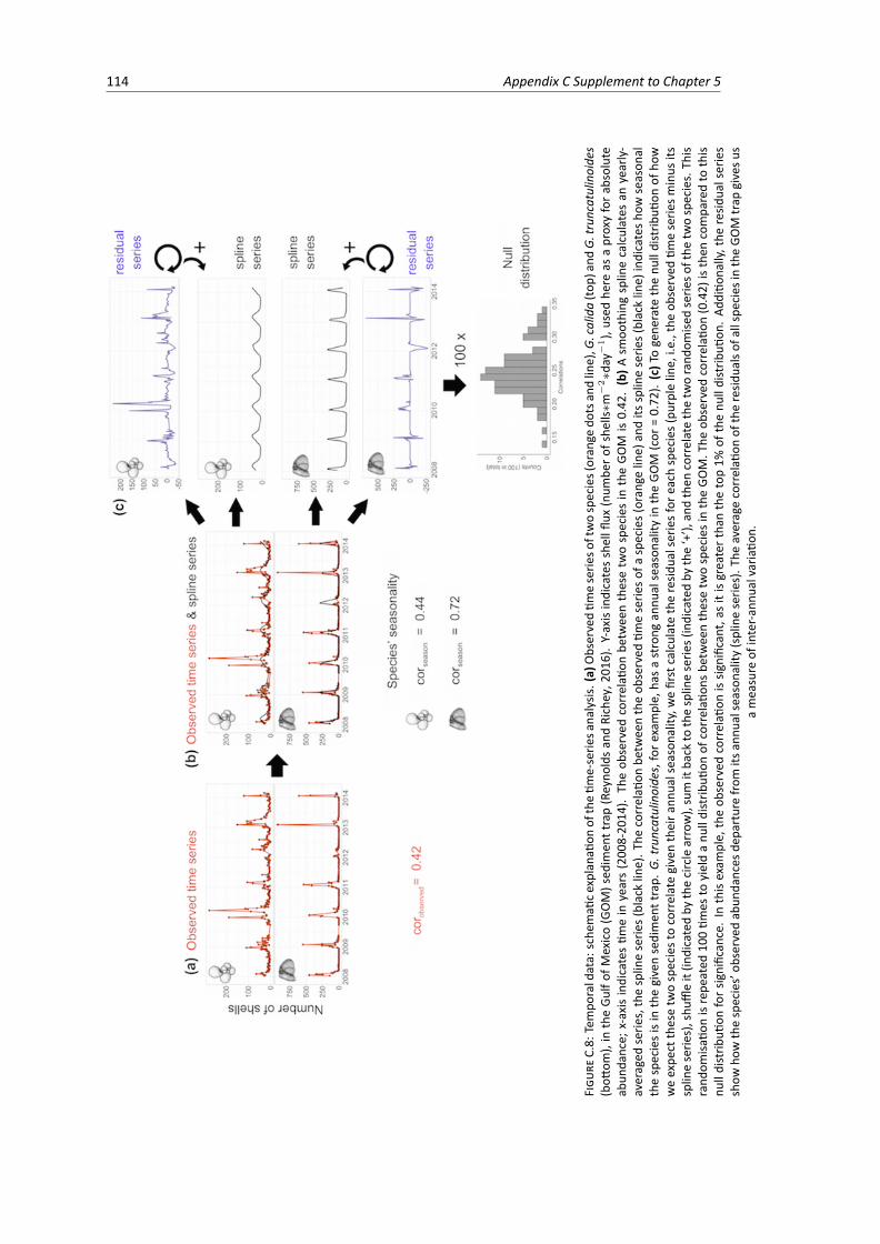
114 Appendix C Supplement to Chapter 5
FIGU
REC.8:
Tempo
raldata:
sche
mati
cexplana
tionof
thetim
e-serie
sana
lysis
.(a)
Observedtim
eserie
softwospecies(oran
gedo
tsan
dline),G
.calida(to
p)an
dG.
trun
catulinoide
s(bott
om),in
theGu
lfof
Mexico(GOM)sed
imen
ttrap(Reyno
ldsan
dRichey,2
016).Y-axisindicatesshellfl
ux(num
bero
fshe
lls⇤m
�2⇤d
ay�1),used
here
asaproxyfora
bsolute
abun
dance;
x-axisindicatestim
ein
years(200
8-20
14).
Theob
served
correlati
onbe
twee
nthesetw
ospeciesin
theGO
Mis0.42
.(b)A
smoo
thingsplinecalculates
anyearly-
averaged
serie
s,thesplineserie
s(blackline).T
hecorrelati
onbe
twee
ntheob
served
timeserie
sofa
species(oran
geline)
andits
splineserie
s(blackline)
indicatesh
owseason
althespeciesisin
thegivensedimen
ttrap.
G.trun
catulinoide
s,fore
xample,
hasastrong
annu
alseason
ality
intheGO
M(cor
=0.72
).(c)Togene
rate
thenu
lldistrib
ution
ofho
wweexpe
ctthesetw
ospeciestocorrelategiventheira
nnua
lseasona
lity,wefirstcalculatetheresid
ualseriesfor
each
species(pu
rpleline,i.e.,theob
served
timeserie
sminus
itssplineserie
s),shu
ffleit(in
dicatedby
thecirclearrow),sum
itba
ckto
thesplineserie
s(indicatedby
the‘+’),
andthen
correlatethetw
orand
omise
dserie
softhe
twospecies.Th
isrand
omisa
tionisrepe
ated
100tim
esto
yieldanu
lldistrib
ution
ofcorrelati
onsbe
twee
nthesetw
ospeciesin
theGO
M.The
observed
correlati
on(0.42)
isthen
compa
redto
this
nulldistrib
ution
fors
ignifican
ce.In
thisexam
ple,
theob
served
correlati
onissig
nifican
t,as
itisgreatertha
nthetop1%
ofthenu
lldistrib
ution
.Ad
ditio
nally,the
resid
ualseries
show
howthespecies’ob
served
abun
dances
depa
rturefrom
itsan
nualseason
ality
(splineserie
s).T
heaveragecorrelati
onof
theresid
ualsof
allspe
cies
intheGO
Mtrap
givesu
sameasure
ofinter-a
nnua
lvariatio
n.
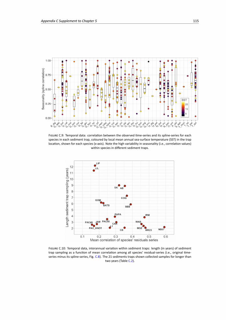
Appendix C Supplement to Chapter 5 115
FIGURE C.9: Temporal data: correlation between the observed time-series and its spline-series for eachspecies in each sediment trap, coloured by local mean annual sea-surface temperature (SST) in the traplocation, shown for each species (x-axis). Note the high variability in seasonality (i.e., correlation values)
within species in different sediment traps.
FIGURE C.10: Temporal data, interannual variation within sediment traps: length (in years) of sedimenttrap sampling as a function of mean correlation among all species’ residual-series (i.e., original time-series minus its spline-series, Fig. C.8). The 21 sediments traps shown collected samples for longer than
two years (Table C.2).

References
Al-Sabouni, N., Kucera, M., Schmidt, D. N., 2007. Vertical niche separation control of di-versity and size disparity in planktonic foraminifera.MarineMicropaleontology 63 (1),75–90.
Alderman, S. E., 1996. M.Sc. thesis: Planktonic foraminifera in the Sea of Okhotsk:population and stable isotopic analysis from a sediment trap. Massachusetts In-stitute of Technology and Woods Hole Oceanographic Institution, https://hdl.han-dle.net/1912/5673.
Aldridge, D., Beer, C., Purdie, D., 2012. Calcification in the planktonic foraminifera Glo-bigerina bulloides linked to phosphate concentrations in surface waters of the NorthAtlantic Ocean. Biogeosciences 9 (5), 1725–1739.
Alizon, S., Kucera,M., Jansen, V. A., 2008. Competition between cryptic species explainsvariations in rates of lineage evolution. Proceedings of the National Academy of Sci-ences 105 (34), 12382–12386.
Allen, A. P., Gillooly, J. F., 2006. Assessing latitudinal gradients in speciation rates andbiodiversity at the global scale. Ecology Letters 9 (8), 947–954.
Allen, A. P., Gillooly, J. F., Savage, V.M., Brown, J. H., 2006. Kinetic effects of temperatureon rates of genetic divergence and speciation. Proceedings of the National Academyof Sciences 103 (24), 9130–9135.
Allen, A. P., Savage, V. M., 2007. Setting the absolute tempo of biodiversity dynamics.Ecology Letters 10 (7), 637–646.
Alroy, J., 1996. Constant extinction, constrained diversification, and uncoordinated sta-sis in north american mammals. Palaeogeography, Palaeoclimatology, Palaeoecology127 (1-4), 285–311.
Alroy, J., 1998. Cope’s rule and the dynamics of bodymass evolution in North Americanfossil mammals. Science 280 (5364), 731–734.
Alroy, J., 2008. Dynamics of origination and extinction in the marine fossil record. Pro-ceedings of the National Academy of Sciences 105 (Supplement 1), 11536–11542.
117
118 REFERENCES
Alzate, A., Bisschop, K., Etienne, R., Bonte, D., 2017. Interspecific competition counter-acts negative effects of dispersal on adaptation of an arthropod herbivore to a newhost. Journal of Evolutionary Biology 30 (11), 1966–1977.
Amante, C., Eakins, B.W., 2009. ETOPO1 1Arc-MinuteGlobal ReliefModel: procedures,data sources and analysis. NOAA Technical MemorandumNESDIS NGDC-24. NationalGeophysical Data Center, NOAA.
Anderson, O. R., Be, A. W., 1976. A cytochemical fine structure study of phagotrophyin a planktonic foraminifer, Hastigerina pelagica (d’Orbigny). The Biological Bulletin151 (3), 437–449.
Anderson, O. R., Spindler, M., Be, A. W., Hemleben, C., 1979. Trophic activity of plank-tonic foraminifera. Journal of the Marine Biological Association of the United King-dom 59 (3), 791–799.
Andre, A., Weiner, A., Quillevere, F., Aurahs, R., Morard, R., Douady, C. J., de Garidel-Thoron, T., Escarguel, G., De Vargas, C., Kucera, M., 2013. The cryptic and the appar-ent reversed: lack of genetic differentiationwithin themorphologically diverse plexusof the planktonic foraminifer Globigerinoides sacculifer. Paleobiology 39 (1), 21–39.
Arenillas, I., Arz, J. A., 2017. Benthic origin and earliest evolution of the first planktonicforaminifera after the Cretaceous/Palaeogene boundary mass extinction. HistoricalBiology 29 (1), 25–42.
Arnold, A. J., Kelly, D., Parker, W., 1995. Causality and Cope’s rule: evidence from theplanktonic foraminifera. Journal of Paleontology 69 (02), 203–210.
Asahi, H., Takahashi, K., 2007. A 9-year time-series of planktonic foraminifer fluxesand environmental change in the Bering sea and the central subarctic Pacific Ocean1990–1999. Progress in Oceanography 72 (4), 343–363.
Atkinson, D., Ciotti, B. J., Montagnes, D. J., 2003. Protists decrease in size linearly withtemperature: ca. 2.5% �c�1. Proceedings of the Royal Society of London. Series B:Biological Sciences 270 (1533), 2605–2611.
Aurahs, R., Goker, M., Grimm, G. W., Hemleben, V., Hemleben, C., Schiebel, R., Kucera,M., 2009a. Using themultiple analysis approach to reconstruct phylogenetic relation-ships among planktonic Foraminifera from highly divergent and length-polymorphicSSU rDNA sequences. Bioinformatics and Biology Insights 3, 155–177.
Aurahs, R., Grimm, G. W., Hemleben, V., Hemleben, C., Kucera, M., 2009b. Geographi-cal distribution of cryptic genetic types in the planktonic foraminifer Globigerinoidesruber. Molecular Ecology 18 (8), 1692–1706.
REFERENCES 119
Aurahs, R., Treis, Y., Darling, K., Kucera, M., 2011. A revised taxonomic and phyloge-netic concept for the planktonic foraminifer species Globigerinoides ruber based onmolecular and morphometric evidence. Marine Micropaleontology 79 (1-2), 1–14.
Aze, T., Ezard, T. H., Purvis, A., Coxall, H. K., Stewart, D. R., Wade, B. S., Pearson, P. N.,2011. A phylogeny of Cenozoic macroperforate planktonic foraminifera from fossildata. Biological Reviews 86 (4), 900–927.
Bailey, S. F., Dettman, J. R., Rainey, P. B., Kassen, R., 2013. Competition both drivesand impedes diversification in a model adaptive radiation. Proc. R. Soc. B 280 (1766),20131253.
Balke, M., Schmidt, S., Hausmann, A., Toussaint, E. F., Bergsten, J., Buffington, M.,Hauser, C. L., Kroupa, A., Hagedorn, G., Riedel, A., et al., 2013. Biodiversity into yourhands - A call for a virtual global natural history ‘metacollection’. Frontiers in Zoology10 (55), 1–9.
Baranowski, U. K., 2013. M.Sc. thesis: Phylogenetic significance of test morphologyand ultrastructure in Recent planktonic Foraminifera inferred from cladistic anal-yses. Eberhard Karls University Tübingen. Dataset: https://doi.org/10.1594/pan-gaea.901825.
Barrows, T. T., Juggins, S., 2004. Compilation of planktic foraminifera LGM assemblagesfrom the Indo-Pacific Ocean. Dataset: https://doi.org/10.1594/PANGAEA.227319.
Barton, A. D., Pershing, A. J., Litchman, E., Record, N. R., Edwards, K. F., Finkel, Z. V.,Kiørboe, T., Ward, B. A., 2013. The biogeography of marine plankton traits. EcologyLetters 16 (4), 522–534.
Barton, K., 2017. MuMIn: Multi-Model Inference, R package version 1.40.0,https://CRAN.R-project.org/package=MuMIn.
Be, A. W., Spero, H. J., Anderson, O. R., 1982. Effects of symbiont elimination and rein-fection on the life processes of the planktonic foraminifer Globigerinoides sacculifer.Marine Biology 70 (1), 73–86.
Be, A. W. H., 1976. Gametogenesis in planktonic foraminifera. Science 192 (4242),890–892.
Be, A.W. H., Caron, D. A., Anderson, O. R., 1981. Effects of feeding frequency on life pro-cesses of the planktonic foraminifer Globigerinoides sacculifer in laboratory culture.Journal of the Marine Biological Association of the United Kingdom 61 (1), 257–277.
Be, A. W. H., Harrison, S. M., Lott, L., 1973. Orbulina universa d’Orbigny in the IndianOcean. Micropaleontology 19 (2), 150–192.
120 REFERENCES
Be, A.W. H., Hutson, W. H., 1977. Ecology of planktonic foraminifera and biogeographicpatterns of life and fossil assemblages in the Indian Ocean. Micropaleontology 23 (4),369–414.
Be, A. W. H., Tolderlund, D. S., 1971. Distribution and ecology of living planktonicforaminifera in surface waters of the Atlantic and Indian Oceans. In: The Micropa-leontology of Oceans. Cambridge University Press, pp. 105–149.
Beer, C. J., Schiebel, R., Wilson, P. A., 2010. Testing planktic foraminiferal shell weight asa surface water [CO2�
3 ] proxy using plankton net samples. Geology 38 (2), 103–106.
Behrenfeld, M. J., Falkowski, P. G., 1997. Photosynthetic rates derived from satellite-based chlorophyll concentration. Limnology and Oceanography 42 (1), 1–20.
Bengtsson, J., 1989. Interspecific competition increases local extinction rate in ametapopulation system. Nature 340 (6236), 713.
Benson, R. B., Campione, N. E., Carrano, M. T., Mannion, P. D., Sullivan, C., Upchurch, P.,Evans, D. C., 2014. Rates of dinosaur body mass evolution indicate 170 million yearsof sustained ecological innovation on the avian stem lineage. PLoS Biology 12 (5),e1001853.
Benton, M. J., 2009. The Red Queen and the Court Jester: species diversity and the roleof biotic and abiotic factors through time. Science 323 (5915), 728–732.
Benton, M. J., Pearson, P. N., 2001. Speciation in the fossil record. Trends in Ecology &Evolution 16 (7), 405–411.
Berger, W. H., Piper, D. J., 1972. Planktonic foraminifera: differential settling, dissolu-tion, and redeposition. Limnology and Oceanography 17 (2), 275–287.
Bijma, J., Erez, J., Hemleben, C., 1990. Lunar and semi-lunar reproductive cycles in somespinose planktonic foraminifers. Journal of Foraminiferal Research 20 (2), 117–127.
Bijma, J., Hemleben, C., 1994. Population dynamics of the planktic foraminifer Glo-bigerinoides sacculifer (Brady) from the central Red Sea. Deep Sea Research Part I:Oceanographic Research Papers 41 (3), 485–510.
Bird, C., Darling, K. F., Russell, A. D., Davis, C. V., Fehrenbacher, J., Free, A., Wyman, M.,Ngwenya, B. T., 2017. Cyanobacterial endobionts within a major marine planktoniccalcifier (Globigerina bulloides, Foraminifera) revealed by 16S rRNA metabarcoding.Biogeosciences 14 (4), 901–920.
Blagoderov, V., Kitching, I. J., Livermore, L., Simonsen, T. J., Smith, V. S., 2012. No spec-imen left behind: industrial scale digitization of natural history collections. ZooKeys209, 133–146.
REFERENCES 121
Blagoderov, V., Penn,M., Sadka,M., Hine, A., Brooks, S., Siebert, D. J., Sleep, C., Cafferty,S., Cane, E., Martin, G., et al., 2017. iCollections methodology: workflow, results andlessons learned. Biodiversity data journal 1 (5), e19893.
Boakes, E. H., McGowan, P. J., Fuller, R. A., Chang-qing, D., Clark, N. E., O’Connor,K., Mace, G. M., 2010. Distorted views of biodiversity: spatial and temporal bias inspecies occurrence data. PLoS Biology 8 (6), e1000385.
Bolnick, D. I., Amarasekare, P., Araujo, M. S., Burger, R., Levine, J. M., Novak, M., Rudolf,V. H., Schreiber, S. J., Urban, M. C., Vasseur, D. A., 2011. Why intraspecific trait varia-tion matters in community ecology. Trends in Ecology & Evolution 26 (4), 183–192.
Brannstrom, A., Sumpter, D. J., 2005. The role of competition and clustering in popula-tion dynamics. Proc. R. Soc. B 272 (1576), 2065–2072.
Brombacher, A., Wilson, P. A., Bailey, I., Ezard, T. H. G., 2017a. The breakdown ofstatic and evolutionary allometries during climatic upheaval. The American Naturalist190 (3), 350–362.
Brombacher, A., Wilson, P. A., Ezard, T. H. G., 2017b. Calibration of the repeatabilityof foraminiferal test size and shape measures with recommendations for future use.Marine Micropaleontology 133, 21–27.
Brown, J. H., 1995. Macroecology. University of Chicago Press, Chicago.
Brown, J. H., Gillooly, J. F., Allen, A. P., Savage, V. M., West, G. B., 2004. Toward ametabolic theory of ecology. Ecology 85 (7), 1771–1789.
Brummer, G.-J. A., Hemleben, C., Spindler, M., 1986. Planktonic foraminiferal ontogenyand new perspectives for micropalaeontology. Nature 319 (6048), 50.
Buckley, H. A., 1973.Globorotalia (Clavatorella) oveyi n. sp., premieremention Recented’un sous-genre de Foraminifere du Neogene. Revue de Micropaleontologie 16 (3),168–172.
Buckley, H. A., 1976. The discovery tablemount chain. Deep Sea Research and Oceano-graphic Abstracts 23 (10), 937–948.
Buckley, H. A., Bevan, J. C., Brown, K. M., Johnson, L. R., 1978. Glauconiteand celadonite: two separate mineral species. Mineralogical Magazine 42 (323),373–382.
Buckley, H. A., Easton, A. J., Johnson, L. R., 1974. Iron and manganese encrustations inRecent sediments. Nature 249, 436–437.
Buckley, H. A., Easton, A. J., Johnson, L. R., 1984. Compositional variations in glauconite.Mineralogical Magazine 48 (346), 119–126.
122 REFERENCES
Buckley, H. A., Johnson, L. R., 1988. Late Pleistocene to Recent sediment deposition inthe central and western Mediterranean. Deep Sea Research Part A. OceanographicResearch Papers 35 (5), 749–766.
Buckley, H. A., Johnson, L. R., Shackleton, N. J., Blow, R. A., 1982. Late Glacial to Recentcores from the eastern Mediterranean. Deep Sea Research Part A. OceanographicResearch Papers 29 (6), 739–766.
Buckley, H. A., Woolley, A. R., 1990. Carbonates of the magnesite–siderite series fromfour carbonatite complexes. Mineralogical Magazine 54 (376), 413–418.
Burki, F., Keeling, P. J., 2014. Rhizaria. Current Biology 24 (3), R103–R107.
Cadotte,M.W., Cardinale, B. J., Oakley, T. H., 2008. Evolutionary history and the effect ofbiodiversity on plant productivity. Proceedings of the National Academy of Sciences105 (44), 17012–17017.
Cadotte, M. W., Tucker, C. M., 2017. Should environmental filtering be abandoned?Trends in Ecology & Evolution 32 (6), 429–437.
Chao, A., Chazdon, R. L., Colwell, R. K., Shen, T.-J., 2006. Abundance-based similarityindices and their estimation when there are unseen species in samples. Biometrics62 (2), 361–371.
Chao, A., Ma, K. H., Hsieh, T. C., Chiu, C.-H., 2016. SpadeR: Species-Richness Pre-diction and Diversity Estimation with R, R package version 0.1.1, https://CRAN.R-project.org/package=SpadeR.
Cifelli, R., 1969. Radiation of Cenozoic planktonic foraminifera. Systematic Zoology18 (2), 154–168.
Cope, E. D., 1887. The origin of the fittest: essays on evolution. D. Appleton& Company,New York.
Cordey, W., Berggren, W., Olsson, R., 1970. Phylogenetic trends in the planktonicforaminiferal genus Pseudohastigerina Banner and Blow, 1959. Micropaleontology16 (2), 235–242.
Coyne, J. A., Orr, H. A., 2004. Speciation. Sinauer Associates, Inc., Sunderland.
Craven, P., Wahba, G., 1978. Smoothing noisy data with spline functions. Numerischemathematik 31 (4), 377–403.
Culver, S. J., 1991. Early Cambrian foraminifera from west Africa. Science 254 (5032),689–691.
REFERENCES 123
Culver, S. J., 2003. Benthic foraminifera across the Cretaceous–Tertiary (K–T) boundary:a review. Marine Micropaleontology 47 (3-4), 177–226.
Cunningham, J. A., Rahman, I. A., Lautenschlager, S., Rayfield, E. J., Donoghue, P. C.,2014. A virtual world of paleontology. Trends in Ecology & Evolution 29 (6), 347–357.
Curry, W., Ostermann, D., Guptha, M., Ittekkot, V., 1992. Foraminiferal production andmonsoonal upwelling in the Arabian Sea: evidence from sediment traps. GeologicalSociety, London, Special Publications 64 (1), 93–106.
Danovaro, R., Snelgrove, P. V., Tyler, P., 2014. Challenging the paradigms of deep-seaecology. Trends in Ecology & Evolution 29 (8), 465–475.
Darling, K. F., Kucera, M., Kroon, D., Wade, C. M., 2006. A resolution for the coilingdirection paradox inNeogloboquadrina pachyderma. Paleoceanography 21 (2), 1–14.
Darling, K. F., Kucera, M., Pudsey, C. J., Wade, C. M., 2004. Molecular evidence linkscryptic diversification in polar planktonic protists to Quaternary climate dynamics.Proceedings of the National Academy of Sciences 101 (20), 7657–7662.
Darling, K. F., Kucera, M., Wade, C. M., 2007. Global molecular phylogeography revealspersistent Arctic circumpolar isolation in a marine planktonic protist. Proceedings ofthe National Academy of Sciences 104 (12), 5002–5007.
Darling, K. F., Kucera, M., Wade, C. M., von Langen, P., Pak, D., 2003. Seasonal distribu-tion of genetic types of planktonic foraminifer morphospecies in the Santa BarbaraChannel and its paleoceanographic implications. Paleoceanography 18 (2).
Darling, K. F., Thomas, E., Kasemann, S. A., Seears, H. A., Smart, C. W., Wade, C. M.,2009. Surviving mass extinction by bridging the benthic/planktic divide. Proceedingsof the National Academy of Sciences 106 (31), 12629–12633.
Darling, K. F., Wade, C. M., 2008. The genetic diversity of planktic foraminifera and theglobal distribution of ribosomal RNA genotypes. Marine Micropaleontology 67 (3-4),216–238.
Darling, K. F., Wade, C. M., Kroon, D., Brown, A. J. L., 1997. Planktic foraminiferal molec-ular evolution and their polyphyletic origins from benthic taxa. Marine Micropaleon-tology 30 (4), 251–266.
Darling, K. F., Wade, C. M., Stewart, I. A., Kroon, D., Dingle, R., Brown, A. J. L., 2000.Molecular evidence for genetic mixing of Arctic and Antarctic subpolar populationsof planktonic foraminifers. Nature 405 (6782), 43.
De La Sancha, N. U., Boyle, S. A., Patterson, B. D., 2017. Getting back to the basics:Museum collections and satellite imagery are critical to analyzing species diversity.BioScience 67 (5), 405–406.
124 REFERENCES
De Vargas, C., Audic, S., Henry, N., Decelle, J., Mahe, F., Logares, R., Lara, E., Berney,C., Le Bescot, N., Probert, I., et al., 2015. Eukaryotic plankton diversity in the sunlitocean. Science 348 (6237), 1261605.
De Vargas, C., Norris, R., Zaninetti, L., Gibb, S. W., Pawlowski, J., 1999. Molecular ev-idence of cryptic speciation in planktonic foraminifers and their relation to oceanicprovinces. Proceedings of the National Academy of Sciences 96 (6), 2864–2868.
De Vargas, C., Zaninetti, L., Hilbrecht, H., Pawlowski, J., 1997. Phylogeny and rates ofmolecular evolution of planktonic foraminifera: SSU rDNA sequences compared tothe fossil record. Journal of Molecular Evolution 45 (3), 285–294.
DeAngelis, D. L., Yurek, S., 2015. Equation-free modeling unravels the behavior of com-plex ecological systems. Proceedings of the National Academy of Sciences 112 (13),3856–3857.
Dekov, V. M., Cuadros, J., Kamenov, G. D., Weiss, D., Arnold, T., Basak, C., Rochette,P., 2010. Metalliferous sediments from the H.M.S. Challenger voyage (1872–1876).Geochimica et Cosmochimica Acta 74 (17), 5019–5038.
Des Roches, S., Post, D. M., Turley, N. E., Bailey, J. K., Hendry, A. P., Kinnison, M. T.,Schweitzer, J. A., Palkovacs, E. P., 2018. The ecological importance of intraspecificvariation. Nature Ecology & Evolution 2, 57–64.
Deuser, W., Ross, E., 1989. Seasonally abundant planktonic foraminifera of the SargassoSea; succession, deep-water fluxes, isotopic compositions, and paleoceanographicimplications. Journal of Foraminiferal Research 19 (4), 268–293.
Deuser,W., Ross, E., Hemleben, C., Spindler,M., 1981. Seasonal changes in species com-position, numbers, mass, size, and isotopic composition of planktonic foraminiferasettling into the deep Sargasso Sea. Palaeogeography, Palaeoclimatology, Palaeoe-cology 33 (1-3), 103–127.
Deyle, E. R., May, R. M., Munch, S. B., Sugihara, G., 2016. Tracking and forecastingecosystem interactions in real time. Proc. R. Soc. B 283 (1822), 20152258.
Dornelas, M., Antao, L. H., Moyes, F., Bates, A. E., Magurran, A. E., Adam, D., Akhmet-zhanova, A. A., Appeltans, W., Arcos, J. M., Arnold, H., et al., 2018. BioTIME: Adatabase of biodiversity time series for the Anthropocene. Global Ecology and Bio-geography 27 (7), 760–786.
Easton, A. J., Buckley, H. A., 1979. Iron meteorites of Group IA and IIA-Study of phos-phide morphology enhanced by dry Cl2 etching. Meteoritics 14 (1), 143–152.
REFERENCES 125
Easton, A. J., Buckley, H. A., 1983. Plessite textures in the Toluca (Group IA) iron me-teorite revealed by the selective attack of chlorine. Mineralogical magazine 47 (3),413–415.
Etienne, R. S., Haegeman, B., Stadler, T., Aze, T., Pearson, P. N., Purvis, A., Phillimore,A. B., 2011. Diversity-dependence brings molecular phylogenies closer to agreementwith the fossil record. Proc. R. Soc. B 279 (1732), rspb20111439.
Evans, M. R., Norris, K. J., Benton, T. G., 2012. Predictive ecology: systems approaches.Phil. Trans. R. Soc. B 367 (1586), 163.
Ezard, T. H. G., Aze, T., Pearson, P. N., Purvis, A., 2011. Interplay between changingclimate and species’ ecology drivesmacroevolutionary dynamics. Science 332 (6027),349–351.
Ezard, T. H. G., Purvis, A., 2016. Environmental changes define ecological limits tospecies richness and reveal the mode of macroevolutionary competition. EcologyLetters 19 (8), 899–906.
Fairbanks, R. G., Sverdlove, M., Free, R., Wiebe, P. H., Be, A. W., 1982. Vertical distri-bution and isotopic fractionation of living planktonic foraminifera from the PanamaBasin. Nature 298 (5877), 841.
Fallet, U., Brummer, G.-J., Zinke, J., Vogels, S., Ridderinkhof, H., 2010. Contrasting sea-sonal fluxes of planktonic foraminifera and impacts on paleothermometry in theMozambique Channel upstream of the Agulhas Current. Paleoceanography 25 (4).
Fallet, U., Ullgren, J. E., Castaneda, I. S., van Aken, H. M., Schouten, S., Ridderinkhof,H., Brummer, G.-J. A., 2011. Contrasting variability in foraminiferal and organic pa-leotemperature proxies in sedimenting particles of the Mozambique Channel (SWIndian Ocean). Geochimica et Cosmochimica Acta 75 (20), 5834–5848.
Fenton, I. S., Pearson, P. N., Jones, T. D., Farnsworth, A., Lunt, D. J., Markwick, P.,Purvis, A., 2016a. The impact of Cenozoic cooling on assemblage diversity in plank-tonic foraminifera. Phil. Trans. R. Soc. B 371 (1691), 20150224.
Fenton, I. S., Pearson, P. N., Jones, T. D., Purvis, A., 2016b. Environmental predictorsof diversity in Recent planktonic foraminifera as recorded in marine sediments. PLoSOne 11 (11), e0165522.
Finlay, B. J., 2002. Global dispersal of free-living microbial eukaryote species. Science296 (5570), 1061–1063.
126 REFERENCES
Fischer, G., Donner, B., Ratmeyer, V., Davenport, R., Wefer, G., 1996. Distinct year-to-year particle flux variations off Cape Blanc during 1988–1991: Relation to �18O-deduced sea-surface temperatures and trade winds. Journal of Marine Research54 (1), 73–98.
Fleet, A. J., Buckley, H. A., Johnson, L. R., 1980. The rare earth element geochemistry ofglauconites and celadonites. Journal of the Geological Society 137 (6), 683–688.
Foote, M., 2000. Origination and extinction components of taxonomic diversity: gen-eral problems. Paleobiology 26 (sp4), 74–102.
Foote, M., Sepkoski, J. J., 1999. Absolute measures of the completeness of the fossilrecord. Nature 398 (6726), 415–417.
Forey, P. L., Fortey, R. A., Kenrick, P., Smith, A. B., 2004. Taxonomy and fossils: a criticalappraisal. Phil. Trans. R. Soc. B 359 (1444), 639–653.
Fraass, A. J., Kelly, D. C., Peters, S. E., 2015. Macroevolutionary history of the plankticforaminifera. Annual Review of Earth and Planetary Sciences 43, 139–166.
Fraile, I., Schulz, M., Mulitza, S., Kucera, M., 2008. Predicting the global distributionof planktonic foraminifera using a dynamic ecosystem model. Biogeosciences 5 (3),891–911.
Fritz, S. A., Schnitzler, J., Eronen, J. T., Hof, C., Bohning-Gaese, K., Graham, C. H., 2013.Diversity in time and space: wanted dead and alive. Trends in Ecology & Evolution28 (9), 509–516.
Fussmann, G. F., Loreau, M., Abrams, P. A., 2007. Eco-evolutionary dynamics of com-munities and ecosystems. Functional Ecology 21 (3), 465–477.
Gardner, J. L., Amano, T., Sutherland, W. J., Joseph, L., Peters, A., 2014. Are naturalhistory collections coming to an end as time-series? Frontiers in Ecology and theEnvironment 12 (8), 436–438.
Gaston, K. J., 2000. Global patterns in biodiversity. Nature 405 (6783), 220–227.
Gaston, K. J., Blackburn, T. M., Greenwood, J. J., Gregory, R. D., Quinn, R. M., Lawton,J. H., 2000. Abundance–occupancy relationships. Journal of Applied Ecology 37 (s1),39–59.
Gaucherel, C., Tramier, C., Devictor, V., Svenning, J.-C., Hely, C., 2018. Where and atwhich scales does the latitudinal diversity gradient fail? Journal of Biogeography45 (8), 1905–1916.
REFERENCES 127
Gleckler, P. J., Durack, P. J., Stouffer, R. J., Johnson, G. C., Forest, C. E., 2016. Industrial-era global ocean heat uptake doubles in recent decades. Nature Climate Change 6,394–398.
Graham, C. H., Ferrier, S., Huettman, F., Moritz, C., Peterson, A. T., 2004. New develop-ments in museum-based informatics and applications in biodiversity analysis. Trendsin Ecology & Evolution 19 (9), 497–503.
Grigoratou, M., Monteiro, F. M., Schmidt, D. N., Wilson, J. D., Ward, B. A., Ridgwell, A.,2019. A trait-based modelling approach to planktonic foraminifera ecology. Biogeo-sciences 16 (7), 1469–1492.
Guerin, G. R., Andersen, A. N., Rossetto, M., van Leeuwen, S., Byrne, M., Sparrow, B.,Rodrigo, M., Lowe, A. J., 2018.Whenmacroecological transitions are a fiction of sam-pling: comparing herbarium records to plot-based species inventory data. Ecography41 (11), 1864–1875.
Hall, A., Buckley, H. A., 1991. Ammonium in glauconite and celadonite. Mineralogicalmagazine 55 (2), 280–282.
Hannisdal, B., Haaga, K. A., Reitan, T., Diego, D., Liow, L. H., 2017. Common specieslink global ecosystems to climate change: dynamical evidence in the planktonic fossilrecord. Proc. R. Soc. B 284 (1858), 20170722.
Harmon, L. J., Harrison, S., 2015. Species diversity is dynamic and unbounded at localand continental scales. The American Naturalist 185 (5), 584–593.
Harnik, P. G., 2011. Direct and indirect effects of biological factors on extinctionrisk in fossil bivalves. Proceedings of the National Academy of Sciences 108 (33),13594–13599.
Hart, M., Hylton, M., Oxford, M., Price, G., Hudson, W., Smart, C., 2003. The searchfor the origin of the planktic Foraminifera. Journal of the Geological Society 160 (3),341–343.
Hayward, B. W., Kawagata, S., 2005. Extinct foraminifera figured in Brady’s ChallengerReport. Journal of Micropalaeontology 24 (2), 171–175.
Hecht, A. D., 1976. An ecologic model for test size variation in Recent planktonicforaminifera; applications to the fossil record. Journal of Foraminiferal Research 6 (4),295–311.
Heerlien, M., Van Leusen, J., Schnoerr, S., de Jong-Kole, S., Raes, N., Van Hulsen, K.,2015. The natural history production line: an industrial approach to the digitizationof scientific collections. Journal on Computing and Cultural Heritage 8 (1), 1–11.
128 REFERENCES
Heim, N. A., Knope, M. L., Schaal, E. K., Wang, S. C., Payne, J. L., 2015. Cope’s rule in theevolution of marine animals. Science 347 (6224), 867–870.
Hemleben, C., Spindler, M., Anderson, O. R., 1989. Modern Planktonic Foraminifera.Springer-Verlag, Inc., New York.
Hijmans, R. J., 2015. geosphere: Spherical Trigonometry, R package version 1.5-7,https://CRAN.R-project.org/package=geosphere.
Hillebrand, H., 2004a. On the generality of the latitudinal diversity gradient. The Amer-ican Naturalist 163 (2), 192–211.
Hillebrand, H., 2004b. Strength, slope and variability of marine latitudinal gradients.Marine Ecology Progress Series 273, 251–267.
Hoeksema, B. W., van der Land, J., van der Meij, S. E., van Ofwegen, L. P., Reijnen,B. T., van Soest, R. W., de Voogd, N. J., 2011. Unforeseen importance of historicalcollections as baselines to determine biotic change of coral reefs: the Saba Bank case.Marine Ecology 32 (2), 135–141.
Hone, D., Keesey, T., Pisani, D., Purvis, A., 2005. Macroevolutionary trends in the Di-nosauria: Cope’s rule. Journal of Evolutionary Biology 18 (3), 587–595.
Hone, D. W., Benton, M. J., 2005. The evolution of large size: how does Cope’s rulework? Trends in Ecology & Evolution 20 (1), 4–6.
Horn, H. S., 1966. Measurement of “overlap” in comparative ecological studies. TheAmerican Naturalist 100 (914), 419–424.
Houlahan, J. E., Currie, D. J., Cottenie, K., Cumming, G. S., Ernest, S., Findlay, C. S., Fuh-lendorf, S. D., Gaedke, U., Legendre, P., Magnuson, J. J., et al., 2007. Compensatorydynamics are rare in natural ecological communities. Proceedings of the NationalAcademy of Sciences 104 (9), 3273–3277.
Hsiang, A. Y., Brombacher, A., Rillo, M. C., Mleneck-Vautravers, M. J., Conn, S., Lord-smith, S., Jentzen, A., Henehan, M. J., Metcalfe, B., Fenton, I., Wade, B. S., Fox,L., Meilland, J., Davis, C. V., Baranowski, U., Groeneveld, J., Edgar, K. M., Movellan,A., Aze, T., Dowsett, H. J., Miller, C. G., Rios, N., Hull, P. M., 2019. Endless Forams:>34,000 modern planktonic foraminiferal images for taxonomic training and auto-mated species recognition using convolutional neural networks. Paleoceanographyand Paleoclimatology (in press).
Hubbell, S. P., 2001. The unified neutral theory of biodiversity and biogeography. Prince-ton University Press.
REFERENCES 129
Huber, B. T., Bijma, J., Darling, K., 1997. Cryptic speciation in the living planktonicforaminifer Globigerinella siphonifera (d’Orbigny). Paleobiology 23 (1), 33–62.
Huber, B. T., Bijma, J., Spero, H. J., 1996. Blue-water SCUBA collection of plank-tonic Foraminifera. In: Methods and Techniques of Underwater Research. AmericanAcademy of Underwater Sciences, pp. 127–132.
Hudson, L. N., Blagoderov, V., Heaton, A., Holtzhausen, P., Livermore, L., Price, B. W.,van der Walt, S., Smith, V. S., 2015. Inselect: automating the digitization of naturalhistory collections. PLoS One 10 (11), e0143402.
Hug, L. A., Baker, B. J., Anantharaman, K., Brown, C. T., Probst, A. J., Castelle, C. J.,Butterfield, C. N., Hernsdorf, A. W., Amano, Y., Ise, K., et al., 2016. A new view of thetree of life. Nature Microbiology 1 (5), 16048.
Hunt, G., Martins, M. J. F., Puckett, T. M., Lockwood, R., Swaddle, J. P., Hall, C. M., Sted-man, J., 2017. Sexual dimorphism and sexual selection in cytheroidean ostracodesfrom the Late Cretaceous of the US Coastal Plain. Paleobiology 43 (4), 620–641.
Hunt, G., Roy, K., 2006. Climate change, body size evolution, and Cope’s rule in deep-seaostracodes. Proceedings of the National Academy of Sciences 103 (5), 1347–1352.
Jablonski, D., 2008a. Biotic interactions and macroevolution: extensions and mis-matches across scales and levels. Evolution 62 (4), 715–739.
Jablonski, D., 2008b. Species selection: theory and data. Annual Review of Ecology,Evolution, and Systematics 39, 501–524.
Jablonski, D., 2017. Approaches to Macroevolution: 2. Sorting of variation, some over-arching issues, and general conclusions. Evolutionary Biology 44 (4), 451–475.
Jensen, S., 1998. Planktische foraminiferen im Europäischen Nordmeer: Verbreitungund Vertikalfluß sowie ihre Entwicklung während der letzten 15000 Jahre. BerichteSonderforschungsbereich, Christian-Albrechts-Universität zu Kiel 313 (75), 1–105.
Johnson, K. G., Brooks, S. J., Fenberg, P. B., Glover, A. G., James, K. E., Lister, A. M.,Michel, E., Spencer, M., Todd, J. A., Valsami-Jones, E., et al., 2011. Climate changeand biosphere response: unlocking the collections vault. BioScience 61 (2), 147–153.
Jonkers, L., Brummer, G.-J. A., Peeters, F. J., van Aken, H. M., De Jong, M. F., 2010. Sea-sonal stratification, shell flux, and oxygen isotope dynamics of left-coiling N. pachy-derma and T. quinqueloba in the western subpolar North Atlantic. Paleoceanographyand Paleoclimatology 25 (2).
Jonkers, L., Hillebrand, H., Kucera, M., 2019. Global change drives modern planktoncommunities away from the pre-industrial state. Nature 570 (7761), 372–375.
130 REFERENCES
Jonkers, L., Kucera, M., 2015. Global analysis of seasonality in the shell flux of extantplanktonic Foraminifera. Biogeosciences 12 (7), 2207–2226.
Jonkers, L., Reynolds, C. E., Richey, J., Hall, I. R., 2015. Lunar periodicity in the shell fluxof planktonic foraminifera in the Gulf of Mexico. Biogeosciences 12 (10), 3061–3070.
Jonkers, L., van Heuven, S., Zahn, R., Peeters, F. J., 2013. Seasonal patterns of shell flux,�18O and �13C of small and large N. pachyderma (s) and G. bulloides in the subpolarNorth Atlantic. Paleoceanography 28 (1), 164–174.
Jost, L., Chao, A., Chazdon, R. L., 2011. Compositional similarity and � (beta) diversity.In: Biological Diversity: frontiers inmeasurement and assessment, 1st Edition. OxfordUniversity Press, pp. 66–84.
Kahn, M. I., 1981. Ecological and paleoecological implications of the phenotypic varia-tion in three species of living planktonic foraminifera from the northeastern PacificOcean (50�N, 145�W). Journal of Foraminiferal Research 11 (3), 203–211.
Keeling, P. J., del Campo, J., 2017. Marine protists are not just big bacteria. CurrentBiology 27 (11), R541–R549.
Keller, G., Abramovich, S., 2009. Lilliput effect in late Maastrichtian plankticforaminifera: Response to environmental stress. Palaeogeography, Palaeoclimatol-ogy, Palaeoecology 284 (1-2), 47–62.
Keltie, J. S., 1898. The German Deep-Sea Expedition. The Geographical Journal 12 (5),494–496.
Kembel, S. W., Cowan, P. D., Helmus, M. R., Cornwell, W. K., Morlon, H., Ackerly, D. D.,Blomberg, S. P., Webb, C. O., 2010. Picante: R tools for integrating phylogenies andecology. Bioinformatics 26 (11), 1463–1464.
Kemp, C., 2015. Museums: The endangered dead. Nature News 518 (7539), 292–294.
Kempe, D. R. C., Buckley, H. A., 1987. Fifty years of oceanography in the Department ofMineralogy, British Museum (Natural History). Bulletin of the British Museum (Natu-ral History) 15 (2), 59–97.
Kennett, J. P., 1976. Phenotypic variation in some Recent and late Cenozoic planktonicforaminifera. In: Foraminifera II. Academic Press New York, pp. 111–170.
Kincaid, E., Thunell, R. C., Le, J., Lange, C. B., Weinheimer, A. L., Reid, F. M., 2000. Plank-tonic foraminiferal fluxes in the Santa Barbara Basin: response to seasonal and inter-annual hydrographic changes. Deep Sea Research Part II: Topical Studies in Oceanog-raphy 47 (5-6), 1157–1176.
REFERENCES 131
King, A. L., Howard, W. R., 2003. Planktonic foraminiferal flux seasonality in Subantarc-tic sediment traps: A test for paleoclimate reconstructions. Paleoceanography andPaleoclimatology 18 (1).
Kingsolver, J. G., Pfennig, D. W., 2004. Individual-level selection as a cause of Cope’srule of phyletic size increase. Evolution 58 (7), 1608–1612.
Kinnison, M. T., Hairston, N. G., Hendry, A. P., 2015. Cryptic eco-evolutionary dynamics.Annals of the New York Academy of Sciences 1360 (1), 120–144.
Kretschmer, K., Jonkers, L., Kucera, M., Schulz, M., 2018. Modeling seasonal and ver-tical habitats of planktonic foraminifera on a global scale. Biogeosciences 15 (14),4405–4429.
Kucera, M., 2007. Planktonic foraminifera as tracers of past oceanic environments. In:Developments in marine geology: Proxies in late Cenozoic paleoceanography. Else-vier, pp. 213–262.
Kucera, M., Rosell-Mele, A., Schneider, R., Waelbroeck, C., Weinelt, M., 2005a. Multi-proxy approach for the reconstruction of the glacial ocean surface (MARGO). Quater-nary Science Reviews 24 (7-9), 813–819.
Kucera, M., Silye, L., Weiner, A. K., Darling, K., Lubben, B., Holzmann, M., Pawlowski,J., Schonfeld, J., Morard, R., 2017. Caught in the act: anatomy of an ongoingbenthic–planktonic transition in amarine protist. Journal of Plankton Research 39 (3),436–449.
Kucera, M., Weinelt, M., Kiefer, T., Pflaumann, U., Hayes, A., Weinelt, M., Chen, M.-T.,Mix, A. C., Barrows, T. T., Cortijo, E., Duprat, J. M., Juggins, S., Waelbroeck, C., 2005b.Compilation of planktic Foraminifera census data, LGM from the Atlantic Ocean.Dataset: https://doi.org/10.1594/PANGAEA.227329.
Kucera, M., Weinelt, M., Kiefer, T., Pflaumann, U., Hayes, A., Weinelt, M., Chen, M.-T., Mix, A. C., Barrows, T. T., Cortijo, E., Duprat, J. M., Juggins, S., Waelbroeck, C.,2005c. Compilation of planktic Foraminifera census data, LGM from the PacificOcean.Dataset: https://doi.org/10.1594/PANGAEA.227327.
Kuroyanagi, A., Kawahata, H., Nishi, H., Honda, M. C., 2002. Seasonal changes in plank-tonic foraminifera in the northwestern North Pacific Ocean: sediment trap experi-ments from subarctic and subtropical gyres. Deep Sea Research Part II: Topical Studiesin Oceanography 49 (24-25), 5627–5645.
Langerhans, R. B., Gifford, M. E., Joseph, E. O., 2007. Ecological speciation in Gambusiafishes. Evolution 61 (9), 2056–2074.
132 REFERENCES
Lazarus, D., 1994. Neptune: a marine micropaleontology database. Mathematical Ge-ology 26 (7), 817–832.
Lazarus, D., Hilbrecht, H., Spencer-Cervato, C., Thierstein, H., 1995. Sympatric specia-tion and phyletic change inGloborotalia truncatulinoides. Paleobiology 21 (1), 28–51.
Leckie, R. M., Bralower, T. J., Cashman, R., 2002. Oceanic anoxic events and plank-ton evolution: Biotic response to tectonic forcing during the mid-Cretaceous. Pale-oceanography 17 (3), 13–1.
LeKieffre, C., Spero, H. J., Russell, A. D., Fehrenbacher, J. S., Geslin, E., Meibom, A., 2018.Assimilation, translocation, and utilization of carbon between photosynthetic symbi-otic dinoflagellates and their planktic foraminifera host. Marine Biology 165 (104),1–15.
Levins, R., Lewontin, R., 1980. Dialectics and reductionism in ecology. Synthese 43 (1),47–78.
Lingwood, P. F., 1981. The dispersal of the collections of HMS Challenger; an example ofthe importance of historical research in tracing a systematically important collection.Archives of Natural History 1 (1), 71–77.
Liow, L. H., Di Martino, E., Voje, K. L., Rust, S., Taylor, P. D., 2016. Interspecific interac-tions through 2 million years: are competitive outcomes predictable? Proc. R. Soc. B283, 20160981.
Lipps, J. H., 1970. Plankton evolution. Evolution 24 (1), 1–22.
Lister, A. M., Climate Change Research Group, 2011. Natural history collections assources of long-term datasets. Trends in Ecology & Evolution 26 (4), 153–154.
Litchman, E., Klausmeier, C. A., 2008. Trait-based community ecology of phytoplankton.Annual review of ecology, evolution, and systematics 39, 615–639.
Litchman, E., Ohman, M. D., Kiørboe, T., 2013. Trait-based approaches to zooplanktoncommunities. Journal of Plankton Research 35 (3), 473–484.
Lloyd, G. T., Pearson, P. N., Young, J. R., Smith, A. B., 2012. Sampling bias and the fossilrecord of planktonic foraminifera on land and in the deep sea. Paleobiology 38 (4),569–584.
Locarnini, R. A., Mishonov, A. V., Antonov, J. I., Boyer, T. P., Garcia, H. E., Baranova,O. K., Zweng, M. M., Paver, C. R., Reagan, J. R., Johnson, D. R., Hamilton, M., Seidov,D., 2013. World Ocean Atlas 2013, Volume 1: Temperature. NOAA Atlas NESDIS 73,1–40.
REFERENCES 133
Lombard, F., Labeyrie, L., Michel, E., Bopp, L., Cortijo, E., Retailleau, S., Howa, H., Joris-sen, F., 2011. Modelling planktic foraminifer growth and distribution using an eco-physiological multi-species approach. Biogeosciences 8 (4), 853–873.
Lomolino, M. V., 2000. Ecology’s most general, yet protean pattern: the species–arearelationship. Journal of Biogeography 27 (1), 17–26.
Malmgren, B., Kennett, J. P., 1976. Biometric analysis of phenotypic variation in RecentGlobigerina bulloides d’Orbigny in the southern Indian Ocean. Marine Micropaleon-tology 1, 3–25.
Malmgren, B. A., Kennett, J. P., 1977. Biometric differentiation between Recent Glo-bigerina bulloides and Globigerina falconensis in the southern Indian Ocean. Journalof Foraminiferal Research 7 (2), 131–148.
Manten, A. A., 1972. C. Wyville Thomson, J. Murray, and the “Challenger” expedition.Earth-Science Reviews 8 (2), 255–266.
Marañón, E., 2015. Cell size as a key determinant of phytoplankton metabolism andcommunity structure. Annual review of marine science 7, 241–264.
Marchant, M., Hebbeln, D., Giglio, S., Coloma, C., Gonzalez, H. E., 2004. Seasonal andinterannual variability in the flux of planktic foraminifera in the Humboldt CurrentSystem off central Chile (30 S). Deep Sea Research Part II: Topical Studies in Oceanog-raphy 51 (20-21), 2441–2455.
Marchant, M., Hebbeln, D., Wefer, G., 1998. Seasonal flux patterns of plankticforaminifera in the Peru–Chile Current. Deep Sea Research Part I: Oceanographic Re-search Papers 45 (7), 1161–1185.
MARGO Project Members, 2009. Constraints on the magnitude and patterns of oceancooling at the Last Glacial Maximum. Nature Geoscience 2 (2), 127–132.
Marquet, P. A., 2009. Macroecological perspectives on communities and ecosystems.In: The Princeton guide to Ecology. Princeton University Press, pp. 213–262.
Marshall, C., Finnegan, S., Clites, E., Holroyd, P., Bonuso, N., Cortez, C., Davis, E., Dietl,G., Druckenmiller, P., Eng, R., et al., 2018. Quantifying the dark data in museum fossilcollections as palaeontology undergoes a second digital revolution. Biology Letters14 (9), 20180431.
Marshall, C. R., Quental, T. B., 2016. The uncertain role of diversity dependence inspecies diversification and the need to incorporate time–varying carrying capacities.Phil. Trans. R. Soc. B 371 (1691), 20150217.
134 REFERENCES
Matthews, T. J., Whittaker, R. J., 2014. Neutral theory and the species abundance distri-bution: recent developments and prospects for unifying niche and neutral perspec-tives. Ecology and Evolution 4 (11), 2263–2277.
Mayfield, M. M., Levine, J. M., 2010. Opposing effects of competitive exclusion on thephylogenetic structure of communities. Ecology Letters 13 (9), 1085–1093.
McGill, B. J., Etienne, R. S., Gray, J. S., Alonso, D., Anderson, M. J., Benecha, H. K., Dor-nelas, M., Enquist, B. J., Green, J. L., He, F., et al., 2007. Species abundance distribu-tions: moving beyond single prediction theories to integration within an ecologicalframework. Ecology Letters 10 (10), 995–1015.
McKinney, M. L., 1997. Extinction vulnerability and selectivity: combining ecologi-cal and paleontological views. Annual Review of Ecology and Systematics 28 (1),495–516.
Meilland, J., Siccha, M., Weinkauf, M. F., Jonkers, L., Morard, R., Baranowski, U.,Baumeister, A., Bertlich, J., Brummer, G.-J., Debray, P., et al., 2019. Highly replicatedsampling reveals nodiurnal verticalmigrationbut stable species-specific vertical habi-tats in planktonic foraminifera. Journal of Plankton Research 41 (2), 127–141.
Meyer, J. R., Kassen, R., 2007. The effects of competition and predation on diversifica-tion in a model adaptive radiation. Nature 446 (7134), 432.
Mittelbach, G. G., Schemske, D. W., Cornell, H. V., Allen, A. P., Brown, J. M., Bush, M. B.,Harrison, S. P., Hurlbert, A. H., Knowlton, N., Lessios, H. A., et al., 2007. Evolution andthe latitudinal diversity gradient: speciation, extinction and biogeography. EcologyLetters 10 (4), 315–331.
Moen, D., Morlon, H., 2014. Why does diversification slow down? Trends in Ecology &Evolution 29 (4), 190–197.
Mohiuddin, M. M., Nishimura, A., Tanaka, Y., 2005. Seasonal succession, vertical dis-tribution, and dissolution of planktonic foraminifera along the Subarctic Front: Im-plications for paleoceanographic reconstruction in the northwestern Pacific. MarineMicropaleontology 55 (3-4), 129–156.
Mohiuddin, M. M., Nishimura, A., Tanaka, Y., Shimamoto, A., 2002. Regional and in-terannual productivity of biogenic components and planktonic foraminiferal fluxes inthe northwestern Pacific Basin. Marine Micropaleontology 45 (1), 57–82.
Mohiuddin, M. M., Nishimura, A., Tanaka, Y., Shimamoto, A., 2004. Seasonality of bio-genic particle and planktonic foraminifera fluxes: response to hydrographic variabil-ity in the Kuroshio Extension, northwestern Pacific Ocean. Deep Sea Research Part I:Oceanographic Research Papers 51 (11), 1659–1683.
REFERENCES 135
Mohtadi, M., Steinke, S., Groeneveld, J., Fink, H. G., Rixen, T., Hebbeln, D., Donner,B., Herunadi, B., 2009. Low-latitude control on seasonal and interannual changes inplanktonic foraminiferal flux and shell geochemistry off south Java: A sediment trapstudy. Paleoceanography 24 (1).
Moller, T., Schulz, H., Kucera, M., 2013. The effect of sea surface properties on shellmorphology and size of the planktonic foraminiferNeogloboquadrina pachyderma inthe North Atlantic. Palaeogeography, Palaeoclimatology, Palaeoecology 391, 34–48.
Mora, C., Tittensor, D. P., Adl, S., Simpson, A. G., Worm, B., 2011. Howmany species arethere on Earth and in the ocean? PLoS Biology 9 (8), e1001127.
Morard, R., Darling, K. F., Mahe, F., Audic, S., Ujiie, Y., Weiner, A. K., Andre, A., Seears,H. A., Wade, C. M., Quillevere, F., et al., 2015. PFR2: a curated database of plank-tonic foraminifera 18S ribosomal DNA as a resource for studies of plankton ecology,biogeography and evolution. Molecular Ecology Resources 15 (6), 1472–1485.
Morard, R., Garet-Delmas, M.-J., Mahe, F., Romac, S., Poulain, J., Kucera, M., Var-gas, C., 2018. Surface ocean metabarcoding confirms limited diversity in planktonicforaminifera but reveals unknown hyper-abundant lineages. Scientific Reports 8 (1),2539.
Morard, R., Quillevere, F., Douady, C. J., de Vargas, C., de Garidel-Thoron, T., Escarguel,G., 2011. Worldwide genotyping in the planktonic foraminifer Globoconella inflata:implications for life history and paleoceanography. PLoS One 6 (10), e26665.
Morard, R., Quillevere, F., Escarguel, G., Ujiie, Y., de Garidel-Thoron, T., Norris, R. D.,de Vargas, C., 2009. Morphological recognition of cryptic species in the planktonicforaminifer Orbulina universa. Marine Micropaleontology 71 (3-4), 148–165.
Morey, A. E., Mix, A. C., Pisias, N. G., 2005. Planktonic foraminiferal assemblages pre-served in surface sediments correspond to multiple environment variables. Quater-nary Science Reviews 24 (7-9), 925–950.
Morisita, M., 1959. Measuring of interspecific association and similarity between com-munities. Memoirs of the Faculty of Science, Kyushu University, Series E Biology 3 (1),65–80.
Mousing, E. A., Ribeiro, S., Chisholm, C., Kuijpers, A., Moros, M., Ellegaard, M., 2017.Size differences of Arctic marine protists between two climate periods–using the pa-leoecological record to assess the importance of within-species trait variation. Ecol-ogy and Evolution 7 (1), 3–13.
Moy, A. D., Howard, W. R., Bray, S. G., Trull, T. W., 2009. Reduced calcification inmodernSouthern Ocean planktonic foraminifera. Nature Geoscience 2 (4), 276–280.
136 REFERENCES
Murray, J. W., 2007. Biodiversity of living benthic foraminifera: How many species arethere? Marine Micropaleontology 64 (3-4), 163–176.
Norris, R. D., 1991. Biased extinction and evolutionary trends. Paleobiology 17 (4),388–399.
Norris, R. D., 2000. Pelagic species diversity, biogeography, and evolution. Paleobiology26 (sp4), 236–258.
Northcote, L. C., Neil, H. L., 2005. Seasonal variations in foraminiferal flux in the South-ern Ocean, Campbell Plateau, New Zealand. Marine Micropaleontology 56 (3-4),122–137.
Novack-Gottshall, P. M., Lanier, M. A., 2008. Scale-dependence of Cope’s rule in bodysize evolution of Paleozoic brachiopods. Proceedings of the National Academy of Sci-ences 105 (14), 5430–5434.
Ohl, M., Lohrmann, V., Breitkreuz, L., Kirschey, L., Krause, S., 2014. The Soul-SuckingWasp by popular acclaim–museum visitor participation in biodiversity discovery andtaxonomy. PLoS One 9 (4), e95068.
Pante, E., Simon-Bouhet, B., 2013. marmap: a package for importing, plotting and an-alyzing bathymetric and topographic data in R. PLoS One 8 (9), e73051.
Parfrey, L. W., Lahr, D. J., Katz, L. A., 2008. The dynamic nature of eukaryotic genomes.Molecular Biology and Evolution 25 (4), 787–794.
Parker, F. L., 1962. Planktonic foraminiferal species in Pacific sediments. Micropaleon-tology 8 (2), 219–254.
Pawlowski, J., Holzmann, M., Berney, C., Fahrni, J., Gooday, A. J., Cedhagen, T., Habura,A., Bowser, S. S., 2003. The evolution of early Foraminifera. Proceedings of the Na-tional Academy of Sciences 100 (20), 11494–11498.
Pawlowski, J., Holzmann, M., Tyszka, J., 2013. New supraordinal classification ofForaminifera: Molecules meet morphology. Marine Micropaleontology 100, 1–10.
Pearse,W.D., Purvis, A., Cavender-Bares, J., Helmus,M. R., 2014.Metrics andmodels ofcommunity phylogenetics. In: Modern Phylogenetic Comparative Methods and theirApplication in Evolutionary Biology. Springer, pp. 451–464.
Pearson, P. N., 1998. Evolutionary concepts in biostratigraphy. In: Unlocking theStratigraphical Record: Advances in Modern Stratigraphy. John Wiley and Sons, pp.123–144.
REFERENCES 137
Pearson, P. N., Shackleton, N., Hall, M., 1997. Stable isotopic evidence for the sym-patric divergence of Globigerinoides trilobus and Orbulina universa (planktonicForaminifera). Journal of the Geological Society 154 (2), 295–302.
Penn, M. G., Cafferty, S., Carine, M., 2018. Mapping the history of botanical collectors:spatial patterns, diversity, and uniqueness through time. Systematics and Biodiversity16 (1), 1–13.
Peter, K. H., Sommer, U., 2013. Phytoplankton cell size reduction in response to warm-ing mediated by nutrient limitation. PloS one 8 (9), e71528.
Peters, S. E., Kelly, D. C., Fraass, A. J., 2013. Oceanographic controls on the diversity andextinction of planktonic foraminifera. Nature 493, 398–401.
Phillimore, A. B., Price, T. D., 2008. Density-dependent cladogenesis in birds. PLoS Biol-ogy 6 (3), e71.
Pigot, A. L., Phillimore, A. B., Owens, I. P., Orme, C. D. L., 2010. The shape and tem-poral dynamics of phylogenetic trees arising from geographic speciation. SystematicBiology 59 (6), 660––673.
Pires, M. M., Silvestro, D., Quental, T. B., 2015. Continental faunal exchange and theasymmetrical radiation of carnivores. Proc. R. Soc. B 282 (1817), 20151952.
Pires, M. M., Silvestro, D., Quental, T. B., 2017. Interactions within and between cladesshaped the diversification of terrestrial carnivores. Evolution 71 (7), 1855–1864.
Poore, R. Z., Tedesco, K. A., Spear, J. W., 2013. Seasonal flux and assemblage compo-sition of planktic foraminifers from a sediment-trap study in the Northern Gulf ofMexico. Journal of Coastal Research 63 (sp1), 6–19.
Quental, T. B., Marshall, C. R., 2010. Diversity dynamics: molecular phylogenies needthe fossil record. Trends in Ecology & Evolution 25 (8), 434–441.
Quillevere, F., Morard, R., Escarguel, G., Douady, C. J., Ujiie, Y., de Garidel-Thoron, T.,De Vargas, C., 2011. Global scale same-specimen morpho-genetic analysis of Trun-corotalia truncatulinoides: A perspective on the morphological species concept inplanktonic foraminifera. Palaeogeography, Palaeoclimatology, Palaeoecology 391 (A),2–12.
R Core Team, 2017. R: A language and environment for statistical computing;https://www.r-project.org.
Rabosky, D. L., 2013. Diversity-dependence, ecological speciation, and the role of com-petition in macroevolution. Annual Review of Ecology, Evolution, and Systematics 44,481–502.
138 REFERENCES
Rabosky, D. L., Chang, J., Title, P. O., Cowman, P. F., Sallan, L., Friedman, M., Kaschner,K., Garilao, C., Near, T. J., Coll, M., et al., 2018. An inverse latitudinal gradient in spe-ciation rate for marine fishes. Nature 559, 392–395.
Rabosky, D. L., Hurlbert, A. H., President, A., Moderator, D., Price, T., 2015. Species rich-ness at continental scales is dominated by ecological limits. The American Naturalist185 (5), 572–583.
Rabosky, D. L., Lovette, I. J., 2008. Density-dependent diversification in north americanwood warblers. Proceedings of the Royal Society B: Biological Sciences 275 (1649),2363–2371.
Rebotim, A., Voelker, A. H., Jonkers, L., Waniek, J. J., Meggers, H., Schiebel, R., Fraile,I., Schulz, M., Kucera, M., 2017. Factors controlling the depth habitat of plank-tonic foraminifera in the subtropical eastern North Atlantic. Biogeosciences 14 (4),827–859.
Reichart, G.-J., Jorissen, F., Anschutz, P., Mason, P. R., 2003. Single foraminiferal testchemistry records the marine environment. Geology 31 (4), 355–358.
Renema, W., Bellwood, D., Braga, J., Bromfield, K., Hall, R., Johnson, K., Lunt, P., Meyer,C., McMonagle, L., Morley, R., et al., 2008. Hopping hotspots: global shifts in marinebiodiversity. Science 321 (5889), 654–657.
Reynolds, C. E., Richey, J. N., 2016. Seasonal flux and assemblage composition of plank-tic foraminifera from the northern Gulf ofMexico, 2008–2014. U.S. Geological SurveyOpen-File Report 2016–1115, 1–14.
Rigual-Hernandez, A. S., Sierro, F. J., Barcena, M. A., Flores, J. A., Heussner, S., 2012.Seasonal and interannual changes of planktic foraminiferal fluxes in the Gulf of Li-ons (NW Mediterranean) and their implications for paleoceanographic studies: Two12-year sediment trap records. Deep Sea Research Part I: Oceanographic ResearchPapers 66, 26–40.
Rillo, M. C., Kucera, M., Ezard, T. H. G., Miller, C. G., 2019a. Surface sediment samplesfrom early age of seafloor exploration can provide a late 19th century baseline of themarine environment. Frontiers in Marine Science 517 (5), 1–6.
Rillo, M. C., Miller, C. G., Kucera, M., Ezard, T. H. G., 2019b. SupplementaryMaterial. Natural History Museum Data Portal (data.nhm.ac.uk). DOI: https://-doi.org/10.5519/0056541.
Rillo, M. C., Whittaker, J., Ezard, T. H. G., Purvis, A., Henderson, A. S., Stukins, S., Miller,C. G., 2016. The unknown planktonic foraminiferal pioneer Henry A. Buckley and his
REFERENCES 139
collection at the Natural History Museum, London. Journal of Micropalaeontology36 (2), 191–194.
Robbirt, K. M., Davy, A. J., Hutchings, M. J., Roberts, D. L., 2011. Validation of biologicalcollections as a source of phenological data for use in climate change studies: a casestudy with the orchid Ophrys sphegodes. Journal of Ecology 99 (1), 235–241.
Roemmich, D., Gould, W. J., Gilson, J., 2012. 135 years of global ocean warming be-tween the Challenger expedition and the Argo Programme. Nature Climate Change2 (6), 425–428.
Rogers, N., 2016. Museum drawers go digital. Science News 352 (6287), 762–765.
Rohl, U., Bralower, T., Norris, R., Wefer, G., 2000. New chronology for the late Paleocenethermal maximum and its environmental implications. Geology 28 (10), 927–930.
Rosindell, J., Hubbell, S. P., Etienne, R. S., 2011. The unified neutral theory of biodiver-sity and biogeography at age ten. Trends in Ecology & Evolution 26 (7), 340–348.
Roy, K., Jablonski, D., Valentine, J. W., 2000. Dissecting latitudinal diversity gradients:functional groups and clades of marine bivalves. Proc. R. Soc. B 267 (1440), 293–299.
Rutherford, S., D’Hondt, S., Prell, W., 1999. Environmental controls on the geographicdistribution of zooplankton diversity. Nature 400, 749–753.
Sachs, J. L., Simms, E. L., 2006. Pathways to mutualism breakdown. Trends in ecology &evolution 21 (10), 585–592.
Salguero-Gómez, R., Jones, O. R., Archer, C. R., Bein, C., de Buhr, H., Farack, C.,Gottschalk, F., Hartmann, A., Henning, A., Hoppe, G., et al., 2016. COMADRE: a globaldata base of animal demography. Journal of Animal Ecology 85 (2), 371–384.
Sandeman, G., 1900. The German deep sea expedition on the ship “Valdivia”. ScottishGeographical Magazine 16 (7), 416–418.
Sauterey, B., Ward, B., Rault, J., Bowler, C., Claessen, D., 2017. The implications of eco-evolutionary processes for the emergence of marine plankton community biogeog-raphy. The American Naturalist 190 (1), 116–130.
Sautter, L. R., Sancetta, C., 1992. Seasonal associations of phytoplankton and plankticforaminifera in an upwelling region and their contribution to the seafloor. MarineMicropaleontology 18 (4), 263–278.
Sautter, L. R., Thunell, R. C., 1989. Seasonal succession of planktonic foraminifera; re-sults from a four-year time-series sediment trap experiment in the Northeast Pacific.Journal of Foraminiferal Research 19 (4), 253–267.
140 REFERENCES
Savage, V. M., Gillooly, J. F., Brown, J. H., West, G. B., Charnov, E. L., 2004. Effects ofbody size and temperature on population growth. The American Naturalist 163 (3),429–441.
Schiebel, R., 2002a. Planktic foraminiferal sedimentation and themarine calcite budget.Global Biogeochemical Cycles 16 (4), 3–1.
Schiebel, R., 2002b. Planktic foraminiferal sedimentation and themarine calcite budget.Global Biogeochemical Cycles 16 (4), 1065.
Schiebel, R., Hemleben, C., 2005. Modern planktic foraminifera. PaläontologischeZeitschrift 79 (1), 135–148.
Schiebel, R., Hemleben, C., 2017. Planktic foraminifers in the modern ocean. Springer,Berlin.
Schilthuizen, M., Vairappan, C. S., Slade, E. M., Mann, D. J., Miller, J. A., 2015. Speci-mens as primary data: museums and open science. Trends in Ecology & Evolution 30,237–238.
Schluter, D., 2013. Speciation andmacroevolution. In: The Princeton guide to Evolution.Princeton University Press, pp. 483–487.
Schluter, D., Pennell, M. W., 2017. Speciation gradients and the distribution of biodi-versity. Nature 546, 48–55.
Schmidt, D. N., Lazarus, D., Young, J. R., Kucera, M., 2006. Biogeography and evolutionof body size in marine plankton. Earth-Science Reviews 78 (3-4), 239–266.
Schmidt, D. N., Rayfield, E. J., Cocking, A., Marone, F., 2013. Linking evolution anddevelopment: Synchrotron Radiation X-ray tomographic microscopy of plankticforaminifers. Palaeontology 56 (4), 741–749.
Schmidt, D. N., Renaud, S., Bollmann, J., Schiebel, R., Thierstein, H. R., 2004a. Size dis-tribution of Holocene planktic foraminifer assemblages: biogeography, ecology andadaptation. Marine Micropaleontology 50 (3), 319–338.
Schmidt, D. N., Thierstein, H. R., Bollmann, J., 2004b. The evolutionary history of sizevariation of planktic foraminiferal assemblages in the Cenozoic. Palaeogeography,Palaeoclimatology, Palaeoecology 212 (1), 159–180.
Schmidt, D. N., Thierstein, H. R., Bollmann, J., Schiebel, R., 2004c. Abiotic forcing ofplankton evolution in the Cenozoic. Science 303 (5655), 207–210.
Schmuker, B., Schiebel, R., 2002. Planktic foraminifers and hydrography of the easternand northern Caribbean Sea. Marine Micropaleontology 46 (3-4), 387–403.
REFERENCES 141
Schoener, T. W., 2011. The newest synthesis: understanding the interplay of evolution-ary and ecological dynamics. Science 331 (6016), 426–429.
Seears, H. A., Darling, K. F., Wade, C. M., 2012. Ecological partitioning and diversity intropical planktonic foraminifera. BMC Evolutionary Biology 12 (54), 1–15.
Sepkoski, J. J., 1978. A kinetic model of Phanerozoic taxonomic diversity. I. Analysis ofmarine orders. Paleobiology 4 (3), 223–251.
Sexton, P. F., Norris, R. D., 2008. Dispersal and biogeography of marine plankton: long-distance dispersal of the foraminifer Truncorotalia truncatulinoides. Geology 36 (11),899–902.
Shackleton, N. J., Wiseman, J. D. H., Buckley, H. A., 1973. Non-equilibrium isotopic frac-tionation between seawater and planktonic foraminiferal tests. Nature 242, 177–179.
Siccha, M., Kucera, M., 2017. ForCenS, a curated database of planktonic foraminiferacensus counts in marine surface sediment samples. Scientific Data 4, 170109.
Simpson, G. G., 1951. The species concept. Evolution 5 (4), 285–298.
Smith, V. S., Blagoderov, V., 2012. Bringing collections out of the dark. ZooKeys 209,1–6.
Sommer, U., Peter, K. H., Genitsaris, S., Moustaka-Gouni, M., 2017. Do marine phyto-plankton follow Bergmann’s rule sensu lato? Biological Reviews 92 (2), 1011–1026.
Spezzaferri, S., Kucera, M., Pearson, P. N., Wade, B. S., Rappo, S., Poole, C. R., Morard,R., Stalder, C., 2015. Fossil and genetic evidence for the polyphyletic nature of theplanktonic foraminifera “Globigerinoides”, and description of the new genus Triloba-tus. PLoS One 10 (5), e0128108.
Spindler, M., Hemleben, C., Salomons, J., Smit, L., 1984. Feeding behavior of someplanktonic foraminifers in laboratory cultures. Journal of Foraminiferal Research14 (4), 237–249.
Stanley, S. M., 1973. An explanation for Cope’s rule. Evolution 27 (1), 1–26.
Storz, D., Schulz, H., Waniek, J. J., Schulz-Bull, D. E., Kucera, M., 2009. Seasonal andinterannual variability of the planktic foraminiferal flux in the vicinity of the AzoresCurrent. Deep Sea Research Part I: Oceanographic Research Papers 56 (1), 107–124.
Strotz, L. C., Allen, A. P., 2013. Assessing the role of cladogenesis in macroevolution byintegrating fossil and molecular evidence. Proceedings of the National Academy ofSciences 110 (8), 2904–2909.

142 REFERENCES
Suarez, A. V., Tsutsui, N. D., 2004. The value of museum collections for research andsociety. BioScience 54 (1), 66–74.
Sugihara, G., May, R., Ye, H., Hsieh, C.-h., Deyle, E., Fogarty, M., Munch, S., 2012. De-tecting causality in complex ecosystems. Science 338 (6106), 496–500.
Sunagawa, S., Coelho, L. P., Chaffron, S., Kultima, J. R., Labadie, K., Salazar, G., Djahan-schiri, B., Zeller, G., Mende, D. R., Alberti, A., et al., 2015. Structure and function ofthe global ocean microbiome. Science 348 (6237), 1261359.
Takagi, H., Kimoto, K., Fujiki, T., Moriya, K., 2018. Effect of nutritional condi-tion on photosymbiotic consortium of cultured Globigerinoides sacculifer (Rhizaria,Foraminifera). Symbiosis 76 (1), 25––39.
Takagi, H., Kimoto, K., Fujiki, T., Saito, H., Schmidt, C., Kucera,M.,Moriya, K., 2019. Char-acterizing photosymbiosis inmodern planktonic foraminifera. Biogeosciences Discus-sions 2019 (1), 1––32.URL
Tedesco, K. A., Thunell, R. C., 2003. Seasonal and interannual variations in planktonicforaminiferal flux and assemblage composition in the Cariaco Basin, Venezuela. Jour-nal of Foraminiferal Research 33 (3), 192–210.
TerHorst, C., 2011. Experimental evolution of protozoan traits in response to interspe-cific competition. Journal of Evolutionary Biology 24 (1), 36–46.
Thomas, E., 2007. Cenozoicmass extinctions in the deep sea: What perturbs the largesthabitat on Earth? In: Large Ecosystem Perturbations: Causes and Consequences. TheGeological Society of America, pp. 1–24.
Thomson, C. W., Murray, J., 1891. Report on the Scientific Results of the Voyage ofHMSChallenger during the years 1872�76. Deep-SeaDeposits. HMStationeryOffice,United Kingdom.
Tittensor, D. P., Mora, C., Jetz, W., Lotze, H. K., Ricard, D., Berghe, E. V., Worm, B.,2010. Global patterns and predictors of marine biodiversity across taxa. Nature 466,1098–1101.
Ujiie, Y., Asami, T., de Garidel-Thoron, T., Liu, H., Ishitani, Y., de Vargas, C., 2012. Lon-gitudinal differentiation among pelagic populations in a planktic foraminifer. Ecologyand Evolution 2 (7), 1725–1737.
Ujiie, Y., Ishitani, Y., 2016. Evolution of a planktonic foraminifer during environmentalchanges in the tropical oceans. PLoS One 11 (2), e0148847.
REFERENCES 143
Ujiie, Y., Kimoto, K., Pawlowski, J., 2008. Molecular evidence for an independent originof modern triserial planktonic foraminifera from benthic ancestors. Marine Micropa-leontology 69 (3-4), 334–340.
Ujiie, Y., Lipps, J. H., 2009. Cryptic diversity in planktic foraminifera in the northwestPacific Ocean. Journal of Foraminiferal Research 39 (3), 145–154.
Ulrich, W., Gotelli, N. J., 2010. Null model analysis of species associations using abun-dance data. Ecology 91 (11), 3384–3397.
Ushio, M., Hsieh, C.-h., Masuda, R., Deyle, E. R., Ye, H., Chang, C.-W., Sugihara, G., Kon-doh, M., 2018. Fluctuating interaction network and time-varying stability of a naturalfish community. Nature 554, 360–363.
Van Sebille, E., Scussolini, P., Durgadoo, J. V., Peeters, F. J., Biastoch, A., Weijer, W.,Turney, C., Paris, C. B., Zahn, R., 2015. Ocean currents generate large footprints inmarine palaeoclimate proxies. Nature Communications 6, 6521.
Van Valkenburgh, B., Wang, X., Damuth, J., 2004. Cope’s rule, hypercarnivory, and ex-tinction in North American canids. Science 306 (5693), 101–104.
Vellend, M., 2010. Conceptual synthesis in community ecology. The Quarterly Reviewof Biology 85 (2), 183–206.
Vellend, M., 2016. The theory of ecological communities. Princeton University Press,Princeton.
Venancio, I. M., Franco, D., Belem, A. L., Mulitza, S., Siccha, M., Albuquerque, A. L. S.,Schulz, M., Kucera, M., 2016. Planktonic foraminifera shell fluxes from a weekly re-solved sediment trap record in the southwestern Atlantic: Evidence for synchronizedreproduction. Marine Micropaleontology 125, 25–35.
Voje, K. L., Holen, Ø. H., Liow, L. H., Stenseth, N. C., 2015. The role of biotic forces in driv-ing macroevolution: beyond the Red Queen. Proc. R. Soc. B 282 (1808), 20150186.
Wade, B. S., Olsson, R. K., 2009. Investigation of pre-extinction dwarfing in Cenozoicplanktonic foraminifera. Palaeogeography, Palaeoclimatology, Palaeoecology 284 (1),39–46.
Wade, B. S., Pearson, P. N., Berggren, W. A., Palike, H., 2011. Review and revision ofCenozoic tropical planktonic foraminiferal biostratigraphy and calibration to the ge-omagnetic polarity and astronomical time scale. Earth-Science Reviews 104 (1-3),111–142.
Walker, M., Johnsen, S., Rasmussen, S. O., Steffensen, J.-P., Popp, T., Gibbard, P., Hoek,W. Z., Lowe, J. J., Andrews, J., Bjorck, S., et al., 2008. TheGlobal Stratotype Section and

144 REFERENCES
Point (GSSP) for the base of the Holocene Series/Epoch (Quaternary System/Period)in the NGRIP ice core. Episodes 31 (2), 264–267.
Wan, S., Jian, Z., Cheng, X., Qiao, P., Wang, R., 2010. Seasonal variations in planktonicforaminiferal flux and the chemical properties of their shells in the southern SouthChina Sea. Science China Earth Sciences 53 (8), 1176–1187.
Wang, S., Chen, A., Fang, J., Pacala, S. W., 2013. Speciation rates decline through timein individual-based models of speciation and extinction. The American Naturalist182 (3), E83–E93.
Ward, D. F., 2012. More than just records: analysing natural history collections for bio-diversity planning. PLoS One 7 (11), e50346.
Ward, D. F., Leschen, R. A., Buckley, T. R., 2015. More from ecologists to support naturalhistory museums. Trends in Ecology & Evolution.
Wardle, D. A., Zackrisson, O., Hornberg, G., Gallet, C., 1997. The influence of island areaon ecosystem properties. Science 277 (5330), 1296–1299.
Webb, C. O., Ackerly, D. D., McPeek, M. A., Donoghue, M. J., 2002. Phylogenies andcommunity ecology. Annual Review of Ecology and Systematics 33 (1), 475–505.
Webb, T. J., 2012. Marine and terrestrial ecology: unifying concepts, revealing differ-ences. Trends in Ecology & Evolution 27 (10), 535–541.
Weber, M. G., Wagner, C. E., Best, R. J., Harmon, L. J., Matthews, B., 2017. Evolutionin a community context: on integrating ecological interactions and macroevolution.Trends in Ecology & Evolution 32 (4), 291–304.
Webster, A. J., Purvis, A., 2002. Testing the accuracy of methods for reconstructing an-cestral states of continuous characters. Proc. R. Soc. B 269 (1487), 143–149.
Wei, K.-Y., Kennett, J. P., 1986. Taxonomic evolution of Neogene planktonic foraminiferaand paleoceanographic relations. Paleoceanography 1 (1), 67–84.
Weiner, A., Aurahs, R., Kurasawa, A., Kitazato, H., Kucera, M., 2012. Vertical niche parti-tioning between cryptic sibling species of a cosmopolitan marine planktonic protist.Molecular Ecology 21 (16), 4063–4073.
Weiner, A. K., Weinkauf, M. F., Kurasawa, A., Darling, K. F., Kucera, M., 2015. Geneticand morphometric evidence for parallel evolution of the Globigerinella calida mor-photype. Marine Micropaleontology 114, 19–35.
Weiner, A. K., Weinkauf, M. F., Kurasawa, A., Darling, K. F., Kucera, M., Grimm, G. W.,2014. Phylogeography of the tropical planktonic foraminifera lineage Globigerinella
REFERENCES 145
reveals isolation inconsistentwith passive dispersal by ocean currents. PLoSOne9 (3),e92148.
Weinkauf, M. F., Kunze, J. G., Waniek, J. J., Kucera, M., 2016. Seasonal variation inshell calcification of planktonic foraminifera in the NE Atlantic reveals species-specificresponse to temperature, productivity, and optimum growth conditions. PLoS One11 (2), e0148363.
Weinkauf, M. F., Moller, T., Koch, M. C., Kucera, M., 2014. Disruptive selection andbet-hedging in planktonic Foraminifera: Shell morphology as predictor of extinctions.Frontiers in Ecology and Evolution 2, 64.
Wiens, J. J., Ackerly, D. D., Allen, A. P., Anacker, B. L., Buckley, L. B., Cornell, H. V.,Damschen, E. I., Jonathan Davies, T., Grytnes, J. A., Harrison, S. P., Hawkins, B. A.,Holt, R. D., McCain, C. M., Stephens, P. R., 2010. Niche conservatism as an emergingprinciple in ecology and conservation biology. Ecology Letters 13 (10), 1310–24.
Winter, M., Devictor, V., Schweiger, O., 2013. Phylogenetic diversity and nature conser-vation: where are we? Trends in Ecology & Evolution 28 (4), 199–204.
Wit, J., Reichart, G.-J., A Jung, S., Kroon, D., 2010. Approaches to unravel seasonal-ity in sea surface temperatures using paired single-specimen foraminiferal �18O andMg/Ca analyses. Paleoceanography and Paleoclimatology 25 (4), 1–15.
Witman, J. D., Roy, K., 2009.Marinemacroecology. University of Chicago Press, Chicago.
Wolfteich, C. M., 1994. M.Sc. thesis: Satellite-derived sea surface temperature,mesoscale variability, and foraminiferal production in the North Atlantic. Mas-sachusetts Institute of Technology and Woods Hole Oceanographic Institution,https://hdl.handle.net/1912/5556.
Wust, G., 1964. The major deep-sea expeditions and Research Vessels 1873-1960: acontribution to the history of oceanography. Progress in Oceanography 2, 1–52.
Yackulic, C. B., 2017. Competitive exclusion over broad spatial extents is a slow pro-cess: evidence and implications for species distribution modeling. Ecography 40 (2),305–313.
Yasuhara, M., Tittensor, D. P., Hillebrand, H., Worm, B., 2015. Combining marinemacroecology and palaeoecology in understanding biodiversity: microfossils as amodel. Biological Reviews 92 (1), 199–215.
Ye, H., Beamish, R. J., Glaser, S. M., Grant, S. C., Hsieh, C.-h., Richards, L. J., Schnute,J. T., Sugihara, G., 2015. Equation-free mechanistic ecosystem forecasting using em-pirical dynamic modeling. Proceedings of the National Academy of Sciences 112 (13),E1569–E1576.
146 REFERENCES
Yoder, J. B., Nuismer, S. L., 2010. When does coevolution promote diversification? TheAmerican Naturalist 176 (6), 802–817.
Zaric, S., Donner, B., Fischer, G., Mulitza, S., Wefer, G., 2005. Sensitivity of plankticforaminifera to sea surface temperature and export production as derived from sed-iment trap data. Marine Micropaleontology 55 (1-2), 75–105.
Zhang, D., 2017. A coefficient of determination for generalized linear models. TheAmerican Statistician 71 (4), 310–316.
Marina Costa RilloCurriculum Vitae
Date of Birth: 25th August 1988
Place of Birth: São Bernardo do Campo, São Paulo, Brazil
Nationalities: Brazilian and Italian
Education
Ph.D. in Ocean and Earth Science Feb 2015 - Jan 2019University of Southampton, UKThe Natural History Museum, UK
Academic Exchange Oct 2016 - Jul 2017MARUM, University of Bremen, Germany
M.Sc. in Evolutionary Biology (MEME Programme) Sep 2012 - Aug 2014GELIFES, University of Groningen, NetherlandsISEM, University of Montpellier, France
B.Sc. in Molecular Sciences Aug 2008 - Aug 2012University of Sao Paulo, Brazil
Academic Exchange, Science Without Borders Apr 2012 - Aug 2012Technical University of Munich, Germany
B.Sc. in Biological Sciences Jan 2007 - Dec 2014University of Sao Paulo, Brazil
147


