Understanding and visualizing microstructure and microstructure variance as a stochastic process

Available online at www.sciencedirect.com

www.elsevier.com/locate/actamat

Acta Materialia 59 (2011) 6387–6400

Understanding and visualizing microstructureand microstructure variance as a stochastic process

Stephen R. Niezgoda a,⇑, Yuksel C. Yabansu b, Surya R. Kalidindi b,c

a Materials Science and Technology Division, Los Alamos National Laboratory, Los Alamos, NM 87545, USAb Department of Mechanical Engineering and Mechanics, Drexel University, Philadelphia, PA 19104, USA

c Department of Materials Science and Engineering, Drexel University, Philadelphia, PA 19104, USA

Received 29 April 2011; received in revised form 28 June 2011; accepted 30 June 2011

Abstract

The study of microstructure–property relationships is a defining concept in the field of materials science and engineering. Despite theparamount importance of microstructure to the field a rigorous systematic framework for the description of structural variance betweensamples of materials with the same processing history and between different materials classes has yet to be adopted. Here the authorsutilize the formalism of stochastic processes to develop a statistical definition of microstructure and develop measures of structural var-iance in terms of the measured variance of estimators of higher order probability distributions. Principal component analysis (PCA) ofhigher order distributions is used to produce visualization of the space spanned by an ensemble of microstructure realizations and forquantification of the structural variance within the ensemble. The structural variance is correlated with the variance in properties andstructure/property maps are produced in the PCA space.Published by Elsevier Ltd. on behalf of Acta Materialia Inc.

Keywords: Microstructure variance; Two-point correlations; Structure–property relationships; Principal component analysis; Property variance

1. Introduction and motivation

The concept of microstructure is fundamental to thefield of materials science and engineering. It can be arguedthat the birth of metallurgy and materials as a physical sci-ence, rather than a craft discipline, was coincidental withthe development of microscopy and metallographic tech-niques. Since the mid 1800s developments in the field havebeen tied to the understanding that materials are nothomogeneous in nature, but possess an internal structureor microstructure that spans several disparate length scales.The near simultaneous development of metallography andstereology to obtain point estimates of microstructural dis-tribution parameters (e.g. average grain size) highlightshow significant the concept of randomness is to the field,and how deeply it permeates our understanding of materi-

1359-6454/$36.00 Published by Elsevier Ltd. on behalf of Acta Materialia Inc

doi:10.1016/j.actamat.2011.06.051

⇑ Corresponding author.E-mail address: [email protected] (S.R. Niezgoda).

als. Despite the central role that structural randomnessplays in material performance and processing we havenot yet developed tools to characterize and quantify micro-structure in a manner that facilitates quantification andvisualization of structural variance.

The recent revolutions in characterization techniques,computers, and CCD cameras have enabled the rapid col-lection of vast amounts of digital two- and three-dimen-sional (3-D) structural information. As the ability tocollect data increases the development of analysis tools tosynthesize raw data into useful materials knowledge mustalso progress in parallel. An understanding of the qualityor information content of the collected data is criticallyneeded, but is currently lacking. For example, “How muchnew information is gained by the addition of new micro-structure datasets to a characterized ensemble, or is addi-tional characterization redundant?” or “When usingcharacterized digital microstructure ensembles as input tonumerical simulation can accurate bounds be placed on

.

http://dx.doi.org/10.1016/j.actamat.2011.06.051

mailto:[email protected]

http://dx.doi.org/10.1016/j.actamat.2011.06.051

6388 S.R. Niezgoda et al. / Acta Materialia 59 (2011) 6387–6400

the tails of the performance distribution or on the probabil-ity of the occurrence of extreme properties?”.

Significant advances have been made in the quantitativedescription of microstructure via statistical measures anddescriptors. The most common measures being the n-pointcorrelation functions [1–6], the lineal path function and thechord length distributions [2,7,8], the nearest neighbor dis-tribution [9,10] or information content (entropic) descrip-tors [11,12]. The emphasis of this literature is on (i)estimating the overall statistics of the material from anensemble of samples and relating the measures to macro-scale or effective properties [3,13–15] or (ii) reconstructingpotential individual realizations corresponding to the esti-mated material statistics [16–18]. This body of work is lar-gely concerned with the average statistics of the material asa whole and limited attention is paid to the observed scatterin statistics at the level of the ensemble and individual real-izations, the relationship between this variance and theobserved distribution in performance, or the identifica-tion/prediction of structural outliers which are likely toexhibit performance measures far from the mean.

The need for the quantification of structural variance ishighlighted by the emergence of the new sub-disciplines ofmaterials by design [19,20], microstructure-sensitive design(MSD) [3] and integrated computational materials engi-neering (ICME) [21]. While the proposed approaches differ,the above frameworks all seek to optimize the microstruc-ture and processing to obtain superior properties and pre-dictable performance and integrate this materialoptimization into the component level design and manu-facturing processes. For these efforts to succeed it is neces-sary to manipulate the microstructure as a continuousdesign variable. More importantly, the statisticallyexpected variation in microstructure must be carriedthrough the integrated design process if defect-sensitiveproperties, such as fatigue and fracture, or localizationphenomena, such as shear banding, are to be considered.

In the view of the authors the quantification of struc-tural variance is best addressed through the formalism ofstochastic processes. A stochastic process can be under-stood as a set of probability rules that assign a functionor random field to every experimental outcome. In the caseof microstructure, each sample or micrograph is an exper-imental outcome, and there exists some set of rules (prob-ability distributions) that assigns a microstructureconstituent to each infinitesimal point in the sample or,equivalently, assigns a local state field to each sample. Inthis work this stochastic process will be referred to as themicrostructure function or simply as the microstructure.Through characterization, realizations of this process areviewed as micrographs or three-dimensional structure data-sets. In turn, the distributions associated with the micro-structure function can be estimated from the collectedmicrographs.

In this work three main ideas will be presented: (i) theformalization of the microstructure concept through thelanguage and mathematics of stochastic processes; (ii) the

construction of reduced order representations of higherorder microstructure distributions for visualizing themicrostructural variance and the microstructural spacespanned by the collected material datasets; (iii) the linkingof structural variance in an ensemble with the measuredvariance in macroscale properties/performance.

2. Methodology: digital microstructures and finite element

analysis

The volume elements used in this study were generatedby thresholding random fields. A 50 � 50 � 50 array waspopulated by sampling from a uniform distributionUð0; 1Þ, the field was then locally averaged by circular con-volution with an isotropic 3-D Gaussian filter with a fullwidth half maximum of 7 (r � 3). The resulting periodicrandom field was thresholded such that the nominal vol-ume fraction of the secondary phase was 0.25. In orderto explore the role of structural variance ensembles con-taining 50 realizations were generated by sampling from alarger ensemble of 2000 generated microstructures. A lowvariance ensemble was sampled from members of the largerensemble with a microstructural distance measure less than25% of the maximum distance (measured as definedbelow), a mid variance ensemble by sampling all memberswithin 50% of the maximum distance, and a high varianceensemble by sampling from the entire ensemble. The threeresulting ensembles had the same average volume fractionof secondary phase, averaged microstructure statistics(two-point correlations) and computed macroscale (effec-tive) properties, but vastly different structural variancemeasures (defined below) and local property distributions.Examples of the generated microstructure realizations areshown in the next section (see Fig. 1). These three ensem-bles represent three distinct materials with the same “aver-age” structure and effective properties, but varydramatically in terms of the microscale structure and local-ized measures of properties/performance. An ensemble ofrealizations corresponding to a fourth distinct materialwas created as a union of the realizations of the other threematerials. While made up of members of the other ensem-bles this combined material has a different distribution ofmicrostructure statistics and properties. The four materialswill be denoted, low, mid, and high variance and combined.

For comparisons between structural variance and vari-ance in properties the effective elastic modulus C�11 andyield stress ry�

11 were evaluated by finite element analysisusing ABAQUS v. 6.9. Each voxel in the 50 � 50 � 50array for each realization was treated as an 8 node linearbrick element with 8 integration points per element. Thetwo phases were considered as elastically and plasticallyisotropic. For the linear elastic simulation the stiff matrixphase was assigned a Young’s modulus of 120 GPa witha Poisson ratio of 0.3, and the compliant secondary phase(nominal 0.25 volume fraction) was assigned a Young’smodulus of 12 GPa with a Poisson ratio of 0.3. Theseassignments result in a contrast ratio of 10 for the

Fig. 1. (Top) Three microstructure realizations from the combined ensemble. For clarity the stiffer elastic phase (local state h1) is made transparent and thelower volume fraction compliant phase (local state h2) is shown in red. (Bottom) The (h1, h1) two-point correlations for the realizations shown above. (Forinterpretation of the references to colour in this figure legend, the reader is referred to the web version of this article.)

S.R. Niezgoda et al. / Acta Materialia 59 (2011) 6387–6400 6389

components of the elastic stiffness tensors for the constitu-ent phases. It is recognized that the simple finite elementmesh used in this study is unlikely to capture the detailsof the local stress concentrations that would arise becauseof the high contrast in the local properties. However, themain focus in this study is on the effective properties asso-ciated with these realizations. The simple finite elementmeshes used were found to provide reasonable predictionsof the effective properties.

A macroscopic displacement was applied in the x1 direc-tion and, in order to maintain consistency with the periodicnature of the volume elements, periodic boundary condi-tions were applied to each positive–negative face pair.For the elastic–plastic simulations the elastic propertiesof each phase were retained and the elastically stiff phasewas assigned a yield stress of 120 MPa and the compliantphase a yield stress of 60 MPa. The boundary conditionfor the elastic–plastic simulations were applied such thatthe macroscopic strain tensor had the form

� ¼��11 0 0

0 0:5�11 00 0 0:5�11

24 35.

3. Interpreting microstructure as a stochastic process

3.1. Brief overview of the terminology and notation of

stochastic processes

The following overview of terminology and notation isby necessity brief; for a more thorough discussion, please

see standard textbooks on the subject, such as Papoulisand Pillai [22]. Consider a probability space defined bythe ordered triplet ðX; F ; PÞ. The first element X istermed the sample space and is a non-empty set of exper-imental outcomes denoted x, F is the set of all possibleevents and is formally defined as a Borel r algebra [22],and P denotes the standard probability measure on F . Arandom variable x is then defined as a function, withdomain X, that maps to each experimental outcome x anumber x(x) such that

The setfx 6 xg is an event for every x

Pfx ¼ 1g ¼ 0 Pfx ¼ �1g ¼ 0ð1Þ

The probability Pfx 6 xg is termed the cumulative dis-tribution (CDF), denoted Fx(x), and the probability den-sity function (PDF) fx(x) is defined as the derivative ofthe CDF. The probability Pfx1 6 x < x2g is given byR x2

x1fxðxÞdx, and from the axioms of probability must nor-

malize to unity upon integrationRþ1�1 fxðxÞdx. Important

statistical parameters of a random variable x include theexpected value or mean given by l ¼ Efxg ¼

Rþ1�1 fxðxÞdx,

the variance r2 ¼ Efðx� lÞ2g, which represents the aver-age square deviation of a random variable from its mean.The concept of a random vector or a random field is astraightforward extension of the random variable. A ran-dom vector is a vector, X ¼ ½x1; . . . ; xn�, whose componentsare random variables. The correlation Rij and covariancematrices Cij of the random vector X are defined (for realrandom variables) as


Rij ¼ EfX iX jg;Cij ¼ EfðX i � liÞðX j � ljÞg ¼ Rij � lilj ð2Þ

A stochastic process x(t) is, by extension, a set of rulesthat assign a function x(t, x) to every experimental out-come x of the experiment X. When interpreting x(t) as arule for assigning a function to an experimental outcomeit is important to understand that these rules take the formof a set of associated probability distributions. To com-pletely determine the statistical properties of a stochasticprocess the nth order distribution functionf ðx1; . . . ; xn; t1; . . . ; tnÞ must be known for all ti, xi and n.For virtually all processes (and microstructures) this isimpossible. Instead, the following first and second orderstatistical descriptors are typically used to partially quan-tify the process. The mean l(t) of the process x(t) is theexpected value of the random variable x(t)

lðtÞ ¼ EfxðtÞg ¼Z þ1

�1xf ðx; tÞdx ð3Þ

and the autocorrelation is defined as

Rðt1; t2Þ ¼ Efxðt1Þxðt2ÞgZ þ1

�1

Z þ1

�1x1x2f ðx1; x2; t1; t2Þdx1dx2

ð4ÞThe autocovariance of a stochastic process is defined

analogously to Eq. (2). A stochastic process is consideredto be wide sense stationary (WSS) if it has a constant meanand its autocorrelation depends only on s ¼ t1 � t2

EfxðtÞg ¼ l 8t; Rfxðt þ sÞxðtÞg ¼ RðsÞ ð5ÞOften when dealing with collected or measured data

only a limited number of independent realizations of aprocess are available. In these cases it is convenient toinvoke the concept of ergodicity and replace the ensembleaverage over a large number of independent realizationswith a volume or time average over a single “large” sam-ple. The development of rigorous conditions under whichergodicity holds for various microstructure statisticsdescribed below is beyond the scope of this paper. In gen-eral it should be realized, however, that such conditionsoften depend on knowledge of higher order statisticsand moments of the stochastic process in question [22].For the purposes of this paper it will be assumed thatall microstructure datasets are WSS and ergodic up totheir second order statistics.

3.2. Microstructure as a stochastic process

The microstructure of virtually all materials of interestin advanced technology applications exhibits rich detailsthat span several hierarchical length scales. A microstruc-ture constituent that can be assigned a distinct local struc-ture or combination of properties can be identified as adistinct local state. The local state is denoted h, and is anelement of the local state space H that identifies the com-plete set of distinct local states that could theoretically be

encountered [3]. For example, at the scale of individualgrains in a polycrystal the local state at material point x

may include the thermodynamic phase q, the local gradientin chemistry or thermodynamic potential l, the local crys-tal lattice orientation g, the state of dislocation a, etc. Inthis way the local state can be considered a random vectorh(x) = [q, l, g, a,...]. The local state distribution fh(h) overthe local state space is understood as the volume density ofmaterial points in the microstructure associated with localstate h. Formally

fhðhÞdh ¼ V h�dh=2

Vð6Þ

where V h�dh=2=V denotes the volume fraction of the micro-structure that associates with local states lying within aninvariant (Haar) measure dh of local state h. One of themost commonly used local state distributions for polycrys-talline materials is the orientation distribution function(ODF) [3,23–26].

In all real materials the local state descriptors that makeup the local state space are tied to length scales that canspan several orders of magnitude. Thus the concept of amaterial point is linked to the smallest relevant local statelength scale. However, for computational modeling thescale of the material point is tied not necessarily to thesmallest lengths scale relevant to the physics but to thesmallest discretization which is computationally practical.In order to effectively integrate the local state informationacross these disparate length scales Adams et al. introducedthe microstructure function m(x, h), which can be inter-preted as a spatially resolved local state distribution [13].In this way microstructure can be inserted into computa-tion tools as a continuously varying function. In this papera slightly different interpretation of the microstructurefunction is adopted. In particular, the microstructure func-tion will be redefined in terms of the concepts in stochasticprocesses described above. This new definition adds clarityand extends the notion of the microstructure function whileretaining its essential features as a key idea behind MSD[3].

In terms of the probability space defined above, the setof all possible events F is the set of all possible spatialarrangements of local states h 2 H . The sample space Xconsists of an ensemble of microstructure realizations(characterized, digital, or even hypothetical), where eachmicrostructure realization is considered an experimentaloutcome x. The microstructure function m(x, h) is inter-preted as a stochastic process that assigns a function, thelocal state distribution field m(x, h, x), to every realization.The notation m(x, h) can take different interpretationsdepending on context [22].

1. An ensemble of microstructure function realizationsm(x, h, x). This ensemble can be real, in the sense thatan ensemble of datasets can be potentially collected(characterized or digitally created). It can also beabstract and exist solely as a mathematical construct.


In this interpretation x, h and x are variables andm(x, h) refers to the set of probability rules that gave riseto the ensemble.

2. A specific instantiation of the given microstructure func-tion or specific outcome of the process m(x, h). In thiscase x and h are variables and x is fixed. Each micro-graph or microstructure dataset is an experimental out-come, the local state found at each spatial position x isthe random variable (or vector) h(x) with associatedprobability distribution fhðhðxÞÞ.

3. If position x is fixed and x and h are variables then m(x,h) indicates the expected state of the microstructurefunction at spatial position x. This is equivalent to ask-ing what is the expected local state at point x orEfhðxÞg ¼

Rh2H hfhðhðxÞÞdh. For microstructures with

gradients or other non-stationary processes this inter-pretation allows an elegant description of how theexpected structure varies with spatial position.

4. If x, h and x are fixed then m(x, h) is simply a number.This is equivalent to asking what volume fraction oflocal state h is found at position x in realization x.

Interpretation 2 is consistent with the work of Adamset al. [3,13]. It is assumed that every infinitesimal materialpoint x 2 x can be associated with a distinct local stateh 2 H . For finite neighborhoods around x, however, therewill exists a distribution of local states.

It is important to understand that the underlying sto-chastic process m(x, h) cannot be observed directly. Themicrostructure function is best understood as a series ofhigher order probability distributions, which describehow the local states are placed in a material relative toeach other. Instead, the function m(x, h, x) can beobserved for an ensemble of many realizations, and isan estimate of the distributions that define m(x, h).

4. Statistics of the microstructure function

Consider a material system where the local state space isdefined by a combination of k microstructure features ofinterest. For any material position x the local state isdescribed by the random vector h = [b1, b2, . . . , bk]. Theprobability that the local state h at material point x is ina region H of the local state space H is given by

PfhðxÞ 2 Hg ¼ZH

f ðb1; b2; . . . ; bk; xÞdb1db2 . . . dbk ð7Þ

and from the axioms of probabilityR

H f ðhðxÞdh ¼ 1; 8x.The PDF f(h, x) is referred to as the first order density of

the microstructure function, and can be interpreted as thespatially resolved volume fraction of local state h. By exten-sion, the nth order PDF of the microstructure function isthe nth order joint density f ðh1; h2; . . . ; hn; x1; x2; . . . xnÞ ofthe random vectors hðx1Þ; . . . ; hðxnÞ. Knowledge of the nthorder PDF is required to completely specify the microstruc-ture function m(x, h).

Calculation of higher order (>2) PDF is at bestimpractical, and more often than not impossible. Aframework defining the spatial statistics of the micro-structure is available in the literature in the form of n-point correlation or n-point statistics [1,2,4,5,27,28]. Pro-vided m(x, h) is WSS, the first order density is indepen-dent of position and f(h, x) = f(h). Distributions in localstate f(h) are often termed the one-point statistics, asthey reflect the probability density of finding a specificlocal state at a randomly selected point in themicrostructure.

Expanding on this idea, for an aribitrary process thetwo-point correlation f2(h1, h2|x1, x2) is the joint densityof occurrence of local state h1 at point x1 and local stateh2 at point x2

f2ðh1; h2jx1; x2Þ ¼ Efmðx1; h1Þmðx2; h2Þg ð8ÞAssuming a stationary process the correlation does not

depend on the absolute end points but only on their sepa-ration r = x2–x1, and the correlation can be written as

f2ðh1; h2jrÞ ¼ Efmðx; h1Þmðxþ r; h2Þg ð9ÞThe average microstructure statistics, the statistics of the

microstructure function, given by Eq. (9) must be estimatedfrom the characterized realizations. Consider a sample spaceX composed of a set of P volumetric regionsðx1;x2; . . . ;xP Þ, where the individual regions have an asso-ciated local state spatial distribution m(x, h, xi). The two-point correlations for the microstructure can be estimated as

f2ðh1; h2jrÞ � bf2ðh1; h2jrÞ ¼ hf2ðh1; h2jr;xiÞi

¼ 1

volðxijrÞ

Zx2xi jr

mðx; h;xiÞmðxþ r; h2xiÞdx

* +ð10Þ

where xijr ¼ fxjx 2 xi \ xþ r 2 xig and h�i denote theensemble average. f2(h1, h2|r, xi) is the estimate of themicrostructure two-point correlation obtained from a sin-gle realization or volume. Eq. (10) is readily identified asa convolution operation which is readily computed via fastFourier transform techniques [3]. Three-point and higherorder correlations can be defined in an analogous manner[3], however, for the remainder of this paper the discussionwill be limited to two-point correlations.

The quality of estimate from a single volume is depen-dent on many factors, including the size and separationof microstructural features and the volume of the realiza-tion. As shown in Fig. 1, the estimate of statistics obtainedfrom different single realizations can vary significantly. Thevariance in estimates of the correlation from different real-izations is a key topic of this paper and will be discussed indetail below. The best estimate of the overall microstruc-ture statistics, as computed by Eq. (10) from the combinedensemble, is shown in Fig. 2. As can be seen, there are nolong-range correlations present and the second phase is iso-tropically distributed.

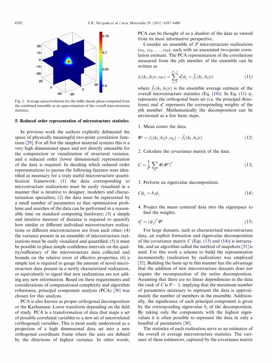
Fig. 2. Average autocorrelation for the stiffer elastic phase computed fromthe combined ensemble as an approximation of the overall microstructurestatistics.


5. Reduced order representation of microstructure statistics

In previous work the authors explicitly delineated thespace of physically meaningful two-point correlation func-tions [29]. For all but the simplest material systems this is avery high dimensional space and not directly amenable forthe computation or visualization of structural variance,and a reduced order (lower dimensional) representationof the data is required. In deciding which reduced orderrepresentations to pursue the following features were iden-tified as necessary for a truly useful microstructure quanti-fication framework: (1) the data corresponding tomicrostructure realizations must be easily visualized in amanner that is intuitive to designer, modelers and charac-terization specialists; (2) the data must be represented bya small number of parameters so that optimization prob-lems and searches of the data can be performed in a reason-able time on standard computing hardware; (3) a simpleand intuitive measure of distance is required to quantifyhow similar or different individual microstructure realiza-tions or different microstructures are from each other; (4)the variance present in an ensemble of microstructure real-izations must be easily visualized and quantified; (5) it mustbe possible to place simple confidence intervals on the qual-ity/sufficiency of the microstructure data collected andbounds on the relative error of effective properties; (6) asimple test is required to gauge the amount of novel micro-structure data present in a newly characterized realization,or equivalently to signal that new realizations are not add-ing any new information. Based on these requirements andconsiderations of computational complexity and algorithmrobustness, principal component analysis (PCA) [30] waschosen for this analysis.

PCA is also known as proper orthogonal decompositionor the Karhunnen–Loeve transform depending on the fieldof study. PCA is a transformation of data that maps a setof possibly correlated variables to a new set of uncorrelated(orthogonal) variables. This is most easily understood as aprojection of a high dimensional data set into a neworthogonal coordinate frame where the axes are definedby the directions of highest variance. In other words,

PCA can be thought of as a shadow of the data as viewedfrom its most informative perspective.

Consider an ensemble of P microstructure realizations(x1, x2, . . . , xP), each with an associated two-point corre-lation estimate. The PCA representation of the correlationsmeasured from the pth member of the ensemble can bewritten as

f2ðh1; h2jr;xP Þ ¼XP�1

j¼1

apj /j þ bf2ðh1; h2jrÞ ð11Þ

where bf2ðh1; h2jrÞ is the ensemble average estimate of theoverall microstructure statistics (Eq. (10)). In Eq. (11) /j

represents the orthogonal basis set (i.e. the principal direc-tions) and ap

j represents the corresponding weights of thepth member. Mathematically the decomposition can beenvisioned as a few basic steps.

1. Mean center the data.

Up ¼ f2ðh1; h2jr;xpÞ � bf2ðh1; h2jrÞ ð12Þ

2. Calculate the covariance matrix of the data.

C ¼ 1

P

XP

UðUpÞT ð13Þ

3. Perform an eigenvalue decomposition.

C/j ¼ bj/j ð14Þ

4. Project the mean centered data into the eigenspace tofind the weights.

apj ¼ ð/jÞ

T Up ð15Þ

For large datasets, such as characterized microstructuredata, an explicit formation and eigenvalue decompositionof the covariance matrix C (Eqs. (13) and (14)) is intracta-ble, and an algorithm called the method of snapshots [31] isused. For this work a scheme to build the representationincrementally (realization by realization) was employed[32]. Building the basis up in this manner has the advantagethat the addition of new microstructure datasets does notrequire the recomputation of the entire decomposition.Assuming that there are no linear dependencies in the datathe rank of C is P � 1, implying that the maximum numberof parameters necessary to represent the data is approxi-mately the number of members in the ensemble. Addition-ally, the significance of each principal component is givenby the corresponding eigenvalue bj of the decomposition.By taking only the components with the highest eigen-values it is often possible to represent the data in only ahandful of parameters [30].

The statistics of each realization serve as an estimator ofthe overall or average microstructure statistics. The vari-ance of these estimators, captured by the covariance matrix

Table 1Eigenvalues for the PCA representation of the two-point correlations ofthe 150 members of the high, mid, and low variance microstructureensembles.

Eigenvalue Value Ratio bj/b1

b1 204.3 1b2 0.8839 0.004326b3 0.7731 0.003784b4 0.6564 0.003213b5 0.3036 0.001486b6 0.0995 0.000487


C, is a straightforward measure of the overall scatter orvariance in microstructure. As will be discussed below indetail, the eigenvalues of C can be directly related to thevariance in properties. Thus, in addition to providing alow dimensional space for visualization and manipulationof the data, PCA also provides a critical measure of thestructural variance in an ensemble.

PCA was also used for reduced order microstructurerepresentation by Sundararaghavan and Zabaras in theirclosely related work on evolutionary material libraries[33–35]. In that work the PCA decomposition was directlyapplied to the collected micrographs in order to construct adynamic database or library of microstructures built on abasis set of eigenstructures, whereas the focus of this workis the exploration and visualization of structural variance.

Fig. 3. The first four principal components for the two-point correlations of thcomponent is seen to be a scaling to correct for volume fraction differencesoscillations.

In a parallel effort the authors have also constructed micro-structure databases in the correlation space rather thandirectly from micrographs. The results of that work anda discussion of the relative merits and disadvantages of thisapproach are being prepared for publication.

PCA was performed on the 150 microstructure realiza-tions composing the high, mid, and low variance materialensembles. For the purposes of discussion and comparisonin this paper all 149 principal directions were kept. Formost applications truncation at 10–15 principal directionswould be sufficient for variance estimation and propertymodeling. Table 1 shows the rate of decay of the eigen-values – by the sixth principal direction the eigenvaluehas decayed to 0.05% of the value of the eigenvalue associ-ated with the first principal direction. Fig. 3 shows the firstfour eigenvectors or principal directions of the dataset. Inthis case the first eigenvector appears almost identical tothe average statistics and can be understood as a scalingfactor that corrects for deviations from the average volumefractions in the individual realizations. The most significanteigenvectors are low frequency modifications to the aver-age, and the later eigenvectors (>4, not shown) generallyoscillate at a higher frequency.

In order to visualize the space spanned by the micro-structure realizations and, more importantly, the structuralvariance the individual realizations from the three ensem-bles were projected into the top three principal directions.

e high, mid, and low variance and combined ensembles. The first principalbetween realizations; the other principal components are low frequency


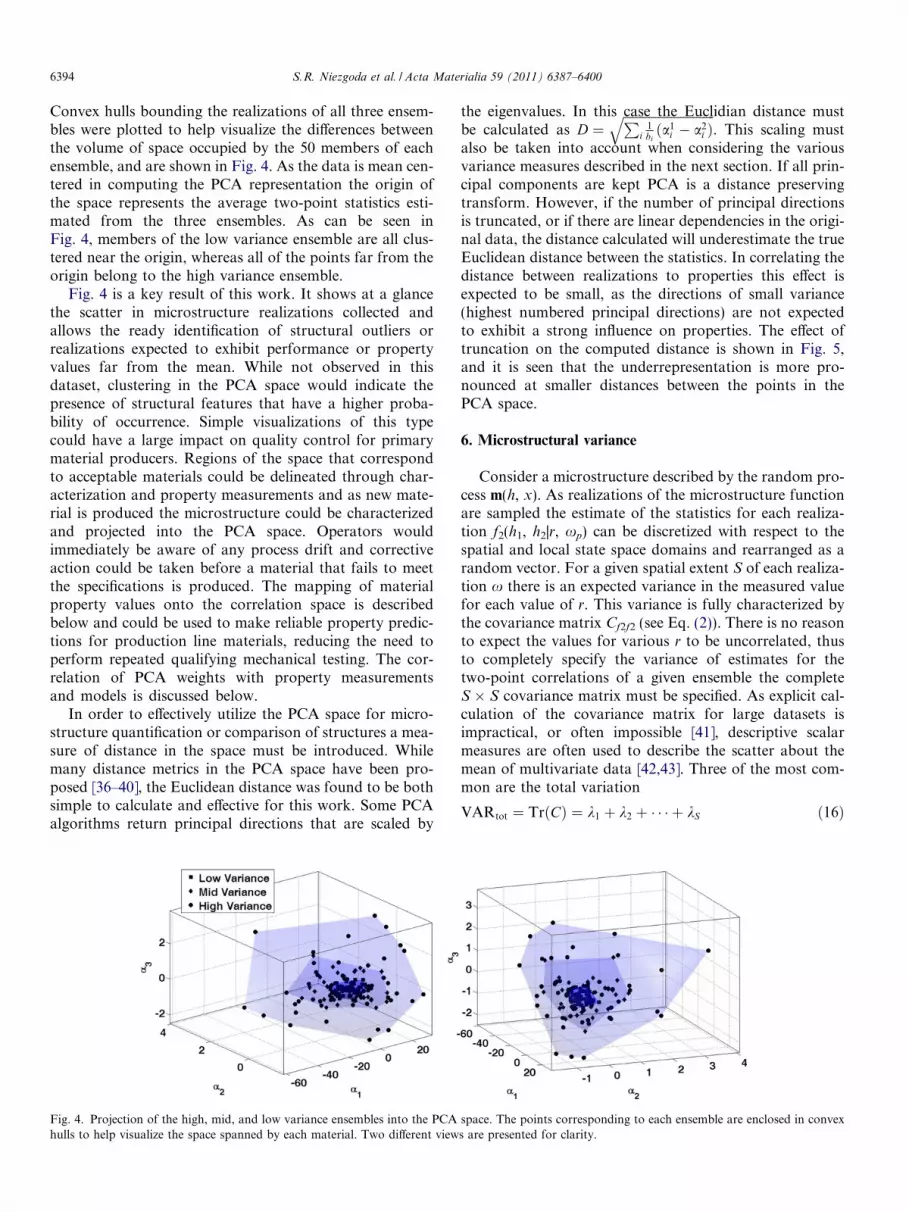
Convex hulls bounding the realizations of all three ensem-bles were plotted to help visualize the differences betweenthe volume of space occupied by the 50 members of eachensemble, and are shown in Fig. 4. As the data is mean cen-tered in computing the PCA representation the origin ofthe space represents the average two-point statistics esti-mated from the three ensembles. As can be seen inFig. 4, members of the low variance ensemble are all clus-tered near the origin, whereas all of the points far from theorigin belong to the high variance ensemble.

Fig. 4 is a key result of this work. It shows at a glancethe scatter in microstructure realizations collected andallows the ready identification of structural outliers orrealizations expected to exhibit performance or propertyvalues far from the mean. While not observed in thisdataset, clustering in the PCA space would indicate thepresence of structural features that have a higher proba-bility of occurrence. Simple visualizations of this typecould have a large impact on quality control for primarymaterial producers. Regions of the space that correspondto acceptable materials could be delineated through char-acterization and property measurements and as new mate-rial is produced the microstructure could be characterizedand projected into the PCA space. Operators wouldimmediately be aware of any process drift and correctiveaction could be taken before a material that fails to meetthe specifications is produced. The mapping of materialproperty values onto the correlation space is describedbelow and could be used to make reliable property predic-tions for production line materials, reducing the need toperform repeated qualifying mechanical testing. The cor-relation of PCA weights with property measurementsand models is discussed below.

In order to effectively utilize the PCA space for micro-structure quantification or comparison of structures a mea-sure of distance in the space must be introduced. Whilemany distance metrics in the PCA space have been pro-posed [36–40], the Euclidean distance was found to be bothsimple to calculate and effective for this work. Some PCAalgorithms return principal directions that are scaled by

Fig. 4. Projection of the high, mid, and low variance ensembles into the PCAhulls to help visualize the space spanned by each material. Two different view

the eigenvalues. In this case the Euclidian distance mustbe calculated as D ¼

ffiffiffiffiffiffiffiffiffiffiffiffiffiffiffiffiffiffiffiffiffiffiffiffiffiffiffiffiffiPi

1bi

a1i � a2

ið Þq

. This scaling mustalso be taken into account when considering the variousvariance measures described in the next section. If all prin-cipal components are kept PCA is a distance preservingtransform. However, if the number of principal directionsis truncated, or if there are linear dependencies in the origi-nal data, the distance calculated will underestimate the trueEuclidean distance between the statistics. In correlating thedistance between realizations to properties this effect isexpected to be small, as the directions of small variance(highest numbered principal directions) are not expectedto exhibit a strong influence on properties. The effect oftruncation on the computed distance is shown in Fig. 5,and it is seen that the underrepresentation is more pro-nounced at smaller distances between the points in thePCA space.

6. Microstructural variance

Consider a microstructure described by the random pro-cess m(h, x). As realizations of the microstructure functionare sampled the estimate of the statistics for each realiza-tion f2(h1, h2|r, xp) can be discretized with respect to thespatial and local state space domains and rearranged as arandom vector. For a given spatial extent S of each realiza-tion x there is an expected variance in the measured valuefor each value of r. This variance is fully characterized bythe covariance matrix Cf2f2 (see Eq. (2)). There is no reasonto expect the values for various r to be uncorrelated, thusto completely specify the variance of estimates for thetwo-point correlations of a given ensemble the completeS � S covariance matrix must be specified. As explicit cal-culation of the covariance matrix for large datasets isimpractical, or often impossible [41], descriptive scalarmeasures are often used to describe the scatter about themean of multivariate data [42,43]. Three of the most com-mon are the total variation

VARtot ¼ TrðCÞ ¼ k1 þ k2 þ � � � þ kS ð16Þ

space. The points corresponding to each ensemble are enclosed in convexs are presented for clarity.

Fig. 5. Demonstration of the effect of truncation on distance measures in the PCA space.


the generalized variance

VARgen ¼ detC ¼ k1k2 . . . kS ð17Þ

and the effective variance

VAReff ¼ ðdetCÞ1=S ¼ ðk1k2 . . . kSÞ1=S ð18Þ

where ki are the eigenvalues of C.All three descriptive measures are easily calculated in the

PCA space. In this case one can use the observations (i)that both the trace and determinant of the covariancematrix are invariant under coordinate transformation and(ii) that the covariance is invariant to shifts in the meanof the data, i.e. ki ¼ bi ¼ r2ðaiÞ, when computed directlyfrom the PCA decomposition. Table 2 shows the computedvariance measures for the high, mid, and low varianceensembles, as well as the complete ensemble formed bythe union of the three sub-ensembles.

The total variation is perhaps the most directly applica-ble scalar measure of the microstructural variance in thePCA space, as the summation is relatively insensitive totruncation of the less significant principal components, ascompared with the generalized variance or effective vari-ance. As will be shown below, the total variation has astrong empirical correlation with the measured varianceof properties. The effective variance and general varianceare useful measures when only considering the first fewprincipal directions. As the eigenvalues bi shrink rapidly

Table 2Comparison of the different variance measures for the high, mid, and low var

Total variation components Genera

3 10 50 149 3

Low 21.67 23.85 28.56 29.32 0.36Mid 102.67 105.59 110.36 111.02 21.12High 501.94 507.17 511.37 512.01 1.80 �Combined 205.94 209.46 214.00 214.69 139.61

the general and effective variance also decrease rapidly asthe number of components is increased.

The generalized variance can be interpreted as a hyper-volume that the distribution of random variables occupiesin the space. Based on this geometric interpretation onemay expect a relationship between the generalized varianceof the first three principal components and the volume ofthe convex hull bounding the microstructure realizationsshown in Fig. 4. It has been observed that the volume ofthe hull scales with ðVARgenÞ1=2, where the constant of pro-portionality depends on a number of factors, including thenumber of samples in the ensemble, spatial extent of therealizations, etc. The observed relationship can be rational-ized by realizing that (assuming a well-behaved distribu-tion) roughly 90% of the realizations will have PCAweights that fall within three standard deviations of themean (the origin). The eigenvalues used to compute thegeneralized variance are trivially proportional to the vari-ance of the PCA weights ai, and the variance is the squareof the standard deviation. Thus the eigenvalues bi of thecovariance can be thought of as squares of some character-istic length scale in the PCA space for the microstructure.This relationship is demonstrated in Fig. 6. This relation-ship was previously noted for two distinct classes of micro-structures, the hazelnut shell and an a/b titanium alloy [44].While it does not appear trivial to a priori predict the con-stant of proportionality and relate the hull volume to anystandard measure of variance in a rigorous manner, the size

iance and combined materials.

lized variance components Effective variance components

3 10 50

0.71 0.40 0.12712.76 0.74 0.1428

103 12.17 1.62 0.14925.18 0.99 0.15

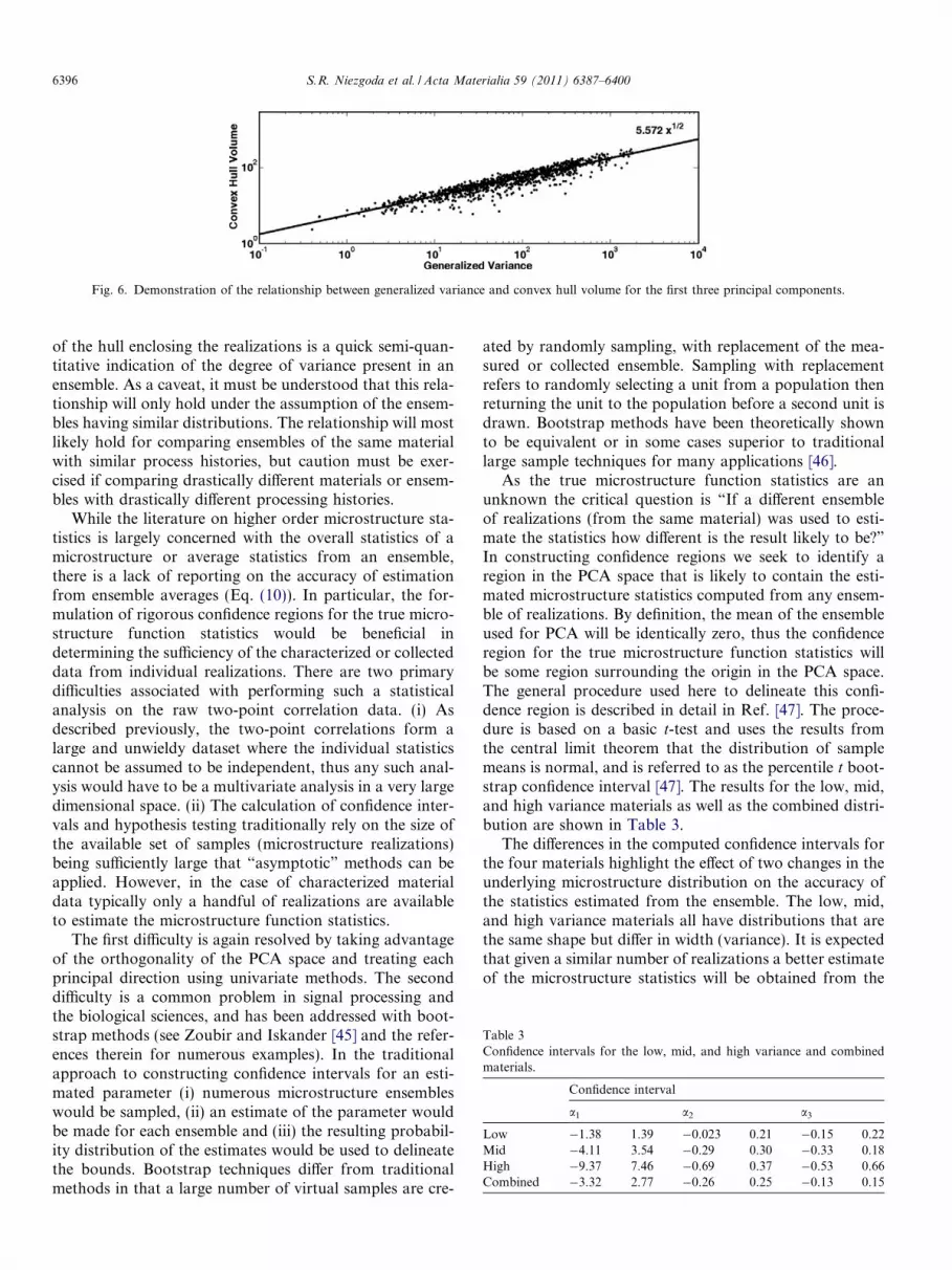
Fig. 6. Demonstration of the relationship between generalized variance and convex hull volume for the first three principal components.

Table 3Confidence intervals for the low, mid, and high variance and combinedmaterials.

Confidence interval

a1 a2 a3

Low �1.38 1.39 �0.023 0.21 �0.15 0.22Mid �4.11 3.54 �0.29 0.30 �0.33 0.18High �9.37 7.46 �0.69 0.37 �0.53 0.66Combined �3.32 2.77 �0.26 0.25 �0.13 0.15


of the hull enclosing the realizations is a quick semi-quan-titative indication of the degree of variance present in anensemble. As a caveat, it must be understood that this rela-tionship will only hold under the assumption of the ensem-bles having similar distributions. The relationship will mostlikely hold for comparing ensembles of the same materialwith similar process histories, but caution must be exer-cised if comparing drastically different materials or ensem-bles with drastically different processing histories.

While the literature on higher order microstructure sta-tistics is largely concerned with the overall statistics of amicrostructure or average statistics from an ensemble,there is a lack of reporting on the accuracy of estimationfrom ensemble averages (Eq. (10)). In particular, the for-mulation of rigorous confidence regions for the true micro-structure function statistics would be beneficial indetermining the sufficiency of the characterized or collecteddata from individual realizations. There are two primarydifficulties associated with performing such a statisticalanalysis on the raw two-point correlation data. (i) Asdescribed previously, the two-point correlations form alarge and unwieldy dataset where the individual statisticscannot be assumed to be independent, thus any such anal-ysis would have to be a multivariate analysis in a very largedimensional space. (ii) The calculation of confidence inter-vals and hypothesis testing traditionally rely on the size ofthe available set of samples (microstructure realizations)being sufficiently large that “asymptotic” methods can beapplied. However, in the case of characterized materialdata typically only a handful of realizations are availableto estimate the microstructure function statistics.

The first difficulty is again resolved by taking advantageof the orthogonality of the PCA space and treating eachprincipal direction using univariate methods. The seconddifficulty is a common problem in signal processing andthe biological sciences, and has been addressed with boot-strap methods (see Zoubir and Iskander [45] and the refer-ences therein for numerous examples). In the traditionalapproach to constructing confidence intervals for an esti-mated parameter (i) numerous microstructure ensembleswould be sampled, (ii) an estimate of the parameter wouldbe made for each ensemble and (iii) the resulting probabil-ity distribution of the estimates would be used to delineatethe bounds. Bootstrap techniques differ from traditionalmethods in that a large number of virtual samples are cre-

ated by randomly sampling, with replacement of the mea-sured or collected ensemble. Sampling with replacementrefers to randomly selecting a unit from a population thenreturning the unit to the population before a second unit isdrawn. Bootstrap methods have been theoretically shownto be equivalent or in some cases superior to traditionallarge sample techniques for many applications [46].

As the true microstructure function statistics are anunknown the critical question is “If a different ensembleof realizations (from the same material) was used to esti-mate the statistics how different is the result likely to be?”In constructing confidence regions we seek to identify aregion in the PCA space that is likely to contain the esti-mated microstructure statistics computed from any ensem-ble of realizations. By definition, the mean of the ensembleused for PCA will be identically zero, thus the confidenceregion for the true microstructure function statistics willbe some region surrounding the origin in the PCA space.The general procedure used here to delineate this confi-dence region is described in detail in Ref. [47]. The proce-dure is based on a basic t-test and uses the results fromthe central limit theorem that the distribution of samplemeans is normal, and is referred to as the percentile t boot-strap confidence interval [47]. The results for the low, mid,and high variance materials as well as the combined distri-bution are shown in Table 3.

The differences in the computed confidence intervals forthe four materials highlight the effect of two changes in theunderlying microstructure distribution on the accuracy ofthe statistics estimated from the ensemble. The low, mid,and high variance materials all have distributions that arethe same shape but differ in width (variance). It is expectedthat given a similar number of realizations a better estimateof the microstructure statistics will be obtained from the


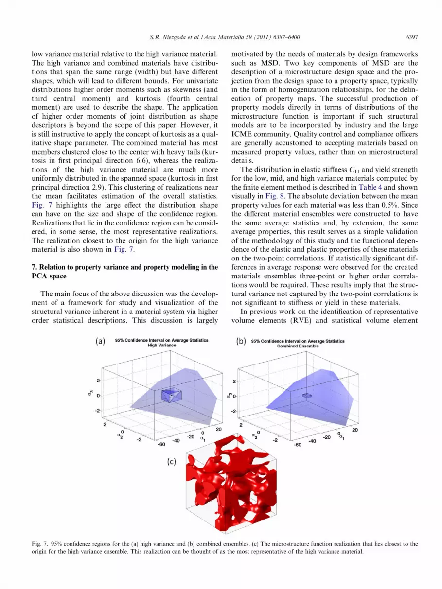
low variance material relative to the high variance material.The high variance and combined materials have distribu-tions that span the same range (width) but have differentshapes, which will lead to different bounds. For univariatedistributions higher order moments such as skewness (andthird central moment) and kurtosis (fourth centralmoment) are used to describe the shape. The applicationof higher order moments of joint distribution as shapedescriptors is beyond the scope of this paper. However, itis still instructive to apply the concept of kurtosis as a qual-itative shape parameter. The combined material has mostmembers clustered close to the center with heavy tails (kur-tosis in first principal direction 6.6), whereas the realiza-tions of the high variance material are much moreuniformly distributed in the spanned space (kurtosis in firstprincipal direction 2.9). This clustering of realizations nearthe mean facilitates estimation of the overall statistics.Fig. 7 highlights the large effect the distribution shapecan have on the size and shape of the confidence region.Realizations that lie in the confidence region can be consid-ered, in some sense, the most representative realizations.The realization closest to the origin for the high variancematerial is also shown in Fig. 7.

7. Relation to property variance and property modeling in the

PCA space

The main focus of the above discussion was the develop-ment of a framework for study and visualization of thestructural variance inherent in a material system via higherorder statistical descriptions. This discussion is largely

Fig. 7. 95% confidence regions for the (a) high variance and (b) combined ensorigin for the high variance ensemble. This realization can be thought of as th

motivated by the needs of materials by design frameworkssuch as MSD. Two key components of MSD are thedescription of a microstructure design space and the pro-jection from the design space to a property space, typicallyin the form of homogenization relationships, for the delin-eation of property maps. The successful production ofproperty models directly in terms of distributions of themicrostructure function is important if such structuralmodels are to be incorporated by industry and the largeICME community. Quality control and compliance officersare generally accustomed to accepting materials based onmeasured property values, rather than on microstructuraldetails.

The distribution in elastic stiffness C11 and yield strengthfor the low, mid, and high variance materials computed bythe finite element method is described in Table 4 and shownvisually in Fig. 8. The absolute deviation between the meanproperty values for each material was less than 0.5%. Sincethe different material ensembles were constructed to havethe same average statistics and, by extension, the sameaverage properties, this result serves as a simple validationof the methodology of this study and the functional depen-dence of the elastic and plastic properties of these materialson the two-point correlations. If statistically significant dif-ferences in average response were observed for the createdmaterials ensembles three-point or higher order correla-tions would be required. These results imply that the struc-tural variance not captured by the two-point correlations isnot significant to stiffness or yield in these materials.

In previous work on the identification of representativevolume elements (RVE) and statistical volume element

embles. (c) The microstructure function realization that lies closest to thee most representative of the high variance material.

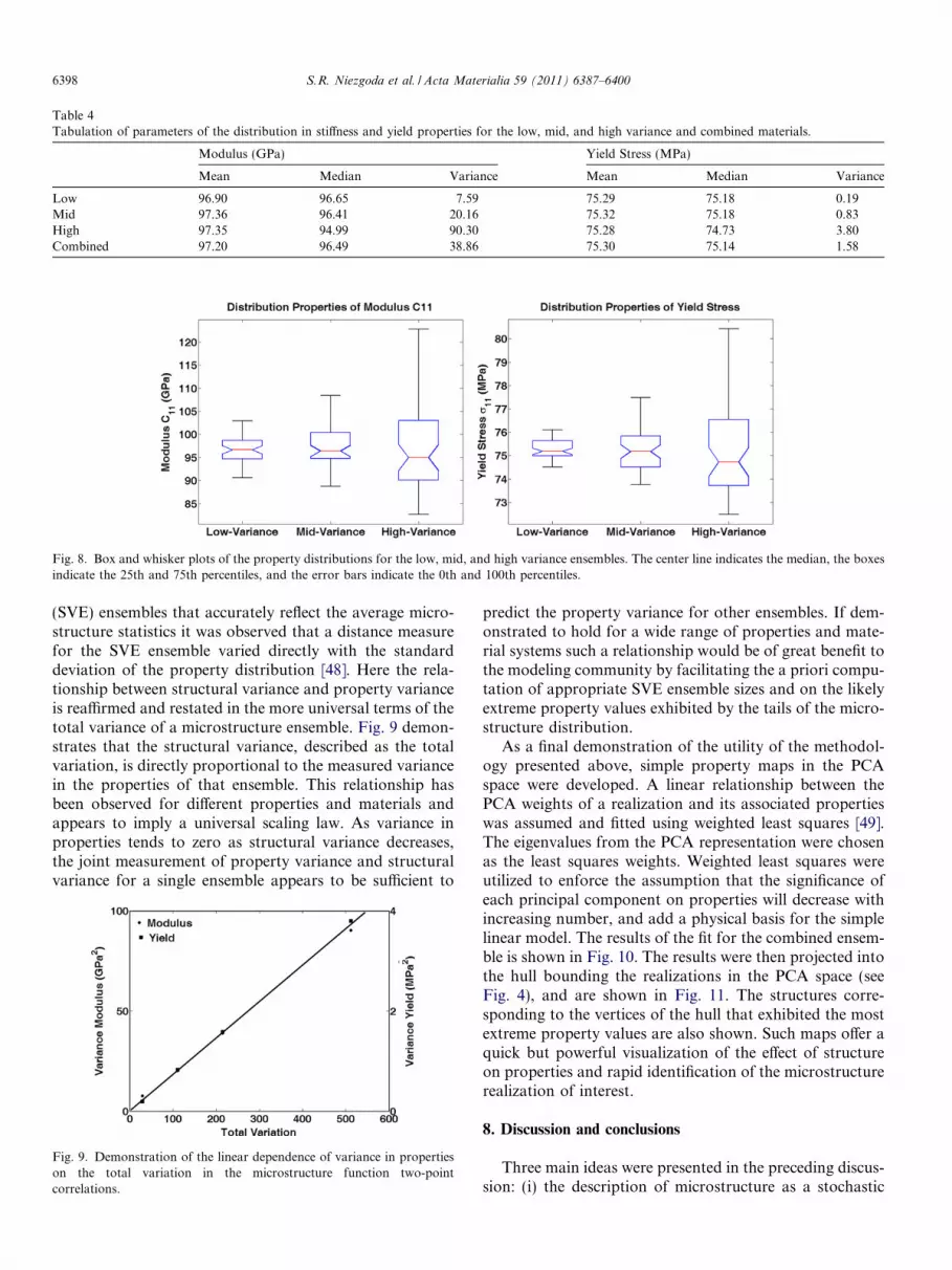
Table 4Tabulation of parameters of the distribution in stiffness and yield properties for the low, mid, and high variance and combined materials.

Modulus (GPa) Yield Stress (MPa)

Mean Median Variance Mean Median Variance

Low 96.90 96.65 7.59 75.29 75.18 0.19Mid 97.36 96.41 20.16 75.32 75.18 0.83High 97.35 94.99 90.30 75.28 74.73 3.80Combined 97.20 96.49 38.86 75.30 75.14 1.58

Fig. 8. Box and whisker plots of the property distributions for the low, mid, and high variance ensembles. The center line indicates the median, the boxesindicate the 25th and 75th percentiles, and the error bars indicate the 0th and 100th percentiles.


(SVE) ensembles that accurately reflect the average micro-structure statistics it was observed that a distance measurefor the SVE ensemble varied directly with the standarddeviation of the property distribution [48]. Here the rela-tionship between structural variance and property varianceis reaffirmed and restated in the more universal terms of thetotal variance of a microstructure ensemble. Fig. 9 demon-strates that the structural variance, described as the totalvariation, is directly proportional to the measured variancein the properties of that ensemble. This relationship hasbeen observed for different properties and materials andappears to imply a universal scaling law. As variance inproperties tends to zero as structural variance decreases,the joint measurement of property variance and structuralvariance for a single ensemble appears to be sufficient to

Fig. 9. Demonstration of the linear dependence of variance in propertieson the total variation in the microstructure function two-pointcorrelations.

predict the property variance for other ensembles. If dem-onstrated to hold for a wide range of properties and mate-rial systems such a relationship would be of great benefit tothe modeling community by facilitating the a priori compu-tation of appropriate SVE ensemble sizes and on the likelyextreme property values exhibited by the tails of the micro-structure distribution.

As a final demonstration of the utility of the methodol-ogy presented above, simple property maps in the PCAspace were developed. A linear relationship between thePCA weights of a realization and its associated propertieswas assumed and fitted using weighted least squares [49].The eigenvalues from the PCA representation were chosenas the least squares weights. Weighted least squares wereutilized to enforce the assumption that the significance ofeach principal component on properties will decrease withincreasing number, and add a physical basis for the simplelinear model. The results of the fit for the combined ensem-ble is shown in Fig. 10. The results were then projected intothe hull bounding the realizations in the PCA space (seeFig. 4), and are shown in Fig. 11. The structures corre-sponding to the vertices of the hull that exhibited the mostextreme property values are also shown. Such maps offer aquick but powerful visualization of the effect of structureon properties and rapid identification of the microstructurerealization of interest.

8. Discussion and conclusions

Three main ideas were presented in the preceding discus-sion: (i) the description of microstructure as a stochastic

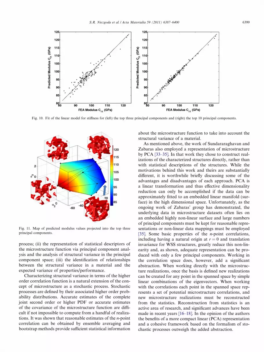
Fig. 10. Fit of the linear model for stiffness for (left) the top three principal components and (right) the top 10 principal components.

Fig. 11. Map of predicted modulus values projected into the top threeprincipal components.


process; (ii) the representation of statistical descriptors ofthe microstructure function via principal component anal-ysis and the analysis of structural variance in the principalcomponent space; (iii) the identification of relationshipsbetween the structural variance in a material and theexpected variance of properties/performance.

Characterizing structural variance in terms of the higherorder correlation function is a natural extension of the con-cept of microstructure as a stochastic process. Stochasticprocesses are defined by their associated higher order prob-ability distributions. Accurate estimates of the completejoint second order or higher PDF or accurate estimatesof the covariance of the microstructure function are diffi-cult if not impossible to compute from a handful of realiza-tions. It was shown that reasonable estimates of the n-pointcorrelation can be obtained by ensemble averaging andbootstrap methods provide sufficient statistical information

about the microstructure function to take into account thestructural variance of a material.

As mentioned above, the work of Sundararaghavan andZabaras also employed a representation of microstructureby PCA [33–35]. In that work they chose to construct real-izations of the characterized structures directly, rather thanwith statistical descriptions of the structures. While themotivations behind this work and theirs are substantiallydifferent, it is worthwhile briefly discussing some of theadvantages and disadvantages of each approach. PCA isa linear transformation and thus effective dimensionalityreduction can only be accomplished if the data can beapproximately fitted to an embedded linear manifold (sur-face) in the high dimensional space. Unfortunately, as theongoing work of Zabaras’ group has demonstrated, theunderlying data in microstructure datasets often lies onan embedded highly non-linear surface and large numbersof principal components must be kept for reasonable repre-sentations or non-linear data mappings must be employed[35]. Some basic properties of the n-point correlations,including having a natural origin at r = 0 and translationinvariance for WSS structures, greatly reduce this non-lin-earity and, as shown, adequate representation can be pro-duced with only a few principal components. Working inthe correlation space does, however, add a significantabstraction. When working directly with the microstruc-ture realizations, once the basis is defined new realizationscan be created for any point in the spanned space by simplelinear combinations of the eigenvectors. When workingwith the correlations each point in the spanned space rep-resents a set of potential microstructure correlations, andnew microstructure realizations must be reconstructedfrom the statistics. Reconstruction from statistics is anactive area of research, and significant advances have beenmade in recent years [16–18]. In the opinion of the authorsthe benefits of a more compact linear (PCA) representationand a cohesive framework based on the formalism of sto-chastic processes outweigh the added abstraction.


While working with the microstructure statistics reducesthe non-linearity of the data, it is worthwhile exploringother dimensionality reduction frameworks. PCA was cho-sen here as it is computationally straightforward, robust,and the basis can be incrementally updated as new realiza-tions are added. While a more compact representation ofthe data may be possible, non-linear dimensionality reduc-tion frameworks are often computationally very expensiveand sensitive to the nature of the embedded manifold onwhich the data lies [50].

ICME is a new materials sub-discipline which seeks tolink computational materials models, rigorous product per-formance analysis, and the simulation and control of man-ufacturing processes. ICME as a discipline partially grewout of the need to move design beyond average propertyand performance considerations and to actively designfor the tails of performance distributions. In the opinionof the authors the integration of these disparate techniquesand data paths required for ICME necessitates a corre-sponding evolution of the way we think about microstruc-ture data. It is the hope of the authors that this work willhelp jumpstart discussions within the field of materials sci-ence and engineering.

Acknowledgements

The authors acknowledge financial support for thiswork from the DARPA-ONR Dynamic 3D Digital Struc-ture project, award no. N000140510504. S.R.N. acknowl-edges additional support for this work from the USDepartment of Energy through the LANL/LDRDProgram.

References

[1] Tewari A, Gokhale AB, Spowart JE, Miracle DB. Acta Mater2004;52:307–19.

[2] Torquato S. Random heterogeneous materials. New York: Springer-Verlag; 2002.

[3] Fullwood DT, Niezgoda SR, Adams BL, Kalidindi SR. Prog MaterSci 2010;55:477–562.

[4] Gokhale AM. Microsc Microanal 2004;10:736–7.[5] Huang M. Int J Solids Struct 2005;42:1425–41.[6] Etingof PI, Sam DD, Adams BL. Philos Mag A Phys Condens Matter

Def Mech Propert 1995;72:199.[7] Lu B, Torquato S. Phys Rev A 1992;45:922.[8] Singh H, Gokhale AM, Lieberman SI, Tamirisakandala S. Mater Sci

Eng A 2008;474:104–11.[9] Ripley BD. Mapped point patterns. Spatial statistics. Hoboken,

NJ: John Wiley and Sons; 2005. p. 144–90.[10] Torquato S. Phys Rev E 1995;51:3170.[11] Piasecki R. Proc R Soc A 2011;467:806–20. doi:10.1098/rspa.2010.

0296.

[12] Burnham KP, Anderson DR, editors. Model selection and multi-model inference: a practical information – theoretic approach. NewYork: Springer; 2002.

[13] Adams BL, Gao X, Kalidindi SR. Acta Mater 2005;53:3563–77.[14] Jiao Y, Stillinger FH, Torquato S. Phys Rev E 2007;76:031110–.[15] Pyrz R. Mater Sci Eng A 1994;177:253–9.[16] Yeong CLY, Torquato S. Phys Rev E 1998;57:495–506.[17] Fullwood DT, Niezgoda SR, Kalidindi SR. Acta Mater 2008;56:

942–8.[18] Zeman J, Sejnoha M. Modell Simul Mater Sci Eng 2007:S325.[19] Olson GB. Science 1997;277:1237–42.[20] Olson GB. Science 2000;228:933–98.[21] National Research Council Committee on Integrated Computational

Materials E. Integrated computational materials engineering: atransformational discipline for improved competitiveness andnational security. Washington, DC: National Academies Press; 2008.

[22] Papoulis A, Pillai SU. Probability, random variables, and stochasticprocesses. Boston, MA: McGraw-Hill; 2002.

[23] Roe R-J. J Appl Phys 1965;36:2024–31.[24] Pospiech J, Lucke K. Acta Metall 1975;23:997–1007.[25] Schmid SM, Casey M, Starkey J. Tectonophysics 1981;78:101–17.[26] Bunge HJ. Texture analysis in materials science: mathematical

methods. London: Butterworths; 1982.[27] Adams BL, Garmestani H, Saheli G. J Comput-Aid Mater Des

2004;11:103–15.[28] Adams BL, Etingof PI, Sam DD. Mater Sci Forum 1994;157:287–94.[29] Niezgoda SR, Fullwood DT, Kalidindi SR. Acta Mater

2008;56:5285–92.[30] Fukunaga K. Introduction to statistical pattern recognition. Boston,

MA: Academic Press; 1990.[31] Turk M, Pentland A. J Cognit Neurosci 1991;3:71.[32] Li Y. Pattern Recognit 2004;37:1509–18.[33] Sundararaghavan V, Zabaras N. Acta Mater 2004;52:4111–9.[34] Sundararaghavan V, Zabaras N. Comp Mater Sci 2005;32:223–39.[35] Ganapathysubramanian B, Zabaras N. J Comput Phys 2008;227:

6612–37.[36] Gower JC. Biometrika 1966;53:325–38.[37] Jian Y, Zhang D, Frangi AF, Jing-yu Y. IEEE Trans Pattern Anal

Machine Intell 2004;26:131–7.[38] Weinberger KQ, Saul LK. J Mach Learn Res 2009;10:207–44.[39] Gardner JW. Sens Actuat B Chem 1991;4:109–15.[40] Beveridge JR, Kai S, Bruce AD, Geof HG. In: IEEE computer society

conference on computer vision and pattern recognition (CVPR’01),vol. 1; 2001. p. 535.

[41] Jain AK, Duin RPW, Jianchang M. IEEE Trans Pattern AnalMachine Intell 2000;22:4–37.

[42] Pena D, Rodrıguez J. J Multivar Anal 2003;85:361–74.[43] Seber GAF. Multivariate observations. Hobocken, NJ: Wiley-Inter-

science; 2004.[44] Niezgoda SR. PhD dissertation, Drexel University, Philadelpha, PA;

2010.[45] Zoubir AM, Iskander DR. Bootstrap techniques for signal process-

ing. England: Cambridge; 2004.[46] Young GA. Stat Sci 1994;9:382–95.[47] Diciccio TJ, Romano JP. J Roy Stat Soc B Methodol 1988;50:338–54.[48] Niezgoda SR, Turner DM, Fullwood DT, Kalidindi SR. Acta Mater

2010;58:4432–45.[49] Bjorck A. Numerical methods for least squares problems. Philadel-

phia, PA: SIAM; 1996.[50] Lee JA, Verleysen M. Nonlinear dimensionality reduction. New York:

Springer; 2007.

http://dx.doi.org/10.1098/rspa.2010.0296

http://dx.doi.org/10.1098/rspa.2010.0296

Documents

Understanding and visualizing microstructure and microstructure variance as a stochastic process