arX

iv:a

stro

-ph/

9408

034v

1 1

1 A

ug 1

994

SISSA REF. 107/94/A

CfA-3915

Cosmic Strings

&

Cosmic Variance

Alejandro Gangui1 ∗ and Leandros Perivolaropoulos2 † ‡

1SISSA – International School for Advanced Studies,

via Beirut 2 – 4, 34013 Trieste, Italy.

2Division of Theoretical Astrophysics

Harvard-Smithsonian Center for Astrophysics

60 Garden St.

Cambridge, Mass. 02138, USA.

Submitted to The Astrophysical Journal

Abstract

By using a simple analytical model based on counting random multiple impulses inflictedon photons by a network of cosmic strings we show how to construct the general q-point tem-perature correlation function of the Cosmic Microwave Background radiation. Our analysisis sensible specially for large angular scales where the Kaiser-Stebbins effect is dominant.Then we concentrate our study on the four-point function and in particular on its zero-laglimit, namely, the excess kurtosis parameter, for which we obtain a predicted value of ∼ 10−2.In addition, we estimate the cosmic variance for the kurtosis due to a Gaussian fluctuationfield, showing its dependence on the primordial spectral index of density fluctuations n andfinding agreement with previous published results for the particular case of a flat Harrison-Zel’dovich spectrum. Our value for the kurtosis compares well with previous analyses butfalls below the threshold imposed by the cosmic variance when commonly accepted param-eters from string simulations are considered. In particular the non-Gaussian signal is foundto be inversely proportional to the scaling number of defects, as could be expected by thecentral limit theorem.

Subject headings: cosmic microwave background - cosmic strings

∗Electronic mail: gangui@tsmi19.sissa.it†Electronic mail: leandros@cfata3.harvard.edu‡Address after September 1, 1994: Department of Physics, M.I.T., Cambridge, MA 02139

1

1 Introduction

A central concept for particle physics theories attempting to unify the fundamental interac-tions is the concept of symmetry breaking. This symmetry breaking plays a crucial role inthe Weinberg-Salam standard electroweak model ( Masiero 1984) whose extraordinary suc-cess in explaining electroweak scale physics reaches a precision rarely found before in otherareas of science (Koratzinos 1994). In the context of the standard Big Bang cosmologicaltheory the spontaneous breaking of fundamental symmetries is realized as a phase transitionin the early universe. Such phase transitions have several exciting cosmological consequencesthus providing an important link between particle physics and cosmology.

A particularly interesting cosmological issue is the origin of structure in the universe.This structure is believed to have emerged by the gravitational growth of primordial matterfluctuations which are superposed on the smooth background required by the cosmologicalprinciple, the main assumption of the Big Bang theory.

The above mentioned link of cosmology to particle physics theories has led to the gener-ation of two classes of theories which attempt to provide physically motivated solutions tothe problem of the origin of structure in the universe. According to the one class of theories,based on inflation, primordial fluctuations arose from zero point quantum fluctuations of ascalar field during an epoch of superluminal expansion of the scale factor of the universe.These fluctuations may be shown to obey Gaussian statistics to a very high degree and tohave an approximately scale invariant power spectrum.

According to the second class of theories, those based on topological defects, primordialfluctuations were produced by a superposition of seeds made of localized energy densitytrapped during a symmetry breaking phase transition in the early universe. Topologicaldefects with linear geometry are known as cosmic strings and may be shown to be consis-tent with standard cosmology unlike their pointlike (monopoles) and planar (domain walls)counterparts which require dilution by inflation to avoid overclosing the universe. Cosmicstrings are predicted to form during a phase transition in the early universe by many butnot all Grand Unified Theories (GUTs).

The main elegant feature of the cosmic string model that has caused significant attentionduring the past decade is that the only free parameter of the model (the effective massper unit length of the wiggly string µ ) is fixed to approximately the same value from twocompletely independent directions. From the microphysical point of view the constraintGµ ≃ (mGUT /mP )2 ≃ 10−6 is imposed in order that strings form during the physicallyrealizable GUT phase transition. From the macrophysical point of view the same constraintarises by demanding that the string model be consistent with measurements of CosmicMicrowave Background (CMB) anisotropies and that fluctuations are strong enough forstructures to form by the present time. This mass-scale ratio for Gµ is actually a veryattractive feature and even models of inflation have been proposed (Freese et al. 1990, Dvaliet al. 1994) where observational predictions are related to similar mass scale relations.

Cosmic strings can account for the formation of large scale filaments and sheets (Vachas-pati 1986; Stebbins et al. 1987; Perivolaropoulos, Brandenberger & Stebbins 1990; Vachas-pati & Vilenkin 1991; Vollick 1992; Hara & Miyoshi 1993), galaxy formation at epochsz ∼ 2 − 3 (Brandenberger et al. 1987) and galactic magnetic fields (Vachaspati 1992b).They also generate peculiar velocities on large scales (Vachaspati 1992a; Perivolaropoulos &

2

Vachaspati 1993), and are consistent with the amplitude, spectral index (Bouchet, Bennett &Stebbins 1988; Bennett, Stebbins & Bouchet 1992; Perivolaropoulos 1993a; Hindmarsh 1993)and the statistics (Gott et al. 1990; Perivolaropoulos 1993b; Moessner, Perivolaropoulos &Brandenberger 1993; Coulson et al. 1993; Luo 1994) of the CMB anisotropies measured byCOBE on angular scales of order θ ∼ 10.

Strings may also leave their imprint on the CMB mainly in three different ways. Thebest studied mechanism for producing temperature fluctuations on the CMB by cosmicstrings is the Kaiser-Stebbins effect (Kaiser & Stebbins 1984; Gott 1985). According to thiseffect, moving long strings present between the time of recombination trec and today produce(due to their deficit angle (Vilenkin 1981)) discontinuities in the CMB temperature betweenphotons reaching the observer through opposite sides of the string. Another mechanism forproducing CMB fluctuations by cosmic strings is based on potential fluctuations on the lastscattering surface (LSS). Long strings and loops present between the time of equal matter andradiation teq and the time of recombination trec induce density and velocity fluctuations totheir surrounding matter. These fluctuations grow gravitationally and at trec they producepotential fluctuations on the LSS. Temperature fluctuations arise because photons haveto climb out of a potential with spatially dependent depth. A third mechanism for theproduction of temperature anisotropies is based on the Doppler effect. Moving long stringspresent on the LSS drag the surrounding plasma and produce velocity fields. Thus, photonsscattered for last time on these perturbed last scatterers suffer temperature fluctuations dueto the Doppler effect.

It was recently shown (Perivolaropoulos 1994) how, by superposing the effects of thesethree mechanisms at all times from trec to today, the power spectrum of the total temperatureperturbation may be obtained. It turns out that (assuming standard recombination) bothDoppler and potential fluctuations at the LSS dominate over post-recombination effects onangular scales below 2. However this is not the case for very large scales (where we willbe focusing in the present paper) and this justifies our neglecting the former two sources ofCMB anisotropies. The main effect of these neglected perturbations is an increase of thegaussian character of the fluctuations on small angular scales.

The main assumptions of the model were explained in (Perivolaropoulos 1993a). Here wewill only review them briefly for completeness. As mentioned above, discontinuities in thetemperature of the photons arise due to the peculiar nature of the spacetime around a longstring which even though is locally flat, globally has the geometry of a cone with deficit angle8πGµ. Several are the cosmological effects produced by the mere existence of this deficitangle (Shellard 1994), e.g., arcsecond-double images from GUT strings at redshifts z ∼ 1,flatten structures from string wakes or elongated filamentary structures from slowly movinglong wiggly strings and, of more relevance in our present work, post-recombination CMBanisotropy (White, Scott and Silk 1994) string induced effects (Kaiser & Stebbins 1984).

The magnitude of the discontinuity is proportional not only to the deficit angle but alsoto the string velocity vs and depends on the relative orientation between the unit vectoralong the string s and the unit photon wave-vector k. It is given by (Stebbins 1988)

∆T

T= ±4πGµvsγsk · (vs × s) (1)

where γs is the relativistic Lorentz factor and the sign changes when the string is crossed.

3

Also, long strings within each horizon have random velocities, positions and orientations.We discretize the time between trec and today by a set of N Hubble time-steps ti such

that ti+1 = ti δ, i.e., the horizon gets multiplied by δ in each time-step. For zrec ∼ 1400 wehave N ≃ logδ[(1400)3/2].

In the frame of the multiple impulse approximation the effect of the string network ona photon beam is just the linear superposition of the individual effects, taking into accountcompensation (Traschen et al. 1986; Veeraraghavan & Stebbins 1990; Magueijo 1992), thatis, only those strings within a horizon distance from the beam inflict perturbations to thephotons.

In the following section we show how to construct the general q-point function of CMBanisotropies at large angular scales produced through the Kaiser-Stebbins effect. Explicitcalculations are performed for the four-point function and its zero-lag limit, the kurtosis.Next, we calculate the (cosmic) variance for the kurtosis assuming Gaussian statistics forarbitrary value of the spectral index and compare it with the string predicted value (section3). Finally, in section 4 we briefly discuss our results.

2 The Four–Point Temperature Correlation Function

According to the previous description, the total temperature shift in the γ direction due tothe Kaiser-Stebbins effect on the microwave photons between the time of recombination andtoday may be written as

∆T

T(γ) = 4πGµvsγs

N∑

n=1

M∑

m=1

βmn(γ) (2)

where βmn(γ) gives us information about the velocity vmn and orientation smn of the mthstring at the nth Hubble time-step and may be cast as βmn(γ) = γ · Rmn, with Rmn =vmn × smn = (sin θmn cos φmn, sin θmn sin φmn, cos θmn) a unit vector whose direction variesrandomly according to the also random orientations and velocities in the string network. InEq.(2), M denotes the mean number of strings per horizon scale, obtained from simulations( Allen & Shellard 1990, Bennett & Bouchet 1988) to be of order M ∼ 10.

Let us now study the correlations in temperature anisotropies. We are focusing here inthe stringy-perturbation inflicted on photons after the time of recombination on their wayto us. Photons coming from different directions of the sky share a common history that maybe long or short depending on their angular separation. We therefore take θtp ≃ z(tp)

−1/2

to be the angular size of the horizon at Hubble time-step tp (1 ≤ p ≤ N). The kickson two different photon beams separated by an angular scale α12 = arccos(γ1 · γ2) greaterthan θtp will be uncorrelated for the time-step tp (no common history up until ∼ tp) butwill eventually become correlated (and begin sharing a common past) afterwards when thehorizon increases, say, at tp′ when θtp′

>∼ α12, i.e., when α12 fits in the horizon scale.Much in the same way, kicks inflicted on three photon beams will be uncorrelated if at

time t any one of the three angles between any two directions (say, α12, α23, α13) is greaterthan θt, the size of the horizon at time t. So, in this case, we will be summing (cf. Eq.(2))over those Hubble time-steps n greater than p, where p is the time-step when the condition

4

θtp = Max[α12, α23, α13] is satisfied. The same argument could be extended to any numberof photon beams (and therefore for the computation of the q–point function of temperatureanisotropies)2.

Let us put the above considerations on more quantitative grounds, by writing the meanq-point correlation function. Using Eq.(2) we may express it as

<∆T

T(γ1)...

∆T

T(γq) >= ξq

N∑

n1,...,nq=1

M∑

m1,...,mq=1

< βm1n1

1 ...βmqnq

q > (3)

where γ1...γq are unit vectors denoting directions in the sky and where βmjnj

j = γj ·Rmjnj withγj = (sin θj cos φj , sin θj sin φj, cosθj). In the previous equation we defined ξ ≡ 4πGµvsγs.For simplicity we may always choose a coordinate system such that θ1 = 0, φ1 = 0 (i.e., γ1 lieson the z axis) and φ2 = π/2. The seemingly complicated sum (3) is in practice fairly simpleto calculate because of the large number of terms that vanish due to lack of correlation, afterthe average is taken. The calculation proceeds by first splitting the product βm1n1

1 ...βmqnqq

into all possible sub-products that correspond to correlated kicks (i.e., βmjnj ’s with the samepair (mj , nj)) at each expansion Hubble-step and then evaluating the ensemble average of

each sub-product by integration over all directions of R. To illustrate this technique weevaluate the two, three and four-point functions below.

The calculation of the two-point function has been performed in (Perivolaropoulos 1993a)but we briefly repeat it here for clarity and completeness. Having a correlated pair ofbeams in γ1 and γ2 directions from a particular time-step p onwards means simply thatRm1n1 = Rm2n2 ⇔ n ≡ n1 = n2 > p, m ≡ m1 = m2; otherwise the R’s remain uncorrelatedand there is no contribution to the mean two-point function. Therefore we will have

∆T

T(γ1)

∆T

T(γ2) = ξ2

N∑

n=p

M∑

m=1

(γ1 · Rmn)(γ2 · Rmn) (4)

where we wrote just the correlated part on an angular scale α12 = arccos(γ1 · γ2). Theuncorrelated part on this scale will vanish when performing the ensemble average 〈·〉. Thusthe mean two-point function may be written as

<∆T

T(γ1)

∆T

T(γ2) >= ξ2 < β1β2 > Ncor(α12) (5)

where

Ncor(α12) ≡ M [N − 3 logδ(1 +α12

θtrec

)] (6)

is the number of correlated ‘kicks’ inflicted on a scale α12 after this scale enters the horizon.θrec is the angular scale of the horizon at the time of recombination. Since we may alwaystake

β1 = (0, 0, 1) · R β2 = (sin α12, 0, cosα12) · R (7)2A general expression (suitable to whatever angular scale and to whatever source of temperature fluc-

tuations) for the three-point correlation function was given in (Gangui, Lucchin, Matarrese and Mollerach1994). Although of much more complexity, similar analysis may be done for the four-point function and acompletely general expression in terms of the angular trispectrum may be found (Gangui & Perivolaropoulos1994).

5

with R = (sin θ cos φ, sin θ sin φ, cosθ), < ∆TT

(γ1)∆TT

(γ2) > may be calculated by integratingover (θ, φ) and dividing by 4π. The result is

<∆T

T(γ1)

∆T

T(γ2) >= ξ2 cos α12

3Ncor(α12) (8)

which may be shown (Perivolaropoulos 1993a) to lead to a slightly tilted scale invariantspectrum on large angular scales.

The three-point function may be obtained in a similar way. However, the superimposedkernels of the distribution turn out to be symmetric with respect to positive and negativeperturbations and therefore no mean value for the three-point correlation function arises (inparticular also the skewness is zero). On the other hand the four-point function is easilyfound and a mean value for the excess kurtosis parameter (Gangui 1994b) may be predicted,as we show below.

In the case of the four-point function we could find terms where (for a particular time-step) the photon beams in directions γ1, γ2 and γ3 are all correlated amongst themselves butnot the beam γ4, which may be taken sufficiently far apart from the other three directions.In such a case we have

〈∆T

T(γ1)

∆T

T(γ2)

∆T

T(γ3)

∆T

T(γ4)〉 −→ 〈∆T

T(γ1)

∆T

T(γ2)

∆T

T(γ3)〉 〈

∆T

T(γ4)〉 (9)

and (cf. (Perivolaropoulos 1993a)) this contribution vanishes.Another possible configuration we could encounter is the one in which the beams are

correlated two by two but no correlation exists between the pairs (for one particular time-step). This yields three distinct possible outcomes, e.g., 〈∆T

T(γ1)

∆TT

(γ2)〉 〈∆TT

(γ3)∆TT

(γ4)〉,and the other two obvious combinations.

The last possibility is having all four photon beams fully correlated amongst themselvesand this yields 〈∆T

T(γ1)

∆TT

(γ2)∆TT

(γ3)∆TT

(γ4)〉c, where the subscript c stands for the connected

part.In a way completely analogous to that for the two-point function, the correlated part for

the combination of four beams gives

∆T

T(γ1)

∆T

T(γ2)

∆T

T(γ3)

∆T

T(γ4) = ξ4

N∑

n=p

M∑

m=1

(γ1 ·Rmn)(γ2 ·Rmn)(γ3 ·Rmn)(γ4 ·Rmn) (10)

Now we are ready to write the full mean four–point function as

〈∆T

T(γ1)

∆T

T(γ2)

∆T

T(γ3)

∆T

T(γ4)〉

=[

〈∆T

T(γ1)

∆T

T(γ2)〉〈

∆T

T(γ3)

∆T

T(γ4)〉+2terms

]

+〈∆T

T(γ1)

∆T

T(γ2)

∆T

T(γ3)

∆T

T(γ4)〉c

= 3[

1

3ξ2Ncor(θ) cos(θ)

]2

+ 〈∆T

T(γ1)

∆T

T(γ2)

∆T

T(γ3)

∆T

T(γ4)〉c (11)

where for simplicity we wrote this equation using the same scale θ for all directions on thesky (first term after the equality sign); after all, we will be interested in the zero lag limit,in which case we will have θ → 0. By using Mathematica (Wolfram 1991) it is simple tofind that the second term includes just the sum of twenty-one combinations of trigonometric

6

functions depending on θi, φi, with i = 1, 2, 3, 4, the spherical angles for the directions γi onthe sky (cf. Eq.(10)). These terms are the only ones which contribute non-vanishingly afterthe integration over the angles θmn, φmn is performed (assuming ergodicity).

When we take the zero lag limit (i.e., aiming for the kurtosis) the above expression getslargely simplified. After normalizing by the squared of the variance σ4 = [1

3ξ2Ncor(0)]2 and

subtracting the disconnected part we get the excess kurtosis parameter

K =1

σ4〈∆T

T

4

(γ1)〉 − 3 =9

5MN≃ (1.125 +0.675

−0.458) × 10−2 (12)

where we took M ≃ 10 and δ = 2 implying N ≃ 16. Quoted errors take into account possiblevariation of δ in the range 1.5 ≤ δ ≤ 3.

Note that for values of the scaling solution M increasing (large number of seeds) theactually small non-Gaussian signal K gets further depressed, as it could be expected fromthe Central Limit Theorem.

3 The r.m.s. excess kurtosis of a Gaussian field

The previous section was devoted to the computation of K, the excess kurtosis parameter,as predicted by a simple analytical model in the framework of the Cosmic String scenario.We might ask whether this particular non-Gaussian signal has any chance of actually beingunveiled by current anisotropy experiments. Needless to say, this could provide a significantprobe of the structure of the relic radiation and furthermore give us a hint on the possiblesources of the primordial perturbations that, after non-linear evolution, realize the large scalestructure of the universe as we currently see it.

However, as it was realized some time ago (Scaramella & Vittorio 1991; Abbott & Wise1984; Srednicki 1993; Gangui 1994a), the mere detection of a non-zero higher order correla-tion function (e.g., the four-point function) or its zero lag limit (e.g., the kurtosis) cannot bedirectly interpreted as a signal for intrinsically non-Gaussian perturbations. In order to tellwhether or not a particular measured value for the kurtosis constitutes a significant evidenceof a departure from Gaussian statistics, we need to know the amplitude of the non-Gaussianpattern produced by a Gaussian perturbation field. Namely, we need to know the r.m.s.excess kurtosis of a Gaussian field.

Let us begin with some basics. Let us denote the kurtosis K ≡ ∫ dΩγ

4π∆TT

4(γ) and assume

that the underlying statistics is Gaussian, namely, that the multipole coefficients amℓ are

Gaussian distributed. Thus, the ensemble average for the kurtosis is given by the well-known formula: 〈K〉 = 3σ4, where σ2 is the mean two–point function at zero lag, i.e., theCMB variance as given by

σ2 ≡ 〈C2(0)〉 =1

4π

∑

ℓ

(2ℓ + 1)

5Q2CℓW2

ℓ (13)

where the Cℓ coefficients (here normalized to Cℓ=2 = 1) are also dependent on the value forthe primordial spectral index of density fluctuations n and are given by the usual expression

7

in terms of Gamma functions (Bond & Efstathiou 1987; Fabbri, Lucchin & Matarrese 1987)

Cℓ =Γ(ℓ + n

2− 1

2)Γ

(

9

2− n

2

)

Γ(

ℓ + 5

2− n

2

)

Γ(3

2+ n

2)

(14)

Q = 〈Q22〉1/2 is the rms quadrupole, simply related to the quantity Qrms−PS defined in

(Smoot et al. 1992; Bennett et al. 1994) by Q =√

4πQrms−PS/T0, with mean temperatureT0 = 2.726 ± 0.01K (Mather et al. 1994). In the previous expression Wℓ represents thewindow function of the specific experiment. Setting W0 = W1 = 0 automatically accountsfor both monopole and dipole subtraction. In the particular case of the COBE experimentalsetup we have, for ℓ ≥ 2, Wℓ ≃ exp

[

−1

2ℓ(ℓ + 1)(3.2)2

]

, where 3.2 is the dispersion of the

antenna–beam profile, which measures the angular response of the detector (e.g. Wright etal. 1992). Sometimes the quadrupole term is also subtracted from the maps and in that casewe also set W2 = 0.

However, 〈K〉 is just the mean value of the distribution and therefore we cannot knowits real value but within some error bars. In order to find out how probable it is to get thisvalue after a set of experiments (observations) is performed, we need to know the varianceof the distribution for K. In other words, we ought to know how peaked the distribution isaround its mean value 〈K〉. The width of the distribution is commonly parameterized bywhat is called the cosmic variance of the kurtosis

σ2CV = 〈K2〉 − 〈K〉2 (15)

It is precisely this quantity what attaches theoretical error bars to the actual value for thekurtosis. Therefore, we may heuristically express the effect of σ2

CV on KGauss as follows:KGauss ≃ 〈K〉 ± σCV , at one sigma level (a good approximation in the case of a narrowpeak). Re-arranging factors we may write this expression in a way convenient for comparingit with K as follows

KCV =KGauss

σ4− 3 ≃ ±σCV

σ4(16)

where KCV is the excess kurtosis parameter (assuming Gaussian statistics) purely due to thecosmic variance. Not only is KCV in general non-zero, but its magnitude increases with thetheoretical uncertainty ( σCV ) due to the limitation induced by our impossibility of makingmeasurements in more than one Universe.

This gives a fundamental threshold that must be overcome by any measurable kurtosisparameter in order for us to be able to distinguish the primordial non-Gaussian signal fromthe theoretical noise in which it is embedded. In other words, unless our predicted value forK exceeds KCV we will not be able to tell confidently that any measured value of K is dueto primordial non-Gaussianities.

Now that we know the expression for the cosmic variance of the kurtosis, let us calculateit explicitly. We begin by calculating 〈K2〉 as follows

〈K2〉 =∫

dΩγ1

4π

∫

dΩγ2

4π〈∆T

T

4

(γ1)∆T

T

4

(γ2)〉 (17)

8

By assuming Gaussian statistics for the temperature perturbations ∆TT

(γ) we may make useof standard combinatoric relations, and get

〈∆T

T

4

(γ1)∆T

T

4

(γ2)〉 = 9 〈∆T

T

2

(γ1)〉2〈∆T

T

2

(γ2)〉2

+ 72 〈∆T

T

2

(γ1)〉〈∆T

T

2

(γ2)〉〈∆T

T(γ1)

∆T

T(γ2)〉2 + 24 〈∆T

T(γ1)

∆T

T(γ2)〉4 (18)

As we know, the ensemble averages are rotationally invariant and therefore 〈∆TT

2(γ1)〉 =

〈C2(0)〉 ≡ σ2 is independent of the direction γ1. Plug this last equation into Eq.(17) and weget

〈K2〉 = 9σ8 + 36σ4

∫ 1

−1

d cos α 〈C2(α)〉2 + 12∫ 1

−1

d cos α 〈C2(α)〉4. (19)

The above integrals may be solved numerically. Then, using this result in the expression forσ2

CV we get KCV , the value for the excess kurtosis parameter of a Gaussian field.It is also instructive to look at Eq.(19) in some more detail, so that the actual dependence

on the spectral index becomes clear. By expanding the mean two-point correlation functionswithin this expression in terms of spherical harmonics and after some long but otherwisestraightforward algebra we find

KCV =

[

72

∑

ℓ(2ℓ + 1)C2ℓW4

ℓ

[∑

ℓ(2ℓ + 1)CℓW2ℓ ]2

+ 24∏4

i=1

∑

ℓi

∑ℓi

mi=−ℓiCℓi

W2ℓi

(

∑

L 4π Hm1,m2,m3+m4

ℓ1, ℓ2 , L Hm3,m4,−m3−m4

ℓ3, ℓ4 , L

)2

[∑

ℓ(2ℓ + 1)CℓW2ℓ ]4

1/2

(20)

where the coefficients Hm1,m2,m3

ℓ1, ℓ2, ℓ3≡ ∫

dΩγYm1

ℓ1(γ)Y m1

ℓ2(γ)Y m3

ℓ3(γ), which can be easily ex-

pressed in terms of Clebsch–Gordan coefficients (Messiah 1976), are only non–zero if theindices ℓi, mi (i = 1, 2, 3) fulfill the relations: |ℓj −ℓk| ≤ ℓi ≤ |ℓj +ℓk|, ℓ1 +ℓ2 +ℓ3 = even andm1 + m2 + m3 = 0. In the above equation the n-dependence is hidden inside the multipolecoefficients Cℓ (cf. Eq.(14)).

Eq.(20) shows an analytic expression for computing KCV which, in turn, represents afundamental threshold for any given non-Gaussian signal. For interesting values of thespectral index (say, between 0.8 <∼ n <∼ 1.3) we find no important variation in KCV , being itsvalue consistent with the Monte-Carlo simulations performed by Scaramella & Vittorio 1991(SV91 hereafter) , see below. These authors concentrated on a Harrison-Zel’dovich spectrum,considered also the quadrupole contribution and took a slightly different dispersion widthfor the window function (3.0 in their simulations).

We coded an IBM RISC 6000 for solving Eq.(20) numerically. We first calculated KCV fora somewhat reduced range for the multipole index ℓ with quadrupole subtracted, 3 ≤ ℓ ≤ 5,so that we were able to test the result with that obtained by using Mathematica. We foundperfect agreement and a value KCV ≃ 1.85 (for n = 1). We may even go further and includethe quadrupole, i.e. 2 ≤ ℓ ≤ 5, and in this case we get KCV ≃ 1.92. This slightly largervalue obtained after including ℓ = 2 is not a new feature and simply reflects the intrinsic

9

theoretical uncertainty of the lowest order multipoles; see e.g. (Gangui et al. 1994) for asimilar situation in the case of the skewness.

Of course KCV ≃ 1.85 (or 1.92 with quadrupole) are still a factor 6 above the value ∼ 0.3found in SV91 (where they included the quadrupole). Our analytical analysis expresses KCV

as a ratio of averages (rather than the average of a ratio as in SV91) and therefore exactagreement should not be expected. But still the main reason for the discrepancy lies in thesmall range for the multipole index ℓ. We therefore increased the value of ℓmax and checkedthat KCV monotonically became smaller and smaller. When we were in the range 3 ≤ ℓ ≤ 10we got KCV ≃ 1.16; instead, for 3 ≤ ℓ ≤ 15 we got KCV ≃ 0.98 (for n = 1) –clearly a sensibledecrease. CPU–time limitations prevent us from carrying out the numerical computations forlarger values of ℓmax (usually ℓmax is chosen of order 30, i.e., beyond those values of ℓ wherethe exponential suppression of the Wℓ makes higher ℓ contribution to the sums negligible),but still we expect KCV to keep on steadily decreasing (we checked that the decrease inKCV was tinier as ℓmax got larger). This, together with some previous experience in similarcomputations (Gangui et al. 1994) makes us believe that in the case appropriately largevalues for ℓmax were used , the SV91 value above mentioned would be attained (taking intoaccount the quadrupole subtraction, of course).

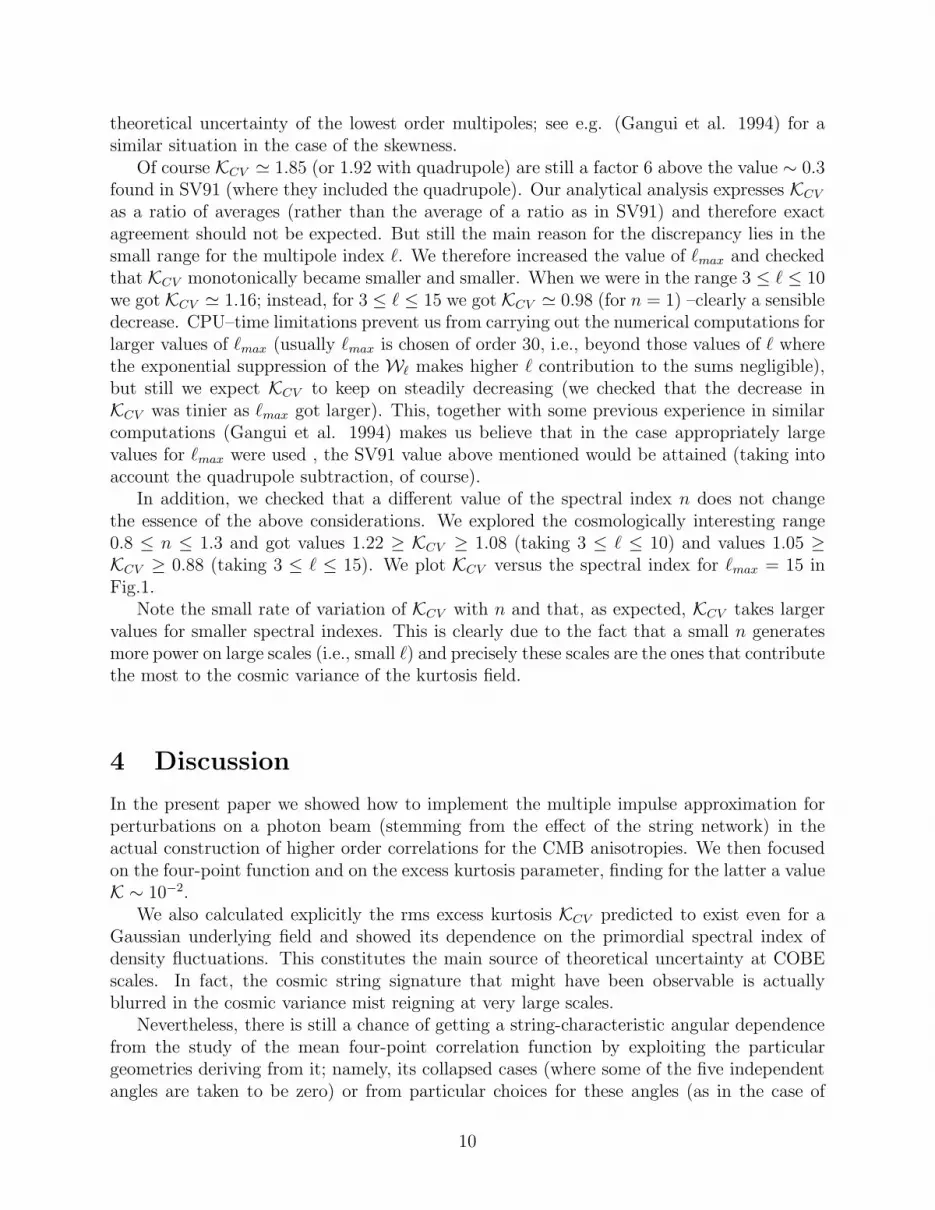
In addition, we checked that a different value of the spectral index n does not changethe essence of the above considerations. We explored the cosmologically interesting range0.8 ≤ n ≤ 1.3 and got values 1.22 ≥ KCV ≥ 1.08 (taking 3 ≤ ℓ ≤ 10) and values 1.05 ≥KCV ≥ 0.88 (taking 3 ≤ ℓ ≤ 15). We plot KCV versus the spectral index for ℓmax = 15 inFig.1.

Note the small rate of variation of KCV with n and that, as expected, KCV takes largervalues for smaller spectral indexes. This is clearly due to the fact that a small n generatesmore power on large scales (i.e., small ℓ) and precisely these scales are the ones that contributethe most to the cosmic variance of the kurtosis field.

4 Discussion

In the present paper we showed how to implement the multiple impulse approximation forperturbations on a photon beam (stemming from the effect of the string network) in theactual construction of higher order correlations for the CMB anisotropies. We then focusedon the four-point function and on the excess kurtosis parameter, finding for the latter a valueK ∼ 10−2.

We also calculated explicitly the rms excess kurtosis KCV predicted to exist even for aGaussian underlying field and showed its dependence on the primordial spectral index ofdensity fluctuations. This constitutes the main source of theoretical uncertainty at COBEscales. In fact, the cosmic string signature that might have been observable is actuallyblurred in the cosmic variance mist reigning at very large scales.

Nevertheless, there is still a chance of getting a string-characteristic angular dependencefrom the study of the mean four-point correlation function by exploiting the particulargeometries deriving from it; namely, its collapsed cases (where some of the five independentangles are taken to be zero) or from particular choices for these angles (as in the case of

10

Figure 1: Excess Kurtosis parameter of a Gaussian temperature fluctuation field as functionof the spectral index.

taking all angles equal).A preliminary analysis (Gangui & Perivolaropoulos 1994) making use of just one non-

vanishing angle in a collapsed configuration as the one mentioned above shows a potentiallyinteresting effect that could eventually increase notably the small non-Gaussian signal, andsuggests that this is indeed a subject worth of further investigation. Some of these alterna-tives are presently under study and we expect to report progress on this subject in a futurepublication.

Acknowledgements: It is a pleasure to thank A. Masiero and Q. Shafi for instructivediscussions, and for having made this collaboration possible by inviting one of us (L.P.) tolecture in the ICTP summer school. A.G. wants also to acknowledge S. Matarrese and D.W.Sciama for encouragement, and R. Innocente and L. Urgias for their kind assistance withthe numerical computations. This work was supported by the Italian MURST (A.G.) andby a CfA Postdoctoral fellowship (L.P.).

References

Abbott, L.F. & Wise, M.B. 1984, ApJ, 282, L47.

11

Allen, B. & Shellard, E. P. S. 1990, Phys. Rev. Lett. 64, 119.

Bennett, D. P., Stebbins, A. & Bouchet, F. R. 1992, Ap.J.Lett. 399, L5.

Bennett, C.L. el al. 1994, ApJ, submitted (preprint astro–ph/9401012).

Bennett, D. P. & Bouchet, F. R. 1988, Phys. Rev. Lett. 60, 257.

Bouchet, F. R., Bennett, D. P. & Stebbins, A. 1988, Nature 335, 410.

Bond, J.R. & Efstathiou, G. 1987, MNRAS, 226, 655.

Brandenberger, R., Kaiser, N., Shellard, E. P. S., and Turok, N. 1987, Phys.Rev. D36, 335.

Coulson, D., Ferreira, P., Graham, P. & Turok, N. 1993, Π in the Sky? CMB Anisotropies

from Cosmic Defects, PUP-TH-93-1429, hep-ph/9310322.

Dvali, G., Shafi, Q., and Schaefer, R 1994, preprint: hep-ph/9406319.

Fabbri, R., Lucchin, F. & Matarrese, S. 1987, ApJ, 315, 1.

Freese, K., Frieman, J.A., and Olinto, A.V. 1990, Phys. Rev. Lett. 65, 3233.

Gangui, A. 1994a, Phys. Rev. D50, xxx. (preprint astro-ph/9406014).

Gangui, A. 1994b, in proceedings of Birth of The Universe & Fundamental Physics, Rome,May 18 - 21, Ed. F. Occhionero, Springer-Verlag, in press.

Gangui, A., Lucchin, F., Matarrese, S. and Mollerach, S. 1994, Astrophys. J. 430, 447.

Gangui, A. and Perivolaropoulos, L. 1994, work in progress.

Gott, R. 1985, Ap.J. 288, 422.

Gott, J. et al. 1990, Ap.J. 352, 1.

Hara T. & Miyoshi S. 1993, Ap. J. 405, 419.

Hindmarsh M. 1993, Small Scale CMB Fluctuations from Cosmic Strings, DAMTP-93-17,astro-ph/9307040.

Kaiser, N. & Stebbins, A. 1984, Nature 310, 391.

Koratzinos, M. invited talk in the “Workshop on perspectives in theoretical and experimen-tal particle physics”, Trieste, 7-8 July, 1994.

Luo, X. 1994, ApJ 427, L71.

Magueijo, J. 1992, Phys. Rev. D46, 1368.

Masiero, A. 1984, in Grand Unification with and without Supersymmetry and Cosmological

Implications, Eds. C. Kounnas et al, World Scientific; (a comprehensive review of thevices and virtues of the standard model).

12

Mather, J. et al. 1994, ApJ, 420, 439.

Messiah, A. 1976, Quantum Mechanics, Vol.2 (Amsterdam: North–Holland).

Perivolaropoulos L. 1993a, Phys.Lett. B298, 305.

Perivolaropoulos L. 1993b, Phys. Rev. D48, 1530.

Perivolaropoulos, L. 1994, Spectral Analysis of CMB Fluctuations Induced by Cosmic Strings,Submitted to the Ap. J., CfA-3591, astro-ph/9402024.

Moessner, R., Perivolaropoulos, L. & Brandenberger, R. 1994, Astrophys. J. 425, 365.

Perivolaropoulos, L., Brandenberger, R. & Stebbins, A. 1990, Phys.Rev. D41, 1764.

Perivolaropoulos, L. & Vachaspati, T. 1994, Ap. J. Lett. 423, L77.

Scaramella, R. & Vittorio, N. 1991, ApJ, 375, 439

Shellard, E. P. S. 1994, Lectures presented at SILARG VIII. To appear in Gravitation: The

spacetime structure, Eds. Letelier P. and Rodrigues W.A., World Scientific.

Smoot, G.F. et al. 1992, ApJ, 396, L1.

Srednicki, M. 1993, ApJ, 416, L1.

Stebbins, A. 1988, Ap. J. 327, 584.

Stebbins, A. et al. 1987, Ap. J. 322, 1.

Traschen, J., Turok, N., and Brandenberger, R. 1986, Phys. Rev. D34, 919.

Vachaspati, T. 1986, Phys. Rev. Lett. 57, 1655.

Vachaspati, T. 1992a, Phys.Lett. B282, 305.

Vachaspati, T. 1992b, Phys. Rev. D45, 3487.

Vachaspati, T. & Vilenkin, A. 1991. Phys. Rev. Lett. 67, 1057-1061.

Veeraraghavan, S. and Stebbins, A. 1990, Astrophys. J. 365, 37.

White, M., Scott, D., and Silk, J. 1994, Ann. Rev. Astron. and Astrophys., to appear.

Vilenkin, A. 1981, Phys.Rev. D23, 852.

Wolfram, S. 1991, Mathematica version 2.0, Addison-Wesley.

Vollick, D. N. 1992, Phys. Rev. D45, 1884.

Wright, E.L. et al. 1992, ApJ, 396, L13.

13