Uncovering energy-efficiency opportunities in data centers

Uncovering energy-efficiency opportunitiesin data centers

H. F. HamannT. G. van Kessel

M. IyengarJ.-Y. Chung

W. HirtM. A. Schappert

A. ClaassenJ. M. Cook

W. MinY. Amemiya

V. LopezJ. A. LaceyM. O’Boyle

The combination of rapidly increasing energy use of data centers(DCs), which is triggered by dramatic increases in IT (informationtechnology) demands, and increases in energy costs and limitedenergy supplies has made the energy efficiency of DCs a centralconcern from both a cost and a sustainability perspective. Thispaper describes three important technology components thataddress the energy consumption in DCs. First, we present a mobilemeasurement technology (MMT) for optimizing the space andenergy efficiency of DCs. The technology encompasses theinterworking of an advanced metrology technique for rapid datacollection at high spatial resolution and measurement-drivenmodeling techniques, enabling optimal adjustments of a DCenvironment within a target thermal envelope. Specific exampledata demonstrating the effectiveness of MMT is shown. Second,the static MMT measurements obtained at high spatial resolutionare complemented by and integrated with a real-time sensornetwork. The requirements and suitable architectures for wired andwireless sensor solutions are discussed. Third, an energy andthermal model analysis for a DC is presented that exploits both thehigh-spatial-resolution (but static) MMT data and the high-time-resolved (but sparse) sensor data. The combination of these twodata types (static and dynamic), in conjunction with innovativemodeling techniques, provides the basis for extending the MMTconcept toward an interactive energy management solution.

IntroductionThe energy consumption of data centers (DCs) has

dramatically increased in recent years, primarily because

of the massive computing demands driven essentially by

every sector of the economy, ranging from accelerating

online sales in the retail business to banking services in

the financial industry. For example, a recent study

estimated the total U.S. DC energy consumption in 2005

to be approximately 1.2% of the total U.S. consumption

(up by 15% from 2000) [1]. The report suggests that most

of the energy-efficiency improvements that resulted from

new technology and system designs have been outpaced

by the continued demand for more computing capacity.

The report also raises concerns regarding the business and

environmental implications of this trend [2].

Consequently, concerns about DC energy efficiency have

resulted in efforts by industrial organizations, academia,

and government to first understand and then measure and

benchmark the energy consumption in DCs [3].

In a typical DC, the total power supplied to the DC

facility (PDC) is split, using a power-switching system,

into a path for the IT (information technology)

equipment and a path for systems that support the IT

equipment. The supporting path may include power

supplied to fans and blowers in air conditioning units

(ACUs, with an associated PACU) and miscellaneous

power consumption (Pmisc), for example, by ACU

humidity controls and power for lights or office spaces.

Furthermore, the support power includes power related

to the chiller system that pumps (or blows) a coolant from

the ACU to the chiller and from the chiller to the cooling

tower. Power is also required for the chiller compression

cycle (Pchiller) as well as for the cooling tower. The supply

of power for the IT equipment itself is maintained via

uninterruptible power supplies (UPSs) and distributed via

power distribution units (PDUs), which in turn power the

IT equipment (PIT). This power distribution system is

�Copyright 2009 by International Business Machines Corporation. Copying in printed form for private use is permitted without payment of royalty provided that (1) eachreproduction is done without alteration and (2) the Journal reference and IBM copyright notice are included on the first page. The title and abstract, but no other portions, of thispaper may be copied by any means or distributed royalty free without further permission by computer-based and other information-service systems. Permission to republish any other

portion of this paper must be obtained from the Editor.

IBM J. RES. & DEV. VOL. 53 NO. 3 PAPER 10 2009 H. F. HAMANN ET AL. 10 : 1

0018-8646/09/$5.00 ª 2009 IBM

also accompanied by some power losses (PPDU). Note

that all dissipated electrical power is eventually converted

into heat, following the second law of thermodynamics.

Typically, a raised floor (RF), on which IT equipment,

PDUs, and ACUs are located, is used to manage the

cooling of the IT equipment. The heat load from the

equipment on the RF is expelled to the environment from

which it is removed by a multistage cooling system, which

may require up to 50% of the total power consumption of

the DC [4].

DC energy efficiency is governed by many factors,

including the location of the DC (and the associated

weather and climate), the support infrastructure

(including such factors as building design, cooling system,

and power delivery technologies), the activities associated

with management of the DC, the IT equipment deployed,

and the associated business demands that differ among

DCs. Recent studies have shown that the level of use of

best practices (e.g., efficient management policies)

achieved in a DC has a significant impact on the energy

efficiency. In particular, power and thermal management

within the existing facility can significantly increase the

overall energy efficiency of the DC, and effective

improvements in such management can be implemented

at low cost, yielding immediate and significant energy

savings [4–6].

In the first part of this paper, we discuss how changes in

the thermal management of the equipment on the RF can

improve DC energy efficiency. Second, we present results

obtained through the use of MMT and demonstrate how

measurement-driven implementation of best practices can

improve DC energy efficiencies by up to 10%. In the third

part, the static MMT-based measurements and models

are extended toward real-time applications by

complementing the original base technology with a real-

time sensor network. Finally, we show how physics-based

and statistical modeling methods can be applied to

predict 3D thermal distributions with high resolution in

space and in time.

Data center cooling efficiency

DC cooling is accomplished via successive, thermally

coupled coolant loops, which consume energy either by

pumping or blowing a coolant or by compression work.

Specifically, the heat generated within a DC is exchanged

to a coolant (i.e., water or air) in the ACU. In most cases,

these ACUs are located directly within the DC room on

the RF, as indicated in Figure 1. The coolant is then

pumped or blown into a refrigeration unit. Often, this

unit is located in a central chiller plant (CP), where all

refrigeration is realized using a large, industrial (e.g.,

centrifugal) chiller system. In some cases, the

refrigeration unit is located within each ACU, typically

using direct expansion (DX) cooling. These systems are

generally less efficient because they are physically smaller

(and thus have more frictional losses through the entire

system) than large-scale CP systems. Finally, the

refrigeration unit is coupled to the ambient temperature

environment. In air-cooled systems, coupling is a heat

exchanger (e.g., with a blower), whereas a water-cooled

system employs a large cooling tower (making use of

evaporative cooling) to couple the chiller system to the

ambient outside temperatures.

To understand energy efficiency in the cooling system,

it is helpful to distinguish between the energy consumed,

for example, by pumps and blowers to transport the

coolant (referred to as the transport cooling power) and

the energy consumed to refrigerate the coolant

(thermodynamic cooling power). For simplification

purposes, we neglect here the relatively small energy

consumption for transporting the coolant to and from the

ACU, to the chiller, and to and from the chiller to the

ambient air. The total cooling power can be

approximated by Pcool ¼ Pchiller þ PACU, where Pchiller

represents the thermodynamic portion and PACU

represents the transport (supporting) portion of the

cooling power. For both terms, a coefficient of

performance (COP), or energy efficiency, can be defined:

COPthermo

’PRF=P

chiller; ð1Þ

COPtrans

’PRF=XNACU

i¼1

Pi

ACU; ð2Þ

IntakeACU

Cold air

Plenum

Perforated tile

Hot aisle

Cold aisle

Hot spots

ACU utilization

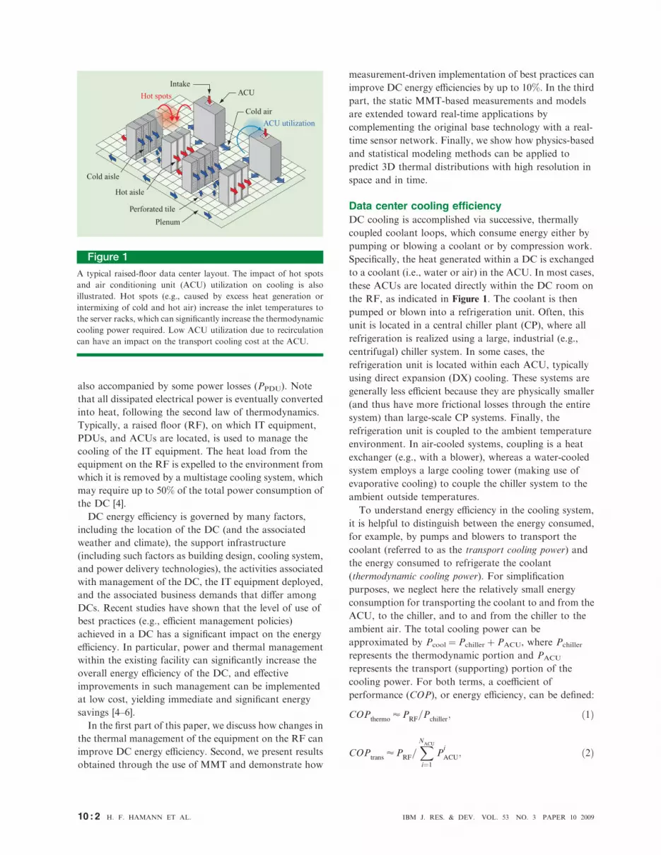
Figure 1

A typical raised-floor data center layout. The impact of hot spots

and air conditioning unit (ACU) utilization on cooling is also

illustrated. Hot spots (e.g., caused by excess heat generation or

intermixing of cold and hot air) increase the inlet temperatures to

the server racks, which can significantly increase the thermodynamic

cooling power required. Low ACU utilization due to recirculation

can have an impact on the transport cooling cost at the ACU.

10 : 2 H. F. HAMANN ET AL. IBM J. RES. & DEV. VOL. 53 NO. 3 PAPER 10 2009

where NACU is the number of active ACUs and PRF is the

total power consumed by the equipment on the DC RF,

i.e., PRF ¼ PIT þ PACU þ PPDU þ Pmisc. The power

consumption of the cooling system can be estimated using

Equations (1) and (2):

Pcool¼ P

RFð1=COP

thermoþ 1=COP

transÞ: ð3Þ

We note from Equation (2) that PRF is a function of

COPtrans, because a reduction of PACU will not only

increase COPtrans but also reduce the power consumed on

the RF.

Figure 1 shows a typical DC on a RF with front-to-

back cooling for the individual servers. In a well-managed

DC, the inlet side of a server faces a cold aisle, whereas

the exhaust side faces a hot aisle. Cold aisles and hot

aisles alternate in the DC. Cooled air from the ACUs is

provided from the plenum (sub-RF area) through

perforated tiles placed in the cold aisles. The hot air from

the server exhaust rises toward the ceiling, from where it

is returned to the ACU intake, then cooled, and then

discharged back into the plenum. Figure 1 illustrates how

improved cooling, i.e., removal of hot spots and

recirculation on the RF, can have an impact on both the

transport and the thermodynamic contributions to the

cooling energy costs.

Hot spots on the RF (e.g., due to excess heat generation

and/or intermixing of cold and hot air) increase the inlet

temperatures to the server racks, which can significantly

increase the required thermodynamic cooling power at the

chiller (Pchiller). Although every chiller system is unique

(e.g., with respect to type, chiller loading, and ambient

conditions), COPthermo in general increases as the chiller

set-point temperature is raised for a given ambient

temperature [7]. A literature search indicates an average

COP improvement by 1.7% per degree Fahrenheit (;3%

per degree Celsius) [5, 7].

We note that an increased temperature set point

(implying fewer hot spots) can also increase the duration

of free cooling opportunities. For example, if the DC has

a heat exchanger to bypass the chiller and couple the

cooling tower water directly to the building chilled water

system, free cooling can be realized if the outside

temperature is ;28F (1.18C) below the actual temperature

set point. However, with a typical chilled water

temperature set point of 448F (6.78C), the impact of the

bypass can be quite limited because the outside

temperatures are already low and the chiller efficiency is

high during this short period of the year, diminishing the

impact on savings. However, if the chilled water

temperature is higher, the duration of free cooling

opportunity typically increases in a disproportionate

manner and extends into periods in which the outside

temperatures are higher and the chiller efficiency is lower,

translating into additional savings.

Another typical example of inefficiency is illustrated in

Figure 1, involving low ACU utilization due to

recirculation, which has an impact on the transport

cooling cost at the ACU. In DCs with an over-

provisioning of cooling resources, it is quite common that

ACUs circulate the air but that the discharged air is

insufficiently reaching the inlets of the servers. In such a

case, the cooling power used by that ACU is low, which

affects the transport COP (COPtrans). For example, if a

large 106-kW ACU with 7.457-kW blower power cools

only 50 kW of heat (atypical value), the COPtrans is only

6.7, even if COPtrans could be twice as large. We note that

the actual cooling capacity of an ACU typically increases

(i.e., for .106 kW) with increasing COPtrans, if one allows

for larger temperature differences between return (intake)

and discharge temperatures of the ACU. In some cases,

ACUs are equipped with a variable frequency drive

(VFD), which can solve this problem by simply

decreasing the blower flow. However, the deployment

base of VFD ACUs is still small; thus, in this paper, we

assume that transport power savings result from turning

off ACUs.

MMT is an effective tool that can help improve the

energy efficiency of a DC by a clear identification of best-

practice measures, which, when implemented properly,

have a positive influence on both COPthermo and

COPtrans. These measures include 1) increasing the chiller

set-point temperature, which reduces the energy needs for

refrigeration (and affects the value of COPthermo), and 2)

lowering the total chilled airflow to reduce the blower and

pumping work performed by the ACUs (which affects

COPtrans).

A mobile measurement technology (MMT 1.0)Although the importance of improving the thermal and

energy management in DCs has been widely recognized, it

can be challenging to implement these concepts. First,

every DC is different, and consequently there are no

general solutions that fit all cases. Therefore, DC

managers are often just lectured to by consultants and

simply given standard, best-practice types of advice.

Thus, for these managers, it is difficult to translate general

recommendations into the context of their specific DCs.

For further consultations, a customized model of the

customer’s unique DC is required. However, in order to

build such a model, typically a detailed survey of the DC

is needed, which can be a time-consuming (and thus

costly) process. Furthermore, existing thermal models

that are based on computational fluid dynamics (CFD)

calculations do not lend themselves to rapid optimization

of the energy consumption of a DC [8]. Alternative

modeling techniques are still under development and need

to be validated and tested [9]. Even if a CFD model were

available, whether it could actually provide dependable

insights in unclear, because the input data often does not

accurately describe the DC under study [10, 11].


The MMT concept was developed to address

these challenges. It exploits a combination of rapid

data gathering and customized modeling to reveal

energy-saving opportunities and to derive specific

recommendations for the DC that is to realize these

savings. For fast data collection, MMT leverages an

emerging measurement tool for which a prototype is

shown in Figure 2(a). The tool ‘‘digitizes’’ [Figure 2(b)] the

room by scanning and quickly logging the most relevant

environmental parameters of the DC, such as

temperature, flow, humidity, and spatial dimensions.

Specifically, MMT uses a network of sensors mounted on

Max. temp.

Min. temp.(a) (b) (c) z � 0.5 feet

(d) z � 1.5 feet (e) z � 2.5 feet (f) z � 3.5 feet

(g) z � 4.5 feet (h) z � 5.5 feet (i) z � 6.5 feet

Figure 2

Monitoring of temperature in the data center: (a) measurement cart for mobile measurement technology; (b) data center layout. Here, the

blue, red, purple, light gray, dark gray, and yellow boxes indicate air conditioning units (ACUs), PDUs, network, server, storage racks, and

miscellaneous equipment, respectively. (c through i) Two-dimensional temperature distributions (see color bar) of an example data center at

different heights (z).


a supporting frame, for which each sensor defines a 3D

(three-dimensional) unit cell (8 in. 3 8 in. 3 12 in.) of the

DC. In combination with a position-tracking device,

measurements of unit cells are repeated during the scan

process throughout the 3D space of the DC, which allows

the construction of 3D images, such as heat maps, of the

space, as illustrated in Figures 2(c) through 2(i). The

current scan time is 2 seconds for each square foot and is

limited by the thermal time response of the sensors, which

have been optimized for this application. Other details of

the measurement technology can be found in Reference

[12]. The 3D data obtained with the measurement cart is

complemented with detailed airflow measurements from

each ACU and all perforated tiles. It is also complemented

by the structural details of the DC layout, as shown in

Figure 2(b), and other specific parameters of the DC,

such as the power supplied by the PDUs. These datasets

are then automatically post-processed in conjunction with

information, for example, about the layout, airflow,

ACU, and power units. Subsequently, this analysis,

together with best-practices considerations, leads to the

identification of specific energy-savings opportunities and

related recommendations [5].

Case study

In order to demonstrate the value of the MMT concept,

we discuss here example data collected from a DC with

about 20,000 square feet of RF space. The DC consisted

of various rooms and several central chiller systems. At

the time of the measurements, 37 ACUs were active, most

of them with a 7.5-kW (10-hp) blower, adding

to ;280 kW for PACU. The total power consumed on the

RF was measured to be 1.48 MW (with 1 MW for IT

equipment), which corresponds to Pchiller¼ 329 kW (with

an average COPthermo ¼ 4.5) and a COPtrans of 5.3 (i.e.,

41% ACU utilization). The MMT-based datasets

included more than 200,000 thermal, 20,000 humidity,

and more than 1,200 airflow measurements. In addition,

we identified and took into account more than 1,600 inlet

temperatures to servers and storage equipment.

Hot spots

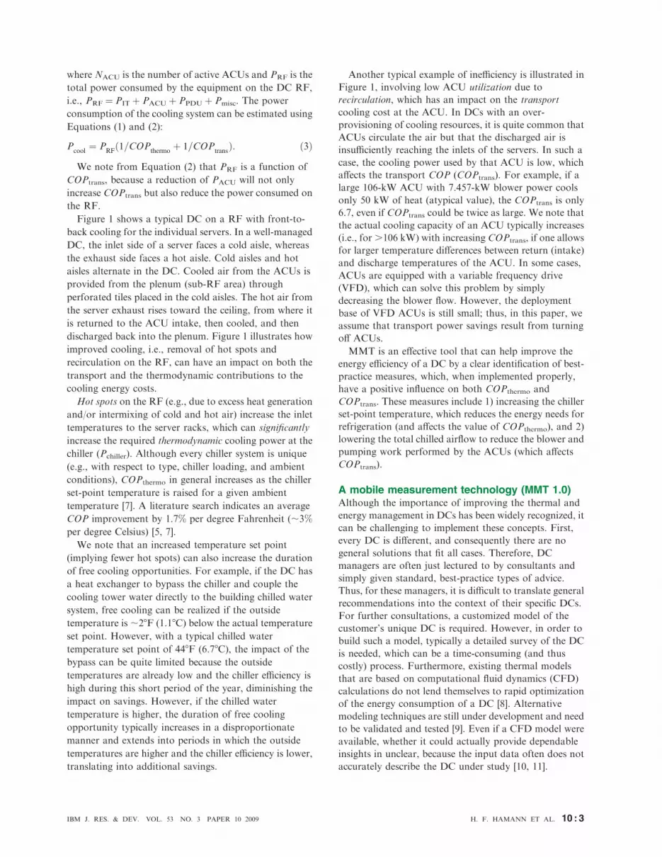
In Figure 3, two histograms of inlet temperatures (for one

location of the example DC) before and after MMT-

based hot-spot mitigation are shown. The histograms are

computed from the 3D temperature distribution in

conjunction with the layout and inlet information

gathered in the MMT survey process. Different data

points across the server inlet area have been averaged to

obtain the inlet temperature. The mean inlet temperature

in Figure 3 is 728F (22.28C), with some servers above

778F (258C).

Application of the MMT concept helps to reduce the

temperature variation across the DC RF by narrowing

the width of the histogram shown in Figure 3. Although

one in general distinguishes between vertical (or

recirculation-induced) hot spots and horizontal

(provisioning-induced) hot spots, we have applied a

simpler model here. In particular, we identified the hottest

server racks (i.e., hot spots) and coldest server racks (i.e.,

cold spots) within the DC and partitioned the airflow

provided to the respective server racks on the basis of the

airflow measurements through the perforated tiles. The

measured inlet temperature increase relative to the

bottom of a server rack, where z¼ 0, is related to the

amount of airflow reaching the respective server in the

hot and cold spots. The resulting temperature gradient is

expressed in units of Fahrenheit per cubic feet per minute

(8F/CFM). Next, the hottest server within that rack is

used to determine by how much the airflow has to be

linearly increased (for a hot spot) or decreased (for a cold

spot) to meet a new temperature target. This rather

simplistic approach works well, as shown in Figure 3(b),

where the hot spots are reduced by 48F (2.28C) simply by

60 70 80 90

Occ

urr

ence

s (

a.u.)

Inlet temperatures (°F)

(b)

Inlet temperatures (°F)

(a)

60 70 80 90

4°F

Occ

urr

ence

s (

a.u

.)

Figure 3

Inlet temperature distribution (top) before and (bottom) after

mobile measurement technology-based hot-spot mitigation. (a.u.:

arbitrary units.)


reallocating (e.g., rearranging) some of the perforated

tiles. In general, the goal of mitigating hot spots is to

increase the set-point temperature of the chiller (here, by

48F, or 2.28C), which in turn will increase the cooling

system efficiency (here, by ;7%). Note that much larger

efficiency improvements can be accomplished for DX

chiller systems or in cases in which the increased set-point

temperature leads to a longer period of free air cooling.

ACU utilization

Application of MMT includes the measurement of

temperature differentials and airflows for each ACU,

which determines the equivalent cooling power provided

by each ACU. In combination with the ACU capacity, in

this example 98 kW for a nominal temperature

differential of 158F, or 8.38C, a relative utilization level

(measured in percentage units) can be determined.

Equivalently, by using Equation (1), a value for COP for

each ACU can be determined [5]. Note that the ACU

capacity increases with larger temperature differentials;

however, we have neglected this minor effect in this

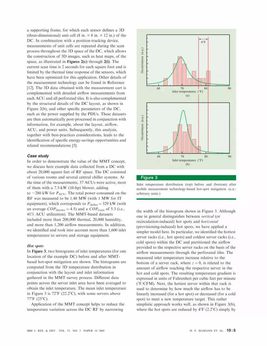
analysis. In Figure 4(a), we show a histogram of the ACU

utilization distribution for the present example with 37

ACUs. Note that the average utilization of 41% is a low

percentage, and the distribution has a large spread.

Increasing the ACU utilization has four benefits. First,

by removing (or turning off) unused ACU capacity, the

transport blower power is instantaneously saved (here,

about 7.5 kW per ACU). Second, less-active ACUs

reduce the RF power (i.e., PRF is a function of the ACU

power), which reduces the chiller load and saves

thermodynamic chiller power. Third, as shown in

Figure 4(b), higher ACU utilization decreases the

discharge temperatures (here, by 28F, or 1.18C, per 10%

utilization improvement) of the ACU because the valve

supplying the coolant is often controlled by the return

(intake) temperature of the ACU. Lower discharge

temperatures will result in lower plenum temperatures,

which in turn can be leveraged to save energy by raising

the chiller set-point temperature. Finally, higher ACU

utilization often translates into larger temperature

differentials across the ACUs, which increases the

capacities of the ACUs.

Referring back to the case study introduced above,

after the MMT survey had been completed, the IT power

consumption increased (because of new server

deployments) by 180 kW (18%) from 1 to 1.18 MW.

Nevertheless, it was recommended to reduce the number

of active ACUs from 37 to 21, a measure that brought the

ACU utilization from 41% up to 75% (with the higher IT

load), a value that still provided sufficient margin in case

of an ACU failure. The increased utilization provides a

significant temperature reduction of the discharge

temperatures of almost 78F (3.98C) in the plenum [see

Figure 4(b)]. In addition, and as shown in Figure 3, hot-

spot temperatures were decreased by 48F (2.28C) after

rearranging the perforated tiles, resulting in a total hot-

spot temperature reduction of 118F (6.18C). This enabled

an increase in the chiller set-point temperature. It was

decided to increase the chiller set point by only 88F

(4.48C) instead of the possible 118F (6.18C) in order to

meet the inlet temperature requirements. In summary,

the MMT survey yielded improved coefficients of

performance for the transport and thermodynamic parts

of the cooling system: COPtrans¼9.8 (previously, 5.3) and

COPthermo ¼ 5.1 (previously, 4.5). Considering the

increased total power consumed on the RF area (now

1.55 MW instead of the original 1.48 MW), the MMT-

induced power savings can be estimated, using

Equation (3), to be 146 kW.

Real-time sensingThe static representation of the DC derived from the

spatially dense thermal distributions obtained with

Occ

urr

ence

s (

a.u

.)

�20 0 20 40 60 80 100 120

�20 0 20 40 60 80 100 12050

60

70

80

ACU utilization (%)

(b)

ACU utilization (%)

(a)

Dis

char

ge

tem

per

ature

(°

F)

Figure 4

Air conditioning unit (ACU) utilization: (a) histogram of ACU

utilization; (b) discharge temperature as a function of ACU

utilization. (a.u.: arbitrary units.)


MMT 1.0 provides an accurate snapshot of the thermal

conditions within a DC at the time of measurement. Over

time, however, the configuration of DC equipment,

including networking and storage devices, as well as the

associated operational conditions and the airflow and

associated cooling system are all subject to continuous

change. A more dynamic measurement and modeling

approach is thus needed to provide actual, real-time

environmental status data and possibly enable predictive

evaluation of hypothetical scenarios. To a large extent,

this might be achievable by deploying a relatively small

number of real-time sensors, in judiciously chosen fixed

locations, that deliver actual measured data either at

regular intervals or upon occurrence of predefined events.

Thus, as explained in the example below, by combining or

fusing the historic static model with information based on

real-time sensor data, a dynamically adjustable model can

be constructed that reflects, or estimates in a more

accurate fashion, the actual environmental state of a DC.

Apart from making use of sensors already built into

some of the computing equipment and racks, the

preferred approach taken for collecting real-time

information covering the entire volume of a DC generally

depends on the particular aspects of a given case. Based

on certain key technical criteria, such as sensed distances

to be covered and expected data load, as well as by

considering case-by-case business-related issues, a

judicious choice must be made from a variety of available

sensor networking technologies. While some cases may be

well served with one specific sensor networking

technology, other situations may require a heterogeneous

approach. For example, an all-wired sensor network may

be the appropriate solution for relatively small and stable

DCs as well as for parts of larger DCs where mostly

stable conditions prevail. A combination of both wired

and wireless sensor networks (WSNs) may be the

preferred approach for much larger and more

dynamically managed DCs. DC areas that undergo

frequent changes over longer periods of time are typically

better served with an all-wireless system, since in this case,

flexibility and ease of installation of such a system can be

fully leveraged. When making technology-related choices,

a key criterion to consider is the cost for deploying the

sensors and their associated network infrastructure. For

example, in existing DCs, the cost for installing a cable

infrastructure for sensors can easily exceed the cost for

the sensor hardware itself, but this argument does not

necessarily apply in the case of a newly built facility.

Given that most of the existing DCs have not been

designed to easily accommodate the deployment of an all-

wired sensor network, the potential deployment costs

become a very important consideration. Thus, an all-

wireless approach or a combination of wired and wireless

sensor networks often offers the best tradeoff when

balancing overall cost with respect to the technical issues,

the flexibility for future network reconfiguration, and

performance requirements. Therefore, in the following

section, we discuss some aspects of WSNs as they relate

to their application in DCs.

Wireless sensor networks

The high density of electrical and electronic equipment

and vast amount of metal-laden racks and infrastructure

typically found in DCs generally present a considerable

challenge for any point-to-point radio communication

link. This challenge is particularly prominent for radios

using limited transmission power, as in the case of

battery-driven, low-power devices. In view of such

limitations, radio signal propagation conditions are

nearly unpredictable, and even more unpredictable in the

case of very dynamically managed DC floors. Thus, DC

settings impose particularly stringent requirements on

WSNs. For example, WSNs should feature 1) reliable

wire-like end-to-end connectivity between data sources

(sensors) and data sinks (applications), 2) robust and

scalable networks and networking protocols, 3) self-

organized, self-healing, and secure network structure

(with minimal network management overhead), 4)

battery-operated devices with a long battery life (up to

several years), 5) no interference with other systems and a

high degree of immunity to potential received interference

from any other equipment or radio system, 6) fast

deployment, easy maintenance, and transparent

application programming, and 7) simple, preferably

automatic, procedures for adding new radio nodes and

related sensors to the network. (Here, a radio node may

serve multiple sensors and actuators.)

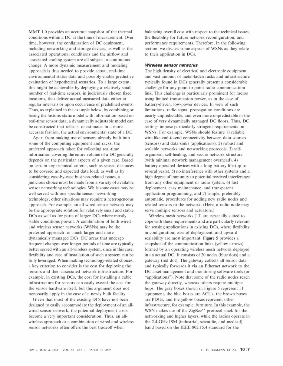
Wireless mesh networks [13] are especially suited to

cope with these requirements and are particularly relevant

for sensing applications in existing DCs, where flexibility

in configuration, ease of deployment, and upward

scalability are most important. Figure 5 provides a

snapshot of the communication links (yellow arrows)

formed by an operating wireless mesh network deployed

in an actual DC. It consists of 20 nodes (blue dots) and a

gateway (red dot). The gateway collects all sensor data

and typically forwards it via an Ethernet network to the

DC asset management and monitoring software tools (or

‘‘applications’’). Note that some of the radio nodes reach

the gateway directly, whereas others require multiple

hops. The gray boxes shown in Figure 5 represent IT

equipment, the blue boxes are ACUs, the brown boxes

are PDUs, and the yellow boxes represent other

infrastructure, for example, furniture. In this example, the

WSN makes use of the ZigBee** protocol stack for the

networking and higher layers, while the radios operate in

the 2.4-GHz ISM (industrial, scientific, and medical)

band based on the IEEE 802.15.4 standard for the


medium access control (MAC) and physical layers

(PHY). The 2.4-GHz band can be used in most

jurisdictions worldwide; however, this widely used

standard for MAC and PHY also allows its use in other

ISM bands, that is, 868 MHz in Europe as well as

915 MHz in the United States and Australia. A wide

variety of both commercial and experimental variants of

standardized as well as proprietary WSNs are currently

being deployed and tested for application in DCs. The

following simple example explains how real-time

temperature data collected by such a network can be used

to update an MMT-based model of a dynamically

changing DC.

Example: Real-time sensing and dynamic models

As an example, consider the following simple method for

combining real-time temperature data, T(r!s, tm),

measured at an actual time tm at sensor locations r!s¼ (xs,

ys, zs), with corresponding data generated by an MMT-

based temperature model, T(r!, t0), earlier validated at

time t0 , tm for r! ¼ (x, y, z) 2 R!, where R

!represents the

validated location domain of the model. As noted, in this

notation, the variable r!s is the vector pointing to the

location of the sensor, and tm stands for the time of

measurement. On the basis of the error functional

DTðr!s; t

mÞ ¼ Tðr!

s; t

mÞ � Tðr!; t

0¼ r!

sÞ; ð4Þ

and the application of some suitable interpolation or

fitting technique, an estimator for the error functional,

DT(r!, tm), can be obtained for any required position

vector r!¼ (x, y, z) 2 R!not covered by the real-time sensor

network. The original MMT-based model T(r!, t0) can

then be updated to reflect an improved model for the

temperature distribution at time tm . t0, for example, by

applying linear superposition:

Tðr!; tmÞ Tðr!; t

0Þ þ DTðr!; t

mÞ: ð5Þ

This and more sophisticated approaches used to merge

real-time data and corresponding historical models can be

extended to environmental parameters other than

temperature, for example, parameters such as airflow, air

pressure, or relative humidity. However, particularly in

the case of dynamically evolving DC environments, the

question arises as to what extent update procedures, such

as indicated by Equation (5), will deteriorate or possibly

even improve the initial accuracy of a model. Clearly, the

answer to this generally complex question largely depends

on the actual changes introduced in the DC over time,

which affect its physical infrastructure (e.g., addition or

removal of server racks) and the magnitude of change in

the environmental parameters. Suitable modeling

approaches that have the potential to provide answers to

this important question are provided in the section

‘‘Physics-based model.’’

Statistical data analysis

The above example provides high-level descriptions of a

strategy that leverages both real-time temperature and

MMT data. Here, we further discuss the details of a

statistical modeling procedure. The modeling procedures

mainly consist of two steps: baseline model and dynamic

model. We adopt T as generic notation for the

temperature measurement in the remainder of the paper.

Further, we let T(r!1, 0), . . . , T(r!N, 0) be the MMT data,

where r!1, . . . , r!N are measurement locations, and the

corresponding environmental variables are X1(0), . . . ,

Xk (0). T(r!1, t), . . . , T(r!n, t) are the real-time

measurements from n fixed sensors located at r!1, . . . , r!n,

where the corresponding environmental variables are

X1(t), . . . , Xk(t). Here, we assume that the system remains

static while MMT data is collected; in other words, all

MMT temperature data are measured hypothetically at

the same time, denoted by time zero (t0).

Baseline model

In this step, we fit a local universal kriging model to the

MMT data to obtain a detailed static temperature map

over the interested space. Since MMT data has very

detailed spatial coverage, the temperature map obtained,

denoted by Tb(r!), where b indicates baseline, provides a

Figure 5

Snapshot of the communication links (yellow arrows) formed by an

operating wireless mesh network deployed in an actual data center,

consisting of sensor nodes (blue dots) and a gateway (red dot). See

text for details.


good approximation to the true temperature at the time

t0, when MMT data is being collected.

As is often the case, physical observables in the real

world are continuous over space, and temperature data is

no exception. Therefore, the locality of the temperature

field has to be respected in a reasonable modeling

approach. To this end, we denote the spatial

neighborhood by ne(r!) according to a certain definition

(such as with a radius e) for any given r!, and further

denote by neðr!Þ the center location of this neighborhood.

The local universal kriging model consists of several

equations:

Tðr!iÞ ¼ Xðr!

iÞbþ eðr!

iÞ; ð6Þ

Xðr!iÞ ¼def

1

jneðr!iÞjX

j2neðr!iÞY r!

j

� �; r!

i� neðr!

iÞ; r!

i� neðr!

iÞ

� �2

24

35; ð7Þ

where b represents the effect of the temperature at other

neighboring locations on the temperature at the center

location. jne(r!i)j is the number of elements in ne(r!i), and

r!2 indicates all quadratic terms between components of r!.

The model can be written in matrix form by vertically

‘‘stacking’’ T(r!i), i ¼ 1, . . . , N and X(r!i), i ¼ 1, . . . , N:

T ¼ Xbþ e; ð8Þ

where cov(e)¼ R is a matrix that models the small-scale

spatial variation (e). Its elements can be parameterized

through a covariance function C(h)¼ r2 exp(�h/a), wherea is a parameter for a typical distance, r2 is a scaling

parameter, and h is a spatial distance. The model

estimation can be done through the iteratively reweighted

generalized least squares procedure [14], as follows:

1. Initialize the starting value b of b.2. Obtain R(h) from the sample variogram of the

residual R¼ T� Xb, where h denotes the variogram

parameters.

3. Update b: b [X0R (h)�1X]�1X0R(h)�1T.4. Repeat steps 2 and 3 until convergence has been

achieved.

Dynamic model

The time variation of temperature is often prominent

because of such factors as CPU usage of the servers and

changes of environmental variables such as ACU

discharge temperatures. Evidently, time variation cannot

be estimated from MMT data. However, those fixed real-

time temperature measurements become useful in spite of

limited spatial locations.

More specifically, let DT(r!, t) ¼defT(r!, t)� Tb(r

!) be

the deviation from the baseline temperature map and

DT(r!i, t)¼ T(r!i, t)� T(r!i), i ¼ 1, . . . , n, be the difference

between the measurements of the fixed sensors at times t

and t0. A universal kriging model with a polynomial trend

function can be fitted to the dataset of DT(r!i, t), i¼ 1, . . . ,

n. An immediate issue arises about how to group the

dataset from multiple time points. This matters because

the covariance function is a key component in kriging

models, and the covariance structure of temperature data

from fixed sensors varies with time. We use Figure 6 to

further illustrate this point by showing the time series of

the temperature data of two adjacent fixed sensors (here,

the unit of time is 5 seconds). The covariance matrix is

0:0213 �0:0008

�0:0008 0:0313

� �

for the first 1,000 time units, whereas it takes the values

0:3160 0:2263

0:2263 0:2255

� �

in the next 2,000 time units. The off-diagonal elements of

these two matrices indicate very different (i.e., statistically

significant) correlation patterns between the two sensors

in the two aforementioned time intervals. The dynamic

correlation structure between sensors calls for

appropriate grouping of the time series into various

regimes. Since the sensor measurements time-wise are

locally stationary, a procedure based on a covariance

matrix of sensor measurements within a moving time

window can be adopted to determine the various regimes.

Time unit (5-second interval)

0 500 1,000 1,500 2,000 2,500 3,00066

67

68

69

70

Tem

per

ature

(°

F)

Figure 6

Time series of the temperature of two adjacent fixed sensors,

illustrating the heterogeneous covariance structure. As an example

of this heterogeneity, during the time interval of 1,000 to ;1,100,

the lower series has a deep drop, while the upper series has a sharp

spike.


Next, a regime-specific universal kriging model with a

polynomial trend function can be fitted:

1. Given a regime g, compute the time average of

DT(r!i, t) :¼ DT(r!i, g) for every fixed sensor i ¼ 1,

. . . , n.

2. Fit a universal kriging modelDT(r!)¼ [1, r, r!2, r!3] cþegto the n sensors data specific to regime g (where c is a

model parameter).

3. Repeat steps 1 and 2 until all predefined regimes have

been covered.

From the estimated time-varying model, we can obtain

an estimate of DT(r!, t) for any r!, denoted by DT(r!, t). Theestimate of the temperature at location r! and time t is

then obtained by superposition T(r!, t)¼Tb(r!)þ DT(r!, t),

which completes the procedure.

Physics-based modelBy combining real-time and high-resolution

measurements, the previous two-step procedure provides

the basis for extending MMT toward an interactive

energy management solution. This data-driven approach

is suitable for fast modeling of the effect of small changes

in environmental variables. On the other hand, if a major

change in a DC (such as rearranging racks) occurs, or if

one wants to explore hypothetical configurations, one

needs to be able to quickly assess the possible impact of

such changes. Therefore, we can adopt a model based on

a set of fundamental physics to simulate this hypothetical

experiment. In this DC thermal modeling methodology,

we separate the airflow from the temperature modeling.

Specifically, we deploy potential flow theory, which

assumes a constant (temperature-independent) air

density, free slipping conditions over boundaries, and

that viscous forces can be neglected. The velocity (flow)

field is given by the gradient of a potential, with the

potential satisfying the Laplace equation. In other words,

the flow field corresponds to a solution of

]2/

]x2þ ]

2/

]y2þ ]

2/

]z2¼ 0;

vx¼ ]/

]x; v

y¼ ]/

]y; v

z¼ ]/

]z;

where / is the flow potential and vx, vy, and vz are the flow

components in the x, y, and z directions, respectively. To

provide boundary conditions for the above problem, one

could, for example, model perforated tiles or the output

of ACUs as sources (]//]z equals the negative of the

value for the measured output velocity from a perforated

tile). Also, one could model the returns to the ACUs as

sinks (/ ¼ 0), while the racks are sinks (]//]x equals the

measured inlet rack flow) and sources (]//]x equals the

negative of the value of the measured outlet rack flow) at

the same time. Once a velocity field v! ¼ (vx, vy, vz) is

obtained, it is used in the energy equation

qcpv gradðTÞ þ divðkgradðT ÞÞ ¼ 0;

with the temperature prescribed at the boundaries (e.g., at

the inlet and outlet of the servers) in order to solve for the

temperature distribution. Here, k is the thermal

conductivity, cp the specific heat, and q the density of air.

The physics-based model is fast to calculate but may

incur a systematic error in its output because of the

assumptions associated with this model. The error,

however, can be modeled with the help of MMT data. Let

T p(r!) be the output from the physics-based model with

the same environmental variables as when MMT data

was collected. First, by a similar procedure as that in the

baseline model, we obtain an estimate of the deviation of

T p(r!) from Tb(r!), that is, DT p(r!) ¼def

T p(r!) � Tb(r!).

Second, we compute the output from the physics-based

model assuming the proposed change to the DC, denoted

by T p(r!, t). The superposition of T p(r!, t) and DT p(r!)

leads to an estimate of T p(r!, t) that reflects the effect of

the change to the DC. Further decisions about whether to

implement the proposed changes in the DC can be made

from the estimated T p(r!, t), according to predefined

criteria. One example of such a criterion involves

temperature values at certain locations that must be

below a critical value during an extended period of time.

ConclusionsIn this paper, we have described three effective mitigation

methods to address the increasing energy consumption

and associated thermal problems in DCs. We 1) showed

how MMT enables improved space and energy

efficiencies of DCs, 2) showed that the static MMT

measurements, obtained with high spatial resolution, can

be combined with real-time sensor data, and 3) provided

an energy and thermal model analysis that exploits both

types of data. These three techniques provide the basis for

further extending the MMT concept toward an

interactive energy management solution. Unlike other

approaches, such as methods based on CFD

(computational fluid dynamics), the MMT concept

requires fewer assumptions, because physics-based

statistical models can often be created with hundreds of

thousands of data points, representing temperature,

airflow, and physical parameters describing the DC

infrastructure. However, further advances in the area of

DC modeling will be required to achieve reliable

predictions from modeled hypothetical scenarios. In

addition, optimal strategies for the placement of a

minimal number of real-time sensors need to be

developed based on static MMT datasets. Further

developments of the MMT concept involve the goal of


integration of MMT into middleware applications

enabling closed-loop control of ACU blowers and servers

(e.g., using clock frequency and supply voltage of

processors), with the goal of establishing a fully

interactive energy management solution for data centers.

AcknowledgmentsWe acknowledge valuable support from many of our

IBM colleagues.

**Trademark, service mark, or registered trademark of ZigBeeAlliance in the United States, other countries, or both.

References1. J. G. Koomey, Estimating Total Power Consumption by

Servers in the U.S. and the World, A report by the LawrenceBerkeley National Laboratory, February 15, 2007; see http://dl.klima2008.net/ccsl/koomey_long.pdf.

2. ‘‘Report to Congress on Server and Data Center EnergyEfficiency,’’ Public Law 109–431, United States Code (2008).

3. Green Grid Industry Consortium, ‘‘Green Grid Metrics—Describing Data Center Power Efficiency,’’ technicalcommittee white paper (February 2007).

4. N. Rasmussen, ‘‘Electrical Efficiency Modeling of DataCenters,’’ white paper, American Power Conversion,Document 113, version 1 (2006).

5. H. F. Hamann, M. Schappert, M. Iyengar, T. van Kessel, andA. Claassen, ‘‘Methods and Techniques for Measuring andImproving Data Center Best Practices,’’ 11th IntersocietyConference on Thermomechanical Phenomena in ElectronicSystems, Orlando, Florida, May 2008, pp. 1146–1152.

6. H. F. Hamann, ‘‘A Measurement-Based Method forImproving Data Center Energy Efficiency,’’ IEEEInternational Conference on Sensor Networks, Ubiquitous andTrustworthy Computing, Taichung, Taiwan, June 11–13, 2008,pp. 312–313.

7. F. W. Yu and K. T. Chan, ‘‘Low-Energy Design forAir-Cooled Chiller Plants in Air-Conditioned Buildings,’’Energy & Buildings 38, No. 4, 334–339 (2006).

8. C. Patel, C. Bash, and C. Belady, ‘‘Computational FluidDynamics Modeling of High Compute Density Data Centersto Assure System Inlet Air Specifications,’’ Proceedings of theASME International Electronic Packaging TechnicalConference and Exhibition, Kauai, Hawaii, July 8–13, 2001; seehttp://www.hpl.americas.hp.net/research/papers/power.pdf.

9. G. Li, M. Li, S. Azarm, J. Rambo, and Y. Joshi, ‘‘OptimizingThermal Design of Data Center Cabinets with a New Multi-Objective Genetic Algorithm,’’ Distributed and ParallelDatabases 21, No. 2/3, 167–192 (2007).

10. M. Iyengar, R. Schmidt, H. Hamann, and J. VanGilder,‘‘Comparison between Numerical and ExperimentalTemperature Distributions in a Small Data Center Test Cell,’’Proceedings of the ASME InterPack Conference, 2007,pp. 819–826.

11. Y. Amemiya, M. Iyengar, H. F. Hamann, M. O’Boyle,M. Schappert, J. Shen, and T. van Kessel, ‘‘Comparison ofExperimental Temperature Results with Numerical ModelingPredictions of a Real-World Compact Data Center Facility,’’Proceedings of the ASME InterPack Conference, Vancouver,Canada, 2007, pp. 871–876.

12. H. F. Hamann, J. Lacey, M. O’Boyle, R. R. Schmidt, andM. Iyengar, ‘‘Rapid Three Dimensional ThermalCharacterization of Large-Scale Computing Facilities,’’ IEEETrans. Comp. Pack. Techn. 31, No. 2, 444–448 (2008).

13. I. F. Akyildiz and X. Wang, ‘‘A Survey on Wireless MeshNetworks,’’ IEEE Commun. Mag. 43, No. 9, S23–S30 (2005).

14. P. J. Green, ‘‘Iteratively Reweighted Least Squares forMaximum Likelihood Estimation, and Some Robust and

Resistant Alternatives,’’ J. R. Statist. Soc. B 46, No. 2,149–192 (1984).

Received June 2, 2008; accepted for publicationJune 26, 2008

Hendrik F. Hamann IBM Research Division, Thomas J.Watson Research Center, P.O. Box 218, Yorktown Heights,New York 10598 ([email protected]). Dr. Hamann is currentlya Research Manager for Photonics and Thermal Physics in thePhysical Sciences department at the IBM T. J. Watson ResearchCenter. He received his Ph.D. degree from the University ofGottingen in Germany, which was followed by a postdoctoralappointment at the University of Colorado where he worked onnear-field optics. His current research interest includes nanoscaleheat transfer and thermal management. He has authored orcoauthored more than 20 peer-reviewed scientific papers, holdsmore than 15 patents, and has more than 25 pending patentapplications. Dr. Hamann is an IBM Master Inventor, a memberof the American Physical Society (APS), the Optical Society ofAmerica (OSA), and the Institute of Electrical and ElectronicsEngineers (IEEE).

Theodore G. van Kessel IBM Research Division, Thomas J.Watson Research Center, P.O. Box 218, Yorktown Heights,New York 10598 ([email protected]). Mr. van Kessel received a B.S.degree in nuclear engineering, an M.S. degree in computer science,and an M.S. degree in electrical engineering from RensselaerPolytechnic Institute. He worked in the commercial nuclearindustry for a number of years on nuclear fuel management beforejoining IBM in 1981 and finally IBM Research in 1986. He hasworked on numerous projects for IBM that include operatingsystem development, semiconductor manufacturing processcontrol, semiconductor process instrumentation, processdevelopment, and data center energy management. Currentprojects include the development of high-performance thermalsolutions for servers and high-power solar photovoltaicapplications.

Madhusudan Iyengar IBM Systems and Technology Group,2455 South Road, Poughkeepsie, New York 12601([email protected]). Dr. Iyengar is a Senior Engineer at the IBMPoughkeepsie Advanced Thermal Laboratory, working on futureenergy-efficient cooling technologies for servers and data centers.He received his B.E. degree in mechanical engineering from theUniversity of Pune, India, in 1994, and his Ph.D. degree inmechanical engineering from the University of Minnesota in 2003.He is a member of the American Society of Mechanical Engineers(ASME), the IEEE, ASHRAE (American Society of Heating,Refrigeration and Air-Conditioning Engineers), and IMAPS(International Microelectronics and Packaging Society). He hascoauthored 62 technical papers, holds 25 U.S. patents, and hasmore than 45 U.S. patents pending. In May 2007, he was chosen tobe an IBM Master Inventor for his contributions to the intellectualproperty portfolio and technical vitality of IBM.

Jen-Yao Chung IBM Research Division, Thomas J. WatsonResearch Center, P.O. Box 218, Yorktown Heights, New York10598 ([email protected]). Dr. Chung received his M.S. andPh.D. degrees in computer science from the University of Illinois atUrbana–Champaign. He is the senior manager for IndustryTechnology and Solutions, at the IBM T. J. Watson ResearchCenter, responsible for identifying and creating emerging solutionswith a focus on ‘‘green computing and business.’’ Prior to this, hewas Chief Technology Officer for IBM Global ElectronicsIndustry. He has also been the senior manager of the ElectronicCommerce and Supply Chain department and program director forthe IBM Institute for Advanced Commerce Technology office.Dr. Chung is Co-Editor-in-Chief of the International Journal of


Service Oriented Computing and Applications, published bySpringer. Dr. Chung is the co-founder and co-chair of the IEEETechnical Committee on Electronic Commerce. He has served asgeneral chair and program chair for many internationalconferences. He has authored or coauthored more than 160technical papers in refereed journals or conference proceedings. Heis a Fellow of the IEEE and a senior member of the ACM.

Walter Hirt IBM Research Division, Zurich ResearchLaboratory, Saumerstrasse 4, 8803 Ruschlikon, Switzerland([email protected]). In 1971, Dr. Hirt received his Ing. HTLdegree in electrical engineering from the HTL Brugg–Windisch,Switzerland. In 1977 and 1979, he received his B.A.Sc. and M.A.Sc.degrees, respectively, from the University of Toronto, Canada. In1988, he earned his Ph.D. degree (Dr. sc. techn.) from the SwissFederal Institute of Technology (ETH), Zurich, Switzerland, forinformation-theoretic work. He joined the IBM Zurich ResearchLaboratory, Ruschlikon, Switzerland, in 1980, where his currentinterests involve sensor networks and their use in energymanagement systems. Dr. Hirt was twice named a Master Inventorat IBM Research.

Michael A. Schappert IBM Research Division, Thomas J.Watson Research Center, P.O. Box 218, Yorktown Heights,New York 10598 ([email protected]). Mr. Schappert received hisM.S. degree from Syracuse University in 2000 in computerengineering and a B.S. degree from Union College in 1987 incomputer science. He joined the T. J. Watson Research Laboratoryin 1981 and has worked on input devices for personal computers,including eye-tracking devices, touch screens, and an infraredwireless mouse and a mouse filter for people with hand tremors.Currently, he is involved with data center optimization to help theoperators reduce power consumption.

Alan Claassen IBM Systems and Technology Group, 3605Highway 52 North, Rochester, Minnesota 55901([email protected]). Mr. Claassen is a Senior Engineer in IBMSystems and Technology Group Laboratory Services, Data CenterServices. In 1978, he received a B.S. degree in mechanicalengineering from California Polytechnic State University, San LuisObispo. In 1984, he received an M.S. degree in mechanicalengineering from Santa Clara University. He worked as a thermalengineer in IBM storage hardware development for many years. Henow supports IBM customers having data center cooling andenergy concerns.

Justin M. Cook IBM Research Division, Thomas J. WatsonResearch Center, P.O. Box 218, Yorktown Heights, New York10598 ([email protected]). Mr. Cook has a B.S. degree ineconomics from the Wharton School of the University ofPennsylvania and an M.B.A. degree from the MIT Sloan School ofManagement. He is a Business Development Manager working tocommercialize technology assets related to solar power, energyefficiency, and research software. At IBM, Mr. Cook previouslyheld the position of Global Business Development Executive,Global Technology Services, working to launch a new venture inthe small/medium business market. Prior to joining IBM,Mr. Cook spent 8 years as a management consultant and played alead role in two successful startups including Silver Oak Solutions(sold to CGI). Mr. Cook is the author of a comprehensive study onthe economic impact of venture capital investing, which formed thebasis for legislation proposed in Arizona (H.B. 2447) and Utah(H.B. 240).

Wanli Min IBM Research Division, Thomas J. Watson ResearchCenter, P.O. Box 218, Yorktown Heights, New York 10598([email protected]). Dr. Min received a bachelor’s degree inphysics from the University of Science and Technology of China in1997. He joined the physics Ph.D. program at the University of

Chicago, and passed the Ph.D. candidacy examination in 1998. In1999, he switched to the statistics Ph.D. program and earned hisPh.D. degree in statistics in 2004. He joined the IBM T. J. WatsonResearch Center in June 2004, where his current research interestsconcentrate on statistical modeling of time-series data, patternrecognition and dimension reduction of high-dimensionalstructured data, and asymptotics of stochastic processes.

Yasuo Amemiya IBM Research Division, Thomas J. WatsonResearch Center, P.O. Box 218, Yorktown Heights, New York10598 ([email protected]). Dr. Amemiya is the manager of theStatistical Analysis and Forecasting Group at the IBM T. J.Watson Research Center. He is an Elected Fellow of the AmericanStatistical Association and has served on the editorial boards ofvarious statistical journals. He manages a group of statisticsresearchers with a broad range of capabilities in methodologicaldevelopment and applied problem solving. His own researchrecord and interest also encompass a variety of statistical areas,including multivariate statistical analysis, longitudinal forecasting,structural equation modeling, and causal/intervention analysis. Heholds a Ph.D. degree in statistics from Iowa State University.

Vanessa Lopez IBM Research Division, Thomas J. WatsonResearch Center, P.O. Box 218, Yorktown Heights, New York10598 ([email protected]). In 1993, Dr. Lopez received a B.B.A.degree in computer information systems from the University ofPuerto Rico, Rıo Piedras Campus, and in 1997 she received aB.A. degree in mathematics from Rutgers, the State University ofNew Jersey. In 2004, Dr. Lopez earned her Ph.D. degree incomputer science from the University of Illinois at Urbana–Champaign, with a specialization in numerical analysis. Prior tojoining IBM, she held a postdoctoral appointment at theComputational Research Division, Lawrence Berkeley NationalLaboratory. She joined the Mathematical Sciences department atthe IBM T. J. Watson Research Center in 2006. Her interests lie inthe area of computational science, with a focus on the numericalsolution of partial differential equations.

James A. Lacey IBM Research Division, Thomas J. WatsonResearch Center, P.O. Box 218, Yorktown Heights, New York10598 ([email protected]). Mr. Lacey has a degree in appliedscience and electronics from the Academy of Aeronautics inQueens, New York. He is currently working as an associateengineer on thermal imaging studies of microprocessors andthermal profiling of data centers. In 2002, he was named an IBMMaster Inventor.

Martin O’Boyle IBM Research Division, Thomas J. WatsonResearch Center, P.O. Box 218, Yorktown Heights, New York10598 ([email protected]). Mr. O’Boyle received his B.S. andM.S. degrees in electrical engineering from the University ofDelaware in 1980 and 1982. He joined IBM Poughkeepsie in 1982,where he worked on fiberoptic networks for mainframe computers.In 1987, he joined manufacturing research at the IBM T. J. WatsonResearch Center in Yorktown Heights, working on microscopyand sensors for the IBM storage and semiconductor manufacturingfacilities, followed by projects in nanophotonics and phase-changestorage. Presently, he is working on sensor deployment in datacenters as part of a new ‘‘green’’ product offering by IBM forimproving thermal and power efficiencies.


Documents

Uncovering energy-efficiency opportunities in data centers