Types of Contact:A Field Experiment on Collaborative and Adversarial Caste Integration

Matt Lowe∗

Job Market Paper

[Please find the latest version here.]

January 18, 2018

Abstract

Integration is a common policy used to reduce discrimination, but different types of integration

may have different effects. This paper estimates the effects of two types of integration: collaborative

and adversarial. I recruited 1,261 young Indian men from different castes and randomly assigned them

either to participate in month-long cricket leagues or to serve as a control group. Players faced varia-

tion in collaborative contact, through random assignment to homogeneous-caste or mixed-caste teams,

and adversarial contact, through random assignment of opponents. Collaborative contact reduces dis-

crimination, leading to more cross-caste friendships and 33% less own-caste favoritism when voting

to allocate cricket rewards. These effects have efficiency consequences, increasing both the quality

of teammates chosen for a future match, and cross-caste trade and payouts in a real-stakes trading

exercise. In contrast, adversarial contact generally has no, or even harmful, effects. Together these

findings show that the economic effects of integration depend on the type of contact.

∗Department of Economics, MIT. E-mail: mlowe@mit.edu. I am grateful for invaluable guidance from Daron Acemoglu,Esther Duflo, Abhijit Banerjee, and Frank Schilbach. Many thanks also to Nikhil Agarwal, David Atkin, Alex Bartik, JoshDean, Stefano DellaVigna, Ben Faber, John Firth, Chishio Furukawa, Siddharth George, Bob Gibbons, Rachel Glennerster,Nick Hagerty, Karla Hoff, Simon Jäger, Donghee Jo, Tetsuya Kaji, Namrata Kala, Supreet Kaur, Gabriel Kreindler, CalvinLai, Sara Lowes, Ben Marx, Maddie McKelway, Yuhei Miyauchi, Rachael Meager, Ben Olken, Arianna Ornaghi, BetsyPaluck, Nishith Prakash, Matthew Rabin, Gautam Rao, Otis Reid, Ben Roth, Carolyn Stein, Jeff Weaver, and Roman Zaratefor helpful comments and suggestions. Thanks also to Prianka Bhatia, Yuxiao Dai, Lakshay Goyal, Omar Hoda, Azfar Karim,Shubham Maurya, Mustufa Patel, Mayank Raj, Anna Ranjan, and Yashna Shivdasani for outstanding research assistance. Iam grateful for financial support from the Weiss Family Fund, J-PAL Governance Initiative, Center for International Studies,MIT-India, and the Shultz Fund. This RCT was pre-registered in the AEA registry with ID #0001856.

1

1 Introduction

Discrimination is costly and persistent. Racial discrimination in the United States contributes to theblack-white wage gap, anti-immigrant sentiment prevents efficiency-improving labor migration, and casteprejudice in India creates barriers to intra-village trade. One possible reason for the persistence of discrim-ination is the de facto segregation of groups. This segregation can perpetuate statistical discrimination,by impeding information diffusion between groups, and arguably taste-based discrimination, by hinder-ing intergroup social interaction. Integration could reduce discrimination, though evidence exists of bothpositive and negative effects of contact with outgroups.1 One explanation for these divergent effects isthat the type of integration affects the shaping of outgroup knowledge and attitudes, a claim which is yetto be investigated in detail.2

This paper uses a field experiment in caste-segregated rural India to study the impact of two types ofintergroup contact: collaborative, where groups share common goals, and adversarial, where they insteadactively compete. I used cricket, the most popular sport in India, to integrate young men from differentcastes. From a sample of 1,261 men, I randomized 800 to play in eight month-long cricket leagues, andassigned the others to a control group. Of those assigned to play, I assigned 35% to homogeneous-casteteams, and the others to mixed-caste teams. This randomization gave the first type of cross-caste contact:collaborative – those on the same team shared the common goal of winning matches, and cooperatedtogether to achieve it. Once teams formed, I chose opponents randomly to create the second type ofcross-caste contact: adversarial – those on opposing teams had opposing goals.

Why should the type of contact matter? I argue that different types of contact provide incentives fordifferent types of intergroup interactions, and that these interactions affect inferences about the friend-liness of outgroups. The Bayesian information processor should fully condition on the type of contact,updating less when teammates are friendly than when opponents are, and updating more when teammatesare hostile than when opponents are. In this case, the type of contact does not systematically affect in-ferences about outgroups – the expected posterior is equal to the prior regardless of whether the contactis collaborative or adversarial. In contrast, agents may commit the “fundamental attribution error” (Rossand Nisbett (2011)), over-attributing the behavior of other-caste players to their types rather than their

1For example, exposure to immigrants increased anti-immigrant voting and attitudes in the US and Europe (Enos (2014),Halla et al. (2017), Tabellini (2018)), yet several papers find that intergroup roommate contact reduces prejudice (Boisjolyet al. (2006), Burns et al. (2015)).

2Allport (1954) hypothesized that intergroup contact would lower prejudice, but only under certain conditions: equal statusbetween groups, support of authority, intergroup cooperation, and common goals. Pettigrew and Tropp (2006) conclude thatthese conditions are not necessary for prejudice reduction, though the observational studies underlying their meta-analysissuffer from selection concerns and a lack of behavioral outcomes. Laboratory experiments (e.g. work on cooperation in theclassroom in the 1970s, culminating in the development of the “jigsaw learning” method, reviewed in Aronson (2011)) haveaddressed selection problems, though at the expense of some realism.

2

incentives. With these errors, collaborative and adversarial contact have opposite effects on inferencesabout the friendliness of other-caste players – collaborative contact improves outgroup inferences, whileadversarial contact worsens them. These inferences can in turn have efficiency consequences, through af-fecting the willingness to engage in cross-caste economic exchange. I designed survey and field exercisesto map to these channels by measuring participants’ willingness to interact with other-castes (as friendsand as teammates), own-caste favoritism, and efficiency in economic exchange. Participants completedthese exercises in the one to three weeks following each league.

My first set of findings consider players’ willingness to interact and own-caste favoritism. Collabo-rative and adversarial contact have opposite effects on self-reported cross-caste friendships.3 Having allother-caste teammates instead of none increases the number of other-caste friends by 1.2, while havingall other-caste opponents instead of none decreases the number of other-caste friends by 5.5. The nega-tive effect is not due to contact with opponents in general – exposure to own-caste opponents has a smallpositive effect on the number of own-caste friends.

These friendship effects are not merely driven by players becoming friends with teammates and dis-liking opponents – collaborative contact also increases cross-caste friendships with non-teammates (par-ticularly non-opponents), and adversarial contact reduces cross-caste friendships with non-opponents. Inturn, this collaborative effect on non-teammates does not come through players becoming friends withthe friends of their other-caste teammates. Instead, these effects together suggest that the two types ofcontact have opposite effects on inferences about the friendliness of other-caste men.

To explore the mechanism for these opposing effects, I exploit data on interactions observed dur-ing matches. Cross-caste interactions with opponents are 50 percentage points more likely to be hostile(arguments or insults), as opposed to friendly (high-fives, compliments, and hugs), than cross-caste in-teractions with teammates. To the extent that players attribute such behavior of other-caste players totheir caste, rather than the situation created by the experiment, these interactions naturally lead to tastesshifting in opposite directions.

In contrast with the effects on tastes for social interaction, both types of contact reduce statisticaldiscrimination (Arrow (1973), Aigner and Cain (1977), Cornell and Welch (1996)), causing more other-caste men to be chosen as teammates for a future match with monetary stakes. Two pieces of evidencesuggest that this result reflects the impact of contact on knowledge about cricket ability. First, the col-laborative effect on other-caste teammate choice is larger for those randomly assigned to have contactwith higher-ability other-caste players. However, the collaborative effect on other-caste friendships is notmediated by teammate ability. Second, when players choose teammates for an alternative match without

3I avoided experimenter demand effects by having participants select friends from a randomly-ordered list of all partici-pants, with caste neither made salient here nor when describing the purpose of the experiment itself.

3

a prize for the winner, both types of contact have smaller effects, but the adversarial effect falls signif-icantly further, to zero. Though adversarial contact conveys information about the ability of other-casteplayers, it also reduces the desire for cross-caste social interaction. When the match has no money atstake, the balance shifts to choosing players on the basis of desired social interaction, fully offsetting theinformational effect of adversarial contact.

To explore the effects of contact on own-caste favoritism, I designed an incentivized voting exercise.Each player voted to determine which representative from each team would receive professional cricketcoaching. In the voting, taste-based and statistical discrimination jointly determine favoritism – playersvote partly based on social preferences (taste-based), and partly based on beliefs about cricket ability(statistical), ranking more talented players higher. I find that collaborative contact reduces own-castefavoritism in voting by up to 33%, while adversarial contact has no effect. Complementary evidencesuggests that the collaborative effect comes mainly through effects on taste-based discrimination. Inparticular, incentivized ability beliefs at baseline are no more likely to be incorrect for other-caste thanown-caste players, limiting the scope for belief correction to explain the results.

My second set of findings explore the efficiency effects of contact. Collaborative contact enhancesefficiency in two ways. First, it increases the quality of teammates chosen for the future match witha cash prize for the winner, as measured by their predicted probability of winning the match. Thoughboth types of contact increase the number of other-caste teammates chosen, only collaborative contactaffects team quality. This finding suggests that collaborative contact could reduce one important costof discrimination emphasized in labor economics: efficiency losses in hiring that occur when employersoverlook talented outgroup candidates in favor of less-talented ingroup candidates (Hsieh et al. (2013)).

Second, collaborative contact increases cross-caste trade by up to 11 percentage points and tradepayouts by 11%, as measured in a trading exercise in which gains from cross-caste trade were introduced.Consistent with the results on team quality, the effect for adversarial contact on cross-caste trade andpayouts is statistically insignificant. The collaborative contact effect is driven by the behavior of thehighest castes, with contact increasing their cross-caste trade by up to 30 percentage points. This resultis not driven by a pure information channel of knowing other-caste players to trade with – collaborativecontact increases cross-caste trade with non-teammates by a similar amount. These results show thatcollaborative contact asymmetrically reduces social barriers to trade: the highest castes can now tradewith those below them in the caste hierarchy, but the opposite is not true, despite relatively symmetriceffects on willingness to interact socially across caste.

Taken together, my findings demonstrate that the type of contact mediates its impact: collaborativecontact increases willingness to interact with men from other castes, reduces own-caste favoritism, andincreases efficiency. In contrast, adversarial contact has no positive impacts, and can even have neg-

4

ative effects. In support of the original “contact hypothesis” of Allport (1954), contact only improvesintergroup relations when the groups have common goals. I rule out three alternative explanations thatchallenge the role of common goals. First, though contact with teammates may be more intensive thanthat with opponents, differences in intensity alone should not lead to opposite effects on tastes for cross-caste social interaction.4 Second, the two types of contact also differ in duration – contact with eachopponent only lasts for one match, whereas contact with each teammate continues for several matches.However, the longer-term nature of collaborative contact does not explain impacts – even the short-termcollaborative contact backup players experience has positive effects. Third, neither type of contact af-fects performance in the matches, showing that the mechanism does not work through income effects orsporting success.

My findings have implications for policy questions such as how to integrate refugees into society,reconcile groups in the aftermath of conflict, and reduce long-running intergroup prejudices. Integrativesports programs exist for these purposes, but evidence on their impact is scarce.5 To estimate the impactof the cricket intervention I compare those randomly assigned to the leagues with those in the purecontrol group. Despite comprising multiple types of contact, the intervention has positive effects overall.Those assigned to mixed teams make more other-caste friends than those in control, choose more other-caste teammates, choose higher quality teams, and engage in more cross-caste trade. Those assigned tohomogeneous-caste teams are also positively affected, though much less than those in mixed teams.

This paper is the first to systematically test for the effects of different types of contact (Paluck et al.(2017), Bertrand and Duflo (2017), Ashraf and Bandiera (2017)). Social psychologists have long spec-ulated that the effects of contact should depend on its type (Allport (1954)), but existing empirical testsmerely study one type of contact in isolation (Pettigrew and Tropp (2006), Carrell et al. (2015), Broock-man and Kalla (2016), Finseraas et al. (2016), Scacco and Warren (2016), Schroeder and Risen (2016),Bazzi et al. (2017)).6 For example, Rao (2014) shows that integration of rich and poor students in Delhischools increases the pro-social behavior of rich students. In his case, the contact entails a mix of col-laborative and adversarial interactions (e.g. through competing on exams) in a school setting. I instead

4More formally, in a learning framework, differences in signal precision should affect the speed of learning, but not thedirection.

5Right to Play reaches one million children weekly with sports-based programs promoting education, health and peacefulcommunities, Soccer for Peace uses sport to unite Jews and Arabs in Israel, and cricket programs unite Hutus and Tutsis inRwanda (Hoult (2016)). Ditlmann and Samii (2016) find mixed effects of an inter-ethnic sports program using a difference-in-differences design. Sport has also been explored as a means of improving intergroup relations through shared nationalexperiences (Depetris-Chauvin and Durante (2017)).

6Examples from history also suggest that economic structure can drive ethnic conflict – whether trade complementaritiesreducing Hindu-Muslim violence (Jha (2013)) or increased labor market competition promoting anti-semitic acts (Becker andPascali (2016)). One possible mechanism for these effects is that economic structure determines the nature of intergroupcontact.

5

investigate the impacts of these two different types of contact separately.The second primary contribution of this paper is to estimate the efficiency effects of contact. A

large literature shows that ethnic diversity and ingroup bias affect efficiency and allocation (Alesina andFerrara (2005), Anderson (2011), Hjort (2014), Burgess et al. (2015), Marx et al. (2016), Fisman et al.(2017)). These papers show that ethnic differences have costs; my paper is the first to show that efficiencyconsequences of integration depend on the nature of contact.

More broadly, this paper complements a large psychology and lab-experiment literature on the ef-fects of group membership (Sherif et al. (1961), Tajfel et al. (1971), Chen and Li (2009), Goette et al.(2012)) by showing that team membership can reduce prejudice in a real-world setting. This paper alsocontributes to a large body of work on caste networks (Munshi (2011), Munshi and Rosenzweig (2016),Banerjee et al. (2013), Banerjee et al. (2010), reviewed in Munshi (2016)) by exploring not just why thesenetworks matter, but also how they form.

The remainder of this paper is organized as follows. Section 2 develops a learning model to explainwhy different types of contact might have different effects. Section 3 provides an overview of India’scaste system, and motivates the use of cricket leagues as a tool for the study of contact. Section 4describes the experimental design and outcomes, while Section 5 explores the effects of both types ofcontact on willingness to interact, own-caste favoritism, and efficiency. Section 6 considers alternativeexplanations for why the type of contact matters, and Section 7 considers whether the effects of contactdiffer by caste. Section 8 investigates the overall effect of the cricket program, and Section 9 concludes.

2 Conceptual Framework

In this section I develop a simple model to show how the type of contact can mediate impacts on futureintergroup behaviors. The starting point is that integration leads to learning about the underlying “types”of other-caste players. The type of integration affects the nature of this learning by changing the structureof signals observed about others.

2.1 Bayesian Information Processing

Each participant is either a good (friendly) or bad (hostile) type, denoted by βi ∈ {βG,βB}. I assumethat each participant knows the types of players from their own caste7 (due to more frequent interaction),

7Subsequent empirical results are consistent with this – for example, own-caste contact has only weak effects on own-castefriendships (Panel B, Table 1).

6

but learns about the types of other-caste players through observing signals of their types during cricketmatches.

For simplicity, assume that two players i and j play together for one match. They face two possibletypes of contact: they either belong to the same team (m = 1) or they are opponents (m = 0). During thematch, each player can either be friendly to the other (y = 1) or be hostile (y = 0). A friendly action couldbe to encourage the other verbally, while a hostile action could be to argue with the other player. Playersi and j each observe one signal (y) from the other about their type.

I assume the net utility of player i being friendly with player j to be

ui j = α +φ11 [βi = βG]+φ2mi j + εi j (1)

where εi j ∼ Logistic(0,1). Good types have greater net utility from being friendly with others than badtypes (φ1 > 0). In addition, since teammates have common goals and opponents do not, players receivegreater net utility from being friendly with teammates than opponents (φ2 > 0).8

This underlying utility micro-founds the signal structure. Defining πβm as P(y = 1 | β ,m), the proba-

bility of seeing the other player be friendly given their type and the type of contact, it follows that

πβm = P

(ui j ≥ 0

)=

eα+φ11[βi=βG]+φ2m

1+ eα+φ11[βi=βG]+φ2m(2)

This signal structure has the following features: (i) πGm > πB

m ∀m: good types are more likely to be friendlythan bad types, whether they are teammates or opponents; (ii) π

β

1 > πβ

0 ∀β : teammates are more likely

to be friendly than opponents, whether good or bad types; and (iii) πG0

πB0>

πG1

πB1

, 1−πG0

1−πB0>

1−πG1

1−πB1

: a mono-

tone likelihood ratio property ensuring that posteriors have an intuitive ordering9 (see SupplementaryAppendix C.1 for all proofs).

Players hold the common and correct prior ρ that others are good types.10 Suppose now that players i

and j are randomly assigned to be teammates or opponents – i.e. as in the experiment, the type of contactis random. After playing the match, each player updates as a rational (Bayesian) information processor.I first consider the case where i rationally conditions on m. Here i recognizes the fact that opponents

8This could be further micro-founded by assuming that players receive utility from winning matches and that being friendlywith teammates increases the probability of winning more than being friendly with opponents.

9For example, if instead 1−πG0

1−πB0<

1−πG1

1−πB1

, it can be the case that players update less negatively after observing hostile behavior

(y = 0) from a teammate than after observing hostile behavior from an opponent. This result is counterintuitive given thathostile behavior should to some extent be expected of opponents.

10As explained below, the most important implications of the model are similar if I instead assume that players hold incorrectpriors.

7

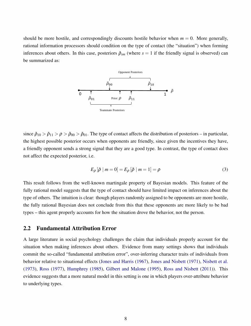
should be more hostile, and correspondingly discounts hostile behavior when m = 0. More generally,rational information processors should condition on the type of contact (the “situation”) when forminginferences about others. In this case, posteriors ρ̃sm (where s = 1 if the friendly signal is observed) canbe summarized as:

𝜌

Prior: 𝜌

Teammate Posteriors

Opponent Posteriors

𝜌01 𝜌11

𝜌10 𝜌00

0 1

since ρ̃10 > ρ̃11 > ρ > ρ̃00 > ρ̃01. The type of contact affects the distribution of posteriors – in particular,the highest possible posterior occurs when opponents are friendly, since given the incentives they have,a friendly opponent sends a strong signal that they are a good type. In contrast, the type of contact doesnot affect the expected posterior, i.e.

Eρ [ρ̃ | m = 0] = Eρ [ρ̃ | m = 1] = ρ (3)

This result follows from the well-known martingale property of Bayesian models. This feature of thefully rational model suggests that the type of contact should have limited impact on inferences about thetype of others. The intuition is clear: though players randomly assigned to be opponents are more hostile,the fully rational Bayesian does not conclude from this that these opponents are more likely to be badtypes – this agent properly accounts for how the situation drove the behavior, not the person.

2.2 Fundamental Attribution Error

A large literature in social psychology challenges the claim that individuals properly account for thesituation when making inferences about others. Evidence from many settings shows that individualscommit the so-called “fundamental attribution error”, over-inferring character traits of individuals frombehavior relative to situational effects (Jones and Harris (1967), Jones and Nisbett (1971), Nisbett et al.(1973), Ross (1977), Humphrey (1985), Gilbert and Malone (1995), Ross and Nisbett (2011)). Thisevidence suggests that a more natural model in this setting is one in which players over-attribute behaviorto underlying types.

8

To model these attribution errors, I assume that players continue to use Bayes’ rule to update beliefs,but fail to condition on m (similar to the approaches of Jehiel (2005), Eyster and Rabin (2005), andmost recently, Furukawa (2017))11 – treating signals from teammates and opponents identically.12 It nowfollows that

Ebρ [ρ̃ | m = 0]< ρ < Eb

ρ [ρ̃ | m = 1] (4)

where the b superscript references the bias. With attribution bias, the type of contact systematicallyaffects the expected posterior, with the two types of contact moving the expected posterior in opposite

directions from the prior. In expectation, players infer that randomly chosen opponents are less likelyto be good types than randomly chosen teammates. Players do so because, conditional on the type ofbehavior observed, players have the same posterior belief regardless of whether the observed behaviorwas from an opponent or from a teammate. Since friendly signals are more likely to be observed fromteammates, this attribution bias leads the expected posteriors to diverge.

2.3 Decisions to Interact

I do not observe ρ̃ directly in the data. Instead, I observe each player’s choices of whom to interactwith and whom to favor. Focusing on the case of social interaction, suppose that players select others asfriends only when ρ̃ > c. Without attribution bias, it follows that

P(ρ̃ > c | m = 0)≶ P(ρ̃ > c | m = 1) (5)

meaning that, without bias, the type of contact has an ambiguous effect on the likelihood of friendship,with the ambiguity depending on the exact cutoff c. For some cutoffs it is even possible for opponentsto be more likely to become friends than teammates. This result holds because an instance of opponentfriendliness is particularly informative of their type. The model with attribution bias does not have thesame ambiguity, since regardless of c it implies that

11I am agnostic as to the source of the lack of conditioning, though one possibility is that conditioning takes cognitiveeffort. In support of this explanation, evidence exists that individuals are more likely to commit the fundamental attributionerror when under cognitive load (Gilbert (1989)). An alternative explanation is that individuals’ motivated “belief in a justworld” leads them to attribute behaviors to internal factors rather than external causes, such that people “get what they deserve”(Benabou and Tirole (2006)).

12Haggag and Pope (2016) study intrapersonal (as opposed to interpersonal in this paper) attribution bias in the context ofconsumer choice: when individuals decide their value of drinking a new drink, they fail to properly condition on the (random)state in which they consumed it last time. Their model of attribution bias does not explicitly map to Bayesian learning, but hasthe advantage of allowing attribution bias to range from zero to one, nesting the extreme cases of perfect and no conditioning.Other papers in economics study intrapersonal attribution errors through the lens of motivated forgetting, e.g. through recallingpast successes more than past failures (Benabou and Tirole (2002), Benabou and Tirole (2006)).

9

Pb (ρ̃ > c | m = 0)≤ Pb (ρ̃ > c | m = 1) (6)

i.e. players are weakly more likely to become friends with teammates than opponents.

2.4 Discussion

Friendliness vs. Ability. In the model, players update only about the friendliness of other-caste players.In the experiment, there is an important second dimension of updating: players learn about the cricketingability of other-caste players. Along this dimension, it is plausible that the type of contact should notaffect updating. Though participants observe very different signals of friendliness from teammates vs.opponents, the signals of cricket ability observed are likely to be similar. In this sense, the type of contactmight systematically affect learning along some dimensions but not others.

Discrimination and Stereotyping. The idea of updating along two dimensions (friendliness and ability)has parallels in both economics and psychology. In economics, models of discrimination largely fall intotwo categories: taste-based (Becker (1957)) and statistical discrimination (Arrow (1973)). Taste-baseddiscrimination concerns the differential treatment of groups conditional on known ability (or productivity)being equivalent. Though usually thought of as a preference-based form of discrimination, we might alsothink of taste-based discrimination as being related to beliefs about whether others are friendly or not.Put differently, distaste for outgroups is quite closely related to the lack of desired social interaction withoutgroups, in that both are independent of beliefs about ability. Statistical discrimination on the otherhand regards discrimination of groups due to beliefs about ability, even in the absence of any distastefor outgroups. This concept maps well to the possibility of players segregating by caste (in teams) notbecause they have a distaste for other castes, but because they have less information about the abilityof other-caste players. Similarly, psychologists have argued that most stereotypes regarding outgroupsfall naturally among two dimensions: warmth and competence (Fiske et al. (2002), Fiske et al. (2007)).These dimensions map to friendliness and ability respectively.

Incorrect Priors. To simplify the exposition, I assume that priors are correct. A more plausible assump-tion may be that priors are incorrect, such that ρ 6= ρ t , where ρ t is the true proportion of other-castes thatare good types. In this case, the type of contact can affect the speed of learning (| ρ t −Eρt [ρ̃ | m = x] |)even in the absence of attribution bias.13 But only with attribution bias can the learning (in expecta-tion) go in opposite directions from the prior, depending on the type of contact. In this sense, even with

13However, the predicted effect of the type of contact on the speed of learning is of ambiguous sign.

10

incorrect priors the model with attribution bias is a more natural model through which to interpret theresults.

Individuals vs. Groups. The model focuses on inferences about the types of individuals. Similarupdating can occur about the caste group as a whole if we assume a second level of uncertainty, regardingthe proportion of types in the caste group. Signals of behavior from individuals are then used to alsoupdate about the group. In the empirics I explore effects of contact on behaviors toward individualsdirectly interacted with, as well as the broader caste group.

3 Background on Caste and Cricket

3.1 A Brief History of Caste

The Indian caste system dates back to as far as 1500 BCE. According to the Manusmriti, an ancientHindu legal text, individuals belong to one of four ordered social categories, called varnas: Brahmins,Kshatriyas, Vaishyas, and Shudras, with the lowest social group, the untouchables, outside of this classsystem altogether. Each of these groups contains hundreds of sub-groups, called jatis, within whichHindus historically must marry. In addition to endogamy, the caste system features norms of contactbetween the groups (e.g. whether food can be shared), residential segregation, and traditional occupations(Ghurye (1932)).

Two theories about the Indian caste system predominate. One is that the caste system has ideologicalorigins which are based on notions of purity and impurity, and which naturally lead to a hierarchy inwhich the pure and impure are opposed (Dumont (1970)). The other theory argues that caste is not merelyIndian tradition, but rather a modern phenomenon, shaped by economic and political interests. Dirks(2011) in particular argues that colonialism molded the caste system – through the British strengtheningcaste affiliation through censuses, branding some castes as “criminal”, and showing preferential treatmentto others in hiring.

In the postcolonial era, caste continues to be a central feature of Indian society. The caste-basedreservation of jobs, begun by the British, was formalized. Erstwhile untouchables, and some others,were classified as Scheduled Castes (SC), with indigenous tribes classified as Scheduled Tribes (ST). Inattempts to correct past discrimination, the government imposed quotas for these groups in governmentjobs, in higher education, and in politics. After the Mandal Commission in 1979, the government ex-tended quotas to include another group of historically disadvantaged castes, the Other Backwards Castes

11

(OBC).Though the core of the caste system rests with the endogamous jatis, the government categories of

General, OBC, and SC/ST, are natural groups to consider when studying discrimination in India (Munshi(2016)).14 These groups follow a traditional hierarchy – with General above OBC, and OBC aboveSC/ST. In this paper I use “cross-caste” to refer to interactions between these three groups,15 and unlessstated otherwise, all subsequent references to caste refer to one of these three groups.

3.2 Caste in Modern India

Discrimination. Despite decades of illegality under the Indian Constitution, discrimination of lowercastes (or “untouchability”) continues to be widespread. Thiry-seven percent of General and OBC house-holds in Uttar Pradesh (25% in India), the Indian state where I ran the experiment, practice untouchability(Desai et al. (2011)). On the opposite side, 27% of Scheduled Caste households in Uttar Pradesh reportexperiencing untouchability in the past five years (19% in India). Despite persistent discrimination, thereis evidence that affirmative action has improved the economic status of low castes. For example, themedian wage premium of non-SC/STs relative to SC/STs fell from 36 to 21% during 1983 to 2004(Hnatkovska et al. (2012)).

Segregation. Castes are segregated through marriage, geography, and social networks. Marriage seg-regates because endogamy is widely practiced – 98% of married women respondents in Uttar Pradeshmarried within caste (Desai et al. (2011)). Though many castes often reside in the same village, geo-graphical segregation results from castes living in separate hamlets. Reflecting these living arrangements,though each jati makes up on average 6% of a village’s population, roughly 50% of food transfers andloans come from within the same jati (Munshi and Rosenzweig (2015)). Figure C1 illustrates the socialsegregation at baseline for three of the eight study locations where I organized cricket leagues. Formally,following Jackson (2010) I measure caste-based homophily as how prevalent friendships are betweensame-caste pairs compared to pairs in the network overall. A measure above one reflects that friendshipsare more likely to be formed within groups than across groups. The average homophily across the eightlocations is 1.93 – study participants are roughly twice as likely to form friendships with a participantfrom the same caste than with a participant in general. For comparison, Jackson (2010) finds race-basedhomophily in US high schools to be lower, at 1.4 on average.

14To focus on caste and not religion, I only considered villages with few or no Muslims for the experiment. In practice,only 2.9% of participants were Muslim. These participants could still be assigned a caste given that Muslim communities arealso formally classified as General, OBC, or SC/ST.

15The grouping of SCs and STs together is reasonable given their similar histories of discrimination and given that only1.6% of participants in this study are STs.

12

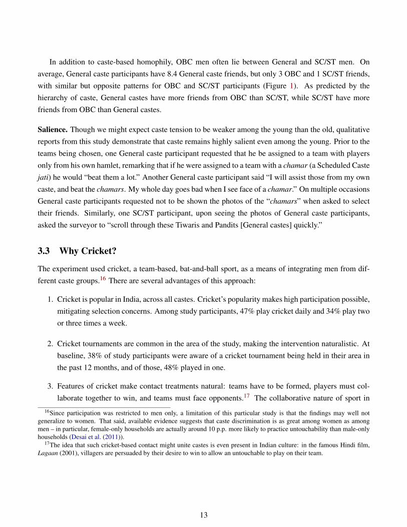
In addition to caste-based homophily, OBC men often lie between General and SC/ST men. Onaverage, General caste participants have 8.4 General caste friends, but only 3 OBC and 1 SC/ST friends,with similar but opposite patterns for OBC and SC/ST participants (Figure 1). As predicted by thehierarchy of caste, General castes have more friends from OBC than SC/ST, while SC/ST have morefriends from OBC than General castes.

Salience. Though we might expect caste tension to be weaker among the young than the old, qualitativereports from this study demonstrate that caste remains highly salient even among the young. Prior to theteams being chosen, one General caste participant requested that he be assigned to a team with playersonly from his own hamlet, remarking that if he were assigned to a team with a chamar (a Scheduled Castejati) he would “beat them a lot.” Another General caste participant said “I will assist those from my owncaste, and beat the chamars. My whole day goes bad when I see face of a chamar.” On multiple occasionsGeneral caste participants requested not to be shown the photos of the “chamars” when asked to selecttheir friends. Similarly, one SC/ST participant, upon seeing the photos of General caste participants,asked the surveyor to “scroll through these Tiwaris and Pandits [General castes] quickly.”

3.3 Why Cricket?

The experiment used cricket, a team-based, bat-and-ball sport, as a means of integrating men from dif-ferent caste groups.16 There are several advantages of this approach:

1. Cricket is popular in India, across all castes. Cricket’s popularity makes high participation possible,mitigating selection concerns. Among study participants, 47% play cricket daily and 34% play twoor three times a week.

2. Cricket tournaments are common in the area of the study, making the intervention naturalistic. Atbaseline, 38% of study participants were aware of a cricket tournament being held in their area inthe past 12 months, and of those, 48% played in one.

3. Features of cricket make contact treatments natural: teams have to be formed, players must col-laborate together to win, and teams must face opponents.17 The collaborative nature of sport in

16Since participation was restricted to men only, a limitation of this particular study is that the findings may well notgeneralize to women. That said, available evidence suggests that caste discrimination is as great among women as amongmen – in particular, female-only households are actually around 10 p.p. more likely to practice untouchability than male-onlyhouseholds (Desai et al. (2011)).

17The idea that such cricket-based contact might unite castes is even present in Indian culture: in the famous Hindi film,Lagaan (2001), villagers are persuaded by their desire to win to allow an untouchable to play on their team.

13

general was apparent to Allport, the originator of the contact hypothesis, who wrote in The Nature

of Prejudice:

Only the type of contact that leads people to do things together is likely to result

in changed attitudes. The principle is clearly illustrated in the multi-ethnic athletic

team. Here the goal is all important: the ethnic composition of the team is irrelevant.

It is the cooperative striving for the goal that engenders solidarity. (Allport (1954))

4. Features of cricket resemble other economic settings. Players exert individual effort for economicincentives. Players must cooperate with team members to maximize performance – with a ten-sion between what is optimal for the team and what is optimal for the individual (as with teamproduction). Teams defer authority to captains (bosses), and teams compete with others (as withcompetition for promotions in firms).

A final motivation for using cricket leagues is the measurement advantages they provide. First, featuresof cricket give natural within-match measures of discrimination, since teams must prioritize some playersover others, as well as pick team captains. These measures are unobtrusive since they must be collectedto score the matches. Second, individual-level ability can be accurately measured given that the mainaims of each player are straightforward and structured. Batters must hit the ball far and bowlers mustthrow the ball fast toward the wickets. Baseline ability measures can then be used as controls whentesting for within-team discrimination. This feature is an advantage relative to other sports. For example,in soccer, ability is more multi-dimensional, with players specialized to their position (e.g. defender),making ability comparisons between players difficult.

3.4 Cricket: A Primer

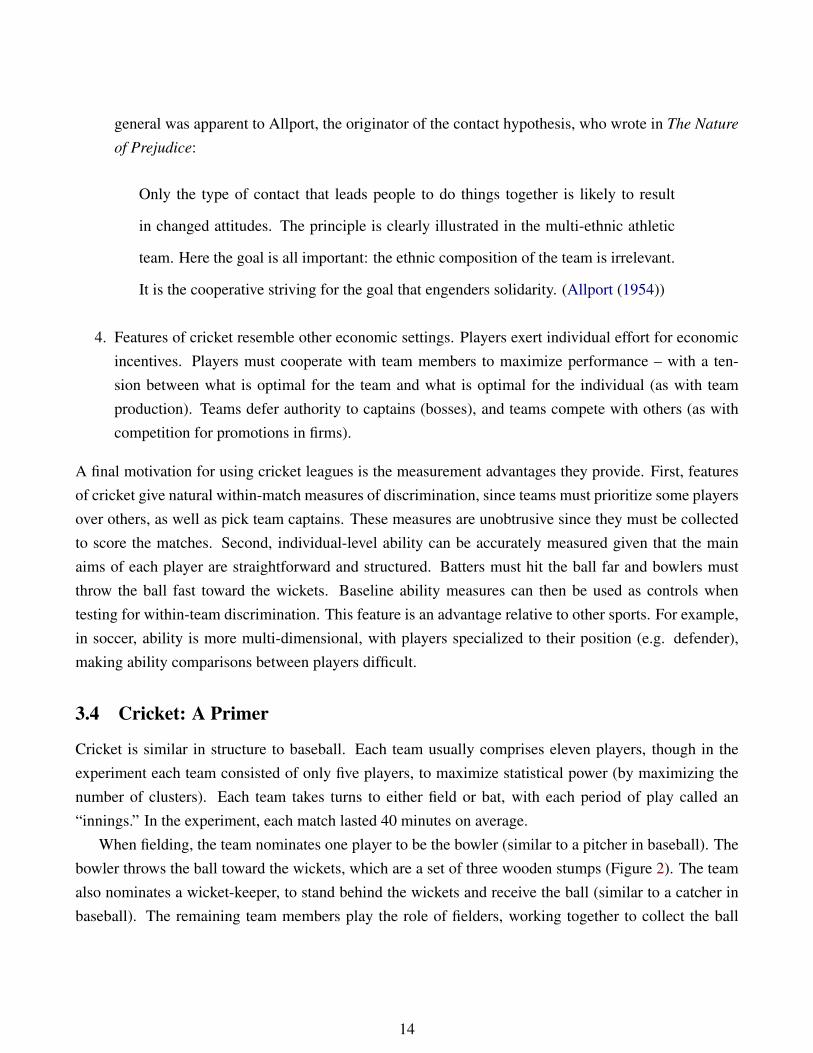
Cricket is similar in structure to baseball. Each team usually comprises eleven players, though in theexperiment each team consisted of only five players, to maximize statistical power (by maximizing thenumber of clusters). Each team takes turns to either field or bat, with each period of play called an“innings.” In the experiment, each match lasted 40 minutes on average.

When fielding, the team nominates one player to be the bowler (similar to a pitcher in baseball). Thebowler throws the ball toward the wickets, which are a set of three wooden stumps (Figure 2). The teamalso nominates a wicket-keeper, to stand behind the wickets and receive the ball (similar to a catcher inbaseball). The remaining team members play the role of fielders, working together to collect the ball

14

and return it to the bowler and the wicket-keeper. When batting, only two members of the team play atany one time, both as batsmen. The batsmen attempt to score as many “runs” as possible, which they doby hitting the ball and then running between the wickets, or by hitting the ball sufficiently far (towardor beyond the “boundary”) such that they score a four or a six. The fielding team attempts to minimizethe number of runs the batting team scores. They can do this, for example, by hitting the wickets whenbowling (meaning the batsman at that end is “dismissed” and must be replaced by the next person in thebatting order), or by catching the ball when it is hit into the air.

Types of Contact in Cricket. Players on the same team share the common goal of winning the match,and must collaborate to achieve this goal. To succeed when batting, batting partners must communicate,discussing when and how much to run between the wickets. They must coordinate their running to avoidbeing dismissed, in the same way that baseball players must coordinate when running between bases.When fielding, all team members are on the field, and to succeed they must cooperate with the bowler andwicket-keeper, who call to receive the ball from where it was hit. At half-time, each team gathers togetherfor a team talk, ostensibly to strategize how to play in the second innings. The collaborative contact incricket entails both learning about the ability of teammates and experiencing cooperative interaction withthem. Each of these channels could potentially affect cross-caste interaction and attitudes.

In addition, I exploit the interaction between opposing teams to identify the effect of adversarialcontact. Teams achieve their common goal by playing competitively against their opposition – bowlingfast, batting hard, and challenging decisions that the umpire (referee) makes in the other team’s favor. Aswith collaborative contact, players learn about the ability of opponents. In contrast, players experiencecompetitive interaction with them. Adversarial and collaborative contact may then have different effects– in particular, their effects on inferences about friendliness are more likely to diverge than their effectson inferences about ability (or statistical discrimination).

4 Experimental Design

4.1 Recruitment and Baseline Activities

Site Selection. Participants were recruited from eight gram panchayats18 (GPs) near Varanasi (a city inUttar Pradesh), with one cricket league organized per GP.19 The experiment ran in three phases, with twoleagues during the first phase, and three during each of the latter phases. The matches were played from

18Local administrative unit comprising several villages.19In some cases the catchment area for a league included an additional neighboring GP, but for simplicity I will refer to

each catchment area as being a single GP.

15

January to July 2017. GPs were selected according to several criteria, including that the GP must have:caste-segregated hamlets, a supportive pradhan (elected village head), roughly equal caste proportions,and an available cricket field.20 From among 100 GPs visited by the field team, eight were chosen thatmet these criteria.

Participant Recruitment. In each GP, surveyors spent the first five days recruiting males aged 14 to30 to play in the upcoming cricket league (see Timeline in Figure 3). We advertised the basic details ofthe leagues using posters (Figure C2), and via direct contact from Sarathi Development Foundation (ourNGO partner) staff. The information made clear that teams would be chosen by the organizers and not bythe participants themselves. This approach may have screened out those more prejudiced against othercastes, making measures of prejudice and effects of collaborative contact potentially underestimates.By targeting particular hamlets, we kept recruitment roughly equally balanced across the three castecategories.21 Men who expressed interested completed a baseline survey and were informed that theirsign-up was not complete until their cricket ability was tested.

Study Construal. Throughout the experiment, we minimized the salience of caste. We did so to avoidpriming (as in Hoff and Pandey (2014)), social desirability bias (Paluck and Shafir (2017)), and threats tothe experiment’s implementation from local resistance. In this spirit, we told participants during baselinethat “we are recruiting men interested in playing in cricket tournaments for money. Our aim is to usecricket tournaments to bring the community together, and to study how cooperative and competitive menare in rural India.” Similarly, when introducing the trading exercise, we told participants that “the tradinggame will allow us to study trading and cooperative behavior in Indian villages.”

Ability Testing. Following the five days of recruitment, surveyors spent five days testing the cricket abil-ity of each participant. Holding the ability testing separately from the baseline survey served a screeningpurpose: by increasing the time cost of signing up, the less enthusiastic participants (who might haveattended fewer matches) were screened out.22 Cricket ability was measured along three dimensions:bowling, batting, and fielding. For bowling, participants bowled six balls towards the wickets, and wemeasured both the speed (using speed guns) and accuracy (by recording the number of times the wicketswere hit, and whether the ball was valid, wide, or a no ball). For batting, a surveyor bowled six ballstowards the wickets, and the participant attempted to hit each ball. We recorded whether each ball was

20Secondary criteria included: large population of interested cricketers, few or no Muslims, not used in piloting, and nocricket tournament running at the same time.

21Of the 1,261 participants, 32.7%, 35% and 32.3% were from General, OBC, and SC/ST castes respectively.22There is evidence of selection: those that did not complete ability testing (308 of 1,569) were less likely to say that they

play cricket daily (31% vs. 47%).

16

hit, and if so whether it was hit sufficiently far to score either a four or a six. For fielding, a surveyorthrew six balls high in the air towards the participant. We recorded how many balls were successfullycaught, and how many times the participant hit the wickets with their return throws. Each team’s abilityresults were made common knowledge within the team by a surveyor who read out the results prior tothe team’s first and second matches. Teams could opt-in to hearing the results again from the third matchonwards but did so for only 7% of the matches. The ability measures are strongly predictive of leagueperformance, as shown in Section 7.

Social Networks. Once the participants were finalized, we administered a short social network survey.Each participant was shown a list of the full names and photos of all other participants and asked whichthey considered to be friends. Though caste cannot be visibly discerned, it is usually signalled stronglyby the last name a person uses. When participants are asked to guess the caste category of a hypotheticalname at endline, they correctly identify the name as belonging to the same or a different caste 80% ofthe time. This figure represents a lower bound on caste recognition during the experiment itself, sincebeyond observing last names, participants may recognize the photo and correctly infer caste throughknowing what hamlet the individual lives in.

4.2 Treatments

League Assignment. In each GP, 100 participants were randomly assigned to play in the cricket league.This randomization was stratified on caste.23 I assigned the remaining participants to the control group.

Team Assignment. I assigned the 100 league players to 20 teams of five players each. 35% of the playerswere randomly assigned to homogeneous-caste teams, making seven out of 20 teams homogeneous-caste.I pooled and randomly ordered the remaining players. Each sequence of five then formed a mixed-casteteam.24

Match Schedule. I scheduled each team to play eight matches, never playing the same team morethan once. The problem of randomly choosing a match schedule is identical to the network problem ofchoosing a random simple regular graph. In this case, each of the teams represents a node in a network.A k-regular graph is a graph where each node is connected to exactly k others. If this graph is simple, nonode is connected to itself (no “loops”) or to another node more than once (no “parallel edges”). A matchschedule in which 20 teams each play eight matches (never playing themselves and never playing against

23Further details of the randomization are in Appendix C.2.24There were 104 mixed-caste teams in total. In principle, homogeneous-caste teams could have occurred here by chance,

but none did, leaving the total number of homogeneous-caste teams at 7*8 = 56.

17

a given team more than once) can be represented by a simple 8-regular graph with 20 nodes. I randomlychose a graph for each league using an existing algorithm, Bollobás’ “pairing method” (see AppendixC.2 for details).

The algorithm generated an adjacency matrix for each league, representing which teams were to playwhich. With these matrices I scheduled 80 matches per league, with the matches randomly ordered. Therandomness of the match schedule ensured that a given player’s exposure to other castes as opponentswas also random.25 Together, the assignment to teams and random match schedule created significantvariation in collaborative and adversarial cross-caste contact (Figure 4).

Recognizing Caste. To avoid explicit references to caste, participants were not directly told the castegroup of their teammates and opponents. However, several features of the experiment enable caste to beidentified implicitly. First, when players are informed of their team assignment by phone, they are toldthe full names and father’s names of their teammates, with these names strongly signalling caste. Second,close interaction with teammates on the pitch, including mandatory team talks, gives opportunities forteammates to learn each other’s caste. Third, the catchment area for each league is sufficiently small thatplayers can recognize their teammates and opponents, even if they are not friends – indeed when playersare asked on the phone whether they know of their randomly assigned teammates, 39% say yes when theteammate is from the same caste, and 27% still say yes when the teammate is from a different caste. Thecorresponding figures for baseline friendships are 15% and 4%, suggesting that even though participantsare far more likely to be friends with members of their own caste, they are not that much more likely toknow them than participants from other castes. Fourth, during the matches the full names of bowlers arecalled out whenever the bowler is to be changed. Fifth, spectators at the matches26 frequently call out thenames of players, and sometimes even refer to players using caste slurs.

4.3 Additional Program Features

Ability Priors. Upon learning their team assignment, we elicited cricket ability priors by asking partici-pants to predict the eventual ranking of themselves and their teammates according to batting strike rate, acommonly used measure of batting ability. The prediction was incentivized – at endline we paid Rs. 50(~$0.80) to those that guessed the ranking correctly. I use the predictions to explore belief correction asa possible mechanism for the effects of contact.

25More precisely, it is random conditional on the caste composition of his own team. For example, if a player has fourother-caste men on his team, he is less likely to be exposed to other-caste opponents than a player with only one other-casteman on his team. All analysis of adversarial contact effects below controls for on-team cross-caste exposure.

26On average, 17 spectators attend each match.

18

Incentives. To track the progress of teams in the league, a league table was updated daily and displayedat the cricket field (Figure C3), making the competition between teams salient. At the end of the league,the best three teams according to this league table won trophies and cash prizes (Rs. 1500/1000/500 or~$23/16/8). Similarly, the best three players (based on number of times voted man-of-the-match27) wontrophies and cash prizes (Rs. 500/350/200 or ~$8/5/3).

We also paid each player a cash incentive based on his cricket performance following each match.The exact type of monetary incentive was randomized. Of the 20 teams participating in each league,I randomized 10 teams to receive Individual Pay and the remaining 10 to receive Team Pay. We paidplayers on Individual Pay teams according to individual performance (giving on-team inequality) whileplayers on Team Pay teams were paid based on team performance (giving on-team equality).28 Theincentive structure affected the competitiveness and payout inequality among teammates, providing a testof whether effects of collaborative contact are sensitive to the heightening of within-team competition.

Backup Protocol. Ideally the control-group players would play no matches at all (preserving their“control-ness” for program evaluation), but 100% attendance among players could not be guaranteed,and cricket matches are difficult to play without a full roster of players. As a result, control participantsserved as backup players.

To preserve a control group with very few matches actually played, we followed a strict backupprotocol. I assigned a priority number randomly to each backup, within each caste. If a particular playercould not attend one of his matches, surveyors called a backup player from the same caste in priorityorder. This protocol ensured that only high-priority backups played frequently – while the three highest-priority backups played six to eight matches on average, the remaining backups played far fewer (FigureC5). Since I chose the priority order randomly conditional on caste, the low-priority backups serve as avalid control group within each caste. In addition, by replacing absent players with someone of the samecaste29 I kept the caste composition of each team constant, preserving the collaborative contact treatment.

Attendance. I took several steps to address concerns of low attendance: (i) we gave a Rs. 10 (~$0.15)show-up fee to each player for each match attended; (ii) we held a lottery for a cricket bat following the

27This voting occurred immediately after each match.28More specifically, the Individual Pay incentive scheme was as follows: when batting, if a player scored one run, he earned

Rs. 2.5 (~$0.04). When bowling, if a player got a wicket, he earned Rs. 35 (~$0.50). In this way, individuals on the sameteam were paid based on their own performance, creating some incentive to compete with one another (e.g. by vying for thefirst slot in the batting order, or for the chance to bowl, in order to make more money). In contrast, players on Team Pay teamswere paid equally: if a player scored one run when batting, each player on his team earned Rs. 0.5 (~$0.01). If a player gota wicket when bowling, each player earned Rs. 7 (~$0.10). Conditional on the same performance, a Team Pay team earnedthe same aggregate payout as an Individual Pay team, but the distribution across players within the team was equalized. Asexpected, Individual Pay players had much more dispersed payouts (Figure C4).

29Of all cases of absent players, 99.9% were replaced with a backup player of the same caste.

19

league for all those who attended at least six matches; (iii) we accommodated weather conditions andconflicting schedules by adjusting match times; and (iv) we required participants to have a phone numberin order to sign up, and we called these phone numbers the day before each match and on the day itselfto remind players to attend. Match attendance averaged 75.6%.

Umpires. Each match required an umpire to make final decisions. I allowed men to sign up to be players,umpires, or both. Seven signed up to be umpires exclusively. We used these men as umpires, but not aspart of the sample of 1,261 for which we measured outcomes. Of the 1,261 that completed their sign-upas players, 281 also signed up to be umpires, of which 156 umpired at least one match.

4.4 Main Outcomes

I measured three sets of outcomes one to three weeks after the completion of each cricket league (seePhase 5 in Figure 3): (i) tastes for social interaction and team formation; (ii) own-caste favoritism invoting; and (iii) trading behavior and trust. These outcomes were measured for all participants, exceptown-caste favoritism in voting, which was not measured for the control group.

Social Interaction. Participants scrolled through a randomly-ordered list of all other participants in theirlocation, seeing each participant’s photo and full name. Surveyors asked them to select the participantsthey would like to spend more time with in the future (Want to Interact w/ ). Restricting responses tothe people they listed, we then asked them to select those they considered friends (Friends). For leaguesthree to eight, surveyors additionally asked participants which people they would specifically not like tospend more time with (Enemies). By matching selections to the caste of each person, I calculated the totalnumber of other-caste men selected for each question. By matching selections to the full network dataon which players were teammates and which were opponents, I was able to distinguish between effectsof contact on individuals played with versus those other-caste men not directly met.

Team Formation. While the social network questions capture tastes for social interaction (or taste-baseddiscrimination), economies feature other important types of network formation – firms decide whomto hire, workers decide whom to work for, and workers decide with whom to work alongside. Thesedecisions depend less on tastes for social interaction and more on beliefs about ability (or statisticaldiscrimination). Though not in a firm context, I mimicked this type of choice by asking participants toselect which players they would like on their team for future matches.

Specifically, we told participants in each league that there would be two additional matches playedin one week. One match would have stakes: there would be Rs. 500 (~$8) awarded to the winning

20

team. The other match would not have stakes: both teams would receive Rs. 250 (~$4) regardless oftheir performance. We asked participants to select their team twice: once for the match with stakes, andonce for the match without. They selected their team by scrolling through the entire list of participants,again seeing their full names and photos. I then randomly selected four players per league (~1.25%probability) to have one of their two team choices implemented, making them the captain of their chosenteam for one of the additional matches.30 I used the team choice data to generate two main outcomes: thenumber of other-caste teammates chosen and the quality of the overall team, as measured by the predictedprobability that the chosen team would win the future match.

By having participants choose a team twice, for matches with and without stakes, I varied the mainfeature of team formation that is distinct from social interaction: that participants had an incentive toselect those who will play the best cricket. This incentive was present for both types of matches, but wasstronger for the match with stakes.

Voting. Beyond willingness to interact, caste differences may affect welfare and allocation throughingroup favoritism (Burgess et al. (2015)). I measured own-caste favoritism with a voting exercise.Surveyors informed league participants that one member of each team would be selected to go on a fieldtrip for professional cricket coaching. The field trip was popular: 96% said they would go if they wereselected and were available. The selection was decided by vote. Each participant ranked players on fourother randomly-chosen teams from one to five, based on his preferences as to who should go on thefield trip. I randomized the order in which they ranked the four teams. We explained to participants inbasic terms that a Condorcet winner would be selected if one existed, and otherwise the winner would bedecided by Borda count. We encouraged participants to vote honestly regardless of their understandingof the voting rule, and explicitly told them that cricketing ability need not factor into their decision – theyshould just rank higher the players they most prefer.

I designed this voting exercise to give a naturalistic measure (given the cricket intervention) of castefavoritism in the allocation of a desirable prize. Furthermore, the exercise has a parallel with anothercaste-based issue of importance: caste-based voting in elections. Interventions have been studied else-where to reduce the prevalence of caste-based or ethnic voting (Banerjee et al. (2010), Casey (2015)),with the hope of having a positive impact on the competence of politicians ultimately elected. Here I testwhether contact has any impact on caste-based voting in an apolitical context.

Trading. I designed the trading exercise to measure potential efficiency gains (or losses) through contact30This approach is related to the “random-lottery incentive system,” popular among experimental economists (see Sprenger

(2015) for an example). Though critiqued by Holt (1986), the method has been defended since by Starmer and Sugden (1991)and Cubitt et al. (1998), who find empirically that subjects treat decisions in isolation, alleviating Holt’s concern that subjectswould treat the choices as a grand meta-lottery.

21

reducing (or increasing) barriers to cross-caste interaction. For this exercise, in the two to three daysfollowing a league’s final match, surveyors visited all participants at their homes, and gave them eachtwo goods: a pair of gloves and a pair of flip-flops, each worth roughly Rs. 100 (~$1.50). The pairs weremis-matched – the participant either received two left-hand or two right-hand gloves, and two left-footor two right-foot flip-flops. Because the goods were mis-matched, participants had an incentive to tradewith one another – the mis-matching created gains from trade.

To provide further gains from trade, we gave participants monetary incentives. Half of the participantsearned Rs. 10 (~$0.16) for each successful trade, while the rest earned Rs. 20 (~$0.32). In addition, wegave incentives for “color-switching” to create specifically cross-caste gains from trade. Each good hada sticker of one of three colors affixed to it. The three colors were assigned to very strongly, though notperfectly, correlate with caste. We informed participants that different colors would be more difficult tofind, but not that colors correlated with caste.31 I randomly selected half of the participants to receive thiscolor-switching bonus, with half of these promised Rs. 50 (~$0.80) and half promised Rs. 100 (~$1.60)per good. The color-switching bonus incentivized cross-caste trade without making caste salient. Thisincentive serves three purposes: (i) it can be used to “price” the effects of treatments; (ii) it ensured that areasonable amount of cross-caste trade actually occurred (increasing power to detect effects); and (iii) bycreating gains from specifically cross-caste trade, providing this incentive permits a test of the efficiencyeffects of contact.

After four or five days passed, surveyors returned to participants to log successful trades (by recordingthe unique ID written on any item they acquired), and to administer the final endline.32 At endline, ifany of the IDs on the gloves were initially assigned to a participant of a different caste, I classified thisparticipant as having made a cross-caste trade. I did the same for the flip-flops.

Trust. To explore cross-caste trust as a potential mechanism for effects on trading I used: (i) a standardtrust game (as created by Berg et al. (1995) and used more recently in India by Castilla (2015)); and (ii)a World Values Survey question on whether the participant thinks that most people can be trusted, or thatyou need to be very careful in dealing with people (as used in Alesina and La Ferrara (2002), Algan andCahuc (2010)).

For the trust game, I partnered each participant with three men from another village – one General

31Participants may have been able to infer the caste-color correlation, though debriefs with surveyors suggest that this rarelyhappened.

32We took two steps to reduce the possibility of fraudulent reporting. First, surveyors took photos of the sticker with theID on the final gloves and flip-flops. This approach reduced the possibility of collusion between surveyors and participantssince surveyors could later be audited if the photo did not match the code entered. Second, after a trade was catalogued, thesurveyor removed and destroyed the sticker so that it could not be used again. In practice, there were no reported cases offraudulent trades.

22

caste, one OBC, and one SC/ST. Participants played the role of the Sender. Senders were allocated Rs. 50(~$0.80) (only with some probability, explained below) and decided how much of the Rs. 50 to transferto another person, the Recipient. Any money transferred was to be tripled. After the transfer took place,the Recipient decided how much money to return. The money returned would not be tripled.

The amount of money that participants send to their partners proxies for trust of own and othercastes,33 and given that the partners are strangers from another village, this measure immediately answersthe question of whether or not contact effects extend to the caste group. Furthermore, since the socialoptimum would require the full amount to be transferred, we can interpret positive effects of treatmentsas moving participants closer to the social optimum, increasing efficiency.

We told Senders and Recipients the age and full name of the other, though a different first name wassubstituted to keep the exact identity of each player secret. This secrecy was common knowledge to bothplayers. We chose as Recipients men with last names that both strongly signalled caste and that wererelatively common among the participants in the Senders’ league.

We did not give the Senders Rs. 50 up front, but rather asked them to state how much of the Rs.50 they would transfer, should they be given it, to each of the three Recipients (in random order). Werandomly chose 20% of the participants to have one of their three trust choices implemented. We in-formed participants that their transfer would happen for at most one of the three Recipients they had beenassigned. Given the complexity of the task, participants also answered several comprehension questionsbefore reporting their choices.

4.5 Empirical Specification

To test for the effects of the two types of contact, I focus on the subsample of participants randomlyassigned to play in the leagues, and primarily use the following empirical specification:

yicl = αcl +βProp. Oth. Caste on Teamicl + γProp. Oth. Caste of Opponentsicl + εicl (7)

where yicl denotes outcome y for participant i from caste c ∈ {General, OBC, SC/ST} playing in leaguel, αcl are caste-by-league fixed effects since these were used as strata for the randomization to teams,and εicl is the error term. To allow for correlated shocks within teams, I cluster standard errors at theteam-level.

The collaborative contact treatment is Prop. Oth. Caste on Teamicl ∈ {0, 0.25, 0.5, 0.75, 1}, whichis the proportion of player i’s four teammates that belong to a different caste. β gives the causal effect

33Though there can be other interpretations – for example, sending more in the trust game might reflect greater altruism,not trust. The World Values Survey question suffers less from this critique.

23

of a player having all other-caste teammates instead of none. The adversarial contact treatment is Prop.Oth. Caste of Opponentsicl , which ranges from 0.35 to 0.975. In this case, given the linearity assumptionand extrapolation beyond the support of the variable, γ identifies the causal effect of a player having allother-caste opponents instead of none.

To distinguish between effects that are due to cross-caste contact and those due to contact with othersin general, it is sometimes appropriate to use the alternative specification:

yicl = λcl +ηProp. Own Caste on Teamicl +θProp. Own Caste of Opponentsicl +uicl (8)

where Prop. Own Caste on Teamicl = 1− Prop. Oth. Caste on Teamicl , and similar for opponent expo-sure. The contact hypothesis (Allport (1954)) claims that, under certain conditions, contact with out-groups should reduce prejudice, not that marginal contact with ingroups should change attitudes towardingroups. This specification tests for this alternative ingroup effect.

4.6 Randomization and Implementation Checks

Balance checks suggest that the randomization was successful (Table C1). Two of sixteen coefficients(for age and whether in school) are statistically significant at the 10% level for the checks on the fullsample (Panel A), and likewise for the checks with the most restrictive analysis sample – participantswith complete data for all endline outcomes (Panel B). Most notably, there are no statistically significanteffects for column 1, the most important baseline variable to test for balance: the number of other-castefriends listed in the social network survey.34

Attrition is low at 6.8%, and not statistically significantly affected by either collaborative or adver-sarial contact. This lack of selective attrition holds for the full sample and for each caste separately.Similarly, there are no statistically significant effects on the number of matches attended, for the fullsample or caste-wise (Table C2). Having other-caste teammates is not a deterrent to playing.

5 The Effects of Collaborative and Adversarial Contact

5.1 Willingness to Interact

Tastes for Social Interaction. Collaborative and adversarial contact have opposite effects on cross-castefriendships (top and middle-panel of Figure 5, Panel A of Table 1). Collaborative contact has a positive

34All results are similar if I control for the number of other-caste friends at baseline, or for age and whether in school, orfor all eight variables used for the balance checks.

24

effect on desired future interaction with participants from other castes and cross-caste friendships. Thosein homogeneous-caste teams want to interact with 7.1 other-caste participants in future, and are friendswith 3.1. The average effect of moving from a homogeneous team to a team with four other-caste men(“full exposure” from now) is to want to interact with 2.4 more other-caste men in future, and to have 1.2more friends. In contrast, adversarial contact has a negative effect on these outcomes, larger in magnitudethan the effect of collaborative contact. An increase in adversarial exposure from the least (35%) to themost (97.5%) implies 3.4 fewer other-caste friends. In contrast with other evidence (Carrell et al. (2015)),the effects of contact are not mediated by the ability of players exposed to (column 4).

The collaborative effect is not due to participants recognizing more faces – if this was the case,participants would also select more people that they don’t like, but this does not happen (bottom-panelof Figure 5, column 3 Panel A of Table 1). Collaborative contact has no statistically significant effect onthe number of other-caste enemies – those that they would specifically not like to spend time with. Thisinsignificant effect also rules out another possibility – that collaborative contact effects come throughlearning about teammates in general, including both that some are friendly, and others are hostile. In thisworld, beliefs about other castes don’t improve on average, they just become more precise. Adversarialcontact also has no significant effect on enemies – the point estimate is negative, and small relative to theoutcome mean.

These effects are different when I consider instead exposure to people from the same caste, usingempirical specification 8 (Panel B of Table 1). Collaborative contact with own-caste participants has apositive but insignificant effect on own-caste desired future interaction and friendships – the magnitudesare roughly one third of the size of the cross-caste collaborative contact effects. This result is consistentwith diminishing returns to contact: social networks are caste segregated to begin with, giving less scopefor forming new network links with members of the same caste.

Own-caste adversarial contact has positive and significant effects – the opposite of the cross-casteeffect. The point estimate of 6.3 for desired future interaction implies that for every 10 additional own-caste opponents faced, a participant wants to spend time with 1.6 more own-caste men in future. In thiscontext, adversarial contact alone does not create friction, but intergroup adversarial contact does. Com-peting against ingroup members has a fundamentally different effect than competing against outgroupmembers.

Individuals vs. Groups. To test whether the effects of contact extend beyond those played with, I exploreeffects of collaborative contact on friendships with non-teammates, and effects of adversarial contact onfriendships with non-opponents.

For the effects of collaborative contact, I define the outcome as the percentage of other-caste friends

25

among those assigned to play on other teams. This definition excludes all backup players, since somebackup players will play as substitutes on the participant’s team. No one in this set of people played ina match with the respondent. Effects of collaborative contact on friendships with these people are notdriven by direct contact as teammates.

For the effects of adversarial contact, I define the outcome as the percentage of other-caste friendsamong low priority backups – those with a priority number of seven or above. There are 173 of thesebackups, and they played an average of only 0.8 matches each. Since they played so little, they would onlyrarely have been played against as opponents. Any effects of adversarial contact on desired interactionwith these people are unlikely to be driven by direct contact as opponents.35

Both collaborative and adversarial contact effects extend to the outgroup as a whole. Collaborativecontact has a positive and statistically significant effect on desired future interaction and friendships withother-caste men in other teams. Adversarial contact again has significant negative effects (Figure 6, Table2). These effects are large: full collaborative exposure increases non-teammate cross-caste friendships by0.17-0.18 standard deviations of the outcome. The effect is stronger for adversarial contact: an increase inadversarial exposure from the least to the most reduces non-opponent cross-caste friendships by 0.54-1.1standard deviations.

Consistent with the negative adversarial effect on cross-caste friendships, the effect of collaborativecontact on non-teammate friendships is statistically significant for non-opponents but insignificant foropponents (Table C3). Collaborative contact increases friendliness to other castes in general, but thiseffect is counteracted when the other castes are faced as opponents. Furthermore, the fact that the ef-fect is driven by non-opponents rules out another possibility – that the effects come through other-casteteammates introducing players to other-caste opponents.

Network Access. Another type of introduction might matter – players may get introduced to the other-caste friends of their other-caste teammates, causing positive effects of collaborative contact beyonddirect interactions. In this scenario, players may not change their general tastes towards interaction withother castes – they may merely get access to a broader network of other-caste men. I use outcome data atthe dyadic-level to test directly for this mechanism, with the following specification:yi j =

(α jcl×Prop. Oth. Caste on Teamicl

)+β1Teammatei j +β2Friend of Oth. Caste Teammatei j + εi j

(9)where yi j is a dummy variable equal to one if participant i listed j as a friend. α jcl are caste-by-league (of participant i) fixed effects fully interacted with participant j fixed effects, and these fixed

35Results are similar if I instead define the outcome as the percentage of other-caste friends from among backups that playedzero matches. This set of people is a select sample, but has the advantage of containing no opponent players at all.

26

effects are fully interacted with the categories of Prop. Oth. Caste on Teamicl . The two remaining re-gressors are dummy variables: Teammatei j is equal to one if j is a teammate of i’s (a direct link), andFriend of Oth. Caste Teammatei j equals one if j is a friend (using baseline data) of any of i’s other-casteteammates (an indirect link). β1 gives the causal effect on friendship of being directly linked (as a team-mate) with a member of a different caste. β2 gives the causal effect on friendship of being indirectlylinked (through a teammate’s existing friendships) with a member of a different caste. Standard errorsare dyadic-robust, allowing residuals to be correlated between any two dyads with a team in common.

For this specification, I restrict only to observations where i and j belong to different castes, andwhere i is in a mixed team (with Prop. Oth. Caste on Teamicl > 0). The intuition behind the specificationis shown visually in Figure C6. In brief, β1 is identified by comparing two players that share the samecaste, league, and collaborative exposure, but belong to different teams. Suppose these players are i andi′, and that player k is a teammate of i’s, but not i′’s. The effect is estimated by asking “how much morelikely is it that i is friends with k after the league is over than i′ is?” Similarly, suppose that there is someplayer j who is an other-caste friend (at baseline) of one of i’s other-caste teammates, but not linked toany of i′’s other-caste teammates. β2 is estimated by asking “how much more likely is it that i is friendswith j after the league is over than i′ is?” Each of these effects is causal since the randomization to teamsensures random assignment of both direct and indirect links (conditional on fixed effects).

Verifying the causal claim, there are no significant differences at baseline (column 1 of Table 3).Players are not more likely to be friends at baseline with future direct or indirect links, when comparedwith other players in the same cell. Assignment to be teammates with a player increases the probabilityof wanting to interact with that player in future by 24 percentage points (column 2) and friendship by13 percentage points (column 3). In contrast, the effect of being indirectly linked to other-caste playersthrough other-caste teammates is a precise zero for both outcomes. Friendship effects beyond teammatesdo not come through network access – players are not getting introduced to the friends of their other-casteteammates. Instead, the effects are most consistent with players changing their general attitudes towardsthe other caste groups.

Taken together, these results on desire for social interaction suggest that the two types of contacthave opposite effects on inferences about the friendliness of other-caste players. To the extent that theseinferences are unrelated to actual “productivity”, we can similarly think of the two types of contact ashaving opposite effects on taste-based discrimination (Becker (1957)). Rao (2014) finds similarly thatcontact (with poor students) can reduce taste-based discrimination, as measured by the willingness tointeract socially with a poor student for two hours following a relay race, and the willingness to go ona play date. In contrast, I show here that contact can also increase taste-based discrimination, when thecontact is of an adversarial nature.

27

Match Interactions. Why do collaborative and adversarial contact have opposite effects on inferencesabout others? The learning model proposes one explanation: the two types of contact incentivize differ-ent types of behaviors. Groups with common goals have incentives to cooperate with and encourage oneanother. In contrast, groups with opposing goals have incentives to undermine one another. These behav-iors may in turn drive opposite inferences about the friendliness of outgroups if players over-attribute thebehavior they observe to individuals (and the caste group) as opposed to the incentives. To test for effectson behaviors, surveyors recorded all instances of friendly and hostile behavior between players duringeach match. Friendly events include high-fives, hugs/taps on backs, and compliments/congratulations.Hostile events include arguments and insults. I use the following dyadic specification to test for whetherthe type of contact affected the nature of actual in-match interactions:

yi jt = αt +αc(i)c( j)+φTeammatei jt +ξi jt (10)

where yi jt is the number of interactions (e.g. number of high-fives) that took place between players i andj during match t. αt are a set of match fixed effects, and αc(i)c( j) are a set of caste of player i-by-casteof player j fixed effects. Teammatei jt is the key regressor: a dummy variable equal to one if i and j

are assigned to the same team, and equal to zero if they are instead opponents during match t. Standarderrors are dyadic-robust at the team-level.

I include only observations where i and j belong to different castes, and exclude any backup players.The dyads are then formed by pairing any two different-caste non-backup players participating in thesame match. It follows that φ is the causal effect on match interactions of a player from a different-castebeing a teammate instead of an opponent.

Interactions with teammates are more frequent, regardless of whether the interaction is friendly orhostile (columns 1-5, Table C4). These effects are intuitive for friendly behavior – sporting norms dic-tate that teams should high-five and congratulate their teammates, but not their opponents. For hostilebehavior, the effects likely reflect the greater communication necessary with teammates in general.

Conditional on interacting, interactions with teammates are 50 percentage points less likely to behostile (column 6). Simply put, the most common interaction with an other-caste opponent is an argu-ment, whereas the most common interaction with an other-caste teammate is a hug. The effects on socialinteraction can then be explained through these interactions leading to corresponding inferences aboutoutgroups.

Team Formation. Apart from distaste for social interaction, the social segregation of castes may providea supportive environment for statistical discrimination (Arrow (1973), Aigner and Cain (1977), Cornelland Welch (1996)). Men may discriminate against other-caste men as a result of imprecise information(relative to own-castes) about their underlying ability or productivity. Furthermore, the effects of contact

28

on statistical discrimination, which depend on the information conveyed about other-caste ability, maybe different to effects on tastes. I explore this possibility by looking at effects on team formation. Herethe choices are payoff-relevant and depend heavily on knowledge about cricketing ability of other-castemen.

Both collaborative and adversarial contact have positive effects on cross-caste team formation for thematch with stakes, with a similar estimated effect: β̂ = 0.72 for collaborative contact (p < 0.01), andγ̂ = 0.75 (p = 0.1) for adversarial contact (Figure 7, Table 4). These effects are roughly 50% of themean of 1.5 other-caste men chosen. To benchmark the collaborative effect, if players chose teammatesrandomly, they would choose other-caste players 67% of the time. In contrast, homogeneous-caste teamschoose other-caste players 29% of the time, whereas those with four other-caste teammates choose other-caste players 51% of the time. Full on-team exposure closes over half of the gap between the choices ofhomogeneous-caste team players and the random benchmark.

Unlike the effects on friendships, the adversarial contact effect on other-caste teammate choice is pos-itive. Though adversarial contact creates animus, it still conveys knowledge about the ability of outgroupmembers – knowledge which is especially important when interaction is infrequent to begin with. Thenet effect of the animus and knowledge is a greater willingness to work together with men from othercastes. This result has parallels with Miller (2017). Miller finds persistent effects of affirmative actionin the US – the black share of employees at establishments continues to grow after establishments areno longer subject to affirmative action regulation. Experience with blacks leads to increased willingnessto work with blacks. Also consistent, Beaman et al. (2009) find that exposure to female leaders in In-dia leads to improved perceptions of female leader effectiveness and more votes for women in future.In contrast, they find no effects on stated and implicit tastes for female leaders. Their interpretation isthat deep preferences are less malleable than beliefs regarding effectiveness. The result in this paperis stronger: adversarial contact increases willingness to play with other-caste men in future, even withnegative effects on friendships, which reflect tastes more directly.

A natural interpretation of this set of results is that while the two types of contact have oppositeeffects on taste-based discrimination (through inferences about friendliness), they both reduce statisticaldiscrimination. Two additional results support this interpretation. First, the effect of collaborative contacton other-caste team choice is significantly greater when a player’s randomly assigned other-caste team-mates have higher measured cricket ability at baseline (columns 3 and 4, Table 4),36 unlike the effectof collaborative contact on cross-caste friendships, which does not differ by teammate ability (column4, Table 1). Tastes for social interaction are then not driven by information about other-caste cricketing

36The interaction with other-caste opponent ability is also positive, but noisily estimated given the smaller variation inaverage ability of opponents.

29

ability, whereas future team formation is.Second, if collaborative contact reduces both taste-based and statistical discrimination, but adversarial

contact only reduces the latter, then removing the stakes for the bonus match should weaken the adver-sarial effect much more than the collaborative effect. Without stakes, motives should shift away frompicking the best cricketers, and toward picking those that are fun to play with, reducing the adversarialcontact effect more. This pattern is borne out in the data. Both types of contact have significantly weakereffects when stakes are removed. However, while collaborative contact continues to have a positive sig-nificant effect, the adversarial contact effect falls significantly more, to -0.04 (bottom-panel of Figure 7,Table 4).

Contact is less likely to affect non-teammate and non-opponent other-castes being chosen as team-mates given the structure of the exercise. Participants can only select a maximum of four players, meaningthat a participant who selects several players from their own team may have no slots left for other-casteplayers from other teams, even if they have become less biased. Despite this limitation, those with moreother-caste players on their team also pick more other-caste players from other teams for a future teamfor the match with stakes (Table C5), despite not having played with them, and despite not knowing moreabout their ability. In contrast, those with more other-caste opponents are not more likely to pick other-caste non-opponents for a future team. This is consistent with adversarial contact revealing the abilityof individual players, such that they get selected. Collaborative contact reveals ability, but it also shiftstastes toward cooperation with other castes more generally.

5.2 Own-Caste Favoritism

Beyond willingness to interact, caste preferences may affect village economies through ingroup fa-voritism in allocation (Fisman et al. (2017)). Most notably in the Indian context, local elected villageheads may show favoritism in distributing public goods to their own group. I explore the effects ofcontact on own-caste favoritism using the voting exercise.

Voting. The voting exercise sheds light on caste favoritism when the stakes are high. General castesshow the most ingroup favoritism in voting, followed by OBCs. Even conditional on age and threeability measures (all of which are predictive), General castes and OBCs rank players from other castessignificantly lower (columns 1 and 2, Table 5). General castes on average rank someone from a differentcaste 0.78 positions lower – this outgroup bias is larger than the effect of the votee being a full twostandard deviations worse in bowling, batting, and fielding ability. The own-caste favoritism of SC/STs issmall and statistically insignificant (column 3), reflecting the asymmetry in caste discrimination. Poolingall castes, and including fixed effects for the player voted on, the outgroup bias amounts to ranking other

30

castes 0.4 positions lower (column 4). Furthermore, this outgroup bias is not merely driven by playershaving more friends from their own caste, and showing favoritism toward them – the estimated bias issimilar when controlling for pairwise friendship links at baseline (column 1, Table C6).

Collaborative contact reduces the outgroup bias by up to one-third (column 5, Table 5, p = 0.08). Thereduction in bias is not merely driven by a reduction in favoritism towards friends (column 2, Table C6).This result complements the results on social interaction and team formation. For both measures, collab-orative contact leads to effects on other castes not interacted with, but in the voting exercise, the stakesare higher. In contrast, the adversarial contact effect is not statistically significant, whether consideringvotes for all other teams (column 5), or just those for non-opponent teams (column 6).

Ability Beliefs. The effect of collaborative contact on caste favoritism in voting could be explained bychanges to either taste-based discrimination or statistical discrimination. In particular, statistical discrim-ination might predominate if contact corrects incorrect beliefs about the cricketing ability of other-casteplayers. This belief correction could cause participants to rank other-caste players relatively higher.Though I cannot completely rule out this explanation, it seems unlikely for two reasons.

First, ability beliefs are not more incorrect for other-caste players than own-caste players at baseline(Table C7). In particular, players are confident in their own abilities – predicting their ranking (from 1 to5) to be 0.57 ranks better than their teammates on average (column 1). Among their four other teammates,they predict that the other-caste players will be 0.15 ranks worse on average. These baseline rankings arepredictive of actual rankings. An increase in predicted rank of one is associated with an increase in actualrank of 0.14 (column 2). Taking the difference between the actual and the predicted rank, the predictionerror is large and significant for the player themselves – consistent with over-confidence (column 3). Incontrast, for teammates there is no statistically significant difference in prediction error between own andother castes – inconsistent with the idea that players have systematically biased beliefs about the relativeability of other castes to begin with. There is also no statistically significant difference in the absolute

prediction error between own and other castes, showing that beliefs about other castes are not noisiereither.

Second, note that a full standard deviation increase in one of the baseline ability measures improvesthe vote by 0.07 to 0.14 ranks (columns 1-3, Table C6). Given these estimates, the magnitude of thecollaborative effect seems too large to be explained only by effects on statistical discrimination. For thisto be the case, we would need full collaborative exposure to lead players to treat other-caste players as if

they are one-third to two-thirds of a standard deviation higher on each of the ability measures. This extentof generalized belief updating seems implausible given that baseline beliefs are anyway no more likelyto be incorrect for other-caste players than own-caste players, and that even those with no collaborative

31

exposure see signals of the ability of the other-caste players they play against.These results together support the claim that collaborative contact affects caste favoritism in voting

primarily through its impact on taste-based, not statistical, discrimination.

5.3 Efficiency

Team Quality. Motivated by evidence of discrimination in hiring (Bertrand and Mullainathan (2004)),and its implications for allocation and efficiency (Hsieh et al. (2013)), I first explore efficiency effectsof contact by estimating effects on the quality of the team chosen for the future match with stakes. Ifcollaborative contact reduces discrimination against other castes, it should follow that participants choosemore other-caste participants as teammates. Moreover, the team itself should be of higher quality overall,since discrimination can cause talented outgroup candidates to be overlooked, sacrificing efficiency.

I use machine learning techniques to measure the quality of chosen teams. First, I develop a linearpredictive model of whether a team wins a given match. Specifically, I divide the sample of 640 matchresults into a training sample (the first 60 matches in each league) and a hold-out sample (the last 20matches in each league) following Mullainathan and Spiess (2017). I consider four sets of “predictors”– pre-determined variables matched to each team – of the outcome of each match. The first set containsonly baseline variables and their squares, including each ability measure for the first to fifth best player ineach team (see Appendix C.3 for full details). The second set additionally includes all possible interactionterms. The third set includes baseline and actual previous league performance variables, and their squares.The fourth is the same as the third, plus all possible interaction terms. I use LASSO for variable selectionamong each of these sets of predictors.37 By running a linear regression of the win dummy on the selectedvariables for the training sample, I estimate the weights to use for prediction. I apply these weights tothe characteristics of the teams chosen by participants for the match with stakes. This exercise yieldspredicted win probabilities for each participant’s chosen team.

Out-of-sample performance is similar across the four sets of possible predictors – around 66% ofmatch outcomes in the hold-out sample are predicted correctly based on the model’s predictions (Table 7),a moderate improvement relative to a “random guessing” benchmark of 50%. Full collaborative exposureincreases the predicted win probability by 3.2 to 4 percentage points, while the effect of adversarialcontact is usually close to zero, and statistically insignificant. Given the stakes of the bonus match, anincreased win probability of 4 percentage points amounts to a small increase in expected winnings of Rs.20 (~$0.30) per team.

There are two plausible explanations for why both types of contact increase the number of other-

37The λ is chosen through 10-fold cross-validation within the training sample.

32

caste teammates chosen, but only collaborative contact increases team quality. First, adversarial contactgives noisier signals of ability for each other-caste player – performance is only observed for one match,whereas teammates are observed repeatedly. Second, since collaborative contact shifts tastes towardsother-caste players more generally, collaborative contact can also cause the selection of other-caste play-ers already known (by everyone) to be talented, by reducing social barriers to interaction.

Trade. To test for effects of contact on the efficiency of economic transactions, I explore behavior in thetrading exercise. Most participants trade successfully – 88% of goods received by those in homogeneous-caste teams are traded, with no statistically significant effect of collaborative or adversarial contact (col-umn 1, Table 8). It follows that any effects on cross-caste trade are not confounded by extensive margineffects.

The color-switch incentives have large effects, increasing cross-caste trade by 22 to 24 percentagepoints relative to a mean in homogeneous-caste teams of 52% (column 2). Collaborative contact hasmarginally insignificant effects – full exposure increases cross-caste trade by six percentage points. Butthis full sample includes those without efficiency gains from cross-caste trade – those without the color-switch incentives. For the half of the sample with potential efficiency gains, full collaborative exposuresignificantly increases cross-caste trade by 11 percentage points (column 3 and Figure 8) and trade pay-outs by Rs. 15 or 11% (column 4). The treatment effect on cross-caste trade is roughly 50% of the effectof the color-switch incentives, which amount to one quarter to one half of a typical local daily wage ofRs. 200.

The trading data show that collaborative contact is a complement of, not a substitute for, incentives forintergroup interaction. Collaborative contact facilitates intergroup cooperation in contexts where thereare incentives for cooperation, but it does not create cooperation on its own. This result makes sense inthe trading exercise – castes are segregated geographically, making own castes the easiest to trade with.Though collaborative contact leads to cross-caste friendships, those friends live further away. Thesefriendships are unlikely to be strong enough to supersede all existing own-caste friends. The sensibleconclusion is to trade nearby where possible, but to trade across caste when the incentives exist.

The effect is notable for three more reasons. First, unlike the effects on willingness to interact,here there is clear evidence that collaborative cross-caste contact leads to further verifiable cross-castecontact. Second, the effect is likely a lower bound given spillovers in the trading network – if a mixed-team player decides to trade across caste (because of treatment) with a homogeneous-team player, bothwill be recorded as having engaged in cross-caste trade, obscuring the actual treatment effect. Third,though this is an effect on trading low-cost goods, cross-caste trading is an important issue in the region.Anderson (2011), for example, argues that cross-caste trade breakdowns in irrigation markets have led to

33

low incomes for low-castes in the same region of this study.Adversarial contact has an insignificant effect on cross-caste trade (whether for the full sample or

the subsample with color-switch incentives) and payouts (columns 2-4). The contrast between this effectand the strong negative effect on cross-caste friendships has two plausible explanations. First, spilloversin the trading network reduce the power to detect negative effects on cross-caste trade – the adversarialcoefficient is in fact negative and large in magnitude, though insignificant. Second, though adversarialcontact reduces the desire for cross-caste social interaction, the trading transactions require only a fewminutes of interaction. Adversarial contact may well not affect fleeting economic transactions like these.On the other hand, economic transactions requiring more intensive interaction (e.g. through monitoringof loan use, or through working together on a joint project) might be more affected.

Mechanisms. The effect of collaborative contact is much larger for General castes, at up to 30 percentagepoints, than the other two caste groups (column 5). This effect does not come through General castestrading with their other-caste teammates – the effects are similarly large when considering only thosecross-caste trades made with other-caste players from other teams (column 6), and the causal effect ofbeing assigned a teammate on trading with that teammate is small and insignificant (Table C8, column2). Furthermore, there is no evidence that General castes are trading with the other-caste friends of theirother-caste teammates (Table C8, column 2). These results show that collaborative contact does notmerely increase cross-caste trading via information (about who to trade with) or network (through whoyou know) channels. Instead, complementing the evidence on willingness to interact and team selection,collaborative contact shifts the tastes of General castes for interaction and cooperation with other-castemen.

In this case, the effects of contact also interact with pre-existing social structure. Collaborative contactis asymmetrically reducing social barriers to trade – making it easier for the high castes to trade with thosebelow them in the hierarchy, but not the reverse. This pattern may be consistent with the asymmetry insocial structure. High castes might not like low castes, but they do not fear them. In contrast, low castesmay well fear high castes. In this context, it may be easier to encourage the dominant group to interactand cooperate with the minority group than vice versa.

Trust. An alternative explanation for the collaborative effect would be that collaborative contact reducesmistrust between castes, permitting the enforcement of trade agreements in the absence of formal con-tracts (Anderson (2011), Bubb et al. (2016)). This mechanism seems unlikely for two reasons. First,though upper castes show the most distrust of other castes in the trust game (columns 1 to 3, Table 6),there is no evidence that collaborative contact affects trust of other castes in other villages (column 4).38

38However, both types of contact reduce the amount sent in the trust game overall, though the effect is statistically insignifi-

34

Second, contract enforcement seems an unlikely barrier to trade in this context given the simplicity ofthe trading exercise. In principle, participants could agree to share monetary incentives once received,requiring some degree of trust. In practice, only 0.3% of trades involved any exchange of money upfront,making it unlikely that participants shared any money ex-post either. Instead, it seems that participantstreated the trades as on-the-spot swaps with no need for trust in the trading partner.

5.4 The Resilience of Collaborative Contact

Collaborative contact increases cross-caste friendships, team formation, and trade, and reduces own-castefavoritism in voting. Adversarial contact has negative or null effects on each of these outcomes. Theseresults suggest that this type of integration can affect future intergroup interaction and attitudes. In thereal world, however, solely collaborative contact is rare – even members of sports teams compete forpositions in the starting line up, co-authors in economics compete on the job market, and colleagues atwork compete for promotion. Organizations may face a tension – efficiency requires meritocracy, butdoes meritocracy undo the collaborative forces that promote cohesion?

I explore this tension directly by exploiting the random assignment of teams to incentives. Half ofthe teams were randomly assigned to receive Team Pay and the rest to receive Individual Pay. IndividualPay creates competition for payouts within teams, conditional on the same proximate on-team contact.As a result, players on Individual Pay teams receive much more dispersed payouts (Figure C4). Theseincentives create the same tension inherent in organizations – players (from different castes) remain onthe same team, but for half the teams there are much stronger incentives for competition.

Even with these incentives, the collaborative effects do not unravel (Table 9). When considering allthe main outcomes, the interaction between collaborative contact and Individual Pay is small and neverstatistically significant. Furthermore, in contrast to the effects of being a teammate vs. opponent oninteractions (Table C4), cross-caste interactions on Individual Pay teams are no more likely to be hostile(Table C9). This pattern of results supports the claim of the model with the fundamental attributionerror: collaborative and adversarial contact have divergent effects through incentivizing different typesof interactions. When the nature of interaction is unaffected, so are the resultant intergroup behaviors.In this case, the common goal that the team shares is sufficient for the positive effects of contact – theeffects are resilient even to the introduction of additional intra-team competition.

cant (p = 0.16) for adversarial contact (column 5). These negative effects suggest that cross-caste contact might affect trust, butuniformly across castes, rather than for one caste in particular. For stated trust, adversarial contact also has a negative effect,with no effect of collaborative contact (column 6). The negative effect of adversarial contact is large in magnitude – goingfrom the least to most adversarial contact in the sample implies a reduction in stated trust of 26 percentage points. Togetherthis evidence suggests that while adversarial contact may reduce trust in general, neither type of contact affects cross-castetrust specifically.

35

6 Alternative Explanations

Across a variety of measures, collaborative and adversarial contact have contrasting effects. I arguethat these effects derive from the fact that collaborative contact involves common goals between groups,whereas with adversarial contact goals are opposing. But there may be other explanations for why thetwo types of contact have different effects. I consider three alternative explanations in this section.

6.1 Intensity of Contact

Though players observe the behaviors of both teammates and opponents during each match, contactwith teammates is somewhat more intensive than contact with opponents – for one thing, teammatesinteract more often, whether these interactions are friendly or hostile (Table C4). We might model thisin a learning framework (as in Section 2) by assuming that signals from teammates are more precisethan signals from opponents. This signal precision argument is unlikely to explain the main resultsfor two reasons. First, in general the signal precision should affect the speed of learning, but not thedirection, inconsistent with the opposite effects on tastes for social interaction (Table 1, 2). Second, evenif signals from opponents are less precise, I still find some evidence of learning about their ability – sinceadversarial contact leads to more other-caste players chosen in the team selection task (Table 4). Thisresult rules out the extreme possibility that players do not learn about their opponents at all.

6.2 Duration of Contact

In the experiment, collaborative contact entails interaction with the same other-caste players many times.If a team had full attendance of the matches, then each player in that team experiences collaborativecontact with only four other people. In contrast, each player experiences adversarial contact with fortyother people (eight matches multiplied by five players). The two types of contact differ not only inwhether they are collaborative, but also in their duration. A competing hypothesis is that it is not theadversarial nature of cross-caste contact that hurts friendships, but rather the short-term nature of thecontact. This could be the case if participants tend to get a bad impression from someone the first timethey meet them, regardless of the context in which they meet. If this is true, then short-term collaborative

contact would itself have negative effects.I test this hypothesis by exploiting another feature of the experimental design: control participants

served as backup players, and these backup players played not just on one team, but on whichever teamthey were asked to play as a substitute. Backup players then experienced cross-caste collaborative con-tact, but it was short-term in nature relative to that of the players assigned to mixed teams. Players in

36

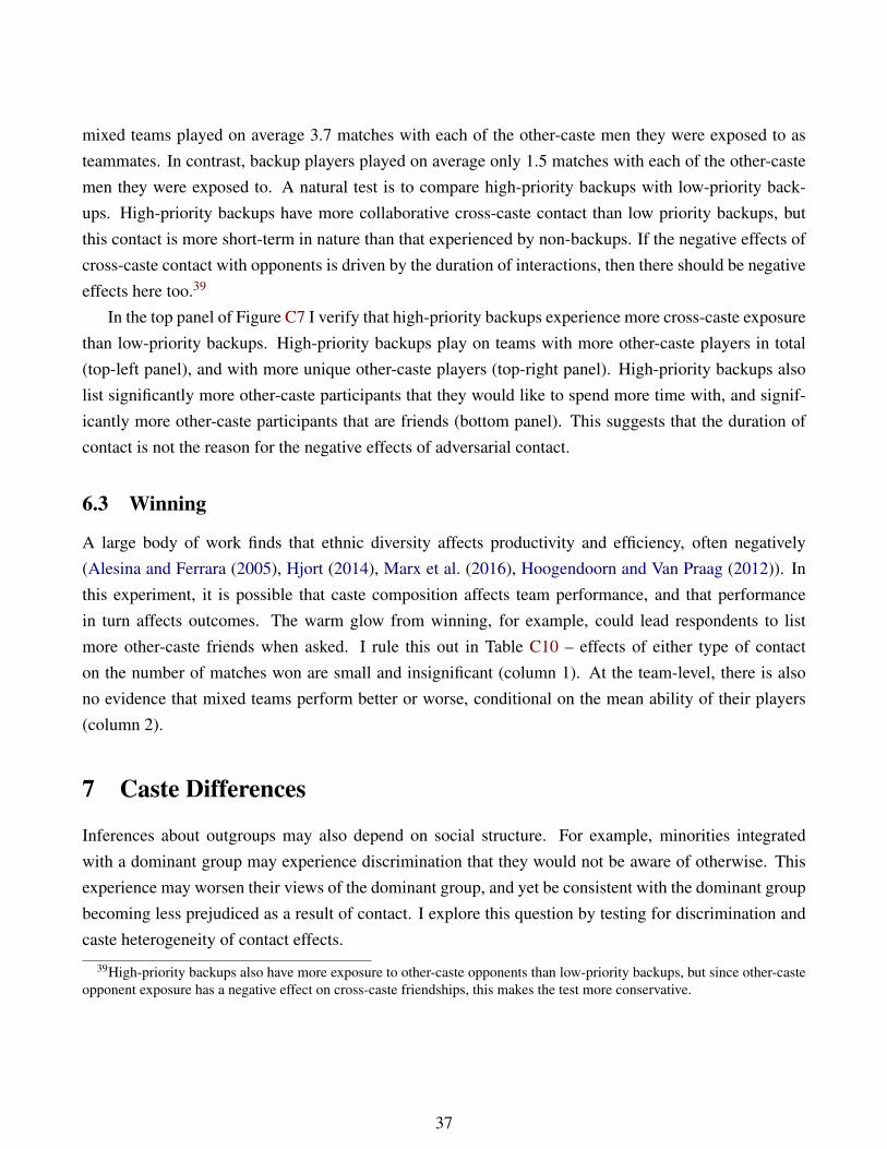
mixed teams played on average 3.7 matches with each of the other-caste men they were exposed to asteammates. In contrast, backup players played on average only 1.5 matches with each of the other-castemen they were exposed to. A natural test is to compare high-priority backups with low-priority back-ups. High-priority backups have more collaborative cross-caste contact than low priority backups, butthis contact is more short-term in nature than that experienced by non-backups. If the negative effects ofcross-caste contact with opponents is driven by the duration of interactions, then there should be negativeeffects here too.39

In the top panel of Figure C7 I verify that high-priority backups experience more cross-caste exposurethan low-priority backups. High-priority backups play on teams with more other-caste players in total(top-left panel), and with more unique other-caste players (top-right panel). High-priority backups alsolist significantly more other-caste participants that they would like to spend more time with, and signif-icantly more other-caste participants that are friends (bottom panel). This suggests that the duration ofcontact is not the reason for the negative effects of adversarial contact.

6.3 Winning

A large body of work finds that ethnic diversity affects productivity and efficiency, often negatively(Alesina and Ferrara (2005), Hjort (2014), Marx et al. (2016), Hoogendoorn and Van Praag (2012)). Inthis experiment, it is possible that caste composition affects team performance, and that performancein turn affects outcomes. The warm glow from winning, for example, could lead respondents to listmore other-caste friends when asked. I rule this out in Table C10 – effects of either type of contacton the number of matches won are small and insignificant (column 1). At the team-level, there is alsono evidence that mixed teams perform better or worse, conditional on the mean ability of their players(column 2).

7 Caste Differences

Inferences about outgroups may also depend on social structure. For example, minorities integratedwith a dominant group may experience discrimination that they would not be aware of otherwise. Thisexperience may worsen their views of the dominant group, and yet be consistent with the dominant groupbecoming less prejudiced as a result of contact. I explore this question by testing for discrimination andcaste heterogeneity of contact effects.

39High-priority backups also have more exposure to other-caste opponents than low-priority backups, but since other-casteopponent exposure has a negative effect on cross-caste friendships, this makes the test more conservative.

37

7.1 Ability and Discrimination

SC/ST players are worse at cricket according to baseline measures, conditional on age (columns 1 to 3,Table C11). Their maximum bowling speed is on average 3.45 km/h slower than that of General castes(0.34 s.d.), and they hit 0.31 fewer fours/sixes (0.24 s.d.), and catch 0.22 fewer balls (0.19 s.d.). OBCplayers do not differ significantly from General castes for any ability measure. The SC/ST differenceaffects payouts – the hypothetical performance-related pay is 25% lower for SC/STs than General castes(column 4). Fifty-eight percent of these payout differences remain after controlling for ability (column5), suggesting that these differences are not just due to ability, but also on-team discrimination.

To earn payouts while playing, individuals must first get the chance to bat (to earn money from scoringruns) and/or the chance to bowl (to earn money from taking wickets).40 Opportunities to bat and bowlare influenced by the team’s allocation choices. Before each match, each team selects a captain fromamong the non-backup players that have attended. The captain, together with the team, then chooses a“batting order” before the match starts. This choice entails ranking the players from one to five, with thetop two players batting first, and the rest waiting their turn to bat. In practice, this order matters becausethose later in the batting order may not get the chance to bat at all, losing the opportunity to make moneyfrom batting. When fielding, each team must also decide which players will bowl. Since there can onlybe one bowler at a time, there are again constraints – it won’t necessarily be the case that all players getthe chance to bowl. In choosing captains, the batting order, and who bowls, teams can show favoritismtowards one caste over others.

Favoritism of upper castes exists for all three types of allocation (Table C12). SC/STs are significantlyless likely to be chosen as captains, and less favored in the batting and bowling orders. This effect changeslittle when ability controls are added (columns 2, 4, and 6). Since ability measures are made commonknowledge prior to the first match, the evidence suggests that teams actively discriminate against lowercastes. Considering the coefficient on age, SC/STs are effectively treated like a General caste four or fiveyears their junior. OBCs also appear to be less favored than General castes, but the effect is much smallerand significant only for batting order choices.

7.2 Contact Effects by Caste

Given the evidence for on-team discrimination against SC/STs, it seems plausible that the integrationin this experiment could have different treatment effects by caste. Such heterogeneity is in fact rarelythe case – the only outcome for which the collaborative contact effect is significantly less positive for

40On average, 14% of players in a given match didn’t get the chance to bat, and 44% didn’t get the chance to bowl.

38

SC/STs (compared with General or OBC castes) is cross-caste trade, as already explained in Section 5.3(upper-panel of Tables C13 and C14). The lack of heterogeneity suggests that affirmative action policiesthat place under-performing and discriminated against minorities in contact with a dominant group maynevertheless lead to improved intergroup relations. Otherwise, no reliable pattern is observed for casteheterogeneity of adversarial contact effects (lower-panel of Tables C13 and C14).

8 The Net Effect of Contact

The results on contrasting effects of different types of contact raise a question: if effects can go eitherway, does the integrative cricket intervention have positive effects overall? Since participants were firstrandomized to either play in the leagues or serve as backup players, I address this question by comparingoutcomes for the backups with those that played in the leagues. Since high-priority backups played onaverage as many, or more, matches than the league players (Figure C5), I exclude backup players withpriority one to three from this analysis. The remaining backup players played on average 1.6 matcheseach, compared with 6.1 matches for league players. Since low-priority backup players still played somematches, I consider these effects to be a lower bound on the overall effects of the program.

While those in homogeneous-caste teams have significantly more other-caste friends, higher teamquality, and send more in the trust game than those in control, these players are not significantly differentto control players when considering other-caste team choice, cross-caste trade, and trade payouts (Figure9, Table 10). League participation alone does not lead to effects on cross-caste interaction and trade. Incontrast, those in mixed teams fare significantly better than control players on all outcomes except trust:they have 1.36 (0.3 s.d.) more other-caste friends, choose 0.45 (0.4 s.d.) more other-caste players fortheir future team for a match with stakes, engage in nine percentage points (0.18 s.d.) more cross-castetrade and make Rs. 12 (0.15 s.d) more in trade payouts.

Using the estimates in Table 10, I can calculate a rough estimate of counterfactual program effects ifparticipants were allowed to choose their own teams. First, those in the control group (low-priority back-ups) chose 1.2 other-caste teammates (column 2). Let us assume this would be the level of cross-casteexposure in the case where participants choose their own teams. In contrast, simple random assignment toteams would ensure players have 2.7 other-caste teammates on average. Assuming that treatment effectsare linear in the number of other-caste teammates (whether self-selected or not), column 5 implies thatthe effect of the program on cross-caste trade would be 40% smaller if participants were able to choosetheir own teams.

Taken together, these results suggest that even a short-term program with collaborative contact mightlead to greater cross-caste interaction and economic exchange, and that preventing self-segregation within

39

the program is crucial for effectiveness.

9 Conclusion

This paper provides evidence that the effects of integration depend on the type of contact. While col-laborative on-team contact increases cross-caste friendships, adversarial contact with opponents reducesthem. Both of these effects extend to the outgroup as a whole. Collaborative contact increases cross-caste friendships even with non-teammates, and adversarial contact harms friendships even with non-opponents. These findings suggest that the two types of contact have opposite effects on inferences aboutthe friendliness of other castes. In contrast, both types of contact convey similar information about theability of other castes, reducing statistical discrimination as measured by the number of other-caste play-ers chosen as future teammates. These effects have broader implications for efficiency. Collaborativecontact, but not adversarial, increases team quality and cross-caste trade when gains from trade exist.

Conceptually, my findings suggest that Allport (1954) was right – contact may reduce prejudice onlyif certain conditions, including that groups have common goals, are met. In this experiment the resultsgo further than this – in the case of adversarial contact it is not just that contact becomes ineffective, itcan even lead group differences to increase.

Though beyond the scope of this paper, many other types of intergroup contact exist: contact in pri-vate versus in public, contact through traumatic experiences, and contact that is known in an advance tobe temporary versus that which is known to be sustained. The conceptual framework in this paper – alearning model with attribution errors – may be applicable to these other cases. In particular, collabo-rative and adversarial contact may have divergent effects on tastes toward social interaction through themechanism of attribution errors. The attributions an individual makes about others depend on the contextin which they interact. If the context promotes cooperative behavior, attributions about cooperativenesswill be made. If the context promotes competitive behavior, individuals will infer others to be compet-itive and selfish. An implication is that it may be possible to design social policies to promote desiredinferences. For example, one intervention might maximize the common goals and cooperation betweengroups to address segregated social networks. Another intervention might maximize the observability ofthe ability of outgroups to address incorrect stereotypes regarding intelligence.

Finally, avenues exist for future work. Researchers might go further by systematically varying theother types of contact that Allport emphasizes: whether groups have equal status and whether there isauthority support of integration. Second, we should test whether the effects of short-term interventionslike the one in this paper have durable effects, or whether groups simply retreat into enclaves in themonths that follow. Third, we should test for the effects of competitive interaction in other economic

40

settings. With anti-immigrant sentiment in mind, competition in labor markets in particular seems worthyof exploration.

41

References

Aigner, D. J. and Cain, G. G. (1977). Statistical theories of discrimination in labor markets. ILR Review,30(2):175–187.

Alesina, A. and Ferrara, E. L. (2005). Ethnic diversity and economic performance. Journal of Economic

Literature, 43(3):762–800.

Alesina, A. and La Ferrara, E. (2002). Who trusts others? Journal of Public Economics, 85(2):207–234.

Algan, Y. and Cahuc, P. (2010). Inherited Trust and Growth. American Economic Review, 100(5):2060–2092.

Allport, G. (1954). The Nature of Prejudice. Garden City, NJ Anchor.

Anderson, S. (2011). Caste as an Impediment to Trade. American Economic Journal: Applied Eco-

nomics, 3(1):239–263.

Aronson, E. (2011). Cooperation in the classroom: The jigsaw method. Printer & Martin Limited.

Arrow, K. (1973). The Theory of Discrimination. Discrimination in Labor Markets, 3(10):3–33.

Ashraf, N. and Bandiera, O. (2017). Social Incentives in Organizations. Mimeo.

Banerjee, A., Duflo, E., Ghatak, M., and Lafortune, J. (2013). Marry for What? Caste and Mate Selectionin Modern India. American Economic Journal: Microeconomics, 5(2):33–72.

Banerjee, A. V., Chassang, S., and Snowberg, E. (2017). Decision theoretic approaches to experimentdesign and external validity. Handbook of Economic Field Experiments, 1:141–174.

Banerjee, A. V., Green, D., Green, J., and Pande, R. (2010). Can Voters be Primed to Choose BetterLegislators? Experimental Evidence from Rural India. Mimeo.

Bazzi, S., Gaduh, A., Rothenberg, A., and Wong, M. (2017). Unity in Diversity? Ethnicity, Migration,and Nation Building in Indonesia. Mimeo.

Beaman, L., Chattopadhyay, R., Duflo, E., Pande, R., and Topalova, P. (2009). Powerful women: doesexposure reduce bias? Quarterly Journal of Economics, 124(4):1497–1540.

Becker, G. S. (1957). The Economics of Discrimination. University of Chicago Press. Google-Books-ID:lLhZAAAAYAAJ.

42

Becker, S. O. and Pascali, L. (2016). Religion, Division of Labor and Conflict: Anti-Semiticsm inGerman Regions over 600 Years. Mimeo, (288).

Benabou, R. and Tirole, J. (2002). Self-confidence and personal motivation. The Quarterly Journal of

Economics, 117(3):871–915.

Benabou, R. and Tirole, J. (2006). Belief in a just world and redistributive politics. The Quarterly journal

of economics, 121(2):699–746.

Berg, J., Dickhaut, J., and McCabe, K. (1995). Trust, reciprocity, and social history. Games and Eco-

nomic Behavior, 10(1):122–142.

Bertrand, M. and Duflo, E. (2017). Field Experiments on Discrimination. Handbook of Economic Field

Experiments, 1:309–393.

Bertrand, M. and Mullainathan, S. (2004). Are Emily and Greg More Employable Than Lakisha andJamal? A Field Experiment on Labor Market Discrimination. American Economic Review, 94(4):991–1013.

Boisjoly, J., Duncan, G. J., Kremer, M., Levy, D. M., and Eccles, J. (2006). Empathy or Antipathy? TheImpact of Diversity. American Economic Review, 96(5):1890–1905.

Broockman, D. and Kalla, J. (2016). Durably reducing transphobia: A field experiment on door-to-doorcanvassing. Science, 352(6282):220–224.

Bubb, R., Kaur, S., and Mullainathan, S. (2016). Barriers to Contracting in Village Economies: A Testfor Enforcement Constraints. Mimeo.

Burgess, R., Jedwab, R., Miguel, E., Morjaria, A., and Padró i Miquel, G. (2015). The Value of Democ-racy: Evidence from Road Building in Kenya. American Economic Review, 105(6):1817–1851.

Burns, J., Corno, L., and La Ferrara, E. (2015). Interaction, prejudice and performance. Evidence fromSouth Africa. Mimeo.

Carrell, S. E., Hoekstra, M., and West, J. E. (2015). The impact of intergroup contact on racial attitudesand revealed preferences. Working Paper 20940, National Bureau of Economic Research.

Casey, K. (2015). Crossing party lines: The effects of information on redistributive politics. American

Economic Review, 105(8):2410–2448.

43

Castilla, C. (2015). Trust and reciprocity between spouses in India. American Economic Review,105(5):621–624.

Chen, Y. and Li, S. X. (2009). Group Identity and Social Preferences. American Economic Review,99(1):431–457.

Cornell, B. and Welch, I. (1996). Culture, information, and screening discrimination. Journal of Political

Economy, 104(3):542–571.

Cubitt, R. P., Starmer, C., and Sugden, R. (1998). On the validity of the random lottery incentive system.Experimental Economics, 1(2):115–131.

Depetris-Chauvin, E. and Durante, R. (2017). One team, one nation: Football, ethnic identity, and conflictin africa. Mimeo.

Desai, S., Vanneman, R., and of Applied Economic Research, N. C. (2011). Indian Human DevelopmentSurvey-II (IHDS-II). Technical report, Ann Arbor, MI: Inter-university Consortium for Political andSocial Research.

Dirks, N. B. (2011). Castes of mind: Colonialism and the making of modern India. Princeton UniversityPress.

Ditlmann, R. K. and Samii, C. (2016). Can intergroup contact affect ingroup dynamics? Insights froma field study with Jewish and Arab-Palestinian youth in Israel. Peace and Conflict: Journal of Peace

Psychology, 22(4):380.

Dumont, L. (1970). Homo Hierarchicus: The Caste System and Its Implications. University of ChicagoPress.

Enos, R. D. (2014). Causal effect of intergroup contact on exclusionary attitudes. Proceedings of the

National Academy of Sciences, 111(10):3699–3704.

Eyster, E. and Rabin, M. (2005). Cursed equilibrium. Econometrica, 73(5):1623–1672.

Finseraas, H., Hanson, T., Johnsen, A. A., Kotsadam, A., and Torsvik, G. (2016). Trust, Ethnic Diversity,and Personal Contact: Experimental Field Evidence. Mimeo.

Fiske, S. T., Cuddy, A. J., and Glick, P. (2007). Universal dimensions of social cognition: Warmth andcompetence. Trends in cognitive sciences, 11(2):77–83.

44

Fiske, S. T., Cuddy, A. J., Glick, P., and Xu, J. (2002). A model of (often mixed) stereotype content: com-petence and warmth respectively follow from perceived status and competition. Journal of personality

and social psychology, 82(6):878.

Fisman, R., Paravisini, D., and Vig, V. (2017). Cultural proximity and loan outcomes. American Eco-

nomic Review, 107(2):457–492.

Furukawa, C. (2017). Why Diaries Help: An Information Processing Model of Mindset Shift. Mimeo.

Ghurye, G. S. (1932). Caste and race in India. A. A. Knopf.

Gilbert, D. T. (1989). Thinking lightly about others: Automatic components of the social inferenceprocess. Unintended thought, 26:481.

Gilbert, D. T. and Malone, P. S. (1995). The correspondence bias. Psychological Bulletin, 117(1):21.

Goette, L., Huffman, D., Meier, S., and Sutter, M. (2012). Competition Between Organizational Groups:Its Impact on Altruistic and Antisocial Motivations. Management Science, 58(5):948–960.

Haggag, K. and Pope, D. (2016). Attribution Bias in Consumer Choice. Technical report, Working Paper.

Halla, M., Wagner, A. F., and Zweimüller, J. (2017). Immigration and Voting for the Far Right. Journal

of the European Economic Association, jvw003.

Hjort, J. (2014). Ethnic divisions and production in firms. Quarterly Journal of Economics, 129(4):1899–1946.

Hnatkovska, V., Lahiri, A., and Paul, S. (2012). Castes and labor mobility. American Economic Journal:

Applied Economics, 4(2):274–307.

Hoff, K. and Pandey, P. (2014). Making up people - The effect of identity on performance in a modern-izing society. Journal of Development Economics, 106(C):118–131.

Holt, C. A. (1986). Preference reversals and the independence axiom. American Economic Review,76(3):508–515.

Hoogendoorn, S. and Van Praag, M. (2012). Ethnic diversity and team performance: A field experiment.Mimeo.

Hoult, N. (2016). Field of dreams. The Telegraph.

45

Hsieh, C.-T., Hurst, E., Jones, C. I., and Klenow, P. J. (2013). The allocation of talent and us economicgrowth. Working Paper 18693, National Bureau of Economic Research.

Humphrey, R. (1985). How work roles influence perception: Structural-cognitive processes and organi-zational behavior. American Sociological Review, pages 242–252.

Jackson, M. O. (2010). An overview of social networks and economic applications. The Handbook of

Social Economics, 1:511–85.

Jehiel, P. (2005). Analogy-based expectation equilibrium. Journal of Economic theory, 123(2):81–104.

Jha, S. (2013). Trade, institutions, and ethnic tolerance: Evidence from South Asia. American political

Science review, 107(4):806–832.

Jones, E. E. and Harris, V. A. (1967). The attribution of attitudes. Journal of Experimental Social

Psychology, 3(1):1–24.

Jones, E. E. and Nisbett, R. E. (1971). The actor and the observer: Divergent perceptions of the causesof behavior.

Marx, B., Pons, V., and Suri, T. (2016). Diversity and team performance in a kenyan organization. Mimeo.

Miller, C. (2017). The Persistent Effect of Temporary Affirmative Action. American Economic Journal:

Applied Economics, 9(3):152–190.

Mullainathan, S. and Spiess, J. (2017). Machine learning: an applied econometric approach. Journal of

Economic Perspectives, 31(2):87–106.

Munshi, K. (2011). Strength in numbers: Networks as a solution to occupational traps. The Review of

Economic Studies, 78(3):1069–1101.

Munshi, K. (2016). Caste and the Indian Economy. Mimeo.

Munshi, K. and Rosenzweig, M. (2015). Insiders and Outsiders: Local Ethnic Politics and Public GoodsProvision. Working Paper 21720, National Bureau of Economic Research. DOI: 10.3386/w21720.

Munshi, K. and Rosenzweig, M. (2016). Networks and misallocation: Insurance, migration, and therural-urban wage gap. American Economic Review, 106(1):46–98.

Nisbett, R. E., Caputo, C., Legant, P., and Marecek, J. (1973). Behavior as seen by the actor and as seenby the observer. Journal of Personality and Social Psychology, 27(2):154.

46

Paluck, E. L., Green, S., and Green, D. P. (2017). The Contact Hypothesis Revisited. Mimeo.

Paluck, E. L. and Shafir, E. (2017). The Psychology of Construal in the Design of Field Experiments.Handbook of Economic Field Experiments, 1:245–268.

Pettigrew, T. F. and Tropp, L. R. (2006). A meta-analytic test of intergroup contact theory. Journal of

personality and social psychology, 90(5):751.

Rao, G. (2014). Familiarity Does Not Breed Contempt: Generosity, Discrimination and Diversity inDelhi Schools. Mimeo.

Ross, L. (1977). The intuitive psychologist and his shortcomings: Distortions in the attribution process.Advances in experimental social psychology, 10:173–220.

Ross, L. and Nisbett, R. E. (2011). The person and the situation: Perspectives of social psychology.Pinter & Martin Publishers.

Scacco, A. and Warren, S. S. (2016). Can Social Contact Reduce Prejudice and Discrimination? Evidencefrom a Field Experiment in Nigeria. Mimeo.

Schroeder, J. and Risen, J. L. (2016). Befriending the enemy: Outgroup friendship longitudinally pre-dicts intergroup attitudes in a coexistence program for Israelis and Palestinians. Group Processes &

Intergroup Relations, 19(1):72–93.

Sherif, M., Harvey, O., White, B. J., Hood, W. R., and Sherif, C. W. (1961). Intergroup conflict and

cooperation: The Robbers Cave experiment, volume 10. University Book Exchange Norman, OK.

Sprenger, C. (2015). An endowment effect for risk: Experimental tests of stochastic reference points.Journal of Political Economy, 123(6):1456–1499.

Starmer, C. and Sugden, R. (1991). Does the random-lottery incentive system elicit true preferences? Anexperimental investigation. American Economic Review, 81(4):971–978.

Tabellini, M. (2018). Gifts of the Immigrants, Woes of the Natives: Lessons from the Age of MassMigration. Mimeo.

Tajfel, H., Billig, M. G., Bundy, R. P., and Flament, C. (1971). Social categorization and intergroupbehaviour. European Journal of Social Psychology, 1(2):149–178.

47

A Figures

Figure 1: Caste-wise Friendships at Baseline

02

46

8N

umbe

r of B

asel

ine

Frie

nds

SC/ST OBC General

SC/ST Listed as FriendsOBC Listed as FriendsGeneral Listed as Friends

Notes: For those that completed the baseline social network survey (1,251 of 1,261 participants) the bars show the meannumber of friends listed of a given caste, averaging across all participants from a given caste. For example, the far-left barshows that SC/ST caste participants report having 7.3 SC/ST friends on average.

48

Figure 2: Cricket Explained

BowlerFielder

Umpire (Referee)

Batsman

Wickets

Notes: This photo was taken during one of the experimental matches. The fielding team comprises one bowler, one wicket-keeper, and three fielders. The batting team comprises two batsmen currently playing, and three sat together waiting their turnto bat.

Figure 3: Timeline

Phase 1: Sign-Up

Day 1

Phase 2: Ability(Finalize Sign-Up)

Day 5 Day 10

Phase 3: Randomization

Background Questions

Ability Testing

Day 13

Phase 4: League(20-30 matches/week)

Day 34

Phase 5: Endline

Endline Outcomes

Day 55

Social Networks

49

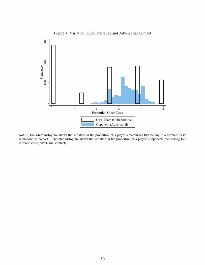
Figure 4: Variation in Collaborative and Adversarial Contact

010

020

030

0Fr

eque

ncy

0 .2 .4 .6 .8 1Proportion Other Caste

Own-Team (Collaborative)Opponent (Adversarial)

Notes: The white histogram shows the variation in the proportion of a player’s teammates that belong to a different caste(collaborative contact). The blue histogram shows the variation in the proportion of a player’s opponents that belong to adifferent caste (adversarial contact).

50

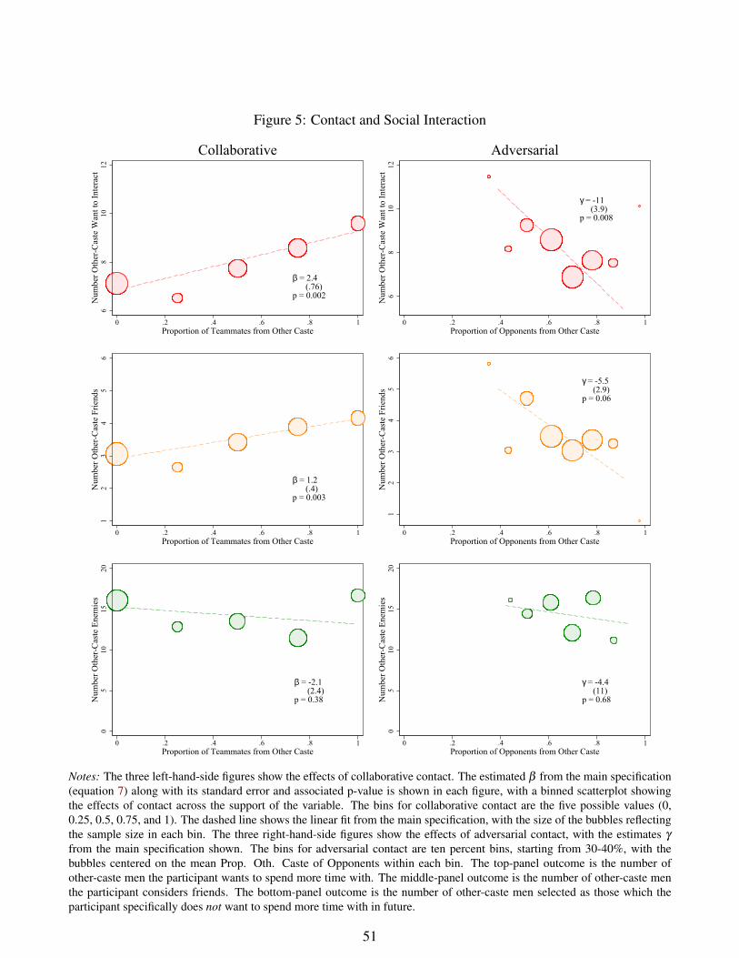
Figure 5: Contact and Social Interaction

β = 2.4 (.76)p = 0.002

68

1012

Num

ber O

ther

-Cas

te W

ant t

o In

tera

ct

0 .2 .4 .6 .8 1Proportion of Teammates from Other Caste

Collaborative

γ = -11 (3.9)p = 0.008

68

1012

Num

ber O

ther

-Cas

te W

ant t

o In

tera

ct

0 .2 .4 .6 .8 1Proportion of Opponents from Other Caste

Adversarial

β = 1.2 (.4)p = 0.003

12

34

56

Num

ber O

ther

-Cas

te F

riend

s

0 .2 .4 .6 .8 1Proportion of Teammates from Other Caste

γ = -5.5 (2.9)p = 0.06

12

34

56

Num

ber O

ther

-Cas

te F

riend

s

0 .2 .4 .6 .8 1Proportion of Opponents from Other Caste

β = -2.1 (2.4)p = 0.38

05

1015

20N

umbe

r Oth

er-C

aste

Ene

mie

s

0 .2 .4 .6 .8 1Proportion of Teammates from Other Caste

γ = -4.4 (11)p = 0.68

05

1015

20N

umbe

r Oth

er-C

aste

Ene

mie

s

0 .2 .4 .6 .8 1Proportion of Opponents from Other Caste

Notes: The three left-hand-side figures show the effects of collaborative contact. The estimated β from the main specification(equation 7) along with its standard error and associated p-value is shown in each figure, with a binned scatterplot showingthe effects of contact across the support of the variable. The bins for collaborative contact are the five possible values (0,0.25, 0.5, 0.75, and 1). The dashed line shows the linear fit from the main specification, with the size of the bubbles reflectingthe sample size in each bin. The three right-hand-side figures show the effects of adversarial contact, with the estimates γ

from the main specification shown. The bins for adversarial contact are ten percent bins, starting from 30-40%, with thebubbles centered on the mean Prop. Oth. Caste of Opponents within each bin. The top-panel outcome is the number ofother-caste men the participant wants to spend more time with. The middle-panel outcome is the number of other-caste menthe participant considers friends. The bottom-panel outcome is the number of other-caste men selected as those which theparticipant specifically does not want to spend more time with in future.

51

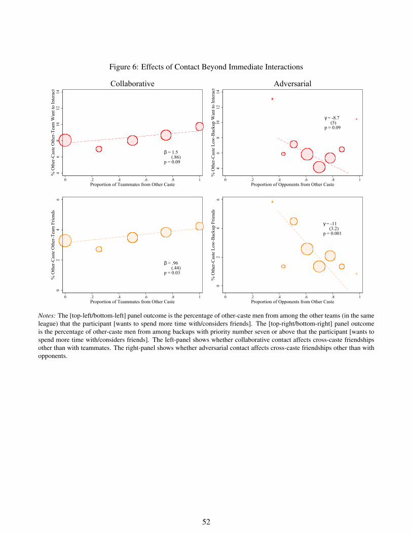
Figure 6: Effects of Contact Beyond Immediate Interactions

β = 1.5 (.86)p = 0.09

46

810

1214

% O

ther

-Cas

te O

ther

-Tea

m W

ant t

o In

tera

ct

0 .2 .4 .6 .8 1Proportion of Teammates from Other Caste

Collaborative

γ = -8.7 (5)p = 0.09

46

810

1214

% O

ther

-Cas

te L

ow-B

acku

p W

ant t

o In

tera

ct

0 .2 .4 .6 .8 1Proportion of Opponents from Other Caste

Adversarial

β = .96 (.44)p = 0.03

02

46

% O

ther

-Cas

te O

ther

-Tea

m F

riend

s

0 .2 .4 .6 .8 1Proportion of Teammates from Other Caste

γ = -11 (3.2)p = 0.001

02

46

% O

ther

-Cas

te L

ow-B

acku

p Fr

iend

s

0 .2 .4 .6 .8 1Proportion of Opponents from Other Caste

Notes: The [top-left/bottom-left] panel outcome is the percentage of other-caste men from among the other teams (in the sameleague) that the participant [wants to spend more time with/considers friends]. The [top-right/bottom-right] panel outcomeis the percentage of other-caste men from among backups with priority number seven or above that the participant [wants tospend more time with/considers friends]. The left-panel shows whether collaborative contact affects cross-caste friendshipsother than with teammates. The right-panel shows whether adversarial contact affects cross-caste friendships other than withopponents.

52

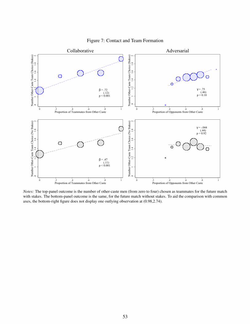
Figure 7: Contact and Team Formation

β = .72 (.12)p < 0.001

.81

1.2

1.4

1.6

1.8

2N

umbe

r Oth

er-C

aste

Tea

m C

hoic

e (S

take

s)

0 .2 .4 .6 .8 1Proportion of Teammates from Other Caste

Collaborative

γ = .75 (.46)p = 0.10

.81

1.2

1.4

1.6

1.8

2N

umbe

r Oth

er-C

aste

Tea

m C

hoic

e (S

take

s)

0 .2 .4 .6 .8 1Proportion of Opponents from Other Caste

Adversarial

β = .47 (.11)p < 0.001

.81

1.2

1.4

1.6

1.8

2N

umbe

r Oth

er-C

aste

Tea

m C

hoic

e (N

o St

akes

)

0 .2 .4 .6 .8 1Proportion of Teammates from Other Caste

γ = -.044 (.44)p = 0.92

.81

1.2

1.4

1.6

1.8

2N

umbe

r Oth

er-C

aste

Tea

m C

hoic

e (N

o St

akes

)

0 .2 .4 .6 .8 1Proportion of Opponents from Other Caste

Notes: The top-panel outcome is the number of other-caste men (from zero to four) chosen as teammates for the future matchwith stakes. The bottom-panel outcome is the same, for the future match without stakes. To aid the comparison with commonaxes, the bottom-right figure does not display one outlying observation at (0.98,2.74).

53

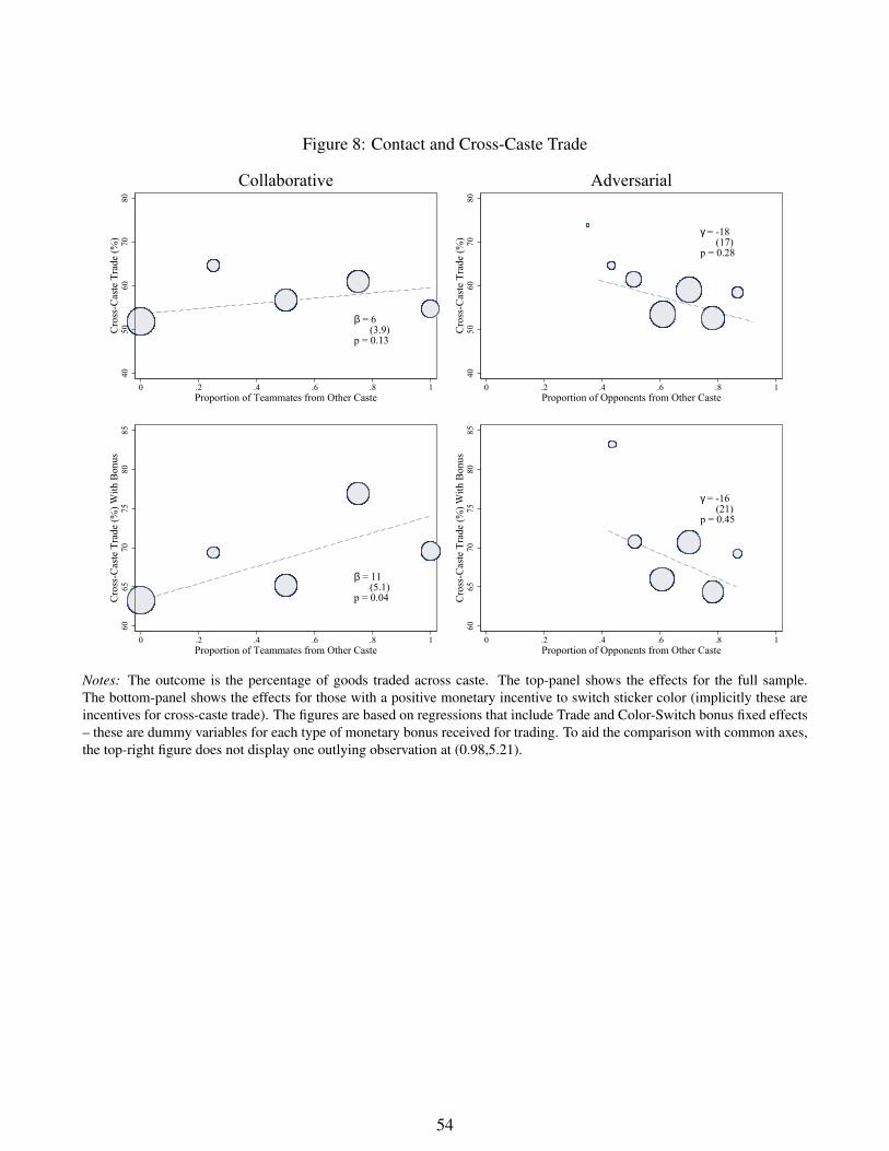
Figure 8: Contact and Cross-Caste Trade

β = 6 (3.9)p = 0.13

4050

6070

80C

ross

-Cas

te T

rade

(%)

0 .2 .4 .6 .8 1Proportion of Teammates from Other Caste

Collaborative

γ = -18 (17)p = 0.28

4050

6070

80C

ross

-Cas

te T

rade

(%)

0 .2 .4 .6 .8 1Proportion of Opponents from Other Caste

Adversarial

β = 11 (5.1)p = 0.04

6065

7075

8085

Cro

ss-C

aste

Tra

de (%

) With

Bon

us

0 .2 .4 .6 .8 1Proportion of Teammates from Other Caste

γ = -16 (21)p = 0.45

6065

7075

8085

Cro

ss-C

aste

Tra

de (%

) With

Bon

us

0 .2 .4 .6 .8 1Proportion of Opponents from Other Caste

Notes: The outcome is the percentage of goods traded across caste. The top-panel shows the effects for the full sample.The bottom-panel shows the effects for those with a positive monetary incentive to switch sticker color (implicitly these areincentives for cross-caste trade). The figures are based on regressions that include Trade and Color-Switch bonus fixed effects– these are dummy variables for each type of monetary bonus received for trading. To aid the comparison with common axes,the top-right figure does not display one outlying observation at (0.98,5.21).

54

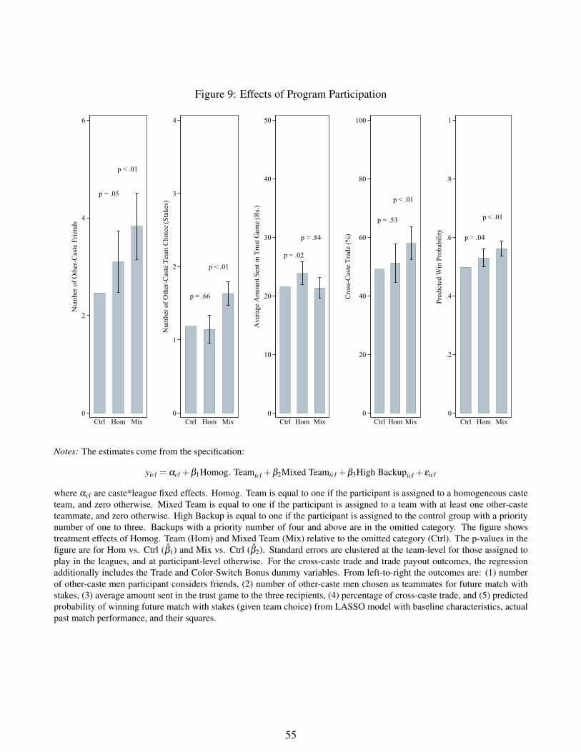
Figure 9: Effects of Program Participation

p = .05

p < .01

0

2

4

6

Num

ber o

f Oth

er-C

aste

Frie

nds

Ctrl Hom Mix

p = .66

p < .01

0

1

2

3

4

Num

ber o

f Oth

er-C

aste

Tea

m C

hoic

e (S

take

s)

Ctrl Hom Mix

p = .02

p = .84

0

10

20

30

40

50

Ave

rage

Am

ount

Sen

t in

Trus

t Gam

e (R

s.)

Ctrl Hom Mix

p = .53

p < .01

0

20

40

60

80

100

Cro

ss-C

aste

Tra

de (%

)

Ctrl Hom Mix

p = .04

p < .01

0

.2

.4

.6

.8

1

Pred

icte

d W

in P

roba

bilit

y

Ctrl Hom Mix

Notes: The estimates come from the specification:

yicl = αcl +β1Homog. Teamicl +β2Mixed Teamicl +β3High Backupicl + εicl

where αcl are caste*league fixed effects. Homog. Team is equal to one if the participant is assigned to a homogeneous casteteam, and zero otherwise. Mixed Team is equal to one if the participant is assigned to a team with at least one other-casteteammate, and zero otherwise. High Backup is equal to one if the participant is assigned to the control group with a prioritynumber of one to three. Backups with a priority number of four and above are in the omitted category. The figure showstreatment effects of Homog. Team (Hom) and Mixed Team (Mix) relative to the omitted category (Ctrl). The p-values in thefigure are for Hom vs. Ctrl (β̂1) and Mix vs. Ctrl (β̂2). Standard errors are clustered at the team-level for those assigned toplay in the leagues, and at participant-level otherwise. For the cross-caste trade and trade payout outcomes, the regressionadditionally includes the Trade and Color-Switch Bonus dummy variables. From left-to-right the outcomes are: (1) numberof other-caste men participant considers friends, (2) number of other-caste men chosen as teammates for future match withstakes, (3) average amount sent in the trust game to the three recipients, (4) percentage of cross-caste trade, and (5) predictedprobability of winning future match with stakes (given team choice) from LASSO model with baseline characteristics, actualpast match performance, and their squares.

55

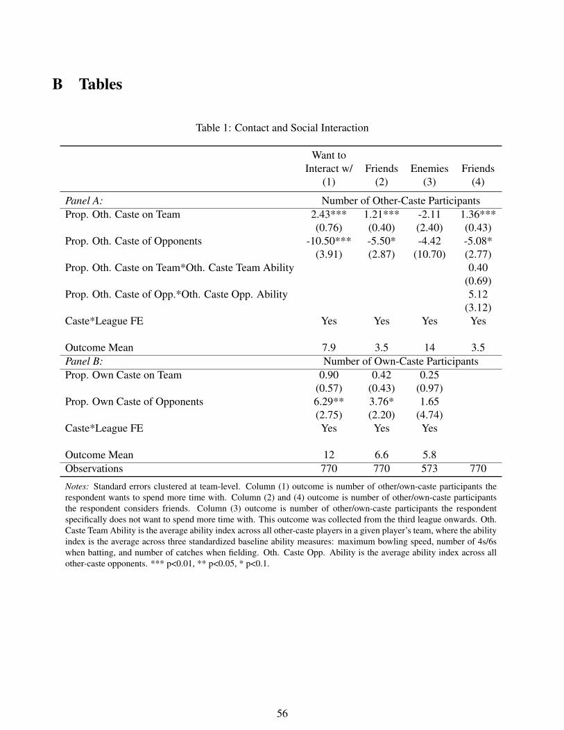
B Tables

Table 1: Contact and Social Interaction

Want toInteract w/

(1)Friends

(2)Enemies

(3)Friends

(4)

Panel A: Number of Other-Caste ParticipantsProp. Oth. Caste on Team 2.43*** 1.21*** -2.11 1.36***

(0.76) (0.40) (2.40) (0.43)Prop. Oth. Caste of Opponents -10.50*** -5.50* -4.42 -5.08*

(3.91) (2.87) (10.70) (2.77)Prop. Oth. Caste on Team*Oth. Caste Team Ability 0.40

(0.69)Prop. Oth. Caste of Opp.*Oth. Caste Opp. Ability 5.12

(3.12)Caste*League FE Yes Yes Yes Yes

Outcome Mean 7.9 3.5 14 3.5Panel B: Number of Own-Caste ParticipantsProp. Own Caste on Team 0.90 0.42 0.25

(0.57) (0.43) (0.97)Prop. Own Caste of Opponents 6.29** 3.76* 1.65

(2.75) (2.20) (4.74)Caste*League FE Yes Yes Yes

Outcome Mean 12 6.6 5.8Observations 770 770 573 770

Notes: Standard errors clustered at team-level. Column (1) outcome is number of other/own-caste participants therespondent wants to spend more time with. Column (2) and (4) outcome is number of other/own-caste participantsthe respondent considers friends. Column (3) outcome is number of other/own-caste participants the respondentspecifically does not want to spend more time with. This outcome was collected from the third league onwards. Oth.Caste Team Ability is the average ability index across all other-caste players in a given player’s team, where the abilityindex is the average across three standardized baseline ability measures: maximum bowling speed, number of 4s/6swhen batting, and number of catches when fielding. Oth. Caste Opp. Ability is the average ability index across allother-caste opponents. *** p<0.01, ** p<0.05, * p<0.1.

56

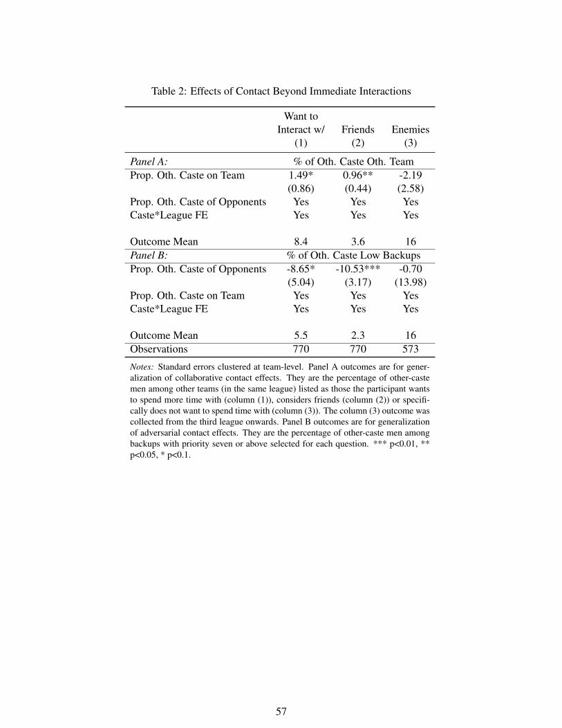
Table 2: Effects of Contact Beyond Immediate Interactions

Want toInteract w/

(1)Friends

(2)Enemies

(3)

Panel A: % of Oth. Caste Oth. TeamProp. Oth. Caste on Team 1.49* 0.96** -2.19

(0.86) (0.44) (2.58)Prop. Oth. Caste of Opponents Yes Yes YesCaste*League FE Yes Yes Yes

Outcome Mean 8.4 3.6 16Panel B: % of Oth. Caste Low BackupsProp. Oth. Caste of Opponents -8.65* -10.53*** -0.70

(5.04) (3.17) (13.98)Prop. Oth. Caste on Team Yes Yes YesCaste*League FE Yes Yes Yes

Outcome Mean 5.5 2.3 16Observations 770 770 573

Notes: Standard errors clustered at team-level. Panel A outcomes are for gener-alization of collaborative contact effects. They are the percentage of other-castemen among other teams (in the same league) listed as those the participant wantsto spend more time with (column (1)), considers friends (column (2)) or specifi-cally does not want to spend time with (column (3)). The column (3) outcome wascollected from the third league onwards. Panel B outcomes are for generalizationof adversarial contact effects. They are the percentage of other-caste men amongbackups with priority seven or above selected for each question. *** p<0.01, **p<0.05, * p<0.1.

57

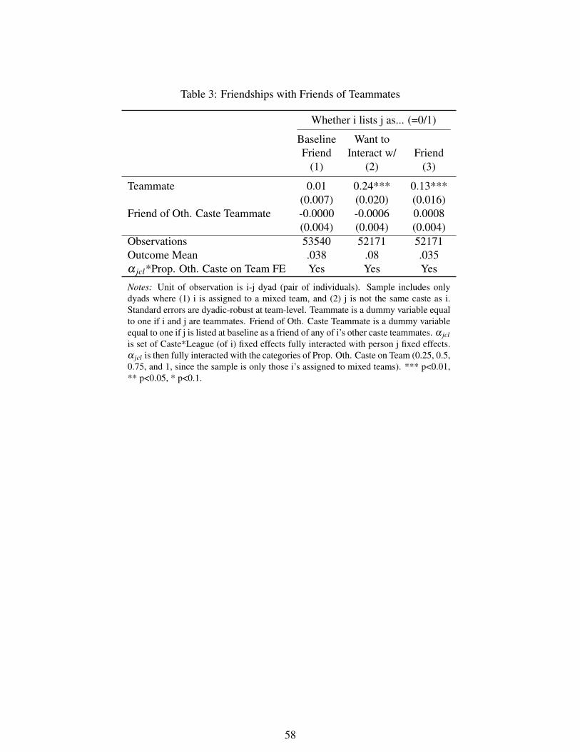
Table 3: Friendships with Friends of Teammates

Whether i lists j as... (=0/1)

BaselineFriend

(1)

Want toInteract w/

(2)Friend

(3)

Teammate 0.01 0.24*** 0.13***(0.007) (0.020) (0.016)

Friend of Oth. Caste Teammate -0.0000 -0.0006 0.0008(0.004) (0.004) (0.004)

Observations 53540 52171 52171Outcome Mean .038 .08 .035α jcl*Prop. Oth. Caste on Team FE Yes Yes Yes

Notes: Unit of observation is i-j dyad (pair of individuals). Sample includes onlydyads where (1) i is assigned to a mixed team, and (2) j is not the same caste as i.Standard errors are dyadic-robust at team-level. Teammate is a dummy variable equalto one if i and j are teammates. Friend of Oth. Caste Teammate is a dummy variableequal to one if j is listed at baseline as a friend of any of i’s other caste teammates. α jclis set of Caste*League (of i) fixed effects fully interacted with person j fixed effects.α jcl is then fully interacted with the categories of Prop. Oth. Caste on Team (0.25, 0.5,0.75, and 1, since the sample is only those i’s assigned to mixed teams). *** p<0.01,** p<0.05, * p<0.1.

58

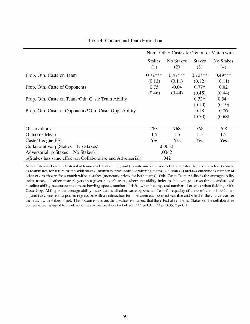
Table 4: Contact and Team Formation

Num. Other Castes for Team for Match with

Stakes(1)

No Stakes(2)

Stakes(3)

No Stakes(4)

Prop. Oth. Caste on Team 0.72*** 0.47*** 0.72*** 0.49***(0.12) (0.11) (0.12) (0.11)

Prop. Oth. Caste of Opponents 0.75 -0.04 0.77* 0.02(0.46) (0.44) (0.45) (0.44)

Prop. Oth. Caste on Team*Oth. Caste Team Ability 0.32* 0.34*(0.19) (0.19)

Prop. Oth. Caste of Opponents*Oth. Caste Opp. Ability 0.18 0.76(0.70) (0.68)

Observations 768 768 768 768Outcome Mean 1.5 1.5 1.5 1.5Caste*League FE Yes Yes Yes YesCollaborative: p(Stakes = No Stakes) .00053Adversarial: p(Stakes = No Stakes) .0042p(Stakes has same effect on Collaborative and Adversarial) .042

Notes: Standard errors clustered at team-level. Column (1) and (3) outcome is number of other castes (from zero to four) chosenas teammates for future match with stakes (monetary prize only for winning team). Column (2) and (4) outcome is number ofother castes chosen for a match without stakes (monetary prizes for both teams). Oth. Caste Team Ability is the average abilityindex across all other caste players in a given player’s team, where the ability index is the average across three standardizedbaseline ability measures: maximum bowling speed, number of 4s/6s when batting, and number of catches when fielding. Oth.Caste Opp. Ability is the average ability index across all other caste opponents. Tests for equality of the coefficients in columns(1) and (2) come from a pooled regression with an interaction term between each contact variable and whether the choice was forthe match with stakes or not. The bottom row gives the p-value from a test that the effect of removing Stakes on the collaborativecontact effect is equal to its effect on the adversarial contact effect. *** p<0.01, ** p<0.05, * p<0.1.

59

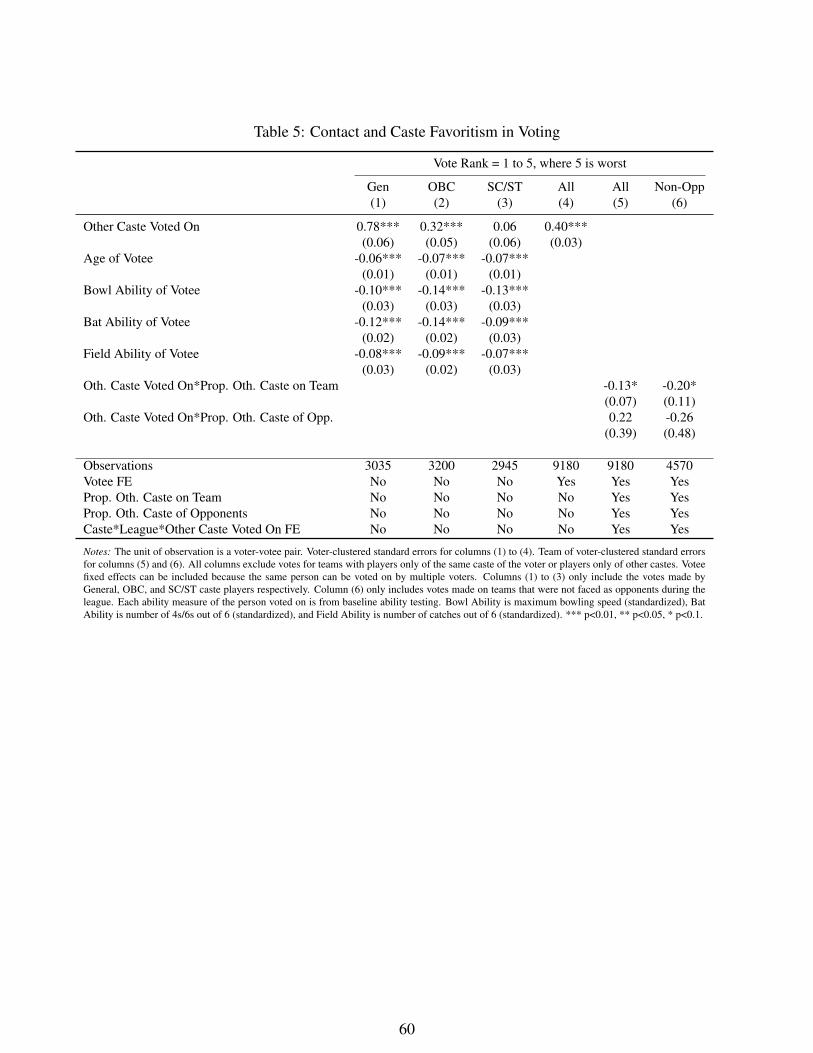
Table 5: Contact and Caste Favoritism in Voting

Vote Rank = 1 to 5, where 5 is worst

Gen(1)

OBC(2)

SC/ST(3)

All(4)

All(5)

Non-Opp(6)

Other Caste Voted On 0.78*** 0.32*** 0.06 0.40***(0.06) (0.05) (0.06) (0.03)

Age of Votee -0.06*** -0.07*** -0.07***(0.01) (0.01) (0.01)

Bowl Ability of Votee -0.10*** -0.14*** -0.13***(0.03) (0.03) (0.03)

Bat Ability of Votee -0.12*** -0.14*** -0.09***(0.02) (0.02) (0.03)

Field Ability of Votee -0.08*** -0.09*** -0.07***(0.03) (0.02) (0.03)

Oth. Caste Voted On*Prop. Oth. Caste on Team -0.13* -0.20*(0.07) (0.11)

Oth. Caste Voted On*Prop. Oth. Caste of Opp. 0.22 -0.26(0.39) (0.48)

Observations 3035 3200 2945 9180 9180 4570Votee FE No No No Yes Yes YesProp. Oth. Caste on Team No No No No Yes YesProp. Oth. Caste of Opponents No No No No Yes YesCaste*League*Other Caste Voted On FE No No No No Yes Yes

Notes: The unit of observation is a voter-votee pair. Voter-clustered standard errors for columns (1) to (4). Team of voter-clustered standard errorsfor columns (5) and (6). All columns exclude votes for teams with players only of the same caste of the voter or players only of other castes. Voteefixed effects can be included because the same person can be voted on by multiple voters. Columns (1) to (3) only include the votes made byGeneral, OBC, and SC/ST caste players respectively. Column (6) only includes votes made on teams that were not faced as opponents during theleague. Each ability measure of the person voted on is from baseline ability testing. Bowl Ability is maximum bowling speed (standardized), BatAbility is number of 4s/6s out of 6 (standardized), and Field Ability is number of catches out of 6 (standardized). *** p<0.01, ** p<0.05, * p<0.1.

60

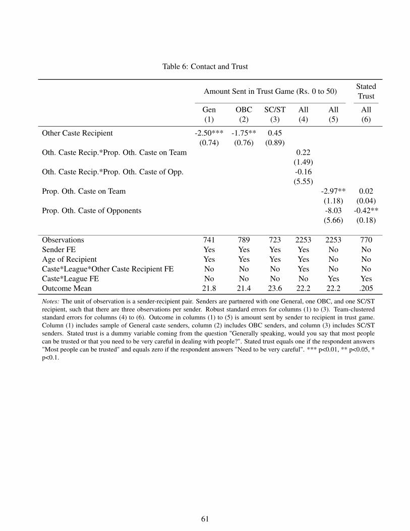
Table 6: Contact and Trust

Amount Sent in Trust Game (Rs. 0 to 50)StatedTrust

Gen(1)

OBC(2)

SC/ST(3)

All(4)

All(5)

All(6)

Other Caste Recipient -2.50*** -1.75** 0.45(0.74) (0.76) (0.89)

Oth. Caste Recip.*Prop. Oth. Caste on Team 0.22(1.49)

Oth. Caste Recip.*Prop. Oth. Caste of Opp. -0.16(5.55)

Prop. Oth. Caste on Team -2.97** 0.02(1.18) (0.04)

Prop. Oth. Caste of Opponents -8.03 -0.42**(5.66) (0.18)

Observations 741 789 723 2253 2253 770Sender FE Yes Yes Yes Yes No NoAge of Recipient Yes Yes Yes Yes No NoCaste*League*Other Caste Recipient FE No No No Yes No NoCaste*League FE No No No No Yes YesOutcome Mean 21.8 21.4 23.6 22.2 22.2 .205

Notes: The unit of observation is a sender-recipient pair. Senders are partnered with one General, one OBC, and one SC/STrecipient, such that there are three observations per sender. Robust standard errors for columns (1) to (3). Team-clusteredstandard errors for columns (4) to (6). Outcome in columns (1) to (5) is amount sent by sender to recipient in trust game.Column (1) includes sample of General caste senders, column (2) includes OBC senders, and column (3) includes SC/STsenders. Stated trust is a dummy variable coming from the question "Generally speaking, would you say that most peoplecan be trusted or that you need to be very careful in dealing with people?". Stated trust equals one if the respondent answers"Most people can be trusted" and equals zero if the respondent answers "Need to be very careful". *** p<0.01, ** p<0.05, *p<0.1.

61

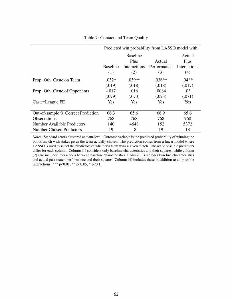
Table 7: Contact and Team Quality

Predicted win probability from LASSO model with

Baseline(1)

BaselinePlus

Interactions(2)

ActualPerformance

(3)

ActualPlus

Interactions(4)

Prop. Oth. Caste on Team .032* .039** .036** .04**(.019) (.018) (.018) (.017)

Prop. Oth. Caste of Opponents -.017 .016 .0084 .03(.079) (.073) (.073) (.071)

Caste*League FE Yes Yes Yes Yes

Out-of-sample % Correct Prediction 66.3 65.6 66.9 65.6Observations 768 768 768 768Number Available Predictors 140 4648 152 5372Number Chosen Predictors 19 18 19 18

Notes: Standard errors clustered at team-level. Outcome variable is the predicted probability of winning thebonus match with stakes given the team actually chosen. The prediction comes from a linear model whereLASSO is used to select the predictors of whether a team wins a given match. The set of possible predictorsdiffer for each column. Column (1) considers only baseline characteristics and their squares, while column(2) also includes interactions between baseline characteristics. Column (3) includes baseline characteristicsand actual past match performance and their squares. Column (4) includes these in addition to all possibleinteractions. *** p<0.01, ** p<0.05, * p<0.1.

62

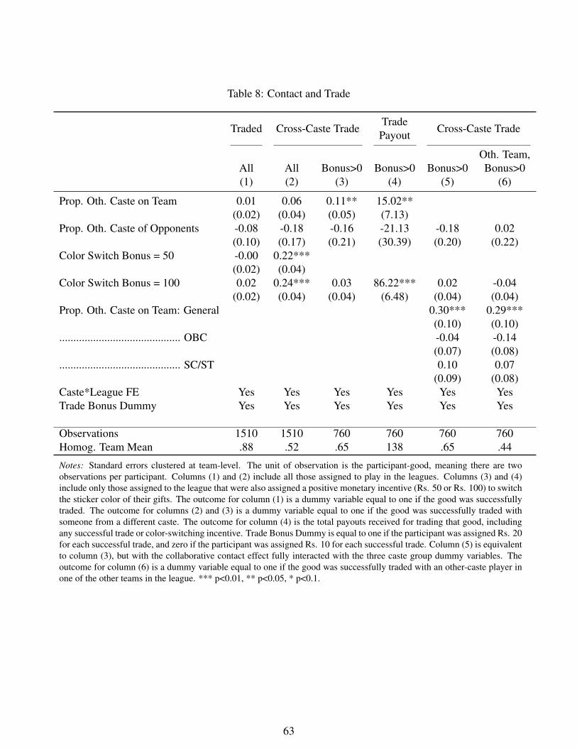
Table 8: Contact and Trade

Traded Cross-Caste TradeTradePayout Cross-Caste Trade

All(1)

All(2)

Bonus>0(3)

Bonus>0(4)

Bonus>0(5)

Oth. Team,Bonus>0

(6)

Prop. Oth. Caste on Team 0.01 0.06 0.11** 15.02**(0.02) (0.04) (0.05) (7.13)

Prop. Oth. Caste of Opponents -0.08 -0.18 -0.16 -21.13 -0.18 0.02(0.10) (0.17) (0.21) (30.39) (0.20) (0.22)

Color Switch Bonus = 50 -0.00 0.22***(0.02) (0.04)

Color Switch Bonus = 100 0.02 0.24*** 0.03 86.22*** 0.02 -0.04(0.02) (0.04) (0.04) (6.48) (0.04) (0.04)

Prop. Oth. Caste on Team: General 0.30*** 0.29***(0.10) (0.10)

........................................... OBC -0.04 -0.14(0.07) (0.08)

........................................... SC/ST 0.10 0.07(0.09) (0.08)

Caste*League FE Yes Yes Yes Yes Yes YesTrade Bonus Dummy Yes Yes Yes Yes Yes Yes

Observations 1510 1510 760 760 760 760Homog. Team Mean .88 .52 .65 138 .65 .44

Notes: Standard errors clustered at team-level. The unit of observation is the participant-good, meaning there are twoobservations per participant. Columns (1) and (2) include all those assigned to play in the leagues. Columns (3) and (4)include only those assigned to the league that were also assigned a positive monetary incentive (Rs. 50 or Rs. 100) to switchthe sticker color of their gifts. The outcome for column (1) is a dummy variable equal to one if the good was successfullytraded. The outcome for columns (2) and (3) is a dummy variable equal to one if the good was successfully traded withsomeone from a different caste. The outcome for column (4) is the total payouts received for trading that good, includingany successful trade or color-switching incentive. Trade Bonus Dummy is equal to one if the participant was assigned Rs. 20for each successful trade, and zero if the participant was assigned Rs. 10 for each successful trade. Column (5) is equivalentto column (3), but with the collaborative contact effect fully interacted with the three caste group dummy variables. Theoutcome for column (6) is a dummy variable equal to one if the good was successfully traded with an other-caste player inone of the other teams in the league. *** p<0.01, ** p<0.05, * p<0.1.

63

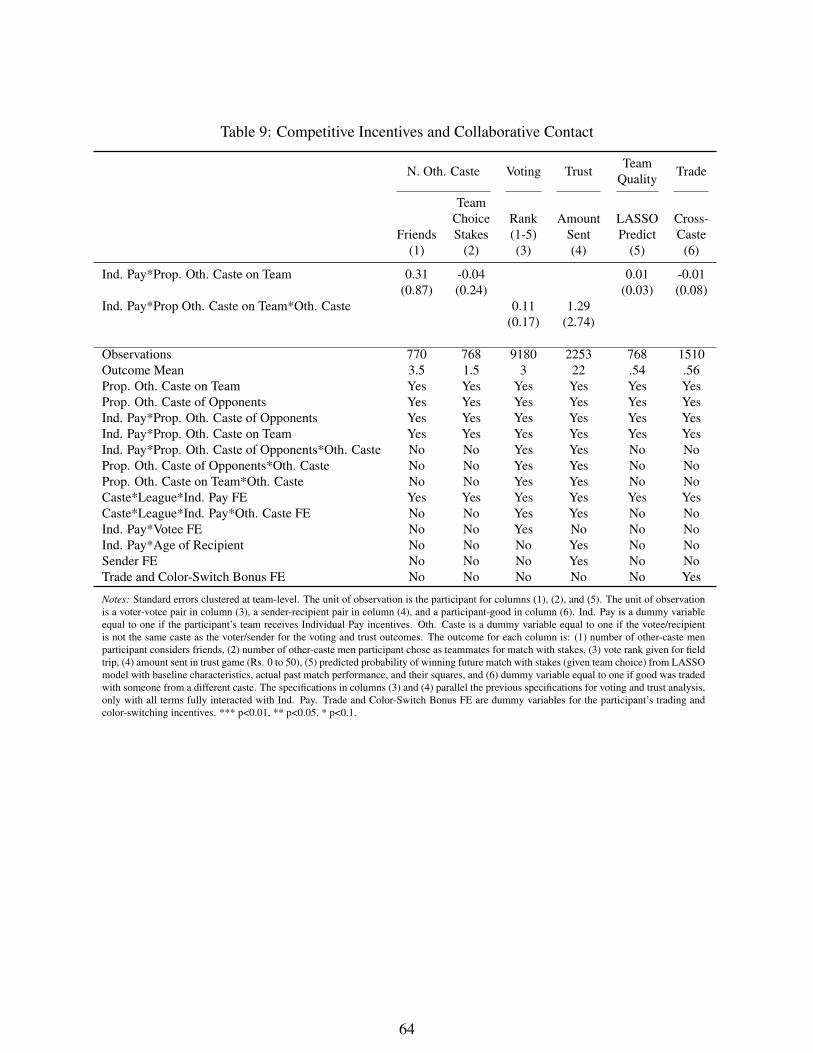
Table 9: Competitive Incentives and Collaborative Contact

N. Oth. Caste Voting TrustTeam

Quality Trade

Friends(1)

TeamChoiceStakes

(2)

Rank(1-5)(3)

AmountSent(4)

LASSOPredict

(5)

Cross-Caste

(6)

Ind. Pay*Prop. Oth. Caste on Team 0.31 -0.04 0.01 -0.01(0.87) (0.24) (0.03) (0.08)

Ind. Pay*Prop Oth. Caste on Team*Oth. Caste 0.11 1.29(0.17) (2.74)

Observations 770 768 9180 2253 768 1510Outcome Mean 3.5 1.5 3 22 .54 .56Prop. Oth. Caste on Team Yes Yes Yes Yes Yes YesProp. Oth. Caste of Opponents Yes Yes Yes Yes Yes YesInd. Pay*Prop. Oth. Caste of Opponents Yes Yes Yes Yes Yes YesInd. Pay*Prop. Oth. Caste on Team Yes Yes Yes Yes Yes YesInd. Pay*Prop. Oth. Caste of Opponents*Oth. Caste No No Yes Yes No NoProp. Oth. Caste of Opponents*Oth. Caste No No Yes Yes No NoProp. Oth. Caste on Team*Oth. Caste No No Yes Yes No NoCaste*League*Ind. Pay FE Yes Yes Yes Yes Yes YesCaste*League*Ind. Pay*Oth. Caste FE No No Yes Yes No NoInd. Pay*Votee FE No No Yes No No NoInd. Pay*Age of Recipient No No No Yes No NoSender FE No No No Yes No NoTrade and Color-Switch Bonus FE No No No No No Yes

Notes: Standard errors clustered at team-level. The unit of observation is the participant for columns (1), (2), and (5). The unit of observationis a voter-votee pair in column (3), a sender-recipient pair in column (4), and a participant-good in column (6). Ind. Pay is a dummy variableequal to one if the participant’s team receives Individual Pay incentives. Oth. Caste is a dummy variable equal to one if the votee/recipientis not the same caste as the voter/sender for the voting and trust outcomes. The outcome for each column is: (1) number of other-caste menparticipant considers friends, (2) number of other-caste men participant chose as teammates for match with stakes, (3) vote rank given for fieldtrip, (4) amount sent in trust game (Rs. 0 to 50), (5) predicted probability of winning future match with stakes (given team choice) from LASSOmodel with baseline characteristics, actual past match performance, and their squares, and (6) dummy variable equal to one if good was tradedwith someone from a different caste. The specifications in columns (3) and (4) parallel the previous specifications for voting and trust analysis,only with all terms fully interacted with Ind. Pay. Trade and Color-Switch Bonus FE are dummy variables for the participant’s trading andcolor-switching incentives. *** p<0.01, ** p<0.05, * p<0.1.

64

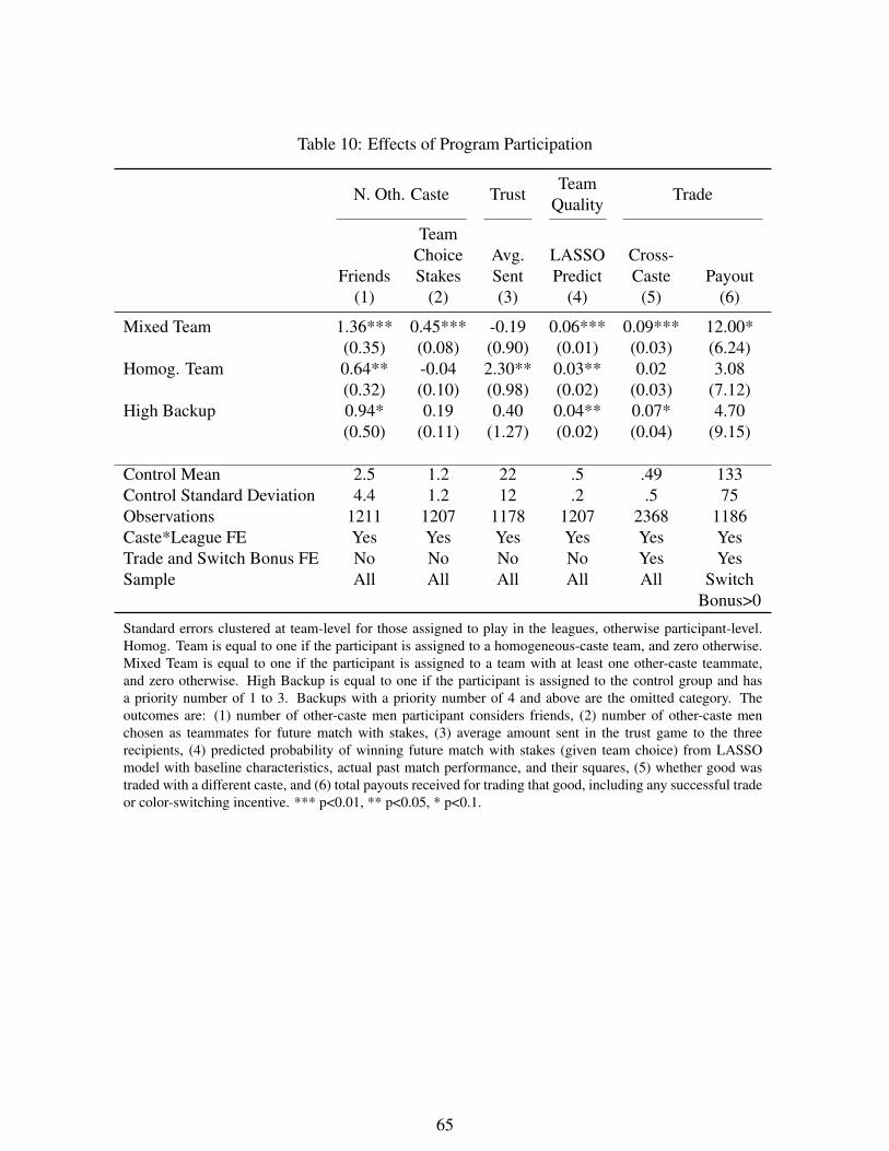
Table 10: Effects of Program Participation

N. Oth. Caste TrustTeam

Quality Trade

Friends(1)

TeamChoiceStakes

(2)

Avg.Sent(3)

LASSOPredict

(4)

Cross-Caste

(5)Payout

(6)

Mixed Team 1.36*** 0.45*** -0.19 0.06*** 0.09*** 12.00*(0.35) (0.08) (0.90) (0.01) (0.03) (6.24)

Homog. Team 0.64** -0.04 2.30** 0.03** 0.02 3.08(0.32) (0.10) (0.98) (0.02) (0.03) (7.12)

High Backup 0.94* 0.19 0.40 0.04** 0.07* 4.70(0.50) (0.11) (1.27) (0.02) (0.04) (9.15)

Control Mean 2.5 1.2 22 .5 .49 133Control Standard Deviation 4.4 1.2 12 .2 .5 75Observations 1211 1207 1178 1207 2368 1186Caste*League FE Yes Yes Yes Yes Yes YesTrade and Switch Bonus FE No No No No Yes YesSample All All All All All Switch

Bonus>0

Standard errors clustered at team-level for those assigned to play in the leagues, otherwise participant-level.Homog. Team is equal to one if the participant is assigned to a homogeneous-caste team, and zero otherwise.Mixed Team is equal to one if the participant is assigned to a team with at least one other-caste teammate,and zero otherwise. High Backup is equal to one if the participant is assigned to the control group and hasa priority number of 1 to 3. Backups with a priority number of 4 and above are the omitted category. Theoutcomes are: (1) number of other-caste men participant considers friends, (2) number of other-caste menchosen as teammates for future match with stakes, (3) average amount sent in the trust game to the threerecipients, (4) predicted probability of winning future match with stakes (given team choice) from LASSOmodel with baseline characteristics, actual past match performance, and their squares, (5) whether good wastraded with a different caste, and (6) total payouts received for trading that good, including any successful tradeor color-switching incentive. *** p<0.01, ** p<0.05, * p<0.1.

65

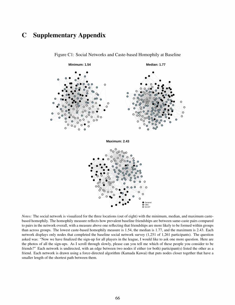
C Supplementary Appendix

Figure C1: Social Networks and Caste-based Homophily at Baseline

Minimum: 1.54

●

●●

●

●●

●

●

●

●

●

●

●

●

●

●

●

●●

●

●

●

●

●

●

●

●

●

●

●

●

●

●

●

●

●

●

●

●

●

●

●

● ● ●

●

●

● ●

●

●

●

●

●

●

●

●

●

●

●

●

●

●

●

●

●

●

●

●

●

●

●

●

● ●

●

●

●

●

●●

●●

●

●

●

●

●

●

●

●

●

●

●

●

●

●

●

●

●

●

●

●

●

●

●

●

●

●

●

●

●

●

●

●

●

●

●

●

●

●

●

●

●

●

●

●

●

●

●

●

●

●

●

●

●

● ●

●

Median: 1.77

●

●

●

●

●

●

●

●

●

●

●

●

●

●

●

●

●

●

●

●●

●

●

●

●

●

●●

●

●

●

●

●

●

●

●

●

●

●●

●

●

●

●

●

●

●

●

●

●

●

●

●

●

●

●

●

●

●

●

●

●

●

●

●

●

●

●

●

●

●

●

●●

●●

●●

●

●

●●

●●

●

●

●

●

●

●

●

●

●

●

●

●

●●

● ●

●

●

●

●

●

●

●

●

●

●

●

●

●

●

●

●●

●

●

●

●

●

●

●

●

●

●

●

●

●

●

●

●

●

●

●

●

●

●

●

●

●

●

●

●

●

●

●

●

●

●

●

●

●

●

●

●

●

●

●

●

●

●●

●●

●

●

●

●

●

●●

●

Maximum: 2.43

●

●

●

● ●

●

●

●

●

●

●

●

●

●

●

●

●●

●

●

●

●

●

●

●

●

●

●

●

●

●

●

●

●

●

●

●

●

●

●

●

●

●

●●

●

●

●

●

●

●

●

●

●

●

●

●

●

●

●

●

●

●

●

●

●

● ●●●

●

●

●

●

●

●

●

●

●

●

●●

●

●

●

●

●

●

●

●

●

●

●

● ●

●

●

●

●

●

●

●

●

●

●

●

●

●

●

● ●

●

●

●

●

●

●

●●

●

● ●

●

●

●

●

●

●

●●

●

●●

●

●

●

●

●

●

●

●

●

●

●●

●

●

●

●

●●●

●

●

●

GeneralOBCSC/ST

Notes: The social network is visualized for the three locations (out of eight) with the minimum, median, and maximum caste-based homophily. The homophily measure reflects how prevalent baseline friendships are between same-caste pairs comparedto pairs in the network overall, with a measure above one reflecting that friendships are more likely to be formed within groupsthan across groups. The lowest caste-based homophily measure is 1.54, the median is 1.77, and the maximum is 2.43. Eachnetwork displays only nodes that completed the baseline social network survey (1,251 of 1,261 participants). The questionasked was: “Now we have finalized the sign-up for all players in the league, I would like to ask one more question. Here arethe photos of all the sign-ups. As I scroll through slowly, please can you tell me which of these people you consider to befriends?” Each network is undirected, with an edge between two nodes if either (or both) participant(s) listed the other as afriend. Each network is drawn using a force-directed algorithm (Kamada Kawai) that puts nodes closer together that have asmaller length of the shortest path between them.

66

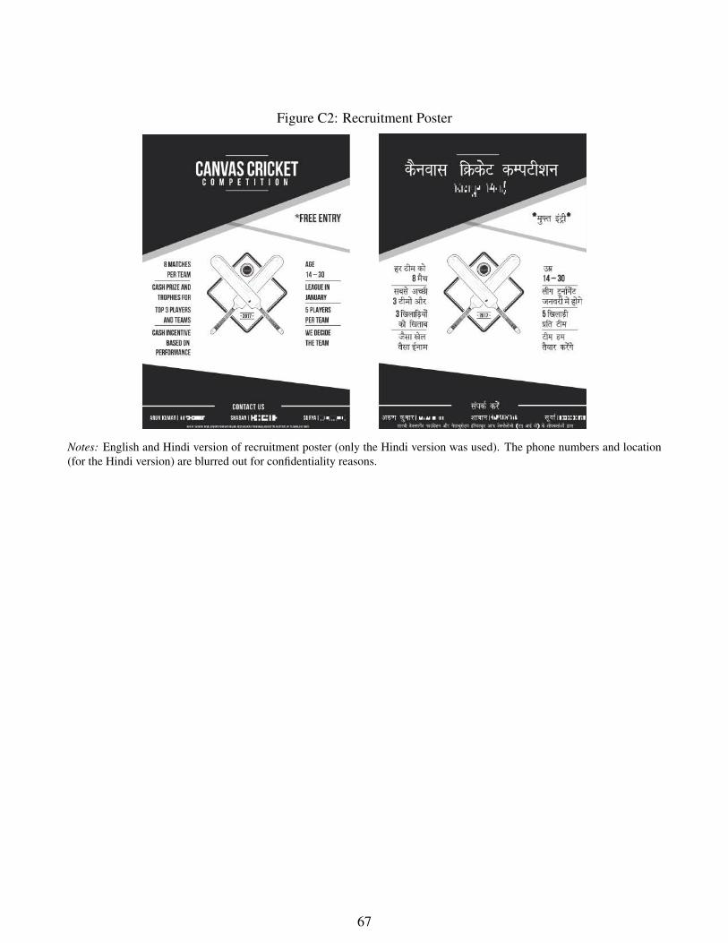
Figure C2: Recruitment Poster

Notes: English and Hindi version of recruitment poster (only the Hindi version was used). The phone numbers and location(for the Hindi version) are blurred out for confidentiality reasons.

67

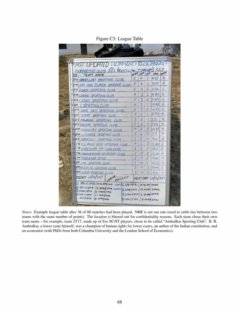
Figure C3: League Table

Notes: Example league table after 36 of 80 matches had been played. NRR is net run rate (used to settle ties between twoteams with the same number of points). The location is blurred out for confidentiality reasons. Each team chose their ownteam name – for example, team 2T17, made up of five SC/ST players, chose to be called “Ambedkar Sporting Club”. B. R.Ambedkar, a lower caste himself, was a champion of human rights for lower castes, an author of the Indian constitution, andan economist (with PhDs from both Columbia University and the London School of Economics).

68

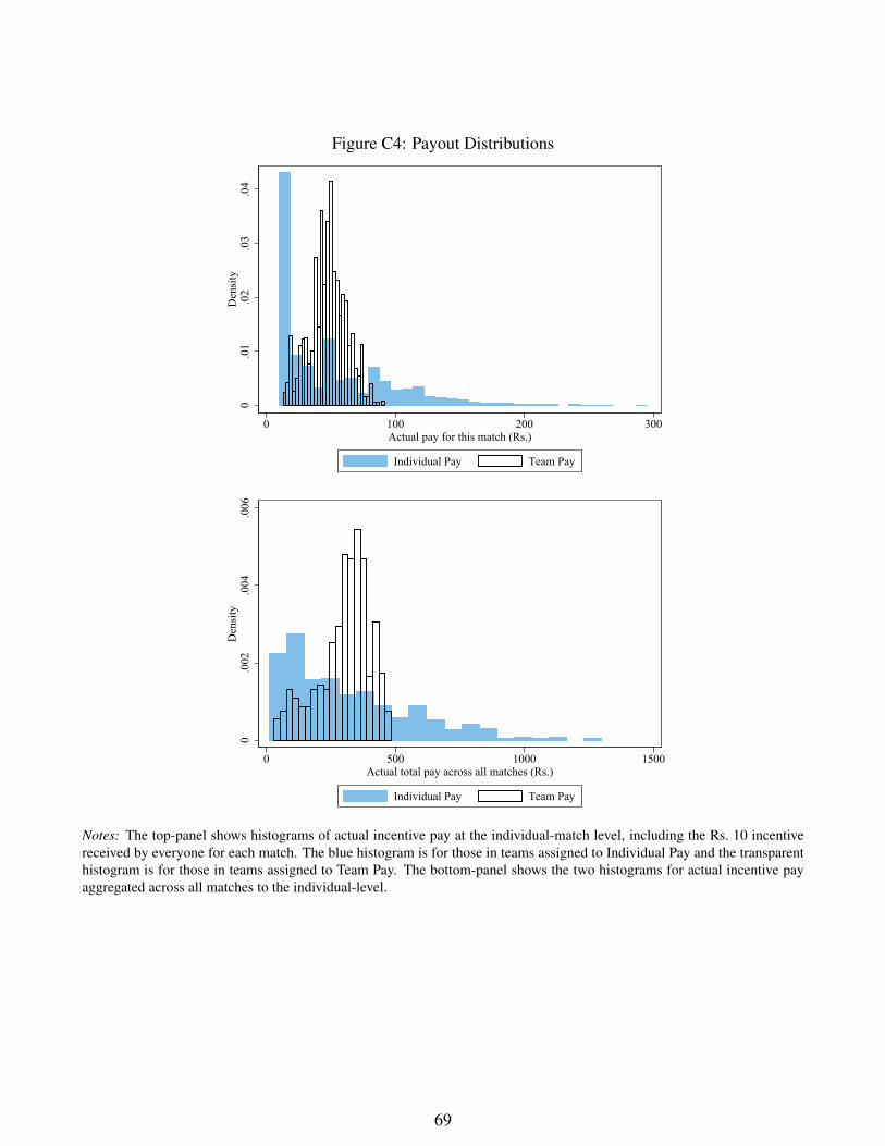
Figure C4: Payout Distributions

0.0

1.0

2.0

3.0

4D

ensi

ty

0 100 200 300Actual pay for this match (Rs.)

Individual Pay Team Pay

0.0

02.0

04.0

06D

ensi

ty

0 500 1000 1500Actual total pay across all matches (Rs.)

Individual Pay Team Pay

Notes: The top-panel shows histograms of actual incentive pay at the individual-match level, including the Rs. 10 incentivereceived by everyone for each match. The blue histogram is for those in teams assigned to Individual Pay and the transparenthistogram is for those in teams assigned to Team Pay. The bottom-panel shows the two histograms for actual incentive payaggregated across all matches to the individual-level.

69

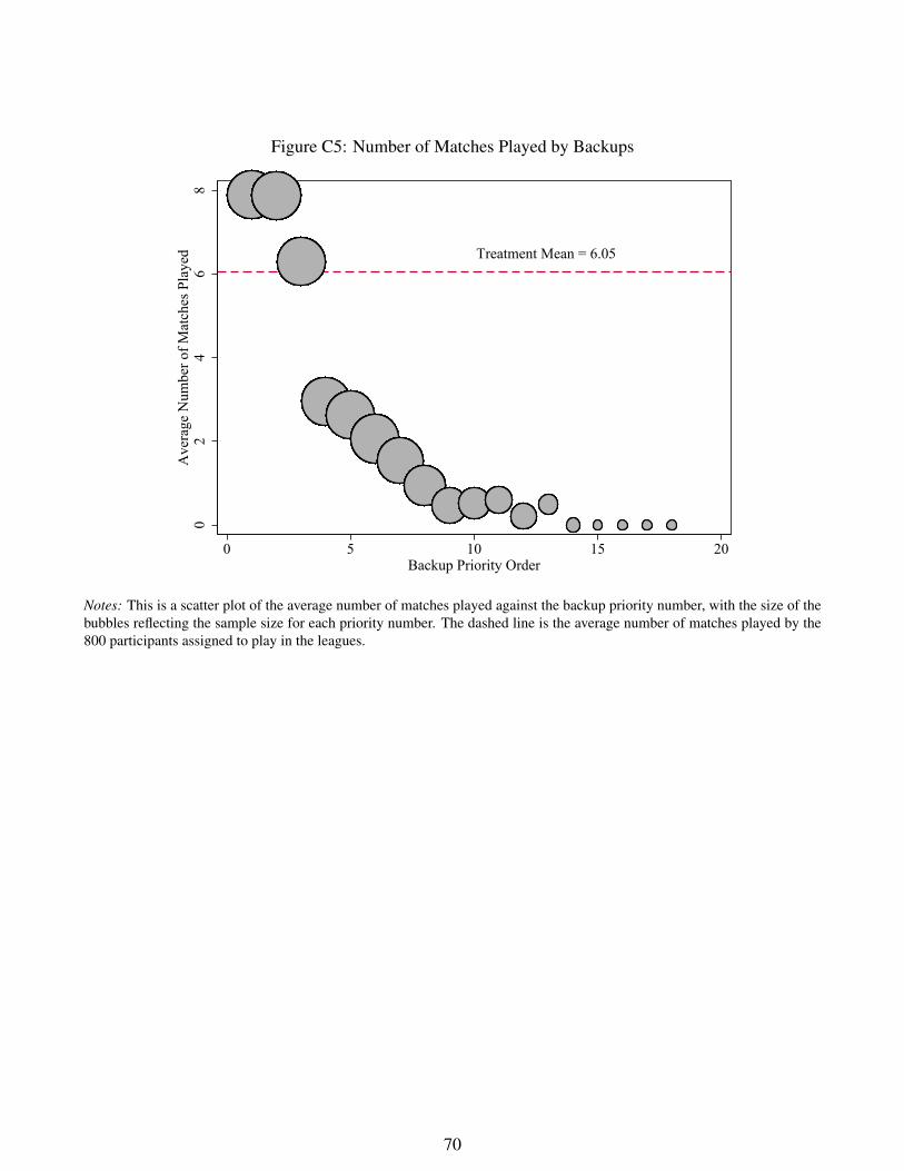
Figure C5: Number of Matches Played by Backups

Treatment Mean = 6.05

02

46

8A

vera

ge N

umbe

r of M

atch

es P

laye

d

0 5 10 15 20Backup Priority Order

Notes: This is a scatter plot of the average number of matches played against the backup priority number, with the size of thebubbles reflecting the sample size for each priority number. The dashed line is the average number of matches played by the800 participants assigned to play in the leagues.

70

Figure C6: Friends of Friends of Teammates – Identification Intuition

Team 1 Team 2

𝑖 𝑖′𝑘

𝑗

𝑗′

Notes: This figure demonstrates the intuition behind the identification of the effect on friendship of being indirectly linked withanother participant. The dashed lines reflect baseline friendship links reported by the other-caste members of Teams 1 and 2.Players i and i′ belong to the same caste (same color) and have the same collaborative contact (Prop. Oth. Caste on Teamicl =Prop. Oth. Caste on Teami′cl = 0.75). Player k is a teammate of i’s, but not a teammate of i′’s. I find the effects of directlinks on friendship by asking “is the probability that i and k are friends after the league is over greater than the probabilitythat i′ and k are friends?”. Similarly, player j is an other-caste friend of an other-caste teammate of i’s (an indirect link),but he is not an indirect link of i′’s. I find the effects on friendship of indirect links by asking “is the probability that i andj are friends after the league is over greater than the probability that i′ and j are friends?” Each of these comparisons is anexample of one within-cell comparison that contributes to identification – the actual estimates come from pooling many suchcomparisons. Finally, j′ is an example of an other-caste player indirectly linked to both i and i′. This player does not contributeto identification of the indirect link effect since there is no variation within this cell.

71

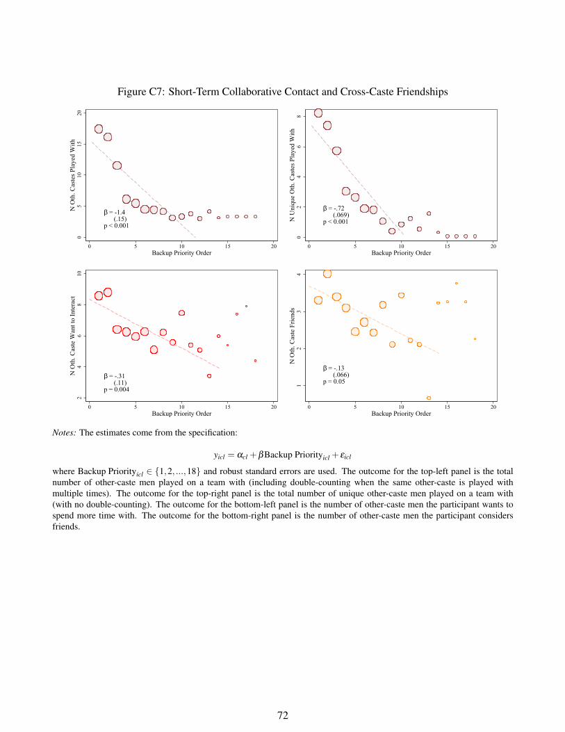
Figure C7: Short-Term Collaborative Contact and Cross-Caste Friendships

β = -1.4 (.15)p < 0.001

05

1015

20N

Oth

. Cas

tes P

laye

d W

ith

0 5 10 15 20Backup Priority Order

β = -.72 (.069)p < 0.001

02

46

8N

Uni

que

Oth

. Cas

tes P

laye

d W

ith

0 5 10 15 20Backup Priority Order

β = -.31 (.11)p = 0.004

24

68

10N

Oth

. Cas

te W

ant t

o In

tera

ct

0 5 10 15 20Backup Priority Order

β = -.13 (.066)p = 0.051

23

4N

Oth

. Cas

te F

riend

s

0 5 10 15 20Backup Priority Order

Notes: The estimates come from the specification:

yicl = αcl +βBackup Priorityicl + εicl

where Backup Priorityicl ∈ {1,2, ...,18} and robust standard errors are used. The outcome for the top-left panel is the totalnumber of other-caste men played on a team with (including double-counting when the same other-caste is played withmultiple times). The outcome for the top-right panel is the total number of unique other-caste men played on a team with(with no double-counting). The outcome for the bottom-left panel is the number of other-caste men the participant wants tospend more time with. The outcome for the bottom-right panel is the number of other-caste men the participant considersfriends.

72

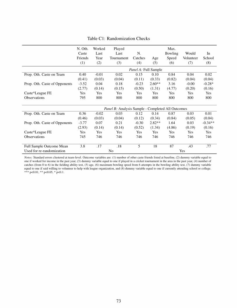
Table C1: Randomization Checks

N. Oth.Caste

Friends(1)

WorkedLastYear(2)

PlayedLast

Tournament(3)

N.Catches

(4)Age(5)

Max.BowlingSpeed

(6)

WouldVolunteer

(7)

InSchool

(8)

Panel A: Full SampleProp. Oth. Caste on Team 0.40 -0.01 0.02 0.15 0.10 0.84 0.04 0.02

(0.41) (0.03) (0.04) (0.11) (0.33) (0.82) (0.04) (0.04)Prop. Oth. Caste of Opponents -3.52 0.04 0.18 -0.23 2.60** 3.16 -0.00 -0.28*

(2.77) (0.14) (0.15) (0.50) (1.31) (4.77) (0.20) (0.16)Caste*League FE Yes Yes Yes Yes Yes Yes Yes YesObservations 795 800 800 800 800 800 800 800

Panel B: Analysis Sample - Completed All OutcomesProp. Oth. Caste on Team 0.36 -0.02 0.03 0.12 0.14 0.87 0.03 0.01

(0.46) (0.03) (0.04) (0.12) (0.34) (0.84) (0.05) (0.04)Prop. Oth. Caste of Opponents -3.77 0.07 0.21 -0.30 2.82** 1.64 0.03 -0.34**

(2.93) (0.14) (0.14) (0.52) (1.34) (4.86) (0.19) (0.16)Caste*League FE Yes Yes Yes Yes Yes Yes Yes YesObservations 745 746 746 746 746 746 746 746

Full Sample Outcome Mean 3.8 .17 .18 5 18 87 .43 .77Used for re-randomization No Yes

Notes: Standard errors clustered at team-level. Outcome variables are: (1) number of other caste friends listed at baseline, (2) dummy variable equal toone if worked for income in the past year, (3) dummy variable equal to one if played in a cricket tournament in the area in the past year, (4) number ofcatches (from 0 to 6) in the fielding ability test, (5) age, (6) maximum bowling speed from 6 attempts in the bowling ability test, (7) dummy variableequal to one if said willing to volunteer to help with league organization, and (8) dummy variable equal to one if currently attending school or college.*** p<0.01, ** p<0.05, * p<0.1.

73

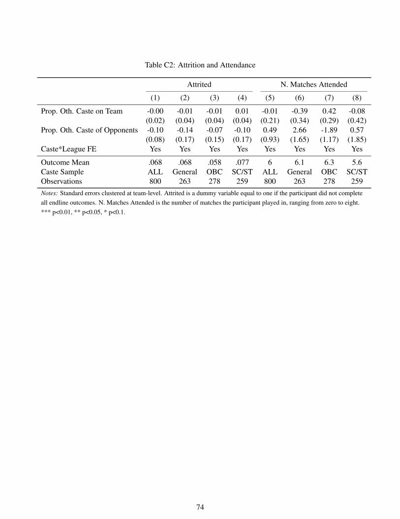
Table C2: Attrition and Attendance

Attrited N. Matches Attended

(1) (2) (3) (4) (5) (6) (7) (8)

Prop. Oth. Caste on Team -0.00 -0.01 -0.01 0.01 -0.01 -0.39 0.42 -0.08(0.02) (0.04) (0.04) (0.04) (0.21) (0.34) (0.29) (0.42)

Prop. Oth. Caste of Opponents -0.10 -0.14 -0.07 -0.10 0.49 2.66 -1.89 0.57(0.08) (0.17) (0.15) (0.17) (0.93) (1.65) (1.17) (1.85)

Caste*League FE Yes Yes Yes Yes Yes Yes Yes Yes

Outcome Mean .068 .068 .058 .077 6 6.1 6.3 5.6Caste Sample ALL General OBC SC/ST ALL General OBC SC/STObservations 800 263 278 259 800 263 278 259Notes: Standard errors clustered at team-level. Attrited is a dummy variable equal to one if the participant did not completeall endline outcomes. N. Matches Attended is the number of matches the participant played in, ranging from zero to eight.*** p<0.01, ** p<0.05, * p<0.1.

74

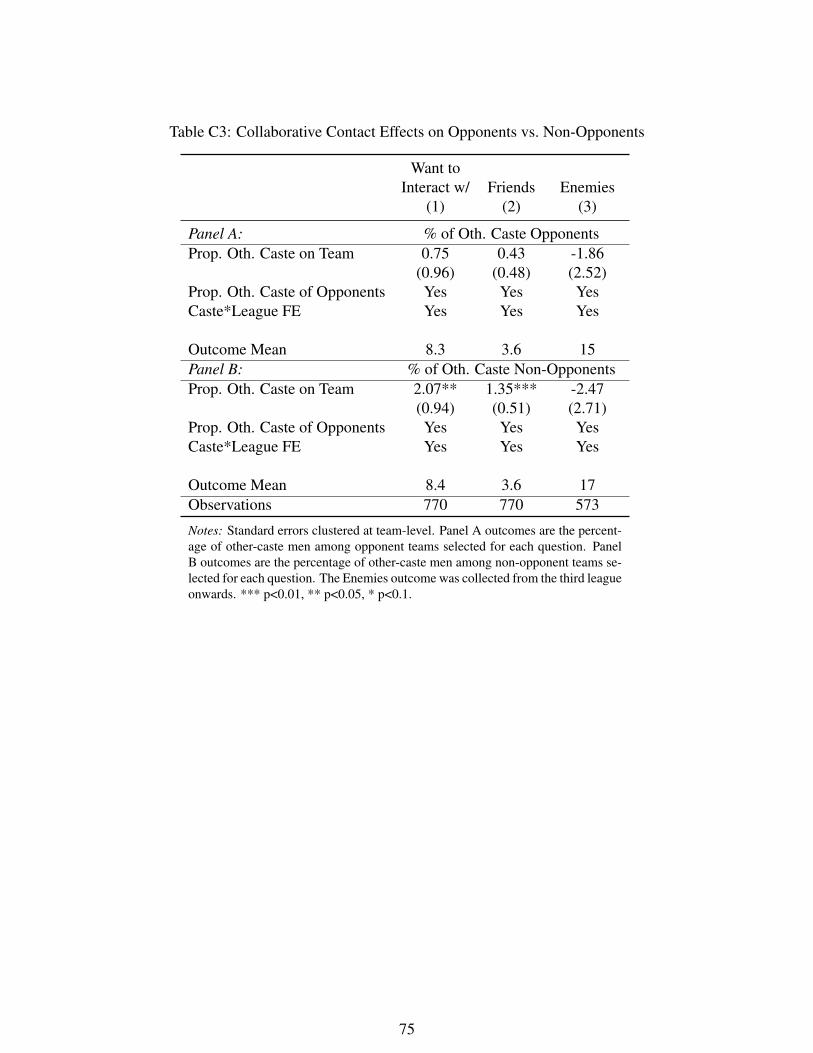
Table C3: Collaborative Contact Effects on Opponents vs. Non-Opponents

Want toInteract w/

(1)Friends

(2)Enemies

(3)

Panel A: % of Oth. Caste OpponentsProp. Oth. Caste on Team 0.75 0.43 -1.86

(0.96) (0.48) (2.52)Prop. Oth. Caste of Opponents Yes Yes YesCaste*League FE Yes Yes Yes

Outcome Mean 8.3 3.6 15Panel B: % of Oth. Caste Non-OpponentsProp. Oth. Caste on Team 2.07** 1.35*** -2.47

(0.94) (0.51) (2.71)Prop. Oth. Caste of Opponents Yes Yes YesCaste*League FE Yes Yes Yes

Outcome Mean 8.4 3.6 17Observations 770 770 573

Notes: Standard errors clustered at team-level. Panel A outcomes are the percent-age of other-caste men among opponent teams selected for each question. PanelB outcomes are the percentage of other-caste men among non-opponent teams se-lected for each question. The Enemies outcome was collected from the third leagueonwards. *** p<0.01, ** p<0.05, * p<0.1.

75

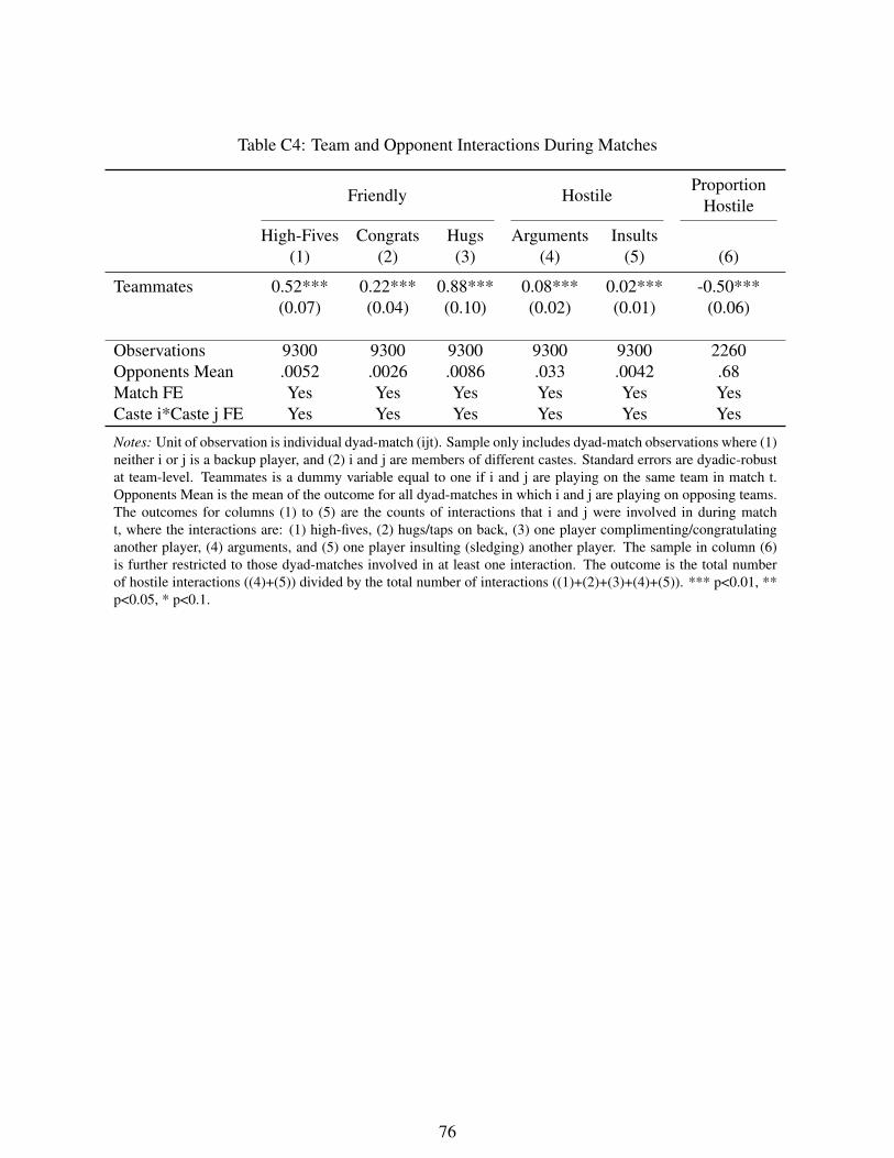
Table C4: Team and Opponent Interactions During Matches

Friendly HostileProportion

Hostile

High-Fives(1)

Congrats(2)

Hugs(3)

Arguments(4)

Insults(5) (6)

Teammates 0.52*** 0.22*** 0.88*** 0.08*** 0.02*** -0.50***(0.07) (0.04) (0.10) (0.02) (0.01) (0.06)

Observations 9300 9300 9300 9300 9300 2260Opponents Mean .0052 .0026 .0086 .033 .0042 .68Match FE Yes Yes Yes Yes Yes YesCaste i*Caste j FE Yes Yes Yes Yes Yes Yes

Notes: Unit of observation is individual dyad-match (ijt). Sample only includes dyad-match observations where (1)neither i or j is a backup player, and (2) i and j are members of different castes. Standard errors are dyadic-robustat team-level. Teammates is a dummy variable equal to one if i and j are playing on the same team in match t.Opponents Mean is the mean of the outcome for all dyad-matches in which i and j are playing on opposing teams.The outcomes for columns (1) to (5) are the counts of interactions that i and j were involved in during matcht, where the interactions are: (1) high-fives, (2) hugs/taps on back, (3) one player complimenting/congratulatinganother player, (4) arguments, and (5) one player insulting (sledging) another player. The sample in column (6)is further restricted to those dyad-matches involved in at least one interaction. The outcome is the total numberof hostile interactions ((4)+(5)) divided by the total number of interactions ((1)+(2)+(3)+(4)+(5)). *** p<0.01, **p<0.05, * p<0.1.

76

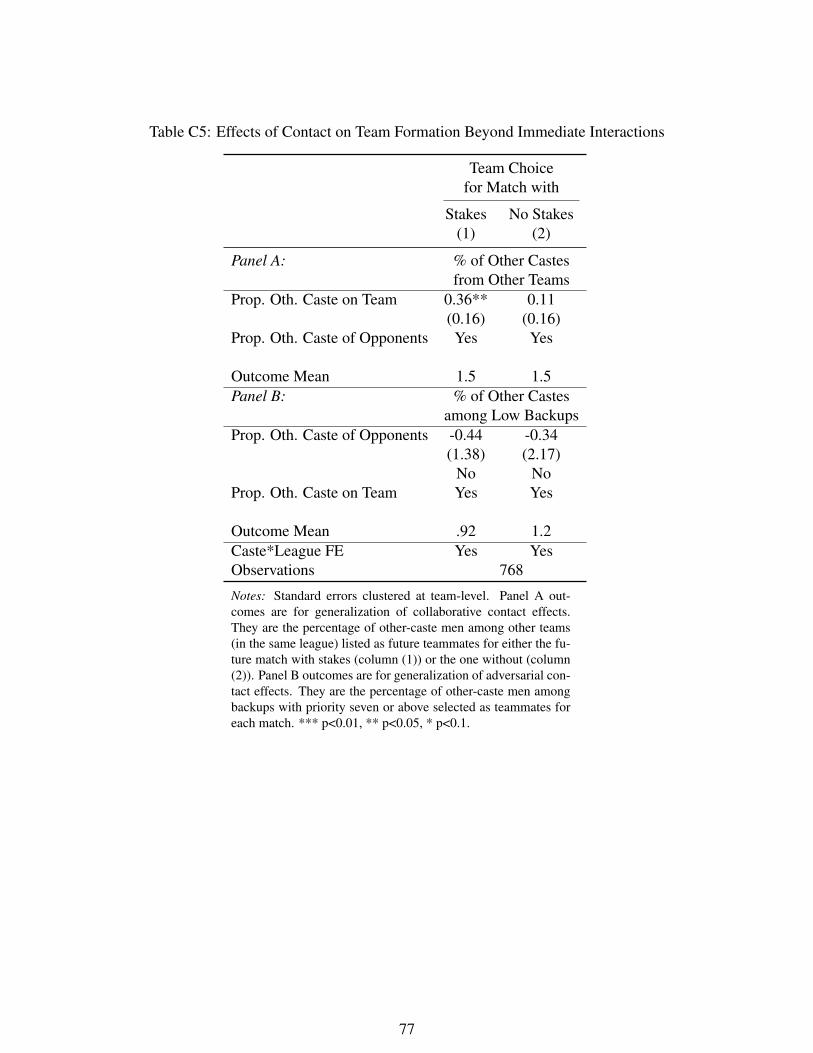
Table C5: Effects of Contact on Team Formation Beyond Immediate Interactions

Team Choicefor Match with

Stakes(1)

No Stakes(2)

Panel A: % of Other Castesfrom Other Teams

Prop. Oth. Caste on Team 0.36** 0.11(0.16) (0.16)

Prop. Oth. Caste of Opponents Yes Yes

Outcome Mean 1.5 1.5Panel B: % of Other Castes

among Low BackupsProp. Oth. Caste of Opponents -0.44 -0.34

(1.38) (2.17)No No

Prop. Oth. Caste on Team Yes Yes

Outcome Mean .92 1.2Caste*League FE Yes YesObservations 768

Notes: Standard errors clustered at team-level. Panel A out-comes are for generalization of collaborative contact effects.They are the percentage of other-caste men among other teams(in the same league) listed as future teammates for either the fu-ture match with stakes (column (1)) or the one without (column(2)). Panel B outcomes are for generalization of adversarial con-tact effects. They are the percentage of other-caste men amongbackups with priority seven or above selected as teammates foreach match. *** p<0.01, ** p<0.05, * p<0.1.

77

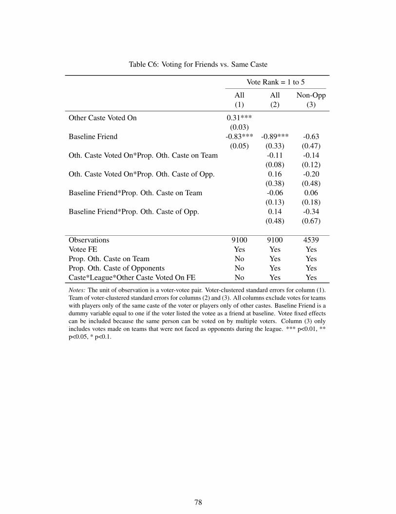
Table C6: Voting for Friends vs. Same Caste

Vote Rank = 1 to 5

All(1)

All(2)

Non-Opp(3)

Other Caste Voted On 0.31***(0.03)

Baseline Friend -0.83*** -0.89*** -0.63(0.05) (0.33) (0.47)

Oth. Caste Voted On*Prop. Oth. Caste on Team -0.11 -0.14(0.08) (0.12)

Oth. Caste Voted On*Prop. Oth. Caste of Opp. 0.16 -0.20(0.38) (0.48)

Baseline Friend*Prop. Oth. Caste on Team -0.06 0.06(0.13) (0.18)

Baseline Friend*Prop. Oth. Caste of Opp. 0.14 -0.34(0.48) (0.67)

Observations 9100 9100 4539Votee FE Yes Yes YesProp. Oth. Caste on Team No Yes YesProp. Oth. Caste of Opponents No Yes YesCaste*League*Other Caste Voted On FE No Yes Yes

Notes: The unit of observation is a voter-votee pair. Voter-clustered standard errors for column (1).Team of voter-clustered standard errors for columns (2) and (3). All columns exclude votes for teamswith players only of the same caste of the voter or players only of other castes. Baseline Friend is adummy variable equal to one if the voter listed the votee as a friend at baseline. Votee fixed effectscan be included because the same person can be voted on by multiple voters. Column (3) onlyincludes votes made on teams that were not faced as opponents during the league. *** p<0.01, **p<0.05, * p<0.1.

78

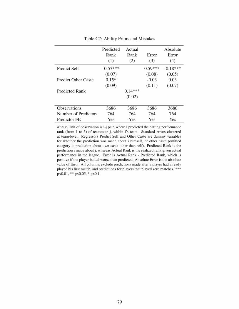
Table C7: Ability Priors and Mistakes

PredictedRank(1)

ActualRank(2)

Error(3)

AbsoluteError(4)

Predict Self -0.57*** 0.59*** -0.18***(0.07) (0.08) (0.05)

Predict Other Caste 0.15* -0.03 0.03(0.09) (0.11) (0.07)

Predicted Rank 0.14***(0.02)

Observations 3686 3686 3686 3686Number of Predictors 764 764 764 764Predictor FE Yes Yes Yes Yes

Notes: Unit of observation is i-j pair, where i predicted the batting performancerank (from 1 to 5) of teammate j, within i’s team. Standard errors clusteredat team-level. Regressors Predict Self and Other Caste are dummy variablesfor whether the prediction was made about i himself, or other caste (omittedcategory is prediction about own caste other than self). Predicted Rank is theprediction i made about j, whereas Actual Rank is the realized rank given actualperformance in the league. Error is Actual Rank - Predicted Rank, which ispositive if the player batted worse than predicted. Absolute Error is the absolutevalue of Error. All columns exclude predictions made after a player had alreadyplayed his first match, and predictions for players that played zero matches. ***p<0.01, ** p<0.05, * p<0.1.

79

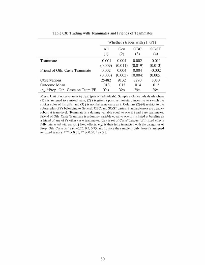
Table C8: Trading with Teammates and Friends of Teammates

Whether i trades with j (=0/1)

All(1)

Gen(2)

OBC(3)

SC/ST(4)

Teammate -0.001 0.004 0.002 -0.011(0.009) (0.011) (0.019) (0.013)

Friend of Oth. Caste Teammate 0.002 0.004 0.004 -0.002(0.003) (0.005) (0.004) (0.005)

Observations 25482 9132 8270 8080Outcome Mean .013 .013 .014 .012α jcl*Prop. Oth. Caste on Team FE Yes Yes Yes Yes

Notes: Unit of observation is i-j dyad (pair of individuals). Sample includes only dyads where(1) i is assigned to a mixed team, (2) i is given a positive monetary incentive to switch thesticker color of his gifts, and (3) j is not the same caste as i. Columns (2)-(4) restrict to thesubsamples of i’s belonging to General, OBC, and SC/ST castes. Standard errors are dyadic-robust at team-level. Teammate is a dummy variable equal to one if i and j are teammates.Friend of Oth. Caste Teammate is a dummy variable equal to one if j is listed at baseline asa friend of any of i’s other caste teammates. α jcl is set of Caste*League (of i) fixed effectsfully interacted with person j fixed effects. α jcl is then fully interacted with the categories ofProp. Oth. Caste on Team (0.25, 0.5, 0.75, and 1, since the sample is only those i’s assignedto mixed teams). *** p<0.01, ** p<0.05, * p<0.1.

80

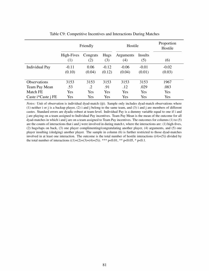
Table C9: Competitive Incentives and Interactions During Matches

Friendly HostileProportion

Hostile

High-Fives(1)

Congrats(2)

Hugs(3)

Arguments(4)

Insults(5) (6)

Individual Pay -0.11 0.06 -0.12 -0.06 -0.01 -0.02(0.10) (0.04) (0.12) (0.04) (0.01) (0.03)

Observations 3153 3153 3153 3153 3153 1967Team Pay Mean .53 .2 .91 .12 .029 .083Match FE Yes Yes Yes Yes Yes YesCaste i*Caste j FE Yes Yes Yes Yes Yes Yes

Notes: Unit of observation is individual dyad-match (ijt). Sample only includes dyad-match observations where(1) neither i or j is a backup player, (2) i and j belong to the same team, and (3) i and j are members of differentcastes. Standard errors are dyadic-robust at team-level. Individual Pay is a dummy variable equal to one if i andj are playing on a team assigned to Individual Pay incentives. Team Pay Mean is the mean of the outcome for alldyad-matches in which i and j are on a team assigned to Team Pay incentives. The outcomes for columns (1) to (5)are the counts of interactions that i and j were involved in during match t, where the interactions are: (1) high-fives,(2) hugs/taps on back, (3) one player complimenting/congratulating another player, (4) arguments, and (5) oneplayer insulting (sledging) another player. The sample in column (6) is further restricted to those dyad-matchesinvolved in at least one interaction. The outcome is the total number of hostile interactions ((4)+(5)) divided bythe total number of interactions ((1)+(2)+(3)+(4)+(5)). *** p<0.01, ** p<0.05, * p<0.1.

81

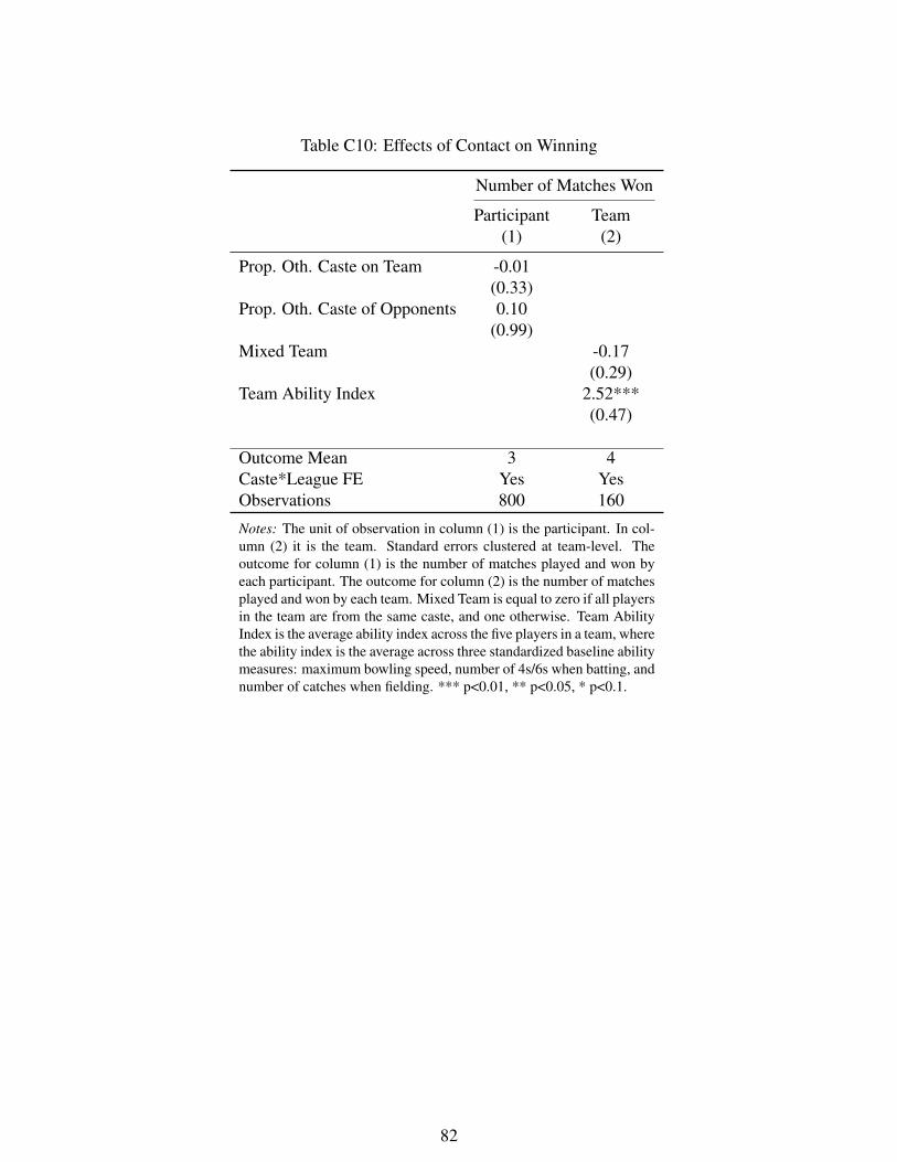
Table C10: Effects of Contact on Winning

Number of Matches Won

Participant(1)

Team(2)

Prop. Oth. Caste on Team -0.01(0.33)

Prop. Oth. Caste of Opponents 0.10(0.99)

Mixed Team -0.17(0.29)

Team Ability Index 2.52***(0.47)

Outcome Mean 3 4Caste*League FE Yes YesObservations 800 160

Notes: The unit of observation in column (1) is the participant. In col-umn (2) it is the team. Standard errors clustered at team-level. Theoutcome for column (1) is the number of matches played and won byeach participant. The outcome for column (2) is the number of matchesplayed and won by each team. Mixed Team is equal to zero if all playersin the team are from the same caste, and one otherwise. Team AbilityIndex is the average ability index across the five players in a team, wherethe ability index is the average across three standardized baseline abilitymeasures: maximum bowling speed, number of 4s/6s when batting, andnumber of catches when fielding. *** p<0.01, ** p<0.05, * p<0.1.

82

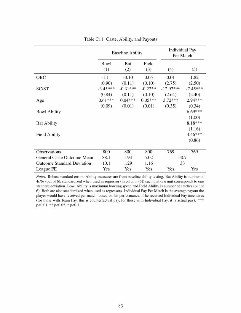
Table C11: Caste, Ability, and Payouts

Baseline AbilityIndividual Pay

Per Match

Bowl(1)

Bat(2)

Field(3) (4) (5)

OBC -1.11 -0.10 0.05 0.01 1.82(0.90) (0.11) (0.10) (2.75) (2.50)

SC/ST -3.45*** -0.31*** -0.22** -12.92*** -7.45***(0.84) (0.11) (0.10) (2.64) (2.40)

Age 0.61*** 0.04*** 0.05*** 3.72*** 2.94***(0.09) (0.01) (0.01) (0.35) (0.34)

Bowl Ability 6.69***(1.00)

Bat Ability 8.18***(1.16)

Field Ability 4.46***(0.86)

Observations 800 800 800 769 769General Caste Outcome Mean 88.1 1.94 5.02 50.7Outcome Standard Deviation 10.1 1.29 1.16 33League FE Yes Yes Yes Yes Yes

Notes: Robust standard errors. Ability measures are from baseline ability testing. Bat Ability is number of4s/6s (out of 6), standardized when used as regressor (in column (5)) such that one unit corresponds to onestandard deviation. Bowl Ability is maximum bowling speed and Field Ability is number of catches (out of6). Both are also standardized when used as regressors. Individual Pay Per Match is the average payout theplayer would have received per match, based on his performance, if he received Individual Pay incentives(for those with Team Pay, this is counterfactual pay, for those with Individual Pay, it is actual pay). ***p<0.01, ** p<0.05, * p<0.1.

83

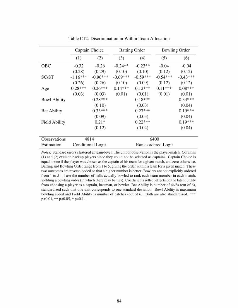
Table C12: Discrimination in Within-Team Allocation

Captain Choice Batting Order Bowling Order

(1) (2) (3) (4) (5) (6)

OBC -0.32 -0.26 -0.24** -0.23** -0.04 -0.04(0.28) (0.29) (0.10) (0.10) (0.12) (0.12)

SC/ST -1.16*** -0.96*** -0.69*** -0.59*** -0.54*** -0.43***(0.26) (0.26) (0.10) (0.09) (0.12) (0.12)

Age 0.28*** 0.26*** 0.14*** 0.12*** 0.11*** 0.08***(0.03) (0.03) (0.01) (0.01) (0.01) (0.01)

Bowl Ability 0.28*** 0.18*** 0.33***(0.10) (0.03) (0.04)

Bat Ability 0.33*** 0.27*** 0.19***(0.09) (0.03) (0.04)

Field Ability 0.21* 0.22*** 0.19***(0.12) (0.04) (0.04)

Observations 4814 6400Estimation Conditional Logit Rank-ordered Logit

Notes: Standard errors clustered at team-level. The unit of observation is the player-match. Columns(1) and (2) exclude backup players since they could not be selected as captains. Captain Choice isequal to one if the player was chosen as the captain of his team for a given match, and zero otherwise.Batting and Bowling Order range from 1 to 5, giving the order within a team for a given match. Thesetwo outcomes are reverse-coded so that a higher number is better. Bowlers are not explicitly orderedfrom 1 to 5 – I use the number of balls actually bowled to rank each team member in each match,yielding a bowling order (in which there may be ties). Coefficients reflect effects on the latent utilityfrom choosing a player as a captain, batsman, or bowler. Bat Ability is number of 4s/6s (out of 6),standardized such that one unit corresponds to one standard deviation. Bowl Ability is maximumbowling speed and Field Ability is number of catches (out of 6). Both are also standardized. ***p<0.01, ** p<0.05, * p<0.1.

84

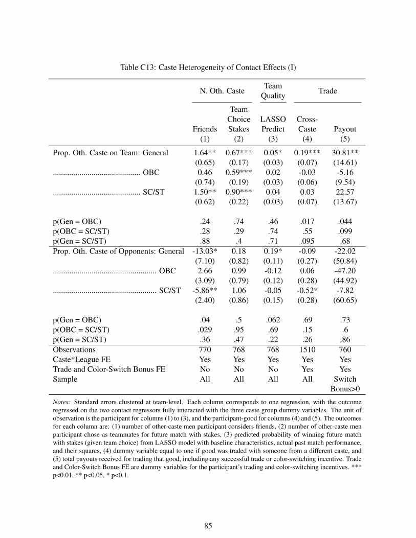
Table C13: Caste Heterogeneity of Contact Effects (I)

N. Oth. CasteTeam

Quality Trade

Friends(1)

TeamChoiceStakes

(2)

LASSOPredict

(3)

Cross-Caste

(4)Payout

(5)

Prop. Oth. Caste on Team: General 1.64** 0.67*** 0.05* 0.19*** 30.81**(0.65) (0.17) (0.03) (0.07) (14.61)

........................................... OBC 0.46 0.59*** 0.02 -0.03 -5.16(0.74) (0.19) (0.03) (0.06) (9.54)

........................................... SC/ST 1.50** 0.90*** 0.04 0.03 22.57(0.62) (0.22) (0.03) (0.07) (13.67)

p(Gen = OBC) .24 .74 .46 .017 .044p(OBC = SC/ST) .28 .29 .74 .55 .099p(Gen = SC/ST) .88 .4 .71 .095 .68Prop. Oth. Caste of Opponents: General -13.03* 0.18 0.19* -0.09 -22.02

(7.10) (0.82) (0.11) (0.27) (50.84)................................................... OBC 2.66 0.99 -0.12 0.06 -47.20

(3.09) (0.79) (0.12) (0.28) (44.92)................................................... SC/ST -5.86** 1.06 -0.05 -0.52* -7.82

(2.40) (0.86) (0.15) (0.28) (60.65)

p(Gen = OBC) .04 .5 .062 .69 .73p(OBC = SC/ST) .029 .95 .69 .15 .6p(Gen = SC/ST) .36 .47 .22 .26 .86Observations 770 768 768 1510 760Caste*League FE Yes Yes Yes Yes YesTrade and Color-Switch Bonus FE No No No Yes YesSample All All All All Switch

Bonus>0

Notes: Standard errors clustered at team-level. Each column corresponds to one regression, with the outcomeregressed on the two contact regressors fully interacted with the three caste group dummy variables. The unit ofobservation is the participant for columns (1) to (3), and the participant-good for columns (4) and (5). The outcomesfor each column are: (1) number of other-caste men participant considers friends, (2) number of other-caste menparticipant chose as teammates for future match with stakes, (3) predicted probability of winning future matchwith stakes (given team choice) from LASSO model with baseline characteristics, actual past match performance,and their squares, (4) dummy variable equal to one if good was traded with someone from a different caste, and(5) total payouts received for trading that good, including any successful trade or color-switching incentive. Tradeand Color-Switch Bonus FE are dummy variables for the participant’s trading and color-switching incentives. ***p<0.01, ** p<0.05, * p<0.1.

85

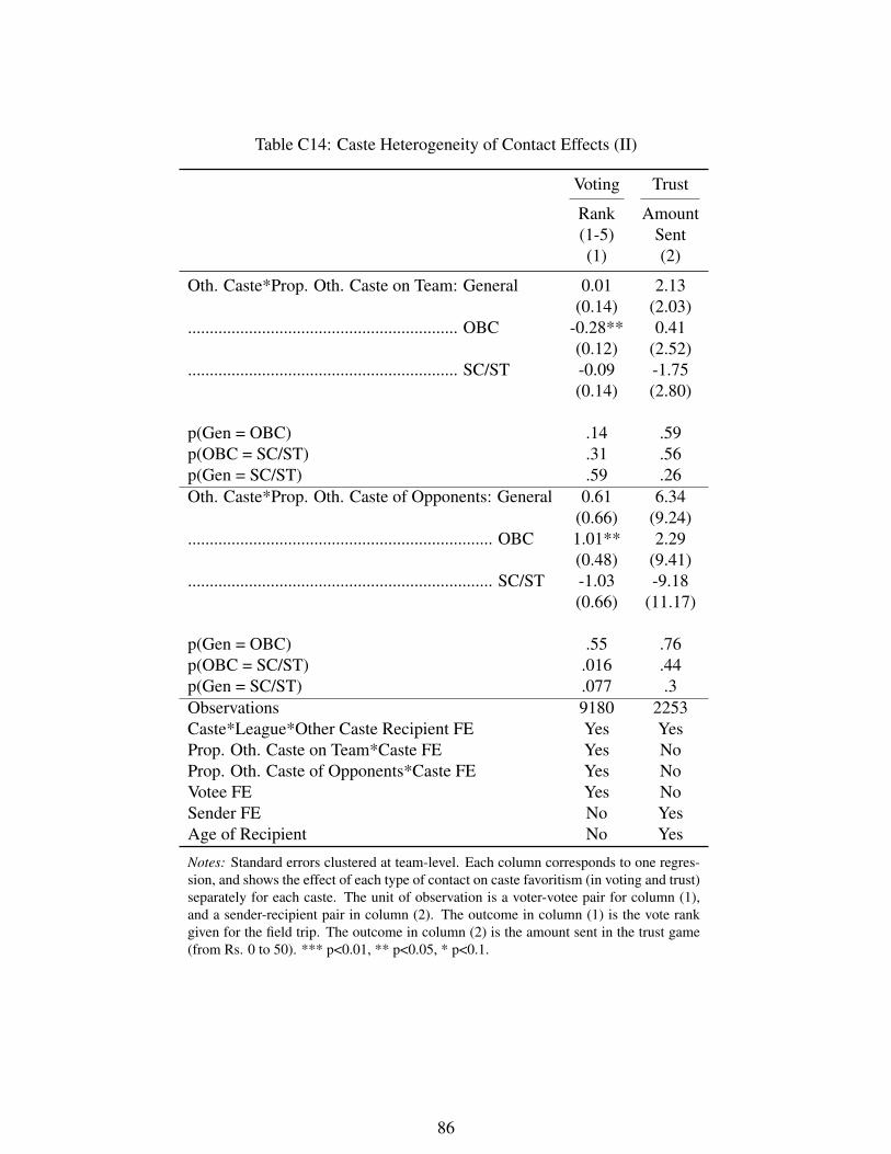
Table C14: Caste Heterogeneity of Contact Effects (II)

Voting Trust

Rank(1-5)(1)

AmountSent(2)

Oth. Caste*Prop. Oth. Caste on Team: General 0.01 2.13(0.14) (2.03)

.............................................................. OBC -0.28** 0.41(0.12) (2.52)

.............................................................. SC/ST -0.09 -1.75(0.14) (2.80)

p(Gen = OBC) .14 .59p(OBC = SC/ST) .31 .56p(Gen = SC/ST) .59 .26Oth. Caste*Prop. Oth. Caste of Opponents: General 0.61 6.34

(0.66) (9.24)...................................................................... OBC 1.01** 2.29

(0.48) (9.41)...................................................................... SC/ST -1.03 -9.18

(0.66) (11.17)

p(Gen = OBC) .55 .76p(OBC = SC/ST) .016 .44p(Gen = SC/ST) .077 .3Observations 9180 2253Caste*League*Other Caste Recipient FE Yes YesProp. Oth. Caste on Team*Caste FE Yes NoProp. Oth. Caste of Opponents*Caste FE Yes NoVotee FE Yes NoSender FE No YesAge of Recipient No Yes

Notes: Standard errors clustered at team-level. Each column corresponds to one regres-sion, and shows the effect of each type of contact on caste favoritism (in voting and trust)separately for each caste. The unit of observation is a voter-votee pair for column (1),and a sender-recipient pair in column (2). The outcome in column (1) is the vote rankgiven for the field trip. The outcome in column (2) is the amount sent in the trust game(from Rs. 0 to 50). *** p<0.01, ** p<0.05, * p<0.1.

86

C.1 Model Proofs

Endogenous Signal Structure

Utility structure implies that πGm > πB

m ∀m:

πGm =

eα+φ1+φ2m

1+ eα+φ1+φ2m ≷eα+φ2m

1+ eα+φ2m = πBm

eα+φ1+φ2m + e2α+φ1+2φ2m ≷ eα+φ2m + e2α+φ1+2φ2m

eα+φ1+φ2m > eα+φ2m

since φ1 > 0. It follows that πβ

1 > πβ

0 ∀β given the symmetry in the problem, and that φ2 > 0.

Utility structure implies that πG0

πB0>

πG1

πB1

:

πG0

πB0=

eα+φ1

1+eα+φ1

eα

1+eα

≷eα+φ1+φ2

1+eα+φ1+φ2

eα+φ2

1+eα+φ2

=πG

1πB

1

e2α+φ1+φ2

(1+ eα+φ1)(1+ eα+φ2)≷

e2α+φ1+φ2

(1+ eα)(1+ eα+φ1+φ2)

1+ eα + eα+φ1+φ2 + e2α+φ1+φ2 ≷ 1+ eα+φ1 + eα+φ2 + e2α+φ1+φ2

eα+φ1+φ2− eα+φ1 ≷ eα+φ2− eα

eφ1eφ2− eφ1 ≷ eφ2−1

eφ1 > 1

since φ1 > 0.

Utility structure implies that 1−πG0

1−πB0>

1−πG1

1−πB1

:

1−πG0

1−πB0=

11+eα+φ1

11+eα

≷1

1+eα+φ1+φ2

11+eα+φ2

=1−πG

11−πB

1

1+ eα

1+ eα+φ1≷

1+ eα+φ2

1+ eα+φ1+φ2

1+ eα + eα+φ1+φ2 + e2α+φ1+φ2 ≷ 1+ eα+φ2 + eα+φ1 + e2α+φ1+φ2

eα+φ1+φ2− eα+φ1 > eα+φ2− eα

from the working above.

87

Posteriors – No Attribution Bias

Posteriors follow from the application of Bayes’ Rule, i.e. that P(βi = βG | y,m) = P(y|βi=βG,m)·P(βi=βG,m)P(y,m) .

It follows that posteriors are:

Teammate: m = 1 Opponent: m = 0

y = 1 ρ̃11 =ρπG

1ρπG

1 +(1−ρ)πB1

ρ̃10 =ρπG

0ρπG

0 +(1−ρ)πB0

y = 0 ρ̃01 =ρ(1−πG

1 )ρ(1−πG

1 )+(1−ρ)(1−πB1 )

ρ̃00 =ρ(1−πG

0 )ρ(1−πG

0 )+(1−ρ)(1−πB0 )

Posteriors – Attribution Bias

In this case, P(βi = βG | y = a,m = 1) = P(βi = βG | y = a,m = 0) = P(βi = βG | y = a). Posteriors arenow the same for teammates and opponents, conditional on the signal observed:

Teammate: m = 1, Opponent: m = 0

y = 1 ρ̃b1 =

ρ(πG1 +πG

0 )ρ(πG

1 +πG0 )+(1−ρ)(πB

1 +πB0 )

y = 0 ρ̃b0 =

ρ(2−πG1 −πG

0 )ρ(2−πG

1 −πG0 )+(1−ρ)(2−πB

1−πB0 )

Expected posteriors now depend on the type of contact (equation 4):

Ebρ [ρ̃ | m = 1] = ρπ

G1 ρ̃

b1 +ρ

(1−π

G1

)ρ̃

b0 +(1−ρ)π

B1 ρ̃

b1 +(1−ρ)

(1−π

B1)

ρ̃b0 > ρ

since ρ̃b1 > ρ̃11 and ρ̃b

0 > ρ̃01 (the posteriors in each state are greater than when conditioning on thesituation, but the probability with which each state occurs is unchanged). Similarly:

Ebρ [ρ̃ | m = 0] = ρπ

G0 ρ̃

b1 +ρ

(1−π

G0

)ρ̃

b0 +(1−ρ)π

B0 ρ̃

b1 +(1−ρ)

(1−π

B0)

ρ̃b0 < ρ

since ρ̃b1 < ρ̃10 and ρ̃b

0 < ρ̃00.

Probability of Selecting Friends – No Attribution Bias

To see equation 5, note that the cutoff c can fall into five relevant regions:

1. 0≤ c < ρ̃01: P [ρ̃ > c | m = 0] = P [ρ̃ > c | m = 1] = 1

2. ρ̃01 ≤ c < ρ̃00: P [ρ̃ > c | m = 0]> P [ρ̃ > c | m = 1]

88

3. ρ̃00 ≤ c < ρ̃11: P [ρ̃ > c | m = 0] = ρπG0 +(1−ρ)πB

0 < ρπG1 +(1−ρ)πB

1 = P [ρ̃ > c | m = 1]

4. ρ̃11 ≤ c < ρ̃10: P [ρ̃ > c | m = 0]> P [ρ̃ > c | m = 1]

5. ρ̃10 ≤ c≤ 1: P [ρ̃ > c | m = 0] = P [ρ̃ > c | m = 1] = 0

Teammates are more likely to become friends than opponents in Region 3, but in Regions 2 and 4 theopposite is true.

Probability of Selecting Friends – Attribution Bias

To see equation 6, note that there are now only three relevant regions for the cutoff:

1. 0≤ c < ρ̃b0 : P [ρ̃ > c | m = 0] = P [ρ̃ > c | m = 1] = 1

2. ρ̃b0 ≤ c < ρ̃b

1 : P [ρ̃ > c | m = 0] = ρπG0 +(1−ρ)πB

0 < ρπG1 +(1−ρ)πB

1 = P [ρ̃ > c | m = 1]

3. ρ̃b1 ≤ c≤ 1: P [ρ̃ > c | m = 0] = P [ρ̃ > c | m = 1] = 0

There are now no regions where opponents are more likely to become friends than teammates. In thissense, the attribution bias model maps more easily to the stylized facts of the empirics. In particular, theattribution bias model is consistent with the results when ρ̃b

0 ≤ c < ρ̃b1 , whereas the Bayesian model is

only consistent with the results when ρ̃b00 ≤ c < ρ̃b

11, a smaller region.

C.2 Randomization Details

Re-randomization

Only caste was used for stratification when randomly assigning participants to the leagues and teams.To avoid other chance imbalances, I re-randomized, following Banerjee et al. (2017). I ran the full ran-domization 100 times, selecting the run with the minimum maximum t-statistic from a series of balancechecks on age, maximum bowling speed, total 4s/6s during the batting test, whether would volunteer, andwhether attend school.

Match Schedule Generation

In principle, to randomly determine the match schedule we need only consider the set of all possiblesimple 8-regular graphs, and randomly choose one. In practice, this set of graphs is too large for thisapproach to be feasible. I instead used an existing algorithm, Bollobás’ “pairing method”, to choose arandom simple 8-regular graph. This algorithm works as follows:

89

1. Start with a set of 20 nodes. Create a set of 20*8 = 160 points, associating each set of 8 points withone of the nodes (teams).

2. Choose two points randomly and pair them.

3. If these two points are associated with the same team (= team playing itself) or are already con-nected (= teams already assigned to play one another), go back to 2.

4. Add an edge (fixture) between the two teams these points are associated with.

5. Remove the two points that have now been successfully paired.

6. If any points are left, go back to 2. and continue pairing.

7. If no points are left, exit. Create adjacency matrix from the resultant team pairings.

Stage three ensures that the resulting graph is simple. In practice, the algorithm may not completesuccessfully (this is more likely as k grows). In these cases, the algorithm is re-started.

C.3 LASSO Variable Selection Details

The linear regression model is:

Winiotl = α +β′ (X i,t−1,l−Xo,t−1,l

)+ εiotl

where observations are at the match-level, Winiotl is a dummy variable equal to one if team i beat team o

in match t ∈ {1,2, ...,60} in league l ∈ {1,2, ...,8}. For each match I choose randomly which team is i

and which is o (without loss of generality). I drop 5 matches that ended in a draw, leaving 475 matchesin the training sample and 155 matches in the hold-out sample.

The vectors of regressors are each defined as differences between the pre-determined characteristicsof team i and team o. For example, xi,t−1,l could be the best (or second best, or mean, or square of themean etc.) baseline batting ability score among the players in team i. What matters for whether team i

wins the match is not the level of these characteristics, but the difference between these characteristicsand the equivalent characteristic for the opposing team. Since teams utilize different backup players atdifferent times, there is variation across different matches even for a given assigned team.

The four sets of predictors considered are:

90

1. Baseline: this set of predictors come only from baseline data. I include all the predictors below, aswell as their squares (140 variables in total).

(a) For each of the following ability measures, I include the score for the 1st/2nd/3rd/4th/5th bestin the team, as well as the mean score across all team members: number of hits when batting(out of 6), number of 4s/6s when batting (out of 6), maximum bowling speed (km/h), medianbowling speed (km/h), number of wickets when bowling (out of 6), number of valid ballswhen bowling (out of 6), number of wide balls when bowling (out of 6), number of catcheswhen fielding (out of 6), and number of wickets when fielding (out of 6).

(b) Age of the oldest/2nd oldest/3rd oldest/4th oldest/5th oldest in the team, as well as the mean.

(c) How regularly each player plays cricket, from most/2nd most/etc., as well as the mean.

(d) Number of General/OBC/SC/ST castes on team.

(e) Whether played in previous tournament in area (mean).

2. Baseline Plus Interactions: this includes all the predictors from (1), plus all possible one-wayinteractions (e.g. the interaction of number of General castes on team with the maximum bowlingspeed of the fastest bowler on the team) (4648 variables in total).

3. Actual Performance: this includes all the predictors from (1), plus the following measures of actualpast league performance, missingness dummy variables, and their squares (152 variables in total).

(a) Cumulative strike rate (total runs/total balls faced) across all previous matches played by anymembers of this team.

(b) Cumulative economy rate (total runs conceded/(total balls bowled/6)) across all previousmatches played by any members of this team.

(c) Cumulative wicket rate (total wickets taken/total balls bowled) across all previous matchesplayed by any members of this team.

(d) Indicator for missing data for (a)-(c) (e.g. first match of league will have no data because noplayer has played any matches yet).

4. Actual Plus Interactions: this includes all the predictors from (3), plus all possible one-way inter-actions (5372 variables in total).

91