Embed Size (px)
Citation preview
Astronomy & Astrophysics manuscript no. nir_sne_submitted c©ESO 2015May 29, 2015
Type Ia Supernova Cosmology in the Near-Infrared,?
V. Stanishev1, 2, A. Goobar3, 4, R. Amanullah3, 4, B. Bassett5, 6, 7, Y.T. Fantaye8, P. Garnavich9, R. Hlozek10, J. Nordin11,P.M. Okouma6, 12, L. Östman3, M. Sako13, R. Scalzo14, and M. Smith15
1 Department of Physics, Chemistry and Biology, IFM, Linköping University, SE-581 83 Linköping, Sweden2 CENTRA - Centro Multidisciplinar de Astrofísica, Instituto Superior Técnico, Av. Rovisco Pais 1, 1049-001 Lisbon, Portugal3 Department of Physics, Stockholm University, Albanova University Center, S–106 91 Stockholm, Sweden4 The Oskar Klein Centre, Stockholm University, S–106 91 Stockholm, Sweden5 African Institute for Mathematical Sciences, 6-8 Melrose Road, Muizenberg, Cape Town, Republic of South Africa6 South African Astronomical Observatory, Observatory, Cape Town, Republic of South Africa7 Department of Maths and Applied Maths, University of Cape Town, Rondebosch 7701, Republic of South Africa8 Department of Mathematics, University of Rome Tor Vergata, Rome, Italy9 Department of Physics, University of Notre Dame, Notre Dame, IN 46556, USA
10 Department of Astrophysical Sciences, Princeton University, Peyton Hall, 4 Ivy Lane, Princeton, NJ 08544, USA11 Institut für Physik, Humboldt-Universität zu Berlin, Newtonstraße 15, 12489 Berlin, Germany12 Department of Physics, University of the Western Cape, Belleville, Cape Town, Republic of South Africa13 Research School of Astronomy and Astrophysics, The Australian National University, Mount Stromlo Observatory, Cotter Road,
Weston ACT 2611, Australia14 Department of Physics and Astronomy, University of Pennsylvania, 209 South 33rd Street, Philadelphia, PA 19104, USA15 School of Physics & Astronomy, University of Southampton, Highfield, Southampton SO17 1BJ, U.K.
Received date; Accepted date
ABSTRACT
Context. Type Ia Supernovae (SNe Ia) have been used as standardizable candles in the optical wavelengths to measure distances withan accuracy of ∼ 7% out to redshift z ∼ 1.5. There is evidence that in the near-infrared (NIR) wavelengths SNe Ia are even betterstandard candles, however, NIR observations are much more time-consuming.Aims. We aim to test whether the NIR peak magnitudes could be accurately estimated with only a single observation obtained closeto maximum light, provided the time of B band maximum and the optical stretch parameter are known.Methods. We present multi-epoch UBVRI and single-epoch J and H photometric observations of 16 SNe Ia in the redshift rangez = 0.037− 0.183, doubling the leverage of the current SN Ia NIR Hubble diagram and the number of SNe beyond redshift 0.04. Thissample was analyzed together with 102 NIR and 458 optical light curves (LCs) of normal SNe Ia from the literature.Results. The analysis of 45 NIR LCs with well-sampled first maximum shows that a single template accurately describes the LCs ifits time axis is stretched with the optical stretch parameter. This allows us to estimate the peak NIR magnitudes of SNe with only fewobservations obtained within 10 days from B-band maximum. The NIR Hubble residuals show weak correlation with ∆M15 and thecolor excess E(B − V), and for the first time we report a dependence on the Jmax − Hmax color. With these corrections the intrinsicNIR luminosity scatter of SNe Ia is estimated to be less than 0.08–0.10 mag, which is smaller than what can be derived for a similarlyheterogeneous sample at optical wavelengths. We find that the intrinsic B − V color of SNe Ia at B-band maximum light is a non-linear function of ∆M15 and estimate its intrinsic scatter to be ∼ 0.04 mag. Analysis of both NIR and optical data show that the dustextinction in the host galaxies corresponds to a low RV ' 1.9.Conclusions. SNe Ia are at least as good standard candles in the NIR as in the optical and are potentially less affected by systematicuncertainties. We extended the NIR SN Ia Hubble diagram to its non-linear part at z ∼ 0.2 and confirmed that it is feasible toaccomplish this result with very modest sampling of the NIR LCs, if complemented by well-sampled optical LCs. With future facilitiesit will be possible to extend the NIR Hubble diagram beyond redshift z ' 1 and our results suggest that the most efficient way toachieve this would be to obtain a single observation close to the NIR maximum.
Key words. stars: supernovae: general – methods: observational – techniques: photometric
1. Introduction
Since the discovery of the accelerated expansion of the universe(Riess et al. 1998; Perlmutter et al. 1999) the world sampleof Type Ia supernovae (SNe Ia) at cosmological distances hasgrown substantially. Mainly thanks to the combined effort fromthe SDSS-II and SNLS surveys, the recent optical SN Ia Hubble
Send offprint requests to: [email protected]? Partly based on observations made with ESO telescopes at the
Paranal Observatory under program IDs 079.A-0192 and 081.A-0734.
diagram was built from 740 well measured objects (Betoule et al.2014, and references therein). These measurements are provid-ing the most accurate study of the expansion history of the uni-verse to date, especially when combined with CMB constraints.However, it is unclear at this point if the precision of the mea-surements of cosmological parameters, most notably the equa-tion of state parameter of the dark energy, will improve signifi-cantly from further increase in the sample of SN Ia at rest-frameoptical wavelengths. Systematic uncertainties, instrumental, as-
Article number, page 1 of 38
arX
iv:1
505.
0770
7v1
[as
tro-
ph.C
O]
28
May
201
5

A&A proofs: manuscript no. nir_sne_submitted
trophysical and cosmological, may pose severe limitations (seeGoobar & Leibundgut 2011, for a recent review).
One area of concern is the non-standard color-brightness re-lation observed in SNe Ia, both nearby and in cosmological sam-ples, implying that the current assumption of a universal redden-ing law independent of redshift may not hold. Similarly, the lightcurve (LC) shape-brightness relation used to calibrate SNe Ialacks strong theoretical explanation, i.e., a redshift evolutioncannot be excluded at this stage.
One alternative that has been proposed is to explore the useof near-infrared (NIR; 1-2.5 µm) observations of SNe Ia. Ob-serving SN Ia in the NIR has several important advantages. First,the extinction corrections are by a factor of 4 − 6 smaller thanin the optical B band. Second, there has been evidence that atmaximum SNe Ia are natural standard candles in the NIR and nocorrection for the LC shape is needed for normal SNe (Meikle2000; Krisciunas et al. 2004a,c; Wood-Vasey et al. 2008). Al-though more recent works by Folatelli et al. (2010) and Kat-tner et al. (2012) do suggest that such a correction may alsobe needed in the NIR, it is much smaller than in the optical.Third, Krisciunas et al. (2004c,b) and later Wood-Vasey et al.(2008) demonstrated that smooth LC templates, the time-axis ofwhich is stretched according to the SN optical stretch parame-ter sopt (Perlmutter et al. 1997), accurately describe rest-frame Jand H-band LCs within 10 days from B-band maximum. Thisraises the possibility to measure accurately the peak NIR mag-nitudes of SNe Ia with even a single observation within a weekfrom B-band maximum, provided the time of B-band maximumand sopt are known. This could be very important because dueto the large atmospheric background, ground-based observationsin the NIR rapidly become prohibitively time-consuming whenobserving faint objects and building well-sampled LCs of high-redshift SNe Ia becomes nearly impossible. The main goal ofthis work is to test the feasibility to measure the NIR peak mag-nitudes with single observation and extend the NIR Hubble dia-gram to intermediate redshifts. We report on the optical UBVRIand NIR J and H measurements of 16 SNe Ia in the redshiftrange z = 0.037 − 0.183. We present the results of the com-bined analysis of this new data-set together with a large set ofpublished SN Ia light curves.
The paper is organized as follows. In Sec. 2 we present thetarget selection, observations, data reduction, photometry andcalibration. Section 3 provides details on the light curve fitting,including the derivation of new NIR LC templates and NIR K-corrections. In Sec. 4 we present our results and in Sec. 5 a dis-cussion followed by our conclusions. Throughout the paper weassume the concordance cosmological model with ΩM = 0.27,ΩΛ = 0.73 and h = 0.708.
2. Observations and data reduction
2.1. Target selection and observing strategy
Between 2007 and 2008 we observed sixteen SNe Ia at redshiftsbetween z = 0.037 and z = 0.183. Details of the targets aregiven in Table 1. The targets were selected from the SNe dis-covered by SDSS-II – 3 SNe, SNfactory (Aldering et al. 2002)– 12 SNe, and ROTSE – 1 SN, to be spectroscopically classifiedbefore maximum light. The early classification was essential inorder to obtain the NIR observations within a week from max-imum and to obtain good enough optical observation to derivethe LC parameters. For each SN, a single NIR observation andmultiple UBVRI observations with cadence of 5 − 7 days wereobtained, except for SNe 2007hz, 2007ih and 2007ik for which
the gri photometry obtained by SDSS-II was used (Sako et al.2014). For most SNe the observations started earlier than 10 daysafter the B-band maximum light.
Most of the SNe in our sample are close to their the hostgalaxy nuclei and the underlying non-uniform galaxy back-ground may significantly degrade the photometry. To remove thegalaxy background contamination we used images of the hostgalaxies of the SNe that we obtained about a year after the mainsurvey, when the SN had faded. In the NIR, template imageswere obtained for all three instruments used. In the optical, tem-plate images were only obtained with ALFOSC at NOT. Thegalaxy template images were aligned with the SN image1, con-volved with a suitable kernel so that the point-spread functions(PSF) of the two images are the same, then scaled to match theflux level of the SN image and subtracted. The SN flux can thenbe correctly measured on the background-subtracted image. Theimage subtraction was done with Alard’s optimal image sub-traction software (Alard & Lupton 1998; Alard 2000), slightlymodified and kindly made available to us by B. Schmidt. SNe2007hz, SNF20080512-008 and SNF20080516-022 were foundto be away of their host galaxies and the galaxy background inthe NIR was not a problem. For these SNe no galaxy referenceimages were obtained and the photometry was performed with-out image subtraction.
2.2. Near infrared imaging
The NIR photometry of the SNe was obtained at three facili-ties. J and H imaging of the three SDSS-II SNe was obtainedat VLT/ISAAC (Moorwood et al. 1998) and nine of the otherswere observed with NOTCAM at the Nordic Optical Telescope.Six SNe were observed at the Japanese InfraRed Survey Facility(IRSF) 1.4m telescope located at SAAO and equipped with theimaging camera SIRIUS, which can simultaneously observe inJHKs bands. Two of the SNe were observed both at IRSF andNOT. All three instruments are equipped with 1024×1024 pixelHawaii detectors and filters from the Mauna Kea ObservatoriesNear-Infrared Filter Set (MKO) (Tokunaga et al. 2002).
The observations consisted of series of dithered images inorder to facilitate the night sky background subtraction. Twilightsky flat-field images were also obtained. The image reductionfollowed with small modifications the scheme outlined in Stan-ishev et al. (2009). All ISAAC images were first corrected forthe effect of ’electrical ghost’ with the recipe ghost within theESO software library Eclipse2. Then dark current and flat-fieldcorrections were applied to all images. The sky background sub-traction was performed with the XDIMSUM package in IRAF.3To estimate the sky background for given image, the 8 exposuresclosest in time were scaled to the same mode and combined withmedian. The combined sky image was scaled to the mode ofthe image and subtracted from it. The pedestal on NIR arrays ishighly variable in time and may be very difficult to remove ac-curately. In some of the images, significant residuals were foundalong the bottom and the middle rows of the array, where thereadout of the two halves of the array starts. To correct for this
1 forth-order B-spline interpolation was used for all image interpola-tions in this paper because it has one of the best interpolation propertiesof all known interpolation schemes, e.g. Thèvenaz et al. (2000).2 available at http://www.eso.org/projects/aot/eclipse/3 All data reduction and calibration was done in IRAF and with ourown programs written in IDL. IRAF is distributed by the National Opti-cal Astronomy Observatories, which are operated by the Association ofUniversities for Research in Astronomy, Inc., under cooperative agree-ment with the National Science Foundation.
Article number, page 2 of 38

Stanishev et al.: Type Ia Supernova Cosmology in the Near-Infrared
Table 1. Details of the SNe observed in this work.
SN ID RA (J2000) Decl. (J2000) zhelio zCMB E(B − V)MW DiscoverySN2007hz 21:03:08.95 −01:01:45.1 0.1393 0.1381 0.070 SDSS-IISN2007ih 21:33:10.77 −00:57:36.5 0.1710 0.1697 0.042 · · ·
SN2007ik 22:38:53.72 −01:10:01.5 0.1830 0.1815 0.043 · · ·
SN2008bz 12:38:57.74 +11:07:46.2 0.0603 0.0614 0.025 ROTSESNF20080510-005 13:38:24.29 +09:40:11.3 0.0840 0.0850 0.024 SNFactorySNF20080512-008 17:03:35.14 +31:21:11.7 0.0840 0.0840 0.030 · · ·
SNF20080512-010 16:11:04.35 +52:27:09.9 0.0630 0.0631 0.018 · · ·
SNF20080516-000 11:22:29.71 +56:24:26.5 0.0720 0.0726 0.009 · · ·
SNF20080516-022 14:59:27.97 +58:00:09.8 0.0740 0.0742 0.013 · · ·
SNF20080517-010 12:36:23.88 +39:30:43.8 0.1200 0.1209 0.014 · · ·
SNF20080522-000 13:36:47.59 +05:08:30.4 0.0450 0.0460 0.023 · · ·
SNF20080522-001 12:51:39.88 −11:59:23.7 0.0490 0.0502 0.039 · · ·
SNF20080522-004 13:11:32.70 −18:39:45.3 0.1050 0.1062 0.069 · · ·
SNF20080522-011 15:19:58.91 +04:54:16.9 0.0370 0.0376 0.037 · · ·
SNF20080606-012 17:43:57.23 +51:22:18.8 0.0790 0.0788 0.031 · · ·
SNF20080610-003 16:17:37.73 +03:28:28.7 0.0930 0.0933 0.054 · · ·
effect the median value of each row was computed with 2σ clip-ping and subtracted. The sky-subtracted images were combinedand the combined image was used to create an object mask withthe IRAF OBJMASK task. The mask was then de-registered toeach individual image and the sky subtraction was repeated, butnow all pixels belonging to objects were excluded during thebackground estimation and the residual pedestal subtraction. Theonly difference was that instead of the median, the mode alongthe image rows was used to remove the residual pedestal.
Before the final image combination residual cosmic ray hitswere identified and cleaned with the Laplacian detection algo-rithm of van Dokkum (2001). ISAAC and NOTCam have signif-icant optical image distortions. We derived corrections for thiseffect using observations of dense stellar fields with astrometryfrom SDSS and combined the images with the DRIZZLE algo-rithm (Fruchter & Hook 2002). For the final combination, theindividual images were also assigned weights in order to opti-mize the signal-to-noise ratio (S/N) for faint point sources. Theweights are inversely proportional to the product of the squareof the seeing, the variance of the sky background and the multi-plicative factor that brings the images to the same flux scale.
2.2.1. Photometry and calibration
The instrumental magnitudes were measured by PSF photome-try with the DAOPHOT package (Stetson 1987) in IRAF. Thephotometric calibration of the SNe observed at ISAAC was ob-tained with standard stars from Persson et al. (1998), whichwere observed as part of ISAAC standard calibration plan. Thezero-points estimated from the standards were transferred tothe SN images assuming atmospheric extinction coefficients ofkJ = 0.05 and kH = 0.04 mag airmass−1. The image zero pointsand their uncertainties for the observations obtained at NOT andSAAO were computed with 2MASS stars in the field-of-view.The final calibrated magnitudes are given in Table 2.
2.3. Optical imaging
For SNe 2007hz, 2007ih and 2007ik the photometry obtained bySDSS-II was used (Sako et al. 2014). For the remaining 13 SNe,the optical observations were obtained with four different instru-ments, ALFOSC, MOSCA and STANCam at the Nordic Optical
Telescope (NOT) equipped with broadband UBVRI filters andANDICAM at CTIO 1.3m telescope operated by the SMARTSConsortium equipped with BVRI filters. Standard fields fromLandolt (2009) were also observed with each instrument. Theobservations were collected between May and July 2008. OnMay 23rd, 2009 the SN fields were re-observed with ALFOSCto obtain reference images for the galaxy subtraction. All CCDimages were bias and flat-field corrected, and trimmed. Cosmicray hits were identified and cleaned with the Laplacian detectionalgorithm of van Dokkum (2001). When multiple exposures perfilter were obtained, they were combined into a single image.
2.3.1. Photometry and calibration
For the optical observations aperture photometry was chosenover PSF photometry because the main instrument used for thesurvey, ALFOSC, has significant PSF variation over the imageand in most SN fields there were not enough bright stars to modelthis effect. The instrumental magnitudes were measured throughdigital apertures with diameter of 2×FWHM.
The standard star fields observed in eight photometric nightswith ALFOSC at NOT were used to calibrate local sequences ofstars around the SNe. Aperture corrections from 2×FWHM to5×FWHM were computed with IRAF.PHOTCAL package andapplied to the measured magnitudes. All standard star measure-ments were fitted simultaneously (with 3σ clipping) with linearequations of the form (Harris et al. 1981):
U = u + ctU (U − B) − k′U X − k′′U X (U − B) + zpU
B = b + ctB (B − V) − k′B X − k′′B X (B − V) + zpB
V = v + ctV (B − V) − k′V X + zpV (1)R = r + ctR (V − R) − k′R X + zpR
I = i + ctI (V − I) − k′I X + zpI ,
where upper-case and lower-case letters denote the standard andinstrumental magnitudes, respectively, ct the color-terms, X theairmass, k′ and k′′ the first- and the second-order extinction coef-ficients and the zp the instrument zero points. The second-orderextinction coefficients k′′ were fixed to −0.03 based on our syn-thetic photometry calculations and past photometric works (seealso Bond 2005). Because the observations were obtained duringa short period of time the data were fitted with common color-terms and instrument zero-points. The standard star observations
Article number, page 3 of 38

A&A proofs: manuscript no. nir_sne_submitted
Table 2. NIR supernova photometry.
SN ID JD−2400000 J H Phasea Instrumentsn2007hz 54359.59 20.904 (0.056) 20.974 (0.096) 7.2 ISAACsn2007ih 54361.63 21.641 (0.086) − 6.5 · · ·
sn2007ih 54359.67 − 21.587 (0.184) 5.1 · · ·
sn2007ik 54362.55 − 21.444 (0.226) 4.5 · · ·
SNF20080510-005 54609.48 20.215 (0.195) 19.919 (0.171) 4.0 NOTCAMSNF20080512-008 54609.55 20.579 (0.095) 20.037 (0.102) 13.7 · · ·
SNF20080512-010 54608.55 19.459 (0.044) 19.475 (0.064) 7.2 · · ·
SNF20080516-000 54608.50 19.077 (0.051) 19.222 (0.067) 1.9 · · ·
SNF20080516-022 54609.50 19.200 (0.045) 19.213 (0.084) −0.3 · · ·
SNF20080517-010 54610.46 20.697 (0.102) 20.888 (0.270) 4.0 · · ·
SNF20080522-000 54627.46 18.319 (0.033) 18.190 (0.031) 5.5 · · ·
SNF20080606-012 54633.47 19.183 (0.027) 19.461 (0.086) 1.5 · · ·
SNF20080610-003 54633.54 19.890 (0.051) 19.770 (0.080) 0.1 · · ·
sn2008bz 54592.31 20.023 (0.265) 18.780 (0.210) 13.0 SIRIUSSNF20080510-005 54609.30 20.063 (0.141) 19.564 (0.150) 3.8 · · ·
SNF20080522-000 54614.28 17.703 (0.018) 17.930 (0.036) −6.0 · · ·
SNF20080522-001 54613.31 18.965 (0.062) 18.719 (0.091) 8.8 · · ·
SNF20080522-004 54614.46 19.861 (0.130) 19.988 (0.276) 5.8 · · ·
SNF20080522-011 54614.37 17.284 (0.017) 17.547 (0.036) −1.9 · · ·
Notes. (a) stretch-corrected rest-frame phase (Eq 3).
with the other three instruments we only used to derive the color-terms, again assuming k′′ = −0.03 for U and B bands.
With the derived transformation equations, the standardmagnitudes of the stars in the SN fields were computed. Theweighted mean and standard deviation of the calibrations fromdifferent nights (weighted by the estimated photometric uncer-tainties) were taken as standard magnitude and its uncertainty.The stars that showed scatter larger than that expected from thephotometric errors were discarded. The final calibrated local se-quences are indicated on the finding charts in Fig. 1 and the mag-nitudes are listed in Table 3.
The calibrated local sequence stars, measured with2×FWHM diameter apertures, were used to compute the imagezero points. For each SN image, a zero-point zpX ≡ zp−k′ X wascalculated for each calibrated star by applying Eqs. 1. The finalimage ZPs and their uncertainty are, respectively, the average ofthe individual ZPs (with 3σ outliers removed if present) and thestandard deviation. The image ZPs were added to the measuredSN magnitudes measured in the galaxy-subtracted images to ob-tain the SN magnitudes in the natural systems of the instrumentsused, mnat.
It is known that Eqs. 1 cannot accurately transform SN pho-tometry into the standard Johnson-Cousins UBVRI photometricsystem (Suntzeff 2000; Stritzinger et al. 2002; Krisciunas et al.2003). For this reason the optical photometry was calibrated withthe method described in Stanishev et al. (2007), which is basedon the S -correction introduced by Stritzinger et al. (2002). Be-cause we take into account the second-order extinction, the cal-ibration equations were slightly modified. The calibration cor-rection from natural magnitudes at airmass X, mnat
X , to standardmagnitudes mstd is computed by means of synthetic photometry:
mstd = mnat −2.5 log(∫
f photλ (λ)Rstd(λ)dλ
)+2.5 log
(∫f photλ (λ)Rnat(λ)p(λ)X dλ
)+const. (2)
Here f photλ (λ) is the photon spectral energy distributions (SED)
of the SN, Rnat(λ) and Rstd(λ) are the responses of the natural
and the standard systems, respectively. Note that Rnat(λ) does notinclude the atmospheric transmission and thus the transmissionof the atmosphere at airmass X = 1 above the site of observation,p(λ), is also included in the calculation. Because the SNe in oursample do not have extensive spectrophotometry we used Hsiaoet al. (2007) spectral template as f phot
λ (λ), corrected for the MilkyWay reddening and red-shifted to the redshift of each SN. Theconstant in Eq. 2 is such that the correction is zero for A0 V starswith all color indices zero. This ensures that for normal starsthe synthetic S -correction gives the same results as the linearcolor-term corrections (Eq. 1). The constant can be determinedfrom synthetic photometry of stars for which both photometryand spectrophotometry is available. In the Appendix we providefull account of the calibration procedure, including a discussionof the uncertainties introduced when the second-order extinctionis not taken into account. The final photometry of the SNe isgiven in Table 4.
3. Light curve fitting
3.1. Template light curve fitting
There are several different LC fitting methods available, stretchparametrization (Perlmutter et al. 1997; Goldhaber et al. 2001),MCLS (Jha et al. 2007), SALT2 (Guy et al. 2007), SiFTO (Con-ley et al. 2008) and multi-color template fitting in the optical(Prieto et al. 2006) and NIR (Krisciunas et al. 2004b; Wood-Vasey et al. 2008) ranges. Mandel et al. (2009) have developeda sophisticated method to fit NIR LCs of SNe Ia, which has alsobeen extended to the optical range (Mandel et al. 2011). Finally,SNooPy (Burns et al. 2011) is another template-based methodthat works in both optical and NIR. However, we chose to de-velop and use our own simpler stretch-based fitter for the follow-ing reasons. First, our primary goal is to test the accuracy of theestimate of SN Ia NIR peak magnitudes from a single observa-tion obtained close to maximum. Krisciunas et al. (2004b) havepresented evidence that the stretch approach could be applied tothe first maximum of J band LCs and that the NIR and the opti-
Article number, page 4 of 38

Stanishev et al.: Type Ia Supernova Cosmology in the Near-Infrared
sn2008bz z=0.060 s=0.935
5 10 15 20 25 30 35
20
18
16
SNF20080510−005 z=0.084 s=1.177
0 10 20 3022
21
20
19
18
17
16
Mag
nitu
de +
con
st
SNF20080512−008 z=0.084 s=1.237
20 30 40 50
22
21
20
19
18
17
16
SNF20080512−010 z=0.063 s=0.743
10 20 30 40
22
20
18
16
SNF20080516−000 z=0.072 s=1.091
0 10 20 30 40 50
21
20
19
18
17
16
15
SNF20080516−022 z=0.074 s=0.947
0 10 20 30 40 5022
20
18
16
Mag
nitu
de +
con
st
SNF20080517−010 z=0.120 s=1.003
0 10 20 30 40
23
22
21
20
19
18
17
SNF20080522−000 z=0.045 s=1.092
−10 0 10 20 30 40 50
20
18
16
14
SNF20080522−001 z=0.049 s=1.138
10 20 30 40 50 60 70
21
20
19
18
17
16
15
SNF20080522−004 z=0.105 s=1.249
10 20 30 40 50t−tBmax
22
21
20
19
18
17
16
Mag
nitu
de +
con
st
SNF20080522−011 z=0.037 s=1.052
0 10 20 30 40 50 60t−tBmax
20
18
16
14
SNF20080606−012 z=0.079 s=0.954
0 10 20 30 40t−tBmax
22
20
18
16
SNF20080610−003 z=0.093 s=1.047
0 10 20 30 40t−tBmax
22
21
20
19
18
17
16
sn2007hz z=0.139 s=1.069
0 10 20 30 40
22
21
20
19
18
17
Mag
nitu
de +
con
st
sn2007ih z=0.171 s=1.184
−10 0 10 20 30 40
23
22
21
20
19
18
sn2007ik z=0.183 s=1.090
−10 0 10 20 30 40
24
22
20
18
Fig. 2. griJH and UBVRIJH LCs and the best fits. For the three SDSS-II SNe (2007hz, 2007ih, 2007ik) from bottom to top are plotted g, r − 0.4,i − 1, J − 2.8 and H − 3.8 (no J for SN 2007ik). For the other 13 SNe are plotted U + 0.8, B, V − 0.2, R − 0.6, I − 1.6, J − 3 and H − 3.5. Note thatthe simultaneous gri or UBVRI fits were only used for these plots. In the analysis we use the results from the simultaneous fits of the g and r, andB and V bands only.
cal stretch are tightly correlated. With the stretch fitting approachwe can now verify this result with a much larger sample of SNewith well-sampled LCs. Second, we use our own prescription tocompute NIR K-corrections. It is based on a collection of NIRspectrophotometry of nearby SNe Ia, which also have NIR pho-tometry. Each spectrum was carefully checked and when neededcorrected to match the photometry. SNooPy (Burns et al. 2011)uses the NIR part of Hsiao et al. (2007) spectral template, which
was warped to match the mean color evolution inferred from sev-eral SNe Ia. We find that this template gives slightly different K-corrections from ours. Third, from the optical LCs we need tBmax ,B and V peak magnitudes, and a LC shape parameter. Consid-ering the above, stretch-based fitter appears to be best suited forour purposes.
Article number, page 5 of 38

A&A proofs: manuscript no. nir_sne_submitted
Table 5. Stretch-∆M15 correspondence.
stretch 0.65 0.67 0.70 0.75 0.80 0.85 0.90 0.95 1.00 1.05 1.10 1.15 1.20 1.34 1.47∆M15 2.000 1.926 1.835 1.653 1.512 1.353 1.212 1.145 1.034 0.937 0.893 0.813 0.766 0.690 0.516
Our fitting program is based on the IDL fitting package MP-FIT4. It can fit multi-color LCs simultaneously using two ap-proaches. The first is to fit the data with rest-frame template LCscoupled with a spectral template to compute K-corrections (Kimet al. 1996) in order to transform from rest-frame to observedmagnitudes. In the second approach a spectral template is red-shifted and directly integrated through the observed filters. Thelatter approach requires that the spectral template is calibratedto match the rest-frame LCs of SNe Ia, which is the case forHsiao et al. (2007) template. This template is generated in sucha way that it matches the UBVRI light curve templates of Knopet al. (2003) and its B − V color at maximum is −0.058 mag. Inboth approaches, the fitted parameters are the common stretchs, the time of B-band maximum light tBmax , and the magnitudeoffsets needed to fit each SN light curve. The LC templates arenormalized to zero magnitude at tBmax and because each templatemagnitude offset is fitted independently, the procedure returnsthe rest-frame SN magnitudes at tBmax . The program is flexibleand one or several fit parameters can be fixed. It also allows thespectral template to be reddened by arbitrary reddening laws.
The stretch parametrization can only be used for U, B or Vbands. In the redder bands SNe Ia show a second maximum (orjust a shoulder in R) and the stretch approach can only be appliedto the first maximum (e.g., Krisciunas et al. 2004b). Therefore,the fits were limited to the observations obtained up to phase+10 stretch-corrected days in J and H bands, and up to phase+35 days in the optical. The stretch-corrected SN phase, φ, isdefined as:
φ = Ct − tBmax
s (1 + z), (3)
where z is the SN host galaxy redshift, s is the stretch and theconstant C is set to 1, unless specified otherwise. The stretch pa-rameter s can be either the optical stretch sopt or the NIR stretchsNIR, which will be defined later.
3.2. Optical light curve parameters
For the analysis of the NIR LCs we need the optical stretchsopt, tBmax , and B and V peak magnitudes. To determine them,the Milky Way extinction-corrected g and r LCs of SNe 2007hz,2007ih and 2007ik by SDSS-II, and the B and V-band LCs ofthe remaining objects up to phase +35 days were fitted simul-taneously5 in a two-iteration procedure. In the first iteration theHsiao et al. (2007) spectral template was integrated through therelevant filters and fitted to the data to obtain the SN B−V colorat tBmax , (B − V)Bmax . The template was then modified to matchthe observed SN (B − V)Bmax color6 and the fitting was repeatedto obtain the final parameters. This two-step procedure has theadvantage that it accounts for the LC shape modification by the
4 available at http://cow.physics.wisc.edu/~craigm/idl/idl.html5 We would like to stress here that in our definition sopt is the commonstretch that makes the template fit both B and V-band LCs simultane-ously6 the template was modified using Fitzpatrick (1999) extinction law,allowing for negative reddening when needed.
redshift of the filters effective wavelength caused by reddening.In particular, the derived stretch parameters are largely free fromthis effect. The optical LC parameters of the SNe from our newsample are shown in Table 9. They indicate that there are no un-derluminous or highly-reddened SNe in our sample. Further, theoptical observations of all but two SNe started before phase +15days and the NIR observations of only two SNe were obtainedafter phase +10 days. For illustration purposes, the simultaneousgri or UBVRI fits are shown in Fig. 2. In the analysis we use theresults from the simultaneous fits of the g and r, and B and Vbands only.
The optical LCs for the literature NIR sample were takenfrom the following sources: Calàn-Tololo (Hamuy et al. 1996),CfA1,2,3 and 4 (Riess et al. 1999; Jha et al. 2006; Hicken et al.2009, 2012), Berkeley (Ganeshalingam et al. 2010), CarnegieSupernova Project (CSP) (Contreras et al. 2010; Stritzingeret al. 2011), Supernova Cosmology Project (SCP) (Kowalskiet al. 2008), K. Krisciunas and collaborators (Krisciunas et al.2004c,b, 2003, 2001, 2000, 2007), SN 1998bu (Hernandez et al.2000; Jha et al. 1999; Suntzeff et al. 1999), SN 2000E (Valentiniet al. 2003), SN 2002bo (Benetti et al. 2004), SN 2002dj (Pig-nata et al. 2008), SN 2003cg (Elias-Rosa et al. 2006), SN 2003du(Stanishev et al. 2007), SN 2005cf (Wang et al. 2009b; Pas-torello et al. 2007b), SN 2008Q (Stanishev et al., in preparation),SN 2011fe (Munari et al. 2013). For the SNe observed in theNIR by Barone-Nugent et al. (2012) (hereafter referred as BN12sample) the optical g and r LCs from Maguire et al. (2012) wereused. The CSP photometry is given in the natural photometricsystems of the CSP telescopes and the observed B and V bandsused were those from Stritzinger et al. (2011). For the other SNethe standard Bessell B and V bands (Bessell & Murphy 2012)were used. If a given SN had optical LCs available from differ-ent sources, the optical parameters associated to it were derivedfrom the LCs that had better phase coverage and sampling. In afew cases it was necessary to combine the optical photometry inorder to obtain more reliable LC fits.
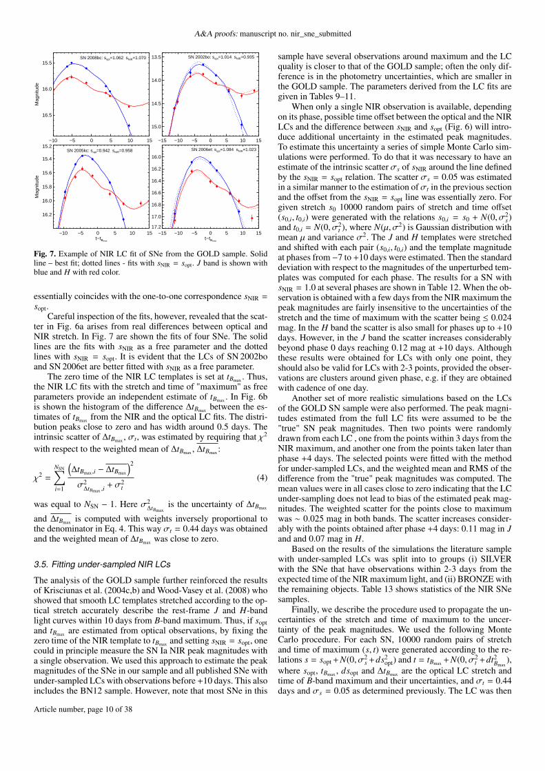
Although analysis of the optical LCs is not the main goalof this paper, all SNe with LCs that allow stretch fitting werealso analyzed. This analysis was performed because it may berelevant and of practical interest for SN cosmology. For manycurrent and future high-redshift SN samples only the rest-frameB and V band are in the optical window. The redder bands arered-shifted in the NIR and are/will be unavailable. The UV partof the spectrum is red-shifted to the optical, but the UV prop-erties of SNe Ia are much less understood and the peak magni-tudes appear to have larger intrinsic scatter (Brown et al. 2010;Milne et al. 2010, 2013). Given this, it is interesting to studyhow well the SN Ia standard candle can be calibrated when onlyrest-frame B and V observations are available, now with muchlarger sample of nearby SNe. In addition, with this large sampleof high-quality LCs we can study the SN intrinsic B − V colorat tBmax , (B − V)Bmax,0 , which is important for estimating the dustextinction in the SN host galaxies.
Using a sub-sample of ∼ 200 SNe with well-sampled LCsand observations within two days from tBmax we derived a newsopt − ∆M15 relation for normal SNe Ia, where ∆M15 is the B-band magnitude decline during the first 15 days after the time ofB-band maximum light. The observed B-band LC were corrected
Article number, page 6 of 38

Stanishev et al.: Type Ia Supernova Cosmology in the Near-Infrared
0.6 0.8 1.0 1.2 1.4stretch
0.5
1.0
1.5
2.0
∆ M
15
this workJha et al. 2006B−band template
Fig. 3. sopt − ∆M15 relation from this work.
Table 6. Average difference between the B and V peak magnitudes, and∆M15 for the SNe in common between the large data sets. Only thesets with more than 10 SNe in common are shown. The number in theparentheses is the 1σ scatter units of 0.001 mag.
Difference NSN B V ∆M15
Berkeley−CSP 16 0.031 (38) 0.045 (25) −0.006 (44)Berkeley−CfA2 10 −0.027 (38) −0.023 (14) 0.032 (44)Berkeley−CfA3 47 −0.008 (43) 0.008 (45) −0.014 (54)CSP−CfA3 30 −0.050 (35) −0.050 (24) −0.007 (56)
to rest-frame B and normalized to zero peak magnitude. The LCswere divided into 0.05 stretch bins. Let sc be the stretch in themiddle of a given bin. Then the time axes of the LCs that fallinto this bin were converted to phases, corrected to the stretch inthe middle of the bin by using Eq. 3 with C = sc and stackedtogether. Smoothing spline was then used to estimate the timemaximum and ∆M15 parameter. The resulting sopt − ∆M15 pairsare given in Table 5. From Fig. 3 it is seen that our relation isclose to the one derived by simply stretching the B-band LC tem-plate, indicating that the stretched template describes the LC ofnormal SNe Ia well. On the other hand the linear relation derivedby Jha et al. (2006), which has been used by many authors, is ap-plicable only in the stretch range 0.85–1.05. In our analysis wefound that the "luminosity – light curve shape" relation for nor-mal SNe Ia is linear (within the scatter) when ∆M15 is used asa LC shape parameter and not the stretch. Thus, we used ∆M15,which was computed from the stretch by cubic spline interpola-tion of the data in Table 5.
In Table 6 we report the weighted mean difference and 1σscatter between the B and V peak magnitudes, and ∆M15 of theSNe in common between the large data sets. Only the sets withmore than 10 SNe in common are considered. One can see thatthere are small systematic differences in the peak magnitudes,which are significant to about 1σ level. The reason for thesesystematic differences are likely related to the photometric cali-bration and different LC sampling. ∆M15 shows relatively largescatter, but no significant bias.
Table 7. NIR spectra of SNe Ia used for computing K-corrections. Thephases of the spectra are relative to the time of the B band maximumlight. The sources of the NIR photometry are given in the text.
SN Phase sopt Ref.SN 1998bu −3,15,22,36 0.973 1,2SN 1999ee −9,0,2,5,8,15,20,23,32,42 1.084 2SN 2000ca 2.7,9.7,17.7,22.6,30.8,38.6 1.065 3SN 2002bo 11 0.928 4SN 2002dj −5.9 0.948 5SN 2003cg −6.5,−4.1,−3.5,4,14,19.6 0.937 6· · · 24,30.5,40SN 2003du −11,−11.5,−5.5,−2.5,2.3,3.4 1.018 7· · · 4.5,12.4,16.2,20.4,30.4SN 2004S 15 0.992 8SN 2005cf −11,−9,−6,−1,1,10,32,42 0.979 9SN 2011fe −16,−14,−11,−8,−4,−1,2,7,11,16 0.905 10
References. (1) Jha et al. (1999); (2) Hamuy et al. (2002); (3) Stani-shev et al., in prep.; (4) Benetti et al. (2004); (5) Pignata et al. (2008);(6) Elias-Rosa et al. (2006); (7) Stanishev et al. (2007); (8) Gall et al.(2012); (9) Pastorello et al. (2007b); (10) Hsiao et al. (2013).
3.3. NIR K-corrections
To compute the NIR K-corrections we used spectrophotometryof nearby SNe Ia that also had NIR photometry available (Ta-ble 7). For the majority of the available spectra the J,H and Kparts were obtained separately with different, non-overlappinginstrument settings. While the relative flux calibration of eachindividual part is probably accurate enough, the cross-band fluxcalibration may not be. Besides, the flux across the strong telluricabsorption bands at ∼ 1.38 µm and ∼ 1.88 µm was not available.Therefore, before computing the K-corrections the spectra hadto be "prepared". The following procedure was applied.
The noisy parts at the edges of the telluric bands were re-moved and the flux across the bands was linearly interpolated.Next, JHK synthetic magnitudes were computed with the ap-propriate effective system responses7 and were compared withthe observed ones. When necessary the J, H and K parts werescaled, the interpolation across the telluric bands was repeatedand new synthetic photometry was computed8. The procedurewas iterated until the synthetic and the observed colors matched.In the cases when the whole NIR spectral range was observedsimultaneously we always found a good match between the syn-thetic and the observed colors, and only interpolation across thetelluric bands was necessary. The spectra were corrected fordust reddening in the Milky Way and the SN host galaxies us-ing E(B − V) values from the Galactic dust map (Schlegel et al.1998) and from the corresponding photometric papers, and cor-rected to rest-frame wavelengths. The spectra at similar phaseswere plotted together and examined. Several spectra with poorS/N, inadequate interpolation across the telluric bands or otherproblems most likely related to the flux calibration were identi-
7 The effective system responses were computed by multiplying the fil-ter transmission, the detector quantum efficiency (QE), two aluminumreflections and the atmosphere transmission at airmass one. When avail-able the filter transmissions and the detector QEs were obtained formthe instrument web-pages, if not, generic filter transmissions and QEsappropriate for the used instrument were used.8 this is needed because in some cases the filters extend over the in-terpolated parts of the spectrum. As the J, H and K parts were scaled,the interpolation changes, which can also affect the computed syntheticmagnitudes to some extent.
Article number, page 7 of 38

A&A proofs: manuscript no. nir_sne_submitted
−20 −10 0 10 20 30 40
0.00
−0.05
−0.10
−0.15
KJJ
z=0.02
Hsiao templatesmoothing spline
−20 −10 0 10 20 30 40
0.0
−0.2
−0.4
−0.6
z=0.07
−20 −10 0 10 20 30 40Phase [t−tBmax
]
0.15
0.10
0.05
0.00
−0.05
KH
H
−20 −10 0 10 20 30 40Phase [t−tBmax
]
0.4
0.2
0.0
−0.2
Fig. 4. Example of computing the NIR J and H K-corrections at z =0.02 (left panels) and z = 0.07 (right panels).
fied and discarded. Details of the final set of spectra are given inTable 7. Note that a few spectra do not cover all JHK bands. Inaddition, few spectra had issues in one band, but were of suffi-cient quality in the others.
To compute K-corrections at any SN phase smoothingsplines were used to interpolate the K-corrections computedfrom the individual spectra. The smoothing splines have greatflexibility to describe the data to any pre-defined rms around thefit. We have computed J− J and H−H K-corrections for severalredshifts between z = 0.002 and z = 0.2 and visually exam-ined the interpolation to tabulate the optimal smoothing param-eter as a function of the redshift. This is a somehow subjectiveprocedure and we tried to select the smoothing parameters insuch a way that the data was well-fitted, but with special careto avoid over-fitting. Examples of the outcome of this procedureare shown in Fig. 4 for two redshifts of z = 0.02 and z = 0.07.The scatter around the smooth curves increases with the redshiftand also depends on partucular filters use (see below). The scat-ter at redshift z = 0.02 is ∼ 0.01 mag in all bands, at z = 0.08it increases to ∼ 0.033 and 0.04 mag, for J and H, respectively,and at z = 0.14 the J and H scatter is ∼ 0.05 and 0.08 mag.These values and the observed increase with the redshift are sim-ilar to the results of Boldt et al. (2014). Note. however, that wedid not color-correct the spectra to follow singe color curve asin Hsiao et al. (2007) and Boldt et al. (2014). As a compari-son in Fig. 4 are also shown the K-corrections computed fromHsiao et al. (2007) template. One can see that there are consider-able differences for some SN phases, including before +10 days,which is interest for our study. Boldt et al. (2014) argue that thedominating part of the scatter is due to intrinsic differences inthe energy distribution of different SNe. Thus, the scatter of theindividual K-corrections around the smoothing spline functionbetween phases −10 and +10 days was tabulated as a functionredshift and added in quadrature to the uncertainties of the peakmagnitudes.
There is no standard photometric system in the NIR and of-ten slightly different filter sets are employed by different obser-vatories. In our analysis we decided to apply K-corrections fromthe different observed filter systems to a single JHKs photomet-ric system, which we chose to be the one defined by the MaunaKea Observatories Near-Infrared Filter Set (MKO) (Tokunagaet al. 2002). As a practical realization of the MKO system weselected the filter/detector combination used by the NOTCam in-strument at the NOT. The observed filter systems that were usedin this work are:
(i) the MKO filters for the 16 new SNe from this work and theSNe from Barone-Nugent et al. (2012) (BN12 set).
(ii) 2MASS (Cohen et al. 2003) for the CfA data set (Wood-Vasey et al. 2008)
(iii) the filters used by The Carnegie Supernova Project (CSP),which are similar to Persson et al. (1998). The CSP fil-ters were used for the CSP data set (Contreras et al. 2010;Stritzinger et al. 2011), the data set from K. Krisciunas andcollaborators (Krisciunas et al. 2004c,b, 2003, 2001, 2000,2007) (the Kri set) and the following SNe from varioussources (the Var set) SN 1998bu (Hernandez et al. 2000;Mayya et al. 1998; Jha et al. 1999), SN 1999ee (Hamuy et al.2002), SN 2000E (Valentini et al. 2003), SN 2002dj (Pignataet al. 2008), SN 2003cg (Elias-Rosa et al. 2006), SN 2003du(Stanishev et al. 2007), SN 2003hv (Leloudas et al. 2009),SN 2004eo (Pastorello et al. 2007a), SN 2005cf (Wang et al.2009b; Pastorello et al. 2007b), and SN 2008Q (Stanishev etal., in preparation).
(iv) the filters of WHIRC instrument were used for SN 2011fe(Matheson et al. 2012).
Strictly speaking the above procedure will work accuratelyonly if the photometry is given in the natural photometric sys-tem defined by the filters. This is the case only for the CSP andCfA data sets, and to a large extent for the Kri data set. The ob-servations of the other SNe were obtained with filters that differfrom those of the photometric systems to which the photometrywas calibrated. Most of our new photometry is tied to 2MASSsystem. The rest of the SN photometry is tied to Persson et al.(1998) or Hunt et al. (1998) systems, which are similar to eachother. Because of this mismatch, it is expected that the photom-etry will contain small systematic uncertainties. To estimate themagnitude of this uncertainty we computed synthetic photome-try with the filters of the four photometric systems consideredin this work at two epochs from the Hsiao spectral template –at NIR maxima and a week after tBmax . We found that the er-rors should be smaller than 0.02 mag. The only exception wasH band a week after tBmax . In this case the error could be as bigas 0.06 mag for most SNe and only for WHIRC observations ofSN 2011fe it could reach 0.1 mag.
3.4. NIR template light curves
There are currently several NIR LC templates available but withexcellent new NIR photometry of many SNe Ia published re-cently (e.g., Contreras et al. 2010; Stritzinger et al. 2011), wedecided to derive new NIR LC templates. From the sample ofSNe with both NIR and optical photometry we discarded knownpeculiar objects (SN 2002cx-likes, SNe 2006bt, 2006ot, and SN1991bg-likes). Further, only the SNe that are suitable for deriv-ing NIR LC templates were selected, e.g. SNe with several ob-servations obtained before phase +10 days and well-distributedalong the LC.
We started by fitting the J and H-band LCs simultaneouslyusing Wood-Vasey et al. (2008) templates and our new NIR K-correction procedure. The templates were stretched with the op-tical stretch sopt and the zero time was fixed to tBmax as in Krisci-unas et al. (2004c,b). Examination of the well-sampled LCs re-vealed that some fits were not very good. The reason appeared tobe that the optical stretch sopt did not provide adequate stretchingto fit the NIR LCs. To further test this we selected a sub-sampleof SNe with well-sampled LCs, which we call "GOLD" sample.For a SN to enter this sample it has to have (i) at least 5 points inJ and/or H band obtained before phase +10 days; (ii) the points
Article number, page 8 of 38

Stanishev et al.: Type Ia Supernova Cosmology in the Near-Infrared
3.0
2.5
2.0
1.5
1.0
0.5
0.0
−0.5
J [m
ag]
σ=0.02 mag (<+10 days)
−10 0 10 20 30 40 50phase [(t−tBmax
)/(sNIR(1+z))]
2.5
2.0
1.5
1.0
0.5
0.0
−0.5
H [m
ag]
σ=0.03 mag (<+10 days)
Fig. 5. The data used to create the J and H light curve templates. Thetemplates are overplotted with red lines. σw is the weighted RMS of thedata around the template during the phases earlier than +10 days.
are evenly-distributed along the LC; (iii) has observations within2 days from the time of NIR maximum. Such SNe allow to per-form the fit of the first NIR LC maximum with the NIR stretchsNIR and the time of maximum as free fitting parameters. The40 objects in the GOLD sample are: SN 1998bu, SN 1999ee,SN 1999ek, SN 2000E, SN 2001cz, SN 2001el, SN 2002bo,SN 2002dj, SN 2003du, SN 2004eo, SN 2004ey, SN 2005M,SN 2005cf, SN 2005el, SN 2005eq, SN 2005hc, SN 2005iq,SN 2005kc, SN 2005ki, SN 2006D, SN 2006X, SN 2006ax,SN 2006et, SN 2006kf, SN 2006le, SN 2006lf, SN 2006os,SN 2007A, SN 2007S, SN 2007af, SN 2007bc, SN 2007bm,SN 2007ca, SN 2007le, SN 2008Q, SN 2008bc, SN 2008fp,SN 2008gp, SN 2008hv and SN 2011fe. SNe 2005el, 2005eq,2005iq, 2006X and 2006ax have LCs from both CSP and CfA,and the LCs were analyzed separately. The fit of the CfA LCof SN 2005iq and SN 2006ac provided very weak constrains onthe stretch and the time of maximum and was moved from theGOLD sample to the SILVER one (see Sec. 3.5). The differencesbetween the peak magnitudes estimated from the CSP and CfAphotometry are at most 0.08 mag. The only exception is H bandof 2006ax, for with the H-band photometry from CfA was 0.22mag fainter than CSP. Even though the analysis of the maximumcolors indicated that those obtained from the CSP photometrywere more likely to be correct also kept the CfA photemetry ofthis SN.
To derive the templates the observed LCs were K-correctedto rest frame magnitudes, normalized to zero magnitude at tBmax ,converted to phases using Eq. 3 with s = sNIR, and stacked to-gether. The data for phases before +10 days were fitted withsmoothing-spline function, manually adjusting the smoothingparameter to achieve a smooth fit that leaves no correlated resid-uals and again taking care to avoid overfitting. A few points that
0.7 0.8 0.9 1.0 1.1 1.2sopt
0.6
0.8
1.0
1.2
1.4
s NIR
a)
−1.5 −1.0 −0.5 0.0 0.5 1.0 1.5(tNIR
Bmax−tBmax
)/(1+z)
0
2
4
6
8
10
12
14
Num
ber
of S
Ne
b)
Fig. 6. (a) - NIR vs. optical stretch parameter. The solid line is thebest-line fit. The four encircled points are the SNe shown in Fig. 7; (b) -histogram of the difference between time of B band maximum estimatedfrom the NIR and optical LC fits from the GOLD sample.
deviated by more than 3σ were removed from the fits. The samewas repeated for the later data and the two fits were stitched to-gether. Because our NIR K-correction are reliable up to phases∼ +40 − 50 days, the data past +50 days was not used. We no-ticed that the NIR stretch sNIR of SNe with sopt ∼ 1 was not 1.For this reason we additionally stretched the template time axisso that the SNe with sopt ∼ 1 also have on average sNIR ∼ 1.
Armed with the new templates the above steps were repeatedto derive our final J and H-band LC templates shown in Fig. 5.The templates were additionally normalized to have zero magni-tude at the first NIR LC peak so that the fitted magnitude offsetsare the rest-frame NIR peak magnitudes. The weighted rms scat-ter of the points around templates9, σw, is σw ' 0.02 mag andσw ' 0.03 mags for J and H, respectively. The small scattershows that the templates describe the LCs of the GOLD samplevery well. Between +10 and +50 days the scatter is considerablylarger, ∼0.13 mag and 0.09 mag for J and H, respectively.
The GOLD SN sample was fitted with the new templates.The NIR LC parameters, together with those derived from theoptical photometry are shown in Table 8. Figure 6a shows theNIR vs. the optical stretch parameters. The best weighted least-squares linear fit to the points is shown with the solid line and it
9 weighted by their photometric errors
Article number, page 9 of 38
A&A proofs: manuscript no. nir_sne_submitted
−10 −5 0 5 10 15t−tBmax
16.2
16.0
15.8
15.6
15.4
15.2
Mag
nitu
de
SN 2005kc: sopt=0.942 sNIR=0.958
−15 −10 −5 0 5 10 15t−tBmax
17.2
17.0
16.8
16.6
16.4
16.2
16.0
SN 2006et: sopt=1.084 sNIR=1.023
−10 −5 0 5 10 15
16.5
16.0
15.5
Mag
nitu
de
SN 2008bc: sopt=1.062 sNIR=1.070
−15 −10 −5 0 5 10 15
15.0
14.5
14.0
13.5
SN 2002bo: sopt=1.014 sNIR=0.935
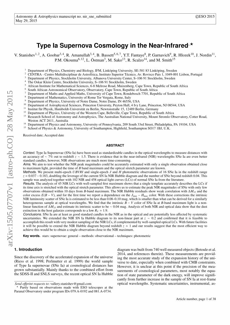
Fig. 7. Example of NIR LC fit of SNe from the GOLD sample. Solidline – best fit; dotted lines - fits with sNIR = sopt. J band is shown withblue and H with red color.
essentially coincides with the one-to-one correspondence sNIR =sopt.
Careful inspection of the fits, however, revealed that the scat-ter in Fig. 6a arises from real differences between optical andNIR stretch. In Fig. 7 are shown the fits of four SNe. The solidlines are the fits with sNIR as a free parameter and the dottedlines with sNIR = sopt. It is evident that the LCs of SN 2002boand SN 2006et are better fitted with sNIR as a free parameter.
The zero time of the NIR LC templates is set at tBmax . Thus,the NIR LC fits with the stretch and time of "maximum" as freeparameters provide an independent estimate of tBmax . In Fig. 6bis shown the histogram of the difference ∆tBmax between the es-timates of tBmax from the NIR and the optical LC fits. The distri-bution peaks close to zero and has width around 0.5 days. Theintrinsic scatter of ∆tBmax , σt, was estimated by requiring that χ2
with respect to the weighted mean of ∆tBmax , ∆tBmax :
χ2 =
NSN∑i=1
(∆tBmax,i − ∆tBmax
)2
σ2∆tBmax ,i
+ σ2t
(4)
was equal to NSN − 1. Here σ2∆tBmax
is the uncertainty of ∆tBmax
and ∆tBmax is computed with weights inversely proportional tothe denominator in Eq. 4. This way σt = 0.44 days was obtainedand the weighted mean of ∆tBmax was close to zero.
3.5. Fitting under-sampled NIR LCs
The analysis of the GOLD sample further reinforced the resultsof Krisciunas et al. (2004c,b) and Wood-Vasey et al. (2008) whoshowed that smooth LC templates stretched according to the op-tical stretch accurately describe the rest-frame J and H-bandlight curves within 10 days from B-band maximum. Thus, if soptand tBmax are estimated from optical observations, by fixing thezero time of the NIR template to tBmax and setting sNIR = sopt, onecould in principle measure the SN Ia NIR peak magnitudes witha single observation. We used this approach to estimate the peakmagnitudes of the SNe in our sample and all published SNe withunder-sampled LCs with observations before +10 days. This alsoincludes the BN12 sample. However, note that most SNe in this
sample have several observations around maximum and the LCquality is closer to that of the GOLD sample; often the only dif-ference is in the photometry uncertainties, which are smaller inthe GOLD sample. The parameters derived from the LC fits aregiven in Tables 9–11.
When only a single NIR observation is available, dependingon its phase, possible time offset between the optical and the NIRLCs and the difference between sNIR and sopt (Fig. 6) will intro-duce additional uncertainty in the estimated peak magnitudes.To estimate this uncertainty a series of simple Monte Carlo sim-ulations were performed. To do that it was necessary to have anestimate of the intrinsic scatter σs of sNIR around the line definedby the sNIR = sopt relation. The scatter σs = 0.05 was estimatedin a similar manner to the estimation ofσt in the previous sectionand the offset from the sNIR = sopt line was essentially zero. Forgiven stretch s0 10000 random pairs of stretch and time offset(s0,i, t0,i) were generated with the relations s0,i = s0 + N(0, σ2
s)and t0,i = N(0, σ2
t ), where N(µ, σ2) is Gaussian distribution withmean µ and variance σ2. The J and H templates were stretchedand shifted with each pair (s0,i, t0,i) and the template magnitudeat phases from −7 to +10 days were estimated. Then the standarddeviation with respect to the magnitudes of the unperturbed tem-plates was computed for each phase. The results for a SN withsNIR = 1.0 at several phases are shown in Table 12. When the ob-servation is obtained with a few days from the NIR maximum thepeak magnitudes are fairly insensitive to the uncertainties of thestretch and the time of maximum with the scatter being ≤ 0.024mag. In the H band the scatter is also small for phases up to +10days. However, in the J band the scatter increases considerablybeyond phase 0 days reaching 0.12 mag at +10 days. Althoughthese results were obtained for LCs with only one point, theyshould also be valid for LCs with 2-3 points, provided the obser-vations are clusters around given phase, e.g. if they are obtainedwith cadence of one day.
Another set of more realistic simulations based on the LCsof the GOLD SN sample were also performed. The peak magni-tudes estimated from the full LC fits were assumed to be the"true" SN peak magnitudes. Then two points were randomlydrawn from each LC , one from the points within 3 days from theNIR maximum, and another one from the points taken later thanphase +4 days. The selected points were fitted with the methodfor under-sampled LCs, and the weighted mean and RMS of thedifference from the "true" peak magnitudes was computed. Themean values were in all cases close to zero indicating that the LCunder-sampling does not lead to bias of the estimated peak mag-nitudes. The weighted scatter for the points close to maximumwas ∼ 0.025 mag in both bands. The scatter increases consider-ably with the points obtained after phase +4 days: 0.11 mag in Jand and 0.07 mag in H.
Based on the results of the simulations the literature samplewith under-sampled LCs was split into to groups (i) SILVERwith the SNe that have observations within 2-3 days from theexpected time of the NIR maximum light, and (ii) BRONZE withthe remaining objects. Table 13 shows statistics of the NIR SNesamples.
Finally, we describe the procedure used to propagate the un-certainties of the stretch and time of maximum to the uncer-tainty of the peak magnitudes. We used the following MonteCarlo procedure. For each SN, 10000 random pairs of stretchand time of maximum (s, t) were generated according to the re-lations s = sopt + N(0, σ2
s +ds2opt) and t = tBmax + N(0, σ2
t +dt2Bmax
),where sopt, tBmax , dsopt and ∆tBmax are the optical LC stretch andtime of B-band maximum and their uncertainties, and σt = 0.44days and σs = 0.05 as determined previously. The LC was then
Article number, page 10 of 38

Stanishev et al.: Type Ia Supernova Cosmology in the Near-InfraredTa
ble
8.L
ight
curv
epa
ram
eter
sof
the
GO
LD
sub-
sam
ple
SNz C
MB
tNIR
Bm
ax−
topt
Bm
axs N
IRJ m
axb,
cH
max
b,c
t Bm
axs o
pt∆
M15
dB
max
bV
att B
max
bR
ef.a
1998
bu0.
0041
6−
0.53
(0.1
5)1.
066
(0.0
26)
11.5
44(0
.014
/0.0
06)
11.6
36(0
.012
/0.0
05)
5095
2.53
(0.0
2)0.
956
(0.0
02)
1.13
5(0
.021
)12
.109
(0.0
02)
11.8
27(0
.001
)V
ar19
99ee
0.01
053
0.00
(0.0
7)1.
074
(0.0
12)
14.7
34(0
.007
/0.0
08)
14.9
82(0
.007
/0.0
09)
5146
9.39
(0.0
1)1.
089
(0.0
02)
0.90
4(0
.020
)14
.873
(0.0
02)
14.6
10(0
.002
)K
ri19
99ek
0.01
759−
0.21
(0.1
6)0.
906
(0.0
19)
15.7
42(0
.011
/0.0
10)
15.9
68(0
.009
/0.0
14)
5148
2.24
(0.0
7)0.
933
(0.0
07)
1.16
8(0
.022
)15
.893
(0.0
05)
15.7
14(0
.004
)K
ri20
00E
0.00
422−
0.48
(0.0
9)0.
984
(0.0
16)
13.2
06(0
.012
/0.0
06)
13.5
74(0
.023
/0.0
05)
5157
6.77
(0.0
3)1.
047
(0.0
03)
0.94
1(0
.021
)13
.009
(0.0
04)
12.8
44(0
.003
)V
ar20
01cz
0.01
570−
0.43
(2.1
6)0.
978
(0.1
40)
15.2
62(0
.125
/0.0
10)
15.6
15(0
.086
/0.0
12)
5210
3.53
(0.0
8)1.
027
(0.0
06)
0.97
4(0
.023
)15
.092
(0.0
06)
15.0
16(0
.004
)K
ri20
01el
0.00
368
0.57
(0.0
6)1.
018
(0.0
09)
12.7
94(0
.012
/0.0
06)
12.9
54(0
.015
/0.0
05)
5218
2.14
(0.0
2)1.
001
(0.0
02)
1.03
2(0
.021
)12
.820
(0.0
03)
12.6
55(0
.002
)K
ri20
02bo
0.00
529−
0.07
(0.1
6)0.
999
(0.0
19)
13.6
48(0
.020
/0.0
07)
13.8
48(0
.013
/0.0
06)
5235
6.95
(0.0
3)0.
935
(0.0
03)
1.16
5(0
.020
)13
.975
(0.0
06)
13.5
45(0
.004
)K
ri20
02dj
0.01
045−
0.43
(0.2
7)0.
951
(0.0
31)
14.4
26(0
.020
/0.0
08)
14.6
73(0
.017
/0.0
09)
5245
0.50
(0.0
2)0.
953
(0.0
02)
1.14
0(0
.021
)13
.975
(0.0
04)
13.8
66(0
.003
)V
ar20
03du
0.00
665−
0.05
(0.1
4)1.
007
(0.0
20)
14.1
27(0
.028
/0.0
07)
14.3
83(0
.021
/0.0
07)
5276
6.15
(0.0
2)1.
022
(0.0
02)
0.98
4(0
.021
)13
.453
(0.0
02)
13.5
69(0
.002
)V
ar20
04eo
0.01
472
0.36
(0.1
3)0.
929
(0.0
17)
15.4
53(0
.007
/0.0
09)
15.7
25(0
.007
/0.0
12)
5327
8.10
(0.0
2)0.
874
(0.0
02)
1.27
7(0
.022
)15
.095
(0.0
04)
15.0
05(0
.004
)C
SP20
04ey
0.01
461−
0.14
(0.2
5)1.
007
(0.0
27)
15.4
19(0
.010
/0.0
09)
15.6
85(0
.010
/0.0
12)
5330
4.32
(0.0
1)1.
019
(0.0
01)
0.99
0(0
.021
)14
.781
(0.0
01)
14.8
67(0
.002
)C
SP20
05M
0.02
561
0.89
(0.0
9)1.
164
(0.0
17)
16.4
12(0
.009
/0.0
13)
16.6
34(0
.007
/0.0
19)
5340
5.64
(0.0
2)1.
136
(0.0
02)
0.83
6(0
.021
)15
.910
(0.0
02)
15.8
95(0
.002
)C
SP20
05cf
0.00
705
0.33
(0.1
3)1.
048
(0.0
16)
13.7
32(0
.012
/0.0
07)
13.8
68(0
.010
/0.0
07)
5353
3.57
(0.0
1)0.
986
(0.0
01)
1.06
8(0
.021
)13
.313
(0.0
03)
13.2
59(0
.002
)V
ar20
05el
0.01
488−
0.37
(0.0
7)0.
837
(0.0
09)
15.4
04(0
.006
/0.0
09)
15.6
43(0
.005
/0.0
12)
5364
6.08
(0.0
2)0.
878
(0.0
03)
1.26
5(0
.022
)14
.882
(0.0
04)
14.9
84(0
.004
)C
SP20
05el
0.01
488
0.00
(0.0
7)0.
793
(0.0
10)
15.3
41(0
.007
/0.0
13)
15.5
87(0
.010
/0.0
05)
5364
6.08
(0.0
2)0.
878
(0.0
03)
1.26
5(0
.022
)14
.882
(0.0
04)
14.9
84(0
.004
)C
fA20
05eq
0.02
833
0.60
(0.2
8)1.
215
(0.0
45)
16.7
81(0
.015
/0.0
14)
17.0
27(0
.017
/0.0
20)
5365
3.57
(0.0
6)1.
157
(0.0
07)
0.80
3(0
.022
)16
.265
(0.0
05)
16.2
36(0
.005
)C
SP20
05eq
0.02
833−
0.40
(0.5
2)1.
191
(0.0
47)
16.7
04(0
.024
/0.0
17)
17.0
99(0
.031
/0.0
12)
5365
3.57
(0.0
6)1.
157
(0.0
07)
0.80
3(0
.022
)16
.265
(0.0
05)
16.2
36(0
.005
)C
fA20
05hc
0.04
445−
0.52
(0.6
7)1.
001
(0.1
06)
17.8
30(0
.039
/0.0
22)
17.9
26(0
.061
/0.0
29)
5366
7.13
(0.0
6)1.
100
(0.0
05)
0.89
3(0
.021
)17
.299
(0.0
03)
17.2
87(0
.003
)C
SP20
05iq
0.03
289
0.57
(0.6
1)0.
751
(0.0
63)
17.2
94(0
.040
/0.0
16)
17.5
00(0
.055
/0.0
23)
5368
7.69
(0.0
3)0.
899
(0.0
04)
1.21
4(0
.022
)16
.782
(0.0
04)
16.7
98(0
.003
)C
SP20
05kc
0.01
387
0.13
(0.0
7)0.
958
(0.0
11)
15.3
55(0
.009
/0.0
09)
15.5
77(0
.010
/0.0
11)
5369
7.57
(0.0
2)0.
942
(0.0
03)
1.15
7(0
.021
)15
.565
(0.0
04)
15.3
54(0
.003
)C
SP20
05ki
0.02
039−
0.44
(0.1
0)0.
817
(0.0
15)
16.0
83(0
.015
/0.0
11)
16.2
75(0
.019
/0.0
16)
5370
5.28
(0.0
2)0.
854
(0.0
02)
1.34
0(0
.022
)15
.540
(0.0
04)
15.5
80(0
.003
)C
SP20
06D
0.00
965−
0.31
(0.2
2)0.
802
(0.0
28)
14.2
76(0
.013
/0.0
11)
14.5
14(0
.014
/0.0
04)
5375
7.50
(0.0
1)0.
830
(0.0
01)
1.41
9(0
.021
)14
.160
(0.0
02)
14.0
42(0
.002
)C
fA20
06X
0.00
429−
0.38
(0.0
6)0.
994
(0.0
09)
12.8
13(0
.005
/0.0
06)
12.9
34(0
.003
/0.0
05)
5378
6.16
(0.0
1)0.
949
(0.0
01)
1.14
7(0
.020
)15
.246
(0.0
02)
13.8
82(0
.002
)C
SP20
06X
0.00
429−
0.46
(0.1
3)0.
976
(0.0
23)
12.8
73(0
.017
/0.0
11)
12.9
24(0
.009
/0.0
05)
5378
6.16
(0.0
1)0.
949
(0.0
01)
1.14
7(0
.020
)15
.246
(0.0
02)
13.8
82(0
.002
)C
fA20
06ax
0.01
798−
0.14
(0.0
5)0.
987
(0.0
07)
15.6
63(0
.007
/0.0
10)
15.9
35(0
.006
/0.0
14)
5382
7.35
(0.0
1)1.
002
(0.0
01)
1.02
9(0
.021
)14
.990
(0.0
02)
15.0
75(0
.001
)C
SP20
06ax
0.01
798−
0.38
(0.1
3)0.
915
(0.0
18)
15.6
61(0
.017
/0.0
14)
16.1
57(0
.033
/0.0
06)
5382
7.35
(0.0
1)1.
002
(0.0
01)
1.02
9(0
.021
)14
.990
(0.0
02)
15.0
75(0
.001
)C
fA20
06et
0.02
162
0.26
(0.1
0)1.
005
(0.0
15)
16.0
23(0
.014
/0.0
12)
16.2
56(0
.015
/0.0
16)
5399
3.74
(0.0
3)1.
084
(0.0
02)
0.90
8(0
.020
)15
.959
(0.0
03)
15.7
83(0
.003
)C
SP20
06kf
0.02
079−
0.26
(0.1
1)0.
737
(0.0
20)
16.2
03(0
.007
/0.0
11)
16.4
14(0
.028
/0.0
16)
5404
1.32
(0.0
2)0.
775
(0.0
03)
1.57
9(0
.022
)15
.930
(0.0
04)
15.8
98(0
.004
)C
SP20
06le
0.01
726−
0.91
(0.4
3)1.
068
(0.0
74)
15.8
57(0
.036
/0.0
14)
16.3
05(0
.037
/0.0
06)
5404
8.21
(0.0
3)1.
096
(0.0
04)
0.89
7(0
.021
)14
.977
(0.0
05)
15.0
15(0
.004
)C
fA20
06lf
0.01
296
0.18
(0.4
1)0.
768
(0.0
58)
14.9
06(0
.033
/0.0
12)
15.2
13(0
.047
/0.0
04)
5404
4.69
(0.0
6)0.
861
(0.0
08)
1.31
7(0
.033
)14
.238
(0.0
17)
14.2
36(0
.010
)C
fA20
06os
0.03
206
0.51
(1.9
1)0.
860
(0.1
28)
17.3
14(0
.131
/0.0
16)
17.3
57(0
.078
/0.0
22)
5406
4.95
(0.3
1)0.
931
(0.0
13)
1.17
0(0
.025
)17
.642
(0.0
13)
17.2
73(0
.007
)C
SP20
07A
0.01
593
0.20
(0.2
1)0.
953
(0.0
40)
15.6
13(0
.020
/0.0
10)
15.9
26(0
.050
/0.0
13)
5411
2.88
(0.0
6)1.
054
(0.0
10)
0.93
2(0
.023
)15
.697
(0.0
05)
15.5
10(0
.004
)C
SP20
07S
0.01
504
0.29
(0.1
1)1.
039
(0.0
12)
15.3
12(0
.008
/0.0
10)
15.5
23(0
.008
/0.0
12)
5414
4.19
(0.0
2)1.
120
(0.0
03)
0.86
3(0
.021
)15
.779
(0.0
04)
15.3
80(0
.003
)C
SP20
07af
0.00
629
0.03
(0.0
2)0.
982
(0.0
03)
13.4
24(0
.002
/0.0
07)
13.5
96(0
.003
/0.0
07)
5417
4.24
(0.0
1)0.
955
(0.0
01)
1.13
7(0
.020
)13
.152
(0.0
02)
13.0
98(0
.002
)C
SP20
07bc
0.02
187
1.00
(0.2
5)0.
878
(0.0
32)
16.2
98(0
.013
/0.0
12)
16.4
88(0
.046
/0.0
17)
5419
9.57
(0.0
7)0.
904
(0.0
07)
1.20
5(0
.024
)15
.868
(0.0
05)
15.8
94(0
.005
)C
SP20
07bm
0.00
745
0.07
(0.0
7)1.
002
(0.0
13)
13.8
72(0
.003
/0.0
07)
14.0
80(0
.009
/0.0
07)
5422
4.38
(0.0
2)0.
916
(0.0
01)
1.18
7(0
.020
)14
.488
(0.0
02)
13.9
47(0
.002
)C
SP20
07ca
0.01
509−
0.16
(0.1
1)1.
012
(0.0
13)
15.5
25(0
.006
/0.0
10)
15.6
57(0
.011
/0.0
12)
5422
7.48
(0.0
2)1.
064
(0.0
03)
0.92
3(0
.020
)15
.906
(0.0
03)
15.6
35(0
.002
)C
SP20
07le
0.00
551
0.46
(0.0
7)1.
053
(0.0
06)
13.7
34(0
.004
/0.0
07)
13.9
30(0
.003
/0.0
06)
5439
8.64
(0.0
5)1.
003
(0.0
04)
1.02
7(0
.023
)13
.904
(0.0
05)
13.5
71(0
.005
)C
SP20
07on
0.00
618
1.26
(0.0
2)0.
761
(0.0
03)
13.0
42(0
.005
/0.0
07)
13.1
16(0
.003
/0.0
07)
5441
9.30
(0.0
1)0.
711
(0.0
01)
1.79
7(0
.022
)13
.020
(0.0
03)
12.9
02(0
.002
)C
SP20
08Q
0.00
689−
0.21
(0.1
2)0.
790
(0.0
23)
13.7
98(0
.024
/0.0
07)
13.9
02(0
.032
/0.0
07)
5450
5.81
(0.0
1)0.
841
(0.0
02)
1.38
3(0
.022
)13
.481
(0.0
03)
13.4
80(0
.003
)V
ar20
08bc
0.01
572−
0.82
(0.0
6)1.
050
(0.0
14)
15.5
25(0
.005
/0.0
10)
15.7
94(0
.008
/0.0
13)
5454
9.93
(0.0
1)1.
062
(0.0
01)
0.92
5(0
.020
)14
.714
(0.0
02)
14.7
93(0
.002
)C
SP20
08fp
0.00
629
0.45
(0.0
5)1.
133
(0.0
12)
13.3
44(0
.002
/0.0
07)
13.5
37(0
.002
/0.0
07)
5473
0.58
(0.0
2)1.
015
(0.0
02)
0.99
9(0
.021
)13
.867
(0.0
03)
13.3
50(0
.002
)C
SP20
08gp
0.03
280
0.34
(0.2
1)1.
070
(0.0
63)
17.2
02(0
.046
/0.0
16)
17.4
41(0
.052
/0.0
23)
5477
9.04
(0.0
2)0.
998
(0.0
02)
1.03
9(0
.021
)16
.460
(0.0
04)
16.4
30(0
.003
)C
SP20
08hv
0.01
359−
0.75
(0.0
5)0.
808
(0.0
05)
15.1
84(0
.015
/0.0
09)
15.4
68(0
.009
/0.0
11)
5481
6.88
(0.0
1)0.
866
(0.0
01)
1.30
1(0
.021
)14
.745
(0.0
03)
14.7
15(0
.002
)C
SP20
11fe
0.00
121−
0.34
(0.0
2)0.
961
(0.0
03)
10.4
43(0
.005
/0.0
06)
10.7
03(0
.003
/0.0
03)
5581
4.97
(0.0
1)0.
938
(0.0
01)
1.16
2(0
.020
)9.
962
(0.0
02)
9.96
3(0
.001
)V
ar
Not
es.(a
)se
ete
xtfo
rthe
refe
renc
esfo
rthe
NIR
phot
omet
ry.(b
)T
heun
cert
aint
ies
are
inun
itsof
0.00
1m
ag.(c
)T
hetw
onu
mbe
rsar
eth
eun
cert
aint
ies
ofth
epe
akm
agni
tude
and
the
K-c
orre
ctio
ns.
(d)
estim
ated
from
our
s opt−
∆M
15re
latio
n.
Article number, page 11 of 38

A&A proofs: manuscript no. nir_sne_submitted
Table 9. Supernova fit parameters. The magnitude uncertainties are given in units of 0.001 mag.
SN Jmaxc,d Hmax
c,d tBmaxa sopt ∆M15
b Bmaxc V at tBmax
c
SN 2007hz 20.274 (71/49) 20.679 (125/80) 350.86 (0.25) 1.069 (0.020) 0.919 (0.026) 19.555 (18) 19.640 (14)SN 2007ih 21.375 (101/65) 21.443 (190/100) 352.61 (0.42) 1.184 (0.046) 0.777 (0.046) 20.767 (25) 20.752 (27)SN 2007ik 21.410 (232/47) − 356.78 (0.28) 1.090 (0.030) 0.903 (0.038) 20.617 (27) 20.662 (28)SNF20080510-005 19.742 (122/34) 19.569 (115/45) 604.39 (0.25) 1.177 (0.029) 0.782 (0.033) 18.826 (22) 18.860 (18)SNF20080512-010 18.706 (130/28) 19.014 (97/35) 602.88 (0.35) 0.743 (0.012) 1.677 (0.047) 18.038 (49) 18.114 (30)SNF20080516-000 18.865 (67/31) 19.101 (71/39) 606.33 (0.51) 1.091 (0.015) 0.902 (0.025) 18.165 (38) 18.275 (22)SNF20080516-022 19.150 (58/31) 19.214 (90/40) 609.79 (0.31) 0.947 (0.015) 1.150 (0.030) 18.379 (21) 18.431 (13)SNF20080517-010 20.348 (125/42) 20.907 (277/68) 605.97 (0.81) 1.003 (0.029) 1.027 (0.069) 19.692 (52) 19.625 (28)SNF20080522-000 17.684 (33/21) 17.887 (30/26) 621.17 (0.13) 1.092 (0.007) 0.901 (0.021) 17.027 (07) 17.023 (06)SNF20080522-001 17.926 (132/23) 18.119 (100/28) 602.83 (0.45) 1.138 (0.021) 0.832 (0.039) 17.422 (49) 17.456 (27)SNF20080522-004 19.286 (237/40) 19.756 (337/58) 606.33 (2.88) 1.260 (0.067) 0.737 (0.040) 18.991 (185) 19.317 (100)SNF20080522-011 17.284 (25/17) 17.521 (43/22) 616.40 (0.15) 1.052 (0.009) 0.935 (0.023) 16.653 (09) 16.724 (09)SNF20080606-012 18.983 (57/33) 19.369 (91/42) 631.93 (0.50) 0.954 (0.017) 1.138 (0.036) 18.684 (36) 18.736 (22)SNF20080610-003 19.794 (77/37) 19.811 (92/51) 633.43 (0.75) 1.047 (0.019) 0.941 (0.032) 18.865 (51) 18.957 (30)
Notes. (a) JD−2454000. (b) estimated from our sopt − ∆M15 relation. (c) The uncertainties are in units of 0.001 mag. (d) The two numbers are theuncertainties of the peak magnitude and the K-corrections.
Table 11. SN fit parameters for the BN12 sample.
SN zCMB Jmaxc,d Hmax
c,d tBmaxa sopt ∆M15
b Bmaxc V at tBmax
c
PTF09dlc 0.06656 18.663 (28/29) 18.948 (26/37) 073.79 (0.14) 0.991 (0.019) 1.056 (0.050) 17.911 (52) 18.051 (21)PTF10hdv 0.05424 18.326 (68/24) 18.520 (51/30) 342.41 (0.82) 1.125 (0.035) 0.855 (0.056) 17.492 (21) 17.552 (22)PTF10hmv 0.03272 − 17.507 (22/20) 351.69 (0.03) 1.130 (0.002) 0.846 (0.021) 17.278 (46) 17.116 (24)PTF10mwb 0.03117 17.137 (79/14) 17.401 (46/20) 390.32 (0.11) 0.885 (0.010) 1.246 (0.033) 16.709 (32) 16.727 (11)PTF10ndc 0.08168 19.283 (47/34) 19.430 (52/44) 389.99 (0.16) 1.091 (0.010) 0.902 (0.022) 18.427 (8) 18.487 (6)PTF10nlg 0.05592 18.674 (36/25) 18.656 (22/31) 391.43 (0.27) 0.968 (0.020) 1.110 (0.047) 18.561 (26) 18.445 (19)PTF10qyx 0.06515 19.028 (40/29) 19.200 (35/36) 426.36 (0.15) 0.913 (0.012) 1.191 (0.026) 18.213 (16) 18.318 (11)PTF10tce 0.03971 17.871 (25/19) 18.016 (20/24) 441.92 (0.27) 1.088 (0.012) 0.905 (0.023) 17.177 (14) 17.096 (11)PTF10ufj 0.07613 19.266 (61/32) 19.354 (40/41) 456.89 (0.13) 1.070 (0.021) 0.919 (0.027) 18.404 (48) 18.529 (21)PTF10wnm 0.06440 18.731 (30/29) 18.997 (29/36) 476.68 (0.08) 1.090 (0.008) 0.903 (0.021) 18.152 (9) 18.129 (6)PTF10wof 0.05131 18.391 (32/24) 18.581 (30/30) 473.81 (0.22) 1.038 (0.011) 0.954 (0.027) 17.943 (35) 17.826 (08)PTF10xyt 0.04831 18.406 (37/23) 18.416 (86/29) 490.85 (0.11) 1.117 (0.021) 0.868 (0.038) 18.452 (24) 18.228 (24)
Notes. (a) JD−2455000. (b) estimated from our sopt − ∆M15 relation. (c) The uncertainties are in units of 0.001 mag. (d) The two numbers are theuncertainties of the peak magnitude and the K-corrections.
Table 12. Peak magnitude uncertainties of a SN with sNIR = 1.0 whenonly single observation is available. The uncertainties of the stretch andthe time of maximum were assumed to be 0.05 and 0.44 days, respec-tively.
Band phase of observation−4 0 4 7 10
J 0.013 0.024 0.049 0.090 0.123H 0.006 0.020 0.008 0.020 0.006
fitted with each perturbed pair (s, t) and the standard deviation ofthe 10000 peak magnitude estimates was added in quadrature tothe uncertainty of the peak magnitude derived by the LC fitter.
4. Results
4.1. Colors at maximum light
4.1.1. (B − V)Bmax
Phillips et al. (1999) were the fist to suggest that the intrinsicB − V color of SNe Ia at maximum (B − V)Bmax,0 is a linear
Table 13. Statistics of the NIR SN samples used in this work: numberof SNe, mean redshift, standard deviation σzCMB around the mean andthe median redshift.
Sample NLCs < zCMB > σzCMB medianGOLD 45 0.0148 0.0095 0.0147SILVER 16 0.0232 0.0113 0.0239BRONZE 29 0.0284 0.0165 0.0266GOLD (z ≥ 0.008) 30 0.0196 0.0081 0.0173SILVER (z ≥ 0.008) 15 0.0244 0.0106 0.0240BRONZE (z ≥ 0.008) 28 0.0293 0.0162 0.0268BN12 12 0.0556 0.0161 0.0559Our new sample 14 0.0942 0.0448 0.0850
function of ∆M15 with a slope of ∼ 0.11. The parameters ofthe (B − V)Bmax,0 − ∆M15 relation were determined by linear fitof the bluest objects (see also Folatelli et al. 2010). The disad-vantage of this approach is that it requires a prior knowledge ofwhich SNe are likely to be unreddened and that only a smallfraction of all available data is used. Here we followed a differ-ent path to study the distribution of observed (B − V)Bmax colors
Article number, page 12 of 38

Stanishev et al.: Type Ia Supernova Cosmology in the Near-Infrared
with the much larger sample available today. Nobili & Goobar(2008) have shown that the intrinsic SN Ia (B − V)Bmax colorhas a dispersion of about 0.05 mag. The observed colors maybe further reddened by interstellar dust along the line of sight,evidence for which is clearly seen as an extended red tail of thecolor distribution in the nearby SN Ia sample. Let us assume asin Jha et al. (2007) that (i) the intrinsic (B − V)Bmax colors follownormal distribution with mean c0 and standard deviation σc, and(ii) that the reddening E(B − V) follows exponential distributionwith scale τe for E(B − V) ≥ 0 mag and is zero otherwise. Un-der these assumptions the probability density function (PDF) ofthe observed (B − V)Bmax color, ρ((B − V)Bmax ; c0, σc, τe), is theconvolution of the two functions (Jha et al. 2007; Marriner et al.2011):
ρ(c; c0, σc, τe) ∝∫ +∞
0exp
(−
(c − c0 − τ)2
2σ2c
)exp
(−τ
τe
)dτ, (5)
where c is the observed (B − V)Bmax color and the integration isover the color excess from extinction, τ.
Figure 8a shows the (B−V)Bmax colors measured with uncer-tainty less than 0.04 mag from 393 LCs. The dotted line has aslope of 0.12. It describes the blue edge of the distribution of theSNe with ∆M15 ≤ 1.4 well, but beyond that the colors are clearlyincreasingly redder than the line. It is clear that a non-linearfunction is need to describe the average intrinsic (B−V)Bmax coloras a function of ∆M15. We tried different functions and found thata simple exponential function worked best, while a second-orderpolynomial was not flexible enough to describe the data.
The parameters of the exponential function that describes(B−V)Bmax,0 were determined by fitting Eq. 5 to the histogram ofE(B − V)obs = (B − V)Bmax − (B − V)Bmax,0 computed in 0.05 magwide bins. Unfortunately, there is no unique way to define thequantity to be minimized. We tried several approaches, whichare appropriate under the reasonable assumption that σc is inde-pendent on ∆M15. First the histogram of the whole data set wasfitted and the parameters that give the lowest σc was selected.The reasoning behind this is that with incorrect parameters thehistogram will be additionally blurred and hence a larger σc willbe derived; the correct parameters should thus give the lowestσc. However, this approach was unsuccessful and the blue edgeof the distribution of the SNe with ∆M15 ≥ 1.4 was not describedwell. The likely reason for this is that the number of SNe with∆M15 > 1.4 is small and the final solution is mostly driven bythe SNe with ∆M15 < 1.4. The approach that we found to workbest to address this problem was to split the sample into threebins – SNe with ∆M15 < 1.1 (182 points), 1.1 ≤ ∆M15 < 1.5(163 points) and ∆M15 ≥ 1.5 (48 points) – and fit histogram ofE(B − V)obs in each bin independently. In the fitting the c0 pa-rameter in Eq. 5 was treated as an unknown constant. It is easy tosee that with the correct (B − V)Bmax,0 − ∆M15 relation σc shouldbe the same in all three bins and the c0’s should be close to zero.Thus, the quantity to minimize was the scatter of σc around themean in the three bins and the scatter of c0 around zero added inquadrature. The τe parameters were not required to be the samein the three bins because the distribution of the reddening maybe different. For example, the SNe with larger ∆M15 are fainterand this may lead to bias against discovering reddened SNe.
With the above procedure the following function was de-rived:
(B − V)Bmax,0 = 0.036 exp[∆M15 − 1.3
0.3455
]− 0.084(±0.01). (6)
This relation is shown with the solid line in Fig. 8a and the his-tograms in the three bins and the best fits in Fig. 8b. The mean
0.8 1.0 1.2 1.4 1.6 1.8∆ M15
0.0
0.5
1.0
1.5
(B−
V) B
max
a)
−0.2 0.0 0.2 0.4 0.6 0.8(B−V)Bmax
−(B−V)Bmax,0
0.0
0.2
0.4
0.6
0.8
1.0
1.2
a.u.
b) ∆M15<1.1 (182)
1.1< ∆M15<1.5 (163)
∆M15>1.5 (48)
Fig. 8. (a) The (B−V)Bmax color of the SNe used in this work as functionof ∆M15. The solid line shows the relation defined by Eq. 6. The dashedline has a slope of 0.12 and is shown for a comparison; (b) histogramsof (B − V)Bmax − (B − V)Bmax ,0 for SNe with ∆M15 < 1.1 (182 objects),1.1 < ∆M15 < 1.3 (163 objects) and ∆M15 > 1.5 (48 objects) with thecorrespondign fits with Eq. 5.
value of σc in the three bins is 0.045 mag with estimated un-certainty of 0.01 mag. The uncertainty of the free term in Eq. 6,±0.01 mag, was estimated from the fits of the histograms, whichgive uncertainty of ∼ 0.01 mag of c0. The constant 1.3 was de-rived empirically. Several values between 1.1 and 1.4 were triedand the one providing the solution with smallest σc was selected.Regarding τe, the following values were derived in the three bins,τe = 0.14±0.02 mag, τe = 0.13±0.02 mag and τe = 0.11±0.04mag. We note that the results are somehow dependent on the bin-ning on ∆M15 and the color, and color error cut (0.04 mag in ourcase). When a larger sample of SNe, especially with ∆M15 > 1.4,becomes available it will be possible to estimate the parametersmore accurately.
The values of σc and τe that we find are close to those ofJha et al. (2007), Ganeshalingam et al. (2010) and Folatelli et al.(2010), which were estimated from the late-time SN Ia colors at+35 days using the Lira-relation (Lira 1995; Phillips et al. 1999).The Lira-relation is considered as one of the best methods to es-timate the host galaxy reddening of SNe Ia. In another analysisof late-time B − V color curves of SNe Ia Burns et al. (2014)introduced a new stretch parameter of the B − V curves, sBV .The authors estimated the intrinsic scatter of the B − V color tobe 0.06 − 0.09 mag. The intrinsic scatter of (B − V)Bmax that weestimate is smaller than the scatter of B − V at late times de-rived by the above authors. This indicates that at least for normalSNe Ia the (B − V)Bmax color should provide as good estimate
Article number, page 13 of 38

A&A proofs: manuscript no. nir_sne_submitted
0.0 0.5 1.0 1.5E(B−V)obs
−0.5
0.0
0.5
J max
−H
max
b)
0.6 0.8 1.0 1.2 1.4 1.6 1.8∆ M15
−0.5
0.0
0.5
J max
−H
max
− This work − GOLD − SILVER − BRONZE − BN12
a)
Fig. 9. (a) Jmax−Hmax color vs. ∆M15. The solid shows the least-squareslinear fit to the GOLD sample; (b) Jmax−Hmax vs. E(B−V)obs. The solidline is the least-squares linear fit to the GOLD sample, the dashed andthe dotted lines are the expected relation for Milky Way-type dust andRB = 2.7 and 4.1, respectively.
of the reddening as the Lira-relation. This may be important forhigh-redshift studies where the observations do not extend to latephases and the extinction must be estimated from the colors atmaximum.
As a final note, we would like to point out that the width ofthe observed color distribution is not determined only by the in-trinsic color scatter σc and and the distribution of the reddening(here parametrized by τe). Several other other factors, such asthe observational errors, the fact that S -corrections were not ap-plied to all data and possible deviation of the fitting LC templatesfrom the real SN LCs will all increase the width of the observeddistribution and lead to overestimate of σc and τe. Some of thesesources of errors may be different for the different samples andtherefore σc should be regarded as a mean value for the wholenearby SN Ia sample. The mean uncertainty of (B−V)Bmax in thesample used in this analysis is ∼ 0.015 mag and taking it intoaccount the true intrinsic scatter σc may be ∼ 0.04 mag.
4.2. Jmax − Hmax, VBmax − Jmax and VBmax − Hmax
Figure 9 shows the Jmax − Hmax color vs. ∆M15 and E(B− V)obs.The Jmax−Hmax color shows a fair amount scatter. largely due toour and the BRONZE samples. The scatter in the GOLD sampleis rather small and the weighted least-squares linear fit indicates
a possible weak dependence on ∆M15 with a slope of 0.14 ±0.06.The fit of the GOLD sample implies that a typical SN Ia with∆M15 = 1.1 has Jmax − Hmax = −0.23 ± 0.02 mag. For χ2/DoFof the fit to be one it is necessary to add 0.08 mag in quadrature tothe errors, which can be interpreted as the intrinsic scatter of theJmax − Hmax color. Similar intrinsic scatter is also inferred fromthe BN12 sample, however, Jmax − Hmax color in this sample issystematically redder by about 0.1 mag.
The GOLD sample also reveals a weak linear relation be-tween Jmax − Hmax and E(B − V)obs. The relation is shown witha solid line in Fig. 9b. The expected relations for Milky Way-type dust with RV = 1.7 and 3.1 are shown with the dashedand the dotted lines, respectively. The slope of the best-fit line,0.12 ± 0.03, is consistent with a low RV value around 1.5. Thefit indicates that an un-reddened SN should have Jmax − Hmax =−0.25 ± 0.03. We also note that there is no apparent dependenceof Jmax − Hmax of the redshift. For both the GOLD sample withmean redshift z ' 0.02 and for our sample with mean redshiftz ' 0.09 Jmax − Hmax color is −0.24 mag.
Our estimate of the intrinsic Jmax − Hmax color of a SN with∆M15 = 1.1 mag is similar to the results of Krisciunas et al.(2004c) and Wood-Vasey et al. (2008). It is also consistent withBurns et al. (2014) who, using a different approach, found thata SN with stretch equal to one has Jmax − Hmax = −023 magwith intrinsic dispersion of 0.09 mag. It is interesting to note,however, that Folatelli et al. (2010) based on part of the data weused in our analysis find it to be close to zero. From Fig. 9 onecan see that this is inconsistent with our results. We also notethat the observed variation of the Jmax −Hmax color is far too bigto be caused by dust extinction of any reasonable law.
Finally, Fig. 10 shows VBmax−Jmax and VBmax−Hmax colors vs.E(B − V)obs. Most of the SNe with E(B − V)obs ≥ 0.4 mag alignalong the line tracing Milky Way-type extinction with RV = 1.7.There is also a set of SNe with E(B − V)obs between 0.1 magand 0.6 mag that seem to follow the line with RV = 3.1. Thetwo SNe with E(B − V)obs < −0.15 mag appear to be outliers.However, one of them SNF20080522-004 has large uncertaintyof the maximum B − V colors of ∼ 0.2 mag. The other objectis SN 2006hx, which is ∼ 1 mag outlier on the optical Hubblediagram, hence its anomalous V−NIR colors.
4.3. SNe Ia as standardizable candles
In this section we use our estimates of the SN peak magnitudesand ∆M15 parameters to re-evaluate the precision of SNe Ia asstandardizable candles. The main goal of this paper is to do thatin the NIR J and H bands. However, because several new largesets of optical observations of nearby SNe Ia have become re-cently available we also analyzed the B and V bands.
To standardize the SN Ia peak magnitudes in band X, mX , weadopt the following two-parameter relation:m∗X = mX − aX × (∆M15 − 1.1) − RYZ
X × E(Y − Z), (7)where E(Y − Z) is the color excess in bands Y and Z caused bydust and which can be converted into absorption in band X viaRYZ
X × E(Y − Z). Throughout this work we use E(B − V), whichwas calculated with the (B − V)Bmax,0 − ∆M15 relation derived inthe previous section, and omit the superscript index of RX .
The aX and RX parameters, and the absolute magnitude inthe band X, MX , of a fiducial SN Ia with ∆M15 = 1.1 were deter-mined by χ2-minimization of:
χ2 =
Nset∑i=1
NSN∑j=1
(m∗X,i, j − Mi
X − µi, j
)2
σ2lc,i, j + σ2
intr,i + σ2ext,i, j
. (8)
Article number, page 14 of 38
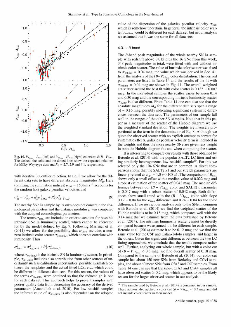
Stanishev et al.: Type Ia Supernova Cosmology in the Near-Infrared
0.0 0.5 1.0 1.5E(B−V)obs
−1.5
−1.0
−0.5
0.0
0.5
1.0
Vm
ax−
Hm
ax
−1.0
−0.5
0.0
0.5
1.0
Vm
ax−
J max
Fig. 10. VBmax −Jmax (left) and VBmax −Hmax (right) colors vs. E(B−V)obs.The dashed, the solid and the dotted lines show the expected relationsfor Milky Way-type dust and RB = 2.7, 2.9 and 4.1, respectively.
with iterative 3σ outlier rejection. In Eq. 8 we allow for the dif-ferent data sets to have different absolute magnitudes Mi
B. Here(omitting the summation indices) σext = 150 km s−1 accounts forthe random host galaxy peculiar velocities and
σ2lc = σ2
mX+ a2
Xσ2∆M15
+ R2Xσ
2(B−V)max
. (9)
The nearby SNe Ia sample by its own does not constrain the cos-mological parameters and the distance modulus µ was computedwith the adopted cosmological parameters.
The terms σintr,i are included in order to account for possibleintrinsic SNe Ia luminosity scatter, which cannot be correctedfor by the model defined by Eq. 7. Following Marriner et al.(2011) we allow for the possibility that σintr,i includes a non-zero intrinsic color scatterσcol,intr,i, which does not correlate withluminosity. Thus
σ2intr,i = σ2
mX ,intr,i + R2Xσ
2col,intr,i, (10)
where σmX ,intr,i is the intrinsic SN Ia luminosity scatter. In princi-ple, σmX ,intr,i includes also contribution from other sources of un-certainty such as calibration uncertainties, possible mismatch be-tween the templates and the actual fitted LCs, etc., which couldbe different in different data sets. For this reason, the values ofthe terms σmX ,intr,i were obtained so that the reduced χ2 is onefor each data set. This approach helps to prevent samples withpoorer-quality data from decreasing the accuracy of the derivedparameters (Amanullah et al. 2010). For low-redshift samplesthe inferred value of σmX ,intr,i is also dependent on the adopted
value of the dispersion of the galaxies peculiar velocity σext,which is somehow uncertain. In general, the intrinsic color scat-terσcol,intr,i could be different for each data set, but in our analysiswe assumed that it was the same for all data sets.
4.3.1. B-band
The B-band peak magnitudes of the whole nearby SN Ia sam-ple with redshift above 0.015 plus the 16 SNe from this work,348 peak magnitudes in total, were fitted with and without in-trinsic color scatter. The value of intrinsic color scatter was fixedto σcol,intr = 0.04 mag, the value which was derived in Sec. 4.1from the analysis of the (B−V)Bmax color distribution. The derivedparameters are listed in Table 14 and the results of the fit withσcol,intr = 0.04 mag are shown in Fig. 11. The overall weighted1σ scatter around the best fit with color scatter is 0.185 ± 0.007mag. In the individual samples the scatter varies between 0.14and 0.30 mag and the corresponding intrinsic luminosity scatterσB,intr is also different. From Table 14 one can also see that theabsolute magnitudes MB for the different data sets span a rangeof ∼ 0.16 mag, possibly indicating significant systematic differ-ences between the data sets. The parameters of our sample fallwell in the ranges of the other SN samples. Note that in this pa-per as a measure of the scatter of the Hubble diagram we usethe weighted standard deviation. The weights are inversely pro-portional to the term in the denominator of Eq. 8. Although wequote the observed scatter with no explicit attempt to correct forsystematic effects, galaxies peculiar velocity term is included inthe weights and thus the more nearby SNe are given less weightin both the Hubble diagram fits and when computing the scatter.
It is interesting to compare our results with those obtained byBetoule et al. (2014) with the popular SALT2 LC fitter and us-ing similarly heterogeneous low-redshift sample10. For this weselected only the 104 SNe that are in common. A direct com-parison shows that the SALT2 x1 and our stretch parameters arelinearly related as sopt = 1.0 + 0.108 x1. The comparison of Bmaxshows only a small offset with a median value of 0.022 mag anda robust estimation of the scatter of 0.042 mag. The median dif-ference between our (B − V)Bmax color and SALT2 c parameteris 0.047 mag with a robust scatter of 0.042 mag. Both differ-ences show small trend with the (B − V)Bmax color with slope0.17 ± 0.04 for the Bmax difference and 0.24 ± 0.04 for the colordifference. If we restrict our analysis only to the SNe in commonwith Betoule et al. (2014) we find the weighted scatter of theHubble residuals to be 0.15 mag, which compares well with the0.14 mag that we estimate from the data published by Betouleet al. (2014). The intrinsic luminosity scatter cannot be directlycompared because we assumed it to be different for each sample.Betoule et al. (2014) estimate it to be 0.12 mag and we find thesame value for the CSP and Calàn-Tololo samples, and larger inthe others. Given the significant differences between the two LCfitting approaches, we conclude that the results compare ratherwell. Further, analyzing our whole sample, but with a color cutof (B − V)Bmax < 0.3 mag, we find overall scatter of 0.18 mag.Compared to the sample of Betoule et al. (2014), our color-cutsample has about 150 new SNe from Berkeley and CfA4 sam-ples, and about 60 more SNe from CfA3 and CSP samples. FromTable 14 one can see that Berkeley, CfA3 and CfA4 samples allhave observed scatter ≥ 0.2 mag, which appears to be the likelyreason for the larger observed scatter in our analysis.
10 The sample used by Betoule et al. (2014) is contained in our sample.These authors also applied a color cut (B − V)Bmax < 0.3 mag and didnot include color scatter in their model.
Article number, page 15 of 38

A&A proofs: manuscript no. nir_sne_submitted
Table 14. Results from the analysis of the optical observations. For each sample are listed the absolute B magnitude, the systematic luminosityscatter, the weighted observed scatter, and the number of used and total SNe.
Data set MB σB,intr σobsb Nused(Ntot) MB σB,intr σobs Nused(Ntot)
Color scatter model σcol,intr = 0.04 mag Pure luminosity scatter model σcol,intr = 0.0 magBerkeley −19.239 (0.023) 0.141 0.201 87 (88) −19.211 (0.022) 0.179 0.196 87 (88)CSP −19.378 (0.026) 0.095 0.163 49 (49) −19.326 (0.024) 0.129 0.142 48 (49)CfA1 −19.369 (0.078) 0.151 0.232 9 (9) −19.336 (0.073) 0.178 0.217 9 (9)CfA2 −19.250 (0.052) 0.130 0.191 14 (14) −19.226 (0.053) 0.180 0.195 14 (14)CfA3 −19.325 (0.023) 0.095 0.184 84 (89) −19.268 (0.025) 0.183 0.212 87 (89)CfA4 −19.272 (0.041) 0.185 0.251 39 (39) −19.248 (0.041) 0.221 0.251 39 (39)Kowalski −19.147 (0.083) 0.125 0.204 6 (6) −19.149 (0.070) 0.140 0.173 6 (6)Krisciunas −19.340 (0.048) 0.0a 0.102 8 (8) −19.311 (0.031) 0.060 0.086 8 (8)Calàn-Tololo −19.311 (0.043) 0.088 0.181 18 (18) −19.292 (0.041) 0.137 0.169 18 (18)BN12 −19.155 (0.047) 0.050 0.162 12 (12) −19.133 (0.050) 0.142 0.171 12 (12)This work −19.214 (0.053) 0.108 0.210 16 (16) −19.211 (0.052) 0.160 0.208 16 (16)Mean MB −19.291 (0.070) 0.185c −19.261 (0.059) 0.180c
aX 2.916 (0.064) 2.692 (0.062)RX 0.720 (0.038) 0.698 (0.037)
Notes. (a) with σB,intr = 0.04 mag the reduced χ2 = 0.6. (b) weighted standard deviation. (c) weighted standard deviation of all points around theHubble line. Its uncertainty is 0.007 mag.
15
16
17
18
19
20
21
B−
a B×(
∆ M
15−
1.1)
−R
B×E
(B−
V) o
bs+
∆ set
B band σ=0.185 magliterature: 332 LCs of 265 SNeour sample: 16 SNe
0.01 0.10zCMB
−1.0
−0.5
0.0
0.5
1.0
Hub
ble
resi
dual
s
0.8 1.0 1.2 1.4 1.6 1.8∆ M15
−1.0
−0.5
0.0
0.5
1.0
1.5
B−
RB×E
(B−
V) o
bs+
∆ set−
µ
0.0 0.5 1.0E(B−V)obs
−1
0
1
2
3
4
B−
a B×(
∆ M
15−
1.1)
+∆ s
et−
µ
RB=2.7RB=4.1best fit
Fig. 11. B-band Hubble diagram. The right panels show the Hubble residual when only the LC shape or the extinction correction is applied.
Scolnic et al. (2014) have claimed that if the color scatteris erroneously treated as luminosity scatter this will lead to bi-ased estimates of aB and RB coefficients. RB in particular can bebiased by as much as 30% toward lower values. These authorsclaim that when the color scatter is treated properly, they recoverthe usual RB ' 4.1 instead of the much lower value found inother SN Ia analyses. In our analysis with and without intrinsiccolor scatter we obtain very similar aB’s. In the analysis withzero color scatter we find RB to be by ∼ 8% lower than in theanalysis with color scatter of σcol,intr = 0.04 mag (Table 14). Inboth cases the value that we recover is RB ∼ 2.7−2.9. Repeatingthe analysis only with the SNe with E(B−V)obs < +0.4 does notchange these values much. From the lower right panel of Fig. 11
one can see that RB = 4.1, shown with the dotted line, is incon-sistent with the data.
To assess the reliability of the estimation of aB and RB weperformed a series of Monte-Carlo simulations. Artificial datasets that have the same number of SNe as the full data set, thesame distributions of (B − V)Bmax , ∆M15 and redshift were gen-erated for several values of aB, RB, luminosity and color scatter.The results confirmed the presence of the bias in RB describedby Scolnic et al. (2014) when the color scatter is treated as pureluminosity scatter. However, the bias was only at the level of≤ 10% and even less in aB. The differences between our resultsand those of Scolnic et al. (2014) are likely due to the differentcolor distributions of the SN samples analyzed. The majority of
Article number, page 16 of 38

Stanishev et al.: Type Ia Supernova Cosmology in the Near-Infrared
the SNe in the sample simulated by Scolnic et al. (2014) have(B − V)Bmax < +0.2 mag and none with (B − V)Bmax > +0.3 mag,while the full nearby sample has many SNe with (B − V)Bmax
mag in the range 0.2–1.5 mag. The larger the color range thebetter is the constrain on RB and there is less room for bias. Forexample, in our case 30% bias means that RB should be 3.9 in-stead of 2.9, but from the lower right panel of Fig. 11 one cansee that RB ' 4 describes the data rather poorly. It should beemphasized, however, that the simulated samples have single RBfor all SNe, which most likely is not the case for any real SNsample. Indeed, in a recent study of optical and NIR photom-etry of a nearby SNe Ia sample Burns et al. (2014) find largevariations of RV from event to event. The same conclusion wasreached by Amanullah et al. (2015), in a study that also includedUV measurements, where the differences in extinction laws arethe largest.
Folatelli et al. (2010) analyzed a sub-sample of the SNe Iaused in our work. They find a stronger dependence of SN Ia peakmagnitudes on ∆M15 with aB ' 1, while we find a smaller valueof aB ' 0.7. The reason for this difference is unclear, but wenote that Folatelli et al. (2010) determined ∆M15 with the linearrelation shown in Fig. 3, which can affect the estimation of aB.
The analysis of the color indices at maximum light suggestedthat several SNe may be reddened by dust with RB ' 4.1 insteadwith the mean value of 2.9 that we find for the whole set (seeFig. 10). The mean color excess of these SNe is ∼ +0.3 mag.If these SNe had to be corrected with RB = 4.1 but we usedRB = 2.9 instead, then their Hubble residuals should have beenon average ∼ +0.3 mag. However, this is not the case and theHubble residuals are on average close to zero. Thus, most likelythe behavior of the maximum colors of these SNe is an intrinsicproperty and not caused by dust extinction with RB = 4.1. Wealso note that all SNe along the RB ' 4.1 line, except for one,belong to the normal-velocity group of SNe Ia (Blondin et al.2012; Wang et al. 2009a). For the whole NIR sample, about 20%belong to the high-velocity group and thus the SNe along theRB ' 2.9 line are mixture of both velocity groups. This suggeststhat the behavior of the maximum colors is most likely unrelatedto the velocity dichotomy noted by Wang et al. (2009a).
4.3.2. NIR Hubble diagram
The model defined by Eqs. 7-10 was also used to analyze theNIR J and H peak magnitudes of the SNe with z ≥ 0.008. Thedata was considered consisting of five SN samples: the new SNobservations presented in this paper, the BN12 sample, and thepublished SN sample, which is split into three sub-samples -GOLD, SILVER and BRONZE. Two of the SNe from our newsample, SN 2008bz and SNF20080512-008, were observed inthe NIR at stretch-corrected phase ∼ +13 days. This is beyondthe range where our fitting method could be used and these twoSNe were excluded from the analysis. Further, two SNe from theCSP sample, SNe 2005ku and 2007hx, were found to be signifi-cantly brighter than the best-fit Hubble line in H band. We con-tacted CSP and they confirmed that most of H band photometryof these two SNe were unreliable (C.Contreras, private commu-nication). Only one H observation of SN 2005ku was deemedgood and the updated photometry was even brighter than thepublished one. For this reason SNe 2005ku and 2007hx werealso excluded. The results of the analysis are shown in Table 15.In addition to the fitted values and uncertainties of aX , RX and theabsolute magnitudes of the different samples, we also give theweighted rms of the whole sample and the five sub-samples, as
well as the systematic luminosity scatter that makes χ2/do f = 1for each of the sub-samples.
The data were first analyzed assuming that SNe Ia are naturalstandard candles in the NIR and no corrections to the peak mag-nitudes are needed. The weighted scatter around the Hubble linewas 0.155 mag in J and 0.140 mag in H, which is better than thescatter we found in our analysis of the optical data. Inspection ofthe Hubble residuals revealed a weak dependence on ∆M15 andthe color excess E(B−V)obs. When the aJ/H and RJ/H correctionterms were included in the analysis the scatter of the Hubbleresiduals decreased to 0.147 mag in J and 0.135 mag in H. Ingeneral, the aJ/H coefficients are fairly small, which combinedwith the lack of many of highly-reddened SNe, is the reason forthe rather small improvement.
Further analysis of of Hubble residuals hinted at possible de-pendence on the Jmax−Hmax color (V−[J/H] were also tested, butthe highest degree of correlation was found with the Jmax −Hmaxcolor). The term:
−γX × [(Jmax − Hmax) − (J − H)0] , (11)
was added to Eq. 7, where (J − H)0 was set to the meanJmax − Hmax color of −0.24 mag. Figure 12 shows the H-bandHubble diagram with the aH , RH and γH correction terms ap-plied. Only the H-band Hubble diagram is shown because wefound that the J- and H-band residuals are highly correlated afterapplying all three corrections. Figures 12(c-e) show the Hubbleresiduals when only two of the aH , RH and γH terms are appliedvs. the quantity multiplied by the third, e.g. Fig. 12(e) shows theHubble residuals vs. Jmax−Hmax when only the aH and RH termsare applied. Figure 12(f) is the same as Fig. 12(e) but for the Jband. With all three corrections included the weighted scatter be-comes 0.14 ± 0.01 mag in both bands. This is somehow surpris-ing because several previous studies have claimed that H-bandHubble diagram has considerably smaller scatter than J (e.g.,Wood-Vasey et al. 2008), but we find that SNe Ia are equallygood standard candles in both bands.
The presence of non-zero γ term is interesting because it hasnot been previously reported. However, the inclusion of the γterm does not lead to a significant decrease of the Hubble resid-uals. The quantity that is most interesting for cosmology is theintrinsic scatter σintr, which should be independent on the pho-tometric uncertainties, as opposed to the scatter of the Hubbleresiduals. From Table 15 one can see that including the γ termdoes not lead to decrease of the inferred σintr in all samples. In Jband BN12 and our samples are strongly affected, SILVER andBRONZE only marginally, and the GOLD is unaffected at all.In H band only SILVER and BRONZE are affected, but the restare not; BN12 and our samples even got worse. It is evident thatthe non-zero γ term is not driven by the best observed GOLDsample, which casts doubt of whether it is real or an artifact ofthe small sample sizes. However, the range of Jmax − Hmax colorin the best-observed GOLD and BN12 samples is smaller thanin the others. Thus, the question of whether the Hubble residu-als depend on the Jmax − Hmax color should be answered in thefuture when a larger sample of well-observed SNe Ia in the NIRbecomes available.
The value of σintr is a very important quantity because it tellsus to what accuracy SNe Ia peak magnitudes could be standard-ized. It is however a quantity that is difficult to estimate as allsources of uncertainties of the peak magnitudes have to be prop-erly accounted for. If that is the case, then all samples shouldgive similar estimates of σintr. However, the exact value of therandom component of galaxy velocities σext is rather uncertain.This uncertainty affects the more nearby GOLD, SILVER and
Article number, page 17 of 38

A&A proofs: manuscript no. nir_sne_submitted
Tabl
e15
.Fit
resu
ltsfo
rthe
who
leN
IRsa
mpl
e.In
addi
tion
toA
,R,γ
and
the
glob
alw
eigh
ted
1σR
MS
scat
ter,
fore
ach
sam
ple
are
also
show
nth
eab
solu
tem
agni
tude
M0,
the
wei
ghte
d1σ
scat
ter
and
the
intr
insi
csc
atte
r.T
henu
mbe
rsin
the
para
thes
esar
eth
eun
cert
anty
ofth
enu
mbe
rabo
veit.
wei
ghte
dG
OL
DSI
LVE
RB
RO
NZ
EB
N12
Our
sam
ple
a XR
Xγ
rms
M0
rms
σin
trM
0rm
sσ
intr
M0
rms
σin
trM
0rm
sσ
intr
M0
rms
σin
trJ
band
−−
−0.
155−
18.6
450.
116
0.09
0−
18.6
290.
171
0.15
4−
18.5
130.
238
0.21
3−
18.4
330.
151
0.14
1−
18.5
850.
271
0.24
7−
−−
(0.0
11)
(0.0
21)
(0.0
15)
(0.0
12)
(0.0
44)
(0.0
32)
(0.0
29)
(0.0
45)
(0.0
32)
(0.0
29)
(0.0
46)
(0.0
34)
(0.0
32)
(0.0
72)
(0.0
53)
(0.0
48)
0.19
50.
391
−0.
145−
18.6
860.
117
0.09
3−
18.6
870.
167
0.15
1−
18.6
270.
186
0.15
6−
18.4
400.
126
0.11
4−
18.5
640.
257
0.23
5(0
.068
)(0
.093
)−
(0.0
10)
(0.0
24)
(0.0
15)
(0.0
12)
(0.0
45)
(0.0
32)
(0.0
29)
(0.0
42)
(0.0
25)
(0.0
21)
(0.0
40)
(0.0
28)
(0.0
25)
(0.0
70)
(0.0
50)
(0.0
46)
0.14
60.
195
1.01
50.
137−
18.6
540.
130
0.10
1−
18.6
570.
175
0.13
9−
18.6
470.
208
0.13
9−
18.5
050.
085
0.02
8−
18.6
820.
164
0.07
9(0
.073
)(0
.105
)(0
.140
)(0
.010
)(0
.027
)(0
.017
)(0
.013
)(0
.048
)(0
.033
)(0
.026
)(0
.046
)(0
.028
)(0
.019
)(0
.029
)(0
.019
)(0
.006
)(0
.047
)(0
.033
)(0
.016
)H
band
−−
−0.
139−
18.3
940.
123
0.09
8−
18.3
830.
168
0.13
9−
18.3
360.
225
0.20
0−
18.2
740.
093
0.07
4−
18.4
210.
179
0.13
2−
−−
(0.0
10)
(0.0
22)
(0.0
16)
(0.0
13)
(0.0
43)
(0.0
32)
(0.0
26)
(0.0
42)
(0.0
31)
(0.0
27)
(0.0
27)
(0.0
20)
(0.0
16)
(0.0
50)
(0.0
37)
(0.0
27)
0.15
70.
205
−0.
134−
18.4
150.
131
0.10
9−
18.4
190.
173
0.14
7−
18.4
080.
198
0.17
2−
18.2
720.
083
0.06
2−
18.4
130.
164
0.11
5(0
.067
)(0
.091
)−
(0.0
10)
(0.0
27)
(0.0
17)
(0.0
14)
(0.0
47)
(0.0
33)
(0.0
28)
(0.0
45)
(0.0
27)
(0.0
23)
(0.0
26)
(0.0
18)
(0.0
13)
(0.0
46)
(0.0
33)
(0.0
23)
0.19
80.
335−
0.90
00.
139−
18.4
430.
113
0.07
9−
18.4
500.
153
0.10
7−
18.3
790.
185
0.12
3−
18.2
070.
121
0.08
6−
18.3
830.
222
0.14
2(0
.066
)(0
.093
)(0
.149
)(0
.010
)(0
.024
)(0
.015
)(0
.010
)(0
.042
)(0
.029
)(0
.020
)(0
.042
)(0
.025
)(0
.017
)(0
.040
)(0
.027
)(0
.019
)(0
.062
)(0
.045
)(0
.029
)
Article number, page 18 of 38

Stanishev et al.: Type Ia Supernova Cosmology in the Near-Infrared
14
16
18
20
22
Hpe
ak−
a H(∆
M15
−1.
1)−
RHE
(B−
V)−
γ H(J
−H
+0.
24)+
∆ set
H bandσ=0.14 mag
A
BN12Bronze
SilverGold
This work
0.01 0.10zCMB
−1.0
−0.5
0.0
0.5
1.0
resi
dual
s
B
0.8 1.0 1.2 1.4 1.6 1.8∆ M15
−1.0
−0.5
0.0
0.5
1.0
HR
+ a
H(∆
M15
−1.
1)
C
0.0 0.5 1.0E(B−V)
−1.0
−0.5
0.0
0.5
1.0
HR
+ R
HE
(B−
V) o
bs
D
−1.0
−0.5
0.0
0.5
1.0
HR
+ γ
H(J
−H
+ 0
.24) E
−0.8 −0.6 −0.4 −0.2 0.0 0.2 0.4J−H
−1.0
−0.5
0.0
0.5
1.0
HR
+ γ
J(J−
H +
0.2
4)
F
J band
Fig. 12. H-band Hubble diagram for the full sample with the aH , RH and γH correction terms included. Panels (c-e) show the Hubble residualswhen only two of the aH , RH and γH terms are applied vs. the quantity multiplied by the third, e.g. in panel (e) the Hubble residuals vs. Jmax −Hmaxwhen only the aH and RH terms are applied. Panel (f) is the same as panel (e) but for the J band. In panel (d) the dashed lines are the extinctioncorrections for Milky Way extinction law with RV = 1.7. The two red point surrounded by black circles are SN 2008bz and SNF20080512-008,which have been excluded from the fit (see text).
BRONZE samples and will have relatively small effect on BN12and our samples. From Table 15 one can see that the BN12 sam-ple suggest that σintr is likely less than 0.1 mag. In J band theBN12 sample has very small σintr ' 0.028 mag (this further dis-cussed later). In J band our new sample also has rather smallσintr ' 0.08 mag but in H is it considerably larger ∼ 0.14 mag.Interestingly, even though we assumed rather conservative esti-mate ofσext = 150 km s−1, the GOLD sample also hasσintr ' 0.1and small observed scatter.
Although σintr from the GOLD, SILVER and BRONZE sam-ples depends on the assumed value of σext, the inferred valuesof σintr can be compared. In general, σintr in the SILVER andBRONZE samples is larger than in the GOLD sample by a factorof 1.2–1.5. Our sample also has largerσintr. Thus, it appear likelythat in spite of our efforts to identify and include all uncertaintiesthat affect the peak magnitudes estimated from incomplete LCs,some additional scatter still creeps in. One possible source ofsuch scatter is systematic deviation from the sNIR = sopt relation.Careful inspection of Fig. 6a reveals that the points in the rangesopt = 0.92 − 1.02 are systematically above the line, while thosethe ranges sopt = 0.8 − 0.9 and sopt = 1.02 − 1.15 are system-atically below it. This raises the interesting possibility that sNIRhas a bi-modal distribution with mean values of sNIR ' 0.8 andsNIR ' 1.05 for the SNe with sopt below and above ∼ 0.91, re-
spectively, but clearly more observations are needed to confirmwhether these systematic trends are real or not.
Despite the differences of the inferred values of σintr and theobserved scatter, the SN Ia absolute magnitudes estimated fromthe GOLD, SILVER, BRONZE and our new samples are in agood agreement. This indicates that using under-sampled LCsdoes not lead to significant bias in estimating the NIR peak mag-nitudes. However, the Barone-Nugent et al. (2012) sample has asystematic offset and is on average 0.15-0.20 mag fainter. Thisdifference is not negligible and appears to be too large to be ex-plained with differences between the photometric systems used.
The dependence of the peak magnitudes on ∆M15 and E(B−V)obs is rather weak. The aX coefficient is ∼ 0.16 − 0.20 in bothbands and is smaller than the estimation of Kattner et al. (2012)assuming bi-modal distribution of SN Ia NIR peak magnitudes.The method used by Kattner et al. (2012) to estimate ∆M15 is thesame as in Folatelli et al. (2010), which likely contributes to thedifferences in aX coefficients. In both J and H, the aX coefficientis more than twice smaller than in B, which further supports theconclusion that SNe Ia are better natural standard candles in theNIR than in the optical. The values of RJ/H that we find are in therange 0.2–0.4, which is is very close to the expected values forMilky Way type of extinction with low RV ' 1.5− 2. In Fig. 12d
Article number, page 19 of 38

A&A proofs: manuscript no. nir_sne_submitted
the dashed line shows the extinction corrections for Milky Wayextinction law with RV = 1.7.
4.4. V − J and V − H color indexes evolution
Krisciunas et al. (2004b) have studied the V−NIR colors ofSNe Ia and found that their evolution between phases −10 and+10 days is fairly uniform. They also showed that SNe with∆M15 < 1.1 mag and ∆M15 > 1.1 follow different V − H loci.We studied the evolution of the V − J and V − H colors withthe SNe of the GOLD sample with E(B − V) < 0.2 mag. Theobserved V , J and H magnitudes, corrected for the Milky Waydust extinction, were converted to rest-frame11 and the observedepochs were converted to stretch-corrected phases using Eq. 3with sopt. The V magnitudes were interpolated at the phases ofthe NIR observations. Most SNe have well-sampled V band LCsand the interpolation was done with smoothing splines. Only ina few cases interpolation from the templates fits was used. Weassumed that the evolution of the colors indexes with the stretch-corrected SN phase is the same for all SNe and that the offsetsbetween color curves of the different SNe arise from differentdust extinction in the host galaxies and possibly from the intrin-sic color scatter. Because the slope of the "luminosity-light curvewidth" relation in V and the NIR bands is different, it is to be ex-pected that the offset may also be a function of the decline rateparameter ∆M15. Under these assumptions and in the ideal caseof no intrinsic color scatter, the observed color curves V − X canbe described by:
V − X = f(V−X)(φ) + R(V−X) E(B− V) + a(V−X)(∆M15 − 1.1), (12)
where X is either J or H, f(V−X)(φ) is the average color evolutionas function of the phase, R(V−X) = RV −RX and a(V−X) = aV − aX .The function f(V−X)(φ) was assumed to be 3rd-order polynomial.To derive its coefficients, and R(V−X) and a(V−X) parameters, thefollowing χ2 statistic was minimized:
χ2 =
NSN∑i=1
Nobs∑j=1
((V − X)∗i, j − f(V−X),i, j(φ)
)2
σ2(V−X),i, j + σ2
intr
, (13)
where
(V − X)∗ = (V − X)−R(V−X) E(B−V)− a(V−X)(∆M15 − 1.1) (14)
and the summation is oven all SNe and observations obtainedbetween phases −11 and +12 days. The term σintr was added sothat the reduced χ2 of the fit was one.
After the first iteration we noted that 4 SNe had color curvessignificantly deviating from the rest. SNe 2002dj, 2006le, 2006lfand 2008gp were all too blue at all epochs. The final parame-ters were estimated without using these SNe. The coefficients ofthe best-fit polynomials, R(V−X), a(V−X) and the weighted stan-dard deviation around the fit are shown in Table 16. They werederived from 22 LCs of 20 SNe with ∆M15 and E(B − V) in theranges 0.79÷1.55 mag and −0.05÷+0.16 mag, respectively. Thecorrected color curves up to phases +45 days and the best fits areshown in Fig. 13, for clarity omitting the error bars.
One can see that the derived R(V−X) parameters are smallerthan what can be expected. From the Hubble diagram analyseswe estimated RV ' 1.9 and RJ/H ' 0.3, and thus R(V−X) shouldbe around 1.6. However, given the small range of E(B − V) andthe relatively large scatter, the sensitivity to R(V−X) is not very
11 this was done during the LC fitting.
−2.0
−1.5
−1.0
−0.5
0.0
V−
J
σ[−11,+12]=0.10 mag
−10 0 10 20 30 40 50SN phase
−1.5
−1.0
−0.5
0.0
0.5
1.0
V−
Hσ[−11,+12]=0.12 mag
Fig. 13. V − J and V − H un-reddened loci for SNe with ∆M15 = 1.1.The 3rd-order polynomial fit of the data between phases −11 and 12days is also shown. For clarity the error bars are not plotted.
good. We also note that the primary goal was to derive the un-reddened loci, the scatter around them and the dependence on∆M15 for the purpose of estimating the V − J and V − H colorexcesses between phases −11 and +12 days. Ideally, in derivingthe loci one should use individual R(V−X) parameters for eachSN, e.g. as in Burns et al. (2014), but the use of common valuefor these low-reddened SNe should have small effect on the finalresult.
The scatter around the loci is 0.10–0.12 mag. This is slightlylarger that the intrinsic scatter of V − J and V − H estimated byBurns et al. (2014). However, we note that part of the scatter ofthe V−NIR colors in our analysis is not statistical. A closer ex-amination of the data shows that most SNe are either bluer orredder than the mean loci at all epochs. This behavior is likelyto be the result of several factors. Using an average R(V−X) valueinstead of individual ones, systematic photometry calibration er-rors and intrinsic color scatter can all cause systematic offset ofthe color curves. The fact that four SNe from the low-reddenedsample had systematically too blue colors clearly demonstratethis point. We note however that the offsets of SNe 2006le and2006lf are too big to be explained by a different extinction law.
5. Discussion
5.1. SNe Ia in the optical
We analyzed the B and V LCs of the largest nearby SN Ia compi-lation to date – 474 LCs from 11 different samples. From a sam-ple of 348 SNe with redshift above z = 0.015 we found that theweighted scatter around the best-fit Hubble line is ∼ 0.18 ± 0.01mag, independent on the assumed nature of the intrinsic scat-ter (color or luminosity). However, the scatter of the individualsamples differs significantly (Table 14) and it is between 0.14
Article number, page 20 of 38

Stanishev et al.: Type Ia Supernova Cosmology in the Near-Infrared
Table 16. Parameters of the 3rd-order polynomials describing the V − Jand V − H colors evolution and the R(V−X) and a(V−X) parameters.
Parameter V − J V − Hc0 −0.59378 −0.83613c1 −0.07383 −0.05885c2 −2.66523E−03 2.88438E−03c3 −1.17256E−07 1.94898E−04a(V−X) 0.320 (0.040) 0.518 (0.052)R(V−X) 0.897 (0.126) 0.800 (0.150)σintr 0.095 0.106RMS [−11,+12] 0.100 0.116
and 0.30 mag for the four largest samples (CSP, Berkeley, CfA3and CfA4). The corresponding intrinsic scatter is also different.These four samples have similar redshift distributions and photo-metric quality, and the scatter that can be introduced in the Hub-ble diagram by the galaxies peculiar velocities and the photomet-ric uncertainties should be similar. The fact that we find differ-ent σintr indicates the presence of additional sample-dependentsource of uncertainty beyond the possible intrinsic SN Ia lumi-nosity scatter because the latter should make the same contribu-tion in all samples.
In the color scatter model the smallest intrinsic scatter σintr =0.1 mag is found in the CSP and CfA3 samples. From a similarlyheterogeneous low-redshift sample, Betoule et al. (2014) find anintrinsic luminosity scatter ∼ 0.12 mag, but without includingcolor scatter in their analysis. In our luminosity scatter modelonly the CSP sample has a comparable intrinsic scatter ∼ 0.13mag and in the other big samples it is larger ∼ 0.18 mag. Inthe smaller samples σintr is within the range found the four bigsamples; in some it even approaches the small value of the CSPsample. Our new sample fits well in the middle of the range.
From Table 14 it is seen that the mean absolute magnitudesvary by up to 0.16 mag between the samples. These relativelylarge differences are somehow surprising because when compar-ing the peak magnitudes of the SNe in common in the largest SNsamples we found differences only up to 0.05 mag (Table 6). Theabsolute magnitudes are derived from the full samples, while forthe peak magnitude comparison only the SNe in common areused. Nevertheless, Berkeley and CfA3 samples have 50 SNe incommon, and CSP and CfA3 30. If the difference of the abso-lute magnitude between these samples reflect systematic uncer-tainties in the photometry, it is reasonable to expect that theseuncertainties will also be noticeable when comparing the peakmagnitudes of 30-50 SNe in common. Whatever the reason forthe differences of the estimated absolute magnitudes is, possiblecalibration and other systematic uncertainties are of serious con-cern for cosmology and Betoule et al. (2014) have demonstratedhow important is that these cross-sample mismatches are undercontrol.
Analyzing the distribution of the maximum B − V colors of393 SNe Ia we found evidence that the intrinsic B − V colorof normal SNe Ia at maximum light is a non-linear function of∆M15. Using our (B − V)Bmax,0 − ∆M15 relation given by Eq. 6 toestimate E(B − V)obs, we find that the nearby SN Ia data is bestdescribed with RB parameter ∼ 2.9 or ∼ 2.7 depending on theassumed origin of the intrinsic scatter. Scolnic et al. (2014) havesuggested that by treating the color scatter properly one shouldrecover the typical Milky Way value of RB = 4.1. Because of thelarge span of the colors of the nearby SN Ia sample our estima-tion of RB ∼ 2.9 is robust and it is easy to see from Fig. 11 thatRB = 4.1 is inconsistent with the data.
5.2. SNe Ia in the NIR
Despite the great success of the optical observations of SNe Ia,the accuracy of the derived cosmological parameters is still lim-ited by a number of systematic uncertainties (see, e.g., Conleyet al. 2011; Betoule et al. 2014). Two sources of such uncer-tainties are the assumptions that the slope of the "luminosity –light curve shape" relation and the properties of the dust grainsdimming the SN light do not change over cosmic time, i.e. theaX and RX parameters in Eq. 7 are the same for all SNe12. Theassumption for constant RX is likely not correct and there is in-creasing evidence for its variation between different events in thenearby universe (Folatelli et al. 2010; Burns et al. 2014; Amanul-lah et al. 2015, and references therein). There are also indicationsthat the most heavily reddened SNe tend to have low RV ∼ 1−2,while in the more moderately reddened events a range of valuesup to RV ∼ 3 is observed. In addition, we do know that the dustproperties in the Milky Way vary depending on the line of sightand this is likely to be the case for other galaxies too. Even ifthe reddening law were to remain unchanged, it is already prob-lematic that different populations would be observed as the red-shift increases. Figure 8 shows that the distribution of (B−V)Bmax
color of the nearby SN Ia sample has an extended red tail due todust extinction. With increasing the redshift more and more ofthe reddened SNe will be missed and the high-redshift samplewill be dominated by low-reddening events. Even if one is to ap-ply color cut to the nearby sample, the distribution of the colorswill still be different between the low- and high-redshift sample,which can introduce systematic differences.
These difficulties are clearly mitigated when shifting the ob-servations to the rest-frame NIR. We find RJ/H ' 0.2 − 0.4 andaJ/H ' 0.15 − 0.20. Compared to the optical, the correction forthe LC shape is by a factor of at least 3.5 smaller and the extinc-tion corrections are by a factor of ∼ 5− 15 smaller. Thus, the ef-fect of possible systematic uncertainties associated with the LCshape and the extinction corrections are greatly reduced in theNIR. Further, our analysis of the largest compilation of SN IaNIR LCs to date confirms previous conclusions that SNe Ia areas good, if not better, standard candles in the NIR as in the op-tical. With corrections for the LC shape and extinction the ob-served scatter around the Hubble line becomes ∼ 0.14 ± 0.01mag, which is similar to the best published value of 0.14 magderived by Betoule et al. (2014) from optical observations ofnearby SNe Ia. After applying the LC shape and the extinctioncorrections it was noticed that the Hubble residuals showed acorrelation with the Jmax − Hmax color in both J and H. Addingthe Jmax − Hmax term in the regression analysis leads to furthersmall reduction of the scatter of the whole sample in J band, buta slight increase is observed in H (Table 15). Even though ouranalysis indicated that this term is statistically significant, fur-ther observations are needed to confirm this finding. It shouldalso be noted that while previous studies have claimed that theH band Hubble diagram has considerably smaller scatter than J(e.g., Wood-Vasey et al. 2008), we find that the scatter is equalin J and H.
More importantly, our analysis suggests that the NIR intrin-sic luminosity scatter of SNe Ia may be better than in the op-tical. Estimating this quantity is a difficult task because it re-quires identifying all other sources of uncertainty and correctlyaccounting for them. In addition, low-redshift samples are sen-sitive to the assumed value of the galaxy velocity dispersion,
12 Small evolution of the mean SN Ia luminosity driven by some globalparameter such as the mean metallicity of the universe cannot be ex-cluded also, but this would be very difficult to probe observationally.
Article number, page 21 of 38

A&A proofs: manuscript no. nir_sne_submitted
the exact value of which is rather uncertain. Considering thatthis latter uncertainty affects greatly the estimation of σintr inthe more nearby samples and the quality of the data in the twohigh-redshift samples, it appears that the BN12 sample is bestsuited to estimate σintr in the NIR. Even without applying anycorrections σintr in BN12 sample is rather small, 0.14 mag in Jand only 0.074 mag in H (Table 15). Including corrections forthe LC shape and the extinction further reduced σintr and in theBN12 sample it becomes 0.11 mag in J and 0.062 mag in H.Finally, adding a correction term proportional to Jmax −Hmax (γ-term) in the regression analysis leads to further decrease of σintrto 0.028 mag in J band for BN12, but a slight increase in H .The γ-term also affects the estimation of σintr in J band in oursample, reducing it from 0.23 mag to 0.08 mag. However, con-sidering that the γ-term does not have the same big effect on σintrin J band of the other samples, the decrease that we see in ourand BN12 samples may be a statistical fluctuation cause by thesomehow small sample sizes.
The particularly small σintr = 0.028 mag in J band of BN12sample is interesting. However, we have traced this small valueto the fact that we included estimation of the uncertainties of theK-correction in the error budget. The combination of excellentLC quality, redshift range and size of the K-corrections uncer-tainty makes the BN12 sample most sensitive to the K-correctionuncertainty. We have assumed that the scatter of the individualK-corrections reflects real difference on the energy distributionin the NIR spectra of different SNe, hence this scatter directlyadds to the uncertainty of the peak magnitudes. However, thismay not necessarily be the case. It is possible that (at least partof) the observed scatter is introduced by our procedure to pre-pare the spectra in the form suitable for computing K-corrections(Sec. 3.3). Matching the spectra to photometry, which potentiallymay contain calibration errors, the interpolation across the tel-luric band, etc., certainly introduce extra scatter in the individualK-correction. However, when using smoothing-spline interpola-tion to compute the K-corrections at the phases of the observa-tion, this additional scatter should be smoothed out and shouldnot be added to the peak magnitudes. More high-quality photom-etry and spectroscopy of nearby SNe Ia are needed in order toseparate the intrinsic variations from the other sources of scatterin the K-corrections. For these reasons in Tables 8-11 the uncer-tainties of the peak magnitudes estimated by the LC fitter and theuncertainties of the K-corrections are given separately. Withoutaddition the uncertainty of the K-corrections σintr = 0.06 magin J band in BN12 sample and the values of σintr in the othersamples/bands are only weakly affected. Given all the uncertain-ties, we can conclude that the NIR intrinsic luminosity scatter ofSNe Ia is likely to be around 0.08–0.10 mag. This is smaller thanboth, our estimate from the optical observations and the value of0.12 mag derived by Betoule et al. (2014) with the SALT2 LCfitter.
5.3. NIR observations at high redshift
In order to provide constrains of the cosmological parameterswith rest-frame NIR observations of SNe Ia, a large sample ofevents out to redshift z = 1 needs to be obtained. However, thiswill be very demanding even for the future biggest telescopes.Therefore the main goal of this study was to test the accuracyof estimating the NIR peak magnitudes of SNe Ia with only asingle observation coupled with good optical data, which is themost efficient approach to use rest-frame NIR observations ofSNe Ia in cosmology. For our purposes we divided the publishedSNe in three groups GOLD, SILVER and BRONZE according to
the sampling of their NIR LCs and analyzed them together withour new sample of 16 SNe and the BN12 sample, both of whichare at higher redshift.
The analysis of the GOLD sample and a series of simulationsgave strong indications that in principle it should be possible toestimate accurately the NIR peak magnitudes with a single ob-servations within 10 days from B band maximum light. By de-sign our new sample contains SNe with single NIR observationsand only two SNe have two observations. Out of 28 SNe in theBRONZE sample, 16 have at most two observations per band,and all the others have three or more observations in at least oneband. Out of the 15 SNe in the SILVER sample, only 4 have2 or less observations. Thus, along with our new sample, theBRONZE one is also well-suited to test the methodology.
From the analysis of the two best samples, GOLD and BN12,we concluded that the intrinsic luminosity scatter σintr of SNe Iain the NIR is likely around 0.08–0.10 mag. We find that σintr in-ferred from the other three samples is larger. Although, we haveidentified and took into account a number of uncertainties in-troduced when using under-sampled NIR LCs, it appears likelythat some additional source(s) of scatter is also present. We es-timate that this additional scatter should be at the level of ∼ 0.1mag in all cases, except for our sample in J with no γ-term cor-rection applied, where it could be 0.2 mag. However, after in-cluding the γ-term σintr in J band in our sample also becomesrather small 0.08 mag. In addition, we found that the absolutemagnitudes estimated from the GOLD, SILVER, BRONZE andour new samples are in a good agreement, indicating that usingunder-sampled LCs does not lead to significant bias in the esti-mated NIR peak magnitudes.
Well-sampled NIR LCs provide the best estimate of the peakmagnitudes and the smallest scatter on the Hubble diagram.However, such LCs will be very difficult, if possible at all, toobtain at redshifts beyond z ∼ 0.5 with current ground-based fa-cilities. NIR observations of SNe Ia beyond z ∼ 0.5 will onlybe possible with the next generation of 40-m class telescopes(ESO Extremely Large Telescope, The Thirty Meter Telescope)and JWST. In our discussion we focus on JWST because its ex-posure time calculator (ETC) is available and we can computethe exposure times needed. In the redshift range z = 0.6 − 1.2the rest-frame J and H bands are shifted to the JWST F200W,F277W and F356W bands, respectively13. The observed peak(Vega) magnitudes of a typical SN Ia at these bands will be∼ 23−24 mag. The JWST ETC estimates that with 15 min expo-sure it should be possible to obtain photometry with S/N' 20−80at NIR maximum light and with S/N' 10 − 45 at 10 days pasttBmax . At maximum, observations out to z ∼ 1.8 will also be pos-sible with exposure times of 40–60 min, but at z > 1.3 the rest-frame optical observations and the SN discovery also becomeproblematic as it needs to be dome in the NIR from space-basedfacilities.
However, obtaining LCs with five points (plus one more ifgalaxy reference image is needed) is a considerable investmentin terms of observing time at the world’s most advanced andexpensive observatory. Our results suggest that a better strategymay be to obtain a larger SN sample with single observation,preferably within 2–3 days from the NIR maximum. Dependingon whether galaxy reference images are needed, with this ap-proach it will be possible to observe by a factor of 3 to 5 moreSNe. Considering the values of the intrinsic luminosity scatterthat we estimate in the different samples and the results of the
13 note however that the JWST bands are twice broader than the red-shifted J and H.
Article number, page 22 of 38
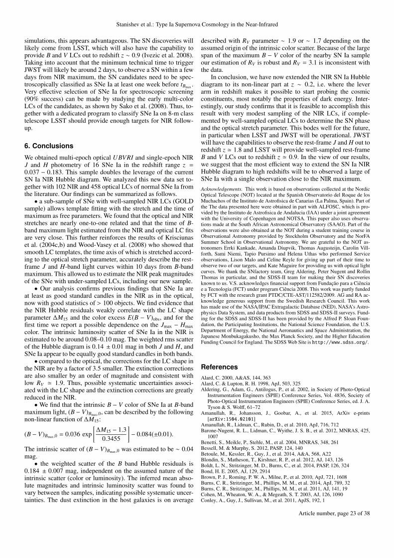
Stanishev et al.: Type Ia Supernova Cosmology in the Near-Infrared
simulations, this appears advantageous. The SN discoveries willlikely come from LSST, which will also have the capability toprovide B and V LCs out to redshift z ∼ 0.9 (Ivezic et al. 2008).Taking into account that the minimum technical time to triggerJWST will likely be around 2 days, to observe a SN within a fewdays from NIR maximum, the SN candidates need to be spec-troscopically classified as SNe Ia at least one week before tBmax .Very effective selection of SNe Ia for spectroscopic screening(90% success) can be made by studying the early multi-colorLCs of the candidates, as shown by Sako et al. (2008). Thus, to-gether with a dedicated program to classify SNe Ia on 8-m classtelescope LSST should provide enough targets for NIR follow-up.
6. Conclusions
We obtained multi-epoch optical UBVRI and single-epoch NIRJ and H photometry of 16 SNe Ia in the redshift range z =0.037 − 0.183. This sample doubles the leverage of the currentSN Ia NIR Hubble diagram. We analyzed this new data set to-gether with 102 NIR and 458 optical LCs of normal SNe Ia fromthe literature. Our findings can be summarized as follows.• a sub-sample of SNe with well-sampled NIR LCs (GOLD
sample) allows template fitting with the stretch and the time ofmaximum as free parameters. We found that the optical and NIRstretches are nearly one-to-one related and that the time of B-band maximum light estimated from the NIR and optical LC fitsare very close. This further reinforces the results of Krisciunaset al. (2004c,b) and Wood-Vasey et al. (2008) who showed thatsmooth LC templates, the time axis of which is stretched accord-ing to the optical stretch parameter, accurately describe the rest-frame J and H-band light curves within 10 days from B-bandmaximum. This allowed us to estimate the NIR peak magnitudesof the SNe with under-sampled LCs, including our new sample.• Our analysis confirms previous findings that SNe Ia are
at least as good standard candles in the NIR as in the optical,now with good statistics of > 100 objects. We find evidence thatthe NIR Hubble residuals weakly correlate with the LC shapeparameter ∆M15 and the color excess E(B − V)obs, and for thefirst time we report a possible dependence on the Jmax − Hmaxcolor. The intrinsic luminosity scatter of SNe Ia in the NIR isestimated to be around 0.08–0.10 mag. The weighted rms scatterof the Hubble diagram is 0.14 ± 0.01 mag in both J and H, andSNe Ia appear to be equally good standard candles in both bands.• compared to the optical, the corrections for the LC shape in
the NIR are by a factor of 3.5 smaller. The extinction correctionsare also smaller by an order of magnitude and consistent withlow RV ' 1.9. Thus, possible systematic uncertainties associ-ated with the LC shape and the extinction corrections are greatlyreduced in the NIR.•We find that the intrinsic B − V color of SNe Ia at B-band
maximum light, (B − V)Bmax,0, can be described by the followingnon-linear function of ∆M15:
(B − V)Bmax,0 = 0.036 exp[∆M15 − 1.3
0.3455
]− 0.084(±0.01).
The intrinsic scatter of (B − V)Bmax,0 was estimated to be ∼ 0.04mag.• the weighted scatter of the B band Hubble residuals is
0.184 ± 0.007 mag, independent on the assumed nature of theintrinsic scatter (color or luminosity). The inferred mean abso-lute magnitudes and intrinsic luminosity scatter was found tovary between the samples, indicating possible systematic uncer-tainties. The dust extinction in the host galaxies is on average
described with RV parameter ∼ 1.9 or ∼ 1.7 depending on theassumed origin of the intrinsic color scatter. Because of the largespan of the maximum B − V color of the nearby SN Ia sampleour estimation of RV is robust and RV = 3.1 is inconsistent withthe data.
In conclusion, we have now extended the NIR SN Ia Hubblediagram to its non-linear part at z ∼ 0.2, i.e. where the leverarm in redshift makes it possible to start probing the cosmicconstituents, most notably the properties of dark energy. Inter-estingly, our study confirms that it is feasible to accomplish thisresult with very modest sampling of the NIR LCs, if comple-mented by well-sampled optical LCs to determine the SN phaseand the optical stretch parameter. This bodes well for the future,in particular when LSST and JWST will be operational. JWSTwill have the capabilities to observe the rest-frame J and H out toredshift z ' 1.8 and LSST will provide well-sampled rest-frameB and V LCs out to redshift z ' 0.9. In the view of our results,we suggest that the most efficient way to extend the SN Ia NIRHubble diagram to high redshifts will be to observed a large ofSNe Ia with a single observation close to the NIR maximum.Acknowledgements. This work is based on observations collected at the NordicOptical Telescope (NOT) located at the Spanish Observatorio del Roque de losMuchachos of the Instituto de Astrofisica de Canarias (La Palma, Spain). Part ofthe The data presented here were obtained in part with ALFOSC, which is pro-vided by the Instituto de Astrofisica de Andalucia (IAA) under a joint agreementwith the University of Copenhagen and NOTSA. This paper also uses observa-tions made at the South African Astronomical Observatory (SAAO). Part of theobservations were also obtained at the NOT during a student training course inObservational Astronomy provided by Stockholm Observatory and the NorFASummer School in Observational Astronomy. We are grateful to the NOT as-tronomers Errki Kankade, Amanda Diupvik, Thomas Augusteijn, Carolin Vill-forth, Sami Niemi, Tapio Pursimo and Helena Uthas who performed Serviceobservations, Lison Malo and Celine Reyle for giving up part of their time toobserve two of our targets, and Kate Maguire for providing us with optical lightcurves. We thank the SNfactory team, Greg Aldering, Peter Nugent and RollinThomas in particular, and the SDSS-II team for making their SN discoveriesknown to us. V.S. acknowledges financial support from Fundação para a Ciênciae a Tecnologia (FCT) under program Ciência 2008. This work was partly fundedby FCT with the research grant PTDC/CTE-AST/112582/2009. AG and RA ac-knowledge generous support from the Swedish Research Council. This workhas made use of the NASA/IPAC Extragalactic Database (NED), NASA’s Astro-physics Data System, and data products from SDSS and SDSS-II surveys. Fund-ing for the SDSS and SDSS-II has been provided by the Alfred P. Sloan Foun-dation, the Participating Institutions, the National Science Foundation, the U.S.Department of Energy, the National Aeronautics and Space Administration, theJapanese Monbukagakusho, the Max Planck Society, and the Higher EducationFunding Council for England. The SDSS Web Site is http://www.sdss.org/.
ReferencesAlard, C. 2000, A&AS, 144, 363Alard, C. & Lupton, R. H. 1998, ApJ, 503, 325Aldering, G., Adam, G., Antilogus, P., et al. 2002, in Society of Photo-Optical
Instrumentation Engineers (SPIE) Conference Series, Vol. 4836, Society ofPhoto-Optical Instrumentation Engineers (SPIE) Conference Series, ed. J. A.Tyson & S. Wolff, 61–72
Amanullah, R., Johansson, J., Goobar, A., et al. 2015, ArXiv e-prints[arXiv:1504.02101]
Amanullah, R., Lidman, C., Rubin, D., et al. 2010, ApJ, 716, 712Barone-Nugent, R. L., Lidman, C., Wyithe, J. S. B., et al. 2012, MNRAS, 425,
1007Benetti, S., Meikle, P., Stehle, M., et al. 2004, MNRAS, 348, 261Bessell, M. & Murphy, S. 2012, PASP, 124, 140Betoule, M., Kessler, R., Guy, J., et al. 2014, A&A, 568, A22Blondin, S., Matheson, T., Kirshner, R. P., et al. 2012, AJ, 143, 126Boldt, L. N., Stritzinger, M. D., Burns, C., et al. 2014, PASP, 126, 324Bond, H. E. 2005, AJ, 129, 2914Brown, P. J., Roming, P. W. A., Milne, P., et al. 2010, ApJ, 721, 1608Burns, C. R., Stritzinger, M., Phillips, M. M., et al. 2014, ApJ, 789, 32Burns, C. R., Stritzinger, M., Phillips, M. M., et al. 2011, AJ, 141, 19Cohen, M., Wheaton, W. A., & Megeath, S. T. 2003, AJ, 126, 1090Conley, A., Guy, J., Sullivan, M., et al. 2011, ApJS, 192, 1
Article number, page 23 of 38

A&A proofs: manuscript no. nir_sne_submitted
Conley, A., Sullivan, M., Hsiao, E. Y., et al. 2008, ApJ, 681, 482Contreras, C., Hamuy, M., Phillips, M. M., et al. 2010, AJ, 139, 519Elias-Rosa, N., Benetti, S., Cappellaro, E., et al. 2006, MNRAS, 369, 1880Fitzpatrick, E. L. 1999, PASP, 111, 63Folatelli, G., Phillips, M. M., Burns, C. R., et al. 2010, AJ, 139, 120Fruchter, A. S. & Hook, R. N. 2002, PASP, 114, 144Gall, E. E. E., Taubenberger, S., Kromer, M., et al. 2012, MNRAS, 427, 994Ganeshalingam, M., Li, W., Filippenko, A. V., et al. 2010, ApJS, 190, 418Goldhaber, G., Groom, D. E., Kim, A., et al. 2001, ApJ, 558, 359Goobar, A. & Leibundgut, B. 2011, Annual Review of Nuclear and Particle Sci-
ence, 61, 251Guy, J., Astier, P., Baumont, S., et al. 2007, A&A, 466, 11Hamuy, M., Maza, J., Pinto, P. A., et al. 2002, AJ, 124, 417Hamuy, M., Phillips, M. M., Suntzeff, N. B., et al. 1996, AJ, 112, 2408Harris, W. E., Fitzgerald, M. P., & Reed, B. C. 1981, PASP, 93, 507Hernandez, M., Meikle, W. P. S., Aparicio, A., et al. 2000, MNRAS, 319, 223Hicken, M., Challis, P., Jha, S., et al. 2009, ApJ, 700, 331Hicken, M., Challis, P., Kirshner, R. P., et al. 2012, ApJS, 200, 12Hsiao, E. Y., Conley, A., Howell, D. A., et al. 2007, ApJ, 663, 1187Hsiao, E. Y., Marion, G. H., Phillips, M. M., et al. 2013, ApJ, 766, 72Hunt, L. K., Mannucci, F., Testi, L., et al. 1998, AJ, 115, 2594Ivezic, Z., Tyson, J. A., Abel, B., et al. 2008, ArXiv e-prints
[arXiv:0805.2366]Jha, S., Garnavich, P. M., Kirshner, R. P., et al. 1999, ApJS, 125, 73Jha, S., Kirshner, R. P., Challis, P., et al. 2006, AJ, 131, 527Jha, S., Riess, A. G., & Kirshner, R. P. 2007, ApJ, 659, 122Kattner, S., Leonard, D. C., Burns, C. R., et al. 2012, PASP, 124, 114Kim, A., Goobar, A., & Perlmutter, S. 1996, PASP, 108, 190Knop, R. A., Aldering, G., Amanullah, R., et al. 2003, ApJ, 598, 102Kowalski, M., Rubin, D., Aldering, G., et al. 2008, ApJ, 686, 749Krisciunas, K., Garnavich, P. M., Stanishev, V., et al. 2007, AJ, 133, 58Krisciunas, K., Hastings, N. C., Loomis, K., et al. 2000, ApJ, 539, 658Krisciunas, K., Phillips, M. M., Stubbs, C., et al. 2001, AJ, 122, 1616Krisciunas, K., Phillips, M. M., & Suntzeff, N. B. 2004a, ApJ, 602, L81Krisciunas, K., Phillips, M. M., Suntzeff, N. B., et al. 2004b, AJ, 127, 1664Krisciunas, K., Suntzeff, N. B., Candia, P., et al. 2003, AJ, 125, 166Krisciunas, K., Suntzeff, N. B., Phillips, M. M., et al. 2004c, AJ, 128, 3034Landolt, A. U. 1992, AJ, 104, 340Landolt, A. U. 2009, AJ, 137, 4186Leloudas, G., Stritzinger, M. D., Sollerman, J., et al. 2009, A&A, 505, 265Lira, P. 1995, Master Thesis, Univ. Chile [astro-ph/9709262]Maguire, K., Sullivan, M., Ellis, R. S., et al. 2012, MNRAS, 426, 2359Mandel, K. S., Narayan, G., & Kirshner, R. P. 2011, ApJ, 731, 120Mandel, K. S., Wood-Vasey, W. M., Friedman, A. S., & Kirshner, R. P. 2009,
ApJ, 704, 629Marriner, J., Bernstein, J. P., Kessler, R., et al. 2011, ApJ, 740, 72Matheson, T., Joyce, R. R., Allen, L. E., et al. 2012, ApJ, 754, 19Mayya, Y. D., Puerari, I., & Kuhn, O. 1998, IAU Circ., 6907, 2Meikle, W. P. S. 2000, MNRAS, 314, 782Milne, P. A., Brown, P. J., Roming, P. W. A., Bufano, F., & Gehrels, N. 2013,
ApJ, 779, 23Milne, P. A., Brown, P. J., Roming, P. W. A., et al. 2010, ApJ, 721, 1627Moorwood, A., Cuby, J.-G., Biereichel, P., et al. 1998, The Messenger, 94, 7Munari, U., Henden, A., Belligoli, R., et al. 2013, New A, 20, 30Nobili, S. & Goobar, A. 2008, A&A, 487, 19Pastorello, A., Mazzali, P. A., Pignata, G., et al. 2007a, MNRAS, 377, 1531Pastorello, A., Taubenberger, S., Elias-Rosa, N., et al. 2007b, MNRAS, 376,
1301Perlmutter, S., Aldering, G., Goldhaber, G., et al. 1999, ApJ, 517, 565Perlmutter, S., Gabi, S., Goldhaber, G., et al. 1997, ApJ, 483, 565Persson, S. E., Murphy, D. C., Krzeminski, W., Roth, M., & Rieke, M. J. 1998,
AJ, 116, 2475Phillips, M. M., Lira, P., Suntzeff, N. B., et al. 1999, AJ, 118, 1766Pignata, G., Benetti, S., Mazzali, P. A., et al. 2008, MNRAS, 388, 971Prieto, J. L., Rest, A., & Suntzeff, N. B. 2006, ApJ, 647, 501Riess, A. G., Filippenko, A. V., Challis, P., et al. 1998, AJ, 116, 1009Riess, A. G., Kirshner, R. P., Schmidt, B. P., et al. 1999, AJ, 117, 707Sako, M., Bassett, B., Becker, A., et al. 2008, AJ, 135, 348Sako, M., Bassett, B., Becker, A. C., et al. 2014, ArXiv e-prints
[arXiv:1401.3317]Schlegel, D. J., Finkbeiner, D. P., & Davis, M. 1998, ApJ, 500, 525Scolnic, D. M., Riess, A. G., Foley, R. J., et al. 2014, ApJ, 780, 37Stanishev, V., Goobar, A., Benetti, S., et al. 2007, A&A, 469, 645Stanishev, V., Goobar, A., Paech, K., et al. 2009, A&A, 507, 61Stetson, P. B. 1987, PASP, 99, 191Stritzinger, M., Hamuy, M., Suntzeff, N. B., et al. 2002, AJ, 124, 2100Stritzinger, M., Suntzeff, N. B., Hamuy, M., et al. 2005, PASP, 117, 810Stritzinger, M. D., Phillips, M. M., Boldt, L. N., et al. 2011, AJ, 142, 156Suntzeff, N. B. 2000, in American Institute of Physics Conference Series, ed.
S. S. Holt & W. W. Zhang, 65–74Suntzeff, N. B., Phillips, M. M., Covarrubias, R., et al. 1999, AJ, 117, 1175Thèvenaz, P., Blu, T., & Unser, M. 2000, IEEE Transactions on Medical Imaging,
19, 739Tokunaga, A. T., Simons, D. A., & Vacca, W. D. 2002, PASP, 114, 180Valentini, G., Di Carlo, E., Massi, F., et al. 2003, ApJ, 595, 779van Dokkum, P. G. 2001, PASP, 113, 1420Wang, X., Filippenko, A. V., Ganeshalingam, M., et al. 2009a, ApJ, 699, L139Wang, X., Li, W., Filippenko, A. V., et al. 2009b, ApJ, 697, 380Wood-Vasey, W. M., Friedman, A. S., Bloom, J. S., et al. 2008, ApJ, 689, 377
Article number, page 24 of 38

Stanishev et al.: Type Ia Supernova Cosmology in the Near-Infrared
Table 4. S-corrected SN photometry. The number in parentheses are the uncertainties.
JD−2400000 U B V R I InstrumentSN 2008bz
54586.409 18.499 (0.032) 18.284 (0.033) 18.182 (0.029) 18.169 (0.019) 18.765 (0.030) ALFOSC54592.441 19.425 (0.055) 18.935 (0.015) 18.499 (0.014) 18.596 (0.029) 19.188 (0.077) MOSCA54598.436 20.284 (0.069) 19.631 (0.019) 18.930 (0.012) 18.766 (0.013) 19.308 (0.024) ALFOSC54610.476 − 20.803 (0.042) 19.739 (0.036) 19.177 (0.029) 19.139 (0.032) STANCam
SNF20080510-00554599.395 18.583 (0.033) 19.055 (0.022) 18.996 (0.020) 18.927 (0.015) 19.166 (0.022) ALFOSC54610.463 19.206 (0.097) 19.139 (0.036) 18.875 (0.047) 18.781 (0.019) 19.246 (0.040) STANCam54618.569 20.201 (0.058) 19.644 (0.025) 19.219 (0.021) 19.186 (0.020) 19.940 (0.044) ALFOSC54624.408 20.837 (0.121) 20.155 (0.029) 19.577 (0.022) 19.421 (0.020) 20.154 (0.052) ALFOSC54636.493 − 21.393 (0.075) 20.307 (0.043) 19.782 (0.058) 19.745 (0.034) ALFOSC
SNF20080512-00854609.616 19.734 (0.057) 19.315 (0.032) 18.851 (0.018) 18.747 (0.019) 19.306 (0.029) STANCam54613.610 − − 19.061 (0.037) 18.931 (0.013) − ALFOSC54618.612 20.953 (0.070) 20.175 (0.018) 19.330 (0.013) 19.070 (0.013) 19.519 (0.023) ALFOSC54624.443 21.133 (0.146) 20.699 (0.037) 19.617 (0.016) 19.145 (0.013) 19.369 (0.020) ALFOSC54635.675 − 21.033 (0.146) 20.219 (0.067) 19.629 (0.027) 19.559 (0.046) STANCam54641.549 − 21.521 (0.127) 20.515 (0.055) 19.918 (0.037) 19.905 (0.032) ALFOSC
SNF20080512-01054612.562 19.413 (0.057) 18.966 (0.025) 18.568 (0.013) 18.545 (0.013) 19.197 (0.029) ALFOSC54618.597 20.396 (0.050) 19.843 (0.018) 19.033 (0.012) 18.784 (0.013) 19.116 (0.020) ALFOSC54626.470 21.239 (0.111) 20.813 (0.028) 19.751 (0.017) 19.111 (0.015) 18.978 (0.016) ALFOSC54635.658 − 21.047 (0.168) 20.279 (0.070) 19.772 (0.040) 19.602 (0.048) STANCam54641.523 − 21.414 (0.115) 20.560 (0.053) 20.000 (0.036) 19.947 (0.050) ALFOSC
SNF20080516-00054611.490 − 18.422 (0.047) 18.261 (0.020) 18.179 (0.013) 18.595 (0.022) STANCam54618.507 19.114 (0.035) 18.813 (0.012) 18.537 (0.012) 18.473 (0.011) 19.086 (0.023) ALFOSC54626.425 20.322 (0.073) 19.628 (0.014) 19.019 (0.011) 18.827 (0.012) 19.321 (0.022) ALFOSC54635.401 − 20.529 (0.104) 19.535 (0.041) 19.032 (0.023) 19.216 (0.099) STANCam54641.401 − 20.897 (0.059) 19.873 (0.024) 19.173 (0.014) 19.141 (0.026) ALFOSC54656.432 − 21.256 (0.100) 20.523 (0.048) 19.936 (0.023) 20.021 (0.056) ALFOSC
SNF20080516-02254611.509 18.229 (0.033) 18.469 (0.019) 18.393 (0.024) 18.321 (0.027) 18.751 (0.027) STANCam54618.583 19.278 (0.032) 18.895 (0.011) 18.620 (0.012) 18.573 (0.014) 19.127 (0.019) ALFOSC54624.459 20.013 (0.062) 19.498 (0.018) 18.980 (0.013) 18.889 (0.014) 19.502 (0.025) ALFOSC54636.515 − 20.820 (0.072) 19.780 (0.045) 19.224 (0.019) 19.257 (0.030) ALFOSC54641.497 − 21.166 (0.050) 20.235 (0.032) 19.358 (0.023) 19.361 (0.029) ALFOSC54648.564 − 21.453 (0.147) − − − ALFOSC54656.455 − 21.691 (0.078) 20.857 (0.039) 20.170 (0.028) 20.298 (0.068) ALFOSC
SNF20080517-01054610.471 − 19.907 (0.046) 19.603 (0.017) 19.479 (0.029) 19.615 (0.023) STANCam54618.532 21.150 (0.101) 20.601 (0.023) 19.965 (0.020) 19.810 (0.019) 20.239 (0.086) ALFOSC54626.443 22.413 (0.258) 21.496 (0.042) 20.534 (0.022) 20.132 (0.019) 20.314 (0.074) ALFOSC54636.451 − − − − 20.273 (0.068) ALFOSC54641.416 − 22.729 (0.152) 21.460 (0.061) 20.868 (0.034) 20.460 (0.061) ALFOSC54648.460 − 22.946 (0.356) 21.864 (0.130) 21.261 (0.135) 20.810 (0.155) ALFOSC
SNF20080522-00054618.556 16.486 (0.021) 17.147 (0.013) 17.126 (0.012) 17.134 (0.011) 17.330 (0.012) ALFOSC54625.591 − 17.269 (0.011) 17.130 (0.021) 17.009 (0.033) 17.409 (0.075) ANDICAM54626.457 17.073 (0.024) 17.267 (0.017) 17.123 (0.009) 17.029 (0.012) 17.491 (0.014) ALFOSC54628.555 − 17.389 (0.022) 17.161 (0.017) 17.075 (0.018) 17.495 (0.066) ANDICAM54631.544 − 17.520 (0.025) 17.260 (0.016) 17.241 (0.046) 17.706 (0.138) ANDICAM54635.560 − 17.846 (0.033) 17.462 (0.029) − − ANDICAM54636.478 18.231 (0.050) 17.904 (0.023) 17.586 (0.028) 17.602 (0.016) 18.141 (0.022) ALFOSC54645.584 − 19.059 (0.037) 18.106 (0.019) 17.801 (0.022) 17.903 (0.059) ANDICAM54650.536 − 19.538 (0.026) 18.381 (0.016) 17.916 (0.016) 17.923 (0.035) ANDICAM
Article number, page 25 of 38

A&A proofs: manuscript no. nir_sne_submitted
Table 4. continued.
JD−2400000 U B V R I Instrument54656.444 − 19.818 (0.018) 18.662 (0.014) 18.079 (0.011) 18.076 (0.012) ALFOSC54658.547 − 19.929 (0.103) 18.770 (0.049) 18.172 (0.051) 18.138 (0.108) ANDICAM54663.537 − 20.190 (0.205) 19.018 (0.065) 18.438 (0.044) 18.378 (0.067) ANDICAM54664.409 − − 18.980 (0.047) 18.487 (0.021) 18.447 (0.051) STANCam54671.400 − 20.303 (0.019) 19.305 (0.013) 18.805 (0.014) 18.854 (0.015) ALFOSC
SNF20080522-00154618.492 18.926 (0.046) 18.460 (0.015) 18.052 (0.011) 17.984 (0.012) 18.608 (0.028) ALFOSC54626.412 19.892 (0.051) 19.308 (0.017) 18.419 (0.011) 18.211 (0.009) 18.567 (0.018) ALFOSC54639.589 − 20.195 (0.161) 19.183 (0.129) 18.427 (0.066) 18.429 (0.106) ANDICAM54640.606 − 20.230 (0.124) 19.212 (0.062) 18.643 (0.051) 18.520 (0.070) ANDICAM54651.522 − 20.643 (0.044) 19.781 (0.045) 19.104 (0.045) 19.204 (0.106) ANDICAM54656.397 − 20.702 (0.126) 19.785 (0.067) 19.270 (0.034) 19.407 (0.063) ALFOSC54661.531 − 20.870 (0.224) 20.049 (0.141) 19.385 (0.105) 19.715 (0.200) ANDICAM54671.388 − 21.076 (0.099) 20.200 (0.037) 19.820 (0.034) 19.976 (0.071) ALFOSC
SNF20080522-00454618.475 20.326 (0.131) 19.740 (0.031) 19.529 (0.023) 19.383 (0.026) 19.932 (0.096) ALFOSC54626.398 − 20.364 (0.030) 19.921 (0.023) 19.762 (0.026) 20.294 (0.078) ALFOSC54636.464 − − 20.635 (0.076) 20.098 (0.045) 20.174 (0.058) ALFOSC54641.388 − 21.563 (0.141) 20.820 (0.067) 20.263 (0.045) 20.292 (0.073) ALFOSC54648.396 − 22.009 (0.558) 21.151 (0.195) 20.317 (0.115) − ALFOSC54656.386 − − − 20.913 (0.161) 20.637 (0.125) ALFOSC
SNF20080522-01154613.600 − 16.845 (0.012) 16.888 (0.012) 16.835 (0.012) 17.061 (0.024) ALFOSC54624.393 17.182 (0.023) 17.085 (0.015) 16.954 (0.012) 16.911 (0.013) 17.431 (0.016) ALFOSC54638.723 − 18.458 (0.068) 17.800 (0.074) 17.501 (0.032) 17.763 (0.044) ANDICAM54650.585 − 19.556 (0.043) 18.386 (0.024) 17.819 (0.027) 17.702 (0.034) ANDICAM54656.468 − 19.720 (0.022) 18.717 (0.014) 18.194 (0.011) 18.111 (0.024) ALFOSC54661.632 − 20.178 (0.209) 18.971 (0.062) 18.458 (0.075) 18.460 (0.073) ANDICAM54664.419 − 19.942 (0.093) 19.036 (0.057) 18.571 (0.025) 18.648 (0.105) STANCam54671.413 − 20.108 (0.019) 19.208 (0.014) 18.798 (0.012) 18.850 (0.023) ALFOSC
SNF20080606-01254636.530 19.298 (0.064) 18.944 (0.023) 18.824 (0.019) 18.724 (0.019) 18.954 (0.034) ALFOSC54641.511 19.861 (0.067) 19.337 (0.017) 19.017 (0.015) 18.951 (0.014) 19.283 (0.024) ALFOSC54648.501 − 20.154 (0.041) 19.435 (0.025) − 19.396 (0.075) ALFOSC54649.677 − 20.264 (0.064) 19.519 (0.052) 19.331 (0.060) 19.669 (0.149) ANDICAM54654.664 − 20.965 (0.170) 19.862 (0.065) 19.415 (0.062) 19.387 (0.141) ANDICAM54663.406 − 21.650 (0.110) 20.532 (0.192) 19.778 (0.089) 19.558 (0.095) ALFOSC54671.427 − 21.901 (0.060) 20.958 (0.036) 20.337 (0.025) 20.127 (0.033) ALFOSC
SNF20080610-00354641.536 20.012 (0.079) 19.456 (0.021) 19.129 (0.016) 18.992 (0.015) 19.548 (0.027) ALFOSC54648.441 20.706 (0.167) 20.013 (0.036) 19.553 (0.026) 19.321 (0.028) 20.093 (0.138) ALFOSC54655.527 − 20.840 (0.022) 19.998 (0.021) 19.596 (0.016) 19.903 (0.060) STANCam54663.391 − − 20.412 (0.106) 19.779 (0.071) 19.883 (0.152) ALFOSC54671.443 − 21.962 (0.052) 20.985 (0.031) 20.217 (0.019) 20.114 (0.029) ALFOSC
Article number, page 26 of 38

Stanishev et al.: Type Ia Supernova Cosmology in the Near-InfraredTa
ble
10.S
ILV
ER
and
BR
ON
ZE
Supe
rnov
aL
Cpa
ram
eter
s
SNz C
MB
J max
dH
max
dt B
max
as o
pt∆
M15
bB
max
Vat
t Bm
axR
ef.c
SILV
ER
sam
ple
2000
ca0.
0245
316
.302
(0.0
28/0
.013
)16
.632
(0.0
25/0
.018
)51
666.
29(0
.12)
1.05
4(0
.008
)0.
932
(0.0
22)
15.5
81(0
.008
)15
.699
(0.0
06)
Kri
2001
ba0.
0306
816
.976
(0.0
15/0
.015
)17
.275
(0.0
24/0
.021
)52
034.
65(0
.14)
1.01
6(0
.009
)0.
997
(0.0
28)
16.2
35(0
.007
)16
.329
(0.0
08)
Kri
2001
bt0.
0144
415
.420
(0.0
29/0
.009
)15
.627
(0.0
28/0
.012
)52
064.
43(0
.03)
0.93
5(0
.004
)1.
165
(0.0
21)
15.3
43(0
.006
)15
.126
(0.0
04)
Kri
2003
cg0.
0053
113
.565
(0.0
54/0
.007
)13
.680
(0.0
54/0
.006
)52
729.
56(0
.03)
0.96
9(0
.005
)1.
108
(0.0
23)
15.8
13(0
.006
)14
.609
(0.0
04)
Var
2005
am0.
0089
813
.954
(0.0
23/0
.007
)14
.200
(0.0
11/0
.008
)53
436.
96(0
.03)
0.77
4(0
.002
)1.
582
(0.0
21)
13.6
49(0
.002
)13
.582
(0.0
02)
CSP
2005
eu0.
0340
717
.014
(0.0
62/0
.018
)17
.339
(0.0
61/0
.016
)53
659.
84(0
.04)
1.04
9(0
.007
)0.
938
(0.0
22)
16.4
37(0
.007
)16
.571
(0.0
07)
CfA
2005
iq0.
0328
917
.471
(0.0
59/0
.018
)17
.627
(0.1
32/0
.015
)53
687.
69(0
.03)
0.89
9(0
.004
)1.
214
(0.0
22)
16.7
82(0
.004
)16
.798
(0.0
03)
CfA
2006
D0.
0096
514
.347
(0.0
17/0
.007
)14
.530
(0.0
13/0
.009
)53
757.
50(0
.01)
0.83
0(0
.001
)1.
419
(0.0
21)
14.1
60(0
.002
)14
.042
(0.0
02)
CSP
2006
ac0.
0239
516
.528
(0.0
78/0
.016
)16
.739
(0.1
02/0
.010
)53
781.
83(0
.08)
0.89
2(0
.007
)1.
229
(0.0
26)
16.1
93(0
.010
)16
.044
(0.0
07)
CfA
2006
bh0.
0104
914
.778
(0.0
13/0
.008
)14
.970
(0.0
15/0
.009
)53
833.
42(0
.01)
0.83
3(0
.001
)1.
409
(0.0
21)
14.3
62(0
.002
)14
.365
(0.0
01)
CSP
2006
gt0.
0435
917
.816
(0.0
69/0
.021
)18
.155
(0.1
13/0
.028
)54
003.
32(0
.10)
0.71
1(0
.006
)1.
797
(0.0
30)
18.2
35(0
.008
)17
.912
(0.0
06)
CSP
2007
as0.
0179
015
.812
(0.0
16/0
.010
)16
.057
(0.0
28/0
.014
)54
181.
61(0
.08)
0.90
9(0
.004
)1.
197
(0.0
21)
15.4
64(0
.003
)15
.388
(0.0
03)
CSP
2007
bd0.
0318
617
.022
(0.0
37/0
.016
)17
.301
(0.0
93/0
.022
)54
206.
78(0
.02)
0.91
0(0
.003
)1.
195
(0.0
21)
16.5
43(0
.005
)16
.553
(0.0
04)
CSP
2007
cq0.
0237
716
.254
(0.0
39/0
.016
)16
.921
(0.1
32/0
.010
)54
280.
27(0
.08)
0.98
5(0
.007
)1.
071
(0.0
27)
15.9
01(0
.006
)15
.887
(0.0
05)
CfA
2007
jg0.
0365
617
.578
(0.0
18/0
.018
)17
.880
(0.0
74/0
.025
)54
366.
51(0
.09)
0.94
2(0
.007
)1.
157
(0.0
22)
17.2
86(0
.005
)17
.196
(0.0
04)
CSP
2008
ia0.
0225
516
.403
(0.0
44/0
.012
)16
.331
(0.0
31/0
.017
)54
813.
04(0
.05)
0.87
2(0
.004
)1.
283
(0.0
24)
15.8
84(0
.004
)15
.867
(0.0
04)
CSP
BR
ON
ZE
sam
ple
2000
bh0.
0239
616
.369
(0.0
84/0
.013
)16
.533
(0.0
33/0
.018
)51
636.
19(0
.20)
1.00
2(0
.005
)1.
029
(0.0
24)
15.9
69(0
.013
)15
.919
(0.0
11)
Kri
2000
bk0.
0266
216
.595
(0.1
54/0
.014
)17
.042
(0.0
55/0
.019
)51
647.
92(0
.09)
0.70
3(0
.003
)1.
825
(0.0
23)
16.7
84(0
.014
)16
.611
(0.0
10)
Kri
2000
ce0.
0164
915
.521
(0.1
28/0
.010
)15
.900
(0.0
34/0
.013
)51
665.
51(0
.38)
1.06
0(0
.005
)0.
927
(0.0
21)
16.9
49(0
.036
)16
.459
(0.0
20)
Kri
2001
cn0.
0150
815
.640
(0.0
57/0
.010
)15
.769
(0.0
43/0
.012
)52
073.
46(0
.11)
0.93
9(0
.004
)1.
160
(0.0
21)
15.3
45(0
.008
)15
.127
(0.0
04)
Kri
2003
hv0.
0051
012
.979
(0.0
67/0
.007
)13
.060
(0.0
26/0
.006
)52
891.
79(0
.08)
0.77
3(0
.003
)1.
585
(0.0
22)
12.4
77(0
.007
)12
.545
(0.0
04)
Var
2004
S0.
0098
514
.605
(0.0
70/0
.007
)14
.744
(0.0
22/0
.009
)53
040.
87(0
.33)
0.99
2(0
.011
)1.
054
(0.0
34)
14.2
08(0
.020
)14
.153
(0.0
14)
Kri
2004
ef0.
0297
317
.317
(0.0
94/0
.015
)17
.612
(0.1
08/0
.021
)53
264.
07(0
.01)
0.86
1(0
.001
)1.
317
(0.0
21)
16.8
73(0
.001
)16
.721
(0.0
01)
CSP
2004
gs0.
0283
016
.925
(0.1
36/0
.014
)17
.067
(0.0
48/0
.020
)53
356.
20(0
.04)
0.76
9(0
.004
)1.
596
(0.0
24)
17.1
69(0
.003
)16
.925
(0.0
04)
CSP
2005
A0.
0183
316
.310
(0.0
98/0
.010
)16
.342
(0.0
29/0
.014
)53
379.
88(0
.07)
0.94
8(0
.005
)1.
148
(0.0
22)
18.1
58(0
.005
)17
.038
(0.0
04)
CSP
2005
ag0.
0803
219
.169
(0.0
81/0
.032
)18
.970
(0.0
57/0
.045
)53
414.
26(0
.14)
1.04
6(0
.009
)0.
942
(0.0
24)
18.4
32(0
.005
)18
.449
(0.0
04)
CSP
2005
al0.
0133
015
.561
(0.0
52/0
.009
)15
.747
(0.0
15/0
.011
)53
430.
57(0
.05)
0.87
9(0
.002
)1.
262
(0.0
22)
14.8
60(0
.003
)14
.958
(0.0
02)
CSP
2005
na0.
0268
316
.512
(0.0
79/0
.016
)17
.027
(0.1
43/0
.012
)53
740.
98(0
.06)
0.94
1(0
.003
)1.
158
(0.0
21)
15.9
66(0
.003
)16
.046
(0.0
03)
CfA
2006
N0.
0142
615
.581
(0.1
19/0
.013
)15
.778
(0.1
29/0
.005
)53
761.
62(0
.12)
0.77
7(0
.005
)1.
574
(0.0
25)
15.1
77(0
.008
)15
.148
(0.0
05)
CfA
2006
br0.
0255
517
.099
(0.0
88/0
.013
)17
.181
(0.0
98/0
.019
)53
852.
16(0
.40)
0.92
1(0
.023
)1.
181
(0.0
37)
19.0
45(0
.023
)18
.135
(0.0
12)
CSP
2006
cp0.
0233
316
.656
(0.0
69/0
.016
)16
.720
(0.0
36/0
.009
)53
896.
88(0
.07)
0.98
8(0
.008
)1.
063
(0.0
28)
15.9
22(0
.008
)15
.829
(0.0
07)
CfA
2006
ej0.
0193
116
.109
(0.0
81/0
.011
)16
.459
(0.0
70/0
.015
)53
975.
82(0
.10)
0.84
2(0
.008
)1.
380
(0.0
34)
15.7
70(0
.009
)15
.783
(0.0
09)
CSP
2006
eq0.
0483
118
.145
(0.1
08/0
.023
)18
.157
(0.1
36/0
.030
)53
978.
15(0
.44)
0.72
4(0
.013
)1.
748
(0.0
53)
18.5
06(0
.035
)18
.156
(0.0
22)
CSP
2006
ev0.
0275
717
.145
(0.0
92/0
.014
)17
.204
(0.0
73/0
.020
)53
989.
70(0
.27)
0.86
5(0
.008
)1.
304
(0.0
33)
17.1
12(0
.021
)16
.925
(0.0
12)
CSP
2006
gj0.
0276
717
.015
(0.0
65/0
.014
)17
.209
(0.0
66/0
.020
)54
000.
48(0
.11)
0.73
3(0
.015
)1.
714
(0.0
60)
17.6
53(0
.008
)17
.294
(0.0
07)
CSP
2006
hb0.
0153
415
.654
(0.1
08/0
.010
)15
.818
(0.0
49/0
.012
)54
003.
69(0
.29)
0.72
9(0
.005
)1.
729
(0.0
29)
15.5
88(0
.029
)15
.385
(0.0
18)
CSP
2006
hx0.
0443
517
.656
(0.0
70/0
.022
)17
.885
(0.1
00/0
.029
)54
021.
93(0
.09)
0.98
4(0
.014
)1.
073
(0.0
39)
17.5
44(0
.021
)17
.793
(0.0
32)
CSP
2006
is0.
0314
916
.596
(0.0
83/0
.016
)17
.022
(0.0
61/0
.022
)54
003.
87(0
.15)
1.24
3(0
.004
)0.
745
(0.0
20)
15.9
34(0
.010
)16
.111
(0.0
07)
CSP
2006
lu0.
0544
918
.702
(0.2
57/0
.026
)18
.427
(0.3
40/0
.033
)54
036.
75(0
.37)
0.99
0(0
.011
)1.
058
(0.0
34)
17.5
56(0
.019
)17
.593
(0.0
12)
CSP
2006
ob0.
0582
018
.460
(0.0
65/0
.027
)18
.685
(0.1
01/0
.034
)54
063.
54(0
.11)
0.77
6(0
.009
)1.
577
(0.0
32)
18.2
10(0
.009
)18
.139
(0.0
09)
CSP
2007
ai0.
0320
016
.876
(0.0
29/0
.016
)16
.948
(0.0
36/0
.022
)54
172.
43(0
.21)
1.15
7(0
.013
)0.
803
(0.0
26)
16.9
68(0
.009
)16
.852
(0.0
06)
CSP
Article number, page 27 of 38

A&A proofs: manuscript no. nir_sne_submittedTa
ble
10.c
ontin
ued.
SNz C
MB
J max
dH
max
dt B
max
as o
pt∆
M15
bB
max
Vat
t Bm
axR
ef.c
2007
nq0.
0438
517
.803
(0.0
88/0
.021
)17
.747
(0.1
27/0
.028
)54
399.
19(0
.11)
0.76
6(0
.006
)1.
604
(0.0
27)
17.4
20(0
.008
)17
.329
(0.0
06)
CSP
2008
C0.
0170
815
.949
(0.0
85/0
.010
)16
.150
(0.0
43/0
.013
)54
467.
29(0
.42)
0.91
8(0
.018
)1.
185
(0.0
31)
15.6
81(0
.027
)15
.476
(0.0
15)
CSP
2008
R0.
0128
815
.290
(0.0
42/0
.009
)15
.368
(0.0
31/0
.011
)54
494.
81(0
.05)
0.68
6(0
.003
)1.
877
(0.0
23)
15.2
92(0
.003
)15
.122
(0.0
03)
CSP
2008
bq0.
0344
617
.152
(0.0
62/0
.017
)17
.609
(0.1
58/0
.024
)54
563.
00(0
.09)
1.06
4(0
.005
)0.
923
(0.0
20)
16.7
04(0
.005
)16
.655
(0.0
03)
CSP
Not
es.(a
)JD−
2455
000.
(b)
estim
ated
from
our
s opt−
∆M
15re
latio
n.(c
)se
ete
xtfo
rth
ere
fere
nces
for
the
NIR
phot
omet
ry.(d
)T
hetw
onu
mbe
rsar
eth
eun
cert
aint
ies
ofth
epe
akm
agni
tude
and
the
K-c
orre
ctio
ns.
Article number, page 28 of 38

A&A–nir_sne_submitted, Online Material p 29
Appendix A: Second-order extinction
The second-order extinction term in U and B bands arises fromthe fact that the transmission of Earth’s atmosphere is not con-stant but decreases rapidly at wavelengths below 5000Å. Thechange of the transmission across the U and B bands is largeenough to cause stars with different spectral energy distributions(SED) to experience slightly different extinction. Thus, the at-mospheric extinction in U and B bands is not constant but it is afunction of the object SED. It can be parametrized as:
kB = k′B + k′′B (B − V) (A.1)kU = k′U + k′′U (U − B), (A.2)
where k′U,B and k′′U,B are the first-order and the second-order ex-tinction. The second-order extinction can be neglected in VRI.Unfortunately, in the majority of the photometric works on SNeIa the second-order extinction term has been neglected. Here wediscuss the uncertainties that are caused by this.
The usual practice in SN photometry is to calibrate the mag-nitudes of the stars in the field of the SN in several photometricnights. This is usually done by deriving the parameters in Eqs. 1by observing Landolt (1992, 2009) standard fields that containboth blue and red stars in photometric conditions, and applyingthe equations to the field stars. Then in non-photometric nightsthe SN magnitudes are calibrated using the field stars as tetrarystandards. Simple re-arrangement of Eqs. 1, taking B band as anexample gives:
B = b + (ctB − k′′B X) (B − V) − k′B X + zpB, (A.3)
If k′′B is not fitted (or fixed to a reasonable value ∼ −0.03), onewould not measure the true color term ctB but rather ctB − k′′B X,i.e. the measured color-term will depend on the airmass of theobservations. The second-order extinction in U and B has beenmeasured and it is about −0.03. Using the spectrophotometricatlas of Stritzinger et al. (2005), various U and B filters, andatmospheric transmission measured at different observatories weestimated k′′B and k′′U by means of synthetic photometry to be∼ −0.03 as well. Therefore, two standard fields observed airmassX = 1 and 2 will give color terms that differ by ∼ 0.03.
Another problem arises because the B−V color index of SNeIa changes from ∼ −0.1 around maximum light to 1.3 about amonth later. If a SN is observed at airmass 1.5 the correctionfor the second-order extinction at maximum and at +30 dayswill be ∼ 0.0 and 0.058 mag, respectively. When the second-order extinction term is not included in the calibration, this willnot be corrected for. While around maximum the effect will benegligible, 1-2 month after maximum the B magnitudes maybeas much as 0.06 mag in error. This will directly affect the B −V color index, which is often used to estimate the host galaxyextinction. Therefore, the estimation of the peak magnitudes canbe affected by as much as 0.18 mag for Milky Way type dustwith RV = 3.1.
Appendix B: S-corrections
Appendix B.1: Photometric systems responses
To recover the effective system responses we follow the meth-ods described in Stanishev et al. (2007). The relevant informa-tion was either taken from Stanishev et al. (2007) or from thecorresponding observatories. Whenever possible measured filtertransmission and CCD QEs were used; if unavailable, specifi-cations from the manufacturer were used. The total system re-sponses were computed by multiplying the filter transmissions
by (a) the CCD quantum efficiency (QE), (b) the reflectivity of atleast two aluminum surfaces, (a) a telluric absorption spectrumat airmass 1.3. The lens and window transmissions were not in-cluded because this information was unavailable. Note that thetransmission of the Earth atmosphere was not included in the cal-culation of the effective U and B bands. The reason is that whencomputing the instrument color terms the second-order extinc-tion has been taken into account. The effect of the atmospherictransmission on the U and B bands is to shift the bands effectivewavelength redward with increasing the airmass of the observa-tions. Taking into account the second-order extinction meant thatthe computed color terms correspond to observations above theatmosphere.
Synthetic magnitudes were calculated from Stritzinger et al.(2005) spectrophotometry of Landolt standard stars,
msyn = −2.5 log(∫
f photλ (λ)Rnat(λ)dλ
). (B.1)
The difference between the synthetic and the observed photome-try was fitted as a function of the observed color indices to com-pute synthetic color-terms (ctsyn), e.g. for B we have:
Bstd − Bsyn = ctsyn(Bstd − Vstd) + zpRnat. (B.2)
For the VRI-bands, the ctsyn’s were close to the observed onesctobs. In some cases small differences exceeding the uncertaintywere accounted for by shifting the filter transmissions until ctsyn
matched ctosb. zpRnatis the zero point for synthetic photometry
with the band Rnat.As in Stanishev et al. (2007) we found that the synthetic U
and B bands were always too blue. This is, to some extent, to beexpected because the neglected optical elements like lenses orwindows, anti-reflection and other coatings will tend to reducethe system sensitivity shortward of ∼4000 Å. To account for thenet effect of these uncertainties we modified the U and B bandsby multiplying them with a Sigmoid function:
F(λ; λ0,∆) =1
1 + exp(−(λ − λ0)/∆). (B.3)
The parameters λ0 and ∆ were selected so that ctsyn matched ctobs
for both U and B.Following Stanishev et al. (2007) we also re-derived the stan-
dard Johnson-Cousins system responses with the revised filterfunctions of Bessell & Murphy (2012). This procedure also gavethe zero points zpRstd
for synthetic photometry with the standardsystem responses Rstd.
Appendix B.2: Computing the S-corrections
The procedure that we used to calculate the S -corrections wasthe same as in Stanishev et al. (2007), but slightly modified toaccount for the fact that the U and B bands did not include theatmospheric transmission. The calibration correction from natu-ral magnitudes at airmass X, mnat
X , to standard magnitudes mstd iscomputed by means of synthetic photometry:
mstd = mnat + S , (B.4)
where S is the S -correction:
S = −2.5 log(∫
f photλ (λ)Rstd(λ)dλ
)+ zpRstd
+2.5 log(∫
f photλ (λ)Rnat(λ)p(λ)X dλ
)− zpRnat
X . (B.5)

A&A–nir_sne_submitted, Online Material p 30
Here f photλ (λ) is the photon spectral energy distributions (SED)
of the SN, Rnat(λ) and Rstd(λ) are the responses of the natural andthe standard systems, respectively, and p(λ) is the transmissionof the atmosphere at airmass X = 1 above the site of observation.Here zpRnat
X is the zero point obtained by fitting Eq. B.2 to thesynthetic magnitudes msyn
X computed with the natural passbandmultiplied by the Earth’s atmosphere transmission at airmass X,e.g.:
msynX = −2.5 log
(∫f photλ (λ)Rnat(λ)p(λ)X dλ
). (B.6)
Comparing Eq. A.3 and Eq. B.4 we see that the term ctB(B−V)−k′′B X(B − V) is just an approximation of the S -correction:
S ' ctB(B − V) − k′′B X(B − V). (B.7)
By the way the zero points in Eq. B.5 are derived, S ' 0.0 forA0 V stars with all color indexes zero, e.g. Vega. This ensuresthat for normal stars the synthetic S -correction will work thesame way as the linear color-term corrections.
The best way to compute the S -corrections for a SN is touse spectrophotometry of the same object. If that is not possiblethe mean spectrum of SNe Ia should be used. In our work wehave used Hsiao et al. (2007) spectral template, corrected for theMilky Way reddening and the redshift of each SN.

A&A–nir_sne_submitted, Online Material p 31
1
2 3
4
5
6
7
8
9
10
11
12
13
14
15
16
SN2008bz
1
2
3 4
5
6
7
8
9
1011
12
13
14
15
SNF20080510−005
1
2
3
4
5
6
7
8
9
10
11
12
13
14
15
16
17
18
19
20
21
22
23
24
25
26
27
28
29
30
31
3233
34
35
36
37
38
3940 41
4243
4445
46
47
48
49
50
51
52
53
SNF20080512−008
12
3
4
5
67
8
9
1011
12
13
14
15
16
17
18
19
20
21
22
23
24
25
26
27
SNF20080512−010
1
2
3
4
5
6
7
8
9 10
11
12
13
14
15
SNF20080516−000
1
2
34
56
7
8
9
10
11
SNF20080516−022
12
3
4
5
6
78
SNF20080517−010
1
23
4
56
7
8
9
SNF20080522−000
1
2
3
4
5
6
7
8
910
11
12
13
14
15
16
17
18
1920
21
SNF20080522−001
12
34
5
6
7
8
9
10 11
12
13
1415
1617
SNF20080522−0041
2
3
4
5
6
7
8
910
11
12
1314
15
16
17
18
1920
21
22
23
SNF20080522−0111
23
4
5
6
7
8
9
10
1112
13
14
15
16
17
18
19
20
21
22
23
2425
26
27
28
29
30
31
32
33
34
35
36
37
38
39
40 41
42
43
44
45
46
47
48
49
50
51
52
SNF20080606−012
12
3
4
5
6
7 8
9
10
11
12
13
14
15
16
17
18
19
20
21
22
23
24
25
26
27
28
29
30
31
32
3334
3536
3738
3940
41
42
43
SNF20080610−003
Fig. 1. Finding charts of the SNe observed in this paper. The SNs are located at the intersection of the two ticks. The numbers mark the localsequence stars. In most cases the number is right-up of the star and in a few cases only it is left-down.

A&A–nir_sne_submitted, Online Material p 32
Table 3. Calibrated magnitudes of the local stars around the SNe. The number in parentheses are the uncertainties.
No. U Nobs B Nobs V Nobs R Nobs I Nobs
SN 2008bz1 15.755 (0.013) 1 15.814 (0.014) 1 15.220 (0.011) 1 14.895 (0.012) 1 14.552 (0.012) 12 16.029 (0.013) 1 16.101 (0.013) 1 15.587 (0.011) 1 15.278 (0.012) 1 14.973 (0.012) 13 17.657 (0.018) 1 16.858 (0.016) 1 15.935 (0.012) 1 15.393 (0.013) 1 14.933 (0.012) 14 19.522 (0.036) 1 18.324 (0.020) 1 17.159 (0.012) 1 16.398 (0.014) 1 15.766 (0.013) 15 20.519 (0.077) 1 19.187 (0.020) 1 17.945 (0.012) 1 17.143 (0.013) 1 16.433 (0.015) 16 19.023 (0.027) 1 18.719 (0.020) 1 17.973 (0.017) 1 17.531 (0.018) 1 17.115 (0.015) 17 20.961 (0.108) 1 19.816 (0.033) 1 18.233 (0.015) 1 17.169 (0.016) 1 15.672 (0.016) 18 18.942 (0.027) 1 19.028 (0.025) 1 18.479 (0.012) 1 18.095 (0.024) 1 17.750 (0.013) 1
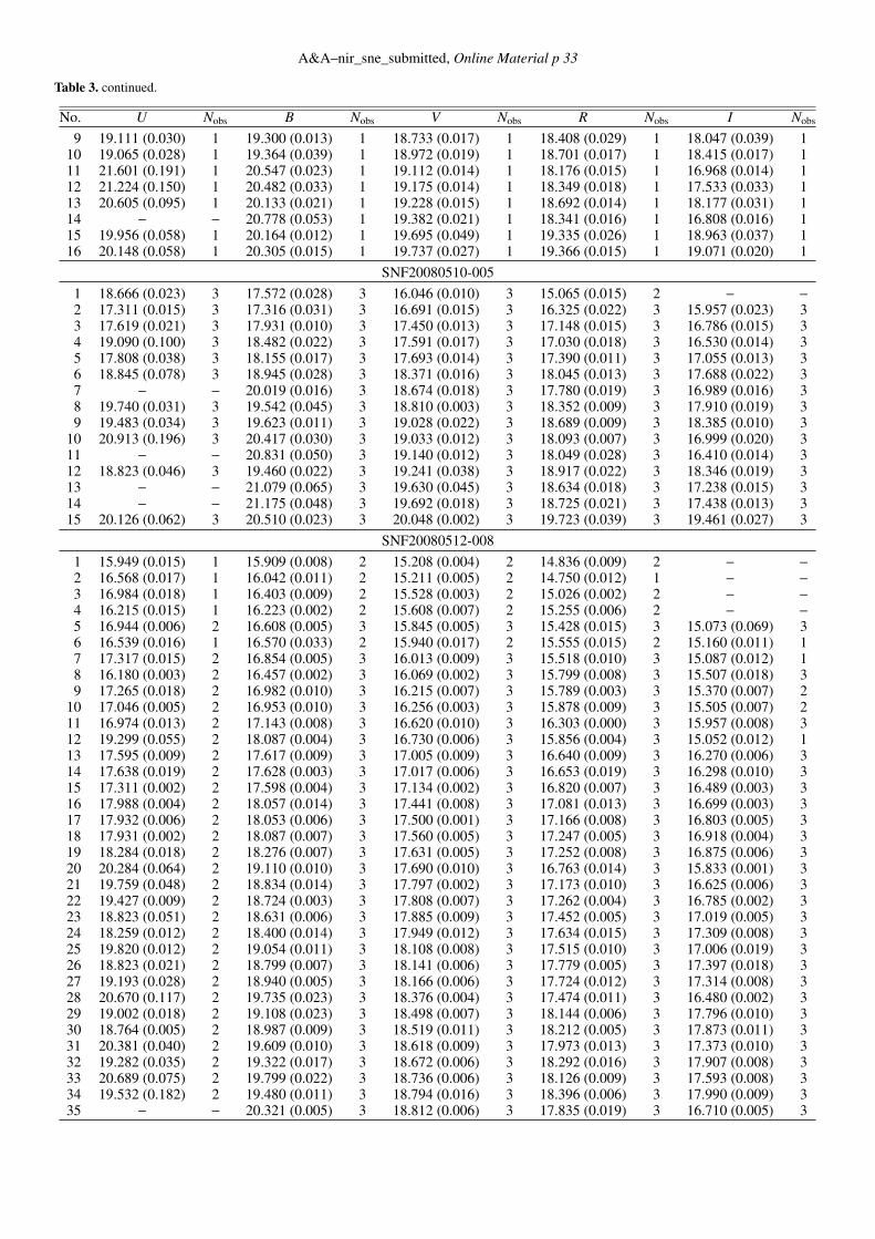
A&A–nir_sne_submitted, Online Material p 33
Table 3. continued.
No. U Nobs B Nobs V Nobs R Nobs I Nobs
9 19.111 (0.030) 1 19.300 (0.013) 1 18.733 (0.017) 1 18.408 (0.029) 1 18.047 (0.039) 110 19.065 (0.028) 1 19.364 (0.039) 1 18.972 (0.019) 1 18.701 (0.017) 1 18.415 (0.017) 111 21.601 (0.191) 1 20.547 (0.023) 1 19.112 (0.014) 1 18.176 (0.015) 1 16.968 (0.014) 112 21.224 (0.150) 1 20.482 (0.033) 1 19.175 (0.014) 1 18.349 (0.018) 1 17.533 (0.033) 113 20.605 (0.095) 1 20.133 (0.021) 1 19.228 (0.015) 1 18.692 (0.014) 1 18.177 (0.031) 114 − − 20.778 (0.053) 1 19.382 (0.021) 1 18.341 (0.016) 1 16.808 (0.016) 115 19.956 (0.058) 1 20.164 (0.012) 1 19.695 (0.049) 1 19.335 (0.026) 1 18.963 (0.037) 116 20.148 (0.058) 1 20.305 (0.015) 1 19.737 (0.027) 1 19.366 (0.015) 1 19.071 (0.020) 1
SNF20080510-0051 18.666 (0.023) 3 17.572 (0.028) 3 16.046 (0.010) 3 15.065 (0.015) 2 − −
2 17.311 (0.015) 3 17.316 (0.031) 3 16.691 (0.015) 3 16.325 (0.022) 3 15.957 (0.023) 33 17.619 (0.021) 3 17.931 (0.010) 3 17.450 (0.013) 3 17.148 (0.015) 3 16.786 (0.015) 34 19.090 (0.100) 3 18.482 (0.022) 3 17.591 (0.017) 3 17.030 (0.018) 3 16.530 (0.014) 35 17.808 (0.038) 3 18.155 (0.017) 3 17.693 (0.014) 3 17.390 (0.011) 3 17.055 (0.013) 36 18.845 (0.078) 3 18.945 (0.028) 3 18.371 (0.016) 3 18.045 (0.013) 3 17.688 (0.022) 37 − − 20.019 (0.016) 3 18.674 (0.018) 3 17.780 (0.019) 3 16.989 (0.016) 38 19.740 (0.031) 3 19.542 (0.045) 3 18.810 (0.003) 3 18.352 (0.009) 3 17.910 (0.019) 39 19.483 (0.034) 3 19.623 (0.011) 3 19.028 (0.022) 3 18.689 (0.009) 3 18.385 (0.010) 3
10 20.913 (0.196) 3 20.417 (0.030) 3 19.033 (0.012) 3 18.093 (0.007) 3 16.999 (0.020) 311 − − 20.831 (0.050) 3 19.140 (0.012) 3 18.049 (0.028) 3 16.410 (0.014) 312 18.823 (0.046) 3 19.460 (0.022) 3 19.241 (0.038) 3 18.917 (0.022) 3 18.346 (0.019) 313 − − 21.079 (0.065) 3 19.630 (0.045) 3 18.634 (0.018) 3 17.238 (0.015) 314 − − 21.175 (0.048) 3 19.692 (0.018) 3 18.725 (0.021) 3 17.438 (0.013) 315 20.126 (0.062) 3 20.510 (0.023) 3 20.048 (0.002) 3 19.723 (0.039) 3 19.461 (0.027) 3
SNF20080512-0081 15.949 (0.015) 1 15.909 (0.008) 2 15.208 (0.004) 2 14.836 (0.009) 2 − −
2 16.568 (0.017) 1 16.042 (0.011) 2 15.211 (0.005) 2 14.750 (0.012) 1 − −
3 16.984 (0.018) 1 16.403 (0.009) 2 15.528 (0.003) 2 15.026 (0.002) 2 − −
4 16.215 (0.015) 1 16.223 (0.002) 2 15.608 (0.007) 2 15.255 (0.006) 2 − −
5 16.944 (0.006) 2 16.608 (0.005) 3 15.845 (0.005) 3 15.428 (0.015) 3 15.073 (0.069) 36 16.539 (0.016) 1 16.570 (0.033) 2 15.940 (0.017) 2 15.555 (0.015) 2 15.160 (0.011) 17 17.317 (0.015) 2 16.854 (0.005) 3 16.013 (0.009) 3 15.518 (0.010) 3 15.087 (0.012) 18 16.180 (0.003) 2 16.457 (0.002) 3 16.069 (0.002) 3 15.799 (0.008) 3 15.507 (0.018) 39 17.265 (0.018) 2 16.982 (0.010) 3 16.215 (0.007) 3 15.789 (0.003) 3 15.370 (0.007) 2
10 17.046 (0.005) 2 16.953 (0.010) 3 16.256 (0.003) 3 15.878 (0.009) 3 15.505 (0.007) 211 16.974 (0.013) 2 17.143 (0.008) 3 16.620 (0.010) 3 16.303 (0.000) 3 15.957 (0.008) 312 19.299 (0.055) 2 18.087 (0.004) 3 16.730 (0.006) 3 15.856 (0.004) 3 15.052 (0.012) 113 17.595 (0.009) 2 17.617 (0.009) 3 17.005 (0.009) 3 16.640 (0.009) 3 16.270 (0.006) 314 17.638 (0.019) 2 17.628 (0.003) 3 17.017 (0.006) 3 16.653 (0.019) 3 16.298 (0.010) 315 17.311 (0.002) 2 17.598 (0.004) 3 17.134 (0.002) 3 16.820 (0.007) 3 16.489 (0.003) 316 17.988 (0.004) 2 18.057 (0.014) 3 17.441 (0.008) 3 17.081 (0.013) 3 16.699 (0.003) 317 17.932 (0.006) 2 18.053 (0.006) 3 17.500 (0.001) 3 17.166 (0.008) 3 16.803 (0.005) 318 17.931 (0.002) 2 18.087 (0.007) 3 17.560 (0.005) 3 17.247 (0.005) 3 16.918 (0.004) 319 18.284 (0.018) 2 18.276 (0.007) 3 17.631 (0.005) 3 17.252 (0.008) 3 16.875 (0.006) 320 20.284 (0.064) 2 19.110 (0.010) 3 17.690 (0.010) 3 16.763 (0.014) 3 15.833 (0.001) 321 19.759 (0.048) 2 18.834 (0.014) 3 17.797 (0.002) 3 17.173 (0.010) 3 16.625 (0.006) 322 19.427 (0.009) 2 18.724 (0.003) 3 17.808 (0.007) 3 17.262 (0.004) 3 16.785 (0.002) 323 18.823 (0.051) 2 18.631 (0.006) 3 17.885 (0.009) 3 17.452 (0.005) 3 17.019 (0.005) 324 18.259 (0.012) 2 18.400 (0.014) 3 17.949 (0.012) 3 17.634 (0.015) 3 17.309 (0.008) 325 19.820 (0.012) 2 19.054 (0.011) 3 18.108 (0.008) 3 17.515 (0.010) 3 17.006 (0.019) 326 18.823 (0.021) 2 18.799 (0.007) 3 18.141 (0.006) 3 17.779 (0.005) 3 17.397 (0.018) 327 19.193 (0.028) 2 18.940 (0.005) 3 18.166 (0.006) 3 17.724 (0.012) 3 17.314 (0.008) 328 20.670 (0.117) 2 19.735 (0.023) 3 18.376 (0.004) 3 17.474 (0.011) 3 16.480 (0.002) 329 19.002 (0.018) 2 19.108 (0.023) 3 18.498 (0.007) 3 18.144 (0.006) 3 17.796 (0.010) 330 18.764 (0.005) 2 18.987 (0.009) 3 18.519 (0.011) 3 18.212 (0.005) 3 17.873 (0.011) 331 20.381 (0.040) 2 19.609 (0.010) 3 18.618 (0.009) 3 17.973 (0.013) 3 17.373 (0.010) 332 19.282 (0.035) 2 19.322 (0.017) 3 18.672 (0.006) 3 18.292 (0.016) 3 17.907 (0.008) 333 20.689 (0.075) 2 19.799 (0.022) 3 18.736 (0.006) 3 18.126 (0.009) 3 17.593 (0.008) 334 19.532 (0.182) 2 19.480 (0.011) 3 18.794 (0.016) 3 18.396 (0.006) 3 17.990 (0.009) 335 − − 20.321 (0.005) 3 18.812 (0.006) 3 17.835 (0.019) 3 16.710 (0.005) 3

A&A–nir_sne_submitted, Online Material p 34
Table 3. continued.
No. U Nobs B Nobs V Nobs R Nobs I Nobs
36 − − 20.064 (0.039) 3 18.836 (0.007) 3 18.017 (0.015) 3 17.295 (0.007) 337 20.194 (0.039) 2 19.757 (0.012) 3 18.916 (0.017) 3 18.419 (0.013) 3 17.933 (0.003) 338 19.465 (0.087) 2 19.587 (0.008) 3 18.960 (0.020) 3 18.577 (0.017) 3 18.199 (0.014) 339 19.184 (0.015) 2 19.455 (0.020) 3 18.975 (0.001) 3 18.649 (0.018) 3 18.332 (0.015) 340 20.594 (0.035) 2 19.929 (0.007) 3 18.993 (0.016) 3 18.436 (0.021) 3 17.920 (0.020) 341 20.297 (0.049) 2 19.840 (0.015) 3 19.004 (0.006) 3 18.518 (0.004) 3 18.038 (0.013) 342 20.044 (0.091) 2 20.048 (0.022) 3 19.340 (0.004) 3 18.971 (0.025) 3 18.573 (0.015) 343 − − 21.181 (0.122) 3 19.634 (0.028) 3 18.602 (0.005) 3 17.321 (0.008) 344 19.703 (0.113) 2 20.046 (0.014) 3 19.663 (0.013) 3 19.399 (0.012) 3 19.039 (0.003) 345 19.792 (0.138) 2 20.136 (0.020) 3 19.667 (0.029) 3 19.380 (0.005) 3 19.032 (0.014) 346 20.997 (0.110) 2 20.570 (0.053) 3 19.683 (0.014) 3 19.122 (0.013) 3 18.644 (0.027) 347 20.842 (0.004) 2 20.635 (0.039) 3 19.724 (0.004) 3 19.211 (0.027) 3 18.738 (0.017) 348 − − 21.342 (0.013) 3 19.797 (0.032) 3 18.782 (0.006) 3 17.300 (0.006) 349 − − 21.013 (0.051) 3 19.813 (0.002) 3 19.030 (0.017) 3 18.258 (0.012) 350 22.579 (0.005) 2 21.085 (0.115) 3 19.830 (0.020) 3 19.030 (0.016) 3 18.344 (0.015) 351 − − 21.715 (0.085) 3 20.197 (0.020) 3 19.215 (0.006) 3 17.927 (0.011) 352 − − 21.787 (0.122) 3 20.384 (0.022) 3 19.367 (0.019) 3 17.881 (0.008) 353 − − 22.473 (0.089) 3 20.747 (0.048) 3 19.526 (0.016) 3 17.655 (0.016) 3
SNF20080512-0101 16.985 (0.024) 2 16.839 (0.009) 3 16.138 (0.009) 3 15.756 (0.002) 2 15.361 (0.013) 12 19.479 (0.005) 2 18.426 (0.006) 3 16.933 (0.006) 3 15.924 (0.005) 2 − −
3 17.406 (0.003) 2 17.607 (0.009) 3 17.056 (0.008) 3 16.733 (0.009) 3 16.367 (0.011) 34 19.239 (0.032) 2 18.354 (0.010) 3 17.351 (0.006) 3 16.738 (0.005) 3 16.196 (0.011) 35 18.066 (0.018) 2 18.071 (0.036) 3 17.408 (0.020) 3 17.037 (0.012) 3 16.654 (0.008) 36 20.373 (0.115) 2 19.086 (0.028) 3 17.660 (0.006) 3 16.722 (0.011) 3 15.795 (0.002) 27 20.927 (0.078) 2 19.750 (0.010) 3 18.286 (0.008) 3 17.329 (0.014) 3 16.241 (0.001) 38 20.458 (0.112) 2 19.528 (0.004) 3 18.560 (0.008) 3 17.934 (0.001) 3 17.413 (0.012) 39 18.794 (0.013) 2 19.087 (0.009) 3 18.661 (0.014) 3 18.365 (0.013) 3 18.040 (0.002) 3
10 19.868 (0.016) 2 19.688 (0.004) 3 18.902 (0.013) 3 18.441 (0.008) 3 17.944 (0.015) 311 19.051 (0.022) 2 19.407 (0.015) 3 18.922 (0.009) 3 18.612 (0.013) 3 18.263 (0.014) 312 19.970 (0.057) 2 19.881 (0.035) 3 19.215 (0.014) 3 18.829 (0.010) 3 18.437 (0.025) 313 21.373 (0.147) 2 20.356 (0.009) 3 19.218 (0.013) 3 18.518 (0.010) 3 17.920 (0.014) 314 − − 20.519 (0.025) 3 19.261 (0.019) 3 18.430 (0.011) 3 17.739 (0.012) 315 19.461 (0.021) 2 19.710 (0.020) 3 19.282 (0.008) 3 19.005 (0.011) 3 18.695 (0.027) 316 19.854 (0.048) 2 19.989 (0.003) 3 19.418 (0.017) 3 19.071 (0.004) 3 18.697 (0.031) 317 19.567 (0.008) 2 19.969 (0.054) 3 19.460 (0.011) 3 19.184 (0.022) 3 18.848 (0.024) 318 20.183 (0.148) 2 20.269 (0.015) 3 19.516 (0.009) 3 19.119 (0.006) 3 18.712 (0.009) 319 19.687 (0.019) 2 20.030 (0.008) 3 19.562 (0.007) 3 19.253 (0.008) 3 18.910 (0.048) 320 22.052 (0.158) 2 21.141 (0.016) 3 19.622 (0.037) 3 18.520 (0.010) 3 16.812 (0.006) 321 22.098 (0.015) 2 21.061 (0.011) 3 19.687 (0.006) 3 18.800 (0.005) 3 17.942 (0.010) 322 20.662 (0.038) 2 20.535 (0.028) 3 19.772 (0.002) 3 19.336 (0.008) 3 18.918 (0.024) 323 21.740 (0.140) 2 21.052 (0.047) 3 19.891 (0.028) 3 19.087 (0.017) 3 18.378 (0.009) 324 − − 21.424 (0.078) 3 20.036 (0.024) 3 19.110 (0.012) 3 18.065 (0.011) 325 − − 21.635 (0.147) 3 20.276 (0.026) 3 19.370 (0.008) 3 18.407 (0.015) 326 − − 21.997 (0.067) 3 20.508 (0.032) 3 19.451 (0.010) 3 17.912 (0.013) 327 20.278 (0.046) 2 20.853 (0.042) 3 20.514 (0.024) 3 20.111 (0.028) 3 19.695 (0.028) 3
SNF20080516-0001 − − 15.750 (0.004) 2 15.145 (0.003) 2 − − − −
2 − − 16.011 (0.000) 2 15.221 (0.007) 2 − − − −
3 16.989 (0.026) 1 16.337 (0.011) 3 15.405 (0.007) 3 14.899 (0.016) 1 − −
4 16.639 (0.022) 1 16.864 (0.004) 4 16.312 (0.006) 4 15.983 (0.008) 4 15.629 (0.013) 35 18.985 (0.046) 1 18.021 (0.004) 4 16.876 (0.008) 4 16.160 (0.008) 4 15.562 (0.012) 36 17.486 (0.024) 1 17.495 (0.017) 3 16.909 (0.007) 4 16.550 (0.004) 4 16.202 (0.012) 47 18.227 (0.031) 1 17.782 (0.004) 4 16.914 (0.003) 4 16.408 (0.008) 4 15.951 (0.015) 48 19.533 (0.067) 1 18.844 (0.019) 4 17.777 (0.004) 4 17.112 (0.009) 4 16.547 (0.011) 49 20.700 (0.153) 1 19.701 (0.012) 4 18.069 (0.014) 4 17.001 (0.005) 4 15.506 (0.021) 4
10 20.644 (0.146) 1 19.436 (0.019) 4 18.106 (0.007) 4 17.223 (0.011) 4 16.288 (0.014) 411 18.760 (0.041) 1 18.802 (0.035) 4 18.172 (0.009) 4 17.828 (0.012) 4 17.442 (0.022) 412 − − 19.641 (0.025) 4 18.325 (0.017) 4 17.482 (0.010) 4 16.612 (0.017) 413 20.302 (0.118) 1 19.659 (0.020) 4 18.346 (0.008) 4 17.493 (0.017) 4 16.729 (0.017) 4
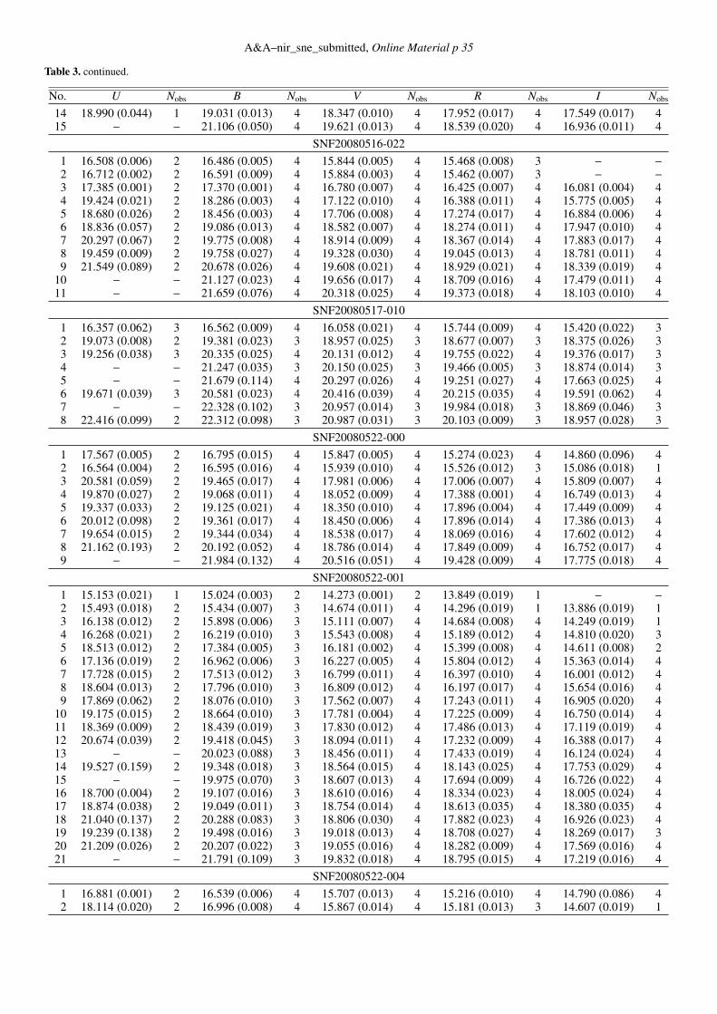
A&A–nir_sne_submitted, Online Material p 35
Table 3. continued.
No. U Nobs B Nobs V Nobs R Nobs I Nobs
14 18.990 (0.044) 1 19.031 (0.013) 4 18.347 (0.010) 4 17.952 (0.017) 4 17.549 (0.017) 415 − − 21.106 (0.050) 4 19.621 (0.013) 4 18.539 (0.020) 4 16.936 (0.011) 4
SNF20080516-0221 16.508 (0.006) 2 16.486 (0.005) 4 15.844 (0.005) 4 15.468 (0.008) 3 − −
2 16.712 (0.002) 2 16.591 (0.009) 4 15.884 (0.003) 4 15.462 (0.007) 3 − −
3 17.385 (0.001) 2 17.370 (0.001) 4 16.780 (0.007) 4 16.425 (0.007) 4 16.081 (0.004) 44 19.424 (0.021) 2 18.286 (0.003) 4 17.122 (0.010) 4 16.388 (0.011) 4 15.775 (0.005) 45 18.680 (0.026) 2 18.456 (0.003) 4 17.706 (0.008) 4 17.274 (0.017) 4 16.884 (0.006) 46 18.836 (0.057) 2 19.086 (0.013) 4 18.582 (0.007) 4 18.274 (0.011) 4 17.947 (0.010) 47 20.297 (0.067) 2 19.775 (0.008) 4 18.914 (0.009) 4 18.367 (0.014) 4 17.883 (0.017) 48 19.459 (0.009) 2 19.758 (0.027) 4 19.328 (0.030) 4 19.045 (0.013) 4 18.781 (0.011) 49 21.549 (0.089) 2 20.678 (0.026) 4 19.608 (0.021) 4 18.929 (0.021) 4 18.339 (0.019) 4
10 − − 21.127 (0.023) 4 19.656 (0.017) 4 18.709 (0.016) 4 17.479 (0.011) 411 − − 21.659 (0.076) 4 20.318 (0.025) 4 19.373 (0.018) 4 18.103 (0.010) 4
SNF20080517-0101 16.357 (0.062) 3 16.562 (0.009) 4 16.058 (0.021) 4 15.744 (0.009) 4 15.420 (0.022) 32 19.073 (0.008) 2 19.381 (0.023) 3 18.957 (0.025) 3 18.677 (0.007) 3 18.375 (0.026) 33 19.256 (0.038) 3 20.335 (0.025) 4 20.131 (0.012) 4 19.755 (0.022) 4 19.376 (0.017) 34 − − 21.247 (0.035) 3 20.150 (0.025) 3 19.466 (0.005) 3 18.874 (0.014) 35 − − 21.679 (0.114) 4 20.297 (0.026) 4 19.251 (0.027) 4 17.663 (0.025) 46 19.671 (0.039) 3 20.581 (0.023) 4 20.416 (0.039) 4 20.215 (0.035) 4 19.591 (0.062) 47 − − 22.328 (0.102) 3 20.957 (0.014) 3 19.984 (0.018) 3 18.869 (0.046) 38 22.416 (0.099) 2 22.312 (0.098) 3 20.987 (0.031) 3 20.103 (0.009) 3 18.957 (0.028) 3
SNF20080522-0001 17.567 (0.005) 2 16.795 (0.015) 4 15.847 (0.005) 4 15.274 (0.023) 4 14.860 (0.096) 42 16.564 (0.004) 2 16.595 (0.016) 4 15.939 (0.010) 4 15.526 (0.012) 3 15.086 (0.018) 13 20.581 (0.059) 2 19.465 (0.017) 4 17.981 (0.006) 4 17.006 (0.007) 4 15.809 (0.007) 44 19.870 (0.027) 2 19.068 (0.011) 4 18.052 (0.009) 4 17.388 (0.001) 4 16.749 (0.013) 45 19.337 (0.033) 2 19.125 (0.021) 4 18.350 (0.010) 4 17.896 (0.004) 4 17.449 (0.009) 46 20.012 (0.098) 2 19.361 (0.017) 4 18.450 (0.006) 4 17.896 (0.014) 4 17.386 (0.013) 47 19.654 (0.015) 2 19.344 (0.034) 4 18.538 (0.017) 4 18.069 (0.016) 4 17.602 (0.012) 48 21.162 (0.193) 2 20.192 (0.052) 4 18.786 (0.014) 4 17.849 (0.009) 4 16.752 (0.017) 49 − − 21.984 (0.132) 4 20.516 (0.051) 4 19.428 (0.009) 4 17.775 (0.018) 4
SNF20080522-0011 15.153 (0.021) 1 15.024 (0.003) 2 14.273 (0.001) 2 13.849 (0.019) 1 − −
2 15.493 (0.018) 2 15.434 (0.007) 3 14.674 (0.011) 4 14.296 (0.019) 1 13.886 (0.019) 13 16.138 (0.012) 2 15.898 (0.006) 3 15.111 (0.007) 4 14.684 (0.008) 4 14.249 (0.019) 14 16.268 (0.021) 2 16.219 (0.010) 3 15.543 (0.008) 4 15.189 (0.012) 4 14.810 (0.020) 35 18.513 (0.012) 2 17.384 (0.005) 3 16.181 (0.002) 4 15.399 (0.008) 4 14.611 (0.008) 26 17.136 (0.019) 2 16.962 (0.006) 3 16.227 (0.005) 4 15.804 (0.012) 4 15.363 (0.014) 47 17.728 (0.015) 2 17.513 (0.012) 3 16.799 (0.011) 4 16.397 (0.010) 4 16.001 (0.012) 48 18.604 (0.013) 2 17.796 (0.010) 3 16.809 (0.012) 4 16.197 (0.017) 4 15.654 (0.016) 49 17.869 (0.062) 2 18.076 (0.010) 3 17.562 (0.007) 4 17.243 (0.011) 4 16.905 (0.020) 4
10 19.175 (0.015) 2 18.664 (0.010) 3 17.781 (0.004) 4 17.225 (0.009) 4 16.750 (0.014) 411 18.369 (0.009) 2 18.439 (0.019) 3 17.830 (0.012) 4 17.486 (0.013) 4 17.119 (0.019) 412 20.674 (0.039) 2 19.418 (0.045) 3 18.094 (0.011) 4 17.232 (0.009) 4 16.388 (0.017) 413 − − 20.023 (0.088) 3 18.456 (0.011) 4 17.433 (0.019) 4 16.124 (0.024) 414 19.527 (0.159) 2 19.348 (0.018) 3 18.564 (0.015) 4 18.143 (0.025) 4 17.753 (0.029) 415 − − 19.975 (0.070) 3 18.607 (0.013) 4 17.694 (0.009) 4 16.726 (0.022) 416 18.700 (0.004) 2 19.107 (0.016) 3 18.610 (0.016) 4 18.334 (0.023) 4 18.005 (0.024) 417 18.874 (0.038) 2 19.049 (0.011) 3 18.754 (0.014) 4 18.613 (0.035) 4 18.380 (0.035) 418 21.040 (0.137) 2 20.288 (0.083) 3 18.806 (0.030) 4 17.882 (0.023) 4 16.926 (0.023) 419 19.239 (0.138) 2 19.498 (0.016) 3 19.018 (0.013) 4 18.708 (0.027) 4 18.269 (0.017) 320 21.209 (0.026) 2 20.207 (0.022) 3 19.055 (0.016) 4 18.282 (0.009) 4 17.569 (0.016) 421 − − 21.791 (0.109) 3 19.832 (0.018) 4 18.795 (0.015) 4 17.219 (0.016) 4
SNF20080522-0041 16.881 (0.001) 2 16.539 (0.006) 4 15.707 (0.013) 4 15.216 (0.010) 4 14.790 (0.086) 42 18.114 (0.020) 2 16.996 (0.008) 4 15.867 (0.014) 4 15.181 (0.013) 3 14.607 (0.019) 1

A&A–nir_sne_submitted, Online Material p 36
Table 3. continued.
No. U Nobs B Nobs V Nobs R Nobs I Nobs
3 17.332 (0.021) 2 17.437 (0.006) 4 16.804 (0.016) 4 16.447 (0.009) 4 16.044 (0.007) 44 17.313 (0.013) 2 17.577 (0.005) 4 17.044 (0.020) 4 16.708 (0.011) 4 16.328 (0.008) 45 17.874 (0.052) 2 17.911 (0.018) 4 17.302 (0.019) 4 16.951 (0.003) 4 16.579 (0.015) 46 18.565 (0.040) 2 18.648 (0.026) 4 18.066 (0.022) 4 17.716 (0.010) 4 17.321 (0.004) 47 18.768 (0.041) 2 18.809 (0.014) 3 18.096 (0.013) 4 17.703 (0.008) 4 17.318 (0.025) 48 18.497 (0.054) 2 18.758 (0.038) 4 18.151 (0.020) 4 17.782 (0.006) 4 17.354 (0.021) 49 19.764 (0.025) 2 19.278 (0.033) 4 18.444 (0.012) 4 17.915 (0.017) 4 17.405 (0.016) 4
10 18.925 (0.002) 2 19.175 (0.014) 4 18.668 (0.024) 4 18.326 (0.020) 4 17.939 (0.019) 411 19.639 (0.151) 2 19.427 (0.053) 4 18.687 (0.020) 4 18.219 (0.011) 4 17.753 (0.026) 412 18.793 (0.060) 2 19.114 (0.032) 3 18.694 (0.012) 4 18.431 (0.016) 4 18.175 (0.037) 413 19.789 (0.092) 2 19.515 (0.049) 4 18.737 (0.023) 4 18.297 (0.019) 4 17.797 (0.022) 414 19.862 (0.156) 2 19.605 (0.046) 4 18.878 (0.026) 4 18.424 (0.018) 4 17.945 (0.006) 315 21.046 (0.160) 2 20.208 (0.148) 4 19.237 (0.043) 4 18.578 (0.010) 4 17.982 (0.009) 416 − − 20.974 (0.077) 4 19.544 (0.027) 4 18.457 (0.019) 4 16.839 (0.005) 417 − − 21.699 (0.263) 3 20.220 (0.034) 4 19.218 (0.010) 4 17.857 (0.014) 4
SNF20080522-0111 16.565 (0.018) 1 16.624 (0.023) 3 16.043 (0.017) 3 15.667 (0.015) 3 15.277 (0.014) 12 17.026 (0.019) 1 16.825 (0.011) 3 16.065 (0.018) 3 15.630 (0.017) 3 15.194 (0.014) 13 18.297 (0.033) 1 17.387 (0.006) 3 16.358 (0.006) 3 15.729 (0.010) 3 15.212 (0.014) 14 19.371 (0.063) 1 18.119 (0.112) 3 16.840 (0.020) 3 15.977 (0.026) 3 15.157 (0.014) 15 18.045 (0.027) 1 17.679 (0.015) 3 16.860 (0.006) 3 16.371 (0.014) 3 15.934 (0.017) 36 17.794 (0.025) 1 17.841 (0.024) 3 17.216 (0.016) 3 16.840 (0.014) 3 16.465 (0.026) 37 17.651 (0.025) 1 18.017 (0.025) 3 17.544 (0.019) 3 17.226 (0.009) 3 16.881 (0.028) 38 19.910 (0.102) 1 19.081 (0.047) 3 17.782 (0.002) 3 16.955 (0.005) 3 16.236 (0.012) 39 19.422 (0.070) 1 18.910 (0.011) 3 17.996 (0.010) 3 17.450 (0.016) 3 17.000 (0.025) 3
10 18.491 (0.035) 1 18.761 (0.014) 3 18.228 (0.018) 3 17.889 (0.006) 3 17.520 (0.024) 311 18.677 (0.041) 1 18.932 (0.035) 3 18.454 (0.006) 3 18.120 (0.008) 3 17.747 (0.039) 312 20.003 (0.101) 1 19.453 (0.012) 3 18.535 (0.020) 3 17.957 (0.009) 3 17.468 (0.030) 313 19.470 (0.067) 1 19.395 (0.040) 3 18.610 (0.005) 3 18.171 (0.008) 3 17.723 (0.020) 314 18.925 (0.052) 1 19.335 (0.031) 3 18.778 (0.009) 3 18.432 (0.014) 3 18.051 (0.029) 315 20.407 (0.161) 1 19.925 (0.037) 3 18.851 (0.014) 3 18.111 (0.008) 3 17.486 (0.022) 316 20.116 (0.135) 1 19.907 (0.017) 3 19.044 (0.031) 3 18.503 (0.018) 3 18.002 (0.027) 317 − − 20.108 (0.005) 3 19.057 (0.017) 3 18.376 (0.023) 3 17.779 (0.024) 318 20.185 (0.130) 1 19.977 (0.031) 3 19.101 (0.007) 3 18.590 (0.020) 3 18.120 (0.042) 319 20.489 (0.168) 1 20.081 (0.055) 3 19.131 (0.014) 3 18.529 (0.016) 3 17.924 (0.018) 320 − − 20.726 (0.065) 3 19.356 (0.016) 3 18.488 (0.013) 3 17.740 (0.030) 321 20.057 (0.123) 1 20.161 (0.018) 3 19.451 (0.020) 3 19.016 (0.024) 3 18.545 (0.037) 322 − − 21.437 (0.167) 3 19.971 (0.029) 3 18.935 (0.024) 3 17.584 (0.033) 323 − − 21.387 (0.055) 3 20.008 (0.029) 3 19.176 (0.018) 3 18.328 (0.011) 3
SNF20080606-0121 16.230 (0.015) 1 16.028 (0.015) 1 15.289 (0.012) 1 − − − −
2 16.481 (0.018) 2 16.509 (0.009) 2 15.877 (0.010) 2 15.521 (0.013) 1 − −
3 17.477 (0.044) 2 16.846 (0.013) 2 15.882 (0.008) 2 15.384 (0.013) 1 − −
4 17.292 (0.015) 2 17.233 (0.009) 2 16.536 (0.003) 2 16.170 (0.002) 2 15.733 (0.013) 15 17.480 (0.033) 2 17.412 (0.005) 2 16.748 (0.009) 2 16.384 (0.006) 2 15.973 (0.013) 16 19.395 (0.122) 2 18.137 (0.035) 2 16.773 (0.009) 2 15.920 (0.003) 2 − −
7 19.091 (0.057) 2 17.984 (0.014) 2 16.832 (0.008) 2 16.148 (0.004) 2 − −
8 17.900 (0.012) 2 17.822 (0.000) 2 17.173 (0.014) 2 16.801 (0.011) 2 16.382 (0.013) 19 19.780 (0.061) 2 18.568 (0.001) 2 17.304 (0.008) 2 16.480 (0.007) 2 15.721 (0.013) 1
10 18.034 (0.043) 2 17.977 (0.011) 2 17.313 (0.011) 2 16.951 (0.003) 2 16.525 (0.013) 111 18.081 (0.022) 2 18.049 (0.022) 2 17.360 (0.002) 2 16.964 (0.010) 2 16.514 (0.013) 112 18.081 (0.022) 2 18.049 (0.022) 2 17.360 (0.002) 2 16.964 (0.010) 2 16.514 (0.013) 113 18.342 (0.043) 2 18.226 (0.006) 2 17.504 (0.016) 2 17.128 (0.004) 2 16.706 (0.013) 114 19.782 (0.099) 2 18.699 (0.011) 2 17.654 (0.011) 2 17.025 (0.006) 2 16.425 (0.013) 115 18.405 (0.010) 2 18.454 (0.025) 2 17.801 (0.009) 2 17.422 (0.001) 2 16.995 (0.013) 116 19.097 (0.084) 2 18.716 (0.020) 2 17.880 (0.004) 2 17.392 (0.004) 2 16.882 (0.013) 117 18.733 (0.088) 2 18.596 (0.009) 2 17.887 (0.009) 2 17.484 (0.002) 2 17.053 (0.013) 118 18.779 (0.054) 2 18.739 (0.008) 2 18.072 (0.014) 2 17.707 (0.012) 2 17.290 (0.013) 119 18.804 (0.070) 2 18.842 (0.029) 2 18.201 (0.005) 2 17.834 (0.001) 2 17.426 (0.013) 120 18.802 (0.078) 2 18.896 (0.013) 2 18.261 (0.006) 2 17.913 (0.008) 2 17.475 (0.013) 1

A&A–nir_sne_submitted, Online Material p 37
Table 3. continued.
No. U Nobs B Nobs V Nobs R Nobs I Nobs
21 19.810 (0.161) 2 19.290 (0.052) 2 18.377 (0.012) 2 17.849 (0.004) 2 17.345 (0.013) 122 18.918 (0.083) 2 18.998 (0.001) 2 18.386 (0.015) 2 18.028 (0.008) 2 17.625 (0.013) 123 18.902 (0.001) 2 19.146 (0.015) 2 18.663 (0.002) 2 18.367 (0.000) 2 17.977 (0.014) 124 19.064 (0.137) 2 19.246 (0.017) 2 18.718 (0.021) 2 18.399 (0.009) 2 17.989 (0.014) 125 18.947 (0.037) 2 19.233 (0.026) 2 18.722 (0.000) 2 18.402 (0.003) 2 17.974 (0.014) 126 20.340 (0.195) 2 19.769 (0.016) 2 18.838 (0.015) 2 18.299 (0.000) 2 17.721 (0.014) 127 21.102 (0.027) 2 20.042 (0.007) 2 18.883 (0.020) 2 18.103 (0.012) 2 17.387 (0.014) 128 − − 19.899 (0.021) 2 19.044 (0.033) 2 18.533 (0.001) 2 18.015 (0.014) 129 20.117 (0.058) 2 19.866 (0.003) 2 19.047 (0.003) 2 18.564 (0.007) 2 18.075 (0.014) 130 − − 20.015 (0.011) 2 19.097 (0.024) 2 18.611 (0.003) 2 18.079 (0.014) 131 19.506 (0.119) 2 19.712 (0.022) 2 19.160 (0.009) 2 18.808 (0.010) 2 18.411 (0.015) 132 19.473 (0.028) 2 19.727 (0.013) 2 19.174 (0.021) 2 18.841 (0.020) 2 18.431 (0.015) 133 − − 20.668 (0.035) 2 19.251 (0.007) 2 18.349 (0.004) 2 17.393 (0.014) 134 19.758 (0.012) 2 19.967 (0.052) 2 19.279 (0.018) 2 18.823 (0.008) 2 18.325 (0.015) 135 − − 20.053 (0.026) 2 19.355 (0.024) 2 18.895 (0.006) 2 18.384 (0.015) 136 19.604 (0.063) 2 19.936 (0.026) 2 19.388 (0.000) 2 19.056 (0.012) 2 18.691 (0.016) 137 − − 20.983 (0.037) 2 19.440 (0.009) 2 18.375 (0.001) 2 16.661 (0.015) 138 20.071 (0.160) 2 20.125 (0.007) 2 19.545 (0.014) 2 19.255 (0.032) 2 18.843 (0.017) 139 − − 21.407 (0.019) 2 19.666 (0.007) 2 18.516 (0.008) 2 16.701 (0.015) 140 − − 21.052 (0.047) 2 19.709 (0.029) 2 18.901 (0.020) 2 18.061 (0.015) 141 20.397 (0.099) 2 20.544 (0.081) 2 19.769 (0.003) 2 19.332 (0.022) 2 18.865 (0.017) 142 19.926 (0.079) 2 20.224 (0.018) 2 19.772 (0.010) 2 19.448 (0.013) 2 19.055 (0.018) 143 − − 21.079 (0.022) 2 19.799 (0.033) 2 18.992 (0.015) 2 18.224 (0.015) 144 − − 21.129 (0.081) 2 19.903 (0.006) 2 19.119 (0.001) 2 18.393 (0.016) 145 − − 21.561 (0.102) 2 19.992 (0.014) 2 19.008 (0.026) 2 17.680 (0.015) 146 − − 21.395 (0.056) 2 20.017 (0.008) 2 19.188 (0.000) 2 18.335 (0.016) 147 − − 20.554 (0.012) 2 20.039 (0.038) 2 19.746 (0.018) 2 19.324 (0.020) 148 − − 21.196 (0.027) 2 20.238 (0.005) 2 19.589 (0.004) 2 18.948 (0.018) 149 − − 21.767 (0.011) 2 20.489 (0.015) 2 19.617 (0.025) 2 18.769 (0.017) 150 22.084 (0.200) 2 22.137 (0.034) 2 20.587 (0.010) 2 19.597 (0.005) 2 18.128 (0.016) 151 − − 22.048 (0.051) 2 20.619 (0.004) 2 19.661 (0.015) 2 18.401 (0.016) 152 − − 21.813 (0.243) 2 20.692 (0.002) 2 19.993 (0.018) 2 19.276 (0.021) 1
SNF20080610-0031 15.941 (0.014) 1 15.862 (0.014) 1 15.215 (0.012) 1 14.846 (0.012) 1 14.582 (0.012) 12 17.660 (0.022) 1 16.605 (0.017) 1 15.506 (0.012) 1 14.842 (0.013) 1 − −
3 16.781 (0.016) 1 16.330 (0.015) 1 15.551 (0.012) 1 15.112 (0.012) 1 − −
4 16.343 (0.014) 1 16.225 (0.014) 1 15.552 (0.012) 1 15.169 (0.012) 1 14.753 (0.012) 15 18.616 (0.030) 2 17.283 (0.018) 2 15.975 (0.007) 2 15.157 (0.013) 1 − −
6 16.493 (0.037) 2 16.560 (0.016) 2 16.002 (0.001) 2 15.685 (0.012) 1 15.327 (0.012) 17 16.549 (0.015) 1 16.698 (0.013) 1 16.161 (0.012) 1 15.817 (0.013) 1 15.438 (0.012) 18 16.910 (0.020) 2 16.946 (0.011) 2 16.324 (0.008) 2 15.973 (0.002) 2 15.608 (0.045) 29 17.444 (0.040) 2 17.210 (0.027) 2 16.460 (0.000) 2 16.065 (0.002) 2 15.643 (0.012) 1
10 16.742 (0.031) 2 17.022 (0.031) 2 16.549 (0.003) 2 16.261 (0.000) 2 15.906 (0.013) 211 17.815 (0.030) 2 17.476 (0.013) 2 16.704 (0.007) 2 16.274 (0.007) 2 15.870 (0.012) 112 17.559 (0.019) 2 17.474 (0.020) 2 16.781 (0.006) 2 16.383 (0.013) 2 15.939 (0.006) 213 17.987 (0.024) 2 18.151 (0.006) 2 17.495 (0.004) 2 17.086 (0.013) 2 16.610 (0.012) 214 17.992 (0.007) 2 18.166 (0.015) 2 17.632 (0.003) 2 17.318 (0.011) 2 16.953 (0.012) 215 18.471 (0.030) 2 18.349 (0.020) 2 17.658 (0.008) 2 17.278 (0.005) 2 16.872 (0.005) 216 20.765 (0.141) 2 19.453 (0.011) 2 18.046 (0.000) 2 17.170 (0.009) 2 16.267 (0.010) 217 20.008 (0.085) 2 19.169 (0.038) 2 18.173 (0.011) 2 17.599 (0.001) 2 17.090 (0.016) 218 19.297 (0.065) 2 19.033 (0.008) 2 18.275 (0.011) 2 17.848 (0.003) 2 17.423 (0.013) 219 20.263 (0.010) 2 19.369 (0.070) 2 18.322 (0.010) 2 17.637 (0.001) 2 17.036 (0.013) 220 19.827 (0.043) 2 19.348 (0.013) 2 18.493 (0.001) 2 18.019 (0.014) 2 17.553 (0.007) 221 − − 20.202 (0.075) 2 18.665 (0.020) 2 17.697 (0.010) 2 16.532 (0.023) 222 18.960 (0.005) 2 19.174 (0.056) 2 18.704 (0.003) 2 18.406 (0.016) 2 18.054 (0.025) 223 19.255 (0.016) 2 19.504 (0.016) 2 19.059 (0.006) 2 18.781 (0.001) 2 18.456 (0.008) 224 20.067 (0.051) 2 19.904 (0.017) 2 19.144 (0.006) 2 18.757 (0.029) 2 18.283 (0.002) 225 − − 20.663 (0.012) 2 19.160 (0.012) 2 18.187 (0.003) 2 16.992 (0.029) 226 21.732 (0.032) 2 20.695 (0.022) 2 19.174 (0.007) 2 18.188 (0.001) 2 16.892 (0.002) 227 − − 20.227 (0.004) 2 19.347 (0.007) 2 18.816 (0.009) 2 18.302 (0.008) 2

A&A–nir_sne_submitted, Online Material p 38
Table 3. continued.
No. U Nobs B Nobs V Nobs R Nobs I Nobs
28 − − 20.608 (0.006) 2 19.347 (0.026) 2 18.548 (0.007) 2 17.791 (0.007) 229 19.510 (0.004) 2 19.815 (0.041) 2 19.349 (0.011) 2 19.026 (0.011) 2 18.682 (0.001) 230 − − 21.039 (0.027) 2 19.386 (0.006) 2 18.351 (0.001) 2 16.825 (0.012) 231 18.971 (0.034) 2 19.954 (0.020) 2 19.552 (0.010) 2 19.399 (0.007) 2 19.195 (0.017) 232 21.493 (0.188) 2 20.610 (0.043) 2 19.595 (0.013) 2 18.906 (0.006) 2 18.321 (0.027) 233 21.461 (0.194) 2 20.654 (0.069) 2 19.609 (0.007) 2 18.961 (0.013) 2 18.301 (0.009) 234 − − 21.073 (0.057) 2 19.644 (0.014) 2 18.707 (0.002) 2 17.530 (0.026) 235 20.202 (0.148) 2 20.334 (0.048) 2 19.658 (0.001) 2 19.268 (0.046) 2 18.798 (0.015) 236 − − 20.694 (0.005) 2 19.667 (0.015) 2 19.036 (0.003) 2 18.472 (0.032) 237 − − 21.194 (0.052) 2 19.720 (0.021) 2 18.705 (0.014) 2 17.205 (0.005) 238 − − 21.016 (0.000) 2 19.906 (0.001) 2 19.162 (0.017) 2 18.502 (0.013) 239 − − 21.765 (0.076) 2 20.178 (0.030) 2 19.167 (0.008) 2 17.691 (0.018) 240 20.458 (0.038) 2 20.739 (0.054) 2 20.264 (0.009) 2 19.973 (0.006) 2 19.649 (0.006) 241 − − 22.000 (0.049) 2 20.326 (0.008) 2 19.349 (0.003) 2 17.902 (0.011) 242 − − 21.666 (0.021) 2 20.369 (0.007) 2 19.560 (0.039) 2 18.833 (0.003) 243 − − 22.120 (0.004) 2 20.610 (0.008) 2 19.695 (0.023) 2 18.563 (0.008) 2


![Colec]ia PLURAL](https://img.dokumen.tips/doc/110x75/6322b86464690856e1094aec/colecia-plural-1677510341.jpg)