Concepts, Theory, and Techniques

TWO-PIECE VON NEUMANN-MORGENSTERN UTILITY FUNCTIONS*

Peter C. Fishburn, The Pennsylvania State University Gary A. Kochenberger, The Pennsylvania State University

ABSTRACT

Thirty empirically assessed utility functions on changes in wealth or return on invest- ment were examined for general features and susceptability to fits by linear, power, and exponential functions. Separate fits were made to below-target data and above-target data. The usual “target” was the no-change point.

The majority of below-target functions were risk seeking; the majority of above- target functions were risk averse; and the most common composite shape was convex- concave, or risk seeking in losses and risk averse in gains. The least common composite was concave-concave. Below-target utility was generally steeper than above-target utility with a median below-to-above slope ratio of about 4.8. The power and exponential rits were substantially better than the linear fits. Power functions gave the best fits in the ma- jority of convex below-target and concave above-target cases, and exponential functions gave the best fits in the majority of concave below-target and convex above-target cases. Several implications of these results for decision making under risk are mentioned.

INTRODUCTION

Although the Von Neumann-Morgenstern expected utility theory [5] [ 141 [27] pertains to a wide variety of risky situations, it has received special attention in monetary settings. Early suggestions on the utility of wealth were made by Gabriel Cramer [in 4, p. 341 and Daniel Bernoulli (31 (41. After the Von Neumann-Morgenstern revival, Friedman and Savage (71 proposed a utility-ol- income function for low-income consumer units that has a convex (risk- preferring or risk-seeking) segment surrounded by two concave (risk-averse) segments to explain, among other things, gambling and insurance-buying behavior.’ Markowitz [20) modified this by suggesting a four-segment bounded util i ty function of wealth that is initially convex, then concave, then turns convex again in the vicinity of present wealth, and ends up concave. Additional com- ments on the Friedman-Savage and Markowitz proposals are made in [ I ] , [ l I ] , [18], [22], and [28].

In contrast to these armchair proposals, several research workers have at- tempted to assess individuals’ utility functions over significant changes in in- dividual or corporate wealth. This work adopts the proposition [I61 that changes

*This research was supported by the Office of Naval Research through Contract No. N00014-75-C-0857 to The Pennsylvania State University. ‘Convexity and concavity are used in the strict sense throughout the paper.

503

504 DECISION SCIENCES [Vol. 10

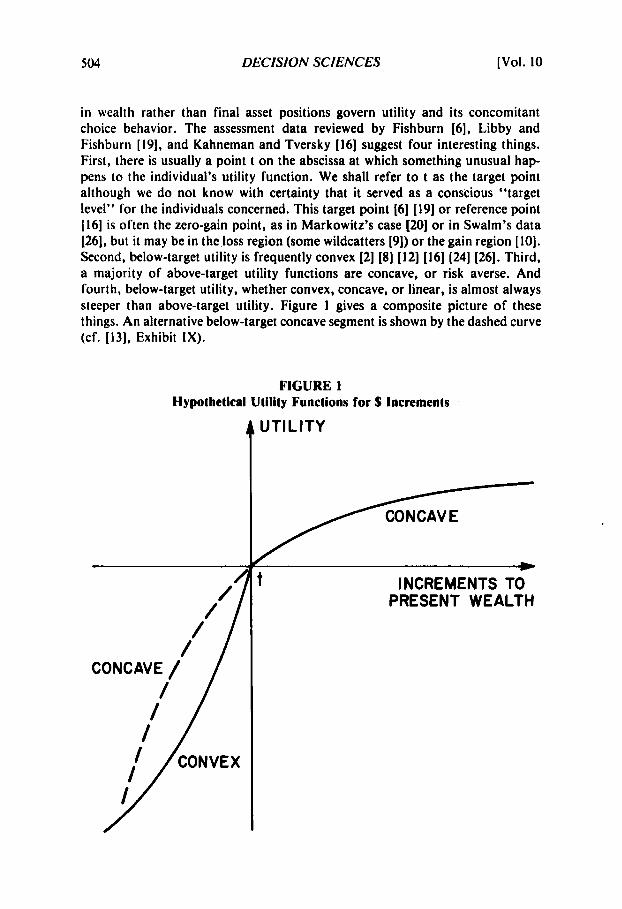
in wealth rather than final asset positions govern utility and its concomitant choice behavior. The assessment data reviewed by Fishburn [6], Libby and Fishburn [ 191, and Kahneman and Tversky [I61 suggest four interesting things. First, there is usually a point t on the abscissa at which something unusual hap- pens to the individual’s utility function. We shall refer to t as the target point although we do not know with certainty that it served as a conscious “target level” for the individuals concerned. This target point [6] [19] or reference point [I61 is often the zero-gain point, as in Markowitz’s case [20] or in Swalm’s data [26], but it may be in the loss region (some wildcatters [9]) or the gain region [lo]. Second, below-target utility is frequently convex [2] (8) [I21 [la] (241 [26]. Third, a majority of above-target utility functions are concave, or risk averse. And fourth, below-target utility, whether convex, concave, or linear, is almost always steeper than above-target utility. Figure 1 gives a composite picture of these things. An alternative below-target concave segment is shown by the dashed curve (cf. [13], Exhibit IX).

FIGURE I Hypothetical Utility Functions for $ Increments

UTILITY t CONCAVE b

INCREMENTS TO PRESENT WEALTH

I9791 UTILITY FUNCTIONS SO5

The present paper has two main purposes. The first is to reexamine the published assessment data to obtain a more precise picture of the things noted in the preceding paragraph. The second is to get an idea of the extent to which sim- ple functional forms yield good fits to the assessment data. In each case, we shall calculate or estimate the best fit for each functional type to the above-target data and to the below-target data. The best-fit criterion used throughout is minimum least squares.

The next section discusses the functional forms that were fit to the data. This is followed by remarks on our fitting methodology. We then list the data sources, identify best fits for each case, and summarize salient aspects of these fits. After a brief discussion of implications for decision making, the paper concludes with an overview of main results.

Although our sample cannot be regarded as random or unbiased, utility assessments from many individuals engaged in different pursuits are represented in the data. Consequently, we feel that these data indicate what might be expected in other situations.

FUNCTIONAL FORMS

The data for each case examined later were transformed linearly so that the transformed target point is x = 0 and the utility at the origin is zero. Three simple functions were fit to the data, and this was done separately for x z 0 and x s 0 . The three functions are the linear (L), power (P), and exponential (E) functions. For x 2 0 , the linear function is L' =cx with c>O; the power function is P' =alx'2 with a, > O and a2>O; and the exponential function is E + = b,( I - e-h2') with b,b2>0. The corresponding functions for x s 0 are obtained from these by replac- ing x by -x and multiplying by -1. They are denoted respectively as L - , P - , and E-. A composite function with form A for x s 0 and form B for x r O is denoted A-B'. Thus, L-L' is a two-piece linear utility function. The functions were chosen for their analytical simplicity and ability to approximate or generate a variety of specific shapes.

Although L is the special case of P with a2= I , we decided to isolate it for three reasons. First, some of the data plots either above or below x = O looked nearly linear, in which case L may provide a very good fit; second, the minimum mean squared error (MMSE) for a minimum least-squares L fit offers a useful benchmark against which to compare the MMSE values of the P and E fits; and third, the best L + and L - fits give an indication of the change in slope of the util- i ty function around x = O which is not unduly confounded with curvature. When a2# 1, it may be noted that the slope of P' at 0' is either zero (a,> 1 ) or infinity (a,< l ) , and the slope of P - at 0- is either zero (a,> 1) or infinity (a2< I).

Because the MMSE of a P fit can never exceed the MMSE of an L f i t , the best fit to the data among the three function types will be a power or exponential f i t . We shall therefore focus part of our attention later on the question of whether power functions or exponential functions tend to yield the best fits over a number of situations. Although the later comparisons between P and E are a matter of

506 DECISION SCIENCES [Vol. 10

fits to subjective empirical data, differences between the functions may help to place the results in perspective, For example, in the risk-averse P' and E' cases, the E' function is bounded above by b, while the P' function increases without bound, and Pratt's [21] local measure of absolute risk aversion r(x) = -u"(x)/u '(x) is positive and constant ( = b,) for E+ but positive and decreasing for P +. For the risk-seeking cases in the positive region with a,> 1 or b, <O, r(x) is negative and constant for E+ and negative and increasing for P', and although both functions grow rapidly, the ratio of E' to P+ approaches infinity as x gets large. The pictures for x 1 0 are essentially reversed.

Finally, we note that P + and E+ have a limiting form that is discontinuous at the origin with u(O)=O and u(x)= k > O for all x>O. This arises from P' when a , = k and a2 goes to zero, and from E' when bl = k and b2 goes to infinity. This form, reflected into the negative quadrant, was used in one below-target case that is identified later as SA4 in Table 1A. This case consists of two below-target data points for which the one farther away from the target has the algebraically larger utility. Because of this there is no best P- or E- fit as such, but with k midway between the two utilities of the data points, we can get the mean squared errors of P- and E- arbitrarily close to the MMSE of the horizontal utility function whose value is k for all x<O.

FITTING THE FUNCTIONS

As noted earlier, the original data were transformed linearly so that the transformed target point and its utility were both zero. Because separate fits were made for the above-target data and the below-target data, we shall describe the transformation used for each, including the reverse transformation that describes the fit of the utility functions in terms of the original data scales. We shall let (1, u,) denote the target point and its utility in the original data format, and let (x, y) be the transformed data point that corresponds to the original data point (x,), yo). As before, u(x) is the function fit to the transformed data, and U(x,) will be the util i ty function in the original data format that corresponds to u(x).

The general linear transformations used for the X,T t data were

x = k,(x,- t), y = k2(yO- u,) with k l , k2>0. ( 1 )

Since yo= u,+ y/k2 and y is the transformed utility data value that is compared to the fi t value u(x),

U(xO)=u,+u(kl(x,-t))/k2 for x,>t (2)

with derivative U '(xu) = (kl/k2)u '(x). The slopes of U at the target point for L * and E ' are therefore U '(t) = (k,/k,)c and U '(t) = (kl/kJblb2, respectively.

The general linear transformations used for the x u s t data were

x=k,(t-xO), y=kI(uu-yu) with k,, k,>O. (3)

1979) UTILITY FUNCTIONS 507

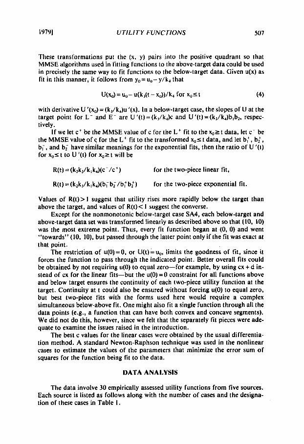
These transformations put the (x, y) pairs into the positive quadrant so that MMSE algorithms used in fitting functions to the above-target data could be used in precisely the same way to fit functions to the below-target data. Given u(x) as f i t in this manner, it follows from yo= uo- y/k4 that

U(x,)=u,-u(k,(t-xo))/k4 for x,st (4)

with derivative U ’(xu) = (kJ/k4)u ’(x). In a below-target case, the slopes of U at the target point for L - and E- are U ’(t) = (k,/k,)c and U ’(t) = (k,/k4)blbz, respec- tively.

I f we let c+ be the MMSE value of c for the L t fit to the x,L t data, let c - be the MMSE value of c for the L + fit to the transformed x o s t data, and let b:, b,’, b;, and b; have similar meanings for the exponential fits, then the ratio of U ‘(1) for x , ~ t to U ’(t) for x , ~ t will be

R(t) = (kzkJk k4)(c - /C ’) for the two-piece linear fit,

R(t)=(k2kj/k,k4)(b;b;/b:b:) for the two-piece exponential fit.

Values of R(t)> I suggest that utility rises more rapidly below the target than above the target, and values of R(t)< 1 suggest the converse.

Except for the nonmonotonic below-target case SA4, each below-target and above-target data set was transformed linearly as described above so that (10, 10) was the most extreme point. Thus, every fit function began at (0, 0) and went “towards” (10, lo), but passed through the latter point only if the fit was exact at that point.

The restriction of u(0) = 0, or U(t) = uo, limits the goodness of fit, since it forces the function to pass through the indicated point. Better overall fits could be obtained by not requiring u(0) to equal zero-for example, by using cx + d in- stead of cx for the linear fits-but the u(O)=O constraint for all functions above and below target ensures the continuity of each two-piece utility function at the target. Continuity at t could also be ensured without forcing u(0) to equal zero, but best two-piece fits with the forms used here would require a complex simultaneous below-above fit. One might also fit a single function through all the data points (e.g., a function that can have both convex and concave segments). We did not do this, however, since we felt that the separately fit pieces were ade- quate to examine the issues raised in the introduction.

The best c values for the linear cases were obtained by the usual differentia- tion method. A standard Newton-Raphson technique was used in the nonlinear cases to estimate the values of the parameters that minimize the error sum of squares for the function being fit to the data.

DATA ANALYSIS

The data involve 30 empirically assessed utility functions from five sources. Each source is listed as follows along with the number of cases and the designa- tion of these cases in Table 1.

508 DECISION SCIENCES [Vol. 10

Swalni 126): 13 cases. Casc SXk i s lor man k in group X. Halter and Dean 112, p. 641: 2 cases. Case HDGI; i s lor a graiii I'iirmcr;

case HDCI' i s lor a collcgc prolessor. Grayson 19): 10 cases. Casc GkAB i s for individual A.B. on page three

hundred aiid k; case Cik i s the case on page three hundred and k. Green [lo]: 3 cases. Casc PGAB i s I'or individual A.B.

. Barnes aiid Keiiimuth 121: 2 cases, lor contractors A (BRA) and

Green's lunctions arc based on percent re1 urii oil investment; all others are bused on dollar increments. We omitted one o l Green's lunctions because ol' slightly ambiguous data, aiid omitted the Halter-Ucaii orchard larmcr's lunctioii which appeared to be exactly linear bclow the target (t =0) and abovc the target with K ( t ) = 4. ( I n addition, two potential functions in Spetzler [25] were not used since we were unaware of them when the analysis was made.) Al l utility assessments in- cludcd changes that involved many thousands 01' dollars.

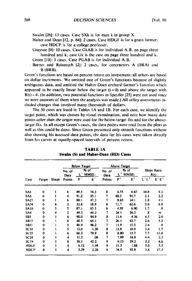
I 'hc 30 cases are listed in Tables I A and ID. For each case, we idciitily tlic target poiill, which was chosen by visual exmaination, aiid note how many data points (>/her rhun rhe origin were used lor the below-target t i t s and lor the abovc- target t i ts. In all except Green's cases, the data points were read lrom the plots as well as this could be done. Since Green presented only smooth lunctions without also showing his asscsscd data points, the data lor his cases were taken directly lrom l i i s curves at equally-spaced intervals o l percent return.

13 (BKB).

TABLE I A Swalm (S) and Halter-Dean (HD) Cases

Below Target Above Target NO. or Qo of NO. or 70 or Slope Ratio Data L- MMSE: Data L' MMSE: R(t)

Casc Target Shape Points P - E- Points P' E' L-L' E - E '

SA I SA6 SA27 SA34 SAlO SA4 s133 SB13 S133 I SCIX SC22 SC24 SCI9 H DCi I; HDC'I'

a I 6 0 I 4 0 I 6 0 4 3 0 3 5 0 4 2 0 I 6 0 1 6 0 1 5 0 I 5 0 I 6 0 I 4 0 I 6 0 I 4 0 I 4

4Y.5 YI.2 88. I 32.8 87. I 44.3 90.0 48.5 86.9 13.0 66.2 11.2 36. I 6.12 3.3Y

74.3 8 93. I 7 Y7.2 7 18.9 8 83.5 6 44.3 7 94.9 8 65. I 7 Y6.2 7

1.30 8 7Y.9 8

.Q6 7 42.2 8 1.w 4 2.26 6

4.55 80.5 9.65

71.7 4.95

24. I 11.6 26. I 11.9 13.8 8.80 7.89 Y.13

11.3 74.9

6.67 91.7 14.1 62.6 6.90

26.2 4.36

42.7 15.5 10.9 13.7 16.8 29.2

92.8 I .88

14.8 Y.3 2.1 2.2 1.8 1.1 3.6 6.9 I .7 .9 .8 OD

4.5 2.0 2.6 5.2 2.6 .a 3.4 1.7 7.7 11.0 4.4 2.5 2.2 6.6 5.0 5.5 3.6 17.3

I9791 UTILITY FUNCTIONS 509

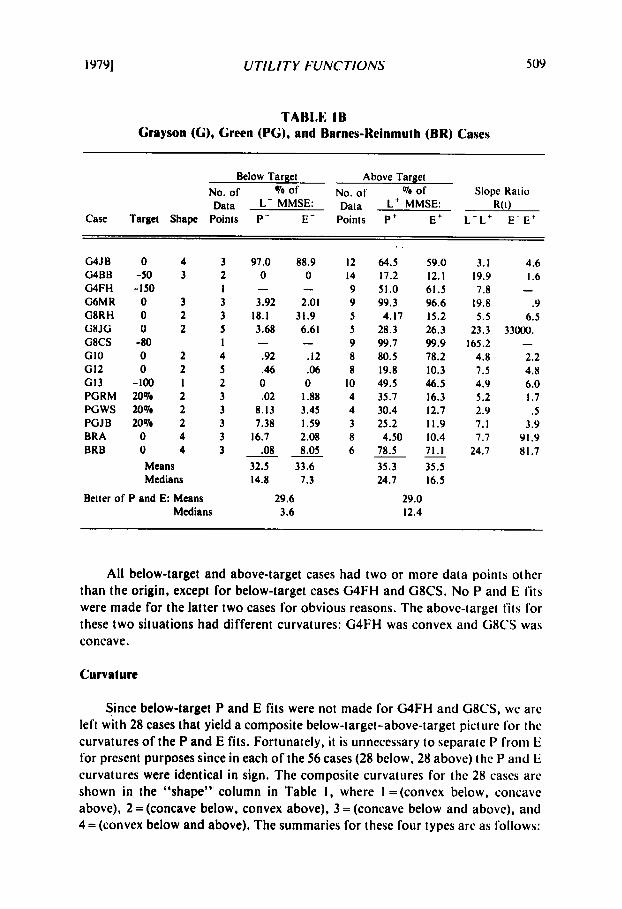
TABLE IB Grayson (GI, Green (PG), and Barnes-Reinrnulh (BR) Cases

Below Target Above Target No. of Yo of No. of Yo of Slope Ratio Data L- MMSE: Data Lt MMSE: R ( 0

Case Target Shape Points P- E- Points P t E + L - L t E - E ’

G4JB O G4BB -50 G4FH -150 G6MR 0 G8RH 0 G8JG 0 G8CS -80 GI0 0 GI2 0 GI3 -100 PGRM 20% PGWS 20% PGJB 20% BRA 0 BRB 0

4 3 3 2

1 3 3 2 3 2 5

I 2 4 2 5 I 2 2 3 2 3 2 3 4 3 4 3

Means Medians

Better of P and E: Means Medians

97.0 0

3.92

3.68

.92

.46 0 .02

8.13 7.38

.08

-

18.1

-

16.7

32.5 14.8

88.9 0

2.01 31.9 6.61

-12 .06 0

I .88 3.45 1.59 2.08 8.05

33.6 7.3

-

-

29.6 3.6

12 14 9 9 5 5 9 8 8

10 4 4 3 8 6

!

64.5 17.2 51.0 99.3

28.3 99.7 80.5 19.8 49.5 35.7 30.4 25.2

78.5 35.3 24.7

4.17

4.50

29.0 12.4

59.0 12. I 61.5 96.6 15.2 26.3 99.9 78.2 10.3 46.5 16.3 12.7 11.9 10.4 71.1 35.5 16.5

-

3.1 4.6 19.9 I .6 7.8 -

19.8 .9 5.5 6.5

23.3 33000. 165.2 -

4.8 2.2 7.5 4.8 4.9 6.0 5.2 I .7 2.9 .5 7.1 3.9 7.7 91.9

24.7 81.7

All below-target and above-target cases had two or more data points other than the origin, except for below-target cases G4FH and G8CS. No P and E fits were made for the latter two cases for obvious reasons. The abovc-target fits lor these two situations had different curvatures: G4FH was convex and GXCS was concave.

Curvature

Since below-target P and E fits were not made for G4FH and GSCS, we arc left with 28 cases that yield a composite below-target-above-target picture lor the curvatures of the P and E fits. Fortunately, i t is unnecessary to separate P froni E lor present purposes since in each of the 56 cases (28 below, 28 above) the P and li curvatures were identical in sign. The composite curvatures for the 28 cases arc shown in the “shape” column in Table 1, where I =(convex below, cotlcavc above), 2 = (concave below, convex above), 3 = (concave below and above), and 4 = (convex below and above). The summaries lor these lour types arc as follows:

5 10 DECISION SCIENCES [Vol. 10

concave convex above above

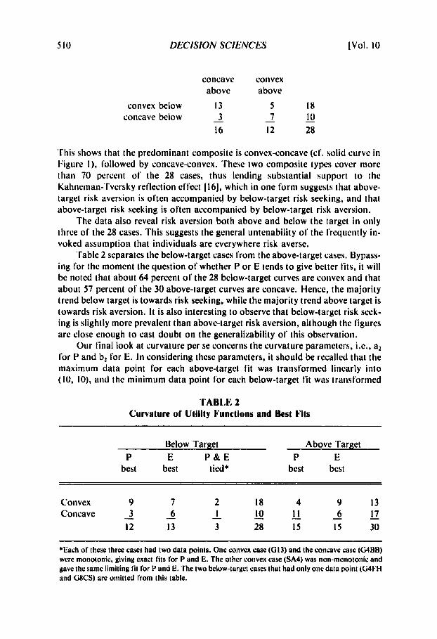
convex below 13 5 18 10 3

16 12 28 - 7 - concave below -

This shows that the predominant composite is convex-concave (cf. solid curve in I;igure I ) , followed by concave-convex. These two composite types cover more than 70 percent of the 28 cases, thus lending substantial support to the Kahneman-Tversky reflection effect [ 161, which in one form suggests that above- target risk aversion is often accompanied by below-target risk seeking, and that above-target risk seeking is often accompanied by below-target risk aversion.

The data also reveal risk aversion both above and below the target in only three of the 28 cases. This suggests the general untenability of the frequently in- voked assumption that individuals are everywhere risk averse.

Table 2 separates the below-target cases from the above-target cases. Bypass- ing for the moment the question of whether P or E tends to give better fits, it will be noted that about 64 percent of the 28 below-target curves are convex and that about 57 percent of the 30 above-target curves are concave. Hence, the majority trend below target is towards risk seeking, while the majority trend above target is towards risk aversion. I t is also interesting to observe that below-target risk seek- ing is slightly more prevalent than above-target risk aversion, although the figures are close enough to cast doubt on the generalizability of this observation.

Our final look at curvature per se concerns the curvature parameters, i.e., a, for P and bL for E. In considering these parameters, it should be recalled that the maximum data point for each above-target fit was transformed linearly into (10, 10). and the minimum data point for each below-target fit was transformed

'I'ABLE 2 Curvature of Utility Functions and Best Fits

Below Target Above Target P E P & E P E

best best tied* best best

Convex 9 7 2 18 4 9 13 17 I

I2 13 3 28 I5 I5 30 - 6 - I 1 - 10 - - 6 - 3 Concave -

*Each of these three cases had two data points. One convex case (613) and the concave case (64Btl) were monotonic, giving exact fits for P and E. The other convex case (SA4) was non-monotonic and gave the same limiting l i t for P and E. The two below-targct cases that had only one data point ((i41:H and GSCS) are omitted from this table.

I9791 UTILITY FUNCTIONS 5 1 I

TABLE 3 Frequency Distributions of Curvature Parameters

Parameter Parameter Interval Below Target Above Target

risk seeking risk averse 10, 1/21 [I /2, 4/51 4 lo (17) 4 (18) [4/5, I 1 6

b2 (E)

risk seeking (13)

1 I

28 30

risk averse (10)

[-1/4, 01 [ -1 , -1/4]

- 0 1-00, -11 -

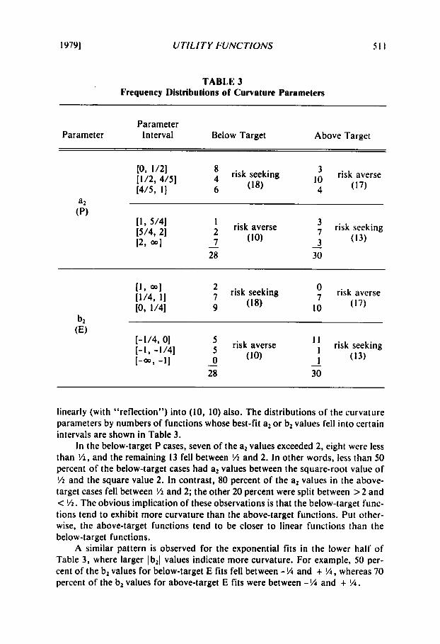
linearly (with “reflection”) into (10, 10) also. The distributions of the curvature parameters by numbers of functions whose best-fit a, or b2 values fell into certain intervals are shown in Table 3.

In the below-target P cases, seven of the a, values exceeded 2, eight were less than %, and the remaining 13 fell between % and 2. In other words, less than 50 percent of the below-target cases had a2 values between the square-root value of ‘/z and the square value 2. In contrast, 80 percent of the a, values in the above- target cases fell between % and 2; the other 20 percent were split between > 2 and < %. The obvious implication of these observations is that the below-target func- tions tend to exhibit more curvature than the above-target functions. Put other- wise, the above-target functions tend to be closer to linear functions than the below-target functions.

A similar pattern is observed for the exponential fits in the lower half of Table 3, where larger Ib,l values indicate more curvature. For example, 50 per- cent of the b2 values for below-target E fits fell between - % and + %, whereas 70 percent of the b2 values for above-target E fits were between - % and + %.

512 DECISION SCIENCES [Vol. 10

Changes in Slope

To examine the extent to which below-target utility increases more rapidly than does above-target utility, we computed the slope ratio R(t) of below-target slope to above-target slope for the two-piece linear fit L-L' and the two-piece ex- ponential fit E-E', This was done for each of the 30 cases in Table I , with the ex- ception of E-E' for cases G4FH and G8CS, since below-target exponentials were not f i t for these cases. The computations for R(t), whose results appear in the final two columns of Table 1, followed the procedure described earlier.

These computations strongly support the proposition that the utility func- tion is steeper below the target than above the target. Cases to the contrary arose only once (SA4) in the 30 L - L ' cases, and were observed four times (SAIO, SB31, G6MR, PGWS) in the 28 applicable E-E' cases. The larger value of R(t) exceeded unity in every instance. The median values of R(t) were about 4.9 for the two-piece linear fits and about 4.7 for the two-piece exponential fits.

There is an absence of correlation between the two methods used to compute R(t) as shown by the fact that the Pearson product-moment correlation coeffi- cient r is virtually zero for the 24 data points for which both R(t) values were be- tween 0 and 20. Although this finding was not fully anticipated and is somewhat unsettling, it does not seem unreasonable in view of the differences between L and E in the neighborhood of the target. Although the lack of correlation leaves open which of the two measures of R(t) better represents the change-of-slope no- tion, it may be of some interest that the assertion that below-target utility in- creases more rapidly than above-target utility is robust against two rather dif- ferent methods of attempting to compute this factor.

Goodness of Fit

We conclude our analysis with comparisons of P versus E and a discussion of the degree to which these functions give good fits to the data. The P versus E comparison will be considered first.

The bottom row of Table 2 shows that P and E were respectively best in 12 and 13 below-target cases and in I5 and I5 above-target cases. Therefore, neither P nor E significantly outperformed the other in either the below-target realm or the above-target realm. Table 2 does reveal one substantial difference between the two functions. To see this, we shall say that a function isflat if it is convex below target or concave above target (these functions flatten out as we move away from t ) and that a function is steep if it is concave below target or convex above target (these functions rise or drop rapidly as we move away from t). Table 2 then yields the following summary picture:

P best E best flat functions 20 13 33

27 28 55 steep functions - 7 - I5 22

I9791 UTILITY FUNCTIONS 513

Hence, P gave a better fit than E in about 61 percent of the 33 flat cases, and E gave a better fit than P in about 68 percent of the 22 steep cases. Both figures are rather significant and permit the conclusion-in the context of the present data-that pbwer functions tend to give better fits to flat data, whereas exponen- tial functions tend to give better fits to steep data. At present, we do not have a reasonable theoretical explanation for this finding.

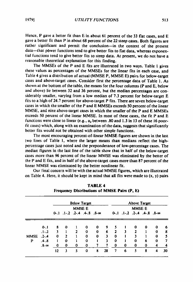
The MMSEs of the P and E fits are illustrated in two ways. Table 1 gives these values as percentages of the MMSEs for the linear fits in each case, and Table 4 gives a distribution of actual (MMSE P, MMSE E) pairs for below-target cases and above-target cases. Consider first the percentage data of Table 1. As shown at the bottom of the table, the means for the four columns (P and E, below and above) lie between 32 and 36 percent, but the median percentages are con- siderably smaller, varying from a low median of 7.3 percent for below-target E fits to a high of 24.7 percent for above-target P fits. There are seven below-target cases in which the smaller of the P and E MMSEs exceeds 50 percent of the linear MMSE, and nine above-target cases in which the smaller of the P and E MMSEs exceeds 50 percent of the linear MMSE. In most of these cases, the fit P and E functions were close to linear (e.g., a2 between .80 and 1.3 in 13 of these 16 poor- fit cases) which, along with an examination of the data, suggests that significantly better fits would not be obtained with other simple functions.

The most encouraging percent-of-linear MMSE figures are shown in the last two lines of Table 1, where the larger means than medians reflect the high- percentage cases just noted and the preponderance of low-percentage cases. The median figures in the last line of the table show that in half of the below-target cases more than 96 percent of the linear MMSE was eliminated by the better of the P and E fits, and in half of the above-target cases more than 87 percent of the linear MMSE was eliminated by the better nonlinear fit.

Our final concern will be with the actual MMSE figures, which are illustrated on Table 4. Here, it should be kept in mind that all fits were made to (x, y) pairs

TABLE 4 Frequency Distributions of MMSE Pairs (P, E)

Below Target Above Target MMSE E MMSE E

@ . I .1-.2 .2-.4 .4-.8 .&OD 0-. I .1-.2 .2-.4 .4-.8 .8- 00

O - . I 8 O I 0 0 9 5 1 0 0 0 6 . l - .2 3 1 2 0 0 6 2 3 2 1 0 8

MMSE.2-.4 0 2 I 0 0 3 0 I 3 1 0 5 P .4-.8 I 0 I 0 I 3 0 I 0 6 0 7

.8-= 0 0 0 0 7 7 0 0 0 0 4 4 I 2 3 5 0 8 2 8 7 6 5 8 4 3 0

5 14 DECISION SCIENCES [Vol. 10

that ranged from (0,O) to (10, 10). Hence, an MMSE value of, say, .25 indicates that the average square of the distance between the fit function and the data point in the vertical direction for the case at hand is .25, which corresponds to an ab- solute vertical distance of .5 in a total range of 10.

The data used for Table 4 show that the medians of the MMSE values for the P fits and for the E fits were both about .21. The corresponding median for the L fits was about 1.86. As might be expected from the preceding discussion, the arithmetic means were somewhat larger than these medians. In computing means, we chose a conservative method in which the total sum of squares for all n cases is divided by the difference between the total number of data points for the n cases and kn, where k is the number of parameters in the fitting function: k = 1 for L, k = 2 for P and E.

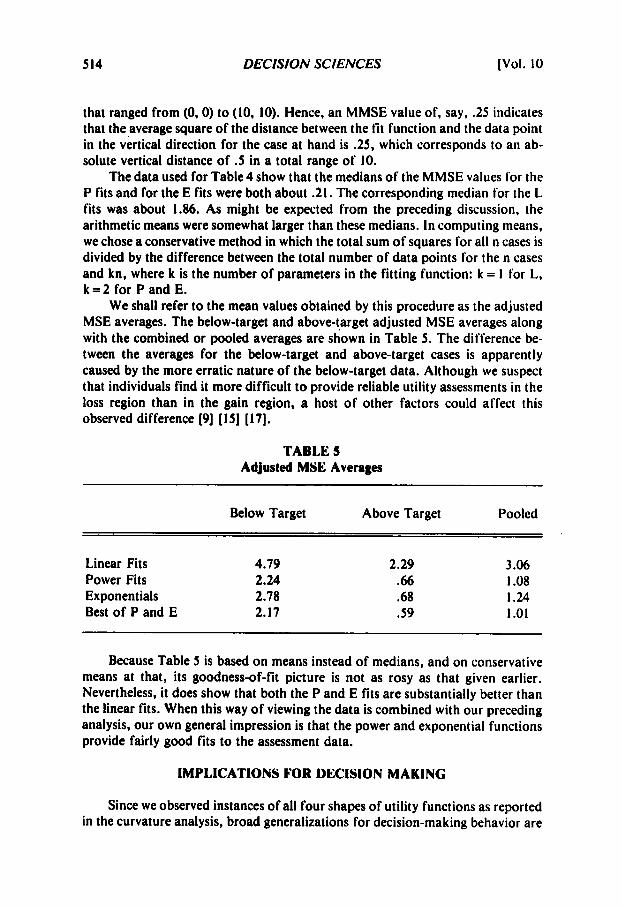
We shall refer to the mean values obtained by this procedure as the adjusted MSE averages. The below-target and above-target adjusted MSE averages along with the combined or pooled averages are shown in Table 5 . The difference be- tween the averages for the below-target and above-target cases is apparently caused by the more erratic nature of the below-target data. Although we suspect that individuals find it more difficult to provide reliable utility assessments in the loss region than in the gain region, a host of other factors could affect this observed difference [9] [IS] [17].

TABLE 5 Adjusted MSE Averages

Below Target Above Target Pooled

Linear Fits 4.79 Power Fits 2.24 Exponentials 2.78 Best of P and E 2.17

2.29 3.06 .66 I .08 .68 I .24 .59 I .01

Because Table 5 is based on means instead of medians, and on conservative means at that, its goodness-of-fit picture is not as rosy as that given earlier. Nevertheless, it does show that both the P and E fits are substantially better than the linear fits. When this way of viewing the data is combined with our preceding analysis, our own general impression is that the power and exponential functions provide fairly good fits to the assessment data.

IMPLICATIONS FOR DECISION MAKING

Since we observed instances of all four shapes of utility functions as reported in the curvature analysis, broad generalizations for decision-making behavior are

I9791 UTILITY FUNCTIONS 515

unwarranted. We shall, however, comment on utility-maximizing behaviors con- nected with several aspects of our analysis. For discussion purposes, the in- dividual's target is taken as the point of no gain and no loss. It will be assumed that u is differentiable except perhaps at x = 0, and we shall say that u is steeper in losses than in gains when u'(-x)> u'(x) for all positive x. Similarly, u is steeper in gains than in losses when u ' (x)>u ' ( -x) for all positive x.

We shall'look first at gambles that are symmetric about a fixed value, xu, so that for any such gamble the probability of receiving more than x,+ y equals the probability of receiving less than x,- y for each y r O . The means of these gambles are equal to xu. We shall refer to the gamble that returns xu with certainty as the sure x, gamble.

Suppose that xu= 0 so that the sure x, gamble is the do-nothing option. I f u is steeper in losses than in gains (the predominant trend of our data), then the do- nothing option will be preferred to every nondegenerate gamble that is symmetric about 0. Moreover, the attractiveness of a symmetric gamble will decrease as its returns distribution spreads out in the manner of a mean-preserving spread as defined by Rothschild and Stiglitz [23]. An individual in this case will prefer the status quo to an even-chance gamble for $I,OOO or -$1 ,OOO, which in turn he will prefer to an even-chance gamble for $2,000 or -$2,000, and so forth. In contrast, i f u is steeper in gains than losses, then his preferences will be reversed and will in- crease as the returns distribution of a gamble that is symmetric about 0 spreads out.

I f the behavior described in the preceding paragraph for a u that is steeper in losses than in gains were true at every xo, then u would be concave or risk averse everywhere. Our data suggest, however, that when xu>O only about 60 percent of the individuals would prefer the sure x,, gamble to the even-chance gamble that returns either 0 or 2xu, and when x,<O only about one third of the individuals would prefer the sure xu gamble (a certain loss) to the even-chance gamble for 0 or 2X".

Consider further the predominant convex-concave u (solid curve in Figure I ) that was apparently exhibited by nearly half the individuals. When xo>O, the at- tractiveness of a gamble symmetric about x, will decrease as the gamble spreads out, provided that (when some returns get into the loss region) u is steeper in losses than in gains. Suppose, however, that x,<O, and let G(y) denote an even- chance gamble for &+ y or &- y with y r O . Then, so long as %+ySO, G(y) will become increasingly attractive as y increases. But if u is steeper in losses than in gains, then G(y) might become less attractive for large y and may be less preferred than the sure xu gamble for sufficiently large y.

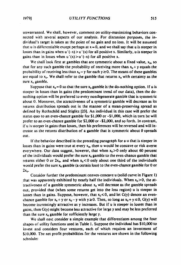
We shall next consider a simple example that differentiates among the four shapes of utility functions used in Table 1. Suppose the individual has 610,OOO to invest and considers four ventures, each of which requires an investment of $lO,OOO. The net profit probabilities for the ventures are shown in the following schedule:

5 16 DECISION SCIENCES [Vol. 10

Venture 310,Ooo -$5,Ooo $0 $10,0@) $2000

A 0.4 0.6 B 0.2 0.2 0.6 C 0.4 0.3 0.3 D 0.2 0.5 0.3

For example, in Venture B, he loses his entire investment capital with probability 0.2, breaks even with probability 0.2, and doubles his money with probability 0.6. Each venture has an expected net profit of $4,000. In Ventures B and D, the loss probability of 0.4 for -$5,000 is split evenly between -$lO,000 and $0. In C and D, the gain probability of 0.6 for $10,000 is split evenly between $0 and $20,000. It is easily seen that the most preferred of the four ventures is

A if u is concave-concave B if u is convex-concave C if u is concave-convex D if u is convex-convex.

For example, if u is convex-concave, then B will be preferred to A, and D will be preferred to C because of the loss split, and B will be preferred to D with A preferred to C because of the gain split. Hence, B is most preferred and C is less preferred when u is convex-concave.

If, in addition to the four ventures, the individual can invest his $lO,OOO in a safe asset that returns a net profit of $1,000, then the choice between his most preferred venture and the safe asset will depend on steepness considerations as well as on curvature. For example, if u is differentiable at the origin and is convex-convex, then it is steeper in gains than in losses and D will be preferred to the safe asset. But if u is convex-concave and much steeper in losses than in gains, then the safe asset may well be preferred to Venture B.

We shall conclude our discussion of utility-maximizing behaviors with a few remarks on lottery tickets and insurance purchases. In both cases, we shall ignore potentially relevant psychological and/or social factors and focus on the. utility implications.

If u is convex-concave and steeper in losses than in gains, then the individual will never purchase a lottery ticket for a large prize. This assumes of course that the cost of the ticket exceeds its expected winnings. If we maintain the assumption that u is convex-concave, but presume that it is steeper in gains than in losses, then the individual might gain in expected utility by buying, say, a $10 ticket that has one chance in 1,ooO of winning a $5,000 prize. For this to happen, however, the difference in steepness on the two sides of the origin must be fairly significant. If we assume about the same gain-to-loss steepness ratios for the four shapes of utility functions in Table 1, then the propensity to buy lottery tickets will be greatest for the convex-convex shape, next greatest for the concave-convex shape, and lowest for the concave-concave shape!.

19791 UTILITY FUNCTIONS 517

As noted in the introduction and in the present study, convex utilities in the loss region seem fairly common. The most obvious implication for decision mak- ing for individuals whose utility functions are convex in the loss region is that such individuals will never buy insurance (when they have a choice) as long as they evaluate the expected loss without insurance to be no greater than the premium amount. Moreover, even if the premium is subsidized and their personal cost is less than the expected loss without insurance, utility-maximizing behavior may still favor no purchase. The picture is very different for individuals that are risk averse in the loss region. We recommend that readers that are interested in a more detailed analysis of insurance-buying decisions consult the illuminating discussion in SIovic et al. [a].

SUMMARY

Data from five sources for thirty empirically assessed utility functions de- fined on changes in wealth or percent return on investment were analyzed for general trends and for their susceptability to representation by simple functional forms. Each of the thirty data sets was divided into below-target data and above- target data, and the functions were fit separately to each subset. In most cases, the target was at the zero-gain point.

About two-thirds of the below-target functions were convex or risk seeking, and slightly less than three-fifths of the above-target functions were concave or risk averse. The predominant composite shape was convex below and concave above (46 percent). Of the other three composite types, the concave-concave was observed least often (1 1 percent).

In essentially all cases, below-target utility was steeper than above-target utility. The median values of below-target slope divided by above-tatget slope as determined by two relatively uncorrelated methods were between 4 and 5 .

Linear, power, and exponential functions were fit to each data subset under the minimum-least-squares criterion. The power and exponential functions gave significantly better fits than the linear function even when the data were adjusted to account for the additional parameter in the nonlinear functions. Without this adjustment, the median minimum MSEs of the linear, power, and exponential fits over all cases were, respectively, about .19, 0.2, and 0.2 for data sets whose minimum and maximum points were at (0,O) and (10, 10). Power functions gave better fits than exponential functions in about three-fifths of the flat data sets (convex below or concave above), whereas exponential functions gave better fits than power functions in about two-thirds of the steep data sets (concave below or convex above).

REFERENCES

[ I ]

121

Archibald, G. C. ‘‘Utility. Risk, and Linearity.” Journd of Po/iticu/Economy. Vol. 67, No. 5 (October 1959). pp. 437-450. Barnes, J . D., and J . E. Reinmuth. “Comparing Imputed and Actual Utility Functions in a Competitive Bidding Setting.” Decision Sciences, Vol. 7, No. 4 (October 1976). pp. 801-812.

518 DECISION SCIENCES [Vol. 10

Bernoulli, D. “Specimen Theoriae Novae de Mensura Sortis.” Commentarii Academiae Scien- tiarum Imperialis Perropolitanae. Vol. 5 (1738). pp. 175-192. Bernoulli, D. “Exposition of a New Theory on the Measurement of Risk.” [Translation of [3] by L. Sommer.] Econometrim, Vol. 22, No. 1 (January 1954). pp. 23-36. Fishburn, P. C. Utility Theory for Dccision Making. New York: John Wiley & Sons, 1970. Fishburn, P. C. “Mean-Risk Analysis with Risk Associated with Below-Target Returns.” American Economic Review, Vol. 67, No. 2 (March 1977). pp. 116126. Friedman, M., and L. J. Savage. “The Utility Analysis of Choices Involving Risk.” Journal of Political Economy, Vol. 56, No. 4 (August 1948). pp. 279-304. Galanter, E., and P. Pliner. “Cross-Modality Matching of Money Against Other Continua.” In Sensation and Mwsurement. Edited by H. R. Moskowitr et al. Dordrecht, Holland: Reidel Publishing Co., 1974. Pp. 65-76. Grayson, C. J. lkcisions Under Uncertainty: Drilling Decisions by Oil and Gas Operators. Cambridge, Mass.: Graduate School of Business, Harvard University, 1960. Green, P. E. “Risk Attitudes and Chemical Investment Decisions.” Chemical Engineering Pro- gress, Vol. 59. No. I (January 1%3). pp. 3 5 4 . Hakansson, N. H. “Friedman-Savage Utility Functions Consistent with Risk Aversion.” Quar- terly Journal of Economics, Vol. 84, No. 3 (August 1970), pp. 472-487. Halter, A. N.. and 0. W. Dean. lkisions Under Uncertainty. Cincinnati, Ohio: South- Western Publishing Co., 1971. Hammond, J. S. “Better Decisions with Preference Theory.” Harvard Business Review, Vol. 45, No. 6 (November-December, 1%7), pp. 123-141. Herstein. 1. N., and J. Milnor. “An Axiomatic Approach to Measurable Utility.” Econo- metrica, Vol. 21 (April 1953). pp. 291-297. Johnson, E. M., and G. P. Huber. T h e Technology of Utility Assessment.” IEEE Transac- tions on Systems, Man, and Cybernetics, Vol. SMC-7, No. 5 (May 1977). pp. 31 1-325. Kahneman, D., and A. Tversky. “Prospect Theory: An Analysis of Decision Under Risk.” Econometric0 (forthcoming). Keeney, R. C., and H. Raiffa. Decisions with Multiple Objectives: Prt$erences and Value Trade- offs. New York: John Wiley and Sons, 1976. Kwang, N. Y. “Why Do People Buy Lottery Tickets? Choices Involving Risk and the Indivisi- bility of Expenditure.” Journul of Political Economy, Vol. 73 (October 1%5), pp. 530-535. Libby, R., and P. C. Fishburn. “Behavioral Models of Risk Taking in Business Decisions: A Survey and Evaluation.” Journal of Accounting Research, Vol. IS (Autumn 1977). pp.

Markowitz, H. “The Utility of Wealth.” Journal of Political Economy, Vol. 60 (April 1952).

Pratt, J. W. “Risk Aversion in the Small and in the Large.” Econometricu, Vol. 32, Nos. 1-2 (January-April 1964), pp. 122-136. Rosett, R. N. “The Friedman-Savage Hypothesis and Convex Acceptance Sets: A Reconcilia- tion.” Quarterly Journal of Economics, Vol. 81 (1%7), pp. 534535. Rothschild, M., and J. E. Stiglitz. “Increasing Risk: 1. A Definition.” Journal of Economic Theory, Vol. 2 (September 1970). pp. 225-243. Slovic, P.; B. Fischhoff; S. Lichtenstein; B. Corrigan; and B. Combs. “Preference for Insuring Against Probable Small Losses: Insurance Implications.” Journal of Risk und Insurance, Vol. 44. No. 2 (June 1977), pp. 237-258. Spetder, C. S. “The Development of a Corporate Risk Policy for Capital Investment Deci- sions.” IEEE Transactions on Systems‘Science and Cybernetics, Vol. SSC-4 (September 1968).

Swalm, R. D. “Utility Theory-Insights into Risk Taking.” Harvard Business Review, Vol. 47 (November-December 1966). pp. 123-136. Von Neumann, J., and 0. Morgenstern. Theory of Games and Economic Behavior. 2nd ed. Princeton, N.J.: Princeton University Press, 1947. Yaari, M. E. “Convexity in the Theory of Choice Under Risk.” Quarterly Journal a/ Economics, Vol. 79 (May 1%5), pp. 278-290.

272-292.

pp. 151-158.

pp. 279-300.