lable at ScienceDirect

Quaternary Science Reviews 28 (2009) 3448–3458

Contents lists avai

Quaternary Science Reviews

journal homepage: www.elsevier .com/locate/quascirev

Tropical glacier fluctuations in the Cordillera Blanca, Peru between 12.5 and 7.6 kafrom cosmogenic 10Be dating

Neil F. Glasser a,*, Samuel Clemmens a, Christoph Schnabel b, Cassandra R. Fenton b, Lanny McHargue c

a Centre for Glaciology, Institute of Geography and Earth Sciences, Aberystwyth University, Ceredigion SY23 3DB, UKb NERC Cosmogenic Isotope Analysis Facility, Scottish Enterprise Technology Park, East Kilbride G75 0QF, UKc NSF-Arizona AMS Laboratory, University of Arizona, Tucson, AZ, USA

a r t i c l e i n f o

Article history:Received 20 May 2009Received in revised form7 October 2009Accepted 10 October 2009

* Corresponding author. Tel.: þ44 1970 622 785; faE-mail address: nfg@aber.ac.uk (N.F. Glasser).

0277-3791/$ – see front matter � 2009 Elsevier Ltd.doi:10.1016/j.quascirev.2009.10.006

a b s t r a c t

We report cosmogenic surface exposure 10Be ages of 21 boulders on moraines in the Jeullesh and TucoValleys, Cordillera Blanca, Peru (w10�S at altitudes above 4200 m). Ages are based on the sea-level athigh-latitude reference production rate and scaling system of Lifton et al. (2005. Addressing solarmodulation and long-term uncertainties in scaling secondary cosmic rays for in situ cosmogenic nuclideapplications. Earth and Planetary Science Letters 239, 140–161) in the CRONUS-Earth online calculator ofBalco et al. (2008. A complete and easily accessible means of calculating surface exposure ages or erosionrates from 10Be and 26Al measurements. Quaternary Geochronology 3, 174–195). Using the Lifton system,large outer lateral moraines in the Jeullesh Valley have a 10Be exposure age of 12.4 ka, inside of which aresmaller moraine systems dated to 10.8, 9.7 and 7.6 ka. Large outer lateral moraines in the Tuco Valleyhave a 10Be exposure age of 12.5 ka, with inner moraines dated to 11.3 and 10.7 ka. Collectively, thesedata indicate that glacier recession from the Last Glacial Maximum (LGM) in the Cordillera Blanca waspunctuated by three to four stillstands or minor advances during the period 12.5–7.6 ka, spanning theYounger Dryas Chronozone (YDC; w12.9–11.6 ka) and the cold event identified in Greenland ice coresand many other parts of the world at 8.2 ka. The inferred fluctuations of tropical glaciers at these times,well after their withdrawal from the LGM, indicate an increase in precipitation or a decrease intemperature in this region. Although palaeoenvironmental records show regional and temporal vari-ability, comparison with proxy records (lacustrine sediments and ice cores) indicate that regionally thiswas a cold, dry period so we ascribe these glacier advances to reduced atmospheric temperature ratherthan increased precipitation.

� 2009 Elsevier Ltd. All rights reserved.

1. Introduction

The tropical glaciers located on low-latitude, high-altitudemountain ranges are highly sensitive components of the environ-ment and appear to react more immediately to fluctuations inclimate than glaciers in the mid- and high-latitudes (Guildersonet al., 1994; Hostetler and Mix, 1999; Hostetler and Clark, 2000;Seltzer et al., 2002). The glaciers of the Cordillera Blanca in Perucomprise more than 25% of all tropical glaciers (Kaser andOsmaston, 2002). Their behaviour since the Little Ice Age maximumand within-valley equilibrium line altitude (ELA) variations are welldocumented (Mark and Seltzer, 2005) but little is known abouttheir long-term glaciological history. Uncertainties surround theresponse of tropical glaciers to essentially ‘‘Southern’’ and

x: þ44 1970 622 659.

All rights reserved.

‘‘Northern’’ Hemisphere episodes during the Lateglacial, theAntarctic Cold Reversal (ACR; w14.5–12.9 ka), the Younger DryasChronozone (YDC; w12.9–11.6 ka) and the cold event identified inGreenland ice cores and many other parts of the world at 8.2 ka(Alley et al., 1997). These glacio-climatic relationships have broadimplications for our understanding of global climate change onglacial timescales.

Existing tropical glacier chronologies are based primarily onminimum 14C ages and relative dating techniques such as lichen-ometry (e.g. Clapperton, 1972; Rodbell, 1992, 1993). Despite this,chronologies for the last glacial cycle and Lateglacial ice coveragehave proved difficult to obtain in the tropics, largely due to the lackof availability of organic material needed for radiocarbon (14C)dating. Farber et al. (2005); Smith et al. (2005a,b, 2008) and Zechet al. (2008) presented chronologies for the tropical Andes usingcosmogenic 10Be isotope dating of boulders on glacial moraines.Farber et al. (2005) concluded that the last glacial cycle comprisedtwo separate glacier advances at w29 and w16.5 ka. Smith et al.

N.F. Glasser et al. / Quaternary Science Reviews 28 (2009) 3448–3458 3449

(2005a,b) suggested that the Local Last Glacial Maximum (LLGM) inPeru was relatively restricted and that the LLGM was earlier in thetropical Andes than elsewhere globally, with glaciers reaching theirgreatest extent in the last glacial cycle w34 ka and receding byw21 ka. Zech et al. (2008) described glacier advances dated to20–25, w15 and 11–13 ka.

The age calculations presented in Farber et al. (2005) and Smithet al. (2005a,b, 2008) use the reference production rate (at sea-levelat high-latitude (SLHL)) and scaling method (to the sample loca-tion) of Stone (2000) combined with a paleomagnetic correctionbased on Nishiizumi et al. (1989) and a best-fit for local pressure-altitude relationship (Farber et al., 2005). However, this methodyielded a SLHL 10Be production rate derived from data from theBreque moraine that is an outlier when compared to other SLHLproduction rates (Balco et al., 2008). Zech et al. (2007a) showed thata recalculation of Smith’s and Farber’s LLGM dates using the SLHLproduction rate and scaling method of Lifton et al. (2005) withoutusing the local best-fit for pressure by Farber et al. (2005) yieldedages between 22 and 25 ka, which agree with the global LGM (seealso Zech et al., 2008 for a discussion of the effects of these differentscaling systems on calculated 10Be ages at low-latitudes and highelevations). Here we do not discuss whether an LLGM occurred inthe Tropical Andes or whether exposure histories are in agreementwith a global LGM. We simply draw attention to the fact that, forthe Peruvian Andes, the only local calibration site is an outlier whencompared to other global 10Be production rates (which still doesnot mean it is wrong) and that different sets of reference produc-tion rates and scaling methods yield quite different results.

In such a situation, the best approach is to calculate ages ina way that they are comparable with other existing datasets in theregion. We therefore report our 10Be ages in the main text using thescaling system of Lifton et al. (2005) so that they are directlycomparable to those of Zech et al. (2007b, 2008). In the tables anddetailed discussion we also include 10Be ages calculated accordingto the scaling system used by Farber et al. (2005). This approach isdescribed in more detail below. In the absence of an agreed‘‘standard’’ scaling method and production rate for the tropicalregions, we report our 10Be concentrations with the understandingthat in the future, ages can be recalculated if an ‘‘agreed upon’’production rate and scaling method differ from the one we havechosen here.

In this paper we present 21 new 10Be dates from boulders onmoraines in two glaciated valleys of the Cordillera Blanca, Peru. Ourresults indicate that the recession of glaciers after the LGM in thisarea of the tropical Andes was punctuated by three to four still-stands or minor advances during the period 12.5–7.6 ka. Our studyalso indicates an absence of LGM moraines in the two valleys; themost prominent and furthest down-valley moraines yield ages thatare potentially concurrent with the Younger Dryas Chronozone inboth the Jeullesh and Tuco Valleys.

2. Geological setting

The Jeullesh and Tuco Valleys lie on the western slope of theCordillera Blanca in Peru with headwall elevations of w5600 andw5500 m a.s.l., respectively (Fig. 1). They have well-developed andsharp-crested lateral and terminal moraines at various distancesfrom their headwalls. Under contemporary climatic conditionsa small cirque glacier, fed by the Nevado Jenhuaracra, occupies theupper basin of Jeullesh Valley (Fig. 2). The Tuco Valley is mainly ice-free, apart from very small niche glaciers in its upper basin. Bothvalleys terminate on outwash plains (w4100 m a.s.l.) above the RioSanta. The valleys have large, well-preserved lateral moraines up to70 m in height that extend onto the plain; inside these area number of smaller (5–10 m in height) terminal moraines enclosed

within the valleys (Fig. 3). Moraine crests contain abundant largequartz-rich granitic boulders, most of which appear unweathered,although commonly their surfaces are wind-polished.

3. Methods and calculation of exposure ages

Geomorphological maps of the Jeullesh and Tuco Valleys (Fig. 2)were made using stereo pairs of w1:50,000 panchromatic aerialphotographs at Unidad de Glaciologıa y Recursos Hıdricos (UGRH)of Instituto Nacional de Recursos Naturales (INRENA) in Huaraz,Peru. Samples for cosmogenic nuclide surface exposure (10Be)dating were collected from quartz-rich granitic and fine-grainedmetamorphic boulders (>1.5 m, b-axis diameter) on moraine crestsfollowing the sampling guidelines of Gosse and Phillips (2001)(Fig. 4; Table 1). All samples are from different boulders exceptsamples JEU12 and JEU13, which were collected from a polishedboulder surface and a knob protruding above the same bouldersurface.

Purified quartz was obtained from the 180 to 500 mm size frac-tion of the crushed rocks and BeO targets were prepared for10Be/9Be analysis using a modification of the method in Wilsonet al. (2008). Sample preparation varied from that described inWilson et al. (2008) in the following ways: (1) initial acid-etchingwas done with a 2:1 mixture of hexafluorosilicic acid (31% wt/wt)and 12 M HCl to reduce the feldspar content without attackingquartz; HF acid was used in the final etch; (2) inherent Al in quartzafter etching was �150 ppm; (3) 330 mg 9Be were added as carrier;and (4) Ti was removed by cation-exchange chromatography usingsulphuric acid. The 10Be/9Be ratios were measured with the 5 MVaccelerator mass spectrometer at SUERC (Freeman et al., 2004,2007) as part of a routine Be run. Measurement is described indetail in Maden et al. (2007) and Schnabel et al. (2007). 10B atomsare so well resolved and the detector lifetime measured that nocorrection procedure is necessary for 10Be count rates. Ion currentsof 9Be16O� were between 5.5 and 6.4 mA in one measurementcampaign and between 3.5 and 4.2 mA in the other. NIST SRM4325with a calibrated 10Be/9Be ratio of 3.06 � 10�11 was used fornormalization. This ratio agrees to within <0.5% with measure-ments from standard materials purchased from Kunihiko Nishii-zumi (2002). The nominal ratios used for primary and secondarystandards disagree with the re-calibration reported by Nishiizumiet al. (2007). However, the production rates used are consistentwith the ratios used in this work. Consequently, for the presentedexposure ages (short compared to the half-life of 10Be) only 10Beconcentrations reported here would be affected by implementing10Be/9Be ratios from Nishiizumi et al. (2007), but not the exposureages.

The 10Be/9Be ratios of the processing blanks prepared with thesamples were 3.5 � 10�15, 4.7 � 10�15 and 5.0 � 10�15, respectively(one-sigma uncertainty of 1 �10�15). The average of these ratioswas subtracted from the Be isotope ratios of the samples. Blank-corrected 10Be/9Be ratios of the samples ranged from 1.8 � 10�13 to2.8 � 10�13. Statistical uncertainties (one-sigma) of 2.5% werereached for all samples within normal measurement times(between 1250 and 2000 s). One-sigma uncertainties of the SUERCAMS measurement include the uncertainty of the samplemeasurement, the uncertainty associated with the measurement ofthe primary standard and the uncertainty of the blank correction.Total one-sigma uncertainties for the concentrations determined atSUERC include the one-sigma uncertainty of the AMS measurementand a 2% uncertainty as a realistic estimate for possible effects ofthe chemical sample preparation which includes the uncertainty ofthe Be concentration of the carrier solution.

Calibration sites for cosmogenic production rates are rare in thetropics, which creates a challenge when determining which

Fig. 1. The Cordillera Blanca, Peru showing the location of the Jeullesh and Tuco Valleys.

N.F. Glasser et al. / Quaternary Science Reviews 28 (2009) 3448–34583450

production rate to use in age calculations (e.g. Farber et al., 2005;Zech et al., 2007b; Balco et al., 2008). As mentioned above, thecalibration site for production rates in the Cordillera Blanca (Farberet al., 2005) does not agree well with other production ratesworldwide. Based on the current lack of knowledge aboutproduction rates in the Central Andes we choose two different waysto calculate exposure ages. The first one is chosen in order to be ableto compare our ages directly with those from Zech et al. (2007b,2008). For this purpose we use the SLHL reference production rateand scaling system of Lifton et al. (2005) in the CRONUS-Earthonline calculator of Balco et al. (2008) (http://hess.ess.washington.edu/math) and using the pressure field according to the NCEP-NCAR reanalysis (http://www.cdc.noaa.gov/ncep_reanalysis/) in

the following version: wrapper script 2.0; main calculator 2.1,constants 2.1, muons 1.1. We refer to these ages as the ‘‘Lifton ages’’(bold font columns, Table 2) and use them for the data given in thetext and figures (Figs. 2 and 5) unless mentioned otherwise. Thereference production rate in the Lifton scheme (as used in Balcoet al., 2008) is 5.39 � 0.52 at/g per year.

In order to also be able to compare our ages to the ones presentedby Farber et al. (2005) and Smith et al. (2005a,b) we use the samebest-fit for local air pressure as presented in Farber et al. (2005) andthe paleomagnetic correction (based on Nishiizumi et al., 1989) inthe time-dependent Lal–Stone scaling system (Lal, 1991; Stone,2000), referred to as the Lm scaling scheme in the CRONUS-Earthonline calculator of Balco et al. (2008). Hereafter, we refer to these

Fig. 2. Geomorphological maps of the Jeullesh and Tuco Valleys showing major moraine crests and sampling locations. Sample numbers refer to the samples listed in Tables 1 and 2.Average exposure ages for each moraine are also listed with their total (internal) one-sigma uncertainties; for average moraine ages that include the (external) uncertainty of theproduction rate of 10Be, see Fig. 8.

N.F. Glasser et al. / Quaternary Science Reviews 28 (2009) 3448–3458 3451

ages as the ‘‘LSF ages’’. The Lifton and the LSF ages are both presentedin Table 2. To illustrate the effect of the paleomagnetic correctionaccording to Nishiizumi et al. (1989) we also present ages calculatedbased on the time-independent Lal–Stone system in Table 2.

Exposure ages from this study based on: (a) the Lifton et al.(2005) scheme; and (b) the time-dependent Lal (1991)/Stone (2000)

Fig. 3. View looking up the Jeullesh Valley, showing the large lateral moraines andsmaller terminal moraines on the valley floor. Using the Lifton scaling scheme, thelateral moraine has an unweighted mean 10Be exposure age of 12.4 ka (based onboulder exposure ages of 11.6 � 0.4, 12.2 � 0.4, 12.8 � 0.4 ka, and 12.8 � 0.4 ka).

with Farber et al. (2005) (LSF) scheme are both plotted in Fig. 5b toillustrate the strong difference between the two calculationmethods and include only the analytical (or internal) uncertainty(Table 2). Lifton exposure ages of boulders from Jeullesh and TucoValley moraines are 15–20% younger than LSF ages. It is important tonote that whichever choice of scaling method and production rate

Fig. 4. Example of sample context. The photograph shows Boulder JEU03 on the crestof the large lateral moraine in the Jeullesh Valley. Using the Lifton scaling scheme, thisboulder has a 10Be exposure age of 12.8 � 0.4 ka.

Table 1List of samples collected from boulders on glacial moraines in the Jeullesh and Tuco Valleys, Cordillera Blanca, Peru in June 2005.

SampleNoa

Latitude Longitude Alt(m)b

Lithology Dimensions(m)c

Context/significance Topographicshieldingd

Thicknessattenuatione

JEU01 10� 00,43.9S

077� 16,15.8W

4290 Quartzite 2 � 1.6 � 0.55 W valley side; large outer lateral moraine 1 0.9751

JEU02 10� 00,23.1S

077� 16,17.3W

4374 Granite 1.85 � 1.3 � 0.8 W valley side; large outer lateral moraine 1 0.9751

JEU03 10� 00,15.6S

077� 16,17.8W

4411 Granite 2.9 � 2.7 � 1.85 W valley side; large outer lateral moraine 1 0.9751

JEU04 10� 00,21.8S

077� 16,12.4W

4317 Granite 3.4 � 2 � 1 Inner lateral moraine, younger than JEU001–003

0.988 0.9751

JEU05 10� 00,21.8S

077� 16,12.3W

4316 Granite 2.2 � 1.5 � 1.2 Inner lateral moraine, younger than JEU001–003

0.988 0.9751

JEU06 10� 00,22.4S

077� 16,05.0W

4328 Granite 3.2 � 3.1 � 1.4 Inner lateral moraine, younger than JEU001–003

0.994 0.9751

JEU07 10� 00,20.6S

077� 16,00.8W

4385 Granite 2 � 1.7 � 1.10 E valley side; large outer lateral moraine 1 0.9751

JEU08 10� 00,27.1S

077� 16,01.9W

4364 Granite 1.2 � 0.8 � 0.5 E valley side; large outer lateral moraine 1 0.9875

JEU09 09� 59,26.6S

077� 15,13.7W

4520 Granite 3.5 � 1.5 � 1.5 High up Jeullish valley, on W side lateralmoraine

0.988 0.9862

JEU10 09� 59,26.9S

077� 15,14.1W

4519 Granite 1.5 � 0.9 � 0.7 High up Jeullish valley, on W side lateralmoraine

0.988 0.9820

JEU11 09� 59,27.2S

077� 15,15.2W

4519 Granite 1.1 � 0.9 � 0.4 High up Jeullish valley, on W side lateralmoraine

0.988 0.9729

JEU12 09� 59,27.8S

077� 15,16.7W

4516 Granite 4.6 � 2.2 � 1.9 High up Jeullish valley, on W side lateral;polished

1 0.9936

JEU13 09� 59,27.8S

077� 15,16.7W

4516 Granite 4.6 � 2.2 � 1.9 High up Jeullish valley, on W side lateral; knob 1 0.9817

JEU14 10� 00,15.9S

077� 16,06.9W

4298 Granite 3.3 � 2.5 � 1.65 Middle Jeullish valley; younger than JEU004–006

0.992 0.9723

JEU15 10� 00,16.8S

077� 16,07.1W

4299 Granite 3.9 � 2.4 � 1 Middle Jeullish valley; younger than JEU004–006

1 0.9836

TUC02 10� 02,27.3S

077� 12,50.2W

4542 Granite 1.5 � 0.6 � 0.45 East valley side, on outer lateral moraine 1 0.9751

TUC03 10� 02,27.5S

077� 12,50.2W

4452 Granite 1.9 � 1.1 � 0.8 East valley side, on outer lateral moraine 1 0.9751

TUC04 10� 03,14.3S

077� 13,12.8W

4318 Granite 1.2 � 0.9 � 0.6 East valley side, on inner lateral moraine 1 0.9590

TUC05 10� 03,10.0S

077� 13,08.2W

4310 Granite 2.1 � 1.6 � 1.0 East valley side, on inner lateral moraine 1 0.9751

TUC08 10� 02,38.0S

077� 13,16.5W

4311 Granite 1.0 � 0.8 � 0.5 Moraine on valley floor; dams L. Aguascocha 1 0.9751

TUC09 10� 02,37.0S

077� 13,15.7W

4309 Granite 1.3 � 0.6 � 0.5 Moraine on valley floor; dams L. Aguascocha 1 0.9751

a JEU ¼ Jeullesh Valley; TUC ¼ Tuco Valleyb Locations and altitude of the samples were recorded using a hand-held Magellan GPS (WGS 84 datum) and are accurate to �4 m. Elevation data are given as metres above

ellipsoid (m.a.e.).c Digital photographs of overall sample locations and close-up photographs of sample sites on the boulders were taken for each sample.d Skyline measurements were collected with an Abney level at all sites where topographic shielding was deemed to be important (i.e. the angle to the horizon was greater

than 20�). Snow corrections in shielding factors are not necessary; contemporary snow cover at these elevations in both valleys is minimal and all sampling sites are locatedbelow the modern snowline. Shielding correction was carried out according to Dunne et al. (1999).

e Samples were collected only from the top 5 cm of the upper surfaces of the boulders using a hammer and chisel.

N.F. Glasser et al. / Quaternary Science Reviews 28 (2009) 3448–34583452

that is used, there is a systematic, sequential decrease in 10Be ages asexpected in each valley; geomorphologically younger morainesyield younger 10Be exposure ages.

Erosion in this region has negligible effects on 10Be ages. Forexample, sample JEU12 (10Be exposure age of 7.4 � 0.2 ka) was takenfrom a polished boulder surface and sample JEU13 (10Be exposureage of 7.5 � 0.2 ka) was taken from a knob protruding above thesame boulder surface. The age agreement between samples JEU12and 13 suggests that very little erosion has occurred since depositionand that protrusions have not formed since moraine formation asa result of large amounts of in situ differential boulder weathering.Long-term rates of boulder erosion in the tropical Andes are docu-mented to be very low, on the order of 0.3–0.5 m per million years(Smith et al., 2005a,b). This means that exposure ages of about14.0 ka appear 50 years older when an erosion rate of 3 � 10�4 mm/a is used in the age calculations (Figs. 3, 4 and 6).

Moraines may have undergone degradation caused by erosion offiner-grained material from moraine crests. This type of erosion couldcause exhumation of boulders, and result in minimum exposure agesof boulder surfaces. This effect on exposure ages was minimized bycollecting boulders that were sitting at the top of moraine crests, withupper surfaces being typically >1 m above the surrounding ground.In addition, preservation of the moraines is quite good, with sharp-crested peaks still apparent (Figs. 3, 4 and 6). In one case, however,a single boulder (sample JEU08) yielded a minimum 10Be age of10.3 ka (Table 2), and was excluded from the mean age of its morainebecause it was considered a statistical outlier (i.e. a calculated agegreater than two standard deviations from the mean of all boulders onthat moraine). Of the five boulders collected from this outermostmoraine in the Jeullesh Valley, this boulder was the only one standing<1 m above the surrounding ground. It is therefore possible that thissample reflects a minimum, exhumation age.

Table 2Details of laboratory and AMS measurements for the 21 samples from the Jeullesh and Tuco Valley analysed in this study. Three sets of boulder ages were calculated using: (1) the Lifton et al. (2005) scaling method; (2) theconstant Lal/Stone scaling method (Lal, 1991; Stone, 2000); and (3) the time-dependent local height/pressure relationship suggested by Farber et al. (2005). The bold font columns represent the most appropriate age model forour samples.

Sample ID forAMSSUERC

10Be(105

at/g)a

s(10Be(at/g))

Lifton ages (Li scheme in Balco et al., 2008) Lal/Stone ages (St scheme in Balco et al., 2008) LSF ages/local air pressure (Lm scheme in Balco et al., 2008)

10Be exp. Age(ka) (Lifton,stdatmosphere)b

Internaluncertainty(ka) (Lifton, stdatmosphere)

Externaluncertainty (ka)(Lifton, stdatmosphere)

Production rate(spall) at/g peryear (Lal/Stoneconstant)

Productionrate(muons) at/g per year

10Be exp.Age (ka)(Lal/Stoneconstant)b

Internaluncertainty(ka) (Lal/Stoneconstant)

Externaluncertainty(ka) (Lal/Stoneconstant)

Localatmosphericpressure(hPa)c

10Be exp. Age(ka) (Lal/Stonetime-dependent)b

Internaluncertainty (ka)(Lal/Stone time-dependent)

Externaluncertainty (ka)(Lal/Stone time-dependent)

JEU01 b1809 5.849 0.188 11.6 0.4 1.2 40.06 0.693 14.4 0.5 1.3 608.4 13.7 0.4 1.2JEU02 b1810 6.458 0.198 12.2 0.4 1.2 41.60 0.708 15.3 0.5 1.4 602.0 14.6 0.4 1.3JEU03 b1812 6.866 0.212 12.8 0.4 1.3 42.29 0.714 16.0 0.5 1.5 599.3 15.2 0.5 1.4JEU07 b1818 6.751 0.211 12.8 0.4 1.3 41.81 0.710 16.0 0.5 1.5 601.2 15.1 0.5 1.4JEU08d b1548 5.499 0.171 10.3 0.3 1.0 41.95 0.714 12.9 0.4 1.2 602.8 12.3 0.4 1.1

JEU04 b1813 5.306 0.172 10.4 0.3 1.1 40.06 0.698 13.1 0.4 1.2 606.3 12.5 0.4 1.1JEU05 b1814 5.520 0.176 10.9 0.3 1.1 40.05 0.698 13.6 0.4 1.3 606.4 13.0 0.4 1.2JEU06 b1815 5.659 0.178 11.0 0.3 1.1 40.51 0.700 13.8 0.4 1.3 605.5 13.2 0.4 1.2

JEU14 b1825 4.858 0.155 9.6 0.3 1.0 39.77 0.693 12.0 0.4 1.1 607.8 11.5 0.4 1.0JEU15 b1845 5.021 0.152 9.7 0.3 1.0 40.58 0.699 12.2 0.4 1.1 607.7 11.6 0.4 1.0

JEU09 b1821 4.644 0.144 7.8 0.2 0.8 44.79 0.741 10.2 0.3 0.9 591.1 9.7 0.3 0.9JEU10 b1549 4.330 0.141 7.3 0.2 0.7 44.58 0.738 9.6 0.3 0.9 591.2 9.1 0.3 0.8JEU11 b1822 4.622 0.156 7.9 0.3 0.8 44.19 0.732 10.3 0.3 1.0 591.1 9.8 0.3 0.9JEU12 b1550 4.482 0.139 7.4 0.2 0.8 45.14 0.747 9.8 0.3 0.9 591.4 9.3 0.3 0.8JEU13 b1551 4.471 0.147 7.5 0.2 0.8 44.60 0.737 9.9 0.3 0.9 591.4 9.4 0.3 0.9

TUC02 b1832 6.803 0.213 11.7 0.4 1.2 44.83 0.737 15.0 0.5 1.4 589.5 14.3 0.4 1.3TUC03 b1833 7.274 0.242 13.3 0.4 1.4 43.10 0.721 16.7 0.6 1.6 596.2 15.7 0.5 1.4

TUC04 b1834 5.566 0.180 11.0 0.4 1.1 39.93 0.691 13.7 0.4 1.3 606.3 13.1 0.4 1.2TUC05 b1819 5.873 0.191 11.5 0.4 1.2 40.46 0.697 14.3 0.5 1.3 606.9 13.7 0.4 1.2

TUC08 b1820 5.493 0.173 10.7 0.3 1.1 40.47 0.697 13.4 0.4 1.2 606.8 12.8 0.4 1.2TUC09 b1835 5.451 0.168 10.6 0.3 1.1 40.43 0.696 13.3 0.4 1.2 606.9 12.7 0.4 1.1

Note: For all ages presented we used the following version of the CRONUS-Earth online exposure age calculator (http://hess.ess.washington.edu; Balco et al., 2008): wrapper script 2.0; main calculator 2.1, constants 2.1, muons1.1. We also present exposure ages calculated according to Lifton et al. (2005) without using the best local pressure fit from Farber et al. (2005) but using the pressure field according to the NCEP-NCAR reanalysis (http://www.cdc.noaa.gov/ncep_reanalysis/) as used in the mentioned version of the online calculator. These ages should be comparable to data from Zech et al. (2007a). To illustrate the effect of the paleomagnetic correction according toNishiizumi et al. (1989) we also present ages calculated on the time-independent Lal–Stone scheme.

a NIST SRM4325 was used for normalization with a calibrated 10Be/9Be ratio of 3.06 � 10�11, which agrees within <0.5% with measurements from standard materials purchased from K. Nishiizumi (2002).b The nominal ratios used for primary and secondary standards disagree with the re-calibration reported by Nishiizumi et al. (2007). However, the production rates used are consistent with the ratios used in this work.

Consequently, for the presented exposure ages (short compared to the half-life of 10Be) only 10Be concentrations reported here would be affected by implementing 10Be/9Be ratios from Nishiizumi et al. (2007), but not theexposure ages.

c Calculated using the local height/pressure relationship described in Farber et al. (2005).d The age of sample JUE08 is more than 2 standard deviations from the average of all five ages of the outermost moraine at the mouth of Jeullesh Valley; it is therefore considered an outlier and excluded from the average age.

N.F.G

lasseret

al./Q

uaternaryScience

Reviews

28(2009)

3448–3458

3453

10

UE

J

20

UE

J

30

UE

J

70

UE

J

80

UE

J

40

UE

J

50

UE

J

60

UE

J

41

UE

J

51

UE

J

90

UE

J

01

UE

J

11

UE

J

21

UE

J

31

UE

J

20

CU

T

30

CU

T

40

CU

T

50

CU

T

80

CU

T

90

CU

T

Exp

so

ure A

ge (ka)

Ex

ps

ou

re

A

ge

(k

a)

Sample Number

Jeullesh ValleyTuco Valley

12.4±0.6

10.8±0.3

9.7±0.3

7.6±0.3

12.5±1.1

11.3±0.4

10.7±0.3

12.4±0.6

Average age of moraine boulders

a

b5

10

15

20

Lifton ages (ka)Lal/Stone with Farber ages (ka)

5

10

15

20

Lifton ages (ka)

Fig. 5. (a) 10Be exposure ages (�internal uncertainty) calculated using Lifton et al. (2005) for the 21 samples analysed in this study. Lines and ages in grey represent averageexposure ages (� internal uncertainty) for each moraine. Sample JEU08 (white circle) is a statistical outlier and was excluded from the calculation of mean age for that moraine (seetext for details). (b) Comparison of Lifton ages and LSF ages for the same samples in (a).

N.F. Glasser et al. / Quaternary Science Reviews 28 (2009) 3448–34583454

4. Results

4.1. The Jeullesh Valley

Fifteen granite boulder samples were analysed from fourmoraines in the Jeullesh Valley (Fig. 5; Tables 1 and 2). BouldersJEU01, JEU02, JEU03, JEU07 and JEU08 were collected from the crestof the large (w70 m high), outermost, sharp-crested lateralmoraine at the mouth of the valley (Fig. 2). Boulder JEU08 (age10.3 � 0.3 ka) is a statistical outlier (i.e. a calculated age greaterthan two standard deviations from the mean of all boulders on thatmoraine) and is excluded. Using the Lifton system, the remainingfour boulders yielded an unweighted mean 10Be exposure age of12.4 ka (based on the mean of four boulder ages of 11.6 � 0.4,12.2 � 0.4, 12.8 � 0.4 and 12.8 � 0.4 ka). Boulders JEU04, JEU05,JEU06, JEU14 and JEU15 were collected from two much smaller(w5–10 m high), subdued moraines on the valley floor, inside thelarge lateral moraine (Fig. 6). The outer of these two smallermoraines has a 10Be exposure age of 10.8 ka (unweighted mean of

three boulders dated to 10.4 � 0.3, 10.9 � 0.3 and 11.0 � 0.3 ka).The inner of these two smaller moraines has a 10Be exposure age of9.7 ka (unweighted mean age of two boulders dated to 9.6 � 0.3and 9.7 � 0.3 ka). Closer to the contemporary glacier, samplesJEU09 to JEU13 were collected from four separate boulders on thesummit of a sharp-crested lateral moraine w1.5 km from theglacier snout (Figs. 2 and 7). The four separate boulder samples onthis moraine (JEU09–JEU12) yield a 10Be exposure age of 7.6 ka(unweighted mean age of four boulders dated to 7.8 � 0.2, 7.3 � 0.2,7.9 � 0.3 and 7.4 � 0.2 ka).

4.2. The Tuco Valley

Six granite boulder samples were analysed from three morainesin the Tuco Valley (Fig. 2; Table 1). Samples TUC02 and TUC03 weretaken from the outer lateral moraine high on the south side of thevalley (Fig. 2; Table 1). The two boulders yielded an unweightedmean 10Be exposure age of 12.5 ka based on boulder exposure agesof 11.7 � 0.4 and 13.3 � 0.4 ka. Samples TUC04 and TUC05 were

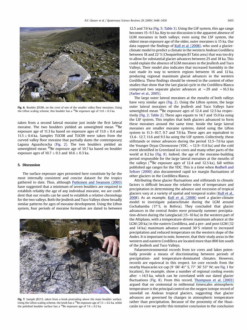
Fig. 6. Boulder JEU06, on the crest of one of the smaller valley floor moraines. Usingthe Lifton scaling scheme, this boulder has a 10Be exposure age of 11.0 � 0.3 ka.

N.F. Glasser et al. / Quaternary Science Reviews 28 (2009) 3448–3458 3455

taken from a second lateral moraine just inside the first lateralmoraine. The two boulders yielded an unweighted mean 10Beexposure age of 11.3 ka based on exposure ages of 11.0 � 0.4 and11.5 � 0.4 ka. Samples TUC08 and TUC09 were taken from thecurved valley floor moraine that partially dams the contemporaryLaguna Aguashcocha (Fig. 2). The two boulders yielded anunweighted mean 10Be exposure age of 10.7 ka based on boulderexposure ages of 10.7 � 0.3 and 10.6 � 0.3 ka.

5. Discussion

The surface exposure ages presented here constitute by far themost internally consistent and concise dataset for the tropicsgathered to date. Thus, although Putkonen and Swanson (2003)have suggested that a minimum of seven boulders are required toestablish reliably the age of any individual moraine, we are confi-dent that our results can be used to establish a relative chronologyfor the two valleys. Both the Jeullesh and Tuco Valleys show broadlysimilar patterns for ages of moraine development. Using the Liftonsystem, four periods of moraine formation are dated to between

Fig. 7. Sample JEU13, taken from a knob protruding above the main boulder surface.Using the Lifton scaling scheme, the knob has a 10Be exposure age of 7.5 � 0.2 ka, whilethe polished boulder surface has a 10Be exposure age of 7.4 � 0.2 ka.

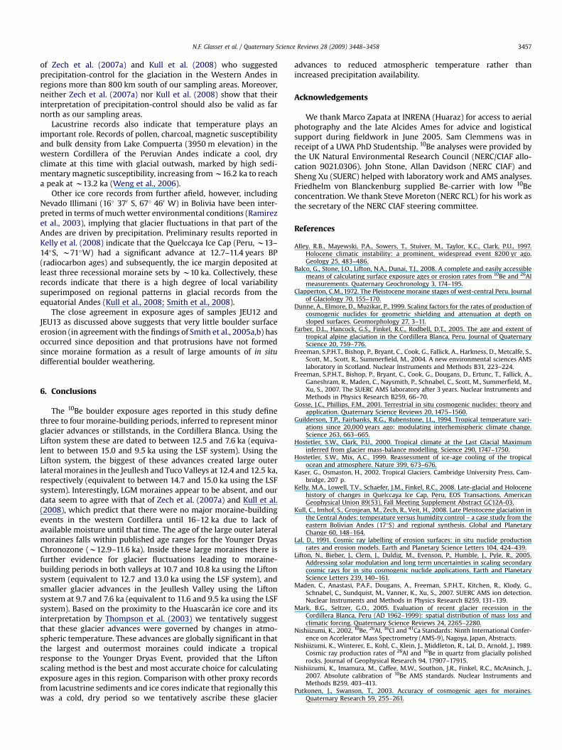
12.5 and 7.6 ka (Fig. 5; Table 3). Using the LSF system, this age rangebecomes 15–9.5 ka. Key to our discussion is the apparent absence ofLGM moraines in both valleys; even using the LSF system, theoldest mean exposure age of the older, outer moraines is 15 ka. Ourdata support the findings of Kull et al. (2008), who used a glacier-climate model to predict a climate in the western Andean Cordillerabetween 18 and 22�S (Choquielimpie/El Tatio area) that was too dryto allow for substantial glacier advances between 25 and 18 ka. Thiscould explain the absence of LGM moraines in the Jeullesh and TucoValleys. Their model also indicates that increased humidity in theeast made its way to western regions between 16 and 12 ka,producing regional maximum glacial advances in the westernCordillera. These findings should be viewed in the context of otherstudies that show that the last glacial cycle in the Cordillera Blancacomprised two separate glacier advances at w29 and w16.5 ka(Farber et al., 2005).

The large outer lateral moraines at the mouths of both valleyshave very similar ages (Fig. 2). Using the Lifton system, the largeouter lateral moraines of the Jeullesh and Tuco Valleys haveunweighted mean 10Be exposure ages of 12.4 and 12.5 ka respec-tively (Fig. 2; Table 2). These ages equate to 14.7 and 15.0 ka usingthe LSF system. This implies that both glaciers advanced to formthese moraines around the same time. Inside the large lateralmoraines are smaller moraine systems, dated using the Liftonsystem to 11.3–10.7, 9.7 and 7.6 ka. These ages are equivalent to13.4– 12.7, 11.6 and 9.5 ka using the LSF system. Collectively, thesestillstands or minor advances during the period 12.5–7.6 ka spanthe Younger Dryas Chronozone (YDC; w12.9–11.6 ka) and the coldevent identified in Greenland ice cores and many other parts of theworld at 8.2 ka (Fig. 8). Indeed, the age of the moraine-buildingperiod responsible for the large lateral moraines at the mouths ofthe valleys (10Be exposure ages of 12.4 and 12.5 ka), fall withinpublished age ranges for the YDC. This is a time when Rodbell andSeltzer (2000) also documented rapid ice margin fluctuations ofother glaciers in the Cordillera Blanca.

Attributing these glacier fluctuations and stillstands to climaticfactors is difficult because the relative roles of temperature andprecipitation in determining the advance and recession of tropicalglaciers vary at a variety of spatial and temporal scales (Kull et al.,2008). As an example, Kull et al. (2008) used a glacier-climatemodel to investigate palaeoclimate during the LGM aroundCochabamba (17�S, in Bolivia). They concluded that glacieradvances in the central Andes were primarily summer precipita-tion-driven during the Lateglacial (15–10 ka) in the western part ofthe Altiplano, with a temperature-driven maximum advance at theLGM (20 ka) in the eastern Cordillera, and a pre- and post-LGM (32and 14 ka) maximum advance around 30�S related to increasedprecipitation and reduced temperature on the western slope of theAndes. It is important to note, however, that their study areas in thewestern and eastern Cordillera are located more than 800 km southof the Jeullesh and Tuco Valleys.

Palaeoenvironmental records from ice cores and lakes poten-tially provide a means of discriminating between periods ofprecipitation- and temperature-dominated climates. However,records are equivocal in this respect. Ice core records from thenearby Huascaran ice cap (9� 060 4100 S, 77� 360 5300 W; see Fig. 1 forlocation), for example, show a number of regional cooling eventsafter w14.5 ka, which can be correlated with our dated glacierfluctuations (Fig. 8). From this record, Thompson et al. (2003)argued that on centennial to millennial timescales atmospherictemperature is the principal control on the oxygen isotope record ofsnowfall on Andean tropical glaciers, suggesting that glacieradvances are governed by changes in atmospheric temperaturerather than precipitation. Because of the proximity of the Huas-caran ice core we prefer this tentative conclusion to the conclusion

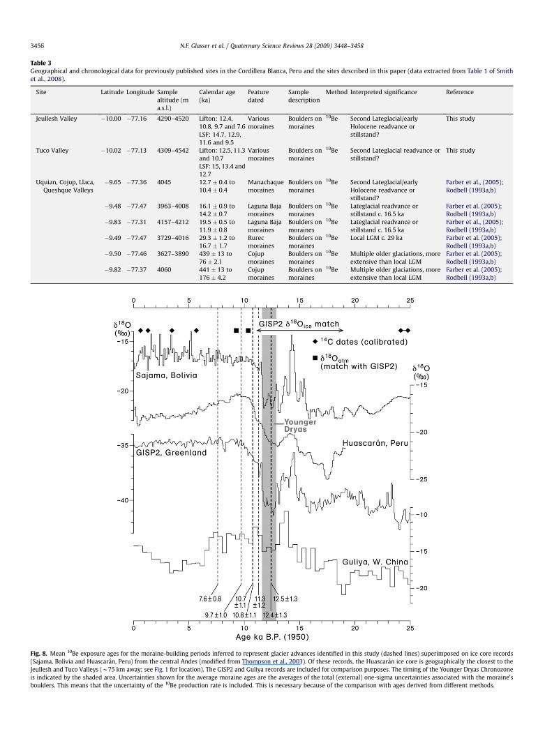
Table 3Geographical and chronological data for previously published sites in the Cordillera Blanca, Peru and the sites described in this paper (data extracted from Table 1 of Smithet al., 2008).

Site Latitude Longitude Samplealtitude (ma.s.l.)

Calendar age(ka)

Featuredated

Sampledescription

Method Interpreted significance Reference

Jeullesh Valley �10.00 �77.16 4290–4520 Lifton: 12.4,10.8, 9.7 and 7.6

Variousmoraines

Boulders onmoraines

10Be Second Lateglacial/earlyHolocene readvance orstillstand?

This study

LSF: 14.7, 12.9,11.6 and 9.5

Tuco Valley �10.02 �77.13 4309–4542 Lifton: 12.5, 11.3and 10.7

Variousmoraines

Boulders onmoraines

10Be Second Lateglacial readvance orstillstand?

This study

LSF: 15, 13.4 and12.7

Uquian, Cojup, Llaca,Queshque Valleys

�9.65 �77.36 4045 12.7 � 0.4 to10.4 � 0.4

Manachaquemoraines

Boulders onmoraines

10Be Second Lateglacial/earlyHolocene readvance orstillstand?

Farber et al., (2005);Rodbell (1993a,b)

�9.48 �77.47 3963–4008 16.1 � 0.9 to14.2 � 0.7

Laguna Bajamoraines

Boulders onmoraines

10Be Lateglacial readvance orstillstand c. 16.5 ka

Farber et al. (2005);Rodbell (1993a,b)

�9.83 �77.31 4157–4212 19.5 � 0.5 to11.9 � 0.8

Laguna Bajamoraines

Boulders onmoraines

10Be Lateglacial readvance orstillstand c. 16.5 ka

Farber et al., (2005);Rodbell (1993a,b)

�9.49 �77.47 3729–4016 29.3 � 1.2 to16.7 � 1.7

Rurecmoraines

Boulders onmoraines

10Be Local LGM c. 29 ka Farber et al. (2005);Rodbell (1993a,b)

�9.50 �77.46 3627–3890 439 � 13 to76 � 2.1

Cojupmoraines

Boulders onmoraines

10Be Multiple older glaciations, moreextensive than local LGM

Farber et al. (2005);Rodbell (1993a,b)

�9.82 �77.37 4060 441 � 13 to176 � 4.2

Cojupmoraines

Boulders onmoraines

10Be Multiple older glaciations, moreextensive than local LGM

Farber et al. (2005);Rodbell (1993a,b)

Fig. 8. Mean 10Be exposure ages for the moraine-building periods inferred to represent glacier advances identified in this study (dashed lines) superimposed on ice core records(Sajama, Bolivia and Huascaran, Peru) from the central Andes (modified from Thompson et al., 2003). Of these records, the Huascaran ice core is geographically the closest to theJeullesh and Tuco Valleys (w75 km away; see Fig. 1 for location). The GISP2 and Guliya records are included for comparison purposes. The timing of the Younger Dryas Chronozoneis indicated by the shaded area. Uncertainties shown for the average moraine ages are the averages of the total (external) one-sigma uncertainties associated with the moraine’sboulders. This means that the uncertainty of the 10Be production rate is included. This is necessary because of the comparison with ages derived from different methods.

N.F. Glasser et al. / Quaternary Science Reviews 28 (2009) 3448–34583456

N.F. Glasser et al. / Quaternary Science Reviews 28 (2009) 3448–3458 3457

of Zech et al. (2007a) and Kull et al. (2008) who suggestedprecipitation-control for the glaciation in the Western Andes inregions more than 800 km south of our sampling areas. Moreover,neither Zech et al. (2007a) nor Kull et al. (2008) show that theirinterpretation of precipitation-control should also be valid as farnorth as our sampling areas.

Lacustrine records also indicate that temperature plays animportant role. Records of pollen, charcoal, magnetic susceptibilityand bulk density from Lake Compuerta (3950 m elevation) in thewestern Cordillera of the Peruvian Andes indicate a cool, dryclimate at this time with glacial outwash, marked by high sedi-mentary magnetic susceptibility, increasing from w16.2 ka to reacha peak at w13.2 ka (Weng et al., 2006).

Other ice core records from further afield, however, includingNevado Illimani (16� 370 S, 67� 460 W) in Bolivia have been inter-preted in terms of much wetter environmental conditions (Ramirezet al., 2003), implying that glacier fluctuations in that part of theAndes are driven by precipitation. Preliminary results reported inKelly et al. (2008) indicate that the Quelccaya Ice Cap (Peru, w13–14�S, w71�W) had a significant advance at 12.7–11.4 years BP(radiocarbon ages) and subsequently, the ice margin deposited atleast three recessional moraine sets by w10 ka. Collectively, theserecords indicate that there is a high degree of local variabilitysuperimposed on regional patterns in glacial records from theequatorial Andes (Kull et al., 2008; Smith et al., 2008).

The close agreement in exposure ages of samples JEU12 andJEU13 as discussed above suggests that very little boulder surfaceerosion (in agreement with the findings of Smith et al., 2005a,b) hasoccurred since deposition and that protrusions have not formedsince moraine formation as a result of large amounts of in situdifferential boulder weathering.

6. Conclusions

The 10Be boulder exposure ages reported in this study definethree to four moraine-building periods, inferred to represent minorglacier advances or stillstands, in the Cordillera Blanca. Using theLifton system these are dated to between 12.5 and 7.6 ka (equiva-lent to between 15.0 and 9.5 ka using the LSF system). Using theLifton system, the biggest of these advances created large outerlateral moraines in the Jeullesh and Tuco Valleys at 12.4 and 12.5 ka,respectively (equivalent to between 14.7 and 15.0 ka using the LSFsystem). Interestingly, LGM moraines appear to be absent, and ourdata seem to agree with that of Zech et al. (2007a) and Kull et al.(2008), which predict that there were no major moraine-buildingevents in the western Cordillera until 16–12 ka due to lack ofavailable moisture until that time. The age of the large outer lateralmoraines falls within published age ranges for the Younger DryasChronozone (w12.9–11.6 ka). Inside these large moraines there isfurther evidence for glacier fluctuations leading to moraine-building periods in both valleys at 10.7 and 10.8 ka using the Liftonsystem (equivalent to 12.7 and 13.0 ka using the LSF system), andsmaller glacier advances in the Jeullesh Valley using the Liftonsystem at 9.7 and 7.6 ka (equivalent to 11.6 and 9.5 ka using the LSFsystem). Based on the proximity to the Huascaran ice core and itsinterpretation by Thompson et al. (2003) we tentatively suggestthat these glacier advances were governed by changes in atmo-spheric temperature. These advances are globally significant in thatthe largest and outermost moraines could indicate a tropicalresponse to the Younger Dryas Event, provided that the Liftonscaling method is the best and most accurate choice for calculatingexposure ages in this region. Comparison with other proxy recordsfrom lacustrine sediments and ice cores indicate that regionally thiswas a cold, dry period so we tentatively ascribe these glacier

advances to reduced atmospheric temperature rather thanincreased precipitation availability.

Acknowledgements

We thank Marco Zapata at INRENA (Huaraz) for access to aerialphotography and the late Alcides Ames for advice and logisticalsupport during fieldwork in June 2005. Sam Clemmens was inreceipt of a UWA PhD Studentship. 10Be analyses were provided bythe UK Natural Environmental Research Council (NERC/CIAF allo-cation 9021.0306). John Stone, Allan Davidson (NERC CIAF) andSheng Xu (SUERC) helped with laboratory work and AMS analyses.Friedhelm von Blanckenburg supplied Be-carrier with low 10Beconcentration. We thank Steve Moreton (NERC RCL) for his work asthe secretary of the NERC CIAF steering committee.

References

Alley, R.B., Mayewski, P.A., Sowers, T., Stuiver, M., Taylor, K.C., Clark, P.U., 1997.Holocene climatic instability: a prominent, widespread event 8200 yr ago.Geology 25, 483–486.

Balco, G., Stone, J.O., Lifton, N.A., Dunai, T.J., 2008. A complete and easily accessiblemeans of calculating surface exposure ages or erosion rates from 10Be and 26Almeasurements. Quaternary Geochronology 3, 174–195.

Clapperton, C.M., 1972. The Pleistocene moraine stages of west-central Peru. Journalof Glaciology 70, 155–170.

Dunne, A., Elmore, D., Muzikar, P., 1999. Scaling factors for the rates of production ofcosmogenic nuclides for geometric shielding and attenuation at depth onsloped surfaces. Geomorphology 27, 3–11.

Farber, D.L., Hancock, G.S., Finkel, R.C., Rodbell, D.T., 2005. The age and extent oftropical alpine glaciation in the Cordillera Blanca, Peru. Journal of QuaternaryScience 20, 759–776.

Freeman, S.P.H.T., Bishop, P., Bryant, C., Cook, G., Fallick, A., Harkness, D., Metcalfe, S.,Scott, M., Scott, R., Summerfield, M., 2004. A new environmental sciences AMSlaboratory in Scotland. Nuclear Instruments and Methods B31, 223–224.

Freeman, S.P.H.T., Bishop, P., Bryant, C., Cook, G., Dougans, D., Ertunc, T., Fallick, A.,Ganeshram, R., Maden, C., Naysmith, P., Schnabel, C., Scott, M., Summerfield, M.,Xu, S., 2007. The SUERC AMS laboratory after 3 years. Nuclear Instruments andMethods in Physics Research B259, 66–70.

Gosse, J.C., Phillips, F.M., 2001. Terrestrial in situ cosmogenic nuclides: theory andapplication. Quaternary Science Reviews 20, 1475–1560.

Guilderson, T.P., Fairbanks, R.G., Rubenstone, J.L., 1994. Tropical temperature vari-ations since 20,000 years ago: modulating interhemispheric climate change.Science 263, 663–665.

Hostetler, S.W., Clark, P.U., 2000. Tropical climate at the Last Glacial Maximuminferred from glacier mass-balance modelling. Science 290, 1747–1750.

Hostetler, S.W., Mix, A.C., 1999. Reassessment of ice-age cooling of the tropicalocean and atmosphere. Nature 399, 673–676.

Kaser, G., Osmaston, H., 2002. Tropical Glaciers. Cambridge University Press, Cam-bridge, 207 p.

Kelly, M.A., Lowell, T.V., Schaefer, J.M., Finkel, R.C., 2008. Late-glacial and Holocenehistory of changes in Quelccaya Ice Cap, Peru, EOS Transactions, AmericanGeophysical Union 89(53), Fall Meeting Supplement Abstract GC12A-03.

Kull, C., Imhof, S., Grosjean, M., Zech, R., Veit, H., 2008. Late Pleistocene glaciation inthe Central Andes: temperature versus humidity control – a case study from theeastern Bolivian Andes (17�S) and regional synthesis. Global and PlanetaryChange 60, 148–164.

Lal, D., 1991. Cosmic ray labelling of erosion surfaces: in situ nuclide productionrates and erosion models. Earth and Planetary Science Letters 104, 424–439.

Lifton, N., Bieber, J., Clem, J., Duldig, M., Evenson, P., Humble, J., Pyle, R., 2005.Addressing solar modulation and long term uncertainties in scaling secondarycosmic rays for in situ cosmogenic nuclide applications. Earth and PlanetaryScience Letters 239, 140–161.

Maden, C., Anastasi, P.A.F., Dougans, A., Freeman, S.P.H.T., Kitchen, R., Klody, G.,Schnabel, C., Sundquist, M., Vanner, K., Xu, S., 2007. SUERC AMS ion detection.Nuclear Instruments and Methods in Physics Research B259, 131–139.

Mark, B.G., Seltzer, G.O., 2005. Evaluation of recent glacier recession in theCordillera Blanca, Peru (AD 1962–1999): spatial distribution of mass loss andclimatic forcing. Quaternary Science Reviews 24, 2265–2280.

Nishiizumi, K., 2002, 10Be, 26Al, 36Cl and 41Ca Standards: Ninth International Confer-ence on Accelerator Mass Spectrometry (AMS-9), Nagoya, Japan, Abstracts.

Nishiizumi, K., Winterer, E., Kohl, C., Klein, J., Middleton, R., Lal, D., Arnold, J., 1989.Cosmic ray production rates of 26Al and 10Be in quartz from glacially polishedrocks. Journal of Geophysical Research 94, 17907–17915.

Nishiizumi, K., Imamura, M., Caffee, M.W., Southon, J.R., Finkel, R.C., McAninch, J.,2007. Absolute calibration of 10Be AMS standards. Nuclear Instruments andMethods B259, 403–413.

Putkonen, J., Swanson, T., 2003. Accuracy of cosmogenic ages for moraines.Quaternary Research 59, 255–261.

N.F. Glasser et al. / Quaternary Science Reviews 28 (2009) 3448–34583458

Ramirez, E., Hoffman, G., Taupin, J.D., Franco, B., Ribstein, P., Caillon, N., Ferron, F.A.,Landais, A., Petit, J.R., Pouyaud, B., Schotterer, U., Simoes, J.C., Stievenard, M.,2003. A new Andean deep ice core from Nevado Illimani (6350 m), Bolivia.Earth and Planetary Science Letters 212, 337–350.

Rodbell, D.T., 1992. Lichenometric and radiocarbon dating of Holocene glaciation,Cordillera Blanca, Peru. The Holocene 2, 19–29.

Rodbell, D.T., 1993a. Subdivision of Late Pleistocene moraines in the CordilleraBlanca, Peru, based on rock-weathering features, soils and radiocarbon dates.Quaternary Research 39, 133–143.

Rodbell, D.T., 1993b. The timing of the last deglaciation in the Cordillera Oriental,northern Peru, based on glacial geology and lake sedimentology. GeologicalSociety of America Bulletin 105, 923–934.

Rodbell, D.T., Seltzer, G.O., 2000. Rapid ice margin fluctuations during the YoungerDryas in the tropical Andes. Quaternary Research 54, 328–338.

Schnabel, C., Reinhardt, L., Barrows, T.T., Bishop, P., Davidson, A., Fifield, L.K.,Freeman, S., Kim, J.Y., Maden, C., Xu, S., 2007. Inter-comparison in 10Be analysisstarting from pre-purified quartz. Nuclear Instruments and Methods in PhysicsResearch B259, 571–575.

Seltzer, G.O., Rodbell, D.T., Baker, P.A., Fritz, S.C., Tapia, P.M., Rowe, H.D., Dunbar, R.B.,2002. Early warming of tropical South America at the Last Glacial–interglacialtransition. Science 296, 1685–1686.

Smith, J.A., Seltzer, G.O., Farber, D.L., Rodbell, D.T., Finkel, R.C., 2005a. Early Local LastGlacial Maximum in the Tropical Andes. Science 308, 678–681.

Smith, J.A., Finkel, R.C., Farber, D.L., Rodbell, D.T., Seltzer, G.O., 2005b. Morainepreservation and boulder erosion in the tropical Andes: interpreting old

surface exposure ages in glaciated valleys. Journal of Quaternary Science 20,735–758.

Smith, J.A., Mark, B.G., Rodbell, D.T., 2008. The timing and magnitude of mountainglaciation in the tropical Andes. Journal of Quaternary Science 23, 609–634.

Stone, J.O., 2000. Air pressure and cosmogenic isotope production. Journal ofGeophysical Research 105 (B10), 23753–23759.

Thompson, L.G., Mosley-Thompson, E., Davis, M.E., Lin, P.N., Henderson, K.,Mashiotta, T.A., 2003. Tropical glacier and ice core evidence of climate changeon annual to millennial time scales. Climatic Change 59, 137–155.

Weng, C., Bush, M.B., Curtis, J.H., Kolata, A.L., Dillehay, T.D., Binford, M.W., 2006.Deglaciation and Holocene climate change in the western Peruvian Andes.Quaternary Research 66, 87–96.

Wilson, P., Bentley, M., Schnabel, C., Clark, R., Xu, S., 2008. Stone run (block stream)formation in the Falkland Islands over several cold stages, deduced fromcosmogenic isotope (10Be and 26Al) surface exposure dating. Journal ofQuaternary Science 23, 461–473.

Zech, R., Kull, C., Kubik, P.W., Veit, H., 2007a. LGM and Late Glacial glacier advancesin the Cordillera Real and Cochabamba (Bolivia) deduced from 10Be surfaceexposure dating. Climate of the Past 3, 623–635.

Zech, R., Kull, C., Kubik, P.W., Veit, H., 2007b. Exposure dating of Late Glacial andpre-LGM moraines in the Cordon de Dona Rosa, Northern/Central Chile(w31�S). Climate of the Past 3, 1–14.

Zech, R., May, J.-H., Kull, C., Ilgner, J., Kubik, P.W., Veit, H., 2008. Timing of the lateQuaternary glaciation in the Andes from w15 to 40�S. Journal of QuaternaryScience 23, 635–647.