arX

iv:h

ep-p

h/99

0932

3v1

10

Sep

1999

Triplet Production by

Linearly Polarized Photons

I.V. Akushevich a, H. Anlauf b, E.A. Kuraev c,P.G. Ratcliffe d and B.G. Shaikhatdenov c,∗

a NC PHEP, Minsk, 220040, Belarusb Fachbereich Physik, Siegen University, 57068, Siegen, Germanyc Joint Institute for Nuclear Research, 141980, Dubna, Russiad Dip. di Scienze, Universita degli Studi dell’Insubria, sede di Como,

via Lucini 3, 22100 Como, Italy

and Istituto Nazionale di Fisica Nucleare, sezione di Milano

September 1999

Abstract

The process of electron-positron pair production by linearly polar-

ized photons is used as a polarimeter to perform mobile measurement

of linear photon polarization. In the limit of high photon energies,

ω, the distributions of the recoil-electron momentum and azimuthal

angle do not depend on the photon energy in the laboratory frame.

We calculate the power corrections of order m/ω to the above dis-

tributions and estimate the deviation from the asymptotic result for

various values of ω.

1 Introduction

The differential cross-section for electron-positron pair production by linearlypolarized photons was derived in a series of papers during the period 1970–1972 [1] (see also [2, 3] and references therein). Expressed as a function ofs = 2mω, where m is the electron mass (which we shall set equal to unity)and ω is the photon energy in the laboratory reference frame, the differentialcross-section with respect to the azimuthal angle, φ, between the photon

∗On leave of absence from the Institute of Physics and Technology, Almaty

1

polarization vector e and the plane containing the initial-photon and recoil-electron momenta, is given by

dσ

dφ

asym

=α3

m2

[

28

9L − 218

27− P

(

4

9L − 20

27

)]

, (1)

withP = ξ1 sin(2φ) + ξ3 cos(2φ), L = ln

s

m2.

Here ξ1 and ξ3 are the Stokes parameters describing the photon polarization,introduced through its spin-density matrix:

ρij = eiej =1

2(1 + σξ)ij .

In the derivation of (1) terms of order m2/s were systematically neglected.The main contribution, ∼ O(L), arises from configurations with small re-coil momentum, q = m2 cos θ

sin2 θ≪ m, where θ is the polar angle of the recoil

electron (i.e., the angle between the initial photon and recoil-electron direc-tions). However, the corresponding events presumably cannot be measuredexperimentally. For the region q ∼ m (θ ∼ 50◦), the doubly differentialcross-section was obtained in [2]:

2πd2σ

dq dφ

asym

=2αr2

0

3

q

ε(ε − 1)2[a0 − b0P ] , (2)

with

r0 =α

m, a0 = 1 +

2ε − 3

qln(q + ε), b0 = 1 − 1

qln(q + ε),

where ε =√

q2 + 1. The comparatively large magnitude of the azimuthalasymmetry

A =b0

a0

=1

7− 1

245q2 +

51

34300q4 + O(q6) ∼ 14% (3)

is, in fact, the reason this process is used for the polarimetry of linearlypolarized photons [3, 4].

The aim of the present paper is to calculate the power corrections oforder 1/s to the asymptotic expression for the asymmetry. The calculationof radiative corrections to the asymptotic expression for the asymmetry is arather difficult problem, which we shall not touch here. A rough estimategives ∆Arad ∼ α

πL ∼ 2 − 3%.

2

The differential cross-section of electron-positron pair photoproductionoff a free electron in the Born approximation is described by eight Feynmandiagrams. It was calculated numerically in particular by K. Mork [5]. Theclosed expression for the unpolarized case is very cumbersome and was firstobtained in a complete form by E. Haug during the period 1975–1985 [6]. Tothe best of our knowledge, the exact analytical expression for the differentialcross-section in the case of a polarized photon has not yet been published.Special attention has been paid to the so-called Bethe-Heitler (BH) subset ofFeynman diagrams, whose contribution does not vanish in the high-energylimit, s → ∞ [7]. The power corrections to this contribution to the totalcross-section, behaving as L3/s [8], indicate the need for the exact expression.

A detailed analysis of the expressions of Haug’s work reveals that theinterference terms of the BH matrix elements with the other three gauge-invariant subsets (which take into account the bremsstrahlung mechanism ofpair creation and Fermi statistics for fermions) turn out to be of the order ofsome percent for s > 50 − 60m2. On the other hand, the difference betweenthe asymptotic and the exact expression is still found to be of the order ofseveral percent for s > 3000m2, i.e., very far above threshold, rendering theasymptotic expression useless in the energy range of interest. Argumentsof positivity of the cross-section provide the relevant upper bound for thepolarized part of the differential cross-section.

In Ref. [9] a Monte Carlo simulation of the process under considerationwas performed using the HELAS code, in which all eight lowest order di-agrams can be numerically treated without approximation. There it wasshown that one might consider only the two leading graphs in a wide rangeof photon energies from 50 to 550 MeV. Note that this observation was madeearlier for the unpolarized case by Haug [6] (who presented his results inexplicit analytical form).

Our paper is organized as follows. After introducing the problem, in sec-tion 2 we analyze the kinematics of the process and give a general expressionfor the differential cross-section taking into account only leading and non-leading (∼ 1/s) contributions. Section 3 is devoted to the derivation of thedifferential cross-section with respect to the azimuthal angle and the recoilmomentum of the electron. In the concluding section we present the cor-rection to the cross-section and asymmetry, together with some numericalestimates. Some details of the calculation may be found in the Appendix.

3

K

p q

−k1

k

p−

−p+

M1

K

p q

p−

−p+

M2

K

p p−

q

−p+

M3

K

p p−

q

−p+

M4

K

p q

p−

−p+

M5

K

p q

p−

−p+

M6

K

p p−

q

−p+

M7

K

p p−

q

−p+

M8

Figure 1: The Feynman diagrams contributing to triplet production

2 Kinematics and differential cross-section

In the Born approximation, the cross-section for the process of pair produc-tion off an electron,

γ(K, e) + e(p) → e(q) + e(p−) + e(p+), (4)

withq = K − k1, p− = p − k, p+ = k1 + k,

is described by eight Feynman diagrams (Fig. 1), which can be combined intofour gauge-invariant subsets. Bearing in mind the desired application to thecase of high photon energies, ω ≫ m, we shall present the total differentialcross-section with leading terms (non-vanishing in the limit s = 2mω → ∞)and terms of order 1/s (non-leading contributions). The first arise from theBH subset, denoted by the indices (12), whereas the non-leading terms comefrom interference of the BH amplitude with the sets denoted (34), (56) and(78), as well as from the BH amplitude itself.

We use the following Sudakov decomposition of the momenta in our prob-lem:

k = αkp′ + βkK + k⊥, k1 = α1p

′ + xK + k1⊥,

4

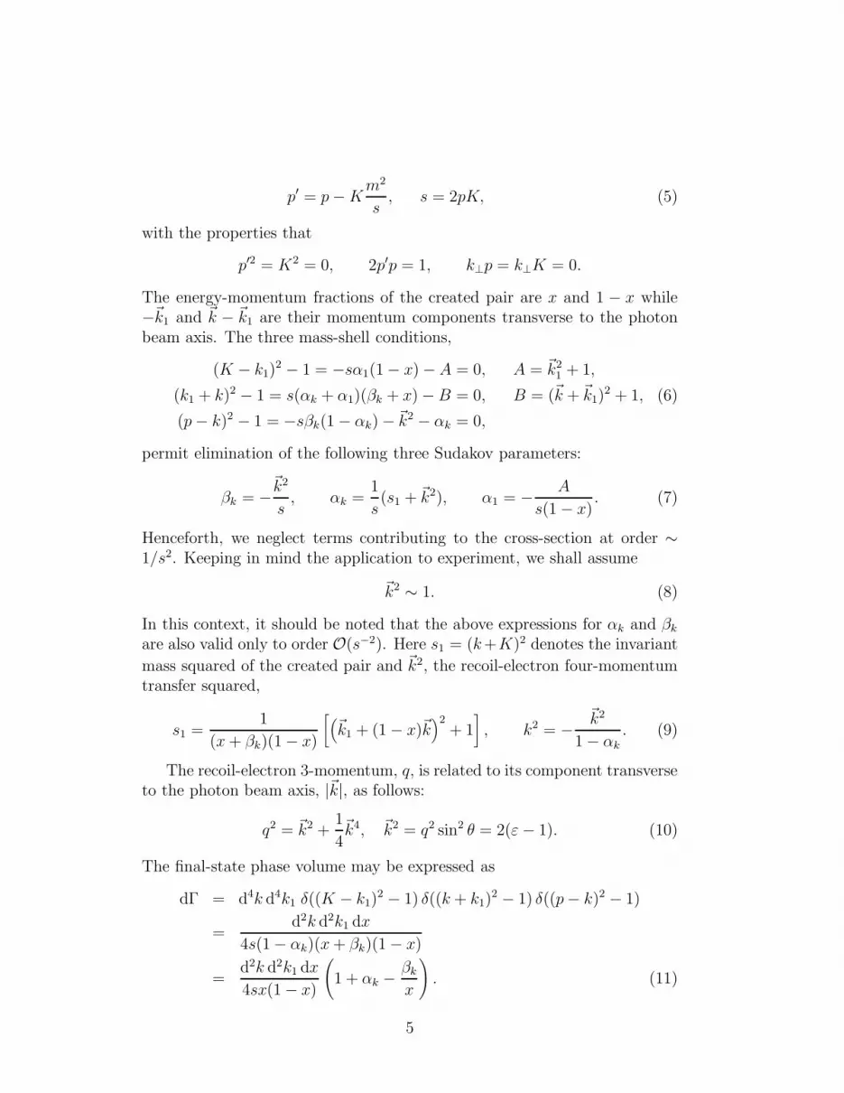
p′ = p − Km2

s, s = 2pK, (5)

with the properties that

p′2 = K2 = 0, 2p′p = 1, k⊥p = k⊥K = 0.

The energy-momentum fractions of the created pair are x and 1 − x while−~k1 and ~k − ~k1 are their momentum components transverse to the photonbeam axis. The three mass-shell conditions,

(K − k1)2 − 1 = −sα1(1 − x) − A = 0, A = ~k2

1 + 1,

(k1 + k)2 − 1 = s(αk + α1)(βk + x) − B = 0, B = (~k + ~k1)2 + 1, (6)

(p − k)2 − 1 = −sβk(1 − αk) − ~k2 − αk = 0,

permit elimination of the following three Sudakov parameters:

βk = −~k2

s, αk =

1

s(s1 + ~k2), α1 = − A

s(1 − x). (7)

Henceforth, we neglect terms contributing to the cross-section at order ∼1/s2. Keeping in mind the application to experiment, we shall assume

~k2 ∼ 1. (8)

In this context, it should be noted that the above expressions for αk and βk

are also valid only to order O(s−2). Here s1 = (k+K)2 denotes the invariant

mass squared of the created pair and ~k2, the recoil-electron four-momentumtransfer squared,

s1 =1

(x + βk)(1 − x)

[

(

~k1 + (1 − x)~k)2

+ 1]

, k2 = −~k2

1 − αk

. (9)

The recoil-electron 3-momentum, q, is related to its component transverseto the photon beam axis, |~k|, as follows:

q2 = ~k2 +1

4~k4, ~k2 = q2 sin2 θ = 2(ε − 1). (10)

The final-state phase volume may be expressed as

dΓ = d4k d4k1 δ((K − k1)2 − 1) δ((k + k1)

2 − 1) δ((p − k)2 − 1)

=d2k d2k1 dx

4s(1 − αk)(x + βk)(1 − x)

=d2k d2k1 dx

4sx(1 − x)

(

1 + αk −βk

x

)

. (11)

5

In terms of these variables, the total differential cross-section may be writtenin the form:

dσ =α3

π2(~k2)2

{

a01212 +

1

s

[

a01212

(

−sαk − sβk

x

)

+ a11212 (12)

− 2~k2

1 − xa1234 +

2~k2

x + βk

a1278 −2~k2

s1

a1256

]}

d2k1 dx d2k,

with

a01212 =

~k2

AB− 4x(1 − x)

R11(B − A)2

A2B2+ 8x(1 − x)

R1(B − A)

AB2

− 4x(1 − x)R

B2,

a11212 =

~k2

(x + βk)

(

B − A

AB−

~k2

AB

)

+ 4~k2

(

(3x − 2)R11(B − A)

AB2+ (1 − x)

R11(B − A)

A2B

)

− 4(3x − 2)R~k2

B2− 4~k2

(

(6x − 4)R1

B2+ (3 − 4x)

R1

AB

)

,

a1234 =1

4

(

B − A

AB−

~k2

AB

)

− 2x(1 − x)R11(B − A)

AB2+ 2x(1 − x)

R

B2

− 2x(1 − x)(

R1(B − A)

AB2− R1

B2

)

,

a1256 =1

2(x + βk)(1 − x)

(

xA

B+ (1 − 2x) − x

~k2

B− (1 − x)

(

B

A−

~k2

A

))

+ 4R11(B − A)

AB− 4(1 − x)

R

B+ 4(1 − x)

R1

A− 4(2 − x)

R1

B,

a1278 = −1

4

(

B − A

AB+

~k2

AB

)

+ 2x(1 − x)R11(B − A)

A2B

− 2x(1 − x)R1

AB(13)

and

R11 = ek1 e∗k1, R1 =1

2(ek1 e∗k + ek e∗k1), R = ek e∗k =

~k2

2(1 + P ).

In general, the limits of variation for the parameters of the created pair areimposed by experimental cuts together with the following relations

(K − k1)0 = w(1 − x) > m, (k1 + k)0 = (x + βk)ω > m,

s1 < s, s = 2ω

6

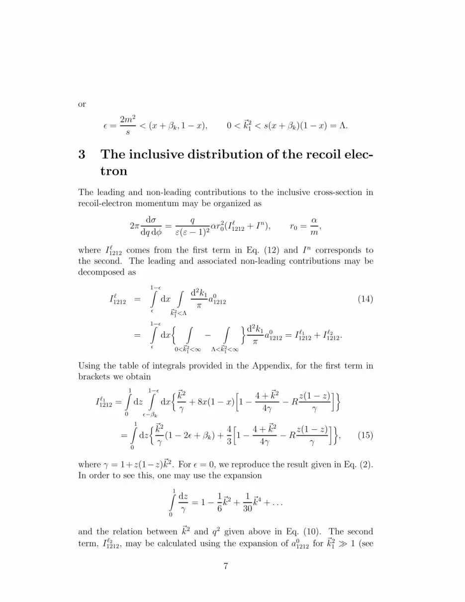
or

ǫ =2m2

s< (x + βk, 1 − x), 0 < ~k2

1 < s(x + βk)(1 − x) = Λ.

3 The inclusive distribution of the recoil elec-

tron

The leading and non-leading contributions to the inclusive cross-section inrecoil-electron momentum may be organized as

2πdσ

dq dφ=

q

ε(ε − 1)2αr2

0(Iℓ1212 + In), r0 =

α

m,

where Iℓ1212 comes from the first term in Eq. (12) and In corresponds to

the second. The leading and associated non-leading contributions may bedecomposed as

Iℓ1212 =

1−ǫ∫

ǫ

dx∫

~k2

1<Λ

d2k1

πa0

1212 (14)

=

1−ǫ∫

ǫ

dx{

∫

0<~k2

1<∞

−∫

Λ<~k2

1<∞

}

d2k1

πa0

1212 = Iℓ11212 + Iℓ2

1212.

Using the table of integrals provided in the Appendix, for the first term inbrackets we obtain

Iℓ11212 =

1∫

0

dz

1−ǫ∫

ǫ−βk

dx{~k2

γ+ 8x(1 − x)

[

1 − 4 + ~k2

4γ− R

z(1 − z)

γ

]}

=

1∫

0

dz{~k2

γ(1 − 2ǫ + βk) +

4

3

[

1 − 4 + ~k2

4γ− R

z(1 − z)

γ

]}

, (15)

where γ = 1+z(1−z)~k2. For ǫ = 0, we reproduce the result given in Eq. (2).In order to see this, one may use the expansion

1∫

0

dz

γ= 1 − 1

6~k2 +

1

30~k4 + . . .

and the relation between ~k2 and q2 given above in Eq. (10). The second

term, Iℓ21212, may be calculated using the expansion of a0

1212 for ~k21 ≫ 1 (see

7

Eq. (30) in the Appendix)

Iℓ21212 = −2~k2

s(L − ln 2 − 1). (16)

The quantity In may also be expressed as a sum: In = Ic1212 + I int.

Consider now the contributions arising from corrections to the leading term(see Eq. (12)):

Ic1212 =

1−ǫ∫

ǫ

dx∫

~k2

1<Λ

d2k1

πa0

1212

(

−αk −βk

x

)

=

1−ǫ∫

ǫ

dx∫

d2k1

πa0

1212

(1 − x)~k2

sx

− 1

s

1−ǫ∫

ǫ

dx

x(1 − x)

∫

~k2

1<Λ

d2k1

πa0

1212

[

1 +(

~k1 + (1 − x)~k)2]

= Ic11212 + Ic2

1212 + Ic31212. (17)

The first term on the RHS of Eq. (17) gives

Ic11212 =

~k2

s

1∫

0

dz{~k2

γ(L − ln 2 − 1) +

8

3

[

1 − 4 + ~k2

4γ− R

z(1 − z)

γ

]}

.

It is convenient also to present the second term as a sum of two parts.The first, containing L2, comes from the a0

1212 term, non-vanishing for bothx → 0 and x → 1:

Ic21212 = −

~k2

s

1−ǫ∫

ǫ

dx

x(1 − x)

∫

d2k1

π

xA + (1 − x)B − x(1 − x)~k2

AB

=~k2

s

1∫

0

dz~k2

γ− 2

~k2

s

[

1

2(L2 − ln2 2) − π2

6

]

. (18)

The remaining terms are

Ic31212 = −4

s

1−ǫ∫

ǫ

dx∫

~k2

1<Λ

d2k1

π

[

xA + (1 − x)B − x(1 − x)~k2

]

[

−R11

(

1

A− 1

B

)2

+ 2R1

(

1

AB− 1

B2

)

− R

B2

]

= r1 + r2.

8

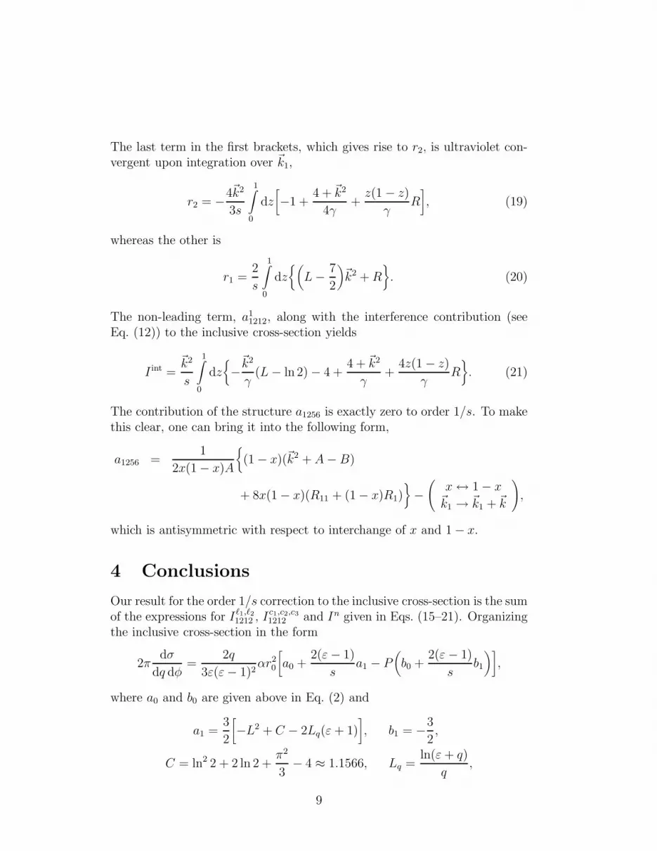
The last term in the first brackets, which gives rise to r2, is ultraviolet con-vergent upon integration over ~k1,

r2 = −4~k2

3s

1∫

0

dz[

−1 +4 + ~k2

4γ+

z(1 − z)

γR]

, (19)

whereas the other is

r1 =2

s

1∫

0

dz{(

L − 7

2

)

~k2 + R}

. (20)

The non-leading term, a11212, along with the interference contribution (see

Eq. (12)) to the inclusive cross-section yields

I int =~k2

s

1∫

0

dz{

−~k2

γ(L − ln 2) − 4 +

4 + ~k2

γ+

4z(1 − z)

γR}

. (21)

The contribution of the structure a1256 is exactly zero to order 1/s. To makethis clear, one can bring it into the following form,

a1256 =1

2x(1 − x)A

{

(1 − x)(~k2 + A − B)

+ 8x(1 − x)(R11 + (1 − x)R1)}

−(

x ↔ 1 − x~k1 → ~k1 + ~k

)

,

which is antisymmetric with respect to interchange of x and 1 − x.

4 Conclusions

Our result for the order 1/s correction to the inclusive cross-section is the sumof the expressions for Iℓ1,ℓ2

1212 , Ic1,c2,c31212 and In given in Eqs. (15–21). Organizing

the inclusive cross-section in the form

2πdσ

dq dφ=

2q

3ε(ε − 1)2αr2

0

[

a0 +2(ε − 1)

sa1 − P

(

b0 +2(ε − 1)

sb1

)]

,

where a0 and b0 are given above in Eq. (2) and

a1 =3

2

[

−L2 + C − 2Lq(ε + 1)]

, b1 = −3

2,

C = ln2 2 + 2 ln 2 +π2

3− 4 ≈ 1.1566, Lq =

ln(ε + q)

q,

9

-0.02

-0.01

0

0.01

0.02

0.03

0.04

0.05

0.06

0.07

10 102

103 0.015

0.02

0.025

0.03

0.035

0.04

0.045

0.05

0.055

0.06

0.5 1 1.5 2

∆A ∆A

s q

q=0.3

q=1.0

q=1.5

s=10

s=50

s=100

a) b)

Figure 2: The dependence of the correction, ∆A, to the asymmetry as afunction of a) s and b) q.

we extract the asymmetry,

A = A + ∆A =b0

a0

+~k2

s

b1a0 − a1b0

a20

. (22)

The expansion of ∆A can be recast in the form (and this is our finalresult),

∆A =3(ε − 1)

sa20

[

L2 − C − 1 + Lq(5 − L2 + C) − 2L2q(ε + 1)

]

. (23)

The the dependence of this quantity on q at fixed s and vice versa is shownin Figs. 2a and b (recall that we have set m = 1).

For small enough s <∼ 10 the terms of order of 1/sn, for n ≥ 2, becomeessential and the approach presented in this paper is not applicable.

We should like to point out that our results are in qualitative agreementwith those obtained using the HELAS code [9] and reported in the talkdelivered at the workshop [4].

Acknowledgments

Three of us (IVA, EAK and BGS) are grateful to the DESY staff for hospital-ity. The work of EAK and BGS was partially supported by the Heisenberg-Landau Programme and the Russian Foundation for Basic Research grant99-02-17730. The work of HA was supported by the Bundesministerium furBildung, Wissenschaft, Forschung und Technologie (BMBF), Germany. EAKis also grateful to L.S. Petrusha for help.

10

Appendix

Since the amplitudes of the gauge-invariant sets of diagrams (3,4), (5,6) and

(7,8) are suppressed by at least one power of ~k2/s as compared to amplitude(1,2), we need only consider interference terms. Thus, for the modulus ofthe matrix element, squared and summed over fermion spin states, we havewithin leading (∼ s2) and non-leading (∼ s) accuracy, in order

∑

|M |2 =(4πα)3

~k2

{

− 2T1234

s(1 − x)− 2T1256

s1

+2T1278

sx+

T1212(1 − αk)2

~k2

}

, (24)

where

T1212 = Tr {( 6q + 1)γµ( 6p + 1)γν}×Tr

{

( 6K− 6k1 + 1)Oµλ12 ( 6k1+ 6k − 1)O

νσ

34

}

eλe∗

σ,

T1234 = Tr{

( 6q + 1)γµ( 6p + 1)γν( 6K− 6k1 + 1)Oµλ12 ( 6k1+ 6k − 1)O

νσ

34

}

eλe∗

σ,

T1256 = Tr{

( 6q + 1)γµ( 6p + 1)Oνσ

56

}

(25)

×Tr{

( 6K− 6k1 + 1)Oµλ12 ( 6k1+ 6k − 1)γν

}

eλe∗

σ,

T1278 = Tr{

( 6q + 1)γµ( 6p + 1)Oνσ

78 ( 6K− 6k1 + 1)Oµλ12 ( 6k1+ 6k − 1)γν

}

eλe∗σ,

Oµλ12 = −x + βk

Bγµ( 6K− 6k1− 6k + 1)γλ −

1 − x

Aγλ(− 6k1 + 1)γµ,

Oµλ34 = − x

Bγµ( 6K− 6k1− 6k + 1)γλ −

1

sγλ( 6p− 6K− 6k + 1)γµ,

Oµλ56 =

1

s[−γλ( 6p− 6K− 6k + 1)γµ + γµ( 6p+ 6K + 1)γλ] ,

Oµλ78 = −1 − x

Aγλ(− 6k1 + 1)γµ +

1

sγµ( 6p+ 6K + 1)γλ,

and q = p − k.The quantities Tijkl are related to the aijkl given in Eq. (13) by

T1212 = 16sx(1 − x) [a01212s + a1

1212],

T1234,1278 = 16s2x(1 − x) a1234,1278,

T1256 = 16sx(1 − x) a1256. (26)

To perform the integration over ~k1, we introduce an ultraviolet cut-off ~k21 < Λ,

which may be omitted when calculating convergent integrals for the correc-tions. The integrals containing A or B are (hereinafter we omit the terms of

11

order of 1/s)

∫

d2~k1

π

1

A2=∫

d2~k1

π

1

B2= 1,

∫

d2~k1

π

R1

B2= −R, (27)

∫

d2~k1

π

R11

A2=

1

2(ln Λ − 1),

∫

d2~k1

π

R11

B2=

1

2(lnΛ − 1) + R.

In order to avoid linearly divergent integrals, we combine denominators asfollows:

1

AB=

1∫

0

dz

[(~k1 + z~k)2 + γ]2,

with γ = 1 + ~k2z(1 − z). Integrating over ~k1 we obtain

∫

d2~k1

π

1

AB=

1∫

0

dz

γ=

1

qln(ε + q) = Lq,

∫ d2~k1

π

R1

AB= −

1∫

0

zdz

γR = −R

1∫

0

dz

2γ, (28)

∫

d2~k1

π

R11

AB=

1∫

0

dz[

1

2(ln Λ − 1) − 1

2ln γ +

z2

γR]

.

To evaluate the quantity r1, we use the following set of integrals:

∫

d2~k1

π[xA + (1 − x)B]

R

B2= R

(

ln Λ + x~k2)

,

∫

d2~k1

π[xA + (1 − x)B]R1

A − B

AB2= −R

(

ln Λ − 1 + x~k2)

, (29)

∫

d2~k1

π[xA + (1 − x)B]R11

A − B

AB=

R +~k2

2

[

ln Λ − 3

2

]

+ x~k2R.

In deriving (16), for a01212 averaged over angles with ~k2

1 ≫ 1, we make use of

a01212|~k2

1≫1

≈~k2

(~k21)

2(1 − 2x(1 − x)) (30)

and to perform the angular averaging in r1 we use

R11(~k~k1)2 → 1

8(~k2

1)2[~k2 + 2R].

12

References

[1] V.F. Boldyshev and Yu.P. Peresun’ko, Yad. Fiz. 13 (1971) 588.

[2] E.A. Vinokurov and E.A. Kuraev, JETP 36 (1973) 602.

[3] V.F. Boldyshev, E.A. Vinokurov, et al., Particles and Fields 25 (1994)696.

[4] R. Pywell and G. Feldman, talk given at the workshop on “PolarizedPhoton Polarimetry”, TJNAF, 2–3 June 1998.

[5] K.J. Mork, Phys. Rev. 160 (1967) 1065.

[6] E. Haug, Z. Naturforschung A30 (1975) 1099; Phys. Rev. D31 (1985)2120; D32 (1985) 1594.

[7] K.S. Suh and H.A. Bethe, Phys. Rev. 115 (1959) 672.

[8] A. Borsellino, Nuovo Cim. 4 (1947) 112;J. Mott, H. Olssen and H. Koch, Rev. Mod. Phys. 41 (1969) part 1.

[9] I. Endo and T. Kobayashi, Nucl. Inst. Meth. A328 (1993) 517.

13