Transferring JIT Manufacturing Philosophy to Service Production Systems

NCCADT-2012, 21ST

APRIL 2012, MAIT, NEW DLEHI-86

Page 1 of 204

Transferring JIT Manufacturing Philosophy to Service

Production Systems Anil Kumar Gupta

DCRUST, Murthal

Abstract

Just- in- Time (JIT) concepts have been successfully implemented in manufacturing

organizations. There is reasonable consensus among researchers that JIT is a useful and

beneficial approach to reduce the manufacturing costs while simultaneously improving the

quality of a product [1]. Numerous organizations have reported time and cost savings due to

JIT practices [2]. However, most of the reported instances of successful and unsuccessful JIT

practices lie with in manufacturing settings.

Service sector worldwide is growing very fast. Consequently, a considerable body of research

was built in Service Operations Management within the past decade; however we could not find any analytical work on the applications of JIT in service sector. Some conceptual article

and case studies [3, 4, 5, 6] have shown that JIT is eminently suited to non-manufacturing

situations as well as, such as in service and administrative work situations. Various researchers [7, 8, and 9] are of the view that service industries can improve their operations

by using techniques and tools similar to the ones used in manufacturing environments.

However, all these studies have been reported at the conceptual level. An attempt on this issue is being made in this paper. A detailed literature survey on the issue is being done and

some research directions for future work have been identified.

Introduction

Service sector worldwide is growing very fast. Service sector constitutes more than 70 percent of the GDP in many developed economies. According to the 1999 Statistical Yearbook (United Nations, 1999) service sector employment is more than 80% in United States and more than 70 percent in Canada, Japan, France, Israel, and Australia. There is no such thing as a service industry. There are only industries whose service components are greater or less than those of other industries. Everybody is in service [10]. Many of the jobs in manufacturing are actually disguised as service jobs . The largest component of internal lead-time for a manufacturer is often in a service department. With the increasing volume of service organizations and their important role in all major industrialized economies, it was imperative for service operations management (SOM) to evolve as a separate field addressing productivity and quality issues in service organizations. Consequently, a considerable body of research was built in SOM within the past decade; however we could not find any survey and modelling work on the applications of JIT in service sector. There is a reasonable consensus among researchers that Just-In-Time (JIT) is a useful and beneficial approach for reducing the manufacturing costs while simultaneously improving the quality of a product (11). Numerous organizations have reported cost cutting and improved quality due to JIT practices (12). Most of the reported instances of successful and unsuccessful JIT practices lie within the manufacturing domain. Some studies of JIT applications in service sector (13, 14, 15) have reported the benefits of improved service to customers, reduced response time/lead time, improved quality, and reduced costs in different service organizations. Researchers (16, 17) have realized that the challenges in service organizations are not necessary of the same nature as manufacturing organizations. Services cannot be treated as merely goods with some odd characteristics. As a matter of fact, the characteristics of most service firms differ widely from those of manufacturing firms. However, some concepts and tools developed in the manufacturing domain can be altered to fit and benefit service organizations. (18) have adapted the concept of Quality Function Deployment (QFD) for service firms. Statistical Process Control (19), just in time, and Quality Circles all originated in manufacturing and then were adopted by SOM researchers to fit service organizations. This paper is built on the premise that the service sector can also benefit from JIT philosophy.

NCCADT-2012, 21ST


Page 2 of 204

Motivation

JIT can be applied to a variety of industries. Among these, services sector has the largest potential for productivity, quality improvement and cost savings. The service sector is growing very rapidly in India. It offers tremendous potential to improve the quality of life as well as provide employment to the educated. Being young in this sector, India has a lot to learn from the experience of the developed countries this regard. Service sector is growing in importance but poorly managed. The management and marketing systems in the services sector continue to suffer from lack of adequate systemization. The techniques for effective service operations management are not fully developed as in manufacturing. Therefore, there is need for transferring JIT and other operations management techniques in service sector. Service Production System

Any discussion of service systems must look at how they differ from manufacturing systems. Prior studies and analyses (20, 21, 22) indicate the main features of a service, which distinguishes it, form a product. These features include: 1. Inseparability of production and consumption

This involves the simultaneous production and consumption, which characterizes many services. Simultaneous production and consumption also eliminates many opportunities for quality control intervention. Unlike manufacturing, where the product can be inspected before delivery, services must rely on a sequence of measures in order to ensure the consistency of output. This emphasizes the importance of process control in services even more so than in manufacturing, since services at times do not deal with a physical product to inspect. 2. The customer is a participant in the service process

Customer is always involved in service production process. Degree of customer involvement may vary. By categorizing services on a continuum ranging from low to high contact; we can better appreciate the trade off between flexibility and efficiency of operations . Generally high contact process technology is more flexible to accommodate the unique needs of diverse customers. When the flexibility is high, efficiency is often low because the conversion process can not be standardized. At the low contact end of the continuum, the process technology can be less flexible, because customers are absent during the conversion process, and consequently the operations can be oriented more towards standardization and efficiency. 3. Intangibility

Because services are performances, ideas or concepts, rather than tangible objects, they often cannot be seen, felt, etc., in the same manner in which goods can be sensed. When buying a product, the consumer may be able to see, feel and test its performance before purchase. With services, the consumer must often rely on the reputation of the service firm. These less measurable considerations have the potential to greatly influence consumers’ perceptions and expectations of quality. 4. Perishability This refers to the concept that a service cannot be saved or inventoried. The inability to store services is a critical feature of most service operations. Vacant hotel rooms, empty airline seats and unfilled appointment times for a doctor are all examples of opportunity losses. Perishabilitym leads to the problem of synchronization supply and demand, potentially causing customers to wait or not to be served at all. 5. Heterogeneity Heterogeneity of services in consequences of explicit and implicit service elements relying on individual preferences and perceptions. 6. Labor Intensiveness

Service operations are labor- intensive.

These features emphasize the essential uniqueness of service management and dispel the common belief that manufacturing management principles can be applied to services without recognition of the uniqueness of the service delivery system.

Literature Review

NCCADT-2012, 21ST


Page 3 of 204

In spite of natural differences between manufacturing and service, there are possible applications and benefits of JIT techniques in service industries. Chase [23] proposed a new way of viewing service operations and showed a classification scheme for service systems and suggested a framework for developing a production policy for the service system. Given the fact that activities in many service systems are sequentially identical to the activities in manufacturing systems, it can be intuitively asserted that service operations can effectively use production techniques to improve their output and, hence, profitability. Levitt [10] suggested a production- line approach to service. Services are thought in humanistic terms and manufacturing in technocratic terms. That is why manufacturing industries are forward looking and efficient while the service industries and customer service are, by comparison primitive and inefficient. Once service in the field receives the same attention as products in the factory, a lot of new opportunities become possible. The solution is to take a manufacturing approach to this activity i.e. the approach that substitutes technology and systems for people. Highly automated and controlled conditions are to be generated in providing services like an assembly line of a car manufacturing company. Weiters [24] while justifying JIT in service industries illustrated that JIT system is not only for reducing the inventory. Most service organizations will not find physical inventory reductions as a major source of financial justification, there are other significant attributes of JIT that offer benefits to these organizations. It eliminates waste, promotes fast changeovers, streamlines the operations, establishes close supplier relations and adjusts quickly to the changes in demand so that products and services can be provided quickly, at less cost and in more variety. The system-wide approach of JIT has greater role to play in services than in manufacturing. Productivity of our service sector becomes even more critical as it gains a larger segment of our economy. One of the first identified areas of JIT applications within the service industry is healthcare sector. Whitson [25] suggested JIT delivery of the items to eliminate inventory in hospital operations. JIT delivery means that the products needed would be available only when they are needed. This assumes that delivery system is reliable. The item would be delivered to the point of use, by passing the warehouse. This would eliminate the storage and excessive handling of the item. If this ideal situation could be realized, it is clear that the number of times that each item is handled would be reduced. The less the items are handled, the less money is spent by the organization getting the necessary items where they need to be. Billesbach and Schniederjans [5] present a case study on JIT applications in administration. They identified JIT elements like employee involvement and empowering of employees which can improve efficiency. They suggested that waste activities (not contributing to any result) should be identified and eliminated. Benson [4] stated that "many of the jobs in manufacturing are actually disguised as service jobs, the largest component of internal lead-time for a manufacturer is often in a service department. If JIT is going to dramatically reduce the overall flow time, the supporting service departments cannot be ignored." Claire [6] called the maintenance function one of the most critical, yet overlooked area of a successful JIT operation. If a maintenance function has to be truly effective it must employ a total maintenance management approach to the control of its four basic resources: maintenance labor, plant equipment, maintenance information, and maintenance inventory. Through a case study he was able to eliminate warehouse, reduce inventory, improve service, improve quality, and lower price levels. The benefits reported were; long-term relationship with vendors, single sourcing, improved quality, improved service, lower prices, simplified ordering and receiving procedures, and decreased costs including purchasing and administrative costs, carrying costs, labor costs etc. Inman and Mehra [13] through some case studies examined the potential for JIT within service industries. These case examples showed that while all the firms under study sought to reduce inventory, it was not the sole aim of any of the firms. Improved service, quality, communication, and pricing also provided the justification for JIT implementation in the service environments. Benefits resulting from JIT adoption by service firms and service

NCCADT-2012, 21ST


Page 4 of 204

environments were many and therefore justifying JIT on the basis of inventory reduction alone is unnecessary and probably considered secondary when compared with the multitude of other potential benefits Lee [26] illustrated the case of a finance company to justify the applications of JIT in service industries. The existing loan process usually takes 12 days. Process was studied in detail and it was found that some of the activities were not adding any value and in JIT system, it is termed as waste. So a process improvement effort started in line with JIT so that there are only value added operations. In the new process, there was no waiting time between processes and operations, and some operations were performed simultaneously in order to reduce the processing time. The new process took four to five days. Another potential area of JIT applications in service sector is hotel industry. Barlow [27] investigated the applicability of JIT techniques in hotel industry. He concluded that hotels would gain financial saving on their inventory by adopting JIT approach. Carlson [28] described a case of JIT applications in warehousing and distribution operations. In this type of service operations, quality, timeliness and cost of services are extremely important to stay competitive. One measures of the effectiveness of JIT application was the reduction of errors and complaints, leading directly to higher productivity. Savings in pick route distance, storage space and the cost of warehousing operations were the other measures Conant [29] discussed the case of JIT application in mail-order operation by a company. The large number of customer complaints on this product line arose on account of information delays on the amount charged and order delivery days. These were caused by the customer waiting times of three or more weeks and a monthly charging of the customers. Order processing involved booking the order on telephone, invoicing, and customer verification, setting an account (for new customers), proof reading, and type setting. The whole process took about four days, due to the daily batch processing. A JIT like operation was achieved by the use of three order batches per day, elimination of new customer setup process, and faster pace of working in order verification area. As a result, the order processing lead -time went down from four days to four hours. The backlog got reduced significantly and a large percentage of the orders were shipped within four days to achieve customer delivery within two weeks. The complaint calls went down sharply. Messmer [30] reported that if an accounting department manages staff like a manufacturer manages inventory, it could increase productivity. The concept of JIT can be applied to staffing through a rigorous process of planning and analysis in which specific tasks and individual workloads are evaluated carefully in order to determine the departmental staffing priorities. This concept of JIT staffing is becoming increasingly prevalent in USA companies. Research issues

From literature survey it has been found that there is reasonable consensus among researchers that JIT can be applied to a variety of service organizations. The studies so far reported in literature are at very conceptual level. No detailed study involving survey, modeling and analysis work on JIT applications in service sector has been reported till date. So there is a need to carry out such studies. Also, there is a need to investigate the following issues;

1) How easy or difficult it is to transfer JIT philosophy to service production system. 2) JIT as a whole may not be applicable to any particular service industry. So there is a

need to identify JIT elements that can be more relevant and easy to implement. Also there is need to identify those areas of a particular service industry those are more relevant to JIT applications.

3) More case studies are needed to expand the base of information in this field. 4) Identification of factors helpful in implementation of JIT in service sector. 5) There are so many intangible and non quantifiable benefits of JIT, so there is a need

to develop accurate, reliable, measurable standards to evaluate accurately the effects of JIT i.e. How to judge the impact of JIT on service quality is another issue for research.

References

NCCADT-2012, 21ST


Page 5 of 204

1. Monden, Y. (1983),"Toyota Production System: A practical approach to production management", Industrial Engineering and Management Press, Atlanta. 2. Korgaonker, M.G. (1992), "Just In Time manufacturing", Macmillan India Limited. 3. Alonso, R.L., and Frasier, C.W. (1991),"JIT hits home: a case study in reducing management delays", Sloan Management Review, pp. 59-67. 4. Benson, Randall J. (1986), “JIT: Not just For the Factory!” APICS 29th Annual

International Conference Proceedings), pp. 370-374. 5. Billesbach, T. and Schniderjans, M. (Third quarter, 1989),"Applicability of JIT techniques in administration", Production and Inventory Management, pp. 40-45 6. Claire, F.V., 1986, “The weakest link? : JIT and maintenance management”, Production

and Inventory Management Review with APICS News, pp. 36,40,44 and 45. 7. Fitzsimmons, J. and Fitzsimmons, M. (1994),"Service management for competitive advantage", McGraw-Hill, New York. 8. Inman, R.A. and Mehra, S. (1990), “JIT Implementation within a service industry: A case study", International Journal of Service Industry Management, Vol. 1, No. 3, pp. 53-61. 9. Lees, J., and Dale, B. (1988), "Quality circles in service industries: A study of their use", The Service Industry Journal, Vol. 8, No. 2. 10. Levitt, T. (Sep-Oct. 1972), " Production line approach to service", Harvard Business Review, pp. 42-52. 11. Miltenberg, G.J., " Changing MRP's Costing Procedure to suit JIT, " Production and

Inventory Management Journal, Vol. 31, No. 2, 1990, pp. 77-83. 12. Crawford, K.M. and Cox, J.M. (1991),"Addressing manufacturing problems through the implementation of just-in-time", Production and Inventory Management Journal, Vol. 32, pp. 33-6. 13. Inman, R.A. and Mehra, S. (1991), “JIT applications for service environments", Production and inventory Management Journal, Vol. 32, No. 3, pp. 16-21. 14. Savage- Moore, W. (Sept. 1988), “The evolution of a JIT environment at Northern Telecom Inc.’s customer service center”, Industrial Engineering, pp. 60-63. 15. Giunipero, L. and Keiser, E. (winter 1987), “JIT purchasing in a non-manufacturing environment: a case study”, Journal of purchasing and material management, pp. 19-25. 16. Bassett, G. (1992), "Operations management for service industries: competing in the service era", Quorum Books, Westport, CT. 17. Norman, R. (1991),"Service management: Strategy and leadership in service business", John Wiley, New York. 18. Behara, R.S. and Chase, R.B. (1993), “Service quality deployment: quality Service by design”, in Rakesh V. Sarin edition, Perspective in Operations Management: Essays in Honor of Elwood S. Buffa, Kluwer Academic Publisher, Norwell, Mass. 19. Apte, U. and Reynolds, C. (May-June 1995) "Quality management at Kentucky fried chicken", Interfaces, Vol. 25, No. 3. 20. Chase, R.B. (1981),"The customer contact approach to services: theoretical bases and practical extensions", Operations Research, Vol. 21, pp. 698-705. 21. Parasuraman, A., Zeithaml, V. and Berry, L. (fall 1985), “A conceptual model of service quality and its implications for future research", Journal of Marketing, Vol. 49, pp. 41-50. 22. Ross, J.E. (1994),"Total Quality Management Text, Cases and Readings", London, Kogan

Page 23. Chase, R.B., and Gravin, D.A. (July-Aug 1989), "The service factory", Harvard Business

Review, pp. 61-69. 24. Weiters, David C. (1984), “Justifying JIT in service industries”, Readings in Zero

inventory, APICS annual international conference proceedings, pp. 166-169. 25. Whitson, D. (Aug. 1997),“Applying JIT systems in health care", IIE solutions, pp. 33-37. 26. LEE, J.Y. (1990), “JIT works for services too", CMA Magazine, Vol. 64, pp. 620-23. 27. Barlow,G.L.(2002), “ Just-in-time: Implementation within the hotel industry- A case study” International Journal of Production Economics, Vol. 80, pp. 155-167 28. Carlson,J.,“Improvement curve analysis of changeovers in JIT environments”, Engineering Cost and Production Economics, Vol. 17, pp. 315-322

NCCADT-2012, 21ST


Page 6 of 204

29. Conant, R. (Sept. 1998), “JIT in a mail order operation: processing time reduced from 4 days to 4 hours ", Industrial Engineering, pp. 34-37. 30. Messer, M. (October 1996),"How JIT Staffing can add value to your accounting department", Management Accounting, pp. 28-31.

NCCADT-2012, 21ST


Page 7 of 204

The Embedded Systems Design Challenges Akanksha Tyagi, Ashutosh Sharma

M.Tech Scholars,Laxmi Devi Institute of Engineering and Technology, Alwar (Raj)

[email protected] [email protected]

Abstract We summarize some current trends in embedded systems design and point out some of their

characteristics, such as the chasm between analytical and computational models, and the gap

between safety critical and best-effort engineering practices. We call for a coherent scientific

foundation for embedded systems design, and we discuss a few key demands on such a

foundation: the need for encompassing several manifestations of heterogeneity, and the need

for constructivity in design. We believe that the development of a satisfactory Embedded

Systems Design Science provides a timely challenge and opportunity for reinvigorating computer science.

1. Introduction

Computer Science is going through a maturing period. There is a perception that many of the original, defining problems of Computer Science either have been solved, or require an unforeseeable breakthrough (such as the P versus NP question). It is a reflection of this view that many of the currently advocated challenges for Computer Science research push existing technology to the limits (e.g., the semantic web [4]; the verifying compiler [15]; sensor networks [6]), to new application areas (such as biology [12]), or to a combination of both (e.g., nanotechnologies; quantum computing). Not surprisingly, many of the brightest students no longer aim to become computer scientists, but choose to enter directly into the life sciences or nano engineering [8]. Our view is different. Following [18, 22], we believe that there lies a large uncharted territory within the science of computing. This is the area of embedded systems design. As we shall explain, the current paradigms of Computer Science do not apply to embedded systems design: they need to be enriched in order to encompass models and methods traditionally found in Electrical Engineering. Embedded systems design, however, should not and cannot be left to the electrical engineers, because computation and software are integral parts of embedded systems. Indeed, the shortcomings of current design, validation, and maintenance processes make software, paradoxically, the most costly and least reliable part of systems in automotive, aerospace, medical, and other critical applications. Given the increasing ubiquity of embedded systems in our daily lives, this constitutes a unique opportunity for reinvigorating Computer Science. In the following we will lay out what we see as the Embedded Systems Design Challenge. In our opinion, the Embedded Systems Design Challenge raises not only technology questions, but more importantly, it requires the building of a new scientific foundation —a foundation that systematically and even-handedly integrates, from the bottom up, computation and physicality [14].

2. Current Scientific Foundations for Systems Design, and their Limitations

The Embedded Systems Design Problem

What is an embedded system? An embedded system is an engineering artifact involving computation that is subject to physical constraints. The physical constraints arise through two kinds of interactions of computational processes with the physical world: (1) reaction to a physical environment, and (2) execution on a physical platform. Accordingly, the two types of physical constraints are reaction constraints and execution constraints. Common reaction constraints specify deadlines, throughput, and jitter; they originate from the behavioral requirements of the system. Common execution constraints put bounds on available processor speeds, power, and hardware failure rates; they originate from the implementation requirements of the system. Reaction constraints are studied in control theory; execution constraints, in computer engineering. Gaining control of the interplay of computation with both kinds of constraints, so as to meet a given set of requirements, is the key to embedded systems design.

NCCADT-2012, 21ST


Page 8 of 204

Systems design in general. Systems design is the process of deriving, from requirements, a model from which a system can be generated more or less automatically. A model is an abstract representation of a system. For example, software design is the process of deriving a program that can be compiled; hardware design, the process of deriving a hardware description from which a circuit can be synthesized. In both domains, the design process usually mixes bottom-up and top-down activities: the reuse and adaptation of existing component models; and the successive refinement of architectural models in order to meet the given requirements. Embedded systems design. Embedded systems consist of hardware, software, and an environment. This they have in common with most computing systems. However, there is an essential difference between embedded and other computing systems: since embedded systems involve computation that is subject to physical constraints, the powerful separation of computation (software) from physicality (platform and environment), which has been one of the central ideas enabling the science of computing, does not work for embedded systems. Instead, the design of embedded systems requires a holistic approach that integrates essential paradigms from hardware design, software design, and control theory in a consistent manner. We postulate that such a holistic approach cannot be simply an extension of hardware design, nor of software design, but must be based on a new foundation that subsumes techniques from both worlds. This is because current design theories and practices for hardware, and for software, are tailored towards the individual properties of these two domains; indeed, they often use abstractions that are diametrically opposed. To see this, we now have a look at the abstractions that are commonly used in hardware design, and those that are used in software design.

Analytical versus Computational Modeling

Hardware versus software design. Hardware systems are designed as the composition of interconnected, inherently parallel components. The individual components are represented by analytical models (equations), which specify their transfer functions. These models are deterministic (or probabilistic), and their composition is defined by specifying how data flows across multiple components. Software systems, by contrast, are designed from sequential components, such as objects and threads, whose structure often changes dynamically (components are created, deleted, and may migrate). The components are represented by computational models (programs), whose semantics is defined operationally by an abstract execution engine (also called a virtual machine, or an automaton). Abstract machines may be nondeterministic, and their composition is defined by specifying how control flows across multiple components; for instance, the atomic actions of independent processes may be interleaved, possibly constrained by a fixed set of synchronization primitives. Thus, the basic operation for constructing hardware models is the composition of transfer functions; the basic operation for constructing software models is the product of automata. These are two starkly different views for constructing dynamical systems from basic components: one analytical (i.e., equation-based), the other computational (i.e., machine-based). The analytical view is prevalent in Electrical Engineering; the computational view, in Computer Science: the net list representation of a circuit is an example for an analytical model; any program written in an imperative language is an example for a computational model. Since both types of models have very different strengths and weaknesses, the implications on the design process are dramatic. Analytical and computational models offer orthogonal abstractions. Analytical models deal naturally with concurrency and with quantitative constraints, but they have difficulties with partial and incremental specifications (non determinism) and with computational complexity. Indicatively, equation based models and associated analytical methods are used not only in hardware design and control theory, but also in scheduling and in performance evaluation (e.g., in networking).

NCCADT-2012, 21ST


Page 9 of 204

Computational models, on the other hand, naturally support nondeterministic abstraction hierarchies and a rich theory of computational complexity, but they have difficulties taming concurrency and incorporating physical constraints. Many major paradigms of Computer Science (e.g., the Turing machine; the thread model of concurrency; the structured operational semantics of programming languages) have succeeded precisely because they abstract away from all physical notions of concurrency and from all physical constraints on computation. Indeed, whole subfields of Computer Science are built on and flourish because of such abstractions: in operating systems and distributed computing, both time-sharing and parallelism are famously abstracted to the same concept, namely, nondeterministic sequential computation; in algorithms and complexity theory, real time is abstracted to big-O time, and physical memory to big-O space. These powerful abstractions, however, are largely inadequate for embedded systems design. Analytical and computational models aim at different system requirements. The differences between equation-based and machine-based design are reflected in the type of requirements they support well. System designers deal with two kinds of requirements. Functional requirements specify the expected services, functionality, and features, independent of the implementation. Extra functional requirements specify mainly performance, which characterizes the efficient use of real time and of implementation resources; and robustness, which characterizes the ability to deliver some minimal functionality under circumstances that deviate from the nominal ones. For the same functional requirements, extra-functional properties can vary depending on a large number of factors and choices, including the overall system architecture and the characteristics of the underlying platform. Functional requirements are naturally expressed in discrete, logic-based formalisms. However, for expressing many extra-functional requirements, real-valued quantities are needed to represent physical constraints and probabilities. For software, the dominant driver is correct functionality, and even performance and robustness are often specified discretely (e.g., number of messages exchanged; number of failures tolerated). For hardware, continuous performance and robustness measures are more prominent and refer to physical resource levels such as clock frequency, energy consumption, latency, mean-time to failure, and cost. For embedded systems integrated in mass-market products, the ability to quantify trade-offs between performance and robustness, under given technical and economic constraints, is of strategic importance. Analytical and computational models support different design processes. The differences between models based on data flow and models based on control flow have far-reaching implications on design methods. Equation-based modeling yields rich analytical tools, especially in the presence of stochastic behaviour. Moreover, if the number of different basic building blocks is small, as it is in circuit design, then automatic synthesis techniques have proved extraordinarily successful in the design of very large systems, to the point of creating an entire industry (Electronic Design Automation). Machine-based models, on the other hand, while sacrificing powerful analytical and synthesis techniques, can be executed directly. They give the designer more fine-grained control and provide a greater space for design variety and optimization. Indeed, robust software architectures and efficient algorithms are still individually designed, not automatically generated, and this will likely remain the case for some time to come. The emphasis, therefore, shifts away from design synthesis to design verification (proof of correctness). Embedded systems design must even-handedly deal with both: with computation and physical constraints; with software and hardware; with abstract machines and transfer functions; with non determinism and probabilities; with functional and performance requirements; with qualitative and quantitative analysis; with Booleans and reals. This cannot be achieved by simple juxtaposition of analytical and computational techniques, but requires their tight integration within a new mathematical foundation that spans both perspectives.

NCCADT-2012, 21ST


Page 10 of 204

3. Current Engineering Practices for Embedded Systems Design, and their

Limitations

Model-based Design

Language-based and synthesis-based origins. Historically, many methodologies for embedded systems design trace their origins to one of two sources: there are language-based methods that lie in the software tradition, and synthesis based methods that come out of the hardware tradition. A language-based approach is centered on a particular programming language with a particular target run-time system. Examples include Ada and, more recently, RT-Java [5]. For these languages, there are compilation technologies that lead to event-driven implementations on standardized platforms (fixed-priority scheduling with preemption). The synthesis-based approaches, on the other hand, have evolved from hardware design methodologies. They start from a system description in a tractable (often structural) fragment of a hardware description language such as VHDL and Verilog and, ideally automatically, derive an implementation that obeys a given set of constraints. Implementation independence. Recent trends have focused on combining both language-based and synthesis-based approaches (hardware/software code sign) and on gaining, during the early design process, maximal independence from a specific implementation platform. We refer to these newer approaches collectively as model-based, because they emphasize the separation of the design level from the implementation level, and they are centered around the semantics of abstract system descriptions (rather than on the implementation semantics). Consequently, much effort in model-based approaches goes into developing efficient code generators. We provide here only a short and incomplete selection of some representative methodologies. Model-based methodologies. The synchronous languages, such as Lustre and Esterel [11], embody abstract hardware semantics (synchronicity) within different kinds of software structures (functional; imperative). Implementation technologies are available for several platforms, including bare machines and time-triggered architectures. Originating from the design automation community, System C [19] also chooses a synchronous hardware semantics, but allows for the introduction of asynchronous execution and interaction mechanisms from software (C++). Implementations require a separation between the components to be implemented in hardware, and those to be implemented in software; different design-space exploration techniques provide guidance in making such partitioning decisions. A third kind of model-based approaches are built around a class of popular languages exemplified by MATLAB Simulink, whose semantics is defined operationally through its simulation engine. More recent modeling languages, such as UML [20] and AADL [10], attempt to be more generic in their choice of semantics and thus bring extensions in two directions: independence from a particular programming language; and emphasis on system architecture as a means to organize computation, communication, and constraints. We believe, however, that these attempts will ultimately fall short, unless they can draw on new foundational results to overcome the current weaknesses of model-based design: the lack of analytical tools for computational models to deal with physical constraints; and the difficulty to automatically transform non computational models into efficient computational ones. This leads us to the key need for a better understanding of relationships and transformations between heterogeneous models. Model transformations. Central to all model-based design is an effective theory of model transformations. Design often involves the use of multiple models that represent different views of a system at different levels of granularity. Usually design proceeds neither strictly top-down, from the requirements to the implementation, nor strictly bottom-up, by integrating library components, but in a less directed fashion, by iterating model construction, model analysis, and model transformation. Some transformations between models can be automated; at other times, the designer must guide the model construction. The ultimate success story in model transformation is the theory of compilation: today, it is difficult to manually improve on the code produced by a good optimizing compiler from programs (i.e., computational models) written in a high-level language. On the other hand, code generators often produce

NCCADT-2012, 21ST


Page 11 of 204

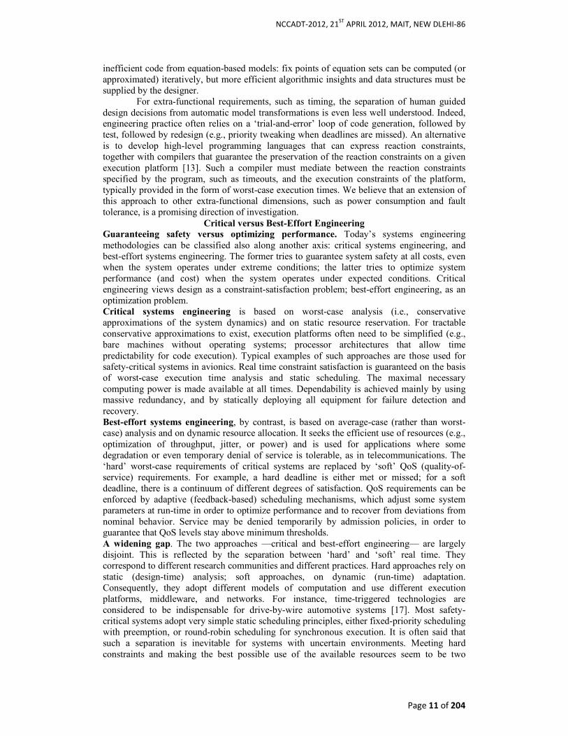
inefficient code from equation-based models: fix points of equation sets can be computed (or approximated) iteratively, but more efficient algorithmic insights and data structures must be supplied by the designer. For extra-functional requirements, such as timing, the separation of human guided design decisions from automatic model transformations is even less well understood. Indeed, engineering practice often relies on a ‘trial-and-error’ loop of code generation, followed by test, followed by redesign (e.g., priority tweaking when deadlines are missed). An alternative is to develop high-level programming languages that can express reaction constraints, together with compilers that guarantee the preservation of the reaction constraints on a given execution platform [13]. Such a compiler must mediate between the reaction constraints specified by the program, such as timeouts, and the execution constraints of the platform, typically provided in the form of worst-case execution times. We believe that an extension of this approach to other extra-functional dimensions, such as power consumption and fault tolerance, is a promising direction of investigation.

Critical versus Best-Effort Engineering

Guaranteeing safety versus optimizing performance. Today’s systems engineering methodologies can be classified also along another axis: critical systems engineering, and best-effort systems engineering. The former tries to guarantee system safety at all costs, even when the system operates under extreme conditions; the latter tries to optimize system performance (and cost) when the system operates under expected conditions. Critical engineering views design as a constraint-satisfaction problem; best-effort engineering, as an optimization problem. Critical systems engineering is based on worst-case analysis (i.e., conservative approximations of the system dynamics) and on static resource reservation. For tractable conservative approximations to exist, execution platforms often need to be simplified (e.g., bare machines without operating systems; processor architectures that allow time predictability for code execution). Typical examples of such approaches are those used for safety-critical systems in avionics. Real time constraint satisfaction is guaranteed on the basis of worst-case execution time analysis and static scheduling. The maximal necessary computing power is made available at all times. Dependability is achieved mainly by using massive redundancy, and by statically deploying all equipment for failure detection and recovery. Best-effort systems engineering, by contrast, is based on average-case (rather than worst-case) analysis and on dynamic resource allocation. It seeks the efficient use of resources (e.g., optimization of throughput, jitter, or power) and is used for applications where some degradation or even temporary denial of service is tolerable, as in telecommunications. The ‘hard’ worst-case requirements of critical systems are replaced by ‘soft’ QoS (quality-of-service) requirements. For example, a hard deadline is either met or missed; for a soft deadline, there is a continuum of different degrees of satisfaction. QoS requirements can be enforced by adaptive (feedback-based) scheduling mechanisms, which adjust some system parameters at run-time in order to optimize performance and to recover from deviations from nominal behavior. Service may be denied temporarily by admission policies, in order to guarantee that QoS levels stay above minimum thresholds. A widening gap. The two approaches —critical and best-effort engineering— are largely disjoint. This is reflected by the separation between ‘hard’ and ‘soft’ real time. They correspond to different research communities and different practices. Hard approaches rely on static (design-time) analysis; soft approaches, on dynamic (run-time) adaptation. Consequently, they adopt different models of computation and use different execution platforms, middleware, and networks. For instance, time-triggered technologies are considered to be indispensable for drive-by-wire automotive systems [17]. Most safety-critical systems adopt very simple static scheduling principles, either fixed-priority scheduling with preemption, or round-robin scheduling for synchronous execution. It is often said that such a separation is inevitable for systems with uncertain environments. Meeting hard constraints and making the best possible use of the available resources seem to be two

NCCADT-2012, 21ST


Page 12 of 204

conflicting requirements. The hard real-time approach leads to low utilization of system resources. On the other hand, soft approaches take the risk of temporary unavailability. Bridging the gap. We think that technological trends oblige us to revise the dual vision and separation between critical and best-effort practices. The increasing computing power of system-on-chip and network-on-chip technologies allows the integration of critical and non critical applications on a single chip. This reduces communication costs and increases hardware reliability. It also allows a more rational and cost-effective management of resources. To achieve this, we need methods for guaranteeing a sufficiently strong, but not absolute, separation between critical and non critical components that share common resources. In particular, design techniques for adaptive systems should make flexible use of the available resources by taking advantage of any complementarities between hard and soft constraints. One possibility may be to treat the satisfaction of critical requirements as minimal guaranteed QoS level. Such an approach would require, once again, the integration of Boolean-valued and quantitative methods.

4. Two Demands on a Solution

Heterogeneity and constructivity. Our vision is to develop an Embedded Systems Design Science that even-handedly integrates analytical and computational views of a system, and that methodically quantifies trade-offs between critical and best-effort engineering decisions. Two opposing forces need to be addressed for setting up such an Embedded Systems Design Science. These correspond to the needs for encompassing heterogeneity and achieving constructivity during the design process. Heterogeneity is the property of embedded systems to be built from components with different characteristics. Heterogeneity has several sources and manifestations (as will be discussed below), and the existing body of knowledge is largely fragmented into unrelated models and corresponding results. Constructivity is the possibility to build complex systems that meet given requirements, from building blocks and glue components with known properties. Constructivity can be achieved by algorithms (compilation and synthesis), but also by architectures and design disciplines. The two demands of heterogeneity and constructivity pull in different directions. Encompassing heterogeneity looks outward, towards the integration of theories to provide a unifying view for bridging the gaps between analytical and computational models, and between critical and best-effort techniques. Achieving constructivity looks inward, towards developing a tractable theory for system construction. Since constructivity is most easily achieved in restricted settings, an Embedded Systems Design Science must provide the means for intelligently balancing and trading off both ambitions.

5. Conclusion

We believe that the challenge of designing embedded systems offers a unique opportunity for reinvigorating Computer Science. The challenge, and thus the opportunity, spans the spectrum from theoretical foundations to engineering practice. To begin with, we need a mathematical basis for systems modeling and analysis which integrates both abstract-machine models and transfer-function models in order to deal with computation and physical constraints in a consistent, operative manner. Based on such a theory, it should be possible to combine practices for critical systems engineering to guarantee functional requirements, with best-effort systems engineering to optimize performance and robustness. The theory, the methodologies, and the tools need to encompass heterogeneous execution and interaction mechanisms for the components of a system, and they need to provide abstractions that isolate the sub problems in design that require human creativity from those that can be automated. This effort is a true grand challenge: it demands paradigmatic departures from the prevailing views on both hardware and software design, and it offers substantial rewards in terms of cost and quality of our future embedded infrastructure. References

1. R. Alur, C. Courcoubetis, N. Halbwachs, T.A. Henzinger, P.-H. Ho, X. Nicollin, A. Olivero, J. Sifakis, and S. Yovine. The algorithmic analysis of hybrid systems. Theoretical Computer Science, 138(1):3–34, 1995.

NCCADT-2012, 21ST


Page 13 of 204

2. F. Balarin, Y. Watanabe, H. Hsieh, L. Lavagno, C. Passerone, and A.L. Sangiovanni-Vincentelli. Metropolis: An integrated electronic system design environment. IEEE Computer, 36(4):45–52, 2003.

3. K. Balasubramanian, A.S. Gokhale, G. Karsai, J. Sztipanovits, and S. Neema. Developing applications using model-driven design environments. IEEE Computer, 39(2):33–40, 2006.

4. T. Berners-Lee, J. Hendler, and O. Lassila. The Semantic Web. Scientific American, 284(5):34–43, 2001.

5. A. Burns and A. Wellings. Real-Time Systems and Programming Languages. Addison-Wesley, third edition, 2001.

6. D.E. Culler and W. Hong. Wireless sensor networks. Commununications of the ACM, 47(6):30–33, 2004.

7. L. de Alfaro and T.A. Henzinger. Interface-based design. In M. Broy, J. Grünbauer, D. Harel, and C.A.R. Hoare, editors, Engineering Theories of Software-intensive Systems, NATO Science Series: Mathematics, Physics, and Chemistry 195, pages 83–104. Springer, 2005.

8. P.J. Denning and A. McGettrick. Recentering Computer Science. Commununications of the ACM, 48(11):15–19, 2005.

9. J. Eker, J.W. Janneck, E.A. Lee, J. Liu, X. Liu, J. Ludvig, S. Neuendorffer, S. Sachs, and Y. Xiong. Taming heterogeneity: The Ptolemy approach. Proceedings of the IEEE, 91(1):127–144, 2003.

10. P.H. Feiler, B. Lewis, and S. Vestal. The SAE Architecture Analysis and Design Language (AADL) Standard: A basis for model-based architecture-driven embedded systems engineering. In Proceedings of the RTAS Workshop on Model-driven Embedded Systems, pages 1–10, 2003.

11. N. Halbwachs. Synchronous Programming of Reactive Systems. Kluwer Academic Publishers, 1993.

12. D. Harel. A grand challenge for computing: Full reactive modeling of a multicellular animal. Bulletin of the EATCS, 81:226–235, 2003.

13. T.A. Henzinger, C.M. Kirsch, M.A.A. Sanvido, and W. Pree. From control models to real-time code using Giotto. IEEE Control Systems Magazine, 23(1):50–64, 2003.

14. T.A. Henzinger, E.A. Lee, A.L. Sangiovanni-Vincentelli, S.S. Sastry, and J. Sztipanovits. Mission Statement: Center for Hybrid and Embedded Software Systems, University of California, Berkeley, http://chess.eecs.berkeley.edu, 2002.

15. C.A.R. Hoare. The Verifying Compiler: A grand challenge for computing research. Journal of the ACM, 50(1):63–69, 2003.

16. ITU-T. Recommendation Z-100 Annex F1(11/00): Specification and Description Language (SDL) Formal Definition, International Telecommunication Union, Geneva, 2000.

17. H. Kopetz. Real-Time Systems: Design Principles for Distributed Embedded Applications. Kluwer Academic Publishers, 1997.

18. E.A. Lee. Absolutely positively on time: What would it take? IEEE Computer, 38(7):85–87, 2005.

19. P.R. Panda. SystemC: A modeling platform supporting multiple design abstractions. In Proceedings of the International Symposium on Systems Synthesis (ISSS), pages 75–80. ACM, 2001.

20. J. Rumbaugh, I. Jacobson, and G. Booch. The Unified Modeling Language Reference Manual. Addison-Wesley, second edition, 2004.

21. J. Sifakis. A framework for component-based construction. In Proceedings of the Third International Conference on Software Engineering and Formal Methods (SEFM), pages 293–300. IEEE Computer Society, 2005.

22. J.A. Stankovic, I. Lee, A. Mok, and R. Rajkumar. Opportunities and obligations for physical computing systems. IEEE Computer, 38(11):23–31, 2005.

23. L. Thiele and R. Wilhelm. Design for timing predictability. Real-Time Systems, 28(2-3):157–177, 2003.

NCCADT-2012, 21ST


Page 14 of 204

Impact of Scheduling rules on performance of Semi

Automated Flexible Manufacturing system Durgesh Sharma, Shivani Yadav, Jagdeep Singh, Ajay Yadav, Vikas

IMS Engineering College, Ghaziabad

[email protected] [email protected] ; [email protected] ; [email protected]

Abstract A semi automated Flexible Manufacturing system is low cost alternative to FMS, which provide

most of features of Flexible Manufacturing System at an affordable cost. The performance of such

system is highly dependent upon the efficient allocation of the limited resources available to the

tasks and hence it is strongly affected by the effective choice of scheduling rules. Out of the many

scheduling rules and processes, the most pertinent and apt method can be used according to the

available resources and environment. This work presents a impact of commonly used scheduling

rules on performance of Semi Automated Flexible Manufacturing System.

Keywords: flexibility, flexible manufacturing system (FMS), Semi Automated Flexible Manufacturing System , scheduling rules, resources 1.0 Introduction:

The tremendous increase in demand for high quality and low cost, low-to-medium volume production of standardised goods with many different variations creates the need for flexible production systems that allow for small product delivery times. This leads to production systems working on small batches, having low setup times and are mainly characterised by many degrees of freedom in the decision making process. This type of system is known as flexible manufacturing systems (FMS). Even though there is no single universally accepted definition of FMS, we are referring to the ones given by (Viswanadham & Narahari, 1992) and (Tempelmeier & Kuhn, 1993) as a production system consisting of identical multipurpose numerically controlled machines (workstations), automated material and tools handling system, load and unload stations, inspection stations, storage areas and a hierarchical control system. Considering the real-world circumstances and more practical approaches (i.e., number of workstations, different parts, variability, customization etc.), the definition of FMS can be referred to the literature study of (Young-On, 1994) on FMS performance. They are highly automated systems that should provide the desired amount of flexibility that allows the system to react in the case of changes, whether predicted or unpredicted. A generic FMS is able to handle a variety of products in small to medium sized lots simultaneously. The productivity and high flexibility of FMS has enabled it to become one of the most suitable manufacturing systems in the current global demand of customized and varied products with shorter life cycles. 1.1 Semi Automated Flexible Manufacturing System:

In developing countries like India, it is often difficult to justify the high initial cost of Flexible Manufacturing System. It is therefore desirable, to look for low cost FMS versions that render most of its expected features, but at an affordable price. One-way to achieve this is by substituting the fully automated Flexible Manufacturing System with less expensive alternatives. These alternatives may result in some deterioration in performance and the same may be quantified. If the resulting investment cost reduction offsets the loss in performance then the low cost alternative may be preferred. Caprihan and Wadhwa (Caprihan and Wadhwa, 1993) termed this type of systems as Semi Automated Flexible Manufacturing System (SAFMS). The lack of computer based integration and automation in SAFMS are represented by different levels of delays present in the system in taking scheduling and dispatching decisions.

NCCADT-2012, 21ST


Page 15 of 204

1.2 Approaches to Scheduling in FMS :

The different approaches available to solve the problem of FMS scheduling can be divided into the following categories:

1. The heuristic approach. 2. The simulation-based approach. 3. The artificial intelligence-based approach

This section deals with the above mentioned approaches one by one. A very common approach to scheduling is to use heuristic rules. This approach offers the advantage of good results with low effort but is very limited since it fails to capture the dynamics of the system. The performance of these rules depends on the state the system is in at each moment, and no single rule exists that is better than the rest in all the possible states that the system may be in. Moreover, there is no established set of rules that is optimal for every FMS since the success of these rules obviously depends on the particular FMS at hand. Thus, it is known that some set of rules gives good results, but deciding which particular rules are the best for a particular configuration has to be done by trial and error. But the performance of these rules depends on the state the system is in at each moment, and no single rule exists that is better than the rest in all the possible states that the system may be in. It would therefore be interesting to use the most appropriate dispatching rule at each moment. The other method of scheduling is Simulation .It is used extensively in the manufacturing industry as a means of modeling the impact of variability on manufacturing system behaviour and to explore various ways of coping with change and uncertainty. Simulation helps find optimal solutions to a number of problems at both design and application stages of Flexible Manufacturing Systems (FMS’s) serving to improve the “flexibility” level. At an advanced stage, scheduling is also done by the intelligent systems which employ expert knowledge. In practice, human experts are the ones that, by using practical rules, make an FMS work to the desired objective. This leads to the idea of a scheduling approach that mimics the behaviour of human experts, that is the emerging field of intelligent manufacturing (Parsaei & Jamshidi Eds, 1995). The literature offers different intelligent techniques for the scheduling of manufacturing systems. Namely, fuzzy logic systems (FLS), artificial neural networks (ANN) and artificial intelligence (AI) used in scheduling. AI based systems (i.e., more precisely expert systems) are useful in scheduling because of their ease in using rules captured from human experts. 2.0 Heuristic Rule-Based System for Scheduling:

Heuristic approaches are the dispatching rules that are generally used to schedule the jobs in a manufacturing system dynamically. Different rules use different priority schemes to prioritise the different jobs competing for the use of a given machine. Each job is assigned a priority index and the one with the lowest index is selected first. Many researchers (Panwalker & Iskander, 1977); (Blackstone, Phillips, & Hogg, 1982); (Baker, 1984); (Russel, Dar-EI, & Taylor, 1987); (Vaspalainen & Mortan, 1987); (Ramasesh, 1990) have evaluated the performance of these dispatching rules on manufacturing systems using simulation. The conclusion to be drawn from such studies is that their performance depends on many factors, such as the criteria that are selected, the system’s configuration, the work load, and so on (Cho & Wysk, 1993). With the advent of FMS’s came many studies analysing the performance of dispatching rules in these systems (Stecke & Solberg, 1981); (Egbelu & Tanchoco, 1984); (Denzler & Boe, 1987); (Choi & Malstrom, 1988); (Henneke & Choi, 1990); (Tang, Yih, & Liu, 1993). (Nof & Solberg, 1979) carried out a study of different aspects of planning and scheduling of FMS. They explore the part mix problem, part ratio problem, and process selection problem. In the scheduling context, they report on three part sequencing situations: 1) Initial entry of parts into an empty system 2) General entry of parts into a loaded system 3) Allocation of parts to machines within the system

NCCADT-2012, 21ST


Page 16 of 204

They examined three initial entry control rules, two general entry rules, and four dispatching rules. Their conclusion was that all these issues were interrelated: performance of a policy in one problem is affected by choices for other problems. (Stecke & Solberg, Loading and control policies for a flexible manufacturing system, 1981) investigated the performance of dispatching rules in an FMS context. They experimented with five loading policies in conjunction with sixteen dispatching rules in the simulated operation of an actual FMS. Under broad criteria, the shortest processing time (SPT) rule has been found to perform well in a jobshop environment (Conway, 1965). Stecke and Solberg, however, found that another heuristic - SPT/TOT, in which the shortest processing time for the operation is divided by the total processing time for the job - gave a significantly higher production rate compared to all the other fifteen rules evaluated. Another surprising result of their simulation study was that extremely unbalanced loading of the machines caused by the part movement minimization objective gave consistently better performance than balanced loading. (Iwata, Murotsu, Oba, & Yasuda, 1982) report on a set of decision rules to control FMS. Their scheme selects machine tools, cutting tools, and transport devices in a hierarchical framework. These selections are based on three rules which specifically consider the alternate resources. (Montazeri & Nan Wassenhove, 1990) have also reported on simulation studies of dispatching rules. (Buzzacot & Shanthikumar, 1980) consider the control of FMS as a hierarchical problem:

• Pre-release phase, where the parts which are to be manufactured are decided, • Input or release control, where the sequence and timing of the release of jobs to the system is

decided, and • Operational control level, where the movement of parts between the machines is decided.

Their relatively simple models stress the importance of balancing the machine loads, and the advantage of diversity in job routing. (Buzzacott, 1982) further stresses the point that operational sequence should not be determined at the pre-release level. His simulation results showed that best results are obtained when: 1) For input control, the least total processing time is used as soon as space is available 2) For operational control, the shortest operation times rule is used. In the study of (Shanker & Tzen, 1985), the formulation of the part selection problem is mathematical; but its evaluation was carried out in conjunction with dispatching rules for scheduling the parts in the FMS. Further, on account of the computational difficulty in the mathematical formulation, they suggested heuristics to solve the part selection problems too. On the average, SPT performed the best. Moreno and Ding (1989) take up further work on heuristics (for part selection) as mentioned above, and present two heuristics which reportedly give better objective values than the heuristics in this (Shanker & Tzen, 1985), however, they are able to do by increasing the complexity of the heuristics. Their heuristic is 'goal oriented' in each iteration, they evaluate the alternate routes of the selected job to see which route will contribute most to the improvement of the objective. Otherwise, their heuristic is the same as that of Shanker and Tzen. When comes the real time scheduling of FMS, heuristic rules are often used. Practically, they can be used effectively, but they are short –sighted in nature. Due to the lack of any predictive and adaptive properties, their success depends on the particular plant that is under study and on the control objectives. These rules refer only to some particular aspects of the scheduling problem, that is, to the ones of interest for the present study. These rules are briefly presented here, for more precise descriptions the work of (Young-On, 1994); (Yao, 1994) and (Joshi & Smith, 1994) can be referred. The heuristic rules are basically concerned with:

1. Sequencing: that is, deciding the ordering of orders to be inserted into the system. 2. Routing: that is, deciding where to send a job for an operation in case of multiple

choices. 3. Priority setting for a job in a machine buffer: that is, deciding which will be the next job

to be served by a machine. Some sequencing rules are:

NCCADT-2012, 21ST


Page 17 of 204

• EDD (Earliest Due Date) : the first order that enters the system is the one with the earliest due date

• FIFO( First In First Out) : the first order that enters the system is the one that arrived first • LTPT( Longest Total Processing Time) : the first order that enters the system is the one

with the longest total processing time • STPT( Shortest Total Processing Time) : the first order that enters the system is the one

with the shortest total processing time. Some routing rules are: • RAN ( RANdom) : the next workstation is randomly chosen • SQL (Shortest Queue Length) : the next workstation is the one with the shortest queue

length • SQW(Shortest Queue Workload) : the next workstation is the one with the shortest queue

workload (the queue workload is defined as the sum of the processing times required by all thejobs waiting to be processed)

Finally, some priority setting rules for jobs in a machine buffer are: • EDD ( Earliest Due Date) : the first job to be processed is the one with the earliest due date • Earliest FIFO (First In First Out) : the first job to be processed is the one that arrived first • HPFS ( Highest Profit First Served) : the first job to be processed is the one that gives the

highest profit • LIFO (Last In First Out) : the first job to be processed is the one that arrived last • LS(Least Slack ) : the first job to be processed is the one with the least slack • MDD (Modified Job Due Date.) : it is a modified version of the EDD • MODD ( Modified Operation Due Date) : it is another modified version of the EDD • SPT ( Shortest Processing Time) : the first job to be processed is the one with the shortest

processing time (on that operation) • SPT/TPT (Shortest Processing Time/Total Processing Time) : the first job to be processed

is the one with the lowest processing time (on that operation) to total processing time ratio

3.0 Motivation for study The motivation for study is derived from the idea that most of the research work focus on highly flexible and highly automated flexible Manufacturing system but very little work has been done on the kind of system that Small and medium industries are using. Most of these industries have partially automated flexible automation. 4.0 Industrial Implications Scheduling is the process of organizing, choosing and timing resource usage to carry out all the activities necessary to produce the desired outputs of activities and resources. In a manufacturing system the objective of scheduling is to optimize the use of resources so that the overall production goals are met. A heuristic based Scheduling Model for SAFM system is aims at making best use of available resources for SAFMS environments.

5.0 Operating environment and problem definition:

To study the performance of SAFM system , we have studied a number of automobile industries in and around Delhi and we have selected one industry from Manesar, Gurgaon. The industry supplies automobile components to many automobile industries like General motors, Maruti, Hero Honda etc. The machine shop set up includes 104 machines , which includes both CNC as well as conventional machines. We have taken a cell of 6 CNC machines for our study. These machines are connected by conveyor belt and decision are taken centrally. It takes some finite time to take decision and implement it.

6.0 The simulation setup

We have taken 6 parts for machining operation. Each part requires 4 to 6 operations. The processing time for machining of part varies from 40 minutes to 100 minutes.

NCCADT-2012, 21ST


Page 18 of 204

Each machine is capable of performing different operations, but no machine can process more than one part at a time. Each part type has several alternative routings. Operations are not divided or interrupted when started. Set up times are independent of the job sequence and can be included in processing times. The scheduling problem is to decide on which rule should be selected for given amount of decision delay. The simulation model have been developed in Java. The results have been verified by hand simulation and comparison with WITNESS.

6.1 The Experimentation and Results Three sets of data are entered as input to the model. Following assumptions are made Case 1: Routing Flexibility : Part can be machined on 6 alternate machines Machine Flexibility : Very high No. of part processed : 100 parts Dispatching rule : MinQ Parameter Varied : Review period delay and Sequencing rules

Fig 1 : MST vs Review Period at different Sequencing rules Analysis of the result : From the fig 1 , it can be seen among three rules SPT performs best at real time, but in case of review period delay beyond 20 min FIFO perform well as compare to other rules. Case 2: Routing Flexibility : Part can be machined on three alternate machines (RF=3) Machine Flexibility : Very high No. of part processed : 100 parts Parameter Varied : Review period delay and Sequencing rules Dispatching rule : MinQ

4500

4700

4900

5100

5300

5500

5700

5900

6100

0 10 20 30 40 50 60

MS

T

Review Period

SPT

LOFO

FIFO

NCCADT-2012, 21ST


Page 19 of 204

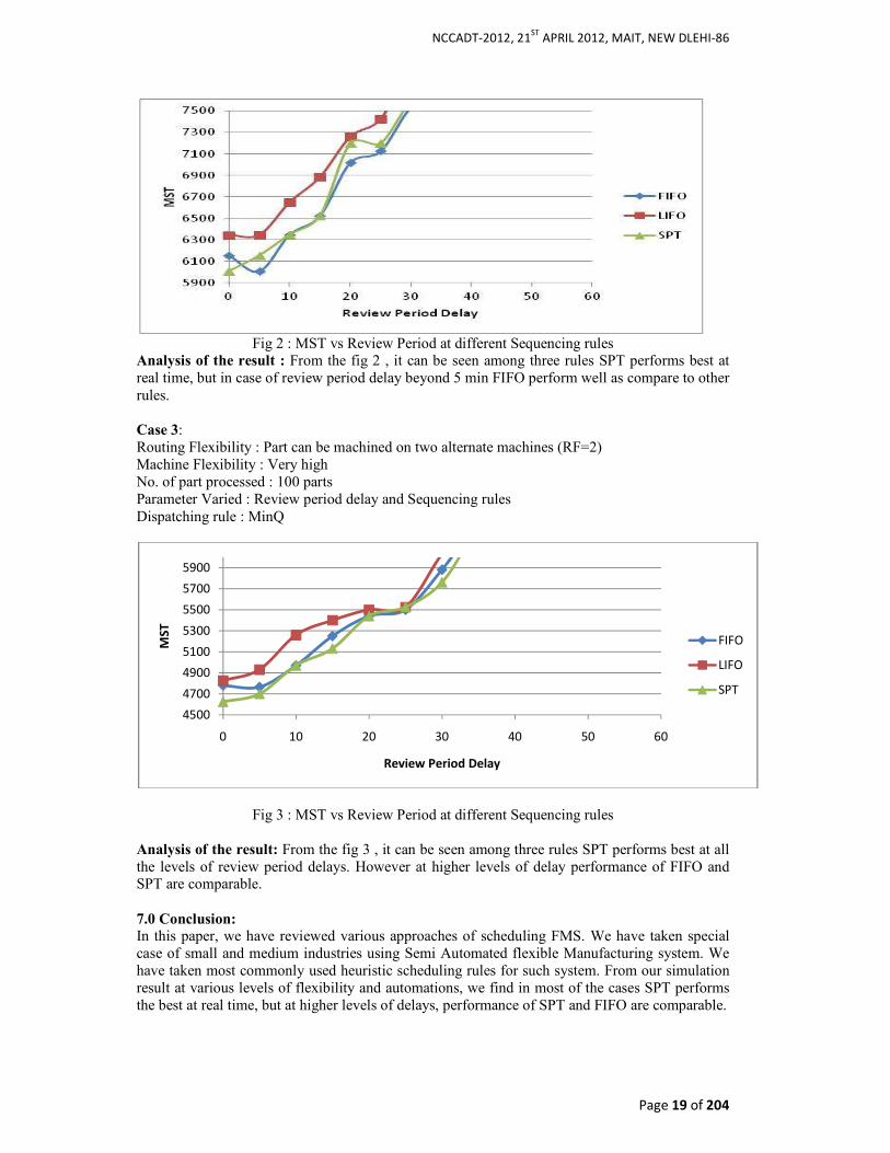
Fig 2 : MST vs Review Period at different Sequencing rules

Analysis of the result : From the fig 2 , it can be seen among three rules SPT performs best at real time, but in case of review period delay beyond 5 min FIFO perform well as compare to other rules. Case 3: Routing Flexibility : Part can be machined on two alternate machines (RF=2) Machine Flexibility : Very high No. of part processed : 100 parts Parameter Varied : Review period delay and Sequencing rules Dispatching rule : MinQ

Fig 3 : MST vs Review Period at different Sequencing rules

Analysis of the result: From the fig 3 , it can be seen among three rules SPT performs best at all the levels of review period delays. However at higher levels of delay performance of FIFO and SPT are comparable.

7.0 Conclusion:

In this paper, we have reviewed various approaches of scheduling FMS. We have taken special case of small and medium industries using Semi Automated flexible Manufacturing system. We have taken most commonly used heuristic scheduling rules for such system. From our simulation result at various levels of flexibility and automations, we find in most of the cases SPT performs the best at real time, but at higher levels of delays, performance of SPT and FIFO are comparable.

4500

4700

4900

5100

5300

5500

5700

5900

0 10 20 30 40 50 60

MS

T

Review Period Delay

FIFO

LIFO

SPT

NCCADT-2012, 21ST


Page 20 of 204

REFERENCES:

1. Baker, K. R. (1984). Sequencing rules and due-date assignments in a job shop. Management Science , 1093-1103.

2. Balci, O. (1990). Guidelines for successful simulation studies. Proceedings of the

1990 Winter Simulation Confeence, (pp. 25-32). 3. Biegel, J., & Davern, J. (1990). Genetic Algorithm and Job Shop Scheduling.

Computers and Industrial Engineering , 19 (1-4), 81-91. 4. Billo, R., Bidanda, B., & Tate, D. (1994 ). A genetic algorithm formulation of the cell

formation problem . Proceedings of the 16 th International Conference on Computers

and Industrial Engineering, (pp. 341-344). 5. Blackstone, Phillips, J. H., & Hogg, G. L. (1982). A State-Of-Art survey of

dispatching rules for manufacturing job shop operations. International Journal Of

Production . 6. Bourne, D. A., & Fox, M. S. (1984). Autonomous manufacturing: automating the job-

shop. IEEE Computer , 76-86. 7. Bruno, G., Elia, A., & Laplace, P. (1986). A rule-based system to schedule

production. IEEE Computer , 32-40. 8. Bullers, W. I., Nof, S. Y., & Whinston, A. B. (1980). Artificial intelligence in

Manufacturing Planning And Control. AIIE Transactions , 351-363. 9. Buzzacot, J. A., & Shanthikumar, J. G. (1980). Models for understanding Flexible

Manufacturing System. AIIE Transactions , 339-349. 10. Buzzacott, J. A. (1982). Optimal operating rules for automated manufacturing

systems. IEEE Transactions On Automatic Control , 80-86. 11. Chiodini, V. (1986). A knowledge based system for dynamic manufacturing

replanning. Symposium on Real Time Optimization inAutomated Manufacturing

Facilities . 12. Cho, H., & Wysk, R. A. (1993). A robust adaptive scheduler for an intelligent

workstation controller. Internatioal Journal Of Production Research , 771-789. 13. Choi, R. H., & Malstrom, E. M. (1988). Evaluation of traditional work scheduling

rules in a flexible manufacturing system with a physucal simulator. Journal Of Manufacturing Systems , 33-45.

14. Conway, R. W. (1965). Priority dispatching and work in process inventory in a job shop. Journal Of Industrial Engineering , 123-130.

15. Denzler, D. R., & Boe, W. J. (1987). Experimental investigation of flexible manufacturing system scheduling rules. International Journal Of Production

Research , 979-994. 16. Dorndorf, U., & Pesch, E. (1995). Evolution Based Learning in a Job Shop

Scheduling Environment. Computers and Operations Research , 22 (1), 25-40. 17. Egbelu, P. J., & Tanchoco, J. A. (1984). Characterization of automated guided

vehicle dispatching rules. International Journal Of Production Research , 359-374. 18. Fox, M. S., Allen, B., & Strohm, G. (1982). Job-shop scheduling: an investigation in

constraint-directing reasoning. Proceedings of the National Conference on Artificial Intelligence, (pp. 155-158).

19. Hall, M. D., & Putnam, G. (1984). An application of expert systems in FMS. Autofact

6 . 20. Hatono I, e. a. (1992). Towards intelligent scheduling for flexible manufacturing:

application of fuzzy inference to realizing high variety of objectives. Proceedings of

the USA/Japan Symposium on Flexible Automation, (pp. 433-440). 21. Henneke, M. J., & Choi, R. H. (1990). Evaluation of FMS parameters on overall

system performance. Computer Industrial Engineering , 105-110. 22. Hintz, G. W., & Zimmermann, H. J. (1989). Theory and methodology A method to

control flexible manufacturing systems. European Journal Of Operational Research , 321-334.

23. Iwata, K., Murotsu, A., Oba, F., & Yasuda, K. (1982). Production scheduling of flexible manufacturing system. Annals of The CRISP , 319-322.

NCCADT-2012, 21ST


Page 21 of 204

24. Jeong, K.-C., & Kim, Y. D. (1998). real-time scheduling mechanism for a flexible manufacturing system : using simulation and dispatching rules. International Journal

Of Production Research , 2609-2626. 25. Joshi, S. B., & Smith, J. S. (1994). Computer Control of Flexible Manufacturing

Systems. Chapman and Hall. 26. Kelton, W. D., Sadowski, R. P., & Stumock, D. T. (2004). Simulation with Arena.

New York: McGraw-Hill. 27. Kopfer, H., & Mattfield, C. (1997). A hybrid search algorithm for the job shop.

Proceedings of the First International Conference on Operations and Quantitative

Management, (pp. 498-505). 28. Kusiak, A., & Chen, M. (1988). Expert systems for planning and scheduling.

European Journal of Operational Research , 113-130. 29. McCulloch, W. S., & Pitts, W. (1943). A logical calculus of the ideas immanent in

nervous activity. Bulletin of Mathematical Biophysics , 115-133. 30. Montazeri, M., & Nan Wassenhove, L. N. (1990). Analysis of scheduling rules for an

FMS. International Journal Of Production Research , 785-802. 31. Nof, S. Y., & Solberg, J. J. (1979). Operational control of item flow in varsatile

manufacturing system. International Journal Of Production Research , 479-489. 32. Osman, I. (2002). focused issue on applied meta-heuristics. Computers and Industrial

Engineering , 205-207. 33. Panwalker, S. S., & Iskander, W. (1977). A survey of scheduling rules. 34. Parsaei, H. R., & Jamshidi Eds, M. (1995). Design and implementation of intelligent

manufacturing system. PTR Prentice Hall. 35. Potvin, J. Y., & Smith, K. A. (2003). Artificial neural networks for combinatorial

optimization. Handbook of Metaheuristics , 429-455. 36. Ramasesh, R. (1990). Dynamic job shop scheduling: a survey of simulation studies.

OMEGA: The International Journal of Management Science , 43-57. 37. Russel, R. S., Dar-EI, E. M., & Taylor, B. W. (1987). A comparative analysis of the

COVERT job sequencing rules using various shop performance measures. International Journal of Production Research , 1523-1540.

38. Sauve, B., & Collinot, A. (1987). , An expert system for scheduling in a flexible manufacturing System. Robotics and Computer-integrated Manufacturing .

39. Schultz, J., & Mertens, P. (1997). A comparison between an expert system, a GA and priority for production scheduling. Proceedings of the First International Conference

on Operations and Quantitative Managemen v, (pp. 505-513). 40. Shanker, K., & Tzen, Y. J. (1985). Loading and dispatching problem in a random

flexible manufacturing system. International Journal Of Production Research , 579-595.

41. Shaw, M. J., Park, S., & Raman, N. (1992). Intelligent scheduling with machine

learning capabilities:The induction of scheduling knowledge. IIE Transactions. 42. Stecke, K. E., & Solberg, J. J. (1981). Loading and control policies for a flexible

manufacturing system. International Journal Of Oroduction Research , 481-490. 43. Stecke, K. E., & Solberg, J. (1981). Loading and control policies for a flexible

manufacturing sysem. Internatinal Journal of Production Research , 481-490. 44. Steffen, M. S. (1986). A survey of artificial intelligence-based scheduling systems.

Fall Industrial Engineering Conference. 45. Tang, L. L., Yih, Y., & Liu, C. Y. (1993). A study on decision rules of a scheduling

model in an FMS. Computer in Industry , 1-13. 46. Tempelmeier, H., & Kuhn, H. (1993). Flexible Manufacturing Systems. John Wiley

and Sons. 47. Vaspalainen, A. J., & Mortan, T. E. (1987). Priority rules for job shops with weighted

tardiness Costs. Management Science , 1035-1047. 48. Viswanadham, N., & Narahari, Y. (1992). Performance Modelling of Automated

Manufacturing Systems. Prentice Hall.

NCCADT-2012, 21ST


Page 22 of 204

49. Yao, D. D. (1994). Stochastic modeling and analysis of manufacturing systems. Springer-Verlag.

50. Young-On, H. (1994). FMS performance versus WIP under different scheduling rules. Master's Thesis VPI & MU .

51. Zadeh, L. A. (n.d.). Fuzzy Sets. Information and Control , 338-353.

NCCADT-2012, 21ST


Page 23 of 204

KNOWLEDGE BASED TROUBLESHOOTING OF

MACHINE BREAKDOWN Prashasti Saxena, Shreya Jain, Sunaina Shivrain, Virangna

Department of Mechanical and Automation Engineering, Indira Gandhi Institute of `Technology, Kashmere Gate, Delhi-06

ABSTRACT Troubleshooting is a common application of case-based reasoning technology. Often in these

cases, the goal is to capture the approaches of troubleshooting experts and put these

troubleshooting best practices in the hands of lesser experienced analysts. Thus we have

tried to develop an expert system that can make the fault diagnosis of the machines efficient,

effective and quick. The fault diagnosis, so far, is largely dominated by manual process and

subjective decision. We intend to improve the operation process of handling faults, using this

diagnostic model based on case based reasoning.

Primary bottleneck to creating efficient troubleshooting base is sound knowledge capture. The paper attempts to overcome it by harnessing it to formidable knowledge base, prepared

after intensive survey of Lathe Machine workshops, study of detailed features of machine

design and analysis of manuals.

ARTICLE OUTLINE

1. Introduction 2. Literature Review 3. Knowledge Acquisition 4. Framework 5. Conclusion 6. Acknowledgement 7. References

1. INTRODUCTION Increasing demand and hands-on users are rendering the customary model of business intelligence applications, originated within departments and isolated from the enterprise, inefficient and ineffective. So there is a greater need of introducing information-rich interactive capabilities to the e-business environment. Hence these information-rich expert systems help in quick diagnosis of the fault. Moreover, complexity of modern machines involving a large number of components poses a great difficulty in identifying potential problems. Also, higher the diagnostic level, greater is the knowledge and expertise required. This requires an expert who has a domain specific knowledge of maintenance, and who knows the "ins-and-outs" of the system. But usually, a competent expert is not available at all times. Also, each subsystem of the machine requires different strategies for diagnosis. These factors lead to slow and inconsistent diagnosis, leading to avoidable extra costs that result from unnecessary replacements and additional downtime. Such costs can be avoided through appropriate expert system which can be used as an intelligent diagnostic system. To build such an expert system, Janus Liang developed a methodology for modelling troubleshooting of an automotive braking system. He developed a knowledge base that reflects the experience and knowledge of domain experts by surveying and interviewing these experts. Human experts solve problems by taking into account all data from the process and use their knowledge to solve them. An expert system uses this same principle but is also shielded from many factors (i.e. stress, emotional situations, etc.) that can affect the human expert. An expert system can also be designed to solve problems with incomplete data and/or non-exact

NCCADT-2012, 21ST


Page 24 of 204

solutions through the use of fuzzy logic in the inference engine. These systems have been proved to be effective tools for representing vague knowledge. They are now widely used to perform troubleshooting and control operations because of these similarities to human reasoning as well as their simplicity. Troubleshooting is a common application of case base technology. Often in these cases, the goal is to capture the approaches of troubleshooting experts and put these troubleshooting best practices in the hands of lesser experienced analysts.

Effective knowledge capture is the primary bottleneck to creating a good troubleshooting case base.The objective is to develop an effective and efficient Fault Diagnosis Expert System for troubleshooting of lathe which fulfills all above discussed requirements.

2. LITERATURE REVIEW Lee et al. [l] defined the word diagnosis as “a symptom of a fault that is observed when the system behaves in a way that is not expected”. The goal of diagnosis was defined by Genesareth [2] as “determining the fault responsible for a set of symptoms”. Thus in real applications, diagnosis is not only the process of finding the location of the fault, rather it needs to be extended to suggest some methods for recovering the system. In this paper, suggestions for restoring are also provided to fulfill this need. So diagnosing of unwanted symptoms in a manufacturing machine can be divided into different levels-from the simplest levels i.e. shallow reasoning to the high-end level, i.e. deep reasoning. Erik L.J. Bohez, Mahasan Thieravarut[3] defined shallow reasoning as “The shallow reasoning approach makes use of heuristic or experience-based knowledge represented as a finite tree”. The diagnosis system based on this approach generally captures the intuitions and past experience of human diagnosticians considered to be experts in some particular field. Deep reasoning, based on deep knowledge, is often referred to as model-based reasoning, because it uses a model of the system as a basis for inference. A model is the formalization of a system so as to represent what the system does and how it works. A model itself is constructed from characteristic information on the structure and behaviour of the system being diagnosed. The expected behaviour of the system is abstracted, and any discrepancies between the observed and expected behaviour are considered to be faults. Though the deep reasoning is flexible but it is slower as compared to shallow reasoning. However shallow reasoning is rigid, in the sense that there may have to be substantial changes in the rules with the addition or deletion of a single component. Also shallow reasoning can diagnose only the known (experienced) cases. Hence, the combination (hybrid reasoning) of these two approaches has been attempted to perform the diagnosis process efficiently (relative to deep reasoning) and effectively (relative to shallow reasoning). Lee et al. [1] presented further strategy by mixing the two strategies to give what they called “hybrid reasoning”. Two possible ways of combination are as follows:

1. Deep first, and then shallow (D-S) 2. Shallow first and then deep (S-D)

Similar work has been carried out but was not classified as such: for example, there is the work of Fink and Lusth [20] in the integrated diagnostic model (IDM). It contains two different types of knowledge, i.e. one type based on experience and one type based on the functions of devices to be diagnosed. For intelligent diagnosis the expert system taking into account the uncertainties should be preferably used. In related studies, Zadeh[4], who first depicted fuzzy sets in 1965, advocated the application of fuzzy set theory in quantitative measures of the human thinking process. An expert system can be designed to solve problems with incomplete data and/or non-exact solutions through the use of fuzzy logic in the inference engine. Kandel claimed that fuzzy rule-based expert systems contain such fuzzy rules in their knowledge base and derive conclusions from user

NCCADT-2012, 21ST


Page 25 of 204

inputs and through a fuzzy reasoning process [6–8]. Later researchers [5,9,10] proved that these systems are effective tools for representing vague knowledge. They are now widely used to perfor troubleshooting and control operations because of these similarities to human reasoning as well as their simplicity [6–8, 11]. Many applications of fuzzy logic have appeared over the years. These include manufacturing [6, 8, 11, 18], reliability analysis [13], economics [6–8,11] and even medical diagnosis [13,16,17]. Many successful instances utilizing expert systems are available to handle customer requirement problems. For instance, Su proposed a malfunction recovery mechanism allowing maintenance personnel and decision makers to solve maintenance tasks cooperatively. Lin used expert system to detect machine breakdowns. Perng et al. applied neural network and expert systems to machine fault diagnosis. However, although the operation processes of expert systems were thoroughly discussed and a prototype system was constructed, requirements from customers still could not be handled. Liu and Chen developed a machine troubleshooting expert system through a fuzzy multi attribute decision-making approach. This system consists of five components and improves the efficiency of the diagnostic process. Fang proposed a method for on-line machine condition monitoring involving a fuzzy feature state relationship matrices and expert system. Many expert systems based on principles defined above have been developed various areas. Wahab, Elkamal, Weshahi and Yalmadi[12] developed an expert system for troubleshooting of brine heater in MSF plant using fuzzy logic. Erik L.J. Bohez , Mahasan Thieravarut developed an expert system for troubleshooting of CNC machines[3]. 3. KNOWLEDGE ACQUISITION The expert system so developed taps in the knowledge and the expertise of the experts working on the lathe machines. This system would thus help in increasing the productivity of the machine by reducing its downtime. Also, this would quicken the process of the inspection, decision making and troubleshooting of the problems, encountered by the operator in the machine while processing or manufacturing job. In an expert system the knowledge base is implemented using IF-THEN rules into the rule base. The accuracy of an expert system is dependent on the quality of knowledge acquisition. Hence a combination of the three- questionnaire, interview and schedule- was employed and an extensive survey was carried out in the following areas :-

Kashmere Gate Market Mori Gate Anand Parbat Udyog Nagar, Peeragarhi

• Some telephonic interviews were also conducted. • We also mailed the questionnaires to some companies namely EIL, Cummins,

Maruti, Mahindra. The data, after collection, has to be processed and analysed in accordance with the outline laid down for the purpose at the time of developing the research plan. This is essential for ensuring that we have all relevant data for making contemplated comparisons and analysis. Technically speaking, processing implies editing, coding, classification and tabulation of collected data so that they are amenable to analysis. So, the collected was studied, classified and tabulated in the following manner. The knowledge based system comprises of the data from the manuals and the expertise of the employees. The system would be able to help in troubleshooting of the failure of the components of the lathe by determination of the root cause of the problem and thus would help in increasing the overall efficiency of machine by fastening the detection of failure area, decision making process, resolution of the problem. Also, it would help in maintaining the product quality and can be employed to reduce the overall machine down time to a minimum level.

NCCADT-2012, 21ST


Page 26 of 204

Table I

Expert systems are designed to solve complex problems by reasoning about knowledge, like an expert, and not by following the procedure of a developer as is the case in conventional programming. . To run an expert system, the engine reasons about the knowledge base like a human. It is divided into THREE parts:-

Fixed, independent of the expert system- the inference engine. The knowledge or rule base- In expert system technology, the rule base is

expressed with IF .-THEN rules which are derived from the knowledge of experts

A dialog interface to communicate with users. The inference engine is a computer program designed to produce a reasoning on rules. In order to produce a reasoning, it is based on logic. With logic, the engine is able to generate new information from the knowledge contained in the rule base and data to be processed. For eg in our system the expert system automatically re-updates its failure-life data of various parts/components of the machine to which it is attached. Since even the same type of lathe machine, supplied by the same supplier, may have different performance characteristic based on inherent variation amongst the machines, hence the system so developed adjusts dynamically to the machine on which its run. Normally the inference engine can run in two different ways:-

— batch: the expert system has all the necessary data to process from the beginning

— conversational method- This becomes necessary when the problem is too complex. The software must "invent" the way to solve the problem, request the missing data from the user, gradually approaching the goal as quickly as possible. The result gives the impression of a dialogue led by an expert.

Now to guide a dialogue, the engine may have several levels of sophistication: - — forward chaining- Forward chaining is the questioning of an expert who has

no idea of the solution and investigates progressively (e.g. fault diagnosis) — backward chaining- the engine has an idea of the target (e.g. is it okay or not?

Or: there is danger but what is the level?). It starts from the goal in hopes of finding the solution as soon as possible.

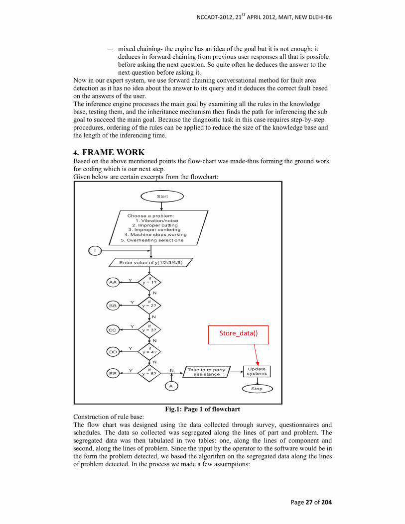
NCCADT-2012, 21ST


Page 27 of 204

— mixed chaining- the engine has an idea of the goal but it is not enough: it deduces in forward chaining from previous user responses all that is possible before asking the next question. So quite often he deduces the answer to the next question before asking it.

Now in our expert system, we use forward chaining conversational method for fault area detection as it has no idea about the answer to its query and it deduces the correct fault based on the answers of the user. The inference engine processes the main goal by examining all the rules in the knowledge base, testing them, and the inheritance mechanism then finds the path for inferencing the sub goal to succeed the main goal. Because the diagnostic task in this case requires step-by-step procedures, ordering of the rules can be applied to reduce the size of the knowledge base and the length of the inferencing time.

4. FRAME WORK Based on the above mentioned points the flow-chart was made-thus forming the ground work for coding which is our next step. Given below are certain excerpts from the flowchart:

Start

Choose a problem:

1. Vibration/noice

2. Improper cutting3. Improper centering

4. Machine stops working

5. Overheating select one

I

AA

BB

CC

DD

EE

Enter value of y(1/2/3/4/5)

ify = 1?

Y

N

Y

Y

N

Y

N

N

NY

AStop

Updatesystems

Take third partyassistance

ify = 2?

ify = 3?

ify = 4?

ify = 5?

Fig.1: Page 1 of flowchart

Construction of rule base: The flow chart was designed using the data collected through survey, questionnaires and schedules. The data so collected was segregated along the lines of part and problem. The segregated data was then tabulated in two tables: one, along the lines of component and second, along the lines of problem. Since the input by the operator to the software would be in the form the problem detected, we based the algorithm on the segregated data along the lines of problem detected. In the process we made a few assumptions:

Store_data()

NCCADT-2012, 21ST


Page 28 of 204

• The operator’s response to the directions of the system and the actions taken according to those directions are 100% accurate.

• The data collected from the survey is considered to be 100% objective answers. • The data was collected from various machines whose suppliers were different. This

will have no effect on any type of lathe machine. The algorithm starts by asking the operator to choose one of the displayed problems which can be detected easily by an operator. We have also provided a provision for catering to a problem other than those displayed, by recording the information for future use i.e. we have implemented forward chaining. Also for each problem detected by the operator, using the component life-data and component list for the problem from the table, we set as default a priority order for the components to be checked for a problem. Each component is checked by the operator according to the problem areas specified by the software. After recognizing the faulty component, the operator is suggested the trouble shooting procedure. Following this, A function named store_data() is run. A provision for function store_data() is provided for modifying this component priority list for each problem according the real time conditions. This helps in taking in the uncertainty of life data variation for lathes of different companies. The store_data() would update the component’s life using the last replacement date and the current replacement date by taking out weighted average of the lives for the component obtained from earlier breakdown maintenance. Also weight of the default life would be assumed 6. Within this function, the component priority order will be modified each time some component is replaced or corrected. This would be done using both the average weighted life and the last maintenance of various components. Thus, the software adjusts to the machine instead of machine adjusting to the software. Also the system so developed is capable of finding faulty component responsible for different detectable problems. However, we still believe that the software can be further improved. Some areas of improvement are:

• Continuous imaging can be implemented along with the software to detect problems not yet solved or problems that are company- specific or conditions-specific. This would help us in implementing deep reasoning.

• Sensors can be implemented to take in real time uncertainties in problem diagnosis which is at the moment done by the operator according to the instructions given by the software.

• Using sensors for detection of problems that are difficult to detect due to magnitude or real time conditions.

5. CONCLUSION The diagnostic model used for this study consists of hybrid reasoning between a deep model and shallow model. The shallow model is faster but limited in its diagnostic capability, so that only known cases are possible while the deep model requires a longer fault searching time. The combination of these models results in an efficient and effective diagnostic model. The hybrid model may have two possible ways of combination-(1) Shallow first, deep late[S-D] (2) Deep first, shallow later [D-S]. Depending on the type of application, its magnitude and its scale one of the above two strategies is used. The implementation of the diagnostic model as an expert system calls for knowledge acquisition. This involves surveying and extracting information from the domain experts. Hence it is the most time-consuming part and the most difficult process in the development of an expert system for this study. Heuristic knowledge for diagnosing the CNC machine is extracted from the maintenance crews and the domain expert. Techniques for acquiring this kind of knowledge are the on-site observation method and the problem description method. Taking into consideration the nature of the source as well as the details required, scheduling was also incorporated. The combination of these sources provides the acquired knowledge.

NCCADT-2012, 21ST


Page 29 of 204

Now this knowledge acquisition is incorporated into the interactive system by three phase modeling. In the three-phase modeling methodology, there are four knowledge component: facts, criteria, thinking mode or the inference engine and rules. Facts cover all data instances, and criteria correspond to the technological requirements of troubleshooting. The thinking mode imitates the intelligence of human experts. Rules are key parameters that control the thinking mode and can be extracted from it. The rule base of the prototype expert system is implemented on the basis of the algorithm mentioned. In our expert system, we use forward chaining conversational method for fault area detection. In order to reduce the size of the knowledge base and the inferencing time, faults are located by direct access to those components which are most prone to failure. Since even the same type of lathe machine, supplied by the same supplier, may have different performance characteristic based on inherent variation amongst the machines, hence the system so developed adjusts dynamically to the machine on which its run. ACKNOWLEDGEMENT We express our sincere thanks to our project guide and mentor Mr Ajay Singholi for his invaluable guidance and continued support. Our HOD Dr Chitra Sharma and college authorities extended full cooperation and allowed us to use their resources whenever we needed them. We express our gratitude to them. Also we express our heartiest gratitude to Mr Vishal Bhatnagar, The findings of erstwhile of researchers served as base for our study. We thank all the writers whom we referred from time to time. We would also like to thank the various people who took part in the survey and provided us with the valuable information. Last but not the least we would like to thank our parents and friends for their continued support.

REFERENCES

1. W.Y. Lee, S.M. Alexander and J.H. Graham, “A diagnostic expert system prototype for CIM”, Comput. Indust. Eng.,22(3) (1992) 337-352

2. M.R. Genesareth, “The use of design description in automated diagnosis”, Arti@. Intel., 24 (1984) 41 l-436.

3. Erik L.J. Bohez , Mahasan Thieravarut,” Expert system for diagnosing computer numerically controlled machines: a case-study”, published in Science direct

4. Zadeh, L. A. (1975). The concept of a linguistic variable and its applications to approximate reasoning, part 1, 2 and 3. Information Science, 8, 199–249, 8, 301–357; 9, 43–80.

5. P. Ross and Q. Shen, Expert Systems, University of Edinburgh, 1995. Graham and P. Jones, Expert system-knowledge uncertainty and decision, Chapman Computing,(1988) 117–158.

6. S.A. Abdul-Wahaba, A. Elkamelb, M.A. Al-Weshahic, A.S. Al Yahmadia, “Troubleshooting the brine heater of the MSF plant using a fuzzy logic-based expert system”, published in Science direct

7. Janus S. Liang,”The methodology of knowledge acquisition and modeling for troubleshooting in automotive braking system”, published in Science direct

8. A.M. Uhrmacher and D. Weyns, Multi-agent systems: simulation and applications, CRC Press, Taylor & Francis Group, NW, USA (2009).

9. M. Wooldridge, An introduction to multi-agent system, Wiley, England (2002). 10. Zhang HL, Van der VC, Yu X, Bil C, Jones T, Fieldhouse I Developing a rule

engine for automated feature recognition from CAD models In:Proceedings of the 35th annual conference of IEEE, IECON ’09, Porto, Portugal, 2009. p. 3925–30..

11. E.S.A. Nasr and A.K. Kamrani, A new methodology for extracting manufacturing features from CAD system. Computers and Industrial Engineering, 51 3 (2006), pp. 389–415.

NCCADT-2012, 21ST


Page 30 of 204

12. J. Ciurana, M.L. G-Romeu and R. Castro, Optimizing process planning using groups of precedence between operations based on machined volume. Engineering Computations, 20 1 (2003), pp. 67–81.

13. H.K. Miao, N. Sridharan and J.J. Shah, CAD/CAM integration using machining features.

14. International Journal of Computer Integrated Manufacturing, 15 4 (2002), pp. 298–318.

15. P.K. Fink and J.C. Lusth, “Expert systems and diagnostic expertise in the mechanical and electrical domains”, IEEE Trans. Syst. Man Cybemet., SMC-27(3) (1987) 340-349.

16. Lathe Manual by Clark. 17. Kothari, C.R., “Research Methodology methods and techniques”, Second revised

edition.

NCCADT-2012, 21ST


Page 31 of 204

NEW TECHNIQUE OF MANUFACTURING

ULTRASONIC TRANSDUCERS: ADDITIVE

MANUFACTURING Madhuri Gupta, Isha Gupta, Sarika Gupta, Juhi Sharma, Akansha Agarwal

(4th

Year, Mechanical and Automation Engineering, Indira Gandhi Institute of Technology)

Abstract Additive manufacturing or rapid, direct, instant, or on-demand manufacturing, is an

automatic process that produces three dimensional objects directly from a digital model by

the successive addition of material(s), without the use of a specialized tooling. This paper

proposes the use of new additive techniques that can be used for manufacturing of

piezoelectric ultrasonic transducers all at once, avoiding hours of cutting and refinement. The

alternate materials for different functioning layers of ultrasound transducer are suggested

after detailed study of 3D CAD model of transducer. This could greatly reduce labour,

production cost and time. This technology also could impact other ultrasound sensors used

for the inspection and measurement of high-value, safety-critical aerospace and industrial components.

Keywords

Additive Manufacturing, Ultrasonic transducers, Stereolithography, Micromachining, Fused Deposition Modelling, Selective Laser Sintering, Laminated Object Manufacturing, Direct Metal Laser Sintering, 3D Printing, Rapid Manufacturing, Plasma deposition manufacturing.

1. Introduction

Additive manufacturing is a manufacturing process which creates physical parts directly from 3D CAD files or data using computer-controlled additive and subtractive fabrication and machining techniques with minimal human intervention. This technique is an extension of Rapid Prototyping to real parts for use as final products (not prototypes) and physically constructs or manifests 3D geometries directly from 3D CAD. The technologies that have been used for many years to do rapid prototyping are now being more widely used for creating parts that are used directly in the final product. Prototypes created using additive fabrication processes have been and are still used in the product design and development process to check form, fit and function to varying degrees. This paper proposes the use of additive technique to manufacture an ultrasound transducer on a single platform. An ultrasound transducer is a thin, tube-like instrument that generates high frequency sound waves that scan surfaces of objects to detect abnormalities. The transducers use a dense array of elements, each converting electrical signals into ultrasound waves, and vice versa. In numerous cases, especially if a workpiece has a complicated geometry or the inspection has to be done in unusual conditions, ultrasonic inspection becomes feasible with the help of transducers, having appropriate acoustic properties. Conventionally ultrasound probes are manufactured by the process of micromachining.

2. Background and Motivation

Additive processes, which generate parts in a layered way, have more than 15 years of history.These processes are not exclusively used for prototyping any longer. The generic and the major specific process characteristics and materials are described, mainly for metallic parts, polymer parts and tooling. Examples and applications are cited ( Levy, Golden N., Schindel Ralf, Kruth J.P (1996). An integrated manufacturing system for rapid tooling based on rapid prototyping was proposed in 2004 (Ding, Yucheng; Lan, Hongbo; Hong, Jun; Wu, Dianliang (2004)) . With further developments, additive manufacturing is now being used in industries. It is used as Freeform Construction: Mega-scale Rapid Manufacturing for construction (Bussel, R.A.; Soar, R.C.; Gibb, A.G.F.; Thorpe, A. (2007)). The major issues facing construction technology and examples of the use of large scale Digital Fabrication in the industry were

NCCADT-2012, 21ST


Page 32 of 204

provided and results from a series of preliminary studies indicate the viability of mega-scale Rapid Manufacturing for construction. (Lim, S.; Buswell, R.A.; Le, T.T.; Austin, S.A.; Gibbs, A.G.F. and Thorpe, T. (2011)) Further research and developments are beingmade in this area also (Shanjani, Yaser; Hu, Youxin; Pilliar, Robert M.; Toyserkani , Ehsan (2011)). . Additive manufacturing provides new opportunities in the manufacture of highly complex and custom-fitting medical devices and products. Researches and study has been done in the design and manufacture of wearable medical devices, implants, prostheses and medical imaging test phantoms (Bibb, Richard; Thompson, Darren; Winder John (2011)). This area is still being explored with further research and studies (Bertol, Liciane Sabadin; Junior, Wilson Kindlein; Pinto da Silva. Fabio; Aumund-Kopp, Claus (2010)). Research on designing direct printing process for improved piezoelectric micro devices was carried out in 2009 (Bathurst, S.P. and Kim, S.G. (2009)) and medical design through Direct metal laser sintering of Ti–6Al–4V was carried out (Bertol, Liciane Sabadin; Junior, Wilson Kindlein; Pinto da Silva. Fabio; Aumund-Kopp, Claus (2010)). Receiving the motivations from the vast literature review, this paper proposes additive manufacturing of ultrasound transducers. Since the manufacturing of ultrasonic transducer is labor intensive and time consuming its cost is very high. Additive manufacturing would help make ultrasound systems more affordable and more accessible to underserved regions.

3. Ultrasonic Transducer

The ultrasonic transducers manufactured by conventional methods/micromachining pose some major problems like: 1. Geometric limitations are imposed by the crystallographic constraints, and

complicated structures are difficult to fabricate. Also the process is not applicable to submicron technology.

2. Micromachines are small and are very difficult to fix. Also, the set up is very costly. 3. The complexity of an ultrasound array leads to a higher cost and reduces reliability. 4. The mechanical properties of most deposited thin-films are usually unknown and

must be measured. Considering the problems stated above, the study proposes the use of additive technology to manufacture an ultrasound probe on a single platform.

4. Additive Manufacturing Technology The basic principle of this technology is that a model, initially generated using a three-dimensional Computer Aided Design (3D CAD) system, can be fabricated directly without the need for process planning. Additive manufacturing (AM) certainly significantly simplifies the process of producing complex 3D objects directly from CAD data. AM needs only some basic dimensional details and a small amount of understanding as to how the AM machine works and materials that are used. The key to how AM works is that parts are made by adding materials in layers; each layer is a thin cross-section of the part derived from the original CAD data. Though each layer has a finite thickness, the thinner each layer is, the closer the final part will be to the original. All AM machines majorly differ in the way materials can be used, layers are created, and how the layers are bonded to each other. Such differences will determine factors like the accuracy, production time, post processing required, material properties and mechanical properties of the final product, and the overall cost of the machine and process. Research and development in this crucial field are enabling a wealth of opportunities for product customization and improved performance. Highly complex components can also be fabricated faster while consuming less material and using less energy. Additive manufacturing also eliminates the need for expensive part tooling and detailed drawing packages, causing a paradigm shift for the design-to-manufacture process. Processes used in AM are:

NCCADT-2012, 21ST


Page 33 of 204

Process Building Process Stereolithography (SLA) Selective curing by exposure to light Selective Laser Sintering (SLS) Selective fusing by the heat of a laser Fused Deposition Modeling (FDM) Extrusion and fusion of filaments 3D Printing Selective application of liquid binder Laminated Object Manufacturing (LOM) Joining of stacked cut-outs Inkjet Layer-wise “printing” of droplets

5. Additive Manufacturing Process for Manufacturing Ultrasound Transducer

5.1 Preparation of CAD Model

Virtually every commercial solid modeling CAD system has the ability to output to an AM machine. This is because the only information that an AM machine requires from the CAD system is the external geometric form. The STL files are generated from 3D CAD data within the CAD system. An STL file describes a raw unstructured triangulated surface by the unit normal and vertices of the triangles using a three-dimensional Cartesian coordinate system. These files only show approximations of the surface or solid entities.

5.2 Material

Additive manufacturing is a material-specific technique. The materials used in the manufacture of ultrasonic transducer in the conventional method of micromachining cannot be conveniently used with the different processes of additive manufacturing like: stereolithography, selective laser sintering, 3D printing, etc. Therefore, an analysis of comparing the important properties of the different compatible materials was done as under. The important properties of different materials used in manufacture of ultrasound probe are:

• Acoustic impedance =density x velocity of sound in that medium. • Attenuation = attenuation coefficient x frequency x distance from source.

Alternate materials for additive manufacturing of ultrasound transducer are suggested as shown below, comparing the major property, acoustic impedance of transducer layers material (since attenuation is an important property of the backing layer):

Layer Material used Alternative

material

Acoustic

impedence for

the material

used (Mrayl)

Acoustic impedence

for the material

suggested (Mrayl)

Backing Layer

Glass in Bakelite/ tungsten in epoxy

Polyamide- Glass filled (PA-GF) (SLS)

30 PA-3.6-3.75 GF-13.2

Titanium powder in Polyurethane resin(3DP)

Titanium-27.3 Polyeurethane- 1.8

Glass silica in ABS(FDM)

ABS- 2.31 Glass silica-13

Alumide (SLS) Al-40.6 PA-3.6-3.75

Matching Layer

Glass/plastic material mixed with tungsten powder/ epoxy resin

Polystyrene(SLS) 3-10 2.42

Polyamide (SLS) 3.6-3.75 ABS (FDM) 2.31 DuraForm PP 100

Plastic-Polypropylene (SLS)

2.4

Polystyrene(SLS) 2.42 Above plastics with Titanium-27.3

NCCADT-2012, 21ST


Page 34 of 204

titanium powder in polyurethane resin(3DP)

Polyeurethane- 1.8

Piezoelectric Layer

Lead Zirconate Titanate (PZT) (FDM,SLS, Inkjet Printing)

28-32

6. Selection of Processes The feasibility of manufacturing the ultrasound probe depends on the material being compatible with the method/ process used. The piezoelectric material can be used in processes like- selective laser sintering, fused deposition modelling and inkjet printing. Comparing the capability of the materials with the processes that can be used, the manufacturing can be achieved by following processes:

• Fused deposition modeling • Selective laser sintering • Inkjet printing

7. Conclusion and Scope

This paper proposes a method for manufacturing of ultrasonic transducers more economically and efficiently with less human intervention and customizing complex geometries of the intricate patterns through additive manufacturing. Additive technology has certain material limitations i.e. only a few specific materials can be used for manufacturing. In context with the ultrasonic transducers, the conventional materials used for manufacturing along with their functions are studied and a suitable alternative is then suggested so that the manufacturing can be made possible via additive technology. Based on the suggested materials a few of the additive manufacturing methods are selected for further research. This technology can further be used for producing more intricate patterns on the face of the ultrasound transducers and also could impact other ultrasound sensors used for the inspection and measurement of high-value, safety-critical aerospace and industrial components.

8. References

1. Lim, S.; Buswell, R.A.; Le, T.T.; Austin, S.A.; Gibbs, A.G.F. and Thorpe, T. (2011), “Developments in construction-scale additive manufacturing processes” Automation

in Construction, In Press. 2. Bibb, Richard; Thompson, Darren; Winder John (2011), “Computed tomography

characterisation of additive manufacturing materials” Medical Engineering &

Physics, Vol. 33, No. 5, pp. 590-596. 3. Shanjani, Yaser; Hu, Youxin; Pilliar, Robert M.; Toyserkani , Ehsan (2011),

“Mechanical characteristics of solid-freeform-fabricated porous calcium polyphosphate structures with oriented stacked layers” Acta Biomaterialia, Vol. 7, No. 4, pp. 1788-1796.

4. Bertol, Liciane Sabadin; Junior, Wilson Kindlein; Pinto da Silva. Fabio; Aumund-Kopp, Claus (2010), “Medical design: Direct metal laser sintering of Ti–6Al–4V” Materials & Design, Vol. 31, No. 8, pp. 3982-3988.

5. Bathurst, S.P. and Kim, S.G. (2009), “Designing direct printing process for improved piezoelectric micro devices”, CIRP Annals – Manufacturing Technology, Vol. 58, No. 1, pp. 193-196.

6. Qian, Ying-Ping; Huang, Ju-Hua; Zhang, Hai-ou; Wang, Gui-Lan (2008), “Direct rapid high-temperature alloy prototyping by hybrid plasma-laser technology” Journal

of Materials Processing Technology, Vol. 208, No. 1-3, pp. 99-104. 7. Bussel, R.A.; Soar, R.C.; Gibb, A.G.F.; Thorpe, A. (2007), “Freeform Construction:

Mega-scale Rapid Manufacturing for construction” Automation in Construction, Vol. 16, No. 2, pp. 224-231.

NCCADT-2012, 21ST


Page 35 of 204

8. Ding, Yucheng; Lan, Hongbo; Hong, Jun; Wu, Dianliang (2004), “An integrated manufacturing system for rapid tooling based on rapid prototyping” Robotics and

Computer-Integrated Manufacturing, Vol. 20, No. 4, pp. 281-288. 9. Microstructure and mechanical behavior of Ti–6Al–4V produced by rapid-layer

manufacturing, for biomedical applications. 10. Rapid manufacturing of metal components by laser forming. 11. Rapid manufacturing and rapid tooling with layer manufacturing (LM) technologies,

state of the art and future. 12. Main future issues. 13. Cheung, H. H. and Choi, S. H. (2009), “A topological hierarchy-based approach to

layered manufacturing of functionally graded multi-material objects” Computers in

Industry, Vol. 60, No. 5, pp. 349-363. 14. Haipeng, Pan and Tianrui, Zhou (2007), “Generation and optimization of slice profile

data in rapid prototyping and manufacturing” Journal of Materials Processing

Technology, Vol. 187-188, pp. 623-626. 15. TSINGHUA SCIENCE AND TECHNOLOGY ISSN 1007-0214 01/38 pp1-12

(2009), “Rapid Prototyping and Manufacturing Technology: Principle, Representative Technics, Applications, and Development Trends” Vol. 14.

16. Windle, J. and Derby, B. (1999), “Inkjet printing of PZT aqueous ceramic suspension”.

17. Venuvinod, Patri K. and Ma, Weiyin, “Rapid Prototyping: laser based and other technologies”.

18. Gibson, Ian; W.Rosen, David and Stucker, Brent, “Additive manufacturing technologies”.

19. Hopkinson, Neil “Rapid Manufacturing: an industrial revolution for the digital age”. 20. Gebhardt Andreas “Rapid prototyping”. 21. K.Kamrani , Ali “Engineering design and rapid prototyping”. 22. Koc, Maummere and Ozel, Turgul “Micro-manufacturing design and manufacturing

of micro products.”

NCCADT-2012, 21ST


Page 36 of 204

Study of Quality System Techniques: A Review Mohit Singh

1, Dr. I.A. Khan

2, Dr. Sandeep Grover

3

1Research Scholar 2Professor 3Professor Dept. of Mech. Engg Dept. of Mech. Engg. Dept. of Mech. Engg. Jamia Millia Islamia Jamia Millia Islamia YMCAUST New Delhi New Delhi Faridabad [email protected] [email protected] [email protected] Abstract

The paper deals with the use of system techniques in the practice of quality management of

real and modern enterprises. The system techniques described in this paper are Analytic

Hierarchy Process (AHP), Graph Theoretic Approach and Technique for Order Preference

by Similarity to Ideal Solution (TOPSIS). AHP is a pair wise comparison technique which

compares the attributes and assess the quality level by considering its different

characteristics which govern the qualitative aspect of the system. The graph theoretic

approach reveals a single numerical index and accordingly it is possible to choose the best

manufacturing process. TOPSIS is employed to obtain a crisp overall performance value for

each alternative to make a final decision.

Keywords: AHP, Topsis, Graph Theoretic Approach

INTRODUCTION

The prime focus of any Industry or organization is to earn more profits at low cost and for this reason evaluation and comparison of quality is very necessary. A company with an excellent manufacturing process produces a quality product which passes stringent inspections and gains customer recognition. The benefits of a good, solid manufacturing process are: Quality Products, Decreased Labour cost, High Employee Morale, Positive image, Higher profits etc. It is therefore important to develop designing aids which would assist designers in the selection of materials and manufacturing processes(1). There are several techniques employed for assessment of quality level of any organization like AHP, Graph Theoretic Approach, TOPSIS etc.

ANALYTIC HIERARCHY PROCESS

The Analytic Hierarchy Process (AHP) has been developed by T. Saaty (1977, 1980, 1988, 1995) and is one of the best known and most widely used MCA approaches. It allows users to assess the relative weight of multiple criteria or multiple options against given criteria in an intuitive manner. In case quantitative ratings are not available, policy makers or assessors can still recognize whether one criterion is more important than another. Therefore, pairwise comparisons are appealing to users. Saaty established a consistent way of converting such pairwise comparisons (X is more important than Y) into a set of numbers representing therelative priority of each of the criteria. The basic procedure to carry out the AHP consists of the following steps:

1. Structuring a decision problem and selection of criteria The first step is to decompose a decision problem into its constituent parts. In its simplest form, this structure omprises a goal or focus at the topmost level, criteria (and subcriteria) at the intermediate levels, while the lowest level contains the options. Arranging all the components in a hierarchy provides an overall view of the complex relationships and helps the decision maker to assess whether the elements in each level are of the same magnitude so that they can be compared accurately. An element in a given level does not have to function as a criterion for all the elements in the level below. Each level may represent a different cut at the problem so the hierarchy does not need to be complete (2) When constructing hierarchies it is essential to consider the environment surrounding the problem and to identify the issues or attributes that contribute

NCCADT-2012, 21ST


Page 37 of 204

to the solution as well as to identify all participants associated with the problem.

2. Priority setting of the criteria by pairwise comparison (weighing) For each pair of criteria, the decision maker is required to respond to a question such as “How important is criterion A relative to criterion B?” Rating the relative “priority”of the criteria is done by assigning a weight between 1 (equal importance) and 9 (extreme importance) to the more important criterion, whereas the reciprocal of this value is assigned to the other criterion in the pair. The weighings are then normalized and averaged in order to obtain an average weight for each criterion.

3. Pairwise comparison of options on each criterion (scoring) For each pairing within each criterion the better option is awarded a score, again, on a scale between 1 (equally good) and 9 (absolutely better), whilst the other option in the pairing is assigned a rating equal to the reciprocal of this value. Each score records how well option “x” meets criterion “Y”. Afterwards, the ratings are normalized and averaged. Comparisons of elements in pairs require that they are homogeneous or close with respect to the common attribute; otherwise significant errors may be introduced into the process of measurement (2).

4. Obtaining an overall relative score for each option In a final step the option scores are combined with the criterion weights to produce an overall score for each option. The extent to which the options satisfy the criteria is weighed according to the relative importance of the criteria. This is done by simple weighted summation. Finally, after judgements have been made on the impact of all the elements and priorities have been computed for the hierarchy as a whole, sometimes and with care, the less important elements can be dropped from further consideration because of their relatively small impact on the overall objective. The priorities can then be recomputed throughout, either with or without changing the judgements (Saaty, 1990).

GRAPH THEORETIC APPROACH

A graph theoretic model is a versatile tool that has been used in various applications. It helps to analyse and understand the system as a whole by identifying system and subsystem up to the component level. The conventional approach of representation vis-a-vis block diagram, flow diagram, schematic representation etc is suitable for the visualisation of relationships/interactions but not for any mathematical analysis. Whereas the mathematical model developed by graph theoretic approach, considers both the contribution of factor itself i.e., the inheritance of factor and extent of dependence among factors i.e., their interactions. This methodology starts from where conventional representations end. This logical and systematic approach uses well-documented applications of graph theory (3-4). Digraph representation is useful for modelling and visual analysis. Matrix representation is useful in analysing the digraph model mathematically and for computer processing. Permanent multinomial function characterises the system uniquely and the permanent value of a multinomial represents the system by a single number, which is useful for comparison, ranking and optimum selection. The value of the Manufacturing Process Index is identified using the unified structural approach called graph – theoretic – methodology. The Graph Theoretic approach is divided into three terms: 1. Digraph representation 2. Matrix representation 3. Permanent function representation

NCCADT-2012, 21ST


Digraph representation: A digraph is used to represent the factors and their interdependencies in terms of nodes and edges. The nodes represent the measure characteristic, whereas edges represent interdependence between them. An example of four – characteristic digraph is shown in figure 1:

Fig. 1. Four – characteristic Quality Digraph

Matrix representation: The digraph provides a visual representation which is fruitful upto a limited extent. If the number of characteristics are increases then the digraph becomes complex, so to resolve this complexity the matrix representation is developed. If the digraph contains N nodes, then its matrix representation is of size N X N, in which diagonal elements represent the dependence among the characteristics. The matrix is also known as the variable permanent matrix (VPM) corresponding to four characteristic digraph is given as

Permanent function representation: To determine the numerical index, the permanent of the matrix, called as Variable permanent function is used here. The permanent function is obtained in a similar manner as its determinant but with all signs positive. This expression is representative of the manufacturing process and contains all possible quality terms of the manufacturing organization. The VPF expression corresponds to the four – characteristic digraph/VPM is represented by equation1 as follows: TOPSIS

VPF = H1 H2 H3H4 + h12 h21 H3 H4 + h13 h31 H2 H4 + h14 h41 H2 H3 + h23 h32 H1 H4 + h24 h42 H1 H3 + h34 h43 H1 H2 + h12 h23 h31 H4 + h13 h32 h21 H4 + h12 h24 h41 H3 + h14 h42 h21 H3 + h13 h34 h41 H2 + h14 h43 h31 H2 + h23 h34 h42 H1 + h24 h43 h32 H1 (1) + h12 h21 h34 h43 + h13 h31 h24 h42 + h14 h41 h23 h32 + h12 h23 h34 h41 + h14 h43 h32 h21 + h13 h34 h42 h21 + h12 h24 h43 h31 + h14 h42 h23 h31 + h13 h32 h24 h41

NCCADT-2012, 21ST


Page 39 of 204

The acronym TOPSIS stands for technique for preference by similarity to the ideal solution (3). TOPSIS was initially presented by Hwang and Yoon (4), Lai et al . (5), and Yoon and Hwang (6). TOPSIS is attractive in that limited subjective input is needed from decision makers. The only subjective input needed is weights. The idea of TOPSIS can be expressed in a series of steps.

(1) Obtain performance data for n alternatives over k criteria. Raw measurements are usually standardized, converting raw measures xij into standardized measures sij.

(2) Develop a set of importance weights wk, for each of the criteria. The basis for these weights can be anything, but, usually, is ad hoc reflective of relative importance. Scale is not an issue if standardizing was accomplished in Step 1.

(3) Identify the ideal alternative (extreme performance on each criterion) s+. (4) Identify the nadir alternative (reverse extreme performance on each criterion) s-. (5) Develop a distance measure over each criterion to both ideal (D+) and nadir (D-). (6) For each alternative, determine a ratio R equal to the distance to the nadir divided by

the sum of the distance to the nadir and the distance to the ideal,

(7) Rank order alternatives by maximizing the ratio in Step 6.

REFERENCES

[1] M.Perzyk, O.K. Mefta, Selection of manufacturing process in mechanical design, Journal of Materials Processing Technology 76 (1998) 198–202.

[2] Satty.T.L,, “The Analytic Hierarchy Process” McGraw –Hill, NewYork, 1990. [3] Y.-J. Lai, T.-Y. Liu and C.-L. Hwang, TOPSIS for MODM, European Journal of

Operational Research 76, (3), 486500, (1994). [4] K. Yoon and C.L. Hwang, Multiple Attribute Decision Making: An Introduction,

Sage, Thousand Oaks, CA, (1995). [5] C.L. Hwang, Y.-J. Lai and T.Y. Liu, A new approach for multiple objective decision

making, Computers &Operations Research 20, 889899, (1993). [6] K.P. Yoon, A reconciliation among discrete compromise solutions, Journal of the

Operational Research Society 38 (3), 277286, (1987).

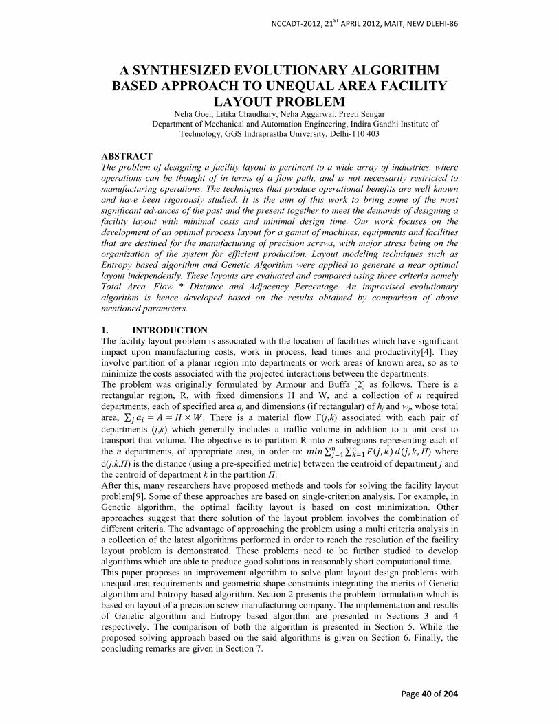
NCCADT-2012, 21ST


Page 40 of 204

A SYNTHESIZED EVOLUTIONARY ALGORITHM

BASED APPROACH TO UNEQUAL AREA FACILITY

LAYOUT PROBLEM Neha Goel, Litika Chaudhary, Neha Aggarwal, Preeti Sengar

Department of Mechanical and Automation Engineering, Indira Gandhi Institute of Technology, GGS Indraprastha University, Delhi-110 403

ABSTRACT

The problem of designing a facility layout is pertinent to a wide array of industries, where

operations can be thought of in terms of a flow path, and is not necessarily restricted to

manufacturing operations. The techniques that produce operational benefits are well known

and have been rigorously studied. It is the aim of this work to bring some of the most

significant advances of the past and the present together to meet the demands of designing a

facility layout with minimal costs and minimal design time. Our work focuses on the

development of an optimal process layout for a gamut of machines, equipments and facilities

that are destined for the manufacturing of precision screws, with major stress being on the organization of the system for efficient production. Layout modeling techniques such as

Entropy based algorithm and Genetic Algorithm were applied to generate a near optimal

layout independently. These layouts are evaluated and compared using three criteria namely Total Area, Flow * Distance and Adjacency Percentage. An improvised evolutionary

algorithm is hence developed based on the results obtained by comparison of above

mentioned parameters.

1. INTRODUCTION

The facility layout problem is associated with the location of facilities which have significant impact upon manufacturing costs, work in process, lead times and productivity[4]. They involve partition of a planar region into departments or work areas of known area, so as to minimize the costs associated with the projected interactions between the departments. The problem was originally formulated by Armour and Buffa [2] as follows. There is a rectangular region, R, with fixed dimensions H and W, and a collection of n required departments, each of specified area aj and dimensions (if rectangular) of hj and wj, whose total area, = = × . There is a material flow F(j,k) associated with each pair of departments (j,k) which generally includes a traffic volume in addition to a unit cost to transport that volume. The objective is to partition R into n subregions representing each of the n departments, of appropriate area, in order to: ,

, , Π) where

d(j,k,Π) is the distance (using a pre-specified metric) between the centroid of department j and the centroid of department k in the partition Π. After this, many researchers have proposed methods and tools for solving the facility layout problem[9]. Some of these approaches are based on single-criterion analysis. For example, in Genetic algorithm, the optimal facility layout is based on cost minimization. Other approaches suggest that there solution of the layout problem involves the combination of different criteria. The advantage of approaching the problem using a multi criteria analysis in a collection of the latest algorithms performed in order to reach the resolution of the facility layout problem is demonstrated. These problems need to be further studied to develop algorithms which are able to produce good solutions in reasonably short computational time. This paper proposes an improvement algorithm to solve plant layout design problems with unequal area requirements and geometric shape constraints integrating the merits of Genetic algorithm and Entropy-based algorithm. Section 2 presents the problem formulation which is based on layout of a precision screw manufacturing company. The implementation and results of Genetic algorithm and Entropy based algorithm are presented in Sections 3 and 4 respectively. The comparison of both the algorithm is presented in Section 5. While the proposed solving approach based on the said algorithms is given on Section 6. Finally, the concluding remarks are given in Section 7.

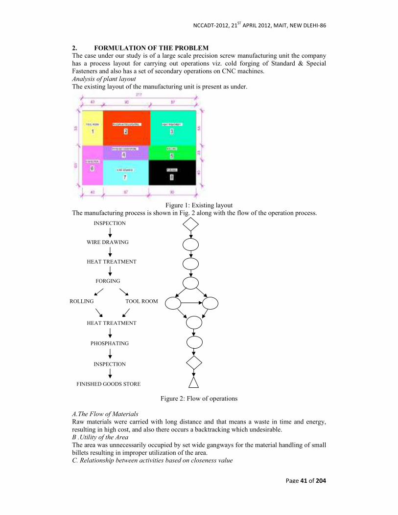
NCCADT-2012, 21ST


Page 41 of 204

2. FORMULATION OF THE PROBLEM The case under our study is of a large scale precision screw manufacturing unit the company has a process layout for carrying out operations viz. cold forging of Standard & Special Fasteners and also has a set of secondary operations on CNC machines. Analysis of plant layout

The existing layout of the manufacturing unit is present as under.

Figure 1: Existing layout

The manufacturing process is shown in Fig. 2 along with the flow of the operation process.

Figure 2: Flow of operations A.The Flow of Materials

Raw materials were carried with long distance and that means a waste in time and energy, resulting in high cost, and also there occurs a backtracking which undesirable. B .Utility of the Area

The area was unnecessarily occupied by set wide gangways for the material handling of small billets resulting in improper utilization of the area. C. Relationship between activities based on closeness value

INSPECTION

WIRE DRAWING

HEAT TREATMENT

FORGING

ROLLING TOOL ROOM

HEAT TREATMENT

PHOSPHATING

INSPECTION

FINISHED GOODS STORE

NCCADT-2012, 21ST


Page 42 of 204

To improve the layout, it is essential to arrange the facilities in the sequence of manufacturing[7]. Then the relationship of each activity in closeness area was considered to make the relationship of each activity in the Activity relationship chart as shown in Fig 2 , and the closeness value are defined as A =absolutely, E = especially important, I = important, O=ordinary closeness, U= unimportant. The details for each activity were described in Table 3, as follows:

Figure 3: Relational graph of each activity

Based on the Activity Relationship chart we get three possible flows given below in table 1:

Product Type Possible flows A 6-7-3-8-5-3-2-6-4 B 6-7-3-8-1-3-2-6-4 C 6-7-3-8-5-1-3-2-6-4

Table 1 : Workflow of the manufacturing process

The important sequence of each activity was rearranged from the most important one to the least important one as shown in Fig 4.

4 6 2 3 1 5 8 7

Figure 4: Sequence of activities The intensities of flow from each activity to another were developed in Fig 5.

Fig5: Work flow intensity

3. GENETIC ALGORITHM

Genetic Algorithm (GA) was first introduced by John Holland in the University of Washington in 1975. GAs are powerful stochastic search and Optimization techniques based

NCCADT-2012, 21ST


Page 43 of 204

on the principles of evaluation theory. The algorithm was implemented using Optimization Toolbox in Matlab. The main steps are as under- Step 1: Initialization

Machine-based representation is selected in this study. A gene denotes a facility to be arranged in one location without reiteration. The chromosome, according to machine based representation, is shown as-

1 2 3 5 4 6 7 8 Step 2: Evaluation

A cost function is used to evaluate the facility layout performance, including the handling cost, the facility moving cost, and the facilities set up cost[20]. The objective function can be expressed as follows: Z= , where cij denotes the cost of moving a unit load of material unit distance between facilities i and j; fij denotes the number of loads or trips required between facilities i and j; dij denotes the distance between facilities i and j. Various linear and non-linerar constraints were applied to eliminate the absolute value sign for the rectilinear distance between the centroid of cell i and the centroid of cell j, also constraints ensure that there is no overlap between any pair of cells. Step 3: Genetic Operators

We selected two-point crossover as it is most suitable for a facility with maximum of 9 departments. The crossover rate is controlled by crossover rate parameter(CR). For mutation a single parent is randomly selected. Then the mutation operator for each of the part just exchanges two randomly chosen elements. The mutation operator is to prevent premature convergence from occurring. The number of mutations performed in a generation is controlled by a mutation rate parameter (MR).

Parameter Values

Population Size, P 50 Crossover rate, CR 0.8 Mutation Rate, MR 0.1 Percentage of solutions replaced by new generation

0.9

Probability of accepting an individual with fitness value less than average as a parent, γ

0.2

Table 2: Parameter settings for the algorithm Step4: Reproduction

The basic part of the selection process is to stochastically select from one generation to create the basis of the next generation. The requirement is that the fittest individuals have a greater chance of survival than weaker ones. The method used for this purpose is the Roulette wheel selection method. Step5:Termination

Two stopping conditions are employed to stop GAs from doing further iteration. First, if the number of iterations exceeds 100(predefined), GAs stops the operation. On the other hand, if the value of objective function does not change within a given number of iterations, the mechanism of GAs is also stopped. Once stopped, the best value of the objective function is obtained. Result

It is observed that the objective function(minimization) drops down rapidly during the beginning period of GA and finally converges to a particular value[21].

NCCADT-2012, 21ST


Page 44 of 204

Figure 6: Optimal layout by Genetic Algorithm

4. ENTROPY ALGORITHM

The Entropy method presents forth a new design approach used in order to solve the facility layout problem [16]. It is concerned with finding the most efficient arrangement of indivisible departments with unequal area requirements within a facility. The algorithm evaluates each possible arrangement by an entropy function, and then the layout with the lowest entropy value is selected as the optimal solution [16]. Decision Variables

The algorithm is based on two variables that indicate the ‘Relationship’ and ‘Prelation’ between every pair of departments. Prelation variable, Pij: It indicates to which degree the activity of one department has to be performed before that of another department. The variables receive values ranging between [-1-1]. The P values are obtained based on the material flow between the departments. Relationship variable, Rij: It indicates the degree of relationship between departments that share resources, information, materials, energy, etc. The variables receive values ranging between [0-1].The relationships between every pair of departments are studied resulting in the following matrices:

X D1 D2 D3 D4 D5 D6 D7 D8 D1 * .130 .72 .0255 .0063 .105 0 .253 D2 -.197 * -.72 .197 0 .72 0 0 D3 -.107 .72 * .105 .257 .197 -.72 .72 D4 -.144 -.045 -.065 * 0 -.72 0 0 D5 .107 .035 .72 .017 * .074 -.035 -.603 D6 -.233 -.72 -.197 .603 -.074 * .72 .035 D7 -.0255 .0082 .72 .0031 .152 -.018 * .197 D8 -.603 -.0255 -.31 -.047 .107 -.233 -.13 *

P D1 D2 D3 D4 D5 D6 D7 D8 D1 * .419 1 .238 .01 .324 0 .419

D2 -

.419 * -1 .419 0 1 0 0

D3 -1 1 * .324 .419 .419 -1 1

D4 -

.238 -

.419 -

.021 * 0 -1 0 0

D5 1 .324 1 .157 * .238 -

.324 -1

D6 -

.324 -1

-.419

1 -

.238 * 1 .324

D7 -

.238 .077 1 .01 .324

-.026

* .419

D8 -1 -

.238 -1

-.077

1 -

.324 -

.419 *

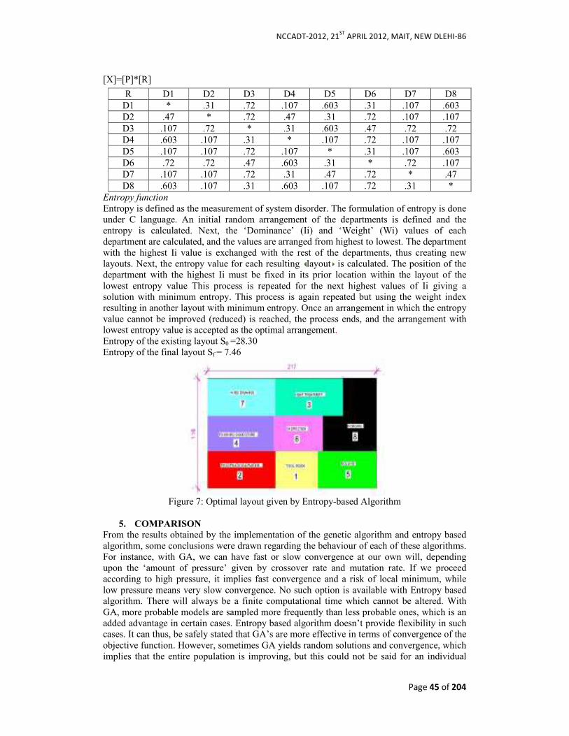
NCCADT-2012, 21ST


Page 45 of 204

[X]=[P]*[R]

Entropy function

Entropy is defined as the measurement of system disorder. The formulation of entropy is done under C language. An initial random arrangement of the departments is defined and the entropy is calculated. Next, the ‘Dominance’ (Ii) and ‘Weight’ (Wi) values of each department are calculated, and the values are arranged from highest to lowest. The department with the highest Ii value is exchanged with the rest of the departments, thus creating new layouts. Next, the entropy value for each resulting layout is calculated. The position of the department with the highest Ii must be fixed in its prior location within the layout of the lowest entropy value This process is repeated for the next highest values of Ii giving a solution with minimum entropy. This process is again repeated but using the weight index resulting in another layout with minimum entropy. Once an arrangement in which the entropy value cannot be improved (reduced) is reached, the process ends, and the arrangement with lowest entropy value is accepted as the optimal arrangement. Entropy of the existing layout S0 =28.30 Entropy of the final layout Sf = 7.46

Figure 7: Optimal layout given by Entropy-based Algorithm

5. COMPARISON

From the results obtained by the implementation of the genetic algorithm and entropy based algorithm, some conclusions were drawn regarding the behaviour of each of these algorithms. For instance, with GA, we can have fast or slow convergence at our own will, depending upon the ‘amount of pressure’ given by crossover rate and mutation rate. If we proceed according to high pressure, it implies fast convergence and a risk of local minimum, while low pressure means very slow convergence. No such option is available with Entropy based algorithm. There will always be a finite computational time which cannot be altered. With GA, more probable models are sampled more frequently than less probable ones, which is an added advantage in certain cases. Entropy based algorithm doesn’t provide flexibility in such cases. It can thus, be safely stated that GA’s are more effective in terms of convergence of the objective function. However, sometimes GA yields random solutions and convergence, which implies that the entire population is improving, but this could not be said for an individual

R D1 D2 D3 D4 D5 D6 D7 D8 D1 * .31 .72 .107 .603 .31 .107 .603 D2 .47 * .72 .47 .31 .72 .107 .107 D3 .107 .72 * .31 .603 .47 .72 .72 D4 .603 .107 .31 * .107 .72 .107 .107 D5 .107 .107 .72 .107 * .31 .107 .603 D6 .72 .72 .47 .603 .31 * .72 .107 D7 .107 .107 .72 .31 .47 .72 * .47 D8 .603 .107 .31 .603 .107 .72 .31 *

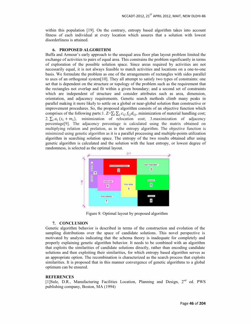
NCCADT-2012, 21ST


Page 46 of 204

within this population [19]. On the contrary, entropy based algorithm takes into account fitness of each individual at every location which assures that a solution with lowest disorderliness is attained.

6. PROPOSED ALGORITHM Buffa and Armour’s early approach to the unequal area floor plan layout problem limited the exchange of activities to pairs of equal area. This constrains the problem significantly in terms of exploration of the possible solution space. Since areas required by activities are not necessarily equal, it is not always feasible to match activities and locations on a one-to-one basis. We formulate the problem as one of the arrangements of rectangles with sides parallel to axes of an orthogonal system[10]. They all attempt to satisfy two types of constraints: one set that is dependent on the structure or topology of the problem such as the requirement that the rectangles not overlap and fit within a given boundary; and a second set of constraints which are independent of structure and consider attributes such as area, dimension, orientation, and adjacency requirements. Genetic search methods climb many peaks in parallel making it more likely to settle on a global or near-global solution than constructive or improvement procedures. So, the proposed algorithm consists of an objective function which comprises of the following parts:1. Z= , minimization of material handling cost; 2. + , minimization of relocation cost; 3.maximization of adjacency percentage[9]. The adjacency percentage is calculated using the matrix obtained on multiplying relation and prelation, as in the entropy algorithm. The objective function is minimized using genetic algorithm as it is a parallel processing and multiple-points utilization algorithm in searching solution space. The entropy of the two results obtained after using genetic algorithm is calculated and the solution with the least entropy, or lowest degree of randomness, is selected as the optimal layout.

Figure 8: Optimal layout by proposed algorithm

7. CONCLUSION

Genetic algorithm behavior is described in terms of the construction and evolution of the sampling distributions over the space of candidate solutions. This novel perspective is motivated by analysis indicating that the schema theory is inadequate for completely and properly explaining genetic algorithm behavior. It needs to be combined with an algorithm that exploits the similarities of candidate solutions directly, rather than encoding candidate solutions and then exploiting their similarities, for which entropy based algorithm serves as an appropriate option. The recombination is characterized as the search process that exploits similarities. It is proposed that in this manner convergence of genetic algorithms to a global optimum can be ensured.

REFERENCES

[1]Sule, D.R., Manufacturing Facilities Location, Planning and Design, 2nd ed. PWS publishing company, Boston, MA (1994)

NCCADT-2012, 21ST


Page 47 of 204

[2]GG Armour and ES. Buffa, A heuristic formulation approach to relative allocation. Manage Sci, 29 (1963), pp. 294–300. [3]E.L. Lawler, The quadratic assignment problem. Manage Sci, 94 (1963), pp. 586–599. [4]F.S. Hillier, Quantitative tools for plan layout analysis. J Ind Eng, 14 1 (1963), pp. 33–40. [5]T.M. Khalil, Facilities relative allocation technique (FRAT). Int J Prod Res,112 (1973), pp. 183–194. [6]Heragu, S.S. Facilities design. An International Thomson Publishing Company,1997. [7]T. Yang and C.-C. Hung, Multiple-attribute decision making methods for plant layout design problem. Robotics Comput-Integrated Manuf, 23 (2007), pp. 126–137. [8]R.D. Meller and K. Gau, The facility layout problem: recent and emerging trends and perspectives. J Manuf Systems, 15 (1996), pp. 351–366. [9]M.J. Rosenblatt, The facilities layout problem: a multigoal approach. Int J Prod Res, 174 (1979), pp. 323–332. [10]K.N. Dutta and S. Sahu, A multigoal heuristic for facilities design problems: MUGHAL. Int J Prod Res, 20 2 (1982), pp. 147–154. [11]T.L. Urban, A multiple criteria model for the facilities layout problem. Int J Prod Res, 25 12 (1987), pp. 1805–1812. [12]B. Malakooti and G.I. D’Souza, Multiple objective programming for the quadratic assignment problem. Int J Prod Res, 25 25 (1987), pp. 285–300. [13]Dhamodharan Raman and Sev V. Nagalingam, Towards Measuring the Effectiveness of a

Facility Layout (2009). [14]Tompkins, J.A. White, J.A. Bozen, Y.A. Frazelle, E.H., Tanchoco, J.M.A and Trevino, J. Facilities Planning, John Wiley, New York, NY (1996) [15]Tompkins, J.A., and White, J.A., 1984, Facilities Planning, Wiley and Sons, New York, NY. [16]Ma Carmen González-Cruz, Eliseo Gómez-Senent Martínez (2010), An entropy-based

algorithm to solve the facility layout design problem. [17]Coly, D.A, “An Introduction to Genetic Algorithms for Scientists and Engineers” World Scientific (1999). [18]GG Armour and ES. Buffa, A heuristic formulation approach to relative allocation. Manage Sci, 29 (1963), pp. 294–300. [19]Chuang, C.-L. Y.-P. (2011). A genetic algorithm for dynamic facility planning in job. Int

J Adv Manuf Technol , pp. 303–309. [20]El-Baz, M. A. (2004). A genetic algorithm for facility layout problems of different. Computers & Industrial Engineering 47 , pp. 233–246. [21]Kyu-Yeul Leea, S.-N. H.-I. (2003). An improved genetic algorithm for facility layout problems having inner structure walls and passages. Computers & Operations Research , pp. 117–138. [22]Ming-Jaan Wanga, M. H.-Y. (2005). A solution to the unequal area facilities layout. Computers in Industry 56 , pp. 207–220. [23]Sarkar, S. G. (2011). Cost optimization by genetic algorithm technique for Y Oscillatory. African Journal of Business Management Vol.5 , pp. 4078-4086. [24]Gómez Gómez, A. F. (n.d.). THE USE OF GENETIC ALGORITHMS TO SOLVE A PLANT LAYOUT PROBLEM. Esc. Tec. Sup. de Ingenieros Industriales de Gijón. [25]B. Malakooti and G.I. D’Souza, Multiple objective programming for the quadratic assignment problem. Int J Prod Res,25 25 (1987), pp. 285–300.

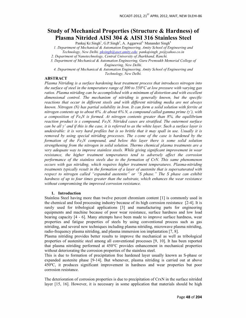
NCCADT-2012, 21ST


Page 48 of 204

Study of Mechanical Properties (Structure & Hardness) of

Plasma Nitrided AISI 304 & AISI 316 Stainless Steel Pankaj Kr.Singh1, G.P.Singh2, A. Aggarwal3, Manander Singh4

1. Department of Mechanical & Automation Engineering, Amity School of Engineering and

Technology, New Delhi. [email protected]; [email protected]

2. Department of Nanotechnology, Central University of Jharkhand, Ranchi.

3. Department of Mechanical & Automation Engineering, Guru Premsukh Memorial College of

Engineering, New Delhi.

4. Department of Mechanical & Automation Engineering, Amity School of Engineering and

Technology, New Delhi.

ABSTRACT

Plasma Nitriding is a surface hardening heat treatment process that introduces nitrogen into

the surface of steel in the temperature range of 300 to 550°C at low pressure with varying gas

ratios. Plasma nitriding can be accomplished with a minimum of distortion and with excellent

dimensional control. The mechanism of nitriding is generally known, but the specific

reactions that occur in different steels and with different nitriding media are not always

known. Nitrogen (N) has partial solubility in Iron. It can form a solid solution with ferrite at

nitrogen contents up to about 6%. At about 6% N, a compound called gamma prime (γ’), with

a composition of Fe4N is formed. At nitrogen contents greater than 8%, the equilibrium

reaction product is ε compound, Fe3N. Nitrided cases are stratified. The outermost surface

can be all γ’ and if this is the case, it is referred to as the white layer. Such a surface layer is

undesirable: it is very hard profiles but is so brittle that it may spall in use. Usually it is

removed by using special nitriding processes. The ε-zone of the case is hardened by the

formation of the Fe3N compound, and below this layer there is some solid solution strengthening from the nitrogen in solid solution. Thermo chemical plasma treatments are a

very adequate way to improve stainless steels. While giving significant improvement in wear

resistance, the higher treatment temperatures tend to adversely affect the corrosion

performance of the stainless steels due to the formation of CrN. This same phenomenon

occurs with gas nitriding, which requires higher treatment temperatures. Plasma-nitriding

treatments typically result in the formation of a layer of austenite that is supersaturated with

respect to nitrogen called “expanded austenite” or “S phase.” The S phase can exhibit

hardness of up to four times greater than the substrate, which enhances the wear resistance

without compromising the improved corrosion resistance.

1. Introduction

Stainless Steel having more than twelve percent chromium content [1] is commonly used in the chemical and food processing industry because of its high corrosion resistance [2-4]. It is rarely used for tribological applications [3] and manufacturing parts for engineering equipments and machine because of poor wear resistance, surface hardness and low load bearing capacity [4 - 6]. Many attempts have been made to improve surface hardness, wear properties and fatigue properties of steels by using conventional process such as gas nitriding, and several new techniques including plasma nitriding, microwave plasma nitriding, radio-frequency plasma nitriding, and plasma immersion ion implantation [7, 8]. Plasma nitriding provides better results to improve the mechanical as well as tribological properties of austenitic steel among all conventional processes [9, 10]. It has been reported that plasma nitriding performed at 450°C provides enhancement in mechanical properties without deteriorating the corrosion properties of the stainless steel. This is due to formation of precipitation free hardened layer usually known as S-phase or expanded austenite phase [9-14]. But whenever, plasma nitriding is carried out at above 450ºC, it produces significant improvement in hardness and wear properties but poor corrosion resistance. The deterioration of corrosion properties is due to precipitation of CrxN in the surface nitrided layer [15, 16]. However, it is necessary in some application that materials should be high

NCCADT-2012, 21ST


Page 49 of 204

hardness, wear as well as good corrosion resistance properties. Therefore, the present investigation is focused to study the mechanical properties of plasma nitrided AISI 304 stainless steel in terms of the improvement surface hardness and other properties. The subsequent post sputtering was performed in an Ar: H2 plasma atmosphere to achieve the good corrosion properties of the samples nitrided above 500°C without CrN precipitation. The phase analysis, surface micro-hardness, and nitrogen diffusion layer thickness/case depth of plasma nitride samples were characterized by X – ray Diffractogram, Vickers microhardness tester, and optical microscope, respectively.

2. Experimental Procedure

AISI 304 and AISI 316 are austenitic stainless steels widely employed in corrosive environments. The main difference between these two steels is with respect to the content of alloying element molybdenum. The amount of Mo in AISI 316 corresponds to about 2% in weight while it is very trace amount in AISI 304 [3]. Samples Ni Cr C Si Mn S Mo P Fe

AISI 304

8.63 16.04 0.04 0.48 1.37 0.005 0.09 0.029 Balance Fe

AISI 316

11.64 15.68 0.10 0.34 1.73 0.031 1.86 0.029 Balance Fe

The sample was in the form of circular disc having diameter 25 mm. Plasma nitriding was carried out in a 500 mm diameter and 500 mm height bell shaped stainless steel vacuum chamber. The samples were first sputter cleaned using 80Ar:20H2 gas mixture. Plasma was generated using a D.C. pulsed power supply having a repetition rate of 10 kHz. Sputter cleaning process was performed for 1 hr at 250°C to remove the native oxide layer and contamination so as to expose a fresh surface of the samples for plasma nitriding. After completing the sputter cleaning process, the mixture of nitrogen and hydrogen gas was introduced in the reactor for plasma nitriding. Plasma nitriding was carried out using gas mixtures of 80N2:20H2 and 20N2:80H2 under a pressure of 4 mbar at 500°C for 24 hours. Micro-hardness measurements were performed on untreated and plasma nitrided samples surface with a Leitz Vickers Hardness tester using a load of 100 g. Case depth of the modified layer was examined by Leitz make optical microscope at a magnification of 100X. X-ray diffraction (XRD) was performed in two – degree grazing incidence diffraction mode using Seifert made XRD-3000 PTS Diffrectometer. Cu anode X-ray tube was operated at 40 kV and 30 mA to get Cu Kα radiation (λ=1.5418 Å). The diffraction patterns were obtained in the 2θ ranges of 40–70° with the step size of 0.1° and counting time of 3 s per step.

3. Results and Discussion

3.1. Structural and Hardness properties of Plasma nitride AISI 304 and AISI 316

stainless steel

Effect of temperature on microstructure

In a plasma nitriding process [5], nitrogen atoms can be driven into the surface of steels or other iron based alloys kept at temperatures in the range 400-650ºC [6] in order to enhance properties such as hardness and tolerance to both corrosion and wear. Thus, this treatment has been straight forwardly applied to tools and machinery parts [7-8]. When comparing traditional nitriding processes (e.g. gas or salt based) low energy PIII results very economically attractive due to the introduction of nitrogen by diffusion with lower energy and gas consumption and allowing a substantial reduction of the treatment temperature and/or the processing time [9]. Austenitic stainless steels, in particular, can be implanted at less than 450ºC so to prevent the precipitation of chrome nitrides which promotes the depletion of chrome and whereby the loss of corrosion resistance in this kind of steels [10]. Ionic nitriding of austenitic steels enables to obtain a meta-stable superficial phase, called expanded austenite, whose depths lie in the order of 1-10 µm and where nitrogen remains in a solid

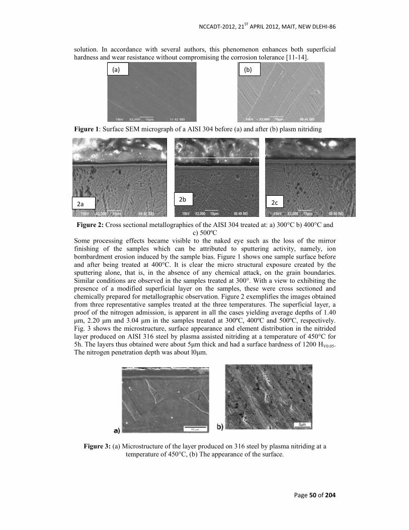
NCCADT-2012, 21ST


Page 50 of 204

solution. In accordance with several authors, this phenomenon enhances both superficial hardness and wear resistance without compromising the corrosion tolerance [11-14]. Figure 1: Surface SEM micrograph of a AISI 304 before (a) and after (b) plasm nitriding

Figure 2: Cross sectional metallographies of the AISI 304 treated at: a) 300°C b) 400°C and c) 500ºC

Some processing effects became visible to the naked eye such as the loss of the mirror finishing of the samples which can be attributed to sputtering activity, namely, ion bombardment erosion induced by the sample bias. Figure 1 shows one sample surface before and after being treated at 400°C. It is clear the micro structural exposure created by the sputtering alone, that is, in the absence of any chemical attack, on the grain boundaries. Similar conditions are observed in the samples treated at 300°. With a view to exhibiting the presence of a modified superficial layer on the samples, these were cross sectioned and chemically prepared for metallographic observation. Figure 2 exemplifies the images obtained from three representative samples treated at the three temperatures. The superficial layer, a proof of the nitrogen admission, is apparent in all the cases yielding average depths of 1.40 µm, 2.20 µm and 3.04 µm in the samples treated at 300ºC, 400ºC and 500ºC, respectively. Fig. 3 shows the microstructure, surface appearance and element distribution in the nitrided layer produced on AISI 316 steel by plasma assisted nitriding at a temperature of 450°C for 5h. The layers thus obtained were about 5µm thick and had a surface hardness of 1200 HV0.05. The nitrogen penetration depth was about l0µm.

Figure 3: (a) Microstructure of the layer produced on 316 steel by plasma nitriding at a

temperature of 450°C, (b) The appearance of the surface.

(a) (b)

2a 2b

2c

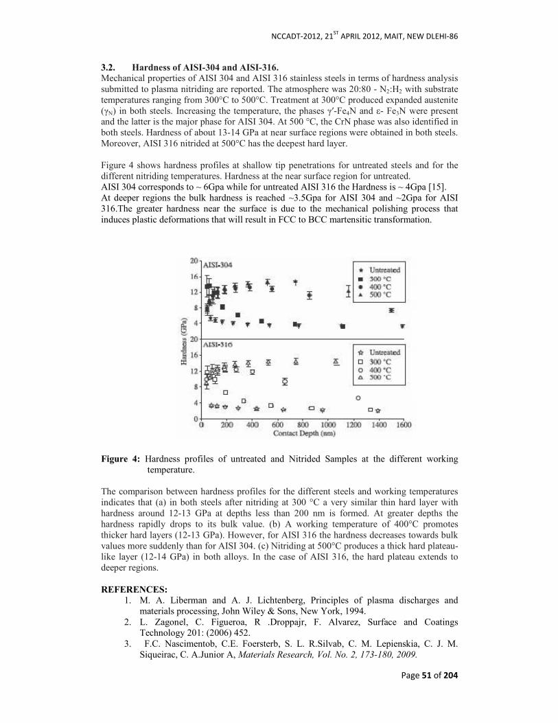
NCCADT-2012, 21ST


Page 51 of 204

3.2. Hardness of AISI-304 and AISI-316.

Mechanical properties of AISI 304 and AISI 316 stainless steels in terms of hardness analysis submitted to plasma nitriding are reported. The atmosphere was 20:80 - N2:H2 with substrate temperatures ranging from 300°C to 500°C. Treatment at 300°C produced expanded austenite (γN) in both steels. Increasing the temperature, the phases γ′-Fe4N and ε- Fe3N were present and the latter is the major phase for AISI 304. At 500 °C, the CrN phase was also identified in both steels. Hardness of about 13-14 GPa at near surface regions were obtained in both steels. Moreover, AISI 316 nitrided at 500°C has the deepest hard layer. Figure 4 shows hardness profiles at shallow tip penetrations for untreated steels and for the different nitriding temperatures. Hardness at the near surface region for untreated. AISI 304 corresponds to ~ 6Gpa while for untreated AISI 316 the Hardness is ~ 4Gpa [15]. At deeper regions the bulk hardness is reached ~3.5Gpa for AISI 304 and ~2Gpa for AISI 316.The greater hardness near the surface is due to the mechanical polishing process that induces plastic deformations that will result in FCC to BCC martensitic transformation.

Figure 4: Hardness profiles of untreated and Nitrided Samples at the different working temperature.

The comparison between hardness profiles for the different steels and working temperatures indicates that (a) in both steels after nitriding at 300 °C a very similar thin hard layer with hardness around 12-13 GPa at depths less than 200 nm is formed. At greater depths the hardness rapidly drops to its bulk value. (b) A working temperature of 400°C promotes thicker hard layers (12-13 GPa). However, for AISI 316 the hardness decreases towards bulk values more suddenly than for AISI 304. (c) Nitriding at 500°C produces a thick hard plateau-like layer (12-14 GPa) in both alloys. In the case of AISI 316, the hard plateau extends to deeper regions.

REFERENCES:

1. M. A. Liberman and A. J. Lichtenberg, Principles of plasma discharges and materials processing, John Wiley & Sons, New York, 1994.

2. L. Zagonel, C. Figueroa, R .Droppajr, F. Alvarez, Surface and Coatings Technology 201: (2006) 452.

3. F.C. Nascimentob, C.E. Foersterb, S. L. R.Silvab, C. M. Lepienskia, C. J. M. Siqueirac, C. A.Junior A, Materials Research, Vol. No. 2, 173-180, 2009.

NCCADT-2012, 21ST


Page 52 of 204

4. F.C. Nascimentob, C. E. Foersterb, S. L. R. da Silvab, C. M. Lepienskia, C. J.M. Siqueirac, C. A. Junior, Materials Research, Vol. 12, No. 2, 173-180, 2009.

5. A. Sakar, Ch. Leroy, H. Michel, Mat. Sci. Eng. A 140, 702 (1991). 6. M. A. Liberman and A. J. Lichtenberg, Principles of plasma discharges and

materials processing, John Wiley & Sons, New York, 1994. 7. L. Zagonel, C. Figueroa, R .Droppajr, F. Alvarez, Surface and Coatings

Technology 201: (2006) 452. 8. F.C. Nascimentob, C.E. Foersterb, S. L. R.Silvab, C. M. Lepienskia, C. J. M.

Siqueirac, C. A.Junior A, Materials Research, Vol. No. 2, 173-180, 2009. 9. F.C. Nascimentob, C. E. Foersterb, S. L. R. da Silvab, C. M. Lepienskia, C. J.M.

Siqueirac, C. A. Junior, Materials Research, Vol. 12, No. 2, 173-180, 2009 10. J. R. Conrad, J. L. Radtke, R. A. Dodd, F. J. Worzala, N.C. Tran, J. Appl. Phys.62,

4591 (1987). 11. G.F. Gomez and M. Ueda, J. of Appl. Phys. 94, 1 (2003). 12. M. A. Bejar, C. González. Rev. Mat. 8, 115 (2003). 13. D. Peix, M.A. Guitar, S.P. Bruhl, N. Mingolo, V. Vanzulli; A. Cabo, E. Forlerer.

Rev.Materia 10, 205 (2005). 14. W. Liang, Appl. Surf. Sci. 211, 308 (2003). 15. E. Menthe, K.-T. Rie ,Surface and Coatings Technology 116 - 119 (1999) 1999 –

204.

NCCADT-2012, 21ST


Page 53 of 204

Microcontroller For All: An application to robotics

Pawan Kumar, NGFCET, Palwal

[email protected] Abstract:

Microcontroller - specially designed for performing single task, is a computer-on-a-chip

usually comprises of I/O ports, RAM, ROM and also CPU. Due to simplicity in design and

pocket friendly prices, microcontroller is widely adopted for various fields including

automobiles, medical science, defense, domestic applications, industrial use, energy

management and lots more domains. In addition to this, microcontrollers are commonly built

using CMOS (Complementary-Metal Oxide Semiconductor) technology resulting optimum

performance with the least consumption of power. Due to performing only single dedicated

task, latency of the task is fast and more reliable.

This technical paper explains wide range of applications of microcontrollers in the field of

robotics. For making different types of robots including wall follower robot, pick & place

robot, agriculture robot, vacuum cleaner robot, fire fighting robot etc., we need different

types of microcontrollers ranging from 8051, PIC, AVR, ARM etc. Microcontroller could be

considered as the heart of any robotic system because the entire hardware of robot is actually

control by the microcontroller. Depending upon the application, embedded engineer burns

the code i.e. HEX file of the program into the microcontroller. Additionally we can also

interface different types of sensors with the microcontroller for different robotics project. For

example in the fire fighting robot we can directly interface LDR (Light Dependent Resistor)

sensor with any pins of microcontroller. In addition to this, in the edge avoiding robot we need to interface IR LED with any pins of microcontroller.

This technical paper explains not only the different types of microcontrollers but also the real

environment programming for different types of microcontrollers including 8051/8052, PIC,

AVR and ARM etc. After reading this technical paper, we not only write the program but also

can modify as per individual requirements. This technical paper explains not only the

hardware but also the real programming environment for mainly 4 microcontrollers i.e.

8051/8052, PIC, AVR and ARM. Additionally this technical paper also brings various screen

shots for different types of microcontrollers which help in understanding different

programming environment for different MCs (Microcontrollers).

Keywords: 8051, ARM, PIC, AVR, KEIL, Burner, MPLAB, Microcontroller, CMOS, RAM,

ROM, Robots, Programs

History

As we know that the concept of the term “Chip” – which integrates several active as well as passive components on a single block, came into existence in the year 1952. Robert Noyce and Jean Hoerni - engineer at Fairchild Semiconductor, brings large-scale production of ICs (Integrated Circuits) in the year 1959. In 1964, SSI (Small-Scale Integration) chips are introduced for various logic gates. In 1960’s, Moore’s law came into existence which states that – “Number of transistors on a chip will be doubled in every year”. In year 1977, Intel developed state-of-the-art technology based chip named Intel 8048 which was initially optimized specially for various control applications. According to Intel Corporation, Intel 8048 was the first time combination of both RAM (Random Access Memory) and ROM (Read Only Memory) on the same chip. As we know that there is always a tradeoff between storage permanence and writing ability. Initially MC came with EPROM (Erasable Programmable Read Only Memory) consisting of MOS (Metal-oxide Semiconductor) transistor. To erase the program of EPROM, ultraviolet light acts the role of eraser. After that in early 1980’s, the concept of EEPROM (Electrically Erasable Programmable Read Only Memory) is being launched which can be electrically erased by the programmer.

NCCADT-2012, 21ST


Page 54 of 204

In 1981, Intel Corporation introduced 8-bit microcontroller called 8051 having 128 bytes of RAM (Random Access Memory) and 4K bytes of on-chip ROM (Read Only Memory). We know that 8051 is the original member of the 8051 family having the following features:

Features of 8051: Feature Quantity ROM 4K bytes RAM 128 bytes Timer 2 I/O pins 32 Serial Port 1 Interrupt Sources 6 Two more members of 8051 family of microcontroller including 8052 and 8031. On the similar way, PIC (Peripheral Interface Controller) was developed by General Instruments in year 1975. General instruments convert their Microelectronics Division and bring Microchip Technology. And now Microchip Technology launched 8-bit PIC16C84 having EEPROM. In 1998, improved version of PIC16C84 including PIC18F84 and PIC18F84A is being launched. In parallel with PIC, AVR (Advanced Virtual RISC Processor) - 8-bit RISC (Reduced Instruction Set Computer) single chip microcontroller, was introduced by ATMEL in 1996. According to ATMEL, AVRs are 4 times faster than that of PIC resulting least consumption of power. Recently AVR brings ATmega 16/32 microcontroller which is 40 pin IC. But how we could ARM (Advanced RISC Machine which is 32-bit reduced instruction set computer. In 1987, Acron Archimedes introduced ARM-based products throughout the globe. In an independent survey, more than one billion mobile phones – incorporating ARM processor, are being sold each year across the globe. And nowadays this 32-bit computer is extensively used in multitude of applications including PDAs, calculators, routers, hard drives, tablets and computer peripherals also. Type (A): 8051 Family (1) 8051 Microcontroller: 8051 microcontroller is a pocket friendly computer-on-a-chip built for performing specified task rather than multiple tasks. Microcontrollers – comprises of ROM, RAM, I/O Ports and also CPU, are generally built using CMOS (Complementary Metal Oxide Semiconductor) technology resulting optimum performance with the least consumption of power. Some salient feature of 8051 includes: 1. ROM – 4K bytes 2. RAM – 128 bytes 3. 6 Interrupts sources 4. 8-bit ALU 5. Input/output Pins – 4 Ports of 8 bits each on a single chip 6. Harvard Memory Architecture 7. Clock frequency – 12 MHZ 8. UART (Universal Asynchronous Receiver Transmitter) 9. Bit addressable 10. Low price (2 ) KEIL Software for 8051Family: KEIL – founded in 1982, provides broad range of development tools including libraries, IDE (Integrated Development Environment), assemblers and also linkers.

NCCADT-2012, 21ST


Page 55 of 204

(3) HEX file: HEX file is a special file which is imported by a programmer into the target IC. Hex file is a kind of file which is actually not for user. (4) Burner for 8051 Family: FLASH Magic is a feature-rich window application which is completely dedicated for 8051 family. Using FLASH Magic, HEX file could be easily transferred into the target IC. (5) Steps for writing target program (available in C/Assembly Language) for 8051 MC: Here we can see that how we can write any program and successful transfer to target IC using FLASH burner.

(a) First write your program either in C or in assembly language. In this paper I am writing the program of generating 10 KHZ square wave in assembly language. (b) Write your program (C or assembly language) in the KEIL software environment. See fig 1:

(c) After writing your program in either c or assembly language, make sure of making HEX file. See fig 2:

(d) Now we have a HEX file of the above program and this HEX file is ready to go at the target IC using FLASH burner. See fig 3:

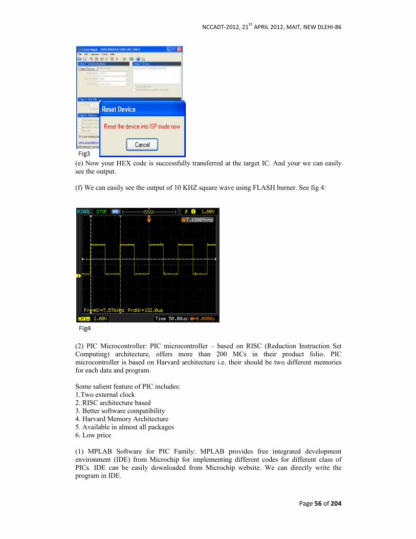
NCCADT-2012, 21ST


Page 56 of 204

(e) Now your HEX code is successfully transferred at the target IC. And your we can easily see the output. (f) We can easily see the output of 10 KHZ square wave using FLASH burner. See fig 4:

(2) PIC Microcontroller: PIC microcontroller – based on RISC (Reduction Instruction Set Computing) architecture, offers more than 200 MCs in their product folio. PIC microcontroller is based on Harvard architecture i.e. their should be two different memories for each data and program. Some salient feature of PIC includes: 1.Two external clock 2. RISC architecture based 3. Better software compatibility 4. Harvard Memory Architecture 5. Available in almost all packages 6. Low price (1) MPLAB Software for PIC Family: MPLAB provides free integrated development environment (IDE) from Microchip for implementing different codes for different class of PICs. IDE can be easily downloaded from Microchip website. We can directly write the program in IDE.

NCCADT-2012, 21ST


Page 57 of 204

(2) HEX file: HEX file is a special file which is imported by a programmer into the target IC. Hex file is a kind of file which is actually not for user. (3) Burner for PIC Family: PICkit2 is very economic development board for the purpose of programming as well as debugging Microchip microcontrollers. (4) Steps for writing target program (available in C/Assembly Language) for PIC MC: Here we can see that how we can write any program and successful transfer to target IC using PICKIT2 burner.

(a) First write your program either in C or in assembly language. In this paper I am writing again the program of generating 10 KHZ square wave in assembly language.

(b) Write your program (C or assembly language) in the IDE software environment.

See fig 5:

(c) After writing your program in either c or assembly language, make sure of making HEX file. See fig 6:

(d) Now we have a HEX file of the above program and this HEX file is ready to go at the target IC using PICKKIT2 burner. See fig 7

NCCADT-2012, 21ST


Page 58 of 204

(e) Now your HEX code is successfully transferred at the target IC. And your we can easily see the output. (f) We can easily see the output of 10 KHZ square wave using PICKKIT2 burner. See fig 8:

(3) AVR Microcontroller: AVR microcontroller – 8-bit RISC single chip microcontroller, is a modified Harvard architecture. AVR was discovered by Atmel in the year 1996. Some salient feature of PIC includes: 1. Harvard Memory Architecture 2. Available in almost all packages 3. Low price (1) WinAVR Software for AVR Family: WinAVR software provides the platform for user for writing and also debugging the program. (2) HEX file: HEX file is a special file which is imported by a programmer into the target IC. Hex file is a kind of file which is actually not for user. (3) Burner for AVR Family: Pony Prog is a serial device programmer which is completely dedicated for AVR family (4) Steps for writing target program (available in C/Assembly Language) for PIC MC: Here we can see that how we can write any program and successful transfer to target IC using PICKIT2 burner.

(a) First write your program either in C or in assembly language. In this paper I am writing again the program of generating 10 KHZ square wave in assembly language.

(b) Write your program (C or assembly language) in the WinAVR software environment. See fig 9

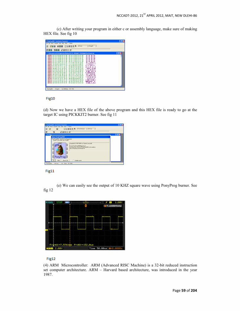
NCCADT-2012, 21ST


Page 59 of 204

(c) After writing your program in either c or assembly language, make sure of making HEX file. See fig 10

(d) Now we have a HEX file of the above program and this HEX file is ready to go at the target IC using PICKKIT2 burner. See fig 11

(e) We can easily see the output of 10 KHZ square wave using PonyProg burner. See

fig 12

(4) ARM Microcontroller: ARM (Advanced RISC Machine) is a 32-bit reduced instruction set computer architecture. ARM – Harvard based architecture, was introduced in the year 1987.

NCCADT-2012, 21ST


Page 60 of 204

Some salient feature of ARM includes:

1. Harvard Memory Architecture 2. Available in almost all packages 3. Most advanced microcontroller

4. Low price

(2) WinARM Software for ARM Family: WinAVR software provides the platform for user for writing and also debugging the program.

(3) HEX file: HEX file is a special file which is imported by a programmer into the target IC. Hex file is a kind of file which is actually not for user.

(4) Burner for ARM Family: FLASH Magic – Same as 8051 (See 8051)

(5) Steps for writing target program (available in C/Assembly Language) for ARM MC: Same as 8051 (See 8051) Note: The working environment for 8051 i.e. KEIL and PIC i.e. MPLAB IDE can be installed at

common computer because both have different programming environment. But due to the

same programming environment for AVR and ARM i.e. notepad programmer need two

different computers for each controller. REFERENCES

(1) Wikipedia

(2) www.TI.com

(3) www.KEIL.com

NCCADT-2012, 21ST


Page 61 of 204

MAXIMUM POWER POINT TRACKER ALGORITHMS

IN SOLAR PHOTO VOLTAIC SYSTEM: THE

ENHANCED SOLAR ENERGY MANAGEMENT

SCHEME

Richa Agrawal* Deepika Agrawal* *Bhiwani Institute of Technology and Sciences,Bhiwani Haryana([email protected])

Abstract

Energy management is a branch is of science for planning, directing, controlling the supply

and consumption of energy. Energy need in India will grow 5-7 times by 2030.Ministry of

India has set an objective of “power to all by 2012”.So according to power survey by

ministry of power, India , We need 100000 mw more power capacity by 2012.The abundant

solar energy can help to meet these challenges. New techniques, alternative material,

efficient conversion methods conversion methods etc. are required to enhance solar

photovoltaic systems.Vast research work has been done in field of solar photovoltaic sector

like developing thin film based high concentration photovoltaic, concentrated solar power

(CSP), Nano solar, photon chasing silicon wafer based photovoltaic etc. These advanced techniques resulted in a 10 percent cost reduction of usage of PV devices .The paper

discusses about the maximum power point tracker (MPPT) which is a power electronic

system. The solar energy is available in different amount at different places and at different

time. The photovoltaic characteristics are nonlinear and have maximum power point at

different instances of time. The power line connects these maximum power points of different

characteristics. The maximum power point tracker (MPPT) tracks this power line so to use

solar energy at its maxima and to deal with the problem of time variable solar energy

availability. The scheme results in higher performance, reliability and enhanced efficiency of

solar energy conversion system. MPPT embedded with new simulation technologies fuzzy, artificial neural networks, artificial intelligence etc can be a revolutionary step in solar

energy management.

Keywords: Energy management, solar photovoltaic systems, concentrated solar power (CSP), nano-solars, maximum power point tracker (MPPT)

INTRODUCTION

Maximum power point tracking (MPPT) [1] is a technique that grid tie inverters, solar battery chargers and similar devices use to get the maximum possible power from one or more solar panels. Maximum Power Point Tracking or MPPT is the algorithm that included in electronic control device use for extracting maximum available power from PV panels, which the maximum power change according to the variations in parameters such as solar radiation, ambient temperature and solar cell temperature. The word photovoltaic (PV) literally means conversion of sunlight directly to electricity. A typical photovoltaic system consists of two major parts: the solar panels that generate DC power from sunlight, and the power electronics that convert DC into standard AC voltages. It is clean, easy- maintenance and have long lifespan .Photo Voltaic (PV) devices serve as current sources whose output varies based on the level of solar radiation and PV panel temperature. Output power depends on solar radiation, PV panel temperature, and output voltage. PV voltage must be optimized based on solar radiation and PV panel temperature to obtain continuous maximum power. The MPPT algorithm is implemented by using microprocessor to check the PV panels output at all time that there is no other higher output power from PV panels in form of current and voltage from the solar radiation at that time. To get the higher power, the MPPT algorithm checks the PV panels output, and compares it to the battery voltage. Solar cells have a complex relationship between solar irradiation, temperature and total resistance that produces a non-linear output efficiency known as the I-V curve. It is the purpose of the MPPT system to sample the output of the cells and apply the proper resistance (load) to obtain maximum power for any given environmental conditions

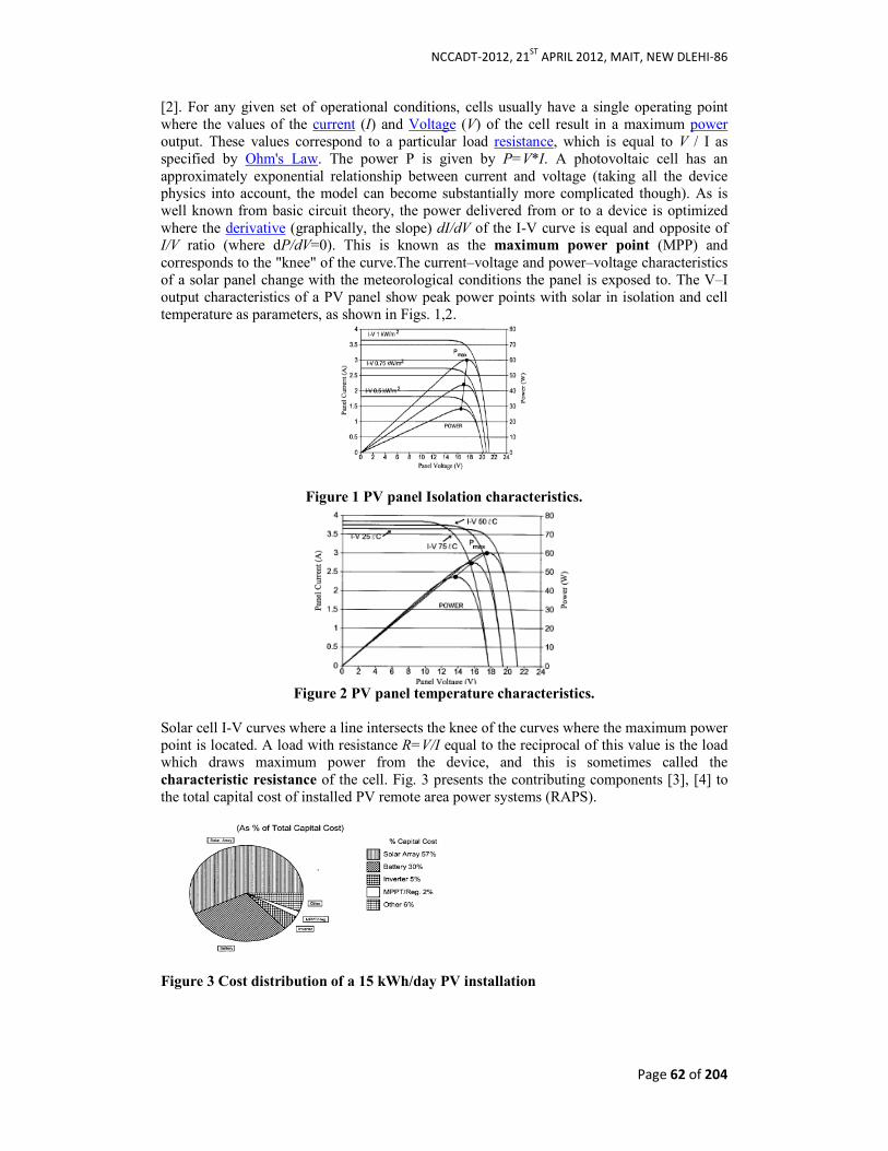
NCCADT-2012, 21ST


Page 62 of 204

[2]. For any given set of operational conditions, cells usually have a single operating point where the values of the current (I) and Voltage (V) of the cell result in a maximum power output. These values correspond to a particular load resistance, which is equal to V / I as specified by Ohm's Law. The power P is given by P=V*I. A photovoltaic cell has an approximately exponential relationship between current and voltage (taking all the device physics into account, the model can become substantially more complicated though). As is well known from basic circuit theory, the power delivered from or to a device is optimized where the derivative (graphically, the slope) dI/dV of the I-V curve is equal and opposite of I/V ratio (where dP/dV=0). This is known as the maximum power point (MPP) and corresponds to the "knee" of the curve.The current–voltage and power–voltage characteristics of a solar panel change with the meteorological conditions the panel is exposed to. The V–I output characteristics of a PV panel show peak power points with solar in isolation and cell temperature as parameters, as shown in Figs. 1,2.

Figure 1 PV panel Isolation characteristics.

Figure 2 PV panel temperature characteristics.

Solar cell I-V curves where a line intersects the knee of the curves where the maximum power point is located. A load with resistance R=V/I equal to the reciprocal of this value is the load which draws maximum power from the device, and this is sometimes called the characteristic resistance of the cell. Fig. 3 presents the contributing components [3], [4] to the total capital cost of installed PV remote area power systems (RAPS).

Figure 3 Cost distribution of a 15 kWh/day PV installation

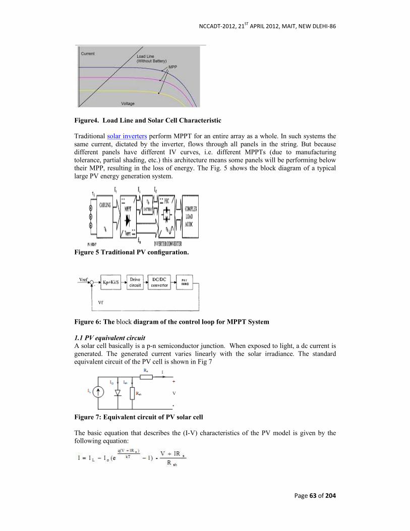
NCCADT-2012, 21ST


Page 63 of 204

Figure4. Load Line and Solar Cell Characteristic

Traditional solar inverters perform MPPT for an entire array as a whole. In such systems the same current, dictated by the inverter, flows through all panels in the string. But because different panels have different IV curves, i.e. different MPPTs (due to manufacturing tolerance, partial shading, etc.) this architecture means some panels will be performing below their MPP, resulting in the loss of energy. The Fig. 5 shows the block diagram of a typical large PV energy generation system.

Figure 5 Traditional PV configuration.

Figure 6: The block diagram of the control loop for MPPT System

1.1 PV equivalent circuit

A solar cell basically is a p-n semiconductor junction. When exposed to light, a dc current is generated. The generated current varies linearly with the solar irradiance. The standard equivalent circuit of the PV cell is shown in Fig 7

Figure 7: Equivalent circuit of PV solar cell

The basic equation that describes the (I-V) characteristics of the PV model is given by the following equation:

NCCADT-2012, 21ST


Page 64 of 204

1.2 Problems in solar energy conversion The problems during solar to electrical conversion are as follows:

• Electrical mismatches. Because of the vagaries of manufacturing, different panels have slightly different I-V curves. The inverter responds only to the average I-V curve. Consequently, it draws too little current for some panels and too much for others, reducing their power output by several percent.

• Partial shading. If the shadow of a tree branch or another solar panel falls on the panel and diminishes the sunlight hitting it. Actually, even a small shadow can completely zero out the power. Because the cells are wired in series, knocking out one can knock out all.

• Temperature fluctuations. As the temperature increases, electrons flow through the semiconductor material of a solar cell more readily and the built-in voltage decreases. The inverter can handle only a limited range of voltages During extreme temperature swings, the voltage will fall outside this range and the energy will be lost..

• Inability to optimize. Whenever the sun’s brightness changes because of cloud cover or the time of day, the inverter needs to find the new optimum

• Incomplete use of available space. Since the length of the strings is dictated by the voltage that the inverter can handle,it cannot make optimum use of the space availableDamage or theft. If a panel breaks or gets stolen (it happens), the whole array can fail. What’s worse, you can’t just replace the lost panel with the latest model; you have to use the exact same model as the original, or else you’ll create an electrical mismatch. Thus a photovoltaic system installed in 2009 is locked into 2009 technology for its 25-year lifetime.

• Brownouts and blackouts: Many solar-powered systems also interface with the power grid, which requires phase synchronization and power factor correction. Fault projection must be built-in to guard against events such as brownouts and blackouts on the public electricity grid.

II. MPPT CHARGE CONTROLLER

A MPPT charge controller works as DC-DC converter by using know how of PV panel and battery characteristics to get the highest conversion power output from PV panels and safely charge battery. 2.1 Main features of MPPT charge controller are as follows:

• In applications where PV panels are energy source, the MPPT charge controller is used to correct for variations in the current-voltage characteristics of the solar cell and shown by I-V curve.

• It is necessary to implement the MPPT charge controller in order to move the PV panels operating voltage close to the peak power point for drawing the maximum available power from PV panels.

• The MPPT charge controller allows the users to use a PV panel with a higher voltage output than operating voltage of the battery system.

• The MPPT charge controller reduces the complexity of the system while the output of the system is high efficiency. Additionally, it can be modified to handle more energy sources. Because the PV panels output power is used to control the DC-DC converter directly.

• The water turbines, wind-power turbines, etc. MPPT charge controller can be applied to other renewable energy sources

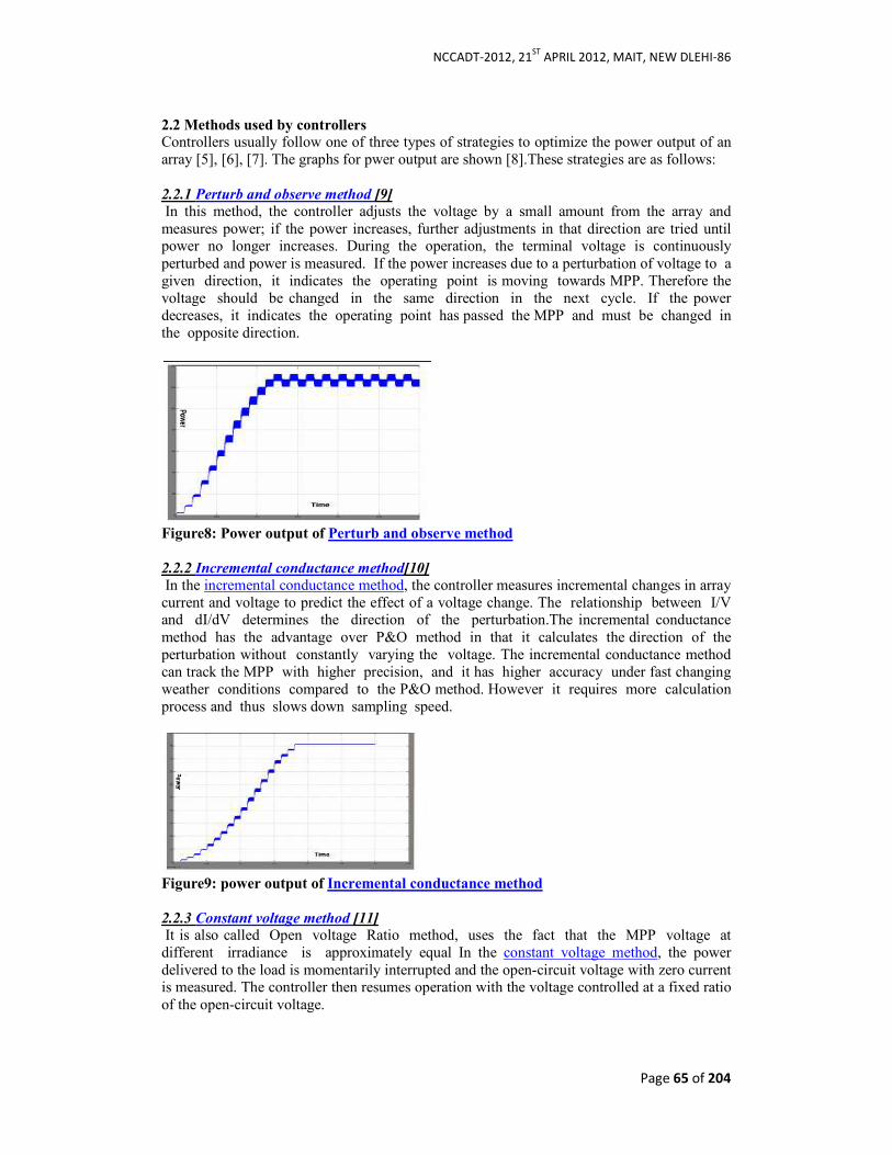
NCCADT-2012, 21ST


Page 65 of 204

2.2 Methods used by controllers Controllers usually follow one of three types of strategies to optimize the power output of an array [5], [6], [7]. The graphs for pwer output are shown [8].These strategies are as follows: 2.2.1 Perturb and observe method [9] In this method, the controller adjusts the voltage by a small amount from the array and measures power; if the power increases, further adjustments in that direction are tried until power no longer increases. During the operation, the terminal voltage is continuously perturbed and power is measured. If the power increases due to a perturbation of voltage to a given direction, it indicates the operating point is moving towards MPP. Therefore the voltage should be changed in the same direction in the next cycle. If the power decreases, it indicates the operating point has passed the MPP and must be changed in the opposite direction.

Figure8: Power output of Perturb and observe method

2.2.2 Incremental conductance method[10] In the incremental conductance method, the controller measures incremental changes in array current and voltage to predict the effect of a voltage change. The relationship between I/V and dI/dV determines the direction of the perturbation.The incremental conductance method has the advantage over P&O method in that it calculates the direction of the perturbation without constantly varying the voltage. The incremental conductance method can track the MPP with higher precision, and it has higher accuracy under fast changing weather conditions compared to the P&O method. However it requires more calculation process and thus slows down sampling speed.

Figure9: power output of Incremental conductance method

2.2.3 Constant voltage method [11] It is also called Open voltage Ratio method, uses the fact that the MPP voltage at different irradiance is approximately equal In the constant voltage method, the power delivered to the load is momentarily interrupted and the open-circuit voltage with zero current is measured. The controller then resumes operation with the voltage controlled at a fixed ratio of the open-circuit voltage.

NCCADT-2012, 21ST


Page 66 of 204

Figure10 : constant voltage method

Figure11: Power output of Constant voltage method

Figur12: Constant voltage algorithm

2.2.4 Fractional Open-Circuit Voltage method The method is based on the observation that, the ratio between array voltages at maximum power VMPP to its open circuit voltage VOC is nearly constant. VMPP ≈ k1 VOC This factor k1 has been reported to be between 0.71 and 0.78. 2.2.5 Fractional Short-Circuit Current method The method results from the fact that, the current at maximum power point IMPP is approximately linearly related to the short circuit current ISC of the PV array. IMPP ≈ K2 ISC (3) Like in the fractional voltage method, k2 is not constant. It is found to be between 0.78 and 0.92. The accuracy of the method and tracking efficiency depends on the accuracy of K2 and periodic measurement of short circuit current. III. BASIC MPPT ALGORITHMS

The Basic MMPT Algorithms Hill climbing method is a well known technique [12] where the duty cycle is increased or decreased or boost DC to DC converter and observe its impact on the array output power. The new value is compared to previous value and according to the result of the comparison; the sign of “slope” is decided. The PWM duty cycle is decided according to this slope.

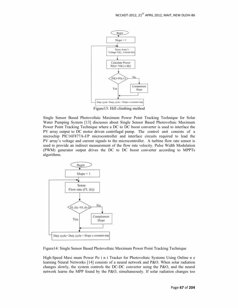
NCCADT-2012, 21ST


Page 67 of 204

Figure13: Hill climbing method

Single Sensor Based Photovoltaic Maximum Power Point Tracking Technique for Solar Water Pumping System [13] discusses about Single Sensor Based Photovoltaic Maximum Power Point Tracking Technique where a DC to DC boost converter is used to interface the PV array output to DC motor driven centrifugal pump. The control unit consists of a microchip PIC16F877A-I/P microcontroller and interface circuits required to lead the PV array’s voltage and current signals to the microcontroller. A turbine flow rate sensor is used to provide an indirect measurement of the flow rate velocity. Pulse Width Modulation (PWM) generator output drives the DC to DC boost converter according to MPPTs algorithms.

Figure14: Single Sensor Based Photovoltaic Maximum Power Point Tracking Technique High-Speed Maxi mum Power Po i n t Tracker for Photovoltaic Systems Using Online n e learning Neural Networks [14] consists of a neural network and P&O. When solar radiation changes slowly, the system controls the DC-DC converter using the P&O, and the neural network learns the MPP found by the P&O, simultaneously. If solar radiation changes too

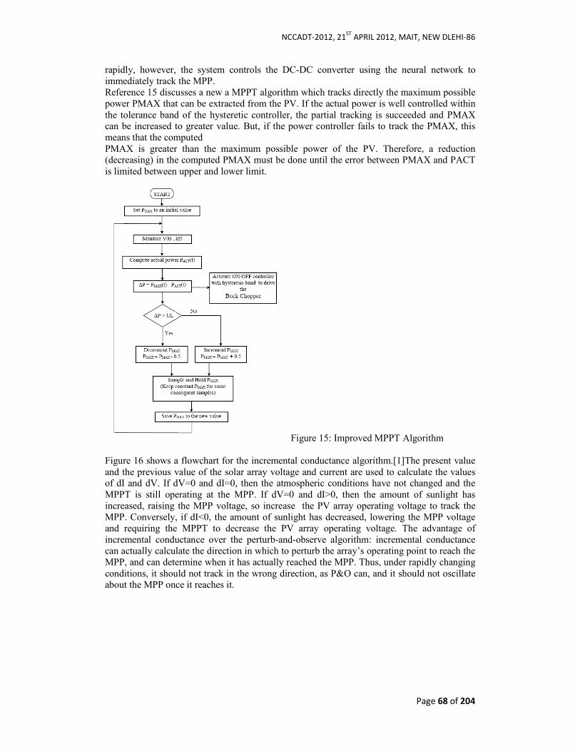
NCCADT-2012, 21ST


Page 68 of 204

rapidly, however, the system controls the DC-DC converter using the neural network to immediately track the MPP. Reference 15 discusses a new a MPPT algorithm which tracks directly the maximum possible power PMAX that can be extracted from the PV. If the actual power is well controlled within the tolerance band of the hysteretic controller, the partial tracking is succeeded and PMAX can be increased to greater value. But, if the power controller fails to track the PMAX, this means that the computed PMAX is greater than the maximum possible power of the PV. Therefore, a reduction (decreasing) in the computed PMAX must be done until the error between PMAX and PACT is limited between upper and lower limit.

Figure 15: Improved MPPT Algorithm Figure 16 shows a flowchart for the incremental conductance algorithm.[1]The present value and the previous value of the solar array voltage and current are used to calculate the values of dI and dV. If dV=0 and dI=0, then the atmospheric conditions have not changed and the MPPT is still operating at the MPP. If dV=0 and dI>0, then the amount of sunlight has increased, raising the MPP voltage, so increase the PV array operating voltage to track the MPP. Conversely, if dI<0, the amount of sunlight has decreased, lowering the MPP voltage and requiring the MPPT to decrease the PV array operating voltage. The advantage of incremental conductance over the perturb-and-observe algorithm: incremental conductance can actually calculate the direction in which to perturb the array’s operating point to reach the MPP, and can determine when it has actually reached the MPP. Thus, under rapidly changing conditions, it should not track in the wrong direction, as P&O can, and it should not oscillate about the MPP once it reaches it.

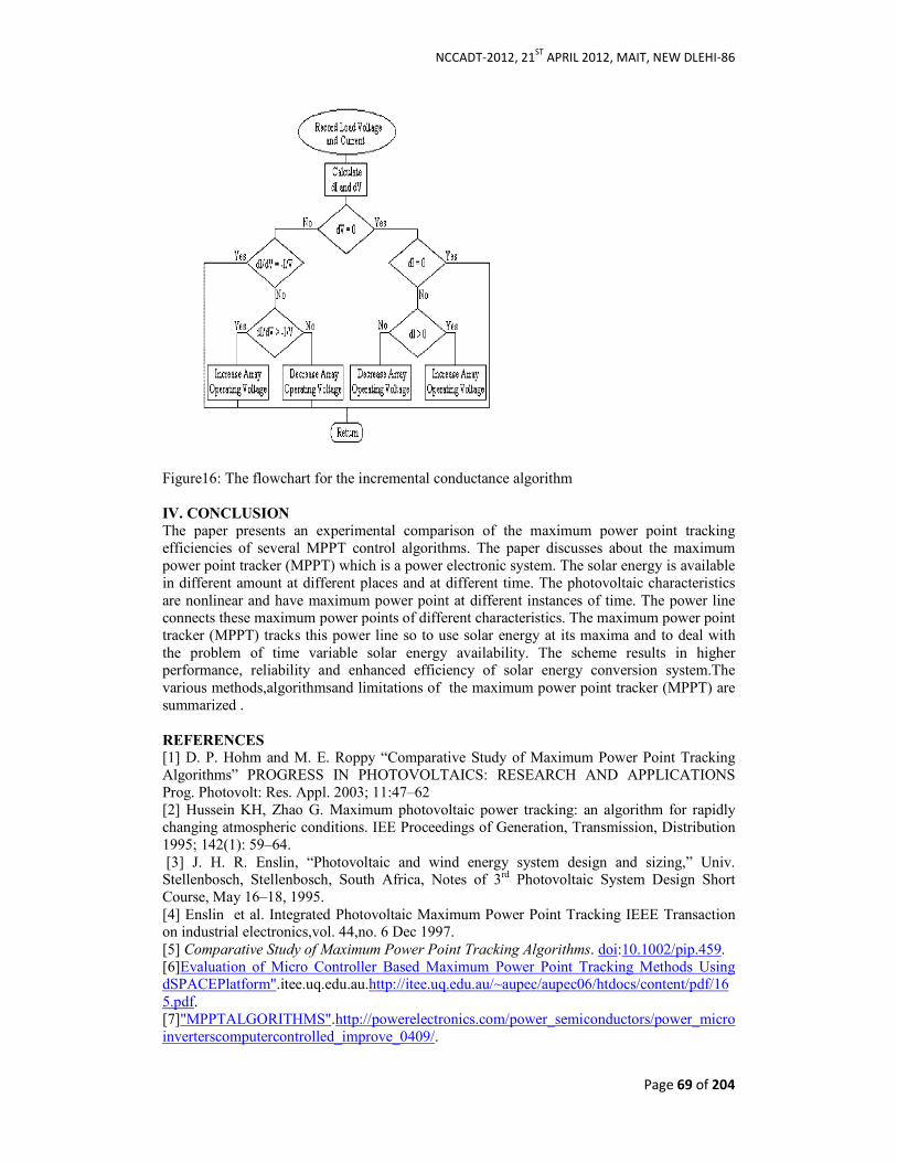
NCCADT-2012, 21ST


Page 69 of 204

Figure16: The flowchart for the incremental conductance algorithm IV. CONCLUSION

The paper presents an experimental comparison of the maximum power point tracking efficiencies of several MPPT control algorithms. The paper discusses about the maximum power point tracker (MPPT) which is a power electronic system. The solar energy is available in different amount at different places and at different time. The photovoltaic characteristics are nonlinear and have maximum power point at different instances of time. The power line connects these maximum power points of different characteristics. The maximum power point tracker (MPPT) tracks this power line so to use solar energy at its maxima and to deal with the problem of time variable solar energy availability. The scheme results in higher performance, reliability and enhanced efficiency of solar energy conversion system.The various methods,algorithmsand limitations of the maximum power point tracker (MPPT) are summarized .

REFERENCES

[1] D. P. Hohm and M. E. Roppy “Comparative Study of Maximum Power Point Tracking Algorithms” PROGRESS IN PHOTOVOLTAICS: RESEARCH AND APPLICATIONS Prog. Photovolt: Res. Appl. 2003; 11:47–62 [2] Hussein KH, Zhao G. Maximum photovoltaic power tracking: an algorithm for rapidly changing atmospheric conditions. IEE Proceedings of Generation, Transmission, Distribution 1995; 142(1): 59–64. [3] J. H. R. Enslin, “Photovoltaic and wind energy system design and sizing,” Univ. Stellenbosch, Stellenbosch, South Africa, Notes of 3rd Photovoltaic System Design Short Course, May 16–18, 1995. [4] Enslin et al. Integrated Photovoltaic Maximum Power Point Tracking IEEE Transaction on industrial electronics,vol. 44,no. 6 Dec 1997. [5] Comparative Study of Maximum Power Point Tracking Algorithms. doi:10.1002/pip.459. [6]Evaluation of Micro Controller Based Maximum Power Point Tracking Methods Using dSPACEPlatform".itee.uq.edu.au.http://itee.uq.edu.au/~aupec/aupec06/htdocs/content/pdf/165.pdf. [7]"MPPTALGORITHMS".http://powerelectronics.com/power_semiconductors/power_microinverterscomputercontrolled_improve_0409/.

NCCADT-2012, 21ST


Page 70 of 204

[8] Yen-Jung Mark Tung “Evaluation of Micro Controller Based Maximum Power Point Tracking Methods Using dSPACE Platform” Australian University Power Engineering Conference 2006. [9] K.H Hussein, I. Muta, T. Hoshino, M. Osakada, Maximum Photovoltaic Power Tracking: an algorithm for rapidly changing atmospheric conditions. [Online], IEEE Proceeding of Generation, Transmission and Distribution, Vol 142, No. 1 Jan 1995. [20th July 2006] [10] X. Wang, Control Design for Distributed Photovoltaic Systems. Masters Thesis, University of Auckland(2004). [11] D.P Hohm, M.E. Ropp, Comparative Study of Maximum Power Point Tracking Algorithm Using an Experimental, Programmable, Maximum Power Point Tracking Test Bed. [Online], Available: IEEE Explore . [12] E. K o u t r o u l i s , K. K a l a i t z a k i s ,N . C Vo u l g a r i s “Development of a. microcontroller based photovoltaic maximum power point tracking control system” IEEE transactions on power electronics, vol 16, pp. 46–54, 2001. [13] Amine DAOUD “Single Sensor Based Photovoltaic Maximum Power Point Tracking Technique for Solar Water Pumping System” Electrical Power Quality and Utilisation, Journal Vol. XIV, No. 2, 2008 [14] Yasushi Kohata, Koichiro Yamauchi, and Masahito Kurihara High-Speed Maximum Power Point Tracker for Photovoltaic Systems Using Online Learning Neural NetworksVol.14 No.6, 2010 Journal of Advanced Computational Intelligence 677 and Intelligent Informatics [15] Mohamed Azab “ A new maximum power point tracking algorithm for photovoltaic arrays” World Academy of Science, Engineering and Technology 44 2008 [16] K. Harada and H. Sakamoto, “High power and high switching frequency dc-to-dc converter using saturable inductor commutation and switched snubber,” in Proc. Annu. IEEE Power Electronics Specialists Conf. (PESC-’91), Boston, MA, June 1991, pp. 148–154. [17] J. J. Schoeman and J. D. van Wyk, “A simplified maximal power controller for terrestrial photovoltaic panel arrays,” in Proc. 13th Annu. IEEE Power Electronics Specialists Conf. (PESC-’82), Cambridge, MA, June 1982, pp. 361–367. [18] D. B. Snyman and J. H. R. Enslin, “Analysis and experimental evaluation of a new MPPT converter topology for PV installations,” in Proc. 18th IEEE Annu. Industrial Electronics Conf. (IECON-’92), San Diego, CA, Nov. 9–13, 1992, pp. 542–547. [19] D. B. Snyman and J. H. R. Enslin, “An experimental evaluation of MPPT converter topologies for PV installations,” Proc. Renewable Energy, vol. 3, no. 8, pp. 841–848, 1993. [20] D. B. Snyman and J. H. R. Enslin, “Simplified maximum power point controller for PV installations,” in Proc. 2nd IEEE Photovoltaics Specialists Conf. (PVSC-’93), Louisville, KY, May 10–14, 1993, pp. 1240–1245. [21] S. M. M. Wolf and J. H. R. Enslin, “Economical, PV maximum power point tracking regulator with simplistic controller,” in Proc. 24th IEEE Power Electronics Specialists Conf. (PESC-’93), Seattle, WA, June 20–24, 1993, pp. 581–587. [22] S. M. M. Wolf and J. H. R. Enslin, “Economical, PV Maximum Power Point Tracking Regulator with simplistic controller,” in Proc. 4th South Africa Universities Power

Engineering Conf. (SAUPEC-’94), Cape Town, South Africa, Jan. 13–14, 1994, pp. 18–21.

NCCADT-2012, 21ST


Page 71 of 204

REFURBISHMENT OF CRUCIAL ENGINE

COMPONENTS BY THERMAL SPRAY COATING Roopa Potdar, Asst. Professor

Maharaja Agrasen Institute of Technology,

Sector 22, Rohini , New Delhi

Abstract Thermal spray coatings are one of the most accepted coatings for surface modifications. Its

ease of application and accessibility has made it a very versatile technique. Some components

of the helicopter engine, whose procurement cost were high was taken for study. The paper

focuses on the systematic procedure adopted for the two components reduction gear and

driven gear. The components after coating were analyzed for fatigue factor and their ability

for resistance to corrosion. A need to understand the HVOF spray processing in order to

develop the optimum conditions and effective control of HVOF spraying to produce a quality coating is needed. Addressing this need for crucial components whose procurement cost is

high and procurement time is long is the main objective.

Keywords— HVOF

I.INTRODUCTION Two crucial components of the helicopter engine like the reduction gear and the driven gear were chosen for the study. Because of the continuous running of these components and its high cost, the wear of these components would lead to the un-serviceability of the engine. The purpose of the study was to increase the life of the two components by coatings, leading to reduced wear of these components, leading to increased serviceable condition of the engine. Hard chrome coating

This process has many disadvantages as it utilizes chromium in the hexa-valent state which is highly carcinogenic and can cause a serious contamination to the environment. Also, the low deposition rate, limited corrosion protection to the substrate and high coating cost are other added disadvantages. These coatings have a low ductility. To overcome these disadvantages of hard chrome coating, High velocity oxygen fuel (HVOF) system was identified and adopted for coating of these two components. However, chrome plate coating was done and the results were compared High velocity oxygen fuel (HVOF) system

Figure 1 shows the sketch of a HVOF system. An internal combustion rocket jet is used to generate supersonic gas velocities of approximately 1800 m/s, generally in the range of Mach 4-5. Combustion fuels are mixed with oxygen in the gun. Fuel, usually propane, propylene or hydrogen is mixed with oxygen and burned in a chamber. These fuels produce temperatures greater than 2700 °C. Sometimes liquid kerosene may be used as fuel and air as oxidizer. The products of combustion are allowed to expand through a nozzle where the gas velocities may become supersonic.

Powder is introduced axially in the nozzle and this is heated and accelerated. The powders to be deposited are fed in to the HVOF gun with the feed rates automatically monitored. This powder is usually fully or partially melted and a high velocity of 550m/sec is achieved. The powder is exposed to the product of combustion and they can be melted in either an oxidizing or reducing environment and significant oxidation of metals and carbides are possible. Powders can be pure metals, metal alloys, cermets like tungsten, carbide/ cobalt, and certain ceramics and polymers. The stand off distance between the gun and the surface of the material being coated is between 15 cm to 30 cm. The proper choice of operating parameters, choice of powder, coating with high densities and bond strengths can be achieved. The coating thickness of 0.5-0.50 mm could be achieved.

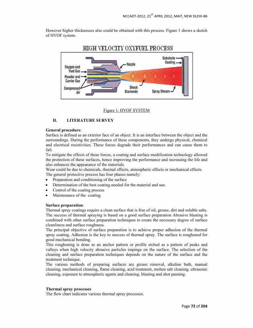
NCCADT-2012, 21ST


Page 72 of 204

However higher thicknesses also could be obtained with this process. Figure 1 shows a sketch of HVOF system.

Figure 1: HVOF SYSTEM

II. LITERATURE SURVEY

General procedure: Surface is defined as an exterior face of an object. It is an interface between the object and the surroundings. During the performance of these components, they undergo physical, chemical and electrical resistivities. These forces degrade their performances and can cause them to fail. To mitigate the effects of these forces, a coating and surface modification technology allowed the protection of these surfaces, hence improving the performance and increasing the life and also enhances the appearance of the materials. Wear could be due to chemicals, thermal effects, atmospheric effects or mechanical effects. The general protective process has four phases namely: • Preparation and conditioning of the surface • Determination of the best coating needed for the material and use. • Control of the coating process • Maintenance of the coating Surface preparation: Thermal spray coatings require a clean surface that is free of oil, grease, dirt and soluble salts. The success of thermal spraying is based on a good surface preparation Abrasive blasting is combined with other surface preparation techniques to create the necessary degree of surface cleanliness and surface roughness. The principal objective of surface preparation is to achieve proper adhesion of the thermal spray coating. Adhesion is the key to success of thermal spray. The surface is roughened for good mechanical bonding. This roughening is done as an anchor pattern or profile etched as a pattern of peaks and valleys when high velocity abrasive particles impinge on the surface. The selection of the cleaning and surface preparation techniques depends on the nature of the surface and the treatment technique. The various methods of preparing surfaces are grease removal, alkaline bath, manual cleaning, mechanical cleaning, flame cleaning, acid treatment, molten salt cleaning, ultrasonic cleaning, exposure to atmospheric agents and cleaning, blasting and shot peening.

Thermal spray processes

The flow chart indicates various thermal spray processes.

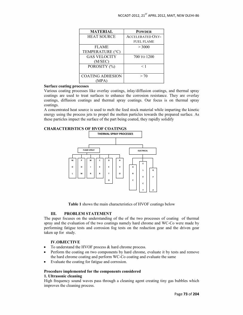
NCCADT-2012, 21ST


Page 73 of 204

Surface coating processes

Various coating processes like overlay coatings, inlay/diffusion coatings, and thermal spray coatings are used to treat surfaces to enhance the corrosion resistance. They are overlay coatings, diffusion coatings and thermal spray coatings. Our focus is on thermal spray coatings. A concentrated heat source is used to melt the feed stock material while imparting the kinetic energy using the process jets to propel the molten particles towards the prepared surface. As these particles impact the surface of the part being coated, they rapidly solidify CHARACTERISTICS OF HVOF COATINGS

Table 1 shows the main characteristics of HVOF coatings below

III. PROBLEM STATEMENT

The paper focuses on the understanding of the of the two processes of coating of thermal spray and the evaluation of the two coatings namely hard chrome and WC-Co were made by performing fatigue tests and corrosion fog tests on the reduction gear and the driven gear taken up for study.

IV.OBJECTIVE

• To understand the HVOF process & hard chrome process. • Perform the coating on two components by hard chrome, evaluate it by tests and remove

the hard chrome coating and perform WC-Co coating and evaluate the same • Evaluate the coating for fatigue and corrosion.

Procedure implemented for the components considered

1. Ultrasonic cleaning

High frequency sound waves pass through a cleaning agent creating tiny gas bubbles which improves the cleaning process.

MATERIAL POWDER

HEAT SOURCE ACCELERATED OXY-FUEL FLAME

FLAME TEMPERATURE (°C)

> 3000

GAS VELOCITY (M/SEC)

700 TO 1200

POROSITY (%) < 1

COATING ADHESION (MPA)

> 70

THERMAL SPRAY PROCESSES

FLSME SPRAY

P

O

W

W

I

R

C

E

R

D

E

T

O

H

V

O

A

R

C

E

L

E

C

T

R

F

P

M

O

L

ELECTRICAL

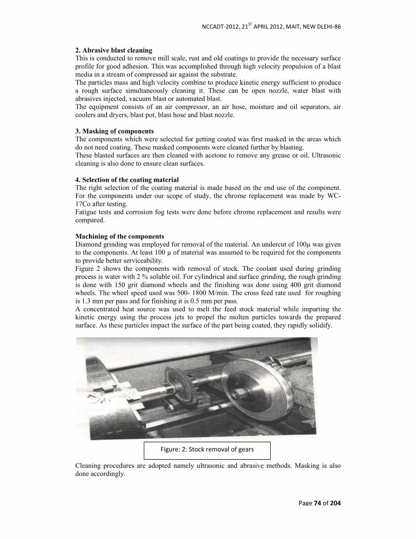
NCCADT-2012, 21ST


Page 74 of 204

2. Abrasive blast cleaning This is conducted to remove mill scale, rust and old coatings to provide the necessary surface profile for good adhesion. This was accomplished through high velocity propulsion of a blast media in a stream of compressed air against the substrate. The particles mass and high velocity combine to produce kinetic energy sufficient to produce a rough surface simultaneously cleaning it. These can be open nozzle, water blast with abrasives injected, vacuum blast or automated blast. The equipment consists of an air compressor, an air hose, moisture and oil separators, air coolers and dryers, blast pot, blast hose and blast nozzle.

3. Masking of components

The components which were selected for getting coated was first masked in the areas which do not need coating. These masked components were cleaned further by blasting. These blasted surfaces are then cleaned with acetone to remove any grease or oil. Ultrasonic cleaning is also done to ensure clean surfaces.

4. Selection of the coating material The right selection of the coating material is made based on the end use of the component. For the components under our scope of study, the chrome replacement was made by WC-17Co after testing. Fatigue tests and corrosion fog tests were done before chrome replacement and results were compared. Machining of the components

Diamond grinding was employed for removal of the material. An undercut of 100µ was given to the components. At least 100 µ of material was assumed to be required for the components to provide better serviceability. Figure 2 shows the components with removal of stock. The coolant used during grinding process is water with 2 % soluble oil. For cylindrical and surface grinding, the rough grinding is done with 150 grit diamond wheels and the finishing was done using 400 grit diamond wheels. The wheel speed used was 500- 1800 M/min. The cross feed rate used for roughing is 1.3 mm per pass and for finishing it is 0.5 mm per pass. A concentrated heat source was used to melt the feed stock material while imparting the kinetic energy using the process jets to propel the molten particles towards the prepared surface. As these particles impact the surface of the part being coated, they rapidly solidify.

Cleaning procedures are adopted namely ultrasonic and abrasive methods. Masking is also done accordingly.

Figure: 2: Stock removal of gears

NCCADT-2012, 21ST


Page 75 of 204

Loading the job for surface coating

The cleaned job is mounted on the job holding device. The coating system is mounted on the robotic system, a robotic manipulator. Again prior to coating a proper masking of unwanted coating region is done. The coating is done with many passes till the sufficient thickness has been built on the component.

The job has been removed from the job holder and the masking material was removed. The component was dispatched so that the final machining could be done to get the component to desired tolerances. Figure 3 shows the sketch of the job loaded on the robotic manipulator.

FIGURE 3

IV.RESULTS & DISCUSSION Micrographs of the two coatings on the components by the two processes are shown in Figure 4 & Figure 5. Figure 4 shows the micrograph of base material and hard chrome coating. Figure 5 shows the micrograph of base material and HVOF WC/17Co coating.

FIGURE 4

NCCADT-2012, 21ST


Page 76 of 204

FIGURE 5

Fatigue test

Fatigue is a very important parameter to be considered for components subjected to constant and variable amplitude loading. Failures of hard chrome plating are due to the initiation and propagation of the micro cracks. Cycles to failure at different stress levels were measured for fatigue specimens coated with hard chrome plate and HVOF WC/17 Co. The following graphs indicate the values obtained with cycles to failure on the horizontal axis and stress on the vertical axis. Figure 6A and 6B shows the graphs of cycles versus stress for base material and hard chrome, cycles versus stress for base material and WC-17Co for the two components.

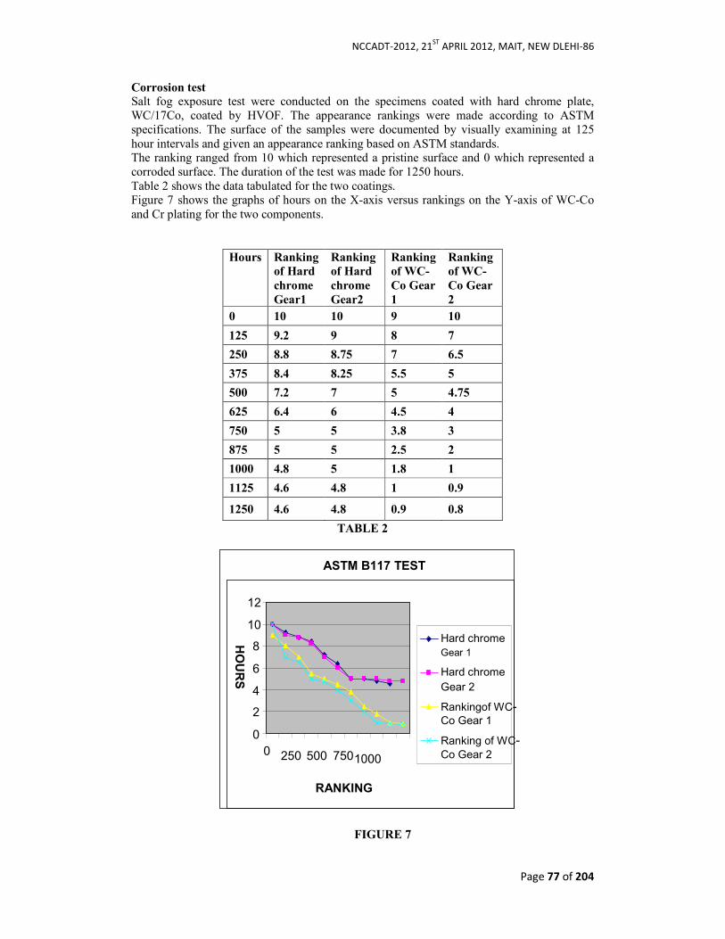
NCCADT-2012, 21ST


Page 77 of 204

Corrosion test

Salt fog exposure test were conducted on the specimens coated with hard chrome plate, WC/17Co, coated by HVOF. The appearance rankings were made according to ASTM specifications. The surface of the samples were documented by visually examining at 125 hour intervals and given an appearance ranking based on ASTM standards. The ranking ranged from 10 which represented a pristine surface and 0 which represented a corroded surface. The duration of the test was made for 1250 hours. Table 2 shows the data tabulated for the two coatings. Figure 7 shows the graphs of hours on the X-axis versus rankings on the Y-axis of WC-Co and Cr plating for the two components.

Hours Ranking

of Hard

chrome

Gear1

Ranking

of Hard

chrome

Gear2

Ranking

of WC-

Co Gear

1

Ranking

of WC-

Co Gear

2

0 10 10 9 10

125 9.2 9 8 7

250 8.8 8.75 7 6.5

375 8.4 8.25 5.5 5

500 7.2 7 5 4.75

625 6.4 6 4.5 4

750 5 5 3.8 3

875 5 5 2.5 2

1000 4.8 5 1.8 1

1125 4.6 4.8 1 0.9

1250 4.6 4.8 0.9 0.8

TABLE 2

FIGURE 7

ASTM B117 TEST

0

2

4

6

8

10

12

0 250 500 7501000

RANKING

HOURS

Hard chrome

Gear 1

Hard chrome

Gear 2

Rankingof WC-Co Gear 1

Ranking of WC-Co Gear 2

NCCADT-2012, 21ST


Page 78 of 204

CONCLUSION

The axial fatigue curves clearly indicate that the fatigue life reduction is less significant with WC-Co coating compared to hard chromium coating. The HVOF coatings in the graphs show increased corrosion resistance in comparison with the hard chrome coated substrate. REFERENCES:

1. J. Stokes, “Theory and Application of the High Velocity Oxy-Fuel (HVOF) Thermal Spray Process”, © Dublin City University (2008), ISBN 1-87232-753-2, ISSN 1649-8232” 2. High Velocity Oxy-Fuel Spraying, Published by the Institute of Materials, Minerals and Mining, Institute of Materials, Minerals and Mining, edited by V. V Sobolev, J Guilemany, J Nutting 3. The Science and Engineering of Thermal spray Coatings by Dr Pawlowski. 4. Substituting Thermal Spraying for Electroplating, by Gansert, Daren and George Grenier. 5. Mechanical Properties and thermal shock resistance of HVOF Sprayed Coatings, “Journal of Thermal Spray Technology”, by Xiaoguang Sun, Shufen Chen, You Wang, Zhaoyi Pan and Liang Wang. 6. The Science and Engineering of Thermal spray Coatings by Dr Pawlowski,. Volume II 7. Understanding of Spray Coating Adhesion through the formation of a single lamella by S. Goutier and M. Vardelle. “A Journal of Thermal Spray Technology” 8. Optimization and Characterization of High Velocity Oxy-fuel Sprayed Coatings: Techniques, Materials, and Applications, Maria Oksa Erja Turunen, Tomi Suhonen, Tommi Varis and Simo-Pekka Hannula 9. Advanced Thermal Spray Coatings for emerging applications by Dr. Lech Pawlowski and.Dr.Christopher.

NCCADT-2012, 21ST


FRAMEWORK FOR TROUBLESHOOTING OF

AUTOMOTIVE AIR CONDITIONING SYSTEMS Sakshi Bansal, Sonal Khullar, Apoorvi Singhal, Priyanka Bhadani

(MECHANICAL AND AUTOMATION ENGINEERING DEPARTMENT,4TH YEAR, INDIRA GANDHI INSTITUTE OF TECHNOLOGY, DELHI)

1. ABSTRACT

Air conditioning has become standard equipment on most vehicles, enhancing traveling

comfort and safety. To stay competitive in today's global economy an automotive repair

company must build on its intellectual capital and create time to innovate and assess more

advanced, complex types of tools to eliminate uncertainty and repetition by the

troubleshooting process. This study presents the framework for troubleshooting of automotive

air conditioning system. The Troubleshooting system uses a new control strategy to enhance the efficiency of the diagnostic process and attempts to spend the least amount of time in

detecting the air conditioner fault accurately, by investigating only portions of the framework.

The troubleshooting system first constructs a flowchart based on the information collected through the surveys. The aim of the proposed paper is to integrate the troubleshooting

process of automotive system into a single architecture for retrieving knowledge and

experience of technicians in automobile repairing field. Apart from the consultation with specialists

In repair field; handbooks and repair manuals for troubleshooting planning are the main

sources of the knowledge used in building the framework for feasibility analysis and process

evaluation of troubleshooting. This framework guides the novice or learner through different

stages of the troubleshooting process enabling the creation of problem-solving list, its

contents include the problems encountered, decision of detecting methods, solution to the

problem encountered, adjusting, and so on. Through the use of information acquired, the

troubleshooting knowledge of automobile air-conditioning system can be effectively

incorporated into the procedure generation framework. Keywords: Troubleshooting, automotive air conditioning system, diagnostic system 2. INTRODUCTION With the advancement of technology in the field of automobile the complexities of the systems have increased drastically. Moreover with the change in lifestyle and increased dependency on the automobiles, people want the most cost effective solution in the minimum time for their vehicle related problems. Therefore, to survive in this competitive world, an automotive repair company must be able to provide the same to satisfy the needs of the customers[5]. The number of automotive businesses working directly on vehicle air conditioning system is also growing rapidly. Air conditioning has become almost standard fit and requires periodic service and maintenance [2]. Thus this paper provides the troubleshooting framework which focuses on the user oriented approach wherein the user identifies problem in the automotive air conditioning system and based on which the repair company drafts its future course of action in the most time efficient manner to rectify the problem. Troubleshooting is a logical and systematic problem solving mechanism, often applied to repair failed products or processes which are complex in nature; wherein the symptoms of the problem can have many possible causes. These causes are likely to undergo a process of elimination to finally arrive at a solution that restores the product or process to its working state [3]. Surveys conducted by us helps to create conceptual frameworks as a methodology to troubleshoot the automotive air conditioning problems in our paper Conceptual frameworks are a type of intermediate theory that attempts to connect all aspects of inquiry (e.g., problem definition, purpose, literature review, methodology, data collection and analysis)[4], which we have demonstrated through flowcharts. The process of the inquiry is taken as a step-wise approach, where the technician first gathers as much information as possible from the

NCCADT-2012, 21ST


customer on the symptoms, vehicle history and conditions upon which the fault occurs; then using the aforesaid flowchart routine, the technician compares the expected behavior with the actual behavior of the automotive air conditioning system. Following this failure diagnosis is performed providing extended information about the underlying cause of a system failure and reveals the kind of fault occurred and the components responsible for it [11]. Depending on the goals of the specific failure diagnosis strategy, this extended information could be useful to technicians during service and at runtime, to allow for a more robust and cost effective failure mitigation mechanism.

3. LITERATURE REVIEW

Air conditioning system in cars are used for controlling temperature and humidity, moreover it also purifies the air thus enhancing user comfort[10].Air conditioning system for vehicle interior has a manually adjusted electrical control circuit unit, actuating a servomotor for driving a control camshaft, to vary the temperature and direction of a ventilating airflow by operation of a number of flap valves in air passages [6]. Today many technical processes are complex and highly integrated [4]. Car problem detection is a complicated process which demands high level of knowledge and skills [1]. When a process has failed, the complexity of the process makes it hard for humans to troubleshoot it [4]. Verma et. al (2010) has proposed a framework on car maintenance and troubleshooting which is capable of assisting the car’s owner and mechanic in dealing with the car problems and troubleshooting them whenever the time is limited. Troubleshooting procedures, almost always have a diagnosis-resolution structure consisting of configurations of symptoms and solution methods [5]. Examining this structure enables us to meaningfully classify the very diverse instances of this genre [8], reveals key design issues, and helps us to identify productive research questions [3]. Liang (2010) describes the generation of Web-based troubleshooting system for automotive refrigeration system using knowledge engineering approach over the Internet. Through the use of web and knowledge approach [9], the troubleshooting knowledge of automobile refrigeration system can be effectively incorporated into the procedure generation framework and a Web-based troubleshooting procedure generation system can also be implemented [5]. Receiving the motivations from the vast literature review, this paper presents a framework for problems identified and their rectification in automotive air conditioning system using flowchart methodology. 4. FRAMEWORK

The framework used in the paper describes the problem solving mechanism using flowcharts, for the various problems identified by the user. Below we have explained the flowchart for the “less cooling” problem of the automotive air conditioning system. When the user identifies the problem as less cooling, then according to our study, the technician should focus mainly on certain areas in a preference order as given in the appendix (figure 1).The causes identified were: lack of refrigerant charge (which depends on when the servicing was done), improper air flow, faulty heater switch, burnt blower resistor wires or fuses , improper refrigerant pressure, leaks in refrigerant pipes, blown out compressor fuses, faulty compressor clutch, faulty condenser or radiator fans, problematic blend door, retrofitting, leaks in HVAC seals and ambient temperature. These problems are converted into potential questions which the technician asks the user, in order to select the most viable solution. Similarly other user identified air conditioning problems have been dealt with efficiency. Flowcharts are also constructed for the following air conditioning problems: 4.1Excessive cooling 4.2Engine overheating causing air conditioning problem 4.3Improper air flow 4.4Water pooling inside the car floor 4.5Less outlet air 4.6Noise in air conditioning system 4.7Vibration in car due to air conditioning system

NCCADT-2012, 21ST


4.8Air conditioner not switching on 4.9Dashboard air control switches 5. CASE STUDY

A car was taken to verify the approach of the troubleshooting framework mentioned in this paper. The problem identified was that the air conditioning system of the car was not switching on. According to the specified framework in Appendix (figure.2), firstly the belts of the compressor were inspected to check if the belts were moving or not. The belts were moving properly, so now the clutch in the compressor was checked if it was turning or not. The clutch was not turning. So compressor fuse was checked. The fuse was not blown so then the pressure cycling switch was inspected by disconnecting it & turning the engine on and connecting the jumper wire across the terminals of the switch. Now again it was checked whether the clutch was engaging or not, it was engaging so the pressure reading was checked. The pressure reading was not greater than 55 psi so the leaks were checked in the system. Leaks were not found so voltage at WOT (wide open throttle) cutoff relay (orange/ green wire) was checked. Voltage was not present at this relay so the voltage at ‘FUSE CHECK’ fuse was checked. The voltage was not continuous. This implies that the fuse was blown out so the fuse was replaced to rectify the problem of air conditioner. Now the air conditioner was switching on. Thus from the above study, it can be case concluded that the framework given in this paper has successfully guided us to troubleshoot the given problem.

6. CONCLUSION

This paper deals with troubleshooting of automotive air conditioning problems effectively in user friendly manner, at a preliminary level .Various problems have been identified through surveys conducted and based on them causes and solutions to the problems are provided in the form of flowcharts. The scope of the paper lies in the transformation of the proposed framework in a web based technology using knowledge based troubleshooting system which would make our troubleshooting procedure time effective and easily accessible. REFERENCES [1]Verma.N, Jindal.Y, Aggarwal.J, Jain.S (2010), “An Approach towards designing of Car Troubleshooting Expert System, International Journal of Computer Applications ,Vol.1, No. 23, pp. 0975 - 8887 [2] Liang.J(2008) ,"The troubleshooting task implementation in automotive chassis using virtual interactive technique and knowledge-based approach”,Journal of Network and

Computer Applications, Volume 31, Issue 4,pp.712–734 [3]Farkas.D.K.(2010),“The Diagnosis-Resolution Structure in Troubleshooting Procedures”, Professional Communication Conference (IPCC), 2010 IEEE International, pp. 12-19 [4] Krysander.M, (2003) “Design and Analysis of Diagnostic Systems Utilizing Structural Methods”, Linköping Studies in Science and Technology,Thesis No. 1038, pp. 1-10 [5] Liang.J.S.(2010), “ A Web-based automotive refrigeration troubleshooting system applying knowledge engineering approach”,Journal Computers in Industry,Vol.61,No.1,pp. 29-43 [6]Pettersen, J. (1993), “A new, efficient and environmentally benign system for car air-conditioning”, International Journal of Refrigeration,Vol.16, No.1, pp. 4-12 [7] Brace, Ian. (2004), “Questionnaire Design: How to Plan, Structure and Write Survey Material, United Kingdom, Kogan Page Business Books, pp.32-40 [8]Oppenheim, A.N., (1999) “Questionnaire design, interviewing and attitude measurement”, New York, Continuum International Publishing Group [9]Kalton, G. (1998), “Introduction to survey sampling”,USA, Sage publications, pp.16-28,70-80

NCCADT-2012, 21ST


[10] Steven, J. (2006), “Automotive air-conditioning and climate control systems”, Butterworth-Heinemann, pp. 264-283 [11] Liang.J (2012), "Methodology of knowledge acquisition and modeling for troubleshooting in automotive braking system" , Journal on Robotics and The Computer-

Integrated Manufacturing, Volume 28, Issue 1,pp. 24–34.

NCCADT-2012, 21ST


CAD/CAM Integration SWAPNIL DEOKAR, IIITDM, Jabalpur, M. Tech. (Design and manufacturing)

E-mail ID- [email protected] ,[email protected], [email protected]

Abstract CAD/CAM is a 21

st century technology that related to the computer involvement in design and

manufacturing. CAD/CAM is a latest technology developed in recent years. The CAD has

main advantages over traditional methods, it enables the designer to examine a large number

of design solutions and CAM simulate the work task may be performed in order to obtain the values of various performance measures in real manufacturing world.

This paper discusses the advantages obtained from CAD/CAM integration. The

applications of CAD/CAM integration used in CNC milling machine and virtual

manufacturing operations have demonstrated the effectiveness of discuss methodology.

Keywords-CAD, CAM, Virtual manufacturing, traditional method

Introduction- Industrial world is witnessed the advent of computer-aided design (CAD) and computer-aided manufacturing (CAM) technologies which significantly improvement in product design and manufacturing. Although CAD and CAM have been significantly developed over the last three decades, they have traditionally been treated as separate activities. Many designers use CAD with little understanding of CAM. This sometimes results in design of non machinable components or use of expensive tools and difficult operations to machine non-crucial geometries. In many cases, design must be modified several times, resulting in increased machining lead times and cost. Therefore, great savings in machining times and costs can be achieved if designers can solve machining problems of the products at the design stage and developing stages. This can only be achieved through the use of fully integrated CAD/CAM systems.

1.1Introduction of CAD

CAD is defined as, “the use of computer systems to assist in the creation, modification, analysis, or optimization of a design.” To perform the CAD operations the computer systems comprise of the software and the hardware. The hardware consists of all the visible components of the computer like processor, motherboard, mouse, keyboard, graphics card etc. The software consists of the program that can implement computer graphics on the computer system and also carry out a number of engineering functions on the computers. The CAD software can carry out a number of engineering functions like analysis of stress-strain subjected on the components, dynamics response of the mechanisms, heat-transfer calculations, etc. Not all the CAD software will perform all the functions. Each CAD software is programmed to carry out specific function. Depending upon the type of the firm or the company, they will choose the CAD software that can perform particular application. However, the most popular CAD software are the ones that can perform design and drawing operations. This CAD software can perform all the designing operations like making various calculations, performing simulations of the designed components, checking them for stress etc. The drawings of these designed components can also be drawn using the CAD software, which help avoiding long and cumbersome process of making the drawings on the drawing board.

1.2Introduction of CAM-

CAM is the acronym for Computer Aided Manufacturing. CAM is defined as, “the use of computer systems to plan, manage, and control the operations of a manufacturing plant through their direct or indirect computer interface with the plant’s resources.” In simple terms using the computers to carry out various manufacturing related activities is

NCCADT-2012, 21ST


called as Computer Aided Manufacturing. The use of the computers can be to plan the manufacturing of the product, to carry out actual manufacturing of the product by linking the computers to machines and programming the computers, et

1.3Introduction to CAD/CAM Integration of CAD and CAM is called as CAD/CAM. In the earlier days the CAD and CAM were considered to be two distinct technologies independent of each other, however, now there has been greater integration of CAD and CAM. CAD stands for Computer Aided Designing and CAM stands for Computer Aided Manufacturing. The combined CAD/CAM is the technology concerned with the use of computers to perform product designing and manufacturing operations. Popular CAD Software

These days a number of CAD software are available in the market, some of these include AutoCAD, CADopia, SolidWorks, Catia, MathCAD, QuickCAD etc. One of the most popular CAD software being used since years is AutoCAD. Popular software for CAM-

There are number of software uses for the CAM like, Magics, CATIA V5, Radan Sheet Metal CAD/CAM, SolidWorks, Alpha CAM etc. In these each software has the ability to make the program for CNC machine for manufacturing Benefits of the CAD Software

CAD software is being used on large scale basis by a number of engineering professionals and firms for various applications. The most common application of CAD software is designing and drafting. Here are some of the benefits of implementing CAD systems in the Companies: 1) Increase in the productivity of the designer: The CAD software helps designer in visualizing the final product that is to be made, it subassemblies and the constituent parts. The product can also be given animation and see how the actual product will work, thus helping the designer to immediately make the modifications if required. CAD software helps designer in synthesizing, analysing, and documenting the design. All these factors help in drastically improving the productivity of the designer that translates into fast designing, lower designing cost and shorter project completion times. 2) Improve the quality of the design: With the CAD software the designing professionals are offered large number of tools that help in carrying out thorough engineering analysis of the proposed design. The tools also help designers to consider large number of investigations. Since the CAD systems offer greater accuracy, the errors are reduced drastically in the designed product leading to better design. Eventually, better design helps carrying out manufacturing faster and reducing the wastages that could have occurred because of the faulty design. 3) Better communications: The next important part after designing is making the drawings. With CAD software better and standardized drawings can be made easily. The CAD software helps in better documentation of the design, fewer drawing errors, and greater legibility. 4) Creating documentation of the designing: Creating the documentation of designing is one of the most important parts of designing and this can be made very conveniently by the CAD software. The documentation of designing includes geometries and dimensions of the product, its subassemblies and its components, material specifications for the components, bill of materials for the components etc. 5) Creating the database for manufacturing: When the creating the data for the documentation of the designing most of the data for manufacturing is also created like products and component drawings, material required for the components, their dimensions, shape etc. 6) Saving of design data and drawings: All the data used for designing can easily be saved and used for the future reference, thus certain components don’t have to be designed again and again. Similarly, the drawings can also be saved and any number of copies can be printed whenever required. Some of the component drawings can be standardized and be used whenever required in any future drawings.

NCCADT-2012, 21ST


Functions Performed by CAM

The functions performed by the computers systems in CAM applications fall under two broad categories, which have been described below: 1) Computer monitoring and control: In these applications the computer is connected directly to the manufacturing process for the purpose of monitoring or controlling the manufacturing process. Here the computer is fed with the program that directs the working of the machine, which is connected to it. Usually in such cases is no operator required to operate the machines, and they have to merely supervise the machine. At a time one operator can take care of more than one number of machines. These machines are also called as Computer Numerically Controlled (CNC) machines. These days the use of CNC machines has become very common. They can carry out the high quality production at a very fast rate that helps the companies remain competitive in the market. 2) Manufacturing Support Applications: In these applications the computer systems are used to assist in various productions related activities like production planning, scheduling, making forecasts, giving manufacturing instructions and other relevant information that can help manage company’s manufacturing resources more effectively. There is no direct interface between the computers and the manufacturing process in this case. In present scenario one just can’t think of manufacturing any product without the use of computers in some or the other way. Either for designing of the product or manufacturing of the product, the use of computers has become compulsory. Since most of the companies do designing or drawing as well as manufacturing, the CAD/CAM has become an inseparable combination. CAD/CAM Integration All the products that have to be then manufactured, have to be designed first and they are sent for manufacturing. Let us see the important processes involved in CAD/CAM integration: 1) Designing of the product: First of all the product has to be designed by considering the applications desired from it and carrying out various stress and strain analysis. All these processes are carried out in the computers using appropriate CAD software. At the end of the designing process the product of appropriate shape and size is found designed. 2) Making the drawings: After designing the product, the assembly drawings and parts drawings of the product have to be made. These drawings are used for the reference purposes and more importantly for manufacturing the product on production shop floor. The drawings are also made by using CAD software. 3) Production planning and scheduling: The production planning and scheduling of the designed product can be carried out in the computers, which helps properly managing the manufacturing resources. There are some special product planning and scheduling software that can be used for this application. This is the CAM part of the product cycle. 4) Manufacturing the product: The manufacturing of the product can be carried by using the computers. The machines that are operated by the computers are called Computer Numerically Controlled or CNC machines. Nowadays the use of CNC machines has become very wide spread. In CNC machines the programming instructions for the manufacturing of the product that has been designed using the CAD software are fed. This program can also be fed directly from the CAD software into the computer of CNC machine. The program gives the appropriate instructions to the computer to carry out the manufacturing of the product as per the required dimensions. The above CAD/CAM process clearly shows how important CAD and CAM are to each other. Both the applications support and complement each other to design and manufacture the product in better way and in shortest possible time.

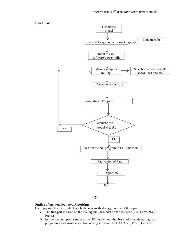
NCCADT-2012, 21ST


Flow Chart- Geometric

model

convert to .iges or .stl format

Input to cam software(power mill)

Make a setup for milling.

Selection of tool, spindle speed, feed rate etc.

Generate a tool path

Transfer the NC program to CNC machine

Fabrication of Part

Inspection

End

Fig.1

Outline of methodology step/Algorithm-

The suggested heuristic, which apply the new methodology, consist of three parts. The first part is based on the making the 3D model on the software (CATIA V5,NX.4,

Pro-E) In the second part simulate the 3D model on the basis of manufacturing part

programing and visual inspection on any software like CATIA V5, Pro-E, Delcam.

Data transfer

No

Yes

Simulate the

model virtually

Generate NC Program

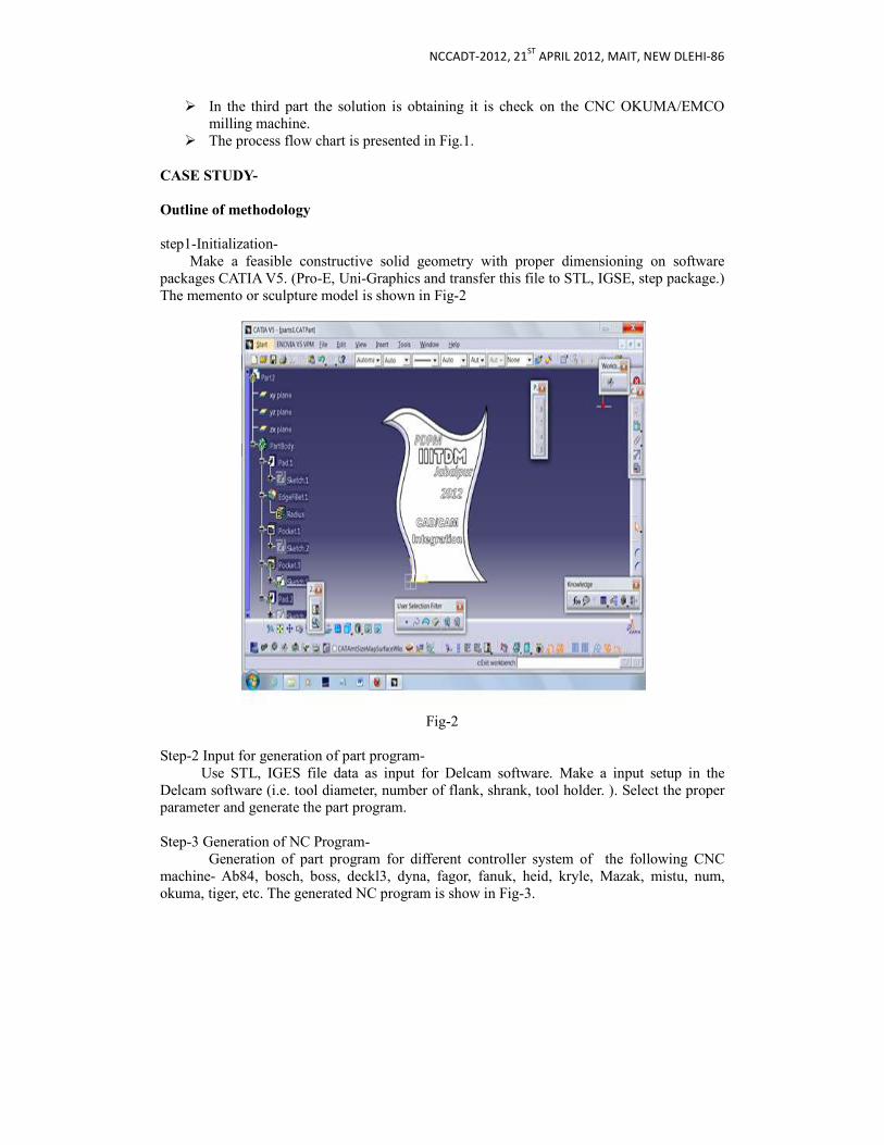
NCCADT-2012, 21ST


In the third part the solution is obtaining it is check on the CNC OKUMA/EMCO milling machine.

The process flow chart is presented in Fig.1. CASE STUDY-

Outline of methodology

step1-Initialization- Make a feasible constructive solid geometry with proper dimensioning on software packages CATIA V5. (Pro-E, Uni-Graphics and transfer this file to STL, IGSE, step package.) The memento or sculpture model is shown in Fig-2

Fig-2

Step-2 Input for generation of part program- Use STL, IGES file data as input for Delcam software. Make a input setup in the Delcam software (i.e. tool diameter, number of flank, shrank, tool holder. ). Select the proper parameter and generate the part program. Step-3 Generation of NC Program- Generation of part program for different controller system of the following CNC machine- Ab84, bosch, boss, deckl3, dyna, fagor, fanuk, heid, kryle, Mazak, mistu, num, okuma, tiger, etc. The generated NC program is show in Fig-3.

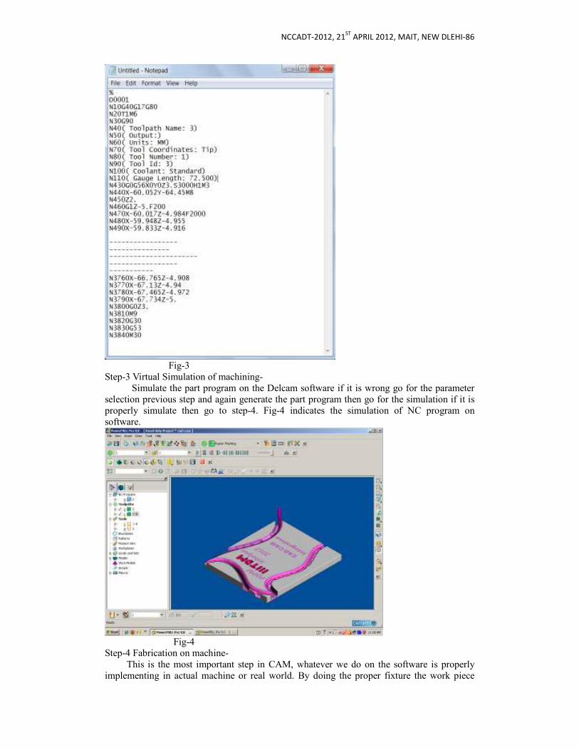
NCCADT-2012, 21ST


Fig-3 Step-3 Virtual Simulation of machining- Simulate the part program on the Delcam software if it is wrong go for the parameter selection previous step and again generate the part program then go for the simulation if it is properly simulate then go to step-4. Fig-4 indicates the simulation of NC program on software.

Fig-4 Step-4 Fabrication on machine- This is the most important step in CAM, whatever we do on the software is properly implementing in actual machine or real world. By doing the proper fixture the work piece

NCCADT-2012, 21ST


fix(set) it on table. Give the output of the Delcam (power mill) NC coding part program to CNC OKUMA milling machine & run the program block by block. Conclusion – In this work several goals have been achieved developing fully integrated CAD/CAM systems. It allows the user to manufacture to make 3D model of contouring profile which is not possible by conventional machine. It gives the part program for the CNC/NC machine which reduces the hazardous effort of programmer also save time and paper cost for the programming. Finishing obtain by the machine is also increases because of good programming. So CAD/CAM integration is the best option in the future for complex manufacturing part.

References:

1 Tehran. Iran (2006), An approach towards fully integration of CAD and CAM technologies, Journal of Achievements in Materials and Manufacturing Engineering, Volume- 18, issue 1-2.

2. Mikell P. Groover and Emory W. Zimmers, Computer Aided Design and Manufacturing,

3. Publication Prentice-Hall, 1984. 4. Stroka, R. and Helis, A., Integration of CAPP and CAD/CAM systems, International

Workshop CA Systems And Technologies. 5. Balic. j. (2006), Intelligence CAD/CAM system for CNC programming-an overview,

APEM Journal ISSN1854-6250 6. Patrick Waurzyniak (February 2010), CAD/CAM Software Drives Innovation,

Manufacturing Engineering, Vol. 144 No. 2 7. Shuhua Yue, Guoxiang Wang, Fei Yin, Yixin Wang, Jiangbo Yang (2003),

Application of an integrated CAD/CAE/CAM system for die casting dies, Journal of Materials Processing Technology 139 -465–468.

8. Programming manual(Okuma), Pub No. 5228-E-R8 (ME33-018-R9) Apr. 2009. 9. Power mill guide manual.

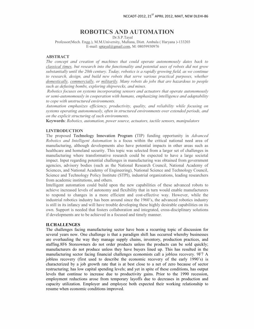
NCCADT-2012, 21ST


ROBOTICS AND AUTOMATION Dr.S.P.Tayal

Professor(Mech. Engg.), M.M.University, Mullana, Distt. Ambala ( Haryana )-133203 E-mail: [email protected], M: 08059930976

ABSTRACT The concept and creation of machines that could operate autonomously dates back to

classical times, but research into the functionality and potential uses of robots did not grow

substantially until the 20th century. Today, robotics is a rapidly growing field, as we continue to research, design, and build new robots that serve various practical purposes, whether

domestically, commercially, or militarily. Many robots do jobs that are hazardous to people

such as defusing bombs, exploring shipwrecks, and mines.

Robotics focuses on systems incorporating sensors and actuators that operate autonomously

or semi-autonomously in cooperation with humans, emphasizing intelligence and adaptability

to cope with unstructured environments.

Automation emphasizes efficiency, productivity, quality, and reliability while focusing on

systems operating autonomously, often in structured environments over extended periods, and

on the explicit structuring of such environments. Keywords: Robotics, automation, power source, actuators, tactile sensors, manipulators

I.INTRODUCTION

The proposed Technology Innovation Program (TIP) funding opportunity in Advanced

Robotics and Intelligent Automation is a focus within the critical national need area of manufacturing, although developments also have potential impacts in other areas such as healthcare and homeland security. This topic was selected from a larger set of challenges in manufacturing where transformative research could be expected to have a large societal impact. Input regarding potential challenges in manufacturing was obtained from government agencies, advisory bodies (such as the National Research Council, National Academy of Sciences, and National Academy of Engineering), National Science and Technology Council, Science and Technology Policy Institute (STPI), industrial organizations, leading researchers from academic institutions, and others. Intelligent automation could build upon the new capabilities of these advanced robots to achieve increased levels of autonomy and flexibility that in turn would enable manufacturers to respond to changes in a more efficient and cost-effective way. However, while the industrial robotics industry has been around since the 1960’s, the advanced robotics industry is still in its infancy and will have trouble developing these highly desirable capabilities on its own. Support is needed that fosters collaboration and integrated, cross-disciplinary solutions if developments are to be achieved in a focused and timely manner.

II.CHALLENGES The challenges facing manufacturing sector have been a recurring topic of discussion for several years now. One challenge is that a paradigm shift has occurred whereby businesses are overhauling the way they manage supply chains, inventory, production practices, and staffing.8F6 Storeowners do not order products unless the products can be sold quickly; manufacturers do not produce unless they have buyers lined up. This has resulted in the manufacturing sector facing financial challenges economists call a jobless recovery. 9F7 A jobless recovery (first used to describe the economic recovery of the early 1990’s) is characterized by a job growth rate that is at best close to a net of zero because of sector restructuring; has low capital spending levels; and yet in spite of these conditions, has output levels that continue to increase due to productivity gains. Prior to the 1990 recession, employment reductions arose from temporary layoffs due to decreases in production and capacity utilization. Employer and employee both expected their working relationship to resume when economic conditions improved.

NCCADT-2012, 21ST


However, after the 1990 recession, there were significant changes in the way the economy behaved. Manufacturing sector restructuring resulted in permanent job loss as employers tried to reduce costs.17F15 Laid-off workers did not return to their previous jobs, but instead needed to be retrained with new skills for entirely new industries. Complicating this situation further, more and more employers chose as manpower staffing solutions temporary hires, outsourcing, or part-time labor rather than to rehire employees. But employment issues are not the only challenges facing the manufacturing sector during these economic periods. After economic downturn periods, output and productivity return fairly quickly, but the recovery of capacity utilization is much slower. Capital spending is reduced in part because there is no incentive to invest in new equipment since excess capacity exists. Technology-based solutions offer possible answers, but only if they can address output and productivity growth and can significantly improve manufacturing quality, capabilities and/or enhance competitive advantages (i.e., make manufacturers more successful). The challenges facing the manufacturing sector are significant enough that they have been looked into and discussed by the government and various national associations, e.g., • The President’s Council of Advisors on Science and Technology (PCAST) recently asked the Science and Technology Policy Institute (STPI) to study18F16 how to create new industries through science, technology, and innovation; and to discuss how to: – Achieve greater customization and scalability; – Furnish heterogeneous mixes of products in small or large volumes while exhibiting mass production efficiency and the flexibility of custom manufacturing; – Respond more rapidly to customer demands; and – Find better ways to transfer scientific and technological advances into processes and products. • A Framework for Revitalizing Manufacturing,, identified the need to support technological developments including: – Federal government investment in research for advanced manufacturing technologies; and – Advanced robotics that enable the retention of manufacturing and can respond rapidly to changes in consumer product demands. • The National Science and Technology Council’s (NSTC) Interagency Working Group on Manufacturing R&D, in their report Manufacturing the Future,20F18 suggested that: – Future competitiveness depends in large part on research, innovation, and how quickly firms and industries can apply and incorporate new technologies into high-value-added products and high-efficiency processes; and – The ability to integrate new designs, processes, and materials in a modular fashion translates into competitive advantages that include shorter product development cycles, more efficient and more flexible supply chains, and new opportunities to deliver value-added products and services to customers. • The report Next Generation Manufacturing Study: Overview and Findings,21F19 developed by the Manufacturing Performance Institute showed that: – There is a need to transform the manufacturing sector into a faster, more flexible set of industries capable of capturing global market share; – Small- and mid-size manufacturers lag behind larger manufacturers in implementing strategic and operational changes; typically facing higher hurdles due to the lack of the same levels of cash, time, and management depth as large firms; and – This resource gap constrains the ability of smaller firms to implement next generation manufacturing strategies, which will become more problematic as manufacturing continues to shift away from large, vertically integrated firms toward smaller and more nimble firms. – Integrating new innovations into manufacturing/advanced manufacturing; and – Planning and control methods that lead to greater yields at faster cycle times than conventional approaches. • A report prepared for the National Association of Manufacturers (NAM), discussed manufacturing sector’s reliance on innovation and investments that can raise productivity faster than other sectors.

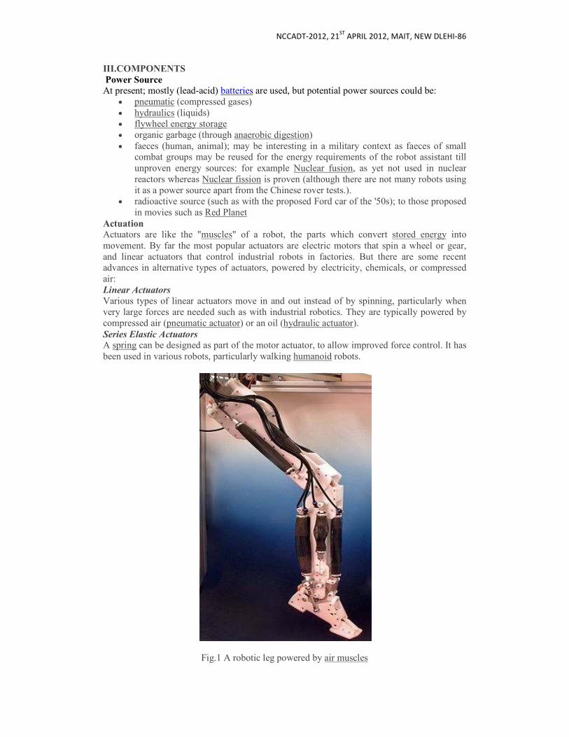
NCCADT-2012, 21ST


III.COMPONENTS

Power Source

At present; mostly (lead-acid) batteries are used, but potential power sources could be: • pneumatic (compressed gases) • hydraulics (liquids) • flywheel energy storage • organic garbage (through anaerobic digestion) • faeces (human, animal); may be interesting in a military context as faeces of small

combat groups may be reused for the energy requirements of the robot assistant till unproven energy sources: for example Nuclear fusion, as yet not used in nuclear reactors whereas Nuclear fission is proven (although there are not many robots using it as a power source apart from the Chinese rover tests.).

• radioactive source (such as with the proposed Ford car of the '50s); to those proposed in movies such as Red Planet

Actuation Actuators are like the "muscles" of a robot, the parts which convert stored energy into movement. By far the most popular actuators are electric motors that spin a wheel or gear, and linear actuators that control industrial robots in factories. But there are some recent advances in alternative types of actuators, powered by electricity, chemicals, or compressed air: Linear Actuators

Various types of linear actuators move in and out instead of by spinning, particularly when very large forces are needed such as with industrial robotics. They are typically powered by compressed air (pneumatic actuator) or an oil (hydraulic actuator). Series Elastic Actuators A spring can be designed as part of the motor actuator, to allow improved force control. It has been used in various robots, particularly walking humanoid robots.

Fig.1 A robotic leg powered by air muscles

NCCADT-2012, 21ST


Piezo Motors

Recent alternatives to DC motors are piezo motors or ultrasonic motors. These work on a fundamentally different principle, whereby tiny piezoceramic elements, vibrating many thousands of times per second, cause linear or rotary motion. There are different mechanisms of operation; one type uses the vibration of the piezo elements to walk the motor in a circle or a straight line.[28] Another type uses the piezo elements to cause a nut to vibrate and drive a screw. The advantages of these motors are nanometer resolution, speed, and available force for their size.[29] These motors are already available commercially, and being used on some robots. Tactile Sensor

Current robotic(C.S.G. Lee et al) and prosthetic hands receive far less tactile information than the human hand. Recent research has developed a tactile sensor array that mimics the mechanical properties and touch receptors of human fingertips. The sensor array is constructed as a rigid core surrounded by conductive fluid contained by an elastomeric skin. Electrodes are mounted on the surface of the rigid core and are connected to an impedance-measuring device within the core. When the artificial skin touches an object the fluid path around the electrodes is deformed, producing impedance changes that map the forces received from the object. The researchers expect that an important function of such artificial fingertips will be adjusting robotic grip on held objects. Vision

Computer vision is the science and technology of machines that see. As a scientific discipline, computer vision (K. S. Fu, et al) is concerned with the theory behind artificial systems that extract information from images. The image data can take many forms, such as video sequences and views from cameras. In most practical computer vision applications, the computers are pre-programmed to solve a particular task, but methods based on learning are now becoming increasingly common. Computer vision systems rely on image sensors which detect electromagnetic radiation which is typically in the form of either visible light or infra-red light. The sensors are designed using solid-state physics. The process by which light propagates and reflects off surfaces is explained using optics. Sophisticated image sensors even require quantum mechanics to provide a complete understanding of the image formation process. There is a subfield within computer vision where artificial systems are designed to mimic the processing and behavior of biological systems, at different levels of complexity. Also, some of the learning-based methods developed within computer vision have their background in biology. Manipulation

Robots need to manipulate objects; pick up, modify, destroy, or otherwise have an effect. Thus the "hands" of a robot are often referred to as end effectors, while the "arm" is referred to as a manipulator (Marco Ceccarelli ). Most robot arms have replaceable effectors, each allowing them to perform some small range of tasks. Some have a fixed manipulator [1] which cannot be replaced, while a few have one very general purpose manipulator, for example a humanoid hand. Mechanical Grippers

One of the most common effectors is the gripper. In its simplest manifestation it consists of just two fingers which can open and close to pick up and let go of a range of small objects. Fingers can for example be made of a chain with a metal wire run through it. Hands that resemble and work more like a human hand include the Shadow Hand. Vacuum Grippers

Vacuum grippers are very simple astrictive devices, but can hold very large loads provided the pretension surface is smooth enough to ensure suction.Pick and place robots for electronic components and for large objects like car windscreens, often use very simple vacuum grippers.

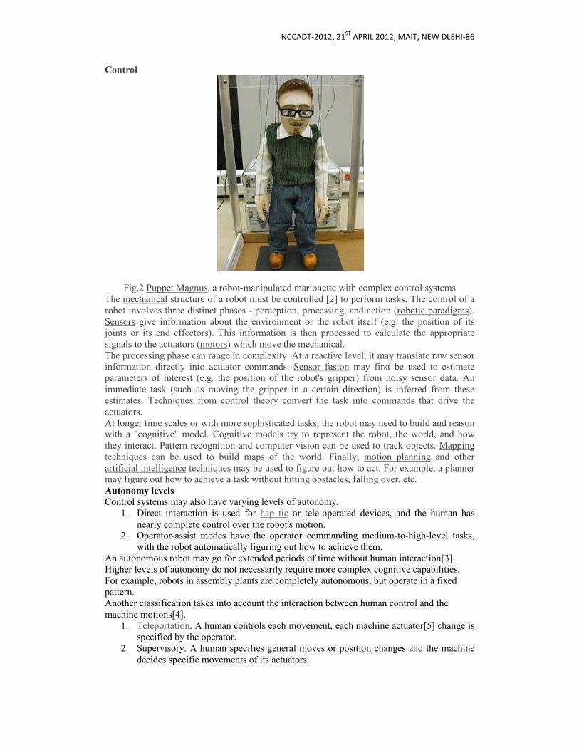
NCCADT-2012, 21ST


Control

Fig.2 Puppet Magnus, a robot-manipulated marionette with complex control systems The mechanical structure of a robot must be controlled [2] to perform tasks. The control of a robot involves three distinct phases - perception, processing, and action (robotic paradigms). Sensors give information about the environment or the robot itself (e.g. the position of its joints or its end effectors). This information is then processed to calculate the appropriate signals to the actuators (motors) which move the mechanical. The processing phase can range in complexity. At a reactive level, it may translate raw sensor information directly into actuator commands. Sensor fusion may first be used to estimate parameters of interest (e.g. the position of the robot's gripper) from noisy sensor data. An immediate task (such as moving the gripper in a certain direction) is inferred from these estimates. Techniques from control theory convert the task into commands that drive the actuators. At longer time scales or with more sophisticated tasks, the robot may need to build and reason with a "cognitive" model. Cognitive models try to represent the robot, the world, and how they interact. Pattern recognition and computer vision can be used to track objects. Mapping techniques can be used to build maps of the world. Finally, motion planning and other artificial intelligence techniques may be used to figure out how to act. For example, a planner may figure out how to achieve a task without hitting obstacles, falling over, etc. Autonomy levels

Control systems may also have varying levels of autonomy. 1. Direct interaction is used for hap tic or tele-operated devices, and the human has

nearly complete control over the robot's motion. 2. Operator-assist modes have the operator commanding medium-to-high-level tasks,

with the robot automatically figuring out how to achieve them. An autonomous robot may go for extended periods of time without human interaction[3]. Higher levels of autonomy do not necessarily require more complex cognitive capabilities. For example, robots in assembly plants are completely autonomous, but operate in a fixed pattern. Another classification takes into account the interaction between human control and the machine motions[4].

1. Teleportation. A human controls each movement, each machine actuator[5] change is specified by the operator.

2. Supervisory. A human specifies general moves or position changes and the machine decides specific movements of its actuators.

NCCADT-2012, 21ST


3. Task-level autonomy. The operator specifies only the task and the robot manages itself to complete it.

4. Full autonomy. The machine will create and complete all its tasks without human interaction.

IV.CONCLUSIONS

Robotics engineers design robots, maintain them, develop new applications for them, and conduct research to expand the potential of robotics. Robots have become a popular educational tool in some middle and high schools, as well as in numerous youth summer camps, raising interest in programming, artificial intelligence and robotics among students. First-year computer science courses at several universities now include programming of a robot in addition to traditional software engineering-based coursework. The Technology Innovation Program was formed to support, promote, and accelerate innovation in the United States through high-risk, high-reward research in areas of critical national need. This research should address societal challenges, i.e., problems or issues confronted by society that when not addressed could negatively affect the overall function and quality of life of the nation, and as such demand government attention. The manufacturing sector is an example of such an area and is in need of novel and innovative solutions both to overcome the manufacturing sector’s latest economic setbacks as well as to establish new levels of global competitive advantages. Advanced Robotics and

Intelligent Automation represents the potential to support technical solutions that could provide a new level of agile and flexible capabilities to an industry that has historically focused on long production runs and large volume manufacturing. The infrastructural technology developments outlined in this paper would enable the development of the next generation of advanced robotic systems capable of also providing greater precision and quality needed to move automation into smaller volume manufacturing, and creating better, higher pay jobs. REFERENCES

1. Marco Ceccarelli, "Fundamentals of Mechanics of Robotic Manipulators" 2. K. S. Fu & R.C. Gonzalez & C.S.G. Lee, Robotics: Control, Sensing, Vision, and

Intelligence (CAD/CAM, robotics, and computer vision) 3. “SP200 With Open Control Center. Robotic Prescription Dispensing System”,

accessed November 22, 2008. 4. “McKesson Empowering HealthCare. Robot RX”, accessed November 22, 2008. 5. “Aethon. You Deliver the Care. TUG Delivers the Rest”, accessed November 22,

2008.

NCCADT-2012, 21ST


Waste Heat recovery and its Utilization in Textile Industry:

An Indian Perspective Umesh Kumar

a,

Dr. M.N. Karimi

b

aResearch Scholar, Department of Mechanical Engineering, Jamia Millia Islamia, New Delhi. bProfessor, Department of Mechanical Engineering, Jamia Millia Islamia, New Delhi.

Abstract: A large amount of thermal energy, either in the form of hot exhaust gases or hot liquid or hot

water vapor is thrown out into the atmosphere from various processing machines in textile mills, which then gets wasted. In Indian textile mills a lot of work has been done to recover

the high-grade heat but the recovery of low grade is an ignored area till date. The facts show

that 30-40% of the total energy which is wasted is in the form of low-grade heat. The present

work is an effort towards finding the scope of waste heat recovery and its utilization in Indian

textile industry by taking case studies of few mills. Indian textile industry is second largest in

the world. Country earns about 27% of the foreign exchange from the export of the textiles. The industry contributes about 14% of the total industrial production of India. Its

contribution to the GDP is about 4% and It accounts for the 21% of the total employment

generated in the economy. Around 35 million people are directly employed in textile manufacturing which is next only to the agriculture .Also the country has the largest acreage

under cotton in the world[1].As per the BEE Textile sector is the fifth largest energy

consuming sector with annual consumption of 4.5 MTOE the specific energy consumption in

this sector is 3000-16100 kcal/kg(thermal) and 0.25-10kW(electrical).[ ]

In spite of the above

facts the sector is nor an organized sector. It is divided in two segments, the organized and

the other unorganized segment. The unorganized sector is still working with age old and

traditional methods which are very inefficient in energy consumption.

This paper deals with finding the ways for recovery of waste heat from different

processes, utilizing it and finding the payback period for the new equipment. The payback

periods calculated here are near about or less than one year, which are very good for the purpose.

Keywords: Textile, Waste Heat, Energy efficiency, Payback

Introduction: Indian textile industry is second largest in the world. Country earns about 27% of the foreign exchange from the export of the textiles. The industry contributes about 14% of the total industrial production of India. Its contribution to the GDP is about 4% and It accounts for the 21% of the total employment generated in the economy[1]. Around 35 million people are directly employed in textile manufacturing which is next only to the agriculture .Also the country has the largest acreage under cotton in the world.

In spite of the above facts the Indian textile industry doesn’t constitute a wholly organized sector. The industry can be classified into two categories, one the organized mill sector and other the unorganized decentralized sector. The organized sector of the textile industry represents the mills. It could be a spinning mill or composite mill[2]. A composite mill is one where the spinning, weaving and processing facilities are carried out under single roof. The unorganized decentralized sector has been found to be engaged mainly in weaving and garmenting activities, which makes it heavily dependent on the organized sector for their yarn requirements. The decentralized sector is comprised of three main segments i.e. power loom, handloom and hosiery. In addition to the above there are readymade garments, Khadi as well as carpet manufacturing units in decentralized sector[3].

NCCADT-2012, 21ST


Nomenclature a discount rate As heat transfer surface area(m2) B benefit C cost d diameter(m) e specific exergy (kj/kg) É exergy rate (kW) EP economical profit (Rs.) F correction factor for multi-pass heat exchanger h specific enthalpy(kJ/kg) i interest rate Ì exergy destruction L length of the tube(m) mass flow rate (kg/s) n number of tubes NGP natural gas price NPV net prestnt value p period P pressure(kPa) ∆Pi pressure drop(kPa) heat transfer rate (kW) s specific entopy (kJ/(kg-K) T temperature TP number of tube passes ∆Tlm log-mean temperature difference (oC) u velocity (m/s) U overall heat transfer coefficient (kW/(m2K)) ε effectiveness η efficiency (%) ρ density( kg/m3) Subscripts cw cold water in inlet II second law o dead state conditions out outlet ww waste water

The organized mill sector has a complete information base on organizational set-up, machining installation, production pattern, employment etc. However, the information base of the decentralized sector on the above parameters is inadequate which prevents it from modernization and from exploiting the economics of scale including the energy efficiency. A major constraint coming in the way of modernization of Indian Textile Industry is the virtual demise over the years of India’s textile machinery industry[4]. The unorganized sector is still using very old machinery and traditional methods, which result in the very low productivity and high wastage of resourced. Since, the textile manufacturing process is characterized by the high consumptions of resources like water, fuel and various chemicals, it becomes a necessity for the industry to switch over to modernization in order t beat the today’s tough competition from foreign players. Cost of energy is a major factor in the textile production. Textile Industry has been identified as an “ Energy Intensive Industry” under energy conservation act. 2001. It

NCCADT-2012, 21ST


consumes 10.4 % of the total industrial consumption of the country. The cost of energy as a percentage of the manufacturing cost in textile industry varies between 12-15%, Which includes electrical and thermal energy. The cost of energy is next only to raw material cost and comparable to the labor cost. On an average the thermal energy requirement per meter of the cloth varies in the range of 4500-5500 kcal whereas 0.45-0.55 kWH of electrical energy goes into its processing. Hence it is clearly understood that the industry is a major energy consumer and It is a fact that the Indian Textile Industry retains a record of lowest efficiency in energy utilization. Thus cost of energy increases. To tackle the increase in energy cost it requires more effective use of energy and recovering the lost energy. Hence energy conservation in a textile mill has a significant importance and should be a priority area for increasing the productivity and maximizing the profit. The total energy saving potential is estimated to be 15% in textile industry[5]. Effective utilization of lost energy in industry is important economically and environmentally for all over the world. Designing efficient and cost effective systems that also meet lower capital and running costs and environmental conditions are the foremost challenges that engineers face. Many possibilities of conserving energy in textile finishing are wasted. Various options available aiming at taking initiatives for energy conservation. Major energy recovery and conservation areas in the textile industry are as follows: (1) Waste water heat recovery;(2) Flash steam recovery;(3) reducing heat loss to environment from dryers. Analysis: The mill under study requires Steam for its process house, which consists of Dyeing Machines, Dryers and Stenters. For meeting the steam requirements the mill has two FBC boilers (Thermax made) each having a capacity of 3 TPH. One of the boiler is stand by. Earlier the steam requirement was met by waste heat recovery boilers from DG sets. But due to increased prices of OIL, in 2008-2009 the company decided to purchase electricity from U.P.S.E.B, The contract demand is 7000 kVA. Now all the EG Boilers are non working and all of the steam load is shifted on to the boiler. On studying the operating parameters of the boiler it is clear that the boiler is running over capacity, due to which the process suffers and production time is increases, which results in loss of profit. One solution of the problem can be to run the second boiler, but it will come out to be an expensive affair. From the above information it is clear that if the plant runs on full load the total steam requirement is 5477.6 kg/hr. Other feasible to utilize the waste heat from dyeing machines is by installing a heat exchanger. The calculations were carried out or the same.A shell and tube heat exchanger is selected for installation. The hot dye liquor, being corrosive in nature, is selected to pass through tubes and cold water through shell. Case Study:- This is a case study of process house. The mill deals into all kind of fabric dyeing, processing, printing and providing services in the processing of the fabric. The plant has a capacity to process 4 million meters of fabric per month the dyeing capacity of the plant is 1.5 million meters per month. The company has the following machines to carry out the processing.

1. Continuous bleach range 1 No. 2. Continuous mercerizing machines 3 Nos. 3. Jiggers 5 Nos. 4. Jet dyeing Machines 10 Nos. 5. Drying Ranges ( Vertical) 2 Nos.

An audit was done in the mill for finding the measures for thermal energy conservation. A large quantity of Hot water was being found to be drained. The heat content of the water may be utilized for various processes if recovered. A Waste heat recovery heat exchanger is being suggested to be installed in the mill. The design and economics were calculated.

i. Discussions:- Efficiency of the boiler is 72% and the evaporation ratio is around 3.7. Average fuel consumption is 17.15 tons per day and the average steam generation is 65 Tons per day

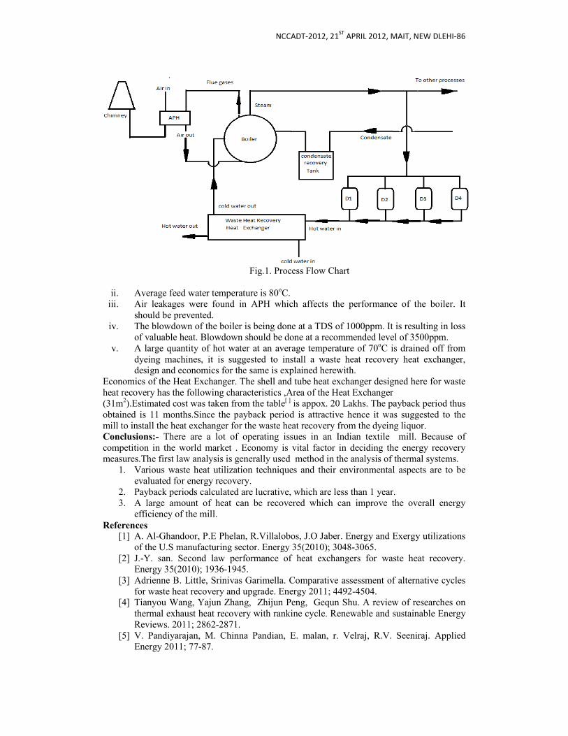
NCCADT-2012, 21ST


Fig.1. Process Flow Chart

ii. Average feed water temperature is 80oC.

iii. Air leakages were found in APH which affects the performance of the boiler. It should be prevented.

iv. The blowdown of the boiler is being done at a TDS of 1000ppm. It is resulting in loss of valuable heat. Blowdown should be done at a recommended level of 3500ppm.

v. A large quantity of hot water at an average temperature of 70oC is drained off from dyeing machines, it is suggested to install a waste heat recovery heat exchanger, design and economics for the same is explained herewith.

Economics of the Heat Exchanger. The shell and tube heat exchanger designed here for waste heat recovery has the following characteristics ,Area of the Heat Exchanger (31m2).Estimated cost was taken from the table[ ] is appox. 20 Lakhs. The payback period thus obtained is 11 months.Since the payback period is attractive hence it was suggested to the mill to install the heat exchanger for the waste heat recovery from the dyeing liquor. Conclusions:- There are a lot of operating issues in an Indian textile mill. Because of competition in the world market . Economy is vital factor in deciding the energy recovery measures.The first law analysis is generally used method in the analysis of thermal systems.

1. Various waste heat utilization techniques and their environmental aspects are to be evaluated for energy recovery.

2. Payback periods calculated are lucrative, which are less than 1 year. 3. A large amount of heat can be recovered which can improve the overall energy

efficiency of the mill. References

[1] A. Al-Ghandoor, P.E Phelan, R.Villalobos, J.O Jaber. Energy and Exergy utilizations of the U.S manufacturing sector. Energy 35(2010); 3048-3065.

[2] J.-Y. san. Second law performance of heat exchangers for waste heat recovery. Energy 35(2010); 1936-1945.

[3] Adrienne B. Little, Srinivas Garimella. Comparative assessment of alternative cycles for waste heat recovery and upgrade. Energy 2011; 4492-4504.

[4] Tianyou Wang, Yajun Zhang, Zhijun Peng, Gequn Shu. A review of researches on thermal exhaust heat recovery with rankine cycle. Renewable and sustainable Energy Reviews. 2011; 2862-2871.

[5] V. Pandiyarajan, M. Chinna Pandian, E. malan, r. Velraj, R.V. Seeniraj. Applied Energy 2011; 77-87.

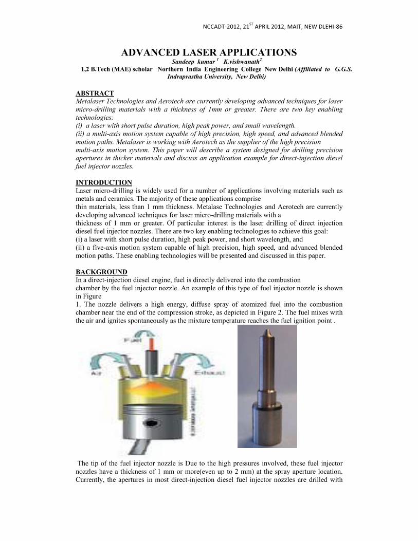
NCCADT-2012, 21ST


ADVANCED LASER APPLICATIONS Sandeep kumar

1 K.vishwanath

2

1,2 B.Tech (MAE) scholar Northern India Engineering College New Delhi (Affiliated to G.G.S.

Indraprastha University, New Delhi)

ABSTRACT Metalaser Technologies and Aerotech are currently developing advanced techniques for laser

micro-drilling materials with a thickness of 1mm or greater. There are two key enabling

technologies: (i) a laser with short pulse duration, high peak power, and small wavelength.

(ii) a multi-axis motion system capable of high precision, high speed, and advanced blended

motion paths. Metalaser is working with Aerotech as the supplier of the high precision

multi-axis motion system. This paper will describe a system designed for drilling precision

apertures in thicker materials and discuss an application example for direct-injection diesel

fuel injector nozzles.

INTRODUCTION

Laser micro-drilling is widely used for a number of applications involving materials such as metals and ceramics. The majority of these applications comprise thin materials, less than 1 mm thickness. Metalase Technologies and Aerotech are currently developing advanced techniques for laser micro-drilling materials with a thickness of 1 mm or greater. Of particular interest is the laser drilling of direct injection diesel fuel injector nozzles. There are two key enabling technologies to achieve this goal: (i) a laser with short pulse duration, high peak power, and short wavelength, and (ii) a five-axis motion system capable of high precision, high speed, and advanced blended motion paths. These enabling technologies will be presented and discussed in this paper. BACKGROUND

In a direct-injection diesel engine, fuel is directly delivered into the combustion chamber by the fuel injector nozzle. An example of this type of fuel injector nozzle is shown in Figure 1. The nozzle delivers a high energy, diffuse spray of atomized fuel into the combustion chamber near the end of the compression stroke, as depicted in Figure 2. The fuel mixes with the air and ignites spontaneously as the mixture temperature reaches the fuel ignition point .

The tip of the fuel injector nozzle is Due to the high pressures involved, these fuel injector nozzles have a thickness of 1 mm or more(even up to 2 mm) at the spray aperture location. Currently, the apertures in most direct-injection diesel fuel injector nozzles are drilled with

NCCADT-2012, 21ST


EDM(electrical discharge machining) in which a hollow, cylindrical electrode is maintained at a controlled distance from the work surface. The electrode is continuously rotated as sparks jump across the gap, eroding a hole in the work piece. The EDM process has several disadvantages : (i) the sacrificial electrode is consumed at a rate equal to or exceeding the injector material removal rate; (ii) the work piece must be submerged in a dielectric fluid that acts to insulate the electrode and work surface; (iii) the dielectric fluid is also used to flush away the minute chips as they are eroded, and thus must be either filtered or discarded; and (iv) production cycle time for EDM micro-drilling of fuel injector nozzles is approximately 24 seconds per hole for a typical 200 µm diameter aperture. REQUIREMENTS OF THE LASER

To successfully micro-drill high aspect ratio apertures in thicker materials, such as in direct-injection diesel fuel injector nozzles, the laser power source must meet three main requirements: (i) short pulse duration, (ii) high peak power, and (iii) short wavelength. The most common laser for drilling is the solid state, diode-pumped, pulsed Nd:YAG laser. A schematic of the Nd:YAG laser is shown in Figure . The laser medium is neodymium (Nd) doped into an yttrium aluminum garnet (YAG) crystal contained in a cavity. This crystal is excited by diodes and emits light with a wavelength of 1064 nm. Mirrors at each end of the cavity reflect the waves back and forth until the build-up of photons is self-sustaining and the laser beam is well-collimated. This phenomenon is called “lasing”. One of the mirrors is partially reflective, allowing the laser beam to exit the cavity. Often, additional cavities are used to produce higher output power. For micro-drilling applications, the laser power is delivered in discrete, high-energy pulses . Once the beam exits the laser, it is generally directed through a processing head containing optics that focus the beam onto the work piece. During processing with the high-energy density laser pulses, the energy concentration at the work piece is so intense that he material directly under the beam is vaporized or ablated with

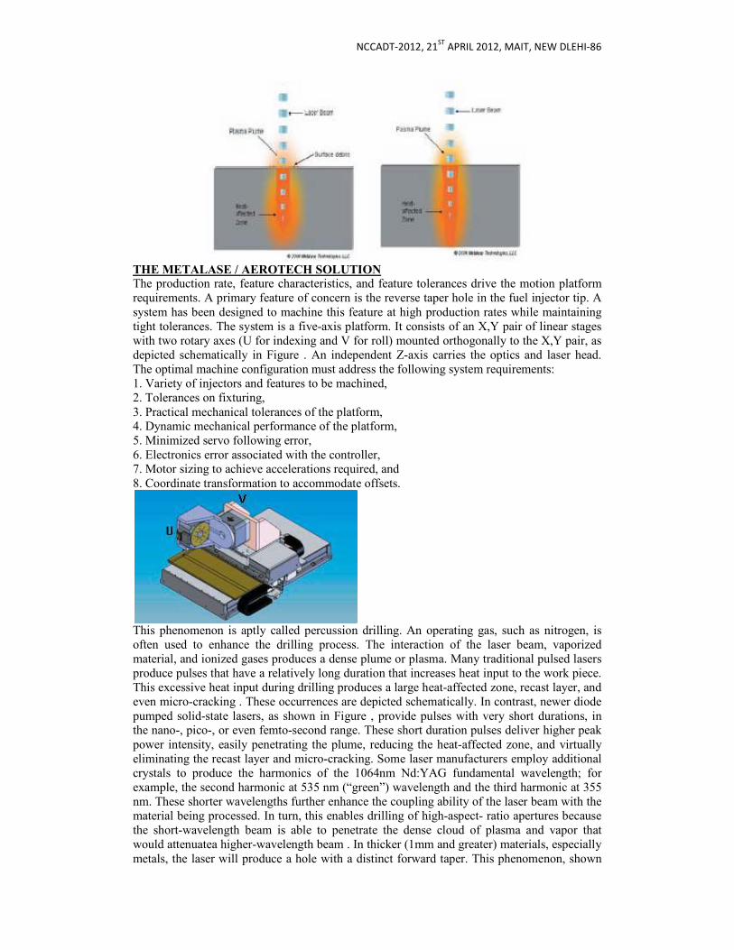
NCCADT-2012, 21ST


THE METALASE / AEROTECH SOLUTION The production rate, feature characteristics, and feature tolerances drive the motion platform requirements. A primary feature of concern is the reverse taper hole in the fuel injector tip. A system has been designed to machine this feature at high production rates while maintaining tight tolerances. The system is a five-axis platform. It consists of an X,Y pair of linear stages with two rotary axes (U for indexing and V for roll) mounted orthogonally to the X,Y pair, as depicted schematically in Figure . An independent Z-axis carries the optics and laser head. The optimal machine configuration must address the following system requirements: 1. Variety of injectors and features to be machined, 2. Tolerances on fixturing, 3. Practical mechanical tolerances of the platform, 4. Dynamic mechanical performance of the platform, 5. Minimized servo following error, 6. Electronics error associated with the controller, 7. Motor sizing to achieve accelerations required, and 8. Coordinate transformation to accommodate offsets.

This phenomenon is aptly called percussion drilling. An operating gas, such as nitrogen, is often used to enhance the drilling process. The interaction of the laser beam, vaporized material, and ionized gases produces a dense plume or plasma. Many traditional pulsed lasers produce pulses that have a relatively long duration that increases heat input to the work piece. This excessive heat input during drilling produces a large heat-affected zone, recast layer, and even micro-cracking . These occurrences are depicted schematically. In contrast, newer diode pumped solid-state lasers, as shown in Figure , provide pulses with very short durations, in the nano-, pico-, or even femto-second range. These short duration pulses deliver higher peak power intensity, easily penetrating the plume, reducing the heat-affected zone, and virtually eliminating the recast layer and micro-cracking. Some laser manufacturers employ additional crystals to produce the harmonics of the 1064nm Nd:YAG fundamental wavelength; for example, the second harmonic at 535 nm (“green”) wavelength and the third harmonic at 355 nm. These shorter wavelengths further enhance the coupling ability of the laser beam with the material being processed. In turn, this enables drilling of high-aspect- ratio apertures because the short-wavelength beam is able to penetrate the dense cloud of plasma and vapor that would attenuatea higher-wavelength beam . In thicker (1mm and greater) materials, especially metals, the laser will produce a hole with a distinct forward taper. This phenomenon, shown

NCCADT-2012, 21ST


schematically in Figure 8, is due to the concentration of heat energy at and near the entrance of the hole. This occurrence is likely, even using the most sophisticated of lasers. Requirements and Design of the Motion System

Because most micro-drilling and micro-machining applications require more than simple percussion drilling of a single aperture, a motion system is often incorporated. These systems can be based either on: 1. Optics that manipulate the laser beam using optical wedges and lenses, 2. Part-positioning, in which the laser beam is fixed and the work piece is manipulated under it, or 3. A combination of 1 and 2.These systems provide simple motions such as rapid scanning in the X-Y plane to produce micro-machined features and/or trepanning in a circular motion to produce apertures with diameters larger than the intrinsic laser spot size. Optical systems have the advantage of speed due to their low inertia. However, their work envelope (typically only 25 mm3) is severely limited compared to a part-positioning system that can have a work envelope up to 300 mm3 or more. Optical systems produce high-quality micro-features in thin components. However, for thicker components the concentration of heat near the surface of the work piece will produce a forward taper, as discussed earlier. Thus, a motion system is required that can compensate for this taper. Very few commercially available optical systems are able to compensate for this forward taper, or are very restricted in their angular scope. Variety of Injectors and Features to be Machined

The injectors are 20 to 50 mm in length, 15 to 30 mm in diameter (at the base) and can have 4 to 20 apertures at a variety of angles with respect to the tip. Additionally, the plane of the holes may not be parallel with the base plane of the injector. The material thickness at the tip is 1mm. A typical reverse taper hole is depicted in Figure 10. Figure 11 shows the resulting trajectories that must be followed by the axes of the machine. DYNAMIC MECHANICAL PERFORMANCE OF THE PLATFORM

The motion platform must have a high servo bandwidth to meet through-put requirements. The dynamic performance of the system depends largely on the stiffness and the location of the center of gravity of the motion platform. The mechanics must be as stiff and lightweight as possible while still achieving low error motion. Optimized selection, location and integration of core elements, such as motors, encoders, and bearings yield a readily controllable system. PRACTICAL TOLERANCES ON FIXTURING

The fixturing requires highly toleranced surfaces to maintain error motions of less than a few microns measured at the injector tip. The load / unload process must also be repeatable to within a few microns. Yet if the fixtured part can be located after loading then it is possible for the motion controller to adjust the trajectory to accommodate for the fixturing error, allowing greater tolerances on fixturing

NCCADT-2012, 21ST


MINIMIZED SERVO FOLLOWING ERROR

The servo control loop must be designed to minimize following error. The following error will be a function of the trajectory and the tuning. The X,Y pair motions are sinusoidal. If it takes 10 passes, for example, to drill a hole in 2 seconds then the bandwidth of the trajectory is 5 Hz. It is reasonable to reach a 10 Hz bandwidth on the X,Y pair in this system configuration and one should expect minimal servo following error. In steady state, the tracking error due to magnitude will be practically zero and the tracking error due to phase will be non-zero. However, if one compensates the X,Y stages to have identical closed loop transfer functions, then the phase error will not affect the quality of the circle as both axis will have the same tracking error. In practice, the transfer functions will be very similar but not identical, and therefore there will be some minimal affect on the quality of the circle made by the X,Y stages. ELECTRONICS ERROR ASSOCIATED WITH THE CONTROLLER

Control electronics can cause following errors due to power transistors switching. Therefore, it is advisable to avoid using PWM amplifiers and instead use linear amplifiers. Other considerations include the encoder resolution, controller sample time, clock stability, and synchronicity. The resolution of the encoders is sufficient for the application to minimize servo dither and quantization error. It is advisable to have at least 10 times the resolution over the accuracy requirement. The resolution of the encoders selected is at least 50 times greater than the required tolerances. The axes are synchronized with a network system clock that drives each axis. Servo loop sample time is 8 kHz, which is sufficient for this application. For instance the digital trajectory generation error depends on the size of the hole, and number of points generated around the circle. At an 8 kHz sample time there will be 1,600 points. Therefore the error due to trajectory generation (eN) will be less than 2.9x10-8 µm, as calculated by where r is the radius of the top of the hole and N is the number of points around the hole. Coordinate Transformations to Accommodate Offsets

The surface of the injector tip where the aperture is to be drilled is not at the intersection of the rotary axes; therefore, it is necessary for the motion controller to perform certain transformations to drill the appropriate hole. This is done using the concept of a virtual pivot point that translates the axes appropriately. When an injector is mounted offset from the point of axis intersection, the transformation must be implemented, where l is the distance from the center of the sac to the intersection of the rotary axis, d is the difference between the top and bottom diameters, θ is the angle of the reverse taper, and φ is the angle of rotation the rotary stage should make. The Z-axis will also have to translate as required to keep the focal point at the cutting depth. SUMMARY

An integrated laser-motion system was designed such that a wide variety of features can be micro-drilled in thicker materials. The effect of the mechanical, electrical, and servo system

NCCADT-2012, 21ST


errors on the motion was considered during the design process to ensure that the resulting features will meet the required tolerances and production rates.

The Metalase / Aerotech system compares well with traditional EDM technology for producing injector spray apertures of 200µm diameter and below. Advantages of the laser-based system are that the laser does not require consumable and can accomplish the drilling in a few seconds per aperture (depending on aperture diameter and wall thickness). In addition, the capital cost of a laser system is competitive with a fully automated EDM micro-drilling system. Additionally, the Metalase / Aerotech laser system is inherently capable of drilling much smaller apertures in production than are possible using traditional EDM techniques. An example is given in Figure . The sophisticated micro-positioning system also en ables a variety of engineered configurations to be micro-drilled in thicker materials. Finally, the addition of the Z-axis to the laser head provides the additional flexibility of adjusting the focus spot location synchronous to laser drilling operation. REFERENCES

1. Marks’ Standard Handbook for Mechanical Engineers, 9th Edition, E.A. Avallone & T. Baumeister, Editors., McGraw-Hill Book Company, 1986. 2. “Diesel Engine Basics”, DieselNet, www.dieselnet.com. 3. L. Rakowski, “Non-Traditional Methods for Making Small Holes”, Modern Machine Shop, June 2002. 4. C. Sommers, Non-Traditional Machining Handbook, Advance Publishing Inc., 1999. 5. 40 CFR 86.004-11; 40 CFR 86.007-11. 6. “Emissions Standards: European Union”, DieselNet, www.dieselnet. com. 7. J. Clarke, et al., “Laser Drilling of Diesel Fuel Injector Nozzles”, Lambda Highlights, No. 62, p. 4, June 2003. 8. S.V. Govorkov, E.V. Slobodtchikov, A.O. Wiessner, D. Basting, “High Accuracy

Microdrilling of Steel with Solid-State UV Laser at 10 mm/sec Rate”, in Proc. SPIE 3933, p. 365, 2000.

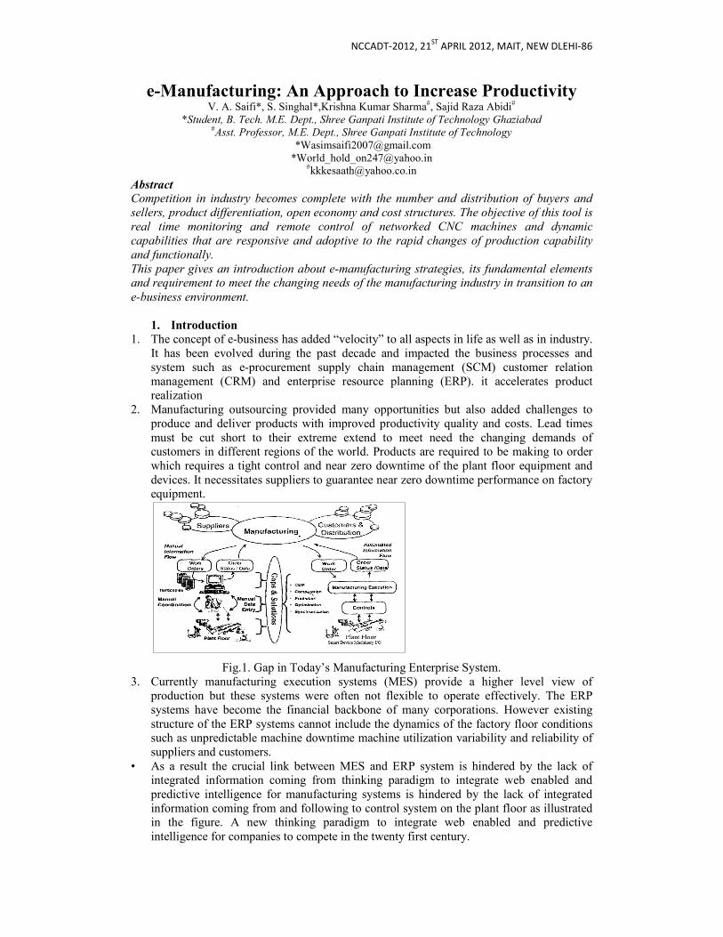
NCCADT-2012, 21ST


e-Manufacturing: An Approach to Increase Productivity V. A. Saifi*, S. Singhal*,Krishna Kumar Sharma#, Sajid Raza Abidi#

*Student, B. Tech. M.E. Dept., Shree Ganpati Institute of Technology Ghaziabad #Asst. Professor, M.E. Dept., Shree Ganpati Institute of Technology

*[email protected] *[email protected]

#[email protected] Abstract Competition in industry becomes complete with the number and distribution of buyers and

sellers, product differentiation, open economy and cost structures. The objective of this tool is

real time monitoring and remote control of networked CNC machines and dynamic

capabilities that are responsive and adoptive to the rapid changes of production capability

and functionally.

This paper gives an introduction about e-manufacturing strategies, its fundamental elements and requirement to meet the changing needs of the manufacturing industry in transition to an

e-business environment.

1. Introduction

1. The concept of e-business has added “velocity” to all aspects in life as well as in industry. It has been evolved during the past decade and impacted the business processes and system such as e-procurement supply chain management (SCM) customer relation management (CRM) and enterprise resource planning (ERP). it accelerates product realization

2. Manufacturing outsourcing provided many opportunities but also added challenges to produce and deliver products with improved productivity quality and costs. Lead times must be cut short to their extreme extend to meet need the changing demands of customers in different regions of the world. Products are required to be making to order which requires a tight control and near zero downtime of the plant floor equipment and devices. It necessitates suppliers to guarantee near zero downtime performance on factory equipment.

Fig.1. Gap in Today’s Manufacturing Enterprise System. 3. Currently manufacturing execution systems (MES) provide a higher level view of

production but these systems were often not flexible to operate effectively. The ERP systems have become the financial backbone of many corporations. However existing structure of the ERP systems cannot include the dynamics of the factory floor conditions such as unpredictable machine downtime machine utilization variability and reliability of suppliers and customers.

• As a result the crucial link between MES and ERP system is hindered by the lack of integrated information coming from thinking paradigm to integrate web enabled and predictive intelligence for manufacturing systems is hindered by the lack of integrated information coming from and following to control system on the plant floor as illustrated in the figure. A new thinking paradigm to integrate web enabled and predictive intelligence for companies to compete in the twenty first century.

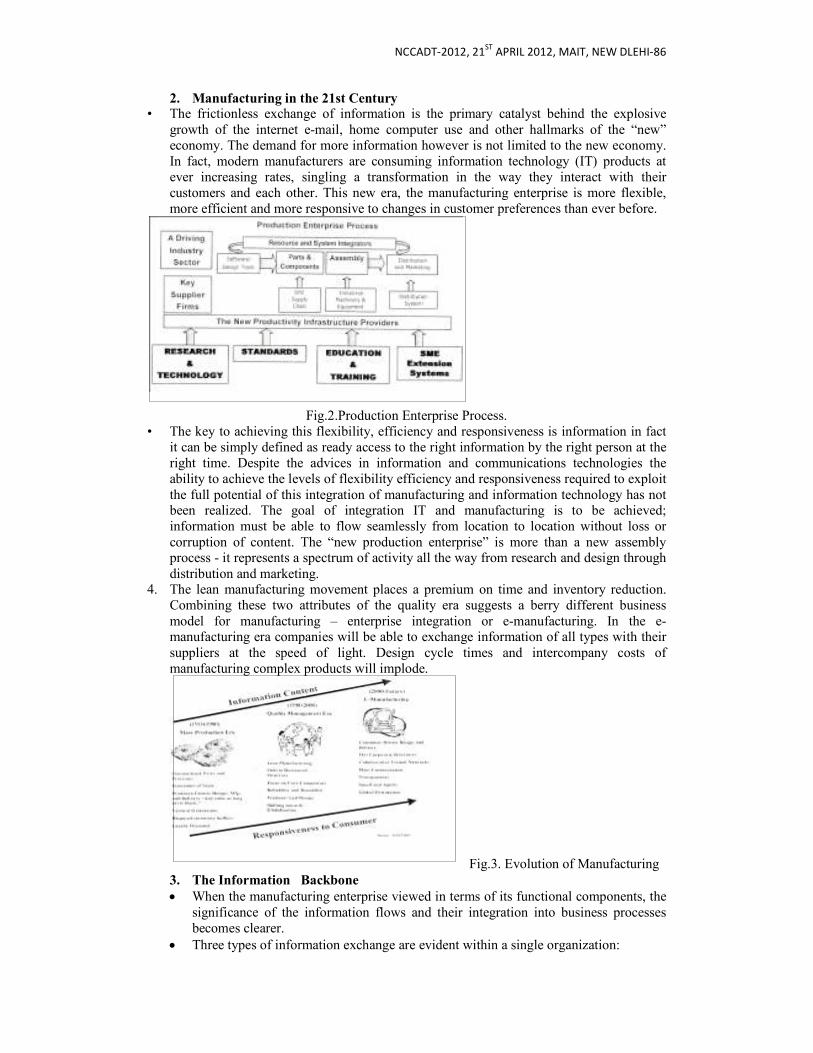
NCCADT-2012, 21ST


2. Manufacturing in the 21st Century • The frictionless exchange of information is the primary catalyst behind the explosive

growth of the internet e-mail, home computer use and other hallmarks of the “new” economy. The demand for more information however is not limited to the new economy. In fact, modern manufacturers are consuming information technology (IT) products at ever increasing rates, singling a transformation in the way they interact with their customers and each other. This new era, the manufacturing enterprise is more flexible, more efficient and more responsive to changes in customer preferences than ever before.

Fig.2.Production Enterprise Process. • The key to achieving this flexibility, efficiency and responsiveness is information in fact

it can be simply defined as ready access to the right information by the right person at the right time. Despite the advices in information and communications technologies the ability to achieve the levels of flexibility efficiency and responsiveness required to exploit the full potential of this integration of manufacturing and information technology has not been realized. The goal of integration IT and manufacturing is to be achieved; information must be able to flow seamlessly from location to location without loss or corruption of content. The “new production enterprise” is more than a new assembly process - it represents a spectrum of activity all the way from research and design through distribution and marketing.

4. The lean manufacturing movement places a premium on time and inventory reduction. Combining these two attributes of the quality era suggests a berry different business model for manufacturing – enterprise integration or e-manufacturing. In the e-manufacturing era companies will be able to exchange information of all types with their suppliers at the speed of light. Design cycle times and intercompany costs of manufacturing complex products will implode.

Fig.3. Evolution of Manufacturing 3. The Information Backbone

• When the manufacturing enterprise viewed in terms of its functional components, the significance of the information flows and their integration into business processes becomes clearer.

• Three types of information exchange are evident within a single organization:

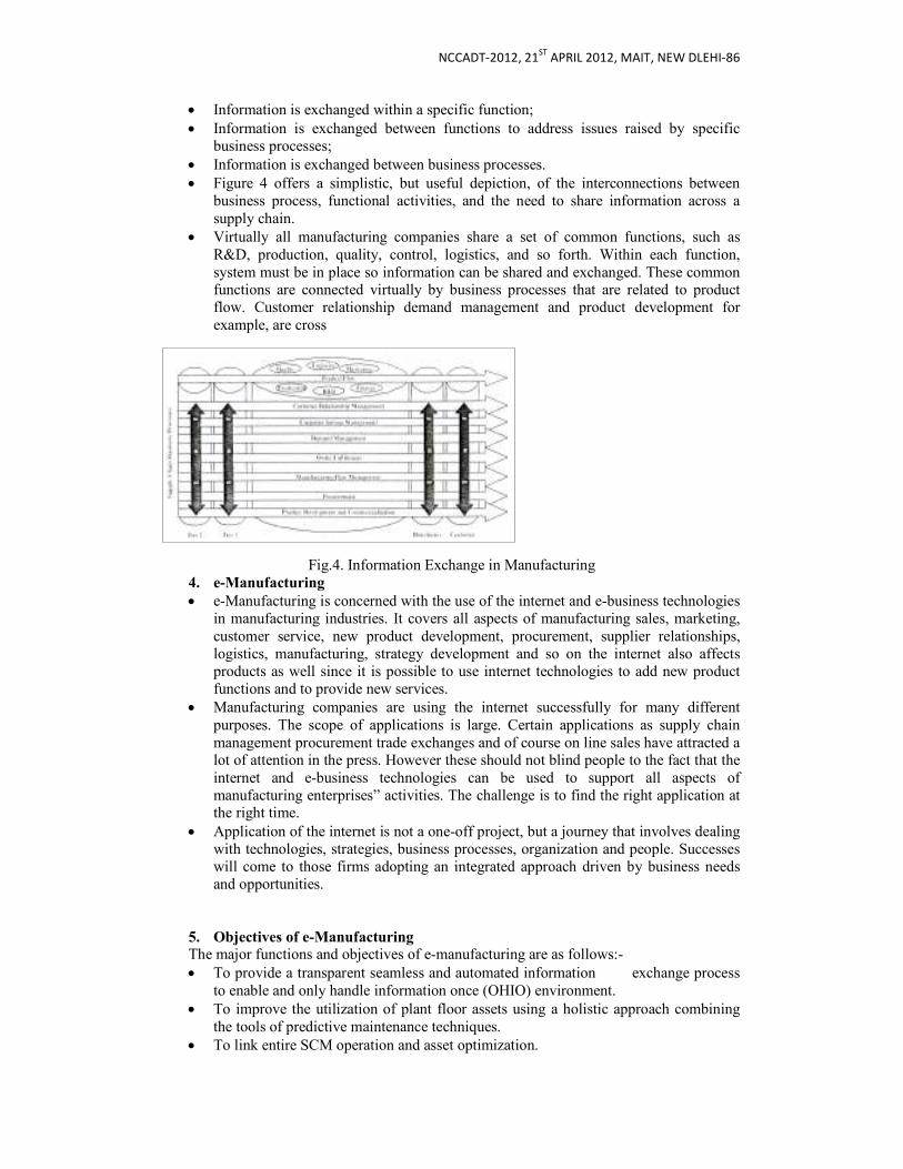
NCCADT-2012, 21ST


• Information is exchanged within a specific function; • Information is exchanged between functions to address issues raised by specific

business processes; • Information is exchanged between business processes. • Figure 4 offers a simplistic, but useful depiction, of the interconnections between

business process, functional activities, and the need to share information across a supply chain.

• Virtually all manufacturing companies share a set of common functions, such as R&D, production, quality, control, logistics, and so forth. Within each function, system must be in place so information can be shared and exchanged. These common functions are connected virtually by business processes that are related to product flow. Customer relationship demand management and product development for example, are cross

Fig.4. Information Exchange in Manufacturing 4. e-Manufacturing

• e-Manufacturing is concerned with the use of the internet and e-business technologies in manufacturing industries. It covers all aspects of manufacturing sales, marketing, customer service, new product development, procurement, supplier relationships, logistics, manufacturing, strategy development and so on the internet also affects products as well since it is possible to use internet technologies to add new product functions and to provide new services.

• Manufacturing companies are using the internet successfully for many different purposes. The scope of applications is large. Certain applications as supply chain management procurement trade exchanges and of course on line sales have attracted a lot of attention in the press. However these should not blind people to the fact that the internet and e-business technologies can be used to support all aspects of manufacturing enterprises” activities. The challenge is to find the right application at the right time.

• Application of the internet is not a one-off project, but a journey that involves dealing with technologies, strategies, business processes, organization and people. Successes will come to those firms adopting an integrated approach driven by business needs and opportunities.

5. Objectives of e-Manufacturing

The major functions and objectives of e-manufacturing are as follows:- • To provide a transparent seamless and automated information exchange process

to enable and only handle information once (OHIO) environment. • To improve the utilization of plant floor assets using a holistic approach combining

the tools of predictive maintenance techniques. • To link entire SCM operation and asset optimization.

NCCADT-2012, 21ST


• To deliver customer services utilizing the latest predictive intelligence methods and tether-free technologies

6. Tools for e-Manufacturing In Rockwell automation it was clearly stated that four competencies such as design operate maintain and synchronize are required for any manufacturer to be a world class manufacturing company. This sets good directions for e-manufacturing research and development: A. Development of intelligent agents for continuous real time remote and distributed

monitoring and analyses of devices machinery and systems to provide the first endmost need elements of predictive maintenance via offering real time information about machine’s performance status (health condition) its capability of producing quality pats (or completing its tasks) etc.

B. Development of remote distributed and web-based quality control systems and their integration with intelligent predictive agents described above in order to identify quality variations and their causes in real time.

C. Development of a dependable and scalable information pipeline/platform for complete transformation optimization and synchronization of plant floor problems issues and solutions with higher- level production maintenance and transaction scheduki9ng systems inventory control systems, supply chain systems and with ERP for dynamic scheduling of production maintenance human and other resource dynamic inventory monitoring and control optimization of energy/power utilization, etc.

D. Development of virtual design platform for collaborative part process tooling design among suppliers design and process engineers and as well as customers for fast validation and decision making. To effectively implement the e- manufacturing enabling tools need to be developed.

• Data and Information Transformation Tools

Data gathering from various machinery and process exit at various levels. However massive raw data are not useful unless they are reduced and transformed into information and knowledge for responsive actions. Hence data mining tools for data reduction representation and prediction adopted for plant floor data need to be developed. A platform is needed to save as a transfer function between the manufacturing data acquisition system and the MES. Tools are needed to core relates data from different formats and transform them to a web deployable information system. These data from different formats and transform them to a web deployable information system. These data can be gathered from traditional control I/O or through a separate wireless data acquisition system using different communication protocols including 802.11, 802.11b, Bluetooth etc. Fig. shows how data and information are transformed from machine and device level to a web- enabled environment. At this level many web-enabled applications can be performed. for example we can perform remote machine calibration through telescopic all bar in different location .experts from machine tool manufacturers can assist users to analyze machine measurement data and perform prognostics for preventive maintenance. Users from different factories or locations can also share this information through these web tools. This will enable users for high quality communications since they all sharing the same set of data formats without any language barriers. • Prediction Tools

Advanced prediction methods and tools need to be developed in order to detect degradation performance loss or trend of failure not faults breakdowns etc. a watchdog agent has been developed and pioneered by the center for intelligent maintenance systems (IMS). It provides continuous monitoring and prognostics of asset degradation and also evaluates asset performance. It is output represents the quantitative measures of the performance of the product or equipment at a given state.

NCCADT-2012, 21ST


References: 1. National Coalition for advanced Manufacturing, (2000). Smart Prosperity: An Agenda for

Enhancing Productivity Growth. Washington D.C. 2. National Research council, (2000). Surviving Supply Chain Integration: Strategies for

small Manufactures. Washington D.C 3. Figures NACFAM (2000), “Interoperability” in NACFAM technical concept paper for

basic manufacturing S&T Initiative. 4. Research Technology Institute. (1995). Interoperability Cost Analysis of the U.S.

Automotive Supply Chain. Gaithersburg, MD: NIST Planning Repot- 99. 5. White paper- “Making Sense of e-manufacturing: A Roadmap for Manufacturers” –

Rockwell Automation. 6. “The Seven Requirement of e-manufacturing” – Modern Material Handling. 7. Patrick W. Moving towards e-factory. SME Manu. Mag2001. 8. Gilgeous, V. (2001), “The Strategic Role of Manufacturing”, International Journal of

Production Research.

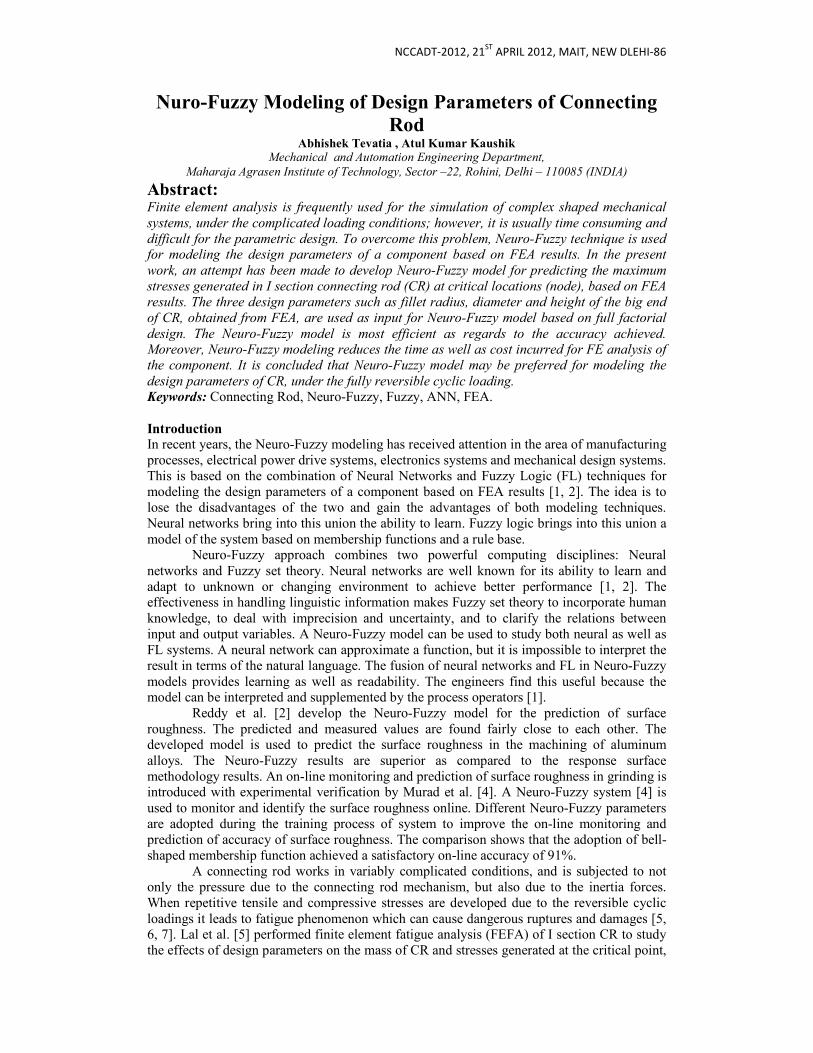
NCCADT-2012, 21ST


Nuro-Fuzzy Modeling of Design Parameters of Connecting

Rod Abhishek Tevatia , Atul Kumar Kaushik

Mechanical and Automation Engineering Department,

Maharaja Agrasen Institute of Technology, Sector –22, Rohini, Delhi – 110085 (INDIA)

Abstract: Finite element analysis is frequently used for the simulation of complex shaped mechanical

systems, under the complicated loading conditions; however, it is usually time consuming and

difficult for the parametric design. To overcome this problem, Neuro-Fuzzy technique is used for modeling the design parameters of a component based on FEA results. In the present

work, an attempt has been made to develop Neuro-Fuzzy model for predicting the maximum

stresses generated in I section connecting rod (CR) at critical locations (node), based on FEA

results. The three design parameters such as fillet radius, diameter and height of the big end

of CR, obtained from FEA, are used as input for Neuro-Fuzzy model based on full factorial

design. The Neuro-Fuzzy model is most efficient as regards to the accuracy achieved. Moreover, Neuro-Fuzzy modeling reduces the time as well as cost incurred for FE analysis of

the component. It is concluded that Neuro-Fuzzy model may be preferred for modeling the

design parameters of CR, under the fully reversible cyclic loading. Keywords: Connecting Rod, Neuro-Fuzzy, Fuzzy, ANN, FEA.

Introduction

In recent years, the Neuro-Fuzzy modeling has received attention in the area of manufacturing processes, electrical power drive systems, electronics systems and mechanical design systems. This is based on the combination of Neural Networks and Fuzzy Logic (FL) techniques for modeling the design parameters of a component based on FEA results [1, 2]. The idea is to lose the disadvantages of the two and gain the advantages of both modeling techniques. Neural networks bring into this union the ability to learn. Fuzzy logic brings into this union a model of the system based on membership functions and a rule base.

Neuro-Fuzzy approach combines two powerful computing disciplines: Neural networks and Fuzzy set theory. Neural networks are well known for its ability to learn and adapt to unknown or changing environment to achieve better performance [1, 2]. The effectiveness in handling linguistic information makes Fuzzy set theory to incorporate human knowledge, to deal with imprecision and uncertainty, and to clarify the relations between input and output variables. A Neuro-Fuzzy model can be used to study both neural as well as FL systems. A neural network can approximate a function, but it is impossible to interpret the result in terms of the natural language. The fusion of neural networks and FL in Neuro-Fuzzy models provides learning as well as readability. The engineers find this useful because the model can be interpreted and supplemented by the process operators [1].

Reddy et al. [2] develop the Neuro-Fuzzy model for the prediction of surface roughness. The predicted and measured values are found fairly close to each other. The developed model is used to predict the surface roughness in the machining of aluminum alloys. The Neuro-Fuzzy results are superior as compared to the response surface methodology results. An on-line monitoring and prediction of surface roughness in grinding is introduced with experimental verification by Murad et al. [4]. A Neuro-Fuzzy system [4] is used to monitor and identify the surface roughness online. Different Neuro-Fuzzy parameters are adopted during the training process of system to improve the on-line monitoring and prediction of accuracy of surface roughness. The comparison shows that the adoption of bell-shaped membership function achieved a satisfactory on-line accuracy of 91%.

A connecting rod works in variably complicated conditions, and is subjected to not only the pressure due to the connecting rod mechanism, but also due to the inertia forces. When repetitive tensile and compressive stresses are developed due to the reversible cyclic loadings it leads to fatigue phenomenon which can cause dangerous ruptures and damages [5, 6, 7]. Lal et al. [5] performed finite element fatigue analysis (FEFA) of I section CR to study the effects of design parameters on the mass of CR and stresses generated at the critical point,

NCCADT-2012, 21ST


under the fully reversible cyclic loading. Tevatia et al. [6, 7] performed FEFA of + section, I section, H section, rectangular section and circular cross-section CR and predicted the fatigue life using Coffin-Manson, Morrow and Smith-Watson-Topper (SWT) strain life theories. Coffin-Manson strain life theory is found to be conservative compared to Morrow and SWT strain life theories.

It is difficult to utilize the FEA results many times for the parametric design. Keeping in view; the author have developed a Neuro-Fuzzy system, which combines reasoning ability of FL and learning ability of ANN for modeling the design parameters of CR, to make it more useful for the stress-strain analysis. The present work is focused on the development of Neuro-Fuzzy model for predicting the maximum stresses generated at the critical locations (node) of CR without performing the FEFA. Based on FEA results, the stresses are calculated corresponding to the three design parameters (fillet radius, diameter and height of the big end) of I section CR. The FEA results are used as input for Neuro-Fuzzy modeling.

Problem Formulation

More recently, fatigue analysis of connecting rods of different cross-sections has been carried out, under the fully reversible cyclic loading conditions in virtual environment [5, 6, 7]. In these works, the modeling of different cross-sections is carried out in parametric Pro/E software, followed by FEFA on ANSYS workbench. The forged steel I section (optimized shape) CR is found to be the best when elastic and plastic strains together are considered (Coffin-Manson theory) for estimating the fatigue life [7]. The readers are requested to refer above cited papers for the detail analysis.

Finite Element Analysis

The FEA of forged steel I section CR is carried out to study the effect of three critical design parameters such as fillet radius, diameter and height of big end. The analysis is based on the full factorial design where all possible combinations of design parameters are realized [8]. The minimum, optimum and maximum values of each design parameters [5] are considered as the three parametric levels for modeling, as shown in Table 1. The twenty seven sets of FEA are performed using full factorial design [8]: = 33 =27 where is the number of design parameters and is the number of levels. Fig. 1 shows the Von Mises stresses distribution in different parts of CR, subjected to a tensile/compressive load of 9500 N.

Table 1: The levels of each design parameter of connecting rod Designing Parameters

Parametric levels (mm)

Level 1 Level 2 Level 3

Radius, ! " 45.0 48.5 52.0

Diameter, # 75.0 80.2 85.0

Height, 45.0 49.3 54.0

Figure 1: FE model of I section CR

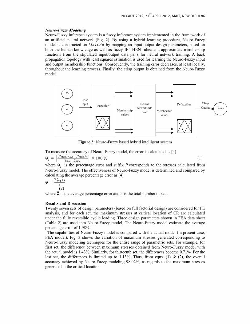
NCCADT-2012, 21ST


Neuro-Fuzzy Modeling

Neuro-Fuzzy inference system is a fuzzy inference system implemented in the framework of an artificial neural network (Fig. 2). By using a hybrid learning procedure, Neuro-Fuzzy model is constructed on MATLAB by mapping an input-output design parameters, based on both the human-knowledge as well as fuzzy IF-THEN rules; and approximate membership functions from the stipulated input/output data pairs for neural network training. A back propagation topology with least squares estimation is used for learning the Neuro-Fuzzy input and output membership functions. Consequently, the training error decreases, at least locally, throughout the learning process. Finally, the crisp output is obtained from the Neuro-Fuzzy model.

Figure 2: Neuro-Fuzzy based hybrid intelligent system

To measure the accuracy of Neuro-Fuzzy model, the error is calculated as [4]

∅ = %&'()*+,-&'(). &'()*+,

% × 100 % (1)

where ∅ is the percentage error and suffix 2 corresponds to the stresses calculated from Neuro-Fuzzy model. The effectiveness of Neuro-Fuzzy model is determined and compared by calculating the average percentage error as [4]

∅3 = ∅45467

8

(2) where ∅3 is the average percentage error and 9 is the total number of sets.

Results and Discussion

Twenty seven sets of design parameters (based on full factorial design) are considered for FE analysis, and for each set, the maximum stresses at critical location of CR are calculated under the fully reversible cyclic loading. Three design parameters shown in FEA data sheet (Table 2) are used into Neuro-Fuzzy model. The Neuro-Fuzzy model estimate the average percentage error of 1.98%. The capabilities of Neuro-Fuzzy model is compared with the actual model (in present case, FEA model). Fig. 3 shows the variation of maximum stresses generated corresponding to Neuro-Fuzzy modeling techniques for the entire range of parametric sets. For example, for first set, the difference between maximum stresses obtained from Neuro-Fuzzy model with the actual model is 1.43%. Similarly, for thirteenth set, the differences become 0.71%. For the last set, the differences is limited up to 1.13%. Thus, from eqns. (1) & (2), the overall accuracy achieved by Neuro-Fuzzy modeling 98.02%, as regards to the maximum stresses generated at the critical location.

!"

#

:; < Neural

network rule base

Crisp Input

Fuzzifier Defuzzifier Crisp

Output Membership

values

Membership values

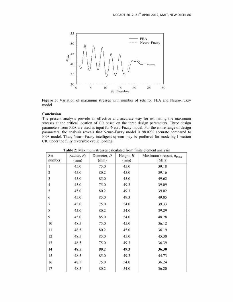
NCCADT-2012, 21ST


Set Number0 5 10 15 20 25 30

σm

ax

30

35

40

45

50

55

FEANeuro-Fuzzy

Figure 3: Variation of maximum stresses with number of sets for FEA and Neuro-Fuzzy model

Conclusion

The present analysis provide an effective and accurate way for estimating the maximum stresses at the critical location of CR based on the three design parameters. Three design parameters from FEA are used as input for Neuro-Fuzzy model. For the entire range of design parameters, the analysis reveals that Neuro-Fuzzy model is 98.02% accurate compared to FEA model. Thus, Neuro-Fuzzy intelligent system may be preferred for modeling I section CR, under the fully reversible cyclic loading.

Table 2: Maximum stresses calculated from finite element analysis Set number

Radius, !" (mm)

Diameter, # (mm)

Height, (mm)

Maximum stresses, :; < (MPa)

1 45.0 75.0 45.0 39.18

2 45.0 80.2 45.0 39.16

3 45.0 85.0 45.0 49.62

4 45.0 75.0 49.3 39.09

5 45.0 80.2 49.3 39.02

6 45.0 85.0 49.3 49.05

7 45.0 75.0 54.0 39.33

8 45.0 80.2 54.0 39.29

9 45.0 85.0 54.0 48.28

10 48.5 75.0 45.0 36.12

11 48.5 80.2 45.0 36.19

12 48.5 85.0 45.0 45.30

13 48.5 75.0 49.3 36.39

14 48.5 80.2 49.3 36.30

15 48.5 85.0 49.3 44.73

16 48.5 75.0 54.0 36.24

17 48.5 80.2 54.0 36.20

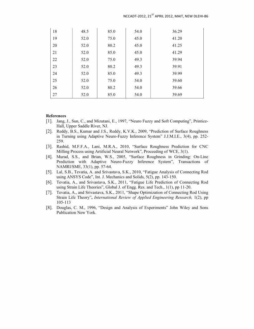
NCCADT-2012, 21ST


18 48.5 85.0 54.0 36.29

19 52.0 75.0 45.0 41.20

20 52.0 80.2 45.0 41.25

21 52.0 85.0 45.0 41.29

22 52.0 75.0 49.3 39.94

23 52.0 80.2 49.3 39.91

24 52.0 85.0 49.3 39.99

25 52.0 75.0 54.0 39.60

26 52.0 80.2 54.0 39.66

27 52.0 85.0 54.0 39.69

References

[1]. Jang, J., Sun, C., and Mizutani, E., 1997, “Neuro Fuzzy and Soft Computing”, Printice-Hall, Upper Saddle River, NJ.

[2]. Reddy, B.S., Kumar and J.S., Reddy, K.V.K., 2009, “Prediction of Surface Roughness in Turning using Adaptive Neuro-Fuzzy Inference System” J.J.M.I.E., 3(4), pp. 252-259.

[3]. Rashid, M.F.F.A., Lani, M.R.A., 2010, “Surface Roughness Prediction for CNC Milling Process using Artificial Neural Network”, Proceeding of WCE, 3(1).

[4]. Murad, S.S., and Brian, W.S., 2005, “Surface Roughness in Grinding: On-Line Prediction with Adaptive Neuro-Fuzzy Inference System”, Transactions of NAMRI/SME, 33(1), pp. 57-64.

[5]. Lal, S.B., Tevatia, A. and Srivastava, S.K., 2010, “Fatigue Analysis of Connecting Rod using ANSYS Code”, Int. J. Mechanics and Solids, 5(2), pp. 143-150.

[6]. Tevatia, A., and Srivastava, S.K., 2011, “Fatigue Life Prediction of Connecting Rod using Strain Life Theories”, Global J. of Engg. Res. and Tech., 1(1), pp 11-20.

[7]. Tevatia, A., and Srivastava, S.K., 2011, “Shape Optimization of Connecting Rod Using Strain Life Theory”, International Review of Applied Engineering Research, 1(2), pp 105-113

[8]. Douglas, C. M., 1996, “Design and Analysis of Experiments” John Wiley and Sons Publication New York.

NCCADT-2012, 21ST


Flexibility and Productivity Issues in Supply Chain

Management Surbhi Upadhyay1, Pooja Kaushik2 ,Shahzad Ahmed3

1. Maharaja Agrasen Institue of Technology,Delhi 2. Guru Premsukh Memorial College of Engineering, Delhi

3. Alfalah School of Engineering and Technology, Dhauj, Haryana

Abstract:

The pressure in today’s manufacturing units is exacerbated by the fact that the modern day

customers want a variety of product models, and as is well known, increasing a product

variety increases complexities, and decreases the efficiency of the manufacturing unit. A well-

designed supply chain management (SCM) system is important business philosophy for

improving competitive advantage in modern world influenced by information technology and

international economics. As a consequence, SCM has gained tremendous amount of attention

in recent years both from the academicians and practitioners. There are various performance

factors which are responsible for efficient working of the system. This paper discusses various philosophies of a manufacturing system and different factors related to SCM.

Keywords: Supply Chain Management, Flexibility, Productivity 1. INTRODUCTION

As we transit into the twenty-first century there are radical changes taking place that are reshaping the industrial landscape of economies. The marketplace has become truly global. There is increasing fragmentation of almost all markets. Customers are requiring smaller quantities of more customized products. Customers want to be treated individually. Most companies have much wider product ranges, are introducing more new products more quickly, and are focusing their marketing. We are on the cusp of the information age and these changes are ushering in new and exciting challenges for western manufacturers.

The trend towards a multiplicity of finished products with short development and production lead times has lead many companies into problems with inventories, overheads, and efficiencies. The term SCM was originally introduced by consultants in the early 1980s and has subsequently gained tremendous attention. Analytically, a typical supply chain, is a network of materials, information, and services processing links with the characteristics of supply transformation, and demand. The term SCM has been used to explain the planning and control of materials and information flows as well as the logistics activities not only internally within a company but also externally between companies.

SCM emphasizes integrating internal activities and decisions with external enterprise partners to promote competitive capability (Li and Wang, 2007). Terssarolo (2007) pointed out that SCM integrates with purchase, operational management, information technology and marketing and other managerial functions. External integration development of supply chain promotes large-scale product schedule performance. This performance increases when internal integration and internal group members combine with external customers and suppliers to enhance mutual product recognition (Lee and Rhee, 2007). Improper management of the supply chain relationship results in direct or indirect bad effects.

The present paper discusses key issues of SCM. Flexibility and productivity are key issues for any manufacturing systems and hence need special discussion. The facts related to flexibility and productivity is discussed in section 2. Different philosophies to make manufacturing systems productive and flexible, are discussed in section 3 .Section 4 reviews the related work on key issues of SCM. The paper is concluded in the last section.

2 FLEXIBILTY AND PRODUCTIVITY

Flexibility and productivity are the two factors for any manufacturing system. The issue of flexibility and productivity is assuming increasing importance in manufacturing decision making. Normally, it is argued that, as flexibility implies more options, change

NCCADT-2012, 21ST


mechanisms and freedom of choice, it would be hampering the productivity both by way of reduced output and more inputs for more options.

Grubbstrom and Olhager (1997) proposed a general definition of the concept of flexibility and analyzed its relationship with the productivity concept departing from a basic economic-theoretic point of view. They showed that flexibility could be defined from properties of production functions in a dynamic context. They concluded that flexibility is a generalization of productivity and substitutability measures adding the element of time, taking care how changes in production state at one time affect changes in set of attainable states at some future times.

Gupta and Singh (2001) defined flexibility as a multi dimensional concept required to respond to uncertainties and changes. There are various types of flexibility, namely, routing, volume, product, product mix, labour, design change, machine, planning, communication and total flexibility. They stated that a particular type of flexibility can be measured taking into account the weight of various parameters contributing to it and the response of an enterprise to these parameters. They highlighted the fact that it is possible to manage flexibility keeping productivity in mind as different types of flexibility have significant relationship with various types of productivity. However, the type of flexibility to be acquired also depends on the present levels of flexibility, cost aspects and preparedness of an enterprise to acquire flexibility.

Sushil (2003) examined the aspects from two viewpoints: one from the output point of view and the other from the input. He highlighted the fact that less flexibility apparently the productivity is high but more of undesired output, whereas more flexibility facilitates more real productivity of desired output. His discussion concluded with fact that though the apparent productivity of a less flexible system may be higher than a more flexible system in a stable environment, in real terms the situation would be reverse in an uncertain and dynamic environment, i.e. the real productivity of a more flexible system is expected to be higher than a less flexible system from both the points of the view of the output and the input.

3. IMPORTANT PHLISPHOSIES TO MAKE MANUFACTURING SYSTEM

FLEXIBLE AND PRODUCTIVE With fast introduction of new models, design changes and high varieties

manufacturing systems are changing from mass production to job shop production system. Since, in general, the productivity of Job shop system is low, various strategies and philosophies are being contemplated to enhance the productivity, reduce the cost of manufacturing and increase the response to the customer.

In this section different theories of manufacturing system are discussed. Various philosophies in respect to manufacturing system which leads to increase in flexibility are: Mass Customization, Supply Chain Management, Flexible Manufacturing System, Lean Manufacturing and Agile Manufacturing. The important facts of these philosophies are highlighted hereafter.

Mass Customization is the customization and personalization of products and services for individual customers at a mass production price. The concept of mass customization is attributed to Stan Davis and was defined by Tseng and Jiao (2001) as "producing goods and services to meet individual customer's needs with near mass production efficiency". Kaplan and Haenlein (2006) concurred, calling it "a strategy that creates value by some form of company-customer interaction at the fabrication / assembly stage of the operations level to create customized products with production cost and monetary price similar to those of mass-produced products".

Mass customization is an important issue in present era due to following factors: 1. End of a mass production era (supply) 2. Individualism (demand) 3. Competition (demand) 4. Profitability (demand) 5. Technological progress (supply)

NCCADT-2012, 21ST


Many implementations of mass customization are operational today, such as software-based product configurators which make it possible to add and/or change functionalities of a core product or to build fully custom enclosures from scratch.

A flexible manufacturing system (FMS) is a manufacturing system in which there is some amount of flexibility that allows the system to react in the case of changes, whether predicted or unpredicted. A FMS is designed to combine the efficiency of mass production line and flexibility of job shop to produce variety of work pieces on group of machine (Chan et al. 1997). This flexibility is generally considered to fall into two categories, which both contain numerous subcategories. In the middle of the 1960s, market competition became more intense. During 1960 to 1970 cost was the primary concern. Later quality became a priority. As the market became more and more complex, speed of delivery became something customer also needed. A new strategy was formulated: Customizability. The companies have to adapt to the environment in which they operate, to be more flexible in their operations and to satisfy different market segments (customizability).

Thus the innovation of FMS became related to the effort of gaining competitive advantage. First of all, FMS is a manufacturing technology. Secondly, FMS is a philosophy. "System" is the key word. Philosophically, FMS incorporates a system view of manufacturing. The buzz word for today’s manufacturer is "agility". An agile manufacturer is one who is the fastest to the market, operates with the lowest total cost and has the greatest ability to "delight" its customers. FMS is simply one way that manufacturers are able to achieve this agility.

Agile manufacturing is a term applied to an organization that has created the processes, tools, and training to enable it to respond quickly to customer needs and market changes while still controlling costs and quality. (Goldam et al,1995). An enabling factor in becoming an agile manufacturer has been the development of manufacturing support technology that allows the marketers, the designers and the production personnel to share a common database of parts and products, to share data on production capacities and problems — particularly where small initial problems may have larger downstream effects. It is a general proposition of manufacturing that the cost of correcting quality issues increases as the problem moves downstream, so that it is cheaper to correct quality problems at the earliest possible point in the process.

Lean manufacturing is the production of goods using less of everything compared to mass production: less waste, less human effort, less manufacturing space, less investment in tools, and less engineering time to develop a new product [Ohno (1988)]. Lean manufacturing is a generic process management philosophy derived mostly from the Toyota Production System (TPS). Lean implementation is focused on getting the right things, to the right place, at the right time, in the right quantity to achieve perfect work flow while minimizing waste and being flexible and able to change. These concepts of flexibility and change are principally required to allow production leveling, using tools like SMED, but have their analogues in other processes such as R&D. Lean aims to make the work simple enough to understand, to do and to manage. To achieve these three at once there is a belief held by some that Toyota's mentoring process (loosely called Senpai and Kohai relationship), so strongly supported in Japan, is one of the best ways to foster Lean Thinking up and down the organizational structure. This is the process undertaken by Toyota as it helps its suppliers to improve their own production Lean techniques are applicable not only in manufacturing, but also in service-oriented industry and service environment.

A supply chain is a network of facilities and distribution options that performs the functions of procurement of materials, transformation of these materials into intermediate and finished products, and the distribution of these finished products to customers. Supply chains exist in both service and manufacturing organizations, although the complexity of the chain may vary greatly from industry to industry and firm to firm. The definition one American professional association put forward is that Supply Chain Management encompasses the planning and management of all activities involved in sourcing, procurement, conversion, and logistics management activities. Importantly, it also includes coordination and collaboration with channel partners, which can be suppliers, intermediaries, third-party service providers,

NCCADT-2012, 21ST


and customers. In essence, Supply Chain Management integrates supply and demand management within and across companies. The key supply chain processes stated by Lambert (2004) are: Customer, Customer service management, Demand management, Order fulfillment, Manufacturing flow management, Supplier relationship management, Product development and commercialization, Returns management.

4. KEY ISSUES OF SCM

Several aspects of supply chain are indicted in literature. This study encompasses key issues related to SCM and tools used for conducting the analysis. Naraharisetti et al (2008) present a novel MILP model for making efficient capacity management and supply chain redesign decisions for a multinational corporation. The model can provide the basis for obtaining the best strategy for investment, involving a variety of real decisions such as facility relocation, disinvestment and technology upgrade.

Oztayasi et al (2011) compare the 13 CRM performances of e-commerce firms using ANP approach. These performance criteria include factors like customer retention, customer retention, customer loyalty, product logistics, social alignment etc. You and Grossmann (2008) propose a bicriterion MILP optimization framework to consider simultaneously economics and responsiveness of multi-site, multi-echelon process supply chain networks. An Ɛ-constraint method has been used for its solution to produce a Pareto-optimal curve, establishing trade-offs between net present value and lead time. Xia and Chen (2010) studied dynamic nature of supply chain risk management and developed strategic decision making model with operational process cycle and product life cycle. Wong et al (2011) identified various factors (Internal Operation, Supplier Relation, Customer Relation, Collective

Efficacy, Schedule Nervousness, and Employee’s Mental State) along the supply chain and used ANN to find to quantify the relative importance of some of the factors in predicting the critical factors

Various indications are found in field of SCM pointing the key research issues. Table 1 presents the results of review. The various research issues, related to SCM, from recent journals are discussed and referred in table 2. The research techniques involved in solving the issues of SCM involves various tools and procedure (refer table 3). Some of them include ISM, data envelopment analysis, ANP, ANN etc.

Table 1: Key research issues in SCM

S.No Issue Reference

1. Revenue sharing Li et al (2009), Hu et al (2010), Ouardighi and Kim (2010) 2. Risk management Wagner and Neshat (2010), Xia and Chen (2011)

3. Performance measurement

Bhagwat and Sharma (2007), Wong and Wong (2007), Cia et al (2009), Baz (2011)

4. Information sharing

Fiala (2005), Ryu et al (2009), Ding et al (2010)

5. Supply chain integration

Kannan and Tan (2005), Wong and Boon-itt (2008)

6. Supply chain coordination

Kannan and Tan (2005), Arshinder et al (2008), Wang and Zhou (2010)

Table 2: Key research findings in SCM

S.No Authors Issue Key findings

1. Kaynak and Hartley (2008)

Quality management (QM)

Discusses customer focus and supplier quality management in the quality management model. Results indicate that supplier quality management is directly related to product/service design and

NCCADT-2012, 21ST


process management. Furthermore, the findings provide evidence of the mediating role of QM practices on firm performance

2. Cai et al (2009)

Performance measurement

Proposes a framework using a systematic approach for improving the key performance indicators (KPIs) in a supply chain. The framework quantitatively analyzes the interdependent relationships among a set of KPIs. It identifies crucial KPI accomplishment costs and proposes performance improvement strategies for decision-makers in supply chain.

3. Thun and Hoenig (2011)

Risk management

The empirical analyses of SC risk management practices are conducted and SC risk factors are identified. Groups are created representing two different approaches to deal with supply chain risks, i.e. reactive and preventive supply chain risk management. The results show that the group using reactive supply chain risk management has higher average value in terms of disruptions resilience or the reduction of the bullwhip effect, whereas the group pursuing preventive supply chain risk management has better values concerning flexibility or safety stocks.

4. Chang et al (2011)

Supplier selection

Presents DEMATEL method to find influential factors in selecting SCM suppliers. The strategy map finds interdependencies among these criteria and their strengths. The current study finds that ‘‘technology ability”, ‘‘stable delivery of goods”, ‘‘lead-time”, and ‘‘production capability” criteria are more influential than other evaluation criteria. These potential evaluate criteria could help businesses forecast appropriate suppliers.

5. Deshpande et al (2011)

Inventory management

Proposes distinguished modelling approach that uses fuzzy goal programming approach to map decision maker’s imprecise and vague aspiration level for goals. The study has reflected the active role of inventory in deciding the nature of a supply chain as a cost effective or a responsive supply chain by changing the inventory policy as the supply chain can be configured to changing needs.

Table 3: Research techniques employed in SCM

S.No Technique Reference

1. Data envelopment Analysis (DEA)

Ramanathan (2007), Wong and Wong (2007), Wu and Olson (2008), Saranga and Moser (2010)

2. Ant colony optimization Silva et al (2009), Wang (2009) 3. Activity based costing Roodhooft and Konings (1997) 4. Graph theory Wagner and Neshat (2010), Pishvaee and Rabbani

(2011), Askarany et al (2010) 5. Fuzzy mixed integer linear

programming Gumus et al (2009), Peidro et al (2010)

6. Simulation Wu and Olson (2008), Longo and Mirabelli (2008), Chan and Zhang (2011)

7. Genetic Algorithm Chan et al (2005), Kubat and yuce (2010), , Zegordi et al (2010)

8. ANP/Fuzzy ANP

5. CONCLUSION:

The aim of this study is to reveal the factors related to SCM. performance variables of any enterprise, i.e flexibility and productivity is discussed. It is concluded that though the apparent productivity of a less flexible system may be higher than a more flexible system in a stable ean uncertain and dynamic environment, i.e. the real productivity of a more flexible system is expected to be higher than a less flexible system from both the points of the view of the output and the input. The salient features of certain manufacturing philosophies being used in Job shop production system are studied. It is found from the study that under influence these philosophies, system moves toward proper balance between productivity and flexivarious research issues related to SCM are also reviewed. The objectives of SCM, which can make a system productive and flexible, are stated and research techniques to achieve these objectives are discussed. Also, the different decision variablalong with the performance parameters. REFERENCES:

1. Hu, Q., Wei, Y. and Xia, Y. (2010). Revenue management for supply chain with two

streams of customers. European Journal of Operational Research. 200(2), pp 5822. Ouardighi, F.L. and Kim, B. (2010). Supply quality management with wholesale

price and revenue -sharing contracts under horizontal competitionof Operational Research

3. Wagner, S.M. and Neshat, N. (2010). Assessing the vulnerusing graph theory. Interantional Journal of Production Economics. 126(1), pp 121129.

4. Xia, D. and Chen, B. (2011). management of supply chain.

5. Bhagwat, R. and Sharma, M.K. (2007). Performamance measurement of supply chain management: A balanced scorecard approach. Computers and industrial engineering. 53(1), pp 43-62.

6. Cai, J., Liu, X., Xiao, Z. and Liu, J. (2009). Improving supply management: A systematic approach to analyzing iterative KPI accomplishment.Decision Support Systems

7. Ryu, S.J., Tsukishima, T. and Onari, H. (2009).information sharing methods in supplyEconomics. 120(1), pp 162

8. Kannan, V.R. and Tan, K.C. (2005). Just in time, total quality management, and supply chain management: understanding their linkages and impact on business performance. Omega 33 (2),

9. Wong, C.Y. and Boonenvironmental uncertainty on supply chain integration in the Thai automotive industry. International journal of production economics. 115 (2), pp 400

10. Longo, F. and Mirabelli. (2008). An advanced supply chain management tool based on modeling and simulation. Computers and Industrial Engineering. 54(3), pp 570588.

11. Chan, F.T.S., Chung, S.H. and Wadhwa, S. (2005). A hybrid genetic algorithm for production and distribution. Omega. 33(4), pp 345

12. Kubat, C. and Yuce, B. (2010). A hybrid intelligent approach for supply chain management system. Journal of Intelligent manufacturing. In press.

13. Tseng, M.L., Chaing, J.H. and Lan, L.W. (2009). Selection of optimal suppliesupply chain management strategy with analytic network process and choquet integral . Computers and Industrial Engineering

NCCADT-2012, 21ST

APRIL 2012, MAIT, NEW DLEHI

Aggarwal et al (2006), Tseng et al (2009), Vinodh et al (2011)

The aim of this study is to reveal the factors related to SCM. The relation ship of the two key performance variables of any enterprise, i.e flexibility and productivity is discussed. It is concluded that though the apparent productivity of a less flexible system may be higher than a more flexible system in a stable environment, in real terms the situation would be reverse in an uncertain and dynamic environment, i.e. the real productivity of a more flexible system is expected to be higher than a less flexible system from both the points of the view of the

he input. The salient features of certain manufacturing philosophies being used in Job shop production system are studied. It is found from the study that under influence these philosophies, system moves toward proper balance between productivity and flexibility. The various research issues related to SCM are also reviewed. The objectives of SCM, which can make a system productive and flexible, are stated and research techniques to achieve these objectives are discussed. Also, the different decision variables related to SCM are studied along with the performance parameters.

Hu, Q., Wei, Y. and Xia, Y. (2010). Revenue management for supply chain with two streams of customers. European Journal of Operational Research. 200(2), pp 582

ighi, F.L. and Kim, B. (2010). Supply quality management with wholesale sharing contracts under horizontal competition. European Journal

of Operational Research. 206(2), pp 329-340 Wagner, S.M. and Neshat, N. (2010). Assessing the vulnerability of supply chain using graph theory. Interantional Journal of Production Economics. 126(1), pp 121

Xia, D. and Chen, B. (2011). A comprehensive decision-making model for risk management of supply chain. Expert Systems with Applications. 38(5), pp 4957Bhagwat, R. and Sharma, M.K. (2007). Performamance measurement of supply chain management: A balanced scorecard approach. Computers and industrial engineering.

Cai, J., Liu, X., Xiao, Z. and Liu, J. (2009). Improving supply chain performance management: A systematic approach to analyzing iterative KPI accomplishment.Decision Support Systems. 46(2), pp 512-521. Ryu, S.J., Tsukishima, T. and Onari, H. (2009).A study on evaluation of demand information sharing methods in supply chain. International Journal of Production

162-175 Kannan, V.R. and Tan, K.C. (2005). Just in time, total quality management, and supply chain management: understanding their linkages and impact on business performance. Omega 33 (2), pp 153–162. Wong, C.Y. and Boon-iit, S. (2008). The influence of institutional norms and environmental uncertainty on supply chain integration in the Thai automotive industry. International journal of production economics. 115 (2), pp 400-410.

nd Mirabelli. (2008). An advanced supply chain management tool based on modeling and simulation. Computers and Industrial Engineering. 54(3), pp 570

Chan, F.T.S., Chung, S.H. and Wadhwa, S. (2005). A hybrid genetic algorithm for ution. Omega. 33(4), pp 345-355.

Kubat, C. and Yuce, B. (2010). A hybrid intelligent approach for supply chain management system. Journal of Intelligent manufacturing. In press. Tseng, M.L., Chaing, J.H. and Lan, L.W. (2009). Selection of optimal suppliesupply chain management strategy with analytic network process and choquet

Computers and Industrial Engineering. 57(1), pp 330-340.


Aggarwal et al (2006), Tseng et al (2009), Vinodh et al

The relation ship of the two key performance variables of any enterprise, i.e flexibility and productivity is discussed. It is concluded that though the apparent productivity of a less flexible system may be higher than a

nvironment, in real terms the situation would be reverse in an uncertain and dynamic environment, i.e. the real productivity of a more flexible system is expected to be higher than a less flexible system from both the points of the view of the

he input. The salient features of certain manufacturing philosophies being used in Job shop production system are studied. It is found from the study that under influence these

bility. The various research issues related to SCM are also reviewed. The objectives of SCM, which can make a system productive and flexible, are stated and research techniques to achieve these

es related to SCM are studied

Hu, Q., Wei, Y. and Xia, Y. (2010). Revenue management for supply chain with two streams of customers. European Journal of Operational Research. 200(2), pp 582-598.

ighi, F.L. and Kim, B. (2010). Supply quality management with wholesale European Journal

ability of supply chain using graph theory. Interantional Journal of Production Economics. 126(1), pp 121-

making model for risk 4957-4966

Bhagwat, R. and Sharma, M.K. (2007). Performamance measurement of supply chain management: A balanced scorecard approach. Computers and industrial engineering.

chain performance management: A systematic approach to analyzing iterative KPI accomplishment.

A study on evaluation of demand International Journal of Production

Kannan, V.R. and Tan, K.C. (2005). Just in time, total quality management, and supply chain management: understanding their linkages and impact on business

iit, S. (2008). The influence of institutional norms and environmental uncertainty on supply chain integration in the Thai automotive

410. nd Mirabelli. (2008). An advanced supply chain management tool based

on modeling and simulation. Computers and Industrial Engineering. 54(3), pp 570-

Chan, F.T.S., Chung, S.H. and Wadhwa, S. (2005). A hybrid genetic algorithm for

Kubat, C. and Yuce, B. (2010). A hybrid intelligent approach for supply chain

Tseng, M.L., Chaing, J.H. and Lan, L.W. (2009). Selection of optimal supplier in supply chain management strategy with analytic network process and choquet

14. Vinodh, S., Ramiya, R.A. and Gautham, S.G. (2011). Application of fuzzy analytic network process for supplieSystems with Applications

15. Wang, S.D. and Zhou, Y.W. (2010). Supply chain newsvendor-type products: Considering advertising effect and two production modes. Computers and industrial engineering. 59(2), pp 220

16. Wang, L.C., Lin, Y.C. and Lin, P.H. (2007). chain control and management system in construction. Informatics. 21(4), pp 377

17. Kayanak, H. and Harmanagement into the supply chain. Journal of Operations Management. 26(4), pp 468-489.

18. Cai, J., Liu, X., Xiao, Z. and Liu, J. (2009). Improving supply chain performance management: A systematic apDecision Support Systems

19. Deshpande, P., Shukla, D. and Tiwari, M.K. (2011). inventory management: A bacterial foraging approachOperational Research. 212(2), pp

20. Ramanathan, R. (2007). Supplier selection problem: integrating DEA with the approaches of total cost of ownership and AHP. Supply Chain Management: An International Journal. 12(4), pp 258

21. Saranga, H. and Moser, R. (201chain management using value chain DEA approach. European Journal of Operational Research. 207(1), pp 197

22. Silva, C.A., Sousa, J.M.C., Runkler, T.A. and Costa, J.M.G. (2009). Distributed supply chain management using ant colony optimization. European Journal of Operational Research. 199(2), pp 349

23. Wang, H.S. (2009). A twosupply chain network design243-252

24. Roodhooft, F. and Konings, J. (1997). Vendor selection and evaluation an activity based costing approach.

25. Wagner, S.M. and Neshat, N. (2010). Assessing the vulnerability of supply chain using graph theory. Interantional Journal of Production Economics. 126(1), pp 121129.

26. Askarany, D., Yazdifar, H. and Askary, S. (2010). Supply chain management, activity based costing and organizational factors. International journal of production economics. 127(2), pp 238

27. Gumus, A.T. and Guneri, A.F. (2009). A multiframework for stochastic and fuzzy supply chains. Expert Systems with Applic36(3, part 1), pp 5565-5575.

28. Peidro, D., Mula, J. Jimenez, M and Botella, M.M. (2010). A fuzzy linear programming based approach for tactical supply chain planning in uncertain planning. European Journal of Operational Research. 205(1), pp 65

29. Gumus, A.T. and Guneri, A.F. (2009). A multiframework for stochastic and fuzzy supply chains. Expert Systems with Applications. 36(3, part 1), pp 5565-5575.

30. Wu, D. and Olson, D.L. (2008). Supply chain risk, simulation and vendInternational Journal of Production Economics. 114(2), pp 646

31. Chan, F.T.S., Kazerooni, A.Q., and Abhary. (1997). A fuzzy approach to operation selection. Engineering application of artificial intelligence, 10, pp 345

32. Goldam, L., Nagel, R.L., and Presis . (1995). Organizations - Strategies for Enriching the Customer

NCCADT-2012, 21ST


Vinodh, S., Ramiya, R.A. and Gautham, S.G. (2011). Application of fuzzy analytic network process for supplier selection in a manufacturing organizationSystems with Applications. 38(1), pp 272-280 Wang, S.D. and Zhou, Y.W. (2010). Supply chain coordination models for

type products: Considering advertising effect and two production modes. ters and industrial engineering. 59(2), pp 220-231.

Wang, L.C., Lin, Y.C. and Lin, P.H. (2007). Dynamic mobile RFID-based supply chain control and management system in construction. Advanced Engineering Informatics. 21(4), pp 377-390. Kayanak, H. and Hartley, J.L. (2008). A replication and extension of quality management into the supply chain. Journal of Operations Management. 26(4), pp

Cai, J., Liu, X., Xiao, Z. and Liu, J. (2009). Improving supply chain performance management: A systematic approach to analyzing iterative KPI accomplishment.Decision Support Systems. 46(2), pp 512-521. Deshpande, P., Shukla, D. and Tiwari, M.K. (2011). Fuzzy goal programming for inventory management: A bacterial foraging approach. European Journal of

. 212(2), pp 325-336. Ramanathan, R. (2007). Supplier selection problem: integrating DEA with the approaches of total cost of ownership and AHP. Supply Chain Management: An International Journal. 12(4), pp 258 – 261 Saranga, H. and Moser, R. (2010). Performance evaluation of purchasing and supply chain management using value chain DEA approach. European Journal of Operational Research. 207(1), pp 197-205. Silva, C.A., Sousa, J.M.C., Runkler, T.A. and Costa, J.M.G. (2009). Distributed

management using ant colony optimization. European Journal of Operational Research. 199(2), pp 349-358. Wang, H.S. (2009). A two-phase ant colony algorithm for multi-echelon defective supply chain network design. European Journal of Operational Research. 1

Roodhooft, F. and Konings, J. (1997). Vendor selection and evaluation an activity based costing approach. European Journal of Operational Research. 96(1), ppWagner, S.M. and Neshat, N. (2010). Assessing the vulnerability of supply chain using graph theory. Interantional Journal of Production Economics. 126(1), pp 121

Askarany, D., Yazdifar, H. and Askary, S. (2010). Supply chain management, activity ed costing and organizational factors. International journal of production

economics. 127(2), pp 238-248. Gumus, A.T. and Guneri, A.F. (2009). A multi-echelon inventory management framework for stochastic and fuzzy supply chains. Expert Systems with Applic

5575. Peidro, D., Mula, J. Jimenez, M and Botella, M.M. (2010). A fuzzy linear programming based approach for tactical supply chain planning in uncertain planning. European Journal of Operational Research. 205(1), pp 65-80

umus, A.T. and Guneri, A.F. (2009). A multi-echelon inventory management framework for stochastic and fuzzy supply chains. Expert Systems with Applications.

5575. Wu, D. and Olson, D.L. (2008). Supply chain risk, simulation and vendor selection. International Journal of Production Economics. 114(2), pp 646-655. Chan, F.T.S., Kazerooni, A.Q., and Abhary. (1997). A fuzzy approach to operation selection. Engineering application of artificial intelligence, 10, pp 345-356. Goldam, L., Nagel, R.L., and Presis . (1995). Agile Competitors and Virtual

Strategies for Enriching the Customer. Van Nostrand Reinhold.


Vinodh, S., Ramiya, R.A. and Gautham, S.G. (2011). Application of fuzzy analytic r selection in a manufacturing organization. Expert

coordination models for type products: Considering advertising effect and two production modes.

based supply Advanced Engineering

tley, J.L. (2008). A replication and extension of quality management into the supply chain. Journal of Operations Management. 26(4), pp

Cai, J., Liu, X., Xiao, Z. and Liu, J. (2009). Improving supply chain performance proach to analyzing iterative KPI accomplishment.

Fuzzy goal programming for European Journal of

Ramanathan, R. (2007). Supplier selection problem: integrating DEA with the approaches of total cost of ownership and AHP. Supply Chain Management: An

0). Performance evaluation of purchasing and supply chain management using value chain DEA approach. European Journal of

Silva, C.A., Sousa, J.M.C., Runkler, T.A. and Costa, J.M.G. (2009). Distributed management using ant colony optimization. European Journal of

echelon defective . 192(1), pp

Roodhooft, F. and Konings, J. (1997). Vendor selection and evaluation an activity . 96(1), pp 97-102

Wagner, S.M. and Neshat, N. (2010). Assessing the vulnerability of supply chain using graph theory. Interantional Journal of Production Economics. 126(1), pp 121-

Askarany, D., Yazdifar, H. and Askary, S. (2010). Supply chain management, activity ed costing and organizational factors. International journal of production

echelon inventory management framework for stochastic and fuzzy supply chains. Expert Systems with Applications.

Peidro, D., Mula, J. Jimenez, M and Botella, M.M. (2010). A fuzzy linear programming based approach for tactical supply chain planning in uncertain

echelon inventory management framework for stochastic and fuzzy supply chains. Expert Systems with Applications.

or selection.

Chan, F.T.S., Kazerooni, A.Q., and Abhary. (1997). A fuzzy approach to operation

Agile Competitors and Virtual . Van Nostrand Reinhold.

NCCADT-2012, 21ST


33. Grubbstrom, R.W., and Olhager,J. (1997). Productivity and flexibility: Fundamental relations between two major properties and performance measures of the production system. International Journal of Production Economics.

34. Gupta,A.B., and Singh,T.P. (2001). Flexibility in an Automobile Manufacturing Enterprise. Global Journal of Flexible systems Management.

35. Ohno, T. (1988).Toyota Production System. Productivity Press, ISBN 0-915299-14-3 36. Sushil. (2003). Flexibility and Productivity. Global Journal of Flexible Systems

Management. 37. Tseng, M.M., and Jiao, J. (2001). Mass Customization in: Handbook of Industrial

Engineering, Technology and Operation Management (3rd ed.), ISBN 0-471-33057-4

NCCADT-2012, 21ST


Critique of Laser Beam Machining Ramakant Rana

1, Lokesh Kr.Kushwaha

2, Roop Lal

3, Rakesh Chander Saini

4, Naveen Solanki

5

1 Lecturer, Mechanical and Automation Engineering dept. MAIT,Delhi 24th Year Student, Mechanical and Automation Engineering dept. MAIT,Delhi

3Asst. Prof., Mechanical Engineering Dept. of Delhi Technological University;Delhi 4 Asst. Prof., Mechanical and Automation Engineering dept. MAIT,Delhi

5Asst. Prof., Mechanical and Automation Engineering dept. MAIT,Delhi.

Abstract

Laser beam machining (LBM) is one of the most widely used thermal energy based non-contact type advance machining process which can be applied for almost whole range of

materials. Laser beam is focused for melting and vaporizing the unwanted material from the

parent material. It is suitable for geometrically complex profile cutting and making miniature

holes in sheetmetal. Among various type of lasers used for machining in industries, CO2 and

Nd:YAG lasers are most established. In recent years, researchers have explored a number of

ways to improve the LBM process performance by analysing the different factors that affect the quality characteristics. The experimental and theoretical studies show that process

performance can be improved considerably by proper selection of laser parameters, material

parameters and operating parameters. This paper reviews the research work carried out so far in the area of LBM of different materials and shapes. It reports about the experimental

and theoretical studies of LBM to improve the process performance. Several modelling and

optimization techniques for the determination of optimum laser beam cutting condition have

been critically examined. The last part of this paper discusses the LBM developments and

outlines the trend for future research.

Keywords: Laser beam machining; Nd:YAG; CO2; HAZ; Kerf; Modelling

1 Introduction:

Emergence of advanced engineering materials, stringent design requirements, intricate shape and unusual size of workpiece restrict the use of conventional machining methods. Hence, it was realized to develop some nonconventional machining methods known as advanced machining processes (AMPs). Nowadays many AMPs are being used in the industry such as:

i. Electro discharge machining, ii. Beam machining processes

a. Laser beam machining (LBM), b. Electron beam machining, c. Ion beam machining and plasma beam machining,

iii. Electrochemical machining, iv. Chemical machining processes (chemical blanking, photochemical machining), v. Ultrasonic machining (USM), and

vi. Jet machining processes a. Abrasive jet machining, b. Water jet machining, c. Abrasive water jet machining.

The laser is also used to perform turning as well as milling operations but major application

of laser beam is mainly in cutting of metallic and non-metallic sheets. This report provides a review on the various research activities carried out in LBM process. The content of report includes

i. A brief introduction of laser and its development, ii. Different LBM configurations and

iii. LBM application for different category of materials. iv. Major areas of LBM research have been discussed under the headings of

a. Experimental studies, b. Modeling and c. Optimization studies.

NCCADT-2012, 21ST


v. In the last, the new challenges and future direction of LBM research have been discussed.

2 Laser beam machining (LBM):

This section provides the basic fundamentals of the LBM process and its variations. 2.1 Light and lasers: Planck has given the concept of quanta in 1900 and in 1920 it was well accepted that apart from wavelike characteristics of light it also shows particle nature while interacting with matters and exchange energy in the form of photons [1]. The initial foundation of laser theory was laid by Einstein who has given the concept of stimulated emission [2]. Townes and Shawlow (1957) produced the first laser known as Ruby Laser [1]. Laser (light amplification by stimulated emission of radiation) is a coherent and amplified beam of electromagnetic radiation. The key element in making a practical laser is the light amplification achieved by stimulated emission due to the incident photons of high energy. A laser comprises three principal components, namely, the lasing medium, means of exciting the lasing medium into its amplifying state (lasing energy source), and optical delivery/feedback system. Additional provisions of cooling the mirrors, guiding the beam and manipulating the target are also important. The laser medium may be a solid (e.g. Nd:YAG or neodymium doped yttrium– aluminium–

garnet), liquid (dye) or gas (e.g. CO2, He, Ne) [2]. Laser light differs from ordinary light because it has the photons of same frequency, wavelength and phase. Thus, unlike ordinary light laser beams are highly directional, have high power density and better focussing characteristics. These unique characteristics of laser beam are useful in processing of materials. Among different type of lasers, Nd:YAG and CO2 are most widely used for LBM application. CO2 lasers have wavelength of 10 mm in infrared region. It has high average beam power, better efficiency and good beam quality. It is suitable for fine cutting of sheet metal at high speed [3]. Nd:YAG lasers have low beam power but when operating in pulsed mode high peak powers enable it to machine even thicker materials. Also, shorter pulse duration suits for machining of thinner materials. Due to shorter wavelength (1 mm) it can be absorbed by high reflective materials which are difficult to machine by CO2 lasers [4]. 2.2 Principle of LBM: The mechanism of material removal during LBM includes different stages such as

(i) Melting, (ii) Vaporization, and (iii) Chemical degradation (chemical bonds are broken which causes the materials to

degrade). When a high energy density laser bream is focussed on work surface the thermal energy is absorbed which heats and transforms the work volume into a molten, vaporized or chemically changed state that can easily be removed by flow of high pressure assist gas jet (which accelerates the transformed material and ejects it from machining zone) [5]. The schematic of LBM has been shown in following Fig. 1.

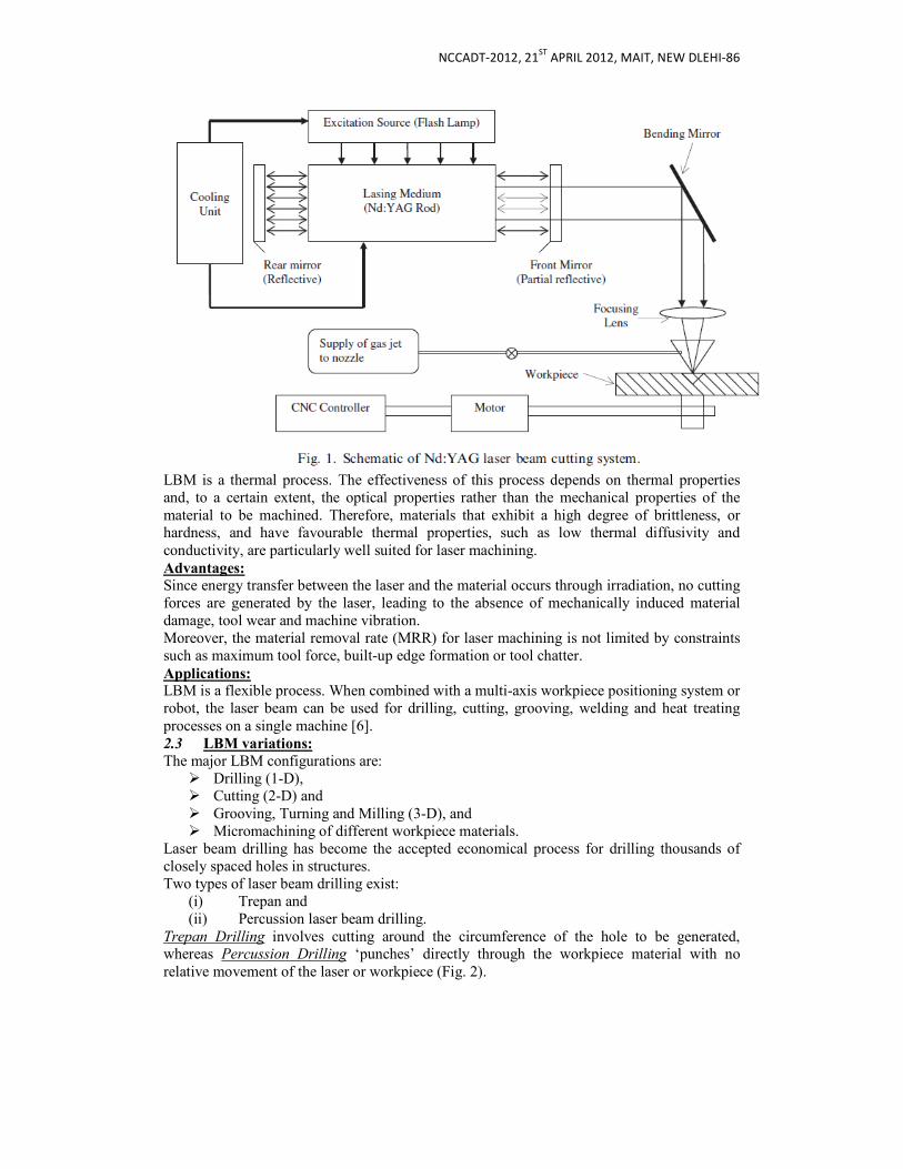
NCCADT-2012, 21ST


LBM is a thermal process. The effectiveness of this process depends on thermal properties and, to a certain extent, the optical properties rather than the mechanical properties of the material to be machined. Therefore, materials that exhibit a high degree of brittleness, or hardness, and have favourable thermal properties, such as low thermal diffusivity and conductivity, are particularly well suited for laser machining. Advantages:

Since energy transfer between the laser and the material occurs through irradiation, no cutting forces are generated by the laser, leading to the absence of mechanically induced material damage, tool wear and machine vibration. Moreover, the material removal rate (MRR) for laser machining is not limited by constraints such as maximum tool force, built-up edge formation or tool chatter. Applications: LBM is a flexible process. When combined with a multi-axis workpiece positioning system or robot, the laser beam can be used for drilling, cutting, grooving, welding and heat treating processes on a single machine [6]. 2.3 LBM variations:

The major LBM configurations are: Drilling (1-D), Cutting (2-D) and Grooving, Turning and Milling (3-D), and Micromachining of different workpiece materials.

Laser beam drilling has become the accepted economical process for drilling thousands of closely spaced holes in structures. Two types of laser beam drilling exist:

(i) Trepan and (ii) Percussion laser beam drilling.

Trepan Drilling involves cutting around the circumference of the hole to be generated, whereas Percussion Drilling ‘punches’ directly through the workpiece material with no relative movement of the laser or workpiece (Fig. 2).

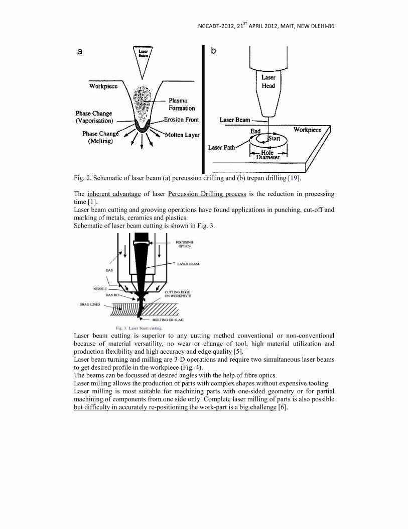
NCCADT-2012, 21ST


Fig. 2. Schematic of laser beam (a) percussion drilling and (b) trepan drilling [19]. The inherent advantage of laser Percussion Drilling process is the reduction in processing time [1]. Laser beam cutting and grooving operations have found applications in punching, cut-off and marking of metals, ceramics and plastics. Schematic of laser beam cutting is shown in Fig. 3.

Laser beam cutting is superior to any cutting method conventional or non-conventional because of material versatility, no wear or change of tool, high material utilization and production flexibility and high accuracy and edge quality [5]. Laser beam turning and milling are 3-D operations and require two simultaneous laser beams to get desired profile in the workpiece (Fig. 4). The beams can be focussed at desired angles with the help of fibre optics. Laser milling allows the production of parts with complex shapes without expensive tooling. Laser milling is most suitable for machining parts with one-sided geometry or for partial machining of components from one side only. Complete laser milling of parts is also possible but difficulty in accurately re-positioning the work-part is a big challenge [6].

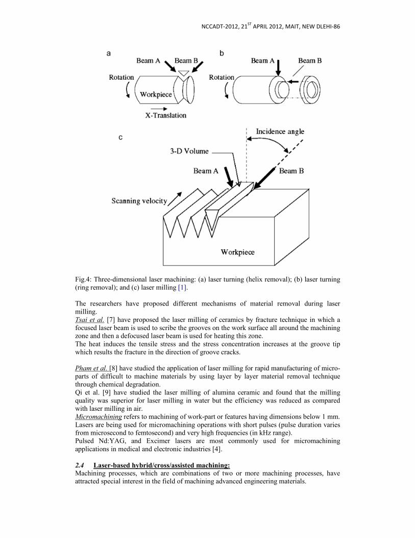
NCCADT-2012, 21ST


Fig.4: Three-dimensional laser machining: (a) laser turning (helix removal); (b) laser turning (ring removal); and (c) laser milling [1]. The researchers have proposed different mechanisms of material removal during laser milling. Tsai et al. [7] have proposed the laser milling of ceramics by fracture technique in which a focused laser beam is used to scribe the grooves on the work surface all around the machining zone and then a defocused laser beam is used for heating this zone. The heat induces the tensile stress and the stress concentration increases at the groove tip which results the fracture in the direction of groove cracks. Pham et al. [8] have studied the application of laser milling for rapid manufacturing of micro-parts of difficult to machine materials by using layer by layer material removal technique through chemical degradation. Qi et al. [9] have studied the laser milling of alumina ceramic and found that the milling quality was superior for laser milling in water but the efficiency was reduced as compared with laser milling in air. Micromachining refers to machining of work-part or features having dimensions below 1 mm. Lasers are being used for micromachining operations with short pulses (pulse duration varies from microsecond to femtosecond) and very high frequencies (in kHz range). Pulsed Nd:YAG, and Excimer lasers are most commonly used for micromachining applications in medical and electronic industries [4].

2.4 Laser-based hybrid/cross/assisted machining: Machining processes, which are combinations of two or more machining processes, have attracted special interest in the field of machining advanced engineering materials.

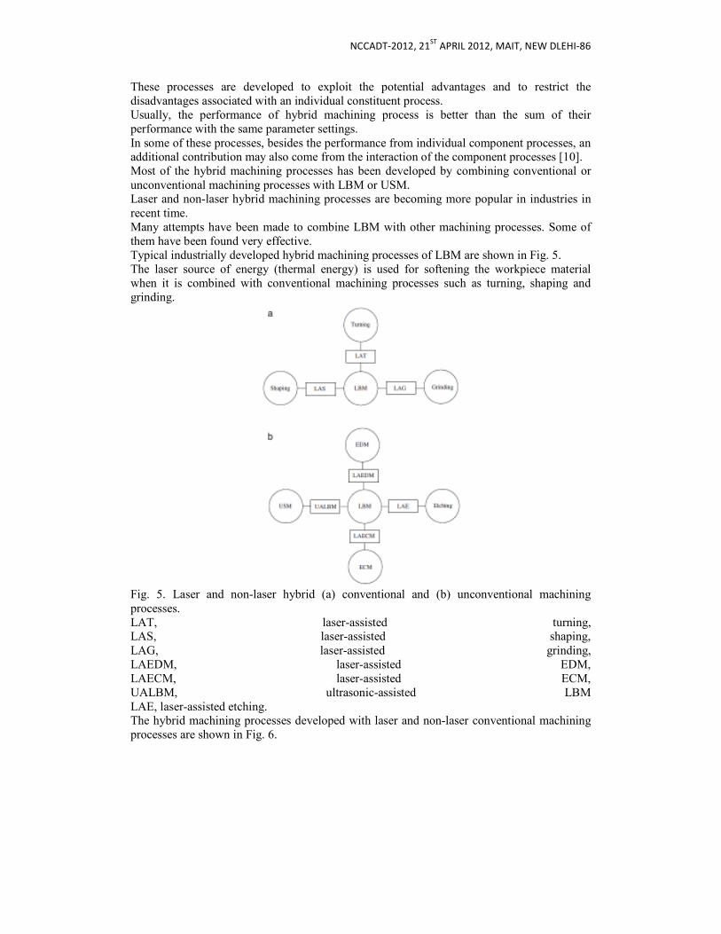
NCCADT-2012, 21ST


These processes are developed to exploit the potential advantages and to restrict the disadvantages associated with an individual constituent process. Usually, the performance of hybrid machining process is better than the sum of their performance with the same parameter settings. In some of these processes, besides the performance from individual component processes, an additional contribution may also come from the interaction of the component processes [10]. Most of the hybrid machining processes has been developed by combining conventional or unconventional machining processes with LBM or USM. Laser and non-laser hybrid machining processes are becoming more popular in industries in recent time. Many attempts have been made to combine LBM with other machining processes. Some of them have been found very effective. Typical industrially developed hybrid machining processes of LBM are shown in Fig. 5. The laser source of energy (thermal energy) is used for softening the workpiece material when it is combined with conventional machining processes such as turning, shaping and grinding.

Fig. 5. Laser and non-laser hybrid (a) conventional and (b) unconventional machining processes. LAT, laser-assisted turning, LAS, laser-assisted shaping, LAG, laser-assisted grinding, LAEDM, laser-assisted EDM, LAECM, laser-assisted ECM, UALBM, ultrasonic-assisted LBM LAE, laser-assisted etching. The hybrid machining processes developed with laser and non-laser conventional machining processes are shown in Fig. 6.

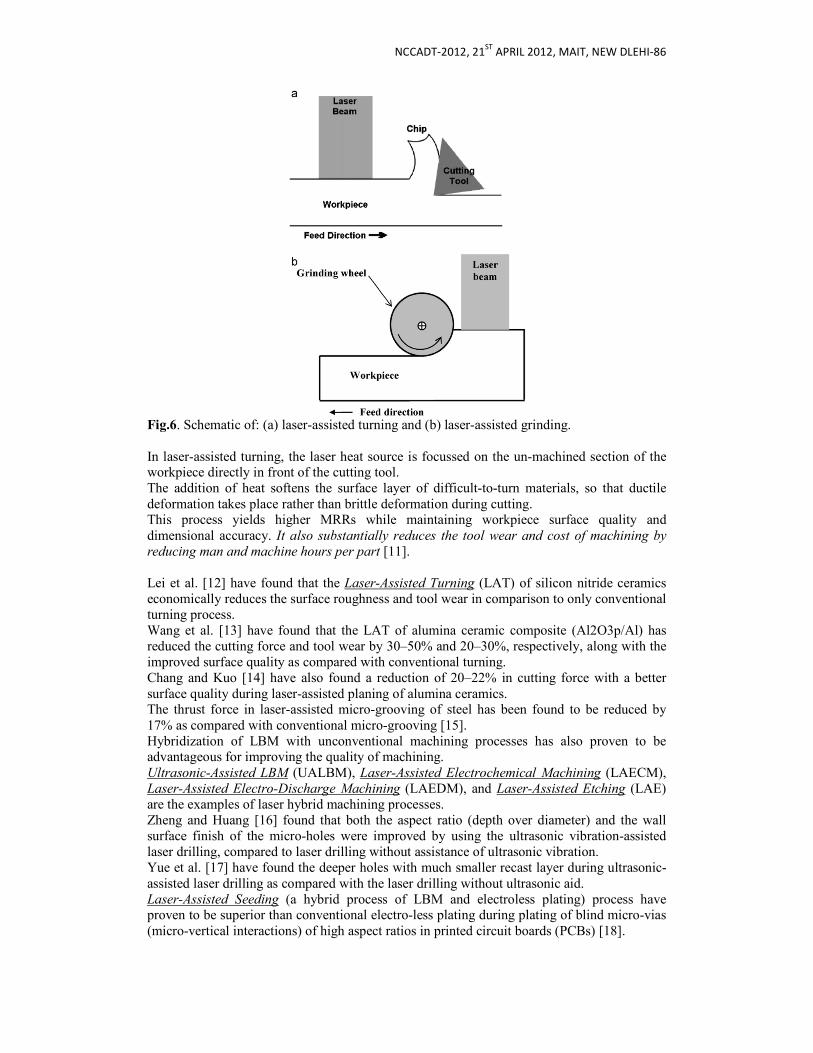
NCCADT-2012, 21ST


Fig.6. Schematic of: (a) laser-assisted turning and (b) laser-assisted grinding. In laser-assisted turning, the laser heat source is focussed on the un-machined section of the workpiece directly in front of the cutting tool. The addition of heat softens the surface layer of difficult-to-turn materials, so that ductile deformation takes place rather than brittle deformation during cutting. This process yields higher MRRs while maintaining workpiece surface quality and dimensional accuracy. It also substantially reduces the tool wear and cost of machining by

reducing man and machine hours per part [11]. Lei et al. [12] have found that the Laser-Assisted Turning (LAT) of silicon nitride ceramics economically reduces the surface roughness and tool wear in comparison to only conventional turning process. Wang et al. [13] have found that the LAT of alumina ceramic composite (Al2O3p/Al) has reduced the cutting force and tool wear by 30–50% and 20–30%, respectively, along with the improved surface quality as compared with conventional turning. Chang and Kuo [14] have also found a reduction of 20–22% in cutting force with a better surface quality during laser-assisted planing of alumina ceramics. The thrust force in laser-assisted micro-grooving of steel has been found to be reduced by 17% as compared with conventional micro-grooving [15]. Hybridization of LBM with unconventional machining processes has also proven to be advantageous for improving the quality of machining. Ultrasonic-Assisted LBM (UALBM), Laser-Assisted Electrochemical Machining (LAECM), Laser-Assisted Electro-Discharge Machining (LAEDM), and Laser-Assisted Etching (LAE) are the examples of laser hybrid machining processes. Zheng and Huang [16] found that both the aspect ratio (depth over diameter) and the wall surface finish of the micro-holes were improved by using the ultrasonic vibration-assisted laser drilling, compared to laser drilling without assistance of ultrasonic vibration. Yue et al. [17] have found the deeper holes with much smaller recast layer during ultrasonic-assisted laser drilling as compared with the laser drilling without ultrasonic aid. Laser-Assisted Seeding (a hybrid process of LBM and electroless plating) process have proven to be superior than conventional electro-less plating during plating of blind micro-vias (micro-vertical interactions) of high aspect ratios in printed circuit boards (PCBs) [18].

NCCADT-2012, 21ST


In LAECM, the laser radiation accelerates the electrochemical dissolution and localizes the area of machining by few microns size which enables the better accuracy and productivity [19]. De Silva et al. [20] have found that LAECM of aluminium alloy and stainless steel have improved the MRR by 54% and 33%, respectively, as compared with electro-chemical machining alone. They also claimed that LAECM has improved the geometrical accuracy by 38%. Li and Achara [21] have found that chemical-assisted laser machining (laser machining within a salt solution) significantly reduces the heat-affected zone and recast layer along with higher MRR as compared with laser machining in air. Li et al. [22] have applied the LBM and EDM sequentially for micro-drilling of fuel injection nozzles. They initially applied the laser drilling to produce the micro-holes and then EDM was used for rimming the drilled micro-holes. They claimed that this hybrid approach has eliminated the recast layer and heat affected zones (HAZs) typically associated with laser drilling. They also claimed that the hybrid process enabled 70% reduction in drilling time as compared with EDM drilling. Electro-chemical or chemical etching processes are combined with laser beam for localized etching to enable selective material removal. The use of LAE has improved the etched quality and etching rate of super-elastic microgripper prepared by cutting of nickel–titanium alloy [23]. 2.5 Remark:

The conclusion that can be drawn from this section is that, the main strength of LBM process lies in its capability to machine almost all type materials in comparison to other widely used advanced machining method such as EDM, ECM and USM. In comparison to jet machining processes, it is quite suitable for cutting small and thin sheets with high cutting rates and can be applied to machine miniature objects unlike other jet machining processes such as water jet, and abrasive water jet machining methods. Though it is non-contact type advanced machining method with high flexibility but thermal nature of the process requires careful control of the laser beam to avoid any undesired thermal effect. Among different variations, only laser drilling and cutting are being used most widely while 3-D LBM operations are not fully developed and a lot of research work is required before they can be put for industrial use. Unlike other, non-conventional energy sources laser beam source of energy can also be used as assistance during conventional machining of difficult-to-machine materials. The laser hybrid machining processes have been found superior to a single non-conventional machining technique in various machining applications. 3 LBM applications:

LBM has wide applications in the field of automobile sectors, aircraft industry, electronic industry, civil structures, nuclear sector and house appliances.

Stainless steel, a distinguishable engineering material used in automobiles and house appliances, is ideally suitable for laser beam cutting [24,25].

Advanced high strength steels (AHSS) machined by laser beam have applications in car industry and boiler works [26].

Titanium alloy sheets used in aerospace industry to make forward compression section in jet engines are cut by lasers [27–29].

Aluminium alloys used in aeronautics are one of the most promising for laser machining implantation [30].

Also, aluminium alloy samples of slot antenna array can be directly fabricated on laser cutting system [31].

Cutting of complex geometry in metallic coronary stents (Fig. 7) for medical application is done by pulsed Nd:YAG laser beam cutting [32,33].

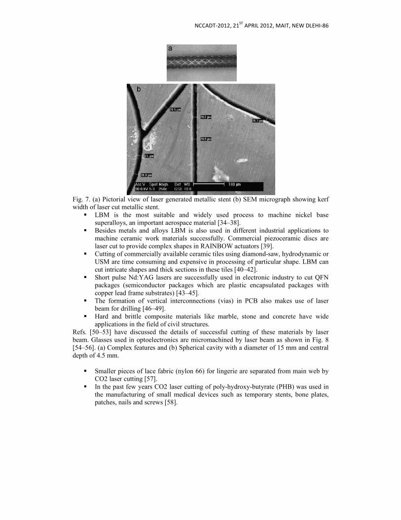
NCCADT-2012, 21ST


Fig. 7. (a) Pictorial view of laser generated metallic stent (b) SEM micrograph showing kerf width of laser cut metallic stent.

LBM is the most suitable and widely used process to machine nickel base superalloys, an important aerospace material [34–38].

Besides metals and alloys LBM is also used in different industrial applications to machine ceramic work materials successfully. Commercial piezoceramic discs are laser cut to provide complex shapes in RAINBOW actuators [39].

Cutting of commercially available ceramic tiles using diamond-saw, hydrodynamic or USM are time consuming and expensive in processing of particular shape. LBM can cut intricate shapes and thick sections in these tiles [40–42].

Short pulse Nd:YAG lasers are successfully used in electronic industry to cut QFN packages (semiconductor packages which are plastic encapsulated packages with copper lead frame substrates) [43–45].

The formation of vertical interconnections (vias) in PCB also makes use of laser beam for drilling [46–49].

Hard and brittle composite materials like marble, stone and concrete have wide applications in the field of civil structures.

Refs. [50–53] have discussed the details of successful cutting of these materials by laser beam. Glasses used in optoelectronics are micromachined by laser beam as shown in Fig. 8 [54–56]. (a) Complex features and (b) Spherical cavity with a diameter of 15 mm and central depth of 4.5 mm.

Smaller pieces of lace fabric (nylon 66) for lingerie are separated from main web by

CO2 laser cutting [57]. In the past few years CO2 laser cutting of poly-hydroxy-butyrate (PHB) was used in

the manufacturing of small medical devices such as temporary stents, bone plates, patches, nails and screws [58].

NCCADT-2012, 21ST


Fig. 8: Laser micro-machining application of glass sample:

Surgeons in various medical fields have applied pulsed laser cutting of tissue for several years [59,60].

Latest generation Q-switched diode pumped solid state lasers (DPSSLs) can be used for industrial applications to produce 3-D intricate profiles by laser milling of a wide variety of materials including aerospace alloys, thermal barrier coatings, tool steels, diamond and diamond substitutes [61].

Werner et al. [62] have recently proposed the application of CO2 laser milling in medical field for producing micro-cavities in bone and teeth tissues without damaging the soft tissues.

3.1 Remarks: The capability of LBM to cut complex shapes and drill micro size holes with close

tolerances in wide variety of materials has opened a new door to industries. Nowadays, industries related to almost all manufacturing fields are adopting the LBM

processes. Some unique applications of LBM involves cutting of stainless steel pipes with high

cutting rates and at less cost than diamond saw cutting, cutting complex shapes in car doors, cutting QFN packages in electronic industries, producing cooling holes in turbine engines in aircraft industry, micro-fabrication of vias in PCB.

The coronary stents used in medical field are micromachined by LBM. Unlike other thermal energy based processes such as EDM and ECM it provides lesser HAZ that makes it suitable for micromachining applications.

4 Major areas of LBM research: state-of-the-art: The research work carried out in the area of LBM can be divided in three parts namely

Experimental studies, Modelling studies and Optimization studies.

4.1 Experimental studies:

Experimental studies on LBM by researchers show the effect of process input parameters such as laser power, type and pressure of assist gas, cutting material thickness and its composition, cutting speed and mode of operation (continuous or pulsed mode) on process performance. The quality characteristics (or process performance) of interest in LBM are MRR,

Machined geometry (kerf width, hole diameter, taper), Surface quality (surface roughness, surface morphology),

NCCADT-2012, 21ST


Metallurgical characteristics (recast layer, heat affected zone, dross inclusion) and

Mechanical properties (hardness, strength, etc.). The important quality characteristics related to laser cutting of sheets are shown in Fig. 9.

• FIGURE 9: Schematic illustration of various cut quality attributes of interest [21]. Kentry: kerf width at entry side; Kexit: kerf width at exit side; Ra: surface roughness; S: thickness of material; 1: oxidized layer; 2: recast layer; and 3: heat affected zone (HAZ).

4.1.1 Material removal rate (MRR):

Voisey et al. [63] have studied the melt ejection phenomena in metals (aluminium, nickel, titanium, mild steel, tungsten, copper and zinc) by conducting Nd:YAG laser drilling experiments at different power densities. It was found that MRR first increases and then decreases after a critical value with increasing power density for all metals tested. The critical value was found as type of metal dependent. Some investigators have used machining speed and/or machining time to represent the MRR. Cutting speed of continuous wave (CW) and pulsed Nd:YAG laser beam was compared in [64] for cutting bare and coated metal plates (0.8–2.0mm thick) of car frame using oxygen assist gas. The cutting speed obtained was more in case of CW laser, bare metal and thinner plate and the highest cutting speed recorded was 5 m/min at an optimum oxygen pressure of 3 bar. Experimental study [65] for cutting stainless steel sheets (up to 2 cm thick) from a long distance (1 m) without using any assist gas was performed in pulsed mode taking pulse frequency (100–200 Hz), peak power (2–5 kW) and cutting velocity (0.05–0.5 m/min) as process variables. The study reveals that low pulse frequencies and high peak powers were found to be favourable for higher cutting speeds. The MRR of mullitealumina ceramic during laser cutting was increased by proper selection of off-axis nozzle angle (optimum value 451) and distance between the impinging point of the gas jet and the laser beam front (optimum value 3 mm) [67]. Experimental study by Lau et al. [68] shows that compressed air removes more material in comparison to argon inert gas during laser cutting of carbon fibre composites.

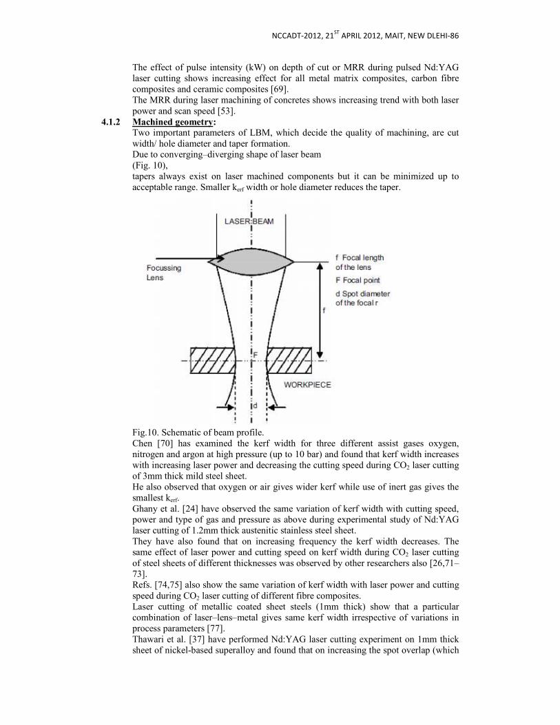
NCCADT-2012, 21ST


The effect of pulse intensity (kW) on depth of cut or MRR during pulsed Nd:YAG laser cutting shows increasing effect for all metal matrix composites, carbon fibre composites and ceramic composites [69]. The MRR during laser machining of concretes shows increasing trend with both laser power and scan speed [53].

4.1.2 Machined geometry: Two important parameters of LBM, which decide the quality of machining, are cut width/ hole diameter and taper formation. Due to converging–diverging shape of laser beam (Fig. 10), tapers always exist on laser machined components but it can be minimized up to acceptable range. Smaller kerf width or hole diameter reduces the taper.

Fig.10. Schematic of beam profile. Chen [70] has examined the kerf width for three different assist gases oxygen, nitrogen and argon at high pressure (up to 10 bar) and found that kerf width increases with increasing laser power and decreasing the cutting speed during CO2 laser cutting of 3mm thick mild steel sheet. He also observed that oxygen or air gives wider kerf while use of inert gas gives the smallest kerf. Ghany et al. [24] have observed the same variation of kerf width with cutting speed, power and type of gas and pressure as above during experimental study of Nd:YAG laser cutting of 1.2mm thick austenitic stainless steel sheet. They have also found that on increasing frequency the kerf width decreases. The same effect of laser power and cutting speed on kerf width during CO2 laser cutting of steel sheets of different thicknesses was observed by other researchers also [26,71–73]. Refs. [74,75] also show the same variation of kerf width with laser power and cutting speed during CO2 laser cutting of different fibre composites. Laser cutting of metallic coated sheet steels (1mm thick) show that a particular combination of laser–lens–metal gives same kerf width irrespective of variations in process parameters [77]. Thawari et al. [37] have performed Nd:YAG laser cutting experiment on 1mm thick sheet of nickel-based superalloy and found that on increasing the spot overlap (which

NCCADT-2012, 21ST


is a function of pulse frequency and cutting speed) the kerf width increases. They also observed that shorter pulse duration yields lower taper kerf compared to a longer duration pulse. Bandyopadhyay et al. [34] have investigated the effect of material type and its thickness on hole taper during Nd:YAG laser drilling of titanium alloy and nickel alloy sheets of different thicknesses. The results show that the hole entry diameter and taper angle are different for different materials and increases with decreasing thickness.

4.1.3 Surface roughness: Surface roughness is an effective parameter representing the quality of machined surface. Ref. [24] shows that surface roughness value reduces on increasing cutting speed and frequency, and decreasing the laser power and gas pressure. Also nitrogen gives better surface finish than oxygen. In Ref. [70] surface roughness value was found to be reduced on increasing pressure in case of nitrogen and argon but air gives poor surface beyond 6 bar pressure. Also, surface finish was better at higher speeds. Ref. [71] shows that the laser power and cutting speed has a major effect on surface roughness as well as striation (periodic lines appearing on the cut surface) frequency (Fig. 12). They have shown that at optimum feed rate, the surface roughness is minimum and laser power has a small effect on surface roughness but no effect on striation frequency. Ref. [37] shows that surface finish improves on increasing the spot overlap. The surface roughness of thick ceramic tiles during CO2 laser cutting is mainly affected by ratio of power to cutting speed, material composition and thickness, gas type and its pressure [40,41]. Use of nitrogen assist gas and lesser power intensities reduce the surface roughness [74]. Pulsed mode CO2 laser cutting gives better surface finish than CW mode [75].

4.1.4 Metallurgical characteristics The change in metallurgical characteristics of laser machined workparts is mainly governed by HAZ. Therefore, it is required to minimize the HAZ during LBM by controlling various factors. Decreasing power and increasing feed rate generally led to a decrease in HAZ [71]. They also observed that increased oxygen pressure increases the HAZ. Pulsed laser cutting of titanium and titanium alloy sheets show that minimum HAZ can be obtained at medium pulse energy, high pulse frequency, high cutting speed and at high pressure of argon assist gas, while use of oxygen assist gas gave maximum HAZ in comparison to nitrogen and argon [27,29]. The microstructural study of CO2 laser machined aluminium alloy show that HAZ increases as the depth of hole drilling increases [30]. Low material thickness and pulse energy gives smaller HAZ while pulse frequency has no significant effect on HAZ for laser cutting of thick sheets of nickel base superalloy [34]. Effect of beam angle during Nd:YAG laser drilling of TBC nickel superalloys show that on increasing the beam angle to surface decreases the HAZ, recast and oxide layer thickness up to 601 after that it remains almost constant (Fig. 13) [38]. HAZ in laser cutting of carbon fibre composites was found more in comparison to EDM [68]. Since most of the materials removed during LBM are by melt ejection, the melt part which is not removed from cavity is resolidified and a recast layer results on side walls and also at bottom of cavity. This recast zone has entirely different property as compared to parent material. Therefore, aim is always to remove or minimize the recast layer. Many researchers have found the effect of parameters on recast layer and

NCCADT-2012, 21ST


tried to minimize it. The observation of recast layer in thick titanium and nickel base alloys during laser drilling show thicker layer at hole entry side. Also, parameters effect show that on increasing the pulse frequency and pulse energy recast layer reduces while increases with material thickness [34]. Effect of beam angle on recast layer was found to be same as of HAZ [38]. A specially designed nozzle was used for laser cutting of thick ceramic plates at an optimum angle and distance from work surface to completely remove the recast layer [67].

4.1.5 Mechanical properties: Researchers have also studied the mechanical properties of laser machined workparts and found that thermal damages and crack formation affect the strength of materials. The hardness of titanium alloy sheet in heat-affected zone was increased by 10% after laser cutting and the crack formation was found to be more by using oxygen or nitrogen assist gas in comparison to argon inert gas [27]. Cosp et al. [42] have found optimum cutting conditions for laser cutting of fine porcelain stoneware to avoid crack formation.

4.1.6 Remarks:

The experimental results discussed above show that the effect of process parameters on process performance are not showing a fixed pattern in different operating ranges. In such cases more scientific experimental study is needed in different range of operating parameters for the prediction of process behaviour. In many experimental results discussed so far, the optimum range of process parameters have been found based on variation of one factor at a time but simultaneous effect of variation of more than one parameters at a time have not been studied in a comprehensive way. Here, it can be concluded that a comprehensive scientific methodology based study is needed for LBM of different advanced engineering materials with all possible input parameters as well as single or multiple performance measure.

4.2 Modelling and optimization studies: Modelling in LBM helps us to get a better understanding of this complex process. Modelling studies are the scientific ways to study the system behaviours. A mathematical model of a system is the relationship between input and output parameters in terms of mathematical equations. On the basis of their origin, models can be divided in three categories e.g. experimental or empirical models, analytical models, and artificial intelligence (AI) based models. Complexity in machining dynamics has forced researchers to find optimal or near optimal machining conditions with discrete and continuous parameters spaces with multimodel, differentiable or non-differentiable objective function or responses finding optimal solutions by a suitable optimization technique based on objective function formulated from model is a critical and difficult task and hence, a large number of techniques has been developed by researchers to solve these type of parameter optimization problems. The literature related to modelling and optimization of LBM is mainly using statistical design of experiments (DOE) such as Taguchi method and response surface method. Several analytical methods based on different solution methodologies, such as exact solution and numerical solution, have also been examined related to LBM. Few researchers concentrated on modelling and optimization of laser beam cutting through AI based techniques such as artificial neural network (ANN) and fuzzy logic (FL).

5 Future directions of LBM research: The major research areas in LBM are discussed in previous sections. Researchers have contributed in different directions but due to complex nature of the process a lot of works are still required to be done. Most of the published works are related to laser cutting followed by drilling and micromachining but 3-D LBM like turning and milling are still

NCCADT-2012, 21ST


awaiting for industrial use. The control of two or more laser beams at different angles simultaneously is not an easy task during 3-D machining. Thickness of material is another constraint during LBM which can be reduced by improving the beam quality. At present, the use of LBM is limited up to complex profile cutting in sheet metals but due to emergence of advanced engineering materials, need is to develop it for cutting of difficult-to-cut materials. So, these developments in LBM can be an area of future research. Most of the experimental works presented in LBM are aimed to study the effect of parameter variations on quality characteristics. Only few researchers have used the scientific methods under the umbrella of DOE for the study of LBM process. Unplanned experimental study includes a lot of undesired factors which affect the performance variations and finally leads to unreliable results. Further, researchers have excluded many important factors such as beam spot diameter, thermal conductivity and reflectivity of workpiece material and the interaction effects among various factors during study which otherwise would affect the performance characteristics differently. In the same way, during theoretical study authors have taken a number of hypothetical assumptions to simplify the problems of LBM which otherwise could be incorporated in their models to enhance the reliability and applicability of the model. Thus, it is desirable to develop the models with no or very few assumptions to get the real solution of the LBM problems quantitatively. The optimization of process variables is a major area of research in LBM. Most of the literature available in this area shows that researchers have concentrated on a single quality characteristic as objective during optimization of LBM. Optimum value of process parameters for one quality characteristic may deteriorate other quality characteristics and hence the overall quality. No literature is available on multi-objective optimization of LBM process and present authors found it as the main direction of future research. Also, various experimental tools used for optimization (such as Taguchi method and RSM) can be integrated together to incorporate the advantages of both simultaneously. Only one literature available so far shows hybrid approach (integration of FD and ANN) for optimization of process variables and more work is required to be done in this area. LBM being a thermal process induces many adverse effects in workpiece material which in turn affects the mechanical properties also. The most of the performance characteristics discussed by various researchers relate to geometrical, metallurgical and surface qualities such as:

Surface roughness, Taper formation and HAZ.

Fatigue strength, micro-hardness, and residual stresses are also important performance measures which are required to be improved. So, improvement of mechanical properties during LBM is a research area of interest.

6 Conclusions: The work presented here is an overview of recent developments of LBM and future research directions. From above discussion it can be concluded that:

1) LBM is a powerful machining method for cutting complex profiles and drilling holes in wide range of workpiece materials. However, the main disadvantage of this process is low energy efficiency from production rate point of view and converging diverging shape of beam profile from quality and accuracy point of view.

2) Apart from cutting and drilling, LBM is also suitable for precise machining of micro-parts. The micro-holes of very small diameters (up to 5 mm) with high aspect ratio (more than 20) can be drilled accurately using nanosecond frequency tripled lasers. Cutting of thin foils (up to 4 mm) has been done successfully with micro-range kerf width.

3) The performance of LBM mainly depends on laser parameters (e.g. laser power, wavelength, mode of operation), material parameters (e.g. type, thickness) and

NCCADT-2012, 21ST


process parameters (e.g. feed rate, focal plane position, frequency, energy, pulse duration, assist gas type and pressure). The important performance characteristics of interest for LBM study are HAZ, kerf or hole taper, surface roughness, recast layer, dross adherence and formation of micro-cracks.

4) The laser beam cutting process is characterized by large number of process parameters that determines efficiency, economy and quality of whole process and hence, researchers have tried to optimize the process through experiment based, analytical, and AI based modelling and optimization techniques for finding optimal and near optimal process parameters but modelling and optimization of laser beam cutting with multi-objective, and with hybrid approach are nonexistent in the literature.

5) The two extreme application areas such as machining of thick materials and machining of micro-parts need considerable research work.

7 References:

[1] G. Chryssolouris, Laser Machining—Theory and Practice. Mechanical Engineering Series, Springer-Verlag, New York Inc., NewYork, 1991.

[2] J.D. Majumdar, I. Manna, Laser processing of materials, Sadhana 28 (3–4) (2003) 495–562.

[3] T. Norikazu, Y. Shigenori, H. Masao, Present and future of lasers for fine cutting of metal plate, Journal of Materials Processing Technology 62 (1996) 309–314.

[4] J. Meijer, Laser beam machining (LBM), state of the art and new opportunities, Journal of Materials Processing Technology 149 (2004) 2–17.

[5] J.K.S. Sundar, S.V. Joshi, Laser cutting of materials, Centre for Laser Processing of Materials, International Advance Research Centre for Powder Metallurgy and New Materials, Hyderabad.

[6] D.T. Pham, S.S. Dimov, P.T. Petkov, Laser milling of ceramic components, International Journal of Machine Tools and Manufacture 47 (2007) 618–626.

[7] C.-H. Tsai, H.-W. Chen, Laser milling of cavity in ceramic substrate by fracture-machining element technique, Journal of Materials Processing Technology 136 (2003) 158–165.

[8] D.T. Pham, S.S. Dimov, P.V. Petkov, T. Dobrev, Laser milling as a ‘rapid’ micromanufacturing process, Proceedings of the I MECH E Part B. Journal of Engineering Manufacture 218 (1) (2004) 1–7.

[9] L. Qi, Y. Wang, L. Yang, Study of Nd:YAG pulsed laser milling Al2O3 ceramic in water and air condition, International Technology and Innovation Conference, Hangzhou, China, November 6–7, 2006, pp. 489–493.

[10] V. Yadava, V.K. Jain, P.M. Dixit, Temperature distribution during electro-discharge abrasive grinding, Machining Science and Technology— An International Journal 6 (1) (2002) 97–127.

[11] J.C. Rozzi, F.E. Pfefferkorn, Y.C. Shin, F.P. Incropera, Experimental evaluation of the laser assisted machining of silicon nitride ceramics, ASME Journal of Manufacturing Science and Engineering 122 (2000) 666–670.

[12] S. Lei, Y.C. Shin, F.P. Incropera, Experimental investigations of thermo-mechanical characteristics in laser-assisted machining of silicon nitride ceramics, ASME Journal of Manufacturing Science and Engineering 123 (2001) 639–646.

[13] Y. Wang, L.J. Yang, N.J. Wang, An investigation of laser-assisted machining of Al2O3 particle reinforced aluminium matrix composites, Journal of Materials Processing Technology 129 (2002) 268–272.

[14] C.-W. Chang, C.-P. Kuo, An investigation of laser-assisted machining of Al2O3 ceramics planning, International Journal of Machine Tools and Manufacture 47 (2007) 452–461.

[15] R. Singh, S.N. Melkote, Characterization of a hybrid laser-assisted mechanical micromachining (LAMM) process for a difficult-tomachine material, International Journal of Machine Tools and Manufacture 47 (2007) 1139–1150.

NCCADT-2012, 21ST


[16] H.Y. Zheng, H. Huang, Ultrasonic vibration-assisted femtosecond laser machining of microholes, Journal of Micromechanics and Microengineering 17 (8) (2007) 58–61.

[17] T.M. Yue, T.W. Chan, H.C. Man, W.S. Lau, Analysis of ultrasonicaided laser drilling using finite element method, Annals of CIRP 45 (1996) 169–172.

[18] E.S.W. Leung, W.K.C. Yung, W.B. Lee, A study of micro-vias produced by laser-assisted seeding mechanism in blind via hole plating of printed circuit board, International Journal of Advanced Manufacturing Technology 24 (2004) 474–484.

[19] K.P. Rajurkar, G. Levy, A. Malshe, M.M. Sundaram, J. McGeough, X. Hu, R. Resnick, A. DeSilva, Micro and nano machining by electro-physical and chemical processes, Annals of CIRP 55 (2) (2006) 643–666.

[20] A.K.M. De Silva, P.T. Pajak, D.K. Harrison, J.A. McGeough, Modelling and experimental investigation of laser assisted jet electrochemical machining, Annals of CIRP 53 (1) (2004) 179–182.

[21] L. Li, A. Achara, Chemical assisted laser machining for the minimization of recast and heat affected zone, Annals of CIRP 53 (2004) 175–178.

[22] L. Li, C. Diver, J. Atkinson, R.G. Wagner, H.J. Helml, Sequential laser and EDM micro-drilling for next generation fuel injection nozzle manufacture, Annals of CIRP 55 (1) (2006) 179–182.

[23] A. Stephen, G. Sepold, S. Metev, F. Vollertsen, Laser-induced liquid-phase jet-chemical etching of metals, Journal of Material Processing Technology 149 (1–3) (2004) 536–540.

[24] K.A. Ghany, M. Newishy, Cutting of 1.2mm thick austenitic stainless steel sheet using pulsed and CW Nd:YAG laser, Journal of Material Processing Technology 168 (2005) 438–447.

[25] B.S. Yilbas, R. Devies, Z. Yilbas, Study into penetration speed during CO2 laser cutting of stainless steel, Optics and Lasers in Engineering 17 (1992) 69–82.

[26] A. Lamikiz, L.N.L. Lacalle, J.A. Sanchez, D. Pozo, J.M. Etayo, J.M. Lopez, CO2 laser cutting of advanced high strength steels (AHSS), Applied Surface Science 242 (2005) 362–368.

[27] L. Shanjin, W. Yang, An investigation of pulsed laser cutting of titanium alloy sheet, Optics and Lasers in Engineering 44 (2006) 1067–1077.

[28] A. Almeida, W. Rossi, M.S.F. Lima, J.R. Berretta, G.E.C. Nogueira, N.U. Wetter, N.D. Vieira Jr., Optimization of titanium cutting by factorial analysis of the pulsed Nd:YAG laser parameters, Journal of Materials Processing Technology 179 (1–3) (2006) 105–110.

[29] B.T. Rao, R. Kaul, P. Tiwari, A.K. Nath, Inert gas cutting of titanium sheet with pulsed mode CO2 cutting, Optics and Lasers in Engineering 43 (2005) 1330–1348.

[30] D. Araujo, F.J. Carpio, D. Mendez, A.J. Garcia, M.P. Villar, R. Garcia, D. Jimenez, L. Rubio, Microstructural study of CO2 laser machined heat affected zone of 2024 aluminium alloy, Applied Surface Science 208–209 (2003) 210–217.

[31] X. Wang, R. Kang, W. Xu, D. Guo, Direct laser fabrication of aluminium-alloy slot antenna array, in: 1st International Symposium on Systems and Control in Aerospace and Astronautics (ISSCAA), 19–21 January 2006, 5pp.

[32] A. Raval, A. Choubey, C. Engineer, D. Kothwala, Development and assessment of 316LVM cardiovascular stents, Materials Science and Engineering A 386 (2004) 331–343.

[33] Y.P. Kathuria, Laser microprocessing of metallic stent for medical therapy, Journal of Materials Processing Technology 170 (2005) 545–550.

[34] S. Bandyopadhyay, J.K.S. Sundar, G. Sundarrajan, S.V. Joshi, Geometrical features and metallurgical characteristics of Nd:YAG laser drilled holes in thick IN718 and Ti–6Al–4V sheets, Journal of Materials Processing Technology 127 (2002) 83–95.

[35] A. Corcoran, L. Sexton, B. Seaman, P. Ryan, G. Byrne, The laser drilling of multi-layer aerospace material systems, Journal of Materials Processing Technology 123 (2002) 100–106.

NCCADT-2012, 21ST


[36] D.K.Y. Low, L. Li, P.J. Byrd, Spatter prevention during the laser drilling of selected aerospace materials, Journal of Materials Processing Technology 139 (2003) 71–76.

[37] G. Thawari, J.K.S. Sundar, G. Sundararajan, S.V. Joshi, Influence of process parameters during pulsed Nd:YAG laser cutting of nickel-base superalloys, Journal of Materials Processing Technology 170 (2005) 229–239.

[38] H.K. Sezer, L. Li, M. Schmidt, A.J. Pinkerton, B. Anderson, P. Williams, Effect of beam angle on HAZ, recast and oxide layer characteristics in laser drilling of TBC nickel superalloys, International Journal of Machine Tools and Manufacture 46 (15) (2006) 1972–1982.

[39] J. Juuti, E. Heinonen, V.-P. Moilanen, S. Leppavuori, Displacement, stiffness and load behaviour of laser-cut RAINBOW actuators, Journal of the European Ceramic Society 24 (2004) 1901–1904.

[40] I. Black, S.A.J. Livingstone, K.L. Chua, A laser beam machining (LBM) database for the cutting of ceramic tile, Journal of MaterialsProcessing Technology 84 (1998) 47–55.

[41] I. Black, K.L. Chua, Laser cutting of thick ceramic tile, Optics and Laser Technology 29 (4) (1997) 193–205.

[42] J.P. Cosp, A.J.R. Valle, J.G. Fortea, P.J.S. Soto, Laser cutting of high-vitrified ceramic materials: development of a method using a Nd:YAG laser to avoid catastrophic breakdown, Materials Letters 55 (2002) 274–280.

[43] C.-H. Li, M.-J. Tsai, R. Chen, C.-H. Lee, S.-W. Hong, Cutting for QFN packaging by diode pumping solid state laser system, Proceedings of IEEE Workshop on Semiconductor Manufacturing Technology (2004) 123–126.

[44] C.-H. Li, M.-J. Tsai, S.-M. Yao, Cutting quality study for QFN packages by Nd:YAG laser, Proceedings of the IEEE International conference on Mechatronics (ICM’05) (2005) 19–24.

[45] C.-H. Li, M.-J. Tsai, C.-D. Yang, Study of optimal laser parameters for cutting QFN packages by Taguchi’s matrix method, Optics and Laser Technology 39 (2007) 786–795.

[46] A. Kestenbaum, J.F. D’Amico, B.J. Blumenstock, M.A. Deangelo, Laser drilling of microvias in epoxy-glass printed circuit boards, IEEE Transactions on Components, Hybrids, and Manufacturing Technology 13 (4) (1990) 1055–1062.

[47] D.M. D’Ambra, M.C.A. Needes, C.R.S. Needes, C.B. Wang, Via formation in green ceramic dielectrics using a Yag laser, Proceedings of the 42nd IEEE conference on Electronic Components and Technology (1992) 1072–1080.

[48] E.K.W. Gan, H.Y. Zheng, G.C. Lim, Laser drilling of micro-vias in PCB substrates, IEEE Electronics Packaging Technology Conference, 2000, pp. 321–326.

[49] C.J. Moorhouse, F. Villarreal, J.J. Wendland, H.J. Baker, D.R. Hall, D.P. Hand, CO2 laser processing of alumina (Al2O3) printed circuit board substrates, IEEE Transactions on Electronics Packaging Manufacturing 28 (3) (2005) 249–258.

[50] M. Boutinguiza, J. Pou, F. Lusquinos, F. Quintero, R. Soto, M.P. Amor, K. Watkins, W.M. Steen, CO2 laser cutting of slate, Optics and Lasers in Engineering 37 (2002) 15–25.

[51] R.M. Miranda, Structural analysis of the heat affected zone of marble and limestone tiles cut by CO2 laser, Materials Characterization 53 (2004) 411–417.

[52] P. Crouse, L. Li, J.T. Spencer, Performance comparison of CO2 and diode lasers for deep-section concrete cutting, Thin Solid Films 453–454 (2004) 594–599.

[53] B.T. Rao, H. Kumar, A.K. Nath, Processing of concretes with a high power CO2 laser, Optics and Laser Technology 37 (2005) 348–356.

[54] S. Nikumb, Q. Chen, C. Li, H. Reshef, H.Y. Zheng, H. Qiu, D. Low, Precision glass machining, drilling and profile cutting by short pulse lasers, Thin Solid Films 47 (7) (2005) 216–221.

[55] Y.S. Lee, W.H. Kang, Laser micro-machining and applications of glasses in optoelectronics, IEEE International Symposium on Electronic Materials and Packaging, 2001, pp. 93–95.

NCCADT-2012, 21ST


[56] M.B. Strigin, A.N. Chudinov, Cutting of glass by picosecond laser radiation, Optics Communications 106 (1994) 223–226.

[57] P. Bamforth, K. Williams, M.R. Jackson, Edge quality optimization for CO2 laser cutting of nylon textiles, Applied Thermal Engineering 26 (2006) 403–412.

[58] D. Lootz, D. Behrend, S. Kramer, T. Freier, A. Haubold, G. Benkieber, K.P. Schmitz, B. Becher, Laser cutting: influence on morphological and physicochemical properties of polyhydroxybutyrate, Biomaterials 22 (2001) 2447–2452.

[59] A.D. Zweig, H.P. Weber, Mechanical and thermal parameters in pulsed laser cutting of tissue, IEEE Journal of Quantum Electronics QE-3 (10) (1987) 1787–1793.

[60] G.A. Peyman, A. Alghadyan, J.H. Peace, A contact Nd:YAG laser to resect large ciliary body and choroidal tumors, International Ophthalmology 11 (1987) 55–61.

[61] M. Henry, P.M. Harrison, I. Henderson, M.F. Brownell, Laser milling: a practical industrial solution for machining a wide variety of materials, Proceedings of SPIE, vol. 5662, 2004, pp. 627–632.

[62] M. Werner, M. Ivaneko, D. Harbecke, M. Klasing, H. Steigerwald, P. Hering, CO2 laser milling of hard tissue, Proceedings of SPIE, vol. 6435, 2007, p. 64350E.

[63] K.T. Voisey, C.F. Cheng, T.W. Clyne, Quantification of melt ejection phenomena during laser drilling, Materials Research Society 617 (2000) J5.6.1–J5.6.7.

[64] D.F. Grevey, H. Desplats, Comparison of the performance obtained with a YAG laser cutting according to the source operation mode, Journal of Material Processing Technology 42 (1994) 341–348.

[65] G. Tahmouch, P. Meyrueis, P. Grandjean, Cutting by a high power laser at a long distance without an assist gas for dismantling, Optics and Laser Technology 29 (6) (1997) 307–316.

[66] T.-C. Chen, R.B. Darling, Parametric studies on pulsed near ultraviolet frequency tripled Nd:YAG laser micromachining of sapphire and silicon, Journal of Materials Processing Technology 169 (2005) 214–218.

[67] F. Quintero, J. Pou, J.L. Fernandez, A.F. Doval, F. Lusquinos, M. Boutinguiza, R. Soto, M.P. Amor, Optimization of an off-axis nozzle for assist gas injection in laser fusion cutting, Optics and Lasers in Engineering 44 (2006) 1158–1171.

[68] W.S. Lau, W.B. Lee, Pulsed Nd:YAG laser cutting of carbon fibre composite materials, Annals of CIRP 39 (1) (1992) 179–182.

[69] W.S. Lau, T.M. Yue, T.C. Lee, W.B. Lee, Un-conventional machining of composite materials, Journal of Materials Processing Technology 48 (1995) 199–205.

[70] S.-L. Chen, The effects of high-pressure assistant-gas flow on highpower CO2 laser cutting, Journal of Material Processing Technology 88 (1999) 57–66.

[71] N. Rajaram, J.S. Ahmad, S.H. Cheraghi, CO2 laser cut quality of 4130 steel, International Journal of Machine Tools and Manufacture 43 (2003) 351–358.

[72] W.W. Duley, J.N. Gonsalves, CO2 laser cutting of thin metal sheets with gas jet assist, Optics and Laser Technology 1 (1974) 78–81.

[73] H.Y. Zheng, Z.Z. Han, Z.D. Chen, W.L. Chen, S. Yeo, Quality and cost comparisons between laser and waterjet cutting, Journal of Material Processing Technology 62 (1996) 294–298.

[74] F.A. Al-Sulaiman, B.S. Yilbas, M. Ahsan, CO2 laser cutting of a carbon/carbon multi-lamelled plain-weave structure, Journal of Material Processing Technology 173 (2006) 345–351.

[75] K.C.P. Lum, S.L. Ng, I. Black, CO2 laser cutting of MDF 1. Determination of process parameter settings, Optics and Laser Technology 32 (2000) 67–76.

NCCADT-2012, 21ST


Conceptual design of Diamond meter Arun Gupta

Indira Gandhi Institute of Tech., Delhi, India [email protected]

Abstract: In Tanishq (Titan Industries Ltd.-Jwellery Division) Plain and diamond studded gold

ornaments are manufactured and are put up for sale at boutiques. To eradicate the

apprehension of the quality of studded Jewellery & to establish the credence of customers in Tanishq the company has planned to device a proposed machine called Diamond Meter

which would measure the 4 traits to assess the quality of the diamonds after fixing on the

jewel, in single system. If it is not feasible in single system, a fewer traits should be measured

in single machine. The company has a plan to pioneer in use of diamond meter at its

boutiques like karat meter. It will direct tangible and intangible benefits to the company

directly and indirectly.

Keywords: X-ray radiography, RGB color measurement method, Heat conduction clarity measurement method 1. Introduction:

The four traits of the diamond are called the 4 Cs of the diamond. The four Cs stand for the following terms:

Cut Clarity Colour Carat

FIG.1 DIFFERENT DIAMOND CUTS

CUT

Cut includes symmetry, proportion and finish of fashioned diamond. It is considered that 98% of brilliance and sparkling depends on cut. Diamond lusture or brilliance is defined as the reflection of a bright white light from the facets of the diamond and is determined by the artistry of the cutting and polishing. CLARITY

Clarity describes the clearness or purity of a diamond. This is determined by the number, size, nature and location of the internal (inclusions) and external (blemishes) imperfections. FIG 2 shows the different clarity grades.

FIG 2: CLARITY GRADING SCALE

In Tanishq only four different quality diamonds are being embellished in studded jewellery. The four qualities are as follows:

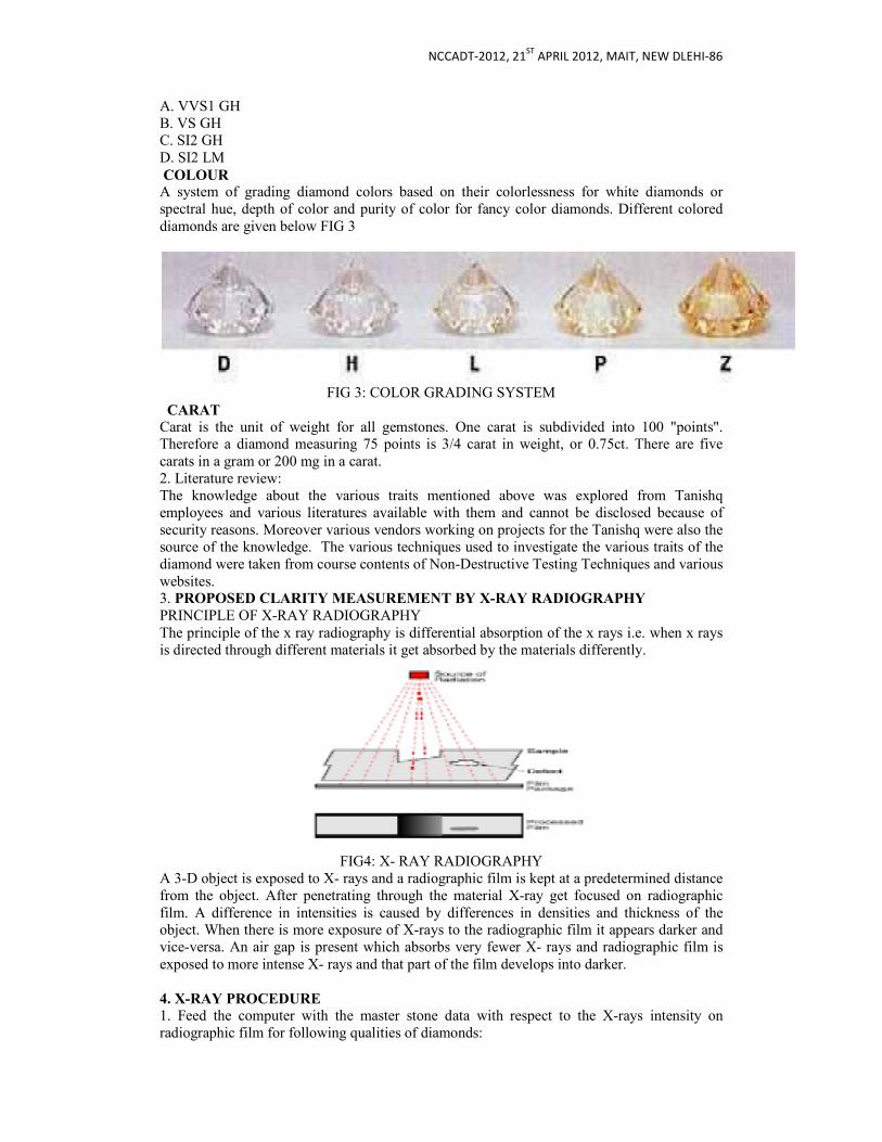
NCCADT-2012, 21ST


A. VVS1 GH B. VS GH C. SI2 GH D. SI2 LM COLOUR A system of grading diamond colors based on their colorlessness for white diamonds or spectral hue, depth of color and purity of color for fancy color diamonds. Different colored diamonds are given below FIG 3

FIG 3: COLOR GRADING SYSTEM CARAT

Carat is the unit of weight for all gemstones. One carat is subdivided into 100 "points". Therefore a diamond measuring 75 points is 3/4 carat in weight, or 0.75ct. There are five carats in a gram or 200 mg in a carat. 2. Literature review: The knowledge about the various traits mentioned above was explored from Tanishq employees and various literatures available with them and cannot be disclosed because of security reasons. Moreover various vendors working on projects for the Tanishq were also the source of the knowledge. The various techniques used to investigate the various traits of the diamond were taken from course contents of Non-Destructive Testing Techniques and various websites. 3. PROPOSED CLARITY MEASUREMENT BY X-RAY RADIOGRAPHY

PRINCIPLE OF X-RAY RADIOGRAPHY The principle of the x ray radiography is differential absorption of the x rays i.e. when x rays is directed through different materials it get absorbed by the materials differently.

FIG4: X- RAY RADIOGRAPHY

A 3-D object is exposed to X- rays and a radiographic film is kept at a predetermined distance from the object. After penetrating through the material X-ray get focused on radiographic film. A difference in intensities is caused by differences in densities and thickness of the object. When there is more exposure of X-rays to the radiographic film it appears darker and vice-versa. An air gap is present which absorbs very fewer X- rays and radiographic film is exposed to more intense X- rays and that part of the film develops into darker. 4. X-RAY PROCEDURE

1. Feed the computer with the master stone data with respect to the X-rays intensity on radiographic film for following qualities of diamonds:

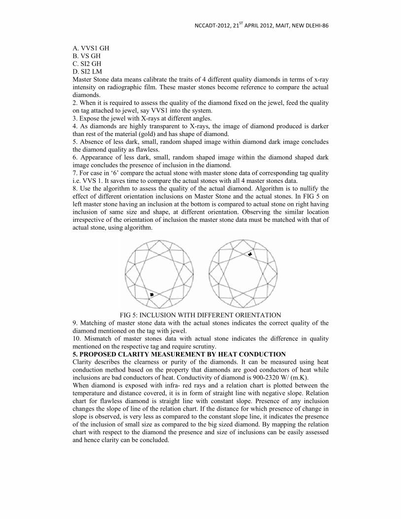
NCCADT-2012, 21ST


A. VVS1 GH B. VS GH C. SI2 GH D. SI2 LM Master Stone data means calibrate the traits of 4 different quality diamonds in terms of x-ray intensity on radiographic film. These master stones become reference to compare the actual diamonds. 2. When it is required to assess the quality of the diamond fixed on the jewel, feed the quality on tag attached to jewel, say VVS1 into the system. 3. Expose the jewel with X-rays at different angles. 4. As diamonds are highly transparent to X-rays, the image of diamond produced is darker than rest of the material (gold) and has shape of diamond. 5. Absence of less dark, small, random shaped image within diamond dark image concludes the diamond quality as flawless. 6. Appearance of less dark, small, random shaped image within the diamond shaped dark image concludes the presence of inclusion in the diamond. 7. For case in ‘6’ compare the actual stone with master stone data of corresponding tag quality i.e. VVS 1. It saves time to compare the actual stones with all 4 master stones data. 8. Use the algorithm to assess the quality of the actual diamond. Algorithm is to nullify the effect of different orientation inclusions on Master Stone and the actual stones. In FIG 5 on left master stone having an inclusion at the bottom is compared to actual stone on right having inclusion of same size and shape, at different orientation. Observing the similar location irrespective of the orientation of inclusion the master stone data must be matched with that of actual stone, using algorithm.

FIG 5: INCLUSION WITH DIFFERENT ORIENTATION

9. Matching of master stone data with the actual stones indicates the correct quality of the diamond mentioned on the tag with jewel. 10. Mismatch of master stones data with actual stone indicates the difference in quality mentioned on the respective tag and require scrutiny. 5. PROPOSED CLARITY MEASUREMENT BY HEAT CONDUCTION Clarity describes the clearness or purity of the diamonds. It can be measured using heat conduction method based on the property that diamonds are good conductors of heat while inclusions are bad conductors of heat. Conductivity of diamond is 900-2320 W/ (m.K). When diamond is exposed with infra- red rays and a relation chart is plotted between the temperature and distance covered, it is in form of straight line with negative slope. Relation chart for flawless diamond is straight line with constant slope. Presence of any inclusion changes the slope of line of the relation chart. If the distance for which presence of change in slope is observed, is very less as compared to the constant slope line, it indicates the presence of the inclusion of small size as compared to the big sized diamond. By mapping the relation chart with respect to the diamond the presence and size of inclusions can be easily assessed and hence clarity can be concluded.

NCCADT-2012, 21ST


FIG 6: TEMPERATURE DISTANCE RELATION CHART

HEAT CONDUCTION PROCEDURE

1. Feed the computer with the master stone data calibrated in terms of heat conduction relation chart. 2. When it is required to assess the quality of the diamond fixed on the jewel, feed the quality on tag attached to jewel, say VVS 1 (very-very slight inclusion) into the system. 3. Focus an infra-red ray on the studded jewel at predetermined angles identical as in case of master stones. 4. Obtain the relation chart between temperature and distance covered and observe the change in its slope 5. The change in slope of the relation chart is due to two reasons: A. Due to presence of the inclusions. B. Infra-red rays passed through the gold part of the jewel and due to difference in the heat conductivity of the gold and diamond. 6. Calibrate the gold with different composition in terms of the slope of the relation chart between Temperature and Distance covered. 7. Confirm the change in slope is due to inclusions only and not by gold. 8. Compare the actual stones with the master stones data using the algorithm similar to that of point 8 x-ray procedure. 9. Matching of master stone data with the actual stones indicates the exact quality of the diamond that is VVS1. 10. Mismatch of master stones data with actual stone indicates the difference in quality on the respective tag and requires scrutiny. 6. PROPOSED COLOUR MEASUREMENT BY RGB VALUES

Colorless and near-colorless diamonds (grades D to J) are the most highly valued and command the highest prices. Diamonds may also have a slight tint of colour, generally yellow to brown, but other colors are seen occasionally. Colour in a diamond is caused by trace elements, usually nitrogen that is trapped in the diamond's internal atomic framework. RGB stands for three primary colors “Red Green Blue”. Every colour consists of these three primary colors only. Each colour has been uniquely assigned RGB nos. (Unique No. for each red, green and blue colour). Any diamond colour can be assigned unique RGB value. RGB values of a diamond cell are shown in FIG 7 captured from “Photoshop” software.

NCCADT-2012, 21ST


FIG 7: RGB VALUES OF A DIAMOND CELL

RGB VALUE PROCEDURE 1. Feed the computer with the master stone data calibrated in terms of RGB values for different available colors’ of diamonds available in Tanishq. These colors are GH and LM 2. Feed the colour on the tag attached to the jewel into the computer. 3. Capture the snapshots of the jewel focusing on diamond using high resolution cameras. 4. Zoom in the picture and reduce the snapshots to diamond image touching the four sides of a rectangle. 5. Make a group of pixels (cell) say 100 pixels. The diamond’s modified snapshot can be divided into number of cells. 6. Obtain the RGB values of each cell and prepare a matrix of these RGB value to compare with the RGB value Matrix of master stones. 7. Match the master stone (of respective tag colour) RGB value matrix with actual stones RGB value matrix. 8. The matching of the two matrices indicates the accurate colour of the diamond mentioned on the jewel tag otherwise send the jewel for manual scrutiny.


Diamond Meter is a proposed instrument that will measure 4 Cs (cut, clarity, colour and carat) of polished diamond after fixing on the jewel in single machine. In this context two concepts for clarity measurement and one concept for colour measurement have been proposed in For clarity measurement, X-ray radiography and heat conduction methods have been proposed in section 4 and 5 respectively while colour measurement method using RGB is described in section 6. For Diamond Meter it is recommended that after monitoring practical implication and economy aspects, clarity measurement by X- ray radiography, should be attempted. Colour measurement by RGB method is tested and popular method and must be attempted.

REFERENCES

1. Jha, Murlidhar and Tomar, Manish, “Diamond Education & Beyond,” 1st Edition, Mumbai, Shree Ramakrishna Export, 2007. 2. http://en.wikipedia.org/wiki/Titan_ (watches) 3. www.diasource.com/fourcs.htm 4. en.wikipedia.org/wiki/Automated

NCCADT-2012, 21ST


DESIGN DEVLOPMENT OF FRONT SUSPENSION

SHOCKER MUNTING OF XYZ VEHICLE

Md. Qamar Tanveer1,Rakesh Chander Saini2,Manish Sharma1, RavinderKumar2, Ramakant Rana2 1 IPEC, Ghaziabad, U.P. 2 MAIT, Rohini Delhi-86

ABSTRACT

A company XYZ has made Off-road vehicle. The suspension system used in the vehicle is the

Double wishbone independent suspension system. In the initial runs of the vehicle under test

condition. The shocker bolt of the suspension system is bend due the different forces which

occurs on it. It very difficult to determine the actual load condition in it the bolt is failing.

Under this research we have studied the suspension system kinematics and the assembly and

suggested the suitable changes in the design of the shocker mounting of the suspension system

with the help of FEM software ANSYS and modeling software ProE.

Fig.1 Actual photo of bended shocker bolt

Keywords: Double wishbone suspension system, kinematics, FEM, ANSYS, ProE. 1. INTRODUCTION

Suspension systems have been widely applied to vehicles, from the horse-drawn carriage with flexible leaf springs fixed in the four corners, to the modern automobile with complex control algorithms. The suspension of a road vehicle is usually designed with two objectives; to isolate the vehicle body from road irregularities and to maintain contact of the wheels with the roadway. Isolation is achieved by the use of springs and dampers and by rubber mountings at the connections of the individual suspension components. From a system design point of view, there are two main categories of disturbances on a vehicle, namely road and load disturbances. Road disturbances have the characteristics of large magnitude in low frequency (such as hills) and small magnitude in high frequency (such as road roughness). Load disturbances include the variation of loads induced by accelerating, braking and cornering. Therefore, a good suspension design is concerned with disturbance rejection from these disturbances to the outputs. Roughly speaking, a conventional suspension needs to be “soft” to insulate against road disturbances and “hard” to insulate against load disturbances. Therefore, suspension design is an art of compromise between these two goals (Wang 2001). Today, nearly all passenger cars use independent front suspensions, because of the better resistance to vibrations. One of the commonly used independent front suspension system is referred as double wishbone suspension.

NCCADT-2012, 21ST


The aim of this study is to develop a shocker mounting to reduce the stress occurring on the shocker bolt. The whole analysis setup is on the shocker mounting assembly. It is based on the simply supported beam. In this case the bolt is resting on the shocker mounting and the force is applied on the center of the bolt. The main consideration of the project is to test the bolt deformation under the plastic deformation. The material and the loading constrains are taken almost to the real world.

2. LITERATURE REVIEW

Attia (2002) presented dynamic modelling of the double wishbone motor-vehicle suspension system using the point-joint coordinate’s formulation. In his paper, the double wishbone suspension system is replaced by an equivalent constrained system of 10 particles. Then the laws of particle dynamics are used to derive the equations of motion of the system. Esat (1999) described a method for optimization of the motion characteristics of a double wishbone front suspension system by using a genetic algorithm. The analysis considered only the kinematics of the system Yamanaka, et.al (2000).developed prototype of optimization system for typical double wishbone suspension system based on genetic algorithms. In this system, the suspension system was analyzed and evaluated by mechanical system simulation software ADAMS Duygu Guler (2006) presented dynamic analysis of the double wishbone suspension in which he study the natural frequencies, body displacements, velocities, and accelerations of a quarter-car with double wishbone suspension are suspension are by considering the proportionally damped system. He used the Matlab programming and analytical approach for the analysis. Umut Erdem GÜNBAS (July 2006) did a finite element stress analysis of front axle double wishbone suspension systems of vehicles for various road conditions. In this study, it is taken as a goal to determine the critical stresses occurring on the Double Wishbone Suspension System by making stress analysis for various road conditions and to recommend constructive precautions if necessary. Stress analysis is made by using I-DEAS which is based on Finite Elements Method. J.P. Modak, P.N. Belkhode and M. S. Dhande (December 2010) worked on the worked on the Kinematics Analysis of the front suspension of an automobile and prediction of steering behaviour. They have worked on suspension linkage which comprises of 3 Dimensional mechanism SCCS (Spherical, Cylindrical, Cylindrical, Spherical, paired). On the basis of six included angles of this four bar chain. This paper details the steering geometry of an automobile. D N Siddhartha Jain, Ratnesh Kumar(2010) worked on kinematic and dynamic analysis of independent suspension system This paper is a result of that work and discusses different aspects of suspension kinematics and dynamics and methods to analyses the suspension system to obtain a optimize suspension geometry Shashidhar. C Soundararajan. S Sritharan. G ,Arunpreya. K (May 2008) worked on design and mass optimization of independent multi link suspension for ride performance on which they have emphasis on automobile mass reduction has significant implications for vehicle ride and suspension design. The ratio between sprung and unsprung weight is one of the most important components of vehicle ride and handling characteristics. Unsprung weight includes the mass of the tires, brakes, suspension linkages and other components that move in unison with the wheels. To get a good vehicle dynamic behavior the unsprung mass of the vehicle should be as low as possible. To meet the above objective topology optimization tool has been used for Independent Rear Suspension (IRS) system which has four aluminum solid links and a lower control arm. The optimization has been carried on the links with the objective of minimum material distribution in the given design space and the constraint to meet the target stiffness and compressive force capacity. This approach enabled us to reduce 13% mass on each link and thereby reduction in unsprung weight and the improvement in ride performance.

NCCADT-2012, 21ST


X. L. Bian, B. A. Song, R. Walter (December 2004) worked on Optimization of steering linkage and double-wishbone suspension via R-W multi-body dynamic analysis. By employing R-W (Roberson and Wittenburg) methodology of multi-body dynamic analysis, both the original and reduced digraph representation of a steering linkage and double-wishbone suspension system were made. The kinematical and constrain equations of this system was obtained after a deducing of its incident matrices and tach matrices. Finally, an optimization model of a steering and suspension mechanism aiming to minimize the steering error was established. The optimization model took the influence caused by wheel bouncing to the steering performance into account and employed two weight functions in order to simulate the actual working condition. This procedure was verified by an example of a passenger vehicle; a group of desirable design variables were defined. V. Gavriloski ,D. Danev, K. Angushev (June 2007) studied and presented a mechatronic approach in vehicle suspension system design. A suspension system consisting of continuously variable semi-active damper and air spring was considered. Active suspensions were not considered due to energy consumption and high production price. Peng, H. et al. (1999) proposed novel approach for the design of active suspension systems. By defining virtual input signals, the dynamics of a quarter-car suspension system was transformed and become independent of vehicle parameters. Standard linear quadratic (LQ) optimization technique was applied to design the virtual inputs. The virtual input signal was used to construct the desired trajectory of a sub loop control system. The sub loop control problem is designed using classical S1S0 control design techniques plus an ad hoe preview enhancement. It was shown that this virtual input based (VIB) approach results in a simple outer loop design because it is independent of system parameters.

3. PROBLEM DEFINITION

Develop a suitable shocker mounting method to avoid shocker hardware breakage when the vehicle is under heavy-duty condition. For example, it would be drop from a cargo plane in the war field. On the other hand, drive on a rough terrain.

3.1. RESEARCH QUESTION

The question formulated for this research project: The project is divided into two parts. The first part contents fundamental study of theory of the suspension system and its components, the factor influencing the load condition, which is later followed by the study of the factor affecting the performance of the shocker mountings.

• What are existing parameters that are used the XYZ suspension system mounting? • What are the existing off-road vehicle using the technical for better vehicle dynamics

stability without having lesser stress on the components like suspension system. • The later stage of the project is to get the result of the existing parameter and what the

factors which will be change the performance of the mounting for the worst-case scenario.

3.2. KNOWLEDGE DOMAIN

The knowledge domain in which this research project is carried out is the domain of the kinematics. The project focuses on the affect the linkages of the suspension system and the mounting charatertics under such an adverse load conditions. It is about the increase the safety factor the occupants. The theme of this project can thus be formulated as “Improving existing shocker mounting to get better performance of the suspension system with less stress factor acting on the components”

3.3. DOMAIN

The intended domain, which is to be used to perform the actual research on, can be roughly formulated as the performance criteria of the suspension mounting. Simply stated, every automobile company has to deal with a changing market or changing customers. Nevertheless, for the purpose of this project this formulation is too extensive. A better

NCCADT-2012, 21ST


demarcation of the domain would be applicable on the automobile companies that work with the off road vehicles.

3.4. ENQUIRING THE ELEMENTS OF THE DOMAIN

The elements in the domain are the existing automobile companies that are into the development of Off-road Vehicle. These need to be extensive research in the existing technology being used. The actual variables belonging to these elements are different design concept and the design parameters. It is a challenge to formulate scores for these variables. After all, when do you find a design reasonable? It is important to define criteria for each concept, which is related to the research question. The concepts that can be distinguished are:

- Manufacturing Oriented. Does the change the assembly process or manufacturing process can change the performance?

- Changes in the design. What kind of design parameter can be seen as changes in the existing design?

- New Design Concept. What are the requirements for a concept to be inculcated in design?

- New Design. What makes a complete change and application of new mounting? These are all questions, which need to be answered in order to acquire correct information. If these actions are not performed, there is the risk of making conclusions afterwards that some results are not satisfactory. These questions are gradually answered in the literature study phase. The major project will discuss these topics in more detail.

3.5. THE FORMAT OF THE OUTCOME

As stated in the research question, the aim will be to distillate the possible result for the change in the existing design or the complete change of the design. These results can be more illustrative on the CAD platform of Pro-E. These platforms will us to save time and money before making of a prototype. CAD model will also be used for the virtual testing of the prototype in various FEA software that can be ANSYS. The main reasons for using a CAD/CAE as a basis for suggesting result as an outcome of the project are the following:

- it gives you direct overview of the complete set of design and their deformation; - it gives handles to the changes in the design quickly; - it guarantees completeness; - it is easy to communicate the result with the rest of the world; - it gives guidelines for classification;

The various steps that can be recognized within the CAD platform are: - Model the existing design of the mounting in the CAD - Exporting the model in the analysis user interface

o Modeling the key points in the CAE. o Generating the real condition in the virtual environment by inputs available

data. o After running the solver, we get the maximum load and max deflection of the

components. - Again modeling the model with new data, which is result of the project study. - The second step will be repeated again, until the red is minimized. - The finally stage will be validate the components in the CAE as well as in the real

condition in the trial run. - It is also important to get the feedback from the real experience, which has been come

from the driver and the condition of the component after going the adverse condition. This will help us to make the design better according the requirement as well as the quality aspects, subsequently: usability, functionality and ability.

NCCADT-2012, 21ST


4. CONCEPT

It’s quite difficult to set design parameter for the suspension system shock mounting of the off road vehicle. But we can concentrate on the simple concept to start the design of the shocker mounting.

4.1. SIMPLY SUPPORTED BEAM: The problem is based on the simply supported beam. If the distance of the shocker mount can be reduce to minimum, the free hanging length can be reduced which in turn minimizes the bending of the bolt. Increasing the thickness of the shocker mounting is not the solution of the problem.

4.2. SIDE DISTANCE:

The distance between the chassis mounting point and the shocker mounting point is very critical. If we increase the distance the flexibility increases, which gives better tighting of the shocker assembly. The assembly but it increases the stress value. On the other hand if the distance is small then the stress value is less but decreases the flexibility for tighten the assembly, further failing the better holding. The approach to the solution was to detect the problem first visually and to assume different load condition under which the bolt is deforming. The standard way to calculate the impact load on the suspension system is to first vehicle tilt the vehicle by 20˚ (design angle of tilt) and then to the gradient of 45˚ (design angle of gradient).under this condition the vehicle is drop from the height of 3 meters. When the vehicle is dropped from this position the height of the vehicle and total impact comes on the single independent suspension system. Otherwise it is very difficult to suggest the impact forces on the Suspension system of an SUV. Going through different research paper, engineers have suggested some value of forces coming on the suspension system under different load conditions. The impact on the tyres is further distributed in the member of the suspension system by simple kinematics. Under this context I have taken the value of the max force determine by Umut Erdem GÜNBAS.

5. INPUT PARAMETERS

In this study, the stress analysis of Double Wishbone Suspension System is made and examine for:

• Position of the vehicle braking in a road bend • Position of the vehicle at bump in a road bend • Position of the vehicle blocked braking in a road bend • Position of the vehicle passing over a hollow in a road bend

A. Stress Analysis Results for Braking In A Road Bend

For braking in a road bend, external forces acting on the suspension system as follows: Lateral Load: 4875 N Axle Load: 6645 N Braking Force: 6777 N Before the stress analysis, forces acting on the Double Wishbone Suspension System are introduced to the program as shown in Figure 2

Figure 2. Forces acting on Double Wishbone Suspension System for braking ina road bend.

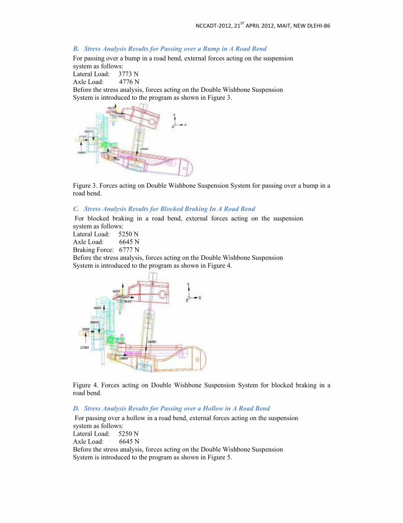
NCCADT-2012, 21ST


B. Stress Analysis Results for Passing over a Bump in A Road Bend

For passing over a bump in a road bend, external forces acting on the suspension system as follows: Lateral Load: 3773 N Axle Load: 4776 N Before the stress analysis, forces acting on the Double Wishbone Suspension System is introduced to the program as shown in Figure 3.

Figure 3. Forces acting on Double Wishbone Suspension System for passing over a bump in a road bend.

C. Stress Analysis Results for Blocked Braking In A Road Bend

For blocked braking in a road bend, external forces acting on the suspension system as follows: Lateral Load: 5250 N Axle Load: 6645 N Braking Force: 6777 N Before the stress analysis, forces acting on the Double Wishbone Suspension System is introduced to the program as shown in Figure 4.

Figure 4. Forces acting on Double Wishbone Suspension System for blocked braking in a road bend.

D. Stress Analysis Results for Passing over a Hollow in A Road Bend

For passing over a hollow in a road bend, external forces acting on the suspension system as follows: Lateral Load: 5250 N Axle Load: 6645 N Before the stress analysis, forces acting on the Double Wishbone Suspension System is introduced to the program as shown in Figure 5.

NCCADT-2012, 21ST


Figure 5. Forces acting on Double Wishbone Suspension System for passing over a hollow in a road bend.

Sl

no. Road Conditions

Force in the

Shock

Absorber

1. Position of the vehicle braking in a road bend

10698 N

2. Position of the vehicle at bump in a road bend

11564 N

3. Position of the vehicle blocked braking in a road bend

10698 N

4. Position of the vehicle passing over a hollow in a road bend

9832 N

Table1. Summary of the forces Maximum Value of the force exerting on the telescopic shock absorber member is under bump condition i.e. 11564 N.

6. ANALYSIS OF FRONT SHOCKER MOUNTING

All the forces are applied on the shocker mount assembly. The forces on the contact of the tire surface area to the ground are transmitted to the member of the suspension system. The final force value which is transmitted to the telescopic shock absorber is taken into consider. The force value and material properties are same for all the conditions.

The basic approach to the problem is the design changes in different scenario. The analysis is conducted on the different model and the deflection is noted. The design with minimum deflection will be recommended. The front suspension system assembly is shown below

Figure 6. Front Suspension System CASE -1

We will consider only the shocker assembly part not whole suspension system. The below figure shows the exploded view of the shocker assembly.

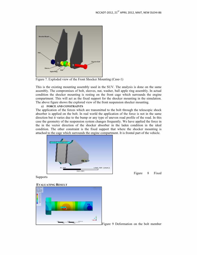
NCCADT-2012, 21ST


Figure 7. Exploded view of the Front Shocker Mounting (Case-1) This is the existing mounting assembly used in the SUV. The analysis is done on the same assembly. The compromises of bolt, sleeves, nut, washer, ball apple ring assembly. In actual condition the shocker mounting is resting on the front cage which surrounds the engine compartment. This will act as the fixed support for the shocker mounting in the simulation. The above figure shows the explored view of the front suspension shocker mounting.

a) FORCE AND CONSTRAINTS The application of the forces which are transmitted to the bolt through the telescopic shock absorber is applied on the bolt. In real world the application of the force is not in the same direction but it varies due to the bump or any type of uneven road profile of the road. In this case the geometry of the suspension system changes frequently. We have applied the force in the in the vector direction of the shocker absorber in the laden condition in the ideal condition. The other constraint is the fixed support that where the shocker mounting is attached to the cage which surrounds the engine compartment. It is frontal part of the vehicle.

Figure 8 Fixed Supports EVALUATING RESULT

Figure 9 Deformation on the bolt member

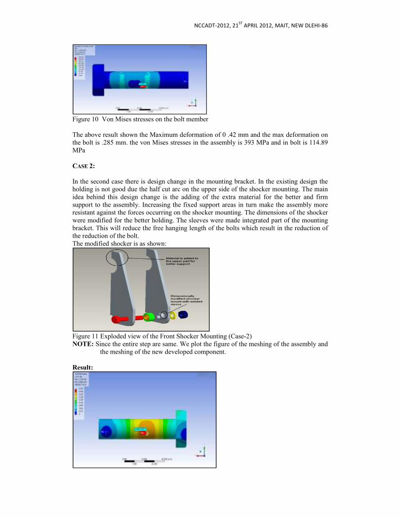
NCCADT-2012, 21ST


Figure 10 Von Mises stresses on the bolt member The above result shown the Maximum deformation of 0 .42 mm and the max deformation on the bolt is .285 mm. the von Mises stresses in the assembly is 393 MPa and in bolt is 114.89 MPa CASE 2:

In the second case there is design change in the mounting bracket. In the existing design the holding is not good due the half cut arc on the upper side of the shocker mounting. The main idea behind this design change is the adding of the extra material for the better and firm support to the assembly. Increasing the fixed support areas in turn make the assembly more resistant against the forces occurring on the shocker mounting. The dimensions of the shocker were modified for the better holding. The sleeves were made integrated part of the mounting bracket. This will reduce the free hanging length of the bolts which result in the reduction of the reduction of the bolt. The modified shocker is as shown:

Figure 11 Exploded view of the Front Shocker Mounting (Case-2) NOTE: Since the entire step are same. We plot the figure of the meshing of the assembly and

the meshing of the new developed component. Result:

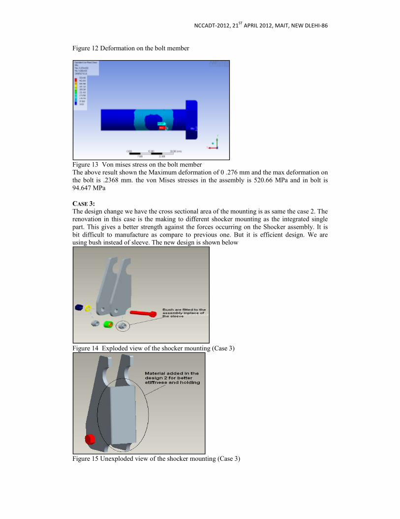
NCCADT-2012, 21ST



Figure 13 Von mises stress on the bolt member The above result shown the Maximum deformation of 0 .276 mm and the max deformation on the bolt is .2368 mm. the von Mises stresses in the assembly is 520.66 MPa and in bolt is 94.647 MPa CASE 3:

The design change we have the cross sectional area of the mounting is as same the case 2. The renovation in this case is the making to different shocker mounting as the integrated single part. This gives a better strength against the forces occurring on the Shocker assembly. It is bit difficult to manufacture as compare to previous one. But it is efficient design. We are using bush instead of sleeve. The new design is shown below

Figure 14 Exploded view of the shocker mounting (Case 3)

Figure 15 Unexploded view of the shocker mounting (Case 3)

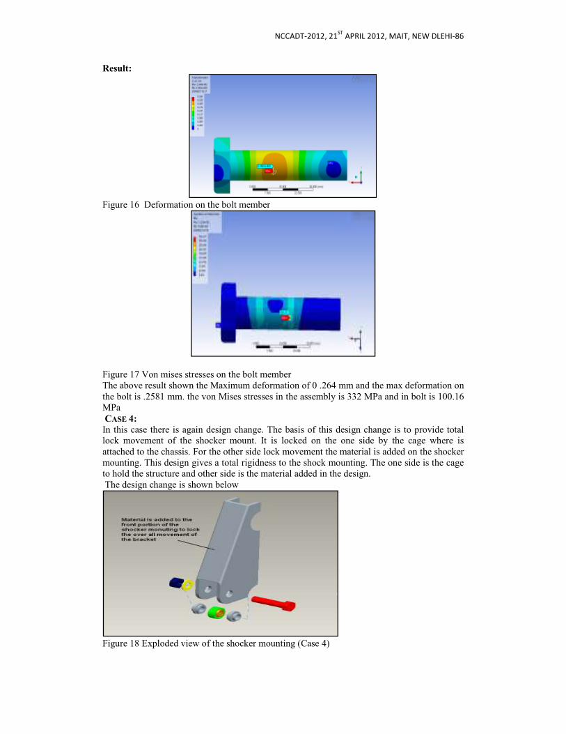
NCCADT-2012, 21ST


Result:


Figure 17 Von mises stresses on the bolt member The above result shown the Maximum deformation of 0 .264 mm and the max deformation on the bolt is .2581 mm. the von Mises stresses in the assembly is 332 MPa and in bolt is 100.16 MPa CASE 4: In this case there is again design change. The basis of this design change is to provide total lock movement of the shocker mount. It is locked on the one side by the cage where is attached to the chassis. For the other side lock movement the material is added on the shocker mounting. This design gives a total rigidness to the shock mounting. The one side is the cage to hold the structure and other side is the material added in the design. The design change is shown below

Figure 18 Exploded view of the shocker mounting (Case 4)

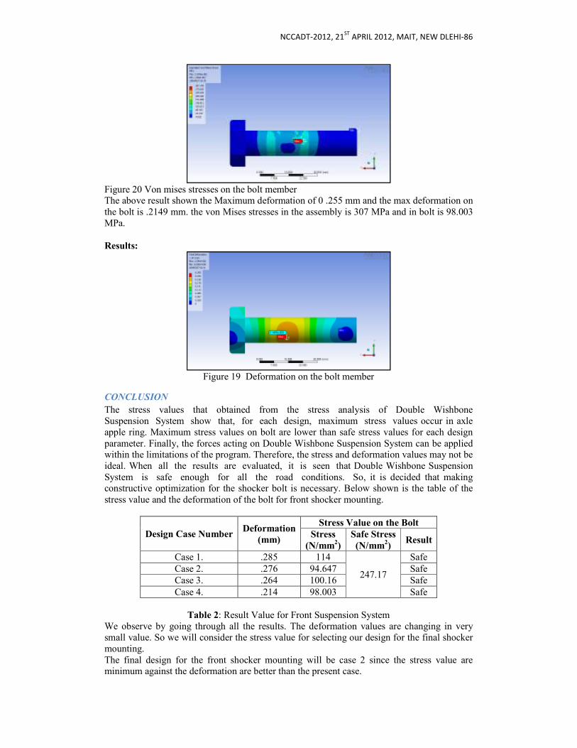
NCCADT-2012, 21ST


Figure 20 Von mises stresses on the bolt member The above result shown the Maximum deformation of 0 .255 mm and the max deformation on the bolt is .2149 mm. the von Mises stresses in the assembly is 307 MPa and in bolt is 98.003 MPa. Results:


CONCLUSION

The stress values that obtained from the stress analysis of Double Wishbone Suspension System show that, for each design, maximum stress values occur in axle apple ring. Maximum stress values on bolt are lower than safe stress values for each design parameter. Finally, the forces acting on Double Wishbone Suspension System can be applied within the limitations of the program. Therefore, the stress and deformation values may not be ideal. When all the results are evaluated, it is seen that Double Wishbone Suspension System is safe enough for all the road conditions. So, it is decided that making constructive optimization for the shocker bolt is necessary. Below shown is the table of the stress value and the deformation of the bolt for front shocker mounting.

Design Case Number Deformation

(mm)

Stress Value on the Bolt Stress

(N/mm2)

Safe Stress

(N/mm2)

Result

Case 1. .285 114

247.17

Safe Case 2. .276 94.647 Safe Case 3. .264 100.16 Safe Case 4. .214 98.003 Safe

Table 2: Result Value for Front Suspension System

We observe by going through all the results. The deformation values are changing in very small value. So we will consider the stress value for selecting our design for the final shocker mounting. The final design for the front shocker mounting will be case 2 since the stress value are minimum against the deformation are better than the present case.

NCCADT-2012, 21ST


REFERENCES:

1. Gwanghun Gim, Parviz E. Nikravesh “Joint coordinate method for analysis and design of multibody system”, KSME Journal, Vol. 7, No. I, pp. 26-34, 1993

2. Timothy M. Allred, “COMPLIANT MECHANISM SUSPENSIONS”, pp.56-65, August 2003

3. D N Siddhartha Jain, Ratnesh Kumar, “kinematic and dynamic analysis of independent suspension system”, Manipal Institute of Technology pp.70-74 May 2008

4. A.Van Berkum, “Chassis and suspension design”, Master’s Thesis, Technische Universiteit Eindhoven, Department of Mechanical Engineering, Section Dynamics and Control Technology pp.69-73, March 2006

5. V. Gavriloski ,D. Danev, K. Angushev, “Mechatronic approach in vehicle suspension system design”, 12th IFToMM World Congress, Besançon (France), June18-21, 2007

6. Brian Krall and Britt Pratt, “Rear Bottom Suspension Optimization”, pp. 11-18, March 14, 2003

7. Cary Henry, Michael Martha, Hussain Kheshroh, Ryan Prentiss, “FSAE Suspension Design” pp.26-37, Nov 11 2003

8. Prof II. Terje Rølvåg, “Design and optimization of Suspension Systems and Components” pp. 29-42, May 31, 2008

9. R Singh, “Dynamic design of automotive system: Engine mounts and structural joints”, Vol. 25, Part 3, June 2000, pp.319-330.

10. Christiaan Best, Chris Hamon, Guillermo Mezzatesta, “Basic Utility Vehicle Suspension Design” pp.9-18, Fall 2002

11. Shashidhar. C Soundararajan. S Sritharan. G ,Arunpreya., “design and mass optimization of independent multi link suspension for ride performance”

12. Kikuo Fujita, Noriyasu Hirokawa, Shinsuke Akagi, Takanori Hirata, “Design optimization of multi-link suspension system for total vehicle handling and stability”, American Institute of Aeronautics and Astronautics, AIAA-98-4787

13. Duygu GÜLER, “dynamic analysis of double wishbone suspension”, Master thesis, Department of Mechanical Engineering, Izmir Institute Of Technology, pp.3-14, July 2006.

14. Attia,H.A.,2002“Dynamic Modelling of the Double Wishbone Motor Vehicle Suspension System”, European Journal of Mechanics A/Solids, Volume 21,pp.167-174.

15. Chandrupatla, T.R. and Belegundu, A.D., 1997. “Beams and Frames”, in Introduction to Finite Elements in Engineering, (Prentice-Hall Inc., Upper Saddle River), p.238.

16. Gillespie, T.D., 1992. “Suspensions”, in Fundamentals of Vehicle Dynamics, (Society of Automotive Engineers, USA), pp.97-117 and pp.237-247.

17. Wang, F., 2001. “Passive Suspensions”, in Design and Synthesis of Active and Passive Vehicle Suspensions, PhD Thesis, Control Group Department of Engineering University of Cambridge, p.85.

18. Wong, J.Y., 1993. “Vehicle Ride Characteristics”, in Theory of Ground Vehicles, (John Wiley & Sons, Canada), pp.348-392.

19. X. L. Bian, B. A. Song, R. Walter “Optimization of steering linkage and double-wishbone suspension via R-W multi-body dynamic analysis, 2004, Springer.

20. Umut Erdem GÜNBA “Finite element stress analysis of front axle double wishbone suspension systems of vehicles for various road conditions”, 2004.

21. P. N. Belkhode, P. V. Washimkar and M. S. Dhande "Predication of Steering Geometry of Front Suspension using Experimental Data Based" IACSIT International Journal of Engineering and Technology, Vol.2, No.6, December 2010 ISSN: 1793-8236

22. X. L. Bian, B. A. Song, R. Walter "Optimization of steering linkage and double-wishbone suspension via R-W multi-body dynamic analysis." Volume 69, Number 1, December 2004 , pp. 38-43(6)

NCCADT-2012, 21ST


Simulation and Analysis of Counter Pressure

Hydroforming Process Manish Sharma

1, Md. Qamar Tanveer

2, Rakesh Chander Saini

3, Naveen Solanki

4, Ramakant

Rana5

1&2 Asst.Prof. in Mechanical Engg. Department of IPEC , 3,4 &5 Asst.Prof. in MAE. Department MAIT , Delhi

ABSTRACT:

The tube hydroforming process has gained increasing attention in recent years. Coordination

of the internal pressurization and axial feeding curves is critical in the tube hydroforming

process to generate successful parts without fracture or wrinkling failure. The stress state at a

given time and location varies with the process history and the design and control of the load

paths. A new process parameter, counter-pressure, is introduced to achieve a favorable tri-

axial stress state during the deformation process. The new process is referred to as Counter pressure hydroforming.

The benefits offered by Counter Pressure hydroforming will be characterized based upon the

amount of wall thinning and final bulged configuration. An analytical model is developed to analyze the stress and strain state in the part (tube) during the Counter Pressure

hydroforming process. The stress-strain condition analyzed will be used to evaluate and

compare thinning for tube hydroforming and Counter Pressure hydroforming. The effect of applying counter-pressure on thin-walled tubes with only internal pressure and combination

of internal pressure and independent axial loading is considered. Finite element analysis is

used to quantify the merits of Counter Pressure hydroforming in terms of final bulged

configuration. A parametric study has been conducted to investigate the effectiveness of

Counter Pressure hydroforming based on the various material properties and process

conditions.

Counter Pressure hydroforming results in different stress and strain states compared to tube

hydroforming. The counter-pressure enabled favorable tri-axial stress state during

deformation that resulted in different thickness and percentage thinning. Finite element analysis showed that for a particular amount of wall thinning there is an increase of around

8% in bulge height for Counter Pressure hydroforming.

Results of this study indicate that Counter Pressure hydroforming can increase expansion i.e. more difficult parts can be designed and manufactured. Also, for a given part geometry,

higher strength and less formable materials can be used.

1. INTRODUCTION

Tube hydroforming has been well-known since the 1950’s. Tube hydroforming has been called by many other names such as bulge forming of tubes (BFT’s), liquid bulge forming (LBF) and hydraulic (or hydrostatic) pressure forming (HPF) depending on the time and country in which it was used [1]. Tube hydroforming (THF) has become a viable method for manufacturing complex automobile parts and an indispensable manufacturing technique in recent years. Hydroformed tube parts have improved strength and stiffness, lower tooling cost, fewer secondary operations, and closed dimensional tolerances compared to stamping processes, thus an overall reduced manufacturing cost [1]. Success of the tube hydroforming process depends on an appropriate combination of loading curve (internal pressure and axial feed at the tube ends), material properties and process conditions. One of the key concerns is to control the deformation process in order to maximize the expansion so that more complex shapes in various applications can be achieved. Analogously, for a given shape a higher strength, lighter weight, less formable, or lower cost material can be adopted. 1.1 Scope of work

The benefits offered by counter pressure hydroforming will be characterized based upon their effect on the amount of thinning and final bulged configuration. The present work is broadly divided into two main categories listed below.

NCCADT-2012, 21ST


a) The stress state at a given time and location varies with the process history and the design and control of the load paths. Since the loading condition in counter pressure hydroforming is different from that of the tube hydroforming, an analytical model is developed to analyze the stress and strain state in the part during the counter pressure hydroforming process. The stress strain condition analyzed will be used to evaluate and compare thinning for tube hydroforming and counter pressure hydroforming processes. The effect of applying counter pressure is also evaluated using finite element simulations based on the final configuration achieved.

2. ANALYSIS OF COUNTER PRESSURE HYDROFORMING

2.1 Procedure of Analysis The Finite element simulation was carried out on LS-DYNA. The pre-processing was done on HYPERMESH. Post –processing was done on HYPERVIEW. The rigid tooling of tube hydroforming consists of (1) Die and (2) Axial punch. The entire pre-processing process can be divided into five steps: 4.1.1 Creating collectors 4.1.2 Creating geometry 4.1.3 Applying boundary condition 4.1.4 Updating cards 4.1.5 Control cards 2.1.1 Creating Collectors

Four types of collectors were created material (mat), property (prop), component (comp) and load collector. 2.1.1.1 Material Collector (*MAT) Material Collector assigns the material properties to the part. Since Counter pressure hydroforming consists of total 3 parts (2 rigid parts and tube), 3 material collectors were created. All the collectors are named according to the part. All the rigid toolings are specified *MAT_RIGID (MAT 20) which is the default rigid material for LS-DYNA. Tube was assigned *MAT_PIECEWISE_LINEAR_PLASTICITY (MAT24). 2.1.1.2 Property Collector (*SECTION_SHELL) One shell section is created for die and punch and one for tube. Each section is assigned the corresponding part. 2.1.1.3 Component Collector (*PART) Three component collectors were created and corresponding materials are assigned to each of them. a) Die – Rigid b) Punch – Rigid c) Tube – Piecewise linear plastic material 2.1.1.4 Load Collector (*BOUNDARY_PRESCRIBED_MOTION_RIGID) A load collector for axial punch movement is created wherein displacement boundary condition in the y direction is prescribed. 2.1.2 Creating Geometry Here a brief description is provided for modeling the parts of Counter Pressure hydroforming process. Before starting to model any part, it is important to select the collector corresponding to the part to be modeled from the global menu. By this all the nodes and the elements that are created are assigned the property of that component. 2.1.2.1 Tube

Modeling of the tube was done using the user controlled cylinder. For this first the nodes were created for selecting the center of the die, major direction and normal direction. Radius, angle of the cylinder and the element density was used to complete the modeling. 2.1.2.2 Die Modeling of the die was done using three user controlled cylinders and then trimming off the unnecessary geometry and filleting the corners. 2.1.2.3 Punch

NCCADT-2012, 21ST


Modeling of the punch was done using user controlled cylinder and combination of circle feature in geometry panel and spline function in 2d panel. 2.1.3 Boundary Condition

2.1.3.1 Contact

For defining the contact between different surface pair’s two different types of contact algorithm were used. 2.1.3.1.1 CONTACT_SURFACE_TO_SURFACE_TITLE

This is used to define the surface contact between Tube- die and Tube – punch. Contact option is specified by selecting master surface and the slave surface. The rigid part was always selected as the master surface and the tube (which is finely meshed) was always selected as the slave surface. The coefficient of static and dynamic friction between the Tube-die was specified as 0.10 and 0.00 respectively. The coefficient of static friction between the tube-punch was specified as 0.30. 2.1.3.1.2 Contact_Single_Surface_Title This is used to define contact for tube in the case of wrinkling. This contact definition would be used if tube surface comes in contact with itself, in case of wrinkling. 2.1.3.2 Pressure An internal pressure of 40 MPa was applied to the tube. All the elements of the pressure component were selected. The magnitude and uniform size was specified. In a shell element pressure always acts in the direction of the normal so to reverse the direction of the pressure negative value of magnitude must be specified. The external counter pressure was applied using LOAD_MASK option in LS-DYNA, which facilitates to apply a distributed load to a subset of elements of tube within a fixed global box. 2.1.3.3 Checking Penetration Penetration option form the tools page was selected. Penetration check was done for a specified contact pair (interface). To avoid penetration two things have to be kept in mind, the normal of the contact pairs should be opposite to each other. If both the normal point towards each other then normal of one of the surface has to be reversed from the normal menu on the tool’s page. The slave surface (tube) should have a finer mesh than the master surface (rigid part). If there is a penetration then the element size of the tube needs to be decreased. 2.1.4 Updating Cards This is the last step in creating the input deck. 2.1.4.1 Mat Collector We have three materials made one for each part. Material property was specified by selecting the material collector. The property specified were: Young’s modulus, density, poisons ratio. It is essential that units should be consistent because LS –DYNA does not have an inbuilt unit. The units selected here are:

Table 2-1: Units used in Simulation Mass Ton

Force N

Pressure MPa

Time Sec

Displacement Mm The other important thing which was specified is the translational and the rotational constraint of the rigid body. 2.1.4.1.1 Die Die was constrained in all translational as well as rotational degree of freedoms. 2.1.4.1.2 Punch

NCCADT-2012, 21ST


Punch was constrained for x and z translation and rotations in all three axes. Only punch displacement in y direction was allowed. 2.1.4.1.3 Tube Since only quarter model of the tube was discretized, it was necessary to constraint tube according to symmetric boundary conditions. 2.1.4.2 Property Collector Shell element, thickness and NIP (number of integration points) was specified for each shell segment. Four noded, Belytschko- Tsay with 5 NIP having a thickness of 1.37 mm was specified for the tube and Belytschko- Tsay with 2 NIP and thickness of 2.00 mm was specified for the rigid parts. 2.1.4.3 Component Collector Material and section property is applied to the component (*PART) in this. 2.1.4.4 Load Collector The translation of the punch was specified using *BOUNDARY_PRESCRIBED_MOTION_RIGID. Displacement boundary condition and load curve were defined. The load curve defines the displacement of the punch with respect to the time. 2.1.5 Control Cards

At the end control cards were added. By these cards the termination time, shell property, contact property and data base plots are defined. 2.2 Analytical Model

Tube deformation is controlled by ‘gradually’ increasing the internal pressure during the application of axial load (Fig. 2-1). The stress state at a given time and location varies with the process history, and the design and control of the load paths. In counter pressure hydroforming an additional process parameter, counter-pressure is added to achieve controlled deformation (Fig. 2-1). The counter pressure hydroforming process will have a different stress state at a given time and location as compared to tube hydroforming.

Figure 2-1: THF and CPHF

Tube hydroforming and Counter Pressure hydroforming will have different stress and strain state in the part. This will result in different wall thinning. The stress and the strain state at the mean diameter of the tube for tube hydroforming can be predicted using the analytical model developed by Ahmed et al [25]. To predict the stress and the strain state at the mean diameter of the tube for Counter Pressure hydroforming a counter pressure term (po) was added to the model already developed by Ahmed et al [25]. The model was developed using the von Mises criterion instead of the Tresca criterion. 2.3 Results and Discussion

(a) Analytical Results

To demonstrate the effect of counter pressure on the thickness change and the estimation of axial force, the following example is considered (Table 2-2).

NCCADT-2012, 21ST


Table 2-2: Properties of a Tube Inner radius, mm A 12.06 Outer radius, mm B 13.43 Initial thickness, mm to 1.37 Length of tube, mm L 107 Punches enter a length, mm x0 10 Unconstrained length, mm X 87 Coefficient of friction M 0.1 Internal pressure, MPa pi 40 Counter pressure, MPa po 7 Yield Strength, MPa σyp 160 Strength coefficient, MPa K 500 Strain hardening exponent, MPa N 0.35

Using the methodology derived earlier, the following parameters were calculated for tube hydroforming and Counter Pressure hydroforming. Counter Pressure hydroforming results in a different stress and a strain state at the mean diameter of the tube. This resulted in different thickness and percentage thinning as given in Table 2-3.

Table 2-3: Difference in Stress and Strain State and Thickness for THF and CPHF

Tube hydroforming produced a thinning of 5.32 % while counter pressure hydroforming produced is 5.09 %. The new process parameter enabled favorable tri-axial stress state during the deformation. The counter pressure provided the back support to the tube material and hence produced the lesser thinning. Inversely, larger tube expansion can be achieved for the given amount of thinning.

(b) Finite Element Analysis –Thinning

The internal hydraulic pressure of 40 MPa was applied as a uniformly distributed load to the tube inner surface. The internal pressure was introduced as a linearly increasing function of time. The axial stroke of 12 mm was applied as a prescribed displacement of the punch. The external counter pressure of 7 MPa was also applied as a linearly increasing function of time. Two different loading conditions were analyzed. The initial run was conducted without applying the external counter pressure (Load Pattern 1 shown in Fig. 2-7 (THF)). Keeping the same internal pressure and axial feed curves, the analysis followed with the application of external counter pressure (Load Pattern 2 shown in Fig. 2-8 (CPHF)).

Tube Hydroforming Counter pressure Hydroforming

Axial Stress, σz (MPa) -229.867 -233.367

Radial Stress, σr (MPa) -10.230 -17.230

Hoop Stress, σθ (MPa) -120.049 -125.299

Effective Stress, : (MPa) 190.211 187.180

Effective Strain, = 0.0632 0.0604

Thickness, ti (mm) 1.2970 1.3002

Percentage Thinning, % 5.32 5.09

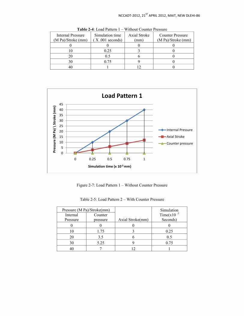
NCCADT-2012, 21ST


Table 2-4: Load Pattern 1 – Without Counter Pressure

Internal Pressure (M Pa)/Stroke (mm)

Simulation time ( X .001 seconds)

Axial Stroke (mm)

Counter Pressure (M Pa)/Stroke (mm)

0 0 0 0 10 0.25 3 0 20 0.5 6 0 30 0.75 9 0 40 1 12 0

Figure 2-7: Load Pattern 1 – Without Counter Pressure

Table 2-5: Load Pattern 2 – With Counter Pressure

Pressure (M Pa)/Stroke(mm)

Axial Stroke(mm)

Simulation Time(x10 -3

Seconds) Internal Pressure

Counter pressure

0 0 0 0

10 1.75 3 0.25

20 3.5 6 0.5

30 5.25 9 0.75

40 7 12 1

0

5

10

15

20

25

30

35

40

45

0 0.25 0.5 0.75 1

Pre

ssu

re (

M P

a)

\S

tro

ke

(m

m)

Simulation time (x 10-3 mm)

Load Pattern 1

Internal Pressure

Axial Stroke

Counter pressure

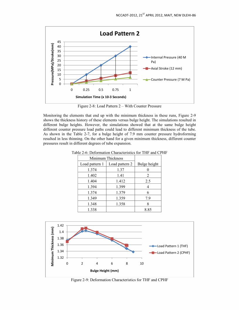
NCCADT-2012, 21ST


Figure 2-8: Load Pattern 2 – With Counter Pressure

Monitoring the elements that end up with the minimum thickness in these runs, Figure 2-9 shows the thickness history of these elements versus bulge height. The simulations resulted in different bulge heights. However, the simulations showed that at the same bulge height different counter pressure load paths could lead to different minimum thickness of the tube. As shown in the Table 2-7, for a bulge height of 7.9 mm counter pressure hydroforming resulted in less thinning. On the other hand for a given minimum thickness, different counter pressures result in different degrees of tube expansion.

Table 2-6: Deformation Characteristics for THF and CPHF

Minimum Thickness

Bulge height Load pattern 1 Load pattern 2

1.374 1.37 0

1.402 1.41 2

1.404 1.412 2.5

1.394 1.399 4

1.374 1.379 6

1.349 1.359 7.9

1.348 1.358 8

1.338 8.85

Figure 2-9: Deformation Characteristics for THF and CPHF

0

5

10

15

20

25

30

35

40

45

0 0.25 0.5 0.75 1

Pre

ssu

re(M

Pa

)/S

tro

ke

(mm

)

Simulation Time (x 10-3 Seconds)

Load Pattern 2

Internal Pressure (40 M

Pa)

Axial Stroke (12 mm)

Counter Pressure (7 M Pa)

1.32

1.34

1.36

1.38

1.4

1.42

0 2 4 6 8 10

Min

imu

m T

hic

kn

ess

(m

m)

Bulge Height (mm)

Load Pattern 1 (THF)

Load Pattern 2 (CPHF)

NCCADT-2012, 21ST


Table 2-7: Bulge Height, Minimum Thickness and Percentage Thinning for THF and CPHF

Bulge Height (mm)

Minimum thickness (mm)

Percentage Thinning

Load Pattern 1, THF 7.90 1.349 1.53 Load Pattern 2, CPHF 7.90 1.359 0.80

Thus, it can be concluded that the different and the favorable stress and strain distributions resulted in less thinning in the case of counter pressure hydroforming. Figure 2-10 and Fig.2-11 show the distribution of the effective stress and the strain for the tube and the counter pressure hydroforming respectively.

Table 2-8: Effective Stress Plot for THF and CPHF

Effective Stress (MPa) Bulge Height

(mm) Load Pattern

1 Load Pattern

2

140 140 0

210 210 2

270 260 4

290 280 6

330 315 8

360 10

Figure 2-10: Effective Stress Plot for THF and CPHF

Table 2-9: Effective Strain Plot for THF and CPHF

Effective Strain Bulge Height

0

50

100

150

200

250

300

350

400

0 2 4 6 8 10 12

Eff

ect

ive

Str

ess

(M

Pa

)

Bulge Height (mm)



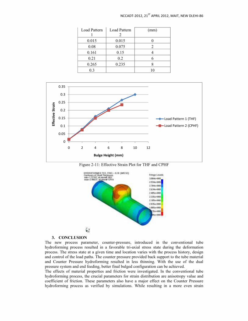
NCCADT-2012, 21ST


Load Pattern 1

Load Pattern 2

(mm)

0.015 0.015 0

0.08 0.075 2

0.161 0.15 4

0.21 0.2 6

0.265 0.235 8

0.3 10

Figure 2-11: Effective Strain Plot for THF and CPHF

3. CONCLUSION

The new process parameter, counter-pressure, introduced in the conventional tube hydroforming process resulted in a favorable tri-axial stress state during the deformation process. The stress state at a given time and location varies with the process history, design and control of the load paths. The counter pressure provided back support to the tube material and Counter Pressure hydroforming resulted in less thinning. With the use of the dual pressure system and end feeding, better final bulged configuration can be achieved. The effects of material properties and friction were investigated. In the conventional tube hydroforming process, the crucial parameters for strain distribution are anisotropy value and coefficient of friction. These parameters also have a major effect on the Counter Pressure hydroforming process as verified by simulations. While resulting in a more even strain

0

0.05

0.1

0.15

0.2

0.25

0.3

0.35

0 2 4 6 8 10 12

Eff

ect

ive

Str

ain

Bulge Height (mm)



NCCADT-2012, 21ST


distribution, the dual tube hydroforming process becomes meritorious in low anisotropy and/or high friction conditions. The process can be introduced to achieve larger expansion and more complex deformation geometry. Also, converting to a higher strength and less formable materials becomes possible.

4. FUTURE WORK As part of future work, effect of material properties, optimization of loading paths can be considered to obtain a superior final bulged configuration. An analytical model could be developed to demonstrate the effect of counter pressure in delaying the onset of Plastic instability and reducing wrinkling. This work only establishes the merit of applying counter pressure. Work has to be done in the area of die and tooling design and implementation of counter pressure in industry. REFERENCES

1. Koc M., and Altan T., 2001, “An overall review of the tube hydroforming (THF) technology,” Journal of Materials Processing and Technology, 108

(3), pp. 384-393. 2. Hosford W.F., and Caddell, R.M., 1983, Metal Forming Mechanics and

Metallurgy, Prentice Hall, Inc., Englewood Cliffs, NJ. 3. Rogersand H.C., and Coffin L.F., Jr., 1967, Final Report, Contract No-66-

0546-d, Naval Air Systems Command. 4. Cockcroft M.G., and Latham D.J., 1968, “Ductility and the workability of

metals,” Journal of Institute of Metals, 96, pp. 33-39. 5. Finckenstein, E., Kleiner, M., Homberg, W., and Szucs, E., 1998, “In-process

punching with pressure fluids in sheet metal forming,” Annals of the CIRP, 47, pp. 207-212.

6. Thiruvarudchel, van S., and Wang, H., 1998, “Hydraulic pressure enhancement of the deep drawing process to yield deeper cups,” Journal of Materials Processing Technology, 82, pp. 156-164.

7. Hein, P. and Vollertsen, F., 1999 “Hydroforming of sheet metal pairs,” Journal of Materials Processing Technology, 87 (1-3), pp. 154-164.

8. Liu, J., Atmetoglu, M., and Altan, T, 2000, “Evaluation of sheet metal formability, viscous pressure forming (VPF) dome test,” Journal of Material Processing Technology, 98, pp. 1-6.

9. Lo, S.-W., Hsu, T.-Z., and Wilson, W. R. D., 1993, “An analysis of the hemispherical-punch hydroforming processes,” Journal of Material Processing Technology, 37, pp. 225-239.

10. Yossifon S., Tirosh J., and Kochavi E., 1984, “On suppression of plastic buckling in hydroforming processes,” International Journal of Mechanical Science, 26 (6-8), pp. 389-402.

11. Yossifon, S. and Tirosh, J., 1985, “Rupture instability in hydroforming deep-drawing process,” International Journal of Mechanical Science, 27 (9), pp. 559-570.

12. Ahmed M., and Hashmi M.S.J., 1997, “Comparison of free and restrained bulge forming by finite element method simulation,” Journal of Materials Processing Technology, 63, pp. 651-654.

13. Nakagawa T., Nakamura K., and Amino H., 1997, “Various applications of hydraulic counter-pressure deep drawing,” Journal of Materials Processing Technology, 71, pp. 160-167.

14. Amino H., Nakamura K., and Nakagawa T., 1990, “Counter-pressure deep drawing and its application in the forming of automobile parts,” Journal of Materials Processing Technology, 23, pp. 243-265.

15. Koc M., and Altan T., 2002, “Prediction of forming limits and parameters in the tube hydroforming process,” International Journal of Machine Tools & Manufacture, 42, pp. 123-138.

16. Mellor P. B., 1962, “Tensile instability in thin-walled tubes,” Journal of Mechanical Engineering Science, 4, pp. 251-256.

NCCADT-2012, 21ST


17. Hillier M.J., 1963, “Tensile plastic instability under complex stress,” International Journal of Mechanical Science, 5, pp. 57-67.

18. Hillier M.J., 1965, “Tensile plastic instability of thin tubes - I,” International Journal of Mechanical Science, 7, pp. 531 – 538.

19. Chakrabarty J., and Alexander J.M., 1969, “Plastic instability of thick-walled tubes with closed ends,” International Journal of Mechanical Science, 1, pp.175-186.

20. El-Sebaie M.G., and Mellor P.B., 1973, “Plastic instability conditions when deep-drawing into a high pressure medium,” International Journal of Mechanical Science, 15, pp. 485-501.

21. Carleer B., van der Kevie G., de Winter L., and van Veldhuizen B., 2000, “Analysis of the effect of material properties on the hydroforming process of tubes,” Journal of Materials Processing Technology, 104, pp. 158 – 166.

22. Manabe K., and Amino M., 2002, “Effects of process parameters and material properties on deformation process in tube hydroforming,” Journal of Materials Processing Technology, 123, pp. 285 – 291.

23. Bodeau N., Lejeune A., and Gelin J. C., 2002, “Influence of material and process parameters on the development and bursting in flange and tube hydroforming,” Journal of Materials Processing Technology, 125 – 126, pp. 849 – 855.

24. Koc M., 2003, “Investigation of the effect of loading path and variation in material properties on robustness of the tube hydroforming process,” Journal of Materials Processing Technology, 133, pp. 276 – 281.

25. Ahmed M., and Hashmi M.S.J., 1997, “Estimation of machine parameters for hydraulic bulge forming of tubular components,” Journal of Materials Processing Technology, 64, pp. 9-23.

26. Asnafi N., and Skogsgardh A., 2000, “Theoretical and experimental analysis of stroke controlled tube hydroforming,” Materials Science and Engineering, A279, pp. 95-110.

27. Rimkus W., Bauer H., and Mihsein M.J.A., 2000, “Design of load-curves for hydroforming applications,” Journal of Materials Processing Technology, 108, pp. 97-105.

28. T. Sokolowski, K. Gerke, M. KocË, M. Ahmetoglu, and T. Altan, 1998, “Evaluation of tube formability and material characteristics in tube hydroforming,” ERC/NSM Report No. THF/ERC/NSM-98-R-025, Ohio State University, Columbus, OH.

29. Dohmann F., and Hartl C., 1996, “Hydroforming – a method to manufacture light weight parts,” Journal of Materials Processing and Technology, 60, pp. 669-676.

30. Website of Variform (http://www.vari-form.com/index.shtml), “Automotive Applications,” Variform, Warren, MI.

31. Ahmetoglu M., and Altan T., 2000, “Tube hydroforming: state-of-the-art and future trends,” Journal of Materials Processing Technology, 98, pp. 25 – 33.

32. Vollertsen F., and Plancak M., 2002, “On possibilities for the determination of the coefficient of friction in hydroforming of tubes,” Journal of Materials Processing Technology, 59 (39), pp. 1-9.

33. Hutchinson M.I., 1988, “Bulge forming of tubular components,” Ph.D. Thesis, Sheffield City Polytechnic, Sheffield, United Kingdom.

34. MacDonald B.J., and Hashmi M.S.J., 2000, “Finite element simulation of bulge forming of a cross-joint from tubular blank,” Journal of Materials Processing Technology, 103, pp. 333-342.

35. Duncan J. L., Hu J., and Marciniak Z., Mechanics of Sheet Metal Forming, Butterworth-Heinemann, Woburn, MA.

36. Asnafi N., 1999, “Analytical modeling of tube hydroforming,” Thin-Walled Structures, 34, pp. 295-330.

NCCADT-2012, 21ST


Productivity Improvement in manufacturing Industry using

Total Quality Management Garima Sharma, Piu Jain

Department of Mechanical & Automation Engineering, Maharaja Agrasain Institute of Technology, Sector 22, Rohini, ,New Delhi.E-mail : @[email protected] , @[email protected]

Abstract The integration of today’s world market leads to globalization in industries and

manufacturing firms. The effect of such globalization is manifold: price competition has

become tougher, product diversification is in higher demand, and safety and reliability of

goods have become indispensable, higher standards of quality in developed countries are also

being applied to markets in developing countries, and so on. In such situation, meting the

customer requirements and business targets becomes difficult. A number of tools and

techniques are available to the modern day managers which can help in effecting such

changes. For such complex situation, TQM proves to be an effective tool for meeting the business goals.

The major challenge faced in a flow process type industry to improve productivity is to

eliminate bottlenecks and reduce cycle time. A flow shop consists of a set of facilities through which work flows in a serial fashion. Methodology adopted for cycle time reduction is time

and motion study, automation, layout improvement by process flow analysis etc.

In the current research, focus is to develop a system to reduce/eliminate bottlenecks, reduce cycle time and cost reduction leading to enhanced productivity. This project is based on

applying the TQM tools for reducing cycle time and increase productivity in a flow type

process industry.

Keywords— TQM, Productivity, Cycle Time, Process Chart, Control Chart.

I. INTRODUCTION The globalization of markets, growing interpenetration of economies, and increased interdependence of economic agents are reshaping the international and national competitive environment. These fundamental changes are prompting the far sighted organizations to re-examine and modify their competitive strategies The interpenetration of economies, and increased interdependence of economic agents are reshaping the international and national competitive environment competitive strategies. Such globalization of markets has affected not only exporters and importers but also domestic players, even small companies, in many ways: price competition has become tougher, product diversification is in higher demand, and safety and reliability of goods have become indispensable, higher standards of quality in developed countries are also being applied to markets in developing countries, and so on. TQM is a combination of quality and management tools through which management and employees can become involved in the continuous improvement of production of goods and services. Total quality management is an approach to the art of management that is originated in the Japanese industry in the 1950’s and has become steadily more popular in the West since the early 1980’s. Its origin can be traced in the work of so called quality Gurus – Juran, Deming, Ishikawa, Crossby, Feigenbaun and countless other people that have studied practiced and tried to refine the process of organizational management. Quality must be designed into the service or built into the product as part of the process. Thus getting thing right the first time, every time is the result of process improvements. Quality management focuses on the needs and wishes of the external customer. This paper discusses concepts of TQM for implementation in manufacturing. This approach should assist companies who are selecting or forming a TQM implementation strategy A second challenge to providers of goods and services is that their stakeholder base has been substantially broadened, and consequently, their social responsibilities have enlarged. The requirement for environmental consideration is a typical example. Another one, product

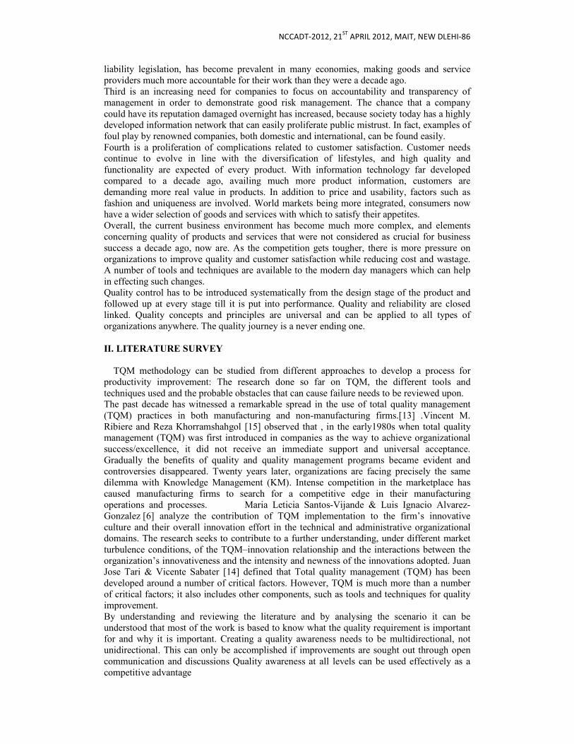
NCCADT-2012, 21ST


liability legislation, has become prevalent in many economies, making goods and service providers much more accountable for their work than they were a decade ago. Third is an increasing need for companies to focus on accountability and transparency of management in order to demonstrate good risk management. The chance that a company could have its reputation damaged overnight has increased, because society today has a highly developed information network that can easily proliferate public mistrust. In fact, examples of foul play by renowned companies, both domestic and international, can be found easily. Fourth is a proliferation of complications related to customer satisfaction. Customer needs continue to evolve in line with the diversification of lifestyles, and high quality and functionality are expected of every product. With information technology far developed compared to a decade ago, availing much more product information, customers are demanding more real value in products. In addition to price and usability, factors such as fashion and uniqueness are involved. World markets being more integrated, consumers now have a wider selection of goods and services with which to satisfy their appetites. Overall, the current business environment has become much more complex, and elements concerning quality of products and services that were not considered as crucial for business success a decade ago, now are. As the competition gets tougher, there is more pressure on organizations to improve quality and customer satisfaction while reducing cost and wastage. A number of tools and techniques are available to the modern day managers which can help in effecting such changes. Quality control has to be introduced systematically from the design stage of the product and followed up at every stage till it is put into performance. Quality and reliability are closed linked. Quality concepts and principles are universal and can be applied to all types of organizations anywhere. The quality journey is a never ending one. II. LITERATURE SURVEY

TQM methodology can be studied from different approaches to develop a process for

productivity improvement: The research done so far on TQM, the different tools and techniques used and the probable obstacles that can cause failure needs to be reviewed upon. The past decade has witnessed a remarkable spread in the use of total quality management (TQM) practices in both manufacturing and non-manufacturing firms.[13] .Vincent M. Ribiere and Reza Khorramshahgol [15] observed that , in the early1980s when total quality management (TQM) was first introduced in companies as the way to achieve organizational success/excellence, it did not receive an immediate support and universal acceptance. Gradually the benefits of quality and quality management programs became evident and controversies disappeared. Twenty years later, organizations are facing precisely the same dilemma with Knowledge Management (KM). Intense competition in the marketplace has caused manufacturing firms to search for a competitive edge in their manufacturing operations and processes. Maria Leticia Santos-Vijande & Luis Ignacio Alvarez-Gonzalez [6] analyze the contribution of TQM implementation to the firm’s innovative culture and their overall innovation effort in the technical and administrative organizational domains. The research seeks to contribute to a further understanding, under different market turbulence conditions, of the TQM–innovation relationship and the interactions between the organization’s innovativeness and the intensity and newness of the innovations adopted. Juan Jose Tari & Vicente Sabater [14] defined that Total quality management (TQM) has been developed around a number of critical factors. However, TQM is much more than a number of critical factors; it also includes other components, such as tools and techniques for quality improvement. By understanding and reviewing the literature and by analysing the scenario it can be understood that most of the work is based to know what the quality requirement is important for and why it is important. Creating a quality awareness needs to be multidirectional, not unidirectional. This can only be accomplished if improvements are sought out through open communication and discussions Quality awareness at all levels can be used effectively as a competitive advantage

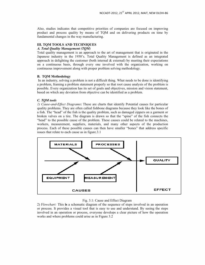
Also, studies indicates that competitive priorities of companies are focused on improving product and process quality by means of TQM and on delivering products on time by fundamental changes in the way manufacturing. III. TQM TOOLS AND TECHNIQUES

A. Total Quality Management (TQM

Total quality management is an approach to the art of management that is originated in the Japanese industry in the 1950’s. Total Quality Management approach in delighting the customer (both internal & external) by meeting their expectations on a continuous basis, through every one involved with the organization, working on continuous improvement along with proper problem so

B. TQM Methodology

In an industry, solving a problem is not a difficult thing. What needs to be done is identifying a problem, framing a problem statement properly so that root cause analysis of the problem is possible. Every organization has its set of goals and objectives, mission and vision statement, based on which any deviation from objective can be identified as a problem.

C. TQM tools

1) Cause-and-Effect Diagrams:

quality problems. They are often called fishbone diagramsa fish. The “head” of the fish is the quality problem, such as damaged zippers on a garment or broken valves on a tire. The diagram is drawn so that th“head” to the possible cause of the problem. These causes could be related to the machines, workers, measurement, suppliers, materials, and many other aspects of the production process. Each of these possible causes can tissues that relate to each cause as in figure.3.1

2) Flowchart: This is a schematic diagram of the sequence of steps involved in an operation or process. It provides a visual tool that is easy to use and understand. By seeing the steps involved in an operation or process, everyone develops a clear picture of how the operation works and where problems could arise as in Figure 3.2

NCCADT-2012, 21ST


Also, studies indicates that competitive priorities of companies are focused on improving product and process quality by means of TQM and on delivering products on time by

mental changes in the way manufacturing.

III. TQM TOOLS AND TECHNIQUES

A. Total Quality Management (TQM)

Total quality management is an approach to the art of management that is originated in the Japanese industry in the 1950’s. Total Quality Management is defined as an integrated approach in delighting the customer (both internal & external) by meeting their expectations on a continuous basis, through every one involved with the organization, working on continuous improvement along with proper problem solving methodology.

In an industry, solving a problem is not a difficult thing. What needs to be done is identifying a problem, framing a problem statement properly so that root cause analysis of the problem is

organization has its set of goals and objectives, mission and vision statement, based on which any deviation from objective can be identified as a problem.

: These are charts that identify Potential causes for quality problems. They are often called fishbone diagrams because they look like the bones of a fish. The “head” of the fish is the quality problem, such as damaged zippers on a garment or broken valves on a tire. The diagram is drawn so that the “spine” of the fish connects the “head” to the possible cause of the problem. These causes could be related to the machines, workers, measurement, suppliers, materials, and many other aspects of the production process. Each of these possible causes can then have smaller “bones” that address specific issues that relate to each cause as in figure.3.1

Fig. 3.1: Cause and Effect Diagram a schematic diagram of the sequence of steps involved in an operation

sual tool that is easy to use and understand. By seeing the steps involved in an operation or process, everyone develops a clear picture of how the operation works and where problems could arise as in Figure 3.2


Also, studies indicates that competitive priorities of companies are focused on improving product and process quality by means of TQM and on delivering products on time by

Total quality management is an approach to the art of management that is originated in the is defined as an integrated

approach in delighting the customer (both internal & external) by meeting their expectations on a continuous basis, through every one involved with the organization, working on

In an industry, solving a problem is not a difficult thing. What needs to be done is identifying a problem, framing a problem statement properly so that root cause analysis of the problem is

organization has its set of goals and objectives, mission and vision statement,

Potential causes for particular because they look like the bones of

a fish. The “head” of the fish is the quality problem, such as damaged zippers on a garment or e “spine” of the fish connects the

“head” to the possible cause of the problem. These causes could be related to the machines, workers, measurement, suppliers, materials, and many other aspects of the production

hen have smaller “bones” that address specific

a schematic diagram of the sequence of steps involved in an operation sual tool that is easy to use and understand. By seeing the steps

involved in an operation or process, everyone develops a clear picture of how the operation

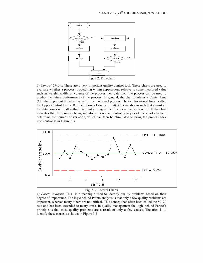
3) Control Charts: These are a very important quality control tool. These charts are used to evaluate whether a process is operating within expectations relative to some measured value such as weight, width, or volume ofpredict the future performance of the process. In general, the chart contains a Center Line (CL) that represent the mean value for the inthe Upper Control Limit(UCL) and Lower Control Limit(LCL) are shownthe data points will fall within this limit as long as the process remains inindicates that the process being monitored is not in control, analysis of the chart can help determine the sources of variation, whichinto control as in Figure 3.3

4) Pareto analysis: This is a technique used to identify quality problems based on their degree of importance. The logic behind Pareto analysis isimportant, whereas many others are not critical. This concept has often been called the 80rule and has been extended to many areas. In quality management the logic behind Pareto’s principle is that most quality proidentify these causes as shown in Figure 3.4

NCCADT-2012, 21ST


Fig. 3.2: Flowchart

are a very important quality control tool. These charts are used to evaluate whether a process is operating within expectations relative to some measured value such as weight, width, or volume of the process then data from the process can be used to predict the future performance of the process. In general, the chart contains a Center Line (CL) that represent the mean value for the in-control process. The two horizontal lines , called the Upper Control Limit(UCL) and Lower Control Limit(LCL) are shown such that almost all the data points will fall within this limit as long as the process remains in-control. If the chart indicates that the process being monitored is not in control, analysis of the chart can help determine the sources of variation, which can then be eliminated to bring the process back

Fig. 3.3: Control Charts is a technique used to identify quality problems based on their

degree of importance. The logic behind Pareto analysis is that only a few quality problems are important, whereas many others are not critical. This concept has often been called the 80rule and has been extended to many areas. In quality management the logic behind Pareto’s principle is that most quality problems are a result of only a few causes. The trick is to identify these causes as shown in Figure 3.4


are a very important quality control tool. These charts are used to evaluate whether a process is operating within expectations relative to some measured value

the process then data from the process can be used to predict the future performance of the process. In general, the chart contains a Center Line

control process. The two horizontal lines , called such that almost all control. If the chart

indicates that the process being monitored is not in control, analysis of the chart can help can then be eliminated to bring the process back

is a technique used to identify quality problems based on their that only a few quality problems are

important, whereas many others are not critical. This concept has often been called the 80–20 rule and has been extended to many areas. In quality management the logic behind Pareto’s

blems are a result of only a few causes. The trick is to

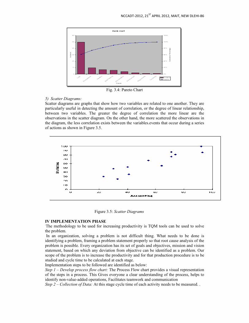
NCCADT-2012, 21ST


Fig. 3.4: Pareto Chart

5) Scatter Diagrams: Scatter diagrams are graphs that show how two variables are related to one another. They are particularly useful in detecting the amount of correlation, or the degree of linear relationship, between two variables. The greater the degree of correlation the more linear are the observations in the scatter diagram. On the other hand, the more scattered the observations in the diagram, the less correlation exists between the variables.events that occur during a series of actions as shown in Figure 3.5.

Figure 3.5: Scatter Diagrams

IV IMPLEMENTATION PHASE .The methodology to be used for increasing productivity is TQM tools can be used to solve the problem. In an organization, solving a problem is not difficult thing. What needs to be done is identifying a problem, framing a problem statement properly so that root cause analysis of the problem is possible. Every organization has its set of goals and objectives, mission and vision statement, based on which any deviation from objective can be identified as a problem. Our scope of the problem is to increase the productivity and for that production procedure is to be studied and cycle time to be calculated at each stage. Implementation steps to be followed are identified as below: Step 1 – Develop process flow chart: The Process Flow chart provides a visual representation of the steps in a process. This Gives everyone a clear understanding of the process, helps to identify non-value-added operations, Facilitates teamwork and communication Step 2 – Collection of Data: At this stage cycle time of each activity needs to be measured. .

NCCADT-2012, 21ST


Step 3 – Cycle time measurement and Preparation of Bar Graph: by means of calculation acceptable Cycle time is established for each stage involved in the production process. A Bar Graph of cycle time versus various stages of production are plotted and all activities that have cycle time above the acceptable levels are identified. Step 4 – Identification of stages and activities: Stages and activities that need improvement are to be identified for improving the productivity. Step 5 – Analysis with the help of cause effect diagram: Cause-and-effect diagrams can reveal key relationships among various variables, and the possible causes provide additional insight into process behavior. Step 6 – Preparation of control chart: Control charts can be established to find the processes within the control. Step 7 – Analyse the causes for time delay: Analysis of causes can be done and elimination of delays can be done. VI. RESULTS AND DISCUSSIONS.

.The present study sought to examine the impact of market demand on the relationships between the use of TQM practices and use of TQM tools for enhancing organizational performance. More specifically, the results of this study support the fact that the higher the degree of market competition, the more positive is the relationships between TQM practices of productivity improvement. The results of this study make a number of important contributions to the existing TQM literature. First, this research identified how simple methods can be used to improve work and work process in flow process manufacturing. The research identified the current methods used using flow process charts and cycle time of each stage. By making simple changes to the process, it can reduce the time taken for each stage to improve the flow and speed up the process. Second, the results of this study contribute and extend the existing TQM literature. From a theoretical perspective, the results show that the adoption of TQM practices and market competition jointly enhance organizational performance. This finding lends further support to the frequently suggested management practices and strategies for achieving improved organization performance in TQM firms. It stresses the importance of TQM practices of customer focus and productivity improvement to enhance customer satisfaction and gain a competitive edge. Specifically, the results of this study suggest TQM practices and tools are the primary determinant of quality performance. As quality performance improves, cycle times are reduced because there is less non-value added times resulting from the need to rework defective products. Moreover, as customers expect a minimum quality standard in all product offerings, firms must respond accordingly. VII. CONCLUSION. This research identified how simple methods and TQM tools can be used to improve work and work process.The research provides the basic guidelines for setting up production goals in a process industry based on sales forecast and calculating required cycle time as per market goals. The cycle times of each activity needs to be studied to identify the cycle time of the specific activity that requires improvement such that the total cycle time can be decreased to increase productivity. Process flow charts can identify the activity responsible for bottle necked cycle time and with the application of TQM tools like why-why analysis and pareto diagram, cause of bottle necks can be analysed and suggest solutions for elimination. The control charts can determine to see that the activity has minimum variation

REFERENCES

(1) Faisal Talib, Zillur Rahman, M.N. Qureshi,” Integrating Total Quality Management and Supply Chain Management: Similarities and Benefits”, Journal of Information Technology and Economic Development 1(1), October 2010 pp. 53-85.

NCCADT-2012, 21ST


(2) H.T Iwarere,” How Far Has the Manufacturing Industry Achieve Total Quality Management in Nigeria”, European Journal of Social Sciences – Volume 15, Number 2 (2010), pp.34-43

(3) A. Pal Pandi, U. Surya Rao and D. Jeyathilagar , “A Study on Integrated Total Quality Management Practices in Technical Institutions - Students’ Perspective” , International Journal of Educational Administration Volume 1 Number 1 (2009), pp. 17-30.

(4) Ling Li, Carol Markowski, Li Xu, Edward Markowski, “TQM—A predecessor of ERP implementation”, Int. J. Production Economics 115 (2008) pp 569–580.

(5) Xingxing Zu , Lawrence D. Fredendall , Thomas J. Douglas , “ The evolving theory of quality management” , The role of Six Sigma, ( 2008),pp 630-650.

(6) Maria Leticia Santos-Vijande, Luis Ignacio A, “Innovativeness and organizational innovation in total quality oriented firms: The moderating role of market turbulence”, Technovation 27 (2007) pp 514–532

(7) Juan Jose Taru, Jose Francisco Molina , Juan Luis Castejon.,” The relationship between quality management practices and their effects on quality outcomes”, European Journal of Operational Research 183 (2007) pp 483–501.

(8) Alexandros G. Psychogios, Constantinos-Vasilios Priporas,” Understanding Total Quality Management in Context: Qualitative Research on Managers’ Awareness of TQM Aspects in the Greek Service Industry”, The Qualitative Report Volume 12 Number 1 March 2007 pp 40-66

(9) Jamshed Siddiqui & Zillur Rahman,” TQM for Information Systems: Are Indian Organizations Ready”,( 2006).pp 125-136. (10) Daniel I. Prajogo, Amrik S. Sohal , “ The relationship between organization strategy,

total Manufacturing Strategies in Thai and Indian Automotive Manufacturing Companies ” , Journal of Manufacturing Systems .,~ Vol. 24/No. 2 (2005), pp 131-143.

(11) M. Sokovic , D. Pavletic , S. Fakin , “Application of Six Sigma methodology for process design” , (2005)management (TQM), quality and organization performance––the mediating role of TQM “ , European Journal of Operational Research 168 (2006) pp 35–50.

(12) T. Laosirihongthong and G.S. Dangayach, “A Comparative Study of Implementation of (13) Vincent K. Chong, Michael J. Rundus, “Total quality management, market competition

and organizational performance”, The British Accounting Review 36 (2004) pp 155–172.

(14) Juan Jose Tar, Vicente Sabater, “Quality tools and techniques: Are they necessary for quality management “, Int. J. Production Economics 92 (2004) pp 267–280.

(15) Vincent M. Ribiere and Reza Khorramshahgol ,” Integrating Total Quality Management and Knowledge Management”, Journal of Management Systems, Vol. XVI, No. 1, 2004, pp 39-54

(16) Hale Kaynak, “The relationship between total quality management practices and their effects on firm performance”, Journal of Operations Management 21 (2003) pp 405–435.

(17) Alvaro D. Taveira, Craig A. James, Ben-Tzion Karsh, Franois Sainfort, “Quality management and the work environment: an empirical investigation in a public sector organization “, Applied Ergonomics 34 (2003) pp 281–291.

(18) H.P.A. Geraedts, R. Montenarie, P.P. van Rijk, “The benefits of total quality management” Computerized Medical Imaging and Graphics 25 (2001) pp 217-220.

(19) Kristy O. Cuaa,, Kathleen E. McKone , Roger G. Schroeder , “Relationships between implementation of TQM, JIT, and TPM and manufacturing performance “ , Journal of Operations Management 19 (2001) pp 675–694.

(20) Montalee Nagswasdi, Christopher OÕBrien, “Patterns of organizational and technological development in the Thai manufacturing industry “, Int. J. Production Economics .1999, pp 599-605.

(21) David J. Lemak, Richard Reed, P.K Satish, “Commitment to Total Quality Management: Is There a Relationship with Firm Performance” Journal of Quality Management, Vol. 29(1997), No. 1.pp. 67-86.

NCCADT-2012, 21ST


(22) Paul Mangiameli, Rhode Island, “An examination of quality performance at different levels in a connected supply chain: a preliminary case study” , Integrated Manufacturing

Systems, MCB University 12/2 (2001) pp 126-133. (23) Robert C. Winn & Robert R. Green , “Applying Total Quality Management to the

Educational Process”, (1998), pp 24-29. (24) Kathy A. Paulson GjerdE and Susan A. Slotnick, “A Multidimensional approach to

manufacturing quality”, Computers ind. Engng Vol. 32, No. 4, (1997), pp 879-889. (25) Thomas C. Powell, “Total Quality Management As Competitive Advantage: A Review

and Empirical Study “, Strategic Management Journal, Vol. 16, (1995), pp 15-37.

NCCADT-2012, 21ST


Optimization of Tooth Strength in Spur Gear Atul Kumar Kaushik, Anil Kumar Dahiya, Ravinder Kumar

Faculty, Deptt. Of MAE, Maharaja Agrasen Institute of Technology, Rohini (New Delhi), India,

Abstract

This paper examines the tooth failure in spur gears. Corrective measures are taken to

avoid tooth damage by introducing profile modification in root fillet. In general, spur gear

with less than 17 numbers of teeth had the problem of undercutting during gear

manufacturing process which minimizes the strength of gear at root. In this study, a novel

design method, namely circular root fillet instead of the standard trochoidal root fillet is

introduced in spur gear and analyzed using ANSYS version 11.0 software. The strength of

these modified teeth is studied in comparison with the standard design. The analysis demonstrates that the novel design exhibit higher bending strength over the standard

trochoidal root fillet gear. The result reveals that the circular root fillet design is particularly

suitable for lesser number of teeth in pinion and where as the trochoidal root fillet gear is more opt for higher number of teeth.

1. Introduction

The objective of the gear drive is to transmit power with comparatively smaller dimensions, runs reasonably free of noise and vibration with least manufacturing and maintenance cost. There is a growing need for higher load carrying capacity and increased fatigue life in the field of gear transmissions. Spitas and Costopoulos [1] have introduced one–sided involute asymmetric spur gear teeth to increase load carrying capacity and combine the meshing properties. Tesfahunegn and Rosa [2] investigated the influence of the shape of profile modifications on transmission error, root stress and contact pressure through non linear finite element approach. Spitas and Costopoulos [3] expressed that the circular fillet design is particularly suitable in gears with small number of teeth (pinion). Fredette and Brown [4] discussed the possibility of reducing gear tooth root stresses by adding internal stress relief features. Ciavarella and Demeliio [5] concluded that the fatigue life is lower on gears with a lesser number of teeth. Hebbal and Math [6] have reduced the root fillet stress in spur gear using internal stress relieving feature of different shapes. Senthilvelan and gnanamoorthy [7] studied the effect of gear tooth fillet radius on the performance of injection moulded nylon 6/6 gears. Tae Hyong Chong and Jae Hyong Myong [8] conducted a study to calculate simultaneously the optimum amounts of tooth profile modification for minimization of vibration and noise. Beghini et al. [9] proposed a simple method to reduce the transmission error for a given spur gear at the nominal torque by means of the profile modification parameters. Researchers focused either on the development of advanced materials or new heat treatment methods or designing the gears with stronger tooth profiles. Gears having standard involute with smaller number of teeth (i.e., less than 17 teeth) had the problem of undercutting. In gear manufacturing process the tooth root fillet is generated as the tip of the cutter removes material from the involute profile resulting teeth that have less thickness at root. This reduces the tooth strength and leads to the crack initiation and propagation at root fillet area. To improve the gear tooth strength many works have been done but all mostly employed positive profile shifting [10-13].These contributions exhibit lower pitting and scoring resistance with lesser contact ratio resulting in more noise and vibration during the power transmission [14].

2. Gear Geometry

The involute spur gear with circular root fillet is illustrated in Figure 1. The point Ó´ is the center of the gear, ‘Oy’ is the axis of symmetry of the tooth and ‘B’ is the point where the involute profile starts from the form circle rs. ‘A’ is the point of tangency of the circular fillet with the root circle rf. ‘D’ laying on (ε2) = ‘OA’ represents the center of the circular fillet. Line (ε3) is tangent to the root circle at A and intersects with line (ε1) at C. The fillet is

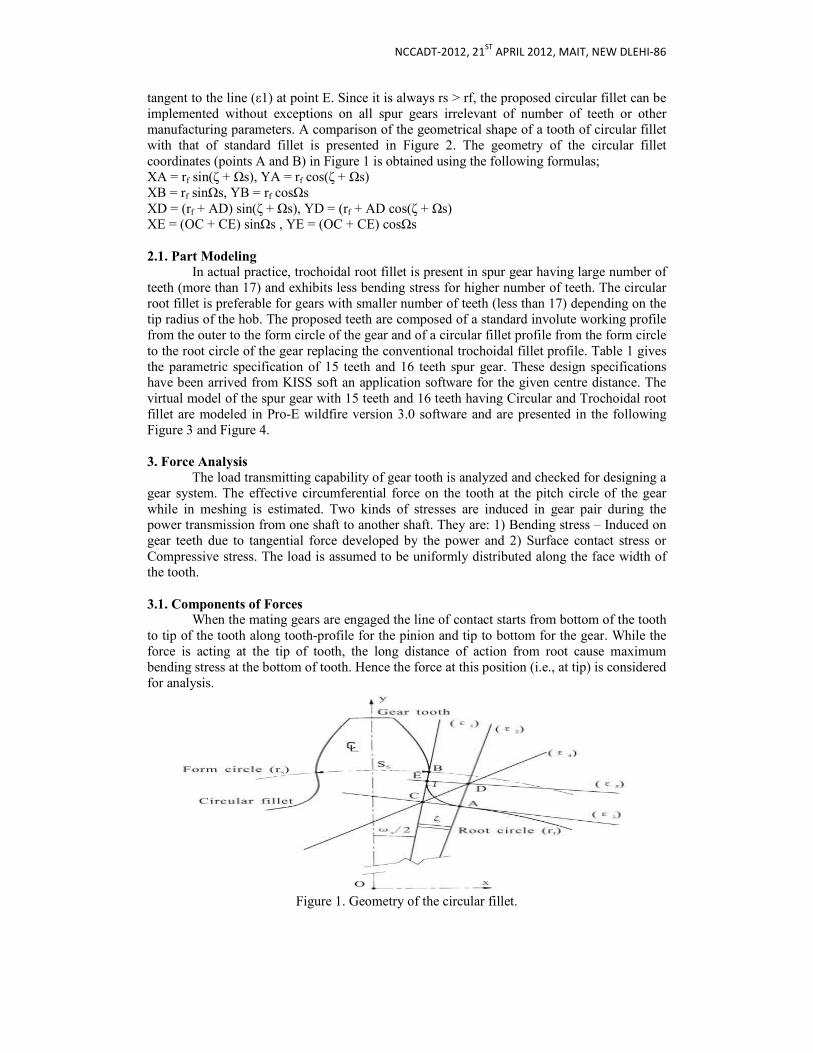
NCCADT-2012, 21ST


tangent to the line (ε1) at point E. Since it is always rs > rf, the proposed circular fillet can be implemented without exceptions on all spur gears irrelevant of number of teeth or other manufacturing parameters. A comparison of the geometrical shape of a tooth of circular fillet with that of standard fillet is presented in Figure 2. The geometry of the circular fillet coordinates (points A and B) in Figure 1 is obtained using the following formulas; XA = rf sin(ζ + Ωs), YA = rf cos(ζ + Ωs) XB = rf sinΩs, YB = rf cosΩs XD = (rf + AD) sin(ζ + Ωs), YD = (rf + AD cos(ζ + Ωs) XE = (OC + CE) sinΩs , YE = (OC + CE) cosΩs

2.1. Part Modeling

In actual practice, trochoidal root fillet is present in spur gear having large number of teeth (more than 17) and exhibits less bending stress for higher number of teeth. The circular root fillet is preferable for gears with smaller number of teeth (less than 17) depending on the tip radius of the hob. The proposed teeth are composed of a standard involute working profile from the outer to the form circle of the gear and of a circular fillet profile from the form circle to the root circle of the gear replacing the conventional trochoidal fillet profile. Table 1 gives the parametric specification of 15 teeth and 16 teeth spur gear. These design specifications have been arrived from KISS soft an application software for the given centre distance. The virtual model of the spur gear with 15 teeth and 16 teeth having Circular and Trochoidal root fillet are modeled in Pro-E wildfire version 3.0 software and are presented in the following Figure 3 and Figure 4.

3. Force Analysis

The load transmitting capability of gear tooth is analyzed and checked for designing a gear system. The effective circumferential force on the tooth at the pitch circle of the gear while in meshing is estimated. Two kinds of stresses are induced in gear pair during the power transmission from one shaft to another shaft. They are: 1) Bending stress – Induced on gear teeth due to tangential force developed by the power and 2) Surface contact stress or Compressive stress. The load is assumed to be uniformly distributed along the face width of the tooth.

3.1. Components of Forces When the mating gears are engaged the line of contact starts from bottom of the tooth

to tip of the tooth along tooth-profile for the pinion and tip to bottom for the gear. While the force is acting at the tip of tooth, the long distance of action from root cause maximum bending stress at the bottom of tooth. Hence the force at this position (i.e., at tip) is considered for analysis.

Figure 1. Geometry of the circular fillet.

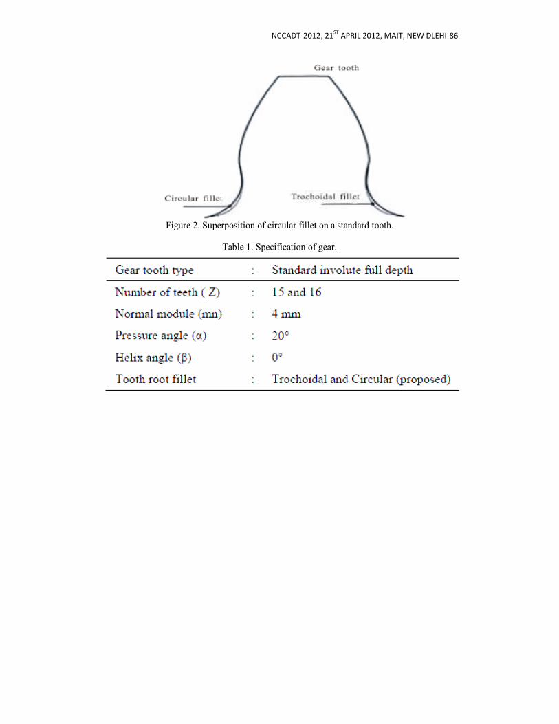
Figure 2. Superposition of circular fillet on a standard tooth.

NCCADT-2012, 21ST


Figure 2. Superposition of circular fillet on a standard tooth.

Table 1. Specification of gear.


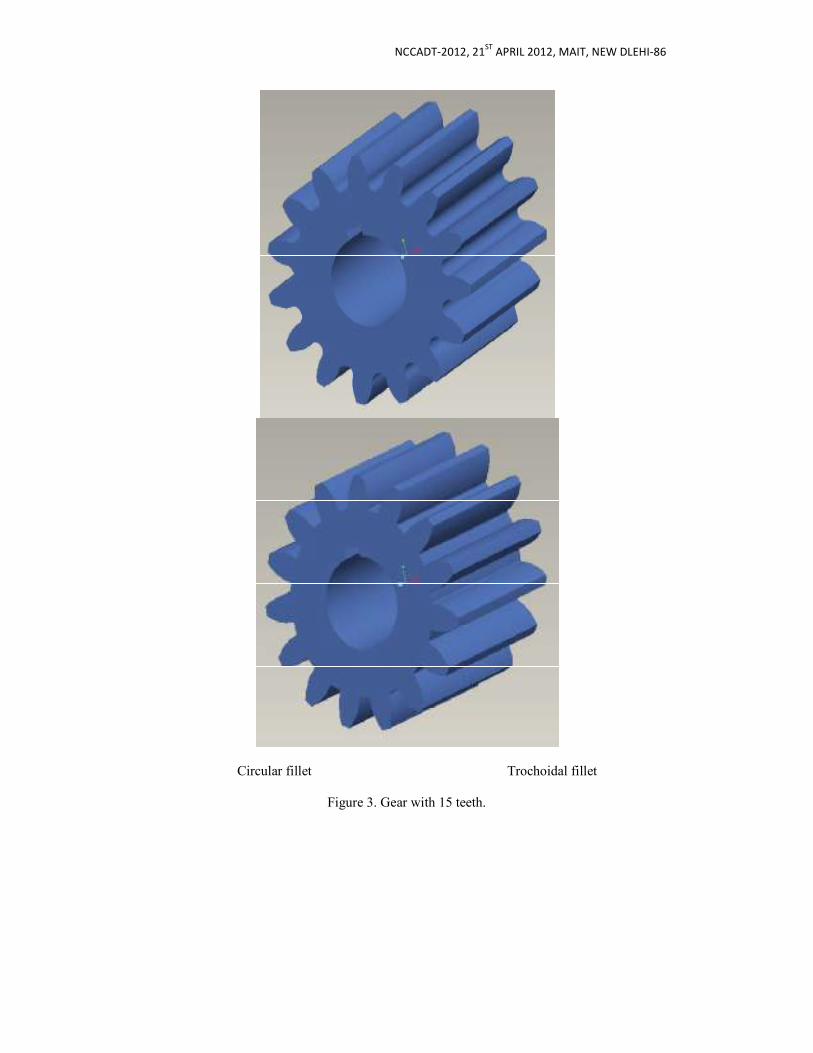
NCCADT-2012, 21ST


Circular fillet Trochoidal fillet

Figure 3. Gear with 15 teeth.

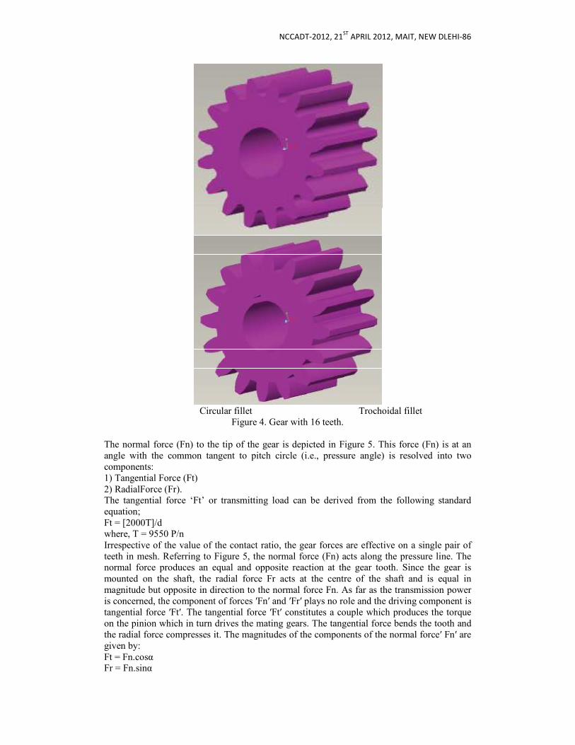
NCCADT-2012, 21ST


Circular fillet Trochoidal fillet

Figure 4. Gear with 16 teeth.

The normal force (Fn) to the tip of the gear is depicted in Figure 5. This force (Fn) is at an angle with the common tangent to pitch circle (i.e., pressure angle) is resolved into two components: 1) Tangential Force (Ft) 2) RadialForce (Fr). The tangential force ‘Ft’ or transmitting load can be derived from the following standard equation; Ft = [2000T]/d where, T = 9550 P/n Irrespective of the value of the contact ratio, the gear forces are effective on a single pair of teeth in mesh. Referring to Figure 5, the normal force (Fn) acts along the pressure line. The normal force produces an equal and opposite reaction at the gear tooth. Since the gear is mounted on the shaft, the radial force Fr acts at the centre of the shaft and is equal in magnitude but opposite in direction to the normal force Fn. As far as the transmission power is concerned, the component of forces ′Fn′ and ′Fr′ plays no role and the driving component is tangential force ′Ft′. The tangential force ′Ft′ constitutes a couple which produces the torque on the pinion which in turn drives the mating gears. The tangential force bends the tooth and the radial force compresses it. The magnitudes of the components of the normal force′ Fn′ are given by: Ft = Fn.cosα Fr = Fn.sinα

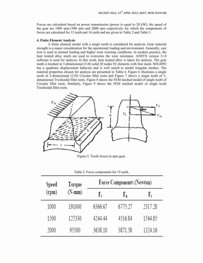
Forces are calculated based on power transmission (power is equal to 20 kW), the speed of the gear are 1000 rpm,1500 rpm and 2000 rpm respectively for which the components of forces are calculated for 15 teeth and 16 teeth and are given in

4. Finite Element Analysis

A finite element model with a single tooth is considered for analysis. Gear material strength is a major consideration for the operational loading and environment. Generally, cast iron is used in normal loading and higher wear resisting conditions. In modern practice, the heat treated alloy steels are used to overcome the wear resistance. ANSYS version 11.0 software is used for analysis. In this work, heat treated alloy is taken for analysis. The gear tooth is meshed in 3-dimensional (3has a quadratic displacement behavior and is well suited to model irregular meshes. The material properties chosen for analysis are presented in Table 4. Figure 6 illustrattooth of 2-dimensional (2-D) Circular fillet roots and Figure 7 shows a single tooth of 2dimensional Trochoidal fillet roots. Figure 8 shows the FEM meshed model of single tooth of Circular fillet roots. Similarly, Figure 9 shows the FEM mesheTrochoidal fillet roots.

Figure 5. Tooth forces in spur gear.

Table 2. Force components for 15 teeth.

NCCADT-2012, 21ST


Forces are calculated based on power transmission (power is equal to 20 kW), the speed of the gear are 1000 rpm,1500 rpm and 2000 rpm respectively for which the components of forces are calculated for 15 teeth and 16 teeth and are given in Table 2 and Table 3.

A finite element model with a single tooth is considered for analysis. Gear material strength is a major consideration for the operational loading and environment. Generally, cast

ding and higher wear resisting conditions. In modern practice, the heat treated alloy steels are used to overcome the wear resistance. ANSYS version 11.0 software is used for analysis. In this work, heat treated alloy is taken for analysis. The gear

dimensional (3-D) solid 20 nodes 92 elements with fine mesh. SOLID92 has a quadratic displacement behavior and is well suited to model irregular meshes. The material properties chosen for analysis are presented in Table 4. Figure 6 illustrates a single

D) Circular fillet roots and Figure 7 shows a single tooth of 2dimensional Trochoidal fillet roots. Figure 8 shows the FEM meshed model of single tooth of Circular fillet roots. Similarly, Figure 9 shows the FEM meshed model of single tooth

Figure 5. Tooth forces in spur gear.

Table 2. Force components for 15 teeth.


Forces are calculated based on power transmission (power is equal to 20 kW), the speed of the gear are 1000 rpm,1500 rpm and 2000 rpm respectively for which the components of

A finite element model with a single tooth is considered for analysis. Gear material strength is a major consideration for the operational loading and environment. Generally, cast

ding and higher wear resisting conditions. In modern practice, the heat treated alloy steels are used to overcome the wear resistance. ANSYS version 11.0 software is used for analysis. In this work, heat treated alloy is taken for analysis. The gear

D) solid 20 nodes 92 elements with fine mesh. SOLID92 has a quadratic displacement behavior and is well suited to model irregular meshes. The

es a single D) Circular fillet roots and Figure 7 shows a single tooth of 2-

dimensional Trochoidal fillet roots. Figure 8 shows the FEM meshed model of single tooth of d model of single tooth

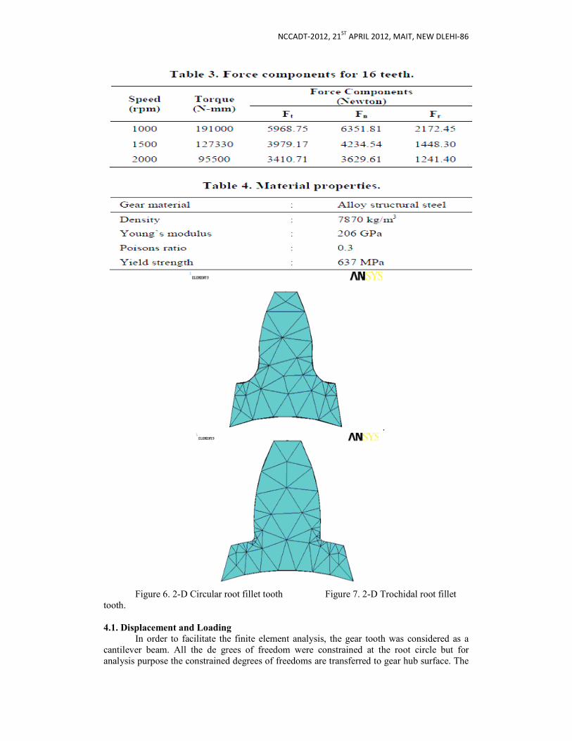
Figure 6. 2-D Circular root fillet tooth tooth.

4.1. Displacement and Loading

In order to facilitate the finite element analysis, the gear tooth was considered as a cantilever beam. All the de grees of freedom were constrained at the root circle but for analysis purpose the constrained degrees of freedoms are transferred to gear hub

NCCADT-2012, 21ST


.

D Circular root fillet tooth Figure 7. 2-D Trochidal root fillet

4.1. Displacement and Loading

In order to facilitate the finite element analysis, the gear tooth was considered as a grees of freedom were constrained at the root circle but for

analysis purpose the constrained degrees of freedoms are transferred to gear hub surface. The


D Trochidal root fillet

In order to facilitate the finite element analysis, the gear tooth was considered as a grees of freedom were constrained at the root circle but for

surface. The

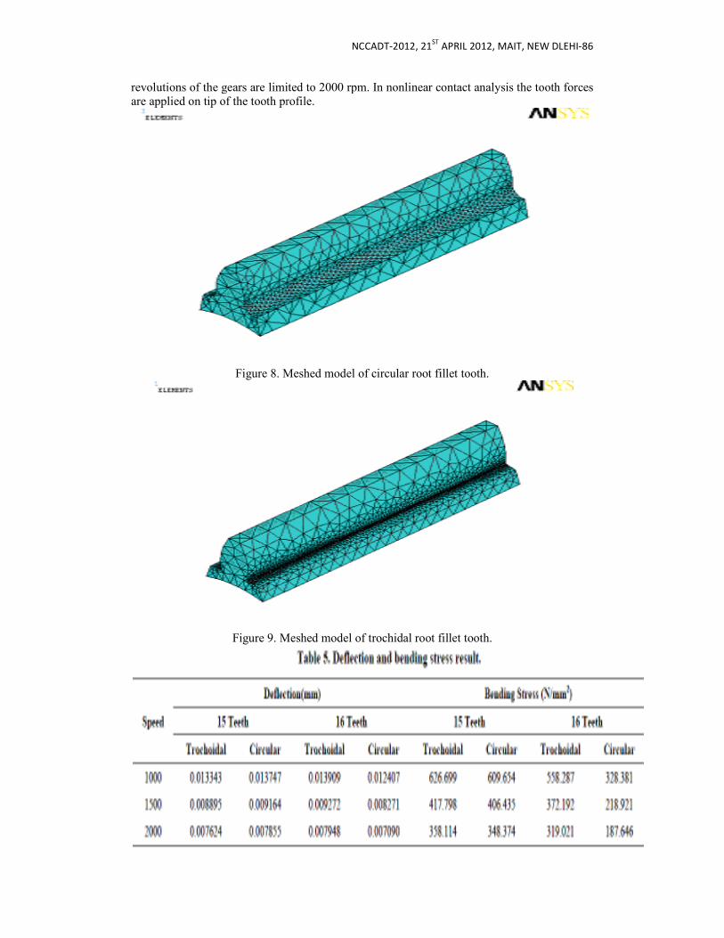
revolutions of the gears are limited to 2000 rpm. In nonlinear contact analysis the tooth forces are applied on tip of the tooth profile.

Figure 8. Meshed model of circular root fillet tooth.

Figure 9. Meshed model of trochidal root fille

NCCADT-2012, 21ST


revolutions of the gears are limited to 2000 rpm. In nonlinear contact analysis the tooth forces are applied on tip of the tooth profile.

Figure 8. Meshed model of circular root fillet tooth.

Figure 9. Meshed model of trochidal root fillet tooth.


revolutions of the gears are limited to 2000 rpm. In nonlinear contact analysis the tooth forces

NCCADT-2012, 21ST



The deflection and bending stress analysis were carried out for the spur gear with 15 teeth and 16 teeth. The induced bending stress and obtained deflection values are presented in Table 5. The investigation reveals that the deflection value of both circular and trochoidal root fillet gears are identical. But, looking in to bending stress the 15T gear generated with circular root fillet have lesser stress (609.654 N/mm2) at 1000 rpm when compared with trochoidal fillet gear (626.699 N/mm2). Correspondingly, the induced bending stress for 16 T circular root fillet gear at 2000 rpm was 348.374 N/mm2 where as it was noticed as 358.114 N/mm2 for 16 T trochoidal root fillet gear. It is observed from ANSYS study that the 16T gear generated with circular root fillet have lesser stress (328.381 N/mm2) at 1000 rpm when compared with trochoidal fillet gear (558.287 N/mm2). Also, the bending stress (187.646 N/mm2) was least for 16 T circular root fillet gear at 2000 rpm when compared with trochoidal root fillet gear (319.021 N/mm2). In sort, the results obtained from ANSYS result shows that the bending stress and deflection values are lesser for Circular root fillet gear irrespective of speed than Trochoidal root fillet gear.

6. Conclusions

The investigation result infers that the deflection in circular root fillet is almost same comparing to the trochoidal root fillet gear tooth. However, there is appreciable reduction in bending stress value for circular root fillet design in comparison to that of bending stress value in trochoidal root fillet design. From the foregoing analysis it is also found that the circular fillet design is more opt for lesser number of teeth in pinion and trochoidal fillet design is more suitable for higher number of teeth in gear (more than 17 teeth) and whatever may be the pinion speed. In addition to that the ANSYS results indicates that the gears with circular root fillet design will result in better strength, reduced bending stress and also improve the fatigue life of gear material. Further work shall be done to ascertain the stiffness and rigidity of gear tooth in the circular root fillet design so that the feasibility of this particular design can be useful to put in practical application in future.

7. References [1] T. Costopoulos and V. Spitas, “Reduction of Gear Fillet Stresses by Using One Sided Involute AsymmetricTeeth,” Mechanism and Machine Theory, Vol. 44, No. 8, 2009, pp. 1524-1534. [2] Y. A. Tesfahunegn and F. Rosa, “The Effects of the Shape of Tooth Profile Modification on the Transmission Error Bending and Contact Stress of Spur Gears,” Journal of Mechanical Engineering Science, Vol. 224, No. 8, 2010, pp. 1749-1758. [3] V. Spitas, T. Costopoulos and C. Spitas, “Increasing the Strength of Standard Involute Gear Teeth with Novel Circular Root Fillet Design,” American Journal of Applied Sciences, Vol. 2, No. 6, 2005, pp. 1058-1064. [4] L. Fredette and M. Brown, “Gear Stress Reduction Using Internal Stress Relief Features,” Journal of Mechanical Design, Vol. 119, No. 4, 1997, pp. 518-521. [5] M. Ciavarella and G. Demelio, “Numerical Methods for the Optimization of Specific Sliding Stress Concentration and Fatigue Life of Gears,” International Journal of fatigue, Vol. 21, No. 5, 1999, pp. 465-474. [6] M. S. Hebbal, V. B. Math and B. G. Sheeparamatti, “A Study on Reducing the Root Fillet Stress in Spur Gear Using Internal Stress Relieving Feature of Different Shapes,” International Journal of RTE, Vol. 1, No. 5, May 2009, pp. 163-165. [7] S. Senthilvelan and R. Gnanamoorthy, “Effects of Gear Tooth Fillet Radius on the Performance of Injection Moulded Nylon 6/6 Gears,” Materials and Design, Vol. 27, No. 8, 2005, pp. 632-639. [8] T. H. Chong, T. H. Myong and K. T. Kim, “Tooth Modification of Helical Gears for Minimization of Vibration and Noise,” International Journal of KSPE, Vol. 2, No. 4, 2001, pp. 5-11.

NCCADT-2012, 21ST


[9] M. Beghini, F. Presicce and C. Santus, “A Method to Define Profile Modification of Spur Gear and Minimize the Transmission Error,” AGMA Fall Technical Meeting, Milwaukee, Wisconsin, October 2004, pp. 1-28. [10] ISO, 6336-3, “Calculation of the Load Capacity of Spurand Helical Gears-Part 3,” Calculation of Bending Strength, 1996. [11] AGMA, 2101-C95, “Fundamental Rating Factors and Calculation Methods for Involute Spur and Helical Gear (Metric Version),” American Gear Manufacturers Association, 1995. [12] H. H. Mabie, C. A. Rogers and C. F. Reinholtz, “Design of Nonstandard Spur Gears Cut by a Hob,” Mechanism and Machine Theory, Vol. 25, No. 6, 1990, pp. 635-644. [13] C. A. Rogers, H. H. Mabie and C. F. Reinholtz, “Design of Spur Gears Generated with Pinion Cutters,” Mechanism and Machine Theory, Vol. 25, No. 6, 1990, pp. 623-634. [14] G. Niemann,“Maschinenelemente,” Band 2, Springer, Verlag, 1965.

NCCADT-2012, 21ST


To Study Effect of Bullwhip effect on Performance of

Supply Chain Ravinder Kumar

Assistant Professor, Department of Mechanical & Automation Engineering,

MAIT, Delhi-86 ABSTRACT The bullwhip effect is associated with the variability of demand upstream. Managers involved

in supply chain are seeking ways to understand this effect. Uncertainty involved in supply

chain leads to the bullwhip effect. In this paper a brief review of supply chain management

concept along with bullwhip effect has been taking. Literature reveals uncertainties related to

raw material, supply, process and demand as experienced by many firms. Bullwhip effect has

adverse effects on supply chain coordination, integration and supply chain performance.

Performance measurement variables are tabulated to provide groundwork for further

research. Accurate and effective information sharing in supply chain with transparency is

found important to avoid bullwhip effect.

Key words: Supply chain management, bullwhip effect, uncertainty in supply chains and performance.

1. INTRODUCTION

With the globalization Indian companies are adopting supply chain and logistics management in a big way. In India, Supply Chain Management (SCM) is being implemented by medium and large-scale industries. Bullwhip effect is a phenomenon that deals with uncertain demand and its consequent effect on supply chain. Uncertainty needs to be certified and critically analyzed to isolate the supply chain from the consequences of Bullwhip effect. This paper deals with the important issue of bullwhip effect in supply chains.

Globalization has opened door of new technologies to India. Technology, to be very correct, is nothing but the process, the way of doing things (Vemekar and Venkatasubramaniam, 2004). New materials are being researched for conventional products. High level of inventories, caused by magnified estimates of demand from supplier side, may even get absolute and may lead to high losses to suppliers. Indian managers dealing in supply chain of these products in which material changes are very fast must keep an eye on false demands so that bullwhip effect may be avoided.

2. Literature Review

Supply chain management is the integration and management of supply chain organizations and activities through cooperative organizational relationships, effective business processes and high levels of information sharing to create high performance value systems that provide member organizations a suitable competitive advantage (Handfield and Nichols, 2003). Author uses the term demand chain management for supply chain management to reflect the fact that the chain should be driven by the market but not by the supplier (Christopher, 1992).

NCCADT-2012, 21ST


Supply chain management consists of four main areas (and six total areas): marketing, logistics, supply management, and operations management; marketing is subsequently composed of competitor orientation, customer orientation, and (supply chain) and coordination (Tomas, 2004). A basic enabler for effective supply chain management is information sharing among link partners. This has been greatly facilitated by recent advances in IT (Lee and Whang, 2000). Supply chain wide IT strategy, profit-sharing due to IT enablement, and high level of supply chain integration are the top three enablers in SCM (Jharkharia and Shankar, 2004). The barriers that significantly affect the IT enablement of a supply chain are also analyzed in this paper so that management may effectively deal with these barriers. Jharkharia and Shankar (2005) indicates that disparity in trading partners, capabilities, and resistance to change to IT enabled SCM, and low level of supply chain integration are among the top-level barriers. Threats of information security, fear of information system breakdown, and fear of supply chain breakdown are the middle level barriers.

3. What Bullwhip Effect Is?

The bullwhip effect has been observed in many firms and literature suggests that it is a very important issue in the field of supply chain coordination. Supply chain is an interlinked set of relationship connecting customers to supplier through a number of intermediate stages such as manufacturing, warehousing and distribution (Christopher and Towilli, 2000). In bullwhip effect the fluctuations in order increases as they move up the supply chain from retailers to wholesalers to manufacturers to suppliers. The bullwhip effect distorts demand information within the supply chain, with different stages having a very different estimate of what demand looks like. The result is a loss of supply chain coordination. (Chopra and Meindl, 2005). The supply chain of Pampers Diapers of Procter and Gamble (P & G) is one of the examples of bullwhip effect in which company registered significant fluctuations in raw material orders from P and G as compared to very small fluctuations in the retail sale (Lee et al. 1997). Basically, even slight to moderate demand uncertainty and variability become magnified when viewed through the eyes of managers at each link in the supply chain (Handfield and Nichols, 2005).

It is a great challenge of supply chain to cope up with variability. All business activity exhibits natural variability in their duration, quality and other attributes. Different accepts of supply chain like sales, delivery time, production rates, transportation time etc, vary around some average value. The more variability in these values, the more difficult and expensive it is to run the chain. By managers inventories are used to buffers variability. Variability in supply amplifies down the chains whereas variability in demand amplifies up the chain. This is termed as bullwhip effect which continuous to be serious problems in many chains (Taylor, 2004).

4. UNCERTAINTIES IN SUPPLY CHAINS

Uncertainty inherent in an environment in which an SC operates propagates through the SC network, and makes SC management and control problems more complex (Davis, 1993). Changes in the business environment due to varying needs to the costumer lead to uncertainty in the decision parameter (Aggarwal et al., 2006).

An SC is linked with an uncertain external environment by customer demand from one side and a raw material supplier from another side. Traditionally, attention has been focused on uncertainty in customer demand. However, uncertainty is inherent in the market at supply side also, and the quantity and quality of raw material delivered from an external supplier may differ from those requested. Uncertainty in parameters in inventory control problems has been most often modeled by probability distributions, usually derived from evidence recorded in the past. However, when there is lack of evidence available or lack of certainty in evidence or

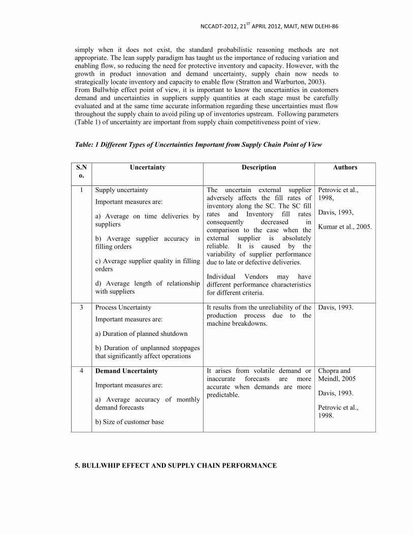
NCCADT-2012, 21ST


simply when it does not exist, the standard probabilistic reasoning methods are not appropriate. The lean supply paradigm has taught us the importance of reducing variation and enabling flow, so reducing the need for protective inventory and capacity. However, with the growth in product innovation and demand uncertainty, supply chain now needs to strategically locate inventory and capacity to enable flow (Stratton and Warburton, 2003). From Bullwhip effect point of view, it is important to know the uncertainties in customers demand and uncertainties in suppliers supply quantities at each stage must be carefully evaluated and at the same time accurate information regarding these uncertainties must flow throughout the supply chain to avoid piling up of inventories upstream. Following parameters (Table 1) of uncertainty are important from supply chain competitiveness point of view.

Table: 1 Different Types of Uncertainties Important from Supply Chain Point of View

S.N

o.

Uncertainty Description Authors

1 Supply uncertainty

Important measures are:

a) Average on time deliveries by suppliers

b) Average supplier accuracy in filling orders

c) Average supplier quality in filling orders

d) Average length of relationship with suppliers

The uncertain external supplier adversely affects the fill rates of inventory along the SC. The SC fill rates and Inventory fill rates consequently decreased in comparison to the case when the external supplier is absolutely reliable. It is caused by the variability of supplier performance due to late or defective deliveries.

Individual Vendors may have different performance characteristics for different criteria.

Petrovic et al., 1998,

Davis, 1993,

Kumar et al., 2005.

3 Process Uncertainty


a) Duration of planned shutdown

b) Duration of unplanned stoppages that significantly affect operations

It results from the unreliability of the production process due to the machine breakdowns.

Davis, 1993.

4 Demand Uncertainty


a) Average accuracy of monthly demand forecasts

b) Size of customer base

It arises from volatile demand or inaccurate forecasts are more accurate when demands are more predictable.

Chopra and Meindl, 2005

Davis, 1993.

Petrovic et al., 1998.

5. BULLWHIP EFFECT AND SUPPLY CHAIN PERFORMANCE

NCCADT-2012, 21ST


Performance of supply chain is characterized by its ability to remain market sensitive without lacking the integration through the chain. Supply chain management is now seen as a governing element in strategy and as an effective way of creating value for costumers. The so-called bullwhip effect, describing growing variation upstream in a supply chain, is probably the most famous demonstration that decentralized decision making can lead to poor supply chain performance. Information asymmetry is one of the most powerful sources of the bullwhip effect. Information sharing of customer demand has an impact on the bullwhip effect. Information technology has lead to centralized information, shorter lead times and smaller batch size (Fiala, 2005). Performance measurement variables have been identified from literature and tabulated in Table 2:

TABLE 2: PERFORMANCE MEASUREMENT VARIABLES

S.No. Performance Measurement

Variables

Description Researchers

1 LEAD TIME

a) Lead time improvement over last 3 years

b) Lead time performance relative to industry

The bullwhip effect increases replenishment lead-time in the supply chain.

Lambert and Sharman, 1990.

Cohen and Lee, 1990

2 INVENTORY

a)Improvement in inventory turns over in last 3 years

b)Inventory turns performance relative to industry

c)Change in level of inventory write off over last 3 years

d) Level of inventory write off relative to industry

Because of bullwhip effect that is variability in demand, the inventory gets piled up with upstream members of supply chain.

Davis, 1993

Lee and Billington, 1992.

3 TIME TO MARKET

a)Improvement of time to market (product development cycle) performance over last 3 years

b)Improvement of time to market (product development cycle) performance relative to industry

Negligible effect but funds for R and D for new product development may be diverted for meeting increased demand.

Bhatnagar and Sohal, 2005

4 QUALITY

a) Improvement of defect rate over last 3 years

b)Improvement of defect rate

No reasonable effect Lambert and Sharman, 1990.

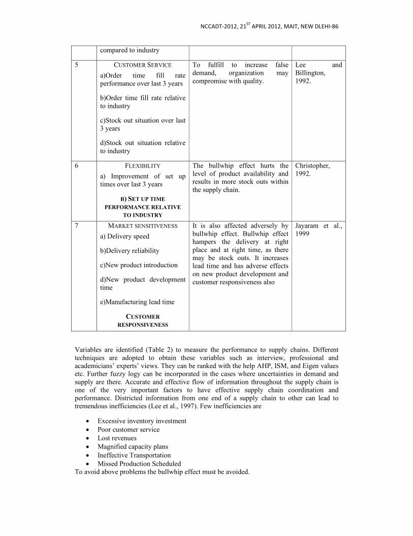
NCCADT-2012, 21ST


compared to industry

5 CUSTOMER SERVICE

a)Order time fill rate performance over last 3 years

b)Order time fill rate relative to industry

c)Stock out situation over last 3 years

d)Stock out situation relative to industry

To fulfill to increase false demand, organization may compromise with quality.

Lee and Billington, 1992.

6 FLEXIBILITY

a) Improvement of set up times over last 3 years

B) SET UP TIME

PERFORMANCE RELATIVE

TO INDUSTRY

The bullwhip effect hurts the level of product availability and results in more stock outs within the supply chain.

Christopher, 1992.

7 MARKET SENSITIVENESS

a) Delivery speed

b)Delivery reliability

c)New product introduction

d)New product development time

e)Manufacturing lead time

CUSTOMER

RESPONSIVENESS

It is also affected adversely by bullwhip effect. Bullwhip effect hampers the delivery at right place and at right time, as there may be stock outs. It increases lead time and has adverse effects on new product development and customer responsiveness also

Jayaram et al., 1999

Variables are identified (Table 2) to measure the performance to supply chains. Different techniques are adopted to obtain these variables such as interview, professional and academicians’ experts’ views. They can be ranked with the help AHP, ISM, and Eigen values etc. Further fuzzy logy can be incorporated in the cases where uncertainties in demand and supply are there. Accurate and effective flow of information throughout the supply chain is one of the very important factors to have effective supply chain coordination and performance. Districted information from one end of a supply chain to other can lead to tremendous inefficiencies (Lee et al., 1997). Few inefficiencies are

• Excessive inventory investment • Poor customer service • Lost revenues • Magnified capacity plans • Ineffective Transportation • Missed Production Scheduled

To avoid above problems the bullwhip effect must be avoided.

NCCADT-2012, 21ST


6. CONCLUSION

In a good supply chain buyers and suppliers should be willing to accommodate the uncertainties and variations in each other’s business. Supply chain provides an area where cost competitiveness can be achieved. In this paper we have tried to explain bullwhip effect in context with supply chains and its effect on the performance of supply chains. Uncertainty in supply chains have also been identified and classified with the help of different researcher’s viewpoint. Different factors that can be used for measuring the performance of supply chains have also been identified. This paper will provide all researchers better understanding of supply chain management and its effect on SC performance.

REFERENCES 1. Aggarwal Ashish, Shanker Ravi and Taiwari MK (2006), “Modeling the metrics of

lean, agile and leagile supply chain: An ANP based approach”, European journal of operational research, 173, pp. 211–225.

2. Bhatnagar and Sohal (2005), “Supply chain competitiveness: measuring the impact of location factors, uncertainty and manufacturing practices”, Technovation, 25, pp.443-456.

3. Christopher, M. and Towilli, DR (2000), "Supply chain migration from lean and functional to agile and customized ", International Journal of Supply chain management, Vol.5 (4), pp. 206-13.

4. Chopra Sunil and Meindl Peter, (2005), Supply Chain Management, Pearson, Prentice Hall, New Delhi.

5. Cohen, M.A. and Lee, H.L., (1990), “Out of touch with customer needs? Spare parts and after sales service”, Sloan Management Review 31(2), 55–66.

8. Christopher, M., (1992). Logistics and Supply Chain Management, Pitman Publishing, London.

9. Davis (1993), “Effective supply chain management”, Sloan Management Review 34(4), 35-46.

10. Fiala (2005), “Information sharing in supply chain”, Omega, The international journal of management science, PP 419-423.

11. Hand Field R. B., And Nichols E.L. JR, (2005), Introduction to supply chain management, Pearson Education.

12. Hand Field R B, and Nichols E.L JR, (2003), Supply chain Redesign, Pearson Education.

13. Jayaram, J., Vickery, S.K. and Droge, C. (1999), “An empirical study of time based competition in the North American automotive supplier industry”, International Journal of Operation and Production Management, Vol. 19 (10), pp 1010-13.

14. Jharkharia Sanjay and Shankar Ravi, (2005), “IT-enablement of supply chains: understanding the barriers”, The Journal of Enterprise Information Management, Vol.18 (1), pp11-27.

15. Jharkharia Sanjay and Shankar Ravi, (2004), “IT enablement of supply chains: modeling the enablers”, International Journals of Productivity and Performance Management, vol. 53 No. 8, pp.700-712

16. Kumar Manoj, Vrat Prem and Shankar Ravi, (2005), “Fuzzy Programming approach for vendor selection problem in a supply chain”, International Journal of Production Economics.

17. Lambert, D.M., Sharman, A., (1990), “ A customer-based competitive analysis for logistics decisions”, International Journal of Physical Distribution and Logistics Management 20(1), 17–24.

18. Lee, H.L., and Billington, C., (1992), “Managing supply chain inventory: pitfalls and Opportunities”, Sloan Management Review, 33(3), pp.65–73.

NCCADT-2012, 21ST


20. Lee, H.L and Whang, S. (2000),”information sharing in supply chain”, International Journal of Technology Management, Vol.20 No.3/4, pp373-87.

21. Lee H., Padmanabhan V., and Whang S, (1997), “The Bullwhip effect in Supply chains, Sloan Management review, pp 93-102.

22. Petrovic, D., Roy R., Petrovic, R., (1998), “Modeling and simulation of a supply chain in an uncertain environment”, European journal of operational research, 109(3), 299-309.

23. Stratton R and Warburton R.D.H., (2003), “The Strategic integration of agile and lean supply”, International journal of production economics, PP 183-198.

24. Taylor David, A., (2004), Supply chains – A Managers Guide, Person Education. 25. Tomas, H. (2004), “Global supply chain management; An integration of scholarly

thoughts”, Industrial Marketing Management, 33, pp.3-5. 26. Vemekar SS and Venkatasubramaniam K, (2004), “Technology, flexibility and

Innovation”, Third Global Conference on flexible systems management, Global Institute of Flexible systems management.

NCCADT-2012, 21ST


INTERPRETIVE STRUCTURAL MODELING(ISM)

ANALYSIS OF FACTORS AFFECTING

IMPLEMENTATION OF LEAN MANUFACTURING Ravinder Kumar1, Anil Kumar Dahiya1, Rakesh Chander Saini1, Md. Qamar Tanveer2

1Assistant Professors, Department of Mechanical & Automation Engineering, MAIT, Delhi-86 2 IPEC, Ghaziabad, U.P.

Abstract

Lean manufacturing is a systematic approach for identifying and eliminating waste in

operations through continuous improvement for doing everything more efficiently, reducing

the cost of operating the system and fulfilling the customers desire for maximum value at the

lowest price. There are certain factors that affect the implementation of lean manufacturing

technology in an organization. In this paper we will analyze some of the factors that affect implementation of lean manufacturing in an organization. An ISM based model has been

developed which provides an extensive insight into the integrated behavior of these factors.

Key words: Lean Manufacturing, management commitment,

1. Introduction

Lean manufacturing is a systematic approach for identifying and eliminating waste in operations through continuous improvement for doing everything more efficiently, reducing the cost of operating the system and fulfilling the customers desire for maximum value at the lowest price. There are certain factors that affect the implementation of lean manufacturing technology in an organization. In this paper we will analyze some of the factors that affect implementation of lean manufacturing in an organization First and most important, top management commitment. This must be a key company objective. It takes a lot of hard work and doesn't happen overnight. It involves a real cultural change in the organization. Lean makes use of many tools and techniques. Every operation is different and no two companies put these improvements in place the same way and use the same tools and techniques the same way. 2. Factors Affecting Implementation of Lean Manufacturing

The factors affecting implementation of lean manufacturing, as shown in table 1, in an organization have been identified from extensive literature review and expert views.

S. No Factors

1 Company Policies (Top Management Interest)

2 Cost of Implementation (Financial Aspect)

3 Worker’s willingness/ motivation/ awareness (Human Resources Aspect)

4 Availability of Infrastructure/Resources

5 Government Policies

6 Plant Layout

7 Intra organization competition

Table 1 Factors affecting Implementation of Lean Manufacturing

3. ISM methodology

Interpretive Structural Modelling (ISM) is an interactive learning process. The method is interpretive in that the group’s judgement decides whether and how items are related; it is structural in that, on the basis of the relationship, an overall structure is extracted from the complex set of items; and it is modelling in that the specific relationships and overall structure

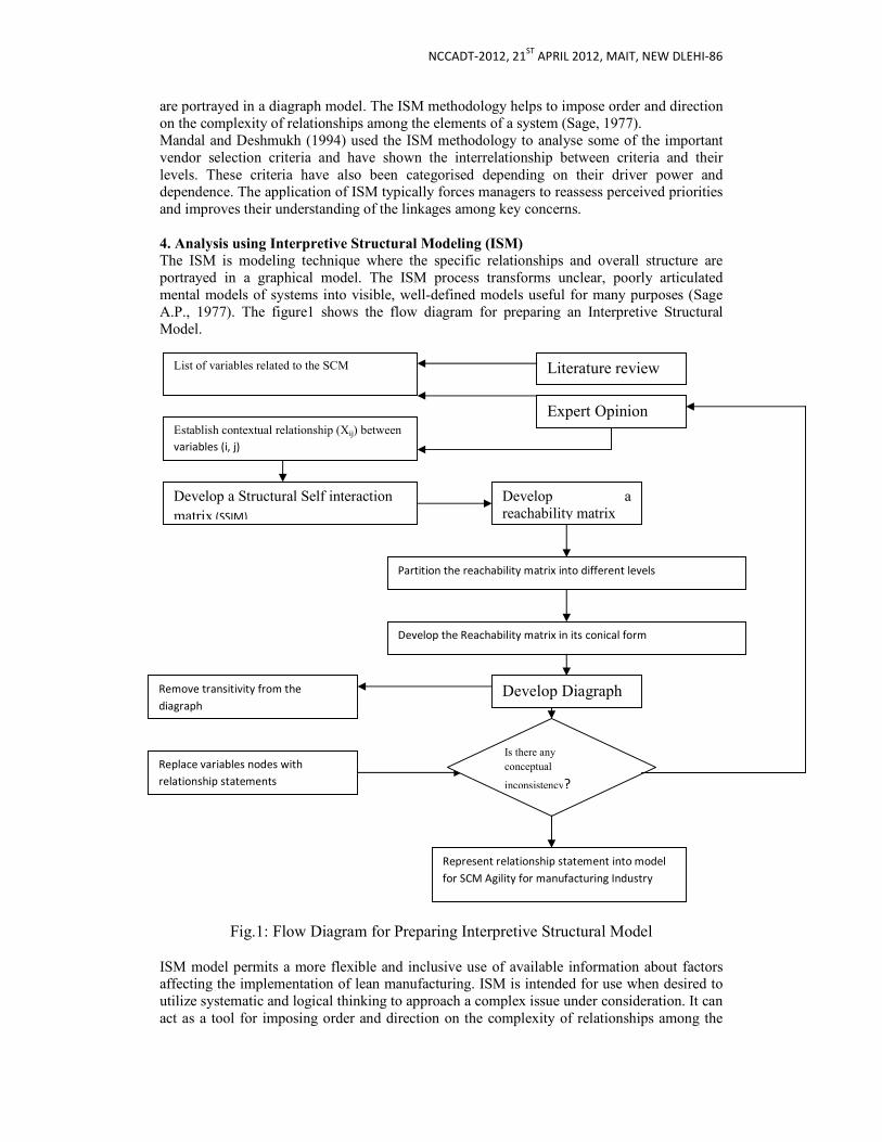
NCCADT-2012, 21ST


are portrayed in a diagraph model. The ISM methodology helps to impose order and direction on the complexity of relationships among the elements of a system (Sage, 1977). Mandal and Deshmukh (1994) used the ISM methodology to analyse some of the important vendor selection criteria and have shown the interrelationship between criteria and their levels. These criteria have also been categorised depending on their driver power and dependence. The application of ISM typically forces managers to reassess perceived priorities and improves their understanding of the linkages among key concerns. 4. Analysis using Interpretive Structural Modeling (ISM)

The ISM is modeling technique where the specific relationships and overall structure are portrayed in a graphical model. The ISM process transforms unclear, poorly articulated mental models of systems into visible, well-defined models useful for many purposes (Sage A.P., 1977). The figure1 shows the flow diagram for preparing an Interpretive Structural Model.

Fig.1: Flow Diagram for Preparing Interpretive Structural Model ISM model permits a more flexible and inclusive use of available information about factors affecting the implementation of lean manufacturing. ISM is intended for use when desired to utilize systematic and logical thinking to approach a complex issue under consideration. It can act as a tool for imposing order and direction on the complexity of relationships among the

List of variables related to the SCM

Agility of manufacturing industry

Establish contextual relationship (Xij) between variables (i, j)

Develop a Structural Self interaction matrix (SSIM)

Develop the Reachability matrix in its conical form

Partition the reachability matrix into different levels

Represent relationship statement into model

for SCM Agility for manufacturing Industry

Develop a reachability matrix

Expert Opinion

Literature review

Develop Diagraph Remove transitivity from the

diagraph

Replace variables nodes with

relationship statements

Is there any conceptual

inconsistency?

NCCADT-2012, 21ST


variables (Jharkharia, S. et. al., 2005; Sage A.P., 1977; Singh, M.D. et. al., 2003). The ISM methodology is an interactive learning process. In ISM, the systematic application of some elementary data is used to explain the complex pattern of contextual relationship among a set of variables. The various steps involved in ISM modeling are as follows: • Identifying of the variables that are relevant to the problem or issue. • Establish the contextual relationship among variables. • Develop a Structural Self-Interaction Matrix (SSIM) of variables, which indicates pair-

wise relationship between variables of the system. • Develop a reachability matrix and check the matrix for transitivity. Transitivity is the

contextual relation is a basic assumption in the ISM which states that if element A is related to B and B to C, then A is necessarily related to C.

• Partition the reachability matrix into different levels. • Remove the transitive links and Construct the ISM model by replacing element nodes

with statements. • Review the ISM model to check for conceptual inconsistency, and make the necessary

modifications. Keeping in mind the contextual relationship for each factor for symbols are used for the type of relation that exists in pair-wise comparison. These symbols are: V for the relation from i to j but not in both directions A for the relation from j to i but not in both directions X for both directions relations from i to j and j to i. O for no relation between i and j.

4.1 Structural Self Interaction Matrix 7 6 5 4 3 2 1

1 A V A V V X

2 A V A V A

3 O X A A

4 O V A

5 O O

6 O

7

4.2 Initial Reachability Matrix

The SSIM has been converted into initial reachability matrix by substituting X, A, V and O by 1 and 0 in the table 2. The substitution of 1s and 0s are as per the following rules:

• If the (i, j) entry in the SSIM is V , the (i, j) entry in the reachability matrix becomes 1 and the (j, i) entry becomes 0;

• If the (i, j) entry in the SSIM is A, the (i, j) entry in the reachability matrix becomes 0 and the (j, i) entry becomes 1;

• If the (i, j) entry in the SSIM is X, the (i, j) entry in the reachability matrix becomes 1 and the (j, i) entry also becomes 1; and

• If the (i, j) entry in the SSIM is O, the (i, j) entry in the reachability matrix becomes 0 and the (j, i) entry also becomes 0.

NCCADT-2012, 21ST


Table 2. Initial Reachability Matrix

1 1 1 1 1 0 1 0

2 1 1 0 1 0 1 0

3 0 1 1 0 0 1 0

4 0 0 1 1 0 1 0

5 1 1 1 1 1 0 0

6 0 0 1 0 0 1 0

7 1 1 0 0 0 0 1

1 2 3 4 5 6 7

4.3 Final Reachability Matrix

The transitivity has been checked as if factor i leads to factor j and factor leads to factor k, then factor i would lead to factor k also. By embedding transitivity a modified reachability matrix is obtained as shown in table 3. Table 3 Final Reachability Matrix

1 1 1 1 1 0 1 0 5

2 1 1 1* 1 0 1 0 5

3 0 1 1 0 0 1 0 3

4 0 0 1 1 0 1 0 3

5 1 1 1 1 1 1* 0 6

6 0 0 1 0 0 1 0 2

7 1 1 1* 1* 0 1* 1 6

1 2 3 4 5 6 7 Driving

Power

Dependence

Power

4 5 7 5 1 7 1

* Not Described 4.4 Level Partition From the final reachability matrix, the reachability and antecedent set for each barrier is found. The reachability set consists of the element itself and the other elements which it may help achieve, whereas the antecedent set consists of the element itself and the other elements which may help in achieving it. Thereafter, the intersection of these sets is derived for all the barriers. The barriers for which the reachability and the intersection sets are the same occupy the top level in the ISM hierarchy. The top-level element in the hierarchy would not help achieve any other element above its own level. Once the top-level element is identified (Table 4), it is separated out from the other elements. Then, the same process is repeated to find out the elements in the next level. This process is continued until the level of each element is found. These levels help in building the diagraph and the final model.

NCCADT-2012, 21ST


Table 4. Level Partition

Number Reachability Set Antecedent Set Intersection Level

1 1,2,3,4,6 1,2,5,7 1,2 III 2 1,2,3,4,6 1,2,3,5,7 1,2,3 III 3 2,3,6 1,2,3,4,5,6,7 2,3,6 II 4 3,4,6 1,2,4,5,7 4 II 5 1,2,3,4,5,6 5 5 IV 6 3,6 1,2,3,4,5,6,7 3,6 I 7 1,2,3,4,6,7 7 7 IV Based on the driving power and dependence these factors affecting plant location has been classified into four categories (Mandal and Deshmukh, 1994) as shown in table 5

Table 5. Driving Power- Dependence Diagram

7

6 5,7 Driver

Variables

Linkage

Variables

5 1 2

4

3 4 3

2 Autonomous

Variables

Dependent

Variables

6

1

1 2 3 4 5 6 7

The first category includes Autonomous factors that have weak Driving power and weak Dependence. There is no autonomous variable identified. The second category consists of dependent variables that have weak driving power but strong dependence. Availability of Infrastructure/resources, Worker’s willingness/ motivation/ awareness/ HR Aspects and Plant layout has been identified in second category. Third category has the linkage variables that have strong driving power and dependence which includes Cost of Implementation (Financial Aspects). The Fourth category includes Independent variables with strong driving power and weak dependence, which are Government Policies, Intra Organization Competition and Company Policies (Top management Interest). From the final reachability matrix and after removing transitivities, an ISM based structure model is generated as shown in figure 2.

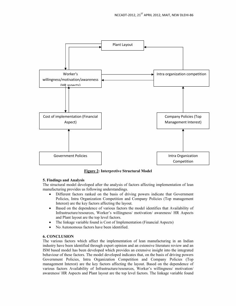
NCCADT-2012, 21ST


Figure 2: Interpretive Structural Model

5. Findings and Analysis

The structural model developed after the analysis of factors affecting implementation of lean manufacturing provides us following understandings.

• Different factors ranked on the basis of driving powers indicate that Government Policies, Intra Organization Competition and Company Policies (Top management Interest) are the key factors affecting the layout.

• Based on the dependence of various factors the model identifies that Availability of Infrastructure/resources, Worker’s willingness/ motivation/ awareness/ HR Aspects and Plant layout are the top level factors.

• The linkage variable found is Cost of Implementation (Financial Aspects) • No Autonomous factors have been identified.

6. CONCLUSION

The various factors which affect the implementation of lean manufacturing in an Indian industry have been identified through expert opinion and an extensive literature review and an ISM based model has been developed which provides an extensive insight into the integrated behaviour of these factors. The model developed indicates that, on the basis of driving powers Government Policies, Intra Organization Competition and Company Policies (Top management Interest) are the key factors affecting the layout. Based on the dependence of various factors Availability of Infrastructure/resources, Worker’s willingness/ motivation/ awareness/ HR Aspects and Plant layout are the top level factors. The linkage variable found

Plant Layout

Worker’s

willingness/motivation/awareness

(HR aspects)

Intra organization competition

Cost of implementation (Financial

Aspect)

Company Policies (Top

Management Interest)

Government Policies Intra Organization

Competition

NCCADT-2012, 21ST


is Cost of Implementation (Financial Aspects). There is no autonomous factor. The absence of autonomous barriers in this study indicates that all the identified barriers influence the process of successful knowledge management. Therefore, it is suggested that management should pay serious attention to all factors. 7. REFERENCES

1. Jharkharia, S. and Shankar, R. (2005) ‘IT-enablement of supply chains: understanding the competitiveness factors’, The Journal of Enterprise Information

Management, Vol. 18, No. 1, pp.11–27. 2. Mandal, A. and Deshmukh, S.G. (1994) ‘Vendor selection using Interpretive

Structural Modelling (ISM)’, International Journal of Operations and Production

Management, Vol. 14, No. 6, pp.52–59. 3. Sage, A.P. (1977) Interpretive Structural Modelling: Methodology for Large Scale

Systems, New York, NY: McGraw-Hill, pp.91–164. 4. Singh, M.D., Shankar, R., Narain, R. and Agarwal, A. (2003) ‘An interpretive

structural modeling of knowledge management in engineering industries’, Journal of

Advances in Management Research, Vol. 1, No. 1, pp.28–40. .

NCCADT-2012, 21ST


ADVANCEMENT IN CAD/CAM/CIM Sheelam Misra

1

1Department of Mechanical engineering, IIMT College of Engineering, Gr. Noida, India

ABSTRACT

The term CAD/CAM means Computer-Aided Design and Computer-Aided Manufacturing. CAD is defined as the use of computer technology to design a part or a product, modify it and also analyze the engineering design. CAD has become popular as the use of the design software’s helps in lower product development costs and shortened design cycles. CAM is defined as the use of computer technology to manufacture or prototype product components with the help of computer numerical control (CNC). Selection of a CAD/CAM system helps in doing the jobs quickly with a greater accurate results and improves the quality of a job. The latest CAD software can produce accurate three-dimensional models of any situation or sequence of events. These are the same tools used to design automobiles, bridges, buildings and almost every other mechanical component imaginable. The software is available to “reverse engineer” an accident scene. Even the people that are involved can be easily modeled accurately, based on their anthropomorphic measurements. Once the models have been created in separate computer files, the forensic scientist has the ability to manipulate each model into its exact position as suggested by whatever photos, GPS data, blueprints, and/or surveillance videos suggest. The disadvantage of CAD and animation has always been its cost, but these days attorneys and their clients are benefiting greatly from the rapid advancement of CAD technology and powerful computer hardware. In recent years, there’s been an exponential reduction in the expense of powerful CAD systems that enable an experienced user to perform a first-class forensic analysis.

KeywordCAD/CAPP/CAM, CIM, AUTOCAD.

Documents

Transferring JIT Manufacturing Philosophy to Service Production Systems