To Pool or Not to Pool: A Partially

Heterogeneous Framework�

Vasilis Sara�disy

University of SydneyNeville Weberz

University of Sydney

This version: December 2009

Abstract

This paper proposes a partially heterogeneous framework for the analysis

of panel data with �xed T , based on the concept of �partitional clustering�.

In particular, the population of cross-sectional units is grouped into clusters,

such that parameter homogeneity is maintained only within clusters. To de-

termine the (unknown) number of clusters we propose an information-based

criterion, which, as we show, is strongly consistent � i.e. it selects the truenumber of clusters with probability one as N !1. Simulation experimentsshow that the proposed criterion performs well even with moderate N and

the resulting parameter estimates are close to the true values. We apply the

method in a panel data set of commercial banks in the US and we �nd four

clusters, with signi�cant di¤erences in the slope parameters across clusters.

Key Words: partial heterogeneity, partitional clustering, information-

based criterion, model selection.

JEL Classi�cation: C13; C33; C51.

�We would like to thank Geert Dhaene, Tom Wansbeek, and seminar participants at the

Tinbergen Institute, University of York, University of Leuven and Erasmus University Rotterdam

for helpful comments and suggestions. We gratefully acknowledge �nancial support from the

Research Unit of the Faculty of Economics and Business, University of Sydney.yCorresponding author. Faculty of Economics and Business, University of Sydney, NSW

2006, Australia. Tel: +61-2-9036 9120; E-mail: v.sara�dis@econ.usyd.edu.au.zSchool of Mathematics and Statistics, University of Sydney, NSW 2006, Australia. Tel:

+61-2-9351 4249; E-mail: n.weber@maths.usyd.edu.au.

1

1 Introduction

Full homogeneity in the slope coe¢ cients of a panel data model is often an assump-

tion that is di¢ cult to justify, both on theoretical grounds and from a practical

point of view. On the other hand, the alternative of imposing no structure on

how these coe¢ cients may vary across individuals may be rather extreme. This

argument is in line with evidence provided by a substantial body of applied work.

For example, Baltagi and Gri¢ n (1997) reject the hypothesis of coe¢ cient homo-

geneity in a panel of gasoline demand regressions across the OECD countries, and

Burnside (1996) rejects the hypothesis of homogeneous production function para-

meters in a panel of US manufacturing industries. Even so, both studies show

that fully heterogeneous models lead to very imprecise estimates of the parameters,

which in some cases have even the wrong sign. Baltagi and Gri¢ n notice that this

is the case despite the fact that there is a relatively long time series in the panel �to the extent that the traditional pooled estimators are superior in terms of root

mean square error and forecasting performance. Furthermore, Burnside suggests

that in general the results of his estimates show signi�cant di¤erences between the

fully homogeneous and the fully heterogeneous models and the conclusions about

the degree of returns to scale in the manufacturing industry would heavily depend

on which one of these two models is used. In the same line Baltagi, Gri¢ n and

Xiong (2000) place the debate between homogeneous versus heterogeneous panel

estimators in the context of cigarette demand and conclude that even with T

(the number of time series observations) relatively large, heterogeneous models for

individual states tend to produce implausible estimates with inferior forecasting

properties, despite the fact that parameter homogeneity is soundly rejected by

the data. Similar conclusions are reached by Baltagi, Bresson and Pirotte (2002)

using evidence from US electricity and gas consumption.

These �ndings indicate that the modelling framework of complete homogene-

ity (pooling) and full heterogeneity may be polar cases, and other intermediate

cases may often provide more realistic solutions in practice. The pooled mean

group estimator (PMGE) proposed by Pesaran, Shin and Smith (1999) is a formal

attempt to bridge the gap between pooled and fully heterogeneous estimators by

imposing partially heterogeneous restrictions related to the time dimension of the

panel. In particular, this intermediate estimator allows the short-run parameters

of the model to be individual-speci�c and restricts the long-run coe¢ cients to be

the same across individuals for reasons attributed to budget constraints, arbitrage

2

conditions and common technologies. This procedure is appealling because it

imposes constraints that can be directly related to economic theory, although it is

mainly designed for panels where both dimensions are large.

In this paper we put forward a modelling framework that imposes partially

heterogeneous restrictions not with respect to the time dimension of the panel, as

PMGE does, but with respect to the cross-sectional dimension, N . In particu-

lar, the population of cross-sectional units is grouped into distinct clusters, such

that within each cluster the parameters are homogeneous and all intra-cluster het-

erogeneity is attributed to the usual individual-speci�c unobserved e¤ects. The

clusters themselves are heterogeneous � that is, the slope coe¢ cients vary acrossclusters.

Naturally, the practical issue of how to cluster the individuals into homoge-

neous groups is central in the paper. Clustering methods have already been advo-

cated in the econometric panel data literature by some researchers; for instance,

Durlauf and Johnson (1995) propose clustering the individuals using regression

tree analysis, and Vahid (1999) suggests a classi�cation algorithm based on a

measure of complexity using the principles of minimum description length and

minimum message length, often employed in coding theory.1 Both these methods

are based on the concept of hierarchical clustering, which involves building a �hier-

archy�from the individual units by progressively merging them into larger clusters.

As a result, the proposed algorithms are theoretically founded for T ! 1 only.

On the other hand, when T is small these algorithms can have poor properties

in terms of determining the appropriate number of clusters. Thus, Vahid (1999)

concludes:

�The classic homogeneity assumption in panel data analysis ... is ab-

solutely necessary and non-testable for the analysis of panel data with

very small T�, page 413.

On the contrary, this paper proposes estimating the unknown number of clus-

ters, as well as the corresponding partition, using an information-based criterion

that is consistent for any �xed T � that is, the probability of estimating the truenumber of clusters approaches one as N ! 1. This is important because most

1Recently, Kapetanios (2006) proposed an information criterion, based on simulated anneal-

ing, to address a related problem � in particular, how to decompose a set of series into a set ofpoolable series for which there is evidence of a common parameter subvector and a set of series

for which there is no such evidence.

3

frequently panel data sets entail a large number of individuals and a small num-

ber of time series observations. Furthermore, it is usually the case when T is

small where some kind of pooling provides substantial e¢ ciency gains over full

heterogeneity. Our method relies on the concept of partitional clustering; instead

of treating each individual as a distinct cluster to begin with (as in hierarchical

clustering), the underlying structure is recovered from the data by grouping the

individuals into a �xed number of clusters using an initial partition, and then

re-allocating each individual into the remaining clusters such that the �nal pre-

ferred partition minimises an objective function. In this paper the residual sum

of squares (RSS) of the estimated model is used as the objective function. The

number of clusters is determined by the clustering solution that minimises RSS

subject to a penalty function that is strictly increasing in the number of clusters.

The penalty re�ects the fact that the minimum RSS of the estimated model is

monotone decreasing in the number of clusters and therefore it tends to over-

parameterise the model by allowing for more clusters than there actually exist.

Hence, the penalty acts essentially as a �lter to ensure that the preferred cluster-

ing outcome partitions between clusters rather than within clusters. The intuition

of the procedure is identical to a standard model selection criterion, although the

study of the asymptotics is more complicated in our case because the number of

individuals contained in a given cluster may vary with N .

The remainder of the paper is as follows. The next section sets out our

partially heterogeneous model and distinguishes the concept of clustering proposed

in the paper from other clustering concepts known in the literature. Section 3

examines the properties of the pooled �xed e¤ects and OLS estimators under

partial heterogeneity. Section 4 formulates the clustering problem, analyses the

objective function and discusses the proposed partitional clustering algorithm.

The �nite-sample performance of the algorithm is investigated in Section 5 using

Monte Carlo experiments. Section 6 illustrates the technique using a random

panel of 551 banking institutions operating in the US, each observed over a period

of 15 years. A �nal section concludes.

2 Model Speci�cation

We consider the following panel data model:

y!it = �0!x!it + �! + �!i + "!it, (1)

4

where y!it denotes the observation on the dependent variable for the ith individual

that belongs to cluster ! at time t, �! = (�!1; :::; �!K)0 is a K � 1 vector of �xed

unknown coe¢ cients, x!it = (x!it1; :::; x!itK)0 is a K � 1 vector of covariates, �!

and �!i denote cluster- and individual-speci�c time-invariant e¤ects respectively

and "!it is a purely idiosyncratic error component. We have ! = 1; :::;, i [2 !] =1; :::; N!, and t = 1; :::; T . This means that the total number of clusters equals ,

the !th cluster has N! individuals, for which there are T time series observations

available. The total number of individuals in all clusters equals N =P

!=1N!

and the total sample size is given by S = NT .

Essentially, model (1) makes a case for pooling the data only within clusters

of individuals and allowing for slope heterogeneity across clusters. One way to

rationalise this is on the basis of the existence of certain unobserved factors or qual-

ities, which decompose the population of individuals into distinct groups, such that

within each group individuals respond similarly to changes in the regressors and

all intra-cluster heterogeneity is attributed to individual-speci�c time-invariant

e¤ects, while individuals from di¤erent clusters may di¤er in terms of these fac-

tors/qualities and therefore they behave in a di¤erent manner. There are several

examples where this set up may apply in practice. For instance, in a model of

economic growth it is natural to think that growth determinants have di¤erent

marginal impacts for di¤erent groups of countries although the number and size

of the clusters is typically unknown. Indeed, recent theories of growth and devel-

opment (e.g. Galor, 1996, and Temple, 1999) suggest the presence of convergence

clubs without specifying club membership or the number of clubs. Another ex-

ample can be drawn from the �nancial industry, where existing evidence (see e.g.

Berger and Humphrey, 1997) appear to suggest that the underlying technology

varies across banking institutions of di¤erent size and therefore pooling the data

may lead to misleading inferences about the returns to scale in the industry.

It is useful to distinguish the concept of clustering proposed in this paper from

other clustering methods or structures of data already familiar in the econometric

literature. In particular, it is common to assume that the errors are independent

across clusters but not within clusters, which gives rise to �clustered standard

errors�. Neglecting this feature in the data and using OLS-type estimates of

the standard errors is likely to lead to biased inferences, although the �rst-order

properties of the estimator remain una¤ected2. There is also some resemblance

between our partially heterogeneous model (1) and �hierarchical� or �nested� or

2See e.g. Cameron and Trivedi (2005, Section 24.5).

5

�multi-level�structures, which allow for a hierarchy of the observations among dif-

ferent levels of data (see e.g. Antweiler, 2001, and Baltagi, Song and Jung, 2001).

For example, y!it could denote the observation of air polution measured by station

i, which is located in city !, at time t and so on. Our partially heterogeneous

model can then be viewed as a single-nested structure. The main di¤erence is

that in a multi-level structure the number of clusters and the corresponding par-

tition are known and the emphasis is on estimating a multi-way error components

model3, while in our framework the total number of clusters, as well as individual

membership into these clusters, need to be estimated. Our partially heterogeneous

model is also conceptually similar to a mixture regression model, except that the

latter involves devising an appropriate probabilistic mechanism that determines

membership of individual i into cluster !4, and requires specifying distributional

assumptions for the components of the mixture. Our model selection criterion is

relatively parsimonious and distribution-free.

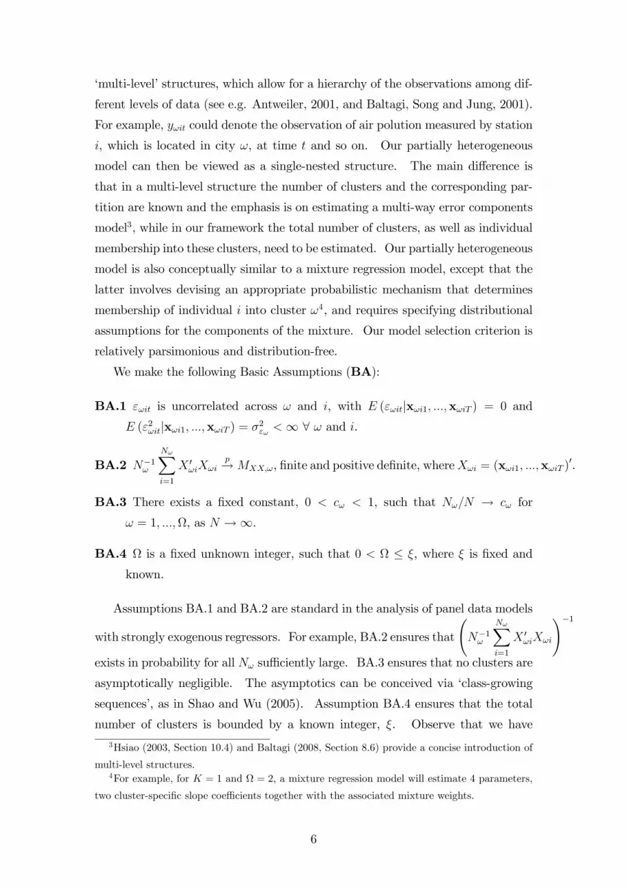
We make the following Basic Assumptions (BA):

BA.1 "!it is uncorrelated across ! and i, with E ("!itjx!i1; :::;x!iT ) = 0 and

E ("2!itjx!i1; :::;x!iT ) = �2"! <1 8 ! and i.

BA.2 N�1!

N!Xi=1

X 0!iX!i

p!MXX;!, �nite and positive de�nite, whereX!i = (x!i1; :::;x!iT )0.

BA.3 There exists a �xed constant, 0 < c! < 1, such that N!=N ! c! for

! = 1; :::;, as N !1.

BA.4 is a �xed unknown integer, such that 0 < � �, where � is �xed and

known.

Assumptions BA.1 and BA.2 are standard in the analysis of panel data models

with strongly exogenous regressors. For example, BA.2 ensures that

N�1!

N!Xi=1

X 0!iX!i

!�1exists in probability for all N! su¢ ciently large. BA.3 ensures that no clusters are

asymptotically negligible. The asymptotics can be conceived via �class-growing

sequences�, as in Shao and Wu (2005). Assumption BA.4 ensures that the total

number of clusters is bounded by a known integer, �. Observe that we have

3Hsiao (2003, Section 10.4) and Baltagi (2008, Section 8.6) provide a concise introduction of

multi-level structures.4For example, for K = 1 and = 2, a mixture regression model will estimate 4 parameters,

two cluster-speci�c slope coe¢ cients together with the associated mixture weights.

6

not imposed any restrictions regarding the distribution of �!i (and �!), which are

allowed to be correlated with X!i, or the serial correlation properties of "!it.

We de�ne

�! = � + �!, (2)

where �! is a K � 1 vector of �xed constants, such thatX!=1

c!�! = 0. (2)

implies that � is a weighted average of the cluster-speci�c coe¢ cients, �!, with

the weights depending on the proportion of individuals that each cluster contains

in the �long term�, i.e. as N grows.

Without any information upon (i) cluster membership and (ii) the size of ,

one can only obtain an estimate of �, and the next section addresses whether �

can be estimated consistently using the standard �xed e¤ects and pooled OLS

estimators.

3 On the Impact of Partial Heterogeneity

Model (1) can be expressed in vector form as follows:

y!i = X!i�!+�T�!i+"!i, (3)

where y!i = (y!i1; :::; y!iT )0, X!i = (x!i1; :::;x!iT )

0, "!i = ("!i1; :::; "!iT )0, �T is a

T � 1 vector of ones and without loss of generality we have imposed �! = 0.5

Ignoring the partially heterogeneous structure in (3) results in the following

regression model:

y!i = X!i� + �T�!i + �!i, �!i = "!i +X!i�!. (4)

De�ne the T � T idempotent matrix QT = IT � T�1�T �0T , which transforms the

observations in terms of deviations from individual-speci�c averages and sweeps

out the time-invariant e¤ects, �!i. We have

QTy!i = QTX!i� +QT�!i, QT�!i = QT"!i +QTX!i�!, (5)

or ey!i = eX!i� + e"!i + eX!i�!, (6)

where ey!i = QTy!i and similarly for the remaining variables.

5This is not a restriction because one can always de�ne ��!i = �!i + k!.

7

The �xed e¤ects estimator is given by

b�FE =

"X!=1

N!Xi=1

eX 0!ieX!i

#�1 " X!=1

N!Xi=1

eX 0!iey!i

#

= �+

"X!=1

N!Xi=1

eX 0!ieX!i

#�1 " X!=1

N!Xi=1

� eX 0!ie"!i + eX 0

!ieX!i�!

�#.

(7)

Taking plims over N yields

plimN!1

�b�FE � �� == plimN!1

"X!=1

N!

N

1

N!

N!Xi=1

eX 0!ieX!i

!#�1(plimN!1

"X!=1

N!

N

1

N!

N!Xi=1

eX 0!ie"!i

!#

+ plimN!1

"X!=1

N!

N

1

N!

N!Xi=1

eX 0!ieX!i

!�!

#)

=

"X!=1

c!�MXX;!

#�1 " X!=1

�MXX;!c!�!

#, (8)

where�MXX;! = plimN!!1

1N!

N!Xi=1

eX 0!ieX!i, the existence of which is guaranteed

from BA.2. As we can see from (8), the �xed e¤ects estimator is not necessarily

consistent. In particular, consistency is achieved when�MXX;!c!�! sums up to

zero and this will occur, for example, when the limiting matrix�MXX;! is orthogo-

nal to the vector c!�! for all !. This would be the case if, say, the�MXX;! matrices

are constant across clusters. However, this condition is unnatural in economic

data sets and therefore it is unlikely to hold true in most empirical applications.

The above result may be quite surprising because in a fully heterogeneous

model, where each individual forms its own cluster such that the model becomes6

yit = �i + �0ixit + "it with �i = � + �i, (9)

exogeneity of the regressors, namely E (�ijxi1; :::;xiT ) = 0, is su¢ cient to ensurethat b�FE is consistent, although not e¢ cient. Similarly, in a fully homogeneousmodel consistency follows because �! = 0. However, as we see here, in the

intermediate case of partial heterogeneity b�FE does not converge to � in gen-

eral. In other words, pooling the data when the slope parameters are partially

heterogeneous has �rst- and second-order implications for the �xed e¤ects estima-

tor. When T is su¢ ciently large, one may deal with this problem by estimating6The subscript ! is omitted in this case because = N .

8

individual-speci�c regressions and clustering the individuals (if required) on the

basis of their estimated coe¢ cients. However, for T �xed this approach may not

even be feasible.

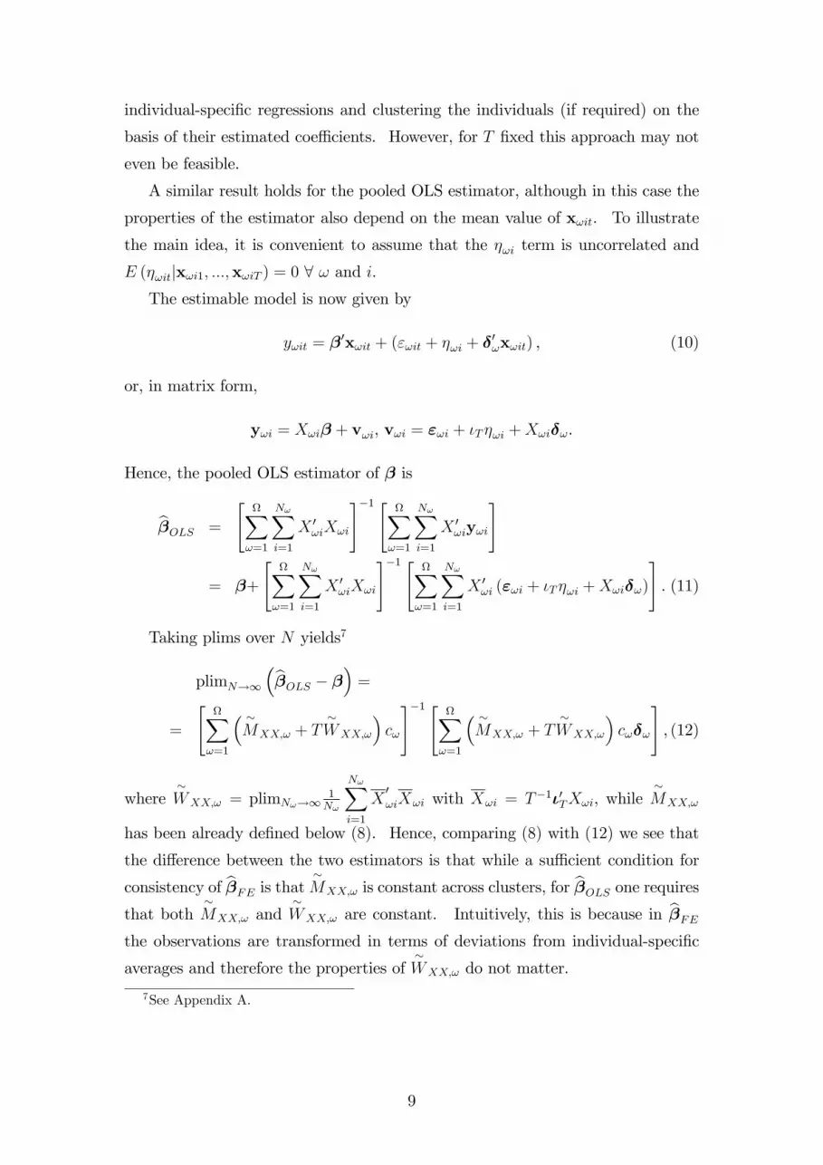
A similar result holds for the pooled OLS estimator, although in this case the

properties of the estimator also depend on the mean value of x!it. To illustrate

the main idea, it is convenient to assume that the �!i term is uncorrelated and

E (�!itjx!i1; :::;x!iT ) = 0 8 ! and i.The estimable model is now given by

y!it = �0x!it + ("!it + �!i + �

0!x!it) , (10)

or, in matrix form,

y!i = X!i� + v!i, v!i = "!i + �T�!i +X!i�!.

Hence, the pooled OLS estimator of � is

b�OLS =

"X!=1

N!Xi=1

X 0!iX!i

#�1 " X!=1

N!Xi=1

X 0!iy!i

#

= �+

"X!=1

N!Xi=1

X 0!iX!i

#�1 " X!=1

N!Xi=1

X 0!i ("!i + �T�!i +X!i�!)

#. (11)

Taking plims over N yields7

plimN!1

�b�OLS � �� ==

"X!=1

� �MXX;! + T

�WXX;!

�c!

#�1 " X!=1

� �MXX;! + T

�WXX;!

�c!�!

#, (12)

where�WXX;! = plimN!!1

1N!

N!Xi=1

X0!iX!i with X!i = T�1�0TX!i, while

�MXX;!

has been already de�ned below (8). Hence, comparing (8) with (12) we see that

the di¤erence between the two estimators is that while a su¢ cient condition for

consistency of b�FE is that �MXX;! is constant across clusters, for b�OLS one requires

that both�MXX;! and

�WXX;! are constant. Intuitively, this is because in b�FE

the observations are transformed in terms of deviations from individual-speci�c

averages and therefore the properties of�WXX;! do not matter.

7See Appendix A.

9

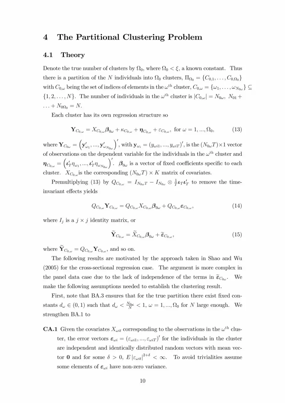
4 The Partitional Clustering Problem

4.1 Theory

Denote the true number of clusters by 0, where 0 < �; a known constant. Thus

there is a partition of the N individuals into 0 clusters, �0 = fC0;1; : : : ; C0;0gwithC0;! being the set of indices of elements in the !th cluster, C0;! = f!1; : : : ; !N0!g �f1; 2; : : : ; Ng: The number of individuals in the !th cluster is jC0;!j = N0!; N01+

: : :+N00 = N:

Each cluster has its own regression structure so

YC0;! = XC0;!�0! + �C0;! + �C0;! + "C0;! ; for ! = 1; :::;0; (13)

whereYC0! =�y0!1 ; :::;y

0!N0!

�0, with y!i = (y!i1; :::; y!iT )

0, is the (N0!T )�1 vectorof observations on the dependent variable for the individuals in the !th cluster and

�C0;! =��0T�!1 ; :::; �

0T�!N0!

�0. �0! is a vector of �xed coe¢ cients speci�c to each

cluster. XC0;! is the corresponding (N0!T )�K matrix of covariates.

Premultiplying (13) by QC0;! = IN0!T � IN0! 1T�T �

0T to remove the time-

invariant e¤ects yields

QC0;!YC0;! = QC0;!XC0;!�0! +QC0;!"C0;! , (14)

where Ij is a j � j identity matrix, or

eYC0;! = eXC0;!�0! + e"C0;! , (15)

where eYC0;! = QC0;!YC0;! , and so on.

The following results are motivated by the approach taken in Shao and Wu

(2005) for the cross-sectional regression case. The argument is more complex in

the panel data case due to the lack of independence of the terms in e"C0! . We

make the following assumptions needed to establish the clustering result.

First, note that BA.3 ensures that for the true partition there exist �xed con-

stants d! 2 (0; 1) such that d! < N0!N

< 1, ! = 1; :::;0 for N large enough. We

strengthen BA.1 to

CA.1 Given the covariates X!it corresponding to the observations in the !th clus-

ter, the error vectors "!i = ("!i1; :::; "!iT )0 for the individuals in the cluster

are independent and identically distributed random vectors with mean vec-

tor 0 and for some � > 0, E j"!itj2+� < 1. To avoid trivialities assume

some elements of "!i have non-zero variance.

10

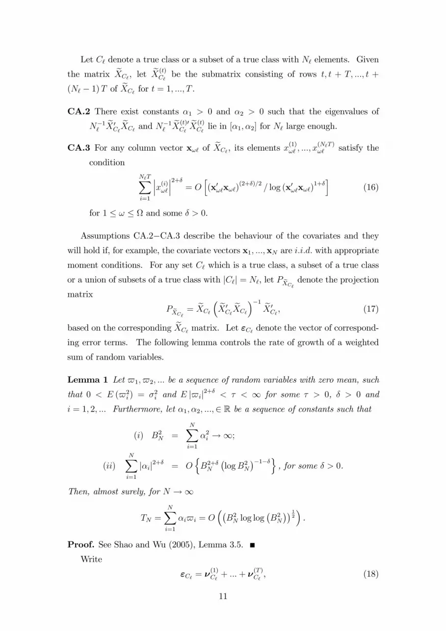
Let C` denote a true class or a subset of a true class with N` elements. Given

the matrix eXC` , let eX(t)C`be the submatrix consisting of rows t; t + T; :::; t +

(N` � 1)T of eXC` for t = 1; :::; T .

CA.2 There exist constants �1 > 0 and �2 > 0 such that the eigenvalues of

N�1`eX 0C`eXC` and N

�1`eX(t)0C`eX(t)C`lie in [�1; �2] for N` large enough.

CA.3 For any column vector x!` of eXC` , its elements x(1)!` ; :::; x

(N`T )!` satisfy the

condition

N`TXi=1

���x(i)!`���2+� = Oh(x0!`x!`)

(2+�)=2= log (x0!`x!`)

1+�i

(16)

for 1 � ! � and some � > 0.

Assumptions CA.2�CA.3 describe the behaviour of the covariates and theywill hold if, for example, the covariate vectors x1; :::;xN are i:i:d: with appropriate

moment conditions. For any set C` which is a true class, a subset of a true class

or a union of subsets of a true class with jC`j = N`, let P eXC` denote the projectionmatrix

P eXC` = eXC`

� eX 0C`eXC`

��1 eX 0C`, (17)

based on the corresponding eXC` matrix. Let "C` denote the vector of correspond-

ing error terms. The following lemma controls the rate of growth of a weighted

sum of random variables.

Lemma 1 Let $1; $2; ::: be a sequence of random variables with zero mean, such

that 0 < E ($2i ) = �2i and E j$ij2+� < � < 1 for some � > 0, � > 0 and

i = 1; 2; ::: Furthermore, let �1; �2; :::;2 R be a sequence of constants such that

(i) B2N =

NXi=1

�2i !1;

(ii)NXi=1

j�ij2+� = OnB2+�N

�logB2

N

��1��o, for some � > 0.

Then, almost surely, for N !1

TN =

NXi=1

�i$i = O��B2N log log

�B2N

�� 12

�.

Proof. See Shao and Wu (2005), Lemma 3.5.

Write

"C` = �(1)C`+ :::+ �

(T )C`, (18)

11

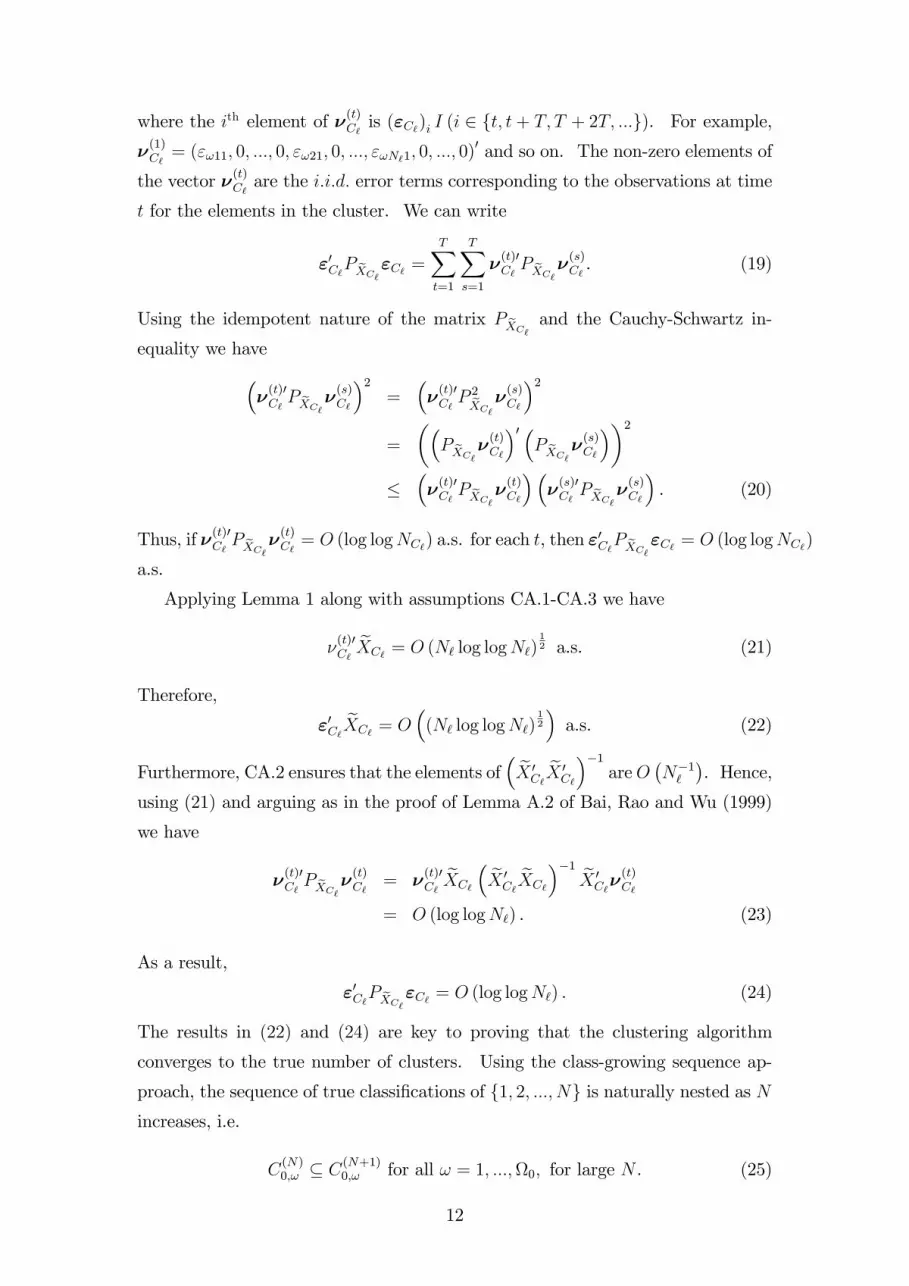
where the ith element of �(t)C` is ("C`)i I (i 2 ft; t+ T; T + 2T; :::g). For example,

�(1)C`= ("!11; 0; :::; 0; "!21; 0; :::; "!N`1; 0; :::; 0)

0 and so on. The non-zero elements of

the vector �(t)C` are the i:i:d: error terms corresponding to the observations at time

t for the elements in the cluster. We can write

"0C`P eXC`"C` =TXt=1

TXs=1

�(t)0C`P eXC`�(s)C` . (19)

Using the idempotent nature of the matrix P eXC` and the Cauchy-Schwartz in-equality we have�

�(t)0C`P eXC`�(s)C`

�2=

��(t)0C`P 2eXC`�(s)C`

�2=

��P eXC`�(t)C`

�0 �P eXC`�(s)C`

��2�

��(t)0C`P eXC`�(t)C`

���(s)0C`P eXC`�(s)C`

�. (20)

Thus, if �(t)0C`P eXC`�(t)C` = O (log logNC`) a.s. for each t, then "

0C`P eXC`"C` = O (log logNC`)

a.s.

Applying Lemma 1 along with assumptions CA.1-CA.3 we have

�(t)0C`eXC` = O (N` log logN`)

12 a.s. (21)

Therefore,

"0C`eXC` = O

�(N` log logN`)

12

�a.s. (22)

Furthermore, CA.2 ensures that the elements of� eX 0

C`eX 0C`

��1areO

�N�1`

�. Hence,

using (21) and arguing as in the proof of Lemma A.2 of Bai, Rao and Wu (1999)

we have

�(t)0C`P eXC`�(t)C` = �

(t)0C`eXC`

� eX 0C`eXC`

��1 eX 0C`�(t)C`

= O (log logN`) . (23)

As a result,

"0C`P eXC`"C` = O (log logN`) . (24)

The results in (22) and (24) are key to proving that the clustering algorithm

converges to the true number of clusters. Using the class-growing sequence ap-

proach, the sequence of true classi�cations of f1; 2; :::; Ng is naturally nested as Nincreases, i.e.

C(N)0;! � C

(N+1)0;! for all ! = 1; :::;0; for large N . (25)

12

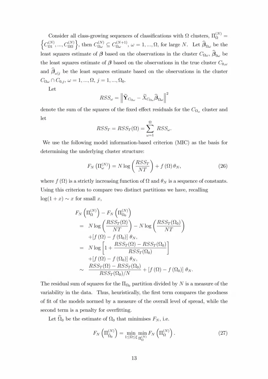
Consider all class-growing sequences of classi�cations with clusters, �(N) =nC(N)1 ; :::; C

(N)

o, then C(N)! � C

(N+1)! , ! = 1; :::;, for large N . Let b�! be the

least squares estimate of � based on the observations in the cluster C!, b�0! bethe least squares estimate of � based on the observations in the true cluster C0;!

and b�!jj be the least squares estimate based on the observations in the clusterC! \ C0;j, ! = 1; :::;, j = 1; :::;0.Let

RSS! = eYC! � eXC!

b�! 2denote the sum of the squares of the �xed e¤ect residuals for the C! cluster and

let

RSST = RSST () =

X!=1

RSS!:

We use the following model information-based criterion (MIC) as the basis for

determining the underlying cluster structure:

FN��(N)!

�= N log

�RSSTNT

�+ f () �N , (26)

where f () is a strictly increasing function of and �N is a sequence of constants.

Using this criterion to compare two distinct partitions we have, recalling

log(1 + x) � x for small x,

FN

��(N)

�� FN

��(N)0

�= N log

�RSST ()

NT

��N log

�RSST (0)

NT

�+[f ()� f (0)] �N ;

= N log

�1 +

RSST ()�RSST (0)

RSST (0)

�+[f ()� f (0)] �N ;

� RSST ()�RSST (0)

RSST (0)=N+ [f ()� f (0)] �N :

The residual sum of squares for the �0 partition divided by N is a measure of the

variability in the data. Thus, heuristically, the �rst term compares the goodness

of �t of the models normed by a measure of the overall level of spread, while the

second term is a penalty for over�tting.

Let b0 be the estimate of 0 that minimises FN , i.e.FN

��(N)b0�= min

1���min�(N)

FN

��(N)

�. (27)

13

The following theorem shows that the criterion in (26) selects the true number

of clusters amongst all class-growing sequences with probability one for N large

enough:

Theorem 2 Let limN!1N�1�N = 0 and limN!1 (log logN)

�1 �N = 1. Sup-

pose that assumptions CA.1-CA.3 and BA.4 hold and �0 is the true clustering

partition corresponding to model (13). Then the MIC criterion is strongly consis-

tent � that is, it selects 0, the true number of clusters among all class-growing

sequences, with probability one as N !1.

Proof. See Appendix B.

The �rst condition in the above theorem prevents estimating too many clusters

asymptotically while the second conditions prevents under-�tting. Similar con-

ditions underlie well-known model selection criteria such as the AIC and the BIC

that are often used in standard model selection. The notable di¤erence is that

our theorem is developed for the purpose of clustering individuals and therefore

the asymptotics are implemented via class-growing sequences.

The above result in fact carries across to the more general model

y!it = �0!x!it + u!it, u!it = �

0!i�t + "!it, (28)

where �!i = (�1!i; :::; �P!i)0, �t = (�1t; :::; �Pt)

0 are both P�1 vectors and give riseto a multi-factor error structure. This can be useful to characterise individual-

speci�c unobserved heterogeneity, captured by �!i, which varies over time, and

also allow for the existence of common unobserved shocks (such as technological

shocks and �nancial crises), captured by �t, the impact of which is di¤erent for

each individual i. The model in (28) reduces back to the structure in (13) by

setting P = 1 and �t = 1 for all t. Writing (28) in vector form we have

YC0;! = XC0;!�0! + (IN0! �)�C0;! + "C0;! , (29)

where � = (�1; :::;�T )0 is a T � P matrix and �C0;! =

��0!1 ; :::;�

0!N0!

�0is a

N0!P � 1 vector. By pre-multiplying the model above by the matrix MC0;! =

IN0!T �IN0!�� (�0�)�1�0

�the model reduces to a classical form similar to (15).

Thus, interpreting eXCl in the various conditions as MClX, we have the following

corollary:

Corollary 3 Let limN!1N�1�N = 0 and limN!1 (log logN)

�1 �N = 1. Sup-

pose that assumptions CA.1-CA.3 and BA.4 hold and �0 is the true clustering

14

partition corresponding to model (28). Then the MIC criterion is strongly consis-

tent � that is, it selects 0, the true number of clusters among all class-growing

sequences, with probability one as N !1.

In practice � is unknown and needs to be replaced with a consistent estimate.

This can be obtained using for example principal components analysis (see e.g.

Connor and Korajzcyk, 1986, and Bai, 2003) or the method of Pesaran (2006).

4.2 Implementation

The number of ways to partition a set of N objects into nonempty subsets is

given by a �Stirling number of the second kind�, which is one of two types of Stirling

numbers that commonly occur in the �eld of combinatorics.8 Stirling numbers of

the second kind are given by the formula

S (N;) =X!=1

(�1)�! !N�1

(! � 1)! (� !)!

=1

!

X!=0

(�1)�!�!

�!N . (30)

The total number of ways to partition a set of N objects into non-overlapping sets

is given by the N th Bell number

BN =NX=1

S (N;) . (31)

To see the order of the magnitude of a Stirling number, for N = 50 and = 2 the

total number of distinct partitions is larger than 5:6 �1014. This implies that if weassumed, rather optimistically, that a given computer was able to estimate 10; 000

panel regressions every second, then one would require about 1790 years to exhaust

all possible partitions. Clearly, a global search over all possible partitions is not

feasible, even with small data sets � a problem that also applies to procedures

based on hierarchical clustering, of course. To deal with this issue, we apply a

hill-climbing algorithm of the kind used in standard partitional cluster analysis

(see, e.g., Everitt, 1993). The algorithm we adopt in this paper can be outlined

in the following steps9:

8See, for example, Rota (1964).9The algorithm is written as an ado �le in Stata 11 and it will available to all Stata users on

the web.

15

1. Given an initial partition and a �xed number of clusters, run the �xed e¤ects

estimator for each cluster separately and calculate RSST ;

2. Re-allocate the ith cross-section to all remaining clusters and obtain the

resulting RSST that arises each time. Finally, allocate the ith individual

into the cluster that achieves the smaller RSST ;

3. Repeat the same procedure for i = 1; :::; N ;

4. Repeat steps 2-3 until RSST cannot be minimised any further.

5. Once the partition that achieves the minimum value of RSST has been de-

termined, repeat steps 1-4 for di¤erent number of clusters;

6. Pick the number of clusters that minimises

N log

�RSSTNT

�+ f () �N , (32)

where f () is a strictly increasing function of and �N is chosen such that

it satis�es the bounds in Theorem 2.

Since only a local search over di¤erent partitions is feasible, the �nal outcome

of such algorithms might be sensitive to the way of choosing the initial partition.

One way to handle this issue is to select the initial partition on the basis of the

slope coe¢ cients estimated for each individual using the T observations. A di¤er-

ent solution would be to select the initial partition based on observed attributes.

Alternatively, one may use several random starts to identify locally optimal so-

lutions and pick up the one that corresponds to the minimum RSST .10 Once

the number of clusters, together with the corresponding partition, has been deter-

mined, it is also possible to cross-validate the results. Several methods have been

proposed in the clustering literature for this purpose. One simple approach in-

volves perturbating the observations and checking whether the clusters are robust

with respect to changes in the data. Kaufman and Rousseeuw (2005) describe

alternative methods.

5 Simulation Study

In this section we carry out a simulation experiment to investigate the performance

of our criterion in �nite samples. Our main focus is on the choice of �N and the

10This is the practice adopted in our simulation experiment that follows.

16

e¤ect of (i) the number of clusters, (ii) the size of N , (iii) the number of regressors

and (iv) the signal-to-noise ratio in the model. We also pay attention to the

properties of the estimators that arise from the estimated partitions, as well as

the pooled �xed e¤ects and OLS estimators.

5.1 Experimental Design

The underlying process is given by

y!it =

KXk=1

�k!xk!it + �!i + "!it,

t = 1; :::; T , i [2 !] = 1; :::; N! and ! = 1; :::;0, (33)

where �!i and "!it are drawn in each replication from i:i:d:N�0; �2�

�and i:i:d:N

�0; �2"!

�respectively, while xk!it is drawn from i:i:d:N

��xk! ; �

2xk!

�.

De�ne y�!it = y!it � �!i, such that (33) can be rewritten as

y�!it =KXk=1

�k!xk!it + "!it, (34)

and let the signal-to-noise ratio be denoted by �! = �2s!=�2"! , where �

2s! and �

2"!

denote the variance of the signal and noise, respectively, for the !th cluster. �2s!

equals

�2s! = var (y�!it � "!it) = var

KXk=1

�k!xk!it

!=

KXk=1

�2k!�2xk!. (35)

This implies that for a given value of��2xk!

Kk=1

and �2"! , the signal-to-noise ratio

for the !th cluster depends on the value of f�k!gKk=1. Thus, for example, scaling

the coe¢ cients upwards by a constant factor will increase � and this may improve

the performance of the model selection criterion; however, there is no natural

way to choose the value of such scalar. Furthermore, notice that for �xed �2"!alternating K will change �2s! and thereby the performance of the criterion may

also be a¤ected. We control both these e¤ects by normalising �2"! = 1, �! = �,

for ! = 1; :::;0 and setting �2xk! = �=��2!kK

�. In this way, the signal-to-noise

ratio in our design is invariant to the choice of K and the scale of f�k!gKk=1.

The values of the slope coe¢ cients are listed in Table 1. We consider � = f4; 8g,N = f100; 400g with T = 10, K = f1; 4g and 0 = f1; 2; 3g.11 We set N1 = 0:7N ,

N2 = 0:3N for 0 = 2 and N1 = 0:4N , N2 = 0:3N , N2 = 0:3N for 0 = 3. This

allows the size of the clusters to be di¤erent. We perform 500 replications in each

11We also set �xk! = 1 for k = 1; :::;K and ! = 1; :::;.

17

experiment. To reduce the computational burden, we �t models with = 1; 2; 3

clusters when 0 = 1, = 1; 2; 3; 4 clusters when 0 = 2 and = 1; 2; 3; 4; 5

clusters when 0 = 3.

To examine the performance of the criterion under a factor error structure, we

set up an additional design where now

"!it = �!i�t + �!it, (36)

where �!i � i:i:dU [�1; 1], �t � i:i:d:N (0; 1) and �!it � i:i:d:N (0; 1). In this

case, �t is estimated in each replication from the vector of principal compo-

nents extracted from y!it and the model is orthogonalised prior to estimation

by premultiplying the T � 1 vectors of observed variables, y!i = (y!i1; :::; y!iT )0

and xk!i = (xk!i1; :::; xk!iT )0 for k = 1; :::; K, by the T � T idempotent matrix

M = IT �H (H 0H)�1H 0, H =�b�1; :::; b�T�0 :

Table 1. Parameter values used in the simulation study.K = 1 K = 4

0 = 1 � = 1 � =

0BB@1:5:752

1CCA

0 = 2�1 = 1�2 = :5

�1 =

0BB@1:5:752

1CCA ; �2 =0BB@

:5:25:3751

1CCA

0 = 3�1 = 1�2 = :5�3 = �:25

�1 =

0BB@1:5:752

1CCA ; �2 =0BB@

:5:25:3751

1CCA ; �3 =0BB@�:2511:50:5

1CCA

5.2 Results

Tables A1-A3 in the appendix report the results of our simulation experiments

in terms of the relative frequency of selecting clusters when the true number

of clusters is 0. The relative frequency of selecting the true number of clusters

is emphasised in bold. Since the property of consistency of b only requires

that f () is stricly increasing in and �N satis�es limN!1N�1�N = 0 and

limN!1 (log logN)�1 �N = 1, there is a broad range of values one can choose.

In this study we set f () = such that

MICj = N log

�RSSTNT

�+ �j for j = 1; :::; 4,

18

where �1 = 2, �2 = logN , �3 = (1= )h(logN) � 1

iand �4 =

pN . MIC1

and MIC2 resemble the Akaike and Bayesian information criteria, respectively,

except that they are applied to the clustering selection problem The choice for

�3 is motivated from the fact that (1= )h(logN) � 1

i! log logN as ! 0

and hence for any su¢ ciently large, the lower bound of Theorem 2 is satis�ed.12

Notice that when N = 100, �3 � �2 for = 3 and �3 � �4 for = 6. Therefore,

we set = 4:5.

As we can see from the tabulated results, MIC1 performs poorly in most cir-

cumstances in that it constantly overestimates the true number of clusters. This

is not surprising as the criterion is not consistent. In fact, its performance de-

teriorates as N increases. MIC2 is a special case of our criterion and performs

somewhat better than MIC1. Notwithstanding, in a lot of cases it largely over-

estimates the number of clusters, especially when 0 = 1; 2. We have explored

further the underlying reason for this result. We found that a larger penalty is

required in the clustering regression problem to prevent over-�tting than what is

typically used in the standard model selection problem. On the other hand, both

MIC3 and MIC4 perform very well in all circumstances. This holds true for all

values of N , K and �. Naturally, the performance of both criteria improves with

larger values of N and �.13

Similar conclusions can be drawn from the model with the factor error struc-

ture, the results of which are reported in Tables A1(b)-A3(b) in the Appendix. In

particular, while MIC1 and MIC2 tend to overestimate the true number of clus-

ters, as before, MIC3 continues to perform very well even for � = 4 and N = 100.

The performance of MIC4 slightly deteriorates in this case, although it behaves

di¤erently toMIC1 andMIC2. In particular, sinceMIC4 has the largest penalty

for over�tting it errs on the side of underestimating the true number of clusters.

All in all, the simulation results show thatMIC3 andMIC4, especially the former,

perform very well under a variety of parametrizations.

Tables A4 and A4(b) in the appendix report the average point estimates of

the parameters for K = 1.14 Standard deviations are reported in parentheses.

�Pooled FE�and �pooled OLS�denote the �xed e¤ects and OLS estimates that

arise by pooling all clusters together, i.e. ignoring cluster-speci�c heterogeneity in

12See e.g. Shao and Wu (2005).13� does not a¤ect the results when 0 = 1 of course.14To save space, we do not report the results obtained for K = 4 because similar conclusions

can be drawn.

19

the slope parameters. FE! denotes the �xed e¤ects estimate of the parameter

for the !th cluster that arises from the estimated partition when 0 is estimated

using MIC3. For the pooled estimators, the true coe¢ cient is taken to be the

weighted average value of the cluster-speci�c unknown slope coe¢ cients, with the

weights determined by the size of the clusters. As we can see, the bias of both

pooled FE and pooled OLS is large and becomes more alike as N increases. The

negative direction of the bias is due to the fact that the clusters with smaller

coe¢ cients exhibit relatively larger leverage because the variance of the regressors

is larger for these clusters. On the other hand, the cluster-speci�c �xed e¤ects

estimators are virtually unbiased even if they are obtained from estimated clusters

and the corresponding estimated partitions. This holds true even for N = 100,

although the performance of the estimators naturally improves as N increases. In

conclusion, we see that the criterion performs well, not only with respect to the

estimate of 0, but also in terms of leading to accurate cluster-speci�c coe¢ cients.

6 Empirical Example

As an illustration of the proposed clustering method, we estimate a partially het-

erogeneous cost function using a panel data set of commercial banks operating in

the United States. The issue of how to estimate scale economies and e¢ ciency

in the banking industry has attracted considerable attention among researchers

due to the signi�cant role that �nancial institutions play in economic prosperity

and growth and, as a result, the major implications that these estimates entail for

policy making.

6.1 Existing Evidence

In an earlier survey conducted by Berger and Humphrey (1997), the authors report

more than 130 studies focusing on the measurement of economies of scale and the

e¢ ciency of �nancial institutions in 21 countries. They conclude that while there

is lack of agreement among researchers regarding the preferred model with which

to estimate e¢ ciency and returns to scale, there seems to be a consensus on the

fact that the underlying technology is likely to di¤er among banks. To this end,

McAllister and McManus (1993) argue that the estimates of the returns to scale in

the banking industry may be largely biased if one applies a single cost function to

the whole sample of banks. This result is likely to remain even if one uses a more

20

�exible functional form in the data, such as the translog form, because this would

restrict, for example, banks of di¤erent size to share the same symmetric average

cost curve. Hence, other interesting possibilities would be precluded, such as �at

segments in the average cost curve over some ranges, or even di¤erent average cost

curves among banks, depending on their size. Thus, the authors conclude:

�These results, taken together, suggest that estimated cost functions

vary substantially depending on the range of bank sizes included in

the sample. This extreme dependence of the results on the choice

of the sample suggests that there are di¢ culties with the statistical

techniques employed�, page 389.

Similarly, Kumbhakar and Tsionas (2008) argue that since the banking indus-

try contains banks of vastly di¤erent size, the underlying technology is very likely

to be di¤erent across banks:

�The distribution of assets across banks is highly skewed. As a result

of this, it is very likely that the parameters of the underlying technology

(cost function in this case) will di¤er among banks�, page 591.

Since this view appears to have been widely adopted in the banking literature,

we estimate a partially heterogeneous cost regression model. A similar approach

conceptually has been followed indirectly by Kaparakis et al (1994), who dis-

tinguish between small and large banks and partition the population into two

equally-sized sub-samples. However, this partioning is rather arbitrary and there

is no formal justi�cation for imposing two clusters.

6.2 The Data Set

The data set consists of a random sample of 551 banks, each observed over a period

of 15 years. These data have been collected from the electronic database main-

tained by the Federal Deposit Insurance Corporation (FDIC).15 The relatively

large size of N implies that the practice of restricting the slope coe¢ cients to be

homogeneous across the whole sample may not be warranted, while the small size

of T prohibits estimating a separate cost function for each individual bank in a

meaningful way.

15See http://www.fdic.gov

21

6.3 Speci�cation of Cost, Outputs and Input Prices

In the theory of banking there is not a univocal approach regarding one�s view of

what banks produce and what purposes they serve. In this paper we follow the

�intermediation� approach, in which the banks are viewed as intermediators of

�nancial and physical resources and produce loans and investments. Under this

approach, outputs are measured in money values and cost �gures include interest

expenses. The selection of inputs and outputs follows closely the study conducted

by Hancock (1986). The variables used in the analysis are: c; the sum of the cost

related to the three input prices that appear below, y1; the sum of industrial,

commercial and individual loans, real estate loans and other loans and leases, y2;

all other assets, pl; the price of labour, measured as total expenses on salaries

and employee bene�ts, divided by the total number of employees, pk; the price of

capital, measured as expenses on premises and equipment, divided by the dollar

value of premises and equipment, and pf ; the price of loanable funds, measured

as total expenses on interest, divided by the dollar value of deposits, federal funds

purchased and other borrowed funds.

Hence, the model is speci�ed as follows16:

c!it = �1!y1;!it + �2!y2;!it + 1!pl;!it + 2!pk;!it + 3!pf;!it + u!it;

u!it = �!i + "!it. (37)

6.4 Results

We cluster the sample of banks into up to six clusters based on the algorithm

developed in Section 4. The initial partition is chosen on the basis of bank size,

which is proxied by the �fteen-year average value of total assets for each individual

bank. Table 2 reports the values ofMICj, j = 1; :::; 4, for = 1; :::; 6. As we can

see, both MIC3 and MIC4 suggest the presence of four clusters. On the other

hand, the performance of MIC2 appears to be similar to MIC1 in that they both

return high scores for 0. This is consistent with the results of the simulation

study, which show that a larger penalty is required in the clustering regression

problem to prevent over-�tting compared to the standard model selection problem.

16All variables are in logs.

22

Table 2. Results for estimating the number of clusters. 1 2 3 4 5 6MIC1 -717:9 -918:5 -958:6 -985:4 -995:8 -1014:4MIC2 -717:1 -917:0 -956:3 -982:4 -992:1 -1010:0MIC3 -699:3 -881:4 -902:9 -911:2 -903:2 -903:1MIC4 -696:4 -875:6 -894:1 -899:1 -888:5 -885:6

Table 3 reports the estimation results obtained for model (37) when = 4.

We adopt a notation similar to the simulation study; in particular, pooled FE

(OLS) denotes the FE (OLS) estimate for the sample as a whole, FEj refers to

the �xed e¤ects estimate for the jth cluster and FE is the weighted average FE

estimate of all clusters with the weights determined by the size of each cluster.

The clusters are sorted in ascending order such that cluster 1 contains on average

the smallest banks and cluster 4 the largest banks.

We can see that there are some large and statistically signi�cant di¤erences in

the value of the coe¢ cients across clusters. For example, the estimated coe¢ cient

of the price of labour, b 1, appears to be strictly decreasing in the size of the banks.This might be explained by the fact that large banks usually make larger in value

loans while the labour cost for an individual loan is the same, which implies that

the labour cost component tends to be smaller for large loans. On the other

hand, the estimated coe¢ cient of loans, b�1, appears to rise as bank size increases,although it remains well below one. This implies that while there are increasing

output returns for both small and large banks, the bene�t of small banks getting

larger is higher than for banks which are already large. In general, we see that

banks of di¤erent size have di¤erent cost drivers and therefore pooling the data

and imposing homogeneity in the slope parameters across the whole sample may

yield misleading results. This becomes apparent when we compare pooled FE

with FE, the di¤erence of which is statistically signi�cant for most coe¢ cients.

23

Table 3. Estimation Resultsa;bb�1 b�2 b 1 b 2 b 3pooled FE :138 :414 :270 :023 :372

(:004) (:005) (:004) (:006) (:008)pooled OLS :247 :432 :257 :003� :342

(:003) (:005) (:006) (:004) (:010)FE1 :037 :036 :720 :005 :442

(:004) (:006) (:005) (:006) (:008)FE2 :051 :330 :533 -:035� :400

(:005) (:007) (:007) (:051) (:007)FE3 :217 :542 :161 :002� :377

(:005) (:008) (:005) (:009) (:012)FE4 :293 :325 :121 :074 :588

(:006) (:007) (:004) (:011) (:011)

FE :141 :298 :402 :010 :451

(a) Standard Errors in Parentheses. (b) � denotesan insigni�cant regressor at the 5% level.

7 Concluding Remarks

Full homogeneity versus full parameter heterogeneity is a topic that has intrigued

research in the analysis of panel data over the last few decades at least. In many

cases the issue remains practically unresolved; for example, Burnside (1996) re-

jected the hypothesis that production function parameters are homogeneous across

a panel of US manufacturing industries. Similarly, Baltagi and Gri¢ n (1997) re-

jected the hypothesis that gasoline demand elasticities were equal across a panel

of OECD countries. Despite this, both studies found that fully heterogeneous

estimators led to very imprecise estimates, which, in some cases, had even the

wrong sign. This paper has proposed an intermediate modelling framework that

imposes only partially heterogeneous restrictions in the parameters, based on the

concept of �partitional clustering�. The unknown number of clusters, together

with the corresponding partition, is estimated using an information-based crite-

rion that is strongly consistent for �xed T . The partitional clustering algorithm

we have developed for Stata 11 is available on the web.

24

References

[1] Antweiler, Werner, �Nested Random E¤ects Estimation in Unbalanced Panel

Data,�Journal of Econometrics 101:2 (2001), 295-313.

[2] Bai, Jushan, �Inferential Theory for Factor Models of Large Dimensions,�

Econometrica 71 (2003), 135-173.

[3] Bai, Zhidong, Calyampudi R. Rao, and Yuehua Wu, �Model Selection with

Data-Oriented Penalty,� Journal of Statistical Planning and Inference 77

(1999), 103-117.

[4] Baltagi, Badi, Econometric Analysis of Panel Data, 4th ed. (West Sussex:

John Willey & Sons, 2008).

[5] Baltagi, Badi H., and James M. Gri¢ n, �Pooled Estimators vs. their Het-

erogeneous Counterparts in the Context of Dynamic Demand for Gasoline,�

Journal of Econometrics 77 (1977), 303-327.

[6] Baltagi, Badi H., James M. Gri¢ n, and Weiwen Xiong, �To Pool or not to

Pool: Homogeneous Versus Heterogeneous Estimators Applied to Cigaretter

Demand,�Review of Economics and Statistics 82:1 (2000), 117-126.

[7] Baltagi, Badi H., Georges Bresson, and Alain Pirotte, �Comparison of Fore-

cast Performance for Homogeneous, Heterogeneous and Shrinkage Estimators.

Some Empirical Evidence fromUS Electricity and Natural-gas Consumption,�

Economics Letters 76 (2002), 375-382.

[8] Baltagi, Badi H., Seuck H. Song, and Byoung C. Jung, �The Unbalanced

Nested Error Component Regression Model,� Journal of Econometrics 101

(2001), 357-381.

[9] Berger, Allen N., and David B. Humphrey, �E¢ ciency of Financial Institu-

tions: International Survey and Directions for Future Research,�European

Journal of Operational Research 98 (1997), 175-212.

[10] Burnside, Craig, �Production Function Regressions, Returns to Scale, and

Externalities,�Journal of Monetary Economics 37 (1996), 177-201.

[11] Cameron, Colin A., and Pravin K. Trivedi, Microeconometrics: Methods and

Applications, (New York: Cambridge University Press, 2005).

25

[12] Connor, Gregory, and Robert A. Korajzcyk, �Performance Measurement with

the Arbitrage Pricing Theory: A New Framework for Analysis,�Journal of

Financial Economics 15 (1986), 373-394.

[13] Durlauf, Steven, and Paul Johnson, �Multiple Regimes and Cross-country

Growth Behaviour,�Journal of Applied Econometrics 10 (1995), 365�384.

[14] Everitt, Brian, Cluster analysis, 3rd ed. (London: Eward Arnold, 2003).

[15] Galor, Oded, �Convergence? Inference from Theoretical Models,�Economic

Journal 106 (1996), 1056-1069.

[16] Hancock, Diana, �A Model of Financial Firm with Imperfect Asset and De-

posit Elasticities,�Journal of Banking and Finance 10 (1986), 37-54.

[17] Hsiao, Cheng, Analysis of Panel Data, 2nd ed. (Cambridge: Cambridge Uni-

versity Press, 2003).

[18] Kapetanios, George, �Cluster Analysis of Panel Datasets Using Non-Standard

Optimisation of Information Criteria,� Journal of Economic Dynamics and

Control 30:8 (2006), 1389-1408.

[19] Kaparakis, Emmanuel I., Stephen M. Miller, and Athanasios G. Noulas

�Short-Run Cost Ine¢ ciency of Commercial Banks: A Flexible Frontier Ap-

proach,�Journal of Money, Credit and Banking 26:4 (1994), 875-893.

[20] Kaufman, Leonard, and Peter J. Rousseeuw, Finding groups in data: An

introduction to cluster analysis, (NY: John Wiley & Sons 1990).

[21] Kumbhakar, Subal C., and Efthymios G. Tsionas, �Scale and e¢ ciency mea-

surement using a semiparametric stochastic frontier model: evidence from the

U.S. commercial banks,�Empirical Economics 34 (2008), 585-602.

[22] McAllister, Patrick H., and Douglas A. McManus, �Resolving the Scale E¢ -

ciency Puzzle in Banking,�Journal of Banking and Finance 17 (1993), 389-

405.

[23] Pesaran, Hashem M., �Estimation And Inference In Large Heterogeneous

Panels With A Multifactor Error Structure,�Econometrica 74:4 (2006), 967-

1012.

26

[24] Pesaran, Hashem M., Yongcheol Shin, and Ron J. Smith, �Pooled Mean

Group Estimation of Dynamic Heterogeneous Panels,�Journal of the Amer-

ican Statistical Association 94 (1999), 621-634.

[25] Rota, Gian-Carlo, �The Number of Partitions of a Set,�American Mathe-

matical Monthly 71:5 (1964), 498-504.

[26] Shao, Qing, and Yuehua Wu, �A Consistent Procedure for Determining the

Number of Clusters in Regression Clustering,�Journal of Statistical Planning

and Inference 135 (2005), 461-476.

[27] Temple, Jonathan, �The New Growth Evidence,�Journal of Economic Lit-

erature 37:1 (1999), 112-156.

[28] Vahid, Farshid, �Partial Pooling: A Possible Answer to Pool or Not to Pool,�

in Cointegration, Causality and Forecasting: Festschrift in Honor of Clive W.

J. Granger, ed. by R. Engle and H. White, 1999.

27

Appendices

A Proof of Equation (12)

We have

plimN!1

�b�OLS � �� == plimN!1

"TXt=1

X!=1

N!N

1

N!

N!Xi=1

X 0!iX!i

!#�1(plimN!1

"TXt=1

X!=1

N!N

1

N!

N!Xi=1

X 0!i"!i

!#

+plimN!1

"TXt=1

X!=1

N!N

1

N!

N!Xi=1

X 0!i�T �!i

!#+ plimN!1

"TXt=1

X!=1

N!N

1

N!

N!Xi=1

X 0!iX!i�!

!#)

= plimN!1

"TXt=1

X!=1

N!N

1

N!

N!Xi=1

�X 0!iX!i + TX

0!iX!i � TX

0!iX!i

�!#�1

�plimN!1

"TXt=1

X!=1

N!N

1

N!

N!Xi=1

�X 0!iX!i + TX

0!iX!i � TX

0!iX!i

�!�!

#

= plimN!1

"TXt=1

X!=1

N!N

1

N!

N!Xi=1

X 0!iQTX!i +

1

N!

N!Xi=1

T X0!iX!i

!#�1

�plimN!1

"TXt=1

X!=1

N!N

1

N!

N!Xi=1

X 0!iQTX!i + T

1

N!

N!Xi=1

X0!iX!i

!�!

#

=

"X!=1

��MXX;! + T

�WXX;!

�c!

#�1 " X!=1

��MXX;! + T

�WXX;!

�c!�!

#. (38)

B Proof of Theorem 2B1. Overparameterised case: 0 < < �.

Write,

FN

��(N)

�� FN

��(N)0

�= N log

�1 +

RSST ()�RSST (0)RSST (0)

�+ [f ()� f (0)] �N ;

= N

�RSST ()�RSST (0)

RSST (0)+ o

�RSST ()�RSST (0)

RSST (0)

��+ [f ()� f (0)] �N :

We need to show that FN��(N)

��FN

��(N)0

�> 0 a.s. for large N . We know [f ()�f (0)] >

0 and, under the conditions of the theorem, �N grows faster than log logN . Further, as N !1;RSST (0)=N is bounded away from 0 and 1 almost surely (see, for example, Lemma 2.1 Bai

et al. (1999)). Thus the result follows if we can show RSST ()�RSST (0) = O(log logN):

28

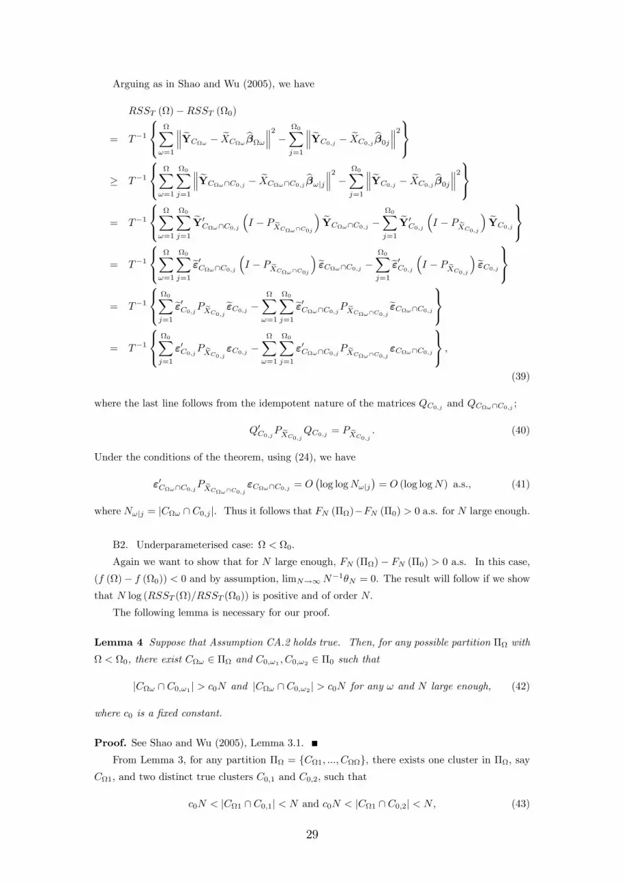
Arguing as in Shao and Wu (2005), we have

RSST ()�RSST (0)

= T�1

8<:X!=1

eYC! � eXC! b�! 2 � 0Xj=1

eYC0;j � eXC0;j b�0j 29=;

� T�1

8<:X!=1

0Xj=1

eYC!\C0;j � eXC!\C0;j b�!jj 2 � 0Xj=1

eYC0;j � eXC0;j b�0j 29=;

= T�1

8<:X!=1

0Xj=1

eY0C!\C0;j

�I � P eXC!\C0j

� eYC!\C0;j �0Xj=1

eY0C0;j

�I � P eXC0;j

� eYC0;j

9=;= T�1

8<:X!=1

0Xj=1

e"0C!\C0;j �I � P eXC!\C0j

�e"C!\C0;j � 0Xj=1

e"0C0;j �I � P eXC0;j

�e"C0;j9=;

= T�1

8<:0Xj=1

e"0C0;jP eXC0;je"C0;j � X

!=1

0Xj=1

e"0C!\C0;jP eXC!\C0;je"C!\C0;j

9=;= T�1

8<:0Xj=1

"0C0;jP eXC0;j"C0;j �

X!=1

0Xj=1

"0C!\C0;jP eXC!\C0;j"C!\C0;j

9=; ,(39)

where the last line follows from the idempotent nature of the matrices QC0;j and QC!\C0;j ;

Q0C0;jP eXC0;jQC0;j = P eXC0;j

. (40)

Under the conditions of the theorem, using (24), we have

"0C!\C0;jP eXC!\C0;j"C!\C0;j = O

�log logN!jj

�= O (log logN) a.s., (41)

where N!jj = jC! \ C0;j j. Thus it follows that FN (�)�FN (�0) > 0 a.s. for N large enough.

B2. Underparameterised case: < 0.

Again we want to show that for N large enough, FN (�)� FN (�0) > 0 a.s. In this case,(f ()� f (0)) < 0 and by assumption, limN!1N

�1�N = 0. The result will follow if we show

that N log (RSST ()=RSST (0)) is positive and of order N:

The following lemma is necessary for our proof.

Lemma 4 Suppose that Assumption CA.2 holds true. Then, for any possible partition � with

< 0, there exist C! 2 � and C0;!1 ; C0;!2 2 �0 such that

jC! \ C0;!1 j > c0N and jC! \ C0;!2 j > c0N for any ! and N large enough, (42)

where c0 is a �xed constant.

Proof. See Shao and Wu (2005), Lemma 3.1.

From Lemma 3, for any partition � = fC1; :::; Cg, there exists one cluster in �, sayC1, and two distinct true clusters C0;1 and C0;2, such that

c0N < jC1 \ C0;1j < N and c0N < jC1 \ C0;2j < N , (43)

29

for N large enough. Denote the family of subsets fC! \ C0;j : j = 1; :::;0; ! = 1; :::;g �fC1 \ C0;1; C1 \ C0;2g by L12. Then

RSST ()�RSST (0)

= T�1

0@ X!=1

eYC! � eXC! b�! 2 � 0Xj=1

eYC0;j � eXC0;j b�0j 21A

= T�1� eYC1\C0;1 � eXC1\C0;1 b�1 2 + eYC1\C0;2 � eXC1\C0;2 b�1 2�+

T�1

0@XL12

eYC!\C0;j � eXC!\C0;j b�! 2 � 0Xj=1

eYC0;j � eXC0;j b�0j 21A .

(44)

Let eX11 = eXC1\C0;1 ; eX11a = � eX 011 0K�jC1\C0;2j

�0, eX12 = eXC1\C0;2 ,

eY012 =

eYC1\C0;1eYC1\C0;2

!; eX012 = eX11eX12

!; e"012 = � e"C1\C0;1e"C1\C0;2

�. (45)

Hence

RSST ()�RSST (0)

� T�1

0@ eY012 � eX012b�012 2 +XL12

eYC!\C0;j � eXC!\C0;j b�!jj 21A

�T�10Xj=1

e"0C0;j �I � P eXC0;j

�e"C0;j , (46)

where b�012 is the least squares estimate of � based on �eY012; eX012�. Since eY012 = eX012�02 +eX11a (�01 � �02) + e"012, we have thatRSST ()�RSST (0)

� T�1

0@eY0012

�I � P eX012

� eY012 +XL12

e"0C!\C0;j �I � P eXC!\C0;j

�e"C!\C0;j1A

�T�10Xj=1

e"0C0;j �I � P eXC0;j

�e"C0;j= T�1 (�01 � �02)

0 eX 011

�I � eX11 � eX 0

11eX11 + eX 0

12eX12��1 eX 0

11

� eX11 (�01 � �02)+T�12 (�01 � �02)

0 eX 011a

�I � P eX012

�e"012 + T�1e"0012 �I � P eX012

�e"012 +T�1

XL12

e"0C!\C0;j �I � P eXC!\C0;j

�e"C!\C0;j � T�1 0Xj=1

e"0C0;j �I � P eXC0;j

�e"C0;j= T�1 (�01 � �02)

0�� eX 0

11eX11��1 + � eX 0

12eX12��1��1 (�01 � �02) +

T�12 (�01 � �02)0 eX 0

11a

�I � P eX012

�e"012 � T�1e"0012P eX012e"012

�T�1XL12

e"0C!\C0;jP eXC!\C0;je"C!\C0;j + T�1 0X

j=1

e"0C0;jP eXC0;je"C0;j ,

(47)

30

using the algebraic identity (A+B)�1 = A�1 � A�1�A�1 +B�1

��1A�1, where A and B are

non-singular matrices.

Since we have assumed j�01 � �02j > 0, given Assumption CA.2 we have

(�01 � �02)0�� eX 0

11eX11��1 + � eX 0

12eX12��1��1 (�01 � �02) � c0N j�01 � �02j .

Using (22), (24) and the Cauchy-Schwartz inequality we see that the other terms in the above

lower bound are of smaller order in N . As RSST (0)=N is bounded away from 0 and 1 almost

surely, we have, for N large enough,

N log

�1 +

RSST ()�RSST (0)RSST (0)

�> N log(1 +K);

for some positive K, and the result follows.

31

Table A1. Simulation results for 0 = 1, "!it is purely idiosyncratic.K = 1 K = 4

N = 100 N = 400 N = 100 N = 400 N = 100 N = 400 N = 100 N = 400� = 4 � = 8 � = 4 � = 8

MIC1 = 1 :013 :000 :013 :000 :000 :000 :000 :000 = 2 :934 :021 :934 :021 :000 :000 :000 :000 = 3 :053 :979 :053 :979 1:00 1:00 1:00 1:00

MIC2 = 1 :013 :018 :013 :018 :631 1:00 :631 1:00 = 2 :987 :964 :987 :964 :369 :000 :369 :000 = 3 :000 :018 :000 :018 :000 :000 :000 :000

MIC3 = 1 1:00 1:00 1:00 1:00 :973 1:00 :973 1:00 = 2 :000 :000 :000 :000 :027 :000 :027 :000 = 3 :000 :000 :000 :000 :000 :000 :000 :000

MIC4 = 1 1:00 1:00 1:00 1:00 1:00 1:00 1:00 1:00 = 2 :000 :000 :000 :000 :000 :000 :000 :000 = 3 :000 :000 :000 :000 :000 :000 :000 :000

Table A2. Simulation results for 0 = 2, "!it is purely idiosyncratic.K = 1 K = 4

N = 100 N = 400 N = 100 N = 400 N = 100 N = 400 N = 100 N = 400� = 4 � = 8 � = 4 � = 8

MIC1 = 1 :000 :000 :000 :000 :000 :000 :000 :000 = 2 :009 :000 :202 :000 :188 :000 :210 :000 = 3 :241 :000 :384 :052 :312 :061 :381 :033 = 4 :750 1:00 :414 :948 :500 :939 :409 :967

MIC2 = 1 :000 :000 :000 :000 :000 :000 :000 :000 = 2 :157 :451 :210 :482 :183 :291 :410 :476 = 3 :343 :482 :389 :495 :395 :307 :403 :419 = 4 :500 :067 :401 :023 :422 :402 :187 :105

MIC3 = 1 :000 :000 :000 :000 :000 :000 :000 :000 = 2 1:00 1:00 1:00 1:00 1:00 1:00 1:00 1:00 = 3 :000 :000 :000 :000 :000 :000 :000 :000 = 4 :000 :000 :000 :000 :000 :000 :000 :000

MIC4 = 1 :000 :000 :000 :000 :000 :000 :000 :000 = 2 1:00 1:00 1:00 1:00 1:00 1:00 1:00 1:00 = 3 :000 :000 :000 :000 :000 :000 :000 :000 = 4 :000 :000 :000 :000 :000 :000 :000 :000

32

Table A3. Simulation results for 0 = 3, "!it is purely idiosyncratic.K = 1 K = 4

N = 100 N = 400 N = 100 N = 400 N = 100 N = 400 N = 100 N = 400� = 4 � = 8 � = 4 � = 8

MIC1 = 1 :000 :000 :000 :000 :000 :000 :000 :000 = 2 :000 :000 :000 :000 :000 :000 :000 :028 = 3 :528 :577 :616 :629 :023 :000 :024 :000 = 4 :472 :421 :384 :371 :432 :000 :441 :000 = 5 :000 :002 :000 :000 :545 1:00 :535 1:00

MIC2 = 1 :000 :000 :000 :000 :000 :000 :000 :000 = 2 :000 :000 :000 :000 :000 :000 :000 :000 = 3 :633 :715 :679 :749 :841 :142 :890 :237 = 4 :367 :285 :321 :251 :159 :545 :110 :454 = 5 :000 :000 :000 :000 :000 :313 :000 :309

MIC3 = 1 :000 :000 :000 :000 :000 :000 :000 :000 = 2 :000 :000 :000 :000 :000 :000 :000 :000 = 3 1:00 1:00 1:00 1:00 1:00 1:00 1:00 1:00 = 4 :000 :000 :000 :000 :000 :000 :000 :000 = 5 :000 :000 :000 :000 :000 :000 :000 :000

MIC4 = 1 :000 :000 :000 :000 :000 :000 :000 :000 = 2 :000 :000 :000 :000 :103 :006 :000 :000 = 3 1:00 1:00 1:00 1:00 :897 :994 1:00 1:00 = 4 :000 :000 :000 :000 :000 :000 :000 :000 = 5 :000 :000 :000 :000 :000 :000 :000 :000

Table A1(b). Simulation results for 0 = 1, "!it = �!i�t + �!it.K = 1 K = 4

N = 100 N = 400 N = 100 N = 400 N = 100 N = 400 N = 100 N = 400� = 4 � = 8 � = 4 � = 8

MIC1 = 1 :015 :000 :015 :000 :000 :000 :000 :000 = 2 :934 :023 :934 :023 :000 :000 :000 :000 = 3 :051 :977 :051 :977 1:00 1:00 1:00 1:00

MIC2 = 1 :021 :032 :021 :032 :533 :698 :533 :698 = 2 :979 :968 :979 :968 :369 :302 :369 :302 = 3 :000 :000 :000 :000 :000 :000 :000 :000

MIC3 = 1 1:00 1:00 1:00 1:00 1:00 1:00 1:00 1:00 = 2 :000 :000 :000 :000 :027 :000 :027 :000 = 3 :000 :000 :000 :000 :000 :000 :000 :000

MIC4 = 1 1:00 1:00 1:00 1:00 1:00 1:00 1:00 1:00 = 2 :000 :000 :000 :000 :000 :000 :000 :000 = 3 :000 :000 :000 :000 :000 :000 :000 :000

33

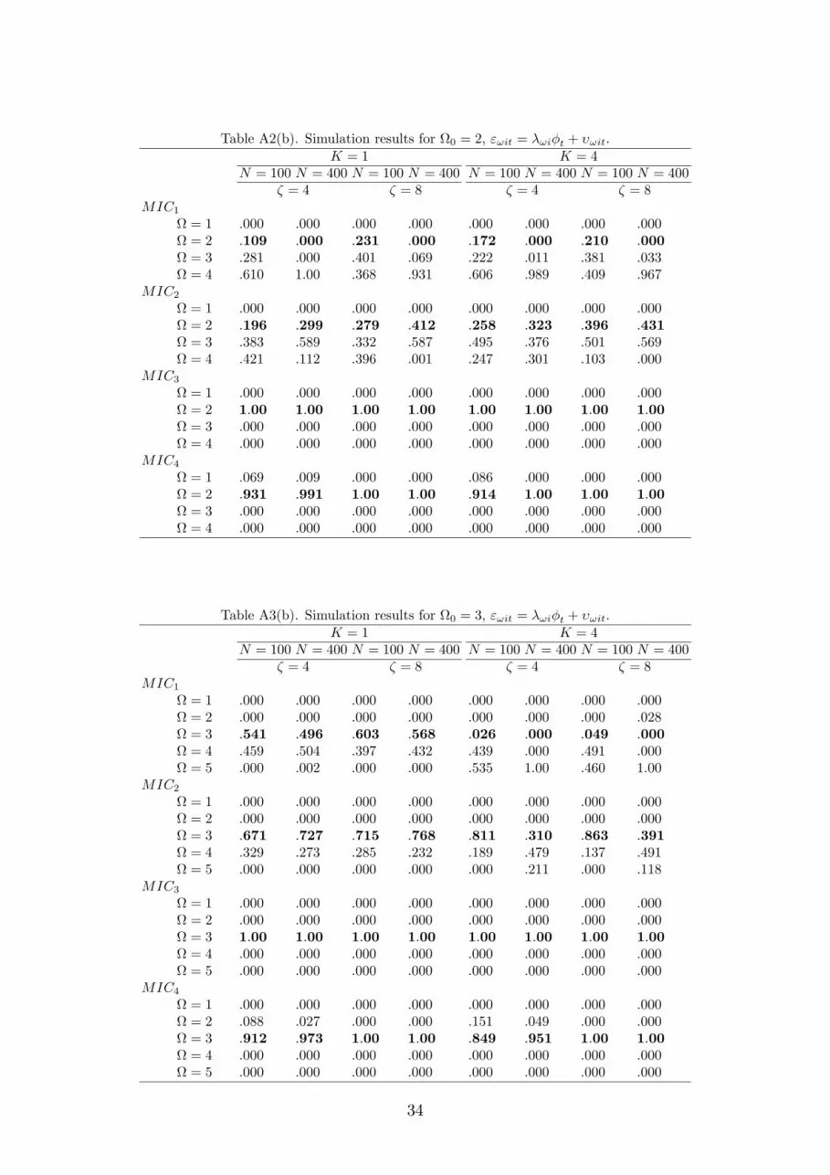
Table A2(b). Simulation results for 0 = 2, "!it = �!i�t + �!it.K = 1 K = 4

N = 100 N = 400 N = 100 N = 400 N = 100 N = 400 N = 100 N = 400� = 4 � = 8 � = 4 � = 8

MIC1 = 1 :000 :000 :000 :000 :000 :000 :000 :000 = 2 :109 :000 :231 :000 :172 :000 :210 :000 = 3 :281 :000 :401 :069 :222 :011 :381 :033 = 4 :610 1:00 :368 :931 :606 :989 :409 :967

MIC2 = 1 :000 :000 :000 :000 :000 :000 :000 :000 = 2 :196 :299 :279 :412 :258 :323 :396 :431 = 3 :383 :589 :332 :587 :495 :376 :501 :569 = 4 :421 :112 :396 :001 :247 :301 :103 :000

MIC3 = 1 :000 :000 :000 :000 :000 :000 :000 :000 = 2 1:00 1:00 1:00 1:00 1:00 1:00 1:00 1:00 = 3 :000 :000 :000 :000 :000 :000 :000 :000 = 4 :000 :000 :000 :000 :000 :000 :000 :000

MIC4 = 1 :069 :009 :000 :000 :086 :000 :000 :000 = 2 :931 :991 1:00 1:00 :914 1:00 1:00 1:00 = 3 :000 :000 :000 :000 :000 :000 :000 :000 = 4 :000 :000 :000 :000 :000 :000 :000 :000

Table A3(b). Simulation results for 0 = 3, "!it = �!i�t + �!it.K = 1 K = 4

N = 100 N = 400 N = 100 N = 400 N = 100 N = 400 N = 100 N = 400� = 4 � = 8 � = 4 � = 8

MIC1 = 1 :000 :000 :000 :000 :000 :000 :000 :000 = 2 :000 :000 :000 :000 :000 :000 :000 :028 = 3 :541 :496 :603 :568 :026 :000 :049 :000 = 4 :459 :504 :397 :432 :439 :000 :491 :000 = 5 :000 :002 :000 :000 :535 1:00 :460 1:00

MIC2 = 1 :000 :000 :000 :000 :000 :000 :000 :000 = 2 :000 :000 :000 :000 :000 :000 :000 :000 = 3 :671 :727 :715 :768 :811 :310 :863 :391 = 4 :329 :273 :285 :232 :189 :479 :137 :491 = 5 :000 :000 :000 :000 :000 :211 :000 :118

MIC3 = 1 :000 :000 :000 :000 :000 :000 :000 :000 = 2 :000 :000 :000 :000 :000 :000 :000 :000 = 3 1:00 1:00 1:00 1:00 1:00 1:00 1:00 1:00 = 4 :000 :000 :000 :000 :000 :000 :000 :000 = 5 :000 :000 :000 :000 :000 :000 :000 :000

MIC4 = 1 :000 :000 :000 :000 :000 :000 :000 :000 = 2 :088 :027 :000 :000 :151 :049 :000 :000 = 3 :912 :973 1:00 1:00 :849 :951 1:00 1:00 = 4 :000 :000 :000 :000 :000 :000 :000 :000 = 5 :000 :000 :000 :000 :000 :000 :000 :000

34

Table A4. Finite sample properties of estimators, "!it is purely idiosyncratic.K = 1, 0 = 2, � = 0:85, � = (1; :5)

0K = 1, 0 = 3, � = 0:475, � = (1; :5;�:25)0

N = 100 N = 400 N = 100 N = 400 N = 100 N = 400 N = 100 N = 400

� = 4 � = 8 � = 4 � = 8

pooled FE :688 :678 :688 :678 -:027 -:039 -:026 -:042

(:013) (:007) (:009) (:005) (:006) (:004) (:004) (:002)

pooled OLS 672 :680 :675 :679 -:047 -:038 -:045 -:036

(:018) (:006) (:013) (:004) (:009) (:004) (:008) (:003)

FE1 1:02 1:02 1:02 1:01 1:03 1:03 1:02 1:01

(:057) (:009) (:016) (:007) (:026) (:013) (:019) (:010)

FE2 :512 :506 :502 :502 :506 :503 :502 :501

(:056) (:008) (:010) (:006) (:017) (:009) (:012) (:007)

FE3 -:251 -:250 -:250 -:250

(:006) (:005) (:004) (:003)

Table A4(b). Finite sample properties of estimators, "!it = �!i�t + �!it.K = 1, 0 = 2, � = 0:85, � = (1; :5)

0K = 1, 0 = 3, � = 0:475, � = (1; :5; -:25)

0

N = 100 N = 400 N = 100 N = 400 N = 100 N = 400 N = 100 N = 400

� = 4 � = 8 � = 4 � = 8

pooled FE :684 :671 :685 :677 -:026 -:031 -:024 -:037

(:013) (:008) (:009) (:005) (:008) (:005) (:005) (:003)

pooled OLS 683 :670 :689 :681 -:025 -:033 -:024 -:037

(:014) (:009) (:010) (:006) (:009) (:005) (:007) (:004)

FE1 1:03 1:01 1:02 1:01 1:03 1:02 1:01 1:00

(:028) (:018) (:016) (:009) (:034) (:017) (:022) (:009)

FE2 :505 :502 :502 :501 :501 :501 :501 :502

(:019) (:011) (:010) (:007) (:020) (:010) (:014) (:008)

FE3 -:247 -:251 -:251 -:250

(:009) (:005) (:005) (:004)

35