Tidal wave simulation III

Nonlinear Tidal Wave Propagation in Shallow Water III: Simulation of the propagation of a progressive tide in a channel of finite

length

Tidal wave propagation in shallow water II

Next Titles

Conservation laws and spectral properties in the simulation of the propagation of a progressive tide in a channel of finite length Melio Sáenz and Christian Le Provost Propagation of a tidal wave in a closed channel. Melio Sáenz and Christian Le Provost

2 M. Sáenz, Ch. Le Provost: convergence and stability

2

Contents

Series Preface .................................................................................................................................................................. 3

Preface ............................................................................................................................................................................. 4

1. Introduction ................................................................................................................................................................. 5

2. Boundary condition permeable to the energy ............................................................................................................ 5

3. Numerical experiments ................................................................................................................................................ 2

4. Error distribution in space-time ................................................................................................................................... 2

5. Maximum error as a time function .............................................................................................................................. 3

6. Dispersion between exact solution and numerical approximation. ............................................................................ 5

Conclusions ...................................................................................................................................................................... 6

Bibliography ..................................................................................................................................................................... 6


Series Preface

This series of documents summarize the main results achieved in addressing the study of

Long Wave Propagation.

The work was started in 1973 under the DEA of Fluid Mechanics held at the Institute of

Mechanics of Grenoble within the Hydrodynamics team led by Prof. Julien Kravtchenko.

Dr. Gabriel Chabert d'Hieres, responsable of CORIOLIS team gave us all the support

necessary to carry out this work, it was led by Christian Le Provost, under whose tutelage

prepared my thesis for the degree of Doctor-Engineer.

Laboratory beloved companions they gave their support and friendship at this early stage:

Andre Temperville, Jean-Louis Kueny, Michel Favre-Marinet, Randel Haverkamp, Louis

Gulli, Dominique Renouard.

This work of documentary collection responds to a need to make available the hearing

unpublished results and I dedicate it to the memory of Cristian Le Provost,

Oceanographer, friend and partner in this adventure of Science.

Melio Sáenz

February 2015


4

Preface

In previous work we have focused on aspects relating to the accuracy of the simulation of the propagation

of long waves in a rectangular constant depth channel and frictionless we find that at a given time, the

first wave front reaches continuity breaks. From this point we do not verify the unicity of the solution.

In the present work we are interested to study the behavior of the numerical models beyond the wave

breaking moment . To do this we must consider a finite lenght channel that is not affected by the breaking

wave. We have chosen the channel length as 3𝜆 / 2.

We need to describe a downstream border of the domain such that it allows that the energy caused by

the disturbance of the flow of water, get out the channel without causing a reflected wave which go back

the channel. This is obtained by applying the invariant Riemann relationship.

It should be noted that we have the exact solution of the problem with which we can compare the results

obtained from the simulation of the phenomenon with the numerical models used.

Realized test confirm the results we obtained on the quality of simulation models with Preissman and

Lax-Wendroff.

This work shows a way to incorporate experimental data in the evaluations of the results obtained with

numerical models.

Melio Sáenz

April 2015


Nonlinear tidal wave propagation in shallow water III:

Simulation of the propagation of a progressive tide in a

channel of finite length

Melio Sáenz1, Christian Le Provost1 1Groupe Hydrodynamique/Institut de Mécanique de Grenoble./Domaine Universitaire,38400 Saint Martin d’Heres,France

Abstract In our interest to evaluate the quality of the results obtained from the numerical models used in the simulation of

the propagation of long waves, we are led to study the behavior of these models under conditions that allow to verify the

uniqueness of solutions. To do this we have limited the channel length for the wave does not reach the surf zone and once

reached the end of the channel, the wave may not be reflected. Numerical experiences were carried out during more than one

period of wave oscillation. The results confirm the conclusions set forth in previous work.

Keywords finite differences, finite length channel, energy radiation, characteristics, Riemann invariants

1. Introduction

We study the propagation of a long wave in a one-dimen-

sional finite length channel such that the wave does not arrive

at the surf zone of its first front, then, in every channel point,

the solution of the initial-boundary value problem describing

the phenomenon, is unique.

Two problems arise from this need: wavefront arriving to the

breaking zone, where the solution is not unique and reflecting

wave generated by energy reflection in the downstream bor-

der. To solve the first problem, we choose a affordable canal

length: lower than a wave length where it is located the

breaking zone. For the second one, we describe the border by

means of the Riemann invariant with which the border is en-

ergy radiating .

* Corresponding author: [email protected]

Roach [1] writes It is easy to conjure up some kind of plausi-

ble boundary conditions but attempt to determine realistic,

accurate and stable methods can be highly frustrating.

Alexander Preissmann suggest a Dirichlet form using a func-

tion related with the discrete mesh [2].

We decide to explore establishing boundary conditions with

help of characteristics equations and its corresponding Rie-

mann's invariants for the hyperbolic partial differential equa-

tions describing the one- dimensional tidal propagation.

2. Boundary condition permeable to the energy

Let Ω be the two-dimensional domain referenced by the sys-

tem of orthogonal axes (𝑋, 𝑡) where 𝑋 is assigned to

spatial coordinates and t the time.

Consider a point 𝑀 (𝑥, 𝑡) ∈ Ω. Through the point 𝑀, there

are two characteristics curves that pass: one belonging to


2

the positive characteristics family and the other to the neg-

ative one.

For a traveling wave, along the positive characteristic propa-

gates the disturbance produced at abscissa 𝑥 = 0 at instant

t=0 , and in the absence of the wave breaking, no disturb-

ance goes up the negative characteristic since it comes

from the rest zone.

Consequently, the idea that we have exploited is to impose as

a boundary condition to the abscissa x = L the absence of

disturbance along the negative characteristic. That is

𝑢(𝐿, 𝑡) − 2√𝑔[ℎ(𝐿) + 𝜁(𝐿, 𝑡)] = −2√𝑔(ℎ(𝐿)

where 𝑢 = 𝑢(𝑥, 𝑡) is the wave propagation velocity at ab-

scissa 𝑥 at time 𝑡 , 𝑔 the constant of gravity; h channel

depth at rest, considered constant, L length of the channel,

𝜁 the difference in elevation of the free surface relative to

the water level in the idle channel

Thus formulated, the problem admits an exact solution which

is the solution presented in [5].

3. Numerical experiments

The movement in the channel is generated by a sinusoidal

oscillation imposed at abscissa 𝑥 = 0 and described

by means of the following equality:

𝑢(0, 𝑡0) = 𝐴 sin (𝜔𝑡0)

and the boundary conditions are obtained from written char-

acteristics relationships as follows

𝑢(0, 𝑡) + 2√𝑔[ℎ(0) + 𝜁(0, 𝑡)] = 2𝐴 sin(𝜔𝑡0) + 2√𝑔ℎ(0)

𝑢(𝐿, 𝑡) − 2√𝑔[ℎ(𝐿) + 𝜁(𝐿, 𝑡)] = −2√𝑔ℎ(𝐿)

The depth at rest is 50 m. The wave excitement period is

44700 s. The magnitude of the velocity at 𝑥 = 0 is equal

to 1.50 m/s. The differential equations are replaced by a finite

differences system of equations [6] [5]. The initial conditions

correspond to the state at rest, the boundary conditions are

introduced to the upstream using the characteristic relation-

ships [6].

Different numerical tests were realized as well for time inter-

vals highest than 3𝑇 / 2: beyond of this time 3𝑇 / 2, the

movement is established across the channel and presents a

periodic character in time with the oscillation period intro-

duced at the border.

Numerical tests we have accrued with the following discreti-

zation: ∆𝑥 =𝜆

30 ; ∆𝑡 =

𝑇

32 , with which we respect the sta-

bility condition. We chose the diffusion coefficient 𝛼 = 0

for the diffusive scheme and θ= 0.52 the weight coefficient

for the scheme Preissmann.

We used the following four numerical models: characteristics,

diffusive, Lax-Wendroff and Preissmann.

4. Error distribution in space-time

When the regime is established we can determine for each

time instant corresponding to the oscillation period, the gap

between the approximate level computed with the numerical

model and the corresponding value obtained from the exact

solution.

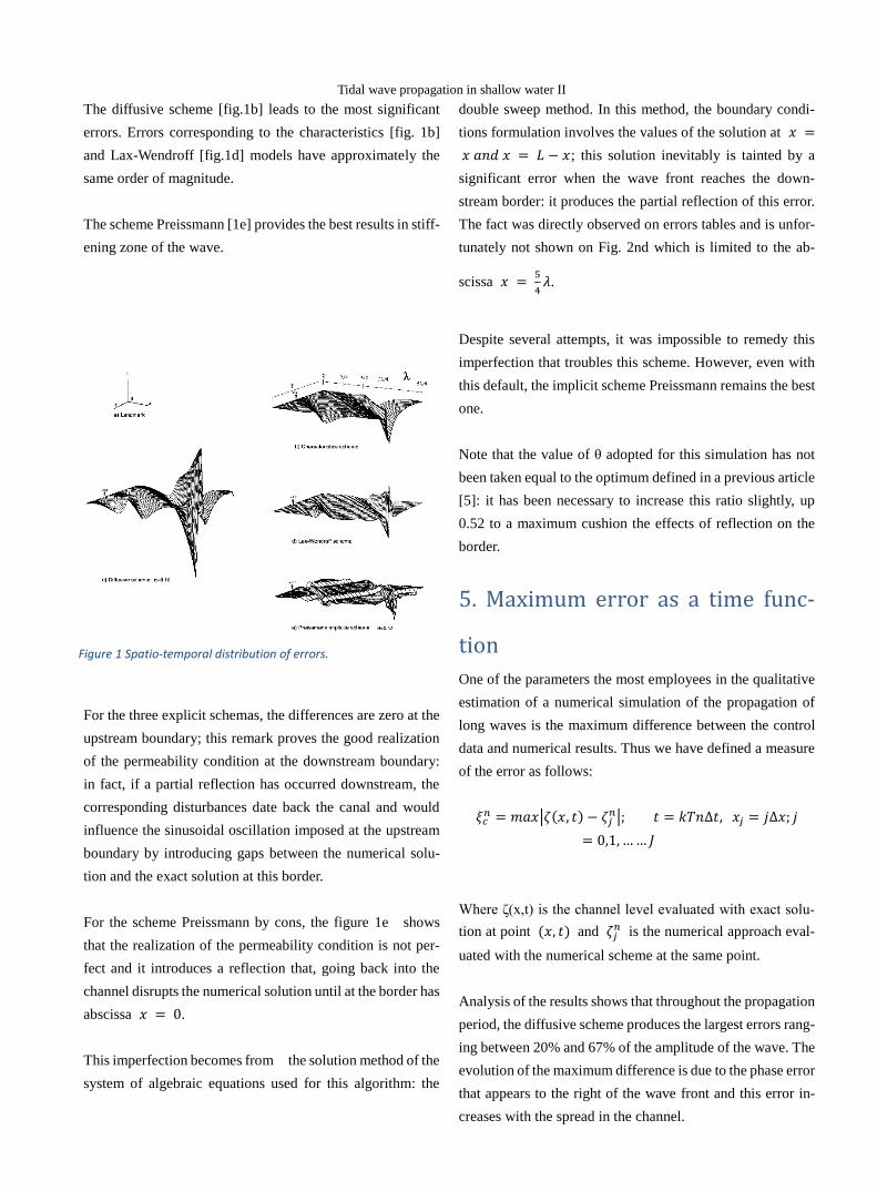
The results are shown in the graphs of fig. 1 located with re-

spect to an orthonormal system (0, 𝑡, 𝑥, 𝜁) (Fig. 1a). Errors

are grouped on an oscillation period of the phenomenon in a

channel length 0 ≤ 𝑥 ≤5

4𝜆 .

We find that the most important errors are related to the wave

front in the results obtained with the four models.


The diffusive scheme [fig.1b] leads to the most significant

errors. Errors corresponding to the characteristics [fig. 1b]

and Lax-Wendroff [fig.1d] models have approximately the

same order of magnitude.

The scheme Preissmann [1e] provides the best results in stiff-

ening zone of the wave.

For the three explicit schemas, the differences are zero at the

upstream boundary; this remark proves the good realization

of the permeability condition at the downstream boundary:

in fact, if a partial reflection has occurred downstream, the

corresponding disturbances date back the canal and would

influence the sinusoidal oscillation imposed at the upstream

boundary by introducing gaps between the numerical solu-

tion and the exact solution at this border.

For the scheme Preissmann by cons, the figure 1e shows

that the realization of the permeability condition is not per-

fect and it introduces a reflection that, going back into the

channel disrupts the numerical solution until at the border has

abscissa 𝑥 = 0.

This imperfection becomes from the solution method of the

system of algebraic equations used for this algorithm: the

double sweep method. In this method, the boundary condi-

tions formulation involves the values of the solution at 𝑥 =

𝑥 𝑎𝑛𝑑 𝑥 = 𝐿 − 𝑥; this solution inevitably is tainted by a

significant error when the wave front reaches the down-

stream border: it produces the partial reflection of this error.

The fact was directly observed on errors tables and is unfor-

tunately not shown on Fig. 2nd which is limited to the ab-

scissa 𝑥 = 5

4𝜆.

Despite several attempts, it was impossible to remedy this

imperfection that troubles this scheme. However, even with

this default, the implicit scheme Preissmann remains the best

one.

Note that the value of θ adopted for this simulation has not

been taken equal to the optimum defined in a previous article

[5]: it has been necessary to increase this ratio slightly, up

0.52 to a maximum cushion the effects of reflection on the

border.

5. Maximum error as a time func-

tion

One of the parameters the most employees in the qualitative

estimation of a numerical simulation of the propagation of

long waves is the maximum difference between the control

data and numerical results. Thus we have defined a measure

of the error as follows:

𝜉𝑐𝑛 = 𝑚𝑎𝑥|𝜁(𝑥, 𝑡) − 𝜁𝑗

𝑛|; 𝑡 = 𝑘𝑇𝑛∆𝑡, 𝑥𝑗 = 𝑗∆𝑥; 𝑗

= 0,1, … … 𝐽

Where ζ(x,t) is the channel level evaluated with exact solu-

tion at point (𝑥, 𝑡) and 𝜁𝑗𝑛 is the numerical approach eval-

uated with the numerical scheme at the same point.

Analysis of the results shows that throughout the propagation

period, the diffusive scheme produces the largest errors rang-

ing between 20% and 67% of the amplitude of the wave. The

evolution of the maximum difference is due to the phase error

that appears to the right of the wave front and this error in-

creases with the spread in the channel.

Figure 1 Spatio-temporal distribution of errors.


4

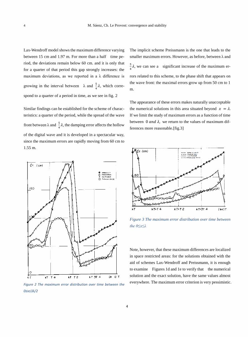
Lax-Wendroff model shows the maximum difference varying

between 15 cm and 1.97 m. For more than a half time pe-

riod, the deviations remain below 60 cm. and it is only that

for a quarter of that period this gap strongly increases: the

maximum deviations, as we reported in a λ difference is

growing in the interval between λ and 5

4𝜆, which corre-

spond to a quarter of a period in time, as we see in fig. 2

Similar findings can be established for the scheme of charac-

teristics: a quarter of the period, while the spread of the wave

front between λ and 5

4𝜆, the damping error affects the hollow

of the digital wave and it is developed in a spectacular way,

since the maximum errors are rapidly moving from 60 cm to

1.55 m.

Figure 2 The maximum error distribution over time between the

0≤x≤3λ/2

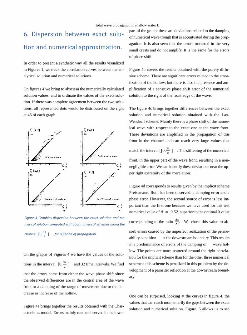
The implicit scheme Preissmann is the one that leads to the

smaller maximum errors. However, as before, between λ and

5

4𝜆, we can see a significant increase of the maximum er-

rors related to this scheme, to the phase shift that appears on

the wave front: the maximal errors grow up from 50 cm to 1

m.

The appearance of these errors makes naturally unacceptable

the numerical solutions in this area situated beyond 𝑥 = 𝜆.

If we limit the study of maximum errors as a function of time

between 0 𝑎𝑛𝑑 𝜆, we return to the values of maximum dif-

ferences more reasonable.[fig.3]

Figure 3 The maximum error distribution over time between

the 0≤x≤λ

Note, however, that these maximum differences are localized

in space restricted areas: for the solutions obtained with the

aid of schemes Lax-Wendroff and Preissmann, it is enough

to examine Figures 1d and 1e to verify that the numerical

solution and the exact solution, have the same values almost

everywhere. The maximum error criterion is very pessimistic.


6. Dispersion between exact solu-

tion and numerical approximation.

In order to present a synthetic way all the results visualized

in Figures 1, we track the correlation curves between the an-

alytical solution and numerical solutions.

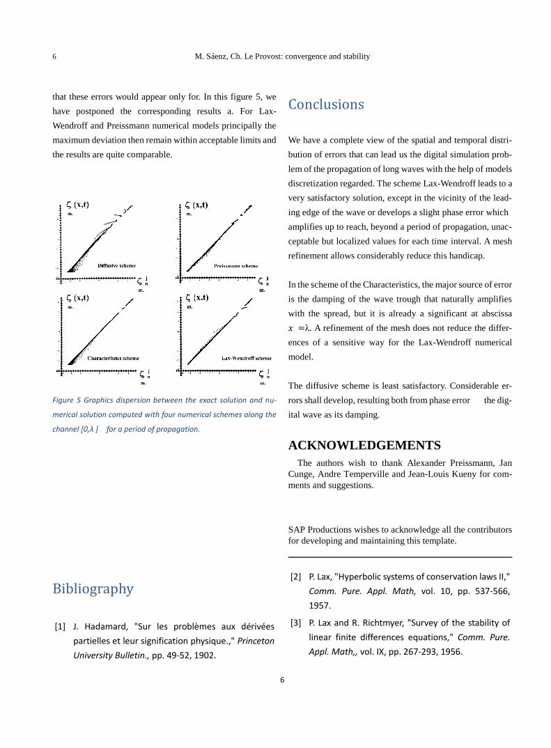
On figures 4 we bring to abscissa the numerically calculated

solution values, and to ordinate the values of the exact solu-

tion. If there was complete agreement between the two solu-

tions, all represented dots would be distributed on the right

at 45 of each graph.

On the graphs of Figures 4 we have the values of the solu-

tions in the interval [0,3𝜆

2 ] and 32 time intervals. We find

that the errors come from either the wave phase shift since

the observed differences are in the central area of the wave

front or a damping of the range of movement due to the de-

crease or increase of the hollow.

Figure 4a brings together the results obtained with the Char-

acteristics model. Errors mainly can be observed in the lower

part of the graph: these are deviations related to the damping

of numerical wave trough that is accentuated during the prop-

agation. It is also seen that the errors occurred in the very

small crests and do not amplify. It is the same for the errors

of phase shift.

Figure 4b covers the results obtained with the purely diffu-

sive scheme. There are significant errors related to the amor-

tization of the hollow; but there is also the presence and am-

plification of a sensitive phase shift error of the numerical

solution to the right of the front edge of the wave.

The figure 4c brings together differences between the exact

solution and numerical solution obtained with the Lax-

Wendroff scheme. Mainly there is a phase shift of the numer-

ical wave with respect to the exact one at the wave front.

These deviations are amplified in the propagation of this

front in the channel and can reach very large values that

match the interval [[0,3𝜆

2 ] . The stiffening of the numerical

front, in the upper part of the wave front, resulting in a non-

negligible error. We can identify these deviations near the up-

per right extremity of the correlation.

Figure 4d corresponds to results given by the implicit scheme

Preissmann. Both has been observed: a damping error and a

phase error. However, the second source of error is less im-

portant than the first one because we have used for this test

numerical value of 𝜃 = 0.52, superior to the optimal θ value

corresponding to the ratio Δx

Δt. We chose this value to ab-

sorb errors caused by the imperfect realization of the perme-

ability condition at the downstream boundary. This results

in a predominance of errors of the damping of wave hol-

low. The points are more scattered around the right correla-

tion for the implicit scheme than for the other three numerical

schemes: this scheme is penalized in this problem by the de-

velopment of a parasitic reflection at the downstream bound-

ary.

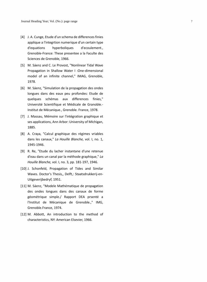
One can be surprised, looking at the curves in figure 4, the

values that can reach momentarily the gaps between the exact

solution and numerical solution. Figure. 5 allows us to see

Figure 4 Graphics dispersion between the exact solution and nu-

merical solution computed with four numerical schemes along the

channel [0,3𝜆

2 ] for a period of propagation.


6

that these errors would appear only for. In this figure 5, we

have postponed the corresponding results a. For Lax-

Wendroff and Preissmann numerical models principally the

maximum deviation then remain within acceptable limits and

the results are quite comparable.

Figure 5 Graphics dispersion between the exact solution and nu-

merical solution computed with four numerical schemes along the

channel [0,λ ] for a period of propagation.

Conclusions

We have a complete view of the spatial and temporal distri-

bution of errors that can lead us the digital simulation prob-

lem of the propagation of long waves with the help of models

discretization regarded. The scheme Lax-Wendroff leads to a

very satisfactory solution, except in the vicinity of the lead-

ing edge of the wave or develops a slight phase error which

amplifies up to reach, beyond a period of propagation, unac-

ceptable but localized values for each time interval. A mesh

refinement allows considerably reduce this handicap.

In the scheme of the Characteristics, the major source of error

is the damping of the wave trough that naturally amplifies

with the spread, but it is already a significant at abscissa

𝑥 =λ. A refinement of the mesh does not reduce the differ-

ences of a sensitive way for the Lax-Wendroff numerical

model.

The diffusive scheme is least satisfactory. Considerable er-

rors shall develop, resulting both from phase error the dig-

ital wave as its damping.

ACKNOWLEDGEMENTS

The authors wish to thank Alexander Preissmann, Jan

Cunge, Andre Temperville and Jean-Louis Kueny for com-

ments and suggestions.

SAP Productions wishes to acknowledge all the contributors

for developing and maintaining this template.

Bibliography

[1] J. Hadamard, "Sur les problèmes aux dérivées

partielles et leur signification physique.," Princeton

University Bulletin., pp. 49-52, 1902.

[2] P. Lax, "Hyperbolic systems of conservation laws II,"

Comm. Pure. Appl. Math, vol. 10, pp. 537-566,

1957.

[3] P. Lax and R. Richtmyer, "Survey of the stability of

linear finite differences equations," Comm. Pure.

Appl. Math,, vol. IX, pp. 267-293, 1956.

Journal Heading Year; Vol. (No.): page range 7

[4] J. A. Cunge, Etude d'un schema de differences finies

applique a l'integrtion numerique d'un certain type

d'equations hyperboliques d'ecoulement.,

Grenoble-France: These presentee a la Faculte des

Sciences de Grenoble, 1966.

[5] M. Sáenz and C. Le Provost, "Nonlinear Tidal Wave

Propagation in Shallow Water I :One-dimensional

model of an infinite channel," IMAG, Grenoble,

1978.

[6] M. Sáenz, "Simulation de la propagation des ondes

longues dans des eaux peu profondes: Etude de

quelques schémas aux differences finies,"

Université Scientifique et Médicale de Granoble.-

Institut de Mécanique., Grenoble. France, 1978.

[7] J. Massau, Mémoire sur l'intégration graphique et

ses applications, Ann Arbor: University of MIchigan,

1885.

[8] A. Craya, "Calcul graphique des régimes vriables

dans les canaux," La Houille Blanche, vol. I, no. 1,

1945-1946.

[9] R. Re, "Etude du lacher instantane d'une retenue

d'eau dans un canal par la méthode graphique," La

Houille Blanche, vol. I, no. 3, pp. 181-197, 1946.

[10] J. Schonfeld, Propagation of Tides and Similar

Waves. Doctor's Thesis,, Delft,: Staatsdrukkerij-en-

Uitgeverijbedryf, 1951.

[11] M. Sáenz, "Modele Mathématique de propagation

des ondes longues dans des canaux de forme

géométrique simple./ Rapport DEA prsenté a

l'Institut de Mécanique de Grenoble.," IMG,

Grenoble.France, 1974.

[12] M. Abbott, An introduction to the method of

characteristics, NY: American Elsevier, 1966.

Documents

Tidal wave simulation III