Three-Dimensional Modeling of Mass Transfer in Porous Media Using the Mixed Hybrid Finite Elements and the Random-Walk Methods

P1: GDX

Mathematical Geology [mg] pp429-matg-369680 March 27, 2002 9:14 Style file version June 30, 1999

Mathematical Geology, Vol. 34, No. 4, May 2002 (C© 2002)

Three-Dimensional Modeling of Mass Transferin Porous Media Using the Mixed Hybrid Finite

Elements and the Random-Walk Methods1

H. Hoteit,2 R. Mose,2,4 A. Younes,3 F. Lehmann,2

and Ph. Ackerer2

A three-dimensional (3D) mass transport numerical model is presented. The code is based on a particletracking technique: the random-walk method, which is based on the analogy between the advection–dispersion equation and the Fokker–Planck equation. The velocity field is calculated by the mixedhybrid finite element formulation of the flow equation. A new efficient method is developed to handlethe dissimilarity between Fokker–Planck equation and advection–dispersion equation to avoid accumu-lation of particles in low dispersive regions. A comparison made on a layered aquifer example betweenthis method and other algorithms commonly used, shows the efficiency of the new method. The codeis validated by a simulation of a 3D tracer transport experiment performed on a laboratory model. Itrepresents a heterogeneous aquifer of about 6-m length, 1-m width, and 1-m depth. The porous mediumis made of three different sorts of sand. Sodium chloride is used as a tracer. Comparisons betweensimulated and measured values, with and without the presented method, also proves the accuracy ofthe new algorithm.

KEY WORDS: mass transport modeling, advection–dispersion equation, random-walk method, lab-oratory model.

INTRODUCTION

The first generation of groundwater quality models was based on classical tech-niques, such as finite difference or finite element methods (see, e.g., Kinzelbach,1986; Pinder and Gray, 1977). These models are used widely, despite the well-known fact that they suffer from numerical diffusion at high grid Peclet numbersand also when the flow is not parallel to the mesh. Seeing the poor results produced

1Received 22 September 2000; accepted 27 June 2001.2Institut de Mecanique des Fluides et des Solides, Université Louis Pasteur de Strasbourg, UMR CNRS7507, 2, Rue Boussingault, F-67000 Strasbourg, France.

3Faculte des Sciences et Techniques, Département Physique et Mécanique, 15 Avenue R. Cassin, B.P.7151, 97715 St Denis Cedex 09, France.

4Now at Ecole Nationale du Génie de l’Eau et de l’Environnement de Strasbourg, Quai Koch-B.P.1039, F-67070 Strasbourg Cedex.

435

0882-8121/02/0500-0435/1C© 2002 International Association for Mathematical Geology

P1: GDX


436 Hoteit, Mose, Younes, Lehmann, and Ackerer

by the codes based on those methods, we have developed a three-dimensional (3D)mass transport model based on the random-walk method. Particle tracking modelsare free from numerical diffusion, but one must be very careful when developing acode based on the random walk especially when the code is used in heterogeneousmedia.

The random-walk model has been developed to be used mostly when theadvection–dispersion equation is strongly advection dominated. This means thatspecial care must be given to the accuracy of the flow field resolution and then anefficient method must be used for particle velocity calculation and advective dis-placement computing. Therefore, we present in the first part the numerical modelused for the resolution of the flow. Then we recall that a dissimilarity is now wellknown between the Fokker–Planck equation and the advection–dispersion equa-tion. If we do not consider this dissimilarity, we will have an accumulation of par-ticles in low dispersive regions. Several authors (Ackerer, 1985; Cordes, Daniels,and Rouve, 1991; Labolle, Fogg, and Tompson, 1996; Labolle, Quastel, and Fogg,1998; Uffink, 1983) have already suggested algorithms to overcome this problem.The assessment of these algorithms has shown that they are not satisfactory. In thispaper a new efficient method is presented to avoid this particle accumulation.

In the last part of the paper, we present the simulation of a 3D tracer experimentperformed on a laboratory model. This simulation shows the absolute necessity ofusing the presented algorithm in heterogeneous media.

THE FLOW MODEL

The velocity field is calculated by a mixed hybrid finite element model (Brezziand Fortin, 1991; Raviart and Thomas, 1977). Because the mixed hybrid finiteelement method (MHFEM) is not well known in the hydrogeology community,we present briefly in the following the basis of this approximation. The flow of anincompressible fluid in porous media is described by

s∂H

∂t−∇ · (K · ∇H ) = Qs (1)

associated with initial, Dirichlet, and Neumann boundary conditions, wheres isthe specific storage coefficient (L−1), H the piezometric head (L),K the hydraulicconductivity tensor (LT−1), andQs the source/sink term (T−1).

The MHFEM consists in a simultaneous approximation of the piezometrichead H and the specific fluxq = −K · ∇H , called the Darcy’s velocity. Thedomain is discretized into parallelepipedic elements. On each elementE, H andq are approximated by (Chavent and Roberts, 1991)

• HE, the mean of the piezometric head in the elementE;• THE,i , the mean of the piezometric head on each side ofE;• qE, the vector defined in the element.

P1: GDX


Three-Dimensional Modeling of Mass Transfer in Porous Media 437

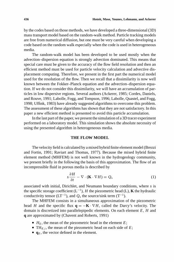
We use the Raviart–Thomas space of lower order as a fundamental approximationspace over the domain. For an elementE of ns sidesAi , the vectorial basis functionswi of this space are defined by the following equation:∫

Ai

wi · nE, j d A= δi j for j = 1, . . . ,ns (2)

whereδi j is the Kronecker symbol;nE, j is the normal unit vector to the edgeAj ; andns= 6 for parallelepipedic elements. The velocityqE is completely determinedby the knowledge of the fluxesQE,i through each sideAi :

qE =nf∑

j=1

QE,i w j (3)

whereQE,i are considered positive for outflow. The velocity vector is approximatedwith vector basis functions that are piecewise linear along all coordinate directions.Therefore the basis property (2) completely determineswi (Fig. 1). Moreover theyverify ∫

E∇ · wi dV =

ns∑j=1

∫Aj

wi · nE, j d A= 1 (4)

Figure 1. The Raviart–Thomas basis functions of a parallelepipedic element of sizelx × ly × lzprojected on the plan (O, U, V).

P1: GDX



The MHFEM ensures an exact mass balance over each element, it gives avelocity throughout all the domain, and the normal component of the velocity iscontinuous across the interelement boundaries.

Discretization of Darcy’s Law

The Darcy’s law is written as

K−1E qE = −(∇H ) (5)

This equation is written in a variational form usingwi as test functions. This leads to∫E

(K−1

E qE)wi dV = −

∫E(∇H ) · wi dV

= HE

∫E∇ · wi dV −

ns∑j=1

THE, j

∫E, j

wi · nE, j d A (6)

Using the properties (2) and (4) of the vectorial functionswi , we get

ns∑j=1

BE,i, j QE, j = HE − THE,i (7)

where

BE,i, j =∫

Ewi · K−1

E · w j · dV. (8)

Fluxes over each side are given by

QE,i = αE,i HE −ns∑

j=1

B−1E,i, j THE, j whereαE,i =

ns∑j=1

B−1E,i, j (9)

Discretization of the Mass Balance Equation

The mass balance equation is discretized using a finite volume formulation inspace ∫

Es∂H

∂tdV +

∫E∇ · (qE) dV =

∫E

Qs dV (10)

and an implicit finite difference scheme in time

|E|sEHn

E − Hn−1E

1t+

ns∑i=1

QnE,i =

∫E

Qns dV (11)

P1: GDX



To find the 13 unknowns (HE,THE,i , QE,i ), we use the variational Darcy’s law (9)and the continuity equation (10). To obtain one equation with THE,i as unknowns,we also use the continuity properties of piezometric heads and fluxes between twoadjacent elementsE andE′.

THE,i = THE′,i and QE,i + QE′,i = 0 (12)

All these relations give a system of equations which can be solved by usingTHi as main unknowns (Chavent and Roberts, 1991).

The interest of this mixed formulation is twofold. First, velocity and piezo-metric heads are obtained simultaneously with the same order of convergence.Second, in the presence of a full permeability tensor, the mixed formulation al-lows the calculation of the flux at the element level without any problem. On theother hand, finite differences do not allow one to calculate simply these fluxes.Moreover, comparisons between the MHFEM and other methods such as finitedifferences and finite element methods have shown the superiority of the mixedhybrid approximation especially in heterogeneous media (Mosé and others, 1994;Semra, 1994).

THE MASS TRANSPORT MODEL

In porous media, the mass transport equation is described by the classicaladvection–dispersion equation which can be written as (Bear, 1979)

∂C

∂t= −∇(UC)+∇(D∇C) (13)

whereC is the concentration (ML−3), U the mean pore velocity vector (ML−1),andD the dispersion tensor (L2T−1).

Two approaches of different nature (eulerien and lagrangien) are generallyused for the resolution of this equation. In this paper we address a lagrangienmethod, the random walk. This method is issued from stochastic physics (Fokker,1914; Planck, 1917, in Gardiner, 1985), and has been used in analysis of diffusionprocesses. Generally, it is defined as the movement of a particle which undergoesa displacement that partially depends on chance.

Preliminary

The mass transport in porous media may be described by a macroscopicdriving force, advection, on which some random fluctuations are added. The ran-dom fluctuations are due to the velocity variations around the average velocity incorrelation with permeability variations of the porous matrix observed at a macro-scopic scale. The theory of stochastic differential equations (Itô, 1951) treats thesefluctuations in a certain mathematical idealization.

P1: GDX



For sake of simplicity, we consider the one-dimensional problem and a ran-domly moving particle. We denote byX the position of this particle at a giventime. We choose a discrete set of timesti with constant time step1t . The impactof the driving force and the fluctuating forces can be described by

1X(ti ) = U (X(ti−1))1t + Z(ti ) (14)

where1X(ti ) = (X(ti )− (X(ti−1), U is the mean pore velocity (LT−1), andZ(ti )the random fluctuations. We assume that the average ofZ, denoted〈Z(ti )〉, is equalto 0. OtherwiseZ would contain a part which acts in a coherent fashion and couldbe added to the driving force. We assume that the fluctuations at different timestiandt j are uncorrelated. Therefore we may postulate that

〈Z(ti )Z(t j )〉 = δi j · M ·1t (15)

whereδi j is the Kronecker symbol which expresses the statistical independenceof Z at timesti andt j andM is a measure of the size of the fluctuations, equal to2D, whereD refers to the dispersion coefficient.

In a nonuniform field (which implies thatD is a function ofX), an importantquestion arises concerning at which time the variableX in D must be taken (e.g.Gardiner, 1985). According to Itô’s definition,D is governed by the value ofXbefore the jump. On the other hand, in Stratonovitch’s definition,D is evaluated atthe point halfway through the time interval, that isD = D(X([ti + ti+1]/2)) whichis closer to the reality, with fluctuations going on all the time. The Stratonovitch’sscheme is difficult to compute, and consequently, the Itô’s scheme is quite widelyused. The stochastic differential equation is then the following (Itô, 1951):

X(ti ) = X(ti−1)+U (X(ti−1))1t + z√

2D(X(ti−1))1t (16)

wherez is a random number issued from a Gaussian distribution with zero meanand unit variance.

It has been shown that this equation is equivalent to the Fokker–Planckequation:

∂W

∂t= −∇(U W)+1(DW) (17)

whereW is the probability density of the variableX(t). Equation (17) can bewritten as

∂W

∂t= −∇(U W)+∇(D∇W)+∇(∇DW) (17 ter)

To be equivalent to the transport equation (13), a term has to be added to the drivingforce:

∂W

∂t= −∇((U +∇D)W)+1(DW) (17 bis)

which is exactly the Fokker–Planck equation withU replaced byU ∗ = U +∇D.

P1: GDX



The equivalent stochastic differential equation to the advection–dispersionequation is then the following:

X(ti ) = X(ti−1)+U ∗(X(ti−1))1t + z√

2D(X(ti−1))1t (18)

whereU ∗ = U + ∂D∂X , which can be replaced by

X(ti ) = X(ti−1)+U ∗(X(ti−1))1t + z√

6D(X(ti−1))1t (19)

wherez is a random number issued from a uniform distribution between−1 and1 (as shown by Uffink, 1990).

The additional term∂D/∂X is due to the dissimilarity between the Fokker–Planck and advection–dispersion equation. The physical meaning of this term isthe conservation of particle flux due to dispersion between two points of spacewhere flow velocities are different. In other words, neglecting this term wouldyield an abnormal accumulation of particles in low dispersive regions. Inside oneelement where the velocity field is smooth (and hence dispersionD), the particleswill be moved according to the modified Fokker–Planck equation (i.e.U ∗ insteadof U ); at the boundary between two elements, where the velocity field, and hencethe dispersion is discontinous, the term∇D cannot be evaluated and we shallpropose a new direct treatment of the movement of the particles.

The Fokker–Planck Approach in Three Dimensionsfor a Smooth Dispersion Tensor

The 3D formulation of the modified Fokker–Planck equation is equivalent to(13) in the case of a smooth dispersion tensor; it is given by

∂W

∂t= −

3∑i=1

∂

∂Xi(U ∗i W)+

3∑i=1

3∑j=1

∂2

∂Xi ∂X j(Di j W) (20)

whereW is the probability density of the variableX(t) and

U ∗i = Ui +3∑

j=1

∂Di j

∂X j

Di j are the elements of the 3D symmetrical dispersion tensor. Their general ex-pression are given by (Bear, 1979)

Di j = αT|U |δi j + (αL − αT)Ui U j /|U | (21)

P1: GDX



whereδi j is the Kronecker symbol (δi j = 1 if i = j and δi j = 0 if i 6= j ); αL

is the longitudinal dispersivity component; andαT is the transversal dispersivitycomponent.

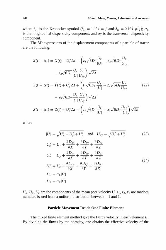
The 3D expressions of the displacement components of a particle of tracerare the following:

X(t +1t) = X(t)+U ∗x1t +(

z1

√6DL

Ux

|U | − z2

√6DT

Uy

Uxy

− z3

√6DT

Uz

|U |Ux

Uxy

)√1t

Y(t +1t) = Y(t)+U ∗y1t +(

z1

√6DL

Uy

|U | + z2

√6DT

Ux

Uxy(22)

− z3

√6DT

Uz

|U |Uy

Uxy

)√1t

Z(t +1t) = Z(t)+U ∗z1t +(

z1

√6DL

Uz

|U | + z3

√6DT

Uxy

|U |)√

1t

where

|U | =√

U2x +U2

y +U2z and Uxy =

√U2

x +U2y (23)

U ∗x = Ux + ∂Dxx

∂X+ ∂Dxy

∂Y+ ∂Dxz

∂Z

U ∗y = Uy + ∂Dyx

∂X+ ∂Dyy

∂Y+ ∂Dyz

∂Z(24)

U ∗z = Uz+ ∂Dzx

∂X+ ∂Dzy

∂Y+ ∂Dzz

∂Z

DL = αL |U |DT = αT|U |

Ux,Uy,Uz are the components of the mean pore velocityU. z1, z2, z3 are randomnumbers issued from a uniform distribution between−1 and 1.

Particle Movement Inside One Finite Element

The mixed finite element method give the Darcy velocity in each elementE.By dividing the fluxes by the porosity, one obtains the effective velocity of the

P1: GDX



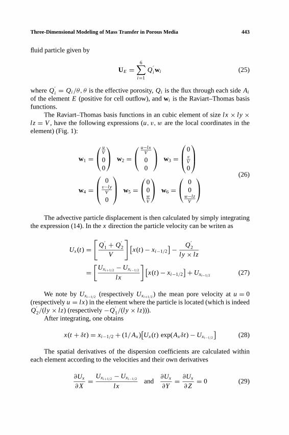
fluid particle given by

UE =6∑

i=1

Q′i wi (25)

whereQ′i = Qi /θ, θ is the effective porosity,Qi is the flux through each sideAi

of the elementE (positive for cell outflow), andwi is the Raviart–Thomas basisfunctions.

The Raviart–Thomas basis functions in an cubic element of sizelx × ly ×lz = V , have the following expressions (u, v, w are the local coordinates in theelement) (Fig. 1):

w1 = u

V

00

w2 = u−lx

V

00

w3 =

0vV

0

(26)

w4 =

0v−ly

V

0

w5 =0

0wV

w6 = 0

0w−lz

V

The advective particle displacement is then calculated by simply integrating

the expression (14). In thex direction the particle velocity can be writen as

Ux(t) =[

Q′1+ Q

′2

V

] [x(t)− xi−1/2

]− Q′2

ly × lz

=[

Uxi+1/2 −Uxi−1/2

lx

] [x(t)− xi−1/2

]+Uxi−1/2 (27)

We note byUxi−1/2 (respectivelyUxi+1/2) the mean pore velocity atu = 0(respectivelyu = lx) in the element where the particle is located (which is indeedQ′2/(ly × lz) (respectively−Q

′1/(ly × lz))).

After integrating, one obtains

x(t + δt) = xi−1/2+ (1/Ax)[Ux(t) exp(Axδt)−Uxi−1/2

](28)

The spatial derivatives of the dispersion coefficients are calculated withineach element according to the velocities and their own derivatives

∂Ux

∂X= Uxi+1/2 −Uxi−1/2

lxand

∂Ux

∂Y= ∂Ux

∂Z= 0 (29)

P1: GDX



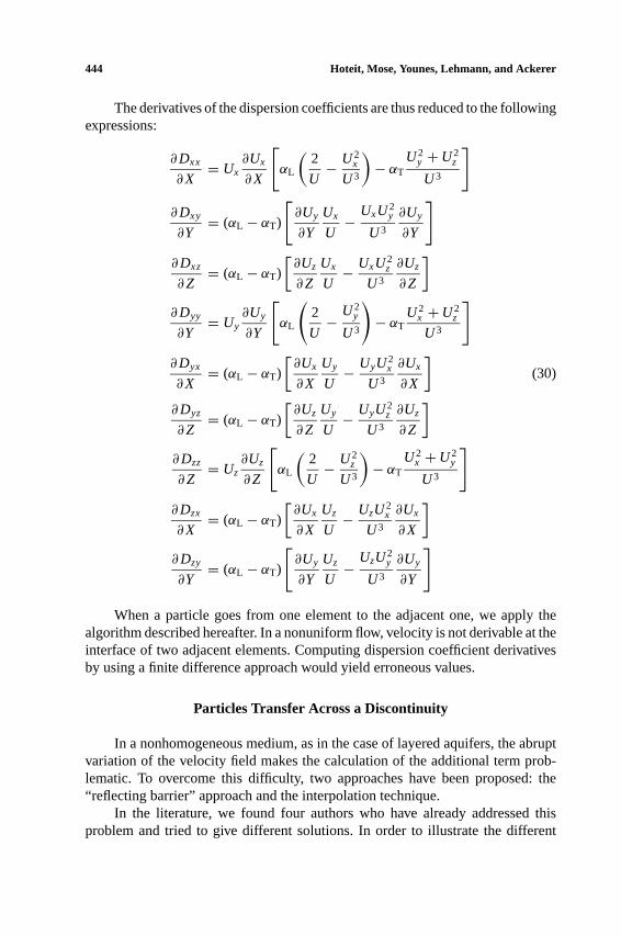
The derivatives of the dispersion coefficients are thus reduced to the followingexpressions:

∂Dxx

∂X= Ux

∂Ux

∂X

[αL

(2

U− U2

x

U3

)− αT

U2y +U2

z

U3

]

∂Dxy

∂Y= (αL − αT)

[∂Uy

∂Y

Ux

U− UxU2

y

U3

∂Uy

∂Y

]∂Dxz

∂Z= (αL − αT)

[∂Uz

∂Z

Ux

U− UxU2

z

U3

∂Uz

∂Z

]∂Dyy

∂Y= Uy

∂Uy

∂Y

[αL

(2

U− U2

y

U3

)− αT

U2x +U2

z

U3

]∂Dyx

∂X= (αL − αT)

[∂Ux

∂X

Uy

U− UyU2

x

U3

∂Ux

∂X

](30)

∂Dyz

∂Z= (αL − αT)

[∂Uz

∂Z

Uy

U− UyU2

z

U3

∂Uz

∂Z

]∂Dzz

∂Z= Uz

∂Uz

∂Z

[αL

(2

U− U2

z

U3

)− αT

U2x +U2

y

U3

]∂Dzx

∂X= (αL − αT)

[∂Ux

∂X

Uz

U− UzU2

x

U3

∂Ux

∂X

]∂Dzy

∂Y= (αL − αT)

[∂Uy

∂Y

Uz

U− UzU2

y

U3

∂Uy

∂Y

]

When a particle goes from one element to the adjacent one, we apply thealgorithm described hereafter. In a nonuniform flow, velocity is not derivable at theinterface of two adjacent elements. Computing dispersion coefficient derivativesby using a finite difference approach would yield erroneous values.

Particles Transfer Across a Discontinuity

In a nonhomogeneous medium, as in the case of layered aquifers, the abruptvariation of the velocity field makes the calculation of the additional term prob-lematic. To overcome this difficulty, two approaches have been proposed: the“reflecting barrier” approach and the interpolation technique.

In the literature, we found four authors who have already addressed thisproblem and tried to give different solutions. In order to illustrate the different

P1: GDX



Figure 2. Schematic presentation of a layered aquifer.

approaches, let us study the case of a layered aquifer in which the flow is parallelto the layers and then we will study also the transfer in the perpendicular direction(Fig. 2).

The upper medium (M1) is a high dispersive medium and the lower (M2) isa low dispersive one.

The following three methods are reflecting-barrier approaches.Uffink (1983) was probably the first who introduced the idea of a semireflect-

ing barrier at the interface. He suggested that a part of the set of particles goingfrom M1 to M2 must be reflected. This part is given by a probability of crossingthe barrier defined by

Pu =√

DY1−√

DY2√DY1+

√DY2

(31)

whereDY1 is the transverse dispersion coefficient in the upper medium andDY2

is the transverse dispersion coefficient in the lower medium.Ackerer (1985) suggested another method. It consists in breaking up the parti-

cle jump through the interface, into two jumps. Let us consider that a particle jumpduration be1t . This jump is broken into two jumps, the first one takes the particleto the interface and it lasts1t1. This jump has the statistic properties of the firstmedium. The second jump starts at the interface with the statistic properties of thesecond medium and it lasts1t2 = 1t −1t1.

Cordes, Daniels, and Rouve (1991) went back to Uffink’s idea (semireflectingbarrier), but changed the probability for a particle to be reflected. They suggested

Pc =√

DY1−√

DY2√DY1

(32)

P1: GDX



The last approach is based on an interpolation technique presented by Labolle,Fogg, and Tompson (1996), and Labolle, Quastel, and Fogg (1998), which consistsin interpolating velocities in the dispersion tensor in order to smooth the dispersiontensor in the vicinity of the interface to eliminate discontinuities. However, asmentioned by the authors, in order to attain the convergence to the true solution,this method requires convergence in time step as well as in the spatial discretizationassociated to the interpolation scheme.

To assess those different methods, we have used each of them to simulatea tracer transport in a bistrata aquifer (Labolle, Fogg, and Tompson, 1996). Thesame number of particles were injected in each layer. In this problem, a correctmodeling technique will maintain a uniform particle number density in each strata,that is,N1/N2 = 1, whereN1 andN2 are the particle numbers in each strata.

As shown in Labolle, Fogg, and Tompson (1996), using no correction fails toobtain uniform number density. In the following, we will compare results obtainedwith the four mentioned methods. To incorporate the technique of Labolle andcoauthors, we linearly interpolate the diffusion coefficient through a unit lengthacross the interface.

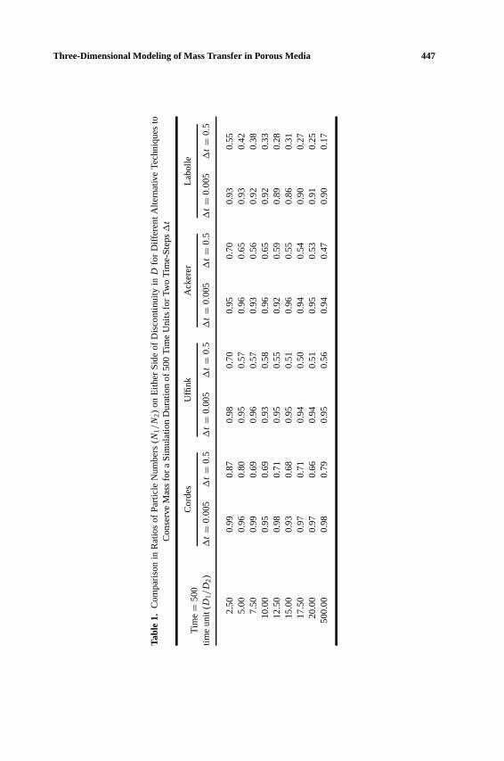
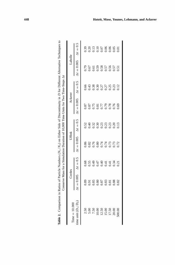
Tables 1 and 2 show the evolution of the number of particle ratios in the layersversus the dispersion coefficient values for each method. We test these methodswith two simulation durations using two time steps1t = 0.005 and1t = 0.5.For the simulation duration of 500 time units, a time step of 0.005 gives goodresults for all methods (for the different ratios of dispersion coefficients). But atime step of 0.5 does not allow one to achieve an acceptable convergence for thefour methods. For the simulation duration of 10,000 time units, neither time step(0.5 and 0.005) attains a satisfactory convergence with all methods.

This study shows that for all methods, the time step has to be adapted tothe time duration of the simulation: in order to achieve convergence, we have todecrease the time step when the time duration increases.

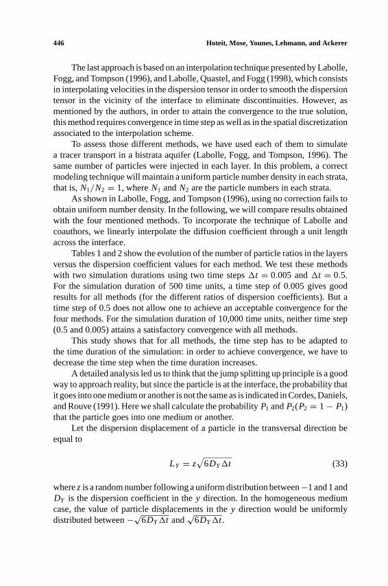
A detailed analysis led us to think that the jump splitting up principle is a goodway to approach reality, but since the particle is at the interface, the probability thatit goes into one medium or another is not the same as is indicated in Cordes, Daniels,and Rouve (1991). Here we shall calculate the probabilityP1 andP2(P2 = 1− P1)that the particle goes into one medium or another.

Let the dispersion displacement of a particle in the transversal direction beequal to

LY = z√

6DY1t (33)

wherez is a random number following a uniform distribution between−1 and 1 andDY is the dispersion coefficient in they direction. In the homogeneous mediumcase, the value of particle displacements in they direction would be uniformlydistributed between−√6DY1t and

√6DY1t .

P1: GDX



Tabl

e1.

Com

paris

onin

Rat

ios

ofP

artic

leN

umbe

rs(

N1/N

2)

onE

ither

Sid

eof

Dis

cont

inui

tyinD

for

Diff

eren

tAlte

rnat

ive

Tech

niqu

esto

Con

serv

eM

ass

for

aS

imul

atio

nD

urat

ion

of50

0T

ime

Uni

tsfo

rTw

oT

ime-

Ste

ps1

t

Cor

des

Uffi

nkA

cker

erLa

bolle

Tim

e=

500

time

unit

(D1/D

2)

1t=

0.00

51

t=

0.5

1t=

0.00

51

t=

0.5

1t=

0.00

51

t=

0.5

1t=

0.00

51

t=

0.5

2.50

0.99

0.87

0.98

0.70

0.95

0.70

0.93

0.55

5.00

0.96

0.80

0.95

0.57

0.96

0.65

0.93

0.42

7.50

0.99

0.69

0.96

0.57

0.93

0.56

0.92

0.38

10.0

00.

950.

690.

930.

580.

960.

650.

920.

3312

.50

0.98

0.71

0.95

0.55

0.92

0.59

0.89

0.28

15.0

00.

930.

680.

950.

510.

960.

550.

860.

3117

.50

0.97

0.71

0.94

0.50

0.94

0.54

0.90

0.27

20.0

00.

970.

660.

940.

510.

950.

530.

910.

2550

0.00

0.98

0.79

0.95

0.56

0.94

0.47

0.90

0.17

P1: GDX



Tabl

e2.

Com

paris

onin

Rat

ios

ofP

artic

leN

umbe

rs(

N1/N

2)

onE

ither

Sid

eof

Dis

cont

inui

tyinD

for

Diff

eren

tAlte

rnat

ive

Tech

niqu

esto

Con

serv

eM

ass

for

aS

imul

atio

nD

urat

ion

of10

,000

Tim

eU

nits

for

Two

Tim

e-S

teps

1t

Cor

des

Uffi

nkA

cker

erLa

bolle

Tim

e=

10,0

00tim

eun

it(D

1/D

2)

1t=

0.00

51

t=

0.5

1t=

0.00

51

t=

0.5

1t=

0.00

51

t=

0.5

1t=

0.00

51

t=

0.5

2.50

0.89

0.68

0.86

0.52

0.87

0.66

0.79

0.39

5.00

0.91

0.55

0.82

0.40

0.87

0.43

0.67

0.20

7.50

0.85

0.49

0.76

0.32

0.75

0.38

0.61

0.13

10.0

00.

800.

470.

800.

300.

810.

300.

590.

1012

.50

0.87

0.40

0.74

0.23

0.77

0.27

0.58

0.07

15.0

00.

830.

410.

740.

230.

790.

270.

570.

0617

.50

0.81

0.41

0.73

0.23

0.78

0.25

0.56

0.06

20.0

00.

880.

340.

730.

200.

760.

230.

570.

0550

0.00

0.82

0.21

0.72

0.13

0.69

0.12

0.51

0.01

P1: GDX



Figure 3. Probability distribution of particle dispersion jumps starting at the interface of the twolayers.

In the nonhomogeneous medium case, the value of particle displacementsin the y direction would be uniformly distributed between−√6 DY11t and√

6 DY21t .To respect the uniform distribution (Fig. 3) of particle displacements in the

whole area (A) of possible displacements, the probability that a particle goes intomediums M1 and M2 is respectively

P1 =√

DY1√DY1+

√DY2

and P2 = 1− P1 =√

DY2√DY1+

√DY2

(34)

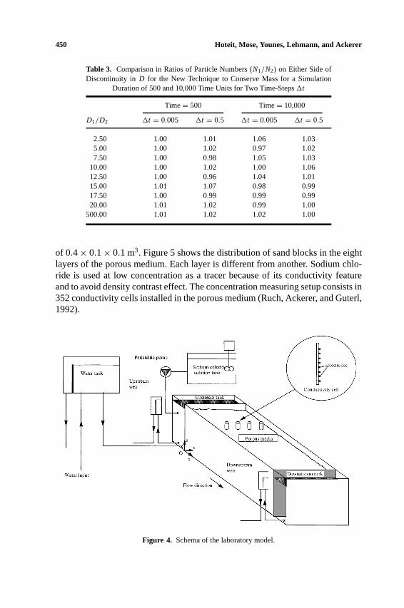
Finally, programming this method is not difficult; after splitting up the jump,the particle is at the interface and then one draws a random numberR from a uni-form distribution between 0 and 1: ifR< P1, the particle goes into the M1 medium,else it goes into the M2 medium. This algorithm must be applied whether the parti-cle comes from one side of the interface or the other. It must also be applied when aparticle goes from one element to the adjacent one, because the tangential velocityunit vector is not continuous from one element to the other. Table 3 clearly showsthat the new method is the only accurate solution of the problem for any ratio ofdispersion coefficients and without any big difficulties of convergence in time step.

MODEL VALIDATION

To validate the model we have simulated a tracer experiment in an heteroge-neous medium performed on a 3D laboratory model (Fig. 4). The porous mediumis 5.6 m in length, 1 m in width, and 0.8 m in depth. It is filled up with threedifferent kinds of sand disposed in eight layers of randomly placed parallelepipeds

P1: GDX



Table 3. Comparison in Ratios of Particle Numbers (N1/N2) on Either Side ofDiscontinuity in D for the New Technique to Conserve Mass for a Simulation

Duration of 500 and 10,000 Time Units for Two Time-Steps1t

Time= 500 Time= 10,000

D1/D2 1t = 0.005 1t = 0.5 1t = 0.005 1t = 0.5

2.50 1.00 1.01 1.06 1.035.00 1.00 1.02 0.97 1.027.50 1.00 0.98 1.05 1.03

10.00 1.00 1.02 1.00 1.0612.50 1.00 0.96 1.04 1.0115.00 1.01 1.07 0.98 0.9917.50 1.00 0.99 0.99 0.9920.00 1.01 1.02 0.99 1.00

500.00 1.01 1.02 1.02 1.00

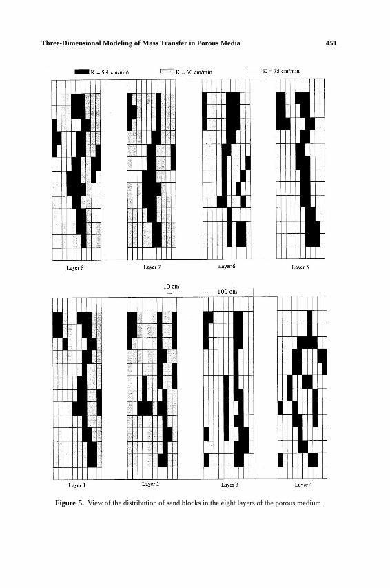
of 0.4× 0.1× 0.1 m3. Figure 5 shows the distribution of sand blocks in the eightlayers of the porous medium. Each layer is different from another. Sodium chlo-ride is used at low concentration as a tracer because of its conductivity featureand to avoid density contrast effect. The concentration measuring setup consists in352 conductivity cells installed in the porous medium (Ruch, Ackerer, and Guterl,1992).

Figure 4. Schema of the laboratory model.

P1: GDX



Figure 5. View of the distribution of sand blocks in the eight layers of the porous medium.

P1: GDX



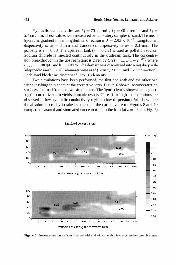
Hydraulic conductivities arek1 = 75 cm/min,k2 = 60 cm/min, andk3 =5.4 cm/min. These values were measured on laboratory samples of sand. The meanhydraulic gradient in the longitudinal direction isJ = 2.03× 10−2. Longitudinaldispersivity isαL = 3 mm and transversal dispersivity isαT = 0.3 mm. Theporosity isε = 0.38. The upstream tank (x = 0 cm) is used as pollution source.Sodium chloride is injected continuously in the upstream tank. The concentra-tion breakthrough in the upstream tank is given byC(t) = Cmax(1− e−βt ), whereCmax= 1.08 g/L andb = 0.0476. The domain was discretized into a regular paral-lelepipedic mesh. 17,280 elements were used (54 inx, 20 iny, and 16 inzdirection).Each sand block was discretized into 16 elements.

Two simulations have been performed, the first one with and the other onewithout taking into account the corrective term. Figure 6 shows isoconcentrationsurfaces obtained from the two simulations. The figure clearly shows that neglect-ing the corrective term yields dramatic results. Unrealistic high concentrations areobserved in low hydraulic conductivity regions (low dispersion). We show herethe absolute necessity to take into account the corrective term. Figures 8 and 10compare measured and simulated concentration in the fifth (atz= 45 cm, Fig. 7)

Figure 6. Isoconcentration surfaces obtained with and without taking into account the corrective term.

P1: GDX



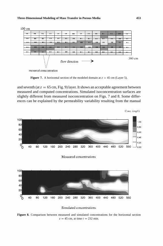
Figure 7. A horizontal section of the modeled domain atz= 45 cm (Layer 5).

and seventh (atz= 65 cm, Fig. 9) layer. It shows an acceptable agreement betweenmeasured and computed concentrations. Simulated isoconcentration surfaces areslightly different from measured isoconcentration on Figs. 7 and 8. Some differ-ences can be explained by the permeability variability resulting from the manual

Figure 8. Comparison between measured and simulated concentrations for the horizontal sectionz= 45 cm, at timet = 232 min.

P1: GDX



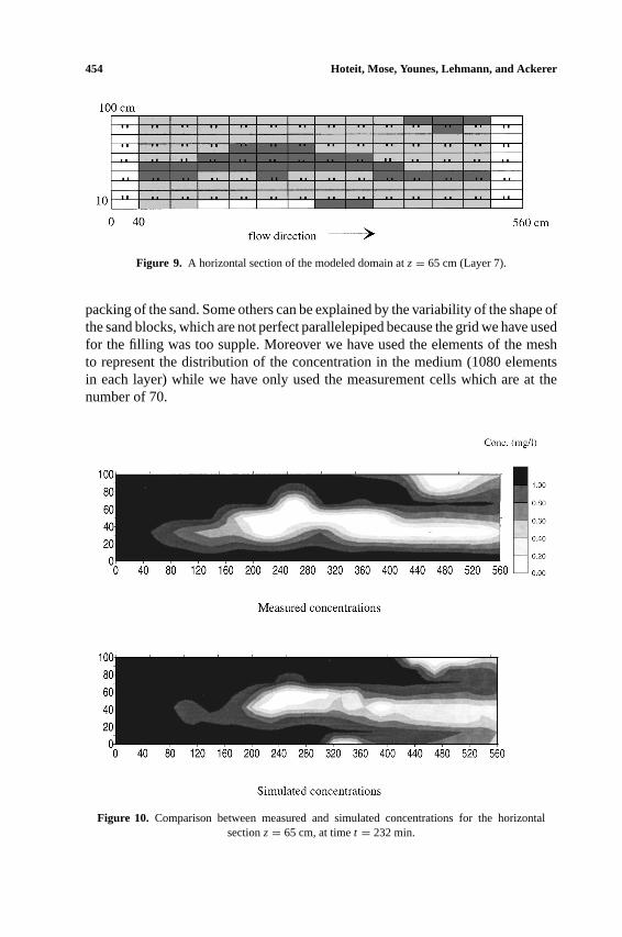
Figure 9. A horizontal section of the modeled domain atz= 65 cm (Layer 7).

packing of the sand. Some others can be explained by the variability of the shape ofthe sand blocks, which are not perfect parallelepiped because the grid we have usedfor the filling was too supple. Moreover we have used the elements of the meshto represent the distribution of the concentration in the medium (1080 elementsin each layer) while we have only used the measurement cells which are at thenumber of 70.

Figure 10. Comparison between measured and simulated concentrations for the horizontalsectionz= 65 cm, at timet = 232 min.

P1: GDX



To conclude with that simulation of Marceau’s experiment, an acceptablematch between measurement and simulation is achieved everywhere.

CONCLUSION

At field scale and especially in heterogeneous media, solute transport is al-ways a 3D phenomenon. Therefore an efficient groundwater quality modelingmust be 3D as well. The random-walk method is a good alternative to classicaltechniques as finite difference and finite elements, which suffer from numericaldiffusion at high Peclet numbers. But classical random-walk models are not effi-cient in simulating mass transport in heterogeneous media because if the additionalterm is not correctly taken into account, particle accumulation can occur in lowdispersion areas. The new method developed in this study allows the conservationof the particle fluxes between high and low dispersive regions. Table 3 (comparedto Tables 1 and 2) shows the efficiency of this method and its superiority on otheralgorithms commonly used. The 3D code, developed in this study takes into ac-count the new algorithm which has been extended to the three directions of space.The code has been verified on hand of a 3D laboratory experiment. Comparisonsbetween simulated and measured values have shown satisfactory results.

In this paper it is also shown that a 3D physical laboratory model is a veryuseful tool in validating numerical models before their use at field scale and alsoto improve our understanding in mass transfer in porous media.

REFERENCES

Ackerer, Ph., 1985, Propagation d’un Fluide en Aquifère Poreux Saturé en Eau. Prise en Compteet Localisation des Héterogeneites par des Outils Théoriques et Expérimentaux: Doctoraldissertation, Université Louis Pasteur de Strasbourg, France, 102 p.

Bear, J., 1979, Hydraulics of groundwater: McGraw-Hill, New York, 569 p.Brezzi, F., and Fortin, M., 1991, Mixed and hybrid finite element methods: Springer, New York,

350 p.Chavent, G., and Roberts, J. E., 1991, A unified physical presentation of mixed, mixed hybrid finite

elements and standard finite difference approximations for the determination of velocities in waterflow problems: Adv. Water Resour., v. 14, no. 6, p. 349–355.

Cordes, C., Daniels, H., and Rouve, G., 1991, A new very efficient algorithm for particle trackingin layered aquifers,in Bensari, D., Brebbia, C. A., and Ouazar, D. eds., 2nd international con-ference on computer methods and water resources, Rabat, Morocco, Computational MechanicsPublications, WIT Press, p. 41–55.

Gardiner, C. W., 1985, Handbook of stochastic methods for physics, chemistry and the natural sciences,2nd edn.: Springer, Berlin, 434 p.

Ito, K., 1951, On stochastical differential equations, Vol. 4: American Mathematical Society, NewYork, p. 289–302.

Kinzelbach, W., 1986, Groundwater modeling: Introduction with sample programs in Basic: Develop-ments in Water Science, 25th edn.: Elsevier, Amsterdam, 333 p.

P1: GDX



Labolle, E. M., Fogg, G. E., and Tompson, A. F. B., 1996, Random-walk simulation of transport inheterogeneous porous media: Local mass conservation problem and implementation methods:Water Resour. Res., v. 32, no. 3, p. 583–593.

Labolle, E. M., Quastel, J., and Fogg, G. E., 1998, Diffusion theory for transport in porous media:Transition probability densities of diffusion processes corresponding to advection–dispersionequations: Water Resour. Res., v. 34, no. 7, p. 1685–1693.

Mose, R., Siegel, P., Ackerer, Ph., and Chavent, G., 1994, Application of the mixed hybrid finite elementapproximation in a groundwater flow model: Luxury or necessity?: Water Resour. Res., v. 30,no. 11, p. 3001–3012.

Pinder, G. F., and Gray, W. G., 1977, Finite element simulation in surface and subsurface hydrology:Academic Press, New York, 295 p.

Raviart, P. A., and Thomas, J. M., 1977, A mixed hybrid finite element method for the second orderelliptic problems, in mathematical aspects of the finite element method, lecture notes in mathe-matics: Springer, New York.

Ruch, M., Ackerer, Ph., and Guterl, P., 1992, A computer driven setup for mass transfer in porousmedia:in proceedings of Hydrocomp’92 international conference on interaction of computationalmethods and measurements in hydraulics and hydrology, Budapest, p. 419–426.

Semra, K., 1994, Modelisation tridimensionnelle du transport d’un traceur en milieu poreux saturéheterogene: Evaluation des théories stochastiques: Doctoral dissertation, Université Louis Pasteurde Strasbourg, France, 125 p.

Uffink, G. J. M., 1985, A random-walk method for the simulation of macrodispersion in a strati-fied aquifer:in proceedings of IAHS symposia, IUGG 18th general assembly, Hamburg, IAHSPublication, v. 65, p. 26–34.

Uffink, G. J. M., 1990, Analysis of dispersion by the random walk method: Doctoral dissertation, DelftUniversity, The Netherlands, 150 p.

Documents

Three-Dimensional Modeling of Mass Transfer in Porous Media Using the Mixed Hybrid Finite Elements and the Random-Walk Methods