Thorp2020 - DSSAT Bushland ET2.pdf - USDA ARS

Contents lists available at ScienceDirect

Computers and Electronics in Agriculture

journal homepage: www.elsevier.com/locate/compag

Comparison of evapotranspiration methods in the DSSAT Cropping System Model: II. Algorithm performance K.R. Thorpa,⁎, G.W. Marekb, K.C. DeJongec, S.R. Evettb

a USDA-ARS, U.S. Arid Land Agricultural Research Center, 21881 N Cardon Ln, Maricopa, AZ 85138, United States b USDA-ARS, Conservation and Production Research Laboratory, 300 Simmons Rd, Unit 10, Bushland, TX 79012, United States c USDA-ARS, Center for Agricultural Resources Research, 2150 Centre Ave, Fort Collins, CO 80526, United States

A R T I C L E I N F O

Keywords: Cotton Evapotranspiration Irrigation Lysimeter Modeling Optimization Simulation Water

A B S T R A C T

Accurate calculations of evapotranspiration (ET) are highly important for agroecosystem model simulations, and improvement of ET algorithms is an on-going model development goal. The objective of this study was to evaluate and compare six ET methods in the Decision Support System for Agrotechnology Transfer (DSSAT) Cropping System Model (CSM) using agronomic and weighing lysimetry data from cotton field studies at Bushland, Texas. Three options were tested for estimating potential ET as required by the DSSAT-CSM: 1) a Priestley-Taylor method, 2) a Penman-Monteith combination equation estimate of grass reference ET with a DSSAT-specific single crop coefficient equation, and 3) the ASCE Standardized Reference ET Equation combined with a dual crop coefficient method for non-stressed conditions. The latter two reference ET methods were adapted to provide reasonable estimates for DSSAT-required potential ET. Additionally, two methods for cal-culation of soil water evaporation were tested, including both the original and updated formulations of Ritchie approaches for DSSAT-CSM. The combinations of the three potential ET and two soil water evaporation ap-proaches led to six possible ET simulation options in the model. A computationally-intensive multiobjective optimization method was used to select among model parameterization options and ensure that modeler bias did not influence ET method comparisons. Among 23 agroecosystem metrics that included lysimeter-based ET, various cotton growth variables, and soil water content in multiple soil layers, the original Ritchie soil water evaporation approach performed statistically equivalent to or better than the more recent Ritchie method (p 0.05). The default ET method in the model, which involved Priestley-Taylor potential ET with the more recent Ritchie soil water evaporation method, was outperformed by other ET methods for 14 of 23 agroeco-system metrics (p 0.05). When the original Ritchie soil water evaporation method was combined with po-tential ET from the ASCE reference ET and dual crop coefficient method, the model performed statistically equivalent to or better than the other five ET options for all but 1 of 23 agroecosystem metrics (p 0.05). Based on three years of cotton data from the Bushland lysimetry fields, a DSSAT-CSM ET approach based on the standardized ET methodologies described by ASCE and FAO-56 combined with the original Ritchie soil water evaporation method provided holistic improvements to model simulations among multiple agroecosystem me-trics.

1. Introduction

A recent landmark effort to compare evapotranspiration (ET) si-mulations among diverse maize (Zea mays L.) models revealed twofold or greater variation in ET estimates for rainfed conditions in central Iowa (Kimball et al., 2019), which suggested that the models require improvements to provide consistent and accurate ET simulations. Among the 29 models intercompared by Kimball et al. (2019), six models involved different ET simulation options with the Decision

Support System for Agrotechnology Transfer (DSSAT) Cropping System Model (CSM) (Jones et al., 2003). The DSSAT-CSM ET methods in-cluded six combinations of three methods for computing potential ET and two methods for computing soil water evaporation, as discussed below in detail. The results were surprising, revealing that an older soil water evaporation algorithm (Ritchie, 1972) outperformed the newer, default evaporation method in the model (Ritchie et al., 2009). Also, a reduced-input potential ET method based on Priestley and Taylor (1972) outperformed two more modern methods based on formulations

https://doi.org/10.1016/j.compag.2020.105679 Received 21 April 2020; Received in revised form 25 June 2020; Accepted 29 July 2020

⁎ Corresponding author. E-mail address: [email protected] (K.R. Thorp).

Computers and Electronics in Agriculture 177 (2020) 105679

Available online 18 August 20200168-1699/ Published by Elsevier B.V.

T

http://www.sciencedirect.com/science/journal/01681699

https://www.elsevier.com/locate/compag

https://doi.org/10.1016/j.compag.2020.105679


mailto:[email protected]


http://crossmark.crossref.org/dialog/?doi=10.1016/j.compag.2020.105679&domain=pdf

of the Penman-Monteith equation (Allen et al., 1998) with associated crop coefficient adjustments. Although the study will remain a dis-tinguished contribution toward evaluation of ET simulation methods, major issues impacting the simulations were that 1) no data were available to quantify amounts of water loss to artificial subsurface drainage systems (which are ubiquitous across the Iowa landscape) and 2) only limited data were available on the status of soil water content profiles. Therefore, further comparisons of the six DSSAT-CSM ET methods are needed for other environments, where water balances are more fully characterized and where artificial subsurface drainage is not a confounding factor.

Although the results of Kimball et al. (2019) provided great insights on the state of ET simulation methodologies, they noted that model parameterization choices made by modelers with different levels of skill and experience may have introduced biases in the model comparisons. Indeed, potential bias issues were readily apparent in the effort to ca-librate the six DSSAT-CSM ET methods for the Kimball et al. (2019) study, a task that was conducted solely by the lead author of the present article. When the goal is to make meaningful comparisons among ET algorithms and state definitively that one method is better than an-other, how does one make model parameterization choices while eliminating subjectivity and bias due to 1) personal opinions on favored simulation approaches, 2) failure to fully consider or even comprehend the appropriate parameter adjustments to be made, 3) the complexities introduced by interacting parameters, 4) the conflicting scenarios where parameter adjustments lead to improved results for one metric (e.g., ET) but worsened results for another metric (e.g., yield) and vice versa, and 5) the lack of protocols for basing model comparisons on statistical inference? These questions led Thorp et al. (2019) to develop a methodology for comparing ET simulation algorithms while reducing the subjectivity of parameterization choices; however, these procedures were only partially developed and implemented for the DSSAT-CSM simulations reported in the Kimball et al. (2019) study.

Thorp et al. (2019) described a computationally-intensive metho-dology for guiding parameterization decisions and making unbiased comparisons of ET methods in an agroecosystem model, and the ap-proach was demonstrated by comparing three ET methods in the Cot-ton2K model. The study used agronomic and ET data from weighing lysimetry fields at a cotton (Gossypium hirsutum L.) field site near Bushland, Texas (Howell et al., 2004; Evett et al., 2012a). In the first of two analysis phases, a Sobol global sensitivity analysis (GSA) (Cariboni et al., 2007; Pianosi et al., 2016; Saltelli et al., 2000; Sobol, 2001) was conducted to identify influential model input parameters, understand model output sensitivities, and provide guidance on appropriate para-meters for adjustment. Results of the GSA guided decisions for the second phase of analysis, in which a multiobjective optimization ap-proach (Taboada et al., 2007) was used to make parameterization choices and evaluate simulation results against multiple agronomic measurements, while considering large numbers of input para-meterization options. Results of the simulation analysis were evaluated using inferential statistics to determine the ET algorithms that per-formed statistically better than others, while collectively considering various types of agronomic measurements. The methodology was useful for comparing ET methods in the Cotton2K model while minimizing, if not eliminating, the subjective parameterization decisions that could make such comparisons less meaningful. The Thorp et al. (2019) methodology is generally applicable for other simulation models and can provide further comparisons of the six ET methods in the DSSAT- CSM, as discussed herein.

The overall goal of the present study was to apply the second phase of the Thorp et al. (2019) methodology to evaluate the performance of six ET methods in the DSSAT-CSM using agronomic data from cotton field studies at Bushland, Texas. Field data for the analysis included ET measurements from four weighing lysimeters at the field site and other agronomic measurements from co-located field experiments that com-pared fully-irrigated, deficit-irrigated, and dryland cotton production.

Specific objectives were to use multiobjective optimization methods with high-performance computing to 1) evaluate the percent root mean squared error (%RMSE) between measured and simulated data for 23 agroecosystem metrics in response to adjustments in 38 influential model input parameters (determined from a prior Sobol GSA) and 2) conduct statistical inference tests among %RMSE results to identify ET simulation options that performed significantly better than others. As reported in a companion paper (Thorp et al., 2020), the influential model input parameters were identified from the first phase of the Thorp et al. (2019) methodology, which involved a Sobol GSA with the DSSAT-CSM using data from the same field site. As compared to the Kimball et al. (2019) study, the present study was unique by conducting DSSAT-CSM ET method comparisons with 1) a different crop (cotton as opposed to maize), 2) a different environment (semi-arid west Texas as opposed to humid central Iowa), 3) more carefully controlled water management conditions (scheduled irrigation management as opposed to rainfed agriculture), 4) a different ET measurement system (weighing lysimetry as opposed to eddy covariance), and 5) a more comprehen-sive computational effort to minimize modeler bias.

2. Materials and methods

2.1. Field experiments

Cotton field experiments to quantify evapotranspiration (ET) of fully-irrigated, deficit-irrigated, and dryland cotton production were conducted in four weighing lysimetry fields at the USDA-ARS Conservation and Production Research Laboratory (CPRL) near Bushland, Texas (35.187°N; 102.097°W; 1170 m above mean sea level) during the 2000 and 2001 growing seasons (Howell et al., 2004). Also, the Bushland Evapotranspiration and Agricultural Remote sensing EX-periment (BEAREX08) quantified ET for fully-irrigated and dryland cotton production at the same site during 2008 (Evett et al., 2012a). The soil texture at the site was predominantly clay loam and silty clay loam, as determined from textural analysis of soil samples (Tolk et al., 1998). Growing season precipitation and short crop reference ET from April through September amounted to 153 and 1324 mm in 2000, 182 and 1244 mm in 2001, and 333 and 1269 mm in 2008, respectively. Strong regional advection from the south and southwest typically led to relatively large reference ET values at the site, and precipitation levels much smaller than reference ET led to water limitation and need for irrigation. In all three seasons, irrigation was applied using a 10-span lateral-move overhead sprinkler irrigation system (Lindsay Manu-facturing, Omaha, Nebraska) equipped with mid-elevation spray ap-plication (MESA) nozzles at a height of approximately 1.5 m above the ground surface. The machine was oriented from north to south, traveled in an east or west direction, and irrigated two lysimetry fields si-multaneously.

Four large weighing lysimeters were installed at the Bushland field site in the 1980’s (Marek et al., 1988) and have been used to monitor ET for a variety of crops for three decades (Evett et al., 2012a, 2016; Howell et al., 1995, 2004). Evett et al. (2012b) described the weighing lysimeters and their relative positions with >110 m fetch among four fields, which were designated using the intercardinal directions (NE, SE, NW, and SW) of each field location. During the 2000 and 2001 cotton studies, the SE and NE lysimetry fields were managed using full and limited irrigation, respectively. Full irrigation was defined as weekly irrigation to replenish root zone soil water content to field ca-pacity, and limited irrigation was half of the full rate. In the 2008 season, both the NE and SE lysimetry fields were fully irrigated. The NW and SW lysimetry fields were not irrigated (dryland production) in 2001 or 2002, and less than 130 mm was applied in the 2008 early season to encourage germination and emergence. Soil water content was periodically measured (i.e., one or two weeks between measure-ments) at two access tube locations in each lysimeter using a calibrated neutron scattering probe (model 503DR1.5 Hydroprobe, CPN

K.R. Thorp, et al. Computers and Electronics in Agriculture 177 (2020) 105679

2

International, Inc., Martinez, California), which provided data from 0.1 to 1.9 m in 0.2 m incremental depths. Specific protocols for weighing lysimetry measurements during the three cotton growing seasons were given by Howell et al. (2004) and Evett et al. (2012a). Howell et al. (1995) discussed the calibration technique for mass measurement within the lysimeter, which can provide ET estimates at time scales less than one hour. More recently, Marek et al. (2014) presented techniques for quality assurance and quality control of data collected from the lysimeters. Based on this post-processing protocol, lysimeter-based ET data (ETC) for the present study was aggregated on a daily basis from 1 January through 31 December in 2000, 2001, and 2008. Furthermore, lysimetry data from 1 January through 31 May was designated as soil water evaporation-dominated ET data (ETS), and lysimetry data from 1 June through 30 September was designated as plant transpiration- dominated ET data (ETP). Note that ETC, ETS, and ETP all represent ET measurements from both crop and soil, and the only difference is the timeframe over which the ET data were collected and accumulated.

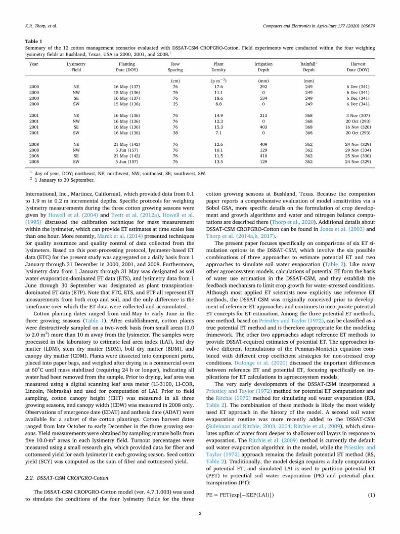
Cotton planting dates ranged from mid-May to early June in the three growing seasons (Table 1). After establishment, cotton plants were destructively sampled on a two-week basis from small areas (1.0 to 2.0 m2) more than 10 m away from the lysimeter. The samples were processed in the laboratory to estimate leaf area index (LAI), leaf dry matter (LDM), stem dry matter (SDM), boll dry matter (BDM), and canopy dry matter (CDM). Plants were dissected into component parts, placed into paper bags, and weighed after drying in a commercial oven at 60°C until mass stabilized (requiring 24 h or longer), indicating all water had been removed from the sample. Prior to drying, leaf area was measured using a digital scanning leaf area meter (LI-3100, LI-COR, Lincoln, Nebraska) and used for computation of LAI. Prior to field sampling, cotton canopy height (CHT) was measured in all three growing seasons, and canopy width (CDW) was measured in 2008 only. Observations of emergence date (EDAT) and anthesis date (ADAT) were available for a subset of the cotton plantings. Cotton harvest dates ranged from late October to early December in the three growing sea-sons. Yield measurements were obtained by sampling mature bolls from five 10.0-m2 areas in each lysimetry field. Turnout percentages were measured using a small research gin, which provided data for fiber and cottonseed yield for each lysimeter in each growing season. Seed cotton yield (SCY) was computed as the sum of fiber and cottonseed yield.

2.2. DSSAT-CSM CROPGRO-Cotton

The DSSAT-CSM CROPGRO-Cotton model (ver. 4.7.1.003) was used to simulate the conditions of the four lysimetry fields for the three

cotton growing seasons at Bushland, Texas. Because the companion paper reports a comprehensive evaluation of model sensitivities via a Sobol GSA, more specific details on the formulation of crop develop-ment and growth algorithms and water and nitrogen balance compu-tations are described there (Thorp et al., 2020). Additional details about DSSAT-CSM CROPGRO-Cotton can be found in Jones et al. (2003) and Thorp et al. (2014a,b, 2017).

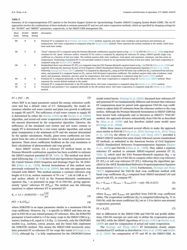
The present paper focuses specifically on comparisons of six ET si-mulation options in the DSSAT-CSM, which involve the six possible combinations of three approaches to estimate potential ET and two approaches to simulate soil water evaporation (Table 2). Like many other agroecosystem models, calculations of potential ET form the basis of water use estimation in the DSSAT-CSM, and they establish the feedback mechanism to limit crop growth for water-stressed conditions. Although most applied ET scientists now explicitly use reference ET methods, the DSSAT-CSM was originally conceived prior to develop-ment of reference ET approaches and continues to incorporate potential ET concepts for ET estimation. Among the three potential ET methods, one method, based on Priestley and Taylor (1972), can be classified as a true potential ET method and is therefore appropriate for the modeling framework. The other two approaches adapt reference ET methods to provide DSSAT-required estimates of potential ET. The approaches in-volve different formulations of the Penman-Monteith equation com-bined with different crop coefficient strategies for non-stressed crop conditions. DeJonge et al. (2020) discussed the important differences between reference ET and potential ET, focusing specifically on im-plications for ET calculations in agroecosystem models.

The very early developments of the DSSAT-CSM incorporated a Priestley and Taylor (1972) method for potential ET computations and the Ritchie (1972) method for simulating soil water evaporation (RR, Table 2). The combination of these methods is likely the most widely used ET approach in the history of the model. A second soil water evaporation routine was more recently added to the DSSAT-CSM (Suleiman and Ritchie, 2003, 2004; Ritchie et al., 2009), which simu-lates upflux of water from deeper to shallower soil layers in response to evaporation. The Ritchie et al. (2009) method is currently the default soil water evaporation algorithm in the model, while the Priestley and Taylor (1972) approach remains the default potential ET method (RS, Table 2). Traditionally, the model design requires a daily computation of potential ET, and simulated LAI is used to partition potential ET (PET) to potential soil water evaporation (PE) and potential plant transpiration (PT):

=PE PET(exp[ KEP(LAI)]) (1)

Table 1 Summary of the 12 cotton management scenarios evaluated with DSSAT-CSM CROPGRO-Cotton. Field experiments were conducted within the four weighing lysimetry fields at Bushland, Texas, USA in 2000, 2001, and 2008.1

Year Lysimetry Planting Row Plant Irrigation Rainfall2 Harvest Field Date (DOY) Spacing Density Depth Depth Date (DOY)

(cm) (p m−2) (mm) (mm) 2000 NE 16 May (137) 76 17.6 292 249 6 Dec (341) 2000 NW 15 May (136) 76 11.1 0 249 6 Dec (341) 2000 SE 16 May (137) 76 18.6 534 249 6 Dec (341) 2000 SW 15 May (136) 25 8.8 0 249 6 Dec (341)

2001 NE 16 May (136) 76 14.9 213 368 3 Nov (307) 2001 NW 16 May (136) 76 12.3 0 368 20 Oct (293) 2001 SE 16 May (136) 76 15.3 403 368 16 Nov (320) 2001 SW 16 May (136) 38 7.1 0 368 20 Oct (293)

2008 NE 21 May (142) 76 12.6 409 362 24 Nov (329) 2008 NW 5 Jun (157) 76 10.1 129 362 29 Nov (334) 2008 SE 21 May (142) 76 11.5 410 362 25 Nov (330) 2008 SW 5 Jun (157) 76 13.5 129 362 24 Nov (329)

1 day of year, DOY; northeast, NE; northwest, NW; southeast, SE; southwest, SW. 2 1 January to 30 September.


3

=PT PET PE (2)

where KEP is an input parameter named the energy extinction coeffi-cient and has a default value of 0.7. Subsequently, the model de-termines whether soil water content and plant root growth is sufficient to supply PE and PT. The sufficiency of soil water content to supply PE is determined by either the Ritchie (1972) or the Ritchie et al. (2009) algorithm, and actual soil water evaporation is the minimum of PE and the amount determined by the evaporation algorithm. Likewise, the sufficiency of the simulated root system and soil water content to supply PT is determined by a root water uptake algorithm, and actual plant transpiration is the minimum of PT and the amount determined by the uptake calculations. Finally, plant stress coefficients are com-puted from the ratio of simulated values for actual and potential tran-spiration. These stress coefficients feedback on the crop simulation to limit calculations of photosynthesis and crop growth.

Since DSSAT version 4.0, a reference ET method based on the Penman-Monteith combination equation has been available to estimate the DSSAT-required potential ET (F, Table 2). The method was devel-oped following Eqs. (3)–(5) in the Food and Agriculture Organization of the United Nations (FAO) Irrigation and Drainage Paper No. 56 (FAO- 56) (Allen et al., 1998). Several formulations of this method were previously evaluated by Sau et al. (2004), but only one approach was released with DSSAT. This method assumes a constant reference crop height of 0.12 m, surface resistance of 70 s m−1, LAI of 2.88 m m−2, and surface albedo of 0.23 in the Penman-Monteith combination equation (Eq. 3 as presented on page 19 in FAO-56), giving approxi-mately “grass” reference ET (ETpm). The method uses the following equations to adjust reference ET to potential ET:

= +K 1.0 (EORATIO 1.0) LAI6.0c (3)

=PET K (ET )c pm (4)

where EORATIO is an input parameter similar to a maximum FAO-56 crop coefficient. However, Eq. 3 is specific to DSSAT and does not ap-pear in FAO-56 or any related primary ET reference. Also, the EORATIO parameter is hard-coded to 1.0 for many crops in the DSSAT-CSM (e.g., maize), leading to Kc equal to 1.0 (Eq. 3). Currently, only the CROPGRO models (e.g., soybean, cotton, peanut, and dry bean) fully implement the EORATIO method. This means the DSSAT-CSM incorrectly simu-lates potential ET as reference ET for crops like maize (DeJonge et al., 2020), although Eq. 3 is fully implemented for the CROPGRO-Cotton

model tested herein. DeJonge et al. (2020) discussed how reference ET and potential ET are fundamentally different and stressed that reference ET computations must be paired with appropriate FAO-56 crop coeffi-cients to adjust daily ET estimates from the reference surface to the crop surface. Although the Penman-Monteith formulation in DSSAT-CSM has been known both colloquially and in literature as DSSAT’s “FAO-56” method, the approach deviates substantially from FAO-56 as described by Allen et al. (1998) and has therefore misled some model users (DeJonge et al., 2020).

While these issues motivated several efforts to make the approach more similar to FAO-56 (Thorp et al., 2010; DeJonge et al., 2012; Thorp et al., 2014b), the efforts of DeJonge and Thorp (2017) provided a DSSAT-CSM ET method that most closely followed current standardized ET methods, as embodied in the American Society of Civil Engineers (ASCE) Standardized Reference Evapotranspiration Equation (Walter et al., 2005) and FAO-56 (Allen et al., 1998). They added a separate reference ET method to estimate DSSAT-required potential ET (G, Table 2), which used the FAO Penman-Monteith equation (Eq. 6 as presented on page 24 in FAO-56) to compute either short crop reference ET (ETo) or tall crop reference ET (ETr), following the algorithms spe-cified in the ASCE Standardized Reference Evapotranspiration Equation documentation (Walter et al., 2005). Furthermore, DeJonge and Thorp (2017) implemented the FAO-56 dual crop coefficient method with basal crop coefficients (Kcb) computed from DSSAT-simulated LAI and paired with ETo to compute PT:

= +K K (K K )(1.0 exp[ SK (LAI)])cb cbmin cbmax cbmin c (5)

=PT K ETcb o (6)

where Kcbmin and Kcbmax are specified from FAO-56 crop coefficient tables. The evaporation coefficient (Ke) is computed following Eq. 71 in FAO-56, with the stress coefficient (Kr) set to 1.0 to derive non-stressed evaporation potential:

=PE K ETe o (7)

Due to differences in the DSSAT-CSM and FAO-56 soil profile defini-tions, FAO-56 concepts are used only to define the evaporation poten-tial (PE), while the DSSAT algorithms of Ritchie (1972) or Ritchie et al. (2009) are used for computation of actual soil water evaporation.

The DeJonge and Thorp (2017) ET formulation closely adapts standardized ET methods as described in Allen et al. (1998) and Walter et al. (2005) for computation of PT and PE in the DSSAT-CSM. As

Table 2 Summary of six evapotranspiration (ET) options in the Decision Support System for Agrotechnology Transfer (DSSAT) Cropping System Model (CSM). The six ET approaches involve the combinations of three methods to estimate potential ET and two soil water evaporation methods, which are specified by changing settings for the “EVAPO” and “MESEV” parameters, respectively, in the DSSAT-CSM management file.

Short EVAPO MESEV Description Name Setting Setting

RR R R Potential ET is computed via a Priestley and Taylor (1972) method, requiring only daily solar irradiance and maximum and minimum air temperatures. Soil water evaporation is computed using the Ritchie (1972) method. These represent the earliest methods in the model, which have been used most widely.

FR F R “Grass” reference ET is computed using the Penman-Monteith combination equation based on Eqs. (3)–(5) in FAO-56 (Allen et al., 1998) using fixed constants for the “grass” reference surface. Potential ET for cotton is computed by adjusting the reference ET using a DSSAT-specific single crop coefficient as a function of leaf area index. The method requires daily solar irradiance, wind speed, and maximum, minimum, and dew point air temperatures. Partitioning of potential ET to soil and plant surfaces is based on an exponential function of leaf area index. Soil water evaporation is computed using the Ritchie (1972) method.

GR G R Standardized short crop reference ET (ETos) is computed using the FAO Penman-Monteith equation based on Eq. 6 in FAO-56 (Allen et al., 1998) and explicitly following the American Society of Civil Engineers (ASCE) Standardized Reference Evapotranspiration Equation (Walter et al., 2005). Following DeJonge and Thorp (2017), potential T is computed by adjusting ETos using an FAO-56 basal crop coefficient (Kcb) calculated from leaf area index, and potential E is computed based on ETos and an FAO-56-based evaporation coefficient. The method requires daily solar irradiance, wind speed, and maximum, minimum, and dew point air temperatures. Soil water evaporation is computed using the Ritchie (1972) method.

RS R S Potential ET is computed identically to the RR method above. Soil water evaporation is computed using the Ritchie et al. (2009) method. These represent the current default methods in the model.

FS F S Potential ET is computed identically to the FR method above. Soil water evaporation is computed using the Ritchie et al. (2009) method. GS G S Potential E and potential T are computed identically to the GR method above. Soil water evaporation is computed using the Ritchie et al. (2009)

method.


4

shown by DeJonge and Thorp (2017), the method also provided si-mulated ET time series that demonstrated expected ET behavior, while the behavior of other DSSAT-CSM ET methods deviated from theore-tical expectations. Because DeJonge and Thorp (2017) did not evaluate or compare the performance of the various DSSAT ET methods against measured ET data, the present study provides further performance as-sessments and comparisons using the three-year cotton data set from the Bushland weighing lysimetry fields. Hereafter, the six ET methods in DSSAT-CSM are denoted RR, FR, GR, RS, FS, and GS, as described in Table 2.

2.3. Simulation workflow

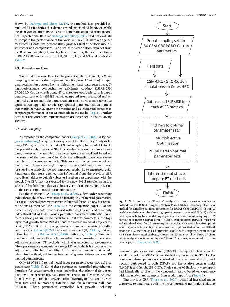
The simulation workflow for the present study included 1) a Sobol sampling scheme to select large numbers (i.e., over 15 million) of input parameterization options from a high-dimensional parameter space, 2) high-performance computing to efficiently conduct DSSAT-CSM CROPGRO-Cotton simulations, 3) a database approach to link input parameter sets with %RMSE values computed from measured and si-mulated data for multiple agroecosystem metrics, 4) a multiobjective optimization approach to identify optimal parameterization options that minimize %RMSE among the metrics, and 5) inferential statistics to compare performance of six ET methods in the model (Fig. 1). Further details of the workflow implementation are described in the following sections.

2.4. Sobol sampling

As reported in the companion paper (Thorp et al., 2020), a Python (www.python.org) script that incorporated the Sensitivity Analysis Li-brary (SALib) was used to conduct Sobol sampling for a Sobol GSA. In the present study, the same SALib algorithm was used for Sobol sam-pling; however, the sampled parameter space was modified based on the results of the previous GSA. Only the influential parameters were included in the present analysis. This ensured that parameter adjust-ments would have meaningful impact on the model output and there-fore lead the analysis toward improved model fit to measured data. Parameters that were deemed non-influential from the previous GSA were fixed, either to default values or based on past experience with the model. The GSA was not repeated for the new Sobol sample. Instead, a subset of the Sobol samples was chosen via multiobjective optimization to identify optimal model parameterizations.

For the previous GSA (Thorp et al., 2020), a first-order sensitivity index threshold of 0.05 was used to identify the influential parameters. As a result, several parameters were influential for only a few but not all of the six ET methods (see Table 2 in the companion paper). For the present study, the data were assessed with a slightly reduced sensitivity index threshold of 0.031, which permitted consistent influential para-meters among all six ET methods for all but two parameters: the top- layer root growth factor (SRGF1) and the maximum basal crop coeffi-cient (KMAX). Both of these parameters remained consistently influ-ential for the Ritchie (1972) evaporation method (R, Table 2) but not influential for the Ritchie et al. (2009) method (S, Table 2). The mod-ified sensitivity index threshold permitted more consistent parameter adjustments among ET methods, which was expected to encourage a fairer performance comparison among ET methods. It is a conservative adjustment, allowing flexibility for a few parameters that would otherwise be fixed, all in the interest of greater fairness among ET method comparisons.

Only 12 of 38 influential model input parameters were crop cultivar parameters (Table 3). Six of these parameters controlled photothermal durations for cotton growth stages, including photothermal time from planting to emergence (PL-EM), from emergence to flowering (EM-FL), from flowering to first boll (FL-SH), from flowering to first seed (FL-SD), from first seed to maturity (SD-PM), and for maximum boll load (PODUR). Three parameters controlled leaf growth, including

maximum photosynthesis rate (LFMAX), the specific leaf area for standard conditions (SLAVR), and the leaf appearance rate (TRIFL). The remaining three parameters controlled the maximum daily growth fraction partitioned to bolls (XFRT) and the relative cultivar width (RWDTH) and height (RHGHT). Their ranges of flexibility were speci-fied identically to that in the companion study, based on experience with the model and examples from model input files (Table 3).

The previous GSA (Thorp et al., 2020) identified increased model sensitivity to parameters defining the soil profile water limits, including

Fig. 1. Workflow for the “Phase 2” analysis to compare evapotranspiration methods in the DSSAT Cropping System Model (CSM), including 1) a Sobol method for sampling 38 input parameters for DSSAT-CSM CROPGRO-Cotton, 2) model simulations on the Ceres high performance computer (HPC), 3) a data-base approach to link model input parameters from Sobol sampling to 23 percent root mean squared error (%RMSE) computations between measured and simulated data for 23 agroecosystem metrics, 4) a multiobjective optimi-zation approach to identify parameterization options that minimize %RMSE among the 23 metrics, and 5) inferential statistics to compare performance of six ET simulation methodologies among the 23 metrics. This “Phase 2” simu-lation analysis was informed by the “Phase 1” analysis, as reported in a com-panion paper (Thorp et al., 2020).


5

http://www.python.org

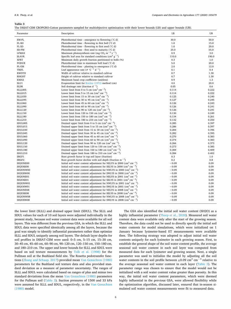
the lower limit (SLLL) and drained upper limit (SDUL). The SLLL and SDUL values for each of 10 soil layers were adjusted individually in the present study, because soil water content data were available for all soil layers. This was different from the previous GSA, in which the SLLL and SDUL data were specified identically among all the layers, because the goal was simply to identify influential parameters rather than optimize SLLL and SDUL uniquely among soil layers. The default layer depths for soil profiles in DSSAT-CSM were used: 0–5 cm, 5–15 cm, 15–30 cm, 30–45 cm, 45–60 cm, 60–90 cm, 90–120 cm, 120–150 cm, 150–180 cm, and 180–210 cm. The upper and lower bounds for SLLL and SDUL were based on soil texture measurements by Tolk et al. (1998) for the Pullman soil at the Bushland field site. The Rosetta pedotransfer func-tions (Zhang and Schaap, 2017) provided mean Van Genuchten (1980) parameters for the Bushland soil texture data and also provided stan-dard deviation as a measure of parameter uncertainty. The ranges of SLLL and SDUL were calculated based on ranges of plus and minus two standard deviations from the mean Van Genuchten (1980) parameters for the Pullman soil (Table 3). Suction pressures of 1500 and 33 kPa were assumed for SLLL and SDUL, respectively, in the Van Genuchten (1980) model.

The GSA also identified the initial soil water content (SH2O) as a highly influential parameter (Thorp et al., 2020). Measured soil water content data were available only after the start of the growing season. Therefore, the data could not be used to directly specify the initial soil water contents for model simulations, which were initialized on 1 January because lysimeter-based ET measurements were available then. The following strategy was adopted to adjust initial soil water contents uniquely for each lysimeter in each growing season. First, to establish the general shape of the soil water content profile, the average seasonal soil water content in each soil layer was computed from measured data for each lysimeter and growing season. Next, a single parameter was used to initialize the model by adjusting all the soil water contents in the soil profile between ±0.09 cm3 cm−3 relative to the average seasonal soil water content in each layer (Table 3). The parameter range was chosen to ensure that the model would not be initialized with a soil water content value greater than porosity. In this way, the initial soil water content parameters, which were deemed highly influential in the previous GSA, were allowed flexibility while the optimization algorithm, discussed later, ensured that in-season si-mulated soil water content measurements were fit to measured data.

Table 3 The DSSAT-CSM CROPGRO-Cotton parameters sampled for multiobjective optimization with their lower bounds (LB) and upper bounds (UB).

Parameter Description LB UB

EM-FL Photothermal time - emergence to flowering (°C d) 30.0 50.0 FL-SH Photothermal time - flowering to first boll (°C d) 1.0 15.0 FL-SD Photothermal time - flowering to first seed (°C d) 1.0 20.0 SD-PM Photothermal time - first seed to maturity (°C d) 25.0 55.0 LFMAX Maximum photosynthesis rate (mg CO2 m−2 s−1) 0.9 3.0 SLAVR Specific leaf area for standard conditions (cm2 g−1) 110.0 190.0 XFRT Maximum daily growth fraction partitioned to bolls (%) 0.3 1.0 PODUR Photothermal time to maximum boll load (°C d) 5.0 20.0 PL-EM Photothermal time - planting to emergence (°C d) 2.0 12.0 TRIFL Leaf appearance rate (# °C−1 d−1) 0.1 0.4 RWDTH Width of cultivar relative to standard cultivar 0.7 1.30 RHGHT Height of cultivar relative to standard cultivar 0.7 1.30 KMAX Maximum basal crop coefficient (unitless) 0.9 1.3 SLU1 Evaporation limit for Ritchie (1972) method (cm) 4.0 20.0 SLDR Soil drainage rate (fraction d−1) 0.05 0.6 SLLL005 Lower limit from 0 to 5 cm (cm3 cm−3) 0.114 0.222 SLLL015 Lower limit from 5 to 15 cm (cm3 cm−3) 0.114 0.222 SLLL030 Lower limit from 15 to 30 cm (cm3 cm−3) 0.125 0.240 SLLL045 Lower limit from 30 to 45 cm (cm3 cm−3) 0.127 0.245 SLLL060 Lower limit from 45 to 60 cm (cm3 cm−3) 0.126 0.243 SLLL090 Lower limit from 60 to 90 cm (cm3 cm−3) 0.126 0.241 SLLL120 Lower limit from 90 to 120 cm (cm3 cm−3) 0.126 0.241 SLLL150 Lower limit from 120 to 150 cm (cm3 cm−3) 0.130 0.249 SLLL180 Lower limit from 150 to 180 cm (cm3 cm−3) 0.134 0.261 SLLL210 Lower limit from 180 to 210 cm (cm3 cm−3) 0.132 0.250 SDUL005 Drained upper limit from 0 to 5 cm (cm3 cm−3) 0.285 0.397 SDUL015 Drained upper limit from 5 to 15 cm (cm3 cm−3) 0.286 0.397 SDUL030 Drained upper limit from 15 to 30 cm (cm3 cm−3) 0.284 0.396 SDUL045 Drained upper limit from 30 to 45 cm (cm3 cm−3) 0.282 0.395 SDUL060 Drained upper limit from 45 to 60 cm (cm3 cm−3) 0.270 0.383 SDUL090 Drained upper limit from 60 to 90 cm (cm3 cm−3) 0.274 0.383 SDUL120 Drained upper limit from 90 to 120 cm (cm3 cm−3) 0.266 0.373 SDUL150 Drained upper limit from 120 to 150 cm (cm3 cm−3) 0.273 0.385 SDUL180 Drained upper limit from 150 to 180 cm (cm3 cm−3) 0.284 0.409 SDUL210 Drained upper limit from 180 to 210 cm (cm3 cm−3) 0.284 0.402 SRGF1 Root growth factor in top soil layer (fraction) 0.3 1.0 SRGF2 Root growth factor decline with soil depth (fraction m−1) 0.2 0.8 SH2ONE00 Initial soil water content adjustment for NELYS in 2000 (cm3 cm−3) −0.09 0.09 SH2OSE00 Initial soil water content adjustment for SELYS in 2000 (cm3 cm−3) −0.09 0.09 SH2ONW00 Initial soil water content adjustment for NWLYS in 2000 (cm3 cm−3) −0.09 0.09 SH2OSW00 Initial soil water content adjustment for SWLYS in 2000 (cm3 cm−3) −0.09 0.09 SH2ONE01 Initial soil water content adjustment for NELYS in 2001 (cm3 cm−3) −0.09 0.09 SH2OSE01 Initial soil water content adjustment for SELYS in 2001 (cm3 cm−3) −0.09 0.09 SH2ONW01 Initial soil water content adjustment for NWLYS in 2001 (cm3 cm−3) −0.09 0.09 SH2OSW01 Initial soil water content adjustment for SWLYS in 2001 (cm3 cm−3) −0.09 0.09 SH2ONE08 Initial soil water content adjustment for NELYS in 2008 (cm3 cm−3) −0.09 0.09 SH2OSE08 Initial soil water content adjustment for SELYS in 2008 (cm3 cm−3) −0.09 0.09 SH2ONW08 Initial soil water content adjustment for NWLYS in 2008 (cm3 cm−3) −0.09 0.09 SH2OSW08 Initial soil water content adjustment for SWLYS in 2008 (cm3 cm−3) −0.09 0.09


6

Five additional water balance parameters were adjusted, including two soil root growth factors (SRGF1 and SRGF2), the soil drainage rate (SLDR), the evaporation limit (SLU1) which was applicable only for the Ritchie (1972) evaporation approach (R, Table 2), and the maximum basal crop coefficient (KMAX) which was influential only for the DeJonge and Thorp (2017) potential ET method with Ritchie (1972) soil water evaporation (GR, Table 2). The root growth factors define the shape of the rooting profile and were calculated using two variables: 1) SRGF1 specified the root growth factor for the top soil layer and 2) SRGF2 specified the linear rate of decline with soil profile depth. Si-milar to the companion study, root growth profiles were specified using a linear decrease from the top soil layer with zero being the smallest possible factor level. Because SRGF1 was non-influential for the Ritchie et al. (2009) evaporation method (Thorp et al., 2020), it was fixed to 1.0 for that case, indicating unrestricted root growth in that layer. Other non-influential soil parameters were fixed based on field mea-surements or experience with the model.

The N parameter of SALib’s Sobol sampling algorithm was set to 158,224 with specification to prepare for calculation of second-order sensitivity effects (although the resulting parameter sets were not used for a second GSA). Thus, the number of n-dimensional parameter sets ( =n 49) chosen was + =N n(2 2) 15, 822, 400, as defined within the Sobol algorithm. The value of N was identical to that used in the companion study based on estimated timeframes for conducting simu-lations via high-performance computing. The total number of para-meters for each lysimeter and growing season combination was 38; however, because initial soil water conditions were permitted to vary uniquely per lysimeter and growing season (as discussed above), the n for the Sobol algorithm was 49.

2.5. Simulations

Similar to the companion study, DSSAT-CSM CROPGRO-Cotton was set up to run 12 simulation scenarios based on the three cotton growing seasons and four uniquely-managed lysimetry fields (Table 1). Simu-lations were initiated on 1 January in each year and concluded on the recorded harvest date for each lysimetry field. Within the SW lysimetry field in 2001, twin rows spaced 25 cm apart were planted on 76 cm centers. Because CROPGRO-Cotton did not consider this planting

configuration, a row spacing of 38 cm (i.e., half of 76 cm) was simu-lated.

Simulations were conducted using USDA’s high-performance com-puting resource called Ceres. A Python script that incorporated the “multiprocessing” package was used to manage simulation tasks among processing cores. With 12 simulation scenarios, 6 ET algorithms, and 15,822,400 parameter sets, the simulation analysis required a total of 1,139,212,800 simulations, which required 327,875 CPU hr on Ceres and approximately 1,639 h of wall-clock time. This study was more computationally expensive than the companion study, which was in part related to the greater number of simulations required. Additional details regarding the simulation set up are presented in the companion paper (Thorp et al., 2020).

2.6. Database method

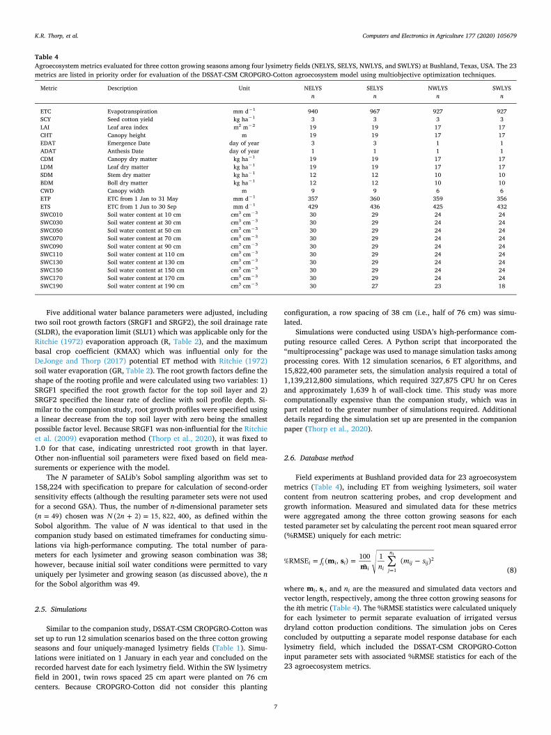
Field experiments at Bushland provided data for 23 agroecosystem metrics (Table 4), including ET from weighing lysimeters, soil water content from neutron scattering probes, and crop development and growth information. Measured and simulated data for these metrics were aggregated among the three cotton growing seasons for each tested parameter set by calculating the percent root mean squared error (%RMSE) uniquely for each metric:

= ==

fn

m sm sm

%RMSE ( , ) 100¯

1 ( )i i i ii i j

n

ij ij1

2i

(8)

where m s,i i, and ni are the measured and simulated data vectors and vector length, respectively, among the three cotton growing seasons for the ith metric (Table 4). The %RMSE statistics were calculated uniquely for each lysimeter to permit separate evaluation of irrigated versus dryland cotton production conditions. The simulation jobs on Ceres concluded by outputting a separate model response database for each lysimetry field, which included the DSSAT-CSM CROPGRO-Cotton input parameter sets with associated %RMSE statistics for each of the 23 agroecosystem metrics.

Table 4 Agroecosystem metrics evaluated for three cotton growing seasons among four lysimetry fields (NELYS, SELYS, NWLYS, and SWLYS) at Bushland, Texas, USA. The 23 metrics are listed in priority order for evaluation of the DSSAT-CSM CROPGRO-Cotton agroecosystem model using multiobjective optimization techniques.

Metric Description Unit NELYS SELYS NWLYS SWLYS n n n n

ETC Evapotranspiration mm d−1 940 967 927 927 SCY Seed cotton yield kg ha−1 3 3 3 3 LAI Leaf area index m2 m−2 19 19 17 17 CHT Canopy height m 19 19 17 17 EDAT Emergence Date day of year 3 3 1 1 ADAT Anthesis Date day of year 1 1 1 1 CDM Canopy dry matter kg ha−1 19 19 17 17 LDM Leaf dry matter kg ha−1 19 19 17 17 SDM Stem dry matter kg ha−1 12 12 10 10 BDM Boll dry matter kg ha−1 12 12 10 10 CWD Canopy width m 9 9 6 6 ETP ETC from 1 Jan to 31 May mm d−1 357 360 359 356 ETS ETC from 1 Jun to 30 Sep mm d−1 429 436 425 432 SWC010 Soil water content at 10 cm cm3 cm−3 30 29 24 24 SWC030 Soil water content at 30 cm cm3 cm−3 30 29 24 24 SWC050 Soil water content at 50 cm cm3 cm−3 30 29 24 24 SWC070 Soil water content at 70 cm cm3 cm−3 30 29 24 24 SWC090 Soil water content at 90 cm cm3 cm−3 30 29 24 24 SWC110 Soil water content at 110 cm cm3 cm−3 30 29 24 24 SWC130 Soil water content at 130 cm cm3 cm−3 30 29 24 24 SWC150 Soil water content at 150 cm cm3 cm−3 30 29 24 24 SWC170 Soil water content at 170 cm cm3 cm−3 30 29 24 24 SWC190 Soil water content at 190 cm cm3 cm−3 30 27 23 18


7

2.7. Multiobjective optimization

Because there were 23 agroecosystem metrics to consider (Table 4), identifying the best parameterization options for DSSAT-CSM CROPGRO-Cotton required multiobjective optimization (MOO) techni-ques (Taboada et al., 2007). The objective function to be optimized incorporated k unique %RMSE calculations, one for each agroecosystem metric ( =k 23), expressed as

= …f f f fm s m s m s m s( , ) ( ( , ), ( , ), , ( , ))k k kMOO 1 1 1 2 2 2 (9)

where the terms are as described for Eq. 8. Eq. 9 represents the set of % RMSE calculations (Eq. 8) for each of k agroecosystem metrics, based on the results of simulations for a given parameter set among nearly 16 million sets tested. The first step toward reduction of plausible para-meter sets was to calculate the subset of Pareto optimal solutions (Cheikh et al., 2010), which were the solutions that were not dominated (or non-dominated) by any other solution. In mathematical terms, a solution x1 dominates another solution x2 if the following two conditions are met:

• f x f x( ) ( )i i1 2 for all …i k{1, 2, , }• <f x f x( ) ( )j j1 2 for at least one …j k{1, 2, , }

In words, a solution dominates another if the %RMSE calculations for k agroecosystem metrics are all less than or equal to that for the other solution, and at least one %RMSE calculation is less than that for the other solution. The goal was to find the parameter sets with %RMSE calculations that were not dominated by the RMSE calculations for any other parameter set. Following the methodology of Thorp et al. (2019), a Python script was developed to calculate the Pareto optimal solution set among the evaluated parameterization options for each DSSAT-CSM ET method and lysimetry field.

A known problem with Pareto optimal sets is that they often remain large and cumbersome, and they do not adequately ease the burden of selecting one or several practical solutions. Following Taboada et al. (2007) and as implemented by Thorp et al. (2019), a “pruning” algo-rithm was developed to reevaluate each Pareto optimal solution and combine the k objective function outcomes (Eq. 9) to a single evalua-tion criterion by assigning k weightings following a predetermined objective function priority. Because ET and crop yield were the most

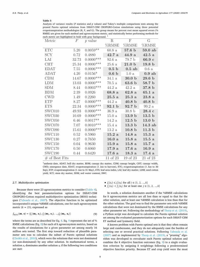
Table 5 Analysis of variance results (F statistics and p values) and Tukey’s multiple comparisons tests among the pruned Pareto optimal solutions from DSSAT-CSM CROPGRO-Cotton simulations using three potential evapotranspiration methodologies (R, F, and G). The group means for percent root mean squared errors (% RMSE) are given for each method and agroecosystem metric, and statistically better performing methods for each metric are highlighted in bold with gray background. 1

1anthesis date, ADAT; boll dry matter, BDM; canopy dry matter, CDM; canopy height, CHT; canopy width, CWD; emergence date, EDAT; evapotranspiration (1 Jan to harvest), ETC; evapotranspiration (1 Jun to 30 Sep), ETP; evapotranspiration (1 Jan to 31 May), ETS; leaf area index, LAI; leaf dry matter, LDM; seed cotton yield, SCY; stem dry matter, SDM; soil water content; SWC.


8

important of agroecosystem metrics in this study, the priority of ob-jective functions were specified in the following order: ETC, SCY, LAI, CHT, EDAT, ADAT, CDM, LDM, SDM, BDM, CWD, ETP, and ETS, fol-lowed by the ten soil water content measurements from top to bottom in the profile (Table 4). The weightings were used to calculate the weighted average among the groups of 23 %RMSE results among all solutions in the Pareto optimal set, and the parameter set with the smallest weighted average was identified. The process was iterated until 1,000 iterations passed without identification of a new pruned solution. The set of pruned Pareto optimal solutions determined from this process was used for all further analysis. For model evaluation purposes, simulated data were estimated based on the median simula-tion result among the pruned Pareto optimal solutions. Additional de-tails on the multiobjective optimization strategy are presented by Thorp et al. (2019).

2.8. ET method comparison

The performance of the six DSSAT-CSM ET methods (Table 2) was compared by conducting an analysis of variance (ANOVA) on %RMSE results for each of the 23 agroecosystem metrics (Table 4) among the pruned Pareto optimal solutions. Tukey’s multiple comparisons tests were also conducted to identify which ET methods resulted in statisti-cally different %RMSE values for each agroecosystem metric (p 0.05), and the smallest of these identified the better ET method for a given metric. Statistical analysis was conducted using the R Project for Sta-tistical Computing software (www.r-project.org).

3. Results

3.1. Inferential statistics

Among the three methods for simulating potential ET, the DeJonge

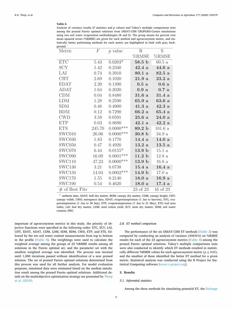
Table 6 Analysis of variance results (F statistics and p values) and Tukey’s multiple comparisons tests among the pruned Pareto optimal solutions from DSSAT-CSM CROPGRO-Cotton simulations using two soil water evaporation methodologies (R and S). The group means for percent root mean squared errors (%RMSE) are given for each method and agroecosystem metric, and sta-tistically better performing methods for each metric are highlighted in bold with gray back-ground. 1

1 anthesis date, ADAT; boll dry matter, BDM; canopy dry matter, CDM; canopy height, CHT; canopy width, CWD; emergence date, EDAT; evapotranspiration (1 Jan to harvest), ETC; eva-potranspiration (1 Jun to 30 Sep), ETP; evapotranspiration (1 Jan to 31 May), ETS; leaf area index, LAI; leaf dry matter, LDM; seed cotton yield, SCY; stem dry matter, SDM; soil water content; SWC


9

http://www.r-project.org

and Thorp (2017) approach (G, Table 2) performed either statistically better than or similarly to the other two potential ET methods for all but two of the agroecosystem metrics (Table 5). Only for emergence date (EDAT) and soil water evaporation from 1 January through 31 May (ETS) did the Priestley-Taylor approach (R, Table 2) and Penman- Monteith combination equation approach (F, Table 2) perform statis-tically better than the DeJonge and Thorp (2017) implementation of the ASCE Standardized Reference ET equation with FAO-56 dual crop coefficients. Likewise, with the exception of anthesis date (ADAT), the F method performed statistically better than or similarly to the R method among all metrics. Regarding differences for EDAT and ADAT, the mean %RMSE differences among metrics were not more than 0.1% and 0.4%, respectively. Thus, although the results were significantly different for EDAT and ADAT, the magnitudes of the error differences did not in-dicate large performance differences. Specifically, EDAT and ADAT were not simulated more than ±2 and ±6 days different from available observations for 95% of simulations among pruned Pareto optimal so-lutions. As compared to the G potential ET method, the F and R methods provided statistically worse simulations for several of the plant-based metrics, including LAI and SDM, while the R method ad-ditionally simulated CHT, CDM, LDM, ETC, ETP and soil water contents from the surface to 90 cm with statistically greater error. The results demonstrated model performance advantages when using the DeJonge and Thorp (2017) approach for potential ET simulations in the DSSAT- CSM.

The poorer performance of the DeJonge and Thorp (2017) approach for ETS (Table 5) may not be of great concern. First, ETS was a lower priority metric. All other ET and plant growth metrics were specified with greater priority in the multiobjective optimization, and only the soil water content metrics were specified with lower priority (Table 4). Second, ETS was specified as ET from 1 January through 31 May, mostly a fallow period prior to crop planting and emergence (Table 1) with secondary importance to ET during the crop growing season. Furthermore, the total amount of ET for ETS (i.e., 145–179 mm) was 2–3 times less than the amount of ET for ETP (i.e., 331–723 mm). The ET for ETP is much more relevant for water use during the cotton growing season, although ETS was included in the analysis due to availability of ET measurements during that time. Finally, as discussed further later, poorer ETS performance was attributed to the combina-tion of the G potential ET method with the Ritchie et al. (2009) soil water evaporation method (GS, Table 2), while the combination of G potential ET with the Ritchie (1972) soil water evaporation method (GR, Table 2) performed similarly to other ET options.

With the Ritchie (1972) soil water evaporation methodology, si-mulations of all 23 agroecosystem metrics were statistically equivalent to or better than that for the Ritchie et al. (2009) method (Table 6). The results clearly showed that simulations of ETC, ETS, and soil water contents at 5 of 10 soil profile depths were statistically better with the Ritchie (1972) method, and none of the metrics were better simulated with the Ritchie et al. (2009) method. The result corroborated findings

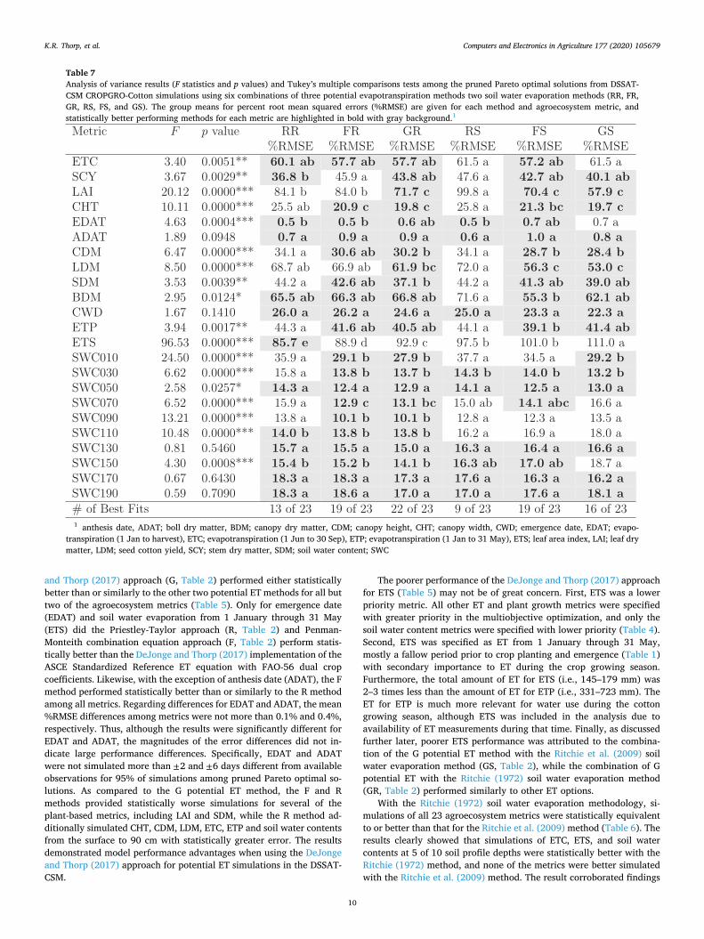
Table 7 Analysis of variance results (F statistics and p values) and Tukey’s multiple comparisons tests among the pruned Pareto optimal solutions from DSSAT- CSM CROPGRO-Cotton simulations using six combinations of three potential evapotranspiration methods two soil water evaporation methods (RR, FR, GR, RS, FS, and GS). The group means for percent root mean squared errors (%RMSE) are given for each method and agroecosystem metric, and statistically better performing methods for each metric are highlighted in bold with gray background.1

1 anthesis date, ADAT; boll dry matter, BDM; canopy dry matter, CDM; canopy height, CHT; canopy width, CWD; emergence date, EDAT; evapo-transpiration (1 Jan to harvest), ETC; evapotranspiration (1 Jun to 30 Sep), ETP; evapotranspiration (1 Jan to 31 May), ETS; leaf area index, LAI; leaf dry matter, LDM; seed cotton yield, SCY; stem dry matter, SDM; soil water content; SWC


10

reported by Kimball et al. (2019), suggesting that the Ritchie et al. (2009) soil water evaporation method requires further development prior to regular use in the DSSAT-CSM.

By assessing the six combinations of potential ET and soil water evaporation options in the DSSAT-CSM, the results showed that the ASCE reference ET and dual crop coefficient method of DeJonge and Thorp (2017) combined with the Ritchie (1972) soil water evaporation method (GR, Table 2) performed statistically equivalent to or better than the other ET options for all but one agroecosystem metric, that is ETS (Table 7). The performance of ET methods using the Ritchie et al. (2009) soil water evaporation method was statistically poorer, parti-cularly for ETC, ETS, and soil water content metrics. Also, simulations based on Priestley and Taylor (1972) potential ET demonstrated poorer performance for many plant growth metrics (LAI, CHT, CDM, LDM, and SDM), transpiration-dominated ET (ETP), and soil water content at several depths. The combination of Priestley and Taylor (1972) po-tential ET with Ritchie et al. (2009) soil water evaporation, which is considered the default ET method in the model, performed most poorly with 14 of 23 agroecosystem metrics simulated statistically better by another method. While the Penman-Monteith combination equation with Ritchie (1972) soil water evaporation (FR, Table 2) performed

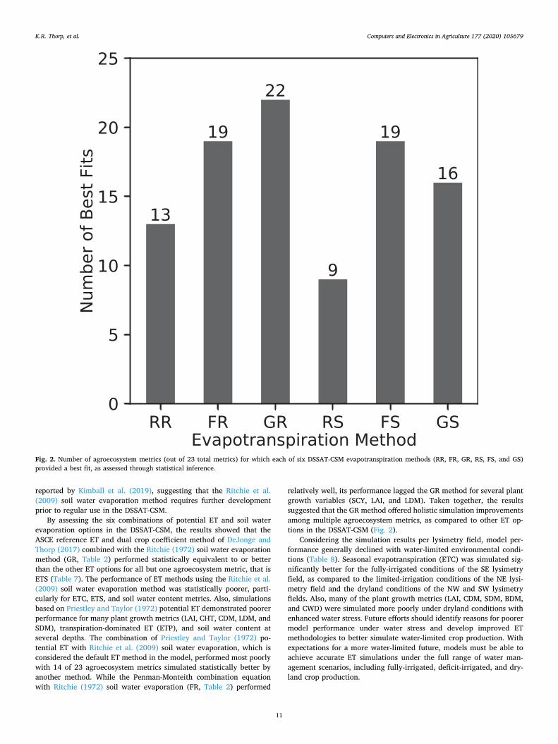
relatively well, its performance lagged the GR method for several plant growth variables (SCY, LAI, and LDM). Taken together, the results suggested that the GR method offered holistic simulation improvements among multiple agroecosystem metrics, as compared to other ET op-tions in the DSSAT-CSM (Fig. 2).

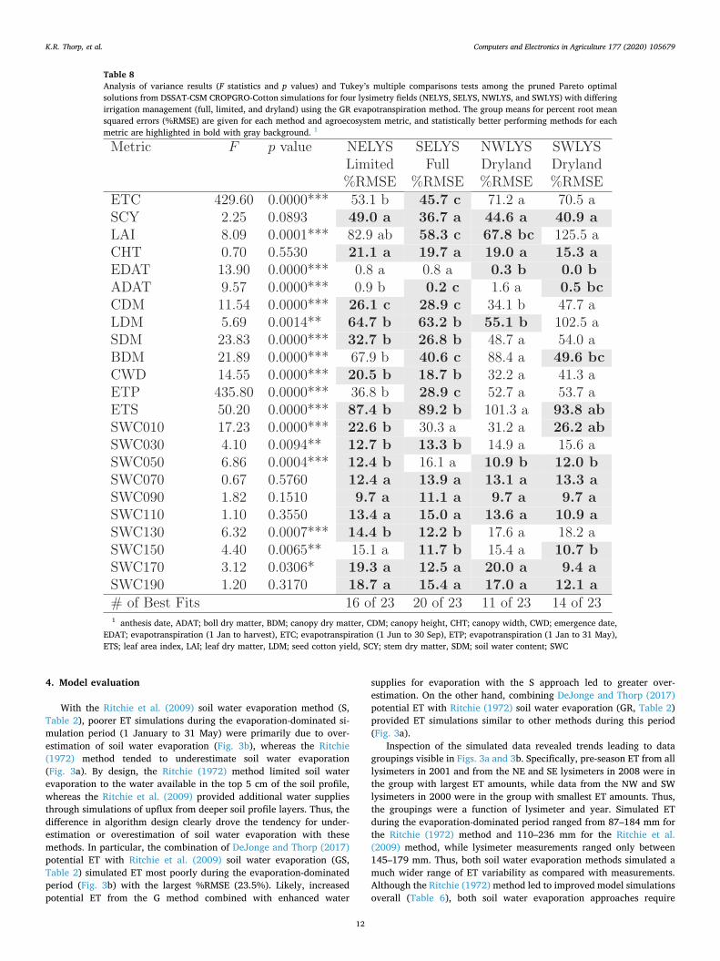
Considering the simulation results per lysimetry field, model per-formance generally declined with water-limited environmental condi-tions (Table 8). Seasonal evapotranspiration (ETC) was simulated sig-nificantly better for the fully-irrigated conditions of the SE lysimetry field, as compared to the limited-irrigation conditions of the NE lysi-metry field and the dryland conditions of the NW and SW lysimetry fields. Also, many of the plant growth metrics (LAI, CDM, SDM, BDM, and CWD) were simulated more poorly under dryland conditions with enhanced water stress. Future efforts should identify reasons for poorer model performance under water stress and develop improved ET methodologies to better simulate water-limited crop production. With expectations for a more water-limited future, models must be able to achieve accurate ET simulations under the full range of water man-agement scenarios, including fully-irrigated, deficit-irrigated, and dry-land crop production.

Fig. 2. Number of agroecosystem metrics (out of 23 total metrics) for which each of six DSSAT-CSM evapotranspiration methods (RR, FR, GR, RS, FS, and GS) provided a best fit, as assessed through statistical inference.


11

4. Model evaluation

With the Ritchie et al. (2009) soil water evaporation method (S, Table 2), poorer ET simulations during the evaporation-dominated si-mulation period (1 January to 31 May) were primarily due to over-estimation of soil water evaporation (Fig. 3b), whereas the Ritchie (1972) method tended to underestimate soil water evaporation (Fig. 3a). By design, the Ritchie (1972) method limited soil water evaporation to the water available in the top 5 cm of the soil profile, whereas the Ritchie et al. (2009) provided additional water supplies through simulations of upflux from deeper soil profile layers. Thus, the difference in algorithm design clearly drove the tendency for under-estimation or overestimation of soil water evaporation with these methods. In particular, the combination of DeJonge and Thorp (2017) potential ET with Ritchie et al. (2009) soil water evaporation (GS, Table 2) simulated ET most poorly during the evaporation-dominated period (Fig. 3b) with the largest %RMSE (23.5%). Likely, increased potential ET from the G method combined with enhanced water

supplies for evaporation with the S approach led to greater over-estimation. On the other hand, combining DeJonge and Thorp (2017) potential ET with Ritchie (1972) soil water evaporation (GR, Table 2) provided ET simulations similar to other methods during this period (Fig. 3a).

Inspection of the simulated data revealed trends leading to data groupings visible in Figs. 3a and 3b. Specifically, pre-season ET from all lysimeters in 2001 and from the NE and SE lysimeters in 2008 were in the group with largest ET amounts, while data from the NW and SW lysimeters in 2000 were in the group with smallest ET amounts. Thus, the groupings were a function of lysimeter and year. Simulated ET during the evaporation-dominated period ranged from 87–184 mm for the Ritchie (1972) method and 110–236 mm for the Ritchie et al. (2009) method, while lysimeter measurements ranged only between 145–179 mm. Thus, both soil water evaporation methods simulated a much wider range of ET variability as compared with measurements. Although the Ritchie (1972) method led to improved model simulations overall (Table 6), both soil water evaporation approaches require

Table 8 Analysis of variance results (F statistics and p values) and Tukey’s multiple comparisons tests among the pruned Pareto optimal solutions from DSSAT-CSM CROPGRO-Cotton simulations for four lysimetry fields (NELYS, SELYS, NWLYS, and SWLYS) with differing irrigation management (full, limited, and dryland) using the GR evapotranspiration method. The group means for percent root mean squared errors (%RMSE) are given for each method and agroecosystem metric, and statistically better performing methods for each metric are highlighted in bold with gray background. 1

1 anthesis date, ADAT; boll dry matter, BDM; canopy dry matter, CDM; canopy height, CHT; canopy width, CWD; emergence date, EDAT; evapotranspiration (1 Jan to harvest), ETC; evapotranspiration (1 Jun to 30 Sep), ETP; evapotranspiration (1 Jan to 31 May), ETS; leaf area index, LAI; leaf dry matter, LDM; seed cotton yield, SCY; stem dry matter, SDM; soil water content; SWC


12

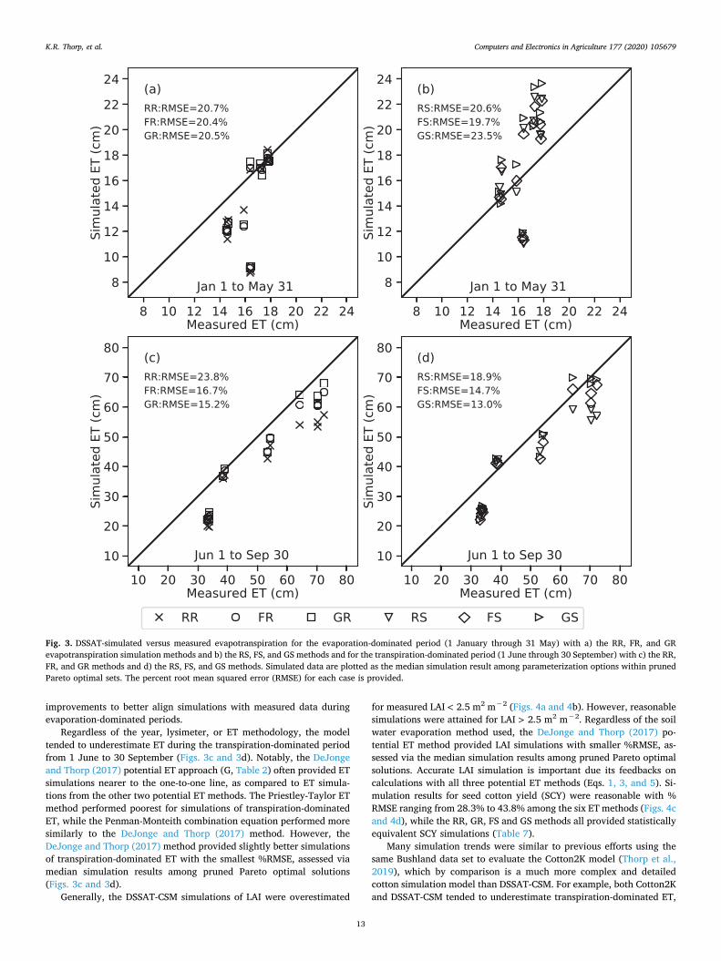
improvements to better align simulations with measured data during evaporation-dominated periods.

Regardless of the year, lysimeter, or ET methodology, the model tended to underestimate ET during the transpiration-dominated period from 1 June to 30 September (Figs. 3c and 3d). Notably, the DeJonge and Thorp (2017) potential ET approach (G, Table 2) often provided ET simulations nearer to the one-to-one line, as compared to ET simula-tions from the other two potential ET methods. The Priestley-Taylor ET method performed poorest for simulations of transpiration-dominated ET, while the Penman-Monteith combination equation performed more similarly to the DeJonge and Thorp (2017) method. However, the DeJonge and Thorp (2017) method provided slightly better simulations of transpiration-dominated ET with the smallest %RMSE, assessed via median simulation results among pruned Pareto optimal solutions (Figs. 3c and 3d).

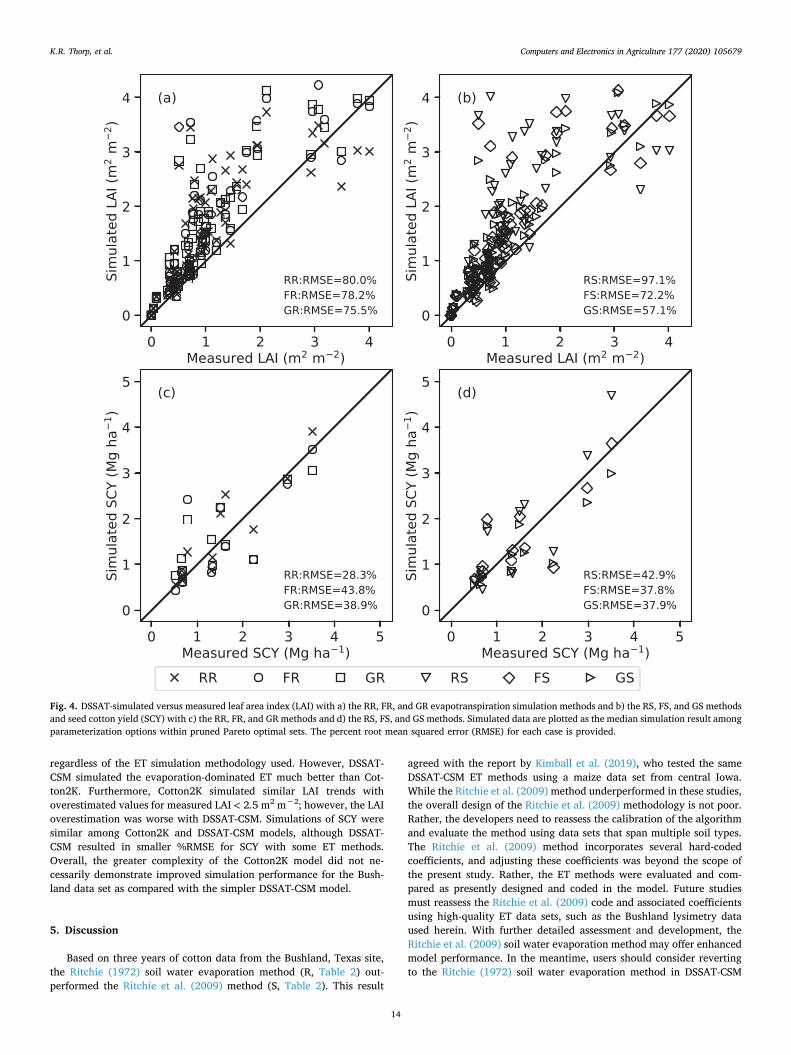
Generally, the DSSAT-CSM simulations of LAI were overestimated

for measured LAI < 2.5 m2 m−2 (Figs. 4a and 4b). However, reasonable simulations were attained for LAI > 2.5 m2 m−2. Regardless of the soil water evaporation method used, the DeJonge and Thorp (2017) po-tential ET method provided LAI simulations with smaller %RMSE, as-sessed via the median simulation results among pruned Pareto optimal solutions. Accurate LAI simulation is important due its feedbacks on calculations with all three potential ET methods (Eqs. 1, 3, and 5). Si-mulation results for seed cotton yield (SCY) were reasonable with % RMSE ranging from 28.3% to 43.8% among the six ET methods (Figs. 4c and 4d), while the RR, GR, FS and GS methods all provided statistically equivalent SCY simulations (Table 7).

Many simulation trends were similar to previous efforts using the same Bushland data set to evaluate the Cotton2K model (Thorp et al., 2019), which by comparison is a much more complex and detailed cotton simulation model than DSSAT-CSM. For example, both Cotton2K and DSSAT-CSM tended to underestimate transpiration-dominated ET,

Fig. 3. DSSAT-simulated versus measured evapotranspiration for the evaporation-dominated period (1 January through 31 May) with a) the RR, FR, and GR evapotranspiration simulation methods and b) the RS, FS, and GS methods and for the transpiration-dominated period (1 June through 30 September) with c) the RR, FR, and GR methods and d) the RS, FS, and GS methods. Simulated data are plotted as the median simulation result among parameterization options within pruned Pareto optimal sets. The percent root mean squared error (RMSE) for each case is provided.


13

regardless of the ET simulation methodology used. However, DSSAT- CSM simulated the evaporation-dominated ET much better than Cot-ton2K. Furthermore, Cotton2K simulated similar LAI trends with overestimated values for measured LAI < 2.5 m2 m−2; however, the LAI overestimation was worse with DSSAT-CSM. Simulations of SCY were similar among Cotton2K and DSSAT-CSM models, although DSSAT- CSM resulted in smaller %RMSE for SCY with some ET methods. Overall, the greater complexity of the Cotton2K model did not ne-cessarily demonstrate improved simulation performance for the Bush-land data set as compared with the simpler DSSAT-CSM model.

5. Discussion

Based on three years of cotton data from the Bushland, Texas site, the Ritchie (1972) soil water evaporation method (R, Table 2) out-performed the Ritchie et al. (2009) method (S, Table 2). This result

agreed with the report by Kimball et al. (2019), who tested the same DSSAT-CSM ET methods using a maize data set from central Iowa. While the Ritchie et al. (2009) method underperformed in these studies, the overall design of the Ritchie et al. (2009) methodology is not poor. Rather, the developers need to reassess the calibration of the algorithm and evaluate the method using data sets that span multiple soil types. The Ritchie et al. (2009) method incorporates several hard-coded coefficients, and adjusting these coefficients was beyond the scope of the present study. Rather, the ET methods were evaluated and com-pared as presently designed and coded in the model. Future studies must reassess the Ritchie et al. (2009) code and associated coefficients using high-quality ET data sets, such as the Bushland lysimetry data used herein. With further detailed assessment and development, the Ritchie et al. (2009) soil water evaporation method may offer enhanced model performance. In the meantime, users should consider reverting to the Ritchie (1972) soil water evaporation method in DSSAT-CSM

Fig. 4. DSSAT-simulated versus measured leaf area index (LAI) with a) the RR, FR, and GR evapotranspiration simulation methods and b) the RS, FS, and GS methods and seed cotton yield (SCY) with c) the RR, FR, and GR methods and d) the RS, FS, and GS methods. Simulated data are plotted as the median simulation result among parameterization options within pruned Pareto optimal sets. The percent root mean squared error (RMSE) for each case is provided.


14

until improvements to the Ritchie et al. (2009) method can be finalized. Regarding the three potential ET methods, the DeJonge and Thorp

(2017) approach that incorporated ASCE Standardized Reference ET with an FAO-56 dual crop coefficient procedure (G, Table 2) out-performed a methodology based on the Penman-Monteith combination equation with a DSSAT-specific crop coefficient procedure (F, Table 2), which in turn outperformed the Priestley-Taylor method (R, Table 2). In the study of Kimball et al. (2019), the exact opposite result was re-ported, although they noted that their result was unexpected and that the differences among the potential ET approaches were generally small relative to differences due to soil water evaporation methods. The op-posite result of Kimball et al. (2019) may be related to the humid en-vironment at the Iowa field site and the limitations of the Iowa field data set to quantify soil water content profiles and water losses to ar-tificial subsurface drainage. Furthermore, the simulations results re-ported by Kimball et al. (2019) were not subjected to the computa-tionally-intensive methodology for guiding parameterization decisions and making unbiased intercomparisons of the ET method performance, as was done herein. As expected, the ET approach based on current standardized methods reported by ASCE (Walter et al., 2005) and in FAO-56 (Allen et al., 1998) led to many statistically significant im-provements of cotton growth and water balance simulations based on data from the Bushland, Texas weighing lysimetry fields.

DeJonge et al. (2020) recently published a letter describing ten-dencies toward improper communication and specification of ET methods in agroecosystem models. The main point was to encourage proper use of standardized ET methods and highlight common confu-sion regarding differences between potential and reference ET methods. The DSSAT-CSM bases ET calculations on the concept of potential ET, likely because the model was originally conceived at a time prior to development of reference ET concepts. As such, the Priestley and Taylor (1972) methodology (R, Table 2) is appropriate for DSSAT-CSM, be-cause Priestley-Taylor is a potential ET method. However, the Penman- Monteith combination equation as currently implemented in DSSAT- CSM (F, Table 2) and the FAO Penman-Monteith equation (G, Table 2) are both reference ET methods. Therefore, their computations of re-ference ET require adjustment using appropriate FAO-56 crop coeffi-cients for non-stressed conditions to provide reasonable estimates of DSSAT-required potential ET. The original formulation of the Penman- Monteith combination equation in DSSAT-CSM (F, Table 2) has re-ceived past criticism (DeJonge and Thorp, 2017; DeJonge et al., 2020), mainly because the method is misnamed as the “FAO-56” method in DSSAT-related communications. However, this method implements neither 1) the FAO formulation of the Penman-Monteith equation nor 2) proper adjustments of Penman-Monteith reference ET using FAO-56 crop coefficients. As such, naming this DSSAT ET method after FAO-56 is misleading to model users who are familiar with FAO-56 as described by Allen et al. (1998). The DeJonge and Thorp (2017) ET methodology (G, Table 2) was programmed to more closely follow the ET method described in FAO-56, but it is not the same as the methodology often described as the “FAO-56” method in the DSSAT-CSM interfaces and literature. Using high-quality ET data sets from the Bushland, Texas lysimetry field, the present study identified the DeJonge and Thorp (2017) ET methodology as a top-performing potential ET method for DSSAT-CSM, while its formulation is also more firmly rooted in current standardized ET methodologies as described by ASCE (Walter et al., 2005) and FAO-56 (Allen et al., 1998). Future efforts will aim to make the DeJonge and Thorp (2017) methodology more readily available to model users and to provide further intercomparisons of DSSAT ET methods for additional crops and environmental conditions.

6. Conclusions

A computationally-intensive simulation methodology (Thorp et al., 2019) was successfully applied to provide statistical comparisons of six ET methods in the DSSAT Cropping System Model. While the simulation

methodology was complex, it enabled statistical comparisons of model performance that were free from subjective choices for model para-meterization. Results suggested that the DeJonge and Thorp (2017) method for potential ET combined with the Ritchie (1972) approach for soil water evaporation provided holistic simulation improvements among multiple agroecosystem metrics measured during three cotton growing seasons with fully-irrigated, deficit-irrigated, and dryland cultivation at Bushland, Texas, and this combination of ET approaches performed statistically better than the other five options. Because the DeJonge and Thorp (2017) method applies the standardized ET con-cepts described in the ASCE Standardized Reference ET Equation (Walter et al., 2005) and in FAO-56 (Allen et al., 1998) to compute DSSAT-required potential ET, the study demonstrated advantages for incorporation of standardized ET methods as an option to improve ET simulations in agroecosystem models. Future work should further evaluate the soil water evaporation methods in the model, with parti-cular focus on improvement of the Ritchie et al. (2009) method.

CRediT authorship contribution statement

K.R. Thorp: Conceptualization, Methodology, Software, Formal analysis, Investigation, Resources, Data curation, Writing - original draft, Writing - review & editing, Visualization, Supervision, Project administration, Funding acquisition. G.W. Marek: Conceptualization, Investigation, Resources, Data curation, Writing - review & editing. K.C. DeJonge: Conceptualization, Methodology, Writing - review & editing, Visualization. S.R. Evett: Investigation, Resources, Writing - review & editing, Supervision, Project administration.

Declaration of Competing Interest

The authors declare that they have no known competing financial interests or personal relationships that could have appeared to influ-ence the work reported in this paper.

Acknowledgments

The authors acknowledge Cotton Incorporated for contributing partial funding for this research. This research used resources provided by the SCINet project of the USDA Agricultural Research Service, ARS project number 0500-00093-001-00-D.

Appendix A. Supplementary material

Supplementary data associated with this article can be found, in the online version, at https://doi.org/10.1016/j.compag.2020.105679.

References

Allen, R.G., Pereira, L.S., Raes, D., Smith, M., 1998. FAO Irrigation and Drainage Paper No. 56. Crop Evapotranspiration: Guidelines for Computing Crop Water Requirements. Food and Agriculture Organization of the United Nations, Rome, Italy.

Cariboni, J., Gatelli, D., Liska, R., Saltelli, A., 2007. The role of sensitivity analysis in ecological modelling. Ecol. Model. 203 (1–2), 167–182.

Cheikh, M., Jarboui, B., Loukil, T., Siarry, P., 2010. A method for selecting Pareto optimal solutions in multiobjective optimization. J. Informat. Math. Sci. 2 (1), 51–62.

DeJonge, K.C., Ascough, J.C., Andales, A.A., Hansen, N.C., Garcia, L.A., Arabi, M., 2012. Improving evapotranspiration simulations in the CERES-Maize model under limited irrigation. Agric. Water Manag. 115, 92–103.

DeJonge, K.C., Thorp, K.R., 2017. Implementing standardized reference evapotranspira-tion and dual crop coefficient approach in the DSSAT Cropping System Model. Trans. ASABE 60 (6), 1965–1981.

DeJonge, K.C., Thorp, K.R., Marek, G.W., 2020. The apples and oranges of reference and potential evapotranspiration: Implications for agroecosystem models. Agric. Environ. Lett. 5, e20011. https://doi.org/10.1002/ael2.20011.

Evett, S.R., Howell, T.A., Schneider, A.D., Copeland, K.S., Dusek, D.A., Brauer, D.K., Tolk, J.A., Marek, G.W., Marek, T.M., Gowda, P.H., 2016. The Bushland weighing lysi-meters: A quarter century of crop ET investigations to advance sustainable irrigation. Trans. ASABE 59 (1), 163–179.

Evett, S.R., Kustas, W.P., Gowda, P.H., Anderson, M.C., Prueger, J.H., Howell, T.A.,


15


http://refhub.elsevier.com/S0168-1699(20)31053-X/h0010










https://doi.org/10.1002/ael2.20011






2012a. Overview of the Bushland Evapotranspiration and Agricultural Remote sen-sing EXperiment 2008 (BEAREX08): A field experiment evaluating methods for quantifying ET at multiple scales. Adv. Water Resour. 50, 4–19.

Evett, S.R., Schwartz, R.C., Howell, T.A., Baumhardt, R.L., Copeland, K.S., 2012b. Can weighing lysimeter ET represent surrounding field ET well enough to test flux station measurements of daily and sub-daily ET? Adv. Water Resour. 50, 79–90.

Howell, T., Schneider, A., Dusek, D., Marek, T., Steiner, J., 1995. Calibration and scale performance of Bushland weighing lysimeters. Trans. ASAE 38 (4), 1019–1024.

Howell, T.A., Evett, S.R., Tolk, J.A., Schneider, A.D., 2004. Evapotranspiration of full-, deficit-irrigated, and dryland cotton on the northern Texas High Plains. J. Irrigation Drainage Eng. 130 (4), 277–285.

Jones, J.W., Hoogenboom, G., Porter, C.H., Boote, K.J., Batchelor, W.D., Hunt, L.A., Wilkens, P.W., Singh, U., Gijsman, A.J., Ritchie, J.T., 2003. The DSSAT cropping system model. Eur. J. Agron. 18 (3–4), 235–265.

Kimball, B.A., Boote, K.J., Hatfield, J.L., Ahuja, L.R., Stockle, C., Archontoulis, S., Baron, C., Basso, B., Bertuzzi, P., Constantin, J., Deryng, D., Dumont, B., Durand, J.-L., Ewert, F., Gaiser, T., Gayler, S., Hoffmann, M., Jiang, Q., Kim, S.-H., Lizaso, J., Moulin, S., Nendel, C., Parker, P., Palosuo, T., Priesack, E., Qi, Z., Srivastava, A., Stella, T., Tao, F., Thorp, K.R., Timlin, D., Twine, T.E., Webber, H., Willaume, M., Williams, K., 2019. Simulation of maize evapotranspiration: An inter-comparison among 29 maize models. Agric. For. Meteorol. 271, 264–284.

Marek, G.W., Evett, S.R., Gowda, P.H., Howell, T.H., Copeland, K.S., Baumhardt, R.L., 2014. Post-processing techniques for reducing errors in weighing lysimeter evapo-transpiration (ET) datasets. Trans. ASABE 57 (2), 499–515.

Marek, T.H., Schneider, A.D., Howell, T.A., Ebeling, L.L., 1988. Design and construction of large weighing monolithic lysimeters. Trans. ASAE 31 (2), 477–484.

Pianosi, F., Beven, K., Freer, J., Hall, J.W., Rougier, J., Stephenson, D.B., Wagener, T., 2016. Sensitivity analysis of environmental models: A systematic review with prac-tical workflow. Environ. Model. Softw. 79, 214–232.

Priestley, C.H.B., Taylor, J., 1972. On the assessment of surface heat flux and evaporation using large-scale parameters. Mon. Weather Rev. 100 (2), 81–92.

Ritchie, J.T., 1972. Model for predicting evaporation from a row crop with incomplete cover. Water Resour. Res. 8 (5), 1204–1213.

Ritchie, J.T., Porter, C.H., Judge, J., Jones, J.W., Suleiman, A.A., 2009. Extension of an existing model for soil water evaporation and redistribution under high water content conditions. Soil Sci. Soc. Am. J. 73 (3), 792–801.

Saltelli, A., Tarantola, S., Campolongo, F., 2000. Sensitivity analysis as an ingredient of modeling. Stat. Sci. 15 (4), 377–395.

Sau, F., Boote, K.J., Bostick, W.M., Jones, J.W., Minguez, M.I., 2004. Testing and im-proving evapotranspiration and soil water balance of the DSSAT crop models. Agron. J. 96 (5), 1243–1257.

Sobol, I.M., 2001. Global sensitivity indices for nonlinear mathematical models and their Monte Carlo estimates. Math. Comput. Simul. 55 (1–3), 271–280.

Suleiman, A.A., Ritchie, J.T., 2003. Modeling soil water redistribution during second- stage evaporation. Soil Sci. Soc. Am. J. 67 (2), 377–386.

Suleiman, A.A., Ritchie, J.T., 2004. Modifications to the DSSAT vertical drainage model for more accurate soil water dynamics estimation. Soil Sci. 169 (11), 745–757.

Taboada, H.A., Baheranwala, F., Coit, D.W., Wattanapongsakorn, N., 2007. Practical solutions for multi-objective optimization: An application to system reliability design problems. Reliab. Eng. Syst. Saf. 92 (3), 314–322.

Thorp, K.R., Ale, S., Bange, M.P., Barnes, E.M., Hoogenboom, G., Lascano, R.J., McCarthy, A.C., Nair, S., Paz, J.O., Rajan, N., Reddy, K.R., Wall, G.W., White, J.W., 2014a. Development and application of process-based simulation models for cotton pro-duction: A review of past, present, and future directions. J. Cotton Sci. 18 (1), 10–47.

Thorp, K.R., Barnes, E.M., Hunsaker, D.J., Kimball, B.A., White, J.W., Nazareth, V.J., Hoogenboom, G., 2014b. Evaluation of CSM-CROPGRO-Cotton for simulating effects of management and climate change on cotton growth and evapotranspiration in an arid environment. Trans. ASABE 57 (6), 1627–1642.

Thorp, K.R., Hunsaker, D.J., Bronson, K.F., Andrade-Sanchez, P., Barnes, E.M., 2017. Cotton irrigation scheduling using a crop growth model and FAO-56 methods: Field and simulation studies. Trans. ASABE 60 (6), 2023–2039.

Thorp, K.R., Hunsaker, D.J., French, A.N., White, J.W., Clarke, T.R., Pinter Jr., P.J., 2010. Evaluation of the CSM-CROPSIM-CERES-Wheat model as a tool for crop water management. Trans. ASABE 53 (1), 87–102.

Thorp, K.R., Marek, G.W., DeJonge, K.C., Evett, S.R., Lascano, R.J., 2019. Novel meth-odology to evaluate and compare evapotranspiration algorithms in an agroecosystem model. Environ. Model. Softw. 119, 214–227.

Thorp, K.R., Marek, G.W., DeJonge, K.C., Evett, S.R., 2020. Comparison of evapo-transpiration methods in the DSSAT Cropping System Model: I. Global sensitivity analysis. Comput. Electron. Agric. https://doi.org/10.1016/j.compag.2020.105658.

Tolk, J.A., Howell, T.A., Evett, S.R., 1998. Evapotranspiration and yield of corn grown on three High Plains soils. Agron. J. 90 (3), 447–454.

Van Genuchten, M.T., 1980. A closed-form equation for predicting the hydraulic con-ductivity of unsaturated soils. Soil Sci. Soc. Am. J. 44 (5), 892–898.

Walter, I.A., Allen, R.G., Elliott, R., Itenfisu, D., Brown, P., Jensen, M.E., Mecham, B., Howell, T.A., Snyder, R., Eching, S., Spofford, T., Hattendorf, M., Martin, D.L., Cuenca, R.H., Wright, J.L., 2005. The ASCE Standardized Reference Evapotranspiration Equation. American Society of Civil Engineers, Reston, VA.

Zhang, Y., Schaap, M.G., 2017. Weighted recalibration of the Rosetta pedotransfer model with improved estimates of hydraulic parameter distributions and summary statistics (Rosetta3). J. Hydrol. 547, 39–53.


16
















































































Documents

Thorp2020 - DSSAT Bushland ET2.pdf - USDA ARS