Document downloaded from:

This paper must be cited as:

The final publication is available at

Copyright

Additional Information

http://hdl.handle.net/10251/121095

Solana-Altabella, A.; Sanchez-Iranzo, M.; Bueso-Bordils, J.; Lahuerta-Zamora, L.; MelladoRomero, AM. (2018). Computer vision-based analytical chemistry applied to determining ironin commercial pharmaceutical formulations. Talanta. 188:349-355.https://doi.org/10.1016/j.talanta.2018.06.008

http://doi.org/10.1016/j.talanta.2018.06.008

Elsevier

* Corresponding author. E-mail address: amellado@cst.upv.es (A.M. Mellado-Romero)

Computer vision-based analytical chemistry applied to determining

iron in commercial pharmaceutical formulations

A. Solana-Altabellaa, M.H. Sánchez-Iranzoa, J.I. Bueso-Bordilsa, L. Lahuerta-Zamoraa,

A.M. Mellado-Romerob,*

a Departamento de Farmacia, Universidad CEU-Cardenal Herrera, c/ Santiago

Ramón y Cajal s/n, 46115 Alfara del Patriarca, Valencia, Spain. b Instituto de Ciencia y Tecnología del Hormigón (ICITECH), Universitat

Politècnica de València, Camino de Vera s/n, 46022 Valencia, Spain.

ABSTRACT

Two different computer vision-based analytical chemistry (CVAC) methods were

developed to quantify iron in the commercial pharmaceutical formulations Ferbisol®

and Ferro sanol®. The methods involve using a digital camera or a desktop scanner to

capture a digital image of a series of Fe2+ standard solutions and the unknown sample

upon reaction with o-phenanthroline. The images are processed with appropriate

software (e.g., the public domain programme ImageJ, from NIH) to obtain a numerical

value (analytical signal) based on colour intensity. The fact that such a value is

proportional to the analyte concentration allows one to construct a calibration graph

from the standards and interpolate the value for the sample in order to determine its

concentration. The results thus obtained were compared with those provided by a

spectrophotometric method and the US Pharmacopoeia’s recommended method. The

differences never exceeded 2%. The two proposed methods are simple and inexpensive;

also, they provide an effective instrumental alternative to spectrophotometric methods

which can be especially beneficial in those cases where purchasing and maintaining a

spectrophotometer is unaffordable.

Keywords:

CVAC, digital camera, desktop scanner, ImageJ, pharmaceutical analysis.

1. Introduction

Iron plays a central role as an active site for proteins effecting O2 and electron

transfer in enzymes (oxidases, reductases and dehydrases) in the biosphere. In

fact, iron is an essential element for oxygen transport and storage through

haemoglobin and myoglobin in higher animals [1–3]. As such, this element is an

essential ingredient of human diet deficiencies in which are the source of a

number of diseases, particularly during childhood, adolescence and pregnancy

[4]. Thus, an iron-deficient diet can lead to a medical condition known as

“ferropenic anaemia”. Correcting iron deficiencies entails using an effective iron

supplement such as a multi-vitamin complex or a specific pharmaceutical

formulation.

A number of methods currently exist for determining iron most of which are

based on volumetric [5], potentiometric [6], anodic stripping voltametric [7],

graphite-furnace [8] or flame atomic absorption [9], inductively coupled plasma

atomic emission spectrometry or inductively coupled plasma mass spectrometry

[10], fluorimetric [10,11] or chemiluminescence [12, 13] measurements.

Spectrophotometry is among the most simple, expeditious and inexpensive

techniques for determining iron in a wide variety of samples. The process usually

involves reacting the iron with a chromogenic chelating agent [14-24].

In this work, we used the well-known spectrophotometric method for iron (II)

based on its reaction with o-phenanthroline (at pH 3.5 by adding sodium acetate)

to form a reddish orange complex [25].

Keeping iron in its reduced state (Fe2+) requires using an appropriate reductant

such as hydroxylamine.

The resulting complex can be quantified spectrophotometrically by its

absorbance at 508 nm.

The decreasing cost and increasing performance of digital imaging hardware

and software have promoted the increasing use of digital photography in

colorimetric qualitative and quantitative tests which have given rise to an

increasingly popular new analytical technique called “computer vision-based

analytical chemistry” (CVAC) [26].

Digital imaging devices (e.g. digital cameras, desktop scanners) use either of

two types of sensors, namely: Complementary Metal Oxide Semiconductors

(CMOS) or Charge Coupled Devices (CCD). A CCD (or a CMOS) is an

electronic device henceforward referred to as a “sensor” consisting of many cells

called “pixels”. Each cell acts as a light-sensitive element and provides an

electrical response to light; the combined responses of a sensor can be digitized

and converted into an image [26-28].

A sensor consisting of 8-bit pixels can respond to 28 = 256 different levels of

grey from 0 (black) to 255 (white). Therefore, each pixel in a captured image can

be assigned a value from 0 to 255 that can be used for calibration. This allows a

digital imaging device to be used as an analytical detector to exploit the vast

amount of information contained in a captured image [26].

The CVAC technique has been increasingly used in research laboratories and

commercial laboratory equipment for more than two decades [26, 28-41]. Low-

cost commercial digital cameras and scanners have been gradually incorporated

into the analytical laboratory, where they are being increasingly used for forensic

[42, 43], telemedicine [27, 48] and, obviously, analytical purposes [26, 44, 46,

47, 49, 50, 53-55].

Using a commercial digital camera in combination with the software ImageJ

recently proved a simple, inexpensive choice for a variety of measurements [27,

45].

Webcams and mobile phone cameras have proved useful for chemical analysis

[46, 47] and even for capturing and transferring the results of biological tests for

glucose and proteins in telemedicine [48].

On the other hand, commercial scanners have been also used to develop

colorimetric methods [49-53].

In line with previous works [54, 55], the proposed method uses digital images

of series of standard solutions in combination with imaging software (ImageJ) to

assign a numerical value for colour intensity. Such a value is proportional to the

concentration of the standard and can be used for calibration. Our method is

similar to the classical spectrophotometric method for the same purpose but has

the advantage that it uses much more simple and inexpensive hardware (viz., a

low-cost digital camera or a desktop scanner) and public domain —and hence

free— software (ImageJ). The results are compared with those provided by the

classical spectrophotometric method and the official, cerimetric method

recommended by the US Pharmacopoeia [56].

2. Material and methods

2.1. General materials

All reagents used were analytical-grade and obtained from the following

suppliers: Panreac (hydroxylamine hydrochloride), J.T. Baker (1 mol L–1

sulphuric acid, ammonium iron (II) sulphate hexahydrate (Mohr’s salt)) and

Scharlab (o-phenanthroline monohydrate, sodium acetate trihydrate). The

cerimetric titration in the USP method was performed with 0.1 mol L–1 cerium

(IV) sulphate (in 0.5 mol L-1 H2SO4) from Scharlab and 0.025 mol L–1 ferroin

from J.T. Baker.

All solutions were prepared in water de-ionized to 18 MΩ⋅cm by reverse

osmosis in a Sybron/Barnstead Nanopure apparatus furnished with a fibre filter of

0.2 μm pore size.

A standard solution containing 100 mg Fe(II) L–1 was prepared by dissolving

0.7 g of Mohr’s salt in 1 mol L–1 H2SO4 and making to volume in a 1 L

volumetric flask.

The solutions were transferred to the supports by using a 1000 μL Labopette®

micropipette.

The commercial pharmaceutical formulations studied were Ferbisol® 100 mg

(50 capsules; BIAL Industrial Farmacéutica, S.A.) and Ferro sanol® 100 mg (50

capsules; UCB Pharma, S.A.).

Absorbance measurements were obtained with a Spectronic Genesis 20 UV–

Vis spectrophotometer. Each image was captured by placing a blank consisting of

a strip of two-sided inkjet paper near the standards and support.

All images were processed by using the public domain software ImageJ for

Windows developed by the National Institutes for Health and freely available for

download at http://rsbweb.nih.gov/ij.

2.2. Material for capturing images with the digital camera

The standards and sample were held in a 11 × 9 cm white ceramic spot plate

with 6 wells holding 3 mL each.

All photographs were taken with a Nikon Coolpix E995 digital camera.

Lighting was provided by two pairs of Philips Master TL-D 36W/840 fluorescent

tubes 1.5 m above the plate.

In order to avoid reflections of the fluorescent tubes on the plate and the

associated artefacts in the images, the camera–plate combination was placed

inside a 40 × 25 × 35 cm white methacrylate box (Fig. 1). Reflections off the

inner walls of the box were avoided by using a diffusion screen consisting of a

420 × 520 mm piece of 60 g/m2 ALBET white filter paper (LabScience code

RM2504252). Also, the plate was placed on a piece of NE 30K black cardboard

(A4, 108 g) from Hermanos Cebrián (Valencia, Spain) for increased contrast.

2.3. Material used for capturing images with the desktop scanner

The standard solutions and sample were placed in a TTP® Zellkultur Testplatte

containing 24 wells holding 3 mL each.

Images were acquired with five different scanner models, namely: HP PSC 1510 All-

in-one, HP Photosmart C3180, Brother DCP-J132W, HP ScanJet 3100 and Acer S2W

3300V.

2.4. General procedure

The experimental work was conducted under the typical chemical conditions of the

well-known spectrophotometric method for determining Fe (II) with o-phenanthroline

[25]. For this purpose, aliquots of 1–5 mL of the 100 mg Fe (II) L–1 standard and a blank

(0 mL) were added to 100 mL volumetric flasks and successively supplied with 20 mL

of water, 2 mL of hydroxylamine, 5 mL of o-phenanthroline and 5 mL of sodium

acetate. These solutions were used to construct the calibration curve for iron (II).

The samples were prepared by adding the contents of 5 capsules of either

pharmaceutical formulation to a beaker containing 250 mL of 1 mol L–1 sulphuric acid

and stirring for 24 h. The resulting suspension was passed through paper filter and made

to 500 mL with more sulphuric acid in a volumetric flask. A 250 µL aliquot of this

solution was made to 100 mL in another flask and reacted identically with the standards.

The solutions were allowed to stand for 15 min, after which the concentration of iron

in each was determined by digital imaging analysis.

2.5. Procedure with the digital camera

Obtaining useful images of the standards and samples required using an appropriate

support in order to enhance the colour of the solutions without interference. A white

ceramic plate with 3 mL wells proved suitable for this purpose as it allowed an image of

all solutions (standards and sample) to be simultaneously obtained under identical

lighting conditions.

Each plate well was filled with 3 mL of a standard solution containing a

concentration within the linear calibration range (0.5 mg L–1) and the plate

photographed together with the white paper strip (Fig. 2a).

The camera was operated in the manual mode in order to avoid the potential

influence of its automatically choosing its own settings. Because using flash could have

resulted in unwanted reflections on the solution surfaces, all lighting was supplied by

the laboratory’s fluorescent strips. Also, any spurious signals due to reflections from

other sources were minimized by placing the camera–plate combination inside a white

methacrylate box lined with a diffusing screen on the inside.

These diffuse lighting conditions allowed the optimum F-stop and shutter speed to be

selected in order to avoid under- and overexposure. The camera was attached to a static

support and photographs were taken at F/6 and a shutter speed of 1/4 s.

2.6. Procedure with the scanner

Accurately capturing the colour of the standards and samples with the scanner

required using a support consisting of a transparent microplate with 24 wells holding 3

mL of solution each. This support allowed an image of the standards and sample to be

simultaneously obtained under identical lighting conditions.

Each microplate well was filled with 2 mL of a solution of the standards or sample

containing concentrations within the linear calibration range (0–5 mg L–1).

The amount of light reflected was maximized by placing a sheet of standard white

paper on the microplate lid. Also, spurious reflections were avoided by covering the

microplate with a piece of thick black cloth prior to scanning the microplate–paper strip

combination (Fig. 2b).

2.7. Processing of images

All images were processed with the software ImageJ. A standardized image not

dependent on the colour temperature of the source of light (namely, two fluorescent

strips or the scanner lamp) was obtained by calibration with a strip of standard white

paper.

The image was white-balanced by using an algorithm described elsewhere [27]. Each

A>B>C operation involved selecting command B from menu A and then sub-command

C from command B. First, the original image was split into three RGB images (Image >

Color > Split Channels). Then a circular region of interest (ROI) in each RGB sub-

image was selected with the drawing tool in the toolbar and placed on the white paper

strip to measure its Mean Brightness (MB) by using the Histogram command (Analyze

> Histogram). Next, on the assumption that the white paper strip reflected 80% of

incident light in each channel (255 × 0.8 = 200), each RGB image was corrected by

multiplying its brightness by 200/MB (Process > Math > Multiply and then enter

200/MB). The corrected sub-images were merged to obtain a new colour image

mimicking one capture under ideally white lighting (Image > Colour > Merge

Channels). This standard image was again split into RGB sub-images, that for the green

channel being inverted and the level of neutral grey (NG) for each standard (or the

sample) measured in the previously selected ROI (Fig. 2c).

The NG level for each standard or sample was taken to be the analytical signal and

used to calculate the corresponding absorbance from [49]

𝑨𝑨𝑨 = 𝐥𝐥𝐥𝑵𝑵𝟐𝟐𝟐

which relates the absorbance of the analyte to its concentration.

2.8. Optimization procedure

The instrumental variables of the imaging process were optimized by using a

univariate procedure. Each variable was examined at different values in order to

establish that leading to the greatest sensitivity (highest slope of the calibration curve).

For this purpose, iron (II) standards containing concentrations over the range 0–5 mg L–

1 were used to obtain three consecutive images that were processed with ImageJ in order

to construct three calibration curves with their respective slopes and coefficients of

determination (r2). The process was optimized in terms of the mean of both parameters

and the standard deviation from the mean slope (N = 3).

3. Results and discussion

3.1. Digital camera

The initial conditions for the capturing process were established in previous work

[55]. A comparison of the calibration curves for the green and blue colour channels —

the red channel is useless owing to the colour of the iron complex— revealed that the

former channel provided a more linear curve—at a similar deviation— and a greater

slope. Therefore, the green channel was selected for subsequent measurements.

The influence of the exposure time was examined by using the camera’s

greatest available aperture (F/3) and a focusing distance of 20 cm at shutter

speeds from the highest (1/30 s) to the lowest (1/4 s); as revealed by the

histograms, the former speed resulted in underexposure and the latter in

overexposure (see Table 1). The slope increased with increasing exposure time;

however, the coefficient of determination declined beyond 1/8 s, so a shutter

speed of 1/15 s was selected as a trade-off for subsequent work.

In taking a photograph, the sensor can be exposed to identical amounts of light

by using different combinations of aperture and exposure time. This phenomenon

is called “reciprocity” and was used to identify the equivalent combinations of

F/3 and a shutter speed of 1/15 s. As can be seen from Table 2, F/6 in

combination with 1/4 s provided the best results in terms of slope and coefficient

of determination, and were thus selected for subsequent work.

The influence of ROI size was examined at three different levels, namely:

20 000, 60 000 and 100 000 pixels. The optimum size was 60 000 pixels (see

Table A in Supplementary material section).

3.2. Scanner

The performance of the scanner was compared with that of the digital camera

by examining the potential influence of a number of instrumental and operational

variables on the acquired images.

Initially, we used five different desktop scanners, all in the “auto” mode, in

order to identify that providing the best results for the intended purpose. Each

scanner was used to acquire images in the green and blue channels that were

processed by using an ROI of a size equivalent to that of a plate well (2500 pixels

for the Brother scanner and 4500 pixels for all others) or, alternatively, a smaller

area (50 pixels) of uniform colour containing no apparent artefacts.

Discrimination was based on the slope and coefficient of determination of the of

the calibration curve. As can be seen from Table 3, the best trade-off between the

two was provided by the Brother DCP-J132W scanner. This model has the added

advantage that, because it is a combo system, it continues to operated even if the

printer runs out of ink.

The influence of the volume of standard solution placed in each well was

examined by using 1, 2 and 3 mL. A volume of 2 mL provided the best

combination of slope and coefficient of determination (see Table B in

Supplementary material section).

A comparison of the measurements on the green and blue channels revealed

that the former resulted in smaller deviations, so it was selected for further work.

The optimum scanner allowed resolution, Gaussian blur, brightness and contrast,

and the image format to be selected. This allowed us to examine the influence of

these settings on the resulting calibration curves. Applying Gaussian blur led to

similar coefficients of determination but reduced the slope of the curve, which

excluded its use to improve the results. Also, using a small ROI (50 pixels)

increased the slope (Table 4).

Scanner resolution ranged from 100 × 100 to 1200 × 1200 dpi. Resolution had

no significant influence on the mean results (N = 3). This led us to select the

lowest available resolution in order to obtain as small and expeditiously

processed files as possible —in fact, the images obtained at the highest

resolutions were too large for processing with ImageJ (see Table C in

Supplementary material section).

As regards ROI size, a circle of 50 pixels led to a significantly greater slope

than one of 2500 pixels, so NG was measured with the smaller size (see Table C

in Supplementary material section).

The influence of the brightness and contrast settings on the calibration curve

was examined by using a range of values in 10 unit steps. Negative values of the

two settings led to underexposed, difficult to process images. Also, the large

differences between using a brightness setting of +20 and one of +30 led us to

test +25 as well; however, we chose to apply +30 to subsequent images as the

optimum trade-off (see Tables D and E in Supplementary material section).

Regarding image compression, we tested the following choices: standard

baseline (i.e., no compression, which is compatible with virtually any hardware

and software), optimized baseline (compressed images) and progressive —which

is useful for the Internet because images are viewed at a low resolution but

downloaded at their actual resolution. All three formats led to similar results, so

optimized baseline was selected in order to save space (see Table F in

Supplementary material section).

3.3 Analytical figures of merit

3.3.1. Calibration curves. Limits of detection and quantitation.

The theoretical limits of detection (CLD) and quantitation (CLQ) were calculated

as 3σb/m and 10σb/m, respectively, σb being the standard deviation of the blank

and m the slope of the calibration graph.

The empirical limit of detection was determined by using standard solutions

containing 0–5 mg L–1 and assuming the limit to coincide with the point where

the calibration curve ceased to be linear and the analytical signal was

indistinguishable from the blank signal.

The theoretical and empirical limits are shown in Table 5.

3.3.2. Within-day and between-day reproducibility.

Within-day reproducibility was determined from images of five different sets

of standard solutions containing 0–5 mg Fe L–1 that were obtained by the same

operator using the same analytical equipment on the same day. The results are

shown in Table 5.

Between-day reproducibility was determined similarly to within-day

reproducibility except that the sets of standards were prepared on different days.

The results are also shown in Table 5.

3.3.3. Determination of Fe (II) in real samples.

Two different commercial formulations of iron (II) (Ferbisol® and Ferro

sanol®) were analysed with the four analytical methods studied, namely: analysis

of digital images obtained with a photographic camera or a desktop scanner,

spectrophotometry [25] and redox titrimetry (cerimetry) [56] —the last is the US

Pharmacopoeia’s recommended method and was used as reference for

comparison. The manufacturers’ stated content in iron of both formulations is 100

mg per capsule.

As can be seen from Table 6, all four methods proved suitable for determining

iron in both formulations, with errors less than 2% in all cases and standard

deviations only slightly higher than those of the officially endorsed method in the

other three.

4. Conclusions

The two proposed methods exhibited good between-day reproducibility (RSD

< 5% with N = 5) that was slightly higher with a photographic camera than with a

scanner. The coefficients of the determination of the calibration curves were

always higher than 0.995 and also slightly better with the camera than with the

scanner.

The analytical results obtained with the two methods were comparable to those

of the US Pharmacopoeia’s recommended method for determining iron (II) in

commercial pharmaceutical formulations (errors less than 2%) and even better

than those for Ferbisol® provided by the classical spectrophotometric method.

Unlike a photographic camera, a scanner requires using no external lighting or

diffusing screen.

The proposed methodology is simple and inexpensive. Thus, it uses a digital

camera or desktop scanner connected to a computer, which is much more

affordable equipment than a conventional spectrophotometer. Also, acquired

images can be processed with user-friendly, free software (ImageJ, developed by

the National Institutes for Health).

Given the current prevalence of increasingly sophisticated and expensive

commercial instruments, the proposed methods provide a very interesting

alternative for quantitative determinations in the absence of economic resources

for purchasing and maintaining a conventional spectrophotometer.

5. Acknowledgements

This research did not receive any specific grant from funding agencies in the public, commercial or not-for-profit sectors.

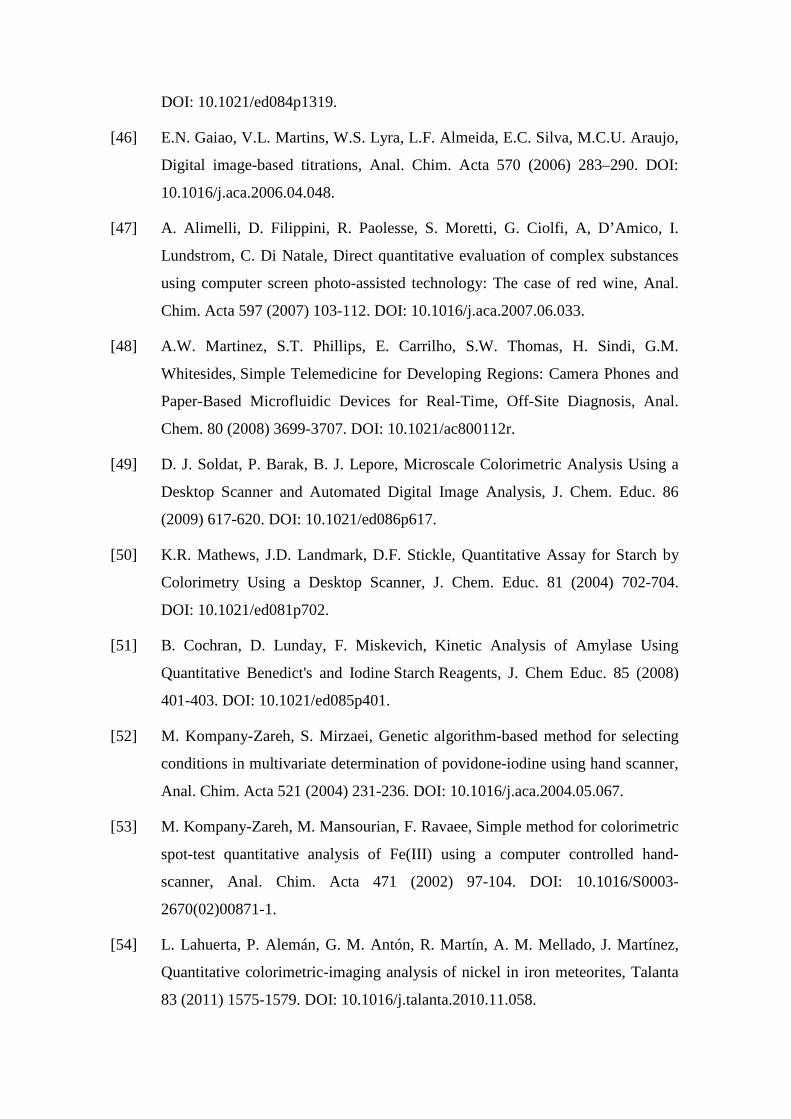
6. References

[1] F. A. Cotton, G. Wilkinson, Advanced Inorganic Chemistry, 3ª ed. (1988),

Wiley Interscience, New York.

[2] P. C. C. Oliveira, J.C. Masini, Sequential injection determination of iron (II) in

antianemic pharmaceutical formulations with spectrophotometric detection,

Anal. Lett. 34 (2001) 389-397. DOI: 10.1081/AL-100102581.

[3] D. Nichols, The Chemistry of Iron, Cobalt and Nickel (1973), Pergamon Press,

Oxford.

[4] A. N. Araujo, J. Gracia, J.L.F.C. Lima, M. Poch, M. Lucia, M.F.S.Saraiva,

Colorimetric determination of iron in infant fortified formulas by Sequential

Injection Analysis, J. Fresenius, Anal. Chem. 357 (1997) 1153-1156. DOI:

10.1007/s002160050322.

[5] D. Tzur, V. Dosortzev, E. Kirowa-Eisner, Titration of low levels of Fe2+ with

electrogenerated Ce4+, Anal. Chim. Acta. 392 (1999) 307-318. DOI:

10.1016/S0003-2670(99)00226-3.

[6] W.H. Mahmoud, Iron Ion-Selective Electrodes for Direct Potentiometry and

Potentiotitrimetry in Pharmaceuticals, Anal. Chim. Acta. 436 (2001) 199-206.

DOI: 10.1016/S0003-2670(01)00892-3.

[7] S. Sundd, S.K. Prasad, A. Kumar, B.B. Prasad, Chelating resin-impregnated

paper chromatography, applications to trace element collection of ferrous and

ferric ions, and determination by differential pulse anodic stripping

voltammetry, Talanta 41 (1994) 1943-1949. DOI: 10.1016/0039-

9140(94)00153-7.

[8] P.C. Aleixo, J.A. Nobrega, Direct determination of iron and selenium in bovine

milk by graphite furnace atomic absorption spectrometry, Food Chem. 83 (2003)

457-462. DOI: 10.1016/S0308-8146(03)00224-3.

[9] S. X. Li, N.S. Deng, Speciation analysis of iron in traditional Chinese medicine

by flame atomic absorption spectrometry, J. Pharm. Biol. Anal. 32 (2003) 51-57.

DOI: 10.1016/S0731-7085(03)00024-4.

[10] V. Balaram, Recent advances in the determination of elemental impurities in

pharmaceuticals – Status, challenges and moving frontiers, Trends in Analytical

Chemistry 80 (2016) 83–95. DOI: 10.1016/j.trac.2016.02.001.

[11] G. Zhu, Z. Zhu, L. Qiu, A fluorometric method for the determination of iron(II)

with fluorescein isothiocyanate and iodine, Anal. Sci. 18 (2002) 1059-1061.

DOI: 10.2116/analsci.18.1059.

[12] P.L. Croot, P. Laan, Continuous shipboard determination of Fe(II) in polar

waters using flow injection analysis with chemiluminescence detection, Anal.

Chim. Acta. 466 (2002) 261-273. DOI: 10.1016/S0003-2670(02)00596-2.

[13] S. Hirata, H. Yoshihara, M. Aihara, Determination of iron(II) and total iron in

environmental water samples by flow injection analysis with column

preconcentration of chelating resin functionalized with N-

hydroxyethylethylenediamine ligands and chemiluminescence detection, Talanta

49 (1999) 1059-1067. DOI: 10.1016/S0039-9140(99)00061-2.

[14] A. Huberman, C. Perez, Nonheme iron determination, Anal. Biochem. 307

(2002) 375-378. DOI: 10.1016/S0003-2697(02)00047-7.

[15] S. Zareba, H. Hopkala, Spectrophotometric determination of Fe(III) in

pharmaceutical multivitamin preparations by azo dye derivatives of

pyrocatechol, J. Pharm. Biol. Anal. 14 (1996) 1351-1354. DOI: 10.1016/S0731-

7085(95)01735-6.

[16] S. S. Yamamura, J. H. Sikes, Use of Citrate-EDTA Masking for Selective

Determination of Iron with 1,10-Phenanthroline, Anal. Chem. 38 (1966) 793-

795. DOI: 10.1021/ac60238a037.

[17] G. F. Lee, W. Stumm. Determination of ferrous iron in the presence of ferric

iron with Bathophenanthroline, J. Am, Water Works Assoc. 52 (1960) 1567-

1574.

[18] L. L. Stookey, Ferrozine---a new spectrophotometric reagent for iron, Anal.

Chem. 42 (1970) 779-781. DOI: 10.1021/ac60289a016.

[19] M. Morine, J. P. Scharff, La chelation des ions fer(III) par l'acide

pyrocatecholdisulfonique-3,5., Anal. Chim. Acta. 60 (1972) 101-108. DOI:

10.1016/S0003-2670(01)81888-2.

[20] I. Mori, M. Toyoda, Y. Fujita, T. Matsuo, K. Taguchi, Preconcentration of 1-(2-

pyridylazo)—2-naphthol—iron(III)-capriquat on a membrane filter, and third-

derivative spectrophotometric determination of iron(III), Talanta 41 (1994) 251-

254. DOI: 10.1016/0039-9140(94)80116-9.

[21] D. Y. Yegorov, A. V. Kozlov, O. A. Azizova, Y. A. Vladimirov, Simultaneous

determination of Fe(III) and Fe(II) in water solutions and tissue homogenates

using desferal and 1,10-phenanthroline, Free Radic. Biol. Med. 15 (1993) 565-

574. DOI: 10.1016/0891-5849(93)90158-Q.

[22] Z. Yi, G. Zhuang, P. R. Brown. R. A. Duce, High-performance liquid

chromatographic method for the determination of ultratrace amounts of iron(II)

in aerosols, rainwater, and seawater, Anal. Chem. 64 (1992) 2826-2830. DOI:

10.1021/ac00046a028.

[23] H. Bagheri, A. Gholami, A. Najafi, Simultaneous preconcentration and

speciation of iron(II) and iron(III) in water samples by 2-

mercaptobenzimidazole-silica gel sorbent and flow injection analysis system,

Anal Chim. Acta. 424 (2000) 233-242. DOI: 10.1016/S0003-2670(00)01151-X.

[24] C. I. Measures, J. Yuan, J. A. Resing, Determination of iron in seawater by flow

injection analysis using in-line preconcentration and spectrophotometric

detection, Mar. Chem. 50 (1995) 3-12. DOI: 10.1016/0304-4203(95)00022-J.

[25] D. A. Skoog, D. M. West, F. J. Holler. Fundamentos de Química Analítica, 4ª

ed. (1997), Reverte, Barcelona.

[26] L.F. Capitán-Vallvey, N. López-Ruiz, A. Martínez-Olmos, M.M. Erenas, A.J.

Palma, Recent developments in computer vision-based analytical chemistry: A

tutorial review, Anal Chim Acta. 899 (2015) 23-56. DOI:

10.1016/j.aca.2015.10.009.

[27] T. Yamamoto, H. Takiwaki, S. Arase, H. Ohshima, Derivation and clinical

application of special imaging by means of digital cameras and Image J freeware

for quantification of erythema and pigmentation, Skin Res. Technol. 14 (2008)

26-34. DOI: 10.1111/j.1600-0846.2007.00256.x.

[28] S. Schlücker, M. D. Schaeberle, S. W. Huffman, I. W. Levin, Raman

Microspectroscopy:  A Comparison of Point, Line, and Wide-Field Imaging

Methodologies, Anal. Chem. 75 (2003) 4312-4318. DOI: 10.1021/ac034169h.

[29] T. Goldmann, A. Zyzik, S. Loeschke, W. Lindsay, E. Vollmer, Cost-effective

gel documentation using a web-cam, J. Biochem. Biophys. Meth. 50 (2001) 91-

95. DOI: 10.1016/S0165-022X(01)00174-9.

[30] G. Y. Fan, M. H. Ellisman, Digital imaging in transmission electron microscopy,

J. Microsc. 200 (2000) 1-13. DOI: 10.1046/j.1365-2818.2000.00737.x.

[31] W.S. Lyra, V.B. dos Santos, A.G.G. Dionízio, V.L. Martins, L.F. Almeida, E. N.

N. Gaião, P. H. G. D. Diniz, E.C. Silva, M.C.U. Araujo, Digital image-based

flame emission spectrometry, Talanta 77 (2009) 1584-1589. DOI:

10.1016/j.talanta.2008.09.057.

[32] Q.S. Hanley, C. W. Earle, F. M. Pennebaker, S. P. Madden, M. B. Denton,

Charge-Transfer Devices in Analytical Instrumentation, Anal. Chem. 68 (1996)

661A-667A. DOI: 10.1021/ac9621229.

[33] D. W. Koppenaal, C.J. Barinaga, M.B.B. Denton, R.P. Sperline, G.M. Hieftje,

G.D. Schilling, F.J. Andrade, J.H. Barnes, MS Detectors, Anal. Chem. 77 (2005)

418A-427A. DOI: 10.1021/ac053495p.

[34] S. Merk, A. Lietz, M. Kroner, M. Valler, R. Heilker, Time-Resolved

Fluorescence Measurements Using Microlens Array and Area Imaging Devices,

Comb. Chem. High Throughput Screen 7 (2004) 45-54.

DOI: 10.2174/138620704772884814.

[35] B. Chakravarti, M. Loie, W. Ratanaprayul, A. Raval, S. Gallagher, D. N.

Chakravarti, A highly uniform UV transillumination imaging system for

quantitative analysis of nucleic acids and proteins, Proteomics 8 (2008) 1789-

1797. DOI: 10.1002/pmic.200700891.

[36] E. Galindo, C.P. Larralde-Corona, T. Brito, M.S. Córdova-Aguilar, B. Taboada,

L. Vega-Alvarado, G. Corkidi, Development of advanced image analysis

techniques for the in situ characterization of multiphase dispersions occurring in

bioreactors, J. Biotechnol. 116 (2005) 261-270. DOI:

10.1016/j.jbiotec.2004.10.018.

[37] D. P. Mesquita, O. Dias, A.L. Amaral, E.C. Ferreira, Monitoring of activated

sludge settling ability through image analysis: validation on full-scale

wastewater treatment plants, Bioprocess Biosyst. Eng. 32 (2009) 361-367. DOI:

10.1007/s00449-008-0255-z.

[38] M.D. Lancaster, M. Goodall, E. T. Bergström, S. McCrossen, P. Myers,

Quantitative measurements on wetted thin layer chromatography plates using a

charge coupled device camera, J. Chromatogr. A. 1090 (2005) 165-171. DOI:

10.1016/j.chroma.2005.06.068.

[39] M.D. Lancaster, M. Goodall, E. T. Bergström, S. McCrossen, P. Myers, Real-

Time Image Acquisition for Absorbance Detection and Quantification in Thin-

Layer Chromatography, Anal. Chem. 78 (2006) 905-911. DOI:

10.1021/ac051390g.

[40] T. Hayakawa, M. Hirai, An Assay of Ganglioside Using Fluorescence Image

Analysis on a Thin-Layer Chromatography Plate, Anal. Chem. 75 (2003) 6728-

6731. DOI: 10.1021/ac0346095.

[41] M. Prosek, I. Vovk, Reproducibility of densitometric and image analysing

quantitative evaluation of thin-layer chromatograms, J. Chromatogr. A. 779

(1997) 329-336. DOI: 10.1016/S0021-9673(97)00442-1.

[42] J.W. Wagner, G.M. Miskelly, Background correction in forensic photography. I.

Photography of blood under conditions of non-uniform illumination or variable

substrate color-theoretical aspects and proof of concept, J. Forensic Sci. 48

(2003) 593-603. DOI: 10.1520/JFS2002303.

[43] J.W. Wagner, G.M. Miskelly, Background Correction in Forensic Photography

II. Photography of Blood Under Conditions of Non-Uniform Illumination or

Variable Substrate Color-Practical Aspects and Limitations, J. Forensic Sci. 48

(2003) 604-613. DOI: 10.1520/JFS2002408.

[44] A.V.I. Hess, Digitally Enhanced Thin-Layer Chromatography: An Inexpensive,

New Technique for Qualitative and Quantitative Analysis, J. Chem. Ed. 84

(2007) 842-847. DOI: 10.1021/ed084p842.

[45] T. Cumberbatch, T. Q. S. Hanley, Quantitative Imaging in the Laboratory: Fast

Kinetics and Fluorescence Quenching, J. Chem. Ed. 84 (2007) 1319-1322.

DOI: 10.1021/ed084p1319.

[46] E.N. Gaiao, V.L. Martins, W.S. Lyra, L.F. Almeida, E.C. Silva, M.C.U. Araujo,

Digital image-based titrations, Anal. Chim. Acta 570 (2006) 283–290. DOI:

10.1016/j.aca.2006.04.048.

[47] A. Alimelli, D. Filippini, R. Paolesse, S. Moretti, G. Ciolfi, A, D’Amico, I.

Lundstrom, C. Di Natale, Direct quantitative evaluation of complex substances

using computer screen photo-assisted technology: The case of red wine, Anal.

Chim. Acta 597 (2007) 103-112. DOI: 10.1016/j.aca.2007.06.033.

[48] A.W. Martinez, S.T. Phillips, E. Carrilho, S.W. Thomas, H. Sindi, G.M.

Whitesides, Simple Telemedicine for Developing Regions: Camera Phones and

Paper-Based Microfluidic Devices for Real-Time, Off-Site Diagnosis, Anal.

Chem. 80 (2008) 3699-3707. DOI: 10.1021/ac800112r.

[49] D. J. Soldat, P. Barak, B. J. Lepore, Microscale Colorimetric Analysis Using a

Desktop Scanner and Automated Digital Image Analysis, J. Chem. Educ. 86

(2009) 617-620. DOI: 10.1021/ed086p617.

[50] K.R. Mathews, J.D. Landmark, D.F. Stickle, Quantitative Assay for Starch by

Colorimetry Using a Desktop Scanner, J. Chem. Educ. 81 (2004) 702-704.

DOI: 10.1021/ed081p702.

[51] B. Cochran, D. Lunday, F. Miskevich, Kinetic Analysis of Amylase Using

Quantitative Benedict's and Iodine Starch Reagents, J. Chem Educ. 85 (2008)

401-403. DOI: 10.1021/ed085p401.

[52] M. Kompany-Zareh, S. Mirzaei, Genetic algorithm-based method for selecting

conditions in multivariate determination of povidone-iodine using hand scanner,

Anal. Chim. Acta 521 (2004) 231-236. DOI: 10.1016/j.aca.2004.05.067.

[53] M. Kompany-Zareh, M. Mansourian, F. Ravaee, Simple method for colorimetric

spot-test quantitative analysis of Fe(III) using a computer controlled hand-

scanner, Anal. Chim. Acta 471 (2002) 97-104. DOI: 10.1016/S0003-

2670(02)00871-1.

[54] L. Lahuerta, P. Alemán, G. M. Antón, R. Martín, A. M. Mellado, J. Martínez,

Quantitative colorimetric-imaging analysis of nickel in iron meteorites, Talanta

83 (2011) 1575-1579. DOI: 10.1016/j.talanta.2010.11.058.

[55] L. Lahuerta, A. M. Mellado, J. Martínez, Quantitative Colorimetric Analysis of

Some Inorganic Salts Using Digital Photography, Anal. Lett. 44 (2011) 1674-

1682. 10.1080/00032719.2010.520394.

[56] Farmacopea de los Estados Unidos (USP), 23ª ed. (1995), The United State

Pharmacopeial Convention USP, Rockville.

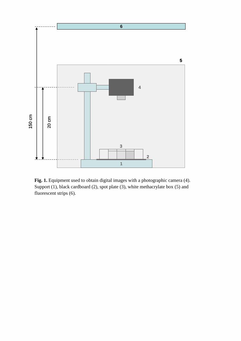
Fig. 1. Equipment used to obtain digital images with a photographic camera (4). Support (1), black cardboard (2), spot plate (3), white methacrylate box (5) and fluorescent strips (6).

20 c

m

150

cm

12

4

6

5

3

20 c

m

150

cm

12

4

6

5

3

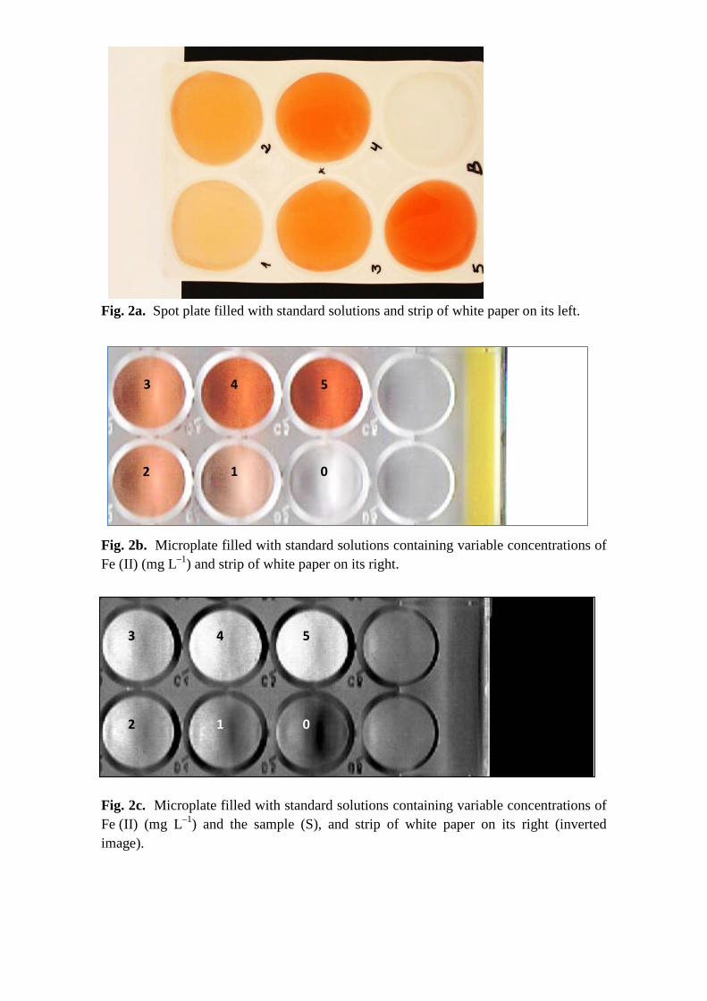
Fig. 2a. Spot plate filled with standard solutions and strip of white paper on its left.

Fig. 2b. Microplate filled with standard solutions containing variable concentrations of Fe (II) (mg L–1) and strip of white paper on its right.

Fig. 2c. Microplate filled with standard solutions containing variable concentrations of Fe (II) (mg L–1) and the sample (S), and strip of white paper on its right (inverted image).

0 1 2

3 4 5

0 1 2

3 4 5

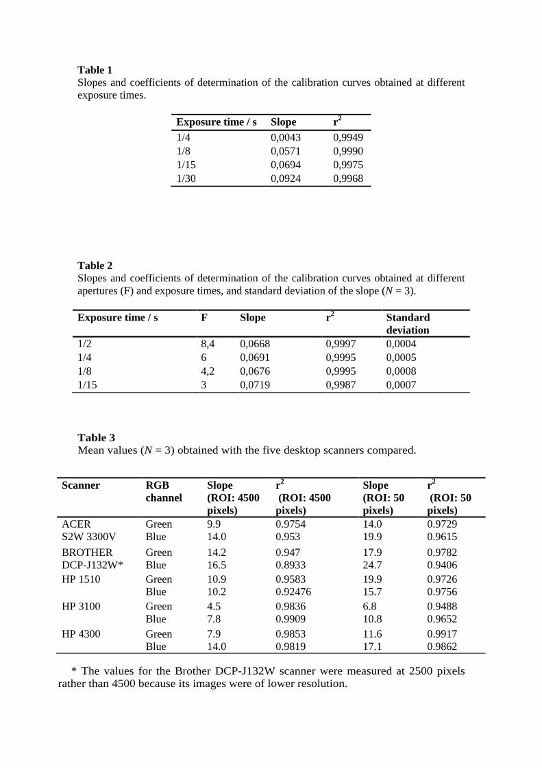
Table 1 Slopes and coefficients of determination of the calibration curves obtained at different exposure times.

Exposure time / s Slope r2 1/4 0,0043 0,9949 1/8 0,0571 0,9990 1/15 0,0694 0,9975 1/30 0,0924 0,9968

Table 2 Slopes and coefficients of determination of the calibration curves obtained at different apertures (F) and exposure times, and standard deviation of the slope (N = 3). Exposure time / s F Slope r2

Standard deviation

1/2 8,4 0,0668 0,9997 0,0004 1/4 6 0,0691 0,9995 0,0005 1/8 4,2 0,0676 0,9995 0,0008 1/15 3 0,0719 0,9987 0,0007

Table 3 Mean values (N = 3) obtained with the five desktop scanners compared.

* The values for the Brother DCP-J132W scanner were measured at 2500 pixels

rather than 4500 because its images were of lower resolution.

Scanner RGB channel

Slope (ROI: 4500 pixels)

r2

(ROI: 4500 pixels)

Slope (ROI: 50 pixels)

r2 (ROI: 50 pixels)

ACER Green 9.9 0.9754 14.0 0.9729 S2W 3300V Blue 14.0 0.953 19.9 0.9615 BROTHER Green 14.2 0.947 17.9 0.9782 DCP-J132W* Blue 16.5 0.8933 24.7 0.9406 HP 1510 Green 10.9 0.9583 19.9 0.9726 Blue 10.2 0.92476 15.7 0.9756 HP 3100 Green 4.5 0.9836 6.8 0.9488 Blue 7.8 0.9909 10.8 0.9652 HP 4300 Green 7.9 0.9853 11.6 0.9917 Blue 14.0 0.9819 17.1 0.9862

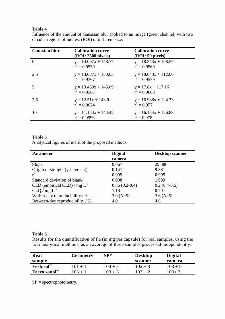
Table 4 Influence of the amount of Gaussian blur applied to an image (green channel) with two circular regions of interest (ROI) of different size. Gaussian blur Calibration curve

(ROI: 2500 pixels) Calibration curve (ROI: 50 pixels)

0 y = 14.097x + 148.77 y = 18.343x + 108.57 r2 = 0.9539 r2 = 0.9569

2.5 y = 13.087x + 150.03 y = 18.043x + 112.06 r2 = 0.9367 r2 = 0.9579

5 y = 13.453x + 145.69 y = 17.8x + 117.16 r2 = 0.9567 r2 = 0.9608

7.5 y = 12.51x + 143.9 y = 16.988x + 124.33 r2 = 0.9624 r2 = 0.957

10 y = 11.154x + 144.42 y = 16.154x + 126.88 r² = 0.9596 r² = 0.978

Table 5 Analytical figures of merit of the proposed methods. Parameter Digital

camera Desktop scanner

Slope 0.067 29.886 Origin of straight (y-intercept) 0.141 9.381 r2 0.999 0.995 Standard deviation of blank 0.008 1.999 CLD (empirical CLD) / mg L-1 0.36 (0.2-0.4) 0.2 (0.4-0.6) CLQ / mg L-1 1.18 0.70 Within-day reproducibility / % 3.0 (N=5) 3.6 (N=5) Between-day reproducibility / % 4.0 4.6 Table 6 Results for the quantification of Fe (in mg per capsule) for real samples, using the four analytical methods, as an average of three samples processed independently. Real sample

Cerimetry SP* Desktop scanner

Digital camera

Ferbisol® 101 ± 1 104 ± 5 102 ± 3 103 ± 5 Ferro sanol® 103 ± 1 103 ± 3 103 ± 2 103± 3 SP = spectrophotometry.