Embed Size (px)
Citation preview

Thermal Physics: Concepts and Practice
Thermodynamics has benefited from nearly 100 years of parallel development with
quantum mechanics. As a result, thermal physics has been considerably enriched in
concepts, technique and purpose, and now has a dominant role in developments of
physics, chemistry and biology. This unique book explores the meaning and applica-
tion of these developments using quantum theory as the starting point.
The book links thermal physics and quantum mechanics in a natural way. Con-
cepts are combined with interesting examples, and entire chapters are dedicated to
applying the principles to familiar, practical and unusual situations. Together with
end-of-chapter exercises, this book gives advanced undergraduate and graduate stu-
dents a modern perception and appreciation for this remarkable subject.
Allen L. Wasserman is Professor (Emeritus) in the Department of Physics, Oregon State
University. His research area is condensed matter physics.

Thermal PhysicsConcepts and Practice
�
ALLEN L. WASSERMANOregon State University
C A M B R I D G E U N I V E R S I T Y P R E S S
Cambridge, New York, Melbourne, Madrid, Cape Town,Singapore, São Paulo, Delhi, Tokyo, Mexico City
Cambridge University PressThe Edinburgh Building, Cambridge CB2 8RU, UK
Published in the United States of America by Cambridge University Press, New York
www.cambridge.orgInformation on this title: www.cambridge.org/9781107006492
c© A. Wasserman 2012
This publication is in copyright. Subject to statutory exceptionand to the provisions of relevant collective licensing agreements,
no reproduction of any part may take place withoutthe written permission of Cambridge University Press.
First published 2012
Printed in the United Kingdom at the University Press, Cambridge
A catalog record for this publication is available from the British Library
Library of Congress Cataloging-in-Publication Data
Wasserman, Allen L.Thermal physics : concepts and practice / Allen L. Wasserman.
p. cm.Includes bibliographical references and index.
ISBN 978-1-107-00649-2 (Hardback)1. Thermodynamics. 2. Entropy. 3. Statistical mechanics. I. Title.
QC311.W37 2011536′.7–dc23
2011036379
ISBN 978-1-107-00649-2 Hardback
Cambridge University Press has no responsibility for the persistence oraccuracy of URLs for external or third-party internet websites referred to
in this publication, and does not guarantee that any content on suchwebsites is, or will remain, accurate or appropriate.
Contents
Preface page xi
1 Introducing thermodynamics 1
1.1 The beginning 1
1.2 Thermodynamic vocabulary 3
1.3 Energy and the First Law 4
1.4 Quantum mechanics, the “mother of theories” 6
1.5 Probabilities in quantum mechanics 9
1.6 Closing comments 11
2 A road to thermodynamics 12
2.1 The density operator: pure states 12
2.2 Mixed states 15
2.3 Thermal density operator ρτop and entropy 20
Problems and exercises 23
3 Work, heat and the First Law 25
3.1 Introduction 25
3.2 Exact differentials 28
3.3 Equations of state 28
3.4 Heat capacity 38
3.5 Concluding remarks 47
Problems and exercises 47
4 A mathematical digression 49
4.1 Thermodynamic differentials 49
4.2 Exact differentials 50
4.3 Euler’s homogeneous function theorem 54
4.4 A cyclic chain rule 55
4.5 Entropy and spontaneous processes 60
4.6 Thermal engines 65
Problems and exercises 70
v
vi Contents
5 Thermodynamic potentials 73
5.1 Introduction 73
5.2 Enthalpy and throttling 79
5.3 Entropy and heat capacity 81
Problems and exercises 83
6 Knowing the “unknowable” 85
6.1 Entropy: ticket to the Emerald City 85
6.2 The bridge 86
6.3 Thermodynamic hamiltonians 87
6.4 Microcanonical (Boltzmann) theory 89
6.5 Gibbs’ canonical theory 93
6.6 Canonical thermodynamics 94
6.7 Degeneracy and Z 96
6.8 Closing comments 103
Problems and exercises 103
7 The ideal gas 106
7.1 Introduction 106
7.2 Ideal gas law 107
7.3 Quasi-classical model 108
7.4 Ideal gas partition function 109
7.5 Thermodynamics of the ideal gas 111
7.6 Gibbs’ entropy paradox 113
7.7 Entropy of mixing 114
7.8 The non-ideal gas 115
Problems and exercises 115
8 The two-level system 117
8.1 Anomalous heat capacity 117
8.2 Schottky model 117
8.3 Two-level systems and negative temperature 120
Problems and exercises 122
9 Lattice heat capacity 123
9.1 Heat capacity of solids 123
9.2 Einstein’s model 124
9.3 Einstein model in one dimension 124
9.4 The three-dimensional Einstein model 128
9.5 Debye model 131
Problems and exercises 133
vii Contents
10 Elastomers: entropy springs 136
10.1 Naive one-dimensional elastomer 136
10.2 Elongation as an extensive observable 138
10.3 Properties of the naive one-dimensional “rubber band” 140
10.4 “Hot rubber bands”: a thermodynamic analysis 143
10.5 A non-ideal elastomer 146
10.6 Three-dimensional elastomer thermodynamics 149
Problems and exercises 151
11 Magnetic thermodynamics 154
11.1 Magnetism in solids 154
11.2 Magnetic work 156
11.3 Microscopic models and uniform fields 160
11.4 Local paramagnetism 161
11.5 Simple paramagnetism 162
11.6 Local paramagnet thermodynamics 164
11.7 Magnetization fluctuations 167
11.8 A model for ferromagnetism 169
11.9 A mean field approximation 170
11.10 Spontaneous magnetization 172
11.11 Critical exponents 173
11.12 Curie–Weiss magnetic susceptibility (T > Tc) 174
11.13 Closing comment 174
12 Open systems 175
12.1 Variable particle number 175
12.2 Thermodynamics and particle number 176
12.3 The open system 176
12.4 A “grand” example: the ideal gas 182
12.5 Van der Waals’ equation 184
12.6 A star is born 186
12.7 Closing comment 191
Problems and exercises 191
13 The amazing chemical potential 192
13.1 Introduction 192
13.2 Diffusive equilibrium 193
13.3 Thermodynamics of chemical equilibrium 196
13.4 A law of mass action 198
13.5 Thermodynamics of phase equilibrium 200
13.6 Gibbs–Duhem relation 201
13.7 Multiphase equilibrium 202
viii Contents
13.8 The Clausius–Clapeyron equation 203
13.9 Surface adsorption: Langmuir’s model 204
13.10 Dissociative adsorption 207
13.11 Crystalline bistability 208
Problems and exercises 210
14 Thermodynamics of radiation 212
14.1 Introduction 212
14.2 Electromagnetic eigen-energies 213
14.3 Thermodynamics of electromagnetism 214
14.4 Radiation field thermodynamics 216
14.5 Stefan–Boltzmann, Planck, Rayleigh–Jeans laws 217
14.6 Wien’s law 220
14.7 Entropy of thermal radiation 221
14.8 Stefan–Boltzmann radiation law 221
14.9 Radiation momentum density 224
Problems and exercises 225
15 Ideal Fermi gas 228
15.1 Introduction 228
15.2 Ideal gas eigen-energies 228
15.3 Grand partition function 229
15.4 Electron spin 230
15.5 Fermi–Dirac thermodynamics 231
15.6 Independent fermion model 233
15.7 The chemical potential (T �= 0) 234
15.8 Internal energy (T �= 0) 236
15.9 Pauli paramagnetic susceptibility 237
15.10 Electron gas model 238
15.11 White dwarf stars 241
Problems and exercises 243
16 Ideal Bose–Einstein system 246
16.1 Introduction 246
16.2 Ideal Bose gas 247
16.3 Bose–Einstein thermodynamics 248
16.4 The ideal BE gas and the BE condensation 249
Problems and exercises 253
17 Thermodynamics and the cosmic microwave background 255
17.1 Introduction 255
17.2 Thermodynamic method 257
ix Contents
17.3 Moving frame thermodynamic potential Ω 257
17.4 Radiation energy flux 261
Problems and exercises 262
Appendix A How pure is pure? An inequality 263
A.1 0 < Tr(ρτ
op
)2 ≤ 1 263
Appendix B Bias and the thermal Lagrangian 264
B.1 Properties of F 264
B.2 The “bias” function 265
B.3 A thermal Lagrangian 266
Appendix C Euler’s homogeneous function theorem 268
C.1 The theorem 268
C.2 The proof 268
Appendix D Occupation numbers and the partition function 269
Appendix E Density of states 271
E.1 Definition 271
E.2 Examples 271
Appendix F A lab experiment in elasticity 275
F.1 Objectives 275
F.2 Results and analysis 277
Appendix G Magnetic and electric fields in matter 278
G.1 Introduction 278
G.2 Thermodynamic potentials and magnetic fields 278
G.3 Work and uniform fields 279
G.4 Thermodynamics with internal fields 283
Appendix H Maxwell’s equations and electromagnetic fields 285
H.1 Maxwell’s equations 285
H.2 Electromagnetic waves 285
H.3 Electromagnetic vector potential 288
H.4 Quantized electromagnetic hamiltonian 290
Appendix I Fermi–Dirac integrals 293
I.1 Introduction 293
I.2 Expansion method: βμ� 1 293

x Contents
Appendix J Bose–Einstein integrals 296
J.1 BE integrals: μ = 0 296
J.2 BE integrals: μ < 0 297
Index 299
Preface
In the preface to his book Statistical Mechanics Made Simple Professor Daniel
Mattis writes:
My own experience in thermodynamics and statistical mechanics, a half century agoat M.I.T., consisted of a single semester of Sears, skillfully taught by the man himself.But it was a subject that seemed as distant from “real” physics as did poetry or Frenchliterature.1
This frank but discouraging admission suggests that thermodynamics may not be a
course eagerly anticipated by many students – not even physics, chemistry or engi-
neering majors – and at completion I would suppose that few are likely to claim it was
an especially inspiring experience. With such open aversion, the often disappointing
performance on GRE2 questions covering the subject should not be a surprise. As a
teacher of the subject I have often conjectured on reasons for this lack of enthusiasm.
Apart from its subtlety and perceived difficulty, which are probably immutable,
I venture to guess that one problem might be that most curricula resemble the ther-
modynamics of nearly a century ago.
Another might be that, unlike other areas of physics with their epigrammatic
equations – Newton’s, Maxwell’s or Schrödinger’s, which provide accessibility and
direction – thermal physics seems to lack a comparable unifying principle.3 Students
may therefore fail to see conceptual or methodological coherence and experience
confusion instead.
With those assumptions I propose in this book alternatives which try to address
the disappointing experience of Professor Mattis and undoubtedly others.
Thermodynamics, the set of rules and constraints governing interconversion and
dissipation of energy in macroscopic systems, can be regarded as having begun with
Carnot’s (1824) pioneering paper on heat-engine efficiency. It was the time of the
industrial revolution, when the caloric fluid theory of heat was just being questioned
and steam-engine efficiency was, understandably, an essential preoccupation. Later
in that formative period Rudolf Clausius introduced a First Law of Thermodynamics
(1850), formalizing the principles governing macroscopic energy conservation.
1 Daniel Mattis, Statistical Mechanics Made Simple, World Scientific Publishing, Singapore (2003).2 Graduate Record Examination: standardized graduate school admission exam.3 R. Baierlein, “A central organizing principle for statistical and thermal physics?”, Am. J. Phys. 63, 108
(1995).
xi
xii Preface
Microscopic models were, at the time, largely ignored and even regarded with
suspicion, to the point where scientific contributions by some proponents of such
interpretations were roundly rejected by the editors of esteemed journals. Even with
the intercession in support of kinetic models by the respected Clausius (1857), they
stubbornly remained regarded as over-imaginative, unnecessary appeals to invisi-
ble, unverifiable detail – even by physicists. A decade later when Maxwell (1866)
introduced probability into physics bringing a measure of statistical rigor to kinetic
(atomic) gas models there came, at last, a modicum of acceptance.
Within that defining decade the already esteemed Clausius (1864) invented a novel,
abstract quantity as the centerpiece of a Second Law of Thermodynamics, a new
principle – which he named entropy – to change forever our understanding of ther-
mal processes and, indeed, all natural processes. Clausius offered no physical inter-
pretation of entropy, leaving the matter open to intense speculation. Ludwig Boltz-
mann, soon to be a center of controversy, applied Maxwell’s microscopic probabil-
ity arguments to postulate a statistical model of entropy based on counting discrete
“atomic” configurations referred to, both then and now, as “microstates”.4 However,
Boltzmann’s ideas on entropy, which assumed an atomic and molecular reality, were
far from universally embraced – a personal disappointment which some speculate
led to his suicide in 1906.
Closing the book on 19th-century thermal physics, J. W. Gibbs reconciled New-
tonian mechanics with thermodynamics by inventing statistical mechanics5 based
on the still mistrusted presumption that atoms and molecules were physical reali-
ties. In this indisputably classic work, novel statistical “ensembles” were postulated
to define thermodynamic averages, a statistical notion later adopted in interpreting
quantum theories. Shortcomings and limited applicability of this essentially New-
tonian approach notwithstanding, it provided prescient insights into the quantum
mechanics, whose full realization was still a quarter century in the future.
Quantum mechanics revolutionized physics and defines the modern scientific era.
Developing in parallel with it, and synergistically benefiting from this reshaped sci-
entific landscape, thermal physics has come to occupy a rightful place among the
pillars of modern physics.
Quantum mechanics’ natural, internally consistent unification of statistics with
microscopic mechanics immediately suggests the possibility of a thermodynamics
derived, in some way, from microscopic quantum averages and quantum proba-
bilities. But thermodynamic systems are not simply the isolated quantum systems
familiar from most quantum mechanics courses. Thermodynamics is about macro-
scopic systems, i.e. many-particle quantum systems that are never perfectly isolated
from the remainder of the universe. This interaction with the “outside” has enormous
4 Boltzmann’s microstates suggested to Planck (1900) what eventually became the quantization he incor-porated into his theory of electromagnetic radiation.
5 J. W. Gibbs, The Elementary Principles of Statistical Mechanics, C. Scribner, New York (1902).
xiii Preface
consequences which, when taken into account quantitatively, clarifies the essence of
thermodynamics.
Many thermal variables may then be approached as macroscopic quantum aver-
ages and their associated thermal probabilities as macroscopic quantum probabili-
ties, the micro-to-macro translation achieved in part by an entropy postulate. This
approach gives rise to a practical organizing principle with a clear pedagogical path
by which thermodynamics’ structure attains the epigrammatic status of “real
physics”.
Thermal physics is nevertheless frequently taught in the spirit of its utile 19th-
century origins, minimizing both 20th- and 21st-century developments and, for the
most part, disregarding the beauty, subtlety, profundity and laboratory realities of
its modern rebirth – returning us to Professor Mattis’ reflections. In proposing a
remedy for his justifiable concerns, the opening chapter introduces a moderate dose
of quantum-based content, both for review and, hopefully, to inspire interest in and,
eventually, better understanding of thermodynamics. The second chapter develops
ideas that take us to the threshold of a thermodynamics that we should begin to
recognize. In Chapter 6 thermodynamics flies from a quantum nest nurtured, ready
to take on challenges of modern physics.
Students and practitioners of thermodynamics come from a variety of disciplines.
Engineers, chemists, biologists and physicists all use thermodynamics, each with
practical or scientific concerns that motivate different emphases, stress different lega-
cies and demand different pedagogical objectives. Since contemporary university
curricula in most of these disciplines integrate some modern physics, i.e. quan-
tum mechanics – if not its mathematical details at least its primary concepts and
aims – the basic thermodynamic ideas as discussed in the first two chapters should
lie within the range of students of science, engineering and chemistry. After a few
chapters of re-acquaintance with classic thermodynamic ideas, the book’s remaining
chapters are dedicated to applications of thermodynamic ideas developed in Chapter
6 in practical and model examples for students and other readers.
Parts of this book first appeared in 1997 as notes for a course in thermal physics
designed as a component of the revised undergraduate physics curriculum at Ore-
gon State University. An objective of this revision was to create paradigmatic mate-
rial stressing ideas common to modern understandings and contemporary problems.
Consequently, concepts and dynamic structures basic to quantum mechanics – such
as hamiltonians, eigen-energies and quantum degeneracy – appear and play impor-
tant roles in this view of thermal physics. They are used to maintain the intended
“paradigm” spirit by avoiding the isolation of thermal physics from developments of
the past 100 years while, hopefully, cultivating in students and teachers alike a new
perception of and appreciation for this absolutely remarkable subject.
This work has been funded in part by NSF Grants: DUE 9653250, 0231194,
0837829.

1 Introducing thermodynamics
The atomistic nature of matter as conceptualized by the Greeks had, by the 19thcentury, been raised by scientists to a high probability. But it was Planck’s law ofradiation that yielded the first exact determination of the absolute size of atoms.More than that, he convincingly showed that in addition to the atomistic struc-ture of matter there is a kind of atomistic structure to energy, governed by theuniversal constant h.
This discovery has almost completely dominated the development of physicsin the 20th century. Without this discovery a workable theory of molecules andatoms and the energy processes that govern their transformations would nothave been possible. It has, moreover, shaken the whole framework of classicalmechanics and electrodynamics and set science the fresh task of finding a newconceptual basis for all of physics. Despite partial success, the problem is stillfar from solved.
Albert Einstein, “Max Planck memorial service” (1948).Original image, Einstein Archives Online, Jerusalem
(trans. A. Wasserman)
1.1 The beginning
Thermodynamics has exceeded the scope and applicability of its utile origins in the
industrial revolution to a far greater extent than other subjects of physics’ classical
era, such as mechanics and electromagnetism. Unquestionably this results from over
a century of synergistic development with quantum mechanics, to which it has given
and from which it has gained clarification, enhancement and relevance, earning for
it a vital role in the modern development of physics as well as chemistry, biology,
engineering, and even aspects of philosophy.
The subject’s fascinating history is intertwined with seminal characters who con-
tributed much to its present form – some colorful and famous with others lesser
known, maligned or merely ignored.
“Atomism” (i.e. molecular models), a source of early conflict, seems to have had
Daniel Bernoulli as its earliest documented proponent when in 1738 he hypothesized
1
2 Introducing thermodynamics
a kinetic theory of gases.1 Although science – thermodynamics in particular – is
now unthinkable without such models, Bernoulli’s ideas were largely ignored and
for nearly a century little interest was shown in matter as based on microscopic con-
stituents. Despite a continuing atmosphere of suspicion, particle models occasionally
reappeared2,3 and evolved, shedding some of their controversy (Joule 1851) while
moving towards firm, accepted hypotheses (Kronig 1856). Adoption of kinetic mod-
els by the respected Rudolf Clausius (1857) began to erode the skeptics’ position
and encourage the new statistical theories of Maxwell (1859) and Boltzmann (1872).
At about the same time van der Waals (1873), theorizing forces between real atoms
and molecules, developed a successful equation of state for non-ideal gases.4 Never-
theless, as the 20th century dawned, controversy continued only slightly abated. J. J.
Thomson’s discovery of the electron (1897) should have finally convinced remaining
doubters of matter’s microscopic essence – but it didn’t. The argument continued into
the 20th century stilled, finally, by the paradigm shift towards “quantized” models.
It all started with Max Planck who in 19005,6 introduced quantized energy into
theories of electromagnetic radiation – and Einstein7 who used quantized lattice
vibrations in his ground-breaking heat capacity calculation. But it would be another
25 years before the inherently probabilistic, microscopic theory of matter – quantum
mechanics – with its quantum probabilities and expectation values – would com-
pletely reshape the scientific landscape and permanently dominate most areas of
physics, providing a basis for deeper understanding of particles, atoms and nuclei
while grooming thermodynamics for its essential role in modern physics.
Thermodynamics is primarily concerned with mechanical, thermal and electro-
magnetic interactions in macroscopic matter, i.e. systems with huge numbers of
microscopic constituents (∼1023 particles). Although thermodynamic descriptions
are generally in terms of largely intuitive macroscopic variables, most macroscopic
behaviors are, at their root, quantum mechanical. Precisely how the classical
1 D. Bernoulli, Hydrodynamica (1738).2 J. Herapath,“On the causes, laws and phenomena of heat, gases, gravitation”, Annals of Philosophy
9 (1821). Herapath’s was one of the early papers on kinetic theory, but rejected by the Royal Society,whose reviewer objected to the implication that there was an absolute zero of temperature at whichmolecular motion ceased.
3 J.J.Waterston,“Thoughts on the mental functions” (1843). This peculiar title was a most likely causeof its rejection by the Royal Society as “nothing but nonsense”. In recognition of Waterston’s unfairlymaligned achievement, Lord Rayleigh recovered the original manuscript and had it published as “Onthe physics of media that are composed of free and perfectly elastic molecules in a state of motion”,Philosophical Transactions of the Royal Society A 183, 1 (1892), nearly 10 years after Waterston’sdeath.
4 Van der Waals’ work also implied a molecular basis for critical points and the liquid–vapor phasetransition.
5 Max Planck,“Entropy and temperature of radiant heat”, Ann. der Physik 1, 719 (1900).6 Max Planck, “On the law of distribution of energy in the normal spectrum”, Ann. der Physik 4, 553
(1901).7 A. Einstein, “Planck’s theory of radiation and the theory of specific heat”, Ann. der Physik 22, 180
(1907).
3 Thermodynamic vocabulary
measurement arises from quantum behavior has been a subject of some controversy
ever since quantum theory’s introduction. But it now seems clear that macroscopic
systems are quantum systems that are particularly distinguished by always being
entangled (however weakly) with an environment (sometimes referred to as a reser-
voir) that is also a quantum system. Although environmental coupling may be con-
ceptually simple and even uninteresting in detail, it has enormous consequences for
quantum-based descriptions of macroscopic matter, i.e. thermodynamics.8
1.2 Thermodynamic vocabulary
A few general, large-scale terms are used in describing objects and conditions of
interest in thermodynamics.
• System: A macroscopic unit of particular interest, especially one whose thermal
properties are under investigation. It may, for example, be a gas confined within
physical boundaries or a rod or string of elastic material (metal, rubber or poly-
mer). It can also be matter that is magnetizable or electrically polarizable.
• Surroundings: Everything physical that is not the system or which lies outside the
system’s boundaries is regarded as “surroundings”. This may be external weights,
an external atmosphere, or static electric and magnetic fields. The system plus
surroundings comprise, somewhat metaphorically, “the universe”.
• Thermal variables: A set of macroscopic variables that describe the state of
the system. Some variables are intuitive and familiar, such as pressure, volume,
elongation, tension, etc. Others may be less intuitive and even abstract – such
as temperature – but, nevertheless, also play important roles in thermodynamics.
These will be discussed in detail in this and later chapters.
• Thermal equilibrium: The final state attained in which thermal state variables
that describe the macroscopic system (pressure, temperature, volume, etc.) no
longer change in time.9 It is only at thermal equilibrium that thermodynamic
variables are well defined. The time elapsed in attaining equilibrium is largely
irrelevant.
8 Macroscopic behavior can be quite different from the behavior of individual constituents (atoms,molecules, nuclei, etc.) As an example, the appearance of spontaneous bulk magnetism in iron (at tem-peratures below some critical temperature Tc) is not a property of individual iron atoms but arises fromlarge numbers of interacting iron atoms behaving collectively.
9 There are, nevertheless, small departures from equilibrium averages, referred to as fluctuations, whosevalues are also part of any complete thermodynamic description.
4 Introducing thermodynamics
1.3 Energy and the First Law
James Joule’s classic contribution on the mechanical equivalent of heat and his theory
of energy reallocation between a system and its surroundings10 (referred to as energy
conservation) led Rudolph Clausius11 to the historic First Law of Thermodynamics:
�U = Q−W. (1.1)
Here W is mechanical work done by the system and Q is heat (thermal energy) added
to the system, both of which are classical quantities associated with surroundings. In
Clausius’ time controversy about reality in atomic models left U with no definitive
interpretation. But being the maximum work which could be theoretically extracted
from a substance it was initially called “intrinsic energy”. As kinetic (atomic) models
gained acceptance (Clausius having played an influential role) U became the mean
kinetic energy of the system’s microscopic constituents or, more generally, as inter-
nal energy. Although the change in internal energy, �U , is brought about by mechan-
ical and thermal, i.e. classical, interactions, quantum mechanics provides a clear and
specific meaning to �U as an average change in energy of the macroscopic sys-
tem as determined from kinetic, potential and interaction energies of its microscopic
constituents, clearly distinguishing it from other energy contributions. The precise
meaning and interrelation of this with similar macroscopic averages provides the
basis for thermodynamics.12
1.3.1 Thermodynamic variables defined
Some thermodynamic concepts and macroscopic variables are familiar from classical
physics while others arise simply from operational experience. Moving beyond this,
quantum mechanics provides definitions and context for not only internal energy U ,
but for other macroscopic (thermodynamic) variables, placing them within a micro-
scopic context that adds considerably to their meaning and their role within thermal
physics. The First Law, in arraying Q and W (both classical) against �U (quan-
tum mechanical), highlights this intrinsic partitioning of macroscopic variables into
“classical”(C) vis-à-vis quantum (Q).
Examples of Q-variables – macroscopic variables having microscopic origins13 –
are:
10 James P. Joule, “On the existence of an equivalent relation between heat and the ordinary forms ofmechanical power”, Phil. Mag. 27, 205 (1850).
11 R. Clausius, “On the moving force of heat, and the laws regarding the nature of heat”, Phil. Mag. 2,1–21, 102–119 (1851).
12 Macroscopic “averages” will be discussed in Chapter 2.13 These are defined by quantum operators.
5 Energy and the First Law
• internal energy: hop (energy of the system’s microscopic constituents – kinetic
plus potential);
• pressure: pop = −(∂ hop∂V
)(pressure arising from a system’s internal constituents);
• electric polarization: Pop;• magnetization: Mop;• elongation (length): χop;• particle number: Nop.
14
Examples of C-variables – classical (macroscopic) variables that exist apart from
microscopic mechanics15 – are:
• temperature: T;
• volume: V;
• static magnetic fields: B or H;
• static electric fields: E or D;16
• elastic tension: τ ;
• chemical potential: μ.17
Interaction energy
Most Q-variables listed above appear from interaction terms added to hop. The fol-
lowing are examples of such variables and their interactions.
a. Tension τ applied to an elastic material produces a “conjugate” elongation χ ,
as described by an interaction operator18
Hχop = −τ · χop. (1.2)
b. A static magnetic induction field B0 contributes an interaction operator
(energy)
HMop = −mop ·B0. (1.3)
14 Variable particle number is essential for thermodynamic descriptions of phase transitions, chemi-cal reactions and inhomogeneous systems. However, the particle number operator is not a part ofSchrödinger’s fixed particle number theory, though it appears quite naturally in quantum field theories.Implementing variable particle number requires operators to create and destroy them and operators tocount them.
15 These are not defined by quantum operators.16 Electromagnetic radiation fields are, on the other hand, representable by quantum field operators Bop
and Eop obtained from a quantum electromagnetic vector potential operator Aop . This will be dis-cussed in Chapter 14, on radiation theory.
17 μ is an energy per particle and is associated with processes having varying particle number.18 The tension τ is said to be conjugate to the elongation χ . The variable and its conjugate comprise a
thermodynamic energy.
6 Introducing thermodynamics
Here mop represents a magnetic moment operator for elementary or compos-
ite particles. The sum19,20
Mop =∑
i
mop(i), (1.4)
represents the total magnetization operator.
c. A static electric field E0 can contribute an interaction operator (energy)
HPop = −pop · E0, (1.5)
where pop represents an electric dipole moment operator and
Pop =∑
i
pop(i) (1.6)
represents the total polarization.21
d. An energy associated with creating “space” for the system is
HWop = popV, (1.7)
with pop representing the system pressure and V the displaced volume.
e. An “open system” energy associated with particle creation and/or destruc-
tion is
HNop = −μNop, (1.8)
where the chemical potential μ (an energy per particle) is conjugate to a par-
ticle number operator Nop. Chemical reactions, phase transitions and other
cases with variable numbers of particles of different species are examples of
open systems.22
1.4 Quantum mechanics, the “mother of theories”
As out of place as rigorous quantum ideas might seem in this introduction to ther-
modynamics, it is the author’s view that they are an essential topic for an approach
that strives to bring unity of structure and calculable meaning to the subject.
19 The field B0 conjugate to mop is the field present prior to the insertion of matter. Matter itself may bemagnetized and contribute to an effective B.
20 There are ambiguities in the thermodynamic roles of static fields, e.g. Maxwell’s local magnetic aver-age B vs. an external B0 and Maxwell’s local electric average E vs. external E0.
21 The field E0 is conjugate to the electric dipole operator pop .22 Variable particle number is intrinsic to thermal physics even though it may be suppressed for simplicity
when particle number is assumed constant.
7 Quantum mechanics, the “mother of theories”
1.4.1 Introduction
Macroscopic variables such as pressure p, magnetization M, elastic elongation χ ,
particle number N , etc. – any (or all) of which can appear in thermodynamic descrip-
tions of matter – have microscopic origins and should be obtainable from quantum
models. The question is: “How?”
Investigating the means by which microscopic models eventually lead to macro-
scopic quantities is the aim of Chapters 2 and 6. Preliminary to that goal, this chap-
ter reviews postulates, definitions and rules of quantum mechanics for typical iso-
lated systems.23 Particular attention is given to probabilities and expectation values
of dynamical variables (observables).24 This provides the basic rules, language and
notation to carry us into Chapter 2 where the question “What is thermodynamics?”
is raised, and then to Chapter 6 where the ultimate question “How does it arise?” is
addressed.
In achieving this goal Chapter 2 will diverge somewhat from the familiar “wave
mechanics” of introductory courses and focus on a less-familiar but closely related
quantum mechanical object called the density operator, ρop. This quantity, although
derived from a quantum state function, goes beyond state function limitations by
adding the breadth and flexibility critical for answering most of our questions about
thermodynamics. It is a “Yellow Brick Road” that will guide us from the land of the
Munchkins to the Emerald City25 – from the microscopic to the macroscopic – from
quantum mechanics to thermodynamics.
1.4.2 A brief review
The review starts with Schrödinger’s famous linear equation of non-relativistic quan-
tum mechanics:
Hopψ (x, t) = ih∂ψ (x, t)
∂t. (1.9)
The solution to Eq. 1.9 is the time-evolving, complex, scalar wavefunction ψ (x, t),
which describes the quantum dynamics of an isolated, fixed particle number, micro-
scopic system.
In the widely used (and preferred) Dirac notation, Eq. 1.9 is identical with
Hop |Ψ 〉 = ih∂
∂t|Ψ 〉 , (1.10)
23 These are the systems described by Schrödinger theory.24 Most of this review material is likely to be familiar from an earlier course in modern physics. If not, it
is recommended that you work alongside one of the many books on introductory quantum mechanics.25 L. Frank Baum, Wizard of Oz, Dover Publications, New York (1996).
8 Introducing thermodynamics
where |Ψ 〉 is the time-dependent state function, or “ket”, corresponding to the wave-
function ψ (x, t), i.e.
〈x |Ψ 〉 ≡ ψ (x, t) . (1.11)
Here |x〉 is an “eigen-ket” of the position operator with x ≡ x1, x2, . . . , xN the coor-
dinates of an N -particle system. As indicated in Eq. 1.11, the wavefunction ψ (x, t)
is merely the “ket” |Ψ 〉 in a coordinate representation.26 Hop is the hamiltonian
operator (inspired by classical dynamics). A hamiltonian operator for a case with
only internal particle dynamics may, for example, be written
hop = Top + Vop, (1.12)
where Top and Vop are kinetic energy and potential energy operators, respectively.27
Additional interaction terms Hintop such as Eqs. 1.2→ 1.8 may appear, depending on
the physical situation, in which case
Hop = hop +Hintop . (1.13)
The quantum state function |Ψ 〉 (see Eq. 1.11) has no classical counterpart and is,
moreover, not even a measurable! But it is nevertheless interpreted as the generating
function for a statistical description of the quantum system – including probabili-
ties, statistical averages (expectation values) and fluctuations about these averages. It
contains, in principle, all that is knowable about the isolated, microscopic system.28
Devising an arbitrary but reasonable quantum knowledge scale, say
1 ⇒ all knowledge, (1.14)
0 ⇒ no knowledge, (1.15)
and using this scale to calibrate “information”, Schrödinger’s quantum state function
has information value 1.29 Unless there is some quantum interaction with the sur-
roundings (i.e. the system is no longer isolated) |Ψ 〉 will retain information value 1
indefinitely.30,31
26 The “ket” |Ψ 〉 is an abstract, representation-independent object. Its only dependence is t , time.27 Vop is assumed to also include particle–particle interactions.28 Whereas probabilities are derivable from the system state function, the reverse is not the
case – state functions |Ψ 〉 cannot be inferred from measurement.29 In Chapter 2 we will introduce a more solidly based mathematical measure of “information”, extending
this arbitrary scale.30 The isolated system state function is a quantity of maximal information. The system’s isolation assures
that no information will “leak” in or out.31 Macroscopic complexity has relaxed absolute reliance on a detailed many-body quantum description
of a macroscopic system. Even at this early point we can foresee that exact (or even approximate)knowledge of the macroscopic (many-body) quantum state function (even if that were possible, whichit is not) is unnecessary for macroscopic descriptions.
9 Probabilities in quantum mechanics
An energy expectation value – an observable – is defined (in terms of the wave-
function) by
〈H(t)〉 =∫
dxψ∗(x, t)Hopψ(x, t) , (1.16)
where ψ∗ (x, t) is the complex conjugate of the wavefunction ψ (x, t). In the more
convenient Dirac notation
〈H〉 = 〈Ψ |Hop|Ψ 〉, (1.17)
where 〈Ψ |, the conjugate to |Ψ 〉, is called a “bra”. The energy expectation value
(sometimes called average value) is often a measurable32 of physical interest.
But neither Eq. 1.16 nor Eq. 1.17 represent thermodynamic state variables. In
particular, 〈h〉 = 〈Ψ |hop|Ψ 〉 is not macroscopic internal energy U , the centerpiece
of the First Law. This is a crucial point that will be further addressed in Chapter 2
when we inquire specifically about thermodynamic variables.
In quantum mechanics, each of nature’s dynamical observables (e.g. momentum,
position, energy, current density, magnetic moment, etc.) is represented by an her-
mitian operator. (An hermitian operator satisfies the condition Ω†op = Ωop, where
† is the symbol for hermitian conjugation. In matrix language hermiticity means
Ω† = (Ω∗)T = Ω , where (Ω∗)T is the complex conjugate-transpose of the matrix
Ω .)33
The quantum theory postulates an auxiliary eigenvalue problem for Ωop (which
represents a typical hermitian operator)
Ωop |ωn〉 = ωn |ωn〉 , (1.18)
with n = 1, 2, 3, . . ., from which the spectrum of allowed quantum observables ωn
(called eigenvalues) is derived. The ωn are real numbers34 and |ωn〉 are their corre-
sponding set of complex eigenfunctions. (For simplicity we assume the eigenvalues
are discrete.) The specific forms required for dynamical hermitian operators will be
introduced as the models require.
1.5 Probabilities in quantum mechanics
According to the Great Probability Postulate of quantum mechanics, the Schrödinger
state function |Ψ 〉 is a generator of all probability information about an isolated
32 The value of this measurable is the average of a very large number of identical measurements onidentical systems with identical apparatus.
33 In the following discussion Ωop is used as a generic symbol for operators representing observables.34 The hermitian property of quantum mechanical operators assures that the eigenvalues will be real
numbers.
10 Introducing thermodynamics
quantum system with fixed number of particles.35 Using the complete orthonormal
set of eigenfunctions determined from Eq. 1.18, a state function |Ψ 〉 can be expressed
as a linear coherent superposition36
|Ψ 〉 =∑
n
|ωn〉〈ωn|Ψ 〉, (1.19)
where the coefficients
p(ωn, t) = 〈ωn|Ψ 〉 (1.20)
are complex probability amplitudes. Coherence as used here implies phase rela-
tions among the terms in the sum which leads to characteristic quantum interference
effects.
The probability that a measurement outcome will be ωn is given by
P(ωn, t) = |〈ωn|Ψ 〉|2 (1.21)
= 〈ωn|Ψ 〉〈Ψ |ωn〉 . (1.22)
The eigenfunction |ωn〉 acts, therefore, as a statistical projector in the sense that with
some appropriate measuring device it projects out from the state function |Ψ 〉 the
statistical probability of measuring ωn . The probabilities P (ωn, t) are normalized in
the usual probabilistic sense, i.e.∑n
P (ωn, t) = 1, (1.23)
which corresponds to state function normalization
〈Ψ |Ψ 〉 = 1 . (1.24)
1.5.1 Expectation values
If the probability of observing the measurable value ωn is P (ωn, t), then its expec-
tation (average) value 〈ω〉 is, as in ordinary statistics,
〈ω〉 =∑
n
ωnP (ωn, t) (1.25)
=∑
n
ωn〈ωn|Ψ 〉〈Ψ |ωn〉 . (1.26)
For the important special case of energy of an isolated (microscopic) system, where
Hop|En〉 = En|En〉, (1.27)
35 The state function |Ψ 〉 depends on time t so that all quantities calculated from it will – in principle –also depend on time.
36 This is the famous linear superposition theorem.
11 Closing comments
with En the allowed eigen-energies (eigenvalues) and |En〉 the corresponding eigen-
functions, the energy expectation value for the state |Ψ 〉 is
〈E〉 =∑
n
En〈En|Ψ 〉〈Ψ |En〉 (1.28)
=∑
n
EnP(En, t) , (1.29)
which is equivalent to Eq. 1.17.
The expectation value of any hermitian observable Ωop is, for a microscopic
system,
〈Ω〉 = 〈Ψ |Ωop |Ψ 〉 . (1.30)
1.6 Closing comments
The main points in this chapter are as follows.
1. Schrödinger’s wavefunctions yield quantum probabilities and quantum expecta-
tion values (averages). But, contrary to expectations, these measurables are not
macroscopic state variables of thermodynamics. Temporarily putting aside this
letdown, the issue will be discussed and resolved in the next chapters.
2. Schrödinger state functions are capable of generating all dynamical information
that can be known about the physical system. They can be said to have “infor-
mation content” 1 and are called pure states. From these few clues it should be
apparent that “information” is a term with relevance in quantum mechanics and,
ultimately, in thermodynamics.
The reader is encouraged to consult the ever-growing number of fine monographs on
quantum mechanics (far too many to list here).
2 A road to thermodynamics
If someone says that he can think or talk about quantum physics without becom-ing dizzy, that shows only that he has not understood anything whatever about it.
Murray Gell-Mann, Thinking Aloud: The Simple and the Complex”,Thinking Allowed Productions, Oakland, California (1998)
2.1 The density operator: pure states
Results from Chapter 1 can, alternatively, be expressed in terms of a density operator
ρop, which is defined (in Dirac notation) as
ρop = |�〉〈�| (2.1)
where the Dirac “ket” |�〉 is a pure Schrödinger state function, and the Dirac “bra”
〈�| is its conjugate. Density operator ρop is clearly hermitian with matrix
elements – the density matrix – in some complete basis |ωi 〉
ρi j = 〈ωi |�〉〈�|ω j 〉, (2.2)
whose diagonal elements
ρi i =|〈�|ωi 〉|2 (2.3)
are identical with the probabilities of Eq.1.21
ρi i =P(ωi ). (2.4)
An introduction to properties of the density operator1 (matrix) will demonstrate that
this object’s value is not merely that of an alternative to the wave equation descrip-
tion in the previous chapter, but that it is capable of defining and accommodating a
broader class of quantum states – in particular, states which are not pure, i.e. states
1 Also called the statistical operator.
12
13 The density operator: pure states
for which information2 content is less than 1. This generalization is a huge stride
towards realizing thermodynamics.3
2.1.1 Traces, expectations and information
If Aop is an operator and its matrix representation is
Ai j = 〈φi |Aop|φ j 〉, (2.5)
then its trace TrAop is defined as the sum of its diagonal matrix elements in the
orthonormal basis |φi 〉,4
TrAop =∑
i
〈φi |Aop |φi 〉. (2.6)
The expectation value 〈�〉 in terms of the pure state density operator ρop is
〈�〉 =∑α
〈φα|ρop�op|φα〉∑α
〈φα|ρop|φα〉 , (2.7)
where |φα〉 is any complete set of states. Using Eq. 2.6, this can be condensed to
〈�〉 = Trρop�op
Trρop. (2.8)
Since |�〉 is normalized,
Trρop =∑α
〈φα|ρop|φα〉 (2.9)
=∑α
〈φα|�〉〈�|φα〉 (2.10)
=∑α
〈�|φα〉〈φα|�〉 (2.11)
= 〈�|�〉 (2.12)
= 1, (2.13)
reducing Eq.2.8 to
〈�〉 = Trρop�op, (2.14)
2 A brief discussion about information appeared in Chapter 1.3 Moreover, the density operator (matrix) can be a measurable. See: R. Newton and B. Young, “Mea-
surability of the spin density matrix”, Annals of Physics 49, 393 (1968); Jean-Pierre Amiet and StefanWeigert, “Reconstructing the density matrix of a spin s through Stern-Gerlach measurements: II”,J. Phys. A 32, L269 (1999).
4 The trace of a matrix is independent of the orthonormal basis in which the matrix is expressed.
14 A road to thermodynamics
where completeness of |φα〉 has been applied. Using as a basis |ωn〉 (the eigenfunc-
tions of �op) Eq. 2.14 becomes, as expected,
〈�〉 =∑
n
ωn |〈�|ωn〉|2 , (2.15)
where, as discussed in Chapter 1,
P(ωn) = |〈�|ωn〉|2 (2.16)
is the probability of finding the system in an eigenstate |ωn〉.The probability P(ωn) is easily shown to be expressible as
P(ωn) = Tr{ρop|ωn〉〈ωn|
}. (2.17)
The brief introduction to information in Chapter 1 is now carried a step further by
defining a new quantity, purity I,
I = Trρop2, (2.18)
as a way to measure information.5 The pure state, Eq. 2.1, now has purity
(information)
I = Trρopρop =∑α
〈φα|�〉〈�|�〉〈�|φα〉 (2.19)
=∑α
〈�|φα〉〈φα|�〉〈�|�〉 (2.20)
= 〈�|�〉 (2.21)
= 1, (2.22)
in agreement with the idea of maximal information on the arbitrary scale devised
in Chapter 1. The pure state density operator ρop carries complete quantum infor-
mation (I = 1) about an isolated microscopic system, in the same way as does its
corresponding state function |�〉, but within a more useful framework. (The best is
still to come!)
The density operator has an equation of motion found by using the time derivative
of the state operator,
5 This is not the only way “information” can be defined. A more thermodynamically relevant definitionwill be expanded upon in Chapter 6.
15 Mixed states
∂ρop
∂t=(
∂
∂t|�〉
)〈�| + |�〉
(〈�| ∂
∂t
)(2.23)
=(− i
hHop|�〉
)〈�| + |�〉
(〈�| i
hHop
)= i
h
(ρopHop −Hopρop
)= i
h
[ρop,Hop
], (2.24)
which, in practical terms, is equivalent to Schrödinger’s equation.6
2.2 Mixed states
At this point it might seem that not much has been gained by introducing the density
operator. So why bother?
Keeping in mind that our interest is in macroscopic quantum systems whose states
are inextricably entangled with those of a quantum environment, the density operator
provides a logical foundation for describing environmental “mixing” and its conse-
quences.7 Although it seems that mixing can only irreparably complicate matters, in
fact it ultimately reveals the essence of thermodynamics, bringing its meaning into
focus.
Pure quantum states, which evolve according to Schrödinger’s equation, can be
individually prepared and then classically combined by some (mechanical) process
or apparatus.8 This combined configuration cannot be a solution to any Schrödinger
equation and is no longer a pure state described by a state function, say |�(ξ)〉. It
can, however, be described by a density operator – in particular a mixed state density
operator ρMop – defined by
ρMop =
∑j
∣∣∣ψ( j)⟩w j
⟨ψ( j)
∣∣∣ (2.25)
with ∑j
w j = 1, (2.26)
where the w j are real, classical, probabilities that the j th pure state density opera-
tor |ψ( j)〉〈ψ( j)| contributes to Eq. 2.25. The sum in Eq. 2.25 is not an example of
the superposition principle. It is not equivalent to or related to any linear coherent
6 The hamiltonian Hop is the full system hamiltonian.7 Even if at some initial time a state starts out pure with maximal information, interactions with the
environment quickly destroy that purity – the larger the system the more rapid the loss of purity.8 A Stern-Gerlach “machine” is such an apparatus. See Example 2.2.1.
16 A road to thermodynamics
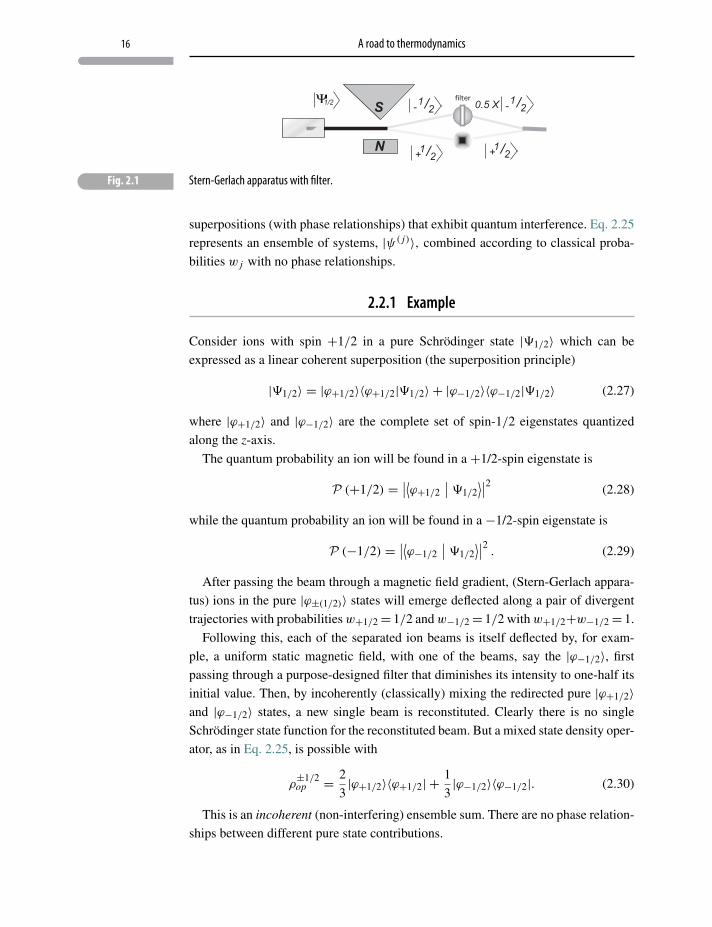
� Fig. 2.1 Stern-Gerlach apparatus with filter.
superpositions (with phase relationships) that exhibit quantum interference. Eq. 2.25
represents an ensemble of systems, |ψ( j)〉, combined according to classical proba-
bilities w j with no phase relationships.
2.2.1 Example
Consider ions with spin +1/2 in a pure Schrödinger state |�1/2〉 which can be
expressed as a linear coherent superposition (the superposition principle)
|�1/2〉 = |ϕ+1/2〉〈ϕ+1/2|�1/2〉 + |ϕ−1/2〉〈ϕ−1/2|�1/2〉 (2.27)
where |ϕ+1/2〉 and |ϕ−1/2〉 are the complete set of spin-1/2 eigenstates quantized
along the z-axis.
The quantum probability an ion will be found in a +1/2-spin eigenstate is
P (+1/2) = ∣∣⟨ϕ+1/2∣∣ �1/2
⟩∣∣2 (2.28)
while the quantum probability an ion will be found in a −1/2-spin eigenstate is
P (−1/2) = ∣∣⟨ϕ−1/2∣∣ �1/2
⟩∣∣2 . (2.29)
After passing the beam through a magnetic field gradient, (Stern-Gerlach appara-
tus) ions in the pure |ϕ±(1/2)〉 states will emerge deflected along a pair of divergent
trajectories with probabilities w+1/2= 1/2 and w−1/2= 1/2 with w+1/2+w−1/2= 1.
Following this, each of the separated ion beams is itself deflected by, for exam-
ple, a uniform static magnetic field, with one of the beams, say the |ϕ−1/2〉, first
passing through a purpose-designed filter that diminishes its intensity to one-half its
initial value. Then, by incoherently (classically) mixing the redirected pure |ϕ+1/2〉and |ϕ−1/2〉 states, a new single beam is reconstituted. Clearly there is no single
Schrödinger state function for the reconstituted beam. But a mixed state density oper-
ator, as in Eq. 2.25, is possible with
ρ±1/2op = 2
3|ϕ+1/2〉〈ϕ+1/2| + 1
3|ϕ−1/2〉〈ϕ−1/2|. (2.30)
This is an incoherent (non-interfering) ensemble sum. There are no phase relation-
ships between different pure state contributions.
17 Mixed states
2.2.2 Mixed state properties
The mixed state density operator has several properties that coincide with those of
the pure state density operator. For example:
1. Using Eqs. 2.25 and 2.26 it is easy to show that the mixed state density operator
has the normalization property
TrρMop = 1. (2.31)
2. The average value of the observable �op for the mixed state is
〈�〉 = TrρMop�op. (2.32)
3. In the mixed state the probability of measuring the observable ωs is
P(ωs) = Tr{ρM
op|ωs〉〈ωs |}. (2.33)
4. Following the steps for deriving Eq. 2.24, the mixed state density operator has an
equation of motion
∂ρMop
∂t= i
h
[ρM
op,Hop
]. (2.34)
2.2.3 Macroscopic consequences
Macroscopic systems are always quantum-coupled to their surroundings, i.e. many-
particle quantum systems entangled with their quantum environment. It is here that
distinctive characteristics of the mixed state density operator cause it to emerge as
the correct object for describing macroscopic (thermodynamic) systems.
Expanding the pure state |�〉 in a linear coherent superposition of system eigen-
states |ωi 〉,|�〉 =
∑i
|ωi 〉〈ωi |�〉, (2.35)
its corresponding density operator is
ρop =∑
i
|〈ωi |�〉|2 |ωi 〉〈ωi | +∑i �= j
|ωi 〉ρi j 〈ω j | (2.36)
whose off-diagonal terms are typical of quantum interference.
The density operator formulation accommodates an approach in which a system,
such as defined by Eq. 2.35, interacts with a quantum environment resulting in an
entangled system–environment density operator. Later, the uninteresting and unmea-
surable environmental degrees of freedom are identified and summed (traced) out,
leaving a reduced density operator consisting of two components.
18 A road to thermodynamics
• The first component is a mixed state density operator ρsop of the system alone,
independent of the environment,
ρsop =
∑i
|〈ωi |�〉|2|ωi 〉〈ωi |. (2.37)
Here P (ωi ) = |〈ωi |�〉|2 are the probabilities of Eq. 2.16 for which∑i
P (ωi ) = 1. (2.38)
Clearly ρsop has less than complete system information.
• The second component is a sum of off-diagonal interference terms containing a
system–environment interaction dependent factor that rapidly decays with time.
This term represents information “lost” to the environment.
The density operator sum of Eqs. 2.37 represents an ensemble of pure system states
having all the mixed state properties exhibited in Eqs. 2.31–2.34.
With the loss of non-diagonal interference terms, the reduced density operator has
crossed a boundary from pure quantum results (displaying interference) into a clas-
sical regime with no quantum interference. This is the meaning and consequence of
entangled environmental decoherence.9−12 Using ρsop macroscopic system averages
can now – in principle – be calculated.
The equation of motion for the density operator ρsop is found by the method leading
to Eq. 2.34, and gives
∂ρsop
∂t= i
h
[ρs
op,Hop
]. (2.39)
Since we are interested in thermal equilibrium, i.e. thermodynamic variables are
not on average changing in time, we also require
∂ρsop
∂t= 0. (2.40)
It therefore follows that at thermal equilibrium[ρs
op,Hop
]= 0, (2.41)
i.e. the mixed state density operator ρsop and the quantum mechanical hamiltonian
Hop commute, guaranteeing that the density operator and the hamiltonian have the
9 E. Joos and H. D. Zeh, “The emergence of classical properties through interaction with the environ-ment”, Z. Phys. B 59, 223 (1985).
10 E. Joos, H. D. Zeh, et al. Decoherence and the Appearance of a Classical World in Quantum Theory,Springer, Berlin (2003).
11 W. H. Zurek, “Decoherence and the transition to the classical”, Phys. Today 44, 36–44 (1991).12 Maximilian Schlosshauer, Decoherence and the Quantum to Classical Transition, Springer, New York
(2007).
19 Mixed states
same set of macroscopic eigenstates. Specifically basing Eq. 2.35 on the linear super-
position generated from the eigenstates of
Hop|Es〉 = Es |Es〉, (2.42)
where Es are macroscopic system eigen-energies and |Es〉 are corresponding
eigenstates, entangled environmental coupling reduces Eq.2.37 to a specific thermal
density operator
ρτop =
∑s
P(Es)|Es〉〈Es |, (2.43)
which commutes with Hop as required and where P(Es) are probabilities the macro-
scopic system has eigen-energies Es .13
2.2.4 Thermodynamic state functions(?)
Applying the hamiltonian of Eq.1.12 the spectrum of macroscopic internal eigen-
energies14 can be found from
hop|εs〉 = εs |εs〉. (2.44)
Furthermore with these eigenstates a thermal density operator can be constructed
ρτop =
∑s
P(εs)|εs〉〈εs | (2.45)
from which, in principle, we can find the following.
1. Internal energy U
U = Trρτophop (2.46)
=∑
s
εsP (εs) . (2.47)
2. Internal pressure p
p = Trρτop
(−∂hop
∂V
). (2.48)
3. Internal energy fluctuations 〈(�U)2〉〈(�U)2〉 = Trρτ
op
(hop − 〈hop〉
)2 (2.49)
= 〈h2op〉 − 〈hop〉2. (2.50)
13 In non-equilibrium thermodynamics ∂ρτop/∂t �= 0, which requires evaluation of Eq. 2.39. This equation
can be studied by a systematic thermodynamic perturbation theory.14 Internal energy is generally taken to be the kinetic and potential energy of constituent particles. Total
energy, on the other hand, reflects energy contributions from all interactions.
20 A road to thermodynamics
Thermodynamics is beginning to emerge from quantum theory. However, there
remains an obstacle – no measurement or set of independent measurements can reveal
ρτop, suggesting that ρτ
op are unknowable! Is this fatal? The question is addressed in
Chapter 6.
2.3 Thermal density operator ρτop and entropy
Macroscopic quantum systems are entangled with an environment. As a result:
1. They are not isolated.
2. They are not representable as pure Schrödinger states.
3. They “leak” information to their environment.
As defined in Eq. 2.1815,16 purity covers the range of values
0 < I = Tr(ρτ
op
)2 ≤ 1 (2.51)
(see Appendix A).
Now, beginning an adventurous progression, purity is replaced by an alternative
logarithmic scale
s = − ln Tr(ρτ
op
)2, (2.52)
which, according to Eq. 2.51, now covers the range 0 ≤ s <∞, where
s = 0 ⇒ complete information, (2.53)
s > 0 ⇒ missing information. (2.54)
Finally, a more physically based alternative to purity (see Appendix B) is defined
as
F = −κ Trρτop ln ρτ
op, (2.55)
where κ is a real, positive scale constant.17 It covers the same range as s but with
different scaling:
F = 0 ≡ complete information (biased probabilities)⇒ pure state,
F > 0 ≡ incomplete information (unbiased probabilities)⇒ mixed state.
Although as introduced here F appears nearly identical to the quantity Gibbs called
entropy, it is not yet the entropy of thermodynamics. As in Example 2.2 below (and
15 The following result is proved in Appendix A.16 Zero “purity” means that all outcomes are equally likely.17 In thermodynamics κ → kB T (Boltzmann’s constant× temperature.)
21 Thermal density operator ρτop and entropy
everywhere else in this book), only the maximum value assumed by F , i.e. Fmax ,
can claim distinction as entropy.
Even quantum mechanics’ exceptional power offers no recipe for finding ρτop (see
Eq. 2.43). Overcoming this obstacle requires that we look outside quantum mechan-
ics for a well-reasoned postulate whose results accord with the measurable, macro-
scopic, physical universe. This is the subject of Chapter 6.
2.3.1 Examples
Example 2.1
Consider a density matrix
ρ =(
1 0
0 0
). (2.56)
After matrix multiplication
(ρ)2 =(
1 0
0 0
)(1 0
0 0
)
=(
1 0
0 0
), (2.57)
so its corresponding purity I = Tr (ρ)2 is
I = Tr (ρ)2 (2.58)
= 1, (2.59)
corresponding to total information – a pure state (totally biased probabilities.) As
introduced in Eq. 2.55,
F/κ = −Trρ ln ρ, (2.60)
whose evaluation requires a little analysis.
If f (M) is a function of the operator or matrix M, then its trace Tr f (M) can be
evaluated by first assuming that the function f (M) implies a power series in that
matrix. For example,
eM = 1+M+ 1
2M2 + · · · . (2.61)
Then, since the trace of an operator (matrix) is independent of the basis in which it
is taken, the trace can be written
Tr f (M) =∑
m
〈m| f (M) |m〉, (2.62)
22 A road to thermodynamics
where the matrix 〈m| f (M) |m〉 is in the basis that diagonalizes M,
M|m〉 = μm |m〉, (2.63)
with μm the eigenvalues of M and |m〉 its eigenfunctions. Referring to Eq. 2.56 we
see ρ is already diagonal with eigenvalues {0, 1}. Therefore18
Fκ= −{1× ln (1)+ 0× ln (0)} (2.64)
= 0, (2.65)
corresponding to a pure state – maximal information (totally biased probabilities).
Example 2.2
Now consider the density matrix
ρ =⎛⎜⎝ 1
20
01
2
⎞⎟⎠ (2.66)
for which matrix multiplication gives
(ρ)2 =⎛⎜⎝ 1
20
01
2
⎞⎟⎠⎛⎝ 1
20
01
2
⎞⎠
=⎛⎜⎝ 1
40
01
4
⎞⎟⎠ . (2.67)
Therefore its purity I is
Tr (ρ)2 = 1
2, (2.68)
which corresponds to a mixed state with less than maximal information. The matrix
of Eq. 2.66, which is already diagonal with eigenvalues{
12 ,
12
}, has
Fk= −
{1
2× ln
(1
2
)+ 1
2× ln
(1
2
)}(2.69)
= ln 2, (2.70)
also implying missing information – not a pure state. Moreover, for a two-
dimensional density matrix F/k = ln 2 is the highest value F/k can attain. This
maximal value, Fmax/k= ln 2, describes least biased probabilities. Furthermore,
18 limx→0
x ln x = 0.
23 Problems and exercises
Fmax is now revealed as the entropy of thermodynamics – the quantity invented by
Clausius,19 interpreted by Boltzmann20 and formalized by Gibbs and especially von
Neumann21,22 (see Appendix B).
Problems and exercises
2.1 In a two-dimensional space a density matrix (hermitian with Trρ = 1) is
ρ =(
α X
X∗ 1− α
).
a. Calculate F/κ = −Trρ ln ρ as a function of α and X .
b. Find α and X that minimize F/κ . What is Fmin/κ?
c. Find α and X that maximize F/κ . What is the entropy Fmax/κ? (See
Section 2.3.1.)
2.2 In a three-dimensional space a density matrix (hermitian with Trρ = 1) is
ρ =⎛⎜⎝ α1 X Y
X∗ α2 Z
Y ∗ Z∗ 1− α1 − α2
⎞⎟⎠ .
Find X, Y, Z , α1 and α2 that maximize F/kB . What is the entropy Fmax/kB?
2.3 Consider two normalized pure quantum states:
|ψ1〉 = 1√3| + 1
2 〉 + ı
√2
3| − 1
2 〉, (2.71)
|ψ2〉 = 1√5| + 1
2 〉 −2√5| − 1
2 〉. (2.72)
where | + 12 〉 and | − 1
2 〉 are orthonormal eigenstates of the operator Sz . Let
them be incoherently mixed by some machine in equal proportions, i.e. w1 =w2 = 1
2 .
a. Find the two-dimensional density matrix (in the basis | + 12 〉, | − 1
2 〉)corresponding to this mixed state.
19 R. Clausius, The Mechanical Theory of Heat, with its Applications to the Steam-Engine and to thePhysical Properties of Bodies, John Van Voorst, London (1867).
20 Ludwig Boltzmann, “Uber die Mechanische Bedeutung des Zweiten Hauptsatzes der Warmetheorie”,Wiener Berichte 53, 195–220 (1866).
21 John von Neumann, Mathematical Foundations of Quantum Mechanics, Princeton University Press(1996).
22 Entropy was also introduced in a context of digital messaging information by Claude Shannon, “Amathematical theory of communication”, Bell System Technical Journal 27, 379–423, 623–656 (1948).
24 A road to thermodynamics
b. Find the average value 〈Sz〉 in a measurement of the mixed state’s Sz spin
components.
c. Find F/κ for this mixed state.
2.4 Consider two normalized pure quantum states:
|ψ1〉 = 1√3| + 1
2 〉 + ı
√2
3| − 1
2 〉 (2.73)
|ψ2〉 = 1√5| + 1
2 〉 −2√5| − 1
2 〉. (2.74)
where | + 12 〉 and | − 1
2 〉 are orthonormal eigenstates of the operator Sz . Let
them be incoherently mixed by some machine such that w1 = 13 , w2 = 2
3 .
a. Find the two-dimensional density matrix (in the basis | + 12 〉, | − 1
2 〉)corresponding to this mixed state.
b. Find the average value 〈Sz〉 in a measurement of the mixed state’s Sz spin
components.
c. Find F/κ for this mixed state.
3 Work, heat and the First Law
. . . there is in the physical world one agent only, and this is called Kraft [energy].It may appear, according to circumstances, as motion, chemical affinity, cohe-sion, electricity, light and magnetism; and from any one of these forms it can betransformed into any of the others.
Karl Friedrich Mohr, Zeitschrift für Physik (1837)
3.1 Introduction
Taking respectful note of Professor Murray Gell-Mann’s epigraphic remark in
Chapter 2, a respite from quantum mechanics seems well deserved. Therefore, the
discussion in Chapter 1 is continued with a restatement of the First Law of Thermo-
dynamics:
ΔU = Q−W, (3.1)
where U is internal energy, a thermodynamic state function with quantum founda-
tions. In this chapter the “classical” terms W (work) and Q (heat) are discussed,
followed by a few elementary applications.
3.1.1 Work, W
Work W is energy transferred between a system and its surroundings by mechan-
ical or electrical changes at its boundaries. It is a notion imported from Newton’s
mechanics with the definition
W =∫
F · dr, (3.2)
where F is an applied force and dr is an infinitesimal displacement. The integral is
carried out over the path of the displacement.
Work is neither stored within a system nor does it describe any state of the system.
Therefore ΔW ?=W f inal −Wini tial has absolutely no thermodynamic meaning!
Incremental work, on the other hand, can be defined as d−W , with finite work being
the integral
W =∫
d−W. (3.3)
25
26 Work, heat and the First Law
The bar on the d is a reminder that d−W is not a true mathematical differential and
that the integral in Eq. 3.3 depends on the path.1
Macroscopic parameters are further classified as:
• extensive – proportional to the size or quantity of matter (e.g. energy, length, area,
volume, number of particles, polarization, magnetization);
• intensive – independent of the quantity of matter (e.g. force, temperature, pressure,
density, tension, electric field, magnetic field).
Incremental work has the generalized meaning of energy expended by/on the system
due to an equivalent of force (intensive) acting with an infinitesimal equivalent of
displacement (extensive) which, in accord with Eq. 3.2, is written as the “conjugate”
pair,
d−W =∑
j
F j︸︷︷︸intensive
extensive︷︸︸︷dx j , (3.4)
where F j is generalized force and dx j is its conjugate differential displacement.
If work takes place in infinitesimal steps, continually passing through equilibrium
states, the work is said to be quasi-static and is distinguished by the representation
d−WQS .
Examples of conjugate “work” pairs, intensive↔ d(extensive) are:
• pressure (p)↔ volume (dV );• tension (τ )↔ elongation (dχ);• stress (σ )↔ strain (dε);• surface tension (Σ)↔ surface area (dAS);• electric field (E)↔ polarization (dP);• magnetic field (B)↔ magnetization (dM);2• chemical potential (μ)↔ particle number (dN ).
(It is often helpful in thermodynamics to think of mechanical work as the equivalent
of raising and lowering weights external to the system.)
Finite work, as expressed by Eq. 3.3, depends on the details of the process and not
just on the process end-points.
The sign convention adopted here3 is
d−W > 0 ⇒ system performs work(
d−Wgasby = p dV
),
d−W < 0 ⇒ work done on the system(d−Wgas
on = −p dV).
1 Work is not a function of independent thermal variables so that d−W cannot be an exact differential.2 The fields used in accounting for electric and magnetic work will be further examined in Chapter 11.3 In the case of pressure and volume as the conjugate pair.
27 Introduction
3.1.2 Heat, Q
Heat Q is energy transferred between a system and any surroundings with which
it is in diathermic contact. Q is not stored within a system and is not a state of
a macroscopic system. Therefore ΔQ ?= Q f inal −Qini tial has no thermodynamic
meaning! On the other hand, incremental heat is defined as d−Q, with finite heat Q as
the integral
Q =∫
d−Q. (3.5)
Finite heat depends on the details of the process and not just the integral’s end-points.
The bar on the d is an essential reminder that d−Q is not a function of tempera-
ture or any other independent variables. It is not a true mathematical differential so
“derivatives” like d−QdT have dubious meaning.
Processes for which Q = 0, either by thermal isolation or by extreme rapidity (too
quickly to exchange heat), are said to be adiabatic.
3.1.3 Temperature, T
Temperature is associated with a subjective sense of “hotness” or “coldness”. How-
ever, in thermodynamics temperature has empirical (objective) meaning through ther-
mometers – e.g. the height of a column of mercury, the pressure of an ideal gas in
a container with fixed volume, the electrical resistance of a length of wire – all of
which vary in a way that allows a temperature scale to be defined. Since there is no
quantum hermitian “temperature operator”, a formal, consistent definition of tem-
perature is elusive. But it is achievable in practice through thermal measurements4
showing, with remarkable consistency, how and where it thermodynamically appears
and that it measures the same property as the common thermometer.
3.1.4 Internal energy, U
As discussed in Chapter 1, internal energy U is a state of the system. Therefore ΔUdoes have meaning and dU is an ordinary mathematical differential5 with
ΔU = U(B)− U(A) =B∫
A
dU, (3.6)
where A and B represent different macroscopic equilibrium states. Clearly, ΔUdepends only on the end-points of the integration and not on any particular ther-
modynamic process (path) connecting them.
4 This subject will be discussed in Chapter 6.5 It is called an exact differential.
28 Work, heat and the First Law
3.2 Exact differentials
All thermodynamic state variables are true (exact) differentials with change in valueas defined in Eq. 3.6. Moreover, state variables are not independent and can be func-tionally expressed in terms of other state variables. Usually only a few are needed tocompletely specify any state of a system. The precise number required is the contentof an important result which is stated here without proof:
The number of independent parameters needed to specify a thermodynamic stateis equal to the number of distinct conjugate pairs (see Section 3.1.1) of quasi-staticwork needed to produce a differential change in the internal energy – plus ONE.6
For example, if a gas undergoes mechanical expansion or compression, the only
quasi-static work is mechanical work, d−WQS = p dV . Therefore only two variables
are required to specify a state. We could then write the internal energy of a system
as a function of any two other state parameters. For example, we can write U =U (T, V ) or U = U(p, V ). To completely specify the volume of a gas we could
write V = V (p, T ) or even V = V (p,U) . The choice of functional dependences is
determined by the physical situation and computational objectives.
If physical circumstances dictate particle number changes, say by evaporation of
liquid to a gas phase or condensation of gas to the liquid phase, or chemical reactions
where atomic or molecular species are lost or gained, a thermodynamic description
requires “chemical work” d−WQS = −μ dN , where dN is an infinitesimal change in
particle number andμ is the (conjugate) chemical potential. Chemical potentialμ is an
intensive variable denoting energy per particle while particle number N is obviously
an extensive quantity. For cases where there is both mechanical and chemical work,
d−WQS = p dV − μ dN , (3.7)
three variables are required and, for example, U = U(T, V, N ) or U = U(p, V, μ).
Incorporating the definitions above, an incremental form of the First Law of Ther-
modynamics is
dU = d−Q− d−W. (3.8)
3.3 Equations of state
Equations of state are functional relationships among a system’s equilibrium state
parameters – usually those that are most easily measured and controlled in the
6 The ONE of the plus ONE originates from the conjugate pair T and dS, where S is entropy, aboutwhich much will be said throughout the remainder of this book. T dS can be thought of as quasi-staticthermal work.
29 Equations of state
laboratory. Determining equations of state, by experiment or theory, is often a primary
objective in practical research, for then thermodynamics can fulfill its role in under-
standing and predicting state parameter changes for particular macroscopic systems.
The following are samples of equations of state for several different types of
macroscopic systems. Their application is central in the Examples subsections below.
1. Equations of state for gases (often called gas laws) take the functional form
f (p, V, T ) = 0, where p is the equilibrium internal gas pressure, V is the gas
volume, T is the gas temperature and f defines the functional relationship. For
example, a gas at low pressure and low particle density, n = N/V , where N is
the number of gas particles (atoms, molecules, etc.), has the equation of state
p − (N/V ) kB T = 0 (3.9)
or, more familiarly (the ideal gas law),
pV = NkB T, (3.10)
where kB is Boltzmann’s constant.7,8
2. An approximate equation of state for two- and three-dimensional metallic mate-
rials is usually expressed as g(σ, ε, T ) = 0, where σ = τ/A is the stress,
ε = (� − �0)/�0 is the strain,9 T is the temperature, and A is the cross-sectional
area. An approximate equation of state for a metal rod is the Hookian behavior
ε = κ σ (3.11)
where κ is a material-specific constant.
3. An equation of state for a uniform one-dimensional elastomeric (rubber-like)
material has the form Λ(τ, χ, T ) = 0, where τ is the equilibrium elastic tension,
χ is the sample elongation, T is the temperature and Λ is the functional relation-
ship. For example, a rubber-like polymer that has not been stretched beyond its
elastic limit can have the simple equation of state
τ −K Tχ = 0, (3.12)
or
σ −K ′T ε = 0, (3.13)
where K and K ′ are material-specific elastic constants.10,11
7 For a derivation see Chapter 7.8 For gases under realistic conditions Eq. 3.10 may be inadequate requiring more complicated equations
of state. Nevertheless, because of its simplicity and “zeroth order” validity, the ideal gas “law” ispervasive in models and exercises.
9 � is the stretched length and �0 is the unstretched length.10 H. M. James and E. Guth, “Theory of elastic properties of rubber”, J. Chem. Phys. 11, 455–481 (1943).11 Comparing these equations of state with Eq. 3.11 suggests a physically different origin for rubber
elasticity. This will be explored in Chapter 10.
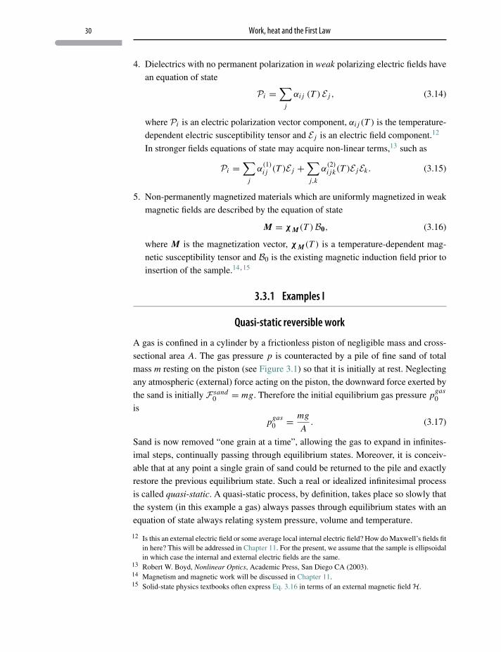
30 Work, heat and the First Law
4. Dielectrics with no permanent polarization in weak polarizing electric fields have
an equation of state
Pi =∑
j
αi j (T ) E j , (3.14)
where Pi is an electric polarization vector component, αi j (T ) is the temperature-
dependent electric susceptibility tensor and E j is an electric field component.12
In stronger fields equations of state may acquire non-linear terms,13 such as
Pi =∑
j
α(1)i j (T )E j +
∑j,k
α(2)i jk(T )E jEk . (3.15)
5. Non-permanently magnetized materials which are uniformly magnetized in weak
magnetic fields are described by the equation of state
M = χ M(T )B0, (3.16)
where M is the magnetization vector, χ M(T ) is a temperature-dependent mag-
netic susceptibility tensor and B0 is the existing magnetic induction field prior to
insertion of the sample.14,15
3.3.1 Examples I
Quasi-static reversible work
A gas is confined in a cylinder by a frictionless piston of negligible mass and cross-
sectional area A. The gas pressure p is counteracted by a pile of fine sand of total
mass m resting on the piston (see Figure 3.1) so that it is initially at rest. Neglecting
any atmospheric (external) force acting on the piston, the downward force exerted by
the sand is initially F sand0 = mg. Therefore the initial equilibrium gas pressure pgas
0
is
pgas0 = mg
A. (3.17)
Sand is now removed “one grain at a time”, allowing the gas to expand in infinites-
imal steps, continually passing through equilibrium states. Moreover, it is conceiv-
able that at any point a single grain of sand could be returned to the pile and exactly
restore the previous equilibrium state. Such a real or idealized infinitesimal process
is called quasi-static. A quasi-static process, by definition, takes place so slowly that
the system (in this example a gas) always passes through equilibrium states with an
equation of state always relating system pressure, volume and temperature.
12 Is this an external electric field or some average local internal electric field? How do Maxwell’s fields fitin here? This will be addressed in Chapter 11. For the present, we assume that the sample is ellipsoidalin which case the internal and external electric fields are the same.
13 Robert W. Boyd, Nonlinear Optics, Academic Press, San Diego CA (2003).14 Magnetism and magnetic work will be discussed in Chapter 11.15 Solid-state physics textbooks often express Eq. 3.16 in terms of an external magnetic field H.
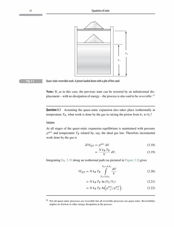
31 Equations of state
� Fig. 3.1 Quasi-static reversible work. A piston loaded down with a pile of fine sand.
Note: If, as in this case, the previous state can be restored by an infinitesimal dis-
placement – with no dissipation of energy – the process is also said to be reversible.16
Question 3.1 Assuming the quasi-static expansion also takes place isothermally at
temperature TR , what work is done by the gas in raising the piston from h1 to h2?
Solution
At all stages of the quasi-static expansion equilibrium is maintained with pressure
pgas and temperature TR related by, say, the ideal gas law. Therefore incremental
work done by the gas is
d−WQS = pgas dV (3.18)
= N kB TR
VdV . (3.19)
Integrating Eq. 3.19 along an isothermal path (as pictured in Figure 3.2) gives
WQS = N kB TR
V2=A h2∫V1=A h1
dV
V(3.20)
= N kB TR ln (V2/V1) (3.21)
= N kB TR ln(
pgas− f /pgas
−o
). (3.22)
16 Not all quasi-static processes are reversible but all reversible processes are quasi-static. Reversibilityimplies no friction or other energy dissipation in the process.
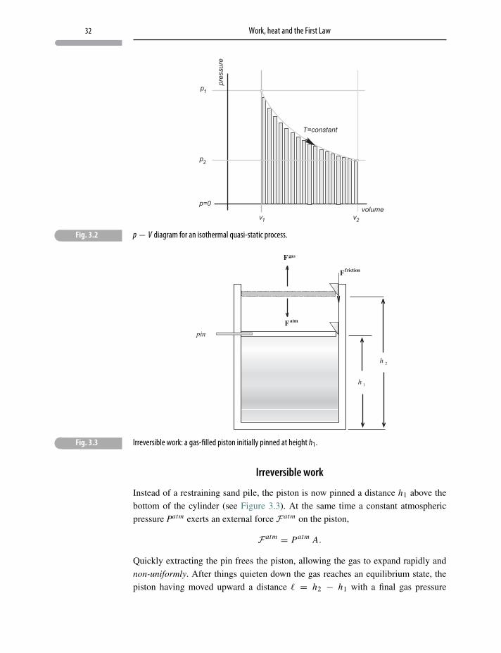
32 Work, heat and the First Law
� Fig. 3.2 p− V diagram for an isothermal quasi-static process.
gas
atm
friction
� Fig. 3.3 Irreversible work: a gas-filled piston initially pinned at height h1.
Irreversible work
Instead of a restraining sand pile, the piston is now pinned a distance h1 above the
bottom of the cylinder (see Figure 3.3). At the same time a constant atmospheric
pressure Patm exerts an external force Fatm on the piston,
Fatm = Patm A.
Quickly extracting the pin frees the piston, allowing the gas to expand rapidly and
non-uniformly. After things quieten down the gas reaches an equilibrium state, the
piston having moved upward a distance � = h2 − h1 with a final gas pressure
33 Equations of state
pgasf = Patm . This isothermal process is characterized by a finite expansion rate and
system (gas) non-uniformity. It is neither quasi-static nor reversible.17
Question 3.2 What isothermal work is done by the rapidly expanding gas in raising
the piston a distance �?
Solution
The gas expands irreversibly so that during expansion a gas law does not apply. But
initially the gas has equilibrium pressure pgas0 with volume V0,
V0 = NkB T
pgas0
. (3.23)
After the piston ceases its erratic motion it returns to rest with the gas in equilibrium
at atmospheric pressure,
pgasf = Patm, (3.24)
with volume
V f = NkB T
Patm. (3.25)
During expansion the gas lifts the piston against a constant force Fatm (equivalent
to raising a weight mg = Fatm in the Earth’s gravitational field).18 The incremental,
irreversible work done by the confined gas (the system) is
d−W = Patm dV (3.26)
which, with constant Patm , is integrated to give
W = Patm (V f − V0). (3.27)
With Eqs. 3.23 and 3.25
W = NkB T
[1− Patm
pgas0
]. (3.28)
17 All real processes in nature are irreversible. Reversibility is a convenient idealization for thermody-namic modeling.
18 The piston starts at rest and returns to rest. There is no change in the piston’s kinetic energy.
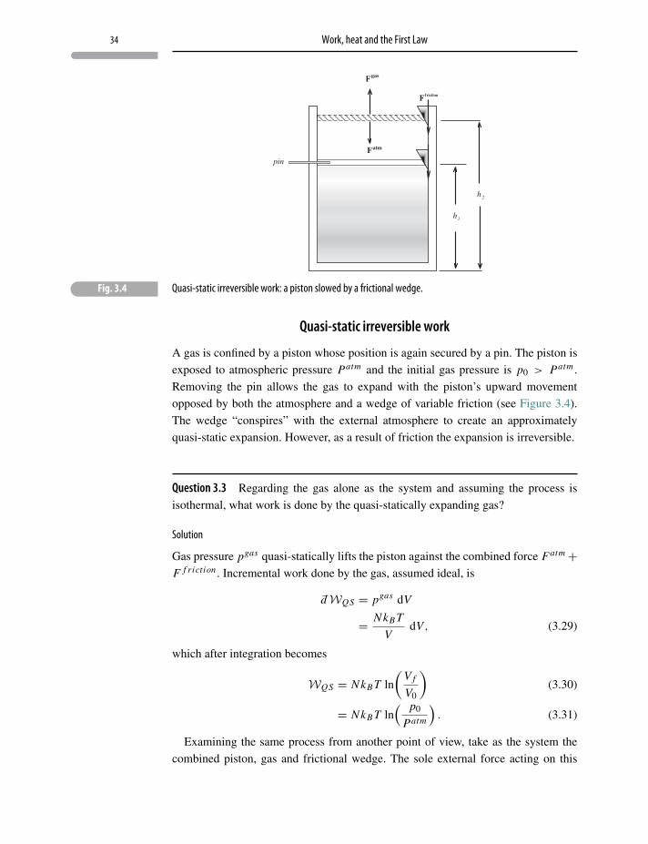
34 Work, heat and the First Law
friction
� Fig. 3.4 Quasi-static irreversible work: a piston slowed by a frictional wedge.
Quasi-static irreversible work
A gas is confined by a piston whose position is again secured by a pin. The piston is
exposed to atmospheric pressure Patm and the initial gas pressure is p0 > Patm .
Removing the pin allows the gas to expand with the piston’s upward movement
opposed by both the atmosphere and a wedge of variable friction (see Figure 3.4).
The wedge “conspires” with the external atmosphere to create an approximately
quasi-static expansion. However, as a result of friction the expansion is irreversible.
Question 3.3 Regarding the gas alone as the system and assuming the process is
isothermal, what work is done by the quasi-statically expanding gas?
Solution
Gas pressure pgas quasi-statically lifts the piston against the combined force Fatm+F f riction . Incremental work done by the gas, assumed ideal, is
d−WQS = pgas dV
= NkB T
VdV, (3.29)
which after integration becomes
WQS = NkB T ln
(V f
V0
)(3.30)
= NkB T ln( p0
Patm
). (3.31)
Examining the same process from another point of view, take as the system the
combined piston, gas and frictional wedge. The sole external force acting on this
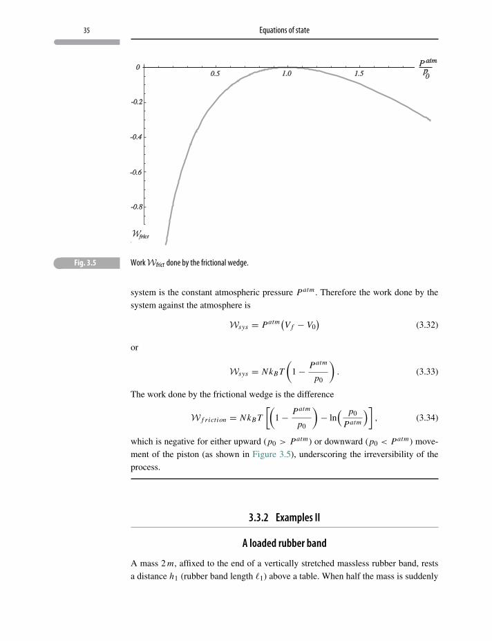
35 Equations of state
� Fig. 3.5 WorkWfrict done by the frictional wedge.
system is the constant atmospheric pressure Patm . Therefore the work done by the
system against the atmosphere is
Wsys = Patm(V f − V0)
(3.32)
or
Wsys = NkB T
(1− Patm
p0
). (3.33)
The work done by the frictional wedge is the difference
W f r iction = NkB T
[(1− Patm
p0
)− ln
( p0
Patm
)], (3.34)
which is negative for either upward (p0 > Patm) or downward (p0 < Patm) move-
ment of the piston (as shown in Figure 3.5), underscoring the irreversibility of the
process.
3.3.2 Examples II
A loaded rubber band
A mass 2 m, affixed to the end of a vertically stretched massless rubber band, rests
a distance h1 (rubber band length �1) above a table. When half the mass is suddenly
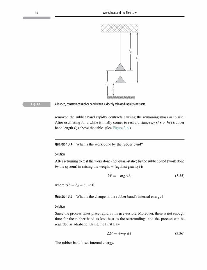
36 Work, heat and the First Law
� Fig. 3.6 A loaded, constrained rubber band when suddenly released rapidly contracts.
removed the rubber band rapidly contracts causing the remaining mass m to rise.
After oscillating for a while it finally comes to rest a distance h2 (h2 > h1) (rubber
band length �2) above the table. (See Figure 3.6.)
Question 3.4 What is the work done by the rubber band?
Solution
After returning to rest the work done (not quasi-static) by the rubber band (work done
by the system) in raising the weight m (against gravity) is
W = −mg��, (3.35)
where �� = �2 − �1 < 0.
Question 3.5 What is the change in the rubber band’s internal energy?
Solution
Since the process takes place rapidly it is irreversible. Moreover, there is not enough
time for the rubber band to lose heat to the surroundings and the process can be
regarded as adiabatic. Using the First Law
�U = +mg ��. (3.36)
The rubber band loses internal energy.
37 Equations of state
Question 3.6 This time, to counteract rubber elasticity, the total mass 2 m is restrained
to rise slowly (quasi-statically) but isothermally. What is the work done by the con-
tracting rubber band?
Solution
We can safely use an equilibrium tension (an elastic state parameter) which acts to
raise the weight. The incremental quasi-static elastic work done by the system is
d−WQS = −τ dχ, (3.37)
where dχ is the differential of elastic extension. Using the “rubber” equation of state,
Eq. 3.12, and integrating over the range of extension χ ,
WQS = −K ′ T0∫
−��
χ dχ (3.38)
= K ′ T (��)2 . (3.39)
A compressed metal rod
A metal rod, cross-sectional area A, is suddenly struck by a sledgehammer, subject-
ing it to a transient but constant compressive (external) force F which momentarily
changes the rod’s length by �� = � f − �0 < 0.
Question 3.7 What is the work done on the rod during the interval that its length
decreases by |��|?
Solution
Sudden compression of the rod implies that it does not pass through equilibrium
states so an equilibrium internal stress in the bar σ = f/A is not defined. But the
mechanical work done on the rod by the constant compressive force is, however,
W = −F ��. (3.40)
Question 3.8 On the other hand, if the rod could be compressed infinitely slowly
(perhaps by a slowly cranked vise) the rod’s internal stress is a well-defined equi-
librium property and the quasi-static incremental work done by the system (i.e.
the rod) is
d−WQS = −Vσ dε, (3.41)
38 Work, heat and the First Law
where V is the rod’s volume, σ is the internal stress and dε = (d�/�) defines the
differential strain. What is the work done by the rod?
Solution
We could now apply an approximate equation of state, such as Eq. 3.11, and get
WQS = −V
ε f∫ε0
(ε/κ) dε (3.42)
= − (V/2κ)(ε2
f − ε20
). (3.43)
3.4 Heat capacity
An infinitesimal amount of thermal energy d−QQS quasi-statically entering or leaving
a system generally produces an infinitesimal change in temperature dT ,
d−QQS = Cα dT (constant α). (3.44)
(Exceptions are certain first-order phase transitions, such as boiling of water or melt-
ing of ice.) The proportionality constant between the two infinitesimals, Cα , together
with the list of state variables, α, that are fixed during the quasi-static process, is
called heat capacity at constant α.19 The units of heat capacity are energy K−1. Spe-
cific heats are alternative intensive quantities, having units energy K−1 per unit mass
or energy K−1 per mole.
3.4.1 Heat transfer at constant volume
If heat is transferred at constant volume,20 by the “definition” in Eq. 3.44,
d−QQS = CV dT (constant volume). (3.45)
Heat capacities can be equivalently expressed in terms of partial derivatives of
state parameters. For example, if a gas performs only quasi-static mechanical work,
the infinitesimal First Law for the process is
dU = d−QQS − p dV, (3.46)
19 The term heat capacity is a legacy from early thermodynamics when heat was regarded as a storedquantity. Although we now know better, the language seems never to have similarly evolved.
20 And constant particle number.
39 Heat capacity
where p dV is quasi-static incremental work done by the gas (system). Since for
this case U can be expressed in terms of two other thermal parameters, choose U =U (T, V ) so that its total differential is
dU =(∂U∂V
)T
dV +(∂U∂T
)V
dT (3.47)
and Eq. 3.46 can then be rewritten
d−QQS =[(
∂U∂V
)T+ p
]dV +
(∂U∂T
)V
dT . (3.48)
Thus, for an isochoric (constant volume) path, i.e. dV = 0,
d−QQS =(∂U∂T
)V
dT (3.49)
and from Eq. 3.45
CV =(∂U∂T
)V. (3.50)
3.4.2 Heat transfer at constant pressure
Thermodynamic experiments, especially chemical reactions, are often carried out in
an open atmosphere where the pressure is constant. In such cases we define
d−QQS = Cp dT (constant pressure). (3.51)
Expressing Cp as the partial derivative of a state parameter requires introducing a
new, abstract, state variable. Here again the infinitesimal First Law description of the
quasi-static process is
dU = d−QQS − p dV . (3.52)
But this time, using
d (pV ) = p dV + V dp, (3.53)
Eq. 3.52 can be rewritten as
d−QQS = d (U + pV )− V dp. (3.54)
Defining
H = U + pV, (3.55)
where H – also a state function – is called enthalpy,21 permits recasting a “new”
differential “law”:
d−QQS = d H − V dp. (3.56)
21 Enthalpy is one of several defined state variables that are introduced to simplify specific thermody-namic constraints. In this case the constraint is constant pressure. Others will be introduced as needed.
40 Work, heat and the First Law
Then, expressing H in terms of T and p, i.e. H = H (T, p) so that a total differen-
tial is
dH =(∂H
∂p
)T
dp +(∂H
∂T
)p
dT, (3.57)
for an isobaric (constant pressure) path, i.e. dp = 0,
d−QQS =(∂H
∂T
)p
dT (3.58)
and we have the definition of Cp in terms of state variables
Cp =(∂H
∂T
)p. (3.59)
Heat capacity measurements play a surprisingly important role in exploring micro-
scopic properties of matter. The unexpectedly low temperature heat capacity of dia-
mond led to a quantum theory of the solid state. Equations of state, together with
heat capacities, can offer a complete thermal picture of most matter.
3.4.3 Examples III
Ideal monatomic gas
An ideal monatomic gas, volume V0, temperature T0, is confined by a frictionless,
movable piston to a cylinder with diathermic walls. The external face of the piston
is exposed to the atmosphere at pressure P0. A transient pulse of heat is injected
through the cylinder walls causing the gas to expand against the piston until it occu-
pies a final volume V f .
Question 3.9 What is the change in temperature of the gas?
Solution
At the beginning and end of the expansion the system is in equilibrium so that an
equation of state applies, i.e. initially P0 V0 = NkB T0 and finally P0 V f = NkB T f .
Therefore
ΔT = P0ΔV
NkB, (3.60)
where ΔT = T f − T0 and Δ V = V f − V0.
41 Heat capacity
Question 3.10 How much heat Q was in the pulse?
Solution
The gas will expand turbulently, i.e. irreversibly, against constant atmospheric pres-
sure P0 (an external “weight”) so that incremental work done by the expanding gas is
d−W = P0 dV . (3.61)
Applying the First Law
Q = ΔU + P0 ΔV (3.62)
and using Eqs. 3.47, 3.50 and 3.60, together with the ideal gas property
(∂u/∂V ) = 0, gives the internal energy change
ΔU = CV ΔT (3.63)
= CV P0ΔV
NkB. (3.64)
Thus the injected heat is
Q =( CV
NkB+ 1
)P0ΔV, (3.65)
where Eqs. 3.62 and 3.64 have been used. Using another ideal gas property22
Cp − CV = NkB (3.66)
and the definition
γ = Cp/CV , (3.67)
Eq. 3.65 can be restated as
Q = γ
γ − 1P0 ΔV . (3.68)
A steel wire
A steel wire, length L and radius ρ, is held with zero tension τ between two firmly
planted rigid vertical posts, as shown in Figure 3.7. The wire, initially at a tempera-
ture TH , is then cooled to a temperature TL .
Question 3.11 Find an expression for the tension τ in the cooled wire.
22 This well-known result for ideal gases is stated, for now, without proof.
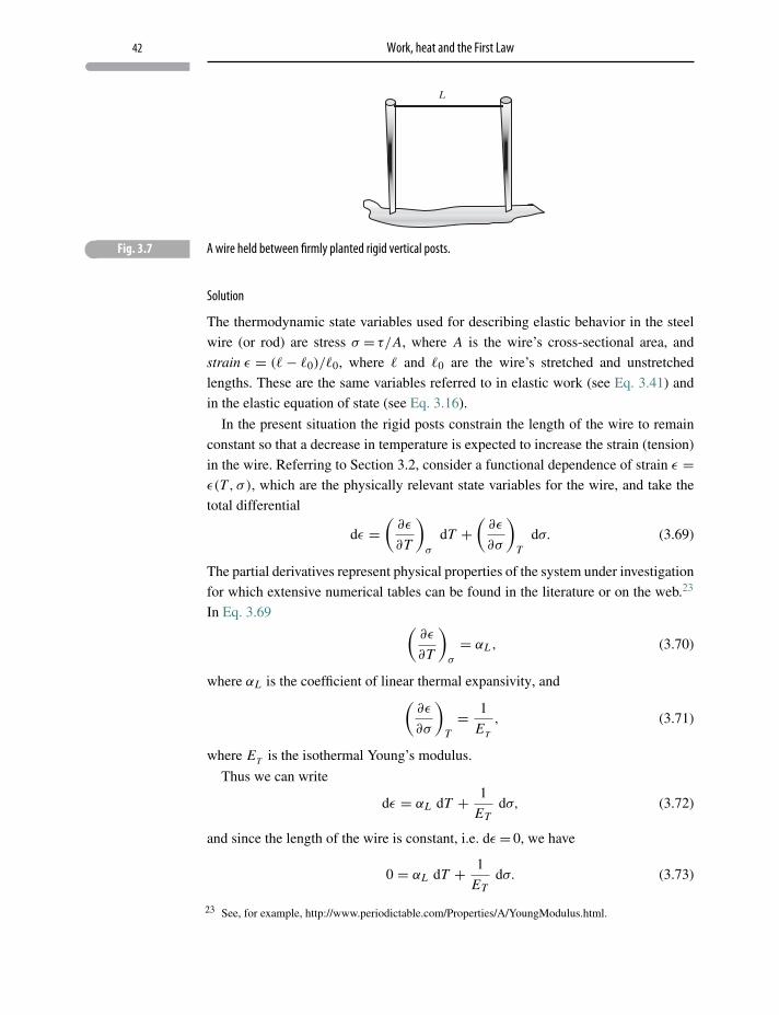
42 Work, heat and the First Law
� Fig. 3.7 A wire held between firmly planted rigid vertical posts.
Solution
The thermodynamic state variables used for describing elastic behavior in the steel
wire (or rod) are stress σ = τ/A, where A is the wire’s cross-sectional area, and
strain ε = (�− �0)/�0, where � and �0 are the wire’s stretched and unstretched
lengths. These are the same variables referred to in elastic work (see Eq. 3.41) and
in the elastic equation of state (see Eq. 3.16).
In the present situation the rigid posts constrain the length of the wire to remain
constant so that a decrease in temperature is expected to increase the strain (tension)
in the wire. Referring to Section 3.2, consider a functional dependence of strain ε =ε(T, σ ), which are the physically relevant state variables for the wire, and take the
total differential
dε =(
∂ε
∂T
)σ
dT +(
∂ε
∂σ
)T
dσ. (3.69)
The partial derivatives represent physical properties of the system under investigation
for which extensive numerical tables can be found in the literature or on the web.23
In Eq. 3.69 (∂ε
∂T
)σ
= αL , (3.70)
where αL is the coefficient of linear thermal expansivity, and(∂ε
∂σ
)T= 1
ET
, (3.71)
where ET is the isothermal Young’s modulus.
Thus we can write
dε = αL dT + 1
ETdσ, (3.72)
and since the length of the wire is constant, i.e. dε= 0, we have
0 = αL dT + 1
ETdσ. (3.73)
23 See, for example, http://www.periodictable.com/Properties/A/YoungModulus.html.
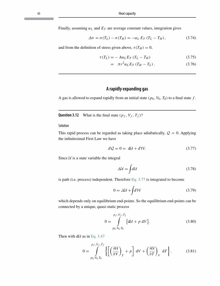
43 Heat capacity
Finally, assuming αL and ET are average constant values, integration gives
Δσ = σ(TL)− σ(TH ) = −αL ET (TL − TH ) , (3.74)
and from the definition of stress given above, τ(TH ) = 0,
τ(TL) =− AαL ET (TL − TH ) (3.75)
= πr2αL ET (TH − TL) . (3.76)
A rapidly expanding gas
A gas is allowed to expand rapidly from an initial state (p0, V0, T0) to a final state f .
Question 3.12 What is the final state (p f , V f , T f )?
Solution
This rapid process can be regarded as taking place adiabatically, Q = 0. Applying
the infinitesimal First Law we have
d−Q = 0 = dU + d−W. (3.77)
Since U is a state variable the integral
ΔU =∫
dU (3.78)
is path (i.e. process) independent. Therefore Eq. 3.77 is integrated to become
0 = ΔU +∫
d−W (3.79)
which depends only on equilibrium end-points. So the equilibrium end-points can be
connected by a unique, quasi-static process
0 =p f ,V f ,T f∫
p0,V0,T0
[dU + p dV
]. (3.80)
Then with dU as in Eq. 3.47
0 =p f ,V f ,T f∫
p0,V0,T0
{[(∂U∂V
)T+ p
]dV +
(∂U∂T
)V
dT
}. (3.81)
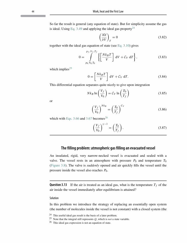
44 Work, heat and the First Law
So far the result is general (any equation of state). But for simplicity assume the gas
is ideal. Using Eq. 3.49 and applying the ideal gas property24(∂U∂V
)T= 0 (3.82)
together with the ideal gas equation of state (see Eq. 3.10) gives
0 =p f ,V f ,T f∫
p0,V0,T0
{[NkB T
V
]dV + CV dT
}, (3.83)
which implies25
0 =[
NkB T
V
]dV + CV dT . (3.84)
This differential equation separates quite nicely to give upon integration
NkB ln
(V f
V0
)= CV ln
(T0
T f
)(3.85)
or (V f
V0
)NkB
=(
T0
T f
)CV
(3.86)
which with Eqs. 3.66 and 3.67 becomes26(V f
V0
)γ−1
=(
T0
T f
). (3.87)
The filling problem: atmospheric gas filling an evacuated vessel
An insulated, rigid, very narrow-necked vessel is evacuated and sealed with a
valve. The vessel rests in an atmosphere with pressure P0 and temperature T0
(Figure 3.8). The valve is suddenly opened and air quickly fills the vessel until the
pressure inside the vessel also reaches P0.
Question 3.13 If the air is treated as an ideal gas, what is the temperature T f of the
air inside the vessel immediately after equilibrium is attained?
Solution
In this problem we introduce the strategy of replacing an essentially open system
(the number of molecules inside the vessel is not constant) with a closed system (the
24 This useful ideal gas result is the basis of a later problem.25 Note that the integral still represents Q, which is not a state variable.26 This ideal gas expression is not an equation of state.
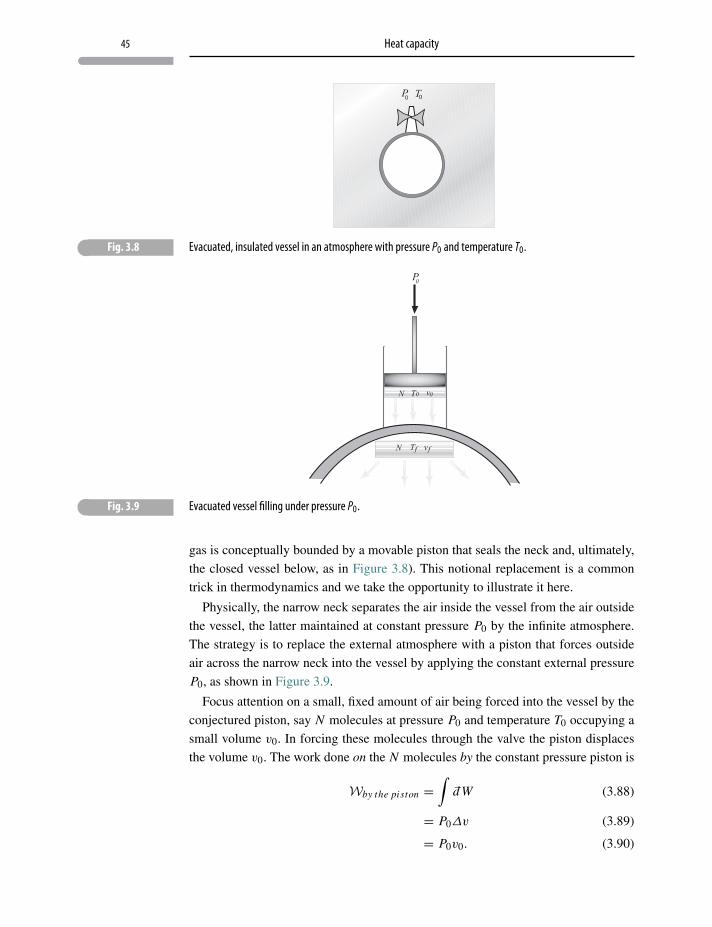
45 Heat capacity
� Fig. 3.8 Evacuated, insulated vessel in an atmosphere with pressure P0 and temperature T0.
� Fig. 3.9 Evacuated vessel filling under pressure P0.
gas is conceptually bounded by a movable piston that seals the neck and, ultimately,
the closed vessel below, as in Figure 3.8). This notional replacement is a common
trick in thermodynamics and we take the opportunity to illustrate it here.
Physically, the narrow neck separates the air inside the vessel from the air outside
the vessel, the latter maintained at constant pressure P0 by the infinite atmosphere.
The strategy is to replace the external atmosphere with a piston that forces outside
air across the narrow neck into the vessel by applying the constant external pressure
P0, as shown in Figure 3.9.
Focus attention on a small, fixed amount of air being forced into the vessel by the
conjectured piston, say N molecules at pressure P0 and temperature T0 occupying a
small volume v0. In forcing these molecules through the valve the piston displaces
the volume v0. The work done on the N molecules by the constant pressure piston is
Wby the piston =∫
d−W (3.88)
= P0Δv (3.89)
= P0v0. (3.90)
46 Work, heat and the First Law
Therefore the work done by the N molecules of gas is
Wby the gas = −P0v0. (3.91)
Once the N molecules get to the other side of the valve and enter the evacuated
rigid-walled vessel, they do no work.27 Therefore the total work done by the gas is
Wtotal = −P0 v0 + 0. (3.92)
Applying the First Law to the N molecules while approximating this sudden process
as adiabatic28
0 = ΔU +Wtotal (3.93)
or
0 = −P0v0 +f∫
0
dU . (3.94)
Choosing to write U = U (V, T ) the total differential is
dU =(∂U∂T
)V
dT +(∂U∂V
)T
dV . (3.95)
Since (∂U∂T
)V= CV (3.96)
and for an ideal gas (∂U∂V
)T= 0 (3.97)
we have
P0v0 = CV(T f − T0
). (3.98)
Then with the ideal gas equation of state
NkB T0 = CV(T f − T0
)(3.99)
followed by Eqs. 3.66 and 3.67, this becomes
T f = γ T0. (3.100)
27 This is evident since no weights are raised or lowered.28 Too fast to allow heat exchange with the external atmosphere or heat to leak outside the vessel.
47 Problems and exercises
At room temperature (T0= 300 K) and for an ideal monatomic gas (γ = 5/3),
Eq. 3.100 gives T f = 500 K, indicating a substantial rise in temperature for the gas
streaming into the vessel.
3.5 Concluding remarks
In this hiatus from quantum mechanics we have resumed the discussion of classical
thermodynamics, emphasizing the distinction between U and purely classical work
W and “heat” Q.
Chapter 4 pauses to develop some mathematical skills essential for thermody-
namic applications.
Problems and exercises
3.1 Isothermal compressibility κT is defined as
κT = − 1
V
(∂V
∂p
)T. (3.101)
a. Describe in words the meaning of κT .
b. Find κT for an ideal gas.
c. A more descriptive gas law is the van der Waals equation(p + aN 2
V 2
)(V − Nb) = NkB T, (3.102)
where the constant b describes volume excluding short-range repulsion
between gas molecules and the constant a takes account of long-range inter-
molecular attraction. Find κT for a van der Waals gas.
3.2 A thick rubber band diameter d is fastened between two rigid vertical posts
a distance L apart. When the temperature is T0 the rubber band has positive
tension τ0.
Assuming rubber has an equation of state
σ = K T ε (3.103)
at what temperature T1 will the tension be τ = 0.9τ0?
48 Work, heat and the First Law
3.3 An ideal gas expands adiabatically from the state (V0, p0) to the state (V f , p f ).
Show that the work done by the expanding gas is
W =(
p0V0 − p f V f)
γ − 1, (3.104)
where
γ = Cp
Cv. (3.105)
3.4 The constant volume heat capacity for a hypothetical nearly ideal gas is, at low
temperature,
CV = a + bT, (3.106)
where a and b are constants. Show that for an adiabatic, reversible expansion
carried out at low temperature
pV γ ≈ exp {(b/a) T } (3.107)
with
γ = Cp
Cv. (3.108)
3.5 Although the heat capacity at constant volume is
CV =(∂U∂T
)V, (3.109)
show that for the heat capacity at constant pressure
Cp �=(∂U∂T
)p
(3.110)
by proving that
Cp =(∂U∂T
)p+ pVα, (3.111)
where α is the volume thermal expansivity
α = 1
V
(∂V
∂T
)p. (3.112)
Note: The heat capacity at constant pressure is
Cp =(∂H
∂T
)p
(3.113)
where enthalpy H is defined as
H = U + pV . (3.114)
4 A mathematical digression
To those who do not know Mathematics it is difficult to get across a real feelingas to the beauty, the deepest beauty of nature. . . . If you want to learn aboutnature, to appreciate nature, it is necessary to understand the language that shespeaks in.
Richard Feynman, The Character of Physical Law, MIT Press (1967)
4.1 Thermodynamic differentials
In thermodynamics the equilibrium state of a system is described by macroscopic
variables, say U, p, T, V, . . ., which can roughly be classified as:
• variables that are readily measurable in a laboratory such as p, V, T, Cv, etc.;
• variables that are less accessible to direct measurement, e.g. U , H, and others, soon
to be introduced.
The choice of variables is generally from among those that appear in thermody-
namic laws, those that can be measured or controlled in laboratories (such as appear
in equations of state) and those defining process constraints, i.e. isothermal, isobaric
or adiabatic. Since physics of interest involves changes in equilibrium macroscopic
states, we must study differential relationships among them. Assuming a state vari-
able φ (x, y, z), where x, y, z are also (independent) state variables, these relation-
ships have the mathematical form
dφ (x, y, z, . . .) =(∂φ
∂x
)y,z,...
dx +(∂φ
∂y
)x,z,...
dy +(∂φ
∂z
)x,y,...
dz . . . ,
(4.1)
where (∂φ
∂x
)y,z,...
,
(∂φ
∂y
)x,z,...
,
(∂φ
∂z
)x,y,...
(4.2)
are partial derivatives, i.e. derivatives with respect to x, y, z, . . . , with the remain-
ing independent variables held constant. In thermodynamics the variables that are
held constant dictate specific experimental conditions and must be retained in all
expressions. They are not merely inconvenient baggage that one is free to carelessly
misplace.
49
50 A mathematical digression
Several mathematical rules associated with differentials and partial differentiation
especially useful in thermodynamics are introduced in this chapter and then applied
in sample scenarios.
4.2 Exact differentials
Finite changes in thermal state parameters, e.g. ΔU , depend only on final and ini-
tial state values and not on the path or process driving the change. This indepen-
dence defines “exactness” of a differential. More generally, exactness of any thermal
parameter, say Y , means that the closed circuit integral∮
dY satisfies the closed
path condition ∮dY = 0. (4.3)
Even though integrals corresponding to finite work∫
d−W =W and finite heat∫d−Q = Q have macroscopic meaning, as stressed earlier W and Q are not state
parameters and do not have exact differentials, i.e.∮
d−W �= 0 and∮
d−Q �= 0. That
is the meaning of the bar on the d.
4.2.1 Exactness
A class of thermodynamic identities called Maxwell relations play an important role
in problem solving strategies by replacing “unfriendly” partial derivatives – i.e. those
that do not obviously represent accessible measurables – with equivalent “friendly”
partial derivatives that contain heat capacities or state variables that are part of an
equation of state. For example, measured values of the following partial derivatives,
called response functions, are found in tables of physical properties of materials1 and
can be placed in the “friendly” category:
κT = −V
(∂p
∂V
)T, isothermal bulk modulus, (4.4)
βT = − 1
V
(∂V
∂p
)T, isothermal compressibility, (4.5)
αp = 1
V
(∂V
∂T
)p, coefficient of thermal expansion. (4.6)
Several elastic coefficients previously encountered in Chapter 3 may also be found
in tables. Partial derivatives in the “unfriendly” category will appear in our analyses
1 See, for example, D.R. Lide (ed.), Chemical Rubber Company Handbook of Chemistry and Physics,CRC Press, Boca Raton, Florida, USA (79th edition, 1998).
51 Exact differentials
and will certainly be recognized. Methods for dealing with them are introduced later
in the chapter.
4.2.2 Euler’s criterion for exactness
If M = M(x, y) is a differentiable function of the independent variables x and y
whose total differential is
dM = A (x, y) dx + B (x, y) dy, (4.7)
where by definition
A (x, y) =(∂M
∂x
)y
(4.8)
and
B (x, y) =(∂M
∂y
)x, (4.9)
then according to Green’s theorem∮dM =
∮ [A (x, y) dx + B (x, y) dy
](4.10)
=∫∫R
[(∂B
∂x
)y−(∂ A
∂y
)x
]dx dy , (4.11)
where R is a two-dimensional region completely enclosed by the integration path.
Then if (∂B
∂x
)y=(∂ A
∂y
)x
(4.12)
it follows that ∮dM = 0 (4.13)
i.e., M is exact. Conversely, if M is exact, i.e. is a thermodynamic state function, then(∂B
∂x
)y=(∂ A
∂y
)x. (4.14)
4.2.3 Entropy: a thermal introduction
Consider the case of a gas expanding quasi-statically, for which the First Law says∫d−QQS =
∫dU +
∫p dV (4.15)
52 A mathematical digression
where p is the gas pressure. In Chapter 1 it was argued, as a matter of definition, that∫d−QQS must depend on the process path, i.e.
∮d−QQS �= 0. Delving deeper, this
claim is tested with Euler’s criterion for exactness.
Beginning with Eq. 3.48, as applied to an ideal gas,
d−QQS =(∂U∂T
)V
dT + p dV (4.16)
= CV dT + NkB T
VdV . (4.17)
Then applying Euler’s criterion we find(∂CV
∂V
)T= 0 (4.18)
and (∂
∂T
NkB T
V
)V�= 0. (4.19)
So for this basic test case d−QQS fails the exactness test and, revisiting old news,
d−QQS is not a true differential.
What may be a surprise however, is that exactness can be “induced” by the expe-
dient of introducing an integrating factor 1/T , in which case Eq. 4.17 becomes
d−QQS
T=(CV
T
)dT +
(NkB
V
)dV . (4.20)
Now applying Euler’s criterion(∂
∂T
[NkB
V
])V= 0 (4.21)
and (∂CV /T
∂V
)T= 0. (4.22)
The “revised” integrand d−QQS/T does pass Euler’s test,∮d−QQS
T= 0, (4.23)
and can therefore be integrated to yield the same result over any path in the T , V
plane. The integrating factor 1/T generates a “new” thermodynamic state function
S, with
dS = d−QQS
T. (4.24)
53 Exact differentials
S is entropy, the same quantity invoked in Chapter 2 but within a different narra-
tive.2 In addition, the quasi-static adiabatic process (d−QQS/T = 0) is equivalent to
dS = 0, an isenthalpic process.
Having identified the new state function S, the incremental First Law for a fixed
number of particles becomes
d−QQS
T= dS = dU
T+ p
TdV (4.25)
or equivalently
dU = T dS − p dV (4.26)
which is called the thermodynamic identity. In the case of variable particle number
the identity becomes
dU = T dS − p dV + μ dN (4.27)
from which (∂U∂S
)V,N
= T, (4.28)(∂U∂V
)S,N
= −p, (4.29)(∂U∂N
)V,S
= μ. (4.30)
Furthermore, writing S = S(U, V, N ) and taking its total differential
dS =(∂S∂U
)V,N
dU +(∂S∂V
)U ,N
dV +(
∂S∂N
)U ,V
dN (4.31)
gives, in association with Eq. 4.27,(∂S∂U
)V,N
= 1
T, (4.32)(
∂S∂V
)U ,N
= p
T, (4.33)(
∂S∂N
)U ,V
= −μ
T. (4.34)
2 Admittedly, this formal emergence of entropy doesn’t reveal “meaning” – a subject with a long andcontentious history – and its thermal introduction is only for an ideal gas. But its generality, indepen-dent of the working substance, although initially assumed, will be established in Chapter 6 with anaxiomatic rendering that assigns “meaning”.
54 A mathematical digression
Eq. 4.32 may be used to define inverse temperature, even though it is not an espe-
cially intuitive or transparent definition.3
With the introduction of thermodynamic identities (Eqs. 4.26 and 4.27) “un-
friendly” partial derivatives can now be “friended”, i.e. recast into more practical
forms involving only variables that appear in an equation of state or heat capacities,
as a few examples will show.
The definition of enthalpy, Eq. 2.44, evolves into something resembling Eq. 4.26,
with
dS = d−QQS
T= dH
T− V
Tdp (4.35)
or equivalently
dH = T dS + V dp . (4.36)
Finally, if the internal energy differential in Eq. 4.26 is replaced by its general
First Law expression (which includes irreversibilty), i.e. dU = d−Q− d−W , then the
entropy differential is
dS = 1
Td−Q+
[d−WQS − d−W
T
]. (4.37)
Since quasi-static (reversible) work is the maximum work available in any thermo-
dynamic process, i.e. d−WQS ≥ d−W , for any real (irreversible) processes,
dS ≥ d−QT
, (4.38)
which is, in essence, the Second Law of Thermodynamics.
4.3 Euler’s homogeneous function theorem
A function ϕ (x, y, z) is homogeneous of order n if
ϕ (λx, λy, λz) = λn ϕ (x, y, z) . (4.39)
Euler’s homogeneous function theorem states: If ϕ (x, y, z) is homogeneous of
order n, then
x
(∂ϕ
∂x
)y,z+ y
(∂ϕ
∂y
)x,z+ z
(∂ϕ
∂z
)x,y= nϕ (x, y, z) . (4.40)
3 However, it is useful in defining “negative temperature”, which will be discussed in Chapter 9.
55 A cyclic chain rule
This seemingly abstract theorem4 has several important thermodynamic implica-
tions. For example, consider the internal energy U as a function of the extensive
variables S, V and N (see Eq. 3.7) and write U = U(S, V, N ). Since S, U , V and
N are extensive they scale according to
U(λS, λ V, λN ) = λU(S, V, N ) , (4.41)
i.e. U(S, V, N ) is a homogeneous function of order 1. Applying Euler’s homoge-
neous function theorem (see Eq. 4.40),
S(∂U∂S
)V,N
+ V
(∂U∂V
)S,N
+N(∂U∂N
)S,V
= U(S, V, N ) . (4.42)
Then, from Eqs. 4.28 and 4.29,
U = S T − V p + μN , (4.43)
where
μ =(∂U∂N
)S,V
(4.44)
is the chemical potential. Note that μ, p and T are intensive state variables conjugate
to the extensive state variables N , V and S.
4.4 A cyclic chain rule
In addition to the familiar chain rule of partial differentiation, i.e.(∂z
∂x
)s
(∂x
∂y
)s=(∂z
∂y
)s
(4.45)
there is the following cyclic chain rule.
Consider a function M(x, y) and its total differential
d M =(∂M
∂x
)y
dx +(∂M
∂y
)x
dy (4.46)
from which, with the additional independent variables m and n, it follows that(∂M
∂m
)n=(∂M
∂x
)y
(∂x
∂m
)n+(∂M
∂y
)x
(∂y
∂m
)n. (4.47)
4 A proof of the theorem is in Appendix C.
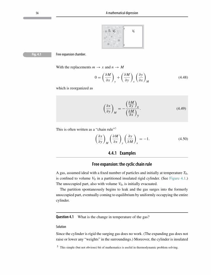
56 A mathematical digression
� Fig. 4.1 Free expansion chamber.
With the replacements m → x and n → M
0 =(∂M
∂x
)y+(∂M
∂y
)x
(∂y
∂x
)M
(4.48)
which is reorganized as
(∂x
∂y
)M= −
(∂M∂ y
)x(
∂M∂x
)y
. (4.49)
This is often written as a “chain rule”5(∂x
∂y
)M
(∂M
∂x
)y
(∂y
∂M
)x= −1. (4.50)
4.4.1 Examples
Free expansion: the cyclic chain rule
A gas, assumed ideal with a fixed number of particles and initially at temperature T0,
is confined to volume V0 in a partitioned insulated rigid cylinder. (See Figure 4.1.)
The unoccupied part, also with volume V0, is initially evacuated.
The partition spontaneously begins to leak and the gas surges into the formerly
unoccupied part, eventually coming to equilibrium by uniformly occupying the entire
cylinder.
Question 4.1 What is the change in temperature of the gas?
Solution
Since the cylinder is rigid the surging gas does no work. (The expanding gas does not
raise or lower any “weights” in the surroundings.) Moreover, the cylinder is insulated
5 This simple (but not obvious) bit of mathematics is useful in thermodynamic problem solving.
57 A cyclic chain rule
so that during the process, Q = 0. (Regarding the expansion as rapid will lead to the
same conclusion.) With
Q = 0 and W = 0 (4.51)
the First Law, ΔU = Q−W , says
ΔU = 0; (4.52)
i.e. internal energy is constant. This constant U process is called a free expansion.
Since U is constant it follows that dU = 0, so taking U = U(T, V ) its total differ-
ential is
dU =(∂U∂T
)V
dT +(∂U∂V
)T
dV = 0 (4.53)
and the temperature change we are looking for is
dT = −(∂U∂V
)T(
∂U∂T
)V
dV . (4.54)
But a little more work is needed to give ΔT in terms of practical thermal variables.
Applying the cyclic chain rule (see Eq. 4.49) to this result we get
dT =(∂T
∂V
)U
dV . (4.55)
The partial derivative is one of the “unfriendly” kind referred to earlier. The objective
now is relating it to a “friendly” partial derivative that corresponds to laboratory
measurables.
Using the thermodynamic identity, Eq. 4.26, apply the Euler exactness criterion to
the differential dS (see Eq. 4.34), in the following way;⎛⎝∂(
1T
)∂V
⎞⎠U
=⎛⎝∂
(pT
)∂U
⎞⎠V
. (4.56)
After carrying out the differentiations it becomes
− 1
T 2
(∂T
∂V
)U= − p
T 2
(∂T
∂U
)V+ 1
T
(∂p
∂U
)V. (4.57)
Applying the “ordinary” chain rule to the last term on the right-hand side and then
substituting Eq. 3.50 (CV ), Eq. 4.57 becomes(∂T
∂V
)U= 1
CV
[p − T
(∂p
∂T
)V
], (4.58)
58 A mathematical digression
which is now in terms of measurable quantities – our objective all along. Finally,
applying the ideal gas equation of state,6
1
CV
[p − T
(∂p
∂T
)V
]= 0, (4.59)
and we see from Eq. 4.55 that an ideal gas undergoing a free expansion remains at
constant temperature.
Question 4.2 What is the change in entropy of the expanded gas?
Solution
Focusing directly on S we write S = S (U, V ) and then take the total differential
dS =(∂S∂U
)V
dU +(∂S∂V
)U
dV . (4.60)
Since this is a free expansion, U = constant (dU = 0) and
dS =(∂S∂V
)U
dV . (4.61)
Then from Eq. 4.33
dS = p
TdV . (4.62)
Then using the ideal gas equation of state
dS = NkB
VdV . (4.63)
Since the expansion is from V0 to 2V0, this is integrated to give
ΔS = S (2V0)− S (V0) = NkB
2V0∫V0
dV
V(4.64)
= NkB ln2V0
V0(4.65)
= NkB ln 2. (4.66)
6 The analysis can be applied to any gas equation of state.
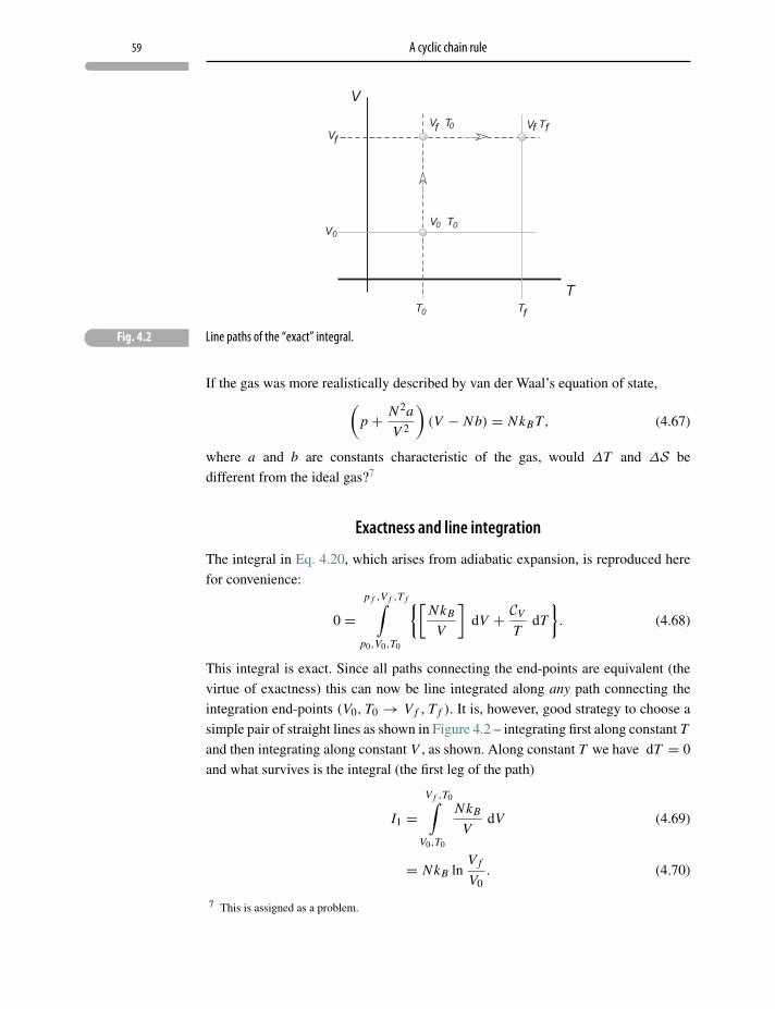
59 A cyclic chain rule
� Fig. 4.2 Line paths of the “exact” integral.
If the gas was more realistically described by van der Waal’s equation of state,(p + N 2a
V 2
)(V − Nb) = NkB T, (4.67)
where a and b are constants characteristic of the gas, would ΔT and ΔS be
different from the ideal gas?7
Exactness and line integration
The integral in Eq. 4.20, which arises from adiabatic expansion, is reproduced here
for convenience:
0 =p f ,V f ,T f∫
p0,V0,T0
{[NkB
V
]dV + CV
TdT
}. (4.68)
This integral is exact. Since all paths connecting the end-points are equivalent (the
virtue of exactness) this can now be line integrated along any path connecting the
integration end-points (V0, T0 → V f , T f ). It is, however, good strategy to choose a
simple pair of straight lines as shown in Figure 4.2 – integrating first along constant T
and then integrating along constant V , as shown. Along constant T we have dT = 0
and what survives is the integral (the first leg of the path)
I1 =V f ,T0∫
V0,T0
NkB
VdV (4.69)
= NkB lnV f
V0. (4.70)
7 This is assigned as a problem.
60 A mathematical digression
The second leg of the path is along constant V as shown in the diagram. Along
this leg dV = 0, so this contribution is
I2 =V f ,T f∫
V f ,T0
CV
TdT (4.71)
= CV lnT f
T0. (4.72)
Summing the two contributions
I1 + I2 = NkB lnV f
V0+ CV ln
T f
T0= 0, (4.73)
which is identical to Eq. 3.84, in Chapter 3.
4.5 Entropy and spontaneous processes
Example 1
As in Chapter 3 (Eqs. 3.18–3.20), consider an ideal gas, initially with volume V0
and pressure p0, confined in a cylinder by a massless, frictionless piston. The piston,
although itself massless, is exposed to the atmosphere and loaded with a pile of fine
sand that is slowly removed, allowing the piston to rise quasi-statically and attain
final gas volume V f and final pressure patm , identical to the surrounding atmosphere.
The gas and surroundings are maintained at temperature T0.
Question 4.3 What is the entropy change of the “universe”?
Solution
Apply the First Law to find QQS , the heat absorbed quasi-statically from the sur-
roundings by the gas. With pressure pgas
QQS =V f∫
V0
pgasdV (4.74)
=V f∫
V0
NkB T0
VdV (4.75)
= NkB T0 lnV f
V0. (4.76)
61 Entropy and spontaneous processes
Therefore the entropy change of the surroundings is
�Ssurr = −QQS
T0(4.77)
= −NkB lnV f
V0. (4.78)
To find the entropy change of the gas we write, at constant temperature,
dS =(∂S∂V
)T
dV . (4.79)
But since (∂S
∂V
)T=(
∂p
∂T
)V
(4.80)
the entropy change of the ideal gas is
�Sgas =V f∫
V0
(∂p
∂T
)V
dV (4.81)
= NkB lnV f
V0. (4.82)
Therefore8 the entropy change of the “universe” is, for this quasi-static reversible
process,
�Suniverse = �Sgas +�Ssurroundings (4.83)
= 0. (4.84)
Example 2
An ideal gas is confined in a cylinder by a massless, frictionless piston. The piston
is pinned some distance above the bottom of the cylinder while exposed to constant
atmospheric pressure Patm (see Figure 3.3). The initial state of the gas is V0, T0, p0 >
Patm . The gas and surroundings are maintained at temperature T0. (See Chapter 3,
Eqs. 3.23–3.28.)
8 A way to arrive at Eq. 4.80 starts from
dU = T dS − p dV
followed by Euler’s exact condition (∂p
∂S
)V= −
(∂T
∂V
)S
and an application of the cyclic chain rule.
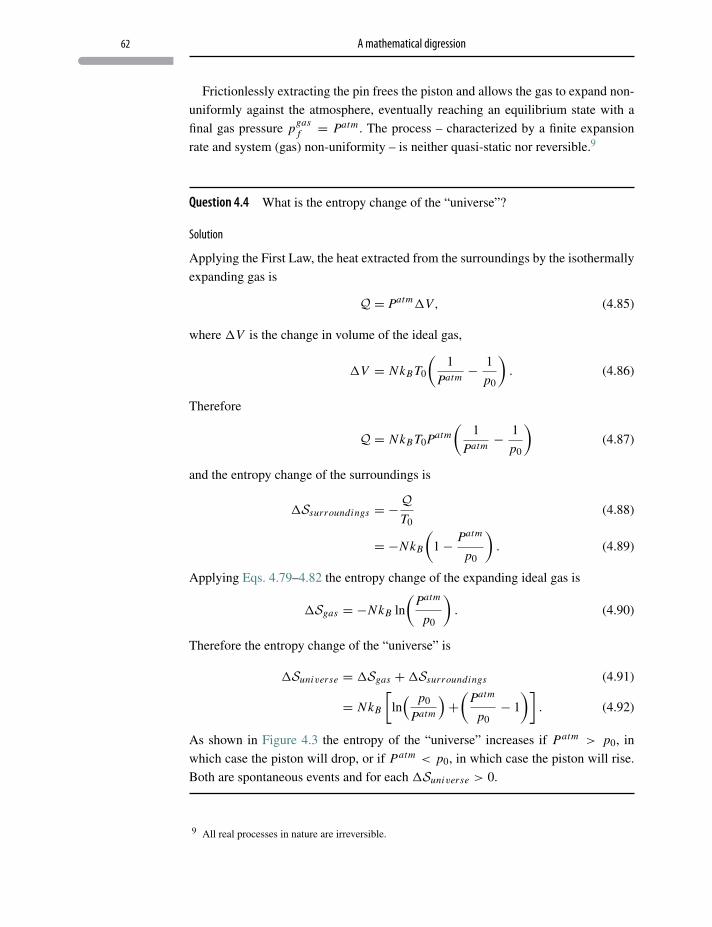
62 A mathematical digression
Frictionlessly extracting the pin frees the piston and allows the gas to expand non-
uniformly against the atmosphere, eventually reaching an equilibrium state with a
final gas pressure pgasf = Patm . The process – characterized by a finite expansion
rate and system (gas) non-uniformity – is neither quasi-static nor reversible.9
Question 4.4 What is the entropy change of the “universe”?
Solution
Applying the First Law, the heat extracted from the surroundings by the isothermally
expanding gas is
Q = Patm�V, (4.85)
where �V is the change in volume of the ideal gas,
�V = NkB T0
(1
Patm− 1
p0
). (4.86)
Therefore
Q = NkB T0Patm(
1
Patm− 1
p0
)(4.87)
and the entropy change of the surroundings is
�Ssurroundings = −QT0
(4.88)
= −NkB
(1− Patm
p0
). (4.89)
Applying Eqs. 4.79–4.82 the entropy change of the expanding ideal gas is
�Sgas = −NkB ln
(Patm
p0
). (4.90)
Therefore the entropy change of the “universe” is
�Suniverse = �Sgas +�Ssurroundings (4.91)
= NkB
[ln( p0
Patm
)+(
Patm
p0− 1
)]. (4.92)
As shown in Figure 4.3 the entropy of the “universe” increases if Patm > p0, in
which case the piston will drop, or if Patm < p0, in which case the piston will rise.
Both are spontaneous events and for each �Suniverse > 0.
9 All real processes in nature are irreversible.
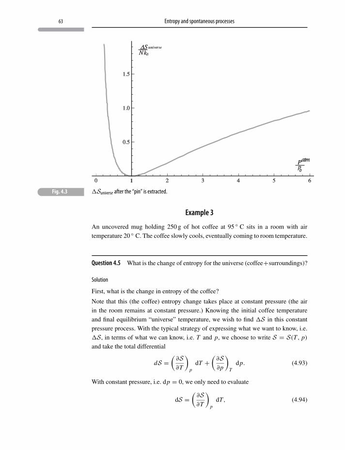
63 Entropy and spontaneous processes
universe
� Fig. 4.3 �Suniverse after the “pin” is extracted.
Example 3
An uncovered mug holding 250 g of hot coffee at 95 ◦ C sits in a room with air
temperature 20 ◦ C. The coffee slowly cools, eventually coming to room temperature.
Question 4.5 What is the change of entropy for the universe (coffee+surroundings)?
Solution
First, what is the change in entropy of the coffee?
Note that this (the coffee) entropy change takes place at constant pressure (the air
in the room remains at constant pressure.) Knowing the initial coffee temperature
and final equilibrium “universe” temperature, we wish to find �S in this constant
pressure process. With the typical strategy of expressing what we want to know, i.e.
�S, in terms of what we can know, i.e. T and p, we choose to write S = S(T, p)
and take the total differential
dS =(∂S∂T
)p
dT +(∂S∂p
)T
dp. (4.93)
With constant pressure, i.e. dp = 0, we only need to evaluate
dS =(∂S∂T
)p
dT, (4.94)
64 A mathematical digression
where
T
(∂S∂T
)p= Cp. (4.95)
Therefore Eq. 4.94 is
dS = 1
TCp dT (4.96)
or
dS = 1
Tm〈cp〉 dT, (4.97)
where m is the mass and 〈cp〉 is an average specific heat per unit mass. Assuming
that, for the coffee, 〈cp〉 = 4184 J kg−1 K−1 is independent of temperature
�Scoffee = m〈cp〉 ln
(T f
T0
)(4.98)
= 0.25 kg · 4184 J kg−1 K−1 · ln(
293 K
368 K
)(4.99)
= −238 J kg−1. (4.100)
The entropy of the coffee decreases.
Since coffee + surroundings = “the universe”, having found the entropy change
of the coffee we need to find the entropy change of the surroundings. Apart from
receiving heat from the coffee, the surroundings are an infinite reservoir with volume,
temperature and pressure remaining constant. So we can apply the First Law to the
constant volume (zero work) surroundings:
Qsur = �Usur. (4.101)
Taking Qcoffee as the heat leaving the coffee, −Qcoffee = Qsur . Then writing for the
surroundings U = U(V,S) and taking the total differential (with dV = 0)
dUsur =(∂Usur
∂Ssur
)V
dSsur (4.102)
= Tsur dSsur (4.103)
where Eq. 4.32 has been used. After integration we have
�Ssur = −Qcoffee
Tsur. (4.104)
To find Qcoffee the First Law is applied to the coffee where we get, assuming negli-
gible liquid volume change,
Qcoffee = �Ucoffee (4.105)
= Cp(T0 − T f ) (4.106)
= m〈cp〉(T0 − T f ). (4.107)
65 Thermal engines
Finally, using this result in Eq. 4.104,
�Ssur = m〈cp〉T f − T0
T f(4.108)
= 0.25 kg · 4184 J kg−1 K−1 · 75 K/293 K (4.109)
= 268 J K−1 (4.110)
so that
�Suniv = �Scoffee +�Ssur (4.111)
= −238 J K−1 + 268 J K−1 (4.112)
= 30 J K−1. (4.113)
The entropy of the universe increases in this and any other spontaneous process.
Cooling a mug of hot coffee by leaving it in a cool room is a spontaneous (irre-
versible) process, i.e. the entropy increase of the universe is a quantitative measure of
its feasibility. The reverse process – the now cool coffee taking energy from the room
to restore its original hot state – without some outside intervention – can “never” hap-
pen! That is the substance of the Second Law.
Examples 2 (Eq. 4.92) and 3 (Eq. 4.113) describe irreversible processes such as
occur in nature whereas Example 1 (Eq. 4.84) describes the idealized quasi-static,
reversible processes often invoked in thermodynamic models.
The Second Law,
�Suniverse ≥ 0, (4.114)
is a measure of nature’s propensity for processes to proceed, when there is no outside
intervention, in a particular direction.
4.6 Thermal engines
A thermal engine is a device that operates in a cycle, during which:
1. a working substance absorbs heat QH from an energy source with which it is in
thermal contact, resulting in thermodynamic changes to the working substance;
2. the working substance exhausts heat QL to an energy sink, also resulting in ther-
modynamic changes to the working substance;
3. external mechanical work W can be realized;
66 A mathematical digression
4. the working substance returns to its initial thermodynamic state, so the change in
any state function per working substance cycle is zero, e.g. ΔU = 0.
Earliest 18th-century engines of various designs used steam exclusively as the work-
ing substance by condensing the steam to cause a partial vacuum, assisting external
atmospheric pressure in driving a piston. Steam’s only active role was to force the
piston back to its starting position. In 1799 Richard Trevithick introduced a more
efficient and compact high-pressure steam engine to drive the piston directly, which
was the forerunner of the portable transportation engine. The steam-driven industrial
revolution had begun.
However, engines of all designs were very inefficient, requiring large quantities of
coal for little useful work output.
From the quest for improved efficiency evolved a new science, thermodynamics,
created in 1824 by Sadi Carnot.10,11
Because of friction and turbulence, real engines are complicated irreversible
devices. But their cycle can be modeled as ideal with accuracy sufficient to esti-
mate their efficiency of operation η, defined as the ratio of mechanical work done
WQS to the heat absorbed from an energy source QH , in each quasi-static engine
cycle,
η = WQS
QH. (4.115)
Typical modern engines are of the combustion design in which burning fuel injects
heat into a working substance which then expands against a piston to perform work.
To return to its initial state, the expanded working substance must, at some point in
the cycle, exhaust heat to a sink (usually the atmosphere or a nearby body of water).
Exhausting heat to a sink is the step in the cycle which guarantees that the efficiency
of any thermodynamic engine is less than 1.
4.6.1 Carnot’s thermal engine
The ideal Carnot engine (see Figure 4.4) operates between an energy source, in which
the working substance (in this case an ideal gas) absorbs heat QH isothermally at
high temperature TH (short dashed curve), and an energy sink, into which heat QL is
isothermally exhausted at a low temperature TL (solid curve). The long dash curves
which close the Carnot cycle are adiabats in which no heat enters or leaves the work-
ing substance.
To calculate the engine efficiency (see Eq. 4.115) the work done in a cycle is
determined by dividing the cycle into its four component paths:
10 S. Carnot, Reflections on the Motive Power of Fire, Dover (1960).11 S. S. Wilson, “Sadi Carnot”, Scientific American 245, 102–114 (1981).
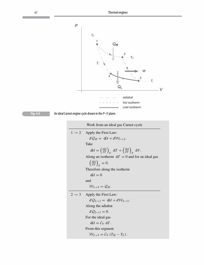
67 Thermal engines
� Fig. 4.4 An ideal Carnot engine cycle drawn in the P–V plane.
Work from an ideal gas Carnot cycle
1 → 2 Apply the First Law:
d−QH = dU + d−W1→2.
Take
dU =(∂U∂T
)V
dT +(∂U∂V
)T
dV .
Along an isotherm dT = 0 and for an ideal gas(∂U∂V
)T= 0.
Therefore along the isotherm
dU = 0
and
W1→2 = QH .
2 → 3 Apply the First Law:
d−Q2→3 = dU + d−W2→3.
Along the adiabat
d−Q2→3 = 0.
For the ideal gas
dU = CV dT .
From this segment
W2→3 = CV (TH − TL) .
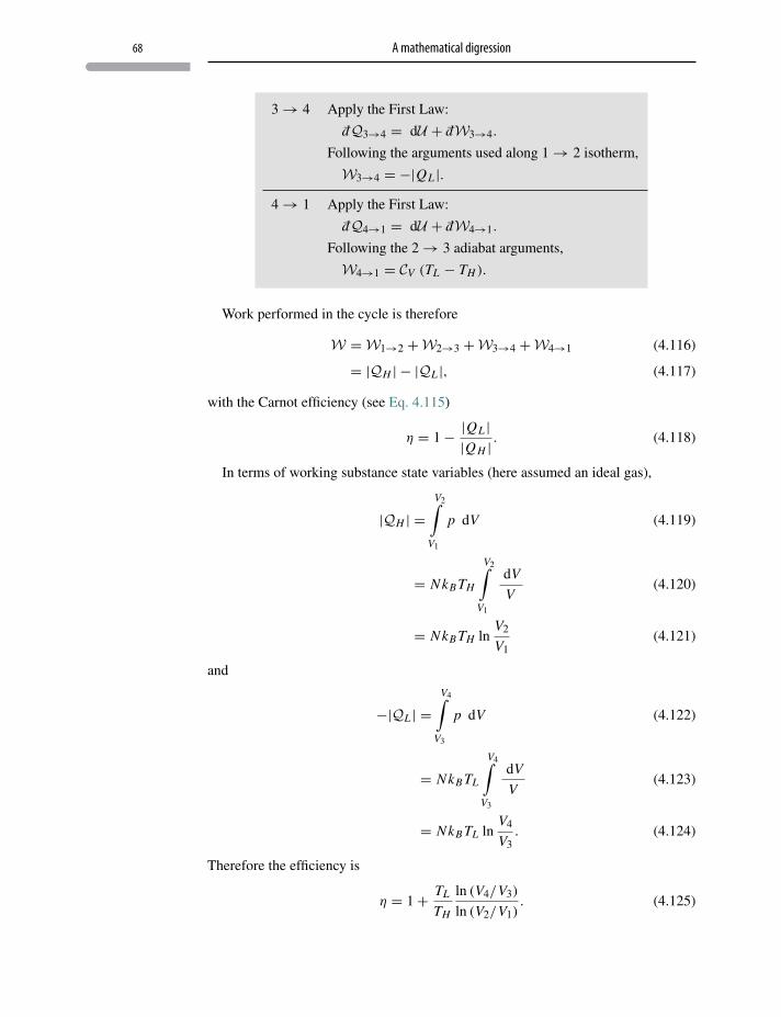
68 A mathematical digression
3 → 4 Apply the First Law:
d−Q3→4 = dU + d−W3→4.
Following the arguments used along 1 → 2 isotherm,
W3→4 = −|QL |.4 → 1 Apply the First Law:
d−Q4→1 = dU + d−W4→1.
Following the 2 → 3 adiabat arguments,
W4→1 = CV (TL − TH ).
Work performed in the cycle is therefore
W =W1→2 +W2→3 +W3→4 +W4→1 (4.116)
= |QH | − |QL |, (4.117)
with the Carnot efficiency (see Eq. 4.115)
η = 1− |QL ||Q H | . (4.118)
In terms of working substance state variables (here assumed an ideal gas),
|QH | =V2∫
V1
p dV (4.119)
= NkB TH
V2∫V1
dV
V(4.120)
= NkB TH lnV2
V1(4.121)
and
−|QL | =V4∫
V3
p dV (4.122)
= NkB TL
V4∫V3
dV
V(4.123)
= NkB TL lnV4
V3. (4.124)
Therefore the efficiency is
η = 1+ TL
TH
ln (V4/V3)
ln (V2/V1). (4.125)
69 Thermal engines
But along the adiabats 2 → 3
TL∫TH
CVdT
T= −NkB
V3∫V2
dV
V(4.126)
and 4 → 1
TH∫TL
CVdT
T= −NkB
V1∫V4
dV
V, (4.127)
which are integrated to give
V4
V1= V3
V2. (4.128)
Therefore the Carnot efficiency expressed in Eq. 4.125 becomes
η = 1− TL
TH. (4.129)
This result is consistent with the Kelvin–Planck statement of the Second Law of
Thermodynamics:
• It is impossible to construct an engine such that heat is cyclically removed from a
reservoir at high temperature with the sole effect of performing mechanical work.
(In some part of the cycle heat must be exhausted and engine efficiency must be
less than 1.)
A hypothetical Carnot engine with operating temperatures TH ∼ 600 K and TL ∼300 K would have an efficiency η ∼ 50%.12
4.6.2 The Carnot cycle – entropy
Any reversible engine cycle can be divided into infinitesimal Carnot segments (adia-
bats and isotherms) as shown in Figure 4.5.
Now, combining Eqs. 4.118 and 4.129, we have the result for a complete Carnot
engine cycle
−|QH |TH
+ |QL |TL
= 0, (4.130)
12 The Carnot engine is the most efficient engine operating between two fixed temperatures.
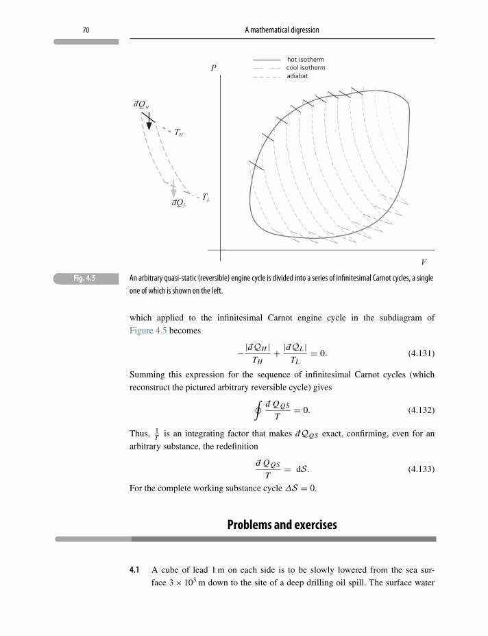
70 A mathematical digression
� Fig. 4.5 An arbitrary quasi-static (reversible) engine cycle is divided into a series of infinitesimal Carnot cycles, a singleone of which is shown on the left.
which applied to the infinitesimal Carnot engine cycle in the subdiagram of
Figure 4.5 becomes
−|d−QH |TH
+ |d−QL |TL
= 0. (4.131)
Summing this expression for the sequence of infinitesimal Carnot cycles (which
reconstruct the pictured arbitrary reversible cycle) gives∮d−QQS
T= 0. (4.132)
Thus, 1T is an integrating factor that makes d−QQS exact, confirming, even for an
arbitrary substance, the redefinition
d−QQS
T= dS. (4.133)
For the complete working substance cycle ΔS = 0.
Problems and exercises
4.1 A cube of lead 1 m on each side is to be slowly lowered from the sea sur-
face 3× 10³ m down to the site of a deep drilling oil spill. The surface water
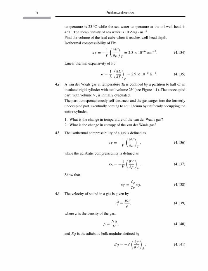
71 Problems and exercises
temperature is 23 ◦C while the sea water temperature at the oil well head is
4 ◦C. The mean density of sea water is 1035 kg ·m−3.
Find the volume of the lead cube when it reaches well-head depth.
Isothermal compressibility of Pb:
κT = − 1
V
(∂V
∂p
)T= 2.3× 10⁻⁶ atm−1. (4.134)
Linear thermal expansivity of Pb:
α = 1
L
(∂L
∂T
)p= 2.9× 10⁻⁵ K−1. (4.135)
4.2 A van der Waals gas at temperature T0 is confined by a partition to half of an
insulated rigid cylinder with total volume 2V (see Figure 4.1). The unoccupied
part, with volume V , is initially evacuated.
The partition spontaneously self-destructs and the gas surges into the formerly
unoccupied part, eventually coming to equilibrium by uniformly occupying the
entire cylinder.
1. What is the change in temperature of the van der Waals gas?
2. What is the change in entropy of the van der Waals gas?
4.3 The isothermal compressibility of a gas is defined as
κT = − 1
V
(∂V
∂p
)T, (4.136)
while the adiabatic compressibility is defined as
κS = − 1
V
(∂V
∂p
)S. (4.137)
Show that
κT = Cp
CVκS . (4.138)
4.4 The velocity of sound in a gas is given by
c2s =
BSρ
, (4.139)
where ρ is the density of the gas,
ρ = Nμ
V, (4.140)
and BS is the adiabatic bulk modulus defined by
BS = −V
(∂p
∂V
)S, (4.141)
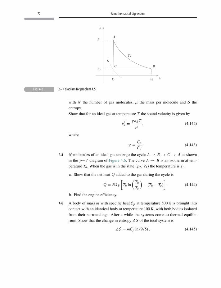
72 A mathematical digression
p
p
p2
1
VV2V1
T
Tc
h
A
C B
� Fig. 4.6 p–V diagram for problem 4.5.
with N the number of gas molecules, μ the mass per molecule and S the
entropy.
Show that for an ideal gas at temperature T the sound velocity is given by
c2s =
γ kB T
μ, (4.142)
where
γ = Cp
CV. (4.143)
4.5 N molecules of an ideal gas undergo the cycle A → B → C → A as shown
in the p−V diagram of Figure 4.6. The curve A → B is an isotherm at tem-
perature Th . When the gas is in the state (p2, V1) the temperature is Tc.
a. Show that the net heat Q added to the gas during the cycle is
Q = NkB
[Th ln
(Th
Tc
)− (Th − Tc)
]. (4.144)
b. Find the engine efficiency.
4.6 A body of mass m with specific heat Cp at temperature 500 K is brought into
contact with an identical body at temperature 100 K, with both bodies isolated
from their surroundings. After a while the systems come to thermal equilib-
rium. Show that the change in entropy ΔS of the total system is
ΔS = mCp ln (9/5) . (4.145)
5 Thermodynamic potentials
Rudolph Clausius obtained distinction by mathematical calculations based on thedynamical theory of heat – calculations which, it is claimed, show the necessityof a Creator and the possibility of miracles.
Obituary notice, New York Times, 26 Aug. 1888
5.1 Introduction
Thermodynamic processes can by design or by nature take place under conditions
in which particular macroscopic parameters – e.g. temperature, pressure, volume,
magnetic field, entropy, particle number – are kept constant. For an experimentalist,
holding some variables constant, such as entropy or internal energy, is inconvenient
or exceptionally difficult, while other variables, such as pressure and temperature,
are easier or more natural to fix. Therefore, in addition to an energy potential U(internal energy) which accommodates constant extensive variables S, V and N ,
other potential functions are introduced which are adapted to fixing other variables.
5.1.1 Internal energy U
The differential
dU = T dS − p dV + μ dN , (5.1)
a consequence of the First Law of Thermodynamics, is called a fundamental equation
or the thermodynamic identity. With U = U(S, V, N ), the total differential is
dU =(∂U∂S
)V,N
dS +(∂U∂V
)S,N
dV +(∂U∂N
)S,V
dN . (5.2)
73
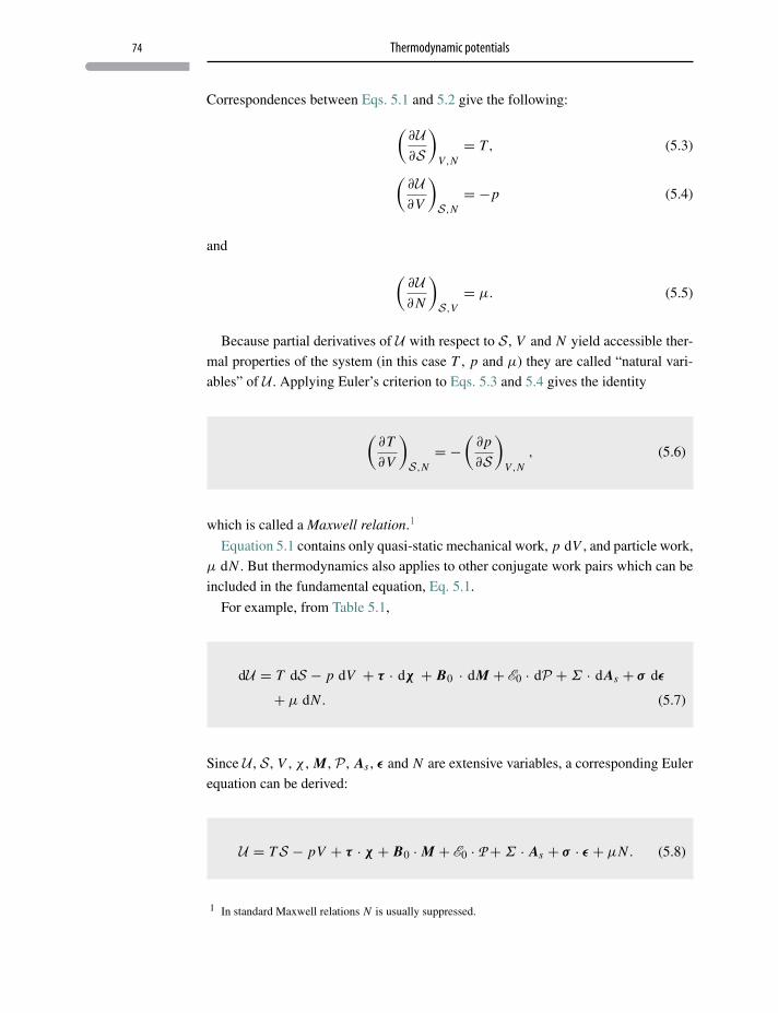
74 Thermodynamic potentials
Correspondences between Eqs. 5.1 and 5.2 give the following:(∂U∂S
)V,N
= T, (5.3)
(∂U∂V
)S,N
= −p (5.4)
and (∂U∂N
)S,V
= μ. (5.5)
Because partial derivatives of U with respect to S, V and N yield accessible ther-
mal properties of the system (in this case T , p and μ) they are called “natural vari-
ables” of U . Applying Euler’s criterion to Eqs. 5.3 and 5.4 gives the identity
(∂T
∂V
)S,N
= −(∂p
∂S
)V,N
, (5.6)
which is called a Maxwell relation.1
Equation 5.1 contains only quasi-static mechanical work, p dV , and particle work,
μ dN . But thermodynamics also applies to other conjugate work pairs which can be
included in the fundamental equation, Eq. 5.1.
For example, from Table 5.1,
dU = T dS − p dV + τ · dχ + B0 · dM + E0 · dP +Σ · dAs + σ dε
+ μ dN . (5.7)
Since U , S, V , χ , M, P , As , ε and N are extensive variables, a corresponding Euler
equation can be derived:
U = TS − pV + τ · χ + B0 · M + E0 · P+Σ · As + σ · ε + μN . (5.8)
1 In standard Maxwell relations N is usually suppressed.
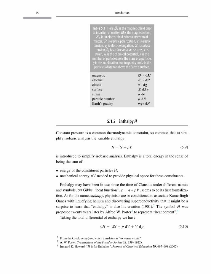
75 Introduction
Table 5.1 Here B0 is the magnetic field priorto insertion of matter, M is the magnetization,
E 0 is an electric field prior to insertion ofmatter,P is electric polarization, τ is elastictension, χ is elastic elongation, Σ is surface
tension, AS is surface area, σ is stress, ε isstrain, μ is the chemical potential, N is the
number of particles, m is the mass of a particle,g is the acceleration due to gravity and z is theparticle’s distance above the Earth’s surface.
magnetic B0 · dMelectric E 0 · dPelastic τ · dχ
surface Σ dASstrain σ dε
particle number μ dNEarth’s gravity mgz dN
5.1.2 Enthalpy H
Constant pressure is a common thermodynamic constraint, so common that to sim-
plify isobaric analysis the variable enthalpy
H = U + pV (5.9)
is introduced to simplify isobaric analysis. Enthalpy is a total energy in the sense of
being the sum of:
• energy of the constituent particles U ;
• mechanical energy pV needed to provide physical space for these constituents.
Enthalpy may have been in use since the time of Clausius under different names
and symbols, but Gibbs’ “heat function”, χ = ε+ pV , seems to be its first formaliza-
tion. As for the name enthalpy, physicists are so conditioned to associate Kamerlingh
Onnes with liquefying helium and discovering superconductivity that it might be a
surprise to learn that “enthalpy” is also his creation (1901).2 The symbol H was
proposed twenty years later by Alfred W. Porter3 to represent “heat content”.4
Taking the total differential of enthalpy we have
dH = dU + p dV + V dp. (5.10)
2 From the Greek enthalpos, which translates as “to warm within”.3 A. W. Porter, Transactions of the Faraday Society 18, 139 (1922).4 Irmgard K. Howard, “H is for Enthalpy”, Journal of Chemical Education 79, 697–698 (2002).
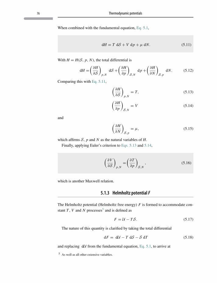
76 Thermodynamic potentials
When combined with the fundamental equation, Eq. 5.1,
dH = T dS + V dp + μ dN . (5.11)
With H = H(S, p, N ), the total differential is
dH =(∂H
∂S
)p,N
dS +(∂H
∂p
)S,N
dp +(∂H
∂N
)S,p
dN . (5.12)
Comparing this with Eq. 5.11, (∂H
∂S
)p,N
= T, (5.13)
(∂H
∂p
)S,N
= V (5.14)
and (∂H
∂N
)S,p
= μ, (5.15)
which affirms S, p and N as the natural variables of H.
Finally, applying Euler’s criterion to Eqs. 5.13 and 5.14,
(∂V
∂S
)p,N
=(∂T
∂p
)S,N
, (5.16)
which is another Maxwell relation.
5.1.3 Helmholtz potential F
The Helmholtz potential (Helmholtz free energy) F is formed to accommodate con-
stant T , V and N processes5 and is defined as
F = U − TS. (5.17)
The nature of this quantity is clarified by taking the total differential
dF = dU − T dS − S dT (5.18)
and replacing dU from the fundamental equation, Eq. 5.1, to arrive at
5 As well as all other extensive variables.
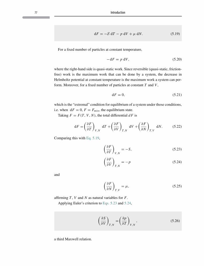
77 Introduction
dF = −S dT − p dV + μ dN . (5.19)
For a fixed number of particles at constant temperature,
−dF = p dV, (5.20)
where the right-hand side is quasi-static work. Since reversible (quasi-static, friction-
free) work is the maximum work that can be done by a system, the decrease in
Helmholtz potential at constant temperature is the maximum work a system can per-
form. Moreover, for a fixed number of particles at constant T and V ,
dF = 0, (5.21)
which is the “extremal” condition for equilibrium of a system under those conditions,
i.e. when dF = 0, F = Fmin , the equilibrium state.
Taking F = F(T, V, N ), the total differential d F is
dF =(∂F
∂T
)V,N
dT +(∂F
∂V
)T,N
dV +(∂F
∂N
)T,V
dN . (5.22)
Comparing this with Eq. 5.19, (∂F
∂T
)V,N
= −S, (5.23)
(∂F
∂V
)T,N
= −p (5.24)
and (∂F
∂N
)T,V
= μ, (5.25)
affirming T , V and N as natural variables for F .
Applying Euler’s criterion to Eqs. 5.23 and 5.24,
(∂S
∂V
)T,N
=(
∂p
∂T
)V,N
, (5.26)
a third Maxwell relation.
78 Thermodynamic potentials
5.1.4 Gibbs potential G
The Gibbs potential (Gibbs free energy) G, defined as
G = U − TS + pV, (5.27)
accommodates experimental constraints on T , p and N . Differentiating Eq. 5.27,
dG = dU − T dS − S dT + p dV + V dp, (5.28)
and substituting dU from Eq. 5.1 its total differential is
dG = −S dT + V dp + μ dN . (5.29)
Writing G = G(T, p, N ), a total differential is
dG =(∂G
∂T
)p,N
dT +(∂G
∂p
)T,N
dp +(∂G
∂N
)T,p
dN , (5.30)
which, on comparison with Eq. 5.29, gives(∂G
∂T
)p,N
= −S, (5.31)
(∂G
∂p
)T,N
= V (5.32)
and (∂G
∂N
)T,p
= μ, (5.33)
confirming T , p and N as natural variables of G. Applying Euler’s criterion to
Eqs. 5.31 and 5.32,
(∂S
∂p
)T,N
= −(∂V
∂T
)p,N
, (5.34)
which is a fourth Maxwell relation.
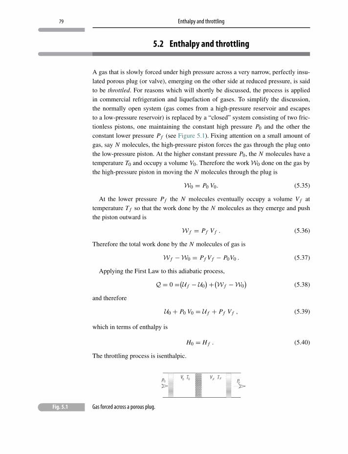
79 Enthalpy and throttling
5.2 Enthalpy and throttling
A gas that is slowly forced under high pressure across a very narrow, perfectly insu-
lated porous plug (or valve), emerging on the other side at reduced pressure, is said
to be throttled. For reasons which will shortly be discussed, the process is applied
in commercial refrigeration and liquefaction of gases. To simplify the discussion,
the normally open system (gas comes from a high-pressure reservoir and escapes
to a low-pressure reservoir) is replaced by a “closed” system consisting of two fric-
tionless pistons, one maintaining the constant high pressure P0 and the other the
constant lower pressure Pf (see Figure 5.1). Fixing attention on a small amount of
gas, say N molecules, the high-pressure piston forces the gas through the plug onto
the low-pressure piston. At the higher constant pressure P0, the N molecules have a
temperature T0 and occupy a volume V0. Therefore the work W0 done on the gas by
the high-pressure piston in moving the N molecules through the plug is
W0 = P0 V0. (5.35)
At the lower pressure Pf the N molecules eventually occupy a volume V f at
temperature T f so that the work done by the N molecules as they emerge and push
the piston outward is
W f = Pf V f . (5.36)
Therefore the total work done by the N molecules of gas is
W f −W0 = Pf V f − P0V0 . (5.37)
Applying the First Law to this adiabatic process,
Q = 0 =(U f − U0)+(W f −W0
)(5.38)
and therefore
U0 + P0 V0 = U f + Pf V f , (5.39)
which in terms of enthalpy is
H0 = H f . (5.40)
The throttling process is isenthalpic.
� Fig. 5.1 Gas forced across a porous plug.
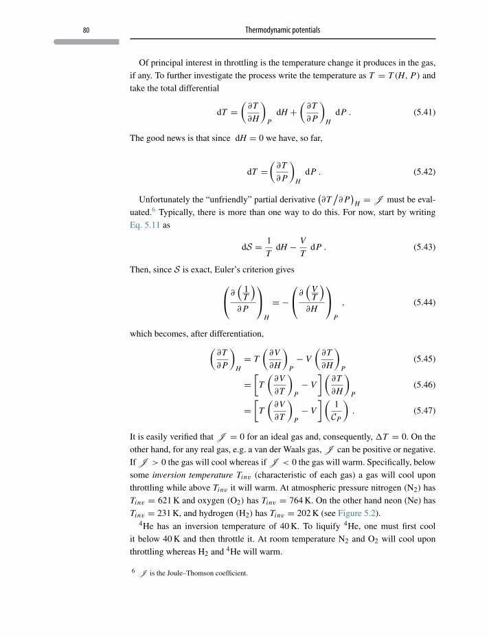
80 Thermodynamic potentials
Of principal interest in throttling is the temperature change it produces in the gas,
if any. To further investigate the process write the temperature as T = T (H, P) and
take the total differential
dT =(∂T
∂H
)P
dH +(∂T
∂P
)H
dP . (5.41)
The good news is that since dH = 0 we have, so far,
dT =(∂T
∂P
)H
dP . (5.42)
Unfortunately the “unfriendly” partial derivative(∂T
/∂P
)H = J must be eval-
uated.6 Typically, there is more than one way to do this. For now, start by writing
Eq. 5.11 as
dS = 1
TdH − V
TdP . (5.43)
Then, since S is exact, Euler’s criterion gives⎛⎝∂(
1T
)∂P
⎞⎠H
= −⎛⎝∂
(VT
)∂H
⎞⎠P
, (5.44)
which becomes, after differentiation,(∂T
∂P
)H= T
(∂V
∂H
)P− V
(∂T
∂H
)P
(5.45)
=[
T
(∂V
∂T
)P− V
](∂T
∂H
)P
(5.46)
=[
T
(∂V
∂T
)P− V
](1
CP
). (5.47)
It is easily verified that J = 0 for an ideal gas and, consequently, �T = 0. On the
other hand, for any real gas, e.g. a van der Waals gas, J can be positive or negative.
If J > 0 the gas will cool whereas if J < 0 the gas will warm. Specifically, below
some inversion temperature Tinv (characteristic of each gas) a gas will cool upon
throttling while above Tinv it will warm. At atmospheric pressure nitrogen (N2) has
Tinv = 621 K and oxygen (O2) has Tinv = 764 K. On the other hand neon (Ne) has
Tinv = 231 K, and hydrogen (H2) has Tinv = 202 K (see Figure 5.2).4He has an inversion temperature of 40 K. To liquify 4He, one must first cool
it below 40 K and then throttle it. At room temperature N2 and O2 will cool upon
throttling whereas H2 and 4He will warm.
6 J is the Joule–Thomson coefficient.
81 Entropy and heat capacity
4
� Fig. 5.2 Joule–Thomson coefficients J for various gases at atmospheric pressure.
5.3 Entropy and heat capacity
Low-temperature heat capacities are among those macroscopic phenomena that
require quantum explanations. For that reason they stand high on the list of impor-
tant thermodynamic experiments. Anomalous low-temperature values in diamond
first suggested to Einstein (1905) that nature was not as classical as was generally
believed at the time, and he applied quantization – as proposed by Planck (1900) – to
develop the first quantum theory of solids 25 years before the arrival of a generally
accepted quantum mechanics.
The appearance of entropy in thermodynamics brings a welcome and important
uniformity to heat capacity definitions. Whereas in Chapter 2 we derived the result
CV =(∂U
∂T
)V, (5.48)
we can instead, by applying the simple chain rule, write(∂U
∂T
)V=(∂U
∂S
)V
(∂S
∂T
)V
(5.49)
followed by Eq. 5.3, arrive at (∂U
∂T
)V= T
(∂S
∂T
)V
(5.50)
so that
CV = T
(∂S
∂T
)V. (5.51)
82 Thermodynamic potentials
Similarly
Cp =(∂H
∂T
)p
(5.52)
=(∂H
∂S
)p
(∂S∂T
)p
(5.53)
= T
(∂S∂T
)p. (5.54)
In general there is a single, convenient heat capacity definition:
Cα = T
(∂S
∂T
)α
. (5.55)
5.3.1 Relationship between Cp and CV
The entropy-based relations Cp = T(∂S/∂T
)p and CV = T
(∂S/∂T
)V put this
problem on a level footing. Considering the final objective, expressing the entropy
as S = S(T, p) is one sensible starting point. Then
dS =(∂S∂T
)p
dT +(∂S∂p
)T
dp, (5.56)
which already contains a piece of the answer, i.e.
dS = Cp
TdT +
(∂S∂p
)T
dp. (5.57)
An equally sensible choice is S = S(T, V ), in which case
dS =(∂S∂T
)V
dT +(∂S∂V
)T
dV (5.58)
= CV
TdT +
(∂S∂V
)T
dV . (5.59)
Then combining Eqs. 5.57 and 5.59 gives(Cp − CV
T
)dT =
[(∂S∂V
)T
dV −(∂S∂p
)T
dp
]. (5.60)
Next:
1. Apply the pair of Maxwell Relations, Eq. 5.26 and Eq. 5.34:(Cp − CV
T
)dT =
[(∂p
∂T
)V
dV +(∂V
∂T
)p
dp
]. (5.61)
83 Problems and exercises
2. Apply the cyclic chain rule to the first partial derivative on the right-hand side:(Cp − CV
T
)dT = −
(∂V
∂T
)p
[(∂p
∂V
)T
dV − dp
]. (5.62)
3. Noting that
dp =(
∂p
∂V
)T
dV +(
∂p
∂T
)V
dT, (5.63)
we finally arrive with (Cp − CV
T
)=(∂V
∂T
)p
(∂p
∂T
)V. (5.64)
For an ideal gas (∂V
∂T
)p= NkB
p(5.65)
and (∂p
∂T
)V= NkB
V, (5.66)
which gives
Cp − CV = NkB, (5.67)
as stated in Eq. 3.66, without proof.
Eq. 5.64 is a result that can be applied to any gas law – for example, to the van der
Waals equation.7
This type of result is not limited to gases. We will later derive a relation between
CB (constant magnetic induction) and CM (constant magnetization) for magnetic
systems, and between Cτ (constant tension) and Cχ (constant elongation) for linear
elastic systems.8
Problems and exercises
5.1 N molecules of an ideal gas at temperature T0 and volume V0 undergo an
isothermal expansion to a volume V1. What is the change in:
a. internal energy of the expanding gas?
b. enthalpy of the expanding gas?
7 Also see problem 5.3.8 χ = 〈χop〉 is the mean elongation.
84 Thermodynamic potentials
c. Helmholtz potential of the expanding gas?
d. Gibbs potential of the expanding gas?
5.2 Show that for an ideal gas
a.
(∂CV
∂p
)T= 0;
b.
(∂Cp
∂V
)T= 0.
5.3 If a gas is not ideal but has the equation of state
p = NkB T
V
[1+ N
VB(T )
], (5.68)
find expressions for:
a.
(∂CV
∂p
)T
;
b.
(∂Cp
∂V
)T
;
c. Cp − CV .
5.4 It is possible for a specific gas to emerge on the low-pressure side of a throt-
tling plug at either a lower or higher temperature than it had entering on the
high-pressure side. Show that for the van der Waals gas, whose equation of
state is (p + aN 2
V 2
)(V − Nb) = NkB T, (5.69)
where a and b are gas-specific temperature-independent constants, that at tem-
perature T0, where
kB T0 = 2a
b
(V − Nb
V
)2
, (5.70)
throttling produces no temperature change.
6 Knowing the “unknowable”
Suppose we were asked to arrange the following in two categories – distance,mass, electric force, entropy, beauty, melody. I think there are the strongestgrounds for arranging entropy alongside beauty and melody and not with thefirst three. Entropy is found only when the parts are viewed in association, and itis by hearing or viewing the parts in association that beauty and melody are dis-cerned . . . The reason why this stranger can pass itself off among the aboriginesof the physical world is that . . . it has a measure number associated with it.
A. Eddington, The Nature of the Physical World, Cambridge University Press(1928)
6.1 Entropy: ticket to the Emerald City
Entropy S was introduced into thermodynamics by Rudolph Clausius1 as a cryptic
state function without a clear intuitive or physical interpretation. Still, he maintained
it to be the basis of a sweeping new, abstract, universal physical principle: “In all
spontaneous processes the entropy of a closed system (system + environment) tends
towards a maximum”, i.e.
ΔS ≥ 0. (6.1)
It was in his series of memoirs (1856–1865) on irreversible heat loss, i.e. inefficiency
of heat engines, that he chose the name entropy (Greek for “transformation”) because
it sounded similar to energy, under the mistaken impression that the two were related.
Clausius’ principle, in which a particular state variable – entropy – always
increases (or remains constant) as a system and its surroundings (i.e. the “universe”)
evolve from one equilibrium state to the next, is called the Second Law of Thermo-
dynamics. The Second Law is not a conservation rule. Moreover, entropy is unlike
objective observables so familiar in physics, such as mass, length, velocity, energy,
acceleration, etc. Instead, emotive analogies or proxies such as disorder, chaos and
disorganization – which point in the right direction – are reasonably applied.
1 R. Clausius, “On the Moving Force of Heat, and the Laws regarding the Nature of Heat itself whichare deducible therefrom” (English translation of original), Phil. Mag. 2, 121, 102119 (1851).
85
86 Knowing the “unknowable”
The following encounter, said to have taken place in 1948, could serve to
acknowledge entropy’s subtle character.Over half a century ago while creating a fledgling Information Theory, Claude
Shannon (of Bell Laboratories) sought advice from Princeton’s famousmathematician–physicist John von Neumann in naming the function central to his[Shannon’s] (information) arguments:2
My greatest concern was what to call it. I thought of calling it information, butthe word is overly used. So I decided to call it uncertainty. When I discussed itwith John von Neumann, he had a better idea. Von Neumann told me – You shouldcall it entropy, for two reasons. In the first place your uncertainty function hasbeen used in statistical mechanics under that name, so it already has a name. Inthe second place, and more important, even after nearly one hundred years nobodyknows what entropy really is, so in a debate you will always have the advantage.
Although entropy is not a part of quantum mechanics, it plays a key role in postulat-
ing a bridge to thermodynamics.
6.2 The bridge
As a consequence of environmental decoherence, a “thermodynamic” density
operator, ρτop,
ρτop =
∑s
P (Es) |Es〉 〈Es | , (6.2)
emerges as – potentially – the quantity essential in the evolution to thermodynamics.
For example, using the macroscopic internal eigen-energies from
hop|εs〉 = εs |εs〉, (6.3)
the average internal energy U enshrined in the First Law could – in principle – be
expressed as
U = Trρτophop (6.4)
or, equivalently, as
U =∑
s
εsP(εs) . (6.5)
This looks promising – but, alas, the P(εs) are unknown and, except in trivial cases,
unknowable. The emerging thermodynamic theory is not complete! Can it ever be?
2 M. Tribus and E. McIrvine,“Energy and information”, Scientific American 225, 179–188 (1971).Reproduced with permission. Copyright 1971 SCIENTIFIC AMERICAN, a division of NatureAmerica, Inc. All rights reserved.
87 Thermodynamic hamiltonians
An alternative is to replace the unknowable P(Es) by inferred “surrogates” P(Es)
with which to construct a “surrogate” thermal density operator ρτop,
ρτop =
∑s
P(Es)|Es〉〈Es |, (6.6)
that describes behavior in accord with the macroscopic physical universe.
6.3 Thermodynamic hamiltonians
A simple dynamical situation would be the just discussed
Hop = hop, (6.7)
in which hop represents the internal energy (kinetic + potential + interaction) of,
say, a gas.3
If gas particles also have a magnetic moment and are in a local magnetic field
B0 – the field prior to insertion of matter4 – a macroscopic hamiltonian is
Hop = hop − Mop · B0, (6.8)
where Mop represents macroscopic magnetization
Mop =∑
i
mop(i). (6.9)
If the particles are molecular dipoles with electric dipole moments Pop in an electric
field E0, then
Hop = hop − Pop · E0, (6.10)
where Pop represents the macroscopic electric polarization.
Euler’s fundamental equation, Eq. 5.8, shows how other “thermodynamic” hamil-
tonians can be formulated by adding physically relevant macroscopic operators (see
Table 5.1). A more general result is then5,6
Hop = hop + popV − σ · εop − τ · χop − B0 · Mop − E0 · Pop −Σ · Asop − μNop.
(6.12)
3 The gas may be atoms or cold molecules (no internal modes) or even electrons.4 This subtle but important point will be discussed in detail in Chapter 11.5 Schrödinger’s non-relativistic wave mechanics is based on closed systems (fixed number of particles).
It makes no provision for destroying and creating particles. Therefore a number operator is not accom-modated within that theory. Particle creation and destruction is, however, integral to quantum fieldtheories so that number operators play a natural role.
6 The particle number operator Nop defines the eigenvalue equation
Nop |N 〉 = n |N 〉 (6.11)
with eigenvalues n = 0, 1, 2, 3, . . .
88 Knowing the “unknowable”
Since the extensive parameters describe a macroscopic system completely,
Eq. 6.12 contains all relevant information to enable a model macroscopic system’s
average total energy to be expressed as
〈Hop〉 = Tr ρτopHop. (6.13)
But the inescapable question remains – what criteria can be devised for construct-
ing the “best” P(Es)? This question has no a-priori answer apart from a postulate that
corresponds to time-tested thermodynamics and describes the measurable universe.7
Towards this goal:
1. Minimize
〈Hop〉 = Tr ρτop Hop (6.14)
=∑
s
P(Es)Es (6.15)
with respect to the P(Es).8,9,10
2. With no a-priori basis for choosing the P(Es) that minimizes Eq. 6.15, they shall
be chosen without “fear or favor”, i.e. with minimum bias11,12,13 (maximum
uncertainty).
Recalling the function(al)14 F of Eq. 2.55,
F [ρ] = −κTrρτop ln ρτ
op, κ > 0, (6.16)
as a measure of bias in a collection of probabilities,15 the function(al)
F[P(E)
]= −κ
∑s
P(Es) ln P(Es) , κ > 0, (6.17)
is taken to be a measure of bias in the probabilities P(Es) and is maximized. (See
Appendix B.)
3. The P(Es) are normalized: ∑s
P(Es) = 1. (6.18)
7 This is not unlike Ludwig Boltzmann’s motivation in postulating S = kB lnW .8 L. H. Thomas, “The calculation of atomic fields”, Proc. Cambridge Phil. Soc. 23, 542–548 (1927).9 E. Fermi,“Un Metodo Statistico per la Determinazione di alcune Priopriet dell’Atomo”, Rend. Accad.
Naz. Lincei 6, 602–607 (1927).10 E. H. Lieb, “Thomas–Fermi and related theories of atoms and molecules”, Rev. Mod. Phys. 53, 603–
641 (1981); Errata 54, 311 (1982).11 J. N. Kapur, Maximum Entropy Models in Science and Engineering, John Wiley and Sons, New York
(1989).12 E. T. Jaynes, “Information theory and statistical mechanics”, Phys. Rev. 106, 620 (1957).13 R. Balian, “Incomplete descriptions and relevant entropies”, Am. J. Phys. 67, 1078 (1999).14 F is a function of functions, which is called a functional.15 See Appendix B.
89 Microcanonical (Boltzmann) theory
To meet these requirements a Lagrangian is formed:
L = −{κ∑
s
P(Es) ln P(Es)+∑
s
P(Es)Es
}− λ0
∑s
P(Es), (6.19)
where λ0 is a Lagrange multiplier and the P(Es) are varied until L is maximized,
i.e. P(Es)→ P(Es).16 As discussed in Appendix B, with κ → kB T a thermal
Lagrangian is
L[P]= −
{kB
∑s
P(Es) ln P(Es)+ T−1∑
s
P(Es)Es
}− λ0
∑s
P(Es).
(6.20)
Then with P → P (least bias), it follows that F[P(E)
]→ F [P(E)] = Fmax ,
and
S = −kB
∑s
P(Es) ln P(Es) , (6.21)
the entropy of thermodynamics.
6.4 Microcanonical (Boltzmann) theory
At the time Boltzmann published his ingenious entropy postulate (1864) skepticism
about molecular models was continuing almost unabated and classical mechanics
was the only operative particle paradigm. Yet his accomplishments were so radical
and ahead of his time that it would take another 25 years for them to be reformulated
by Max Planck as quantization.
With our 150-year advantage, we illustrate a thermodynamic density operator ρτop
approach to Boltzmann’s fundamental thermodynamic contribution.
Consider a many-particle, closed system with:
• a fixed number of particles N ,
• a fixed volume V ,
• an isolated g0-fold degenerate macroscopic eigen-energy ε0,α ,
ε0,α ≡{ε0,1 = ε0,2 = ε0,3 = · · · = ε0,g0
}. (6.22)
16 This is equivalent to minimizing the Helmholtz potential, as in Section 5.1.3.
90 Knowing the “unknowable”
These effectively constitute Boltzmann’s “microcanonical” conditions. For this model
system the average hamiltonian (internal energy) is
U =∑
sα=1,2,...,g0
PB (εs,α)εs,α δs,0, (6.23)
where PB(εs,α
)is the probability that the system is in one of the degenerate macro-
scopic particle states with eigen-energy εs,α . The Kronecker δs,α selects from within
this spectrum a g0-fold degenerate single value ε0,α . Therefore, after summing over
the index s, Eq. 6.23 becomes
U =g0∑
α=1
PB (ε0,α)ε0,α. (6.24)
The remaining sum over α covers the g0-fold degeneracy.17
To determine the surrogate probabilities PB(ε0,α) (i.e. ρτop) a thermal Lagrangian
L[PB]
is postulated which, when maximized with respect to the PB(ε0,α), mini-
mizes both macroscopic energy[Tr ρτ
opHop
]and any “bias” (see Eq. 6.20) in the
choice of PB(ε0,α). In particular,
L[PB]= −kB
g0∑α=1
PB (ε0,α)
ln PB (ε0,α)− T−1
g0∑α=1
PB (ε0,α)ε0,α
− λ0
g0∑α=1
PB (ε0,α), (6.25)
where λ0 is a Lagrange multiplier that insures normalized “surrogate” probabili-
ties.18 The thermal Lagrangian used here, and in the remaining examples of this
book, is discussed and justified in Appendix B.
If results from this procedure are in agreement with an observable macroscopic
universe and with time-honored thermodynamics – whose validity is not in doubt –
the Yellow Brick Road will have guided us, at last, to the Emerald City.
(The procedure resembles a maximum entropy formalism of E. T. Jaynes.19,20
Jaynes’ formulation is, fundamentally, a statistical method in cases of partial infor-
mation (Bayesian statistics). It adopts Gibbs–Shannon21 communication (informa-
tion) theory (see Section 6.1) and is the basis of the “information theory” approach
17 Boltzmann pictured “microstates” (classical configurations) contributing to a single classical “internalenergy”.
18 The Internet is a rich source of tutorials on this powerful mathematical technique that is widelyused in physics and other technical fields. See, for example, www.slimy.com/∼steuard/teaching/tutorials/Lagrange.html and www.cs.berkeley.edu/∼klein/papers/lagrange-multipliers.pdf
19 E. T. Jaynes, “Information theory and statistical mechanics”, Phys. Rev. 106, 620 (1957).20 E. T. Jaynes, “Information theory and statistical mechanics II”, Phys. Rev. 108, 171 (1957).21 Claude E. Shannon, “Prediction and entropy”, Bell System Tech. J., 30, 50 (1951).
91 Microcanonical (Boltzmann) theory
to statistical mechanics applied by several authors.22,23,24 Here, rather than pursuing
alternative classical statistics, a reasoned path from quantum mechanics via decoher-
ence to ρτop – and hence to thermal physics – is postulated.)
Differentiating25 the thermal Lagrangian with respect to the PB(ε0,α) and setting
the resulting expressions to zero we have
−kB
(ln PB (ε0,α
)+ 1)− T−1ε0,α − λ0 = 0; α = 1, 2, 3, . . . , g0, (6.26)
where g0 is the degeneracy of the eigen-energy ε0,α . Solving for each of the proba-
bilities PB(ε0,α) we find
PB (ε0,α) = exp
{(−T−1ε0,α − λ0)
kB− 1
}. (6.27)
Applying normalization
g0∑α=1
PB (ε0,α) = g0∑
α=1
exp
{(−T−1ε0,α − λ0)
kB− 1
}= 1 (6.28)
which after summing α gives
g0 exp
{(−T−1ε0 − λ0)
kB− 1
}= 1. (6.29)
From Eq. 6.27 the Boltzmann probabilities are therefore
PB (ε0,α) = 1
g0(6.30)
and from Eqs. 6.24 and 6.30 the (internal) energy is
U =g0∑
α=1
PB (ε0,α)ε0,α (6.31)
=g0∑
α=1
1
g0ε0,α (6.32)
= ε0. (6.33)
22 A. Katz, Principles of Statistical Mechanics, W.H. Freeman, San Francisco (1967).23 R. Baierlein, Atoms and Information Theory, W.H. Freeman, San Francisco (1971).24 Myron Tribus, Thermodynamics and Thermostatics, D. Van Nostrand Company Inc., New York (1961).25 The Lagrangian is a functional of the P(ε) so the required process is functional differentiation as is done
in Lagrangian (classical) mechanics. However, in this uncomplicated case functional differentiation isa subtlety we can pretend to be unaware of.
92 Knowing the “unknowable”
U is identified with the g0-fold degenerate macroscopic Boltzmann eigen-energy ε0.
Finally, from Eqs. 6.30 and 6.21 the entropy is
S = −kB
g0∑α=1
PB (ε0,α)
ln PB (ε0,α)
(6.34)
= −kB
g0∑α=1
1
g0ln
1
g0(6.35)
= kB ln g0. (6.36)
An imaginary trip to Vienna’s Zentralfriedhof cemetery finds a tombstone bearing
Boltzmann’s stony visage. Above the sculpture is carved his enduring formula for
entropy S,
S = k log W, (6.37)
where k was later to become kB , the Boltzmann constant26,27 and “log” is the natural
logarithm. Comparing Eqs. 6.36 and 6.37, W (Boltzmann’s number of microstates)28
corresponds to g0 – the degeneracy of the eigen-energy ε0.29,30
If Boltzmann’s equation for entropy, Eq. 6.37, is regarded here as the fundamen-
tal “equation of motion” of thermodynamics then, in much the same way that the
Lagrangian of classical mechanics generates Newton’s Laws, the postulated ther-
mal Lagrangian, Eq. 6.25, generates Boltzmann’s “equation of motion”. This effec-
tively provides a central organizing principle whose absence in thermal and statistical
physics has already been duly noted by Baierlein.31
Equations 6.36 and 6.37 provide relatively easily grasped insights into entropy:
• High degeneracy – more statistically equivalent states – means greater uncer-
tainty (i.e. less information) about any particular outcome → less “bias” (higher
entropy).
• In evolving from configurations of high predictability (large “bias”) to ones of low
predictability (minimum “bias”) the entropy increases – the essence of the Second
Law.
26 Boltzmann’s constant is universally abbreviated kB .27 M. Planck seems to have been the first to write entropy in this form and k was initially called Planck’s
constant. Yes! Another one!28 W represents the German wahrscheinlichkeit (probability), i.e. W = 1
g0.
29 The logarithm in Boltzmann’s theory is consistent with the thermal Lagrangian postulate.30 Of course, Boltzmann knew nothing about quantum eigen-energies. That time was nearly half a century
away. His idea of degeneracy was “microstate” counting, i.e. classical “microscopic” configurationswhich corresponded to a single classical internal energy.
31 R. Baierlein, Am J. Phys. 63, 108 (1995).
93 Gibbs’ canonical theory
6.5 Gibbs’ canonical theory
J.W. Gibbs’ “canonical” theory32 may be seen as an extension of the microcanon-
ical case for a closed system (constant particle number) with many internal eigen-
energies
hop|εs〉 = εs |εs〉, (6.38)
some of which may be degenerate.
A thermal Lagrangian will again be taken as
L[P]= −kB
∑s
P(εs) ln P(εs)− T−1∑
s
P(εs) εs − λ0
∑s
P(εs). (6.39)
Maximizing L[P]
by (functionally) differentiating with respect to P(εs) and setting
the results to zero, we get the set of equations (one for each eigen-index s)
−kB [ln P(εs)+ 1]− T−1εs − λ0 = 0, s = 1, 2, 3, . . . , (6.40)
whose solutions are
P(εs) = exp
{(−T−1εs − λ0
kB
)− 1
}. (6.41)
Defining β = 1kB T and then imposing normalization to eliminate λ0 gives the
result
P(εs) = exp(−βεs)∑σ
exp {−βεσ } . (6.42)
Replacing the denominator in Eq. 6.42 with
Z =∑σ
exp (−βεσ ), (6.43)
which is Gibbs’ partition function, we can write
P(εs) = exp (−βεs)
Z . (6.44)
32 This is commonly called the “canonical ensemble”. But quantum mechanics already brings with it anensemble interpretation, so an extra use of that term seems redundant.
94 Knowing the “unknowable”
Note again that the sums are over all states, some of which may be degenerate.
Explicitly accounting for degeneracy in carrying out the partition function sum33
Z =∑σ ′
g(εσ ′)exp(−βεσ ′), (6.45)
where g(εσ ′) is the degeneracy of the state |εσ ′ 〉.
6.6 Canonical thermodynamics
1. Internal energy:
U = 〈hop〉 (6.46)
=∑
s
εsP(εs) (6.47)
which is identical with
U = −∂ lnZ∂β
. (6.48)
2. Entropy:
S = −kB
∑s
P(εs) ln P(εs) (6.49)
= −kB
∑s
exp(−βεs)
Z [−βεs − lnZ] (6.50)
= UT+ kB lnZ. (6.51)
Then with Eq. 6.48
S = −kB β∂
∂βlnZ + kB ln Z (6.52)
33 The commonly used symbol Z arises from the German Zustandssumme – the sum over states,a reminder of what has to be summed!
95 Canonical thermodynamics
and finally
S = −kBβ2 ∂
∂β
(1
βlnZ
). (6.53)
3. Pressure:
Since the pressure operator is pop = −(∂hop
∂V
)T
thermodynamic pressure is
p =∑
s
−(∂εs
∂V
)T
P(εs) (6.54)
where εs(V ) is assumed known. Applying Eq. 6.43 this is identical to
p = 1
β
(∂ lnZ∂V
)T. (6.55)
4. Helmholtz potential F :
From Eq. 6.51 and the definition of the Helmholtz potential (see Eq. 5.17) it
follows that
F = − 1
βln Z, (6.56)
which from Eqs. 6.53 and 6.55 follow the usual thermodynamic results
S = −(∂F
∂T
)V
p = −(∂F
∂V
)T.
(6.57)
Although Z is not a measurable, it is among the most important quantities in statis-
tical thermodynamics.
96 Knowing the “unknowable”
6.7 Degeneracy and Z
The sum in Eq. 6.45 is over discrete energies. State “multiplicity” (degeneracy) is
taken into account by the factor g(εs).
There are, generally, two sources of degeneracy:
1. Microscopic degeneracy: Generally arising from solutions to the eigenvalue
problem
Hop|Es〉 = Es |Es〉, (6.58)
in which several eigenstates, e.g. |E1〉, |E2〉, |E3〉, . . ., correspond the same
eigen-energy. This source of degeneracy will be referred to as internal degen-
eracy. For example the spin independent s-states of the hydrogen atom are 1-fold
degenerate (this is called non-degenerate). If spin is included, the s-states of the
hydrogen atom are 2-fold degenerate.
2. Macroscopic (configurational) degeneracy: Usually associated with systems com-
posed of large numbers of macroscopic, energetically equivalent, configurations,
e.g. lattices. These degeneracies can usually be determined by combinatoric argu-
ments.
6.7.1 Examples
Example 1
A simple model of a crystal consists of N sites, each occupied by an atom34 with
spin 12 . With no local magnetic field (B = 0) the two spin states, identified with
quantum numbers sz = ± 12 (or, as cartoons, ↑,↓), have identical eigen-energies, i.e.
they are internally 2-fold degenerate.
In this case there is a combination of internal and configurational degeneracy.
Since each atom is 2-fold degenerate, for N identical atoms the degeneracy factor is
g = 2× 2× 2× 2 . . . (6.59)
= 2N . (6.60)
If, for definiteness, this state is taken to have energy ε = 0, then according to
Eq. 6.45
Z = 2N e−β× 0 (6.61)
= 2N . (6.62)
34 Spin–spin interaction is neglected.
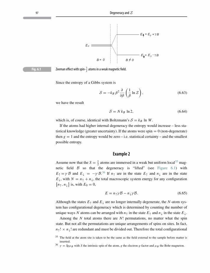
97 Degeneracy andZ
� Fig. 6.1 Zeeman effect with spin- 12 atoms in a weak magnetic field.
Since the entropy of a Gibbs system is
S = −kB β2 ∂
∂β
(1
βlnZ
), (6.63)
we have the result
S = N kB ln 2, (6.64)
which is, of course, identical with Boltzmann’s S = kB ln W .
If the atoms had higher internal degeneracy the entropy would increase – less sta-
tistical knowledge (greater uncertainty). If the atoms were spin = 0 (non-degenerate)
then g = 1 and the entropy would be zero – i.e. statistical certainty – and the smallest
possible entropy.
Example 2
Assume now that the S = 12 atoms are immersed in a weak but uniform local35 mag-
netic field B so that the degeneracy is “lifted” (see Figure 6.1) with
E↑ = γ B and E↓ = −γ B.36 If n↑ are in the state E↑ and n↓ are in the state
E↓, with N = n↑ + n↓, the total macroscopic system energy for any configuration{n↑, n↓
}is, with E0 = 0,
E = n↑γB − n↓γB. (6.65)
Although the states E↑ and E↓ are no longer internally degenerate, the N -atom sys-
tem has configurational degeneracy which is determined by counting the number of
unique ways N atoms can be arranged with n↑ in the state E↑ and n↓ in the state E↓.
Among the N total atoms there are N ! permutations, no matter what the spin
state. But not all the permutations are unique arrangements of spins on sites. In fact,
n↑! × n↓! are redundant and must be divided out. Therefore the total configurational
35 The field at the atom site is taken to be the same as the field external to the sample before matter isinserted.
36 γ = SgμB with S the intrinsic spin of the atom, g the electron g-factor and μB the Bohr magneton.
98 Knowing the “unknowable”
degeneracy for the particular macroscopic energy E in Eq. 6.65 is
g(N , n↑, n↓) = N !n↑! n↓! . (6.66)
Consequently the partition function (sum over states) for the system in a magnetic
field is
Z =∑
n↑,n↓n↑+n↓=N
N !n↑ × n↓
exp[−β
(n↑ − n↓
)γB
], (6.67)
which is just the binomial expansion of
Z =(
e−βγB + eβγB)N
. (6.68)
The internal energy of the system is37
U = − ∂
∂βlnZ (6.69)
= NγB eβγB − e−βγB
eβγB + e−βγB , (6.70)
and from Eq. 6.53 the entropy is
S = NkB
{ln(
eβγB + e−βγB)− βγB
(eβγB − e−βγB
eβγB + e−βγB
)}. (6.71)
Example 3
A simple model of a linear elastomer38 consists of a chain with N identical links
each of length � (see Figure 6.2). The elastomer can be stretched under tension until
its maximum length is Lmax = N�. (A thin rubber band is an imperfect but helpful
illustration.) In this simplified model the linkage energies are very weak so that each
molecule (link) can point either to the left or to the right – and only to the left or right
– with negligible energy difference.39 Referring to Eq. 6.45, the partition function
for this model depends only on configurational degeneracy.
The fully extended polymer with length L = N� (see Figure 6.2) has only one
possible configuration (actually two, since the links can all point to the left or all to
the right). If the tension is relaxed the elastomer will retract to length L < Lmax as
depicted in Figure 6.3.
37 Strictly speaking, with E0 = 0, the internal energy U = 0. The result given here is a magnetic energy.38 An elastic polymer.39 Although not without significant deficiencies, the model is useful for understanding unusual elastic
and thermodynamic properties of rubber and other elastic polymers.
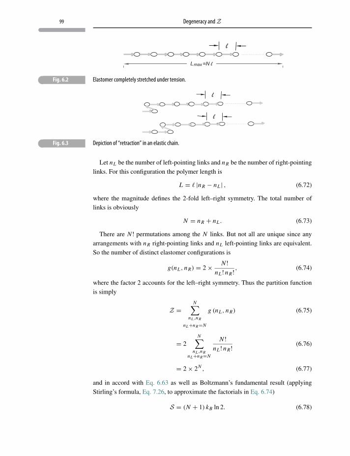
99 Degeneracy andZ
� Fig. 6.2 Elastomer completely stretched under tension.
� Fig. 6.3 Depiction of “retraction” in an elastic chain.
Let nL be the number of left-pointing links and nR be the number of right-pointing
links. For this configuration the polymer length is
L = � |nR − nL | , (6.72)
where the magnitude defines the 2-fold left–right symmetry. The total number of
links is obviously
N = nR + nL . (6.73)
There are N ! permutations among the N links. But not all are unique since any
arrangements with nR right-pointing links and nL left-pointing links are equivalent.
So the number of distinct elastomer configurations is
g(nL , nR) = 2× N !nL ! nR ! , (6.74)
where the factor 2 accounts for the left–right symmetry. Thus the partition function
is simply
Z =N∑
nL ,nR
nL+nR=N
g (nL , nR) (6.75)
= 2N∑
nL ,nRnL+nR=N
N !nL ! nR ! (6.76)
= 2× 2N , (6.77)
and in accord with Eq. 6.63 as well as Boltzmann’s fundamental result (applying
Stirling’s formula, Eq. 7.26, to approximate the factorials in Eq. 6.74)
S = (N + 1) kB ln 2. (6.78)
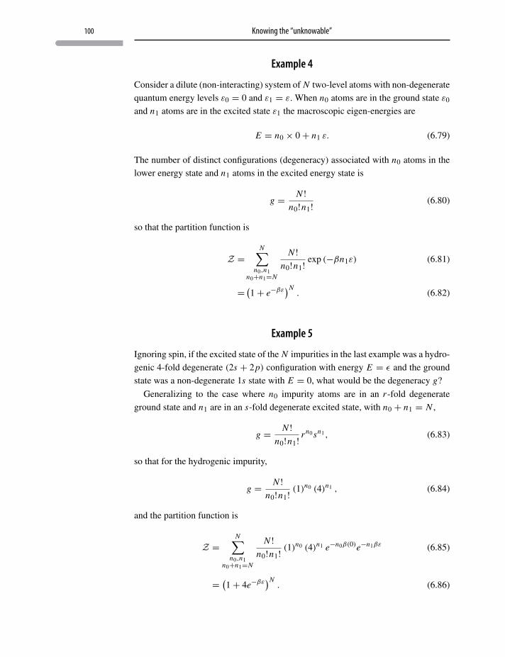
100 Knowing the “unknowable”
Example 4
Consider a dilute (non-interacting) system of N two-level atoms with non-degenerate
quantum energy levels ε0 = 0 and ε1 = ε. When n0 atoms are in the ground state ε0
and n1 atoms are in the excited state ε1 the macroscopic eigen-energies are
E = n0 × 0+ n1 ε. (6.79)
The number of distinct configurations (degeneracy) associated with n0 atoms in the
lower energy state and n1 atoms in the excited energy state is
g = N !n0!n1! (6.80)
so that the partition function is
Z =N∑
n0,n1n0+n1=N
N !n0!n1! exp (−βn1ε) (6.81)
= (1+ e−βε)N
. (6.82)
Example 5
Ignoring spin, if the excited state of the N impurities in the last example was a hydro-
genic 4-fold degenerate (2s + 2p) configuration with energy E = ε and the ground
state was a non-degenerate 1s state with E = 0, what would be the degeneracy g?
Generalizing to the case where n0 impurity atoms are in an r -fold degenerate
ground state and n1 are in an s-fold degenerate excited state, with n0 + n1 = N ,
g = N !n0!n1! r
n0sn1, (6.83)
so that for the hydrogenic impurity,
g = N !n0!n1! (1)
n0 (4)n1 , (6.84)
and the partition function is
Z =N∑
n0,n1n0+n1=N
N !n0!n1! (1)
n0 (4)n1 e−n0β(0)e−n1βε (6.85)
= (1+ 4e−βε
)N. (6.86)
101 Degeneracy andZ
Note: In the case of an arbitrary number of states with energies ε1, ε2, . . . , εm , and
degeneracies s1, s2, . . . , sm with site occupancies n1, n2, . . . , nm ,
g = N !n1!n2! . . . nm ! s
n11 sn2
2 . . . snmm , (6.87)
which is a generalized multinomial coefficient40 with a corresponding partition
function
Z =N∑
n1,n2,...,nmn1+n2+···+nm=N
N !n1!n2! . . . nm ! s
n11 sn2
2 . . . snmm e−βε1n1e−βε2n2 . . . e−βεm nm (6.88)
= (s1e−βε1 + s2e−βε2 + · · · + sme−βεm
)N. (6.89)
Example 6
Consider a lattice of N identical one-dimensional quantum harmonic oscillators,
each oscillator with allowed eigen-energies
Ei = hω0
(ni + 1
2
)(6.90)
where ω0 is the oscillator’s natural frequency, i = 1, 2, 3, . . . , N and ni = 1, 2,
3, . . . ,∞ are the i th oscillator’s allowed quantum numbers. The eigen-energies of
the entire oscillator lattice are
E(n) =N∑
i=1
Ei (6.91)
= hω0 N
2+ hω0
N∑i=1
ni (6.92)
= hω0 N
2+ hω0n, (6.93)
where n is the total lattice quantum number,41
n =N∑
i=1
ni . (6.94)
40 This result and its widely used generalizations can be found in M. Abramowitz and I. Segun, Handbookof Mathematical Functions, Dover (1965), Chapter 24.
41 Here we have the opportunity to introduce the idea of quasi-particles, which are notional particlesused to represent the energy excitations of fields. In this case the harmonic oscillator is representedby quasi-particles identified with a “phonon” field, i.e. the quantum numbers n. Clearly these quasi-particles must be “notional” in the sense that, even though there is a fixed number N of vibrating atoms,there is no similar quasi-particle number n conservation.
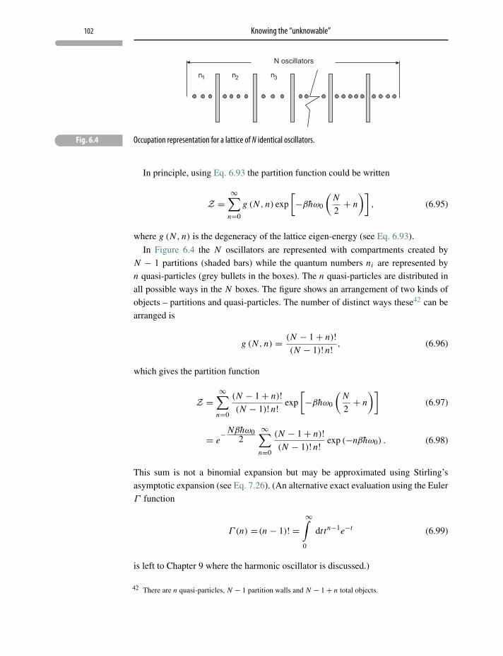
102 Knowing the “unknowable”
� Fig. 6.4 Occupation representation for a lattice of N identical oscillators.
In principle, using Eq. 6.93 the partition function could be written
Z =∞∑
n=0
g (N , n) exp
[−βhω0
(N
2+ n
)], (6.95)
where g (N , n) is the degeneracy of the lattice eigen-energy (see Eq. 6.93).
In Figure 6.4 the N oscillators are represented with compartments created by
N − 1 partitions (shaded bars) while the quantum numbers ni are represented by
n quasi-particles (grey bullets in the boxes). The n quasi-particles are distributed in
all possible ways in the N boxes. The figure shows an arrangement of two kinds of
objects – partitions and quasi-particles. The number of distinct ways these42 can be
arranged is
g (N , n) = (N − 1+ n)!(N − 1)! n! , (6.96)
which gives the partition function
Z =∞∑
n=0
(N − 1+ n)!(N − 1)! n! exp
[−βhω0
(N
2+ n
)](6.97)
= e−Nβhω0
2∞∑
n=0
(N − 1+ n)!(N − 1)! n! exp (−nβhω0) . (6.98)
This sum is not a binomial expansion but may be approximated using Stirling’s
asymptotic expansion (see Eq. 7.26). (An alternative exact evaluation using the Euler
Γ function
Γ (n) =(n − 1)! =∞∫
0
dt tn−1e−t (6.99)
is left to Chapter 9 where the harmonic oscillator is discussed.)
42 There are n quasi-particles, N − 1 partition walls and N − 1+ n total objects.
103 Problems and exercises
6.8 Closing comments
Boltzmann’s pre-quantum insight linked degeneracy (multiplicity) with entropy. But
as indicated here, Boltzmann’s conjecture follows, in principle, by applying the ther-
mal Lagrangian postulate introduced in this chapter in the special circumstance of
a single, isolated, degenerate macroscopic eigen-energy. Applying the same rule to
a continuous spectrum of macroscopic eigen-energies leads to Gibbs’ “canonical”
case. With the thermal Lagrangian (least-biased postulate) thermal physics becomes
a direct consequence of macroscopic quantum theory.
Thermodynamics was a serious and practical science long before there was a quan-
tum mechanics. Doubtless, it will continue to be widely applied in its pragmatic,
time-honored classical form by engineers and chemists in which the role played by
quantum mechanics may be of only academic interest or of no interest at all.
But quantum mechanics lends modern thermodynamics its distinctive and pro-
found character in which microscopic models can be used as a basis for even the
most exotic macroscopic systems. This union has fashioned one of the most versatile
and widely applied paradigms in modern science.
Problems and exercises
6.1 A hypothetical macroscopic system hamiltonian hop has eigen-energies and
eigenstates given by
hop|φ j 〉 = φ j |φ j 〉, (6.100)
where the eigenvalues are
φ j = jγ, j = 0, 1, 2, . . . ,∞. (6.101)
Here γ is a positive constant and each eigenstate |φ j 〉 is j-fold degenerate.
a. Find P j , the least biased, normalized
(∞∑j=1
P j = 1
)probability of the
macroscopic outcome φ j = jγ .
b. What is the entropy of the hypothetical system?
c. Find the average value 〈hop〉 = Trρτop hop.
d. Find the mean uncertainty⟨(Δφ j
)2⟩=
∞∑j=1
(φ j −
⟨hop
⟩)2 P j . (6.102)
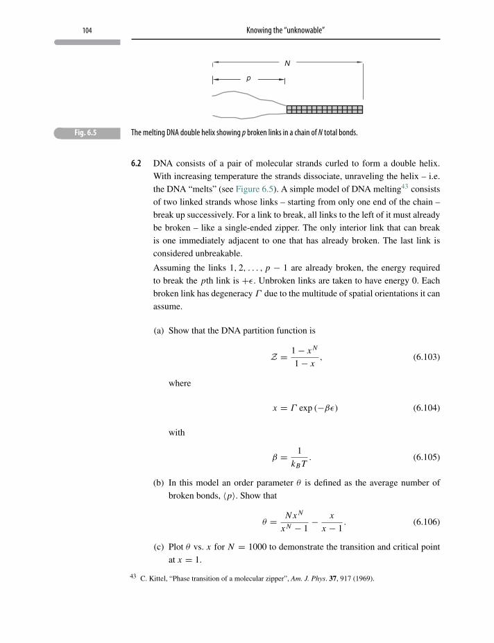
104 Knowing the “unknowable”
p
N
� Fig. 6.5 The melting DNA double helix showing p broken links in a chain of N total bonds.
6.2 DNA consists of a pair of molecular strands curled to form a double helix.
With increasing temperature the strands dissociate, unraveling the helix – i.e.
the DNA “melts” (see Figure 6.5). A simple model of DNA melting43 consists
of two linked strands whose links – starting from only one end of the chain –
break up successively. For a link to break, all links to the left of it must already
be broken – like a single-ended zipper. The only interior link that can break
is one immediately adjacent to one that has already broken. The last link is
considered unbreakable.
Assuming the links 1, 2, . . . , p − 1 are already broken, the energy required
to break the pth link is +ε. Unbroken links are taken to have energy 0. Each
broken link has degeneracy Γ due to the multitude of spatial orientations it can
assume.
(a) Show that the DNA partition function is
Z = 1− x N
1− x, (6.103)
where
x = Γ exp (−βε) (6.104)
with
β = 1
kB T. (6.105)
(b) In this model an order parameter θ is defined as the average number of
broken bonds, 〈p〉. Show that
θ = N x N
x N − 1− x
x − 1. (6.106)
(c) Plot θ vs. x for N = 1000 to demonstrate the transition and critical point
at x = 1.
43 C. Kittel, “Phase transition of a molecular zipper”, Am. J. Phys. 37, 917 (1969).
105 Problems and exercises
(d) Show that for Nε � 1 the entropy of “zipper” DNA is
S = θ lnΓ. (6.107)
Hint:
SN−1 = 1+ x + x2 + . . .+ x N−1 (6.108)
= 1− x N
1− x. (6.109)
7 The ideal gas
J. Willard Gibbs is probably the most brilliant person most people have neverheard of.
Bill Bryson, A Short History of Nearly Everything, Broadway Publishing, NY(2003)
7.1 Introduction
An ideal gas is a collection of uncorrelated identical particles with negligible forces
of interaction.1 These particles can be fundamental particles such as electrons, pro-
tons or neutrons or even quarks. They can be more complex systems such as atoms,
atomic nuclei or molecules. Particle specifics determine, especially at low tempera-
tures, details of their ideal gas behavior even without mutual interactions. For exam-
ple, in addition to the usual translational motion, molecules can rotate or vibrate,
imparting additional properties to these ideal gases. Most interesting however, are
low-temperature behaviors associated with quantum mechanical properties.
Even before quantum mechanics had attained a generally accepted form, W. Pauli2
conjectured that only one electron can occupy a single-particle energy eigen state –
a restriction called the Pauli exclusion principle (PEP).
The following year, E. Fermi3 and P. Dirac4 further showed that quantum mechan-
ics required all particles – depending on their intrinsic spin S, which can be integer
or half-integer – to belong to one of two possible classes:
1. Particles with half-integer spin (S = 12 ,
32 ,
52 , . . .) obey the Pauli exclusion prin-
ciple and are thus called Fermi–Dirac (FD) particles, or fermions. Members of
this class are quarks, electrons, protons, neutrons and neutrinos, as well as their
antiparticles, and many composite systems. For example, He3 is a composite of 2
protons, 2 electrons and 1 neutron, each with spin 12 . This odd-number aggregate
1 Just enough interaction to eventually reach thermal equilibrium.2 W. Pauli, “On the connexion between the completion of electron groups in an atom with the complex
structure of spectra”, Z. Phys. 31, 765 (1925).3 E. Fermi, “Sulla quantizzazione del gas perfetto monoatomico,” Rend. Lincei 3, 145 (1926).4 P. Dirac, “On the theory of quantum mechanics”, Proc. Royal Soc. A 112, 661 (1926).
106
107 Ideal gas law
ensures that He3 has 12 -integer spin. Electrons (together with a uniform positive
background) constitute a gas of Fermi–Dirac particles.
2. Particles with integer spin (S = 0, 1, 2, . . .) have no eigenstate occupation
restriction. Integer-spin particles are called Bose–Einstein (BE) particles, or
bosons. Although most bosons are composite systems, e.g. the H atom (1 pro-
ton and 1 electron), He4 (2 protons, 2 electrons and 2 neutrons) and mesons
(2 spin- 12 quarks), there are elementary particle bosons, e.g. W± and Z parti-
cles, carriers of the weak nuclear force and gluons which are associated with the
strong nuclear force. Also included is the γ : particle (photon) and the feverishly
sought Higgs boson H 0. But in this era of boson condensate physics, composite
boson systems, such as atoms of Li7, Na23, K41, Rb85 and Rb87, are a focus of
interest.
In the case of many-particle systems enormous differences exist between low-
temperature behavior of He3 (fermions) and He4 (bosons). These distinctions will be
discussed in Chapters 15 and 16.
7.2 Ideal gas law
In the limit of low particle density and high temperature, ideal FD and BE gasses
shed nearly all their quantum properties so that century-and-a-half-old kinetic (clas-
sical) gas models successfully describe much of their thermodynamic behavior, in
particular the equation of state
pV = NkB T, (7.1)
where p is the gas pressure, N is a fixed number of particles, V the confining volume,
T the gas temperature and kB is Boltzmann’s constant.5 However, in the final analysis
the quasi-classical theory is internally inconsistent and must be rescued by quantum
corrections.
Taking the opportunity to apply a thermal Lagrangian to a physical problem whose
results (and contradictions) are well known, gaseous atoms and molecules are mod-
eled near room temperature and atmospheric pressure as ideal and “quasi-classical”.
The “ideal gas” is so important in thermodynamic pedagogy as well as for many
low-order approximations that we forgo absolute rigor for the present, returning to
the subject in Chapter 15 with a more credible approach.
5 A gas which obeys Eq. 7.1 can be used as an operational thermometer in which T defines the absolute(K) temperature scale.
108 The ideal gas
7.3 Quasi-classical model
The single-particle microscopic hamiltonian operator for non-interacting particles is
hop = − h2
2m∇2 (7.2)
with an eigenvalue equation
hop|εs〉 = εs |εs〉 (7.3)
with εs the microscopic eigen-energies.
Consider now a low-density system consisting of N independent particles each
with mass m confined to a volume V (no FD or BE occupation restrictions). Each
particle can occupy any of the allowed microscopic eigen-energies ε1, ε2, ε3, . . .
with the corresponding macroscopic eigen-energies
E (n1, n2, n3, . . .) = n1ε1 + n2ε2 + n3ε3 + . . . , (7.4)
where n1 particles are in the state ε1, n2 particles are in the state ε2, etc., with a fixed
total number of particles
n1 + n2 + n3 + . . . = N . (7.5)
Guided by discussions in Chapter 6 the thermal Lagrangian is
L [P] = −kB
N∑n1,n2,n3,...=0,1,2...n1+n2+···+nN=N
P(n1, n2, . . .) ln P(n1, n2, . . .)
− T−1N∑
n1,n2,n3,...=0,1,2...n1+n2+···+nN=N
P(n1, n2, . . .)[n1ε1 + n2ε2 + n3ε3 + · · · + nN εN ]
− λ0
N∑n1,n2,n3,...=0,1,2...n1+n2+···+nN=N
P (n1, n2, . . .). (7.6)
With β = 1/kB T , maximizing L [P]
P (n1, n2, . . . , nN ) = exp {−β(n1ε1 + n2ε2 + . . .+ nN εN )}N∑
n1,n2,n3,...=0,1,2...n1+n2+···+nN=N
exp {−β(n1ε1 + n2ε2 + . . .+ nN εN )}.
(7.7)
109 Ideal gas partition function
The denominator is the partition function Z and the sums are over all states. Follow-
ing the procedure for calculating a partition function,
Z =N∑
n1,n2,...=0,1,2,...n1+n2+...=N
gN (n1, n2, . . .) exp {−β(n1ε1 + n2ε2 + · · · + nN εN )} , (7.8)
where
gN (n1, n2, . . .) = N !n1! n2! n3! . . . (7.9)
is the configurational degeneracy of an N -particle state6 with macroscopic eigen-
energies given by Eq. 7.4. Therefore
Z =N∑
n1,n2,...=0,1,2,...n1+n2+...=N
N !n1!n2! . . . exp {−β(n1ε1 + n2ε2 + · · · + nN εN )} , (7.10)
which is the expansion of
Z = (e−βε1 + e−βε2 + e−βε3 + . . .
)N. (7.11)
Although Eq. 7.11 is mathematically correct, the physical result is not! For at
its heart is a problem in many-particle quantum mechanics with no rigorous semi-
classical argument.7 Indeed, J. W. Gibbs quickly realized that applying Eq. 6.53 to
Eq. 7.11 did not result in an extensive entropy. To correct this, the partition function
was appended by an ad-hoc 1N ! prefactor (known as the Gibbs correction).8 With
this correction, the partition function becomes
Z = 1
N !(e−βε1 + e−βε2 + e−βε3 + . . .
)N. (7.12)
7.4 Ideal gas partition function
Practical ideal gas results can be obtained from Eq. 7.12 by applying the quantum
mechanical energy states of free particles confined to a cube9,10 of side L (volume
6 See Chapter 6.7 This issue will be addressed in Chapter 15.8 The correction is a consequence of normalizing quantum many-particle state functions.9 Periodic boundary conditions are almost universally applied for free particles and fields. But in this
problem we choose the equivalent and probably more familiar “large 3-D box” boundary conditions.10 Lower dimensional systems, which are of considerable importance in modern materials science, might
be dealt with in an analogous way.
110 The ideal gas
V = L3),
εν = h2
2m
(πL
)2(ν2
x + ν2y + ν2
z
), (7.13)
where νx , νy, νz = 1, 2, 3, . . . The eigen-energies in Eq. 7.13 correspond to particles
with purely translation modes, e.g. a monatomic gas or a polyatomic gas without
vibrational, rotational or electronic excitations.11
Using the energies in Eq. 7.13 and the partition function, Eq. 7.12,
Z = 1
N !
⎡⎢⎣ ∞∑νx ,νy ,νz=1
e−β h2
2m
(πL
) (ν2
x + ν2y + ν2
z
)⎤⎥⎦N
, (7.14)
which is
Z = 1
N !
⎡⎢⎣ ∞∑νx=1
e−β h2
2m
(νxπ
L
)2⎤⎥⎦
3N
. (7.15)
Substituting the new counting variable
kx = πνx
L(7.16)
implies
L
πΔkx = Δνx . (7.17)
Since the quantities ν j , . . . are the integers 1, 2, . . . it follows that all Δν j ≡ 1 and
the partition function is
Z = 1
N !
⎡⎢⎣ ∞∑νx=1
Δνx e−β h2
2m
(νxπ
L
)2⎤⎥⎦
3N
→ 1
N !
⎡⎢⎣ L
π
∞∑kx
Δkx e−β h2
2mk2
x
⎤⎥⎦3N
.
(7.18)
When the cube becomes large, i.e. L →∞, it follows that Δkx → dkx , and the sum
over Δkx in Eq. 7.18 can be replaced by the equivalent integral
Z = 1
N !
⎡⎢⎣ L
π
∞∫0
dkx e−β h2
2mk2
x
⎤⎥⎦3N
. (7.19)
11 These eigen-energies are also appropriate for ideal FD and BE quantum gases so long as FD andBE occupation number restrictions are observed. FD and BE quantum gases have strikingly differentpartition functions, even with the same allowed eigen-energies. (See Chapters 15 and 16.)
111 Thermodynamics of the ideal gas
Using the standard Gaussian integral result
∞∫0
dx e−αx2 = 1
2
√π
α, (7.20)
the partition function is
Z = 1
N !
[L
2π
√2mπ
βh2
]3N
(7.21)
= 1
N !(nQ V
)N, (7.22)
where
nQ =(
m
2πh2β
) 32
(7.23)
is the quantum concentration – a particle density parameter that measures the gas’s
degree of dilution. In particular, if n/nQ � 1, where n= N/V is the particle con-
centration, then the gas is sufficiently dilute for the quasi-classical ideal gas result
Eq. 7.21 to apply. If, on the other hand, n/nQ � 1 quantum considerations are
inescapable and the arguments that brought us this far are inadequate.12,13
7.5 Thermodynamics of the ideal gas
This ideal gas model is replete with familiar thermodynamic results:
1. Internal energy U :
With P (n1, n2, . . .) from Eq. 7.7, the internal energy is
U =N∑
n1,n2,n3,...=0,1,2,...n1+n2+···+nN=N
P (n1, n2, . . .) [n1ε1 + n2ε2 + n3ε3 + · · · + nN εN ] ,
(7.24)
which is identical with
U = −∂ lnZ∂β
. (7.25)
Using Eq. 7.21 together with Stirling’s approximation
12 See Chapters 15 and 1613 In addition to the quantum mechanical 1/N !, Planck’s constant h also appears in the partition
function – yet another intrusion of quantum mechanics. Equation 7.21 shows that even the classicalideal gas – often imagined as tiny billiard balls banging about in a box – has quantum imprinting.
112 The ideal gas
n! ∼ nne−n, n � 1,
ln n! ∼ n ln n − n, n � 1,(7.26)
we have
U = 3N
2β(7.27)
= 3
2N kB T . (7.28)
2. Heat capacity CV :
With only translational (kinetic) energy
CV =(∂U∂T
)V
(7.29)
= 3
2N kB . (7.30)
3. Entropy S:
S = kBβ2(
∂
∂β
)(− 1
βlnZ
)(7.31)
= NkB
[5
2+ 3
2ln
(m
2πh2β
)− ln
(N
V
)](7.32)
= NkB
[5
2+ ln
(nQ
n
)], (7.33)
which is called the Sackur–Tetrode equation.14,15
4. Helmholtz potential F :
Applying Stirling’s approximation to Eq. 6.56, where it was shown that
F = − 1
βlnZ, (7.34)
we find
F = −N
β
(ln
nQ
n+ 1
). (7.35)
14 The inclusion of 1/N ! – the Gibbs correction – is a fundamental quantum mechanical result derivedfrom the requirement that under permutation of identical particles the many-particle state vectorchanges, at most, by a phase factor.
15 The Gibbs 1/N ! correction makes an essential contribution to the entropy. Without it
S ?= N kB
[32 + ln
(V nQ
)], which does not satisfy Euler’s homogeneity condition S (λV ) = λS (V ).
S would not be extensive.
113 Gibbs’ entropy paradox
5. Equation of state:
The expression for pressure is
p = 1
β
(∂ lnZ∂V
)T
(7.36)
= −(∂F
∂V
)T, (7.37)
giving the “ideal gas law”
p = NkB T
V. (7.38)
7.6 Gibbs’ entropy paradox
Consider a cylinder that is partitioned into two sections with volumes V1 and V2
so that the total volume is V = V1 + V2. N1 and N2 absolutely identical ideal gas
molecules occupy the volumes V1 and V2, respectively – same quantum concentra-
tion, same temperature T , same concentration n. If the partition magically dissolves
the identical gases will spontaneously mix and occupy the total volume V with the
equilibrium temperature and concentration unchanged.
Objectively, nothing has happened. There is no way to distinguish between the
“before” and “after”. There is no change in the state of knowledge. For this process
mixing has, apparently, no objective meaning! Is there a change in entropy?
The Sackur–Tetrode equation gives the entropy of the original system (before the
partition dissolves) as
S = S1 + S2 (7.39)
= N1kB
[ln(nQ/n
)+ 5
2
]+ N2kB
[ln(nQ/n
)+ 5
2
](7.40)
= NkB
[ln(nQ/n
)+ 5
2
], (7.41)
which is identical to the entropy of the system after the partition disintegrates –
entirely in accord with physical intuition and our interpretation of entropy’s infor-
mational meaning.16
If, however, the partition function of Eq. 7.22 had not been “quantum” corrected
by the Gibbs 1/N ! there would be an increase in the entropy after the partition dis-
integrates, which, based on our understanding of entropy, is nonsense!
16 Note that when calculating thermodynamic averages such as U or p the Gibbs 1/N ! correction cancels.The same cancellation does not occur in entropy calculations.
114 The ideal gas
7.7 Entropy of mixing
Consider the situation just described, but now with two different ideal gases, a and
b, with unique quantum concentrations naQ and nb
Q . Initially, species a occupies a
volume Va and species b occupies a volume Vb. The partition function for gas a is
Za =(
VanaQ
)Na
Na ! (7.42)
and the partition function for gas b is
Zb =(
VbnbQ
)Nb
Nb! . (7.43)
Applying the Sackur–Tetrode equation to each species, the total initial entropy is
S = Sa + Sb (7.44)
= NakB
[5
2+ ln
(na
Q/na
)]+ NbkB
[5
2+ ln
(nb
Q/nb
)], (7.45)
where na = Na/Va and nb = Nb/Vb.
After the chamber partition magically dissolves and the gases mix, the total entropy
of the mixed system is
Sa+b = NakB
{ln[(Va + Vb) na
Q/Na
]+ 5
2
}+ NbkB
{ln[(Va + Vb) nb
Q/Nb
]+ 5
2
}. (7.46)
Defining an entropy of mixing as Smixing = Sa+b − (Sa + Sb) then
Smixing = NakB ln
(Va + Vb
Va
)+ NbkB ln
(Va + Vb
Vb
)> 0. (7.47)
The mixing entropy Smixing has the same value even if the partition functions had
not been Gibbs (quantum) corrected by 1/N !. Moreover, Eq. 7.47 now says –
nonsensically – that a finite mixing entropy remains even after the limit
naQ → nb
Q (7.48)
has been taken! Mixing entropy is obviously not a continuous function of nQ . This,
physically, may be attributable to the “quantization” of mass units.
115 Problems and exercises
7.8 The non-ideal gas
The idea of a “classical” ideal gas is clearly a fiction since h and the Gibbs
correction factor 1/N !, both from quantum mechanics, must appear in the ideal gas
entropy. Moreover, atoms and molecules in a real gas do interact and with significant
consequences. An approximate equation of state that improves upon the ideal gas
law is due to van der Waals (1873) who took account of long-range attraction and
short-range repulsion between particles. Van der Waals’ equation not only improves
descriptions of gas phase thermodynamics, it also suggests gas–liquid phase
transitions and gas critical points as consequences of interactions. This eponymous
equation of state is:17 [p + (N/V )2 a
](V − Nb) = NkB T, (7.49)
where a and b are coefficients characteristic of specific gases.18
The van der Waals equation, by quantitatively providing two parameters that char-
acterize real molecules, would seem to have settled a bitter ongoing debate of the
times: Did gases, and matter in general, have microscopic structure? But it didn’t.
Problems and exercises
7.1 Assume an N -particle ideal gas in two-dimensions with eigen-energies
En = h2
2m
(πL
)2(n2
x + n2y
), (7.50)
where
nx , ny = 1, 2, 3, . . . (7.51)
The confining surface area is
A = L2. (7.52)
(a) Write an expression for the partition function Z2D of the two-dimensional
ideal gas.
(b) Find the internal energy U2D of the gas.
(c) Find the heat capacity CA for the two-dimensional gas.
(d) Find the entropy S2D of the gas.
17 A derivation of the van der Waals equation is given in Chapter 13.18 R. C. Weast (ed.), Handbook of Chemistry and Physics (53rd edn.), Chemical Rubber Co., Cleveland
(1972).
116 The ideal gas
7.2 The quantity
πT =(∂U∂V
)T
(7.53)
is called internal pressure and expresses the role of particle–particle interac-
tions in the behavior of a gas. Find πT for
(a) an ideal gas;
(b) a van der Waals gas;
(c) a gas with the equation of state
p = NkB T
V
[1+ N
VB(T )
]. (7.54)
8 The two-level system
A theory is the more impressive the greater the simplicity of its premises, themore different kinds of things it relates and the more extended is its area ofapplicability.
A. Einstein. Reproduced by permission of Open Court Publishing Company, adivision of Carus Publishing Company, from Albert
Einstein: Philosopher-Scientist, edited by Paul Arthur Schilpp (The Library ofLiving Philosophers Volume VII), 1949, 1951 and 1970 by The Library
of Living Philosophers
8.1 Anomalous heat capacity
Insulators or semiconductors containing impurities with closely spaced electronic or
nuclear ground states1 show an anomalous low-temperature heat capacity peak – the
so-called Schottky anomaly.2 It is an example of microscopic quantum effects having
macroscopic (thermodynamic) signatures.
8.2 Schottky model
A simple model for the “Schottky” anomalous heat capacity consists of a crystal
containing a dilute3 concentration of N identical atomic impurities, each having the
same pair of closely spaced, non-degenerate energy levels – a lower state ε1 and a
higher state ε2. If, at some temperature T , n1 impurity atoms are in the low energy
state and n2 are in the higher energy state, the macroscopic eigen-energies are
E(n1, n2) = n1ε1 + n2ε2, (8.1)
1 Usually degenerate low-energy states whose degeneracy is lifted by crystalline electric fields, magneticfields, spin-orbit coupling or hyperfine interactions.
2 The phenomenon is named for Walter Hermann Schottky (1886–1976).3 Diluteness insures negligible inter-atomic effects.
117
118 The two-level system
with the thermal Lagrangian
L = −kB
∑n1,n2
n1+n2=N
P (n1, n2) ln P (n1, n2)
− T−1∑n1,n2
n1+n2=N
P (n1, n2) (n1ε1 + n2ε2)− λ0
∑n1,n2
n1+n2=N
P (n1, n2), (8.2)
where P (n1, n2) is the probability that n1 impurity atoms are in the state ε1 and n2
are in the state ε2. The sums are over all states. The method of Lagrange multipliers
gives the probabilities
P (n1, n2) = e−β(n1ε1+n2ε2)
Z (8.3)
with the partition function
Z =∑n1,n2
n1+n2=N
e−β(n1ε1+n2ε2), (8.4)
which again represents a sum over all states. One way to calculate this sum is by
explicitly including a configurational degeneracy (see Chapter 6)
g(n1, n2) = N !n1! n2! (8.5)
to give
Z =N∑
n1,n2n1+n2=N
N !n1! n2!e
−β(n1ε1+n2ε2), (8.6)
which is the binomial expansion of4
Z = (e−βε1 + e−βε2
)N. (8.7)
The thermodynamic properties that follow from Eq. 8.7 are:
1. Internal energy:
U = − ∂
∂βln Z (8.8)
= Nε1e−βε1 + ε2e−βε2
e−βε1 + e−βε2. (8.9)
4 Some authors prefer to calculate the partition function – one atom at a time – and then take the productof N single-atom partition functions. This avoids the mathematics of combinatoric analysis in obtain-ing g. But it also evades the macroscopic character of the physics.
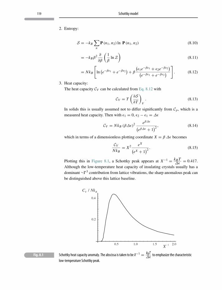
119 Schottky model
2. Entropy:
S = −kB
∑n
P (n1, n2) ln P (n1, n2) (8.10)
= −kBβ2 ∂
∂β
(1
βlnZ
)(8.11)
= NkB
[ln(e−βε1 + e−βε2
)+ β
(ε1e−βε1 + ε2e−βε2
)(e−βε1 + e−βε2
) ]. (8.12)
3. Heat capacity:
The heat capacity CV can be calculated from Eq. 8.12 with
CV = T
(∂S∂T
)V. (8.13)
In solids this is usually assumed not to differ significantly from Cp, which is a
measured heat capacity. Then with ε1 = 0, ε2 − ε1 = Δε
CV = NkB (βΔε)2 eβΔε(eβΔε + 1
)2, (8.14)
which in terms of a dimensionless plotting coordinate X = β Δε becomes
CV
NkB= X2 eX(
eX + 1)2
. (8.15)
Plotting this in Figure 8.1, a Schottky peak appears at X−1 = kB TΔε
= 0.417.
Although the low-temperature heat capacity of insulating crystals usually has a
dominant∼T 3 contribution from lattice vibrations, the sharp anomalous peak can
be distinguished above this lattice baseline.
� Fig. 8.1 Schottky heat capacity anomaly. The abscissa is taken to be X−1 = kBTΔε
to emphasize the characteristiclow-temperature Schottky peak.
120 The two-level system
In the high-temperature limit, X � 1, Eq. 8.15 reduces to
CV
NkB→ X2
4(8.16)
=(
Δε
2kB T
)2
. (8.17)
At low temperature, X � 1, Eq. 8.15 becomes
CV
NkB→ X2e−X (8.18)
=(
Δε
kB T
)2
e− Δε
kB T , (8.19)
which has the limiting Schottky behavior
limT→0
CV = 0. (8.20)
8.3 Two-level systems and negative temperature
Writing internal energy, Eq. 8.9, as
U = NΔε
1+ eβΔε(8.21)
a dimensionless internal energy Φ = UNΔε
can be defined. Then the entropy of
Eq. 8.12,
S = NkB
[ln(1+ e−βΔε
)+ βΔε
eβΔε + 1
], (8.22)
can be re-expressed in terms of Φ as
SNkB
= (Φ − 1) ln (1−Φ)−Φ lnΦ, (8.23)
which is plotted in Figure 8.2.
From the “thermodynamic identity” written as
T dS = NΔε dΦ + pdV (8.24)
or
dS = N Δε
TdΦ + p
TdV, (8.25)
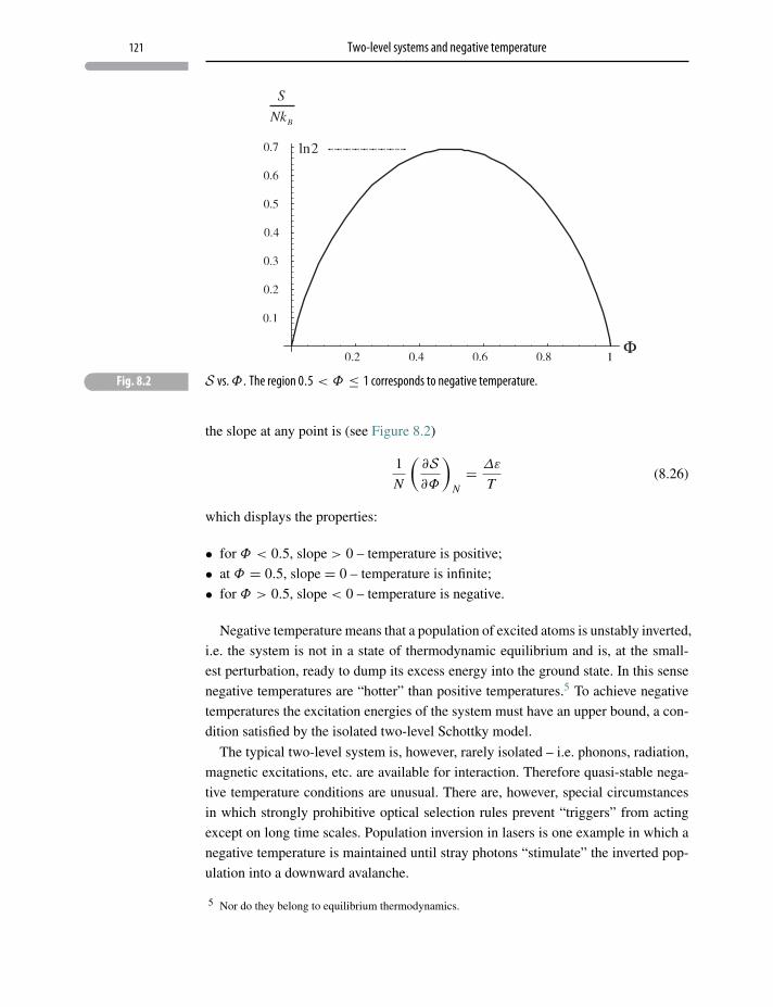
121 Two-level systems and negative temperature
� Fig. 8.2 S vs. Φ. The region 0.5 < Φ ≤ 1 corresponds to negative temperature.
the slope at any point is (see Figure 8.2)
1
N
(∂S∂Φ
)N= Δε
T(8.26)
which displays the properties:
• for Φ < 0.5, slope > 0 – temperature is positive;
• at Φ = 0.5, slope = 0 – temperature is infinite;
• for Φ > 0.5, slope < 0 – temperature is negative.
Negative temperature means that a population of excited atoms is unstably inverted,
i.e. the system is not in a state of thermodynamic equilibrium and is, at the small-
est perturbation, ready to dump its excess energy into the ground state. In this sense
negative temperatures are “hotter” than positive temperatures.5 To achieve negative
temperatures the excitation energies of the system must have an upper bound, a con-
dition satisfied by the isolated two-level Schottky model.
The typical two-level system is, however, rarely isolated – i.e. phonons, radiation,
magnetic excitations, etc. are available for interaction. Therefore quasi-stable nega-
tive temperature conditions are unusual. There are, however, special circumstances
in which strongly prohibitive optical selection rules prevent “triggers” from acting
except on long time scales. Population inversion in lasers is one example in which a
negative temperature is maintained until stray photons “stimulate” the inverted pop-
ulation into a downward avalanche.
5 Nor do they belong to equilibrium thermodynamics.
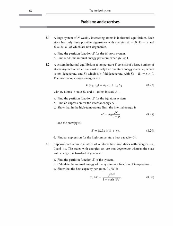
122 The two-level system
Problems and exercises
8.1 A large system of N weakly interacting atoms is in thermal equilibrium. Each
atom has only three possible eigenstates with energies E = 0, E = ε and
E = 3ε, all of which are non-degenerate.
a. Find the partition function Z for the N -atom system.
b. Find U/N , the internal energy per atom, when βε � 1.
8.2 A system in thermal equilibrium at temperature T consists of a large number of
atoms N0 each of which can exist in only two quantum energy states: E1 which
is non-degenerate, and E2 which is p-fold degenerate, with E2− E1 = ε > 0.
The macroscopic eigen-energies are
E (n1, n2) = n1 E1 + n2 E2 (8.27)
with n1 atoms in state E1 and n2 atoms in state E2.
a. Find the partition function Z for the N0 atom system.
b. Find an expression for the internal energy U .
c. Show that in the high-temperature limit the internal energy is
U = N0pε
1+ p(8.28)
and the entropy is
S = N0kB ln (1+ p) . (8.29)
d. Find an expression for the high-temperature heat capacity CV .
8.3 Suppose each atom in a lattice of N atoms has three states with energies −ε,
0 and +ε. The states with energies ±ε are non-degenerate whereas the state
with energy 0 is two-fold degenerate.
a. Find the partition function Z of the system.
b. Calculate the internal energy of the system as a function of temperature.
c. Show that the heat capacity per atom, CV /N , is
CV /N = β2ε2
1+ cosh (βε). (8.30)
9 Lattice heat capacity
I believe that no one who has won, through long years of experience, a reasonablyreliable sense for the not always easy experimental evaluation of a theory, willbe able to contemplate these results without immediately becoming convincedof the huge logical power of the quantum theory.
W. Nernst, Z. fur Elektrochem. 17, 265–275 (1911) [trans. A. Wasserman]
9.1 Heat capacity of solids
The nearly 200-year-old Dulong–Petit “rule” for molar heat capacities of crystalline
matter, cv , predicts the constant value
cv = 3
2NA kB (9.1)
= 24.94 J mole−1, (9.2)
where NA is Avagadro’s number. Although Dulong–Petit, which assumes solids
to be dense, classical, ideal gases (see Eq. 7.29), is in amazingly good agreement
with the high-temperature (∼300 K) molar heat capacities of many solids, it fails
to account for the observed rapid fall in cv at low temperature. An especially large
effect in diamond caught Einstein’s (1907) attention and with extraordinary insight
he applied Planck’s “quanta” to an oscillator model of an atomic lattice to predict a
universal decline in cv as T → 0 K. Several years later, when low-temperature molar
heat capacities could be accurately measured, they were indeed found to behave in
approximate agreement with Einstein’s prediction.1 It was this result that ultimately
succeeded in making the case for quantum theory and the need to radically reform
physics to accommodate it.
1 The cv in metals has an additional very-low-temperature contribution ∼ T from conduction electrons,which, of course, Einstein could not account for.
123
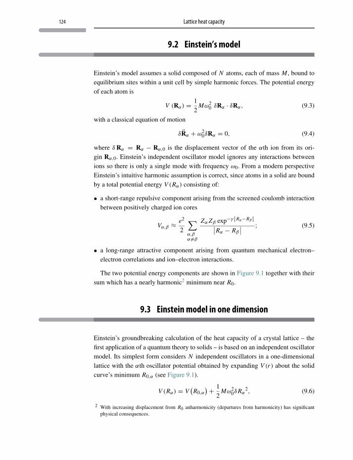
124 Lattice heat capacity
9.2 Einstein’s model
Einstein’s model assumes a solid composed of N atoms, each of mass M , bound to
equilibrium sites within a unit cell by simple harmonic forces. The potential energy
of each atom is
V (Rα) = 1
2Mω2
0 δRα · δRα, (9.3)
with a classical equation of motion
δRα + ω20δRα = 0, (9.4)
where δ Rα = Rα − Rα,0 is the displacement vector of the αth ion from its ori-
gin Rα,0. Einstein’s independent oscillator model ignores any interactions between
ions so there is only a single mode with frequency ω0. From a modern perspective
Einstein’s intuitive harmonic assumption is correct, since atoms in a solid are bound
by a total potential energy V (Rα) consisting of:
• a short-range repulsive component arising from the screened coulomb interaction
between positively charged ion cores
Vα,β ≈ e2
2
∑α,βα �=β
Zα Zβ exp−γ |Rα−Rβ |∣∣Rα − Rβ
∣∣ ; (9.5)
• a long-range attractive component arising from quantum mechanical electron–
electron correlations and ion–electron interactions.
The two potential energy components are shown in Figure 9.1 together with their
sum which has a nearly harmonic2 minimum near R0.
9.3 Einstein model in one dimension
Einstein’s groundbreaking calculation of the heat capacity of a crystal lattice – the
first application of a quantum theory to solids – is based on an independent oscillator
model. Its simplest form considers N independent oscillators in a one-dimensional
lattice with the αth oscillator potential obtained by expanding V (r) about the solid
curve’s minimum R0,α (see Figure 9.1).
V (Rα) = V(R0,α
)+ 1
2Mω2
0δRα2, (9.6)
2 With increasing displacement from R0 anharmonicity (departures from harmonicity) has significantphysical consequences.
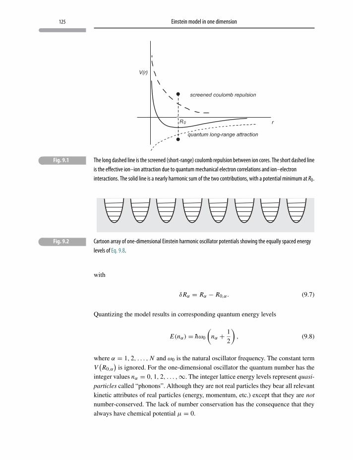
125 Einstein model in one dimension
� Fig. 9.1 The long dashed line is the screened (short-range) coulomb repulsion between ion cores. The short dashed lineis the effective ion–ion attraction due to quantum mechanical electron correlations and ion–electroninteractions. The solid line is a nearly harmonic sum of the two contributions, with a potential minimum at R0.
� Fig. 9.2 Cartoon array of one-dimensional Einstein harmonic oscillator potentials showing the equally spaced energylevels of Eq. 9.8.
with
δRα = Rα − R0,α. (9.7)
Quantizing the model results in corresponding quantum energy levels
E(nα) = hω0
(nα + 1
2
), (9.8)
where α = 1, 2, . . . , N and ω0 is the natural oscillator frequency. The constant term
V(R0,α
)is ignored. For the one-dimensional oscillator the quantum number has the
integer values nα = 0, 1, 2, . . . ,∞. The integer lattice energy levels represent quasi-
particles called “phonons”. Although they are not real particles they bear all relevant
kinetic attributes of real particles (energy, momentum, etc.) except that they are not
number-conserved. The lack of number conservation has the consequence that they
always have chemical potential μ = 0.
126 Lattice heat capacity
With all N atoms contributing, the macroscopic eigen-energies are
E (n) = Nhω0
2+ hω0
N∑α=1
nα (9.9)
= Nhω0
2+ hω0n (9.10)
with
N∑α=1
nα = n. (9.11)
9.3.1 Partition function for one-dimensional Einstein model
From the thermal Lagrangian
L = −kB
∞∑n=0
P(n) ln P(n)− 1
T
N∑n=0
P(n)[βhω0
(N
2+ n
)]− λ0
N∑n=0
P(n) (9.12)
it follows that
P(n) =exp
[−βhω0
(N
2+ n
)]Z . (9.13)
Emphasizing the role of degeneracy in performing the partition function’s sum
over all states, Eqs. 6.96 and 6.97 are used. The partition function is therefore written
Z =∞∑
n=0
(N − 1+ n)!(N − 1)! n! exp
[−βhω0
(N
2+ n
)](9.14)
= e−Nβhω0
2∞∑
n=0
(N − 1+ n)!(N − 1)! n! exp (−nβhω0) . (9.15)
The resulting sum is not entirely obvious, although it can be approximated using the
Stirling formula, Eq. 7.26. But with an integral representation of the Γ function,
Γ (n) = (n − 1)! =∞∫
0
dt tn−1e−t , (9.16)
we can make the replacement
(N + n − 1)! =∞∫
0
dt t (N+n−1)e−t (9.17)
127 Einstein model in one dimension
so the partition function becomes
Z = e−Nβhω0
2
∞∫0
dtt N−1e−t
(N − 1)!∞∑
n=0
1
n! tn e−nβhω0 . (9.18)
Summing over n (to get an exponential) and then integrating over t (again using the
Γ function)
Z = eNβhω0
2(eβhω0 − 1
)N. (9.19)
Evaluation of the one-dimensional oscillator partition function in this way is not
especially difficult, but it is not obviously extensible to higher dimensionality or to
other physically interesting models.
9.3.2 Phonons and the one-dimensional oscillator
A preferable route, using Eq. 9.10 for the eigen-energies, has the one-dimensional
oscillator partition function
Z =∞∑
n1=0
∞∑n2=0
. . .
∞∑nN=0
exp
[−β
(Nhω0
2+ hω0
N∑α=1
nα
)](9.20)
= e−βNhω0/2∞∑
n1=0
∞∑n2=0
. . .
∞∑nN=0
exp
[−βhω0
N∑α=1
nα
], (9.21)
where the sum over states is equivalent to the sum over all numbers of phonons nα .
Explicitly summing over α gives a product of N identical geometrical series
Z = e−βNhω0
2
⎛⎝ ∞∑n1=0
exp [−βhω0n1]
⎞⎠⎛⎝ ∞∑n2=0
exp [−βhω0n2]
⎞⎠ · · ·×⎛⎝ ∞∑
nN=0
exp [−βhω0nN ]
⎞⎠ (9.22)
and hence
Z = e−βNhω0/2( ∞∑
n=0
e−βhω0n)N
, (9.23)
128 Lattice heat capacity
which is summed to give the result
Z = eβNhω0/2(eβhω0 − 1
)N, (9.24)
identical to Eq. 9.19.
9.4 The three-dimensional Einstein model
The three-dimensional Einstein model, although suggesting a better approximation,
still falls short of what is physically observed. (See the Debye model discussion
later in the chapter.) Here the coordinate components x, y, z, of the αth independent
oscillator displacements are taken into account with the eigen-energies
E(nα,x , nα,y, nα,z
) = hω0(nα,x + nα,y + nα,z + 3/2
), (9.25)
where again α = 1, 2, 3, . . . , N and nα,x , nα,y, nα,z = 0, 1, 2, . . . ,∞ with ω0 the
oscillator frequency. The N -oscillator lattice has the macroscopic eigen-energies
Ex,y,z = 3Nhω0
2+ hω0
N∑α=1
(nα,x + nα,y + nα,z
). (9.26)
9.4.1 Partition function for the three-dimensional Einstein model
Using the result of Eq. 9.26, the thermal Lagrangian is as Eq. 9.12 and the partition
function written
Z = e−3Nβhω0
2∞∑
n1,x=0n1,y=0n1,z=0
∞∑n2,x=0n2,y=0n3,z=0
. . .
×∞∑
nN ,x=0nN ,y=0nN ,z=0
exp
{−β
[hω0
N∑α=1
(nα,x + nα,y + nα,z
)]}. (9.27)
The sum is managed, as in Section 9.3.2, by first explicitly summing over α in the
exponential. Then, because the three coordinate sums (nα,x , nα,y, nα,z) are
129 The three-dimensional Einstein model
identical, what remains is
Z = e−3βNhω0
2
⎛⎝ ∞∑n1=0
exp [−βhω0n1]
⎞⎠3⎛⎝ ∞∑n2=0
exp [−βhω0n2]
⎞⎠3
· · ·⎛⎝ ∞∑
nN=0
exp [−βhω0nN ]
⎞⎠3
(9.28)
and finally
Z = e−3Nβhω0
2
( ∞∑n=0
e−βhω0n)3N
, (9.29)
where the remaining sum gives
Z =[
e−βhω0
2(
1
1− e−βhω0
)]3N
. (9.30)
9.4.2 Thermodynamics of the three-dimensional Einstein model
Following steps from previous chapters, the internal energy is
U = − ∂
∂βlnZ (9.31)
= 3Nhω0
[1
2+ 〈n〉
], (9.32)
where3
〈n〉 = 1(eβhω0 − 1
) . (9.33)
Therefore for the three-dimensional model
CV =(∂U
∂T
)V
= −kBβ2(∂U
∂β
)V
= 3NkB(βhω0)
2 eβhω0(eβhω0 − 1
)2. (9.34)
3 〈n〉 is the average phonon (quasi-particle) occupation number. It is also loosely referred to as a Bose–Einstein “function”.
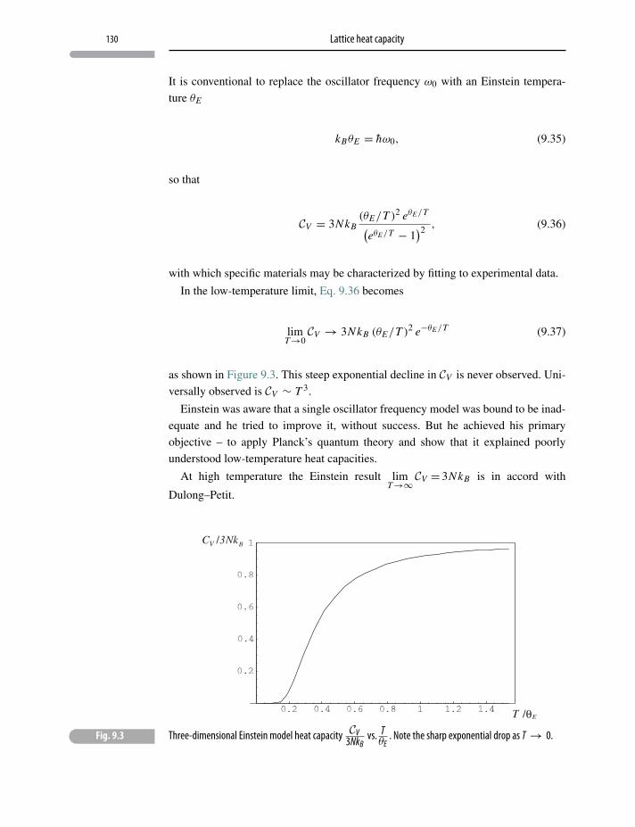
130 Lattice heat capacity
It is conventional to replace the oscillator frequency ω0 with an Einstein tempera-
ture θE
kBθE = hω0, (9.35)
so that
CV = 3NkB(θE/T )2 eθE/T(
eθE/T − 1)2
, (9.36)
with which specific materials may be characterized by fitting to experimental data.
In the low-temperature limit, Eq. 9.36 becomes
limT→0
CV → 3NkB (θE/T )2 e−θE/T (9.37)
as shown in Figure 9.3. This steep exponential decline in CV is never observed. Uni-
versally observed is CV ∼ T 3.
Einstein was aware that a single oscillator frequency model was bound to be inad-
equate and he tried to improve it, without success. But he achieved his primary
objective – to apply Planck’s quantum theory and show that it explained poorly
understood low-temperature heat capacities.
At high temperature the Einstein result limT→∞ CV = 3NkB is in accord with
Dulong–Petit.
V
� Fig. 9.3 Three-dimensional Einstein model heat capacity CV3NkB
vs. TθE
. Note the sharp exponential drop as T → 0.
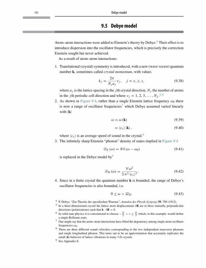
131 Debye model
9.5 Debye model
Atom–atom interactions were added to Einstein’s theory by Debye.4 Their effect is to
introduce dispersion into the oscillator frequencies, which is precisely the correction
Einstein sought but never achieved.
As a result of atom–atom interactions:
1. Translational (crystal) symmetry is introduced, with a new (wave vector) quantum
number k, sometimes called crystal momentum, with values
k j = 2π
N j a jν j , j = x, y, z, (9.38)
where a j is the lattice spacing in the j th crystal direction, N j the number of atoms
in the j th periodic cell direction and where ν j = 1, 2, 3, . . . , N j .5,6
2. As shown in Figure 9.4, rather than a single Einstein lattice frequency ω0 there
is now a range of oscillator frequencies7 which Debye assumed varied linearly
with |k|ω = ω (k) (9.39)
= 〈cs〉 |k| , (9.40)
where 〈cs〉 is an average speed of sound in the crystal.8
3. The infinitely sharp Einstein “phonon” density of states implied in Figure 9.4
DE (ω) = Nδ (ω − ω0) (9.41)
is replaced in the Debye model by9
DD (ω) = Vω2
2π2 〈cs〉3 . (9.42)
4. Since in a finite crystal the quantum number k is bounded, the range of Debye’s
oscillator frequencies is also bounded, i.e.
0 ≤ ω < ΩD. (9.43)
4 P. Debye, “Zur Theorie der spezifischen Waerme”, Annalen der Physik (Leipzig) 39, 789 (1912).5 In a three-dimensional crystal the lattice atom displacements δR are in three mutually perpendicular
directions (polarizations) such that k · δR = 0.6 In solid state physics it is conventional to choose − N
2 < ν ≤ N2 which, in this example, would define
a single Brillouin zone.7 One might say that the atom–atom interactions have lifted the degeneracy among single atom oscillator
frequencies ω0.8 There are three different sound velocities corresponding to the two independent transverse phonons
and single longitudinal phonon. This turns out to be an approximation that accurately replicates thesmall-|k| behavior of lattice vibrations in many 3-D crystals.
9 See Appendix E.
132 Lattice heat capacity
Einstein oscillator frequency w0
ωω 0
� Fig. 9.4 Mode-dependent frequencies. The solid curve represents an approximate result for a real lattice. kmax is theBrillouin zone boundary for the crystal (−kmax < k ≤ kmax). The dashed line represents Debye’s linearapproximation. The slope of the dashed line is the average speed of sound in the crystal. ΩD is the Debyeapproximation’s highest attained frequency. The horizontal fine line at ω = ω0 represents the dispersion ofan Einstein lattice.
Within the Debye model ΩD is found from
∞∫0
dωDE (ω) =ΩD∫0
dωDD (ω), (9.44)
i.e. the total number of modes, 3N , is the same in both models, so that
ΩD =(
6π2〈cs〉3 N/V)1/3
. (9.45)
Whereas the Einstein internal energy UE is (see Eq. 9.32)
UE = 3h
∞∫0
ω dω
Einstein density of states︷ ︸︸ ︷{Nδ (ω − ω0)}
[1
2+ 1
eβhω − 1
](9.46)
= 3Nω0
[1
2+ 1
eβhω0 − 1
], (9.47)
133 Problems and exercises
the changes introduced by Debye give instead the internal energy UD (see
Appendix E),
UD = h
ΩD∫0
ω dω
Debye density of states︷ ︸︸ ︷{3V ω2
2π2〈cs〉3} [
1
2+ 1
eβhω − 1
](9.48)
= 3V
2π3h3〈cs〉3β4
βhΩD∫0
dx x3(
1
2+ 1
ex − 1
). (9.49)
9.5.1 Thermodynamics of the Debye lattice
At high temperature, βhΩD � 1, the integral in Eq. 9.49 can be approximated by
expanding ex ∼= 1+ x . Then using Eq. 9.44 the Debye internal energy is
limT→∞UD = V
2π2
(ΩD
〈cs〉)3
kB T (9.50)
= 3NkB T, (9.51)
consistent with the Dulong–Petit rule. At low temperature, βhΩD � 1, and defining
hΩD =kBΘD, (9.52)
with ΘD the Debye temperature, the internal energy integral can be approximated as
limT→0
UD → 3V
2π3h3〈cs〉3β4
∞∫0
dxx3(
1
2+ 1
ex − 1
), (9.53)
from which, with Eq. 9.45, follows the low-temperature heat capacity
limT→0
CV ∗ → 6k4B
π2h3〈cs〉3× π4
15T 3 (9.54)
= NkB
(12π4
5
)×(
T
ΘD
)3
. (9.55)
The CV ∼= T 3 behavior is almost universally observed in three-dimensional solids.
Examples of Debye temperatures are given in Table 9.1.
Problems and exercises
9.1 Two-dimensional materials are now widely fabricated and investigated. Within
the framework of Debye’s model for lattice vibrations find the low-temperature
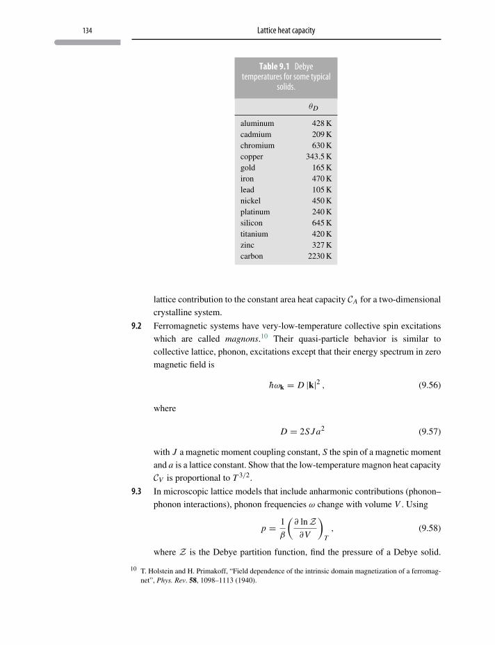
134 Lattice heat capacity
Table 9.1 Debyetemperatures for some typical
solids.
θD
aluminum 428 Kcadmium 209 Kchromium 630 Kcopper 343.5 Kgold 165 Kiron 470 Klead 105 Knickel 450 Kplatinum 240 Ksilicon 645 Ktitanium 420 Kzinc 327 Kcarbon 2230 K
lattice contribution to the constant area heat capacity CA for a two-dimensional
crystalline system.
9.2 Ferromagnetic systems have very-low-temperature collective spin excitations
which are called magnons.10 Their quasi-particle behavior is similar to
collective lattice, phonon, excitations except that their energy spectrum in zero
magnetic field is
hωk = D |k|2 , (9.56)
where
D = 2S Ja2 (9.57)
with J a magnetic moment coupling constant, S the spin of a magnetic moment
and a is a lattice constant. Show that the low-temperature magnon heat capacity
CV is proportional to T 3/2.
9.3 In microscopic lattice models that include anharmonic contributions (phonon–
phonon interactions), phonon frequencies ω change with volume V . Using
p = 1
β
(∂ lnZ∂V
)T, (9.58)
where Z is the Debye partition function, find the pressure of a Debye solid.
10 T. Holstein and H. Primakoff, “Field dependence of the intrinsic domain magnetization of a ferromag-net”, Phys. Rev. 58, 1098–1113 (1940).
135 Problems and exercises
Therefore in taking the volume derivative, Eq. 9.58, 〈cs〉 and hence ΘD depend
on volume.
Express the pressure in terms of the dimensionless Grüneisen parameter γ ,
γ ≡ − V
ΘD
(dΘD
dV
). (9.59)
10 Elastomers: entropy springs
Mr. McGuire: “I want to say one word to you. Just one word.”Benjamin: “Yes, sir.”Mr. McGuire: “Are you listening?”Benjamin: “Yes, I am.”Mr. McGuire: “Plastics.”
The Graduate (1967)1
10.1 Naive one-dimensional elastomer
Crystalline matter and polymeric materials exhibit considerable difference in elastic
behaviors. Under applied stress σ all solids experience strain (elongation) ε. But
crystalline materials also exhibit a property of “stiffness” due to accompanying large
increases in bond energy. These materials also completely lose their elastic properties
at small values of strain, ε ∼ 0.001. Polymeric materials, such as a common rubber
band, are neither “stiff” nor, generally, do they lose elasticity even under large strain.
To see that something quite distinctive must account for elasticity differences
between polymers and crystalline materials, one need only compare values of isother-
mal Young’s moduli
ET =(∂σ
∂ε
)T. (10.1)
Values for crystalline materials are given in Table 10.1 and for polymeric materials
in Table 10.2. Young’s moduli in crystalline matter can be as much as four orders of
magnitude larger than for polymeric materials. What makes them so different is that
elastic polymers are “softly” linked chains of chemical monomers whose “rubbery”
elasticity is associated with freedom for monomer units to bend, rotate and randomly
stack, with negligible energy cost. Figure 10.1 illustrates the structure of the polymer
polyethylene in which ethylene molecules (monomers) are joined in chains. Elas-
tomer flexibility is enabled by unhindered unit rotation about a carbon “backbone”.
Truly “rubbery” materials retain their elastic behavior even when subject to strains
of ε ∼ 1–3, which is much larger than for metals.
1 Courtesy of The Internet Movie Database (http://www.imdb.com). Used with permission.
136
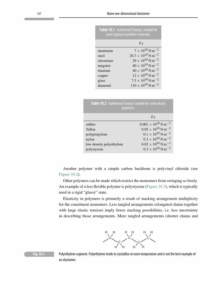
137 Naive one-dimensional elastomer
Table 10.1 Isothermal Young’s moduli forsome typical crystalline materials.
ET
aluminum 7× 10¹⁰ N m−2
steel 20.7× 10¹⁰ N m−2
chromium 29× 1010 N m−2
tungsten 40× 1010 N m−2
titanium 40× 1010 N m−2
copper 12× 1010 N m−2
glass 7.5× 10¹⁰ N m−2
diamond 110× 1010 N m−2
Table 10.2 Isothermal Young’s moduli for some elasticpolymers.
ET
rubber 0.001× 10¹⁰ N m−2
Teflon 0.05× 10¹⁰ N m−2
polypropylene 0.1× 10¹⁰ N m−2
nylon 0.3× 10¹⁰ N m−2
low density polyethylene 0.02× 10¹⁰ N m−2
polystyrene 0.3× 10¹⁰ N m−2
Another polymer with a simple carbon backbone is polyvinyl chloride (see
Figure 10.2).
Other polymers can be made which restrict the monomers from swinging so freely.
An example of a less flexible polymer is polystyrene (Figure 10.3), which is typically
used in a rigid “glassy” state.
Elasticity in polymers is primarily a result of stacking arrangement multiplicity
for the constituent monomers. Less tangled arrangements (elongated chains together
with large elastic tension) imply fewer stacking possibilities, i.e. less uncertainty
in describing those arrangements. More tangled arrangements (shorter chains and
� Fig. 10.1 Polyethylene segment. Polyethylene tends to crystallize at room temperature and is not the best example ofan elastomer.
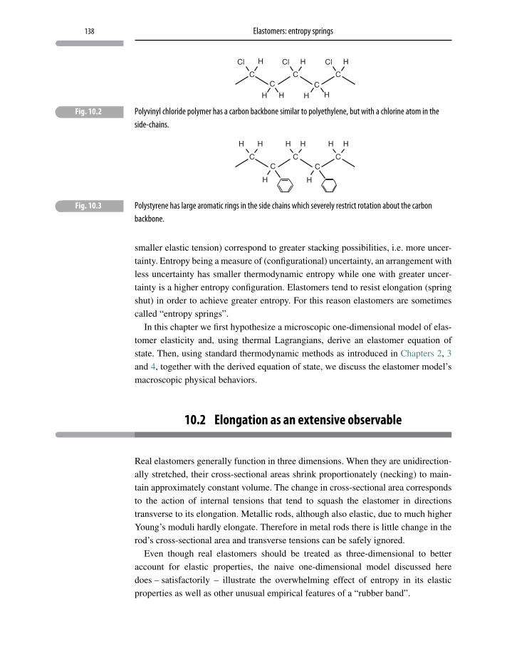
138 Elastomers: entropy springs
� Fig. 10.2 Polyvinyl chloride polymer has a carbon backbone similar to polyethylene, but with a chlorine atom in theside-chains.
� Fig. 10.3 Polystyrene has large aromatic rings in the side chains which severely restrict rotation about the carbonbackbone.
smaller elastic tension) correspond to greater stacking possibilities, i.e. more uncer-
tainty. Entropy being a measure of (configurational) uncertainty, an arrangement with
less uncertainty has smaller thermodynamic entropy while one with greater uncer-
tainty is a higher entropy configuration. Elastomers tend to resist elongation (spring
shut) in order to achieve greater entropy. For this reason elastomers are sometimes
called “entropy springs”.
In this chapter we first hypothesize a microscopic one-dimensional model of elas-
tomer elasticity and, using thermal Lagrangians, derive an elastomer equation of
state. Then, using standard thermodynamic methods as introduced in Chapters 2, 3
and 4, together with the derived equation of state, we discuss the elastomer model’s
macroscopic physical behaviors.
10.2 Elongation as an extensive observable
Real elastomers generally function in three dimensions. When they are unidirection-
ally stretched, their cross-sectional areas shrink proportionately (necking) to main-
tain approximately constant volume. The change in cross-sectional area corresponds
to the action of internal tensions that tend to squash the elastomer in directions
transverse to its elongation. Metallic rods, although also elastic, due to much higher
Young’s moduli hardly elongate. Therefore in metal rods there is little change in the
rod’s cross-sectional area and transverse tensions can be safely ignored.
Even though real elastomers should be treated as three-dimensional to better
account for elastic properties, the naive one-dimensional model discussed here
does – satisfactorily – illustrate the overwhelming effect of entropy in its elastic
properties as well as other unusual empirical features of a “rubber band”.
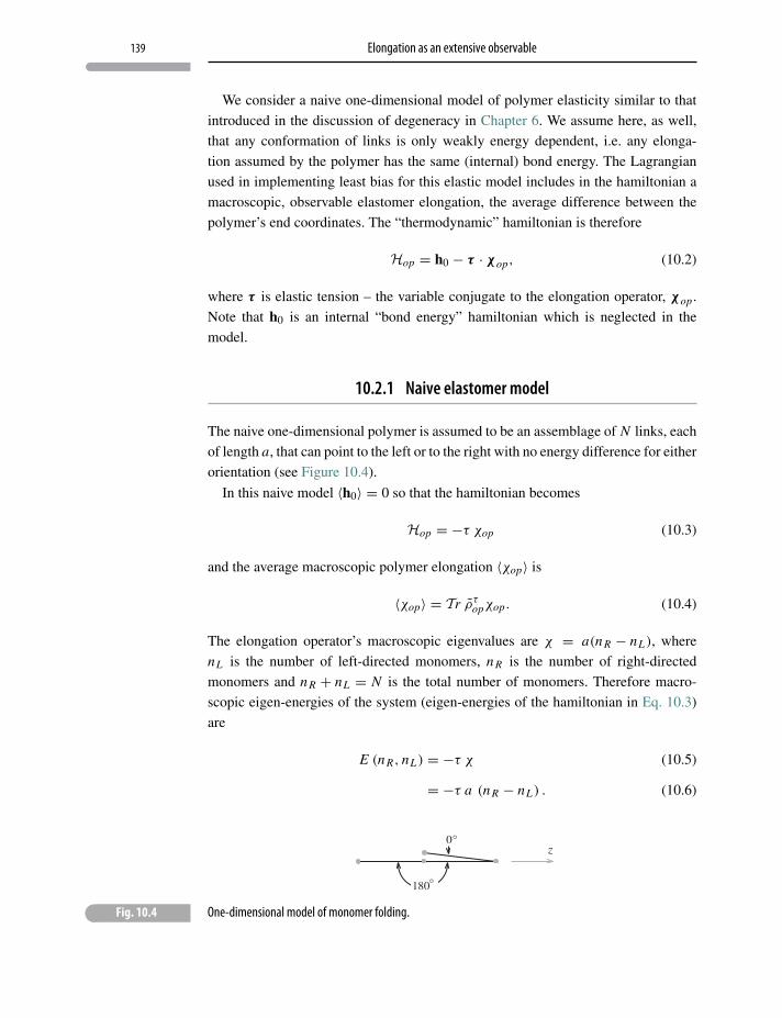
139 Elongation as an extensive observable
We consider a naive one-dimensional model of polymer elasticity similar to that
introduced in the discussion of degeneracy in Chapter 6. We assume here, as well,
that any conformation of links is only weakly energy dependent, i.e. any elonga-
tion assumed by the polymer has the same (internal) bond energy. The Lagrangian
used in implementing least bias for this elastic model includes in the hamiltonian a
macroscopic, observable elastomer elongation, the average difference between the
polymer’s end coordinates. The “thermodynamic” hamiltonian is therefore
Hop = h0 − τ · χop, (10.2)
where τ is elastic tension – the variable conjugate to the elongation operator, χop.
Note that h0 is an internal “bond energy” hamiltonian which is neglected in the
model.
10.2.1 Naive elastomer model
The naive one-dimensional polymer is assumed to be an assemblage of N links, each
of length a, that can point to the left or to the right with no energy difference for either
orientation (see Figure 10.4).
In this naive model 〈h0〉 = 0 so that the hamiltonian becomes
Hop = −τ χop (10.3)
and the average macroscopic polymer elongation 〈χop〉 is
〈χop〉 = Tr ρτopχop. (10.4)
The elongation operator’s macroscopic eigenvalues are χ = a(nR − nL), where
nL is the number of left-directed monomers, nR is the number of right-directed
monomers and nR + nL = N is the total number of monomers. Therefore macro-
scopic eigen-energies of the system (eigen-energies of the hamiltonian in Eq. 10.3)
are
E (nR, nL) = −τ χ (10.5)
= −τ a (nR − nL) . (10.6)
� Fig. 10.4 One-dimensional model of monomer folding.
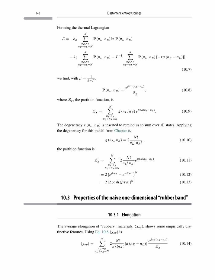
140 Elastomers: entropy springs
Forming the thermal Lagrangian
L = −kB
N∑nR ,nL
nR+nL=N
P (nL , nR) ln P (nL , nR)
− λ0
N∑nR ,nL
nR+nL=N
P (nL , nR)− T−1N∑
nR ,nLnR+nL=N
P (nL , nR) [−τa (nR − nL)]],
(10.7)
we find, with β = 1kB T ,
P (nL , nR) = eβτa(nR−nL )
Zχ
, (10.8)
where Zχ , the partition function, is
Zχ =N∑
nL ,nRnL+nR=N
g (nL , nR) eβτa(nR−nL ). (10.9)
The degeneracy g (nL , nR) is inserted to remind us to sum over all states. Applying
the degeneracy for this model from Chapter 6,
g (nL , nR) = 2N !
nL ! nR ! , (10.10)
the partition function is
Zχ =N∑
nL ,nRnL+nR=N
2N !
nL ! nR !eβτa(nR−nL ) (10.11)
= 2(eβ a τ + e−β a τ
)N(10.12)
= 2 [2 cosh (βτa)]N . (10.13)
10.3 Properties of the naive one-dimensional “rubber band”
10.3.1 Elongation
The average elongation of “rubbery” materials, 〈χop〉, shows some empirically dis-
tinctive features. Using Eq. 10.8 〈χop〉 is
〈χop〉 =N∑
nL ,nRnL+nR=N
2N !
nL !nR ! [a (nR − nL)]eβτa(nR−nL )
Zχ
(10.14)
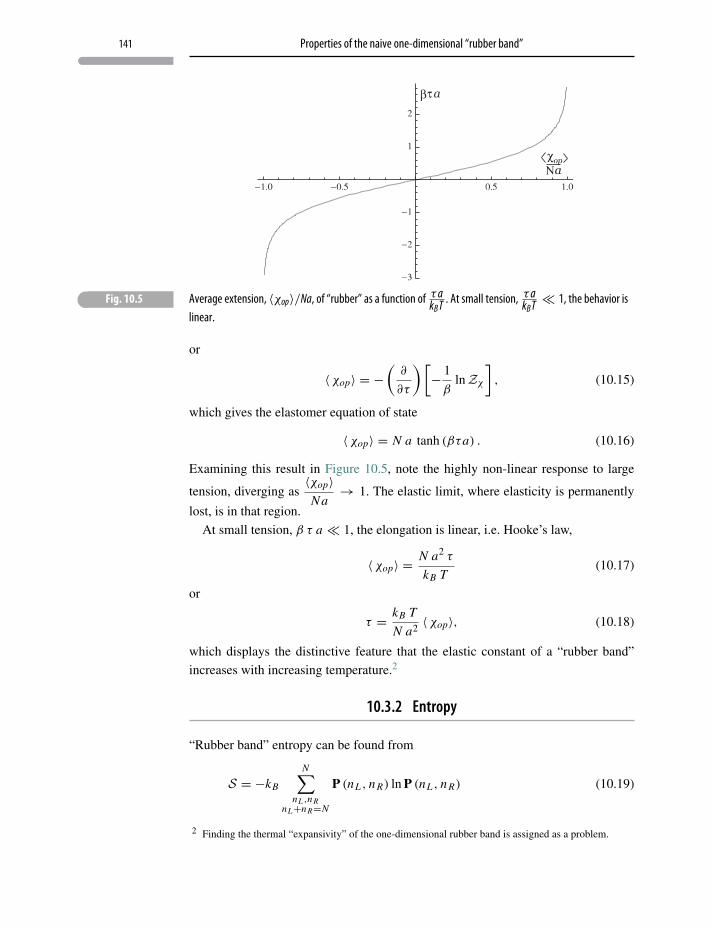
141 Properties of the naive one-dimensional “rubber band”
� Fig. 10.5 Average extension, 〈χop〉/Na, of “rubber” as a function of τ akBT . At small tension, τ a
kBT � 1, the behavior islinear.
or
〈χop〉 = −(
∂
∂τ
)[− 1
βlnZχ
], (10.15)
which gives the elastomer equation of state
〈χop〉 = N a tanh (βτa) . (10.16)
Examining this result in Figure 10.5, note the highly non-linear response to large
tension, diverging as〈χop〉Na
→ 1. The elastic limit, where elasticity is permanently
lost, is in that region.
At small tension, β τ a � 1, the elongation is linear, i.e. Hooke’s law,
〈χop〉 = N a2 τ
kB T(10.17)
or
τ = kB T
N a2〈χop〉, (10.18)
which displays the distinctive feature that the elastic constant of a “rubber band”
increases with increasing temperature.2
10.3.2 Entropy
“Rubber band” entropy can be found from
S = −kB
N∑nL ,nR
nL+nR=N
P (nL , nR) ln P (nL , nR) (10.19)
2 Finding the thermal “expansivity” of the one-dimensional rubber band is assigned as a problem.
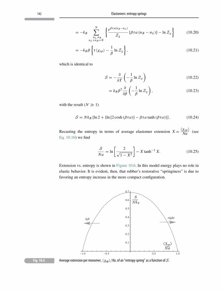
142 Elastomers: entropy springs
= −kB
N∑nL ,nR
nL+nR=N
{eβτa(nR−nL )
Zχ
[βτa (nR − nL)]− lnZχ
}(10.20)
= −kBβ
{τ 〈χop〉 − 1
βlnZχ
}, (10.21)
which is identical to
S = − ∂
∂T
(− 1
βlnZχ
)(10.22)
= kBβ2 ∂
∂β
(− 1
βlnZχ
), (10.23)
with the result (N � 1)
S = NkB [ln 2+ {ln [2 cosh (βτa)]− βτa tanh (βτa)}] . (10.24)
Recasting the entropy in terms of average elastomer extension X = 〈χop〉Na (see
Eq. 10.16) we find
SNa
= ln
[2√
1− X2
]− X tanh−1 X. (10.25)
Extension vs. entropy is shown in Figure 10.6. In this model energy plays no role in
elastic behavior. It is evident, then, that rubber’s restorative “springiness” is due to
favoring an entropy increase in the more compact configuration.
� Fig. 10.6 Average extension per monomer, 〈χop〉/Na, of an “entropy spring” as a function ofS .
143 “Hot rubber bands”: a thermodynamic analysis
10.4 “Hot rubber bands”: a thermodynamic analysis
If a thick real rubber band is quickly stretched and then abruptly relaxed several
times in rapid succession, it cannot fail to be noticed that the rubber band warms.
Even without sensitive thermometry the temperature rise can be detected by placing
the rubber band against the center of your forehead or against your upper lip, both
of which are sensitive to temperature. The thermodynamics of this successive pair of
processes can be qualitatively studied using the one-dimensional polymer model.3,4
If the elastomer is stretched so quickly that there is insufficient time for it to
exchange heat with the surroundings, then the process can be described as adiabatic
(d−Q = 0). In that case,
0 = dU + d−W. (10.26)
Since U is a state variable5 the integral
B∫A
dU = U (B)− U (A) (10.27)
only depends on end-points and not path. Then W also depends on end-points, and
a quasi-static path can be chosen, i.e.
d−WQS = −τ dL . (10.28)
The remaining problem-solving steps are typical of those in Chapters 3–5 but adapted
to the elastic model.
Starting with the First Law
d−Q = dU − τ dL (10.29)
and applying the adiabatic (fast stretching) condition, we have6
0 = dU − τ dL . (10.31)
Taking the differential of U = U (T, L)
dU =(∂U∂T
)L
dT +(∂U∂L
)T
dL , (10.32)
3 The elastic properties of a typical elastomer have, in principle, weak (but not zero) internal energydependence. In the interest of clarity this energy dependence is, in the one-dimensional model, entirelyignored. To continue the present discussion a dose of reality must be restored. This comes in the form ofa non-zero internal energy. But as will be seen, its microscopic origin and its magnitude are irrelevant.
4 For simplicity, the average extension 〈χop〉 will now be replaced by L .5 Note that now hop ≥ 0 so that U �= 0.6 Alternatively it might be better to evaluate
dT =(∂T
∂L
)S
dL . (10.30)
144 Elastomers: entropy springs
Eq. 10.31 becomes
0 =(∂U∂T
)L
dT +[(
∂U∂L
)T− τ
]dL . (10.33)
However, the constant length heat capacity is
CL =(∂U∂T
)L, (10.34)
which leaves only the partial derivative(∂U∂L
)T
(10.35)
to be evaluated. A way forward7 is to use the Helmholtz potential F = U − TS and
take the constant temperature partial derivative(∂U∂L
)T=(∂F
∂L
)T+ T
(∂S∂L
)T. (10.36)
This is handled by noting that combining the (elastic) thermodynamic identity
T dS = dU − τ dL (10.37)
with the differential of Helmholtz potential
dF = dU − T dS − S dT (10.38)
gives
dF = −S dT + τ dL (10.39)
and the identification (∂F
∂L
)T= τ. (10.40)
To simplify the last term in Eq. 10.36, apply the Euler criterion to the exact differen-
tial dF , i.e. Eq. 10.39,
−(∂S∂L
)T=(
∂τ
∂T
)L, (10.41)
which is a Maxwell relation. Finally Eq. 10.36 becomes(∂U∂L
)T= τ − T
(∂τ
∂T
)L
(10.42)
and Eq. 10.33 reduces to
CL
TdT =
(∂τ
∂T
)L
dL . (10.43)
7 A different but equivalent method was used on a similar partial derivative in Chapter 2.
145 “Hot rubber bands”: a thermodynamic analysis
Using the approximate (linearized) elastomer equation of state, Eq. 10.17, we find(∂τ
∂T
)L= kB L
Na2, (10.44)
arriving at the differential equation
CL
TdT = kB
Na2L dL , (10.45)
which is easily integrated to give
T f
T0= exp
(L2
f − L20
κ2
), (10.46)
where8
κ−2 = 1
2〈CL 〉(
kB
Na2
). (10.47)
Thus, as a consequence of adiabatic stretching, i.e. L f > L0, the elastomer warms!
10.4.1 Abruptly relaxed rubber band
When the rubber band is suddenly allowed to relax under no effective restraint (snaps
shut) we still have a fast process with d−Q = 0. But relaxing without restraint means
that no work is done by the rubber band, i.e. d−W = 0. This process is thermo-
dynamically identical to the free expansion of a confined gas studied in Chapter 3.
Therefore, from the First Law, there is no internal energy change, dU = 0.
This suggests that to find the temperature change in the rapidly relaxed “rubber
band”, we write, as in Chapter 3, the infinitesimal
dT =(∂T
∂L
)U
dL . (10.48)
We are again temporarily blocked by an “unfriendly” partial derivative. But with the
skill gained in Chapters 3–5 we start by applying the cyclic chain rule(∂T
∂L
)U= −
(∂U∂L
)T
(∂U∂T
)−1
L(10.49)
and using Eqs. 10.34 and 10.42 from above
dT = 1
CL
[T
(∂τ
∂T
)L− τ
]dL , (10.50)
which, together with the linearized polymer equation of state, shows that the tem-
perature of an unrestrained, rapidly relaxed elastomer does not change! Therefore
a perceptible temperature increase can accumulate by repeated adiabatic stretching
and abrupt (unrestrained) relaxation of the rubber band. Try it!
8 Assuming an average value of CL .
146 Elastomers: entropy springs
10.4.2 Entropy change in the relaxing elastomer
A rubber band snaps shut when the elongating constraint (tension) is suddenly
released. Of course it does. What else would you expect from a rubber band? What
governs this spontaneous process? As alluded to above, it is an expected increase in
the entropy of the universe (i.e. the rubber band).9 To calculate the change in entropy
in this constant U process write
dS =(∂S∂L
)U
dL . (10.51)
What seems to be an unusual partial derivative has been considered previously in
Chapter 3 where we first applied the cyclic chain rule to get(∂S∂L
)U= −
(∂U∂L
)S
(∂U∂S
)−1
L. (10.52)
Then from the thermodynamic identity, Eq. 10.37, we find both(∂U∂L
)S= τ (10.53)
and(∂U∂S
)L= T, (10.54)
so that Eq. 10.51 reduces to
dS = − τ
TdL . (10.55)
Using the linearized equation of state this further reduces to the differential
expression
dS = − kB
Na2L dL , (10.56)
which is integrated to give
�S = kB
2Na2
(L2
0 − L2f
)> 0. (10.57)
Spontaneous, unrestrained contraction of a stretched rubber band is driven by
increased entropy of the “universe”.
10.5 A non-ideal elastomer
Instead of the one-dimensional elastomer consider a model elastomer as a three-
dimensional bundle of roughly parallel but weakly interacting chains (directed, say,
9 A pretty modest-sized universe, to be sure.
147 A non-ideal elastomer
in the z-direction). The general picture is that each chain is a system of N links
(N � 1), each of length a, which can swivel around the bond at any polar or azimuthal
angle θ, φ with respect to the primary z-axis. However, now an interchain energy,
assumed to be proportional to sin θ , is introduced. But to simplify the model we
assume that these links can only point in transverse {±x,±y} directions as well as
the longitudinal z-direction.
All links pointing parallel to the primary z-axis are taken to have identical energy,
E = 0, while rotationally hindered links bending in {±x,±y} directions (subject
to zero mean displacements in the x- and y-directions) acquire an average energy
E = ε. Such an interaction introduces non-ideality in a simple but plausible
way – reminiscent of cross-linking that takes place in vulcanization of rubber. In the
limit ε → 0 transverse links are as easily created as longitudinal links so that links
meander randomly in three dimensions. In this limit the elastomer may be thought
of as ideal in an analogous sense to a three-dimensional non-interacting gas being
ideal. (More will be said about this comparison below.) For ε �= 0 the transverse
link interaction energy causes meandering to become biased and the elastomer is no
longer ideal.
As before, we formulate a thermal Lagrangian tailored to the model described
above, and obtain “surrogate” probabilities and a partition function for the system.
The partition function yields all necessary thermodynamic detail from which the
microscopic interaction parameter ε can, presumably, be found by a suitable experi-
ment.
The macroscopic hamiltonian is
Hop = h0 − τ · Xop, (10.58)
where h0 accounts for the macroscopic “cross-linking” bond energy, Xop is the
length vector operator whose average 〈Xop〉 has components in any of three mutually
perpendicular directions and τ is the elastic tension vector conjugate to the displace-
ment operator.
Within the framework of the three-dimensional elastomer model the macroscopic
eigen-energies of Hop are
E(n±x , n±y, n±z
) = (n+x + n−x + n+y + n−y
)ε
− τx a (n+x − n−x )− τya(n+y − n−y
)− τza (n+z − n−z) , (10.59)
where n±q are the discrete number of links in the±q directions, with q = x, y, z the
mutually perpendicular coordinate directions and a the length per link. The thermal
Lagrangian L for this model is therefore
148 Elastomers: entropy springs
L = −kB
∑n
P(n) ln P(n)
− T−1
[{∑n
P(n)[(
n+x + n−x + n+y + n−y)ε]}
−{∑
n
P(n)[τx a (n+x − n−x )+ τya
(n+y − n−y
)+ τza (n+z − n−z)]}]
− λ0
∑n
P(n), (10.60)
with T the absolute temperature, and where
P(n) ≡ P(n±x , n±y, n±z
)(10.61)
is the probability there are n±x , n±y, n±z links of each type. The symbolic sum∑n
≡∑
n+x ,n−xn+y ,n−yn+z ,n−z
(10.62)
is over the integers{n±x , n±y, n±z
}so that, for example, the average value of the
longitudinal component of the elastomer length vector 〈Lz〉 is
〈Lz〉 = a∑
n
P(n) (n+z − n−z) (10.63)
and the internal energy U is
U =∑
n
P(n)(n+x + n−x + n+y + n−y
)ε (10.64)
with the “ideal” elastomer characterized by limε→0
U = 0. Maximizing the Lagrangian
L with respect to the P(n) we obtain
P(n) = e−βε(n+y+n−y+n+x+n−x) e−βaτz(n+z−n−z)
ZX, (10.65)
where τx = τy = 0 (required by 〈Lx 〉 = 〈L y〉 = 0) has been imposed. The normal-
izing denominator
ZX =∑
n
e−βε(n+y+n−y+n+x+n−x) e−βaτz(n+z−n−z) (10.66)
is the partition function. Equation 10.66 is summed by using the degeneracy g(n) of
the macroscopic eigen-energies
g(n±x , n±y, n±z
) = N !n+x !n−x !n+y !n−y !n+z !n−z ! (10.67)
149 Three-dimensional elastomer thermodynamics
to give the partition function
ZX =∑
n
N !n+x !n−x !n+y !n−y !n+z !n−z !e
−βε(n+y+n−y+n+x+n−x) e−βaτz(n+z−n−z),
(10.68)
the sum now being over distinct integer values restricted by the fixed total
n+x + n−x + n+y + n−y + n+z + n−z = N . (10.69)
Equation 10.68 is just the multinomial expansion of
ZX =[e−βτza + e+βτza + 4e−βε
]N. (10.70)
10.6 Three-dimensional elastomer thermodynamics
Substituting probabilities of Eq. 10.65 into
S = −kB
N∑n
P (n) ln P (n) (10.71)
gives the thermodynamic entropy
S = βkB
(U − τz 〈Lz〉 + 1
βlnZX
). (10.72)
Defining GX , an elastic Gibbs potential, as
GX = − 1
βln ZX , (10.73)
Eq. 10.72 is rewritten as
GX = U − TS − τz 〈Lz〉. (10.74)
Taking the total differential of GX and using the fundamental law expression
T dS = dU − τz d〈Lz〉, (10.75)
where d〈Lz〉 is an infinitesimal change in elastomer length, we also find
dGX = −S dT − 〈Lz〉 dτz (10.76)
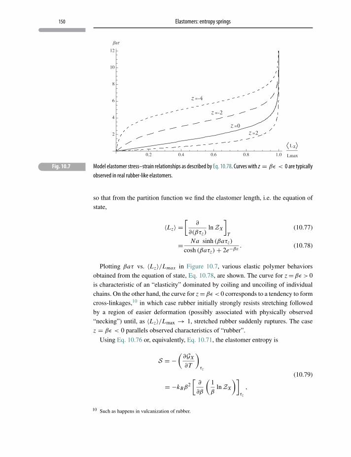
150 Elastomers: entropy springs
zz
z
z
� Fig. 10.7 Model elastomer stress–strain relationships as described by Eq. 10.78. Curves with z = βε < 0 are typicallyobserved in real rubber-like elastomers.
so that from the partition function we find the elastomer length, i.e. the equation of
state,
〈Lz〉 =[
∂
∂(βτz)lnZX
]T
(10.77)
= Na sinh (βaτz)
cosh (βaτz)+ 2e−βε. (10.78)
Plotting βaτ vs. 〈Lz〉/Lmax in Figure 10.7, various elastic polymer behaviors
obtained from the equation of state, Eq. 10.78, are shown. The curve for z=βε > 0
is characteristic of an “elasticity” dominated by coiling and uncoiling of individual
chains. On the other hand, the curve for z=βε < 0 corresponds to a tendency to form
cross-linkages,10 in which case rubber initially strongly resists stretching followed
by a region of easier deformation (possibly associated with physically observed
“necking”) until, as 〈Lz〉/Lmax → 1, stretched rubber suddenly ruptures. The case
z = βε < 0 parallels observed characteristics of “rubber”.
Using Eq. 10.76 or, equivalently, Eq. 10.71, the elastomer entropy is
S = −(∂GX
∂T
)τz
= −kBβ2[
∂
∂β
(1
βlnZX
)]τz
,
(10.79)
10 Such as happens in vulcanization of rubber.
151 Problems and exercises
which evaluates to
S = NkB
{ln 2+ ln
[2e−βε + cosh (βτza)
]+ β[2ε − aτzeβε sinh (βτza)
]2+ eβε cosh (βτza)
}.
(10.80)
Finally, from Eqs. 10.73, 10.74, 10.78 and 10.80, the internal energy is
U = 2Nε
2+ eβε cosh (βaτz). (10.81)
10.6.1 An experiment
The typical undergraduate thermal physics course seems to lack realistic hands-on
laboratory exercises, especially ones that might explore the synergy between sta-
tistical theory, microscopic parameters and experiment. Perhaps this is a result of
historical precedence in which gases – with easy kinetic theory visualizations –
enjoy perceived pedagogical simplicity. Although having a disproportionate role in
thermodynamic instruction they are not especially convenient subjects for non-trivial
laboratory studies in a classroom setting nor are statistical theories of non-ideal
gases – which should be the basis for exploring any experimental synergy – easily
accessible at the undergraduate level.
In Appendix F macroscopic thermodynamic (lab) measurements are used to find
a microscopic interaction energy ε as modeled in the three-dimensional elastomer of
Section 10.6
Problems and exercises
10.1 Find the linear thermal expansivity
α = 1
L
(∂L
∂T
)τ
(10.82)
for the “naive” one-dimensional rubber band.
10.2 Find the mean fluctuations in the average one-dimensional polymer elongation
〈χop〉〈(�χ)2〉 = 〈(χop − 〈χop〉
)〉2 (10.83)
for the naive polymer model.
10.3 A macromolecule is composed of a chain of N chemically identical molecu-
lar monomers for which two distinct states are accessible. At equilibrium N0
units are in the molecular ground state with energy E0 and N1 units are in an
152 Elastomers: entropy springs
excited state with energy E1. Both states are non-degenerate. The ground state
monomer length is � = λ while in the excited state it has length � = (1+ δ) λ,
0 < δ � 1.
a. Write an expression for the polymer partition function Z .
b. Find an equation of state describing the total length L as a function of chain
tension τ and temperature T , L = L (τ, T ).
10.4 A one-dimensional polymer that emulates piezoelectric behaviors is modeled
as N = (nR + nL) molecular links of which nR are right-pointing (+x) and
nL are left-pointing (−x). Each link has length λ and fixed electric dipole
moment p . When placed in a uniform electric field E0,x , each right-pointing
link has an energy
εR = −p · E0 (10.84)
while each left-pointing link has an energy
εL = +p · E0. (10.85)
The implied “piezoelectric” behaviors are:
i. a mechanical tension τ applied along the longitudinal +x-direction, result-
ing in an electric polarization P in that direction;
ii. an electric field E0 applied in, say, the +x-direction, resulting in a mechan-
ical deformation �� in that direction.
The thermodynamic hamiltonian for this model is taken to be
h = h0 − τχop − E0 · Pop (10.86)
so that the corresponding macroscopic eigen-energies are
E = Nε0 − τλ (nR − nL)− E0 · p (nR − nL) (10.87)
with the average length
〈χop〉 = λ 〈nR − nL〉 (10.88)
and the average polarization
〈Pop〉 = p 〈nR − nL〉. (10.89)
It is assumed that h0 is field independent and ε0 ≈ 0.
153 Problems and exercises
a. Write a thermal Lagrangian corresponding to the model.
b. Write a partition function for this piezoelectric polymer in the form
Z =∑
E
g (E)e−βE (10.90)
and evaluate the expression.
c. Find the entropy of the model in terms of β and p · E0.
d. Find the Helmholtz potential F in terms of β and p · E0.
e. Find the average polymer length 〈χop〉 in terms of β and P · E0.
A characterizing piezoelectric property is the coefficient
ξ =(∂P∂τ
)β,E
. (10.91)
f. Describe ξ in words.
g. Find ξ in terms of β and p · E0.
11 Magnetic thermodynamics
The nation that controls magnetism controls the universe.“Diet Smith”, from Chester Gould’s Dick Tracy comic strip (1960)
11.1 Magnetism in solids
Lodestones – fragments of magnetic1 FeO+ Fe2 O3 (Fe3 O4) – although known to
the ancients were, according to Pliny the Elder, first formally described in Greek
6th-century BCE writings. By that time they were already the stuff of myth, super-
stition and amazing curative claims, some of which survive to this day. The Chinese
used lodestones in navigation as early as 200 BCE and are credited with inventing
the magnetic compass in the 12th century CE.
Only in the modern era has magnetism become well understood, inspiring count-
less papers, books2 and more than a dozen Nobel prizes in both fundamental and
applied research.
11.1.1 Forms of macroscopic magnetism
Paramagnetism
In an external magnetic field B the spin-state degeneracy of local (atomic) or itiner-
ant (conduction) electronic states is lifted (Zeeman effect). At low temperature this
results in an induced macroscopic magnetic moment whose vector direction lies par-
allel to the external field. This is referred to as paramagnetism.3
For most materials removing the external field restores spin-state degeneracy,
returning the net moment to zero.
1 Named, as one story goes, for Magnus, the Greek shepherd who reported a field of stones that drewthe nails from his sandals.
2 See e.g. Stephen Blundell, Magnetism in Condensed Matter, Oxford Maser Series in Condensed MatterPhysics (2002); Daniel C. Mattis, Theory of Magnetism Made Simple, World Scientific, London (2006);Robert M. White, Quantum Theory of Magnetism: Magnetic Properties of Materials, 3rd rev. edn,Springer-Verlag, Berlin (2007).
3 Itinerant (conduction) electron paramagnetism is referred to as spin or Pauli paramagnetism.
154
155 Magnetism in solids
Diamagnetism
Macroscopic magnetization may also be induced with a magnetization vector anti-
parallel to the external field, an effect called diamagnetism. In conductors diamag-
netism arises from the highly degenerate quantum eigen-energies and eigenstates
(referred to as Landau levels)4 formed by interaction between mobile electrons and
magnetic fields. Diamagnetism is also found in insulators, but largely from surface
quantum orbitals rather than interior bulk states.5 Both cases are purely quantum
phenomena, leaving macroscopic diamagnetism without an elementary explanatory
model.6,7 All solids show some diamagnetic response, but it is usually dominated by
any paramagnetism that may be present.
At high magnetic fields and low temperatures very pure metals exhibit an oscilla-
tory diamagnetism called the de Haas–van Alphen effect whose source is exclusively
the Landau levels.8
“Permanent” magnetism
“Permanent” magnetism refers to macroscopic magnetization taking place without
any external magnetic fields. Several examples of this phenomenon are:
• Ferromagnetism: this is an ordered state of matter in which local paramagnetic
moments interact to produce an effective internal magnetic field resulting in col-
lective alignment of moments throughout distinct regions called domains. Due to
these internal interactions, domains can remain aligned even after the external field
is removed.
Ferromagnetic alignment abruptly disappears at a material-specific temperature
called the Curie temperature Tc, at which point ordinary local paramagnetism
returns.
• Antiferromagnetism: at low temperatures, interactions between adjacent identical
paramagnetic atoms, ions or sub-lattices can induce collective “anti-alignment” of
adjacent paramagnets, resulting in a net zero magnetic moment.
• Ferrimagnetism: at low temperatures, interactions between unequivalent paramag-
netic atoms, ions or sub-lattices can produce collective “anti-alignment” of moments,
resulting in a small residual magnetization.
In both ferrimagnetism and antiferromagnetism, increasing temperature
weakens “anti-alignment” with the collective induced moments approaching a
4 L. Landau, “Diamagnetism of metals”, Z. Phys. 64, 629 (1930).5 D. Ceresoli et al., “Orbital magnetization in crystalline solids”, Phys. Rev. B 74, 24408 (2006).6 Niels Bohr, Studier over Metallernes Elektrontheori, Kbenhavns Universitet (1911).7 Hendrika Johanna van Leeuwen, “Problèmes de la théorie électronique du magnetisme”, Journal de
Physique et le Radium 2, 361 (1921).8 D. Shoenberg, Magnetic Oscillations in Metals, Cambridge University Press, Cambridge (1984).
156 Magnetic thermodynamics
maximum. Then, at a material-specific temperature called the Néel temperature
TN , anti-alignment disappears and the material becomes paramagnetic.
In this chapter general concepts in the thermodynamics of magnetism and magnetic
fields are discussed as well as models of local paramagnetism and ferromagnetism.
11.2 Magnetic work
Central to integrating magnetic fields and magnetizable systems into the First Law of
Thermodynamics is formulating magnetic work. Using Maxwell fields,9 the energy
generated within a volume V in a time δt , by an electric field E acting on true charge
currents J – Joule heat – is10
δWM = −δt∫V
J · E dV . (11.1)
Therefore the quasi-static and reversible11 magnetic work done by the system is
δWMQS = δt
∫V
J · E dV . (11.2)
Using the Maxwell equation (in cgs–Gaussian units)12
∇ ×H = 4π
cJ + 1
c
δDδt
, (11.3)
the work done by the system is
δWMQS = δt
⎧⎨⎩ c
4π
∫V
(∇ ×H ) · E dV − 1
4π
∫V
δDδt· E dV
⎫⎬⎭ . (11.4)
Using the vector identity
U · ∇ × V = ∇ · (V × U)+ V · ∇ × U, (11.5)
9 Maxwell fields in matter and free space are the local averages that appear in his equations of electro-magnetism.
10 Since heat and work are not state functions they do not have true differentials, so the wiggly δs areused instead to represent incremental work in an interval of time δt .
11 In specifying reversibility non-reversible hysteresis effects are excluded.12 Even though they have fallen out of pedagogical favor in E&M textbooks, cgs units offer unrivaled
clarity in presenting the subtle issues involved in thermodynamics of magnetic and electric fields.
157 Magnetic work
this becomes
δWMQS = δt
⎧⎨⎩ c
4π
⎡⎣∫V
∇ · (H × E) dV +∫V
H · ∇ × E dV
⎤⎦− 1
4π
∫V
δDδt· E dV
⎫⎬⎭ . (11.6)
The first integral on the right can be transformed by Gauss’ theorem into a surface
integral. But since the fields are static (non-radiative), they fall off faster than 1r2 so
that for a very distant surface the surface integral can be neglected. Then, with the
Maxwell equation (Faraday’s Law)
∇ × E = −1
c
(δBδt
), (11.7)
incremental work done by the system is
δWMQS = −δt
⎧⎨⎩ 1
4π
∫V
H · δBδt
dV + 1
4π
∫V
δDδt· E dV
⎫⎬⎭ (11.8)
= −⎧⎨⎩ 1
4π
∫V
H · δB dV + 1
4π
∫V
δD · E dV
⎫⎬⎭ , (11.9)
where the integrals are over the volume of the sample and surrounding free space.
(Note: The “wiggly” deltas in δB(x), δH (x) and δD(x) represent functional changes,
i.e. changes in the fields (states) not the coordinates. The fields themselves are func-
tions of coordinates x and are not just simple variables.)
Limiting the discussion to magnetic phenomena, the magnetic contribution to
quasi-static work done by the system is therefore
δWMQS = −
⎧⎨⎩ 1
4π
∫V
H · δB dV
⎫⎬⎭ , (11.10)
so that a fundamental magnetic thermodynamic equation for δU becomes
δU = T δS − p dV + 1
4π
∫V
H · δB dV . (11.11)
From the Helmholtz potential, F = U − TS,
δF = δU − T δS − S dT, (11.12)
158 Magnetic thermodynamics
which when combined with Eq. 11.11 gives the change δF :
δF = −S dT − pdV + 1
4π
∫V
H · δB dV . (11.13)
Defining magnetic enthalpy H as
H = U + pV − 1
4π
∫V
B ·H dV (11.14)
gives, with Eq. 11.11, an enthalpy change δH :
δH = T δS + V dp − 1
4π
∫V
B · δH dV . (11.15)
Finally, a magnetic Gibbs potential G is defined as
G = F + pV − 1
4π
∫V
B ·H dV , (11.16)
which with Eq. 11.13 gives the Gibbs potential change δG:
δG = −S dT + V dp − 1
4π
∫V
B · δH dV . (11.17)
Magnetization density13 M and polarization density14 P are inserted by the linear
constitutive relations
H = B − 4πM (11.18)
and
D = E + 4π P (11.19)
allowing quasi-static magnetic work to be written
δWM1
QS =⎧⎨⎩ 1
4π
∫V
B · δB dV −∫V ′
M · δB dV
⎫⎬⎭ (11.20)
13 Total magnetic moment per unit volume.14 Total electric dipole moment per unit volume.
159 Magnetic work
or
δWM2
QS =⎧⎨⎩ 1
4π
∫V
H · δH dV +∫V ′
H · δM dV
⎫⎬⎭ , (11.21)
and quasi-static electric work to be written
δWP1
QS =⎧⎨⎩−1
4π
∫V
D · δD dV +∫V ′
P · δD dV
⎫⎬⎭ (11.22)
or
δWP2
QS =⎧⎨⎩−1
4π
∫V
E · δE dV −∫V ′
E · δP dV
⎫⎬⎭ . (11.23)
The first terms in all alternatives are total field energies – integrals over all space,
both inside and outside matter. The second terms are integrals over V ′ which include
only the volume of magnetized (polarized) matter. Since magnetic (electric) ther-
modynamics is primarily concerned with matter that is magnetized (polarized), one
practice is to bravely ignore the total field energies. Another is to absorb the field
energies into the internal energy U . Since neither option is entirely satisfactory a
third way is discussed in Section 11.3 below.
Nevertheless, these results – in terms of local average fields – are general and
thermodynamically correct.15 But they are not convenient to apply. Nor are they the
fields that appear in microscopic magnetic (electric) quantum hamiltonians. In quan-
tum magnetic (electric) models the hamiltonians for individual magnetic (electric)
moments depend only on the field before the sample is introduced. After the sample
is introduced internal fields can additionally result from:
a. interactions between internal moments as additional terms in the hamiltonian –
these interactions may be approximately treated as “effective fields” acting in
addition to the external field (see, for example, Section 11.6, below);
b. internal “demagnetizing” fields arising from fictitious surface “poles” induced by
B0;16
c. internal currents induced by the applied field (especially in conductors).17
15 δWM2
QS and δWP2
QS have the correct form for work – intensive × extensive.16 “Demagnetizing” fields introduce sample shape dependence into the magnetic properties.17 T. Holstein, R.E. Norton and P. Pincus, “de Haas–van Alphen effect and the specific heat of an electron
gas”, Physical Review B 8, 2649 (1973).
160 Magnetic thermodynamics
11.3 Microscopic models and uniform fields
Microscopic models of magnetic and electric hamiltonians are expressed in terms of
uniform applied fields (B0, E0) present before matter is introduced. This emphasis on
applied fields (rather than average Maxwell fields within matter) results in thermo-
dynamic relations somewhat different from Eqs. 11.11 to 11.17 above. Focusing on
magnetic effects in the absence of internal magnetic interactions, quasi-static mag-
netic work done by the system is (see Eq. G.23 in Appendix G)
d−WMQS = −B0 · dM. (11.24)
Since B0 is uniform, a total macroscopic magnetization vector M has been defined as:
M =∫V ′〈M〉 dV , (11.25)
with 〈M〉 the average magnetization per unit volume.18
Therefore thermodynamic differential relations become (see Eqs. G.24, G.26, G.25
and G.27)
T dS = dU∗ + p dV − B0 · dM,
T dS = dH∗ − V dp + M · dB0,
dF∗ = −SdT − p dV + B0 · dM,
dG∗ = −S dT + V dp − M · dB0,
(11.27)
where the starred potentials are
U∗ = U + 1
8π
∫V
B20 dV, (11.28)
H∗ = H + 1
8π
∫V
B20 dV, (11.29)
F∗ = F + 1
8π
∫V
B20 dV, (11.30)
G∗ = G + 1
8π
∫V
B20 dV . (11.31)
18 Similarly
d−W PQS = E0 · dP . (11.26)
161 Local paramagnetism
11.4 Local paramagnetism
The classical energy of a magnetic moment m in an average local (Maxwell) mag-
netic field B is
E = −m ·B. (11.32)
For fundamental magnetic moments (electrons, protons, neutrons, etc.) quantum
mechanics postulates an operator replacement m → mop, and a quantum param-
agnetic hamiltonian
HM = −mop · B0, (11.33)
where B0 is the uniform field present before matter is introduced.19
The paramagnetic hamiltonian for a solid consisting of N identical moments fixed
at crystalline sites i is
Hop = h0 − B0 ·N∑
i=1
mop (i) , (11.34)
where mop(i) is a magnetic moment operator20 and h0 is any non-magnetic part of
the hamiltonian.21,22 The “magnetization” operator (total magnetic moment per unit
volume) is
Mop = 1
V
N∑i=1
mop(i). (11.37)
One objective is to find the macroscopic equation of state 〈M〉 = M(T,B0), where
〈M〉 is the average magnetization per unit volume,
〈M〉 = Tr ρτop Mop. (11.38)
19 Appendix G includes a discussion of the implications and limitations of using B0 in the thermo-dynamics.
20 mop is proportional to an angular momentum (spin) operator Sop , with
mop = gγB
hSop . (11.35)
Here g is the particle g-factor and γB = eh2mc is the Bohr magneton (cgs–Gaussian units.)
For a spin = 12 atom the quantum mechanical z-component spin operator Sz is taken with two
eigenstates and two eigenvalues
Sz
∣∣∣∣±1
2
⟩= ± h
2
∣∣∣∣±1
2
⟩(11.36)
21 It is assumed that there are no interactions corresponding to internal fields, Bint .22 Field–particle current terms HA ·J = 1
2m
(pop − q
c Aop)2, where Aop is the vector potential oper-
ator, are ignored.
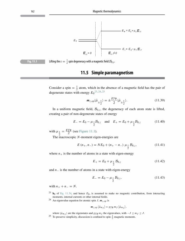
162 Magnetic thermodynamics
� Fig. 11.1 Lifting the s = 12 spin degeneracy with a magnetic fieldB0,z .
11.5 Simple paramagnetism
Consider a spin = 12 atom, which in the absence of a magnetic field has the pair of
degenerate states with energy E023,24,25
mz,op|μ± 12〉 = ±gγB
2|μ± 1
2〉. (11.39)
In a uniform magnetic field, B0,z , the degeneracy of each atom state is lifted,
creating a pair of non-degenerate states of energy
E− = E0 − μ 12B0,z and E+ = E0 + μ 1
2B0,z (11.40)
with μ 12= gγB
2 (see Figure 11.1).
The macroscopic N -moment eigen-energies are
E (n+, n−) = N E0 + (n+ − n−) μ 12B0,z, (11.41)
where n+ is the number of atoms in a state with eigen-energy
E+ = E0 + μ 12B0,z (11.42)
and n− is the number of atoms in a state with eigen-energy
E− = E0 − μ 12B0,z, (11.43)
with n+ + n− = N .
23 h0 of Eq. 11.34, and hence E0, is assumed to make no magnetic contribution, from interactingmoments, internal currents or other internal fields.
24 An eigenvalue equation for atomic spin J , mz,op is
mz,op∣∣μm J
⟩ = gγB m J∣∣μm J
⟩,
where |μm J 〉 are the eigenstates and gγB m J the eigenvalues, with −J ≤ m J ≤ J .25 To preserve simplicity, discussion is confined to spin- 1
2 magnetic moments.
163 Simple paramagnetism
The probabilities P(εs) required for the thermodynamic density operator
ρτop =
∑s
P(εs)|Es〉〈Es | (11.44)
are found by constructing the thermal Lagrangian
L = −kB
N∑n+,n−=0
P (n+, n−) ln P (n+, n−) − λ0
N∑n+,n−=0
P (n+, n−)
− T−1N∑
n+,n−=0
P (n+, n−)[
N E0 + μ 12(n+ − n−)B0,z
](11.45)
using the N -atom macroscopic eigen-energies of Eq. 11.41. The resulting probabili-
ties are
P (n+, n−) = e−β
[N E0 + μ 1
2(n+ − n−)B0,z
]ZM
, (11.46)
where β = 1/kB T , and the denominator (the paramagnetic partition function) is
ZM =N∑
n+,n−n++n−=N
g (n+, n−)e−β
[N E0 + μ 1
2(n+ − n−)B0,z
]. (11.47)
The sum over all states is accounted for by the configurational degeneracy
g (n+, n−) = N !n+ ! n− ! (11.48)
so that
ZM =N∑
n+,n−n++n−=N
N !n+ ! n− !e
−β
[N E0 + μ 1
2(n+ − n−)B0,z
], (11.49)
which is the binomial expansion of
ZM = e−βN E0
(eβμ 1
2B0,z + e
−βμ 12B0,z
)N
(11.50)
=[
2e−βE0 cosh
(βμ 1
2B0,z
)]N
. (11.51)
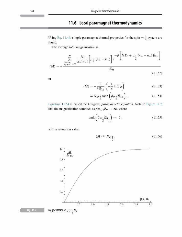
164 Magnetic thermodynamics
11.6 Local paramagnet thermodynamics
Using Eq. 11.46, simple paramagnet thermal properties for the spin = 12 system are
found.
The average total magnetization is
〈M〉 = −
N∑n−,n+
n++n−=N
N !n+!n−!
[μ 1
2(n+ − n−)
]e−β
[N E0 + μ 1
2(n+ − n−)B0,z
]
ZM
(11.52)
or
〈M〉 = − ∂
∂B0,z
(− 1
βlnZM
)(11.53)
= N μ 12
tanh
(βμ 1
2B0,z
). (11.54)
Equation 11.54 is called the Langevin paramagnetic equation. Note in Figure 11.2
that the magnetization saturates as βμ1/2B0 →∞, where
tanh
(βμ 1
2B0,z
)→ 1, (11.55)
with a saturation value
〈M〉 ≈ Nμ 12. (11.56)
� Fig. 11.2 Magnetization vs. βμ 12B0.
165 Local paramagnet thermodynamics
The linear region where βμ 12B0 � 1 is called the Curie regime. In that case
tanh
(βμ 1
2B0,z
)≈ βμ 1
2B0,z (11.57)
and
〈M〉 ≈ Nβμ212B0,z . (11.58)
The average energy (including the magnetization-independent energy) is
〈Hop〉 =
N∑n+,n−
N !n+!n−! [NE0 + (n+ − n−)μ 1
2B0,z]e
−β[NE0 + (n+ − n−)μ 12B0,z]
ZM
(11.59)
so that internal energy is
U = − ∂
∂βlnZM + B0,z〈M〉, (11.60)
which is simply
U = N E0. (11.61)
Comparing Eq. 11.53 with Eq. 11.27 we see that the uniform field Gibbs potential
is found from the uniform field partition function, Eq. G.23,
G M = − 1
βlnZM , (11.62)
as discussed in Appendix G.
From Eq. 11.27 the entropy is
S = −(∂G M
∂T
)p,B0,z
(11.63)
= kBβ2(∂G M
∂β
)p,B0,z
(11.64)
= NkB
{ln 2+ ln
[cosh
(βμ 1
2B0,z
)]− βμ 1
2B0,z tanh
(βμ 1
2B0,z
)}. (11.65)
The entropy is represented in Figure 11.4 below. Note that as βμ 12B0,z → 0 the
entropy attains its maximum value Smax = NkB ln 2, reflecting the original zero
field two-fold degeneracy of the atom states.
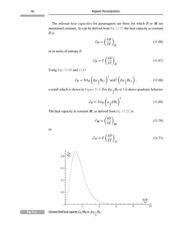
166 Magnetic thermodynamics
The relevant heat capacities for paramagnets are those for which B or M are
maintained constant. As can be derived from Eq. 11.27 the heat capacity at constant
B is
CB =(∂H
∂T
)B
(11.66)
or in terms of entropy S
CB = T
(∂S∂T
)B. (11.67)
Using Eqs. 11.65 and 11.67
CB = NkB
(βμ 1
2B0,z
)2
sech2(βμ 1
2B0,z
), (11.68)
a result which is shown in Figure 11.3. For βμ 12B0� 1 it shows quadratic behavior
CB ≈ NkB
(μ 1
2βB0
)2
. (11.69)
The heat capacity at constant M, as derived from Eq. 11.27, is
CM =(∂U∂T
)M
(11.70)
or
CM = T
(∂S∂T
)M
. (11.71)
� Fig. 11.3 Constant field heat capacity CB/NkB vs. βμ 12B0.
167 Magnetization fluctuations
This time Eqs. 11.70 and 11.61 are used and obviously give26
CM = 0 (11.72)
11.7 Magnetization fluctuations
Magnetization “fluctuations” ΔM are defined by
ΔM ≡ M − 〈M〉 (11.73)
and “mean square magnetic fluctuations” (uncertainty) are27,28⟨(ΔM)2
⟩= 〈(M − 〈M〉)2〉 (11.74)
= 〈M2〉 − 〈M〉2, (11.75)
where
〈M2〉 = −
N∑n−,n+
N !n+!n−!
[μ 1
2(n+ − n−)
]2
e−β
[N E0 + μ 1
2(n+ − n−)B0,z
]
ZM.
(11.76)
Taking this result together with ZM and 〈M〉 (as calculated in Eq. 11.52), the mean
square fluctuations are
〈M2〉 − 〈M〉2 = 1
β2
∂2
∂B20
lnZM (11.77)
= Nμ212
sech2(βμ 1
2B0
). (11.78)
Expressed as dimensionless “root mean square fluctuations”√〈M2〉 − 〈M〉2〈M〉 = 1
√N sinh
(βμ 1
2B0.z
) , (11.79)
26 Alternatively, the general relation CM − CB = T(∂B∂T
)M
(∂M∂T
)B
, which can be simplified to CM −CB = −T
[(∂M∂T
)B
]2 [(∂M∂B
)T
]−1with its more straightforward partial derivatives, confirms the
zero result. Derivation of these results is assigned as a problem.27 Generally speaking, vanishingly small fluctuations assure meaningful thermodynamic descriptions.28 Fluctuations are formally associated with thermal state functions that have quantum operator represen-
tations. For example, temperature does not have well-defined fluctuations since there is no quantumtemperature operator. See e.g. C. Kittel, “Temperature fluctuation: an oxymoron”, Physics Today 41(5),93 (1988).
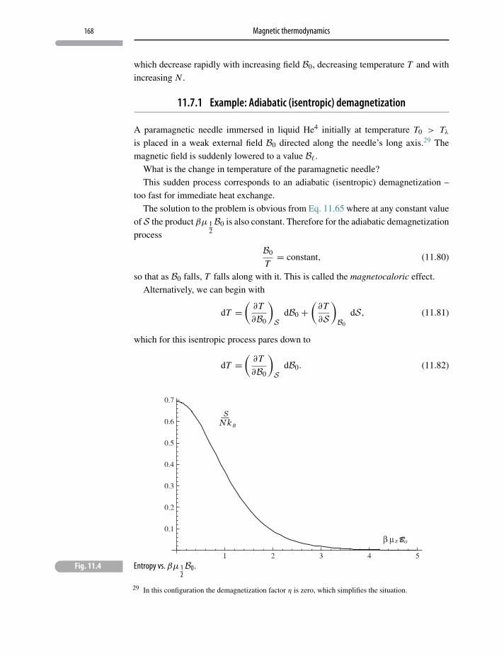
168 Magnetic thermodynamics
which decrease rapidly with increasing field B0, decreasing temperature T and with
increasing N .
11.7.1 Example: Adiabatic (isentropic) demagnetization
A paramagnetic needle immersed in liquid He4 initially at temperature T0 > Tλ
is placed in a weak external field B0 directed along the needle’s long axis.29 The
magnetic field is suddenly lowered to a value B�.
What is the change in temperature of the paramagnetic needle?
This sudden process corresponds to an adiabatic (isentropic) demagnetization –
too fast for immediate heat exchange.
The solution to the problem is obvious from Eq. 11.65 where at any constant value
of S the product βμ 12B0 is also constant. Therefore for the adiabatic demagnetization
process
B0
T= constant, (11.80)
so that as B0 falls, T falls along with it. This is called the magnetocaloric effect.
Alternatively, we can begin with
dT =(
∂T
∂B0
)S
dB0 +(∂T
∂S
)B0
dS, (11.81)
which for this isentropic process pares down to
dT =(
∂T
∂B0
)S
dB0. (11.82)
� Fig. 11.4 Entropy vs. βμ 12B0.
29 In this configuration the demagnetization factor η is zero, which simplifies the situation.
169 A model for ferromagnetism
Applying the cyclic chain rule (see Chapter 4)
(∂T
∂B0
)S= −
(∂S
∂B0
)T(
∂S
∂T
)B0
(11.83)
= − T
CB
(∂S
∂B0
)T. (11.84)
Using the Gibbs potential expression as given in Eq. 11.27, and applying Euler’s
theorem, we have a Maxwell relation(∂S∂B0
)T=(∂M∂T
)B0
(11.85)
so that Eq. 11.82 is now
dT = − T
CB
(∂M∂T
)B0
dB0. (11.86)
Inserting CB from Eq. 11.69 and M from Eq. 11.58
dT
T= dB0
B0(11.87)
which is integrated to finally give
T f =(B�
B0
)T0, (11.88)
i.e. the needle cools.
11.8 A model for ferromagnetism
In the previous sections, paramagnetism is modeled as N independent local magnetic
moments. But in general these moments can interact to produce, approximately, an
internal magnetic field acting in addition to the external field resulting in an average
total effective field B∗.Short-range, nearest-neighbor magnetic moment coupling is frequently described
by the Heisenberg exchange interaction,30
Hex (i, i ′) = −1
2mop (i)Ki,i ′ mop
(i ′), (11.89)
30 W. Heisenberg, “Mehrkörperproblem und Resonanz in der Quantenmechanik”, Zeitschrift für Physik38, 441 (1926).
170 Magnetic thermodynamics
where mop (i) is the magnetic moment operator for the i th site and Ki,i ′ is an inter-
action which couples the moment at i with the moment at a nearest-neighbor site, i ′.The macroscopic Heisenberg hamiltonian31 is taken to be
H = −N∑
i=1
B0 · Mop (i)− 1
2
N∑i=1
z∑i ′=1
Mop (i) ·Ki,i ′ ·Mop(i ′), (11.90)
where z is the total number of nearest-neighbor moments. The double sum32 includes
only terms with i �= i ′.Apart from in one or two dimensions, this many-body problem has, generally, no
analytic solution. But an approximation – a mean field approximation (MFA)33 – can
be applied to replace the many-body model by an effective “one-body” model and
plausibly account for the phenomenon of ferromagnetism.
11.9 A mean field approximation
In preparation for applying the MFA, rewrite Eq. 11.90 as
H = −N∑
i=1
{B0 + 1
2
z∑i ′=1
Ki, i ′ Mop(i ′)} · Mop (i) , (11.91)
where, assuming an isotropic system, all z nearest neighbors can be treated as iden-
tical, i.e. Ki,i ′ → K.
The essence of a mean field approximation is the identity
mop(i ′)
mop (i) = [mop
(i ′)− 〈mop〉
] [mop (i)− 〈mop〉
]+ mop
(i ′) 〈mop〉 + 〈mop〉mop (i)− 〈mop〉〈mop〉, (11.92)
where 〈mop〉 is the average magnetic moment, i.e. M/N , the magnetization per site.
The MFA neglects the first term, i.e. the product of fluctuations around the mag-
netization, whereas the last term contributes a constant value. The hamiltonian of
Eq. 11.91 can then be written in its “mean field” form34
H = 1
2zNK〈mop〉2 −
N∑i=1
{B0 + z 〈mop〉K
} · mop (i) , (11.93)
31 Curiously, the Heisenberg “magnetic” interaction does not originate from magnetic arguments. Itssource is strictly interatomic electronic interactions, in particular from the electron exchange interac-tion in the hydrogen molecule.
32 The factor 12 compensates for the ultimate double counting by the double sum.
33 P Weiss, “L’hypothese du champ moleculaire et la propriete ferrmognetique,” J. Phys. (Paris) 6, 661(1907).
34 The doubled mean field sum over i and i ′ (terms 2 and 3 in Eq. 11.92) cancels the factor 12 .
171 A mean field approximation
which includes the constant term from the MFA (see Eq. 11.92). The external field
B0 is now supplemented by an “internal” field, Bint
Bint = z 〈mop〉K (11.94)
= z
NM K (11.95)
so a total “effective” field B∗ at the i th site is
B∗ (i) = B0 (i)+ Bint (i) (11.96)
= B0 (i)+ z
NK M (i) (11.97)
giving rise to a mean field hamiltonian
H = 1
2M · Bint −
N∑i=1
B∗ (i) · mop (i) . (11.98)
This has the effect of replacing B0 in the paramagnet partition function of Eq. 11.51
by B∗, in which case
ZM∗ = e−12βM·Bint
[2 cosh
(βμ 1
2B∗)]N
, (11.99)
with a Gibbs potential35
G∗ = − 1
βlnZM∗ (11.100)
= 1
2M · Bint − N
βln
(2 coshβμ 1
2B∗). (11.101)
In the absence of an external field, i.e. B0 = 0, we find from Eqs. 11.53, 11.97 and
11.99
M = N μ 12
tanh
(βμ 1
2
zKN
M), (11.102)
which is a transcendental equation in M that describes the possibility of finite mag-
netization even in the absence of an external field.
35 The constant term from the MFA has interesting thermodynamic consequences to be discussed inAppendix G (see Eq. G.30).
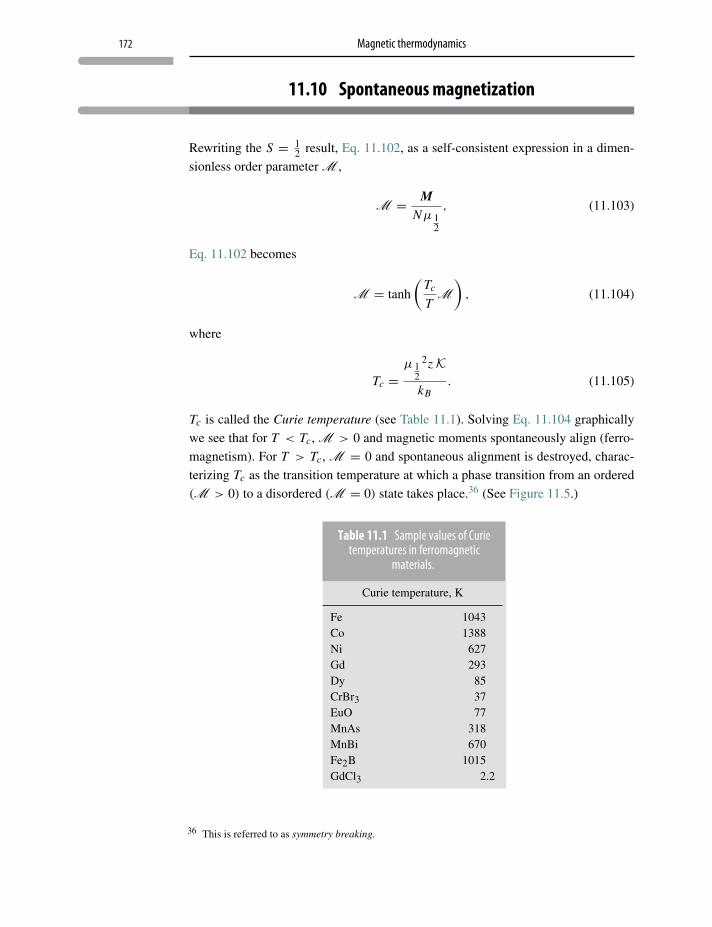
172 Magnetic thermodynamics
11.10 Spontaneous magnetization
Rewriting the S = 12 result, Eq. 11.102, as a self-consistent expression in a dimen-
sionless order parameter M ,
M = MNμ 1
2
, (11.103)
Eq. 11.102 becomes
M = tanh
(Tc
TM
), (11.104)
where
Tc =μ 1
2
2z K
kB. (11.105)
Tc is called the Curie temperature (see Table 11.1). Solving Eq. 11.104 graphically
we see that for T < Tc, M > 0 and magnetic moments spontaneously align (ferro-
magnetism). For T > Tc, M = 0 and spontaneous alignment is destroyed, charac-
terizing Tc as the transition temperature at which a phase transition from an ordered
(M > 0) to a disordered (M = 0) state takes place.36 (See Figure 11.5.)
Table 11.1 Sample values of Curietemperatures in ferromagnetic
materials.
Curie temperature, K
Fe 1043Co 1388Ni 627Gd 293Dy 85CrBr3 37EuO 77MnAs 318MnBi 670Fe2B 1015GdCl3 2.2
36 This is referred to as symmetry breaking.
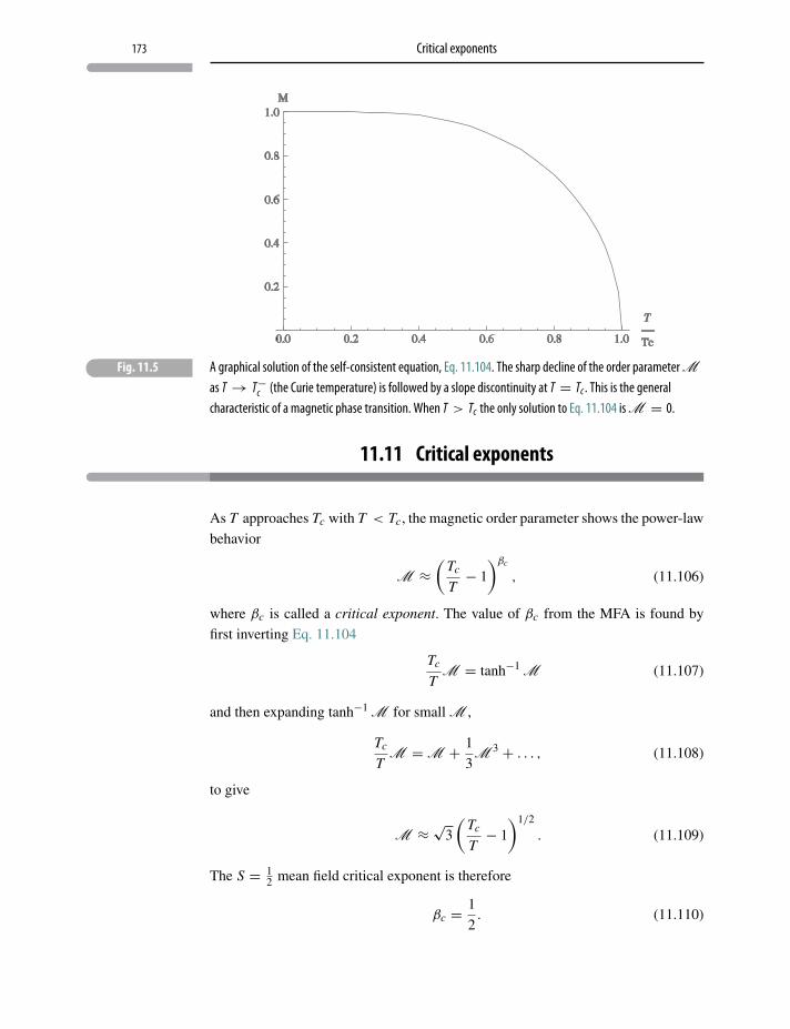
173 Critical exponents
� Fig. 11.5 A graphical solution of the self-consistent equation, Eq. 11.104. The sharp decline of the order parameter Mas T → T−c (the Curie temperature) is followed by a slope discontinuity at T = Tc . This is the generalcharacteristic of a magnetic phase transition. When T > Tc the only solution to Eq. 11.104 is M = 0.
11.11 Critical exponents
As T approaches Tc with T < Tc, the magnetic order parameter shows the power-law
behavior
M ≈(
Tc
T− 1
)βc
, (11.106)
where βc is called a critical exponent. The value of βc from the MFA is found by
first inverting Eq. 11.104
Tc
TM = tanh−1 M (11.107)
and then expanding tanh−1 M for small M ,
Tc
TM =M + 1
3M 3 + . . . , (11.108)
to give
M ≈ √3
(Tc
T− 1
)1/2
. (11.109)
The S = 12 mean field critical exponent is therefore
βc = 1
2. (11.110)
174 Magnetic thermodynamics
11.12 Curie–Weiss magnetic susceptibility (T > Tc)
When T > Tc and with no external field, i.e. B0 = 0, nearest-neighbor inter-
actions are no longer sufficient to produce spontaneous magnetization. However,
upon re-introduction of an external field B0 induced paramagnetic moments will
still contribute internal fields, so that within an MFA a total internal field is again B∗,as in Eq. 11.97.
For T � Tc Eq. 11.102 can be expanded37 and solved for 〈M〉 to give
〈M〉 =μ2
12
kB(T − Tc)
−1 B0, (11.111)
where Tc is as defined in Eq. 11.105. With a magnetic susceptibility χM defined as38
〈M〉 = χMB0, (11.112)
we have
χM =μ2
12
kB(T − Tc)
−1 , (11.113)
which is called the Curie–Weiss law. When T � Tc, this is a satisfactory description
for magnetic susceptibility. But it fails near T ≈ Tc, where the formula displays a
singularity.39
The Curie–Weiss law is often expressed in terms of1
χM, which is (advantageously)
linear in T − Tc.
11.13 Closing comment
The study of magnetic matter remains a vast and varied topic that drives contempo-
rary research, both fundamental and applied. The examples discussed in this chapter
(paramagnetism and ferromagnetism) are but introductory samples of the role played
by quantum mechanics in understanding macroscopic magnetism.
37 tanh (x) ≈ x − 13 x3.
38 Unlike magnetization, magnetic susceptibility has no strict thermodynamic definition. In the case of
non-linear materials an isothermal susceptibility χM =(
∂M∂B0
)T
is a more practical definition.39 Tc experimentally determined from Curie–Weiss behavior is usually higher than Tc determined from
the ferromagnetic phase transition.
12 Open systems
If to any homogeneous mass in a state of hydrostatic stress we suppose aninfinitesimal quantity of any substance to be added, the mass remaining homo-geneous and its entropy and volume remaining unchanged, the increase of theenergy of the mass divided by the quantity of the substance added is the (chemi-cal) potential for that substance in the mass considered.
J.W. Gibbs, “On the equilibrium of heterogeneous substances”,Trans. Conn. Acad., vol. III, 108–248 (1876)
12.1 Variable particle number
J. W. Gibbs ingeniously extended thermodynamics to include processes involving
systems with variable particle number1,2 – processes that include:
1. Phase transitions: Macroscopic matter transforms – abruptly – into different
physically distinctive phases, usually accompanied by changes in symmetry and
discontinuities in properties. Examples of phase changes are:
(a) melting: Asolid � Aliquid ;
(b) magnetization: paramagnet � ferromagnet;
(c) evaporation: Aliquid � Avapour ;
(d) sublimation: Asolid � Avapour ;
(e) normal � superconductor;
(f) normal He4 � Bose–Einstein condensate.
2. Atoms, molecules or particles combine and recombine as different chemical units:
(a) chemical reactions:
n A A + nB B . . . � nx X + nY Y . . . (12.1)
1 Willard Gibbs, “On the equilibrium of heterogeneous substances”, Trans. Conn. Acad., vol. III,343–524 (1878).
2 Willard Gibbs, “On the equilibrium of heterogeneous substances”, Amer. Jour. of Sci. (3), vol. XVI,441–458 (1878).
175
176 Open systems
where n A, nB , . . . , nX , nY , . . . are integer numbers of the chemical partici-
pants, A, B, . . . , X, Y, . . .;
(b) fundamental particle interactions – electron–positron annihilation:
e+ + e− → γ + γ. (12.2)
12.2 Thermodynamics and particle number
The hamiltonians H and state functions |Ψ 〉 in Schrödinger’s quantum mechanics
define microscopic dynamics for systems with a fixed number of particles (closed
systems). These, so far, have been our quantum reference in understanding macro-
scopic systems. However, for many systems or processes this is physically or mathe-
matically inadequate. By introducing into the hamiltonian a particle number operator
Nop and its eigenvalue equation
Nop|N 〉 = N |N 〉 (12.3)
with eigenvalues N = 0, 1, 2, . . . and eigenfunctions |N 〉, together with a particle
number fluctuation operator defined as
ΔNop = Nop − 〈Nop〉, (12.4)
quantum mechanics (and thermodynamics) can logically and formally be extended to
include variable particle number – the defining property of open systems. The number
operator is not part of Schrödinger mechanics but belongs to quantum field theory, a
quantum formulation far beyond any plan for this book. Yet a number operator and its
eigenvalue property (see Eq. 12.3) are the basis of Gibbs’ prescient “Grand Canon-
ical” thermodynamics, a topic discussed and applied in this and several remaining
chapters.
12.3 The open system
12.3.1 Formalities
The hamiltonian Hop, which constitutes the basis for open system thermodynam-
ics, is
Hop = hop − μNop, (12.5)
177 The open system
which now includes “particle” work dWN = −μ d〈Nop〉, where μ is the chemical
potential for a single component species. In the case where there are M chemically
distinct components,
Hop = hop −M∑i
μi
⟨N i
op
⟩, (12.6)
where μi is a chemical potential for the i th chemical component.
While not significantly modifying the canonical formalism – in particular the
commutation relation [ρτ
op, Hop
]= 0 (12.7)
is still satisfied – introducing μNop does have formal and thermodynamic conse-
quences.
The single-species open system thermal Lagrangian which incorporates Eq. 12.5
now becomes
L = −kB
∑N=0,1,2,...
∑s
{P[εs(N ), N ] ln P[εs(N ), N ]
}
− 1
T
∑N=0,1,2,...
{∑s
P[εs(N ), N ][εs(N )− Nμ]}
− λ0
∑N=0,1,2...
{∑s
P[εs(N ), N ]}, (12.8)
where P[εs(N ), N ] is the normalized probability for:
• N particles;
• N -particle eigen-energies εs(N ).
The “hat” worn by P distinguishes it from closed system (canonical) probabilities.
Maximizing L with respect to variations in P[εs(N ), N ] gives
P[εs(N ), N ] = e−β[εs (N )−μN ]∑N=0,1,2,...
{∑s
e−β[εs(N )−μN ]} , (12.9)
where the normalizing denominator
Zgr =∑
N=0,1,2,...
{∑s
e−β[εs (N )−μN ]
}(12.10)
is the grand partition function. As in the canonical case, the s-sum covers all
N -particle eigenstates |εs(N )〉 whereas the newly introduced N -sum covers all par-
ticle numbers N = 0, 1, 2, . . . (i.e. eigenvalues of Nop).
178 Open systems
Re-parsing Eq. 12.10 we can equivalently write
Zgr =∑
N=0,1,2,...
eβμN
{∑s
e−β εs (N )
}, (12.11)
which emphasizes the underlying form
Zgr =∑
N=0,1,2,...
eβμNZ(N ), (12.12)
where
Z (N ) =∑
s
e−β εs (N ) (12.13)
is an N -particle partition function.
12.3.2 Grand thermodynamics
The quantum formulation having been adapted for variable particle number, result-
ing in probabilities P[εs(N ), N ], its consequences for thermodynamics can now be
examined.
1. Average system particle number 〈Nop〉,
〈Nop〉 =
∑N=0,1,2,...
N∑s
e−β[εs (N )−μN ]
∑N=0,1,2,...
∑s
e−β[εs (N )−μN ] , (12.14)
is written in terms of Eq. 12.10, the grand partition function, as3
〈Nop〉 = 1
β
(∂
∂μlnZgr
)T,V
. (12.15)
2. System internal energy U ,
U =
∑N=0,1,2,...
∑sεs(N )e−β[εs (N )−μN ]
∑N=0,1,2,...
∑s
e−β[εs (N )−μN ] (12.16)
can be rearranged as
U = −(
∂
∂βlnZgr
)μ,V
+ μ〈Nop〉. (12.17)
3 〈Nop〉 is a continuous state variable.
179 The open system
3. Assuming a volume dependence εs(N , V ), pressure p is
p =
∑N=0,1,2,...
∑s
[−∂εs(N , V )
∂V
]e−β[εs (N )−μN ]
∑N=0,1,2,...
∑s
e−β[εs (N )−μN ] (12.18)
which in terms of the grand partition function is
p = 1
β
(∂
∂VlnZgr
)T,μ
. (12.19)
4. Entropy S,
S = −kB
∑N=0,1,2,...
∑s
{P[εs(N ), N ] ln P[εs(N ), N ]
}, (12.20)
becomes, with Eqs. 12.9 and 12.10,
S = −kB
∑N=0,1,2,...
∑s
{[e−β(εs−μN )
Zgr
] [− lnZgr − β(εs − μN )]}
(12.21)
= −kB β
(−U − 1
βlnZgr + μ〈Nop〉
). (12.22)
Then with Eq. 12.17
S = −kBβ2
[∂
∂β
(1
βlnZgr
)μ,V
]. (12.23)
12.3.3 Grand potential
In addition to the grand partition function an open system grand potential, Ωgr , is
defined
Ωgr = − 1
βlnZgr . (12.24)
180 Open systems
Using Ωgr Eq. 12.22 can be rearranged as
Ωgr = U − TS − μ〈Nop〉. (12.25)
With the Helmholtz potential F = U − TS we also have
Ωgr = F − μ〈Nop〉 (12.26)
and in terms of the Gibbs potential G = U − T S + pV
Ωgr = G − μ〈Nop〉 − p V . (12.27)
Summarizing the grand potential’s role in the thermodynamics of open systems,
Eqs. 12.15, 12.17, 12.23 and 12.19 can be re-expressed as
〈Nop〉 = −(∂Ωgr
∂μ
)T,V
,
U =[
∂
∂β
(βΩgr
)]μ,V
+ μ〈Nop〉,
p = −(∂Ωgr
∂V
)T, μ
,
S = kB β2(∂Ωgr
∂β
)μ,V
.
(12.28)
Finally, differentiating Ωgr = Ωgr (T, V, μ),
dΩgr =(∂Ωgr
∂T
)V, μ
dT +(∂Ωgr
∂V
)T, μ
dV +(∂Ωgr
∂μ
)T, V
dμ (12.29)
implies, from Eq. 12.28, the thermodynamic relation
dΩgr = −S dT − p dV − 〈Nop〉 dμ. (12.30)
181 The open system
12.3.4 G, Ωgr and Euler’s theorem
Combining Eqs. 12.27 and 12.30 the differential of the Gibbs potential is
dG = −S dT + V dp + μ d〈Nop〉 (12.31)
so that its natural variables are T, p and 〈Nop〉. With 〈Nop〉 the only extensive vari-
able among them we write G(T, 〈Nop〉, p
)in the Euler form,
G(T, λ〈Nop〉, p
) = λ G(T, 〈Nop〉, p
), (12.32)
indicating that G is homogeneous in 〈Nop〉 of degree 1. Applying Euler’s homogene-
ity theorem (see Chapter 4) gives
〈Nop〉(
∂G
∂〈Nop〉)
p, T
= G(T, 〈Nop〉, p
). (12.33)
But from Eq. 12.31 (∂G
∂〈Nop〉)
p, T
= μ (12.34)
which leads to
G(T, 〈Nop〉, p
) = μ〈Nop〉. (12.35)
For a multispecies system, say A1, A2, A3, . . ., this is generalized as
G =∑i=1
μAi 〈Nop〉Ai . (12.36)
According to Eq. 12.30 the natural variables of Ωgr are T, V and μ, of which only
V is extensive. Writing Ωgr = Ωgr (T, V, μ) (see Eq. 12.30) in its Euler form
Ωgr (T, λV, μ) = λΩgr (T, V, μ) (12.37)
(denoting that Ωgr is homogeneous in V of degree 1). Applying Euler’s homoge-
neous function theorem
V
(∂Ωgr
∂V
)T, μ
= Ωgr , (12.38)
182 Open systems
which, upon substituting from Eq. 12.28, becomes
Ωgr = −pV . (12.39)
This – as we will see in the next section – is a useful result for deriving equations of
state.
12.4 A “grand” example: the ideal gas
The grand partition function is applied to the ideal gas. Examples are then given that
build on the ideal gas to model more complex physical systems.
Using results from Chapter 7 together with Eq. 12.12,
Zgr =∑
N=0,1,2,...
eβμNZ (N ) (12.40)
=∑
N=0,1,2,...
eβμN 1
N !(nQ V
)N (12.41)
=∑
N=0,1,2,...
ζ N 1
N !(nQ V
)N, (12.42)
where
ζ = eβμ (12.43)
is called the fugacity and where, as defined in Chapter 7,
nQ =(
m
2πh2β
)3/2
. (12.44)
Summing Eq. 12.42 gives the ideal gas grand partition function4
Zgr = eζnQ V (12.45)
and the ideal gas grand potential
Ωgr = −ζnQ V
β. (12.46)
4 The ideal gas, even in this “grand” picture, is still semi-classical requiring the ad-hoc corrections ofChapter 7.
183 A “grand” example: the ideal gas
12.4.1 Ideal gas thermodynamic properties
1. From Eqs. 12.28 and 12.46 the average particle number is
〈Nop〉 = ζnQ V, (12.47)
which is solved to obtain the ideal gas chemical potential5
μ = 1
βln〈Nop〉nQ V
. (12.48)
2. Similarly, from Eq. 12.28 the internal energy U is
U = 3〈Nop〉2β
. (12.49)
3. Again using Eq. 12.28 the entropy is
S = 〈Nop〉[
5
2kB − ln
〈Nop〉nQ V
](12.50)
which is the Sackur–Tetrode equation of Chapter 7.
4. Using Eqs. 12.35 and 12.48 the Gibbs potential for the ideal gas is
G(T, 〈Nop〉, p
) = 〈Nop〉β
ln〈Nop〉nQ V
, (12.51)
which is identical with
G(T, 〈Nop〉, p
) = μ〈Nop〉. (12.52)
5. Finally, using Eq. 12.39 and the ideal gas value for Ωgr , i.e. Eq. 12.46,
ζnQ V
β= pV, (12.53)
5 Since nQ (the quantum concentration) depends on h, even the so-called “classical” ideal gas has aquantum mechanical marker, suggesting “classical thermodynamics” is an oxymoron.
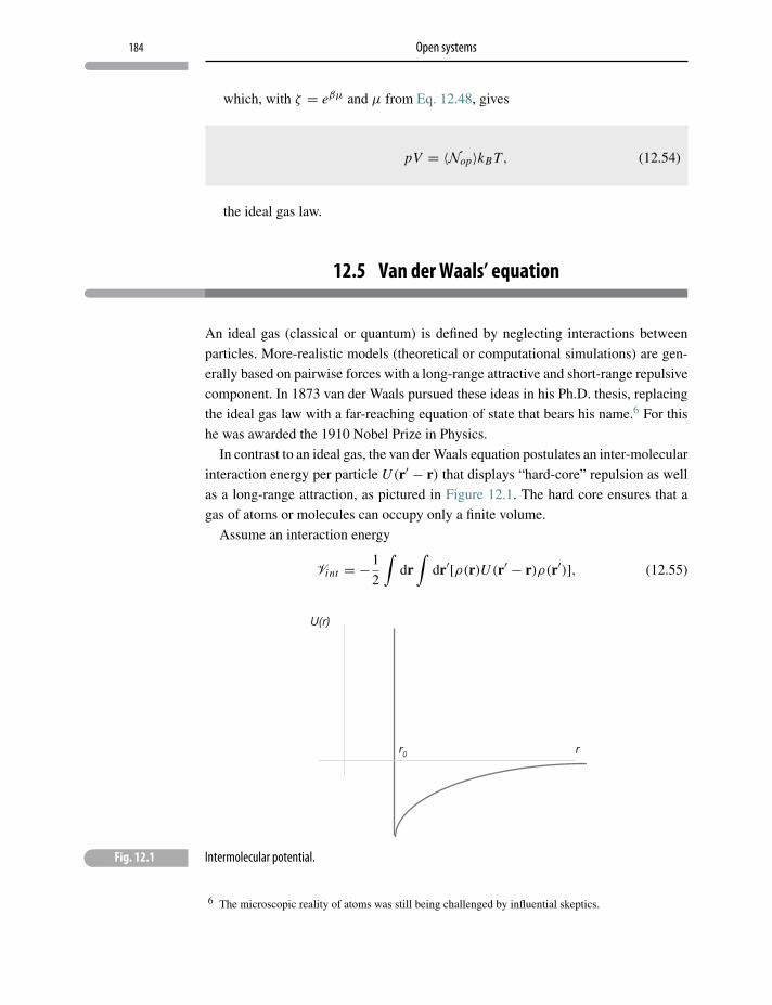
184 Open systems
which, with ζ = eβμ and μ from Eq. 12.48, gives
pV = 〈Nop〉kB T, (12.54)
the ideal gas law.
12.5 Van der Waals’ equation
An ideal gas (classical or quantum) is defined by neglecting interactions between
particles. More-realistic models (theoretical or computational simulations) are gen-
erally based on pairwise forces with a long-range attractive and short-range repulsive
component. In 1873 van der Waals pursued these ideas in his Ph.D. thesis, replacing
the ideal gas law with a far-reaching equation of state that bears his name.6 For this
he was awarded the 1910 Nobel Prize in Physics.
In contrast to an ideal gas, the van der Waals equation postulates an inter-molecular
interaction energy per particle U (r′ − r) that displays “hard-core” repulsion as well
as a long-range attraction, as pictured in Figure 12.1. The hard core ensures that a
gas of atoms or molecules can occupy only a finite volume.
Assume an interaction energy
Vint = −1
2
∫dr∫
dr′[ρ(r)U (r′ − r)ρ(r′)], (12.55)
� Fig. 12.1 Intermolecular potential.
6 The microscopic reality of atoms was still being challenged by influential skeptics.
185 Van der Waals’ equation
with the density in units of particle number per unit volume. This many-particle
intermolecular interaction is manageable in the MFA,7,8 in which case
Vint = −1
2
∫dr∫
dr′{2ρ(r′)− 〈ρ〉}〈ρ〉U (r− r′) (12.57)
with 〈ρ〉 a uniform particle density,
〈ρ〉 = N
V. (12.58)
The first term in Eq. 12.57 evaluates to
−〈ρ〉∫
dr∫
dr′ρ(r′)U (r− r′) = −V 〈ρ〉∫
drU (r)ρ(r) (12.59)
which, with ρ(r) = 〈Nop(r)〉/V and assuming gas uniformity, becomes (noting
Figure 12.1)
= −4πN
V〈Nop〉
∞∫r0
U (r)r2 dr. (12.60)
Representing the integral as
a = 4π
∞∫r0
U (r)r2 dr, (12.61)
and noting that the second term in Eq. 12.57 evaluates to an ignorable constant, the
mean field interaction potential is9
Vint = −Na〈Nop〉
V, (12.62)
and the grand partition function is
Zgr =∑
N=0,1,2...
eβ
[μ+a
〈Nop〉V
]N
Z(N ) (12.63)
= exp
⎧⎪⎨⎪⎩nQV eβ
[μ+a
〈Nop〉V
]⎫⎪⎬⎪⎭ . (12.64)
7 The essence of a mean field approximation is the identity
ρ(x′)ρ(x) = [ρ(x′)− 〈ρ〉][ρ(x)− 〈ρ〉] + ρ(x′)〈ρ〉 + 〈ρ〉ρ(x)− 〈ρ〉〈ρ〉 (12.56)
where 〈ρ〉 is the average density. The MFA neglects the first term, i.e. fluctuations around the averagedensity.
8 Peter Palffy-Muhoray, “The single particle potential in mean field theory”, Am. J. Phys. 70, 433–437(2002).
9 This term is the inter-particle contribution to the internal energy.
186 Open systems
From this we find
〈Nop〉 = 1
β
(∂
∂μlnZgr
)T,V
(12.65)
= 1
β
(∂
∂μ
)nQ V e
β
[μ+a
〈Nop〉V
](12.66)
= nQ V eβ
[μ+a
〈Nop〉V
], (12.67)
with the van der Waals chemical potential
μ = −a〈Nop〉
V+ 1
βln〈Nop〉nQ V
. (12.68)
Finally, the pressure is
p = 1
β
(∂
∂Vln Zgr
)T,μ
(12.69)
= 〈Nop〉βV
− a
( 〈Nop〉V
)2
, (12.70)
with an equation of state, thus far,
p + a
( 〈Nop〉V
)2
= 〈Nop〉βV
. (12.71)
The final step in the van der Waals argument assigns a minimum gas volume
Vmin = b〈Nop〉 as the fully packed space occupied by the gas molecules, where
b = π6 r3
0 is the hard-core restricted volume per molecule. Thus, the van der Waals
equation of state becomes[p + a
( 〈Nop〉V
)2][V − 〈Nop〉b] = 〈Nop〉
β. (12.72)
[V − 〈Nop〉b] is usually labeled V ∗, the “effective volume”.
12.6 A star is born
Star formation takes place inside cold (T ∼ 10 K), dense interstellar regions of molec-
ular hydrogen (H2), carbon monoxide (CO) and dust, called giant molecular clouds
(GMCs). The process of star formation is one of gravitational collapse, triggered by
mutual gravitational attraction within the GMC, to form a region called a protostar.
GMCs have typical masses of 6×10⁶ solar masses, densities of 100 particles per cm3
187 A star is born
and diameters of 9.5 × 10¹⁴ km. The process of collapse resembles a phase transi-
tion in that its onset occurs at critical GMC values of temperature (Tc), mass (mc)
and pressure (pc). Once begun, the collapse continues until the GMC is so hot and
compact that nuclear fusion begins and a star is born (≈10–15× 106 years).
12.6.1 Thermodynamic model
A thermodynamic model for a GMC is an ideal gas with mutual gravitational attrac-
tion between the gas particles. Were it not for gravitational effects the GMC equation
of state would simply be pV = NkB T . But an attractive gravitational potential (pro-
portional to 1/ |r|) contributes the additional interaction energy
Vgrav = −1
2G∫
dr∫
dr′[ρ(r)
1
|r− r′|ρ(r′)]
(12.73)
with ρ(r) the mass density of the cloud and G the universal gravitational constant.
The many-particle gravitational interaction is manageable for this application in a
mean field approximation (MFA), in which each particle sees the average potential
of all the other particles as an effective interaction, i.e.
Veff = −1
2
∫dr〈ρ〉%(r). (12.74)
Applying an MFA (see footnote Eq. 12.56) the potential %(r) is
%(r) = G∫
dr′ {2ρ(r′)− 〈ρ〉}
|r− r′| , (12.75)
with 〈ρ〉 a uniform particle mass density
〈ρ〉 = NmH
V(12.76)
= 3NmH
4π R3, (12.77)
and where
ρ(r) = m H 〈Nop(r)〉/V (12.78)
is the particle density function. Here N is the number of molecules in the GMC, with
m H the mass of a hydrogen molecule (assumed to be the dominant species in the
GMC) and V the cloud’s volume.
Poisson’s equation under the MFA (see Eq. 12.75) is
∇2%(r) = 4πG{2ρ(r)− 〈ρ〉}, (12.79)
188 Open systems
which suggests Gauss’ gravitational flux law for integrating Eq. 12.75. In this “bare
bones” model all GMC radial mass dependence is ignored, the cloud being assumed
spherical with uniform density.10,11 Under this uniformity assumption ρ(r) → 〈ρ〉and using Gauss’ flux law
%(r) = 2πG
3〈ρ〉(r2 − 3R2), 0 < r � R, (12.80)
so that
Ve f f = 1
2〈ρ〉
R∫0
dr 4πr2%(r) (12.81)
= −3GM2
5R(12.82)
= −N m H3GM
5R. (12.83)
As in Eq. 12.40, a grand partition function may now be written
Zgr =∑
N=0,1,2,...
eβ
[μ+ 3m H GM
5R
]N
Z(N ), (12.84)
which from Eq. 12.63 is12
Zgr = exp
⎧⎪⎨⎪⎩nQ V eβ
[μ+ 3m H GM
5R
]⎫⎪⎬⎪⎭ . (12.85)
Using this we find:
1. the mean number of hydrogen molecules in the GMC:
〈Nop〉 = 1
β
(∂
∂μlnZgr
)T,V
(12.86)
= 1
β
(∂
∂μ
)nQ V e
β
[μ+m H
(3GM
5R
)](12.87)
= nQ V eβ
[μ+m H
(3GM
5R
)]; (12.88)
2. the chemical potential:
μ = −m H
(3GM
5R
)+ 1
βln〈Nop〉nQ V
; (12.89)
10 This simplification has obvious shortcomings. Nevertheless, main features of gravitational collapse arepreserved.
11 W.B. Bonnor, “Boyle’s law and gravitational instability”, Mon. Notices Roy. Astron. Soc. 116, 351(1956).
12 The factor 3/5 is due to assumed spherical symmetry of the GMC.
189 A star is born
3. the pressure in the GMC:
p = 1
β
(∂
∂Vln Zgr
)T,μ
, (12.90)
which, with R =(
3V4π
)1/3and Eq. 12.89, gives the GMC equation of state
p = 〈Nop〉kB T
V− 〈Nop〉m H
5
(4π
3
)1/3
GMV−4/3. (12.91)
Restoring M = 〈Nop〉m H the equation of state becomes
p = 〈Nop〉kB T
V− 〈Nop〉2m2
H
5
(4π
3
)1/3
GV−4/3. (12.92)
12.6.2 Collapse criterion
A criterion for collapse is that the cloud’s adiabatic compressibility
κS = − 1
V
(∂V
∂p
)S
(12.93)
= 1
V γ
(∂V
∂p
)T, (12.94)
becomes infinite.13 At that critical point the cloud becomes gravitationally unstable,
spontaneously shrinking until some new pressure source (nuclear fusion) overcomes
gravity.14 As a first step towards visualizing Eq. 12.92, set γ = 15
(4π3
)1/3. Then
form the dimensionless variables
p = (G3 M2β4m4H )p (12.98)
13 As previously defined, γ = Cp/CV .14 This is equivalent to the Jeans criterion, [J. H. Jeans, “The stability of a spherical nebula”, Phil. Trans.
Royal Soc. (London). Series A 199, 1 (1902)] that the velocity of sound cs in the GMC becomesimaginary! Since the velocity of sound in a gas is
c2s =
KSρ
, (12.95)
where KS is the gas’ adiabatic bulk modulus,
KS = −V
(∂p
∂V
)S
(12.96)
= γ V
(∂p
∂V
)T, (12.97)
and ρ is its density, the Jeans criterion is that the adiabatic bulk modulus (the reciprocal of compress-ibility) becomes zero.
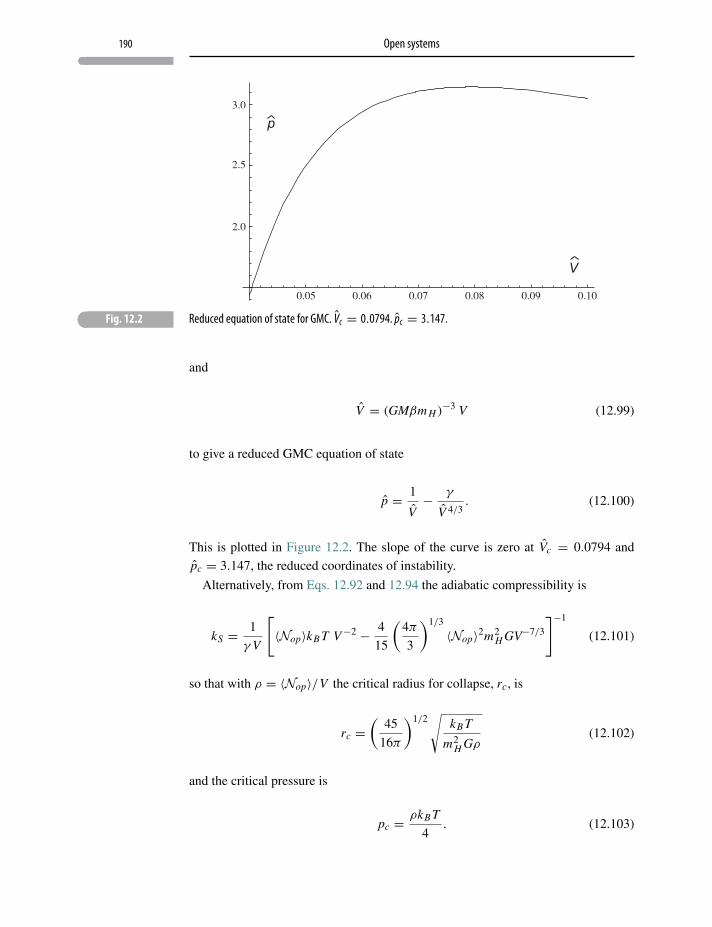
190 Open systems
� Fig. 12.2 Reduced equation of state for GMC. Vc = 0.0794. pc = 3.147.
and
V = (GMβm H )−3 V (12.99)
to give a reduced GMC equation of state
p = 1
V− γ
V 4/3. (12.100)
This is plotted in Figure 12.2. The slope of the curve is zero at Vc = 0.0794 and
pc = 3.147, the reduced coordinates of instability.
Alternatively, from Eqs. 12.92 and 12.94 the adiabatic compressibility is
kS = 1
γ V
[〈Nop〉kB T V−2 − 4
15
(4π
3
)1/3
〈Nop〉2m2H GV−7/3
]−1
(12.101)
so that with ρ = 〈Nop〉/V the critical radius for collapse, rc, is
rc =(
45
16π
)1/2√
kB T
m2H Gρ
(12.102)
and the critical pressure is
pc = ρkB T
4. (12.103)
191 Problems and exercises
Star formation is triggered by GMC compression to p ≈ pc by collisions with
other GMCs or compression by a nearby supernova event. Alternatively, galactic
collisions can trigger bursts of star formation as the gas clouds in each galaxy are
compressed.
12.7 Closing comment
Beginning with a thermal Lagrangian, Eq. 12.8, the grand canonical picture unfolds,
introducing the indispensable chemical potential and bringing a workable methodol-
ogy to open systems – physical situations in which particle number is variable and
particle interactions can be included. The next chapter discusses the chemical poten-
tial’s role in diffusion within inhomogeneous systems and extends μ’s application to
chemical reactants and distinct physical phases.
Problems and exercises
12.1 Find the internal energy of a van der Waals gas.
12.2 Find Cp − CV for the van der Waals gas.
13 The amazing chemical potential
Gibbs’ “Equilibrium of Heterogeneous Substances” has practically unlimitedscope. It spells out the fundamental thermodynamic theory of gases, mixtures,surfaces, solids, phase changes, chemical reactions, electrochemical cells, sedi-mentation and osmosis. It has been called, without exaggeration, the Principia ofThermodynamics.
William H. Cropper, Great Physicists, Oxford University Press US (2004)
13.1 Introduction
The chemical potential μ, a creation of J. W. Gibbs,1 is the essential state vari-
able for studying the thermodynamics of open systems, in particular chemical reac-
tions, phase transitions, non-uniform systems, surfaces and other cases which can
be characterized by varying particle number.2,3,4,5 Although sometimes regarded
as vague,6 when Schrödinger’s fixed particle number theory is extended by includ-
ing Hopen =−μNop, μ provides both utility and clarity. Thermal Lagrangians now
provide unambiguous rules governing a variety of diffusive processes.
In order to improve understanding of the thermodynamics of reactions, phase
transformations and heterogeneous diffusion, this chapter includes supplementary
examples and applications of the chemical potential.
1 J. W. Gibbs, “A method of geometrical representation of the thermodynamic properties of substancesby means of surfaces”, Transactions of the Connecticut Academy (1873).
2 G. Cook and R. H. Dickerson, “Understanding the chemical potential”, Am. J. Phys. 63, 73742 (1995).3 T. A. Kaplan, “The chemical potential”, J. of Stat. Physics. 122, 1237–1260 (2006).4 R. Baierlein, “The elusive chemical potential”, Am. J. Phys. 69, 423 (2001).5 G. Job and F. Herrmann, “Chemical potential – a quantity in search of recognition”, Eur. J. Phys. 27,
353–371 (2006).6 In the preface to Introduction to Solid State Physics (Wiley, New York, 1971), C. Kittel writes:
“A vague discomfort at the thought of the chemical potential is still characteristic of a physics edu-cation. This intellectual gap is probably due to the obscurity of the writings of J. Willard Gibbs whodiscovered and understood the matter 100 years ago.”
192
193 Diffusive equilibrium
13.2 Diffusive equilibrium
Consider a single system (equivalently referred to as a phase) at temperature T and
pressure p composed of, say, two distinct species A and B. Allow the species to
initially be diffusively isolated and chemically non-reactive. This species composite
can be described in terms of an open system macroscopic hamiltonian
Hcomposi te = hop −[μA N A
op + μB N Bop
](13.1)
with a corresponding thermal Lagrangian
L = −kB P ln P− λ0P− 1
T〈hop〉 + 1
T
[μA〈N A
op〉 + μB〈N Bop〉], (13.2)
where for total species isolation μA �= μB and where abbreviations
P ln P =∑
N=0,1,2,...
{∑s
P [εs(N ) , N ] ln P [εs (N ) , N ]
}(13.3)
P =∑
N=0,1,2,...
{∑s
P [εs (N ) , N ]
}(13.4)
imply sums over all species, as does 〈hop〉.If the two species A and B are in complete diffusive contact, at equilibrium the
individual 〈Nop〉 and 〈N Bop〉 are no longer distinguishable being replaced by the
cumulative 〈Nop〉 = 〈N Aop〉 + 〈N B
op〉 and, therefore, by the corresponding thermal
Lagrangian
L = −kB P ln P− λ0P− 1
T〈hop〉 + μ
T
[〈N A
op〉 + 〈N Bop〉], (13.5)
i.e. if species A and B freely diffuse, A and B must have the same chemical potential,
μA = μB = μ.
13.2.1 Examples
In the following examples of diffusive equilibrium the ideal gas provides an easily
understood model for illustrating the versatile role of the chemical potential.
Ideal gas in the Earth’s gravitational field
At a distance z above – but close to – the Earth’s surface, ideal gas molecules experi-
ence a quasi-classical gravitational potential energy per particle P E = mgz. Here g
194 The amazing chemical potential
is the Earth’s gravitational constant and m the molecular mass. As introduced earlier
(see Table 5.1 and Chapter 12), a thermal Lagrangian, and hence Zgr , can be written
to reflect this additional gravitational potential (work) contribution:
Zgr =∑
N=0,1,...
eβ(μ−mgz)NZ (N ) , (13.6)
where Z (N ) is the N -particle (canonical) partition function for the ideal gas (see
Chapter 7)
Z (N ) = 1
N !(nQ V
)N. (13.7)
Upon summing N Eq. 13.6 becomes
Zgr = exp[eβ(μ−mgz)nQ V
], (13.8)
and then, as also shown in Chapter 12 (see Eq. 12.15), the average particle number
at a distance z > 0 above the Earth’s surface is
〈Nop (z)〉 = 1
β
(∂
∂μlnZgr
)T,V
(13.9)
= 1
β
(∂
∂μ
)eβ(μ−mgz)nQ V (13.10)
= eβμe−βmgznQ V . (13.11)
The chemical potential of gas molecules at any height z is, therefore,
μ (z) = 1
βln〈Nop (z)〉
nQ V+ mgz. (13.12)
Gas particles (at height z) can freely diffuse to any adjacent level, say z±Δz, so that
in diffusive equilibrium μ must be uniform throughout the atmosphere, i.e. indepen-
dent of z. At ground level, i.e. z = 0, the chemical potential for ideal gas molecules is
μ (0) = 1
βln〈Nop (0)〉
nQ V, (13.13)
so in diffusive equilibrium Eqs. 13.12 and 13.13 are equated to give
〈Nop (z)〉 = 〈Nop (0)〉e−βmgz, (13.14)
the well-known “barometric” equation.
Charged ideal gas between capacitor plates
Ideal gas molecules, each with charge q, lie between a pair of large, parallel capacitor
plates placed a distance d apart and charged to a potential V = Ex d, where Ex is
195 Diffusive equilibrium
a uniform electric field between the plates. An electric potential energy per particle,
P E =−qx Ex adds, quasi-classically, to the N -particle ideal gas eigen-energies so
that, as in Eq. 13.11, the number of charged molecules a distance x from the positive
plate is
〈Nop (x)〉 = eβμeβqx Ex nQ V . (13.15)
Solving for the chemical potential,
μ (x) = 1
βln〈Nop (x)〉
nQ V− q x Ex . (13.16)
When x = 0 (the positive plate),
μ (0) = 1
βln〈Nop (0)〉
nQ V. (13.17)
For diffusive equilibrium, in the region between the plates μ is independent of x and
〈Nop (x)〉 = 〈Nop (0)〉eβqx Ex . (13.18)
At x = d , i.e. the negative plate,
〈Nop (d)〉 = 〈Nop (0)〉eβqV , (13.19)
where V = Ex d is the electric potential difference between the plates.
Ideal gas in a rotating cylinder
Ideal gas particles, mass m, in a cylinder rotating with angular frequency ω, acquire
a rotational potential energy per particle (in the rotating frame), which,
quasi-classically, is P Erot =− 12 mω2r2. Here r is a particle’s radial distance from
the cylinder axis. The grand partition function is
Zgr =∑
N=0,1,...
eβ(μ+ 1
2 mω2r2)
NZ (N ) , (13.20)
where Z (N ) is, as in Eq. 13.7, the N -particle (canonical) ideal gas partition func-
tion. After summing N , at a distance r from the axis of rotation the average particle
number is
〈Nop (r)〉 = 1
β
(∂
∂μlnZgr
)T,V
(13.21)
= 1
β
(∂
∂μ
)eβ(μ− 1
2 mω2r2)nQ V (13.22)
= eβμeβ2 mω2r2
nQ V . (13.23)
196 The amazing chemical potential
Hence, the chemical potential at r is
μ (r) = 1
βln〈Nop (r)〉
nQ V− 1
2mω2r2, (13.24)
whereas the chemical potential at r = 0 is
μ (0) = 1
βln〈Nop (0)〉
nQ V. (13.25)
In diffusive equilibrium μ must be uniform throughout the cylinder, i.e. indepen-
dent of r , giving the radial distribution of particles in a centrifuge
〈Nop (r)〉 = 〈Nop (0)〉 exp
(β
2mω2r2
). (13.26)
13.3 Thermodynamics of chemical equilibrium
Consider the concrete example of a system at temperature T containing three species
A, B and AB. Initially allow all three species to be non-interacting so that a thermal
Lagrangian is
L = −kB P ln P− λ0P− 1
T〈Hop〉 + 1
T
[μA〈N A
op〉 + μB〈N Bop〉 + μAB〈N AB
op 〉],
(13.27)
where μA, μB and μAB are the chemical potentials for each of the isolated species.
Now let the species react according to the chemical equation
A + B � AB. (13.28)
In such a chemical reaction all reactants and products coexist with small fluctuations
about mean equilibrium concentrations of the participants.7 This balanced chemical
equation defines “atom” diffusion such that at equilibrium only the average atom
sums
〈N Aop〉 + 〈N AB
op 〉 = νA (13.29)
and
〈N Bop〉 + 〈N AB
op 〉 = νB (13.30)
7 There are a few rare chemical reactions where concentrations of reactants and products oscillate intime so that “equilibrium” is never attained.
197 Thermodynamics of chemical equilibrium
are still identifiable. These constraints coordinate with a diffusive equilibrium con-
dition
μA + μB = μAB (13.31)
to give the thermal Lagrangian
L = −kB P ln P− λ0P− 1
T〈hop〉
+ 1
T
[μA
(〈N A
op〉 + 〈N ABop 〉
)+ μB
(〈N B
op〉 + 〈N ABop 〉
)]. (13.32)
As a second example consider a hypothetical reaction among the diatoms A2, B2
and the molecule AB,
A2 + B2 � 2 AB. (13.33)
Assuming uniform reaction temperature T and pressure p, consider the chemical
species as initially non-reactive. In that case the thermal Lagrangian is
L = −kB P ln P− λ0P− 1
T〈hop〉 + 1
T
[μA2〈N A2
op 〉 + μB2〈N B2op 〉 + μAB〈N AB
op 〉].
(13.34)
According to Eq. 13.33 the atom-reaction constraints for this case are
〈N A2op 〉 +
〈N ABop 〉2
= νA (13.35)
and
〈N B2op 〉 +
〈N ABop 〉2
= νB, (13.36)
where νA and νB are the still identifiable equilibrium atom numbers. These reaction
constraints coordinate with chemically reactive equilibrium
μA2 + μB2 = 2μAB , (13.37)
resulting in the thermal Lagrangian
L = −kB P ln P− λ0P− 1
T〈hop〉
+ 1
T
[μA2
(〈N A2
op 〉 +1
2〈N AB
op 〉)+ μB2
(〈N B2
op 〉 +1
2〈N AB
op 〉)]
(13.38)
derived from Eq. 13.34.
198 The amazing chemical potential
These results can be generalized to any chemical reaction, e.g.
a1 A1 + a2 A2 + a3 A3 � z1 Z1 + z2 Z2 + z3 Z3, (13.39)
in which case the atom reaction constraints are
〈N A1op 〉 +
a1
z3〈N Z3
op 〉 = νa1 , (13.40)
〈N A2op 〉 +
a2
z3〈N Z3
op 〉 = νa2 , (13.41)
〈N A3op 〉 +
a3
z3〈N Z3
op 〉 = νa3 , (13.42)
〈N Z1op 〉 −
z1
z3〈N Z3
op 〉 = νz1 , (13.43)
〈N Z2op 〉 −
z2
z3〈N Z3
op 〉 = νz2 , (13.44)
where νa1 , νa2 , νa3 , νz1 and νz2 are still identifiable atom numbers in accord with the
chemically diffusive equilibrium condition
a1 μA1 + a2 μ
A2 + a3 μA2 − z1 μ
Z1 − z2 μZ2 − z3 μ
Z3 = 0 (13.45)
to generate the thermal Lagrangian.
L = −kB P ln P− λ0P− 1
T〈hop〉 + 1
T
[μA1
(〈N A1
op 〉 +a1
z3〈N Z3
op 〉)
+ μA2
(〈N A2
op 〉 +a2
z3〈N Z3
op 〉)+ . . .+ μZ2
(〈N Z2
op 〉 −z2
z3〈N Z3
op 〉)]
. (13.46)
13.4 A law of mass action
Chemical reactions such as (hypothetically) defined in Eqs. 13.28, 13.33, 13.39 do
not usually go to completion. A sealed reaction “vessel” contains an equilibrium
mixture of reactants and products. For example, the gaseous reaction
3H2+N2 � 2 NH3 (13.47)
in which at thermal equilibrium
3μH2 + μN2 − 2μNH3 = 0, (13.48)
yields only a small amount of NH3 (ammonia), with reactants H2 and N2 still having
a substantial presence. The equilibrium concentrations of reactants and products in
199 A law of mass action
the closed reaction “vessel” is, however, well described by a “law of mass action”
which is a consequence of Eq. 13.48. This “law” is arrived at by first exponentiating
Eq. 13.48:
exp(3μH2
)× exp(μN2
)exp
(2μNH3
) = 1 (13.49)
or [exp
(μH2
)]3 × [exp
(μN2
)][exp
(μNH3
)]2= 1. (13.50)
Continuing in the spirit of the example, assume all participating gases g are ideal
and at sufficiently low temperature that no internal modes of the reactive molecules
(rotational, vibrational or electronic) are excited. In which case
βμg = ln
[C (g)
n(g)Q
](13.51)
= ln
⎧⎨⎩[
m(g)
2πh2β
]−3/2
C (g)
⎫⎬⎭ , (13.52)
where m(g) is the molecular mass of the gas g and
C (g) = 〈N (g)op 〉V
(13.53)
is the gas concentration. From this follows a typical “mass action” result
[C NH3
]2[C H2
]3 [C N2
] ={
nH2Q
}3 {nN2
Q
}{
nNH3Q
}2(13.54)
= K (T ), (13.55)
where K depends only on T . Specific mass action constants K are associated with
different chemical reactions or molecular models. If, for example, in the previous
model temperature is raised sufficiently to excite molecular rotational and vibration
(internal modes) the N -particle canonical partition function becomes
Z (N ) = 1
N ! [Zint]N [nQ V
]N (13.56)
where Zint is the partition function for the internal (rotational and vibrational) modes.
In that case we redefine nQ for the molecular gas g
n(g)Q → Z (g)
int n(g)Q = n(g)
int (13.57)
200 The amazing chemical potential
so that the mass action expression becomes[C NH3
]2[C H2
]3 [C N2
] = Kint (T ) , (13.58)
where
Kint (T ) ={
nH2int
}3 {nN2
int
}{
nNH3int
}2. (13.59)
13.5 Thermodynamics of phase equilibrium
A phase is a chemically and physically uniform macroscopic state of matter. Vapor,
liquid and solid are among the familiar examples of phases. Other examples include
different coexisting crystal structures with the same chemical composition or the
more exotic He4–Bose–Einstein condensate phases. Phase equilibrium describes a
situation in which two or more homogeneous regions (phases) coexist in thermody-
namic equilibrium within a rigid container but are separated by physical boundaries.
An example are the three phases of H2O – ice, liquid water and water vapor – in
which any two or all three can coexist. Distinct phases may also exist within a given
state, such as in solid iron alloys and in the several phases that can coexist for liq-
uid states. Those phases that are possible depend on temperature and pressure. If
two coexisting phases, designated α and β, composed of a single species, freely
exchange particles at temperature T within a fixed volume(V α + V β
), then a ther-
mal Lagrangian is8
LE,N ,V = −kB
[Pα ln Pα + Pβ ln Pβ
]− λ0αPα − λ0β Pβ
− 1
T
[〈hα
op〉 + 〈hβop〉]− 1
T〈 pop〉
(V α + V β
)+ μ
T
[〈N α
op〉 + 〈N βop〉],
(13.60)
with
Tα = Tβ = T,
μα = μβ = μ,
〈 pαop〉 = 〈 pβ
op〉 = 〈 pop〉.(13.61)
8 Mechanical energy, p V , is included in the Lagrangian.
201 Gibbs–Duhem relation
13.6 Gibbs–Duhem relation
Long before he published his monumental treatise on statistical mechanics Gibbs had
already extended the fundamental equation of thermodynamics to include particle
transfer. For a single phase and a single species the fundamental equation becomes
T dS = dU + p dV − μ d〈Nop〉. (13.62)
When U is expressed in terms of its natural variables
U = U(S, V, 〈Nop〉
), (13.63)
all of which are extensive, then in the Euler form
U(λS, λV, λ〈Nop〉
) = λU (S, V,N ) . (13.64)
Euler’s homogeneous function theorem gives
S(∂U∂S
)V,〈Nop〉
+ V
(∂U∂V
)S,〈Nop〉
+〈Nop〉(
∂U∂〈Nop〉
)V,S
= U(S, V, 〈Nop〉
).
(13.65)
Comparing this with Eq. 13.62, the fundamental equation is effectively integrated
to get
U − TS + V p − μ〈Nop〉 = 0. (13.66)
Taking the total differential
dU − T dS − S dT + V dp + p dV − μ d〈Nop〉 − 〈Nop〉 dμ = 0 (13.67)
and combining it with the fundamental equation Eq. 13.62, we have for a single
phase with one species
−S dT + V dp − 〈Nop〉 dμ = 0. (13.68)
This is called the Gibbs–Duhem equation. In the case of a single phase with M
species Gibbs–Duhem becomes
−S dT + V dp −M∑i
〈Nop〉i dμi = 0, (13.69)
showing that intensive variables T, p, μi are not independent.
202 The amazing chemical potential
13.7 Multiphase equilibrium
Gibbs–Duhem opens the door to basic understanding of coexistence between differ-
ent phases, such as between liquid water and water vapor, or between ice and liquid
water, etc.
Begin by rewriting Eq. 13.68 in the form
dμ = −s dT+v dp (13.70)
where intensive quantities
s = S〈Nop〉 v = V
〈Nop〉 (13.71)
have been defined. Taking advantage of p and T as natural variables, for two phases,
α and β, at the same T and p and composed of only a single species (pure phases),
the chemical potentials are
μ(α) = μ(α)(p, T ) , (13.72)
μ(β) = μ(β)(p, T ) . (13.73)
If these phases are to coexist, then
μ(α)(p, T ) = μ(β)(p, T ) , (13.74)
which is a “system” of one equation with two unknowns, T and p. Although there
is no unique solution, T can be found in terms of p so that the α and β phases can
coexist along some curve in the {p, T }-plane.
Now suppose there are three pure phases, α, β and γ . Then for coexistence between
the three phases
μ(α)(p, T ) = μ(β)(p, T ) , (13.75)
μ(α)(p, T ) = μ(γ )(p, T ) , (13.76)
which is a “system” of two equations and two unknowns with a unique solution – a
single point in the {p, T }-plane. The three phases can coexist at what is called a
triple point.9 Figure 13.1 is an example of a phase diagram for a single component
system, e.g. water10 in which temperature and pressure form the coordinate axes. As
shown in the diagram, only certain phases are possible at a particular temperature
and pressure, with each phase separated from the others by a curve in the {p, T }9 Triple point of water: Ttp = 273.16 K, ptp = 0.006 04 atm (1 atm = 101.3 k Pa).
10 The experimental solid–liquid boundary for water has an anomalous negative slope so the diagram isonly an approximate representation for water. This is due to the peculiarity of ice being less dense thanliquid water.
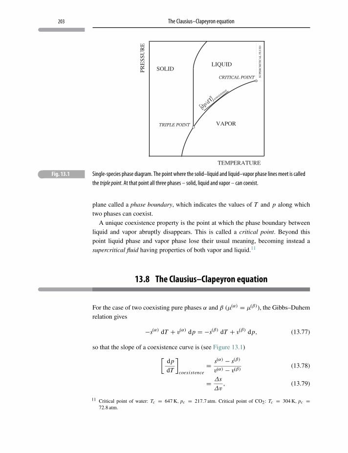
203 The Clausius–Clapeyron equation
dp/dT
coexistence
� Fig. 13.1 Single-species phase diagram. The point where the solid–liquid and liquid–vapor phase lines meet is calledthe triple point. At that point all three phases – solid, liquid and vapor – can coexist.
plane called a phase boundary, which indicates the values of T and p along which
two phases can coexist.
A unique coexistence property is the point at which the phase boundary between
liquid and vapor abruptly disappears. This is called a critical point. Beyond this
point liquid phase and vapor phase lose their usual meaning, becoming instead a
supercritical fluid having properties of both vapor and liquid.11
13.8 The Clausius–Clapeyron equation
For the case of two coexisting pure phases α and β (μ(α) = μ(β)), the Gibbs–Duhem
relation gives
−s(α) dT + v(α) dp = −s(β) dT + v(β) dp, (13.77)
so that the slope of a coexistence curve is (see Figure 13.1)[dp
dT
]coexistence
= s(α) − s(β)
v(α) − v(β)(13.78)
= Δs
Δv, (13.79)
11 Critical point of water: Tc = 647 K, pc = 217.7 atm. Critical point of CO2: Tc = 304 K, pc =72.8 atm.
204 The amazing chemical potential
which is called the Clausius–Clapeyron equation. As a concrete example that relates
to Figure 13.1 let α ≡ � (liquid phase), and β ≡ g (gas phase). Then Δs is the
liquid–gas entropy difference per particle and Δv is the liquid–gas volume difference
per particle. Moreover
Δs = Qvap
〈Nop〉T , (13.80)
where Qvap/〈Nop〉 is the heat of vaporization per particle,12 so that[dp
dT
]coexistence
= Qvap
T 〈Nop〉Δv. (13.81)
In generalQvap
T 〈Nop〉Δvis not a simple function of p and T so that integrating
Eq. 13.81 to obtain the vapor pressure may not be straightforward. On the other
hand, assuming an ideal gas phase and since, in general, v(gas) � v(�), the differential
equation simplifies to [dp
dT
]coexistence
= p Qvap
kB T 2. (13.82)
Since generally v(solid) < v(�) for most systems, as suggested in Figure 13.1, the
solid–liquid coexistence curve is nearly vertical but positively sloped. In the unusual
case of water for which v(solid) > v(�) the curve is also nearly vertical, but now
slightly negatively sloped.
13.9 Surface adsorption: Langmuir’s model
In the process of film growth or surface doping, atoms or molecules in gas phase
or in dilute solution bind to the film surface (Figure 13.2). A theory of solid sur-
face coverage by these molecules was formulated by Irving Langmuir (1916), the
acknowledged pioneer of surface chemistry.
Assumptions of the model are as follows.
1. The solid surface is in contact with ideal monatomic gas atoms at temperature T
and pressure p0.
2. There are a fixed number of sites N on the surface available for bonding.
3. Each surface site can be only singly occupied (monolayer coverage).
4. Adsorption at a given site is independent of occupation of neighboring sites (no
interactions).
12 The heat required to evaporate one particle.
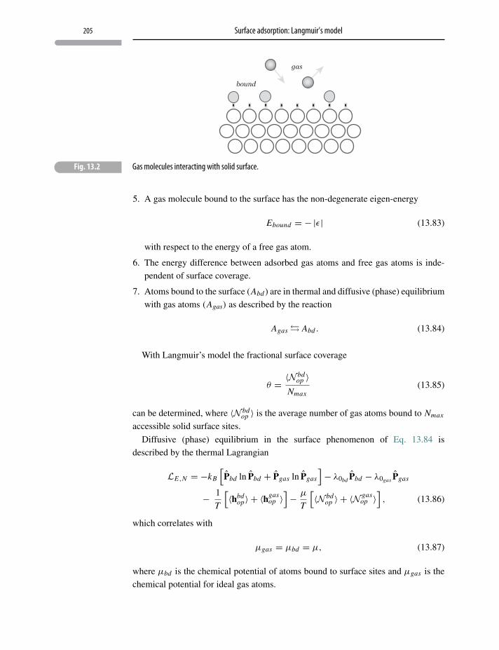
205 Surface adsorption: Langmuir’s model
� Fig. 13.2 Gas molecules interacting with solid surface.
5. A gas molecule bound to the surface has the non-degenerate eigen-energy
Ebound = − |ε| (13.83)
with respect to the energy of a free gas atom.
6. The energy difference between adsorbed gas atoms and free gas atoms is inde-
pendent of surface coverage.
7. Atoms bound to the surface (Abd ) are in thermal and diffusive (phase) equilibrium
with gas atoms (Agas) as described by the reaction
Agas � Abd . (13.84)
With Langmuir’s model the fractional surface coverage
θ = 〈N bdop 〉
Nmax(13.85)
can be determined, where 〈N bdop 〉 is the average number of gas atoms bound to Nmax
accessible solid surface sites.
Diffusive (phase) equilibrium in the surface phenomenon of Eq. 13.84 is
described by the thermal Lagrangian
LE,N = −kB
[Pbd ln Pbd + Pgas ln Pgas
]− λ0bd Pbd − λ0gas Pgas
− 1
T
[〈hbd
op〉 + 〈hgasop 〉
]− μ
T
[〈N bd
op 〉 + 〈N gasop 〉
], (13.86)
which correlates with
μgas = μbd = μ, (13.87)
where μbd is the chemical potential of atoms bound to surface sites and μgas is the
chemical potential for ideal gas atoms.
206 The amazing chemical potential
Finding the average number of atoms bound to surface sites 〈N bdop 〉 follows dis-
cussions in Chapter 12 where it was shown that
〈N bdop 〉 =
Nmax∑N=0
∑s
Ne−β{[Es (N )]−μbd N }
Nmax∑N=0
∑s
e−β{[Es (N )]−μbd N }, (13.88)
with the number of bound atoms limited by Nmax and where Es(N ) = −N |ε|. The
denominator in Eq. 13.88 is the grand partition function Zgr ,
Zgr =Nmax∑N=0
eβμbd NZ (N ), (13.89)
where Z (N ) is the (canonical) partition function for N -bound atoms
Z (N ) = g (N , Nmax ) eNβ|ε| . (13.90)
Since the bound atom’s only eigen-energy (see Eq. 13.83) has the configurational
degeneracy
g (N , Nmax ) = Nmax !(Nmax − N )! N ! (13.91)
the grand partition function is
Zgr =Nmax∑N=0
Nmax!(Nmax − N )! N !e
Nβ(μbd+|ε|) (13.92)
=[1+ eβ(μbd+|ε|)
]Nmax(13.93)
and the fractional surface coverage is (see Eq. 13.88)
θ = 〈N bdop 〉
Nmax(13.94)
= 1
Nmax× 1
β
∂
∂μbdlnZgr (13.95)
= eβμbd eβ|ε|
1+ eβμbd eβ|ε|. (13.96)
The ideal gas in contact with the surface has the chemical potential (see Eq. 12.48)
μgas = 1
βln〈N gas
op 〉nQ V
. (13.97)
207 Dissociative adsorption
Equating the chemical potentials (see Eq. 13.87) (diffusive equilibrium) and using
the ideal gas equation of state p0V = 〈N gasop 〉β
gives the Langmuir fractional surface
coverage
θ = p0
Π0 + p0, (13.98)
where Π0 is the temperature-dependent factor
Π0 = nQ e−β|ε|
β. (13.99)
This is known as the Langmuir isotherm.
13.10 Dissociative adsorption
A diatomic gas molecule, say A2, may not simply bind to a surface site, but may
dissociate, with each component atom binding to a single site. This is referred to as
dissociative adsorption and is described by the “chemical reaction”
A2 � 2Abound . (13.100)
Therefore, the thermal equilibrium chemical potentials satisfy
μA2 − 2μA = 0, (13.101)
where μA2 is the chemical potential of the ideal diatomic gas and μA is the chemical
potential of surface bound atoms. The ideal diatomic gas in contact with the surface
has the chemical potential
μA2 =1
βln〈N A2
op 〉n A2
int V, (13.102)
which includes the effect of internal (rotational and vibrational) modes (see
Eq. 13.56). Once again taking Ebound = − |ε| the fractional surface occupation is,
according to Eq. 13.96,
θ = eβμA eβ|ε|
1+ eβμA eβ|ε|. (13.103)
Now applying Eq. 13.101 the surface coverage is
θ = e(1/2)βμA2 eβ|ε|
1+ e(1/2)βμA2 eβ|ε|. (13.104)
Using the ideal gas result, Eq. 13.102, we finally have
θ =√
p
ΠD +√p, (13.105)
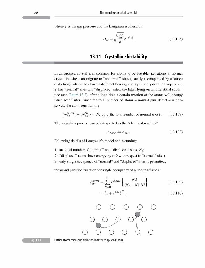
208 The amazing chemical potential
where p is the gas pressure and the Langmuir isotherm is
ΠD =√
n A2int
βe−β|ε|. (13.106)
13.11 Crystalline bistability
In an ordered crystal it is common for atoms to be bistable, i.e. atoms at normal
crystalline sites can migrate to “abnormal” sites (usually accompanied by a lattice
distortion), where they have a different binding energy. If a crystal at a temperature
T has “normal” sites and “displaced” sites, the latter lying on an interstitial sublat-
tice (see Figure 13.3), after a long time a certain fraction of the atoms will occupy
“displaced” sites. Since the total number of atoms – normal plus defect – is con-
served, the atom constraint is
〈N normop 〉 + 〈N dis
op 〉 = Nnormal(the total number of normal sites) . (13.107)
The migration process can be interpreted as the “chemical reaction”
Anorm � Adis . (13.108)
Following details of Langmuir’s model and assuming:
1. an equal number of “normal” and “displaced” sites, Ns ;
2. “displaced” atoms have energy ε0 > 0 with respect to “normal” sites;
3. only single occupancy of “normal” and “displaced” sites is permitted;
the grand partition function for single occupancy of a “normal” site is
Znormgr =
Ns∑N=0
eNβμn
{Ns !
(Ns − N )!N !}
(13.109)
= (1+ eβμn
)Ns, (13.110)
� Fig. 13.3 Lattice atoms migrating from “normal” to “displaced” sites.
209 Crystalline bistability
while the grand partition function for single occupancy of a “displaced” site is
Z intergr =
Ns∑N=0
eNβμdis
{Ns !
(Ns − N )!N !eNβε0
}(13.111)
= (1+ eβε0 eβμdis
)Ns. (13.112)
From grand partition functions, Eqs. 13.110 and 13.112,
〈N normop 〉 = 1
β
∂
∂μnormlnZnorm
gr (13.113)
= Nsλnorm
1+ λnorm(13.114)
and
〈N disop 〉 =
1
β
∂
∂μdislnZdis
gr (13.115)
= Nsλdise−βε0
1+ λdise−βε0, (13.116)
where
λnorm = eβμnorm (13.117)
and
λdis = eβμdis . (13.118)
At thermal equilibrium
μnorm = μdis (13.119)
or
λnorm = λdis = λ. (13.120)
Applying Eq. 13.107(Nnormal = Ns) together with Eqs. 13.114, 13.116, 13.120,
λ
1+ λ+ λe−βε0
1+ λe−βε0= 1, (13.121)
we find
λ = eβε0/2. (13.122)
Therefore, according to Eq. 13.116 the average fractional occupation of “displace-
ment” sites is
〈N disop 〉
Ns= 1
1+ exp (βε0/2)(13.123)
as shown in Figure 13.4.
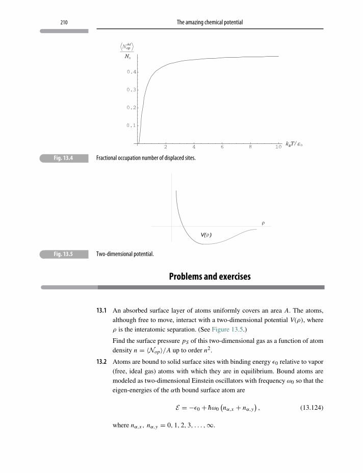
210 The amazing chemical potential
ε
� Fig. 13.4 Fractional occupation number of displaced sites.
ρ
ρ
� Fig. 13.5 Two-dimensional potential.
Problems and exercises
13.1 An absorbed surface layer of atoms uniformly covers an area A. The atoms,
although free to move, interact with a two-dimensional potential V(ρ), where
ρ is the interatomic separation. (See Figure 13.5.)
Find the surface pressure pS of this two-dimensional gas as a function of atom
density n = 〈Nop〉/A up to order n2.
13.2 Atoms are bound to solid surface sites with binding energy ε0 relative to vapor
(free, ideal gas) atoms with which they are in equilibrium. Bound atoms are
modeled as two-dimensional Einstein oscillators with frequency ω0 so that the
eigen-energies of the αth bound surface atom are
E = −ε0 + hω0(nα,x + nα,y
), (13.124)
where nα,x , nα,y = 0, 1, 2, 3, . . . ,∞.
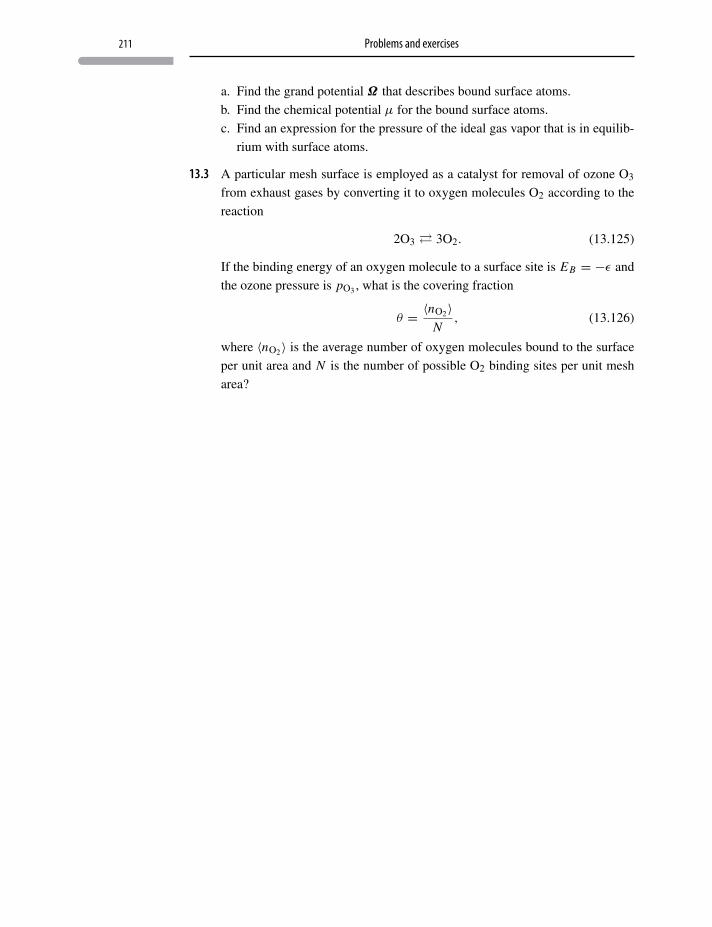
211 Problems and exercises
a. Find the grand potential Ω that describes bound surface atoms.
b. Find the chemical potential μ for the bound surface atoms.
c. Find an expression for the pressure of the ideal gas vapor that is in equilib-
rium with surface atoms.
13.3 A particular mesh surface is employed as a catalyst for removal of ozone O3
from exhaust gases by converting it to oxygen molecules O2 according to the
reaction
2O3 � 3O2. (13.125)
If the binding energy of an oxygen molecule to a surface site is EB = −ε and
the ozone pressure is pO3 , what is the covering fraction
θ = 〈nO2〉N
, (13.126)
where 〈nO2〉 is the average number of oxygen molecules bound to the surface
per unit area and N is the number of possible O2 binding sites per unit mesh
area?
14 Thermodynamics of radiation
A new scientific truth does not triumph by convincing its opponents and makingthem see the light, but because its opponents eventually die, and a new generationgrows up that is familiar with it.
Max Planck, Scientific Autobiography and Other Papers,Copyright: Philosophical Library
14.1 Introduction
In 1900 Max Planck discovered that the temperature-dependent law of radiating
bodies could not be derived solely from Maxwellian electrodynamics according to
which the energy of an electromagnetic field is1
E = 1
2
∫dx[E(x, t)2 + B(x, t)2
]. (14.1)
Planck arrived, instead, at results consistent with the relevant electromagnetic experi-
ments by treating radiation of a given frequency ν as though it consisted of “packets”
of energy – “photons” – each with energy hν, with a corresponding electromagnetic
field energy
EPlanck = nhν, (14.2)
where n = 0, 1, 2, . . . is the number of “photons” in the packet and h is Planck’s
universal constant.
Planck’s hypothesis2 was the initial link in the chain of 20th-century discoveries
that is quantum physics.
1 In rationalized cgs units.2 Likely inspired by Boltzmann’s concept of “microstates”.
212
213 Electromagnetic eigen-energies
14.2 Electromagnetic eigen-energies
Proceeding directly to the thermodynamics of radiation, Eq. 14.2 is replaced by
the electromagnetic quantum eigen-energies for photons of a single mode k having
polarization λ
Ek,λ = hνk,λ
[n (k, λ)+ 1
2
], (14.3)
where n (k, λ) = 0, 1, 2, . . . is the number of photons. k and λ are quantum numbers
for a single photon of frequency νk,λ.3
Photons are fundamental particle-like “excitations” of the electromagnetic field.
They have zero mass and are their own antiparticle. They can be created and absorbed
(destroyed) without number conservation and therefore have zero chemical potential.
They appear in an almost limitless variety of atomic, molecular or nuclear processes
as well as continuous radiation (synchrotron radiation) associated with kinematic
acceleration of particles. The photon carries “spin” angular momentum ±h corre-
sponding to right and left circular polarization.
The Maxwellian total electromagnetic energy (see Eq. 14.1) is similarly replaced
by the quantum average
〈HE M 〉 =∑λ=1,2
∑k
hνk,λ
[〈nop (k, λ)〉 + 1
2
](14.4)
where HE M is the electromagnetic hamiltonian,
HE M =∑λ=1,2
∑k
hνk,λ
[nop(k, λ)+ 1
2
]. (14.5)
The “photon” mode number operator nop(k, λ) is identified by a three-component
wave vector k, with k ≡ kx , ky, kz , and two mutually perpendicular polarization
directions λ ≡ λ1, λ2. The eigenvalues of nop (k, λ) are n(k, λ) = 0, 1, 2, . . . and
〈nop(k, λ)〉 is the average number of photons in that mode. The wave vector k is the
direction of propagation of the photon and the polarization λ is the vector direction
of the concurrent electric field E (see Figure H.1). In free space the two-component
polarization vector is perpendicular (transverse) to k. This follows from the Maxwell
equation4 ∇ · E = 0. For electromagnetic radiation in free space, the energy of a
3 Arriving at Planck’s result from Maxwell’s equations is the realm of quantum field theories, the detailsof which are well beyond the scope of this book. Nevertheless, for completeness an outline of themethod is discussed in Appendix H.
4 Since there is no analog to this Maxwell equation in crystalline elastic equations of motion, thereremain three phonon polarizations.
214 Thermodynamics of radiation
photon associated with a particular mode (k, λ) is
hνk,λ = h
2πc |k| , (14.6)
which depends only on the magnitude |k| and is independent of the polarization λ.
Here c is the speed of light in vacuum. As indicated in Appendix H, in free space
〈nop (k, λ)〉, the average number of photons in the mode (k, λ) also depends only on|k| and is independent of the polarization λ.
14.3 Thermodynamics of electromagnetism
Based on macroscopic electromagnetic eigen-energies given by Eq. 14.3 (see
Appendix H), a thermal electromagnetic Lagrangian LE M is constructed:
LE M = −kB
∑nk,λ
P(nk,λ) ln P(nk,λ)− λ0
∑nk,λ
P(nk,λ)
− 1
T
∑nk,λ
P(nk,λ)∑
kλ=1,2
{hνk,λ
(nk,λ + 1
2
)}, (14.7)
where P(nk,λ
)is the probability that nk,λ photons are in the mode k with polarization
λ. The sum ∑nk,λ
(14.8)
ranges over nk,λ = 0, 1, 2, . . . for each mode k and both polarizations (λ = 1, 2).
The Lagrange multiplier λ0 assures normalized probabilities. Following familiar pro-
cedures, we find from Eq. 14.7
P(nk,λ
) =exp
⎧⎪⎪⎨⎪⎪⎩−β∑
kλ=1,2
hνk,λ
(nk,λ + 1
2
)⎫⎪⎪⎬⎪⎪⎭∑nk,λ
exp
⎧⎪⎪⎨⎪⎪⎩−β∑
kλ=1,2
hνk,λ
(nk,λ + 1
2
)⎫⎪⎪⎬⎪⎪⎭, (14.9)
where the normalizing denominator is the thermal equilibrium electromagnetic par-
tition function,
ZE M =∑nk,λ
exp
⎧⎨⎩−β∑λ=1,2
∑k
hνk,λ
(nk,λ + 1
2
)⎫⎬⎭. (14.10)
215 Thermodynamics of electromagnetism
14.3.1 Thermodynamics for a single photon mode
To simplify evaluation of Eq. 14.10 we first examine the partition function for a
single mode kα
ZαE M =
∑nkα,λ=0,1,2,3,...
exp
⎧⎨⎩−β∑λ=1,2
hνkα,λ
(nkα,λ +
1
2
)⎫⎬⎭, (14.11)
where ∑nkα,λ=0,1,2,3,...
(14.12)
is the sum over all integer photon numbers for a single mode (kα, λ). Explicitly
summing over both polarizations in the exponent of Eq. 14.11,
ZαE M = e−βhνkα
∑nka ,1
exp[−βhνkα
(nkα,1
)] ∑nka ,2
exp[−βhνkα
(nkα,2
)](14.13)
= e−βhνkα
⎧⎨⎩∑nka ,1
exp[−βhνkα
(nkα,1
)]⎫⎬⎭2
, (14.14)
where the factor e−βhνkα results from the vacuum radiation term in the eigen-
energies. The sum over photon numbers nkα,1= 0, 1, 2, . . . is just a geometric series,
giving for the single mode kα and both polarizations
ZαE M =
⎡⎣e−βhνkα
21
1− e−βhνkα
⎤⎦2
. (14.15)
14.3.2 Average photon number
From Eq. 14.9 the average number of photons in the single mode kα with a single
polarization λ = 1, say 〈nkα,1〉, is
〈nkα,1〉 =
∑nkα,1
nkα,1 exp{−βhνkα,1 nkα,1
}∑
nkα,1
exp{−βhνkα,1 nkα,1
} . (14.16)
This is identical with
〈nkα,1〉 =[
1
2hνka ,1
∂
∂βln(−Zα
E M
)]− 1
2(14.17)
= 1
eβhνka ,1 − 1, (14.18)
which is called a Planck distribution function.
216 Thermodynamics of radiation
14.3.3 Helmholtz potential and internal energy
The Helmholtz potential Fα for a single mode kα is
Fα = − 1
βlogZα
E M (14.19)
= hνkα+ 2
βlog
(1− e−βhνkα
). (14.20)
Similarly, for a single mode kα (counting both polarizations) the radiation field
internal energy Uα is
Uα = − ∂
∂βln Zα
E M (14.21)
= hνkα
(eβhνkα + 1
eβhνkα − 1
)(14.22)
= 2hνkα
(1
2+ 1
eβhνkα − 1
)(14.23)
= 2hνkα
(1
2+ 〈nkα
〉). (14.24)
14.4 Radiation field thermodynamics
The thermal electromagnetic field assembles all photon modes k with both transverse
polarizations λ = 1, 2, requiring the full evaluation of Eq. 14.10. Rewriting ZE M as
ZE M =⎡⎣ ∑
nk1=0,1,2,...
e−βhνk1
(nk1+1/2
)⎤⎦2 ⎡⎣ ∑nk2=0,1,2,...
e−βhνk2
(nk2+1/2
)⎤⎦2
. . .
(14.25)
=∏
k
[e−βhνk
(1
1− e−βhνk
)2], (14.26)
in analogy with Eqs. 14.19 and 14.24 the Helmholtz potential FE M is
FE M = − 1
β
∑k
ln
[e−βhνk
(1
1− e−βhνk
)2]
(14.27)
=∑
k
[hνk + 2
βln(
1− e−βhνk)]
(14.28)
and the internal energy UE M is
UE M = 2∑
k
hνk
(1
2+ 〈nk〉
). (14.29)
217 Stefan–Boltzmann, Planck, Rayleigh–Jeans laws
14.5 Stefan–Boltzmann, Planck, Rayleigh–Jeans laws
In the limit of macroscopic volume V the sum over k in Eq. 14.29 is replaced by (see
Appendix H)
∞∑k
⇒ V
(2π)3
∞∫−∞
dkx
∞∫−∞
dky
∞∫−∞
dkz, (14.30)
so that ignoring the divergent, constant vacuum energy
UE M = 2V
(2π)3
∞∫−∞
dkx
∞∫−∞
dky
∞∫−∞
dkz
(hνk
eβhνk − 1
). (14.31)
But in vacuum we have Eq. 14.6 so that the integrals can be carried out in spherical
coordinates, in which case
∞∫−∞
dkx
∞∫−∞
dky
∞∫−∞
dkz =2π∫
0
dϕ
π∫0
dθ sin θ
∞∫0
d |k| |k|2 (14.32)
and the internal energy UE M is (with h = 2πh)
UE M = hcV
π2
∞∫0
d |k| |k|3(
1
eβhc|k| − 1
). (14.33)
The integral can be brought into a more standard form with the substitution
|k| = x
βhc(14.34)
so that
UE M = hcV
π2 (βhc)4
∞∫0
dx x3(
1
ex − 1
). (14.35)
The integral in Eq. 14.35 is one of several similar integrals that appear in thermal
radiation theory. They are somewhat subtle to evaluate but they can be found in
comprehensive tables or computed with Mathematica with the result
∞∫0
dx x3(
1
ex − 1
)= π4
15(14.36)
so that the radiation energy density is
UE M
V= π2
15β4 (hc)3. (14.37)
This is called the Stefan–Boltzmann radiation law.
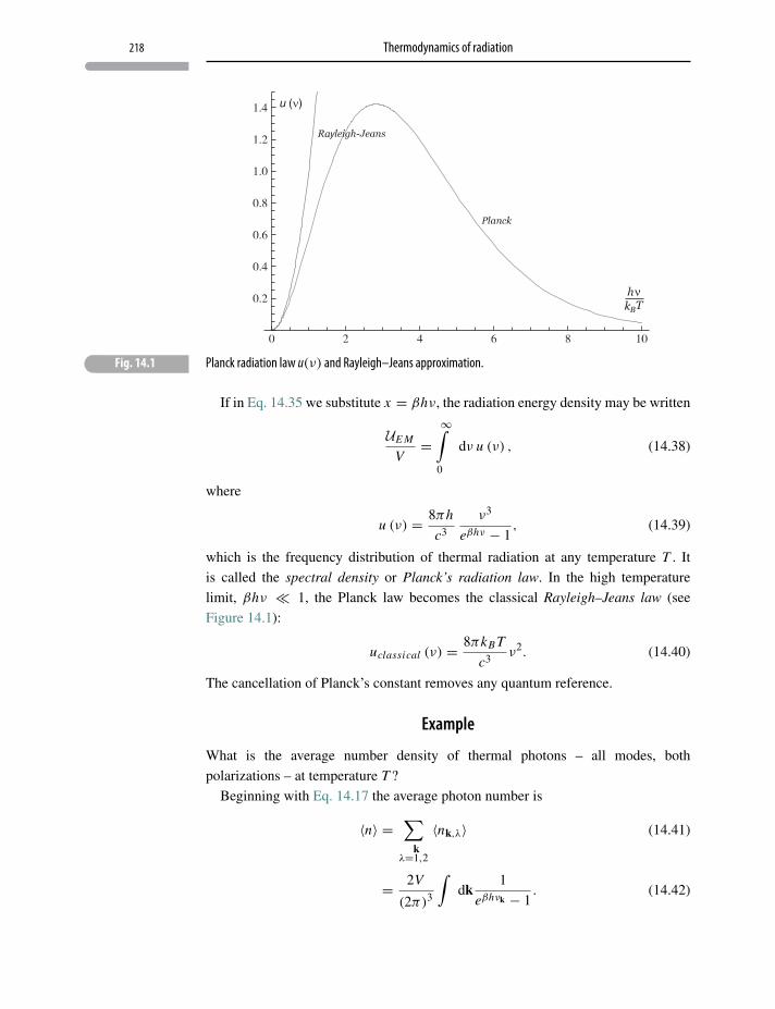
218 Thermodynamics of radiation
u (n)
� Fig. 14.1 Planck radiation law u(ν) and Rayleigh–Jeans approximation.
If in Eq. 14.35 we substitute x = βhν, the radiation energy density may be written
UE M
V=
∞∫0
dν u (ν) , (14.38)
where
u (ν) = 8πh
c3
ν3
eβhν − 1, (14.39)
which is the frequency distribution of thermal radiation at any temperature T . It
is called the spectral density or Planck’s radiation law. In the high temperature
limit, βhν � 1, the Planck law becomes the classical Rayleigh–Jeans law (see
Figure 14.1):
uclassical (ν) = 8πkB T
c3ν2. (14.40)
The cancellation of Planck’s constant removes any quantum reference.
Example
What is the average number density of thermal photons – all modes, both
polarizations – at temperature T ?
Beginning with Eq. 14.17 the average photon number is
〈n〉 =∑
kλ=1,2
〈nk,λ〉 (14.41)
= 2V
(2π)3
∫dk
1
eβhνk − 1. (14.42)
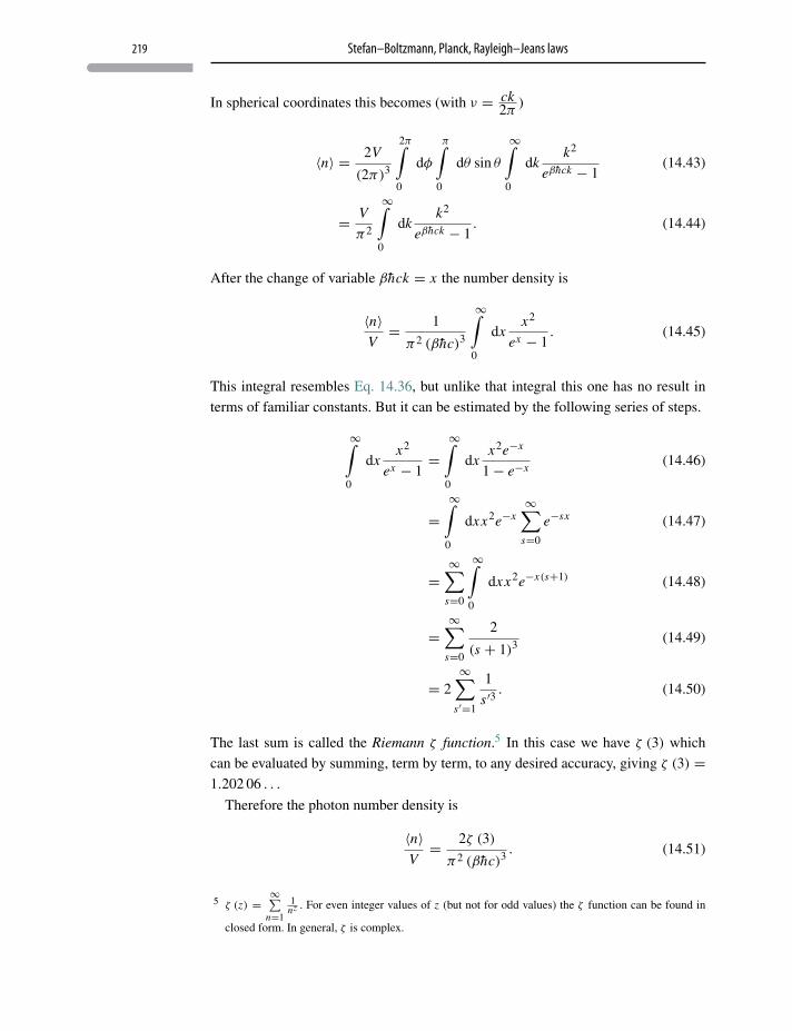
219 Stefan–Boltzmann, Planck, Rayleigh–Jeans laws
In spherical coordinates this becomes (with ν = ck2π )
〈n〉 = 2V
(2π)3
2π∫0
dφ
π∫0
dθ sin θ
∞∫0
dkk2
eβhck − 1(14.43)
= V
π2
∞∫0
dkk2
eβhck − 1. (14.44)
After the change of variable βhck = x the number density is
〈n〉V= 1
π2 (βhc)3
∞∫0
dxx2
ex − 1. (14.45)
This integral resembles Eq. 14.36, but unlike that integral this one has no result in
terms of familiar constants. But it can be estimated by the following series of steps.
∞∫0
dxx2
ex − 1=
∞∫0
dxx2e−x
1− e−x(14.46)
=∞∫
0
dxx2e−x∞∑
s=0
e−sx (14.47)
=∞∑
s=0
∞∫0
dxx2e−x(s+1) (14.48)
=∞∑
s=0
2
(s + 1)3(14.49)
= 2∞∑
s′=1
1
s′3. (14.50)
The last sum is called the Riemann ζ function.5 In this case we have ζ (3) which
can be evaluated by summing, term by term, to any desired accuracy, giving ζ (3) =1.202 06 . . .
Therefore the photon number density is
〈n〉V= 2ζ (3)
π2 (βhc)3. (14.51)
5 ζ (z) =∞∑
n=1
1nz . For even integer values of z (but not for odd values) the ζ function can be found in
closed form. In general, ζ is complex.
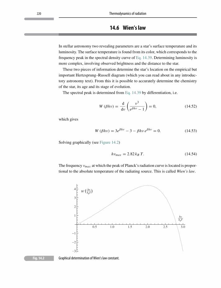
220 Thermodynamics of radiation
14.6 Wien’s law
In stellar astronomy two revealing parameters are a star’s surface temperature and its
luminosity. The surface temperature is found from its color, which corresponds to the
frequency peak in the spectral density curve of Eq. 14.39. Determining luminosity is
more complex, involving observed brightness and the distance to the star.
These two pieces of information determine the star’s location on the empirical but
important Hertzsprung–Russell diagram (which you can read about in any introduc-
tory astronomy text). From this it is possible to accurately determine the chemistry
of the star, its age and its stage of evolution.
The spectral peak is determined from Eq. 14.39 by differentiation, i.e.
W (βhν) = d
dν
(ν3
eβhν − 1
)= 0, (14.52)
which gives
W (βhν) = 3eβhν − 3− βhν eβhν = 0. (14.53)
Solving graphically (see Figure 14.2)
hνmax = 2.82 kB T . (14.54)
The frequency νmax at which the peak of Planck’s radiation curve is located is propor-
tional to the absolute temperature of the radiating source. This is called Wien’s law.
� Fig. 14.2 Graphical determination of Wien’s law constant.
221 Stefan–Boltzmann radiation law
14.7 Entropy of thermal radiation
The entropy of thermal radiation is
SE M = −kB
∑nk,λ=0,1,2,...
P(nk,λ) ln P(nk,λ), (14.55)
with P(nk,λ) as found in Eq. 14.9. This is equivalent to
SE M = −kBβ2 ∂
∂βln ZE M (14.56)
= kBβ2(∂FE M
∂β
)V, (14.57)
where ZE M is the partition function (see Eq. 14.10) and FE M is the electromagnetic
Helmholtz potential (see e.g. Eq. 14.19). Completing the full radiation field calcula-
tion of Eq. 14.19 requires summing over all modes. Substituting x = βhν into that
equation and ignoring the vacuum field contribution (it does not depend on β), the
Helmholtz potential is the integral
FE M = 8πV
β4 (hc)3
∞∫0
dx x2 ln(1− e−x). (14.58)
Integrating by parts gives
FE M = 8πV
3β4 (hc)3
∞∫0
dxx3
(ex − 1)(14.59)
= − Vπ2
45h3c3β4, (14.60)
where the integral Eq. 14.36 has been used. Finally, applying Eq. 14.56, the
entropy is
SE M = 4π2kB V
45 (βhc)3(14.61)
which is proportional to VT3, consistent with a conjecture that with increasing
“radius” the temperature of the “universe” falls proportional to 1/T .
14.8 Stefan–Boltzmann radiation law
An object at temperature T radiates electromagnetic energy from its surface (see
Figure 14.3). The energy radiated per unit area per unit time (energy current density)
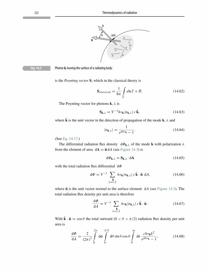
222 Thermodynamics of radiation
� Fig. 14.3 Photon k leaving the surface of a radiating body.
is the Poynting vector S, which in the classical theory is
Sclassical = 1
8π
∫V
dx E × B. (14.62)
The Poynting vector for photons k, λ is
Sk,λ = V−1hνk〈nk,λ〉 c k, (14.63)
where k is the unit vector in the direction of propagation of the mode k, λ and
〈nk,λ〉 = 1
eβhνk − 1. (14.64)
(See Eq. 14.17.)
The differential radiation flux density dΦk,λ of the mode k with polarization λ
from the element of area dA = n dA (see Figure 14.3) is
dΦk,λ = Sk,λ · dA (14.65)
with the total radiation flux differential dΦ
dΦ = V−1∑
kλ=1,2
hνk〈nk,λ〉 c k · n dA, (14.66)
where n is the unit vector normal to the surface element dA (see Figure 14.3). The
total radiation flux density per unit area is therefore
dΦ
dA= V−1
∑k
λ=1,2
hνk〈nk,λ〉 c k · n. (14.67)
With k · n = cos θ the total outward (0 < θ < π/2) radiation flux density per unit
area is
dΦ
dA= 2
(2π)3
2π∫0
dφ
π/2∫0
dθ sin θ cos θ
∞∫0
dkchνkk2
eβhνk − 1, (14.68)
223 Stefan–Boltzmann radiation law
which is integrated to give
dΦ
dA= π2 (kB T )4
60h3c2(14.69)
or
dΦ
dA= σB T 4, (14.70)
where
σB = π2kB4
60h3c2(14.71)
= 5.67× 10⁻⁸ W m−2 K−4 (14.72)
is called the Stefan–Boltzmann constant.
Example: Surface temperature of exoplanet Gliese 581d
Gliese 581, an M-class red-dwarf star, has an approximate radius of 2× 10⁵ km and
an effective surface temperature about 3480 K. A recently discovered exoplanet, des-
ignated Gliese 581d, orbits 3.27 × 10⁷ km from the star. Assuming the star and the
exoplanet behave as perfect absorbers and radiators, estimate the surface temperature
of Gliese 581d.
4π R2∗σB T 4∗︸ ︷︷ ︸energy rate radiated from star
×
fraction intercepted by planetary disk︷ ︸︸ ︷{πr2
p
4π R2∗→p
}(14.73)
= 4πr2pσB T 4
p︸ ︷︷ ︸energy rate reradiated from planet
(14.74)
where rp is the exoplanet radius, Tp is the exoplanet temperature, R∗ is the star radius
and R∗→p is the exoplanet’s orbital radius.
After simplification we have
Tp =(
R2∗4R2∗→p
)1/4
T∗. (14.75)
In particular, for Gliese 581d
Tg = 192 K, (14.76)
not too far off from the “Goldilocks” zone of supporting life.
224 Thermodynamics of radiation
14.9 Radiation momentum density
The momentum p of a photon (a massless particle) is related, by special relativity, to
its energy Eγ by
p = Eγ
c. (14.77)
Therefore the radiated momentum flux density Π per unit area from an object at
temperature T is
dΠ
dA= V−1
∑k
λ=1,2
hνk〈nk,λ〉k · n, (14.78)
which is evaluated, as in Eqs. 14.67–14.69, to give
dΠ
dA= π2 (kB T )4
60h3c3. (14.79)
Example: Star dust blow-out
When stars are formed by gravitational collapse they are initially embedded in
“cocoons” of tiny silicate dust particles, a dust so dense that at this stage the star
can be detected only from secondary infrared radiation emitted by the heated dust.
When the newly formed star reaches a sufficiently high temperature, the radiation
from the star begins blowing out the dust cocoon, allowing the star to be seen in
visible light.
Assuming that the radiation absorption cross-section of a dust particle is approx-
imately half of the physical cross-section and the dust particles have radii a <
10−7 m, at what stellar temperature will all cocoon dust particles be blown away
from the star?
The total momentum density per unit time radiated by the star is
Π = π2 (kB T∗)4
60h3c3× 4π R2∗, (14.80)
where T∗ is the star’s temperature and R∗ is its radius. Therefore the momentum
density per unit time intercepted by a dust particle of radius a at a distance Rdust
from the star is
Πdust = π2 (kB T∗)4
60h3c3× 4π R2∗ ×
(πa2
4π R2dust
). (14.81)
225 Problems and exercises
Taking into account the estimated 50% absorption cross-section, the momentum
density per unit time absorbed by a dust particle is
Π Adust =
π2 (kB T∗)4
60h3c3× 4π R2∗ ×
(πa2
4π R2dust
)× (1/2) . (14.82)
On the other hand, the force of gravity acting on the particle is, by Newton’s law
of gravitation,
Fgrav = G M∗R2
dust
×(
4πa3
3ρdust
), (14.83)
where G is the gravitational constant and ρdust = 3×10³ kg m−3 is the approximate
density of silicate dust.
For the radiation-momentum absorbing dust particle to be in gravitational equilib-
rium
π2 (kB T∗)4
60h3c3× 4π R2∗ ×
(πa2
4π R2dust
)× (1/2) = G M∗
R2dust
×(
4πa3
3ρdust
), (14.84)
where M∗ is the mass of the star, so that
T 4∗ =8a
3× cG M∗ρdust
σB R2∗, (14.85)
where σB is the Stefan–Boltzmann constant (see Eq. 14.71).
Assuming, for numerical specificity, that the newly formed star is sun-like with 1
solar mass and 1 solar radius, i.e.
M∗ = 1.99× 1030 kg (14.86)
R∗ = 6.95× 10⁸ m (14.87)
G = 6.67× 10⁻¹¹ N m2 kg−2, (14.88)
the dust blow-out temperature is T ≈ 6000 K, independent of the distance between
the star and the dust particles.
Problems and exercises
14.1 Show that the work done by photons during an isentropic expansion is
W =(
π2
15h3c3
)k4
B
(Ti − T f
)Vi T
3i , (14.89)
where the subscripts i and f refer to initial and final states.
226 Thermodynamics of radiation
14.2 The total energy radiated by the Sun and received per unit time per unit area
at the Earth’s orbital distance is KS , the solar constant, which has the value
KS = 0.136 J s−1 cm−2.
The mean Earth–Sun distance is RE S = 1.5×10¹¹ m and the radius of the Sun
is approximately R� = 7× 10⁸ m.
Find the effective blackbody temperature of the Sun.
14.3 Show that the average square fluctuation of blackbody internal energy
〈(ΔU)2〉 = 〈(U − 〈U〉)2〉 (14.90)
is equal to
〈(ΔU)2〉 = ∂2
∂β2lnZ. (14.91)
14.4 Gliese 581 is an M-class red dwarf star which lies in the constellation Libra. It
has an approximate radius of 2× 10⁵ km and an effective surface temperature
about 3480 K.
Estimate the peak frequency at which the star radiates energy.
14.5 Consider a volume V containing thermal equilibrium electromagnetic radia-
tion at a temperature T . Given that the partition function for electromagnetic
radiation is (neglecting zero-point energy)
Z =∏
k
{(1− e−βhωk
)−2}, (14.92)
with the product over all modes k and counting both polarizations, evaluate
Eq. 14.91 and show that the average square fluctuation in electromagnetic
energy is
〈(ΔU)2〉 = 4
15h3c3(kB T )5 . (14.93)
14.6 Find the average square fluctuation in blackbody radiation particle number.
Hint: You may need the integrals
∞∫0
dxx3(
1
ex − 1
)= π4
15,
∞∫0
dxx4ex
(ex − 1)2= 4π4
15. (14.94)
14.7 The ideal Carnot engine operates reversibly between an energy source, in which
the working substance (usually an ideal gas) absorbs heat isothermally at high
temperature, and an energy sink, to which it exhausts heat isothermally at a low
temperature. The remaining curves which close the Carnot cycle are adiabats.
The efficiency η of such an engine is defined as
η = Wr
QH, (14.95)
227 Problems and exercises
where Wr is the work done in the cycle and QH is the heat absorbed from the
high-temperature energy source.
If light is used as the working substance, find the Carnot engine efficiency.
14.8 When nucleons collide at very high energy, say by shooting a proton beam into
a metallic target, they annihilate and produce an amount of energy W mainly
in the form of short-lived subatomic pions (quark–antiquark pairs), which can
be positively charged π+, negatively charged π− or neutral π0. The π+ and
π− are particle–antiparticle pairs while the π0 is its own antiparticle. The
pions have ultra-relativistic energies so their rest masses are negligible, i.e.
they behave like “photons” with energies
E = hc |k| (14.96)
with periodic boundary conditions
|k|2 = kx2 + ky
2 + kz2 (14.97)
where
k j = 2π
Lν j ; ν j = 0,±1,±2, . . . (14.98)
Whereas photons have two polarizations (λ1 and λ2), pions are regarded as
having three polarizations (π+, π0, π−). Assuming:
• the pions have zero chemical potential,
• thermal equilibrium is rapidly reached (times shorter than the pion life-
times),
• all the collision energy is produced within a volume Vπ ,
a. find an expression, in terms of W and Vπ , for the temperature of the pion
“spark”;
b. find an expression, in terms of W and Vπ , for the mean number of pions
produced in the collision.
15 Ideal Fermi gas
Why is it that particles with half-integer spin are Fermi particles whereas parti-cles with integer spin are Bose particles? An explanation has been worked outby Pauli from complicated arguments from quantum field theory and relativity.He has shown that the two must necessarily go together . . . but we have not beenable to reproduce his arguments on an elementary level. This probably means wedo not have a complete understanding of the fundamental principle involved. . .
R. P. Feynman, R.B. Leighton and M. Sands, Feynman Lectures on Physics,Volume 3, Chapter 4, Section 1, Addison-Wesley, Reading, MA (1963)
15.1 Introduction
Particles with half-integer angular momentum obey the Pauli exclusion principle
(PEP) – a restriction that a non-degenerate single-particle quantum state can have
occupation number of only 0 or 1. This restriction was announced by W. Pauli in
1924 for which, in 1945, he received the Nobel Prize in Physics. Soon after Pauli, the
exclusion principle was generalized by P. Dirac and E. Fermi who – independently
– integrated it into quantum mechanics. As a consequence half-integer spin particles
are called Fermi–Dirac particles or fermions. PEP applies to electrons, protons, neu-
trons, neutrinos, quarks – and their antiparticles – as well as composite fermions such
as He3 atoms. Thermodynamic properties of metals and semiconductors are largely
determined by electron (fermion) behavior. Metals, for example, exhibit the uniquely
fermionic low-temperature heat capacity CV ∝ T , while some Fermi–Dirac systems
undergo a transition to a distinctive superconducting state with signature properties
of magnetic flux exclusion (no interior B field) and zero electrical resistivity.
15.2 Ideal gas eigen-energies
The eigen-energies and eigenfunctions of any ideal (non-interacting) gas are con-
structed from the eigenvalue problem
228
229 Grand partition function
hop|εs〉 = εs |εs〉 (15.1)
with εs the single-particle eigen-energies and |εs〉 the corresponding single-particle
eigenstates. hop is the single-particle hamiltonian operator for the i th particle1:
hop (i) = − h2
2m∇2
i + V (i) . (15.2)
Generally V (i) represents some charge-neutralizing positive background poten-
tial, e.g. positive ions, so obtaining a solution to the single-particle problem, i.e.
Eqs. 15.1 and 15.2, may be computationally intensive. It is often convenient to
assume that the background ions are replaced by a uniform positive charge, the free
electron approximation. Presuming a solution to this reduced problem is obtained,
we can proceed to investigate Fermi–Dirac system thermodynamics.
15.3 Grand partition function
A many-particle (open system) thermodynamic hamiltonian is
Hop = hop − μNop, (15.3)
where the many-particle hamiltonian Hop is a sum of single-particle hamiltonians
Hop =∑i=1
{hop (i)− μNop (i)
}. (15.4)
The macroscopic eigen-energies of Hop are
E (n1, n2, . . . ) =∑
s
(εs − μ) ns, (15.5)
where ns = 0, 1, 2, . . . are the number of particles occupying the single-particle
eigenstate |εs〉 and μ is the system chemical potential. The sum over s is a sum over
all states.2
However, temporarily ignoring spin, each (non-degenerate) single-particle state is
restricted by the PEP to have occupation number 0 (no particles) or 1 (one particle),
i.e. ns = 0 or 1. Constructing a thermal Lagrangian3
1 This applies to particles of either spin.2 Each single-particle state can be pictured as an “open system” into and out of which particles “diffuse”
so that in thermodynamic (diffusive) equilibrium all particles have the same chemical potential.3 See Appendix B.
230 Ideal Fermi gas
LF D = −kB
∑n1,n2,...= 0,1
PF D (n1, n2, . . . ) ln PF D (n1, n2, . . . )
− 1
T
∑n1,n2,...= 0,1
PF D (n1, n2, . . . )∑
s
(εs − μ)ns
− λ0
∑n1,n2,...= 0,1
PF D (n1, n2, . . . ), (15.6)
where λ0 insures normalization.
PF D (n1, n2, . . . ) is the probability there are n1 particles in the single-particle
state |ε1〉, n2 particles in the single-particle state |ε2〉, etc. and where the occupation
numbers are restricted by the PEP, so that the sums mean∑n1,n2,...=0,1
⇒∑
n1=0,1
∑n2=0,1
. . . (15.7)
Maximizing LF D with respect to PF D(n1, n2, . . . ) we find the probabilities
PF D (n1, n2, . . . ) = e−β
∑s(εs−μ)ns
∑n1,n2,...= 0,1
e−β
∑s(εs−μ)ns
. (15.8)
The denominator in Eq. 15.8 is identified as the grand partition function,
ZFDgr =
∑n1,n2,...= 0,1
e−β
∑s(εs−μ)ns
. (15.9)
It is evaluated by rearranging the sum over states s in the exponential to give
ZFDgr =
∏s
∑ns=0,1
e−β(εs−μ) ns (15.10)
and summing ns = 0, 1
ZFDgr =
∏s
[1+ e−β(εs−μ)
]. (15.11)
15.4 Electron spin
Taking electron spin into account, a pair of single-particle states, |εs,↑〉, |εs,↓〉 emerges
with corresponding eigen-energies εs,↑ and εs,↓. Assuming them initially to be non-
degenerate
ZFDgr =
∏s
[1+ e−β(εs,↑−μ)
] [1+ e−β(εs,↓−μ)
]. (15.12)
231 Fermi–Dirac thermodynamics
However, in zero magnetic field a two-fold degeneracy arises with εs,↑ = εs,↓ = εs
producing the partition function
ZFDgr =
∏s
[1+ e−β(εs−μ)
]2. (15.13)
15.5 Fermi–Dirac thermodynamics
Thermodynamic properties of Fermi–Dirac systems are determined from �FDgr , the
grand potential,
�FDgr = −
1
βlnZFD
gr , (15.14)
which, with Eq. 15.13, is
�FDgr = −
2
β
∑s
ln[1+ e−β(εs−μ)
], (15.15)
where the sum∑s
is over all states |εs〉.1. The average particle number 〈Nop〉 follows from Eq. 15.8,
〈Nop〉 =2∏s
[ ∑ns=0,1
nse−β(εs−μ)ns
]∏s
[ ∑ns=0,1
e−β(εs−μ)ns
] , (15.16)
the factor 2 accounting for spin degeneracy. An equivalent result is
〈Nop〉 = −(∂�FD
gr
∂μ
)T,V
(15.17)
= 2∑
s
[1
e β(εs−μ) + 1
](15.18)
= 2∑
s
〈nFDs 〉, (15.19)
where 〈nFDs 〉 is a single-particle average occupation number for the state |εs〉,
〈nFDs 〉 =
[1
e β(εs−μ) + 1
], (15.20)
which is called the Fermi–Dirac function.
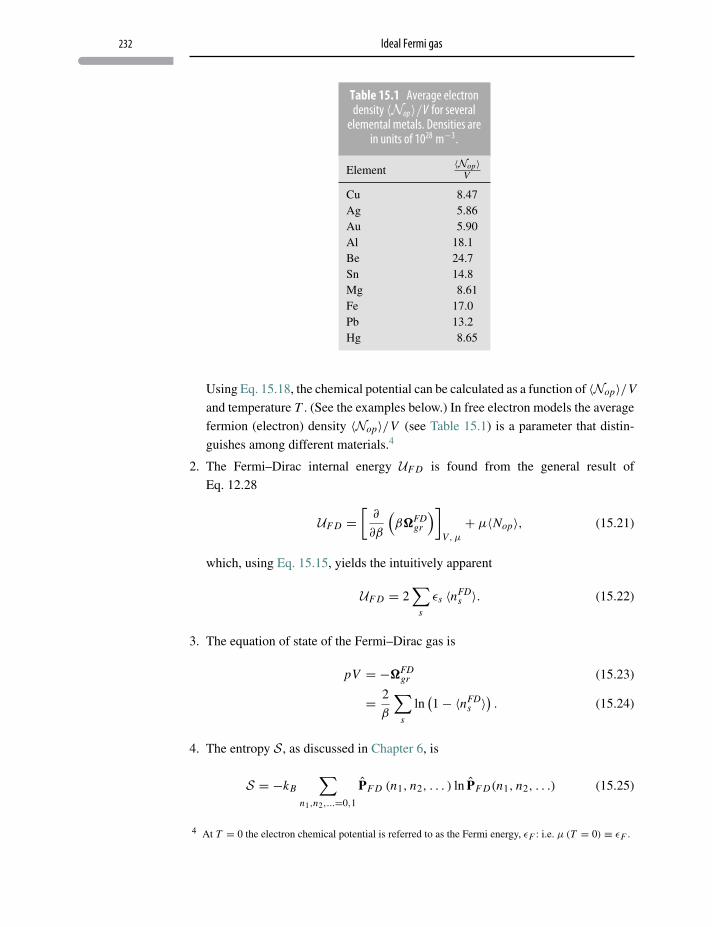
232 Ideal Fermi gas
Table 15.1 Average electrondensity 〈Nop〉/V for several
elemental metals. Densities arein units of 1028 m−3.
Element〈Nop〉
V
Cu 8.47Ag 5.86Au 5.90Al 18.1Be 24.7Sn 14.8Mg 8.61Fe 17.0Pb 13.2Hg 8.65
Using Eq. 15.18, the chemical potential can be calculated as a function of 〈Nop〉/V
and temperature T . (See the examples below.) In free electron models the average
fermion (electron) density 〈Nop〉/V (see Table 15.1) is a parameter that distin-
guishes among different materials.4
2. The Fermi–Dirac internal energy UF D is found from the general result of
Eq. 12.28
UF D =[
∂
∂β
(β�FD
gr
)]V, μ
+ μ〈Nop〉, (15.21)
which, using Eq. 15.15, yields the intuitively apparent
UF D = 2∑
s
εs 〈nFDs 〉. (15.22)
3. The equation of state of the Fermi–Dirac gas is
pV = −�FDgr (15.23)
= 2
β
∑s
ln(1− 〈nFD
s 〉) . (15.24)
4. The entropy S, as discussed in Chapter 6, is
S = −kB
∑n1,n2,...=0,1
PF D (n1, n2, . . . ) ln PF D(n1, n2, . . .) (15.25)
4 At T = 0 the electron chemical potential is referred to as the Fermi energy, εF : i.e. μ (T = 0) ≡ εF .
233 Independent fermion model
where PF D(n1, n2, . . . ) is as in Eq. 15.8. Equivalently,
S = kBβ2
[∂�FD
gr
∂β
]μ,V
(15.26)
= −2kB
∑s
[(1− 〈nFD
s 〉) ln(1− 〈nFD
s 〉)+ 〈nFDs 〉 ln 〈nFD
s 〉] . (15.27)
15.6 Independent fermion model
The independent fermion approximation for metals usually includes interactions with
a static background of positive ions (band structure approximation) but neglects
both electron–electron repulsion (correlations) and interactions with vibrating ions
(electron–phonon interactions).5
Independent fermion thermodynamics begins with �FDgr (see Eq. 15.15) where,
using Dirac’s delta-function6
∞∫−∞
dω f (ω) δ (ω − εs) = f (εs) , (15.28)
�FDgr may be strategically rewritten as
�FDgr = −
2
β
∞∫0
dω∑
s
δ (ω − εs) ln[1+ e−β(ω−μ)
]. (15.29)
Identifying the density of single-particle states D (ω) (see Appendix E)7
D (ω) =∑
s
δ (ω − εs), (15.30)
�FDgr becomes
�FDgr = −
2
β
∞∫0
dωD (ω) ln[1+ e−β(ω−μ)
]. (15.31)
5 These interactions can often be summarized for individual systems by a few parameters, such as aneffective mass m∗ and an electron–phonon coupling constant λ. The “Fermi gas” model has beensuccessful in describing many metals and semiconductors.
6 δ (ω − εs ) is the Dirac delta function.7 Density of single-particle states defined here does not include a factor 2 for spin. (See Eq. E.21.)
234 Ideal Fermi gas
Introducing a density of states also enables some experimental results to be used in
electronic structure calculations.8
Using the δ function in an identical way, Eqs. 15.18 and 15.22 become
〈Nop〉 = 2
∞∫0
dωD (ω)
e β(ω−μ) + 1(15.32)
and
UF D = 2
∞∫0
dωωD (ω)
e β(ω−μ) + 1. (15.33)
Evaluating, or even approximating, integrals Eqs. 15.32, 15.33 and related types
that appear in degenerate fermion models (βμ� 1) requires specialized techniques.
The simplest of these is Sommerfeld’s asymptotic approximation, which is discussed
in Appendix I.9,10
15.7 The chemical potential (T �= 0)
Thermodynamic properties of a degenerate Fermi gas (βμ � 1) can be expressed
as expansions11 in T . In particular, the chemical potential is determined from the
density〈Nop〉
V by expanding the right-hand side of Eq. 15.32 about μ = εF to linear
order, where εF (Fermi energy) is the symbol assigned to the chemical potential at
T = 0, to give
〈Nop〉 = 2
∞∫0
dωD (ω)
e β(ω−εF ) + 1+ β (μ− εF )
2
∞∫0
dωD (ω) sech2[β
2(ω − εF )
].
(15.34)
8 Approximate densities of states can be obtained from optical or tunneling experiments.9 Sommerfeld’s asymptotic approximation is not an expansion in the usual Taylor series sense. It takes
advantage of the property that for T ≈ 0 the Fermi–Dirac function 〈nFDs 〉 approaches the unit step
function at ω ≈ E f (see Figure 15.1).10 With increasing temperature, βμ� 1, the steepness of the step declines over a width ∼ kB T , eventu-
ally taking the form of a smooth exponential 1e β(ω−μ)+1
→ e−β(ω−μ).11 These expansions are not the usual convergent Taylor series type but belong to a category called asymp-
totic expansions. These, generally, must be handled with care.
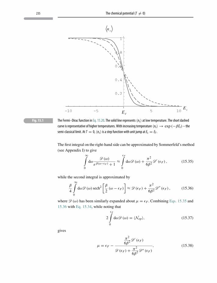
235 The chemical potential (T �= 0)
� Fig. 15.1 The Fermi–Dirac function in Eq. 15.20. The solid line represents 〈ns〉 at low temperature. The short dashedcurve is representative of higher temperatures. With increasing temperature 〈ns〉 → exp (−βEs) – thesemi-classical limit. At T = 0, 〈ns〉 is a step function with unit jump at Es = EF .
The first integral on the right-hand side can be approximated by Sommerfeld’s method
(see Appendix I) to give∞∫
0
dωD (ω)
e β(ω−εF ) + 1≈
εF∫0
dωD (ω)+ π2
6β2D ′ (εF ) , (15.35)
while the second integral is approximated by
β
4
∞∫0
dωD (ω) sech2[β
2(ω − εF )
]≈ D (εF )+ π2
6β2D ′′ (εF ) , (15.36)
where D (ω) has been similarly expanded about μ = εF . Combining Eqs. 15.35 and
15.36 with Eq. 15.34, while noting that
2
εF∫0
dωD (ω) = 〈Nop〉, (15.37)
gives
μ = εF −π2
6β2 D ′ (εF )
D (εF )+ π2
6β2 D ′′ (εF )
, (15.38)
236 Ideal Fermi gas
which to order T 2 is
μ = εF − π2
6β2
D ′ (εF )
D (εF ). (15.39)
In the degenerate regime (where this expansion applies) chemical potential
decreases with increasing temperature. At very high temperature (where this expan-
sion clearly does not apply) μ→−∞.
15.8 Internal energy (T �= 0)
Similar to the argument above, the internal energy (Eq. 15.33) is first expanded about
μ = εF ,
∞∫0
dωωD (ω)
e β(ω−μ) + 1≈
∞∫0
dωωD (ω)
e β(ω−εF ) + 1+ β (μ− εF )
4
∞∫0
dωωD (ω)
× sech2[β
2(ω − εF )
]. (15.40)
Applying Sommerfeld’s approximation to the first term on the right-hand side,
∞∫0
dωωD (ω)
e β(ω−εF ) + 1≈
εF∫0
dω ωD (ω)+ π2
6β2
{d
dω′[ω′D
(ω′)]}
ω′=εF
, (15.41)
while the second term becomes∞∫
0
dωωD (ω) sech2[β
2(ω − εF )
]≈ 4
βεFD (εF ) . (15.42)
Combining Eqs. 15.40, 15.41, 15.42 with 15.39
U = 2
εF∫0
dωωD (ω)+ π2
3β2D (εF ) (15.43)
from which the constant volume heat capacity
CV =(∂U∂T
)V
237 Pauli paramagnetic susceptibility
is
CV = 2π2
3k2
BD (εF ) T, (15.44)
quite different from both the constant-valued classical result and the T 3 phonon con-
tribution.12 Macroscopic heat capacity is proportional to D (εF ), the density of states
of the Fermi system evaluated at the Fermi energy, a microscopic quantum property.
This particular form follows because the PEP allows only an effective number of
particles near εF , i.e. Nef f ∼ NkB T , to participate in low-temperature thermal pro-
cesses.
15.9 Pauli paramagnetic susceptibility
In the presence of an external magnetic field B0, the spin degeneracy of conduc-
tion electrons is lifted (Zeeman splitting) and the single-particle states in Eq. 15.48
become
εs,↑ → εs +Δ, (15.45)
εs,↓ → εs −Δ, (15.46)
where
Δ = m · B0, (15.47)
with m the electron magnetic moment. In that case
ZFDgr =
∏s
[1+ e−β(εs+Δ−μ)
] [1+ e−β(εs−Δ−μ)
](15.48)
and
�FDgr = −
1
β
∑s
{ln[1+ e−β(εs+Δ−μ)
]+ ln
[1+ e−β(εs−Δ−μ)
]}, (15.49)
where the sum∑s
is over all states |εs〉. Using the single-particle density of states
D(ω), the sums are replaced by integrals13
ΩFDgr = −
1
β
⎧⎨⎩∞∫
0
dωD(ω) ln[1+e−β(ω+Δ−μ)
]+∞∫
0
dωD(ω) ln[1+e−β(ω−Δ−μ)
]⎫⎬⎭ .
(15.50)
12 The single-particle density of states defined in this work does not include the factor 2 for spin.13 The reason for not having incorporated the spin factor 2 into the density of states should now be
apparent.
238 Ideal Fermi gas
For weak fields, expansions in Δ produce
ln[1+ e−β(ω+Δ−μ)
]+ ln
[1+ e−β(ω−Δ−μ)
]≈ 2 ln
[1+ e−β(ω−μ)
]+ 1
4β2Δ2 sech2
[β
2(ω−μ)
](15.51)
so that keeping only the term of order Δ2
ΩFDgr ≈ −
1
β
⎧⎨⎩β2
4Δ2
∞∫0
dωD(ω) sech2[β
2(ω − μ)
]⎫⎬⎭ . (15.52)
The integral is done as discussed in Appendix I, giving in the degenerate limit
(βμ� 1)
ΩFDgr ≈ −Δ2D(εF ) (15.53)
where from Eq. 15.39 only the leading term is used. With
M = −(
∂
∂B0ΩFD
gr
)T, μ
(15.54)
= 2m2B0D(εF ) (15.55)
the Pauli susceptibility, χM = M/B0, is14
χM = 2m2D(εF ) . (15.56)
15.10 Electron gas model
The electron gas model is used to describe the behavior of simple metals. It assumes
a macroscopic collection of non-interacting spin-half particles, neutralized only by a
uniform positive background, with a single-particle hamiltonian for the i th particle
hop (i) = − h2
2m∇2
i . (15.57)
Choosing periodic boundary conditions (see Appendix G), the single-particle eigen-
energies are
ε (k) = h2 |k|22m
, (15.58)
where k j ( j = x, y, z) are quantum numbers which assume the values
k j = 2π
Lν j (15.59)
14 If the density of states is defined to include the factor 2 for electron spin, as some authors prefer,χM = m2D(εF ).
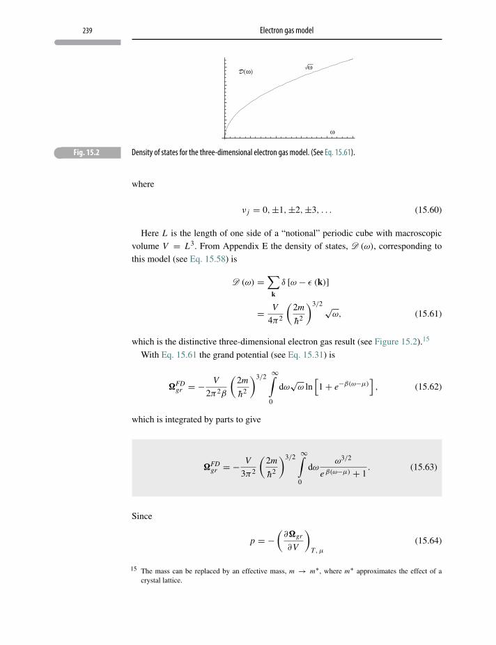
239 Electron gas model
� Fig. 15.2 Density of states for the three-dimensional electron gas model. (See Eq. 15.61).
where
ν j = 0,±1,±2,±3, . . . (15.60)
Here L is the length of one side of a “notional” periodic cube with macroscopic
volume V = L3. From Appendix E the density of states, D (ω), corresponding to
this model (see Eq. 15.58) is
D (ω) =∑
k
δ [ω − ε (k)]
= V
4π2
(2m
h2
)3/2√ω, (15.61)
which is the distinctive three-dimensional electron gas result (see Figure 15.2).15
With Eq. 15.61 the grand potential (see Eq. 15.31) is
�FDgr = −
V
2π2β
(2m
h2
)3/2 ∞∫0
dω√ω ln
[1+ e−β(ω−μ)
], (15.62)
which is integrated by parts to give
�FDgr = −
V
3π2
(2m
h2
)3/2 ∞∫0
dωω3/2
e β(ω−μ) + 1. (15.63)
Since
p = −(∂�gr
∂V
)T, μ
(15.64)
15 The mass can be replaced by an effective mass, m → m∗, where m∗ approximates the effect of acrystal lattice.
240 Ideal Fermi gas
the fermion gas pressure is
pFD = 1
3π2
(2m
h2
)3/2 ∞∫0
dωω3/2
e β(ω−μ) + 1. (15.65)
In the degenerate case (βμ � 1), Eq. 15.65 is expanded in powers of T by
applying the steps in Appendix I, starting with an expansion of the integrand about
μ = εF ,
∞∫0
dωω3/2
e β(ω−μ) + 1=
∞∫0
dωω3/2
e β(ω−εF ) + 1
+ β (μ− εF )
4
∞∫0
dωω3/2 sech2[β
2(ω − εF )
]. (15.66)
The first integral on the right-hand side is approximated using Sommerfeld’s method
∞∫0
dωω3/2
e β(ω−εF ) + 1≈ 2
5ε
5/2F + π2
4β2ε
1/2F , (15.67)
while the second integral is
∞∫0
dωω3/2 sech2[β
2(ω − εF )
]≈ 4
βε
3/2F . (15.68)
Therefore Eq. 15.66, together with Eqs. 15.67, 15.68 and 15.39, gives the pressure
of a degenerate (βμ� 1) Fermi–Dirac gas model
pFD = 2
15π2
(2m
h2
)3/2
ε5/2F
(1+ 5π2
12β2ε2F
). (15.69)
Unlike a classical ideal gas for which p ≈ T , the pressure of a degenerate Fermi–
Dirac gas is nearly independent of temperature.
Finally, in the Fermi gas model we have (see Eq. 15.37)
〈Nop〉V
= 1
2π2
(2m
h2
)3/2εF∫
0
dω√ω (15.70)
= 1
3π2
(2m
h2
)3/2
ε3/2F (15.71)
241 White dwarf stars
or
εF = h2
2m
(3π2 〈Nop〉
V
)2/3
(15.72)
permitting thermodynamic properties to be expressed in terms of the fermion density
(e.g. Table 15.1).
15.11 White dwarf stars
The thermodynamics of stars is a study in self-gravitating systems – a titanic struggle
between gravity, which compresses stellar matter, and outward gas pressure usually
associated with high temperatures within stellar interiors.16 As a result of nuclear and
chemical evolution, equilibrium between these forces is in constant flux, resulting in
continuous stellar transformations.
Stars that are not too massive, say of the order of our Sun’s mass, eventually “burn”
nearly all their core hydrogen resulting in a cooler stellar core richer in helium (and
heavier nuclei). Consequently gas pressure is reduced which, seemingly, throws the
dynamical advantage to gravitational forces, suggesting the star’s continued collapse,
perhaps without limit. Although ordinary gas pressure is no longer capable of resist-
ing gravitational collapse, star stability can now be maintained by quantum behavior
of degenerate (but not necessarily relativistic) electrons, whose source is the now
fully ionized He atoms.
These stars can collapse to radii of the order of the Earth’s while maintaining
masses of the order of the Sun – a density of 106 times that of water. Such stars were
discovered by British astronomer William Herschel (1783) who failed to realize their
significance. These relatively near (on a galactic scale) but intrinsically dim stars are
called white dwarfs. They are intermittently resurrected corpses in the evolutionary
stellar graveyard for stars of about a solar mass and less.
15.11.1 White dwarf thermodynamics
A white dwarf star can be modeled as densely packed He nuclei at the star’s hot
central region. The He nuclei intermingle with a degenerate (βμ � 1) electron gas
whose origin is the fully ionized He atoms.
16 High temperatures result from nuclear fusion at the star’s center in which hydrogen “burns” to heliumand, eventually, heavier nuclei including carbon and oxygen.
242 Ideal Fermi gas
The degenerate electron gas behavior is governed by the PEP, so using Eqs. 15.69
and 15.72, the nearly temperature-independent outward pressure of the degenerate
electron gas component is
pe =(3π2
)2/3
5
(h2
me
)( 〈N eop〉
V
)5/3
, (15.73)
where me is the electron mass and〈N e
op〉V
is the electron number density. The stellar
mass, M , is approximately
M = 2〈N eop〉m He, (15.74)
where m He is the mass of a He nucleus.
The star’s dense He core exerts inward gravitational pressure
pcore = −(∂�core
gr
∂V
)T, μ
(15.75)
where, for He nuclei (treated classically),
�coregr = − V
3π2
(2m He
h2
)3/2 ∞∫0
dωω3/2e−β(ω−μ+W ) (15.76)
= V(2π3
)1/2β5/2
(m He
h2
)3/2
eβ(μ−W ), (15.77)
with W the mean field gravitational potential energy per He nucleus (see Chapter 12).
Assuming a uniform, spherically distributed mass
ρ = M
V(15.78)
= 3M
4π R3, (15.79)
where R is the star radius, we find, as in Section 12.6.1,
W = −m He3G M
5R, (15.80)
where G is the universal gravitational constant.
Applying Eq. 15.75 the inward He nuclear core pressure is
pcore = 1(2π3
)1/2β5/2
(m He
h2
)3/2
e β(μ−W ) − 1
5√π
G M2
V 1/3
(m He
βh2
)3/2
×( √
2
3π2
)1/3
e β(μ−W ). (15.81)
243 Problems and exercises
Next, applying Eq. 15.17 to Eq. 15.77, the average number of He nuclei is
〈N Heop 〉 =
V√2
(m He
πβh2
)3/2
e β(μ−W ). (15.82)
Therefore, substituting for the chemical potential μ, the nuclear core pressure
becomes
pcore = 〈N Heop 〉
βV− 1
5
(4π
3
)1/3 G M2
V 4/3(15.83)
where the first term is the classical ideal He gas pressure, which is negligible for this
cool star. The total pressure – i.e. the equation of state – for the white dwarf star is
therefore
ptotal =(3π2
)2/3
5
(h2
me
)( 〈N eop〉
V
)5/3
− 1
5
(4π
3
)1/3 G M2
V 4/3. (15.84)
At mechanical equilibrium ptotal = 0, giving(3π2
)2/3
5
(h2
me
)( 〈N eop〉
V
)5/3
= 1
5
(4π
3
)1/3 G M2
V 4/3, (15.85)
which, with
〈N eop〉 = 2〈N He
op 〉 (charge neutrality) (15.86)
= M
2m He, (15.87)
yields the remarkable (non-relativistic) white dwarf mass–radius condition[34/3π2/3h2
8G(m He)5/3me
]= RM1/3. (15.88)
Problems and exercises
15.1 Eventually the Sun will pass through a red giant phase and collapse into a white
dwarf star (≈ 6×10⁹ years). Neglecting the shedding of mass in the red dwarf
stage, what fraction of its present radius will the Sun be?
15.2 Consider a white dwarf star in an advanced stage of evolution with nearly all
its fully degenerate electrons behaving ultra-relativistically
hω ≈ cp (15.89)
where c is the speed of light and p = h |k|.
244 Ideal Fermi gas
(a) Find the single-particle density of states D(ω).
(b) Find an expression for the star’s pressure.
(c) Find a critical mass (in solar mass units) beyond which the star is no longer
stable and will gravitationally collapse into a neutron star or a black hole.
15.3 An uncharged degenerate, spin-half Fermi gas (say He3) at pressure p and tem-
perature T is confined to one half of a rigid insulated chamber, of total volume
V . The other half of the chamber is empty (vacuum). The partition separating
the two halves suddenly dissolves and the Fermi gas freely and adiabatically
flows to occupy the entire chamber (free expansion). Find the change in tem-
perature of the Fermi gas.
15.4 A cylinder is separated into two compartments by a sliding frictionless piston.
Each compartment is occupied by an ideal Fermi gas, say A and B, which
differ only in that A is composed of particles of spin 12 while B is composed
of particles of spin 32 . Find the relative equilibrium density of the two gases:
a. at T = 0 K;
b. as T →∞.
15.5 A degenerate Fermi gas of non-interacting electrons moves in a uniform pos-
itive background confined to one dimension. (An example is the conducting
polymer trans-polyacetylene.)
a. Find an expression for the single-particle density of states D (ω) of inde-
pendent particles in one dimension.
b. Find the leading non-zero term for the chemical potential of a one-
dimensional conductor as a function of temperature in the limit of high
degeneracy βμ� 1.
15.6 In E. Fermi’s model for ultra-high energy particle collisions17 a microscopic
“fireball” is created consisting of:
(a) ultra-relativistic nucleon-antinucleon pairs:
• protons (two up quarks and one down quark),
• antiprotons (two up antiquarks and one down antiquark),
• neutrons (one up quark and two down quarks),
• antineutrons (one up antiquark and two down antiquarks);
(b) Ultra-relativistic pions π−, π+ and π0:
i. π−, negatively charged (down quark and anti-up quark),
ii. π+, positively charged (up quark and anti-down quark),
iii. π0, uncharged and is its own antiparticle (up quark - anti-up quark –
down quark - anti-down quark superposition).
17 E. Fermi, “High energy nuclear events”, Prog. Theoret. Phys. (Japan), 5, 570–583 (1950).
245 Problems and exercises
All nucleons are spin-half Fermi–Dirac particles. All pions are spin-zero Bose–
Einstein particles.
At these high energies particles have negligible rest masses, i.e. they behave
like photons (except for their statistics) with zero chemical potential and
energies
E = hc |k| (15.90)
with periodic boundary conditions
|k|2 = kx2 + ky
2 + kz2, (15.91)
where
k j = 2π
Lν j ; ν j = 0,±1,±2, . . . (15.92)
Dynamic assumptions are:
i. Interaction between pions and nucleons is so strong that statistical equilib-
rium is attained in times less than pion lifetimes.
ii. Energy and charge are conserved.
iii. The energy available in the center of mass system, W , is released in a small
volume V = 43π R3, where R is the Compton wavelength R ≈ h
μc.
iv. Angular momentum conservation is ignored.
a. Find an expression for the temperature T ∗ of the “fireball” in terms of
W and V .
b. Find the average density of pions and of nucleons produced.
c. Show that the internal energy per unit volume for the fermion “fire-
ball” is exactly 72 the internal energy per unit volume for the photon
(EM radiation) “fireball”. Consider two alternative scenarios:
(1) The “fireball” is entirely composed of ultra-relativistic spin-half
fermions.
(2) The “fireball” is entirely composed of photons.
Note: The four distinct fermion varieties give rise to eight-fold degeneracy, i.e.
each of the four created particles has two spin polarizations.
You may need the following integrals:
∞∫0
dxx3(
1
ex + 1
)= 7π4
120;
∞∫0
dxx3(
1
ex − 1
)= π4
15. (15.93)
16 Ideal Bose–Einstein system
From a certain temperature on, the molecules “condense” without attractive forces;that is, they accumulate at zero velocity. The theory is pretty, but is there alsosome truth to it?
Albert Einstein, Letter to Ehrenfest (Dec. 1924). Abraham Pais,Subtle Is the Lord: The Science and the Life of Albert Einstein,
Oxford University Press, New York (1982)
16.1 Introduction
For over 50 years the low-temperature liquid state of uncharged, spinless He4 was
the only system in which a Bose–Einstein (BE) condensation was considered experi-
mentally realized.1,2,3 In that case, cold (<2.19 K) liquid He4 passes into an extraor-
dinary phase of matter called a superfluid, in which the liquid’s viscosity and entropy
become zero.
With advances in atomic cooling4,5 (to ≈ 10−9 K) the number of Bose systems
which demonstrably pass into a condensate has considerably increased. These include
several isotopes of alkali gas atoms as well as fermionic atoms that pair into integer-
spin (boson) composites.6
Although an ideal Bose gas does exhibit a low-temperature critical instability, the
ideal BE gas theory is not, on its own, able to describe the BE condensate wave state.7
In order for a theory of bosons to account for a condensate wave state, interactions
between the bosons must be included. Nevertheless, considerable interesting physics
is contained in the ideal Bose gas model.
1 Peter Kapitza, “Viscosity of liquid helium below the λ-point”, Nature 141, 74 (1938).2 John F. Allen and Don Misener, “Flow of liquid helium II”, Nature 141, 75 (1938).3 Allan Griffin, “New light on the intriguing history of superfluidity in liquid 4He”, J. Phys.: Condens.
Matter 21, 164220 (2009).4 M.H. Anderson, J.R. Ensher, M.R. Matthews, C.E. Wieman and E.A. Cornell, “Observation of Bose–
Einstein condensation in a dilute atomic vapor”, Science 269, 198 (1995).5 Eric A. Cornell and Carl E. Wieman, “The Bose–Einstein Condensate”, Scientific American 278, 40
(1998).6 C. A. Regal, M. Greiner and D. S. Jin, “Observation of resonance condensation of fermionic atom
pairs”, Phys. Rev. Lett. 92, 040403 (2004).7 V.L. Ginzburg and L.D. Landau, Zh. Eksp. Teor. Fiz. 20, 1064 (1950).
246
247 Ideal Bose gas
16.2 Ideal Bose gas
The Bose–Einstein (BE) system allows any occupation number, n = 0, 1,
2, 3, . . . ,∞, so that the thermal Lagrangian is
LBE = −kB
∞∑n1=0
· · ·∞∑
nN=0
PBE(n1, n2, . . .) ln PBE(n1, n2, . . .)
− 1
T
⎧⎨⎩∞∑
n1=0
· · ·∞∑
nN=0
PBE(n1, n2, . . .)∑
s
(Es − μ) ns
⎫⎬⎭− λ0
∞∑n1=0
· · ·∞∑
nN=0
PBE(n1, n2, . . .) , (16.1)
where PBE(n1, n2, . . . ) is the probability8 there are n1 particles in the single-particle
state |E1〉, n2 particles in the single-particle state |E2〉, etc. Maximizing the thermal
Lagrangian in the usual way gives the Bose–Einstein probabilities
PBE(n1, n2, . . .) = e−β
∑s
ns(Es−μ)
∞∑n1=0
· · ·∞∑
nN=0e−β
∑s
ns(Es−μ). (16.2)
The denominator is the BE grand partition function
ZBEgr =
∞∑n1=0
· · ·∞∑
nN=0
e−β
∑s
ns(Es−μ)
(16.3)
=∏
s
∞∑ns=0
e−βns(Es−μ). (16.4)
The infinite sum over ns converges only for e−β(Es−μ) < 1. Thus if the minimum
value in the Es energy spectrum is taken to be zero, convergence is guaranteed only
if μ < 0. As will soon be shown, this convergence criterion has astonishing physical
implications!
Assuming convergence of the ns sum, the BE grand partition function is
ZBEgr =
∏s
(1
1− e−β(Es−μ)
)(16.5)
8 These are “surrogate” probabilities.
248 Ideal Bose–Einstein system
and the corresponding grand potential is
�BE = 1
β
∞∑s=0
ln(
1− eβμe−βEs). (16.6)
16.3 Bose–Einstein thermodynamics
Applying the probabilities from Eq. 16.2:
1. Average number of particles in the pth single-particle state is
〈n pBE〉 =
∞∑n p=0
n pe−βn p(E p−μ)
∞∑n p=0
e−βn p(E p−μ)(16.7)
or
〈n pBE〉 = 1
β
⎡⎣ ∂
∂μln
∞∑n p=0
e−βn p(E p−μ)
⎤⎦T
. (16.8)
After carrying out the sum and differentiation in Eq. 16.8 the BE average occu-
pation number for the single particle state |E p〉 is
〈n pBE〉 = 1
eβ(E p−μ) − 1. (16.9)
Similarly, the average total particle number is
〈N BEop 〉 =
∑p=0
〈n pBE〉 (16.10)
= ∂
∂μΩBE
gr (16.11)
=∑p=0
1
eβ(E p−μ) − 1. (16.12)
But Eq. 16.9 presents a problem. Since the lowest value of E p is taken to be
zero, if μ > 0 the average number of particles in state |E p〉 is negative, which is
nonsense. It clearly must be that
249 The ideal BE gas and the BE condensation
μBE ≤ 0. (16.13)
This constraint (already mentioned above) has implications that will be discussed
in the next sections.
2. Internal energy of the ideal BE system is the intuitive result
UB E =∑p=0
E p〈nBEp 〉. (16.14)
16.3.1 The quasi-classical limit
The distinction between 〈nBEp 〉 and 〈nFD
p 〉 – i.e. the sign in the denominator – has
enormous physical consequences at low temperature. But in the limit μ→−∞, i.e.
the quasi-classical limit, where n/nQ ≤ 1, all distinctions disappear,
〈nBEp 〉 ≡ 〈nFD
p 〉 → eβμe−βE p . (16.15)
16.4 The ideal BE gas and the BE condensation
Using the free-particle eigenstates and density of states previously applied in Fermi–
Dirac thermodynamics the spin = 0 (no spin degeneracy) BE grand potential (see
Eq. 16.6) is
ΩBEgr = −
1
β
(V
4π2
)(2m
h2
)3/2 ∞∫0
dω√ω ln
(1− eβμe−βω
)(16.16)
with μ ≤ 0. Integrating by parts
ΩBEgr = −
V
6π2
(2m
h2
)3/2 ∞∫0
dωω3/2
eβ(ω−μ) − 1(16.17)
and then applying Eq. 16.11 gives
〈N BEop 〉 =
V
4π2
(2m
h2
)3/2 ∞∫0
dωω1/2
eβ(ω−μ) − 1. (16.18)
Now recalling the Fermi–Dirac expression
〈N FDop 〉 =
V
2π2
(2m
h2
)3/2 ∞∫0
dωω1/2
eβ(ω−μ) + 1, (16.19)
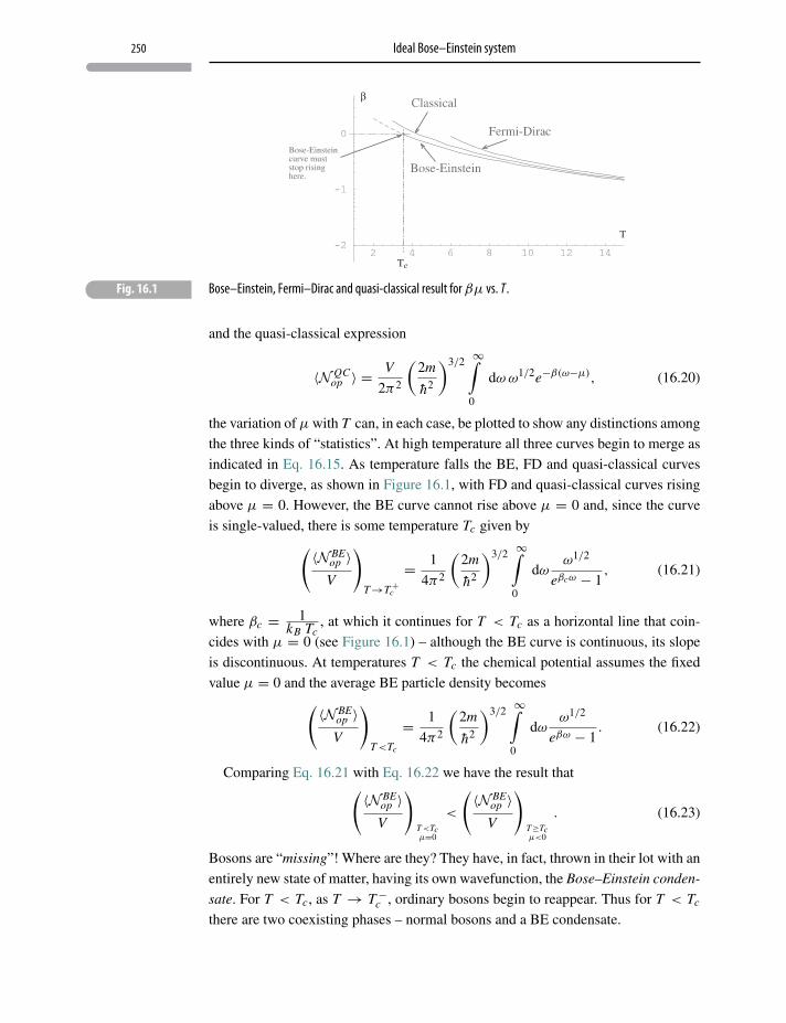
250 Ideal Bose–Einstein system
� Fig. 16.1 Bose–Einstein, Fermi–Dirac and quasi-classical result for βμ vs. T .
and the quasi-classical expression
〈N QCop 〉 =
V
2π2
(2m
h2
)3/2 ∞∫0
dωω1/2e−β(ω−μ), (16.20)
the variation of μ with T can, in each case, be plotted to show any distinctions among
the three kinds of “statistics”. At high temperature all three curves begin to merge as
indicated in Eq. 16.15. As temperature falls the BE, FD and quasi-classical curves
begin to diverge, as shown in Figure 16.1, with FD and quasi-classical curves rising
above μ = 0. However, the BE curve cannot rise above μ = 0 and, since the curve
is single-valued, there is some temperature Tc given by( 〈N BEop 〉V
)T→T+c
= 1
4π2
(2m
h2
)3/2 ∞∫0
dωω1/2
eβcω − 1, (16.21)
where βc = 1kB Tc
, at which it continues for T < Tc as a horizontal line that coin-
cides with μ = 0 (see Figure 16.1) – although the BE curve is continuous, its slope
is discontinuous. At temperatures T < Tc the chemical potential assumes the fixed
value μ = 0 and the average BE particle density becomes( 〈N BEop 〉V
)T<Tc
= 1
4π2
(2m
h2
)3/2 ∞∫0
dωω1/2
eβω − 1. (16.22)
Comparing Eq. 16.21 with Eq. 16.22 we have the result that( 〈N BEop 〉V
)T<Tcμ=0
<
( 〈N BEop 〉V
)T≥Tcμ<0
. (16.23)
Bosons are “missing”! Where are they? They have, in fact, thrown in their lot with an
entirely new state of matter, having its own wavefunction, the Bose–Einstein conden-
sate. For T < Tc, as T → T−c , ordinary bosons begin to reappear. Thus for T < Tc
there are two coexisting phases – normal bosons and a BE condensate.
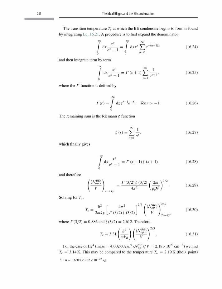
251 The ideal BE gas and the BE condensation
The transition temperature Tc at which the BE condensate begins to form is found
by integrating Eq. 16.21. A procedure is to first expand the denominator
∞∫0
dxxs
ex − 1=
∞∫0
dxxs∞∑
n=0
e−(n+1)x (16.24)
and then integrate term by term
∞∫0
dxxs
ex − 1= Γ (s + 1)
∞∑ν=1
1
νs+1, (16.25)
where the Γ function is defined by
Γ (r) =∞∫
0
dz zr−1e−z; Re r > −1. (16.26)
The remaining sum is the Riemann ζ function
ζ (s) =∞∑
n=1
1
ns, (16.27)
which finally gives
∞∫0
dxxs
ex − 1= Γ (s + 1) ζ (s + 1) (16.28)
and therefore ( 〈N BEop 〉V
)T→T+c
= Γ (3/2) ζ (3/2)
4π2
(2m
βch2
)3/2
. (16.29)
Solving for Tc,
Tc = h2
2mkB
[4π2
Γ (3/2) ζ (3/2)
]2/3 ( 〈N BEop 〉V
)2/3
T→T+c
(16.30)
where Γ (3/2) = 0.886 and ζ (3/2) = 2.612. Therefore
Tc = 3.31
(h2
mkB
)( 〈N BEop 〉V
)2/3
. (16.31)
For the case of He4 (mass = 4.002 602 u,9 〈N BEop 〉/V = 2.18×1022 cm−3) we find
Tc = 3.14 K. This may be compared to the temperature Tλ = 2.19 K (the λ point)
9 1 u = 1.660 538 782× 10−27 kg.
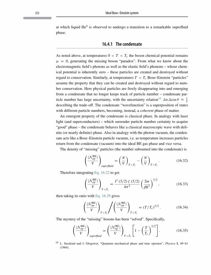
252 Ideal Bose–Einstein system
at which liquid He4 is observed to undergo a transition to a remarkable superfluid
phase.
16.4.1 The condensate
As noted above, at temperatures 0 < T < Tc the boson chemical potential remains
μ = 0, generating the missing boson “paradox”. From what we know about the
electromagnetic field’s photons as well as the elastic field’s phonons – whose chem-
ical potential is inherently zero – these particles are created and destroyed without
regard to conservation. Similarly, at temperatures T < Tc Bose–Einstein “particles”
assume the property that they can be created and destroyed without regard to num-
ber conservation. Here physical particles are freely disappearing into and emerging
from a condensate that no longer keeps track of particle number – condensate par-
ticle number has large uncertainty, with the uncertainty relation10 ΔnΔcos θ ≈ 12
describing the trade-off. The condensate “wavefunction” is a superposition of states
with different particle numbers, becoming, instead, a coherent phase of matter.
An emergent property of the condensate is classical phase. In analogy with laser
light (and superconductors) – which surrender particle number certainty to acquire
“good” phase – the condensate behaves like a classical macroscopic wave with defi-
nite (or nearly definite) phase. Also in analogy with the photon vacuum, the conden-
sate acts like a Bose–Einstein particle vacuum, i.e. as temperature increases particles
return from the condensate (vacuum) into the ideal BE gas phase and vice versa.
The density of “missing” particles (the number subsumed into the condensate) is( 〈N BEop 〉V
)superfluid
=(
N
V
)T>Tc
−(
N
V
)T<Tc
. (16.32)
Therefore integrating Eq. 16.22 to get( 〈N BEop 〉V
)T<Tc
= Γ (3/2) ζ (3/2)
4π2
(2m
βh2
)3/2
, (16.33)
then taking its ratio with Eq. 16.29 gives( 〈N BEop 〉V
)T<Tc
/( 〈N BEop 〉V
)T>Tc
= (T/Tc)3/2 . (16.34)
The mystery of the “missing” bosons has been “solved”. Specifically,( 〈N BEop 〉V
)superfluid
=( 〈N BE
op 〉V
)T>Tc
[1−
(T
Tc
)3/2]. (16.35)
10 L. Susskind and J. Glogower, “Quantum mechanical phase and time operator”, Physica 1, 49–61(1964).
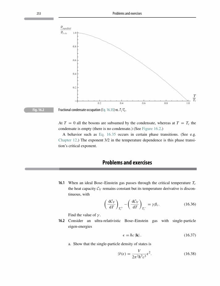
253 Problems and exercises
� Fig. 16.2 Fractional condensate occupation (Eq. 16.35) vs. T/Tc .
At T = 0 all the bosons are subsumed by the condensate, whereas at T = Tc the
condensate is empty (there is no condensate.) (See Figure 16.2.)
A behavior such as Eq. 16.35 occurs in certain phase transitions. (See e.g.
Chapter 12.) The exponent 3/2 in the temperature dependence is this phase transi-
tion’s critical exponent.
Problems and exercises
16.1 When an ideal Bose–Einstein gas passes through the critical temperature Tc
the heat capacity CV remains constant but its temperature derivative is discon-
tinuous, with (dCV
dT
)T+c−(
dCV
dT
)T−c= γβc. (16.36)
Find the value of γ .
16.2 Consider an ultra-relativistic Bose–Einstein gas with single-particle
eigen-energies
ε = hc |k| . (16.37)
a. Show that the single-particle density of states is
D(ε) = V
2π2h3c3ε2. (16.38)
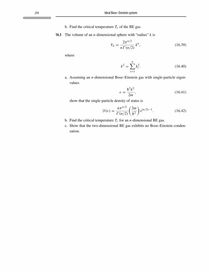
254 Ideal Bose–Einstein system
b. Find the critical temperature Tc of the BE gas.
16.3 The volume of an n-dimensional sphere with “radius” k is
Vn = 2πn/2
nΓ (n/2)kn, (16.39)
where
k2 =n∑
i=1
k2i . (16.40)
a. Assuming an n-dimensional Bose–Einstein gas with single-particle eigen-
values
ε = h2k2
2m, (16.41)
show that the single-particle density of states is
D(ε) = nπn/2
Γ (n/2)
(2m
h2
)ε(n/2)−1. (16.42)
b. Find the critical temperature Tc for an n-dimensional BE gas.
c. Show that the two-dimensional BE gas exhibits no Bose–Einstein conden-
sation.
17 Thermodynamics and the cosmicmicrowave background
We are quantifying the cosmos in a different way to open up a new windowfor understanding the universe in its earliest times. Researchers have long beenworking to test cosmological models for how the universe developed, but previ-ously have not been able to collect data that could provide a picture this clear.
Lyman Page, Princeton University, WMAP co-investigator (2006)
17.1 Introduction
The once super-hot but now cold afterglow from the creation of the universe has
been studied by the satellites COBE1 and WMAP2. WMAP’s continuing task, and
that of the European Space Agency’s Planck satellite, is to measure small-scale tem-
perature anisotropies in the cosmic microwave background (CMB) in order to better
determine cosmological parameters which are a test of inflationary scenarios.3
The satellite moves through the microwave background with a local group velocity|v| = 627 ± 22 km s−1 in the galactic coordinate4 direction
(l: 276◦ ± 3◦,
b: 33◦ ± 3◦)
relative to the CMB rest frame, so that WMAP’s local velocity param-
eter is∣∣vc∣∣ = 0.002. Relativistic effects will therefore produce measurable temper-
ature variations that must be subtracted from the total signal.5 This effect was first
1 COsmic Background Explorer.2 Wilkinson Microwave Anisotropy Probe.3 M. White and J. D. Cohn, “Resource letter: TACMB-1: The theory of anisotropies in the cosmic
microwave background”, Am. J. Phys. 70, 106–118 (2002).4 A celestial coordinate system centered on the Sun and aligned with the apparent center of the Milky
Way galaxy. The “equator" is aligned to the galactic plane. l represents galactic longitude; b is galacticlatitude.
5 M. Kamionkowski and L. L. Knox, “Aspects of the cosmic microwave background dipole”, Phys. Rev.D 67, 63001–63005 (2003).
255
256 Thermodynamics and the cosmic microwave background
calculated exactly by Peebles and Wilkinson (PW)6 only a few years after the dis-
covery of the CMB.7
The intent in this chapter is not to re-derive the well-known PW result, but is
solely to discuss relativity in blackbody thermodynamics by applying the “thermal
Lagrangian” formulation8 and, by happenstance, deriving the PW result.
To find thermodynamic properties measured in a frame of reference moving with
velocity v through a blackbody radiation rest frame (CMB), we start with a “ther-
modynamic” hamiltonian which contains, in addition to the formal electromagnetic
quantum hamiltonian, the energy (work) required to transport the satellite through
the radiation field,
Hop =∑
kλ=1,2
hωk,λ
[a†
k,λak,λ + 1
2
]−
∑k
λ=1,2
v · pop, (17.1)
where
pop = hka†k,λ ak,λ, (17.2)
and
a†k,λ ak,λ = Nop (k, λ) (17.3)
is the photon number operator whose eigenvectors and eigenvalues are given by
a†k,λ ak,λ
∣∣nk,λ⟩ = nk,λ
∣∣nk,λ⟩. (17.4)
Here k is the photon wavevector, λ = 1, 2 covers the two transverse photon polariza-
tions, and nk,λ = 0, 1, 2, . . . is the occupation number of photons with wavevector kand polarization λ.
The eigen-energies of the thermodynamic hamiltonian (including the contribution
from the satellite’s uniform velocity v relative to the CMB rest frame) are, from
Eq. 17.1,
E (n) =∑
kλ=1,2
hωk,λ
[nk,λ + 1
2
]−
∑k
λ=1,2
v · hknk,λ. (17.5)
6 P. J. E. Peebles and D. T. Wilkinson, “Comment on the anisotropy of the primeval fireball”, Phys. Rev.174, 2168 (1968).
7 A. A. Penzias and R. W. Wilson, “A measurement of excess antenna temperature at 4080 Mc/s”, Astro-physical Journal 142, 419–421 (1965).
8 See Appendix B.
257 Moving frame thermodynamic potential Ω
17.2 Thermodynamic method
Using the eigen-energies of Eq. 17.5, the moving frame thermal Lagrangian is
L = −kB
∑nk,λ
P(nk,λ
)ln P
(nk,λ
)
− 1
τ
∑nk,λ
P(nk,λ
)⎧⎪⎪⎨⎪⎪⎩∑
kλ=1,2
hωk,λ
[nk,λ + 1
2
]−
∑k
λ=1,2
v · hknk,λ
⎫⎪⎪⎬⎪⎪⎭− λ0
∑nk,λ
P(nk,λ
). (17.6)
The P(nk,λ
)are probabilities that nk,λ photons are in the mode k with polarization
λ. Here τ is the temperature in the moving frame. Maximizing the Lagrangian of
Eq. 17.6 with respect to P(nk,λ
)(following by now familiar steps) gives, in the
moving frame, the probabilities
P(nk,λ
) =exp
⎧⎪⎨⎪⎩−β∑
kλ=1,2
[hωk,λ
(nk,λ + 1
2
)− hnk,λ |v| |k| cos θ
]⎫⎪⎬⎪⎭∑nk,λ
exp
⎧⎪⎨⎪⎩−β∑
kλ=1,2
[hωk,λ
(nk,λ + 1
2
)− hnk,λ |v| |k| cos θ
]⎫⎪⎬⎪⎭, (17.7)
where β = (kBτ)−1 and θ is the angle (in the moving frame) between the local
velocity vector v and the direction of CMB observation. The frequency ωk,λ is also
in the moving frame. The denominator in Eq. 17.7 is identified as the moving frame
blackbody partition function.
17.3 Moving frame thermodynamic potential Ω
The thermodynamic entropy S is
S = −kB
∑nk,λ
P(nk,λ
)ln P
(nk,λ
), (17.8)
which after substituting the probabilities of Eq. 17.7 is evaluated to give
τS = U − v · 〈p〉op + 1
βln Z, (17.9)
258 Thermodynamics and the cosmic microwave background
where U is the moving frame blackbody internal energy, 〈pop〉 is the moving frame
average radiation momentum and Z is the moving frame blackbody partition func-
tion. We can now define a moving frame thermodynamic potential function
Ω = − 1
βln Z (17.10)
where, from the denominator of Eq. 17.7,
Z =∏
k
{∑nk
exp[−hβnk (ωk − |v| |k| cos θ)
]}2
(17.11)
with “squaring” accounting for the two transverse photon polarizations. Combining
Eqs. 17.9 and 17.10 we can write
Ω = U − τS − v · 〈pop〉. (17.12)
Moreover, by direct differentiation of Eq. 17.8, we find a corresponding thermody-
namic identity, i.e. a moving frame “fundamental equation”
τ dS = dU + p dV − v · d ⟨pop⟩, (17.13)
where p is the moving frame radiation pressure. Combining this with the total dif-
ferential of Eq. 17.12,
dΩ = − p dV − S dτ − 〈pop〉 · dv, (17.14)
from which follow the thermodynamic results
S = −(∂Ω
∂τ
)V ,v
,
p = −(∂Ω
∂ V
)τ,v
,
〈pop〉 = −(∂Ω
∂v
)τ,V
.
(17.15)
259 Moving frame thermodynamic potential Ω
17.3.1 Moving frame blackbody thermodynamics
The partition function of Eq. 17.11 is evaluated by first summing over nk to get
Z =∏
k
⎧⎨⎩ 1
1− exp{−β
[hc |k| (1− |v/c| cos θ)
]}⎫⎬⎭
2
, (17.16)
where ω = c |k| has been used. In the CMB rest frame v = 0 and β → β, where
β = (kB T0)−1 with T0 the CMB rest frame temperature.
The moving frame thermodynamic potential is
Ω = − 1
βln Z (17.17)
= 2
β
∑k
ln{
1− exp{−β
[hc |k| (1− |v/c| cos θ)
]}}. (17.18)
In the large volume limit this is expressed as the integral
Ω = V
2π2β
2π∫0
dϕ
π∫0
dθ sin θ
∞∫0
d |k| |k|2
× ln{
1− exp[−βhc |k| (1− |v/c| cos θ)
]}, (17.19)
which, with the change in variable
z = βhc (1− |v/c| cos θ) , (17.20)
dz = βhc |v/c| sin θdθ, (17.21)
followed by an integration by parts, is
Ω = − π2k4B
45h3c3× V τ 4(
1− |v/c|2)2. (17.22)
Using this result with Eq. 17.15, the moving frame radiation pressure is
p = π2k4B
45h3c3× τ 4(
1− |v/c|2)2. (17.23)
Again applying Eq. 17.15, we find an expression for the “moving frame” entropy
S = 4
3× π2k4
B
45h3c3× V τ 3(
1− |v/c|2)2. (17.24)
However, in the CMB rest frame
S0 = 4
3× π2k4
B
45h3c3× V0T 3
0 , (17.25)
260 Thermodynamics and the cosmic microwave background
where V0 is a rest frame volume and T0 is the rest frame temperature. But entropy is
not altered by changing reference frames,9 so that S = S0. In the moving frame the
rest frame volume is Lorentz-contracted,
V = V0
√1− |v/c|2, (17.26)
so that equating Eqs. 17.24 and 17.25 gives
1[1− |v/c|2]3/2
τ 3 = T 30 (17.27)
so that
τ = T0
[1− |v/c|2
]1/2, (17.28)
which is the Lorentz transformation for temperature.10
Completing this part of the discussion, an application of Eq. 17.15 gives
〈pop〉 = − 4k4Bπ
2vτ 4V
45h3c5(1− |v/c|2)3
. (17.29)
Finally, with Eqs. 17.29, 17.24 and 17.22, we get from Eq. 17.12 the moving frame
radiation field internal energy U
U = π2k4B V
15h3c3
(1+ 1
3 |v/c|2)
(1− |v/c|2)3
τ 4 (17.30)
or
U = U0
(1+ 1
3 |v/c|2)
(1− |v/c|2)1/2
, (17.31)
where
U0 = π2k4B T 4
0 V0
15h3c3(17.32)
is the rest frame radiation field energy (see Eq. 14.37).11 Finally, since entropy is
Lorentz invariant, for quasi-static heat transfer
dS = d−Qτ= d−Q
T0(17.33)
9 N. G. Van Kampen, “Relativistic thermodynamics of moving systems”, Phys. Rev. 173, 295 (1968).10 D. Mi, H. Y. Zhong and D. M. Tong, “Different proposals for relativistic temperature transforms: Whys
and wherefores”, Mod. Phys. Lett. 24, 73–80 (2009).11 C. Møller, The Theory of Relativity, Clarendon Press, Oxford (1952).
261 Radiation energy flux
so that
d−Q = d−Q(
1− v2
c2
)1/2
. (17.34)
17.4 Radiation energy flux
That part of the CMB anisotropy (frequency ωk,λ and velocity v at a particular angle
θ with respect to the local group velocity) which arises solely from satellite motion
with respect to the microwave CMB rest frame provides a “base” anisotropy to be
subtracted12 from the microwave signal in order to obtain the anisotropy of the 13.7
billion year old CMB fireball itself.
For this we write the Poynting vector S (θ, v) (energy per unit time per unit detec-
tor area) observed from the angle θ with respect to the moving frame velocity v. For
a single mode k and one polarization λ,
d∣∣Sk,λ (θ, v)
∣∣dA
=(
1/V)
chωk,λ 〈n (k, λ; θ, v)〉 k|k| ·
v|v| , (17.35)
where Sk,λ (θ, v) is the radiation flux for the mode k with polarization λ, and〈n (k, λ; θ, v)〉 is the moving frame average photon occupation number. Using
Eq. 17.7 we find directly
〈n (k, λ; θ, v)〉 = 1
eβh(ωk,λ − |v| |k| cos θ
)− 1
, (17.36)
which is a Bose–Einstein average occupation number. With ωk,λ = c |k| and in the
large volume limit the sum in Eq. 17.35 – including both polarizations – becomes,
per unit solid angle dΩ , the integral
d2∣∣Sk,λ (θ, v)
∣∣dA dΩ
= 2V
(2π)3
(1/V
)c2h
∞∫0
d |k| |k|3
eβhc |k| [1− (|v|/c) cos θ]− 1
.
(17.37)
Integrating over all modes k for a particular radiation reception angle θ gives
d2∣∣Sk,λ (θ, v)
∣∣dAdΩ
= π
60c2h3 (1− |v/c| cos θ)4 β4(17.38)
= πk4B T 4
0 (1− |v/c|)2
60c2h3 (1− |v/c| cos θ)4. (17.39)
12 Along with other known galactic radiation corrections.
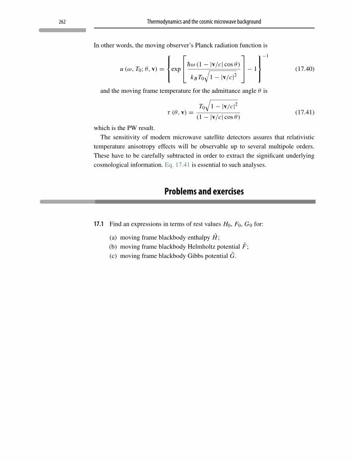
262 Thermodynamics and the cosmic microwave background
In other words, the moving observer’s Planck radiation function is
u (ω, T0; θ, v) =
⎧⎪⎨⎪⎩exp
⎡⎢⎣hω (1− |v/c| cos θ)
kB T0
√1− |v/c|2
⎤⎥⎦− 1
⎫⎪⎬⎪⎭−1
(17.40)
and the moving frame temperature for the admittance angle θ is
τ (θ, v) = T0
√1− |v/c|2
(1− |v/c| cos θ)(17.41)
which is the PW result.
The sensitivity of modern microwave satellite detectors assures that relativistic
temperature anisotropy effects will be observable up to several multipole orders.
These have to be carefully subtracted in order to extract the significant underlying
cosmological information. Eq. 17.41 is essential to such analyses.
Problems and exercises
17.1 Find an expressions in terms of rest values H0, F0, G0 for:
(a) moving frame blackbody enthalpy H ;
(b) moving frame blackbody Helmholtz potential F ;
(c) moving frame blackbody Gibbs potential G.
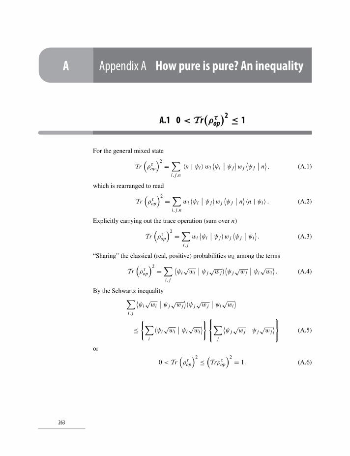
A Appendix A How pure is pure? An inequality
A.1 0 < T r(ρτ
op)2 ≤ 1
For the general mixed state
Tr(ρτ
op
)2 =∑i, j,n
〈n | ψi 〉wi⟨ψi
∣∣ ψ j⟩w j
⟨ψ j
∣∣ n⟩, (A.1)
which is rearranged to read
Tr(ρτ
op
)2 =∑i, j,n
wi⟨ψi
∣∣ ψ j⟩w j
⟨ψ j
∣∣ n⟩ 〈n | ψi 〉 . (A.2)
Explicitly carrying out the trace operation (sum over n)
Tr(ρτ
op
)2 =∑i, j
wi⟨ψi
∣∣ ψ j⟩w j
⟨ψ j
∣∣ ψi⟩. (A.3)
“Sharing” the classical (real, positive) probabilities wk among the terms
Tr(ρτ
op
)2 =∑i, j
⟨ψi√wi
∣∣ ψ j√w j⟩ ⟨ψ j√w j
∣∣ ψi√wi⟩. (A.4)
By the Schwartz inequality∑i, j
⟨ψi√wi
∣∣ ψ j√w j⟩ ⟨ψ j√w j
∣∣ ψi√wi⟩
≤{∑
i
⟨ψi√wi
∣∣ ψi√wi⟩}⎧⎨⎩∑
j
⟨ψ j√w j
∣∣ ψ j√w j⟩⎫⎬⎭ (A.5)
or
0 < Tr(ρτ
op
)2 ≤(Trρτ
op
)2 = 1. (A.6)
263
B Appendix B Bias and the thermal Lagrangian
B.1 Properties of F
We seek a functional1 of probabilities F(P1, P2, P3, . . . ) that serves as a mathe-
matical measure of “bias” (uncertainty). The possibilities for F can be considerably
narrowed by imposing reasonable properties:2
1. Probabilities Ps are normalized to unity.
2. F(P1, P2, P3, . . . ) is a continuous function of the Ps .
3. Any incremental changes in any of the Ps produce only incremental changes in
F(P1, P2, P3, . . .).
4. F(P1, P2, P3, . . .) is a symmetric function of its arguments. No change in order-
ing of the arguments can change the value of the function.
5. F(P1, P2, P3, . . .) is a minimum when all probabilities but one are zero (only one
possible outcome – completely biased).
6. F(P1, P2, P3, . . .) is a maximum when all probabilities are equal (completely
unbiased).
7. If an event of zero probability is added to the set, the value of the function remains
unchanged, i.e.
F(P1, P2, P3, . . . , 0) = F(P1, P2, P3, . . . ) . (B.1)
8. For the case in which all probabilities Ps are equal, i.e.
P1 = p, P2 = p, P3 = p, . . . , Pn = p, (B.2)
a function f (n) is defined
F(p, p, p, . . . , Pn = p) ≡ f (n) (B.3)
such that f (n) is a monotonically increasing function of n. (More distinct out-
comes mean decreasing bias; fewer mean increased bias.)
1 The abbreviation P(εs ) ≡ Ps is used.2 J. N. Kapur, Maximum Entropy Models in Science and Engineering, John Wiley and Sons, New York
(1989).
264
265 The “bias” function
9. There is an addition rule for combining “bias” functions of independent events.
For example, consider two independent probability distributions corresponding to
events P and Q,
P = {P1, P2, P3, . . . , Pn} , (B.4)
Q = {Q1, Q2, Q3, . . . , Qm} , (B.5)
with “bias” functions
FP (P1, P2, P3, . . . , Pn) , (B.6)
FQ(Q1, Q2, Q3, . . . , Qm) . (B.7)
Let there be a set of joint events
P ∪ Q = {P1 Q1, P1 Q2, . . . , P2 Q1, P2 Q2, P2 Q3, . . . , Pm Pn} (B.8)
with “bias” function
FP∪Q(P1 Q1, P1 Q2, . . . , P2 Q1, P2 Q2, P2 Q3, . . . , Pm Pn) . (B.9)
The addition rule is
FP∪Q(P1 Q1, P1 Q2, . . . , P2 Q1, P2 Q2, P2 Q3, . . . , Pm Pn)
= FP (P1, P2, P3, . . . , Pn)+ FQ(Q1, Q2, Q3, . . . , Qm) . (B.10)
The addition rule excludes, for example, forms like purity I.
10. In the special case that all probabilities are equal, applying Eq. B.3 together with
the addition rule Eq. B.10 gives
f (n × m) = f (n)+ f (m) (B.11)
and
f(m y) = y f (m) ; y > 0. (B.12)
B.2 The “bias” function
From Eq. B.11 we can guess a solution
f (m) = κ ln m (B.13)
and since f (m) is a monotonically increasing function of m, κ is a positive constant.
In particular, since there are m events with equal probability p, that probability must
266 Bias and the thermal Lagrangian
be p = 1/m, so
F(p, p, p, . . .) = −κmp ln p, (B.14)
which, in the present restricted case p1 = p2 = p3 = . . . = pm , may be written
F(p, p, p, . . .) = −κ
m∑r=1
pr ln pr . (B.15)
Relaxing this restriction to include pr that differ in value, say Pr , the result becomes
a general “bias” function
F(P1, P2, P3, . . . , Pm) = −κ
m∑r=1
Pr ln Pr (B.16)
which has the form of Gibbs–Shannon entropy.
B.3 A thermal Lagrangian
The method chosen for determining the “best” P(εs) is to:
1. Minimize the average total energy
〈H〉 =n∑
r=1
P(εr ) εr (B.17)
with respect to variations in the P. Here εr are macroscopic eigen-energies of the
hamiltonian,
H = h0 −∑m=1
Xm xm (B.18)
and where Xm and xm are conjugate intensive and extensive variables, respec-
tively (see Eq. 6.12).
2. Simultaneously minimize bias among the P by maximizing the “bias” functional
(see Eq. B.16)
F[P]= −κ
n∑r=1
P(εr ) ln P(εr ). (B.19)
3. Maintain normalizationn∑
r=1
P(εr ) = 1. (B.20)
267 A thermal Lagrangian
Forming '[P], a functional combining “bias” and average energy with a Lagrange
multiplier λ0 to enforce normalization of the P(εr ),
'[P]={−κ
n∑r=1
P(εr ) ln P(εr )−n∑
r=1
P(εr ) εr
}− λ0
n∑r=1
P(εr ) . (B.21)
'[P]
is then maximized with respect to the P(εr ) by setting the functional deriva-
tives δ'/δP equal to zero:
δ'
δP= 0 =− κ
(ln P(εr )+ 1
)− εr − λ0; r = 1, 2, . . . , n, (B.22)
along with
n∑r=1
P(εr ) = 1. (B.23)
The “best” P(εr ) are then
P(εr ) =exp
(−κ−1εr
)Z , (B.24)
where
Z =n∑
s=1
exp(−κ−1εs
), (B.25)
with κ still to be determined.
Taking the constant κ → kB T the functional '[P]
becomes
L [P] = −kB
n∑r=1
P(εr ) ln P(εr )− 1
T
n∑r=1
P(εr ) εr − λ0
n∑r=1
P(εr ) . (B.26)
Now, identifying the entropy
S = −kB
n∑r=1
P(εr ) ln P(εr ) (B.27)
and β =(kB T )−1,
P(εr ) =exp(−βεr )
Z , (B.28)
with
Z =n∑
s=1
exp(−βεs) , (B.29)
this becomes identical to determining the equilibrium thermodynamic configuration
by maximizing a negative Helmholtz potential functional−F [P] (see Section 5.1.3).
C Appendix C Euler’s homogeneousfunction theorem
C.1 The theorem
If f (x1, x2, x3, . . . , xN ) is a function with the property
f (λx1, λx2, λx3, . . . , λxN ) = λn f (x1, x2, x3, . . . , xN ) , (C.1)
it is said to be homogeneous of order n. Then, according to Euler’s homogeneous
function theorem,
N∑i=1
xi
(∂ f
∂xi
)= n f (x1, x2, . . . , xN ) . (C.2)
C.2 The proof
Differentiating Eq. C.1 with respect to λ
d
dλf (λx1, λx2, λx3, . . . , λxN ) = d
dλλn f (x1, x2, x3, . . . , xN ) . (C.3)
But
d
dλf (λx1, λx2, . . . , λxN ) =
N∑i=1
∂ f
∂ (λxi )
d (λxi )
dλ(C.4)
=N∑
i=1
∂ f
∂ (λxi )xi (C.5)
andd
dλλn f (x1, x2, x3, . . . , xN ) = nλn−1 f (x1, x2, x3, . . . , xN ) . (C.6)
Now, setting λ = 1,
N∑i=1
xi
(∂ f
∂xi
)= n f (x1, x2, . . . , xN ) . (C.7)
268
D Appendix D Occupation numbers and thepartition function
Explicit determination of the “eigenstate” degeneracy g(E)1 has been used in arriv-
ing at Eq. 8.6. In some circumstances this is too limited or inconvenient for calculat-
ing a partition function.
A different method is demonstrated by reconsidering the two-level Schottky prob-
lem of Section 8.2. The macroscopic eigen-energies may be written with a different
emphasis as
E
{[n1
1
n12
];[
n21
n22
];[
n31
n32
]; . . .
[nN
1
nN2
]}=
N∑j=1
(ε1n j
1 + ε2n j2
), (D.1)
where [n j
1
n j2
](D.2)
represents j th atom occupation number pairs, which for the two-level example of
Section 8.2 – where only ε1 or ε2 can be occupied on each atom – are(n j
1 = 1
n j2 = 0
)and
(n j
1 = 0
n j2 = 1
). (D.3)
The sum over j in Eq. D.1 is over all atom occupation pairs. Using Eq. D.1 the
partition function is
Z =∑
[n1
1n1
2
],
[n2
1n2
2
],...,
[nN
1nN
2
] exp
⎧⎨⎩−β
N∑j=1
(ε1n j
1 + ε2n j2
)⎫⎬⎭ (D.4)
=
⎧⎪⎪⎪⎨⎪⎪⎪⎩∑
[n1n2
] exp{−β
(ε1n1 + ε2n2
)}⎫⎪⎪⎪⎬⎪⎪⎪⎭
N
, (D.5)
1 Similar to Boltzmann’s “microstate” count, i.e. his classical idea of an “internal energy degeneracy”.
269
270 Occupation numbers and the partition function
where the remaining sum is over the occupation pair[n1
n2
]≡
(1
0
)and
(0
1
), (D.6)
i.e. there are only two terms, which gives
Z = (e−βε1 + e−βε2
)N. (D.7)
E Appendix E Density of states
E.1 Definition
The density of states D (ω) of a quantum system is simply the number of states at the
energy level ω. This number is determined by sifting through all the quantum eigen-
energies εs of the system and counting how many belong in the energy bin ε = ω.
If there is degeneracy among the eigen-energies, e.g. ε1 = ε2 = . . . = εg = ω, all g
of these degenerate energies must find their way into the energy bin ω.
Finding a density of states D (ω) is a mathematical counting process defined by
D (ω) =∑
s
δ (ω − εs), (E.1)
where δ (ω − εs) is the Dirac delta function which carries out the task of adding εs
to the number of states accumulating in bin ω.
The Dirac delta function has the property of a well-chosen unity in the sense that
1 =∞∫
−∞dω δ (ω − εs) . (E.2)
In calculating a density of states the eigen-energy subscript s is usually replaced
by quantum numbers that identify the eigen-energies, so that counting in Eq. E.1 can
take place over quantum numbers.
E.2 Examples
Example 1
Consider a one-dimensional system of independent particles with only kinetic energy
ε (k) = h2k2
2m, (E.3)
271
272 Density of states
where
−∞ < k <∞. (E.4)
Here εs in Eq. E.1 is replaced by ε (k), where k is the free particle quantum number
and the density of single-particle states is written
D (ω) =∑
k
δ [ω − ε (k)] (E.5)
=∑
k
δ
[ω − h2k2
2m
](E.6)
with the sum over εs replaced by a sum over k.
The property of the Dirac delta function that is used in density of states calcula-
tions is
δ[
f (k)] =∑
k0
δ (k − k0)∣∣∣ ddk f (k)
∣∣∣k=k0
(E.7)
where k0 denotes the zeros of f (k)
f (k0) = 0 (E.8)
and the sum in Eq. E.7 is over k0, all the zeros of f (k).
In this one-dimensional case where
D (ω) =∑
k
δ[
f (k)]
(E.9)
with
f (k) = ω − h2k2
2m, (E.10)
locating its zeros we find the pair
k01 = +√
2mω
h2(E.11)
and
k02 = −√
2mω
h2. (E.12)
Next, the denominator in Eq. E.7 is evaluated,∣∣∣∣ d
dkf (k)
∣∣∣∣k=k01
= h2 |k01|m
, (E.13)∣∣∣∣ d
dkf (k)
∣∣∣∣k=k02
= h2 |k02|m
, (E.14)
273 Examples
so that, finally, the density of states is written
D (ω) =∑
k
⎧⎪⎨⎪⎩δ (k − k01)
h2
m
√2mω
h2
+ δ (k − k02)
h2
m
√2mω
h2
⎫⎪⎬⎪⎭ . (E.15)
In the case of a macroscopically long line of particles the k-values become closely
spaced so that in one dimension the “sum” becomes the integral
∑k
→ L
2π
∞∫−∞
dk, (E.16)
where L is the line length.1,2
The integral is easily evaluated to give
D (ω) = L
π
√m
2h2ω. (E.19)
The density of single-particle states is customarily given per unit length,
D (ω)
L= 1
π
√m
2h2ω. (E.20)
If there is spin degeneracy a factor g may be included,
D (ω)
L= g
1
π
√m
2h2ω, (E.21)
where g = 2 in the case spin = 12 .
Example 2
In the case of the three-dimensional Debye model3
ω = 〈cs〉 |k| . (E.22)
1 In two dimensions
∑k
→ A
(2π)2
∞∫−∞
∞∫−∞
dkx dky (E.17)
with A the two-dimensional area.2 In three dimensions
∑k
→ V
(2π)3
∞∫−∞
∞∫−∞
∞∫−∞
dkx dky dkz (E.18)
with V the three-dimensional volume.3 In this example the distinction between longitudinal (1 mode) and transverse (2 modes) phonons is
ignored, using instead an average speed of sound 〈cs 〉 and a degeneracy g = 3.
274 Density of states
Therefore, since the zero of Eq. E.22 is
|k|0 = ω/〈cs〉, (E.23)
we can write
D (ω) = V
(2π)3
⎡⎣4π
∞∫0
1
〈cs〉δ (|k| − ω/〈cs〉) |k|2 d |k|⎤⎦ (E.24)
to finally give
D (ω) = 3V
2π2
ω2
〈cs〉3 , (E.25)
where the approximated mode degeneracy (1 longitudinal+ 2 transverse) is accounted
for by the inserted factor g= 3.

F Appendix F A lab experiment in elasticity
F.1 Objectives
Here we will explore the possibility of finding the microscopic interchain interac-
tion energy ε for a particular elastomer sample using macroscopic thermodynamic
measurements. The experiment also serves to emphasize the physical meaning and
importance of the partial derivatives that are crucial in applying thermodynamics.
The experiment is based on the theoretical discussion in Section 10.5 on a non-
ideal elastomer model. We start by writing elastic tension τ as a function of length
L = 〈Lz〉 and temperature T , i.e. τ = τ (L , T ). The corresponding tension differen-
tial is
dτ =(∂τ
∂L
)T
d L +(
∂τ
∂T
)L
dT . (F.1)
If we perform an experiment in which a rubber band’s length L is held fixed, the
tension differential becomes
dτ =(
∂τ
∂T
)L
dT . (F.2)
Furthermore, applying a Maxwell relation(∂S∂L
)T= −
(∂τ
∂T
)L, (F.3)
we can replace Eq. F.2 by
dτ = −(∂S∂L
)T
dT, (F.4)
which demonstrates that−(∂S/∂L)T , a quantity in which we have some interest (see
the discussion below), is the slope on a τ vs. T curve acquired at fixed elastomer
length.
Now consider the Helmholtz potential F
F = U − TS (F.5)
and its derivative with respect to L at constant T(∂F∂L
)T=(∂U∂L
)T− T
(∂S∂L
)T. (F.6)
275
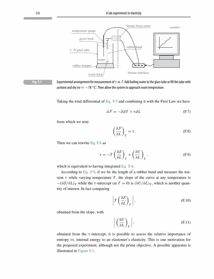
276 A lab experiment in elasticity
� Fig. F.1 Experimental arrangement for measurement of τ vs. T . Add boiling water to the glass tube or fill the tube withacetone and dry ice≈ −78 ◦C. Then allow the system to approach room temperature.
Taking the total differential of Eq. F.5 and combining it with the First Law we have
dF = −SdT + τd L (F.7)
from which we note (∂F∂L
)T= τ. (F.8)
Then we can rewrite Eq. F.6 as
τ = −T
(∂S∂L
)T+(∂U
∂L
)T, (F.9)
which is equivalent to having integrated Eq. F.4.
According to Eq. F.9, if we fix the length of a rubber band and measure the ten-
sion τ while varying temperature T, the slope of the curve at any temperature is
−(∂S/∂L)T while the τ -intercept (at T = 0) is (∂U/∂L)T , which is another quan-
tity of interest. In fact comparing ∣∣∣∣T (∂S∂L
)T
∣∣∣∣ , (F.10)
obtained from the slope, with ∣∣∣∣ (∂U
∂L
)T
∣∣∣∣ , (F.11)
obtained from the τ -intercept, it is possible to assess the relative importance of
entropy vs. internal energy to an elastomer’s elasticity. This is one motivation for
the proposed experiment, although not the prime objective. A possible apparatus is
illustrated in Figure F.1.
277 Results and analysis
F.2 Results and analysis
1. Using the Vernier instrumentation and Logger-Pro computer software, obtain best
τ vs. T linear fits to the data. Identify the values of the slope and the τ -intercept.
2. Determine if the elasticity of this rubber band is entropy or internal energy driven.
3. Now we must see what the experiment can say about the parameter ε. Accord-
ing to the model’s thermodynamics as expressed in Eqs. 10.78 and 10.80 of
Chapter 10, (∂S∂L
)T= −kBβ
{τ + 2ε sinh (βaτ )
a[eβε + 2 cosh (βaτ )
]} . (F.12)
Verify this result.
Also, from Eqs. 10.78 and 10.81,(∂U
∂L
)T= − 2ε sinh (βaτ )
a[eβε + 2 cosh (βaτ )
] . (F.13)
Verify this result.
Now expand Eqs. F.12 and F.13 for small τ. The resulting series have only odd
powers of τ. Do the same thing with the equation of state and use that result to
eliminate τ from each of the expansions obtained from F.12 and F.13. This gives(∂S∂L
)T
∼= −kB[1+ 2e−βε (1+ βε)
] (L/Na2
). (F.14)
Verify this result.
It also gives (∂U
∂L
)T
∼= −2ε e−βε(
L/Na2). (F.15)
Verify this result.
4. Evaluate Eqs. F.14 and F.15 in the limit ε → 0. Compare these results with ideal
gas counterparts, i.e. (∂S/∂V )T and (∂U/∂V )T .
5. To this order the ratio of Eq. F.14 and Eq. F.15 does not contain the length param-
eter L/Na2 and can therefore be used to estimate the interaction energy ε.
6. Use the experimental results to evaluate ε and(L/Na2
). (You may have to use
Maple or Mathematica to solve the equations.)
G Appendix G Magnetic and electric fields inmatter
G.1 Introduction
Magnetic and electric fields and their response functions (magnetization and polar-
ization) are generally defined, consistent with Maxwell’s equations, as local averages
over microscopic regions. Except for special sample geometries and field orienta-
tions, these fields within matter:
• differ from external fields;
• are non-uniform inside matter and in the surrounding free space.
This can make thermodynamic calculations and experimental interpretation a non-
trivial problem.1
G.2 Thermodynamic potentials and magnetic fields
With magnetic work, as in Eq. 11.10, the fundamental equation becomes
T δS = δU + pdV − 1
4π
∫V
H · δBdV . (G.1)
The Helmholtz potential differential δF is
δF = −SdT − pdV + 1
4π
∫V
H · δBdV . (G.2)
1 Experimentalists strive to fabricate samples which conform to special geometries for which internaldemagnetizing fields are usually – but not always – negligible.
278
279 Work and uniform fields
The enthalpy differential δH is
δH = T δS + V dp − 1
4π
∫V
B · δH dV . (G.3)
The Gibbs potential differential δG is
δG = −SdT + V dp − 1
4π
∫V
B · δH dV . (G.4)
These results are based on average local fields (Maxwell’s equations) and are valid
for any mechanism of magnetization. They include, in principle, internal interactions.
G.3 Work and uniform fields
Microscopic-based theory and experiment can be properly compared only if mag-
netic models use practical expressions for thermodynamic work in the case of matter
being inserted into previously uniform external fields (B0, E0).2,3,4
To the experimentalist this means:
• constraining free currents that create the external field H0 to remain unchanged
when matter is inserted into the field, so that ∇ ×H = ∇ ×H0;
• constraining free charges that create the external field D0 to remain unchanged
when matter is inserted into the field, so that ∇ ·D = ∇ ·D0.
Because magnetization M and polarization P are both zero in the absence of
matter, the defining constitutive relations for H and D,
H = B − 4πM, (G.5)
D = E + 4πP, (G.6)
specify that before the sample is introduced H0 = B0 and D0 = E0. After the sample
is introduced B, H , E and D become the local average fields.
2 L.D. Landau, L.P. Pitaevskii and E.M. Lifshitz, Electrodynamics of Continuous Media, 2nd edition,Elsevier, Amsterdam (1984).
3 V. Heine, “The thermodynamics of bodies in static electromagnetic fields”, Proc. Camb. Phil. Soc. 52,546–552 (1956).
4 E. A. Guggenheim, Thermodynamics: An Advanced Treatment for Chemists and Physicists, North-Holland, Amsterdam (1967).
280 Magnetic and electric fields in matter
From this point we examine only magnetic contributions, the electric field case
being formulated by parallel arguments.
For the uniform pre-existent field (prior to insertion of matter) B0 = H0 and we
can construct the identity
1
4π
∫V
B0 · δBdV − 1
4π
∫V
H0 · δBdV = 0, (G.7)
and use it to construct yet another identity for the difference between magnetic work
with average Maxwellian fields (see Eq. 11.9) and magnetic energy of the uniform
field before matter is introduced, namely
1
4π
∫V
H · δBdV − 1
4π
∫V
B0 · δB0 dV
= 1
4π
∫V
(H −H0) · δBdV + 1
4π
∫V
B0 · (δB − δB0) dV . (G.8)
Using the constitutive equation relating B and H
(H −H0) = (B − B0)− 4πM (G.9)
and
(δH − δH0) = (δB − δB0)− 4πδM, (G.10)
where B0 and H0 are the prior existing fields, allows the right-hand side of Eq. G.8
to be re-expressed in terms of magnetization as
1
4π
∫V
H · δBdV − 1
4π
∫V
B0 · δB0 dV
= 1
4π
∫V
(H −H0) · δBdV + 1
4π
∫V
B0 · [(δH − δH0) + 4πδM] dV
= 1
4π
∫V
(H −H0) · δB dV + 1
4π
∫V
B0 · (δH − δH0) dV +∫V
B0 · δM dV .
(G.11)
Applying
B = ∇ ×A, (G.12)
δB = ∇ × δA, (G.13)
B0 = ∇ ×A0, (G.14)
δB0 = ∇ × δA0, (G.15)
281 Work and uniform fields
where A and A0 are static magnetic vector potentials, the first term on the final line
of Eq. G.11 is
1
4π
∫V
(H −H0) · ∇ × δA dV (G.16)
and the second term is
1
4π
∫V
(∇ ×A0) · (δH − δH0) dV . (G.17)
Then, with the vector identity
U · ∇ × V = V · ∇ ×U +∇ · (V ×U ) (G.18)
the integral G.16 is transformed
1
4π
∫V
(H −H0) · ∇ × δA dV
→ 1
4π
∫V
δA · ∇ × (H −H0) dV − 1
4π
∫V
∇ · [δA× (H −H0)] dV .
(G.19)
Similarly, the integral G.17 is transformed
1
4π
∫V
(∇ ×A0) · (δH − δH0) dV
→ 1
4π
∫V
A0 · ∇ × (δH − δH0) dV − 1
4π
∫V
∇ · [A · ∇ × (δH − δH0)] dV .
(G.20)
Both resulting integrals, Eqs. G.19 and G.20, are zero since:
• The currents that create the external field are constrained to remain unchanged
when introducing the sample into the field. Therefore in the first terms of each of
these integrals, ∇ × (H −H0) = 0 = ∇ × (δH − δH0).
• The second term of each integral can be turned into a surface integral (Gauss’
theorem) on a very distant surface where static (non-radiative) fields fall off faster
than 1r2 .
With these simplifications Eq. G.11 is rearranged to become
1
4π
∫V
H · δBdV = 1
4π
∫V
B0 δB0 dV +∫V ′
B0 · δMdV . (G.21)
282 Magnetic and electric fields in matter
The left-hand side is the magnetic work with average local fields while the right-hand
side involves:
• the total magnetic field energy before insertion of matter;
• the energy associated with the magnetic material in the prior existing external
field, B0.
Since B0 is constant and M = 0 outside matter, the volume in the second term,
V ′, covers magnetized material only. Therefore, whether or not M is uniform,
M =∫V ′
MdV, (G.22)
where M is the total magnetization. The final result is therefore
1
4π
∫V
H · δBdV = V
8πδ (B0)
2 + B0 · dM. (G.23)
Applying Eq. G.1 the resulting thermodynamic relations are
T dS = dU∗ + pdV − B0 · dM, (G.24)
T dS = dH∗ − V dp +M · dB0, (G.25)
dF∗ = −SdT − pdV + B0 · dM, (G.26)
dG∗ = −SdT + V dp −M · dB0, (G.27)
each having the advantage of B0 being a simple independent variable rather than
a function of position. (The field energies V δ (B0)2 /8π have been included in the
internal energy and hence into the thermodynamic potentials, which are now distin-
guished by superscripted stars.)
283 Thermodynamics with internal fields
G.4 Thermodynamics with internal fields
But of course there is no free lunch. Although the potentials F∗ and G∗, as defined in
Eqs. G.26 and G.27, are convenient thermodynamic state functions (with
mathematical properties discussed in Chapter 4), they take no account of effective
contributions to B from the remaining magnetized matter. However, they can be used
in the usual thermodynamic calculations where, say, from Eq. G.27 the magnetiza-
tion M is given by
M = −(∂G∗
∂B0
)p,T
, (G.28)
but it is a magnetization that takes no account of any internal fields. They are not true
free energies.
Nor do they carry information about currents and fields inside matter. For example,
the kinetic energy in the hamiltonian cannot simply be p2/2m because that would
ignore consequences of the external field within matter. The kinetic energy should be
H = 1
2m
{p − e
c(A0 +A)
}2, (G.29)
where A0 is an external vector potential and A is the internal vector potential whose
source is the currents induced by the external field and which interacts with internal
currents via the interaction hamiltonian A · p.
Specifically, the final term in the mean field decomposition in Chapter 11
mop(i′)mop(i) = [mop(i
′)− 〈mop〉][mop(i)− 〈mop〉]+mop(i
′)〈mop〉 + 〈mop〉mop(i)− 〈mop〉〈mop〉 (G.30)
constitutes an internal magnetic contribution to the Gibbs potential (see Eqs. 11.97
and 11.98)
WMFA = −1
2Bint ·M (G.31)
so that the Gibbs potential G∗ becomes
G∗ = G∗ − 1
2Bint ·M (G.32)
= G∗ − zK2N
M ·M, (G.33)
where G∗ denotes this additional dependence on the effective field, Eq. 11.97.
Furthermore
dG∗ = dG∗ − zKN
M dM (G.34)
284 Magnetic and electric fields in matter
= −SdT −MdB0 − zKN
M dM (G.35)
= −SdT −Md
(B0 + zK
NM)
(G.36)
= −SdT −MdB∗, (G.37)
which means that as a result of the internal field the magnetization is now
M = −(∂G∗
∂B∗
)T
. (G.38)
Therefore, re-examining Eq. 11.99 we see a proper role for B∗ in the following way:
M = 1
β
(∂
∂B∗ lnZM∗)
T(G.39)
= Nμ 12
tanh(βμ 12B∗). (G.40)
Another internal field of practical importance is the so-called “demagnetization”
field. Demagnetization is defined through geometrically based factors η j (demag-
netization factors), which describe a uniform field Hint, j inside an ellipsoid arising
from magnetization
Hint, j =H0, j − 4πη j,kMk, (G.41)
with j = x , y, z. Formally, its source is the fictitious, classical magnetic surface
“poles” arising from the applied field H0. Demagnetization factors (actually ten-
sors) η j,k depend on sample geometry and are obviously responsible for magnetic
anisotropy. Calculating demagnetization “factors” for different geometries remains
an on-going activity in the field of practical magnetics.5
Applying the constitutive equation
Hint, j = Bint, j − 4πM j (G.42)
to Eq. G.41, we have (ignoring, for simplicity, the tensor character of η) the
effective field
Bint, j = B0, j + 4π(1− η)M j . (G.43)
5 M. Beleggia, M. DeGraff and Y. Millev, “Demagnetization factors of the general ellipsoid”, Phil. Mag86, 2451 (2006).
H Appendix H Maxwell’s equations andelectromagnetic fields
H.1 Maxwell’s equations
Electric fields E (x, t) and magnetic fields B (x, t) in free space satisfy the differential
Maxwell relations1
∇ · E(x, t) = 0, (H.1)
∇ · B(x, t) = 0, (H.2)
∇ × E(x, t) = −1
c
∂B (x, t)∂t
, (H.3)
∇ × B(x, t) = 1
c
∂E (x, t)∂t
. (H.4)
Unlike Schrödinger’s wave mechanics, which retains some suggestion of classical
particle dynamics, a quantum theory of radiation is guided by Maxwell’s field rela-
tionships and Planck’s photon postulate, which Dirac used in his theory of quantum2
fields.
H.2 Electromagnetic waves
In classical theory time-varying electric and magnetic fields propagate in free space
as waves with velocity c. This can be seen by combining the last of Maxwell’s equa-
tions, Eq. H.4, with Maxwell’s first equation, Eq. H.1, to give the wave equation for
an electric field
∇2E (x, t) = 1
c2
∂2E (x, t)
∂t2. (H.5)
1 In rationalized cgs units.2 P. A. M. Dirac, “Quantum theory of emission and absorption of radiation”, Proc. Roy. Soc. (London),
A114, 243 (1927).
285
286 Maxwell’s equations and electromagnetic fields
Similarly, Eqs. H.2 and H.3 are combined for a corresponding wave equation for the
magnetic field
∇2B (x, t) = 1
c2
∂2B (x, t)
∂t2. (H.6)
H.2.1 Solution in free space – periodic boundary conditions
Imagine a cube with side L and volume V = L3 within which a solution to Eq. H.5
is assumed consisting of the sum of propagating waves,
E j (x, t) = 1√V
∞∫−∞
dω
2π
∑k
e j (k, ω) eik·xe−iωt , (H.7)
where E j is the j th component of the Maxwell electric field vector ( j = x, y, z) and
e j is, correspondingly, the Fourier vector component of the kth propagating wave
amplitude. The vector k in Eq. H.7 defines the spatial direction in which that partic-
ular Fourier component propagates (its direction of propagation). Each propagation
vector k is identified as a mode index.
The solutions within the notional cubic volume are supplemented by sensible (but
synthetic) boundary conditions according to which translation in any direction x, y
or z by the finite side length L results in exactly the same electric fields, i.e.
E j (x+ L, t) = 1√V
∞∫−∞
dω
2π
∑k
e j (k, ω) eik·(x+L)e−iωt = E j (x, t) . (H.8)
These are called periodic boundary conditions. They are used in nearly all field the-
ories, classical and quantum. When the cube is finally made large enough to really
look like infinite free space it hardly matters what goes on at the boundaries since
the cube’s surface-to-volume ratio is rapidly diminishing to zero.
But in order for Eq. H.8 to hold, the following restrictions on k must apply:
kx L = 2πnx ; nx = 0,±1,±2, . . . , (H.9)
ky L = 2πny; ny = 0,±1,±2, . . . , (H.10)
kz L = 2πnz; nz = 0,±1,±2, . . . , (H.11)
i.e. under periodic boundary conditions the propagation vectors can have only dis-
crete positive and negative values
k j = 2πn j
L. (H.12)
However, as can be seen from Eq. H.12, in the limit of a large volume, i.e. L →∞,
the spacing between successive values of k j becomes infinitesimal. This important
287 Electromagnetic waves
result allows the sums in Eq. H.19 (and other similar sums) to be treated as
integrals.
Properties of wave solutions
Substituting Eq. H.7 into the wave equation Eq. H.5,
∇2
⎧⎨⎩ 1√V
∞∫−∞
dω
2π
∑k
e j (k, ω) eik·xe−iωt
⎫⎬⎭ = 1√V
∞∫−∞
dω
2π
∑k
[−k · k] e j
× (k, ω) eik·xe−iωt (H.13)
and
1
c2
∂2
∂t2
⎧⎨⎩ 1√V
∞∫−∞
dω
2π
∑k
e j (k, ω) eik·xe−iωt
⎫⎬⎭ = 1√V
∞∫−∞
dω
2π
∑k
[−ω2
c2
]e j
× (k, ω) eik·xe−iωt , (H.14)
showing that Eq. H.7 is a wave equation solution only if
k2 = ω2
c2, (H.15)
where
k2 = kx2 + ky
2 + kz2, (H.16)
i.e. the magnitude of the propagation vector k is proportional to the frequency ω.
Of course, the solution must also satisfy the first of Maxwell’s equations, i.e. Eq.
H.1, which also has important implications. Taking the divergence of Eq. H.7 and
setting it equal to zero,
∇ · E = 1√V
∞∫−∞
dω
2π
∑k
[kx ex (k, ω)+ kyey (k, ω)+ kzez (k, ω)
]eik·xe−iωt = 0,
(H.17)
from which is concluded
k · e (k, ω) = 0, (H.18)
i.e. the Fourier vector amplitude e (k, ω) must be perpendicular to the propagation
vector k. The Fourier vector amplitude e (k, ω) can then be expressed in terms of two
mutually perpendicular unit vectors, ε (k, 1) and ε (k, 2) – a pair for each mode k –
both of which are perpendicular to the propagation vector k, i.e. ε (k, λ)·k = 0 where
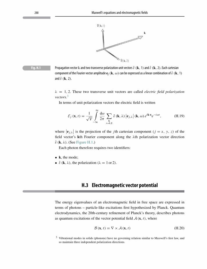
288 Maxwell’s equations and electromagnetic fields
� Fig. H.1 Propagation vector k and two transverse polarization unit vectors ε (k, 1) and ε (k, 2). Each cartesiancomponent of the Fourier vector amplitude ej (k, ω) can be expressed as a linear combination of ε (k, 1)and ε (k, 2).
λ = 1, 2. These two transverse unit vectors are called electric field polarization
vectors.3
In terms of unit polarization vectors the electric field is written
E j (x, t) = 1√V
∞∫−∞
dω
2π
∑k
λ=1,2
ε (k, λ)∣∣e j,λ
∣∣ (k, ω) eik·xe−iωt , (H.19)
where∣∣e j,λ
∣∣ is the projection of the j th cartesian component ( j = x, y, z) of the
field vector’s kth Fourier component along the λth polarization vector direction
ε (k, λ). (See Figure H.1.)
Each photon therefore requires two identifiers:
• k, the mode;
• ε (k, λ), the polarization (λ = 1 or 2).
H.3 Electromagnetic vector potential
The energy eigenvalues of an electromagnetic field in free space are expressed in
terms of photons – particle-like excitations first hypothesized by Planck. Quantum
electrodynamics, the 20th-century refinement of Planck’s theory, describes photons
as quantum excitations of the vector potential field A (x, t), where
B (x, t) = ∇ ×A (x, t) (H.20)
3 Vibrational modes in solids (phonons) have no governing relation similar to Maxwell’s first law, andso maintain three independent polarization directions.
289 Electromagnetic vector potential
and
E (x, t) = −∇ϕ − 1
c
∂
∂tA (x, t) , (H.21)
where φ is a scalar potential. Because the vector potential is not unique, gauge fixing
is required. One common choice is
∇ · A (x, t) = 0, (H.22)
which is called the Coulomb gauge4 or, alternatively, the transverse gauge (since
A → A⊥).5,6 In the Coulomb gauge and in the absence of sources we can take
φ ≡ 0.
In this gauge the classical wave equation becomes
∇2A⊥ − ∂2A⊥∂t2
= 0. (H.23)
The (transverse) vector potential can be expanded in a Fourier series of plane
waves
A⊥ (x, t) =∑
kλ=1,2
(1
2Vωk
) 12 [
ε (k, λ) ak,λ (t) eik·x + ε∗ (k, λ) a∗k,λ (t) e−ik·x] ,(H.24)
where ak,λ and a∗k,λ are complex coefficients, ωk = c |k| is the vacuum electromag-
netic dispersion relation and the coefficient (2Vωk)− 1
2 is chosen with an eye towards
simplifying the final result.
It follows from the Coulomb gauge condition that
k · ε (k, λ) = 0, λ = 1, 2, (H.25)
where the unit polarization vectors themselves are chosen to be mutually perpendic-
ular and therefore satisfy the orthogonality condition
ε (k, μ) · ε∗ (k, γ ) = δμ,γ . (H.26)
The classical (transverse) electric field is from Eqs. H.21 and H.24 (ignoring cir-
cular or elliptical polarization)
E⊥ (x, t) = 1
c
∑k
λ=1,2
(1
2Vωk
)1/2
ε (k, λ)[∂ak,λ (t)
∂teik·x + ∂a∗k,λ (t)
∂te−ik·x
].
(H.27)
4 Because Coulomb’s law is satisfied in this gauge.5 This gauge restricts the vector potential to have only transverse components.6 This gauge has the same consequence as Maxwell’s first law, i.e. Coulomb’s law.
290 Maxwell’s equations and electromagnetic fields
However, by inserting the expansion Eq. H.24 into the wave equation Eq. H.23 the
following simplifying results are obtained:
∂ak,λ
∂t= −iωkak,λ (H.28)
and
∂a∗k,λ∂t
= iωka∗k,λ (H.29)
so that
E⊥ (x, t) = i
c
∑k
λ=1,2
( ωk
2V
)1/2ε (k, λ)
[ak,λ (t) eik·x − a∗k,λ (t) e−ik·x] . (H.30)
The transverse magnetic field is, similarly,
B⊥ (x, t) = ∇ ×A⊥
= i∑
kλ=1,2
(1
2Vωk
)1/2 [k× ε (k, λ)
] [ak,λ (t) eik·x − a∗k,λ (t) e−ik·x] .
(H.31)
H.4 Quantized electromagnetic hamiltonian
The field theoretic canonical quantization procedure postulates the complex coeffi-
cients in the expansions for Eqs. H.30 and H.31 “morph” into Fock space operators
ak,λ � ⇒ aop (k, λ) , (H.32)
a∗k,λ � ⇒ a†op (k, λ) , (H.33)
where the operators fulfill equal time commutator relations[aop (k, μ) , a†
op
(k′, μ′
)] = δk,k′ δμ,μ′ , (H.34)[aop
† (k, μ) , aop† (k′, μ′)] = 0, (H.35)[
aop (k, μ) , aop(k′, μ′
)] = 0, (H.36)
where
a†op(k, μ) aop(k, μ) = nop(k, μ) (H.37)
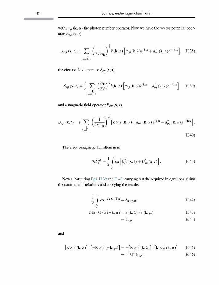
291 Quantized electromagnetic hamiltonian
with nop (k, μ) the photon number operator. Now we have the vector potential oper-
ator Aop (x, t)
Aop (x, t) =∑
kλ=1,2
(1
2Vωk
) 12ε (k, λ)
[aop(k, λ)eik·x + a†
op(k, λ)e−ik·x] , (H.38)
the electric field operator Eop (x, t)
Eop (x, t) = i
c
∑k
λ=1,2
( ωk
2V
) 12ε(k, λ)
[aop(k, λ)eik·x − a†
op(k, λ)e−ik·x] (H.39)
and a magnetic field operator Bop (x, t)
Bop (x, t) = i∑
kλ=1,2
(1
2Vωk
) 12 [
k× ε (k, λ)] [
aop (k, λ) eik·x − a†op (k, λ) e−ik·x] .
(H.40)
The electromagnetic hamiltonian is
HE Mop = 1
2
∫V
dx[E2
op (x, t)+ B2op (x, t)
]. (H.41)
Now substituting Eqs. H.39 and H.40, carrying out the required integrations, using
the commutator relations and applying the results
1
V
∫V
dx eik·xeik·x = δk+p,0, (H.42)
ε (k, λ) · ε (−k, μ) = ε (k, λ) · ε (k, μ) (H.43)
= δλ,μ (H.44)
and
[k× ε (k, λ)
] · [−k× ε (−k, μ)] = −[k× ε (k, λ)
] · [k× ε (k, μ)]
(H.45)
= −|k|2 δλ,μ, (H.46)
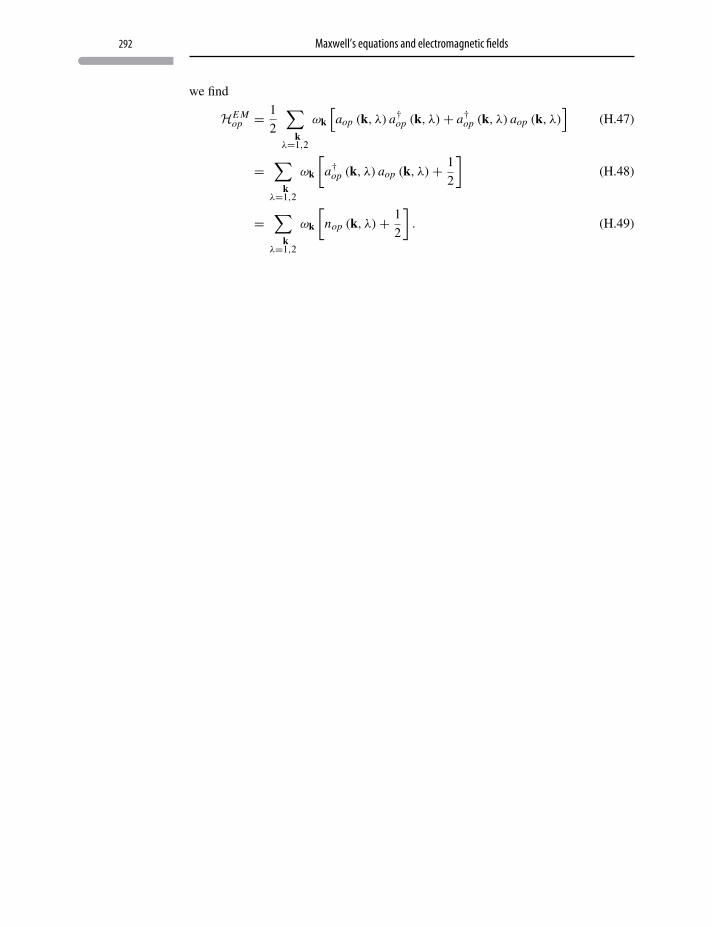
292 Maxwell’s equations and electromagnetic fields
we find
HE Mop = 1
2
∑k
λ=1,2
ωk
[aop (k, λ) a†
op (k, λ)+ a†op (k, λ) aop (k, λ)
](H.47)
=∑
kλ=1,2
ωk
[a†
op (k, λ) aop (k, λ)+ 1
2
](H.48)
=∑
kλ=1,2
ωk
[nop (k, λ)+ 1
2
]. (H.49)
I Appendix I Fermi–Dirac integrals
I.1 Introduction
The typical Fermi–Dirac integral in the theory of metals and semiconductors has the
form
I FD (μ) =∞∫
0
dωs (ω)D (ω)1
eβ(ω−μ) + 1, (I.1)
where D (ω) is the density of states and s (ω) is some function of ω, often a fractional
or integer power, such that D (ω) s (ω) is analytic (differential) near ω ≈ μ. (When
this is not the case, special techniques can be applied.1)
Analytic evaluation of these integrals is not possible so several approximations
and numerical methods have appeared over the years.2,3,4,5
I.2 Expansion method: βμ� 1
The Sommerfeld asymptotic expansion, which is the earliest published result,6 exploits
the approximate property that
d
dω
[1
eβ(ω−μ) + 1
]" − 1
βδ (ω − μ) , βμ� 1. (I.2)
1 A. Wasserman, T. Buckholtz and H. E. Dewitt, “Evaluation of some Fermi–Dirac integrals”, J. Math.Phys. 11, 477 (1970).
2 W. B. Joyce and R. W. Dixon, “Analytic approximations for the Fermi energy of an ideal Fermi gas”,Appl. Phys. Lett. 31, 354 (1977).
3 A. Wasserman, “Fermi–Dirac integrals”, Phys. Letters 27A, 360 (1968).4 T. M. Garoni, N. E. Frankel and M. L. Glasser, “Complete asymptotic expansions of the Fermi–Dirac
integrals”, J. Math. Phys. 42, 1860 (2001).5 Raseong Kim and Mark Lundstrom, Notes on Fermi–Dirac Integrals (3rd edition) (2008)
(http://nanohub.org/resources/5475).6 A. Sommerfeld, “Zur Elekronentheorie der Metalle auf Grund der Fermischen Statisik”, Z. Phys. 47, 1
(1928).
293
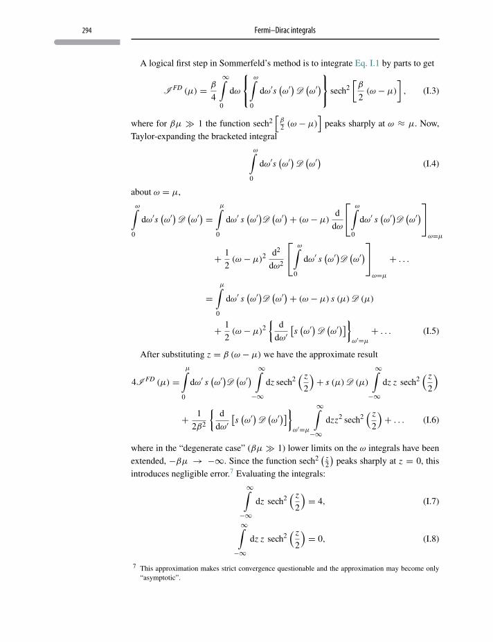
294 Fermi–Dirac integrals
A logical first step in Sommerfeld’s method is to integrate Eq. I.1 by parts to get
I FD (μ) = β
4
∞∫0
dω
⎧⎨⎩ω∫
0
dω′s(ω′)D(ω′)⎫⎬⎭ sech2
[β
2(ω − μ)
], (I.3)
where for βμ � 1 the function sech2[β2 (ω − μ)
]peaks sharply at ω ≈ μ. Now,
Taylor-expanding the bracketed integral
ω∫0
dω′s(ω′)D(ω′)
(I.4)
about ω = μ,
ω∫0
dω′s(ω′)D(ω′) = μ∫
0
dω′ s(ω′)D(ω′)+ (ω − μ)
d
dω
⎡⎣ ω∫0
dω′ s(ω′)D(ω′)⎤⎦
ω=μ
+ 1
2(ω − μ)2 d2
dω2
⎡⎣ ω∫0
dω′ s(ω′)D(ω′)⎤⎦
ω=μ
+ . . .
=μ∫
0
dω′ s(ω′)D(ω′)+ (ω − μ) s (μ)D (μ)
+ 1
2(ω − μ)2
{d
dω′[s(ω′)D(ω′)]}
ω′=μ
+ . . . (I.5)
After substituting z = β (ω − μ) we have the approximate result
4I FD (μ) =μ∫
0
dω′ s(ω′)D(ω′) ∞∫−∞
dz sech2( z
2
)+ s (μ)D (μ)
∞∫−∞
dz z sech2( z
2
)
+ 1
2β2
{d
dω′[s(ω′)D(ω′)]}
ω′=μ
∞∫−∞
dzz2 sech2( z
2
)+ . . . (I.6)
where in the “degenerate case” (βμ � 1) lower limits on the ω integrals have been
extended, −βμ → −∞. Since the function sech2( z
2
)peaks sharply at z = 0, this
introduces negligible error.7 Evaluating the integrals:
∞∫−∞
dz sech2( z
2
)= 4, (I.7)
∞∫−∞
dz z sech2( z
2
)= 0, (I.8)
7 This approximation makes strict convergence questionable and the approximation may become only“asymptotic”.
295 Expansion method: βμ� 1
∞∫−∞
dz z2 sech2( z
2
)= 4π2
3, (I.9)
∞∫−∞
dz z3 sech2( z
2
)= 0, (I.10)
we have the approximate result
I FD (μ) =μ∫
0
dω′ s(ω′)D(ω′)+ π2
6β2
{d
dω′[s(ω′)D(ω′)]}
ω′=μ
+ . . . (I.11)
J Appendix J Bose–Einstein integrals
J.1 BE integrals: μ = 0
In the Bose–Einstein (BE) problem we encounter two kinds of integrals. The first
appears when T < Tc so that μ = 0. These have the form
IB E =∞∫
0
dxxs
ex − 1. (J.1)
They can be done by first expanding the denominator
∞∫0
dxxs
ex − 1=
∞∫0
dx xs∞∑
n=0
e−(n+1)x (J.2)
and then integrating term by term
∞∫0
dxxs
ex − 1= Γ (s + 1)
∞∑ν=1
1
νs+1(J.3)
where the Γ -function is defined by
Γ (r) =∞∫
0
dz zr−1e−z, Re (r) > −1. (J.4)
The remaining sum is the Riemann ζ function
ζ (s) =∞∑
n=1
1
ns(J.5)
which finally gives
∞∫0
dxxs
ex − 1= Γ (s + 1) ζ (s + 1) . (J.6)
296
297 BE integrals: μ < 0
J.2 BE integrals: μ < 0
The second class of integrals is best demonstrated by the specific example
⟨N B E
op
⟩= V
4π2
(2m
h2
)3/2 ∞∫0
dωω1/2(
1
eβ(ω−μ) − 1
)(J.7)
= V
4π2
(2m
h2
)3/2 ∞∫0
dωω1/2(
λe−βω
1− λe−βω
), (J.8)
where λ = eβμ and therefore λe−βω < 1. Expanding the denominator in a binomial
series
⟨N B E
op
⟩= V
4π2
(2m
h2
)3/2 ∞∫0
dω1/2λe−βω∞∑
n=0
λne−nβω (J.9)
and integrating term by term⟨N B E
op
⟩= V
4π2
(2m
h2
)3/2 [Γ (3/2)
β3/2
](λ+ λ2
23/2+ λ3
33/2+ · · ·
)(J.10)
= V
4π2
(2m
h2
)3/2 [Γ (3/2)
β3/2
]ζ (3/2, λ) , (J.11)
where
ζ (s, λ) = λ+ λ2
2s+ λ3
3s+ · · · (J.12)
is a generalized ζ function. The function as studied by mathematicians (and in the
computational arsenal of, say, Mathematica) is Lerch’s Φ function (also called
Hurwitz–Lerch ζ function) defined as
Φ (z, s, a) =∞∑
n=0
zn
(n + a)s , (J.13)
where any term for which the denominator is “zero” is excluded. But the generalized
ζ function appearing in Bose–Einstein integrals is
ζ (s, z) =∞∑
n=1
zn
ns(J.14)
which is related to Lerch’s Φ function by
ζ (s, z) = zΦ (z, s, 1) . (J.15)
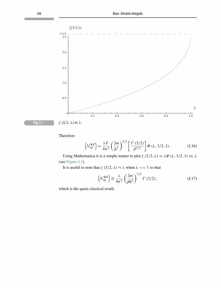
298 Bose–Einstein integrals
� Fig. J.1 ζ (3/2, λ) vs. λ.
Therefore ⟨N B E
op
⟩= λV
4π2
(2m
h2
)3/2 [Γ (3/2)
β3/2
]Φ (λ, 3/2, 1) . (J.16)
Using Mathematica it is a simple matter to plot ζ (3/2, λ) = λΦ (λ, 3/2, 1) vs. λ
(see Figure J.1).
It is useful to note that ζ (3/2, λ) ≈ λ when λ << 1 so that⟨N B E
op
⟩ ∼= λ
4π2
(2m
βh2
)3/2
Γ (3/2) , (J.17)
which is the quasi-classical result.
Index
adiabaticdefinition, 27demagnetization, 168sudden process as, 36throttling, 79
adiabatic process, 43antiferromagnetism, 155
bias in probabilities, 267define, 266entropy, 267measure of, 264
Boltzmann, xiiconstant, 29microcanonical theory, 89
Bose–Einsteincondensate, 246, 250condensate wave function, 252condensation, 249grand potential, 248integrals, 296internal energy, 249occupation number, 248thermodynamics, 248
bosons, 107, 250, 252, 253
Carnot, xicycle, 69engine, 66
chemical potential, 5, 6, 26, 28, 192chemical reactions, 196Clausius, 2, 85Clausius, historical note, xi, xiicoherent, 10, 252cosmic microwave background (CMB), 255
Debye model, 131Debye temperature, 133density of states, 273internal energy, 133heat capacity, 133
decoherence, 18, 86, 91degeneracy, 94, 96
elastomer, 99
hydrogenic, 100internal quantum, 96macroscopic, 96one-dimensional harmonic oscillator, 101
demagnetizationfactor, 284field, 284tensor, 284
density of statesdefinition, 271one dimension, particles in, 271
density operator, 7definition, 12density matrix, 12density matrix, examples, 21equation of motion, 14information and the, 13mixed state, 15properties, 12pure state, 12, 14thermal, defined, 19
diamagnetism, 155diathermic, 40differential, 49
exact, 28, 50Euler’s criterion, 51Green’s theorem, 51
diffusive equilibrium, 193Dirac delta function
definition, 233property, 272
Dirac notation, 9
Einstein modelone-dimensional, 124
partition function, 126thermal Lagrangian, 126
three-dimensional, 128Einstein temperature, 130heat capacity, 130internal energy, 129partition function, 128
299
300 Index
Einstein, historical note, 2elasticity
elongation, 7, 26entropy, 141equation of state, 141extension, 37lab experiment, 151, 275non-ideal equation of state, 150one-dimensional model, 136partition function, 140tension, 5, 26, 29thermodynamics of, 143three-dimensional non-ideal, 147
elastomer, 29, 98degeneracy, 99
electricconstitutive relation, 279field, 5, 30fields in matter, 278polarization, 26, 30susceptibility tensor, 30
electromagneticMaxwell’s equations, 285polarizations, 288vector potential, 288wave equation, classical, 289waves, 285
electromagnetic fieldhamiltonian, quantized, 290, 291operator, quantized, 291
energymicroscopic system, 10
ensembles, xiienthalpy, 54
definition, 39, 75Maxwell’s relation, 75
entropy, xii, xiii, 20, 21, 58, 60, 85, 92definition, 53examples, 60of mixing, 114
equation of state, 28dielectric, 30
equilibriumthermodynamic, definition, 3
Euler’s homogeneous function theorem,54, 268
proof, 268exoplanet surface temperature, 223
Fermi energy, 232Fermi gas model, 233Fermi–Dirac
average particle number, 231chemical potential, 234, 236electron gas model, 238free electron approximation, 229function, 231grand partition function, 230grand potential, 231heat capacity, 236integrals, 293internal energy, 232, 236occupation number, 231pressure, equation of state, 232thermodynamics, 231
fermions, 106ferrimagnetism, 155ferromagnetism, 155
critical exponent, 173Curie–Weiss susceptibility, 174Gibbs potential, 171Heisenberg exchange, 169Heisenberg model, 169order parameter, 172
fieldenergy, 282external, 279external magnetic, 282local average, 282magnetic, effective, 283mean, 283
fieldsdemagnetizing, 278
First Law of Thermodynamics, 4heat, 25, 27incremental, 28work, 25, 26
force, 25free expansion, 56functional, 88, 266
gamma function, 251gas law, 29
ideal, 29derivation, 107
pressure, 29temperature, 29van der Waals, 59, 115
derivation, 184Gibbs, xii
canonical theory, 93correction, 109entropy paradox, 113partition function, 93
301 Index
Gibbs potential, 78magnetic, 283
Gibbs–Duhem equation, 201grand canonical
entropy, 179Euler’s theorem, 181ideal gas example, 182internal energy, 178particle number, 178partition function, 177potential function, 179pressure, 179thermodynamics, 178
heat, 4, 66heat capacity, 38
constant pressure, 39constant volume, 38Dulong–Petit, 123entropy, 81
Helmholtz potentialcanonical, 95definition, 76Maxwell’s relation, 76
ideal gas, 106barometric equation, 194charged, 194entropy, Sackur–Tetrode equation, 112heat capacity, 112Helmholtz potential, 112in Earth’s gravitational field, 193in rotating cylinder, 195internal energy, 111pressure, equation of state, 113thermal Lagrangian, 108
information, 11, 18missing, 22purity, 14Shannon, 86
internal energy, 4, 9, 19, 27, 36blackbody, moving frame, 260free expansion, 57Maxwell’s relation, 73
isenthalpic, 53isochoric, 39isothermal, 31, 37
law of mass action, 198line integration, 59
macroscopic, xiiaverages, 4definition, 3
magnetic
constitutive relation, 279
field
internal, 283
fields, in matter, 278
thermodynamic potentials, 278
magnetism, 154
constitutive relation, 158
de Haas–van Alphen effect, 155
enthalpy, 158
fundamental equation, 157, 160
Gibbs potential, 158
Helmholtz potential, 158
internal fields, 283
magnetic field, 5, 30
magnetic moment, 6
magnetic susceptibility, 30
magnetic work, 156, 158
magnetization, 26, 282
fluctuations, 167
magnetization vector, 160
work in applied fields, 160
Mattis, xi, xiii
Maxwell, xii
thermodynamic relations, 50, 74, 76–78
mean field approximation, 283
ferromagnetism, 170
gravitational interaction, 187
van der Waals equation, 185
microstates, xii
minimum bias, 88, 266
mixed state, 15
negative temperature, 120
normalization, state function, 10
open systems, 6, 192
operator
density, thermodynamic, 86
elongation, 5
fluctuations, 19
function of, 21
hamiltonian, 8
hamiltonian, thermal, 87
hermitian, 9, 11
magnetization, 5
particle number, 6
polarization, 5
pressure, 5
quantum hamiltonian, 5
trace, definition, 13
vector potential, 5
302 Index
paramagnetism, 154, 161Curie regime, 165entropy, 165fluctuations, 167Gibbs potential, 165heat capacity, 166magnetization, 164partition function, 163thermal Lagrangian, 163thermodynamics, 164
partial differentiation, 50, 55partition function, 93
blackbody moving frame, 259ideal gas, 109
Pauli exclusion principle, 106, 228Pauli susceptibility, 237periodic boundary conditions, 239phonons, 125Planck radiation function, CMB, 262Planck, historical note, 2polymer
rubber, 29rubber band, 36
Poynting vector, 222blackbody, moving frame, 261
pressure, 19, 26, 179purity, 20, 21, 263
quantum“bra”, 9“ket”, 8, 9average value, 10eigenfunctions, 9, 11eigenvalues, 9, 11expectation value, 8–11fluctuations, 8hamiltonian, 5, 8microscopic, 7probabilities, 8probability, 9probability amplitude, 10pure state, 11, 12state function, 8superposition theorem, 10wavefunction, 7, 11
quantum concentration, nQ , 111
radiation thermodynamics, moving frame, 259
Schottky model, 117heat capacity, 119two-level system, 117
Schrödinger, equation, 7
Schwartz inequality, 263Second Law of Thermodynamics, 54, 65, 69, 85specific heat, 38stars
formation of, 186giant molecular clouds, 187gravitational collapse, 189gravitational equation of state, 189
state function, 8normalization, 13
Stern–Gerlach, 16strain, 26, 42
definition, 29stress, 26, 42
definition, 29surface adsorption, 204
dissociative, 207Langmuir isotherm, 207Langmuir model, 204
temperature, 5, 27tension
surface, 26thermal expansivity, 42thermal Lagrangian
Bose–Einstein, 247canonical theory, 93CMB, 257definition, 267elastic, 138, 140Fermi–Dirac, 229microcanonical theory, 90open system, 177radiation, 214Schottky two-level model, 118
thermal radiationentropy, 221hamiltonian, classical, 212Helmholtz potential, 216momentum density, 224partition function, 215Planck constant, 212Plank quantization, 212stardust blow-out, 225Stefan–Boltzmann law, 217, 221thermodynamics of, 214Wien’s law, 220
thermodynamic identity, 53thermodynamics
equilibrium states, 30fluctuations, definition, 3surroundings, 4
303 Index
surroundings, definition, 3system, definition, 3
throttling, 79
van der Waals, equation, 186van der Waals, historical note, 2variables
conjugate pairs, 26extensive, 26intensive, 26state, 28thermal, 3
white dwarf stars, 241mass–radius constant, 243
work, 4, 25electric, 159irreversible, 33, 34, 62magnetic, 159quasi-static, 30, 34, 37reversible, 31
Young’s modulus, 42, 136
zeta function, 251