THERE IS NO CHAOS IN STOCK MARKETS

JAMAL MUNSHI

ABSTRACT: The elegant simplicity of the Efficient Market Hypothesis (EMH) is its greatest weakness because human nature

demands complicated answers to important questions and Chaos Theory readily fills that demand for complexity claiming that it

reveals the hidden structure in stock prices. In this paper we take a close look at the Rescaled Range Analysis tool of chaos

theorists and show that their findings are undermined by weaknesses in their methods1.

1. INTRODUCTION

Stock market data have thwarted decades of effort by mathematicians and statisticians to discover their

hidden pattern. Simple time series analyses such as AR, MA, ARMA, and ARIMA2 were eventually

replaced with more sophisticated instruments of torture such as spectral analysis but the data refused to

confess. The failure to discover the structure in price movements convinced many researchers that the

movements were random. The random walk hypothesis (RWH) of Osborne and others (Osborne, 1959)

(Bachelier, 1900) was developed into the efficient market hypothesis (EMH) by Eugene Fama (Fama,

1965) (Fama, Efficient Capital Markets: A Review of Theory and Empirical Work, 1970), which serves

as a foundational principle of finance.

The `weak form of the EMH implies that movements in stock returns are random events independent of

historical values. The rationale is that prices contain all publicly available information and if patterns did

exist, arbitrageurs would take advantage of them and thereby quickly eliminate them. Both the RWH and

the EMH came under immediate attack from technical analysts and this attack continues to this day partly

because the statistics used in tests of the EMH are controversial. The null hypothesis states that the market

is efficient. The test then consists of presenting convincing evidence that it is not. The tests usually fail.

Many argue that the failure of these tests represent a Type II error, that is, a failure to detect a real effect

because of low power of the statistical test employed. It is therefore logical to conjecture that the reason

for the failure of statistics to reject the EMH is not the strength of the theory but the weakness of the

statistics. If that is the case, perhaps a different and more powerful mathematical device that allowed for

more complexity might be successful in discovering the hidden structure of stock prices.

In the early seventies, it appeared that Catastrophe Theory was just such a device (Zeeman, 1974)

(Zeeman, Catatstrophe Theory, 1976). It had a seductive ability to mimic long bull market periods

followed by catastrophic crashes. But it proved to be a mathematical artifact. Its properties could not be

generalized. It yielded no secret structure or patterns in stock prices. The results of other non-EMH

models such as the Rational Bubble theory (Diba, 1988) and the Fads Theory (Camerer, 1989) are equally

unimpressive for the same reasons.

1 Date June, 2014

Key words and phrases: rescaled range analysis, fractal, chaos theory, statistics, Monte Carlo, stock returns Author affiliation: Professor Emeritus, Sonoma State University, Rohnert Park, CA, 94928, munshi@sonoma.edu 2 Auto Regressive, Moving Average, Auto Regressive Moving Average, Auto Regressive Integrated Moving Average

2. THEORY

Many economists feel that the mathematics of time series implied by Chaos Theory (Mandelbrot B. ,

1963) is a promising alternative. If time series data have a memory of the past and behave accordingly

even to a small extent then much of what appears to be random behavior may turn out to be part of the

deterministic response of the system. Certain non-linear dynamical system of equations can generate time

series data that appear remarkably similar to the behavior of stock market prices.

Research in this area of finance is motivated by the idea that by using new mathematical techniques

hidden structures can be discovered in what appears to be a random time series. One technique, attributed

to Lorenz (Lorenz, 1963), uses a plot of the data in phase space to detect patterns called strange attractors

(Bradley, 2010) (Peters E. , 1991). Another method proposed by Takens (Takens, 1981) uses an algorithm

to determine the `correlation dimension' of the data (Wikipedia, 2014) (Schouten, 1994). A low

correlation dimension indicates a deterministic system. A high correlation dimension is indicative of

randomness.

The correlation dimension technique has yielded mixed results with stock data. Halbert White and others

working with daily returns of IBM concluded that the correlation dimension was sufficiently high to

regard the time series as white noise (White, 1988) although Scheinkman (Scheinkman, 1989) et al claim

to have found that a significant deterministic component in weekly returns.

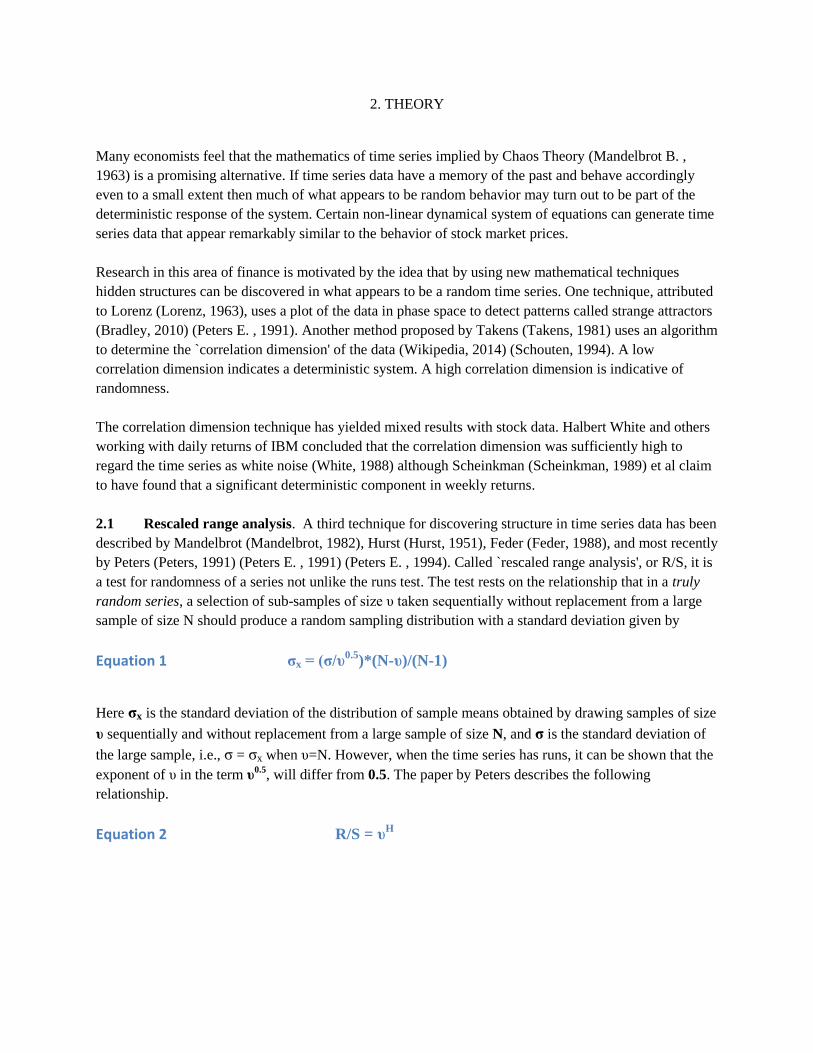
2.1 Rescaled range analysis. A third technique for discovering structure in time series data has been

described by Mandelbrot (Mandelbrot, 1982), Hurst (Hurst, 1951), Feder (Feder, 1988), and most recently

by Peters (Peters, 1991) (Peters E. , 1991) (Peters E. , 1994). Called `rescaled range analysis', or R/S, it is

a test for randomness of a series not unlike the runs test. The test rests on the relationship that in a truly

random series, a selection of sub-samples of size υ taken sequentially without replacement from a large

sample of size N should produce a random sampling distribution with a standard deviation given by

Equation 1 σx = (σ/υ0.5

)*(N-υ)/(N-1)

Here σx is the standard deviation of the distribution of sample means obtained by drawing samples of size

υ sequentially and without replacement from a large sample of size N, and σ is the standard deviation of

the large sample, i.e., σ = σx when υ=N. However, when the time series has runs, it can be shown that the

exponent of υ in the term υ0.5

, will differ from 0.5. The paper by Peters describes the following

relationship.

Equation 2 R/S = υH

where R is the range of the sequential running totals of the deviations of the sub-sample values from the

sub-sample mean3, S is the standard deviation of the sub- sample, and υ is the size of the sub-sample . The

`H' term is called the Hurst constant or the Hurst exponent. It serves as a measure of the fractal and non-

random nature of the time series. If the series is random H will have a value of 0.5 as shown in Equation

1, but if it has runs the H exponent will be different from 0.5.

If there is a tendency for positive runs, that is, increases are more likely to be followed by increases and

decreases are more likely to be followed by decreases, then H will be greater than 0.5 but less than 1.0.

Values of H between 0 and 0.5 are indicative of negative runs, that is increases are more likely to be

followed by decreases and vice versa. Hurst and Mandelbrot have found that many natural phenomena

previously thought to be random have high H-values that are indicative of a serious departure from

independence and randomness (Hurst, 1951).

Once `H' is determined for a time series, the autocorrelation in the time series is computed as follows:

Equation 3 CN = 2(2H-1)

-1

CN is the correlation coefficient and its magnitude may be interpreted as the degree to which the elements

of the time series are dependent on historical values. The interpretation of this coefficient used by Peters

to challenge the EMH is that it represents the percentage of the variation in the time series that can be

explained by historical data. The weak form of the EMH implies that this correlation is zero; i.e., that the

observations are independent of each other. Therefore, evidence of such a correlation can be interpreted to

mean that the weak form of the EMH does not hold.

Peters (Peters E. , 1991) (Peters E. , 1994) studied monthly returns of the S&P500 index, 30-year

government T-bond, and the excess of stocks returns over the bond returns and computed the R/S values

for all three time series data for eleven sequential sub-sample sizes. He found very high values of H and

CN and therefore rejected the EMH null hypothesis. His papers and books on the subject have generated a

great deal of interest in R/S research with many papers reporting a serious departure from randomness in

stock returns previously assumed to be random (Pallikari, 1999) (Bohdalova, 2010) (Jasic, 1998)

(McKenzie, 1999) (Mahalingam, 2012). We now examine this methodology in some detail.

3 The sum of these values is of course zero by definition but the intermediate values in the running sub-totals will

have a range that is related to the tendency for the data to have positive or negative runs.

3. METHODOLOGY

An appropriate time series that is sufficiently long to facilitate sequential sub-sampling without

replacement is selected for R/S analysis. It will be sampled in cycles. In each cycle, of many sub-

sampling cycles, sub-samples are taken sequentially and without replacement. The sub-sample sizes are

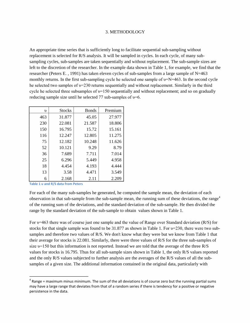
left to the discretion of the researcher. In the example data shown in Table 1, for example, we find that the

researcher (Peters E. , 1991) has taken eleven cycles of sub-samples from a large sample of N=463

monthly returns. In the first sub-sampling cycle he selected one sample of υ=N=463. In the second cycle

he selected two samples of υ=230 returns sequentially and without replacement. Similarly in the third

cycle he selected three subsamples of υ=150 sequentially and without replacement; and so on gradually

reducing sample size until he selected 77 sub-samples of υ=6.

υ Stocks Bonds Premium

463 31.877 45.05 27.977

230 22.081 21.587 18.806

150 16.795 15.72 15.161

116 12.247 12.805 11.275

75 12.182 10.248 11.626

52 10.121 9.29 8.79

36 7.689 7.711 7.014

25 6.296 5.449 4.958

18 4.454 4.193 4.444

13 3.58 4.471 3.549

6 2.168 2.11 2.209 Table 1 υ and R/S data from Peters

For each of the many sub-samples he generated, he computed the sample mean, the deviation of each

observation in that sub-sample from the sub-sample mean, the running sum of these deviations, the range4

of the running sum of the deviations, and the standard deviation of the sub-sample. He then divided the

range by the standard deviation of the sub-sample to obtain values shown in Table 1.

For υ=463 there was of course just one sample and the value of Range over Standard deviation (R/S) for

stocks for that single sample was found to be 31.877 as shown in Table 1. For υ=230, there were two sub-

samples and therefore two values of R/S. We don't know what they were but we know from Table 1 that

their average for stocks is 22.081. Similarly, there were three values of R/S for the three sub-samples of

size υ=150 but this information is not reported. Instead we are told that the average of the three R/S

values for stocks is 16.795. Thus for all sub-sample sizes shown in Table 1, the only R/S values reported

and the only R/S values subjected to further analysis are the averages of the R/S values of all the sub-

samples of a given size. The additional information contained in the original data, particularly with

4 Range = maximum minus minimum. The sum of the all deviations is of course zero but the running partial sums

may have a large range that deviates from that of a random series if there is tendency for a positive or negative persistence in the data.

reference to variance, is lost and gone forever. As we shall see later, this information loss is a serious

weakness in R/S research methodology.

Once all the values of υ and the average R/S for sub-samples of each size are tabulated as shown in Table

1, the researcher is ready to estimate the value of H by utilizing Equation 2 which states the relationship

between υ and R/S. To do that, the researcher first renders Equation 2 into linear form by taking the

natural logarithm of both sides to yield

Equation 4 ln(R/S) = H*ln(υ)

Equation 4 implies that there is a linear relationship between ln(R/S) and ln(υ) and that the slope of this

line is H. To estimate the value of H the researcher takes the natural logarithms of the R/S values and for

the corresponding values of υ and then carries out OLS5 linear regression between the logarithms to

estimate the slope using the regression model

Equation 5 y=b0+b1x

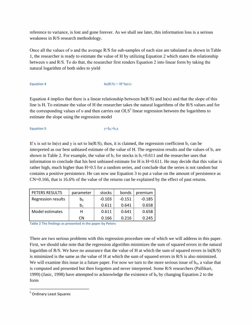
If x is set to ln(υ) and y is set to ln(R/S), then, it is claimed, the regression coefficient b1 can be

interpreted as our best unbiased estimate of the value of H. The regression results and the values of b1 are

shown in Table 2. For example, the value of b1 for stocks is b1=0.611 and the researcher uses that

information to conclude that his best unbiased estimate for H is H=0.611. He may decide that this value is

rather high, much higher than H=0.5 for a random series, and conclude that the series is not random but

contains a positive persistence. He can now use Equation 3 to put a value on the amount of persistence as

CN=0.166, that is 16.6% of the value of the returns can be explained by the effect of past returns.

PETERS RESULTS parameter stocks bonds premium

Regression results b0 -0.103 -0.151 -0.185

b1 0.611 0.641 0.658

Model estimates H 0.611 0.641 0.658

CN 0.166 0.216 0.245 Table 2 The findings as presented in the paper by Peters

There are two serious problems with this regression procedure one of which we will address in this paper.

First, we should take note that the regression algorithm minimizes the sum of squared errors in the natural

logarithm of R/S. We have no assurance that the value of H at which the sum of squared errors in ln(R/S)

is minimized is the same as the value of H at which the sum of squared errors in R/S is also minimized.

We will examine this issue in a future paper. For now we turn to the more serious issue of b0, a value that

is computed and presented but then forgotten and never interpreted. Some R/S researchers (Pallikari,

1999) (Jasic, 1998) have attempted to acknowledge the existence of b0 by changing Equation 2 to the

form

5 Ordinary Least Squares

Equation 6 R/S = CυH

Equation 7 C=exp(b0).

For example, in Table 2, the C and H values for stocks is C=e-0.103

=0.902 and H=0.611. So we get a sense

that the value of b0 now has a place in R/S research but we still have no attempt by researchers to interpret

C or to examine the relationship between C and H.

In fact, there is an inverse relationship between C and H that works like a see-saw. Higher values of C are

associated with lower values of H and lower values of C are associated with higher values of H. This

relationship presents the second methodological problem for R/S research because it implies that the

values of H and C must be evaluated together as a pair and not in isolation. Alternately, one could fix the

regression intercept at zero where C=1 and compare H values directly at the cost of increasing the error

sum of squares in the regression. We investigate these possibilities in the next section.

Yet a third issue in chaos research that must be investigated is that the way they are structured often leads

to a high probability spurious findings. First, the α level of hypothesis tests is usually set to α=0.05. This

means that five percent of the time researchers will find an effect in random data. Recent studies of the

irreproducibility of results in the social sciences has led many to insist that this error level should be set to

α=0.001 (Johnson, 2013). In many R/S papers, the false positive error rate is further exacerbated by

multiple comparisons that are made without a Bonferroni adjustment of the α level (Mundfrom, 2006).

For example, if five comparisons are made at α=0.05, the possibility of finding an effect in random data

rises to 1.05^5-1 or 27% - an unacceptable rate of the production of spurious and irreproducible results.

4. DATA ANALYSIS

For a demonstration of R/S analysis and the methodological issues we raised, we have selected four time

series of daily returns and four series of weekly returns each with N=2486. The stocks and stock indexes

selected for study are listed in Table 3. The number of cycles and the sub-sample sizes to use are

arbitrarily assigned as follows. The sub-samples are taken in six cycles. In the first cycle we take one

sample of υ=2486; in the second cycle, two samples of υ=1243 each; in the third cycle four samples of

υ=621 each; in the fourth cycle, eight samples of υ=310 each; in the fifth cycle, sixteen samples of υ=155

each; and in the sixth cycle we take thirty two samples of υ=77 each. In each cycle the samples are taken

sequentially and without replacement. We then compute the value of R/S for each sample of each series.

These values are shown in Table 5. Average R/S values as they would appear in conventional research are

shown for reference in Table 4. All data and Microsoft Excel computational files are available in the

online data archive of this paper (Munshi, 2014)6.

6 The use of the R/S analysis spreadsheet is explained in the Appendix

Symbol Name From To Returns N

IXIC NASDAQ Composite Index 2004 2014 daily 2486

DJI Dow Jones Industrial Average 2004 2014 daily 2486

BAC Bank of America 2004 2014 daily 2486

CL Colgate Palmolive 2004 2014 daily 2486

SPX S&P500 Index 1966 2014 weekly 2486

CAT Caterpillar 1966 2014 weekly 2486

BA Boeing 1966 2014 weekly 2486

IBM IBM 1966 2014 weekly 2486

Table 3 Returns series selected for R/S analysis

υ IXIC DJI BAC CL SPX CAT BA IBM

2486 67.103 71.259 72.107 41.150 65.899 42.414 62.702 61.596

1243 40.069 39.317 55.765 31.469 52.971 30.363 48.096 44.789

621 26.854 23.887 29.925 21.898 34.672 25.526 35.427 36.034

310 20.426 17.773 18.719 15.808 23.039 19.659 24.614 25.140

155 14.387 13.072 14.453 12.458 15.099 13.723 15.373 14.998

77 9.487 9.231 9.370 8.977 9.796 9.204 9.938 10.614

Table 4 The average value of R/S for each value of υ

By comparing the values of R/S in Table 4 with those in Table 5 for the same value of υ we can see that

there is a great deal of variance among the actual observed R/S values and that this variance simply

vanishes from the data when the average value is substituted for them. Of course, the reduction of

variance thus achieved increases the precision of the regression with higher values for R-squared and

correspondingly lower values for the variance of the residuals and the standard error of the regression

coefficient b1. As a result, it appears that we have estimated H with a great deal of precision but this

precision is illusory and fictional because it does not actually exist in the data.

Yet another problem created by throwing away the actual data and substituting one average value of R/S

to represent many observed values of R/S is that the R/S values at lower values of υ are not weighted

sufficiently in the least squares procedure and therefore the regression is unduly influenced by the large

samples. For example the squared residuals of R/S values for υ=155 carries a weight=16 if the actual data

are used in the regression instead of weight=1 when one average value is substituted for sixteen

observations. The variance and weighting problems together act to corrupt the regression procedure.

We therefore choose to carry out our regression using the data in Table 5 instead of the average values in

Table 4. With Equation 6 as our empirical model, we take the logarithm of both sides to obtain regression

model as ln(R/S)=C+H*ln(υ). Linear regression is carried out between y=ln(R/S) and x=ln(υ) and the

regression coefficients b0 and b1 are used as our unbiased estimate of the parameters in Equation 6 as

H=b1 and C=exp(b0). These results are summarized in Table 6.

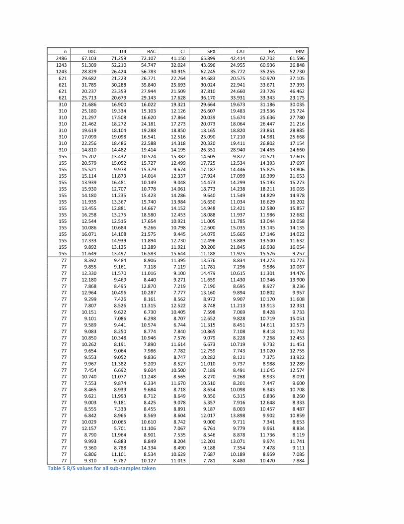
n IXIC DJI BAC CL SPX CAT BA IBM

2486 67.103 71.259 72.107 41.150 65.899 42.414 62.702 61.596

1243 51.309 52.210 54.747 32.024 43.696 24.955 60.936 36.848 1243 28.829 26.424 56.783 30.915 62.245 35.772 35.255 52.730

621 29.682 21.223 26.771 22.764 34.683 20.575 50.970 37.105 621 31.785 30.288 35.840 25.693 30.024 22.941 33.671 37.393 621 20.237 23.359 27.944 21.509 37.810 24.660 23.726 46.462 621 25.713 20.679 29.143 17.628 36.170 33.931 33.343 23.175

310 21.686 16.900 16.022 19.321 29.664 19.673 31.186 30.035 310 25.180 19.334 15.103 12.126 26.607 19.483 23.536 25.724 310 21.297 17.508 16.620 17.864 20.039 15.674 25.636 27.780 310 21.462 18.272 24.181 17.273 20.073 18.064 26.447 21.216 310 19.619 18.104 19.288 18.850 18.165 18.820 23.861 28.885 310 17.099 19.098 16.541 12.516 23.090 17.210 14.981 25.668 310 22.256 18.486 22.588 14.318 20.320 19.411 26.802 17.154 310 14.810 14.482 19.414 14.195 26.351 28.940 24.465 24.660

155 15.702 13.432 10.524 15.382 14.605 9.877 20.571 17.603 155 20.579 15.052 15.727 12.499 17.725 12.534 14.393 17.697 155 15.521 9.978 15.379 9.674 17.187 14.446 15.825 13.806 155 15.114 11.873 14.014 12.337 17.924 17.099 16.399 21.653 155 13.939 16.481 10.149 9.048 14.473 14.299 15.193 15.273 155 15.930 12.707 10.778 14.061 18.773 14.238 18.211 16.065 155 14.180 11.235 15.423 14.286 9.640 11.549 14.829 14.978 155 11.935 13.367 15.740 13.984 16.650 11.034 16.629 16.202 155 13.455 12.881 14.667 14.152 14.948 12.421 12.580 15.857 155 16.258 13.275 18.580 12.453 18.088 11.937 11.986 12.682 155 12.544 12.515 17.654 10.921 11.005 11.785 13.044 13.058 155 10.086 10.684 9.266 10.798 12.600 15.035 13.145 14.135 155 16.071 14.108 21.575 9.445 14.079 15.665 17.146 14.022 155 17.333 14.939 11.894 12.730 12.496 13.889 13.500 11.632 155 9.892 13.125 13.289 11.921 20.200 21.845 16.938 16.054 155 11.649 13.497 16.583 15.644 11.188 11.925 15.576 9.257

77 8.392 9.484 8.906 11.395 13.576 8.834 14.273 10.773 77 9.855 9.161 7.118 7.119 11.781 7.296 9.586 10.067 77 12.330 11.570 11.016 9.100 14.479 10.615 11.301 14.476 77 12.180 9.469 8.440 9.271 11.659 11.430 10.346 13.900 77 7.868 8.495 12.870 7.219 7.190 8.695 8.927 8.236 77 12.964 10.496 10.287 7.777 13.160 9.894 10.802 9.957 77 9.299 7.426 8.161 8.562 8.972 9.907 10.170 11.608 77 7.807 8.526 11.315 12.522 8.748 11.213 13.913 12.331 77 10.151 9.622 6.730 10.405 7.598 7.069 8.428 9.733 77 9.101 7.086 6.298 8.707 12.652 9.828 10.719 15.051 77 9.589 9.441 10.574 6.744 11.315 8.451 14.611 10.573 77 9.083 8.250 8.774 7.840 10.865 7.108 8.418 11.742 77 10.850 10.348 10.946 7.576 9.079 8.228 7.268 12.453 77 10.262 8.191 7.890 11.614 6.673 10.719 9.732 11.451 77 9.654 9.064 7.986 7.782 12.759 7.743 13.020 12.755 77 9.553 9.052 9.836 8.747 10.282 8.121 7.375 13.922 77 9.967 11.382 9.209 8.527 11.010 9.737 8.988 12.289 77 7.454 6.692 9.604 10.500 7.189 8.491 11.645 12.574 77 10.740 11.077 11.248 8.565 8.270 9.268 8.933 8.091 77 7.553 9.874 6.334 11.670 10.510 8.201 7.447 9.600 77 8.465 8.939 9.684 8.718 8.634 10.098 6.343 10.708 77 9.621 11.993 8.712 8.649 9.350 6.315 6.836 8.260 77 9.003 9.181 8.425 9.078 5.357 7.916 12.648 8.333 77 8.555 7.333 8.455 8.891 9.187 8.003 10.457 8.487 77 6.842 8.966 8.569 8.604 12.017 13.898 9.902 10.859 77 10.029 10.065 10.610 8.742 9.000 9.711 7.341 8.653 77 12.157 5.701 11.106 7.067 6.761 9.779 9.961 8.834 77 8.790 11.964 8.901 7.535 8.546 8.878 11.736 8.119 77 9.993 6.883 8.849 8.204 12.201 13.071 9.974 11.741 77 9.360 8.788 14.334 8.490 9.188 7.354 7.478 9.111 77 6.806 11.101 8.534 10.629 7.687 10.189 8.959 7.085 77 9.310 9.787 10.127 11.013 7.781 8.480 10.470 7.884

Table 5 R/S values for all sub-samples taken

IXIC DJI BAC CL SPX CAT BA IBM

C=exp(b0) 0.9550 1.0012 0.7339 1.3406 0.6999 1.1850 0.7721 0.9346

H=b1 0.5282 0.5065 0.5810 0.4352 0.6030 0.4741 0.5872 0.5548

R2 0.8627 0.8639 0.8594 0.8382 0.8472 0.8211 0.8478 0.8395

σH 0.0270 0.0257 0.0301 0.0245 0.0328 0.0283 0.0319 0.0311

Table 6 Results of linear regression on the natural logarithms of the data in Table 5

In Table 6, the R2 value expresses the percentage of the total sum of squared deviations from the mean

that is explained by the regression. These values are quite a bit lower than the R2 values

7 one usually

encounters in R/S research but they are probably more realistic. Similarly the standard error in the

estimation of H listed as σH in Table 6 are higher but more reliable for the same reasons.

If we scan Table 6 for H values that appear to be very different from H=0.5, CL and SPX stand out with

CL showing a rather low value of H and SPX a somewhat high value. This is of course the line of

reasoning conventionally taken. However, if we also look at the values of C we find something very

interesting. Colgate Palmolive (CL), with a value of H unusually lower than H=0.5 shows a value of C

that is unusually higher than C=1. In the same way, the S&P500 Index (SPX) with a value of H unusually

higher than the neutral value of H=0.5 shows a value of C that is correspondingly lower than the neutral

value of C=1. The DJIA Index (DJI) appears to be in the middle of these extremes with an H value very

close to H=0.5 and a C value very close to C=1.

In fact, if we compare all the H and C values we can discern the see-saw effect mentioned earlier. Values

of H greater than 0.5 correspond with values of C less than 1.0 and values of H less than 0.5 correspond

with values of C greater than 1.0. Therefore, to interpret the regression results in terms of persistence in

the data and chaos in stock prices, we must first understand the relationship between C and H in a random

series that has no persistence, no memory, and no chaos. To do that we took forty random samples of size

n=2486 from a Gaussian distribution with μ=0 and σ=1 and computed the R/S values using the same sub-

sampling strategy that we used for the stock returns. Linear regression between ln(R/S) and ln(υ) was

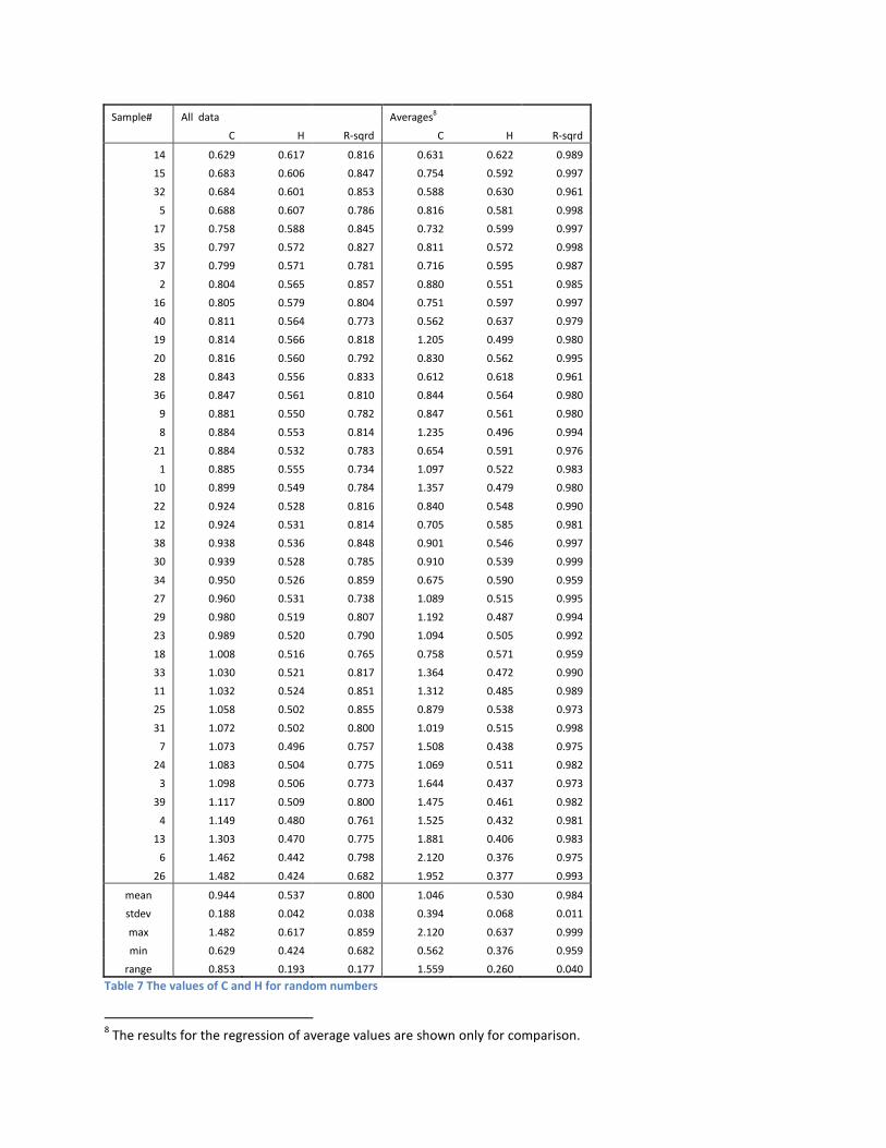
carried out for each of the forty samples. The regression results are shown in Figure 1 and Table 7.

Figure 1 Observed relationship between C and H in random numbers

7 well above 0.95

y = -0.4199x - 0.6572 R² = 0.9717

-1

-0.8

-0.6

-0.4

-0.2

0

-0.6 -0.4 -0.2 0 0.2 0.4 0.6

ln(H

)

ln(C)

Sample# All data Averages8

C H R-sqrd C H R-sqrd

14 0.629 0.617 0.816 0.631 0.622 0.989

15 0.683 0.606 0.847 0.754 0.592 0.997

32 0.684 0.601 0.853 0.588 0.630 0.961

5 0.688 0.607 0.786 0.816 0.581 0.998

17 0.758 0.588 0.845 0.732 0.599 0.997

35 0.797 0.572 0.827 0.811 0.572 0.998

37 0.799 0.571 0.781 0.716 0.595 0.987

2 0.804 0.565 0.857 0.880 0.551 0.985

16 0.805 0.579 0.804 0.751 0.597 0.997

40 0.811 0.564 0.773 0.562 0.637 0.979

19 0.814 0.566 0.818 1.205 0.499 0.980

20 0.816 0.560 0.792 0.830 0.562 0.995

28 0.843 0.556 0.833 0.612 0.618 0.961

36 0.847 0.561 0.810 0.844 0.564 0.980

9 0.881 0.550 0.782 0.847 0.561 0.980

8 0.884 0.553 0.814 1.235 0.496 0.994

21 0.884 0.532 0.783 0.654 0.591 0.976

1 0.885 0.555 0.734 1.097 0.522 0.983

10 0.899 0.549 0.784 1.357 0.479 0.980

22 0.924 0.528 0.816 0.840 0.548 0.990

12 0.924 0.531 0.814 0.705 0.585 0.981

38 0.938 0.536 0.848 0.901 0.546 0.997

30 0.939 0.528 0.785 0.910 0.539 0.999

34 0.950 0.526 0.859 0.675 0.590 0.959

27 0.960 0.531 0.738 1.089 0.515 0.995

29 0.980 0.519 0.807 1.192 0.487 0.994

23 0.989 0.520 0.790 1.094 0.505 0.992

18 1.008 0.516 0.765 0.758 0.571 0.959

33 1.030 0.521 0.817 1.364 0.472 0.990

11 1.032 0.524 0.851 1.312 0.485 0.989

25 1.058 0.502 0.855 0.879 0.538 0.973

31 1.072 0.502 0.800 1.019 0.515 0.998

7 1.073 0.496 0.757 1.508 0.438 0.975

24 1.083 0.504 0.775 1.069 0.511 0.982

3 1.098 0.506 0.773 1.644 0.437 0.973

39 1.117 0.509 0.800 1.475 0.461 0.982

4 1.149 0.480 0.761 1.525 0.432 0.981

13 1.303 0.470 0.775 1.881 0.406 0.983

6 1.462 0.442 0.798 2.120 0.376 0.975

26 1.482 0.424 0.682 1.952 0.377 0.993

mean 0.944 0.537 0.800 1.046 0.530 0.984

stdev 0.188 0.042 0.038 0.394 0.068 0.011

max 1.482 0.617 0.859 2.120 0.637 0.999

min 0.629 0.424 0.682 0.562 0.376 0.959

range 0.853 0.193 0.177 1.559 0.260 0.040

Table 7 The values of C and H for random numbers

8 The results for the regression of average values are shown only for comparison.

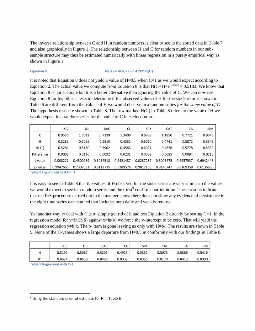
The inverse relationship between C and H in random numbers is clear to see in the sorted data in Table 7

and also graphically in Figure 1. The relationship between H and C for random numbers in our sub-

sample structure may thus be estimated numerically with linear regression in a purely empirical way as

shown in Figure 1.

Equation 8 ln(H) = -0.6572 - 0.4199*ln(C)

It is noted that Equation 8 does not yield a value of H=0.5 when C=1 as we would expect according to

Equation 2. The actual value we compute from Equation 8 is that H(C=1)=e-0.6572

= 0.5183. We know that

Equation 8 is not accurate but it is a better alternative than ignoring the value of C. We can now use

Equation 8 for hypothesis tests to determine if the observed values of H for the stock returns shown in

Table 6 are different from the values of H we would observe in a random series for the same value of C.

The hypothesis tests are shown in Table 8. The row marked H(C) in Table 8 refers to the value of H we

would expect in a random series for the value of C in each column.

IXIC DJI BAC CL SPX CAT BA IBM

C 0.9550 1.0012 0.7339 1.3406 0.6999 1.1850 0.7721 0.9346

H 0.5282 0.5065 0.5810 0.4352 0.6030 0.4741 0.5872 0.5548

H( C ) 0.5284 0.5180 0.5902 0.4583 0.6021 0.4826 0.5778 0.5332

Difference 0.0002 0.0116 0.0092 0.0231 0.0009 0.0085 0.0094 0.0216

t-value 0.008221 0.4500939 0.3054518 0.9421487 0.0287287 0.3006475 0.2957537 0.6942445

p-value 0.9947665 0.7307531 0.8112735 0.5189576 0.9817158 0.8140747 0.8169358 0.6136656

Table 8 Hypothesis test for H

It is easy to see in Table 8 that the values of H observed for the stock series are very similar to the values

we would expect to see in a random series and the t-test9 confirms our intuition. These results indicate

that the R/S procedure carried out in the manner shown here does not show any evidence of persistence in

the eight time series data studied that includes both daily and weekly returns.

Yet another way to deal with C is to simply get rid of it and test Equation 2 directly by setting C=1. In the

regression model for y=ln(R/S) against x=ln(υ) we force the y-intercept to be zero. That will yield the

regression equation y=b1x. The b0 term is gone leaving us only with H=b1. The results are shown in Table

9. None of the H-values shows a large departure from H=0.5 in conformity with our findings in Table 8.

IXIC DJI BAC CL SPX CAT BA IBM

H 0.5192 0.5067 0.5205 0.4925 0.5332 0.5073 0.5366 0.5416

R2 0.8624 0.8639 0.8498 0.8332 0.8355 0.8170 0.8413 0.8390

Table 9 Regression with C=1

9 Using the standard error of estimate for H in Table 6

5. CONCLUSIONS

It is proposed that the findings of persistence and chaotic behavior in stock returns by the application of

Rescaled Range Analysis are not real but artifacts of the methodology employed. The regression

procedure normally employed yields values for H and C and the interpretation of H in isolation without

consideration of the corresponding value of C can lead to spurious results. We also note that the practice

of averaging sub-sample R/S values and then using that average as if it were an observation can also

introduce serious errors in the estimation of H and the standard error of H. Yet another weakness of

conventional R/S research is the use of high values of α in hypothesis tests and the absence of Bonferroni

corrections for multiple comparisons. Under these circumstances we see no evidence of non-randomness

in R/S research. We conclude that stock returns are a random walk and that the weak form of the Efficient

Market Hypothesis has not been proven wrong by the R/S methodology.

6. REFERENCES

Bachelier, L. (1900). Théorie de la Spéculation. Annales Scientifique de l'École Normale .

Bohdalova, M. a. (2010). Markets, Information and their Fractal Analysis. Retrieved 2014, from g-casa.com:

http://www.g-casa.com/conferences/budapest/papers/Bohdalova.pdf

Bradley, L. (2010). Strange attractors. Retrieved 2014, from Space telescope science institute:

http://www.stsci.edu/~lbradley/seminar/attractors.html

Camerer, C. (1989). Bubbles and Fads in Asset Prices. Journal of Economic Surveys , 3-41.

Chen, N. R. (1983). Chen, Naifu, Economic forces and the stock market: testing the APT and alternate asset pricing

theories. Working pape .

Chen, N. (1983). Some empirical tests of the theory of arbitrage pricing. Journal of Finance , Dec p414.

Diba, B. (1988). The Theory of Rational Bubbles in Stock Prices. The Economic Journal , vol 98 No. 392 p746-754.

Dybvig, P. a. (1985). Yes, the APT is Testable. Journal of Finance .

Fama, E. (1970). Efficient Capital Markets: A Review of Theory and Empirical Work. Journal of Finance , 25 (2): 383–

417.

Fama, E. (1965). The Behavior of Stock Market Prices. Journal of Business , 38: 34–105.

Feder, J. (1988). Fractals. NY: Plenum Press.

Hurst, H. (1951). Long term storage capacity of reservoirs. Transactions of the American Society of Civil Engineers ,

Vol. 116, p770.

Jasic, T. (1998). Testing of nonlinearity and determinstic chaos in monthly Japanese stock market returns. Zagreb

International Review of Economics and Business , Vol. 1 No. 1 pp. 61-82.

Johnson, V. E. (2013, November). Revised Standards for Statistical Evidence. Retrieved December 2013, from

Proceedings of the National Academy of Sciences: http://www.pnas.org/content/110/48/19313.full

Kryzanowski, L. S. (1994). Kryzanowski, Lawrence, Simon LalSome tests of APT mispricing using mimicking

portfolios. Financial Review , v29: 2, p153.

Lorenz, E. (1963). Deterministic nonperiodic flow. Lorenz, Journal of the Atmospheric Sciences , 20 (2): 130–141.

Mahalingam, G. (2012). Persistence and long range dependence in Indian stock market returns. Retrieved 2014,

from IJMBS: http://www.ijmbs.com/24/gayathri.pdf

Mandelbrot, B. (1982). The Fractal Geometry of Nature. NY: Freeman.

Mandelbrot, B. (1963). The variation of certain speculative prices. Journal of Business , 36 (4): 394–419.

McKenzie, M. (1999). Non-periodic Australian stock market cycles. Retrieved 2014, from RMIT University:

http://mams.rmit.edu.au/ztghsoxhhjw1.pdf

Mundfrom, D. (2006). Bonferroni adjustments in tests for regression coefficients. Retrieved 2014, from University

of Northern Colorado: http://mlrv.ua.edu/2006/Mundfrom-etal-MLRV-3.pdf

Munshi, J. (2014). RS data archive. Retrieved 2014, from Dropbox:

https://www.dropbox.com/sh/bu1mdjtg9mvlmfa/AACLwFys7FMblJzJPGandpjfa

Osborne, M. (1959). Brownian motion in the stock market. Operations Research vol 7 , 145-173.

Pallikari, F. a. (1999). A rescaled range analysis of random events. Journal of Scientific Exploration , Vol 13. No. 1

pp. 25-40.

Peters, E. (1991). A Chaotic Attractor for the S&P500. Financial Analysts Journal , Vol.47 No. 2 p55.

Peters, E. (1991). Chaos and order in the capital markets : a new view of cycles, prices, and market volatility. NY:

John Wiley and Sons.

Peters, E. (1994). Fractal market analysis. NY: John Wiliey and Sons.

Roll, R. (1977). A critique of the asset pricing theory's tests. Journal of Financial Economics , March, p129.

Roll, R. a. (1980). An empirical investigation of the arbitrage pricing theory. Journal of Finance , Dec p1073.

Roll, R. a. (1980). Roll,An empirical investigation of the arbitrage pricing theory. Journal of Finance , p1073.

Ross, S. (1976). The arbitrage theory of capital pricing. Journal of Economic Theory , v13, p341, 1976.

Scheinkman, J. (1989). Nonlinear dynamics and stock returns. Journal of Business , Vol. 62 p. 311.

Schouten, J. (1994). Estimation of the dimension of a noisy attractor. Retrieved 2014, from Google Scholar:

http://scholar.google.co.th/scholar_url?hl=en&q=http://repository.tudelft.nl/assets/uuid:bd5339a0-24e5-4362-

b378-

adc7c60cac99/aps_schouten_1994.pdf&sa=X&scisig=AAGBfm36mO9vIeHfx7XnQ_zLbcHlaxZD6Q&oi=scholarr&ei=

mkRzU92RKYSskAXfz4D4BA&ved=0CCoQgAMoADAA

Shanken, J. (1982). The arbitrage pricing theory: is it testable? Retrieved 2014, from The University of Utah:

http://home.business.utah.edu/finmll/fin787/papers/shanken1982.pdf

Shanken, J. (1982). The Arbitrage Pricing Theory: Is it Testable? Journal of Finance , 1129-1140.

Sharpe, W. (1962). A simplified model for porftolio returns. Management Science , p277.

Sharpe, W. (1964). Capital asset prices: a theory of market equilibrium under conditions of risk. Journal of Finance ,

v19, p425.

Takens, F. (1981). Detecting strange attractors in turbulence. In D. A.-S. Young, Dynamical Systems and Turbulence

(pp. 366-381). Springer-Verlag.

University of South Carolina. (2014). Multicollinearity and variance inflation factors. Retrieved 2014, from

University of South Carolina: http://www.stat.sc.edu/~hansont/stat704/vif_704.pdf

Virginia Tech. (2014). Methods for multiple linear regression analysis. Retrieved 2014, from vt.edu:

http://scholar.lib.vt.edu/theses/available/etd-219182249741411/unrestricted/Apxd.pdf

White, H. (1988). Economic prediction using neural networks: the case of IBM daily stock returns. White, H.,

"Economic prediction using neuraNeural Networks IEEE International Conference , White, H., "Economic prediction

using neural networks: the case of IBM daily stock returpp.451,458 vol.2.

Wikipedia. (2014). Autoregressive Model. Retrieved 2014, from Wikipedia:

http://en.wikipedia.org/wiki/Autoregressive_model

Wikipedia. (2014). Correlation dimension. Retrieved 2014, from Wikipedia:

http://en.wikipedia.org/wiki/Correlation_dimension

Wikipedia. (2014). Roll's Critique. Retrieved 2014, from wikipedia: http://en.wikipedia.org/wiki/Roll's_critique

Zeeman, E. (1976). Catatstrophe Theory. Scientific American , 65-83.

Zeeman, E. (1974). On the unstable behavior of stock exchanges. Journal of Mathematical Economics , 39-49.

APPENDIX

The Microsoft Excel file that computes R/S values is called "rescaled range analysis worksheet". Use paste values to

put a column of returns data of sample size 2486 starting on cell A6 of the worksheet called "RS Computation".

Then go to the worksheet called "Regression". All your R/S values are there along with the regression results.