The weak lambda calculus as a reasonable machine

The Weak Lambda Calculus

as a Reasonable Machine ?

Ugo Dal Lago and Simone Martini ∗

Dipartimento di Scienze dell’Informazione, Universita di Bologna,Mura Anteo Zamboni 7, 40127 Bologna, Italy.

Abstract

We define a new cost model for the call-by-value lambda-calculus satisfying theinvariance thesis. That is, under the proposed cost model, Turing machines andthe call-by-value lambda-calculus can simulate each other within a polynomial timeoverhead. The model only relies on combinatorial properties of usual beta-reduction,without any reference to a specific machine or evaluator. In particular, the cost of asingle beta reduction is proportional to the difference between the size of the redexand the size of the reduct. In this way, the total cost of normalizing a lambda termwill take into account the size of all intermediate results (as well as the number ofsteps to normal form).

Key words: Lambda calculus, Computational complexity, Invariance thesis, Costmodel

1 Introduction

Any computer science student knows that all computational models are exten-sionally equivalent, each of them characterizing the same class of computablefunctions. However, the definition of complexity classes by means of computa-tional models must take into account several differences between these models,in order to rule out unrealistic assumptions about the cost of the computationsteps. It is then usual to consider only reasonable models, in such a way thatthe definition of complexity classes remain invariant when given with referenceto any such reasonable model. If polynomial time is the main concern, thisrequirement takes the form of the invariance thesis [15]:

? Extended and revised version of [5], presented at Computability in Europe 2006.∗ Corresponding author.

Preprint submitted to Elsevier Science

Reasonable machines can simulate each other within a polynomially-boundedoverhead in time and a constant-factor overhead in space.

Once we agree that Turing machines provide the basic computational model,then many other machine models are proved to satisfy the invariance thesis.Preliminary to the proof of polynomiality of the simulation on a given machine,is the definition of a cost model, stipulating when and how much one shouldaccount for time and/or space during the computation. For some machines(e.g., Turing machines) this cost model is obvious; for others it is much lessso. An example of the latter kind is the type-free lambda-calculus, where thereis not a clear notion of constant time computational step, and it is even lessclear how one should count for consumed space.

The idea of counting the number of beta-reductions [8] is just too naıve, be-cause beta-reduction is inherently too complex to be considered as an atomicoperation, at least if we stick to explicit representations of lambda terms.Indeed, in a beta step

(λx.M)N →M{x/N},there can be as many as |M | occurrences of x inside M . As a consequence,M{x/N} can be as big as |M ||N |. As an example, consider the term n 2, wheren ≡ λx.λy.xny is the Church numeral for n. Under innermost reduction thisterm reduces to normal form in 3n− 1 beta steps, but there is an exponentialgap between this quantity and the time needed to write the normal form, thatis 2n. Under outermost reduction, however, the normal form is reached in anexponential number of beta steps. This simple example shows that taking thenumber of beta steps to normal form as the cost of normalization is at leastproblematic. Which strategy should we choose 1 ? How do we account for thesize of intermediate (and final) results?

Clearly, a viable option consists in defining the cost of reduction as the timeneeded to normalize a term by another reasonable abstract machine, e.g. aTuring machine. However, in this way we cannot compute the cost of reduc-tion from the structure of the term, and, as a result, it is difficult to computethe cost of normalization for particular terms or for classes of terms. Anotherinvariant cost model is given by the actual cost of outermost (normal order)evaluation, naively implemented [11]. Despite its invariance, it is a too gener-ous cost model (and in its essence not much different from the one that countsthe numbers of steps needed to normalize a term on a Turing machine). Whatis needed is a machine-independent, parsimonious, and invariant cost model.Despite some attempts [9,11,12] (which we will discuss shortly), a cost model

1 Observe that we cannot take the length of the longest reduction sequence, becausein several cases this would involve too much useless work. Indeed, there are non-strongly-normalizing terms that can be normalized in one single step, and yet donot admit a longest finite reduction sequence (e.g., F (∆ ∆)).

2

of this kind has not appeared yet.

To simplify things, we attack in this paper the problem for the weak call-by-value lambda-calculus, where we do not reduce under an abstraction and wealways fully evaluate an argument before firing a beta redex. Although simple,it is a calculus of paramount importance, since it is the reduction model ofany call-by-value functional programming language. For this calculus we de-fine a new, machine-independent cost model and we prove that it satisfies theinvariance thesis for time. The proposed cost model only relies on combina-torial properties of usual beta-reduction, without any reference to a specificmachine or evaluator. The basic idea is to let the cost of performing a beta-reduction step depend on the size of the involved terms. In particular, thecost of M → N will be related to the difference |N | − |M |. In this way, thetotal cost of normalizing a lambda term will take into account the size of allintermediate results (as well as the number of steps to normal form). The lastsection of the paper will apply this cost model to the combinatory algebra ofclosed lambda-terms, to establish some results needed in [4]. We remark thatin this algebra the universal function (which maps two terms M and N tothe normal form of MN) adds only a constant overhead to the time neededto normalize MN . This result, which is almost obvious when viewed from theperspective of lambda-calculus, is something that cannot be obtained in therealm of Turing machines.

1.1 Previous Work

The two main attempts to define an invariant cost model share the referenceto optimal lambda reduction a la Levy [13], a parallel strategy minimizing thenumber of (parallel) beta steps (see [2]).

Frandsen and Sturtivant [9] propose a cost model essentially based on thenumber of parallel beta steps to normal form. Their aim is to propose a mea-sure of efficiency for functional programming language implementations. Theyshow how to simulate Turing machines in the lambda calculus with a poly-nomial overhead. However, the paper does not present any evidence on theexistence of a polynomial simulation in the other direction. As a consequence,it is not known whether their proposal is invariant.

More interesting contributions come from the literature of the nineties on op-timal lambda reduction. Lamping [10] was the first to operationally presentthis strategy as a graph rewriting procedure. The interest of this technique forour problem stems from the fact that a single beta step is decomposed intoseveral elementary steps, allowing for the duplication of the argument, thecomputation of the levels of nesting inside abstractions, and additional book-

3

keeping work. Since any such elementary step is realizable on a conventionalmachine in constant time, Lamping’s algorithm provides a theoretical basisfor the study of complexity of a single beta step. Lawall and Mairson [11] giveresults on the efficiency of optimal reduction algorithms, highlighting the so-called bookkeeping to be the bottleneck from the point ot view of complexity.A consequence of Lawall and Mairson’s work is evidence on the inadequacy ofthe cost models proposed by Frandsen and Sturtivant and by Asperti [1], atleast from the point of view of the invariance thesis. In subsequent work [12],Lawall and Mairson proposed a cost model for the lambda calculus basedon Levy’s labels. They further proved that Lamping’s abstract algorithm sat-isfies the proposed cost model. This, however, does not imply by itself theexistence of an algorithm normalizing any lambda term with a polynomialoverhead (on the proposed cost). Moreover, studying the dynamic behaviourof Levy labels is clearly more difficult than dealing directly with the numberof beta-reduction steps.

1.2 Research Directions

The results of this paper should be seen as a first step of a broader projectto study invariant cost models for several λ-calculi. In particular, we haveevidence that for some calculi and under certain conditions we can take thenumber of beta reduction steps as an invariant cost model. Indeed, take theweak call-by-value calculus and suppose you are allowed to exploit sharingduring reduction by adopting implicit representations of lambda-terms. Weconjecture that the normal form of any term M can be computed in timeO(p(|M |, n)), where p is a fixed polynomial and n is the number of beta stepsto normal form. This result crucially depends on the ability of exploitingsharing and cannot be obtained when working with explicit representationsof lambda-terms. But at this point the question is the following: should wetake into account the time needed to produce the explicit normal form fromits implicit representation?

Moreover, we are confident that simple cost models could be defined for thehead linear reduction [6] and for the weak calculus with sharing [3].

2 Syntax

The language we study is the pure untyped lambda-calculus endowed withweak (that is, we never reduce under an abstraction) and call-by-value reduc-tion. Constants are not needed, since usual data structures can be encodedin the pure fragment of the calculus, as we are going to detail in Section 4.

4

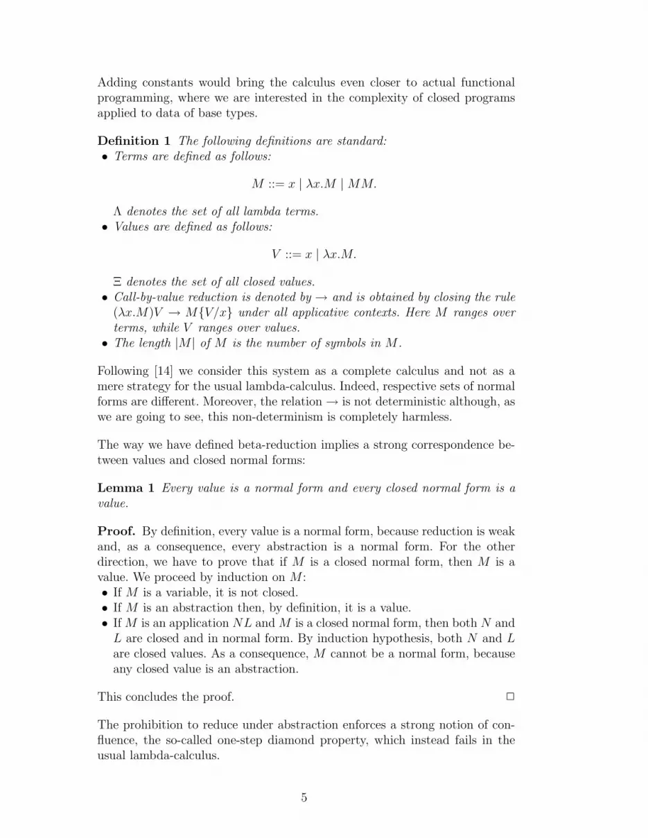
Adding constants would bring the calculus even closer to actual functionalprogramming, where we are interested in the complexity of closed programsapplied to data of base types.

Definition 1 The following definitions are standard:• Terms are defined as follows:

M ::= x | λx.M |MM.

Λ denotes the set of all lambda terms.• Values are defined as follows:

V ::= x | λx.M.

Ξ denotes the set of all closed values.• Call-by-value reduction is denoted by → and is obtained by closing the rule

(λx.M)V → M{V/x} under all applicative contexts. Here M ranges overterms, while V ranges over values.• The length |M | of M is the number of symbols in M .

Following [14] we consider this system as a complete calculus and not as amere strategy for the usual lambda-calculus. Indeed, respective sets of normalforms are different. Moreover, the relation→ is not deterministic although, aswe are going to see, this non-determinism is completely harmless.

The way we have defined beta-reduction implies a strong correspondence be-tween values and closed normal forms:

Lemma 1 Every value is a normal form and every closed normal form is avalue.

Proof. By definition, every value is a normal form, because reduction is weakand, as a consequence, every abstraction is a normal form. For the otherdirection, we have to prove that if M is a closed normal form, then M is avalue. We proceed by induction on M :• If M is a variable, it is not closed.• If M is an abstraction then, by definition, it is a value.• If M is an application NL and M is a closed normal form, then both N and

L are closed and in normal form. By induction hypothesis, both N and Lare closed values. As a consequence, M cannot be a normal form, becauseany closed value is an abstraction.

This concludes the proof. 2

The prohibition to reduce under abstraction enforces a strong notion of con-fluence, the so-called one-step diamond property, which instead fails in theusual lambda-calculus.

5

Proposition 1 (Diamond Property) If M → N and M → L then eitherN ≡ L or there is P such that N → P and L→ P .

Proof. By induction on the structure of M . Clearly, M cannot be a variablenor an abstraction so M ≡ QR. We can distinguish two cases:• If M is a redex (λx.T )R (where R is a value), then N ≡ L ≡ T{x/R},

because we cannot reduce under lambdas.• If M is not a redex, then reduction must take place inside Q or R. We can

distinguish four sub-cases:• If N ≡ TR and L ≡ UR, where Q→ T and Q→ U , then we can apply

the induction hypothesis.• Similarly, if R→ T and R→ U , where N ≡ QT and L ≡ QU , then we

can apply the induction hypothesis.• If N ≡ QT and L ≡ UR, where R→ T and Q→ U , then N → UT and

L→ UT .• Similarly, if N ≡ UR and L ≡ QT , where R → T and Q → U , then

N → UT and L→ UT .


As an easy corollary of Proposition 1 we get an equivalence between all normal-ization strategies— once again a property which does not hold in the ordinarylambda-calculus. This is a well-known consequence of the diamond property:

Corollary 1 (Strategy Equivalence) M has a normal form iff M is stronglynormalizing.

Proof. Observe that, by Proposition 1, if M is diverging and M → N , thenN is diverging, too. Indeed, if M ≡M0 →M1 →M2 → . . ., then we can builda sequence N ≡ N0 → N1 → N2 → . . . in a coinductive way:• If M1 ≡ N , then we define Ni to be Mi+1 for every i ≥ 1.• If M1 6≡ N then by proposition 1 there is N1 such that M1 → N1 and

N0 → N1.

Now, we prove by induction on n that if M →n N , with N normal form,then M is strongly normalizing. If n = 0, then M is a normal form, thenstrongly normalizing. If n ≥ 1, assume, by way of contraddiction, that M isnot strongly normalizing. Let L be a term such that M → L→n−1 N . By theabove observation, L cannot be strongly normalizing, but this goes againstthe induction hypothesis. This concludes the proof. 2

But we can go even further: in this setting, the number of beta-steps to thenormal form does not depend on the evaluation strategy.

Lemma 2 (Parametrical Diamond Property) If M →n N and M →m

L then there is a term P such that N →l P and L→k P where l ≤ m, k ≤ n

6

and n + l = m + k.

Proof. We will proceed by induction on n + m. If n + m = 0, then P willbe N ≡ L ≡ M . If n + m > 0 but either n = 0 or m = 0, the thesis easilyfollows. So, we can assume both n > 0 and m > 0. Let now Q and R be termssuch that M → Q→n−1 N and M → R→m−1 L. From Proposition 1, we candistinguish two cases:• Q ≡ R, By induction hypothesis, we know there is T such that N →l T

and L →k T , where l ≤ m − 1 ≤ m, and k ≤ n − 1 ≤ n. Moreover(n− 1) + l = (m− 1) + k, which yields n + l = m + k.• There is T with Q → T and R → T . By induction hypothesis, there are

two terms U,W such that T →i U , T →j W , N →p U , L →q W , wherei ≤ n− 1, j ≤ m− 1, p, q ≤ 1, n− 1 + p = 1 + i and m− 1 + q = 1 + j. Byinduction hypothesis, there is P such that U →r P and W →s P , wherer ≤ j, s ≤ i and r + i = s + j. But, summing up, this implies

N→p+r P

L→q+s P

p + r ≤ 1 + j ≤ 1 + m− 1 = m

q + s ≤ 1 + i ≤ 1 + n− 1 = n

p + r + n = (n− 1 + p) + 1 + r = 1 + i + 1 + r

= 2 + r + i = 2 + s + j = 1 + 1 + j + s

= 1 + m− 1 + q + s = q + s + n.


The following result summarizes what we have obtained so far:

Proposition 2 For every term M , there are at most one normal form Nand one integer n such that M →n N .

Proof. Suppose M →n N and M →m L, with N and L normal forms. Then,by lemma 2, there are P, k, l such that N →l P and L→k P and n+l = m+k.But since N and L are normal forms, P ≡ N , P ≡ L and l = k = 0, whichyields N ≡ L and n = m. 2

Given a term M , the number of steps needed to rewrite M to its normal form(if the latter exists) is uniquely determined. As we sketched in the introduction,however, this cannot be considered as the cost of normalizing M , at least ifan explicit representation of the normal form is to be produced as part of thecomputational process.

7

3 An Abstract Time Measure

We can now define an abstract time measure and prove some of its properties.The rest of the paper is devoted to proving the invariance of the calculus withrespect to this computational model.

Intuitively, every beta-step will be endowed with a positive integer cost bound-ing the difference (in size) between the reduct and the redex. The sum of costsof all steps to normal form gives the cost of normalizing a term.Definition 2 • Concatenation of α, β ∈ N∗ is simply denoted as αβ.• � will denote a subset of Λ × N∗ × Λ. In the following, we will write

Mα� N standing for (M, α, N) ∈�. The definition of � (in SOS-style)

is the following:

Mε

� M

M → N n = max{1, |N | − |M |}

M(n)� N

Mα� N N

β� L

Mαβ� L

Observe we charge max{1, |N | − |M |} for every step M → N . In this way,the cost of a beta-step will always be positive.• Given α = (n1, . . . , nm) ∈ N∗, define ||α|| = ∑m

i=1 ni.

Observe that Mα� N iff M →|α| N , where |α| is the length of α as a sequence

of natural numbers. This can easily be proved by induction on the derivation

of Mα� N .

In principle, there could be M, N, α, β such that Mα� N , M

β� N and

||α|| 6= ||β||. The confluence properties we proved in the previous section,however, can be lifted to this new notion of weighted reduction. First of all,the diamond property and its parameterized version can be reformulated asfollows:

Proposition 3 (Diamond Property Revisited) If M(n)� N and M

(m)� L,

then either N ≡ L or there is P such that N(m)� P and L

(n)� P .

Proof. We can proceed as in Proposition 1. Observe that if Mα� N , then

MLα� NL and LM

α� LN . We go by induction on the structure of M .

Clearly, M cannot be a variable nor an abstraction so M ≡ QR. We candistinguish five cases:• If Q ≡ λx.T and R is a value, then N ≡ L ≡ T{x/R}, because R is a

variable or an abstraction.

• If N ≡ TR and L ≡ UR, where Q(n)� T and Q

(m)� U , then we can apply

the induction hypothesis, obtaining that T(m)� W and U

(n)� W . This, in

8

turn, implies N(m)� WR and L

(n)� WR.

• Similarly, if N ≡ QT and L ≡ QU , where R(n)� T and R

(m)� U , then we

can apply the induction hypothesis.

• If N ≡ QT and L ≡ UR, where R(n)� T and Q

(m)� U , then N

(m)� UT and

L(n)� UT .

• Similarly, if N ≡ UR and L ≡ QT , where R(n)� T and Q

(m)� U , then

N(m)� UT and L

(n)� UT .


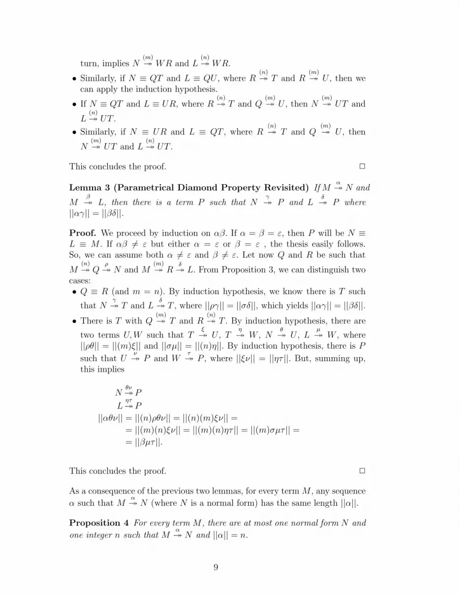
Lemma 3 (Parametrical Diamond Property Revisited) If Mα� N and

Mβ� L, then there is a term P such that N

γ� P and L

δ� P where

||αγ|| = ||βδ||.

Proof. We proceed by induction on αβ. If α = β = ε, then P will be N ≡L ≡ M . If αβ 6= ε but either α = ε or β = ε , the thesis easily follows.So, we can assume both α 6= ε and β 6= ε. Let now Q and R be such that

M(n)� Q

ρ� N and M

(m)� R

δ� L. From Proposition 3, we can distinguish two

cases:• Q ≡ R (and m = n). By induction hypothesis, we know there is T such

that Nγ� T and L

δ� T , where ||ργ|| = ||σδ||, which yields ||αγ|| = ||βδ||.

• There is T with Q(m)� T and R

(n)� T . By induction hypothesis, there are

two terms U,W such that Tξ� U , T

η� W , N

θ� U , L

µ� W , where

||ρθ|| = ||(m)ξ|| and ||σµ|| = ||(n)η||. By induction hypothesis, there is P

such that Uν� P and W

τ� P , where ||ξν|| = ||ητ ||. But, summing up,

this implies

Nθν� P

Lητ� P

||αθν|| = ||(n)ρθν|| = ||(n)(m)ξν|| == ||(m)(n)ξν|| = ||(m)(n)ητ || = ||(m)σµτ || == ||βµτ ||.


As a consequence of the previous two lemmas, for every term M , any sequence

α such that Mα� N (where N is a normal form) has the same length ||α||.

Proposition 4 For every term M , there are at most one normal form N and

one integer n such that Mα� N and ||α|| = n.

9

Proof. Suppose Mα� N and M

β� L, with N and L normal forms. Then, by

Lemma 2, there are P, γ, δ such that Nγ� P and L

δ� P and ||αγ|| = ||βδ||.

But since N and L are normal forms, P ≡ N , P ≡ L and γ = δ = ε, whichyields N ≡ L and ||α|| = ||β||. 2

We are now ready to define the abstract time measure which is the core of thepaper.

Definition 3 (Difference cost model) If Mα� N , where N is a normal

form, then Time(M) is ||α||+ |M |. If M diverges, then Time(M) is infinite.

Observe that this is a good definition, in view of Proposition 4. In other

words, showing Mα� N suffices to prove Time(M) = ||α|| + |M |. This will

be particularly useful in the following section.

As an example, consider again the term n 2 we discussed in the introduction.It reduces to normal form in one step, because we do not reduce under theabstraction. To force reduction, consider E ≡ n 2 x, where x is a (free)variable; E reduces to

F ≡ λyn.(λyn−1 . . . (λy2.(λy1.x2y1)

2y2)2 . . .)2yn

in Θ(n) beta steps. However, Time(E) = Θ(2n), since at any step the size ofthe term is duplicated. Indeed, the size of F is exponential in n.

4 Simulating Turing Machines

In this and the following sections we will show that the difference cost modelsatisfies the polynomial invariance thesis. The present section shows how toencode Turing machines into the lambda calculus.

The first thing we need to encode is a form of recursion. We denote by H theterm MM , where M ≡ λx.λf.f(λz.xxfz). H is a call-by-value fixed-pointoperator: for every value N , there is α such that

HNα� N(λz.HNz),

||α|| = O(|N |).

The lambda term H provides the necessary computational expressive powerto encode the whole class of computable functions.

The simplest objects we need to encode in the lambda-calculus are finite sets.

10

Elements of any finite set A = {a1, . . . , an} can be encoded as follows:

paiqA ≡ λx1. . . . .λxn.xi .

Notice that the above encoding induces a total order on A such that ai ≤ aj

iff i ≤ j.

Other useful objects are finite strings over an arbitrary alphabet, which willbe encoded using a scheme attributed to Scott [16]. Let Σ = {a1, . . . , an} bea finite alphabet. A string in s ∈ Σ∗ can be represented by a value psqΣ∗

asfollows, by induction on s:

pεqΣ∗ ≡λx1. . . . .λxn.λy.y ,

paiuqΣ∗ ≡λx1. . . . .λxnλy.xipuqΣ∗.

Observe that representations of symbols in Σ and strings in Σ∗ depend on thecardinality of Σ. In other words, if u ∈ Σ∗ and Σ ⊂ ∆, puqΣ∗ 6= puq∆∗

. Besidesdata, we want to be able to encode functions between them. In particular, theway we have defined numerals lets us concatenate two strings in linear timein the underlying lambda calculus. In some situations, it is even desirable toconcatenate a string with the reversal of another string.

Lemma 4 Given a finite alphabet Σ, there are terms AC (Σ), AS (Σ) andAR(Σ) such that for every a ∈ Σ and u, v ∈ Σ∗ there are α, β, γ such that

AC (Σ)paqΣpuqΣ∗ α� pauqΣ∗

,

AS (Σ)puqΣ∗pvqΣ∗ β

� puvqΣ∗,

AR(Σ)puqΣ∗pvqΣ∗ γ

� purvqΣ∗,

and

||α||= O(1),

||β||= O(|u|),||γ||= O(|u|).

Proof. The three terms are defined as follows:

11

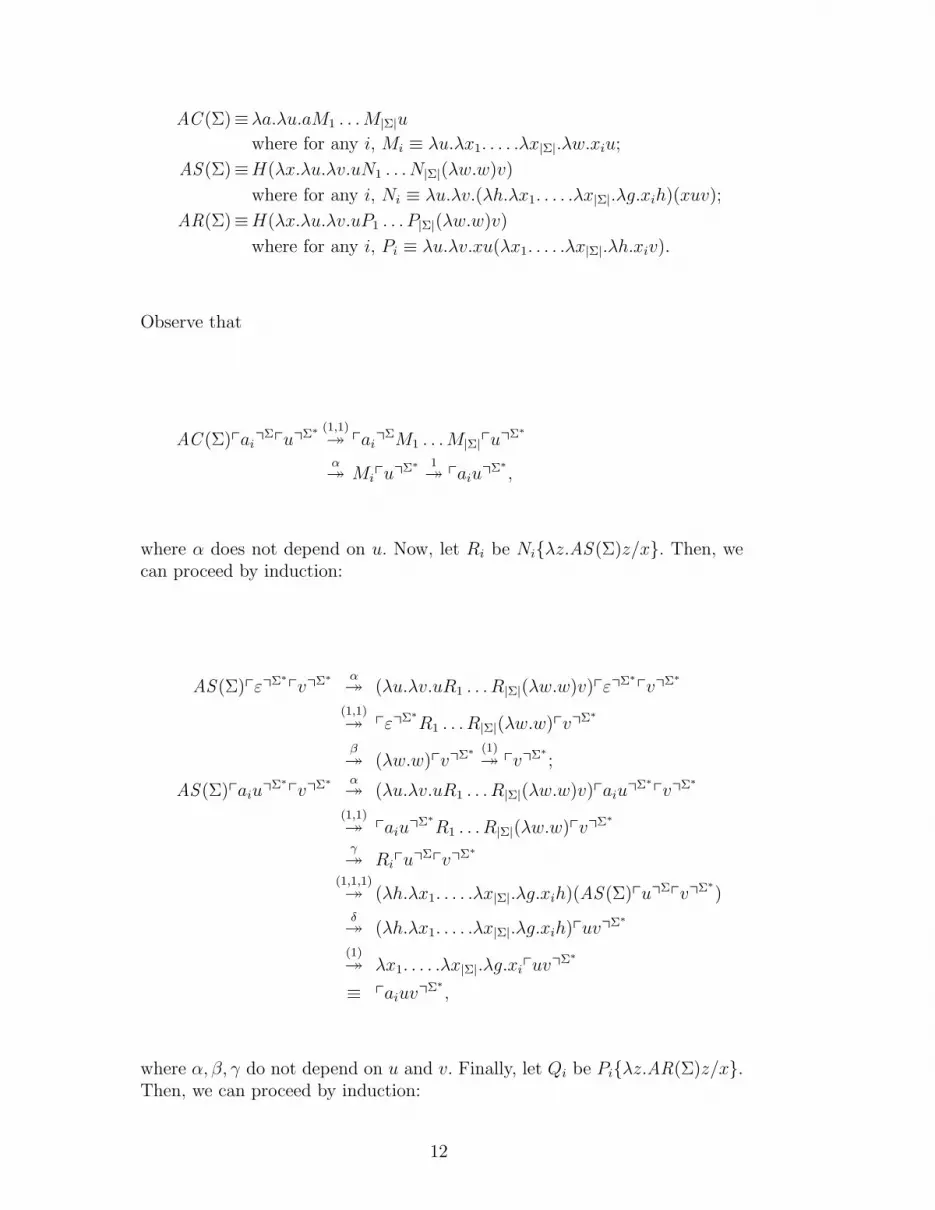
AC (Σ)≡λa.λu.aM1 . . . M|Σ|u

where for any i, Mi ≡ λu.λx1. . . . .λx|Σ|.λw.xiu;

AS (Σ)≡H(λx.λu.λv.uN1 . . . N|Σ|(λw.w)v)

where for any i, Ni ≡ λu.λv.(λh.λx1. . . . .λx|Σ|.λg.xih)(xuv);

AR(Σ)≡H(λx.λu.λv.uP1 . . . P|Σ|(λw.w)v)

where for any i, Pi ≡ λu.λv.xu(λx1. . . . .λx|Σ|.λh.xiv).

Observe that

AC (Σ)paiqΣpuqΣ∗ (1,1)

� paiqΣM1 . . . M|Σ|puqΣ∗

α� MipuqΣ∗ 1

� paiuqΣ∗,

where α does not depend on u. Now, let Ri be Ni{λz.AS (Σ)z/x}. Then, wecan proceed by induction:

AS (Σ)pεqΣ∗pvqΣ∗ α

� (λu.λv.uR1 . . . R|Σ|(λw.w)v)pεqΣ∗pvqΣ∗

(1,1)� pεqΣ∗

R1 . . . R|Σ|(λw.w)pvqΣ∗

β� (λw.w)pvqΣ∗ (1)

� pvqΣ∗;

AS (Σ)paiuqΣ∗pvqΣ∗ α

� (λu.λv.uR1 . . . R|Σ|(λw.w)v)paiuqΣ∗pvqΣ∗

(1,1)� paiuqΣ∗

R1 . . . R|Σ|(λw.w)pvqΣ∗

γ� RipuqΣpvqΣ∗

(1,1,1)� (λh.λx1. . . . .λx|Σ|.λg.xih)(AS (Σ)puqΣpvqΣ∗

)δ� (λh.λx1. . . . .λx|Σ|.λg.xih)puvqΣ∗

(1)� λx1. . . . .λx|Σ|.λg.xipuvqΣ∗

≡ paiuvqΣ∗,

where α, β, γ do not depend on u and v. Finally, let Qi be Pi{λz.AR(Σ)z/x}.Then, we can proceed by induction:

12

AR(Σ)pεqΣ∗pvqΣ∗ α

� (λu.λv.uQ1 . . . Q|Σ|(λw.w)v)pεqΣ∗pvqΣ∗

(1,1)� pεqΣ∗

Q1 . . . Q|Σ|(λw.w)pvqΣ∗

β� (λw.w)pvqΣ∗ (1)

� pvqΣ∗;

AR(Σ)paiuqΣ∗pvqΣ∗ α

� (λu.λv.uQ1 . . . Q|Σ|(λw.w)v)paiuqΣ∗pvqΣ∗

(1,1)� paiuqΣ∗

Q1 . . . Q|Σ|(λw.w)pvqΣ∗

γ� QipuqΣpvqΣ∗

(1,1,1)� AR(Σ)puqΣpaivqΣ∗

δ� puraivqΣ∗ ≡ p(aiu)rvqΣ∗

,

where α, β, γ do not depend on u, v. 2

The encoding of a string depends on the underlying alphabet. As a conse-quence, we also need to be able to convert representations for strings in onealphabet to corresponding representations in a bigger alphabet. This can bedone efficiently in the lambda-calculus.

Lemma 5 Given two finite alphabets Σ and ∆, there are terms CC (Σ, ∆)and CS (Σ, ∆) such that for every a0, a1, . . . , an ∈ Σ there are α and β with

CC (Σ, ∆)pa0qΣ α

� pu0q∆∗

;

CS (Σ, ∆)pa1 . . . anqΣ∗ β

� pu1 . . . unq∆∗

;

where for any i, ui =

ai if ai ∈ ∆

ε otherwise,

and

||α||= O(1),

||β||= O(n).

Proof. The two terms are defined as follows:

13

CC (Σ, ∆)≡λa.aM1 . . . M|Σ| ,

where for any i, Mi ≡

paiq∆∗if ai ∈ ∆

pεq∆∗otherwise.

CS (Σ, ∆)≡H(λx.λu.uN1 . . . N|Σ|(pεq∆∗)),

where for any i, Ni ≡

λu.(λv.λx1. . . . .λx|∆|.λh.xiv)(xu) if ai ∈ ∆

λu.xu otherwise.

Observe that

CC (Σ, ∆)paiqΣ

(1)� paiq

ΣM1 . . . M|Σ|

α�

paiq∆∗if ai ∈ ∆

pεq∆∗otherwise.

Let Pi be Ni{λz.CS (Σ, ∆)z/x}. Then:

CS (Σ, ∆)pεqΣ∗ α� (λu.uP1 . . . P|Σ|pεq∆∗

)pεqΣ∗

(1)� pεqΣ∗

P1 . . . P|Σ|pεq∆∗

β� pεq∆∗

;

CS (Σ, ∆)paiuqΣ∗ γ� (λu.uP1 . . . P|Σ|pεq∆∗

)paiuqΣ∗

(1)� paiuqΣ∗

P1 . . . P|Σ|pεq∆∗

δ� PipuqΣ∗

(1,1)�

(λv.λx1. . . . .λx|∆|.λh.xiv)(CS (Σ, ∆)puqΣ∗) if ai ∈ ∆

CS (Σ, ∆)puqΣ∗otherwise,

where α, β, γ, δ do not depend on u. 2

A deterministic Turing machineM is a tuple (Σ, ablank , Q, qinitial , qfinal , δ) con-sisting of:• A finite alphabet Σ = {a1, . . . , an};• A distinguished symbol ablank ∈ Σ, called the blank symbol ;• A finite set Q = {q1, . . . , qm} of states ;• A distinguished state qinitial ∈ Q, called the initial state;• A distinguished state qfinal ∈ Q, called the final state;• A partial transition function δ : Q × Σ ⇀ Q × Σ × {←,→, ↓} such that

δ(qi, aj) is defined iff qi 6= qfinal .

14

A configuration for M is a quadruple in Σ∗ × Σ × Σ∗ × Q. For example, ifδ(qi, aj) = (ql, ak,←), then M evolves from (uap, aj, v, qi) to (u, ap, akv, ql)(and from (ε, aj, v, qi) to (ε, ablank , akv, ql)). A configuration like (u, ai, v, qfinal)is final and cannot evolve. Given a string u ∈ Σ∗, the initial configurationfor u is (ε, a, v, qinitial) if u = av and (ε, ablank , ε, qinitial) if u = ε. The stringcorresponding to the final configuration (u, ai, v, qfinal) is uaiv.

A Turing machine (Σ, ablank , Q, qinitial , qfinal , δ) computes the function f : ∆∗ →∆∗ (where ∆ ⊆ Σ) in time g : N → N iff for every u ∈ ∆∗, the initialconfiguration for u evolves to a final configuration for f(u) in g(|u|) steps.

A configuration (s, a, v, q) of a machine M = (Σ, ablank , Q, qinitial , qfinal , δ) isrepresented by the term

p(u, a, v, q)qM ≡ λx.xpurqΣ∗paqΣ pvqΣ∗

pqqQ.

We now encode a Turing machine M = (Σ, ablank , Q, qinitial , qfinal , δ) in thelambda-calculus. Suppose Σ = {a1, . . . , a|Σ|} and Q = {q1, . . . , q|Q|} We pro-ceed by building up three lambda terms:• First of all, we need to be able to build the initial configuration for u from

u itself. This can be done in linear time.• Then, we need to extract a string from a final configuration for the string.

This can be done in linear time, too.• Most importantly, we need to be able to simulate the transition function

ofM, i.e. compute a final configuration from an initial configuration (if itexists). This can be done with cost proportional to the number of stepsMtakes on the input.

The following three lemmas formalize the above intuitive argument:

Lemma 6 Given a Turing machine M = (Σ, ablank , Q, qinitial , qfinal , δ) andan alphabet ∆ ⊆ Σ there is a term I(M, ∆) such that for every u ∈ ∆∗,

I(M, ∆)puq∆∗ α� pCqM where C is the initial configuration for u and ||α|| =

O(|u|).

Proof. I(M, ∆) is defined as

H(λx.λu.uM1 . . . M|∆|N),

where

N ≡ p(ε, ablank , ε, qinitial)qM;

Mi≡λu.(xu)(λu.λa.λv.λq.(λw.(λx.xupaiqΣwq))(AC (Σ)av)).

Let Pi be Mi{λz.I(M, ∆)z/x}. Then,

15

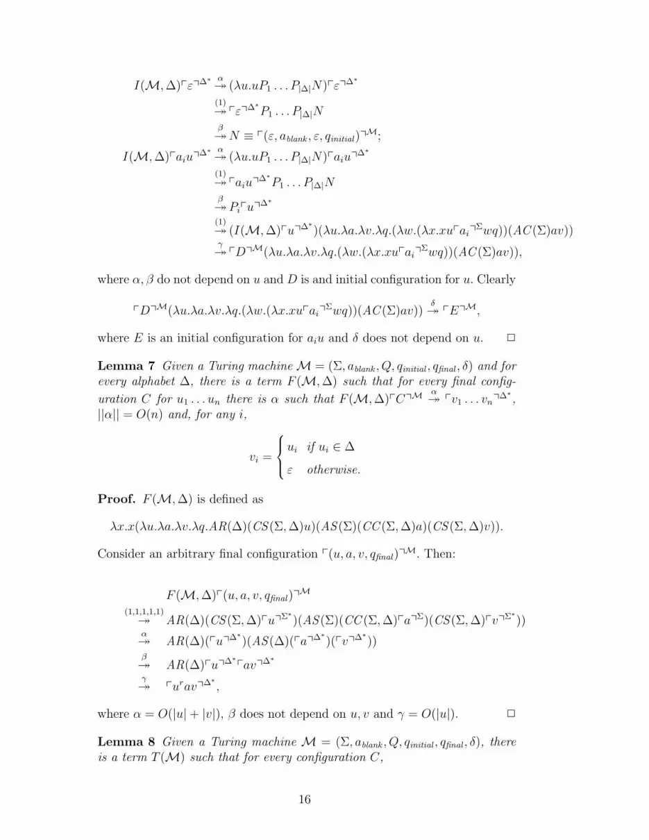
I(M, ∆)pεq∆∗ α� (λu.uP1 . . . P|∆|N)pεq∆∗

(1)� pεq∆∗

P1 . . . P|∆|Nβ� N ≡ p(ε, ablank , ε, qinitial)q

M;

I(M, ∆)paiuq∆∗ α� (λu.uP1 . . . P|∆|N)paiuq∆∗

(1)� paiuq∆∗

P1 . . . P|∆|Nβ� Pipuq∆∗

(1)� (I(M, ∆)puq∆∗

)(λu.λa.λv.λq.(λw.(λx.xupaiqΣwq))(AC (Σ)av))

γ� pDqM(λu.λa.λv.λq.(λw.(λx.xupaiq

Σwq))(AC (Σ)av)),

where α, β do not depend on u and D is and initial configuration for u. Clearly

pDqM(λu.λa.λv.λq.(λw.(λx.xupaiqΣwq))(AC (Σ)av))

δ� pEqM,

where E is an initial configuration for aiu and δ does not depend on u. 2

Lemma 7 Given a Turing machineM = (Σ, ablank , Q, qinitial , qfinal , δ) and forevery alphabet ∆, there is a term F (M, ∆) such that for every final config-

uration C for u1 . . . un there is α such that F (M, ∆)pCqMα� pv1 . . . vnq∆∗

,||α|| = O(n) and, for any i,

vi =

ui if ui ∈ ∆

ε otherwise.

Proof. F (M, ∆) is defined as

λx.x(λu.λa.λv.λq.AR(∆)(CS (Σ, ∆)u)(AS (Σ)(CC (Σ, ∆)a)(CS (Σ, ∆)v)).

Consider an arbitrary final configuration p(u, a, v, qfinal)qM. Then:

F (M, ∆)p(u, a, v, qfinal)qM

(1,1,1,1,1)� AR(∆)(CS (Σ, ∆)puqΣ∗

)(AS (Σ)(CC (Σ, ∆)paqΣ)(CS (Σ, ∆)pvqΣ∗))

α� AR(∆)(puq∆∗

)(AS (∆)(paq∆∗)(pvq∆∗

))β� AR(∆)puq∆∗

pavq∆∗

γ� puravq∆∗

,

where α = O(|u|+ |v|), β does not depend on u, v and γ = O(|u|). 2

Lemma 8 Given a Turing machine M = (Σ, ablank , Q, qinitial , qfinal , δ), thereis a term T (M) such that for every configuration C,

16

• if D is a final configuration reachable from C in n steps, then there exists

α such that T (M)pCqMα� pDqM; moreover ||α|| = O(n);

• the term T (M)pCqM diverges if there is no final configuration reachablefrom C.

Proof. T (M) is defined as

H(λx.λy.y(λu.λa.λv.λq.q(M1 . . . M|Q|)uav)),

where, for any i and j:

Mi≡λu.λa.λv.a(N1i . . . N

|Σ|i )uv;

N ji ≡

λu.λv.λx.xupajqΣvpqiqQ if qi = qfinal

λu.λv.x(λz.zupakqΣvpqlqQ) if δ(qi, aj) = (ql, ak, ↓)

λu.λv.x(uP1 . . . P|Σ|P (AC (Σ)pakqΣv)pqlqQ) if δ(qi, aj) = (ql, ak,←)

λu.λv.x(vR1 . . . R|Σ|R(AC (Σ)pakqΣu)pqlqQ) if δ(qi, aj) = (ql, ak,→);

Pi≡λu.λv.λq.λx.xupaiqΣvq;

P ≡λv.λq.λx.xpεqΣ∗pablankq

Σvq;

Ri≡λv.λu.λq.λx.xupaiqΣvq;

R≡λu.λq.λx.xupablankqΣpεqΣ∗

q.

To prove the thesis, it suffices to show that

T (M)pCqMβ� T (M)pEqM,

where E is the next configuration reachable from C and β is bounded by aconstant independent of C. We need some abbreviations:

∀i.Qi≡Mi{λz.T (M)z/x};∀i, j.T j

i ≡N ji {λz.T (M)z/x}.

Suppose C = (u, aj, v, qi). Then

T (M)pCqMγ� pqiq

QQ1 . . . Q|Q|puqΣ∗pajq

ΣpvqΣ∗

δ� QipuqΣ∗

pajqΣpvqΣ∗

(1,1,1)� pajq

ΣT 1i . . . T

|Σ|i puqΣ∗

pvqΣ∗

ρ� T j

i puqΣ∗pvqΣ∗

,

where γ, δ, ρ do not depend on C. Now, consider the following four cases,depending on the value of δ(qi, aj):

17

• If δ(qi, aj) is undefined, then qi = qfinal and, by definition T ji ≡ λu.λv.λx.xupajqΣvpqiqQ.

As a consequence,

T ji puqΣ∗

pvqΣ∗ (1,1)� λx.xpuqΣ∗

pajqΣpvqΣ∗

pqiqQ

≡ p(u, aj, v, qi)qM.

• If δ(qi, aj) = (ql, ak, ↓), then T ji ≡ λu.λv.(λz.T (M)z)(λz.zupakqΣvpqlqQ).

As a consequence,

T ji puqΣ∗

pvqΣ∗ (1,1)� (λz.T (M)z)(λz.zpuqΣ∗

pakqΣpvqΣ∗

pqlqQ)

(1)� T (M)(λz.zpuqΣ∗

pakqΣpvqΣ∗

pqlqQ)

≡ T (M)pEqM.

• If δ(qi, aj) = (ql, ak,←), then

λu.λv.x(uP1 . . . P|Σ|P (AC (Σ)pajqΣv)pqlq

Q).

As a consequence,

T ji puqΣ∗

pvqΣ∗ (1,1)� (λz.T (M)z)(puqΣ∗

P1 . . . P|Σ|P (AC (Σ)pakqΣpvqΣ∗

)pqlqQ).

Now, if u is ε, then

(λz.T (M)z)(puqΣ∗P1 . . . P|Σ|P (AC (Σ)pakq

ΣpvqΣ∗)pqlq

Q)η� (λz.T (M)z)P (AC (Σ)pakq

ΣpvqΣ∗)pqlq

Q

ξ� (λz.T (M)z)P (pakvqΣ∗

)pqlqQ)

(1,1)� (λz.T (M)z)p(ε, ablank , akv, ql)q

M

(1)� T (M)p(ε, ablank , akv, ql)q

M,

where η, ξ do not depend on C. If u is tap, then

(λz.T (M)z)(purqΣ∗U1 . . . U|Σ|U(AC (Σ)pakq

ΣpvqΣ∗)pqlq

Q)π� (λz.T (M)z)UpptrqΣ∗

(AC (Σ)pakqΣpvqΣ∗

)pqlqQ

θ� (λz.T (M)z)UpptrqΣ∗

(pakvqΣ∗)pqlq

Q)(1,1)� (λz.T (M)z)p(t, ap, akv, ql)q

M

(1,1)� T (M)p(t, ap, akv, ql)q

M,

where π, θ do not depend on C.• The case δ(qi, aj) = (ql, ak,→) can be treated similarly.


18

At this point, we can give the main simulation result:

Theorem 1 If f : ∆∗ → ∆∗ is computed by a Turing machine M in timeg, then there is a term U(M, ∆) such that for every u ∈ ∆∗ there is α with

U(M, ∆)puq∆∗ α� pf(u)q∆∗

and ||α|| = O(g(|u|))

Proof. Simply define U(M, ∆) ≡ λx.F (M, ∆)(T (M)(I(M, ∆)x)). 2

Noticeably, the just described simulation induces a linear overhead: every stepof M corresponds to a constant cost in the simulation, the constant cost notdepending on the input but only onM itself.

5 Evaluating Terms with Turing Machines

We informally describe a Turing machine R computing the normal form of agiven input term, if it exists, and diverging otherwise. If M is the input term,R takes time O((Time(M))4).

First of all, let us observe that the usual notation for terms does not take intoaccount the complexity of handling variables, and substitutions. We introducea notation in the style of deBruijn [7], with binary strings representing occur-rences of variables. In this way, terms can be denoted by finite strings in afinite alphabet.Definition 4 • The alphabet Θ is {λ, @, 0, 1,I}.• To each lambda term M we can associate a string M# ∈ Θ+ in the standard

deBruijn way, writing @ for (prefix) application. For example, if M ≡(λx.xy)(λx.λy.λz.x), then M# is @λ@I0IλλλI10. In other words, freeoccurrences of variables are translated intoI, while bounded occurrences ofvariables are translated intoIs, where s is the binary representation of thedeBruijn index for that occurrence.• The true length ||M || of a term M is the length of M#.

Observe that ||M || grows more than linearly on |M |:

Lemma 9 For every term M , ||M || = O(|M | log |M |). There is a sequence{Mn}n∈N such that |Mn| = Θ(n), while ||Mn|| = Θ(|Mn| log |Mn|).

Proof. Consider the following statement: for every M , the string M# containsat most 2|M |−1 characters from {λ, @} and at most |M | blocks of charactersfrom {0, 1,I}, the length of each of them being at most 1+dlog2 |M |e. Provingthat would imply the thesis. We proceed by induction on M :• If M is a variable x, then M# isI. The thesis is satisfied, because |M | = 1.• If M is λx.N , then M# is λu, where u is obtained from N# by replacing

19

Fig. 1. The status of some tapes after step 1

Preredex @@

Functional λλ@@I1I0I0

Argument λI0

Postredex λI0

some blocks in the formIwithIs, where |s| is at most dlog2 |M |e. Moreover,any block I s (where s represents n) must be replaced by I t (where trepresents n + 1). As a consequence, the thesis remains satisfied.• If M is NL, then M# is @N#L# and the thesis remains satisfied.

This proves ||M || = O(|M | log |M |). For the second part, define

Mn ≡ λx.

n times︷︸︸︷λy. . . . .λy .

n + 1 times︷︸︸︷x . . . x .

Clearly,

M#n ≡

n + 1 times︷︸︸︷λ . . . λ

n times︷︸︸︷@Iu . . . @IuIu,

where u is the binary coding of n (so |u| = Θ(log n)). As a consequence:

|M |= 3n + 3 = Θ(n);

||M ||= |M#| = 3n + 2 + (n + 1)|u| = Θ(n log n).


The Turing machine R has nine tapes, expects its input to be in the firsttape and writes the output on the same tape. The tapes will be referred to asCurrent (the first one), Preredex , Functional , Argument , Postredex , Reduct ,StackTerm, StackRedex , Counter . R operates by iteratively performing thefollowing four steps:

1. First of all, R looks for redexes in the term stored in Current (call it M),by scanning it. The functional part of the redex will be put in Functionalwhile its argument is copied into Argument . Everything appearing before(respectively, after) the redex is copied into Preredex (respectively, inPostredex ). If there is no redex in M , then R halts. For example, considerthe term (λx.λy.xyy)(λz.z)(λw.w) which becomes @@λλ@@ I 1 I 0 I0λI0λI0 in deBruijn notation. Figure 1 summarizes the status of sometapes after this initial step.

2. Then, R copies the content of Functional into Reduct , erasing the firstoccurrence of λ and replacing every occurrence of the bounded variableby the content of Argument . In the example, Reduct becomes λ@@λ I0I0I0.

20

Fig. 2. How the stack evolves while processing @λI0λI0

@λIλI0 F@

@λI0λI0 F@Aλ

@λI0λI0 S@

@λI0λI0 S@

@λI0λI0 S@Aλ

@λI0λI0 ε

@λI0λI0 ε

3. R replaces the content of Current with the concatenation of Preredex ,Reduct and Postredex in this particular order. In the example, Currentbecomes @λ@@λ I 0 I 0 I 0λ I 0, which correctly correspond to(λy.(λz.z)yy)(λw.w).

4. Finally, the content of every tape except Current is erased.

Every time the sequence of steps from 1 to 4 is performed, the term M inCurrent is replaced by another term which is obtained from M by performinga normalization step. So, R halts on M if and only if M is normalizing andthe output will be the normal form of M .

Tapes StackTerm and StackRedex are managed in the same way. They helpkeeping track of the structure of a term as it is scanned. The two tapes canonly contain symbols Aλ, F@ and S@. In particular:• The symbol Aλ stands for the argument of an abstraction;• the symbol F@ stands for the first argument of an application;• the symbol S@ stands for the second argument of an application;

StackTerm and StackRedex can only be modified by the usual stack operations,i.e. by pushing and popping symbols from the top of the stack. Anytime a newsymbol is scanned, the underlying stack can possibly be modified:• If @ is read, then F@ must be pushed on the top of the stack.• If λ is read, then Aλ must be pushed on the top of the stack.• IfI is read, then symbols S@ and Aλ must be popped from the stack, until

we find an occurrence of F@ (which must be popped and replaced by S@)or the stack is empty.

For example, when scanning the term @λ I 0λ I 0, the underlying stackevolves as in Figure 2 (the symbol currently being read is underlined).

Now, consider an arbitrary iteration step, where M is reduced to N . We claimthat the steps 1 to 4 can all be performed in O((||M ||+ ||N ||)2). The followingis an informal argument.

21

• Step 1 can be performed with the help of auxiliary tapes StackTerm andStackRedex . Current is scanned with the help of StackTerm. As soon as Rencounter a λ symbol in Current , it treats the subterm in a different way,copying it into Functional with the help of StackRedex . When the subtermhas been completely processed (i.e. when StackRedex becomes empty), themachine can verify whether or not it is the functional part of a redex. Itsuffices to check the topmost symbol of StackTerm and the next symbolin Current . We are in presence of a redex only if the topmost symbol ofStackTerm is F@ and the next symbol in Current is either λ orI. Then, Rproceeds as follows:• If we are in presence of a redex, then the subterm corresponding to the

argument is copied into Argument , with the help of StackRedex ;• Otherwise, the content of Functional is moved to Preredex and Functional

is completely erased.• Step 2 can be performed with the help of StackRedex and Counter . Initially,R simply writes 0 into Counter , which keeps track of λ-nesting depth of thecurrent symbol (in binary notation) while scanning Functional . StackRedexis used in the usual way. Whenever we push Aλ into StackRedex , Counter isincremented by 1, while it is decremented by 1 whenever Aλ is popped fromStackRedex . While scanning Functional , R copies everything into Reduct .If R encounters a I, it compares the binary string following it with theactual content of Counter . Then it proceeds as follows:• If they are equal, R copies to Reduct the entire content of Argument .• Otherwise, R copies to Reduct the representation of the variable occur-

rences, without altering it.

Lemma 10 If M →n N , then n ≤ Time(M) and |N | ≤ Time(M).

Proof. Clear from the definition of Time(M). 2

Theorem 2 R computes the normal form of the term M in O((Time(M))4)steps.

6 Closed Values as a Partial Combinatory Algebra

If U and V are closed values and UV has a normal form W (which must bea closed value), then we will denote W by {U}(V ). In this way, we can giveΞ the status of a partial applicative structure, which turns out to be a partialcombinatory algebra. The abstract time measure induces a finer structure onΞ, which we are going to illustrate in this section. In particular, we will be ableto show the existence of certain elements of Ξ having both usual combinatorialproperties as well as bounded behaviour. These properties are exploited in [4],where elements of Ξ serves as (bounded) realizers in a semantic framework.

22

In the following, Time({U}(V )) is simply Time(UV ) (if it exists). Moreover,couples of terms can be encoded in the usual way: 〈V, U〉 will denote the termλx.xV U .

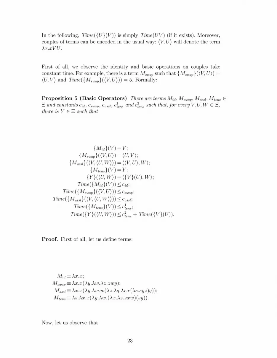
First of all, we observe the identity and basic operations on couples takeconstant time. For example, there is a term Mswap such that {Mswap}(〈V, U〉) =〈U, V 〉 and Time({Mswap}(〈V, U〉)) = 5. Formally:

Proposition 5 (Basic Operators) There are terms Mid , Mswap , Massl , Mtens ∈Ξ and constants cid , cswap, cassl , c1

tens and c2tens such that, for every V, U,W ∈ Ξ,

there is Y ∈ Ξ such that

{Mid}(V ) = V ;

{Mswap}(〈V, U〉) = 〈U, V 〉;{Massl}(〈V, 〈U,W 〉〉) = 〈〈V, U〉, W 〉;

{Mtens}(V ) = Y ;

{Y }(〈U,W 〉) = 〈{V }(U), W 〉;Time({Mid}(V ))≤ cid ;

Time({Mswap}(〈V, U〉))≤ cswap ;

Time({Massl}(〈V, 〈U,W 〉〉))≤ cassl ;

Time({Mtens}(V ))≤ c1tens ;

Time({Y }(〈U,W 〉))≤ c2tens + Time({V }(U)).

Proof. First of all, let us define terms:

Mid ≡λx.x;

Mswap ≡λx.x(λy.λw.λz.zwy);

Massl ≡λx.x(λy.λw.w(λz.λq.λr.r(λs.syz)q));

Mtens ≡λs.λx.x(λy.λw.(λx.λz.zxw)(sy)).

Now, let us observe that

23

MidV(1)� V ;

Mswap〈V, U〉(1)� 〈V, U〉(λy.λw.λz.zwy)(1)� (λy.λw.λz.zwy)V U(1)� (λw.λz.zwV )U(1)� (λw.λz.zwV )U(1)� 〈U, V 〉;

Massl〈V, 〈U,W 〉〉(1)� 〈V, 〈U,W 〉〉(λy.λw.w(λz.λq.λr.r(λs.syz)q))(1)� (λy.λw.w(λz.λq.λr.r(λs.syz)q))V 〈U,W 〉(1)� (λw.w(λz.λq.λr.r(λs.sV z)q))〈U,W 〉(1)� 〈U,W 〉(λz.λq.λr.r(λs.sV z)q)(1)� (λz.λq.λr.r(λs.sV z)q)UW(1)� λr.r(λs.sV U)W ) ≡ 〈〈V, U〉, W 〉;

MtensV(1)� λx.x(λy.λw.(λx.λz.zxw)(V y)) ≡ Y,

Y 〈U,W 〉(1)� 〈U,W 〉(λy.λw.(λx.λz.zxw)(V y))(1)� (λy.λw.(λx.λz.zxw)(V y))UW(1)� (λw.(λx.λz.zxw)(V U))W(1)� (λx.λz.zxW )(V U).

2

There is a term in Ξ which takes as input a pair of terms 〈V, U〉 and computesthe composition of the functions computed by V and U . The overhead isconstant, i.e. do not depend on the intermediate result.

Proposition 6 (Composition) There are a term Mcomp ∈ Ξ and two con-stants c1

comp , c2comp such that, for every V, U,W, Z ∈ Ξ, there is X ∈ Ξ such

that:

{Mcomp}(〈V, U〉) = X;

{X}(W ) = {V }({U}(W ));

Time({Mcomp}(〈V, U〉))≤ c1comp ;

Time({X}(W ))≤ c2comp + Time({U}(W )) + Time({V }({U}(W ))).

24

Proof. First of all, let us define the term:

Mcomp ≡ λx.x(λx.λy.λz.x(yz)).


Mcomp〈V, U〉(1)� 〈V, U〉(λx.λy.λz.x(yz))(1)� (λx.λy.λz.x(yz))V U(1)� (λy.λz.V (yz))U

(1)� λz.V (Uz) ≡ X,

XW(1)� V (UW )


We need to represent functions which go beyond the realm of linear logic. Inparticular, terms can be duplicated, but linear time is needed to do it.

Proposition 7 (Contraction) There are a term Mcont ∈ Ξ and a constantccont such that, for every V ∈ Ξ:

{Mcont}(V ) = 〈V, V 〉;Time({Mcont}(V ))≤ ccont + |V |.

Proof. First of all, let us define the term:

Mcont ≡ λx.λy.yxx.


McontV(n)� 〈V, V 〉,

where n ≤ |V |. 2

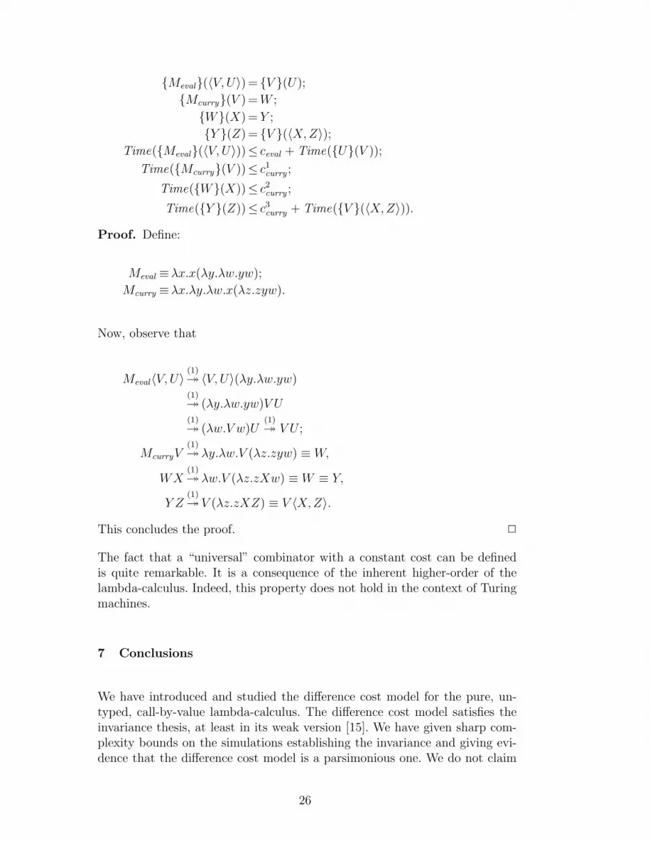
From a complexity viewpoint, what is most interesting is the possibility toperform higher-order computation with constant overhead. In particular, theuniversal function is realized by a term Meval such that {Meval}(〈V, U〉) ={V }(U) and Time({Meval}(〈V, U〉)) = 4 + Time({U}(V )).

Proposition 8 (Higher-Order) There are terms Meval , Mcurry ∈ Ξ and con-stants ceval , c1

curry , c2curry , c3

curry such that, for every V, U ∈ Ξ, there areW, X, Y, Z ∈ Ξ such that:

25

{Meval}(〈V, U〉) = {V }(U);

{Mcurry}(V ) = W ;

{W}(X) = Y ;

{Y }(Z) = {V }(〈X, Z〉);Time({Meval}(〈V, U〉))≤ ceval + Time({U}(V ));

Time({Mcurry}(V ))≤ c1curry ;

Time({W}(X))≤ c2curry ;

Time({Y }(Z))≤ c3curry + Time({V }(〈X, Z〉)).

Proof. Define:

Meval ≡λx.x(λy.λw.yw);

Mcurry ≡λx.λy.λw.x(λz.zyw).

Now, observe that

Meval〈V, U〉(1)� 〈V, U〉(λy.λw.yw)(1)� (λy.λw.yw)V U(1)� (λw.V w)U

(1)� V U ;

McurryV(1)� λy.λw.V (λz.zyw) ≡ W,

WX(1)� λw.V (λz.zXw) ≡ W ≡ Y,

Y Z(1)� V (λz.zXZ) ≡ V 〈X,Z〉.


The fact that a “universal” combinator with a constant cost can be definedis quite remarkable. It is a consequence of the inherent higher-order of thelambda-calculus. Indeed, this property does not hold in the context of Turingmachines.

7 Conclusions

We have introduced and studied the difference cost model for the pure, un-typed, call-by-value lambda-calculus. The difference cost model satisfies theinvariance thesis, at least in its weak version [15]. We have given sharp com-plexity bounds on the simulations establishing the invariance and giving evi-dence that the difference cost model is a parsimonious one. We do not claim

26

this model is the definite word on the subject. More work should be done,especially on lambda-calculi based on other evaluation models.

The availability of this cost model allows to reason on the complexity of call-by-value reduction by arguing on the structure of lambda-terms, instead ofusing complicated arguments on the details of some implementation mech-anism. In this way, we could obtain results for eager functional programswithout having to resort to, e.g., a SECD machine implementation.

We have not treated space. Indeed, the very definition of space complexity forlambda-calculus—at least in a less crude way than just “the maximum inkused” [11] —is an elusive subject which deserves better and deeper study.

References

[1] Andrea Asperti. On the complexity of beta-reduction. In Proc. 23rd ACMSIGPLAN Symposium on Principles of Programming Languages, pages 110–118, 1996.

[2] Andrea Asperti and Stefano Guerrini. The Optimal Implementation ofFunctional Programming Languages, volume 45 of Cambridge Tracts inTheoretical Computer Science. Cambridge University Press, 1998.

[3] Tomasz Blanc, Jean-Jacques Levy, and Luc Maranget. Sharing in the weaklambda-calculus. In Processes, Terms and Cycles, volume 3838 of LNCS, pages70–87. Springer, 2005.

[4] Ugo Dal Lago and Martin Hofmann. Quantitative models and implicitcomplexity. In Proc. Foundations of Software Technology and TheoreticalComputer Science, volume 3821 of LNCS, pages 189–200. Springer, 2005.

[5] Ugo Dal Lago and Simone Martini. An invariant cost model for the lambdacalculus. In A. Beckmann et al., editor, Logical Approaches to ComputationalBarriers, Second Conference on Computability in Europe, CiE 2006, volume3988 of Lecture Notes in Computer Science, pages 105–114. Springer, 2006.

[6] Vincent Danos and Laurent Regnier. Head linear reduction. Manuscript, 2004.

[7] Nicolaas Govert de Bruijn. Lambda calculus with nameless dummies, a tool forautomatic formula manipulation, with application to the church-rosser theorem.Indagationes Mathematicae, 34(5):381–392, 1972.

[8] Mariangiola Dezani-Ciancaglini, Simona Ronchi della Rocca, and LorenzaSaitta. Complexity of lambda-terms reductions. RAIRO InformatiqueTheorique, 13(3):257–287, 1979.

[9] Gudmund Skovbjerg Frandsen and Carl Sturtivant. What is an efficientimplementation of the lambda-calculus? In Proc. 5th ACM Conference on

27

Functional Programming Languages and Computer Architecture, pages 289–312,1991.

[10] John Lamping. An algorithm for optimal lambda calculus reduction. In Proc.17th ACM SIGPLAN Symposium on Principles of Programming Languages,pages 16–30, 1990.

[11] Julia L. Lawall and Harry G. Mairson. Optimality and inefficiency: What isn’t acost model of the lambda calculus? In Proc. 1996 ACM SIGPLAN InternationalConference on Functional Programming, pages 92–101, 1996.

[12] Julia L. Lawall and Harry G. Mairson. On global dynamics of optimalgraph reduction. In Proc. 1997 ACM SIGPLAN International Conference onFunctional Programming, pages 188–195, 1997.

[13] Jean-Jacques Levy. Reductions correctes et optimales dans le lambda-calcul.Universite Paris 7, Theses d’Etat, 1978.

[14] Simona Ronchi Della Rocca and Luca Paolini. The parametric lambda-calculus.Texts in Theoretical Computer Science: An EATCS Series. Springer-Verlag,2004.

[15] Peter van Emde Boas. Machine models and simulation. In Handbook ofTheoretical Computer Science, Volume A: Algorithms and Complexity (A),pages 1–66. MIT Press, 1990.

[16] Christopher Wadsworth. Some unusual λ-calculus numeral systems. In J.P.Seldin and J.R. Hindley, editors, To H.B. Curry: Essays on Combinatory Logic,Lambda Calculus and Formalism, pages 215–230. Academic Press, 1980.

28

Documents

The weak lambda calculus as a reasonable machine