Embed Size (px)
Citation preview
Separability and translatability of sequential termrewrite systems into the lambda calculus
Sugwoo Byun
Kyungsung University, Korea
E-mail: [email protected]
and
Richard Kennaway
University of East Anglia, Norwich, U.K.
E-mail: [email protected]
and
Vincent van Oostrom
Universiteit Utrecht, The Netherlands
E-mail: [email protected]
and
Fer-Jan de Vries
ETL, Tsukuba, Japan
E-mail: [email protected]
1
Orthogonal term rewrite systems do not currently have any semantics
other than syntactically-based ones such as term models and event struc-
tures. For a functional language which combines lambda calculus with
term rewriting, a semantics is most easily given by translating the rewrite
rules into lambda calculus and then using well-understood semantics for the
lambda calculus. We therefore study in this paper the question of which
classes of TRS do or do not have such translations.
We demonstrate by construction that forward branching orthogonal term
rewrite systems are translatable into the lambda calculus. The translation
satisfies some strong properties concerning preservation of equality and
of some inequalities. We prove that the forward branching systems are
exactly the systems permitting such a translation which is, in a precise
sense, uniform in the right-hand sides.
Connections are drawn between translatability, sequentiality and sep-
arability properties. Simple syntactic proofs are given of the non-
translatability of a class of TRSs, including Berry’s F and several variants
of it.
Key Words: separability, translation of term rewrite systems, lambda calculus, sequen-
tiality
1. INTRODUCTION
Our previous work [5, 6] on translation of TRSs into lambda calculus has consid-
ered only constructor TRSs, that is, those in which a symbol which appears at the
root of a left-hand side does not appear anywhere else in any left-hand side. In this
paper we consider a larger class of orthogonal systems which can be translated into
constructor systems. We generalise the notion of separability from [5, 6], and show
by construction that all strongly separable orthogonal systems have a translation
into a constructor system of a very simple form, which in turn has a translation
to lambda calculus. The translation is, in a sense we will define, uniform in the
right-hand sides of the original system. We also obtain simple syntactic proofs of
the non-translatability of several systems, such as variants of Berry’s F .
The translation problem can be motivated from the viewpoint of functional pro-
grams as TRSs, to be given meaning by translation to lambda calculus, or imple-
mentation via implementations of lambda calculus such as in [1]. One can also
consider functional programs as lambda expressions (usually in some form of typed
lambda calculus), and define implementations by translation into rewrite systems,
such as in [12]. Reverse compilation can be seen as translating such a rewrite system
back into lambda calculus.
2. DEFINITIONS
2.1. Basics
We assume familiarity with the basic concepts and notations of term rewrite
systems.
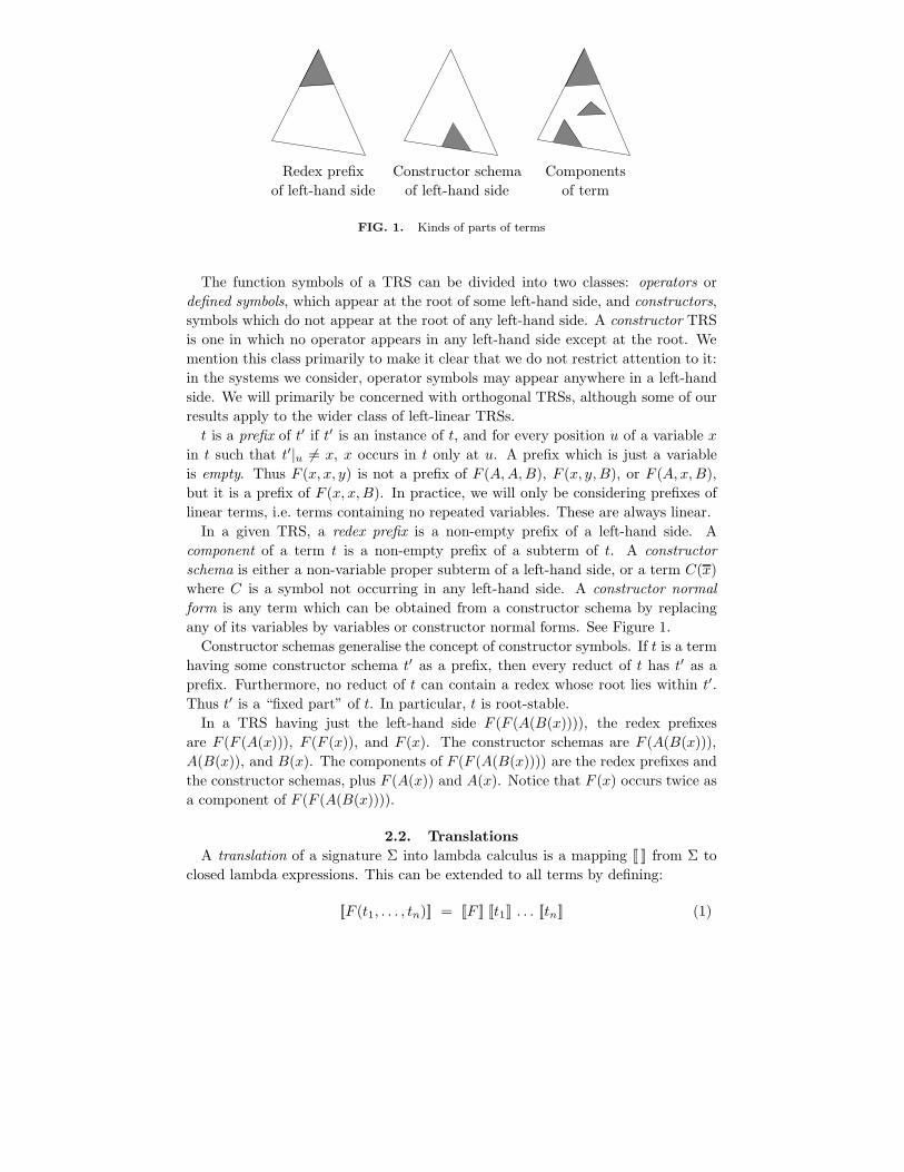
Redex prefix Constructor schema Components
of left-hand side of left-hand side of term
FIG. 1. Kinds of parts of terms
The function symbols of a TRS can be divided into two classes: operators or
defined symbols, which appear at the root of some left-hand side, and constructors,
symbols which do not appear at the root of any left-hand side. A constructor TRS
is one in which no operator appears in any left-hand side except at the root. We
mention this class primarily to make it clear that we do not restrict attention to it:
in the systems we consider, operator symbols may appear anywhere in a left-hand
side. We will primarily be concerned with orthogonal TRSs, although some of our
results apply to the wider class of left-linear TRSs.
t is a prefix of t′ if t′ is an instance of t, and for every position u of a variable x
in t such that t′|u 6= x, x occurs in t only at u. A prefix which is just a variable
is empty. Thus F (x, x, y) is not a prefix of F (A,A,B), F (x, y,B), or F (A, x,B),
but it is a prefix of F (x, x,B). In practice, we will only be considering prefixes of
linear terms, i.e. terms containing no repeated variables. These are always linear.
In a given TRS, a redex prefix is a non-empty prefix of a left-hand side. A
component of a term t is a non-empty prefix of a subterm of t. A constructor
schema is either a non-variable proper subterm of a left-hand side, or a term C(x)
where C is a symbol not occurring in any left-hand side. A constructor normal
form is any term which can be obtained from a constructor schema by replacing
any of its variables by variables or constructor normal forms. See Figure 1.
Constructor schemas generalise the concept of constructor symbols. If t is a term
having some constructor schema t′ as a prefix, then every reduct of t has t′ as a
prefix. Furthermore, no reduct of t can contain a redex whose root lies within t′.
Thus t′ is a “fixed part” of t. In particular, t is root-stable.
In a TRS having just the left-hand side F (F (A(B(x)))), the redex prefixes
are F (F (A(x))), F (F (x)), and F (x). The constructor schemas are F (A(B(x))),
A(B(x)), and B(x). The components of F (F (A(B(x)))) are the redex prefixes and
the constructor schemas, plus F (A(x)) and A(x). Notice that F (x) occurs twice as
a component of F (F (A(B(x)))).
2.2. Translations
A translation of a signature Σ into lambda calculus is a mapping [[ ]] from Σ to
closed lambda expressions. This can be extended to all terms by defining:
[[F (t1, . . . , tn)]] = [[F ]] [[t1]] . . . [[tn]] (1)
[[x]] = x (2)
Given a TRS R over Σ, a translation of R is a translation of Σ which satisfies
certain conditions. What these conditions should be is not obvious. Many different
concepts of a translation have appeared in the literature. At a minimum, it should
certainly map each rule of R to an equality of lambda calculus, and thus map all
equalities between terms to equalities of lambda calculus. If this were the only con-
dition, many TRSs would have a trivial translation which mapped all terms other
than variables to the same lambda expression, simply by defining the translation of
each n-ary symbol F to be λx1 . . . xnx.x. It is not enough to require preservation of
equality: some inequalities should also be preserved. However, if we have two rules
A(x) → x and B(x) → x, it does not seem reasonable to disallow translating both
A and B by λx.x. The terms whose inequality we will require to be preserved are
the constructor schemas. In an orthogonal TRS, constructor schemas that differ
other than in the names of their variables are never equal. We will require that
they are translated into lambda expressions which are not merely unequal, but in
a sense provably unequal, as defined by the notion of strong separability.
Definition 2.1. A tuple of lambda expressions t1, . . . , tn is separable if for any
tuple of lambda expressions s1, . . . , sn there is a context C[ ] such that C[ti] = si
for all i.
It is strongly separable if C[ ] can be chosen so as to contain (whether free or
bound) none of the free variables of t1, . . . , tn.
C[ ] is called a (strongly) separating context.
In the above definition, we can without loss of generality take s1, . . . , sn to be a
tuple of distinct new variables.
Separability is as defined in [2], although we find it technically more convenient
to speak of tuples rather than sets of expressions. Note that a tuple containing
repeated elements is never separable. Strong separability is our extension of the
concept. The terms x and y are separable (by the context (λxy.[ ])s1s2) but they
are not strongly separable. In this paper we are primarily concerned with strong
separability.
We will also require that the free variables of a constructor schema be “exposed”
in its translation, in the following sense.
Definition 2.2. An occurrence at position u of a free variable x of a lambda-
expression t is exposed if there is a context C[ ] containing none of the free variables
of t such that C[t] reduces to x, and the final occurrence of x is a descendant of u.
x is exposed in t if some occurrence of x is.
The property of x being exposed in t is equivalent to that of λxy.t being left-
invertible [4], where y is a tuple of all the free variables of t excluding x. Left-
invertibility of a lambda expression M means that there is a lambda expression N
such that for a new variable x, N(Mx) = x.
We can now present our notion of a translation.
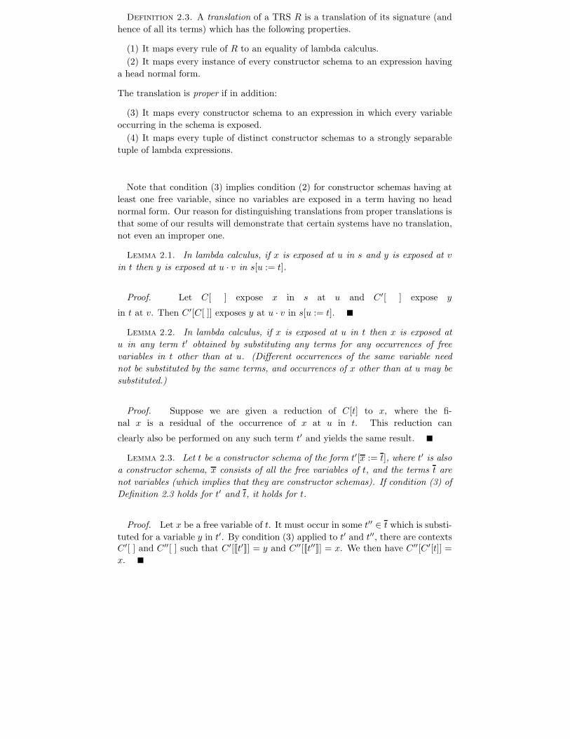
Definition 2.3. A translation of a TRS R is a translation of its signature (and
hence of all its terms) which has the following properties.
(1) It maps every rule of R to an equality of lambda calculus.
(2) It maps every instance of every constructor schema to an expression having
a head normal form.
The translation is proper if in addition:
(3) It maps every constructor schema to an expression in which every variable
occurring in the schema is exposed.
(4) It maps every tuple of distinct constructor schemas to a strongly separable
tuple of lambda expressions.
Note that condition (3) implies condition (2) for constructor schemas having at
least one free variable, since no variables are exposed in a term having no head
normal form. Our reason for distinguishing translations from proper translations is
that some of our results will demonstrate that certain systems have no translation,
not even an improper one.
Lemma 2.1. In lambda calculus, if x is exposed at u in s and y is exposed at v
in t then y is exposed at u · v in s[u := t].
Proof. Let C[ ] expose x in s at u and C′[ ] expose y
in t at v. Then C′[C[ ]] exposes y at u · v in s[u := t].
Lemma 2.2. In lambda calculus, if x is exposed at u in t then x is exposed at
u in any term t′ obtained by substituting any terms for any occurrences of free
variables in t other than at u. (Different occurrences of the same variable need
not be substituted by the same terms, and occurrences of x other than at u may be
substituted.)
Proof. Suppose we are given a reduction of C[t] to x, where the fi-
nal x is a residual of the occurrence of x at u in t. This reduction can
clearly also be performed on any such term t′ and yields the same result.
Lemma 2.3. Let t be a constructor schema of the form t′[x := t], where t′ is also
a constructor schema, x consists of all the free variables of t, and the terms t are
not variables (which implies that they are constructor schemas). If condition (3) of
Definition 2.3 holds for t′ and t, it holds for t.
Proof. Let x be a free variable of t. It must occur in some t′′ ∈ t which is substi-
tuted for a variable y in t′. By condition (3) applied to t′ and t′′, there are contextsC′[ ] and C′′[ ] such that C′[[[t′]]] = y and C′′[[[t′′]]] = x. We then have C′′[C′[t]] =
x.
In the constructor TRSs which arise in practice, this lemma usually allows proper-
ness of a translation to be established by checking condition (3) of Definition 2.3
just for the terms C(x), for constructor symbols C.
2.3. Uniform translations
The left-hand sides of a TRS specify what is a redex. The right-hand sides specify
how to reduce each type of redex. We are interested in translations which use as
little information as possible about the right-hand sides. The lambda expressions
to which such translations map the function symbols embody a strategy for finding
redexes which is determined solely by the left-hand sides of the system. We call
these uniform translations.
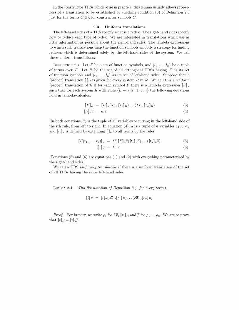
Definition 2.4. Let F be a set of function symbols, and (l1, . . . , ln) be a tuple
of terms over F . Let R be the set of all orthogonal TRSs having F as its set
of function symbols and (l1, . . . , ln) as its set of left-hand sides. Suppose that a
(proper) translation [[ ]]R is given for every system R in R. We call this a uniform
(proper) translation of R if for each symbol F there is a lambda expression [[F ]]usuch that for each system R with rules li → ri|i : 1 . . . n the following equations
hold in lambda-calculus:
[[F ]]R = [[F ]]u(λx1.[[r1]]R) . . . (λxn.[[rn]]R) (3)
[[li]]ua = aix (4)
In both equations, xi is the tuple of all variables occurring in the left-hand side of
the ith rule, from left to right. In equation (4), a is a tuple of n variables a1 . . . an
and [[li]]u is defined by extending [[ ]]u to all terms by the rules:
[[F (t1, . . . , tk)]]u = λa.[[F ]]ua([[t1]]ua) . . . ([[tk]]ua) (5)
[[x]]u = λa.x (6)
Equations (5) and (6) are equations (1) and (2) with everything parameterised by
the right-hand sides.
We call a TRS uniformly translatable if there is a uniform translation of the set
of all TRSs having the same left-hand sides.
Lemma 2.4. With the notation of Definition 2.4, for every term t,
[[t]]R = [[t]]u(λx1.[[r1]]R) . . . (λxn.[[rn]]R)
Proof. For brevity, we write ρi for λxi.[[ri]]R and ρ for ρ1 . . . ρn. We are to prove
that [[t]]R = [[t]]uρ.
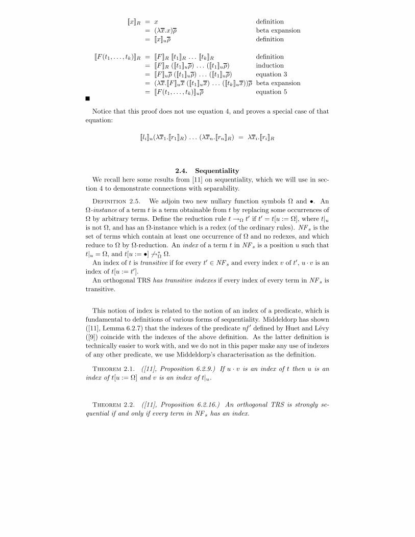
[[x]]R = x definition
= (λx.x)ρ beta expansion
= [[x]]uρ definition
[[F (t1, . . . , tk)]]R = [[F ]]R [[t1]]R . . . [[tk]]R definition
= [[F ]]R ([[t1]]uρ) . . . ([[t1]]uρ) induction
= [[F ]]uρ ([[t1]]uρ) . . . ([[t1]]uρ) equation 3
= (λx.[[F ]]ux ([[t1]]ux) . . . ([[tk]]ux))ρ beta expansion
= [[F (t1, . . . , tk)]]uρ equation 5
Notice that this proof does not use equation 4, and proves a special case of that
equation:
[[li]]u(λx1.[[r1]]R) . . . (λxn.[[rn]]R) = λxi.[[ri]]R
2.4. Sequentiality
We recall here some results from [11] on sequentiality, which we will use in sec-
tion 4 to demonstrate connections with separability.
Definition 2.5. We adjoin two new nullary function symbols Ω and •. An
Ω-instance of a term t is a term obtainable from t by replacing some occurrences of
Ω by arbitrary terms. Define the reduction rule t →Ω t′ if t′ = t[u := Ω], where t|uis not Ω, and has an Ω-instance which is a redex (of the ordinary rules). NF s is the
set of terms which contain at least one occurrence of Ω and no redexes, and which
reduce to Ω by Ω-reduction. An index of a term t in NF s is a position u such that
t|u = Ω, and t[u := •] 6→∗Ω Ω.
An index of t is transitive if for every t′ ∈ NF s and every index v of t′, u · v is an
index of t[u := t′].
An orthogonal TRS has transitive indexes if every index of every term in NF s is
transitive.
This notion of index is related to the notion of an index of a predicate, which is
fundamental to definitions of various forms of sequentiality. Middeldorp has shown
([11], Lemma 6.2.7) that the indexes of the predicate nf ′ defined by Huet and Levy
([9]) coincide with the indexes of the above definition. As the latter definition is
technically easier to work with, and we do not in this paper make any use of indexes
of any other predicate, we use Middeldorp’s characterisation as the definition.
Theorem 2.1. ([11], Proposition 6.2.9.) If u · v is an index of t then u is an
index of t[u := Ω] and v is an index of t|u.
Theorem 2.2. ([11], Proposition 6.2.16.) An orthogonal TRS is strongly se-
quential if and only if every term in NF s has an index.
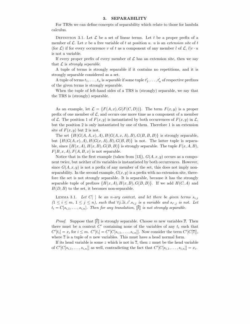
3. SEPARABILITY
For TRSs we can define concepts of separability which relate to those for lambda
calculus.
Definition 3.1. Let L be a set of linear terms. Let t be a proper prefix of a
member of L. Let x be a free variable of t at position u. u is an extension site of t
(for L) if for every occurrence v of t as a component of any member l of L, l|v · u
is not a variable.
If every proper prefix of every member of L has an extension site, then we say
that L is strongly separable.
A tuple of terms is strongly separable if it contains no repetitions, and it is
strongly separable considered as a set.
A tuple of terms t1, . . . , tn is separable if some tuple t′1, . . . , t′n of respective prefixes
of the given terms is strongly separable.
When the tuple of left-hand sides of a TRS is (strongly) separable, we say that
the TRS is (strongly) separable.
As an example, let L = F (A, x), G(F (C,D)). The term F (x, y) is a proper
prefix of one member of L, and occurs one more time as a component of a member
of L. The position 1 of F (x, y) is instantiated by both occurrences of F (x, y) in L,
but the position 2 is only instantiated by one of them. Therefore 1 is an extension
site of F (x, y) but 2 is not.
The set H(G(A,A, x), A),H(G(A, x,A), B), G(B,B,B) is strongly separable,
but H(G(A, x), A),H(G(x,A), B), G(B,B) is not. The latter tuple is separa-
ble, since H(x,A),H(x,B), G(B,B) is strongly separable. The tuple F (x,A,B),
F (B, x,A), F (A,B, x) is not separable.
Notice that in the first example (taken from [13]), G(A, x, y) occurs as a compo-
nent twice, but neither of its variables is instantiated by both occurrences. However,
since G(A, x, y) is not a prefix of any member of the set, this does not imply non-
separability. In the second example, G(x, y) is a prefix with no extension site, there-
fore the set is not strongly separable. It is separable, because it has the strongly
separable tuple of prefixes H(x,A),H(x,B), G(B,B). If we add H(C,A) and
H(D,B) to the set, it becomes non-separable.
Lemma 3.1. Let C[ ] be an n-ary context, and let there be given terms si,j
(1 ≤ i ≤ m, 1 ≤ j ≤ n), such that ∀j.∃i, i′.si,j is a variable and si′,j is not. Let
ti = C[si,1, . . . , si,n]. Then for any translation, [[t]] is not strongly separable.
Proof. Suppose that [[t]] is strongly separable. Choose m new variables x. Then
there must be a context C′ containing none of the variables of any ti such that
C′[ti] = xi for i ≤ m. C′[ti] = C′[C[si,1, . . . , si,n]]. Now consider the term C′[C[z]],
where z is a tuple of n new variables. This must have a head normal form.
If its head variable is some z which is not in z, then z must be the head variable
of C′[C[si,1, . . . , si,n]] as well, contradicting the fact that C′[C[si,1, . . . , si,n]] = xi.
Therefore its head variable must be some zj ∈ z. Let i and
i′ be such that si,j is a variable, say x, and si′,j is not a vari-
able. Then x is the head variable of the head normal form of
C′[C[si,1, . . . , si,n]], contradicting the fact that C′[C[si,1, . . . , si,n]] = xi.
Theorem 3.1. In a given TRS, let t be a redex-prefix having no extension site.
Let r be the tuple of right-hand sides of the rules whose left-hand sides t is a prefix
of. Let s be the tuple of distinct instances of t which occur as proper subterms of
left-hand sides. Let t be the concatenation of s and r. Then for any translation,
[[s]] is not strongly separable.
Proof. The maximal common prefix of t is some n-ary context C[ ].
Let ti = C[si,1, . . . , si,n]. The absence of an extension site implies that the
terms si,j satisfy the hypothesis of Lemma 3.1. This establishes the theorem.
This immediately establishes the non-translatability for certain TRSs.
Theorem 3.2. The following set of rules (“Berry’s F”) has no proper transla-
tion:
F (x,A,B) → 0
F (B, x,A) → 1
F (A,B, x) → 2
Proof. The prefix F (x, y, z) has no extension site. The tuple t con-
sidered by Theorem 3.1 is (0, 1, 2). The theorem implies that any trans-
lation must map these to a tuple which is not strongly separable. But
it is a tuple of distinct constructors, so the translation cannot be proper.
Another way of putting this theorem is that if 0, 1, and 2 are taken to be the
Church numerals (or the numerals of any other numeral system in the lambda cal-
culus) then the equations have no solution in lambda calculus. This has previously
only been proved by domain-theoretic arguments.
Note that the system has many improper translations. For example, let [[F ]] =
λxyz.t, where t is closed, and define [[0]] = [[1]] = [[2]] = t. [[A]] and [[B]] are arbitrary.
Theorem 3.3. Every orthogonal TRS with a uniform translation is strongly sep-
arable.
Proof. Let there be given an orthogonal TRS which is not strongly separable,
and a uniform translation [[ ]] of it. We will derive a contradiction.
By non-strong separability there is a proper redex prefix t with no extension
site. Let x be a free variable of t. Choose a left-hand side lx which contains t as
a component and does not instantiate x. (This is possible by the absence of an
extension site for t.) Take a TRS R in which the corresponding right-hand side is
x. Then B([[lx]]R) = x. Because lx is an instance of t, it follows that B([[t]]) must
contain x free. Therefore every free variable of t is free in B([[t]]).
Let x be the variable having the leftmost-outermost occurrence in B([[t]]).
Let lx be as above. Choose a TRS R in which x is not free in
rx. There exist lambda expressions M1, . . . ,Mk in which x is not free
such that [[t]]M1, . . . ,Mk = x. Therefore [[lx]]M1, . . . ,Mk = x. There-
fore [[rx]]M1, . . . ,Mk = x. But x is not free in rx, contradiction.
4. CONNECTIONS BETWEEN SEPARABILITY AND
SEQUENTIALITY
4.1. Strong sequentiality and index transitivity
Suppose that t and t′ are terms in NF s and that t has an index at u. The
property of strong sequentiality implies that for at least one index v of t′, u · v is
an index of t. Strong separability makes the additional requirement that an index
v can be chosen independently of t and u. v is what we have called an extension
site of t′. We could also call it a separating index of t′. Index transitivity makes the
even stronger requirement that for every index v of t′, u ·v is an index of t, i.e. that
every index of every redex-prefix is separating. These remarks establish the next
theorem.
Theorem 4.1. If an orthogonal TRS is strongly sequential and has transitive
indexes it is strongly separable. If an orthogonal TRS is strongly separable it is
strongly sequential.
Theorem 4.2. Neither of the implications of Theorem 4.1 can be reversed.
Proof. The following system is strongly separable but does not have transitive
indexes.
F (A,B) → . . .
G(F (C, x)) → . . .
The proper redex prefixes are F (x, y), F (A, x), F (x,B), G(x), and G(F (x, y)).
We have chosen the variables such that in each prefix, x is instantiated in every
occurrence of that prefix in a left-hand side. Therefore the system is strongly
separable. Consider the terms G(Ω), F (Ω,Ω), and G(F (Ω,Ω)). The first two have
indexes at 1 and 2 respectively, but 1 · 2 is not an index of the third. Therefore the
system does not have transitive indexes.
Now consider the system obtained by adding the following rule to the above:
H(F (x,D)) → . . .
This system is still strongly sequential, but the redex-prefix F (x, y) does not have
any variable which is instantiated by every occurrence of F (x, y) in a left-hand
side. F (x, y) thus has no extension site, and the system is not strongly separable.
Theorem 4.3. Let there be given an orthogonal TRS. For each redex prefix t,
let U be the set of positions of free variables of t which are instantiated by every
occurrence of t as a prefix of a left-hand side. Then the system is strongly sequential
with transitive indexes if and only if for every proper redex prefix t, the set U is
nonempty, and every member of U is an extension site of t.
Proof. Let t be a proper redex prefix and U be as described. Then tΩ ∈ NF s and
U is the set of indexes of tΩ. If U is empty, the system is not strongly sequential.
Supose that U is nonempty, but some member u of U is not an extension site of t.
Then there is a left-hand side t′ in which t occurs as a redex-component at some
position v, such that t′ | v · u is a variable. Let t′′ = t′Ω[v := Ω]. Then v is an index
of t′′, u is an index of tΩ, and v ·u is not an index of t′′[v := tΩ]. This demonstrates
that the system does not have transitive indexes.
For the converse, suppose that the condition on U holds for all redex prefixes.
Let t ∈ NF s. We will define a set I(t) of positions of Ω in t by an inductive
construction, and prove that these are the indexes of t.
For any position u of t, define Ωu(t) to be the normal form of t by Ω-reduction
subject to the constraint that no reduction is performed at any prefix of u. Let
t′ = Ω〈 〉(t). Then t′ must be a redex-prefix. Let U be the positions of t′ which are
instantiated by every occurrence of t′ as a redex prefix. U is nonempty and every
member is an extension site of t′.
If t′ = t (the base case of the induction) then every member of U is an index of
t. Define I(t) = U and I ′(t) = U .
Otherwise, consider the terms tu = t|u for all u ∈ U . Each of these is smaller
than t, so we apply this construction to obtain for each one a set I(tu). Define
I(t) = u · v|v ∈ I(tu) and I ′(t) = U ∪ I(t).
It is immediate from this construction that I(t) is nonempty. The auxiliary set
I ′(t) will be technically useful in the proof. It has the important property that for
all u ∈ I(t), and all v < u such that t|v →∗Ω Ω, v ∈ I ′(t).
We can now prove that I(t) consists of indexes of t. Suppose that for some t,
some member of I(t) were not an index. Take t to be of minimal size such that this
is so, and let u ∈ I(t) be a non-index. Let t′ = Ωu(t)[u := •]. This must contain
an Ω-redex at one or more prefixes of u. Consider the innermost such redex, at
position v. Let u = v · w. We know that v ∈ I ′(t) and w ∈ I(t′|v). By induction,
if t′|v is smaller than t, then w is an index of t′|v, and therefore t′[u := •] cannot
have an Ω-redex at v, contradiction. Therefore t′|v must be t itself. As a member
of I(t), u is constructed as a chain v ·w · . . ., where each of v, v ·w, etc. is in I ′(t). If
there were exactly one segment, then t[u := •] would not be an Ω-redex. Otherwise,
the tail u′ = w · . . . is not only an index of I(t|v), but an extension site of it. This
implies that in this case also, t[u := •] cannot be an Ω-redex.
This establishes that every member of I(t) is an index of t. If all other occurrences
of Ω in t are replaced by •, the construction of I(t) allows one to Ω-reduce the
resulting term to Ω. Therefore I(t) contains all the indexes of t.
It remains to prove that indexes are transitive. Suppose that t and t′ are in
NF s, u ∈ I(t), and v ∈ I(t′). Then u ∈ I ′(t[u := t′]), and u · v ∈ I(t[u := t′]).
For constructor systems, all strongly sequential systems are index-transitive
([11]), and therefore for constructor systems, the strongly separable systems co-
incide with both of the other classes.
4.2. Forward branching and inductive sequentiality
Inductive sequentiality is defined by [8], which proves it equivalent to the forward
branching systems defined by [14, 7]. We shall prove both equivalent to strong
separability for orthogonal systems.
The definition of forward branching systems is easier to work with. These are
defined in terms of the notion of an index tree for an orthogonal TRS. (Despite the
name, it is actually a type of graph.)
An index tree for an orthogonal TRS is a finite state automaton. Its non-terminal
states are pairs (t, u), where t is a redex prefix and u is an index of t, and its
terminal states are the left-hand sides of the system. Its initial state is the pair
(Ω, 〈 〉). Its transition function is in two parts: the transfer function and the failure
function. The transfer function maps pairs ((t, u), A), where (t, u) is a state and A
is a function symbol, to states of the index tree. If ((t, u), A) is mapped to state s,
this should be interpreted as a transition labelled A from (t, u) to s. s always has
the form (t′, u′) or t′, where t′ = t[u := A(x)]. The failure function defines a set of
unlabelled transitions from some non-terminal states to states.
An index tree defines a reduction algorithm for the TRS. We will not go into
detail, but the intuition is that when one is at a state (t, u), one has established
that t is a prefix of the term being evaluated, and u is the position of the node of
the term to be inspected next. The transfer function defines what state to go to
for each of the symbols that can extend t at u and still have a redex prefix. The
failure function defines what to do if some other symbol is found. In that case,
some subterm of t may have to be evaluated instead, and the failure transition will
go to a state labelled with that subterm.
A forward branching index tree is one in which every node is accessible from
the initial state without failure transitions. What this means is that if a failure
transition from (t, u) goes to a state labelled with t′ = t|v (either a terminal or
a non-terminal state), then if we had begun by using the index tree to evaluate
a term of which t′ was a prefix, we would have arrived at that same state. The
evaluation strategy proceeds independently of the context in which the term with
prefix t′ occurred.
Note that for forward branching index trees, in each non-terminal state (t, u), u
is determined by t, so we can consider the state to be redex prefixes and the chosen
index to be given by a function U from non-terminal states to indexes.
An orthogonal TRS is defined to be forward branching if there is a forward
branching index tree whose terminal states are its left-hand sides. The example of
a non-strongly separable system in section 3 is also not forward branching. This is
not a coincidence. Notice how the decision of which argument of a term G(. . . , . . .)
to evaluate next depends on the context it was encountered: if as part of a term
H(G(. . . , . . .), A), then the first, but if as part of H(G(. . . , . . .), B), then the second.
This is an example of a general connection between strong separability and forward
branching.
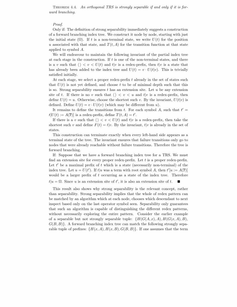
Theorem 4.4. An orthogonal TRS is strongly separable if and only if it is for-
ward branching.
Proof.
Only if: The definition of strong separability immediately suggests a construction
of a forward branching index tree. We construct it node by node, starting with just
the initial state (Ω). If t is a non-terminal state, we write U(t) for the position
u associated with that state, and T (t, A) for the transition function at that state
applied to symbol A.
We will endeavour to maintain the following invariant of the partial index tree
at each stage in the construction. If t is one of the non-terminal states, and there
is a v such that 〈 〉 < v < U(t) and t|v is a redex-prefix, then t|v is a state that
has already been added to the index tree and U(t) = v · U(t|v). This is trivially
satisfied initially.
At each stage, we select a proper redex-prefix t already in the set of states such
that U(t) is not yet defined, and choose t to be of minimal depth such that this
is so. Strong separability ensures t has an extension site. Let u be any extension
site of t. If there is no v such that 〈 〉 < v < u and t|v is a redex-prefix, then
define U(t) = u. Otherwise, choose the shortest such v. By the invariant, U(t|v) is
defined. Define U(t) = v · U(t|v) (which may be different from u).
It remains to define the transitions from t. For each symbol A, such that t′ =
t[U(t) := A(x)] is a redex-prefix, define T (t, A) = t′.
If there is a v such that 〈 〉 < v < U(t) and t|v is a redex-prefix, then take the
shortest such v and define F (t) = t|v. By the invariant, t|v is already in the set of
states.
This construction can terminate exactly when every left-hand side appears as a
terminal state of the tree. The invariant ensures that failure transitions only go to
nodes that were already reachable without failure transitions. Therefore the tree is
forward branching.
If: Suppose that we have a forward branching index tree for a TRS. We must
find an extension site for every proper redex-prefix. Let t is a proper redex-prefix.
Let t′ be a maximal prefix of t which is a state (necessarily non-terminal) of the
index tree. Let u = U(t′). If t|u was a term with root symbol A, then t′[u := A(x)]
would be a larger prefix of t occurring as a state of the index tree. Therefore
t|u = Ω. Since u is an extension site of t′, it is also an extension site of t.
This result also shows why strong separability is the relevant concept, rather
than separability. Strong separability implies that the whole of redex pattern can
be matched by an algorithm which at each node, chooses which descendant to next
inspect based only on the last operator symbol seen. Separability only guarantees
that such an algorithm is capable of distinguishing the different redex patterns,
without necessarily exploring the entire pattern. Consider the earlier example
of a separable but not strongly separable tuple: H(G(A, x), A),H(G(x,A), B),
G(B,B). A forward branching index tree can match the following strongly sepa-
rable tuple of prefixes: H(x,A),H(x,B), G(B,B). If one assumes that the term
that one is matching is indeed an instance of one of the three given terms, then this
is sufficient to determine which one, but it does not explore the entire pattern.
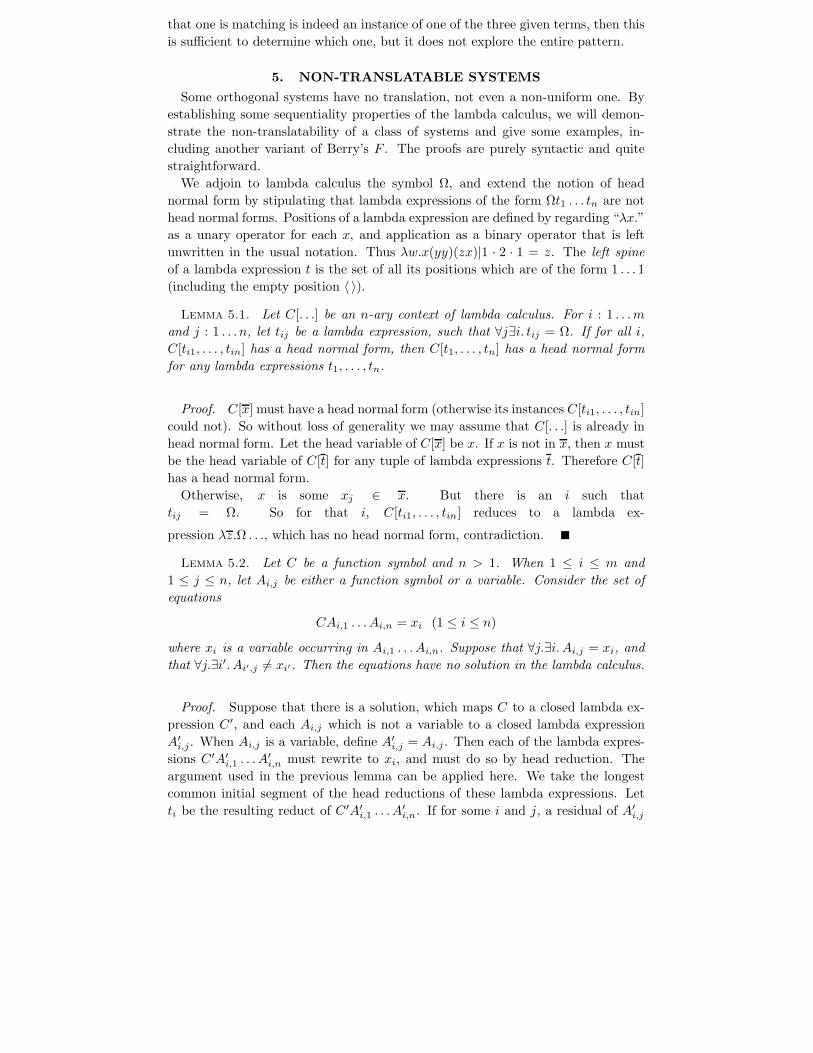
5. NON-TRANSLATABLE SYSTEMS
Some orthogonal systems have no translation, not even a non-uniform one. By
establishing some sequentiality properties of the lambda calculus, we will demon-
strate the non-translatability of a class of systems and give some examples, in-
cluding another variant of Berry’s F . The proofs are purely syntactic and quite
straightforward.
We adjoin to lambda calculus the symbol Ω, and extend the notion of head
normal form by stipulating that lambda expressions of the form Ωt1 . . . tn are not
head normal forms. Positions of a lambda expression are defined by regarding “λx.”
as a unary operator for each x, and application as a binary operator that is left
unwritten in the usual notation. Thus λw.x(yy)(zx)|1 · 2 · 1 = z. The left spine
of a lambda expression t is the set of all its positions which are of the form 1 . . . 1
(including the empty position 〈 〉).
Lemma 5.1. Let C[. . .] be an n-ary context of lambda calculus. For i : 1 . . .m
and j : 1 . . . n, let tij be a lambda expression, such that ∀j∃i. tij = Ω. If for all i,
C[ti1, . . . , tin] has a head normal form, then C[t1, . . . , tn] has a head normal form
for any lambda expressions t1, . . . , tn.
Proof. C[x] must have a head normal form (otherwise its instances C[ti1, . . . , tin]
could not). So without loss of generality we may assume that C[. . .] is already in
head normal form. Let the head variable of C[x] be x. If x is not in x, then x must
be the head variable of C[t] for any tuple of lambda expressions t. Therefore C[t]
has a head normal form.
Otherwise, x is some xj ∈ x. But there is an i such that
tij = Ω. So for that i, C[ti1, . . . , tin] reduces to a lambda ex-
pression λz.Ω . . ., which has no head normal form, contradiction.
Lemma 5.2. Let C be a function symbol and n > 1. When 1 ≤ i ≤ m and
1 ≤ j ≤ n, let Ai,j be either a function symbol or a variable. Consider the set of
equations
CAi,1 . . . Ai,n = xi (1 ≤ i ≤ n)
where xi is a variable occurring in Ai,1 . . . Ai,n. Suppose that ∀j.∃i. Ai,j = xi, and
that ∀j.∃i′. Ai′,j 6= xi′ . Then the equations have no solution in the lambda calculus.
Proof. Suppose that there is a solution, which maps C to a closed lambda ex-
pression C′, and each Ai,j which is not a variable to a closed lambda expression
A′i,j . When Ai,j is a variable, define A′
i,j = Ai,j . Then each of the lambda expres-
sions C′A′i,1 . . . A′
i,n must rewrite to xi, and must do so by head reduction. The
argument used in the previous lemma can be applied here. We take the longest
common initial segment of the head reductions of these lambda expressions. Let
ti be the resulting reduct of C′A′i,1 . . .A′
i,n. If for some i and j, a residual of A′i,j
lies on the left spine of ti, then this must be so for that j and all i. But for some
i, Ai,j = xi, so for that i, ti must be xi, otherwise it cannot reduce to xi. There-
fore for all other i′, t′i is a residual of Ai′,j , and therefore cannot reduce to xi′
unless Ai′,j = xi′ . But this contradicts the condition that for some i′, Ai′,j 6= xi′ .
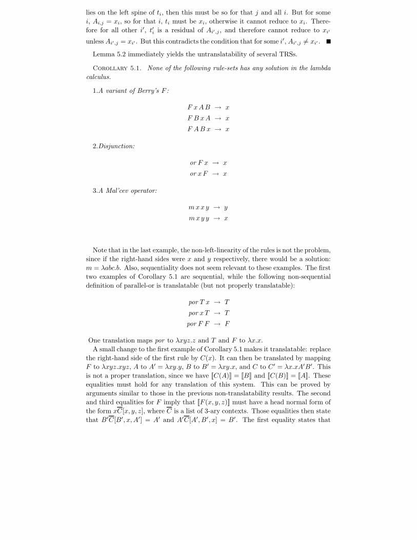
Lemma 5.2 immediately yields the untranslatability of several TRSs.
Corollary 5.1. None of the following rule-sets has any solution in the lambda
calculus.
1.A variant of Berry’s F :
F xAB → x
F B xA → x
F AB x → x
2.Disjunction:
or F x → x
or xF → x
3.A Mal’cev operator:
mxxy → y
mxy y → x
Note that in the last example, the non-left-linearity of the rules is not the problem,
since if the right-hand sides were x and y respectively, there would be a solution:
m = λabc.b. Also, sequentiality does not seem relevant to these examples. The first
two examples of Corollary 5.1 are sequential, while the following non-sequential
definition of parallel-or is translatable (but not properly translatable):
por T x → T
por xT → T
por F F → F
One translation maps por to λxyz.z and T and F to λx.x.
A small change to the first example of Corollary 5.1 makes it translatable: replace
the right-hand side of the first rule by C(x). It can then be translated by mapping
F to λxyz.xyz, A to A′ = λxy.y, B to B′ = λxy.x, and C to C′ = λx.xA′B′. This
is not a proper translation, since we have [[C(A)]] = [[B]] and [[C(B)]] = [[A]]. These
equalities must hold for any translation of this system. This can be proved by
arguments similar to those in the previous non-translatability results. The second
and third equalities for F imply that [[F (x, y, z)]] must have a head normal form of
the form xC[x, y, z], where C is a list of 3-ary contexts. Those equalities then state
that B′C[B′, x, A′] = A′ and A′C[A′, B′, x] = B′. The first equality states that
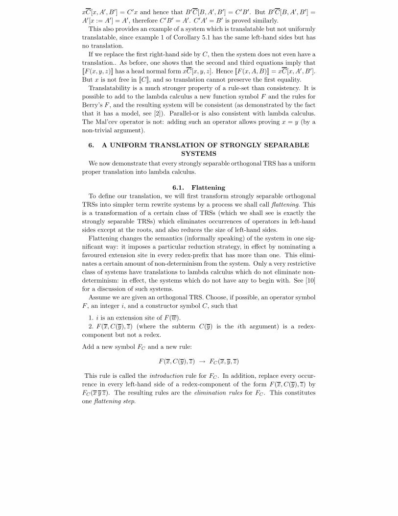
xC[x,A′, B′] = C′x and hence that B′C[B,A′, B′] = C′B′. But B′C[B,A′, B′] =
A′[x := A′] = A′, therefore C′B′ = A′. C′A′ = B′ is proved similarly.
This also provides an example of a system which is translatable but not uniformly
translatable, since example 1 of Corollary 5.1 has the same left-hand sides but has
no translation.
If we replace the first right-hand side by C, then the system does not even have a
translation.. As before, one shows that the second and third equations imply that
[[F (x, y, z)]] has a head normal form xC[x, y, z]. Hence [[F (x,A,B)]] = xC[x,A′, B′].
But x is not free in [[C]], and so translation cannot preserve the first equality.
Translatability is a much stronger property of a rule-set than consistency. It is
possible to add to the lambda calculus a new function symbol F and the rules for
Berry’s F , and the resulting system will be consistent (as demonstrated by the fact
that it has a model, see [2]). Parallel-or is also consistent with lambda calculus.
The Mal’cev operator is not: adding such an operator allows proving x = y (by a
non-trivial argument).
6. A UNIFORM TRANSLATION OF STRONGLY SEPARABLE
SYSTEMS
We now demonstrate that every strongly separable orthogonal TRS has a uniform
proper translation into lambda calculus.
6.1. Flattening
To define our translation, we will first transform strongly separable orthogonal
TRSs into simpler term rewrite systems by a process we shall call flattening. This
is a transformation of a certain class of TRSs (which we shall see is exactly the
strongly separable TRSs) which eliminates occurrences of operators in left-hand
sides except at the roots, and also reduces the size of left-hand sides.
Flattening changes the semantics (informally speaking) of the system in one sig-
nificant way: it imposes a particular reduction strategy, in effect by nominating a
favoured extension site in every redex-prefix that has more than one. This elimi-
nates a certain amount of non-determinism from the system. Only a very restrictive
class of systems have translations to lambda calculus which do not eliminate non-
determinism: in effect, the systems which do not have any to begin with. See [10]
for a discussion of such systems.
Assume we are given an orthogonal TRS. Choose, if possible, an operator symbol
F , an integer i, and a constructor symbol C, such that
1. i is an extension site of F (w).
2. F (x,C(y), z) (where the subterm C(y) is the ith argument) is a redex-
component but not a redex.
Add a new symbol FC and a new rule:
F (x,C(y), z) → FC(x, y, z)
This rule is called the introduction rule for FC . In addition, replace every occur-
rence in every left-hand side of a redex-component of the form F (x,C(y), z) by
FC(x y z). The resulting rules are the elimination rules for FC . This constitutes
one flattening step.
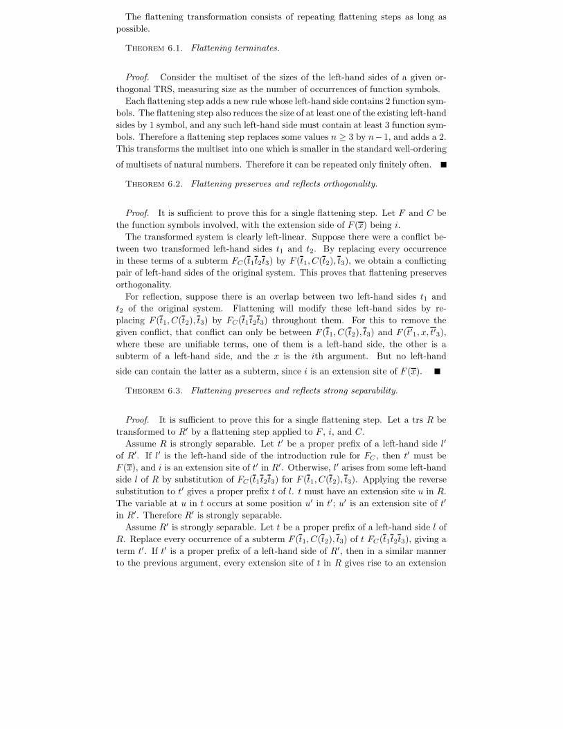
The flattening transformation consists of repeating flattening steps as long as
possible.
Theorem 6.1. Flattening terminates.
Proof. Consider the multiset of the sizes of the left-hand sides of a given or-
thogonal TRS, measuring size as the number of occurrences of function symbols.
Each flattening step adds a new rule whose left-hand side contains 2 function sym-
bols. The flattening step also reduces the size of at least one of the existing left-hand
sides by 1 symbol, and any such left-hand side must contain at least 3 function sym-
bols. Therefore a flattening step replaces some values n ≥ 3 by n−1, and adds a 2.
This transforms the multiset into one which is smaller in the standard well-ordering
of multisets of natural numbers. Therefore it can be repeated only finitely often.
Theorem 6.2. Flattening preserves and reflects orthogonality.
Proof. It is sufficient to prove this for a single flattening step. Let F and C be
the function symbols involved, with the extension side of F (x) being i.
The transformed system is clearly left-linear. Suppose there were a conflict be-
tween two transformed left-hand sides t1 and t2. By replacing every occurrence
in these terms of a subterm FC(t1t2t3) by F (t1, C(t2), t3), we obtain a conflicting
pair of left-hand sides of the original system. This proves that flattening preserves
orthogonality.
For reflection, suppose there is an overlap between two left-hand sides t1 and
t2 of the original system. Flattening will modify these left-hand sides by re-
placing F (t1, C(t2), t3) by FC(t1t2t3) throughout them. For this to remove the
given conflict, that conflict can only be between F (t1, C(t2), t3) and F (t′1, x, t′3),
where these are unifiable terms, one of them is a left-hand side, the other is a
subterm of a left-hand side, and the x is the ith argument. But no left-hand
side can contain the latter as a subterm, since i is an extension site of F (x).
Theorem 6.3. Flattening preserves and reflects strong separability.
Proof. It is sufficient to prove this for a single flattening step. Let a trs R be
transformed to R′ by a flattening step applied to F , i, and C.
Assume R is strongly separable. Let t′ be a proper prefix of a left-hand side l′
of R′. If l′ is the left-hand side of the introduction rule for FC , then t′ must be
F (x), and i is an extension site of t′ in R′. Otherwise, l′ arises from some left-hand
side l of R by substitution of FC(t1t2t3) for F (t1, C(t2), t3). Applying the reverse
substitution to t′ gives a proper prefix t of l. t must have an extension site u in R.
The variable at u in t occurs at some position u′ in t′; u′ is an extension site of t′
in R′. Therefore R′ is strongly separable.
Assume R′ is strongly separable. Let t be a proper prefix of a left-hand side l of
R. Replace every occurrence of a subterm F (t1, C(t2), t3) of t FC(t1t2t3), giving a
term t′. If t′ is a proper prefix of a left-hand side of R′, then in a similar manner
to the previous argument, every extension site of t in R gives rise to an extension
site of t′ in R′. t′ may fail to be such a prefix, however, if t contains a subterm
of the form F (x), at some position u. But in this case, since i is an extension site
of F (x), u · i must be an extension site of t. Therefore R is strongly separable.
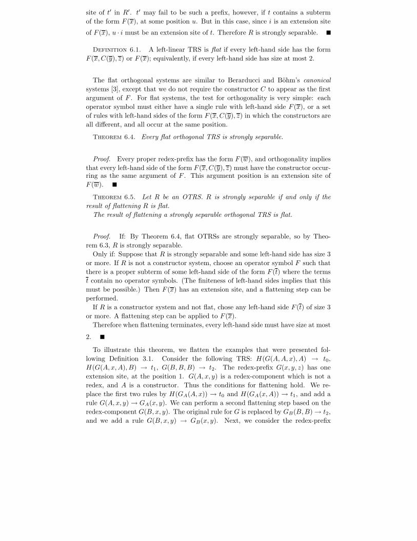
Definition 6.1. A left-linear TRS is flat if every left-hand side has the form
F (x,C(y), z) or F (x); equivalently, if every left-hand side has size at most 2.
The flat orthogonal systems are similar to Berarducci and Bohm’s canonical
systems [3], except that we do not require the constructor C to appear as the first
argument of F . For flat systems, the test for orthogonality is very simple: each
operator symbol must either have a single rule with left-hand side F (x), or a set
of rules with left-hand sides of the form F (x,C(y), z) in which the constructors are
all different, and all occur at the same position.
Theorem 6.4. Every flat orthogonal TRS is strongly separable.
Proof. Every proper redex-prefix has the form F (w), and orthogonality implies
that every left-hand side of the form F (x,C(y), z) must have the constructor occur-ring as the same argument of F . This argument position is an extension site of
F (w).
Theorem 6.5. Let R be an OTRS. R is strongly separable if and only if the
result of flattening R is flat.
The result of flattening a strongly separable orthogonal TRS is flat.
Proof. If: By Theorem 6.4, flat OTRSs are strongly separable, so by Theo-
rem 6.3, R is strongly separable.
Only if: Suppose that R is strongly separable and some left-hand side has size 3
or more. If R is not a constructor system, choose an operator symbol F such that
there is a proper subterm of some left-hand side of the form F (t) where the terms
t contain no operator symbols. (The finiteness of left-hand sides implies that this
must be possible.) Then F (x) has an extension site, and a flattening step can be
performed.
If R is a constructor system and not flat, chose any left-hand side F (t) of size 3
or more. A flattening step can be applied to F (x).
Therefore when flattening terminates, every left-hand side must have size at most
2.
To illustrate this theorem, we flatten the examples that were presented fol-
lowing Definition 3.1. Consider the following TRS: H(G(A,A, x), A) → t0,
H(G(A, x,A), B) → t1, G(B,B,B) → t2. The redex-prefix G(x, y, z) has one
extension site, at the position 1. G(A, x, y) is a redex-component which is not a
redex, and A is a constructor. Thus the conditions for flattening hold. We re-
place the first two rules by H(GA(A, x)) → t0 and H(GA(x,A)) → t1, and add a
rule G(A, x, y) → GA(x, y). We can perform a second flattening step based on the
redex-component G(B, x, y). The original rule for G is replaced by GB(B,B) → t2,
and we add a rule G(B, x, y) → GB(x, y). Next, we consider the redex-prefix
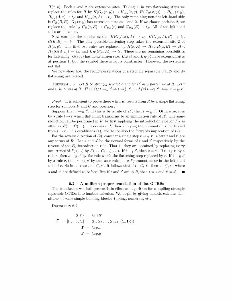
H(x, y). Both 1 and 2 are extension sites. Taking 1, in two flattening steps we
replace the rules for H by H(GA(x, y)) → HGA(x, y), H(GB(x, y)) → HGB
(x, y),
HGA(A, x) → t0, and HGA
(x,A) → t1. The only remaining non-flat left-hand side
is GB(B,B). GB(x, y) has extension sites at 1 and 2. If we choose position 2, we
replace this rule by GB(x,B) → GBB(x) and GBB
(B) → t2. All of the left-hand
sides are now flat.
Now consider the similar system H(G(A, x), A) → t0, H(G(x,A), B) → t1,
G(B,B) → t2. The only possible flattening step takes the extension site 2 of
H(x, y). The first two rules are replaced by H(x,A) → HA, H(x,B) → HB,
HA(G(A, x)) → t0, and HB(G(x,A)) → t1. There are no remaining possibilities
for flattening. G(x, y) has no extension site. HA(x) and HB(x) have extension sites
at position 1, but the symbol there is not a constructor. However, the system is
not flat.
We now show how the reduction relations of a strongly separable OTRS and its
flattening are related.
Theorem 6.6. Let R be strongly separable and let R′ be a flattening of R. Let t
and t′ be terms of R. Then (1) t →R t′ ⇒ t →+
R′ t′, and (2) t →∗R t′ ⇐⇒ t →∗
R′ t′.
Proof. It is sufficient to prove these when R′ results from R by a single flattening
step for symbols F and C and position i.
Suppose that t →R t′. If this is by a rule of R′, then t →′R t′. Otherwise, it is
by a rule l → r which flattening transforms to an elimination rule of R′. The same
reduction can be performed in R′ by first applying the introduction rule for FC as
often as F (. . . , C(. . .), . . .) occurs in l, then applying the elimination rule derived
from l → r. This establishes (1), and hence also the forwards implication of (2).
For the reverse direction of (2), consider a single step t →R′ t′, where t and t′ are
any terms of R′. Let s and s′ be the normal forms of t and t′ respectively by the
reverse of the FC -introduction rule. That is, they are obtained by replacing every
occurrence of FC(. . .) by F (. . . , C(. . .), . . .). If t →I t′, then s = s′. If t →E t′ by a
rule r, then s →R s′ by the rule which the flattening step replaced by r. If t →R t′
by a rule r, then s →R s′ by the same rule, since FC cannot occur in the left-hand
side of r. So in all cases, s →∗R s′. It follows that if t →∗
R′ t′, then s →∗R s′, where
s and s′ are defined as before. But if t and t′ are in R, then t = s and t′ = s′.
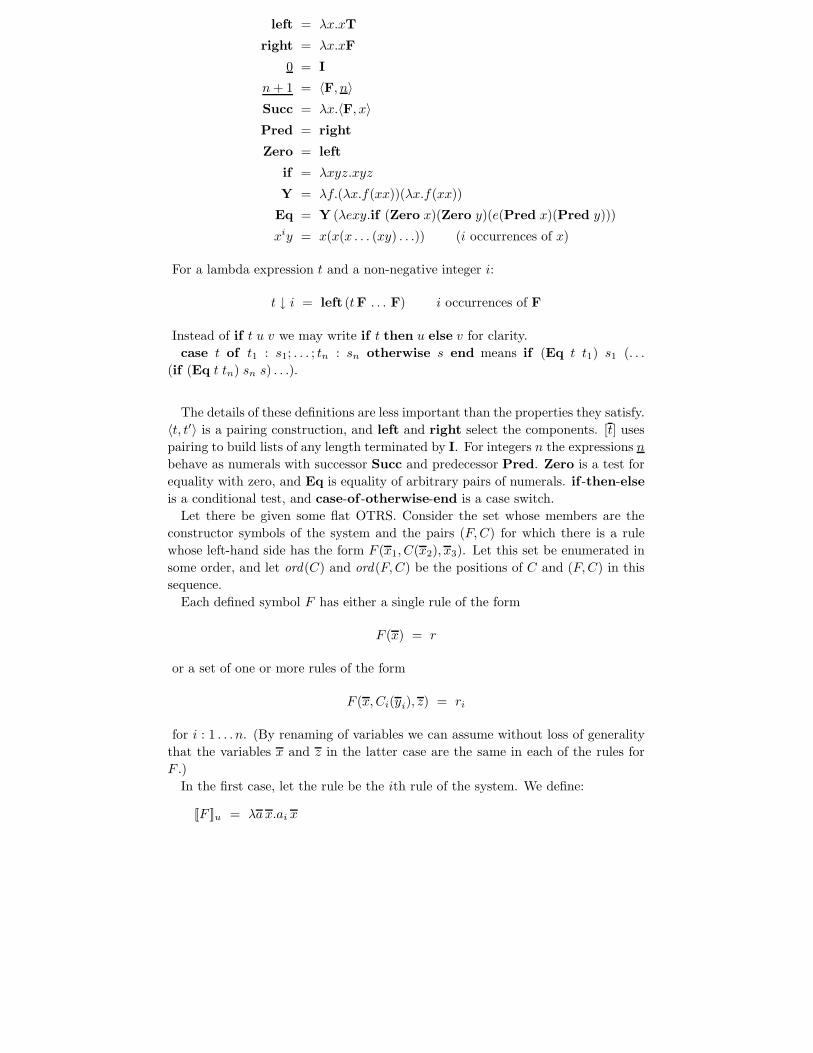
6.2. A uniform proper translation of flat OTRSs
The translation we shall present is in effect an algorithm for compiling strongly
separable OTRSs into lambda calculus. We begin by giving lambda calculus defi-
nitions of some simple building blocks: tupling, numerals, etc.
Definition 6.2.
〈t, t′〉 = λz.ztt′
[t] = [t1, . . . , tn] = 〈t1, 〈t2 . . . , 〈tn−1, 〈tn, I〉〉〉〉
T = λxy.x
F = λxy.y
left = λx.xT
right = λx.xF
0 = I
n + 1 = 〈F, n〉
Succ = λx.〈F, x〉
Pred = right
Zero = left
if = λxyz.xyz
Y = λf.(λx.f(xx))(λx.f(xx))
Eq = Y (λexy.if (Zero x)(Zero y)(e(Pred x)(Pred y)))
xiy = x(x(x . . . (xy) . . .)) (i occurrences of x)
For a lambda expression t and a non-negative integer i:
t ↓ i = left (tF . . . F) i occurrences of F
Instead of if t u v we may write if t then u else v for clarity.
case t of t1 : s1; . . . ; tn : sn otherwise s end means if (Eq t t1) s1 (. . .
(if (Eq t tn) sn s) . . .).
The details of these definitions are less important than the properties they satisfy.
〈t, t′〉 is a pairing construction, and left and right select the components. [t] uses
pairing to build lists of any length terminated by I. For integers n the expressions n
behave as numerals with successor Succ and predecessor Pred. Zero is a test for
equality with zero, and Eq is equality of arbitrary pairs of numerals. if -then-else
is a conditional test, and case-of -otherwise-end is a case switch.
Let there be given some flat OTRS. Consider the set whose members are the
constructor symbols of the system and the pairs (F,C) for which there is a rule
whose left-hand side has the form F (x1, C(x2), x3). Let this set be enumerated in
some order, and let ord(C) and ord(F,C) be the positions of C and (F,C) in this
sequence.
Each defined symbol F has either a single rule of the form
F (x) = r
or a set of one or more rules of the form
F (x,Ci(yi), z) = ri
for i : 1 . . . n. (By renaming of variables we can assume without loss of generality
that the variables x and z in the latter case are the same in each of the rules for
F .)
In the first case, let the rule be the ith rule of the system. We define:
[[F ]]u = λa x.ai x
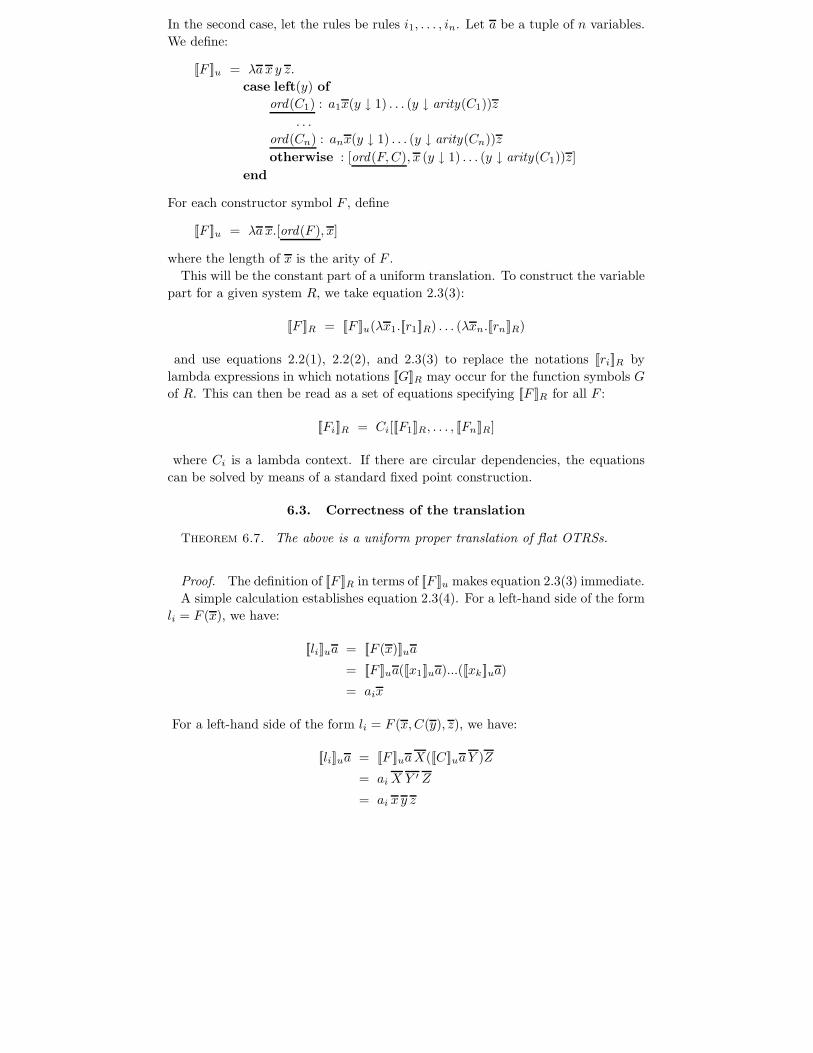
In the second case, let the rules be rules i1, . . . , in. Let a be a tuple of n variables.
We define:
[[F ]]u = λa x y z.
case left(y) of
ord(C1) : a1x(y ↓ 1) . . . (y ↓ arity(C1))z
. . .
ord(Cn) : anx(y ↓ 1) . . . (y ↓ arity(Cn))z
otherwise : [ord(F,C), x (y ↓ 1) . . . (y ↓ arity(C1))z]
end
For each constructor symbol F , define
[[F ]]u = λa x.[ord(F ), x]
where the length of x is the arity of F .
This will be the constant part of a uniform translation. To construct the variable
part for a given system R, we take equation 2.3(3):
[[F ]]R = [[F ]]u(λx1.[[r1]]R) . . . (λxn.[[rn]]R)
and use equations 2.2(1), 2.2(2), and 2.3(3) to replace the notations [[ri]]R by
lambda expressions in which notations [[G]]R may occur for the function symbols G
of R. This can then be read as a set of equations specifying [[F ]]R for all F :
[[Fi]]R = Ci[[[F1]]R, . . . , [[Fn]]R]
where Ci is a lambda context. If there are circular dependencies, the equations
can be solved by means of a standard fixed point construction.
6.3. Correctness of the translation
Theorem 6.7. The above is a uniform proper translation of flat OTRSs.
Proof. The definition of [[F ]]R in terms of [[F ]]u makes equation 2.3(3) immediate.
A simple calculation establishes equation 2.3(4). For a left-hand side of the form
li = F (x), we have:
[[li]]ua = [[F (x)]]ua
= [[F ]]ua([[x1]]ua)...([[xk ]]ua)
= aix
For a left-hand side of the form li = F (x,C(y), z), we have:
[[li]]ua = [[F ]]ua X([[C]]uaY )Z
= ai X Y ′ Z
= ai x y z
where
Xi =df [[xi]]a
= xi
Yi =df [[yi]]a
= yi
Y ′i =df [ord(C), y] ↓ i
= yi
Zi =df [[zi]]a
= zi
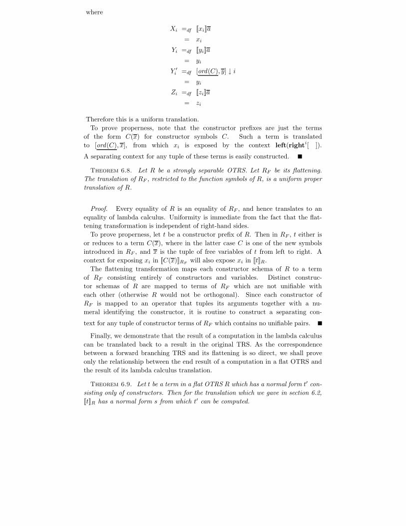
Therefore this is a uniform translation.
To prove properness, note that the constructor prefixes are just the terms
of the form C(x) for constructor symbols C. Such a term is translated
to [ord(C), x], from which xi is exposed by the context left(righti[ ]).
A separating context for any tuple of these terms is easily constructed.
Theorem 6.8. Let R be a strongly separable OTRS. Let RF be its flattening.
The translation of RF , restricted to the function symbols of R, is a uniform proper
translation of R.
Proof. Every equality of R is an equality of RF , and hence translates to an
equality of lambda calculus. Uniformity is immediate from the fact that the flat-
tening transformation is independent of right-hand sides.
To prove properness, let t be a constructor prefix of R. Then in RF , t either is
or reduces to a term C(x), where in the latter case C is one of the new symbols
introduced in RF , and x is the tuple of free variables of t from left to right. A
context for exposing xi in [[C(x)]]RFwill also expose xi in [[t]]R.
The flattening transformation maps each constructor schema of R to a term
of RF consisting entirely of constructors and variables. Distinct construc-
tor schemas of R are mapped to terms of RF which are not unifiable with
each other (otherwise R would not be orthogonal). Since each constructor of
RF is mapped to an operator that tuples its arguments together with a nu-
meral identifying the constructor, it is routine to construct a separating con-
text for any tuple of constructor terms of RF which contains no unifiable pairs.
Finally, we demonstrate that the result of a computation in the lambda calculus
can be translated back to a result in the original TRS. As the correspondence
between a forward branching TRS and its flattening is so direct, we shall prove
only the relationship between the end result of a computation in a flat OTRS and
the result of its lambda calculus translation.
Theorem 6.9. Let t be a term in a flat OTRS R which has a normal form t′ con-
sisting only of constructors. Then for the translation which we gave in section 6.2,
[[t]]R has a normal form s from which t′ can be computed.
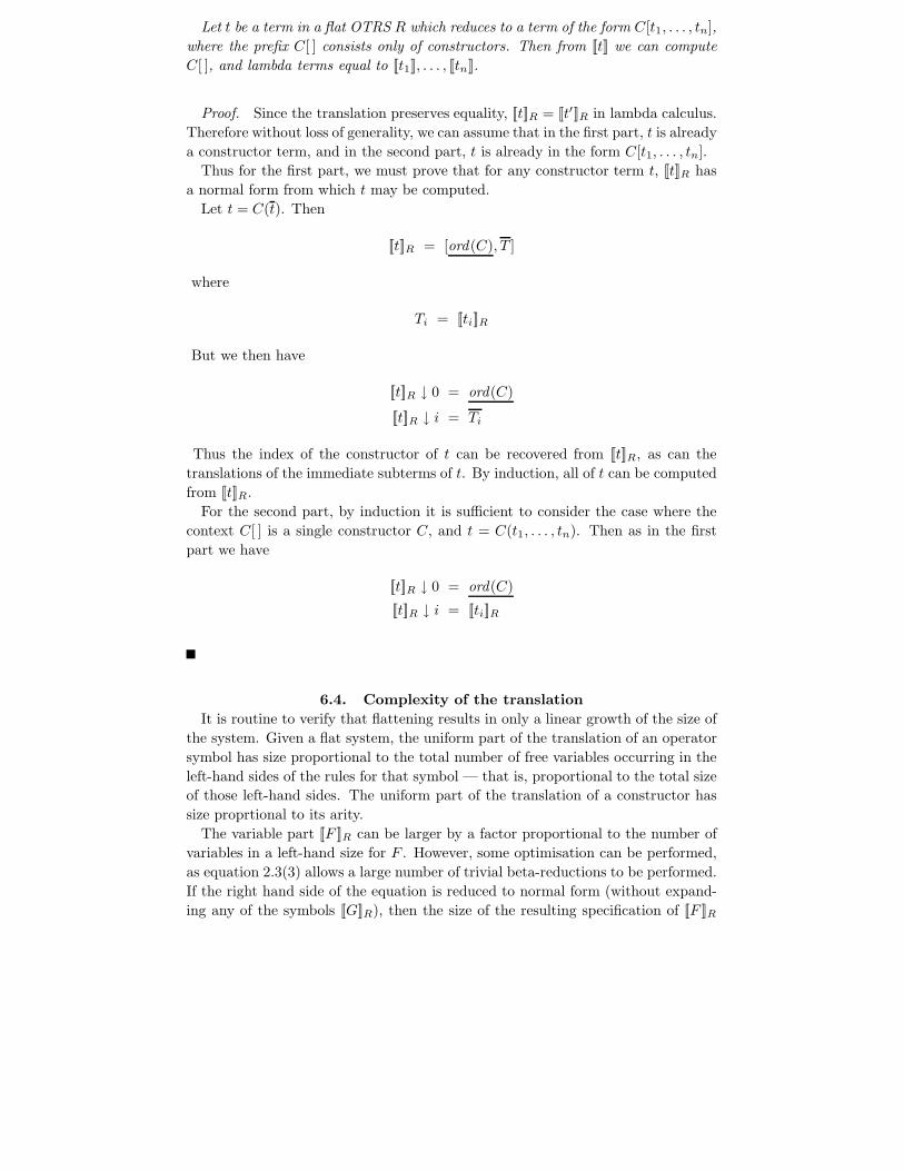
Let t be a term in a flat OTRS R which reduces to a term of the form C[t1, . . . , tn],
where the prefix C[ ] consists only of constructors. Then from [[t]] we can compute
C[ ], and lambda terms equal to [[t1]], . . . , [[tn]].
Proof. Since the translation preserves equality, [[t]]R = [[t′]]R in lambda calculus.
Therefore without loss of generality, we can assume that in the first part, t is already
a constructor term, and in the second part, t is already in the form C[t1, . . . , tn].
Thus for the first part, we must prove that for any constructor term t, [[t]]R has
a normal form from which t may be computed.
Let t = C(t). Then
[[t]]R = [ord(C), T ]
where
Ti = [[ti]]R
But we then have
[[t]]R ↓ 0 = ord(C)
[[t]]R ↓ i = Ti
Thus the index of the constructor of t can be recovered from [[t]]R, as can the
translations of the immediate subterms of t. By induction, all of t can be computed
from [[t]]R.
For the second part, by induction it is sufficient to consider the case where the
context C[ ] is a single constructor C, and t = C(t1, . . . , tn). Then as in the first
part we have
[[t]]R ↓ 0 = ord(C)
[[t]]R ↓ i = [[ti]]R
6.4. Complexity of the translation
It is routine to verify that flattening results in only a linear growth of the size of
the system. Given a flat system, the uniform part of the translation of an operator
symbol has size proportional to the total number of free variables occurring in the
left-hand sides of the rules for that symbol — that is, proportional to the total size
of those left-hand sides. The uniform part of the translation of a constructor has
size proprtional to its arity.
The variable part [[F ]]R can be larger by a factor proportional to the number of
variables in a left-hand size for F . However, some optimisation can be performed,
as equation 2.3(3) allows a large number of trivial beta-reductions to be performed.
If the right hand side of the equation is reduced to normal form (without expand-
ing any of the symbols [[G]]R), then the size of the resulting specification of [[F ]]R
becomes proportional to the total size of all the rules for [[F ]]R. The subsequent
fixed-point extraction adds only a constant amount.
It is more difficult to obtain a meaningful comparison of the cost of reductions
in the original system and in the transformed system. Any such comparison would
have to consider such things as the implementation of the case operation (we have
defined it as a linear search, but other definitions are possible), and the mechanism
for pattern-matching in an implementation of the original system. This gets into
details of implementation which cannot be realistically be studied in this abstract
setting.
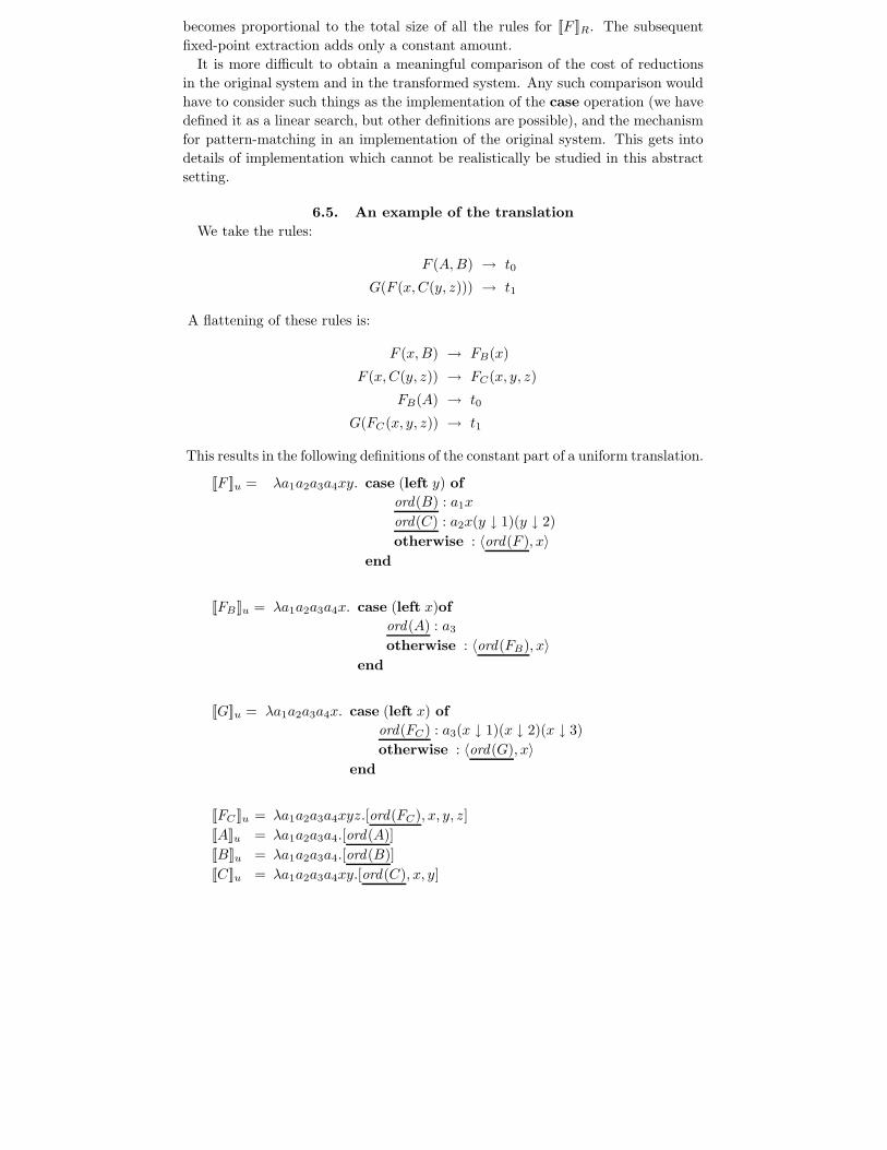
6.5. An example of the translation
We take the rules:
F (A,B) → t0
G(F (x,C(y, z))) → t1
A flattening of these rules is:
F (x,B) → FB(x)
F (x,C(y, z)) → FC(x, y, z)
FB(A) → t0
G(FC(x, y, z)) → t1
This results in the following definitions of the constant part of a uniform translation.
[[F ]]u = λa1a2a3a4xy. case (left y) of
ord(B) : a1x
ord(C) : a2x(y ↓ 1)(y ↓ 2)
otherwise : 〈ord(F ), x〉
end
[[FB ]]u = λa1a2a3a4x. case (left x)of
ord(A) : a3
otherwise : 〈ord(FB), x〉
end
[[G]]u = λa1a2a3a4x. case (left x) of
ord(FC) : a3(x ↓ 1)(x ↓ 2)(x ↓ 3)
otherwise : 〈ord(G), x〉
end
[[FC ]]u = λa1a2a3a4xyz.[ord(FC), x, y, z]
[[A]]u = λa1a2a3a4.[ord(A)]
[[B]]u = λa1a2a3a4.[ord(B)]
[[C]]u = λa1a2a3a4xy.[ord(C), x, y]
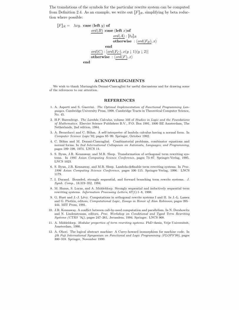
The translations of the symbols for the particular rewrite system can be computed
from Definition 2.4. As an example, we write out [[F ]]R, simplifying by beta reduc-
tion where possible:
[[F ]]R = λxy. case (left y) of
ord(B) :case (left x)of
ord(A) : [[t0]]Rotherwise : 〈ord(FB), x〉
end
ord(C) : [ord(FC), x(y ↓ 1)(y ↓ 2)]
otherwise : 〈ord(F ), x〉
end
ACKNOWLEDGMENTS
We wish to thank Mariangiola Dezani-Ciancaglini for useful discussions and for drawing someof the references to our attention.
REFERENCES
1. A. Asperti and S. Guerrini. The Optimal Implementation of Functional Programming Lan-guages. Cambridge University Press, 1998. Cambridge Tracts in Theoretical Computer Science,No. 45.
2. H.P. Barendregt. The Lambda Calculus, volume 103 of Studies in Logic and the Foundationsof Mathematics. Elsevier Science Publishers B.V., P.O. Box 1991, 1000 BZ Amsterdam, TheNetherlands, 2nd edition, 1984.
3. A. Berarducci and C. Bohm. A self-interpreter of lambda calculus having a normal form. InComputer Science Logic’92, pages 85–99. Springer, October 1992.
4. C. Bohm and M. Dezani-Ciancaglini. Combinatorial problems, combinator equations andnormal forms. In 2nd International Colloquium on Automata, Languages, and Programming,pages 189–199, 1974. LNCS 14.
5. S. Byun, J.R. Kennaway, and M.R. Sleep. Transformation of orthogonal term rewriting sys-tems. In 1995 Asian Computing Science Conference, pages 73–87. Springer-Verlag, 1995.LNCS 1023.
6. S. Byun, J.R. Kennaway, and M.R. Sleep. Lambda-definable term rewriting systems. In Proc.1996 Asian Computing Science Conference, pages 106–115. Springer-Verlag, 1996. LNCS1179.
7. I. Durand. Bounded, strongly sequential, and forward branching term rewrite systems. J.Symb. Comp., 18:319–352, 1994.
8. M. Hanus, S. Lucas, and A. Middeldorp. Strongly sequential and inductively sequential termrewriting systems. Information Processing Letters, 67(1):1–8, 1998.
9. G. Huet and J.-J. Levy. Computations in orthogonal rewrite systems I and II. In J.-L. Lassezand G. Plotkin, editors, Computational Logic, Essays in Honor of Alan Robinson, pages 395–444. MIT Press, 1991.
10. J.R. Kennaway. A conflict between call-by-need computation and parallelism. In N. Dershowitzand N. Lindenstrauss, editors, Proc. Workshop on Conditional and Typed Term RewritingSystems (CTRS ’94), pages 247–261, Jerusalem, 1994. Springer. LNCS 968.
11. A. Middeldorp. Modular properties of term rewriting systems. PhD thesis, Vrije Universiteit,Amsterdam, 1990.
12. A. Ohori. The logical abstract machine: A Curry-howard isomorphism for machine code. In4th Fuji International Symposium on Functional and Logic Programming (FLOPS’99), pages300–318. Springer, November 1999.
13. B. Salinier and R. Strandh. Simulating forward-branching systems with constructor systems.In Proc. CAAP’97. Springer-Verlag, 1997. Lecture Notes in Computer Science.
14. R. Strandh. Classes of equational programs that compile into efficient machine code. In Proc.3rd Int. Conf. on Rewriting Techniques and Applications, pages 449–461. Springer-Verlag,1989. Lecture Notes in Computer Science 355.


