The Use of Flexible Manufacturing Capacity in Pharmaceutical Product Introductions

Decision SciencesVolume 40 Number 2May 2009

C© 2009, The AuthorJournal compilation C© 2009, Decision Sciences Institute

The Use of Flexible Manufacturing Capacityin Pharmaceutical Product Introductions∗Chester G. ChambersCarey School of Business, Johns Hopkins University, Baltimore, MD 21201,e-mail: [email protected]

Eli M. Snir†Information Technologies and Operations Management, Cox School of Business, SouthernMethodist University, Dallas, TX 75275-0333, e-mail: [email protected],[email protected]

Asad AtaEngineering Management, Information and Systems, School of Engineering, SouthernMethodist University, Dallas, TX 75275-0123, e-mail: [email protected]

ABSTRACT

This work considers the value of the flexibility offered by production facilities thatcan easily be configured to produce new products. We focus on technical uncertaintyas the driver of this value, while prior works focused only on demand uncertainty.Specifically, we evaluate the use of process flexibility in the context of risky new productdevelopment in the pharmaceutical industry. Flexibility has value in this setting due tothe time required to build dedicated capacity, the finite duration of patent protection,and the probability that the new product will not reach the market due to technical orregulatory reasons. Having flexible capacity generates real options, which enables firmsto delay the decision about constructing product-specific capacity until the technicaluncertainty is resolved. In addition, initiating production in a flexible facility can enablethe firm to optimize production processes in dedicated facilities. The stochastic dynamicoptimization problem is formulated to analyze the optimal capacity and allocationdecisions for a flexible facility, using data from existing literature. A solution to thisproblem is obtained using linear programming. The result of this analysis shows boththe value of flexible capacity and the optimal capacity allocation. Due to the substantialcosts involved with flexibility in this context, the optimal level of flexible capacity isrelatively small, suggesting products be produced for only short periods before initiatingconstruction of dedicated facilities.

Subject Areas: Flexible Capacity, Markov Decision Processes, OperationsStrategy, Optimization, Pharmaceutical Manufacturing, and Real Options.

∗We thank Jeff Kennington, Dick Helgason, John Semple, participants at the Information Technologiesand Operations Management Department seminar, and participants at the 19th Annual Conference of theProduction and Operations Management Society for helpful comments on previous drafts of this article. Weare especially indebted to Eli Olinick for his ongoing support and advice throughout this research program.All remaining errors and omissions are solely our responsibility.

†Corresponding author.

243

244 Flexible Manufacturing Capacity in Pharmaceutical Product Introductions

INTRODUCTION

Increasing manufacturing flexibility is a key strategy for improving responsive-ness in the face of an uncertain future. One type of flexibility, known as processflexibility, is defined as the ability to produce different types of products in thesame plant or production facility at the same time (Jordan & Graves, 1995). Sev-eral earlier works have looked at the value of process flexibility in the face ofdemand uncertainty. Our purpose is to consider the value of such flexibility thatstems from technical uncertainty, where “technical” refers to risks independent ofmarket forces. For example, the probabilities that a development project will failbefore a resulting marketable product can be introduced. While the focus of thisresearch is the pharmaceutical industry, the methodology is broadly applicable.

Van Mieghem (2003) provides a broad review on the topic of capacity man-agement and flexibility including several works in which a firm must select capacitylevels in a system including dedicated and/or flexible facilities. These works in-clude Jordan and Graves (1995), which focuses upon process flexibility in theface of uncertain demand for a portfolio of M products. The key finding is thata limited amount of flexibility, carefully allocated, provides the great majority ofthe potential benefits achievable with total flexibility. In their context, having anetwork of M plants making M products in which each plant can produce onlytwo products is almost as profitable as having M plants, each able to produce allM products. This suggests that, while having enough flexibility to respond to anyscenario has some appeal, the optimal use of a relatively small amount of flexiblecapacity may constitute an optimal policy.

Van Mieghem (1998) considers a two-product firm considering investment indedicated capacity for each product along with flexible capacity that can produceeither. This work shows that the optimal level of flexible capacity is affected bythe correlation between product demands, product prices, investment costs, andmultivariate demand uncertainty. More recent work includes Graves and Tomlin(2003), which investigates the extent to which this concept applies to multistagesupply chains.

Bish and Wang (2004) extends the analysis of Van Mieghem (1998) by con-sidering how the ability of the firm to adjust pricing affects its resource investmentstrategy. In this work a monopolistic producer facing linear demand will choseto invest in dedicated and/or flexible capacity in a two-product setting where thesize of the market for each product is the uncertainty under consideration. Bish,Muriel, and Biller (2005) applied a parallel analysis focused upon the allocationof jobs between two plants with flexible capacity in a make-to-order environment.

The common thread connecting these works is that they focus on the value ofprocess flexibility that exists due to demand uncertainty. However, when consid-ering the development of new products, decision makers must also manage highlevels of technical uncertainty, and in some cases this factor is the primary driverof the value of flexibility. As an example, consider the case study of Eli Lilly(Pisano & Rossi, 1994; Pisano, 1997). The firm was considering options for theproduction of synthetic chemicals that were the main ingredients in new ethicalpharmaceuticals. They wrestled with a decision concerning the construction of aflexible facility that would be capable of producing a wide array of compoundsincluding new molecular entities (NMEs) yet to be discovered. The decision was

Chambers, Snir, and Ata 245

difficult for several reasons. Chief among them was the fact that flexible capacitywas four times as costly to build as dedicated capacity and the yield was 50%lower.

Flexible capacity has great value in this setting for several reasons other thanuncertain sales levels. U.S.-based pharmaceutical firms typically acquire patentprotection for NMEs if they believe that the entity may have some therapeuticvalue. However, these patents have a finite lifespan and “generic” copies of theproducts containing these compounds are introduced very quickly after patent ex-piration. Effectively, any delay in product introduction becomes a day of lost salesthat cannot be recovered (Eapen, 2000). On the other hand, NMEs are compoundsthat have never previously been produced on a large scale. Firms often need toconstruct new production lines or even new plants specifically designed to makea single compound. This is an expensive, time consuming process. A third factorcentral to this setting is that a firm does not have the ability to unilaterally de-cide to introduce a new drug to the marketplace. Food and Drug Administration(FDA) review and approval is required at the end of several phases along the way.Managers in this industry relay tales of production lines being built, supplied,staffed, and ready to operate only to find that the firm’s application for permissionto sell the product has been denied. This leaves the firm with production capacitydedicated to a single product that cannot be produced (Spradlin, 2000). This com-bination of a finite economic product life, the long time required to build dedicatedcapacity, and uncertainty over whether a product may proceed to the next phase,gives process flexibility great value. The objective of this article is to develop andpresent an analysis that can identify the optimal level of flexible capacity and theoptimal utilization of this capacity accounting for required investments, techni-cal uncertainty, and options for the firm launching new products in an uncertainenvironment.

Our analysis focuses on the introduction of ethical pharmaceuticals in whichproduction is synonymous with the chemical synthesis of new compounds. Whilethe data surrounding particular products are treated as proprietary, we make liberaluse of published data to populate our model in order to provide examples, andto convey insights. Our approach is generalizable in which the parameters of themodel that we formulate can easily be adapted to a particular firm. To evaluate theimpact of ambiguity in model parameters we evaluate the model under a varietyof different assumptions.

We pursue our aims through the development and analysis of a discrete time,infinite horizon, stochastic, dynamic programming (DP) model with a finite statespace. We take advantage of the structure of our model to solve this DP using linearprogramming (LP). This approach is rare in the literature because other methodsfor solving large DP problems, such as policy iteration, are computationally moreefficient. However, we choose to approach the problem in this manner for severalreasons. First, LP is a tool that most practitioners are familiar with, and it is fareasier to explain results using a tool that the audience has seen before. The termsuncovered in the optimal solution of the resulting LP problem include the relativelikelihood of any particular scenario. This is quite valuable to the manager be-cause it offers an entirely intuitive interpretation of the model’s results, allowinga straightforward interpretation of the optimal allocation rules. Second, our for-mulation is quite general in that it can be applied to a large class of DP problems


and can provide useful results in many settings other than the one considered here.Third, the computational “penalty” for using LP to solve this problem is quitesmall. The examples we will discuss involve LP problems with roughly 1,000variables and 250 constraints. Such problems are routinely solved in a matter of afew seconds on any desktop PC. Policy iteration is likely to solve such a problemin something on the order of 10% of that time. (Filar & Vrieze, 1997). However,such an improvement is negligible for the problem instances considered here.

The key decisions in this context are intertwined and made simultaneously. Acompany must decide how much flexible capacity to own and the future allocationof that capacity to new products as they arrive in a probabilistic fashion. Creatingflexible capacity is synonymous with developing real options for future exercise.Increased capacity is analogous to purchasing more options. As a project arrivesat decision points the firm has to decide whether to exercise the real option,by reserving corresponding flexible capacity or to keep the option, by decidingto begin construction of a dedicated facility for the current project. A decisionto exercise the option also includes the duration of the assignment of the project tothe flexible facility. Thus, evaluation of the choice to exercise the option is morecomplex than a “one-time” decision. When a product is moved to a dedicatedfacility later in its life cycle, the flexible capacity again becomes free, and theoption to use it for the next product returns.

Our analysis suggests that the optimal level of flexible capacity is signif-icantly less than the amount required to allow all products to be produced in aflexible facility at the start of their life cycle. This is analogous to the findings ofJordan and Graves (1995). The prohibitive cost of flexible capacity, the reducedefficiency of using such a facility, and the shape of the value function for additionalflexible capacity are the main drivers of this result. With such limited capacity, theallocation decisions become all the more important. We find that, given the profitmaximizing level of flexible capacity, it is optimal to produce products for whichexpected demand is rather low in a flexible facility long enough to gain produc-tion experience. This experience would reduce the construction cost of dedicatedcapacity eventually built to house the product. We also find that for products withlarger expected demands the optimal amount of time that it is produced in theflexible facility is even shorter. This is because the lower process yield, typical ofmore flexible resources, makes the firm more eager to build a dedicated facility.We also find that, in many instances the optimal policy is to produce a productin a flexible facility for a span of time that is strictly less than would be chosento maximize the expected payoff associated with that product. In other words, thefirm is willing to sacrifice some of the profitability of a single product to preservethe option to use flexible capacity in the next period for a product that may arriveat that time.

The next section discusses the problem setting more formally as well as thekey variables and parameters used in our model. We also provide more specificsabout this problem in the pharmaceutical industry, including estimates of therelevant probabilities, costs, and revenue values. We outline the optimal policygiven infinite flexible capacity. We then formulate the more realistic problem ofassigning jobs to a flexible facility in the presence of a capacity constraint. Thisproblem is solved using representative data, and the results are discussed. We alsodiscuss the application of our approach under different initial assumptions.


PROBLEM SETTING: NEW MOLECULAR ENTITIESAND PHARMACEUTICAL MANUFACTURING

Developing and commercializing a single pharmaceutical product is expensive,complex, and risky. DiMasi, Hansen, and Grabowski (2003) estimate the expectedtotal preapproval cost at over $800 million per approved project. An industryprofile produced by the Pharmaceutical Research and Manufacturers of America(Pharmaceutical Research and Manufacturers of America, 2004) estimates globalR&D expenditures in the industry at roughly $33 billion in 2003 while only 33NMEs were approved by the FDA in that same year. These figures illustrate thathuge expenditures are routinely made in an environment of high uncertainty.

One tool to help manage these risks is the technical feasibility of very highlevels of process flexibility (Raju & Cooney, 1995). This is made possible by theuse of reaction vessels, which are lined with very stable materials that are highlyresistant to corrosion. These vessels are connected with flexible tubing so thatmaterial flow may be tailored to different production processes. Such systems alsoinclude an array of complex scrubbers, filters, agitators, heat exchangers, and otherdevices, which may be moved into or out of the production stream upon demand.Our modeling is consistent with Pisano (1997), which reports that managers at EliLilly estimate that these facilities may cost as much as four times the price of anequivalent amount of dedicated capacity and the yield is 50% as high.

Throughout this research we refer to the effort to create a marketable productas a development “project.” The actual “product” is the result of a project thatreaches successful completion including FDA approval. We focus on the firm’sdecision about which resources to dedicate to that product’s production at thebeginning of its economic life. Due to the novelty of the product as a new discovery,dedicated capacity takes considerable time to build. Thus, decisions about wherethis product will be produced at the start of its economic life must be made severalperiods prior to product launch. For example, Genzyme recently announced thestart of construction in 2007 of a new manufacturing plant in France at an estimatedcost of EUR 105 million. This plant will be configured to produce Thymoglobulinbecause the firm anticipates regulatory approvals for its use in treating acuterejection in transplant patients beginning in 2010 (PharmaWatch, 2007). In aparallel fashion, we focus on decision points 3 years prior to expected productlaunch, treat time in a discrete manner, and consider the possibility of, at most,one project reaching such a decision point in a single period. (We discuss how torelax this assumption later.) We also assume that the arrival time and success ofeach development project is independent of the outcomes associated with all otherprojects.

Conceptually, our model focuses on the random arrival of projects, each ofwhich is associated with a target launch date for a new product 3 years hence.Clearly, the motivation for undertaking each project is the possibility of realizingprofitable sales upon its successful completion. These sales levels can only berealized if capacity exists to meet product demand. If it takes 3 years to creatededicated capacity, and if the decision about where a new product will be manu-factured is not made at least 3 years before FDA approval, the firm risks having aproduct that could have been sold were it not for the lack of production capacity.Torabzadeh, Woodruff, and Sen (1998) argue that pharmaceutical firms have a


strong incentive to initiate production immediately upon FDA approval. Beyondthe obvious cash flow implications, there is a significant negative impact on stockprice due to the delayed production of an approved drug. This argument appearsto be consistent with firm behavior. For example the drug Propecia was approvedby the FDA on December 23, 1997, and was on pharmacy shelves by January 4,1998 (Merck Annual Report, 1998). In addition, the gross margins on pharmaceu-tical products motivate industry representatives to state that “although productionscheduling seems quite complicated, it’s really come down to a pretty simple dic-tum: Never stock out!” (Pisano & Rossi, 1994). Given these facts, we assumethat the firm has made a strategic decision to require that production capacity beavailable immediately after FDA approval.

We can use historical data to estimate an arrival rate. Empirical research hasfound that between 1990 and 1994 the top 10 drug companies launched an averageof 0.45 NMEs a year, (Carr, 1998) and the number of NME’s approved in a yearhas actually declined from a high of 53 in 1996 to only 33 in 2003 (Reepmeyer,2006). We note that this number may significantly differ from the number of new“products” that a firm introduces. Our focus is upon truly new compounds that donot have a prior production history. Packaging an active ingredient in a new waymay be marketed as a new product but that does not imply that a new productionprocess is needed for the active ingredient. Focusing only on truly new entitiesmakes it reasonable to use 1-year time increments and relatively low arrival rateswhen modeling this setting.

Flexible facilities have demonstrated a useful life of several decades in thisindustry. In fact, some facilities built 40 years ago are still operational. This impliesthat the use of an infinite time horizon is appropriate. While firms may have well-defined expectations about project arrivals over the very short term, it is impossibleto predict project arrivals with certainty over an infinite horizon. Therefore, wemodel the arrival process of new products as a multinomial variable with λ definedas the probability that a project reaches a critical decision point in any period.We set λ at 50% to be consistent with prior works including the detailed financialmodel of Myers and Howe (1997). This means the probability that a decision mustbe made in a given period is 50%.

We have a 50% chance of a “birth” that represents a new project about whicha decision must be made concerning its production 3 years in the future. The3 years prior to product launch envelopes the end of two distinct phases, whichwe refer to as Phases 1 and 2. The end of Phase 1 is the completion of clinicaltrials. We define P1 as the probability that a project deemed viable 3 years priorto a targeted product launch will still be deemed viable at the end of Phase 1, 1year prior to the targeted launch date. Myers and Howe (1997) estimate this valueby considering historical data to be 85%. Phase 2 is the FDA’s review period.Since the introduction of the Prescription Drug User Fee Act of 1992, the FDA hasset a target for this review at 1 year (Ng, 2004). This is consistent with reportedtrends (Keyhani, Diener-West, & Powe, 2006). We define P2 as the likelihoodthat the project will reach the market given that an application to market it hasbeen submitted to the FDA. The Director of the FDA Office on New Drugs hasrecently stated that this probability is 75% (Dickinson, 2006). Equivalently, ourmodel assumes that new projects are “born” at time t with a probability λ. At time(t + 2) a project “dies” with probability (1 − P1). At time (t + 3) this project “dies”


with probability (1 − P2). The probability that this project “survives” to become aproduct at time (t + 3) is given by P1P2.

Net Payoff From a Decision on the Use of Flexible Capacity

We define a set of possible decisions as K (indexed by k) and index a set of states (I)by i. We define Ci,k as the expected net present value of the cash flows associatedwith making decision k when in state i. In our formulation, the decision k representsthe number of periods that the NME may be manufactured in a flexible facilitybefore being moved to a dedicated facility. For example, a decision k = 1 representsa commitment by the firm to reserve capacity in its flexible facility 3 years henceso that the product can be produced there (if approved) during the first year of itseconomic life. This decision allows the firm to defer the decision on whether toconstruct dedicated capacity for one period. Because the risk that we focus uponis associated with the time to build this capacity, we only consider k ≤ 3. In thiscontext, a decision of k = 0 implies that the flexible facility is not used and thatconstruction of dedicated capacity for this project initiates immediately.

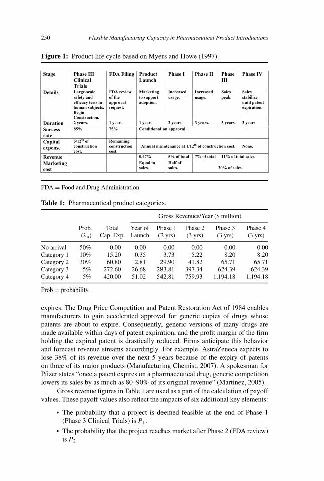
A sizeable body of prior research has focused upon net revenue projections forethical pharmaceuticals. These works include Myers and Howe (1997), the Officeof Technology Assessment (U.S. Congress, Office of Technology Assessment,1993), Scherer (1993), Grabowski and Vernon (1990, 1994), DiMasi (1995, 2001),and Grabowski, Vernon, and DiMasi (2002). We use the results from this bodyof earlier work to estimate the payoffs that result from each specific decision(k) in state (i). In particular, we make extensive use of the results of Myers andHowe (1997). Their analysis includes division of the product space into five types.Type 1 shows the lowest sales levels and Type 5 shows the highest, with Type 3being labeled as “average.” Because the projected cash flows from the two lowestcategories are virtually identical for the first 3 years of product production, wecombine these types. We thus populate our model with five categories, includinga null category for no product arrival. In our description, a Category 2 project islabeled “average.” We assume that the firm is willing to assign each product to onesuch category upon reaching the decision point and makes its decisions based onthis categorization. This parallels the assumptions of the works mentioned above.We note that this is not an assumption that the firm literally knows what saleswill be years into the future, only that some expected value of capacity requiredand resulting cash flows is associated with each project at the decision point.Figure 1 reflects the framework and data used in Myers and Howe (1997) that areof particular interest to us. Table 1 shows the expected payoffs associated with theproduct categories and stages discussed.

The population of our model with representative data begins with the esti-mates of total gross revenues, and capital expenditures calculated by Myers andHowe (1997). That work also provides estimates of the probability that a productin a given category will arrive in the next year, which is labeled λa, in Table 1.

These revenue projections treat the end of the product’s patent life as theend of its economic life. A new compound is typically patented 4–5 years prior toproduct launch and the patent lasts for 17 years. In cases where the manufactureof a drug is highly profitable, competing firms are motivated to create genericsubstitutes for the product and to introduce them to market as soon as the patent


Figure 1: Product life cycle based on Myers and Howe (1997).

Stage Phase III ClinicalTrials

FDA Filing Product Launch

Phase I Phase II Phase III

Phase IV

Details Large-scalesafety and efficacy tests in human subjects. Begin Construction.

FDA review of the approval request.

Marketingto support adoption.

Increasedusage.

Increasedusage.

Salespeak.

Salesstabilize until patent expiration.

Duration 2 years. 1 year. 1 year. 2 years. 3 years. 3 years. 3 years.

Successrate

85% 75% Conditional on approval.

Capitalexpense

5/12th of constructioncost.

Remaining constructioncost.

Annual maintenance at 1/12th of construction cost. None.

Revenue 0.47% 5% of total 7% of total 11% of total sales.

Marketingcost

Equal to sales.

Half of sales. 20% of sales.

FDA = Food and Drug Administration.

Table 1: Pharmaceutical product categories.

Gross Revenues/Year ($ million)

Prob. Total Year of Phase 1 Phase 2 Phase 3 Phase 4(λa) Cap. Exp. Launch (2 yrs) (3 yrs) (3 yrs) (3 yrs)

No arrival 50% 0.00 0.00 0.00 0.00 0.00 0.00Category 1 10% 15.20 0.35 3.73 5.22 8.20 8.20Category 2 30% 60.80 2.81 29.90 41.82 65.71 65.71Category 3 5% 272.60 26.68 283.81 397.34 624.39 624.39Category 4 5% 420.00 51.02 542.81 759.93 1,194.18 1,194.18

Prob = probability.

expires. The Drug Price Competition and Patent Restoration Act of 1984 enablesmanufacturers to gain accelerated approval for generic copies of drugs whosepatents are about to expire. Consequently, generic versions of many drugs aremade available within days of patent expiration, and the profit margin of the firmholding the expired patent is drastically reduced. Firms anticipate this behaviorand forecast revenue streams accordingly. For example, AstraZeneca expects tolose 38% of its revenue over the next 5 years because of the expiry of patentson three of its major products (Manufacturing Chemist, 2007). A spokesman forPfizer states “once a patent expires on a pharmaceutical drug, generic competitionlowers its sales by as much as 80–90% of its original revenue” (Martinez, 2005).

Gross revenue figures in Table 1 are used as a part of the calculation of payoffvalues. These payoff values also reflect the impacts of six additional key elements:

• The probability that a project is deemed feasible at the end of Phase 1(Phase 3 Clinical Trials) is P1.

• The probability that the project reaches market after Phase 2 (FDA review)is P2.


• Marketing expenses are expressed as percentages of gross revenue as shownin Figure 1.

• Variable production costs are also expressed as percentages of gross rev-enue.

• The timing of capital expenditures that take place both prior to and subse-quent to product launch is consistent across all projects.

• Production experience in a flexible facility impacts the cost of dedicatedcapacity to follow if and only if the new product is produced in the flexiblefacility for at least 2 years. This impact is denoted by the scale deflatorparameter, SD.

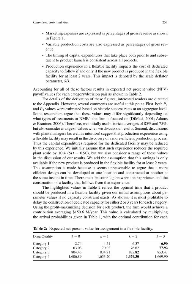
Accounting for all of these factors results in expected net present value (NPV)payoff values for each category/decision pair as shown in Table 2.

For details of the derivation of these figures, interested readers are directedto the Appendix. However, several comments are useful at this point. First, both P1

and P2 values were estimated based on historic success rates at an aggregate level.Some researchers argue that these values may differ significantly depending onwhat types of treatments or NME’s the firm is focused on (DiMasi, 2001; Adams& Brantner, 2006). Therefore, we initially use historical averages of 85% and 75%,but also consider a range of values when we discuss our results. Second, discussionswith plant managers (as well as intuition) suggest that production experience usinga flexible facility may result in the discovery of a more efficient production process.Thus the capital expenditures required for the dedicated facility may be reducedby this experience. We initially assume that such experience reduces the requiredplant scale by 10% (SD = 0.90), but we also consider a range of these valuesin the discussion of our results. We add the assumption that this savings is onlyavailable if the new product is produced in the flexible facility for at least 2 years.This assumption is made because it seems unreasonable to argue that a moreefficient design can be developed at one location and constructed at another atthe same instant in time. There must be some lag between the experience and theconstruction of a facility that follows from that experience.

The highlighted values in Table 2 reflect the optimal time that a productshould be produced in a flexible facility given our initial assumptions about pa-rameter values if no capacity constraint exists. As shown, it is most profitable todelay the construction of dedicated capacity for either 2 or 3 years for each category.Using the profit-maximizing decision for each product, the firm would achieve acontribution averaging $150.6 M/year. This value is calculated by multiplyingthe arrival probabilities given in Table 1, with the optimal contribution for each

Table 2: Expected net present value for assignment in a flexible facility.

Drug Quality k = 0 k = 1 k = 2 k = 3

Category 1 2.74 4.51 6.37 6.90Category 2 63.03 70.02 76.62 77.92Category 3 804.45 834.91 855.82 853.47Category 4 1,606.89 1,653.20 1,679.30 1,669.90


category from Table 2. We designate the optimal decision as k∗. By comparing thebest case results (with k = k∗) to the base case results (k = 0) we can deduce theannual value added by flexibility. This value can be calculated as

5∑a=1

λa(Ca,k∗ − Ca,0). (1)

Using Equation (1) we find that flexibility is worth $11 M/year. If we treatthis as an infinite horizon problem with a 9% discount rate, we deduce that processflexibility has a total value of $122.9 M to this firm. (Discount rates are discussedin the Appendix.) In order to receive all of this benefit, it is necessary to haveenough flexible capacity to produce two Category 4 drugs simultaneously: one inthe second year of its life cycle, and one in the first year. Under the assumptions ofMyers and Howe (1997), the NPV of the capital expenditures necessary to enablethe firm to do this is $444 M. Clearly, the advantages available through the use offlexibility do not justify the investment needed to fully acquire them. Therefore,we must consider the use of lower levels of flexible capacity.

THE FINITE CAPACITY PROBLEM

We extend the analysis by including a constraint on the amount of flexible capacitythat is available. We add two assumptions in order to make economic sense of thissetting.

(i) A product may be assigned to the flexible facility in a given period onlywhen enough capacity is available to produce that period’s demand for thatproduct.

(ii) One product is not displaced from a facility to make room for another.

In the presence of a capacity constraint, the firm must make the tradeoffbetween maximizing the return on a single product and risking the unavailabilityof flexible capacity for use if another product arrives while the facility is “busy.”In effect, this is a decision about when to exercise the real option of using flexiblecapacity. This decision includes how much of that capacity to use and for howlong. Thus the firm must deduce a profit maximizing policy that accounts for thiscapacity restriction in a dynamic setting.

State Space

Given any finite level of flexible capacity, we are interested in the decision ofwhether to reserve a portion of that capacity for an arriving project at the currenttime (t) and the duration of that assignment (k). To assess the feasibility of a decisiona decision maker needs to know how much capacity is available. This requires someknowledge of past arrivals, the associated decisions, and whether these projectsare still viable. To reflect these needs we define a state space that includes allinformation relevant to a decision in the current period. A brief explanation of thestate space is provided here. The complete list of the resulting states is available


from the authors upon request. Each state can be written as a collection of fivedigits.

• The leftmost digit represents the arrival in period (t − 2). It takes a valueranging from 0 to 4, where 0 means no project reached a decision point inthat period.

• The second digit represents the decision made in period (t − 2), k = 0, 1,2, or 3.

• The third digit represents the arrival in period (t − 1). Again, it can be0 to 4.

• The fourth digit is the decision taken in period (t − 1), indexed by 0 to 3.• The rightmost digit is the current arrival, indexed by 0 to 4.

Using this notation we generate the list of possible states. In period (t − 2)one of 5 project types could have arrived and one of four decisions could have beenmade. Similarly, in period (t − 1), one of five projects types could have arrivedand one of four decisions could have been made. We also have five possible arrivaltypes in the current period. Thus we can have as many as (5 × 4) × (5 × 4) ×5 = 2000 states. However, we take advantage of the structure of the problem toreduce this number dramatically. When considering an arrival in period (t − 2),this arrival can only be relevant to the next decision if the decision k = 3 was made.If a different decision was made the project would not require flexible capacity inconjunction with the current arrival. If a project arrived in period (t − 1) it canonly be relevant if the decision k = 2, or k = 3 was made. Consequently we cancompletely describe the relevant state space using (5 × 1) × (5 × 2) × 5 = 250states. As an example, the state “13234” corresponds to an arrival of a Type 1project two periods ago and an associated decision of k = 3. A Type 2 productarrived in period (t − 1) and the decision k = 3 was made and both of these projectsare still viable at the current time. The fifth digit shows that a project of Category 4has just reached the decision point.

For each of the 250 possible states, representing different decision nodes,there are four possible decisions, k = 0, 1, 2, 3. Together there are 250 × 4 = 1,000decision variables in the resulting optimization problem.

Transition Probabilities

Calculating the probability of moving from state i in period t to state j in period(t + 1) involves three factors: the arrival of a new project at (t + 1), the death ofan old project in period t, and the decision made at time t. The probability that aproject arrives of type a is λa, as explained earlier. This is the likelihood that thenext state ( j) carries a label with the rightmost digit of a.

To convey additional insights regarding the transitions among states let usagain focus on the state “13234” referenced earlier. The first two digits “13”indicate that a Category 1 project arrived two periods ago and a decision k = 3 wasmade at that point. The fact that these values are nonzeros tells us that this projectwas deemed viable at the end of both Phases 1 and 2. If this project had died ateither of these points, the first two digits of the current state would be “00.” The


value of the first two digits in the state space reached in the next period (t + 1) willeither be the third and fourth digits in the current state “23” or they will be “00.”The Category 2 project that arrived one period ago was associated with a decisionk = 3. With probability P2 the value of the first two digits in the next state reachedwill be “23.” With probability (1 − P2) the project from two periods ago fails andthe first two digits in the next state reached will be “00.”

The third and fourth digits of the state reached one period in the future dependupon the arrival in the current period and the decision made. The fifth digit in thecurrent state of “4” means that a Category 4 project has just arrived. If the currentdecision is k = 0 or k = 1, then we know that the third and fourth digits of thenext state reached will be “00.” In the case of k = 0, this is due to the fact that wedecide not to use the flexible resource. In the case of k = 1, this is due to the factthat the flexible resource was “reserved” for only one period and is freed beforethe next arrival. Hence, this decision is not relevant to the decision made in thefollowing period. On the other hand, if the current decision is k = 2, then the thirdand fourth digits in the next state will be “42.” Finally, the fifth digit in the nextstate reached simply reflects the next arrival, taking on values 0–4.

Speaking more generally, for any state, a digit that references a project willchange to a zero in the next state if the product is assigned to the flexible facilityfor less than 2 years, or if it fails. Because project arrivals are independent ofall decisions, the probabilities of arrivals and the impacts of decisions constitutea simple “birth–death” process such that birth probabilities can be multiplied bysuccess and death probabilities to fully deduce all pij values.

Formulation

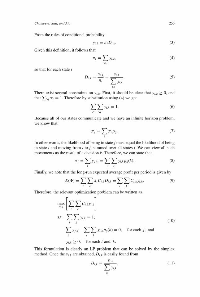
The resulting problem is an instance of a Unichain Markov Decision Process,meaning that the system can be described using a single recurrent state space, andall relevant history is contained in each state’s definition (Putterman, 1994). Atechnical discussion of our approach is available in Putterman (1994) or Filar andVrieze (1997). We endeavor to provide a more intuitive explanation of the logic ofour approach below. Assuming risk neutrality and an infinite planning horizon wedefine the long-run expected average profit per unit time as the metric of interest.For any policy � we may define the expected average profit per unit time, V(�) as

V (�) =∑∀i

πiDi,kCi,k, (2)

where � maps a specific decision k onto each state i, π i is the probability of beingin state i under policy �, and Di,k is probability of making decision k given thatthe system is in state i. Thus, a policy � can be stated as a vector if Di,k values.We seek the policy �∗ that has V (�∗) ≥ V (�) for all �. This can be viewedas a collection of decisions that maximizes (2). It is convenient to uncover thispolicy and V(�∗) simultaneously by formulating the decision as an LP problem asfollows. Let yi,k be the steady-state unconditional probability that the system is instate i and decision k is made; that is

yi,k = Pr{state ≡ i, decision ≡ k}.


From the rules of conditional probability

yi,k = πiDi,k. (3)

Given this definition, it follows that

πi =∑∀k

yi,k, (4)

so that for each state i

Di,k = yi,k

πi

= yi,k∑∀k

yi,k

. (5)

There exist several constraints on yi,k. First, it should be clear that yi,k ≥ 0, andthat

∑∀i πi = 1. Therefore by substitution using (4) we get∑

∀i

∑∀k

yi,k = 1. (6)

Because all of our states communicate and we have an infinite horizon problem,we know that

πj =∑

i

πipij. (7)

In other words, the likelihood of being in state j must equal the likelihood of beingin state i and moving from i to j, summed over all states i. We can view all suchmovements as the result of a decision k. Therefore, we can state that

πj =∑

k

yj,k =∑

i

∑k

yi,kpij(k). (8)

Finally, we note that the long-run expected average profit per period is given by

E(�) =∑

i

∑k

πiCi,kDi,k =∑

i

∑k

Ci,kyi,k. (9)

Therefore, the relevant optimization problem can be written as

maxyi,k

[∑i

∑k

Ci,kyi,k

]

s.t.∑

i

∑k

yi,k = 1,

∑k

yj,k −∑

i

∑k

yi,kpij(k) = 0, for each j, and

yi,k ≥ 0, for each i and k.

(10)

This formulation is clearly an LP problem that can be solved by the simplexmethod. Once the yi,k are obtained, Di,k is easily found from

Di,k = yi,k∑k

yi,k

. (11)


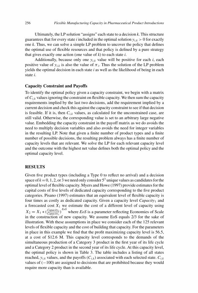
Ultimately, the LP solution “assigns” each state to a decision k. This structureguarantees that for every state i included in the optimal solution yi,k > 0 for exactlyone k. Thus, we can solve a simple LP problem to uncover the policy that definesthe optimal use of flexible resources and that policy is defined by a pure strategythat gives exactly one action (one value of k) to each state i.

Additionally, because only one yi,k value will be positive for each i, eachpositive value of yi,k is also the value of π i. Thus the solution of the LP problemyields the optimal decision in each state i as well as the likelihood of being in eachstate i.

Capacity Constraint and Payoffs

To identify the optimal policy given a capacity constraint, we begin with a matrixof Ci,k values ignoring the constraint on flexible capacity. We then sum the capacityrequirements implied by the last two decisions, add the requirement implied by acurrent decision and check this against the capacity constraint to see if that decisionis feasible. If it is, then Ci,k values, as calculated for the unconstrained case, arestill valid. Otherwise, the corresponding value is set to an arbitrary large negativevalue. Embedding the capacity constraint in the payoff matrix as we do avoids theneed to multiply decision variables and also avoids the need for integer variablesin the resulting LP. Note that given a finite number of product types and a finitenumber of possible decisions, the resulting problem always has a finite number ofcapacity levels that are relevant. We solve the LP for each relevant capacity leveland the outcome with the highest net value defines both the optimal policy and theoptimal capacity level.

RESULTS

Given five product types (including a Type 0 to reflect no arrival) and a decisionspace of k = 0, 1, 2, or 3 we need only consider 53 unique values as candidates for theoptimal level of flexible capacity. Myers and Howe (1997) provide estimates for thecapital costs of five levels of dedicated capacity corresponding to the five productcategories. Pisano (1997) estimates that an equivalent level of flexible capacity isfour times as costly as dedicated capacity. Given a capacity level Capacity1 anda forecasted cost X1 we estimate the cost of a different level of capacity using

X2 = X1 ∗ ( Capacity2Capacity1

)EoS

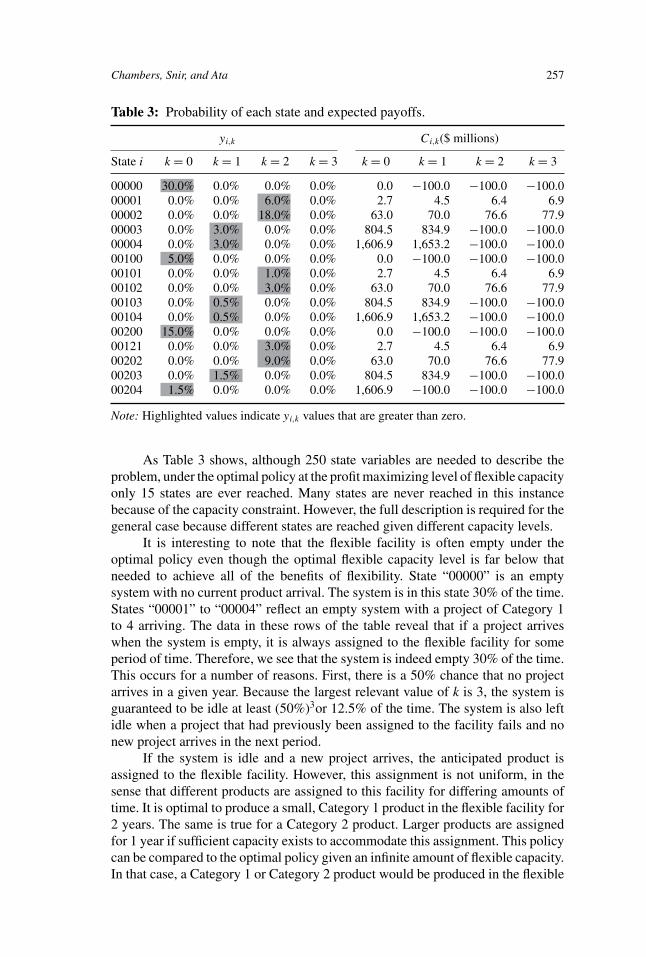
where EoS is a parameter reflecting Economies of Scalein the construction of new capacity. We assume EoS equals 2/3 for the sake ofillustration. With these assumptions in place we consider each of the 125 relevantlevels of flexible capacity and the cost of building that capacity. For the parametersin place in this example we find that the profit maximizing capacity level is 56.5,at a cost of $12.6 M. This capacity level corresponds to the demands of thesimultaneous production of a Category 3 product in the first year of its life cycleand a Category 2 product in the second year of its life cycle. At this capacity level,the optimal policy is shown in Table 3. The table includes a listing of all statesreached, yi,k values, and the payoffs (Ci,k) associated with each selected state. Ci,k

values of (−100) are assigned to decisions that are prohibited because they wouldrequire more capacity than is available.


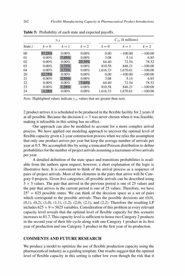
Table 3: Probability of each state and expected payoffs.

yi,k Ci,k($ millions)

State i k = 0 k = 1 k = 2 k = 3 k = 0 k = 1 k = 2 k = 3

00000 30.0% 0.0% 0.0% 0.0% 0.0 −100.0 −100.0 −100.000001 0.0% 0.0% 6.0% 0.0% 2.7 4.5 6.4 6.900002 0.0% 0.0% 18.0% 0.0% 63.0 70.0 76.6 77.900003 0.0% 3.0% 0.0% 0.0% 804.5 834.9 −100.0 −100.000004 0.0% 3.0% 0.0% 0.0% 1,606.9 1,653.2 −100.0 −100.000100 5.0% 0.0% 0.0% 0.0% 0.0 −100.0 −100.0 −100.000101 0.0% 0.0% 1.0% 0.0% 2.7 4.5 6.4 6.900102 0.0% 0.0% 3.0% 0.0% 63.0 70.0 76.6 77.900103 0.0% 0.5% 0.0% 0.0% 804.5 834.9 −100.0 −100.000104 0.0% 0.5% 0.0% 0.0% 1,606.9 1,653.2 −100.0 −100.000200 15.0% 0.0% 0.0% 0.0% 0.0 −100.0 −100.0 −100.000121 0.0% 0.0% 3.0% 0.0% 2.7 4.5 6.4 6.900202 0.0% 0.0% 9.0% 0.0% 63.0 70.0 76.6 77.900203 0.0% 1.5% 0.0% 0.0% 804.5 834.9 −100.0 −100.000204 1.5% 0.0% 0.0% 0.0% 1,606.9 −100.0 −100.0 −100.0

Note: Highlighted values indicate yi,k values that are greater than zero.

As Table 3 shows, although 250 state variables are needed to describe theproblem, under the optimal policy at the profit maximizing level of flexible capacityonly 15 states are ever reached. Many states are never reached in this instancebecause of the capacity constraint. However, the full description is required for thegeneral case because different states are reached given different capacity levels.

It is interesting to note that the flexible facility is often empty under theoptimal policy even though the optimal flexible capacity level is far below thatneeded to achieve all of the benefits of flexibility. State “00000” is an emptysystem with no current product arrival. The system is in this state 30% of the time.States “00001” to “00004” reflect an empty system with a project of Category 1to 4 arriving. The data in these rows of the table reveal that if a project arriveswhen the system is empty, it is always assigned to the flexible facility for someperiod of time. Therefore, we see that the system is indeed empty 30% of the time.This occurs for a number of reasons. First, there is a 50% chance that no projectarrives in a given year. Because the largest relevant value of k is 3, the system isguaranteed to be idle at least (50%)3or 12.5% of the time. The system is also leftidle when a project that had previously been assigned to the facility fails and nonew project arrives in the next period.

If the system is idle and a new project arrives, the anticipated product isassigned to the flexible facility. However, this assignment is not uniform, in thesense that different products are assigned to this facility for differing amounts oftime. It is optimal to produce a small, Category 1 product in the flexible facility for2 years. The same is true for a Category 2 product. Larger products are assignedfor 1 year if sufficient capacity exists to accommodate this assignment. This policycan be compared to the optimal policy given an infinite amount of flexible capacity.In that case, a Category 1 or Category 2 product would be produced in the flexible


plant for 3 years. Category 3 and 4 products would be produced there for 2 years.Inspection of our results at all capacity levels reveals that a Category 2 product isalways made in the flexible facility for 2 years if sufficient capacity is availableto make this possible. Intuition suggests that larger products should take fulladvantage of the flexible capacity; thus the decision to produce Category 3 andCategory 4 products in the flexible facility for only 1 year apparently leaves muchof the potential benefit from flexibility “on the table.” However, this decision isreasonable given the fact that most projects that do arrive are of Category 2. Thelikelihood of a Category 2 arrival is three times larger then the likelihood of thearrival of a more promising project. Therefore, if the firm chooses to produce aCategory 3 or 4 product in the flexible facility for more than 1 year, it runs therisk of not having the capacity available in the relatively likely case of having an“Average” project come along in the next period. On the other hand, producinga Category 1 product in this facility for 2 years carries no such risk because thecapacity needed for this product is so small, such an assignment does not impactlater decisions.

The smaller products (Categories 1 and 2) will use the flexible facility for 2years if possible. This is reasonable given that we have assumed that a 2-year delaybuys the firm a significant cost savings in the form of the ability to reduce the scaleof the dedicated capacity needed for the remainder of the product life cycle.

Table 3 can be interpreted as the optimal exercise of a set of real options.Note that cases exists in which a product arrives and sufficient capacity is availableto produce that product in the flexible facility for up to 3 years yet the optimalpolicy is to utilize this flexible capacity to make this product for fewer than 3 years.A decision k = 2 in this instance illustrates that the value of being able to exercisethe option to use this capacity in the next period exceeds the incremental gainof an additional year’s use of the flexible facility for this product. In fact, giventhe parameter values in place in this example, k = 3 is never optimal, even whenthe facility is empty. The small incremental value of an additional year in theflexible facility is outweighed by the implicit penalty of not having the capacityavailable if another project arrives.

Levels of Flexible Capacity

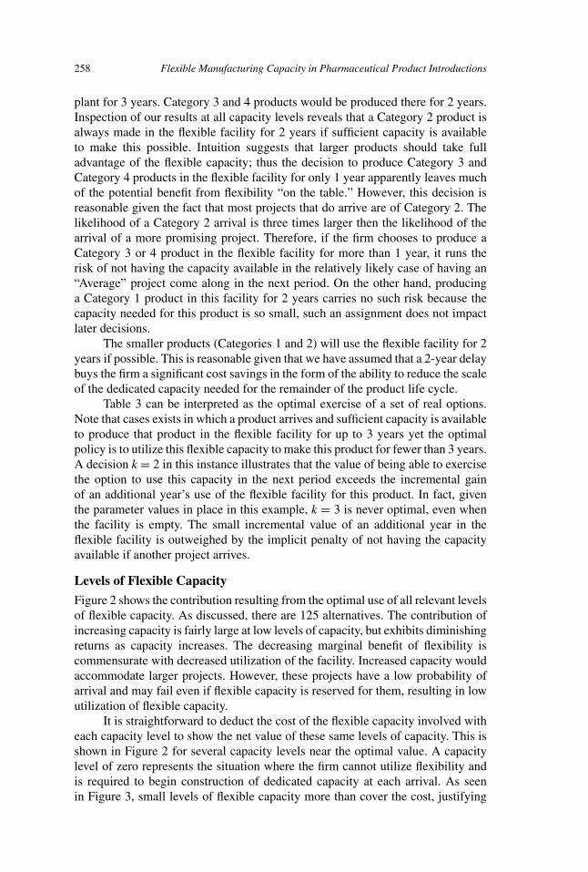
Figure 2 shows the contribution resulting from the optimal use of all relevant levelsof flexible capacity. As discussed, there are 125 alternatives. The contribution ofincreasing capacity is fairly large at low levels of capacity, but exhibits diminishingreturns as capacity increases. The decreasing marginal benefit of flexibility iscommensurate with decreased utilization of the facility. Increased capacity wouldaccommodate larger projects. However, these projects have a low probability ofarrival and may fail even if flexible capacity is reserved for them, resulting in lowutilization of flexible capacity.

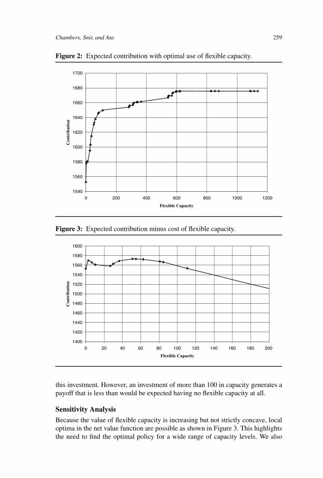
It is straightforward to deduct the cost of the flexible capacity involved witheach capacity level to show the net value of these same levels of capacity. This isshown in Figure 2 for several capacity levels near the optimal value. A capacitylevel of zero represents the situation where the firm cannot utilize flexibility andis required to begin construction of dedicated capacity at each arrival. As seenin Figure 3, small levels of flexible capacity more than cover the cost, justifying


Figure 2: Expected contribution with optimal use of flexible capacity.

1540

1560

1580

1600

1620

1640

1660

1680

1700

0 200 400 600 800 1000 1200

Flexible Capacity

Con

trib

utio

n

Figure 3: Expected contribution minus cost of flexible capacity.

1400

1420

1440

1460

1480

1500

1520

1540

1560

1580

1600

0 20 40 60 80 100 120 140 160 180 200

Flexible Capacity

Con

trib

utio

n

this investment. However, an investment of more than 100 in capacity generates apayoff that is less than would be expected having no flexible capacity at all.

Sensitivity Analysis

Because the value of flexible capacity is increasing but not strictly concave, localoptima in the net value function are possible as shown in Figure 3. This highlightsthe need to find the optimal policy for a wide range of capacity levels. We also


note that the net value of flexible capacity presents itself as a fairly flat plot in thevicinity of the optimal value. This suggests that our results may be rather robust inthe sense that small changes in parameter values are not likely to result in dramaticchanges in the optimal level of flexible capacity.

Several inputs to our model are continuous variables. These lend themselvesto analyzing the sensitivity of our results to changes in their values. In particular,the optimal policy and optimal level of flexible capacity are clearly functions ofthe success probabilities, P1 and P2. The studies by DiMasi (2001) and Adamsand Brantner (2006) indicate that success probabilities for different stages varyfor drugs targeting different ailments. Using average long-term success rates maynot be appropriate for a specific firm. Evaluating the optimal flexible capacity as afunction of these success rates enhances the applicability of our results. Intuitionalso suggests that the value of flexible capacity is a function of SD. This drivesthe reduction in expenditures for dedicated capacity resulting from productionexperience in a flexible facility. Consider the decision k = 2 for a Category 4product. This decision has an expected payoff of

Ci,k=2

=

⎡⎢⎢⎢⎢⎣

−P10.15X′

4

(1 + r1)2

+ P1P2

(1 + r1)3

{13∑

τ=1

Rτ (a)

(1 + r2)τ− 0.20X′

4 − 0.25X′4

(1 + r2)−

8∑τ=1

(0.05X′

4

(1 + r2)τ

)}⎤⎥⎥⎥⎥⎦ ,

(12)

where X′4 is the required capital expenditure for dedicated capacity to produce this

product. (The derivation is discussed in the Appendix.) This value is strictly lessthan X4 because the experience gained in 2 years of production in the flexiblefacility reduces the required scale of the facility dedicated to this product. Notethat if Ci,k=2 > 0, then it must be true that Ci,k=2 is monotonically increasing in P2,and decreasing in X′

4. We also note that because Ci,k=2 must equal 0 at P1 = 0 andCi,k=2 is linear in P1, then it must be true that Ci,k=2 is increasing in P1 as well.However, this does not make it clear whether the optimal level of flexible capacityis either increasing or decreasing in these parameters, because these payoffs mustbe compared to the payoffs achievable with no such capacity and the expectedpayoffs from all projects in the absence of flexible capacity are also increasing inP1 and P2 for the same reasons. To explore these issues we used our approachto uncover the optimal level of flexible capacity for a set of scenarios includingthose shown below. Table 4 shows selected values of P1, P2, and SD along withthe optimal capacity level.

If the firm has the parameter values that we initially assumed, the optimalamount of flexible capacity is 56.55 as shown in the first row of data in Table 4in bold. The second and third rows include a relatively low value of P1 and avery high value of this parameter, respectively. Comparison of the optimal level offlexible capacity in these three scenarios suggests that our recommendation is notsensitive to the value of this parameter. This is reasonable given that changes inP1 increase all payoffs, whether flexible capacity is available or not. The next two


Table 4: Profit maximizing level of flexible capacity for several scenarios.

Scale Deflator Optimal Amount ofP1 P2 Parameter Flexible Capacity

85% 75% 90% 56.5560% 75% 90% 56.55100% 75% 90% 56.5585% 60% 90% 56.5585% 100% 90% 2.8085% 75% 70% 56.5585% 75% 100% 2.80100% 100% 90% 2.80

rows lend themselves to a similar comparison of outcomes given relatively lowand high P2 values. Again, we see that the recommended level of flexible capacityis rather robust in the sense that if we were to find that we have overestimated thisparameter, our capacity decision would be unchanged. On the other hand, if thisparameter is very high, we find that very little flexible capacity is justified. Thisis reasonable in that an absence of uncertainty dramatically reduces the value offlexibility. At the extreme, when P1 = P2 = 100% the value of flexible capacity isvery low. This value remains positive due to the opportunities for learning that thisresource presents, but apparently, this value is only worth the expense for Category1 products.

We represent an increase in the significance of learning via production in aflexible system by reducing SD. A dramatic reduction in this value has surprisinglylittle impact on the optimal level of flexible capacity.

Alternative Problem Settings

Other changes to the problem setting can be accommodated by modifying the statespace. For example, one can argue that firms with a large portfolio of productionfacilities should be able to use this experience to shorten the construction time fornew plants. If this time is reduced from 3 years to 2 years the model referencedearlier can still be used. The Ci,k values must be adjusted to reflect the shorterconstruction time and the decision k = 3 has no appeal. Recall that the decisionsk = 0 and k = 1 have no bearing on resource availability for the currently consideredproject, as flexible capacity is freed before the current arrival requires it. Thereforethe only decision that matters in period (t − 1) is k = 2. Thus, the fact that a projectis relevant to capacity availability tells us that last period’s decision must havebeen k = 2. Therefore, we only need (5 × 1) × 5 states to define this system. Thestate space is completely determined by the Category of last period’s arrival whenit is still relevant and the Category of this period’s arrival. Table 5 shows the yi,k

and Ci,k values at the profit maximizing level of flexible capacity.When construction time is reduced from 3 years down to 2 years, the optimal

policy and optimal capacity level are very similar. In this particular case theoptimal capacity level is in fact identical to the case explored earlier. This is quitereasonable when one observes that the payoffs from the decisions made are nearlyidentical and the main elements of the reasoning are unchanged. When a Category


Table 5: Probability of each state and expected payoffs.

yi,k Ci,k ($ millions)

State i k = 0 k = 1 k = 2 k = 0 k = 1 k = 2

00 37.25% 0.00% 0.00% 0.00 −100.00 −100.0001 0.00% 7.45% 0.00% 3.08 5.14 6.8502 0.00% 0.00% 22.35% 64.40 72.54 78.5203 0.00% 3.73% 0.00% 810.58 846.21 −100.0004 0.00% 3.73% 0.00% 1,616.33 1,670.61 −100.0020 12.75% 0.00% 0.00% 0.00 −100.00 −100.0021 0.00% 2.55% 0.00% 3.08 5.14 6.8522 0.00% 0.00% 7.65% 64.40 72.54 78.5223 0.00% 1.28% 0.00% 810.58 846.21 −100.0024 1.28% 0.00% 0.00% 1,616.33 1,670.61 −100.00

Note: Highlighted values indicate yi,k values that are greater than zero.

2 product arrives it is scheduled to be produced in the flexible facility for 2 years ifat all possible. Because the decision k = 3 was never chosen when it was feasible,making it infeasible in this setting has no effect.

Our approach can also be modified to account for a more complex arrivalprocess. We have applied our modeling approach to uncover the optimal level offlexible capacity given a 2-year construction process when we relax the assumptionthat only one product arrives per year but keep the average number of arrivals peryear at 0.5. We accomplish this by using a truncated Poisson distribution to defineprobabilities for the number of project arrivals assuming a maximum of two arrivalsper year.

A detailed definition of the state space and transitions probabilities is avail-able from the authors upon request; however, a short explanation of the logic isillustrative here. It is convenient to think of the arrival process as a sequence ofpairs of project arrivals. Most of the elements in the pairs that arrive will be Cate-gory 0 projects. Given five categories, all possible arrivals can be described using5 × 5 values. The pair that arrived in the previous period is one of 25 values andthe pair that arrives in the current period is one of 25 values. Therefore, we have252 = 625 possible states. We can think of the decision space as a set of pairswhich correspond to the possible arrivals. Thus the possible decisions are (0,0),(0,1), (0,2), (1,0), (1,1), (1,2), (2,0), (2,1), and (2,2). Therefore the resulting LPincludes 625 × 9 = 5625 variables. Consideration of this problem at every relevantcapacity level reveals that the optimal level of flexible capacity for this scenarioincreases to 83.7. This capacity level is sufficient to house two Category 2 productsin the second year of their life cycle along with one Category 1 product in its firstyear of production and one Category 3 product in the first year of its production.

COMMENTS AND FUTURE RESEARCH

We produce a model to optimize the use of flexible production capacity using thepharmaceutical industry as a guiding template. Our results suggest that the optimallevel of flexible capacity in this setting is rather low even though the risk that it


is used to address is often categorized as extremely high. This result stems fromseveral causes. First, flexible capacity in this setting is quite expensive. However,we note that even when we focus on the benefit of flexible capacity and ignore itscost, the payoff from having that capacity produces a very flat function. Many ofthe factors that increase the payoff resulting from a decision to use flexible capacityalso increase the payoff if that capacity were not available. Our results suggest thatfirms managing in uncertain environments should focus much of their attentionon the optimal use of flexible resources to maximize the value of the flexibilitythat they present. We also see that given a capacity constraint it is optimal to keepflexible resources idle a significant part of the time. This surprising result is due tothe fact that reserving flexible capacity for a task gives up the real option of usingit for another task that may come along.

It is important to note that our main results are surprisingly robust withregard to the value of several important parameters. On the other hand, it doesappear that the optimal level of flexible capacity is driven by characteristics of thearrival process of new projects. Applying our approach to consider problems withdifferent arrival processes is straightforward but can become a sizable task. Forexample, the problem that we focused on here involving a 3-year time to build, andat most, one project arrival in each period involves 250 states and four possibledecisions for each state. Thus, the resulting LP has 1,000 variables. The problemthat we addressed with a 2-year construction period and up to two arrivals in aperiod is analyzed using an LP with 5,625 variables. As the number of possiblearrivals grows, the problem size can grow very quickly. For example if we allowthree projects to arrive in a year and each project is in one of five categories, and weallow five possible decisions for each product that arrives we can have as many as33 (53)2 = 421,875 variables in the resulting LP. This number can be dramaticallyreduced by taking advantage of the problem structure. For example, the state spacecan be reduced by observing that many permutations of the possibilities defininga state are redundant, and many past decisions are not relevant to future resourceavailability. If the demand requirements of products in different categories can bestated as simple multiples of each other, then it would be easier to see a priori thatsome decisions are not feasible. Eliminating infeasible decisions before creatingthe LP reduces the problem size because some theoretically possible states thatwill never be reached can be eliminated from the analysis.

Our treatment of this problem has the advantage of being easily adjusted toinclude alternate parameter values. Firm-specific data can be incorporated easilyto evaluate the use of existing capacity, and projected capacity levels can beincluded to evaluate the attractiveness of additional investments. The larger valueof this work is that it presents a straightforward way to consider flexible capacityallocation in a number of settings. The solution procedure is independent of thealgorithm or heuristic used to deduce the payoff values. Also, software capableof handling LP’s of comparable size is plentiful. We can foresee applications ofthe ideas of this work in any firm using a combination of flexible manufacturingsystems and dedicated production lines, or a firm holding a network of productionfacilities, some of which function as job shops while others are dedicated to aspecific product or product family. This approach can also be applied to the taskof assigning work to employees, where less experienced workers may only beproficient in one type of task while more senior employees may be viewed as


flexible resources. Hopefully, this work will stimulate the application of similarideas to other problems of interest. The many problems amenable to this approachshould provide a fruitful area of study for future research. [Received: February2007. Accepted: July 2008.]

REFERENCES

Adams, C. P., & Brantner, V. V. (2006). Estimating the cost of new drug develop-ment: Is it really $802 million? Health Affairs, 25(2), 420–428.

Bish, E. K., Muriel, A., & Biller, S. (2005). Managing flexible capacity in amake-to-order environment. Management Science, 51(2), 167–180.

Bish, E. K., & Wang, Q. (2004). Optimal investment strategies for flexible re-sources, considering pricing and correlated demands. Operations Research,52(6), 954–964.

Carr, G. (1998). Survey: The pharmaceutical industry. The Economist, February19, S1–S18.

Chan, J. (2007). Genzyme to construct new facility for Thymoglobulin. Phar-maWatch: Biotechnology, 6(7), 20.

Dickinson, J. G. (2006). Slowdown in approvals not safety related: FDA. MedicalMarketing & Media, 41(12), 15.

DiMasi, J. A. (1995). Success rates for new drugs entering clinical testing in theUnited States. Clinical Pharmacology & Therapeutics, 58(1), 1–14.

DiMasi, J. A. (2001). Risks in new drug development: Approval success rates forinvestigational drugs. Clinical Pharmacology & Therapeutics, 69(5), 297–307.

DiMasi, J. A., Hansen, R. W., & Grabowski, H. G. (2003). The price of innovation:New estimates of drug development costs. Journal of Health Economics,22(2), 151–185.

Dixit, A. K., & Pindyck, R. S. (1994). Investment under uncertainty. Princeton,NJ: Princeton University Press.

Eapen, G. R. (2000). Pharmaceutical R&D investing: A real options approach. Pro-ceedings of the Conference on How to Apply Real Options to Your StrategicInvestment Decisions. Chicago, IL: IQPC, April 4–5.

Filar, J. A., & Vrieze, K. (1997). Competitive markov decision processes. NewYork, NY: Springer-Verlag.

Grabowski, H. G., & Vernon, J. M. (1990). A new look at the returns and risks topharmaceutical R&D. Management Science, 36(7), 804–821.

Grabowski, H. G., & Vernon, J. M. (1994). Returns to R&D on new drug intro-ductions in the 1980s. Journal of Health Economics, 13(4), 383–406.

Grabowski, H. G., Vernon, J. M., & DiMasi, J. A. (2002). Returns on research anddevelopment for 1990s new drug introductions. PharmacoEconomics, 20(3),11–29.

Graves, S. C., & Tomlin, B. T. (2003). Process flexibility in supply chains. Man-agement Science, 49(7), 907–919.


Jordan, W. C., & Graves, S. C. (1995). Principles on the benefits of manufacturingprocess flexibility. Management Science, 41(4), 577–594.

Keyhani, S., Diener-West, M., & Powe, N. (2006). Are development timesfor pharmaceuticals increasing or decreasing? Health Affairs, 25(2), 461–468.

Manufacturing Chemist. (2007). AstraZeneca plans fundamental business changes,while Pfizer cuts jobs at UK plants. 78(10), 7.

Martinez, M. (2005). Pfizer to close Barceloneta’s Cruce Davila injectable-operation plant, leaving 350 jobless. Caribbean Business, 33(42), 11–12.

Merck. (1998). Annual report, 1998. Whitehouse Station, NJ: Author.

Myers, S. C., & Howe, C. D. (1997). A life cycle financial model of pharma-ceutical R&D. Working paper #41-97. Cambridge, MA: Sloan School ofManagement, Program on the Pharmaceutical Industry.

Ng, R. (2004). Drugs: From discovers to approval. Hobeken, NJ: Wiley.

Pharmaceutical Research and Manufacturers of America. (2004). Industry profile2004. Washington, DC: Author.

Pisano, G. P. (1997). The development factory: Unlocking the potential of processinnovation. Boston, MA: Harvard Business School Publishing.

Pisano, G. P., & Rossi, S. (1994). Eli Lilly and Company: The flexible facilitydecision—1993. Harvard Business School Case Series, 9-694-074. Boston,MA: Harvard Business School Publishing.

Putterman, M. L. (1994). Markov decision processes: Discrete stochastic dynamicprogramming. Wiley Series in Probability and Mathematical Statistics. NewYork, NY: Wiley.

Raju, G. K., & Cooney, C. L. (1995). ‘Benchmarking’ pharmaceutical manufac-turing performance. Boston, MA: MIT’s Program on the PharmaceuticalIndustry.

Reepmeyer, G. (2006). Risk-sharing in the pharmaceutical industry. Heidelberg,Germany: Physica-Verlag Publishing.

Scherer, F. M. (1993). Pricing, profits, and technological progress in the pharma-ceutical industry. Journal of Economic Perspectives, 7(3), 97–115.

Spradlin, T. (2000). Lessons about options from a pharmaceutical R&D project.Proceedings of the Conference on How to Apply Real Options to Your Strate-gic Investment Decisions. Chicago, IL: IQPC, April 4–5.

Torabzadeh, K. M., Woodruff, C. G., & Sen, N. (1998). FDA Decisions on newdrug applications and the market value of pharmaceutical firms. AmericanBusiness Review, 12(2), 42–51.

U.S. Congress, Office of Technology Assessment. (1993). Pharmaceutical R&D:Costs, risks and rewards, OTA-H-522. Washington, DC: U.S. GovernmentPrinting Office.

Van Mieghem, J. A. (1998). Investment strategies for flexible resources. Manage-ment Science, 44(8), 1071–1078.


Van Mieghem, J. A. (2003). Capacity management, investment, and hedging: Re-view and recent developments. Manufacturing & Service Operations Man-agement, 5(4), 269–302.

APPENDIX: CALCULATION OF Ci,k VALUES

The notation used to describe the evaluation of Ci,k values is shown in Table A1.Note that Mkgτ , λa, P1, P2, r1, r2, and Xa values are taken from Myers and

Howe (1997) and are as shown in Figure 1 and Table 1. Values of SC, FC, andEoS are taken from Pisano (1997). We use this data to calculate net revenue for aCategory a product that has been on the market for τ years as

Rτ (a) = GRτ (a){1 − COGSτ − Mkgτ }, (A1)

where GRτ (a) is the Gross Revenue/year as shown in Table 1. Note that COGS =FC for τ ≤ k. Otherwise, COGS = SC. From Figure 1 we see that Capital Expen-ditures for dedicated capacity for a Category a product are given (Xa) and that thedistribution of these expenditures over time are 15%, 3 years prior to opening the

Table A1: Notation.

Parameter Definition/comments

Ci,k Expected NPV of cash flows associated with making decision k when in state i.τ How long a product has been on the market, in years.Mkgτ Percentage of sales spent on product-specific marketing efforts for a product

that has been on the market for τ years (100% for τ = 1, 50% for τ = 2,20% for τ > 2).

SC Parameter for Cost of Goods Sold (COGS) stated as a percent of sales indedicated facilities: 25%.

FC Parameter for the COGS stated as a percent of sales for flexible facilities:37.5%.

EoS Parameter reflecting the change in capital cost associated with building afacility of different size: 2/3.

i State at start of period.k Decision expressed as integral number of periods a product may use the

flexible facility for production with allowable values of 0,1,2,3.λa Probability of an arrival of a category a product in a given period (a range

from 0 to 4).P1 Likelihood that a project will remain viable after Phase III testing: 85%.P2 Likelihood that a project will reach market if it has reached the final approval

stage: 75%.r1 Pre-Launch Discount Rate, applied to cash flows realized prior to product

launch: 9%.r2 Post-Launch Discount Rate, applied to cash flows realized only after product

launch, 6%.SD Scale deflator parameter of 1 – (The drop in plant size resulting from

production experience gained in flexible facility prior to completion ofdedicated facility): 90%.

Xa Capital expenditure associated with a dedicated facility with capacity toproduce a Category a product.


plant, followed by 20% and 25%, 2 years prior to the plant’s opening and 1 yearprior to its opening respectively. After the plant is operational an additional 5% ofXa is spent in each of the first 8 years of the plant’s operation. Myers and Howe(1997) argues that expenditures made prior to product launch are more risky thanexpenditures and revenues realized after product launch. They also set r1 = 9%and r2 = 6%. We apply the same values here. (This is also discussed in Dixit andPindyck (1994)). Thus, post-launch expenditures and revenues are discounted backto the point of launch at the rate r2. This value is combined with any pre-launchcash flows back to time t using the pre-launch rate r1.

When considering state i, we can only make a decision for the current arrival.Thus all states (i) that have the same digit in the fifth position have equivalent Ci,k

values. Therefore, WLOG we can reference Ci,k using a set of 5Ca,k values foreach k. Note that C0,k is simply 0 for all k. With this background in place, we maywrite Ca,k=0 values as

Ca,k=0 =[−0.15Xa − 0.20Xa

(1 + r1)− P1

0.25Xa

(1 + r1)2+ P1P2

(1 + r1)3

×{

13∑τ=1

Rτ (a)

(1 + r2)τ−

8∑τ=1

(0.05Xa

(1 + r2)τ

)}]. (A2)

For example, given the arrival of a Category 2 product we have X2 = 60.8, andRτ (2) ≡ {2.81, 29.9, 29.9, 41.8, 41.8, 41.8, 65.7, 65.7, 65.7, 65.7, 65.7, 65.7} foryears t + 3 to t + 14, respectively. Substitution into (A2) yields the value shownin Table 2. Similarly, we may write Ca,1 values as

Ca,k=1 =[− 0.15Xa

(1 + r1)− P1

0.20Xa

(1 + r1)2+ P1P2

(1 + r1)3

×{

13∑τ=1

Rτ (a)

(1 + r2)τ− 0.25Xa −

8∑τ=1

(0.05Xa

(1 + r2)τ

)}]. (A3)

We note that these values will always differ from Ca,0 values for a givenproduct category because when k = 1, less capital is put at risk prior to theresolution of uncertainty. Thus k = 1 presents a deferral option to the firm, whichalways has value.

If k = 2 or 3, the scale of the facility required for the dedicated capacityis reduced by (1 − SD). Since Economies of Scale are considered here we mustadjust the required Capital Expenditures accordingly. Formally, we have

Xda = Xa ∗

(Capacitya ∗ SD

Capacitya

)EoS

= Xa(SD)EoS. (A4)

Here Xda is the Capital Expenditure associated with dedicated capacity required to

satisfy demand for a Category a product. We use the annual sales in Phase IV asthe value of Capacitya. Given these definitions we may write Ci,k=2 and Ci,k=3

values as


Ci,k=2 =⎡⎢⎢⎢⎢⎣

−P10.15Xd

a

(1 + r1)2

+ P1P2

(1 + r1)3

{13∑

τ=1

Rτ (a)

(1 + r2)τ− 0.20Xd

a − 0.25Xda

(1 + r2)−

8∑τ=1

(0.05Xd

a

(1 + r2)τ

)}⎤⎥⎥⎥⎥⎦(A5)

and

Ci,k=3 = P1P2

(1 + r1)3

⎡⎢⎢⎢⎢⎣

−0.15Xda − 0.20Xd

a

(1 + r2)− 0.25Xd

a

(1 + r2)2

+{

13∑τ=1

Rτ (a)

(1 + r2)τ−

8∑τ=1

(0.05Xd

a

(1 + r2)τ

)}⎤⎥⎥⎥⎥⎦ . (A6)

Again, direct substitution yields the values shown in Table 2.

Chester G. Chambers is an assistant professor of operations management at theCarey School of Business, Johns Hopkins University. He received his PhD fromDuke University. His research interests include manufacturing strategy, productioneconomics, and real options. His prior publications include articles in ManagementScience, IIE Transactions, Production and Operations Management, and EuropeanJournal of Operational Research.

Eli M. Snir is an assistant professor of Information Technologies and Opera-tions Management (ITOM) in the Cox School of Business of Southern MethodistUniversity. His research encompasses economic aspects of online markets, infor-mation and technology, and the interaction between them. Within this domain heis interested in viable structures for online procurement markets, economic aspectsof trading in these markets including supply chain contractual mechanisms. Hisresearch appears in leading journals including Management Science and DecisionSciences. Eli received his PhD from the University of Pennsylvania in 2001. Hisaccomplishments have been recognized by the National Association of PurchasingManagement, which awarded him a dissertation grant and by Decision Sciencesfor Outstanding Reviewer in 2006.

Asad Ata is a doctoral candidate in Operations Research with the Departmentof Engineering Management, Information and Systems at Southern MethodistUniversity, Dallas TX. He completed his masters from Arizona State Universityand bachelors from Indian Institute of Technology, Kharagpur. He has worked as ateaching and research assistant and later as an industrial mentor for undergraduatestudents. He has also served as a referee for the POMS Journal. He has been amember of INFORMS, IEEE, POM and PMI. Currently he manages various ITtelecommunication projects in his role as a systems analyst and program managerin the industry where he has worked for 10 years.

Documents

The Use of Flexible Manufacturing Capacity in Pharmaceutical Product Introductions