The Unmixing of Atmospheric Trace Gases From Hyperspectral Satellite Data

320 IEEE TRANSACTIONS ON GEOSCIENCE AND REMOTE SENSING, VOL. 50, NO. 1, JANUARY 2012

The Unmixing of Atmospheric Trace GasesFrom Hyperspectral Satellite Data

Pia Addabbo, Student Member, IEEE, Maurizio di Bisceglie, Member, IEEE, and Carmela Galdi, Member, IEEE

Abstract—A new approach for the retrieval of the verticalcolumn concentrations of trace gases, from hyperspectral satel-lite reflectances, is presented. The investigation moves from thegeneral rationale of independent component analysis, but theconstraint of perfect independence among sources is replaced bya minimum dependence concept that proves more reasonable forthe application at hand. The unmixing of the gas spectra and theirconcentrations is achieved from linear mixtures obtained from thelogarithm of the spectral reflectance. After a proper preprocessingstage aimed at reducing major residual dependences caused byatmospheric scattering, trace-gas retrieval is carried out througha minimization of a statistical cost function, subject to the physicalconstraint that the resulting spectra must be nonnegative. Theexperimental analysis relies on the retrieval of sulfur dioxideduring volcanic emissions using data from the National Aero-nautics and Space Administration Ozone Monitoring Instrument.To validate the procedure, reference reflectance spectra having aknown profile of sulfur dioxide are generated with the MODerateresolution atmospheric TRANsmission software, and the retrievedconcentration is compared with the theoretical one. Performancein the presence of shot and detector noise has also been analyzedstarting from pure simulated spectral reflectances.

Index Terms—Atmospheric trace gases, blind source separation(BSS), Ozone Monitoring Instrument (OMI), spectral unmixing,sulfur dioxide.

I. INTRODUCTION

R ECENT research has clearly demonstrated that hyper-spectral satellite observations can be successfully used

to map atmospheric trace-gas concentrations throughout theplanet. Retrieval algorithms play a primary role in this process,and several techniques have been developed during the lastdecade to improve estimation of the atmospheric and pollutionconstituents, both in terms of accuracy and minimum detectableamounts. The main concept underlying almost all estimationprocedures is the absorption spectroscopy. Differential opticalabsorption spectroscopy (DOAS) is, perhaps, the most widelyused technique for retrieving trace-gas abundances in the openatmosphere using the narrow-band absorption structures in thenear UV, visible, and near-infrared wavelength regions.

The basic principle of DOAS is to separate broad- andnarrow-band spectral structures in the absorption spectrum

Manuscript received September 30, 2010; revised January 26, 2011,April 28, 2011, July 5, 2011, and August 25, 2011; accepted August 31, 2011.Date of publication November 7, 2011; date of current version December 23,2011. This work was supported in part by the Italian Ministry of Environmentthrough the Centro Euro Mediterraneo per i Cambiamenti Climatici.

The authors are with the Dipartimento di Ingegneria, Università degli Studidel Sannio, 82100 Benevento, Italy.

Color versions of one or more of the figures in this paper are available onlineat http://ieeexplore.ieee.org.

Digital Object Identifier 10.1109/TGRS.2011.2171692

in order to isolate the characteristic structures of the gas.The separation of the broad-band extinction, due to Rayleighscattering and Mie scattering, is achieved by fitting a low-order polynomial to the optical density simultaneously withthe absorption cross sections of all relevant absorbers. As aresult of this procedure, the integrated amount of molecules perunit area averaged over all contributing light paths through theatmosphere—the slant column density—is retrieved. The slantcolumns are then converted into vertical columns using air massfactors (AMFs), computed at a single wavelength [1].

DOAS is a flexible technique but is subject to some limita-tions. Multiple atmospheric components can be detected withDOAS, but the technique can be effectively used only in thepresence of clear narrow electronic transition structures inthe considered range of wavelengths [2]. Satellite spectrora-diometer technology allows reliable measurements of trace-gasconcentrations when gas components have absorption bands asnarrow as 10 nm [1]. The accuracy and precision of DOASmeasurements depend on several factors: Instrument noise,uncertainty of temperature, atmospheric conditions, slant path,and other minor contributions [3]. Additional complicationsarise because different species may have absorption peaks inthe same wavelength range so that the measurement of a trace-gas concentration can be positively or negatively influencedby other species. The sulfur dioxide molecule, for example,exhibits a relatively strong narrow vibrational band from 260 to340 nm; in the same wavelength range, there is also absorptionby the ozone molecule. The aforementioned factors generateestimation errors that are visible, for example, in some cases oflow SO2 concentration when retrievals of slightly negative slantcolumn values are possible. Larger negative biases are, instead,often associated with deep convective clouds [4].

Finally, DOAS needs radiative transfer model (RTM) calcu-lations to convert observed column densities to vertical columndensities or concentrations. One drawback of RTMs is that theresults depend on the accuracy of their initialization, particu-larly regarding the trace-gas and aerosol vertical distributionsand the optical characteristics of the aerosol particles. If thisinitialization information is not enough detailed, the RTMresults could be inaccurate [1].

We propose, in this paper, a different approach based onindependent component analysis (ICA), whose essence is theunmixing of the spectral waveforms of individual trace gaseson the basis of their statistical independence, providing, atthe same time, the estimation of their concentrations. Thisnew approach is deeply different from DOAS, which uses aparametric approach, and tries to reduce, as much as possible,the need of a priori information. ICA is a special case of blindsource separation (BSS), a procedure for separating a set ofunknown signals from observations of mixtures of such signals.

0196-2892/$26.00 © 2011 IEEE

ADDABBO et al.: UNMIXING OF ATMOSPHERIC TRACE GASES FROM HYPERSPECTRAL SATELLITE DATA 321

In the most general case, very little information is assumedabout the mixing process; ICA relies on the case where themixture is a linear superposition and the unknown signals arestatistically independent. A classical example of mixing wherethe ICA application proved quite successful is the so-calledcocktail party problem, where a number of people are talkingsimultaneously and one wants to isolate a single discussion.ICA procedures try to solve the source separation problem byfinding a transformation matrix that maximizes the statisticalindependence among sources. Recently, it has been proposedas a tool to unmix hyperspectral data into a collection ofreflectance spectra of the components (end-member signatures)and the corresponding abundance fractions at each pixel [5],[6]. ICA application to spectral unmixing requires that a num-ber of reflectance observations are available in the form of alinear mixing of independent unknown trace-gas cross sections,where the elements of the mixing matrix are the gas concen-trations, which are unknown as well. Finding the independentcomponents consists in finding the coefficients (concentrations)that maximize a measure of independence among the crosssections. Afterward, given the coefficients, cross sections canbe retrieved as a solution of a linear system, i.e., as a linearsuperposition of the observed reflectances. The main weaknessof the ICA-based approach is that different chemical species donot necessarily exhibit independent spectra because of the sim-ilarities of their chemical structures. Therefore, the separationproblem can be inaccurate, reflecting the fact that the goal ofachieving independent spectra was inconsistent.

Least Dependent component Analysis (LDA) [7] andconstrained ICA [8], respectively, relax the hypothesis thatsignal sources can be linearly decomposed into exactly inde-pendent sources and admit the introduction of a more generalcost function to incorporate additional information about thesources. Retrieval of trace gases having known absorptioncross sections, or cross sections with small deviations aroundthe standard shape, can be therefore addressed through theaforementioned approaches. Accordingly, a new method forestimating trace-gas concentrations from satellite observationsis presented, and the procedure is validated in the case of SO2

retrievals from the Ozone Monitoring Instrument (OMI) onboard AURA platform.

This paper is organized as follows. In Section II, the linearobservation model is defined, starting from the Beer–Lambertlaw. In Section III, the retrieval algorithm is explained. Resultsusing hyperspectral satellite data and MODerate resolutionatmospheric TRANsmission (MODTRAN)-simulated spectraare presented in Sections IV and V, respectively. Finally,Section VI shows the conclusions and final remarks.

II. PROBLEM STATEMENT

According to the Beer–Lambert law, the transmitted intensityof the radiation I1(λ) through the atmosphere can be ex-pressed as

I1(λ) = I0(λ) exp

⎛⎝−

n∑j=1

Njσj(λ)− P (λ)

⎞⎠ (1)

where I0(λ) is the incident radiation, the exponent is a linearcombination of n absorption cross sections σj(λ) (in square

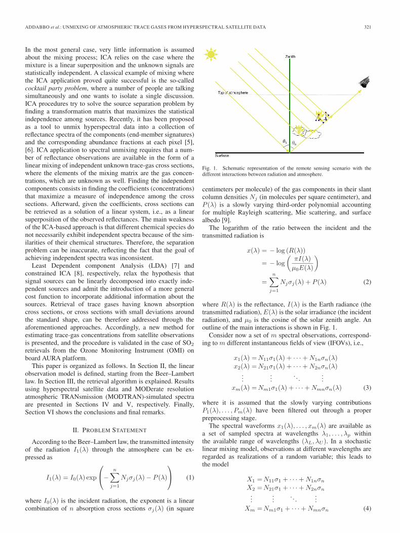
Fig. 1. Schematic representation of the remote sensing scenario with thedifferent interactions between radiation and atmosphere.

centimeters per molecule) of the gas components in their slantcolumn densities Nj (in molecules per square centimeter), andP (λ) is a slowly varying third-order polynomial accountingfor multiple Rayleigh scattering, Mie scattering, and surfacealbedo [9].

The logarithm of the ratio between the incident and thetransmitted radiation is

x(λ) = − log (R(λ))

= − log

(πI(λ)

μ0E(λ)

)

=

n∑j=1

Njσj(λ) + P (λ) (2)

where R(λ) is the reflectance, I(λ) is the Earth radiance (thetransmitted radiation), E(λ) is the solar irradiance (the incidentradiation), and μ0 is the cosine of the solar zenith angle. Anoutline of the main interactions is shown in Fig. 1.

Consider now a set of m spectral observations, correspond-ing to m different instantaneous fields of view (IFOVs), i.e.,

x1(λ) =N11σ1(λ) + · · ·+N1nσn(λ)

x2(λ) =N21σ1(λ) + · · ·+N2nσn(λ)...

.... . .

...xm(λ) =Nm1σ1(λ) + · · ·+Nmnσn(λ) (3)

where it is assumed that the slowly varying contributionsP1(λ), . . . , Pm(λ) have been filtered out through a properpreprocessing stage.

The spectral waveforms x1(λ), . . . , xm(λ) are available asa set of sampled spectra at wavelengths λ1, . . . , λp withinthe available range of wavelengths (λL, λU ). In a stochasticlinear mixing model, observations at different wavelengths areregarded as realizations of a random variable; this leads tothe model

X1 =N11σ1 + · · ·+N1nσn

X2 =N21σ1 + · · ·+N2nσn

......

. . ....

Xm =Nm1σ1 + · · ·+Nmnσn (4)


where X1, . . . , Xm and σ1, . . . , σn are now random variables,whose realizations are available, taken at the different wave-lengths λ1, . . . , λp. Using vector notation, we get

X = Nσ (5)

where X = [X1, . . . , Xm]T, σ = [σ1, . . . , σn]T, and N =

{Nij}i=1,...,m,j=1,...,n is the m× n mixing matrix of the slantcolumn densities, with m ≥ n.

Equation (5) should be solved in terms of the sources σwhen the mixing matrix N is unknown. This is a standard BSSproblem that, under the hypothesis of statistical independenceamong sources, can be solved using an ICA approach thatgives estimates of both independent sources and mixing matrix.Direct application of ICA to the model (5) is, however, notappropriate for two main reasons.

1) The ICA solves a BSS problem when the number of sourcesis known, whereas in a gas mixture, the presence of allcomponents cannot be always assumed. For instance, in avolcanic eruption, atmospheric trace gases can be foundin high concentrations in some image areas, whereas otherareas exhibit close to zero concentrations. In the linearmixing model (5), each source should be assumed at least inone of the m observations; otherwise, the mixing matrix Nhas one or more zero columns, and the ICA algorithm wouldconverge to an inconsistent result. To regularize the problemand, at the same time, drive the solution toward a set oftrace-gas components of interest, we define a contaminatedmixing model, with m = n, where the first n− 1 sourcesσ1, . . . , σn−1 are the absorption cross sections of the giventrace-gas components and the last source σn is the mixtureof all other components in the atmosphere that we arenot interested to separate. Contamination corresponds toadding a known concentration of the trace-gas waveformsσ1, . . . , σn−1 to the last n− 1 rows of the mixing model.Thus, the first observation is defined as the uncontaminatedlog reflectance of the pixel under test, and the other n− 1observations are the sum of the log reflectance plus theabsorption cross section of one of the trace-gas componentsof interest. The contaminated model turns out to be

x1(λ) = − log (R(λ))

x2(λ) = − log (R(λ)) + cσ1(λ)

. . .

xn(λ) = − log (R(λ)) + cσn−1(λ) (6)

where c is the contamination factor defined as 2.69 ·1016 mol/cm2, corresponding to the concentration of1 Dobson unit (DU), which is a standard unit of measureof atmospheric trace-gas column density. This is enough toensure that the ICA problem is well posed.

The corresponding stochastic contaminated model is

X1 = N1σ1 + · · ·+ Nn−1σn−1 +Nnσn

X2 = (N1 + c)σ1 + · · ·+ Nn−1σn−1 +Nnσn

......

. . ....

...Xn = N1σ1 + · · ·+ (Nn−1 + c)σn−1 +Nnσn.

(7)

2) In most applications, the spectral sources are not exactlyindependent. This happens when chemical compounds in amixture share common or similar structural groups [10]. Inaddition, scattering from air molecules, aerosols, and cloudsas well as absorption from the ground often dominate theextinction of sunlight. Extinction from scattering andabsorption from the ground usually varies smoothly withwavelength and represents a source of dependence amongspectra. An easy way to remove the slower component isto use a high-pass filter in a preprocessing stage, and this isalso the first step of a DOAS procedure. The filter removesthe slowly varying components and extracts spectralinformation which is more independent from source tosource. In this work, the high-pass filter is achieved bysubtracting from the observations X their low-pass-filteredversions, i.e.,

P = X−P∗ (8)

where P and P∗ are the high- and low-pass-filtered versionsof X, respectively. For the case at hand, a Savitzky–Golayfilter is used as a low-pass filter; it is widely used inthe absorption spectroscopy community for its ability toprovide smoothing without significant loss of resolution[11], [12]. After filtering, (5) takes the form

P = NU (9)

with U as the high-pass-filtered version of the crosssections σ. Since the high-pass filter does not change themixing matrix, ICA can be applied on the signal P directly.The high-pass filtering is not usually able to remove alldependences among the spectral sources, and this couldstill compromise the unmixing process. LDA relaxes thehypothesis of perfect independence among the originalsources by introducing constraints in the model, based onthe a priori physical information.

III. TRACE-GAS RETRIEVAL VIA SOURCE SEPARATION

Given the linear mixture (9) of source components U withunknown concentrations, the unmixing problem is solved viaa matrix transformation of the high-pass-filtered vector ofobservations P that makes the output Y as independent aspossible, i.e.,

Y = WP = WNU. (10)

It is evident that, if W is equal to the inverse of the mixingmatrix, the transformed vector Y corresponds exactly to thesource components.

The problem of finding the linear transformation (10) thatmakes data independent can be organized in two steps: First, awhitening, to make data uncorrelated, with the same variance,and then, a coordinate rotation that preserves whiteness andgets data independence. This means that the transformationmatrix is decomposed as W = RV, where V = Λ

−1/2P UT

Pis the whitening matrix, defined through eigenvalues ΛP andeigenvectors UP of the covariance matrix of P, and R is aunitary rotation matrix that can be found by maximizing a mea-sure of independence. Coordinate rotations in n dimensions are


more conveniently decomposed into multiplications involvingGivens rotation matrices G(ij) [13], i.e.,

R =

n−1∏i=1

⎛⎝ n∏

j=i+1

G(ij)

⎞⎠ (11)

where the rotation matrix is given by

G(ij) =

⎛⎜⎜⎜⎝

Ii−1

cosφij sinφij

Ij−i−1

− sinφij cosφij

In−j

⎞⎟⎟⎟⎠ (12)

where empty positions should be replaced with zeros, In is then× n identity matrix, and 1 ≤ i < j ≤ n. The angles φij canbe seen as generalized Euler angles.

A measure for statistical dependence among random vari-ables is mutual information: It is always nonnegative and iszero if and only if all variables are mutually independent. Itis defined as the Kullback–Leibler divergence between the jointprobability density function p(y1, . . . , yn) and the product ofthe marginal densities p(yi), namely,

I(Y1,. . ., Yn)=

∫p(y1, . . . , yn)

× log

[p(y1, . . . , yn)

p(y1), . . . , p(yn)

]dy1, . . . , dyn. (13)

Using the Shannon differential entropy, defined as

H(Y1, . . . , Yn) = −∫p(y1, . . . , yn)

× log[p(y1, . . . , yn)] dy1, . . . , dyn (14)

the mutual information of the observables can be expressedas [14]

I(Y1, . . . , Yn) =

n∑i=1

H(Yi)−H(Y1, . . . , Yn). (15)

It can be shown [15] that minimizing the mutual informationwith respect to the rotation angles is equivalent to minimizingthe sum of the Shannon entropies of the observed randomvariables. In fact, the differential entropy of the linear trans-formation (10) can be written as [14]

H(Y1, . . . , Yn) = H(P1, . . . , Pn)− log (|W|) (16)

that is independent from the rotation angles because the firstterm is the joint entropy of observations and the second termis equal to log(|R||V|) = log(|V|) and independent from rota-tion because the determinant of the unitary matrix R is equalto one. Thus, the problem can be formulated as follows: Findthe rotation parameters φij such that the sum of the Shannonentropies is minimum.

This is a pure blind approach that is not the most useful forour case where some knowledge on the trace-gas absorptioncross section can be treated as an a priori constraint in the LDAto drive the separation of the desired components [8]. This addi-tional knowledge can be incorporated into a cost function where

one element is the measurement of the statistical independenceamong sources and the other is the mean square error betweenthe first n− 1 retrieved sources and the known absorption crosssections of interest. The constrained minimization process, afternormalization of the two components, can be formulated asfollows: Find the rotation parameters φij such that the costfunction

α

n∑i=1

H(Yi) + (1− α)

n−1∑i=1

E[(Yi − σi)

T(Yi − σi)]

(17)

is minimum, where E[·] denotes the expectation and α is aconstant value. Selecting α = 1 corresponds to unconstrainedsource estimation, whereas α = 0 corresponds to the minimiza-tion of the mean square error. In the algorithm implementation,α should be chosen sufficiently close to one to ensure that theminimization process is not constrained to converge toward aknown waveform. This is relevant because the actual absorptioncross sections may deviate from the reference in the real sce-nario where temperature, pressure, and environmental parame-ters are unknown. It is also worth to note that the mean squareerror is evaluated on a model where only rotations are admittedand should not be confused with an unconstrained least squareminimization that should have been carried out by varying allelements of the mixing matrix. The minimization procedure isimplemented by evaluating (17) for any rotation and findingthe global minimum subject to the additional consistency rulethat all rotations must produce nonnegative waveforms, in viewthat the original sources must be positive by definition. Theentropies are evaluated very efficiently using spacing estimates,as reported in [15]. We recall that different realizations of therandom variables Yi, required for the estimation of entropyand expectation, are available taking observations at differentwavelengths.

After minimization of the cost function, the estimated mixingmatrix can be calculated as

N∗ = (W∗)−1 = (R∗V)−1 (18)

and the estimated sources can be recovered by applying theunmixing transformation W∗ to the original signal mixture,namely,

⎡⎢⎣σ∗1(λ)...

σ∗n(λ)

⎤⎥⎦ = W∗

⎡⎢⎣x1(λ)

...xn(λ)

⎤⎥⎦ . (19)

We underline that the estimated sources σ∗i (λ) can be slightly

different from the reference sources. Deviations may arise fromtemperature, pressure, or other atmospheric conditions andnoise.

The estimated mixing matrix coefficients can be easily con-verted into trace-gas concentrations in Dobson units. To thisend, we remember that the contamination previously introducedin the original observables is not physical and must be removed.Second, the slant column measurements must be converted intovertical column measurements. Finally, the problem that thevertical column is not necessarily at the Earth boundary layershould be considered.


The removal of the contamination can be achieved by nor-malizing the ith component of the first row of N∗ to the dif-ference N ∗

i+1,i −N ∗1i corresponding to 1 DU; hence, the total

slant column density N ∗i , in Dobson units, can be evaluated as

N ∗i =

N ∗1i

N ∗i+1,i −N ∗

1i

. (20)

Afterward, an AMF is used to convert from slant column tovertical column density [16]. For low solar zenith angles, wecan simply use the geometric AMF, which is a straightforwardfunction of the solar zenith angle θs and the satellite viewingangle θv, i.e.,

AMF = sec θs + sec θv (21)

leading to the total vertical column density N ∗vi = N ∗

i /AMF .

IV. RESULTS DERIVED FROM HYPERSPECTRAL

SATELLITE DATA

The unmixing procedure has been applied to the retrieval ofsulfur dioxide SO2 volcanic emission using data from the OMIhyperspectral sensor and the SO2 reference spectrum derivedfor the SCanning Imaging Absorption spectroMeter for At-mospheric CartograpHY (SCIAMACHY) preflight model [17].Two algorithms are currently adopted to produce accurate mea-surements of SO2 from OMI data: the band residual difference(BRD) algorithm [18] and the linear fit (LF) algorithm [19].The BRD is based on the evaluation of differential residuals dueto the trace gas at several wavelength pairs; spectral bands areselected where large absorption peaks are displayed to improvethe algorithm accuracy and the discrimination from other gases.The LF algorithm is based on fitting a linearized RTM plus alow-order polynomial to the logarithm of the reflectance spec-trum. The OMI-data-product file contains four estimates of thetotal SO2 column, corresponding to four a priori profiles for theSO2 vertical distribution considered in the retrieval algorithm.The four vertical profiles were selected to represent typical SO2

vertical distributions in four regimes: the planetary boundarylayer (PBL; below 2 km) and the Lower TRopospheric layer(TRL; between 2 and 5 km) from anthropogenic sources, theMiddle TRopospheric layer (TRM; between 5 and 10 km)produced by volcanic degassing, and the upper troposphericand STratospheric Layer (STL; between 15 and 20 km) usuallyproduced by explosive volcanic eruption. The PBL columns areproduced using the BRD algorithm, while TRL, TRM, and STLcolumns are produced with the LF algorithm.

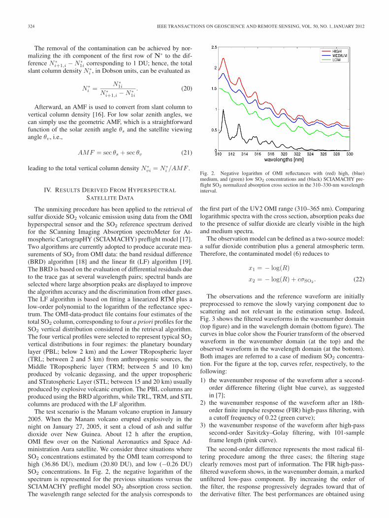
The test scenario is the Manam volcano eruption in January2005. When the Manam volcano erupted explosively in thenight on January 27, 2005, it sent a cloud of ash and sulfurdioxide over New Guinea. About 12 h after the eruption,OMI flew over on the National Aeronautics and Space Ad-ministration Aura satellite. We consider three situations whereSO2 concentrations estimated by the OMI team correspond tohigh (36.86 DU), medium (20.80 DU), and low (−0.26 DU)SO2 concentrations. In Fig. 2, the negative logarithm of thespectrum is represented for the previous situations versus theSCIAMACHY preflight model SO2 absorption cross section.The wavelength range selected for the analysis corresponds to

Fig. 2. Negative logarithm of OMI reflectances with (red) high, (blue)medium, and (green) low SO2 concentrations and (black) SCIAMACHY pre-flight SO2 normalized absorption cross section in the 310–330-nm wavelengthinterval.

the first part of the UV2 OMI range (310–365 nm). Comparinglogarithmic spectra with the cross section, absorption peaks dueto the presence of sulfur dioxide are clearly visible in the highand medium spectra.

The observation model can be defined as a two-source model:a sulfur dioxide contribution plus a general atmospheric term.Therefore, the contaminated model (6) reduces to

x1 = − log(R)

x2 = − log(R) + cσSO2. (22)

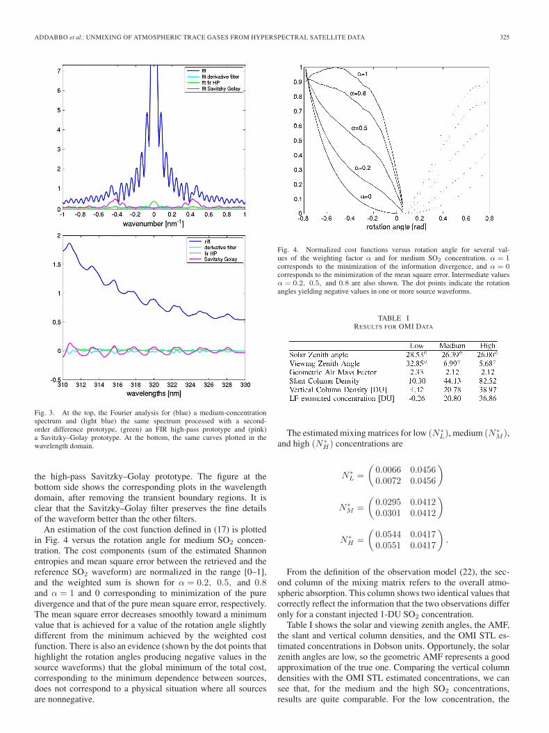
The observations and the reference waveform are initiallypreprocessed to remove the slowly varying component due toscattering and not relevant in the estimation setup. Indeed,Fig. 3 shows the filtered waveforms in the wavenumber domain(top figure) and in the wavelength domain (bottom figure). Thecurves in blue color show the Fourier transform of the observedwaveform in the wavenumber domain (at the top) and theobserved waveform in the wavelength domain (at the bottom).Both images are referred to a case of medium SO2 concentra-tion. For the figure at the top, curves refer, respectively, to thefollowing:1) the wavenumber response of the waveform after a second-

order difference filtering (light blue curve), as suggestedin [7];

2) the wavenumber response of the waveform after an 18th-order finite impulse response (FIR) high-pass filtering, witha cutoff frequency of 0.22 (green curve);

3) the wavenumber response of the waveform after high-passsecond-order Savitzky–Golay filtering, with 101-sampleframe length (pink curve).

The second-order difference represents the most radical fil-tering procedure among the three cases; the filtering stageclearly removes most part of information. The FIR high-pass-filtered waveform shows, in the wavenumber domain, a markedunfiltered low-pass component. By increasing the order ofthe filter, the response progressively degrades toward that ofthe derivative filter. The best performances are obtained using


Fig. 3. At the top, the Fourier analysis for (blue) a medium-concentrationspectrum and (light blue) the same spectrum processed with a second-order difference prototype, (green) an FIR high-pass prototype and (pink)a Savitzky–Golay prototype. At the bottom, the same curves plotted in thewavelength domain.

the high-pass Savitzky–Golay prototype. The figure at thebottom side shows the corresponding plots in the wavelengthdomain, after removing the transient boundary regions. It isclear that the Savitzky–Golay filter preserves the fine detailsof the waveform better than the other filters.

An estimation of the cost function defined in (17) is plottedin Fig. 4 versus the rotation angle for medium SO2 concen-tration. The cost components (sum of the estimated Shannonentropies and mean square error between the retrieved and thereference SO2 waveform) are normalized in the range [0–1],and the weighted sum is shown for α = 0.2, 0.5, and 0.8and α = 1 and 0 corresponding to minimization of the puredivergence and that of the pure mean square error, respectively.The mean square error decreases smoothly toward a minimumvalue that is achieved for a value of the rotation angle slightlydifferent from the minimum achieved by the weighted costfunction. There is also an evidence (shown by the dot points thathighlight the rotation angles producing negative values in thesource waveforms) that the global minimum of the total cost,corresponding to the minimum dependence between sources,does not correspond to a physical situation where all sourcesare nonnegative.

Fig. 4. Normalized cost functions versus rotation angle for several val-ues of the weighting factor α and for medium SO2 concentration. α = 1corresponds to the minimization of the information divergence, and α = 0corresponds to the minimization of the mean square error. Intermediate valuesα = 0.2, 0.5, and 0.8 are also shown. The dot points indicate the rotationangles yielding negative values in one or more source waveforms.

TABLE IRESULTS FOR OMI DATA

The estimated mixing matrices for low (N ∗L), medium (N ∗

M ),and high (N ∗

H) concentrations are

N ∗L =

(0.0066 0.04560.0072 0.0456

)

N ∗M =

(0.0295 0.04120.0301 0.0412

)

N ∗H =

(0.0544 0.04170.0551 0.0417

).

From the definition of the observation model (22), the sec-ond column of the mixing matrix refers to the overall atmo-spheric absorption. This column shows two identical values thatcorrectly reflect the information that the two observations differonly for a constant injected 1-DU SO2 concentration.

Table I shows the solar and viewing zenith angles, the AMF,the slant and vertical column densities, and the OMI STL es-timated concentrations in Dobson units. Opportunely, the solarzenith angles are low, so the geometric AMF represents a goodapproximation of the true one. Comparing the vertical columndensities with the OMI STL estimated concentrations, we cansee that, for the medium and the high SO2 concentrations,results are quite comparable. For the low concentration, the


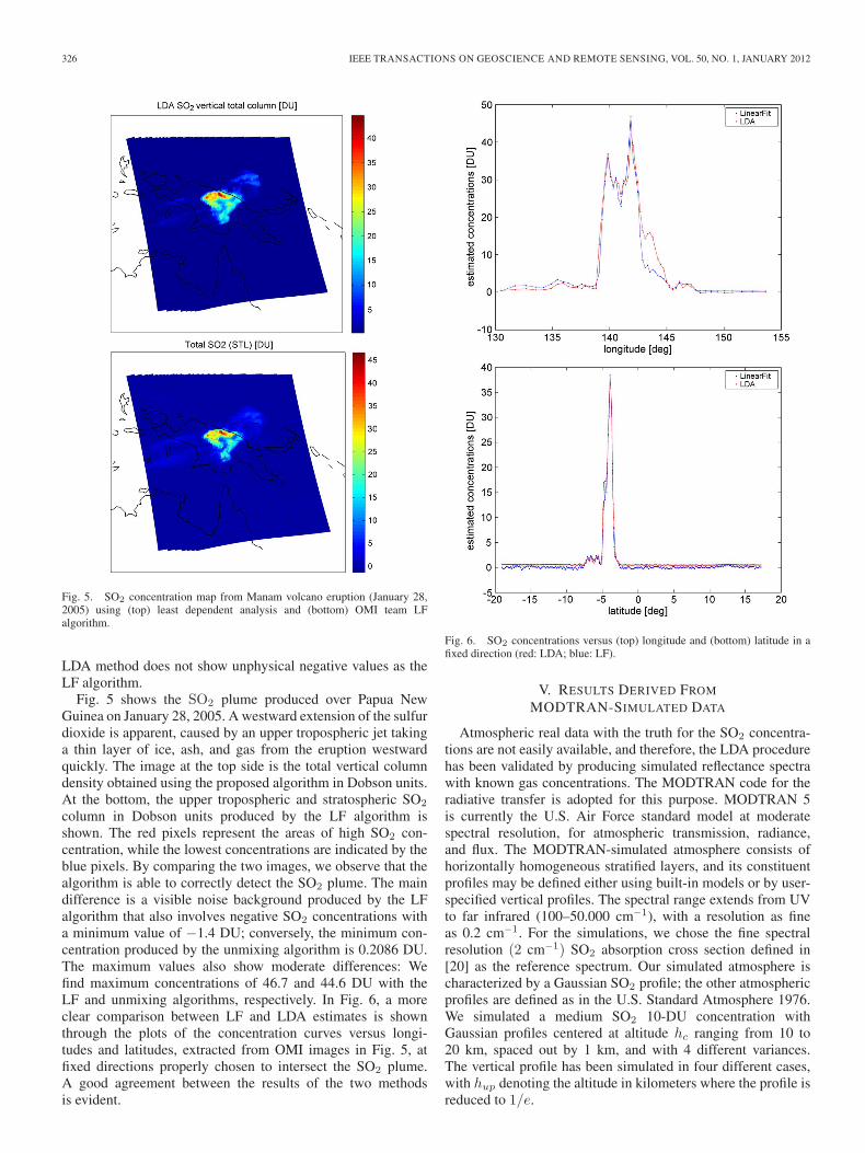
Fig. 5. SO2 concentration map from Manam volcano eruption (January 28,2005) using (top) least dependent analysis and (bottom) OMI team LFalgorithm.

LDA method does not show unphysical negative values as theLF algorithm.

Fig. 5 shows the SO2 plume produced over Papua NewGuinea on January 28, 2005. A westward extension of the sulfurdioxide is apparent, caused by an upper tropospheric jet takinga thin layer of ice, ash, and gas from the eruption westwardquickly. The image at the top side is the total vertical columndensity obtained using the proposed algorithm in Dobson units.At the bottom, the upper tropospheric and stratospheric SO2

column in Dobson units produced by the LF algorithm isshown. The red pixels represent the areas of high SO2 con-centration, while the lowest concentrations are indicated by theblue pixels. By comparing the two images, we observe that thealgorithm is able to correctly detect the SO2 plume. The maindifference is a visible noise background produced by the LFalgorithm that also involves negative SO2 concentrations witha minimum value of −1.4 DU; conversely, the minimum con-centration produced by the unmixing algorithm is 0.2086 DU.The maximum values also show moderate differences: Wefind maximum concentrations of 46.7 and 44.6 DU with theLF and unmixing algorithms, respectively. In Fig. 6, a moreclear comparison between LF and LDA estimates is shownthrough the plots of the concentration curves versus longi-tudes and latitudes, extracted from OMI images in Fig. 5, atfixed directions properly chosen to intersect the SO2 plume.A good agreement between the results of the two methodsis evident.

Fig. 6. SO2 concentrations versus (top) longitude and (bottom) latitude in afixed direction (red: LDA; blue: LF).

V. RESULTS DERIVED FROM

MODTRAN-SIMULATED DATA

Atmospheric real data with the truth for the SO2 concentra-tions are not easily available, and therefore, the LDA procedurehas been validated by producing simulated reflectance spectrawith known gas concentrations. The MODTRAN code for theradiative transfer is adopted for this purpose. MODTRAN 5is currently the U.S. Air Force standard model at moderatespectral resolution, for atmospheric transmission, radiance,and flux. The MODTRAN-simulated atmosphere consists ofhorizontally homogeneous stratified layers, and its constituentprofiles may be defined either using built-in models or by user-specified vertical profiles. The spectral range extends from UVto far infrared (100–50.000 cm−1), with a resolution as fineas 0.2 cm−1. For the simulations, we chose the fine spectralresolution (2 cm−1) SO2 absorption cross section defined in[20] as the reference spectrum. Our simulated atmosphere ischaracterized by a Gaussian SO2 profile; the other atmosphericprofiles are defined as in the U.S. Standard Atmosphere 1976.We simulated a medium SO2 10-DU concentration withGaussian profiles centered at altitude hc ranging from 10 to20 km, spaced out by 1 km, and with 4 different variances.The vertical profile has been simulated in four different cases,with hup denoting the altitude in kilometers where the profile isreduced to 1/e.


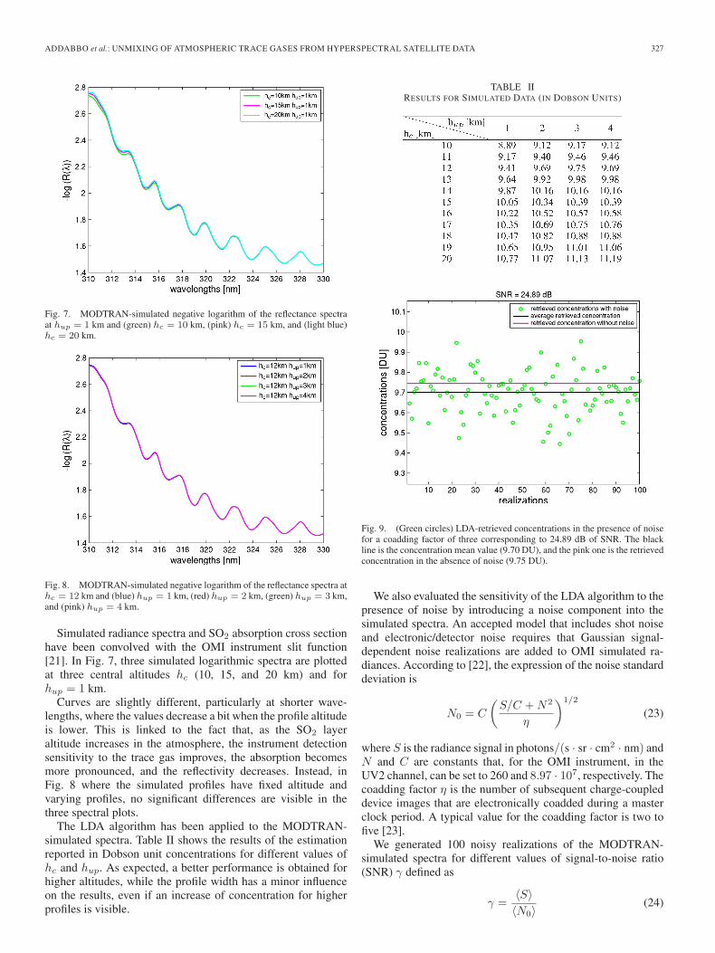
Fig. 7. MODTRAN-simulated negative logarithm of the reflectance spectraat hup = 1 km and (green) hc = 10 km, (pink) hc = 15 km, and (light blue)hc = 20 km.

Fig. 8. MODTRAN-simulated negative logarithm of the reflectance spectra athc = 12 km and (blue) hup = 1 km, (red) hup = 2 km, (green) hup = 3 km,and (pink) hup = 4 km.

Simulated radiance spectra and SO2 absorption cross sectionhave been convolved with the OMI instrument slit function[21]. In Fig. 7, three simulated logarithmic spectra are plottedat three central altitudes hc (10, 15, and 20 km) and forhup = 1 km.

Curves are slightly different, particularly at shorter wave-lengths, where the values decrease a bit when the profile altitudeis lower. This is linked to the fact that, as the SO2 layeraltitude increases in the atmosphere, the instrument detectionsensitivity to the trace gas improves, the absorption becomesmore pronounced, and the reflectivity decreases. Instead, inFig. 8 where the simulated profiles have fixed altitude andvarying profiles, no significant differences are visible in thethree spectral plots.

The LDA algorithm has been applied to the MODTRAN-simulated spectra. Table II shows the results of the estimationreported in Dobson unit concentrations for different values ofhc and hup. As expected, a better performance is obtained forhigher altitudes, while the profile width has a minor influenceon the results, even if an increase of concentration for higherprofiles is visible.

TABLE IIRESULTS FOR SIMULATED DATA (IN DOBSON UNITS)

Fig. 9. (Green circles) LDA-retrieved concentrations in the presence of noisefor a coadding factor of three corresponding to 24.89 dB of SNR. The blackline is the concentration mean value (9.70 DU), and the pink one is the retrievedconcentration in the absence of noise (9.75 DU).

We also evaluated the sensitivity of the LDA algorithm to thepresence of noise by introducing a noise component into thesimulated spectra. An accepted model that includes shot noiseand electronic/detector noise requires that Gaussian signal-dependent noise realizations are added to OMI simulated ra-diances. According to [22], the expression of the noise standarddeviation is

N0 = C

(S/C +N2

η

)1/2

(23)

where S is the radiance signal in photons/(s · sr · cm2 · nm) andN and C are constants that, for the OMI instrument, in theUV2 channel, can be set to 260 and 8.97 · 107, respectively. Thecoadding factor η is the number of subsequent charge-coupleddevice images that are electronically coadded during a masterclock period. A typical value for the coadding factor is two tofive [23].

We generated 100 noisy realizations of the MODTRAN-simulated spectra for different values of signal-to-noise ratio(SNR) γ defined as

γ =〈S〉〈N0〉

(24)


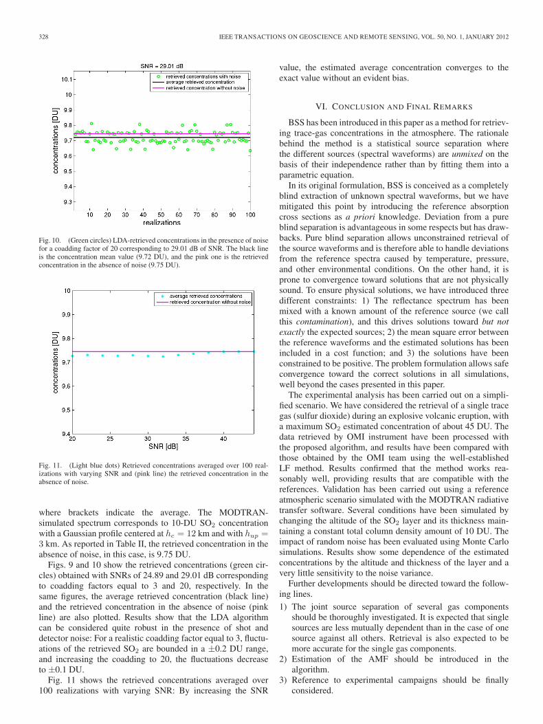
Fig. 10. (Green circles) LDA-retrieved concentrations in the presence of noisefor a coadding factor of 20 corresponding to 29.01 dB of SNR. The black lineis the concentration mean value (9.72 DU), and the pink one is the retrievedconcentration in the absence of noise (9.75 DU).

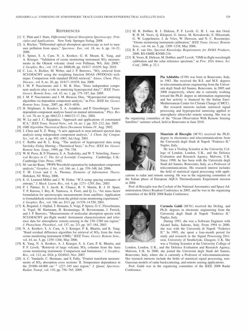
Fig. 11. (Light blue dots) Retrieved concentrations averaged over 100 real-izations with varying SNR and (pink line) the retrieved concentration in theabsence of noise.

where brackets indicate the average. The MODTRAN-simulated spectrum corresponds to 10-DU SO2 concentrationwith a Gaussian profile centered at hc = 12 km and with hup =3 km. As reported in Table II, the retrieved concentration in theabsence of noise, in this case, is 9.75 DU.

Figs. 9 and 10 show the retrieved concentrations (green cir-cles) obtained with SNRs of 24.89 and 29.01 dB correspondingto coadding factors equal to 3 and 20, respectively. In thesame figures, the average retrieved concentration (black line)and the retrieved concentration in the absence of noise (pinkline) are also plotted. Results show that the LDA algorithmcan be considered quite robust in the presence of shot anddetector noise: For a realistic coadding factor equal to 3, fluctu-ations of the retrieved SO2 are bounded in a ±0.2 DU range,and increasing the coadding to 20, the fluctuations decreaseto ±0.1 DU.

Fig. 11 shows the retrieved concentrations averaged over100 realizations with varying SNR: By increasing the SNR

value, the estimated average concentration converges to theexact value without an evident bias.

VI. CONCLUSION AND FINAL REMARKS

BSS has been introduced in this paper as a method for retriev-ing trace-gas concentrations in the atmosphere. The rationalebehind the method is a statistical source separation wherethe different sources (spectral waveforms) are unmixed on thebasis of their independence rather than by fitting them into aparametric equation.

In its original formulation, BSS is conceived as a completelyblind extraction of unknown spectral waveforms, but we havemitigated this point by introducing the reference absorptioncross sections as a priori knowledge. Deviation from a pureblind separation is advantageous in some respects but has draw-backs. Pure blind separation allows unconstrained retrieval ofthe source waveforms and is therefore able to handle deviationsfrom the reference spectra caused by temperature, pressure,and other environmental conditions. On the other hand, it isprone to convergence toward solutions that are not physicallysound. To ensure physical solutions, we have introduced threedifferent constraints: 1) The reflectance spectrum has beenmixed with a known amount of the reference source (we callthis contamination), and this drives solutions toward but notexactly the expected sources; 2) the mean square error betweenthe reference waveforms and the estimated solutions has beenincluded in a cost function; and 3) the solutions have beenconstrained to be positive. The problem formulation allows safeconvergence toward the correct solutions in all simulations,well beyond the cases presented in this paper.

The experimental analysis has been carried out on a simpli-fied scenario. We have considered the retrieval of a single tracegas (sulfur dioxide) during an explosive volcanic eruption, witha maximum SO2 estimated concentration of about 45 DU. Thedata retrieved by OMI instrument have been processed withthe proposed algorithm, and results have been compared withthose obtained by the OMI team using the well-establishedLF method. Results confirmed that the method works rea-sonably well, providing results that are compatible with thereferences. Validation has been carried out using a referenceatmospheric scenario simulated with the MODTRAN radiativetransfer software. Several conditions have been simulated bychanging the altitude of the SO2 layer and its thickness main-taining a constant total column density amount of 10 DU. Theimpact of random noise has been evaluated using Monte Carlosimulations. Results show some dependence of the estimatedconcentrations by the altitude and thickness of the layer and avery little sensitivity to the noise variance.

Further developments should be directed toward the follow-ing lines.1) The joint source separation of several gas components

should be thoroughly investigated. It is expected that singlesources are less mutually dependent than in the case of onesource against all others. Retrieval is also expected to bemore accurate for the single gas components.

2) Estimation of the AMF should be introduced in thealgorithm.

3) Reference to experimental campaigns should be finallyconsidered.


REFERENCES

[1] U. Platt and J. Stutz, Differential Optical Absorption Spectroscopy: Prin-ciples and Applications. New York: Springer-Verlag, 2008.

[2] A. Ritcher, “Differential optical absorption spectroscopy as tool to mea-sure pollution from space,” Spectrosc. Eur., vol. 18, no. 6, pp. 14–21,2006.

[3] E. Spinei, S. A. Carn, N. A. Krotkov, G. H. Mount, K. Yang, andA. Krueger, “Validation of ozone monitoring instrument SO2 measure-ments in the Okmok volcanic cloud over Pullman, WA, July 2008,”J. Geophys. Res., vol. 115, no. D00L08, pp. 10 817–10 839, Sep. 2010.

[4] C. Lee, A. Richter, M. Weber, and J. P. Burrows, “SO2 retrieval fromSCIAMACHY using the weighting function DOAS (WFDOAS) tech-nique: Comparison with standard DOAS retrieval,” Atmos. Chem. Phys.Discuss., vol. 8, no. 20, pp. 10 817–10 839, Jun. 2008.

[5] J. M. P. Nascimento and J. M. B. Dias, “Does independent compo-nent analysis play a role in unmixing hyperspectral data?,” IEEE Trans.Geosci. Remote Sens., vol. 43, no. 1, pp. 175–187, Jan. 2005.

[6] J. M. P. Nascimento and J. M. Bioucas Dias, “Hyperspectral unmixingalgorithm via dependent component analysis,” in Proc. IEEE Int. Geosci.Remote Sens. Symp., 2007, pp. 4033–4036.

[7] H. Stögbauer, A. Kraskov, S. A. Astakhov, and P. Grassberger, “Least-dependent-component analysis based on mutual information,” Phys. Rev.E, vol. 70, no. 6, pp. 066123-1–066123-17, Dec. 2004.

[8] W. Lu and J. C. Rajapakse, “Approach and applications of constrainedICA,” IEEE Trans. Neural Netw., vol. 16, no. 1, pp. 203–212, Jan. 2005.

[9] OMI Algorithm Theoretical Basis Document Volume IV, Aug. 2002.[10] J. Chen and X. Z. Wang, “A new approach to near-infrared spectral data

analysis using independent component analysis,” J. Chem. Inf. Comput.Sci., vol. 41, no. 4, pp. 992–1001, Jul./Aug. 2001.

[11] C. Ruffin and R. L. King, “The analysis of hyperspectral data usingSavitzky–Golay filtering—Theoretical basis,” in Proc. IEEE Int. Geosci.Remote Sens. Symp., 1999, pp. 756–758.

[12] W. H. Press, B. P. Flannery, S. A. Teukolsky, and W. T. Vetterling, Numer-ical Recipes in C: The Art of Scientific Computing. Cambridge, U.K.:Cambridge Univ. Press, 1992.

[13] M. van der Baan, “PP/PS Wavefield separation by independent componentanalysis,” Geophys. J. Int., vol. 166, no. 1, pp. 339–348, Jul. 2006.

[14] T. M. Cover and J. A. Thomas, Elements of Information Theory.Hoboken, NJ: Wiley, 2006.

[15] E. G. Learned-Miller and J. W. Fisher, “ICA using spacing estimates ofentropy,” J. Mach. Learn. Res., vol. 4, pp. 1271–1295, Dec. 2003.

[16] P. I. Palmer, D. J. Jacob, K. Chance, R. V. Martin, R. J. D. Spurr,T. P. Kurosu, I. Bey, R. Yantosca, A. Fiore, and Q. Li, “Air mass factorformulation for spectroscopic measurements from satellites: Applicationto formaldehyde retrievals from the global ozone monitoring experiment,”J. Geophys. Res., vol. 106, no. D13, pp. 14 539–14 550, 2001.

[17] K. Bogumil, J. Orphal, T. Homann, S. Voigt, P. Spietz, O. C. Fleischmann,A. Vogel, M. Hartmann, H. Kromminga, H. Bovensmann, J. Frerick,and J. P. Burrows, “Measurements of molecular absorption spectra withSCIAMACHY pre-flight model: Instrument characterization and refer-ence data for atmospheric remote-sensing in the 230–2380 nm region,”J. Photochem. Photobiol., vol. 157, no. 2/3, pp. 167–184, 2003.

[18] N. A. Krotkov, S. A. Carn, A. J. Krueger, P. K. Bhartia, and K. Yang,“Band residual difference algorithm for retrieval of SO2 from the Auraozone monitoring instrument (OMI),” IEEE Trans. Geosci. Remote Sens.,vol. 44, no. 5, pp. 1259–1266, May 2006.

[19] K. Yang, N. A. Krotkov, A. J. Krueger, S. A. Carn, P. K. Bhartia, andP. F. Levelt, “Retrieval of large volcanic SO2 columns from the Auraozone monitoring instrument: Comparison and limitations,” J. Geophys.Res., vol. 112, no. D24, p. D24S43, Nov. 2007.

[20] A. C. Vandaele, C. Hermans, and S. Fally, “Fourier transform measure-ments of SO2 absorption cross sections: II. Temperature dependence inthe 29 000–44 000 cm−1 (227–345 nm) region,” J. Quant. Spectrosc.Radiat. Transf., vol. 110, pp. 756–765, 2009.

[21] M. R. Dobber, R. J. Dirksen, P. F. Levelt, G. H. J. van den Oord,R. H. M. Voors, Q. Kleipool, G. Jaross, M. Kowalewski, E. Hilsenrath,G. W. Leppelmeier, J. de Vries, W. Dierssen, and N. C. Rozemeijer,“Ozone monitoring instrument calibration,” IEEE Trans. Geosci. RemoteSens., vol. 44, no. 5, pp. 1209–1238, May 2006.

[22] R. F. van Oss, Spectral Knowledge Requirements for DOAS Products,2000. RS-OMIE-KNMI-216.

[23] R. Voors, R. Dirksen, M. Dobber, and P. Levelt, “OMI in-flight wavelengthcalibration and the solar reference spectrum,” in Proc. ESA Atmos. Sci.Conf., 2006, p. 32.1.

Pia Addabbo (S’09) was born in Benevento, Italy,in 1983. She received the B.S. and M.S. degreesin telecommunications engineering from the Univer-sità degli Studi del Sannio, Benevento, in 2005 and2008 respectively, where she is currently workingtoward the Ph.D. degree in information engineeringand her activity is financed by the Italian Euro-Mediterranean Center for Climate Change (CMCC).

Her research interests include statistical signalprocessing and hyperspectral unmixing applied toatmospheric ultraviolet remote sensing. She was in

the organizing committee of the “Ocean Observation With Remote SensingSatellites” summer school, held in Benevento in June 2010.

Maurizio di Bisceglie (M’91) received the Ph.D.degree in electronics and telecommunications fromthe Università degli Studi di Napoli “Federico II,”Naples, Italy.

He was a Visiting Scientist at the University Col-lege of London, London, U.K., and the DefenceEvaluation and Research Agency, Malvern, U.K.Since 1998, he has been with the Università degliStudi del Sannio, Benevento, Italy, as a Professor oftelecommunications. His research interest includesthe field of statistical signal processing with appli-

cations to radar and remote sensing. He was in the organizing committee ofthe Italian phase of European AQUA Thermodynamic Experiment missionin 2004.

Prof. di Bisceglie was the Cochair of the National Aeronautics and Space Ad-ministration Direct Readout Conference in 2005, and he was in the organizingcommittee of the IEEE 2008 Radar Conference.

Carmela Galdi (M’01) received the Dr.Eng. andPh.D. degrees in electronic engineering from theUniversità degli Studi di Napoli “Federico II,”Naples, Italy.

During 1993, she was a Software Engineer withAlcatel Italia, Salerno, Italy. From 1994 to 2000,she was with the Università di Napoli “FedericoII.” In 1995, she spent a four-month period forstudy and research in the Signal Processing Divi-sion, University of Strathclyde, Glasgow, U.K. Shewas a Visiting Scientist at the University College of

London, London, U.K., and the Defence Evaluation and Research Agency,Malvern, U.K. In 2000, she joined the Università degli Studi del Sannio,Benevento, Italy, where she is currently a Professor of telecommunications.Her research interests include the fields of statistical signal processing, non-Gaussian models of radar backscattering, and remote sensing applications.

Prof. Galdi was in the organizing committee of the IEEE 2008 RadarConference.

Documents

The Unmixing of Atmospheric Trace Gases From Hyperspectral Satellite Data