The Textbook Case for Industrial Policy ... - Dave Donaldson

The Textbook Case for Industrial Policy:Theory Meets Data∗

Dominick Bartelme

University of Michigan

Arnaud Costinot

MIT

Dave Donaldson

MIT

Andres Rodriguez-Clare

UC Berkeley

November 2021

Abstract

The textbook case for industrial policy is well understood. If some sectors are

subject to external economies of scale, whereas others are not, a government should

subsidize the first group of sectors at the expense of the second. The empirical rele-

vance of this argument, however, remains unclear. In this paper we develop a strategy

to estimate sector-level economies of scale and evaluate the gains from such policy

interventions in an open economy. Our results point towards significant and hetero-

geneous economies of scale across manufacturing sectors, but gains from industrial

policy that are hardly transformative, even among the most open economies.

∗Contact: [email protected], [email protected], [email protected], [email protected]. Weare grateful to Susanto Basu, Jonathan Eaton, Giammario Impullitti, Yoichi Sugita, and David Weinstein fordiscussions, to Tishara Garg, Daniel Haanwinckel and Walker Ray for outstanding research assistance, andto many seminar and conference participants for comments. Costinot and Donaldson thank the NSF (grant1559015) for financial support.

1 Introduction

The textbook case for industrial policy is well understood. In sectors subject to externaleconomies of scale, private marginal costs of production are higher than social ones. Thiscreates a rationale for Pigouvian subsidies equal to the difference between the two, withthe associated welfare gains equal to the area of the Harberger triangle located betweenthe demand and social marginal cost curves, as illustrated in Figure 1.

The empirical relevance of the previous considerations is another matter. In his origi-nal discussion of optimal industrial policy, Pigou (1920) already noted: “Attempts to de-velop and expand [these theoretical results] are sometimes frowned upon on the groundthat they cannot be applied to practice. For, it is argued, though we may be able to saythat [...] economic welfare would be increased by granting bounties to industries fallinginto one category and by imposing taxes on those falling into another category, we arenot able to say to which of our categories the various industries of real life belong.”

One hundred years later, the challenges that Pigou identified remain major obstaclesto the pursuit of industrial policy. The goal of our paper is to narrow this gap between the-ory and data. We show how to estimate economies of scale across manufacturing sectorsusing data that is commonly available. Having identified the sectors that should be subsi-dized at the expense of others, we then explore the welfare gains from optimal industrialpolicies as well as how trade openness, and the access to trade policy instruments, mayaffect the design of industrial policy and its welfare implications.

Our main findings are twofold. First, there are sizable and heterogeneous economiesof scale across manufacturing sectors, which opens up the possibility of substantial inter-sectoral misallocation. Second, despite these significant economies of scale in manufac-turing, the gains from industrial policy that we estimate are hardly transformative, re-flecting the fact that little reallocation across sectors actually takes place in response tothe optimal industrial policy, even in the most open economies.

Section 2 presents our theoretical framework. Our baseline analysis focuses on a Ri-cardian economy with multiple sectors, each subject to external economies of scale. Ourfocus on this environment is motivated by its long intellectual history—from the work ofMarshall (1920) to Graham’s (1923) famous argument for trade protection and the formaltreatment of external economies of scale in Chipman (1970) and Ethier (1982)—as well asthe recent emergence of the Ricardian model as a workhorse model for quantitative work.Within this environment, we provide sufficient statistics for the structure of, as well as the

1

O Q∗

D

MC(Q∗)

Quantity

Price

MC(Q)

Q

SMCs

Figure 1: The Textbook Case for Industrial Policy

Notes: Due to external economies of scale in a sector, private marginal cost MC exceeds social marginalcost SMC and so output Q is less than the social optimum Q∗. The optimal industrial policy is a subsidys = MC(Q∗)− SMC(Q∗), which gives rise to gains equal to the area of the grey Harberger triangle.

welfare gains from, optimal policy.Our first theoretical result establishes that, in the presence of optimal trade policy,

the optimal industrial policy takes the form of an employment subsidy whose level onlydepends on the elasticity of productivity with respect to sector size, or “scale elasticity.”Our second theoretical result shows that, up to a second-order approximation, the welfaregains from industrial policy are equal to half the product of the scale elasticity and thechange in sector size that it generates, summed across all sectors and weighted by theshare of each sector in GDP.

Section 3 describes our empirical strategy to estimate scale elasticities. It builds ontwo simple observations. First, if there are positive economies of scale, larger sectorsshould tend to sell their products at lower prices. Second, if prices are lower in thosesectors, quantities demanded should tend to be higher. It follows that one can estimatescale elasticities by tracing out the impact of exogenous (i.e., demand driven) variation insector size on equilibrium quantities.

We operationalize this general idea by assuming that within each sector: (i) produc-tivity is a log-linear function of total sector employment, so that we have constant scaleelasticities; and (ii) that the demand for output from different countries is a log-linearfunction of their prices, so that we have constant trade elasticities.1 Under these restric-

1These parametric restrictions are satisfied by the multi-sector gravity models analyzed in Kucheryavyyet al. (2017), a set that includes models with perfect competition and external economies of scale, as in thispaper, but also models with monopolistic competition and free entry, in which case scale effects arise from

2

tions, the (log of) export prices from a country is proportional to (the log of) its sectorsize, with a slope given by the scale elasticity; and the revealed (log of) export prices isproportional to (the log of) its bilateral exports, with a slope given by the inverse of thetrade elasticity. Given existing estimates of sector-level trade elasticities in the literature,we can therefore estimate sector-level scale elasticities using a log-linear regression ofbilateral exports, adjusted by the trade elasticity, on sector size.

Since idiosyncratic productivity differences across countries and sectors affect bothsector size and bilateral exports, identification of scale elasticities requires demand-sideinstrumental variables (IVs) that are positively correlated with sector size yet uncorre-lated with productivity shocks. To construct such instruments, we exploit variation incountries’ population and preferences, by multiplying the former with estimates of struc-tural demand residuals in each country-sector pair. The logic of our IV strategy is that,within each sector, employment should be higher in countries that are larger and/or havea stronger taste for goods from that sector. Under the assumption that population and de-mand residuals are uncorrelated with idiosyncratic productivity shocks, sector-by-sector,the previous procedure provides valid (and, in practice, strong) instruments for sectorsize at the country level. Importantly, our identification strategy deliberately draws oncross-sectional variation alone, so as to isolate the long-run notion of scale economies thatanimates the textbook case for industrial policy.

Section 4 presents our estimates of scale elasticities. Drawing on a cross-section of 61of the world’s largest countries in 2010, our results point to statistically significant scaleelasticities in every 2-digit manufacturing sector, with an average of 0.17. There is alsosubstantial heterogeneity, with sector-level estimates ranging from 0.08 to 0.42.2 Threeauxiliary findings lend support to the validity of these estimates. First, consistent withexpected simultaneity bias in an open economy under elastic demand, in which sectorsize responds positively to productivity, in every sector we find that our demand-basedIV estimate is lower than its corresponding OLS estimate. Second, while our baselineestimates are obtained from a single cross-section associated with data for the year 2010,we obtain very similar estimates from the other years in our dataset (1995, 2000, and2005). And finally, consistent with the logic of our demand-based IV, these results arelargely invariant to the inclusion of flexible supply-side controls.

Section 5 uses our empirical estimates to evaluate the gains from industrial policy.

product differentiation and love of variety within industries, as in Krugman (1980).2Interestingly, the previous numbers are below the inverse of the trade elasticity in all sectors, implying

that scale effects are weaker than those implicitly assumed in trade models with monopolistic competition àla Krugman (1980) or Melitz (2003), as discussed in Costinot and Rodríguez-Clare (2014) and Kucheryavyy,Lyn and Rodríguez-Clare (2017).

3

We find that gains from industrial policy in our baseline calibration range from 0.56%to 1.78% of GDP, with larger gains for more open economies. On average, gains fromoptimal industrial policy are equal to 0.98%. These modest gains from industrial policydo not reflect modest “wedges.” According to our estimates of scale elasticities, if laborwas to reallocate fully to the manufacturing sector with the largest scale elasticity, theaverage welfare gains predicted by the areas of Harberger triangles would be equal to18.4%. Modest gains instead reflect the fact that only modest labor reallocations take placefrom “low-wedge” to “high-wedge” sectors, both because of inelastic domestic demand(due to a low estimated elasticity of substitution between sectors) and inelastic foreigndemand (due to estimates of trade elasticities that are also small). Graphically, Harbergertriangles have large heights, but small bases, even for the most open countries.

Section 6 extends our theoretical and empirical analysis to a general environment fea-turing multiple factors of production and input-output linkages across sectors. We showthat the structure of optimal industrial policy is remarkably similar to that in our baselineenvironment, with a correlation between the optimal industrial policy estimated in thetwo environments equal to 0.99. In terms of the magnitude of the welfare gains, though,the introduction of input-output linkages raises the average gains from industrial policyfrom 0.98% to 3.11%. This derives both from a mechanical increase in the tax base, sincegross output rather than value added is being subsidized, and from larger reallocationsacross sectors, since subsidizing a sector now also tends to lower the price of inputs inthat sector.

Because of the prominence of industrial policy in accounts of development and under-development, there is a large literature studying the rationale and potential consequencesof industrial policy, as reviewed in Harrison and Rodríguez-Clare (2010) and Lane (2020).More recent work along these lines includes reduced-form empirical analysis on the con-sequences of the Napoleonic blockade (Juhasz, 2018) and South Korea’s transition to amilitary dictatorship (Lane, 2017), as well as theoretical work on optimal industrial pol-icy in the presence of financial frictions (Itskhoki and Moll, 2019 and Liu, 2019). There is,however, a dearth of work that has tried to combine both theory and empirics in order toestimate the benefits that textbook industrial policy could achieve in practice.

A notable exception is Lashkaripour and Lugovskyy (2018), which studies a monop-olistically competitive environment à la Krugman (1980) where the elasticity of substi-tution between domestic varieties may differ from the elasticity of substitution betweendomestic and foreign varieties. In this model, the scale elasticity is indirectly determinedby the elasticity of substitution between domestic varieties, whereas the trade elasticityis determined by the elasticity of substitution between domestic and foreign varieties, so

4

estimates of these two demand elasticities, obtained from monthly exchange rate varia-tion in Colombia, can be used to calculate the effects of optimal policy. In contrast, ourempirical strategy directly identifies scale elasticities from the responses of sector-levelproductivity, as revealed by exports, to changes in sector size caused by long-run varia-tion in domestic demand.

Our paper also relates to a large literature that uses gravity models for counterfac-tual analysis, including Kucheryavyy et al. (2017) who develop the generalization of theRicardian model with industry-level economies of scale used in our estimation of thegains from industrial policy. As discussed in Kucheryavyy et al. (2017), the quantitativepredictions of gravity models hinge on two key elasticities: trade elasticities and scaleelasticities. While the former have received significant attention in the empirical litera-ture (see for instance Head and Mayer, 2013), the latter have not. Scale economies, whenintroduced in gravity models, are instead indirectly calibrated using information aboutthe elasticity of substitution across goods in monopolistically competitive environments,as emphasized by Costinot and Rodríguez-Clare (2014). One of the goals of our paper isto offer more direct and credible evidence about scale elasticities for use in quantitativemulti-sector gravity models.

In line with the aforementioned quantitative trade literature, we focus on the estima-tion of scale effects that operate at the level of a country-sector pair. This matches thelevel at which industrial policy is most often enacted, as illustrated by the recent “Madein China 2025” initiative or its US counterpart, the “United States Innovation and Com-petition Act of 2021”. A related literature in urban and regional economics estimates ag-glomeration effects at the sub-national level, as surveyed in Rosenthal and Strange (2004)and Combes and Gobillon (2015). Depending on whether these agglomeration effects areregion- or region-and-sector-specific, this creates an additional rationale for place-basedpolicies, as in Kline and Moretti (2014), or so called cluster policies, as in Duranton (2011).

Our empirical analysis at the country-sector level is most closely related to Caballeroand Lyons (1992) and Basu and Fernald (1997) who estimate returns to scale for US man-ufacturing sectors at the two-or three-digit levels. A distinctive feature of our empiricalstrategy is that we do not rely on measures of real output, or price indices, collected bystatistical agencies. Instead, we use existing estimates of trade elasticities to infer suchprices. This provides a theoretically-grounded way to adjust for potential quality differ-ences across origins within the same sector, as discussed in detail in Bartelme et al. (2019),as well as an approach that works symmetrically for a large set of countries around theworld, albeit one that can only be applied to estimate scale elasticities in tradable sec-tors. Although tradable manufacturing sectors have been the traditional focus of indus-

5

trial policy—from Japan, South Korea and Taiwan in the 20th century to China in the21st—this is a non-trivial limitation of our approach (which we will have to deal with byconsidering a wide range of scale elasticities outside manufacturing in our counterfactualanalysis).

Finally, the general idea of using trade data to infer economies of scale bears a di-rect relationship to empirical tests of the home-market effect; see e.g. Head and Ries(2001), Davis and Weinstein (2003), and Costinot et al. (2019). Indeed, the home-marketeffect—that is, a positive effect of demand on exports—implies the existence of economiesof scale at the sector level. Our empirical strategy is also closely related to previous workon revealed comparative advantage; see e.g. Costinot, Donaldson and Komunjer (2012)and Levchenko and Zhang (2016). The starting point of these papers, like ours, is thattrade flows contain information about relative costs of production, a point also empha-sized by Antweiler and Trefler (2002).

2 Theory

2.1 Baseline Environment

Consider an economy with many countries, indexed by i or j, and many sectors, indexedby k. Labor is the only factor of production, with Li the fixed labor supply in each country.

Technology. Production is subject to local external economies of scale that depend ontotal employment in each sector. Holding total employment fixed, firm-level productionfunctions exhibit constant returns to scale.3 If firms from an origin country i use ìj,k unitsof labor to produce good k for a destination country j, they can deliver yij,k units of goodk to consumers in that country with

yij,k = Aij,kEk(Li,k)ìj,k.

3In our working paper (Bartelme et al., 2019), we have allowed each sector to comprise multiple goods,each potentially produced by heterogeneous firms. In this more general environment, the critical assump-tion is constant returns to scale at the level of each good, but not at the level of firms. As is well understood,constant returns to scale at the good level may reflect the free entry of heterogeneous firms, each subject todecreasing returns to scale, as in Hopenhayn (1992).

6

Transportation costs, if any, are reflected in Aij,k, while external economies of scale arereflected in Ek(Li,k), with Li,k denoting total employment in sector k and country i,

Li,k = ∑jìj,k. (1)

From now on, we simply refer to Li,k as sector size.

Preferences. In each destination country j, there is a representative agent with utility,

uj(cj),

where cj ≡ {cij,k}i,k is the vector of consumption and cij,k denotes consumption of good kfrom a particular origin i in a destination country j.4

Prices and Taxes. There are three types of ad-valorem taxes: import tariffs {tmij,k}, export

taxes {txij,k}, and employment subsidies {sj,k}. These taxes create wedges between the

prices and wages faced by consumers {pij,k, wj} and those faced by firms {qij,k, vj,k},

pij,k = (1 + tmij,k) pij,k, (2)

qij,k = (1− txij,k) pij,k, (3)

vj,k = (1− sj,k)wj (4)

where pij,k denotes the world (untaxed) price of a good k produced by country i and soldin country j. Net revenues from all taxes and subsidies imposed in any country j arerebated through a lump-sum transfer, Tj, to the representative agent in that country.

2.2 Competitive Equilibrium

In a competitive equilibrium, firms maximize profits; consumers maximize their utility;good and labor markets clear; and governments balance their budgets.

4For expositional purposes, we have restricted economies of scale to operate through physical produc-tivity. As shown in our working paper (Bartelme et al., 2019) one can easily extend our analysis to allowsector size to affect quality. Formally, if we were to assume more generally that yij,k = Aij,kEy

k (Li,k)ìj,kand uj({Ec

k(Li,k)cij,k}), then external economies of scale would affect quality-adjusted productivity viaEk(Li,k) ≡ Ec

k(Li,k)Eyk (Li,k), without any further implication for our analysis.

7

Profit Maximization. For any origin country i, any destination country j, and any sectork, profit maximization requires

(ìj,k, yij,k) ∈ argmax(`,y){qij,ky− vi,k`|y = Aij,kEk(Li,k)`}. (5)

We let πij,k(qij,k, vi,k, Li,k) denote the value function associated with (5), i.e. the profit func-tions of firms from country i selling good k in country j.

Utility Maximization. For any destination country j, utility maximization requires

cj ∈argmaxc{uj(c)|∑i,k

pij,kcij,k = wjLj + ∑i,k

πji,k + Tj}. (6)

We let Vj(pj, wjLj + ∑i,k πji,k + Tj) denote the value function associated with (6), i.e. theindirect utility function in country j, with pj ≡ {pij,k}i,k the vector of good prices faced byconsumers in that country.

Market Clearing. All good and labor markets clear,

cij,k = yij,k, (7)

∑j,k

ìj,k = Li. (8)

Government Budget Balance. For any country i, the government’s budget is balanced,

Ti = −∑k

si,kwiLi,k + ∑j 6=i,k

tmji,k pji,kcji,k + ∑

j 6=itxij,k pij,kyij,k. (9)

Definition. A competitive equilibrium with employment subsidies, {sj,k}, import tar-iffs, {tm

ij,k}, and export taxes, {txij,k} corresponds to an allocation, {cij,k, ìj,k, yij,k}, with

sector sizes, {Li,k}, good prices, {pij,k, qij,k, pij,k}, and wages, {wi, vi,k}, and lump-sumtransfers, {Tj}, such that equations (1)-(9) hold.

2.3 Optimal Industrial and Trade Policy

The Government’s Problem. Let τ ≡ {sj,k, tmij,k, tx

ij,k} denote the full vector of employ-ment subsidies and trade taxes around the world. Each competitive equilibrium withtaxes τ induces equilibrium utility levels {Uj(τ)}. The government’s problem in any

8

country j is to choose its policy τj ≡ {sj,k, tmij,k, tx

ji,k}i 6=j,k to maximize the utility of its rep-resentative agent,

maxτj

Uj(τ), (10)

taking employment subsidies and trade taxes in other countries as given. In the rest ofour analysis, an optimal industrial and trade policy τ∗j ≡ {s∗j,k, tm∗

ij,k, tx∗ji,k}i 6=j,k refers to an

interior solution to (10).To simplify the characterization of the optimal trade policy, we assume that country

j is “small” in the sense that import prices, { pij,k}i 6=j,k, and other foreign equilibriumvariables, {cim,k, ìm,k, yim,k, Li,k, pim,k, qim,k, pim,k, wi, vi,k, Tm}i 6=j,m 6=j,k, are treated as inde-pendent of τj, while export prices, { pji,k}i 6=j,k, are allowed to vary with its exports, pji,k =

pji,k(yji,k), reflecting the fact that goods may be differentiated by country of origin.5

The Structure of Optimal Taxes. To characterize the structure of optimal taxes in coun-try j, it is convenient to start from the following identity,

Uj(τ) = Vj(pj(τ), Ij(τ)),

where both country j’s consumer prices pj and its income Ij ≡ wjLj + ∑i,k πji,k + Tj areexpressed as functions of τ. For a small change in country j’s employment subsidies andtrade taxes dτj that generates changes in equilibrium prices and quantities, a standardenvelope argument implies that

dUj/λj = −∑k

sj,kwjdLj,k + ∑i 6=j,k

tmij,k pij,kdcij,k + ∑

i 6=j,ktx

ji,k pji,kdyji,k

+ ∑k

εEj,k(1− sj,k)wjdLj,k + ∑

i 6=j,kε

pji,k pji,kdyji,k. (11)

where λj denotes the marginal utility of income in country j, εEj,k ≡ d ln Ek(Lj,k)/d ln Lj,k

denotes the elasticity of productivity with respect to sector size, which we will simplyrefer to as the scale elasticity, and ε

pji,k ≡ d ln pji,k(yji,k)/d ln yji,k denotes the elasticity of

5The small economy assumption is an implicit restriction on the primitives—preferences, technology,and labor endowments—described in Section 2.1. It holds if preferences are weakly separable across sectorsand rest-of-the-world expenditure shares on goods from country j converge to zero within each sector, aswe will assume in the quantitative analysis of Sections 5 and 6. In the context of a simple Armington model,Costinot and Rodríguez-Clare (2014) show that the optimal import tariff is very close to the one predictedby the small economy approximation, reflecting the fact that even the largest countries account for a verysmall fraction of expenditure in the rest of the world.

9

export prices with respect to export volumes.6

The first three terms in equation (11) represent the marginal increases in the dead-weight loss from employment subsidies, import tariffs, and export taxes, respectively,whereas the final two terms represent the gains for country j of correcting the two sourcesof distortions: external economies of scale, as captured by ∑k εE

j,k(1 − sj,k)wjdLj,k, andmonopoly power in world markets, as captured by ∑i 6=j,k ε

pji,k pji,kdyji,k. At the optimal

policy mix, changes in utility associated with any tax variation should be zero, leading tothe following necessary condition,

∑k

s∗j,kw∗j dLj,k − ∑i 6=j,k

tm∗ij,k p∗ij,kdcij,k − ∑

i 6=j,ktx∗

ji,k p∗ji,kdyji,k

= ∑k

εE∗j,k (1− s∗j,k)w

∗j dLj,k + ∑

i 6=j,kε

p∗ji,k p∗ji,kdyji,k, (12)

where asterisks denote variables in the equilibrium with optimal policy in country j. Con-dition (12) states that the marginal cost from taxation should be equal to its marginal ben-efit in terms of reducing distortions. It is immediate that (12) holds for (i) s∗j,k = εE∗

j,k /(1 +εE∗

j,k ), (ii) tm∗ij,k = 0; and (iii) tx∗

ji,k = −εp∗ji,k. Distortions caused by external economies of

scale are best targeted by employment subsidies, whereas those caused by endogenousexport prices are best targeted by export taxes. Since the prices of foreign goods are notmanipulable, no import tariffs are necessary.

More generally, optimal industrial and trade policies can be characterized as follows:

Proposition 1. In our baseline environment the optimal industrial and trade policy are such that:(i) s∗j,k = (sj + εE∗

j,k )/(1 + εE∗j,k ); (ii) tm∗

ij,k = tj; and (iii) tx∗ji,k = 1− (1 + tj)(1 + ε

p∗ij,k) for some sj

and tj.

The formal proof can be found in Appendix A.2. The two shifters, sj and tj, reflecttwo distinct sources of tax indeterminacy. First, since labor supply is perfectly inelastic,a uniform employment subsidy sj only affects the level of wages in country j, but leavesthe equilibrium allocation unchanged. Second, a uniform change in all trade taxes againaffects the level of prices in country j, but leaves the trade balance condition and theequilibrium allocation unchanged, an expression of Lerner Symmetry. In the rest of ouranalysis, we normalize both sj and tj to zero.

It is worth noting that many assumptions imposed previously can be relaxed with-out affecting Proposition 1. In terms of technology, our proof does not require the exis-tence of a single factor and a linear production function. It can accommodate arbitrary

6Details are provided in Appendix A.1. Similar variational arguments can be found in Greenwald andStiglitz (1986) and Costinot and Werning (2018), among many others.

10

convex technologies, a feature that we will use in Section 6 when introducing multiplefactors of production and input-output linkages. Our proof can also accommodate ex-ternal economies of scale Ej,k(·) that are both country-and-sector specific; the restrictionthat Ej,k(·) = Ek(·) will only be used for identification in Section 3. Finally, our focuson a small economy is only relevant for the structure of optimal trade policy. For a largecountry, the optimal trade trade taxes would depend on the elasticities of export and im-port prices with respect to the entire vector of imports and exports, as described in Dixit(1985), not just exports within a given sector and destination, as described in Proposition1. But regardless of whether country j is small or not, the optimal industrial policy, whichis the main focus of our analysis, is given by εE∗

j,k /(1 + εE∗j,k ).

7

The Welfare Gains from Optimal Taxes. We define the welfare gains from optimaltaxes, W∗j , as the variation in country j’s income under laissez-faire that would be equiv-alent to moving from laissez-faire, τj = 0, to the optimal policy mix, τj = τ∗j . Omittingforeign taxes for notational convenience, W∗j is implicitly given by the solution to

Vj(pj(τ∗j ), Ij(τ

∗j )) = Vj(pj(0), Ij(0) + W∗j ). (13)

Likewise, we define the gains from optimal industrial policy, W Ij , as the gains from intro-

ducing optimal employment subsidies s∗j ≡ {s∗j,k} conditional on having already imposedoptimal trade taxes t∗j ≡ {tm∗

ij,k, tx∗ji,k}i 6=j,k, and conversely, the welfare gains from optimal

trade policy, WTj , as the gains from introducing the optimal trade taxes t∗j conditional on

having already imposed optimal employment subsidies s∗j ,


∗j )) = Vj(pj(0, t∗j ), Ij(0, t∗j ) + W I

j ), (14)


∗j )) = Vj(pj(s∗j , 0), Ij(s∗j , 0) + WT

j ). (15)

By definition, W∗j , W Ij , and WT

j are all positive since the underlying changes in policybring the economy towards full efficiency.8

7This derives from the fact that the welfare impact of marginal changes in sector sizes would still beequal to ∑k[ε

E∗j,k (1− s∗j,k)− s∗j,k]w

∗j dLj,k. The critical assumption for the structure of industrial policy is that

external economies of scale are country-and-sector specific. More generally, if productivity in a given coun-try and sector were allowed to vary with the size of other sectors, then optimal industrial policy woulddepend on the elasticities of productivity with respect to the full vector of sector size, not just own-sectorsize. This is analogous to the issue that arises for trade policy as we go from a small to a large country.

8In contrast, starting from laissez-faire and only imposing the industrial or trade policy characterizedin Proposition 1 may reduce welfare, as policies that only target a subset of distortions may aggravate theothers. As an extreme example, imagine an economy that: (i) exports all of its output, so that employmentsubsidies and export taxes are perfect substitutes; and (ii) features ε

p∗ij,k = −εE∗

j,k /(1 + εE∗j,k ) for all i, j, and k

11

Building on the first-order necessary conditions used to characterize optimal policies,our next result offers a second-order approximation to these gains.

Proposition 2. In our baseline environment, up to a second-order approximation, the welfaregains from optimal taxes satisfy

W∗jIj' 1

2 ∑k

wjLj,k

Ij·(∆Lj,k)

∗

Lj,k· εE∗

j,k +12 ∑

i 6=j,k

pji,kyji,k

Ij·(∆yji,k)

∗

yji,k· εp∗

ji,k, (16)

where (∆Lj,k)∗ and (∆yji,k)

∗ denote the employment and export changes associated with impos-ing τ∗j and all other variables are evaluated under laissez-faire. Likewise, up to a second-orderapproximation, gains from industrial and trade policy satisfy

W Ij

Ij' 1

2 ∑k

wjLj,k

Ij·(∆Lj,k)

I

Lj,k· εE∗

j,k , (17)

WTj

Ij' 1

2 ∑i 6=j,k

pji,kyji,k

Ij·(∆yji,k)

T

yji,k· εp∗

ji,k, (18)

where (∆Lj,k)I denotes the employment change associated with imposing s∗j , conditional on hav-

ing already imposed optimal trade taxes, and (∆yji,k)T denotes the export change associated with

imposing t∗j , conditional on having already imposed optimal employment subsidies.

The formal proof can be found in Appendix A.3. Like the proof of Proposition 1, itremains valid for arbitrary convex technologies, including those featuring multiple fac-tors and input-output linkages as in Section 6, and it only uses the restriction to a smalleconomy in order to characterize the welfare gains from trade policy.

Proposition 2 can be viewed as the mathematical counterpart, in general equilibrium,of Figure 1. In each of the second-order approximations displayed in equations (16)-(18),the welfare gains correspond to a weighted sum of the areas of Harberger triangles, withweights given by employment shares, wjLj,k/Ij, for industrial policy and export shares,pji,kyji,k/Ij, for trade policy. The height of each triangle is equal to the magnitude of theunderlying distortion, either εE∗

j,k or εp∗ji,k, whereas the base of each triangle is equal to the

changes in employment and exports generated by the policies targeting those distortions,∆Lj,k/Lj,k and ∆yji,k/yji,k.9

under laissez-faire. In this case, laissez-faire replicates the optimal allocation because the optimal employ-ment subsidy exactly cancels out the export tax. Thus only imposing s∗j,k = εE∗

j,k /(1 + εE∗j,k ) in the absence of

trade taxes or only imposing tx∗ji,k = −ε

p∗ij,k in the absence of employment subsidies would necessarily lower

welfare.9Although we refer to our triangles as Harberger triangles, it is worth pointing one important concep-

12

For gains from industrial policy to be large, Proposition 2 highlights two conditions.First, production processes need to display large external economies of scale—such thata nation’s productivity in a given sector is increasing in the size of that sector—and scaleeconomies that differ in strength across sectors—such that any productivity-enhancingexpansion of scale in one sector does not just lead to an equal and opposite decline in pro-ductivity elsewhere in the economy.10 Second, countries need to produce highly substi-tutable and tradable goods—such that a country can simultaneously expand employmentin one sector and find useful domestic or foreign substitutes for the sector that it choosesto shrink. These are the conditions that lead to large changes in employment, ∆Lj,k/Lj,k.Likewise, for gains form trade policy to be large, world prices need to be highly manipu-lable, as reflected in high values of ε

p∗ji,k, and trade flows need to be responsive to changes

in trade policy, as reflected in high values of ∆yji,k/yji,k.

3 Empirical Strategy

We aim now to quantify the benefits that a country can be expected to enjoy if it enactedthe optimal industrial and trade policy described above. Doing so relies on estimates ofscale and export price elasticities, {εE∗

j,k , εp∗ji,k}i 6=j,k. The latter can be directly recovered from

existing estimates of so-called “gravity equations”, as we discuss in detail below. In thissection, we describe a procedure for obtaining estimates of Ek(·) and, in turn, {εE∗

j,k }.

3.1 General Idea

Our empirical strategy for estimating external economies of scale builds on two observa-tions. First, the presence of external economies of scale should be reflected in prices. Ev-erything else being equal, if there are positive external economies of scale, larger sectorsshould tend to sell their products at lower prices. Second, lower prices should themselvesbe reflected in higher quantities demanded for goods in that sector. Combining these twoobservations, one can therefore identify the presence of external economies by tracing outthe impact of exogenous variation in sector size on quantities demanded.

tual distinction between Proposition 2 and the standard Harberger triangle analysis (see e.g. Hines, 1999).The standard analysis fixes the primitives of the economy and introduces small exogenous taxes in order toevaluate their welfare cost. Our exercise instead varies the primitives of the economy in order to generatesmall endogenous optimal taxes and evaluate their welfare gains. At a technical level, this distinction isreflected in the fact that the terms appearing in our Taylor expansion are εE∗

j,k or εp∗ji,k and not s∗j,k or tx∗

ji,k.10If εE∗

j,k = εE∗j for all k, then ∑k

wj Lj,kIj· ∆Lj,k

Lj,k· εE∗

j,k =wjIj

εE∗j ∑k ∆Lj,k = 0.

13

Formally, the profit-maximization condition (5) implies the equality of producer priceand marginal cost for any good k produced by country i for destination j,

qij,k =vi,k

Aij,kEk(Li,k). (19)

Similarly, the utility-maximization condition (6) implies the equality of relative consumerprice and the marginal rate of substitution for any good k sold by two countries in desti-nation j. That is,

pij,k

p1j,k=

uij,k(cj)

u1j,k(cj), (20)

where uij,k(cj) is the partial derivative of uj(·) with respect to the quantity cij,k evaluatedat the consumption vector cj and prices are expressed relative to those of goods fromcountry 1. Combining these expressions, using the non-arbitrage conditions (2)-(4) relat-ing producer and consumer prices, and averaging across destination countries implies

1J ∑

jDDi0,k0{ln uij,k(cj)} = −DDi0,k0{ln Ek(Li,k)} −

1J ∑

jDDi0,k0{ln αij,k}, (21)

where αij,k ≡ Aij,k(1− txij,k)/[(1− si,k)(1 + tm

ij,k)] is the tax-adjusted productivity of firmsfrom country i exporting good k to destination j, DDi0,k0 {·} is the double differencerelative to a reference country i0 and a reference sector k0, e.g., DDi0,k0{ln uij,k(cj)} ≡[ln uij,k(cj) − ln ui0 j,k(cj)] − [ln uij,k0(cj) − ln ui0 j,k0(cj)], and J is the number of destina-tions.11

In this cross-sectional difference-in-differences, the first difference, taken between coun-try i and country i0, reflects the fact that, as in equation (20), consumer choices reveal onlyrelative prices, whereas the second difference, taken between sector k and sector k0, de-rives from a desire to eliminate the endogenous wage wi that is part of vi,k in equation(19). Lastly, the average over destinations j on the left-hand side is introduced to focuson the fact that, when buying from a given origin i and sector k, consumers in many lo-cations j are facing potentially distinct prices and have distinct preferences, but they allface a price that is influenced by the origin-sector’s size Li,k, to the extent that externaleconomies of scale are active.12

Equation (21) is the starting point of our empirical analysis. Given existing estimates

11It should be clear that the absence of internal decreasing returns to labor at the sector-level plays a keyrole in establishing equations (19) and (21). If such forces were active, our empirical strategy would onlyidentify the combination of external and internal scale effects.

12While equation (21) focuses on averages across all destinations, it would be equally valid from a theo-retical standpoint to use averages across any subsets of destinations with positive trade flows. For instance,

14

of consumer’s preferences, uj(·), this equation corresponds to a nonparametric regressionof the form, y = h(x) + ξ. The left-hand side variable “y” can be measured using dataon consumption choices cij,k or, as we do below, data on expenditures, Xij,k ≡ pij,kcij,k.The first term on the right-hand side, which depends on external economies of scale,Ek(·), is the unknown function “h” to be estimated; it is evaluated at observable industrysizes Li,k, corresponding to “x”. And the second term, which depends on 1

J ∑j ln αij,k,is the structural error term “ξ”. While Li,k is endogenous and hence may be correlatedwith 1

J ∑j ln αij,k, suitable instrumental variables can be used to achieve nonparametricidentification of Ek(·), as in Newey and Powell (2003).13

3.2 Parametric Model

In theory, one could point-identify external economies of scale, Ek(·), by tracing out non-parametrically the impact of exogenous changes in sector sizes {Li,k} on consumptionchoices {cj}. In practice, our dataset will include only 61 countries. So, estimation in-evitably needs to proceed parametrically, as we now describe.

Functional Form Assumptions. We assume that external economies of scale satisfy

Ek(Li,k) = Lγki,k. (22)

Hence, scale elasticities are constant within each sector, εE∗i,k = γk, but may vary across

sectors, as is critical for industrial policy considerations, as seen in Propositions 1 and 2.Similarly, we restrict preferences to be nested CES,

uj = (∑k

β1

ρ+1j,k C

ρρ+1j,k )

ρ+1ρ , (23)

Cj,k = (∑i

cθk

1+θkij,k )

1+θkθk , (24)

our model also implies

1J ∑

j 6=iDDi0,k0{ln uij,k(cj)} = −DDi0,k0{ln Ek(Li,k)} −

1J ∑

j 6=iDDi0,k0{ln αij,k}.

In practice, this “leave-out” specification, excluding domestics sales, leads to estimates of externaleconomies of scale that are very similar to the baseline estimates reported in Table 1 below.

13The interested reader can find further details in our working paper, Bartelme et al. (2019).

15

with 1 + θk the elasticity of substitution between goods from different origins, 1 + ρ theelasticity of substitution between goods from different sectors, and the taste shifters β j,k

normalized such that ∑k β j,k = 1 for all j.14 As is well known, such preferences give riseto a so-called “gravity equation” for within-sector trade flows, with θk the (sector-level)trade elasticity.15

Baseline Specification. As established in Appendix B.1, substituting for uj and Ek usingequations (22)-(24), we can rewrite equation (21) as

Yi,k = δi + δk + γk ln Li,k + εi,k, (25)

where Yi,k ≡ (1J ∑j ln Xij,k)/θk is the log expenditure Xij,k on goods from country i in sector

k averaged across all destinations and adjusted by the trade elasticity θk, and δi and δk arecountry and sector fixed effects, respectively. The productivity shock, εi,k ≡ 1

J ∑j ln αij,k −E[1

J ∑j ln αij,k|i]−E[1J ∑j ln αij,k|k]+E[1

J ∑j ln αij,k], is demeaned so that E[εi,k|i] = 0 for all iand E[εi,k|k] = 0 for all k, where E[εi,k|i] refers to expectation holding i fixed (and hencethe expectation is taken across k only), and analogously for E[εi,k|k].

To gain intuition about how equation (25) identifies scale elasticities, consider a hypo-thetical dataset with only two sectors, k ∈ {Food,Textiles}, three exporters, i ∈ {Canada,Costa Rica, France}, and one importer, j ∈ {United States}. Suppose that these three ex-porters have the same productivity in all sectors, εi,k = 0, but that because of demand-sideconsiderations, they have different sector sizes: LFra,Food/LCan,Food > LFra,Text/LCan,Text =

1 and LCos,Text/LCan,Text > LCos,Food/LCan,Food = 1.16 Differencing out the country andsector fixed effects in equation (25) then implies

γFood =(ln XFraUS,Food − ln XCanUS,Food)/θFood − (ln XFraUS,Text − ln XCanUS,Text)/θText

LFra,Food − ln LCan,Food,

γText =(ln XCosUS,Text − ln XCanUS,Text)/θText − (ln XCosUS,Food − ln XCanUS,Food)/θFood

ln LCos,Text − LCan,Text.

14The absence of bilateral taste shifters βij,k in equation (24) is without loss of generality, as units ofaccount can always be chosen such that it holds, with the productivity term Aij,k adjusted accordingly. Wecome back to this point briefly in Section 3.4.

15While the preferences in (23) and (24) correspond to an Armington model of trade, Costinot etal.’s (2012) multi-sector extension of Eaton and Kortum’s (2002) Ricardian model delivers observationallyequivalent “gravity equations”. The same micro-foundations can be invoked in the presence of externaleconomies of scale, as in Kucheryavyy et al. (2017), with identical implications for our analysis, as shownin our working paper, Bartelme et al. (2019).

16The assumption that France and Costa Rica have the same employment as Canada in the textile andfood sectors, respectively, simplifies the algebra, but is not critical for identification. All that matters is thatFrance and Costa Rica have different distributions of employment, LFra,Food/LFra,Text 6= LCos,Food/LCos,Text.

16

Intuitively, for a given difference in sector size, ln LFra,Food − ln LCan,Food > 0, the scaleelasticity in the food sector γFood is larger if: (i) the country with a large food sectorexports more to the US than the country with a small food sector, i.e, ln XFraUS,Food −ln XCanUS,Food is larger; (ii) US imports in the food sector are less responsive to changes inprices, i.e., θFood is lower; and (iii) the country with a large food sector has a higher wage,as revealed by its relative exports in the textile sector, i.e., (ln XFraUS,Text− ln XCanUS,Text)/θText

is lower. The scale elasticity in the textiles sector γText is identified in a similar manner bycomparing the exports of Costa Rica and Canada to the US.

This example operationalizes the general idea, described in Section 3.1, that one canidentify scale elasticities, i.e., by how much increases in employment lowers unit costsand, in turn, prices, by tracing out how changes in employment affect consumptionchoices and, in turn, expenditures. All that is required to go from the latter to the for-mer is an estimate of demand that maps changes in expenditures into changes prices.Under our parametric assumptions, this boils down to knowledge of the trade elasticitiesθk.

In practice, of course, bilateral trade flows may depend on productivity shocks, εi,k 6=0, and as noted at the end of Section 3.1, sector size ln Li,k may respond endogenouslyto these shocks, E[ln Li,k × εi,k|k] 6= 0 for all k. Estimation of the vector of supply-sideparameters {γk} thus requires at least as many demand-side instrumental variables. Wenow describe a procedure for constructing such variables.

3.3 Instrumental Variables

In our model, sector size Li,k is an endogenous object determined by countries’ factorsupply, preferences, technology and taxes. In addition, the adjusted productivity resid-ual εi,k in our baseline specification (25) depends on technology and taxes. To constructinstrumental variables, we propose to exploit variation in countries’ factor supply andpreferences, which we will assume to be orthogonal to the unobserved variation in tech-nology and taxes.

To fix ideas, consider first the special case where upper-level preferences are Cobb-Douglas (ρ → 0). In the absence of trade, the level of sectoral employment Li,k predictedby our model would then be βi,k × Li, where βi,k can be directly obtained as the share ofexpenditure by country i on goods from sector k across all origins, xi,k ≡ ∑j Xji,k/ ∑j,l Xji,l,and Li can be proxied by country i’s population, Li. Given the magnitude of trade costsin practice, we would expect xi,k × Li to remain a good predictor of Li,k in the presence oftrade in this Cobb-Douglas special case.

17

Our instrumental variables generalize the previous idea to the case where ρ may bedifferent from zero. The key difference between the Cobb-Douglas and CES case is thatthe demand shifters βi,k used to predict sectoral employment no longer satisfy βi,k = xi,k.Under CES, equations (23) and (24) instead imply

βi,k =xi,k/(Pi,k)

−ρ

∑l xi,l/(Pi,l)−ρ , (26)

where Pi,k ≡ (∑j p−θkji,k )

−1/θk is sector k’s price index in country i. Provided that ρ is differ-ent from zero, the adjustment by 1/(Pi,k)

−ρ is required to purge expenditure shares fromprices and, in turn, the technological and tax considerations that may affect them. Section4.2 describes in detail how we obtain estimates of sector-level price indices, Pi,k, and theelasticity of substitution, ρ, in order to recover estimates of the demand residuals βi,k viaequation (26). Given such estimates, we then construct a measure of demand-predictedsector size as Li,k ≡ βi,k × Li, which will serve as the basis for constructing our IVs as theinteraction of sector indicator variables and Li,k. This will deliver consistent estimates ofthe parameters {γk} under the exclusion restriction,

E[ln Li,k × εi,k|k] = 0 for all k. (27)

This requires that there be no systematic relationship, within any sector k, between acountry’s demand-predicted sector size ln Li,k and the productivity shock εi,k.17

3.4 Threats to the Exclusion Restriction

By construction, the (log) demand-predicted sector size variable consists of two parts,ln Li,k = ln Li + ln βi,k. There are therefore two potential sources of violation for the aboveexclusion restriction,

E[ln Li × εi,k|k] 6= 0, for some k, (28)

E[ln βi,k × εi,k|k] 6= 0, for some k. (29)

Though condition (27) may, in principle, hold when both violations exactly compensateeach other, it is hard to imagine such a situation being relevant in practice. We thereforediscuss each of these two sources of violation separately.

The first violation (28) arises, for instance, if there are country-wide scale effects that

17Appendix B.1 explicitly describes the two stages of our IV strategy using dummy variable notation.

18

are heterogeneous across sectors, as in Aij,k ∝ (Li)Γk . As demonstrated in Appendix B.2,

this leads to an overestimate of the extent of external economies of scale γk in any sectork with higher than average values of country-wide scale effects, Γk > E[Γk]. It should beclear, however, that the source of bias in this scenario is not the existence of country-widescale effects, but their heterogeneity across sectors.

The second violation arises if countries that have a higher propensity to buy in somesectors, because of preference considerations, also tend to have a higher propensity to sellin those same sectors, because of technological or tax considerations. More specifically,suppose that βi,k ∝ (αi,k)

φ, with ln αi,k ≡ 1J ∑j ln αij,k −E[1

J ∑j ln αij,k|i]. As demonstratedin Appendix B.2, if φ > 0, this leads to an overestimate of the extent of economies of scale,and more so in sectors where Var(εi,k|k) is higher. It is worth noting that the issue here isnot the standard concern about supply and demand residuals being correlated because ofquality considerations. Such a correlation would affect the structural interpretation of ourtax-adjusted productivity measures αij,k, but leave the rest of our analysis unchanged.18

The source of bias here is more subtle. It requires, for instance, countries with lower costsin a given sector k to develop tastes that are tilted towards goods from that sector (whichmay be important for cultural goods subject to habit formation, like particular food itemsin Atkin (2013), but is not something we expect to be prevalent among the 15 manufactur-ing sectors that we consider) or countries with stronger tastes for consumption in sectork to impose policies set to favor production in that sector (despite optimal policy in ourmodel being only a function of the elasticities θk and γk, as discussed in Section 5).

The previous discussion implicitly focuses on biases arising from the structural pa-rameters, Li and βi,k, being systematically correlated with the productivity shocks, εi,k.Even if they are not, our exclusion restriction may also fail if the difference between thetrue parameters, Li and βi,k, and our proxies for these parameters, Li and βi,k, is itself cor-related with εi,k, perhaps because of misspecification of preferences in equations (23) and(24), bias in the estimation of ρ, or some other form of measurement error. To alleviateconcerns about these potential sources of biases in our estimates of scale elasticities, Sec-tion 4.4 reports the robustness of our results to the inclusion of controls for various sourcesof productivity differences across countries and sectors. Section 6 further introduces con-trols for cost differences deriving from multiple factors of production and tradable inputs.

18Formally, suppose that preferences take the form uj({Bij,kcij,k}i,k), with Bij,k a measure of the qual-ity of good k sold by country i in country j. The standard concern is that Aij,k and Bij,k may be pos-itively correlated. To see that this is irrelevant for our empirical analysis, note that starting from thismore general model, one can always define quality-and-tax-adjusted measures of productivity, αij,k ≡Aij,kBij,k(1− tx

ij,k)/[(1− si,k)(1 + tmij,k)], without any further implication.

19

4 Empirical Results

4.1 Data

To estimate scale elasticities γk in equation (25) and construct our instrumental variableswe need measures of bilateral trade flows Xij,k, population Li, and sector size Li,k. Wediscuss each of these in turn.

Bilateral Trade Flows. We obtain data on bilateral trade flows Xij,k from the OECD’sInter-Country Input-Output (ICIO) tables. This source documents bilateral trade among61 major exporters i and importers j, listed in Table C.1. ICIO tables report all bilateralflows, including domestic sales Xii,k, in each sector, a feature that we use below to con-struct aggregate measures of expenditure, Xj,k ≡ ∑i Xij,k and Xj ≡ ∑i,k Xij,k, as well assales, Si,k ≡ ∑j Xij,k and Si ≡ ∑j,k Xij,k. We focus our empirical analysis on 15 manufac-turing sectors k defined at a similar level to the 2-digit SIC and listed in Table 1.19 Ourbaseline estimates use ICIO data from 2010 but we report similar estimates from the otheravailable cross-sections (1995, 2000, and 2005).

Population. We take our measure of population Li from the “POP” variable in the PennWorld Tables version 9.0. In practice this variable is highly correlated with alternativemeasures such as the total labor force.

Sector Size. According to the baseline model developed here, the total wage bill in asector is equal to total sales across all destinations, wiLi,k = Si,k. In turn, the share of totalemployment allocated to a given sector k is equal to the share of its sales, Si,k/Si. Usingcountry i’s population Li as a measure of its labor supply Li, we can therefore constructsector size Li,k as (Si,k/Si)Li.20

4.2 Estimates of Auxiliary Elasticities

Our estimation of scale elasticities γk via equation (25) requires estimates of two auxiliaryparameters: (i) trade elasticities θk in each sector, to construct the dependent variable;

19We omit a 16th manufacturing sector, “Recycling and manufacturing not elsewhere classified”, fromthe estimation, as this label covers a small amount of output in a range of highly heterogeneous activities.

20Given this measure of sector size, any discrepancy between population and labor supply in efficiencyunits is therefore also implicitly part of the error term εi,k in equation (25). That is, if Li = (exp χi)Li, thenεi,k also includes χiγk −E[χiγk|i]−E[χiγk|k] + E[χiγk], with our exclusion restriction (27) applying to thisterm as well—though, as we describe in Section 4.3, our estimates are robust to the inclusion of controls forper-capita GDP interacted with sector indicators, which lends support to this assumption.

20

and (ii) the elasticity of substitution between manufacturing sectors ρ + 1, to constructour demand-side instruments. We begin with a discussion of these auxiliary estimates.

Trade Elasticities. Nested CES preferences in (23) and (24) imply the following log-linear relationship between expenditure shares Xij,k/Xj,k and relative prices pij,k/Pj,k withinany sector k:

ln(Xij,k/Xj,k) = −θk ln(pij,k/Pj,k). (30)

Equation (30) is at the core of a vast “gravity” literature, reviewed in Head and Mayer(2013), that provides estimates of trade elasticities θk by finding exogenous sources ofvariation in pij,k and using fixed effects or other strategies to control for Pj,k. Rather thanreestimating trade elasticities θk ourselves by combining the data on bilateral trade flowsXij,k presented in Section 4.1 with additional data on prices pij,k or shifters of these prices,such as import tariffs and shipping costs, we use existing estimates of θk from three re-cent studies: Caliendo and Parro (2015), Shapiro (2016), and Giri, Yi and Yilmazkuday(2021). Although none of the structural models considered in these papers feature exter-nal economies of scale, the empirical procedures that they develop starting from equation(30) are fully consistent with our model. This is because productivity levels, regardless ofwhether they are exogenous (as in the three previous papers) or endogenous (as in ours),are either differenced out or absorbed by fixed effects in their empirical procedures. Assuch, the trade elasticities that they estimate are fully portable into our analysis, as shownin Appendix B.3. Table B.1 reports the estimates of trade elasticities from these prior stud-ies. For our baseline analysis, we set θk equal to the median of their estimates, within eachsector, as reported in column (4). We explore the sensitivity of our results to using alter-native trade elasticities in Section 5.4.

Elasticity of Substitution Between Sectors. Nested CES preferences in (23) and (24)further imply that the share of expenditure in country j on sector k is given by

ln(Xj,k/Xj) = −ρ ln(Pj,k/Pj) + ln β j,k, (31)

where Pj = (∑s β j,sP−ρj,s )−1/ρ is the overall price index for country j. We estimate ρ via the

following specificationln Xj,k = φj + φk − ρ ln Pj,k + φj,k, (32)

where φj is treated as a country fixed effect and φk is treated as a sector fixed effect. In theabsence of data on the price index Pj,k, we use a proxy obtained by averaging equation(30) across all origins, ln Pj,k ≡ 1

J ∑i ln(Xij,k/Xj,k)/θk. This means that, after controlling

21

for φj and φk, the structural error term, φj,k, comprises both the preference shock fromequation (31), ln β j,k, and the average of the log-productivity across all origin countriesfor that sector and destination, ln αj,k ≡ 1

J ∑i ln αij,k, each demeaned across countries andsectors, as further described in Appendix B.4. Our price proxy Pj,k captures the fact that,everything else being equal, an exporter i should tend to have a larger share of sales indestination j and sector k when the price index Pj,k in that same destination and sectoris high, with the trade elasticity θk controlling the steepness of this relationship, Pj,k ∝(Xij,k/Xj,k)

1/θk . The logic is the same as in the formula for the welfare gains from tradein Arkolakis et al. (2012), with the market share of domestic producers and the tradeelasticity revealing the CES price index in a destination, Pj,k ∝ (Xjj,k/Xj,k)

1/θk . Since theprevious logic can be applied to any exporter, our proxy instead uses the simple averageacross all i in order to minimize the role of idiosyncratic productivity differences.21

For standard reasons, OLS estimates of the demand elasticity ρ based on this expres-sion would suffer from simultaneity bias. We therefore use an IV procedure in whichthe instruments for ln Pj,k in (32) are formed from the product of country j’s log popu-lation ln Lj and a full set of sector indicators. The relevance of such instruments drawson the supply-side logic of our economies of scale model. In particular, we expect largecountries to be relatively productive (and hence have relatively low price indices Pj,k) insectors with relatively large scale elasticities, γk; this, in turn, means that the impact ofpopulation on prices should vary in distinct ways across sectors. In line with the pre-vious logic, we will later confirm that there is a strong (inverse) correlation between thefirst-stage coefficients obtained here, on each sector interaction variable, and the sector’scorresponding estimate of γk. The validity of this IV procedure relies on the exclusionrestriction: E[ln Lj × φj,k|k] = 0. Recalling that the error term includes both ln β j,k andln αj,k, it requires no systematic tendency for larger countries (those with higher values ofln Lj) to have stronger preferences for a given sector k (higher values of ln β j,k) or accessto better technologies to source good k (higher values of ln αj,k).22

Our estimate of ρ is reported in Table B.3, with the corresponding first-stage resultsin Table B.2. The IV estimate is ρ = 0.28, implying an elasticity of substitution (i.e.ρ + 1 = 1.28) in the substitutes range. This IV estimate is lower than the OLS estimate (of

21Summing across all i also allows us to control for the impact of wages and sector sizes on expenditureshares through the sector fixed effect φk, as shown in Appendix B.4. We come back to the choice of our priceproxies in the sensitivity analysis of Section 4.4.

22This second condition mirrors the orthogonality condition between population and productivityshocks, E[ln Li × εi,k|k] = 0, discussed in Section 3.4. There we were ruling out systematic advantagesof larger countries as sellers in specific sectors, i.e. higher values of 1

J ∑j ln αij,k. Here we are also ruling outsystematic advantages of larger countries as buyers in those same sectors, i.e. higher values of 1

J ∑i ln αij,k.

22

ρ = 1.65), as is consistent with the presence of increasing returns at the sector level. Thatis, when supply curves slope downwards, positive demand shocks lead to reductions inprices. Hence, the OLS estimate of the impact of prices on expenditure shares, which con-founds a truly downward-sloping demand curve with the negative correlation betweendemand shocks and prices, will be an underestimate of −ρ, leading to an overestimate ofρ.

Reassuringly, our IV estimate of ρ = 0.28 is similar to that seen in prior work us-ing alternative sources of variation. For example, Redding and Weinstein (2018) estimateρ = 0.36 using 4-digit U.S. import data and Oberfield and Raval (2021) obtain estimatesof ρ based on 2-digit production data that range from −0.14 to 0.27 depending on thespecification.23 Sections 4.4 and 5.4 demonstrate how our broad conclusions about theeffects of industrial policy are insensitive to using, both for constructing IVs and conduct-ing counterfactual analysis, values of ρ throughout our estimated 95% confidence interval(−0.12 to 0.68), a range that also spans the estimates from other work discussed here.

4.3 Estimates of Scale Elasticities

We now return to the estimation of scale elasticities γk. We begin by reporting OLS esti-mates of γk in column (1) of Table 1.

All of these estimates imply precisely-estimated economies of scale, i.e. γk > 0, butas previously discussed, we expect OLS to deliver biased estimates of true economiesof scale. For this reason we turn to the IV procedure described in Section 3.3, whichrelies on the demand-side instruments constructed from Li,k ≡ βi,k × Li, with βi,k =

[xi,k/(Pi,k)−ρ]/[∑l xi,l/(Pi,l)

−ρ] and ρ = 0.28 (see Table B.3).The IV estimates of γk are reported in column (2) of Table 1, with summary statistics

indicating the strength of the instruments in columns (4) and (5) and the first-stage coef-ficients themselves summarized in Table B.4.24 These are our preferred estimates of thestrength of economies of scale within each of the 15 manufacturing sectors in our sample.The results point to substantial economies of scale—with an average scale elasticity of

23At higher levels of aggregation (that is, across the broad categories of agriculture, manufacturing, andservices), Herrendorf et al. (2013) obtain −0.19 using US time series consumption data and Comin et al.(2021) estimate −0.50 using cross-country panel data.

24For each first-stage regression, Table B.4 reveals that the demand-based IV for any given sector has astrong correlation with its own sector size and a far weaker correlation with any other sector’s size. Con-sequently, as seen in column (4) of Table 1, the conventional F-statistic from the 15 instruments in eachfirst-stage equation is large and the Sanderson and Windmeijer (2016) F-statistic in column (5), which as-sesses the extent to which each first-stage is affected by independent variation in the instruments from thatin the other 14 first-stages, is considerably larger. Figure B.1 provides a visualization of the first-stage rela-tionships for each sector and Figure B.2 does the same for the corresponding reduced-form relationships.

23

Table 1: Estimates of Sector-Level Scale Elasticities (γk)

Reduced- First-stage SWOLS IV form F-stat F-stat

Sector (1) (2) (3) (4) (5)

Food, Beverages and Tobacco 0.24 0.22 0.25 172.8 1176.6(0.01) (0.02) (0.03)

Textiles 0.14 0.12 0.14 105.6 1999.7(0.01) (0.01) (0.02)

Wood Products 0.15 0.13 0.15 156.9 1126.9(0.02) (0.02) (0.02)

Paper Products 0.18 0.15 0.17 155.9 1671.5(0.01) (0.01) (0.02)

Coke/Petroleum Products 0.09 0.09 0.13 15.4 383.0(0.01) (0.01) (0.02)

Chemicals 0.27 0.24 0.29 63.3 902.6(0.01) (0.02) (0.03)

Rubber and Plastics 0.45 0.42 0.50 94.8 1426.4(0.03) (0.04) (0.06)

Mineral Products 0.19 0.17 0.20 279.1 1091.7(0.02) (0.01) (0.02)

Basic Metals 0.11 0.09 0.11 184.7 1234.1(0.01) (0.01) (0.02)

Fabricated Metals 0.14 0.12 0.13 179.7 2020.7(0.02) (0.02) (0.02)

Machinery and Equipment 0.28 0.24 0.29 122.2 1334.4(0.02) (0.02) (0.03)

Computers and Electronics 0.09 0.08 0.09 77.6 608.3(0.01) (0.01) (0.02)

Electrical Machinery, NEC 0.10 0.08 0.10 113.9 1193.0(0.01) (0.01) (0.02)

Motor Vehicles 0.20 0.18 0.24 86.6 1055.1(0.01) (0.01) (0.02)

Other Transport Equipment 0.20 0.18 0.22 26.4 745.1(0.01) (0.02) (0.03)

Notes: Column (1) reports the OLS estimate, and column (2) the IV estimate, of equation (25). Column (3) re-ports the reduced form coefficients. The instruments are the log of (country population × sectoral demandshifter), interacted with sector indicators. Column (4) reports the conventional F-statistic, and column (5)the Sanderson-Windmeijer F-statistic, from the first-stage regression corresponding to the endogenous re-gressor formed by interacting the log of sector size with an indicator for the sector named in each row. Allregressions include exporter and sector fixed effects. Standard errors in parentheses are clustered at theexporter level.

24

0.167—that are statistically significantly different from zero in every sector. At the sametime, there is widespread heterogeneity, with estimates ranging from γk = 0.08 in theComputers and Electronics and Electrical Machinery, NEC sectors to γk = 0.42 in theRubber and Plastics sector.25 We can easily reject the hypothesis of coefficient equalityat the 1% level. As highlighted by Proposition 2, this heterogeneity is important for thescope for industrial policy.

To understand what moments in the data lead us to the previous conclusion, note thatestimating γk in our baseline specification is equivalent to estimating ξk ≡ θkγk in thefollowing alternative specification,

1J ∑

jln Xij,k = θkδi + θkδk + ξk ln Li,k + θkεi,k,

where we have multiplied both the left- and right-hand side variables of equation (25) bythe trade elasticity θk. Our IV estimates in Rubber and Electronics are ξRubber = 0.714and ξElectronics = 0.864. Since the (median of) existing estimates of trade elasticitiesin these two sectors are θRubber = 1.7 and θElectronics = 10.8 (see Table B.1) we con-clude that the scale elasticities must be significantly smaller in Electronics than Rub-ber: γElectronics = 0.864/10.8 = 0.08 � γRubber = 0.714/1.7 = 0.42. Intuitively, ifchanges in employment have similar effects on bilateral trade flows in the two sectors(ξRubber ' ξElectronics), but bilateral trade flows are much less sensitive to changes in costsin Rubber than in Electronics (θRubber � θElectronics), then the impact of changes in em-ployment on costs must be much smaller in Electronics (γElectronics � γRubber).26

Another feature of these estimates is that, in each sector, the OLS estimate of γk islarger than its corresponding IV estimate. This upward OLS bias is to be expected inan open economy in which countries specialize in sectors where they have a compara-tive advantage; further, it is consistent with our finding that the elasticity of substitutionbetween sectors, ρ + 1, is greater than one, which magnifies the impact of productivity

25This finding of significant economies of scale in manufacturing is consistent with prior estimates us-ing alternative empirical strategies. For example, Caballero and Lyons (1992) estimate a scale elasticity for(pooled) US manufacturing sectors of 0.07-0.29 depending on the instrument used, Basu and Fernald (1997)estimate that the equivalent of γk for (a weighted average of) US manufacturing sectors is 0.06, Antweilerand Trefler (2002) use international trade data and a Heckscher-Ohlin-Vanek approach to estimate scaleelasticities ranging from 0-0.40 among the set of manufacturing sectors in which precise estimates are ob-tained, and Costinot et al. (2019) estimate a value of γk = 0.25 for the global pharmaceutical sector.

26Across sectors, our empirical results imply less variation in the elasticities ξk of average bilateral tradeflows with respect to employment, which range from 0.71 to 0.97, than in the existing estimates of tradeelasticities θk, which range from 1.7 to 10.8 in Table B.1. As a result, the correlation between scale elasticitiesγk and trade elasticities θk is −0.87.

25

differences on specialization.27

Finally, column (3) reports the reduced-form parameter estimates of the impact of pre-dicted (log) demand ln Li,k in each sector on the dependent variable, Yi,k ≡ (1

J ∑j ln Xij,k)/θk.We see that countries with higher predicted demand in a sector tend to have larger valuesof Yi,k in that sector. This is again consistent with the existence of increasing returns at thesector level, which implies that positive shocks to domestic demand cause lower pricesand, in turn, greater exports. This is a manifestation of the home-market effect.28

4.4 Sensitivity to Alternative Samples and Specifications

As characterized by Propositions 1 and 2, the estimates of scale economies γk in Table1 shape both the structure of and the gains from optimal industrial policy. Before turn-ing to such implications of our γk estimates, we describe three exercises that probe theirsensitivity to alternative samples and specifications.

Heterogeneity over time. The estimates of γk in Table 1 are obtained from a single cross-section (2010). As a first robustness check, we re-estimate the scale elasticity parametersγk in each of the other cross-sections that are available to us (from 1995, 2000, and 2005),as well as a specification that pools across all years, 1995-2010. These estimates, displayedin Table B.5, are very similar to each other and to those reported in Table 1—indeed, in allthree years the correlation with our 2010 baseline is 0.99. This finding highlights how ourconclusions are not specific to one particular year. More broadly, it is also consistent withour focus on long-run scale elasticities that we do not expect to vary over time.

Alternative Instrumental Variables. To construct our instrumental variables, we usedemand residuals βi,k = [xi,k/(Pi,k)

−ρ]/[∑l xi,l/(Pi,l)−ρ] whose value depends both on

our estimate of the upper-level elasticity ρ as well as our price proxies, Pi,k. Our secondrobustness exercise explores the sensitivity of our estimates of γk to using alternative de-mand residuals. We start by recomputing βi,k under alternative values of ρ = −0.9, 0, and2, a range that goes well beyond the 95th confidence interval around our point estimateρ = 0.28 in Table B.3. It includes the Cobb-Douglas special case, ρ = 0, for which no price

27An estimate of ρ that is close to 0 and trade volumes that are low for the average country, however,imply that the OLS bias is not large, ranging between 0 and 0.04 across sectors in Table 1.

28Echoing that view, the first-stage results (reported in Table B.2) corresponding to the estimation of theelasticity substitution ρ show that the impact of country size on sector-level prices is negative in all sectorsbut one. Further, the correlation between these sector-specific first-stage coefficients and the estimates ofγk is −0.90, which is strongly consistent with the negative correlation one would again expect to obtain ifsectors with stronger scale economies see larger price reductions due to scale.

26

proxies are required. Even if there were no measurement error in our price proxies, Pi,k =

Pi,k, using a value of ρ that is distinct from its true value ρ creates a wedge between the es-timated and the true demand residuals, βi,k/βi,k = (Pi,k)

ρ−ρ/[∑l βi,l(Pi,l)ρ−ρ]. Thus, even

if the true demand residuals satisfy the exclusion restriction, E[ln βi,k × εi,k|k] = 0, thisrestriction may not be satisfied for the estimated demand residuals, E[ln βi,k × εi,k|k] 6= 0,leading to a bias in our IV estimates of scale elasticities γk whose magnitude would scaleup with the difference between ρ and ρ. The estimates of γk displayed in columns (2)-(4)of Table B.6 conform with that observation, though they are all close to our baseline es-timates, also reported in column (1) of Table B.6. These small differences are consistentwith the small difference between the OLS and IV estimates of γk documented in Table 1.

The fact that we use price proxies Pi,k rather than the true prices Pi,k is another sourceof measurement error in the construction of the demand residuals βi,k and a potentialsource of bias in the IV estimation of γk. Equation (30) implies that the log differencebetween the two prices is equal to the average of the log prices across exporters in agiven sector and destination, ln Pi,k − ln Pi,k = −1

J ∑jlnpji,k. Hence, even if we knew thetrue upper-level elasticity, ρ = ρ, there would still be a wedge between the estimatedand the true demand residuals, βi,k/βi,k = exp(−1

J ∑jlnpji,k)ρ/[∑ βi,l exp(−1

J ∑jlnpjl,k)ρ].

This would lead to upward bias in the estimates of γk if consumers in more productivecountries also tend to face lower average prices (for example because country i’s localproductivity in sector k, Aii,k, mechanically lowers domestic prices pii,k) or downwardbias if the opposite pattern prevails (for example because country i’s higher productivityin sector k tends to lower its neighbors’ employment, Lj,k, and in turn, to raise their exportprices, pji,k). To address this endogeneity concern, we consider an alternative price proxyPalt

i,k ≡1J ∑j∈D(i) ln(Xji,k/Xi,k)/θk that builds on the same strategy as in Section 4.2 of

inferring price indices from exporters’ markets shares, but only incorporates the exporterslocated in a “doughnut” D(i) that excludes all countries whose distance to country i is lessthan half the median distance between countries in our sample. The estimates of γk usingthese alternative price proxies are reported in column (5) of Table B.6. Reassuringly, theyare very similar to the baseline estimates reported in column (1).

Additional Controls. As discussed above, our estimation procedure requires that eachcountry’s comparative advantage—deriving from cost differences across sectors k andexporting countries i, which are absorbed in the error term εi,k of equation (25)—is or-thogonal to our demand-side instruments. One test of this requirement is that addingobservable proxies for comparative advantage should not substantially change our es-timates of γk. We report here several variants of this idea that are based on Ricardian

27

comparative advantage, deriving from productivity differences alone, consistent with themodel of Section 2. Section 6 presents additional robustness checks based on other sourcesof cost differences (coming from multiple factors of production and tradable intermediateinputs) across countries and sectors.

A prominent source of Ricardian comparative advantage stems from heterogeneity ininstitutions across countries and the differential implications that those institutions havefor productivity across sectors. Following the empirical literature surveyed by Nunn andTrefler (2014), we model this as an interaction between two components: (i) country-level proxies for institutional quality and (ii) sector-level characteristics. For the countrycomponent, we use both a measure of contract enforcement and a measure of financialdevelopment, thereby encompassing the sources of comparative advantage stressed inLevchenko (2007) and Nunn (2007) as well as Beck (2002) and Manova (2008).29 For thesector component, we use a full set of sector indicator variables, which has the benefit ofcontrolling for any form of systematic Ricardian comparative advantage based on con-tract enforcement or financial development. As an extension to this procedure we addregressors formed from interactions between the exporter’s per capita GDP and sectorindicators, which hence controls for any potential reason for relatively rich countries tobe differentially productive in certain sectors.30

The results from both of these exercises are reported in Table B.7. In each case, wesee only minor changes in the estimates of γk as compared to our baseline (a correlationof 0.99 in both extensions), suggesting that our IV strategy utilizes variation in sectorsize driven by factors that are orthogonal to observable sources of Ricardian comparativeadvantage. This lends credence to the view that our estimates draw only on demand-sidevariation in order to identify the supply-side scale economies γk.

5 The Textbook Gains from Industrial Policy

5.1 The Calibrated Economy

We focus on a world economy that comprises the 61 countries from the ICIO dataset,the 15 manufacturing sectors for which we have estimated scale economies, as well asthe 17 non-manufacturing sectors also included in the ICIO dataset. Throughout our

29Following Nunn (2007), we measure contract enforcement by the “rule of law” variable due to Kauf-mann, Kraay and Mastruzzi (2003) (in 1997-98) and financial development by the (log of the) ratio of privatebank credit to GDP (in 1997).

30We obtain data on per-capita GDP by dividing the real output variable, “RGDPO”, in the Penn WorldTables by Li.

28

quantitative exercise, we maintain the parametric restrictions imposed in equations (22)-(24). Thus, scale elasticities are given by γk, whereas trade elasticities are given by θk andthe elasticity of substitution between sectors is given by 1 + ρ.

To calibrate γk, we use the IV estimates reported in column (2) of Table 1 for all man-ufacturing sectors and set γk = 0 for all non-manufacturing sectors. This implies thatthere are welfare gains from reallocating resources from non-manufacturing to manufac-turing sectors which have γk > 0, and so the overall gains from industrial policy will behigher than if we had set γk in non-manufacturing to some positive value. We consideralternative cases in the sensitivity analysis of Section 5.3.

To calibrate θk, we use the median values of the trade elasticities from recent studiesreported in column (5) of Table B.1 for each manufacturing sector, in line with the empir-ical analysis of Section (4), and we set θk = 5.8 for all non-manufacturing sectors, whichis the median elasticity throughout manufacturing.

Finally, we set ρ = 0.28, in line with the IV estimate for manufacturing sectors reportedin column (2) of Table B.3. This implies the same elasticity of substitution between man-ufacturing and non-manufacturing sectors as within the set of manufacturing sectors. Aswe discuss further below, this leads to higher gains from industrial policy than if we hadassumed an elasticity of substitution between manufacturing and non-manufacturing be-low one, as estimated in some recent studies, e.g., Comin, Lashkari and Mestieri (2021)and Cravino and Sotelo (2019). Overall, our calibration choices are on the more aggressiveside, to give a chance for industrial policy to yield high gains—yet as we discuss below,even with these choices, the gains are on the low side.

Following the theoretical analysis of Section 2.3, we treat each country as small. Un-der the assumption of nested CES preferences, as a given country j becomes arbitrarilysmall relative to other countries, sector-level prices and expenditures, Pj,k and Xj,k, be-come independent of the prices of its exports, pji,k, and the price elasticities ε

p∗ij,k converge

to −1/(1 + θk). Under the normalization sj = tj = 0, the optimal industrial and tradepolicy described in Proposition 1 are therefore given by

s∗j,k =γk

1 + γk, for all k, (33)

tx∗ji,k =

11 + θk

, for all k and i 6= j, (34)

tm∗ij,k = 0, for all k and i. (35)

Given estimates of the optimal policies, we compute counterfactual equilibria underthose policies using exact hat algebra, as in Dekle, Eaton and Kortum (2008), under the

29

Table 2: Gains from Optimal Policies, Selected Countries

Fully Optimal Policy Trade Policy Industrial PolicyCountry (1) (2) (3)

United States 0.72% 0.50% 0.58%China 0.97% 0.43% 0.83%Germany 1.16% 1.86% 1.10%Ireland 1.86% 3.96% 1.78%Vietnam 1.74% 1.80% 1.13%

Avg., Unweighted 1.34% 1.49% 0.98%Avg., GDP-weighted 0.94% 0.87% 0.76%Notes: Column (1) reports the gains associated with fully optimal policies, as defined in equation (13);column (2) reports the gains associated with optimal trade policy, as defined in equation (15); and column(3) reports the gains associated with optimal industrial policy, as defined in equation (14). All gains arereported as a share of initial income.

assumption that the initial equilibrium observed in the data (corresponding to 2010, thefinal year in the ICIO dataset) features neither taxes nor subsidies and that trade deficitsDi correspond to transfers across countries which we hold fixed in the counterfactualequilibria. The full non-linear system of equations that determines these counterfactualchanges can be found in Appendix C.1.

5.2 Baseline Results

Table 2 shows the gains from optimal trade and industrial policy for a subset of countriesas well as the average across countries, both unweighted and weighted by GDP. Resultsfor each of the 61 countries in our dataset can be found in Table C.1 in Appendix C.2.

Column (1) reports the gains from the fully optimal policy, defined in equation (13)and expressed as a share of initial income. This corresponds to the welfare gains of goingfrom laissez-faire to export taxes equal to 1/(1 + θk) and employment subsidies equalto γk/(1 + γk). The separate gains from optimal industrial and trade policy, defined inequations (14) and (15) and again expressed as a share of initial income, are reported incolumns (2) and (3) respectively.

The results in Table 2 reveal that the gains from fully optimal policy (column 1) areon average 1.34%. The gains from optimal industrial policy (column 3) are smaller thanthose from optimal trade policy (column 2): focusing on the unweighted average acrosscountries, these gains are 0.98% and 1.49%, respectively. Interestingly, the gains from fullyoptimal policy are often lower than the gains from optimal trade policy, reflecting the fact

30

CHN

DEU

IRL

USA

VNM

0.5

11.

52

Exac

t Gai

ns fr

om In

dust

rial P

olic

y

0 .5 1 1.5 2Area of Harberger Triangles

Figure 2: Exact Policy Gains versus Areas of Harberger Triangles

Notes: Figure 2 reports the exact gains from industrial policy (as a share of initial income) on the y-axis,as defined in equation (14), against the second-order approximation from Proposition 2 on the x-axis, asdescribed in equation (17). The solid line is the line of best fit and the dashed line is the 45◦ line.

that using only industrial policy ignoring their terms-of-trade implications leads to largewelfare losses in some countries.

The gains from industrial policy are closely aligned with those predicted by the areasof Harberger triangles in Proposition 2, as can be seen in Figure 2, which reports the exactgains from industrial policy generated by the model plotted against the second-orderapproximation in equation (17). A linear regression of the exact gains on our second-order approximation yields a slope equal to 0.88 and an R2 equal to 0.97.31

Modest gains from industrial policy do not reflect modest “wedges.” According toour estimates of scale elasticities, if all labor were to reallocate to the manufacturing sectorwith the largest scale elasticity γk = 0.42, the average welfare gains predicted by the areaof the Harberger triangles would be equal to 18.4%.32 Modest gains instead reflect thefact that only modest labor reallocations take place from “low-wedge” to “high-wedge”sectors. This is due to a relatively low elasticity of substitution between sectors and to

31Harberger triangles also provide good approximations for the gains from fully optimal policy andoptimal trade policy, with corresponding slope and R2 given by 1.40 and 0.90 for the fully optimal policyand 0.80 and 0.98 for optimal trade policy.

32Specifically, the sector with the largest elasticity γk = 0.42 is Rubber and Plastic. If labor were tofully reallocate to that sector, the welfare change in a given country j predicted by equation (17) wouldbe 1

2 × [(1− Lj,Rubber/Lj) × 0.42− ∑k 6=Rubber(Lj,k/Lj)γk]. The average of the previous number across allcountries in our dataset is equal to 0.184.

31

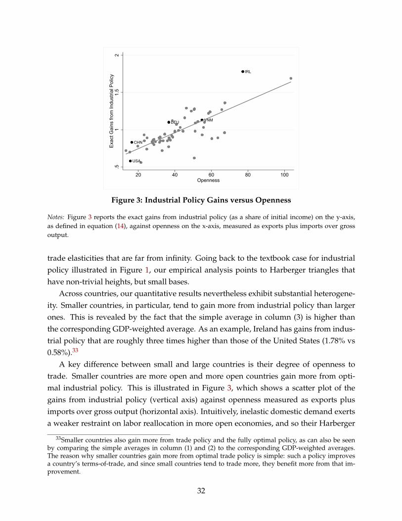
CHN

DEU

IRL

USA

VNM.5

11.

52

Exac

t Gai

ns fr

om In

dust

rial P

olic

y

20 40 60 80 100Openness

Figure 3: Industrial Policy Gains versus Openness

Notes: Figure 3 reports the exact gains from industrial policy (as a share of initial income) on the y-axis,as defined in equation (14), against openness on the x-axis, measured as exports plus imports over grossoutput.

trade elasticities that are far from infinity. Going back to the textbook case for industrialpolicy illustrated in Figure 1, our empirical analysis points to Harberger triangles thathave non-trivial heights, but small bases.

Across countries, our quantitative results nevertheless exhibit substantial heterogene-ity. Smaller countries, in particular, tend to gain more from industrial policy than largerones. This is revealed by the fact that the simple average in column (3) is higher thanthe corresponding GDP-weighted average. As an example, Ireland has gains from indus-trial policy that are roughly three times higher than those of the United States (1.78% vs0.58%).33

A key difference between small and large countries is their degree of openness totrade. Smaller countries are more open and more open countries gain more from opti-mal industrial policy. This is illustrated in Figure 3, which shows a scatter plot of thegains from industrial policy (vertical axis) against openness measured as exports plusimports over gross output (horizontal axis). Intuitively, inelastic domestic demand exertsa weaker restraint on labor reallocation in more open economies, and so their Harberger

33Smaller countries also gain more from trade policy and the fully optimal policy, as can also be seenby comparing the simple averages in column (1) and (2) to the corresponding GDP-weighted averages.The reason why smaller countries gain more from optimal trade policy is simple: such a policy improvesa country’s terms-of-trade, and since small countries tend to trade more, they benefit more from that im-provement.

32

triangles have larger bases, leading to bigger gains from industrial policy. In line withthe previous intuition, a cross-country regression of ∑k |(∆Lj,k)

I/Lj| on openness yields astrong positive relationship with an R2 of 0.84.

An additional implication of the Harberger formula described in equation (17) is that,for given elasticities (∆Lj,k)

I/Lj,k, countries with higher employment in sectors with strongerscale economies should benefit more from industrial policy. Our quantitative results arealso consistent with this observation: countries with a higher correlation between Lk/Land γk do indeed have higher gains from optimal industrial policy. However, this chan-nel accounts for a smaller fraction of the cross-country variation in the gains compared tothe openness channel discussed above: a regression of the gains from industrial policy onopenness yields R2 = 0.62, while adding the variable ∑k Lk/L · γk as a predictor increasesthe R2 to 0.77.

5.3 Gains from Industrial Policy in the Presence of Trade Agreements

The previous quantitative results assume that countries are free to pursue their unilat-erally optimal trade policies. In practice, explicit trade agreements or implicit threats offoreign retaliation may prevent countries from doing so. How would such considerationsaffect the gains from industrial policy?

We address this issue under two benchmark scenarios. In the first case, countries areforced to set zero trade taxes, but still face incentives to manipulate their terms-of-tradeusing industrial policy, as in Lashkaripour and Lugovskyy (2018). In the second, weassume that, despite the availability of other policy instruments, trade agreements havebeen designed to internalize terms-of-trade externalities and restore global efficiency, asin Bagwell and Staiger (2001).34

Under the first scenario, we numerically find the employment subsidies that maxi-mize utility in a given country conditional on zero trade taxes. As mentioned above, theseconstrained-optimal employment subsidies involve a compromise between the textbookPigouvian motive of internalizing production externalities and the goal of improving thecountry’s terms-of-trade.35 Column (2) of Table 3 reports the gains from industrial pol-

34Another potentially interesting scenario would be to consider the gains from industrial and trade pol-icy in an environment where all countries simultaneously impose policies non-cooperatively. Although westop short of analyzing such Nash equilibria, we expect countries to be less open when they all choose tradetaxes in a non-cooperative manner and, in turn, the gains from industrial policy to be smaller, consistentwith the results of Figure 3. Indeed, when considering counterfactual autarkic economies, we find gainsfrom industrial policy that are 0.46% on average.

35As an example, consider an economy that exports all its output. In this case employment subsidiesequal to 1− ( 1

1+γk)( 1+θk

θk) would perfectly replicate the effect of both the employment subsidies and export

33

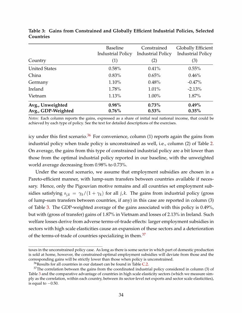
Table 3: Gains from Constrained and Globally Efficient Industrial Policies, SelectedCountries

Baseline Constrained Globally EfficientIndustrial Policy Industrial Policy Industrial Policy

Country (1) (2) (3)

United States 0.58% 0.41% 0.55%China 0.83% 0.65% 0.46%Germany 1.10% 0.48% -0.47%Ireland 1.78% 1.01% -2.13%Vietnam 1.13% 1.00% 1.87%

Avg., Unweighted 0.98% 0.73% 0.49%Avg., GDP-Weighted 0.76% 0.53% 0.35%Notes: Each column reports the gains, expressed as a share of initial real national income, that could beachieved by each type of policy. See the text for detailed descriptions of the exercises.

icy under this first scenario.36 For convenience, column (1) reports again the gains fromindustrial policy when trade policy is unconstrained as well, i.e., column (2) of Table 2.On average, the gains from this type of constrained industrial policy are a bit lower thanthose from the optimal industrial policy reported in our baseline, with the unweightedworld average decreasing from 0.98% to 0.73%.

Under the second scenario, we assume that employment subsidies are chosen in aPareto-efficient manner, with lump-sum transfers between countries available if neces-sary. Hence, only the Pigouvian motive remains and all countries set employment sub-sidies satisfying sj,k = γk/(1 + γk) for all j, k. The gains from industrial policy (grossof lump-sum transfers between countries, if any) in this case are reported in column (3)of Table 3. The GDP-weighted average of the gains associated with this policy is 0.49%,but with (gross of transfer) gains of 1.87% in Vietnam and losses of 2.13% in Ireland. Suchwelfare losses derive from adverse terms-of-trade effects: larger employment subsidies insectors with high scale elasticities cause an expansion of these sectors and a deteriorationof the terms-of-trade of countries specializing in them.37

taxes in the unconstrained policy case. As long as there is some sector in which part of domestic productionis sold at home, however, the constrained-optimal employment subsidies will deviate from those and thecorresponding gains will be strictly lower than those when policy is unconstrained.

36Results for all countries in our dataset can be found in Table C.2.37The correlation between the gains from the coordinated industrial policy considered in column (3) of

Table 3 and the comparative advantage of countries in high scale elasticity sectors (which we measure sim-ply as the correlation, within each country, between its sector-level net exports and sector scale elasticities),is equal to −0.50.

34

.4.6

.81

Gai

ns fr

om In

dust

rial P

olic

y

0 .05 .1 .15Scale Elasticity Outside Manufacturing (γNM)

(a) Scale Elasticity Outside Manufacturing

.8.9

11.

11.

2G

ains

from

Indu

stria

l Pol

icy

.8 1 1.2 1.4 1.6Elasticity of Substitution Between Sectors (1+ρ)

(b) Elasticity of Substitution Between Sectors

Figure 4: Gains from Industrial Policy, Alternative Parameter Values

Notes: Figure 4a reports the (global, unweighted average) gains from industrial policy, as defined in equa-tion (14), for different values of the scale elasticity outside manufacturing, γNM. Figure 4b does the samefor different values of the elasticity of substitution between sectors, 1 + ρ. Large circles indicate baselineparameter values used in Table 2.

5.4 Sensitivity to Calibrated Parameters

We conclude this section by exploring the sensitivity of our findings with respect to themain parameters used in our quantitative exercise: scale elasticities γk, trade elasticitiesθk, and the elasticity of substitution between sectors ρ.

Scale Economies in Non-Manufacturing. We begin with the implications of the valueof scale economies in non-manufacturing sectors, a parameter that we denote γNM. Ourbaseline assumption of γNM = 0—in which only manufacturing sectors exhibit economiesof scale—fits the traditional view behind industrial policy. But in the absence of strong ev-idence to suggest that industrial sectors have superior economies of scale, it is importantto explore the quantitative implications of this assumption.

To shed light on this issue, Figure 4a plots the average of the estimated gains fromoptimal industrial policy (across all countries in the world) as a function of γNM.38 Notsurprisingly, as we start raising γNM from zero, the relative size of manufacturing andnon-manufacturing sectors in the competitive equilibrium gets closer to its optimal valueand the gains from industrial policy fall. Indeed, the gains are minimized when γNM isequal to around 0.13, close to the average of the manufacturing sector γk values of 0.167.

38We continue to calculate the gains from optimal policy as described in equations (33)-(35); that is, nowthat γNM > 0 the optimal policy includes an employment in non-manufacturing sectors.

35

Our baseline finding that the gains from optimal industrial policy are relatively modesttherefore appears to hold across a wide range of reasonable values for scale elasticitiesoutside manufacturing, in line with the fact that these modest gains derive from Har-berger triangles with modestly sized bases rather than heights.

Elasticity of Substitution Across Sectors. We next consider the role played by the elas-ticity of substitution 1 + ρ. In our baseline analysis, we have used our IV estimate ρ =

0.28. Table B.3 implies a 95% confidence interval of [−0.12, 0.68] for this estimate. In Fig-ure 4b, we therefore plot the average gains from optimal industrial policy throughout thisrange. As discussed above, we expect that a higher ρ would lead to larger reallocationsin response to optimal industrial policy and, in turn, larger welfare gains. Qualitatively,this is confirmed in Figure 4b. Quantitatively, however, we see that even for ρ = 0.68, theaverage gains from industrial policy are only 1.18%.

Trade Elasticities. Trade elasticities play a dual role in our analysis: first, they affect thedemand functions that we use to estimate scale elasticities γk in equation (25); and second,they shape the gains from optimal policy for any given value of γk. Our baseline estimatesused θk from prior estimates in the literature, taking the median estimate of θk, withineach sector, across three recent studies in the literature. We now instead estimate thegains from industrial and trade policy when drawing trade elasticities from each of thosethree studies in turn. In each case we repeat the entire two-step estimation procedurefrom Section 4 for the new vector of θk values under consideration.39

The results of this exercise are shown in Table C.3 in Appendix C.4. Although there is awide range of trade elasticity estimates across these three studies (as seen in Table B.1), theaverage estimated gains from industrial policy remain fairly similar for two out of three ofthese studies, about 1.15% as compared to the baseline average gains of 0.98%. The outlieris column (3) of Table C.3, which draws on estimates from Caliendo and Parro (2015) thatcontain a much broader range of trade elasticities across sectors, from 0.4 to 64.9, than theother studies. Using these parameter estimates leads, in turn, to significantly larger gainsfrom industrial policy, equal to 3.28% on average. Our baseline analysis, which focuseson the median of trade elasticities across studies, is purposefully designed to attenuatethe potential effects of outliers.

39In some cases this procedure results in γkθk ≥ 1, which leads to multiplicity of equilibria, as pointedout by Kucheryavyy et al. (2017). Since the solution of the counterfactual equilibrium under optimal policybecomes numerically unstable as γkθk approaches one from below, we cap the value of γk such that γkθk isnever higher than 0.98.

36

6 Beyond Ricardian Economies

In previous sections, we have explored the structure and welfare consequences of optimalindustrial and trade policy in a Ricardian environment in the tradition of Graham (1923),Chipman (1970), and Ethier (1982). In this final section, we extend our earlier analysis toricher environments featuring multiple factors of production and input-output linkages.

6.1 General Environment

Consider a generalized version of the environment of Section 2.1. Each country is nowendowed with both labor and physical capital, Li and Ki, and all production functionsnow use labor, physical capital, and intermediate goods from other countries and sectors,

yij,k = Aij,kEk(Zi,k)zij,k,

zij,k = fk(ìj,k, kij,k, mij,k),

where mij,k ≡ {moij,sk} denotes the vector of intermediate inputs, moij,sk, from a givenorigin country o and source sector s used by firms producing good k in country i andexporting it to country j, kij,k denotes the amount of physical capital that they use, and fk

is homogeneous of degree one in all inputs.40 The relevant measure of sector size is nowgiven by the total use of the composite input in country i and sector k,

Zi,k = ∑j

zij,k. (36)

In terms of policy, each country j’s government can still tax imports and exports, at ratestmij,k and tx

ji,k, as well as subsidize purchases of the composite input at rate sj,k, leading tothe arbitrage condition

vj,k = (1− sj,k)wj,k, (37)

where wj,k denotes the price received by firms from country j producing sector k’s com-posite input and vj,k denotes the price paid by the firms purchasing it. The rest of the

40We allow for Hicks-neutral differences across countries and sectors, but restrict sector-level productionfunctions, fk, to be constant across countries. In our theoretical analysis, this restriction can be dispensedwith. In our quantitative analysis, the assumption of a common fk across countries helps to avoid compu-tational problems arising from the combination of economies of scale and very imbalanced input-outputtables in some countries, while still allowing differences in factor endowments to act as a source of compar-ative advantage.

37

equilibrium conditions can be found in Appendix A.4.

6.2 Revisiting the Structure of Optimal Policy

Within this environment, we can use the same strategy as in Section 2.3 to characterizethe optimal production subsidies, s∗j,k, and trade taxes, tx∗

ji,k and tm∗ij,k. The same Pigouvian

logic leads to the following generalization of Proposition 1.

Proposition 3. In the general environment of Section 6.1 the optimal industrial and trade policyare such that: (i) s∗j,k = εE∗

j,k /(1 + εE∗j,k ); (ii) tm∗

ij,k = tj; and (iii) tx∗ji,k = 1− (1 + tj)(1 + ε

p∗ij,k) for

some tj.

The formal proof can be found in Appendix A.4.2. The only difference between Propo-sitions 1 and 3 comes from the level of industrial policy. Since the total supply of the com-posite input generating the externality, ∑k Zi,k, is elastic, the absolute level of the scaleelasticity is no longer irrelevant and there is no longer an indeterminacy in the level ofthe input subsidy, sj: optimal subsidies now require sj = 0.

To go from theory to data, we maintain the same parametric restrictions as in Section3.2—that is, Ek and uj satisfy equations (22)-(24)—and assume that fk is nested CES,

fk(ìj,k, kij,k, mij,k) = [(ìj,k)ak(kij,k)

1−ak ]bk ∏s[Ms({moij,sk}o)]

bsk , (38)

Ms({moij,sk}o) = (∑o

mθs

1+θsoij,sk)

1+θsθs , (39)

with bk + ∑s bsk = 1 and ak ∈ [0, 1], with average shares consistent with the OECD’s ICIOtables. The estimation of scale elasticities γk can then proceed following the same stepsas in Section 3 given knowledge of the sector-level production function fk that maps la-bor, physical capital, and intermediate goods into a country-and-sector specific compositefactor. The counterpart of our baseline specification (25) is

YIOi,k = δi + δk + γk ln Zi,k + εi,k, (40)

where YIOi,k ≡

1J ∑j(ln Xij,k/θk) + (1 − ak)bk ln(ri/wi) + ∑s bsk ln(Pi,s/wi) now also con-

trols for differences in relative factor prices, ri/wi, and relative intermediate good prices,Pi,s/wi, as described in Appendix B.5.1. This adjustment is necessary to isolate the impactof external economies of scale on quantities demanded.

Figure 5 plots the optimal industrial policy s∗j,k = γk/(1+ γk) estimated in the generalenvironment of Section 6.1 against the optimal industrial policy s∗j,k = γk/(1 + γk) esti-

38

0.1

.2.3

Beyo

nd R

icar

dian

Eco

nom

ies

0 .1 .2 .3Ricardian Economies

Figure 5: Optimal Industrial Policy, Beyond Ricardian Economies

Notes: The y-axis reports the optimal industrial policy s∗j,k = γk/(1 + γk) estimated for 15 manufacturingsectors in the environment with capital and input-output linkages, as described in Section 6.1, whereas thex-axis reports the optimal industrial policy s∗j,k = γk/(1 + γk) estimated in the baseline environment, asdescribed in Section 2.1.

mated in the Ricardian environment of Section 2.1 for the same 15 manufacturing sectors.All observations are close to but below the 45-degree line (illustrated in green).41 Theaverage optimal subsidy in manufacturing sectors is about 28% lower in the presence ofphysical capital and input-output linkages. This reflects the fact that our baseline estima-tion does not control for variation in the price of intermediate goods. Since each sectorand country sources a large fraction of its inputs from itself, countries with larger sectorsalso tend to have lower input prices. Controlling for input prices in our modified esti-mating equation (40) removes this source of upward bias in our baseline estimation. Re-markably, the identity of the sectors that should be subsidized remains unchanged, witha correlation between the optimal policies estimated in the two models equal to 0.99.42

39

CHN

DEU

IRL

USA

VNM

02

46

Beyo

nd R

icar

dian

Eco

nom

ies

0 2 4 6Ricardian Economies

Figure 6: Gains from Industrial Policy, Beyond Ricardian Economies

Notes: Figure 6 reports the gains from industrial policy, as defined in equation (14), in the environmentwith capital and input-output linkages, as described in Section 6.1, on the y-axis, against the gains fromindustrial policy in the baseline environment, as described in Section 2.1, on the x-axis.

6.3 Revisiting the Gains from Optimal Policy

While the structure of optimal policy is very similar to that in our baseline environment,the consequences of such policy are not. As can be seen from Figure 6, the gains fromoptimal industrial policy are significantly larger in the presence of physical capital andinput-output linkages. The average gains estimated here are equal to 3.11%, about threetimes larger than in a Ricardian environment.43 To understand why the gains from opti-mal policy are higher in this more general environment, it is useful to turn to the followinggeneralization of Proposition 2.

Proposition 4. In the general environment of Section 6.1, up to a second-order approximation,

41All estimates of γk remain statistically significant at the 5% level and the instruments remain strong byconventional standards (with the lowest first-stage SW F-statistic equal to 132.0). Full estimates are reportedin Table B.8.

42Since none of the estimates of trade elasticities discussed in Appendix B.3 are affected by the presenceof physical capital and input-output linkages, the structure of optimal trade policy is trivially unchanged.

43The counterpart of the exact hat algebra of Section 5 used for the counterfactual analysis in this sec-tion can be found in Appendix C.5, whereas the gains from industrial policy for all countries can be foundin Table C.4 in Appendix C.5.2, along with the gains from trade policy and the fully optimal policy. Forcompleteness, we also report the sensitivity of these numbers to the values of the scale elasticity outsidemanufacturing (γNM), the elasticity of substitution between sectors (ρ), and the trade elasticity (θk) in Ap-pendix C.5.4.

40

the welfare gains from optimal taxes satisfy

W∗jIj' 1

2 ∑k

wj,kZj,k

Ij·(∆Zj,k)

∗

Zj,k· εE∗

j,k +12 ∑

i 6=j,k

pji,kyji,k

Ij·(∆yji,k)

∗

yji,k· εp∗

ji,k, (41)

where (∆Zj,k)∗ and (∆yji,k)

∗ denote the input and export changes associated with imposing τ∗j andall other variables are evaluated under laissez-faire. Likewise, up to a second-order approximation,gains from industrial and trade policy satisfy

W Ij

Ij' 1

2 ∑k

wjZj,k

Ij·(∆Zj,k)

I

Zj,k· εE∗

j,k , (42)

WTj

Ij' 1

2 ∑i 6=j,k

pji,kyji,k

Ij·(∆yji,k)

T

yji,k· εp∗

ji,k, (43)

where (∆Zj,k)I denotes the input change associated with imposing s∗j , conditional on having al-

ready imposed optimal trade taxes, and (∆yji,k)T denotes the export change associated with impos-

ing t∗j , conditional on having already imposed optimal employment subsidies.

The formal proof can be found in Appendix A.4.3. The key distinction between Propo-sitions 2 and 4 comes from the “shares”, wj,kZj,k/Ij and pji,kyji,k/Ij, appearing in equations(41)-(43). The numerators, wj,kZj,k and pji,kyji,k/Ij, are gross flows, since gross output iswhat is being subsidized by industrial policy and taxed by trade policy. In contrast, thedenominator, Ij, still measures total value added in country j. Thus “shares” now add upto numbers that are strictly greater than one, which mechanically raises the gains associ-ated with both industrial and trade policy.

Quantitatively, the mechanical adjustment from value added to gross flows plays animportant role in generating these larger gains. Starting from the second-order approxi-mations in Proposition 2 and substituting the “shares” from Proposition 4, while keepingeverything else constant, reduces the difference between the gains from industrial policyin the two environments by about one half.44

The other force behind the larger industrial policy gains in the environment with phys-ical capital and input-output linkages are the larger “elasticities” of the quantities beingtaxed, ∆Zj,k/Zj,k. In the Ricardian environment of Section 2.1, the average elasticity ofsector size |(∆Li,k)

I/Li,k| associated with optimal industrial policy is 0.44; in the generalenvironment of this section the average elasticity of sector size |(∆Zj,k)

I/Zj,k| is equal to

44Like in the baseline Ricardian environment, our second-order formulas provide good approximationsin the general environment of Section 6.1. This can be seen from Figure C.1 in Appendix C.5.3.

41

0.61. Intuitively, since each sector and country sources a large fraction of its inputs fromitself, input-output loops magnify the impact of sector-specific subsidies by further low-ering the (pre-subsidy) average input costs faced by firms in the subsidized sector, thesame way they magnify the effects of productivity shocks in Jones (2011).

Overall, though, gains from industrial policy remain significantly smaller than the po-tential gains that one might have expected given the magnitude of scale elasticities thatwe have estimated (18.4% in the simple back-of-the-envelope calculations of Section 5.2).This reflects the fact that while the wedges that we have estimated empirically are sub-stantial, the cross-sectoral reallocations taking place under the optimal policy are fairlymodest in all our quantitative exercises.

7 Concluding Remarks

A major source of skepticism about industrial policy is that governments simply do notknow which sectors should be subsidized at the expense of others. In this paper, wehave focused on the textbook case for industrial policy, in which the rationale for suchpolicy arises from the existence of external economies of scale; we have shown how, inthis environment, one can use commonly available trade and production data to estimateeconomies of scale at the sector-level; and, in turn, we have characterized the structureand consequences of optimal industrial policy.

Empirically, we find that sector-level economies of scale indeed exist and do differsubstantially across manufacturing sectors. Yet, even under our optimistic assumptionthat governments maximize welfare and have full knowledge of the underlying economy,our baseline analysis points towards gains from optimal industrial policy that are hardlytransformative, ranging from an average across countries of 0.98% of GDP in our base-line analysis to 3.11% in the general environment with physical capital and input-outputlinkages.

To put these numbers in perspective, recall that South Korea, a country often presentedas an industrial policy success story, experienced gains in real GDP per capita of 6.82%per year from 1960 to 1989, as documented in Rodrik (1995). A 3.11% long-run welfareincrease is nothing to spit at, but a miracle it is not.

Intuitively, for the textbook gains from industrial policy to be large, two sets of condi-tions should hold. First, production processes should exhibit significant external economiesof scale that differ in strength across sectors—conditions that would give rise to a Har-berger triangle with a large height in Figure 1. Second, high elasticities of substitu-tion and trade openness should allow significant reallocations of resources across sec-

42

tors—conditions that would give rise to a Harberger triangle with a large base in Figure1. Across our quantitative exercises, given low elasticities of demand, the non-trivial gapbetween social and marginal costs that we have inferred remains too small to generatelarge gains from industrial policy, even for the most open economies.

There are, of course, many other market failures that industrial policy may target.Alleviating financial distortions, as in Itskhoki and Moll (2019) and Liu (2019), solvingcoordination failures, as in Murphy et al. (1989), Rodrik (1996) and Buera et al. (2021),and fostering sectors with positive spillovers to the rest of the economy, as in Greenwaldand Stiglitz (2006), may all, in theory, generate transformative gains from industrial pol-icy. Our results, however, offer little empirical support for the notion that these gains canarise from the textbook case based on external economies of scale, at least at the level ofaggregation considered in our analysis. An interesting open question is whether allowingfor more granular economies of scale, within both more narrowly defined sectors and re-gions, may magnify the gains from policy intervention by combining features of optimalindustrial and trade policy, as emphasized in this paper, with those of optimal place-based policy, as emphasized in Fajgelbaum and Gaubert (2020) and Rossi-Hansberg et al.(2019). We hope that the combination of theory and empirics developed in this paper willprove useful in making progress on this and other related questions.

43

References

Antweiler, Werner and Daniel Trefler, “Increasing Returns and All That: A View FromTrade,” American Economic Review, 2002, 92 (1), 93–119.

Arkolakis, Costas, Arnaud Costinot, and Andres Rodríguez-Clare, “New Trade Models,Same Old Gains?,” American Economic Review, 2012, 102 (1), 94–130.

Atkin, David, “Trade, Tastes and Nutrition in India,” American Economic Review, 2013, 103(5).

Bagwell, Kyle and Robert W. Staiger, “Domestic Policies, National Sovereignty, and In-ternational Economic Institutions,” The Quarterly Journal of Economics, 2001, 116 (2), 519–562.

Bartelme, Dominick, Arnaud Costinot, Dave Donaldson, and Andres Rodríguez-Clare,“The Textbook Case for Industrial Policy: Theory Meets Data,” NBER working paper26193, 2019.

Basu, S. and J.G. Fernald, “Returns to Scale in U.S. Production: Estimates and Implica-tions,” Journal of Political Economy, 1997, 105, 249–283.

Beck, Thorsten, “Financial development and international trade: is there a link?,” Journalof International Economics, 2002, 57 (1), 107–131.

Buera, Francisco J, Hugo Hopenhayn, Yongseok Shin, and Nicholas Trachter, “Big Pushin Distorted Economies,” Technical Report, National Bureau of Economic Research2021.

Caballero, Ricardo J. and Richar K. Lyons, “External Effects in U.S. Procyclical Produc-tivity,” Journal of Monetary Economics, 1992, 29 (209-225).

Caliendo, Lorenzo and Fernando Parro, “Estimates of the Trade and Welfare Effects ofNAFTA,” Review of Economic Studies, 2015, 82 (1), 1–44.

Chipman, John S., “External Economies of Scale and Competitive Equilibrium,” TheQuarterly Journal of Economics, 1970, 84 (3), 347–385.

Combes, Pierre-Philippe and Laurent Gobillon, “The empirics of agglomerationeconomies,” in Gilles Duranton, J. Vernon Henderson, and William C. Strange, eds.,Handbook of regional and urban economics, Vol. 5, Elsevier, 2015, pp. 247–348.

44

Comin, Diego, Danial Lashkari, and Marti Mestieri, “Structural Change with Long-RunIncome and Price Effects,” Econometrica, 2021, 89 (1), 311–374.

Costinot, Arnaud and Andres Rodríguez-Clare, “Trade Theory with Numbers: Quan-tifying the Consequences of Globalization,” in Gita Gopinath, Elhanan Helpman, andKenneth Rogoff, eds., Handbook of International Economics, Vol. 4, New York: Elsevier,2014.

and Ivan Werning, “Robots, Trade, and Luddism: A Sufficient Statistics to OptimalTechnology Regulation,” NBER working paper 25103, 2018.

, Dave Donaldson, and Ivana Komunjer, “What Goods Do Countries Trade? A Quan-titative Exploration of Ricardo’s Ideas,” Review of Economic Studies, 2012, 79 (2), 581–608.

, , Margaret Kyle, and Heidi Williams, “The More We Die, The More We Sell? ASimple Test of the Home-Market Effect,” Quarterly Journal of Economics, 2019, 134 (2),843–894.

Cravino, Javier and Sebastian Sotelo, “Trade Induced Structural Change and the SkillPremium,” American Economic Journal: Macroeconomics, 2019, 11 (3), 289–326.

Davis, Donald R. and David Weinstein, “Market access, economic geography and com-parative advantage: an empirical test,” Journal of Intermational Economics, 2003, 59, 1–23.

Dekle, Robert, Jonathan Eaton, and Samuel Kortum, “Global Rebalancing with Gravity:Measuring the Burden of Adjustment,” IMF Staff Papers, 2008, 55 (3), 511–540.

Dixit, Avinash K., “Tax Policy in Open Economies,” in Martin Feldstein, ed., Handbook ofPublic Economics, Vol. 1, Elsevier, 1985.

Duranton, Gilles, “California Dreamin’: The Feeble Case for Cluster Policies,” Review ofEconomic Analysis, 2011, 3, 3–45.

Eaton, Jonathan and Samuel Kortum, “Technology, Geography and Trade,” Econometrica,2002, 70 (5), 1741–1779.

Ethier, Wilfred J., “Decreasing Costs in International Trade and Frank Graham’s Argu-ment for Protection,” Econometrica, 1982, 50 (5), 1243–1268.

Fajgelbaum, Pablo D. and Cecile Gaubert, “Optimal Spatial Policies, Geography, andSorting,” Quarterly Journal of Economics, 2020, 135 (2), 959–1036.

45

Giri, Rahul, Kei-Mu Yi, and Hakan Yilmazkuday, “Gains from Trade: Does SectoralHeterogeneity Matter?,” Journal of International Economics, 2021, 129, 103429.

Graham, Frank D., “Some Aspects of Protection Further Considered,” The Quarterly Jour-nal of Economics, 1923, 37 (2), 199–227.

Greenwald, Bruce and Joseph E Stiglitz, “Helping infant economies grow: Foundationsof trade policies for developing countries,” American Economic Review, 2006, 96 (2), 141–146.

Greenwald, Bruce C. and Joseph E. Stiglitz, “Externalities in Economies with ImperfectInformation and Incomplete Markets,” Quarterly Journal of Economics, 1986, 101 (2), 229–264.

Harrison, Ann E. and Andres Rodríguez-Clare, “Trade, Foreign Investment, and Indus-trial Policy for Developing Countries,” in Dani Rodrik and Mark Rosenzweig, eds.,Handbook of Development Economics, Vol. 5, Elsevier, 2010.

Head, Keith and John Ries, “Increasing Returns versus National Product Differentiationas an Explanation for the Pattern of U.S.-Canada Trade,” American Economic Review,2001, 91 (4), 858–876.

and Thierry Mayer, “Gravity Equations: Toolkit, Cookbook, Workhorse,” in GitaGopinath, Elhanan Helpman, and Kenneth Rogoff, eds., Handbook of International Eco-nomics, Vol. 4, New York: Elsevier, 2013.

Herrendorf, Berthold, Richard Rogerson, and Akos Valentinyi, “Two Perspectives onPreferences and Structural Transformation,” American Economic Review, 2013, 103 (7),2752–89.

Hines, James R., “Three Sides of Harberger Triangles,” Journal of Economic Perspectives,1999.

Hopenhayn, Hugo A., “Entry, Exit, and Firm Dynamics in Long Run Equilibrium,” Econo-metrica, 1992, 60 (5), 1127–1150.

Itskhoki, Oleg and Benjamin Moll, “Optimal Development Policies with Financial Fric-tions,” Econometrica, 2019, 87 (1), 139–173.

Jones, Charles I., “Intermediate Goods and Weak Links in the Theory of Economic De-velopment,” American Economic Journal: Macroeconomics, 2011, 3 (2), 1–28.

46

Juhasz, Reka, “Temporary Protection and Technology Adoption: Evidence from theNapoleonic Blockade,” American Economic Review, 2018, 108 (11), 3339–3376.

Kaufmann, Daniel, Aart Kraay, and Massimo Mastruzzi, “Governance Matters III: Gov-ernance Indicators for 1996–2002,” 2003. World Bank Working Paper No. 3106.

Kline, Patrick and Enrico Moretti, “People, Places, and Public Policy: Some SimpleWelfare Economics of Local Economic Development Programs,” Annual Review of Eco-nomics, 2014, 6, 629–662.

Krugman, Paul, “Scale Economies, Product Differentiation, and the Pattern of Trade,”The American Economic Review, 1980, 70 (5), 950–959.

Kucheryavyy, Konstantin, Gary Lyn, and Andres Rodríguez-Clare, “Grounded byGravity: A Well-Behaved Trade Model with Industry-Level Economies of Scale,” mimeoUC Berkeley, 2017.

Lane, Nathan, “Manufacturing Revolutions: Industrial Policy and Networks in SouthKorea,” mimeo IIES, 2017.

, “The New Empirics of Industrial Policy,” Journal of Industry, Competition and Trade,2020, 20 (209-234).

Lashkaripour, Ahmad and Vova Lugovskyy, “Scale Economies and the Structure ofTrade and Industrial Policy,” mimeo Indiana University, 2018.

Levchenko, Andrei A., “Institutional quality and international trade,” Review of EconomicStudies, 2007, 74 (3), 791–819.

and Jing Zhang, “The Evolution of Comparative Advantage: Measurement and Wel-fare Implications,” Journal of Monetary Economics, 2016, 78, 96–111.

Liu, Ernest, “Industrial Policies in Production Networks,” Quarterly Journal of Economics,2019, 134 (4), 1883–1948.

Manova, Kalina, “Credit constraints, equity market liberalizations and internationaltrade,” Journal of International Economics, 2008, 76 (1), 33–47.

Marshall, Alfred, Principles of Economics, An Introductory Volume, London: Mcmillan,eighth edition, 1920.

Melitz, Marc J., “The Impact of Trade on Intra-Industry Reallocations and AggregateIndustry Productivity,” Econometrica, 2003, 71 (6), 1695–1725.

47

Murphy, Kevin M, Andrei Shleifer, and Robert W Vishny, “Industrialization and thebig push,” Journal of political economy, 1989, 97 (5), 1003–1026.

Newey, W.K. and J.L. Powell, “Instrumental Variable Estimation in Nonparametric Mod-els,” Econometrica, 2003, 71 (5), 1565–1578.

Nunn, Nathan, “Relationship-specificity, incomplete contracts, and the pattern of trade,”Quarterly Journal of Economics, 2007, 122 (2), 569–600.

and Daniel Trefler, “Domestic Institutions as a Source of Comparative Advantage,”in G. Gopinath, E. Helpman, and K. Rogoff, eds., Handbook of International Economics,Vol. 4, Elsevier, 2014.

Oberfield, Ezra and Devesh Raval, “Micro Data and Macro Technology,” Econometrica,2021, 89 (2), 703–732.

Pigou, A. C., The Economics of Welfare, Macmillan, 1920.

Redding, Stephen J. and David Weinstein, “Accounting for Trade Patterns,” 2018. NBERworking paper 24051.

Rodrik, Dani, “Getting interventions right: how South Korea and Taiwan grew rich,”Economic Policy, 1995, 10 (20), 53–107.

, “Coordination failures and government policy: A model with applications to EastAsia and Eastern Europe,” Journal of international economics, 1996, 40 (1-2), 1–22.

Rosenthal, Stuart S. and William C. Strange, “Evidence on the Nature and Sources ofAgglomeration Economies,” in J.V. Henderson and J.F. Thisse, eds., Handbook of Regionaland Urban Economics, Vol. 4, Elsevier, 2004.

Rossi-Hansberg, Esteban, Pierre-Daniel Sarte, and Felipe Schwartzman, “CognitiveHubs and Spatial Redistribution,” NBER Working Paper 26267, 2019.

Sanderson, Eleanor and Frank Windmeijer, “A weak instrument F-test in linear IV mod-els with multiple endogenous variables,” Journal of Econometrics, 2016, 190 (2), 212–221.

Shapiro, Joseph, “Trade Costs, CO2, and the Environment,” American Economic Journal:Economic Policy, 2016, 8 (4), 220–54.

Simonovska, Ina and Michael Waugh, “Different Trade Models, Different Trade Elastic-ities?,” mimeo, 2012.

48

A Online Appendix: Theory

A.1 Derivation of Equation (11)

Proof. Start from the identity,

Uj(τ) = Vj(pj(τ), Ij(τ)), (A.1)

with the total income of country j’s representative agent equal to

Ij(τ) = wjLj + ∑i,k

πji,k −∑k

sj,kwjLj,k + ∑j 6=i,k

tmij,k pij,kcij,k + ∑

j 6=itx

ji,k pji,kyji,k.

Totally differentiating (A.1) implies

dUj = ∑i,k

∂Vj

∂pij,k× dpij,k +

∂Vj

∂Ij×{

Ljdwj + ∑i,k

[∂πji,k

∂qji,kdqji,k +

∂πji,k

∂vj,kdvj,k +

∂πji,k

∂Lj,kdLj,k

]+∑

k(dvj,k − dwj)Li,k + ∑

k(vj,k − wj)dLi,k + ∑

i,k(dpij,k − dpij,k)cij,k

+∑i,k(pij,k − pij,k)dcij,k +∑

i,k(dpji,k − dqji,k)yji,k + ∑

i,k( pji,k − qji,k)dyji,k

}. (A.2)

Next, apply the Envelope Theorem to the utility maximization problem of country j’s representa-

tive agent and the profit maximization problem of its firms. This implies

∂Vj

∂pij,k= −

∂Vj

∂Ijcij,k, for all i and k, (A.3)

∂πji,k

∂qji,k= yji,k, for all i and k, (A.4)

∂πji,k

∂vj,k= −`ji,k for all i and k. (A.5)

Substituting (A.3)-(A.5) into (A.2) gives

dUj =∂Vj

∂Ij×{

∑k(vj,k − wj)dLj,k + ∑

i,k(pij,k − pij,k)dcij,k + ∑

i,k( pji,k − qji,k)dyji,k

+ ∑i,k

∂πji,k

∂Lj,kdLj,k − ∑

i 6=j,kcij,kdpij,k + ∑

i 6=j,kyji,kdpji,k

}, (A.6)

49

where we have also used the good market clearing condition (7) for local goods, cjj,k = yjj,k, as

well as country j’s labor market clearing condition (8). To conclude, note that

∂πji,k

∂Lj,k= vj,k

E′k(Lj,k)

Ek(Lj,k)`ji,k for all i and k, (A.7)

dpij,k = 0 for all i 6= j and k, (A.8)

dpji,k = p′ji,k(yji,k)dyji,k for all i 6= j and k. (A.9)

Combining (2)-(4) with (A.6)-(A.9) and letting λj ≡ ∂Vj/∂Ij, εEj,k ≡ d ln Ek(Lj,k)/d ln Lj,k, and ε

pji,k ≡

d ln pji,k(yji,k)/d ln yji,k, (A.6) simplifies into (11).

A.2 Proof of Proposition 1

Proof. Start from equation (12),

∑k

s∗j,kw∗j dLj,k − ∑i 6=j,k


i 6=j,ktx∗

ji,k pji,kdyji,k

= ∑k

εE∗j,k w∗j (1− s∗j,k)dLj,k + ∑

i 6=j,kε

p∗ji,k p∗ji,kdyji,k.

Since the previous condition must hold for any feasible variation, it must hold, in particular, for

variations that: (i) decrease domestic sales in sector 1 and increase domestic sales in sector k so

that dLj,k = −dLj,1, holding all other equilibrium variables fixed; (ii) increase the imports of good

1 from country 1 and increase the imports of good k from country i, dcij,k = −p∗1j,1p∗ij,k

dc1j,1, holding all

other equilibrium variables fixed; or (iii) decrease the imports of good 1 from country 1, increase

the exports of good k to country i, dyji,k =p∗1j,1

p∗ji,k(

1+εp∗ji,k

)dc1j,1, and decrease its domestic sales of good

k, dyjj,k = −A∗jj,kA∗ji,k

dyji,k, holding all other equilibrium variables fixed. Specializing (12) to variations

(i)-(iii), respectively, imply

s∗j,k = [s∗j,1 − εE∗j,1 (1− s∗j,1) + εE∗

j,k ]/(1 + εE∗j,k ),

tm∗ij,k = tm∗

1j,1,

tx∗ji,k = 1− (1 + tm∗

1j,1)(1 + εp∗ji,k).

Setting sj = s∗j,1 − εE∗j,1 (1− s∗j,1) and tj = tm∗

1j,1 concludes the proof of Proposition 1.

A.3 Proof of Proposition 2

Proof. We first approximate the gains from fully optimal policies, W∗j , and then show how a similar

argument can be used to approximate the gains from industrial and trade policy, W Ij and WT

j .

50

Part I: Derivation of Equation (16).

Proof. Consider a set of world economies, each associated with distinct external economies of

scale, {Ek(·)}, and inverse import demand functions, { pji,k(·)}i 6=j,k, that generate distinct optimal

policies τ∗j ≡ {s∗j,k, tm∗ij,k, tx∗

ji,k}i 6=j,k in country j as well as distinct elasticities ε∗j ≡ {εE∗j,k , ε

p∗ji,k}i 6=j,k

in the equilibrium associated with these optimal policies. Let W∗j (ε∗j ) denote country j’s welfare

gains from optimal policy for each of these world economies. It varies with ε∗j for two reasons:

(i) through the direct effect of the underlying changes in {Ek(·)} and { pji,k(·)}i 6=j,k on equilibrium

prices and quantities, and (ii) the indirect effect of these changes on the value of the optimal

taxes, τ∗j ≡ {sj,k(ε∗j ), tm

ij,k(ε∗j ), tx

ji,k(ε∗j )} ≡ τj(ε

∗j ), with sj,k(ε

∗j ) ≡ εE∗

j,k /(1 + εE∗j,k ), tm

ij,k(ε∗j ) ≡ 0, and

txji,k(ε

∗j ) ≡ −ε

p∗ji,k, as shown in Proposition 1 under the normalization sj = tj = 0. To keep track of

these direct and indirect effects, rewrite equation (13) as

Vj( pj(τj(ε∗j ), ε∗j ), Ij(τj(ε

∗j ), ε∗j )) = Vj( pj(0, ε∗j ), Ij(0, ε∗j ) + W∗j (ε

∗j )), (A.10)

with the second argument of pj(τj(ε∗j ), ε∗j ) and Ij(τj(ε

∗j ), ε∗j ) capturing the direct effect on prices

and income of {Ek(·)} and { pji,k(·)}i 6=j,k. The goal is to show that as ε∗j → 0, the difference between

W∗j (ε∗j ) and 1

2 ∑k wj∆Lj,kεE∗j,k + 1

2 ∑i 6=j,k pji,k∆yji,kεp∗ji,kn goes to zero at a rate no slower than |ε∗j |3,

W∗j (ε∗j ) =

12 ∑

kwj(∆Lj,k)

∗εE∗j,k +

12 ∑

i 6=j,kpji,k(∆yji,k)

∗εp∗ji,k + O(|ε∗j |3), (A.11)

which is the formal counterpart of the approximation displayed in equation (16).

To establish this result, start from the second-order Taylor expansion,

W∗j (ε∗j ) = W∗j (0) + [DεW∗j ]

′ε∗j =0ε∗j +

12(ε∗j )

′[HεW∗j ]ε∗j =0ε∗j + O(|ε∗j |3), (A.12)

with DεW∗j ≡ {dW∗j /dε∗j,n} the vector of first derivatives with respect to all elasticities, ε∗j ≡{ε∗j,n}, with the convention ε∗j,n = εE∗

j,k if n = (k, E) and ε∗j,n = εp∗ji,k if n = (i, k, p), and HεW∗j ≡

{d2W∗j /(dε∗j,ndε∗j,m)} the associated Hessian. First, note that gains from optimal policy are zero if

ε∗j = 0,

W∗j (0) = 0. (A.13)

Second, differentiate (A.10) with respect ε∗j,n,

∂Vj(τj(ε∗j ), ε∗j , 0)

∂τj,n

dτj,n

dε∗j,n+

∂Vj(τj(ε∗j ), ε∗j , 0)

∂ε∗j,n=

∂Vj(0, ε∗j , W∗j (ε∗j ))

∂ε∗j,n+

∂Vj(0, ε∗j , W∗j (ε∗j ))

∂Wj

dW∗jdε∗j,n

, (A.14)

with Vj(τj, ε∗j , Wj) ≡ Vj( pj(τj, ε∗j ), Ij(τj, ε∗j ) +Wj) and τj,n is the policy associated with the elasticity

ε∗j,n, i.e., τj,n(ε∗j ) = sj,k(ε

∗j ) if n = (k, E) and τj,n(ε

∗j ) = tx

ij,k(ε∗j ) if n = (i, k, p). At the optimal policy

mix, τ∗j = τj(ε∗j ), we know that ∂Vj(τj(ε

∗j ), ε∗j , 0)/∂τj,n = 0. Noting that (∂Vj/∂Wj)(τj,ε∗j ,Wj)=0 =

51

λj 6= 0, where λj denotes the marginal utility of income in the laissez-faire equilibrium with

ε∗j = 0, equations (A.13) and (A.14) then imply

[DεW∗j ]ε∗j =0 = 0. (A.15)

Third, differentiate (A.14) with respect to ε∗j,m,

∂V2j (τj(ε

∗j ), ε∗j , 0)

∂τj,m∂τj,n

dτj,n

dε∗j,n

dτj,m

dε∗j,m+

∂V2j (τj(ε

∗j ), ε∗j , 0)

∂ε∗j,m∂τj,n

dτj,n

dε∗j,n+

∂2Vj(τj(ε∗j ), ε∗j , 0)

∂τj,m∂ε∗j,n

dτj,m

dε∗j,m+

∂2Vj(τj(ε∗j ), ε∗j , 0)

∂ε∗j,m∂ε∗j,n

=∂2Vj(0, ε∗j , W∗j (ε

∗j ))

∂ε∗j,m∂ε∗j,n+

∂2Vj(0, ε∗j , W∗j (ε∗j ))

∂Wj∂ε∗j,n

dW∗jdε∗j,m

+∂2Vj(0, ε∗j , W∗j (ε

∗j ))

∂ε∗j,m∂Wj

dW∗jdε∗j,n

+∂2Vj(0, ε∗j , W∗j (ε

∗j ))

∂W2j

dW∗jdε∗j,m

dW∗jdε∗j,n

+∂Vj(0, ε∗j , W∗j (ε

∗j ))

∂Wj

d2W∗jdε∗j,mdε∗j,n

.

Evaluated at ε∗j = 0, the previous expression implies

d2W∗j (0)

dε∗j,mdε∗j,n=

1λj

[∂V2

j

∂τj,m∂τj,n

dτj,n

dε∗j,n

dτj,m

dε∗j,m+

∂V2j

∂ε∗j,m∂τj,n

dτj,n

dε∗j,n+

∂2Vj

∂τj,m∂ε∗j,n

dτj,m

dε∗j,m

](τj,ε∗j ,Wj)=0

, (A.16)

where we have used (A.15) and (∂Vj/∂Wj)(τj,ε∗j ,Wj)=0 = λj. Next, compute the cross-derivatives

of Vj. We start from equation (11). Using the present notation and the fact that optimal tariffs are

zero, it can be rearranged as

1λ∗j

∂Vj(τj(ε∗j ), ε∗j , 0)

∂τj,n= −∑

ks∗j,kwj

∂Lj,k

∂τj,n+ ∑

i 6=j,ktx∗

ji,k ˆpji,k∂yji,k

∂τj,n+ ∑

kεE∗

j,k (1− s∗j,k)wj∂Lj,k

∂τj,n+ ∑

i 6=j,kε

p∗ji,k

ˆpji,k∂yji,k

∂τj,n,

where λ∗j is the marginal utility of income under the optimal policy mix and all equilibrium prices

and quantities appearing on the right-hand side with hats are treated as functions of (τj(ε∗j ), ε∗j ).

Differentiating a second time with respect to ωj,m ∈ {τj,m, εj,m} and using τ∗j = τj(ε∗j ), we obtain

∂(

1/λ∗j

)∂ωj,m

∂Vj

∂τj,n+

1λ∗j

∂2Vj

∂ωj,m∂τj,n= ∑

k

(−

∂s∗j,k∂ωj,m

+∂[εE∗

j,k (1− s∗j,k)]

∂ωj,m

)(wj

∂Lj,k

∂τj,n

)

+ ∑i 6=j,k

(∂tx∗

ji,k

∂ωj,m−

∂(−εp∗ji,k)

∂ωj,m

)(ˆpji,k

∂yji,k

∂τj,n

).

52

Since ∂Vj(τj(ε∗j ), ε∗j , 0)/∂τj,n = 0 at the optimal policy mix, this yields

1λj

(∂2Vj

∂sj,k∂τj,n

)(τj,ε∗j ,Wj)=0

=

(−wj(1 + εE∗

j,k )∂Lj,k

∂τj,n

)(τj,ε∗j )=0

, (A.17)

1λj

(∂2Vj

∂εE∗j,k ∂τj,n

)(τj,ε∗j ,Wj)=0

=

(wj(1− s∗j,k)

∂Lj,k

∂τj,n

)(τj,ε∗j )=0

, (A.18)

1λj

(∂2Vj

∂txji,k∂τj,n

)(τj,ε∗j ,Wj)=0

=

(ˆpji,k

∂yji,k

∂τj,n

)(τj,ε∗j )=0

, (A.19)

1λj

(∂2Vj

∂εp∗ji,k∂τj,n

)(τj,ε∗j ,Wj)=0

=

(ˆpji,k

∂yji,k

∂τj,n

)(τj,ε∗j )=0

. (A.20)

By definition, τj(ε∗j ) ≡ {sj,k(ε

∗j ), tm

ij,k(ε∗j ), tx

ji,k(ε∗j )} satisfies

dτj,n

dε∗j,n=

dsj,k(ε∗j )

dεE∗j,k

=1

(1 + εE∗j,k )

2, if n = (k, E), (A.21)

dτj,n

dε∗j,n=

dtxji,k(ε

∗j )

dεp∗ji,k

= −1, if n = (i, k, p). (A.22)

Equations (A.12)-(A.22) imply

W∗j (ε∗j ) =

12 ∑

k,n

(wj(1− sj,k)

∂Lj,k

∂τj,n

dτj,n

dε∗j,n

)(τj,ε∗j )=0

ε∗j,nεE∗j,k

+12 ∑

i 6=j,k,n

(ˆpji,k

∂yji,k

∂τj,n

dτj,n

dε∗j,n

)(τj,ε∗j )=0

ε∗j,nεp∗ji,k + O(|ε∗j |3). (A.23)

To simplify the previous expression, note that a zero-order Taylor approximation implies

wj ≡ wj(0, ε∗j ) = wj(0, 0) + O(|ε∗j |), (A.24)

pji,k ≡ ˆpji,k(0, ε∗j ) = ˆpji,k(0, 0) + O(|ε∗j |). (A.25)

Note also that

(∆Lj,k)∗ ≡ Lj,k(τj(ε

∗j ), ε∗j )− Lj,k(0, ε∗j ) = Lj,k(τj(ε

∗j ), ε∗j )− Lj,k(0, 0) + Lj,k(0, 0)− Lj,k(0, ε∗j ),

(A.26)

(∆yji,k)∗ ≡ yji,k(τj(ε

∗j ), ε∗j )− yji,k(0, ε∗j ) = yji,k(τj(ε

∗j ), ε∗j )− yji,k(0, 0) + yji,k(0, 0)− yji,k(0, ε∗j ).

(A.27)

53

First-order Taylor approximations therefore imply

Lj,k(τj(ε∗j ), ε∗j )− Lj,k(0, 0) = ∑

n

(∂Lj,k

∂τj,n

dτj,n

dε∗j,n+

∂Lj,k

∂ε∗j,n

)(τj,ε∗j )=0

ε∗j,n + O(|ε∗j |2), (A.28)

Lj,k(0, ε∗j )− Lj,k(0, 0) = ∑n

(∂Lj,k

∂ε∗j,n

)(τj,ε∗j )=0

ε∗j,n + O(|ε∗j |2), (A.29)

yji,k(τj(ε∗j ), ε∗j )− yji,k(0, 0) = ∑

n

(∂yji,k

∂τj,n

dτj,n

dε∗j,n+

∂yji,k

∂ε∗j,n

)(τj,ε∗j )=0

ε∗j,n + O(|ε∗j |2), (A.30)

yji,k(0, ε∗j )− yji,k(0, 0) = ∑n

(∂yji,k

∂ε∗j,n

)(τj,ε∗j )=0

ε∗j,n + O(|ε∗j |2). (A.31)

Combining equations (A.23)-(A.31) as well as noting that sj,k, (∆Lj,k)∗, (∆yji,k)

∗, εE∗j,k , ε

p∗ji,k = O(|ε∗j |)

and aO(|ε∗j |b)O(|ε∗j |c) = O(|ε∗j |b+c) for any a, b, and c, we obtain (A.11).

Part II: Derivation of Equation (17).

Proof. Like in Part I, to keep track of the direct and indirect effects associated with changes in ε∗j ,

rewrite equation (14) as


∗j ), ε∗j )) = Vj( pj((0, tj(ε

∗j )), ε∗j ), Ij((0, tj(ε

∗j )), ε∗j ) + W I

j (ε∗j )), (A.32)

with tj(ε∗j ) ≡ {tm

ij,k(ε∗j ), tx

ji,k(ε∗j )}. The goal is now to show that as ε∗j → 0, the difference between

W Ij (ε∗j ) and 1

2 ∑k wj(∆Lj,k)IεE∗

j,k goes to zero at a rate no slower than |ε∗j |3,

W Ij (ε∗j ) =

12 ∑

kwj(∆Lj,k)

IεE∗j,k + O(|ε∗j |3), (A.33)


The first part of the proof is unchanged with

W Ij (ε∗j ) = W I

j (0) + [DεW Ij ]′ε∗j =0ε∗j +

12(ε∗j )

′[HεW Ij ]ε∗j =0ε∗j + O(|ε∗j |3), (A.34)

W Ij (0) = 0. (A.35)

54

Compared to Part I, differentiating (A.32) with respect ε∗j,n now implies

∂Vj(τj(ε∗j ), ε∗j , 0)

∂τj,n

dτj,n

dε∗j,n+

∂Vj(τj(ε∗j ), ε∗j , 0)

∂ε∗j,n

=∂Vj((0, tj(ε

∗j )), ε∗j , W I

j (ε∗j ))

∂ε∗j,n+

∂Vj((0, tj(ε∗j )), ε∗j , W I

j (ε∗j ))

∂Wj

dW Ij

dε∗j,n

+ ∑m

∂Vj((0, tj(ε∗j )), ε∗j , W I

j (ε∗j ))

∂tj,m

dtj,m

dε∗j,n, (A.36)

which still yields

[DεW Ij ]ε∗j =0 = 0. (A.37)

Compared to Part I, differentiating (A.36) and evaluating it at ε∗j = 0 then implies

d2W Ij (0)

dε∗j,mdε∗j,n=

1λj

[∂V2

j∂τj,m∂τj,n

dτj,ndε∗j,n

dτj,mdε∗j,m

+∂V2

j∂ε∗j,m∂τj,n

dτj,ndε∗j,n

+∂2Vj

∂τj,m∂ε∗j,n

dτj,mdε∗j,m

](τj,ε∗j ,Wj)=0

if ε∗j,n = εE∗j,k , ε∗j,m = εE∗

j,l ,

1λj

[∂V2

j∂τj,m∂τj,n

dτj,ndε∗j,n

dτj,mdε∗j,m

+∂V2


dτj,ndε∗j,n

]if ε∗j,n = εE∗

j,k , ε∗j,m = εp∗ji,l ,

1λj

[∂V2

j∂τj,m∂τj,n

dτj,ndε∗j,n

dτj,mdε∗j,m

+∂2Vj

∂τj,m∂ε∗j,n

dτj,mdε∗j,m

](τj,ε∗j ,Wj)=0

if ε∗j,n = εp∗ji,k, ε∗j,m = εE∗

j,l ,

0 if ε∗j,n = εp∗ji,k, ε∗j,m = ε

p∗jd,l .

Since the cross-derivatives of Vj and the derivatives of τj displayed in equations (A.17)-(A.22) are

unchanged, the previous expression yields

d2W Ij (0)

dε∗j,mdε∗j,n=

(

wj(1− s∗j,k)∂Lj,k∂τj,m

dτj,mdε∗j,m

)(τj,ε∗j )=0

if ε∗j,n = εE∗j,k , ε∗j,m = εE∗

j,l ,

0 otherwise.

(A.38)

Combining equations (A.34), (A.35), (A.37), and (A.38), we obtain

W Ij (ε∗j ) =

12 ∑

k,l

(wj(1− sj,k)

∂Lj,k

∂sj,l

dsj,l

dεE∗j,l

)(τj,ε∗j )=0

εE∗j,l εE∗

j,k + O(|ε∗j |3).

The final part of the argument is the same as in Part I, now applied to

(∆Lj,k)I ≡ Lj,k(τj(ε

∗j ), ε∗j )− Lj,k((0, tj(ε

∗j )), ε∗j ),

55

using the first-order Taylor approximations,

Lj,k(τj(ε∗j ), ε∗j )− Lj,k(0, 0) = ∑

n

(∂Lj,k

∂τj,n

dτj,n

dε∗j,n+

∂Lj,k

∂ε∗j,n

)(τj,ε∗j )=0

ε∗j,n + O(|ε∗j |2),

Lj,k((0, tj(ε∗j )), ε∗j )− Lj,k(0, 0) = ∑

n

(∑m

∂Lj,k

∂tj,m

dtj,m

dε∗j,n+

∂Lj,k

∂ε∗j,n

)(τj,ε∗j )=0

ε∗j,n + O(|ε∗j |2).

Part III: Derivation of Equation (15).

Proof. Like in Parts I and II, rewrite equation (15) as


∗j ), ε∗j )) = Vj( pj((sj(ε

∗j ), 0), ε∗j ), Ij((sj(ε

∗j ), 0), ε∗j ) + WT

j (ε∗j )), (A.39)

with sj(ε∗j ) ≡ {sj,k(ε

∗j )}. The goal is now to show that as ε∗j → 0, the difference between WT

j (ε∗j )

and 12 ∑i 6=j,k pji,k(∆yji,k)

Tεp∗ji,k goes to zero at a rate no slower than |ε∗j |3,

WTj (ε

∗j ) =

12 ∑

i 6=j,kpji,k(∆yji,k)

Tεp∗ji,k + O(|ε∗j |3), (A.40)


The first part of the proof is again unchanged with

WTj (ε

∗j ) = WT

j (0) + [DεWTj ]′ε∗j =0ε∗j +

12(ε∗j )

′[HεWTj ]ε∗j =0ε∗j + O(|ε∗j |3), (A.41)

WTj (0) = 0. (A.42)

Compared to Parts I and II, differentiating (A.39) with respect ε∗j,n implies

∂Vj(τj(ε∗j ), ε∗j , 0)

∂τj,n

dτj,n

dε∗j,n+

∂Vj(τj(ε∗j ), ε∗j , 0)

∂ε∗j,n

=∂Vj((sj(ε

∗j ), 0), ε∗j , WT

j (ε∗j ))

∂ε∗j,n+

∂Vj((sj(ε∗j ), 0), ε∗j , WT

j (ε∗j ))

∂Wj

dWTj

dε∗j,n

+ ∑m

∂Vj((sj(ε∗j ), 0), ε∗j , WT

j (ε∗j ))

∂sj,m

dsj,m

dε∗j,n, (A.43)

which still yields

[DεWTj ]ε∗j =0 = 0. (A.44)

56

Compared to Parts I and II, differentiating (A.43) and evaluating it at ε∗j = 0 then implies

d2WTj (0)

dε∗j,mdε∗j,n=

0 if ε∗j,n = εE∗j,k , ε∗j,m = εE∗

j,l ,

1λj

[∂V2

j∂τj,m∂τj,n

dτj,ndε∗j,n

dτj,mdε∗j,m

+∂2Vj

∂τj,m∂ε∗j,n

dτj,mdε∗j,m

](τj,ε∗j ,Wj)=0

if ε∗j,n = εE∗j,k , ε∗j,m = ε

p∗ji,l ,

1λj

[∂V2

j∂τj,m∂τj,n

dτj,ndε∗j,n

dτj,mdε∗j,m

+∂V2


dτj,ndε∗j,n

](τj,ε∗j ,Wj)=0

if ε∗j,n = εp∗ji,k, ε∗j,m = εE∗

j,l ,

1λj

[∂V2

j∂τj,m∂τj,n

dτj,ndε∗j,n

dτj,mdε∗j,m

+∂V2


dτj,ndε∗j,n

+∂2Vj

∂τj,m∂ε∗j,n

dτj,mdε∗j,m

](τj,ε∗j ,Wj)=0

if ε∗j,n = εp∗ji,k, ε∗j,m = ε

p∗jd,l .

Using again the fact that the cross-derivatives of Vj and the derivatives of τj displayed in equations

(A.17)-(A.22) are unchanged, this yields

d2WTj (0)

dε∗j,mdε∗j,n=

(

ˆpji,k∂yji,k∂τj,m

dτj,mdε∗j,m

)(τj,ε∗j )=0

if ε∗j,n = εp∗ji,k, ε∗j,m = ε

p∗jd,l ,

0 otherwise.

(A.45)

Combining equations (A.41), (A.42), (A.44), and (A.45), we obtain

WTj (ε

∗j ) =

12 ∑

d 6=j,i 6=j,k,l

(ˆpji,k

∂yji,k

∂txjd,l

dtxjd,l

dεp∗jd,l

)(τj,ε∗j )=0

εp∗jd,lε

p∗ji,k + O(|ε∗j |3).

The final part of the argument is the same as in Parts I and II, now applied to

(∆yji,k)T ≡ yji,k(τj(ε

∗j ), ε∗j )− yji,k((sj(ε

∗j ), 0), ε∗j ),

using the first-order Taylor approximations,

yji,k(τj(ε∗j ), ε∗j )− yji,k(0, 0) = ∑

n

(∂yji,k

∂τj,n

dτj,n

dε∗j,n+

∂yji,k

∂ε∗j,n

)(τj,ε∗j )=0

ε∗j,n + O(|ε∗j |2),

yji,k(0, ε∗j )− yji,k(0, 0) = ∑n

(∑m

∂yji,k

∂sj,m

dsj,m

dε∗j,n+

∂yji,k

∂ε∗j,n

)(τj,ε∗j )=0

ε∗j,n + O(|ε∗j |2).

57

A.4 Beyond Ricardian Economies

A.4.1 Competitive Equilibrium with Physical Capital and Input-Output Linkages.

For any origin i, any destination j, and any sector k, the profit maximization condition (5) gener-

alizes to

(ìj,k, kij,k, mij,k, zsij,k) ∈ argmax(`,k,m,z){wi,kz− wi`− rik−∑

o,spoi,smo,s|z = fk(`, k, m)}, (A.46)

(zdij,k, yij,k) ∈ argmax(z,y){qij,ky− vi,kz|y = Aij,kEk(Zi,k)z}, (A.47)

with ri the rental rate of capital in country i. Below we let πinputij,k (wi,k, wi, ri, {poi,s}o,s) denote the

value function associated with (A.46) and πoutputij,k (qij,k, vi,k, Zi,k) denote the value function associ-

ated with (A.47), with πij,k ≡ πinputij,k + π

outputij,k . The market clearing conditions generalize to

cij,k + ∑d,l

mijd,kl = yij,k, (A.48)

zdij,k = zs

ij,k, (A.49)

∑j,k

ìj,k = Li, (A.50)

∑j,k

kij,k = Ki. (A.51)

The government’s budget constraint generalizes to

Ti = −∑k

si,kwi,kZi,k + ∑j 6=i,k

tmji,k pji,k(cji,k + ∑

d,ldmjid,kl) + ∑

j 6=itxij,k pij,kyij,k. (A.52)

In the environment with physical capital and input-output linkages, a competitive equilibrium

with input subsidies, {sj,k}, import tariffs, {tmij,k}, and export taxes, {tx

ij,k} corresponds to an al-

location, {cij,k, ìj,k, kij,k, mij,k, zsij,k, zd

ij,k, yij,k}, with sector sizes, {Zi,k}, good prices, {pij,k, qij,k, pij,k},and input prices, {wi, ri, wi,k, vi,k}, and lump-sum transfers, {Tj}, such that equations (2), (3), (6),

(36), (37), and (A.46)-(A.52) hold.

A.4.2 Proof of Proposition 3

Let us first show that in the environment with physical capital and input-output linkages, equation

(11) generalizes to

dUj/λj = −∑k

sj,kwj,kdZj,k + ∑i 6=j,k

tmij,k pij,k(dcij,k + ∑

d,ldmijd,kl) + ∑

i 6=j,ktx

ji,k pji,kdyji,k

+ ∑k

εEj,k(1− sj,k)wj,kdZj,k + ∑

i 6=j,kε

pji,k pji,kdyji,k, (A.53)

58

where the extra term, ∑d,l dmijd,kl , captures the changes in the imports of intermediate goods from

country i in sector k. We follow the same steps as in Appendix A.1 and start from the identity,

Uj(τ) = Vj(pj(τ), Ij(τ)), (A.54)

The total income of country j’s representative agent is now

Ij(τ) =wjLj + rjKj + ∑i,k

πinputji,k + ∑

i,kπ

outputji,k

−∑k

sj,kwj,kZj,k + ∑j 6=i,k

tmij,k pij,k(cij,k + ∑

d,lmijd,kl) + ∑

j 6=itx

ji,k pji,kyji,k.

Totally differentiating (A.54) therefore implies

dUj = ∑i,k

∂Vj

∂pij,k× dpij,k

+∂Vj

∂Ij×{

Ljdwj + Kj drj + ∑i,k

∂πinputji,k

∂wj,kdwj,k +

∂πinputji,k

∂wjdwj +

∂πinputji,k

∂rjdrj + ∑

o,s

∂πinputji,k

∂poj,sdpoj,s

+∑

i,k

∂πoutputji,k

∂qji,kdqji,k +

∂πoutputji,k

∂vj,kdvj,k +

∂πoutputji,k

∂Zj,kdZj,k

+∑

k(dvj,k − dwj,k)Zj,k + ∑

k(vj,k − wj,k)dZj,k + ∑

i,k(dpij,k − dpij,k)(cij,k + ∑

d,lmijd,kl)

+∑i,k(pij,k − pij,k)(dcij,k + ∑

d,ldmijd,kl)−∑

i,k(dqji,k − dpji,k)yji,k −∑

i,k(qji,k − pji,k) dyji,k

}. (A.55)

59

Applying the Envelope Theorem to the utility maximization problem of country j’s representative

agent and the profit maximization problem of the firms now implies

∂Vj

∂pij,k= −

∂Vj

∂Ijcij,k, for all i and k, (A.56)

∂πinputji,k

∂wj,k= zs

ji,k, for all i and k, (A.57)

∂πinputji,k

∂wj= −`ji,k, for all i and k, (A.58)

∂πinputji,k

∂rj= −k ji,k, for all i and k, (A.59)

∂πinputji,k

∂poj,s= −moji,sk, for all i, k, o, and s, (A.60)

∂πoutputji,k

∂qji,k= yji,k, for all i and k, (A.61)

∂πoutputji,k

∂vj,k= −zd

ji,k, for all i and k. (A.62)

Substituting (A.56)-(A.62) into (A.55) then gives an equation analogous to equation (A.6),

dUj =∂Vj

∂Ij×{

∑k(vj,k − wj,k)dZj,k + ∑

i,k(pij,k − pij,k)(dcij,k + ∑

d,ldmijd,kl)−∑

i,k(qji,k − pji,k)dyji,k

+∑i,k

∂πoutputji,k

∂Zj,kdZj,k − ∑

i 6=j,k(cij,k + ∑

d,lmijd,kl)dpij,k + ∑

i 6=j,kyji,kdpji,k

},

where we have also used the good market clearing condition (A.48) for local goods, cjj,k = yjj,k +

∑d,l mjjd,kl , as well as country j’s market clearing conditions (A.49)-(A.50) for composite inputs,

labor, and capital. The final part of the argument is the same as in Appendix A.1 and omitted.

Proof. Since changes in utility associated with any tax variation should be zero at the optimal

policy mix, equation (A.53) implies

∑k

s∗j,kw∗j,kdZj,k − ∑i 6=j,k


i 6=j,ktx∗

ji,k p∗ji,kdyji,k

= ∑k

εE∗j,k (1− s∗j,k)w

∗j,kdZj,k + ∑

i 6=j,kε

p∗ji,k p∗ji,kdyji,k, (A.63)

where now εEj,k ≡ d ln Ek(Zj,k)/d ln Zj,k. Now consider a variation that lowers final consumption

of the domestic good in sector k and raises the use of that good as an intermediate by firms in that

sector so that dZj,k > 0, holding all other equilibrium variables fixed. Specializing (A.63) to this

60

variation implies

s∗j,k = εE∗j,k /(1 + εE∗

j,k ).

The variations leading to the characterization of optimal import and export taxes are the same as

in the proof of Proposition 1 and omitted.

A.4.3 Proof of Proposition 4

Proof. The only difference between the environment with and without physical capital and input-

output linkages comes from the expression for the first-order welfare change. Without physical

capital and input-output linkages, the proof of Proposition 2 uses the fact that

1λ∗j

∂Vj(τj(ε∗j ), ε∗j , 0)

∂τj,n

= −∑k

s∗j,kwj∂Lj,k

∂τj,n+ ∑

i 6=j,ktx∗


∂τj,n+ ∑

kεE∗

j,k (1− s∗j,k)wj∂Lj,k

∂τj,n+ ∑

i 6=j,kε

p∗ji,k

ˆpji,k∂yji,k

∂τj,n.

With physical capital and input-output linkages, equation (A.53) instead implies

1λ∗j

∂Vj(τj(ε∗j ), ε∗j , 0)

∂τj,n

= −∑k

s∗j,kwj,k∂Zj,k

∂τj,n+ ∑

i 6=j,ktx∗


∂τj,n+ ∑

kεE∗

j,k (1− s∗j,k)wj,k∂Zj,k

∂τj,n+ ∑

i 6=j,kε

p∗ji,k

ˆpji,k∂yji,k

∂τj,n.

Going through the same steps as in the proof of Proposition 2 delivers equations (41)-(43).

61

B Online Appendix: Empirics

B.1 Baseline Specification

Given our parametric assumptions in (22), (23) and (24), equation (21) implies

1J ∑

j[

1θk(ln Xij,k − ln Xi0 j,k)−

1θk0

(ln Xij,k0 − ln Xi0 j,k0)]

= γk(ln Li,k − ln Li0,k)− γ1(ln Li,k0 − ln Li0,k0) +1J ∑

j[ln αij,k − ln αi0 j,k − (ln αij,k0 − ln αi0,k0)].

This can be written equivalently as

Yi,k = δi + δk + γk ln Li,k + ε i,k,

with the following definitions

Yi,k ≡(1J ∑

jln Xij,k)/θk,

ε i,k ≡1J ∑

j,tln αij,k −E[

1J ∑

jln αij,k|i]−E[

1J ∑

jln αij,k|k] + E[

1J ∑

jln αij,k],

δi ≡− γ1 ln Li,k0 + Yi,k0 − ε i,k0 ,

δk ≡− γk ln Li0,k + Yi0,k − ε i0,k + γk0 ln Li0,k0 −Yi0,k0 + ε i0,k0 .

By construction of the productivity shocks ε i,k, we have

E[ε i,k|i] = 0 for all i,

E[ε i,k|k] = 0 for all k.

In dummy variable notation, the second and first stages corresponding to our IV estimator can be

expressed as,

Yi,k = ∑n∈I

δn × 1n=i + ∑n∈K

δn × 1n=k + ∑n∈K

γn × (1n=k × ln Li,n) + ε i,k, (B.1)

(1n=k × ln Li,n) = ∑m∈I

δm,n × 1m=i + ∑m∈K

δm,n × 1m=k + ∑m∈K

γm,n × (1m=k × ln Li,m) + εni,k, for all n ∈ K,

(B.2)

where I and K denote the set of countries and sectors, respectively; {1n=i}n∈I is a vector of

country-specific dummy variables; {1n=k}n∈K is a vector of sector-specific dummy variables; and

εni,k is the first-stage residual. In equation (B.2) the coefficient γm,n represents the (conditional on

other regressors) projection of the endogenous variable (1n=k × ln Li,n) on the instrument (1m=k ×

62

ln Li,m). Table B.4 reports the “diagonal” element (i.e. γn,n) of the matrix of these first-stage

coefficients, as well as the maximum (in absolute value) of the “off-diagonal” coefficients (i.e.

maxm 6=n |γm,n|), for each sector n ∈ K.

B.2 Threats to the Exclusion Restriction

Condition (28). By definition, we have

ε i,k ≡1J ∑

jln αij,k −E[

1J ∑

jln αij,k|i]−E[

1J ∑

jln αij,k|k] + E[

1J ∑

jln αij,k],

αij,k ≡ Aij,k(1− txij,k)/[(1− si,k)(1 + tm

ij,k)].

Suppose that Aij,k ∝ (Li)Γk and that other determinants of productivity as well as taxes and subsi-

dies are orthogonal to Li. Then,

E[ln Li × ε i,k|k]

= E[ln Li × {1J ∑

jln Aij,k −E[

1J ∑

jln Aij,k|i]−E[

1J ∑

jln Aij,k|k] + E[

1J ∑

jln Aij,k]}|k]

= ΓkE[(lnLi)2|k]−E(Γk|i)E[(ln Li)

2|k]− Γk(E[ln Li|k])2 + E[Γk ln Li]E[ln Li|k]

= ΓkE[(ln Li)2]−E(Γk)E[(ln Li)

2]− Γk(E[ln Li])2 + E[Γk ln Li]E[ln Li].

By the Law of Iterated Expectations, E[Γk ln Li] = E[E(Γk ln Li|k)] = E[ΓkE(ln Li|k)] = E[Γk]E[ln Li].

Thus, the previous expression simplifies into

E[ln Li × ε i,k|k] = [Γk −E(Γk)]×Var(ln Li).

Condition (29). Similarly, suppose that βi,k ∝ (αi,k)φ, with ln αi,k ≡ 1

J ∑j ln αij,k−E[ 1J ∑j ln αij,k|i]

and other determinants of βi,k orthogonal to ε i,k. Then

E[ln βik × ε i,k|k]

=φE[(ε i,k + E[1J ∑

jln αij,k|k]−E[

1J ∑

jln αij,k])× ε i,k|k]

= φE[(ε2i,k|k)] + φE[ε i,k|k]× (E[

1J ∑

jln αij,k|k]−E[

1J ∑ lnj αij,k]).

Since E[ε i,k|k] = 0, this simplifies into

E[ln βik × ε i,k|k] = φ×Var(ε i,k|k).

63

B.3 Estimation of Trade Elasticities

B.3.1 Specifications from Prior Studies

We first demonstrate that the empirical specifications used to estimate sector-level trade elasticities

by Caliendo and Parro (2015), Shapiro (2016), and Giri, Yi and Yilmazkuday (2021) remain valid

in the context of our model.

Caliendo and Parro’s (2015) Specification. In our model, (2), (3), (4), and (19) imply

pij,k =(1 + tm

ij,k)

(1− txij,k)

(1− si,k)wi

Aij,kEk(Li,k). (B.3)

Using this expression to substitute for the consumer price into (30) implies

ln(Xij,k/Xj,k) = ψj,k + ψi,k − θk ln(1 + tmij,k) + ψij,k, (B.4)

where ψj,k, ψi,k, and ψij,k are such that

ψj,k ≡ θk × ln Pj,k,

ψi,k ≡ θk × (− ln(1− si,k)− ln wi + ln Ek(Li,k)),

ψij,k ≡ θk × (ln Aij,k + ln(1− txij,k)).

Starting from (B.4) and comparing bilateral trade flows between three countries, i, j, and l, within

any given sector, k, we obtain (using our notation) Caliendo and Parro’s (2015) specification,

ln(

Xij,kXli,kXjl,k

Xl j,kXji,kXil,k

)= −θk ln

[(1 + tm

ij,k)(1 + tmlj,k)(1 + tm

jl,k)

(1 + tmlj,k)(1 + tm

ji,k)(1 + tmil,k)

]+ ψijl,k,

with ψijl,k ≡ ψij,k − ψl j,k + ψl j,k − ψji,k + ψjl,k − ψil,k.

Shapiro’s (2016) Specification. Starting again from (B.4) and letting ξij,k ≡ Aij,k(1+ shippingij,k),

with shippingij,k denoting the observed freight costs between country i and country j in sector k,

we obtain (using our notation) Shapiro’s (2016) specification,

ln(Xij,k/Xj,k) = ψj,k + ψi,k − θk ln(1 + shippingij,k) + ψij,k,

with ψij,k ≡ θk × (ln ξij,k + ln(1− txij,k)− ln(1 + tm

ij,k)).

64

Giri et al.’s (2021) Specification. Starting directly from equation (30) implies

θk = −∑i,j[ln(Xij,k/Xj,k)− ln(Xii,k/Xi,k)]

∑i,j[ln(pij,k/Pj,k)− ln(pii,k/Pi,k)].

This is the starting point of Giri et al.’s (2021) SMM estimation using micro-level price data, as in

Simonovska and Waugh (2012).45

B.3.2 Estimates from Prior Studies

Table B.1: Trade Elasticity (θk) Estimates from Prior Studies

CP Shapiro GYY MedianSector (1) (2) (3) (4)

Food, Beverages and Tobacco 2.6 5.3 3.6 3.6Textiles 8.1 18.6 4.4 8.1Wood Products 11.5 5.9 4.2 5.9Paper Products 16.5 5.8 3.0 5.8Coke/Petroleum Products 64.9 9.0 3.8 9.0Chemicals 3.1 1.6 3.8 3.1Rubber and Plastics 1.7 1.6 4.1 1.7Mineral Products 2.4 12.9 5.1 5.1Basic Metals 3.3 12.9 8.9 8.9Fabricated Metals 7.0 12.9 5.1 7.0Machinery and Equipment 1.5 10.8 3.3 3.3Computers and Electronics 13.0 10.8 3.3 10.8Electrical Machinery, NEC 12.9 10.8 3.3 10.8Motor Vehicles 1.8 6.9 4.5 4.5Other Transport Equipment 0.4 6.9 4.5 4.5

Notes: This table reports estimates of the trade elasticity θk from prior studies, matched as closely as possibleto our sector classification. Column (1) refers to Table 1, column (4) in Caliendo and Parro (2015); column(2) to Table 4, column (2) in Shapiro (2016); column (3) to Table 4 in Giri et al. (2021); and column (4) reportsthe median of columns (1)-(3).

45Compared to the other two procedures, this estimator takes into account the existence of differentiatedvarieties within each sector. Although we have abstracted from modeling such heterogeneity explicitly inSection 2, it can be accommodated without changing any of our results, as shown in our working paperBartelme et al. (2019).

65

B.4 Estimation of Elasticity of Substitution Between Sectors

B.4.1 Baseline Specification

Equation (30) implies

ln Pj,k =1J ∑

i

1θk

ln(Xij,k/Xj,k) +1J ∑

iln pij,k.

Equation (B.3) and the definition of αij,k ≡ Aij,k(1− txij,k)/[(1− si,k)(1 + tm

ij,k)] further imply

pij,k =wi

αij,kEk(Li,k).

Letting ln Pj,k ≡ 1J ∑i ln(Xij,k/Xj,k)/θk, ln αj,k ≡ 1

J ∑i ln αij,k, and ln χk ≡ 1J ∑i ln[Ek(Li,k)/wi], equa-

tion (31) can be rearranged as

ln Xj,k = φj + φk − ρ ln Pj,k + φj,k,

where φj, φk, and φj,k are such that

φj ≡ ln(XjPρj ) + E[ln(β j,kα

ρj,k)|j],

φk ≡ ln χk + E[ln(β j,kαρj,k)|k]−E[ln(β j,kα

ρj,k)],

φj,k ≡ ln(β j,kαρj,k)−E[ln(β j,kα

ρj,k)|j]−E[ln(β j,kα

ρj,k)|k] + E[ln(β j,kα

ρj,k)].

By construction, the error term φj,k is demeaned so that

E[φj,k|j] = 0 for all j,

E[φj,k|k] = 0 for all k.

The additional orthogonality conditions imposed by our IV estimator are

E[ln Lj × φj,k|k] = 0 for all k.

In dummy variable notation, the second and first stages corresponding to our IV estimator can be

expressed as,

ln Xj,k = ∑n∈I

φn × 1n=i + ∑n∈K

φn × 1n=k − ρ ln Pj,k + φj,k, (B.5)

ln Pj,k = ∑n∈I

φn × 1n=i + ∑n∈K

φn × 1n=k + ∑n∈K

ρn × (1n=k × Lj) + φj,k. (B.6)

66

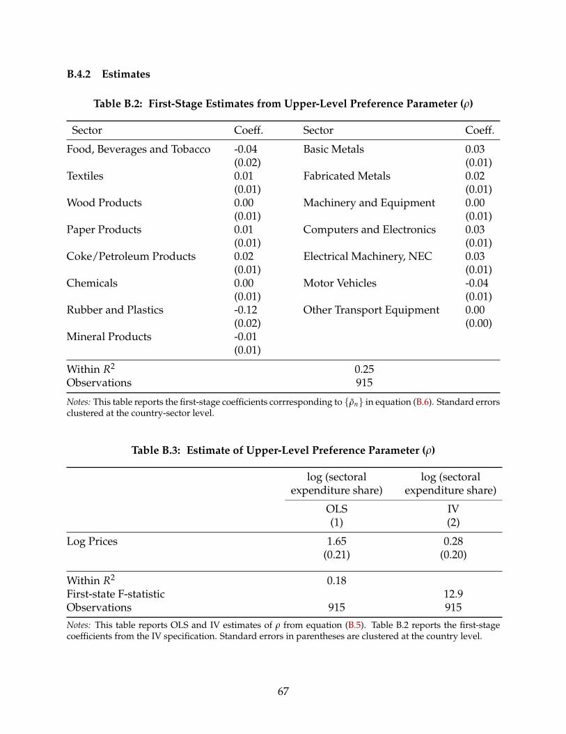
B.4.2 Estimates

Table B.2: First-Stage Estimates from Upper-Level Preference Parameter (ρ)

Sector Coeff. Sector Coeff.

Food, Beverages and Tobacco -0.04 Basic Metals 0.03(0.02) (0.01)

Textiles 0.01 Fabricated Metals 0.02(0.01) (0.01)

Wood Products 0.00 Machinery and Equipment 0.00(0.01) (0.01)

Paper Products 0.01 Computers and Electronics 0.03(0.01) (0.01)

Coke/Petroleum Products 0.02 Electrical Machinery, NEC 0.03(0.01) (0.01)

Chemicals 0.00 Motor Vehicles -0.04(0.01) (0.01)

Rubber and Plastics -0.12 Other Transport Equipment 0.00(0.02) (0.00)

Mineral Products -0.01(0.01)

Within R2 0.25Observations 915

Notes: This table reports the first-stage coefficients corrresponding to {ρn} in equation (B.6). Standard errorsclustered at the country-sector level.

Table B.3: Estimate of Upper-Level Preference Parameter (ρ)

log (sectoral log (sectoralexpenditure share) expenditure share)

OLS IV(1) (2)

Log Prices 1.65 0.28(0.21) (0.20)

Within R2 0.18First-state F-statistic 12.9Observations 915 915

Notes: This table reports OLS and IV estimates of ρ from equation (B.5). Table B.2 reports the first-stagecoefficients from the IV specification. Standard errors in parentheses are clustered at the country level.

67

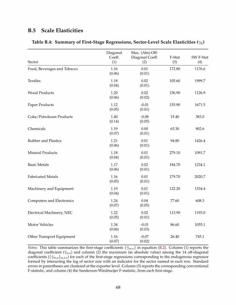
B.5 Scale Elasticities

Table B.4: Summary of First-Stage Regressions, Sector-Level Scale Elasticities (γk)

Diagonal Max. (Abs) Off-Coeff. Diagonal Coeff. F-Stat SW F-Stat

Sector (1) (2) (3) (4)

Food, Beverages and Tobacco 1.16 0.01 172.80 1176.6(0.06) (0.01)

Textiles 1.18 0.02 105.60 1999.7(0.04) (0.01)

Wood Products 1.20 0.02 156.90 1126.9(0.06) (0.02)

Paper Products 1.12 -0.01 155.90 1671.5(0.05) (0.01)

Coke/Petroleum Products 1.40 -0.08 15.40 383.0(0.14) (0.05)

Chemicals 1.19 0.00 63.30 902.6(0.07) (0.01)

Rubber and Plastics 1.21 0.01 94.80 1426.4(0.06) (0.01)

Mineral Products 1.18 0.01 279.10 1091.7(0.04) (0.01)

Basic Metals 1.17 0.02 184.70 1234.1(0.06) (0.01)

Fabricated Metals 1.16 0.01 179.70 2020.7(0.05) (0.01)

Machinery and Equipment 1.19 0.01 122.20 1334.4(0.04) (0.01)

Computers and Electronics 1.24 0.04 77.60 608.3(0.07) (0.05)

Electrical Machinery, NEC 1.22 0.02 113.90 1193.0(0.05) (0.01)

Motor Vehicles 1.34 -0.01 86.60 1055.1(0.06) (0.03)

Other Transport Equipment 1.16 -0.07 26.40 745.1(0.07) (0.02)

Notes: This table summarizes the first-stage coefficients {γm,n} in equation (B.2). Column (1) reports thediagonal coefficient (γn,n) and column (2) the maximum (in absolute value) among the 14 off-diagonalcoefficients ({γm,n}m 6=n) for each of the first-stage regressions corresponding to the endogenous regressorformed by interacting the log of sector size with an indicator for the sector named in each row. Standarderrors in parentheses are clustered at the exporter level. Column (3) reports the corresponding conventionalF-statistic, and column (4) the Sanderson-Windmeijer F-statistic, from each first-stage.

68

Table B.5: Estimates of Sector-Level Scale Elasticities (γk), Heterogeneity over Time

IV IV IV IV1995 2000 2005 All Years

Sector (1) (2) (3) (4)

Food, Beverages and Tobacco 0.17 0.18 0.20 0.19(0.02) (0.02) (0.02) (0.02)

Textiles 0.10 0.10 0.11 0.11(0.02) (0.02) (0.01) (0.01)

Wood Products 0.07 0.10 0.11 0.10(0.03) (0.03) (0.02) (0.02)

Paper Products 0.11 0.09 0.14 0.12(0.02) (0.02) (0.02) (0.01)

Coke/Petroleum Products 0.07 0.06 0.08 0.08(0.02) (0.01) (0.01) (0.01)

Chemicals 0.21 0.20 0.22 0.22(0.02) (0.02) (0.02) (0.02)

Rubber and Plastics 0.41 0.37 0.40 0.40(0.06) (0.06) (0.05) (0.05)

Mineral Products 0.13 0.14 0.16 0.15(0.02) (0.02) (0.02) (0.02)

Basic Metals 0.06 0.06 0.08 0.07(0.02) (0.01) (0.01) (0.01)

Fabricated Metals 0.08 0.08 0.10 0.10(0.02) (0.02) (0.02) (0.02)

Machinery and Equipment 0.20 0.19 0.21 0.21(0.03) (0.03) (0.02) (0.02)

Computers and Electronics 0.05 0.05 0.07 0.06(0.02) (0.01) (0.01) (0.01)

Electrical Machinery, NEC 0.06 0.05 0.07 0.06(0.02) (0.02) (0.02) (0.01)

Motor Vehicles 0.16 0.16 0.18 0.17(0.02) (0.02) (0.01) (0.01)

Other Transport Equipment 0.14 0.15 0.15 0.15(0.03) (0.02) (0.02) (0.02)

Observations 915 914 913 3,657

Notes: Columns (1)-(3) report the IV estimates of equation (25) when the sample is a single cross-sectionof countries and sectors from the indicated year; column (4) does the same for a sample that pools acrossall years. The instruments are the log of (country population × sectoral demand shifter), interacted withsector indicators. The regressions in columns (1)-(3) include exporter and sector fixed effects, while theregression in column (4) includes exporter-year and sector-year fixed effects. Standard errors in parenthesesare clustered at the exporter level.

69

-6-4

-20

24

-4 -2 0 2 4

(a) Food, Beverages and Tobacco

-50

5

-5 0 5

(b) Textiles

-50

5

-5 0 5

(c) Wood Products

-6-4

-20

24

-4 -2 0 2 4

(d) Paper Products

-10

-50

510

-4 -2 0 2 4

(e) Coke/Petroleum Products

-10

-50

5

-4 -2 0 2 4

(f) Chemicals

-10

-50

5

-4 -2 0 2 4

(g) Rubber and Plastics

-50

5

-4 -2 0 2 4

(h) Mineral Products

-10

-50

5

-5 0 5

(i) Basic Metals

-6-4

-20

24

-4 -2 0 2 4

(j) Fabricated Metals

-50

5

-4 -2 0 2 4

(k) Machinery and Equipment

-50

5

-4 -2 0 2 4

(l) Computers and Electronics

-50

5

-4 -2 0 2 4

(m) Electrical Machinery, NEC

-10

-50

5

-5 0 5

(n) Motor Vehicles

-50

5

-4 -2 0 2 4

(o) Other Transport Equipment

Figure B.1: First-Stage Fit, Scale Elasticity Estimation

Notes: Each sub-figure corresponds to a sector. To construct the figure for any given sector, n, we proceedas follows. Step 1: project the endogenous variable corresponding to sector n (an interaction between ln Li,kand an indicator for k = n) on all other regressors in equation (25), namely a country fixed effect, a sectorfixed effect, and the 14 other interactions between sector indicators and (log) sector size. Step 2: project theinstrument corresponding to sector n (an interaction between ln Li,k and an indicator for k = n) on the sameregressors as in the previous step. The figure for sector n then plots the residuals from step 1 on the y-axisagainst those from step 2 on the x-axis, for the I observations with k = n.

70

-1-.5

0.5

11.

5

-4 -2 0 2 4

(a) Food, Beverages and Tobacco

-1-.5

0.5

1

-5 0 5

(b) Textiles

-1-.5

0.5

-5 0 5

(c) Wood Products

-1-.5

0.5

1

-4 -2 0 2 4

(d) Paper Products

-1-.5

0.5

1

-4 -2 0 2 4

(e) Coke/Petroleum Products

-2-1

01

2

-4 -2 0 2 4

(f) Chemicals

-4-2

02

-4 -2 0 2 4

(g) Rubber and Plastics

-1-.5

0.5

1

-4 -2 0 2 4 6

(h) Mineral Products

-.50

.51

-5 0 5

(i) Basic Metals

-1-.5

0.5

1

-4 -2 0 2 4

(j) Fabricated Metals

-2-1

01

2

-5 0 5

(k) Machinery and Equipment

-.50

.5

-5 0 5

(l) Computers and Electronics

-.50

.5

-5 0 5

(m) Electrical Machinery, NEC

-1.5

-1-.5

0.5

1

-5 0 5

(n) Motor Vehicles

-1.5

-1-.5

0.5

1

-4 -2 0 2 4

(o) Other Transport Equipment

Figure B.2: Reduced-Form Fit, Scale Elasticity Estimation

Notes: Each sub-figure corresponds to a sector. To construct the figure for any given sector, n, we pro-ceed as follows. Step 1: project Yi,k on a country fixed effect, a sector fixed effect, and the 14 instruments(interactions between sector indicators and ln Li,k) defined for all sectors apart from n. Step 2: project thesector-n instrument (an interaction between ln Li,k and an indicator for k = n) on the same regressors as inthe previous step. The figure for sector n then plots the residuals from step 1 on the y-axis against thosefrom step 2 on the x-axis, but only for the I observations with k = n.

71

Table B.6: Estimates of Sector-Level Scale Elasticities (γk), Alternative IVs

Baseline ρ=-.9 ρ=0 ρ=2 Top 50% DistancesSector (1) (2) (3) (4) (5)

Food, Beverages and Tobacco 0.22 0.22 0.22 0.24 0.23(0.02) (0.02) (0.02) (0.04) (0.02)

Textiles 0.12 0.12 0.12 0.14 0.13(0.01) (0.01) (0.01) (0.03) (0.01)

Wood Products 0.13 0.13 0.13 0.14 0.13(0.02) (0.02) (0.02) (0.03) (0.03)

Paper Products 0.15 0.15 0.15 0.17 0.16(0.01) (0.01) (0.01) (0.03) (0.01)

Coke/Petroleum Products 0.09 0.08 0.09 0.10 0.10(0.01) (0.01) (0.01) (0.02) (0.01)

Chemicals 0.24 0.24 0.24 0.26 0.25(0.02) (0.02) (0.02) (0.03) (0.02)

Rubber and Plastics 0.42 0.41 0.41 0.45 0.44(0.04) (0.04) (0.04) (0.07) (0.04)

Mineral Products 0.17 0.16 0.17 0.19 0.18(0.01) (0.01) (0.01) (0.03) (0.01)

Basic Metals 0.09 0.09 0.09 0.11 0.10(0.01) (0.02) (0.01) (0.02) (0.01)

Fabricated Metals 0.12 0.11 0.12 0.14 0.13(0.02) (0.02) (0.02) (0.03) (0.02)

Machinery and Equipment 0.24 0.24 0.24 0.26 0.26(0.02) (0.02) (0.02) (0.03) (0.02)

Computers and Electronics 0.08 0.07 0.08 0.10 0.09(0.01) (0.02) (0.01) (0.03) (0.01)

Electrical Machinery, NEC 0.08 0.07 0.08 0.10 0.09(0.01) (0.02) (0.01) (0.02) (0.01)

Motor Vehicles 0.18 0.18 0.18 0.19 0.19(0.01) (0.01) (0.01) (0.02) (0.01)

Other Transport Equipment 0.18 0.17 0.18 0.20 0.19(0.02) (0.02) (0.02) (0.03) (0.02)

Notes: IV estimates of equation (25) for alternative values of the demand residuals βi,k entering demand-predicted sector size Li,k ≡ βi,k × Li. Column (1) repeats column (2) from Table 1 for purposes of compari-son. Columns (2)-(4) construct demand residuals βi,k using alternative values of the upper-level preferenceparameter ρ. Column (5) constructs demand residuals βi,k using alternative price proxies Pi,k, as describedin Section 4.4. All regressions include exporter and sector fixed effects. Standard errors in parentheses areclustered at the exporter level.

72

Table B.7: Estimates of Sector-Level Scale Elasticities (γk), Additional Controls

Sector (1) (2) (3)

Food, Beverages and Tobacco 0.22 0.23 0.23(0.02) (0.03) (0.03)

Textiles 0.12 0.10 0.09(0.01) (0.02) (0.01)

Wood Products 0.13 0.13 0.13(0.02) (0.02) (0.02)

Paper Products 0.15 0.16 0.16(0.01) (0.03) (0.02)

Coke/Petroleum Products 0.09 0.07 0.07(0.01) (0.02) (0.02)

Chemicals 0.24 0.27 0.28(0.02) (0.02) (0.02)

Rubber and Plastics 0.42 0.53 0.55(0.04) (0.02) (0.04)

Mineral Products 0.17 0.19 0.20(0.01) (0.03) (0.01)

Basic Metals 0.09 0.07 0.06(0.01) (0.02) (0.01)

Fabricated Metals 0.12 0.12 0.12(0.02) (0.02) (0.01)

Machinery and Equipment 0.24 0.26 0.27(0.02) (0.02) (0.01)

Computers and Electronics 0.08 0.06 0.06(0.01) (0.02) (0.02)

Electrical Machinery, NEC 0.08 0.06 0.05(0.01) (0.02) (0.01)

Motor Vehicles 0.18 0.19 0.19(0.01) (0.02) (0.01)

Other Transport Equipment 0.18 0.19 0.19(0.02) (0.02) (0.02)

(Contract enforcement)×(sector fixed-effects) X X(Financial development)×(sector fixed-effects) X X(GDP per capita)×(sector fixed-effects) X

Notes: IV estimates of equation (25). All regressions include exporter and sector fixed effects. Column (1)repeats column (2) from Table 1 for purposes of comparison. Standard errors in parentheses are clusteredat the exporter level. The number of observations for column (1) is 915 and for columns (2) and (3) it is 735.

73

B.5.1 Beyond Ricardian Economies

Like in Appendix C.5, we assume that production functions take the nested CES form as in equa-

tions (38) and (39). Maintaining our other parametric restrictions described in equations (22)-(24),

this leads to the following generalization of equation (25),

YIOi,k = δi + δk + γk ln Zi,k + ε i,k, (B.7)

where the left-hand side variable now also controls for differences in input costs across sectors,

YIOi,k ≡

1J ∑

j(ln Xij,k/θk) + (1− ak)bk ln(ri/wi) + ∑

sbsk ln(Pi,s/wi). (B.8)

To measure YIOi,k and Zi,k, we first draw on trade and national accounts data in order to obtain

{ak, bk, bsk, ri, wi}. We use the OECD’s ICIO tables to compute bsk as the share of total input costs of

firms from sector k spent on intermediate goods from sector s. This also gives us the value added

share bk = 1− ∑s bsk. Unfortunately, this dataset does not report labor shares of value added ak,

so we obtain those from the World Input Output Database (after creating an industry concordance

with our dataset) by computing the ratio of total labor spending by firms from sector k to total

value added by those firms.46 We next compute factor prices wi and ri by using the formulas

wi = (∑k akbkSi,k)/Li and ri = (∑k(1− ak)bkSi,k)/Ki, with Li and Ki as in the Penn World Tables

9.0 (the variables “POP” and “CK”, respectively), and with Si,k ≡ ∑j Xij,k representing total sales

by country i in sector k.

In order to measure YIOi,k and Zi,k, we also need proxies of price indices in both traded sectors,

k ∈ T , and non-traded sectors, k ∈ N . For traded sectors, we use the same approach as in Section

4.2 and use as our proxy for ln Pi,k,

ln Pi,k ≡1J ∑

jln(Xji,k/Xi,k)/θk, for all k ∈ T . (B.9)

For non-traded sectors k ∈ N , we turn to the zero-profit conditions,

ln Pi,k = akbk ln wi + (1− ak)bk ln ri + ∑s

bsk ln Pi,s + ϕi,k, for all k ∈ N ,

with ϕi,k ≡ −[ln Aii,k + akbk ln ak + (1− ak)bk ln(1− ak) + bk ln bk + ∑s bsk ln bsk], where we have

invoked our baseline assumption of no scale economies in non-manufacturing sectors, which in-

clude all non-tradable sectors. The vector of non-tradable prices, ln PNi ≡ {ln Pi,k}k∈N , that solves

46We use data from 2005-2007, since there are minor discrepancies between total value added and thesum of labor and capital compensation in the data for later years. Results are not sensitive to this choice.

74

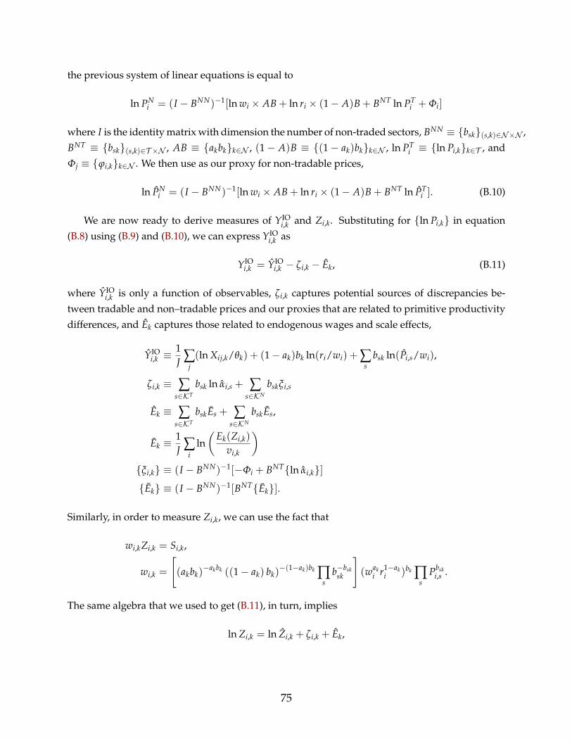
the previous system of linear equations is equal to

ln PNi = (I − BNN)−1[ln wi × AB + ln ri × (1− A)B + BNT ln PT

i + Φi]

where I is the identity matrix with dimension the number of non-traded sectors, BNN ≡ {bsk}(s,k)∈N×N ,

BNT ≡ {bsk}(s,k)∈T ×N , AB ≡ {akbk}k∈N , (1− A)B ≡ {(1− ak)bk}k∈N , ln PTi ≡ {ln Pi,k}k∈T , and

Φj ≡ {ϕi,k}k∈N . We then use as our proxy for non-tradable prices,

ln PNi = (I − BNN)−1[ln wi × AB + ln ri × (1− A)B + BNT ln PT

i ]. (B.10)

We are now ready to derive measures of YIOi,k and Zi,k. Substituting for {ln Pi,k} in equation

(B.8) using (B.9) and (B.10), we can express YIOi,k as

YIOi,k = YIO

i,k − ζi,k − Ek, (B.11)

where YIOi,k is only a function of observables, ζi,k captures potential sources of discrepancies be-

tween tradable and non–tradable prices and our proxies that are related to primitive productivity

differences, and Ek captures those related to endogenous wages and scale effects,

YIOi,k ≡

1J ∑

j(ln Xij,k/θk) + (1− ak)bk ln(ri/wi) + ∑

sbsk ln(Pi,s/wi),

ζi,k ≡ ∑s∈KT

bsk ln αi,s + ∑s∈KN

bskξi,s

Ek ≡ ∑s∈KT

bskEs + ∑s∈KN

bskEs,

Ek ≡1J ∑

iln(

Ek(Zi,k)

vi,k

){ξi,k} ≡ (I − BNN)−1[−Φi + BNT{ln αi,k}]

{Ek} ≡ (I − BNN)−1[BNT{Ek}].

Similarly, in order to measure Zi,k, we can use the fact that

wi,kZi,k = Si,k,

wi,k =

[(akbk)

−akbk ((1− ak) bk)−(1−ak)bk ∏

sb−bsk

sk

](wak

i r1−aki )bk ∏

sPbsk

i,s .

The same algebra that we used to get (B.11), in turn, implies

ln Zi,k = ln Zi,k + ζi,k + Ek,

75

with

ln Zi,k ≡ ln(Si,k/wi)− (1− ak)bk ln(ri/wi)−∑s

bsk ln(Pi,s/wi)− ln

[(akbk)


sb−bsk

sk

].

Combining (B.7) and (B.11), we obtain

YIOi,k = δi + δk + γk ln Zi,k + ε i,k (B.12)

with

ε i,k ≡ε i,k + (γk + 1)ζi,k −E[(γk + 1)ζi,k|i]−E[(γk + 1)ζi,k|k] + E[(γk + 1)ζi,k],

δi ≡δi + E[(γk + 1)ζi,k|i]−E[(γk + 1)ζi,k],

δk ≡δk + E[(γk + 1)ζi,k|k] + (γk + 1)Ek.

Our estimation of γk then proceeds via the instrumental variable procedure described in Sec-

tion 3.3. The only difference comes from the way we estimate the demand parameters βi,k to

construct demand-predicted sector size Li,k ≡ βi,k × Li. Rather than using (26), which depends on

the share xi,k of expenditure by country i on goods from sector k across all origins, we use

βi,k =xF

i,k/(Pi,k)−ρ

∑l xFi,l/(Pi,l)−ρ

,

which only depends on the share xFi,k of final expenditure by country i on goods from sector k

across all origins. The exclusion restriction then continues to be given by

E[ln Li,k × ε i,k|k] = 0, for all k,

with the error term ε i,k in (B.12) now comprising the productivity of country i in both sector k and

in other sectors (via the IO linkages due to non-tradable sectors that gives rise to ζi,k).

OLS and IV estimates of the scale elasticity parameters γk from equation (B.7) are reported in

Table B.8.

76

Table B.8: Estimates of Sector-Level Scale Elasticities (γk), Beyond RicardianEconomies

First-stage SWOLS IV F-stat F-stat

Sector (1) (2) (3) (4)

Food, Beverages and Tobacco 0.23 0.17 34.6 214.3(0.01) (0.03)

Textiles 0.10 0.07 75.4 273.1(0.01) (0.02)

Wood Products 0.11 0.09 14.0 132.0(0.02) (0.02)

Paper Products 0.15 0.09 23.7 653.5(0.01) (0.03)

Coke/Petroleum Products 0.07 0.07 13.6 215.4(0.02) (0.02)

Chemicals 0.27 0.20 27.3 244.1(0.01) (0.02)

Rubber and Plastics 0.48 0.38 26.6 354.6(0.03) (0.04)

Mineral Products 0.16 0.12 15.4 314.4(0.02) (0.02)

Basic Metals 0.08 0.06 14.3 177.4(0.01) (0.03)

Fabricated Metals 0.11 0.07 35.6 299.1(0.02) (0.02)

Machinery and Equipment 0.28 0.19 23.8 286.9(0.02) (0.02)

Computers and Electronics 0.06 0.04 21.5 197.1(0.01) (0.02)

Electrical Machinery, NEC 0.06 0.04 38.3 521.2(0.01) (0.02)

Motor Vehicles 0.18 0.14 34.2 372.5(0.01) (0.02)

Other Transport Equipment 0.18 0.14 20.7 0.0(0.02) (0.03)

Notes: Column (1) reports the OLS estimate, and column (2) the IV estimate, of equation (B.7). The in-struments are the log of (country population × sectoral demand shifter), interacted with sector indicators.Column (3) reports the conventional F-statistic, and column (4) the Sanderson-Windmeijer F-statistic, fromthe first-stage regression corresponding to the endogenous regressor formed by interacting the log of sectorsize with an indicator for the sector named in each row. All regressions include exporter and sector fixedeffects. Standard errors in parentheses are clustered at the exporter level.

77

C Online Appendix: Counterfactuals

C.1 Construction of Counterfactual Equilibria

We first describe a competitive equilibrium as the solution to a system of non-linear equations. We

then show how to use this system to conduct counterfactual and welfare analysis.

Competitive Equilibrium with Taxes and Subsidies. Starting from (1)-(9), we can de-

scribe a competitive equilibrium with employment subsidies, {sj,k}, import tariffs, {tmij,k}, export

taxes, {txij,k}, as a set of sector sizes, {Li,k}, within-sector expenditure shares, {xij,k ≡ Xij,k/Xj,k},

between-sector expenditure shares, {xj,k ≡ Xj,k/ ∑l∈K Xj,l}, consumer prices, {pij,k}, price indices,

{Pj,k}, wages, {wj}, and lump-sum transfers, {Tj}, such that

wiLi,k =1

(1− si,k)∑

j

1− txij,k

1 + tmij,k

xij,kxj,k(wjLj + Tj + Dj),

xij,k =p−θk

ij,k

∑i′ p−θki′ j,k

,

xj,k =β j,kP−ρ

j,k

∑k′ β j,k′P−ρj,k′

,

pij,k =(1 + tm

ij,k)(1− si,k)wi

(1− txij,k)Aij,kLγk

i,k,

Pj,k = (∑i

p−θkij,k )

−1/θk ,

Li = ∑k

Li,k,

Tj = ∑i,k

tmij,k

1 + tmij,k

xij,kxj,k(wjLj + Tj + Dj) + ∑i,k

[tx

ji,k −sj,k(1− tx

ji,k)

1− sj,k

]xji,k

1 + tmji,k

xi,k(wiLi + Ti + Di),

where Dj denotes the trade deficit of country j, with ∑j Dj = 0, and where we use the convention

tmii,k = tx

ii,k = 0 for all i and k.

Counterfactual Changes. Suppose that the initial equilibrium has no taxes or subsidies. We

are interested in a counterfactual equilibrium with taxes, subsidies, and transfers:

txij,k, tm

ij,k, si,k, Tj 6= 0 for some i, j, k.

For any endogenous variable with value x in the initial equilibrium and x′ in the counterfactual

equilibrium, we let x = x′/x denote the proportional change in this variable. We assume that Djs

are fixed and do not change as we move to the counterfactual equilibrium. After simplifications,

78

counterfactual changes are given by the solution to

wi Li,kSi,k =1

(1− si,k)∑

j

(1− txij,k)xij,k

1 + tmij,k

xj,k

(wjSj + Tj + Dj

Sj + Dj

)Xij,k, (C.1)

xij,k =p−θk

ij,k

∑i′ p−θki′ j,k xi′ j,k

, (C.2)

xj,k =P−ρ

j,k

∑k′ P−ρj,k′ xj,k′

, (C.3)

pij,k =(1 + tm

ij,k)(1− si,k)wi

(1− txij,k)Lγk

i,k, (C.4)

Pj,k = (∑i

p−θkij,k xij,k)

−1/θk , (C.5)

Si = ∑k

Li,kSi,k, (C.6)

Tj =∑i,k

tmij,k xij,k xj,k

1 + tmij,k

(wjSj + Tj + Dj

Sj + Dj

)Xij,k

+ ∑i,k

[tx


ji,k)

1− sj,k

]xji,k xi,k

1 + tmji,k

(wiSi + Ti + Di

Si + Di

)Xji,k, (C.7)

where bilateral trade flows Xij,k, sectoral sales, Si,k ≡ ∑j Xij,k, and total sales Si = ∑j,k Xij,k are all

observed in the initial equilibrium. Once changes in the previous variables have been computed

using (C.1)-(C.7), welfare changes are given by

Uj =wjSj + Tj + Dj

Sj + Dj

1Pj

,

Pj = (∑k

P−ρj,k xj,k)

−1/ρ.

Under the assumption that country i0 is small and that only country i0 imposes trade taxes and

employment subsidies, the system is as described above for country i0; that is, equations (C.1)-

(C.7) continue to hold if either i or j is equal to i0. For all other countries, we set wi = Pi,k = Li,k = 1

for all k and drop equations (C.1)-(C.7).47

47Since foreign wages are unaffected by changes in country i0’s policies, our assumption that Djs arefixed is equivalent to assuming that Djs are constant fractions of foreign GDP.

79

C.2 Gains from Optimal Policies

Table C.1: Gains from Optimal Policies


Argentina 1.14% 0.88% 0.93%Australia 0.96% 0.54% 0.56%Austria 1.23% 1.92% 1.07%Belgium 1.33% 1.41% 0.99%Brazil 0.89% 0.41% 0.72%Brunei Darussalam 2.41% 0.91% 0.96%Bulgaria 1.41% 1.77% 1.09%Cambodia 1.87% 0.77% 0.88%Canada 1.01% 1.31% 0.87%Chile 1.32% 0.83% 0.87%China 0.97% 0.43% 0.83%Hong Kong 1.46% 1.12% 0.63%Colombia 1.14% 0.44% 0.78%Costa Rica 1.58% 0.88% 0.99%Croatia 1.46% 0.79% 0.85%Cyprus 1.95% 0.91% 0.93%Czech Republic 1.26% 2.59% 1.27%Denmark 1.33% 1.78% 0.99%Estonia 1.57% 2.12% 1.11%Finland 1.00% 1.68% 0.91%France 0.97% 1.13% 0.83%Germany 1.16% 1.84% 1.10%Greece 1.12% 0.82% 0.72%Hungary 1.37% 3.51% 1.37%Iceland 1.24% 1.95% 0.99%India 1.07% 0.56% 0.74%Indonesia 1.28% 0.65% 0.89%Ireland 1.86% 3.96% 1.77%Israel 1.12% 1.66% 0.88%Italy 0.94% 1.20% 0.85%Japan 0.79% 0.56% 0.70%Latvia 1.15% 1.21% 0.86%

80

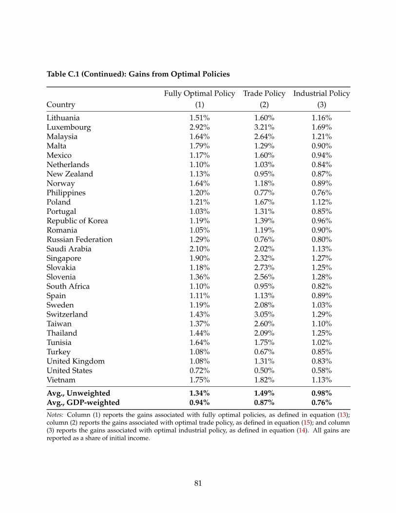
Table C.1 (Continued): Gains from Optimal Policies


Lithuania 1.51% 1.60% 1.16%Luxembourg 2.92% 3.21% 1.69%Malaysia 1.64% 2.64% 1.21%Malta 1.79% 1.29% 0.90%Mexico 1.17% 1.60% 0.94%Netherlands 1.10% 1.03% 0.84%New Zealand 1.13% 0.95% 0.87%Norway 1.64% 1.18% 0.89%Philippines 1.20% 0.77% 0.76%Poland 1.21% 1.67% 1.12%Portugal 1.03% 1.31% 0.85%Republic of Korea 1.19% 1.39% 0.96%Romania 1.05% 1.19% 0.90%Russian Federation 1.29% 0.76% 0.80%Saudi Arabia 2.10% 2.02% 1.13%Singapore 1.90% 2.32% 1.27%Slovakia 1.18% 2.73% 1.25%Slovenia 1.36% 2.56% 1.28%South Africa 1.10% 0.95% 0.82%Spain 1.11% 1.13% 0.89%Sweden 1.19% 2.08% 1.03%Switzerland 1.43% 3.05% 1.29%Taiwan 1.37% 2.60% 1.10%Thailand 1.44% 2.09% 1.25%Tunisia 1.64% 1.75% 1.02%Turkey 1.08% 0.67% 0.85%United Kingdom 1.08% 1.31% 0.83%United States 0.72% 0.50% 0.58%Vietnam 1.75% 1.82% 1.13%


81

C.3 Gains from Constrained and Globally Efficient Industrial Policies

Table C.2: Gains from Constrained and Globally Efficient Industrial Policies


Country (1) (2) (3)

Argentina 0.93% 0.65% 0.24%Australia 0.56% 0.59% 0.75%Austria 1.07% 0.54% 0.00%Belgium 0.99% 0.62% 0.00%Brazil 0.72% 0.57% 0.59%Brunei Darussalam 0.96% 1.98% 1.11%Bulgaria 1.09% 0.65% 0.83%Cambodia 0.88% 1.20% 1.79%Canada 0.87% 0.48% 0.69%Chile 0.87% 0.79% 0.61%China 0.83% 0.65% 0.46%Hong Kong 0.63% 1.01% 0.76%Colombia 0.78% 0.78% 1.27%Costa Rica 0.99% 0.89% 1.63%Croatia 0.85% 0.95% 1.27%Cyprus 0.93% 1.40% 2.64%Czech Republic 1.27% 0.47% -0.25%Denmark 0.99% 0.70% -0.18%Estonia 1.11% 0.77% 0.76%Finland 0.91% 0.42% -0.27%France 0.83% 0.47% 0.49%Germany 1.10% 0.48% -0.47%Greece 0.72% 0.66% 1.31%Hungary 1.37% 0.49% -0.37%Iceland 0.99% 0.61% -0.22%India 0.74% 0.66% 0.64%Indonesia 0.89% 0.79% 0.77%Ireland 1.77% 1.01% -2.13%Israel 0.88% 0.56% 0.15%Italy 0.85% 0.42% 0.20%Japan 0.70% 0.50% 0.14%Latvia 0.86% 0.58% 1.20%

82

Table C.2 (Continued): Gains from Constrained and Globally Efficient IndustrialPolicies


Country (1) (2) (3)

Lithuania 1.16% 0.77% 0.78%Luxembourg 1.69% 1.72% 0.66%Malaysia 1.21% 0.75% -0.35%Malta 0.90% 1.02% 1.15%Mexico 0.94% 0.65% 1.16%Netherlands 0.84% 0.54% -0.28%New Zealand 0.87% 0.61% 0.28%Norway 0.89% 1.02% 0.68%Philippines 0.76% 0.66% 0.63%Poland 1.12% 0.54% 0.51%Portugal 0.85% 0.48% 0.88%Republic of Korea 0.96% 0.56% -0.23%Romania 0.90% 0.54% 0.95%Russian Federation 0.80% 0.90% 0.74%Saudi Arabia 1.13% 1.59% 0.86%Singapore 1.27% 0.98% -1.11%Slovakia 1.25% 0.38% 0.13%Slovenia 1.28% 0.56% 0.13%South Africa 0.82% 0.63% 0.77%Spain 0.89% 0.55% 0.51%Sweden 1.03% 0.49% -0.33%Switzerland 1.29% 0.73% -0.31%Taiwan 1.10% 0.52% -0.07%Thailand 1.25% 0.60% -0.50%Tunisia 1.02% 0.91% 1.58%Turkey 0.85% 0.65% 0.98%United Kingdom 0.83% 0.56% 0.66%United States 0.58% 0.41% 0.55%Vietnam 1.13% 1.00% 1.87%

Avg., Unweighted 0.98% 0.73% 0.49%Avg., GDP-Weighted 0.76% 0.53% 0.35%Notes: Each column reports the gains, expressed as a share of initial income, that could be achieved by eachtype of policy. See the text for detailed descriptions of the exercises.

83

C.4 Sensitivity to Calibrated Parameters

Table C.3: Gains from Industrial Policy, Alternative Trade Elasticities (θk)

Baseline CP Shapiro GYYCountry (1) (2) (3) (4)

United States 0.58% 2.46% 0.76% 0.63%China 0.83% 2.96% 1.09% 0.79%Germany 1.10% 5.09% 0.38% 1.11%Ireland 1.78% 3.54% 2.61% 2.25%Vietnam 1.13% 5.35% 1.60% 1.22%

Avg., Unweighted 0.98% 3.28% 1.13% 1.14%Avg., GDP-Weighted 0.76% 2.92% 0.80% 0.84%Corr. with Baseline - 0.38 0.71 0.85Notes: Each column reports the gains from industrial policy, as defined in equation and (14), for the cor-responding trade elasticity estimates reported in Table B.3. Column (1) replicates the baseline calculation,which uses the median trade elasticity in each sector across the studies in columns (2)-(4). Columns (2)-(4)reports a similar calculation using trade elasticity estimates from each of these studies (Caliendo and Parro,2015; Shapiro, 2016; and Giri et al., 2021) individually. The last row reports the correlation, across countries,of the gains from industrial policy with those in column (1).

84

C.5 Beyond Ricardian Economies

C.5.1 Construction of Counterfactuals

Competitive Equilibrium with Taxes and Subsidies. Starting from equations (2), (3), (6),

(36), (37), and (A.46)-(A.52), we can describe a competitive equilibrium with production subsidies,

{sj,k}, import tariffs, {tmij,k}, and export taxes, {tx

ij,k}, as a set of sector sizes, {Li,k, Ki,k, Zi,k}, within-

sector expenditure shares, {xij,k}, between-sector final expenditure shares, {xFj,k}, between-sector

expenditures, {Xj,k}, consumer prices, {pij,k}, sector price indices, {Pj,k}, wages, {wj}, rental rates,

{rj}, and lump-sum transfers, {Tj}, such that

wi,kZi,k =1

(1− si,k)∑

j

1− txij,k

1 + tmij,k

xij,kXj,k,

wiLi,k = akbkwi,kZi,k

riKi,k = (1− ak)bkwi,kZi,k

xij,k =p−θk

ij,k

∑i′ p−θki′ j,k

,

xFj,k =

β j,kP−ρj,k

∑k′ β j,k′P−ρj,k′

,

Xj,k = xFj,k(wjLj + rjKj + Tj + Dj

)+ ∑

i,sbks

1− txji,s

1 + tmji,s

xji,sXi,s,

pij,k =(1 + tm

ij,k)(1− si,k)wi,k

(1− txij,k)Aij,kZγk

i,k,

Pj,k = (∑i

p−θkij,k )

−1/θk ,

wi,k =

[(akbk)


sb−bsk

sk

](wak

i r1−aki )bk ∏

sPbsk

i,s ,

Li = ∑k

Li,k,

Ki = ∑k

Ki,k,

Tj = ∑i,k

tmij,k

1 + tmij,k

xij,kXj,k + ∑i,k

[tx


ji,k)

1− sj,k

]xji,kXi,k.

Counterfactual Changes. The counterfactual changes associated with moving from laissez-

faire to a counterfactual equilibrium with employment subsidies, export taxes, and import tariffs

85

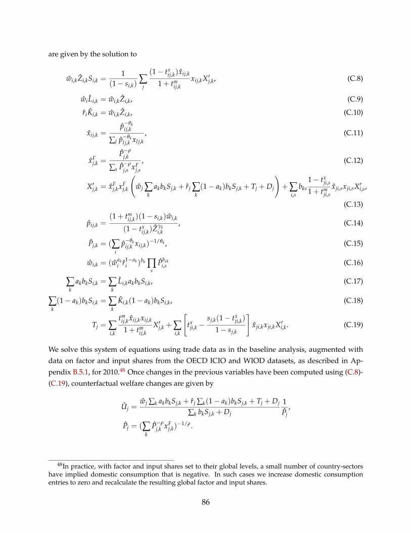
are given by the solution to

wi,kZi,kSi,k =1

(1− si,k)∑

j

(1− txij,k)xij,k

1 + tmij,k

xij,kX′j,k, (C.8)

wi Li,k = wi,kZi,k, (C.9)

riKi,k = wi,kZi,k, (C.10)

xij,k =p−θk

ij,k

∑l p−θkl j,k xl j,k

, (C.11)

xFj,k =

P−ρj,k

∑s P−ρj,s xF

j,s

, (C.12)

X′j,k = xFj,kxF

j,k

(wj ∑

kakbkSj,k + rj ∑

k(1− ak)bkSj,k + Tj + Dj

)+ ∑

i,sbks

1− txji,s

1 + tmji,s

xji,sxji,sX′i,s,

(C.13)

pij,k =(1 + tm

ij,k)(1− si,k)wi,k

(1− txij,k)Zγk

i,k, (C.14)

Pj,k = (∑i

p−θkij,k xij,k)

−1/θk , (C.15)

wi,k = (waki r1−ak

i )bk ∏s

Pbski,s (C.16)

∑k

akbkSi,k = ∑k

Li,kakbkSi,k, (C.17)

∑k(1− ak)bkSi,k = ∑

kKi,k(1− ak)bkSi,k, (C.18)

Tj = ∑i,k

tmij,k xij,kxij,k

1 + tmij,k

X′j,k + ∑i,k

[tx


ji,k)

1− sj,k

]xji,kxji,kX′i,k. (C.19)

We solve this system of equations using trade data as in the baseline analysis, augmented with

data on factor and input shares from the OECD ICIO and WIOD datasets, as described in Ap-

pendix B.5.1, for 2010.48 Once changes in the previous variables have been computed using (C.8)-

(C.19), counterfactual welfare changes are given by

Uj =wj ∑k akbkSj,k + rj ∑k(1− ak)bkSj,k + Tj + Dj

∑k bkSj,k + Dj

1Pj

,

Pj = (∑k

P−ρj,k xF

j,k)−1/ρ.

48In practice, with factor and input shares set to their global levels, a small number of country-sectorshave implied domestic consumption that is negative. In such cases we increase domestic consumptionentries to zero and recalculate the resulting global factor and input shares.

86

Under the assumption that country i0 is small and that only country i0 imposes trade taxes and

employment subsidies, we follow the same procedure as in Appendix C.1 and impose wi = ri =

Pi,k = Li,k = Ki,k = 1 for all k and i 6= i0.

87

C.5.2 Gains from Optimal Policies

Table C.4: Gains from Optimal Policies, Beyond Ricardian Economies


Argentina 3.33% 5.23% 3.39%Australia 2.35% 1.22% 1.83%Austria 2.97% 12.92% 3.53%Belgium 3.44% 10.09% 3.59%Brazil 2.65% 1.15% 2.50%Brunei Darussalam 4.43% 1.40% 2.43%Bulgaria 2.62% 9.54% 2.67%Cambodia 3.96% 1.97% 2.81%Canada 2.30% 8.62% 2.55%Chile 3.11% 2.52% 2.89%China 3.48% 1.44% 3.44%Hong Kong 2.81% 1.99% 1.69%Colombia 2.71% 1.63% 2.27%Costa Rica 3.07% 2.35% 2.60%Croatia 3.01% 2.71% 2.43%Cyprus 2.88% 2.22% 1.67%Czech Republic 3.28% 16.99% 4.61%Denmark 3.04% 7.28% 3.01%Estonia 2.85% 13.33% 2.56%Finland 2.44% 7.10% 2.90%France 2.29% 5.52% 2.67%Germany 3.44% 10.73% 4.59%Greece 1.92% 2.81% 1.59%Hungary 3.20% 21.62% 4.31%Iceland 2.85% 3.29% 2.66%India 2.86% 1.98% 2.63%Indonesia 3.30% 2.10% 2.83%Ireland 4.40% 17.84% 5.28%Israel 2.37% 7.85% 2.69%Italy 2.30% 6.44% 2.78%Japan 2.47% 2.58% 2.82%Latvia 2.07% 4.02% 1.87%

88

Table C.4 (Continued): Gains from Optimal Policies, Beyond Ricardian Economies


Lithuania 3.38% 8.31% 3.46%Luxembourg 4.81% 43.29% 3.36%Malaysia 4.49% 17.47% 4.94%Malta 3.95% 3.90% 2.64%Mexico 2.75% 8.28% 2.80%Netherlands 2.93% 5.24% 2.85%New Zealand 2.51% 2.36% 2.37%Norway 3.84% 4.04% 3.09%Philippines 3.17% 5.65% 2.90%Poland 2.92% 11.73% 3.55%Portugal 2.03% 9.36% 2.19%Republic of Korea 4.04% 8.93% 4.82%Romania 2.30% 7.77% 2.63%Russian Federation 3.24% 2.25% 2.66%Saudi Arabia 3.77% 8.44% 3.09%Singapore 5.48% 10.00% 5.26%Slovakia 2.69% 17.00% 3.73%Slovenia 2.99% 17.77% 3.86%South Africa 2.64% 5.42% 2.62%Spain 2.72% 8.45% 3.05%Sweden 3.34% 11.71% 4.04%Switzerland 3.12% 11.78% 3.55%Taiwan 3.98% 11.35% 4.54%Thailand 4.11% 14.91% 5.31%Tunisia 3.67% 7.10% 3.34%Turkey 3.02% 3.50% 3.06%United Kingdom 2.39% 7.07% 2.48%United States 1.82% 1.92% 1.86%Vietnam 3.74% 5.29% 3.34%


89

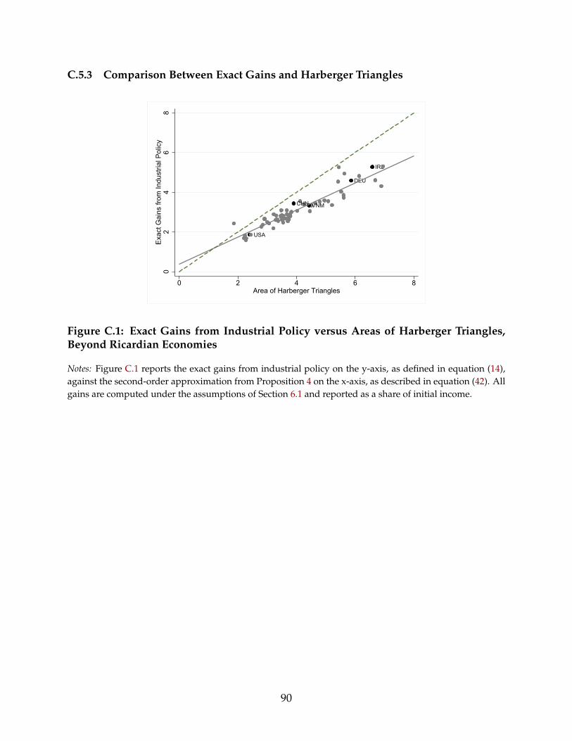
C.5.3 Comparison Between Exact Gains and Harberger Triangles

CHN

DEU

IRL

USA

VNM

02

46

8Ex

act G

ains

from

Indu

stria

l Pol

icy

0 2 4 6 8Area of Harberger Triangles

Figure C.1: Exact Gains from Industrial Policy versus Areas of Harberger Triangles,Beyond Ricardian Economies

Notes: Figure C.1 reports the exact gains from industrial policy on the y-axis, as defined in equation (14),against the second-order approximation from Proposition 4 on the x-axis, as described in equation (42). Allgains are computed under the assumptions of Section 6.1 and reported as a share of initial income.

90

C.5.4 Sensitivity to Calibrated Parameters

2.8

33.

23.

43.

63.

8G

ains

from

Indu

stria

l Pol

icy

0 .05 .1 .15Scale economies in non - manufacturing (γNM)

(a) Scale Elasticity Outside Manufacturing

2.8

33.

23.

4G

ains

from

Indu

stria

l Pol

icy

.8 1 1.2 1.4 1.6Elasticity of substitution between sectors ( 1 + ρ)

(b) Elasticity of Substitution Between Sectors

Figure C.2: Gains from Industrial Policy, Alternative Parameter Values, Beyond Ricar-dian Economies

Notes: Figure C.2a reports the gains from industrial policy, as defined in equation (14), , computed under theassumptions of Section 6.1 for different values of the scale elasticity outside manufacturing, γNM. FigureC.2b does the same for different values of the elasticity of substitution between sectors, 1 + ρ.

91

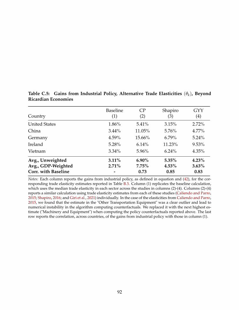
Table C.5: Gains from Industrial Policy, Alternative Trade Elasticities (θk), BeyondRicardian Economies

Baseline CP Shapiro GYYCountry (1) (2) (3) (4)

United States 1.86% 5.41% 3.15% 2.72%China 3.44% 11.05% 5.76% 4.77%Germany 4.59% 15.66% 6.79% 5.24%Ireland 5.28% 6.14% 11.23% 9.53%Vietnam 3.34% 5.96% 6.24% 4.35%

Avg., Unweighted 3.11% 6.90% 5.35% 4.23%Avg., GDP-Weighted 2.71% 7.75% 4.53% 3.63%Corr. with Baseline - 0.73 0.85 0.83Notes: Each column reports the gains from industrial policy, as defined in equation and (42), for the cor-responding trade elasticity estimates reported in Table B.3. Column (1) replicates the baseline calculation,which uses the median trade elasticity in each sector across the studies in columns (2)-(4). Columns (2)-(4)reports a similar calculation using trade elasticity estimates from each of these studies (Caliendo and Parro,2015; Shapiro, 2016; and Giri et al., 2021) individually. In the case of the elasticities from Caliendo and Parro,2015, we found that the estimate in the "Other Transportation Equipment" was a clear outlier and lead tonumerical instability in the algorithm computing counterfactuals. We replaced it with the next highest es-timate ("Machinery and Equipment") when computing the policy counterfactuals reported above. The lastrow reports the correlation, across countries, of the gains from industrial policy with those in column (1).

92

Documents

The Textbook Case for Industrial Policy ... - Dave Donaldson