The Role of GPS Precipitable Water Vapor and Atmosphere Stability Indexin the Statistically Based Rainfall Estimation Using MTSAT Data

DWI PRABOWO YUGA SUSENO AND TOMOHITO J. YAMADA

Faculty of Engineering, Hokkaido University, Hokkaido, Japan

(Manuscript received 27 August 2012, in final form 25 July 2013)

ABSTRACT

A rainfall estimation method was developed based on the statistical relationships between cloud-top

temperature and rainfall rates acquired by both the 10.8-mm channel of the Multi-Functional Transport

Satellite (MTSAT) series and the Automated Meteorological Data Acquisition System (AMeDAS) C-band

radar, respectively. The method focused on cumulonimbus (Cb) clouds and was developed in the period of

June–September 2010 and 2011 over the landmass of Japan and its surrounding area. Total precipitable water

vapor (PWV) and atmospheric vertical instability were considered to represent the atmospheric environ-

mental conditions during the development of statistical models. Validations were performed by comparing

the estimated values with the observed rainfall derived from the AMeDAS rain gauge network and the

Tropical Rainfall Measuring Mission (TRMM) 3B42 rainfall estimation product. The results demonstrated

that the models that considered the combination of total PWV and atmospheric vertical instability were

relatively more sensitive to heavy rainfall than were the models that considered no atmospheric environ-

mental conditions. The use of such combined information indicated a reasonable improvement, especially in

terms of the correlation between estimated and observed rainfall. Intercomparison results with the TRMM

3B42 confirmed that MTSAT-based rainfall estimations made by considering atmospheric environmental

conditions were more accurate for estimating rainfall generated by Cb cloud.

1. Introduction

Geostationary satellites make frequent observations

with continuous spatial coverage, providing useful in-

formation for rainfall monitoring and the early warning

of storms (Feidas and Cartalis 2001;Wardah et al. 2008).

Thermal infrared data (TIR) centered at 10.8mm are

commonly used to detect cloud-top temperature for use

in rainfall estimation (Haile et al. 2010). Lower tem-

peratures are assumed to correspond to relatively cold

and thick clouds, which tend to produce high rainfall

intensity (Kuligowski 2003). However, clouds are es-

sentially opaque to TIR, which cannot reveal the vertical

profile of clouds that produce rainfall. To complement

TIR data, microwave (MW)-based rainfall estimations

are used, as MW radiation has the ability to penetrate

clouds, thus allowing for a more direct measurement of

the rainfall column and vertical cloud structure. Several

well-known algorithms have advantages when using

complementary information in TIR and MW data, such

as the Precipitation Estimation from Remotely Sensed

InformationusingArtificialNeuralNetworks (PERSIANN;

Sorooshian et al. 2000) and the Tropical Rainfall Mea-

suring Mission (TRMM) 3B42 algorithm (Huffman

et al. 2007). These products are easily accessible through

their dedicated server via the Internet and can be used

for water resource management purposes. However, the

products are mainly delivered at 0.258 and 3-hourly

spatial and temporal resolutions, respectively, which are

relatively too coarse for certain hydrologic applications

such as the detection of flash floods in small ungauged

catchments. The aim of this study is to develop a rainfall

estimation method based on a combination of TIR and

MW that can be applied for the monitoring of flash

floods; hence, rainfall information with high temporal

resolution is necessary.

To combine TIR and MW for rainfall estimation, a

statistical model that represents the relationship between

them is commonly implemented (Vicente et al. 1998;

Haile et al. 2010; Kinoti et al. 2010). Rainfall estimation

Corresponding author address: Dwi Prabowo Yuga Suseno,

River and Watershed Engineering Laboratory, Faculty of Engi-

neering, Hokkaido University, N13W8 Kita-Ku, Sapporo-Shi 060-

8628, Hokkaido, Japan.

E-mail: dwiprab@yahoo.com

1922 JOURNAL OF HYDROMETEOROLOGY VOLUME 14

DOI: 10.1175/JHM-D-12-0128.1

� 2013 American Meteorological Society

using a TIR and MW statistical model as a function of

TIR is considered to be suitable for convective clouds,

but not suitable for nonconvective clouds (Kuligowski

2003). For separating convective and nonconvective

clouds, cloud classification data should be considered

during the development of the TIR and MW statistical

model (Suseno and Yamada 2011). However, the use of

a single statistical model for the estimation of rainfall

is limited because of the variety of physical processes

associated with rainfall generation, which eventually

influences the relationship between cloud-top temper-

ature and rainfall rates (Vicente et al. 1998).

According to Doswell et al. (1996), deep moist con-

vection normally occurs during the warm season, when

high moisture content is possible and buoyant instability

promotes strong upward vertical motions. In this study,

precipitable water vapor (PWV) and atmospheric verti-

cal instability, both of which are related to the devel-

opment of deep convective clouds, were investigated.

The objectives of the study were to assess how a combi-

nation of total PWV and atmospheric vertical instability

conditions improves TIR-based rainfall estimations using

a statistical model by focusing on cumulonimbus (Cb)

cloud systems and to validate the estimated rainfall by

comparison with observed rainfall during convective

storm rainfall events.

2. Study area and materials

The study area was Japan and its surrounding area

within 308–508N, 1208–1508E (window size 208 3 308).The two time periods examined were June–September

of 2010 and 2011.

The collocated data pairs (i.e., obtained in the same

geographical area during the same time periods) of TIR

andMWwere used to develop a statistical model for the

estimation of rainfall. TIR images were acquired from

the Multi-Functional Transport Satellite (MTSAT), par-

ticularly from the 10.8-mm channel (TIR1). TheMW-based

rainfall rate observationswere derived from theAutomated

Meteorological Data Acquisition System (AMeDAS)

C-band radar data (RR). The 12.0-mm MTSAT image

channel (TIR2) was used in conjunction with TIR1 to

develop a cloud-type classification system and cloud

height images. In the study region, the spatial resolution

of MTSAT data was approximately 5 3 5 km. The tem-

poral resolutions of the MTSAT and C-band radar data

were 1 h and 10min, respectively.

Relative humidity derived from rawinsonde data is

suitable to represent themoisture factor andwas used by

Vicente et al. (1998). However, such data have limita-

tions in their spatial and temporal sampling. Therefore,

we used a PWV estimated from ground-based GPS

networks to represent the total PWV. These data can

offer spatiotemporal improvements in moisture obser-

vation when compared with radiosonde observations

(Iwabuchi et al. 2006). GPS-PWV data are point-based

measurements that represent the total atmospheric wa-

ter vapor contained in a vertical column of unit area.

GPS-PWVdata have a temporal resolution of 10min and

are acquired by more than 1200 stations, giving a mean

spacing of about 17km across the land area of Japan.

To represent atmospheric vertical instability, the

Showalter stability index (SSI) was used. The SSI’s com-

putation relies on vertical temperature profile information

provided by a mesoscale model from the Japan Meteo-

rological Agency (JMA; Saito et al. 2006). These data

have a 3-hourly temporal resolution and are provided at

0000, 0300, 0600, 0900, 1200, 1500, 1800, and 2100 UTC.

The spatial resolution of these datasets is approximately

0.18.For validation purposes, we compared the estimated

rainfall with hourly AMeDAS-observed rainfall data.

The TRMM 3B42 rainfall estimation data product

(Huffman et al. 2007) that has a spatial and temporal

resolution of 0.258 3 0.258 and 3 hourly, respectively,

was also used as a reference for performing an inter-

comparison with the rainfall estimation result.

3. Methods

To retrieve the rainfall from TIR, statistical relation-

ships between the cloud-top temperature and rainfall

rates derived from TIR1 and RR, respectively, were de-

veloped. To determine a collocated data pair between

TIR1 and RR, because the AMeDAS C-band radar has

a 10-min temporal resolution, instantaneous rainfall

data were selected every 30min from the AMeDAS

C-band radar. Here we extracted TIR1 only for Cb cloud

systems. A cloud classification method developed by

Suseno and Yamada (2012) was employed to discrimi-

nate Cb from other cloud types. This cloud classification

method uses an upper threshold in two-dimensional

spectral spaces (TIR1 versus DTIR12IR2) to define the Cb

cloud type, that is, 2K for DTIR12IR2 and 225K for TIR1.

Consequently, the statistical model developed can be

used only for TIR1 , 225K.

Before developing the statistical relationships, a paral-

lax correction must be performed on theMTSAT images

(bothTIR1 andTIR2).We followed the parallax correction

procedures used byVicente et al. (2002). The principle of

this algorithm is to relocate the apparent position of the

cloud on the Earth based on the cloud height at its

correct geographical location, relative to the MTSAT

satellite height and position. The cloud height information

was estimated from the MTSAT images according to

DECEMBER 2013 SU SENO AND YAMADA 1923

a method developed by Hamada and Nishi (2010). The

cloud height estimation method also utilized TIR1 versus

DTIR12IR2 spectral space, trained by CloudSat. The

parallax-corrected MTSAT images that resulted from

this process were used to generate further statistical

relationships including rainfall retrieval processes.

The TIR1 and RR statistical relationships differ de-

pending on the availability of precipitable water vapor

and the atmospheric vertical instability during the de-

velopment of convective clouds. Several atmospheric

situations were considered to investigate the character-

istics of the TIR1 and RR statistical relationships, that is,

considering only water vapor availability (PWV), con-

sidering only atmospheric vertical instability (SSI), and

considering a combination of water vapor availability

and atmospheric vertical instability (CMB). The TIR1

and RR statistical relationships obtained under these

conditions were evaluated by comparing them with the

TIR1 and RR statistical relationships without consider-

ing any atmospheric environmental conditions (ORG).

The TIR1 and RR data pairs were acquired from the

collocated images to create a modified exponential

model, which was formulated as follows:

RR5 aeb/TIR1 , (1)

where a and b are the regression coefficients and e is the

natural log. The parallax correction described abovewas

performed mainly to define the correct geographic loca-

tion of the clouds. However, offset errors due to time and

navigation differences between MTSAT and AMeDAS

C-band radar still remain. Temporal averaging was

applied to minimize the effect of such offset errors on

rainfall estimation. Temporal averaging was applied to

RR for equal TIR1 classes with 18 Kelvin intervals. For

each TIR1 class interval, the RR was averaged and as-

signed to the corresponding TIR1 to match the MTSAT

data (Vicente et al. 1998; Kinoti et al. 2010).

Twenty-eight convective systems over the land area of

Japan during the period of June–September 2010 and

June–August 2011 were recognized by visually inspecting

theTIR1 image, followed by a cloud classification using the

Suseno andYamada (2012) algorithm. Furthermore, the

GPS-PWV and SSI that represented the atmospheric

environmental situations corresponding with those

convective storm events were obtained based on those

with the closest acquisition time to the collocated TIR1

image. The instantaneous GPS-PWV data at the 30-min

acquisition were chosen, whereas the SSI data at 3-

hourly intervals that were the closest to the collocated

TIR1 image were utilized. A resampling procedure was

conducted for GPS-PWV and SSI data using the same

georeference as the TIR1 image to ensure that the maps

spatially matched each other.

We identified the level at which the total PWV as well

as atmospheric vertical instability influenced the rainfall

intensity to the greatest extent. Figures 1a and 1b show

a frequency histogram of the accumulated number of Cb

pixels that produced high rainfall rates (.20mmh21)

against the GPS-PWV and SSI levels, respectively, from

the 28 storm cases over the land area of Japan. Two

peaks are observed around 55 and 61mm, which are

where the highest rainfall intensity occurred under these

PWV conditions. A threshold value around 58mm was

FIG. 1. Histogram showing the frequency of Cb pixels that produce high rainfall intensity (.20mmh21) according to

(a) GPS-PWV levels and (b) SSI levels.

1924 JOURNAL OF HYDROMETEOROLOGY VOLUME 14

determined to separate the PWV condition that most

influenced high-intensity rainfall. A similar analysis for

SSI was performed to identify the value for which SSI

most contributed to high rainfall intensity. Figure 1b

shows that high rainfall intensity mostly occurred for an

SSI around 12. Here we consider that an SSI # 12 is

a relatively unstable condition that produces convective

storms. To discriminate atmospheric situations that

eventually influence the characteristic TIR1 and RR sta-

tistical relationships, a value of 58mm for GPS-PWVand

12 for SSI are proposed as threshold values.

Eight modified exponential models were developed

according to TIR1 and RR data pairs, which were dis-

criminated based on predefined atmospheric environ-

mental situations, that is, models that consider only

PWV and SSI, namely, PWV1 (GPS-PWV $ 58mm),

PWV2 (GPS-PWV, 58mm), SSI1 (SSI#12), and SSI2

(SSI . 12), and models that combine GPS-PWV and

SSI, namely, CMB1 (GPS-PWV$ 58mmandSSI#12),

CMB2 (GPS-PWV , 58mm and SSI # 12), CMB3

(GPS-PWV$ 58mm and SSI . 12), and CMB4 (GPS-

PWV , 58mm and SSI . 12). For purposes of com-

parison, one model (ORG) that did not consider any

environmental variable was also generated.

The estimated rainfall was calculated based on TIR1

by applying a suitable TIR1 and RR statistical model

matched with the current atmospheric environmental

situation. The performance of rainfall estimations made

by considering and not considering atmospheric envi-

ronmental conditions was measured by comparing with

observed rainfall on a pixel-to-pixel basis in a window

box 18 3 18 in size. Here the pixel values of estimated

rainfall and their corresponding observed rainfall

contained in this 18 3 18 window box were compared.

An incompatible spatial domain exists between rainfall

observations (obtained as point data) and satellite-

based precipitation records (captured as grid data), and

therefore, the point-based rainfall observations were

transformed into the area domain by using an inverse

distance-weighting interpolation (Haile et al. 2010). The

averaging process during interpolation also minimizes the

geolocation error.

The estimation of the rainfall was evaluated by sta-

tistical tests, that is, the correlation coefficient r, bias,

and root-mean-square error (RMSE), which are defined

as follows (Ebert 2007):

r5

�N

i51

(Ei 2E)(Oi2O)ffiffiffiffiffiffiffiffiffiffiffiffiffiffiffiffiffiffiffiffiffiffiffiffiffi�N

i51

(Ei 2E)

s ffiffiffiffiffiffiffiffiffiffiffiffiffiffiffiffiffiffiffiffiffiffiffiffiffiffi�N

i51

(Oi 2O)

s (perfect score5 1),

(2)

bias51

N�N

i51

(Ei 2Oi) (perfect score5 0), and

(3)

RMSE5

ffiffiffiffiffiffiffiffiffiffiffiffiffiffiffiffiffiffiffiffiffiffiffiffiffiffiffiffiffiffiffiffiffiffi1

N�N

i51

(Ei 2Oi)2

s(perfect score5 0), (4)

where Ei and Oi are the estimated and observed rain-

fall of ith data, E and O are the average values of the

estimated and observed rainfall, and N is the number of

data points recorded during the period that a Cb was

detected.

An intercomparison between the statistical models

and the TRMM 3B42 datasets was also conducted.

TRMM 3B42 provides the best estimates of precip-

itation in each grid box for each observation time

(Huffman et al. 2007). Because it was delivered at 3-hourly

temporal resolution, the instantaneous MTSAT esti-

mated rainfall that was closest to the TRMM 3B42 was

chosen for this comparison. A process of resampling into

TRMM 3B42 (spatial resolution 0.258 3 0.258) was per-formed to ensure that they were spatially comparable to

the estimated rainfall datasets. TRMM 3B42 is not only

detecting convective rainfall but also all other types of

rainfall that could be observed; therefore, the comparison

was performed only for the resampled MTSAT pixels

that contained 100% Cb cloud type. The resampling

process was also conducted on the interpolated rainfall

observation map. For the intercomparison purpose, a

pixel-to-pixel-based comparison within a 18 3 18 windowbox was also adopted. This means that each pixel value

from both TRMM 3B42 and MTSAT estimated rainfall

after resampling was compared with the resampled ob-

served rainfall map within the 18 3 18 window box.

4. Results and discussion

An example ofTIR1 on 29 June 2010 at 0132UTC over

part of Kyushu Island, Japan (see the box area in

Fig. 2a), before and after parallax correction is shown in

Figs. 2b and 2c, respectively. The figures represent the

distribution of cloud-top temperature values, while the

white gaps in between the pixels in the parallax-corrected

image represent the distance of cloud displacement. The

collocated AMeDAS C-band radar data (black dots) are

overlaid onto them. The TIR1 before the parallax cor-

rection (see the dashed yellow area in Fig. 2b) indicates

the presence of some relatively warmer cloud pixels that

correspond with relatively high rainfall rates (denoted

by relatively larger black dots). Furthermore, after ap-

plying the parallax correction (see the dashed yellow

area in Fig. 2c), the location of these warm pixels is

DECEMBER 2013 SU SENO AND YAMADA 1925

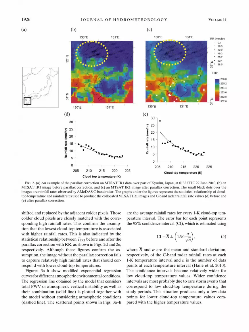
shifted and replaced by the adjacent colder pixels. Those

colder cloud pixels are closely matched with the corre-

sponding high rainfall rates. This confirms the assump-

tion that the lowest cloud-top temperature is associated

with higher rainfall rates. This is also indicated by the

statistical relationship betweenTIR1 before and after the

parallax correction with RR, as shown in Figs. 2d and 2e,

respectively. Although these figures confirm the as-

sumption, the imagewithout the parallax correction fails

to capture relatively high rainfall rates that should cor-

respond with lower cloud-top temperatures.

Figures 3a–h show modified exponential regression

curves for different atmospheric environmental conditions.

The regression line obtained by the model that considers

total PWV or atmospheric vertical instability as well as

their combination (solid line) is plotted together with

the model without considering atmospheric conditions

(dashed line). The scattered points shown in Figs. 3a–h

are the average rainfall rates for every 1-K cloud-top tem-

perature interval. The error bar for each point represents

the 95% confidence interval (CI), which is estimated using

CI5R6

�1:96

sffiffiffin

p�, (5)

where R and s are the mean and standard deviation,

respectively, of the C-band radar rainfall rates at each

1-K temperature interval and n is the number of data

points at each temperature interval (Haile et al. 2010).

The confidence intervals become relatively wider for

low cloud-top temperature values. Wider confidence

intervals aremost probably due to rare storm events that

correspond to low cloud-top temperature during the

study periods. This situation produces only a few data

points for lower cloud-top temperature values com-

pared with the higher temperature values.

FIG. 2. (a) An example of the parallax correction on MTSAT IR1 data over part of Kyushu, Japan, at 0132 UTC 29 June 2010, (b) an

MTSAT IR1 image before parallax correction, and (c) an MTSAT IR1 image after parallax correction. The small black dots over the

images are rainfall rates observed by AMeDAS C-band radar. The graphs under the figures represent the statistical relationship of cloud-

top temperature and rainfall rates used to produce the collocatedMTSAT IR1 images and C-band radar rainfall rate values (d) before and

(e) after parallax correction.

1926 JOURNAL OF HYDROMETEOROLOGY VOLUME 14

According to Fig. 3a, a high rainfall rate can be pro-

duced only by relatively high PWV conditions ($58mm)

at TIR1 around 200K. For the relatively low PWV con-

ditions (,58mm) shown in Fig. 3b, the model can only

estimate a lower rainfall intensity up to a cloud-top

temperature around 205K. This implies that total PWV

contributes strongly to the generation of high rainfall

rates. Figures 3c and 3d show the regression curves

generated by relatively unstable (SSI , 12) and stable

(SSI . 12) atmospheric situations, respectively. Both

regression curves almost coincide with the regression

curve for the situation without consideration of atmo-

spheric conditions. However, when we examine Fig. 3d

more carefully, it can be seen that some heavy rainfall

events occur under relatively stable atmospheric con-

ditions. Even though the number of such events is small

(indicated by the wide confidence interval), they influence

the shape of the regression line. One of the reasons for

this condition is the limitations in spatial and temporal

resolution of SSI. A relatively coarse spatial resolution

would lead to an SSI that does not adequately separate

the high and low rainfall rates corresponding to the at-

mospheric vertical instability conditions. A low tempo-

ral resolution results in spatial shifting between rainfall

and the SSI because of the time discrepancy during data

acquisition. Figures 3e–h show the regression curves for

the situation where total PWV and atmospheric vertical

instability are combined. The figures indicate that the

specific situation for combined total PWV and atmo-

spheric vertical instability can be represented by different

regression curves.

Before moving to the next stage (i.e., to measure the

performance of MTSAT rainfall estimation by compar-

ing the results with observed rainfall), a cross-correlation

analysis was conducted to determine the lag time between

them. The grid values at the coordinate locations of sta-

tion 74181 (3383305900N, 13383204800E) and station 87321

(3281305200N, 131890200E) were extracted from hourly esti-

mated and observed rainfall data during the period of

16–20 September 2011. Figures 4a and 4b show the cross

correlograms of estimated rainfall (colored bars) and ob-

served rainfall for both locations. These figures indicate a

1-h time lag between estimated and observed rainfall,

which implies that the rainfall detected by satellite could

be observed as real rainfall by a rain gauge after 1h.

The performance of the statistical models was tested

in three case studies: 1) at 0630–1330 UTC 22 June 2010

over Kyushu island (beginning of summer; hereafter

case A), 2) at 1532–2132 UTC 24August 2011 over Nara

prefecture (middle of summer; hereafter case B), and

3) at 1732–0532 UTC 19–20 September 2011 over

Kyushu island (end of summer; hereafter case C). Figure

5a shows the locations of these three case studies; each

location is bounded by a 18 3 18 window box.

FIG. 3. The modified exponential regression models corresponding to different atmospheric environmental conditions: (a) PWV1,

(b) PWV2, (c) SSI1, (d) SSI2, (e) CMB1, (f) CMB2, (g) CMB3, and (h) CMB4 (solid line) compared to the model without considering

atmospheric environmental conditions (ORG; dashed line).

DECEMBER 2013 SU SENO AND YAMADA 1927

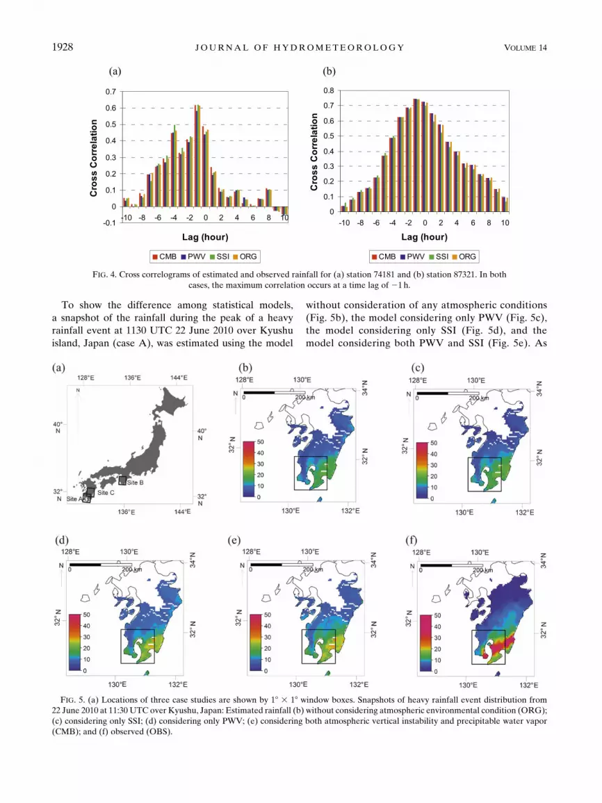
To show the difference among statistical models,

a snapshot of the rainfall during the peak of a heavy

rainfall event at 1130 UTC 22 June 2010 over Kyushu

island, Japan (case A), was estimated using the model

without consideration of any atmospheric conditions

(Fig. 5b), the model considering only PWV (Fig. 5c),

the model considering only SSI (Fig. 5d), and the

model considering both PWV and SSI (Fig. 5e). As

FIG. 4. Cross correlograms of estimated and observed rainfall for (a) station 74181 and (b) station 87321. In both

cases, the maximum correlation occurs at a time lag of 21 h.

FIG. 5. (a) Locations of three case studies are shown by 18 3 18 window boxes. Snapshots of heavy rainfall event distribution from

22 June 2010 at 11:30 UTC over Kyushu, Japan: Estimated rainfall (b) without considering atmospheric environmental condition (ORG);

(c) considering only SSI; (d) considering only PWV; (e) considering both atmospheric vertical instability and precipitable water vapor

(CMB); and (f) observed (OBS).

1928 JOURNAL OF HYDROMETEOROLOGY VOLUME 14

explained above, there was a 1-h time lag between

estimated rainfall and observed rainfall; therefore,

the estimated rainfall results were compared with in-

terpolated observed rainfall (Fig. 5f) for the following

hour (i.e., 1230 UTC). Compared with the observed

rainfall, MTSAT rainfall estimations did not represent

local strong rainfall events very well, even though in the

wider spatial domain, they provided a reasonable

representation of the spatial distribution of rainfall.

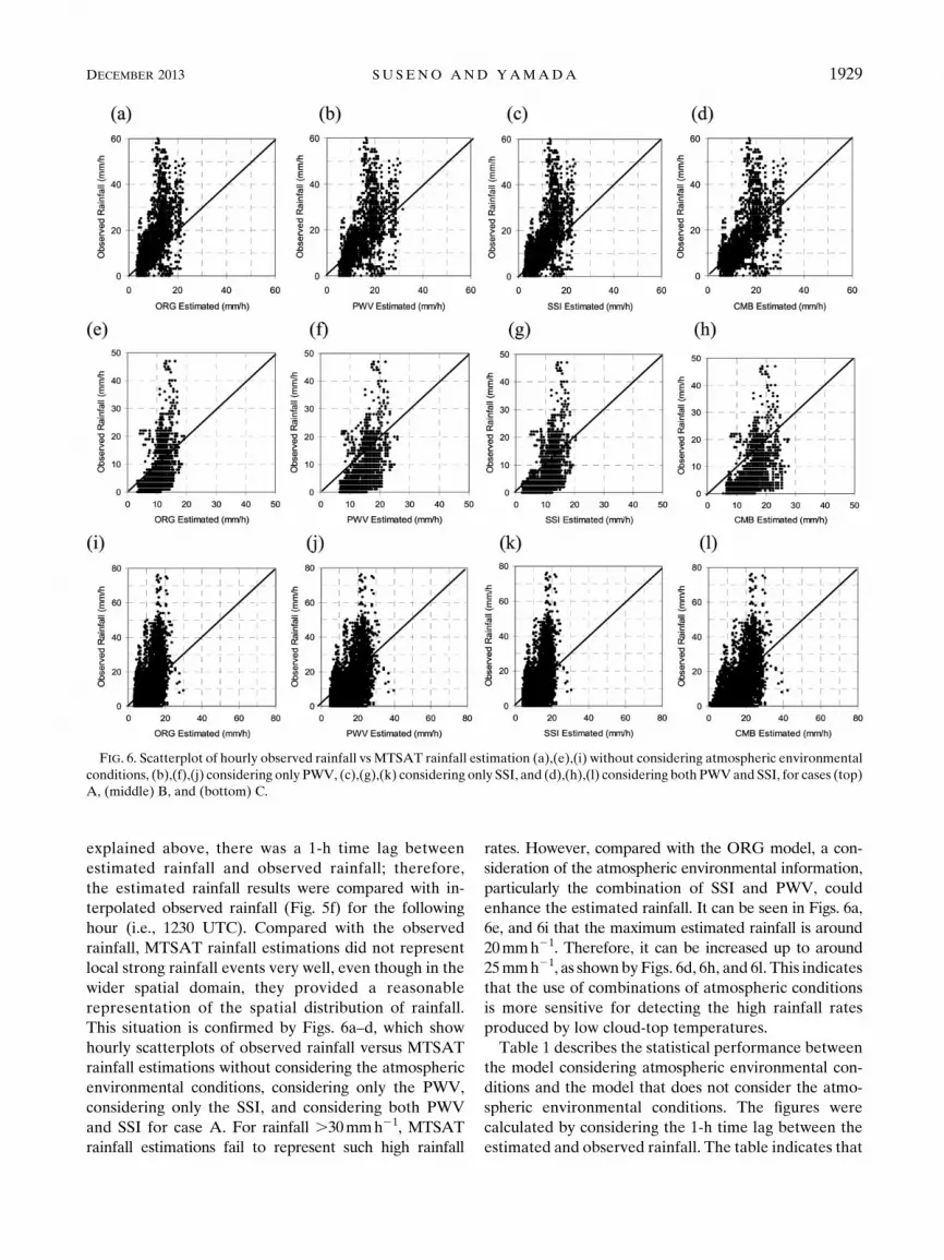
This situation is confirmed by Figs. 6a–d, which show

hourly scatterplots of observed rainfall versus MTSAT

rainfall estimations without considering the atmospheric

environmental conditions, considering only the PWV,

considering only the SSI, and considering both PWV

and SSI for case A. For rainfall .30mmh21, MTSAT

rainfall estimations fail to represent such high rainfall

rates. However, compared with the ORG model, a con-

sideration of the atmospheric environmental information,

particularly the combination of SSI and PWV, could

enhance the estimated rainfall. It can be seen in Figs. 6a,

6e, and 6i that the maximum estimated rainfall is around

20mmh21. Therefore, it can be increased up to around

25mmh21, as shownby Figs. 6d, 6h, and 6l. This indicates

that the use of combinations of atmospheric conditions

is more sensitive for detecting the high rainfall rates

produced by low cloud-top temperatures.

Table 1 describes the statistical performance between

the model considering atmospheric environmental con-

ditions and the model that does not consider the atmo-

spheric environmental conditions. The figures were

calculated by considering the 1-h time lag between the

estimated and observed rainfall. The table indicates that

FIG. 6. Scatterplot of hourly observed rainfall vs MTSAT rainfall estimation (a),(e),(i) without considering atmospheric environmental

conditions, (b),(f),(j) considering only PWV, (c),(g),(k) considering only SSI, and (d),(h),(l) considering both PWVand SSI, for cases (top)

A, (middle) B, and (bottom) C.

DECEMBER 2013 SU SENO AND YAMADA 1929

in terms of bias and RMSE, the use of atmospheric en-

vironmental conditions for rainfall estimation does not

produce a meaningful improvement when compared to

the model that does not consider any atmospheric en-

vironmental conditions. However, the model that con-

siders the combination of total PWV and atmospheric

vertical instability demonstrates a reasonable improve-

ment in terms of correlation. This improvement in per-

formance in terms of correlation supported the observation

that combinations of parameters are more sensitive in

detecting high rainfall rates produced by low cloud-top

temperatures, as explained in the paragraph above.

The results of an intercomparison between the

MTSAT rainfall estimation and the TRMM 3B42 data

product for casesA, B, and C are presented in Figs. 7a–e,

7f–j, and 7k–o, respectively. Their statistical perfor-

mance is described in Table 2. As shown in Figs. 7a, 7f,

and 7k, the scatterplots indicate that the TRMM 3B42

TABLE 1. Comparison of the TIR1 and RR statistical models considering total PWV and atmospheric vertical instability (CMB, PWV,

and SSI) and the model without considering total PWV and atmospheric vertical instability (ORG) for cases A, B, and C. Boldface

numbers show the best statistical results.

Case A Case B Case C

Sample

size r

Bias

(mmh21)

RMSE

(mmh21)

Sample

size r

Bias

(mmh21)

RMSE

(mmh21)

Sample

size r

Bias

(mmh21)

RMSE

(mmh21)

CMB 3588 0.66 1.0 8.6 4758 0.54 7.8 9.4 8975 0.54 4.6 9.9

PWV 3588 0.66 0.2 8.6 4758 0.51 4.7 7.0 10 484 0.51 5.7 10.8

SSI 3588 0.65 22.4 9.2 4758 0.61 7.3 8.7 8475 0.61 0.9 8.9

ORG 3588 0.65 23.0 9.5 4758 0.48 5.0 7.2 10 484 0.51 0.8 9.5

FIG. 7. Scatterplot of 3-hourly observed rainfall vs (a),(f),(k) TRMM 3B42, (b),(g),(l) MTSAT rainfall estimation without considering

atmospheric environmental conditions, (c),(h),(m) considering only PWV, (d),(i),(n) considering only SSI, and (e),(j),(o) considering both

PWV and SSI), for cases (top) A, (middle) B, and (bottom) C.

1930 JOURNAL OF HYDROMETEOROLOGY VOLUME 14

data product was more scattered than MTSAT rainfall

estimations for case A and was overestimated to a larger

extent for cases B and C. These conditions were con-

firmed by the lower correlations than those for the

MTSAT rainfall estimations (see Table 2). The bias and

RMSE of TRMM 3B42 are also larger than theMTSAT

rainfall estimations, except for case C. These results

suggest that MTSAT rainfall estimations perform better

than the TRMM 3B42 data product.

5. Conclusions

A method of rainfall estimation based on the statis-

tical relationships between TIR1 and RR was developed

for heavy rainfall generated by convective cloud in Ja-

pan and the surrounding area. TIR1 and RR data were

acquired fromMTSAT IR1 andAMeDASC-band radar,

respectively, for the periods of June–September 2010 and

2011. A parallax error correction was performed for the

MTSAT datasets. To differentiate between convective

and nonconvective cloud, the Suseno and Yamada

(2012) algorithm cloud classification algorithm was ap-

plied to the parallax-corrected MTSAT datasets. The

total PWVand atmospheric vertical instability conditions

during the convection process, which influence the TIR1

and RR statistical relationships, were investigated. These

atmospheric environmental conditions were represented

byGPS-PWVand SSI, respectively. Values of 58mm for

GPS-PWV and 12 for SSI were proposed as thresholds

for discriminating such atmospheric environmental

conditions. Eight modified exponential models were de-

veloped according to TIR1 and RR data pairs, which were

discriminated based on predefined atmospheric environ-

mental situations, that is, models that considered only

PWV and SSI, namely, PWV1 (GPS-PWV $ 58mm),

PWV2 (GPS-PWV, 58mm), SSI1 (SSI#12), and SSI2

(SSI . 12), and models that combined GPS-PWV and

SSI, namely, CMB1 (GPS-PWV$ 58mm and SSI#12),

CMB2 (GPS-PWV , 58mm and SSI # 12), CMB3

(GPS-PWV $ 58mm and SSI . 12), and CMB4 (GPS-

PWV, 58mm and SSI. 12). One model, ORG, which

did not consider GPS-PWV and SSI, was also generated.

Several different regression curves for the statistical

relationships of TIR1 and RR were produced, especially

by combining PWV and SSI conditions. Because of the

occurrence of rare storm events that corresponded to

low cloud-top temperatures during this study period, the

confidence intervals of the statistical model became

relatively wider for low cloud-top temperature values.

When compared with the model that did not consider

any atmospheric environmental conditions, the use of at-

mospheric environmental conditions for making rainfall

estimations enhanced the accuracy of rainfall estimation,

particularly when using the model that considered a com-

bination of total PWV and atmospheric vertical instability,

and eventually improved the performance, particularly

in terms of correlation. However, MTSAT rainfall esti-

mation was not successful in representing local heavy

rainfall events, even though it performed reasonably

well when predicting the rainfall spatial distribution at a

wider spatial domain.

The intercomparison results between MTSAT IR1–

based rainfall estimations and the TRMM 3B42 data

product demonstrated that MTSAT IR1–based rainfall

estimations either considering or not considering total

PWV and atmospheric vertical instability produced a

reasonably better performance than the TRMM 3B42

data product.

Because of the limitation of the number of samples that

were used in this research, the full variety of physical

processes associated with convective rainfall generation

may not have been included. Therefore, more samples

should be included in the development and validation of

statistical models to reach a more definite conclusion.

Acknowledgments. The authors sincerely thank the

Hitachi Zosen Corporation for providing an immense

number of reliable datasets of GPS precipitable water.

TABLE 2. Comparison of MTSAT IR1–based rainfall estimations considering and not considering total PWV and atmospheric vertical

instability and the TRMM 3B42 rainfall estimation product for cases A, B, and C. MTSAT-CMB, MTSAT-PWV, and MTSAT-SSI refer

to MTSAT IR1–based rainfall estimations considering the combination of PWV and SSI, PWV only, and SSI only. MTSAT-ORG refers

to aMTSAT IR1–based rainfall estimation considering no atmospheric environmental conditions. Boldface numbers show best statistical

results.

Case A Case B Case C

Sample

size r

Bias

(mmh21)

RMSE

(mmh21)

Sample

size r

Bias

(mmh21)

RMSE

(mmh21)

Sample

size r

Bias

(mmh21)

RMSE

(mmh21)

MTSAT-CMB 10 0.62 1.0 5.0 8 0.32 9.0 9.8 28 0.55 3.1 8.4

MTSAT-PWV 10 0.48 20.2 5.4 8 0.60 8.0 8.3 28 0.54 2.6 7.8

MTSAT-SSI 10 0.65 21.7 5.1 8 20.21 4.6 5.7 28 0.52 21.2 6.4

MTSAT-ORG 10 0.64 22.2 5.6 8 0.34 5.8 6.2 28 0.55 20.4 5.3

TRMM 3B42 10 20.33 6.2 12.6 8 20.02 8.6 13.1 28 0.51 -0.1 7.8

DECEMBER 2013 SU SENO AND YAMADA 1931

This study was partially supported by the Research

Program on Climate Change Adaptation, Ministry of

Education, Culture, Sports, Science and Technology,

Japan (RECCA/MEXT); the MEXT SOUSEI program

(theme C-i-C); the Integrated Study Project on Hydro-

Meteorological Prediction and Adaptation to Climate

Change in Thailand (IMPAC-T); the Science and Tech-

nology Research Partnership for Sustainable Devel-

opment; the JST-JICA; and the Japan andCoreResearch

for Evolutional Science and Technology program

(CREST/JST). The anonymous reviewers are deeply

thanked for their valuable and very helpful comments.

REFERENCES

Doswell, C. A., III, H. E. Brooks, and R. A. Maddox, 1996:

Flash flood forecasting: An ingredient-based meth-

odology. Wea. Forecasting, 11, 560–581, doi:10.1175/

1520-0434(1996)011,0560:FFFAIB.2.0.CO;2.

Ebert, E. E., cited 2007: Forecast verification: Issues, methods and

FAQ. [Available online at http://www.cawcr.gov.au/projects/

verification/].

Feidas, H., and C. Cartalis, 2001: Monitoring mesoscale convec-

tive cloud systems asscociated with heavy storms using

Meteosat imagery. J. Appl. Meteor., 40, 491–512, doi:10.1175/

1520-0450(2001)040,0491:MMCCSA.2.0.CO;2.

Haile, A. T., T. Rientjes, A. Gieske, and M. Gebremichael,

2010: Multispectral remote sensing for rainfall detection and

estimation at the source of the Blue Nile river. Int. J. Appl.

Earth Obs. Geoinf., 12 (Suppl.), S76–S82, doi:10.1016/j.

jag.2009.09.001.

Hamada, A., and N. Nishi, 2010: Development of a cloud-top height

estimation method by geostationary satellite split-window

measurement trained with CloudSat data. J. Appl. Meteor.

Climatol., 49, 2035–2049, doi:10.1175/2010JAMC2287.1.

Huffman, G. J., and Coauthors, 2007: The TRMM Multisatellite

Precipitation Analysis (TMPA): Quasi-global, multiyear,

combined-sensor precipitation estimates at fine scales. J. Hy-

drometeor., 8, 38–55, doi:10.1175/JHM560.1.

Iwabuchi, T., C. Roken, L. Mervart, and M. Kanzaki, 2006: Now-

casting and weather forecasting, Real time estimation of ZTD

in GEONET, Japan. Location, 1, 44–49.

Kinoti, J., Z. Su, T. Woldai, and B. Maathuis, 2010: Estimation of

spatial–temporal rainfall distribution using remote sensing

techniques: A case study of Makanya catchment, Tanzania.

Int. J.Appl.EarthObs.Geoinf., 12 (Suppl.), S90–S99, doi:10.1016/

j.jag.2009.10.003.

Kuligowski, J., cited 2003: Remote sensing in hydrol-

ogy. [Available online at http://www.nws.noaa.gov/iao/

InternationalHydrologyCourseCD1/1029/wmo_bk.ppt.]

Saito, K., and Coauthors, 2006: The operational JMA nonhydrostatic

mesoscale model. Mon. Wea. Rev., 134, 1266–1298, doi:10.1175/MWR3120.1.

Sorooshian, S., K.-L. Hsu, X. Gao, H. V. Gupta, B. Imam,

and D. Braithwaite, 2000: Evaluation of PERSIANN

system satellite-based estimates of tropical rainfall.

Bull. Amer. Meteor. Soc., 81, 2035–2046, doi:10.1175/

1520-0477(2000)081,2035:EOPSSE.2.3.CO;2.

Suseno, D. P. Y., and T. J. Yamada, 2011: The use of cloud type

classification to improve geostationary based rainfall estima-

tion. Proc. Ninth Int. Symp. on Southeast Asian Water Envi-

ronment, Bangkok, Thailand.

——, and——, 2012: Two-dimensional threshold-based cloud type

classification using MTSAT data. Remote Sens. Lett., 3, 737–

746, doi:10.1080/2150704X.2012.698320.

Vicente, G. A., R. A. Scofield, and W. P. Menzel, 1998: The

operational GOES infrared rainfall estimation tech-

nique. Bull. Amer. Meteor. Soc., 79, 1883–1898, doi:10.1175/

1520-0477(1998)079,1883:TOGIRE.2.0.CO;2.

——, J. C. Devenport, and R. A. Scofield, 2002: The role of oro-

graphic and parallax correction on real time high resolution

satellite rainfall rate distribution. Int. J. Remote Sens., 23, 221–

230, doi:10.1080/01431160010006935.

Wardah, T., S.H.AbuBakar,A. Bardosy, andM.Maznorian, 2008:

Use of geostationary meteorological satellite images in con-

vective rain estimation for flash-flood forecasting. J. Hydrol.,

356, 283–298, doi:10.1016/j.jhydrol.2008.04.015.

1932 JOURNAL OF HYDROMETEOROLOGY VOLUME 14