Local evolvability of statistically neutral GasNet robot controllers

BioSystems 69 (2003) 223–243

Local evolvability of statistically neutralGasNet robot controllers

Tom Smitha,b,∗, Phil Husbandsa,c, Michael O’Sheaa,ba Centre for Computational Neuroscience and Robotics (CCNR), University of Sussex, Brighton, UK

b School of Biological Sciences, University of Sussex, Brighton, UKc School of Cognitive and Computing Sciences, University of Sussex, Brighton, UK

Abstract

In this paper we introduce and apply the concept oflocal evolvabilityto investigate the behaviour of populations during evolu-tionary search. We focus on the evolution ofGasNetneural network controllers for a robotic visual discrimination problem, show-ing that the evolutionary process undergoes long neutral fitness epochs. We show that the local evolvability properties of the searchspace surrounding a group ofstatistically neutralsolutions do vary across the course of an evolutionary run, especially duringperiods of population takeover. However, once takeover is complete there is no evidence for further increase in local evolvabilityacross fitness epochs. We also see no evidence for the neutral evolution of increased solution robustness, but show that this may bedue to the ability of evolutionary algorithms to focus search on volumes of the fitness landscape with above average robustness.© 2002 Elsevier Science Ireland Ltd. All rights reserved.

Keywords:Local evolvability; Neutral evolution; Fitness landscape; Evolutionary algorithm; Evolutionary robotics; Solution robustness

1. Introduction

In this paper, we investigate the dynamics of evo-lutionary search on the large, noisy, heterogenousfitness landscape underlying an evolutionary roboticsexperiment. We show that the evolution of successfulcontrollers can be characterised by long fitness epochsduring which the best individuals in the populationmove along statistically neutral networks, interspersedby short periods of fitness increase. By defininglocalevolvabilitymeasures of the search space surroundingsolutions, we investigate whether the properties ofa set of statistically neutral solutions change duringthe course of an evolutionary run. We also investi-gate the difference between the statistically neutral

∗ Corresponding author.E-mail address:[email protected] (T. Smith).

solutions generated during the evolutionary process,and statistically neutral solutions encountered over anon-adaptive neutral walk.

1.1. Local evolvability and thetransmission function

Evolvability is loosely defined as the capacity toevolve, alternatively the ability of an individual orpopulation to generate fit variants(Altenberg, 1994;Marrow, 1999; Wagner and Altenberg, 1996). Evolv-ability is therefore more closely allied with the poten-tial for fitness than with fitness itself; two equal fitnessindividuals or populations may have very differentevolvabilities (Turney, 1999). Closely related defi-nitions of evolvability explicitly make the link withincrease in solution complexity over time(Nehaniv,2000), and the evolution of the genotype-to-phenotypemapping(McMullin, 2000).

0303-2647/02/$ – see front matter © 2002 Elsevier Science Ireland Ltd. All rights reserved.PII: S0303-2647(02)00139-9

224 T. Smith et al. / BioSystems 69 (2003) 223–243

It has also been argued that there may be trends forevolvability to increase during evolution(Altenberg,1994; Wagner and Altenberg, 1996; Dawkins, 1989;Turney, 1999). However, as evolvability is more di-rectly related to fitness potential than fitness itself,long-term change cannot be due to straight fitness se-lection. Thus any trend towards change in evolvabilitycan only be understood through some higher orderselection mechanism, by which evolution tends to re-tain solutions, or their descendants, with more evolv-able genetic systems (Dawkins, 1989; Kirschner andGerhart, 1998, argue for such mechanisms underwhich evolvability may be selected for).

Researchers in both biology and evolutionary com-putation often link evolvability with the propertiesof the search space. For example,Burch and Chao(2000) show that the evolvability of RNA virusescan be understood in terms of their mutational neigh-bourhood, while many evolutionary computation re-searchers (see e.g.Ebner et al., 2001; Marrow, 1999)argue that changing the properties of the search space(through such mechanisms as adding neutrality) canaffect evolvability as evidenced by the speed ofevolution. The interest in evolvability for evolution-ary computation practitioners is thus tied closely towork on properties of the search space which influ-ence the ease of finding good solutions in the space(Weinberger, 1990; Hordijk, 1996; Jones and Forrest,1995; Naudts and Kallel, 2000).

In this paper, we identify thelocal evolvabilityofsolution(s) as some measure based on the fitness ofoffspring from those solution(s). We define a set offour metrics of local evolvability (seeSmith et al.,2002a, for further details):

Ea = P(Fo ≥ Fp) (1)

Eb = 〈Fo〉 (2)

Ec = 〈Fo〉75,100 (3)

Ed = 〈Fo〉0,25 (4)

whereFp, Fo are the fitnesses of the parent and off-spring solutions, and〈Fo〉75,100, 〈Fo〉0,25 the expectedfitnesses over the top and bottom quartiles of the off-spring solutions. ThusEa is the probability of off-spring solutions being of greater or equal fitness tothe parent,Eb the expected offspring fitness,Ec the

expected fitness over the top quartile of offspring fit-nesses, andEd the expected fitness over the bottomquartile of offspring fitnesses.

The four metrics can be similarly defined oversome population, e.g. a population of solutions atsome time-point during evolution, as the local evolv-ability calculated over offspring from all individualsin that population. InSmith et al. (2002a)we haveused the metrics calculated over samples of equal fit-ness solutions to derivefitness evolvability portraitsfor the set of NK (Kauffman, 1993)and terracedNK landscapes(Newman and Engelhardt, 1998). Themetrics are plotted against fitness, and used to de-scribe the ruggedness, local modality and neutralityof the spaces.

This tight definition of local evolvability in termsof the search space surrounding solutions (or popula-tions of solutions) allows us to track the behaviour ofpopulations during evolution. In particular, we focuson a population of solutions that are indistinguishablefrom each other in terms of their fitness, investigatingwhether they move to areas of the search space thatare distinguishable in terms of their local evolvabilityproperties. SeeSection 6for experimental details oncalculating the evolvability metrics.

1.2. Adaptive evolution on neutral networks

In the neutral theory of molecular evolution,Kimura(1983)argues that the majority of genotypic mutationsmay be selectively neutral. There is increasing evi-dence for such neutral evolution in a number of fields,including RNA secondary structure(Grüner et al.,1996), bacteria(Elena et al., 1996), evolvable hard-ware (Vassilev and Miller, 2000), and digital organ-isms(Adami, 1995). Evolution on fitness landscapeswith high levels of neutrality is typically characterisedby periods during which fitness does not increase, orfitness epochs, interspersed by short periods of rapidfitness increase, i.e.epochal evolution(van Nimwegenet al., 1997; Crutchfield and van Nimwegen, 1999)orpunctuated equilibrium(Eldredge and Gould, 1972;Gould and Eldredge, 1977).

During fitness epochs, genotype structure maynot be conserved, as the evolving population movesthrough networks of connected equal fitness solutions,or neutral networks. Eventually, aportal genotype ofhigher fitness may be discovered, and the population

T. Smith et al. / BioSystems 69 (2003) 223–243 225

moves up to the higher fitness neutral network; thetime spent in neutral evolution is related to the sizeof the network and the number of portal genotypes(argued byvan Nimwegen and Crutchfield (2000)tobe an entropy barrier, very different to thefitnessbarrier of low fitness genotypes that must be passedto escape from local optima). Despite the undirectednature of the neutral movement, genotypic changemay lay down structure required for the final portalgenotype to be discovered.

Recent work describing the population dynamicsof evolving populations on neutral networks has ar-gued that with large enough populations and muta-tion rates, the population will tend to move towardsvolumes of the neutral network where solutions havemore neutral neighbours than on average across theneutral network, i.e. the neutral evolution of robust-ness(van Nimwegen et al., 1999). Similarly, Wilke(2001)shows epochal evolution in theaverage fitnessof the population, despite the highest fitness in the pop-ulation remaining constant; the fitter genotypes moveneutrally toflatterareas of the search space containingmore neutral neighbours. Thus the average populationfitness increases despite the highest fitnesses remain-ing fixed; evolution of populations can be adaptiveeven during neutral fitness epochs. As in the evolutionof evolvability, any adaptation during neutral move-ment can be explained through higher-level selection,in which solutions (or their descendants) of greater ro-bustness are likely to be retained in the evolutionarypopulation.

Having defined our metrics of local evolvabilityover the fitness distribution of solution offspring, weare now in a position to investigate the behaviour ofpopulations evolving along neutral networks in an ex-tremely noisy genotype-to-fitness mapping space, inwhich the initial genotype translates to an intermediateneural network phenotype, with the final fitness mea-suring how well this network performs over time incontrolling a robot engaged in solving a visual shapediscrimination task.

2. An evolutionary robotics search space

One of the new styles of Artificial Intelligence tohave emerged recently is evolutionary robotics(Cliffet al., 1993; Nolfi and Floreano, 2000; Floreano and

Mondada, 1994; Husbands and Meyer, 1998). Theevolutionary process involves evaluating, over manygenerations, whole populations of robot control sys-tems specified by artificial genotypes. These are in-terbred using a Darwinian scheme in which the fittestindividuals are most likely to produce offspring. Fit-ness is measured in terms of how good a robot’sbehaviour is according to some evaluation criterion.

Artificial neural networks (ANNs) have been suc-cessfully used in a large number of evolutionaryrobotics experiments (for an overview seeNolfi andFloreano, 2000). Typically, external sensory data isused for the network input, and the network output isused to control the robot motors. Other styles of con-trol architectures have also been used for evolutionaryrobotics experiments, notably genetic programming(Koza, 1992), classifier systems(Holland, 1975)andevolvable hardware(Thompson, 1998). In previouswork, we have investigated the use of non-standardneural network architectures, focusing on developingcontrol structures that produce successful solutions infewer evaluations using artificial evolution(Husbandset al., 1998). In experiments on a variety of roboticstasks, we have shown that a particular style of net-work, the “GasNet”, is particularly amenable to evolu-tionary search.

2.1. The GasNet architecture

The GasNet is an arbitrarily recurrent ANN aug-mented with a model of diffusing gaseous modulation,in which the instantaneous activation of a node is afunction of both the inputs from connected nodes andthe current concentration of gas(es) at the node. Thusin addition to the standard electrical activity ‘flowing’between nodes, an abstract process analogous to thediffusion of gaseous modulators such as Nitric Oxideis at work (Philippides et al., 2000). In this process,the virtual gases do not alter the electrical activityin the network directly but rather act by chang-ing the gain of transfer function mapping betweennode input and output in a concentration dependentmanner.

The network underlying the GasNet model is a dis-crete time-step, recurrent neural network with a vari-able number of sigmoid transfer function nodes. Thesenodes are connected by either excitatory (with a weightof +1) or inhibitory (with a weight of−1) links with


the outputOni , of nodei at time-stepn determined bya continuous mapping from the sum of its inputs, asdescribed by the following equation:

Oni = tanh

kni

∑j∈Ci

wjiOn−1j + Ini

+ bi

(5)

whereCi is the set of nodes with connections to nodei and wji = ±1 depending on whether the link isexcitatory or inhibitory and multiplies the input fromnode j (which is the output from nodej from theprevious time-step).Ini is the external (sensory) inputto nodei at timen, andbi is a genetically set bias. Eachnode has a genetically set default transfer functionparameterk0

i , which can be altered at each time-stepby the concentration of the diffusing virtual gas atnodei to givekni .

2.2. Gas diffusion in the networks

In order to incorporate the gas concentration model,the network is placed in a 2D plane, with node po-sitions specified genetically. The GasNet diffusionmodel is controlled by two genetically specified pa-rameters namely the radius of influencer around theemitting node, and the rate of build up and decays.Spatially, the gas concentration varies as an inverseexponential of the distance from the emitting nodewith a spread governed byr, with the concentrationset to zero for all distances greater thanr (Eq. (6)).This is loosely analogous to the length constant ofthe natural diffusion of nitric oxide, related to its rateof decay through chemical interaction. The maxi-mum concentration at the emitting node is one andthe concentration builds up and decays from thisvalue linearly as defined byEqs. (7) and (8)at a ratedetermined bys. The governing equations are:

C(d, t) ={e−2d/r × T(t) d < r

0 else(6)

T(t)=

H

(t−tes

)emitting

H

[H

(ts−tes

)−H

(t−tss

)]not emitting

(7)

H(x) =

0 x ≤ 0

x 0< x < 1

1 else

(8)

whereC(d, t) is the concentration at a distancedfrom the emitting node at timet, te the time at whichemission was last turned on,ts the time at whichemission was last turned off, ands (controlling theslope of the functionT ) is genetically determined foreach node. To summarise, within a radius ofr fromthe node, gas builds up (and decays) linearly to amaximum ofe−2d/r in s time-steps. The total concen-tration at a node is then determined by summing theconcentrations from all other emitting nodes (nodesare not affected by their own concentration, to avoidrunaway positive feedback).

2.3. Modulation by the gases

There are two virtual gases in the network, gas 1 andgas 2, which increase and decreasekni (seeEq. (5)) re-spectively in a concentration dependent fashion. Boththe type of gas emitted by a node and the conditionsunder which it emits are specified genetically. Nodesemit either (a) gas 1, (b) gas 2 or (c) no gas, and emis-sion occurs when either (a) the node activity increasesbeyond the electrical threshold 0.5, or (b) the localconcentration of gas 1 increases beyond the threshold0.1, or (c) the local concentration of gas 2 increases be-yond the threshold 0.1. The concentration-dependentmodulation is described byEqs. (9)to (12), with trans-fer parameters updated on every time-step as the net-work runs. Thus we have:

kni = P[indni ] (9)

P = {−4.0,−2.0,−1.0,−0.5,−0.25,

0.0,0.25,0.5,1.0,2.0,4.0} (10)

indni = f(ind0i + Cn1(N − ind0

i )− Cn2ind0i ) (11)

f(x) =

0 x ≤ 0

�x� 0< x < N

N else

(12)

where P[i] refers to theith element of setP, indniis nodei’s index into the setP of possible discretevalueskni can assume,N is the number of elements


in P, ind0i is the genetically set default value forindi,

Cn1 is the concentration of gas 1 at nodei on time-stepn andCn2 is the concentration of gas 2 at nodei ontime-stepn. Both gas concentrations lie in the range[0,1].

Thus, the concentration of each gas is directly pro-portional to any change in indni , with a correspondingchange inkni . Although the change inkni is non-linearthese values represent a smooth change in the slope ofthe transfer function. Since the transfer functions canchange throughout the lifetime of the network, thissystem provides a form of network plasticity not seenin most other ANNs.

2.4. Visual shape discrimination

The evolutionary task at hand is a visual shape dis-crimination task; starting from an arbitrary position

Fig. 1. Screen shot of the simulated arena and robot. The bottom-right view shows the robot position in the arena with the triangle andsquare. Fitness is evaluated on how close the robot approaches the triangle. The top-right view shows what the robot ‘sees’, along withthe pixel positions selected by evolution for visual input. The top-left view shows the instantaneous activity of all nodes in the neuralnetwork. The bottom-left view shows the robot control neural network.

and orientation in a black-walled arena, the robot mustnavigate under extremely variable lighting conditionsto one shape (a white triangle) while ignoring the sec-ond shape (a white square). Fitness over a single trialwas taken as the fraction of the starting distance movedtowards the triangle by the end of the trial period,and the evaluated fitness was returned as the averageover 16 trials of the controller from different initialconditions:

F = 1

136

i=16∑i=1

i

(1 − DFi

DSi

)(13)

whereDFi is the distance to the triangle at the endof the ith trial, andDSi the distance to the triangleat the start of the trial, and thei trials are sorted indescending order of 1− DF/DS . Thus good trials,in which the controller moves some way towards the


triangle, receive a smaller weighting than bad trials,encouraging robust behaviour on all 16 trials.

Success in the task was taken when an evaluatedfitness of 1.0 was obtained over thirty successive gen-erations of the evolutionary algorithm. In the workreported here, fitness evaluations are carried out ina verified minimal simulation (Jakobi, 1998), seeFig. 1 for screen-shot of a fitness evaluation in sim-ulation. Evolved controllers have been successfullytransferred to the real robot(Husbands et al., 1998).As in many problems requiring controllers to providesensor-to-motor mappings over time, fitnesses areextremely time consuming to evaluate (in the workpresented here, evaluating a sample of 106 fitnessestakes around 24 h on a Pentium II 700 MHz machine)and inherently extremely noisy.

Fig. 2shows the distribution of fitnesses from a sin-gle controller over 10,000 evaluations. It should beemphasised that the environmental noise for the robotcontrollers is not simply variation in the received fit-ness score, but is a crucial feature of the robot mini-mal simulation model. Controllers must evolve to berobust to such noise, so as to successfully transfer tothe real world; two controllers may be of equal fitnesswhen evaluated in a noiseless environment, but maybe of very different fitnesses in the full noise model.Although the level of noise in the model is higher than

Fig. 2. The fitness distribution of a single genotype evaluated 10,000 times in the minimal simulation evaluation environment. 95% of thefitnesses lie in the range [0.1343,0.2856], with possible controller fitness∈ [0,1].

that found in the real world, to successfully evolverobot controllers in simulation able to operate success-fully in the real world this noise is necessary(Jakobi,1998). Since we are interested in the properties of land-scapes defined by genotype-to-fitness mappings thatare used in real problems, we need to develop waysof understanding these kinds of landscape.

2.5. The solution representation

The neural network robot controllers were encodedas variable length strings of integers, with each integerallowed to lie in the range [0,99]. Each node in thenetwork was coded for by nineteen parameters, con-trolling such properties as node connections, sensorinput, node bias, and all the variables controlling gasdiffusion as described inSections 2.2 and 2.3. Both therobot control network, an arbitrarily recurrent ANN,and the robot sensor input morphology, i.e. the posi-tion of the input pixels on the visual array, were un-der evolutionary control. Thus mutation of solutions(Section 2.6) is able to produce offspring with vary-ing network architecture, network node properties andsensor morphology. In all experiments, the GA pop-ulation were initially seeded with networks contain-ing 10 neurons. For further details seeHusbands et al.(1998), Smith and Philippides (2000).


Fig. 3. Pseudo-code for the asynchronously updating evolutionary algorithm.

2.6. The evolutionary algorithm andmutation operator

A distributed asynchronously updating evolution-ary algorithm was used, with a population of 100solutions arranged on a 10× 10 grid. Fitness wasawarded on the fraction of the distance moved towardsthe triangle over a series of 16 runs with differentinitial conditions, seeEq. (13). Parents were chosenwith probability proportional to their fitness rankedin ascending order over the mating ‘pool’ consistingof a randomly chosen grid-point plus its eight nearestneighbours. The parent solution was mutated to createthe offspring solution which was placed back in themating pool, replacing a solution chosen with proba-bility proportional to their fitness ranked in descend-ing order over the mating pool. One generation wasspecified as 100 such breeding events.Fig. 3 showsthe pseudo-code for the evolutionary algorithm.

Three mutation operators were applied to solutionswith probabilityµ% during evolution (for the experi-ments detailed here,µ = 4). First, each integer in thestring had aµ% probability of mutation in a GaussiandistributionN(0,10) centred on its current value (20%of these mutations completely randomised the inte-ger). Second, there was aµ% chance pergenotypeofadding one neuron to the network, i.e. increasing thegenotype length by 19. Third, there was aµ% chanceper genotype of deleting one randomly chosen neuronfrom the network, i.e. decreasing the genotype length

by 19. It should be noted that the value ofµ = 4 usedin these experiments is a much larger level of mutationthan typically used in artificial evolution optimisation(and certainly much larger than in biological evolu-tion). However, lower levels of mutation produce ex-tremely slow evolution of successful solutions(Smithet al., 2002b); in Section 6.1we see that the num-ber of neutral mutations at this mutation rate is stillsignificant.

3. Statistical neutrality

In Section 1.2we discussed the possible adapta-tion of populations during neutral movement fitnessepochs. However, as we have seen in the previoussection, the fitness landscape defined by the GasNetcontrollers is inherently extremely noisy; neutrality insuch a landscape is not trivial to define. Even the re-peated evaluation of the same controller produces awide range of possible scores (Fig. 2), so how can weidentify different solutions of equal fitness?

In this paper we use the concept of statistical neu-trality, based on solution fitness distributions. Two so-lutions are defined to be statistically neutral if it islikely that the two distributions of fitnesses are drawnfrom the same distribution. More precisely, two fitnessdistributions are defined to be statistically neutral ifwe fail to reject the null hypothesis that they are notsignificantly different. Such a probabilistic definition


of neutrality seems practical for the noisy fitness land-scape we are investigating, and owes much in spirit tothe “nearly neutral” theory(Ohta, 1992), where smallfitness differences may be swamped by finite popula-tion sampling effects. Even if real underlying fitnessdifferences exist between our statistically neutral so-lutions, they are unlikely to be observed by the evolu-tionary process.

In practice, we generate small distributions of fit-nesses for each sample in the population, and comparewith the fitness distribution from some test solution.If the Student’st-test (Press et al., 1992)probabil-ity for the sample and test distributions being drawnfrom the same distribution is not smaller than somevalueνS , we argue that the sample and test solutionscan be considered to be statistically neutral. Althoughthis statistical definition of neutrality will not identifyevery solution correctly - some solutions of equal fit-ness may be rejected while others of different fitnessmay be included, we argue that it has merit whenconsidering the neutrality of solutions in noisy fit-ness landscapes. In the experiments carried out in thenext section we takeνS = 0.1, i.e. two solutions aresaid to have different fitnesses if there is less than10% probability of their fitness distributions beingdrawn from a single distribution. The two solutionsare statistically neutral otherwise.

Fig. 4. Best and mean fitness of the population over generations for a single GasNet evolutionary run.

4. Fitness epochs in GasNet evolution

In previous work, we have shown the amenabilityof the GasNet architecture to evolutionary search forgood robot controllers(Husbands et al., 1998; Smithand Philippides, 2000). An ongoing project aims toexplain the observed evolutionary speed difference interms of the properties of the underlying fitness land-scapes of the GasNet and other neural network archi-tectures.

Fig. 4 shows a typical GasNet evolutionary run,with the population best and mean evaluated fitnessesplotted over time. Both fitnesses climb quickly froman initial near-zero random performance, with a longperiod of apparent stasis (albeit a noisy stasis), be-fore the best fitness reaches 100% around generation480. In terms of robot controller behaviour, the pe-riod of apparent stasis corresponds to approaching thefirst white object seen in the arena, thus hitting thetriangle on approximately 50% of evaluations (the se-lective fitness shown inFig. 4 is below 50% due tothe weighting on evaluations, seeSection 2.4). Thehigh fitnesses seen after generation 480 correspondto approaching the triangle on every single evalua-tion, while the lower fitnesses seen in the first fewgenerations correspond to ballistic behaviours such as“move straight forward”. Other GasNet evolutionary


runs show similar behaviour; long periods of appar-ent stasis interspersed with short periods of fitness in-crease, although in many cases there is more than oneperiod of apparent stasis.

4.1. Apparently neutral fitness epochs

In Fig. 5(a)we show the best and mean fitnessesover the same evolutionary run shown inFig. 4,with fitness evaluated in a noiseless environment. Itappears to be the case that fitness reaches a staticlevel very quickly, around generation 10, then staysconstant until generation 477 with a few short-livedhigher fitness ‘blips’. However, although the noiselessenvironment fitness evaluation scenario lends supportto the hypothesis that the apparent stasis period is in-deed a fitness epoch, it is not nearly the full story. InFig. 5(b), we show the best fitness found in the pop-ulation over time, with the fitness of every individualcalculated as the mean fitness over 10 evaluations ina noisy environment. Two points need to be made.First, the best fitness in the population in a noisyenvironment is clearly increasing after the generationat which the noiseless environment reached apparentfitness stasis, up to at least generation 60. Second, thebest fitness over the period from generations 100–477appears to remain constant, and there is also someevidence for the neutral period to start earlier, aroundgeneration 60.

AlthoughFig. 5 strengthens the hypothesis that thefitness of the best solutions really does not changeover long periods of the evolutionary run, we need toapply the notion of statistical neutrality to see whetherthis really holds up.

4.2. Statistically neutral fitness epochs

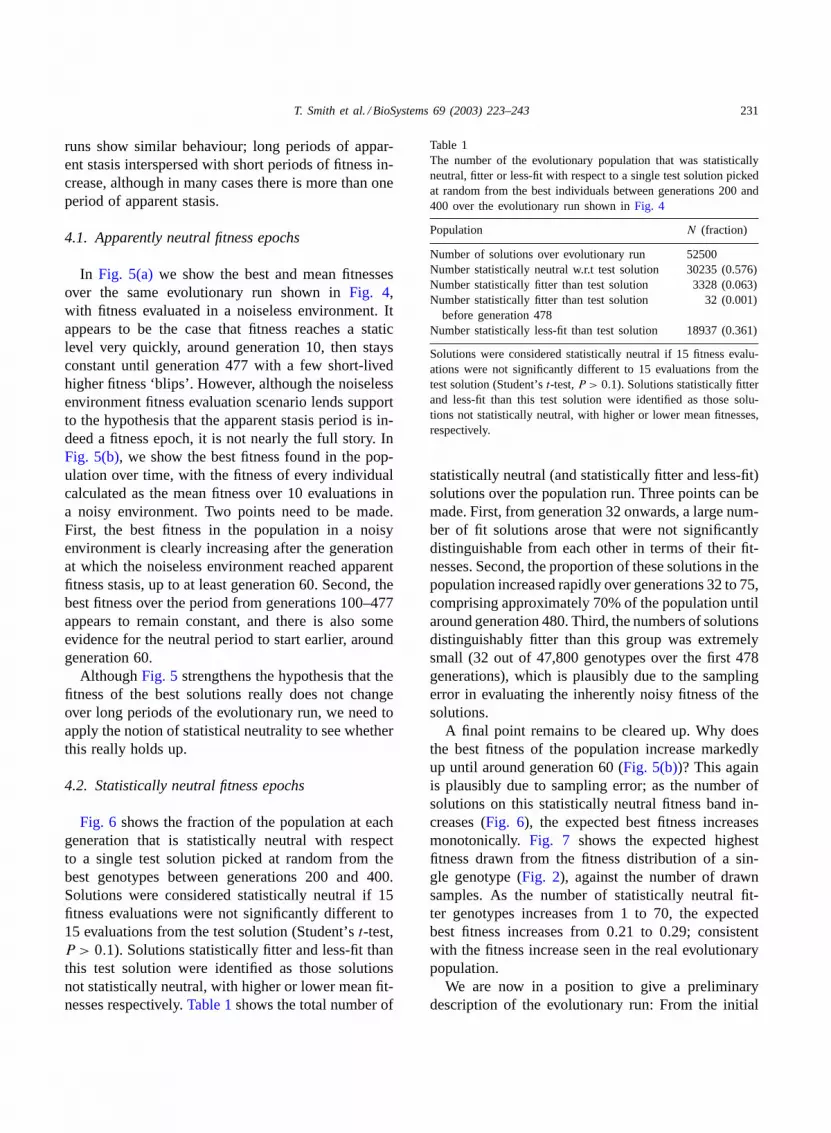
Fig. 6 shows the fraction of the population at eachgeneration that is statistically neutral with respectto a single test solution picked at random from thebest genotypes between generations 200 and 400.Solutions were considered statistically neutral if 15fitness evaluations were not significantly different to15 evaluations from the test solution (Student’st-test,P > 0.1). Solutions statistically fitter and less-fit thanthis test solution were identified as those solutionsnot statistically neutral, with higher or lower mean fit-nesses respectively.Table 1shows the total number of

Table 1The number of the evolutionary population that was statisticallyneutral, fitter or less-fit with respect to a single test solution pickedat random from the best individuals between generations 200 and400 over the evolutionary run shown inFig. 4

Population N (fraction)

Number of solutions over evolutionary run 52500Number statistically neutral w.r.t test solution 30235 (0.576)Number statistically fitter than test solution 3328 (0.063)Number statistically fitter than test solution

before generation 47832 (0.001)

Number statistically less-fit than test solution 18937 (0.361)

Solutions were considered statistically neutral if 15 fitness evalu-ations were not significantly different to 15 evaluations from thetest solution (Student’st-test,P > 0.1). Solutions statistically fitterand less-fit than this test solution were identified as those solu-tions not statistically neutral, with higher or lower mean fitnesses,respectively.

statistically neutral (and statistically fitter and less-fit)solutions over the population run. Three points can bemade. First, from generation 32 onwards, a large num-ber of fit solutions arose that were not significantlydistinguishable from each other in terms of their fit-nesses. Second, the proportion of these solutions in thepopulation increased rapidly over generations 32 to 75,comprising approximately 70% of the population untilaround generation 480. Third, the numbers of solutionsdistinguishably fitter than this group was extremelysmall (32 out of 47,800 genotypes over the first 478generations), which is plausibly due to the samplingerror in evaluating the inherently noisy fitness of thesolutions.

A final point remains to be cleared up. Why doesthe best fitness of the population increase markedlyup until around generation 60 (Fig. 5(b))? This againis plausibly due to sampling error; as the number ofsolutions on this statistically neutral fitness band in-creases (Fig. 6), the expected best fitness increasesmonotonically. Fig. 7 shows the expected highestfitness drawn from the fitness distribution of a sin-gle genotype (Fig. 2), against the number of drawnsamples. As the number of statistically neutral fit-ter genotypes increases from 1 to 70, the expectedbest fitness increases from 0.21 to 0.29; consistentwith the fitness increase seen in the real evolutionarypopulation.

We are now in a position to give a preliminarydescription of the evolutionary run: From the initial


Fig. 5. (a) Best and mean fitness of the population over generations from the same evolutionary run shown inFig. 4, with fitness evaluatedin a simulated environment without sensor and motor noise; (b) the best fitness found in the population from the same evolutionary run,with fitness set as the mean evaluated fitness over 10 evaluations in a noisy environment.


Fig. 6. The fraction of the evolutionary population over generations that was statistically neutral with respect to a single test solutionpicked at random from the best individuals between generations 200 and 400. Solutions were considered statistically neutral if 15 fitnessevaluations were not significantly different to 15 evaluations from the test solution (Student’st-test,P > 0.1).

random population we quickly evolve fixed ballis-tic solutions that approach the triangle on some ofthe evaluations. Around generation 32 we see thefirst emergence of controllers able to approach bright

Fig. 7. The expected highest fitness drawn from the fitness distribution of a single genotype (Fig. 2), against the number of drawn samples.With low numbers of fit solutions in the population, the expected best fitness remains near the mean of the noisy fitness distribution.However as the number of fitter genotypes increases, the apparent best fitness also increases; this leads to the apparent rise in the populationbest fitness seen inFig. 5(b) before generation 60.

objects, so finding the triangle on 50% of evalua-tions. Controllers showing this behaviour rapidly takeover the population, leading to a long fitness epoch.Finally, on generation 477 we see the evolution of


controllers able to approach the triangle on signifi-cantly more than 50% of evaluations. This innovationleads rapidly to 100% fitness.

So we see that the evolutionary run does indeedshow fitness epochs, during which the population ismainly comprised of solutions which are not distin-guishable from each other in terms of fitness. But whatis the population doing during this period - is it stuckin some local fitness optimum or moving in the searchspace along neutral networks?

Fig. 8. The Euclidean distance moved over time by the centre-of-mass of all genotypes of length 171 in the population for three differentfitness scenarios: (a) the GasNet evolutionary run analysed in the previous section; (b) evolution on a flat landscape where each solutionreceives the same evaluated fitness; (c) Evolution in the neighbourhood of a locally-optimal peak. The distance moved over the lastgeneration and over the last 10 generations are plotted.

5. Genotypic change during a GasNet fitnessepoch

The key feature distinguishing a population diffus-ing along a neutral network from that stuck at a localoptimum is the movement of the population in geno-type space, typically measured through the Euclideandistance moved by the population centre-of-mass, orcentroid, over time. This approach is complicated bythe variable length encoding scheme used in this paper


(seeSection 2.5for details of the solution representa-tion), in which the neural network controllers can addand delete nodes in the network.

The approach taken here is to analyse the centroidmovement over only those genotypes in the populationof a certain length; in this section we focus only onthose genotypes encoding solutions of nine nodes, i.e.genotypes of length 171 (applying the same results toother length solutions produces comparable results).In particular we can compare the observed centroidmovement with the population movement over land-scapes of known fitness.

5.1. Movement of the population centroid

Fig. 8 shows the Euclidean distance moved overtime by the centre-of-mass of all genotypes of length171 in the population for three different fitness land-scapes. Each subplot shows the distance moved bythe centroid over one generation (solid line), andthe distance moved over 10generations (dotted line),scaled by both the genotype length and possible rangeof each genotype locus (remember fromSection 2.5that each locus on the genotype is an integer in therange [0,99]). Fig. 8(a) shows the distance movedby the centroid for the same evolutionary run anal-ysed in the previous section, while for comparison

Fig. 9. The average movements of the population centroids per generation for evolution over the GasNet landscape, flat landscape, andlocally-optimal landscape (error bars show the S.D.).

Fig. 8(b) and (c)show the distance moved by thepopulation under the same evolutionary algorithm,but evolving in a flat landscape and in the neigh-bourhood of a local optimum respectively (for thelocal optimum movement analysis, the evolutionarypopulation was seeded with mutated copies of theoptimal solution in a landscape where fitness wassimply evaluated as the mean of the genotype locusvalues).

The main point to note fromFig. 8 is that the cen-troid movements for the GasNet evolution (Fig. 8(a))are roughly 50% of the flat landscape evolution(Fig. 8(b)), but significantly greater than the move-ment seen in the locally-optimal landscape. Thisis backed up by the average movements shown inFig. 9. It is likely that the sharp jumps in the cen-troid movements seen inFig. 8(a) and (b)are likelyto be due to the varying length nature of the mu-tation operator; evolution in fixed length flat land-scapes (figure not shown) does not show such sharpjumps.

From this we argue that the distance moved by thelength 171 population centroid (and indeed all otherlength centroids analysed) is consistent with the hy-pothesis that the population is moving significantlyduring the statistically neutral fitness epoch, and notstuck in a local optimum.

236T.

Sm

ithe

ta

l./Bio

Syste

ms

69

(20

03

)2

23

–2

43

Fig. 10. The centre-of-mass for the length 171 solutions plotted as individual networks over generations. SeeSection 2.1for details of the neural network control architecture.


5.2. Visualising the population centroid

Although it is not possible to accurately visu-alise the population centre-of-mass over our highdimensional fitness landscape, we can plot the neuralnetwork robot control solution corresponding to thiscentroid. Fig. 10 does just that for the length 171population centroids on generations 100, 200, 300and 400.

It should be stressed that the networks shown inFig. 10 are not necessarily viable robot control solu-tions, rather they are the ‘average’ network definedby the mean centroid of all other network genotypes.The main point to note is that the network struc-tures are very different; the population movementshown in the previous section does not merely alterconnection weights and other node properties, butmassively changes the entire network structure. Theperiod during the fitness epoch is certainly not spentcircling some local fitness optimum. The populationis moving neutrally through significant volumes ofthe search space. In the next section we focus onwhether there is adaptation of the population duringthis neutral movement, through application of thelocal evolvability measures to the statistically neutralpopulation.

6. Local evolvability over fitness epochs

In Section 1.1we defined four metrics of lo-cal evolvability based on the fitness distributions ofoffspring surrounding a solution, or population ofsolutions. In this section we calculate these metricsfor the statistically neutral populations identified inSection 4.2, plotting the metrics over generations.From this we can focus on the question of whethersolutions that are indistinguishable in terms of fitnessshow differences in terms of the properties of thesurrounding search space.

We calculate the local evolvability metrics as fol-lows. Over each generation, each individual in thestatistically neutral population was identified, andthe fitness distribution calculated through saving thefitness of 1,000 offspring created through 1,000 ap-plications of the mutation operator (Section 2.6) tothat individual. Each of the offspring was also testedto determine whether they were statistically neutral

(or statistically fitter or less-fit) with respect to theparent solution. The local evolvability metrics at eachgeneration were calculated by combining the off-spring fitness distributions from each individual in thestatistically neutral sample at that generation. Thuswe can determine the number of neutral or greaterfitness offspringEa (from the numbers of statisticallyneutral, fitter or less-fit offspring), the expected off-spring fitnessEb, and the expected upper and lowerquartiles of the offspring fitnesses,Ec andEd (fromthe combined offspring fitness distributions).

Fig. 11 shows the highest and expected offspringfitnesses, and the probability of obtaining non-deleterious mutations over time.Fig. 12 shows theexpected fitnesses over the top and bottom quartileof offspring fitnesses. The first point to note is thatthere is clearly some variation in the local evolvabilitymetrics over generations. This is a significant point;solutions that are indistinguishable from each other interms of their evaluated fitnesses may be distinguish-able from each other in terms of the local propertiesof the surrounding search space over the course of anevolutionary run.

The second main point to note is that the changein local evolvability for the statistically neutral so-lutions is more marked at the beginning and end ofthe fitness epoch than during the epoch, i.e. both dur-ing takeover of the population at generations 32–75(grey band), and after the discovery of fitter solutionsat generation 477. In particular, we see that the ex-pected offspring fitness and highest offspring fitness(Fig. 11(a)), and the expected fitness over both the topand bottom quartiles of offspring (Fig. 12(a) and (b))show evidence of increase during the takeover period.It is possible that this is in part due to the same sta-tistical sampling error described inSection 4.2; as thestatistically neutral solutions take over the population,the expected fitness will increase due to the increasednumber of samples. However, the expected fitness in-creases could not be due to this effect, so it is likelythat the population has moved to a “better” area ofspace with higher local evolvability, i.e. solutions havegreater fitness offspring on average. During the fit-ness epoch there is little evidence for increase in localevolvability, but once the high fitness solutions havebeen discovered on generation 477, there is a sharpincrease in the highest offspring fitness and expectedupper quartile offspring fitness, with a decrease in the


Fig. 11. The local evolvability metrics plotted against generation, calculated over the statistically neutral populations identified inSection 4.2.The grey band (generations 32 to 75) shows the period of takeover by the statistically neutral population, while the dot-dash line atgeneration 477 is the end of the fitness epoch, at this time-point fitter genotypes were evolved: (a) the highest and expected offspringfitness,Eb; (b) the probability of each offspring being of equal or higher fitness, i.e. a non-deleterious mutationEa.


Fig. 12. The local evolvability metrics plotted against generation,seeFig. 11 for details: (a) the expected offspring fitness over thetop quartile of offspring fitnesses,E25

c ; (b) the expected offspringfitness over the bottom quartile of offspring fitnesses,E25

d .

probability of non-deleterious mutations and the ex-pected fitness over the bottom quartile.

We can now give a much fuller description of thebehaviour of the population during evolution than thatgiven earlier. During the takeover of the evolution-ary population on generations 32–75, there is someevidence for increase in local evolvability as shownby the increase in highest and expected offspring fit-nesses. However, once takeover has occurred, there

is no evidence for change in local evolvability—thepopulation is not moving neutrally to better volumesof the search space. Once the fitter portal genotypesare discovered on generation 477, the number of so-lutions on the statistically neutral network drops dra-matically, and there is evidence that the remainder arenot as robust as during the fitness epoch. So overall wesee little evidence for an increase in local evolvabilityduring the neutral fitness epoch, except in the earlystages during takeover of the evolutionary population.Following the arguments for adaptation on neutral net-works given inSection 1.2, we might find this resultsurprising: why do we not see neutral evolution ofrobustness?

6.1. Evolutionary algorithms and evolution ofrobustness

It is often argued that population evolutionary algo-rithms provide robustness “for free” (see e.g.(Eigen,1987; Huynen and Hogeweg, 1994; Thompson,1997)), in the sense that the evolutionary search pro-cess identifies solutions more insensitive to mutationthan on average across the space. This might explainwhy we did not see evidence for the neutral evolutionof robustness in the previous section; the evolution-ary algorithm may already have discovered extremelyrobust areas of the search space.

Fig. 13 shows the probability of obtaining equaloffspring from the statistically neutral sample overthe evolutionary run (Fig. 13(a)), and the fractionof attempted mutations which were accepted as sta-tistically neutral over a neutral walk (Fig. 13(b)).The neutral walk was generated as follows. Froma starting solution, the best individual in the pop-ulation on generation 100, the mutation operatorwas applied successively, and only statistically neu-tral mutations accepted. The fraction of acceptedmutations asymptotically approaches the degree ofneutrality over the neutral network(van Nimwegenet al., 1999). Fig. 13(a)shows this asymptotic neu-trality plotted; as can be seen the neutrality over thefitness epoch is over three times the neutral walkasymptotic value, although after fitter solutions arediscovered on generation 477 this ratio drops sharply.It appears that the evolutionary population showsfar greater robustness than on average across thespace.


Fig. 13. The fraction of statistically neutral mutations over (a) the evolutionary population, and (b) the population sampled over neutralwalk. The neutral walk was started from the best individual in the evolutionary population on generation 100, with successive mutationsbeing accepted if the mutated solution was statistically neutral with respect to the solution at the start of the walk. A number of walks werecarried out, and all showed similar behaviour. Asymptotically, the fraction of accepted steps converges to the degree of neutrality acrossthe neutral network(van Nimwegen et al., 1999); plotted across (a) we see that this average neutrality is far lower than the neutrality seenin the evolutionary population.


7. Discussion

The literature dealing with the dynamics of artifi-cial evolutionary search on “real” problem spaces, inthe sense of problems not primarily defined for anal-ysis, is not well developed. Major exceptions includethe work on RNA folding landscapes (see e.g.Reidyset al., 2001; Grüner et al., 1996), evolvable hard-ware experiments (see e.g.Thompson et al., 1999;Vassilev and Miller, 2000) and the evolution of digitalorganisms such as Avida (see e.g.Wilke et al., 2001).In this paper we have investigated in detail a singleevolutionary run on an evolutionary robotics fitnesslandscape, evolving neural network controllers for arobotic visual discrimination problem.

Through the use ofstatistical neutralityof solutions,i.e. solutions that are indistinguishable in terms ofevaluated fitness, we have investigated the behaviourof a set of selectively neutral solutions over the courseof an evolutionary run. We have shown that the evo-lutionary run does show a long fitness epoch duringwhich the majority of solutions in the population arestatistically neutral with respect to each other. Duringthis period the population moves significantly in geno-type space; fitness is conserved but genotype structureis not. By defining a set of local evolvability metrics(Smith et al., 2002a)we have investigated the regionsof search space surrounding the statistically neutralsample, showing that although they are indistinguish-able in terms of their fitnesses, there is variation inthe search space through which they move. In partic-ular, we saw variation at the boundaries of the fitnessepoch, both during takeover of the population by thestatistically neutral population and once fitter geno-types are discovered, however we saw no evidence forchange in local evolvability during the bulk of the fit-ness epoch. Finally, through statistically neutral walks,we showed that the evolutionary population occupiesvolumes of the search space that are far more robustthan on average across the space.

The evolution of robustness may turn out to be afundamental organisational principle in understandingthe dynamics of evolutionary search. The pressure onsolutions to produce more and more viable offspringmay be important in all phases of evolution, duringboth neutral fitness epochs and hill-climbing episodes,and population-based evolutionary search is extremelygood at exploiting this pressure in order to drive the

population towards robust areas of the fitness space.The argument that such evolution of robustness canoccur during fitness epochs is an attractive idea, how-ever it may well be the case that in many noisy realworld problems we do not see further neutral evolu-tion of robustness from a population already producedthrough evolutionary search.

Our concluding remarks are on the relationship be-tween local evolvability and evolvability. Althoughevolvability is typically discussed in terms of changeover time, in some sense that change must start fromthe current location of the solution in the search space.In the absence of a rigorous definition of evolvabil-ity, the properties of the local search space seem asgood a place as any to start trying to identify solutionevolvability.

Acknowledgements

The authors would like to thank the three anony-mous reviewers, Andy Philippides, Inman Harvey,Lionel Barnett and all the members of the Cen-tre for Computational Neuroscience and Robotics(http://www.cogs.sussex.ac.uk/ccnr/) for constructivediscussion. We would also like to thank the SussexHigh Performance Computing Initiative (http://www.hpc.sussex.ac.uk/) for computing support. TS isfunded by a BTexaCT Future Technologies Groupsponsored Biotechnology and Biology Science Re-search Council Case award (http://www.btexact.com/projects/ftg/).

References

Adami, C., 1995. Self-organized criticality in living systems. Phys.Lett. A 203, 29–32.

Altenberg, L., 1994. The evolution of evolvability in geneticprogramming. In: Kinnear Jr., K.E., (Ed.), Advances inGenetic Programming, Chapter 3, MIT Press, Cambridge,Massachusetts, pp. 47–74.

Burch, C.L., Chao, L., 2000. Evolvability of an RNA virus isdetermined by its mutational neighbourhood. Nature 406, 625–628.

Cliff, D.T., Harvey, I., Husbands, P., 1993. Explorations inevolutionary robotics. Adapt. Behav. 2 (1), 71–104.

Crutchfield, J.P. and van Nimwegen, E., 1999. The evolutionaryunfolding of complexity. In: Landweber, L.F., Winfree, E.,Lipton, R., Freeland, S. (Eds.), Proceedings of a DIMACSWorkshop on Evolution as Computation. Springer, Berlin.

http://www.cogs.sussex.ac.uk/ccnr/

http://www.hpc.sussex.ac.uk/

http://www.hpc.sussex.ac.uk/

http://www.btexact.com/projects/ftg/

http://www.btexact.com/projects/ftg/


Dawkins, R., 1989. Artificial life, In: Langton, C. (Ed.),Proceedings of the Interdisciplinary Workshop on the Synthesisand Simulation of Living Systems, Santa Fe Institute Studies inthe Sciences of Complexity, vol. VI. Addison-Wesley, Redwood,California, pp. 201–220.

Ebner, M., Langguth, P., Albert, J., Shackleton, M., Shipman, R.,2001. On neutral networks and evolvability. In: Proceedings ofthe 2001 Congress on Evolutionary Computation: CEC2001,IEEE Press, Piscataway, New Jersey, pp. 1–8.

Eigen, M., 1987. New concepts for dealing with the evolutionof nucleic acids. In: Proceedings of the Cold Spring HarborSymposia on Quantitative Biology, Vol. LII.

Eldredge, N., Gould, S., 1972. Punctuated equilibria: an alternativeto phyletic gradualism. In: Schopf, T. (Ed.), Models inPaleobiology, Freeman, San Francisco, California, pp. 82–115.

Elena, S., Cooper, V., Lenski, R., 1996. Punctuated evolutioncaused by selection of rare beneficial mutations. Science 272,1802–1804.

Floreano, D., Mondada, F., 1994. Automatic creation of anautonomous agent: genetic evolution of a neural-network drivenrobot. In: Cliff, D., Husbands, P., Meyer, J.-A., Wilson, S.,(Eds.), From Animals to Animats 3, Proceedings of the ThirdInternational Conference on Simulation of Adaptive Behaviour,SAB94. MIT Press, Cambridge, Massachusetts.

Gould, S., Eldredge, N., 1977. Punctuated equilibria: the tempoand mode of evolution reconsidered. Paleobiology 3, 115–151.

Grüner, W., Giegerich, R., Strothmann, D., Reidys, C., Weber,J., Hofacker, I., Stadler, P., Schuster, P., 1996. Analysis ofRNA sequence structure maps by exhaustive enumeration. PartI. Neutral networks; Part II. Structures of neutral networksand shape space covering. Monathefte Chem. 127 (355–374),375–389.

Holland, J., 1975. Adaptation in Natural and Artificial Systems.University of Michigan Press, Ann Arbor, Michigan.

Hordijk, W., 1996. A measure of landscapes. Evol. Comput. 4 (4),335–360.

Husbands, P., Meyer, J.-A. (Eds.), (1998). Evolutionary Robotics,Proceedings of the First European Workshop, EvoRobot98,Springer, Berlin.

Husbands, P., Smith, T., Jakobi, N., O’Shea, M., 1998. Betterliving through chemistry: evolving GasNets for robot control.Connect. Sci. 10 (3–4), 185–210.

Huynen, M., Hogeweg, P., 1994. Pattern generation in molecularevolution: exploitation of the variation in RNA landscapes. J.Mol. Evol. 39, 71–79.

Jakobi, N., 1998. Evolutionary robotics and the radical envelopeof noise hypothesis. Adapt. Behav. 6, 325–368.

Jones, T., Forrest, S., 1995. Fitness distance correlation as ameasure of problem difficulty for genetic algorithms. In:Eshelmann, L. (Ed.), Proceedings of the Sixth InternationalConference on Genetic Algorithms (ICGA95), Morgan,Kaufmann, San Mateo, California, pp. 184–192.

Kauffman, S., 1993. The Origins of Order: Self-Organization andSelection in Evolution. Oxford University Press, Oxford, UK.

Kimura, M., 1983. The Neutral Theory of Molecular Evolution.Cambridge University Press, Cambridge, UK.

Kirschner, M., Gerhart, J., 1998. Evolvability. Proceedings of theNational Academy of Sciences, USA 95, 8420–8427.

Koza, J.R., 1992. Genetic Programming: On the Programmingof Computers by Means of Natural Selection. MIT Press,Cambridge, Massachusetts.

Marrow, P., 1999. Evolvability: evolution, computation, biology.In: Wu, A. (Ed.), Proceedings of the 1999 Genetic andEvolutionary Computation Conference Workshop Program(GECCO-99 Workshop on Evolvability), Morgan Kaufmann,San Mateo, California, pp. 30–33.

McMullin, B., 2000. The Von Neumann self-reproducing archi-tecture, genetic relativism and evolvability. In: Maley,C., Boudreau, E. (Ed.), Workshop Proceedings: SeventhInternational Conference on the Simulation and Synthesis ofLiving Systems (Artificial Life 7), 1–2 August 2000, ReedCollege, Portland, OR, USA, pp. 11–14.

Naudts, B., Kallel, L., 2000. A comparison of predictive measuresof problem difficulty in evolutionary algorithms. IEEE Trans.Evol. Comput. 4 (1), 1–15.

Nehaniv, C., 2000. Measuring evolvability as the rate of comp-lexity increase. In: Maley, C., Boudreau, E. (Eds.), Work-shop Proceedings: Seventh International Conference on theSimulation and Synthesis of Living Systems (Artificial Life 7)1–2 August 2000, Reed College, Portland, OR, USA, pp. 55–57.

Newman, M., Engelhardt, R., 1998. Effects of selective neutralityon the evolution of molecular species. Proc. Roy. Soc. Lond.B 265, 1333–1338.

Nolfi, S., Floreano, D., 2000. Evolutionary Robotics: The Biology,Intelligence and Technology of Self-Organizing Machines. MITPress, Cambridge, Massachusetts.

Ohta, T., 1992. The nearly neutral theory of molecular evolution.Annu. Rev. Ecol. System. 23, 263–286.

Philippides, A., Husbands, P., O’Shea, M., 2000. Four-dimensionalneuronal signaling by nitric oxide: a computational analysis. J.Neurosci. 20 (3), 1199–1207.

Press, W., Teukolsky, S., Vetterling, W., Flannery, B., 1992.Numerical Recipes in C: The Art of Scientific Computing, 2nded. Cambridge University Press, Cambridge, UK.

Reidys, C., Forst, C., Schuster, P., 2001. Replication and mutationon neutral networks. Bull. Math. Biol. 63 (1), 57–94.

Smith, T., Husbands, P., Layzell, P., O’Shea, M., 2002a. Fitnesslandscapes and evolvability. Evol. Computat. 10 (1), 1–34.

Smith, T., Husbands, P., Philippides, A., O’Shea, M., 2002b.Evaluating the effectiveness of biologically-inspired robotcontrol networks through operational analysis. In: Workshop onBiologically-Inspired Robotics: The Legacy of W. Gray Walter.Hewlett-Packard Laboratories, Bristol, U.K., pp. 280–287.

Smith, T., Philippides, A., 2000. Nitric oxide signalling in realand artificial neural networks. BT Technol. J. 18 (4), 140–149.

Thompson, A., 1997. Evolving inherently fault-tolerant systems.In: Proceedings of the Institution Mechanical Engineers Part I211, 365–371.

Thompson, A., 1998. Hardware Evolution: Automatic Design ofElectronic Circuits in Reconfigurable Hardware by ArtificialEvolution, Distinguished Dissertation Series. Springer, Berlin.

Thompson, A., Layzell, P., Zebulum, R.S., 1999. Explorationsin design space: unconventional electronics design throughartificial evolution. IEEE Trans. Evol. Computat. 3 (3), 167–196.


Turney, P., 1999. Increasing evolvability considered as a large-scaletrend in evolution. In: Wu, A. (Ed.), Proceedings of the 1999Genetic and Evolutionary Computation Conference WorkshopProgram (GECCO-99 Workshop on Evolvability), MorganKaufmann, San Mateo, California, pp. 43–46.

van Nimwegen, E., Crutchfield, J., 2000. Metastable evolutionarydynamics: crossing fitness barriers or escaping via neutral paths?Bull. Math. Biol. 62 (5), 799–848.

van Nimwegen, E., Crutchfield, J., Huynen, M., 1999. Neutralevolution of mutational robustness. Proc. Natl. Acad. Sci.U.S.A. 96, 9716–9720.

van Nimwegen, E., Crutchfield, J., Mitchell, M., 1997. Finitepopulations induce metastability in evolutionary search. Phys.Lett. A 229, 144–150.

Vassilev, V., Miller, J., 2000. The advantages of landscapeneutrality in digital circuit evolution. In: Miller, J., Thompson,

A., Thomson, P., T., F. (Eds.), Proceedings of theThird International Conference on Evolvable Systems: FromBiology to Hardware (ICES’2000), Vol. 1801 of lecturenotes in computer Science. Springer, Berlin, pages 252–263.

Wagner, G., Altenberg, L., 1996. Complex adaptations and theevolution of evolvability. Evolution 50 (3), 967–976.

Weinberger, E., 1990. Correlated and uncorrelated fitnesslandscapes and how to tell the difference. Biol. Cybernet. 63,325–336.

Wilke, C., 2001. Adaptive evolution on neutral networks. Bull.Math. Biol. 63, 715–730.

Wilke, C., Wang, J., Ofria, C., Lenski, R., Adami, C., 2001.Evolution of digital organisms at high mutation rates leads tosurvival of the flattest. Nature 412, 331–333.

Documents

Local evolvability of statistically neutral GasNet robot controllers