The Rest-Frame Optical Luminosity Density, Color, and Stellar Mass Density of the Universe from z = 0 to z = 3

arX

iv:a

stro

-ph/

0307

149

v2

9 Se

p 20

03Accepted for Publication in ApJPreprint typeset using LATEX style emulateapj v. 5/14/03

THE REST-FRAME OPTICAL LUMINOSITY DENSITY, COLOR, AND STELLAR MASS DENSITY OF THEUNIVERSE FROM Z=0 TO Z=3 1

Gregory Rudnick2, Hans-Walter Rix3, Marijn Franx4, Ivo Labbe4, Michael Blanton5, Emanuele Daddi6,Natascha M. Forster Schreiber4, Alan Moorwood6, Huub Rottgering4, Ignacio Trujillo3, Arjen van de Wel4,

Paul van der Werf4, Pieter G. van Dokkum7, & Lottie van Starkenburg4

Accepted for Publication in ApJ

ABSTRACT

We present the evolution of the rest-frame optical luminosity density, jrestλ , of the integrated rest-

frame optical color, and of the stellar mass density, ρ∗, for a sample of Ks-band selected galaxiesin the HDF-S. We derived jrest

λ in the rest-frame U , B, and V -bands and found that jrestλ increases

by a factor of 1.9 ± 0.4, 2.9 ± 0.6, and 4.9 ± 1.0 in the V , B, and U rest-frame bands respectivelybetween a redshift of 0.1 and 3.2. We derived the luminosity weighted mean cosmic (U − B)rest and(B − V )rest colors as a function of redshift. The colors bluen almost monotonically with increasingredshift; at z = 0.1, the (U − B)rest and (B − V )rest colors are 0.16 and 0.75 respectively, while atz = 2.8 they are -0.39 and 0.29 respectively. We derived the luminosity weighted mean M/L∗

V usingthe correlation between (U − V )rest and log10M/L∗

V which exists for a range in smooth SFHs andmoderate extinctions. We have shown that the mean of individual M/L∗

V estimates can overpredictthe true value by ∼ 70% while our method overpredicts the true values by only ∼ 35%. We find thatthe universe at z ∼ 3 had ∼ 10 times lower stellar mass density than it does today in galaxies with lV> 1.4 × 1010 h−2

70 L⊙. 50% of the stellar mass of the universe was formed by z ∼ 1 − 1.5. The rateof increase in ρ∗ with decreasing redshift is similar to but above that for independent estimates fromthe HDF-N, but is slightly less than that predicted by the integral of the SFR(z) curve.

Subject headings: Evolution — galaxies: formation — galaxies: high redshift — galaxies: stellarcontent — galaxies: galaxies

1. INTRODUCTION

A primary goal of galaxy evolution studies is to eluci-date how the stellar content of the present universe wasassembled over time. Enormous progress has been madein this field over the past decade, driven by advances overthree different redshift ranges. Large scale redshift sur-veys with median redshifts of z ∼ 0.1 such as the SloanDigital Sky Survey (SDSS; York et al. 2000) and the 2dFGalaxy Redshift Survey (2dFGRS; Colless et al. 2001),coupled with the near infrared (NIR) photometry fromthe 2 Micron All Sky Survey (2MASS; Skrutskie et al.1997), have recently been able to assemble the completesamples, with significant co-moving volumes, necessaryto establish crucial local reference points for the local lu-minosity function (e.g. Folkes et al. 1999; Blanton et al.2001; Norberg et al. 2002; Blanton et al. 2003c) and thelocal stellar mass function of galaxies (Bell et al. 2003a;

1 Based on observations with the NASA/ESA Hubble SpaceTelescope, obtained at the Space Telescope Science Institute,which is operated by the AURA, Inc., under NASA contractNAS5-26555. Also based on observations collected at the Euro-pean Southern Observatories on Paranal, Chile as part of the ESOprogramme 164.O-0612

2 Max-Planck-Institut fur Astrophysik, Karl-Schwarzschild-Strasse 1, Garching, D-85741, Germany,[email protected]

3 Max-Planck-Institut fur Astronomie, Konigstuhl 17, Heidel-berg, D-69117, Germany

4 Leiden Observatory, PO BOX 9513, 2300 RA Leiden, Nether-lands

5 Department of Physics, New York University, 4 WashingtonPlace, New York, NY 10003

6 European Southern Observatory, Karl-Schwarzschild-Strasse2, 85748 Garching, Germany

7 Astronomy Department, Yale University, P.O. Box 208101,New Haven, CT 06520-8101

Cole et al. 2001).At z . 1, the pioneering study of galaxy evolution was

the Canada France Redshift Survey (CFRS; Lilly et al.1996). The strength of this survey lay not only in thelarge numbers of galaxies with confirmed spectroscopicredshifts, but also in the I-band selection, which enabledgalaxies at z . 1 to be selected in the rest-frame optical,the same way in which galaxies are selected in the localuniverse.

At high redshifts the field was revolutionized by theidentification, and subsequent detailed follow-up, of alarge population of star-forming galaxies at z > 2(Steidel et al. 1996). These Lyman Break Galaxies(LBGs) are identified by the signature of the redshiftedbreak in the far UV continuum caused by interveningand intrinsic neutral hydrogen absorption. There areover 1000 spectroscopically confirmed LBGs at z > 2,together with the analogous U-dropout galaxies identi-fied using Hubble Space Telescope (HST) filters. Theindividual properties of LBGs have been studied in greatdetail. Estimates for their star formation rates (SFRs),extinctions, ages, and stellar masses have been estimatedby modeling the broad band fluxes (Sawicki & Yee 1998;hereafter SY98; Papovich et al. 2001; hereafter P01;Shapley et al. 2001). Independent measures of their kine-matic masses, metallicities, SFRs, and initial mass func-tions (IMFs) have been determined using rest-frame UVand optical spectroscopy (Erb et al. 2003; Pettini et al.2000, 2001, 2002; Shapley et al. 2001).

Despite these advances, it has proven difficult to rec-oncile the ages, SFRs, and stellar masses of individualgalaxies at different redshifts within a single galaxy for-mation scenario. Low redshift studies of the fundamental

2 Cosmic Mass Density Evolution

plane indicate that the stars in elliptical galaxies musthave been formed by z > 2 (e.g., van Dokkum et al.2001) and observations of evolved galaxies at 1 < z < 2indicate that the present population of elliptical galaxieswas already in place at z & 2.5 (e.g., Benitez et al. 1999;Cimatti et al. 2002; but see Zepf 1997). In contrast,studies of star forming Lyman Break Galaxies spectro-scopically confirmed to lie at z > 2 (LBGs; Steidel et al.1996, 1999) claim that LBGs are uniformly very youngand a factor of 10 less massive than present day L∗ galax-ies (e.g., SY98; P01; Shapley et al. 2001).

An alternative method of tracking the build-up of thecosmic stellar mass is to measure the total emissivityof all relatively unobscured stars in the universe, thuseffectively making a luminosity weighted mean of thegalaxy population. This can be partly accomplished bymeasuring the evolution in the global luminosity densityj(z) from galaxy redshift surveys. Early studies at in-termediate redshift have shown that the rest-frame UVand B-band j(z) are steeply increasing out to z ∼ 1(e.g., Lilly et al. 1996; Fried et al. 2001). Wolf et al.(2003) has recently measured j(z) at 0 < z < 1.2 fromthe COMBO-17 survey using ∼25,000 galaxies with red-shifts accurate to ∼ 0.03 and a total area of 0.78 de-grees. At rest-frame 2800A these measurements confirmthose of Lilly et al. (1996) but do not support claimsfor a shallower increase with redshift which goes like(1+z)1.5 as claimed by Cowie, Songaila, & Barger (1999)and Wilson et al. (2002). On the other hand, the B-band evolution from Wolf et al. (2003) is only a factorof ∼ 1.6 between 0 < z < 1, considerably shallowerthan the factor of ∼ 3.75 increase seen by Lilly et al.(1996). At z > 2 measurements of the rest-frame UVj(z) have been made using the optically selected LBGsamples (e.g., Madau et al. 1996; Sawicki, Lin, & Yee1997; Steidel et al. 1999; Poli et al. 2001) and NIR se-lected samples (Kashikawa et al. 2003; Poli et al. 2003;Thompson 2003) and, with modest extinction correc-tions, the most recent estimates generically yield rest-frame UV j(z) curves which, at z > 2, are approximatelyflat out to z ∼ 6 (cf. Lanzetta et al. 2002). Dickinson etal. (2003; hereafter D03) have used deep NIR data fromNICMOS in the HDF-N to measure the rest-frame B-band luminosity density out to z ∼ 3, finding that it re-mained constant to within a factor of ∼ 3. By combiningj(z) measurements at different rest-frame wavelengthsand redshifts, Madau, Pozzetti, & Dickinson (1998) andPei, Fall, & Hauser (1999) modeled the emission in allbands using an assumed global SFH and used it toconstrain the mean extinction, metallicity, and IMF.Bolzonella, Pello, & Maccagni (2002) measured NIR lu-minosity functions in the HDF-N and HDF-S and findlittle evolution in the bright end of the galaxy popu-lation and no decline in the rest-frame NIR luminositydensity out to z ∼ 2. In addition, Baldry et al. (2002)and Glazebrook et al. (2003a) have used the mean opti-cal cosmic spectrum at z ∼ 0 from the 2dFGRS and theSDSS respectively to constrain the cosmic star formationhistory.

Despite the wealth of information obtained from stud-ies of the integrated galaxy population, there are majordifficulties in using these many disparate measurementsto re-construct the evolution in the stellar mass density.

First, and perhaps most important, the selection criteriafor the low and high redshift surveys are usually vastlydifferent. At z < 1 galaxies are selected by their rest-frame optical light. At z > 2, however, the dearth ofdeep, wide-field NIR imaging has forced galaxy selec-tion by the rest-frame UV light. Observations in therest-frame UV are much more sensitive to the presenceof young stars and extinction than observations in therest-frame optical. Second, state-of-the-art deep surveyshave only been performed in small fields and the effectsof field-to-field variance at faint magnitudes, and in therest-frame optical, are not well understood.

In the face of field-to-field variance, the globally av-eraged rest-frame color may be a more robust charac-terization of the galaxy population than either the lu-minosity density or the mass density because it is, tothe first order, insensitive to the exact density normal-ization. At the same time, it encodes information aboutthe dust obscuration, metallicity, and SFH of the cosmicstellar population. It therefore provides an importantconstraint on galaxy formation models which may be re-liably determined from relatively small fields.

To track consistently the globally averaged evolutionof the galaxies which dominate the stellar mass budgetof the universe – as opposed to the UV luminosity bud-get – over a large redshift range a different strategy thanUV selection must be adopted. It is not only desirableto measure j(z) in a constant rest-frame optical band-pass, but it is also necessary that galaxies be selected bylight redward of the Balmer/4000A break, where the lightfrom older stars contributes significantly to the SED.To accomplish this, we obtained ultra-deep NIR imag-ing of the WFPC2 field of the HDF-S (Casertano et al.2000) with the Infrared Spectrograph And Array Camera(ISAAC; Moorwood et al. 1997) at the Very Large Tele-scope (VLT) as part of the Faint Infrared ExtragalacticSurvey (FIRES; Franx et al. 2000). The FIRES dataon the HDF-S, detailed in Labbe et al. (2003; hereafterL03), provide us with the deepest ground-based Js andH data and the overall deepest Ks-band data in anyfield allowing us to reach rest-frame optical luminositiesin the V -band of ∼ 0.6 Llocal

∗ at z ∼ 3. First resultsusing a smaller set of the data were presented in Rud-nick et al. (2001; hereafter R01). The second FIRESfield, centered on the z = 0.83 cluster MS1054-03, has∼ 1 magnitude less depth but ∼ 5 times greater area(Forster Schreiber et al. 2003).

In the present work we will draw on photometric red-shift estimates, zphot for the Ks-band selected sample inthe HDF-S (R01; L03), and on the observed SEDs, toderived rest-frame optical luminosities Lrest

λ for a sam-ple of galaxies selected by light redder than the rest-frame optical out to z ∼ 3. In § 2 we describe theobservations, data reduction, and the construction ofa Ks-band selected catalog with 0.3 − 2.2µm photom-etry, which selects galaxies at z < 4 by light redwardof the 4000A break. In § 3 we describe our photomet-ric redshift technique, how we estimate the associateduncertainties in zphot, and how we measure Lrest

λ forour galaxies. In § 4 we use our measures of Lrest

λ forthe individual galaxies to derive the mean cosmic lumi-nosity density, jrest

λ and the cosmic color and then usethese to measure the stellar mass density ρ∗ as a func-

Rudnick et al. 3

tion of cosmic time. We discuss our results in § 5 andsummarize in § 6. Throughout this paper we assumeΩM = 0.3, ΩΛ = 0.7, and Ho = 70 h70 km s−1Mpc−1

unless explicitly stated otherwise.

2. DATA

A complete description of the FIRES observations, re-duction procedures, and the construction of photometriccatalogs is presented in detail in L03; we outline the im-portant steps below.

Objects were detected in the Ks-band image with ver-sion 2.2.2 of the SExtractor software (Bertin & Arnouts1996). For consistent photometry between the space andground-based data, all images were then convolved to0.′′48, the seeing in our worst NIR band. Photometrywas then performed in the U300, B450, V606, I814, Js, H ,and Ks-band images using specially tailored isophotalapertures defined from the detection image. In addition,a measurement of the total flux in the Ks-band, Ktot

s,AB,was obtained using an aperture based on the SExtractorAUTO aperture8. Our effective area is 4.74 square ar-cminutes, including only areas of the chip which were wellexposed. All magnitudes are quoted in the Vega systemunless specifically noted otherwise. Our adopted conver-sions from Vega system to the AB system are Js,vega =Js,AB - 0.90, Hvega = HAB - 1.38, and Ks,vega = Ks,AB -1.86 (Bessell & Brett 1988).

3. MEASURING PHOTOMETRIC REDSHIFTS ANDREST-FRAME LUMINOSITIES

3.1. Photometric Redshift Technique

We estimated zphot from the broad-band SED usingthe method described in R01, which attempts to fit theobserved SED with a linear combination of redshiftedgalaxy templates. We made two modifications to the R01method. First, we added an additional template con-structed from a 10 Myr old, single age, solar metallicitypopulation with a Salpeter (1955) initial mass function(IMF) based on empirical stellar spectra from the 1999version of the Bruzual & Charlot (1993) stellar popula-tion synthesis code. Second, a 5% minimum flux errorwas adopted for all bands to account for the night-to-night uncertainty in the derived zeropoints and for tem-plate mismatch effects, although in reality both of theseerrors are non-gaussian.

Using 39 galaxies with reliable FIRES photome-try and spectroscopy available from Cristiani et al.(2000), Rigopoulou et al. (2000), Glazebrook (2003b)9,Vanzella et al. (2002), and Rudnick et al. (2003) we mea-sured the redshift accuracy of our technique to be〈 |zspec − zphot| / (1 + zspec) 〉 = 0.09 for z < 3 . Thereis one galaxy at zspec =2.025 with zphot = 0.12 but witha very large internal zphot uncertainty. When this ob-ject is removed, 〈 |zspec − zphot| / (1 + zspec) 〉 = 0.05 atzspec > 1.3.

For a given galaxy, the photometric redshift probabil-ity distribution can be highly non-Gaussian and containmultiple χ2 minima at vastly different redshifts. An ac-curate estimate of the error in zphot must therefore not

8 The reduced images, photometric catalogs, photo-metric redshift estimates, and rest-frame luminositiesare available online through the FIRES homepage athttp://www.strw.leidenuniv.nl/∼fires.

9 available at http://www.aao.gov.au/hdfs/

only contain the two-sided confidence interval in the lo-cal χ2 minimum, but also reflect the presence of alternateredshift solutions. The difficulties of measuring the un-certainty in zphot were discussed in R01 and will not berepeated in detail here. To improve on R01, however,we have developed a Monte Carlo method which takesinto account, on a galaxy-by-galaxy basis, flux errorsand template mismatch. These uncertainty estimatesare called δzphot. For a full discussion of this methodsee Appendix A.

Galaxies with Ktots,AB ≥ 25 have such high photometric

errors that the zphot estimates can be very uncertain. AtKtot

s,AB < 25, however, objects are detected at better thanthe 10-sigma level and have well measured NIR SEDs,important for locating redshifted optical breaks. For thisreason, we limited our catalog to the 329 objects thathave Ktot

s,AB < 25, lie on well exposed sections of the

chip, and are not identified as stars (see §3.1.1).

3.1.1. Star Identification

To identify probable stars in our catalog we did notuse the profiles measured from the WFPC2-imagingbecause it is difficult to determine the size at faintlevels. At the same time, we verified that the stellartemplate fitting technique identified all bright un-saturated stars in the image. Instead, we comparedthe observed SEDs with those from 135 NextGenversion 5.0 stellar atmosphere models described inHauschildt, Allard, & Baron (1999) and available athttp://dilbert.physast.uga.edu/∼yeti/mdwarfs.html.We used models with log(g) of 5.5 and 6, effective tem-peratures ranging from 1600 K to 10,000 K, andmetallicities of solar and 1/10th solar. We identified anobject as a stellar candidate if the raw χ2 of the stellarfit was lower than that of the best-fit galaxy templatecombination. Four of the stellar candidates from thistechnique (objects 155, 230, 296, and 323) are obviouslyextended and were excluded from the list of stellarcandidates. Two bright stars (objects 39 and 51) werenot not identified by this technique because they aresaturated in the HST images and were added to the listby hand. We ended up with a list of 29 stars that hadKtot

s,AB < 25 and lie on well exposed sections of the chip.These were excluded from all further analysis.

3.2. Rest-Frame Luminosities

To measure the Lrestλ of a galaxy one must combine its

redshift with the observed SED to estimate the intrinsicSED. In practice, this requires some assumptions aboutthe intrinsic SED.

In R01 we derived rest-frame luminosities from thebest-fit combination of spectral templates at zphot, whichassumes that the intrinsic SED is well modeled by ourtemplate set. We know that for many galaxies the best-fittemplate matches the position and strength of the spec-tral breaks and the general shape of the SED. There are,however, galaxies in our sample which show clear resid-uals from the best fit template combination. Even forthe qualitatively good fits, the model and observed fluxpoints can differ by ∼ 10%, corresponding to a ∼ 15%error in the derived rest-frame color. As we will see in§4.2, such color errors can cause errors of up to a factorof 1.5 in the V -band stellar mass-to-light ratio, M/L∗

V .


Here we used a method of estimating Lrestλ which does

not depend directly on template fits to the data but,rather, interpolates directly between the observed bandsusing the templates as a guide. We define our rest-frame photometric system in Appendix B and explainour method for estimating Lrest

λ in Appendix C.We plot in Figure 1 the rest-frame luminosities vs. red-

shift and enclosed volume for the Ktots,AB < 25 galaxies in

the FIRES sample. The different symbols represent dif-ferent δzphot values and since the derived luminosity istightly coupled to the redshift, we do not independentlyplot Lrest

λ errorbars. The tracks indicate the Lrestλ for dif-

ferent SED types normalized to Ktots,AB = 25, while the

intersection of the tracks in each panel indicates the red-shift at which the rest-frame filter passes through ourKs-band detection filter. There is a wide range in Lrest

λat all redshifts and there are galaxies at z > 2 with Lrest

λmuch in excess of the local L∗ values. Using the fullFIRES dataset, we are much more sensitive than in R01;objects at z ≈ 3 with Ktot

s,AB = 25 have lV≈ 0.6∗Llocal∗,V , as

defined from the z=0.1 sample of Blanton et al. (2003c;hereafter B03). As seen in R01 there are many galax-ies at z > 2, in all bands, with Lrest

λ ≥Llocal∗ . R01

found 10 galaxies at 2 ≤ z ≤ 3.5 with lB> 1011 h−270 L⊙

and inferred a brightening in the luminosity function of∼ 1 − 1.3 magnitudes. We confirm their result whenusing the same local luminosity function (Blanton et al.2001). Although this brightening is biased upwards byphotometric redshift errors, we find a similar brighteningof approximately ∼ 1 magnitude after correction for thiseffect. As also noticed in R01, we found a deficit of lumi-nous galaxies at 1.5 . z . 2 although this deficit is notas pronounced at lower values of Lrest

λ . The photomet-ric redshifts in the HDF-S, however, are not well testedin this regime. To help judge the reality of this deficitwe compared our photometric redshifts on an object-by-object basis to those of the Rome group (Fontana et al.2000)10 who derived zphot estimates for galaxies in theHDF-S using much shallower NIR data. We find gen-erally good agreement in the zphot estimates, althoughthere is a large scatter at 1.5 < z < 2.0. Both sets ofphotometric redshifts show a deficit in the zphot distribu-tion, although the Rome group’s gap is less pronouncedthan ours and is at a slightly lower redshift. In addi-tion, we examined the photometric redshift distributionof the NIR selected galaxies of D03 in the HDF-N, whichhave very deep NIR data. These galaxies also showed agap in the zphot distribution at z ∼ 1.6. Together theseresults indicate that systematic effects in the zphot de-terminations may be significant at 1.5 < z < 2.0. Onthe other hand, we also derived photometric redshifts fora preliminary set of data in the MS1054-03 field of theFIRES survey, whose filter set is similar, but which hasa U instead of U300 filter. In this field, no systematic de-pletion of 1.5 < z < 2 galaxies was found. It is thereforenot clear what role systematic effects play in comparisonto field-to-field variations in the true redshift distribu-tion over this redshift range. Obtaining spectroscopicredshifts at 1.5 < z < 2 is the only way to judge theaccuracy of the zphot estimates in this regime.

We have also split the points up according to

10 available at http://www.mporzio.astro.it/HIGHZ/HDF.html

whether or not they satisfied the U-dropout criteria ofGiavalisco & Dickinson (2001) which were designed topick unobscured star-forming galaxies at z & 2. As ex-pected from the high efficiency of the U-dropout tech-nique, we find that only 15% of the 57 classified U-dropouts have zphot < 2. As we will discuss in §4.1we measured the luminosity density for objects with lV> 1.4 × 1010 h−2

70 L⊙. Above this threshold, thereare 62 galaxies with 2 < z < 3.2, of which 26 are notclassified as U-dropouts. These non U-dropouts numberamong the most rest-frame optically luminous galaxiesin our sample. In fact, the most rest-frame optically lu-minous object at z < 3.2 (object 611) is a galaxy whichfails the U-dropout criteria. 10 of these 26 objects, in-cluding object 611, also have J−K > 2.3, a color thresh-old which has been shown by Franx et al. (2003) andvan Dokkum et al. (2003) to efficiently select galaxies atz > 2. These galaxies are not only luminous but alsohave red rest-frame optical colors, implying high M/L∗

values. Franx et al. (2003) showed that they likely con-tribute significantly (∼ 43%) to the stellar mass budgetat high redshifts.

3.2.1. Emission Lines

There will be emission line contamination of the rest-frame broad-band luminosities when rest-frame opticalemission lines contribute significantly to the flux in ourobserved filters. P01 estimated the effect of emission linesin the NICMOS F160W filter and the Ks filter and foundthat redshifted, rest-frame optical emission lines, whoseequivalent widths are at the maximum end of those ob-served for starburst galaxies (rest-frame equivalent width∼ 200A), can contribute up to 0.2 magnitudes in theNIR filters. In addition, models of emission lines fromCharlot & Longhetti (2001) show that emission lines willtend to drive the (U − B)rest color to the blue more eas-ily than the (B − V )rest color for a large range of models.Using the UBV photometry and spectra of nearby galax-ies from the Nearby Field Galaxy Survey (NFGS; Jansenet al. 2000a; Jansen et al. 2000b) we computed the ac-tual correction to the (U − B)rest and (B − V )rest

colors as a function of (B − V )rest. For the bluest galax-ies in (B − V )rest, emission lines bluen the (U − B)rest

colors by ∼ 0.05 and the (B − V )rest colors only by< 0.01. Without knowing beforehand the strength ofemission lines in any of our galaxies, we corrected ourrest-frame colors based on the results from Jansen et al.We ignored the very small correction to the (B − V )rest

colors and corrected the (U − B)rest colors using theequation:

(U−B)corrected = (U−B)−0.0658×(B−V )+0.0656 (1)

which corresponds to a linear fit to the NFGS data.These effects might be greater for objects with strongAGN contribution to their fluxes.

4. THE PROPERTIES OF THE MASSIVE GALAXYPOPULATION

In this section we discuss the use of the zphot and Lrestλ

estimates to derive the integrated properties of the pop-ulation, namely the luminosity density, the mean cosmicrest-frame color, the stellar mass-to-light ratio M/L∗,and the stellar mass density ρ∗. As will be described

Rudnick et al. 5

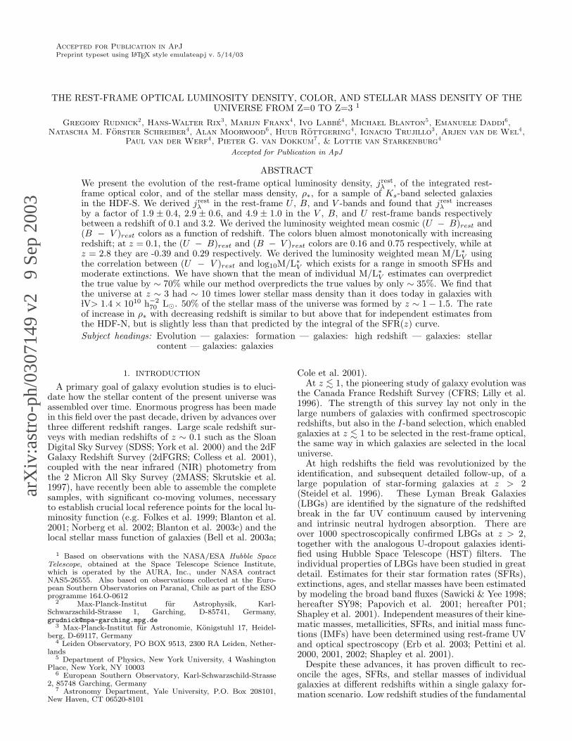
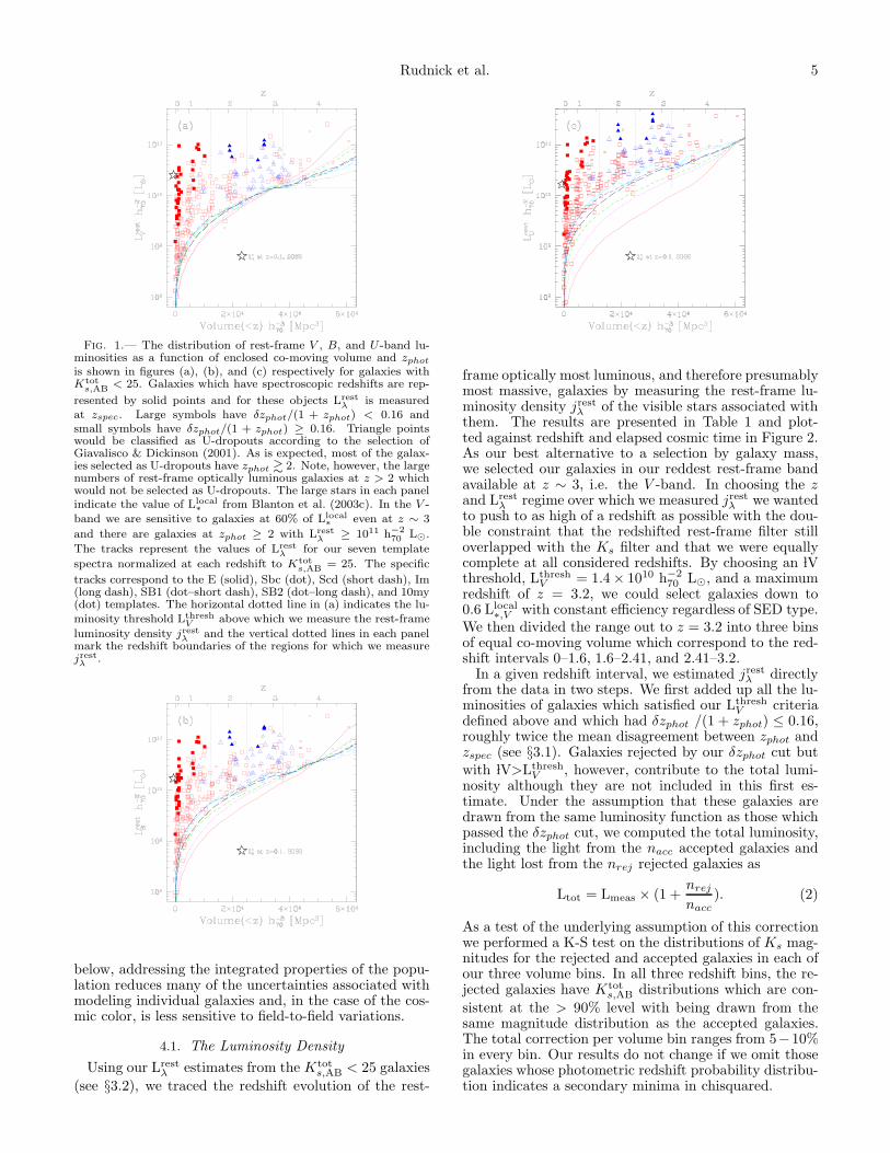
Fig. 1.— The distribution of rest-frame V , B, and U -band lu-minosities as a function of enclosed co-moving volume and zphot

is shown in figures (a), (b), and (c) respectively for galaxies withKtot

s,AB< 25. Galaxies which have spectroscopic redshifts are rep-

resented by solid points and for these objects Lrestλ

is measuredat zspec. Large symbols have δzphot/(1 + zphot) < 0.16 andsmall symbols have δzphot/(1 + zphot) ≥ 0.16. Triangle pointswould be classified as U-dropouts according to the selection ofGiavalisco & Dickinson (2001). As is expected, most of the galax-ies selected as U-dropouts have zphot & 2. Note, however, the largenumbers of rest-frame optically luminous galaxies at z > 2 whichwould not be selected as U-dropouts. The large stars in each panelindicate the value of Llocal

∗ from Blanton et al. (2003c). In the V -band we are sensitive to galaxies at 60% of Llocal

∗ even at z ∼ 3

and there are galaxies at zphot ≥ 2 with Lrestλ

≥ 1011 h−270 L⊙.

The tracks represent the values of Lrestλ

for our seven template

spectra normalized at each redshift to Ktots,AB

= 25. The specific

tracks correspond to the E (solid), Sbc (dot), Scd (short dash), Im(long dash), SB1 (dot–short dash), SB2 (dot–long dash), and 10my(dot) templates. The horizontal dotted line in (a) indicates the lu-minosity threshold Lthresh

Vabove which we measure the rest-frame

luminosity density jrestλ

and the vertical dotted lines in each panelmark the redshift boundaries of the regions for which we measurejrestλ

.

below, addressing the integrated properties of the popu-lation reduces many of the uncertainties associated withmodeling individual galaxies and, in the case of the cos-mic color, is less sensitive to field-to-field variations.

4.1. The Luminosity Density

Using our Lrestλ estimates from the Ktot

s,AB < 25 galaxies

(see §3.2), we traced the redshift evolution of the rest-

frame optically most luminous, and therefore presumablymost massive, galaxies by measuring the rest-frame lu-minosity density jrest

λ of the visible stars associated withthem. The results are presented in Table 1 and plot-ted against redshift and elapsed cosmic time in Figure 2.As our best alternative to a selection by galaxy mass,we selected our galaxies in our reddest rest-frame bandavailable at z ∼ 3, i.e. the V -band. In choosing the zand Lrest

λ regime over which we measured jrestλ we wanted

to push to as high of a redshift as possible with the dou-ble constraint that the redshifted rest-frame filter stilloverlapped with the Ks filter and that we were equallycomplete at all considered redshifts. By choosing an lVthreshold, Lthresh

V = 1.4 × 1010 h−270 L⊙, and a maximum

redshift of z = 3.2, we could select galaxies down to0.6 Llocal

∗,V with constant efficiency regardless of SED type.We then divided the range out to z = 3.2 into three binsof equal co-moving volume which correspond to the red-shift intervals 0–1.6, 1.6–2.41, and 2.41–3.2.

In a given redshift interval, we estimated jrestλ directly

from the data in two steps. We first added up all the lu-minosities of galaxies which satisfied our Lthresh

V criteriadefined above and which had δzphot /(1 + zphot) ≤ 0.16,roughly twice the mean disagreement between zphot andzspec (see §3.1). Galaxies rejected by our δzphot cut butwith lV>Lthresh

V , however, contribute to the total lumi-nosity although they are not included in this first es-timate. Under the assumption that these galaxies aredrawn from the same luminosity function as those whichpassed the δzphot cut, we computed the total luminosity,including the light from the nacc accepted galaxies andthe light lost from the nrej rejected galaxies as

Ltot = Lmeas × (1 +nrej

nacc

). (2)

As a test of the underlying assumption of this correctionwe performed a K-S test on the distributions of Ks mag-nitudes for the rejected and accepted galaxies in each ofour three volume bins. In all three redshift bins, the re-jected galaxies have Ktot

s,AB distributions which are con-

sistent at the > 90% level with being drawn from thesame magnitude distribution as the accepted galaxies.The total correction per volume bin ranges from 5−10%in every bin. Our results do not change if we omit thosegalaxies whose photometric redshift probability distribu-tion indicates a secondary minima in chisquared.


Uncertainties in the luminosity density were computedby bootstrapping from the Ktot

s,AB < 25 subsample. Thismethod does not take cosmic variance into account andthe errors may therefore underestimate the true error,which includes field-to-field variance.

Redshift errors might effect the luminosity density ina systematic way, as they produce a large error in themeasured luminosity. This, combined with a steep lu-minosity function can bias the observed luminosities up-wards, especially at the bright end. This effect can becorrected for in a full determination of the luminosityfunction (e.g., Chen et al. 2003), but for our applicationwe estimated the strength of this effect by Monte-Carlosimulations. When we used the formal redshift errors weobtained a very small bias (6%), if we increase the photo-metric redshift errors in the simulation to be minimallyas large as 0.08 ∗ (1 + z), we still obtain a bias in theluminosity density on the order of 10% or less.

Because we exclude galaxies with faint rest-frame lumi-nosities or low apparent magnitudes, and do not correctfor this incompleteness, our estimates should be regardedas lower limits on the total luminosity density. One pos-sibility for estimating the total luminosity density wouldbe to fit a luminosity function as a function of redshiftand then integrate it over the whole luminosity range.We don’t go faint enough at high redshift, however, totightly constrain the faint-end slope α. Because extrap-olation of jrest

λ to arbitrarily low luminosities is very de-pendent on the value of α, we choose to use this simpleand direct method instead. Including all galaxies withKtot

s,AB < 25 raises the jrestλ values in the z = 0− 1.6 red-

shift bin by 86%, 74%, and 66% in the U , B, and V -bandsrespectively. Likewise, the jrest

λ values would increase by38%, 35%, and 44% for the z = 1.6− 2.41 bin and wouldincrease by 5%, 5%, and 2% for the z = 2.41 − 3.2 bin,again in the U , B, and V -bands respectively.

The dip in the luminosity density in the second lowestredshift bin of the (a) and (b) panels of Figure 2 can betraced to the lack of intrinsically luminous galaxies atz ∼ 1.5 − 2 (§3.2; R01). The dip is not noticeable in theU -band because the galaxies at z ∼ 2 are brighter withrespect to the z < 1.6 galaxies in the U -band than in theV or B-band, i.e. they have bluer (U − B)rest colors and(U − V )rest colors than galaxies at z < 1.6. This lackof rest-frame optically bright galaxies at z ∼ 1.5−2 mayresult from systematics in the zphot estimates, which arepoorly tested in this regime and where the Lyman breakhas not yet entered the U300 filter, or may reflect a truedeficit in the redshift distribution of Ks-band luminousgalaxies (see §3.2).

At z . 1 our survey is limited by its small volume. Forthis reason, we supplement our data with other estimatesof jrest

λ at z . 1.We compared our results with those of the SDSS

as follows. First, we selected SDSS Main samplegalaxies (Strauss et al. 2002) with redshifts in theSDSS Early Data Release (Stoughton et al. 2002)in the EDR sample provided by and described byBlanton et al. (2003a). Using the product kcorrectv1 16 (Blanton et al. 2003b), for each galaxy we fit anoptical SED to the 0.1u0.1g0.1r0.1i0.1z magnitudes, aftercorrecting the magnitudes to z = 0.1 for evolution usingthe results of Blanton et al. (2003c). We projected this

SED onto the UBV filters as described by Bessell (1990)to obtain absolute magnitudes in the UBV Vega-relativesystem. Using the method described in Blanton et al.(2003a) we calculated the maximum volume Vmax withinthe EDR over which each galaxy could have been ob-served, accounting for the survey completeness map andthe flux limit as a function of position. 1/Vmax then rep-resents the number density contribution of each galaxy.From these results we constructed the number densitydistribution of galaxies as a function of color and abso-lute magnitude and the contribution to the uncertain-ties in those densities from Poisson statistics. While thePoisson errors in the SDSS are negligible, cosmic vari-ance does contribute to the uncertainties. For a morerealistic error estimate, we use the fractional errors onthe luminosity density from Blanton et al. (2003c). Forthe SDSS luminosity function, our Lthresh

V encompasses54% of the total light.

In Figure 2 we also show the jrestλ measurements from

the COMBO-17 survey (Wolf et al. 2003). We used acatalog with updated redshifts and 29471 galaxies atz < 0.9, of which 7441 had lV>Lthresh

V (the J2003 cata-log; Wolf, C. private communication). Using this cata-log we calculated jrest

λ in an identical way to how it wascalculated for the FIRES data. We divided the datainto redshift bins of ∆z = 0.2 and counted the lightfrom all galaxies contained within each bin which had lV>Lthresh

V . The formal 68% confidence limits were cal-culated via bootstrapping. In addition, in Figure 2 we in-dicate the rms field-to-field variations between the threespatially distinct COMBO-17 fields. As also pointed outin Wolf et al. (2003), the field-to-field variations domi-nate the error in the COMBO-17 jrest

λ determinations.Bell et al. (2003b) point out that uncertainties in the

absolute calibration and relative calibration of the SDSSand Johnson zeropoints can lead to . 10% errors in thederived rest-frame magnitudes and colors of galaxies. Toaccount for this, we add a 10% error in quadrature withthe formal errors for both the COMBO-17 and SDSSluminosity densities. These are the errors presented inTable 1 and Figure 2.

In Figure 2a we also plot the jrestV value of luminous

LBGs determined by integrating the luminosity functionof Shapley et al. (2001) to Lthresh

V . A direct comparisonbetween our sample and theirs is not entirely straight-forward because the LBGs represent a specific class ofnon-obscured, star forming galaxies at high redshift, se-lected by their rest-frame far UV light. Nonetheless, ourjrestλ determination at z = 2.8 is slightly higher than their

determination at z = 3, indicating either that the HDF-Sis overdense with respect to the area surveyed by Shapleyet al. or that we may have galaxies in our sample whichare not present in the ground-based LBG sample.

D03 have also measured the luminosity density in therest-frame B-band but, because they do not give theirluminosity function parameters except for their lowestredshift bin, it is not possible to overplot their luminositydensity integrated down to our lV limit.

4.1.1. The Evolution of jrestλ

We find progressively stronger luminosity evolutionfrom the V to the U -band: whereas the evolution is quiteweak in V , it is very strong in U . The jrest

λ in our high-est redshift bin is a factor of 1.9 ± 0.4, 2.9 ± 0.6, and

Rudnick et al. 7

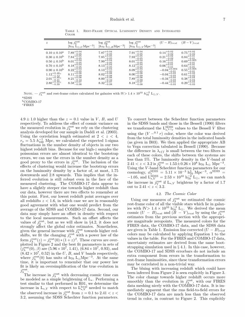
Table 1. Rest-Frame Optical Luminosity Density and IntegratedColor

z log jrestU

log jrestB

log jrestV

(U − B)rest (B − V )rest

[h70 L⊙,U Mpc−3] [h70 L⊙,BMpc−3] [h70 L⊙,V Mpc−3]

0.10 ± 0.10a 7.89+0.04−0.05 7.87+0.04

−0.05 7.91+0.04−0.05 0.14+0.02

−0.02 0.75+0.02−0.02

0.30 ± 0.10b 7.84+0.05−0.05 7.85+0.05

−0.05 7.93+0.05−0.05 0.21+0.02

−0.02 0.84+0.01−0.01

0.50 ± 0.10b 8.01+0.04−0.05 7.99+0.04

−0.05 8.01+0.04−0.05 0.16+0.01

−0.01 0.69+0.005−0.01

0.70 ± 0.10b 8.18+0.04−0.05 8.13+0.04

−0.05 8.12+0.04−0.05 0.06+0.01

−0.01 0.64+0.01−0.01

0.90 ± 0.10b 8.22+0.04−0.05 8.13+0.04

−0.05 8.09+0.04−0.05 −0.04+0.004

−0.01 0.55+0.005−0.01

1.12+0.48−1.12

c 8.11+0.08−0.09 8.02+0.08

−0.08 8.00+0.08−0.09 −0.04+0.03

−0.03 0.61+0.02−0.02

2.01+0.40−0.41

c 8.21+0.08−0.10 8.00+0.08

−0.10 7.89+0.08−0.09 −0.34+0.04

−0.03 0.38+0.04−0.04

2.80+0.40−0.39

c 8.58+0.07−0.08 8.32+0.07

−0.08 8.18+0.07−0.08 −0.44+0.04

−0.03 0.29+0.04−0.03

Note. — jrestλ

and rest-frame colors calculated for galaxies with lV> 1.4 × 1010 h−270 L⊙,V .

aSDSSbCOMBO-17cFIRES

4.9 ± 1.0 higher than the z = 0.1 value in V , B, and Urespectively. To address the effect of cosmic variance onthe measured evolution in jrest

λ we rely on the clusteringanalysis developed for our sample in Daddi et al. (2003).Using the correlation length estimated at 2 < z < 4,ro = 5.5 h−1

100 Mpc, we calculated the expected 1-sigmafluctuations in the number density of objects in our twohighest redshift bins. Because for our high-z samples thepoissonian errors are almost identical to the bootstraperrors, we can use the errors in the number density as agood proxy to the errors in jrest

λ . The inclusion of theeffects of clustering would increase the bootstrap errorson the luminosity density by a factor of, at most, 1.75downwards and 2.8 upwards. This implies that the in-ferred evolution is still robust even in the face of themeasured clustering. The COMBO-17 data appear tohave a slightly steeper rise towards higher redshift thanour data, however there are two effects to remember atthis point. First, our lowest redshift point averages overall redshifts z < 1.6, in which case we are in reasonablygood agreement with what one would predict from theaverage of the SDSS and COMBO-17 data. Second, ourdata may simply have an offset in density with respectto the local measurements. Such an offset affects thevalues of jrest

λ , but as we will show in §4.2, it does notstrongly affect the global color estimates. Nonetheless,given the general increase with jrest

λ towards higher red-shifts, we fit the changing jrest

λ with a power law of theform jrest

λ (z) = jrestλ (0) ∗ (1 + z)β. These curves are over-

plotted in Figure 2 and the best fit parameters in sets of(jrest

λ (0), β) are (5.96×107, 1.41), (6.84×107, 0.93), and(8.42× 107, 0.52) in the U , B, and V bands respectively,where jrest

λ (0) has units of h70 L⊙Mpc−3. At the sametime, it is important to remember that our power lawfit is likely an oversimplification of the true evolution injrestλ .The increase in jrest

λ with decreasing cosmic time canbe modeled as a simple brightening of L∗. Performing atest similar to that performed in R01, we determine theincrease in L∗,V with respect to Llocal

∗,V needed to match

the observed increase in jrestλ from z = 0.1 to 2.41 < z <

3.2, assuming the SDSS Schechter function parameters.

To convert between the Schechter function parametersin the SDSS bands and those in the Bessell (1990) filterswe transformed the LSDSS

∗,0.1rvalues to the Bessell V filter

using the (V −0.1 r) color, where the color was derivedfrom the total luminosity densities in the indicated bands(as given in B03). We then applied the appropriate ABto Vega correction tabulated in Bessell (1990). Becausethe difference in λeff is small between the two filters ineach of these colors, the shifts between the systems areless than 5%. The luminosity density in the V -band at2.41 < z < 3.2 is jrest

V = 1.53±0.26×108 h70 L⊙ Mpc−3.Using the V -band Schechter function parameters for ourcosmology, φSDSS

∗ = 5.11 × 10−3 h370 Mpc−3, αSDSS =

−1.05, and LSDSS∗,V = 2.53 × 1010 h−2

70 L⊙, we can match

the increase in jrestV if L∗,V brightens by a factor of 1.7

out to 2.41 < z < 3.2.

4.2. The Cosmic Color

Using our measures of jrestλ we estimated the cosmic

rest-frame color of all the visible stars which lie in galax-ies with lV> 1.4 × 1010 h−2

70 L⊙. We derived the meancosmic (U − B)rest and (B − V )rest by using the jrest

λestimates from the previous section with the appropri-ate magnitude zeropoints. The measured colors for theFIRES data, the COMBO-17 data, and the SDSS dataare given in Table 1. Emission line corrected (U − B)rest

colors may be calculated by applying Equation 1 to thevalues in the table. For the FIRES and COMBO-17 data,uncertainty estimates are derived from the same boot-strapping simulation used in § 4.1. In this case, however,the COMBO-17 and SDSS errorbars do not include anextra component from errors in the transformation torest-frame luminosities, since these transformation errorsmay be correlated in a non-trivial way.

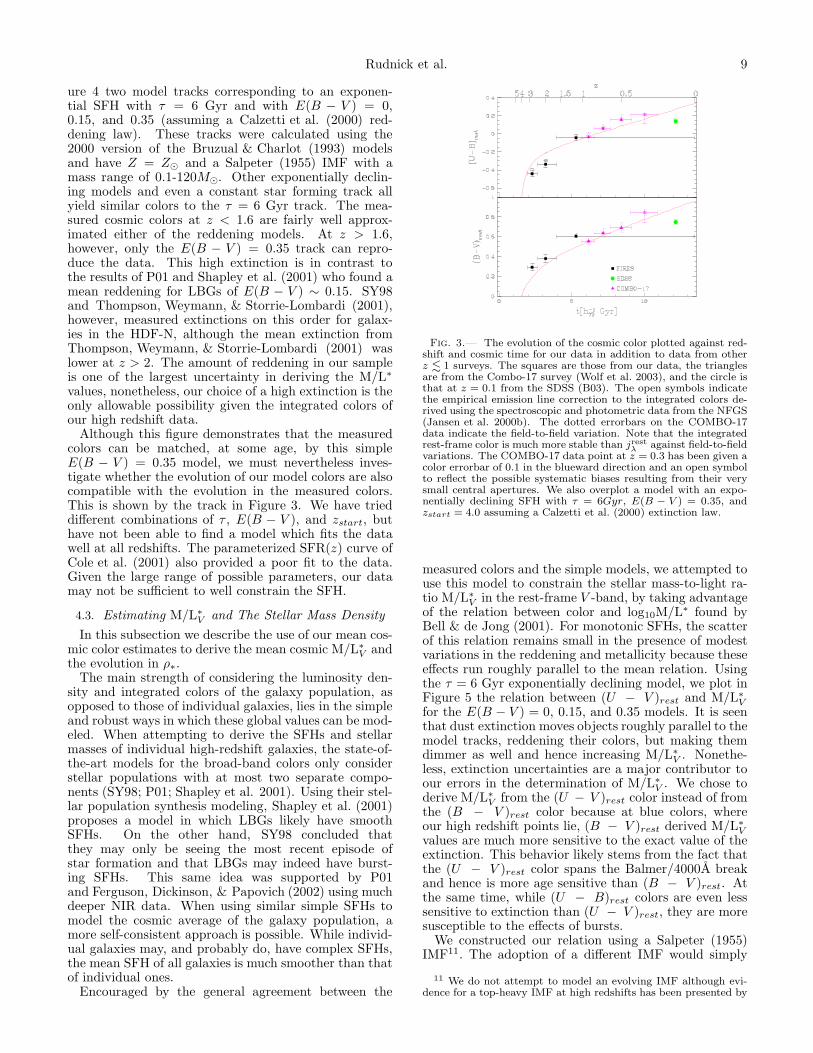
The bluing with increasing redshift which could havebeen inferred from Figure 2 is seen explicitly in Figure 3.The color change towards higher redshift occurs moresmoothly than the evolution in jrest

λ , with our FIRESdata meshing nicely with the COMBO-17 data. It is im-mediately apparent that the rms field-to-field errors forthe COMBO-17 data are much less than the observedtrend in color, in contrast to Figure 2. This explicitly


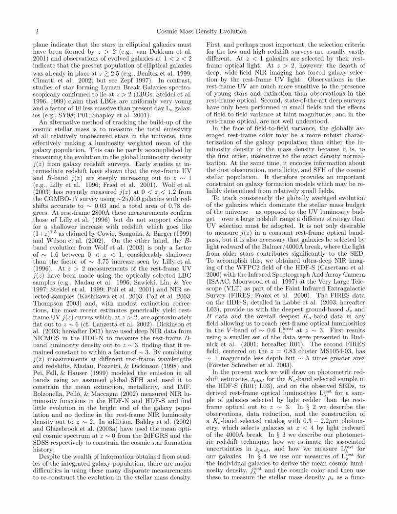
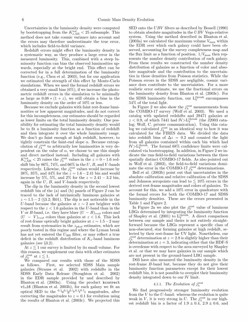
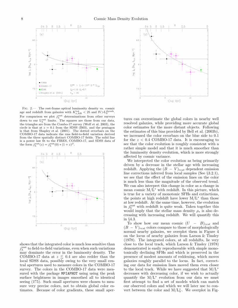
Fig. 2.— The rest-frame optical luminosity density vs. cosmicage and redshift from galaxies with Ktot

s,AB< 25 and lV>Lthresh

V .

For comparison we plot jrestλ

determinations from other surveys

down to our Lrestλ

limits. The squares are those from our data,the triangles are from the Combo-17 survey (Wolf et al. 2003), thecircle is that at z = 0.1 from the SDSS (B03), and the pentagonis that from Shapley et al. (2001). The dotted errorbars on theCOMBO-17 data indicate the rms field-to-field variation derivedfrom the three spatially distinct COMBO-17 fields. The solid lineis a power law fit to the FIRES, COMBO-17, and SDSS data ofthe form jrest

λ(z) = jrest

λ(0) ∗ (1 + z)β .

shows that the integrated color is much less sensitive thanjrestλ to field-to-field variations, even when such variations

may dominate the error in the luminosity density. TheCOMBO-17 data at z . 0.4 are also redder than thelocal SDSS data, possibly owing to the very small cen-tral apertures used to measure colors in the COMBO-17survey. The colors in the COMBO-17 data were mea-sured with the package MPIAPHOT using using the peaksurface brightness in images smoothed all to identicalseeing (1.′′5). Such small apertures were chosen to mea-sure very precise colors, not to obtain global color es-timates. Because of color gradients, these small aper-

tures can overestimate the global colors in nearby wellresolved galaxies, while providing more accurate globalcolor estimates for the more distant objects. Followingthe estimates of this bias provided by Bell et al. (2003b),we increased the color errorbars on the blue side to 0.1for the z < 0.4 COMBO-17 data. It is encouraging tosee that the color evolution is roughly consistent with arather simple model and that it is much smoother thanthe luminosity density evolution, which is more stronglyaffected by cosmic variance.

We interpreted the color evolution as being primarilydriven by a decrease in the stellar age with increasingredshift. Applying the (B − V )rest dependent emissionline corrections inferred from local samples (See §3.2.1),we see that the effect of the emission lines on the coloris much less than the magnitude of the observed trend.We can also interpret this change in color as a change inmean cosmic M/L∗ with redshift. In this picture, whichis true for a variety of monotonic SFHs and extinctions,the points at high redshift have lower M/L∗ than thoseat low redshift. At the same time, however, the evolutionin jrest

V with redshift is quite weak. Taken together thiswould imply that the stellar mass density ρ∗ is also de-creasing with increasing redshift. We will quantify thisin §4.3.

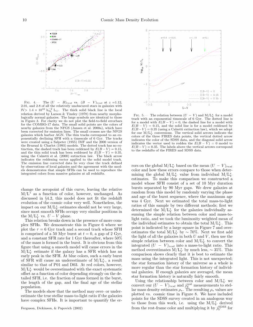
To show how our mean cosmic (U − B)rest and(B − V )rest colors compare to those of morphologicallynormal nearby galaxies, we overplot them in Figure 4on the locus of nearby galaxies from Larson & Tinsley(1978). The integrated colors, at all redshifts, lie veryclose to the local track, which Larson & Tinsley (1978)demonstrated is easily reproduceable with simple mono-tonically declining SFHs and which is preserved in thepresence of modest amounts of reddening, which movesgalaxies roughly parallel to the locus. In fact, correct-ing our data for emission lines moved them even closerto the local track. While we have suggested that M/L∗

decreases with decreasing color, if we wish to actuallyquantify the M/L∗ evolution from our data we mustfirst attempt to find a set of models which can matchour observed colors and which we will later use to con-vert between the color and M/L∗

V . We overplot in Fig-

Rudnick et al. 9

ure 4 two model tracks corresponding to an exponen-tial SFH with τ = 6 Gyr and with E(B − V ) = 0,0.15, and 0.35 (assuming a Calzetti et al. (2000) red-dening law). These tracks were calculated using the2000 version of the Bruzual & Charlot (1993) modelsand have Z = Z⊙ and a Salpeter (1955) IMF with amass range of 0.1-120M⊙. Other exponentially declin-ing models and even a constant star forming track allyield similar colors to the τ = 6 Gyr track. The mea-sured cosmic colors at z < 1.6 are fairly well approx-imated either of the reddening models. At z > 1.6,however, only the E(B − V ) = 0.35 track can repro-duce the data. This high extinction is in contrast tothe results of P01 and Shapley et al. (2001) who found amean reddening for LBGs of E(B − V ) ∼ 0.15. SY98and Thompson, Weymann, & Storrie-Lombardi (2001),however, measured extinctions on this order for galax-ies in the HDF-N, although the mean extinction fromThompson, Weymann, & Storrie-Lombardi (2001) waslower at z > 2. The amount of reddening in our sampleis one of the largest uncertainty in deriving the M/L∗

values, nonetheless, our choice of a high extinction is theonly allowable possibility given the integrated colors ofour high redshift data.

Although this figure demonstrates that the measuredcolors can be matched, at some age, by this simpleE(B − V ) = 0.35 model, we must nevertheless inves-tigate whether the evolution of our model colors are alsocompatible with the evolution in the measured colors.This is shown by the track in Figure 3. We have trieddifferent combinations of τ , E(B − V ), and zstart, buthave not been able to find a model which fits the datawell at all redshifts. The parameterized SFR(z) curve ofCole et al. (2001) also provided a poor fit to the data.Given the large range of possible parameters, our datamay not be sufficient to well constrain the SFH.

4.3. Estimating M/L∗V and The Stellar Mass Density

In this subsection we describe the use of our mean cos-mic color estimates to derive the mean cosmic M/L∗

V andthe evolution in ρ∗.

The main strength of considering the luminosity den-sity and integrated colors of the galaxy population, asopposed to those of individual galaxies, lies in the simpleand robust ways in which these global values can be mod-eled. When attempting to derive the SFHs and stellarmasses of individual high-redshift galaxies, the state-of-the-art models for the broad-band colors only considerstellar populations with at most two separate compo-nents (SY98; P01; Shapley et al. 2001). Using their stel-lar population synthesis modeling, Shapley et al. (2001)proposes a model in which LBGs likely have smoothSFHs. On the other hand, SY98 concluded thatthey may only be seeing the most recent episode ofstar formation and that LBGs may indeed have burst-ing SFHs. This same idea was supported by P01and Ferguson, Dickinson, & Papovich (2002) using muchdeeper NIR data. When using similar simple SFHs tomodel the cosmic average of the galaxy population, amore self-consistent approach is possible. While individ-ual galaxies may, and probably do, have complex SFHs,the mean SFH of all galaxies is much smoother than thatof individual ones.

Encouraged by the general agreement between the

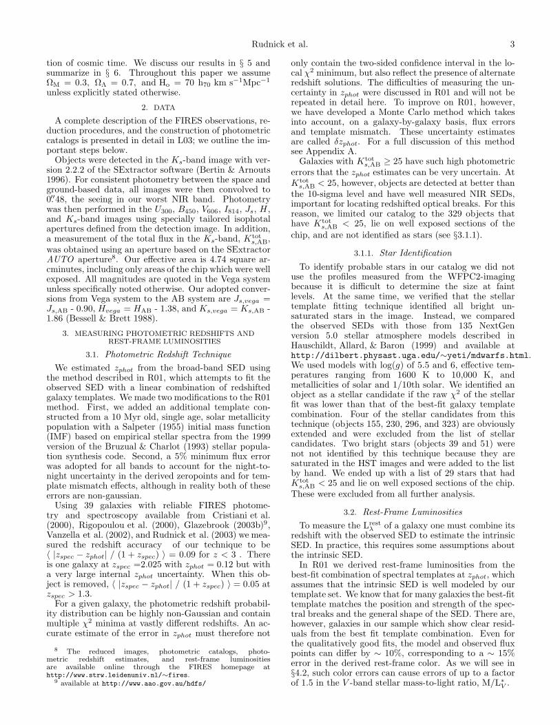
Fig. 3.— The evolution of the cosmic color plotted against red-shift and cosmic time for our data in addition to data from otherz . 1 surveys. The squares are those from our data, the trianglesare from the Combo-17 survey (Wolf et al. 2003), and the circle isthat at z = 0.1 from the SDSS (B03). The open symbols indicatethe empirical emission line correction to the integrated colors de-rived using the spectroscopic and photometric data from the NFGS(Jansen et al. 2000b). The dotted errorbars on the COMBO-17data indicate the field-to-field variation. Note that the integratedrest-frame color is much more stable than jrest

λagainst field-to-field

variations. The COMBO-17 data point at z = 0.3 has been given acolor errorbar of 0.1 in the blueward direction and an open symbolto reflect the possible systematic biases resulting from their verysmall central apertures. We also overplot a model with an expo-nentially declining SFH with τ = 6Gyr, E(B − V ) = 0.35, andzstart = 4.0 assuming a Calzetti et al. (2000) extinction law.

measured colors and the simple models, we attempted touse this model to constrain the stellar mass-to-light ra-tio M/L∗

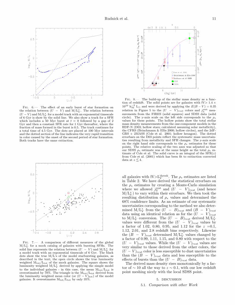
V in the rest-frame V -band, by taking advantageof the relation between color and log10M/L∗ found byBell & de Jong (2001). For monotonic SFHs, the scatterof this relation remains small in the presence of modestvariations in the reddening and metallicity because theseeffects run roughly parallel to the mean relation. Usingthe τ = 6 Gyr exponentially declining model, we plot inFigure 5 the relation between (U − V )rest and M/L∗

V

for the E(B − V ) = 0, 0.15, and 0.35 models. It is seenthat dust extinction moves objects roughly parallel to themodel tracks, reddening their colors, but making themdimmer as well and hence increasing M/L∗

V . Nonethe-less, extinction uncertainties are a major contributor toour errors in the determination of M/L∗

V . We chose toderive M/L∗

V from the (U − V )rest color instead of fromthe (B − V )rest color because at blue colors, whereour high redshift points lie, (B − V )rest derived M/L∗

V

values are much more sensitive to the exact value of theextinction. This behavior likely stems from the fact thatthe (U − V )rest color spans the Balmer/4000A breakand hence is more age sensitive than (B − V )rest. Atthe same time, while (U − B)rest colors are even lesssensitive to extinction than (U − V )rest, they are moresusceptible to the effects of bursts.

We constructed our relation using a Salpeter (1955)IMF11. The adoption of a different IMF would simply

11 We do not attempt to model an evolving IMF although evi-dence for a top-heavy IMF at high redshifts has been presented by


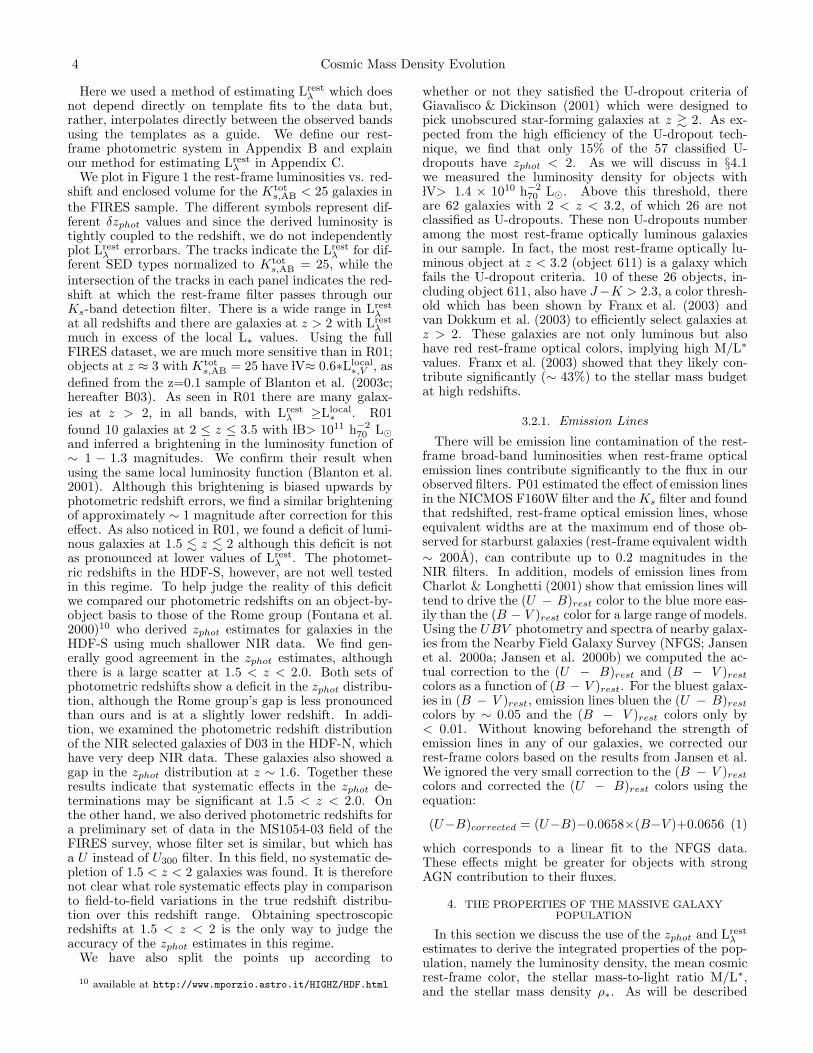
Fig. 4.— The (U − B)rest vs. (B − V )rest at z =1.12,2.01, and 2.8 of all the relatively unobscured stars in galaxies with lV> 1.4 × 1010 h−2

70 L⊙. The thick solid black line is the localrelation derived by Larson & Tinsley (1978) from nearby morpho-logically normal galaxies. The large symbols are identical to thosein Figure 3. For clarity we do not plot the field-to-field errorbarsfor the COMBO-17 data. The small solid points are the colors ofnearby galaxies from the NFGS (Jansen et al. 2000a), which havebeen corrected for emission lines. The small crosses are the NFGSgalaxies which harbor AGN. The thin tracks correspond to an ex-ponentially declining SFH with a timescale of 6 Gyr. The trackswere created using a Salpeter (1955) IMF and the 2000 version ofthe Bruzual & Charlot (1993) models. The dotted track has no ex-tinction, the dashed track has been reddened by E(B −V ) = 0.15,and the thin solid track has been reddened by E(B − V ) = 0.35,using the Calzetti et al. (2000) extinction law. The black arrowindicates the reddening vector applied to the solid model track.The emission line corrected data lie very close the track definedby observations of local galaxies and the agreement with the mod-els demonstrates that simple SFHs can be used to reproduce theintegrated colors from massive galaxies at all redshifts.

change the zeropoint of this curve, leaving the relativeM/L∗ as a function of color, however, unchanged. Asdiscussed in §4.2, this model does not fit the redshiftevolution of the cosmic color very well. Nonetheless, theimpact on our M/L∗

V estimates should not be very large,since most smooth SFHs occupy very similar positions inthe M/L∗

V vs. U − V plane.This relation breaks down in the presence of more com-

plex SFHs. We demonstrate this in Figure 6 where weplot the τ = 6 Gyr track and a second track whose SFHis comprised of a 50 Myr burst at t = 0, a gap of 2 Gyr,and a constant SFR rate for 1 Gyr thereafter, where 50%of the mass is formed in the burst. It is obvious from thisfigure that using a smooth model will cause errors in theM/L∗

V estimate if the galaxy has a SFR which has anearly peak in the SFH. At blue colors, such a early burstof SFR will cause an underestimate of M/L∗

V , a resultsimilar to that of P01 and D03. At red colors, however,M/L∗

V would be overestimated with the exact systematicoffset as a function of color depending strongly on the de-tailed SFH, i.e. the fraction of mass formed in the burst,the length of the gap, and the final age of the stellarpopulation.

The models show that the method may over- or under-estimate the true stellar mass-to-light ratio if the galaxieshave complex SFHs. It is important to quantify the er-

Ferguson, Dickinson, & Papovich (2002)

Fig. 5.— The relation between (U − V ) and M/L∗V

for a modeltrack with an exponential timescale of 6 Gyr. The dotted line isfor a model with E(B − V ) = 0, the dashed line for a model withE(B − V ) = 0.15, and the solid line is for a model reddened byE(B−V ) = 0.35 (using a Calzetti extinction law), which we adoptfor our M/L∗

Vconversions. The vertical solid arrows indicate the

colors of the three FIRES data points, the vertical dotted arrowindicates the color of the SDSS data, and the diagonal solid arrowindicates the vector used to redden the E(B − V ) = 0 model toE(B−V ) = 0.35. The labels above the vertical arrows correspondto the redshifts of the FIRES and SDSS data.

rors on the global M/L∗V based on the mean (U − V )rest

color and how these errors compare to those when deter-mining the global M/L∗

V value from individual M/L∗V

estimates. To make this comparison we constructed amodel whose SFH consist of a set of 10 Myr durationbursts separated by 90 Myr gaps. We drew galaxies atrandom from this model by randomly varying the phaseand age of the burst sequence, where the maximum agewas 4 Gyr. Next we estimated the total mass-to-lightratios of this sample by two different methods; first wedetermined the M/L∗

V for the galaxies individually as-suming the simple relation between color and mass-to-light ratio, and we took the luminosity weighted mean ofthe individual estimates to obtain the total M/L∗

V . Thispoint is indicated by a large square in Figure 7 and over-estimates the total M/L∗

V by ∼ 70%. Next we first addthe light of all the galaxies in both U and V , then use thesimple relation between color and M/L∗

V to convert theintegrated (U − V )rest into a mass-to-light ratio. Thismethod overestimates M/L∗

V by much less, ∼ 35%. Thiscomparison shows clearly that it is best to estimate themass using the integrated light. This is not unexpected;the star formation history of the universe as a whole ismore regular than the star formation history of individ-ual galaxies. If enough galaxies are averaged, the meanstar formation history is naturally fairly smooth.

Using the relationship between color and M/L∗V we

convert our (U − V )rest and jrestV measurements to stel-

lar mass density estimates ρ∗. The resulting ρ∗ values areplotted vs. cosmic time in Figure 8. We have includedpoints for the SDSS survey created in an analogous wayto those from this work, i.e. using the M/L∗

V derivedfrom the rest-frame color and multiplying it by jSDSS

V for

Rudnick et al. 11

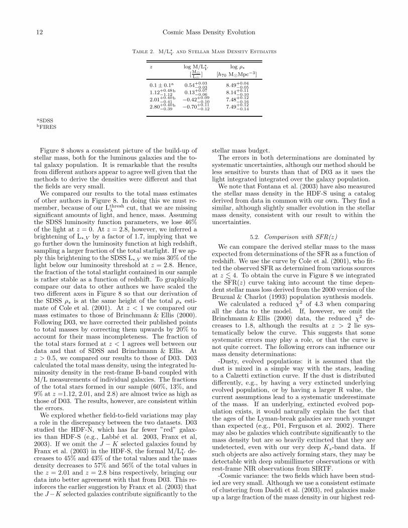
Fig. 6.— The effect of an early burst of star formation onthe relation between (U − V ) and M/L∗

V. The relation between

(U − V ) and M/L∗V for a model track with an exponential timescale

of 6 Gyr is show by the solid line. We also show a track for a SFHwhich includes a 50 Myr burst at t = 0 followed by a gap of 2Gyr and then a constant SFR rate for 1 Gyr thereafter, where thefraction of mass formed in the burst is 0.5. The track continues fora total time of 4.5 Gyr. The dots are placed at 100 Myr intervalsand the dotted section of the line indicates the very rapid transitionin color caused by the onset of the second period of star formation.Both tracks have the same extinction.

Fig. 7.— A comparison of different measures of the globalM/L∗

V for a mock catalog of galaxies with bursting SFHs. Thesolid line represents the relation between (U − V ) and M/L∗

V fora model track with an exponential timescale of 6 Gyr. The blackdots show the true M/L’s of the model starbursting galaxies, asdescribed in the text; the open circle shows the true luminosityweighted Mtot/Ltot of the mock galaxies. The square shows theluminosity weighted M/L∗

V derived by applying the simple modelto the individual galaxies - in this case, the mean Mtot/Ltot isoverestimated by 70%. The triangle is the Mtot/Ltot derived fromthe luminosity weighted mean color (or (U − V )tot) of the modelgalaxies. It overestimates Mtot/Ltot by only 35%.

Fig. 8.— The build-up of the stellar mass density as a func-tion of redshift. The solid points are for galaxies with lV> 1.4 ×

1010 h−270 L⊙ and were derived by applying the E(B − V ) = 0.35

relation in Figure 5 to the (U − V )rest colors and jrestλ

mea-surements from the FIRES (solid squares) and SDSS data (solidcircle). The y-axis scale on the left side corresponds to the ρ∗values for these points. The hollow points show the total stellarmass density measurements from the one-component models in theHDF-N (D03; hollow stars; calculated assuming solar metallicity),the CFRS (Brinchmann & Ellis 2000; hollow circles), and the 2dF-GRS + 2MASS (Cole et al. 2001; hollow hexagon). The dottederrorbars on the D03 points reflect the systematic mass uncertain-ties resulting from metallicity and SFH changes. The y-axis scaleon the right hand side corresponds to the ρ∗ estimates for thesepoints. The relative scaling of the two axes was adjusted so thatour SDSS ρ∗ estimate was at the same height as the total ρ∗ es-timate of Cole et al. The solid curve is an integral of the SFR(z)from Cole et al. (2001) which has been fit to extinction correcteddata at z . 4.

all galaxies with lV>LthreshV . The ρ∗ estimates are listed

in Table 2. We have derived the statistical errorbars onthe ρ∗ estimates by creating a Monte-Carlo simulationwhere we allowed jrest

V and (U − V )rest (and henceM/L∗

V ) to vary within their errorbars. We then took theresulting distribution of ρ∗ values and determined the68% confidence limits. As an estimate of our systematicuncertainties corresponding to the method we also deter-mined M/L∗

V from the (U − B)rest and (B − V )rest

data using an identical relation as for the (U − V )rest

to M/L∗V conversion. The (U − B)rest derived M/L∗

V

values were different from the (U − V )rest values bya factor of 1.02, 0.80, 0.95, and 1.12 for the z =0.1,1.12, 2.01, and 2.8 redshift bins respectively. Likewisethe (B − V )rest determined M/L∗

V values changed bya factor of 0.99, 1.11, 1.15, and 0.80 with respect to the(U − V )rest values. While the (U − V )rest values arevery similar to those derived from the other colors, the(U − V )rest color is less susceptible to dust uncertaintiesthan the (B − V )rest data and less susceptible to theeffects of bursts than the (U − B)rest data.

The derived mass density rises monotonically by a fac-tor of ∼ 10 all the way to z ∼ 0.1, with our low redshiftpoint meshing nicely with the local SDSS point.

5. DISCUSSION

5.1. Comparison with other Work


Table 2. M/L∗V

and Stellar Mass Density Estimates

z log M/L∗V

log ρ∗

[M⊙

L⊙] [h70 M⊙Mpc−3]

0.1 ± 0.1a 0.54+0.03−0.03 8.49+0.04

−0.05

1.12+0.48−1.12

b 0.13+0.07−0.06 8.14+0.11

−0.10

2.01+0.40−0.41

b −0.42+0.09−0.10 7.48+0.12

−0.16

2.80+0.40−0.39

b −0.70+0.11−0.12 7.49+0.12

−0.14

aSDSSbFIRES

Figure 8 shows a consistent picture of the build-up ofstellar mass, both for the luminous galaxies and the to-tal galaxy population. It is remarkable that the resultsfrom different authors appear to agree well given that themethods to derive the densities were different and thatthe fields are very small.

We compared our results to the total mass estimatesof other authors in Figure 8. In doing this we must re-member, because of our Lthresh

λ cut, that we are missingsignificant amounts of light, and hence, mass. Assumingthe SDSS luminosity function parameters, we lose 46%of the light at z = 0. At z = 2.8, however, we inferred abrightening of L∗,V by a factor of 1.7, implying that wego further down the luminosity function at high redshift,sampling a larger fraction of the total starlight. If we ap-ply this brightening to the SDSS L∗,V we miss 30% of thelight below our luminosity threshold at z = 2.8. Hence,the fraction of the total starlight contained in our sampleis rather stable as a function of redshift. To graphicallycompare our data to other authors we have scaled thetwo different axes in Figure 8 so that our derivation ofthe SDSS ρ∗ is at the same height of the total ρ∗ esti-mate of Cole et al. (2001). At z < 1 we compared ourmass estimates to those of Brinchmann & Ellis (2000).Following D03, we have corrected their published pointsto total masses by correcting them upwards by 20% toaccount for their mass incompleteness. The fraction ofthe total stars formed at z < 1 agrees well between ourdata and that of SDSS and Brinchmann & Ellis. Atz > 0.5, we compared our results to those of D03. D03calculated the total mass density, using the integrated lu-minosity density in the rest-frame B-band coupled withM/L measurements of individual galaxies. The fractionsof the total stars formed in our sample (60%, 13%, and9% at z =1.12, 2.01, and 2.8) are almost twice as high asthose of D03. The results, however, are consistent withinthe errors.

We explored whether field-to-field variations may playa role in the discrepancy between the two datasets. D03studied the HDF-N, which has far fewer ”red” galax-ies than HDF-S (e.g., Labbe et al. 2003, Franx et al,2003). If we omit the J − K selected galaxies found byFranx et al. (2003) in the HDF-S, the formal M/L∗

V de-creases to 45% and 43% of the total values and the massdensity decreases to 57% and 56% of the total values inthe z = 2.01 and z = 2.8 bins respectively, bringing ourdata into better agreement with that from D03. This re-inforces the earlier suggestion by Franx et al. (2003) thatthe J−K selected galaxies contribute significantly to the

stellar mass budget.The errors in both determinations are dominated by

systematic uncertainties, although our method should beless sensitive to bursts than that of D03 as it uses thelight integrated integrated over the galaxy population.

We note that Fontana et al. (2003) have also measuredthe stellar mass density in the HDF-S using a catalogderived from data in common with our own. They find asimilar, although slightly smaller evolution in the stellarmass density, consistent with our result to within theuncertainties.

5.2. Comparison with SFR(z)

We can compare the derived stellar mass to the massexpected from determinations of the SFR as a function ofredshift. We use the curve by Cole et al. (2001), who fit-ted the observed SFR as determined from various sourcesat z . 4. To obtain the curve in Figure 8 we integratedthe SFR(z) curve taking into account the time depen-dent stellar mass loss derived from the 2000 version of theBruzual & Charlot (1993) population synthesis models.

We calculated a reduced χ2 of 4.3 when comparingall the data to the model. If, however, we omit theBrinchmann & Ellis (2000) data, the reduced χ2 de-creases to 1.8, although the results at z > 2 lie sys-tematically below the curve. This suggests that somesystematic errors may play a role, or that the curve isnot quite correct. The following errors can influence ourmass density determinations:

-Dusty, evolved populations: it is assumed that thedust is mixed in a simple way with the stars, leadingto a Calzetti extinction curve. If the dust is distributeddifferently, e.g., by having a very extincted underlyingevolved population, or by having a larger R value, thecurrent assumptions lead to a systematic underestimateof the mass. If an underlying, extincted evolved pop-ulation exists, it would naturally explain the fact thatthe ages of the Lyman-break galaxies are much youngerthan expected (e.g., P01, Ferguson et al. 2002). Theremay also be galaxies which contribute significantly to themass density but are so heavily extincted that they areundetected, even with our very deep Ks-band data. Ifsuch objects are also actively forming stars, they may bedetectable with deep submillimeter observations or withrest-frame NIR observations from SIRTF.

-Cosmic variance: the two fields which have been stud-ied are very small. Although we use a consistent estimateof clustering from Daddi et al. (2003), red galaxies makeup a large fraction of the mass density in our highest red-

Rudnick et al. 13

shift bins. Since red galaxies have a very high measuredclustering from z ∼ 1 (e.g., Daddi et al. 2000, Mccarthyet al. 2001) up to possibly z ∼ 3 (Daddi et al. 2003),large uncertainties remain.

-Evolving Initial Mass Function: the light which we seeis mostly coming from the most massive stars present,whereas the stellar mass is dominated by low mass stars.Changes in the IMF would immediately lead to differentmass estimates but if the IMF everywhere is identical (aswe assume), then the relative masses should be robust. Ifthe IMF evolves with redshift, however, systematic errorsin the mass estimate will occur.

-A steep galaxy mass function at high redshift: if muchof the UV light which is used to measure the SFR at highredshifts comes from small galaxies which would fall be-low our rest-frame luminosity threshold then we may bemissing significant amounts of stellar mass. Even themass estimates of D03, which were obtained by integrat-ing the luminosity function, are very sensitive to the faintend extrapolation in their highest redshift bin.

5.3. The Build-up of the Stellar Mass

The primary goal of measuring the stellar mass den-sity is to determine how rapidly the universe assembledits stars. At z ∼ 2 − 3, our results indicate that theuniverse only contained ∼ 10% of the current stellarmass, regardless of whether we refer only to galaxies at lV> 1.4× 1010 h−2

70 L⊙ or whether we use the total massestimates of other authors. The galaxy population inthe HDF-S was rich and diverse at z > 2, but even so itwas far from finished in its build-up of stellar mass. Byz ∼ 1, however, the total mass density had increased toroughly half its local value, indicating that the epoch of1 < z < 2 was an important period in the stellar massbuild-up of the universe.

A successful model of galaxy formation must not onlyexplain our global results, but also reconcile them withthe observed properties of individual galaxies at all red-shifts. For example, a population of galaxies at z ∼1 − 1.5 has been discovered (the so called extremely redobjects or EROs), roughly half of which can be fit withformation redshifts higher than 2.4 (Cimatti et al. 2002)and nearly passive stellar evolution thereafter. Our re-sults, which show that the universe contained only ∼ 10%as many stars at z ∼ 2 − 3 as today would seem to indi-cate that any population of galaxies which formed mostof its mass at z & 2 can at most contribute ∼ 10% of thepresent day stellar mass density. At z ∼ 1 − 1.5, wherethe EROs reside, the universe had assembled roughly halfof its current stars. Therefore, this would imply that theold EROs contribute about ∼ 20% of the mass budgetat their epoch. Likewise, it should be true that a largefraction of the stellar mass at low redshift should residein objects with mass weighted stellar ages correspond-ing to a formation redshift of 1 < z < 2. In support ofthis, Hogg et al. (2002) recently have shown that ∼ 40%of the local luminosity density at 0.7µm, and perhaps∼ 50% of the stellar mass comes from centrally con-centrated, high surface brightness galaxies which havered colors. In agreement with the Hogg et al. (2002)results, Bell et al. (2003a) and Kauffmann et al. (2003)also found that ∼ 50 − 75% of the local stellar massdensity resides in early type galaxies. Hogg et al. (2002)suggest that their red galaxies would have been formed

at z & 1, fully consistent with our results for the rapidmass growth of the universe during this period.

6. SUMMARY & CONCLUSIONS

In this paper we presented the globally averaged rest-frame optical properties of a Ks-band selected sampleof galaxies with z < 3.2 in the HDF-S. Using our verydeep 0.3 − 2.2µm, seven band photometry taken as partof the FIRE Survey we estimated accurate photomet-ric redshifts and rest-frame luminosities for all galaxieswith Ktot

s,AB < 25 and used these luminosity estimates to

measure the rest-frame optical luminosity density jrestλ ,

the globally averaged rest-frame optical color, and thestellar mass density for all galaxies at z < 3.2 with lV> 1.4 × 1010 h−2

70 L⊙. By selecting galaxies in therest-frame V -band, we selected them in a way much lessbiased by star formation and dust than the traditionalselection in the rest-frame UV and much closer to a se-lection by stellar mass.

We have shown that jrestλ in all three bands rises out

to z ∼ 3 by factors of 4.9±1.0, 2.9±0.6, and 1.9±0.4 inthe U , B, and V -bands respectively. Modeling this in-crease in jrest

λ as an increase in L∗ of the local luminosityfunction, we derive that L∗ must have brightened by afactor of 1.7 in the rest-frame V -band.

Using our jrestλ estimates we calculate the (U − B)rest

and (B − V )rest colors of all the visible stars in galaxieswith lV> 1.4×1010 h−2

70 L⊙. Using the COMBO-17 datawe have shown that the mean color is much less sensitiveto density fluctuations and field-to-field variations thaneither jrest

λ or ρ∗. Because of their stability, integratedcolor measurements are ideal for constraining galaxy evo-lution models. The luminosity weighted mean colors lieclose to the locus of morphologically normal local galaxycolors defined by Larson & Tinsley (1978). The meancolors monotonically bluen with increasing redshift by0.55 and 0.46 magnitudes in (U − B)rest and (B − V )rest

respectively out to z ∼ 3. We interpret this color changeprimarily as a change in the mean stellar age. The jointcolors can be roughly matched by simple SFH models ifmodest amounts of reddening (E(B−V ) < 0.35) are ap-plied. In detail, the redshift dependence of (U − B)rest

and (B − V )rest cannot be matched exactly by the sim-ple models, assuming a constant reddening and constantmetallicity. However, we show that the models can stillbe used, even in the face of these small disagreements, torobustly predict the stellar mass-to-light ratios M/L∗

V ofthe integrated cosmic stellar population implied by ourmean rest-frame colors. Variations in the metallicity doesnot strongly affect this relation and it holds for a varietyof smooth SFHs. Even the IMF only affects the nor-malization of this relation, not its slope, assuming thatthe IMF everywhere is the same. The reddening, whichmoves objects roughly along this relation is, however, alarge source of uncertainty. Using these M/L∗

V estimatescoupled with our jrest

λ measurements, we derive the stel-lar mass density ρ∗. These globally averaged estimates ofthe mass density are more reliable than those obtainedfrom the mean of individual galaxies determined usingsmooth SFHs, primarily because the cosmic mean SFHis plausibly much better approximated as being smooth,whereas the SFHs of individual galaxies are almost defi-nitely not.

The stellar mass density, ρ∗, increases monotonically


with increasing cosmic time to come into good agreementwith the other measured values at z . 1 with a factor of∼ 10 increase from z ∼ 3 to the present day. Within therandom uncertainties, our results agree well with thoseof Dickinson, Papovich, Ferguson, & Budavari (2003) inthe HDF-N although our ρ∗ estimates are systematicallyhigher than in the HDF-N. Taken together, the HDF-Nand HDF-S paint a picture in which only ∼ 5 − 15% ofthe present day stellar mass was formed by z ∼ 2. Byz ∼ 1, however, the stellar mass density had increased to∼ 50% of its present value, implying that a large fractionof the stellar mass in the universe today was assembledat 1 < z < 2. Our ρ∗ estimates slightly underpredictthe stellar mass density derived from the integral of theSFR(z) curve at z > 2. A resolution of the small ap-parent discrepancy between different fields, and betweenthe predictions from optical observations will in part re-quire deeper NIR data, to probe further down the massfunction, and wider fields with multiple pointings to con-trol the effects of cosmic variance. In addition, largeamounts of follow-up optical/NIR spectroscopy are re-quired to help control systematic effects in the zphot esti-mates. The 25 square arcminute MS1054-03 data takenas part of FIRES and the ACS/ISAAC GOODS obser-vations of the CDF-S region will be very helpful for suchstudies. Observations with SIRTF will also improve thesituation by accessing the rest-frame NIR, where obscu-ration by dust becomes much less important. Finally,systematics in the M/L∗ estimates may exist because ofa lack of constraint on the faint end slope of the stellarIMF.

We still have to reconcile global measurements of thegalaxy population with what we know about the agesand SFHs of individual galaxies. Our globally deter-mined quantities are quite stable and may serve as robustconstraints on theoretical models, which must correctlymodel the global build-up of stellar mass in addition tomatching the detailed properties of the galaxy popula-tion.

GR would like to thank Jarle Brinchmann and Frankvan den Bosch for useful discussions in the process ofwriting this paper, Christian Wolf for providing addi-tional COMBO-17 data products, and Eric Bell andMarcin Sawicki for giving comments on an earlier ver-sion of the paper. GR would also like to acknowledgethe generous travel support of the Lorentz center andthe Leids Kerkhoven-Bosscha Fonds, and the financialsupport of Sonderforschungsbereich 375.

Funding for the creation and distribution of the SDSSArchive has been provided by the Alfred P. Sloan Foun-dation, the Participating Institutions, the National Aero-nautics and Space Administration, the National Sci-ence Foundation, the U.S. Department of Energy, theJapanese Monbukagakusho, and the Max Planck Soci-ety. The SDSS Web site is http://www.sdss.org/.

The SDSS is managed by the Astrophysical Re-search Consortium (ARC) for the Participating Institu-tions. The Participating Institutions are The Univer-sity of Chicago, Fermilab, the Institute for AdvancedStudy, the Japan Participation Group, The Johns Hop-kins University, Los Alamos National Laboratory, theMax-Planck-Institute for Astronomy (MPIA), the Max-

Planck-Institute for Astrophysics (MPA), New MexicoState University, University of Pittsburgh, PrincetonUniversity, the United States Naval Observatory, and theUniversity of Washington.

http://www.sdss.org/

Rudnick et al. 15

APPENDIX

DERIVATION OF zphot UNCERTAINTY

Given a set of formal flux errors, one way to broaden the redshift confidence interval without degrading the accuracy(as noticed in R01) is to lower the absolute χ2 of every χ2 (z) curve without changing its shape (or the location of theminimum). By scaling up all the flux errors by a constant factor, we can retain the relative weights of the points in theχ2 without changing the best fit redshift and SED, but we do enlarge the redshift interval over which the templatescan satisfactorily fit the flux points. Since we believe the disagreement between zspec and zphot is due to our finite andincomplete template set, this factor should reflect the degree of template mismatch in our sample, i.e., the degree bywhich our models fail to fit the flux points. To estimate this factor we first compute the fractional difference betweenthe model and the data ∆i,j for the jth galaxy in the ith filter,

∆i,j =(fmod

i,j − fdati,j )

fdati,j

(A1)

where fmod are the predicted fluxes of the best-fit template combination and fdat are our actual data. For each galaxywe calculated

∆j =

√

√

√

√

1

Nfilt − 1

Nfilt∑

i=2

∆2i,j (A2)

where we have ignored the contributions of the U -band. While the U -band is important in finding breaks in the SEDs,the exact shapes of the templates are poorly constrained blueward of the rest-frame U -band and the U -data oftendeviates significantly from the best-fit model fluxes.

To determine the mean deviation of all of the flux points from the model ∆dev we then averaged over all galaxiesin our complete FIRES sample with Ktot

s,AB < 22 (for which the systematic zphot errors should dominate over those

resulting from photometric errors) to obtain

∆dev =1

Ngal

Ngal∑

j=1

|∆j | . (A3)

We find ∆dev = 0.08, which includes both random and systematic deviations from the model. We modified theMonte-Carlo simulation of R01 by calculating, for each object j,

⟨

S

N

⟩

j

=

√

√

√

√

∑Nfilt

i=2

(

fi

δfi

)2

Nfilt − 1(A4)

again excluding the U -band. We then scaled the flux errors, for each object, using the following criteria:

δf ′

i =

δfi :

⟨

S

N

⟩

j

≤1

∆dev

δfi∆dev

⟨

S

N

⟩

j

:

⟨

S

N

⟩

j

>1

∆dev

. (A5)

The photometric redshift error probability distribution is computed using the δf ′i ’s. Note that this procedure will not

modify the zphot errors of the objects with low S/N where the zphot errors are dominated by the formal photometricerrors. The resulting probability distribution is highly non-Gaussian and using it we calculate the upper and lower68% confidence limits on the redshift zhi

phot and zlowphot respectively. As a single number which encodes the total range

of acceptable zphot’s, we define δzphot ≡ 0.5 ∗ (zhiphot − zlow

phot).Figure 6 from L03 shows the comparison of zphot to zspec. For these bright galaxies, it is remarkable that our new

photometric redshift errorbars come so close to predicting the difference between zphot and the true value. Somegalaxies have large δzphot values even when the local χ2 minimum is well defined because there is another χ2 minimumof comparable depth that is contained in the 68% redshift confidence limits. There are galaxies with δzphot < 0.05.Some of these are bright low redshift galaxies with large rest-frame optical breaks, which presumably place a strongconstraint on the allowed redshift. Many of these galaxies, however, are faint and the δzphot is unrealistically low.

Even though these faint galaxies have⟨

SN

⟩

j≤ 1

∆dev, they still can have high S/N in the B450 or V606 bandpasses and

hence have steep χ2 curves and small inferred redshift uncertainties. In addition, many of these galaxies have zphot

> 2 and very blue continuum longward of Lyα. The imposed sharp discontinuity in the template SEDs at the onsetof HI absorption causes a very narrow minimum in the χ2 (z) curve, and hence a small δzphot, but likely differs fromthe true shape of the discontinuity because we use the mean opacity values of Madau (1995), neglecting its varianceamong different lines of sight.

It is difficult to develop a scheme for measuring realistic photometric redshift uncertainties over all regimes. Theδzphot estimate derives the zphot uncertainties individually for each object, but can underpredict the uncertainties in


some cases. Compared to the technique of R01 however, a method based completely on the Monte-Carlo techniqueis preferable because it has a straightforwardly computed redshift probability function. This trait is desirable forestimating the errors in the rest-frame luminosities and colors and for this reason we will use δzphot as our uncertaintyestimate in this paper.

REST-FRAME PHOTOMETRIC SYSTEM

To define the rest-frame U , B, and V fluxes we use the filter transmission curves and zeropoints tabulated in Bessell(1990), specifically his UX , B, and V filters. The Bessell zeropoints are given as magnitude offsets with respect to asource which has constant fν and AB = 0. The AB magnitude is defined as

ABν = −2.5 ∗ log10〈fν〉 − 48.58 (B1)

where 〈fν〉 is the flux fν(ν) observed through a filter T (ν) and in units of ergs s−1cm−2Hz−1. Given the zeropointoffset ZPν for a given filter, the Vega magnitude mν is then

mν = ABν − ZPν = −2.5 ∗ log10〈fν〉 − 48.58 − ZPν . (B2)

All of our observed fluxes and rest-frame template fluxes are expressed in fλ. To obtain rest-frame magnitudes in theBessell (1990) system, we must calculate the conversion from fλ to fν for the redshifted rest-frame filter set. The fluxdensity of an SED with fλ(λ) integrated through a given filter with transmission curve T (λ) is

〈fλ〉 =

∫

fλ(λ′)T ′(λ′)dλ′

∫

T ′(λ′)dλ′(B3)

or

〈fν〉 =

∫

fν(ν′)T ′(ν′)dν′

∫

T ′(ν′)dν′. (B4)

Since∫

fλ(λ′)T ′(λ′)dλ′ =

∫

fν(ν′)T ′(ν′)dν′ (B5)

we can convert to 〈fν〉 through

〈fν〉 = 〈fλ〉 ∗

∫

T ′(λ′)dλ′

∫

T ′(ν′)dν′(B6)

and use 〈fν〉 to calculate the apparent rest-frame Vega magnitude through the redshifted filter via Eq. B2.

ESTIMATING REST-FRAME LUMINOSITIES

We derive for any given redshift, the relation between the apparent AB magnitude mλzof a galaxy through a

redshifted rest-frame filter, its observed fluxes 〈fλi,obs〉 in the different filters i, and the colors of the spectral templates.At redshift z, the rest-frame filter with effective wavelength λrest has been shifted to an observed wavelength

λz = λrest × (1 + z) (C1)

and we define the adjacent observed bandpasses with effective wavelengths λl and λh which satisfy

λl < λz ≤ λh. (C2)

We now defineCobs ≡ mobs,λl

− mobs,λh(C3)

where mobs,λland mobs,λh

are the AB magnitudes which correspond to the fluxes 〈fλl,obs〉 and 〈fλh,obs〉 respectively.We then shift each template in wavelength to the redshift z and compute,

Ctempl ≡ mtempl,λl− mtempl,λh

, (C4)

where mtempl,λland mtempl,λh

are the AB magnitudes through the λl and λh observed bandpasses (including theatmospheric and instrument throughputs). We sort the templates by their Ctempl values, Ctempl,a, Ctempl,b, etc., andfind the two templates such that

Ctempl,a ≤ Cobs < Ctempl,b. (C5)

We then define for the ath templateCλl,z,a ≡ mtempl,λl

− mtempl,λz(C6)

where mtempl,λzis the apparent AB magnitude of the redshifted ath template through the redshifted λrest filter.

We point out that because our computations always involve colors, they are not dependent on the actual templatenormalization (which cancels out in the difference). Taking our observed color Cobs and the templates with adjacent“observed” colors Ctempl,a and Ctempl,b, we can interpolate between Cλl,z,a and Cλl,z,b

mobs,λl− mλz

= Cλl,z,a + (Cobs − Ctempl,a) ×

(

Cλl,z,b − Cλl,z,a

Ctempl,b − Ctempl,a

)

(C7)

Rudnick et al. 17

and solve for mλz.

When Cobs lies outside the range of the Ctempl’s, we simply take the two nearest templates in observed Ctempl spaceand extrapolate Eq. C7 to compute mλz

.Equation C7 has the feature that mλz

≈ mobs,λlwhen λz = λl (and hence when Cλl,z,a and Cλl,z,b ≈ 0). While

this method still assumes that the templates are reasonably good approximations to the true shape of the SEDs it hasthe advantage that it does not rely on exact agreement. Galaxies whose observed colors fall outside the range of thetemplates can also be easily flagged. A final advantage of this method is that the uncertainty in mλz

can be readilycalculated from the errors in the observed fluxes.

From mλz, we compute the rest-frame luminosity by applying the K-correction and converting to luminosity units

Lrest

L⊙

= 10−0.4(mλz− M⊙,λrest

− ZPλrest) ×

(

DL

10pc

)2

× (1 + z)−1 × h−2 (C8)

where M⊙,λrestis the absolute magnitude of the sun in the λrest filter (M⊙,U = +5.66, M⊙,B = +5.47, and

M⊙,V = +4.82 in Vega magnitudes; Cox 2000), ZPλrestis the zeropoint in that filter (as in Eq. B2 but expressed at

λ and not at ν), and DL is the distance modulus in parsecs. Following R01, we correct this luminosity by the ratioof the Ktot

s flux to the modified isophotal aperture flux (see L03). This adjustment factor, which accounts both forthe larger size of the total aperture and the aperture correction, changes with apparent magnitude and it ranges from1.23, at 20 <Ktot

s,AB ≤ 24, to 1.69, at 24 <Ktots,AB ≤ 25, and it has an RMS dispersions of 0.17 and 0.49 in the two

magnitude bins respectively.The uncertainty in the derived Lrest

λ has contributions both from the observational flux errors and from the redshiftuncertainty, which causes λz to move with respect to the observed filters. The first effect is estimated by propagatingthe observed flux errors through Eq. C7. As an example, object 531 at zphot =2.20 has Ktot

s,AB = 24.91 and signal-to-noise in the Ks-band of 8.99 and 5.43 in our modified isophotal and total apertures respectively. The resultant errorin lV purely from flux errors is then 26%. At Ktot

s,AB ≈ 24, the typical signal-to-noise in the Ks-band increases to ≈ 13

and ≈ 6.3 in our modified isophotal and total apertures respectively and the error Lrestλ decreases accordingly.

To account for the redshift dependent error in the calculated luminosity, we use the Monte-Carlo simulation describedfirst in R01 and updated in §A. For each Monte-Carlo iteration we calculate the rest-frame luminosities and determinethe 68% confidence limits of the resulting distribution. The 68% confidence limits in Lrest

λ can be highly asymmetric,just as for zphot. For objects with Ktot

s,AB . 25 we find that the contributions to the total Lrestλ error budget are

dominated by the redshift errors rather than by the flux errors.


REFERENCES

Arnouts, S. et al. 2002, MNRAS, 329, 355Baldry, I. K. et al. 2002, ApJ, 569, 582Barger, A. J., Cowie, L. L., & Richards, E. A. 2000, AJ, 119, 2092Bell, E. F. & de Jong, R. S. 2001, ApJ, 550, 212Bell, E. F., McIntosh, D. H., Katz, N., & Weinberg, M. D. 2003,

ApJ, 585, L117Bell, E. F., Wolf, C., Meisenheimer, K., Rix, H.-W., Borch, A.,

Dye, S., Kleinheinrich, K., McIntosh, D. H. 2003, submitted toApJ, astro-ph/0303394

Benitez, N., Broadhurst, T., Bouwens, R., Silk, J., & Rosati, P.1999, ApJ, 515, L65

Bertin, E. & Arnouts, S. 1996, A&AS, 117, 393Bessell, M. S. & Brett, J. M. 1988, PASP, 100, 1134Bessell, M. S. 1990, PASP, 102, 1181Blanton, M. R. et al. 2001, AJ, 121, 2358Blanton, M. R. et al. 2003a, ApJ, in press (astro-ph/0209479)Blanton, M. R. et al. 2003b, AJ, 125, 2348Blanton, M. R. et al. 2003c, ApJ, 592, 819Bolzonella, M., Pello, R., & Maccagni, D. 2002, A&A, 395, 443Brinchmann, J. & Ellis, R. S. 2000, ApJ, 536, L77Bruzual A., G. & Charlot, S. 1993, ApJ, 405, 538Calzetti, D., Armus, L., Bohlin, R. C., Kinney, A. L., Koornneef,

J., & Storchi-Bergmann, T. 2000, ApJ, 533, 682Casertano, S. et al. 2000, AJ, 120, 2747Charlot, S. & Longhetti, M. 2001, MNRAS, 323, 887Chen, H. et al. 2003, ApJ, 586, 745Cimatti, A. et al. 2002, A&A, 381, L68Cohen, J. G., Hogg, D. W., Blandford, R., Cowie, L. L., Hu, E.,

Songaila, A., Shopbell, P., & Richberg, K. 2000, ApJ, 538, 29Cole, S. et al. 2001, MNRAS, 326, 255Coleman, G. D., Wu, C. -C., & Weedman, D. W. 1980, ApJS, 43,

393Colless, M. et al. 2001, MNRAS, 328, 1039Cowie, L. L., Songaila, A., & Barger, A. J. 1999, AJ, 118, 603Cox, A. N. 2000, Allen’s astrophysical quantities, (4th ed. New

York: AIP Press; Springer)Cristiani, S. et al. 2000, A&A, 359, 489Daddi, E., Cimatti, A., Pozzetti, L., Hoekstra, H., Rottgering,

H. J. A., Renzini, A., Zamorani, G., & Mannucci, F. 2000, A&A,361, 535

Daddi, E. et al. 2003, ApJ, 588, 50Dickinson, M., Papovich, C., Ferguson, H. C., & Budavari, T. 2003,

ApJ, 587, 25Eisenhardt, P. & Dickinson, M. 1992, ApJ, 399, L47Erb, D. K., Shapley, A. E., Steidel, C. C., Pettini, M., Adelberger,

K. L., Hunt, M. P., Moorwood, A. F. M., & Cuby, J. 2003, ApJ,591, 101

Ferguson, H. C., Dickinson, M., & Papovich, C. 2002, ApJ, 569,L65

Fernandez-Soto, A., Lanzetta, K. M., & Yahil, A. 1999, ApJ, 513,34

Folkes, S. et al. 1999, MNRAS, 308, 459Forster Schreiber, N. et al. in preparationFontana, A., D’Odorico, S., Poli, F., Giallongo, E., Arnouts, S.,

Cristiani, S., Moorwood, A., & Saracco, P. 2000, AJ, 120, 2206Fontana, A. et al. 2003, ApJ, 594, L9Franx, M. et al. 2003, ApJ, 587, L79Frenk, C. S., White, S. D. M., Efstathiou, G., & Davis, M. 1985,

Nature, 317, 595Fried, J. W. et al. 2001, A&A, 367, 788Fukugita, M., Shimasaku, K., & Ichikawa, T. 1995, PASP, 107, 945Fukugita, M., Ichikawa, T., Gunn, J. E., Doi, M., Shimasaku, K.,

& Schneider, D. P. 1996, AJ, 111, 1748Giavalisco, M., Steidel, C. C., Adelberger, K. L., Dickinson, M. E.,

Pettini, M., & Kellogg, M. 1998, ApJ, 503, 543Giavalisco, M. & Dickinson, M. 2001, ApJ, 550, 177Glazebrook, K. et al. 2003, in preparationGlazebrook, K. et al. 2003, ApJ, 587, 55Hauschildt, P. H., Allard, F., & Baron, E. 1999, ApJ, 512, 377Hogg, D. W. et al. 2002, AJ, 124, 646Huchra, J. P. 1977, ApJ, 217, 928Jansen, R. A., Franx, M., Fabricant, D., & Caldwell, N. 2000, ApJS,

126, 271

Jansen, R. A., Fabricant, D., Franx, M., & Caldwell, N. 2000, ApJS,126, 331

Kashikawa, N. et al. 2003, AJ, 125, 53Kauffmann, G., White, S. D. M., & Guiderdoni, B. 1993, MNRAS,

264, 201Kauffmann, G., Colberg, J. M., Diaferio, A., & White, S. D. M.

1999, MNRAS, 303, 188Kauffmann, G. et al. 2003, MNRAS, 341, 33Kinney, A. L., Calzetti, D., Bohlin, R. C., McQuade, K., Storchi-

Bergmann, T., & Schmitt, H. R. 1996, ApJ, 467, 38Labbe, I. et al. 2003, AJ, 125, 1107Lanzetta, K. M., Yahata, N., Pascarelle, S., Chen, H., & Fernandez-

Soto, A. 2002, ApJ, 570, 492Larson, R. B. & Tinsley, B. M. 1978, ApJ, 219, 46Lilly, S. J., Le Fevre, O., Crampton, D., Hammer, F., & Tresse, L.

1995, ApJ, 455, 50Lilly, S. J., Le Fevre, O., Hammer, F., & Crampton, D. 1996, ApJ,

460, L1Madau, P. 1995, ApJ, 441, 18Madau, P., Pozzetti, L., & Dickinson, M. 1998, ApJ, 498, 106Madau, P., Ferguson, H. C., Dickinson, M. E., Giavalisco, M.,

Steidel, C. C., & Fruchter, A. 1996, MNRAS, 283, 1388McCarthy, P. J. et al. 2001, ApJ, 560, L131Moorwood, A. F. 1997, Proc. SPIE, 2871, 1146Norberg, P. et al. 2002, MNRAS, 336, 907Papovich, C., Dickinson, M., Ferguson, H. C., 2001, ApJ, 559, 620Pei, Y. C., Fall, S. M., & Hauser, M. G. 1999, ApJ, 522, 604Pettini, M., Steidel, C. C., Adelberger, K. L., Dickinson, M., &

Giavalisco, M. 2000, ApJ, 528, 96Pettini, M., Shapley, A. E., Steidel, C. C., Cuby, J., Dickinson, M.,

Moorwood, A. F. M., Adelberger, K. L., & Giavalisco, M. 2001,ApJ, 554, 981

Pettini, M., Rix, S. A., Steidel, C. C., Adelberger, K. L., Hunt,M. P., & Shapley, A. E. 2002, ApJ, 569, 742

Poli, F., Menci, N., Giallongo, E., Fontana, A., Cristiani, S., &D’Odorico, S. 2001, ApJ, 551, L45

Poli, F. et al. 2003, ApJ, 593, L1Rigopoulou, D. et al. 2000, ApJ, 537, L85Rudnick, G. et al. 2003, in preparationRudnick, G., Franx, M., Rix, H.-W., Moorwood, A., Kuijken, K.,

van Starkenburg, L., van der Werf, P., Rottgering, H., Labbe, I.2001, AJ, 122, 2205

Salpeter, E. E. 1955, ApJ, 121, 161Sawicki, M. J., Lin, H., & Yee, H. K. C. 1997, AJ, 113, 1Scalo, J. M. 1986, Fundamentals of Cosmic Physics, 11, 1Schade, D. et al. 1999, ApJ, 525, 31Seaton, M. J. 1979, MNRAS, 187, 73PShapley, A. E., Steidel, C. C., Adelberger, K. L., Dickinson, M.,

Giavalisco, M., & Pettini, M. 2001, ApJ, 562, 95Skrutskie, M. F. et al. 1997, ASSL Vol. 210: The Impact of Large

Scale Near-IR Sky Surveys, 25Somerville, R. S., Primack, J. R., & Faber, S. M. 2001, MNRAS,

320, 504Steidel, C. C., Giavalisco, M., Pettini, M., Dickinson, M., &

Adelberger, K. L. 1996, ApJ, 462, L17Steidel, C. C., Adqelberger, K. L., Giavalisco, M., Dickinson, M.,

& Pettini, M. 1999, ApJ, 519, 1Stoughton, C. et al. 2002, AJ, 123, 485Strauss, M. A. et al. 2002, AJ, 124, 1810Thompson, R. I., Weymann, R. J., & Storrie-Lombardi, L. J. 2001,

ApJ, 546, 694Thompson, R. I. 2003, ApJin press, astro-ph/0306594van de Ven, G., van Dokkum, P. G., & Franx, M. 2003, submitted

to MNRAS, astro-ph/0211566van Dokkum, P. G., Franx, M., Kelson, D. D., & Illingworth, G. D.

2001, ApJ, 553, L39van Dokkum, P. G. et al. 2003, ApJ, 587, L83Vanzella, E. et al. 2002, A&A, 396, 847Williams, R. E. et al. 1996, AJ, 112, 1335Wilson, G., Cowie, L. L., Barger, A. J., & Burke, D. J. 2002, AJ,

124, 1258Wolf, C., Meisenheimer, K., Rix, H.-W., Borch, A., Dye, S., &

Kleinheinrich, M. 2003, A&A, 401, 73York, D. G. et al. 2000, AJ, 120, 1579

http://arXiv.org/abs/astro-ph/0209479

Rudnick et al. 19

Zepf, S. E. 1997, Nature, 390, 377

Documents

The Rest-Frame Optical Luminosity Density, Color, and Stellar Mass Density of the Universe from z = 0 to z = 3