The quantification with FDG as seen by a physician

Nuclear Medicine and Biology 40 (2013) 720–730

Contents lists available at SciVerse ScienceDirect

Nuclear Medicine and Biology

j ourna l homepage: www.e lsev ie r .com/ locate /nucmedb io

The quantification with FDG as seen by a physician

Guido Galli a, Luca Indovina b, Maria Lucia Calcagni a, Luigi Mansi c,⁎, Alessandro Giordano a

a Istituto di Medicina Nucleare, Università Cattolica del Sacro Cuore, Rome, Italyb Dipartimento di Bioimmagini e Scienze Radiologiche, U.O.C. di Fisica Sanitaria, Università Cattolica del Sacro Cuore, Rome, Italyc Dipartimento “Medico Chirurgico di Internistica Clinica e Sperimentale F. MAGRASSI and A. LANZARA”, Medicina Nucleare, Seconda Università di Napoli, Naples, Italy

a r t i c l e i n f o

⁎ Corresponding author. Luigi Mansi, Medicina NuclPiazza Miraglia, 80138, Naples, Italy.

E-mail address: [email protected] (L. Mansi).

0969-8051/$ – see front matter © 2013 Published bhttp://dx.doi.org/10.1016/j.nucmedbio.2013.06.009

Article history:Received 22 April 2013

c.

Received in revised form 8 June 2013Accepted 8 June 2013

Keywords:FDGMetabolic rateCompartmental modelMRgluInflux constantSimplified methods © 2013 Published by Elsevier In

a
1. Premise The goal of this review is to suggest, from the point of view of
esedy's-t/gne.aleicegeeygr

dle

ns

fe

Þ

ds

fn

Although, at the present, in the routine practice, the qualitativanalysis of PET with F-18 Fluoro-deoxyglucose (FDG) remainindispensable and sufficient for clinical purposes, a quantitativapproach may add a significant contribution, when rigorous anreliable. In particular, a quantitative analysis may already be clinicallapplied for indications as a better definition of a specificitythreshold, a more precise prognostic stratification, a correct evaluation of the tumor response and/or of the disease's evolution. The coseffectiveness of this approach may be found in better definindiagnostic and therapeutic strategies. Conversely to be applied ithe clinical practice the method has to be as easy as possiblTherefore the final goal is to apply the simplest method to allowreliable quantitative evaluation. To arrive to this result, applicabusing simplified methods hopefully including also repeated statimages, it is important to validate the new procedures versus thalready verified more rigorous and precise measurements. Beinacceptable in the clinical practice a lower precision with respect to thone required in the research, it is mandatory to avoid problems to thpatient, as those connected with an intra-arterial sampling. Similarlcannot be applied in the routine a procedure too long or requirinovermuch expertise and performing tools, therefore non diffusible foa clinical use.

ottse

eare, Seconda Università di Napoli,

y Elsevier Inc.

physician, which are at the present the simplified methods that coulbe easily and widely applied in the clinical practice for a reliabquantification with FDG.

2. Introduction

We can begin by saying that the quantitative study with PositroEmission Tomography (PET) and F-18-fluoro-deoxyglucose (FDG) hatwo main purposes:

■ A (primary): non-invasively determine local consumption oglucose (MRgluc) in normal and pathological tissues, using thwell-known relationship:

MRglu ¼ Ki⋅Gl

LCð1

where we define Ki as “Influx Constant”, Gl as “Glycemia” anLC as the “Lumped Constant”. In practice, for the reasondiscussed below, LC is reasonably assumed = 1.

■ B (secondary): evaluate pathophysiological changes omechanisms that govern glucose's transport, incorporatioand metabolism.

We define “primary” as the first aim because it better answers tthe needs of a department of “clinical” nuclear medicine. This is noonly for the practical importance of MRglu (example: to monitor ivariations in the course of therapy) but also because MRglu can b

eroey,

e1

g.aes

fe'seG-en4

e,neettisedsd

ner-y

Þ

Þ

ftso

Þ

uc

e

t)fleeeonCf

Þ

ottees,ss,fe

aoaal

en.

ÞiÞ

e:su2

e

dfssisesoyse

721G. Galli et al. / Nuclear Medicine and Biology 40 (2013) 720–730

evaluated fairly accurately using relatively simplemethods.We defin“secondary” as purpose B (even though it may be paramount foresearch) because metabolism can be assessed only partially (up tglucose's phosphorylation). For that, it is necessary to evaluatparameters in a compartmental model, i.e. in a more complex wanon feasible in a routine practice.

3. Reminder

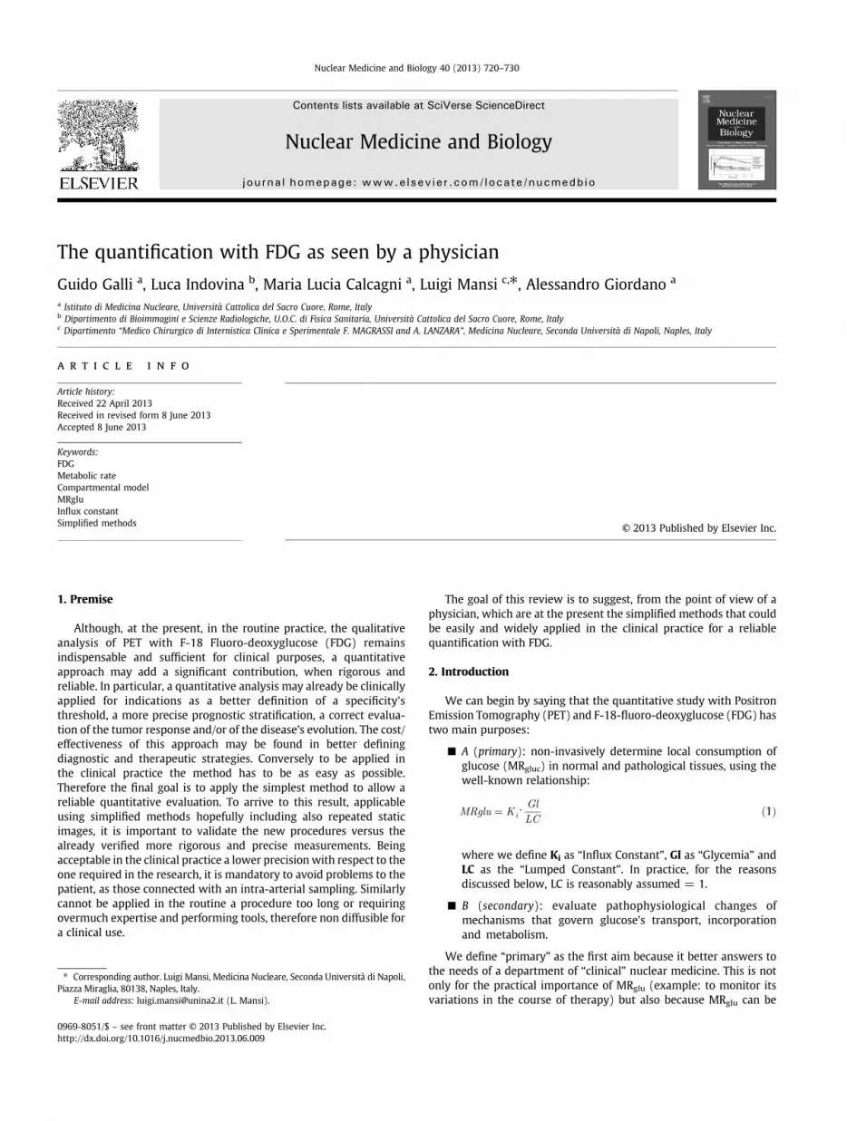
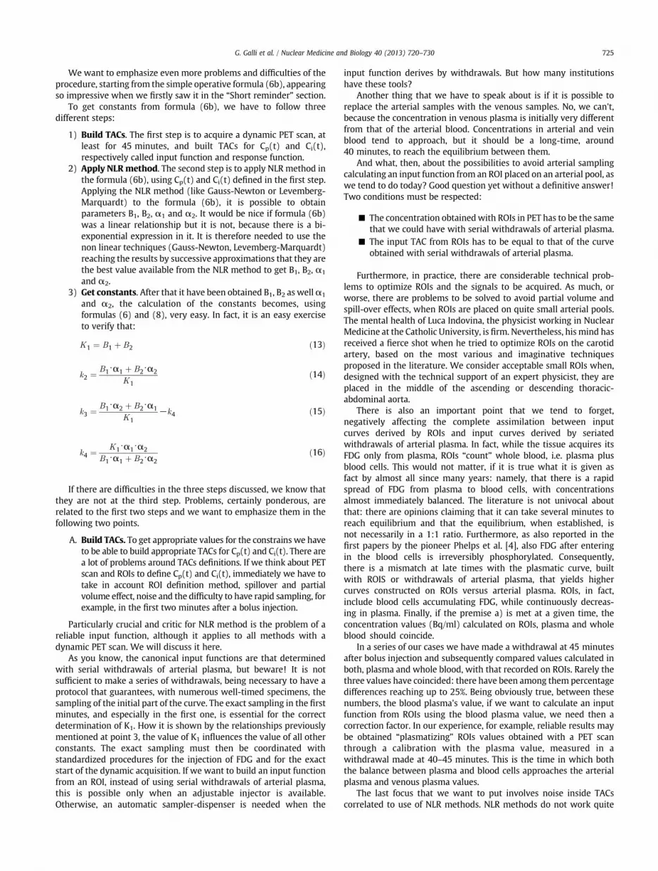
The FDG classic compartmental model can be represented by thscheme reported in Fig. 1. With K as the transfer constant. Krepresents the concentration's fraction (activity per volume unit, e.KBq/ml) of labeled FDG that in the time unit moves from the plasmcompartment into the tissue compartment of free FDG. In thliterature, this constant is usually denoted by a capital K, the otherbeing indicated with a blood/ml of tissue/min (tissue density =1.04 g/ml), while k2, k3 and k4 are rate constants and have units omin−1. The return from the tissue compartment of “free” FDG to thplasma is denoted by k2.k3, which refers to the concentrationfraction of “free” FDG phosphorylated in the unit's time by hexokinasmoving to FDG “bound” compartment. If phosphorylated FDundergoes dephosphorylation by phosphatases, it has to be considered also a constant k4, concerning free FDG which goes back into thsecond compartment. This is not the case for all tissues: as example, icase of a PET performed within one hour after the FDG's injection, kcould be fixed to zero in normal brain, neglecting phosphatassimplifying themodel. Conversely, to perform a correct determinatioof MRglu in tissues with high phosphatase activity, k4 is always to bincluded in the quantitative analysis. It has to be pointed out that thprevious statement, universally accepted for standard studies, is noshared by all the scientists when a cerebral PET scan is performed alonger times, i.e. many hours after FDG's injection. In fact, the brainone of the tissues capable of breaking down glycogen to generatglucose and by necessity can therefore dephosphorylate glucose (anFDG). The difference between normal brain and cerebral tumor(which have low k4) has been the basis for the proposal of a delayeimaging in brain neoplasm [1].

Looking at Fig. 1, defining Cp the time course of the concentratioof FDG in plasma, Cf that of non phosphorylated FDG in the tissuunder examination (f standing for “free”) and Cb that of phosphoylated FDG (b standing for “bound”), the model can be described bthe linear differential equations of first order:

dCf tð Þdt

¼ K1⋅cp tð Þ− k2þ k3ð Þ⋅cf tð Þ þ k4⋅cb tð Þ ð2a

dCb tð Þdt

¼ k3⋅cf tð Þ−k4⋅cb tð Þ ð2b

These differential equations describe instantaneous changes oconcentration in Cf and in Cb as a balance between inputs and outpu(the reader should reflect a little on it). The problem, in our case, is tfind the value of the constants because it is with the relationship:

Ki⋅ ¼k2⋅k3k2 þ k3

ð3

aln,

aÞ

Bound18F-FDG-6P

K1 k3

k4k2

Free18F-FDG

PlasmaVessel

Fig. 1. The FDG compartmental model with a plasma vessel and two tissuecompartments (“free” 18F-FDG and “bound” phosphorylated 18F-FDG-6P).

that is determined Ki, the “Influx Constant”, needed to calculateMRgl

described in formula (1).If we could sample the compartments, i.e. to evaluate the tim

course of concentration in Cp in addition to Cf and Cb, the problemwould be very easily resolved. In fact, the derivatives of Cf (i.e. dCf/dand of Cb (i.e. dCb/dt) can be obtained with simple formulas onumerical calculation: it can just be applied using a common multiplinear regression (through the origin, without intercepts) to get thunknowns, namely the constants. Indeed, it is preferred, to mitigatthe problems caused by the noise of the data, to apply a regression tthe equation that is obtained by the integral of both members iformulas (2a) and (2b). As example, using formula (2a), forwould be:

Cf tð Þ ¼ K1⋅∫cp tð Þ⋅dt− k2þ k3ð Þ⋅∫cf tð Þ⋅dt þ k4⋅∫cb tð Þ⋅dt ð4

The problem, in the case of PET and FDG, is that it is not possible tresolve analytically formulas (2a), (2b) and (4) because it is nopossible to measure Cf and Cb in PET and, in this sense, it is nopossible, using formula (4), to get the unknowns constants that wneed. What we can do in PET to get the unknowns constants, is to usthe sampled signal in a region of interest in tissue that representusing the FDG compartmental model theory, the sum of Cf and Cb plua small quota of FDG that it is in the intratissue blood vesseldecreasing over time. We indicate the sampled signal in a region ointerest in tissue with Ci. We can define Ci as the total ResponsFunction (RF) for the region of interest in the tissue.

So… let's focus on the problem.We have Ci, the sampled signal inregion of interest in the tissue acquired in a PET scan, and we have tget the unknowns constants using it. To do it, we have to look formathematical description of the sampled Ci, using the compartmenttheory and using formulas (2a) and (2b).

Omitting in this paper the mathematical process regarding howyou can reach formula (5), it is known that formula (5) is thmathematical description of the sampled Ci, obtained as the solutioof equations (2a) and (2b) for an instantaneous bolus injection of FDG

Ci tð Þ ¼ K1

α2−α1⋅ k3 þ k4−α1ð Þ⋅ exp −α1⋅tð Þ þ α2−k3−k4ð Þ⋅ exp −α2⋅tð Þh

ð5

The exponents in formula (5), α1 and α2, are related to thconstants K1, k2, k3 and k4 and are derived from themexponents and constants are linked by mathematical relationshipthat allow switching from one to the other and vice versa. If yoget Ci with a PET scan, it is possible to get values of α1 and αand from them it is possible to get the unknowns constants, likwe need.

The expression in the second member in formula (5) is calleImpulse Response Function, IRF, and describes the time course othe concentration in the tissue, if the activity of the labeled FDG waintroduced instantly, at time 0, not followed by other activitie(Dirac pulse), it is also called the Transfer function, TF, and itexpressed in fractions of the unit because it is supposed that thactivity introduced as an impulse is unitary (= 1). In reality, it doenot happen in this way, because the tracer arrives continuously tthe tissue, carried by the plasma, at a concentration (Cp) initialldetermined by the injected activity and which gradually decreaseover time. Take into account that tracers arrive continuously to thtissue, Ci(t), the Response Function (RF) for the compartmentmodel, has to be obtained with a mathematical convolutiobetween TF and the actual course of the plasma concentrationCp(t), obtaining:

C i tð Þ¼ K1

α2−α1⋅ k3þk4−α1ð Þ⋅exp −α1⋅tð Þþ α2−k3−k4ð Þ⋅ exp −α2⋅tð ÞÞh i

⊗Cp tð Þ þ Vb⋅Cp tð Þ ð6

rt

Þ

-eysalayeg

oenny

),nhneni-eloest

ree)

sxoo,re

as-ddts

n

Þ

e-thfa4seaefeh

etisre

yeeelfisef

isterefgy,

e

isise:ef

722 G. Galli et al. / Nuclear Medicine and Biology 40 (2013) 720–730

or, if we define two new variables, B1 and B2, just to write in a showay formula (6a), we have:

Ci tð Þ ¼ B1⋅ exp−α1⋅tð Þ þ B2⋅ exp

−α2⋅tð ÞÞh i

⊗Cp tð Þ þVb⋅Cp tð Þ ð6b

where ∅ indicates the convolution operation and Vb · Cp represents the portion of FDG in the blood that circulates within thtissue. We added Vb · Cp in formula (6a) and (6b) as theorrequests. Measuring Ci, often, in the calculations, to give us a lescomplex problem, the quota of FDG that it is in the interstitiblood vessels is neglected or, alternatively, it is assigned to Vb

conventional value, considered plausible, to give us an easier wato reach the solution, i.e., to get the unknown constants. On thother hand this assumption may result in an error when studyinhighly perfused tissues.

Ok. Now we know that, solving equation (6b), it is possible tget, at first B1, B2, α1 and α2, and, secondarily, from them, thunknown constants, including also the derived Influx constant iformula (3) and the correlated local consumption of glucose iformula (1) … but there is one more difficult discussion, especiallfor a physician.

The unknown constants of the function reported in formula (6alinearly correlated to parameters B1, B2, α1 and α2 iformula (6b), cannot be obtained, as it would be desirable, witthe usual multiple linear regression, since the function is nolinear, given the presence of exponentials. We must thereformake use of non-linear regression techniques to get the unknowconstants. To apply the linear regression, limitations and simplfication must be accepted. As example, Patlak's method (sebelow) requires giving the determination of the individuaconstants and, as first approximation, accepts that k4 is fixed tzero. As an alternative, it is needed to apply artifices, such as th“decomposition of compartments” in the method of Blomqvi(see below).

Using formula (6a) or linear regression methods like Patlak oBlomqvist, it has to be clear that the operator has to collect two TimActivity Curves (TACs) to describe, during the scan time in PET, thactivity concentration (Bq/ml), at any time, in the blood vessel (Cpand in the tissue of interest (Ci).

In the following pages, in the description of the various methodused to quantify MRglu, we will not always refer to the compleformula (6a) reported in this section, which has been utilized tclarify the general aspects of the issue. Instead, we shall refer t“operational formulas” that represent a derivation, mostly simplifiedof the general ones: they are those used in practice and then those fowhich are more interesting, from a clinical point of view, to sepossibilities, difficulties and limitations.

Given the above, let's look at the various methods alonglogical-historical track and try to highlight the connectionbetween them. The first used approach has been the autoradiographic method, the prototype of the “static methods”, so callebecause based on a single scan. They have to be distinguishefrom the “dynamic methods”, based on a series of measuremenacquired in a PET scan over time.

dnsd-l

alr]ye

les;y

4. Autoradiographic method

It is precisely based on the three compartment model showein Fig. 1 and used by Sokoloff to study glucose metabolism ithe brains of normal albino rats n 1977 [2]. This model is thuvalid for the normal brain but, afterwards, has been extende(without much critical evaluation) to other tissues and considered valid even in pathological situations. The operationa

formula that allows in the autoradiographic method to obtaiMRglu is:

MRglu ¼Gl Ci Tð Þ−K1⋅ exp − k2þk3ð Þ⋅Tð Þ⋅∫

T

0

Cp tð Þ⋅ exp k2þk3ð Þ⋅t⋅dt" #

LC⋅ ∫T

0

Cp tð Þ⋅dt− exp − k2þk3ð Þ⋅Tð Þ⋅∫T

0

Cp tð Þ⋅ exp k2þk3ð Þ⋅t⋅dt" # ð9

where Gl is the “Glycemia”, LC the “Lumped constant”, Ci(T) thintegral of FDG concentration (integral of: free + bound phosphorylated) at time T and Cp(t) the plasma concentration profiles avarious times. In formula (9), all that follows the “minus” (−), botat the numerator and at the denominator, refers to the amount ofree (non-phosphorylated) FDG. In Sokoloff's article [2], time T iswell-determined time, 45 minutes after the injection of C-1deoxyglucose, in which the rat was decapitated. Then brain's slicewere placed in contact with a film, for the autoradiography: thblackening, which can be quantified reading the film withdensitometer, was proportional to the local concentrations of thtracer in the various structures of the brain. The timing course othe concentration in the blood, Cp(t), needed to calculate thintegral from the beginning (t = 0) to T, was evaluated witseriated samples.

If we look at formula (9), we see that the problem is to get thunknown constants k2 and k3 to obtain, in essence, the exponen(k2 + k3), which appears four times in formula (9). This amountimportant also when using different methods to evaluate MRglu. Afteall, we have already found (k2 + k3) in the relationship used to definthe Influx Constant Ki in formula (3).

Then let's see what the meaning of (k2 + k3) is. The quantit(k2 + k3) is the constant of disappearance, per time unit, of the fre(non-phosphorylated) FDG, which arrived to the tissue. The glucosinstead is present in the blood at a constant rate (or at least: the modassumes that the glycemia does not vary during the period oobservation). Then, it does not disappear from the tissue and itcontinuously renewed remaining at constant concentration. So thFDG constant of the disappearance represents the renewal constant othe non phosphorylated glucose.

As you may recall from your studies at school, the half-lifeobtained by dividing 0.693 (i.e. ln(2)) for the value of the constanof disappearance, (k2 + k3), as we defined it. Take, for example, thvalues of the constants given by Feng et al. [3]. Although this papeis neither recent nor easy to read, it is a good overview of the wholissue of “quantification” in the normal human. A simpler review othe topic, useful for physicians, is quoted in Ref. [4]. So, in Fenarticle, constants are k2 = 0.102, k3 = 0.130 and, consequentiallk2 + k3 = 0 .232 . The hal f - l i f e i s then 0 .693/0 .232 =2.987 minutes. This quantity is called by Sokoloff “Half-life of thprecursor pool”.

Therefore, in less than three minutes, free FDG in the tissuealready reduced by half! If we consider 5 times the half-life (as itmade in radiation protection, in the event of contamination, to b“practically” sure that there is no more contaminant radioactivity) then2.987 × 5 = 14.93 minutes. Less than 15 minutes is thereforsufficient to reduce the free FDG concentration in the tissue (ocourse we are considering the free FDG produced following an initi“impulse” administration) to negligible values. In this sense, at latetimes, 45 minutes or 1 hour, this value will be almost 0! Phelps [5remarks that after only a few minutes about 90% of the tissue activitis in the form of FDG-6-PO4.As we shall see below, on this principle arbased the simplified methods of quantification.

It is important to stress that, under standard physiologicaconditions, to consider rapid and substantial the decrease of the freFDG's tissue concentration helps to validate the simplified methodconversely, during a dynamic/static PET scan, “free” FDG in tissue ma

ots

eee-de

3

e,:

Þ

f

”

e

ness

teg3

isdsfd

g

f-)d

)yf

etoet

e-?tnisto

0,?

Þ

aen

Þ

Þ

nee

llele

eetsals,ndl.ttsisee

radfat-ee,ryne,'srfhr


remain sizeable, due to the ongoing delivery of FDG from blood ttissue. This activity, also if occasionally, could contribute as significanbackground, impacting semi-quantitative or quantitative measuresuch as, respectively, SUV or MRglu.

Let's go back to the Sokoloff's method. Obviously, it cannot btransferred toman as it is (someonemight object to the beheading of thpatient!). Fortunately, PET became clinically available allowing thassessment of the tissue concentration at a single time T (corresponding to that of the scan for imaging, usually performed between 30’ an60’). At that time the method was considered ideal. Therefore thmethod quickly became established because:

• We can enter in the formula (9) the mean values of k1, k2, kconstants predetermined in a reference population. In this casthe Sokoloff formula (9) reduces to the simple operational one

MRglu ¼ Gl

LC⋅ k1⋅k3k2 þ k3

⋅Ci Tð Þ−Cf Tð Þ

Cb Tð Þ ð10

WhereCi(T) is the total FDGconcentration seenby the scan, andCandCb are themeanvalues at timeTof the concentrationsof “freeand“boundmetabolized”(phosphorylated)FDG,calculatedbythmean constants values, from the reference population.

• As predetermined constants for the reference population caalso be used. Constants determined by Sokoloff [6] varying whitand grey matter structures for albino rat, although similar valuehave been reported, as well as in dogs and rats, even in primate(macaque) next to man.

• Although human patient could have individual constants thadeviate from the standard values we have from our referencpopulation, this affects very little the evaluation of MRglu usinformula (9) because even large variation of the constants k2 and kresults could be obtained with formula (10). To demonstrate thbehavior, Sokoloff [6] analyzed the variation of the integrateprecursor pool, as he defined it in his article, with different valueof the sum k2 + k3. In Sokoloff's paper there is clear evidence ohow much flexibility you can have for the constant values k2 ank3, when using the “autoradiographic method.”

• At that time there was commercial software facilitatinthe calculations.

5. Simplified methods

After that, technological advances have allowed the collection odynamic curves, the autoradiographic method has gradually transferred the role of reference system to the Non Linear Regression (NLRmethod (a complex procedure that cannot be certainly includebetween the simplified methods: see below).

At this point, do we have to think that the proposed formula (10from Sokoloff has only historical interest? No, because mansimplified methods, after all, may be considered an application othe autoradiographic method.

We are convinced that simplified approaches are useful, becausthey are the only “practical” way to have Ki and from it a quite righvalue of MRgluc in a department of clinical nuclear medicine. Thighlight it, go back to the Sokoloff operative formula (9) and observthe term e−(k2 + k3) × T, appearing both at the numerator and athe denominator.

Already alerted and knowing that (k2 + k3) is the constant for thdisappearance of free FDG, we ask ourselves: if the initial concentration in tissue was, for example, 1 kBq/ml, which would be at 1 hourDoing the calculation, using again Feng data [3], it will be verified tha1 × e−0.232 × 60 kBq/ml equals to 0.0000009 kBq/ml, i.e. almost 0! Ithe operative Sokoloff's formula (9), the term e−(k2 + k3)T

multiplicative everything that follows the minus sign (−), both athe numerator and at the denominator: if, like it is, it tends t

0 overincreasing t, then all that follows the minus sign tends to bealways at increasing t. What would the formula (9) be when t is lateIt remains that MRglu is determined by:

MRglu ¼ Gl

LC⋅ Ci Tð Þ

∫T

0

Cp tð Þ⋅dt≈ Gl

LC⋅Ki ð10b

because, like reported in formula (21), it is possible, withsimplification discussed in the Patlak method (see below), to writthe following relationship, used frequently as reference formula imost simplified method:

Ci Tð Þ∫T0 CptÞ⋅dt

¼ Ki ð11a

when T is at late times. Really, the quantity:

Ci Tð Þ∫T0 CptÞ⋅dt

ð11b

is formerly known as Fractional Uptake Ratio (FUR) and it is only aapproximation of Ki. FUR does not take into account not only the freinterstitial FDG, however small, but even that which circulates in thinterstitial blood vessels.

An approximation is good enough for practical use and asimplified methods are based on this principle: they are valid to thextent that it is valid, as in the autoradiographic method, a singmeasurement of the concentration in the tissue at a late time.

Rhodes et al. [7] were the first to work on a simplification of thoriginal formula, although this possibility was already hinted in thoriginal work by Sokoloff. Their contribution has been very importanalso because they firstly applied the metabolic study in brain gliomain vivo, furthermore confirming the presence of a preferentiglycolysis. Moreover, they realized that in pathological conditionespecially in those with a significant reduction of MRglu (such as istroke), the operational formula (10), that uses pre-determineconstants, performs poorly. Other researchers, such as Hutchins et a[8], have attempted to solve this problem by proposing differenformulas; that is not the case here to examine because it is norelevant from the clinical point of view. The work of Rhodes hainspired other simplified methods based on the same principle. Itinteresting to note that his pivotal paper could find difficulties to baccepted today by some frowning referees, being based on thanalysis of only seven patients.

The various simplified methods differ from each other only fothe way in which the denominator, i.e. the integral of plasmconcentrations in formula (10b), is evaluated. Normally standarfunctions are used to “calibrate” each single case: with a sample owhole blood [9] or else with an early arterial or late venous plasmsampling [10]. In literature, two simplified methods most frequenly cited and, furthermore, compared by various authors with th“reference methods” (such as NLR and/or Patlak), are, for examplthe Sadato [11] and the Hunter [9] methods. It is important, in ouopinion, to have knowledge of these two approaches to eventualladopt them. Those who have tested both of them prefer, igeneral, the Hunter method. Nevertheless, in our experiencrelated to a series of lung cancer, results obtained using Sadatoapproach were almost equivalent to those obtained with Huntemethod, having as further major advantage the lack of need oblood sampling. We will not insist further on the subject, althougwe are convinced of the usefulness of these procedures in nucleamedicine practice.

r,g

Þ

nyye,

Þ

nndnsh,seAey

h

d,ea

d

oreisyte

eyhee

9syd


6. SUV

What has been said about the simplified methods also applies fothat over-simplified index that is the SUV. In the ordinary sense, SUVif we use, as example, the known corrected formula for SUV usinbody weight,

SUV ¼ Ci Tð ÞA0=bw

¼ Ci Tð ÞNF

ð11c

where A0 is the administered Activity and bw is the body weight. Iformula (11c) we considered the ratio administered Activity/bodweight as a normalization factor indicated with NF. It follows, brewriting formula (11c), that Ci(T) = SUV × NF and, if we substitutin formula (11a), Ci(T) with SUV × NF, we have:

Ki ¼SUV ⋅NF∫T0 CptÞ⋅dt

ð12

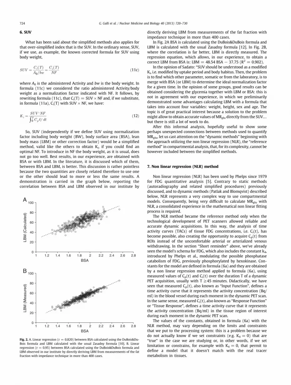
So, SUV (independently if we define SUV using normalizatiofactor including body weight (BW), body surface area (BSA), leabody mass (LBM) or other correction factor) would be a simplifiemethod, valid like the others to obtain Ki, if you could find aoptimal NF. To introduce in NF the body weight, as it is usual, doenot go too well. Best results, in our experience, are obtained witBSA or with LBM. In the literature, it is discussed which of thembetween BSA and LBM, is better. This discussion is rather pointlesbecause the two quantities are closely related therefore to use onor the other should lead to more or less the same results.demonstration is carried in the graph below, reporting thcorrelation between BSA and LBM observed in our institute b

0

20

40

60

80

100

BSA

LBM

(C

alcu

late

d)

0

20

40

60

80

100

1 1.2 1.4 1.6 1.8 2 2.2 2.4 2.6 2.8

BSA1 1.2 1.4 1.6 1.8 2 2.2 2.4 2.6 2.8

LBM

(M

easu

red)

A

B

Fig. 2. A. Linear regression (r = 0.820) between BSA calculated using the DuBois&Du-Bois formula and LBM calculated with the usual Zasadny formula [10]. B. Linearregression (r = 0.95) between BSA calculated using the DuBois&DuBois formula andLBM observed in our institute by directly deriving LBM from measurements of the fatfraction with impedance technique in more than 400 cases.

directly deriving LBM from measurements of the fat fraction witimpedance technique in more than 400 cases.

In Fig. 2A BSA is calculated using the DuBois&DuBois formula anLBM is calculated with the usual Zasadny formula [12]. In Fig. 2Bwhere the correlation is far better, LBM is directly measured. Thregression equation, which allows, in our experience, to obtaincorrect LBM from BSA is: LBM = 48.54 BSA − 37.75 (R2 = 0.902).

In the opinion of Sadato: “SUV should be understood as a modifieKi, i.e. modified by uptake period and body habitus. Then, the problemis to find which other parameter, somatic or from the laboratory, is tmerge with BSA (or LBM) to determine the ideal normalization factofor a given time. In the opinion of some groups, good results can bobtained considering the glycemia together with LBM or BSA: thisnot in agreement with our experience, in which we preliminarildemonstrated some advantages calculating LBM with a formula thatakes into account four variables: weight, height, sex and age. Thtopic is of great practical interest because a solution to the problemmight allow to obtain accurate values ofMRglu directly from the SUV…but there is still a lot of work to do.

After this informal analysis, hopefully useful to show somperhaps unexpected connections between methods used to quantifMRglu, let us cast attention on the “dynamic methods” beginning witthe approach utilizing the non linear regression (NLR), the “referencmethod” in compartmental analysis, that, for its complexity, cannot bhowever included between the simplified methods.

alhg

edes

sy4,e-dgicea/.”

tsst

etseetor

7. Non linear regression (NLR) method

Non linear regression (NLR) has been used by Phelps since 197for FDG quantitative analysis [5]. Contrary to static method(autoradiography and related simplified procedures) previousldiscussed, and to dynamic methods (Patlak and Blomqvist) describebelow, NLR represents a very complex way to use compartmentmodels. Consequently, being very difficult to calculate MRglu witNLR, a consolidated experience in the mathematical non linear fittinprocess is required.

The NLR method became the reference method only when thtechnological development of PET scanners allowed reliable anaccurate dynamic acquisitions. In this way, the analysis of timactivity curves (TACs) of tissue FDG concentrations, i.e. Ci(t), habecome possible, also creating the opportunity to acquire Cp(t) fromROIs instead of the uncomfortable arterial or arterialized venouwithdrawing. In the section “Short reminder” above, we've alreadseen the model's schema for FDG, which also includes the constant kintroduced by Phelps et al., modulating the possible phosphatascatabolism of FDG, previously phosphorylated by hexokinase. Constants for the model are defined in formula (6a) and they are obtaineby a non linear regression method applied to formula (6a), usinmeasured values of Cp(t) and Ci(t) over the duration T of a dynamPET acquisition, usually with T ≥45 minutes. Didactically, we havseen that measured Cp(t), also known as “Input Function”, definestime activity curve that it represents the activity concentration (Bqml) in the blood vessel during each moment in the dynamic PET scanIn the same sense, measured Ci(t), also known as “Response Functionor “Tissue Response”, defines a time activity curve that it representhe activity concentration (Bq/ml) in the tissue region of intereduring each moment in the dynamic PET scan.

The values of the constants, obtained in formula (6a) with thNLR method, may vary depending on the limits and constrainthat we put to the processing system: this is a problem because wdo not actually know if we set constraints (e.g. K4 = 0) that ar“true” in the case we are studying or, in other words, if we selimitation or constrains, for example with K4 = 0, that permit tdefine a model that it doesn't match with the real tracemetabolism in tissues.

egn.e

t),

np.-n)i-et)e1

1

ge

Þ

Þ

Þ

Þ

tee

eeToalr

aa

dtaesttyrhctna,e.e

s

o't,tnd

gs!

ea.e

-rds.rsds,e-

t,tdtsssdstoisegy,ltrt,-ele

sneeetaynahal

se


We want to emphasize even more problems and difficulties of thprocedure, starting from the simple operative formula (6b), appearinso impressive when we firstly saw it in the “Short reminder” sectio

To get constants from formula (6b), we have to follow thredifferent steps:

1) Build TACs. The first step is to acquire a dynamic PET scan, aleast for 45 minutes, and built TACs for Cp(t) and Ci(trespectively called input function and response function.

2) Apply NLR method. The second step is to apply NLR method ithe formula (6b), using Cp(t) and Ci(t) defined in the first steApplying the NLR method (like Gauss-Newton or LevembergMarquardt) to the formula (6b), it is possible to obtaiparameters B1, B2, α1 and α2. It would be nice if formula (6bwas a linear relationship but it is not, because there is a bexponential expression in it. It is therefore needed to use thnon linear techniques (Gauss-Newton, Levemberg-Marquardreaching the results by successive approximations that they arthe best value available from the NLR method to get B1, B2, αand α2.

3) Get constants. After that it have been obtained B1, B2 as wellαand α2, the calculation of the constants becomes, usinformulas (6) and (8), very easy. In fact, it is an easy exercisto verify that:

K1 ¼ B1 þ B2 ð13

k2 ¼ B1⋅α1 þ B2⋅α2

K1ð14

k3 ¼ B1⋅α2 þ B2⋅α1

K1−k4 ð15

k4 ¼ K1⋅α1⋅α2

B1⋅α1 þ B2⋅α2ð16

If there are difficulties in the three steps discussed, we know thathey are not at the third step. Problems, certainly ponderous, arrelated to the first two steps and we want to emphasize them in thfollowing two points.

A. Build TACs. To get appropriate values for the constrains we havto be able to build appropriate TACs for Cp(t) and Ci(t). There ara lot of problems around TACs definitions. If we think about PEscan and ROIs to define Cp(t) and Ci(t), immediately we have ttake in account ROI definition method, spillover and partivolume effect, noise and the difficulty to have rapid sampling, foexample, in the first two minutes after a bolus injection.

Particularly crucial and critic for NLR method is the problem ofreliable input function, although it applies to all methods withdynamic PET scan. We will discuss it here.

As you know, the canonical input functions are that determinewith serial withdrawals of arterial plasma, but beware! It is nosufficient to make a series of withdrawals, being necessary to haveprotocol that guarantees, with numerous well-timed specimens, thsampling of the initial part of the curve. The exact sampling in the firminutes, and especially in the first one, is essential for the correcdetermination of K1. How it is shown by the relationships previouslmentioned at point 3, the value of K1 influences the value of all otheconstants. The exact sampling must then be coordinated witstandardized procedures for the injection of FDG and for the exastart of the dynamic acquisition. If we want to build an input functiofrom an ROI, instead of using serial withdrawals of arterial plasmthis is possible only when an adjustable injector is availablOtherwise, an automatic sampler-dispenser is needed when th

input function derives by withdrawals. But how many institutionhave these tools?

Another thing that we have to speak about is if it is possible treplace the arterial samples with the venous samples. No, we canbecause the concentration in venous plasma is initially very differenfrom that of the arterial blood. Concentrations in arterial and veiblood tend to approach, but it should be a long-time, aroun40 minutes, to reach the equilibrium between them.

And what, then, about the possibilities to avoid arterial samplincalculating an input function from an ROI placed on an arterial pool, awe tend to do today? Good question yet without a definitive answerTwo conditions must be respected:

■ The concentration obtainedwith ROIs in PET has to be the samthat we could have with serial withdrawals of arterial plasm

■ The input TAC from ROIs has to be equal to that of the curvobtained with serial withdrawals of arterial plasma.

Furthermore, in practice, there are considerable technical problems to optimize ROIs and the signals to be acquired. As much, oworse, there are problems to be solved to avoid partial volume anspill-over effects, when ROIs are placed on quite small arterial poolThe mental health of Luca Indovina, the physicist working in NucleaMedicine at the Catholic University, is firm. Nevertheless, hismind hareceived a fierce shot when he tried to optimize ROIs on the carotiartery, based on the most various and imaginative techniqueproposed in the literature. We consider acceptable small ROIs whendesigned with the technical support of an expert physicist, they arplaced in the middle of the ascending or descending thoracicabdominal aorta.

There is also an important point that we tend to forgenegatively affecting the complete assimilation between inpucurves derived by ROIs and input curves derived by seriatewithdrawals of arterial plasma. In fact, while the tissue acquires iFDG only from plasma, ROIs “count” whole blood, i.e. plasma plublood cells. This would not matter, if it is true what it is given afact by almost all since many years: namely, that there is a rapispread of FDG from plasma to blood cells, with concentrationalmost immediately balanced. The literature is not univocal abouthat: there are opinions claiming that it can take several minutes treach equilibrium and that the equilibrium, when established,not necessarily in a 1:1 ratio. Furthermore, as also reported in thfirst papers by the pioneer Phelps et al. [4], also FDG after enterinin the blood cells is irreversibly phosphorylated. Consequentlthere is a mismatch at late times with the plasmatic curve, buiwith ROIS or withdrawals of arterial plasma, that yields highecurves constructed on ROIs versus arterial plasma. ROIs, in facinclude blood cells accumulating FDG, while continuously decreasing in plasma. Finally, if the premise a) is met at a given time, thconcentration values (Bq/ml) calculated on ROIs, plasma and whoblood should coincide.

In a series of our cases we have made a withdrawal at 45 minuteafter bolus injection and subsequently compared values calculated iboth, plasma and whole blood, with that recorded on ROIs. Rarely ththree values have coincided: there have been among them percentagdifferences reaching up to 25%. Being obviously true, between thesnumbers, the blood plasma's value, if we want to calculate an inpufunction from ROIs using the blood plasma value, we need thencorrection factor. In our experience, for example, reliable results mabe obtained “plasmatizing” ROIs values obtained with a PET scathrough a calibration with the plasma value, measured inwithdrawal made at 40–45 minutes. This is the time in which botthe balance between plasma and blood cells approaches the arteriplasma and venous plasma values.

The last focus that we want to put involves noise inside TACcorrelated to use of NLR methods. NLR methods do not work quit

eelstgy

aerichd

ee]alyeyhnsdet

ete?eenrf

aistt

el,tdgis

Þ

Þ

Þ

Þ

ali,nalo

Þ

aae

Þ

ed

Þ

.es.d!disern-g

eity-s.hrddnalsh

eee4


well if noise is present in TACs, as in reality they always are. The mornoise is present the more NLR methods give us noisy results. If thnoise is consistent, even the most sophisticated mathematicatechniques can lead to surprises. Can you remove noise from curvewith the usual smoothing procedures? It is convenient in the inpufunction but you don't do it in the response function. Smoothinprocedures modify the curve altering its shape. Consequently thecould affect parameters to be determined.

Regarding the input function, you should reconstruct curves withmathematical function that it is in full compliance with it. For thblood curve it is usual to use a fit with a tri-exponential function fodata acquired after a bolus injection. This is possible if the dynamacquisition is sufficiently long and the input function is sampled wita sufficient number of points to be fitted, quite well, with a goostatistical program.

B. Using NLR methods. To work well, iterative methods requirstarting values as close as possible to values to bdetermined. We use, usually, constants given by Feng [3and they seem to work. Since, however, they are for normtissues, we are not absolutely certain that results obtained bstudying pathological tissues, as a malignant tumor, arentirely accurate. In particular, results may be not completelcorrect when the processing system offer results with a higor very high coefficient of variation (CV%), especially wheyou work with a lot of noise in the TACs. This event happennot infrequently, so that someone recommends to discarresults with a CV greater than 50%. The results depend, as whave previously said, also from constraints and limitations thaface processing.

We conclude this paragraph with a question: is it possible to usNLR method in a routine practice, having available personnel nofamiliar with NLR methods? In other words, what could be the valuof the NLR method if carried out in a standard nuclear medicine labWe will not answer… to avoid being considered impolite. Let the usof the NLR method to specialized centers. For the large majority of th“standard clinical” nuclear medicine labs is certainly better to learand to be well trained in the following method which is, in ouopinion, the best in the clinical practice to get an appropriate value oMRglu with formula (1).

8. Rutland-Patlak's method

Generally known only by the name of Patlak [13], who gave itgoodmathematical formulation [14], or as Patlak-Gjeddemethod, thprocedure was firstly conceived, but for completely differenpurposes, by Rutland [15,16], who tried to have it recognized, buwithout much success.

The method of Rutland-Patlak is connected to the threconstants K1, k2 and k3 defined for the FDG compartment modewithout k4. Starting from the compartmental model, it is in facpossible to demonstrate that, with a fixed k4 equal to zero anconsidering Cp, under steady state conditions, constant comparinto the strong time dependence factor exp(−(k2 + k3)t), Ci(t)given by the following formula:

Ci tð Þ ¼ K1⋅k3k2 þ k3ð Þ ⋅∫

T

0

Cp tð Þ⋅dt þ K1⋅k2k2 þ k3ð Þ2 ⋅Cp tð Þ ð18

If we define:

VD ¼ K1⋅k2k2 þ k3ð Þ2 ð18a

Ki ¼K1⋅k3k2 þ k3ð Þ ð18b

we can re-write formula (18) as follows:

Ci tð Þ ¼ Ki⋅∫T

0

Cp tð Þ⋅dt þVD⋅Cp tð Þ ð19

For a practical use you can stop here because, using a statisticprogram available for any computer, you can get both VD and Kmaking a multiple linear regression passing through the origi(without intercept). This approach has some advantages of statisticprecision, also avoiding the next step that everyone does, that is tdivide both members by Cp(t) to obtain:

Ci tð ÞCp tð Þ ¼ Ki⋅

∫T

0

Cp tð Þ⋅dt

Cp tð Þ þ VD ð19a

which is nothing more than the usual equation of a straight line: Y =a X + b where a = Ki and b = VD. It is therefore sufficient to drawstraight line on graph paper and see the slope (a, i.e. Ki) or, better, fitstraight line with the linear regression method to have not only thslope Ki, but also VD.

Let us now return to the formula (19a), that can be rewritten:

Ci tð Þ−VD⋅Cp tð Þ

∫T

0

Cp tð Þ⋅dt¼ Ki ð20

Knowing that at late times VD · Cp(t) becomes negligible, becausthe concentration in the plasma is rapidly reduced, it can be assumethat the more t increases the more it is true that:

Ci tð Þ

∫T

0

Cp tð Þ⋅dt¼ Ki ð21

Formula (21) is identical to formula (11a) previously discussedThis formula shows that Rutland-Patlak is, conceptually, a bridgbetween the compartmental model and the simplified methodBut, then, why is it not sufficient to use a simplified method anwhy do we need Patlak? Because Rutland-Patlak method is betterIn fact, in simplified methods, Ci at the numerator is representeby a single value, the one detected at the time T of the scan. This a major cause of error, being possible at time T an inappropriatmeasurement is made, due to conditions as a casually highestatistical noise or a movement of the patient. Conversely, ithe Rutland-Patlak the entire tissue time activity curve contributes to form the numerator, therefore significantly reducincalculation mistakes.

The great advantage of Rutland-Patlak method is that valuof Ki is directly determined with a simple linearization andis not necessary to get each constant, which avoids mandrawbacks presented in NLR method. Furthermore, the procedure is easy to make and very robust in computational termStill the method well tolerates the noise, not being too mucaffected even by small movements of the patient. Another majoadvantage is that administration of FDG is done with a standarintravenous injection, not requiring all the arrangements needefor the NLR method. A great merit of the Patlak method is, iour opinion, that the value of Ki is estimated with statisticprecision much greater than that offered by the NLR method, ait can be seen by comparing the %CV obtained with botmethods.

Then, we must be familiar with the principles and thapplications of the Rutland-Patlak method. A good support can bgiven by reading books and didactic papers, also the old ones, as theditorial published in Nuclear Medicine Communications in 199

ts

oifryf

eeooegistise,eeeneeenee.

sisnal],tegyeeel-

ely×lyee

tetald,d

f

f

rh

e-

Þ

rge

Þ

,

Þ

Þ

Þ

ef

Þ

Þ

Þ

Þ

Þ

).syss,gfe,

C1

PlasmaVessel

C2

p3

P1

p2

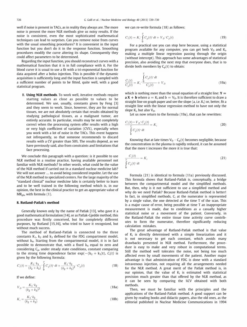
Fig. 3. The Blomqvist schema of the disaggregated compartments for FDG.


[17]. Together with the positive issues we have to learn also limiand conditions of use:

• The method is valid if you can be sure that there is nphosphatase catabolism of the phosphorylated FDG (i.e.K4 = 0). This is true for normal brain tissue, probably also fobrain tumors and perhaps for lung cancer. It is not true for mansub-diaphragmatic organs, such as the liver, and for cancers othe digestive system.

• The determination must be made at the steady-state, i.e. when thconcentration of free FDG in plasma is balanced with that of thfree FDG in the tissue. This does not mean that the twconcentrations have identical values: it means that their ratidoes not change continuing over time. From that moment, if wagain refer to formula (19a), Y has a rectilinear course comparinto X. The linearity should be checked fitting a straight line, whichalso the best way to get the slope Ki. It has to be pointed out thathe name “graphical method” given to the Rutland-Patlak,partially literarily inappropriate, being not completely resolvablas in old times, with graph paper and a ruler. In fact, beforequilibrium, Y has a curvilinear course. Then the fit of Y must bdone starting at a certain time after the introduction of FDG. Thstandardway is to start at 10 minutes after the FDG administratiountil the end of the dynamic phase (typically at 1 hour) but therare theoretical and experimental data reported in the literaturthat may suggest a start at 20–25 minutes. There are also thoswho argue that the best linearity occurs in very late times, betwee45' and 2 hours after the FDG's injection [18]: it will certainly btrue but to do a fitting at that time is not practical for a clinical us

The value of Ki, evaluated with the Rutland-Patlak method, is often lesthan that calculated with the NLR method. Although this discrepancygenerally imputed as a fault to the method, we are not sure that it is. Ifact, if the defect is systematic, how it may be explained that in severcases Ki values are quite similar? In the already cited paper by Feng [3it is clearly evident, comparing figures 12 and 13 in his article, thaMRglu determined with the Rutland-Patlak is identical to thosdetermined with the classic autoradiographic method, also assuminK4 = 0. Our suspicion is therefore that the value of Ki is reduced not ba defect of the Patlak but for the presence of phosphatase activity in thtissue that we are considering. In fact, if K4 is different from 0, the slopof Y decreases, with consequent reduction of Ki. Further studies arneeded to better understand this discrepancy, not clearly acknowedged in the literature papers discussing this issue.

The Rutland-Patlak is also criticized because it provides only thvalue of Ki and not the values of individual constants. This is not entiretrue: the initial input of FDG in the tissue is given by Ci (initial) = K1Cp (initial). If you write K1 = Ci (initial)/Cp (initial) you immediaterealize that the termon the right is nothing but the first point of Y in thRutland-Patlak method! So information on K1, although inaccurate duto the presence of noise, can be given by the Rutland-Patlak.

From the reading of the paragraphs above it is clearly evident thawe consider the Rutland-Patlak as the method to be preferred in thclinical practice in nuclear medicine. This opinion is so strong thawhen we have had the possibility to compare in our experimentdata Ki calculated both with the Rutland-Patlak and by NLR methowe havemade use of the first to assess the reliability of the second annot vice versa.

Now we can move to discuss another interesting method olinearization, the method of Blomqvist [19,20].

9. Blomqvist's method

The method is based on an artifice: the disaggregation ocompartments according to the scheme reported in Fig. 3.

In this model P1, P2 and P3, which can be determined with a linearegression, are related to the k constants from relationships whic

h
allow to get k1, k2 and k3. C1 and C2 do not correspond to tcompartments of free and that phosphorylated FDG. Instead Blomqvist shows that it is their sum that corresponds to them, i.e.:
C1 þ C2 ¼ Cf þ Cb ð22

Blomqvist shows that the disaggregation does not alteproperties and values of the constants, leading to the followinoperational equation, which applies to the model with threconstants (without k4).

Ci tð Þ ¼ P1⋅∫Cp tð Þ⋅dt−p2⋅∫Ci tð Þ⋅dt þ p3⋅∬CP tð Þ⋅dt ð23

Obtained P parameters from a simple multiple linear regressionthe individual constants are calculated from the relations:

K1 ¼ P1 ð24a

k2 ¼ p2−p3=p1 ð24b

k3 ¼ p3=p1 ð24c

and, like we know, Ki is again equal to the known formula (3).The method has been extended also by Feng [3] also to th

determination of K4. It is sufficient to do the double integral both othe curve of the tumor as well as that of the blood. The formula is:

Ci tð Þ ¼ P1⋅∫Cp tð Þ⋅dt þ p2⋅∬CP tð Þ⋅dt þ p3⋅∫Ci tð Þ⋅dtþ p4⋅∬Ci tð Þ⋅dt ð25

and the relationships to find the individual constants become:

K1 ¼ P1 ð26a

k2 ¼ p3− p2=p1ð Þ ð26b

k3 ¼ −p3−k2−k4 ð26c

k4 ¼ −p34=k2 ð26d

Ki, again, is obtained from the constants using the usual formula (3If you make integrals with simple numerical methods (a

trapezoid or Simpson), the realization of the procedure, with anstatistical program making multiple linear regression, is as easy athat of the Rutland-Patlak. Furthermore the Blomqvist offercompared to the “simplified competitors”, the prospect of obtaininindividual constants. In addition, variables are all in the form ointegrals and it is hoped that this will minimize the problem of noisso troublesome for the NLR method. This is very tempting but:

s-

e

e,eat

uf

e2.hdh

2,stisl

al1laoh

rr

-dnt

e

heh

s.ete

gae,Ite.e,s.e1,”,eeddy

et,ee.efdayn

ts

Table 1Constants obtained, in our example (a patient with lung cancer), with four differentmethods.

Method K1 (CV%) k2 (CV%) k3 (CV%) k4 (CV%)

NLR (3 constant) 0.4358 (6) 0.7099 (7) 0.1198 (7) -NLR (4 constant) 0.4949 (11) 0.9026 (24) 0.1439 (21) 0.0040 (100)Blomqvist (3 constant) 0.2913 (1) 0.3358 (4) 0.0870 (12) -Blomqvist (4 constant) 0.2774 (5) 0.2923 (13) 0.0733 (87) −0.0040 (63)

In parenthesis we reported the coefficient of variation, CV%, obtained for eachparameter in each method.


• The reconstruction of the tumor curve with the parameterprovided by Blomqvist method is not always entirely satisfactory, especially in the initial part.

• The value of Ki is generally good and similar to that given by thRutland-Patlak (but then that would be enough!).

• The values for each constant almost always differ, more or littlfrom those given by the NLR method, as recognized by the samBlomqvist: “The correlation for K1 was good but there wassystematic difference between the two methods. The agreemenwas less good for k3 and still worse for k2”.

10. Thinking about methods

To better compare and understand different methods, below yocan see an example from our series also reported in Fig. 4. It is a case oa lung tumor, studied with a dynamic acquisition for 45 minutes.

Fig. 4 shows TACS from blood vessel (input function) and fromtissue region of interest (tissue response).

Proceeding to the determination of Ki in our example with thoutlined methods, we have obtained results reported in Tables 1 and

It is interesting to note that the value of Ki, calculated witlinearized methods (Patlak and Blomqvist) and with simplifiemethods (Sadato, Hunter, Wakita) is close to those calculated witthe most diffuse “reference” method (NLR method).

Always using our example in lung cancer, looking to values k1, kk3 and k4 in Table 1, we can read that, NLR method and Blomqvimethods give very different constants but, in Table 2, value of Ki

similar with all methods. But, then, as regards the individuaconstants, why are the “real ones” so different in Table 1?

To try to answer this question, we have to look at our experimentdata (i.e. the tissue response in Fig. 4). In this way, constants in Tablehave to be able to give us, using each method and the specific formufor each one, the same experimental curve we see in Fig. 4. We tried tdo it, using also the plasmatic curve, obtained, in our example, witROIs in ascending aorta.

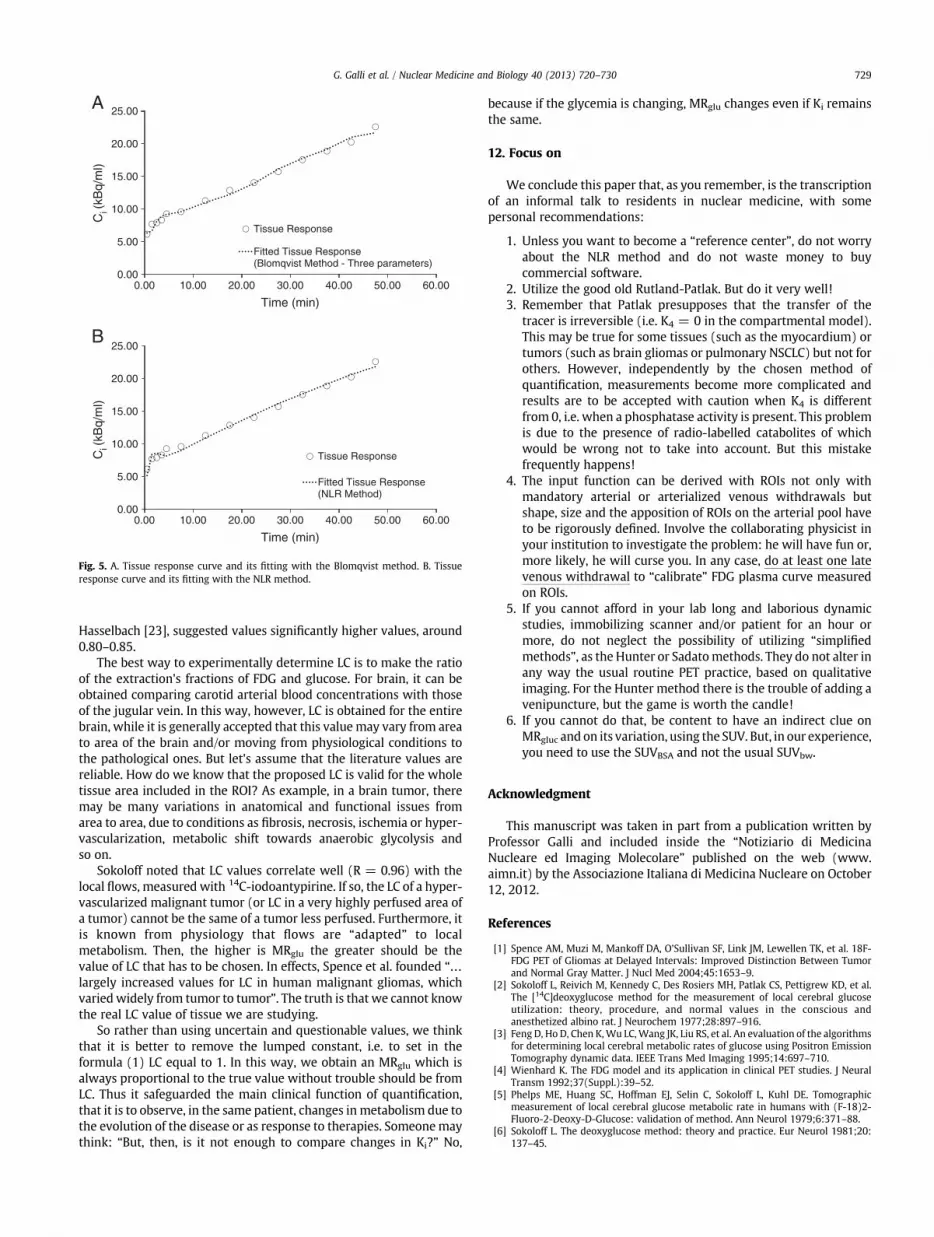
In Fig. 5A and B is reported the rebuilt tissue response for ouexample, using the relative constants obtained from us in Table 1 foBlomqvist (with tree constants) and NLR methods.

As we see, with the 3 constants the Blomqvist method reconstruction in Figure (6A) is satisfactory. The same results are obtaineusing the 4-constant Blomqvist method: the graph is not showbecause it is almost identical to that of Figure 6B for NLR method thait is in good agreement with experimental data.

We insisted with this example because it gives us somconclusions of important practical value:

1) The constants may be different, but Ki made witconstants is little affected by them. This is because thresult depends on the relations between constants whic

0

10

20

30

40

50

60

70

80

0.00 10.00 20.00 30.00 40.00 50.00

Ci (

kBq/

ml)

Time (min)

Tissue Response

Input Function

Fig. 4. Input function and tissue response curve from our series. It is a case of a lungtumor, studied with a dynamic acquisition for 45 minutes.

may exist even if the individual constants differ in the valueIn the known relationship for Ki in formula (3), at thnumerator, the same product can be obtained with differenfactors while at the denominator, the same sum may bcalculated with different addends.

2) The tumor curve can be correctly reconstructed also usindifferent constants. This conclusion better precise limitswidespread belief: that the reconstruction of the tissue curvusing the obtained constants, needs to be check its reliability.is not true: the reconstruction is a “quality control” to be donbut does not guarantee the values of the individual constants

3) It is not appropriate to draw conclusions randomly or, worsclinical inferences from the value of the individual constantWe know that k3, as reported in the literature, is related to thhexokinase activity. If you look again to our example in Tableyou can see that any researchers using PET in a disease “Xprocessing their data with the Blomqvist method would havconcluded: “The disease X does not affect the hexokinasactivity”. Who had done the same thing, using the NLR methoin our example, would instead conclude: “In the patients affectewith X disease the hexokinase activity seems exalted.” A verdifferent conclusion!

4) Is it important to determine the value of each singlconstant? In our opinion, it is a waste of time and efforgiven the uncertainties mentioned above, to make thescalculations in a contest where there is not a lot of experiencAfter all, those who know literature can tell us what decisivclinical progress has been made thanks to the determination othe celebrated k1 and k3 constants? We do not know yet antherefore let us be content to evaluate well only Ki, to havereliable MRgluc. We can leave to researchers the chance to plawith the individual constants waiting for results applicable iclinical routine.

e),frC)d

11. The “Lumped constant”

To finish this paper, we want briefly make few commenconcerning the lumped constant (LC), which, as you recall, it is thratio betweenMRFDG andMRglu. Given the relationship in formula (1it is clear that the value of MRglu depends essentially on the value oLC. Usually values for LC are taken from literature, but these are fafrom unanimous. For normal brain, as example, different values for Lare proposed by three pioneers as Phelps (LC = 0.42), Sokoloff (0.46and Reivich (0.52) [21]. Other researchers, such as Spence [22] an

Table 2Influx constant values obtained in our example (patient with lung cancer) with sevendifferent methods.

NLR(3 constant)

NLR(4 constant)

Blomqvist(3 constant)

Blomqvist(4 constant)

Rutland-Patlak

Hunter Sadato

Ki 0.0629 0.0681 0.0599 0.0556 0.0617 0.0568 0.0620

Linear (Blomqvist and Rutland-Patlak), nonlinear (NLR) and simplified (Hunter andSadato) methods are reported.

d

oeeeaoelee

r-d

er-fitle

h

keis

,oyo,

s

ne

yy

e).rrfdt

he

htenr,ed

icrdnea

ne,

ya.r

F-or

l.sed

sn

al

ic2-

0:

0.00

5.00

10.00

15.00

20.00

25.00

Tissue Response

Fitted Tissue Response(NLR Method)

0.00

5.00

10.00

15.00

20.00

25.00

0.00 10.00 20.00 30.00 40.00 50.00 60.00

Ci (

kBq/

ml)

Ci (

kBq/

ml)

Time (min)

0.00 10.00 20.00 30.00 40.00 50.00 60.00

Time (min)

Tissue Response

Fitted Tissue Response(Blomqvist Method - Three parameters)

A

B

Fig. 5. A. Tissue response curve and its fitting with the Blomqvist method. B. Tissueresponse curve and its fitting with the NLR method.


Hasselbach [23], suggested values significantly higher values, aroun0.80–0.85.

The best way to experimentally determine LC is to make the ratiof the extraction's fractions of FDG and glucose. For brain, it can bobtained comparing carotid arterial blood concentrations with thosof the jugular vein. In this way, however, LC is obtained for the entirbrain, while it is generally accepted that this valuemay vary from areto area of the brain and/or moving from physiological conditions tthe pathological ones. But let's assume that the literature values arreliable. How do we know that the proposed LC is valid for the whotissue area included in the ROI? As example, in a brain tumor, thermay be many variations in anatomical and functional issues fromarea to area, due to conditions as fibrosis, necrosis, ischemia or hypevascularization, metabolic shift towards anaerobic glycolysis anso on.

Sokoloff noted that LC values correlate well (R = 0.96) with thlocal flows, measured with 14C-iodoantypirine. If so, the LC of a hypevascularized malignant tumor (or LC in a very highly perfused area oa tumor) cannot be the same of a tumor less perfused. Furthermore,is known from physiology that flows are “adapted” to locametabolism. Then, the higher is MRglu the greater should be thvalue of LC that has to be chosen. In effects, Spence et al. founded “…

largely increased values for LC in human malignant gliomas, whicvariedwidely from tumor to tumor”. The truth is that we cannot knowthe real LC value of tissue we are studying.

So rather than using uncertain and questionable values, we thinthat it is better to remove the lumped constant, i.e. to set in thformula (1) LC equal to 1. In this way, we obtain an MRglu whichalways proportional to the true value without trouble should be fromLC. Thus it safeguarded the main clinical function of quantificationthat it is to observe, in the same patient, changes in metabolism due tthe evolution of the disease or as response to therapies. Someonemathink: “But, then, is it not enough to compare changes in Ki?” N

because if the glycemia is changing, MRglu changes even if Ki remainthe same.

12. Focus on

We conclude this paper that, as you remember, is the transcriptioof an informal talk to residents in nuclear medicine, with sompersonal recommendations:

1. Unless you want to become a “reference center”, do not worrabout the NLR method and do not waste money to bucommercial software.

2. Utilize the good old Rutland-Patlak. But do it very well!3. Remember that Patlak presupposes that the transfer of th

tracer is irreversible (i.e. K4 = 0 in the compartmental modelThis may be true for some tissues (such as the myocardium) otumors (such as brain gliomas or pulmonary NSCLC) but not foothers. However, independently by the chosen method oquantification, measurements become more complicated anresults are to be accepted with caution when K4 is differenfrom 0, i.e. when a phosphatase activity is present. This problemis due to the presence of radio-labelled catabolites of whicwould be wrong not to take into account. But this mistakfrequently happens!

4. The input function can be derived with ROIs not only witmandatory arterial or arterialized venous withdrawals bushape, size and the apposition of ROIs on the arterial pool havto be rigorously defined. Involve the collaborating physicist iyour institution to investigate the problem: he will have fun omore likely, he will curse you. In any case, do at least one latvenous withdrawal to “calibrate” FDG plasma curve measureon ROIs.

5. If you cannot afford in your lab long and laborious dynamstudies, immobilizing scanner and/or patient for an hour omore, do not neglect the possibility of utilizing “simplifiemethods”, as the Hunter or Sadatomethods. They do not alter iany way the usual routine PET practice, based on qualitativimaging. For the Hunter method there is the trouble of addingvenipuncture, but the game is worth the candle!

6. If you cannot do that, be content to have an indirect clue oMRgluc and on its variation, using the SUV. But, in our experiencyou need to use the SUVBSA and not the usual SUVbw.

Acknowledgment

This manuscript was taken in part from a publication written bProfessor Galli and included inside the “Notiziario di MedicinNucleare ed Imaging Molecolare” published on the web (wwwaimn.it) by the Associazione Italiana di Medicina Nucleare on Octobe12, 2012.

References

[1] Spence AM, Muzi M, Mankoff DA, O’Sullivan SF, Link JM, Lewellen TK, et al. 18FDG PET of Gliomas at Delayed Intervals: Improved Distinction Between Tumand Normal Gray Matter. J Nucl Med 2004;45:1653–9.

[2] Sokoloff L, Reivich M, Kennedy C, Des Rosiers MH, Patlak CS, Pettigrew KD, et aThe [14C]deoxyglucose method for the measurement of local cerebral glucoutilization: theory, procedure, and normal values in the conscious ananesthetized albino rat. J Neurochem 1977;28:897–916.

[3] Feng D, Ho D, Chen K,Wu LC,Wang JK, Liu RS, et al. An evaluation of the algorithmfor determining local cerebral metabolic rates of glucose using Positron EmissioTomography dynamic data. IEEE Trans Med Imaging 1995;14:697–710.

[4] Wienhard K. The FDG model and its application in clinical PET studies. J NeurTransm 1992;37(Suppl.):39–52.

[5] Phelps ME, Huang SC, Hoffman EJ, Selin C, Sokoloff L, Kuhl DE. Tomographmeasurement of local cerebral glucose metabolic rate in humans with (F-18)Fluoro-2-Deoxy-D-Glucose: validation of method. Ann Neurol 1979;6:371–88.

[6] Sokoloff L. The deoxyglucose method: theory and practice. Eur Neurol 1981;2137–45.

os.

egw

d

org

n-e5:

2-a

inb

tsb

n

n

d

l.d. J

n

l.n

tete5:

sese

GG


[7] Rhodes CG, Wise RJ, Gibbs JM, Frackowiak RS, Hatazawa J, Palmer AJ, et al. In vivdisturbance of the oxidative metabolism of glucose in human cerebral gliomaAnn Neurol 1983;14:614–26.

[8] Hutchins GD, Holden JE, Koeppe RA, Halama JR, Gatley SJ, Nickles RJ. Alternativapproaches to single scan estimation of cerebral glucose metabolic rate usinglucose analogues, with particular application to ischemia. J Cereb Blood FloMetab 1984;4:35–40.

[9] Hunter GJ, Hamberg LM, Alpert NM, Choi NC, Fischman AJ. Simplifiemeasurement of deoxyglucose utilization rate. J Nucl Med 1996;37:950–5.

[10] Wakita K, Imahori Y, Ido T, Fujii R, Horii H, Shimizu M, et al. Simplification fmeasuring input function of FDG Pet: investigation of 1-point blood samplinmethod. J Nucl Med 2000;41:1484–90.

[11] Sadato N, Tsuchida T, Nakaumra S, Waki A, Uematsu H, Takahashi N, et al. Noinvasive estimation of the net influx constant using the standardized uptakvalue for quantification of FDG uptake of tumours. Eur J Nucl Med 1998;2559–64.

[12] Zasadny KR, Wahl RL. Standardized Uptake Values of normal tissues at PET with[Fluorine-18]-Fluoro-2-deoxy-D-glucose: Variations with body weight andmethod for correction. Radiology 1993;189:847–50.

[13] Patlak CS, Blasberg RG, Fenstermacher JD. Graphical evaluation of blood-to-bratransfer constants from multiple-time uptake data. J Cereb Blood Flow Meta1983;3:1–7.

[14] Patlak CS, Blasberg RG. Graphical evaluation of blood-to-brain transfer constanfrom multiple-time-uptake data: generalization. J Cereb Blood Flow Meta1985;5:584–90.

[15] Rutland MD. A single injection technique for subtraction of blood background i131I-hippuran renograms. Br J Radiol 1979;52:134–7.

[16] Rutland MD. Mean transit times without deconvolution. Nucl Med Commu1981;2(6):337–44.

[17] Peters AM. Graphical analysis of dynamic data: the Patlak-Rutland plot. Nucl MeCommun 1994;15:669–72.

[18] Lucignani G, Schmidt KC, Moresco RM, Striano G, Colombo F, Sokoloff L, et aMeasurement of regional cerebral glucose utilization with fluorine-18-FDG anPET in heterogeneous tissues: theoretical considerations and practical procedureNucl Med 1993;34:360–9.

[19] Blomqvist G. On the construction of functional maps in positron emissiotomography. J Cereb Blood Flow Metab 1984;4:629–32.

[20] Blomqvist G, Stone-Elander S, Halldin C, Roland PE, Widén L, Lindqvist M, et aPositron emission tomographic measurements of cerebral glucose utilizatiousing [11-C]D-glucose. J Cereb Blood Flow Metab 1990;10:467–83.

[21] Reivich M, Alavi A,Wolf A, Fowler J, Russell J, Arnett C, et al. Glucosemetabolic rakinetic parameter determination in humans: the lumped constant and raconstants for 18F-FDG and 11C-deoxyglucose. J Cereb Blood Flow Metab 1985;179–92.

[22] Spence AM, Muzi M, Graham MM, O'Sullivan F, Krohn KA, Link JM, et al. Glucometabolism in human gliomas measured quantitatively with PET, [C-11] glucoand FDG: analysis of FDG lumped constant. J Nucl Med 1998;39:440–8.

[23] Hasselbalch SG, Madsen PL, Knudsen GM, Holm S, Paulson OB. Calculation of FDlumped constant by simultaneous measurements of global glucose and FDmetabolism in humans. J Cereb Blood Flow Metab 1998;18:154–60.

Documents

The quantification with FDG as seen by a physician