The NinthFederal ForecastersConference - 1997

Papers and Proceedings

Edited byDebra E. Gerald

National Center for Education Statistics

Office ofU.S. Department of Education

Educational Research and Improvement

For sale by the U.S. Government Printing OfficeSuperintendent of Documents, Mail Stop SSOP, Washington, DC 20402-9328

ISBN 0-16 -049530-X

U.S. Department of EducationRichard W. RileySecretary

Office of Educational Research and ImprovementRicky T. TakaiActing Assistant Secretary

National Center for Education StatisticsPascal D. Forgione, Jr.Commissioner

The National Center for Education Statistics (NCES) is the primary federal entity for collecting, analyzing,and reporting data related to education in the United States and other nations. it fulfills a congressionalmandate to collect, collate, analyze, and report full and complete statistics on the condition of education inthe United States; conduct and publish reports and specialized analyses of the meaning and significanceof such statistics; assist state and local education agencies in improving their statistical systems; andreview and report on education activities in foreign countries.

NCES activities are designed to address high priority education data needs; provide consistent, reliable,complete, and accurate indicators of education status and trends; and report timely, useful, and highquality data to the U.S. Department of Education, the Congress, the states, other education policy makers,practitioners, data users, and the general public.

We strive to make our products available in a variety of formats and in language that is appropriate to avariety of audiences. You, as our customer, are the best judge of our success in communicatinginformation effectively. If you have any comments or suggestions about this or any other NCES product orreport, we would like to hear from you. Please direct your comments to:

National Center for Education StatisticsOffice of Educational Research and ImprovementU.S. Department of Education555 New Jersey Avenue NWWashington, DC 20208-5574

April 1998

The NCES World Wide Web Home Page ishttp: //nces.ed.gov

Suggested Citation

U.S. Department of Education. National Center for Education Statistics. The Ninth Federal ForecastedConference -1997, NCES 98–1 34, Debra E. Gerald, Editor. Washington, DC: 1998.

Content Contact:Debra E. Gerald(202) 219-1581

Federal Forecasters Conference Committee

Stuart BernsteinBureau of Health ProfessionsU. S. Department of Health and Human Services

Paul CampbellBureau of the CensusU.S. Department of Commerce

Debra E. GeraldNational Center for Education StatisticsU.S. Department of Education

Howard N Fullerton, Jr.Bureau of Labor StatisticsU.S. Department of Labor

Karen S. HamrickEconomic Research ServiceU.S. Department of Agriculture

Stephen A. MacDonaldEconomic Research ServiceU.S. Department of Agriculture

Jeffrey OsmintU.S. Geological Survey

John H. PhelpsHealth Care Financing AdministrationDepartment of Health and Human Services

Norman C. SaundersBureau of Labor StatisticsU.S. Department of Labor

Clifford WoodruffBureau of Economic AnalysisU.S. Department of Commerce

Peg YoungU.S. Department of Veterans Affairs

...111

Federal Forecasters Conference Committee

(Left to right) Peg Young, Department of Veterans Affairs, Stuart Bernstein, Bureau of Health Professions, HowardN. Fuiierton, Jr., Bureau of Labor Statistics, Norman C. Saunders, Bureau of Labor Statistics, Paui Campbell,Bureau of the Census, Jeffrey Osmint, U.S. Geological Survey, Karen S. Hamrick Economic Research Service,and Debra E. Gerald, National Center for Education Statistics. (Not pictured): Stephen A. MacDonald, EconomicResearch Service, John H. Phelps, Health Care Financing Administration,Economic Analysis.

and Clifford Woodruff, Bureau of

v

Foreword

In the tradition of past meetings of federal forecasters, the Ninth Federal Forecasters Conference (FFC-97) heldon September 11, 1997, in Washington, DC, provided a forum where forecasters from different federal agenciesand other organizations could meet and discuss various aspects of forecasting in the United States. The themewas “Forecasting In An Era of Diminishing Resources.”

One hundred and fifty forecasters attended the day-long conference. The program included opening remarks byNorman C. Saunders and welcoming remarks from Katharine G. Abraham, Commissioner of Labor Statisticsfrom the Bureau of Labor Statistics. Katherine K. Wallman, Chief Statistician of the United States Office ofManagement and Budget, delivered the keynote address. The address was followed by a panel discussion withcomments from Katharine G. Abraham, J. Steven Landefeld, Director of the Bureau of Economic Analysis, andAlan R. Tupek, Deputy Director, Division of Science Resources Studies, National Science Foundation. PaulCampbell of the Bureau of the Census and Jeffrey Osmint of U.S. Geological Survey presented awards for 1996Best Conference Paper and a Special Award for Presentation. Debra E. Gerald of the National Center forEducation Statistics and Karen S. Hamrick of the Economic Research Service presented awards from the 1997Federal Forecasters Forecasting Contest.

In the afternoon, two concurrent sessions were held featuring 26 papers presented by forecasters from the FederalGovernment, private sector, and academia. A variety of papers were presented dealing with topics related toagriculture, the economy, education, health, labor and issues regarding community policies, forecast evaluation,futures research, and global forecasting. These papers are included in these proceedings. Another product of theFFC-97 is the Federal Forecasters Directory 1997.

vii

.

Acknowledgments

Many individuals contributed to the success of the Ninth Federal Forecasters Conference (FFC-97). First andforemost, without the support of the cosponsoring agencies and dedication of the Federal Forecasters OrganizingCommittee, FFC-97would nothave been possible. Debra E. Gerald of the National Center for EducationStatistics served as lead chairperson and developed conference materials. Jeffrey Osmint of the U.S. GeologicalSurvey organized the keynote presentation and Norman C. Saunders of the Bureau of Labor Statistics organizedthe panel discussion. Stephen M. MacDonald of the Economic Research Service (ERS) prepared theannouncement and call for papers and provided conference materials. Karen S. Harnrick of ERS organized theafternoon concurrent sessions and conducted the Federal Forecasters Forecasting Contest. Howard N Fullerton,Jr., of the Bureau of Labor Statistics secured conference facilities and handled logistics. Peg Young of theDepartment of Veterans Affairs provided conference materials.

Also, recognition goes to Stuart Bernstein of the Bureau of Health Professions, Paul Campbell of the Bureau ofthe Census, John H. Phelps of the Health Care Financing Administration, and Clifford Woodruff of the Bureauof Economic Analysis for their support of the Federal Forecasters Conference.

A special appreciation goes to Peg Young and the International Institute of Forecasters for their support of thisyear’s conference.

A deep appreciation goes to Thomas F. Hady, retired from the Economic Research Service, for reviewing thepapers presented at the Eighth Federal Forecasters Conference and selecting awards for the 1996 Best ConferencePaper and a Special Award for Presentation.

In addition, many thanks go to Linda D. Felton and Patricia A. Saunders of the Economic Research Service forassembling the conference materials into packets and staffing the registration desk.

Last, special thanks go to all presenters, discussants, and attendees whose participation made FFC-97 a verysuccessful conference.

ix

1997 FEDERAL FORECASTERSFORECASTING CONTEST

WINNER

Tancred C. M. LidderdaleEnergy Information Administration

HONORABLE MENTIONKen Beckman, U.S. Geological Survey

Patrick Walker, Administrative Office of the United States CourtsThomas D. Snyder, National Center for Education Statistics

Joel Greene, Economic Research ServicePeggy Podolak, U.S. Department of Energy

John Golmant, Administrative Office of the United States CourtsW. Vance Grant, National Library of Education

Betty W. Su, Bureau of Labor StatisticsDavid Torgerson, Economic Research Service

CONTEST ANSWERSU.S. Civilian Unemployment Rate 4.9%

Treasury Bond Ask Yield 6.64%Cash Price of Cotton $0.7090Average Temperature 72.5°

Lead team in the American League East Winning Percentage 0.625

1996 BEST CONFERENCE PAPER

WINNER

“An Interactive Expert System for Long-Term Regional

“Beyond

Economic Projections”

Gerard Paul AmanBureau of Economic Analysis

HONORABLE MENTION

Ten Years: The Need to Look Further”

R.M. MonacoUniversity of Maryland

John H. PhelpsHealth Care Financing Administration

“California’s Growing and Changing Population:Results from the Census Bureau’s 1996 State

Population Projections”

Larry SinkBureau of the Census

SPECIAL A WARD FOR PRESENTA TION

“World Agriculture to 2005”

Stephen A. MacDonald (Chair)Jaime A. Castaneda

Mark V. SimoneCarolyn L. Whitton

Economic Research Service

. . .xiii

Contents

Announcement . . . . . . . . . . . . . . . . . . . . . . . . . . . . . . . . . . . . . . . . . . . . . . . . . . .. Inside CoverFederal Forecasters Conference Committee . . . . . . . . . . . . . . . . . . . . . . . . . . . . . . . . . . . . . . .. iiiForeword . . . . . . . . . . . . . . . . . . . . . . . . . . . . . . . . . . . . . . . . . . . . . . . . . . . . . . . . . . . . ..viiAcknowledgments . . . . . . . . . . . . . . . . . . . . . . . . . . . . . . . . . . . . . . . . . . . . . . . . . . . . . . ..ixFederal Forecasters Forecasting Awards . . . . . . . . . . . . . . . . . . . . . . . . . . . . . . . . . . . . . . . . ..xiBest Paper and Special Presentation Awards . . . . . . . . . . . . . . . . . . . . . . . . . . . . . . . . . . . . ..xiii

MORNING SESSION

Forecasting in an Era of Diminishing Resources . . . . . . . . . . . . . . . . . . . . . . . . . . . . . . . . . . ...1

CONCURRENT SESSIONS I

THE ECONOMIC OUTLOOK

The Economic Outlook (Abstract),Ed Gamber, Congressional Budget Office . . . . . . . . . . . . . . . . . . . . . . . . . . . . . . . . . . . . . ...11

U.S. Economic Outlook for 1998 and 1999,Paul A. Sundell, Economic Research Service . . . . . . . . . . . . . . . . . . . . . . . . . . . . . . . . . . . . . . 13

The Long-Term Economic Outlook: Is This the EraofDiminishing Resources?R. M. Monaco, INFORUM, University ofMarykmd . . . . . . . . . . . . . . . . . . . . . . . . . . . . . . ...17

INDUSTRY MODELING AT THE BUREAU OF LABOR STATISTICS

A Model of Detailed Industry Labor Demand,James C. Franklin, BureauofLabor Statistics . . . . . . . . . . . . . . . . . . . . . . . . . . . . . . . . . . . ...25

AModel ofDetailed Personal Consumption Expenditures,Janet E. Pfleeger, BureauofLabor Statistics . . . . . . . . . . . . . . . . . . . . . . . . . . . . . . . . . . . . ...35

A Commodity-Specific Model for Projecting Import Demand,Betty W. Su, Bureau of Labor Statistics . . . . . . . . . . . . . . . . . . . . . . . . . . . . . . . . . . . . . . . ...45

A Model of New Nonresidential Equipment Investment,Jay M. Berman, Bureau of Labor Statistics . . . . . . . . . . . . . . . . . . . . . . . . . . . . . . . . . . . . . ...53

GLOBAL FORECASTING AND FORESIGHT

Global Forecasting and Foresight (Abstract),Kenneth W. Hunter, World Future Society . . . . . . . . . . . . . . . . . . . . . . . . . . . . . . . . . . . . . ...61

COMMUNITY POLICY MODELS

The Impact of Medicare Cavitation Payment Reform: A Simulation Analysis,Timothy D. McBride et al., University of Missouri -St. Louis . . . . . . . . . . . . . . . . . . . . . . . ...65

The Community Policy Analysis System (ComPAS),Thomas G. Johnson and James K. Scott, Rural Policy Research Institute,University of Missouri - Columbia . . . . . . . . . . . . . . . . . . . . . . . . . . . . . . . . . . . . . . . . . . ...85

Projections of Regional Economic and Demographic Impacts of Federal Policies,Glenn L. Nelson, Rural Policy Research Institute, University of Missouri - Columbia . . . . . . . ● . . 91

xv

TOPICS IN FORECASTING

Forecasting Farm Nonreal Estate Loan Rates:Ted Covey, Economic Research Service . . . .

Revising the Producer Prices Paid by FarmersDavid Torgerson and John Jinkins, Economic

The Basis Approach,. . . . . . . . . . . . . . . . . . . . . . . . . . . . . . . . . . . . . 103

Forecasting System,Research Service . . . . . . . . . . . . . . . . . . . . . . ...107

A Revised Phase Plane Model of the Business Cycle,Foster Morrison and Nancy L. Morrison, Turtle Hollow Associates, Inc. . . . . . . . . . . . . . . . . . . 115

The Educational Requirements of Jobs: A New way of Lookingat Training Needs (Abstract),Darrel Patrick Wash, Bureau of Labor Statistics . . . . . . . . . . . . . . . . . . . . . . . . . . . . . . . . . . . 123

CONCURRENT SESSIONS II

FORECASTING CROP PRICES UNDER NEW FARM LEGISLATION

Forecasting Crop Prices Under New Farm Legislation,Peter A. Riley, Economic Research Service . . . . . . . . . . . . . . . . . . . . . . . . . . . . . . . . . . . ...129

Forecasting Annual Farm Prices of U.S. Wheat in a New Policy Era,Linwood A. Hoffman, James N. Barnes, and Paul C. Westcott,Economic Research Service . . . . . . . . . . . . . . . . . . . . . . . . . . . . . . . . . . . . . . . . . . . . . . ...133

An Annual Model for Forecasting Corn Prices,Paul C. Westcott, Economic Research Service . . . . . . . . . . . . . . . . . . . . . . . . . . . . . . . . . ...147

Forecasting World Cotton Prices,Stephen MacDonald, Economic Research Service . . . . . . . . . . . . . . . . . . . . . . . . . . . . . . . . . . 153

FORECAST EVALUATION

An Evaluation of the Census Bureau’s 1995 to 2025 State PopulationProjections-One Y-LaterPaul R. Campbell, U.S. Bureau of the Census . . . . . . . . . . . . . . . . . . . . . . . . . . . . . . . . . . ...161

Evaluating the 1995 BLS Labor Force Projections,Howard N Fullerton, Jr., Bureau of Labor Statistics . . . . . . . . . . . . . . . . . . . . . . . . . . . . . . . . . 179

Industry Employment Projections, 1995: An Evaluation,Arthur Andreassen, Bureau of Labor Statistics . . . . . . . . . . . . . . . . . . . . . . . . . . . . . . . . . ...195

Evaluating the 1995 Occupational Employment Projections,Carolyn M. Veneri. Bureau of Labor Statistics . . . . . . . . . . . . . . . . . . . . . . . . . . . . . . . . . ...205

xvi

EARLY WARNING AND THE NEED FOR INFORMATION SHARING

Early Warning and Futures Research: An Argument for Collaboration and IntegrationAmong Professional Disciplines,Kenneth W. Hunter, World Future Society . . . . . . . . . . . . . . . . . . . . . . . . . . . . . . . . . . . . ...225

FORECASTING PROGRAM EXPENDITURES

“Projections of Elementary and Secondary Public Education Expenditures by State,William J. Hussar, National Center for Education Statistics . . . . . . . . . . . . . . . . . . . . . . . . . . . 245

Medicaid Forecasting Practices,Dan Williams, Baruch College . . . . . . . . . . . . . . . . . . . . . . . . . . . . . . . . . . . . . . . . . . . . ...277

Consumer Health Accounts: What Can They Add to Medicare Policy Analysis?R. M. Monaco, INFORUM, University of Maryland, andJ.H. Phelps, H e a l t h Financing Administration . . . . . . . . . . . . . . . . . . . . . . . . . . . . . . ...295

xvii

The NinthFederal Forecasters Conference

Forecasting in an Era of Diminishing Resources

Photos by Department of Labor Staff Photographer

Forecasting In An Era of Diminishing Resources

Keynote Speaker:

Panelists:

Katherine K WallmanOffice of Management and Budget

Katharine G. AbrahamCommissioner of Labor StatisticsBureau of Labor Statistics, U.S. Department of Labor

J. Steven LandefeldDirectorBureau of Economic Analysis, U.S. Department of Commerce

Alan R TupekDeputy DirectorDivision of Science Resources StudiesNational Science Foundation

This session examined the federal forecasters’ role in a shrinking federal sector. The critical scrutiny of thegovernment’s role in society has affected federal forecasting. Budgetary realities, widespread skepticismregarding efficacy of social engineering, and spending priorities have cut resources available to many forecastingagencies--often drastically. The outlook for forecasting resources at the individual and institutional level is veryuncertain.

The keynote speaker and panelists looked at the appropriate role of the public sector in an information economy;how forecasters can maintain timely, reliable forecasting with shrinking resources for themselves and fellowagencies; and how forecasters can contribute to answering these questions for policymakers and the public.

The Ninth Federal ForecastersConference was held on

September 11,1997 at the Bureauof Labor Statistics. These photos

highlight the morning session.

Katherine K. Wallman, Chief Statistician,Office of Management and Budget delivers thekeynote address.

Katherine K. Wallman makes a point about collaborationamong federal agencies.

Katharine G. Abraham and J. Steven Landefeld addressquestions from the audience.

John H. Phelps, Health Care Financing Administration,poses a question to the panelists.

4

Katherine G. Abraham, Commissioner of Labor Statistics,Bureau of Labor Statistics (right), J. Steven Landefeld,Director, Bureau of Economic Analysis (below left), andAlan R. Tupek, Deputy Director of Division of ScienceResources Studies, National Science Foundation (belowright), lead off the panel discussion on getting the job donewith fewer resources in the wake of downsizing.

Following the morning session, Debra E. Gerald,National-Center for Education Statistics (NCES)presents an award to one of the 1997 FederalForecasters Forecasting Contest winners, ThomasD. Snyder, NCES.

5

m. . .

Concurrent Sessions I

7

THE ECONOMIC OUTLOOK

Chair: Ed GamberCongressional Budget Office

The Economic Outlook (Abstract),Ed Gamber, Congressional Budget Office

U.S. Economic Outlook for 1998 and 1999,Paul A. Sundell, Economic Research Service, U.S. Department of Agriculture

The Long-Term Economic Outlook: Is This the Era of Diminishing Resources?R. M. Monaco, INFORUM, Department of Economics, University of Maryland

Discussant: Herman O. SteklerDepartment of Economics, The George Washington University

The Economic Outlook

Chair: Ed GamberCongressional Budget Office

The U.S. economy is currently in its seventh year of expansion with the unemployment rate at a 23 year low andthe inflation rate (by some measures) falling. How long can this economic nirvana last? Will growth slow on itsown or will the Federal Reserve step on the brakes? Will inflation remain unbelievably calm or will it soon beginto rise? Over the longer term, what are the prospects for economic growth over the next 5 to 10 years? This paneldiscussion will present varying viewpoints on these and related questions about the economic outlook for the UnitedStates. Ed Gamber will discuss the short-term outlook (the current and next quarter). Paul Sundell will discuss thetwo-year outlook and Ralph Monaco will discuss the 5- to 10-year outlook. Herman Stekler will critique theforecasts.

Panelists: Ed GamberCongressional Budget Office

Paul SundellEconomic Research Service, U.S. Department of Agriculture

R. M. MonacoINFORUM, Department of Economics, University of Maryland

Discussant: Herman O. SteklerDepartment of Economics, The George Washington University

11

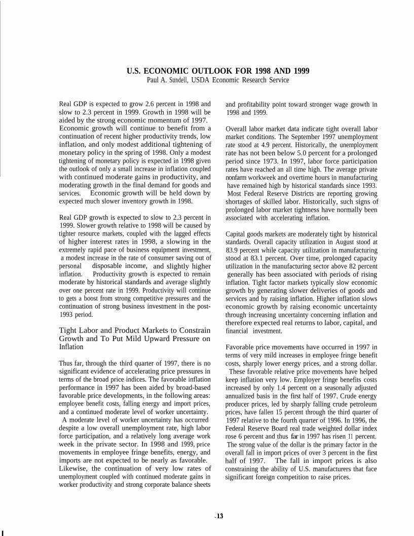
U.S. ECONOMIC OUTLOOK FOR 1998 AND 1999Paul A. Sundell, USDA Economic Research Service

Real GDP is expected to grow 2.6 percent in 1998 andslow to 2.3 percent in 1999. Growth in 1998 will beaided by the strong economic momentum of 1997.Economic growth will continue to benefit from acontinuation of recent higher productivity trends, lowinflation, and only modest additional tightening ofmonetary policy in the spring of 1998. Only a modesttightening of monetary policy is expected in 1998 giventhe outlook of only a small increase in inflation coupledwith continued moderate gains in productivity, andmoderating growth in the final demand for goods andservices. Economic growth will be held down byexpected much slower inventory growth in 1998.

Real GDP growth is expected to slow to 2.3 percent in1999. Slower growth relative to 1998 will be caused bytighter resource markets, coupled with the lagged effectsof higher interest rates in 1998, a slowing in theextremely rapid pace of business equipment investment,a modest increase in the rate of consumer saving out of

personal disposable income, and slightly higherinflation. Productivity growth is expected to remainmoderate by historical standards and average slightlyover one percent rate in 1999. Productivity will continueto gets a boost from strong competitive pressures and thecontinuation of strong business investment in the post-1993 period.

Tight Labor and Product Markets to ConstrainGrowth and To Put Mild Upward Pressure onInflation

Thus far, through the third quarter of 1997, there is nosignificant evidence of accelerating price pressures interms of the broad price indices. The favorable inflationperformance in 1997 has been aided by broad-basedfavorable price developments, in the following areas:employee benefit costs, falling energy and import prices,and a continued moderate level of worker uncertainty.A moderate level of worker uncertainty has occurred

despite a low overall unemployment rate, high laborforce participation, and a relatively long average workweek in the private sector. In 1998 and 1999, pricemovements in employee fringe benefits, energy, andimports are not expected to be nearly as favorable.Likewise, the continuation of very low rates ofunemployment coupled with continued moderate gains inworker productivity and strong corporate balance sheets

and profitability point toward stronger wage growth in1998 and 1999.

Overall labor market data indicate tight overall labormarket conditions. The September 1997 unemploymentrate stood at 4.9 percent. Historically, the unemploymentrate has not been below 5.0 percent for a prolongedperiod since 1973. In 1997, labor force participationrates have reached an all time high. The average privatenonfarm workweek and overtime hours in manufacturinghave remained high by historical standards since 1993.Most Federal Reserve Districts are reporting growingshortages of skilled labor. Historically, such signs ofprolonged labor market tightness have normally beenassociated with accelerating inflation.

Capital goods markets are moderately tight by historicalstandards. Overall capacity utilization in August stood at83.9 percent while capacity utilization in manufacturingstood at 83.1 percent. Over time, prolonged capacityutilization in the manufacturing sector above 82 percentgenerally has been associated with periods of risinginflation. Tight factor markets typically slow economicgrowth by generating slower deliveries of goods andservices and by raising inflation. Higher inflation slowseconomic growth by raising economic uncertaintythrough increasing uncertainty concerning inflation andtherefore expected real returns to labor, capital, andfinancial investment.

Favorable price movements have occurred in 1997 interms of very mild increases in employee fringe benefitcosts, sharply lower energy prices, and a strong dollar.

These favorable relative price movements have helpedkeep inflation very low. Employer fringe benefits costsincreased by only 1.4 percent on a seasonally adjustedannualized basis in the first half of 1997. Crude energyproducer prices, led by sharply falling crude petroleumprices, have fallen 15 percent through the third quarter of1997 relative to the fourth quarter of 1996. In 1996, theFederal Reserve Board real trade weighted dollar indexrose 6 percent and thus far in 1997 has risen 11 percent.The strong value of the dollar is the primary factor in theoverall fall in import prices of over 3 percent in the firsthalf of 1997. The fall in import prices is alsoconstraining the ability of U.S. manufacturers that facesignificant foreign competition to raise prices.

These favorable specific price developments are notexpected to continue into 1998 and 1999. Benefit costsare expected to accelerate as health care costs move momin line with wage costs. As growth in developedcountries outside the U.S. picks up in 1998 and 1999,energy prices should pick up. The value of the dollar isexpected to gradually weaken in the second half of 1998and 1999. A weaker dollar is expected as economicgrowth and asset returns gradually increase in developedcountries outside the U.S. and large U.S. trade deficitspersist.

Worker Concerns Over Job Security Should Lessenand put Upward Pressure on Wages In 1998 and1999

Although the unemployment rate has fallen below 5.0percent in recent months, other measures of labor markettightness involving job prospects and job search time failto indicate as much job tightness as suggested by theunemployment rate and average hours worked data. Theperceived continued difficulties of unemployed workersin finding new employment has been a factor inmoderating wage increases despite a low unemploymentrate and along average workweek. The employment costsurvey indicated wages and salaries increased 3.4 percentin 1996 and at a 3.6 percent annualized rate in the firsthalf of 1997.

The continued relatively long duration of average timespent unemployed and the continued relatively highlevels of job layoffs, given the low level of theunemployment rate, have lowered worker job security.Unemployment data indicates that the duration ofunemployment for the unemployed remains relativelyhigh and that job losses remain the dominant source ofunemployment. Since the beginning of the currentexpansion in the spring of 1991, the duration ofunemployment for those who are unemployed hasactually increased. Normally, the duration ofunemployment for the unemployed falls in an economicexpansion. Further evidence of continued workeruncertainty is that roughly 45 percent of thoseunemployed are unemployed because of losing theirprevious job.

Worker uncertainty and its inhibiting impact on wagegains should decline in 1998 and 1999. A slower pace ofcorporate restructuring, the continuation of tight labormarket conditions, as well as moderate gains in laborproductivity, strong corporate balance sheets, andmoderate increases incorporate profits in 1998 and 1999point toward a modest to moderate acceleration in therate of wage gains.

Recent Trend of Higher Productivity Growth ShouldContinue into 1998 and 1999

Productivity has rebounded sharply in recent quarters.Over the 1992 through 1995 period, nonfarm businessproductivity grew at an annual rate of only 0.2 percent ayear. Since the end of 1995 through the second quarterof 1997, nonfarm productivity has grown at a rate of 1.5percent. The stronger productivity numbers for 1996 and1997 are the result of strong business investment (since1993) that has increased the amount and quality ofcapital available per worker. Gradually improvingworker skills that have allowed workers to better utilizeimprovements in capital and technology are also a factorin recent productivity gains. Increased domestic andforeign competition have also boosted productivity inrecent years and should continue to boost productivity in1998 and 1999.

Demand Side Factors Point To Slower Growth in1998 and 1999 As Well

Although the recovery is currently in its seventh year, theeconomy has failed to generate the sectoral imbalancesthat turn a mature but slowing economic recovery into arecession. Inflation has remained low, thus reducingeconomic uncertainty and promoting relatively low reallong term interest rates. Consumers are not currentlyoverspending relative to their income, confidence levels,or balance sheets. Corporate balance sheets haveimproved substantially in recent years. Improvedcorporate balance sheets are allowing firms to raise moreand less expensive capital. The banking system remainsliquid, highly profitable, and desires to expand lending,

especially in the business loan area.

Despite the lack of major sectoral imbalances, growth inaggregate demand should slow in 1998 and 1999.Business investment both in terms of fixed capital andinventory should slow in 1998 and 1999. Strongbusiness investment since 1993 has reduced the capacityutilization rate in manufacturing by 1.5 percent sinceearly 1995. Lower capacity utilization rates haveresulted in a smaller gap between the actual and desiredcapital stock, which should slow the pace of businessfixed investment Very lean inventories relative to salesentering 1997 have encouraged business firms to increaseinventories by over $70 billion per quarter in the first halfof 1997. As inventories move closer to desired levelsrelative to current sales levels and growth in finaldemand slows in 1998 and 1999, growth in inventoriesshould slow significantly.

14

Growth in consumer spending should slow in 1998 and1999 as consumers raise their savings rate somewhat

above the 4.0 percent level of the first half of 1997. Thesavings rate has been held down in the first half of 1997by record levels of consumer confidence, strong gains inhousehold wealth from the strong stock market, andstrong growth in household durable demand resultingfrom the robust growth in residential investment in 1996and 1997. The savings rate is expected to increasemodestly or possible moderately in 1998 and 1999.Among the factors expected to raise the savings rateinclude slightly lower consumer confidence, slower gainsin household financial wealth (resulting primarily frommuch slower gains in equity prices), continuedtightening of consumer lending standards by commercialbanks, higher interest rates, and reduced pent-up demandfor consumer durables.

Real government spending is expected to continue itstrend of very slow growth in 1998 and 1999. Combinedreal federal and state and local spending grew 0.5

percent in 1996 and 0.7 percent in the first half of 1997.Real federal government spending is expected to declineat an annual rate of 1.1 percent in 1998 and 1999. Stateand local spending is expected to rise at slightly above 2percent rate in real terms in 1998 and 1999.

Federal Reserve policy is expected to raise the target forthe federal funds rate to 6 percent by late spring of 1998.Federal Reserve pronouncements have showedcontinued concern over tight labor market conditions.As the pace of inflation accelerates slightly and economicgrowth remains strong in the second half of 1997, theforecast assumes the Federal Reserve reacts quickly toraise the federal funds rate. Inflation as measured by theGDP deflator is expected to average 2.6 percent in thesecond half of 1998 and 2.7 percent in 1999.

The increase in the federal funds rate and slightly higherinflation is expected to push the average ten yearTreasury bond rate to 6.7 percent by the second half of1998 and 1999. Higher short and Iong-term interestrates can be expected to raise required returns on equityinstruments, thus further slowing the demand for fundsby business fins. Given the substantial lags between atightening of monetary policy and real economic growth,the impacts of higher long-term interest rates areexpected to be felt more in 1999 than 1998.

Little Improvement In Net Exports Expected in 1998or 1999

The real trade deficit, as measured by net exportswidened by over $30 billion in the first half of 1997.U.S. exports will benefit from expected stronger growthin developed countries outside of the U.S. in 1998 and1999 relative to 1997. Slower expected growth in U.S.inventories in 1998 and 1999 is a positive factor inslowing expected growth of U.S. imports. However,the positive impacts of stronger growth in foreigndeveloped countries and slower U.S. inventoryaccumulation on net exports will be offset by continuedrelatively strong U.S. growth and the lagged effects ofthe large rise in the real value of the dollar since late1995. The value of the dollar is expected to slowlydecline over the latter half of 1998 and 1999 as realgrowth and expected asset returns gradually increase inother developed countries. Persistent large U.S. tradedeficits will put additional downwardpressure on the dollar by reducing the willingness offoreigners to hold additional dollar denominated assets.

15

The Long-Term

Introduction

Economic Outlook: Is This the

R. M. Monaco

Era of Diminishing Resources?

Inforum/Department of EconomicsUniversity of Maryland

College Park, MD 20742ralph@inforum .umd.edu

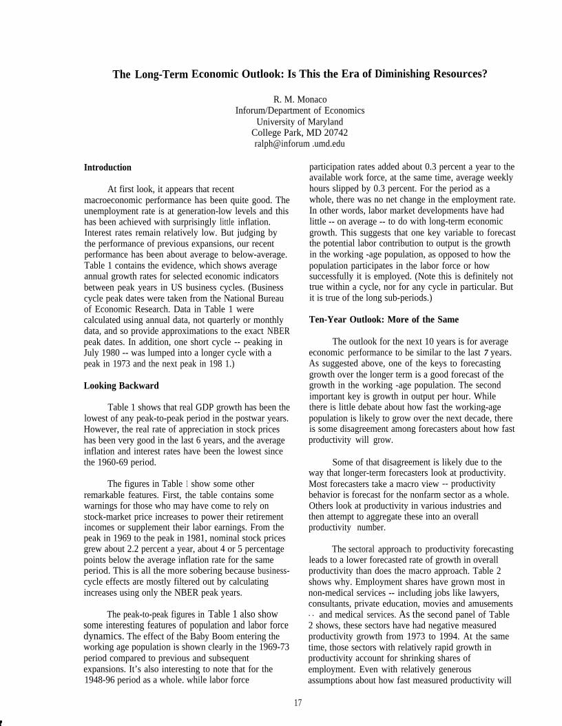
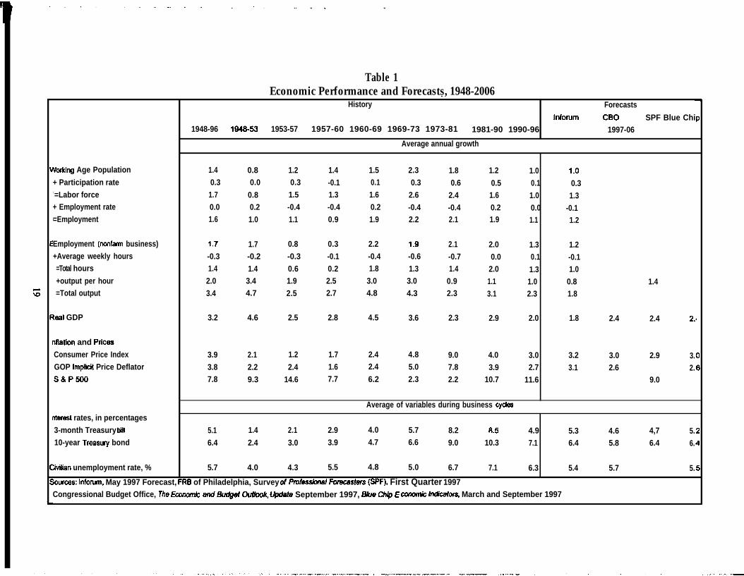
At first look, it appears that recentmacroeconomic performance has been quite good. Theunemployment rate is at generation-low levels and thishas been achieved with surprisingly little inflation.Interest rates remain relatively low. But judging bythe performance of previous expansions, our recentperformance has been about average to below-average.Table 1 contains the evidence, which shows averageannual growth rates for selected economic indicatorsbetween peak years in US business cycles. (Businesscycle peak dates were taken from the National Bureauof Economic Research. Data in Table 1 werecalculated using annual data, not quarterly or monthlydata, and so provide approximations to the exact NBERpeak dates. In addition, one short cycle -- peaking inJuly 1980 -- was lumped into a longer cycle with apeak in 1973 and the next peak in 198 1.)

Looking Backward

Table 1 shows that real GDP growth has been thelowest of any peak-to-peak period in the postwar years.However, the real rate of appreciation in stock priceshas been very good in the last 6 years, and the averageinflation and interest rates have been the lowest sincethe 1960-69 period.

The figures in Table 1 show some otherremarkable features. First, the table contains somewarnings for those who may have come to rely onstock-market price increases to power their retirementincomes or supplement their labor earnings. From thepeak in 1969 to the peak in 1981, nominal stock pricesgrew about 2.2 percent a year, about 4 or 5 percentagepoints below the average inflation rate for the sameperiod. This is all the more sobering because business-cycle effects are mostly filtered out by calculatingincreases using only the NBER peak years.

The peak-to-peak figures in Table 1 also showsome interesting features of population and labor forcedynamics. The effect of the Baby Boom entering theworking age population is shown clearly in the 1969-73period compared to previous and subsequentexpansions. It’s also interesting to note that for the1948-96 period as a whole. while labor force

17

participation rates added about 0.3 percent a year to theavailable work force, at the same time, average weeklyhours slipped by 0.3 percent. For the period as awhole, there was no net change in the employment rate.In other words, labor market developments have hadlittle -- on average -- to do with long-term economicgrowth. This suggests that one key variable to forecastthe potential labor contribution to output is the growthin the working -age population, as opposed to how thepopulation participates in the labor force or howsuccessfully it is employed. (Note this is definitely nottrue within a cycle, nor for any cycle in particular. Butit is true of the long sub-periods.)

Ten-Year Outlook: More of the Same

The outlook for the next 10 years is for averageeconomic performance to be similar to the last 7 years.As suggested above, one of the keys to forecastinggrowth over the longer term is a good forecast of thegrowth in the working -age population. The secondimportant key is growth in output per hour. Whilethere is little debate about how fast the working-agepopulation is likely to grow over the next decade, thereis some disagreement among forecasters about how fastproductivity will grow.

Some of that disagreement is likely due to theway that longer-term forecasters look at productivity.Most forecasters take a macro view -- productivitybehavior is forecast for the nonfarm sector as a whole.Others look at productivity in various industries andthen attempt to aggregate these into an overallproductivity number.

The sectoral approach to productivity forecastingleads to a lower forecasted rate of growth in overallproductivity than does the macro approach. Table 2shows why. Employment shares have grown most innon-medical services -- including jobs like lawyers,consultants, private education, movies and amusements. . and medical services. As the second panel of Table2 shows, these sectors have had negative measuredproductivity growth from 1973 to 1994. At the sametime, those sectors with relatively rapid growth inproductivity account for shrinking shares ofemployment. Even with relatively generousassumptions about how fast measured productivity will

grow in the next 10 years, (last column of Table 2), itis hard for the economy to get to 1 percent overallproductivity, let alone the 1.4 percent predicted bymost forecasters (shown in the last panel of Table 1).

Forecasting productivity growth is relativelydifficult, and both the macro and sectoral approacheshave advantages and disadvantages. Perhaps the chieflesson to take away from Table 2 is that there a set offactors that point in the direction of continued slowmeasured productivity growth. This tends to raise theprobability that we will observe continued slow growthin the future, rather than a productivity rebound, assome are projecting.

The productivity forecast is clouded by manymeasurement issues, some of which have been broughtto the fore by the recent investigation into whether theConsumer Price Index overstates inflation. Ifconsumer price increases have been overstated, then“real” purchases in these sectors have been understated,which implies that “real” production has beenunderstated. If we have accurately counted the numberof hours worked in the sector, then the understatementof output implies an understatement of productivity.

The problem of measuring output is especiallydifficult in the services sectors, which account for alarge portion of employment. For many of thesesectors, there is virtually no data available on the“quantity” of services provided. For sectors like themedical services sector, while you can easily count thenumber of doctor or hospital visits and thus obtain aquantity index, it is apparent to even casual observersthat a lot of quality change has taken place. Qualitychange obviously needs to be accounted for if we areto measure productivity well. Some estimates suggestthat productivity growth in the medical services sectormay be understated by several percentage points ayear!

These thoughts put us in a Catch-22. We maybelieve that true productivity growth for the next 10years will be close to or even higher than the 1.4percent annual rate predicted by many analysts.However, based on the figures we have, it appears 1.4percent will be hard to achieve. The forecast containedin the Inforum column of Table 1 is a forecast based onnumbers that we have, even though we believe thatthey substantially understate the actual rate ofproductivity growth. At the moment, we simply don’thave enough information to do otherwise.

More Than Ten Years After

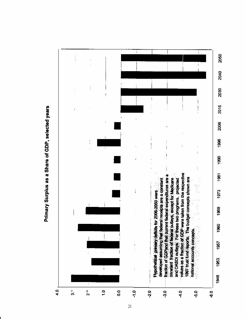
The outlook after about 10 years is not especiallygood. Despite recent legislation to balance the federalbudget by 2002, the projected changes in the agestructure of the population, (Table 3) combined withthe structure of federal entitlement programs(Medicare and OASDI in particular) suggest very largefederal deficits (Graph 1).

Without steps to keep the federal deficit fromballooning when the Baby Boomers reach federalprogram retirement age (20 11), the share of nationalincome devoted to savings will drop dramatically.According to the standard economic growth model, thiswill lead to increasingly lower rates of capitalformation, increasingly higher interest rates, andincreasingly lower labor productivity growth.

The projected deficit problem is so severe thatreasonable economic simulation models cannotmeaningfully calculate the economic outlook -- themodels break -- unless taxes are raised, benefits arereduced, or other federal outlays are reduced. The taxincreases projected to lead to sensible model results arelarge. Pay-as-you go financing -- raising taxes tomatch spending increases -- leads to a doubling ofpayroll tax rates to keep the federal budget balanced(Monaco and Phelps, mimeo 1997).

The expectation of rising federal deficits andtheir actual onset will probably bring on a host of“structural” changes in the economy. When we thinkabout what these adjustments might be, we round upthe two usual suspects: higher taxes and reductions inbenefits (including raising the retirement age). Inclosing, however, here is some speculation about otherways the economy will adjust:

Surprisingly large increases in labor forceparticipation among the 65.

Encouragement of immigration.

Encouragement of fertility.

Changing the entitlement nature of Medicare andSocial Security. At some point, governmentpayments will be linked to “need” rather thanage.

Analysts will adjust too. Over the next severalyears, we will likely redefine service price and outputmeasures. This will reduce the severity of themeasured productivity slowdown after 1973, andprovides a “truer” picture of real economic well-being.

18

. . ., . .“ -- - .- . - . . .

Table 1Economic Performance and Forecasts, 1948-2006.

History ForecastsInfomm CBO SPF Blue Chi

1948-96 194&53 1953-57 1957-60 1960-69 1969-73 1973-81 1981-90 1990-96 1997-06

Average annual growth

!brtdng Age Population 1.4 0.8 1.2 1.4 1.5 2.3 1.8 1.2 1.0 1.0+ Participation rate 0.3 0.0 0.3 -0.1 0.1 0.3 0.6 0.5 0.1 0.3: =Labor force 1.7 0.8 1.5 1.3 1.6 2.6 2.4 1.6 1.0 1.3+ Employment rate 0.0 0.2 -0.4 -0.4 0.2 -0.4 -0.4 0.2 0.0 -0.1=Employment 1.6 1.0 1.1 0.9 1.9 2.2 2.1 1.9 1.1 1.2

Employment (nonfarm business) 1.7 1.7 0.8 0.3 2.2 1.9 2.1 2.0 1.3 1.2+Average weekly hours -0.3 -0.2 -0.3 -0.1 -0.4 -0.6 -0.7 0.0 0.1 -0.1=Total hours 1.4 1.4 0.6 0.2 1.8 1.3 1.4 2.0 1.3 1.0+output per hour 2.0 3.4 1.9 2.5 3.0 3.0 0.9 1.1 1.0 0.8 1.4=Total output 3.4 4.7 2.5 2.7 4.8 4.3 2.3 3.1 2.3 1.8

Ieal GDP 3.2 4.6 2.5 2.8 4.5 3.6 2.3 2.9 2.0 1.8 2.4 2.4 2.4

nflation and PticesConsumer Price Index 3.9 2.1 1.2 1.7 2.4 4.8 9.0 4.0 3.0 3.2 3.0 2.9 3.GOP Impticit Price Deflator 3.8 2.2 2.4 1.6 2.4 5.0 7.8 3.9 2.7 3.1 2.6 2.s& P500 7.8 9.3 14.6 7.7 6.2 2.3 2.2 10.7 11.6 9.0

Average of variables during business cycJes

nterest rates, in percentages3-month Treasury bill 5.1 1.4 2.1 2.9 4.0 5.7 8.2 8.5 4.9 5.3 4.6 4,7 5.10-year Treaswy bond 6.4 2.4 3.0 3.9 4.7 6.6 9.0 10.3 7.1 6.4 5.8 6.4 6.

Wilian unemployment rate, % 5.7 4.0 4.3 5.5 4.8 5.0 6.7 7.1 6.3 5.4 5.7 5.

kmrces: Inforum, May 1997 Forecast, FRB of Philadelphia, Survey CM Pm6sskwa/ FOmcastem (SPF), First Quarter 1997Congressional Budget Office, The Economic ad B@@ ~, L4$date September 1997, 8/ue Ch@ E cormrnk h?dcetors, March and September 1997

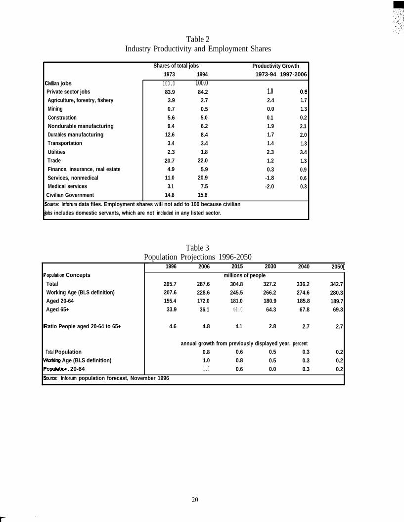
Table 2Industry Productivity and Employment Shares

Shares of total jobs Productivity Growth1973 1994 1973-94 1997-2006

Civilian jobsPrivate sector jobsAgriculture, forestry, fisheryMining

ConstructionNondurable manufacturingDurables manufacturingTransportation

UtilitiesTradeFinance, insurance, real estateServices, nonmedicalMedical services

Civilian Government

100.0 100.083.93.90.75.69.4

12.63.42.3

20.74.9

11.03.1

14.8

84.22.70.55.06.28.43.41.8

22.0

5.920.9

7.515.8

1.02.40.00.11.91.71.4

2.31.2

0.3-1.8-2.0

0.81.71.30.22.12.01.33.41.3

0.90.60.3

1

Source: Inforum data files. Employment shares will not add to 100 because civilianjobs includes domestic servants, which are not included in any listed sector.

opulation Concepts

TotalWorking Age (BLS definition)Aged 20-64Aged 65+

Ratio People aged 20-64 to 65+

Total PopulationVoting Age (BLS definition)‘opulation, 20-64

Table 3Population Projections 1996-2050

1996 2006 2015 2030 2040 2050[millions of people I

265.7 287.6 304.8 327.2 336.2 342.7207.6 228.6 245.5 266.2 274.6 280.3155.4 172.0 181.0 180.9 185.8 189.733.9 36.1 44.0 64.3 67.8 69.3

4.6 4.8 4.1 2.8 2.7 2.7

annual growth from previously displayed year, percent0.8 0.6 0.5 0.3 0.21.0 0.8 0.5 0.3 0.21.0 0.6 0.0 0.3 0.2

Source: Inforum population forecast, November 1996

20

II

I I I

It

,

I I I

I I II

I I

I I

I 1

I I

III

LI

II u I

I I I

‘-;:;~!;,I

1 II I

II It

I

t1

I

i-

1 I

~

I

I I1.

1,

(I I

,

0 0@i m

I

I

I

(,

II

I

I I I

I

I I I

21

.’,

,,

INDUSTRY MODELING AT THE BUREAU OF LABOR STATISTICS

Chair: Norman C. SaundersBureau of Labor Statistics, U.S. Department of Labor

A Model of Detailed Industry Labor Demand,James C. Franklin, Bureau of Labor Statistics, U.S. Department of Labor

A Model of Detailed Personal Consumption Expenditures,Janet E. Pfleeger, Bureau of Labor Statistics, U.S. Department of Labor

A Commodity-Specific Model for Projecting Import Demand,Betty W. Su, Bureau of Labor Statistics, U.S. Department of Labor

A Model of New Nonresidential Equipment Investment,Jay M. Berman, Bureau of Labor Statistics, U.S. Department of Labor

23

A MODEL OF DETAILED INDUSTRY LABOR DEMAND

James C. Franklin, Bureau of Labor StatisticsBureau of Labor Statistics, 2 Massachusetts A v e . N.E. Room 2135, Washington, DC 20212

Introduction

Within the Bureau of Labor Statistics (BLS), the Officeof Employment Projections (OEP) is charged withdeveloping long term projections of employment byindustry and occupation. These projections aredeveloped to facilitate understanding of current andfuture labor market conditions and are disseminated foruse in career guidance and public policy planning thatis related to employment issues. A system of severalcomponent models is used by OEP to develop theseprojections. This paper presents the industry levellabor model. The labor model and its sub-componentsare defined and the integration of the labor model withthe larger OEP projections system is described.

The labor model

The labor model is actually a group of equations andidentities which are solved independently. The maincomponent of the labor model is the equation thatestimates the demand for wage and salary hours. It isderived from a constant elasticity of substitution (CES)production fiction. The remaining equations andidentities are necessitated by the availability of dataand the relationship of the labor model to the othercomponents of the OEP projections system. The laborequation which estimates demand for wage and salaryhours is based on a theoretical economic structurewhile the other estimated equations are time and othervariable extrapolations.

The CES derived labor equation

The demand for wage and salary hours for eachindustry is estimated using the first order conditions ofa CES production function modified to include a timevariable. The time variable captures disembodiedtechnical change or shifts in the production functionthat do not affect the labor and capital ratio. Theseshifts of the production indicate increased efficienciesin the use of the capital and labor inputs.

The basic form of the production function is:

Equation 1

Y= f(t,L,K)

where:Y real outputL laborK capital stockt time

The model assumes perfect competition and profitmaximization so that:

both factors are indispensable in the production ofoutput – ~(O,K)=~(O,L)=O

both marginal products are nomegative —dfm=x), aflx=xl

and the marginal products are equal to the real factorprices — ~f/t3L = w/p, i3f/i3K = r/p

where ‘w,r,p’ are the nominal prices for labor, capitaland output.

It is also assumed the rate of growth of disembodiedtechnical change is proportionate and constant.

The functional form of the labor demand model is:

Equation 2

Y = Aemt[~ L-P+ (1 - ~)K-fl]-fiwhere

A6PYL

Kmt

is a scale parameter, A > O;is a distribution parameter, O <5<1is a substitution parameter, ~ 2-1is real outputis labor, measured as annual wage and salaryhours in millionsis the capital stockis disembodied technical change growth rateis time, measured as the year

The marginal product of labor can be written:

25

where A‘ = ~A-fland g = -flm .The perfect competition and profit maximkationassumptions require that:

( )

Y 1+/3 w#tf~8~ — = _L ‘ P

wherew is nominal wagesP is the output price

Solving for labor productivity:

;=(A%%’)2(;)*

taking logs:

0

1MO-ML) =J - - ----------—

_g*$+1 ; p+l

lr@)p+l

then solving for labor:

hi(L)1

lrI(A)0

lW——-p+l

-&+l@)— — –‘ ‘p+l p+l p

results in the final basic form of the equation. Theestimated form of the equation is:

Equation 3

( )lnL=tzO +alt+azln Y+a~ln y

P

Other equations and identities

Equation 3 requires estimated data for real output,nominal wage, and output price by industry for asolution. The output level is supplied by the input-output system as an exogenous variable. The industryprice and wage data are estimated using projectedvariables from the macro-economic model whichproduces the aggregate projections in the OEPprojection system.

Given an industry’s output, wage and output price,equation 3 will solve for the required wage and salaryhours. The end product of OEP’S projection system,however, includes the employment level by industry forwage and s a l a r y and self-employed and unpaid family.The solution for equation 3 must be converted to anemployment level for wage and salary using anextrapolated estimate for each industry’s average

hours. The number of self-employed and

unpaid family for each industry and their hours mustalso be estimated.

Industry average hourly wage estimation

The nominal average hourly wage for each industry isestimated in a two step process. First, an all industrynominal average hourly wage is estimated as a functionof the BLS series employment cost index. Theemployment cost index is estimated by the macromodel for the projection period. Second, the nominalaverage hourly wage for each industry is estimated as afunction of the all industry average hourly wage. Thefollowing equations are used to estimate the industryaverage hourly wage.

Equation 4

TotAHW = aO + a1ECIFJ5 +a2ur

Equation 5

AH~ = aO +alTotAHW: aO= O

whereTotAHW is the total average hourly wageEC.lWS is the employment compensation index

for wage and salaryAHWj is the average hourly wage for industry iur is the aggregate unemployment rateai are constants/coefficients

Industryprice index estimation

The price index for each industry is estimated with thefollowing equation:

Equation 6

ln(p,) = aO +al in(P)

where:pi is the price chain

industryweighted index for each

P is the GDP chain weighted price indexai are constantskodiicients

Industry average weekly hours estimation

Average weekly hours for both wage and salary andself-employed and unpaid family are estimated as afunction of the year and the aggregate unemploymentrate.

26

Equation 7

AWHi = aO +alt +a3ur

where

t is time measured as the yearA WHi “ are average weekly hours for each industryur is the aggregate unemployment ratean : are constantd~fflcients

Industry self-employed and unpaid family estimation

The number of self-employed and unpaid family foreach industry was derived by using an estimate of theratio of the self-employed and unpaid family to totalemployment to derive the level of total employment foreach industry from the level of wage and salary, andthen subtracting the wage and salary from the totalemployment. The logit transformation of the self-employed and unpaid family workers ratio to totalemployment was estimated as a function of the yearand the aggregate unemployment rate using thefollowing equation.

Equation 8

(R)In SR— = aO +alt +a3ur1-s

whereSR is the ratio (self-employed and unpaid family

workers/total employment)t is time, measured as the yearur is the aggregate unemployment rate&li are constants/coefficien@

Employment, hours and average weekly hours identity

Employment, measured in thousands, for wage andsalary, and self-employed and unpaid family, is relatedto the annual hours measured in millions and theaverage weekly hours by the following identity.

Equation 9

where

Ei employment level in thousandsLi annual hours, measured in millionsA WHi average weekly hours

Projections of labor demand

The initial projections of industry employment aredeveloped according to the following procedureimplemented for each industry.

1.

2.

3.

4.

5.

6.

7.

8.

The industry demands for wage and salary hoursin millions are projected.

Wage and salary annual average weekly wage andsalary hours are estimated.

The industry levels of wage and salary jobs inthousands are then derived from the estimation ofhours and average weekly hours.

The ratio of self-employed and unpaid familyworkers to total employment is extrapolated.

The extrapolated ratio is then used to derive thelevel of self-employed and unpaid family workersfrom the number of wage and salary jobs.

Self-employed and unpaid family average weeklyhours are estimated.

The hours for self-employed and unpaid familyworkers are then derived from their estimatedaverage weekly hours and the estimated number ofself-employed and unpaid family workers.

Finally, wage and salary, and self-employed andunpaid family worker employment and hours arecombined to calculate a total level of employmentand hours for each industry.

Data sources

The output measures follow the definitions andconventions used by the Bureau of Economic Analysis(BEA) in its input-output tables, published every fiveyears. These industry output measures are based onproducer’s value and include both primary andsecondary products and services. The main datasources for compiling the output time series formanufacturing industries are the Census and AnnualSurvey of Manufactures. Data sources fornonmanufacturing industries are more varied. Theyinclude the Semite Annual Survey, National Incomeand Product Accounts (NIPA) data on newconstruction and personal consumption expenditures,IRS data on business receipts, and many other sources.The constant dollar industry output estimates for themost recent years are based on BLS employment dataand trend projections of productivity. The output seriesare benchmarked to the BEA input-output tables for1987 which was adjusted by BLS to reflect the 1987

27

SIC revision, National Income and Product Accountrevisions, and to place the tables more consistently onan SIC basis.

The annual price data are developed in a manner so asto conform to BEA’s national income and productaccounts. For manufacturing, they are based onindustry sector price index data collected by BLS.Nonmanufacturing prices use a variety of differentsources, in many instance the BLS consumer priceindex data. In industries where such underlying pricedata have not yet been developed, imputations of pricechange are made by the BEA from other data series.

The employment data come from the BLS currentemployment statistics (the establishment data series forwage and salary jobs and average weekly hours), thecurrent population survey (for self-employed andunpaid family worker jobs, agricultural employmentexcept for agricultural services, and private householdemployment), ES202 Employment and Wages datacollected for the unemployment insurance program(agricultural services and total wages paid), and someunpublished data sources within the Bureau. Averagehourly wages were calculated using the ES202 wagedata and the annual hours estimate developed from thecurrent employment statistics data for each industry,except for the government sector.

All data series are developed on an annual basis. Thebeginning and ending years differ between the dataseries. The industry output and price series begins in1972; the employment series varies by industry, theearliest year being 1958; the wage data series begins in1975. The industry output and price data end in 1996,although for most industries the 1995 and 1996 datapoints are extrapolations. The employment data alsoends in 1996. The wage data ends in 1994. Theregression estimates, limited by common years, arebased on data from 1975 through 1994.

Regression and results`

All regression estimates for the equations of the labormodel are estimated using ordinary least squares.With the exception of the agricultural and public

sectors, employment levels and hours are estimatedusing the equations and procedures previouslyoutlined.

The output for the public sectors is comprised ofcompensation, making the wage variable in equation 3redundant. Consequently, the wage variable is droppedfrom the regression equation for the public sector.

The wage variable for the agricultural sectors is alsodropped because the wage data from the ES202covered employment and wages program is notcomplete for the agricultural sectors. Not allemployment in the agricultural sectors is covered bythe unemployment insurance program.

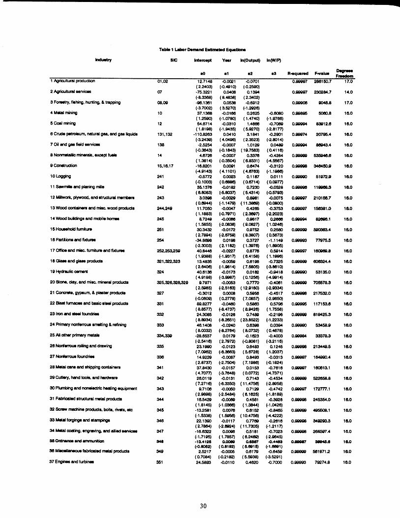
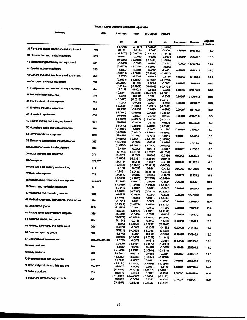
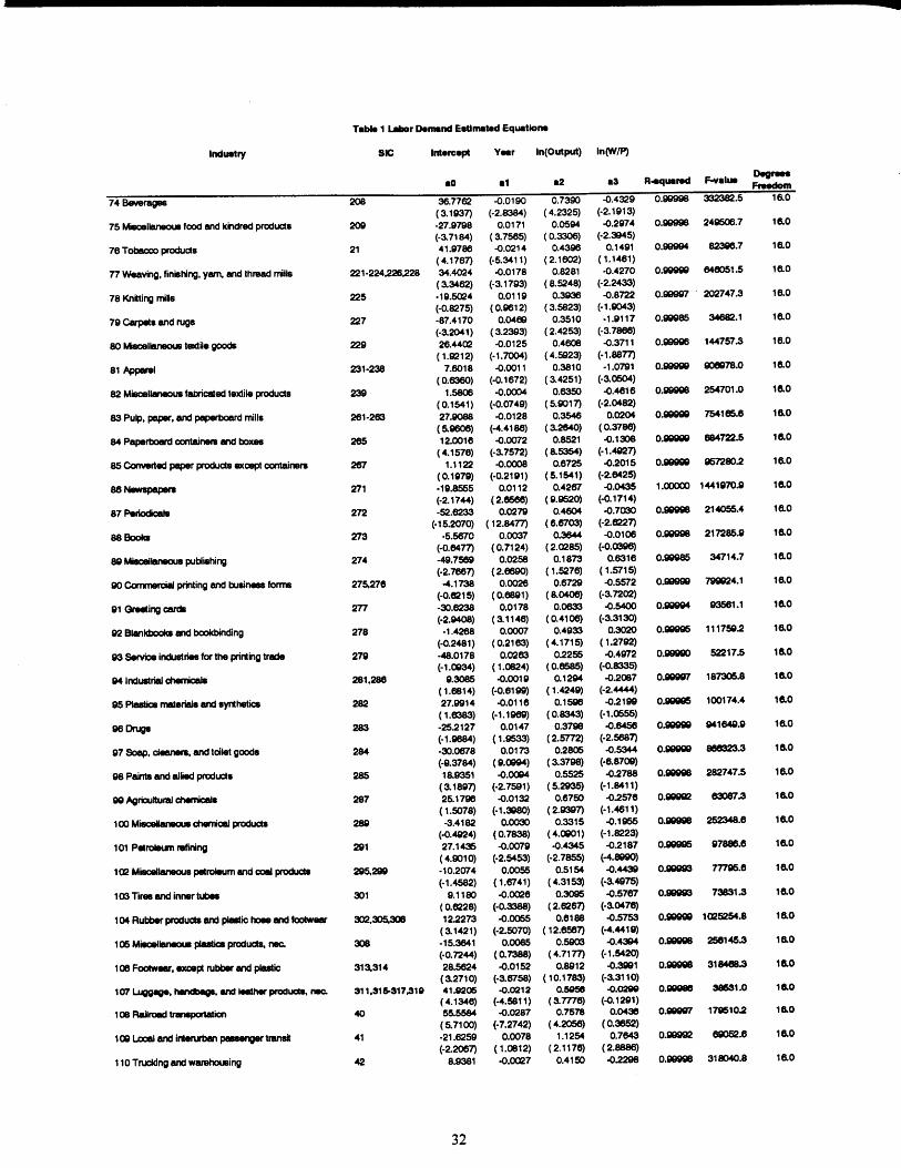
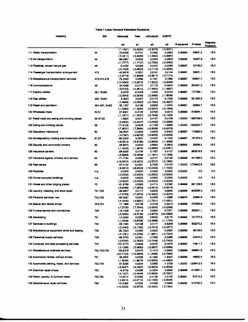
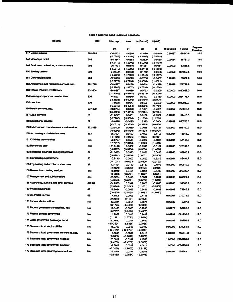
The sectoring plan which OEP uses to define theindustries consists of 185 sectors, 8 of which arespecial accounting industries that have no associatedemployment. Sectors 170 through 179 are governmentindustries and sectors 1 through 3 are agriculturalindustries. That leaves 164 industries for whichemployment is estimated using the fidly expressedlabor equation. The discussion of the regression resultswill focus on these 164 industries. The regressionstatistics for all industries are listed in table 1.

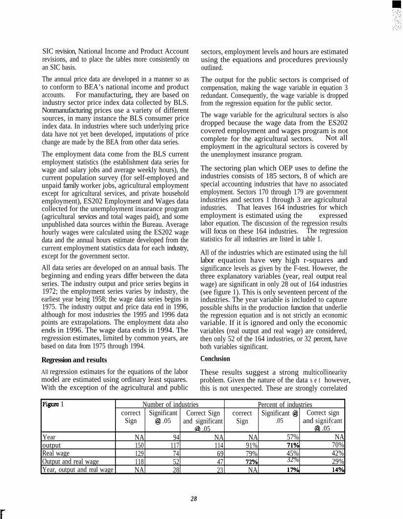
All of the industries which are estimated using the fulllabor equation have very high r-squares andsignificance levels as given by the F-test. However, thethree explanatory variables (year, real output realwage) are significant in only 28 out of 164 industries(see figure 1). This is only seventeen percent of theindustries. The year variable is included to capturepossible shifts in the production function that underliethe regression equation and is not strictly an economicvariable. If it is ignored and only the economicvariables (real output and real wage) are considered,then only 52 of the 164 industries, or 32 percent, haveboth variables significant.

Conclusion

These results suggest a strong multicollinearityproblem. Given the nature of the data s e t however,this is not unexpected. These are strongly correlated

lFigure 1 Number of industries Percent of industriescorrect Significant Correct Sign correct Significant @ Correct sign

Sign @ .05 and significant Sign .05 and signifcant@ .05 @ .05

Year NA 94 NA NA 57% NAoutput 150 117 114 91% 71% 70%Real wage 129 74 69 79% 45% 42%Output and real wage 118 52 47 72~0 32% 29%Year, output and real wage NA 28 23 NA 17% 14yo

28

time series data. The usual recourse is to add or dropvariables, or to enrich the data by adding data points.Since the labor equation is a formally structured model,adding or dropping variables has limited appeal. Thewage variable is dropped for those sectors for whichthe available data does not conform to the demands ofthe model. Otherwise the preference is to leave themodel as specified. As for adding data points, all theavailable data in the time series is being used. Thefinal option is to do nothing about the multicollinearityproblem, and this is warranted for several reasons.First, the labor model is a formal model based onstrong economic principals. Second, t h emulticollinearity does not invalidate the significance ofthe regression equations. It does make analysis of theexplanatory power of the individual variablesproblematic. Since the purpose of the labor model isprojections work, the explanatory power of thevariables are of lessor importance than the significanceof the whole equation. And finally, the labor model inpractice seems to perform well enough. Its principalpurpose is to estimate an initial level of projectedemployment by industry. The OEP projections processis an iterative one with several points of subjectivereview. Consequently, the labor model is not expectedto produce a final and publishable projection withoutreview and adjustment. As an estimator of the initialindustry level employment projections and an adjunctto subjective analysis it has proved useful.

29

A Model of Detailed Personal Consumption Expenditures

Janet E. PfleegerBureau of Labor Statistics, Washington, DC 20212

Introduction

The final product of the Office of EmploymentProjections is medium term (10 year) projections ofover 500 occupations and 185 industries. The 6 stepsinvolved in developing these projections are: 1 ) thesize and demographic composition of the labor force; 2)the growth of the aggregate economy; 3) final demandor gross domestic product (GDP) subdivided byconsuming sector and product; 4) inter-industryrelationships (input-output); 5) indust~ output andemployment; and 6) occupational employment.

The Personal Consumption Expenditures (PCE) Modelfalls under step 3. Within step 3, each component ofGDP is projected—PCE, business investment,government spending and foreign trade. This paperpresents a dynamic model for PCE that projectsconsumer spending for 80 product groups. 1 It wasoriginally estimated by Houthakker-Taylo# in the mid-1960’s and is based on the theory that current consumerpurchases depend not only on current income andrelative prices, but on a stock variable representingeither the adjustment of a pre-existing inventory of theproduct in question to a desired or equilibrium level, orhabit formation from past consumption.

The Functional FormThe standard approach to demand analysis involvesestimation of the following demand equation:

(1) qit =fi(Xt,J2it,zll, z2t,...,zn*,Uit)

where:qit: per capita consumption of the ith commodityin year tf.: function whose mathematical form is specifiedl;terx,: per capita real disposable income

Pit: deflated price of the ith commodityZ,zz:It 2t’”””’ nt

any other explanatory variables, suchas the price of one or more substitute or complimentarygoods of the ith commodity, lagged values of xt or pit,or a time trend.Uit: disturbance term representing both the effectof variables that are not explicitly introduced into theequation and errors in measurement of qit.

Derivation of the PCE ModelA structural equation corresponding to the abovefunctional form is specified as:

(2) q,=a+bs, +cx, +dp, +u,where:

state variable:: state coefficientc: short-run derivative of consumption withrespect to income (the marginal propensity to consume)d: short-run derivative of consumption withrespect to relative price

To define the state variable in (2), the change in eitherof the two types of stocks (inventory or habit formation)is assumed to be new purchases less the depreciation ofexisting stock, where the depreciation rate is assumedconstant. This stock depreciation equation is expressedas:

(3) S, =q, -es,where:s: the rate of change in the stockand either

e= a constant rate of stock depreciation forgoodsor

e=a constant rate at which habit-formationwears off

s can now be eliminated by combining (2) and (3):

(4) st=qt–(elb) *(q, -a–cxl–dpf)

Differentiating (2) with respect to time, substituting (4)for ~ , and combining the different variables yields:

(5) q,= ae+(b–e)q~+cex, +dep, +ci +dpt

(5) is a first-order difference equation that deals onlywith the variables q, x and p, all of which are ‘observed’variables.

Before estimating the model, qt must be eliminatedfrom the right hand side of(5). For computationalreasons, it is also desirable to eliminate the current year

35

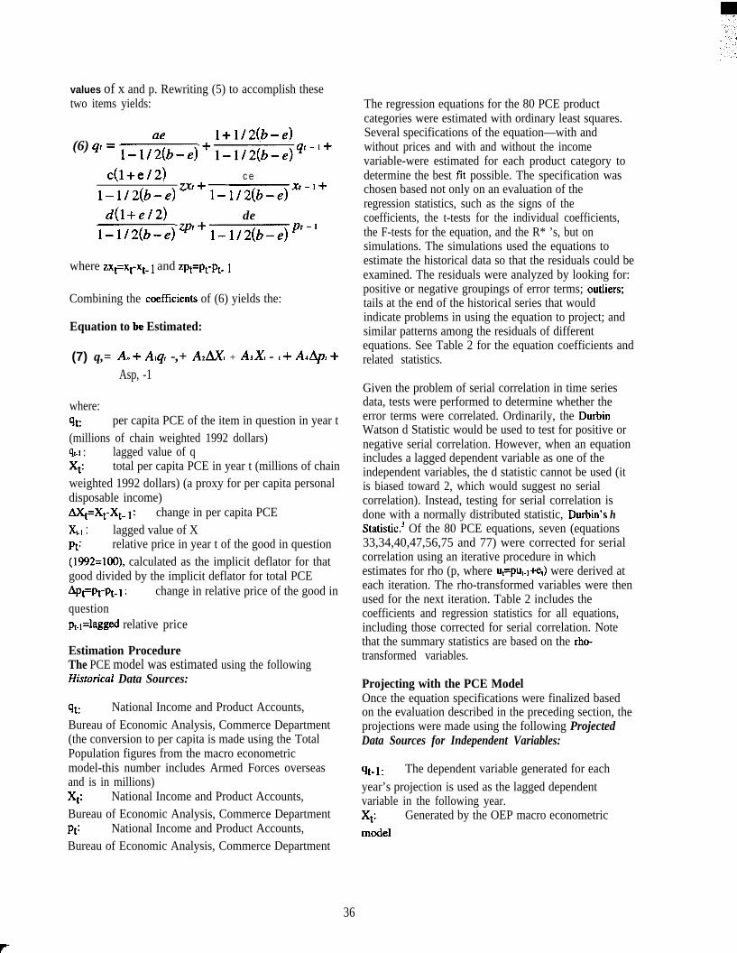
values of x and p. Rewriting (5) to accomplish thesetwo items yields:

ae 1+1/2(b–e)(6) q,=

l–1/2(b–e) +l–112(b–e)q’-’+c(l+e/2) ce. .

l–l12(b–e) “+1-1 /2(b-e)x’-’+d(l+e/2) de

l–1/2(b–e) wt+l-112(b–e)pr-’

where zx~xt-xt- 1 and zpt=pt-pt- 1

Combining the cwfficients of (6) yields the:

Equation to be Estimated:

(7) q,= A.+ A,q, -,+ A2AX + A~X, - ,+ AApt +Asp, -1

where:% per capita PCE of the item in question in year t(millions of chain weighted 1992 dollars)q~.1 : lagged value of qXt: total per capita PCE in year t (millions of chainweighted 1992 dollars) (a proxy for per capita personaldisposable income)Axt=xt-x~- 1: change in per capita PCEX,.1 : lagged value of XPt: relative price in year t of the good in question(1992=100), calculated as the implicit deflator for thatgood divided by the implicit deflator for total PCEAPt=Pt-Pt-l : change in relative price of the good inquestionpt-l=laggd relative price

Estimation ProcedureThe PCE model was estimated using the followingHiston”cal Data Sources:

% National Income and Product Accounts,Bureau of Economic Analysis, Commerce Department(the conversion to per capita is made using the TotalPopulation figures from the macro econometricmodel-this number includes Armed Forces overseasand is in millions)Xt: National Income and Product Accounts,Bureau of Economic Analysis, Commerce DepartmentPt: National Income and Product Accounts,

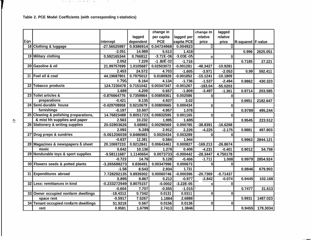
The regression equations for the 80 PCE productcategories were estimated with ordinary least squares.Several specifications of the equation—with andwithout prices and with and without the incomevariable-were estimated for each product category todetermine the best fit possible. The specification waschosen based not only on an evaluation of theregression statistics, such as the signs of thecoefficients, the t-tests for the individual coefficients,the F-tests for the equation, and the R* ’s, but onsimulations. The simulations used the equations toestimate the historical data so that the residuals could beexamined. The residuals were analyzed by looking for:positive or negative groupings of error terms; outliers;tails at the end of the historical series that wouldindicate problems in using the equation to project; andsimilar patterns among the residuals of differentequations. See Table 2 for the equation coefficients andrelated statistics.

Given the problem of serial correlation in time seriesdata, tests were performed to determine whether theerror terms were correlated. Ordinarily, the DurbinWatson d Statistic would be used to test for positive ornegative serial correlation. However, when an equationincludes a lagged dependent variable as one of theindependent variables, the d statistic cannot be used (itis biased toward 2, which would suggest no serialcorrelation). Instead, testing for serial correlation isdone with a normally distributed statistic, Durbin’s hStatistic.3 Of the 80 PCE equations, seven (equations33,34,40,47,56,75 and 77) were corrected for serialcorrelation using an iterative procedure in whichestimates for rho (p, where u~put-l+et) were derived ateach iteration. The rho-transformed variables were thenused for the next iteration. Table 2 includes thecoefficients and regression statistics for all equations,including those corrected for serial correlation. Notethat the summary statistics are based on the rho-transformed variables.

Projecting with the PCE ModelOnce the equation specifications were finalized basedon the evaluation described in the preceding section, theprojections were made using the following ProjectedData Sources for Independent Variables:

%1: The dependent variable generated for each

year’s projection is used as the lagged dependentvariable in the following year.Xt: Generated by the OEP macro econometricmodel

Bureau of Economic Analysis, Commerce Department

36

Pt: the implicit deflator for the good in question iscalculated using a double exponential smoothingtechnique 4 and the implicit deflator for total PCE comesfrom OEP’S macro econometric model

How the PCE Model Fits into the OEPThe results from the PCE model were then converted toprojections of consumer spending by commoditythrough a projected bridge table. The bridge table is

based on the Input-Output Tables published every 5years by the Bureau of Economic Analysis (BEA). Thecommodity specific projections are converted toindustry output projections using “Use” and “Make”tables, which are also based on the Input-Output Tablesfrom BEA. The ultimate product of the OEP—industryand employment projections—are then derived fromthese projected outputs.

1 See Table 1 fore the list of the 80 product groups.2 H.S. Houthakker and Lester D. Taylor. Consumer Demand in the United States, 1929-1970, Analyses andProjections, Cambridge: Harvard University Press; 1966.3 h = (l–5DW)~-where:DW= Durbin Watson d Statisticn= number of observationsS2= s squared, the estimated variance of the estimated coefficient of the lagged dependent variable4 The technique fits a trend model across time such that the most recent data are weighted more heavily than data inthe early part of the series. The weight of an observation is given by an exponential function of the number ofperiods that the observation extends into the past relative to the current period.

37

.,

Table

1234567

L PCE Product Categories

Motor vehiclesTires, tubes, and partsHousehold furnitureHousehold appliancesChina, glassware, and utensilsVideo & audio products, computing equipment, & musical instrumentsOther durable housefumishings (floor coverings, clocks, lamps& art, textile

products)

8 Jewelry and watches9 Ophthalmic and orthopedic products

10 Books and maps11 Wheel goods, durable toys, and sports equipment12 Food for off-premise consumption (excluding alcohol)131415161718192021222324

Iampshades)glass products; and plastic products]25262728293031323334353637383940414243444546474849

Purchased meals and beveragesFood furnished to employeesFood produced and consumed on farmsAlcoholic beverages (in off-premise)ShoesClothing and luggageMilitary issue clothingGasoline and oilOther fuelsTobacco productsToilet articles and preparationsSemidurable house furnishings [misc. textile products(bmshes, brooms,

Cleaning and miscellaneous household supplies & paper productsStationery and writing suppliesDrug preparations and sundriesMagazines, newspapers, and sheet musicNondurable toys and sporting goodsFlowers, seeds, and potted plantsExpenditures abroad by U.S. residentsPersonal remittances to nonresidentsSpace rent from owner-occupied nonfarm dwellingsRent ikom tenant-occupied nonfarrn dwellingsRental value of farm dwellingsOther housing (hotels and other lodging placesElectricityGasTelephone and telegraphWater and sanitary servicesDomestic servicesOther household operationAutomobile repairBridge, tunnel, ferry and road tollsAutomobile insurance less claims paidIntracity mass transitTaxicabsRailway transportationXntercity bus

38

505152535455

56575859606162636465666768697071727374757677787980

Airline transportationOther intercity transportationPhysiciansDentistsOther professional medical servicesHospitals and nursing homes55A Hospitals55B Nursing homesCleaning, storage, and repair of clothing& shoesMiscellaneous personal, clothing, and jewelry servicesBarbershops, beauty parlors, and health clubsHealth insuranceBrokerage charges and investment counselingBank service chargesServices furnished without payment by financial intermeditiesExpense of handling life insuranceLegal servicesFuneral and burial expensesOther personal business servicesRadio and television repairMotion picture admissionsLegitimate theater admissionsAdmissions to sports eventsClubs and fraternal organizationsCommercial participant amusementsPari-mutuel net receiptsOther recreation servicesHigher educationElementary and secondary educationOther private education and researchReligious and welfare activitiesForeign travel by U.S. residentsExpenditures in the U.S. by foreigners

39

. .

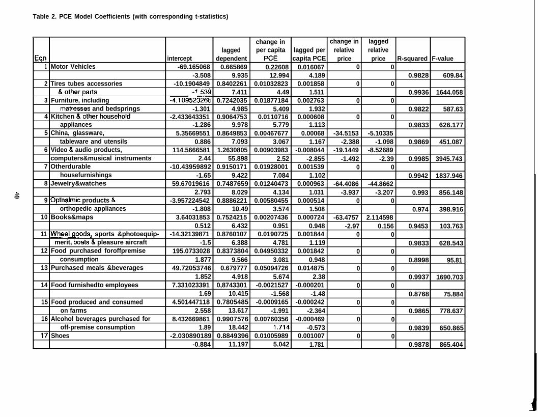
Table 2. PCE Model Coefficients (with corresponding t-statistics)

F

change in change in laggedlagged per capita lagged per relative relative

Eqn intercept dependent PCE capita PCE price price R-squared F-value1 Motor Vehicles -69.165068 0.665869 0.22608 0.016067 0 0

-3.508 9.935 12.994 4.189 0.9828 609.842 Tires tubes accessories -10.1904849 0.8402261 0.01032823 0.001858 0 0

&otherparts -1 339 7.411 4.49 1.511 0.9936 1644.0583 Furniture, including -4.10952~266 0.7242035 0.01877184 0.002763 0 0

matresses and bedsprings -1.301 4.985 5.409 1.932 0.9822 587.634 Kitchen &otherhousehold -2.433643351 0.9064753 0.0110716 0.000608 0 0

appliances -1.286 9.978 5.779 1.113 0.9833 626.1775 China, glassware, 5.35669551 0.8649853 0.00467677 0.00068 -34.5153 -5.10335

tableware and utensils 0.886 7.093 3.067 1.167 -2.388 -1.098 0.9869 451.0876 Video & audio products, 114.5666581 1.2630805 0.00903983 -0.008044 -19.1449 -8.52689

computers&musical instruments 2.44 55.898 2.52 -2.855 -1.492 -2.39 0.9985 3945.7437 Otherdurable -10.43959892 0.9150171 0.01928001 0.001539 0 0

housefurnishings -1.65 9.422 7.084 1.102 0.9942 1837.9468 Jewelry&watches 59.67019616 0.7487659 0.01240473 0.000963 -64.4086 -44.8662

2.793 8.029 4.134 1.031 -3.937 -3.207 0.993 856.1489 Opthalmic products & -3.957224542 0.8886221 0.00580455 0.000514 0 0

orthopedic appliances -1.808 10.49 3.574 1.508 0.974 398.91610 Books&maps 3.64031853 0.7524215 0.00207436 0.000724 -63.4757 2.114598

0.512 6.432 0.951 0.948 -2.97 0.156 0.9453 103.76311 Wheelgoods, sports &photoequip- -14.32139871 0.8760107 0.0190725 0.001844 0 0

merit, boats& pleasure aircraft -1.5 6.388 4.781 1.119 0.9833 628.54312 Food purchased foroffpremise 195.0733028 0.8373804 0.04950332 0.001842 0 0

consumption 1.877 9.566 3.081 0.948 0.8998 95.8113 Purchased meals &beverages 49.72053746 0.679777 0.05094726 0.014875 0 0

1.852 4.918 5.674 2.38 0.9937 1690.70314 Food furnishedto employees 7.331023391 0,8743301 -0.0021527 -0.000201 0 0

1.69 10.415 -1.568 -1.48 0.8768 75.88415 Food produced and consumed 4.501447118 0.7805485 -0.0009165 -0.000242 0 0

on farms 2.558 13.617 -1.991 -2.364 0.9865 778.63716 Alcohol beverages purchased for 8.432669861 0.9907576 0.00760356 -0.000469 0 0

off-premise consumption 1.89 18.442 1.714 -0.573 0.9839 650.86517 Shoes -2.030890189 0.8849396 0.01005989 0.001007 0 0

-0.884 11.197 5.042 1.781 0.9878 865.404

. . . . . . . . . . . . . . . . .

Table 2. PCE Model Coefficients (with corresponding t-statistics)

change in change in laggedlagged per capita lagged per relative relative

Eqn intercept dependent PCE capita PCE price price R-squared F-value18 Clothing & luggage -27.56525987 0.9386914 0.04724968 ~ 0.004923 0 0

-2.051 14.989 5.513 1.418 0.996 2625.05119 Military clothing 0.592165344 0.766812 -3.72E-06 -3.03E-05 o 0

2.052 7.229 -1 .80E-02 -1.716 0.7185 27.22120 Gasoline & oil 21.99757699 1.0105687 0.02503072 -0.001281 -48.3427 -10.9281

2.453 24.572 4.703 -1.605 -3.971 -2.053 0.99 592.41121 Fuel oil & coal 44.19687801 0.7975012 0.0180928 -0.001852 -15.1241 -10.1809

1.795 8.164 4.134 -1.736 -1.537 -2.494 0.9862 430.32322 Tobacco products 124.7230478 0.7151042 0.00347347 -0.001267 -183.04 -55.0203

1.689 4.209 0.657 -1.809 -3.497 -1.361 0.9714 203.58523 Toilet articles & -0.876664776 0.7359864 0.00859361 0.002586 0 0

preparations -0.421 9.135 4.937 3.02 0.9951 2182.64724 Semi-durable house -0.429708958 0.9210679 0.00800665 0.000434 0 0

furnishings -0.197 10.507 4.957 1.078 0.9789 495.24425 Cleaning & polishing preparations, 14.76823488 0.8051723 0.00832595 0.001165 0 0

& mist hh supplies and paper 2.563 10.232 1.995 1.695 0.9545 223.51226 Stationery & writing supplies 20.02803626 0.68983 0.00296569 0.000785 -38.8391 -16.6268

2.093 5.285 2.912 2.226 -4.225 -2.175 0.9881 497.80327 Drug preps & sundries -5.061206039 0.8486983 0.0020434 0.003289 0 0

-0.637 12.381 0.584 1.944 0.9963 2844.12128 Magazines & newspapers & sheet 20.10697233 0.9212841 0.00643461 0.000827 -169.213 -26.8674

music 0.642 10.136 1.276 0.406 -4.231 -0.401 0.9012 54.75829 Nondurable toys & sport supplies -9.58111687 1.1140654 0.0073733 -0.000442 -28.3447 4.750178

-0.723 14.76 5.128 -0.456 -1.711 1.008 0.9979 2854.92430 Flowers seeds & potted plants -3.265688273 0.836491 0.00347996 0.000673 0 0

-1.58 8.543 2.934 1.731 0.9846 679.90331 Expenditures abroad 7.728292135 0.8939302 0.00060746 -0.000396 -20.7369 -0.71437

0.895 9.867 0.212 -0.977 -2.842 -0.074 0.9445 102.16832 Less: remittances in kind -0.233272949 0.8075157 -0.0002 -3.22E-05 o 0

-0.604 7.707 -0.555 -1.015 “ 0.7477 31.61333 Owner occupied nonfarm dwellings -18.4312 0.7342 0.0131 0.0311 0 0

space rent -0.5917 7.5267 1.1884 2.6888 0.9931 1487.02334 Tenant occupied nonfarm dwellings 51.9219 0.567 0.0156 0.0136 0 0

rent 0.9581 1.6799 2.7413 1.3846 0.9455 179.3034

..—

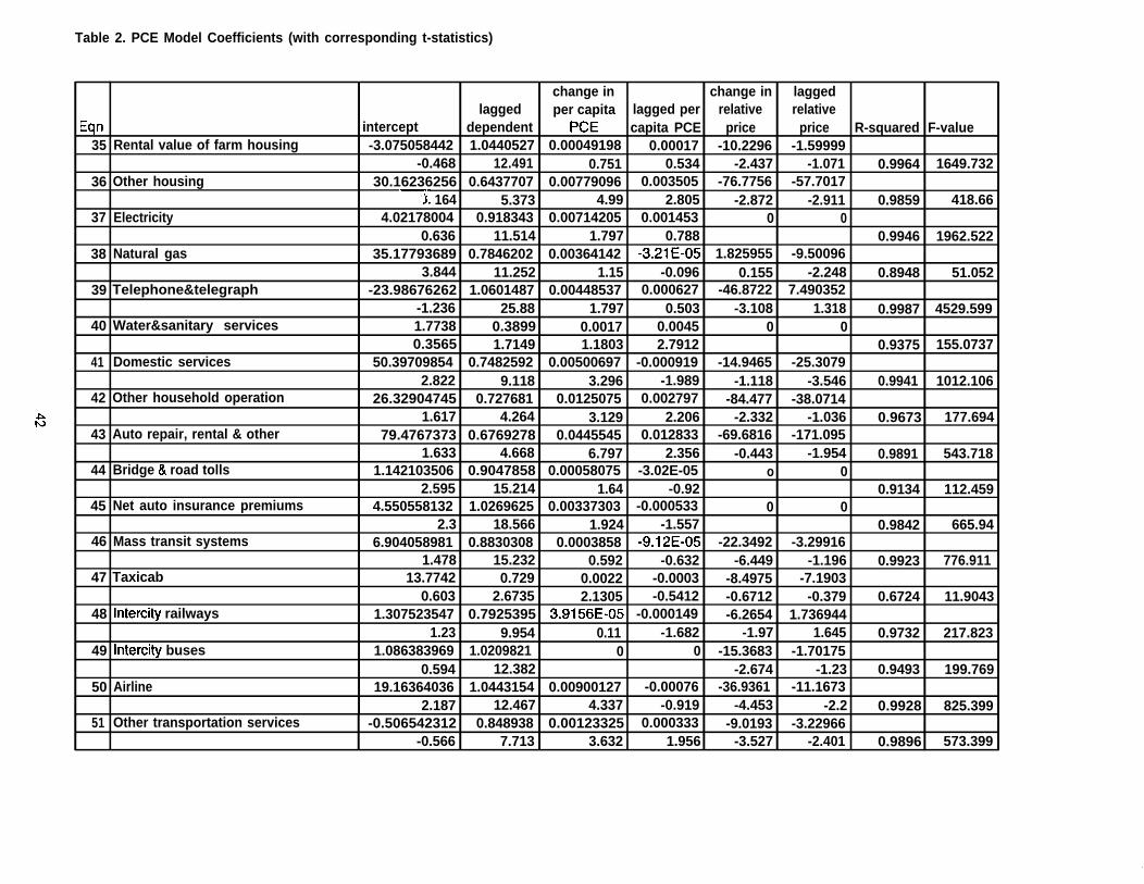
Table 2. PCE Model Coefficients (with corresponding t-statistics)

change in change in laggedlagged per capita lagged per relative relative

Eqn intercept dependent PCE capita PCE price price R-squared F-value35 Rental value of farm housing -3.075058442 1.0440527 0.00049198 0.00017 -10.2296 -1.59999

-0.468 12.491 0.751 0.534 -2.437 -1.071 0.9964 1649.73236 Other housing 30.16236256 0.6437707 0.00779096 0.003505 -76.7756 -57.7017

‘J. 164 5.373 4.99 2.805 -2.872 -2.911 0.9859 418.6637 Electricity 4.02178004 0.918343 0.00714205 0.001453 0 0

0.636 11.514 1.797 0.788 0.9946 1962.52238 Natural gas 35.17793689 0.7846202 0.00364142 -3.21E-05 1.825955 -9.50096

3.844 11.252 1.15 -0.096 0.155 -2.248 0.8948 51.05239 Telephone&telegraph -23.98676262 1.0601487 0.00448537 0.000627 -46.8722 7.490352

-1.236 25.88 1.797 0.503 -3.108 1.318 0.9987 4529.59940 Water&sanitary services 1.7738 0.3899 0.0017 0.0045 0 0

0.3565 1.7149 1.1803 2.7912 0.9375 155.073741 Domestic services 50.39709854 0.7482592 0.00500697 -0.000919 -14.9465 -25.3079

2.822 9.118 3.296 -1.989 -1.118 -3.546 0.9941 1012.10642 Other household operation 26.32904745 0.727681 0.0125075 0.002797 -84.477 -38.0714

1.617 4.264 3.129 2.206 -2.332 -1.036 0.9673 177.69443 Auto repair, rental & other 79.4767373 0.6769278 0.0445545 0.012833 -69.6816 -171.095

1.633 4.668 6.797 2.356 -0.443 -1.954 0.9891 543.71844 Bridge & road tolls 1.142103506 0.9047858 0.00058075 -3.02E-05 o 0

2.595 15.214 1.64 -0.92 0.9134 112.45945 Net auto insurance premiums 4.550558132 1.0269625 0.00337303 -0.000533 0 0

2.3 18.566 1.924 -1.557 0.9842 665.9446 Mass transit systems 6.904058981 0.8830308 0.0003858 -9.12E-05 -22.3492 -3.29916

1.478 15.232 0.592 -0.632 -6.449 -1.196 0.9923 776.91147 Taxicab 13.7742 0.729 0.0022 -0.0003 -8.4975 -7.1903

0.603 2.6735 2.1305 -0.5412 -0.6712 -0.379 0.6724 11.904348 Intercity railways 1.307523547 0.7925395 3.9156E-05 -0.000149 -6.2654 1.736944

1.23 9.954 0.11 -1.682 -1.97 1.645 0.9732 217.82349 Intercity buses 1.086383969 1.0209821 0 0 -15.3683 -1.70175

0.594 12.382 -2.674 -1.23 0.9493 199.76950 Airline 19.16364036 1.0443154 0.00900127 -0.00076 -36.9361 -11.1673

2.187 12.467 4.337 -0.919 -4.453 -2.2 0.9928 825.39951 Other transportation services -0.506542312 0.848938 0.00123325 0.000333 -9.0193 -3.22966

-0.566 7.713 3.632 1.956 -3.527 -2.401 0.9896 573.399

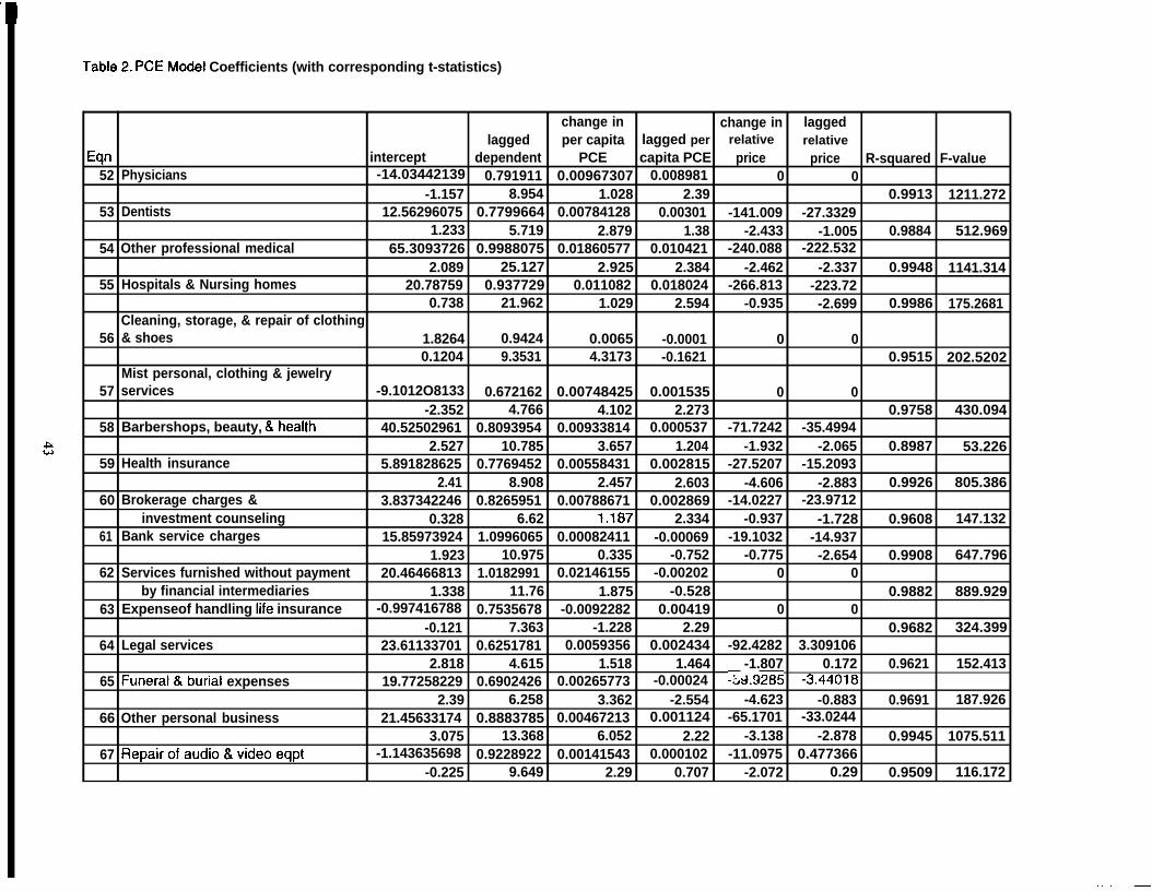
Table2. PCEModel Coefficients (with corresponding t-statistics)

change in change in laggedlagged per capita lagged per relative relative

Eqn intercept dependent PCE capita PCE price price R-squared F-value52 Physicians -14.03442139 0.791911 0.00967307 0.008981 0 0

-1.157 8.954 1.028 2.39 0.9913 1211.27253 Dentists 12.56296075 0.7799664 0.00784128 0.00301 -141.009 -27.3329

1.233 5.719 2.879 1.38 -2.433 -1.005 0.9884 512.96954 Other professional medical 65.3093726 0.9988075 0.01860577 0.010421 -240.088 -222.532

2.089 25.127 2.925 2.384 -2.462 -2.337 0.9948 1141.31455 Hospitals & Nursing homes 20.78759 0.937729 0.011082 0.018024 -266.813 -223.72

0.738 21.962 1.029 2.594 -0.935 -2.699 0.9986 175.2681Cleaning, storage, & repair of clothing

56 & shoes 1.8264 0.9424 0.0065 -0.0001 0 00.1204 9.3531 4.3173 -0.1621 0.9515 202.5202

Mist personal, clothing & jewelry57 services -9.1012O8133 0.672162 0.00748425 0.001535 0 0

-2.352 4.766 4.102 2.273 0.9758 430.09458 Barbershops, beauty, &health 40.52502961 0.8093954 0.00933814 0.000537 -71.7242 -35.4994

2.527 10.785 3.657 1.204 -1.932 -2.065 0.8987 53.22659 Health insurance 5.891828625 0.7769452 0.00558431 0.002815 -27.5207 -15.2093

2.41 8.908 2.457 2.603 -4.606 -2.883 0.9926 805.38660 Brokerage charges & 3.837342246 0.8265951 0.00788671 0.002869 -14.0227 -23.9712

investment counseling 0.328 6.62 1.187 2.334 -0.937 -1.728 0.9608 147.13261 Bank service charges 15.85973924 1.0996065 0.00082411 -0.00069 -19.1032 -14.937

1.923 10.975 0.335 -0.752 -0.775 -2.654 0.9908 647.79662 Services furnished without payment 20.46466813 1.0182991 0.02146155 -0.00202 0 0

by financial intermediaries 1.338 11.76 1.875 -0.528 0.9882 889.92963 Expenseof handling Iife insurance -0.997416788 0.7535678 -0.0092282 0.00419 0 0

-0.121 7.363 -1.228 2.29 0.9682 324.39964 Legal services 23.61133701 0.6251781 0.0059356 0.002434 -92.4282 3.309106

2.818 4.615 1.518 1.464 -1.807 0.172 0.9621 152.41365 Funeral&burial expenses 19.77258229 0.6902426 0.00265773 -0.00024 -~,9;9285 -3.44018

2.39 6.258 3.362 -2.554 -4.623 -0.883 0.9691 187.92666 Other personal business 21.45633174 0.8883785 0.00467213 0.001124 -65.1701 -33.0244

3.075 13.368 6.052 2.22 -3.138 -2.878 0.9945 1075.51167 Repairofaudio& videoeqpt -1.143635698 0.9228922 0.00141543 0.000102 -11.0975 0.477366

-0.225 9.649 2.29 0.707 -2.072 0.29 0.9509 116.172

..-. . ..—

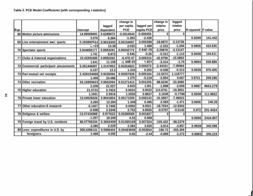
Table 2. PCE Model Coefficients (with corresponding t-statistics)

change in change in laggedlagged per capita lagged per relative relative

Eqn intercept dependent PCE capita PCE price price R-squared F-value68 Motion picture admissions 14.99069691 0.6289972 -0.0014543 -0.000455 0 0

3.076 6.384 -1.283 -2.438 0.9299 141.44269 Live entertainment excl. sports 0.183892514 0.9616302 0.00154097 0.000286 -18.8872 -3.13738

u.123 13.38 2.035 1.468 -2.333 -1.294 0.9856 410.63570 Spectator sports 5.944692177 0.8583291 0.00042772 -2.64E-05 -3.29878 -3.13147

1.741 9.973 0.545 -0.26 -0.312 -1.112 0.9458 104.61171 Clubs & fraternal organizations 15.42291685 0.8992262 -6.47E-07 0.000315 -42.9759 -15.0852

1.641 11.159 -1 .00E-03 1.931 -3.314 -1.75 0.9894 559.88972 Commercial participant amusements 5.361446897 1.0147802 0.00264823 0.000272 -2.44101 -7.39964

0.237 13.3 1.316 0.355 -0.038 -0.313 0.9939 970.40573 Pari-mutuel net receipts 2.428194668 0.9235094 0.00057839 -0.000184 -12.5072 1.118777

1.406 24.486 1.375 -5.218 -3.954 0.667 0.9721 209.28674 Other recreation 33.16959623 0.9502094 0.01271414 0.001205 -88.6246 -33.3085

2.208 21.527 4.503 1.001 -1.898 -3.009 0.9987 4663.27975 Higher education 21.5723 0.7922 0.0024 0.0023 114.6761 -19.3651

1.1651 2.5916 1.2555E 0.8837 2.1638 -0.7786 0.9508 111.982276 Private lower education 12.04526626 0.9041854 0.00171505 0.000143 -41.5907 -7.49022

3.265 12.284 1.349 0.495 -2.583 -1.471 0.9606 146.2677 Other education & research -0.1457 0.7466 0.0069 0.0021 -18.7034 -12.9302

-0.008 2.3246 3.753 0.8555 -0.5707 -0.5145 0.972 201.442478 Religious & welfare -13.07434988 0.977623 0.02280565 0.001827 0 0

-1.257 18.309 4.02 0.968 0.9956 2434.80779 Foreign travel by U.S. residents 86.07765334 0.3663459 0.01365169 0.007324 -105.422 -98.2379

3.385 2.229 2.383 3.655 -3.814 -3.857 0.9828 342.09880 Less: expenditures in U.S. by 308.5286131 0.5986434 0.00493658 -0.003654 -196.72 -355.309

foreigners 2.499 4.292 0.65 -2.44 -0.899 -2.272 0.9883 505.219

A COMMODITY-SPECIFIC MODEL FOR PROJECTING IMPORT DEMAND

Betty W. SuBureau of Labor statistics, Washington, DC 20212

Introduction

The purpose of developing an import model is to refinethe Bureau of Labor Statistics (.BLS) projectionsmethod in the area of imports. In previous projections,imports had been treated in a manner analogous toexports.l The drawback with this, however, is that thecommodity distribution of imports is not directlyinfluenced by the sectoral composition of demand. Toremedy this, we have developed a set of cornrnodity-speci.fic import fimctions. This import model is beingused for the first time in the Bureau’s projectionsSystem. z

The study described here is a model which estimatesimport flows for 107 commodities.3 This modeloperates as one of several sub-models within the BLSemployment projections model system. The mostimportant element of this model is its commoditydetail. As will be apparent, import demands varyconsiderably by commodity.

A Commodity-Specific Import Model

Import demand basically depends on the consumer’sincome, the price of imports, and the price of the othergoods; in this case, the price of domestic goods,because individuals allocate their income amongconsumable commodities in an effort to achievemaximum satisfaction. This suggests that for aneconomy we may write import demand as:

M = f(Y, p., pY)

where

M: Import demandY : Domestic incomeP “m. Price levels of importsPy : Price levels of domestic goods

In addition to income and price, the two key variables,the Learner and Stem model suggested that otherpossible explanatory variables should also beconsidered. A complex demand phenomenon requiresmore variables than the usual two. Five other variablesare described in the Learner and Stem model:4

1. Lagged variable: It is particularly important inmeasuring the influence of past changes in theindependent variables on the current behavior ofimports.

2. The capacity-utilitition variable: An increase indomestic demand may not be met immediately by priceincreases. Rather, domestic producers may ration theavailable supply by delaying deliveries. The consumermay look to foreign sources of supply to avoid thedelay in delivery and pay two prices for the goods hedesires during the waiting period. Capacity utilizationis a proxy to reflect the length of queues at home andabroad.

3. The dollar’s exchange rate: It significantly afhct theprices of foreign goods transacted from othercurrencies to the U.S. dollars.

4. Dummy variables for unusual periods: It allows forthe effects on imports of unusual occurrences such as astrike, war, or natural disaster. Such variables wouldassume a value of one for the duration of the unusualperiod and zero otherwise.

5. Credit variable: It indicates the availability andterms at which credit is provided for the financing ofimports. Such a variable is important in linking thecurrent and capital accounts of balance of payments.

The variables discussed above are in general the mostimportant ones, especially for the manufacturingindustries, although the list is by no means all-inclusive. Many other explanatory variables willsuggest themselves in particular situations.

For empirical, data availability, and accommodatingreaso~ a cmnrnodity-specific import model is formedusing a log-linear least squares regression:

(1) logW = * + al logyit + a2 logM M + a310gR +dogpk + D

where

M: The volume (value) ofcommodity, 1992 dollars.

imports for that

45

Y:

R

P:

D:

and

t:“.1.

Total supply (domestic output plus imports) ofthat commodity, 1992 dollars.Trade-weighted U.S. dollar’s exchange rate,1990=100.Relative price irnpor@ 1992=100, defined asthe ratio of import price deflator for thatcommodity to comparable domestic producerprice deflator for that commodity.Dummy variable for the eff’ upon importsof unusual occurrences such as a strike, war,natural disaster, or oil price shock. One forthe duration of the unusual period and zerootherwise.

time periodith commodity

It is important to note that in this model, total supply,defined as domestic output plus imports, is chosen as aproxy to reflect the economy-wide demand as well as totest the sensitivity of import demand.

Estimation Procedure, Data Sources, andIU@wssion Results

The import model estimates the import trend bycommodity. The data used to implement this importmodel are primarily developed by BLS, Office ofEmployment Projections (OEP) commodity time-seriesdata base. The import and domestic output data areestimated by OEP at 3-digit SIC level. The trade-weighted U.S. dollar’s exchange rates are obtainedfrom the OEP’s macro econometric model data base.The domestic producer price index and import priceindex are also developed iiom OEP’S data base andBLS estimates.

The regression equation is mtimakd with ordinaryleast squares. Several specifications of equation (1) areedmated foreachcornmodity. l%isismzesmrytoensure the estimation technique yields a reasonablecoefficient in terms of the sign and statisticalsignificance. The expected sign for the coefficient oftotal supply (al) and the coefficient of laggeddependent variable (az) should be positive, and thecoefficient of exchange rate (as) should also hold apositive sign. On the other ban* the price coefficient(@) shodd have a negative sign. u the variablecoefficients show a wrong si~ the variable aredropped fkom the estimated equation. For this reaso~eight specifications of equation(1) are used as:

(1.1) 10*= a+ allogyit + a2WM it-l + @@k+aJogPti + D

(1.2) 10*= aJogYh + aJogM N + a310gRt+ ~ogpit+D

(1.3) loghk= m + allogyk + a210gM it-l + a310@? + D

(1.4) loghlit= allogYit + aJogM it.1 + aJogRt + D

(1.5) 10~k= ~ + allogyfi + azloghl it-l + do@% + D

(1.6) loghlti= allogYit + aJogM it-l + do@% + D

(L7) logh&= m + allogyit + aJogM it-l + D

(1.8) logh&= allogyit + azlogM it-l + D

To choose among the 8 equations for each commodity,the equations are estimated over the 1977-93 period.of the 107 commodities, 2 commodities-woodcontainers and miscellaneous wood products(timmtity 14) and Office and miscehus fbrnitureand fixtures (Commodity 17)-have data available onlyin the period of 1978-1993 and 1983-1993respedvely; 4 commodities-oil and gas field seMces(Commodity 7), construction (Commodity 9),partitions and fixtures (CommO@ 16), and metalcoating, engraving, and allied seMces (Commodity34)-show no import values in the input-outputaccounts.

Table 1 shows the results that the explanatory variablecoefficients have the %orrect” sign. Historicalsimulation is also tested to examine how closely eachsimulated variable tracks its corresponding data series.Other statistics such as R-sq~ F-values, and t-statistics are also shown in table 1.

The Projections of Commodity Trends andAggregate Trends

To solve the projections, the variables of exchange ratecan be produced by the OEP’S macro econometricmodel, but the outputs and prices by commodity mustbe extrapolated fkom the estimated historical series.For this set of projections, due to time constraints, theprojected total supply for the import model is notiteratively derived. In@@ the historical total supplyseries is extrapolated and used as a proxy.

As mentioned earlier, this model deals with 107 goods.However, the OEP projections system contains 185commodities or industries. These include 107 goo@

46

72 services, and 6 special industries. Outside ofagriculture, mining, and manufacturing, import entriesonly exist in 21 seMces and 2 special industries. (SeeAppendix.) Among the 21 seMces, almost all of theirtime-series data on imports are available only from1986 to 1993. In order to project sewices of imports,an alternative estimating method is used.

Import demand is initially projected by the macroeconometric model, which generates values for 8 majorend-use categories of imports-7 for goods and 1 forsexvices. The single cohmm of seMces control isallocated among commodities based on the estimatesfor a most recent historical year distribution. Twospecial industries-noncomparable importss and scrap,used and secondhand goods, are treated as dummycommodities, and are projected based on theirhistorical trends of the commodity as a share of totalimports.

To make sure the goods estimates from the model areconsistent with the macro controls, the 107 estimatesplus the 2 special ones are then disaggregate into 7columns based on the bridge table developed by OEP.

Footnotes

Obviously, summation dMerences are expected fkomthese two estimates. The Werences are then carefidlyexamined ant generally, scaling adjustments areintroduced in order to reproduce the macro modelcontrol values. The macro model controls maythemselves be modified indeveloped detail at theprojection.

Conclusion

response to the more finelycommodity level of the

Since the import model is being developed and used forthe first time in the projection system extensive workis needed to improve the model. This includes inparticular the generation of proxy variables. Forexample, to avoid the technical simulation probleushould the lagged total supply, rather than the currentvalue, be used as an explanatory variable in the model?To operate this import model, the price equation isessential, and a price model is also needed as a vehicleto fit the import model. It is hoped that further workwith the model will truly improve the projections in thearea of imports.

‘ For expo@ the projection process involves allocating tha projected 3 See Table 1 fw the M of 107 commodities.category control W generated hxn the macro ccimometric model to 4kmWr,W VV/miE.a ndS~RObCrtM. Ouantitative htenmtionalcommdtica baacdon pattcmgesthtcd fbrareccnt hiatofical year Economics (130stoQ M/k Allyn and IhcoQ Inc. 1970).bridge table. 3 h-~~le~(l)-~”~--c

2 Thk ayatcm waa developed by the CMke of Employment Rojcctiq producti~ e.g., coffee beam and ~, of (2) the item is prchssdBumu of Labor Statistics Ike projcctiona cover the fiture size snd and used outside the U. S., such as consular f- andCoquWkion of tha labor fbrcc, aggregate

Commlmicatioaaconomic growtl& detailed -,w(3)bkkti~e,m&wti~=dti-

ealmtes ofhdustrial pductimand imhshhl aadoocupationalCqkymuW

Appendix: A List of Import-Related Services and Special Industries

1 Railroad transportation2 Water transportation3 Air transportation4 Electric utilities5 Gas utilities6 Wholesale trade7 Depository institutions8 Insurance carriers9 Advertising

10 Personnel supply seMces11 Computer and data processing seMces12 Miscellaneous business seMces

13 Miscellaneous repair seMces14 Motion pictures15 Producers, orchestras, and entertainers16 Legal seMces17 Educational seMces18 Engineering and architectural seMces19 Research and testing seMces20 Management and public relations21 Accounting, auditing, and other seMces22 NoncomParable imports23 Scrap, used and secondhand goods

47

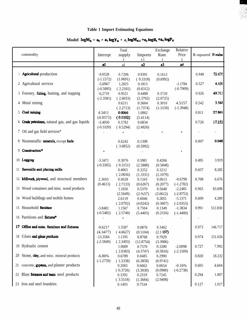
Table 1 Import Estimating Equations

Model logMh = ~ + al logYh + a2 loglklkl +a3 Io* +% 10#it

Total Exchange RelativeIntercept supply Imports Rate Price

t t-1 t tcommodity R-squared F-vah

aO al a2 a3 a4

1

2

3

4

5

6

7

8

9

10

11

12

13

14

15

16

17

18

19

20

21

22

23

Agricuhra.1 production

Agricultural services

Forestry, fim hunting, and trapping

Metal mining

Coalmining

crude Petrolq natural gas, and gas liquids

-9.0528(-1.1572)-5,6967(-0.5895)-6,2719(-2.3581)

0.7296(1.0691)1,2825

( 2.2181)0.9521

( 2.6033)0.6211

( 2.2713)

(:E2)0.5782

( 0.5294)

0.9391( 9.3318)

0.1813(0.6312)0.4489(2.3792)0.3604(1.7374)1.0862

(5.4114)0.6834(2.4926)

.

0.1612(0.6992)

0.948

0.527

0.926

0.542

0.811

0.726

.

0.007

0.495

0.657

0.708

0.965

0.609

0.991

.

0.973

0.974

0.727

0.820

0.605

0.294

0.127

72.67:

4.455

49.712

3.54$

27.86S

17.251

.

0.048

3.919

8.285

6.676

83.698

4.289

312.830

146.717

151.656

7.992

18.232

4.604

1.807

1.017

-1.1784(-0.7009)

0.3720(2.0725)0.3010(1.3159)

4.5157(-1.3948)

4.3411(4.0572)-3.4050(-0.3320)

.Oil and gas field services*

Nonmetallic miIMl&3, except fhds

~on*

m&m8

%VIdS aud @Ul@ XUih

MiUworlq plyvo@ and structural members

Wood containers and misc. wood products

Wood buildings and mobile homes

Household fiuniture

Partitions and Mums*

Of#iceandmisc.llhmiture and fixtwes

Glass andglassproducts

Hydraulic cement

Stone, Ckijf, and misc. mineral products

concrete, gypsuQ and plaster products

Blast fhmacesandbasic steel products

Iron and steel foundries

. .

0.6242( 3.6852)

0.1398(0.5992)

.. .

-3.3471(-0.3365)

0.3076( 0.3151)

0.4063( 2.0656)

0.6628( 2.7133)

1.1650(2.5649)2.6119

( 2.0702)1.1567

( 2.5740)

0.5981(2.5888)0.3252(1.3331)0.1343(0.6267)0.5370(2.%57)0.6846(4.0242)0.7504(5.4403)

0.4266(0.5848)0.3212(2.1079)0.0613(0.2077)0.5640

(3.0612)0.2855(0.3607)0.1349(0.2316)

.

2.3693(0.4613)

-0.6799(-1.2782)-2.2485

(-2.8753)-5.1375

(-2.0353)-1.3834

(-1.4400).

-3.8482(-0.5482)

. .

-9.6217(4.3477)-13.3584(-2.5849)

1.5587( 4.6627)

1.1195( 2.3493)

1.0689( 2.0383)0.6789

( 1.5338)0.2065

( 0.3726)0.3392

( 3.5518)0.1403

0.0876(0.5104)0.8768

(12.8754)0.7570(4.3747)0.8485(6.3858)0.6662(3.3930)0.2319(1.3684)0.7534

0.3462(2.1 157)0.7029(3.3986)0.3280(0.5816)0.2990(0.9741)0.0654(0.0980)0.7245(2.9408)

-2.0098(-2.1509)

-6.86%(-1.2759)

-0.16%(-0.2738)

48

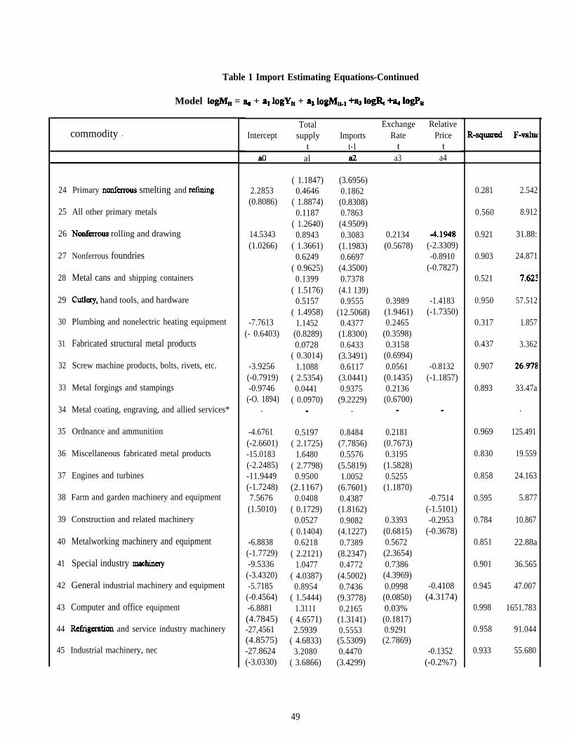
Table 1 Import Estimating Equations-Continued

Model logMk = ~ + al logYk + az logltll~.l +a3 Io* @ logPk

commodity ~

24

25

26

27

28

29

30

31

32

33

34

35

36

37

38

39

40

41

42

43

44

45

Primary nonfimous smelting and reftig

All other primary metals

Nonkrmus rolling and drawing

Nonferrous foundries

Metal cans and shipping containers

Cutlexy, hand tools, and hardware

Plumbing and nonelectric heating equipment

Fabricated structural metal products

Screw machine products, bolts, rivets, etc.

Metal forgings and stampings

Metal coating, engraving, and allied services*

Ordnance and ammunition

Miscellaneous fabricated metal products

Engines and turbines

Farm and garden machinery and equipment

Construction and related machinery

Metalworking machinery and equipment

Special industry machirmy

General industrial machinery and equipment

Computer and office equipment

Reiligeration and service industry machinery

Industrial machinery, nec

Total Exchange RelativeIntercept supply Imports Rate Price

t t-1 t taO al S2 a3 a4

2.2853(0.8086)

14.5343(1.0266)

-7.7613(- 0.6403)

-3.9256(-0.7919)-0.9746

(-O. 1894).

-4.6761(-2.6601)-15.0183(-2.2485)-11.9449(-1.7248)7.5676(1.5010)

-6.8838(-1.7729)-9.5336(-3.4320)-5.7185(-0.4564)-6.8881(4.7845)-27,4561(4.8575)-27.8624(-3.0330)

( 1.1847)0.4646

( 1.8874)0.1187

( 1.2640)0.8943

( 1.3661)0.6249

( 0.9625)0.1399

( 1.5176)0.5157

( 1.4958)1.1452

(0.8289)0.0728

( 0.3014)1.1088

( 2.5354)0.0441

( 0.0970).

0.5197( 2.1725)

1.6480( 2.7798)

0.9500(2.1167)

0.0408( 0.1729)0.0527

( 0.1404)0.6218

( 2.2121)1.0477

( 4.0387)0.8954

( 1.5444)1.3111

( 4.6571)2.5939

( 4.6833)3.2080

( 3.6866)

(3.6956)0.1862(0.8308)0.7863(4.9509)0.3083(1.1983)0.6697(4.3500)0.7378(4.1 139)0.9555

(12.5068)0.4377(1.8300)0.6433(3.3491)0.6117(3.0441)0.9375

(9.2229).

0.8484(7.7856)0.5576(5.5819)1.0052

(6.7601)0.4387(1.8162)0.9082(4.1227)0.7389(8.2347)0.4772(4.5002)0.7436(9.3778)0.2165(1.3141)0.5553(5.5309)0.4470(3.4299)

0.2134(0.5678)

0.3989(1.9461)0.2465

(0.3598)0.3158(0.6994)0.0561(0.1435)0.2136(0.6700)

.

0.2181(0.7673)0.3195(1.5828)0.5255(1.1870)

0.3393(0.6815)0.5672(2.3654)0.7386(4.3969)0.0998(0.0850)0.03%(0.1817)0.9291(2.7869)

4.1948(-2.3309)-0.8910

(-0.7827)

-1.4183(-1.7350)

-0.8132(-1.1857)

.

-0.7514(-1.5101)-0.2953

(-0.3678)

-0.4108(4.3174)

-0.1352(-0.2%7)

bquared F-valw

0.281

0.560

0.921

0.903

0.521

0.950

0.317

0.437

0.907

0.893

0.969

0.830

0.858

0.595

0.784

0.851

0.901

0.945

0.998

0.958

0.933

2.542

8.912

31.88:

24.871

7.623

57.512

1.857

3.362

26.978

33.47a

.

125.491

19.559

24.163

5.877

10.867

22.88a

36.565

47.007

1651.783

91.044

55.680

49

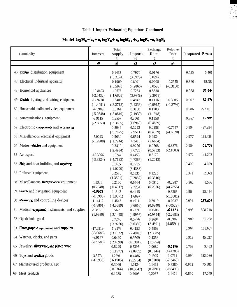
Table 1 Import Estimating Equations-Continued

Model 1-= ~+ al logYh+ ~ log& +a3 1- +q IogPk

commodity

46

47

48

49

50

51

52

53

54

55

56

57

58

59

60

61

62

63

64

65

66

67

68

Ekctric distribution equipment

Electrical industrial apparatus

Household appliances

Ekctric lighting and wiring equipment

Household audio and video equipment

communications equipment

Electronic canponents and mcewories

Miscellaneous electrical equipment

Motor vehicks and equipment

Aerospace

Ship and boat building and mpaking

Railroad equipment

Miscellaneous tnmqmtation equipment

Seamh and navigation equipment

Meamring and controlling devices

Medical equipmen~ instruments, and supplies

Ophthalmic goods

~O@Xll@iC equipment and sqqdks

Watches, clocks, and parts

Jewelry, SihkXW& and Phlted ware

Toys and spwting goods

Manufactured products, nec

Meat products

Total Exchange RelativeIntercept supply Imports Rate Price

t t-1 t taO al a2 a3 d

-10.8493(-2.0432)-12.9278(-1.4091)-4.5989(-5.0848)-8.9115(-2.6053)

-5.0043(-1.9908)

-15.3566(-3.8324)

1.3331(0.2948)4.%27(-1.5993)-11.4412(-1.8801)23.8178(1.9989)

-17.0319(-3.0686)-6.9177(-1.9585)

-3.5574(-1.1998)

0.1463( 0.3174)0.1909

( 0.5070)1.0676

( 1.6803)1.8406

( 3.2718)1.0164

( 5.0819)1.3557

( 3.3605)0.8949

( 5.7875)0.5630

( 1.7244)0.3419

( 2.4934)1.6244

( 4.7193)0.1465

( 1.0299)0.2573

(1.3501)0.2160

( 0.4917)1 .3n3

( 1.8871)1.4547

( 4.3689)0.5699

( 2.1495)0.7246

( 3.9766)1.95%

( 3.1522)0.6490

( 2.4099)0.5229

( 1.1977)1.2691

( 6.1905)0.3066

( 0.5364)0.1238

0.7970(3.5975)0.8991(4.2866)0.7264(3.99%)0.4847(3.4233)0.3150(2.1930)0.3061(1.6960)0.3222(2.9511)0.6524(4.3410)0.9276(7.6726)0.4453(4.7387)0.7795(3.4388)0.5535(3.2887)0.6764(2.7254)0.4415(1.6097)0.4011(3.6610)0.7371(4.9998)0.5776(5.6330)0.4153(2.4916)0.9509

(10.3815)0.5395(2.0955)0.4486(5.2754)1.0124

(10.5947)0.7905

0.0176(0.0247)0.0208(0.0596)0.5338(2.3079)0.1116(0.0915)0.1983(1.1948)0.1358(0.4859)0.0388(0.4589)0.4934(2.6634)0.0708(0.5783)0.3172(1.2013)

0.1223(0.3516)0.0912(0.2536)

0.3019(0.6940)0.1508(0.9824)0.2694(3.4%1)0.4859(2.3885)0.4353(1.5954)0.0082(0.0244)0.1925(0.8208)0.1462(0.7091)0,2087

-0.2555(-0.3150)

-0.3905(-0.37%)

-0.7747(-4.6320)

-0.8376(-2.1803)

-0.2987(4).7855)-0.8263

(-1.0881)-0.0237(-00529)4.1423

(-2.2683)-0.8982

(4.8591)

3.2196(4).4783)-1.0711

(-2.3463)-0.8380

(-0.8498)-0.1471

R-squared F-vah.u

0.555

0.860

0.928

0.967

0.986

0.%7

0.994

0.977

0.954

0.972

0.402

0.371

0.562

0.864

0.991

0.995

0.980

0.964

0.918

0.759

0.994

0.962

0.850

5.40!

18.38

51.94

81.47t

272.001

118.9X

487.934

168.485

61.75#

141.202

4.699

2.56(I

3.536

25.414

287.60d

508.218

150.288

108.667

45.027

9.453

452.086

75.385

17.049

50

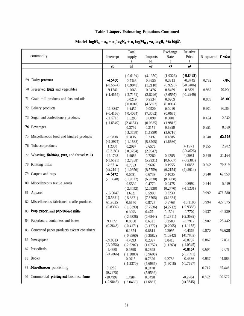
Table 1 Import Estimating Equations-Continued

Model logMk = ~ + al logYk + az logMk.l +as 10g& +% l@it

commodity

69

70

71

72

73

74

75

76

77

78

79

80

81

82

83

84

85

86

87

88

89

90

Dairy prOdUCtS

Preserved tits and vegetables

Grain mill products and fats and oils

Bakery products

Sugar and confectionery products

Beverages

Miscellaneous food and kindred products

Tobacco products

Weaving, finim y- and thread milk

Knitting mills

Carpets and rugs

Miscellaneous textile goods

Apparel

Miscellaneous fabricated textile products

hip, paper, and paperboard III&

Paperboard containers and boxes

Converted paper products except containers

Newspapers

Periodicals

Books

Misceilaueous publishing

Commercial pinting and business f-

Total Exchange RelativeIntercept supply Imports Rate Price

t t-1 t taO al d a3 a4

4.5460(-0.5574)-9.1740(-1.4554)

-11.6847(-0.4166)-11.5713(-1.6349)

-1.9838(41.8974)

1.2300(0.2189)-19.1748(-1.6621)-2.6714(4).2191)45472(-1.3948)

-16.6047(-5.5881)61.9525(0.8302)

9.1072(0.2648)

-39.8313(-3.2656)-1.4988(-0.2866)

0.1285(0.2675)-10.4999(-2.9846)

( 0.6194)0.7%3

( 0.9043)1.2665

( 2.7194)0.0219

( 0.0918)1.1452

( 0.4064)1.6290

(2.4151)0.3792

( 3.3738)0.3115

( 1.1563)0.2087

( 0.3754)1.9686

( 2.7358)0.7553

( 1.0650)0.6591

( 1.9822)0.5539

( 2.3052)1.6921

( 5.3871)0.5570

( 1.5393)0.6955

( 2.9328)0.8868

( 0.4171)0.1874

( 0.6560)4.7893

( 2.6207)0.9598

( 1.3880)0.2615

( 1.3370)

1.4904( 3.0460)

(4.1350)0.3655(1.2110)0.3476(2.6246)0.9534(4.5897)0.9520(7.3062)0.0090(0.0335)0.2151(1.1990)0.7397(5.6705)0.6575(2.0947)0.7260(5.9931)0.9607(8.5759)0.6739(6.9830)0.4770(2.0938)0.5980(7.8705)0.8727(7.7536)0.4751(2.6844)0.6521(3.1772)0.8814(9.2582)0.2397(1.0752)0.2698(0.9608)0.7326(5.6987)0.9470(5.9536)0.3498(1.6887)

(1.9326)0.3813(0.9228)0.8459(3.6597)0.0269(0.0904)0.0419(0.0685)0.6001(1.9813)0.5859(3.6716)0.1885(1.8660)

0.4285(0.6667)0.1955(0.2154)0.1035(0.3968)0.0475(0.2770)0.3230(3.1624)0.6768(4.2712)0.1501(1.2311)0.2580(0.2965)0.2095(1.0342)0.8413(1.1263)

0.2783(1.6018)

(4M492)-0.3745

(-0.9406)-0.6821

(-1.6346)

4.1971(-0.4626)4).3081

(-0.2383)-1.0833

(4).5614)

-0.3992(-1.3231)

-15.1106(-0.9383)-0.7702

(-2.3692)-3.7912

(-1.1155)-0.4369

(4).7882)-0.8787

(-1.0345)4.8114

(-1.7091)-0.4336

(-1.7587)

-0.2784(4).9845)

R-squared l?-vahu

0.782

0.962

0.859

0.901

0.424

0.651

0.940

0.355

0.919

0.%2

0.940

0.644

0.992

0.994

0.937

0.902

0.970

0.867

0.604

0.937

0.717

0.%2

9.86:

70.00(

26.3(X

36.36:

2.942

8.069

62.19!

2.202

31.164

70.319

62.959

5.419

476.580

427.575

44.539

25.442

%.628

17.851

6.0%

44.883

35.446

102.577

51

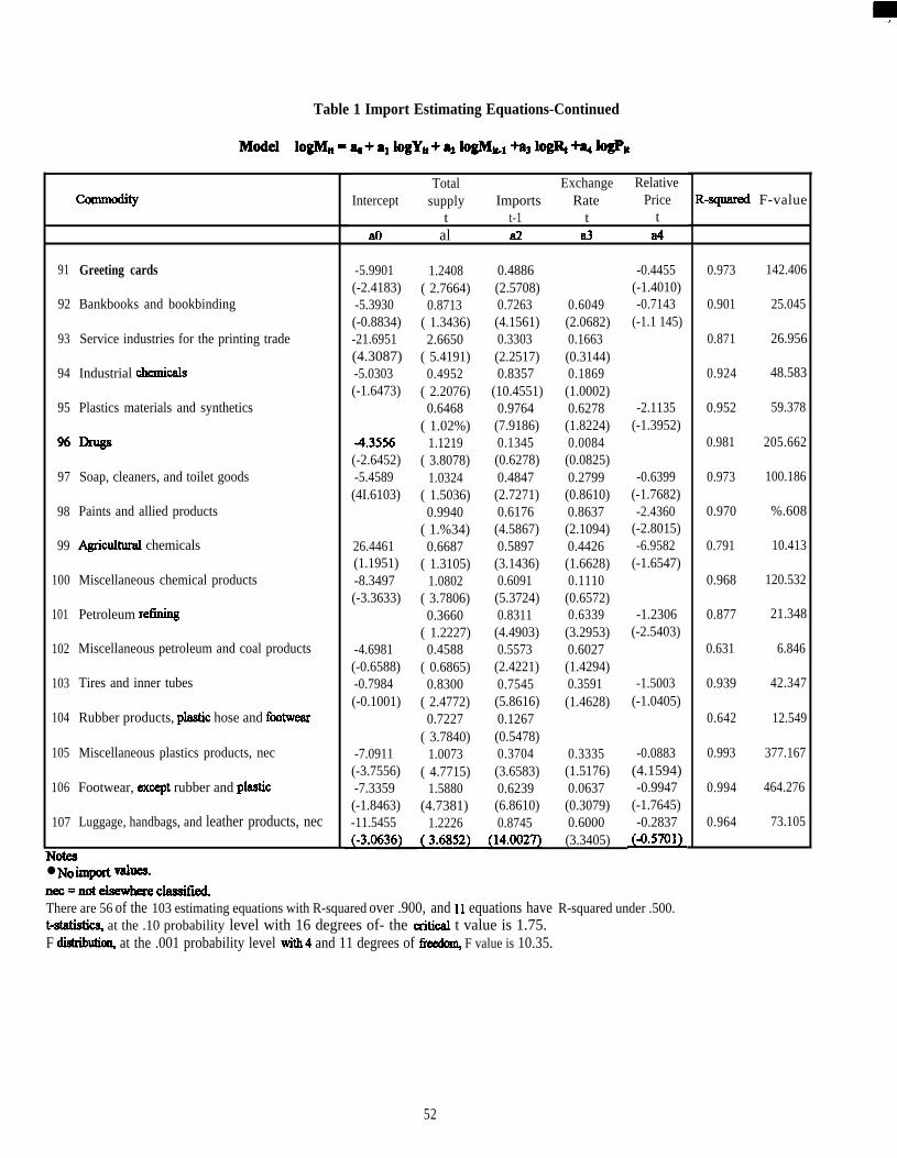
m.,

Table 1 Import Estimating Equations-Continued

Conunodity

91

92

93

94

95

%

97

98

99

100

101

102

103

104

105

106

107

Greeting cards

Bankbooks and bookbinding

Service industries for the printing trade

Industrial ChCllliCdS

Plastics materials and synthetics

Soap, cleaners, and toilet goods

Paints and allied products

i@iCUkllld chemicals

Miscellaneous chemical products

Petroleum retlning

Miscellaneous petroleum and coal products

Tires and inner tubes

Rubber products, pklStiC hose and fwtwear

Miscellaneous plastics products, nec

Footwear, except rubber and phlStiC

Luggage, handbags, and leather products, nec

● No - V&ES.nec=notelsewkeclassified.

Total Exchange RelativeIntercept supply Imports Rate Price

t t-1 t taO al d a3 a4

-5.9901(-2.4183)-5.3930(-0.8834)-21.6951(4.3087)-5.0303(-1.6473)

4.3556(-2.6452)-5.4589(4I.6103)

26.4461(1.1951)-8.3497(-3.3633)

-4.6981(-0.6588)-0.7984(-0.1001)

-7.0911(-3.7556)-7.3359(-1.8463)-11.5455

1.2408( 2.7664)

0.8713( 1.3436)2.6650

( 5.4191)0.4952

( 2.2076)0.6468

( 1.02%)1.1219

( 3.8078)1.0324

( 1.5036)0.9940

( 1.%34)0.6687

( 1.3105)1.0802

( 3.7806)0.3660

( 1.2227)0.4588

( 0.6865)0.8300

( 2.4772)0.7227

( 3.7840)1.0073

( 4.7715)1.5880

(4.7381)1.2226

@!EL

0.4886(2.5708)0.7263(4.1561)0.3303(2.2517)0.8357

(10.4551)0.9764(7.9186)0.1345(0.6278)0.4847(2.7271)0.6176(4.5867)0.5897(3.1436)0.6091(5.3724)0.8311(4.4903)0.5573(2.4221)0.7545(5.8616)0.1267(0.5478)0.3704(3.6583)0.6239(6.8610)0.8745

(14.0027~

0.6049(2.0682)0.1663(0.3144)0.1869(1.0002)0.6278(1.8224)0.0084(0.0825)0.2799(0.8610)0.8637(2.1094)0.4426(1.6628)0.1110(0.6572)0.6339(3.2953)0.6027(1.4294)0.3591(1.4628)

0.3335(1.5176)0.0637(0.3079)0.6000(3.3405)

-0.4455(-1.4010)-0.7143

(-1.1 145)

-2.1135(-1.3952)

-0.6399(-1.7682)-2.4360

(-2.8015)-6.9582

(-1.6547)

-1.2306(-2.5403)

-1.5003(-1.0405)

-0.0883(4.1594)-0.9947

(-1.7645)-0.2837

k!w!u

kpred F-value

0.973

0.901

0.871

0.924

0.952

0.981

0.973

0.970

0.791

0.968

0.877

0.631

0.939

0.642

0.993

0.994

0.964

142.406

25.045

26.956

48.583

59.378

205.662

100.186

%.608

10.413

120.532

21.348

6.846

42.347

12.549

377.167

464.276

73.105

There are 56 of the 103 estimating equations with R-squared over .900, and 11 equations have R-squared under .500.t4atisti~ at the .10 probability level with 16 degrees of- the cxitical t value is 1.75.F distributi~ at the .001 probability level with4 and 11 degrees of fhdorn, F value is 10.35.

52

A MODEL OF NEW NONRESIDENTIAL EQUIPMENT INVESTMENT

Jay M. BermanBureau of Labor Statistics, Washington, D.C. 20212

Overview

The overall steps taken to estimate new nonresidentialbusiness investment, by type were:(1)

(2)

(3)

A model was derived to estimate total capitalstocks on hand, by industry. The model was usedto estimate the demand for capital for 53 industries.See Appendix A.Along with developed annual rates of efficiencyloss, the implied new investment, by industry wasdetermined.Developed investment flows tables to translate thenew investment, by industry estimates to newinvestment, by type of asset. The investment flowstable estimated the investment demand for 22 typesof nonresidential new equipment. See Appendix B.

L Capital Stocks, by industry Model

CES production functionThe demand for capital was estimated using the firstorder conditions of a CES (constant elasticity ofsubstitution) production fhnction modified to include atime variable. The time variable is meant to capturedisembodied technical change or shifls in theproduction arising from long term increasedefficiencies in the use of inputs.

The basic formThe basic linearly homogeneous production fimction is:

Equation 1:

where:Y outputL laborK capitalt time

Model assumptions

Y = J(t, L,K)

The model assumes perfect competition and profitmaximization so that:both factors are indispensable in the production ofoutput,

j(O,K) =j(O,L) = Oboth marginal products are nonnegative,

MP~ = t3fl~L => O, MP~= @%K => Oand the marginal products are equal to the real factorprices,

ZY7~L = wfp, 8j78K = rlpwhere w, r, and p are the nominal price of labor,capital, and output.

The functional formThe fictional form of the capital demand model is:

Equation 2:

Y = Aemt [&Z-pwhere

Y outputK capitalL labor

+(l-@K-~]-”fl

A the efficiency parameter: indicates thestate of technology, A>O

6 the distribution parameter: indicatesthe relative factor shares in theproduct, 0<6<1

P the substitution parameter:determines the value of the (constant)elasticity of substitution, -1 <&O

m the rate of growth of disembodiedtechnical change

t time (measured as the year)

The derivation of the capital demand model

Estimating the CES and using the conditions of profitmaximization, the marginal product of capital can bewritten:

where(1 3)A,– -

APand

g=-m”

Assuming perfect competition and profit maximization,the marginal product can be set to equal the real rentalcost of capital:

( )Y l+p

Ae@ ~ =~P

whereK producers capital stocksY industry output

53

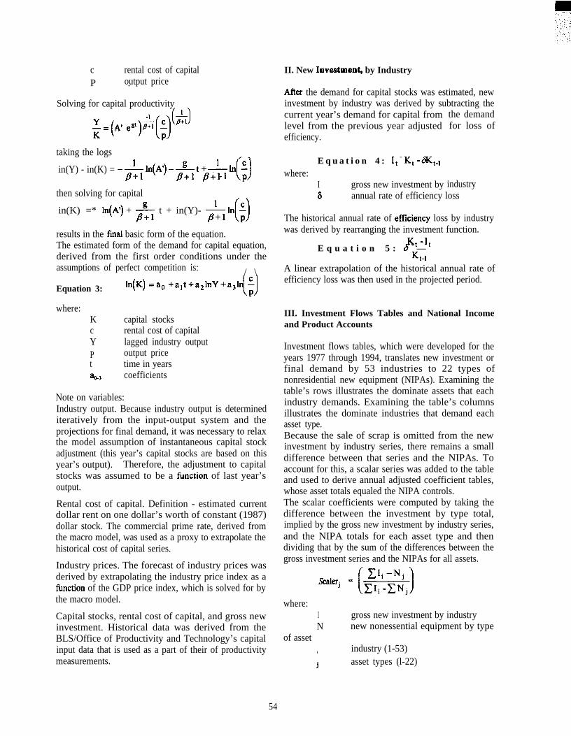
c rental cost of capitaloutput priceP .

Solving for capital productivity(1)

taking the logs Xxin(Y) - in(K) = -* ln(A’) -~t +~ln(g~

p+l p+l p

then solving for capital . .

in(K) =* ln(A’) + fi t + in(Y)- A ln(~)p+l p

results in the final basic form of the equation.The estimated form of the demand for capital equation,derived from the first order conditions under theassumptions of perfect competition is: / \

Equation 3: [)In(K) =aO +a1t+a21nY+a31n :

P

where:K capital stocksc rental cost of capitalY lagged industry outputP output pricet time in years%3 coefficients

Note on variables:Industry output. Because industry output is determinediteratively from the input-output system and theprojections for final demand, it was necessary to relaxthe model assumption of instantaneous capital stockadjustment (this year’s capital stocks are based on thisyear’s output). Therefore, the adjustment to capitalstocks was assumed to be a finction of last year’soutput.

Rental cost of capital. Definition - estimated currentdollar rent on one dollar’s worth of constant (1987)dollar stock. The commercial prime rate, derived fromthe macro model, was used as a proxy to extrapolate thehistorical cost of capital series.

Industry prices. The forecast of industry prices wasderived by extrapolating the industry price index as afi.mction of the GDP price index, which is solved for bythe macro model.

Capital stocks, rental cost of capital, and gross newinvestment. Historical data was derived from theBLS/Office of Productivity and Technology’s capitalinput data that is used as a part of their of productivitymeasurements.

II. New Investmen& by Industry

After the demand for capital stocks was estimated, newinvestment by industry was derived by subtracting thecurrent year’s demand for capital fromlevel from the previous year adjustedefficiency.

E q u a t i o n 4 : It = K~ -&t.lwhere:

I gross new investment by

the demandfor loss of

industry6 annual rate of efficiency loss

The historical annual rate of efllciency loss by industrywas derived by rearranging the investment function.

K~ -ItE q u a t i o n 5 : 8 = —

K~.lA linear extrapolation of the historical annual rate ofefficiency loss was then used in the projected period.

III. Investment Flows Tables and National Incomeand Product Accounts

Investment flows tables, which were developed for theyears 1977 through 1994, translates new investment orfinal demand by 53 industries to 22 types ofnonresidential new equipment (NIPAs). Examining thetable’s rows illustrates the dominate assets that eachindustry demands. Examining the table’s columnsillustrates the dominate industries that demand eachasset type.Because the sale of scrap is omitted from the newinvestment by industry series, there remains a smalldifference between that series and the NIPAs. Toaccount for this, a scalar series was added to the tableand used to derive annual adjusted coefficient tables,whose asset totals equaled the NIPA controls.The scalar coefficients were computed by taking thedifference between the investment by type total,implied by the gross new investment by industry series,and the NIPA totals for each asset type and thendividing that by the sum of the differences between thegross investment series and the NIPAs for all assets.

(Z1 XNjl~Ii-NjSCdcXj = .-

1

where:1 gross new investment by industryN new nonessential equipment by type

of asseti industry (1-53)

j asset types (l-22)

54

The projected gross investment by industry series wasthen transposed against the 1994 investmentcoefficients table to derive the initial projected NIPAcontrols.

IV. Problems’

(1) The historical data obtained from the Office ofProductivity &d Technology is in 1987 constant, fixedweighted, dollars. Furthermore, the data will not beconverted to 1992 constant, chain weighted, dollarsuntil the end of 1997. Therefore, instead of rebasing

the entire historical data base, the final new investmentby industry estimates were rebased before beingtranslated, via the flows table, to new investment bytype of asset. The rebasing ratio formula is as follows:

2006 C, 1992$=( )

1992: K,1992 $ *2006. ~ 1987$1992: C,1987$ “ ‘

(2) Due to time constraints, the lagged projectedindustry outputs for the capital stocks model wasnot iteratively derived. Instead, the historicalindustry output series in 1987 dollars wasextrapolated and used as a proxy.

55

Appendix A: Industry Codes (1987 SIC codes in parentheses)1 -.2 . .3 . .4 . .5 -.6 -.7 . .8 .-9 . .10 --11 --12 --13 --14 --

15 --16 --17 --18 --19 --20 --21 --22 --23 --24 --25 --26 --27 --

Agricultural services, forestry, and fisheriesMetal mining (10)Coal mining (1 1,12)Oil and gas extraction (13)Nonmetallic minerals, except fhels (14)Construction (15,16,17)Lumber and wood products (24)Furniture and fixtures (25)Stone, clay, and glass products (32)Primary Metal Industries (33)Fabricated metal products (34)Industrial machinery and equipment (35)Electronic and other electric equipment (36)Transportation equipment, including motor

vehicles (37)Instruments and related products (38)Miscellaneous manufacturing industries (39)Food and kindred products (20)Tobacco manufactures (21)Textile mill products (22)Apparel and other textile products (23)Paper and allied products (26)Printing and publishing (27)Chemicals and allied products (28)Petroleum and coal products (29)Rubber and miscellaneous products (30)Leather and leather products (31)Railroad transportation (40)

28 --29 --30 --31 --32 --33 --34 --35 --36 --37 --38 --39 --40 --41 --42 --43 --44 --45 --46 --47 --48 --49 --50 --51 --52 --

Local and interurban passenger transit (41)Trucking and warehousing (42)Water transportation (44)Transportation by air (45)Pipelines, except natural gas (46)Transportation services (47)Communications (48)Utilities (49)Wholes trade (50,5 1)Retail trade (52 - 59)Deposito~ institutions (60)Non depository institutions (61, 67)Security and commodity brokers (62)Insurance carriers, agents, brokers, and serviceReal estate (65,66)Hotels and other lodging places (70)Personal services (72)Business services (73)Auto repair, services, and parking (75)Miscellaneous repair services (76)Motion pictures (78)Amusement and recreation services (79)Health services (80)Legal services (81)Educational services (82)

53 -- Social services, museums, etc. (83,84,86,87,89)

Appendix B: Final Demand Sectors1 . . 13 -- Electrical transmission, distribution, and2 . .

3 -.4 --

5 . .

6 .-

7 .-

8 -9 .-

10--11 --12--

Furniture and fixturesFabricated metal productsEngines and turbinesTractorsAgricultural machinery, except tractorsConstruction machinery, except tractorsMining and oilfield machineryMetalworking machinerySpecial industry machinery, n.e.cGeneral industrial, including materials handling,OffIce, computing, and accounting machineryService industry machinery

14--15 --16--17--18--19--2 0 - -21 --

2 2 - -

industrial apparatusCommunication equipmentElectrical equipment, n.e.c.Trucks, buses, and truck trailersAutosAircrallShips and boatsRailroad equipmentInstruments; photocopy and relatedequipmentOther nonresidential equipment

56

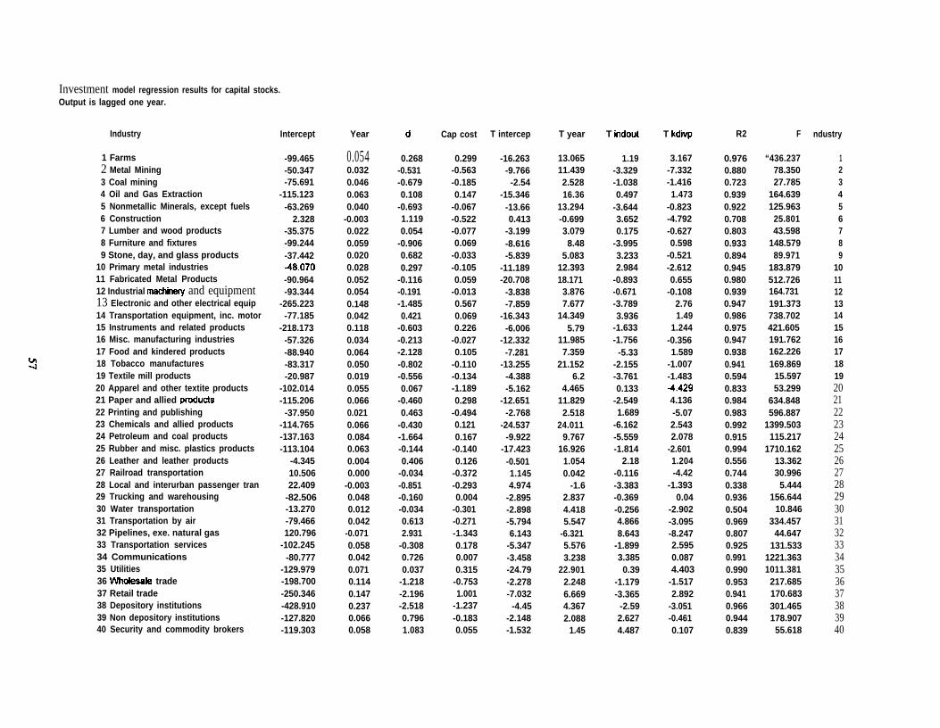
Investment model regression results for capital stocks.Output is lagged one year.

Industry

1 Farms2 Metal Mining3 Coal mining4 Oil and Gas Extraction5 Nonmetallic Minerals, except fuels6 Construction7 Lumber and wood products8 Furniture and fixtures9 Stone, day, and glass products

10 Primary metal industries11 Fabricated Metal Products12 Industrial machine~ and equipment13 Electronic and other electrical equip14 Transportation equipment, inc. motor15 Instruments and related products16 Misc. manufacturing industries17 Food and kindered products

V14 18 Tobacco manufactures

19 Textile mill products20 Apparel and other textite products21 Paper and allied prducts22 Printing and publishing23 Chemicals and allied products24 Petroleum and coal products25 Rubber and misc. plastics products26 Leather and leather products27 Railroad transportation28 Local and interurban passenger tran29 Trucking and warehousing30 Water transportation31 Transportation by air32 Pipelines, exe. natural gas33 Transportation services34 Communications35 Utilities36 Whotesala trade37 Retail trade38 Depository institutions39 Non depository institutions40 Security and commodity brokers

Intercept

-99.465-50.347-75.691

-115.123-63.269

2.328-35.375-99.244-37.442+8.070-90.964-93.344

-265.223-77.185

-218.173-57.326-88.940-83.317-20.987

-102.014-115.206

-37.950-114.765-137.163-113.104

-4.34510.50622.409

-82.506-13.270-79.466120.796

-102.245-80.777

-129.979-198.700-250.346-428.910-127.820-119.303

Year

0.0540.0320.0460.0630.040

-0.0030.0220.0590.0200.0280.0520.0540.1480.0420.1180.0340.0640.0500.0190.0550.0660.0210.0660.0840.0630.0040.000

-0.0030.0480.0120.042

-0.0710.0580.0420.0710.1140.1470.2370.0660.058

0.268-0.531-0.6790.108

-0.6931.1190.054

-0.9060.6820.297

-0.116-0.191-1.4850.421

-0.603-0.213-2.128-0.802-0.5560.067

-0.4600.463

-0.430-1.664-0.1440.406

-0.034-0.851-0.160-0.0340.6132.931

-0.3080.7260.037

-1.218-2.196-2.5180.7961.083

Cap cost

0.299-0.563-0.1850.147

-0.067-0.522-0.0770.069

-0.033-0.1050.059

-0.0130.5670.0690.226

-0.0270.105

-0.110-0.134-1.1890.298

-0.4940.1210.167

-0.1400.126

-0.372-0.2930.004

-0.301-0.271-1.3430.1780.0070.315

-0.7531.001

-1.237-0.1830.055

T intercep

-16.263-9.766

-2.54-15.346

-13.660.413

-3.199-8.616-5.839

-11.189-20.708

-3.838-7.859

-16.343-6.006

-12.332-7.281

-13.255-4.388-5.162

-12.651-2.768

-24.537-9.922

-17.423-0.5011.1454.974

-2.895-2.898-5.7946.143

-5.347-3.458-24.79-2.278-7.032

-4.45-2.148-1.532

T year

13.06511.4392.52816.36

13.294-0.6993.0798.48

5.08312.39318.1713.8767.677

14.3495.79

11.9857.359

21.1526.2

4.46511.8292.518

24.0119.767

16.9261.0540.042

-1.62.8374.4185.547

-6.3215.5763.238

22.9012.2486.6694.3672.088

1.45

T indout

1.19-3.329-1.0380.497

-3.6443.6520.175

-3.9953.2332.984

-0.893-0.671-3.7893.936

-1.633-1.756

-5.33-2.155-3.7610.133

-2.5491.689

-6.162-5.559-1.814

2.18-0.116-3.383-0.369-0.2564.8668.643

-1.8993.3850.39

-1.179-3.365

-2.592.6274.487

T kdivp

3.167-7.332-1.4161.473

-0.823-4.792-0.6270.598

-0.521-2.6120.655

-0.1082.761.49

1.244-0.3561.589

-1.007-1.4834.4294.136-5.072.5432.078

-2.6011.204-4.42

-1.3930.04

-2.902-3.095-8.2472.5950.0874.403

-1.5172.892

-3.051-0.4610.107

R2

0.9760.8800.7230.9390.9220.7080.8030.9330.8940.9450.9800.9390.9470.9860.9750.9470.9380.9410.5940.8330.9840.9830.9920.9150.9940.5560.7440.3380.9360.5040.9690.8070.9250.9910.9900.9530.9410.9660.9440.839

F

“436.23778.35027.785

164.639125.963

25.80143.598

148.57989.971

183.879512.726164.731191.373738.702421.605191.762162.226169.869

15.59753.299

634.848596.887

1399.503115.217

1710.16213.36230.996

5.444156.644

10.846334.457

44.647131.533

1221.3631011.381217.685170.683301.465178.90755.618

ndustry

123456789

10111213141516171819202122232425262728293031323334353637383940

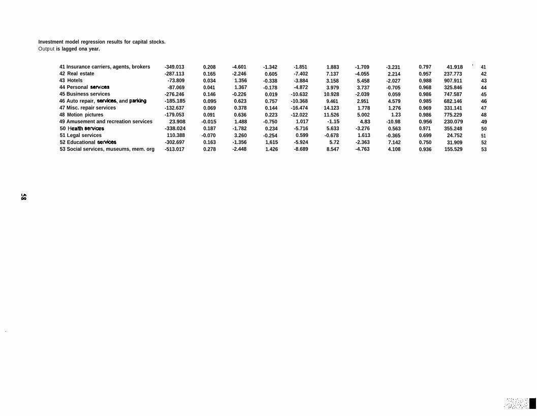
Investment model regression results for capital stocks.Output is lagged ona year.

41 Insurance carriers, agents, brokers42 Real estate43 Hotels44 Personal servioes45 Business services46 Auto repair, sendces, and paddng47 Misc. repair services48 Motion pictures49 Amusement and recreation services50 Heatth sewices51 Legal services52 Educational sendces53 Social services, museums, mem. org

-349.013-287.113

-73.809-87.069

-276.246-185.185-132.637-179.053

23.908-338.024110.388

-302.697-513.017

0.2080.1650.0340.0410.1460.0950.0690.091

-0.0150.187

-0.0700.1630.278

-4.601-2.2461.3561.367

-0.2260.6230.3780.6361.488

-1.7823.260

-1.356-2.448

-1.3420.605

-0.338-0.1780.0190.7570.1440.223

-0.7500.234

-0.2541,6151.426

-1.851-7.402-3.884-4.872

-10.632-10.368-16.474-12.022

1.017-5.7160.599

-5.924-8.689

1.8837.1373.1583.979

10.9289.461

14.12311.526

-1.155.633

-0.6785.72

8.547

-1.709-4.0555.4583.737

-2.0392.9511.7785.0024.83

-3.2761.613

-2.363-4.763

-3.2312.214

-2.027-0.7050.0594.5791.276

1.23-10.980.563

-0.3657.1424.108

0.7970.9570.9880.9680.9860.9850.9690.9860.9560.9710.6990.7500.936

41.918 “237.773907.911325.846747.587682.146331.141775.229230.079355.248

24.75231.909

155.529

41424344454647484950515253

L

GLOBAL FORECASTING AND FORESIGHT

Chair: Kenneth W. HunterWorld Future Society

Global Forecasting and Foresight (Abstract),Kenneth W. Hunter, World Future Society

59

Global Forecasting and Foresight

Chair: Kenneth W. HunterWorld Future Society

Professional fitures researchers are currently initiating an examination of the theories, methods and practices thatcomprise the foundation of global fitures research, education, and policy advising. Forecasting and definingpolicy and planning assumptions for several decades ahead is a critical component of fhtures research. Inaddition, new initiatives for collaborative fbtures programs in major policy areas and for international anddomestic regions are driving the need to strengthen the core capacity for integrating knowledge and models,baselines and assumptions, research agendas, and collaborative research support systems. This panel will discussseveral of the new programs and initiatives in the area of Mures research.

Panelists:

Kenneth W. HunterWorld Future Society’s 1999 Conf~ce “Frontiers of the 21st Century” and President, Collaborative FuturesInternational

Dennis PiragesDirector, The Harrison Rogram on the Future Global Agen@ University of Maryland, College Park

Paul J. RunciResearch Scientist, Battelle Pacific Northwest National Laboratory, Richland, Washington

Jerome C. GlennExecutive Director, Millennium Reject, United Nations University

61

n

COMMUNITY POLICY MODELS

Chair: James K. ScottCommunity Policy Analysis CenterUniversity of Missouri - Columbia

The Impact of Medicare Cavitation Payment Reform: A Simulation Analysis,Timothy D. McBride et al., University of Missouri - St. Louis

Community Policy Analysis System (ComPAS),Thomas G. Johnson and James K. Scott, Rural Policy Institute,University of Missouri - Columbia

Projections of Regional Economic and Demographic Impacts of Federal Policies,Glenn L. NelsonRural Policy Research Institute, University of Missouri - Columbia

63

The Impact of Medicare Cavitation Payment Reform:A Simulation Analysis

September 1997

Timothy D. McBride*hdrew F. Coburn

Sam CordesRobert A. CrittendenCharles W. Fluharty

J. Patrick HartKeith J. Mueller

Wayne W. Myers

Rura[ Policy Research Institute (R UPRI) Rural Health PanelUniversity of Missouri

Columbia, MO

*For ilimther information, contact the lead author at the following address: Timothy McBride, Department ofEconomics, University of Missouri-St. Louis, 8001 Natural Bridge Rd., St. Louis, MO 63121-4499. Electronic mailaddress: mcbride@umsl.edu

Paper presented at the Federal Forecasting Conference, Washington, D.C., September 11, 1997.

An ongoing Congressional Special Grant administered through the Cooperative State Research Education andExtension Service, U.S. Department of Agriculture continues to provide core support for this panel’s activities,including this report. The Robert Wood Johnson Foundation recently provided significant additional support forthis effort. However, none of the aforementioned organizations or agencies are responsible for the specific contentof this report.

65

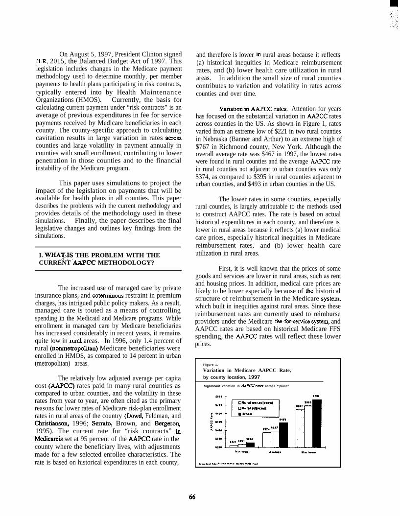
On August 5, 1997, President Clinton signedH.R. 2015, the Balanced Budget Act of 1997. Thislegislation includes changes in the Medicare paymentmethodology used to determine monthly, per memberpayments to health plans participating in risk contracts,typically entered into by Health MaintenanceOrganizations (HMOS). Currently, the basis forcalculating current payment under “risk contracts” is anaverage of previous expenditures in fee for servicepayments received by Medicare beneficiaries in eachcounty. The county-specific approach to calculatingcavitation results in large variation in rates acrosscounties and large volatility in payment annually incounties with small enrollment, contributing to lowerpenetration in those counties and to the financialinstability of the Medicare program.

This paper uses simulations to project theimpact of the legislation on payments that will beavailable for health plans in all counties. This paperdescribes the problems with the current methodology andprovides details of the methodology used in thesesimulations. Finally, the paper describes the finallegislative changes and outlines key findings from thesimulations.

I. WH+IS THE PROBLEM WITH THECURRENT AAPCC METHODOLOGY?

The increased use of managed care by privateinsurance plans, and coterminous restraint in premiumcharges, has intrigued public policy makers. As a result,managed care is touted as a means of controllingspending in the Medicaid and Medicare programs. Whileenrollment in managed care by Medicare beneficiarieshas increased considerably in recent years, it remainsquite low in rural areas. In 1996, only 1.4 percent ofrural (nonmetropolitan) Medicare beneficiaries wereenrolled in HMOS, as compared to 14 percent in urban(metropolitan) areas.

The relatively low adjusted average per capitacost (AAPCC) rates paid in many rural counties ascompared to urban counties, and the volatility in theserates from year to year, are often cited as the primaryreasons for lower rates of Medicare risk-plan enrollmentrates in rural areas of the country (Dowd, Feldman, andChristianso~ 1996; Semato, Brown, and Bergeron,1995). The current rate for “risk contracts” inMedicareis set at 95 percent of the AAPCC rate in thecounty where the beneficiary lives, with adjustmentsmade for a few selected enrollee characteristics. Therate is based on historical expenditures in each county,

and therefore is lower in rural areas because it reflects(a) historical inequities in Medicare reimbursementrates, and (b) lower health care utilization in ruralareas. In addition the small size of rural countiescontributes to variation and volatility in rates acrosscounties and over time.

Y~cc Iaks . Attention for yearshas focused on the substantial variation in AAPCC ratesacross counties in the US. As shown in Figure 1, ratesvaried from an extreme low of $221 in two rural countiesin Nebraska (Banner and Arthur) to an extreme high of$767 in Richmond county, New York. Although theoverall average rate was $467 in 1997, the lowest rateswere found in rural counties and the average AAPCC ratein rural counties not adjacent to urban counties was only$374, as compared to $395 in rural counties adjacent tourban counties, and $493 in urban counties in the US.

The lower rates in some counties, especiallyrural counties, is largely attributable to the methods usedto construct AAPCC rates. The rate is based on actualhistorical expenditures in each county, and therefore islower in rural areas because it reflects (a) lower medicalcare prices, especially historical inequities in Medicarereimbursement rates, and (b) lower health careutilization in rural areas.

First, it is well known that the prices of somegoods and services are lower in rural areas, such as rentand housing prices. In addition, medical care prices arelikely to be lower especially because of tie historicalstructure of reimbursement in the Medicare systemwhich built in inequities against rural areas. Since thesereimbursement rates are currently used to reimburseproviders under the Medicare fee-for-semice syste~ andAAPCC rates are based on historical Medicare FFSspending, the AAPCC rates will reflect these lowerprices.

Figure 1.

Variation in Medicare AAPCC Rate,by county location, 1997

Significant variation in AAPCC rates across “’place”

E3ElS403

A$767

+

%-. R.** ?“k, &.”.C.+ 1“- ,Uu?nl, 11..hb ?Wl

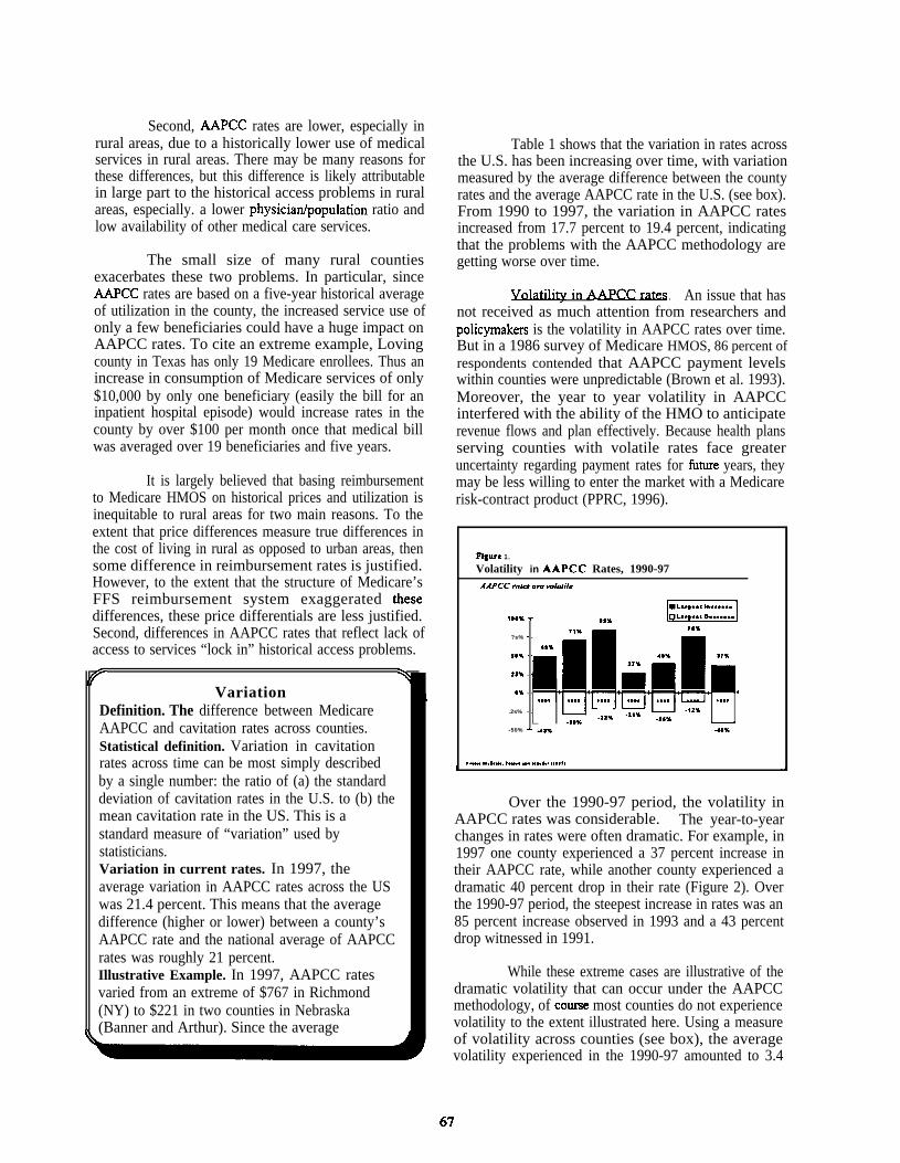
Second, AAPCC rates are lower, especially inrural areas, due to a historically lower use of medicalservices in rural areas. There may be many reasons forthese differences, but this difference is likely attributablein large part to the historical access problems in ruralareas, especially. a lower physiciadpopulation ratio andlow availability of other medical care services.

The small size of many rural countiesexacerbates these two problems. In particular, sinceAAPCC rates are based on a five-year historical averageof utilization in the county, the increased service use ofonly a few beneficiaries could have a huge impact onAAPCC rates. To cite an extreme example, Lovingcounty in Texas has only 19 Medicare enrollees. Thus anincrease in consumption of Medicare services of only$10,000 by only one beneficiary (easily the bill for aninpatient hospital episode) would increase rates in thecounty by over $100 per month once that medical billwas averaged over 19 beneficiaries and five years.

It is largely believed that basing reimbursementto Medicare HMOS on historical prices and utilization isinequitable to rural areas for two main reasons. To theextent that price differences measure true differences inthe cost of living in rural as opposed to urban areas, thensome difference in reimbursement rates is justified.However, to the extent that the structure of Medicare’sFFS reimbursement system exaggerated thesedifferences, these price differentials are less justified.Second, differences in AAPCC rates that reflect lack ofaccess to services “lock in” historical access problems.p q

VariationDefinition. The difference between MedicareAAPCC and cavitation rates across counties.Statistical definition. Variation in cavitationrates across time can be most simply describedby a single number: the ratio of (a) the standarddeviation of cavitation rates in the U.S. to (b) themean cavitation rate in the US. This is astandard measure of “variation” used bystatisticians.Variation in current rates. In 1997, theaverage variation in AAPCC rates across the USwas 21.4 percent. This means that the averagedifference (higher or lower) between a county’sAAPCC rate and the national average of AAPCCrates was roughly 21 percent.Illustrative Example. In 1997, AAPCC ratesvaried from an extreme of $767 in Richmond(NY) to $221 in two counties in Nebraska(Banner and Arthur). Since the average

Table 1 shows that the variation in rates acrossthe U.S. has been increasing over time, with variationmeasured by the average difference between the countyrates and the average AAPCC rate in the U.S. (see box).From 1990 to 1997, the variation in AAPCC ratesincreased from 17.7 percent to 19.4 percent, indicatingthat the problems with the AAPCC methodology aregetting worse over time.

m WCC rti . An issue that hasnot received as much attention from researchers andpolicymakers is the volatility in AAPCC rates over time.But in a 1986 survey of Medicare HMOS, 86 percent ofrespondents contended that AAPCC payment levelswithin counties were unpredictable (Brown et al. 1993).Moreover, the year to year volatility in AAPCCinterfered with the ability of the HMO to anticipaterevenue flows and plan effectively. Because health plansserving counties with volatile rates face greateruncertainty regarding payment rates for fbture years, theymay be less willing to enter the market with a Medicarerisk-contract product (PPRC, 1996).

Figure 1.

Volatility in AAPCC Rates, 1990-97AAPCC rata arc wlntile

1*OU T 8s% -

71%?s% - -

49%n% - - $7%

2s% -

on - -***?

.2s% - .

— .s0%.22% -26%

-50% - .43% 4*U

s- u.al140, *.4 .md U“*. ,1,,9,J

Over the 1990-97 period, the volatility inAAPCC rates was considerable. The year-to-yearchanges in rates were often dramatic. For example, in1997 one county experienced a 37 percent increase intheir AAPCC rate, while another county experienced adramatic 40 percent drop in their rate (Figure 2). Overthe 1990-97 period, the steepest increase in rates was an85 percent increase observed in 1993 and a 43 percentdrop witnessed in 1991.

While these extreme cases are illustrative of thedramatic volatility that can occur under the AAPCCmethodology, of coume most counties do not experiencevolatility to the extent illustrated here. Using a measureof volatility across counties (see box), the averagevolatility experienced in the 1990-97 amounted to 3.4

67

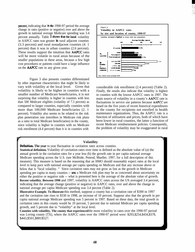
percen~ indicating that in tie 1990-97 period the averagechange in rates (positive or negative) over and above thegrowth in national average Medicare spending was 3.4percent annually. Table 2showsthat thelocal volatilityin AAPCC rates was greater in rural adjacent counties(3.3 percent) and rural nonadjacent counties (4. 1percent) than it was in urban counties (2.6 percent).These results support the intuition that AAPCC rateswill be more volatile in rural areas because of thesmaller populations in these areas, because a few highcost procedures or patients could have a large influenceon the AAPCC rate in any given year.

Figure 3 also presents counties differentiatedby other important characteristics that might be likely tovary with volatility at the local level. Given thatvolatility is likely to be higher in counties with asmaller number of Medicare beneficiaries, it is notsurprising that volatility is higher in counties with lessthan 500 Medicare eligibles (volatility of 7.3 percent) ascompared to larger counties, especially counties withmore than 100,000 Medicare beneficiaries (2. 1percent). Volatility also seems to be related to the riskplan penetration rate (enrollees in Medicare risk plansas a ratio to total Medicare beneficiaries) in the county,since volatility is higher in counties with no Medicarerisk enrollment (4.4 percent) than it is in counties with

Figure 3.

Volatility in AAPCC ratesby size and location of county, 1990-97Volatility ia rates is highert in areas with low population

Aueraw VOMNly, 1,s6-s7

0% 2% 4% 6% s%

A8 COIMIW#

By7.1%

Number Soo.me

Of t .000-e ,esm

Mrdkare t o.000-ee.eeeredpkets 100,000 of mote

[..”. M.Uw&. ?..I.4 .4 M“il.s ,1..7,

considerable risk enrollment (2.4 percent) (Table 2).Finally, the results also indicate that volatility is highestin counties with the lowest AAPCC rates in 1997. Themain source of volatility in a county’s AAPCC rate isfluctuations in service use patterns because AAPCC arebased on the five years of recent historical expendituresin the county for recipients not enrolled in healthmaintenance organizations. Thus, the AAPCC rate is afunction of utilization and prices, both of which havebeen lower in rural counties, the latter a function ofrecent Medicare reimbursement policies. Consequently,the problem of volatility may be exaggerated in rural

VolatilityIkftitiOn. The year to year fluctuation in cavitation rates across counties.Statistical definition. Volatility of cavitation rates over time is defined as the absolute value of (a) theannual growth in the cavitation rates for a year less (b) the growth rate in per capita national averageMedicare spending across the U.S. (see McBride, Penrod, Mueller, 1997, for a full description of thismeasure). This measure is based on the reasoning that an HMO should reasonably expect rates at the locallevel to keep pace with national average per capita spending on Medicare and that any increase above orbelow that is “local volatility. ” Since cavitation rates may not grow as fast as the growth in Medicarespending per capita in many counties -- arm a Medicare risk plan may be as concerned about uncertainty oneither the positive or negative side -- what is presented here is the average of the absolute value of growth.Recent volatility. Between 1990 and 1997, volatility is AAPCC rates across the US averaged 3.4 percent,indicating that the average change (positive or negative) in AAPCC rates, over and above the change innational average per capita Medicare spending was 3.4 percent (Table 2).Illustrative Example. To illustrate this method, suppose a county has a cavitation rate of $300 in 1997and the cavitation rate rises to $330 in 1998, an increase of 10 percent. Suppose also that the growth in percapita national average Medicare spending was 5 percent in 1997. Based on these data, the total growth incavitation rates in this county would be 10 percent, 5 percent due to national Medicare per capita spendinggrowth, and 5 percent due to “volatility” at the local level.Counties with volatility. The county that experienced the most volatility in rates over the 1990-97 periodwas Loving county (TX), where the AAPCC rates over the 1990-97 period were: $293,$254,$434,$378,$443,$501,$881$527.

68

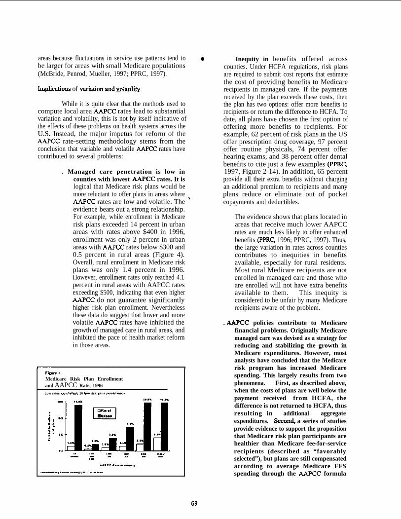
areas because fluctuations in service use patterns tend tobe larger for areas with small Medicare populations(McBride, Penrod, Mueller, 1997; PPRC, 1997).

Impkalims of Vaxialhruld Volatlllfy. .

While it is quite clear that the methods used tocompute local area AAPCC rates lead to substantialvariation and volatility, this is not by itself indicative ofthe effects of these problems on health systems across theU.S. Instead, the major impetus for reform of theAAPCC rate-setting methodology stems from theconclusion that variable and volatile AAPCC rates havecontributed to several problems:

. Managed care penetration is low incounties with lowest WCC rates. It islogical that Medicare risk plans would bemore reluctant to offer plans in areas whereAAPCC rates are low and volatile. Theevidence bears out a strong relationship.For example, while enrollment in Medicarerisk plans exceeded 14 percent in urbanareas with rates above $400 in 1996,enrollment was only 2 percent in urbanareas with AAPCC rates below $300 and0.5 percent in rural areas (Figure 4).Overall, rural enrollment in Medicare riskplans was only 1.4 percent in 1996.However, enrollment rates only reached 4.1percent in rural areas with AAPCC ratesexceeding $500, indicating that even higherAAPCC do not guarantee significantlyhigher risk plan enrollment. Neverthelessthese data do suggest that lower and morevolatile AAPCC rates have inhibited thegrowth of managed care in rural areas, andinhibited the pace of health market reformin those areas.

Figure 4.

Medicare Risk Plan Enrollmentand AAPCC Rate, 1996Low rates contm”bufc 10 \ow risk plm pCtICtrllIiOtl

1s%

● ☎

.T 14.a%

LnORural

■ Urban

3.8%

1.42.9%

0.s 1.0

s“,!.. ,-., ,.* m.r.,,a ,— ,numl, M..* h-,

● Inequity in benefits offered acrosscounties. Under HCFA regulations, risk plansare required to submit cost reports that estimatethe cost of providing benefits to Medicarerecipients in managed care. If the paymentsreceived by the plan exceeds these costs, thenthe plan has two options: offer more benefits torecipients or return the difference to HCFA. Todate, all plans have chosen the first option ofoffering more benefits to recipients. Forexample, 62 percent of risk plans in the USoffer prescription drug coverage, 97 percentoffer routine physicals, 74 percent offerhearing exams, and 38 percent offer dentalbenefits to cite just a few examples (PPRC,1997, Figure 2-14). In addition, 65 percentprovide all their extra benefits without chargingan additional premium to recipients and many

$ plans reduce or eliminate out of pocketcopayments and deductibles.

The evidence shows that plans located inareas that receive much lower AAPCCrates are much less likely to offer enhancedbenefits (PPRC, 1996; PPRC, 1997). Thus,the large variation in rates across countiescontributes to inequities in benefitsavailable, especially for rural residents.Most rural Medicare recipients are notenrolled in managed care and those whoare enrolled will not have extra benefitsavailable to them. This inequity isconsidered to be unfair by many Medicarerecipients aware of the problem.

. &APCC policies contribute to Medicarefinancial problems. Originally Medicaremanaged care was devised as a strategy forreducing and stabilizing the growth inMedicare expenditures. However, mostanalysts have concluded that the Medicarerisk program has increased Medicarespending. This largely results from twophenomena. First, as described above,when the costs of plans are well below thepayment received from HCFA, thedifference is not returned to HCFA, thusresulting in additional aggregateexpenditures. Secon& a series of studiesprovide evidence to support the propositionthat Medicare risk plan participants arehealthier than Medicare fee-for-servicerecipients (described as “favorablyselected”), but plans are still compensatedaccording to average Medicare FFSspending through the AAPCC formula

(PPRC, 1997). Thus favorable selectioncontributes to increases in Medicarespending.

. Policies contribute to inadequateMedicare reimbursement rates in ruralareas. Since Medicare risk plans haveactually led to an increase in Medicarespending, risk plans have actuallycontributed to the fmcial problems facingMedicare. Over the years, the majorresponse by Congress to financial problemsin Medicare has been to reduce the growthin reimbursement rates for providers,especially hospitals and physicians. Thusthe problems w i t h t h e AAPCCmethodology described above havecontributed to continued restraint on thegrowth of reimbursement rates for ruralproviders and have impeded efforts toreduce inequity in rates.

II. DESCRIPTION OF PROVISIONS TOREFORM AAPCC METHODOLOGY

On August 5, 1997, President Clinton signedH.R. 2015, the Balanced Budget Act of 1997. Table 3presents an outline of the change considered here. Asindicated in the table, the adjusted cavitation rate in agiven year would be equal to the greatm ofl

(I) a blended cavitation rate,l determined as

(ii)

(iii)

the weighted average of the area-specificadjusted cavitation rate (ASACR) and theinput-price-adjusted national adjustedcavitation rate (IPANACR) phased in oversix years until rates are based on a50%/50% average of the ASACR andIPANACR rates,

a floor, initially set at $367 in 1998 andindexed for Medicare per capita spendinggrowth thereafter, and

a hold harmless rate, set at 102 percent ofthe area’s adjusted cavitation rate in theprevious year.

lNote the terminology “blended cavitation rate” isthe term used to describe this method in the literature (PPRC,1996; PPRC and ProPAC, 1995), but not typically in any ofthe proposed legislation.

While this formula seems complicate~ essentially it setsthe new cavitation rate at the blended rate, although thecavitation rate is not allowed to fall below the payment“floor” or a “hold harmless” rate.

The provision for blending the cavitation ratesis designed to achieve the objective of equalizingcavitation rates across counties, since this method usesthe area-specific cavitation rate (ASACR) and averagesit with the input-price-adjusted national adjustedcavitation rate (IPANACR). The ASACR is based on theprevious WCC rates in the county. The IPANACR isessentially based on the average of AAPCC rates acrossthe US (called the USPCC, the United States per capitacost), adjusted to reflect variations in local prices acrosscounties. Adjusting rates for local prices is done in therealization that the prices facing managed careorganizations vary across areas. The price index forcomputing the IPANACR is specified in the legislationand constructed using price indices computed by HCFAto set reimbursement rates for hospitals and physicians.

To calculate the blended cavitation rate, eachpiece of legislation uses an “area-specific percentage”(ASP) to weight the ASACR and a “national percentage”@P) to weight the IPANACR. Since essentially &kPCCrates under current law are based on 100 percent of thearea-specific rate, these percentages are phased in overtime, until the applicable percentages are reached in2002. The ASP is set at 50 percent in the year 2003 andphased in over the 1998-2003 period, set at 90, 82,74,66,58 and 50 percent in those six years.

The floor is also used to equalize cavitation ratesacross counties and is used to reflect the realization thathistorical prices and utilization may be so low that itwould not be possible for any managed care organizationto operate in a local area if the cavitation rate fell toolow. Thus, the floor is designed to guarantee that eachcounty has a cavitation rate that would make MCOSviable in that area. The hold harmless provision isdesi~ed as a protection against fluctuations in cavitationrates, guarantee that the growth in cavitation rates is atleast 2 percent in I!hture years.

In each year, the ASACR and IPANACR will beincreased by the national average per capita growthpercentage (NAPCGP), basically the average nationalincrease in per capita Medicare spending, less somespecified percentages in the period 1998 through 2001.In 1998, 0.8 percentage points are subtracted from thegrowth rate, while 0.5 percentage points are subtractedfrom the growth rate in the period 199 through 2001.This provision is important because it guarantees thatrates in the fiture will increase a steady and predictable

70

rate, thus removing the year-to-year volatility that hasbeen witnessed in previous years.

A “budget neutrality adjustment” (BNA) is usedin all pieces of legislation to insure that the aggregatepayments made under the proposed policies shall beequal to the aggregate payments that would have beenmade if the rates had been calculated with the area-specific percentage (ASP) set equal to 100 percent. Inother words, total expenditures under these provisions arenot allowed to exceed what would have been paid ifevery county was paid their area-specific rate and nocounty was affected by provisions such as the floor andblended rates. If the budget neutrality provision istriggere~ it is used only to adjust blended cavitationrates. For example, if expenditures under the proposedlegislation exceed expenditures that would have beenmade otherwise by 5 percent, then blended rates wouldbe reduced by 5 percent.

The legislation reduces local area cavitationrates (the ASACR) for the amount of spending made inthe county for the graduate medical education (GME)pro-. This program pays hospitals for expendituresincurred for education of medical residents. Since theseexpenditures are included in the payments to hospitalsunder the fee-for-service portion of the Medicareprogr~ these payments will implicitly be included inthe calculation of A4PCC payments. This is consideredto be a problem since the AAPCC payments are made notto hospitals, but to managed care organizations. Thus,the payments designed to help defray educationexpenditures may never reach the hospital. In H.R. 2015,GME expenditures are carved out from the cavitationrates over a five year period with 20,40, 60, 80, and 100percent of GME spending carved out in the years 1998through 2002, respectively.

From this summary, several provisions areimportant in the eventual setting of cavitation rates acrosscounties. Key factors in the determination of the newMedicare cavitation rates are the percentages used in theblended rates, the methods used to set the floor, thecarving out of GME payments, and the use ofstandardized predictable growth rates in the setting offbture cavitation rates.

HI. SIMULATION METHODS AND DATA

The Rural Policy Research Institute (RUPRI)Health Panel has constructed a comprehensive data setand simulation model that is used to simulate the effectsof the policy changes described here. This file, called the

RUPRI Medicare Cavitation County Data File, wasconstructed by merging data from several sources, butprimarily from obtained from the Health Care FinancingAdministration (HCFA). The file contains over 1,300variables that generally fall into the following categories:

o00

0

0

0

0

0

Historical AAPCC rates, 1990-97Medicare enrollment in county, 1996Number of enrollees in Medicare HMOS,1996

including details on enrollment byeach plan enrolling in the county

Number of Medicare HMO plans withMedicare emollees enrolled in the plan bycounty (includes distinction for whetherplan includes county in its GeographicService Area )Characteristics of Medicare risk plansoffered in the county. For each plan dataincludes:

Name and location of planDates of HCFA contractType of plan (risk, demo, or cost)Type of HMO (staff, group or IPA)Profitinon-profit status of planBenefits offered by plan (e.g.,preventive, dental, eye, ear, drugs)Premium charged by plan

County share of Graduate MedicalEducation (GME) and DisproportionateShare (DSH) spendingAn “input price adjustment” for the county,based on the formula described belowCounty descriptive variables (Beale codes,population, population in poverty)

In general, most of this data was originally obtained fromthe Health Care Financing Administration, from filesavailable on the Internet. However, additional data wasobtained directly from other HCFA offices, specificallythe Office of the Actuary and the Office of ManagedCare. Finally, additional data was obtained from the1990 Census, the Economic Research Service and theFederal Register.

The data from each of these sources was mergedat the county-level using the county FIPS code and thecounty name (since FIPS code was not available for theHCFA data). There is not a one-to-one correspondencebetween the FIPS county code and the code assigned byHCFA. However, mismatches were corrected in allcases, except for Alaska counties. Due toincompatibilities between the HCFA and FIPSclassifications, all Alaska counties were dropped fromthe analysis. Data from U.S. territories (Guam, PuertoRico, Virgin Islands) was also dropped fkom the analysis.

71

The file containing “input price adjustments”(IPA) was computed at the local level by the RUPIUHealth Panel by inputting data on Medicare ProspectivePayment System (PPS) rates and Resource BasedRelative Value System (RBRVS) rates reported at thecounty level in the Federal Register (Federal Register,1996). The IPA was computed according to the formulaspecified in legislation dealing with this issue. Inparticular, the legislation specifies, in part: “Medicareservices shall be divided into 2 types of services: part Aservices and part B sewices . . . . The proportions.. for partA services shall be the ratio (expressed as a percentage)of the national average annual per capita rate ofpayment forpart A for 1997 to the total national averageannual per capita rate ofpayment for parts A and B for1997, andforpart B services shall be 100 percent minusthe Part A ratio . . . . For part A services, 70 percent ofpayments attributable to such services shall be adjustedby the index used under section 1886(d)(3)(E) to a@stpayment rates for relative hospital wage levels forhospitals located in the payment area involved; for partB services, 66 percent of payments attributable to suchservices shall be adjusted by the index of the geographicarea factors under section 1848(e) used to adjustpayment rates for pilysicians’ services furnished in thepayment area, and of the remaining 34 percent of theamount ofsuch payments, 40percent shall be a~usted bythe index for relative hospital wage levels]. ” (Source:1997 Balanced Budget Act, HR 2015).

As noted above, H.R. 2015 specifies the use ofa “budget neutrality adjustment” (BNA) to insure that theaggregate of the payments under shall be no greater thanthe aggregate payments that would have been made if theprevious AAPCC-based methodology were continued.The budget neutrality adjustment (BNA) was computedby aggregating expenditures for risk enrollees acrosscounties using the multiple of (a) cavitation rates thatwould exist in absence of the legislation (i.e., 100 percentof the area-specific cavitation rates) and the (b)enrollment in Medicare risk plans. Then the BNA wascomputed as equal to:

BNA = [Spending using area-specific rates]/[Spending using new legislated rates]

As specified in the legislation, this BNA is applied to thecavitation rates if the BNA is less than one in thedefinition defined above. I reality, it has been found thatthe BNA would not be triggered under any of thelegislation proposed to date because the legislation hasthe effect of lowering rates, relative to the area-specificrates, in counties with high HMO enrollment.

Assumptions are made about several key factorsin the determination of the new Medicare cavitation rates

under proposed policies. These include the determinationof the BNA, the national average per capita growthpercentage (NAPCGP), and the determination of theinput-price-adjusted national adjusted cavitation rate(IPANACR). In particular, the IPANACR would be useddirectly in the formula for a Medicare area, both in theblended cavitation rate and often in the “floor,” set atsome percentage of the IPANACR. Thus, importantassumptions had to be made about:

(a) growth in the “national average per capitagrowth percentage” and “area-specificcavitation rates.” Recent CongressionalBudget Office (CBO) estimates of thegrowth in Medicare spending were used forthis purpose (CBO, 1997a), and

(b) growth in the Consumer Price Index (CPI).CBO estimates (CBO, 1997b) were alsoused to compute projected increases in theCPI, to use in computing the value ofcavitation rates in “constant dollars.”

Some assumptions have to be made in the simulationsdue to the uncertainty about the future. Actual Medicarerisk plan enrollment in December of 1996 is used todetermine aggregate spending under policy provisions,especially when computing the budget neutralityadjustment (BNA). In reality, actual enrollment in thefuture will be used for this purpose. Actual enrollment inrisk plans in the future is likely to be much higher thanenrollment in 1996. However, the growth in enrollmentwill not affect the estimates here unless the growth inenrollment is radically different across counties.

IV. SIMULATION RESULTS

Tables 4 through 8 summarize the detail of thesimulation results. Table 4 presents descriptive statisticssummarizing the effects of the proposals on variousmeasures including the mean or average cavitation ratesand the lowest or minimum cavitation rate found in anycounty. In addition, the tables present measures of theaverage variation in rates across counties and the averagevolatility in rates across time since, as indicated above,most analysts have concluded that the variation andvolatility in AAPCC rates are the biggest problems withthe current methodology for setting rates. Finally thetable presents the percentage of counties that would havecavitation rates set by the provision setting a “floor” oncavitation rates and the percentage of Medicare eligiblesresiding in counties that would receive the floor.

72

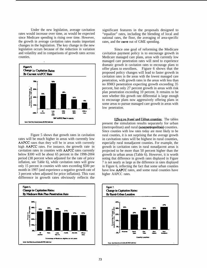
Under the new legislation, average cavitationrates would increase over time, as would be expectedsince Medicare spending is rising over time. However,the growth in average cavitation rates masks importantchanges in the legislation. The key change in the newlegislation occurs because of the reduction in variationand volatility and in comparisons of growth rates acrosscounties.

_ in Qitation RatsI$ycum!ntAAPaRate

ih24%

1%

lm7AAPcciMo tncOlSwy

Figure 5 shows that growth rates in cavitationrates will be much higher in areas with currently lowAAPCC rates than they will be in areas with currentlyhigh AAPCC rates. For instance, the growth rate incavitation rates in counties with AAPCC rates currentlybelow $300 will be about 65 percent in the 1998-2004period (38 percent when adjusted for the rate of priceinflation, see Table 6), while cavitation rates will growonly 15 percent in counties with rates exceeding $500 permonth in 1997 (and experience a negative growth rate of3 percent when adjusted for price inflation). This vastdifference in growth rates obviously reflects the

significant features in the proposals designed to“equalize” rates, including the blending of local andnational rates, the floor, the averaging of area-specificrates, and the came out of GME spending.

Since one goal of reforming the Medicarecavitation payment policy is to encourage growth inMedicare managed care plans, areas with currently lowmanaged care penetration rates will need to experiencedramatic growth in cavitation rates to encourage plans tooffer plans to enrollees. Figure 6 shows that theproposed policy changes will lead to faster growth incavitation rates in the areas with the lowest managed carepenetration, with growth rates in the areas with less thanno HMO penetration expecting growth exceeding 35percent, but only 27 percent growth in areas with riskplan penetration exceeding 10 percent. It remains to beseen whether this growth rate differential is large enoughto encourage plans now aggressively offering plans insome areas to pursue managed care growth in areas withlow penetration.

m~. The tablespresent the simulation results separately for urban(metropolitan) and rural (nonrnetropolitan) counties.Since counties with low rates today are most likely to berural counties, it is not surprising that the average growthin cavitation rates will be highest in rural counties,especially rural nonadjacent counties. For example, thegrowth in cavitation rates in rural nonadjacent areas isprojected to be more than 50 percent higher than thegrowth in urban areas (Table 6). However, it is worthnoting that difference in growth rates displayed in Figure7 is not nearly as large as the difference in rates displayedin Figure 6, reflecting the fact that some urban countieshave low AAPCC rates, and some rural counties havehigher AAPCC rates.

73

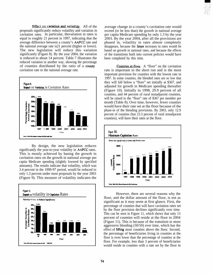
ct on v . All of theproposals significantly reduce volatility and variation incavitation rates. In particular, thevariation in rates isequal to roughly 21 percent in 1997, indicating that theaverage difference between a county’s AAPCC rate andthe national average rate is21 percent (higher or lower).The new legislation will reduce this variationsignificantly (Figure 8). By the year 2004, the variationis reduced to about 14 percent. Table 7 illustrates thereduced variation in another way, showing the percentageof counties distributed by the ratio of a coun~’cavitation rate to the national average rate.

Fifye 8.Inqact on Viuiation in Cavitation Rates

19% 19%

17%

1

16%

l-u

15%

19371 SS81Q39zooo2x)lmQm m4

Year

By design, the new legislation reducessignificantly the year-to-year volatility in AAPCC rates.This is mostly achieved by basing the growth incavitation rates on the growth in national average percapita Medicare spending (slightly lowered by specifiedamounts). The results indicate that volatility, which was3.4 percent in the 1990-97 period, would be reduced toonly 1.3 percent under most proposals by the year 2003(Figure 9). This measure of volatility indicates the

Figlle 9.hrqlact on volatility in ckpitation RatesVdwiliv in Rata is Rc&dSig@YOItly

25%

1.3% 1.3% 1 .3% 1.3%

al1 .0%

L0.3%

Year

Su= adl+k-jlbm4haR(2uwo) t*lw

average change in a county’s cavitation rate wouldexceed (or be less than) the growth in national averageper capita Medicare spending by only 1.3 by the year2003. By the year 2004, after all the provisions arephased in, volatility in rates almost completelydisappears, because the fiture increases in rates would bebased on growth in national rates, and because the effectsof the transitions built into current policies would havebeen completed by this time.

. A “floor” on the cavitationrate is important in the short run and is the mostimportant provision for counties with the lowest rate in1997. In some counties, the blended rates are so low thatthey will fall below a “floor” set initially at $367, andadjusted for growth in Medicare spending thereafter(Figure 10). Initially in 1998, 29.9 percent of allcounties, and 44 percent of rural nonadjacent counties,will be raised to the “floor” rate of $367 per member permonth (Table 8). Over time, however, fewer countieswould have their rate set at the floor because of thephase-in of the blending provisions. By 2003, only 12.9percent of counties (but 23.3 percent of rural nonadjacentcounties), will have their rates at the floor.

Figm 10.Mnimrn Gpitation Rate

RIUc3 tire signl$candy itt urau wiilt Iowst mtcs

$5001 S460

5464

S429S409

2s400$392

$367S376

2%C@o

j; ~

%u $221

S200 .-:

1997199e lm2000mlzf)cQm 2U04Year

However, there are several reasons why thefloor, and the dollar amount of the floor, is not assignificant as it may seem at first glance. First, thepercentage of counties that will have cavitation rates setby the floor provision declines significantly over time.This can be seen in Figure 11, which shows that only 13percent of counties will reside at the floor in 2004(Figure 11). This is because of the transition to moreaggressive blending (50/50) over time, which has theeffect of liftig most counties above the floor. Second,the percentage of beneficiaries living in counties at thefloor is even lower than the percentage of counties at thefloor. For example, less than 3 percent of beneficiarieswould reside in counties with a rate set by the floor in

74

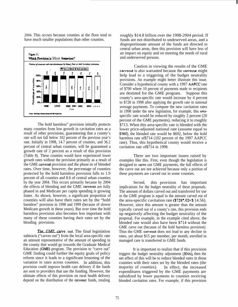
2004. This occurs because counties at the floor tend tohave much smaller populations than other counties.

Figuell.W&h Pnwidon’is Most IrmOrtant?Parcm @cowttta with mrc dactminal by Maul, jlou M hold Imnnks \w&iwl

100%

+ -4 +1996 1999 Zow Zool Zou? ZO03 2 0 0 4

Year

The hold harmless” provision initially protectsmany counties from low growth in cavitation rates as aresult of other provisions, guaranteeing that a county’srate will not fall below 102 percent of the previous year’srate. Initially in 1998, 14.7 percent of counties, and 36.2percent of central urban counties, will be guaranteed agrowth rate of 2 percent as a result of this provision(Table 8). These counties would have experienced lowergrowth rates without the provision primarily as a result ofthe GME carveout provision and the phase-in of blendedrates. Over time, however, the percentage of countiesprotected by the hold harmless provision falls to 1.9percent of all counties and 8.6 of central urban countiesby the year 2004. This occurs primarily because by 2004the effects of blending and the GME carveout are fullyphased in and Medicare per capita spending is growingfaster. As shown, however, a significant proportion ofcounties will also have their rates set by the “holdharmless” provision in 1998 and 1999 (because of slowerMedicare growth in these years). But over time the holdharmless provision also becomes less important withmany of these counties having their rates set by theblending provisions.

11~. The final legislationsubtracts (“carves out”) from the local area-specific ratean amount representative of the amount of spending inthe county that would go towards the Graduate MedicalEducation (GME) program. The provision to “carve out”GME finding could further the equity goals of policyreform since it leads to a significant lessening of thevariation in rates across counties. In addition, thisprovision could improve health care delivery if the fundsare sent to providers that use the funding. However, theultimate effects of this provision on rural health deliverydepend on the distribution of the carveout funds, totaling

roughly $14.8 billion over the 1998-2004 period. Iffunds are not distributed to undeserved areas, and adisproportionate amount of the funds are directed tocentral urban areas, then this provision will have less ofan impact on equity and on meeting the needs of ruraland underserved persons.

Caution in viewing the results of the GMEcarveout is also warranted because the carveout mighthelp lead to a triggering of the budget neutralityprovisions. An example might better illustrate this issue.Consider a hypothetical county with a 1997 AAPCC rateof $700 where 10 percent of payments made to recipientsare destined for the GME program. Suppose thiscounty’s area-specific rate would increase by 4 percentto $728 in 1998 after applying the growth rate in nationalaverage payments. To compute the new cavitation ratesin 1998 under the new legislation, for example, this area-specific rate would be reduced by roughly 2 percent (20percent of the GME payments), reducing it to roughly$713. When this area-specific rate is blended with thelower price-adjusted national rate (assume equal to!$500), the blended rate would be $692, below the holdharmless rate of$714 (102 percent of the 1997 AAPCCrate). Thus, this hypothetical county would receive acavitation rate of$714 in 1998.

There are two important issues raised byexamples like this. First, even though the legislation isdesigned to caxve out GME payments, the full effects ofthe carve out are not achieved because only a portion ofthese payments are carved out in some counties.

Second, this provision has importantimplications for the budget neutrality of these proposals.The amount of dollars carved out and transferred for usein the GME program is equal to the amount carved out ofthe area-specific cavitation rate ($728*.02=$ 14.56).However, since this amount is greater than the amounttypically carved out of a county’s rate, this provision endsup negatively affecting the budget neutrality of theproposal. For example, in the example cited above, theblended rate would also have been $714 without theGME carve out (because of the hold harmless provision).Thus the GME carveout does not lead to any decline inrates, yet about $15 per member, per month, enrolled inmanaged care is transferred to GME funds.

It is important to realize that if this provisiontriggers the budget neutrality adjustment (BNA), then thenet effect of this will be to reduce blended rates in thosecounties with their rates set by the blended rates (themajority of counties). In effect, the increasedexpenditures triggered by the GME payments aresubsidized by lower payments to counties receivingblended cavitation rates. For example, if this provision

75

leads to expenchtires that exceed expenditures that wouldhave been made otherwise by 2 percent, then blendedrates (and not the floor and hold harmless rates) will bereduced across the board by 2 percent.

Despite this discussion, the budget neutralityproblems created by the GME carve out are not large,primarily because GME finds are carved out over a five-year period.

VII. IMPLICATIONS

This paper presents detailed findings about theeffects of the Balanced Budget Act on Medicarecavitation rates in the 1997-2004 period. However, theultimate impact of these policy changes is not clear fromthese results. In particular, there are important questionsabout the impact of these proposed changes on the ruralhealth system. In particular:

. If cavitation rates are increased, willenrollment increase? In other words, ifthe cavitation rates are increased in ruralareas and other areas with low AAPCCrates, will this increase in rates lead tomore penetration of managed care plans?And will it encourage more recipients toenroll in managed care plans?

In the counties with the lowest AAPCCrates in 1997, the increases in cavitationrates will be significant, but it is not clearwhether this will be enough to spursignificant growth in managed care.Further research on this question willprovide some evidence. However, ifenrollment is not significantly spurred bythis legislation, then the importance of thelegislation is significantly reduced.

. How much of increase will actually flowto rural counties? In particular, paymentsto Medicare risk plans go directly tomanaged care organizations (MCOS). It isnot clear how much of these funds willflow back to the counties where therecipients live. MCOS will keep some ofthe funds for administrative costs mdprofits. In addition, if the MCO is anurban-based plan, then those administrativecosts will remain in the urban area even ifthe recipient lives in a rural area.

. How much of increase will flow to ruralproviders? Since some of the cavitationrate will be kept by MCOS to cover theircosts, this will reduce the finds that mightflow to rural providers. In addition, it iswell known that MCOS achieve their costsavings primarily through reducedhospitalizations and by making contractswith providers for discounted or reducedreimbursement rates. All this might lead tothe conclusion that rural providers(especially hospitals and physicians) mayactually see a drop in revenue aftercavitation rates are increased, especially ifit spurs some recipients to switch fromMedicare FFS to an MCO plan. It isdifficult to predict the outcome, and it willdiffer by county. Also, some providers --such as primary care providers -- will likelybe impacted positively by increasedmanaged care enrollment, while other ruralproviders -- especially specialist physiciansand hospitals -- may be impactednegatively.

. Ultimately, the goal of Medicare reformpolicy should be improving the deliveryof health care to recipients, if possiblewithin budgetary constraints. Iflegislation to increase cavitation rates spursincreases in enrollment in MCOS, theultimate impact on the health care receivedby recipients will depend of course on thequality of care provided by the MCO.There is considerable controversy about theimpact of MCOS on the quality of care.However, early evidence suggested thatmanaged care did not significantly reducethe quality of care and may have increasedit. However, more recent evidencefocusing more directly on populations atrisk (e.g., the elderly, seriously ill,disabled) suggests that the health carereceived by these population groups maybe adversely affected by enrollment inmanaged care plans. Measuring this effectis very difticult, however, and much furtherresearch is being conducted on that.

To assess the impacts of the new methods for computingMedicare cavitation rates on the issues raised here,further research is needed and this research is beingpursued now in further extension of this work.

76.

REFERENCES

Brown, R. S., D.G. Clemen~ J.W. Hill, S.M. Retchin, andJ.W. Bergeron, “Do Health MaintenanceOrganizations Work for Medicare”, HealthCare Financing Review (Fall, 1993): 7-23.

CBO (Congressional Budget Office). 1997a. “CBOJanuary ~ 1997 Ba seline: Medicare andMedicaid.” Washington: CBO, January 16.

CBO (Congressional Budget Office). 1997b. lhetouhkllsd Y. “ ean

98-2.QQZ. Washington: CBO, January.

Dowd, B., R. Feldman, and J. Christianson. 1996.Competitive Pn”cing for Medicare. Washington,D. C.: The AEI Press.

Federal Register. 1996. “Rules and Regulations”EcdmalXe@x 61: 170 (August 30), pp.46256-46266.

GAO (General Accounting Office). 1997a. “HCFACould Promptly Reduce Excess Payments byImproving Accuracy of County PaymentRates,” GAOfl-HEHS 97-78, February 25.

GAO (General Accounting Office). 1997b. “MedicareHMOS: HCFA Can Promptly EliminateHundreds of Millions in Excess Payments,”GAO-HEHS 97-16, April.

GAO (General Accounting Office). 1997c. “MedicareHMO Enrollment: Area Differences Affectedby Factors Other Than Payment Rates.” GAO-HEHS 97-37, May.

McBride, Timothy D., Joan Penrod, Keith Mueller.1997. “Volatility in Medicare AAPCC Rates:1990- 1997,” 16(5,September/October): 172-180.

PPRC (Physician Payment Review Commission). 1996.~. Washington:GPO.

PPRC (Physician Payment Review Commission). 1997.~-. Washington:GPO.

PPRC and ProPAC (Prospective Payment ReviewCommission). 1995. MnLRqmt to Cmgmss

ge.d_Cm. Washington:GPO, October.

77

Porell, F. W., and C.P. Tompkins, “Medicare RiskContracting: Identifying Factors Associatedwith Market Exit,” Inquiry (Summer, 1993):157-169.

Rural Policy Research Institute (RUPRI) Rural HealthExpert Panel. 1997a. “The Rural Implications ofMedicare AAPCC Cavitation PaymentChanges: An Analysis of the Balanced BudgetAct of 1997,” Rural Policy Research InstituteRural Policy Brief PB97-2, August.

Rural Policy Research Institute (RUPRI) Rural HealthExpert Panel. 1997b. “The Rural Implicationsof Medicare AAPCC Cavitation PaymentChanges: Assessment and Simulation FindingsRegarding Proposals Before the House/SenateConference Committee On BudgetReconciliation,” Rural Policy Research InstituteWorking Paper P97-9, July.

Rural Policy Research Institute (RUPRI) Rural HealthExpert Panel. 1997c. “The Rural Implications ofMedicare AAPCC Cavitation PaymentChanges: Background Assessment andSimulation Results of Key LegislativeProposals,” Rural Policy Research InstituteWorking Paper P97-8, May.

Rural Policy Research Institute (RUPRI) Rural HealthExpert Panel. 1997d. “Achieving Equity inRural Medicare Cavitation Payment: Reformsof the AAPCC Methodology,” RUPRI RuralPolicy Brief 1:1, February.

Rural Policy Research Institute, Rural Health ExpertPanel. 1996. “Anticipated Impacts of the RuralHealth Improvement Act,” Rural PolicyResearch Institute Working Paper P96-5, July.

Serrate, C., R.S. Brown, and J. Bergeron. 1995. “WhyDo So Few HMOS Offer Medicare Risk Plans inRural Areas?,” Health Care Financing Review(Fall): 85-97.

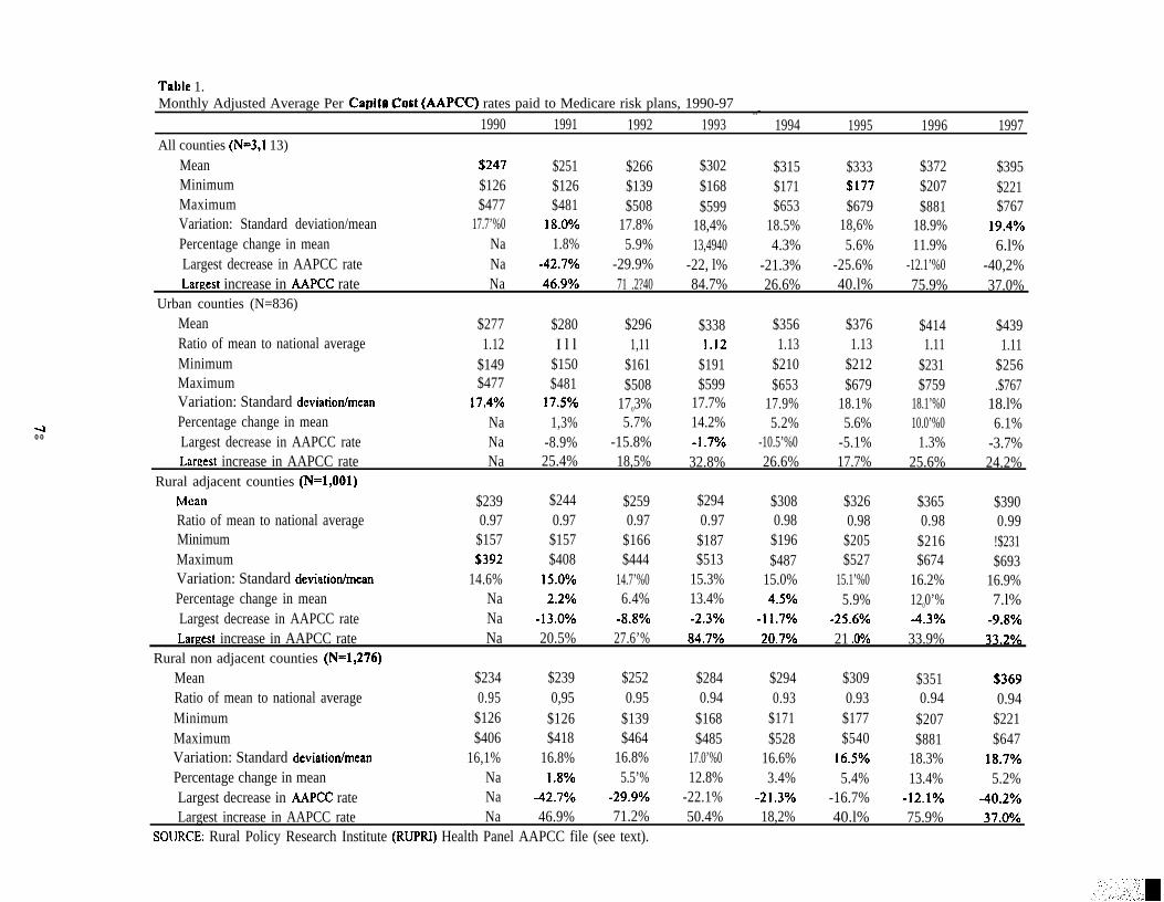
400

Tal)lc 1.Monthly Adjusted Average Per Capita Cost (AAPCC) rates paid to Medicare risk plans, 1990-97 ..-

1990 1991 1992 1993 1994 1995 1996 1997All counties (N=3,1 13)

Mean !$247 $251 $266 $302 $315 $333 $372 $395Minimum $126 $126 $139 $168 $171 !$177 $207 $221Maximum $477 $481 $508 $599 $653 $679 $881 $767Variation: Standard deviation/mean 17.7’%0 18.0’%0 17.8% 18,4% 18.5% 18,6% 18.9% 19.4!40Percentage change in mean Na 1.8% 5.9% 13,4940 4.3% 5.6% 11.9% 6.l%Largest decrease in AAPCC rate Na -42.7Y0 -29.9% -22, l% -21.3% -25.6% -12.1’%0 -40,2%Largest increase in AAPCC rate Na 46.9’XO 71 .2?40 84.7% 26.6% 40.l% 75.9% 37.0%

Urban counties (N=836)Mean $277 $280 $296 $338 $356 $376 $414 $439Ratio of mean to national average 1.12 I l l 1,11 1,12 1.13 1.13 1.11 1.11Minimum $149 $150 $161 $191 $210 $212 $231 $256Maximum $477 $481 $508 $599 $653 $679 $759 .$767Variation: Standard deviatiordmean 17’4’XO 17.5’XO 1703% 17.7% 17.9% 18.1% 18.1’%0 18.l%Percentage change in mean Na 1,3% 5.7% 14.2% 5.2% 5.6% 10.0’%0 6.1%Largest decrease in AAPCC rate Na -8.9% -15.8% -1.7Y0 -10.5’%0 -5.1% 1.3% -3.7%Largest increase in AAPCC rate Na 25.4% 18,5% 32.8% 26.6% 17.7% 25.6% 24.2%

Rural adjacent counties (N=1,001)Mcm $239 $244 $259 $294 $308 $326 $365 $390Ratio of mean to national average 0.97 0.97 0.97 0.97 0.98 0.98 0.98 0.99Minimum $157 $157 $166 $187 $196 $205 $216 !$231Maximum !$392 $408 $444 $513 $487 $527 $674 $693Variation: Standard deviationlmean 14.6% 15.070 14.7’%0 15.3% 15.0% 15.1’%0 16.2% 16.9%Percentage change in mean Na 2.2’%0 6.4% 13.4% 4.5’%0 5.9% 1200’% 7.l%Largest decrease in AAPCC rate Na -13.OYO -8.8’XO -2.3Y0 -11.7’XO -25.6Y0 -4.3Y0 -9.8’%0Largest increase in AAPCC rate Na 20.5% 27.6’% 84.7’XO 20.7’XO 21 .0’%0 33.9% 33.2’%0

Rural non adjacent counties (N=1,276)Mean $234 $239 $252 $284 $294 $309 $351 !$369Ratio of mean to national average 0.95 0,95 0.95 0.94 0.93 0.93 0.94 0.94Minimum $126 $126 $139 $168 $171 $177 $207 $221Maximum $406 $418 $464 $485 $528 $540 $881 $647Variation: Standard deviationlmean 16,1% 16.8% 16.8% 17.0’%0 16.6% 16.5?40 18.3% 18.7V0Percentage change in mean Na 1.8’%0 5.5’% 12.8% 3.4% 5.4% 13.4% 5.2%Largest decrease in &lPCC rate Na -42.7?40 -29.9’70 -22.1% -21.3Y0 -16.7% -12.lYO -40.2V0Largest increase in AAPCC rate Na 46.9% 71.2% 50.4% 18,2% 40.l% 75.9% 37.O’XO

SOIJRCE: Rural Policy Research Institute (RUPRI) Health Panel AAPCC file (see text).

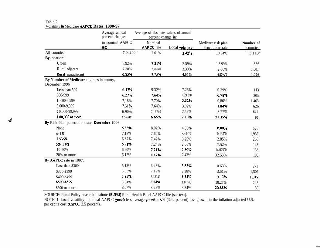
Table 2.Volatility in Medicare MPCC Rates, 1990-97

Average annual Average of absolute values of annualpercent change percent change in:in nominal AAPCC Nominal Medicare risk plan Number ofrittc AAPCC rate Local voia[~ Penetration rate counties

All counties-. —. .

7.04?40 -7.61% 3A2% 10.94% ‘ 3,113”

Ily location:Urban 6.92% 7.21?40 2.59% 1 3.99% 836Rural adjacent 7.38% 7,76940 3.30% 2.06% 1,001Rural nonadjacent 6.85?40 7.75’XO 4.05% 0.57%’0 1,276

By Number of Medicare eligibles in county,December 1996

Less than 500 6. 17’%0 9.32% 7.26% 0.39% 113500-999 6.27’XO 7.64?40 4.79’?40 0.78V0 205I ,000-4,999 7,18% 7.70% 3.52’?40 0086% 1,4635,000-9,999 7.31’XO 7.64% 3.02% 1.84V0 626I 0,000-99,999 6.90% 7.17’%0 2.59% 8.27% 641I 00,000 or mOre 6.57?40 6,66% 2.10% 21.35’70 65

By Risk Plan penetration rate, Dccembcr 1996None 6.88V0 8.02% 4.36% 0.00Y0 528o- I Yo 7.18% 7.64% 3.349”0 0.13$’0 1,9361 ‘XO-5Y0 6.87% 7.42% 3.25% 2.85% 2605?40- 1 Ovo 6.91!40 7.24% 2.60% 7.52% 14310-20% 6.90% 7.21?40 2.80’?XO 14.079’0 13820% or more 6.12% 6.47’XO 2.43% 32.53% 108

By AAPCC rate in 1997:Less than $300 5.13% 6.43% 3.88’3fo 0.63%$300-$399

2716.53% 7.19% 3.38% 3.51% 1,506

$400-s499 7.85’XO 8.18?40 3.3W0 9. 13’%0S500-S599

1,0498.54% 8.84?40 3.44’?40 18.27% 248

$600 or more 8.67% 8.75% 3.34% 20.88V0 39

SOURCE: Rural Policy research Institute (RUPR1) Rural Health Panel AAPCC file (see text).NOTE: 1. Local volatility= nominal AAPCC growth less average growth in CP1 (3.42 percent) less growth in the inflation-adjusted U.S.per capita cost (USPCC, 3.5 percent).

—

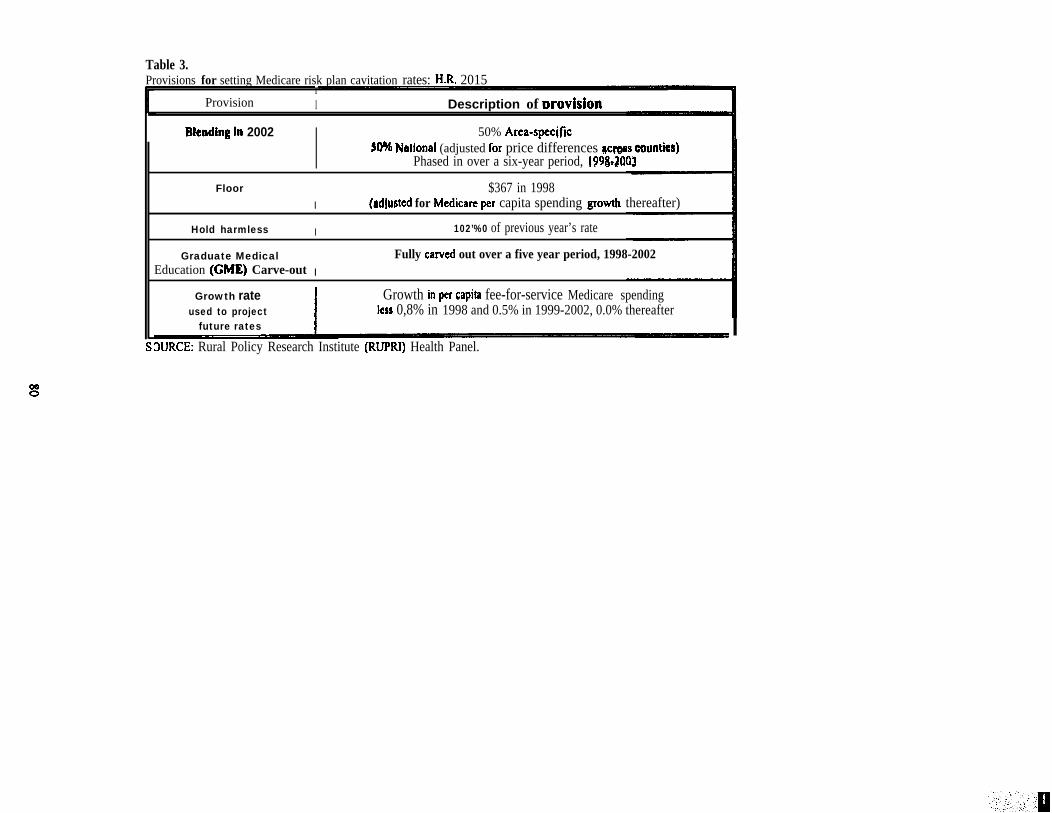
Table 3.Provisions for setting Medicare risk plan cavitation rates: H.R. 2015

rProvision I Description of movision

Mending h 2002 I 50% Area-specificW% National (adjusted for price differences acnws counties)

Phased in over a six-year period, 199&zO03

Floor

I

$367 in 1998(adjusted for Medicare per capita spending growth thereafter)

Hold harmless I 102’%0 of previous year’s rate

Graduate MedicalI

Fully cawed out over a five year period, 1998-2002Education (GME) Carve-out

Growth rate

I

Growth in per capita fee-for-service Medicare spendingused to project lCSS 0,8% in 1998 and 0.5% in 1999-2002, 0.0% thereafter

future rates●

WRCE: Rural Policy Research Institute (RUPRI) Health Panel.

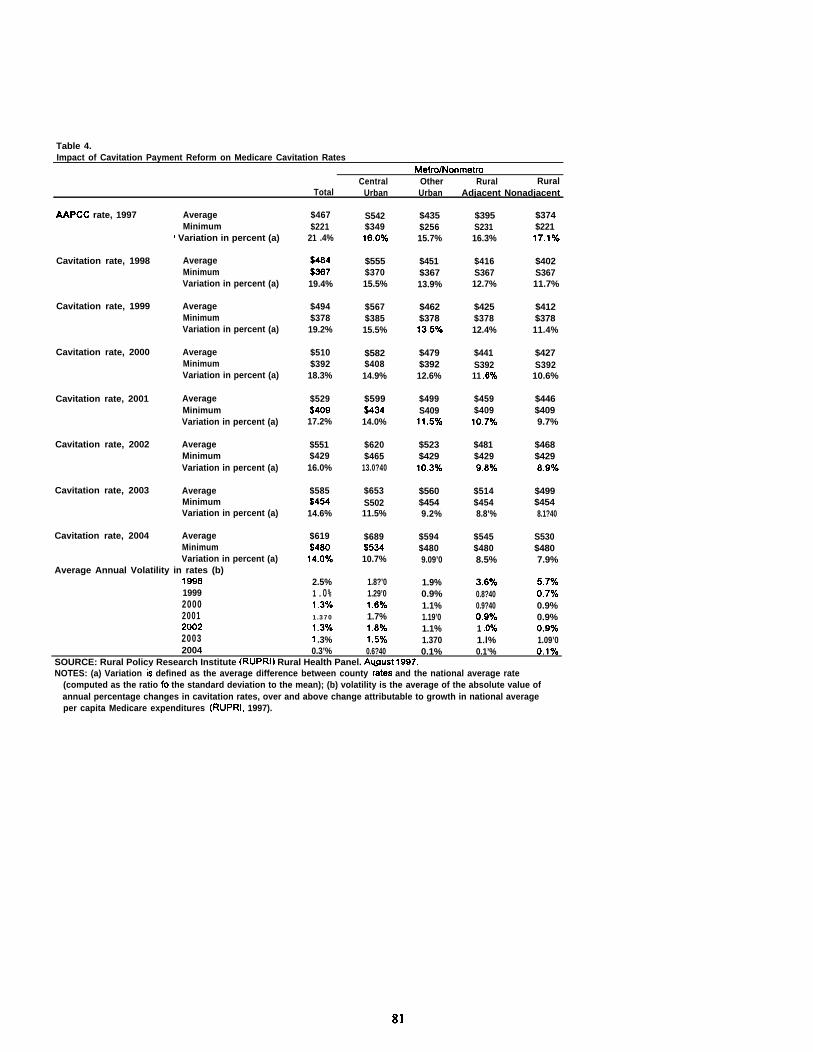
Table 4.Impact of Cavitation Payment Reform on Medicare Cavitation Rates

Metra/NonmetroCentral Other Rural Rural

Total Urban Urban Adjacent Nonadjacent

AAPCC rate, 1997

Cavitation rate, 1998

Cavitation rate, 1999

Cavitation rate, 2000

Cavitation rate, 2001

Cavitation rate, 2002

Cavitation rate, 2003

Cavitation rate, 2004

AverageMinimum

‘ Variation in percent (a)

AverageMinimumVariation in percent (a)

AverageMinimumVariation in percent (a)

AverageMinimumVariation in percent (a)

AverageMinimumVariation in percent (a)

AverageMinimumVariation in percent (a)

AverageMinimumVariation in percent (a)

AverageMinimumVariation in percent (a)

Average Annual Volatility in rates (b)199819992000200120022003

$467$221

21 .4%

$484$36719.4%

$494$37819.2%

$510$392

18.3%

$529S409

17.2%

$551$42916.0%

$585$45414.6%

$619

2.5%1 .0%1.Zyo1.370

1.3~o1 .3%

S542$34916.0°k

$555$37015.5%

$567$38515.5%

$582$40814.9%

$599$43414.0%

$620$465

13.0?40

$653S50211.5%

$689$53410.7%

1.8?’01.29’01.6701.7%1.8?401.5%

$435$25615.7%

$451$36713.9%

$462$378~3.5Yo

$479$39212.6%

$499S40911.570

$523$42910.3’3!0

$560$4549.2%

$594$4809.09’0

1.9%0.9%1.1%1.19’01.1%1.370

$395S23116.3%

$416S36712.7%

$425$37812.4%

$441S39211 .6°A

$459$409lo.Tyo

$481$4299.8?40

$514$4548.8’%

$545$4808.5%

3.6V00.8?400.9?400.9~o1 .O%1.l%

$374$22117.1%

$402S36711.7%

$412$37811.4%

$427S39210.6%

$446$4099.7%

$468$4298.9V0

$499$4548.1?40

S530$4807.9%

5.70Xo0.7700.9%0.9%0.9~o1.09’0

2004 0.3’% 0.6?40 0.1% 0.1’% 0.1?0SOURCE: Rural Policy Research Institute (RUPRI) Rural Health Panel. Auaust 1997.NOTES: (a) Variation is defined as the average difference between county rites and the national average rate

(computed as the ratio fo the standard deviation to the mean); (b) volatility is the average of the absolute value ofannual percentage changes in cavitation rates, over and above change attributable to growth in national averageper capita Medicare expenditures (RUPRI, 1997).

‘,

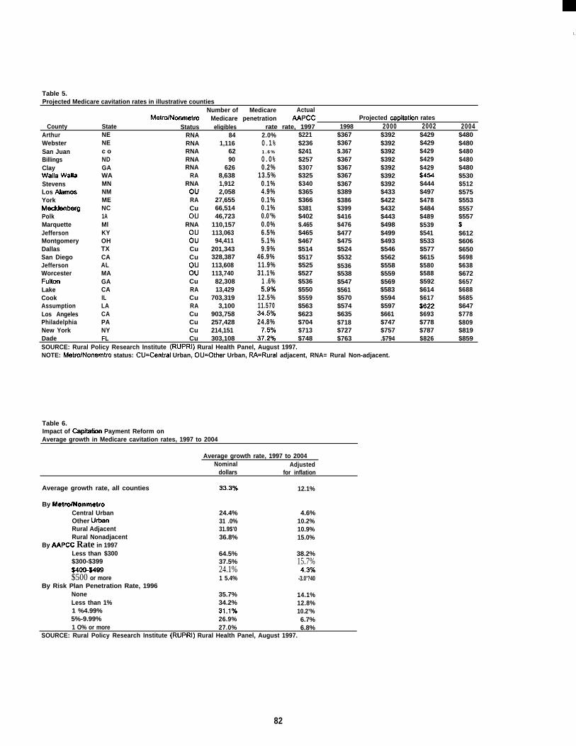
Table 5.Projected Medicare cavitation rates in illustrative counties

Number of Medicare ActualMetro/Nonmetro Medicare penetration /V4Pcc Projected capitatiin rates

County State Status eligibles rate rate, 1997 1998 2000 2002 2004Arthur NE RNA 84 2.0% $221 $367 $392 $429 $480Webster NE RNASan Juan c o RNABillings ND RNAClay GA RNAWalla Walla WA RAStevens MN RNALos Alamos NM OuYork ME RAMecklenberg NC CuPolk 1A OuMarquette Ml RNAJefferson KY OuMontgomery OH OuDallas TX CuSan Diego CA CuJefferson AL OuWorcester MA OuFulton GA CuLake CA RACook IL CuAssumption LA RALos Angeles CA CuPhiladelphia PA Cu

1,1166290

6268,6381,9122,058

27,65566,51446,723

110,157113,06394,411

201,343328,387113,608113,74082,30813,429

703,3193,100

903,758257,428214,151

0.1%1.6%

0.0%0.2%

13.5%0.1%4.9%0.1%0.1%0.0’%0.0%6.5%5.1%9.9%

46.9%11.9%31.1%

1 .6%5.970

12.5%11.57034.57024.8%

T.syo

$236$241$257$307$325$340$365$366$381$402$.465$465$467$514$517$525$527$536$550$559$563$623$704$713

$367$.367$367$367$367$367$389$386$399$416$476$477$475$524$532$536$538$547$561$570$574$635$718$727

$392$392$392$392$392$392$433$422$432$443$498$499$493$546$562$558$559$569$583$594$597$661$747$757

$429$429$429$429$454$444$497$478$484$489$539$541$533$577$615$580$588$592$614$617S622$693$778$787

$480$480$480$480$530$512$575$553$557$557

$612$606$650$698$638$672$657$688$685$647$778$809$819New York NY Cu

Dade FL Cu 303,108 37.2?J’o $748 $763 .$794 $826 $859SOURCE: Rural Policy Research Institute (RUPRI) Rural Health Panel, August 1997.NOTE: Metro/Nonemtro status: CU=Central Urban, OU=Other Urban, RA=Rural adjacent, RNA= Rural Non-adjacent.

Table 6.Impact of Capitatiin Payment Reform onAverage growth in Medicare cavitation rates, 1997 to 2004

Average growth rate, 1997 to 2004Nominal Adjusted

dollars for inflation

Average growth rate, all counties aB.Byo 12.1%

By Metro/NonmetroCentral Urban 24.4% 4.6%Other Utian 31 .0% 10.2%Rural Adjacent 31.9$’0 10.9%Rural Nonadjacent 36.8% 15.0%

By AAPCC Rate in 1997Less than $300 64.5% 38.2%$300-$399 37.5%S400-S499

15.7%24.1% 4.370

$500 or more 1 5.4% -3.0’?40By Risk Plan Penetration Rate, 1996

None 35.7% 14.1%Less than 1% 34.2% 12.8%1 %4.99% 31.170 10.2’%5%-9.99% 26.9% 6.7%1 O% or more 27.0% 6.8%

SOURCE: Rural Policy Research Institute (RUPRI) Rural Health Panel, August 1997.

82

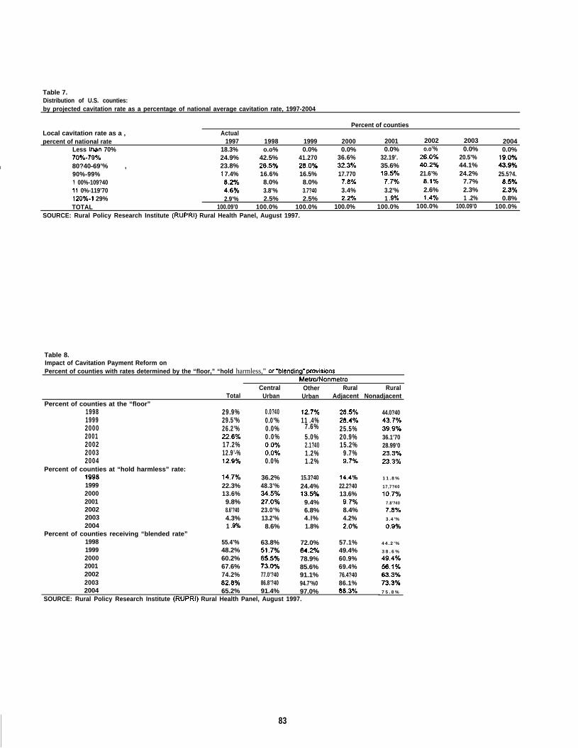
Table 7.Distribution of U.S. counties:by projected cavitation rate as a percentage of national average cavitation rate, 1997-2004

Percent of countiesLocal cavitation rate as a , Actualpercent of national rate 1997 1998 1999 2000 2001 2002 2003 2004

Less than 70% 18.3% o.o% 0.0% 0.0% 0.0% o.o’% 0.0% 0.0%I 70Y0-799!0 24.9% 42.5% 41.270 36.6% 32.19’. 26.09’o 20.5’% 19.070I 80?40-69’% , 23.8% 26.5V0 28.OVO 32.37. 35.6% 40.2yo 44.1% 43.970

90%-99% 1 7.4% 16.6% 16.5% 17.770 19.570 21.6’% 24.2% 25.5?4.1 00%-109?40 8.270 8.0% 8.0% 7.8V0 7.770 8.170 7.7% 8.59611 0%-119’70 4.69’o 3.8’% 3.7?40 3.4% 3.2’% 2.6% 2.3% 2.3V0120’Yo-1 29% 2.9’% 2.5% 2.5% 2.29fo 1 .99!0 1.470 1 .2% 0.8%TOTAL 100.09’0 100.0% 100.0% 100.0% 100.0% 100.0% 100.09’0 100.0%

SOURCE: Rural Policy Research Institute (RUPRI) Rural Health Panel, August 1997.

Table 8.Impact of Cavitation Payment Reform onPercent of counties with rates determined by the “floor,” “hold harmless,” or “blending” provisions

Metro/NonmetroCentral Other Rural Rural

Total Urban Urban Adjacent NonadjacentPercent of counties at the “floor”

1998 29.9% 0.0?40 12.7?’o 28.57.1999 29.5’% 0.0’% 11 .4% 28.4V02000 26.2’% 0.0% 7.6% 25.5%2001 22.6V0 0.0% 5.0% 20.9%2002 17.2% 0.0!40 2.1?40 15.2%2003 12.9’-% 0.070 1.2% 9.7%2004 12.9?/o 0.0% 1.2% 9.7yo

Percent of counties at “hold harmless” rate:1998 ~4.7~o 36.2% 15.3?40 14.4~o1999 22.3% 48.3’% 24.4% 22.2?402000 13.6% 34.570 13.5V0 13.6%2001 9.8% 27.0’%. 9.4% 9.7~o2002 8.6’?40 23.0’% 6.8% 8.4%2003 4.3% 13.2’% 4.l% 4.2%2004 1 .9’MO 8.6% 1.8% 2.070

Percent of counties receiving “blended rate”1998 55.4’% 63.8% 72.0% 57.1%1999 48.2% 51.7% 64.2V0 49.4%2000 60.2% 65.5’%0 78.9% 60.9%2001 67.6% 73.OVO 85.6% 69.4%2002 74.2% 77.0’?40 91.1% 76.4?402003 82.8°& 86.8’?40 94.7’%0 86.1%2004 65.2% 91.4% 97.0% 88.370

SOURCE: Rural Policy Research Institute (RUPRI) Rural Health Panel, August 1997.

44.0?4043.7!4039.9~o36.1’7028.99’023.3~o23.3’?40

11.8%

17,7?40

lt).7yo

7.8’?40

7.870

3.4’%

().9yo

44.2’%

38 .6%

49.470

56.170

63.3’XO

73.370

75 .8%

83

m,..$.

P-

THE COMMUNITY POLICY ANALYSIS SYSTEM (COMPAS)A PROPOSED NATIONAL NETWORK

OF ECONOMETRIC COMMUNITY IMPACT MODELS

Thomas G. JohnsonJames K. Scott

Rural Policy Research Institute:University of Missouri-Columbia

Devolution of authority and responsibility from theFederal Government to state and local governments is,and will continue to be, one of the most dominantpublic policy issue for communities for the nextdecade. Block grants, deregulation, welfme reform,health care reform, education reform, agriculturalpolicy reform, various state waivers, and other termsfill the national policy dialogue and all are symptomaticof devolution.

To communities, especially rural communities,devolution spells the end of many of the safety nets thatprotected local governments, school districts and otherpublic entities from some economic and socialhardships. At the same time devolution enhancesopportunities for local leadership and increases thereturns to aggressive and innovative public decisionmaking. In this environrnen~ the value of economic andsocial information, accurate projections and analyses ofpolicy alternatives is particularly great. This in turn iscreating an opportunity for those involved in thedecision support sciences.

The Community Policy Analysis System (COMPAS)initiative is a response to this opportunity. It addressesthe information needs of policy makers at the Federal,state and local levels. At the Federal level, there is agrowing need for a better understanding of the localconsequences of federal policy, especially policy thatdevolves responsibility to local governments.Similarly, state governments require information on theconsequences of their policies on local governments asboth state and local responsibilities change.

The need, under these emerging circumstances, forbetter decision support at the local level is obvious.The diversity of conditions in rural communities meansthat generic, or aggregated decision support toolsprobably conceal more than they reveal. Broadgeneralizations about policy impacts are usually

uninformative at best, misleading at worst. It is clear,for example, that to conclude that trade liberalizationwill lead to overall increases in income andemployment is an important aggregate projection but ittells us little about the changes that will be experiencedby individual communities or what their optimumresponses to these changes might be.

In response to these policy trends, a group of regionaleconomists and rural social scientists have identified aset of modeling tools which can be used to providepolicy decision support for state and local governmentofllcials, including input-output modeling, cost.benefitanalysis, and industrial targeting. In addition, the grouphas developed a plan to build a collaborativecommunity policy analysis network that will eventuallyextend to selected rural communities in twenty-fivestates. With initial support from the Rural PolicyResearch Institute (RUPRI), the four regional ruraldevelopment centers and a variety of other sources, thegroup has also outlined the structure of econometriccommunity models for each state that will compare theeconomic, demographic, and fiscal impacts of a varietyof economic or policy scenarios. The models areintended to be used in conjunction with other decisiontools to provide maximal flexibility and a capacity forrapid response to queries by local and state policydecision makers. This paper will focus on thespecification and development of the COMPASeconometric community models. It will describe theconceptual fkamework of the proposed models, reporton applications of the models in two states, and brieflydiscuss plans for fbture development and support of theCOMPAS network. The plan takes into account therealities of secon~ data availability at thecommunity level and it attempts to build on cmentconceptual foundations from the social sciences andregional science. It is evolutionary in that it will bedesigned to be flexible and continually improved upon;and it addresses the institutional and constitutional

85

differences among states and communities.

The COMPAS model discussed below is basedprimarily on the authors’ experiences with the VirginiaImpact Project (VIP) model, and Missouri’s Show MeCommunity Impact Model which have evolved over thelast decade. However, these models, are themselvesjust a recent chapter in a long tradition of communitymodeling by rural development researchers (seeHalstead, Leistri@ and Johnson for a history of justsome of these models). The novel aspect of this projectis the attempt to create models for communitiesthroughout the nation.

KEY PRINCIPLES

There are many considerations involved in modeling acommunity for policy analysis. The followingassumptions are based on conceptual logic and/orempirical studies of communities. Each are reflected inthe proposed COMPAS framework.

1. While economic and social relationships knowno geopolitical boundaries, policy provisions,public services, taxing authority, and data, do.Therefore, county, municipal, and publicservice boundaries should be at the basis ofany policy model.

2. Communities within states share commonconstitutional limitations and responsibilities,and have developed comparable institutions.

3. Communities with similar economic baseshave similar economic structures. Because ofthe importance of climatic, geographic, socialand political influences, economic bases arefrequently quite homogeneous acrossgeographic regions.

4. Communities of similar size and with similargeographic relationships to nearby larger andsmaller communities, petiorm similar centralplace roles and are likely to exhibit similarresponses to economic (and policy) stimuli.

5. The fi.mdamental engine for economic growth,decline, and change at the local level isemployment. Community impacts are effectedthrough the labor market which allocates jobsbetween the currently unemployed, residentsof nearby communities (incommuters), currentresidents who work outside the community

(outcommuters), and new entrants to the locallabor market.

6. Changes in employment, unemployment,commuting, labor force, population, schoolenrollment and income, lead to changes inhousing needs, property tax base, publicservice demands, and transfers to householdsand local governments.

These principles guided the estimation anddevelopment of the Virginia Impact Projection (VIP)model and the Show Me Model for Missouricommunities. Both models are systems ofeconometrically estimated equations for rural towns,counties and cities in the respective states, using bothcross-sectional and time series data. Experience withthe estimation of these models indicates that withcareful selection of variables and fi.mctional form,stable coefficients can be estimated for communitieswith a wide variety of sizes and economic bases. Basicinstitutional differences cannot be captured with asingle set of parameter estimates, however.Furthermore, attempts to apply the model to other stateshave underscored the importance of differences in thestructure of public service provision. Therefore, onlystates with very similar local government structures willbe candidate for grouping together.

MODEL STRUCTURE

While many different model structures could generatecomparable policy analyses, the COMPAS models willshare a basic structure, The COMPAS models willbased on the assumptions above as well as others aboutthe way in which rural and small city economies work,about the way in which local governments makedecisions, and about the conditions under which localpublic services are provided. In the following pages,the first and most simple of the COMPAS models willbe described.

Labor Market Equations

The labor market concept plays a central role in theCOMPAS models. The models are built on theassumption that economic growth is caused largely byexogenous increases in employment. This is not to saythat employment at the community level is notresponsive to local conditions but rather, that theseresponses will be dealt with as direct changes or shocksto be introduced to the models. In this simple model,

86

demand can be viewed as perfectly inelastic at the locally employed residents and locally employedexogenous level of employment. Total labor supply is non-residents or incommuters. Locally employedperfectly elastic at the prevailing regional or national residents equals the resident labor force lesswage level (adjusted for local cost of living, amenities, unemployed outcommuters. These relationships areetc.). Labor supply is composed of two components: described below in Figure 1.

In- and out-commuters are separated here, rather thancombined into net commuters, because they exhibitdifferent in preferences for public services, spatialamenities, occupational characteristics of households,and because sub-markets for different labor skillspersist Labor force and incommuters are positivecomponents of supply and outcommuting is a negativecomponent. Unemployment is a residual negativecomponent of supply. Eliminating wages from thecomponent supply curves by substituting the inversedemand curve, as amended, derives the expressions.This introduces employment (demand) to the supplycomponents. More formally, the model is developed asfollows:

(1) %=)5.

equates demand and supply (local employment andemployed labor force from all locations). The demandctuve is

(2) x, - f(w).(where w is the wage rate) which when invertedbecomes

(3) w ‘g&J.

Decomposing labor supply into its components gives

( 4 1 &=& -x”-&+&

Each component of supply is a function of employmentand a vector of supply shifters,

where, X,, is labor demand (local emplcyment), X, islabor supply, made up of its components, & (residentlabor force), X, (outcornmuters), X, (incommuters), andy(unemployed), w is the wage rate, and the 2s aresupply shifters for the various components of supply.Given the discussion and the conceptual model above,equations 4 through 7 can be expressed as follows inequations 8 through 11.’

(8) Unemployed = Labor Force + Inccmunuters -Employment - Outcommuters

All three components of labor supply will be primarilydetermined by employment in the location in question.In addition, they will depend on relative housingconditions, costs of living, quality of public services,tax levels, the mix of jobs, and similar variables in thelocation of employment, versus alternative locations. Avery important variable in the supply components isarea of the data unit. Smaller units will include fewerresident laborers, and define more as outcommuntersand incommuters because the cross the borders of theunit. Larger units will incorporate more destinationsand residences of workers and, therefore, define moreworkers as being locally employed, and thus fewerwtconunuters an d incommuters. In addition,commuting will depend on the distance between placeof residence and place of work.

(9) Labor force = @!rnployrnenf housingconditions, cost of living, public services,taxes, industry mix, area).

(10) Outcommuting = f@mploymmt, external

87

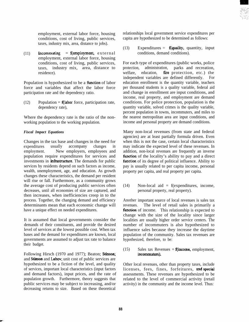
employment, external labor force, housingconditions, cost of living, public services,taxes, industry mix, area, distance to jobs).

(11) Incommuting = f(employment, ex te rna lemployment, external labor force, housingconditions, cost of living, public services,taxes, industry mix, area, distance toresidence).

Population is hypothesized to be a fi.mction of laborforce and variables that affect the labor forceparticipation rate and the dependency ratio.

(12) Population = f(labor force, participation rate,dependency rate),

Where the dependency rate is the ratio of the non-working population to the working population.

Fiscal Impact Equations

Changes in the tax base and changes in the need forexpenditures usually accompany changes inemployment. New employers, employees andpopulation require expenditures for services andinvestments in infi-astructure. The demands for publicservices by residents depend on such factors as income,wealth, unemployment, age, and education. As growthchanges these characteristics, the demand per residentwill rise or fall. Furthermore, as a community growsthe average cost of producing public services oftendecreases, until all economies of size are captured, andthen increases, when inefficiencies creep in to theprocess. Together, the changing demand and efficiencydeterminants mean that each economic change willhave a unique effect on needed expenditures.

It is assumed that local governments consider thedemands of their constituents, and provide the desiredlevel of services at the lowest possible cost. When taxbases and the demand for expenditures are known, localgovernments are assumed to adjust tax rate to balancetheir budget.

Following Hirsch (1970 and 1977); Beaton; Stinson;and Stinson and Lubov; unit cost of public services arehypothesized to be a fiction of the level, and qualityof services, important local characteristics (input factorsand demand factors), input prices, and the rate ofpopulation growth. Furthermore, theory suggests thatpublic services may be subject to increasing, and/ordecreasing returns to size. Based on these theoretical

relationships local government service expenditures percapita are hypothesized to be determined as follows:

(13) Expenditures = f(quality, quantity, inputconditions, demand conditions).

For each type of expenditures (public works, policeprotection, administration, parks and recreation,welfare, education, fwe protection, etc.) theindependent variables are defined differently. Foreducation enrollment is the quantity variable, teachersper thousand students is a quality variable, federal aidand change in enrollment are input conditions, andincome, real property, and employment are demandconditions. For police protection, population is thequantity variable, solved crimes is the quality variable,percent population in towns, incommuters, and miles tothe nearest metropolitan area are input conditions, andincome and personal property are demand conditions.

Many non-local revenues (from state and federalagencies) are at least partially formula driven. Evenwhen this is not the case, certain local characteristicsmay indicate the expected level of these revenues. Inaddition, non-local revenues are frequently an inverseIlmction of the locality’s ability to pay and a directfimction of its degree of political influence. Ability topay is usually related to per capita income, personalproperty per capita, and real property per capita.

Non-local aid = f(expenditures, income,personal property, real property).

important source of local revenues is sales tax

(14)

Anotherrevenues. The level of retail sales is primarily afimction of income. This relationship is expected tochange with the size of the locality since largerlocalities are usually higher order service centers. Thenumber of incommuters is also hypothesized toinfluence sales because they increase the daytimepopulation of the community. Sales tax revenues arehypothesized, therefore, to be:

(15) Sales tax Revenues = f(income, employment,incommuters).

Other local revenues, other than property taxes, includelicenses, fees, fines, forfeitures, and specialassessments. These revenues are hypothesized to berelated to the level of commercial activity (retailactivity) in the community and the income level. Thus:

88

(16) Other Tax Revenues = f(Sales tax revenues,income).

Real property includes both residential and businessproperty and, therefore, will be influenced by the levelof personal income as well as the size of the economicbase. Both personal and real property are hypothesizedto be positively related to the number of outcommuterssince these families represent a source of wealth that isnot supported by the local economic base.

(17) Real Property = f(income, employment,outcommuters),

(18) Personal Property = f(income, outcommuters).

There are a number of ways to close this type of mode.In the case of the VIP model it is assumed that local

government expenditures are determined first, and realand personal property tax rates are set to cover thoseexpenditures not met by non-local aid and sales taxrevenues and other tax revenues. This implicitlyassumes that budgets are balanced each year. Analternate assumption (the one used in the Show Me) isthat the tax rate remains constant and that economicchanges lead to fiscal deficits or surpluses.

THE MODELS APPLIED

To date, the VIP and Show Me models have beendeveloped for forty to fifty communities. Similarmodels have been developed and applied in the severalcommunities in Iowa (Swenson, 1996), Idaho (Fox andCooke, 1996) and Wisconsin (Deller and Shields,1996). Local advisory committees are usuallyappointed to review the baseline projections, help formthe scenarios, review the model’s projection, and tohelp interpret the results. The models have been usedfor a variety of purposes including analyses ofannexations, jurisdictional mergers, new industries,

existing industries, industry closures, universityresearch parks, shopping centers, residentialdevelopments, location of industrial sites and, andgeneral development strategies. They have also beenused for goal planning for several communities. Goalplanning with the models is achieved by estimating theconditions necessary to bring about a desired set ofterminal conditions.

The models have generally been popular with local andstate governments. Policy makers are generallysomewhat skeptical until they come to appreciate theinformation generated and become more confident inthe projections. Repeat users of the model’sprojections especially like the comparability of theresults from case to case, and across communities.

DISCUSSION

The devolution of policy decisions from central to localcontrol will bring communities many new opportunitiesand many significant new challenges. Especially thosethat are small or othenvise disadvantaged may nowneed the capacity to assess the fiture impacts of avariety of expected or proposed changes. TheCommunity Policy Analysis System is one approachfor rural development researchers to assist indeveloping that capacity.

COMPAS models now exist in at least five states.Preliminary plans are now in place to extend that toseven, fifteen, and ultimately twenty-five states overthe next three years. In the next six months, researchersinvolved in this initiative will review, refine and test theconceptual framework of the COMPAS models andspeci~ data and research standards that will makeresults from these models comparable and compatible.If resources are available, these researchers will form anetwork designed to provide analysis of thecommunity impacts of local, state and federal policyalternatives.

89

REFERENCES

Beaton W. Patrick. The Determinants of Police Protection Expenditures. National Tax Journal 24 (1974): 335-349.

Deller, Steve and Martin Shields. The Wisconsin Extension Fiscal Impact Model: Preliminary Results. Presented atthe Community Economic Modeling Conference. June, 1996. Madison, Wisconsin.

Fox, Linnette and Stephen Cooke. Data for the Idaho Fiscal Impact Model. Presented at the Community EconomicModeling Conference. June, 1996. Madison, Wisconsin.

Halstead, John M., F. Larry Leistritz, and Thomas G. Johnson. 1991. The Role of Fiscal Impact Models in ImpactAssessments. Impact Assessment Bulletin 9 (Fall): 43-54.

Hirsch, Werner Z. Economics of State and Local Government. McGraw-Hill, New York, 1970.

Hirsch, Werner Z. Output and Costs of Local Government Services, Paper for the National Conference onNon-Metropolitan Community Services Research, Ohio State University, Columbus, Ohio, January 21, 1977,

Johnson Thomas G. A Description of the VIP Model, Unpublished manuscript, Department of AgriculturalEconomics, Virginia Tech, Blacksburg, Virginia, April 1991.

Johnson, Thomas G. Representative Community Analysis, paper presented in a symposium entitled, “Rural Impactsof Public Policies: Improved Analytic Frameworks,” at the annual meetings of the American AgriculturalEconomics Association, Orlando, Florida, August 2, 1993.

Stinson, Thomas F. The Dynamics of the A@stment Period in Rapid Growth Communities, Prepared forPresentation at the WAEA Annual Meetings, Bozeman, Montana, July 24, 1978.

Stinson, Thomas F. and Andrea Lubov. Segmented Regression, Threshold Eflects, and Police likpenditures inSmall Cities. American Journal of Amicultural Economics 64 (November) 1982:738-746.

Swenson, David. Spatial/Institutional Interrelationships. Presented at the Community Economic ModelingConference. June, 1996. Madison, Wisconsin.

‘ If ones estimate of employment is defined as jobs, rather than the number of persons employed, then it will include second jobs.In this case, employment as defined here equals jobs less second jobs. Alternatively, one must augment the supply of labor by the number ofindividuals holding second and third jobs.

90

I

PROJECTIONS OF REGIONAL ECONOMIC AND DEMOGRAPHIC IMPACTSOF FEDERAL POLICIES

Glenn L. Nelson. Chair. Regional Analysis Work Group,Rural Policy Research Institute, University of Missouri, Columbia, Missouri 65211

Improved information on the regional impacts off~ral policies would address an important need ofdecision makers, including citizens who make theirpolitical choices seriously. Regional variations in thedemographic and economic environment lead toregional variations in the impacts of federal policies.For example. the percentage of the population that iselder~y and that is poor varies by region; manyprograms use age and income as factors indetermining eligibility and payments. Looking atanother important example, regional economies va~in the importance of new investment and ofinternational competition; the change in the realinterest rate due to changes in the federal budgetdeficit wili have Merent impacts in tierent regions.Little is known about these regional variations becausefw analysts are studying them.

The objective of the work described in this paperis to provide estimates of the regional demographicand economic impacts of current and proposed federalpolicies. The primary audience consists of decisionmakers and their stai%s at the f~ral level. Animportant secondary audience consists of state andlocal decision makers and of citizens who seekinformation on f~ral policies in order to influencepolicy in an informed manner. Another importantaudience consists of researchers who seek bettermethods of sub-national analyses and improved data.

The remainder of this paper will address theresearch design for this project, the explicit inclusionof the f-ml budget deficit, mwiel solutionprocedures, Medicare and Medicaid data, apreliminary baseline solution, and analyses ofalternative policies.

Research Design

This research produces information on sub-national regions as traditionally defined and on countygroupings representing the rural-urban continuum.The four subnational regions used in the analysis areshown in Figure 1. They follow the boundaries of fourRural Development Centers who are clientele for thiswork. A larger number of smaller sub-nationalregions would be desirable, but the use of only fourregions is not a major problem at this stage of the

Figure 1. RUPRI Sub-Natioml Regions

NorthCentral

West

North-east

u south

research.The counties within each sub-national region are

partitioned into four categories representing the rural-urban continuum. Nonrnetropolitan counties notadjacent to a metropolitan area makeup the most ruralcategory. Nonrnetropolitan counties adjacent to ametropolitan area make up a rural category which isless remote from a large urban concentration thanother nonrnetropolitan counties, The central cities ofthe 32 largest metropolitan areas are represented by 62densely populated counties and are the most urbancategory. The remaining metrqmlitan counties makeup a less densely settled urban category.

These categories are proving to be workable, butthey have signifhnt problems. I would prefer adefinition that treats rural and urban as partitions on asymmetrical continuum rather than the current out-&t@ urban-centered definition of metropolitan andnonmetropolitan. I am currently exploring thesuggestion of John Adams to use relative densitywithin the nation and state, to which I would add athird factor of relative &nsity within a sub-nationalregion such as those in Figure 1.

Several large counties of mixed rural-urbancharacter lessen the distinctions between thecategories. For purposes of analyses, we shouldpartition six large counties in southern California andthe four large counties containing Duluth, PhoenizReno, and Tucson into their rurai and urban parts. We

91

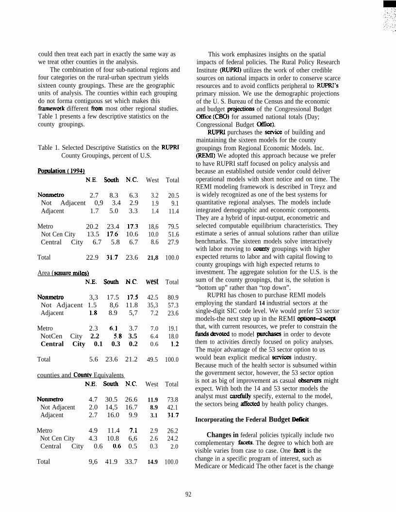
could then treat each part in exactly the same way aswe treat other counties in the analysis.

The combination of four sub-national regions andfour categories on the rural-urban spectrum yieldssixteen county groupings. These are the geographicunits of analysis. The counties within each groupingdo not forma contiguous set which makes thisfimnework different horn most other regional studies.Table 1 presents a few descriptive statistics on thecounty groupings.

This work emphasizes insights on the spatialimpacts of federal policies. The Rural Policy ResearchInstitute (RUPRI) utilizes the work of other crediblesources on national impacts in order to conserve scarceresources and to avoid conflicts peripheral to RUPRI’Sprimary mission. We use the demographic projectionsof the U. S. Bureau of the Census and the economicand budget pro~ons of the Congressional BudgetOffke (CBO) for assumed national totals (Day;Congressional Budget Offke).

RUPRI purchases the seMce of building andmaintaining the sixteen models for the countygroupings from Regional Economic Models. Inc.(REMI) We adopted this approach because we preferto have RUPRI staff focused on policy analysis andbecause an established outside vendor could deliveroperational models with short notice and on time. TheREMI modeling framework is described in Treyz andis widely recognized as one of the best systems forquantitative regional analyses. The models includeintegrated demographic and economic components.They are a hybrid of input-output, econometric andselected computable equilibrium characteristics. Theyestimate a series of annual solutions rather than utilizebenchmarks. The sixteen models solve interactivelywith labor moving to county groupings with higherexpected returns to labor and with capital flowing tocounty groupings with high expected returns toinvestment. The aggregate solution for the U.S. is thesum of the county groupings, that is, the solution is“bottom up” rather than “top down”.

RUPRI has chosen to purchase REMI modelsemploying the standard 14 industrial sectors at thesingle-digit SIC code level. We would prefer 53 sectormodels-the next step up in the REMI options-+xceptthat, with current resources, we prefer to constrain thefimds &voted to model pchases in order to devotethem to activities directly focused on policy analyses.The major advantage of the 53 sector option to uswould bean explicit medical seMces industry.Because much of the health sector is subsumed withinthe government sector, however, the 53 sector optionis not as big of improvement as casual obsemrs mightexpect. With both the 14 and 53 sector models theanalyst must carefidly specify, external to the model,the sectors being affixted by health policy changes.

Incorporating the Federal Budget DefW

Changes in federal policies typically include twocomplementary f-. The degree to which both arevisible varies from case to case. One fiwet is thechange in a specific program of interest, such asMedicare or Medicaid The other facet is the change

Table 1. Selected Descriptive Statistics on the RUPRICounty Groupings, percent of U.S.

Potndation ( 1994}N.E. SOUth N.C. West Total

Nonmetro 2.7 8.3 6.3Not Adjacent 0,9 3.4 2.9Adjacent 1.7 5.0 3.3

3.21.91.4

20.59.1

11.4

Metro 20.2 23.4 17.3Not Cen City 13.5 17.6 10.6Central City 6.7 5.8 6.7

18,610.08.6

79.551.627.9

Total 22.9 31,7 23.6 21,8 100.0

Area (sauare miles]N,E, SOllth N.C. west Total

Nonrnetro 3,3 17.5 17.5Not Adjacent 1.5 8,6 11.8Adjacent 1.8 8.9 5,7

42.535,3

7.2

80.957.323.6

Metro 2.3 6.1 3.7NotCen City 2.2 5.8 3.5Central City 0.1 0.3 0.2

7.06.40.6

19.118.0

1.2

Total 5.6 23.6 21.2 49.5 100.0

counties and Countv EquivalentsN.E. SOUth N.C. West Total

Nonmetro 4.7 30.5 26.6Not Adjacent 2.0 14,5 16.7Adjacent 2.7 16.0 9.9

11.98.93.1

73.842.131.7

Metro 4.9 11.4 7.1Not Cen City 4.3 10.8 6,6Central City 0.6 0.6 0.5

2.92.60.3

26.224.2

2.0

Total 9,6 41.9 33.7 14.9 100.0

92

in the federal fiscal situation and programmatic mixwhich accompanies the specific program at the centerof the discussion. For example, a cut in projectedMedicare expenditures is associated with acombination of a lower f~ral budget deficit, lowerf~ral taxes, and increased spending on other f~ralprograms.

Good policy analysis should take into accountboth facets. Ignoring one facet reduces the Scientilcrigor of the analysis and leads to erroneous estimates.In addition, citizens and decision makers dMer in therelative importance they place on the facets. Ananalyst who ignores, for example, the positive effectsof deficit reduction while fining on the negativeeffects of cuts in projected Medicare spending isappropriately viewed as adopting a partisan stance. InRUPRI we seek a long term, constructive, non-partisanengagement with decision makers.

Many local and regional policy analyses haveviolated this principle. A lack of attention to theelT&ts of changes in the f-ral budget deficit hasbeen a particular. important problem in many cases.

One of the important strengths of the RUPRIanalysis is that it accounts for changes in the feralbudget deficit. This is especially imptant in policyanalyses of proposals to lower projected federal budgetdeficits by cutting projected entitlement spending onthe baby boom population when its members becomeeligible for programs targeted on the elderly.

The particular manner in which RUPRIincorporates the federal budget deficit is applicable tomany other modeling situations. The REMI modeldoes not have an explicit f~ral fiscal component.The effects of federal fiscal actions consistent withexisting policies (the “baseline” solution) areincorporated as follows. (The table references in theremainder of this paragraph refer to Council ofEconomic Advisers. These tables illustrate theidentity being discussed and provide historical &ta. )First. CBO estimates of national GDP and of thefederal budget deficit are adopted as RUPRIassumptions. Second we in RUPRI estimate nationalgross saving by major component for each year in theprojection period. These components include thef~ral budget deficit. federal consumption of fixedcapital. state and local government saving. personalsaving. and gross business saving (Table B-30).

Third we estimate the components of nationalgross investment: gross private domestic investment,gross government investment. net exports. and netforeign investment other than net exports (Tables B-22and B-3 1). Fourth. having now estimated theinvestment and net export portions of GDP, weestimate how the remaining portion is di~ided between

consumption and government. taking into account thepreviously estimated gross government investment(Tables B-1 and B-18). In conclusion, the estimates ofconsumption, investment, government, and net exportsare the variables that reflect RUPIU assumptions withregard to the f~ral budget deficit-as well asnumerous other matters.

The analysis of a proposed policy alternativeproceeds analogously to the above pr*e. Thechange in the f~ral budget tilcit as well as theprogrammatic change are introduced explicitly in theformulation of macroeconomic assumptions. Ingeneral, this explicit consideration of the change in thef~ral budget deficit leads to the conclusion that thepolicy change aikcts every component of GDP, andoften total GDP as well.

Consistent National and Sub-National Solutions

The sixteen models for the county groupings mustbe solved in a manner that preserves the rigor of thestructure within the models driving the solution (thatis, the rigor of a “bottom up” approach) and that alsoincorporates the assumptions with respect to nationalGDP by major component. This is accomplished bysolving the system of sixteen models iteratively,making changes in selected assumptions in the modelsin each iteration, until the summations from thesixteen models match the assumed national totals.

In slightly more detail, the solution procedureflows as follows. First, assumptions are made in themodels with respect to demographic variables such asbirth rates, death rates, and immigration and withrespect to economic variables such as labor forceparticipation. productivity, exports. imports, andgovermnent spending that we believe will lead tonational demographic and economic outcomesconsistent with our assumptions. Sem@ we solve themodels as an interactive system and compute sumsover the sixteen models to derive national totals.Third we compare the output of the models with ourassumptions. If the output is consistent with ourassumptions. we have a satisfiwtoIY solution which weproceed to analyze. If the output di.Hers significantlyfrom our assumptions with regard to national totals,we return to step one noted above,

Medicare and Medicaid Data

RUPRI scientists are analyzing Medicare andMedicaid policies because of their importance to thenation, their rapid growth since inception, and theirrapid projected growth in the future--especially whenthe members of the post-war baby generation become

93

eligible. The analysis of policy alternatives has beenslowed by the poor quality of the data.

RUPRI has contributed significantly to a markedimprovement in readily accessible county-levelMedicare &ta. When RUPRI regional scientistsbegan work on Medicare in 1994, they found that thecounty-level data from the Consolidated Federal FundsReport, originally estimated by the Health CareFinancing Administration (HCFA) and disseminatedby the U.S. Bureau of the Census, were poorlydocumented and inaccurate. These Medicareestimates were also used by the Bureau of EconomicAnalysis (BEA) in estimating “medical transferpayments” in the Regional Economic InformationSystem (REIS). Working with the Oflke of the_ in HCFA RUPRI developed a superiorcounty-level &ta base and disseminated it in 1995(Nelson and Braschler). BEA began utilizing thesehigher quality Medicare data in REIS with the releaseof its county-level CD-ROM in September 1997(Bureau of Economic Analysis). This recent releasealso marks the first occasion in which BEA isdisseminating an explicit Medicare series, in contrastto the previous practice of issuing an aggregate totalcontaining Medicare and other medical transfers. TheCensus Bureau has not changed its sources andmethods as of early September 1997.

The available county-level Medicaid data areneedlessly inaccurate. As of September 1997 the bestsource of county-level Medicaid payments is the BEACD-ROM (Bureau of Economic Analysis). BEAobtains these data through direct contacts withindividual states. BEA has actual county-level data on34 states of which 26 are uptodate (Bureau ofEconomic Analysis, Table F). For those states notproviding data, BEA estimates county payments usingthe distribution of AFDC payments, which is likelyinaccurate because the majority of Medicaid paymentsgo to the elderly population rather than the AFDCppulation.

HCFA manages the Medicaid StatisticalInformation System (MSIS) project which currentlyincludes 34 states, The recent balanced-budgetlegislation contains a provision requiring all states toparticipate in the MSIS project, so this itiormationsource will be increasingly complete as time passes,The MSIS records include a county identifier andcould be used to produce county-level data. HCFA hasdeclined to produce these data in its responses toRUPRI requests.

The needed next step to improve our countyMedicaid &ta base is for HCFA to compile county-level Medicaid payment data for those states in theMSIS project and to provide the data to BEA. BEA

could then incorporate these data in its REIS CD-ROM which is distributed widely at low cost. If thiswere done, the BEA would lack actual county-levelMedicaid for only seven states--and this gap woulddecline in the future as the MSIS project expands, Solong as the gap in coverage exists, a better countyestimation procedure should be developed for thosestates not supplying county data to either HCFA orBEA.

As is often the case, improvements in theinformation base underlying the analysis of policieshave been an important component of good policyanalysis.

Baseline Solution

Elements of the initial baseline solution from thecurrent models and methods are displayed in Tables2-6, (A baseline from an earlier, simpler mdelwithout explicit attention to the federal budget deficitwas published in 1995; see Braschler, Nelson, andVan der Sluis.) This baseline was estimated using theCBO current policy projections as of January, 1997(CBO). These initial projections are of interestprimarily because they help us to understand andcritique the models.

The insights of informcx$ concerned people mustbe solicited and then incorporated into the estimatesbefore the baseline becomes an insightfid tool forpolicy purposes. This has not yet occurred with thisbaseline. The baseline will change significantly insubsequent revisions in order to reflect the consensusof experts as well as to incorporate updated CBOprojections. Readers should keep these points in mindas they review the results in Tables 24, I solicit andwelcome f~ck from readers who have commentson the results.

I will not attempt a summary of the projections inthis paper, The following are three, related f~turesthat surprise me and warrant further attention. Therelative competitive position of central cities isprojected to improve markedly, especially in theNortheast and North Central regions. The projectedchanges in manufacturing jobs are often markedlydifferent from recent trends. The ratios of variablessuch as jobs to population and income to gross productchange in ways not consistent with recent trends.

We in RUPRI find it intellectually and practicallysatis$ing that the critique of these projections mustinclude experts on trends in urban areas, andespecially in central cities, if we are to gain insights onlikely trends in rural areas. Regional economic anddemographic changes are typically the result ofrelative shifts in causaI variables in multiple regions

94

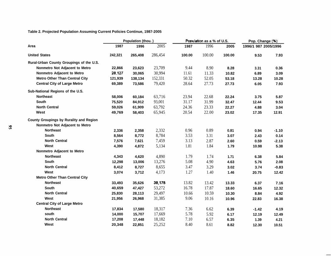
Table 2. Projected Population Assuming Current Policies Continue, 1987-2005

Area

United States

Rural-Urban County Groupings of the U.S.Nonmetro Not Adjacent to MetroNonmetro Adjacent to MetroMetro Other Than Central CityCentral City of Large Metro

Sub-National Regions of the U.S.NortheastSouthNorth CentralWest

County Groupings by Rurality and RegionNonmetro Not Adjacent to Metro

NortheastSouthNorth CentralWest

Nonmetro Adjacent to MetroNortheastSouthNorth CentralWest

Metro Other Than Central CityNortheastSouthNorth CentralWest

Central City of Large MetroNortheastsouthNorth CentralWest

Population (thou. )1987

242,321

22,86628,127

121,93969,389

58,00675,52059,02649,769

2,3368,5647,5764,390

4,34312,2988,4123,074

33,49340,65925,83021,956

17,83414,00017,20820,348

1996

265,408

23,62330,065

138,13473,586

60,18484,91261,90958,403

2,3588,7727,6214,872

4,62013,0068,7273,712

35,62647,42728,11326,968

17,58015,70717,44822,851

2005

286,454

23,70930,994

152,33179,420

63,71693,00163,79265,945

2,3328,7847,4595,134

4,89013,2768,6554,173

38,17853,27229,49731,385

18,31717,66918,18225,252

Pomktion as a % of U.S.1987

100.00

9.4411.6150.3228.64

23.9431.1724.3620.54

0.963.533.131.81

1.795.083.471.27

13.8216.7810.669.06

7.365.787.108.40

1996

100.00

8.9011.3352.0527.73

22.6831.9923.3322.00

0.893.312.871.84

1.744.903.291.40

13.4217.8710.5910.16

6.625.926.578.61

2005

100.00

8.2810.8253.1827.73

22.2432.4722.2723.02

0.813.072.601.79

1.714.633.021.46

13.3318.6010.3010.96

6.396.176.358.82

Pop. Change (OA)1996/1 987 2005/1996

9.53

3.316.89

13.286.05

3.7512.444.88

17.35

0.942.430.59

10.98

6.385.763.74

20.75

6.3716.658.84

22.83

-1.4212.19

1.3912.30

7.93

0.363.09

10.287.93

5.879.533.04

12.91

-1.100.14

-2.135.38

5.842.08

-0.8312.42

7.1612.324.92

16.38

4.1912.494.21

10.51

—

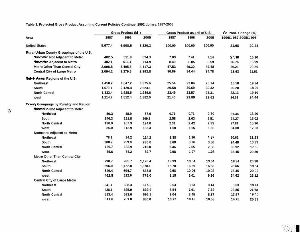
Table 3. Projected Gross Product Assuming Current Policies Continue, 1992 dollars,

Gross Product (bil. )

1987-2005

Gross Product as a % of U.S.Area

United States

Rural-Urban County Groupings of the U.S.Nonmetro Not Adjacent to MetroNonmetro Adjacent to MetroMetro Other Than Central CityCentral City of Large Metro

Sub+atiinal Regions of the U.S.NortheastSouthNorth Centralwest

Co@ Groupings by Rurality and RegionNonmetro Not Adjacent to Metro

NortheastSouthNorth Centralwest

Nonmetro Adjacent to MetroNortheastSouthNorth Centralwest

Metro Other Than Central CityNortheastSouthNorth Centralwest

Central City of Large MetroNortheastSouthNorth Centralwest

1987

5,677.4

402.5482.1

2,698.52,094.2

1,450.21,679.11,333.41,214.7

40.3146.3130.985.0

78.1208.7139.755.6

790.7896.0549.4462.5

541.1428.1513.4611.6

1996

6,908.5

511.9611.1

3,405.82,379.6

1,647.22,120.41,628.51,512.4

48.9181.8167.3113.9

94.2259.8182.974.2

935.71,152.8

694.7622.6

568.3525.9583.6701.8

2005

8,320.3

594.3714.9

4,117.32,893.8

1,975.62,523.11,939.61,882.0

57.9209.1194.0133.3

114.2296.0215.0

89.7

1,126.41,378.1

833.8779.0

677.1639.9696.8880.0

1987

100.00

7.098.49

47.5336.89

25.5429.5823.4921.40

0.712.582.311.50

1.383.682.460.98

13.9315.789.688.15

9.537.549.04

10.77

1996

100.00

7.418.85

49.3034.44

23.8430.6923.5721.89

0.712.632.421.65

1.363.762.651.07

13.5416.6910.069.01

8.237.618.45

10.16

2005

100.00

7.148.59

49.4834.78

23.7430.3223.3122.62

0.702.512.331.60

1.373.562.581.08

13.5416.5610.029.36

8.147.698.37

10.58

Gr. Prod. Change (%)1996/1 987 2005/1 996

21.68

27.1826.7626.2113.63

13.5826.2822.1324.51

21.3424.2727.8134.00

20.6124.4830.9233.45

18.3428.6626.4534,62

5.0322.8513.6714.75

20.44

16.1016.9920.8921.61

19.9418.9919.1024.44

18.4015.0215.9617.03

21.2313.9317.5520.89

20.3819.5420.0225.12

19.1421.6819.4025.39

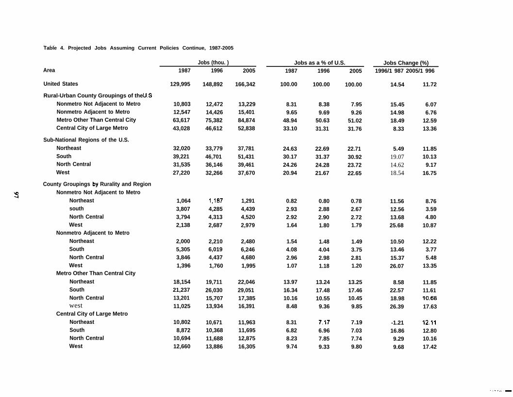
Table 4. Projected Jobs Assuming Current Policies Continue, 1987-2005

Area

United States

Rural-Urban County Groupings of the U.SNonmetro Not Adjacent to MetroNonmetro Adjacent to MetroMetro Other Than Central CityCentral City of Large Metro

Sub-National Regions of the U.S.NortheastSouthNorth CentralWest

County Groupings by Rurality and RegionNonmetro Not Adjacent to Metro

3NortheastsouthNorth CentralWest

Nonmetro Adjacent to MetroNortheastSouthNorth CentralWest

Metro Other Than Central CityNortheastSouthNorth Centralwest

Central City of Large MetroNortheastSouthNorth CentralWest

Jobs (thou. )1987

129,995

10,80312,54763,61743,028

32,02039,22131,53527,220

1,0643,8073,7942,138

2,0005,3053,8461,396

18,15421,23713,20111,025

10,8028,872

10,69412,660

1996

148,892

12,47214,42675,38246,612

33,77946,70136,14632,266

1,1874,2854,3132,687

2,2106,0194,4371,760

19,71126,03015,70713,934

10,67110,36811,68813,886

2005

166,342

13,22915,40184,87452,838

37,78151,43139,46137,670

1,2914,4394,5202,979

2,4806,2464,6801,995

22,04629,05117,38516,391

11,96311,69512,87516,305

Jobs as a % of U.S.1987

100.00

8.319.65

48.9433.10

24.6330.1724.2620.94

0.822.932.921.64

1.544.082.961.07

13.9716.3410.168.48

8.316.828.239.74

1996

100.00

8.389.69

50.6331.31

22.6931.3724.2821.67

0.802.882.901.80

1.484.042.981.18

13.2417.4810.559.36

7.176.967.859.33

2005

100.00

7.959.26

51.0231.76

22.7130.9223.7222.65

0.782.672.721.79

1.493.752.811.20

13.2517.4610.459.85

7.197.037.749.80

Jobs Change (%)1996/1 987 2005/1 996

14.54

15.4514.9818.498.33

5.4919.0714.6218.54

11.5612.5613.6825.68

10.5013.4615.3726.07

8.5822.5718.9826.39

-1.2116.869.299.68

11.72

6.076.76

12.5913.36

11.8510.139.17

16.75

8.763.594.80

10.87

12.223.775.48

13.35

11.8511.6110.6817.63

12. ~112.8010.1617.42

. . . ..-

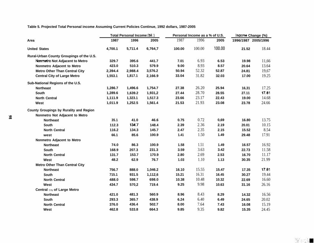
Table 5. Projected Total Personal income Assuming Current Policies Continue, 1992 dollars, 1987-2005

Area

United States

Rural-Urban County Groupings of the U.S.Nonmetro Not Adjacent to MetroNonmetro Adjacent to MetroMetro Other Than Central CityCentral City of Large Metro

Sub-National Regions of the U.S.NortheastSouthNorth CentralWest

County Groupings by Rurality and RegionNonmetro Not Adjacent to Metro

NortheastSouthNorth Centralwest

Nonmetro Adjacent to MetroNortheastSouthNorth CentralWest

Metro Other Than Central CityNortheastSouthNorth CentralWest

Central City of Large MetroNortheastSouthNorth CentralWest

Total Personal Income [bil. )1987 1996 2005

4,700.1

329.7423.0

2,394.41,553.1

1,286.71,289.61,111.91,011.9

35.1112.3116.266.1

74.0168.9131.748.2

756.7715.1488.0434.7

421.0293.3376.0462.8

5,711.4

395.6510.3

2,988.41,817.1

1,496.61,639.21,323.11,252.5

41.0134.7134.385.6

86.3207.3153.762.9

888.0931.5598.7570,2

481.3365.7436.4533.8

6,764,7

441.7579.9

3,576.22,166.9

1,754.71,931,21,517.31,561.4

46.6148.4145.7100.9

100.9231.3170.976.7

1,046.21,112,6

698.0719.4

560.9438.9502.7664.3

Personal Income as a % of U.S.1987

100.00

7.019.00

50.9433.04

27.3827.4423.6621.53

0.752.392.471.41

1.583.592.801.03

16.1015.2110.389.25

8.966.248.009.85

1996

100.00

6.938.93

52.3231.82

26.2028.7023.1721.93

0.722.362.351.50

1.513.632.691.10

15.5516.3110.489.98

8.436.407.649.35

2005

100.00

6.538.57

52.8732.03

25.9428.5522.4323.08

0,692.192.151.49

1.493.422.531.13

15.4716.4510.3210.63

8.296.497.439.82

Inoome Change (%)1996/1987 2005/1996

21.52

19.9820.6424.8117.00

16,3127.1119.0023.78

16.8020.0115.5229.48

16.5722.7316.7030.35

17.3530.2722.6931.16

14.3224.6516.0815.35

18.44

11,6613.6419,6719.25

17.2517.8114.6824.66

13.7510.158.54

17.91

16.9211.5811.1721.99

17.8119.4416.6026.16

16.5620.0215.1924.45

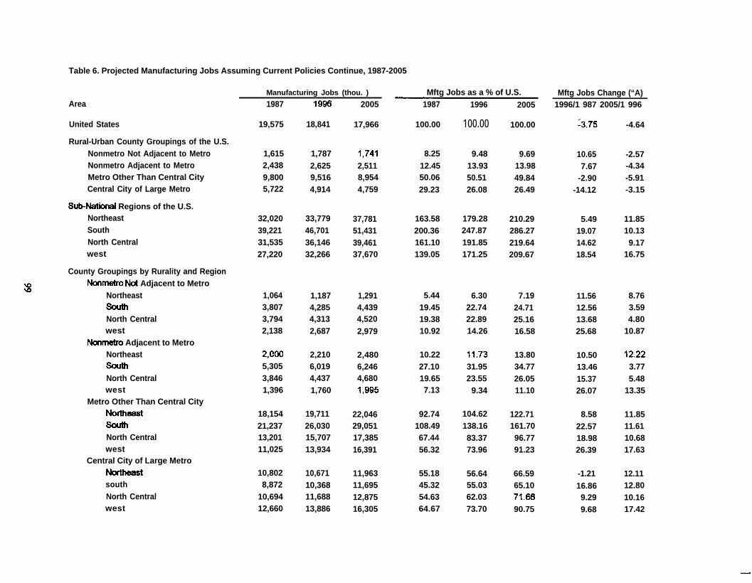
Table 6. Projected Manufacturing Jobs Assuming Current Policies Continue, 1987-2005

Area

United States

Rural-Urban County Groupings of the U.S.Nonmetro Not Adjacent to MetroNonmetro Adjacent to MetroMetro Other Than Central CityCentral City of Large Metro

SuHlatiial Regions of the U.S.NortheastSouthNorth Centralwest

County Groupings by Rurality and Region

w Nonmetro NcX Adjacent to Metrow

Northeast

North Centralwest

Nonmetro Adjacent to MetroNortheast

North Centralwest

Metro Other Than Central CityWheast

North Centralwest

Central City of Large MetroNoftheastsouthNorth Centralwest

Manufacturing Jobs (thou. )

1987

19,575

1,6152,4389,8005,722

32,02039,22131,53527,220

1,0643,8073,7942,138

2,CO05,3053,8461,396

18,15421,23713,20111,025

10,8028,872

10,69412,660

1996

18,841

1,7872,6259,5164,914

33,77946,70136,14632,266

1,1874,2854,3132,687

2,2106,0194,4371,760

19,71126,03015,70713,934

10,67110,36811,68813,886

2005

17,966

1,7412,5118,9544,759

37,78151,43139,46137,670

1,2914,4394,5202,979

2,4806,2464,6801,995

22,04629,05117,38516,391

11,96311,69512,87516,305

Mftg Jobs as a % of U.S.1996 20051987

100.00

8.2512.4550.0629.23

163.58200.36161.10139.05

5.4419.4519.3810.92

10.2227.1019.657.13

92.74108.4967.4456.32

55.1845.3254.6364.67

100.00

9.4813.9350.5126.08

179.28247.87191.85171.25

6.3022.7422.8914.26

11.7331.9523.55

9.34

104.62138.1683.3773.96

56.6455.0362.0373.70

100.00

9.6913.9849.8426.49

210.29286.27219.64209.67

7.1924.7125.1616.58

13.8034.7726.0511.10

122.71161.7096.7791.23

66.5965.1071.6690.75

Mftg Jobs Change (“A)1996/1 987 2005/1 996

10.657.67

-2.90-14.12

5.4919.0714.6218.54

11.5612.5613.6825.68

10.5013.4615.3726.07

8.5822.5718.9826.39

-1.2116.869.299.68

-4.64

-2.57-4.34-5.91-3.15

11.8510.139.17

16.75

8.763.594.80

10.87

A2.223.775.48

13.35

11.8511.6110.6817.63

12.1112.8010.1617.42

—

and thus cannot be analyzed correctly in isolation.Rural and urban are intimately related. Our analyticframeworks and our mental world images shouldreflect this.

Analyses of Alternative Policies

We in RUPRI have not yet applied the currentversion of the models to the analysis of policyalternatives. We are preparing to do a simulation ofMedicare cuts used to lower the federal budget deficitor federal taxes. I am currently studying the degree towhich rural beneficiaries of Medicare purchase theservices of urban health providers. This informationwill bean important input into the appropriate spatialallocation of the direct impacts of Medicare cuts.

At this point we know, as shown in Table 7, thatMedicare payments tend to equal a larger proportionof personal income in rural than urban areas;Medicare payments in Table 7 are allocated to theresidence of the beneficiaries in contrast to thelocation of the provider, These results suggest thatcuts in Medicare projected spending will have greateradverse effixts in rural than urban areas. However,the forces associated with the fti outcome aresufficiently comple~ as outlined in this paper, that theresults of the analysis are not a foregone conclusion.Decision makers need this information. We shouldprovide it to them.

Table 7. Medicare Payments Relative to PersonalIncome, 1993, percent

SubNational Region of the U.S.N.E. South N.C. West Total

NonmetroNot AdjacentA$jacent

MetroNot Cen CityCentral City

Total

3,25 4,05 3,29 2,94 3.533,18 4.04 3.44 2.45 3.423.29 4,05 3,16 3,74 3,61

2.66 2.64 2.34 2.22 2.482,47 2.77 2.27 2.09 2.452.98 2.32 2,43 2,35 2,54

2,71 2.95 2.54 2.30 2.65

References

Adams. John S. “Classi@ing Settled Areas of theUnited States: Conceptual Issues and Proposalsfor New Approaches.” m Metromditan andNonmetrotwlitan Areas: New Amroaches toGewzraphic Definition. Working Paper No. 12,Population Division, U.S. Bureau of the Census,Washington, D, C., September 1995. pp. 9-83.

Braschler, Curtis. Glem Nelson, and Evert Van derSluis. 1995 RUPRI Rural Baseline. Report P95-1,Rural Policy Research Institute, University ofMissouri. April 21, 1995.

Bureau of Economic Analysis, U.S. Department ofCommerce. “Regional Economic InformationSystem, 1969-95.” CD-ROM available fromRegional Economic Information System. BEA.Washington, DC. September 1997.

Congressional Budget ~lce. The Economic andBudget outlook: Fiscal wars 1998-2007. U.S.Government Printing CMce, Washington. DC.January 1997.

Council of Economic Advisers. Economic Reuort ofthe President. U.S. Government Printing OfHce,Washin@on, DC, February 1997.

Day, Jennifer Cheesernan. Population Projections ofthe United States bv ke, Sex. Race. and HisrxmicOrkin: 1995 to 2050. U.S. Bureau of the Census,Current Population Reports, P25-1 130, U.S.Government Printing Oflke. Washington, DC.1996,

Nelson, Glenn, and Curtis Braschler. Nonmetrouolitanand Metropolitan Medicare Enrollments andPavments. Data Report P95-7, Rural PolicyResearch Institute, University of Missouri,September 13, 1995.

Treyz, George 1, Retional Economic Modelimz: ASystematic Awreach to Economic Forecastingand Policv Analvsis. Boston: IUuwer AcademicPublishers, 1993.

Sources: Medicare payments horn OfHce of theActuary, HCFA with fiuther manipulations byRUPRI; personal income horn BEA.

100

TOPICS IN FORECASTING

Chair: Karen S. HamrickEconomic Research Service, U.S. Department of Agriculture

Forecasting Farm Nonreal Estate Loan Rates: The Basis Approach,Ted Covey, Economic Research ServiceU.S. Department of Agriculture

Revising the Producer Prices Paid by Farmers Forecasting System,David Torgerson and John Jinkins, Economic Research ServiceU.S. Department of Agriculture

A Revised Phase Plane Model of the Business Cycle,Foster Morrison and Nancy L. MorrisonTurtle Hollow Associates, Inc.

The Educational Requirements of Jobs: A New way of Looking at Training Needs(Abstract),Darrel Patrick Wash, Bureau of Labor StatisticsU.S. Department of Labor

101

FORECASTING FARM NONREAL ESTATE LOAN RATES:THE BASIS APPROACH

Ted CoveyEconomic Research Service

U.S. Department of Agriculture

“Basis” is the difference between a commodity’s cashprice for immediate local delivery (spot price) and itsnearby fhtures price:

(1) BASIS = SPOT PRICE - FUTURES PRICE

There exist as many bases as there are local cashmarkets for that commodity. Given that Iitures-cashprice relationships change daily, a commodity’s basishas both a regional and temporal aspect, differing withrespect to time and location. The t%tures price is thatcommodity’s nearby fitures price which will expire atleast one month following the month of occurrence ofthe local spot price.

Farmers will use their average basis for a particularperiod to make a forecast of their future basis, called theexpected basis. For example, if the average local basisfor the past three years (1994, 1995, and 1996) for thefirst week in August was 103 cents per bushel, then theexpected basis for the first week of August 1997 for thatlocal cash market is 103 cents per bushel. Methods ofcalculating the average and therefore expected basisvary; and there is no empirically demonstrated superiorapproach.

On the day of the forecast, the farmer uses that day’ssettle fitures price FP for the delivery monthimmediately following the anticipated future marketingmonth and adds his expected basis E(B) to calculate apredicted spot price E(SP):

(2) E(SP) = FP + E(B)

For example, suppose on May 1, 1997, a farmer wishesto forecast his local spot price for corn for the first weekNovember 1997, a possible marketing date. If his pastaverage basis for the first week in November is -7 centsper bushel and the May 1, 1997 corn settle futures pricefor December 1997 delivery is 269 cents per bushel,then his forecasted spot price for the fwst week inNovember 1997 is:

262 cents/bu. = 269 cents/bu. -7 cents/ bu.

This approach has been advocated and extensively usedto forecast agricultural product prices (Peck; Hauser etal.; Irwin et al.; Liu et al; Howard; McDonald and Hein;Kamara; Fama and French; French).

This paper will evaluate whether this approach may beusefid in forecasting the price of debt in agriculturalcredit markets.

MethodUsing the basis forecast approach developed incommodity markets as an analogy, the equation forforecasting interest rates on farm loans is:

(3) E(LR) = FY + E(B)

or the expected farm loan rate E(LR) is equal to theyield calculated from the nearby interest rate futuresprice FY plus the expected nearby basis E(B).

Data for spot prices will consist of quarterly averageeffective interest rates on new nonreal estate farm loans(all loans) made by commercial agricultural banks.Agricultural banks are those that have a proportion offarm loans (both real plus nonreal estate) to total loansthat is greater than the unweighed average of allcommercial banks (usually around 16Yo) from 1977-1994. These rates are taken born a quarterly surveyconducted by the Federal Reserve on the first full weekof the second month of each quarter.

The nearby futures price consists of the expected yieldcalculated from the settle price for the U.S. T-billfutures contract (International Monetary Market of theChicago Mercantile Exchange) for delivery in themonth following the month of the Fed’s farm loan ratesurvey. This settle futures price and yield is based onthe average settle futures price for the 5 days of the firstfull week of the second month of each quarter,concurrent with the Fed’s survey. For a simple exampleof the method of calculating the expected futures yieldFY see Chance pp. 302-304.

A basis series for each quarter is calculated bysubtracting the interest rate on nonreal estate loans for aparticular quarter from the expected futures yield

103

.-.

calculated for that quarter. The historical basis series isthen used to calculate an average and therefore expectedbasis E(B) series.

Two methods of calculating the average basis will beused; each generating a different expected basis andtherefore a different expected loan rate. The firstapproach will calculate the expected basis as an averageof the four bases for the four quarters previous to theforecasted quarter. For example, the average of thebases of the four quarters for 1990 is used as theexpected basis for the first quarter of 1991.

The second approach uses last year’s actual or realizedbasis for the same quarter as the expected basis for thatquarter this year. For example, the basis observed in thefirst quarter of 1990 is the expected basis for the firstquarter of 1991.

These two approaches are based on commonly usedmethods of calculating an expected basis in agriculturalcommodity markets.

As an example of calculating an expected loan rateE(LR) for the next quarter, assume it is the third weekin October 1994 and the frost approach is used tocalculate an expected basis E(B). If in the fourthquarter of 1994 the average of the last 4 quarters’ (i.e.all 4 quarters of 1994) bases is 2.85’%0 (= E(B)) and thesettle fhture price on that day for March 1995 T-billsgives a yield of 5.75% (= FY), then that day’ forecastfor the 1995 first quarter loan rate E(LR) is:

8.6%= 5.75% i- 2.85%

The two different approaches to calculating an expectedbasis allowing testing two different fbtures or basisforecasting models. The forecasts generated by thesetwo basis models (BAVG and BLAG) will be contrastedto forecasts issued by: 1) NAIVE: a naive model wherenext quarter’s loan rate is the same as this quarter’s; 2)TREND: a “trend is your friend” model where nextquarter’s loan rate is equal to this quarter’s loan rateplus the change between this quarter and last quarter;and 3) COMP: a composite model with it’s forecastsgenerated as an unweighed average of the forecasts ofthe four other models.

whether futures can contribute to price discovery infarm loan markets.

A total of 68 out-of-sample forecasts will be issued byeach of the 5 forecast models starting with the firstquarter of 1978 through the fourth quarter of 1994.

Forecast accuracy will be evaluated by standardstatistical methods: root mean squared error (rinse),mean absolute error (mae), mean absolute percentageerror (mape), mean forecast error (mfe), and the rangeof the forecast error of each model (range).

ResultsTable 1 shows the rankings of the 5 different modelsbased on the different statistical results calculated usingthe 68 out-of-sample forecasts generated by each modelfor the period 1978:1-1994:4.

The BAVG model (the model which used a movingaverage of the past four quarterly bases as the expectedbasis) issued the “best” forecasts based on three of thefive forecast criteria: range, rinse, and mape. TheTREND model placed fmt in mfe, and the compositemodel placed first on the basis of mae.

With all 5 forecast criteria are considered together(averaged and assigned equal weights), COMP issuesthe best forecasts, while the best-performing fi.duresmodel BAVG still outperforms the best performingnonfbtures model NAIVE.

ConclusionsThe superior forecast performance of the model relyingon fitures information BAVG over the best forecastmodel relying solely on information in cash pricesNAIVE suggest that fbtures plays a price discovery rolein farm loan markets.

Future research should consider the role of interest rateexpectations in affecting farmer financial decision-making, the costs to fmers of forecast error, and howforecasts relying on fhtures might reduce those costs bygenerating better-informed credit decisions.

The NAIVE and TREND models rely solely oninformation contained in cash prices. The two basismodels rely on the relationship between the cash andfutures market. Comparing the forecast errors betweenthe cash only (NAIVE and TREND) vs. cash andfhtures (BLAG and BAVG) models allows a test of

104

References Tablel. Rankings of Forecast Models

Chance, Don M. An Introduction to Options & Futures.2nd ed. The Dryden Press. Harcourt Brace JovanovichPublishers; New York; 1992.

Fama, Eugene F. and K. R. French. CommodityFutures Prices: some evidence on forecast power,premiums, and’the theory of storage. Journal ofBusiness 60(1987):55-73.

French, K. R. Detecting Spot Price Forecasts in FuturesPrices. Journal of Business 60(1987):S39-S54.

Hauser R. J., et al. Basis Expectations and SoybeanHedging Effectiveness. North Central Journal ofAgricultural Economics. 12( 1990): 125-36.

Howard, C. T. “Are T-bill Futures Good Forecasters ofInterest Rates? The Journal of Futures Markets1(1982):305-15.

Irwin, S. et ali. The Forecast Performance of LivestockFutures Prices: a comparison of USDA expertpredictions. The Journal of Futures Markets.14(1994):861-75.

Kamara, A. Forecasting Accuracy and theDevelopment of a Financial Market: the T-bill fhturesmarket. The Journal of Futures Markets10(1 990):397-405.

Lui, Shi-Miin; et al. Forecasting the Nearby Basis ofLive Cattle. The Journal of Futures Markets14(1994):259-74.

McDonald, Scott and S. Hein. Futures Rates andForward Rates on Prediction of Near-term T-bill Rates.The Journal of Futures Markets 9(1989):249-62.

ModelsNAIVE TREND BAVG BLAG COMP

Criteria:

range 2 5 1 4 3

rrnse 3 5 1 4 2

mfe 4 1 5 3 2

mae 2 4 3 5 1

mape 3 4 1 5 2

overall 3 4 2 5 1

The “overall” criteria is based on the average of theother 5 criteria, each weighted equally. The numbers1-5 ranks each model on its forecast error relative to theother 5 models under a particular forecast error criteria.A” 1” indicates the smallest forecast error, a “5”indicates the largest forecast error.

Peck, Anne. Hedging and Income Stability.American Journal of Agricultural Economics57(1975):410-19.

105

m$.

. . .

REVISING THE PRODUCER PRICES PAID BY FARMERS FORECASTING SYSTEM

David Torgerson and John Jinkins, Economic Research Service/USDA

Summary

The prices paid by farmers ten-year-ahead projectionequations had last been estimated in the early 1990s.The Economic Research Service (ERS) revised thissystem using expert judgment and regression. Wedescribe how the revision was done, focusing on thefertilizer and fuel price equations. The revisedfertilizer price and he] price equations are superior, inforecast accuracy, to the associated ARIMA(autoregressive integrated moving average) and the oldequation. For fuel prices, the superiority of the newregression equation to the optimal ARIMA evaporatesat the end of the out-of-sample forecasting period.

Introduction

The aggregate prices paid by farmers index and itssubindices are forecast by the ERS of USDA as part ofthe ten-year-ahead President’s Budget baselineforecasting process. The index is constructed like theBureau of Labor Statistics (BLS) producer price index(for the items used in farm production.) In particular,the prices paid by farmers subindices are used inforecasting farm production expenses. The NationalAgricultural Statistical Service (NASS) of USDA, theagency which produces the historical values for theseindices, reformulated most of the subindices whenchanging the benchmark year to 1992 from 1977. Forexample, some of the prices which had been takenfrom the NASS survey of farmers for AgriculturalPrices were instead taken from BLS’S PPI price series.As a result of the rebenchmarking and the change inestimation procedure, the statistical properties of theprices paid by farmers (PPF) subindices changeddrastically. For this reason, ERS reestimated the pricespaid forecasting equations of the 16 sub-components ofthe index of prices paid by farmers. We describe theequation revision, focusing on the prices paid forfertilizer (PPFERT) and the prices paid for fuel(PPFUEL) forecast equations.

The criteria for the new forecasting equations were:

(1) the exogenous variables had to be available fromthe USDA baseline process, the forecasting activity towhich the new equations were to be added.

(2) the equations should pass the phone call (PC) testfor reasonable structure. As forecasts are inevitably inerror, it is desirable to easily explain those errors interms of changes in variables apparently tied to therelevant farmers prices paid index when the phone callscome. The economics consistent with the equationshad to be simple and transparent.

(3) as a Government agency forecast simplicity andtransparency of methodology were important.

(4) the forecasting equations should produce forecastssuperior to those obtained from a simple ARIMAmodel.

(5) the equations had to be operational for the summer1997 baseline and documented in the June 1997 issueof the Agricultural Inputs and Finance Situation andOutlook Report.

To meet these objectives John Jinkins of the RuralEconomy Division (RED) of ERS created a committeeincluding representatives from NASS and the parts ofERS involved in the budget baseline process.Committee members Jinkins and Torgerson estimatedthe new equations. At each committee meeting three tofive equations were reviewed and critiqued. As a resultof committee discussion, some equations were again re-estimated.

To fulfill criteria 1 to 3, and recognizing that therevised price index data were limited to annual seriesfrom 1974 to 1995, it was decided that all the newequations were to be linear, log-linear or in percentagechange. C.W.J. Granger and Paul Newbold inForecasting Economic Time Series (GN) criticized theuse of linear regressions for forecasting because of theproblem of spurious correlation. A regression equationcould show a good in-sample fit as measured by R*,and perform miserably in out-of-sample forecasting.

107

The example GN presented was aregression of onerandom walk on another random walk resulting in goodin-sample R2 but a poor forecasting petiormance out-of-sample. We guard against this problem by the PCcriteria and the use of out-of-sample testing. Equationswhich contain variables related by economic theoryappear to be somewhat resistant to the spuriouscorrelation problem. Table 1 presents the functionalform of all the resulting forecasting equations.

To illustrate the forecast reestimation we review thedevelopment of two of the more important forecastingequations. As data revisions had only been back to1974, we backcasted using the percent change in theold indices back to 1970. We then estimated theequations over 1970-1990 to reserve the 1991 to 1996observations for out-of-sample testing. (For the fuelprice equation, the 1988 to 1996 period was reservedfor out-of-sample testing to mitigate the problemsrelated to the volatile oil market of 1990 and 1991.The panel thought it unlikely that the next twenty yearswould have three oil supply shocks.) The old set ofequations, estimated in the early 1990s, was the secondbenchmark. Those equations, given the large datarevisions for many of the price subindices, had to berevised to maintain forecast credibility.

There are three types of prices paid by farmersequations: (1) prices determined by farm sector supplyand demand (2) prices determined by demand from thefarm sector and supply from the general economy and(3) prices determined by the general economy. The oldfeed price paid equation, is close to an accountingidentity, given the abundance of commodity price dataforecasted in the budget baseline. With the major feedingredient prices as explanatory variables, the equationerror term reflects markup changes and other randomshocks which would not be easily improved upon. Forthe feed price equation it was only necessary to re-estimated the old equation with new data as theforecasts based on actual grain prices were excellent.

Other prices, such as the fertilizer prices paid index(PPFERT) reflect an interplay of the farm sector andoverall economy. Fertilizer prices are demand drivenby farm commodity prices, acreage decisions, and otherspecifically agricultural variables. The supply side isstrongly influenced by the price of energy, as naturalgas is the largest variable cost in producing ammonia-based fertilizers. We examine this equation in detail.

There is a widespread recognition of macro-prices,prices which agriculture is subject to but aredetermined by economy-wide forces. Using less than

3 percent of total liquid fiels, U.S. farming has smallinfluence on liquid fbel prices. The fiel prices paid byfmers index (PPFUEL) is the macro-price examinedin detail.

Modus Operandi

We present the results of our search for “good”forecasting equations for fertilizer and fuel prices intable 2 and figure 1, and table 3 and figure 2,respectively. Each forecast equation developmentstarted with estimation of an autoregressive movingaverage (ARMA) model of the specific prices paidsubindex. The dependent variable is the level of thevariable in question. The independent variables can bethought of as lags of the variable reflected in themoving average (MA) terms; the correlations of thedependent variable with itself across time periods arereflected in the autoregressive (AR) terms. Amaximum likelihood estimation is done to computethese estimates. For a sample this small (21observations), only fmt and second order MA and ARterms were estimated. Any standard econometricspackage such as SAS or EVIEWS can be used toestimate AR and MA coefficients and select theoptimal orders for the AR and MA, concomitantly.

The problem with the above procedure is thateconomic variables seldom pass the statistical tests forstationarity as required for the optimality of the ARMAestimator. The first assumption for stationarity to holdis that the mean of the variable, say the fertilizer priceindex, is constant. The second stationarity assumptionis that the covariance between fertilizer prices invarious periods depends only on the differencesbetween the time periods. Most of the indices of pricespaid by farmers are not stationary as measured bystandard statistical tests.

The standard operating procedure is to difference avariable until the transformed (difference) variablepasses the standard stationarity test--the augmentedDickey-Fuller test (DFT). Seldom do economicvariables need to be difference more then twice toattain stationarity, Why do an ARMA as the DFT onundifferenced data are very likely to reject stationarityand an ARMA model which incorrectly assumedstationarity would generally do quite poorly inforecasting, with rapidly increasing forecast exror as theforecast period lengthened? The DFT for stationarityis not a very powerful test so that it will “often” rejecta series which is actually stationary, Further, theARMA estimation process will be an independent testfor some kinds of nonstationarity, Finally, running an

108

ARMA is easier than running a regression and oftengives some insight into the process which generated thedata. We refer to the estimation of ARMA on levels ofa variable explained as naive ARMA. All the orders ofintegration were determined by DFTs.

The next step - was to estimate an ARMA on theintegrated series. For both fuel and fertilizer prices,differencing once made the series stationary. Thedifference between the current fertilizer price paid andthe previous price paid is the appropriate variable forARMA estimation. We will refer to this as the ARIMAmodel of fertilizer prices--as the once differencefertilizer price is consistent with stationarity. To get anactual forecast, one simply adds the ARIMA estimateddifference to the series value in the previous period.

To give the old forecasting equation a fair chance, weestimated the reduced form with the same variables andfunctional form as the old forecasting equation usingnew data. We label this oldhew in tables 2 and 3below.

The new specification of the forecasting equations wasdeveloped by committee. The small amounts of data,the desire to be understandable, and time constraintsprevented any use of sophisticated techniques. Theshortage of data was the binding constraint. (Thecutting room floor models which were rejected for verybad Durbin-Watson statistics and bad forecastingperformances are not included here.)

We should point out that none of these regressionmodels was the explicit result of taking structural formmodels of supply and demand and solving themexplicitly for a specific reduced form. [n using theterm structural models we simply mean regressionequations with variables which are apparently relatedto the prices paid index.

And of course, the out-of-sample model forecastperformance is important in sorting the wheat from thechaff. A major contribution of the time series literatureis emphasizing out-of-sample forecasting as a way tovalidate economic models. Many would go evenfurther and say that if a model does not forecast wellout-of-sample it is not a valid reflection of reality.

Fertilizer Prices Paid Forecast Equation

PPFERT is the variable forecasted. Table 2 reports thestandard statistics for each competing forecastingequation. Greater detail is available in tables 2athrough 2h, available from the authors on request.

Figure 1 graphically depicts the competing forecastequations. A result of the DFTs is that the regressionequations were not balanced in the sense of allvariables in the regression equation having the sameorder of integration. In particular, the crude oil price(RAC) in the new regression equation(PPFERTFNEW) is integrated of degree 2. That is, theWC has to be difference and that result differenceagain to be consistent with stationarity, as tested by theDFT. The standard t-tests implicitly assume both thedependent and independent variables are integrated ofthe same order. In this case they are not, sincePPFERT is integrated of degree one. So one can get aspurious correlation problem by including variables notrelated to the forecasted variable in the forecastingequation even though the t-test says they are related.That is why GN note that having variables of differentorders within a regression equation makes for potentialproblems for use in out-of-sample forecasting.

The use of out-of-sample forecasting should mitigatethe potential problem of an equation with a good in-sample fit producing a bad forecast.

The ARMA (PPFERTFARMA) summary statisticsverifi the results of DFT for PPFERT. Indeed not onlyis the price index not stationary but the estimated ARcoefficient is slightly above one, indicating unstablebehavior, likely that of a random walk. Note that themseout is larger for the old forecast equation estimatedwith the new data (labeled oldhew in Table 2 withequation name PPFERTFOLD in Figure 1) than forPPFERTFARMA. The old/old regression had a nonsignificant constant while big8acres (the sum of theacreage of the eight highest acreage planted crops) isclose to significant. The old equation with new datahad the situations reversed. The instability inherent insuch drastic changes in which variables are apparentlysignificant greatly detracts from the confidence oneplaces in either equation and may well reflect aspurious conflation problem. The evidence against theoldhew formulation is overwhelming when the mseoutis sharply in favor of the naive ARMA and the basiccoefficients are unstable. Further, the laggeddependent variable (PPFERT(- 1 )) tends to bias the DWupward as well as make for more potential out-of-sample forecast error. Getting rid of lagged dependentvariables was a major operational goal of updating theforecasting equations. The old fertilizer price equationwith new data performed very poorly in terms of R2 ifPPFERT(- 1 ) (the actual fertilizer index lagged oneperiod) was omitted, revealing that an equationrestructuring necessary.

109

On several grounds then, the competition is betweenthe new regression equation (PPFERTFNEW) and thefirst difference ARIMA formulation(PPFERTARIMA). The big8acre and the constantwere insignificant in an equation with the average ofthe current market year and prior market year price ofcom averaged (avg(compr& compr(- 1 )). (This gives aflavor of forecasting with expected values sincefertilizer is purchased prior to the marketing year cornprice being determined. It is not fi.dly consitent withusing expectations in a more rigorous sense since theexpected com price is not determined endogenously inthe estimated model.) And the crude oil price (RAC)was significant with those variables while the log of thereal crude oil price term was not. So the RAC andaverage com price, over the current and priormarketing year, were the first two variables selected forthe new forecasting equation.

In the committee discussions of the above preliminaryversion of the new forecasting equation, it was pointedout that there had been an improvement in fertilizerinput quality over time. Further, it was noted at thetime most fertilizer was purchased the average comprice for the current marketing year was not known.

We dealt with the fertilizer quality improvement byadding a simple time trend which proved superior interms of out-of-sample forecasting to using any of thestandard inflation variables. This change also made theR* comparable to the old equation’s R*. The final formof the new regression equation then had the currentcrude oil price, the average of the expected com priceand the previous marketing year com price, and a timetrend. Since com prices are forecast in the baseline, theforecasted com price was used in the actual fertilizerprice forecasts. The superior mseout of the newstructural equation is tabulated in Table 2 and showngraphically as PPFERTFNEW in Figure 1. Eitherrepresentation dramatically demonstrates the strikingforecasting superiority of the new equation relative tothe other candidates.

Since the mseout of an equation difference is notcomparable with a level equation, it is necessary tolook at the actual out-of-sample forecast to determinewhich fommlation is superior in forecasting. Figure 1graphically shows the clear superiority of the newstructural equation over even the best ARIMA. Themoral of this story is that a good structural equationbeats an ARIMA. (But a bad structural equation can beworse than a naive ARMA as the above comparison ofPPFERTFARMA and PPFERTFOLD seen in Figure 1clearly demonstrate.)

Farm Fuel Prices Paid Index Forecast

PPFUEL is the variable to be forecasted. Table 3summarizes the standard statistics for alternativeforecasting equations. More detail is in tables 3athrough 3h, available from the authors on request.Figure 2 graphically depicts the comparative forecasts.As above, all variables in the structural equations donot have the same order of integration. Again, thecrude oil price (RAC) and price paid by farmers forfuel (PPFUEL) are integrated of degree 2 and 1respectively. The lack of order consistency ofdependent and independent variables could mean poorout-of-sample forecasting for both the old and newregression equations.

The ARMA (PPFUELFARMA) supports the results ofDFT for the fuel price index. The fuel price index isnot stationary and the estimated AR coefficient isabove one, indicating explosively unstable behavior,likely a random walk. Note that the mean-squarederror in the out of forecast period (mseout) for theARMA is larger than that statistic for the old forecastequation estimated with the new data (labeled old/new).The old/old regression had decent t-statistics for allcoefilcients. The old forecast structure for fuel pricesmay be superior in forecasting to the naive ARMA insharp contrast to the fertilizer price situation. Figure 2indicates both the old equation with new data(PPFUELFOLD) and the ARMA are quite badforecasting models relative to the ARIMA or the newregression model. Further, the farmers prices paid fuelindex lagged one year (PPFUEL1(- 1 )) tends to bias theDurbin-Watson upward. Yet even so the measuredDurbin-Watson is smaller than the R2. This stronglysuggests out-of-sample forecasting problems. As in thecase of the fertilizer price forecast equation, finding areplacement for the lagged dependent variable was amajor goal. (Some analysts would have appropriatelyused the Durbin h test in the presence of laggeddependent variables to test for first orderautocorrelation. We chose not to since we were gettingrid of lagged endogenous variables anyway.Forecasting out ten years with lagged dependentvariables is problematic at best and we did not expectto have any final equation with lagged endogenousvariables. )

In summary, ARMA (PPFUELFAIUVL4) is bad and theoldhew equation (PPFUELFOLD) is only marginallybetter in a forecasting sense. This reflects the typicalsituation in attempting to forecast a number of yearsout using with ARMAs on undifferenced data andregression equations with lagged dependent variables.

110

F--

The new equation reported in Table 3 and depicted inFigure 2 as PPFUELFNEW is not the first newequation. Having PPFUEL as a function of RAC andPPI lagged one period for 1970 to 1990 had R2 go upmarginally compared to the old equation’s R2. But thelagged endogenous variable is no longer needed andthe Durbin-Watson has improved. Further, without thelagged endogenous variable, the Durbin-Watson is avalid test for serial correlation. Still the Durbin-Watson was smaller than the R2, making forecastingproblematic as this equation fits the typical spuriouscorrelation pattern detailed in GN. To mitigate this andthe problem of the unstable oil market during 1990 and1991 we shortened the estimation period to 1970-1987,and reserved a larger out-of-sample period (1988 to1996) to test the reestimated equation.

The in-sample problems remain. The Durbin-Watsonis smaller than the R2. But the coefficients of RAC andPP1(- 1 ) continue to be significant and the mseout isnoticeably lower than the ARIMA.

In some sense, the structural fuel price forecastingequation is more satisfactory than analogous fuel priceequation. Again, the crude oil price (RAC) replaces thenatural log of the real crude oil price. The PPI laggedone year (PPI(- 1 )) is superior to a time trend inprojecting the tendency of fuel prices to rise over time.The use of the PPI makes it far easier to interpret thefuel price equation than a time trend does, as priorinflation is a partial explanation of higher fuel pricestoday.

The ARIMA model of the first difference of the fuelprice is an improvement over the naive ARMA. Again,the gain is not as dramatic as in the case of fertilizerprices. Neither the AR nor MA terms are statisticallysignificant. This is not crucial, as t-statistics are not asdefinitive in an ARIMA context as they are in theregression framework.

The new regression equation and the first differenceARIMA formulation are again the apparentcompetitors. Since the mseout of an equationdifference is not comparable with a level equation oneneeds to look at the actual forecasts to see whether thenew equation or the ARIMA is superior in forecasting.Figure 2 reflects a better out-of-sample forecastingrecord for the improved structural fuel price equation(PPFUELFNEW) r e l a t i v e t o t h e ARIMA(PPFUELFARIMA). Note the forecast superiority islost at the end of the forecast period, 1994-1996.

Nevertheless, because of simplicity, interpretability,and overall forecast superiority the new structuralequation is the best choice, despite the marginalforecast victory. Using criteria 1 to 3 the margin ofvictory of the new fiel price structural model over theARIMA is larger than in the fertilizer price situation.

Implications

With some effort, it is possible to beat ARIMA inforecasting. When human capital is lost it sometimesis possible to partly recover by taking a fresh look atthe data and in a fairly economical fashion use expertjudgment in the formulation of the equations instead ofthe forecasting process directly. The involvement ofthe producers of the prices paid indices and as well asthe users of the prices paid index forecasts made theequation revision process feasible.

111

m--

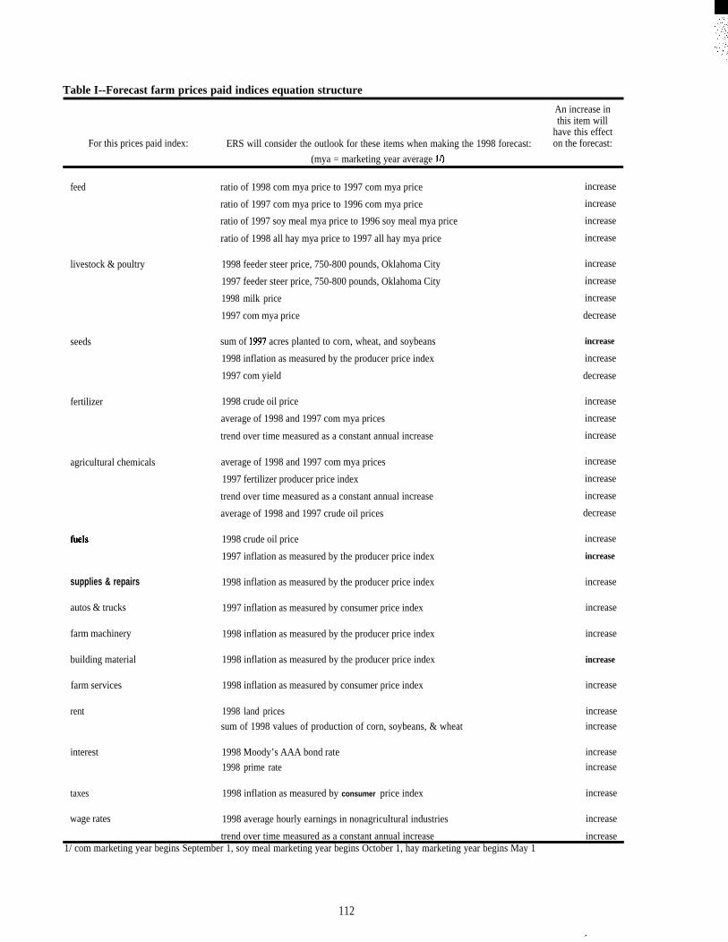
Table I--Forecast farm prices paid indices equation structure

An increase inthis item will

have this effectFor this prices paid index: ERS will consider the outlook for these items when making the 1998 forecast: on the forecast:

(mya = marketing year average 1/)

feed ratio of 1998 com mya price to 1997 com mya price increase

ratio of 1997 com mya price to 1996 com mya price increase

ratio of 1997 soy meal mya price to 1996 soy meal mya price increase

ratio of 1998 all hay mya price to 1997 all hay mya price increase

livestock & poultry

seeds

fertilizer

agricultural chemicals

fbels

supplies & repairs

autos & trucks

farm machinery

building material

farm services

rent

interest

1998 feeder steer price, 750-800 pounds, Oklahoma City increase

1997 feeder steer price, 750-800 pounds, Oklahoma City increase

1998 milk price increase

1997 com mya price decrease

sum of 1997 acres planted to corn, wheat, and soybeans increase

1998 inflation as measured by the producer price index increase

1997 com yield decrease

1998 crude oil price increase

average of 1998 and 1997 com mya prices increase

trend over time measured as a constant annual increase increase

average of 1998 and 1997 com mya prices increase

1997 fertilizer producer price index increase

trend over time measured as a constant annual increase increase

average of 1998 and 1997 crude oil prices decrease

1998 crude oil price increase

1997 inflation as measured by the producer price index increase

1998 inflation as measured by the producer price index increase

1997 inflation as measured by consumer price index increase

1998 inflation as measured by the producer price index increase

1998 inflation as measured by the producer price index increase

1998 inflation as measured by consumer price index increase

1998 land prices increase

sum of 1998 values of production of corn, soybeans, & wheat increase

1998 Moody’s AAA bond rate

1998 prime rate

increase

increase

taxes 1998 inflation as measured by consumer price index increase

wage rates 1998 average hourly earnings in nonagricultural industries increase

trend over time measured as a constant annual increase increase1/ com marketing year begins September 1, soy meal marketing year begins October 1, hay marketing year begins May 1

112

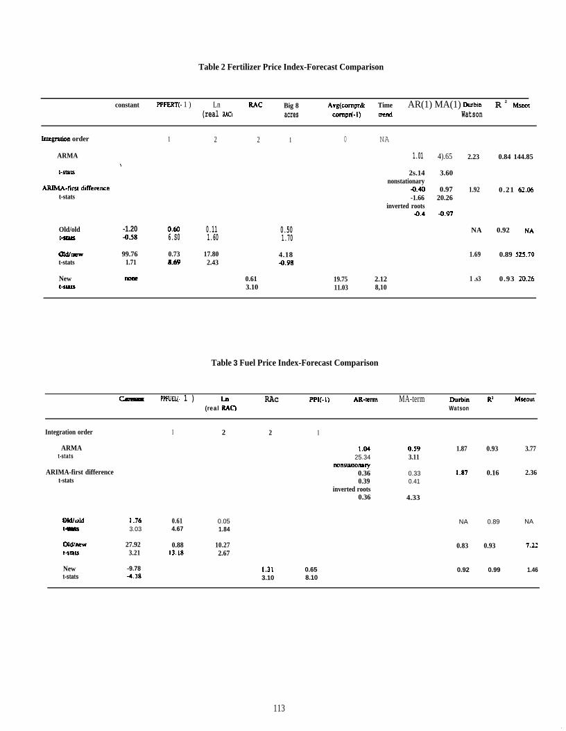
Table 2 Fertilizer Price Index-Forecast Comparison

constant PPFERT(- 1 ) Ln RAc Big 8 Avg(compr& Time AR(1) MA(1) Durbm R 2 Mseot(real WC) acres Compr(-1) uend Watson

Intcgtation order

ARMA

t-smts

ARIMA-fkst differcnset-stats

Old/oldC=

awmwt-stats

Newt-stata

1 2

-1.20 O.a 0.11-0.38 6.S0 1.60

99.76 0.73 17.801.71 8.tw 2.43

2

nom 0.613.10

1 0 NA

1.01 4).65

2s.14 3.60nonstationary

43.40 0.97-1.66 20.26

inverted roots4.4 4.97

0.501.70

4.1843.98

19.75 2.1211.03 8,10

2.23 0.84 144.85

1.92 0.21 6?.06

NA 0.92 NA

1.69 0.89 S25.79

1 .s3 0.93 20.26

Table 3 Fuel Price Index-Forecast Comparison

PPFUEL(- 1 ) In RAc PP1(-1) AR-tmn MA-term Durbin R2 Mseout(real RAc) Watson

Integration order 1 2 2 1

ARMAt-stats

ARIMA-first differencet-stats

1.0425.34

tUXIStXION~0.360.39

inverted roots0.36

0.593.11

0.330.41

4.33

1.87 0.93 3.77

1.87 0.16 2.36

Okkld J .?$ 0.61 0.05 NA 0.89 NAt- 3.03 4.67 1.84

C31dhww 27.92 0.88 10.27 0.83 0.93 7.~~HnLs 3.21 13.18 2.67

New -9.78 1.3i 0.65 0.92 0.99 1.46t-stats 4.38 3.10 8.10

113

. ..

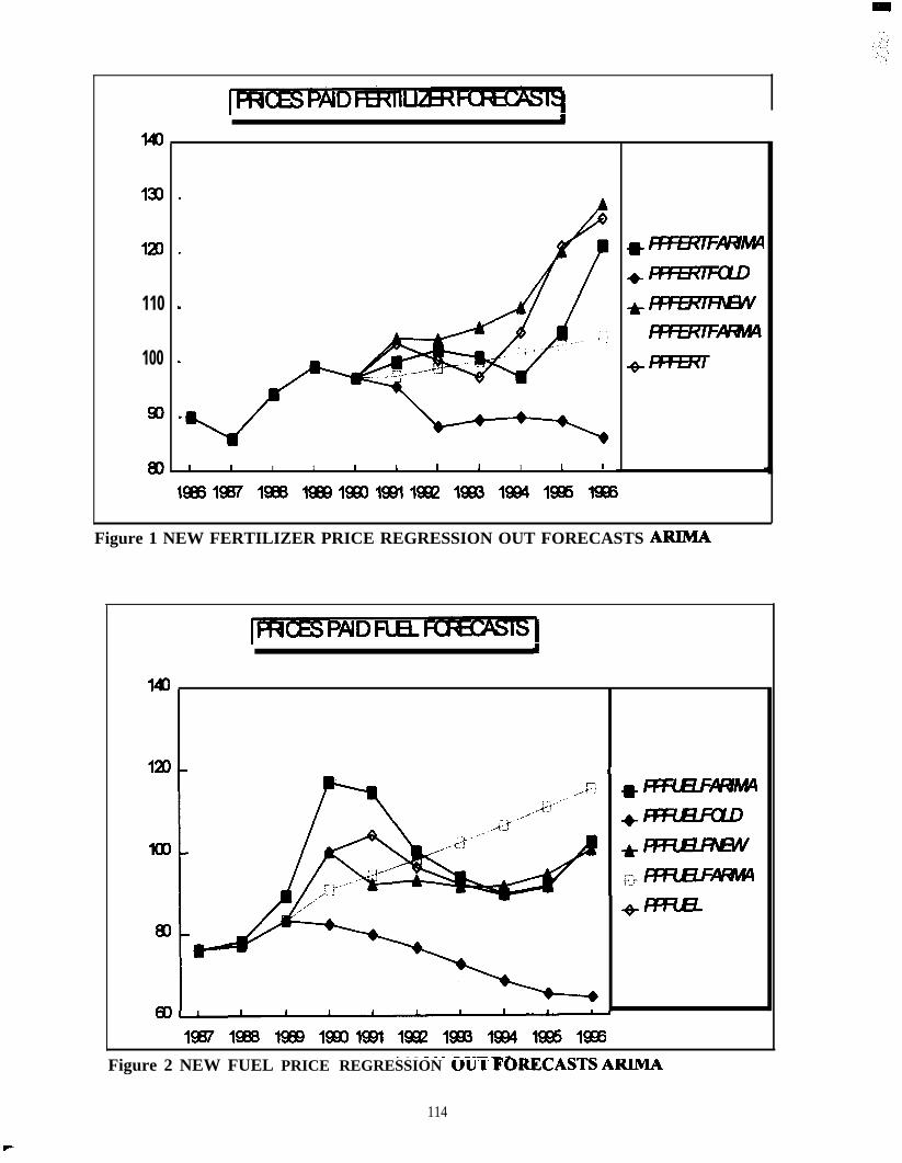
‘MO

130

120

110

100

90

00

.

.

.

.

1 I I 1 1 1 I 1 1 t I

wu?’7uwM4

Rm?lwww/

1W6 1907 1968 lW 1s0 ml wm 19m 19e4 1s6 19e6

Figure 1 NEW FERTILIZER PRICE REGRESSION OUT FORECASTS ARIMA

140

120

100

m

60

E=- 1

. . , , , n 1 . .

* #uiEuiiAM+Iu=LemD#uLEmEw++ m%Emww4

1987 1968 19e9 1s0 lsl 19W mm 1s4 1s 19e6—— ———— —--— ..— — . — — —

Figure 2 NEW FUEL PRICE REGRESSION OU-l JKM?.ECASTS ARIMA

114

F-

A REVISED PHASE PLANE MODEL OF THE BUSINESS CYCLE

Foster Morrison & Nancy L. MorrisonT u r t l e HO11OW A s s o c i a t e s , I n c .

PO BOX 3639Gaithersburg, MD 20885-3639

Phone: 301-762-5652Fax: 301-762-2044

email : 71054. 1061@compuserve .com

1. MACROECONOMIC FORECASTING

The overwhe lming major i ty o f macro-e c o n o m i c d a t a series a re p roduced byf e d e r a l a g e n c i e s , mos t ly o n e s i nUSDOC ( U . S . Department of Commerce)and in the Depar tment o f Labor . Al 1macroeconomic fo recas te r s , whe ther ing o v e r n m e n t , academe, or the private

s e c t o r , a r e highly d e p e n d e n t u p o nt h e s e d a t a s e r i e s .

ln 1995 USDOC began a process of pri-vati.zing production of the indices ofleading, coincident, and lagging in-dicators. Changes resulting fromthis action did provide additionalverification of the robustness of amodel based on these indices, butthey also raised serious questionsabout the difficulties individualsand small organizations will have inaccessing this data economically andin a timely manner.

2. WHAT ARE BUSINESS CYCLES?

An awareness of cycles other than thedaily alternation Of night and dayand t h e a n n u a l p r o g r e s s i o n o f thes e a s o n s h a s e x i s t e d t h r o u g h o u t h i s -t o r y . T h e biblical s t o r y o f J o s e p h ,which s t r a d d l e s G e n e s i s a n d E x o d u s ,is one example [Genes i s 4 1 , 42 , 47 ;Exodus 1$ 13; Anderson, 1966].

By interpreting the dreams of Pharaohto mean that 7 years of abundant har-vests would be followed by 7 years offamine conditions, Joseph warned theEgyptians to store enough grain from

t he good yea r s to cover the shor t f a l lin t h e b a d o n e s . Biblical s c h o l a r sp lace t h e time f r a m e a t a b o u t 1635BCE, bu t the re a re no suppor t ing ma-t e r i a l s i.n any known Egyptiansources . Even so , the s to ry demon-s t r a t e s a n e a r l y a w a r e n e s s o f cli-matic cycles ‘and how these can affectthe economy and poli t ics .

Joseph rose t o high positions in t h eE g y p t i a n g o v e r n m e n t , b u t his p o l i t i -ca l ca ree r came to an abrup t end wi ththe reign of a new Pharaoh . Eventu-ally the Hebrews departed from Egypt,bear ing t h e b o n e s o f Joseph withthem. This shows how changing polit-ical a n d s o c i a l c o n d i t i o n s c a n a l t e rt h e s i t u a t i o n o f f e d e r a l f o r e c a s t e r s .Recent changes have not been so dras-tic, b u t t h e r e a r e n u m e r o u s c h a l -lenges f o r f o r e c a s t e r s , w h e t h e r inthe government o r n o t , w h o u s e f e d -e r a l d a t a a n d s e r v i c e s .

Co l l ec t ion o f de ta i l ed macroeconomicd a t a did n o t begin in t h e UnitedS t a t e s u n t i l a f t e r W o r l d W a r 1 1 .T h i s , however, h a d n o t p r e v e n t e d t h elaunching of economics as an academicdiscipline, b e g i n n i n g with t h e w o r kof Adam Smith (1723-1790) [Samuel son& Temin, 19761.

In the depths of the Great Depres-sion, Edward R. Dewey, then ChiefEconomic Analyst at USDOC$ was as-signed the task of discovering whathad caused this economic catastrophe.With this began his decades longstudy of cycles, which produced a

115

b-

large number of publications [Dewey,1970; Dewey & Mandino, 1971].

Dewey co l l ec ted and ana lyzed a hugeamount o f da ta , s o m e o f i t g o i n g a sfar back as the Middle A g e s . What helacked , h o w e v e r , w e r e s o m e o f t h en e c e s s a r y t o o l s d e v e l o p e d in more re-c e n t d e c a d e s . Computers had becomecommon by 1960, b u t t h e y w e r e e x -t r e m e l y e x p e n s i v e a n d a v a i l a b l e o n l yt o p r i v a t e a n d public o r g a n i z a t i o n swith l a r g e b u d g e t s ; t h i s b e g a n t ochanged in 1980.

Nonlinear f e e d b a c k s , a p o s s i b l e c a u s eo f c y c l e s , were little k n o w n e x c e p tt o a f e w s p e c i a l i s t s . J a y F o r r e s t e r[ 1 9 6 1 ] f o u n d e d a s p e c i a l t y c a l l e dsys tem dynamics , which used nonlinearODE S ( o r d i n a r y d i f f e r e n t i a l equa-t i o n s ) and mainframe c o m p u t e r s t omodel i n d u s t r i a l and economic Sys -terns.

However, chaos and rounding errors,and especially their mutual in-teractions , make numerical solutionsof nonlinear ODES too unstable to beuseful for forecasting. Whether suchmodels are really any better qualita-tively for policy analysis than “backof the envelope” calculations is de-batable. System dynamics is in astall [Wils, 1988].

Time series methods are quite suit-able for analyzing and forecastingwhat might be called cycles. The yoffer a wide variety of algorithmsfor spectral analysis, correlationanalysis, linear filtering, and lin-ear prediction. Various softwarepackages allow one to use all thesetechniques with little concern as towhat they assume and what they imply.

Fortunately, there is a very simpledynamical interpretation of time se-ries analysis. It is a non-homogeneous linear ODE with constantcoefficients where the “right-handside” is “noise” rather than asmooth, mathematical function

[Jordan, 1972]. To be valid, thecorresponding homogeneous ODE musthave only damped solutions; the realcomponents of its (possibly complex)eigenvalues must be negative. Theconcept extends readily to systems ofequations and to difference equations[Morrison, 1991a].

The dynamical interpretation of atime series model of the businesscycle is an aggregate of all marketsdecaying toward equilibrium. As aneconomic theory it asserts that thecharacteristic damping time of thissystem is significantly longer thanthe sampling interval [Morrison,1991b] . This is certainly more plau-sible than static equilibrium and hasmany practical ramifications forforecasting and decision making.

3. CONSTRUCTING THE BUSINESS CYCLEMODEL

To construct a business cycle modelone needs data. GDP (gross domesticproduct) data have been available ona quarterly basis since 1947, but themost recent revision by USDOC goesback only to 1959. Some estimates ofearlier annual values can be found;the HANDBOOK OF CYCLICAL INDICATORS[19841 lists peaks and troughs of thebusiness cycle back to December 1854.

A far better model can be con-structed, however, using the indicesof leading and coincident indicators[Morrison & Morrison, 1997]. The senot only provide a phase plane plot,the y al so provide numbers on amonthly basis. Some economists douse the index of lagging indicatorsin creating forecasts, but we havenot incorporated it into our businesscycle model.

Due to growth and inflation, a trendmust be subtracted from the data,whether it is the GDP or any of the 3indices. Time series methods implic-itly assume the data has a zero mean

116

value . Before detrending, the datamust first be converted to logarithmsto achieve stationarity. It is per-cent deviations from the trends thatare fairly consistent, not absolutedeviations.

For the business cycle and other eco-nomic data we have developed the rampfilter as a trend model. It does notchange the trend as new data pointsare added, a problem with polynomialor other multiple regressions. Theextrapolation of this trend model isalways stable, which is never true ofpolynomials of degree 2 or higher.And unlike a moving average, the rampfilter trend is not displaced down(up) when the data values are in-creasing (decreasing) [Morrison &Morrison, 1997].

Since the indices can be forecastwith a fair degree of reliability for2 months ahead, the business cyclemodel is up to date. Delays in col-lection and analysis cause the in-dices to be released about 2 monthsafter the fact. GDP data are notonly delayed, but provided only on aquarterly basis.

The phase plane model of the businesscycle, with a l-year forecast, hasbeen published in our newsletterCRITICAL FACTORS since August 1992,when it replaced 3-year forecasts ofthe 3 indices. A 60-point ramp fil-ter is used for both the trend modeland in the forecasts. The ramp fil-ter formulas are given in our earlierpaper [Morrison & Morrison, 1997], soanybody can duplicate the historicalmodel .

4. DIMINISHING FEDERAL RESOURCES

During the past two decades or so,users of federal services and datahave been faced with growing userfees and, in some cases, 10SS of ac-cess when programs are curtailed orcanceled. The private sector has

done much the same (recall the roadmaps that once were free at any gasstation) and for the same reason: tosave money.

Privatization has been used in at-tempts to save tax dollars. This mayinvolve contracting out a specificactivity or attempting to make an en-tire agency self-supporting. Usersmay be disrupted by more than higherfees or loss of the benefit, if com-petitors do not face similar prob-lems.

In the case of the business cyclemodel , the anticipated disruptionshad been the regular revisions of theindices, especially the ones involv-ing movement ‘of the base year forwardin time. A positive aspect of thishad been that it demonstrated robust-ness in the model [Morrison & Morri-son, 1997].

In 1995 USDOC announced a plan toturn over the production of the in-dices to a private organization.There was no contract money for sup-porting the indices in the future andthe successful bidder would incursignificant expenses in assuming theresponsibility. No mechanism was in-cluded in the contract to guaranteefuture creation and distribution ofthe indices or to exercise qualitycontrol .

Fortunately, a number of highly qual-ified organizations stepped forwardto meet the challenge and they of-fered bids. The winner was The Con-ference Board, Inc. (TCB), a well re-garded, New York city-based, not-for-profit organization.

From the viewpoint of index users,the privatization process seemed tooffer more risks than rewards. TCBmight decide to stop producing theindices or it might raise the cost ofaccess . Changes might make the in-dices better, or it might make themworse . These indices are not just

117

weighted averages and constructingthem is an arcane craft.

If production of the indices ceased,it would be feasible to recreatethem, since current federal agencyplans are to continue production ofall the component series. This, how-ever, would entail considerable ef-fort and might create more delays.There is always the possibility ofdeveloping new indices, just as thereis of making the business cycle modelmore elaborate, using the index oflagging indicators or other datasources.

5. CHANGES DUE TO PRIVATIZATION

For the data for the month of Decem-ber 1995, USDOC and The ConferenceBoard collaborated to produce the in-dices. Then for about a year TCBcontinued to produce the indices us-ing the established USDOC algorithm.But starting with the values for De-cember 1996, the algorithm waschanged along with the base year(advanced from 1987 to 1992).

Two components were removed from theleading index because they seem notto work as well anymore: 1) changesin sensitive materials prices and 2)changes in unfilled orders fordurable goods. The yield curve, thedifference between the interest rateon 10-year Treasury notes and thefederal funds rate, has been added,so that the number of components is10 rather than 11.

Some economists have been rec-ommending this new statistic and TCBmoved quickly to implement the change[Estrella & Mishkin, 19961. An at-tractive feature of this data seriesis that it is easy to collect and un-ambiguous, like stock market indices.The replaced series required an ex-tensive data collection effort (ofmany different numbers) and making alot of assumptions and ex-

trapolations . The USDOC had beenrather hesitant in making changes, sothis first improvement is due toprivatization.

But is the new leading index reallybetter? According to TCB itself, itis a marginal improvement, not abreakthrough. Our business cyclemodel changed significantly more thanit did when USDOC last made a majorrevision of the indices. (The radialcoordinates did drop roughly in half,but the phase angles shifted only bya few degrees.)

Compare the phase plane plot in Fig-ure 1 with the one from our previouspaper [Morrison & Morrison, 1997].The roughly &lliptical curve has ro-tated about 30 degrees counterclock-wise , but the major quadrant cross-ings were virtually the same. Thenew and revised indices extend backonly to 1959 (not 1947), so the re-vised model itself does not start un-til December 1963 (the ramp filtertrend model requires 60 points fromthe past). Among the older cyclesthat can be compared, the most no-ticeable change is that the dive intothe 3rd quadrant during the recessionof 1974-75 was not as pronounced.

When USDOC similarly moved the baseyear for GDP from 1987 to 1992, italso started the new data series with1959. One reason for cutting seriesshort is that changing economic con-ditions make it very difficult tocompare data from one year with thatfrom another year decades earlier orlater . Some indicators that workedwell before no longer do. The prod-uct mix in GDP has changed signifi-cantly. During its final major revi-sion of the indices before privati-zation, USDOC had used differentweighting for two time periods in oneof the indices.

As a result of the curtailed timecoverage, the business cycle modelsfrom the two data series can be

118

F-

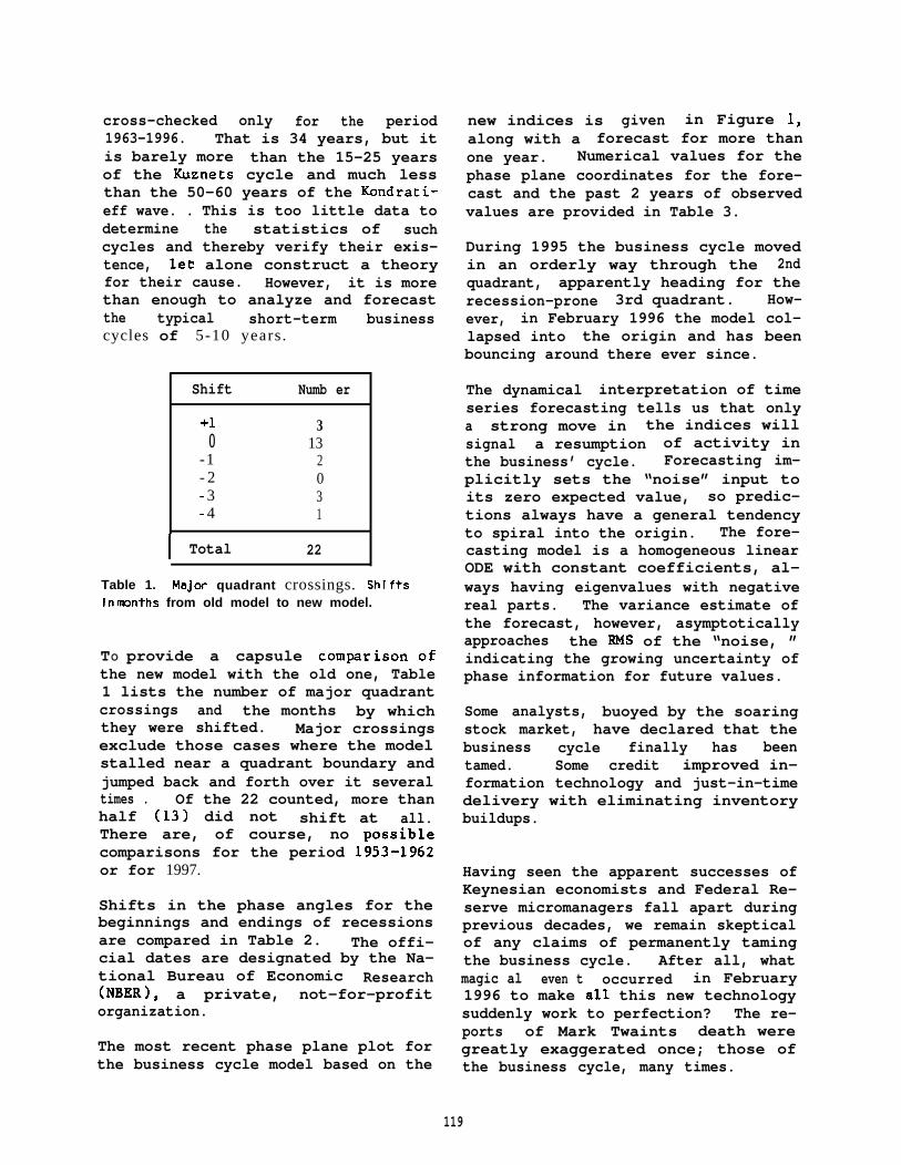
cross-checked only for the period1963-1996. That is 34 years, but itis barely more than the 15-25 yearsof the Kuznets cycle and much lessthan the 50-60 years of the Kondrati-eff wave. . This is too little data todetermine the statistics of suchcycles and thereby verify their exis-tence, let alone construct a theoryfor their cause. However, it is morethan enough to analyze and forecastthe typical short-term businesscycles of 5-10 years.

new indices is given in Figure 1,along with a forecast for more thanone year. Numerical values for thephase plane coordinates for the fore-cast and the past 2 years of observedvalues are provided in Table 3.

During 1995 the business cycle movedin an orderly way through the 2ndquadrant, apparently heading for therecession-prone 3rd quadrant. How-ever, in February 1996 the model col-lapsed into the origin and has beenbouncing around there ever since.

Shift Numb er

+1 30 13

-1 2- 2 0- 3 3- 4 1

.

I Total 22

Table 1. MaJor quadrant crossings. stllf+sin months from old model to new model.

TO provide a capsule comprison ofthe new model with the old one, Table1 lists the number of major quadrantcrossings and the months by whichthey were shifted. Major crossingsexclude those cases where the modelstalled near a quadrant boundary andjumped back and forth over it severaltimes . Of the 22 counted, more thanhalf (13) did not shift at all.There are, of course, no possible

comparisons for the period 1953-1962or for 1997.

Shifts in the phase angles for thebeginnings and endings of recessionsare compared in Table 2. The offi-cial dates are designated by the Na-tional Bureau of Economic Research(NBER), a private, not-for-profitorganization.

The most recent phase plane plot forthe business cycle model based on the

The dynamical interpretation of timeseries forecasting tells us that onlya strong move in the indices willsignal a resumption of activity inthe business’ cycle. Forecasting im-plicitly sets the “noise” input toits zero expected value, so predic-tions always have a general tendencyto spiral into the origin. The fore-casting model is a homogeneous linearODE with constant coefficients, al-ways having eigenvalues with negativereal parts. The variance estimate ofthe forecast, however, asymptoticallyapproaches the RMS of the “noise, ”indicating the growing uncertainty ofphase information for future values.

Some analysts, buoyed by the soaringstock market, have declared that thebusiness cycle finally has beentamed. Some credit improved in-formation technology and just-in-timedelivery with eliminating inventorybuildups.

Having seen the apparent successes ofKeynesian economists and Federal Re-serve micromanagers fall apart duringprevious decades, we remain skepticalof any claims of permanently tamingthe business cycle. After all, whatmagic al even t occurred in February1996 to make all this new technologysuddenly work to perfection? The re-ports of Mark Twaints death weregreatly exaggerated once; those ofthe business cycle, many times.

119

I Time Frame Begin Z(old) Z(new) End Z(old) Z(new)

1963-72 12/69 210 214 11 /70 238 2451972-76 11/73 95 111 03/75 219 2311976-84 01 /80 204 212 07 /80 228 2461976-84 07/81 264 273 11 /82 307 3051983-96 07 /90 221 233 03/91 241 258

Table 2. P h a s e angles (Z) in degrees at official (according to Nat ional

Bureau of Economic Research) beginnings and ends of recessions. Notethat the 1976-1984 cycie had an official “doubie dip” r e c e s s i o n .

90°

BUSINESS CYCLE (1990 - 1997)FORECAST MADE ON 9/3/97 +31

EXPANSION

I96/uL

1 8 0 ° 1

- 3

-J%F ‘2 ‘ 3

0 °

f

B l)’- 2

t$

9 2 / 0 1

RECESSION%

IA FORECASTO ACTUAL VALUE

91 /01w 2!00

● JANUARY VALUETCB 92

Figure 1. The current cycle with September forecast. The business cycie modei is a phasep l a n e p i o t o f d e t r e n d e d ieading a n d c o i n c i d e n t i n d i c a t o r s , a s X - a n d Y - c o o r d i n a t e s ,

respective y. Normai cycies foiiow a c o u n t e r c l o c k w i s e roughiy eiiipticai p a t h w i t h

o c c a s i o n a l s t a l l s a n d reversais. T i m e i s i n d i c a t e d aiong the cycie p a t h . Expansionsoccur in the f i rst quadrant (between 0° and 90°) and contract ions in the third quadrant(between 180° and 2700). Other angies (second and fourth quadrants) denote t ransi t ionperiods. An “official” (Nationai Bureau of Economic Research) beginning of a recession is

indicated by a iabel ‘tB’t and an end by ~’E.”

120

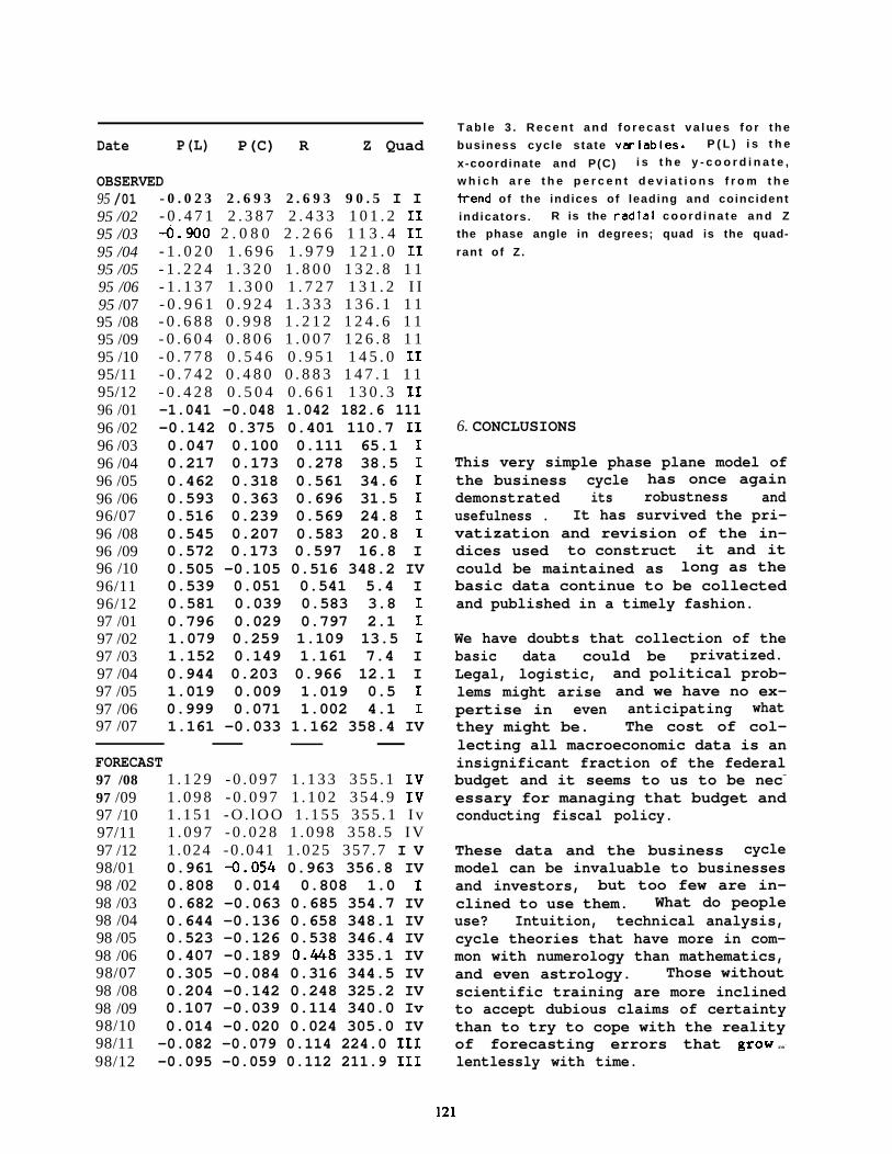
Date P(L) P(C) R Z Quad

OBSERVED95 /0195 /0295 /0395 /0495 /0595 /0695 /0795 /0895 /0995 /1095/1195/1296 /0196 /0296 /0396 /0496 /0596 /0696/0796 /0896 /0996 /1096/1196/1297 /0197 /0297 /0397 /0497 /0597 /0697 /07

- 0 . 0 2 3 2 . 6 9 3 2 . 6 9 3 9 0 . 5 I I- 0 . 4 7 1 2 . 3 8 7 2 . 4 3 3 1 0 1 . 2 114.900 2 . 0 8 0 2 . 2 6 6 1 1 3 . 4 11- 1 . 0 2 0 1 . 6 9 6 1 . 9 7 9 1 2 1 . 0 11- 1 . 2 2 4 1 . 3 2 0 1 . 8 0 0 1 3 2 . 8 1 1- 1 . 1 3 7 1 . 3 0 0 1 . 7 2 7 1 3 1 . 2 I I- 0 . 9 6 1 0 . 9 2 4 1 . 3 3 3 1 3 6 . 1 1 1- 0 . 6 8 8 0 . 9 9 8 1 . 2 1 2 1 2 4 . 6 1 1- 0 . 6 0 4 0 . 8 0 6 1 . 0 0 7 1 2 6 . 8 1 1- 0 . 7 7 8 0 . 5 4 6 0 . 9 5 1 1 4 5 . 0 11- 0 . 7 4 2 0 . 4 8 0 0 . 8 8 3 1 4 7 . 1 1 1- 0 . 4 2 8 0 . 5 0 4 0 . 6 6 1 1 3 0 . 3 11-1.041 -0.048 1.042 182.6 111-0.142 0.375 0.401 110.7 110.047 0.100 0.111 65.1 I0.217 0.173 0.278 38.5 I0.462 0.318 0.561 34.6 I0.593 0.363 0.696 31.5 I0.516 0.239 0.569 24.8 I0.545 0.207 0.583 20.8 I0.572 0.173 0.597 16.8 I0.505 -0.105 0.516 348.2 IV0.539 0.051 0.541 5.4 I0.581 0.039 0.583 3.8 I0.796 0.029 0.797 2.1 I1.079 0.259 1.109 13.5 I1.152 0.149 1.161 7.4 I0.944 0.203 0.966 12.1 I1.019 0.009 1.019 0.5 I0.999 0.071 1.002 4.1 I1.161 -0.033 1.162 358.4 IV

FORECAST97 /0897 /0997 /1097/1197 /1298/0198 /0298 /0398 /0498 /0598 /0698/0798 /0898 /0998/1098/1198/12

1 . 1 2 9 - 0 . 0 9 7 1 . 1 3 3 3 5 5 . 1 lV1 . 0 9 8 - 0 . 0 9 7 1 . 1 0 2 3 5 4 . 9 lV1 . 1 5 1 - O . l O O 1 . 1 5 5 3 5 5 . 1 I v1 . 0 9 7 - 0 . 0 2 8 1 . 0 9 8 3 5 8 . 5 I V1 .024 -0 .041 1 .025 357 .7 I V0.961 4.054 0.963 356.8 IV0.808 0.014 0.808 1.0 I0.682 -0.063 0.685 354.7 IV0.644 -0.136 0.658 348.1 IV0.523 -0.126 0.538 346.4 IV0.407 -0.189 0.48 335.1 IV0.305 -0.084 0.316 344.5 IV0.204 -0.142 0.248 325.2 IV0.107 -0.039 0.114 340.0 Iv0.014 -0.020 0.024 305.0 IV-0.082 -0.079 0.114 224.0 111-0.095 -0.059 0.112 211.9 111

T a b l e 3 . R e c e n t a n d f o r e c a s t v a l u e s f o r t h e

business cycle state variabieso P ( L ) i s t h e

x-coordinate and P(C) i s t h e y - c o o r d i n a t e ,

w h i c h a r e t h e p e r c e n t d e v i a t i o n s f r o m t h e

trend of the indices of leading and coincident

indicators. R is the radiai c o o r d i n a t e a n d Z

the phase angle in degrees; quad is the quad-

rant of Z .

6. CONCLUSIONS

This very simple phase plane model ofthe business cycle has once againdemonstrated its robustness andusefulness . It has survived the pri-vatization and revision of the in-dices used to construct it and itcould be maintained as long as thebasic data continue to be collectedand published in a timely fashion.

We have doubts that collection of thebasic data could be privatized.Legal, logistic, and political prob-lems might arise and we have no ex-pertise in even anticipating whatthey might be. The cost of col-lecting all macroeconomic data is aninsignificant fraction of the federalbudget and it seems to us to be nec-

essary for managing that budget andconducting fiscal policy.

These data and the business cyclemodel can be invaluable to businessesand investors, but too few are in-clined to use them. What do peopleuse? Intuition, technical analysis,cycle theories that have more in com-mon with numerology than mathematics,and even astrology. Those withoutscientific training are more inclinedto accept dubious claims of certaintythan to try to cope with the realityof forecasting errors that grow re-

lentlessly with time.

191

7 ● REFERENCES

Anderson, B. W., 1957: UNDERSTANDING THE OLDTESTAMENT, 2nd Edition, Prentice-Hail, inc.,Engiewood Ciiffs, NJ.

Dewey, E. R., 1970: CYCLES: SELECTED WRiTiNGS,

F o u n d a t i o n f o r t h e S t u d y o f Cycies, P i t t s -

burgh, PA.

Dewey, E.R. with O. Mandino, 1971: CYCLES: THE

Mysterious FCRCES THAT TR i GGER EVENTS,

Hawthorn Books, inc., New York.

Estrei la, A. & F.S. Mishkin, 1 9 9 6 : “ P r e d i c t i n g

U-S. R e c e s s i o n s : Financiai Variables as Lead-

i n g indicators,!! FEDERAL RESERVE BANK OF KW

YORK RESEARCH PAPER No. %09, New York (in

p r e s s : REViEW W ECONOMiCS & S t a t i s t i c s ) .

Forrester, J . W . , 1 9 6 1 : industrial DYNAMICS,The MiT Press, Cambridge, MA.

HANDBCK)K OF CYCLiCAL iNDiCATG/S: A SUPPLEMENT

TO THE BUSiNESS CONDITIONS DIGEST, 1984: US

D e p t . o f Conmwce, Bur. of Economic Anaiysis,

Washington, DC.

Jordan, S.K., 1972: “Seif-mnsistent Statisti-

cal Modeis f o r t h e G r a v i t y Anomaiy, Verticai

Defiecl’ions, & U n d u l a t i o n s o f t h e Geoid,” J.

GEOPHYS. RES., vol. 77, No. 20, pp. 3 6 6 0 - 3 6 7 0 .

Morr ison, F . , 1991a: lliE ART OF MCOELiNG DY-

NAMIC SYSTEMS: FORECASTING FOR CHAOS, RANDOM-

N E S S , & D e t e r m i n i s m , Wiiey-i nterscience, kw

York.

M o r r i s o n , F . 1991b: “ L i n e a r Fiitering: W h a t ,

Why, & HOW,” THE JOURNAL OF BUSINESS FORECAST-

ING, Voi. 10, No. 1

FOB 1 5 9 , S t a t i o n C ,

for singie i s s u e ] .

M o r r i s o n , F . & N.L.

Piane M o d e i o f t h e

FEDERAL F~ECASTERS

( S p r i n g ) , p p 1 3 - 1 8 [JBF,

Flushing, NY 11367, $15

Morrison, 1997: “A Phase

B u s i n e s s Cycie,’l IHE 8 T H

CONFERENCE - 1996 & THE

7TH FEDERAL FORECASTERS CONFERENCE - 1994,

COMBiNED PAPERS & PROCEEDINGS, NCES 97-341,

Debra E. Geraid, Editor, Washington, DC.4

Samueison, P.A. w i t h P . T e m i n , 1 9 7 6 : E C O -

NOMICS, 1 0 t h e d i t i o n , McGraw-Hi ii Book Co.,

New York.

Wiis, w., 1988: OVERViEW OF SYSTEM DYNAMiCS

T H E WCRLD OVER, Croon DeVries, 55 Parkweg,

3603 AB Maarssen, Netherlands.

122

The Educational Requirements of Jobs: ALooking At Training Needs

New Way of

Darrel Patrick Wash, Bureau of Labor Statistics, U.S. Department of Labor

This study presents a new way of classi~ing occupations by training requirements. This more detailed approach,which now covers several different categories of employer-provided training as well as the more traditionalacademic training categories, k presented, along with a discussion of how it can be combined with previouslydeveloped estdates of occupational net replacements to formulate a much clearer picture of fiture education andtraining demand.

123

Concurrent Sessions II

125

FORECASTING CROP PRICES UNDER NEW FARM LEGISLATION

Chair: Peter A. RileyEconomic Research Service, U.S. Department of Agriculture

Forecasting Crop Prices Under New Farm Legislation,Peter Riley, Economic Research ServiceU.S. Department of Agriculture

Forecasting Annual Farm Prices of U.S. Wheat in a New Policy Er~Linwood A. Hoffman, James N. Barnes, and Paul C. Westcott,Economic Research ServiceU.S. Department of Agriculture

An Annual Model for Forecasting Corn prices,Paul C. Westcott, Economic Research ServiceU.S. Department of Agriculture

Forecasting World Cotton Prices,Stephen MacDonald, Economic Research ServiceU.S. Department of Agriculture

127

Forecasting Crop Prices Under New Farm Legislation

byPeter A. Riley

Economic Research SewiceU.S. Department of Agriculture

The tradition of strong government involvement in agriculture is starting to break down aroundthe world. This tendency has been particularly evident in the United States over the last few yearsand especially since 1996, when the most recently enacted f- legislation sharply reducedgovernment intervention and gave more weight to market forces. This has prompted areevaluation of forecasts that have been heavily shaped by policy variables. This paper will set thestage for presentations on price forecasting for 3 major U. S. field crops.

USDA regularly forecasts a variety of annual supply and demand components for the major fieldcrops, as well as f- prices. These are published monthly and are widely used by f-ers,processors, and other market participants, as well as USDA policy makers. The price forecastsare particularly important as critical input for other calculations and forecasts, such as farmincome and food prices. 1

I will focus on three main points as an introduction to the specific forecasting models. The firstconcerns the relevance and importance of accurate forecasting of agricultural prices for the farmsector and the economy as a whole. Second, forecasting in the agricultural sector involves somespecial challenges not necessarily encountered in other sectors. Third, there is a brief overview ofthe broad changes in agricultural policies that have occurred in the last few years that haveprompted a new look at our forecasting tools.

Importance of Agricultural Price Forecasts

The monetary amounts involved in crop prices may seem small at first glance. However, the hugequantities produced add up to very large sums. For example, U.S. com production has averagedmore than 8.9 billion bushels a year between 1994 and 1996. Thus just a one-cent change in thefarm price of com represents a change of $89 million for the economy, with fhrmers capturingthat much more or less revenue while end users pay a corresponding amount more or reap thesavings.

The actual magnitude of changes in farm prices is typically much larger (for reasons that will bediscussed later). Using the same years as above (1 994-96), the annual variation in season averagefarm price of com has averaged nearly 59 cents per bushel, translating into huge sums at the

* USDA does not forecast the U.S. farm price of cotton because this is prohibited by law.Today’s cotton presentation will examine a world cotton price.

129

national level--an average approaching $5.3 billion. Ironically, these last 3 years have been one ofthe most volatile periods in the history in the com market. For the other 2 crops discussed today,wheat and cotton, both the absolute quantity of production and the variability are smaller.

Although the role of crop prices may seem obscure to some people outside of agriculture, they dohave a very large impact on the general economy by several measures. The multiplier effects ofchanges in prices of corn, wheat, and cotton will be felt at various levels and have implications forinflation. Spending by farmers in rural communities and expenditures on capital goods such astractors and other f- equipment and land expenditures, whether through purchases or leases,are prime examples.

Another dimension of the general importance of these commodity prices is their use as rawmaterials for other products. Among the cases reviewed today, wheat is probably the mostappreciated by the general public when they consume bread, pasta, bagels, and other bakedgoods. Cotton is also easily recognized in its clothing and textile applications. Perhaps com isthe least obvious with most of its use as a feed for livestock and poultry and as an input for manyfood and industrial products. These include com sweeteners used in the major soft drinks and atremendous variety of processed foods.

Finally, the farm price has a important role in shaping our export competitiveness. The UnitedStates has a consistently strong positive trade balance in agriculture. Although the U.S. is theworld’s leading exporter of wheat, corn, and cotton, the marketplace for each commodity ishighly competitive and our market shares are far from assured.

Special Challenges for Agricultural Price Forecasts

Agriculture has some special features that have an important bearing on forecasting under anypolicy regime. Foremost is the large variability in supply and prices, largely stemming fromweather impacts. As mentioned earlier, there is considerable price volatility fi-om year to year formost field crops, and similarly on a monthly, weekly, or even daily basis.

Weather plays an important role in determining the size of annually produced crops, and thereforeis the major culprit underlying large production variability. Most field crop production iscritically dependent on rainfall, with only small portions of the crops produced under irrigation.Droughts, high temperatures, excessive moisture, and other weather factors often harm yields andreduce output. Sometimes, conditions are excellent, pushing production beyond expectations.Swings in production also reflect changes in plantings so the total area devoted to a crop can varyfrom year to year. The driving force behind acreage changes are primarily economic as fmersanticipate net returns from competing crops. Weather can also play a role, generally in a negativesense, whez for example, it is too wet to plant a particular crop on time.

Demand for these crops is generally much steadier than supply, but demand changes can also addto the variability in prices. Domestic demand for wheat for food use is ftirly inelastic, but aportion of the crop is fed to livestock and this portion is more variable. Domestic use of cottonhas been relatively steady in recent years. Although cotton competes with manmade fibers,

130

substitution in the short run is quite limited. Domestic com use displays strong annual variability,in large part because of the changes in supply. Some com demand can be characterized asinelastic, including industrial uses such as starch and sweeteners and food use in breakfast cereals.However, the largest category of com is used as a livestock feed and this portion fluctuatesgreatly, reflecting changes in animal inventories, livestock cycles, competition with otherfeedstuffs, and large swings in the supply and price of corn.

International developments play an important role in agricultural markets and tend to increaseprice variability. Each of the crops discussed today is highly dependent on exports. Exports ofcom have accounted for around 20-25 percent of total disappearance in recent years, cottonexports more than 40 percent, and wheat around 50 percent. These sectors are thus vulnerable tothe export fluctuations which are common for most field crops. Many inter-related factorsaccount for this, such as changes in import demand, the availability of exports from competingsuppliers, policy factors such as export subsidies and import tariffs, and tastes and preferences.

Probably, everyone vaguely remembers the sporadic grain import binges of the Soviet Unionduring the 1970’s and 1980’s that added instability to world markets. This is the extreme case ofvariability in agricultural trade, but unexpected spurts or sharp drops in imports and exports byother countries on a smaller scale are not that uncommon, with corresponding effects on fiirmcommodity prices.

Changes in the Policy Environment

There is a ve~ strong tradition of heavy government intervention in U.S. agriculture that startedin the early years of the 1930’s Depression. At that time, the Government began to provide pricesupports to farmers and started programs to idle acres to avoid overproduction. Over the years,these basic elements were continued, with many variations and often complex formulas that werelittle understood by many people outside the farm economy.

During the mid- 1980’s, policy changes began to take effect to reduce the role of government andallow more market influence. This stemmed from a f- crisis partly triggered by a decliningexport market share as competitors undercut high U. S. prices. Thus, policies shifted somewhat,and U.S. price supports were reduced to enhance competitiveness. Another important step at thetime was to start reducing large stocks of grain and other crops that had accumulated when thegovernment offered an assured home for virtually all the major fields crops. By the early 1990’s,like many other sectors of the economy, agriculture had reduced inventories. This reflected bothbudgetary pressures in the public sector reducing publicly held stocks and developments in theprivate sector adopting a “just in time” deliveries approach.

While still heavily shaped by government decisions, these and other changes initiated in 1985 fmlegislation and continued by legislation in 1990 gradually were introducing more market forces toshape production decisions. Then in 1996, a more radical Farm Bill was enacted, signaling a moreabrupt break with past tradition. Often called “Freedom to Farm,” the new law essentiallyallowed f-ers to make decisions completely free from government influence.

131

,“. .,..

, .

Nearly all government f- programs were eliminated, such as the acreage “setaside” or modernland idling program used when supplies were very large. Another important change was the endof the “base acres” concept under which f-ers devoted a certain amount of land to a particularcrop in order to qualifj for farm program benefits. This tended to keep acreage at fairlypredictable levels depending on various program parameters. Now, farmers have completeflexibility to plant what they wmt based entirely on market signals.

New Forecasting Approaches Contribute to USDA Market Analysis

The presentations to follow will look at forecasting models for 3 agricultural commodities andhow analysts are dealing with the changing policy setting. Many of the broad similarities havebeen mentioned, and now some of the distinct traits of each market will be discussed. The comand wheat papers focus on U. S. policy change, and the cotton paper deals with the interaction ofpolicy variables in a global setting. The forecasting approaches can accurately be characterized asconstantly evolving, as analysts incorporate more years of data and react to shifts in policies.

The context in which these forecasting models are used at USDA is important. First, these areapplied tools that are used to help develop price forecasts that, except for cotton, are regularlypublished. USDA publishes a longer-term projection annually, while the forecast for the nearbyyear is published monthly. The latter price forecast is released at 8:30 AM on the day of thereports, along with various supply and demand elements. Thus, much of the analysis isconducted during the night, incorporating new information made available to USDA economistsonly shortly before being released to the public. The quick turnaround of this process requireshighly practical tools. Second, the price is just one component of a broader analysis of supply,use, and stocks. These price models may be embedded in spreadsheets to provide a simultaneousdetermination of prices to changes in supply or demand forecasts. USDA presents thisinformation in commodity “balance sheets” to provide a consistent analysis of each market.

132

FORECASTING ANNUALLinwood A. Hoffman, James

Introduction

FARM PRICES OF U.S. WHEAT IN A NEW POLICY ERAN. Barnes and Paul C. Westcott, U.S. Department of Agriculture, ERS

Information regarding wheat prices is critical to marketp~rticipants who are making decisions about managingprice risk. Market information is also important topolicymakers who have to assess the impacts of domesticor international events upon wheat farm prices.

Concern about U.S. wheat farm prices rose significantlyduring the 1995/96 crop year, as world crop shortfallscaused USDA’s price projection for the crop year to risefrom a range of $3.25-$3.45 per bushel in May 1995 to$4.20-$4.50 per bushel in November 1995. Two yearslater, as world production recovered, producers’ wheatprices are expected to fall. USDA’s price projection for1997/98 dropped from a range of $3.60-$4.20 in May1997 to $3.05-$3.65 in August 1997.

Price information has become even more important due,in pati, to changes in U.S. agricultural policy. Passage ofThe Federal Agriculture Improvement and Reform Act of1996 (1996 Act) continues the sector’s trend towardmarket orientation. The Farmer-Owned Reserve (FOR)is suspended and wheat loan rates are capped at the 1995level of $2.58 per bushel, well below current andexpected future market prices. Such a situation suggestslittle, if any, government stockholding, which may

contribute to increased price sensitivity.

The 1996 Act also eliminated government priceassurances. Under the 1996 Act, annual productionflexibility contract payments remain fixed regardless ofmarket prices, in contrast to deficiency payments whichvaried inversely to market prices. Consequently,producers face greater risk of income volatility becauseof market price variation.

Previous analyses have studied relationships betweenprices and ending stocks for com (Baker and Menzie;Van Meir; Westcott, Hull, and Green), wheat (Westcott,Hull, and Green), and rice (Hoffman, Livezey, andWestcott; and Lin, Novick, and Livezey) as a priceforecasting tool. Whether such a relationship cancontinue to provide short and long term price forecasts inthe new policy environment remains to be seen.

The purpose of this article is to present a model designedto forecast the U.S. season average price of wheat at the

farm level.’ The U.S. Department of Agricultureanalyzes agricultural commodity markets on a monthlybasis and publishes annual current year marketinformation, including price projections. Because ofchanges in policy, price forecasting equations need to bere-evaluated.

Background: Factors Affecting theU.S. Farm Price of Wheat

Some of the most important variables to be considered inforecasting the price of wheat include supply and demandfactors and domestic agricultural policy (AppendixTables 1, 2, and 3). Prices are determined by theinteraction of the supply and demand functions which areinfluenced by government policies. The supply anddemand components are briefly discussed because theyaffect the stocks and use variables which are included inthe price equation.2 Agricultural policies may also affectthe factors of supply and demand. Many of these effectsare captured in the stocks or use variables and those thatare not will be accounted for separately in the pricemodel.

Wheat Supply

The elements of supply are beginning stocks, imports,and production. Wheat is the principal food grain in theUnited States and throughout much of the world. TheUnited States is the third largest producer of wheat in theworld, averaging 61.6 million metric tons in 1994-96, or11 percent of world production. U.S. wheat’s farm valueof production totaled $9.8 billion in 1996, the fourthlargest of all field crops or 11.4 percent of total U.S. cropvalue.

Be?innin Q Stocks--Last year’s carryover becomes thecurrent year’s beginning stocks. Large or small carryoverlevels usually have the most impact on price. Largestocks can provide a cushion in a short crop year or a lowcarryover may exacerbate a low production situation.

1 This price model is one of many price forecasting tools usedby the USDA. Other price forecasts used by USDA are based on futuresmarket prices and other econometric models. Anal ysts’ expeti opinionsalso enter into the forecasting process.

2 Stocks are equal to ending carryover inventories and userefers to total use of a commodity, both total domestic and export use.

133

h?u2Qm--wheat imPorts ‘ere a n insililnificant factor forU.S. supply for many years. Imports were fairly low involume and less than 1 percent of supply between 1960and 1989. However, wheat imports became an issue inthe 1993/94 marketing year, as they reached 109 millionbushels, including products, or 4 percent of supply.Imports have since declined to about 3 percent of supply,but the U.S. remains an attractive market for Canadianwheat.

Production--U.S. wheat production, the major componentof suppl y, is determined jointly by the area harvested forgrain and yield per acre. Until the 1996 Act, acreageplanted and harvested was affected by farm programrequirements and participation rates. The relationshipbetween area planted and harvested varies substantiallyby region although it is fairly stable at the national level.Producers in cattle feeding areas typically graze out someof their wheat fields, rather than harvesting them forgrain.

Prior to 1992, sharp declines or increases in planted areawere usually the result of changes in governmentprograms requiring acres to be idled. In an effort tocontrol production, support farm income, and limitgovernment costs, various acreage limitation programswere employed, such as the acreage reduction program,paid land diversion, 50/92, 0/92, and 0/85.s These supplymanagement programs were eliminated in the 1996 Act.Thus, market prices rather than farm programs now havea greater influence on acreage planted to wheat.

Average U.S. wheat yields have risen from around 30bushels per acre in the mid- 1970’s to an average of 38bushels per acre in the 1990’s. Wheat yield growth hasslowed in the last 15 years. Many factors affect U.S.yields, including climatic conditions, weather, farmmanagement practices, variety, and soil type.

Wheat Demand

Components of wheat demand are food use, feed andresidual, seed, exports, and carryover stocks. Domesticuse is a growing component of total U.S. wheatdisappearance because of increased food use. Domesticuse claims about 50 percent of total disappearance, upfrom an average 40 percent during 1975-84.

3 If supplies were estimated to be in excess by the U.S.Department of Agriculture, acreage reduction programs (ARPs) wererequired and paid land diversion programs (PLDs) were permitted.Wheat producers had the option of under-planting their maximumpayment acres and receiving deficiency payments on a portion of theunder-planted acres (0,50/85-92).

Food--Food use has been the largest and most stablecomponent of domestic use, characterized by a steadygrowth rate. Wheat is unique because it is the only cerealgrain with sufficient gluten to produce bread withoutrequiring mixing with another grain. The domesticdemand for wheat food use is relatively unaffected bychanges in wheat prices and disposable income and isclosely tied to population, tastes. and preferences.

Feed and Residual--Feed and residual use is morevariable than food use and is related to corn/wheat pricesand wheat crop quality. Wheat feed use is particularlyprominent at wheat harvest time when wheat prices arelow and new crop corn and sorghum have not beenharvested. Feed and residual use totaled about 19 percentof total disappearance in the 1986 and 1990 crop years,years of lower wheat prices, compared to about 6 percentduring 1988 and 1995, years of higher wheat prices. Theresidual component includes negligible quantities ofwheat used for alcoholic beverages and estimation errorfrom other categories.

&!2!l&-ExPorts are imPortant to the U“s” wheat market!as U.S. exports account for about half of totaldisappearance. Wheat exports accounted for 11.7 percentof the total value of U.S. agricultural exports or $7.0billion in fiscal 1996. The United States is the world’slargest exporter of wheat with a world market share ofabout 33 percent.

Food Aid under P. L.480, guaranteed export credit, andspecial export programs have been very helpful to U.S.wheat exports. The Export Enhancement Program (EEP)4

was important to U.S. wheat exports between 1986 and1994 as over half of the U.S. exports in some of theseyears received EEP subsidies (Fig. 1). EEP has not beenused for U.S. wheat exports since July 1995. It is unclearwhether EEP will be used in the future, but the 1996 Actauthorizes its use at reduced levels.

Carrvover Stocks--Carryover stocks reached levelsgreater than 1 billion bushels between 1981 and 1987,with ending stocks representing an average of 60 percentof one year’s use. However, as policies steered the sector

4 The Export Enhancement Program was initiated in May1985 under the Commodity Credit Corporation (CCC) Charter Act andlater formally authorized by the Food Security Act of 1985 and extendedby the Food Agriculture Conservation and Trade Act of 1990 and the1996 Act. The major objective of this program is to help U.S. exporterscompete against unfair trade practices used by other countries. Exportbonuses were used to make U.S. agricultural commodities competitivein world markets. Exporters received generic certificates prior toNovember 1991 and cash bonuses thereafter.

134

.

toward greater market orientation, ending stocks declinedand a more balanced supply and use situation arose in199 I -96 with an average stocks-to-use ratio of 21percent.

Agricultural Policies

Domestic agricultural policies may also affect the factorsof supply and! demand. Many of these effects arecaptured in the stocks or use variables. For example,Government price support programs have affected levelsof carryover stocks over time. Between the 1973 and1996 farm bills, the loan program,5 farmer-ownedreserve, food security reserve and production controlshave been used to support prices. Also, various exportprograms may enhance consumption of wheat bysubsidizing the price of wheat. How these programsaffected the price and stocks-to-use relationship isimportant for modeling wheat prices. Situations wherepolicies altered the market price and stocks-to-userelationship must be specifically accounted for in theprice equation. Consequently, a review of agriculturalpolicies is necessary to determine when adjustments tothe price and stocks-to-use relationship occurred.

The Agriculture and Consumer Protection Act of 1973changed the existing income programs by replacing thewheat certificate program with the target price concept(Hat-wood and Young). Carryover stocks consisted onlyof free stocks in 1974-76 and the stocks-to-use ratioranged from 26 to 65 percent for those years. Becausegroins and oilseeds generally had favorable prices during1974-76 there was an effort to make farm programs moremarket oriented. The target price accompanied withdeficiency payments was designed to support incomewithout affecting market price. However, strong prices in1974-76 Icd to increased production and larger stocks(Appendix Tables I and 2).

The Food and Agriculture Act of 1977 established thefarmer-owned groin reserve (FOR), which was inresponse to the growing importance of exports and thepotential for greater global demand and price instability.

5 Price suppon for wheat producers is provided throughnonrecourse loans at the announced price support loan rate. Aparticipating farmer can pledge his crop as collateral to the CommodityCredit C’orporatwn (CCC) and then recewe a 9-n~onth loan pledged at apredetermined mte per bushel. If the market price is above the loan mteplus Interest. the producer usually repays the loan with interest,However. it’ the market price M below the loan rate plus interest, theproducer may forfeit the wheat at the end of the loan term to theCommodity Credit Corporation in full satwt’action of the loan.

In return for loans and annual storage payments, farmersagreed not to market their grain for an extended period (3to 5 years), unless the average farm price reached aspecified level called the release price. The farmer-owned reserve allowed the producer to maintainownership of the grain in contrast to a situation where aproducer would forfeit stocks to the government at lowprices under the regular loan program with no opportunityto realize a gain if prices rose.

Entry into the wheat FOR, the FOR loan rate, and theregular wheat loan rate appeared to heavily supportannual farm prices during the late seventies to mid-eighties (Figs. 2. 3, and 4). Prices approached the loanrate in 1977. the year when the Farmer-Owned Reservewas introduced. Minimum loan rates were written intoThe Agriculture and Food Act of 1981. The regular loanrate for wheat was $3 a bushel in 1980 and reached $3.65in 1983. Defaults to the CCC began to rise and CCCstock levels surged. Loan rates were reduced to $3.30 in1984 and 1985. During the mid- 1980s, market priceswere pressured downward when accumulated CCC stockswere released upon the market. In retrospect. loan ratesin the early 1980’s were set so high that they supportedprices above market clearing levels.

During 1980-82, the FOR was implemented as a priceenhancement tool by offering producers reserve loans atrates above the regular loan rate. This situation raisedquestions about the FOR’s goals, price stability or priceenhancement. The FOR loan rate was set at $4.00 perbushel in 1982/83, $0.45 above the regular loan rate.Harvested acres were the second highest ever in 1982/83and this contributed to a rise in ending stocks to 1.52billion bushels of which over I billion bushels were in theFOR (Fig. 3).

The Food Security Wheat Reserve was created in the1980/8 1 marketing year to provide a government-heldreserve of up to 4 million metric tons of wheat foremergency food needs in developing countries. Thisreserve was also part of the Government’s response tocriticism for the Russian grain embargo. In general thisreserve has not been a factor in the wheat market duringthe 1990’s, although some wheat was released during the1995/96 marketing year. The authority for the FoodSecurity Wheat Reserve was repealed with the 1996 Actand a new Food Security Commodity Reserve wasestablished that includes wheat, corn, grain sorghum, andrice,

Because of large stock buildups, the Food Security Act(FSA) of 1985 was designed to increase U.S.competitiveness in world markets and to support farm

la<

income (Hoffman, Schwartz, and Chomo). The FSAmoved agriculture toward a more market-oriented farmpolicy that would enable farmers to respond to economicand market signals. The legislation lowered loan ratesand provided discretionary authority for their adjustment,modified the FOR to prevent large buildups in stocks,reversed upward trends in target prices, generally frozeprogram yields, and authorized EEP and initiated theTargeted Export Assistance Program (TEAP) to promoteagricultural exports in response to subsidizedcompetition. The Conservation Reserve Program wasimplemented with a goal of retiring 40-45 million acresof highly erodible cropland from production for a periodof 1O-15 years.G

In 1986 stocks had been equal to 83 percent of total usebut declined to 16 percent in 1995 (Fig. 4). Genericcertificates helped reduce the level of government andFOR stocks.

The Food, Agriculture, Conservation, and Trade Act of1990 as well as the subsequent Omnibus BudgetReconciliation Act of 1990 (OBRA), followed the groundwork laid by the FSA of 1985. The main goals of theFACT Act of 1990 were to further reduce spending, tohelp maintain farm income growth through expandingexports, and to enhance the environment. Majormechanisms used to accomplish reduced budgetexpenditures and improved agricultural competitivenesswere reduced payment acres (as authorized by theOmnibus Budget Reconciliation Act) and plantingflexibility. The Conservation Reserve Program of the1985 FSA was altered to cover lands adversely affectingwater quality and wetlands, and a new Water QualityProtection Program was added.

6 A program where producers sign contracts to convertenvironmentally sensitive cropland to approved conservation uses for a10 to 15 year period, in exchange for rental payments and payments toshare costs of establishing conservation practices. The CRP program isavailable to participants and non-participants in the annual farmprograms. The producer submits a bid for a 10 or 15 year contractstating the annual payment they would accept to convert this land to aconserving use. If the bid is accepted, USDA pays an annual rent to keepthis land in a conservation use. There were about 9 million acres ofwheat base acres voluntarily enrolled in the CRP in 1997. Obviously,such a program reduces wheat’s production potential.

7 Negotiable certificates, which do not specify a certaincommodity, issued by USDA in lieu of cash payments to commodityprogram patiicipants and sellers of agricultural products. The cetiificatescan be used to acquire stocks held as collateral on Government loans orowned by the Commodity Credit Corporation. Farmers have receivedgeneric certificates as payment for participation in numerous Governmentprograms. Grain merchants and commodity groups also have beenissued certificates through the Export Enhancement Program and theTargeted Export Assistance Program.

The Food, Agriculture, Conservation, and Trade (FACT)Act of 1990 continued keeping commodity loan rates lowand reducing the role of the Farmer-Owned Reserve,thereby phasing out government-owned stocks as astabilizing device. Wheat FOR activity declined under the1990 Farm Bill and ceased during the 1993/94 marketingyear. Annual acreage reduction programs helpedmaintain stabilization. The stocks-to-use and pricerelationship seems to have changed for the years of 1990through 1994. Some of the factors that may have causedthis change include a change in EEP programadministration where subsidies were switched fromgeneric certificates to cash; passage of trade agreements,the Canada-U.S. Free Trade Agreement and the NorthAmerican Free Trade Agreement, allowing for increasedtrade between Canada and the U. S.; and a general policychange that minimizes government stocks.

The 1996 Act continues the trends of the previous twomajor farm acts toward greater market orientation,thereby gradually reducing the Government’s commodityprogram influence in the agricultural sector (Young andWestcott). Annual production flexibility contractpayments replace the deficiency payment income supportmechanism. Price support programs are continued butloan rates are kept at minimal levels, the FOR issuspended, annual supply control programs areeliminated, and planting decisions are decoupled fromprogram parameters.

The 1996 Act continues the marketing loan provisions forwheat but since the wheat loan rate is capped at the 1995level of $2.58 per bushel, significant activity under theseprovisions is unlikely. Marketing loan provisions forwheat began with the 1993 crop year. This program hashad little effect on wheat prices because prices havegenerally been above the loan rate8.

Analytical Framework

This section illustrates how stocks are related to supplyand demand within a general equilibrium model anddevelops the statistical model.

A general equilibrium model is illustrated which reflectscompetitive behavior (Labys; Westcott). The modelfeatures supply, demand, stocks, and a market-clearingidentity.

8 In 1993, some loan deficiency payments (LDPs) weremade to wheat farmers. Most payments were for soft red winter wheatlocated in certain Texas counties. Total wheat LDPs paid to farmerswere less than $1 million.

136

s = f, (p, z. flp)

D = fl(p, y. Z)

] = fl(p, Z. flp, D9094)’

S-D-1=0

where endogenous variablesdemand. 1 = ending stocks,Exogenous variables are flp =

are: S = supply, D =and p = market prices.FOR and loan program, y

= disposable income, D9094 = a period of an apparentshift in the pricing relationships, and z = other exogenousvariables.

With the system in equilibrium, prices can be determinedfrom the inverse of the stocks function. At that price, thesupply and demand levels give an ending stocks estimatewhich is consistent with the equilibrium price, throughthe price-ending stocks relationship.

In the inverse stocks function-price determinationequation, prices are negatively related to stocks. Endingstocks of an annual storable commodity, such as wheat,reflect the relationship between supply and use (Labys).If total use rises relative to supply, farm prices tend to riseas ending stocks decline. On the other hand, if supplyrises relative to total use, prices tend to decline as endingstocks accumulate.

p = f7-’(l/D, flp, D9094)

The stocks variable is transformed to reflect stocksrelative to total consumption (Westcott). Therefore, thestocks variable (I) is expressed as a percent of total use(l/D). This has particular importance over time asdemand for carryover stocks may increase because ofgrowth in the size of the wheat sector, measured here bytotal demand.

Prices are expected to be positively related to the loanrate, especially in those years that loan rates were set highrelative to market prices and the loan program andfarmer-owned reserve isolated stocks from themarketplace. Price support and stabilization measurestend to increase the price received by producers usuallythrough government purchases.

9 Additional determinants of stock demand include differencesbetween current and expected futures prices and interest rates.

Entry into the wheat FOR, FOR loan rates, and regularloan rates tended to limit price reductions especiallyduring 1979-85 (Fig. 1, Appendix Table 2, and Fig. 2).Many grain price models have been estimated with thedependent variable of price minus loan rate. Thisrelationship was used in past unpublished wheat priceforecasting equations, by Baker and Menzie’s annual comprice model, and by Van Meir’s analysis of com pricesand stocks, Such a dependent variable is no longer validin today’s market as market prices are well above supportprices.

Although there was a return to market orientation during1986-96, some of the different relationships found from1990 through 1994 could be due to a number of factors(Fig. 4). First, EEP program administration may accountfor some of this change because program subsidiesswitched from generic certificates to cash in November1991. Second, passage of trade agreements, CFTA andNAFTA, allows for increased trade between Canada andthe U.S. Third, general policy level changes minimizegovernment stocks. Additional research is required toexplain these relationships.

Model Specification

The price-carryout stocks relationship, equation (1),specifies annual producer price as a function of thestocks-to-use ratio, loan rates for the period 1979 through1985, and a dummy variable to capture a shift in thepricing relationships during 1990 through 1994. Basedon the relationships observed in figure 4, it appears thata logarithmic functional form would best fit the databetween 1975 through 1996. A double log function isspecified and estimated with ordinary least squares (OLS)regression to explain the all-wheat price with 22observations.

(1) Log(P) = a + b Log(I/D) + c Log(FLP)*(D7985)

+ d (D9094)

Where:

P = Weighted season average farm price for all wheat.’”a = intercept term. It is hypothesized that this coefficient

10 This price is computed by the USDA’s NationalAgricultural Statistics Service. A monthly survey is conducted todetermine the price producers receive. These prices are weighted by themonthly percent of marketing for the total marketing year. In theprocess each of the five wheat classes are taken into account to arrive

at an all wheat price.

137

,:

.,

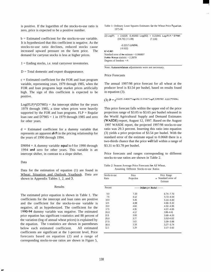
is positive. If the logarithm of the stocks-to-use ratio iszero, price is expected to be a positive number.

Table 1: Ordinary Least Squares Estimates for the Wheat Price Equat]on,1975-96

b = Estimated coefficient for the stocks-to-use variable.It is hypothesized that this coefficient is negative. As thestocks-to-use ratio declines, reduced stocks causeincreased upward pressure on the farm price. Thedemand for carryout stocks is less at higher prices.

1 = Ending stocks, i.e. total carryover inventories.

(2) Log(P) = 2,6225 -0,40263 Log(l/D) + 0.21941 Log(FLP) * D7985(19,73) (-l 1.08) (7.116)

-0.2217 (D9094).(-5.522)

R2=0.883Standard error of the estimate = 0.066807l.)urbin-Watson statistic = 2,2679Degrees of freedom = 18

Note: Autocorrelation adjustments were not necessary.

D = Total domestic and export disappearance.Price Forecasts

c = Estimated coefficient for the FOR and loan programvariable, representing years, 1979 through 1985, when theFOR and loan programs kept market prices artificiallyhigh. The sign of this coefficient is expected to bepositive.

Log(FLP)*(D7985) = An intercept shifter for the years1979 through 1985, a time when prices were heavilysupported by the FOR and loan programs. FLP = Regularloan rate and D7985 = 1 in 1979 through 1985 and zerofor other years.

d = Estimated coefficient for a dummy variable thatrepresents an apparent shifl in the pricing relationship forthe years of 1990 through 1994.

D9094 = A dummy variable equal to 1 for 1990 through1994 and zero for other years. This variable is anintercept shifter, in contrast to a slope shifter.

Data

Data for the estimation of equation (1) are found inWheat: Situation and Outlook Yearbook. Data areshown in Appendix Tables 1, 2, and 3.

Results

The estimated price equation is shown in Table 1. Thecoefficients for the intercept and loan rates are positiveand the coefficient for the stocks-to-use variable isnegative, all as hypothesized. The coefficient for the1990-94 dummy variable was negative. The estimatedprice equation has significant t-statistics and 88 percent ofthe variation (log of annual wheat prices) is explained bythe equation. The t-statistics are shown in parenthesesbelow each estimated coefficient. All estimatedcoefficients are significant at the 1-percent level, Priceforecasts based on equation (2) and a range ofcorresponding stocks-to-use ratios are shown in Figure 5,

The annual 1997/98 price forecast for all wheat at theproducer level is $3.54 per bushel, based on results foundin equation (3).

(3) p= e,2.6225-o4o263*Log(l/D)+o.2l94l*Log,FLP)*D7985-o22,7*D9o)4)

This price forecast falls within the upper end of the priceprojection range of $3.05 to $3.65 per bushel released inthe World Agricultural Supply and Demand Estimates(WASDE) report, August 12, 1997. Based on the August1997 WASDE report, the projected 1997/98 stocks-to-useratio was 29.3 percent. Inserting this ratio into equation(3) yields a price projection of $3.54 per bushel. With thestandard error of the estimate equal to 0.0668 there is atwo-thirds chance that the price will fall within a range of$3.31 to $3.78 per bushel.

Price forecasts and ranges corresponding to differentstocks-to-use ratios are shown in Table 2.

Table 2: Season Average Price Forecasts for All Wheat,Assuming Different Stocks-to-use Ratios

Stocks-to-use Price Price RangeRatio ProjectIon + I Standard error of

Estimate

Percent

5.07.5

10.012.515.017.520.022.525.027.530.032.5

------ Dollarx per Bushei -------

7.206.125.454,984.634.354.123.933,773.633.503,39

6.74--7.705.72--6.545.10--5.834.66--5.324.32--4.954.07--4.653.86--4.413.68--4.203,52-4.023,39--3.883,27--3,743.17--3.62

138

Model Performance

The performance of the wheat price equation was deemedsatisfactory (Fig 6). i i Although it captured only 6 of the8 turning points in the period 1975-96, the mean absoluteerror for the period was $0.150 per bushel or a meanabsolute percentage error of 4.8 percent. The meanabsolute error ranged from $0.006/bushel in 1990 to$0.329htshel in’ 1977. In comparison, the mean absolutepercentage error for corn price forecasts during the period1975-96 for a similar model was $0.12 per bushel and themean absolute percentage error was 5 percent (Westcott1 997).

Conclusions

The wheat price forecasting model presented a stocks-to-use ratio to explain the annual farm price of wheat. Adouble log price equation was estimated which related thestocks-to-use ratio of wheat to the annual producer price.[n-sample performance of this model was deemedsatisfactory with 88 percent of the price variationexplained. Although the wheat price equation had strongstatistical properties, further efforts are needed to explainthe relationships during the period of 1990 through 1994.This time period may have been affected partly affectedby interactions with the global wheat marketplace and bythe U.S. EEP program, factors not explicitly representedby the model.

This price model should be used with care. The modelmay omit other factors that can influence price.However, it is argued that the effects of these variablesare largely captured in the stocks and use variables. Themain variables included in this model. stocks and use,may be related to each other in ways that suggest use ofestimation techniques more sophisticated than regressionanalysis. Nevertheless, this model provides a stronganalytical tool in the arena of price forecasting. It issimple and easy to use and has reasonable forecastingaccuracy.

Suggestions for Further Research

Several additional approaches seem warranted with thestocks-to-use model.

. The relationship between nominal wheat prices andinflation should be examined.

● The relationship between free stocks and prices shouldbe examined, thereby removing the stocks that wereisolated from the marketplace by Government programs.Also, what relationship exits between Governmentstocks/total stocks and prices?

. The effects of EEP, imports, and other global marketinteractions should be explored. What effects has EEPhad on the U.S. producer price for wheat? How havethese effects affected the level of imports? Also, haveimports affected the U.S. producer price for wheat?

. The different effects of food, feed, and export demandshould be explored, to represent valuations of wheatquality factors implicit in different uses.

Lastly, is a stocks-to-use model, simultaneous set ofequations model, or simulation model adequate toforecast prices in the new policy era? Each model typerelies upon past observations influenced by past policiesand events. In the past 22 years the wheat sector has beenfree of government and FOR stocks for only 3 years,1974-76. Are there other approaches that would be moreappropriate?

References

Baker, Allen and Keith Menzie. “Drought Effects onCorn Price Forecasts,” Feed Situation and Outlook

-. Fds-307? August 1988! PP.~5-~8”

Gardner, Bruce L. “The Political Economy of U.S.Export Subsidies for Wheat”, National Bureau ofEconomic Research, Working Paper No. 4747, May1994.

Gardner, Bruce L. and Richard Gray. “The Impact ofCanadian and U.S. Farm Policies on Grain Productionand Trade.” University of Maryland and University ofSaskatchewan, respectively. Paper prepared for aworkshop on the Canada/U. S. Joint Commission onGrains, New Orleans, Louisiana. February 22-23, 1995.

Harwood, Joy L. and Edwin Young. “Part 1: Wheat,” achapter in Food Grains: Backmound for 1990 FarmLe~islation. C. Edwin Young, Editor, Ag. Info. Bull. No.602. August 1990.

Hoffman, Linwood A., Sara Schwartz, and Grace V.Chomo. Wheat: Backg o d or 1995 Farm Legislation.r u n fAg. Econ. Rpt. No. 712. April 1995.

llPert”ormance was based on in-sample statistics. Insufficientobservations preclude out of sample statistics.

139

w’

Hoffman, Linwood A., Janet Livezey, and Paul Westcott.“Relationships Between Annual Farm Prices and EndingStocks of Rough Rice”. Rice Situation and OutlookReport. U.S. Department of Agriculture, EconomicResearch Service, RS-60, April 1991.

Labys, Walter C. Dvnamic Commod yit Models:Spedification. Estimation. and Simulation. LexingtonBooks, D.C. Heath and Company, Lexington,Massachusetts. 1973. pp. 109-166.

Lin, William, Andrew Novick, and Janet Livezey.“Projecting the Market Price for Rice in 1988/89: TheStocks-to-Price Relationship,” Rice Situation andOutlook. RS-53. October 1988, pp.8- 11.

U.S. Department of Agriculture. heat: s ituation andOutlook Yearbook. Economic Research Service, WHS-1997. March 1997.

U.S. Department of Agriculture. World Azricultural~t)lv and Demand Estimateq. Approved by the WorldAgricultural Outlook Board. WASDE-329, August 12,1997.

Van Meir, Lawrence W. “Relationships Among EndingStocks, Prices, and Loan Rates for Corn,’’FeedOutlookand Situation. Fds-290, August 1983, pp. 9-13.

Westcott, Paul C. “An Annual Model for ForecastingCorn Prices,” a paper presented to the 1997 FederalForecasters Conference, Washington, D. C., September11, 1997.

Westcott, Paul C., David B. Hull, and Robert C. Green.“Relationships between Quarterly Corn Prices andStocks,” &ricultural Economics Researc h. Vol. 37, No.1, Winter 1985, pp. 1-7.

Westcott, Paul C., David B. Hull, and Robert C. Green.“Relationships Between Quarterly Wheat Prices andStocks,” Wheat Outlook and Situation. WS-268, June1984, pp. 9-13.

Young, C. Edwin and Paul C. Westcott. The 1996 U.S.Farm Act Increases Market Orientation. Ag. Info. Bull.No. 726. August 1996.

140

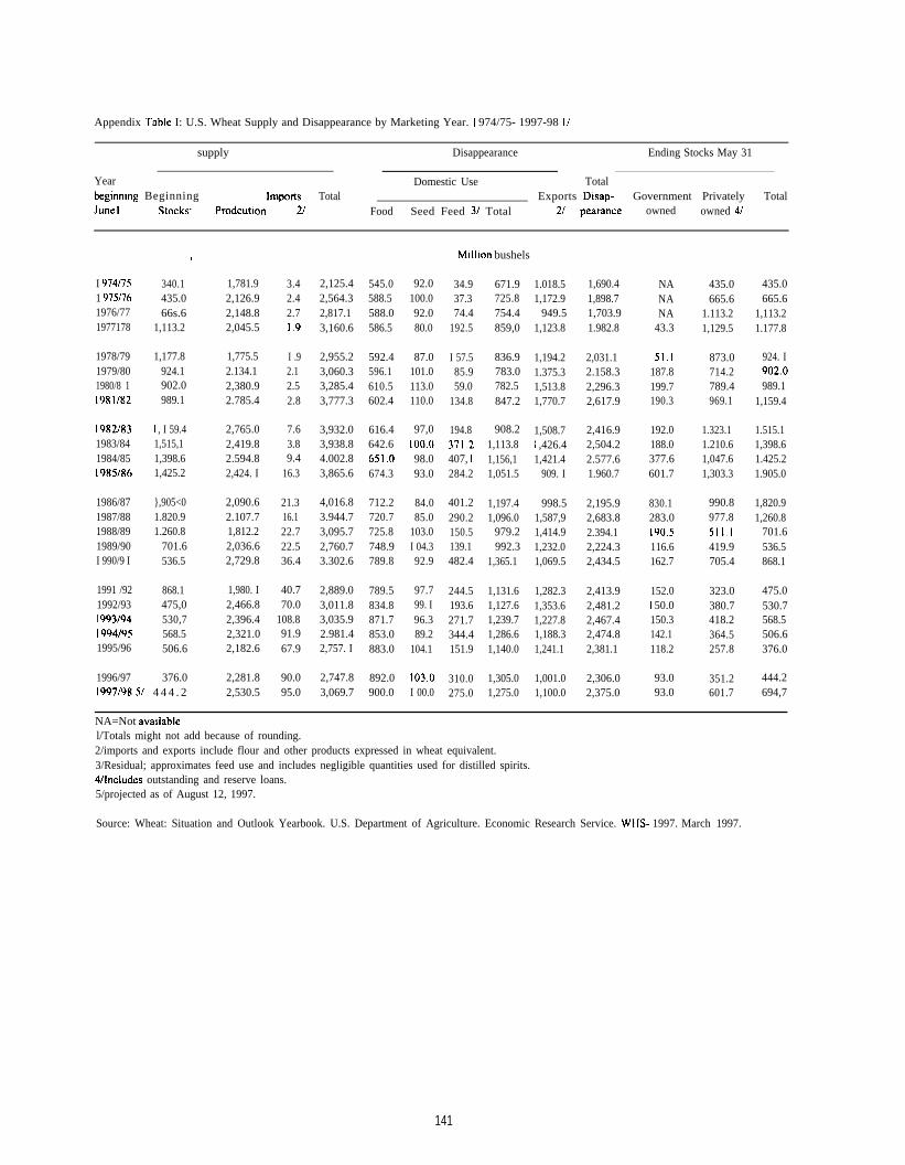
Appendix Table I: U.S. Wheat Supply and Disappearance by Marketing Year. ] 974/75- 1997-98 1/

supply Disappearance Ending Stocks May 31

Year Domestic Use Totalbqynning Beginning lmpcms Total Exports Disap- Government Privately TotalJunel Stocks- Prodcutlon 2/ Food Seed Feed 31 Total 2/ pearance owned owned 4/

, Milhon bushels

I 9741751 975/761976/771977178

1978/791979/801980/8 11981 /82

1982/831983/841984/851985/86

1986/871987/881988/891989/90I 990/9 I

1991 /921992/93I 993194I 994/951995/96

1996/97

340.1435.066s.6

1,113.2

1,177.8924.1902.0989.1

I , I 59.41,515,11,398.61,425.2

},905<01.820.91.260.8

701.6536.5

868.1475,0530,7568.5506.6

376.0

1,781.92,126.92,148.82,045.5

3.42.42.71.9

2,125.42,564.32,817.13,160.6

545.0588.5588.0586.5

92.0100.092.080.0

34.937.374.4

192.5

671.9725.8754.4859,0

1.018.51,172.9

949.51,123.8

1,690.41,898.71,703.91.982.8

NANANA

43.3

51. I187.8199.7190.3

192.0188.0377.6601.7

830.1283.0190.5116.6162.7

152.0I 50.0150.3142.1118.2

93.093.0

435.0665.6

1.113.21,129.5

435.0665.6

1,113.21.177.8

1,775.52.134.12,380.92.785.4

I .92.12.52.8

2,955.23,060.33,285.43,777.3

592.4596.1610.5602.4

87.0101.0113.0110.0

I 57.585.959.0

134.8

836.9783.0782.5847.2

1,194.21.375.31,513.81,770.7

2,031.12.158.32,296.32,617.9

873.0714.2789.4969.1

924. I902.0989.1

1,159.4

2,765.02,419.82.594.82,424. I

7.63.89.4

16.3

3,932.03,938.84.002.83,865.6

616.4642.6651.O674.3

97,0100.098.093.0

194.8371.2407, !284.2

908.21,113.81,156,11,051.5

1,508.7! ,426.41,421.4

909. I

2,416.92,504.22.577.61.960.7

1.323.11.210.61,047.61,303.3

1.515.11,398.61.425.21.905.0

2,090.62.107.71,812.22,036.62,729.8

21.316.122.722.536.4

4,016.83.944.73,095.72,760.73.302.6

712.2720.7725.8748.9789.8

84.085.0

103.0I 04.392.9

401.2290.2150.5139.1482.4

1,197.41,096.0

979.2992.3

1,365.1

998.51,587,91,414.91,232.01,069.5

2,195.92,683.82.394.12,224.32,434.5

990.8977.8511.1419.9705.4

1,820.91,260.8

701.6536.5868.1

1,980. I2,466.82,396.42,321.02,182.6

40.770.0

108.891.967.9

2,889.03,011.83,035.92.981.42,757. I

789.5834.8871.7853.0883.0

97.799. I96.389.2

104.1

244.5193.6271.7344.4151.9

1,131.61,127.61,239.71,286.61,140.0

1,282.31,353.61,227.81,188.31,241.1

2,413.92,481.22,467.42,474.82,381.1

323.0380.7418.2364.5257.8

475.0530.7568.5506.6376.0

2,281.82,530.5

90.095.0

2,747.83,069.7

892.0900.0

103.OI 00.0

310.0275.0

1,305.01,275.0

1,001.01,100.0

2,306.02,375.0

351.2601.7

444.2694,71997/98 5/ 4 4 4 . 2

NA=Not availablel/Totals might not add because of rounding.2/imports and exports include flour and other products expressed in wheat equivalent.3/Residual; approximates feed use and includes negligible quantities used for distilled spirits.4/lnciudes outstanding and reserve loans.5/projected as of August 12, 1997.

Source: Wheat: Situation and Outlook Yearbook. U.S. Department of Agriculture. Economic Research Service. WHS- 1997. March 1997.

141

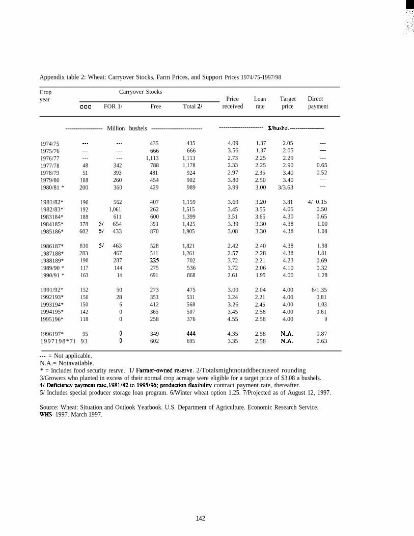
Appendix table 2: Wheat: Carryover Stocks, Farm Prices, and Support Prices 1974/75-1997/98

Crop Carryover Stocksyear Price Loan Target Direct

ccc FOR 1/ Free Total 21 received rate price payment

1974/751975/761976/771977/781978/791979/801980/81 *

1981/82*1982/83*1983184*1984185*1985186*

1986187*1987188*1988189*1989/90 *1990/91 *

1991/92*1992193*1993194*1994195*1995196*

1996197*

------------------- Million bushels -------------------------- --------------------- $/bushel -----------------

---------4851

188200

190192188378602

830283190117163

152150150142118

951997198*7I 93

---------

342393260360

5621,061

6115/ 65451 433

5/ 463467287144

14

5028

600

00

435666

1,113788481454429

407262600393870

528511225

275691

273353412365258

349602

435666

1,1131,178

924902989

1,1591,5151,3991,4251,905

1,8211,261

702536868

475531568507376

695

4.093.562.732.332.973.803.99

3.693.453.513.393.08

2.422.573.723.722.61

3.003.243.263.454.55

4.353.35

1.371.372.252.252.352.503.00

3.203.553.653.303.30

2.402.282.212.061.95

2.042.212.452.582.58

2.582.58

2.052.052.292.903.403.40

3/3.63

3.814.054.304.384.38

4.384.384.234.104.00

4.004.004.004.004.00

N.A.N.A.

---------

0.650.52

------

4/ 0.150.500.651.001.08

1.981.810.690.321.28

6/1.350.811.030.61

0

0.870.63

--- = Not applicable.N.A.= Notavailable.* = Includes food security resrve. l/Farmer-ov.medreserve. 2/Totalsmightnotaddbecauseof rounding3/Growers who planted in excess of their normal crop acreage were eligible for a target price of $3.08 a bushels.4/Deficiencypaymentrate, 1981/82to1995/96;productiontlexibility contract payment rate, thereafter.5/ Includes special producer storage loan program. 6/Winter wheat option 1.25. 7/Projected as of August 12, 1997.

Source: Wheat: Situation and Outlook Yearbook. U.S. Department of Agriculture. Economic Research Service.WHS- 1997. March 1997.

142

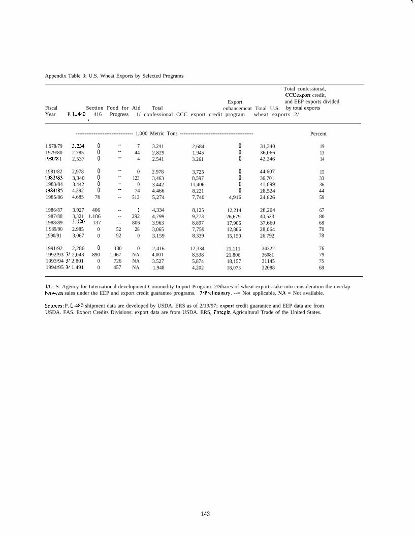
Appendix Table 3: U.S. Wheat Exports by Selected Programs

Total confessional,CCCexport credit,

Export and EEP exports dividedFiscal Section Food for Aid Total enhancement Total U.S. by total exportsYear P. L.480 416 Progress 1/ confessional CCC export credit program wheat exports 2/

I

-------------------------------- 1,000 Metric Tons ----------------------------------------- Percent

1 978/79 3,2341979/80 2.7851980/8 1 2,537

0 --0 --0 --

744

4

0123

074

513

1292806

280

0NANANA

3.2412,8292.541

2,6841,9453.261

000

31,34036,06642.246

191314

1981/82 2,9781982/83 3,3401983/84 3.4421984/85 4.3921985/86 4.685

0 --0 --0 --0 --

76 --

2.9783,4633.4424.4665,274

3,7258,597

11,4068,2217,740

0000

4,916

44,60736,70141,69928,52424,626

1533364459

1986/87 3.9271987/88 3,3211988/89 3+()~()1 989/90 2.9851990/91 3,067

406 --1.186 --

137 --0 520 92

4,3344,7993.9633,0653.159

8,1259,2738,8977,7598.339

12,21426,67917,90612,80615,150

28,20440,52337,66028,06426.792

6780687078

1991/92 2,2861992/93 3/ 2,0431993/94 3/ 2.8011994/95 3/ 1.491

0 130890 1,067

0 7260 457

2,4164,0013.5271.948

12,3348,5385,8744,202

21,11121.80618,15718,073

34322360813114532088

76797568

l/U. S. Agency for International development Commodity Import Program. 2/Shares of wheat exports take into consideration the overlapbetween sales under the EEP and export credit guarantee programs. 3/Prelin~inary. --= Not applicable. NA = Not available.

!%urces: P. L.480 shipment data are developed by USDA. ERS as of 2/19/97; export credit guarantee and EEP data are fromUSDA. FAS. Export Credits Divisions: export data are from USDA. ERS, Foregin Agricultural Trade of the United States.

143

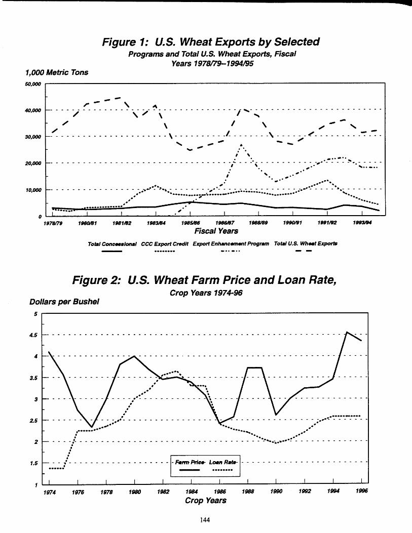
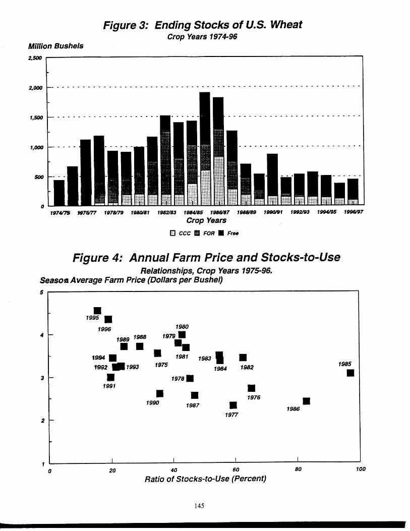
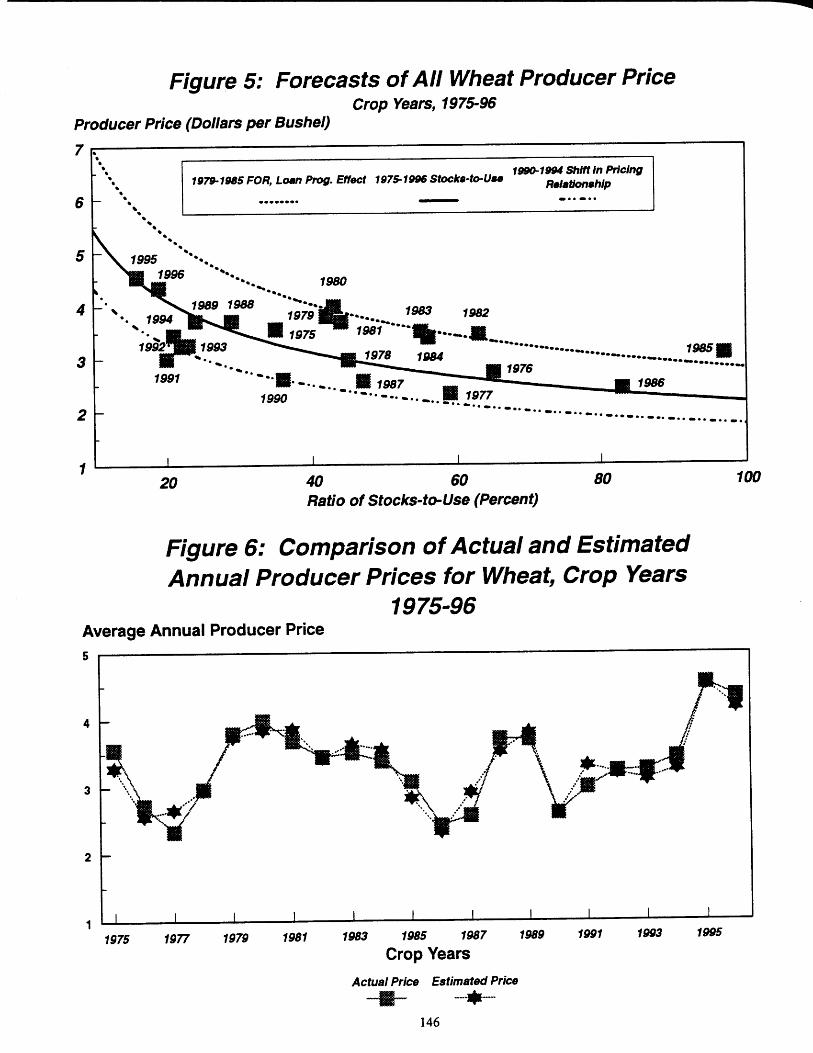
AN ANNUAL MODEL FOR FORECASTING CORN PRICESPaul C. Westcott, Economic Research Service, USDA

The U.S. com crop plays a major role in theagricultural sector. As a source of income to farmers,com is the largest crop in terms of cash receipts. Overthe last 5 years, com cash receipts have averaged morethan $16 billion; accounting for about 17 percent oftotal crop cash receipts. Corn also has an importantrole in linkages within the agricultural sector amongvarious crops and between crops and livestock. Corncompetes with other crops for land in farmers’production decisions, particularly soybeans. Corn isalso the largest feed grain used by the livestock sector.Further, the U.S. is the largest exporter of corn,accounting for over 70 percent of global com trade thusfhr in the 1990s. Consequently, events which affect thecorn sector and com prices are carefully watched bymany subsectors within agriculture.

New agricultural legislation enacted in 1996fundamentally changed the nature of farm commodityprograms in the United States, furthering trendstowards market orientation in the sector. In particular,changes in the income support program shifted much ofthe risk of price volatility from the Government toproducers (see Young and Westcott). As a result,market information affecting com prices is particularlyimportant under the 1996 Farm Act as farmers seek tomake informed farm management decisions to managerisk and other market participants work within a moremarket-oriented agricultural sector.

To provide market information regarding theagricultural sector, each month the U.S. Department ofAgriculture (USDA) analyzes major agriculturalcommodity markets and publishes annual supply,demand, and price projections for the current year.Additionally, once a year USDA publishes longer-term,10-year projections for the agricultural sector thatinclude commodity supply, demand, and prices.

This paper examines some of the factors that affectfarm-level com prices. An annual fiarnework isemployed to develop a com price model, designed tobe used in USDA’s projection activities in conjunctionwith ongoing commodity market analysis of supply anddemand factors. The relationship estimated builds on2 types of factors that influence prices--market supplyand demand conditions, and Government price supportprograms.

Market forces, as measured by supply and demand,influence prices. Year-ending stocks of an annuallyproduced commodity, such as corn, summarize theeffects of both supply and demand factors during theyear, and are a usetil indicator of price movements forthe commodity. Annual prices for grains tend to havea strong negative correlation with their ending stocks.High stocks typically result in lower prices, while lowstocks put upward pressure on prices.

Government programs have also been important ininfluencing farm-level prices for grains. Someprograms have influenced prices indirectly by placingrestrictions on the use of land for agriculturalproduction, for example. Historically, the nonrecoursecommodity loan program has directly affected pricesby providing support to farm-level prices and affectingmarket equilibrium in some periods. The key policyvariable used in the price modeling effort in this paperis the price support loan rate. However, the role of theloan rate in influencing prices has differed historicallyas the nature of the commodity loan program haschanged under different farm legislation.

Previous Research

Many com price models have employed the stocks-to-use ratio to represent market conditions in explainingmovements in com prices. The stocks-to-use ratio isdefined as stocks of the commodity at the end of aparticular time period divided by use of the commodityduring that time period. As such, market conditions ofsupply and demand are summarized in this measure.Van Meir, and Baker and Menzie used stocks-to-useratios in annual frameworks analyzing com prices,while Westcott, Hull, and Green used such an approachin a quarterly model for com prices. Numerous otherunpublished annual com price models using stocks-to-use ratios have been used internally within USDA in itsforecasting activities. In each model, the stocks-to-usevariable is negatively related to com prices andprovides a downward sloping nonlinear cuwe of pricesplotted against ending stocks-to-use,

To represent the effects of Governmental price supportprograms on prices, many grain price models have beenestimated with the dependent variable of price minusloan rate. The Baker and Menzie annual com price

147

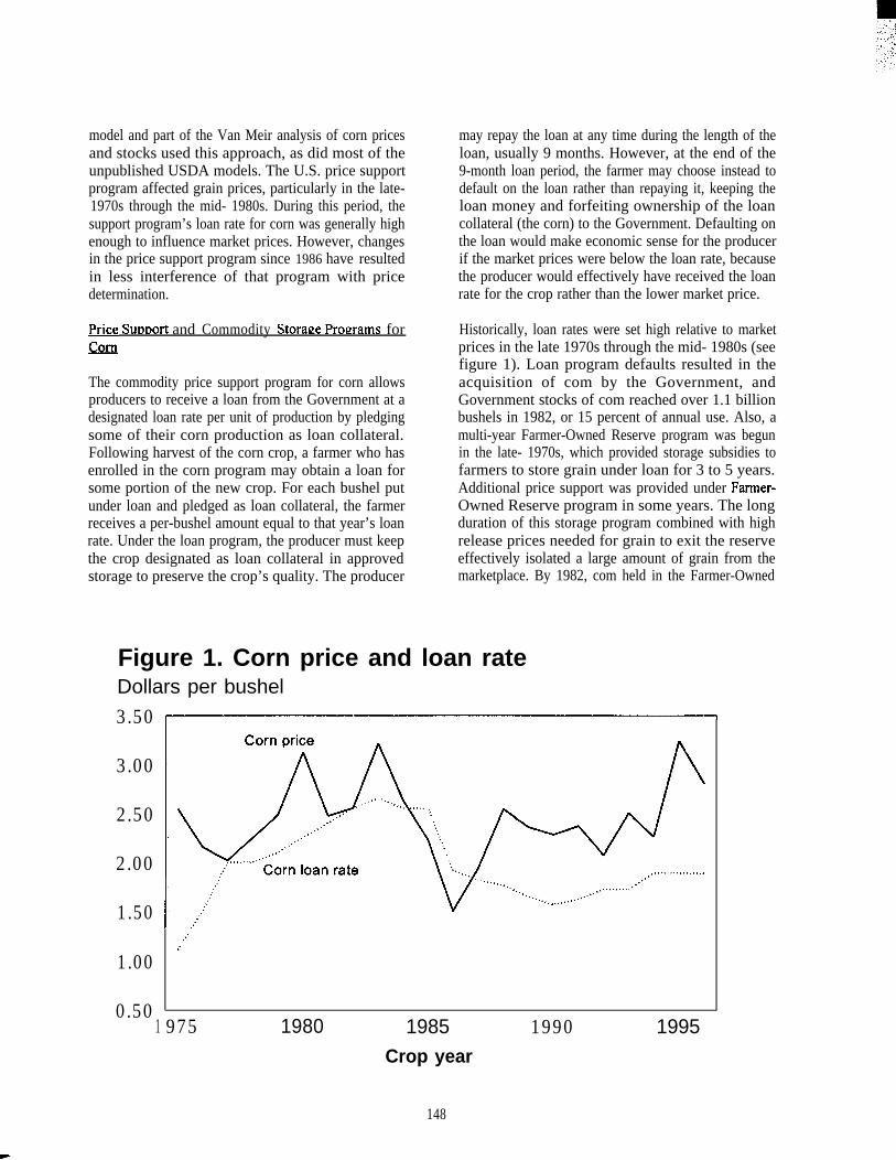
model and part of the Van Meir analysis of corn pricesand stocks used this approach, as did most of theunpublished USDA models. The U.S. price supportprogram affected grain prices, particularly in the late-1970s through the mid- 1980s. During this period, thesupport program’s loan rate for corn was generally highenough to influence market prices. However, changesin the price support program since 1986 have resultedin less interference of that program with pricedetermination.

J%ice Sumort and Commodity Storage Promams forQ2!ll

The commodity price support program for corn allowsproducers to receive a loan from the Government at adesignated loan rate per unit of production by pledgingsome of their corn production as loan collateral.Following harvest of the corn crop, a farmer who hasenrolled in the corn program may obtain a loan forsome portion of the new crop. For each bushel putunder loan and pledged as loan collateral, the farmerreceives a per-bushel amount equal to that year’s loanrate. Under the loan program, the producer must keepthe crop designated as loan collateral in approvedstorage to preserve the crop’s quality. The producer

may repay the loan at any time during the length of theloan, usually 9 months. However, at the end of the9-month loan period, the farmer may choose instead todefault on the loan rather than repaying it, keeping theloan money and forfeiting ownership of the loancollateral (the corn) to the Government. Defaulting onthe loan would make economic sense for the producerif the market prices were below the loan rate, becausethe producer would effectively have received the loanrate for the crop rather than the lower market price.

Historically, loan rates were set high relative to marketprices in the late 1970s through the mid- 1980s (seefigure 1). Loan program defaults resulted in theacquisition of com by the Government, andGovernment stocks of com reached over 1.1 billionbushels in 1982, or 15 percent of annual use. Also, amulti-year Farmer-Owned Reserve program was begunin the late- 1970s, which provided storage subsidies tofarmers to store grain under loan for 3 to 5 years.Additional price support was provided under Farrner-Owned Reserve program in some years. The longduration of this storage program combined with highrelease prices needed for grain to exit the reserveeffectively isolated a large amount of grain from themarketplace. By 1982, com held in the Farmer-Owned

Figure 1. Corn price and loan rateDollars per bushel

3.50

3.00

2.50

2.00

1.50

1.00

0.501

,.’

.’

975 1980 1985 1990 1995Crop year

148

m-

Reserve rose to almost 1.9 billion bushels, about 26percent of annual use.

Changes in the price support program since 1986 haveresulted in less interference of that program with pricedetermination., Farm legislation enacted in 1985significantly changed the loan program and the effectof price supports on market prices, starting in 1986.Prices supports for grains were sharply reduced. Theloan rate for corn was lowered from $2.55 per bushelfor 1985 to $1.92 per bushel in 1986. Additionally, nofurther com was permitted to enter the Farmer-OwnedReserve during 1986-1990. Also, com in the reservewas more accessible to the marketplace as a new policyinstrument introduced under the 1985 farm law, genericcertificates, allowed early access to grain in the reservebefore its contract expiration. Essentially, the loanprogram continued to provide producers a source ofshort term liquidity, but it no longer supported comprices.

Policy changes since 1990 have continued to keep theprice supporting aspects of the loan program at aminimum. Since 1986, the com loan rate has rangedfrom $1.57 per bushel to $1.92 per bushel, well belowmarket prices for com in most years. Implementationof marketing loans for com starting in 1993, whichallow repayment of loans at less than the original loanrate, fhrther reduced the loan program’s potential effecton market prices. As a consequence, since 1986, pricedetermination for com has largely occurred in themarketplace based on supply and demand conditionswithout the influence of the Government price supportprogram.

The Model

The general framework used here relating prices toending stocks derives from an equilibrium model. Inits simplest form, without the Government pricesupport program, supply, demand, and stocks are eacha fi.mction of price, with the market-clearing,equilibrium condition of determining the price at whichsupply equals demand plus stocks (equations 1-4).

(1) S= f(p) (Supply fhnction)

(2) D=g(p) (Demand function)

(3) K=h(p) (Stocks Iimction)

(4) S- D-K=O (Equilibrium condition)

S is supply, D is demand, K is ending stocks, and p ismarket price. Supply is positively related to pricewhile demand and stocks are negatively related toprice.

In equilibrium, prices can be determined from theinverse of the supply, demand, or stocks fhnction.Taking the inverse of the stocks fimction provides aprice determination equation, with prices negativelyrelated to stocks.

(5) p = h-l(K) (Inverse stocks function;price equation)

Introducing the Government price support loanprogram adds to the stocks fimction by incorporatingthe commodity loan rate to the function, as representedin equation 3a.

(3a) K = h (p; LR) (Stocks fi.mction withGovernment loanprogram)

K’ is the revised stocks fimction and LR represents theloan rate. The Government loan program provides anadditional feature to stockholding behavior thatdepends on the loan rate incentive to use the loanprogram,

With this alternative stocks function, the inverse stocksfunction gives the following price determinationequation.

(5a) p = h-i(K; LR)

Prices would be expected to be negatively related tostocks. Prices would be expected to be positivelyrelated to the loan rate, particularly in those years thatloan rates were set high relative to market clearingprice levels and the Farmer-Owned Reserve isolatedstocks from the marketplace, thereby resulting ininterference of the loan program with pricedetermination.

Mode ImplementatloQ1.

The fictional form used to estimate equation 5a forannual com prices is logarithmic. Semi-log andexponential Iimctional forms can alternatively be usedand provide similar estimation results to thosepresented here.

(6) Ln (p)= a + b Ln (K’AJ)

+ c Ln (LR) * Dum7985

149

U represents annual com utilization, Dum7985represents a dummy variable equal to 1 in 1979-1985and equal to O in other years, and a, b, and c areparameters to be estimated.

In equation 6, stocks (K’) are measured relative to anindicator of the “scale of activity” in the com sector,represented by the realized level of demand, actualutilization (U). This adjustment is needed because ofgrowth in the com sector over the last 20 years, so aparticular level of stocks today represents a smallerportion of total use (or realized industry demand) thanthe same level of stocks in 1975. The result is a stocks-to-use variable commonly used in price models,providing a measure of relative market tightness for thecommodity. The expected sign of the stocks-to-usecoefficient (b) is negative.

The interaction term of the loan rate (LR) times thedummy variable (Dum7985) represents the effects ofthe loan program on com prices from the late-l 970sthrough the mid- 1980s. The years chosen for theinteraction term were when the commodity loanprogram, in conjunction with the structure of theFarmer-Owned Reserve program, resulted in the loanrate interfering with the sector reaching its marketclearing price level. Loan rates were relatively high inthose years and the multi-year Farmer-Owned Reserveprogram, with high release prices, isolated thosereserve stocks from the market. The price supportingaspects of the loan program in those years imply thatthe expected sign for the coefficient (c) for the loan rateinteraction term is positive.

The specification of the interaction term represents anintercept shift related to the loan rate rather than a slopeshift related to the stocks-to-use variable. Analternative specification that included a slope shiftadjustment for 1979-1985 produced a result that wasnot statistically significant.

Farm-level prices used to estimate the model are seasonaverage prices collected by the U.S. Department ofAgriculture’s National Agricultural Statistics Serviceand re-published in the Economic Research Service’sFeed Situation and Outlook Yearbook (March 1997).Stocks, utilization, and loan rate data also are from theFeed Situation and Outlook Yearbook.

Model Resul@

The model was estimated using ordinary least squaresregression, with annual data from 1975 through 1996.The estimated logarithmic regression equation is

(7) Ln (p)= 1.539-0.2426 Ln (K’/U)(19.2) (9.1)

+ 0.2896 Ln (LR) * Dum7985(7.3)

R*= 0.845 D.W. = 1.854

with t-statistics shown in parentheses under eachcoefficient.

Over 84 percent of the variation in annual com pricesis explained by estimated equation 7. Each coefllcienthas the expected sign, with a negative sign for thestocks-to-use variable and a positive sign for the loanrate shift variable. Each coefllcient is significant at the1 percent level.

A graph of the regression equation results is shown infigure 2, adjusting from logarithms to levels of eachvariable. Corn prices are plotted against ending stocks-to-use ratios. The circles in figure 2 represent thehistorical observations for the 1975-1996 estimationperiod. The lower price curve applies for all yearsexcept 1979-1985 and represents the equation thatwould currently be used for forecasting com prices.The higher price curve represents the years 1979-1985,which incorporates the average price supporting effectof high loan rates in those years. The averagedifference between the 2 price curves for the1979-1985 period is about 60 cents a bushel.

Model Evaluatio~

Figure 3 shows a graph of the predicted values derivedfrom estimated equation 7 along with the actual comprices. In general, the price model tracks actual comprices well. Most differences between the modelestimate and the actual com price are less than 15 centsa bushel. The largest difference is in 1988, the year ofa major drought in the Corn Belt region of the UnitedStates.

150

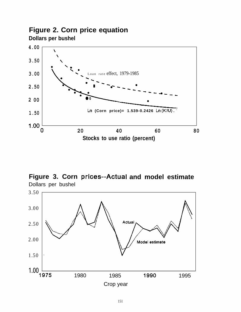
Figure 2. Corn price equationDollars per bushel

4.00

3.50

3.00

2.50

2 00

1.50

\\\

● ✼

L o a n r a t e effect, 1979-1985

a-●

●

●

● 0●

--

Ln (Corn price)= 1.539-0.2426 Ln (K’/U) . –

20Stocks

40to use ratio

Figure 3. Corn prices--ActuaDollars per bushel

3.50

3.00

2.50

2.00

1.50

60(percent)

80

and model estimate

1.001975 1980 1985 1990 1995

Crop year

151

.,

Table 1 --Model performsnce measures. se ected De1 riods

Mean Mean absoluteTime Deriod absolute error ~ercenQge error

Cents per bushel Percent

1975-1996 12.1 5.1

1990-1996 9.7 4.6

Table 1 shows mean absolute errors and mean absolutepercentage errors for the full estimation period,1975 -1!396, and for a selected subsample of recentyears covering 1990-1996. For the full sample, themean absolute error is about 12 cents a bushel, with amean absolute percentage error of about 5 percent.Importantly, for price forecasting applications, modelperformance is somewhat better in recent years (the1990s), with a mean absolute error under 10 cents abushel and a mean absolute percentage error of 4.6percent. These statistical performance measuresindicate good performance for the corn price model.

Cone lusion~

The corn price model presented in this paper uses astocks-to-use ratio formulation. The model alsoaddresses issues regarding the historical influence ofGovernment commodity loan and storage programs oncom price determination. Loan programs are shown tohave had an effect on corn prices in the late-l 970sthrough mid- 1980s. However, with farm programchanges of 1985 farm legislation, lower loan rates andother features of commodity loan and storage programshave not had as much influence on prices over the lastdecade. Price determination now occurs in themarketplace, based on supply and demand factors. Thestocks-to-use ratio used in the model captures thesemarket effects.

The statistical performance measures as well as thegraph of actual prices and model estimates indicategood performance for the corn price model. This isparticularly the case given the large range of cornprices over the sample period used to estimate themodel (1975- 1996) as well as the changing nature ofthe influence of Government programs on com pricedetermination.

The relatively simple structure of the estimated reducedform model for com prices and the model’s minimaldata requirements lend itself to easy use in com priceforecasting applications in conjunction with marketanalysis of supply and demand conditions. Inparticular, the model is used within USDA as part ofthe Department’s short-term market analysis and long-term projections activities.

Baker, Allen and Keith Menzie. “Drought Effects onCorn Price Forecasts,” Feed Situation and OutlookReport, FdS-307, USDA-ERS, August 1988, pp.25-28.

Lin, William, Peter Riley, and Sam Evans. FeedGrains: Background for 1995 Farm Legislation.AER-7 14, USDA-ERS, April 1995.

U.S. Department of Agriculture. Economic ResearchService. Feed Situation and Outlook Yearbook.FDS-1 997, March 1997.

U.S. Department of Agriculture. Economic ResearchService. Storage Subsidy Programs. Staff ReportAGES-9075, December 1990.

Van Meir, Lawrence W. “Relationships AmongEnding Stocks, Prices, and Loan Rates for Corn,” FeedOutlook and Situation Report, FdS-290, USDA-ERS,August 1983, pp. 9-13.

Westcott, Paul C., David B. Hull, and Robert C. Green.“Relationships between Quarterly Corn Prices andStocks,” Agricultural Economics Research, Vol. 37,No. 1, Winter 1985, pp. 1-7.

Young, C. Edwin and Paul C. Westcott. The 1996U.S. Farm Act Increases Market Orientation,Agricultural Information Bulletin 726, August 1996.

152

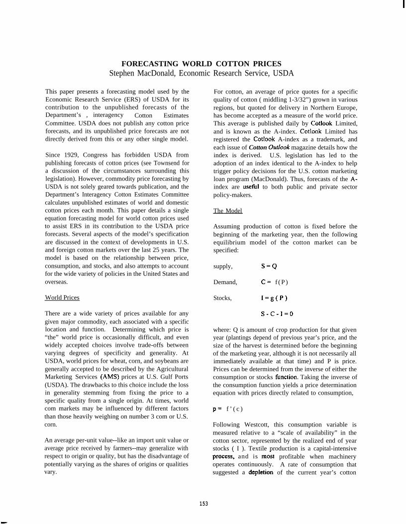
FORECASTING WORLD COTTON PRICESStephen MacDonald, Economic Research Service, USDA

This paper presents a forecasting model used by theEconomic Research Service (ERS) of USDA for itscontribution to the unpublished forecasts of theDepartment’s , interagency Cotton EstimatesCommittee. USDA does not publish any cotton priceforecasts, and its unpublished price forecasts are notdirectly derived from this or any other single model.

Since 1929, Congress has forbidden USDA frompublishing forecasts of cotton prices (see Townsend fora discussion of the circumstances surrounding thislegislation). However, commodity price forecasting byUSDA is not solely geared towards publication, and theDepartment’s Interagency Cotton Estimates Committeecalculates unpublished estimates of world and domesticcotton prices each month. This paper details a singleequation forecasting model for world cotton prices usedto assist ERS in its contribution to the USDA priceforecasts. Several aspects of the model’s specificationare discussed in the context of developments in U.S.and foreign cotton markets over the last 25 years. Themodel is based on the relationship between price,consumption, and stocks, and also attempts to accountfor the wide variety of policies in the United States andoverseas.

World Prices

There are a wide variety of prices available for anygiven major commodity, each associated with a specificlocation and function. Determining which price is“the” world price is occasionally difficult, and evenwidely accepted choices involve trade-offs betweenvarying degrees of specificity and generality. AtUSDA, world prices for wheat, corn, and soybeans aregenerally accepted to be described by the AgriculturalMarketing Services (AMS) prices at U.S. Gulf Ports(USDA). The drawbacks to this choice include the lossin generality stemming from fixing the price to aspecific quality from a single origin. At times, worldcom markets may be influenced by different factorsthan those heavily weighing on number 3 com or U.S.corn.

An average per-unit value--like an import unit value oraverage price received by farmers--may generalize withrespect to origin or quality, but has the disadvantage ofpotentially varying as the shares of origins or qualitiesvary.

For cotton, an average of price quotes for a specificquality of cotton ( middling 1-3/32”) grown in variousregions, but quoted for delivery in Northern Europe,has become accepted as a measure of the world price.This average is published daily by Cotlook Limited,and is known as the A-index. Cotlook Limited hasregistered the Cotlook A-index as a trademark, andeach issue of Cotton Out/ook magazine details how theindex is derived. U.S. legislation has led to theadoption of an index identical to the A-index to helptrigger policy decisions for the U.S. cotton marketingloan program (MacDonald). Thus, forecasts of the A-index are usefi.d to both public and private sectorpolicy-makers.

The Model

Assuming production of cotton is fixed before thebeginning of the marketing year, then the followingequilibrium model of the cotton market can bespecified:

supply, S.Q

Demand, c= f ( P )

Stocks, I=g(P)

S-C-1=0

where: Q is amount of crop production for that givenyear (plantings depend of previous year’s price, and thesize of the harvest is determined before the beginningof the marketing year, although it is not necessarily allimmediately available at that time) and P is price.Prices can be determined from the inverse of either theconsumption or stocks finction. Taking the inverse ofthe consumption function yields a price determinationequation with prices directly related to consumption,

p= f ’ ( c )

Following Westcott, this consumption variable ismeasured relative to a “scale of availability” in thecotton sector, represented by the realized end of yearstocks ( I ). Textile production is a capital-intensiveprocess; and is mo~toperates continuously.suggested a depIetion

profitable when machineryA rate of consumption that

of the current year’s cotton

153

supply before the availability of the following year’sharvest would suggest a period during which textileproducers would have no income to meet their fixedcosts. Uncertainty regarding the size, timing, andtransportation of the following year’s crop suggestsconsumption should never be large enough tocompletely deplete the year’s supply by, or evenshortly after, the end of the year. Thus, we are left witha relationship stating prices are directly proportional tothe ratio of consumption and ending stocks, and theimplication that over a long time period thisproportionality can shift as the risk of beginning thenext marketing year with low supplies varies,

p= f-](C/I, Z)

where z is the set of exogenous factors that can shiftthe relationship between current year price anduse/stocks. Figure 1 illustrates how trends in inflation-adjusted cotton prices and global use/stocks havevaried since 1971. The growing divergence betweenthese two variables suggests the relationship has notbeen constant.

In this model the exogenous shift variables include:dummies representing different U.S. agricultural policyregimes, dummies for a few years of specific economicor policy shocks, variables capturing the impact of U.S.payments to cotton exporters (under a program that hasmade payments to both domestic users and exporters ofcotton), and variables capturing consumers’expectations of changes in the cost of consumingcotton. A real U.S. exchange rate is also included as aseparate variable since much of the world’sconsumption occurs in economies where neither costsnor returns are calculated in U.S. dollars. This could bespecified by adjusting the A-index (which is reportedin terms of U.S. currency) by the exchange rate.However, exchange rate changes are not exactly thesame as changes in product prices (Goldstein andKhan), so the exchange rate was used as an explanatoryvariable, and the price remained in U.S. currency.

Given the somewhat ad-hoc nature of the exogenousshift variables introduced into the model, hypothesistesting of parameter values is not reliable, However,the model is still suitable for forecasting purposes sincethe large number of explanatory variables ( 11 ) suggeststhe danger is greater that the model includes irrelevantvariables than is the danger that it omits relevantvariables. Omitting relevant variables introduces biasand inconsistency into the parameter estimates for theincluded variables, in most cases (Pindyck andRubinfeld). Irrelevant variables reduce efilciency but

do not introduce bias or inconsistency, and, when theconcern is with forecasting rather than hypothesistesting, the cost of mistakenly excluding a relevantvariable is greater than the cost of including one that isirrelevant. Therefore, some variables for which theorysuggests inclusion, but test statistics suggest omission,remain in the model.

Data

The dependent variable ( P ) was an unweighedmarketing year average of the daily A-index in U.S.currency, adjusted by the U.S. GDP deflator. This isthe deflator used for all the real prices in USDA’sbaseline forecasts. The stocks variable ( I ) is worldending stocks according to USDA’s official database,minus China’s ending stocks. Similarly, theconsumption variable ( C ) is world consumption minusChina’s consumption, plus an additional factor. Theadditional factor added to consumption is net importsby China. These data are published in USDA’s Cottonand Wool Situation and Outlook Yearbook. Theseadjustments largely reflect the uncertainty regarding theactual amount of cotton produced, consumed, andstored in China. One source of this uncertainty is thelack of a clear relationship between China’s apparentdomestic cotton supplies and its trade volume.Regardless of whether or not China’s consumption andstocks have been correctly estimated, China’sgovernment prevents the rest of the world fromaccessing China’s stocks at will, and preventsconsumers in China from accessing world stocks atwill. In a given year, China’s most important effect onworld prices comes from its trade, which either adds tocotton consumption when China is a net importer, oreffectively reduces world consumption when China isa net exporter. These adjustments are similar to thosefollowed by the International Cotton AdvisoryCommittee (ICAC) in its world price forecastingmodel. One difference is that the ICAC includesChina’s trade as a separate variable rather than addingit to consumption or stocks.

The model was estimated over 1971-95, since 1971 isinitial year of the macroeconomic database developedfor ERS’S long-range baseline forecasting for thePresident’s Budget (USDA). A semi-logarithmicilmctional form is used since the non-linear relationshipcaptured turning points slightly better.

The estimated equation is (t-statistics in parentheses):

154

Ln(P) = 7.70-0.47 Dum8695 -0.22 Dum9195(23.8) (5.1) (3.0)

-0.29 Dum8485 + 0.54 Dum73 + 0.15 Dum7476(3.9) (6.8) (2.8)

-0.74 Step2 -0.44 Step2d + 2.87 Infl -0.45 Prodd(0.5) (1.0) (1.97) (2.6)

-0.004 Xr + 0.~8 C/l(1.97) (3.9)

R2= .98 D.W .= 2.54

Figure 2 illustrates the performance of themodel.

estimated

Dum8695 is a variable with the value of 1 during 1986-1995 and zero otherwise. Dum9 195 is a variable withthe value 1 during 1991-1995 and zero otherwise.These dummies correspond to shifts in U.S. agriculturalpolicy which significantly changed the relationshipbetween prices and stockholding for all commodities inthe United States, the world’s largest cottonstockholder throughout much of the period analyzed.The United States has held as much as 35 percent of theworld’s non-Chinese stocks before 1986, but hasremained below 20 percent every year since 1988.

Recall the divergence in trends in prices and the worlduse/stock ratio illustrated in Figure 1. While some ofthis divergence represents improvements in globalcommunication, transportation, and trade that reducethe risk of not holding stocks, a large part of thedivergence represents progressive changes in U.S.government efforts to keep U.S. cotton stocks off themarket.

Dum8485 is a variable with the value 1 in 1984-1985and O otherwise. It represents the combined effect ofanticipation of the 1985 U.S. farm legislation and ashift in China’s trade policy. The 1985 U.S. farmlegislation lowered the high loan rates of the 1981legislation and opened U.S. stocks to world markets fora variety of commodities. World prices fell inmarketing year 1984 as the legislation took shape,partly in anticipation of lower prices in the subsequentyear, and continued falling as lower priced productionand pent-up stocks from the United States subsequentlybecame available. These years also mark the initiationof large exports by Chin% only a few years after Chinahad culminated 19 years of continuous net imports bybecoming the world’s largest importer. Between 1980and 1985, China went from the world’s largest importer

to the world’s largest exporter. China has generallybeen a net importer since then. Thus, it is notaltogether clear if Dum8485 is capturing just the effectof U.S. policy, Chinese policy, or both.

Dum73 and Dum7476 are variables with the value 1 in,respectively, 1973 and 1974-76. The first oil shockand the USSR’s “great grain robbery” (Morgan) of theearly 1970’s introduced significant volatility intocommodity prices. Efforts to capture the volatility inexpectations associated with this price volatilitythrough other variables such as inflation and exchangerates were not completely successful. Simplespecification test ing (Durbin-Watson statistics)indicated that a model that included the years 1971-76with two associated dummies was superior to one thatexcluded these years. In general, a modeler must usejudgement to distinguish between outliers that are soextreme that they suggest measurement error or sim i Iarflaws and events that contain valuable informationabout the process being modeled (Pindyck andRubinfeld).

U.S. MarketinP Loan Program

Step2 is expenditure on exported cotton in a given yearby the U.S. government under Step 2 of the cottonmarketing loan program, divided by the value of allU.S. cotton exports that year. Export values are fromUSDA’s Outlook for U.S. Agricultural Exports anddata on the spending for Step 2 are Ilom USDA’s FarmService Agency. Direct expenditures to support exportsare thereby converted into percent equivalents. Boththe export and expenditure data are on a fiscal year, butthe difference between fiscal and marketing year isonly 2 months, and the two months are those typicallywith the lowest export activity.

Step 2 of the marketing loan program was introducedin the 1990 U.S. farm legislation (MacDonald), so thevariable is zero before 1991. Note that this program isalso available to domestic consumers of cotton, andwas therefore unaffected by the Uruguay RoundAgreement. However, the United States unilaterallymodified the program in 1996 to shift the expenditureseven further in favor of domestic cotton consumers.This suggests that the relationship betweenexpenditures under Step 2 and prices will be differentin the future than what has been estimated here.

The expected sign of this variable is negative, as is theexpected sign of the other variable associated with theStep 2 program, Step2d. Step2d is the first differenceof the Step2 variable. Since the expenditures on

155

exported cotton under the Step 2 program acted like anexport subsidy by a large exporter when they occurredduring 1991-1995, they would be expected to lower theworld price of the commodity (Tweeten). The Step2dvariable is intended to capture the additional effect ofchanges in the expenditures. The Step 2 program is notin effect continuously, and if market participantsassumed the previous year’s expenditures were a guideto the current year, Step2d is the adjustment in theirexpectations.

Step 2 payments to exporters were equivalent to 2-3percent of the value of global raw cotton trade in 1992and 1993, and the relationship between U.S. and worldprices appears to have shified since the step 2 programbegan. During 1972-90, the average premiumMemphis 1-3/32” cotton received in Northern Europeto the A-index was 3.4 percent (excluding the policytransition period just before the 1985 farm legislationtook effect). During 1990-96 the average premium was6.8 percent. The shift from 3.4 percent to 6.8 percentmay stem from the introduction of a price wedgebetween U.S. and world cotton prices through the Step2 program. Some of this price wedge would derivefrom higher U.S. prices, but some would derive fromlower world prices (Tweeten). The t-statistics for theseparameters do not support the hypothesis that either issignificantly different from O. But, as noted earlier,the specification of this model does not lend itself tohypothesis testing. Both variables remain in the modeldue to their ability to improve short-run forecasts whenrecent years of data are dropped from the sample, andout of sample forecasts derived for those years.

One difficulty in determining the impact of the Step 2on world prices is that Step 2 payments are correlatedwith the appearance of inexpensive Central Asiancotton on world markets. The ICAC, rather thanincluding Step 2 data in their model, incorporates thebartered share of Central Asian exports (ICAC). Whiletheory suggests that payments like Step 2 would put aprice wedge between U.S. and world prices, thewidening gap between the price of U.S. cotton and theA-index may also reflect changes in the A-index. Lowproduction costs and falling domestic demand withinthe Former Soviet Union (FSU) meant increasedquantities of Central Asian cotton were available atextraordinarily low cost in the early 1990’s. Significantquantities of FSU cotton were held by formerconsumers which had acquired cotton under traditionalbarter arrangements, and marketing outside of the FSUwas novel for Central Asian exporters. Thus much ofthe cotton left Central Asia under barter arrangements,resulting in its availability on world markets for low

prices when sold for convertible currencies. Illustrativeof the shift in costs to non-FSU markets is the shift inCentral Asian cotton’s rank among exporters: from atypical position of the third least expensive cotton inthe world during the late 1980’s, to consistently theleast expensive during the early 1990’s. More recentlyit has ranked closer to second least expensive.

Prices were particularly low during the 1992 marketingyear when, in addition to the influx of Central Asiancotton, China was a net exporter for the only timebetween 1988-96, and India was exporting afler anunusual decline in its cotton consumption. Much of themarketing year 1993/94 Step 2 export expenditureswere based on commitments made during the 1992/93.

Expectations of exogenous changes in the future cost ofprocuring cotton are assumed to be encompassed bycurrent year inflation and by an average change inproduction over the last 2 years.

Infl is the annual percent change in the U.S. GDPdeflator. It has been assumed that consumers andstockholders believe the current year’s inflation rate isthe best guide to future inflation, which influencestheir willingness to accept a given price at a givenuse/stocks ratio. If inflation is higher, they will accepta higher price, since it reduces the likelihood they willbe able to consummate postponed transactions later ata lower price. The estimated parameter has theexpected positive sign.

Prodd is the average of the percent difference betweenthe previous year’s world production (excluding China)and each of the preceding 2 years. The preceding yearis used because current year’s actual production isgenerally not known until late in the year. While it isa safe assumption that the size of the crop is largelydetermined before the year begins, the poorcommunication and transportation infrastructure of thedeveloping countries that account for much of theworld’s cotton production mean that early seasonestimates of production are unreliable.

Also, since developing countries heavily intervene intheir economies, the price signals their producersreceive are often at variance from those suggested byworld prices. The best guide to the nature of the pricesignals many cotton producers receive, and to theirability to respond to them, is the resulting change inproduction. Since much of government economicpolicy, and the shifts in weather and insect pressures

156

w“

that influence yields, are exogenous from world pricesignals, it is appropriate to incorporate the pastperformance information as an instrument representingthese complex factors in a consumer’s calculation of anappropriate price. As Prodd rises (declines) it isindicative of a rising (falling) exogenous trend incotton availability, and price should fall (rise). Thus,the expected sign of the estimated parameter isnegative. ‘l’he’ estimated parameter’s sign is inaccordance with this expectation.

Finally, Xr is the International Monetary Fund’s trade-weighted, real exchange rate index for the UnitedStates. Weighting exchange rates by some othermeasure than the value of U.S. merchandise trademight seem appropriate, but since a significant portionof cotton imports are for producing textiles whoseultimate consumption occurs in developing countries,the IMF’s weights seemed generalizable.

As the index rises, the strength of the dollar increases,and the cost of cotton in other currencies rises. Thus,as the exchange rate index rises, foreign consumers areless willing to pay a given price in dollars, and theexpected sign of the exchange rate variable parameterestimate is negative. The estimate’s sign is inaccordance with this expectation.

Conclusions

Forecasting a price open to as many changinginfluences as the A-index is difficult. Even after yearsof global economic liberalization, governmentintervention in world cotton markets is significant. Thesecond largest consumer of cotton in the world, India,continues to regulate its exports through quotas, and thesecond largest exporter, Uzbekistan, seems imperviousto changes in world prices.

This model has been built by step-wise regression overseveral years. The variables associated with the Step 2program are the only variables in the model where t-statistics show a pronounced lack of significance. Theyremain in the model nonetheless since theory suggestsa they will affect prices, and because out of sampletesting with truncated data sets gives far more accurateestimates for 1994 and 1995. The change in the Step 2program since 1996 also means that even correctlymodeling the impact of the program on past prices willbe insufficient for forecasting prices in the future.

The mean absolute percent error of the model is 4.4percent over 1971-1995, and the error for its first out ofsample estimate (1996) is 4.7 percent. While this is

promising, the new U.S. Step 2 program, and thepossible specification errors concerning some of theother variables, suggest that further stepwise revisionsin this forecasting model will be needed.

References

Goldstein, Morris, and Moshin S. Khan. “Incomeand Price Effects in Foreign Trade.” In Handbook ofInternational Economics, Vol. II. R. W. Jones andP.B. Kenan (cd.). Elsevier Science Publishers.Amsterdam, Netherlands. 1985.

International Cotton Advisory Committee. Review ofthe World Cotton Situation. Various issues.

MacDonald, Stephen. “Cotton Marketing LoanProgram Shifts Away from Imports.” AgriculturalOutlook. July 1997.

Morgan, Dan. Merchants of Grain. Penguin Books.Harmondswotth, England. 1980.

Pindyck, Robert S., and Daniel L. Rubinfeld.Econometric Models & Economic Forecasts.McGraw-Hill. New York. 1981.

U.S. Department of Agriculture. Economic ResearchService. Cotton and Wool Situation and OutlookYearbook. Various issues.

U.S. Department of Agriculture. Economic ResearchService. International Agricultural BaselineProjections to 2005. Agricultural Economic ReportsNumber 750. Washington, DC. 1997.

Townsend, Terry P. “This Was a High-PoweredInstrument That Sent Its Projectile To the Vitals ofthe Industry--why USDA Does Not Forecast CottonPrices.” In 1989 Proceedings of the Cotton BeltwideConferences. National Cotton Council. 1989.

Tweeten, Luther. Agricultural Trade: Principles andPolicies. Westview Press. Boulder, CO. 1992.

Valderrama, Carlos. “ Modeling International CottonPrices.” In 1993 Proceedings of the Cotton BeltwideConferences. National Cotton Council. 1993.

Westcott, Paul C. “An Annual Model for ForecastingCorn Prices.” Paper presented to Ninth FederalForecasters Conference. Washington, DC.September 1997.

157

w..

. .

. .. .\-

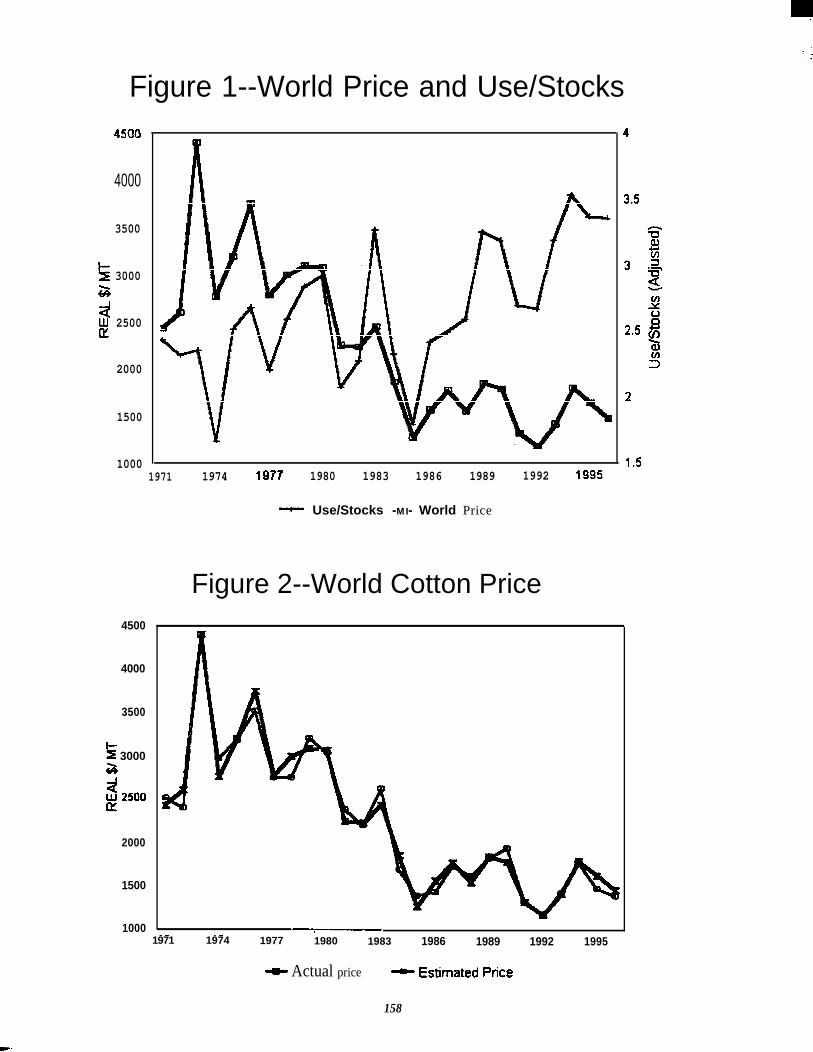
Figure 1--World Price and Use/Stocks4500

4000

3500

s 3000az!U& 2500

2000

1500

10001971 1974 1977 1980 1983 1986 1989 1992 1995

~ Use/Stocks -MI- World Price

Figure 2--World Cotton Price4500

4000

3500

+= 3000a

duJ z500u

2000

1500

1000 -—.-— -—1971 1974 1977 1980 1983 1986 1989 1992 1995

+ Actual price - E~rnated Price

158

FORECAST EVALUATION

Chair: Norman C. SaundersBureau of Labor Statistics, U.S. Department of Labor

An Evaluation of the Census Bureau’s 1995 to 2025 State PopulationProjections-One Year LaterPaul R. Campbell, Bureau of the CensusU.S. Department of Commerce

Evaluating the 1995 BLS Labor Force Projections,Howard N Fullerton, Jr., Bureau of Labor StatisticsU.S. Department of Labor

Industry Employment Projections, 1995: An Evaluation,Arthur Andreassen, Bureau of Labor StatisticsU.S. Department of Labor

Evaluating the 1995 Occupational Employment Projections,Carolyn M. Veneri, Bureau of Labor StatisticsU.S. Department of Labor

159

“An Evaluation of the Census Bureau’s 1995 to 2025 State Population Projections --One Year Later”

Paul R. Campbell, U.S. Bureau of the Census and the Federal Forecasters Conference

Abstract. This paper evaluates the Census Bureau’s 1996state population projection results using recent populationestimates. ] Besides reporting on the accuracy of theprojections, the paper evaluates the components used inthe projections. The results and discussions are useful inidentifying which components of change - births, deaths,interstate migration, and international migration - need tobe fullher refined in order to improve future statepopulation projections produced by the Census Bureau.

Introduction. One step toward improving a frequentlyused population projection model is to examine theaccuracy of the results. This study examines the resultsof the Census Bureau’s recent state projections for July 1,1996 using the latest available state estimates for thesame date. The detailed methodology and results for thestate projections for the 1995-2025 period are available inPopulation Paper Listing 47 ( PPL-47, see Campbell,1996a). Besides state population projection totals thispaper also examines the components of populationchange: births, deaths, state-to-state migration, and netinternational migration. The evaluation of projectionsagainst post-census estimates is an important qualitycontrol tool for both the producers and users of theprojections. This evaluation considers the reliability ofthe projections, identifies changes in population trends,and addresses’ issues related to the efficiency of thecurrent projection model.

The Census Bureau’s state population projections haverecently been evaluated by the producers of theprojections, see Campbell ( 1996b), Wetrogan andCampbell (1990), and Sink (1989 and 1990), as well asother researchers, Smith and Sincich (1992), interested inaccuracy and bias. While demographers at the CensusBureau are frequently evaluating their elaborateprojection model to improve the quality of the results,others are concerned with identifying competing modelsthat may yield just as reliable results.

Some researchers have classified and compared varioussources of state population projection totals, includingthose produced by the Census Bureau. Smith and

Sincich (1992) have identified four general categories:(1) trend projections, where historical trends in statestotal population are extrapolated using mathematicalformulas or statistical techniques; (2) ratio projections,where state population is expressed as a proportion of thenation and the historical trends in proportions areextrapolated and applied to independent projections of thenational population; (3) cohort-component projections,where births, deaths, and migration are projectedseparately for each age-sex cohort in the statespopulation; and (4) structural-causal projections, whererelating population change to economic and/or othervariables are used to project state population. In someinstances these categories overlap.

Smith and Sincich (1992) have evaluated various statepopulation projections for the 1960 to 1990 period --several trend and ratio extrapolation techniques, anARIMA time series model, the Census Bureau’s cohort-component model, and structural models developed bythe Bureau of Economic Analysis (which relatesmigration to projections in employment) and the NationalPlanning Association (economic based model). Theyused the Mean Absolute Percentage Error (MAPE),which is the average error when the direction of error(i.e., positive or negative) are ignored, as well as severalother techniques that measure forecast error. They foundno support for the argument that complex and/orsophisticated projection techniques produce moreaccurate or less biased forecasts than simple, naivetechniques. Nevertheless, less complex projectionmodels usually do not produce as much detaileddemographic information.

This paper f~st describes the evaluation techniques usedin this study and gives a brief overview of the CensusBureau’s state population estimates and projectionsmethodology used to obtain 1996 figures. Second, theevaluation undertaken compares 1996 state populationprojection totals with corresponding state populationestimates. Next, 1995-96 state population projectioncomponents of change are compared with correspondingstate estimates. Finally, the conclusions sectionsummarizes the implications of the results for theimprovement of future state population projections.

‘This paper was presented earlier at the Population Association ofAmerica Meeting, Washington, DC, March 1997.

161

Methods. The Census Bureau’s population projectionsare not forecasts (or predictions) of future populations.However, the evaluation of population projections isoften referred to as the measurement of forecast error.Smith and Sincich ( 1992) note that forecast error refers tothe percentage difference between a population projectionand the ‘true’ population enumerated or estimated for thesame year. To evaluate forecast error in this study, themean absolute percentage error (MAPE) was derived,where:

MAPE=( 100/n) *2[lprojection -estirnatel/estimate]

MAPEs were developed for the United States (the statesand the District of Columbia), where n equaled 51, andfor each census region or division, where n equaled thenumber of states in each region or division (seeArmstrong, 1978, and Smith and Sincich, 1992, forseveral alternative forecast error measurements).

Additionally, the net and percent population differencesat the state level are used to compare the projections andestimates. The results show the size and direction ofgrowth in the state populations and their components ofchange.

There can be some problems with aggregation over statesto get MAPEs (or other statistics) if states differ in thepredictability of their population. For instance, percentdifferences and MAPEs (1) cannot be calculated wheneither populations or components equal zero, or (2) arenot very meaningful when percentages are greater than100 percent.

State Estimates for 1996. State population estimatesused to measure forecast error in the state populationprojections were derived from the Census Bureau’sannual county estimates. These estimates were obtainedfrom a demographic procedure called the “componentchange” method (U.S. Bureau of the Census, 1996a, andU.S. Department of Commerce, 1996). The “componentchange” method update’s population estimates usingadministrative records data for counties. The countypopulation estimates for 1996 were derived from thecontinuous process of updating the 1990 enumeratedcensus population distributions. State estimates wereobtained by summing up the appropriate county estimates.For a detailed discussion on the production of state andcounty estimates, see Byerly and Deardorff (1995).

It is important to note that the 1995 (one year-out) stateprojection totals are more consistent with preliminarystate estimate totals, since the 1995 projections aresummed prorata to the preliminary 1995 state estimatesby age and sex ( released in January 1996, see U.S.Bureau of the Census, 1996b). In other words, the 1995total state population estimates (released during January1996, U.S. Bureau of the Census, 1996a) are a secondround of state population estimates. The state estimatesare not ‘truth’, since subnational estimates are likely to beupdated again as corrections or revisions to administrativerecords data become available during the post-censalperiod. The ‘true’ state population estimates may not becompleted until the next census has been taken and anintercensal evaluation is completed. What this implies isthat for 1995 an evaluation is available for preliminary1995 state population estimate totals using revised 1995state population estimate totals, see Table 1.

Until the state population estimates for the 1990s areaccepted as ‘truth’, the 1996 state estimates (released inDecember 1996) may not bean ideal evaluation standard.The 1996 estimates are likely to be updated when the1997 subnational estimates are released, as well as afterthe 2000 census. However, it appears that current stateestimates are sufficient for an early comparison toprovide useful information. The resulting MAPEs for thepreliminary 1995 state estimates and the updated 1995state estimates in Table 1 suggest that error in the 1995estimates are fairly low. The 1995 MAPEs are muchlower than the one year-out results in previousevaluations (Campbell, 1996b).

State Projections for 1996. The Census Bureau’s statepopulation projection model is a complex demographicmodel that projects the geographic growth of populationsby accounting for annual aging, fertility, mortality,internal migration, and international migration of statepopulations. State population projections prepared forJuly 1, 1995 to 2025 use the cohort-component method.Each component of population change -- births, deaths,internal migration (domestic or state-to-state migrationflows), and international migration (immigration andemigration) -- requires separate projection assumptionsfor each birth cohort by single year of age, sex, race, andHispanic origin. The race and Hispanic origin groupsprojected were non-Hispanic White; non-Hispanic Black;non-Hispanic American Indian, Eskimo, and Aleut; non-Hispanic Asian and Pacific Islander; Hispanic White,Hispanic Black, Hispanic American Indian, Eskimo, andAleut; and Hispanic Asian and Pacific Islander. Thedetailed components used in the state population

162

projections are derived from vital statistics, administrativerecords, 1990 census data, state population estimates(U.S. Bureau of the Census, 1996c), and the middle seriesof the national population projections (in report P25-1130, see Day, 1996).

The cohort-component method is based on the traditionaldemographic accounting system:

\

P, =P()+B

where:P,P,,

BDDIM

DOM

IIM

IOM

-D+ D I M - DOM+IIM-IOM

population at the end of the periodpopulation at the beginning of theperiodbirths during the perioddeaths during the perioddomestic in-migration during theperioddomestic out-migration during theperiod (Both DIM and DOM areaggregations of the state-to-statemigration flows)international in-migration during theperiodinternational out-migration duringthe period

To produce population projections with this model,separate data sets were created for each component.Detailed assumptions and procedures by which these datawere generated by single year of age, sex, race, andHispanic origin are described in report PPL-47(Campbell, 1996a). Overall the assumptions concerningthe future levels of fertility, mortality, and internationalmigration are consistent with the assumptions developedfor the national population projections (Day, 1996).

Once the data for each component were developed, thecohort-component method was applied producing thedetailed demographic projections. For each projectionyear the base population for each state was disaggregateinto race and Hispanic origin categories (the eight groupspreviously identified), by sex, and single year of age (O to85+). Components of change are individually applied toeach group to project the next year’s population. Survivalrates were used to survive each age-sex-race/ethnic2group forward one year. The internal redistribution of the

‘Hispanic origin is referred to as an ethnic group. Hispanic originmay be any race group.

population was accomplished by applying the appropriatestate-to-state migration rates to the survived population ineach state. The projected out-migrations were subtractedfrom the state of origin and added to the state ofdestination (as in-migrants). Next, the appropriatenumber of immigrants from abroad were added to eachgroup, while emigrants were subtracted. The populationsunder one year of age were created by applying theappropriate age-race/ethnic-specific birth rates to femalesof childbearing age. The number of births by sex andrace/ethnicity were survived forward and exposed to theappropriate migration rate to yield the population underone year of age. The results for each age group wereadjusted to be consistent with the national populationprojections by single years of age, sex, andrace/ethnicity. 3 The entire process was then repeated foreach year of the projections.

Although, two sets of state population projections wereprepared, the only component specified differently ineach projection model was the domestic migrationcomponent. The dynamic possibilities of change in state-to-state migration makes it the most difficult componentto forecast. Migration trends projected in Report PPL-47are based on matched Internal Revenue Service (IRS) taxreturn data sets containing 19 annual observations (from1975-76 to 1993-94) on each of the 2,550 state-to-statemigration flows.4 The two projection series provide userswith different scenarios based on past domestic migrationtrends. Both sets of state projections are summed andadjusted by age, sex, race and Hispanic origin to agreewith the national population projection middle series. Abrief description of each series follows: (1) Series A usesa time series model. The first five years of projectionsuse the time series projections exclusively. The next tenyears of projections are interpolated from the time seriesprojections toward the mean of the series, while the final15 years use the series mean exclusively. (2) Series B isan economic model. Changes in state-to-state migrationrates are derived from the Bureau of Economic Analysisprojected changes in employment in the origin and thedestination states.

‘The state projections for one year-out are a special case becausethey were controlled first to the 1995 national population projectionsby age, sex, race, and Hispanic origin; and second to the preliminary1995 state estimates, which were only mailable by age and sex.

devaluation of the migration models was performed bywithholding the recent data md using the models to predict thewithheld data (i.e., 1975-76 to 1992-93 data wem used to predict1993-94). For a discussion of the evaluation of previous migrationmodels see Sink (1990),

Findings -- Table 1 presents a comparison of the MAPEsfor the Census Bureau’s 1996 state population projections(both Series A and B). These projections represent a leadtime of two years-out from the base year of 1994.Examining the MAPEs for the United States, its regions,and its divisions suggests that most results in Series Bwere slightly more accurate than those in Series A. Asnoted earlier, the 1995 MAPEs for the state populationtotals, in table 1, should be viewed as estimate errorbetween the first round (or preliminary) state estimatesand the second round of the state estimates.

In Series A, the maximum MAPEs for the 1996 divisionprojections was 0.8 percent compared to 0.7 percent forSeries B. Most division projections were within 0.4percent of the estimates, see Figure 1. For both Series Aand B, the results for the West are much worse than forthe rest of the country.

Table 2 presents a comparison of the net and percentdifferences between the projected and estimated totalpopulations for the United States, regions, divisions, andstates. In essence, it shows which states have the mostaccurate projection results. In Series A for 1996projections, states ranged from -2.0 to 1.6 percentdifference between the projections and estimates, whileSeries B had a slightly narrower range of percentdifferences from -1.9 to 1.3 percent. Outliers in Series Ashowing the greatest percent differences betweenprojections and estimates were Arizona (-2.0 percent),Idaho (1.0 percent), Alaska (1.2 percent), Hawaii (1.4percent), and Wyoming (1.6 percent). Three of the sameoutliers (Arizona 1.9 percent, Hawaii 1.1 percent, andWyoming 1.3 percent) were found in Series B, seeFigures 2 and 3. Except for outliers, states’ percentdifferences in 1996 were fairly accurate, ranging fromless than plus or minus 1.0 percent.

Components of Change for 1996. The components ofchange account for the growth or decline in statepopulation. The comparison of the state projectioncomponents of change in report PPL-47 withcorresponding state estimate components of change inpress release CB96-224 (see U.S. Department ofCommerce, 1996) is useful to identify the accuracy of thebirth, death, net internal migration, and net internationalmigration components.

The states’ fertility and mortality rates were projectedfollowing trends (i.e., rate of change) in correspondingnational rates. However, the states’ annual fertility andmortality components (annual vital events, i.e., total

births and total deaths) were not controlled or summed tocorresponding national projection components.International migration rates for states were assumed tobe constant and consistently follow national trends overthe 30-year projection period. In the present evaluation,the states estimated internal migration componentincludes federal citizens movement5. The residualcomponent calculated for state estimates was excluded.bThe residual component is the net difference between thesum of the states’ components of change and the nationalcontrols.7

One should be cautious in comparing the state estimatesand projections components of change, since this involvesseveral inconsistence. There are five reasons for beingcautious in comparing the net and percent differences onthe components of population change. First, the stateestimates and projections use different data sets andmethodologies. State projections use a cohort componentmodel and many static assumptions, while state estimatesuse a county “component change” model. Second, whenthe state estimates components are close to zero and verydifferent from state projections components; the resultingpercent differences can be extremely large (more than 100percent). The percent difference also cannot becalculated when the state component equals zero. Third,the state estimates and projections models diverge in theirdemographic accounting of the movement of the domesticand international migration components. When thecomponents of change are summed (i.e., births - deaths,+/- domestic migration, +/- international migration), theresults equal the net population change for the statesestimates for 1995-96. The components of change for thestate projections are not controlled back to the nationaltotals; therefore, the sum of the components does notequal to the net population change in the state projectionsfor the periods studied. Fourth, residual changesintroduced through state and national controls can causeproblems for this evaluation in the state projections, sincesome net differences (or residual differences) areintroduced when the projections are summed and adjusted

“’Federal citizen movement component is the net movement offederally associated civilians and military personnel to each statefrom outside the country,” see U.S. Bureau of the Census (1996a).

The exclusion of the residual component from the state estimatesand projections components imply that the sum of the componentsshown in table 3 will not equal the net population change.

7“R~idual is the eff~t of national controls on subnationalestimates. It is the difference between the implementation of thenational estimates model and the county/state estimates models.”U.S. Bureau of the Census, 1996a.

164

to the age and sex distribution of the national populationprojections. Finally, the error in one component maycompound errors in other components. For example,projecting too many migrants increases the population,which may raise the number of births, if they are a moreyouthful population. This analysis identifies whichcomponents of change account for the most errors in theprojections.

Findings -- Es’tirnated components of population changefor states shown in Table 3 identify the gains or declinesof state population through births, deaths, internalmigration, and international migration for the period July1, 1995 to July 1, 1996. Among the four regions, theWest and South, followed by the Midwest, had the fastestgrowth.

Fertility and mortality levels are expected to be static orslow to change in comparison to changes in migrationtrends. Consequently, projected birth and deathcomponents are likely to be more accurate than projectedinternal migration or international migration components.Although natural increase (births minus deaths) hasplayed a major role in this growth, domestic migration inthe South and international migration in the Westaccounted for the regional differences. Areas having thegreatest population losses through domestic migrationwere the Middle Atlantic states in the Northeast and thePacific states in the West.

Table 4 shows the results of calculating 1996 componentsof change MAPEs for Series A projections in reportPPL-47 using the most recent state population estimates.The birth component is the most accurate component formost regions and divisions, followed by the deathcomponent. While both migration components are majorsources of error in the state projections, domesticmigration is consistently the least accurate componentacross all regions and divisions. Additionally, theMAPEs for the domestic migration components are thehighest (greater than 100 percent) in the West, Midwest,and South regions, see Figure 4.

Table 5 shows the net and percent differences betweenthe projected and estimated components of statepopulation change for 1996. The results show the generalaccuracy of each component of change. Clearly, the birthcomponent is the most accurate, followed by the deathcomponent. The direction of the error varied with abouthalf the states having too many birth and the other halfhaving too few births, while deaths were most often toohigh for most states. The fertility and mortality

methodology in the current projections need to be furtherreviewed to identify the reasons for (1) predicting toomany deaths for most states and (2) a number of outlierson both components with a difference of 10 percent ormore.

As expected, the major sources of errors in the stateprojections were the state-to-state migration component,followed by the international migration component.Frequently, both projected migration components are toolow, however, in these projections, the domesticmigration was too high for most states, while immigrationwas too low. Contrary to these findings, California, withthe largest share of the nation’s domestic and internationalmovement, was too low on the domestic migrationcomponent (projected in excess of 207,874 out-migrantsin 1996) and too high on immigration (a surplus of44,907 immigrants in 1996).

Conclusions. The MAPEs calculated using statepopulation totals imply that the projections are fairlyaccurate (less than 0.5 percent error) for all regions butthe West. Furthermore, the current two years-outprojection results are within the range of forecast errorfound in previous state projection results one year-out(see Table 6).

The high net and percent differences for several states inthe West point to the difficulty of the migration models inpredicting turning points or the reversal in migrationstreams. Clearly, states like Alaska, Arizon% Hawaii, andCalifornia are outliers (with the least accurateprojections) in the current and previous sets ofprojections.

This was the second time an economics model was usedto predict domestic migration flows. In this instance, theeconomics model (Series B), which uses inputs from theBureau of Economic Analysis, produced slightly moreaccurate projections than the time series model (SeriesA). The economic model, seems useful, but also failed topredict reversal or turn-around in migration trends.Future refinements of the current economic model maybehampered by the fact that current subnational economicprojections may not be updated.

Past evaluations -- In essence, the evaluation processbegan with the examination of the internal migrationcomponent long before each set of state projections wasproduced. The internal migration component, the mostdifficult component to predict, often suffers the greatestloss of accuracy over the projection horizon. Past

165

b-

evaluations of our internal migration models indicatedthat the mean predicts more accurately than our timeseries model for projections ten or more years out, towhich the necessary adjustments were made.g

Similar to previous projections those in report PPL-47 donot adequately predict turning points in the domesticmigration flows. It appears that these changes are linkedregionally, which may require more complex nmdeling topredict trends. For example, as California began to havelosses through domestic migration, other states in theregion began to show rapid growth. Internationalimmigration also peaked during 1992-93 then began todecline. For an evaluation of forecast errors in previousstate projections in Current Population ReportP25-1111,see Campbell, 1996b and 1994.

Implications for Future Projections -- This evaluation didnot attempt to examine the methodological errorsintroduced by other differences in the projections andestimates. Several methodological problems that arelikely to contribute to projection inaccuracies are asfollows: (1) dated domestic and internationalmigration rates based on the retrospective data from the1990 census; (2) projections based on inadequate orincomplete baseline race and Hispanic origincharacteristics; and (3) problems caused by controllingthe projections to the national estimates and projections,and less detailed state estimates. The state-to-statemigration models used in the projections makes noattempt to forecast turning points in migration. Therecurring problem of failing to produce accurateprojections for states in the West suggests that perhapsmore attention should be directed to the potential forchanges in those states with more rapid growth than in thepast. Perhaps, a sub-state projection model would bettercapture and extrapolate emerging migration trends thanthe current state-to-state projection model.

Future work on state population projections at the CensusBureau will explore the possibility of producing sub-statelevel projections. For instance, metropolitan -nonmetropolitan projections may identify counter sub-state migration trends that could improve our ability toproject state populations accurately.

Additionally, the current state projections wereconstrained by pressures from users for moredemographic characteristics based on less detailed dataand fewer staff resources. The future evaluation andtracking of the Census Bureau’s state populationprojections on detailed demographic characteristics (age,sex, race, and Hispanic origin) should further identify theessential refinements necessary to produce more accuratestate population projections.

“Smith and Sincich (1990) evaluating several simple forecastingtechniques for state projections found that 10 years of base data areadequate for accurate projections, however more lengthy base perioddata are needed for longrange forecasts for the most rapidly growingstates.

166

References

Armstrong, J. Scott, 1978, Lon~-Ran~e Forecasting:From Crvstal Ball to Comrwter, John Wiley & Sons, NewYork.

Byerly, Edwin R., and Kevin Deardorff, 1995, Nationaland State Po~ulation Estimates: 1990 to 1994, Us.Bureau of the Census, Current Population Reports, P25-1127, GPO, Washington, D.C.

Campbell, Paul R., 1997, Pormlation Projections: States.1995-2025, Current Population Reports, P25-113 1, U.S.Bureau of the Census, Government Printing Office,Washington, DC.

Campbell, Paul R., 1996a, “Population Projections forStates, by Age, Sex, Race, and Hispanic Origin: 1995 to2025,” PPL-47, U.S. Bureau of the Census, PopulationDivision, October. For data files see Census Bureau,Population Division, PE-45 (a tape or diskettes) or go tothe INTERNET at http://www.census. gov.

Campbell, Paul R., 1996b, “How accurate were theCensus Bureau’s state population projections for the early1990’s?”, Federal Forecasters Conference in Washington,DC.

Campbell, Paul R., 1994, Population Projections forStates. by A~e. Sex, Race, and HisDanic Origin: 1993 to2020, Current Population Reports, P25-111 1, U.S.Government Printing Office, Washington, DC.

Campbell, Paul R, 1991, “Evaluating the Age Distributionin State Populations,” Federal ForecastersConference/1991, Papers and Proceeding of theConference, Washington, DC.

Day, Jennifer Cheeseman, 1996, Population Projectionsof the United States by A~e, Sex, Race, and HispanicOrigin: 1995 to 2050, U.S. Bureau of the Census,Current Population Reports, Series P25- 1130,Government Printing Office, Washington, DC.

Sink, Larry D., 1989, “The Efficacy of Economic andDemographic Models in Predicting Interstate MigrationRates,” Paper presented at the Western Regional ScienceAssociation Meeting, April.

Smith, Stanley K., and Terry Sincich, 1990, “TheRelationship between the Length of the Base Period andPopulation Forecast Errors,” Journal of AmericanStatistical Association, vol. 85, no. 410, June.

Smith, Stanley K., and Terry Sincich, 1992, Evaluatingthe Forecast Accuracy and Bias of Alternative PopulationProjections for States, International Journal ofForecasting, vol. 8, pp. 495-508, North-Holland.

Wetrogan, Signe I., 1990, Projections of the Populationof States by AEe, Sex, and Race: 1989 to 2010, CurrentPopulation Reports, P-25, No. 1053, GPO, Washington,DC.

Wetrogan, Signe I., 1988, Projections of the Populationof States, by AEe, Sex, and Race: 1988 to 2010, CurrentPopulation Reports, P-25, No. 1017, GPO, Washington,DC.

Wetrogan, Signe I., and Paul R. Campbell, 1990,“Evaluation of State Population Projections,” PaperPresented at the Population Association of America,Toronto, Canada, May 3-5.

U.S. Bureau of the Census, 1996a, “Estimates ofPopulation and Demographic Components of Change forStates: Annual Time Series, 1990-96,” ST-96-1, data fileissued by the Population Distribution Branch.

U.S. Bureau of the Census, 1996b, PE-38, “Population ofStates by Single Years of Age and Sex: 1990 to 1995,”Population Division.

U.S. Bureau of the Census, 1996c, PE-47, “Estimates ofthe Population of States by Age, Sex, Race, and HispanicOrigin: 1990 to 1994,” on 3 diskettes, PopulationDivision.

U.S. Department of Commerce, 1996, News, “ PopulationGrowth Remains Fastest in Western and Southern States,Census Bureau Reports,” U.S. Bureau of the Census,Press Release CB96-224 issued 12/30/96.

Sink, Larry D., 1990, “Evaluating Migration Projections,”Paper presented at Federal-State Cooperative Programsfor Population Projections Conference held in May.

167

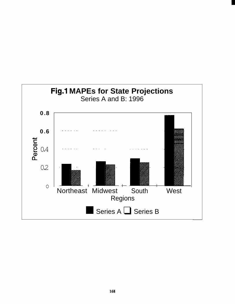
0 8●

0 6●

04●

02●

o

Fig.1 MAPEs for State ProjectionsSeries A and B: 1996

----

----

+

.-

. .

.-

---- . .

---- --

--- ---

---- ---

t +——

Northeast Midwest South WestRegions

■ Series A ❑ Series B

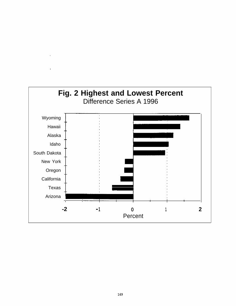
Fig. 2 Highest and Lowest PercentDifference Series A 1996

Wyoming

Hawaii

Alaska

Idaho

South Dakota

New York

Oregon

California

Texas

Arizona1 1

-2 - 1 0 1 2Percent

169

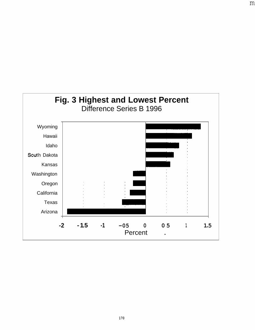
m

Fig. 3 Highest and Lowest PercentDifference Series B 1996

Sou<

Wyoming

Hawaii

Idaho

h Dakota

Kansas

Washington

Oregon

California

Texas

Arizona

-2 - 1 5● -1 -05 0 0 5 1 15●Percent ●

170

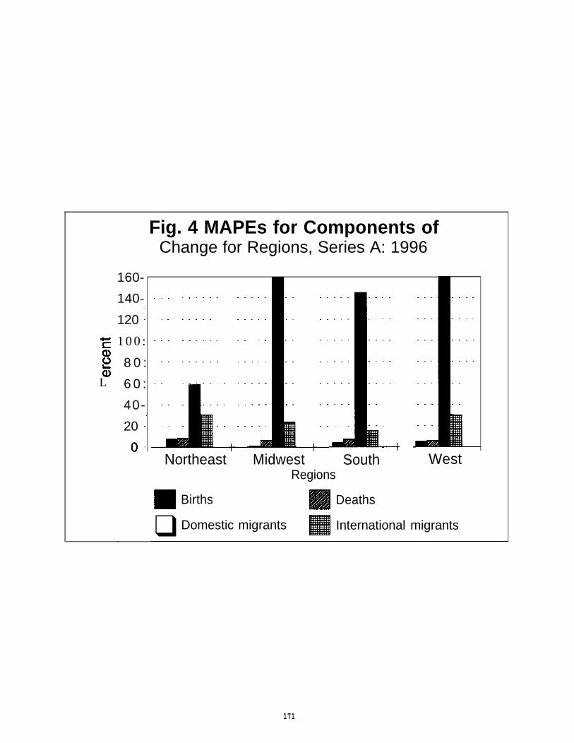
L

Fig. 4 MAPEs for Components ofChange for Regions, Series A: 1996

160-

140-

120 ;

100:

8 0 :

6 0 :

40-

20 ;

o

---

. .

---

--

. . .

--

. .

-.. . .-

---- . .

-.. . .-

---- .-

. .

.-

-.

+

. .

-.

. .

. .

. .

. .

--

—

. . . --

.-. --

-. . .

. . . .-

--- .-

--- --

. . .

+

--

-.

. .

-.

. .

--

.-

—

.-

--

-.

--

. .

--

+

Northeast Midwest South WestRegions

Births Deaths

❑ Domestic migrants International migrants

--

--

--

--

171

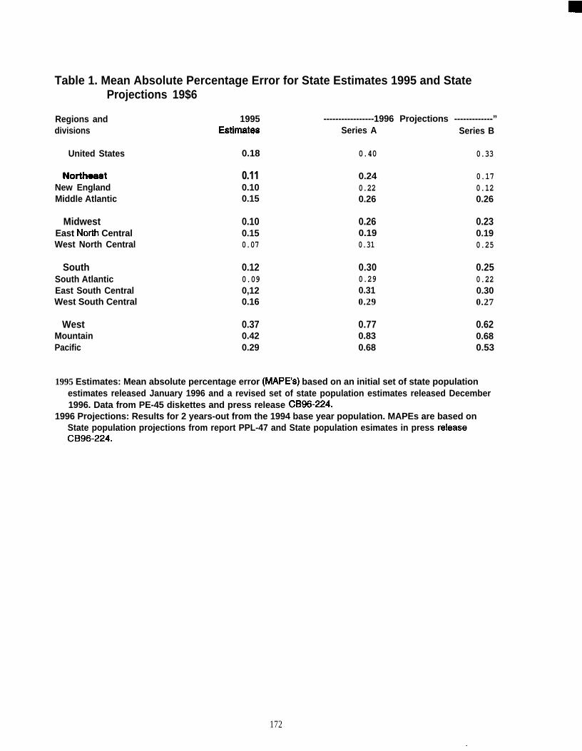
Table 1. Mean Absolute Percentage Error for State Estimates 1995 and StateProjections 19$6

Regions and 1995 -----------------1996 Projections -------------”divisions Estimates Series A Series B

United States 0.18 0.40 0.33

Nol’the8st 0.11 0.24 0.17New England 0.10 0.22 0.12Middle Atlantic 0.15 0.26 0.26

Midwest 0.10 0.26 0.23East North Central 0.15 0.19 0.19West North Central 0.07 0.31 0.25

South 0.12 0.30 0.25South Atlantic 0.09 0.29 0.22East South Central 0,12 0.31 0.30West South Central 0.16 0.29 0.27

West 0.37 0.77 0.62Mountain 0.42 0.83 0.68Pacific 0.29 0.68 0.53

172

1995 Estimates: Mean absolute percentage error (MAPE’s) based on an initial set of state populationestimates released January 1996 and a revised set of state population estimates released December1996. Data from PE-45 diskettes and press release CB96-224.

1996 Projections: Results for 2 years-out from the 1994 base year population. MAPEs are based onState population projections from report PPL-47 and State population esimates in press re!easeCB96-224.

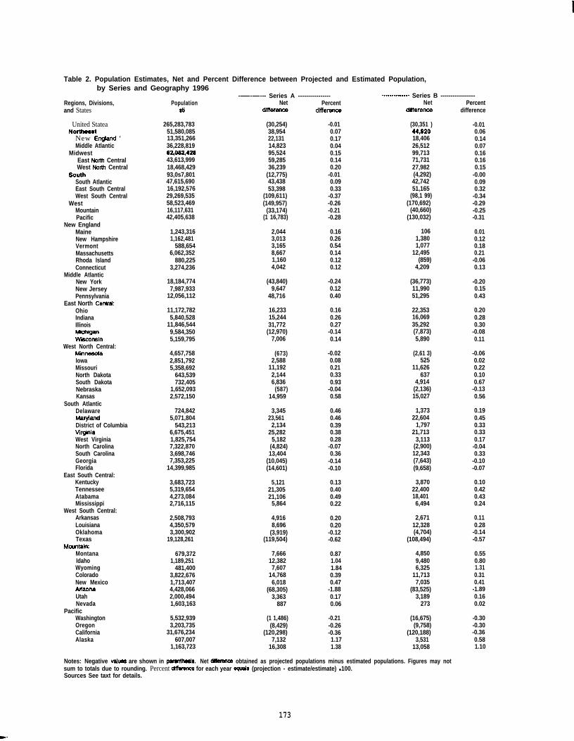
Table 2. Population Estimates, Net and Percent Difference between Projected and Estimated Population,by Series and Geography 1996

Regions, Divisions,and States

United StateaNortheaat

New Engfand ‘Middle Atlantic

MidwestEast Nofih CentralWest Notth Central

SouthSouth AtlanticEast South CentralWest South Central

WestMountainPacific

New EnglandMaineNew HampshireVermontMassachusettsRhoda IslandConnecticut

Middle AtlanticNew YorkNew JerseyPennsylvania

East North Centrat:OhioIndianaIllinoisMich@anWsconsin

West North Central:MkmeeotaIowaMissouriNorth DakotaSouth DakotaNebraskaKansas

South AtlanticDelawareMa@andDistrict of ColumbiaVkginiaWest VirginiaNorth CarolinaSouth CarolinaGeorgiaFlorida

East South Central:KentuckyTennesseeAtabamaMississippi

West South Central:ArkansasLouisianaOklahomaTexas

MountairxMontanaIdahoWyomingColoradoNew MexicoArfzonaUtahNevada

PacificWashingtonOregonCaliforniaAlaska

Population

265,283,78351,580,08513,351,26636,228,81962,08&42843,613,99918,468,42993,0s7,80147,615,69016,192,57629,269,53558,523,46916,117,63142,405,638

1,243,3161,162,481

588,6546,062,352

880,2253,274,236

18,184,7747,987,933

12,056,112

11,172,7825,840,528

11,846,5449,584,3505,159,795

4,657,7582,851,7925,358,692

643,539732,405

1,652,0932,572,150

724,8425,071,804

543,2136,675,4511,825,7547,322,8703,698,7467,353,225

14,399,985

3,683,7235,319,6544,273,0842,716,115

2,508,7934,350,5793,300,902

19,128,261

679,3721,189,251

481,4003,822,6761,713,4074,428,0662,000,4941,603,163

5,532,9393,203,735

31,676,234607,007

1,163,723

----------- Series A ----------------Net

dtiarence

(30,254)38,95422,13114,82395,52459,28536,239

(12,775)43,43853,398

(109,611)(149,957)

(33,174)(1 16,783)

2,0443,0133,1658,6671,1604,042

(43,840)9,647

48,716

16,23315,24431,772

(12,970)7,006

(673)2,588

11,1922,1446,836

(587)14,959

3,34523,561

2,13425,282

5,182(4,824)13,404

(10,045)(14,601)

5,12121,30521,106

5,864

4,9168,696

(3,919)(119,504)

7,66612,3827,607

14,7686,018

(68,305)3,363

887

(1 1,486)(8,429)

(120,298)7,132

16,308

Percentdflerenca

-0.010.070.170.040.150.140.20

-0.010.090.33

-0.37-0.26-0.21-0.28

0.160.260.540.140.120.12

-0.240.120.40

0.160.260.27

-0.140.14

-0.020.080.210.330.93

-0.040.58

0.460.460.390.380.28

-0.070.36

-0.14-0.10

0.130.400.490.22

0.200.20

-0.12-0.62

0.871.041.840.390.47

-1.880.170.06

-0.21-0.26-0.361.171.38

------—--- Series B -----------------Net

dflerence

(30,351 )U,92018,40626,51299,71371,73127,982(4,292)42,74251,165

(98,1 99)(170,692)

(40,660)(130,032)

1061,3801,077

12,495(859)

4,209

(36,773)11,99051,295

22,35316,06935,292(7,873)5,890

(2,61 3)525

11,626637

4,914(2,136)15,027

1,37322,604

1,79721,713

3,113(2,900)12,343(7,643)(9,658)

3,87022,40018,4016,494

2,67112,328(4,704)

(108,494)

4,8509,4806,325

11,7137,035

(83,525)3,189

273

(16,675)(9,758)

(120,188)3,531

13,058

Percentdifference

-0.010.060.140.070.160.160.15

-0.000.090.32

-0.34-0.29-0.25-0.31

0.010.120.180.21

-0.060.13

-0.200.150.43

0.200.280.30

-0.080.11

-0.060.020.220.100.67

-0.130.56

0.190.450.330.330.17

-0.040.33

-0.10-0.07

0.100.420.430.24

0.110.28

-0.14-0.57

0.550.801.310.310.41

-1.890.160.02

-0.30-0.30-0.360.581.10

Notes: Negative vafuea are shown in pamtheaia. Net diffemnos obtained as projected populations minus estimated populations. Figures may notsum to totals due to rounding. Percent differenoa for each year equala (projection - estimate/estimate) ● 100.Sources See taxt for details.

173

.,.,”.,., ,

,“

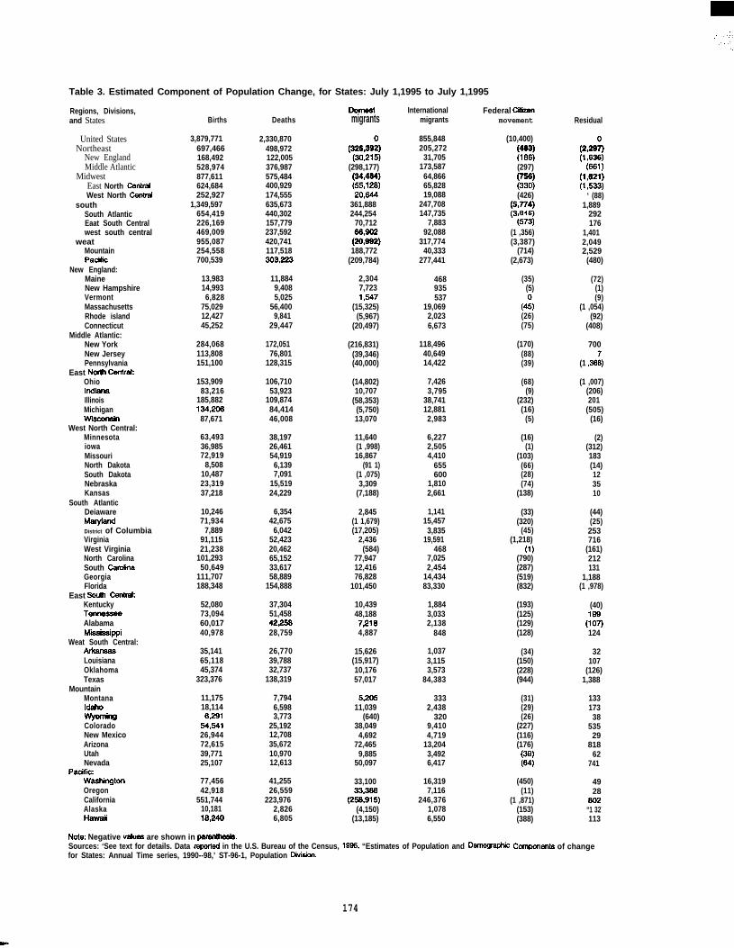
Table 3. Estimated Component of Population Change, for States: July 1,1995 to July 1,1995

Regions, Divisions,and States

United StatesNortheast

New EnglandMiddle Atlantic

MidwestEast North CentraiWest North Centrai

southSouth AtlanticEaat South Centralwest south central

weatMountainPaafic

New England:MaineNew HampshireVermontMassachusettsRhode islandConnecticut

Middle Atlantic:New YorkNew JerseyPennsylvania

East M Central:OhioIndiiIllinoisMichiganWk3c0nain

West North Central:MinnesotaiowaMissouriNorth DakotaSouth DakotaNebraskaKansas

South AtlanticDeiawareMarytandDistrict of ColumbiaVirginiaWest VirginiaNorth CarolinaSouth CarofhaGeorgiaFlorida

East south cerrtrd:KentuckyTemwaeaeAlabamaMiippi

Weat South Central:

LouisianaOklahomaTexas

MountainMontanaId-w-ColoradoNew MexicoArizonaUtahNevada

Paafic:WashhgtonOregonCaliforniaAlaskaHawtM

Births

3,879,771697,466168,492528,974877,611624,684252,927

1,349,597654,419226,169469,009955,087254,558700,539

13,98314,9936,828

75,02912,42745,252

284,068113,808151,100

153,90983,216

185,882134@687,671

63,49336,98572,919

8,50810,48723,31937,218

10,24671,934

7,88991,11521,238

101,29350,649

111,707188,348

52,08073,09460,01740,978

35,14165,11845,374

323,376

11,17518,1146#91

54,54126,94472,61539,77125,107

77,45642,918

551,74410,18118&10

Deaths

2,330,870498,972122,005376,987575,484400,929174,555635,673440,302157,779237,592420,741117,518303J?23

11,8849,4085,025

56,4009,841

29,447

172,05176,801

128,315

106,71053,923

109,87484,41446,008

38,19726,46154,9196,1397,091

15,51924,229

6,35442,675

6,04252,42320,46265,15233,61758,889

154,888

37,30451,45842$?5828,759

26,77039,78832,737

138,319

7,7946,5983,773

25,19212,70835,67210,97012,613

41,25526,559

223,9762,8266,805

migrants

(32239:](298,177)[gA&l;

20;844361,888244,254

70,712

(%%188,772

(209,784)

2,3047,7231,547

(15,325)(5,967)

(20,497)

(216,831)(39,346)(40,000)

(14,802)10,707

(58,353)(5,750)13,070

11,640(1 ,998)16,867

(91 1)(1 ,075)3,309

(7,188)

2,845(1 1,679)(17,205)

2,436(584)

77,94712,41676,828

101,450

10,43948,1887$164,887

15,626(15,917)10,17657,017

5$0511,039

(640)38,0494,692

72,4659,885

50,097

33,100

(22,%(4,150)

(13,185)

Internationalmigrants

855,848205,272

31,705173,58764,86665,82819,088

247,708147,735

7,88392,088

317,77440,333

277,441

468935537

19,0692,0236,673

118,49640,64914,422

7,4263,795

38,74112,8812,983

6,2272,5054,410

655600

1,8102,661

1,14115,4573,835

19,591468

7,0252,454

14,43483,330

1,8843,0332,138

848

1,0373,1153,573

84,383

3332,438

3209,4104,719

13,2043,4926,417

16,3197,116

246,3761,0786,550

Federal ciiZSllmovement

(10,400)p]

(297)$56]

(426)$s774]

{573)(1 ,356)(3,387)

(714)(2,673)

(35)(5)

(4:)(26)(75)

(170)(88)(39)

(68)(9)

(232)(16)

(5)

(16)(1)

(103)(66)(28)(74)

(138)

(33)(320)

(45)(1,218)

(1)(790)(287)(519)(832)

(193)(125)(129)(128)

(34)(150)(228)(944)

(31)(29)(26)

(227)(116)(176)~]

(450)(11)

(1 ,871)(153)(388)

Residual

f,2!3~

{861)~,&3]

‘ (88)1,889

292176

1,4012,0492,529

(480)

(72)(1)(9)

(1 ,054)(92)

(408)

700

(1 ,36~)

(1 ,007)(206)201

(505)(16)

(2)(312)183(14)123510

(44)(25)253716

(161)212131

1,188(1 ,978)

(40)

(%)124

32107

(126)1,388

13317338

53529

81862

741

4928

“1 32-

113

Note Negative veha are shown in pamhaie.Sources: ‘See text for details. Data rewted in the U.S. Bureau of the Census, 1996, “Estimates of Population and Demw@ic COmpments of changefor States: Annual Time series, 1990--98,’ ST-96-1, Population Dwiaion.

174

m-

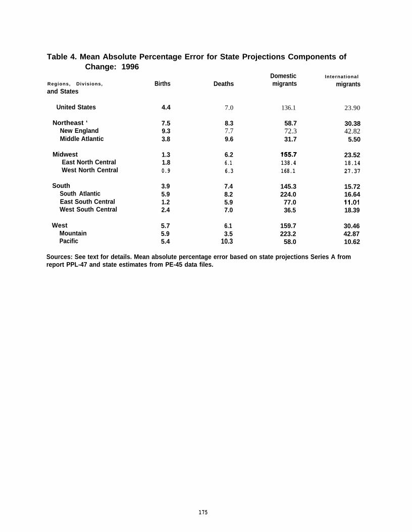
Table 4. Mean Absolute Percentage Error for State Projections Components ofChange: 1996

Domestic International

Regions, Divisions, Births Deaths migrants migrantsand States

United States 4.4 7.0 136.1 23.90

Northeast ‘ 7.5 8.3 58.7 30.38New England 9.3 7.7 72.3 42.82Middle Atlantic 3.8 9.6 31.7 5.50

Midwest 1.3 6.2 155.7 23.52East North Central 1.8 6.1 138.4 18.14West North Central 0.9 6.3 168.1 27.37

South 3.9 7.4 145.3 15.72South Atlantic 5.9 8.2 224.0 16.64East South Central 1.2 5.9 77.0 11.01West South Central 2.4 7.0 36.5 18.39

West 5.7 6.1 159.7 30.46Mountain 5.9 3.5 223.2 42.87Pacific 5.4 10.3 58.0 10.62

Sources: See text for details. Mean absolute percentage error based on state projections Series A fromreport PPL-47 and state estimates from PE-45 data files.

175

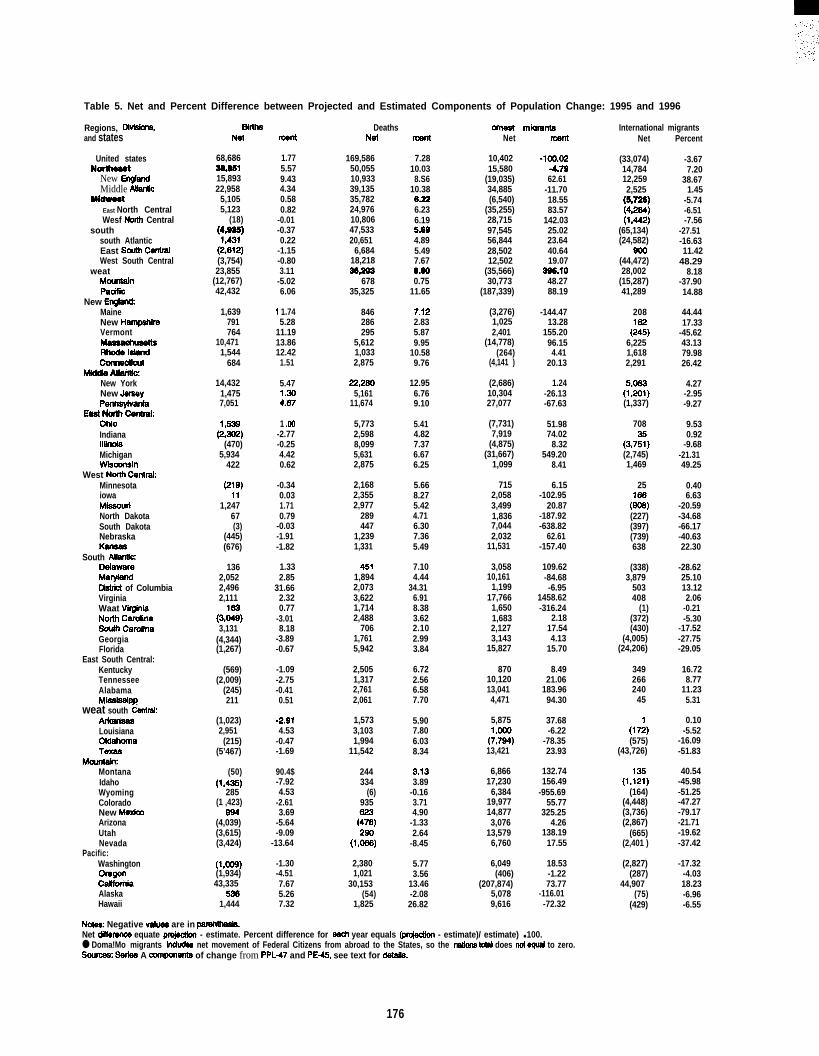
Table 5. Net and Percent Difference between Projected and Estimated Components of Population Change: 1995 and 1996

Regions, Dividons,and states

United statesNortheaat

New En@andMiddle AtiSldiC

Midwoat

East North CentralWesf Nom Central

southsouth AtlanticEast SMh CentratWest South Central

weat

PadficNew En@mct

MaineNew HamoahiraVermont

Rhoda ldand

Mf&%&%~dNew YorkNew JemayPenn@vanta

E#d NOtth Centrat:

IndianalltindaMichiganW~in

West NotUI CentrakMinnesotaiowaMlaaouriNorth DakotaSouth DakotaNebraska

South AtlanticDafawaraMafyiandDiatdcf of ColumbiaVirginiaWaat VifginiaNofth CarolhaSouttI CamfinaGeorgiaFlorida

East South Central:KentuckyTennesseeAlabama

weat south Cantrat:

LouisianaOkfahomaTexaa

MountalmMontanaIdahoWyomingColoradoNew MexiooArizonaUtahNevada

Pacific:WashingtonOqorlCaliimiaAlaskaHawaii

Siftha DeathsNet

68,68635,55115,89322,958

5,1055,123

(18)(f~)

(2:612)(3,754)23,855

(12,767)42,432

1,639791764

10,4711,544

684

14,4321,4757,051

(i%)(470)

5,934422

(2;;)

1,24767(3)

(445)(676)

1362,0522,4962,111

(3,A%)3,131

(4,344)(1,267)

(569)(2,009)

(245)211

(1,023)2,951(215)

(5’467)

(50)(1s435)

285(1 ,423)

(4,039)(3,615)(3,424)

(1,009)(1,934)43,335

1,444

Notes Negative vatuea are in pamthaaia.

1.775.579.434.340.580.82

-0.01-0.370.22

-1.15-0.803.11

-5.026.06

f 1.745.28

11.1913.8612.42

1.51

5.47

:::

1 .(M-2.77-0.254.420.62

-0.340.031.710.79

-0.03-1.91-1.82

1.332.85

31.662.320.77

-3.018.18

-3.89-0.67

-1.09-2.75-0.410.51

-2.914.53

-0.47-1.69

90.4$-7.924.53

-2.613.69

-5.64-9.09

-13.64

-1.30-4.517.675.267.32

Net

169,58650,05510,93339,13535,78224,97610,80647,53320,651

6,68418,21836W

67835,325

846286295

5,6121,0332,875

222805,161

11,674

5,7732,5988,0995,6312,875

2,1682,3552,977

289447

1,2391,331

4511,8942,0733,6221,7142,488

7061,7615,942

2,5051,3172,7612,061

1,5733,1031,994

11,542

244334

(6)935

(%)

(l,2&)

2,3801,021

30,153(54)

1,825

7.2810.038.S6

10.38&226.236.195.694.895.497.678.800.75

11.65

7.122.835.879.95

10.589.76

12.956.769.10

5.414.827.376.676.25

5.668.275.424.716.307.365.49

7.104.44

34.316.918.383.622.102.993.84

6.722.566.587.70

5.907.806.038.34

3.133.89

-0.163.714.90

-1.332.64

-8.45

5.773.56

13.46-2.0826.82

Net

10,40215,580

(19,035)34,885(6,540)

(35,255)28,71597,54556,84428,50212,502

(35,566)30,773

(187,339)

(3,276)1,0252,401

(14,778)(264)

(4,141 )

(2,686)10,30427,077

(7,731)7,919

(4,875)(31,667)

1,099

7152,0583,4991,8367,0442,032

11,531

3,05810,1611,199

17,7661,6501,6832,1273,143

15,827

87010,12013,0414,471

5,875

(;%)13,421

6,86617,2306,384

19,97714,8773,076

13,5796,760

6,049(406)

(207,874)5,0789,616

-100.02-4.7s62.61

-11.7018.5583.57

142.0325.0223.6440.6419.07

3e5.lo48.2788.19

-144.4713.28

155.2096.154.41

20.13

1.24-26.13-67.63

51.9874.02

8.32549.20

8.41

6.15-102.95

20.87-187.92-638.82

62.61-157.40

109.62-84.68-6.95

1458.62-316.24

2.1817.544.13

15.70

8.4921.06

183.9694.30

37.68-6.22

-78.3523.93

132.74156.49

-955.6955.77

325.254.26

138.1917.55

18.53-1.2273.77

-116.01-72.32

International migrantsNet

(33,074)14,78412,2592,525

&7213;

(1:442)(65,134)(24,582)

(44,472)28,002

(15,287)41,289

208

(%6,2251,6182,291

(?%)(1,337)

708

(3,7R)(2,745)1,469

25

(E)(227)(397)(739)638

(338)3,879

503408

(1)(372)(430)

(4,005)(24,206)

349266240

45

(1A)(575)

(43,726)

(1,;:)(164)

(4,448)(3,736)(2,867)

(665)(2,401 )

(2,827)(287)

44,907(75)

(429)

Percent

-3.677.20

38.671.45

-5.74-6.51-7.56

-27.51-16.6311.42

48.298.18

-37.9014.88

44.4417.33

-45.6243.1379.9826.42

4.27-2.95-9.27

9.530.92

-9.68-21.3149.25

0.406.63

-20.59-34.68-66.17-40.6322.30

-28.6225.1013.122.06

-0.21-5.30

-17.52-27.75-29.05

16.728.77

11.235.31

0.10-5.52

-16.09-51.83

40.54-45.98-51.25-47.27-79.17-21.71-19.62-37.42

-17.32-4.0318.23-6.96-6.55

Net diffemnoa equate pmjactbn - estimate. Percent difference for eaoh year equals (pmjadion - estimate)/ estimate) ● 100.● Doma!Mo migrants indudea net movement of Federal Citizens from abroad to the States, so the natjona totai does not equal to zero.SOIJ- series A wrnponenta of change from PPL47 and PE-45, see text for detaile.

176

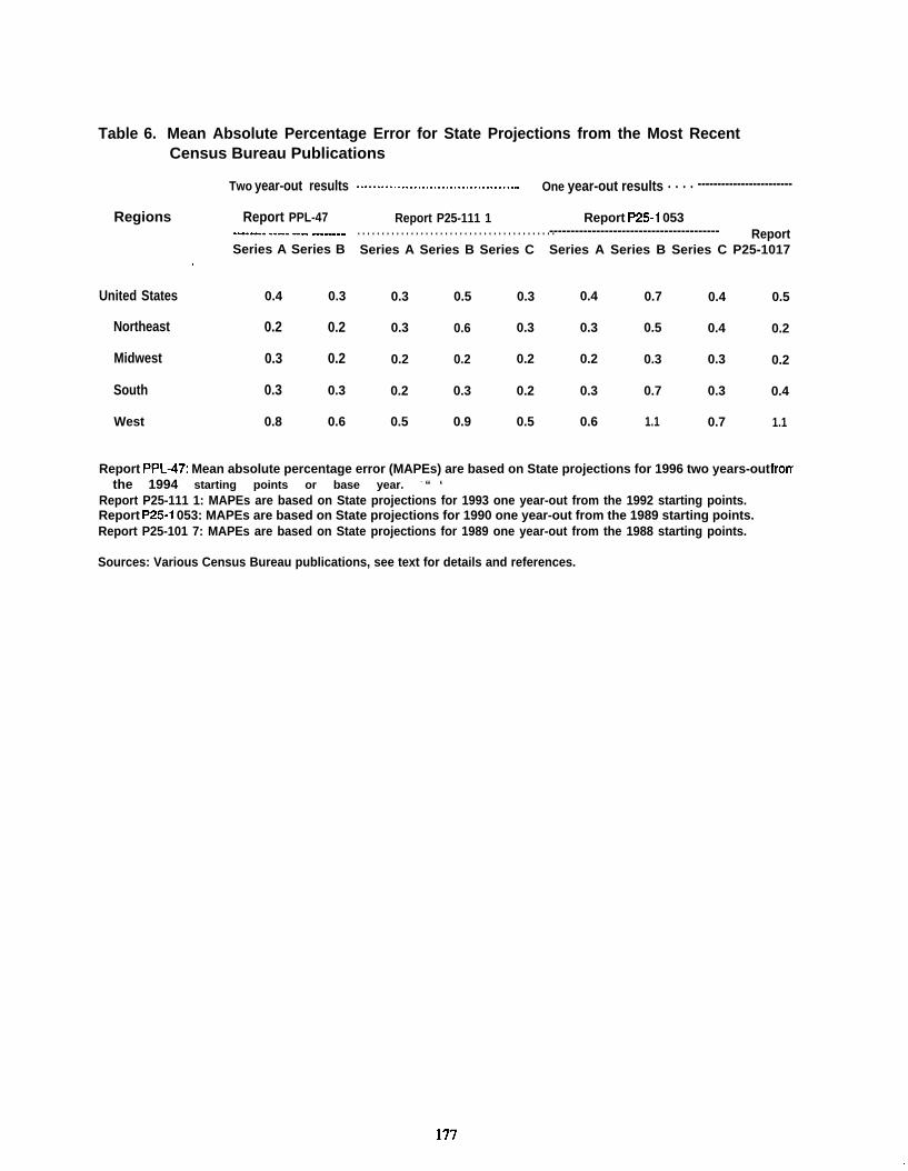
Table 6. Mean Absolute Percentage Error for State Projections from the Most RecentCensus Bureau Publications

Two year-out results

Regions ‘ Report PPL-47.------- .--.. --.. ----.-..,Series A Series B

t

United States 0.4 0.3

Northeast 0.2 0.2

Midwest 0.3 0.2

South 0.3 0.3

West 0.8 0.6

. . . . . . . . . . . . . . . . . . . . . . . . . . . . . . . . . . . . . . ..- One year-out results . . . . ------------------------

Report P25-111 1. . . . . . . . . . . . . . . . . . . . . . . . . . . . . . . . . . . . . . . . .Series A Series B Series C

0.3 0.5 0.3

0.3 0.6 0.3

0.2 0.2 0.2

0.2 0.3 0.2

0.5 0.9 0.5

Report P25-1 053---------------------------------------- ReportSeries A Series B Series C P25-1017

0.4 0.7 0.4 0.5

0.3 0.5 0.4 0.2

0.2 0.3 0.3 0.2

0.3 0.7 0.3 0.4

0.6 1.1 0.7 1.1

Report PPL-47: Mean absolute percentage error (MAPEs) are based on State projections for 1996 two years-out frorrthe 1994 starting points or base year. - “ ‘

Report P25-111 1: MAPEs are based on State projections for 1993 one year-out from the 1992 starting points.Report P25-1 053: MAPEs are based on State projections for 1990 one year-out from the 1989 starting points.Report P25-101 7: MAPEs are based on State projections for 1989 one year-out from the 1988 starting points.

Sources: Various Census Bureau publications, see text for details and references.

177

. .

:,. . . m

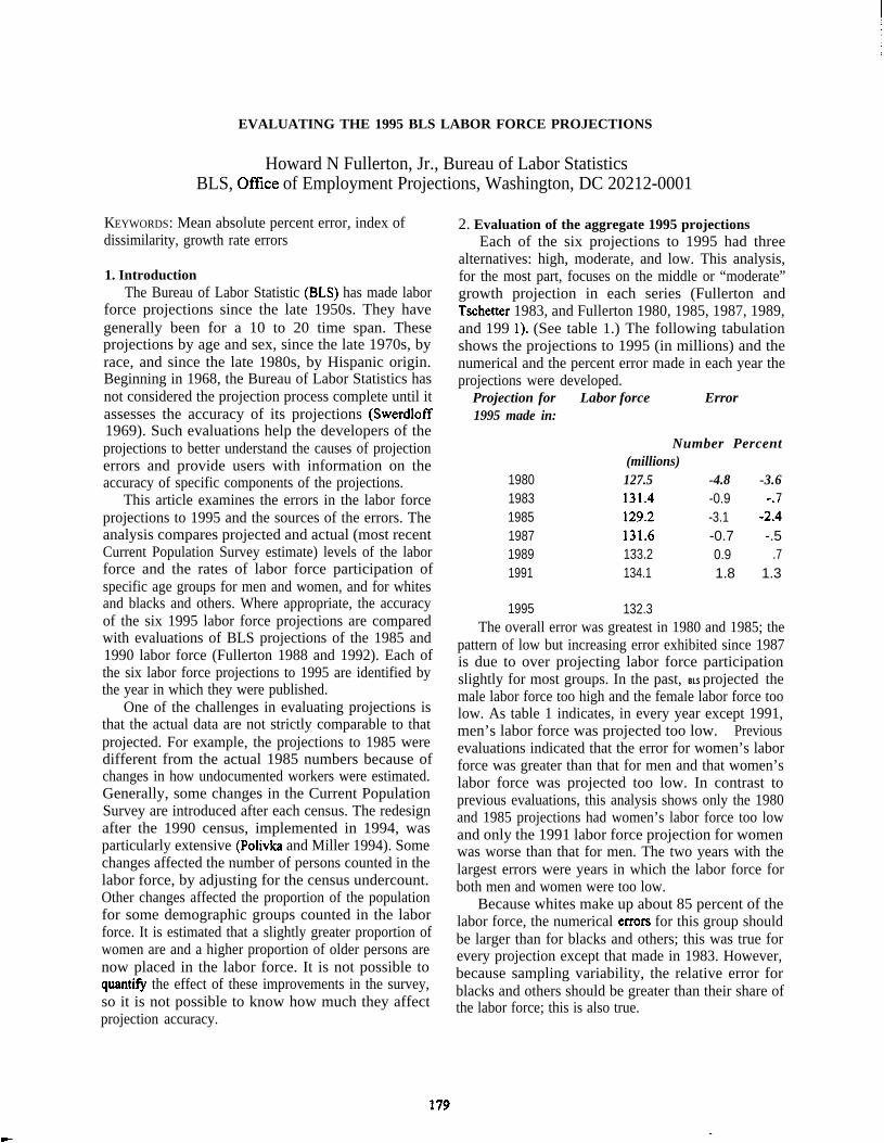
EVALUATING THE 1995 BLS LABOR FORCE PROJECTIONS

Howard N Fullerton, Jr., Bureau of Labor StatisticsBLS, OffIce of Employment Projections, Washington, DC 20212-0001

KEYWORDS: Mean absolute percent error, index ofdissimilarity, growth rate errors

1. IntroductionThe Bureau of Labor Statistic (BLS) has made labor

force projections since the late 1950s. They havegenerally been for a 10 to 20 time span. Theseprojections by age and sex, since the late 1970s, byrace, and since the late 1980s, by Hispanic origin.Beginning in 1968, the Bureau of Labor Statistics hasnot considered the projection process complete until itassesses the accuracy of its projections (Swerdloff1969). Such evaluations help the developers of theprojections to better understand the causes of projectionerrors and provide users with information on theaccuracy of specific components of the projections.

This article examines the errors in the labor forceprojections to 1995 and the sources of the errors. Theanalysis compares projected and actual (most recentCurrent Population Survey estimate) levels of the laborforce and the rates of labor force participation ofspecific age groups for men and women, and for whitesand blacks and others. Where appropriate, the accuracyof the six 1995 labor force projections are comparedwith evaluations of BLS projections of the 1985 and1990 labor force (Fullerton 1988 and 1992). Each ofthe six labor force projections to 1995 are identified bythe year in which they were published.

One of the challenges in evaluating projections isthat the actual data are not strictly comparable to thatprojected. For example, the projections to 1985 weredifferent from the actual 1985 numbers because ofchanges in how undocumented workers were estimated.Generally, some changes in the Current PopulationSurvey are introduced after each census. The redesignafter the 1990 census, implemented in 1994, wasparticularly extensive (Polivka and Miller 1994). Somechanges affected the number of persons counted in thelabor force, by adjusting for the census undercount.Other changes affected the proportion of the populationfor some demographic groups counted in the laborforce. It is estimated that a slightly greater proportion ofwomen are and a higher proportion of older persons arenow placed in the labor force. It is not possible toquantifi the effect of these improvements in the survey,so it is not possible to know how much they affectprojection accuracy.

2. Evaluation of the aggregate 1995 projectionsEach of the six projections to 1995 had three

alternatives: high, moderate, and low. This analysis,for the most part, focuses on the middle or “moderate”growth projection in each series (Fullerton andTschetter 1983, and Fullerton 1980, 1985, 1987, 1989,and 199 1). (See table 1.) The following tabulationshows the projections to 1995 (in millions) and thenumerical and the percent error made in each year theprojections were developed.

Projection for1995 made in:

198019831985198719891991

1995

Labor force Error

Number Percent(millions)127.5 -4.8 -3.6131.4 -0.9 7129.2 -3.1 -;:4131.6 -0.7 -.5133.2 0.9 .7134.1 1.8 1.3

132.3The overall error was greatest in 1980 and 1985; the

pattern of low but increasing error exhibited since 1987is due to over projecting labor force participationslightly for most groups. In the past, BLS projected themale labor force too high and the female labor force toolow. As table 1 indicates, in every year except 1991,men’s labor force was projected too low. Previousevaluations indicated that the error for women’s laborforce was greater than that for men and that women’slabor force was projected too low. In contrast toprevious evaluations, this analysis shows only the 1980and 1985 projections had women’s labor force too lowand only the 1991 labor force projection for womenwas worse than that for men. The two years with thelargest errors were years in which the labor force forboth men and women were too low.

Because whites make up about 85 percent of thelabor force, the numerical emors for this group shouldbe larger than for blacks and others; this was true forevery projection except that made in 1983. However,because sampling variability, the relative error forblacks and others should be greater than their share ofthe labor force; this is also true.

179

.

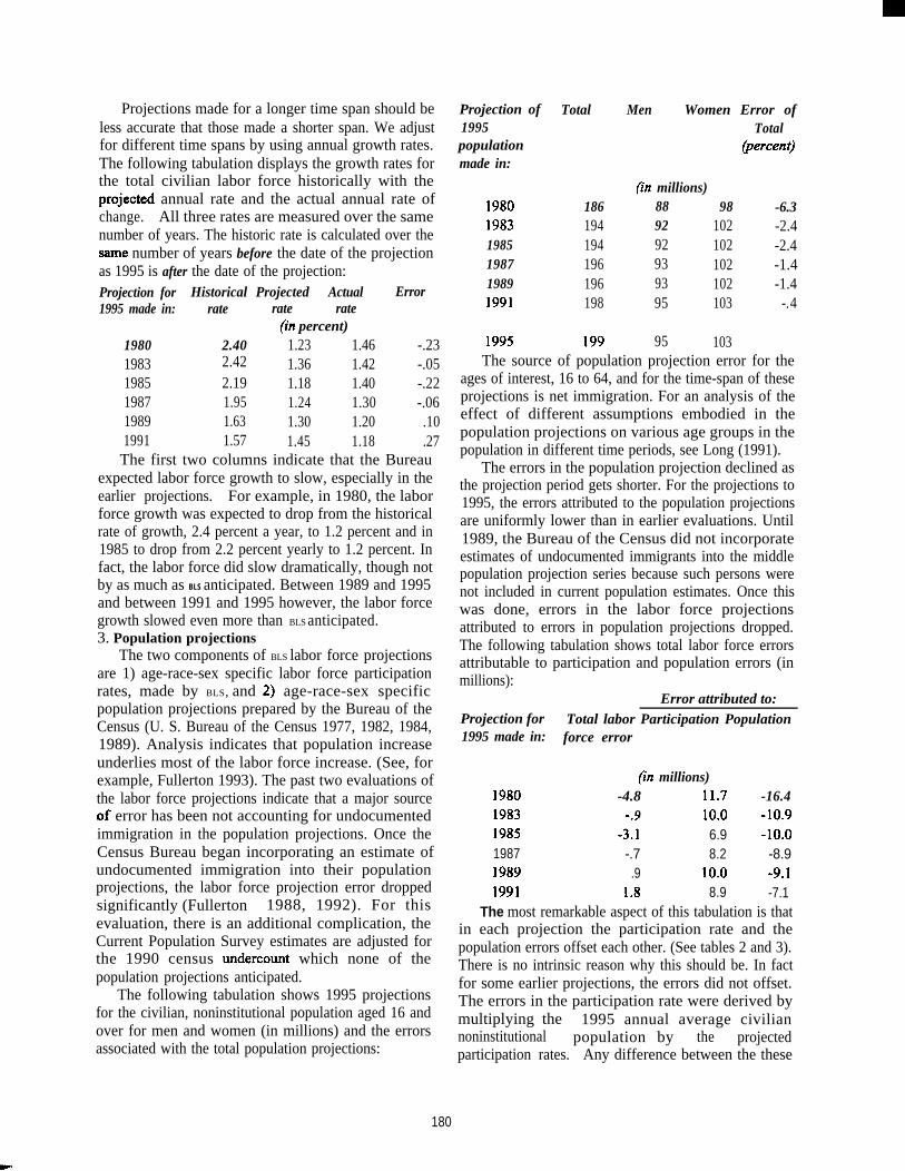
Projections made for a longer time span should beless accurate that those made a shorter span. We adjustfor different time spans by using annual growth rates.The following tabulation displays the growth rates forthe total civilian labor force historically with theprojected annual rate and the actual annual rate ofchange. All three rates are measured over the samenumber of years. The historic rate is calculated over thesame number of years before the date of the projectionas 1995 is after the date of the projection:Projection for Historical Projected Actual Error1995 made in: rate rate rate

(in percent)1980 2.40 1.23 1.46 -.231983 2.42 1.36 1.42 -.051985 2.19 1.18 1.40 -.221987 1.95 1.24 1.30 -.061989 1.63 1.30 1.20 .101991 1.57 1.45 1.18 .27The first two columns indicate that the Bureau

expected labor force growth to slow, especially in theearlier projections. For example, in 1980, the laborforce growth was expected to drop from the historicalrate of growth, 2.4 percent a year, to 1.2 percent and in1985 to drop from 2.2 percent yearly to 1.2 percent. Infact, the labor force did slow dramatically, though notby as much as BLS anticipated. Between 1989 and 1995and between 1991 and 1995 however, the labor forcegrowth slowed even more than BLS anticipated.3. Population projections

The two components of BLS labor force projectionsare 1) age-race-sex specific labor force participationrates, made by BLS, and 2) age-race-sex specificpopulation projections prepared by the Bureau of theCensus (U. S. Bureau of the Census 1977, 1982, 1984,1989). Analysis indicates that population increaseunderlies most of the labor force increase. (See, forexample, Fullerton 1993). The past two evaluations ofthe labor force projections indicate that a major sourceof error has been not accounting for undocumentedimmigration in the population projections. Once theCensus Bureau began incorporating an estimate ofundocumented immigration into their populationprojections, the labor force projection error droppedsignificantly (Fullerton 1988, 1992). For thisevaluation, there is an additional complication, theCurrent Population Survey estimates are adjusted forthe 1990 census undercount which none of thepopulation projections anticipated.

The following tabulation shows 1995 projectionsfor the civilian, noninstitutional population aged 16 andover for men and women (in millions) and the errorsassociated with the total population projections:

Projection of1995populationmade in:

198019831985198719891991

1995

Total

186194194196196198

199

Men Women Error ofTotal

@ercent)

(i% millions)88 98 -6.392 102 -2.492 102 -2.493 102 -1.493 102 -1.495 103 -.4

95 103The source of population projection error for the

ages of interest, 16 to 64, and for the time-span of theseprojections is net immigration. For an analysis of theeffect of different assumptions embodied in thepopulation projections on various age groups in thepopulation in different time periods, see Long (1991).

The errors in the population projection declined asthe projection period gets shorter. For the projections to1995, the errors attributed to the population projectionsare uniformly lower than in earlier evaluations. Until1989, the Bureau of the Census did not incorporateestimates of undocumented immigrants into the middlepopulation projection series because such persons werenot included in current population estimates. Once thiswas done, errors in the labor force projectionsattributed to errors in population projections dropped.The following tabulation shows total labor force errorsattributable to participation and population errors (inmillions):

Error attributed to:Projection for Total labor Participation Population1995 made in: force error

(in millions)1980 -4.8 11.7 -16.41983 9 10.0 -10.91985 -L 6.9 -10.01987 -.7 8.2 -8.91989 .9 10.0 -9.11991 1.8 8.9 -7.1

The most remarkable aspect of this tabulation is thatin each projection the participation rate and thepopulation errors offset each other. (See tables 2 and 3).There is no intrinsic reason why this should be. In factfor some earlier projections, the errors did not offset.The errors in the participation rate were derived bymultiplying the 1995 annual average civiliannoninstitutional population by the projectedparticipation rates. Any difference between the these

180

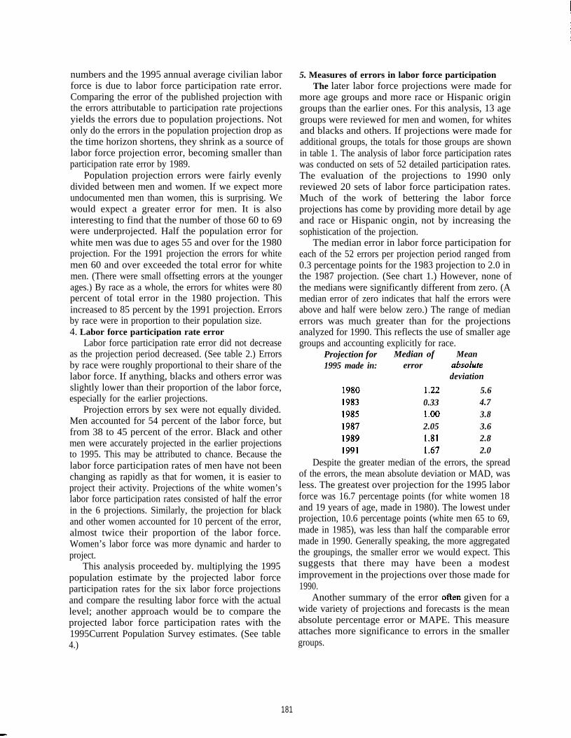
numbers and the 1995 annual average civilian laborforce is due to labor force participation rate error.Comparing the error of the published projection withthe errors attributable to participation rate projectionsyields the errors due to population projections. Notonly do the errors in the population projection drop asthe time horizon shortens, they shrink as a source oflabor force projection error, becoming smaller thanparticipation rate error by 1989.

Population projection errors were fairly evenlydivided between men and women. If we expect moreundocumented men than women, this is surprising. Wewould expect a greater error for men. It is alsointeresting to find that the number of those 60 to 69were underprojected. Half the population error forwhite men was due to ages 55 and over for the 1980projection. For the 1991 projection the errors for whitemen 60 and over exceeded the total error for whitemen. (There were small offsetting errors at the youngerages.) By race as a whole, the errors for whites were 80percent of total error in the 1980 projection. Thisincreased to 85 percent by the 1991 projection. Errorsby race were in proportion to their population size.4. Labor force participation rate error

Labor force participation rate error did not decreaseas the projection period decreased. (See table 2.) Errorsby race were roughly proportional to their share of thelabor force. If anything, blacks and others error wasslightly lower than their proportion of the labor force,especially for the earlier projections.

Projection errors by sex were not equally divided.Men accounted for 54 percent of the labor force, butfrom 38 to 45 percent of the error. Black and othermen were accurately projected in the earlier projectionsto 1995. This may be attributed to chance. Because thelabor force participation rates of men have not beenchanging as rapidly as that for women, it is easier toproject their activity. Projections of the white women’slabor force participation rates consisted of half the errorin the 6 projections. Similarly, the projection for blackand other women accounted for 10 percent of the error,almost twice their proportion of the labor force.Women’s labor force was more dynamic and harder toproject.

This analysis proceeded by. multiplying the 1995population estimate by the projected labor forceparticipation rates for the six labor force projectionsand compare the resulting labor force with the actuallevel; another approach would be to compare theprojected labor force participation rates with the1995Current Population Survey estimates. (See table4.)

5. Measures of errors in labor force participationThe later labor force projections were made for

more age groups and more race or Hispanic origingroups than the earlier ones. For this analysis, 13 agegroups were reviewed for men and women, for whitesand blacks and others. If projections were made foradditional groups, the totals for those groups are shownin table 1. The analysis of labor force participation rateswas conducted on sets of 52 detailed participation rates.The evaluation of the projections to 1990 onlyreviewed 20 sets of labor force participation rates.Much of the work of bettering the labor forceprojections has come by providing more detail by ageand race or Hispanic ongin, not by increasing thesophistication of the projection.

The median error in labor force participation foreach of the 52 errors per projection period ranged from0.3 percentage points for the 1983 projection to 2.0 inthe 1987 projection. (See chart 1.) However, none ofthe medians were significantly different from zero. (Amedian error of zero indicates that half the errors wereabove and half were below zero.) The range of medianerrors was much greater than for the projectionsanalyzed for 1990. This reflects the use of smaller agegroups and accounting explicitly for race.

Projection for Median of Mean1995 made in: error absoiute

deviation

1980 1.22 5.61983 0.33 4.71985 1.00 3.81987 2.05 3.61989 1.81 2.81991 1.67 2.0

Despite the greater median of the errors, the spreadof the errors, the mean absolute deviation or MAD, wasless. The greatest over projection for the 1995 laborforce was 16.7 percentage points (for white women 18and 19 years of age, made in 1980). The lowest underprojection, 10.6 percentage points (white men 65 to 69,made in 1985), was less than half the comparable errormade in 1990. Generally speaking, the more aggregatedthe groupings, the smaller error we would expect. Thissuggests that there may have been a modestimprovement in the projections over those made for1990.

Another summary of the error ofien given for awide variety of projections and forecasts is the meanabsolute percentage error or MAPE. This measureattaches more significance to errors in the smallergroups.

181

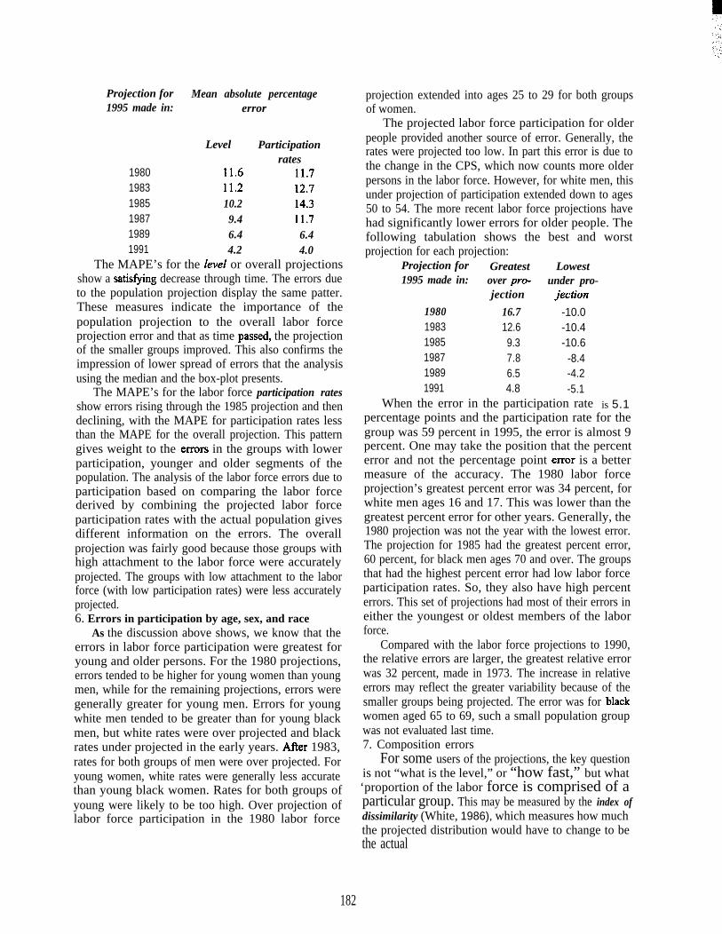
Projection for1995 made in:

198019831985198719891991

Mean absolute percentageerror

Level Participationrates

11.6 11.711.2 12.710.2 14.39.4 11.76.4 6.44.2 4.0

The MAPE’s for the level or overall projectionsshow a satis~ing decrease through time. The errors dueto the population projection display the same patter.These measures indicate the importance of thepopulation projection to the overall labor forceprojection error and that as time passe~ the projectionof the smaller groups improved. This also confirms theimpression of lower spread of errors that the analysisusing the median and the box-plot presents.

The MAPE’s for the labor force participation ratesshow errors rising through the 1985 projection and thendeclining, with the MAPE for participation rates lessthan the MAPE for the overall projection. This patterngives weight to the emors in the groups with lowerparticipation, younger and older segments of thepopulation. The analysis of the labor force errors due toparticipation based on comparing the labor forcederived by combining the projected labor forceparticipation rates with the actual population givesdifferent information on the errors. The overallprojection was fairly good because those groups withhigh attachment to the labor force were accuratelyprojected. The groups with low attachment to the laborforce (with low participation rates) were less accuratelyprojected.6. Errors in participation by age, sex, and race

As the discussion above shows, we know that theerrors in labor force participation were greatest foryoung and older persons. For the 1980 projections,errors tended to be higher for young women than youngmen, while for the remaining projections, errors weregenerally greater for young men. Errors for youngwhite men tended to be greater than for young blackmen, but white rates were over projected and blackrates under projected in the early years. After 1983,rates for both groups of men were over projected. Foryoung women, white rates were generally less accuratethan young black women. Rates for both groups ofyoung were likely to be too high. Over projection oflabor force participation in the 1980 labor force

projection extended into ages 25 to 29 for both groupsof women.

The projected labor force participation for olderpeople provided another source of error. Generally, therates were projected too low. In part this error is due tothe change in the CPS, which now counts more olderpersons in the labor force. However, for white men, thisunder projection of participation extended down to ages50 to 54. The more recent labor force projections havehad significantly lower errors for older people. Thefollowing tabulation shows the best and worstprojection for each projection:

Projection for Greatest Lowest1995 made in: over pro- under pro-

jection jection

1980 16.7 -10.01983 12.6 -10.41985 9.3 -10.61987 7.8 -8.41989 6.5 -4.21991 4.8 -5.1

When the error in the participation rate is 5.1percentage points and the participation rate for thegroup was 59 percent in 1995, the error is almost 9percent. One may take the position that the percenterror and not the percentage point emor is a bettermeasure of the accuracy. The 1980 labor forceprojection’s greatest percent error was 34 percent, forwhite men ages 16 and 17. This was lower than thegreatest percent error for other years. Generally, the1980 projection was not the year with the lowest error.The projection for 1985 had the greatest percent error,60 percent, for black men ages 70 and over. The groupsthat had the highest percent error had low labor forceparticipation rates. So, they also have high percenterrors. This set of projections had most of their errors ineither the youngest or oldest members of the laborforce.

Compared with the labor force projections to 1990,the relative errors are larger, the greatest relative errorwas 32 percent, made in 1973. The increase in relativeerrors may reflect the greater variability because of thesmaller groups being projected. The error was for blackwomen aged 65 to 69, such a small population groupwas not evaluated last time.7. Composition errors

For some users of the projections, the key questionis not “what is the level,” or “how fast,” but what‘proportion of the labor force is comprised of aparticular group. This may be measured by the index ofdissimilarity (White, 1986), which measures how muchthe projected distribution would have to change to bethe actual

182

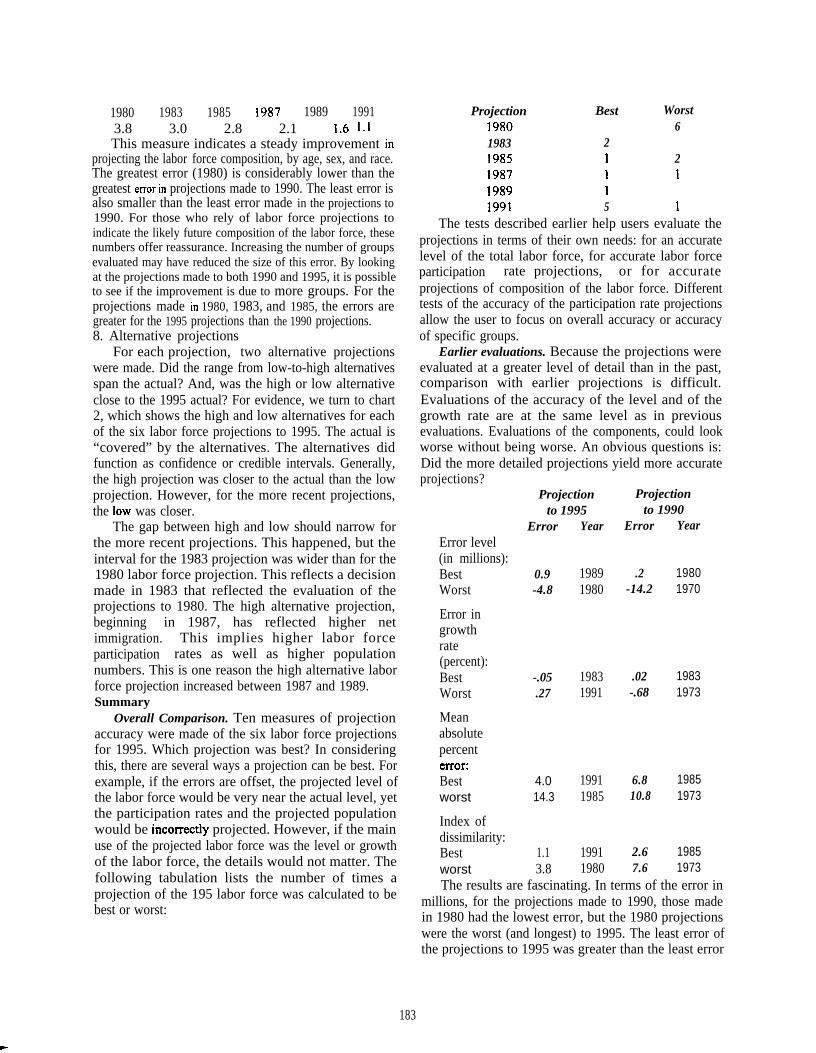
1980 1983 1985 1987 1989 19913.8 3.0 2.8 2.1 1.6 1.1This measure indicates a steady improvement in

projecting the labor force composition, by age, sex, and race.The greatest error (1980) is considerably lower than thegreatest enor in projections made to 1990. The least error isalso smaller than the least error made in the projections to1990. For those who rely of labor force projections toindicate the likely future composition of the labor force, thesenumbers offer reassurance. Increasing the number of groupsevaluated may have reduced the size of this error. By lookingat the projections made to both 1990 and 1995, it is possibleto see if the improvement is due to more groups. For theprojections made in 1980, 1983, and 1985, the errors aregreater for the 1995 projections than the 1990 projections.8. Alternative projections

For each projection, two alternative projectionswere made. Did the range from low-to-high alternativesspan the actual? And, was the high or low alternativeclose to the 1995 actual? For evidence, we turn to chart2, which shows the high and low alternatives for eachof the six labor force projections to 1995. The actual is“covered” by the alternatives. The alternatives didfunction as confidence or credible intervals. Generally,the high projection was closer to the actual than the lowprojection. However, for the more recent projections,the low was closer.

The gap between high and low should narrow forthe more recent projections. This happened, but theinterval for the 1983 projection was wider than for the1980 labor force projection. This reflects a decisionmade in 1983 that reflected the evaluation of theprojections to 1980. The high alternative projection,beginning in 1987, has reflected higher netimmigration. This implies higher labor forceparticipation rates as well as higher populationnumbers. This is one reason the high alternative laborforce projection increased between 1987 and 1989.Summary

Overall Comparison. Ten measures of projectionaccuracy were made of the six labor force projectionsfor 1995. Which projection was best? In consideringthis, there are several ways a projection can be best. Forexample, if the errors are offset, the projected level ofthe labor force would be very near the actual level, yetthe participation rates and the projected populationwould be incomectly projected. However, if the mainuse of the projected labor force was the level or growthof the labor force, the details would not matter. Thefollowing tabulation lists the number of times aprojection of the 195 labor force was calculated to bebest or worst:

Projection Best Worst1980 61983 21985 1 21987 1 11989 11991 5 1

The tests described earlier help users evaluate theprojections in terms of their own needs: for an accuratelevel of the total labor force, for accurate labor forceparticipation rate projections, or for accurateprojections of composition of the labor force. Differenttests of the accuracy of the participation rate projectionsallow the user to focus on overall accuracy or accuracyof specific groups.

Earlier evaluations. Because the projections wereevaluated at a greater level of detail than in the past,comparison with earlier projections is difficult.Evaluations of the accuracy of the level and of thegrowth rate are at the same level as in previousevaluations. Evaluations of the components, could lookworse without being worse. An obvious questions is:Did the more detailed projections yield more accurateprojections?

Error level(in millions):BestWorst

Error ingrowthrate(percent):BestWorst

Meanabsolutepercentemor:Bestworst

Index ofdissimilarity:Bestworst

Projectionto 1995

Error

0.9-4.8

-.05.27

4.014.3

1.13.8

Year

19891980

19831991

19911985

19911980

Projectionto 1990

Error

.2-14.2

.02-.68

6.810.8

2.67.6

Year

19801970

19831973

19851973

19851973

The results are fascinating. In terms of the error inmillions, for the projections made to 1990, those madein 1980 had the lowest error, but the 1980 projectionswere the worst (and longest) to 1995. The least error ofthe projections to 1995 was greater than the least error

183

m-

,. ,

.’

to 1990, but the worst error to 1995 was almost a thirdthe worst error to 1990. If the error is measured by theannual growth rate, once again, the best (least error) forthe 1995 projection was greater than the best projectionto 1990, but the worst 1995 error was significantlybetter than the worst 1990 error. The 1991 projection to1995 was the worst, even though it was the shortest.Focusing on the best projections to 1990 and 1995,leads one to say that the 1995 projections were not asgood as the 1990 ones. Looking at the worst errors(MINIMAX) leads to the opposite conclusion.

Looking at the two remaining measures, which doreflect the greater detail evaluated, one gets a mixedpicture. The best 1995 projection was better than thebest projection made to 1990, but the worst to 1995 hada greater error than the worst 1990 projection. For thethree projections that were evaluated earlier to 1990,the MAPE’s for 1995 are higher than for 1990. Theadditional 5 years has resulted in lower accuracy. Thehighest MAPE for the 1995 projections is the same asthe highest for the 1990 projections, but the two mostrecent projections have lower MAPE’s than any of theprojections to 1990. This suggests that the errors for thegroups with lower participation rates were improved inthe 1995 projections.

For those interested in the composition of the laborforce, the index of dissimilarity indicates that the bestprojection to 1995 had an error less than half the bestprojection to 1990 and that the worst projection to 1995had half the error of the worst projection to 1990.

The projection for 1990 made in 1983 had a greatestrelative error of 17 percent, for 1995, the greatestrelative error for the projection to 1995 made in 1983was 53 percent. The greatest MAD was less than thegreatest for 1990 and the least was just less than theleast for 1990. The median MAD for 1995 (3.7) wasless than the median MAD for 1990 (4.05). Eventhough the groups being analyzed in 1995 are smallerand thus more variable than the groups for 1990, thespread of errors is smaller. The greater variabilityresulted in the extreme errors being greater than in1990.

BLS labor force projections to 1995 weremarginally better than the projections to 1990 becausethe Bureau of the Census is projecting the populationmore accurately, because BLS is not projecting as farforward as in the past, and because the labor force itselfis not growing as rapidly. However, the most stablepopulation groups, white, non-Hispanics, are expectedto be a smaller portion of the future labor force. Thus,fiture labor force projections may not be as accurate.As the baby boom ages, projecting their labor forceactivity at the older ages should also be more difficult.

ReferencesFullerton Jr., Howard N (1980), “The 1995 labor force:a first look,” Monthly Labor Review, December, pp. 11-21.Fullerton, Howard N, and Tschetter, John (1983), “The1995 labor force: a second look,’ , Monthly LaborReview, November; pp. 3-10.(1985), “The 1995 labor force: BLS’S latestprojections,” Monthly Labor Review, November pp. 17-25

(1987), “Labor force projections: 1986 to 2000”,Monthly Labor Review, September, pp. 19-39(1988), “An evaluation of labor force projectionsto 1985,” Monthly Labor Review, November, pp. 7-17.(1989), “New labor force projections, spanning1988 to 2000,” Monthly Labor Review, November, pp.3-12

(1991), “Labor force projections: the baby boommoves on,” Monthly Labor Review, November, pp. 31-44.

(1992), “Evaluation of labor force projections to1990,” Monthly Labor Review, August, pp. 3-14.Long, John (1991), “Relative effects of fertility,mortality, and immigration of projections of agestructure,” in Wolfgang Lutz, cd., Future DemographicTrends in Europe and North America (Academic Press,New York), pp. 503-22.Polivka, Anne E., and Miller, Stephen M. (1994), “TheCPS after the redesign: refocusing the economic lens.”Paper presented at the (Labor Statistics MeasurementIssues Conference, Conference on Research in Incomeand Wealth, Washington, DC, December, availablefrom the Bureau of Labor Statistics).Swerdloff, Sol (1969) “How good were manpowerprojections for the 1960’ s,” Monthly Labor Review,November, pp. 17-22.U. S. Bureau of the Census (1 977), Current PopulationReports, “Projections of the Population of the UnitedStates: 1977 to 2050,” P-25, No. 704;U. S. Bureau of the Census (1982), Current PopulationReports, “Projections of the Population of the UnitedStates: 1982 to 2050,” P-25, No. 922;U. S. Bureau of the Census (1 984), Current PopulationReports, “Projections of the Population of the UnitedStates: 1983 to 2080,” P-25, No. 952;U. S. Bureau of the Census (1 989), Current PopulationReports, “Projections of the Population of the UnitedStates by Age, Sex, and Race: 1987 to 2080,” P-25, No.1018.White, Michael J., “Segregation and DiversityMeasures in Population Distribution,” PopulationIndex, Summer 1986, pp. 198-221.

184

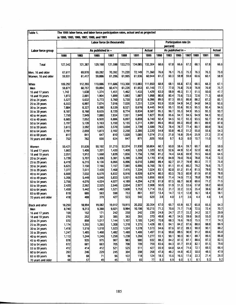
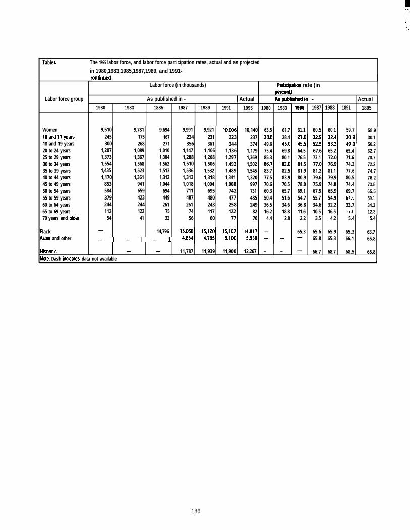
Table 1. The 1995 labor force, and labor force participation rates, actual and as projectedin 1980,1983,1985,1987,1989, and 1991-

Labor force group

Women16and17years18 and 19 years20 to 24 years25 to 29 years30 to 34 years35 to 39 years40 to 44 years45 to 49 years50 to 54 years55 to 59 years60 to 64 years65 to 69 years70 years and older

lack*n and other

lisQanic

:ontinuedLabor force (in thousands) Partki@on rate (in

As published in - I Actual Aspublishedin - I Actual1980 1983 1885 1987 1989 1991 1995 1980 1983

9,510245300

1,2071,3731,5541,4351,170

853584379244112

54

—

9,781175268

1,0891,3671,5681,5231,361

941659423244122

41

9,694167271

1,0101,3041,5621,5131,3121,044

694449261

7532

14,796

– l – l – 1

9,991234356

1,1471,2881,5101,5361,3131,018

711487261

7456

9,921231361

1,1061,2681,5061,5321,3181,004

69548024311760

10,OO6I223344

1,1361,2971,4921,4891,3411,008

742477258122

77

10,140 63.5237 38.fl374 49.6

1,179 75.41,369 85.31,502 86.71,545 83.71,320 77.5

997 70.6731 60.3485 50.4249 36.5

82 16.270 4.4

61.728.445.069.880.182.()82.583.970.565.751.634.618.8

2.8

—

1885 1987 1988 1891 1895

61.1 60.5 60.1 59.7

64.576.581.581.980.978.069.154.736.811.6

67.6 65.2 65.473.1 72.0 71.677.0 76.9 74.381.2 81.1 77.679.6 79.9 80.575.9 74.8 74.467.5 65.9 69.755.7 54.9 54.(I34.6 32.2 33.710.5 16.5 17.a

58.930.150.262.770.772.274.776.273.565.559.134.312.3

2.2 3.5 4.2 5.4 5.4

65.3 65.6 65.9 65.3 63.7— 65.8 65.3 66.1 65.8

— 66.7 68.7 68.5 65.8— — 11,787 11,939 11,900 12,267 – –Iote: Dash indiites data not available J

186

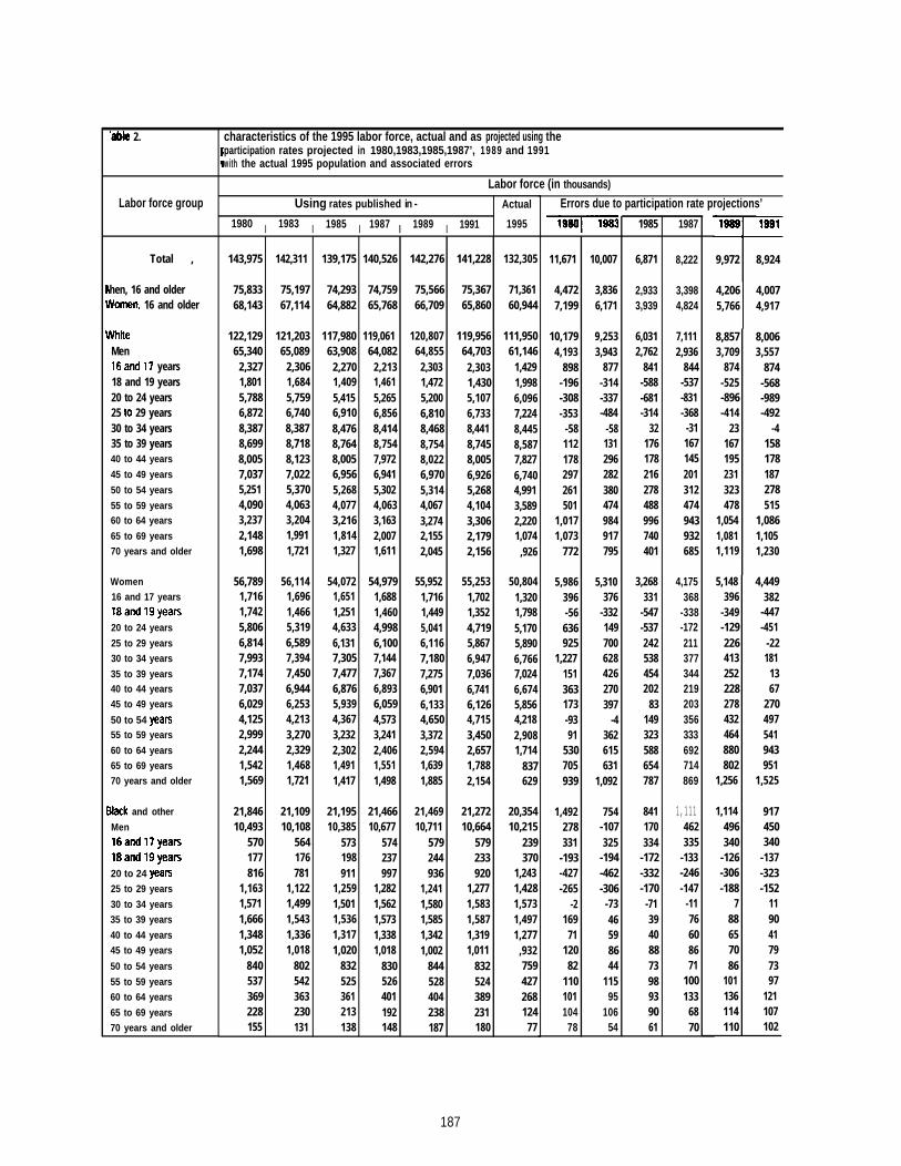
Table 2.

Labor force group

Total ,

hen, 16 and olderMmen, 16 and older

YhiieMen16and17 years18 and 19 years20 to 24 years25 to 29 years30 to 34 years35 to 39 years40 to 44 years

45 to 49 years

50 to 54 years

55 to 59 years60 to 64 years

65 to 69 years70 years and older

Women16 and 17 years18and19years

20 to 24 years

25 to 29 years30 to 34 years

35 to 39 years40 to 44 years45 to 49 years

50 to 54 years55 to 59 years

60 to 64 years65 to 69 years70 years and older

IIack and other

Men16and17years

18and19years

20 to 24 yean25 to 29 years

30 to 34 years35 to 39 years

40 to 44 years45 to 49 years

50 to 54 years

55 to 59 years60 to 64 years

65 to 69 years70 years and older

characteristics of the 1995 labor force, actual and as projected using theparticipation rates projected in 1980,1983,1985,1987’, 1989 and 1991with the actual 1995 population and associated errors

Labor force (in thousands)

Using rates published in - Actual

1980 I 1983 I 1985 I 1987 I 1989 I 1991 1995

143,975 142,311 139,175 140,526 142,276 141,228 132,305

75,833 75,197 74,293 74,759 75,566 75,367 71,36168,143 67,114 64,882 65,768 66,709 65,860 60,944

122,129 121,203 117,980 119,061 120,807 119,956 111,95065,340 65,089 63,908 64,082 64,855 64,703 61,146

2,327 2,306 2,270 2,213 2,303 2,303 1,4291,801 1,684 1,409 1,461 1,472 1,430 1,9985,788 5,759 5,415 5,265 5,200 5,107 6,0966,872 6,740 6,910 6,856 6,810 6,733 7,2248,387 8,387 8,476 8,414 8,468 8,441 8,4458,699 8,718 8,764 8,754 8,754 8,745 8,5878,005 8,123 8,005 7,972 8,022 8,005 7,8277,037 7,022 6,956 6,941 6,970 6,926 6,7405,251 5,370 5,268 5,302 5,314 5,268 4,9914,090 4,063 4,077 4,063 4,067 4,104 3,5893,237 3,204 3,216 3,163 3,274 3,306 2,2202,148 1,991 1,814 2,007 2,155 2,179 1,0741,698 1,721 1,327 1,611 2,045 2,156 ,926

56,789 56,114 54,072 54,979 55,952 55,253 50,8041,716 1,696 1,651 1,688 1,716 1,702 1,3201,742 1,466 1,251 1,460 1,449 1,352 1,7985,806 5,319 4,633 4,998 5,041 4,719 5,1706,814 6,589 6,131 6,100 6,116 5,867 5,8907,993 7,394 7,305 7,144 7,180 6,947 6,7667,174 7,450 7,477 7,367 7,275 7,036 7,0247,037 6,944 6,876 6,893 6,901 6,741 6,6746,029 6,253 5,939 6,059 6,133 6,126 5,8564,125 4,213 4,367 4,573 4,650 4,715 4,2182,999 3,270 3,232 3,241 3,372 3,450 2,9082,244 2,329 2,302 2,406 2,594 2,657 1,7141,542 1,468 1,491 1,551 1,639 1,788 8371,569 1,721 1,417 1,498 1,885 2,154 629

21,846 21,109 21,195 21,466 21,469 21,272 20,35410,493 10,108 10,385 10,677 10,711 10,664 10,215

570 564 573 574 579 579 239177 176 198 237 244 233 370816 781 911 997 936 920 1,243

1,163 1,122 1,259 1,282 1,241 1,277 1,4281,571 1,499 1,501 1,562 1,580 1,583 1,5731,666 1,543 1,536 1,573 1,585 1,587 1,4971,348 1,336 1,317 1,338 1,342 1,319 1,2771,052 1,018 1,020 1,018 1,002 1,011 ,932

840 802 832 830 844 832 759537 542 525 526 528 524 427369 363 361 401 404 389 268228 230 213 192 238 231 124155 131 138 148 187 180 77

Errors due to participation rate projections’

11,671 10,007

4,472 3,8367,199 6,171

10,179 9,2534,193 3,943

898 877-196 -314-308 -337-353 -484

-58 -58112 131178 296297 282261 380501 474

1,017 9841,073 917

772 795

5,986 5,310396 376-56 -332636 149925 700

1,227 628151 426363 270173 397-93 -491 362

530 615705 631939 1,092

1,492 754278 -107331 325

-193 -194-427 -462-265 -306

-2 -73169 46

71 59120 8682 44

110 115101 95104 10678 54

1985

6,871

2,9333,939

6,0312,762

841-588-681-314

32176178216278488996740401

3,268331

-547-537242538454202

83149323588654787

841170334

-172-332-170

-713940887398939061

1987

8,222

3,3984,824

7,1112,936

844-537-831-368

-31167145201312474943932685

4,175368

-338-172211377344219203356333692714869

1,111462335

-133-246-147

-1176608671

100133

6870

9,972 8,924

4,206 4,0075,766 4,917

8,857 8,0063,709 3,557

874 874-525 -568-896 -989-414 -492

23 -4167 158195 178231 187323 278478 515

1,054 1,0861,081 1,1051,119 1,230

5,148 4,449396 382

-349 -447-129 -451226 -22413 181252 13228 67278 270432 497464 541880 943802 951

1,256 1,525

1,114 917496 450340 340

-126 -137-306 -323-188 -152

7 1188 9065 4170 7986 73

101 97136 121114 107110 102

187

., ’...-

,:

.<’

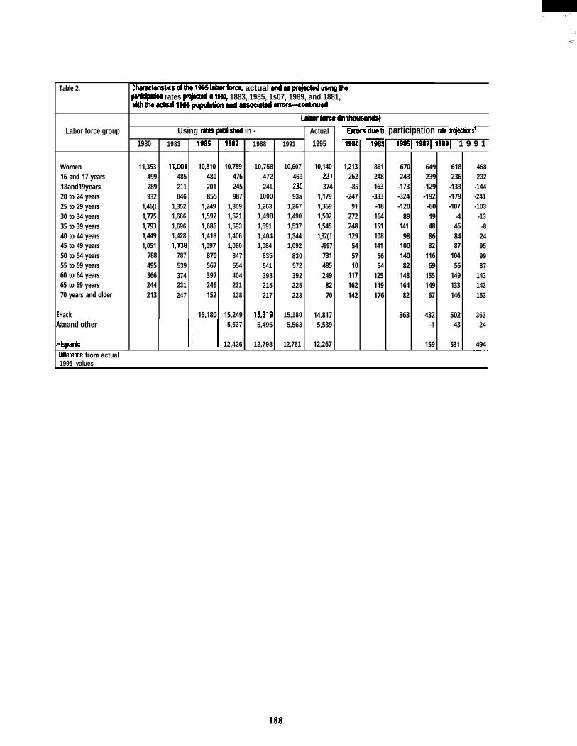
Table 2.

Labor force group

Women16 and 17 years18and19years20 to 24 years25 to 29 years30 to 34 years35 to 39 years40 to 44 years45 to 49 years50 to 54 years55 to 59 years60 to 64 years65 to 69 years70 years and older

HackAsian and other

Ikpanic1Difference from actual

m . .uhamcwwsofthe 19951aborforce# actual endasprajededusingtheWtki@on rates -in 18M, 1883,.1985, 1s07, 1989, and 1881,withtheactual 1895popuwonand MsoclaM ermrs-cwtinued

Using rate$ publii in -

1980

11,353499289932

1,46(I1,7751,7931,4491,051

788495366244213

1983

11,001485211846

1,3521,6661,6961,4281,13EI

787539374231247

1885

10,810480201855

1,2491,5921,6861,4181,097

870567397246152

15,180

1987

10,789476245987

1,3091,5211,5931,4061,080

847554404231138

15,249

II 5,537

12,426

1988 1991

10,758 10,607472 469241 230

1000 93a1,263 1,2671,498 1,4901,591 1,5371,404 1,3441,084 1,092

835 830541 572398 392215 225217 223

15,319 15,1805,495 5,563

12,798 12,761

Actual

1995

10,140237374

1,1791,3691,5021,5451,32(.I

#997731485249

8270

14,8175,539

12,267

-mTm

1,213262-85

-24791

272248129545710

117162142

861248

-163-333

-181641511081415654

125149176

participation rate projecbs’19851 19871 19881 1 9 9 1

670 649 618243 239 236

-173 -129 -133-324 -192 -179-120 -60 -107

89 19 -4141 48 4698 86 84

100 82 87140 116 10482 69 56

148 155 149164 149 13382 67 146

363 432 502-1 -43

159 531

468232

-144-241-103

-13-824959987

143143153

36324

494

1995 values

188

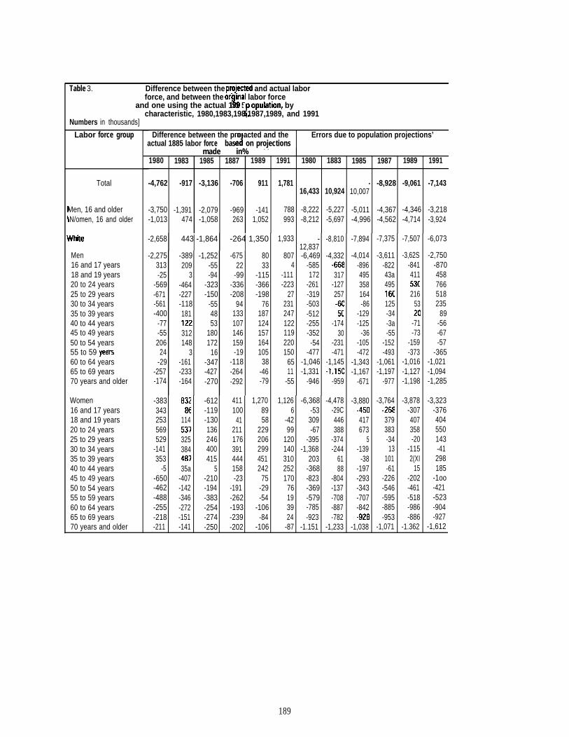
Table 3. Difference between the pro@cted and actual laborforce, and between the ori ‘inal labor force

Land one using the actual 1 1 5 opulation, byfcharacteristic, 1980,1983,198,1987,1989, and 1991

Numbers in thousands]

Labor force group

Total

Men, 16 and olderN/omen, 16 and older

tVhite

Men16 and 17 years18 and 19 years20 to 24 years25 to 29 years30 to 34 years35 to 39 years40 to 44 years45 to 49 years50 to 54 years55 to 59 yeals60 to 64 years65 to 69 years70 years and older

Women16 and 17 years18 and 19 years20 to 24 years25 to 29 years30 to 34 years35 to 39 years40 to 44 years45 to 49 years50 to 54 years55 to 59 years60 to 64 years65 to 69 years70 years and older

Difference between the pro-acted and the Errors due to population projections’actual 1885 labor force bas on projections

made in% - -

1980 1983 1985 1887 1989 1991 1980 1883 1985 1987 1989 1991

-4,762 -917 -3,136 -706 911 1,781 - -8,928 -9,061 -7,14316,433 10,924 10,007

-3,750 -1,391 -2,079 -969 -141 788 -8,222 -5,227 -5,011 -4,367 -4,346 -3,218-1,013 474 -1,058 263 1,052 993 -8,212 -5,697 -4,996 -4,562 -4,714 -3,924

-2,658 I443 -1,864 I-264 1,350

-2,275 -389313 209-25 3

-569 -464-671 -227-561 -118-400 181

-77 122-55 312206 148

24 3-29 -161

-257 -233-174 -164

-383 832343 86253 114569 537529 325

-141 384353 481

-5 35a-650 -407-462 -142-488 -346-255 -272-218 -151-211 -141

-1,252 -675 80-55 22 33-94 -99 -115

-323 -336 -366-150 -208 -198

-55 94 7648 133 18753 107 124

180 146 157172 159 164

16 -19 105-347 -118 38-427 -264 -46-270 -292 -79

-612 411-119 100-130 41136 211246 176400 391415 444

5 158-210 -23-194 -191-383 -262-254 -193-274 -239-250 -202

1,2708958

229206299451242

75-29-54

-106-84

-106

1,933

8074

-111-223

27231247122119220150

6511

-55

- -8,81012,837-6,469 -4,332

-585 -668172 317

-261 -127-319 257-503 -6C-512 50-255 -174-352 30

-54 -231-477 -471

-1,046 -1,145-1,331 -1,15C

-946 -959

1,126 -6,368 -4,4786 -53 -29C

-42 309 44699 -67 388

120 -395 -374140 -1,368 -244310 203 61252 -368 88170 -823 -804

76 -369 -13719 -579 -70839 -785 -88724 -923 -782

-87 -1.151 -1,233

-7,894

-4,014-896495358164-86

-129-125

-36-105-472

-1,343-1,167

-671

-3,880-450417673

5-139

-38-197-293-343-707-842-92fl

-1,038

-7,375

-3,611-82243a495160125-34-3a-55

-152-493

-1,061-1,197

-977

-3,764-26E!379383-3413

101-61

-226-546-595-885-953

-1,071

-7,507

-3,62S-841411530216

5320

-71-73

-159-373

-1,016-1,127-1,198

-3,878-307407358-20

-1152(XI

15-202-461-518-986-886

-1.362

-6,073

-2,750-870458766518235

89-56-67-57

-365-1,021-1,094-1,285

-3,323-376404550143-41298185

-1oo-421-523-904-927

-1,612

189

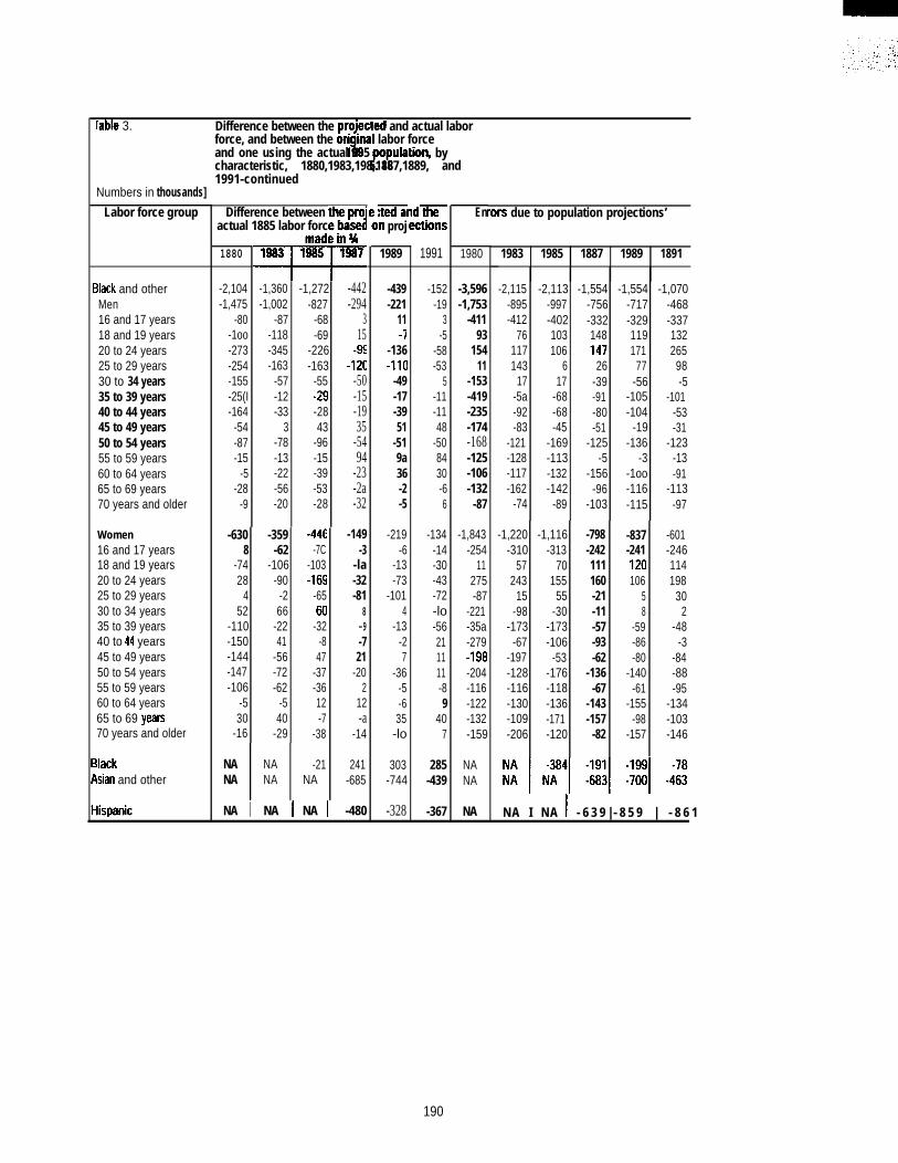
Table 3. Difference between the Droiected and actual laborforce, and between the br- “inal labor force

‘$8and one using the actual 1 5F’

ulation, bycharacteristic, 1880,1983,198,1887,1889, and1991-continued

Numbers in thousands]

Labor force group Difference between pro’actual 1885 labor force bas‘J

tied alIn proj

En Irs due to population projections’

1880 1989 1991 1980 1983 1985 1887 1989 1891

IIack and otherMen16 and 17 years18 and 19 years20 to 24 years25 to 29 years30 to 34 years35 to 39 years40 to 44 years45 to 49 years50 to 54 years55 to 59 years60 to 64 years65 to 69 years70 years and older

-2,104-1,475

-80-1oo-273-254-155-25(I-164

-54-87-15

-5-28

-9

-1,360-1,002

-87-118-345-163

-57-12-33

3-78-13-22-56-20

-1,272-827

-68-69

-226-163

-55-29-2843

-96-15-39-53-28

-442-294

315

-9$-12C

-50-15-1935

-5494

-23-2a-32

-439-221

11-1

-136-11(I

-49-17-3951

-519a36-2-5

-152-19

3-5

-58-53

5-11-1148

-508430-66

-3,596-1,753

-41193

15411

-153-419-235-174-168-125-106-132

-87

-2,115-895-412

76117143

17-5a-92-83

-121-128-117-162

-74

-2,113 -1,554 -1,554 -1,070-997 -756 -717 -468-402 -332 -329 -337103 148 119 132106 147 171 265

6 26 77 9817 -39 -56 -5

-68 -91 -105 -101-68 -80 -104 -53-45 -51 -19 -31

-169 -125 -136 -123-113 -5 -3 -13-132 -156 -1oo -91-142 -96 -116 -113

-89 -103 -115 -97

-1,220 -1,116-310 -313

57 70243 155

15 55-98 -30

-173 -173-67 -106

-197 -53-128 -176-116 -118-130 -136-109 -171-206 -120

-798-242111160-21-11-57-93-62

-136-67

-143-157

-82

-837-241120106

58

-59-86-80

-140-61

-155-98

-157

-601-246114198

302

-48-3

-84-88-95

-134-103-146

Women16 and 17 years18 and 19 years20 to 24 years25 to 29 years30 to 34 years35 to 39 years40 to 44 years45 to 49 years50 to 54 years55 to 59 years60 to 64 years65 to 69 y~rs70 years and older

-630 -359 -44[8 -62 -7C

-74 -106 -10328 -90 -16S

4 -2 -6552 66 6C

-110 -22 -32-150 41 -8-144 -56 47-147 -72 -37-106 -62 -36

-5 -5 1230 40 -7

-16 -29 -38

-149-3

-la-32-81

8-9-721

-202

12-a

-14

-219-6

-13-73

-1014

-13-27

-36-5-635-lo

-134-14-30-43-72-lo-56211111-89

407

-1,843-254

11275-87

-221-35a-279-19a-204-116-122-132-159

lacksian and other

NANA

NANA

-21NA

241-685

303-744

285-439

NANA

NA I NA I - 6 3 9 | - 8 5 9 | - 8 6 1NA I NA I NA I -480Iispanic -328 -367 NA

190

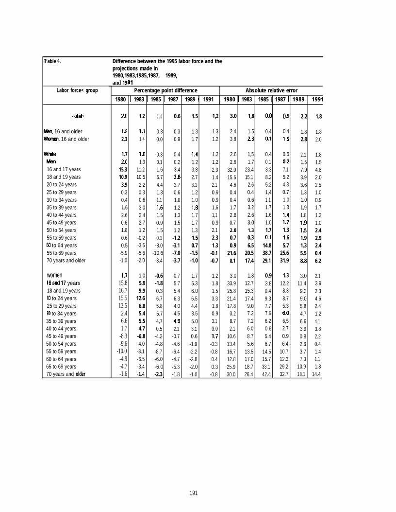
‘able 4. Difference between the 1995 labor force and theprojections made in1980,1983,1985,1987, 1989,and 19

Labor force< group

Totab

km, 16 and olderfomen, 16 and older

ilhne

16 and 17 years18 and 19 years20 to 24 years25 to 29 years30 to 34 years35 to 39 years40 to 44 years45 to 49 years50 to 54 years55 to 59 years60 to 64 years55 to 69 years70 years and older

women16and17 years18 and 19 years20 to 24 years25 to 29 years30 to 34 years35 to 39 years40 to 44 years45 to 49 years50 to 54 years55 to 59 years60 to 64 years65 to 69 years70 years and older

Percentage point difference Absolute relative error

1980 I 1983 I 1985 [ 1987 I 1989 I 1991 1980 I 1983 I 1985 I 1987 I 1989 1991

2.0

1.82.3

1.72.(I

15.310.9

3.90.30.41.62.60.61.80.60.5

-5.9-1.0

1.715.816.715.513.5

2.46.61.7

-8.3-9.6

-10.0-4.9-4.7-1.6

1.2

1.11.4

1 .(I1.3

11.210.5

2.20.30.63.02.42.71.2

-0.2-3.5-5.6-2.0

1.05.99.9

12.66.85.45.54.7

-6.8-4.0-8.1-6.5-3.4-1.4

0.0

0.30.0

-0.30.11.65.74.41.31.11,61.50.91.50.1

-8.0-10,6

-3.4

-0.6-1.80.36.75.85.74,70.5

-4.2-4.8-8.7-6.0-6.0-2.3

0.6 1.5 1,2 3.0 1,8 0.0 ().9 2.2 1.8

0.3 1.3 1.3 2.4 1.5 0.4 0.4 1.8 1.80.9 1.7 1.2 3.8 2.3 0,1 1.5 2.8 2.0

0.4 1.4 1.2 2.6 1,5 0.4 0.6 2.1 1.80.2 1.2 1.2 2.6 1.7 0.1 0.2 1.5 1.53.4 3.8 2.3 32.0 23.4 3.3 7.1 7.9 4.83,6 2.7 1.4 15.6 15.1 8.2 5.2 3.9 2.03.7 3.1 2.1 4.6 2.6 5.2 4.3 3.6 2.50.6 1.2 0.9 0.4 0.4 1,4 0.7 1.3 1.01.0 1.0 0.9 0.4 0.6 1.1 1.0 1.0 0.91.2 1,8 1,6 1.7 3.2 1.7 1.3 1,9 1.71.3 1.7 1,1 2.8 2.6 1.6 1.4 1.8 1.21.5 1.7 0.9 0.7 3.0 1.0 1.7 1.9 1.01.2 1.3 2.1 2.0 1.3 1.7 1.3 1.5 2.4

-1.2 1.5 2.3 0.7 0.3 0.1 1.6 1.9 2.9-3.1 0.7 1.3 0.9 6.5 14.8 5.7 1.3 2.4-7.0 -1.5 -O.1 21.6 20.5 38.7 25.6 5.5 0.4-3.7 -1.0 -0.7 8.1 17.4 29.1 31.9 8.8 6.2

0.7 1.7 1.2 3.0 1.8 0.9 1.3 3.0 2.15.7 5.3 1.8 33.9 12.7 3.8 12.2 11.4 3.95.4 6.0 1.5 25.8 15.3 0.4 8.3 9.3 2.36.3 6.5 3.3 21.4 17.4 9.3 8.7 9.0 4.64.0 4.4 1.8 17.8 9.0 7.7 5.3 5.8 2.44.5 3.5 0.9 3.2 7.2 7.6 6.o 4.7 1.24,9 5.0 3.1 8.7 7.2 6.2 6,5 6.6 4.12.1 3.1 3.0 2.1 6.0 0.6 2.7 3.9 3.8

-0.7 0.6 1.7 10.6 8.7 5.4 0.9 0.8 2.2-4.6 -1.9 -0.3 13.4 5.6 6.7 6.4 2.6 0.4-6.4 -2.2 -0.8 16,7 13.5 14.5 10.7 3.7 1.4-4.7 -2.8 0.4 12.8 17.0 15.7 12.3 7.3 1.1-5.3 -2.0 0.3 25.9 18.7 33.1 29,2 10.9 1.8-1.8 -1.0 -0.8 30.0 26.4 42.4 32.7 18.1 14.4

191

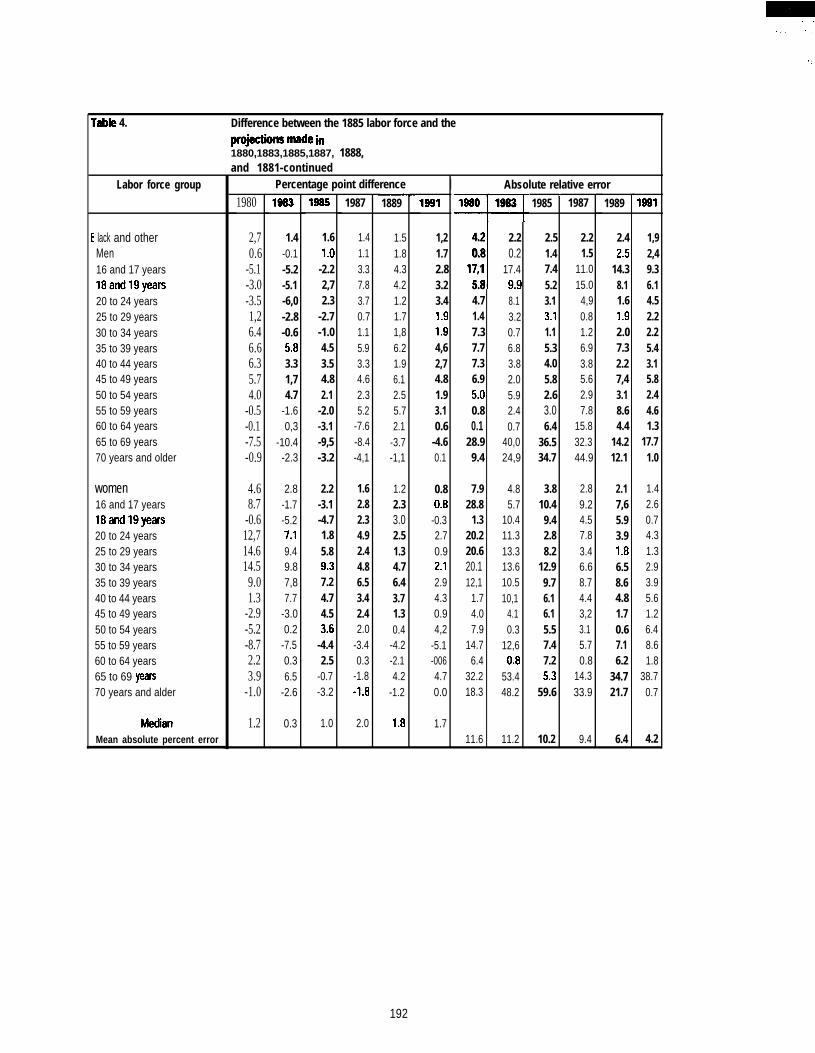
.,f,. ‘ . .

,.

MM(! 4. Difference between the 1885 labor force and thepfo~iS made h1880,1883,1885,1887, 1888,and 1881-continued

Labor force group

lack and otherMen16 and 17 years18and19years20 to 24 years25 to 29 years30 to 34 years35 to 39 years40 to 44 years45 to 49 years50 to 54 years55 to 59 years60 to 64 years65 to 69 years70 years and older

women16 and 17 years18and19years20 to 24 years25 to 29 years30 to 34 years35 to 39 years40 to 44 years45 to 49 years50 to 54 years55 to 59 years60 to 64 years65 to 69 yetlrS70 years and alder

MadanMean absolute percent error

Percentage point difference

1980

2,70.6

-5.1-3.0-3.51,26.46.66.35.74.0

-0.5-0.1-7.5-0.9

4.68.7

-0.612,714.614.5

9.01.3

-2.9-5.2-8.72.23.9

-1.0

1.2

1983

1.4-0.1-5.2-5.1-6,0-2.8-0.65,83.31,74.7

-1.60,3

-10.4-2.3

2.8-1.7-5.27,19.49.87,87.7

-3.00.2

-7.50.36.5

-2.6

0.3

1885

1.61.0

-2.22,72.3

-2.7-1.04.53.54.82.1

-2.0-3.1-9,5-3.2

2.2-3.1-4.71.85.89.37.24.74.53,6

-4.42.5

-0.7-3.2

1.0

1987

1.41.13.37.83.70.71.15.93.34.62.35.2

-7.6-8.4-4,1

1.62.82.34.92.44.86.53.42.42.0

-3.40.3

-1.8-loa

2.0

1889

1.51.84.34.21.21.71,86.21.96.12.55.72.1

-3.7-1,1

1.22.33.02.51.34.76.43.71.30.4

-4.2-2.14.2

-1.2

1,8

I Absolute relative error

1991

1,21.72.83.23.41.91.94,62,74.81.93.10.6

-4.60.1

0.80,8

-0.32.70.92,12.94.30.94,2

-5.1-0064.70.0

1.7

11880

4.20.8

17,15.84.71.47.37.77.36.95,00.80.1

28.99.4

7.928.8

1.320.220.620.112,1

1.74.07.9

14.76.4

32.218.3

11.6

71983

2.20.2

17.49.98.13.20.76.83.82.05.92.40.7

40,024,9

4.85.7

10.411.313.313.610.510,1

4.10.3

12,60.8

53.448.2

11.2

*1985

2.51.47.45.23.13.11.15.34.05.82.63.06.4

36.534.7

3.810.49.42.88.2

12.99.76.16.15.57.47.25.3

59.6

10.2

1987

2.21.5

11.015.0

4,90.81.26.93.85.62.97.8

15.832.344.9

2.89.24.57.83.46.68.74.43,23.15.70.8

14.333.9

9.4

1989

2.42,5

14.38.11.61.92.07.32.27,43.18.64.4

14.212.1

2.17,65.93.91.86.58.64.81.70.67.16.2

34.721.7

6.4

1881

1,92,49.36.14.52.22.25.43.15.82.44.61.3

17.71.0

1.42.60.74.31.32.93.95.61.26.48.61.8

38.70.7

4.2

192

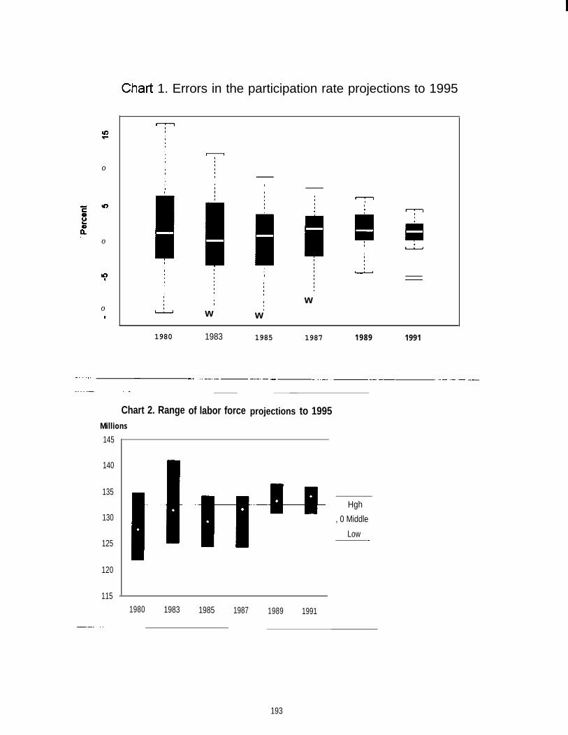
Chati 1. Errors in the participation rate projections to 1995

#It1I,II1,1I,I*II

t I11IIoI1I1#

:t

I

1IIII

11I 1I*

I

o-#

I#I1I

III

I1IIItI111I

d-l

I*1,8#

111I#1#,

-1IIII11,1#,

y

t1,1II

ww

oI w

1980 1983 1985 1987 1989 1991

- . . . . . . . . — -. . .. —...- ._,_ ----- .— --- -------- -— -— . ..-- .— --- ..—----- ..— — __ — ——

projections to 1995Chart 2. RangeMillions

of labor force

145

140

135

130

125

120

115

-u----# Hgh

, 0 Middle

Low

—

—

1980 1983 1985 1987 1989 1991

. .—..

193

Industry employment projections,1995: an evaluationArthur Andreassen

Office of Employment ProjectionsBureau of Labor Statistics

. U.S. Department of LaborThe Bureau of Labor Statistics’ 1984 to 1995 -

employment projections underestimated thegrowth of ~age and salary employment by 6.5million employees. Manufacturing employmentwas over-projected by 2.2 million whileemployment in the service and governmentindustries was under-projected by 6.8 million.Those major industrial sectors which wereprojected to have healthy growth rates did so andthe sectors projected to have moderate ornegative rates actually did grow slowly ordeclined. Projections of industry employmenthowever showed a much greater deviation fromwhat actually occurred than did the sectoremployment projections..

Major Industry Sectors

Considering the condition of the economy in1984 and the economic turmoil of the prioreleven years viz. a viz. inflation, recessions andunemployment, the picture projected for 1995was uncannily accurate. Fortunately, over theprojected period the economy was not impactedby outside shocks approaching those of thepreceding eleven years so trends in industryemployment were mainly responses to domesticeconomic forces. Along with those few shocksthat did actually occur were some errors withinthe macro assumptions that netted to an under-projection of jobs. These errors were included anunder projection of the labor force of 3 millionpersons, an unemployment rate projected to be6% as opposed to the actual 5.670, productivityprojected to grow 20% versus an actual 13%growth and, finally an under projection of totaljobs of 8 million. The combination of thesesometimes offsetting errors resulted in the GrossDomestic Product (GDP) growth rate to be overproject at 38% as opposed to the actual31 %.The following discussion focuses on wage andsalary employment as opposed to totalemployment, total includes wage and salary plusunpaid family and self employed workers.Further, employment in this study refers to a jobsconcept as opposed to a person conceDt which

exceeds the percent of the total labor forceemployed by the amount of multiple job holdingby some workers. It is for this reason that theactual employment is a larger percent of the laborforce than that projected.

As can be seen, (table 1.), the projected 1995distribution of employment by sector closelymatches the actual distribution. The projectedshares of only two sectors, agriculture andwholesale trade, were wrong in direction ascompared with 1984. Agriculture employmentgrew faster than projected because theagricultural services component of this industryshowed more vigor than expected. Agriculturestill held in 1995 the 1.7% share it had in 1984rather than dropping to a projected 1.290.Agriculture is the only sector whose employmentwas projected to decline but which actuallyincreased. Wholesale trade at a 5.7!Z0 share in1984 was projected to rise to a 5.990 share butactually dropped to 5.3910. More actual growth inthe service sectors and less growth in the goodssectors than projected accounted for thisdiscrepancy since service output requires lesstrade to distribute than does goods output.Wholesale trade is the also only sector whoseemployment growth was incorrectly projectedbe faster than the total employment growth(18. 1% as compared to 15.9% for total) butturned out to be slower; the actual rates are

to

13.6%J for wholesale trade and 22.7% for total.Not one sector whose employment was projectedto grow slower than total actually grew faster.

195

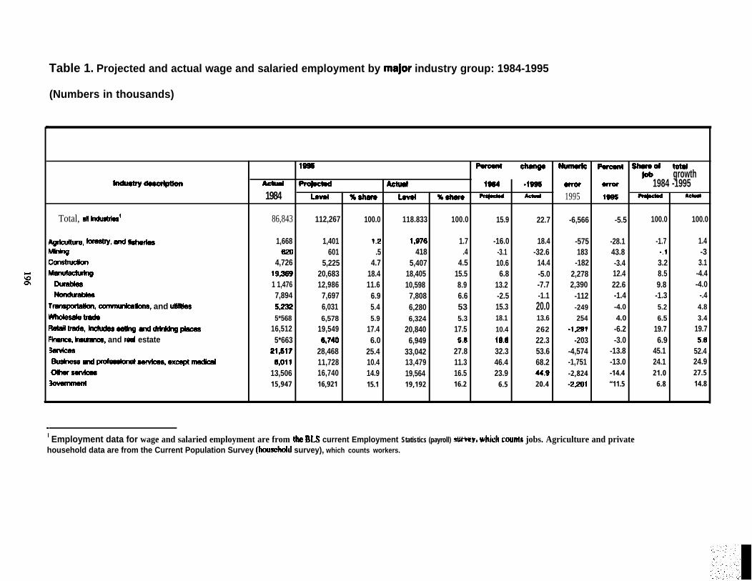
Table 1. Projected and actual wage and salaried employment by major industry group: 1984-1995

(Numbers in thousands)

1- Parcent w ~ Pafeant Shuaof totatw

$f——Y~growth

1664 -1995 amor armr 1984 -19951984 Laval %ahare Levat %ahare ~ - 1995 16$5 ~ -

Total, alt hUlUaWM1 86,843 112,267 100.0 118.833 100.0 15.9 22.7 -6,566 -5.5 100.0 100.0

me, w, and ~ 1,668 1,401 1.2 1,076 1.7 -16.0 18.4 -575 -28.1 -1.7 1.4601 .5 418 .4 -3.1 -32.6 183 43.8 -.1 -3

4,726 5,225 4.7 5,407 4.5 10.6 14.4 -182 -3.4 3.2 3.1Manufectudng 19,389 20,683 18.4 18,405 15.5 6.8 -5.0 2,278 12.4 8.5 -4.4

1 1,476 12,986 11.6 10,598 8.9 13.2 -7.7 2,390 22.6 9.8 -4.07,894 7,697 6.9 7,808 6.6 -2.5 -1.1 -112 -1.4 -1.3 -.4

r~,comm@ca60ns, and utiliws 5X42 6,031 5.4 6,280 53 15.3 20.0 -249 -4.0 5.2 4.8whOk@atnBda 5*568 6,578 5.9 6,324 5.3 18.1 13.6 254 4.0 6.5 3.4Rataittrada, hdudaaeaUng andddnkhgptaWS 16,512 19,549 17.4 20,840 17.5 10.4 262 -lal -6.2 19.7 19.7Rnanca, Insunmw, and fad estate 5*663 6,740 6.0 6,949 5.8 18.0 22.3 -203 -3.0 6.9 5.8

21817 28,468 25.4 33,042 27.8 32.3 53.6 -4,574 -13.8 45.1 52.4Eusblaaa &ld pm&adm# aawfcaa, exeept nladkd 0,011 11,728 10.4 13,479 11.3 46.4 68.2 -1,751 -13.0 24.1 24.9Other swvteea 13,506 16,740 14.9 19,564 16.5 23.9 4.9 -2,824 -14.4 21.0 27.5

15,947 16,921 15.1 19,192 16.2 6.5 20.4 -2201 “11.5 6.8 14.8

‘ Employment data for wage and salaried employment are from the WS current Employment Statistics (payroll) WWY, whi~h counts jobs. Agriculture and privatehousehold data are from the Current Population Survey (household survey), which counts workers.

.. !.,,“.1

Manufacturing employment was projected todrop from a 20% share to 18.4% but this fellshort of the actual decline to 15 .5?10. Employmentin this sector was projected to rise from 1984’slevel of 19.3 million but instead fell to 18.4million. These projections were made in 1984 asthe economy was emerging from the deepest oftwo recessions. It was assumed thatmanufacturing would recover from its recessionloses as exports and domestic demand fordurable goods increased. This did not occur.Durable goods employment was the only sectorprojected to be greater in 1995 than in 1984 butwhich turned out to be lower. The nondurablegoods employment level had too great aprojected decline while mining’s was too little.Construction’s employment grew as wasprojected, but the actual increase was slightlygreater. Both the business service sector and theother service sector increased their shares ofemployment by growing faster than total, asprojected, but both did so at a greater rate.Together the employment in the business servicesector and the other service sector increased theirshare of total employment from 22.2% in 1984 to27.8% in 1995 and except for a slight increase of

0.4% by retail trade these two were the onlysectors whose share did not just hold steady orhave a decline. The 1984 to 1995 percent increasein employment of the business service sector wasthree times that of the total while that of the otherservices sector was twice. Governmentemployment fell as a share as projected but theactual drop was much less than projected.

Ultimately it is the satisfaction of GDP thatdetermines industry output and thus itsemployment. Output is produced either todirectly satisfy demand or to be used as an inputby other industries whose output is sold todemand. Changes over time to the structure ofdemand and the production process affect thedistribution of industry employment. As onemoves down the chain from total demand todemand by major sector to demand by industrythe econometric relationships become less stablewith more deviation introduced to the projectedresults. Projections of gross domestic product bymajor demand sector is the next step in theprocess of deriving industry outputs (see Table2.).

197

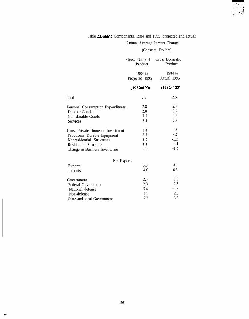
Table 2.Demand Components, 1984 and 1995, projected and actual:

Annual Average Percent Change

(Constant Dollars)

Gross National Gross DomesticProduct Product

1984 to 1984 toProjected 1995 Actual 1995

Total

Personal Consumption ExpendituresDurable GoodsNon-durable GoodsServices

Gross Private Domestic InvestmentProducers’ Durable EquipmentNonresidential StructuresResidential StructuresChange in Business Inventories

(1977=100)

2.9

2.82.81.93.4

2.83.82.02.10.3

(1992=100)

2.5

2.73.71.92.9

1.84.7

-1.21.4-4.0

Net ExportsExports 5.6 8.1Imports -4.0 -6.3

Government 2.5 2.0Federal Government 2.8 0.2National defense 3.4 -0.7Non-defense 1.1 2.5State and local Government 2.3 3.3

198

Changes have been made in the definition andcalculation of real demand since the year 1984such that a comparison of the projected with theactual dollar values of 1995 GDP is difficult.Therefore only relative values will be discussed.A total GDP that was projected to grow at a2.9% aierage annual rate only grew 2.5%. Thisslower growth occurred because the actual higheremployment level and lower unemployment ratewere offset by a lower growth in productivity.Although few years display a complete lack ofdestabilizing forces, 1995 could be consideredvery stabile. Even though it was the fourth yearafter the last recession the upturn was still notshowing signs of major imbalances and a lowunemployment rate was accompanied by lowinflation and interest rates.

Within total GDP personal consumptionexpenditures (PCE) is the hugest and moststabile sector and its projection was right on.This fortuitous event resulted from someoffsetting within PCE. Among the threecomponents of PCE was a correct projectionnon-durable consumption and an underprojection of durable consumption balanced byan over projection of service consumption. Thegrowth rate of gross private domestic investment,the most variable of demand sectors, was overprojected due to a too low projection ofequipment swamped by a too high projection ofconstruction and inventories. Producer durableequipment demand in 1995 has benefited fromthe purchases of computer and communicationsequipment purchases by business which hasdownsized and sought to increase productivity.Non-residential construction has still notrecovered from the tax encouraged over buildingof the middle eighties; residential construction nolonger benefits from the demand it had when thebaby boomers were entering the home buyingage. Change in business inventories is just that,the increase or decrease in the inventory stockover a year. At end 1995 business’ were in theprocess of working off an excess of inventoriesand this created the large negative shown.

helped exports despite the tepid growth by theU.S. main trading partners. Import growthreflected the continuing healthy domesticeconomy as well as imports of unexpectedlycheap oil. Although exports grew faster thanimports the U.S. still had a foreign trade deficitbecause exports started from a lower base thanimports. Projected government demand was onlyslightly higher than actual due to within sectoroffsets, i.e., defense purchases were much lowerwhile non-defense and State and local purchaseswere higher than projected. The unexpectedending of the Cold War reversed the defensebuildup which had started in the late seventies.Projected cut backs in non-defense spending didnot occur. State and local governments continuedto increase spending on health and education.

The impact of all this on sector employmentresults in some surprises. For instance, althoughprojected durable purchases by persons andbusinesses were too low projected durablemanufacturing employment was too high.Defense purchases are heavily weighted towardsdurable goods so an over projection herecounterbalanced the durable demand underprojection. Downsizing by manufacturingcompanies has resulted in the contracting out ofmany operations that were previously done inhouse, this outsourcing moves the enumeration ofemployees performing service functions from themanufacturing sector to the service sector. Inaddition, although healthy growth in foreigntrade was projected, the actual growth wasgreater still and an larger part than expected ofdurable demand was satisfied by imports.Inventory change, which primarily consists ofmanufactured goods, was over projected. Theprojected employment for the construction sectorturned out to be close to actual because an over-protected demand was offset almost exactly byan over-projected productivity increase. Finaldemand is one outlet for industry output, theother is purchases by other industries to be usedas inputs. Since little of the output of theagriculture and metal mining industries, is sold asfinal demand errors in the projected demand of

Trade, both the export and the import industries which use them ‘m inputs will affect

components, grew even more vigorously than the their projected employment. Mining and a

smart growth projected. The value of the dollar number of manufacturing industries’ employment

reached a trade weighted low in 1995 which were over-projected as a result of the over-protection of durable goods output. Further,

199

although the personal consumption of serviceswas over projected the employment in the servicesector was still under projected because of theunexpected heavy use of contracted services asinputs on the part of manufacturing industries.

When one moves from major sector employmentto industry employment the errors in assumptionsand in GDP have a more serious impact (table 3).Right off ones sees evidence of what will is arecurrent theme of these projections, agriculturalservices, as with almost all services, was underprojected. Mining employment was overprojected partly because it was expected that oilprices would continue to increase to double the$25 per barrel price of 1984 whereas it actuallywas at $20 in 1995. Higher international oilprices would have made more domesticproduction profitable while also decreasingimports causing more domestic employment.Coal mining employment was also expected to behelped as cheap domestic coal would besubstituted for the more expensive oil and morecoal would be exported. Metal mining sells mostof its output as inputs to durable manufacturingindustries whose output fell.

Of the 122 industries in this study manufacturingrepresents 75, a 61% share of the industries whileits employment share is only 15?40. Within thisindustry scheme not one manufacturing industryhad as many as one million jobs. Durable goodsencompass 44 industries with employment in 30of these actually less in 1995 than in 1984 whileonly 10 were projected to do so. Lowemployment in those durable goods industriesthat are defense related such as ordnance,aerospace, ship building and communicationsequipment reflect the slow down in defensepurchases., while an unforeseen surge in importsin the computer industry caused employment tocome in at half the projected level. On the otherhand, actual employment in nine durable goodsindustries exceeded the projected level. In one ofthese, the motor vehicle industry, an increase ofU.S. production by foreign companies replacedsubstituted for both imports and the drop indefense demand. Non-durable manufacturingcomprise 31 industries and, although the totalsector employment projection was close, the

industries themselves show a mixed bag ofresults. Most of the industries have a smallamount of employment and for the large ones theprojections were close. The processed foodindustries did much better than expected. Drugsactually grew at a healthier rate than projectedcaused the faster than expected growth in theheath service and government health industries.The transportation industries were slightly underprojected with the utilities industries overprojected, the latter reflecting deregulation.Trade was slightly under projected in the retailarea.

When we get to the service industries is hard tochose the brightest star since what could beviewed as very optimistic projections were easilysurpassed in reality. The business serviceindustry, admittedly a catch all, increased by 5.4million or almost 50% over the 1984 level. Thisindustry has been driven in part by temporaryhelp suppliers and reflects the downsizing andcost cutting that has been going on in the rest ofthe economy. Many firms are replacingpermanent employees with temporary ones inorder to save on benefit costs and to have moreflexibility with their production levels. Further,this industry is where employees will beclassified if they supply such services asaccounting, marketing, personnel and computerconsulting, etc. on a contract basis to firms thatpreviously performed these services in house.Finally, state and local governments added 2.8million employees, twice what was projected aseducation and heath output surpassed what wasprojected. In general, the industries which are thelargest and most important in the economy wereprojected to grow the fastest and this actuallyoccurred. The smaller industries, especially indurable manufacturing did not do as well asprojected but these were not projected to havelarge growth anyway.

An important result of evaluating projections isto highlight the changes, especially theunexpected ones, in the economic structure thathave transpired since the projections were madeand reflect what these changes mean and howthey can be ameliorated.

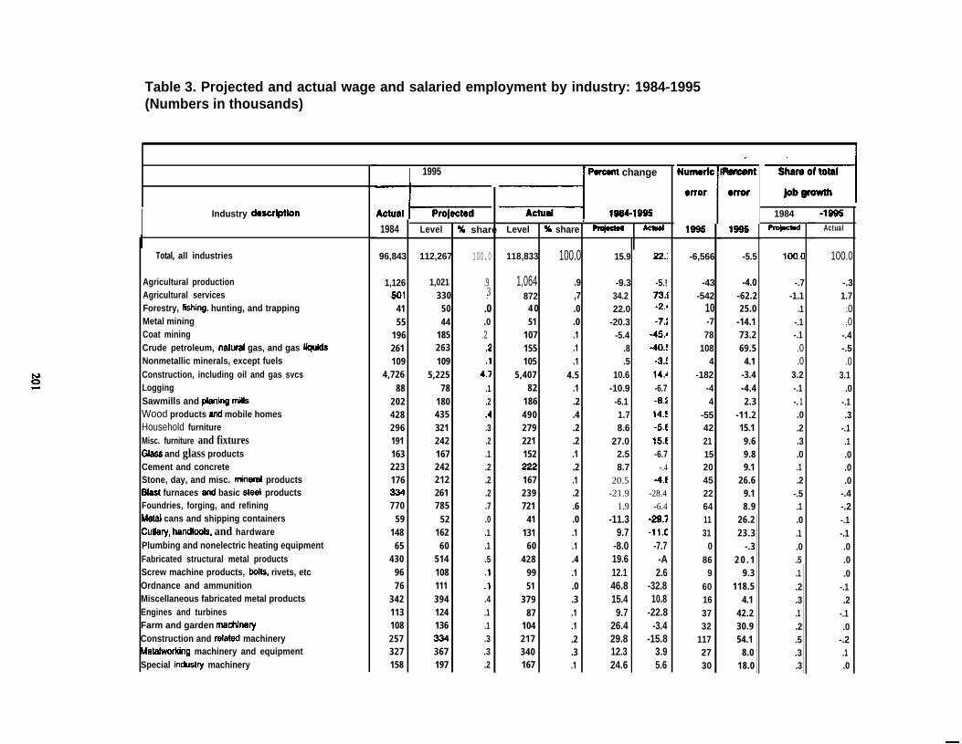
Table 3. Projected and actual wage and salaried employment by industry: 1984-1995(Numbers in thousands)

I Industry descrtptton

Total, all industries

Agricultural productionAgricultural servicesForestry, fish@g, hunting, and trappingMetal miningCoat miningCrude petroleum, naturat gas, and gas tiquidsNonmetallic minerals, except fuelsConstruction, including oil and gas svcsLoggingSawmills and ptaning mitlsWood products and mobile homesHousehold furnitureMisc. furniture and fixturesGtass and glass productsCement and concreteStone, day, and misc. mineraf productsBfast furnaces and basic steet productsFoundries, forging, and refiningMetaf cans and shipping containersCutfery, handtools, and hardwarePlumbing and nonelectric heating equipmentFabricated structural metal productsScrew machine products, bofts, rivets, etcOrdnance and ammunitionMiscellaneous fabricated metal productsEngines and turbinesFarm and garden machhwyConstruction and retated machineryMetafwwtdng machinery and equipmentSpecial indust~ machinery

I 1995 PWWnt change

1984 Level % share

96,843 112,267

1,126 1,021501 330

41 5055 44

196 185261 263109 109

4,726 5,22588 78

202 180428 435296 321191 242163 167223 242176 212

261770 785

59 52148 16265 60

430 51496 10876 111

342 394113 124108 136257327 367158 197

100.0

.9.3.

.0

.0.2.2.1

4.7.1.2.4.3.2.1.2.2.2.7.0.1.1.5.1.1.4.1.1.3.3.2

n

Level % share ~ -

118,833 100.0

1,064 .9872 ,7

4 0 .051 .0

107 .1155 .1105 .1

5,407 4.582 .1

186 .2490 .4279 .2221 .2152 .1

.2167 .1239 .2721 .6

41 .0131 .160 .1

428 .499 .151 .0

379 .387 .1

104 .1217 .2340 .3167 .1

15.9 22.;

-9.3 -5.! 34.2 73.{

22.0 .2.4

-20.3 -7.:-5.4 45.4

.8 *O.!

.5 .3.4

10.6 14.4

-10.9 -6.7-6.1 -8.:1.7 14.:

8.6 -5.[27.0 15.[

2.5 -6.78.7 -.4

20.5 -4.(-21.9 -28.4

1.9 -6.4-11.3 -29.1

9.7 -11.C-8.0 -7.719.6 -A12.1 2.646.8 -32.815.4 10.89.7 -22.8

26.4 -3.429.8 -15.812.3 3.924.6 5.6

.

TNumedc Percent

error error

1995

-6,566

-43-542

10-778

1084

-182-44

-55422115204522641131

086

960163732

1172730

1995

-5.5

-4.0-62.225.0

-14.173.269.5

4.1-3.4-4.42.3

-11.215.19.69.89.1

26.69.18.9

26.223.3

-.3 2 0 . 1

9.3118.5

4.142.230.954.1

8.018.0

1Share of total

job growth

1984

1OO.(I

-.7-1.1

.1-.1-.1.0.0

3.2-.1-. 1.0.2.3.0.1.2

-.5.1.0.1.0.5.1.2.3.1.2.5.3.3

-1995Actual

100.0

-.31.7.0.0

-.4-.5.0

3.1.0

-.1.3

-.1.1.0.0.0

-.4-.2-.1-.1.0.0.0

-.1.2

-.1.0

-.2.1.0

—

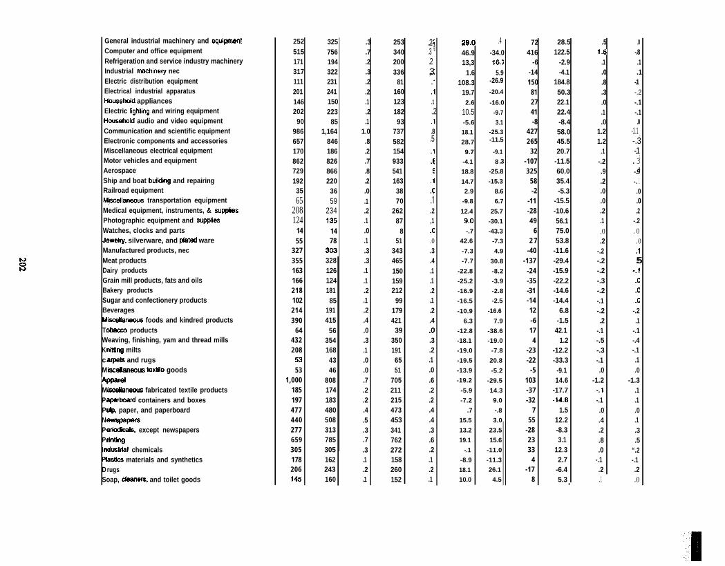
General industrial machinery and equipmmtComputer and office equipmentRefrigeration and service industry machineryIndustrial machmery necElectric distribution equipmentElectrical industrial apparatusHousehotd appliancesElectric tighting and wiring equipmentHousehofd audio and video equipmentCommunication and scientific equipmentElectronic components and accessoriesMiscellaneous electrical equipmentMotor vehicles and equipmentAerospaceShip and boat buitdhg and repairingRailroad equipmentMjscetlaneous transportation equipmentMedical equipment, instruments, & supptiesPhotographic equipment and sup~lesWatches, clocks and partsJewefry, silverware, and pfated wareManufactured products, necMeat productsDairy productsGrain mill products, fats and oilsBakery productsSugar and confectionery productsBeveragesMkceflaneoua foods and kindred productsTObacco productsWeaving, finishing, yam and thread millsKnitting miltscarpets and rugsMiscellaneous textite goodsApparefMisceflaneous fabricated textile productsPaperboard containers and boxesPufp, paper, and paperboardNewspapersPeriodiis, except newspapersPrintingIndustrial chemicalsPtastics materials and syntheticsDrugsSoap, cteaners, and toilet goods

252515171317111201146202

909866571708627291923565

208124

1455

327355163166218102214390

64432208

5353

1,000185197477440277659305178206145

325756194322231241150223

851,164

846186826866220

3659

234135

1478

32812612418185

191415

563541684346

808174183480508313785305162243160

.3

.7

.2

.3

.2

.2

.1

.2

.11.0

.8

.2

.7

.8

.2

.0

.1

.2

.1

.0

.1

.3

.3.1.1.2.1.2.4.0.3.1.0.0.7.2.2.4.5.3.7.3.1.2.1

253340200336

8116012318293

7375821549335411633870

26287

851

343465150159212

9917942139

3501916551

705211215473453341762272158260152

..2#.3.3

.2,.3

.1

.1

.1

.2

.1

.8.5 .1.f

G. .

.1

.C

.1

.2,1.a.0.3.4.1.1.2.1.2.4.0.3.2.1.0.6.2.2.4.4.3.6.2.1.2.1

29.0 .446.9 -34.013,3 16.1

1.6 5.9108.3 -26.9

19.7 -20.4

2.6 -16.0

10.5 -9.7

-5.6 3.1

18.1 -25.3

28.7 -11.5

9.7 -9.1

-4.1 8 .3

18.8 -25.8

14.7 -15.3

2.9 8.6

-9.8 6.7

12.4 25.7

9,0 -30.1

-.7 -43.3

42.6 -7.3

-7.3 4.9

-7.7 30.8

-22.8 -8.2

-25.2 -3.9

-16.9 -2.8

-16.5 -2.5

-10.9 -16.6

6.3 7.9

-12.8 -38.6

-18.1 -19.0

-19.0 -7.8

-19.5 20.8

-13.9 -5.2

-19.2 -29.5

-5.9 14.3

-7.2 9.0

.7 -.8

15.5 3.0

13.2 23.5

19.1 15.6

-.1 -11.0

-8.9 -11.3

18.1 26.1

10.0 4.5

72416

-6-14150

812741-8

427265

32-107325

58-2

-11-2849

62 7

-40-137

-24-35-31-1412-6174

-23-22

-5103-37-32

755

-282333

4-17

8

28.5122.5

-2.9-4.1

184.850.322.122.4-8.458.045.520.7

-11.560.035.4-5.3

-15.5-10.656.175.053.8

-11.6-29.4-15.9-22.2-14.6-14.4

6.8-1.5

42.11.2

-12.2-33.3

-9.114.6

-17.7-14.8

1.512.2-8.33.1

12.32.7

-6.45.3

.51.6

.1 .1

.0 .1

.8

.3

.0

.1

.01.21.2

.1-.2.9.2.0.0.2.1.0.2

-.2-.2-.2-.3-.2-.1-.2.2

-.1-.5-.3-.1.0

-1.2-. 1-.1.0.4.2.8.0

-.1.2

.0-.8

-.1-.2-.1-.1.0

-1.1.3-.3

-.1.3.3.9-.9

-. 1.0.0.2

-.2. 0. 0.1c.5

-.1.C.C.C

-.2.1

-.1-.4-.1.1.0

-1.3.1.1.0.1.3.5

“.2-.1.2

.1 | .0

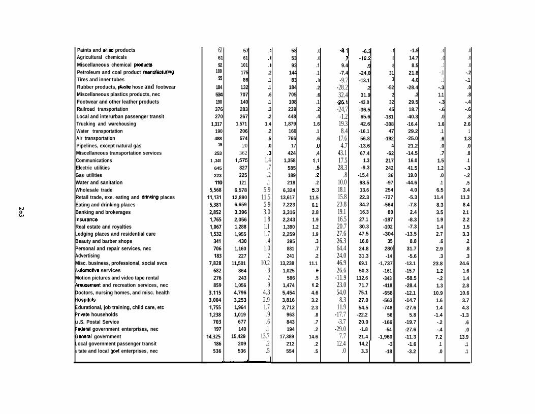
Now

Paints and atlied productsAgricultural chemicalsMiscellaneous chemical product6Petroleum and coal product manuf*@lg

Tires and inner tubesRubber products, ptastic hose and footwearMiscellaneous plastics products, necFootwear and other leather productsRailroad transportationLocal and interurban passenger transitTrucking and warehousingWater transportationAir transportationPipelines, except natural gasMiscellaneous transportation servicesCommunicationsElectric utilitiesGas utilitiesWater and sanitationWholesale tradeRetail trade, exe. eating and drintdng placesEating and drinking placesBanking and brokeragesI nsuranceReal estate and royaltiesLedging places and residential careBeauty and barber shopsPersonal and repair services, necAdvertisingMisc. business, professional, social svcsA utomotive servicesMotion pictures and video tape rentalAmusement and recreation services, necDoctors, nursing homes, and misc. healthHospitalsEdurational, job training, child care, etcPrivate householdsu .S. Postal ServiceFederal government enterprises, necG eneral governmentLocal government passenger transits tate and local govt enterprises, nec

626192

18995

184534190376270

1,317190488

19

253

1 ,340

645

223

1105,568

11,1315,3812,8521,7651,0671,532

341706183

7,828682276859

3,1153,0041,7551,238

703197

14,325186536

5761

10117586

132707140283267

1,571206574

20362

1,575827225121

6,57812,8906,6593,3962,0561,2881,955

4301,160

22711,501

864243

1,0564,7963,2531,9641,019

677140

15,429209536

.1

.1

.1

.2

.1

.1

.6

.1.3.2

1.4.2.5.0.3

1.4.7.2.1

5.911.55.93.01.81.11.7

.41.0

.210.2

.8

.2

.94.32.91.7

.9

.6

.113.7

.2

.5

585393

14483

184705108239448

1,879160766

17424

1,358585189218

6,32413,6177,2233,3162,2431,3902,259

395881241

13,2381,025

5861,4745,4543,8162,712

963843194

17,389212554

.0

.0

.1

.1

.1

.2

.6

.1

.2

.41.6

.1

.6,0,4

1,1.5,2.2

5.311.56.12.81.91.21.9

.3

.7

.211.1

,9.5

1.24.63.22.3

.8

.7

.214.6

.2

.5

-8.1,7

9.4-7.4-9.7

-28.232.4

-26,1-24,7

-1.219.38.4

17.64.7

43.117.528.3

.810.018.115.823.819.116.520.727.626.364.424.046.926.6

-11.923.054.0

8.311.9

-17.7-3.7

-29.07.7

12.4.0

-6.3-12.2

.9-24,0-13.1

.231.9

-43.0-36.565.642.6

-16.156.8

-13.667.4

1.3-9.3

-15.498.513.622.334.216.327.130.347.516.024.831.369.150.3

112.671.775.127.054.5

-22.220.0-1.821.414.23.3

-188

313

-522

3245

-181-308

47-192

4-6221724236

-97254

-727-564

80-187-102-304

35280-14

-1,737-161-343-418-658-563-748

56-166

-54-1,960

-3-18

-1.914.78.5

21.84.0

-28.4.3

29.518.7

-40.3-16.429.2

-25.021.2

-14.516.041.519.0

-44.64.0

-5.3-7.82.4

-8.3-7.3

-13.58.8

31.7-5.6

-13.1-15.7-58.5-28.4-12.1-14.7-27.6

5.8-19.7-27.6-11.3

-1.6-3.2

.0

.0

.1-.1-.1-.31.1-.3-.6.0

1.6.1.6.0.7

1.51.2.0.1

6.511.48.33.51.91.42.7

.62.9

.323.8

1.2-.21.3

10.91.61.4

-1.4-.2-.4

7.2.1.0

.0

.0

.0-.2-.1.0.8

-.4-.6.8

2.61

1.3.0.8.1

-.3-.2.5

3.411.38.42.12.21.53.3

.2

.8

.324.6

1.61.42.8

10.63.74.3

-1.3.6.0

13.9.1.1

EVALUATING THE 1995 OCCUPATIONAL EMPLOYMENT PROJECTIONS

Carolyn M. VeneriBureau of Labor Statistics, Washington, D.C. 20212

The Bureau’s occupational employment projectionscaptured most general occupational trends over the1984-95 period. Some of the most glaring inaccuraciesin the pro~ctions for detailed occupations reflect theconservative nature of projected growth rates that wasidentified in previous evaluations. Although the impactof inaccurate industry employment projections on theoccupational employment projections was significant,the projections of the changes in the utilization ofoccupations by industry resulted in the biggest sourceof projection error as in past evaluations.

Major Occupational GroupsThe direction of employment change was projectedcorrectly for all nine of the major occupational groups.The absolute projection error was less than 10 percentfor eight out of the nine groups, and 11.3 percent forprofessional specialty occupations, the majoroccupational group with the largest absolute error. (Seetable 1.)

Projected employment was lower than actualin six major groups: executive, administrative, andmanagerial occupations; professional specialtyoccupations; marketing and sales occupations;administrative support occupations, including clerical:services occupations; and operators, fabricators, andlaborers. Employment was overestimated for precisionproduction, craft and repair occupations, andtechnicians and related support occupations. This lattergroup was projected the most accurately with projectedemployment less than 1 percent more than actualemployment. The decline in employment was slightlyoverestimated for agriculture, forestry, fishing andrelated occupations.

Not only was the direction of employmentchange anticipated correctly for all the major groups,but the projected distribution of employment growthamong the groups was relatively accurate. i Forexample, the professional specialty occupational grouphad the largest absolute numerical error, nearly 2million, but the share of total employment growth wasunder-projected by only 3.4 percent. Thus, theprojection for total employment—low by about 7.3million— had an impact on projection accuracy.

The largest error in the projected share ofemployment growth was for precision production, craft,and repair occupations. This group’s share of totalemployment growth was over-projected by about 7

percent, in line with employment being over-protected by 886,000. For each major group,however, the same pattern of projection ofemployment growth and projection of share ofemployment growth does not apply. In the case ofoperators, fabricators, and laborers, for example,employment was slightly under-projected but theshare of employment growth was over-projected.The projected share of total employment growthwas almost exact for marketing and sales workers,although the level of employment was under-projected. (See table 1.)

The fastest growing occupational groupshad the largest absolute projection errors.Technicians and related support was projected tobe the fastest growing group, but was outpaced byfour other groups. The two actual leaders,professional specialty and executive,administrative and managerial occupations, wereprojected to grow faster than average, but not asfast as they really did grow.

Administrative support workers, includingclerical, made up the largest group of workers in1984 and was also projected to be, even though itdid not grow more slowly than average, asprojected. The projection error for this group was8.3 percent. The group’s projected slow growthwas based on the anticipated effect of the rapidspread of computerized office equipment. As aresult, many clerical occupations were correctlyprojected to grow slowly or decline. However,employment increased more rapidly than projectedin several large clerical occupations such as billand account collectors, adjustment clerks, andteachers aides and educational assistants.

Projection errors were also relatively largefor both the service occupations and marketing andsales occupations. Each of these groups grewfaster than projected and together they accountedfor a combined employment growth of about 8.1million jobs rather than the expected 5.6 million.More than 60 percent of the projection error of 1.1million for the marketing and sales occupations canbe attributed to an under-projection of twooccupations, cashiers andThese occupations accountedof almost 700,000 workers.

retail salespersons.for an underestimate

205

Projection errors for agriculture, forestry,fishing, and related occupations, and operators,fabricators, and laborers were relatively small. Part ofthis accuracy can be attributed to growth amongoccupations less effected by technological change suchas transportation and material moving occupations andnursery workers and animal caretakers, except farm.Conversely, precision production, craft, and repairoccupations were over-projected by almost a millionworkers. Since employment of these workers isconcentrated in the construction and manufacturingindustries, the projected increase in employment wastied primarily to the projections for those industries.

Professional specialty occupations grew byabout 4.7 million over the 1984-1995 period, almost 2million more than projected. Significant errors in theprojections for detailed occupations with sizableemployment had a tremendous impact on the overallprojection error for this group. For example, an under-projection for five ,professional specialty occupations–computer systems analysts, engineers, and scientists;college and university faculty, adult and vocationaleducation teachers, registered nurses, and socialworkers-contributed significantly to the under-projection of professional workers. Under-projectionof these occupations accounted for about 38 percent ofunderestimated employment for this major group. Thefact that the projection error for professional specialtyoccupations was only 11.3 percent, though, can beattributed to some offsetting of this under-projectioncaused by an over-projection of engineers.2

Detailed occupationsThe evaluation of the 1995 projections covered 348detailed occupations. Table 2 presents data on the 207occupations for which 1984 employment was greaterthan 50,000, ranked by absolute projection error.3 Theabsolute percent errors for all 348 averaged about 24percent. More than three-fiflhs of the occupations,however, had below-average errors.

The Bureau can only evaluate the projectionsfor occupations that had comparable definitions insurveys used to compile employment data in the baseyear and the target year of the projections.Consequently, in past evaluations, relatively fewoccupations could be evaluated because ofclassification system changes. However, many moreoccupations maintained comparability between 1984and 1995 than in past evaluation periods, because theOES survey occupational classification remained verystable over that period. As a result, the number ofoccupations included in this evaluation is much largerthan in past evaluations. 4

2

Projection error is inversely related toemployment size, as past projection evaluationshave indicated. In 1984, fewer than 100,000workers were employed in 211 of the 348occupations included in the evaluation. These 211had an average projection error of about 29percent, whereas 32 occupations with more than500,000 workers in 1984 had an average error ofabout 12.2 percent.

The direction of employment change wasprojected correctly for more than 70 percent of theoccupations included in the evaluation.Employment growth was forecast for the majorityof the occupations. Of the 231 occupations forwhich employment actually grew from 1984 to1995, an increase was projected for all but 16.However, of the 117 occupations for whichemployment declined, only 37 were projected todecline over the period.

The errors among the occupationsincluded in the evaluation ranged widely. (Seetable 2.) For example, the difference betweenprojected and actual employment wasunderestimated by about 42 percent for physiciansassistants, but overestimated by about 190 percentfor roustabouts. Since roustabouts are primarilyconcentrated in the oil and gas industry, thisprojection reveals how the effects of incorrectindustry projections can impact the projections forindividual occupations.

The last two columns in table 2 presentthe projected and actual share of the overallemployment increase for each of the 207occupations for which 1984 employment wasgreater than 50,000. Although there are somenotable exceptions, the projected shares for thedetailed occupations, like the major groups, arerelatively accurate.

Sources of errorErrors in the projections for the detailedoccupations included in the evaluation canultimately be traced back to errors in assumptionsor judgment, resulting in incorrectly projectedchanges in staffing patterns, industry projections,or a combination of both. In order to identifi thesources of error, two simulated matrices werecreated. The first of these was generated bymultiplying the projected 1995 staffing patterns ofindustries by actual 1995 industry employment.The second was produced by multiplying the actual1995 staffing patterns by projected employment byindustry. The first simulation reveals the outcomeif the Bureau projected perfect industry

06

employment totals and the second if it had projectedperfect occupational staffing patterns. Table 2 presentsprojection errors from the two simulated matricescreated to analyze these effects.

In viewing the projection levels and errors forthe detailed occupations, it is possible to identify theeffects analytical judgments had on the individualprojections. Analyses of underlying trends or impactsof technological change were used in developing boththe indust~ projections and the projected staffingpatterns of industries. As mentioned in ArthurAndreassen’s contribution to this article, industryemployment projections were impacted byunanticipated economic changes.s Employment inmanufacturing, for example, did not increase asprojected, but declined because of a number of factors,including a reduction in defense spending, rapid growthof imports, and a trend towards outsourcing all types ofservices. In contrast, employment in services grew at amuch faster rate than predicted.

The effect of industry errors on theoccupational employment may be clearly seen in anexample taken from table 2. Earlier, it was mentionedthat one of the largest projection errors occurred forroustabouts, around 190 percent. Examining theprojection errors from both simulations, shown in table2, one can see clearly that the error is attributable moreto incorrect industry projections for the related oil andgas industries than to the projected staffing pattern: theerror in the simulation using actual staffing patterns andprojected industry totals is 115 percent while it is only38 percent with actual industry totals and projectedstaffing patterns.

Job clusters. In investigating sources of projectionerror, it is helpful to examine groups of relatedoccupations, or job clusters. A number of such clustershave been selected for closer examination in thissection because they show large projection errors orhighlight specific sources of error. For example, theunder-projection of the education industry affected theprojections for education-related occupations. Thisconclusion is supported by a review of the twosimulated matrices for the projection errors for collegeand university faculty and teachers’ aides andeducational assistants. Between 1984 and 1995,employment of college and university faculty wasprojected to decline about 14 percent, thoughemployment actually increased around 12 percent. Theprojected decline was based primarily on the U.S.Department of Education’s National Center forEducation Statistics’ projected drop in collegeenrollments reflecting the shrinking population of 18-to 24- year olds. Enrollment rates, however, increased

during the 1980s as colleges enrolled greaternumbers of older individuals and enrollment ratesof students of traditional college age rose morerapidly than expected.

Due to similar misconceptions aboutenrollments in higher education, employment ofadult and vocational education teachers also wassignificantly under-projected. However, theabsolute percent error for adult and vocationaleducation teachers is actually larger in thesimulation using the projected staffing patterns andactual 1995 industry totals than in the simulationusing actual staffing patterns and projectedindustry employment. (See table 3.) This indicatesthat the error in projecting this group of teacherswas in fact more the result of the underlyingassumptions or judgments that went intodetermining the utilization of the workers in theeducation industry, rather than the projection forthe education industry. Although moderatelyrising demand for adult education was anticipated,the declining population of 18-22 year olds wasexpected to lead to declining demand forvocational education and training. However, thegrowing number of both entry-level andexperienced workers in need of vocational trainingor retraining in order to update job skills and keepup with rapidly changing technology, had more ofan impact on demand for these teachers than wasanticipated.

Likewise, errors in projections for selectcomputer-related occupations were a significantcontributing factor in the underestimate ofemployment for professional specialtyoccupations.s A closer examination of thesimulated matrices for certain others reveals thecause of error to be largely a result of incorrectassumptions behind the projections of theutilization of these workers by industry. (See table4.) In the case of computer programmers, verysignificant increases were projected across allindustries as improvements in both computerhardware and software made computer technologymore versatile, cheaper, and easier to use. But itwas precisely these improvements that led to moremoderate growth as computer users, othercomputer professionals, and automation were ableto take over many of the tasks previouslyperformed by only programmers. Similarly,moderate increases were expected for computeroperators and operators of peripheral EDPequipment across all industries as computer usagerose throughout the economy. However,expanding technologies not only reduced both the

207

R-

size and cost of computer equipment, but alsoautomated the tasks previously performed by numerousoperators.

In contrast to programmers, significantdecreases were projected across all industries for dataentry keyers, composing, as a result of anticipatedtechnological change. Although the trend was correctlyanticipated, it appears that technology had more of aneven greater impact on data entry keyers, composingthan was projected. Virtually the entire error for thisprojection can be attributed to incorrect staffingpatterns.

Overall industry employment for healthservices was underestimated significantly for hospitals,as well as doctors, nursing homes, and miscellaneoushealth services. Absolute errors for health-relatedoccupations ranged from 53 percent for emergencymedical technicians to 1 percent for pharmacists.Although the industry projections had a profoundimpact on estimated employment for these occupations,much of the error in the individual health-relatedoccupations also can be attributed to errors in stafllngpatterns. (See table 5.) For example, the 1984projection of a growing demand for physicians’assistants wits realized as the health care industry beganto focus more and more on cost containment. TheBureau projected the employment of physicians’assistants to increase moderately in hospitals andsignificantly in outpatient care facilities. However, theprojection was too conservative. Similarly, the impactof a growing demand for rehabilitation and long termcare services was underestimated, as employment ofoccupational therapists, projected to grow much fasterthan average, 36 percent, grew by 159 percent. In thecase of licensed practical nurses, the projection wasrelatively accurate, off only 4 percent, resulting fromboth the under-projected industry totals for healthservices and incorrect stafllng patterns that offset eachother. Along with changes in patient care requirements,the trend toward reliance on nursing personnel withhigher levels of clinical skill was expected to slowgrowth among licensed practical nurses. However,rapid industry growth in health services and an agingpopulation spurred more demand than originallyexpected in nursing homes and residential carefacilities.

The BLS evaluation of industry projectionsalso revealed that employment in manufacturing wasprojected to increase over the 1984-95 period ratherthan decline. As a result, the majority of the decliningoccupations that were projected to increase are inmanufacturing-including engineers, precisionproduction workers, machine operators and tenders,and hand workers and fabricators. For example,

employment of workers concentrated in industriesthat manufacture computer and office equipment,electrical industrial apparatus, electroniccomponents and accessories, and aerospace, suchas those listed in table 6, was projected to growslightly when in fact it fell from 1984 to 1995. Asindicated in the table, the projected industry totalswere the major contributing factor to the error forthese occupations.

Implications for future analysesThe most recent occupational projections

to be evaluated were those ending in the year 1990.Looking at the major occupational groups, we canreadily see that the projecticms for 1995 appearmore accurate overall than do the 1990 projections.No major group was off by more than in the pastand the largest absolute error for a major groupwas only 11.3 percent compared to 22 percent in1990 for the group-marketing and salesoccupations. It is important to remember,however, that projections on such an aggregatescale are by their nature uncertain. Becauseindividual occupations, and not major groups, areanalyzed, errors are compounded as theseoccupations are combined. The detailedoccupations that comprise each group can be largeenough that any error in their individual projectioncan affect the outcome for the overall major group.

In developing the detailed 1984-95occupational projections, analysts reviewed allavailable data from both the OES survey andCurrent Population Survey (CPS) and projectedchanges in the occupation-industry cellsaccordingly, bringing knowledge gained throughexperience and studies in preparing theOccupational Outlook Handbook. As a result,numerous changes were made to the occupationalcoefficients-changes affecting the proportion ofan occupation within each industry-as analyticaljudgments were translated into numericalestimates. The bulletin Employment Projectionsfor 1995: Data and Methodk, indicates that, inorder to maintain consistency among thejudgments of the analysts, guidelines for increasingor decreasing coefficients were implemented todevelop the initial projected coefllcients for alloccupations across all industries: small change-1to 4 percent; moderate change-5 to 9 percent;significant change— 10 to 20 percent; and verysignificant change-20 percent or more.7 Theevaluation of the 1984-95 projections has providedanalysts the fwst chance to look back at this work.

208

Prior to the current evaluation, every BLSevaluation of its occupational projections revealed theprojections to be conservative. As the analysis of boththe individual projections for detailed occupations andFlandbook percent-change ranges indicate, the 1984-95projections are also on the conservative side. Themajority of the occupational projections were clusteredaround average growth, when, in actuality, more appearto have grown much faster than the average or to havedeclined. The inherent conservatism contributed tooverall errors in staffhg patterns as well, and part ofthe reason appears to have been that analysts were tooconservative in projecting the matrix coefficients. Thistrend towards conservatism is recognized by the Bureauand since 1984, guidelines for projecting changes in theoccupational coefficients have been revised. Forexample, when developing the most recent round ofprojections horn 1994-2005, the Bureau set forth thefollowing guidelines for interpreting the projectedrange of changes in the coefficients: small change—1 Opercent; moderate—20 percent; significant-35percent; and very significant-50 percent or more.Expanding the range for identi~ing small, moderate,and large changes should clearly have an impact on theconservatism inherent in the methodology.

With the help of the simulated matricesprepared for the current evaluation, however, it hasbeen possible to pinpoint the major source of error foreach detailed occupation. Although the impact of goodindustry projections on developing good occupationalprojections cannot be underestimated, the chiefweakness appears to be in projecting the staffingpatterns. In the simulated matrix for which theprojected staffkg patterns were applied to actual 1995industry totals, the sum of the absolute errors, weightedby 1995 employment, was 7.7 percent. By contrast, inthe matrix for which actual 1995 staffing patterns wereapplied to projected 1995 industry totals, the sum of theabsolute errors weighted by 1995 employment droppedto 5.6 percent.

In addition to the influence of conservativecoefllcient change factors on the projections, theimpacts of features such as technological change andtrends that were not filly realized contributedsignificant y to errors in staffing patterns. Incorrectanalytical judgments relating to the rate and impact oftechnological change and to trends such as outsourcingand the growth of temporary help agencies played alarge role in this regard. The analysis behind theprojection for typists is a case in point. For example,the use of computers and word processing equipmentwas expected to have a negative impact on employmentof typists and word processors across all industries.But because it was assumed that a very large number of

establishments were already using such equipment,and because future technological advances incomputing technology were not fully realized atthe time, the declining trend in employment oftypists and word-processors was not expected toaccelerate. The analysis wound upunderestimating the impact of changingtechnology, as actual employment in 1995 fellshort of projected employment by more than 290thousand workers.

Similar to unforeseeable events such asthe reduction in defense spending resulting fromthe breakup of the Soviet Union, changes broughtabout by technology are becoming harder topredict. For example, the impact of InternetTechnology is nowhere near being fully realizedtoday, just as the expansion of computertechnology into both the home and workplace andthe impact of the personal computer, wasrecognized but not fully accounted for in pastprojection cycles.

Technical noteProjections framework. The 1984-95 projectionsof occupational employment were developedwithin the framework of an industry-occupationmatrix containing 378 industries and over 500occupations. Data used to develop the 1984” matrixand projected 1995 matrix came from a variety ofsources. For industries covered by theOccupational Employment Statistics (OES) survey,the most current survey data were used to developthe occupational distribution or staffing patternsfor estimating 1984 wage and salary employment.Employment by occupation in each industry werederived by multiplying the occupationaldistribution of employment by 1984 wage andsalary worker employment for each industry,which were obtained from the BLS CurrentEmployment Statistics (CES) survey. Both theCES and OES surveys are surveys of businessestablishments, covering only wage and salaryworkers. The 1984 CPS data were used to developthe occupational distribution patterns for workersin agriculture and private households, as well as todevelop economy wide estimates of self-employedand unpaid family workers by occupation.Occupational distribution patterns for the FederalGovernment were developed from data compiledby the OffIce of Personnel Management. NationalCenter For Education Statistics (NCES) data onteachers were used for these workers as were datafrom other independent sources for selectoccupations.

209

P“

The most recent OES survey data available todevelop the 1984 matrix came from the followingsurvey years: mining, construction, finance, insurance,real estate, and services, other than hospitals andeducation, 199 1; trade, transportation, communications,public utilities, and State and local governments, 1982;manufacturing industries and hospitals, 1983. The OESsurvey occupational classification system was revisedsignificantly in 1983 to make it compatible with thenewly released Standard Occupational Classification(soC). As a result, only the 1983 survey ofmanufacturing and hospitals conformed to the 1983classification so the 1981 and 1982 data were forcedinto the new 1983 configuration.9 However, someoccupations were split into more than one occupationor had not been previously identified separately. Oneof the difllculties in evaluating the 1984-95 set ofprojections results fi-om the 1984 matrix beingconstructed with OES survey data collected prior to1983. The Bureau has developed a national industry-occupation matrix time series covering the 1983-95period. The series is as consistent as possible with theoccupational classification used in the 1994 matrixwhich was the most current matrix available at the timeof development. 10 The actual 1995 employment dataused for purposes of this evaluation were taken fromthat time series. The 1986 matrix, the first matrix inwhich all of the OES survey data came from surveysconducted afier 1983, was used to develop the 1984data. For this reason, the original 1984-95 publishedmatrix data was not comparable to the actual 1984 and1995 data published in the historical time series.

In order to reconcile the projected matrix withthe historical time series for the purpose of theevaluation, simulated 1984-95 projections were created.To develop these projections, each employment cellcoefllcient (percent of industry employment accountedfor by the occupation) in the 1984 matrix in thehistorical time series was multiplied by the 1984-95percent change in that coefficient (change factor) in theoriginal 1984 and 1995 matrices, and the resultingdistribution of occupational employment by industrywas then benchmarked to the projected industryemployment in the original 1995 industry projections.In the resulting simulated projections for mostoccupations, the projected 1984-95 percent changesremained the same or were very close to the originalprojections, but the data were defined consistently withthe historical time series. Employment of self-employed and unpaid fmily workers was takendirectly from the original published 1984-1995projections, because the CPS data in 1984 werecomparable to the CPS data in 1995, with some minorexceptions. Occupations in the historical matrix that

did not appear in the original 1984-95 projectionsmatrix were aggregated into the appropriateresiduals; for example, loan interviewers wereaggregated into the “all other clerical occupations”residual.

Once the data were prepared, the next taskwas to select the occupations for evaluation.Occupations were selected only if they met certaincriteria. To begin with, all residual occupationswere dropped fkom the evaluation, becauseoccupations for which there were only aggregateddata were not necessarily comparable, as indicatedin the preceding paragraph. Of the remainingdetailed occupations, only those for which thedefinition remained comparable over the timeperiod were included. Occupations also weredropped if examination of the historical time seriesindicated inconsistencies with logical expectationsfor the year to year total employment trend withlogical expectations. Because occupations coveredin the OES surveys changed over time asimprovements in the quality of the survey weremade, problems occurred in the development of acomparable time series. In order to make thehistorical time series as consistent as possible withthe 1994 matrix, a number of steps were taken toachieve uniformity over time. 11 For example,occupations appearing in an earlier matrix thatwere collapsed in the 1994 matrix were alsocollapsed in the time series. Finally, sevenoccupations were eliminated because the base yearnumbers from the original 1984 published matrixwere so different from those in the historical 1984matrix that they did not appear comparable.Consequently, additional occupations wereeliminated because the difference in employmentbetween the original 1984 published matrix and the1984 historical matrix was too large based onspecific criteria. 12

Other data errors. The discussion thus far hasfocused on errors in individual projections whichcan be traced back to incorrectly anticipatedchanges in staffing patterns or incorrect industryprojections. Also, comparability problemsstemming from inconsistencies in the classificationsystem over time were highlighted. However, it isimportant to bear in mind that other data problemsexist and that differences in actual and projectedemployment levels are not necessarily due toprojection errors. Consequently, real employmenttrends in an occupation may not necessarily bemeasured by a comparable survey 10 years apart.And although survey data are generally considered

210

to be fact. sampling and response errors certainly hadan impact on the data in both the initial and terminalyears of the projection period evaluated.

Footnotes

1 In discussing ,the accuracy of the projected distribution ofemployment growth among major groups, it is worth addressing aclaim made by John H. Bishop in a recent article evaluating theaccuracy of BLS projections that “The BLS systematically under-projects the growth of skilled jobs and over-projects the growth ofunskilled jobs.” (See John H. Bishop, “IS the Market for CollegeGraduates Headed for a Bust? Demand and Supply Responses toRising College Wage Premiums” New England Economic Review.May/June 1996. pp. 115-134. quote from p. 123.) In his comparisonof projected and actual growth for the major occupational groupsfrom 1984 to 1995. Bishop concluded that BLS projected shares ofemployment growth for professional. technical. and managerial jobs.and operative. laborer. and service jobs were ““far off the mark.”’ Ifwe examine theprojected and actual shares of employment growthpresented in table 1. however. this does not appear to be the case.Using Current Population Survey (CPS) based data as the ‘“actual”data to compare with the projections rather OES survey-based datawhich is what is used by BLS in developing the projections. Bishopconcluded that from 1984 to 1995. professional, technical. andmanagerial jobs accounted for 58.3 percent of employment growthand operative. laborer. and semice jobs accounted for 15.9 percent.However. OES survey-based data paints a different picture. Theproblem is that the two data sources are not comparable when oneestimates employment growth shares for the major occupationalgroups. BLS industry-occupation matrix data (see table 1) indicatethat professional. technical. and managerial jobs accounted for only38.5 percent of employment growth from 1984 to 1995. which ismuch closer to the projected 35.5 percent. Likewise. operative.laborer. and service jobs accounted for 26.3 percent which is onlyslightly lower than the projected 27.8 percent. (John H. Bishop andShani Carter. ““How accurate are recent BLS occupationalprojections?”” ,Wonfhly Labor Revie\t!. October 1991. pp. 37-43; andJohn H. Bishop and Shani Carter. ““The Worsening Shonage ofCollege-Graduate Workers.”” Educational Evaluation and PolicyAnaosis. Fail 1991. pp.221 -46.)2 More details on assumptions leading to the over-projection ofengineers are presented in the Occupational Outlook Quarter;’(Bureau of Labor Statistics. Fall 1997).3 Detail on all 348 occupations included in the evaluation isavailable from the OftIce of Employment Projections. Datacomparing employment. percent changes. and employment growthcategories for all 348 occupations included in the evaluation appearin the Fall 1997 Occupational Outlook Quarter~’.4 Only 132 occupations were covered in the evaluation of the 1990projections. (See Neal H. Rosenthal. “-Evaluating the 1990Projections of Occupational Employment.”” .Vonthly Labor Review.August 1992. pp. 32-48.)5 See page 00.6 The detailed professional occupation with the largest under-estimate was computer systems analysts. engineers. and scientists.So as not to lose a group with significant employment change in theevaluation. the three occupations were combined in order toaccommodate the change in the occupational classification whencomputer engineers and the residual. all other computer scientists.were added to the OES survey in 1989. Though it is notclassification pure—that is to say. a change occurred with theaddition of computer engineers in 1989— the combined group is

assumed to account for the same group of workers for whichprojections were developed in 1984. The OES Surveydefinition of what computer engineers do is: “Analyze dataprocessing requirements to plan EDP system to provide systemcapabilities required for projected work loads. Plan layout andinstallation of new systems or modifications of existing system.May set up and control analog or hybrid computer systems tosolve scientific or engineering problems” (OccupafionafEmployment Statistics Dictionary of Occupations). Because thetitle “computer engineer” is ofien interpreted to denoteengineers who design computer hardware. it is likely that someworkers in the group were being collected as part of all otherengineers or as, electrical and electronics engineers. However,the historical time series does not reveal any tremendous shiftin employment when the title was added. indicating computerengineers were already distributed between electrical andelectronic engineers and other computer professionals. CPSdata reveal a similar trend and there is no separate category forcomputer engineers.

Some shitl in employment away from engineersprobably accounts for a portion of the growth in thisoccupation. Nonetheless. even with the addition of the title“computer engineer.’” the phenomenal growth of computer-related occupations was underestimated, in large part due to theunanticipated rapid advancement of computing technology,particularly the expansion of personal computers. Over the1984-95 period. employment of computer systems analysts andscientists was projected to increase 64 percent, making it oneof the ten projected fastest growing occupations. However,employment actually increased 181 percent over this period.7 See Employment Projections for 1995: Data and Methods,Bulletin 2253 (Bureau of Labor Statistics. April 1986).S Prior to 1990. NCES data were used for teachers, preschooland teachers. kindergarten and elementary school. However, inthe 1990. 1992. and 1994 matrices. OES survey data for theseoccupations were used. but the OES classification was differentthan that used by NCES—teachers. elementary and teachers.preschool and kinderganen. Similar difllculties wereencountered with higher education teachers. For these reasons.employment data for the elementary, preschool, andkindergarten teaching occupations were rolled up in thehistorical time series. but dropped from this evaluation.“ A comprehensive methodological statement outlining the datasources and procedures is published in EmploymentProjections for 1995: Data and Methods.‘“ For more information on the methodology used to developthe projections. see the appendix to the series of articles under“Employment Outlook: 1994-2005.”” Monthly Labor Review,November 1995. pp.85-87; and the BLS Handbook of Methods,Bulletin 2490 (Bureau of Labor Statistics. April 1997)..1 [ For a more comprehensive methodological statement , 7heNational lndust~-Occupation Employment Matrix 1983-1995Time Series technical note is available from OffIce ofEmployment Projections.12 Occupations were dropped if employment for 1984 differedby more than 40,000. but less than 100.000 from the original1984 level to the actual 1984 level in the historical matrix andthe percent difference in 1984 employment was more than 50percent: and if employment for 1984 differed by more than100.000 from the original 1984 level to the actual 1984 level inthe historical matrix and the percent difference in 1984employment was more than 30 percent.

211

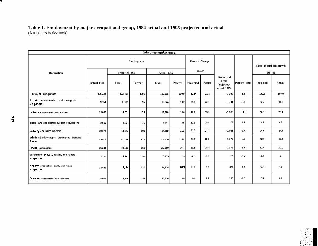
Table 1. Employment by major occupational group, 1984 actual and 1995 projected and actual(Numbers in thousands)

Industrv-occupation matrix

Occupation

-, –__ —r—.--— ---------

Employment Percent Change

Share of total job growth

Projected 1995 Actual 1995 1984-95 1984-95

Numerical

Actual 1984 Level Percent Level Percent Projected Actualerror

Percent error(projected-

Projected Actual

actual 1995)

Total, all occupations 106,729 122,758 100.0 130,009 100.0 15.0 21.8 -7,250 -5.6 100.0 100.0

lxecutive, administrative, and managerial9,95 I I I ,933 9.7 13,244 10.2 19.9 33.1 -1,311 -9.9 12.4 14.1

wcupations

%fessional specialty occupations 13,020 15,701 12.8 17,696 13.6 20.6 35.9 -1,995 -11.3 16.7 20. I

technicians and related support occupations 3,535 4,564 3.7 4,54 I 3.5 29.1 28.5 23 0.5 6.4 4.3

ularketing and sales workers 10,978 13,322 10.9 14,389 11.1 21.3 31.1 -1,068 -7.4 14.6 14.7

administrative support occupations, including

:Ierical19,670 21,731 17.7 23,710 18.2 10.5 20.5 -1,979 -8.3 12.9 17.4

krvice occupations 16,244 19,510 15.9 20,889 16. I 20.1 28.6 -1,379 -6.6 20.4 20.0

agriculture, forest~, fishing, and related

wupations3,798 3,641 3.0 3,779 2.9 -4.1 -0.5 -138 -3.6 -1.0 -0.1

%cision production, craft, and repair

wwpations13,469 15,110 12.3 14,224 10.9 12.2 5.6 886 6.2 10.2 3.2

)perators, fabricators, and laborers 16,064 17,246 14.0 17,536 13.5 7.4 9.2 -290 -1.7 7.4 6.3

.,..:, .-.-:1

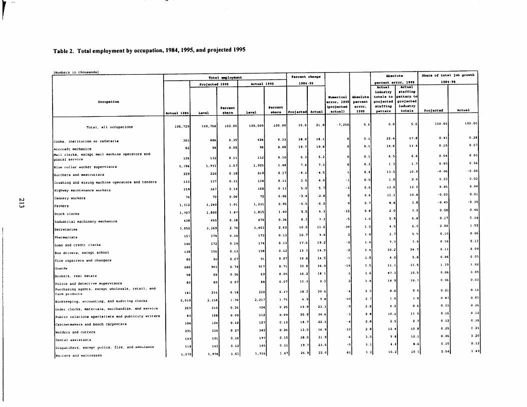
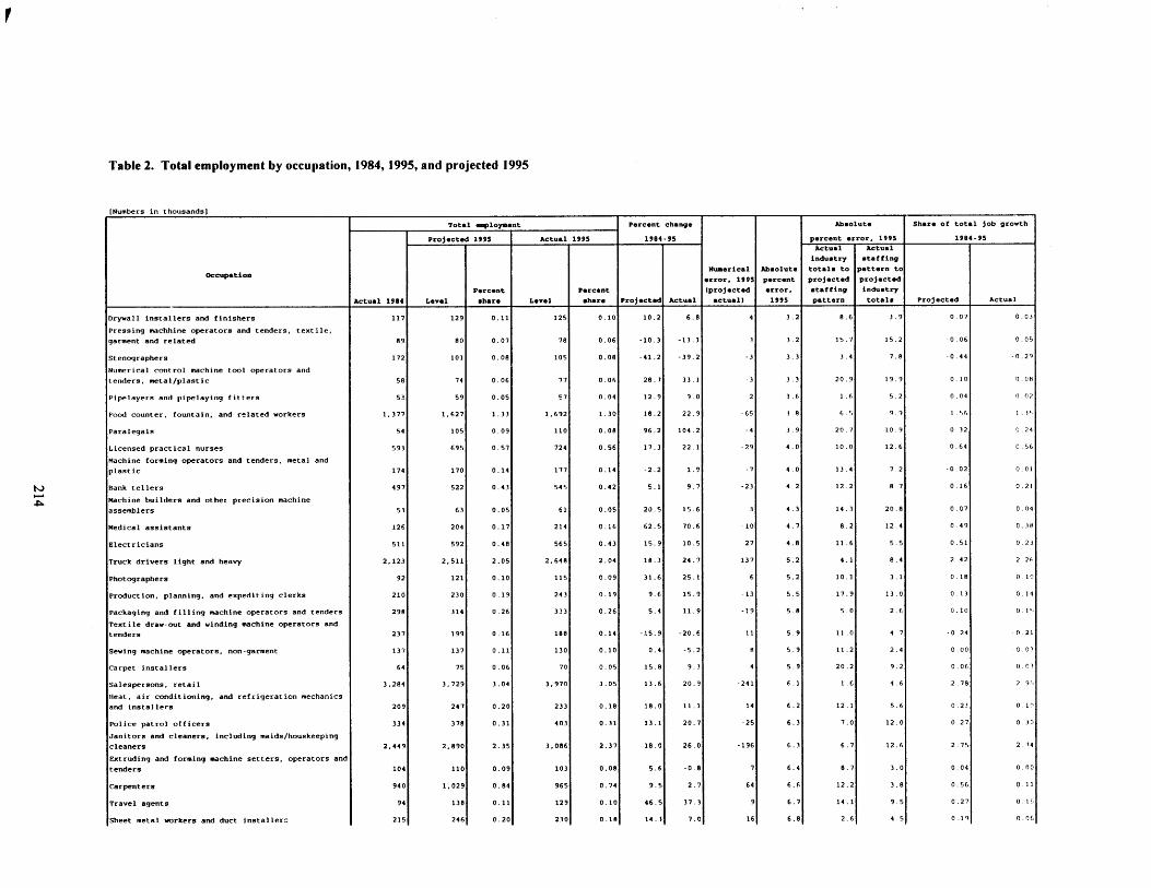
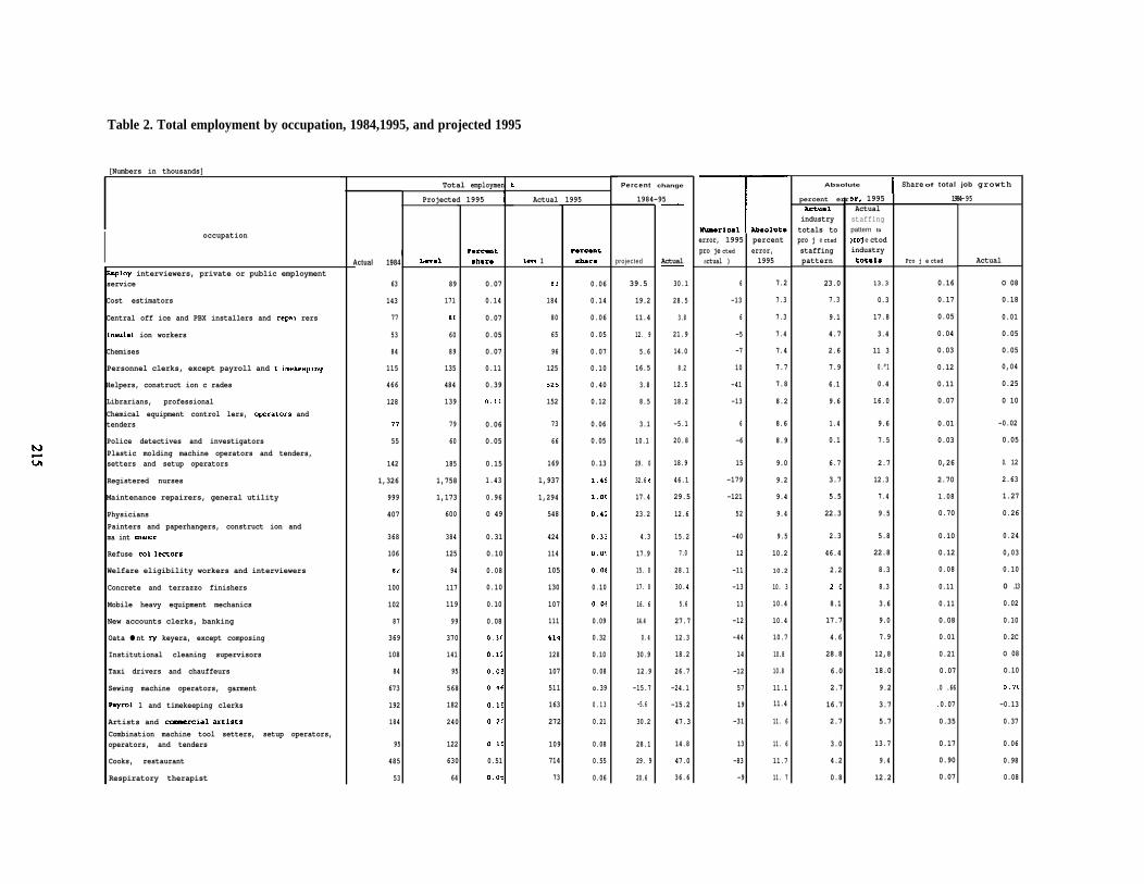
Table 2. Total employment by occupation, 1984,1995, and projected 1995

[Numbers in thousands]

I occupation

SmplOy interviewers, private or public employmentservice

Cost estimators

Central off ice and PBX installers and repal rers

Insulat ion workers

Chemises

Personnel clerks, except payroll and c imekeeplng

Helpers, construct ion c rades

Librarians, professional

Chemical equipment control lers, cperators andtenders

Police detectives and investigators

Plastic molding machine operators and tenders,setters and setup operators

Registered nurses

Maintenance repairers, general utility

Physicians

Painters and paperhangers, construct ion andma int ensnce

Refuse CO1 lectors

Welfare eligibility workers and interviewers

Concrete and terrazzo finishers

Mobile heavy equipment mechanics

New accounts clerks, banking

Oata ● nt ry keyera, except composing

Institutional cleaning supervisors

Taxi drivers and chauffeurs

Sewing machine operators, garment

Payrol 1 and timekeeping clerks

Artists and comercial artista

Combination machine tool setters, setup operators,operators, and tenders

Cooks, restaurant

Respiratory therapist

IActual 1984

63

143

77

53

84

115

466

128

77

55

142

1,326

999

407

368

106

82

100

102

87

369

108

84

673

192

184

95

485

53

Total employmen

Projected 1995 I

L*vQ1

89

171

86

60

89

135

484

139

79

60

185

1,758

1,173

600

384

125

94

117

119

99

370

141

95

568

182

240

122

630

64

Porcont

shara

0.07

0.14

0.07

0.05

0.07

0.11

0.39

0.11

0.06

0.05

0.15

1.43

0.96

0 49

0.31

0.10

0.08

0.10

0.10

0.08

0.3C

0.12

O.oe

o.4f

0.1!

0.2C

O.lc

0.51

0.0:

tActual 1995

Laws 1

83

184

80

65

96

125

325

152

73

66

169

1,937

1,294

548

424

114

105

130

107

111

414

128

107

511

163

272

109

714

73

Porcontsharm

0.06

0.14

0.06

0.05

0.07

0.10

0.40

0.12

0.06

0.05

0.13

1.4s

1.OC

0.42

0.33

0.0$

O.of

0.10

O.o8

0.09

0.32

0.10

0.08

o.39

0. 1 3

0.21

0.08

0.55

0.06

Percent change

1984-95

projected

39.5

19.2

11.4

12. 9

5.6

16.5

3.8

8.5

3.1

10.1

29. 0

32.6617.4

23.2

4.3

17.9

15. 0

17. 0

16. 6

14.4

0.4

30.9

12.9

-15.7

-5.6

30.2

28.1

29. 9<

20.6

Actual

30.1

28.5

3.8

21.9

14.0

8.2

12.5

18.2

-5.1

20.8

18.9

46.1

29.5

12.6

15.2

7.0

28.1

30.4

5.6

27.7

12.3

18.2

26.7

-24.1

-15.2

47.3

14.8

47.0

36.6

error, 1995 percentpro je cted error,

actual ) 1995

6

-13

6

-5

-7

10

-41

-13

6

-6

15

-179

-121

52

-40

12

-11

-13

11

-12

-44

14

-12

57

19

-31

13

-83

-9

7.2

7.3

7.3

7.4

7.4

7.7

7.8

8.2

8.6

8.9

9.0

9.2

9.4

9.4

9.5

10.2

10.2

10. 3

10.4

10.4

10.7

10.8

10.8

11.1

11.4

11. 6

11. 6

11.7

11. 7

Absolute I Share of total job growth

percent err

Actualindustrytotals topro j e ctad

staffingpattern

23.0

7.3

9.1

4.7

2.6

7.9

6.1

9.6

1.4

0.1

6.7

3.7

5.5

22.3

2.3

46.4

2.2

2.0

8.1

17.7

4.6

28.8

6.0

2.7

16.7

2.7

3.0

4.2

0.8

m, 1995 1984-Actual

staffingpattern to

ro e ctodindustrytotals Pro j e cted

13.3

0.3

17.8

3.4

11 3

0.”1

0.4

16.0

9.6

7.5

2.7

12.3

7.4

9.5

5.8

22.8

8.3

8.3

3.6

9.0

7.9

12,8

18.0

9.2

3.7

5.7

13.7

9.4

12.2

0.16

0.17

0.05

0.04

0.03

0.12

0.11

0.07

0.01

0.03

0,26

2.70

1.08

0.70

0.10

0.12

0.08

0.11

0.11

0.08

0.01

0.21

0.07

.0 .66

.0.07

0.35

0.17

0.90

0.07

95

Actual

O 08

0.18

0.01

0.05

0.05

0,04

0.25

0 10

-0.02

0.05

0. 12

2.63

1.27

0.26

0.24

0,03

0.10

0 .13

0.02

0.10

0.2C

O 08

O.l0

-0.70

-0.13

0.37

0.06

0.98

0.08

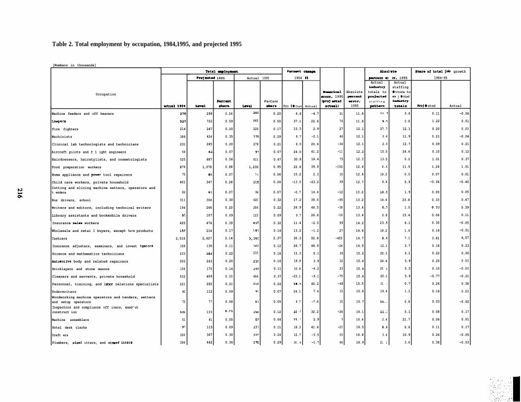
Table 2. Total employment by occupation, 1984,1995, and projected 1995

[Numbers in thousands]

Occupation

Machine feeders and off bearers

Lsvyers

Fire fighters

Machinists

Clinical lab technologists and technicians

Aircraft pilots and f 1 ight engineers

Hairdressers, hairstylists, and cosmetologists

Food preparation workers

Home appliance and power tool repairers

Child care workers, private household

Cutting and slicing machine setters, operators andt endera

Bus drivers, school

Writers and editors, including technical writers

Library assistants and bookmobile drivers

I Insurance ssles workersWholesale and retai 1 buyers, except farm products

Cashiers

Insurance adjusters, examiners, and invest igators

Science and mathematics technicians

Autanotive body and related repairers

Bricklayers and stone masons

Cleaners and servants, private household

Personnel, training, and lakmr relations specialists

Underwriters

Woodworking machine operators and tenders, settersand setup operators

Inspectors and compliance off icers, exe@’utconstruct ion

Machine assemblers

Hotel desk clerks

Draft ers

Plumbers, pipef itters, and steamf itters

hotual 1*M

270

527

214

386

231

66

525

B79

75

401

82

311

194

97

425

1B9

2,016

109

233

202

154

532

221

9C

72

12C

51

97

326

384

Total ~loymant

ProjO&d 1995 Actual

PucantLaval Sbaro L8val

296 0.24

722 0.59

247 0.20

424 0.35

245 0.20

82 0.07

687 0.56

1,078 0.88

86 0.07

347 0.28

B1 0.07

364 0.30

246 0.20

107 0.09

474 0.39

214 0.17

2,627 2.14

138 0.11

268 0.22

243 0.20

170 0.14

409 0.33

262 0.21

112 0.09

77 0.06

133 o.~1

61 0.05

115 0.09

367 0.30

442 0.36

265

645

220

378

279

93

611

1,230

7-i

308

94

42C

284

123

415

187

3,08C

162

233

21C

14E

484

31C

9i

6:

15[

52

131

31:

37f

Porcsot

1995 1904

ParCantSbara Pro j ● Ctad

0.20

0.50

0.17

0.29

0.21

0.07

0.47

0.95

0.06

0.24

0.07

0.32

0.22

0.09

0.32

0.14

2.37

0.12

0.18

0.16

0.11

0.37

0.24

0.07

0.05

0.12

0.04

0.11

0.24

0.29

6.6

37.1

15.3

9.7

6.0

24.0

30.8

22.6

15.2

-13.5

-0.7

17.2

26.9

9.7

11.4

13.2

30.3

26.7

15.3

19.9

10.6

-23.1

18.5

24.1

6.7

10, $

19. e

18.3

12.7

14. s

)5

Ilu9aricaluror, 1995(proj aotod

Actual 8etual)

-4.7 31

22.6 76

2.9 27

-2.1 46

20.6 -34

41.2 -11

16.4 75

39.9 -152

2.3 10

-23.2 39

14.4 -12

35.0 -55

46.5 -38

26.6 -16

-2.5 59

-1.2 27

52.8 -453

48.9 -24

0.1 35

3.9 32

-4.2 23

-9.1 -75

40.2 -48

7.4 15

-7.8 10

32.2 -26

2.9 9

41.6 -23

-3.5 53

-1.7 64

Ab801

parcant eI

Actualiadustry

Absolute totals topsrcant projactodarror, s t a f f i n g

1995 pattorrl

11.8

11.8

12.1

12.1

12.1

12.2

12.3

12.4

12.6

12.7

13.2

13.2

13.4

13.4

14.2

14.6

14.7

14.9

15.2

15.4

15.4

15.4

15.5

15.6

15.7

16.1

16.4

16.5

16.8

16.9

11.79.E

27.7

0.4

2.3

15.5

13.5

O.c

16.2

6.4

10.9

14.6

6.9

2.8

23.5

18.2

8.e

12.1

25.3

24.4

20. i

20.1

15. :

19.4

~5.:

11.2

2.4

8.f

3.4

21. i

Luta Sbar. of total job growth

x, 1995 1984-95Actualstaffing● ttora to>ro j ● ctadimduatrytotals Proj ● ctod Actual

0.8 0.11

3.8 1.22

12.1 0.20

11.9 0.23

12.7 0.09

24.6 0.10

0.2 1.01

11.5 1.24

0.0 0.07

5.9 -0.34

1.9 0.00

23.8 0.33

1.0 0.33

15.4 0.06

6.1 0.30

1.6 0.16

7.1 3.81

3.7 0.18

9.3 0.22

5.9 0.25

3.3 0.10

5.9 -0.77

0.7 0.26

1.3 0.14

0.8 0.03

5.1 0.08

21.7 0.06

8.6 0.11

10.9 0.26

3.6 0.36

-0.06

0.51

0.03

-0.04

0.21

0.12

0.37

1.51

0.01

-0.40

0.05

0.47

0.39

0.11

-0.05

-0.01

4,57

0.23

0.00

0.03

-0.03

-0.21

0.38

0.03

-0.02

0.17

0.01

0.17

-0.05

-0.03

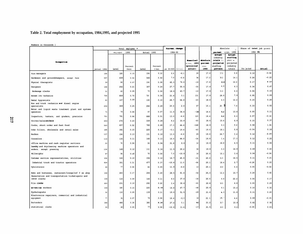
Table 2. Total employment by occupation, 1984,1995, and projected 1995

Numbers in thoussnds ]

Oeeupatioa

Farm managers

Gardeners and groundskeepers, except farm

Physical therapists

Designers

BBrokerage clerks

Automot ive mechanics

Dental hygienists

Bus and truck mechanics and diesel enginesspecialists

Water and liquid waste treatment plant and systemsoperators

Inspectors, testers, and graders, precision

Driver/sales workere

Cooks, short order and fast food

OOrder fillers, wholesale and retail sales

Roofers

Counselors

Office machine and cash register servicers

Laundry and drycleaning machine operators andenders. except pressing

Millwrights

Customer service representatives, utilities

IIndustrial truck end tractor operators

Upholsterers

Hosts and hostesses, restaurant/lounge/cof f ee ahop

Reservation and transportation ticket agents andtravel clerks

File clerke

Recreation workers

Pychologists

Electronics repairers, commercial and industrialequipment

Bartenders

statistical clerks

Actual 1984

164

597

59

198

51

706

83

256

71

701

253

543

188

137

116

53

130

87

104

426

68

158

106

223

154

92

77

366

6S

Total employmen

Pro j roject

Level

180

639

86

252

60

859

107

309

79

791

276

637

182

156

135

70

145

94

122

301

77

203

115

231

180

110

91

466

60

1995

Percent

shere

0.15

0.52

0.07

0.21

0.05

0.70

0.09

0.25

0.06

0.64

0.23

0.52

0.15

0.13

0.11

0.06

O.l2

O.o8

O.l0

0.31

0.06

0.17

0.09

0.19

0.15

0.09

0.07

0.38

0.05

Actual 1995

Percent

Level s hare

154

545

104

307

73

728

130

262

97

668

339

785

225

131

168

58

1 8 2

78

152

477

64

255

145

292

220

139

76

385

77

0.12

0.42

0.08

0.24

0.06

0.56

0.10

0.20

0.07

0.51

0.26

0.60

0.17

0.10

0.13

0.04

0.14

0.06

0.12

0.37

0.05

0.20

0.11

0.22

0.10

0.11

0.06

0.3C

0.06

Psrcamt cha~o I I I Absolute I Share of total job growth,.

1984-95

Mumaricale r r o r , 1995{projactad

pro j e cted Actual SCtuel)

9.8 -6.1 26

7.0 -0.8 94

45.3 76.6 -19

27.7 55.5 -55

18.0 43.7 -13

21.6 3.1 131

28.7 56.9 -23

20.4 2.0 47

11.6 36.6 -18

13.0 -4.6 123

9.2 33.9 -63

17.3 44.6 -148

-3.1 19.6 -43

13.5 -4.6 25

16.0 44.0 -34

31.8 9.9 12

11.5 39.2 36

7.0 -10.9 16

16.7 45.9 -31

-10.6 11.0 -96

11.9 -6.8 13

28.5 61.4 -52

9.0 37.0 -30

3.4 30.6 -61

16.8 47.7 -48

19.0 51.5 -29

18.4 -2,3 16

27.4 5.1 82

-12.6 11.4 -17

porcant errActualindustry

Ahsoluta totda top.rcmt projoctad

error, staffing199s pmttorm

17.0

17.2

17.8

17.9

17.9

17.9

18.0

10.1

18.4

18.4

18.5

18.9

19.0

19.0

19.9

19.9

19.9

20.0

20.0

20.1

20.1

20,3

20.5

20.8

20.9

21.0

21 1

21.2

21.5

17.0

36.2

6.6

4.9

11.2

28.9

6.5

28. 9

5.2

5.2

15.6

9.3

18.1

24.7

1.s

18.8

5.0

15.1

31.5

18.4

16.8

12.2

4.8

16.0

4.1

6.5

15.3

35.7

16.0

or, 1995 1984-ActuslStaffimgpttern to

projected

industrytotals Pro je cted

0.8

14.1

12.2

4.3

6.4

7.9

12.2

7.4

13.8

9.0

6.9

9.4

0.8

3.4

17.3

4.5

14.9

3.6

16.5

2.7

5.6

10.7

22.2

6.8

15.2

11.6

4.4

10.9

9.2

0.10

0.26

0.17

0.34

0.06

0.95

0.15

0.33

0.05

0.57

0.15

0.58

-0.04

0.12

0.12

0.11

0.09

0.04

0.11

-0.28

0.05

0.28

0.06

0.05

0.16

0.11

0.09

0.62

-0.05

.95

Actual

-0.04

-0.22

(1 Iq

0.47

0.10

0.09

0.20

0.02

0.11

-0.14

0.37

1.04

0.16

.0.03

0.22

0.02

0.22

-0.04

0.21

0.22

-0.02

0.42

0.17

0.29

0.32

0.20

-0.01

0 08

0.03

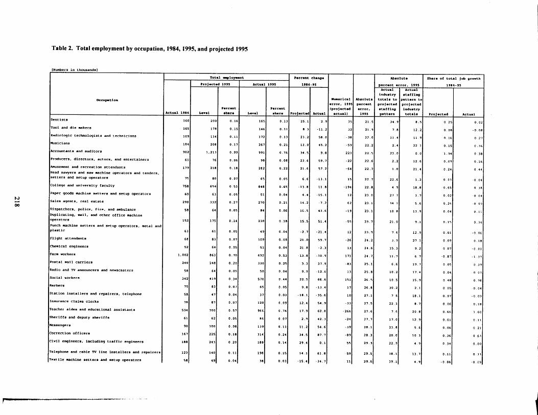
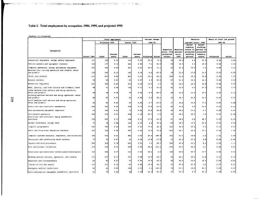
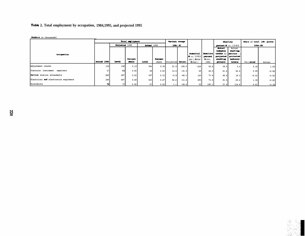
TabJe 2. Total employment by occupation,

[Mumbers in thousands]

I

1984,1995, and projected 1995

mtal ~l~t Berceot Ohsnga *oluta Shsrm of total job ~outbProjscted 1995 Aotual 1995 1904- w pecoeot ● rro=, 1 9 9 5 19s4-95

XOtual Actuali@aaetry •ta~f iog

oc~tion Uumerical Abeoluto totsze to pattero t o

● rror, 1995 poroont prsjscted projeotedPuceot Puoent (pro j ● ctsd ● rror, Stdfiog hdllstry

Actual L9C4 Level Shera LeWel share Projected AOtud ● ctual ) 199s pettsrn totals Pro j Scted Actual

Adjustment clerks 130 158 0.13 384 0.30 21.9 196.0 -226 50.8 59.5 0.4 0.18 1.09

Precision instrument repairers 57 65 0.05 39 0.03 13.4 -31.3 26 65.0 21.4 22.4 0.05 -0.08

Sewice station attendants 289 287 0.23 167 0.13 -0.8 -42.1 120 71.4 85.6 16.3 -0.01 -0.52

Electrical snd electronics engineers 399 607 0.49 3s3 0.27 52.2 -11.4 253 71.8 41.4 20.2 1.30 -0.20

Roustabouts 78 79 0.06 27 0.02 1.1 -65.2 52 190.1 37.6 114.6 0.01 -0.22

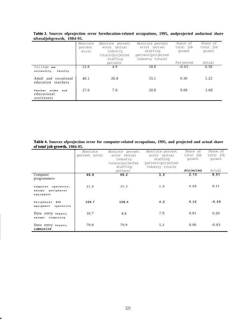
Table3. Sources ofprojection error foreducation-related occupations, 1995, andprojected andactuai shareoftotaljobgrowth, 1984-95.

I Absolute Absolute percent Absolute percent Share of Share ofpercent error (actual error (actual total job total joberror industry staffing growth growth

totals/projected pattern/projectedstaffing industry totals)pattern) Projected Actual

College and 22.8 4.9 18.8 -0.65 0.38university, faculty IAdult and vocationaleducat ion teachers

40.1 26.4 15.1 0.30 1.22

Teacher aides and 27.6 7.6 20.8 0.66 1.60educat ionala s s i s t a n t s

Table4. Sources ofprojection error for computer-related occupations, 1995, and projected and actual shareoftotaljobgrowth, 1984-95.

Absolute Absolute percent Absolute percent Share of Share of

Computerprogrammers

C o m p u t e r o p e r a t o r s ,

e x c e p t p e r i p h e r a l

e q u i p m e n t

P e r i p h e r a l E D P

e q u i p m e n t o p e r a t o r s

Data entry k e y e r s ,

e x c e p t c o m p o s i n g

Data entry k e y e r s ,

composinq

percent error error (actual error (actual total job total jobindustry staffing growth growth

totals/projected pattern/projectedstaffing industry totals)pattern) Projecteci Actual

4 0 . 0 4 6 . 2 3 . 3 2 . 1 3 0 . 5 1

3 1 . 0 3 5 . 3 1 . 6 0 . 6 8 0.11

1 0 0 . 7 1 0 8 . 4 4 . 2 0 . 1 2 - 0 . 0 5

10.7 4.6 7.9 0.01 0.20

79.8 79.9 5.3 0.06 -0.03

221

. ..”,.

.,.. “

.,. ,

Table 5. Sources of projection error for health-related occupations, 1995, and projected and actual share oftotal job growth, 1984-95.

Absolute Absolute percent Absolute percent Share of Share ofpercent error (actual error (actual t o t a l j o b t o t a l j o b

e r r o r i n d u s t r y s t a f f i n g g r o w t h g r o w t ht o t a l s / p r o j e c t e d p a t t e r n / p r o j e c t e d

s t a f f i n g i n d u s t r y t o t a l s )p a t t e r n ) Projected Actual

P h y s i c i a n s

a s s i s t a n t s

Occupationalt h e r a p i s t s

Occupationaltherapya s s i s t a n t s a n da i d e s

E m e r g e n c y

m e d i c a l

t e c h n i c i a n s

Licensedp r a c t i c a lnurses

47.4 39.9 13.0 0.05 0.15

41.9 33.8 13.6 0.01 0.03

5 3 . 1 3 9 . 0 2 3 . 1 0 . 0 2 0 . 3 3

4 . 0 1 0 . 0 12.6 0.64 0.56

Table6. Sourcesof projection errorfor production workers, 1995,and projected and actualshareof totaljobgrowth, 1984-95.

Absolute Absolute percent Absolute percent Share of Share of

A i r c r a f t

assemblers ,p r e c i s i o n

E l e c t r i c a l a n de l e c t r o n i cequipmentassemblers ,p r e c i s i o n

Electromechanicalequipmentassemblers ,p r e c i s i o n

E l e c t r i c a l a n de l e c t r o n i cassemblers

percent error (actual error (actual total job total joberror industry staffing growth growth

totalslprojected pattern/projectedstaffing pattern) industry totals)

Projected Actual27.1 16.0 52.1 0 . 0 2 - 0 . 0 1

3 8 . 9 6 . 8 4 8 . 7 0 . 1 9 - 0 . 1 2

55.1 0 . 7 42.3 0 . 0 9 - 0 . 0 5

3 7 . 6 4 . 6 4 3 . 0 0 . 2 7 - 0 . 1 6

222

EARLY WARNING AND THE NEED FOR INFORMATION SHARING

Chair: Kenneth W. HunterWorld Future Society

Early Warning and Futures Research: An Argument for Collaboration and IntegrationAmong Professional Disciplines,Kemeth W. Hunter, World Future Society

223

.’. ,

Early Warning and Futures Research

An Argument for Collaboration and Integration Among Professional Disciplines1

bKemeth W. Hunter, CPA

September 10, 1997

For contact:Tel: 3015964743Fax: 3015960946E-mail: khunter100Qaol.comMail: 9738 Basket Ring Road, Columbia, MD 21045Positions:Chair, World Future Societ y’s 1999 Conference on “Frontiers of the 21st Century”Senior Associate, The Harrison Program on the Future Global Agenda, University of Maryland,College ParkPresident, Collaborative Futures International

225

Early Warning Professional Services and Accountability for Actions and Inaction

Early warning is a professional responsibility and service provided by manydisciplines in most institutions to inform direction-setting policy making andimplementation, including course corrections and emergent y responses. Policymakers and their advisors are accountable for their inaction as well as actions. Inthe current era of large scale systemic transformations missed opportunities can bevery costly to individual institutions and civil society in the long run, thus makingaccountability for inaction especially important today.

Early warning, like futures research, is not a traditional discipline itself, but is acritical responsibility of most professionals. However, the traditional professions donot use these terms in describing their functions and services. Therefore, we haveto look to what they do and what they call it to assess the nature of early warningand futures research methods and practices today. I will begin that task in thispaper.

In my judgment, early warning and futures research are based on implicit generalmental models of the relationships among values, change drivers and shapers, andinstitutions. Change drivers include demographic and technologic forces. Changeshapers include ecological systems constrains and patterns of change in institutions,such as globalization and restructuring into more modular and networkedrelationships. These forces impact all institutions and create a wide range ofdirection-setting policy choices. Values shape the criteria used explicitly andimplicitly in making those choices. Inaction is an implicit choice not to changedirections by the institution.

Each professional discipline has evolved its own process and language for doing itswork. However, all professionals do share responsibilities. All professionals advisetheir individual and organizational clients on critical choices. They base theiradvice on their understanding of changing conditions and relative capabilities of theclient and their assessment of the likely consequences and risks of alternativeactions and inaction. That is what being a professional is all about. As real worldsituations get more complex -- the choices involve larger scale systems -- we need toengage a wider range of disciplines collaboratively. Since the languages andunderlying paradigms are different, policy makers confront a difficult to impossibletask of information integration and evaluation of choices.

In my opinion, we in the professions should take the initiative to collaborate andintegrate our knowledge and services in support of direction-setting policy makingfor large scale systems. Let me illustrate. In my view, the following ten large scalehuman systems are undergoing transformational changes thus driving complexpolicy choices for everyone:

226

1. Life relationships: gender, generational, family, rational-creative, spiritualand work.2. Civil society and communities; neighborhood cohesion; tolerance andcultural passions and identities; confronting enduring ethnic, religious, racialand nationalistic conflicts.3. Human capacity development: leaning, knowledge building, and wellness4. Human services for vulnerable and troubled people and peoples to lessenhuman suffering and build connections to communities.5. Eco-econo-socio systems: climate change, water, energy, ecosecurity,sustainability.6. Habitats and mobility: megacities, communities, corridors, gateways,regional systems, and logistics.7. Big collaborative science.8. Big emerging markets: China, India, Indonesia, Brazil and Russia.9. Global standards and best practices; accountabilitytransparency and reporting.10. Dealing with wrong-doing: early warning, earlypolice, justice.

and governance;

intervention, military,

In my opinion we do share this agenda of major changes and share a basic mentalmodel as professionals. These provide a starting point for collaboration andintegration of our professional knowledge and skills to meet our early warning andfutures research responsibilities more effectively.

Early warning of what? .

First, however, we need to wrestle with the question “early warning of what?”Policy makers and the public want warning of potential events, changes inrelationships, and changes in systems capabilities with possible significantconsequences. These of course are interrelated, but the way we think and talk abouteach is a little different.

Events involve both substantive action and timing. Significant events can bebreakthroughs on one end of a continuum and crises on the other. In fact what maybe a crisis for some institutions and indiviciuals are likely to be breakthroughs or atleast opportunities for others. Actions on tobacco and greenhouse gases areillustrations. By events we usually mean the action that gives public recognition toa major change and drives the need for attention. However, breakthroughs andcrises do not happen spontaneously. Collapses of political regimes usually resultfrom long-term disintegration and corruption at the core. Scientific “discoveries”result from years of hard thinking and work to make them happen. Effectivemonitoring of actions or inaction of key people and institutions can provide earlysignals of the possibility of a major event at some time. However, anticipating theexact timing of the “capping” event is very difficult, even when they appear to begetting near. Nevertheless, informing policy makers and the public of the nature,likelihood and timing of a major event is a critical early warning service.

227

Understanding changing relationships is also fundamental to all policy choices. Theend of the Cold War, the diffusion of information technology, climate change, andchanging gender and generational relationships all make it certain that futureconditions will be significantly different. We all do make assumptions about whatthose changing relationships and future conditions are likely toprofessional judgments about them into our policy advice.

be and put our

and routinePolitical regimes,

companies, churches,

Large scale systems and organizations involve well establishedrelationships and thus relatively rigid structures and processes.militaries, social security systems, tax systems, industries, largeetc., are all such systems. Significantly changing such systems means changing theirdesign, rules, practices and processes and getting everyone involved to adapt --changing the culture as well as the structure and functions. These are complexundertakings as we experience with Russia and China and in many traditionalindustries. Some institutions disintegrate, usually from inaction, incompetence andcorruption at the core; they eventually implode. At the same time new ventures arecontinuously created and some “take off” in a rapid process of integration ofknowledge, vision, resources, and opportunities. There are thresholds involvedhere which when passed result in transformation, takeoff or collapse of the system.Early warning is most effective when we understand the system dynamics and wemake informed assessments of the thresholds and monitor movement of systemstoward them.

Understanding the likelihood and nature of critical events and changes inrelationships and systems requires knowledge and skills from many disciplines.Integrative fields such as ecological security, sustainable development, economicsecurity, human capacity development, human services and humanitarianassistance, bioengineering, etc., all illustrate progress in shaping multipledisciplinary approaches. These enhance our early warning capabilities. We need todo much more such collaborative work.

Early Warning Methods and Practices

I find it most useful to group early warning and futures research professionalapproaches, methods and practices into five sectors of work: (1) security and politics;(2) business and finance; (3) human rights, development and assistance; (4) ecology;and (5) integration (see attached chart “Defining and Assessing Institutions, TheirImportant Relationships and Integrativesketches of the approaches of the groupshope to learn and be corrected by people

Capac~ties”). Following thumbnail(these are based on my understanding; Imore knowledgeable about each):

1. Security and politics.

Military and political intelligenceinformation on changing military

professionals provide continuousand diplomatic conditions, assessment

228

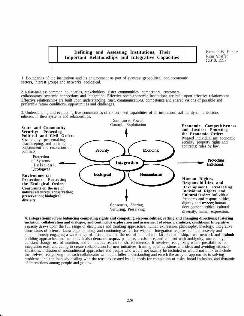
Defining and Assessing Institutions, Their Kenneth W. HunterImportant Relationships and Integrative Capacities Rims Shaffer

July 8, 1997

1. Boundaries of the institutions and its environment as part of systems: geopolitical, socioeconomicsectors, interest groups and networks, ecological.

2. Relationships: common boundaries, stakeholders, sister communities, competitors, customers,collaborators, systemic connections and integration. Effective socio-economic institutions are built upon effective relationships.Effective relationships are built upon understanding, trust, communications, competence and shared visions of possible andpreferable future conditions, opportunities and challenges.

3. Understanding and evaluating five communities of concern and capabilities of all institutions and the dynamic tensionsinherent in their systems and relationships:

Dominance, Power,

State and CommunitySecurity: ProtectingPolitical and Civil Order:Sovereignty, peacemaking,peacekeeping, and policing;containment and resolution ofconflicts.

Protectionof Systems:

P o l i t i c a l , ~EcOlogiti

EnvironmentalProtection: Protectingthe Ecological Order:Constraints on the use ofnatural resources; conservation;preservation; biologicaldiversity.

Control, Exploitation

Consensus, Sharing,Nurturing, Preserving

Economic Competitivenessand Justice: Protectingthe Economic Order:Rugged individualism; economicsecurity; property rights andcontracts; rules by law.

Human Rights,Responsibilities andDevelopment: ProtectingIndividual Rights andCultural Order: Individualfreedoms and responsibilities,dignity and respecc humandevelopment; ethics; culturaldiversity, human expression.

4. Integrationinvolves balancing competing rights and competing responsibilities; setting and changing directions; fosteringinclusion, collaboration and dialogue; and continuous exploration and assessment of ideas, paradoxes, conditions. Integrativecapacity draws upon the full range of disciplines and thinking approaches, human expression, philosophy, theology, integrativedimensions of science, knowledge building, and continuing search for wisdom. Integration requires comprehensively andsimultaneously engaging a wide range of institutions and the use of our full tool kit of relationship, trust, network and institutkbuilding approaches and methods. It also demands respecq patience, persistence, and comfort with ambiguity, uncertainty,constant change, use of intuition, and continuous search for shared interests. It involves recognizing where possibilities forintegration exist and acting to create collaboration for new initiatives; framing open questions and ideas and avoiding either/orsituations; inclusion of nontraditional approaches and people who would not usually be included or would not think to includethemselves; recognizing that each collaborator will add a fuller understanding and enrich the array of approaches to solvingproblems; and continuously dealing with the tensions created by the needs for completion of tasks, broad inclusion, and dynamicof interactions among people and groups.

229

m--

.,. .. .

information on potential threats and risks of military and diplomaticconflicts, analytic information on alternative strategies and their likelyconsequences. It uses massive information collection (by both human andelectronic observation and interception) and analysis capabilities and has useda closed and compartmentalized organization and reporting structure. It hasevolved its own means and methods and traditionally has been reluctant toshare information, methods or models with others. Today the intelligencecommunity is actively seeking to comect with other communities to broadenits scope and services.

Criminal intelligence provides information on alleged criminal activities forcommunity security, law enforcement, and criminal prosecution. It uses awide range of investigatory means and methods, involving fieldinvestigations, monitoring, and scientific analysis of evidence. Organizedcrime, drug trafficking and corruption are major systematic focuses. Earlywarning has not been an explicit, priority function. However, recognition of(1) the extent and negative impacts of corruption on civil society andeconomic development and (2) the threats to financial systems of large scalefraud, calls for the criminal justice community to work on such political andbusiness systems problems. Similarly, the prosecution for war crimes bringscriminal justice people directly into the horrific actions and hostile conditionsof failed states. However, as we develop more integrated approaches andmethods of dealing with criminal systems, the traditional separation ofmilitary and police functions by the United States and other developedcountries is being breached. This illustrates the importance of values inshaping collaborative institutions.

Country financial risk assessment and early warning of financial trouble arefunctions of the international and United States financial institutions withthe International Monetary Fund and the US Export-Import Bank havingoperational activities. These institutions have extensive financial exposurein troubled countries and have had significant losses in several failed states.They now are broadening the range of factors they formally consider inassessing risk to include non-financial factors. They are extending theircollaboration accordingly.

2. Business and commercial finance.

Business intelligence and risk assessment include an expanding array ofcommercial analytic services. An example is The Economist IntelligenceUnit, which integrates information from the various econometric serviceswith the journalistic coverage of the Economist and Financial Times newsservice. These services cover not only economic conditions, but political,social, and environmental conditions and trends. While they are relativelyshort-term in their focus, they do discuss long-term structural changes ofmajor significance. The commercial financial community also uses many

230

rating and risk assessment practices, such as those of Dunn and Bradstreet.be effective the rating services must be anticipatory and provide earlywarning for investors.

Economic indicator functions movide information on trends in economic

To

conditions and serve to guide ~conomic research and policy analysis. Theseservices use statistical (survey and time series) methods. Their processes arebpen; their information is disseminates and uses widely. They have evolvedwell structured and disciplined approaches and methods that theyenthusiastically share in the belief that the indicators will be improved asuser provided feedback to guide enhancements. The models used are ofeconomic relationships and systems. Major restructuring of internationaleconomic and political relationships, industries and organizations is drivingthe demand for overhauling economic models and statistical series to reflectnew reality.

Corporate public issues management is a professional approach to identifyingand addressing emerging and emergency public policy issues by somebusinesses. Anticipating potential public issues and being prepared to engagein shaping policy responses is the objective. A network of professionalcorporate public issues managers share experiences.

Corporate strategic planners tend to focus on the organization and itsoperations over the next few years. However, the initial steps in theirprocesses do frequently involve external and longer-term inquiry. Theseinclude identifying a range of demographic, technological, socio-economic,and political changes; creating a set of forecasts of plausible future conditions5 to 10 years ahead; and designing alternative business strategies for thetransition period. This type of analysis can identify needed policy changes toguide organizations or sectors toward preferred future conditions and awayfrom adverse conditions. Professional associations of plamers sharemethodological experiences. Real corporate strategies are highly confidential.

Market research is one of the most extensive and intensive early warning andfutures research business functions. Business choices about markets andproducts and service design and delivery bring together information, ideasand judgments from all disciplines and functions. Market research uses awide range of survey methods combined with demographic analyses. Theymonitor customer opinions and satisfaction closely. New ideas are fieldtested. They monitor competitors and their customers also. They assesschanging markets rigorously. Product, service and market policies arereconsider regularly. They evaluate successes, failures, and missedopportunities for lessons learned. They consider this intelligence and theirdecisions highly confidential and do not share anything.

231

Financial auditing and reporting provide information to policy makers andthe public on financial conditions of organizations. Accountants’responsibility for assessing enterprise’s capacity to continue as a “goingconcerns” is a critical early warning function. The accounting profession hasstandards for reporting and auditing. Most countries use certification andlicensing of individuals. With globe spanning, real-time financial marketsand systems and organizational networks, where does the boundary of theentity being audited end for purposes of determining its financial conditionand “going concern” capabilities? What are the entit y’s long-term financialrisks for environmental and health damage? What is the “going concern”status of an enterprise that is not changing? The auditing community (ofwhich I am a member) has hardly begun to open this Pandora’s box. To do sowill require broad collaboration and integration with other disciplines. Ibelieve that is achievable.

3. Human rights, development and services

Human rights monitoring has focused on calling attention to ongoingviolations of human rights and seeking actions to stop the practices. Throughnetworks of volunteer and professional observers using increasingly rigorousdocumentation, communications, and advocacy methods human rightsviolations have become better understood and reported. Early warning hasinvolved identification of minorities at risk of abuse and of patterns ofbehavior by regimes that typically include human rights violations. Todaygreater attention is being given to employing statistical methods, integratinghuman rights monitoring with policy making, providing public informationand education, broadening monitoring capabilities, and expandingpreventive approaches. Models are of patterns of abuse and of dispute andconflict processes. These activities are open and increasingly involveintegration with other policy areas, including the linkage to trade andinvestment practices. In my opinion the human rights treaty regimes and thesupporting reporting requirements provide a potentially effective basis forassessing country accountability for political, social and economic conditionsand their plans and progress in meeting basic human needs.

Emergency management and human services include anticipation of possibledisasters and creation of response capabilities. The United Nations HighCommissioner for Refugees, Red Cross, CARE, and other relief organizationsare the front line of services. Since they respond to all types of disasters, theyuse a mix of early warning approaches drawing upon the services that forecastnatural disasters, the intelligence services warnings of military and politicalconflicts, and their own vast network of people in the field. They strive tointegrate their activities with other international and national organizationsthat have responsibilities and capabilities for addressing emergencyconditions. Their work is open and cooperative. The models used are ofdisaster relief and recovery processes. Human made disasters in Central

232

Africa, Somalia, Bosnia, Cambodia, and more continue to drive the search formore effective early warning and early intervention approaches andmethods. However, the international institutions are unable to interveneunless requested by the sovereign government which is usually unwilling orunable to do so early enough.

Community and regional human service providers wish to move toward‘more integrated preventive and anticipatory approaches to meeting the needsof vulnerable people. Human service professionals have traditionally useddiagnostic and remedial approaches and a wide range of specialists andspecialized services. The reason for the renewed interest in integrated andearly assistance is recognition that people and groups in vulnerableconditions have a wide range of problems and require more integratedstrategies to work their way out of them. We need to devote more attentionto identifying the early signals of deteriorating conditions and strategies forearly support.

Social indicators, to parallel the economic indicators, have been evolving inthe United States and internationally. The Federal Forecasters network, theSocial Indicators network, counterparts in other regions, and the UnitedNations Statistical Office could serve as focal points and facilitators forcontinuing improvement of social statistical systems. However, there is noconsensus on key indicators of social conditions and the specific roles theycould play in policy making. There is no early warning capability. Thehuman rights treaty regimes provide a generally agreed upon set of socio-economic factors that I believe should be the foundation for social indicatorswork. However, there is little professional integration between the humanrights monitoring and the social statistics professional communities.

Disease control and prevention professionals provide information on diseaseconditions and forecasts of their spread and likely health and health careimpacts. Health care providers and health researchers in the field providedata through international reporting systems; then disease control groupsanalyze it. They use survey research methods extensively. These activitiesare open and involve extensive sharing of data, methods and models. Thescientific method guides this work. They operate a variety of notificationsand public educational processes. The extent of collaboration with others isillustrated by the current work on the potential long-term health effects ofglobal climate change and from increased attention to the threats of micro-organisms.

4. Ecology

Ecosystem monitoring provides information on ecological conditions andforecasts potential crises, including storms and earthquakes. The models usedare of natural systems and the data is acquired by physical monitoring. More

233

m-,.,

recently attention is on global modeling and analysis of the interaction ofnatural systems and human built and operated systems. The purpose is toassess the potential consequences of long-term demographic andtechnological changes and industrial development on the global ecosystemand the consequences of climate change. These activities are open andinvolve extensive collaboration and sharing of data, methods and models.The scientific method guides this work. Weather forecasting and earthquakemonitoring are the most developed systems. The work on climate changebeing coordinated by the World Meteorological Organization’sIntergovernmental Panel on Climate Change illustrates the capacity to drawupon the knowledge of scientists from around the world and to synthesizetheir contributions into an integrated report for the public, peers and policypeople.

Local ecosystems are also being examined. Work over several decades on theChesapeake Bay and newer work on the Lake Tahoe ecosystem areillustrative. In each case, early warnings of deteriorating water conditionsdrove action to establish extensive regional collaborative monitoring andevaluation processes. The President’s Council on Sustainable Developmentserves to foster these initiatives and to support the sharing of expertise.

Eco-diplomacy by international institutions can serve as an early warningcapability on potential ecological crises and conflicts. This new initiative canserve to draw together information from monitoring systems around theworld to document and report on changing ecological conditions. Thisknowledge can be used with the many stakeholders involved tocollaboratively seek means of avoiding conflict and ecological crises anddesign pathways to sustainability.

5. Integration for policy makers and the public

Futures research can serve as an integrative function. It does not do it now. Iam developing initiatives through the World Future Society’s ProfessionalMembership, The Harrison Program on the Future Global Agenda of theUniversity of Maryland, and Collaborative Futures International. The WorldFuture Society, with a general member of 30,000 and a professionalmembership of 1,500, provides publishing and convening services. TheHarrison Program is the home of the Society’s professional membershipconducts education and research programs on major global issues andstructural changes. Collaborative Futures International is being designedsupport the design and development of collaborative programs and to

to

support the establishment of centers for convening, learning and knowledgesharing, and futures research. We are developing a proposal for a “Global2030 Program” that will serve to integrate our best knowledge about the worldover the first three decades of the next century; ideas and collaborators arebeing sought. A five-year calendar of events is being developed.

234

Technology forecasting and assessment have served as a major integrativeservice. The former Congressional Office of Technology Assessments (whichthe Congress abolished in the Fall of 1995) described its work as providingdecision makers “with objective analyses of the emerging, difficult, and oftenhighly technical issues of our time.” The act establishing OTA specified:

s “The basic function of the Office shall be to provide early indications ofthe probable beneficial and adverse impacts of the applications oftechnology and to develop other coordinate information which mayassist the Congress. In carrying out such functions, the Office shall: (1)identify existing or probable impacts of technology or technologicalprograms; (2) where possible, ascertain cause-and-effect relationships;(3) identify alternative technological methods of implementing specificprograms; (4) identify alternative programs for achieving requisitegoals; (5) make estimates of alternative methods and programs; (6)present findings of completed analyses to the appropriate legislativeauthorities; (7) identify areas where additional research or datacollection is required to provide adequate support for the assessmentand estimates described in paragraphs (1) through (5) of this subsection;and (8) undertake such additional associated activities as theappropriate authorities . . . may direct.”

This charter ‘clearly linked early warning with decision making and directedOTA to perform the policy analysis functions needed to make thecomections. We still need such technology assessment services. Severalformer leaders of OTA have created the Institute for Technology Assessmentto do that.

Formal and prominent policy plaming and evaluation functions in theFederal government were abolished in 1981 and have not been reestablishedin any organized form. Existing Inspector General, General AccountingOffice, and staff offices are reactive for the most part and very narrow in theirapproaches. While they could serve integrative and policy level earlywarning services, they do not. one of these days something will happen todrive the rebuilding of policy integration capabilities in the Congress or theExecutive branch. This should not be recreation of the old approach. Weshould base it on today’s and tomorrow’s technology. Design anddevelopment of “decision technology systems” should be one element.Another should be a focus on policy implementation, including theidentification of possible implementation obstacles. By mapping the path ofimplementation through the full array of institutions and processes involvedin carrying out a policy direction or change, it should be possible to identifyand assess the likely responses of stakeholders. This procedure can provideearly warning of the risk of delay, blockage, or redirection duringimplementation. Policy evaluation professionals should monitor actualimplementation and focuses on systemic weaknesses and obstacles. Themodels used in this type of work would be of bureaucratic and decision

235

making processes and organizational behavior and development. Whiletoday we are in the middle of major restructuring of policies, programs andorganizational relationships, little attention is being given to theimplementability of the proposed changes - little early warning is beingprovided.

I have outlined this range of approaches to make two points. First, there is a richarray of capabilities for early warning and futures research support for policymaking. Second, we need collaborative approaches. For example, early signals forassessing the risk of failure of a state or other system can come from any of thesesources. Signals coming from multiple sources can more quickly provide a pictureof a deteriorating situation. Furthermore, very early signals can come frommonitoring the extent to which a state or other institution is ~o~ responding tolong-term structural changes in its environment -- is falling behind by inaction.Demographic, technological and ecological forces are very slow to impactinstitutions until they pass some thresholds of tolerance. We can creatingintegrating and boundary-spanning theories, methods and practices.

Common early warning and collaborative futures program functions and generalprocess

In all types of professional work common functions and processes have evolved.Professional associations develop and test theories and share ideas and experiences,and refine processes and practices. In my view, for early warning and futuresresearch the following eight-steps comprise a general process. (My colleague Dr.Rims Shaffer and I have developed this model for use with organizations andgroups interested in adding futures research thinking and methods to their decisionmaking processes; a book is under way.) Following are sketches of the eight stepsillustrated in the chart.

1. Define and describe the target systems and institutions, their core processes,and their important relationships visually and analytically. The entities forwhich policy is being made include countries, regions, communities, businesssectors, corporations, nonprofit enterprises, religions, public services, humanrights and responsibilities, scientific sectors, etc. Five key features of systemsneed to be addressed. (1) The major components of the organization and itsinfrastructure. (2) The core capabilities, including knowledge, skills,techniques, and talent. (3) Important relationships and the strength of thecomections -- boundary spamers, gateways. (4) Important flows of ideas,people, information, financial resources, products and services, etc. (5)Evolution -- important processes of change, pioneering, adaptation andperiodic transformation. From this information we can define theboundaries of the system and institutions and the nature of its connectionswith others.

236

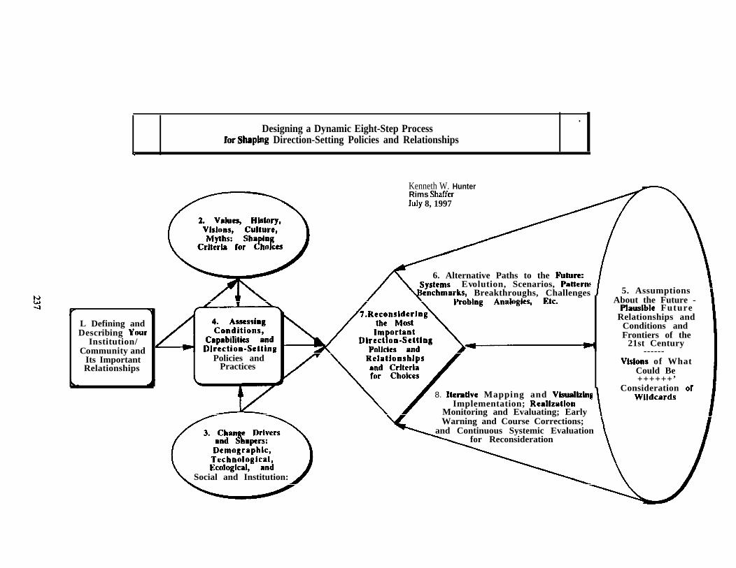
Designing a Dynamic Eight-Step Process.

for Shap\ng Direction-Setting Policies and Relationships9

L Defining andDescribing Your

Institution/Community and

Its ImportantRelationships

●

Kenneth W. HunterRims ShafferJUIY 8, 1997

6. Alternative Paths to the Fbture:Evolution, Scenarios, Pattern!

enchmarks, Breakthroughs, Challenges

Policies andPractices

8. Iterattve Mapping and VlsuallzbqImplementation; Reallzatlon

Monitoring and Evaluating; EarlyWarning and Course Corrections;

and Continuous Systemic Evaluationfor Reconsideration

Social and Institution:

5. AssumptionsAbout the Future -

Plauslble FutureRelationships and

Conditions andFrontiers of the

21st Century------

Vlslons of WhatCould Be++++++’

Consideration of

. .,,.

2. Understand the values, history, visions, culture and myths that shape thecriteria for making choices. Every institution and the people operating in itmake their day-to-day decisions and shape their actions and relationships onthe basis of their understanding of the values of the entity and their own.These values and behavior evolve and comprise a culture. Responses toearlier events and shared expectations help shape these values. Inorganizations, we articulate them as myths and visions, missions and goals,codes of conducts, guidelines and operational manuals, and in ourcontinuous dialogues about the enterprise. Understanding why aninstitution works the way it does, why it makes the choices it does and thushow it is likely to respond to early signals of change requires deepunderstanding of its values.

3. Understand major change drivers and shapers and their impacts on currentand future conditions. Early warning and futures research involve extensiveand intensive monitoring, forecasting and impact assessment of at least fourgroups of change drivers and shapers. (1) Demographic change drivers,including population growth globally and locally, differential growth amongregions and groups, differential income and wealth among regions andgroups, aging and increases in longevity, and increases in mobility. (2)

. Technological change drivers, including the increasing array of digitaltechnologies, advances in the biological technologies, new and improvedmaterials, new nano technologies, and continuing struggles with nucleartechnologies. (3) Ecological change shapers, including climate change, usablewater limits, ecologically sustainable energy sources, maintenance ofbiological diversity, and human relationships with microorganisms. (4)Macro patterns in institutional change that shape individual entity’senvironment, including globalization processes, shifting from hierarchical tomore modular and networked structures, acceleration in the pace of change,becoming real time all the time with global communications and mobility,and renewed emphasis on ethics, opemess and rule by law. In addition, weneed to identify and assess change drivers that are specific to the institutionswe are working with.

4. Assess current conditions, capabilities and direction-setting policies andpractices. Brutally honest and rigorous assessments are hard to do before acrisis occurs. Nevertheless, effective early warning and futures research aredependent up it. Auditing, investigating, inspecting, surveillance, and manyother such functions provide information and evidence of conditions.Process and policy evaluation provide information for assessing currentmactices as well as ~olicies, since txactices mav be at odds with ~olicv. InA

some casespioneering

These firstthoroughly

practice; lag in’ imple~enting cha~ges and in other; the; arework well ahead of current policy.

four steps involve understanding the present situations asand rigorously as we can. The next two steps jump to the future.

238

The last two steps focus on present direction-setting policy choices and theiri m p l e m e n t a t i o n . -

5. Assumptions about the future -- visiom of what conditions could bese~eral decades ahead. Futures research work underlying impact assessmentsin Step 3 above also shapes assumptions about the next few decades.Forecasting and statistical capabilities allow us to make fairly useful sets ofdeinographic and infrastructure assumptions about the next three decades --the next generation of people and the useful life of much infrastructure.Using 2030 or so as the foresight period also shifts the nature of the policydiscussion to “the legacy for future generations” by actions of current policymakers. One set of assumptions includes those that are highly probable -providing a relatively surprise free vision of the future. In addition, we needto define sets of potential crises and breakthroughs that would result insignificantly different futures. Each disciplinary group has its forecasters andsets of assumptions and visions. Policy analysis and futures research canintegrate them for use in policy making.

6. Analysis and consideration of alternative paths to the future – systemsevolution, scenarios, patterns, benchmarks, breakthroughs, challenges andthreats, probing analogies, etc. Today scenarios are a popular practice fordescribing and considering policy options and their consequences. Whetherdeveloped as such stories or as more rigorous policy and implementationanalyses, “alternative paths to the future” are critical features of early warningand futures research work or at least they should be. My preference is to useour full professional policy analysis tool kit rather than relying on one or afew tools. Modeling the system or institution, developing alternative paths,conducting implementation analyses of alternatives, assessing costs andbenefits, etc., are all necessary components. Information and analytictechnologies make this work far more effective today. We should be givinggreat attention to the integration of our approaches and methods into“decision technology systems.” (I have been thinking about designingdecision technology systems for some time and now believe the latesttechnology is making it really possible now. In addition, Dr. Shaffer and I aredeveloping an organizational behavior and development continuumapproach for creating sets of scenarios for more tailored to setting direction-setting policies.)

7. Reconsider important direction-setting policies and relationships andcriteria for choices. Today changing conditio~ are forcing reconsideration ofpolicies everywhere. Will ideology and political power overwhelm thenormal analytic and dialogue phases of policy reconsideration? In the 1970swe gave much attention to the systematic reconsideration of public poliaes.The driving proposal was for “sunset” provisions to be incorporated into alllegislation authorizing major programs. This Was to serve as an actionforcing mechanism for reconsideration. while the idea died and most form

{I 239

of systemic policy work were discontinued in the 1980s, the need still existsand the political institutions are in gridlock over their incapacity to do thiscore function. Nevertheless, professionals and professional institutions needto be more rigorous in their work and advising of policy making institutions.This means doing all the functions described above continuously in order tobe able to synthesize knowledge for use by the public and policy makers intheir own ways in the chaotic policy arenas of the non-analytic real world.We need to give special attention to reconsideration of the criteria for choices-- the values underlying all of the evaluations, dialogue and debate. Values,facts and opinions get hopelessly confused in the public discourse and it is thecontinuing responsibility of professionals to clarify wherever possible duringthe policy making process. Mixing lobbying and special interest advocacywith professional analysis and advising undermines the credibility of thelatter and contributes to the public and political confusion, cynicism andgridlock. It is up to the professions to address the conduct of their members.

8. Iterative mapping and visualizing implementation; realization monitoringand evaluation; early warning and course corrections; and continuoussystemic evaluation for reconsideration. Choosing a new policy direction isjust one step in a continuous process. Implementation is the path torealization. We need to provide visions and maps for guidingimplementation. We monitor and evaluate changing conditions, provideearly warning, and offer course corrections. Thus the iterative cycle ofprofessional work continues.

Evaluation of early warning and futures research performance

How should our professional early warning and futures research work beevaluated? Using the “accuracy of our forecasts and warnings” as the key measure isinappropriate and counterproductive. If we do our work effectively it should notinclude “forecasts” but should present ranges of plausible assumptions about thefuture. We should present “warnings” as likely consequences of inaction or specificproposed actions. Furthermore, policy action and implementation will change thefuture, making our earlier analyses outdated..

We should be evaluated on the effectiveness of our informing policy makers andthe public. It seems to me there are three dimensions of such evaluation. First isthe assessment of the policy makers with whom we work and who use theknowledge we develop in collaboration with them. Second is the public judgmentof our service which to a large degree is filter through the media with whom wedeal directly as information users and as professional peers. This leads to the thirddimension that is the judgment of ourselves as professional peers.

Credibility of all professions is dependent upon their own capacity to establish andadhere to performance and conduct standards. Early warning and futures research

240

are in their infancy in this regard. Establishing professional groups to continuouslyexamine theories, methods and practices in use and proposed is an important firststep. In my view we should strive to strengthen the early warning and futuresresearch component of each professional discipline while also developingintegrative theories and methods.

Closing 1

The purpose of this paper has been to pull together my own thoughts on earlywarning and futures research in order to participate in dialogues on strengtheningour services to policy makers and the public. I look forward to engaging in thesedialogues at upcoming meetings being convened by the National IntelligenceCouncil, the Federal Forecasters Conference, The Harrison Program on the FutureGlobal Agenda, the World Future Society, and in other forums. We have not hadsuch a serious professional dialogue for several decades and I am pleased toparticipate again.

Again, I encourage you to join in the professional meetings and collaborativefutures programs being developed. My coordinates for contact are on the cover.

241

E, .

FORECASTING PROGIUiM EXPENDITURES

Chair: Karen S. HamrickEconomic Research Service, U.S. Department of Agriculture

Projections of Elementary and Secondary Public Education Expenditures by State,William J. Hussar, National Center for Education StatisticsU.S. Department of Education

Medicaid Forecasting Practices,Dan Williams, Baruch College

Consumer Health Accounts: What Can They Add to Medicare Policy Analysis?R. M. Monaco, INFORUM, University of Maryland, andJ.H. Phelps, Health Care Financing Administration

243

.

PROJECTIONS OF ELEMENTARY AND SECONDARY PUBLIC EDUCATIONEXPENDITURES BY STATE

byWilliam J. Hussar

National Center for Education Statistics

I. Introduction

The National Center for Education Statistics (NCES)has been producing projections of education financestatistics at the national level for approximatelyhventy-five years. For the fmt time, NCES isinvestigating the development of state projections forone of its finance statistics, public elementary andsecondary current expenditures. This paper presents amethodology for producing a set of preliminary statecurrent expenditure forecasts. Two tests of theseprojections are examined later in this paper.

The frost of this paper’s eight sections is thisintroduction. The second section is a review of theliterature on examining cument elementary andsecondary school expenditure using time series data.

The third section presents the five combinations ofestimation technique and pooling techniques whichwere used in this analysis, as well as the sources of thedata.

The fourth section examines a model for elementaryand secondary expenditures similar to one that StephenBarro developed in the early 1970’s. This model wasestimated using the five estimatiotipocdingtechniques presented in the third part of this paper.Ex-post mean absolute percentage errors (M.APES)were calculated for each state using the fiveestimation/pooling techniques. These MAPES areexamined, together with those fkom a naive model inwhich cun-ent expenditures in each state were assumedto increase throughout the forecast period at theaverage annual growth rate of the previous three years.

The results concerning the estimation coefficientslargely followed expectations for each of theestimation/pooling techniques. Using the ex-postMAPEs as a measure of forecasting ability, oneestimation/pooling technique was found to be superior.

While the Barro model performed well, there was a

serious problem with using it to produce stateprojections: there are no independently producedprojections of one of its key independent variables andof the price deflator used for current expenditures.Hence, an alternative model was produced for whichthere are forecasts for all the variables. Both thecoefficients and the MAPEs of alternative model wereexamined in the fifth section of the paper. The resultswere very similar to those from the Barro model andagain the results for one estimation/pooling techniquewere superior. Following Barre’s example, Alaska andHawaii had been excluded from the sample. Theywere included in a final set of estimations.

Two sets of state projections were produced. The fmtset was produced using the model developed in sectionfive. An alternative set is the one presented in thispaper, in which the state projections have beenadjusted to equal the national totals from theProjections of Education Statistics to 2005. TheProjections of Education Statistics to 2005 was used inthe adjustments as the forecasts underlying theprojections presented in that edition were producedabout the same time as those used here.

In the seventh section, the results from two tests of thestate forecasts are examined. In the fmt test theprojections for 1993-94 are compared to the actualvalues produced by National Center for EducationStatistics. In the second test, the projections for 1994-95 and 1995-96 are compared to the National Centerfor Education Statistics most recent Early Estimates.Of these tests, the fmt is obviously the strongest. Theother test can only indicate if a state’s projections seemgrossly wrong.

In the final section, there is a summary and adiscussion of possible fhture work in this area.

II. Review

There has been a large body of work both theoreticaland empirical, on the demand for local public services

245

m’.

m.,

such as education. In most models, there are typicallyfour types of variables; 1) a measure of income; 2) ameasure of intergovernmental aid for education; 3) ameasure of the price of providing one more dollar ofeducation expenditures per pupil; and 4) one or moremeasures of voter tastes for education. Largelyconsistent results have been found for a great numberof empirical studies which have been conducted usingthis framework. Most of the empirical work oneducation expenditures has used cross-sectional data.There has been a limited amount of work using datawhich are simply time series data or are pooled timeseries and cross-sectional data.

As noted in the introduction, the National Center forEducation Statistics (NCES) has been producingprojections of national education statistics for twenty-five years. It has been producing projections ofelernentiuy and secondary cuxrent expenditures usingan econometric model yearly since 1987.

The national NCES model has three independentvariables; one for each of the first three categories ofvariables mentioned above; 1) personal disposableincome per capita in real dollars, 2) revenue receiptsfrom state sources per capita in real dollars, and 3) theratio of the enrollment to the population. (While theratio of enrollment to the population was not a directmeasure of the price of education, it was a measurethat had been successfidly used in other studies.)

In the early 1970’s Robert Barro developed a modelfor the demand for education expenditures by state.This model could have been used to produce state levelexpenditure forecasts though it does not seem to everhave been used for that purpose. It is that model thatforms the basis for the analysis presented in this paper.

Barro examined education expenditures using pooledtime-series cross-sectional data. He conducted hisanalysis using data for the contiguous states for everyother school year from 1951-52 to 1967-68. Batro’smodel had as its dependent variable school spendingper pupil in real 1964-65 dollars. Barro used aneducation price deflator that he developed for thisstudy.

The Barro model can be found in table 1. It had sevenindependent variables. ‘The of these, income percapita in real dollars, the sum of state and federal aid

for education in real dollars, and the ratio of theenrollment to the population multiplied by the ratio ofan education price index and the CPI, corresponded toeach of the fmt three types of variables listed above.The coefficients of those three variables were allsignificant and followed expectations.

The Barro model had four additional variables. Achange in the enrollment was found to have a negativeimpact on expenditures. Having a low populationdensity was found to have positive effect on educationexpenditures. There were two variables whichmeasured the impact of being of a state being in theSouth. These two variables had opposing effects oncurrent expenditures for the southern states: a dummyvariable for southern states had a negative coefficientyet a variable which measured the different impact ofaid in the South had a positive coefficient.

III. Estimation/Pooling Techniques and DataSources

A. Estimation/Pooling Techniques

The two models presented in this paper were estimatedusing five different combinations of estimationtechniques and the methods for pooling the datz 1) allthe states were pooled together and ordinary leastsquares (OLS) was used to estimate the model; 2) thestates were pooled into nine regions, OLS was used toestimate the model, and there were state dummyvariables; 3) the states were pooled into nine regionsand one of several generalized least squares techniqueswas used to estimate the model; 4) the model wasestimated for each state using OLS; and 5) the modelwas estimated for each state using ARl. (Also seetable 2.)

As noted above, there are several alternativespecifications for the generalized least squarestechnique. Kmenta suggests one specification, thecross-sectionally comelated a n d time-wiseautoregressive procedure for a sample such as thestates of the United States.

The cross-sectionally comelated and time-wiseautoregressive procedure of the econometrics packageSHAZAM was used when the model was estimatedusing the generalized least squares technique.

246

L?-”

The nine regions used in this analysis can be found intable 3.

B. Data

A data base similar to that used by Barro wasconstructed. Following Barre, it consisted of data foreach of thg forty-eight contiguous states and theDistrict of Columbia for each year from 1970-71 to1992-93. Data for Alaska and Hawaii were alsocollected but were not used in the initial estimations ofthe models.

Most of the historical education data were fromNCES’S Common Core of Data. This included data forcurrent expenditures, revenue receipts from statesources, revenue receipts from federal sources, andenrolhnent as measured by average daily attendance.

The economic consulting fm DRVMcGraw-Hillprovided the historical data and the forecasts fordisposable income, state and local government taxpayments by state. DRI/McGraw-Hill also providedthe national consumer price index and the nationalprice deflator for personal consumption expenditureswhich was used to place disposable income in constantdollars.

The economic projections from DR1/McGraw-Hillwere produced in early 1995, shortly after theproduction of the forecasts of the nationai economyused in production of the Projections of EducationStatistics to 2005. As the projections were producedclose in time, the state productions will be treated as ifthey had been produced with the Projections ofEducation Statistics to 2005.

Forecasts for average daily attendance for each statewere required, both to be used as a component of anindependent variable and also to produce forecasts fortotal current expenditures. Two sets of projectionswere produced for each state. The fwst set of forecastsfor each state was calculated by multiplying eachstate’s fall enrollment projections as presented in theProjections of Education Statistics to 2005 by thatstate’s average value of the ratio of average dailyattendance to the population for the previous ten years.This method is similar to the method used to produce

the national projections for average daily attendance.A second set of projections was produced for each

state by altering each state’s projection by the samepercent so that the sum of the state projections equaledthe national projections in the Projections of EducationStatistics to 2005.

A Barro type education price index was constructed byusing the National Education Association’s teachersalary time series to measure personnel costs and theconsumer price index to measure other costs.

N . The Barro Model

This part of the paper presents the results horn there-estirnation of the Barro model. The results of theestimations of the Barro model using each of thepooling/estimation techniques are compared using ex-post MAPEs.

Table 4 contains specifications of the Barro model foreach of the five estimation/pooling techniques. UnlikeBarre’s original estimations, most of the variables werein log form. The log form was used for all theestimation presented in this paper because of resultsfrom BOX-COX tests for fictional form that wereconducted when preparing the NCES nationalprojections.

The only time the specification was identical to thatused by Barro was when the data were poolednationally and ordinary least squares was used.

When the states were broken up by tegion or state,there was no reason for either the SOUTH dummyvariable or the variable LTGRANTS to be present.Further, in some of the regions, there was no variationin the density variable. Hence, when estimating theBarro model using data pooled either regionally or bystate, those three variables were excluded.

A. Results of the Estimations

Table 5 shows a summary of the estimations of theBarro model using the five estimatiodpoolingtechniques. (The results for each estimation areavailable in a longer version of this paper availablehorn the author.)

Ordinary Least Squares with Data PooledNationally

247

IP-

These results are similar to those from the originalstudy by Barro presented in table 1. The coefficientsof all the variables except the change in enrollmentvariable (GRADA) had the same signs as in the Banostudy and were significant.

Ordinary Least Squares, Data Pooled Regionally,and Dummy Variables

The coefficient for the income, state aid and pricevariables were significant for most of the regions. Thecoefficient for the change in enrollment variable wassignificant for only two regions.

Generalized Least Squares and Data PooledRegionally

The coefficient for the income, state aid and pricevariables were significant for most of the regions. Thecoefllcient for the change in enrollment variable wassignificant for only three regions.

Ordinary Least Squares and Each State ExaminedIndividually

For most of the states, the coefficients of the incomeand price variables were significant. For about half thestates, the coefllcient of the state aid variable wassignificant. For less than half the states, the coefficientfor the change in enrollment variable was significant.

ARl and Each State Examined Individually

The results for ARl were very similar to those forOLS. For most of the states, the coefficients of theincome and price variables were significant. For abouthalf the states, the coefllcient of the state aid wassignificant. For less than half the states, the coei%cientfor the change in enrollment variable was significant.

B. Forecast Evaluation of the Barro Model

Mean absolute percentage emors (MAPEs) werecalculated for each technique for producing forecaststo measure forecast accuracy. For the naive model,MAPEs were computed for the case in which cumentexpenditures per pupil in constant dollars wereassumed to increase throughout the forecast period atthe average annual growth rate of the last three years.The MAPEs from each estimation/pooling technique

were compared to the MAPEs fkom the naive model.

To produce the state MAPEs, for each estimation-pooling technique, a series of ex-post forecasts werecalculated. This was done by excluding fkom one tofive observations Ilom the end of the sample. Then,forecasts were calculated using the parameter estimatesand the actual values for the independent variables.This produced five one-year-out ex-post forecasts, fourtwo-year-out ex-post forecasts, three three-year-out ex-post forecasts, two four-year-out ex-post forecasts, andone five-year-out ex-post forecast.

These ex-post forecasts were then compared to theactual values. In this paper, MAPEs were calculated asthe primary measures of forecast accuracy. As up tofive years were excluded from the sample period toproduce the ex-post forecast five different ex-postMAPEs were calculated. The one-year-out MAPEexamines the accuracy of the five one-year-outforecasts, the two-year-out MAPE examines theaccuracy of the four two-year-out forecasts and soforth.

The formula used to calculate the MAPE can be foundin table 6.

The MAPE is one of several measures for forecastevaluation. Another standard measure is the root meansquare error (rinse). These will not be examined sincethey were very similar to those for the MAPEs.

The Naive Model

First, we shall examine the MAPEs from the naivemodel. The naive model produced relatively lowMAPEs for a large number of states (table 7). Forty-five states had a fret-year-out MAPE of less than 5percent and fifteen had a five-year-out MAPE of lessthan 5 percent. There were some states, however, thathad quite large MAPEs, such as Louisiana.

Ordinary Least Squares and Data PooledNationally

The MAPEs were generally higher than those Ilom thenaive model. When compared to the naive model,only eight states had a lower one-year-out MAPEusing this estimation of the Barro model. (See table 8for the number of states which have a MAPE less than

k-

the naive model for each estimatiordpoolingtechnique.) The MAPEs for this estimation techniquedo not compare favorably to those calculated using thenaive model.

Ordinary Least Squares, Data Pooled Regionally,and Dummy Variables

The results are mixed for this estimation/poolingtechnique. Only twenty-three states had one-year-outMAPEs less than those from the naive model.However, at least thirty-three states had MAPEs lessthan those of the naive model for each of the otherforecast horizons.

Generalized Least Squares and Data PooledRegionally

Unlike the case for the other estimation/poolingtechniques, the ex-post MAPEs were generally lowerthan those from the naive model for the one-year-outMAPEs. Thirty-four states had one-year-out MAPEswhich were smaller for this estimation of the Bamomodel than for the naive model. When thisestimation/pooling technique was use~ a majority ofstates had two-year-out through four-year-out MAPEsthat were smaller than those from the naive model aswell.

The results for the five-year-out MAPEs whengeneralized least squares was used are not directlycomparable to those for the other estimation/poolingtechniques. Generalized least squares could not beused to estimate the Bmo model for the South Atlanticregion due to a lack of observations. Hence, there areonly 40 five-year-out MAPEs this estimation/poolingtechnique rather than 49.

Ordinary Least Squares and Each State ExaminedIndividually

For twenty-one states, the one-year-out MAPEs forthis estimation of the Barro model were lower thanthose of the naive model. However, for the two-year-out through the four-year-out time horizons, theMAPEs were lower than those of the naive model forat least thixty-one states.

ARl and Each State Examined Individually

For eighteen states, the one-year-out MAPEs for thisestimation were lower than those of the naive model.However, for at least thirty-four states, the two-year-out through five-year-out MAPEs were lower thanthose of the naive model.

c . Summary of the Results of the BarroModel

Results of the estimations of the Barro model showedthat the estimated coefficients generally followedexpectations no matter which estimation poolingtechnique was used. Also, the technique of breakingthe states up into regions and using generalbd leastsquares, performed best as a method for producingforecasts when using ex-post MAPEs were used as thecriteria.

v . The Forecasting Model

There are problems with using the Baxro model aspreviously estimated as a forecasting tool as not all therequired data are available (table 9). First there are noindependently produced forecasts of the educationprice index used to adjust current expenditures so nocunent dollar projections could be produced. Secon&there are no independently produced projections of theindependent variable state and federal revenue receiptsfor education. To solve these difficulties, alternativesfor the education price index and state and federalrevenue receipts for education were found.

As a substitute for the education price index, thenational consumer price index was used. Theconsumer price index has been used successfidly withNCES’S national education expenditures.

State and local tax payments were used as a substitutefor state and f~eral revenue receipts for education.This variable acts as a measure of the general financialposition of each state. It lacks any measure of theactions of federal govermnen$ but this may not be amajor difficulty since federaI aid for education makesup only a small portion of elementary and secondaryeducation revenue.

The national forecasts for the consumer price indexand the state forecasts of state and local governmenttax payments were provided by the economicforecasting firm, DRVMcGraw-Hill.

,.

249

KE-

m.’

.-,

Hence, an alternative model, which will be called theForecasting model, was developed using thesesubstitutes. The alternative specifications for thedifferent estimation/pooling techniques can be found intable 10.

The Forecasting model was estimated using the fiveestimation/pooling techniques used to estimate theBarro model. In presenting these results, there are twodifferences born the presentation of the Barro model.First only statistically significant variables wereincluded in the estimation of the Forecasting modelpresented here. The second difference only concernsthe presentation of the case when each state wasexamined separately. Rather than presenting theresults for both ordinary least squares and ARl foreach state, the results fi-om only one estimation arepresented for each state. The value of the Durbin-Watson test were used to determine which resultsshould be presented. A summary of the dfierencesbehveen the Forecasting model and the Barro modelcan be found in table 11.

A. The Forecasting Model

Ordinary Least Squares and Data PooledNationally

Two variables that had been included in the estimationof the Barro model, the change in average dailyattendance and the dummy variable for southern states,were excluded here because they were not statisticallysignificant (table 12).

Ordinary Least Squares, Data Pooled Regionally,and Dummy Variables

The income variable was included in the estimationsof all nine regions. The state aid variable was includedin the estimations of seven of the regions and the pricevariable was included in the estimations of five of theregions. The change in enrollment variable wasincluded in the estimation of only two regions (table12).

Generalized Least Squares and Data PooledRegionally

The income variable was included in the estimations of

all nine regions. ‘The state aid variable was included inthe estimations of eight of the regions and the pricevariable was included in the estimations of seven of theregions. The change in enrollment variable wasincluded in the estimation of only12).

Ordinary Least Squares/ARlExamined Individually

While estimations were producedleast squares and ARl, only

three regions (table

and Each State

using both ordinaryone estimation is

considered for each state. The Durbin-Watson statisticsfor each state were examined to chose which equationwould be presented. For approximately two thirds ofthe states, the results of the ARl estimation arepresented.

In thirty-two equations, the income variable wasincluded. In twenty-six equations, the aid variable wasincluded. In thirty-one equations, the price variablewas included. In twenty-two, the change in enrollmentvariable was included (table 12).

B. Forecast Evaluation of the ForecastingModel

As with the Barro model, ex-post MAPEs werecompared to those from a naive model in whichcurrent expenditures per pupil in constant dollars wasassumed to increase at the average annual growth rateof the last three years. These naive forecasts weredifferent forecasts than those used to evaluate thealternative estimations of the Barro model becausediffkrent price indexes were used with the dependentvariable. Those MAPEs computed for the naiveforecasts estimated using the consumer price indexwere higher than those estimated using the educationprice index for most states.

Ordinary Least Squares and Data PooledNationally

This specification does not do well when compared tothe naive model (table 13). Only eight states had one-year-out MAPEs less than that from the naive model.

Ordinary Least Squares, Data Pooled Regionally,and Dummy Variables

250

The one-year-out MAPEs for this estimation/poolingtechnique were lower than those of the naive model foronly eighteen states (table 13). However, the two-year-out MAPEs for this technique were lower forthirty-two states. and the other types of MAPE weregenerally lower for this technique.

Generalized hast Squares and Data PooledRegionally

As was the case with the Barro model, the MAPEs forthis estirnationlpooling technique (table 13) aregenerally lower than those of the otherestimation/pooling techniques. Thirty-three states hadone-year-out MAPEs less than the naive model androughly forty states had two through four-year-outMAPEs less than the naive model.

Ordinary Least Squares/ARl and Each StateExamined Individually

Only sixteen states had one-year-out MAPEs lowerthan those of the naive model (table 13). For twothrough five-year-out periods, for most states, thisestimatiodpooling technique did do better than thenaive model.

c . Summary of the Results of the ForecastingModel.

As with the estimations of the Barro model, theestimated coefficients of the Forecasting modelgenerally followed expectations no matter whichestimation pooling technique was used. Given thesimilarity of results between these two models for allthe estimation/pooling techniques, the Forecastingmodel was used to produce the state forecasts.

Secon~ the technique of breaking the states up intoregions and using generalized least squares, performedbest as a method for producing forecasts when usingex-post MAPEs as the criteria. This superiority wasstrongest for the one-year-out MAPEs but also held forthe two-year-out MAPEs, three-year-out MAPEs andfour-year-out MAPEs as well.

D. Forecasting Models for Alaska and Hawaii

This paper analyzes models using a database similar toBarre’s which excluded two states, Alaska and Hawaii.

In order to produce projections for the entire country,projections for those two states were needed. Twooptions were considered: 1) estimate equations forAlaska and Hawaii separately using either OLS orAR1; and 2) include the two states in their respectiveregions (the Pacific North West for Alaska and thePacific South West for Hawaii) and re-estimate themodel using the generalized least squares. In the end,the generalized least squares method for each of thestates, including Alaska and Hawaii, was chosen toproduce the state forecasts.

VI. Forecasts by State

A set of forecasts for cument expenditures per pupil inaverage daily attendance for the fifty states and theDistrict of Columbia were produced using thegeneralixd least squares estimations. Those forecastswere multiplied by the unadjusted state forecasts foraverage daily attendance to produce the forecasts fortotal cuxrent expenditures. Both sets of projections areavailable in a data appendix which is available tlomthe author.

-.A comparison of a forecast for the United States as awhole produced by summing up the state forecasts wascompared with the national projections from bothProjections of Education Statistics to 2005 andProjections of Education Statistics to 2007 (table 14).The projections produced by summing up the stateprojections were only slightly higher than the nationalfigures from Projections of Education Statistics to2005. (While the forecasts were produced in 1964-65dollars, they are presented in this paper using 1992-93dollars.)

If state projections are ever presented in theProjections of Education Statistics, the stateprojections will be adjusted by the same proportion sothat the sum of the states projections equals thenational projection. That same method was used hereproducing an adjusted set of state projections, equal tothose in Projections of Education Statistics to 2005.Projections of Education Statistics to 2005 had similareconomic projections as used for the state f~asts inthis paper. As the projections were produced so closein time, the state projections will be treated as if theyhad been produced with the Projections of EducationStat&tics to 2005. The adjusted current expenditureprojections were divided by the adjusted projections

251

E- .-

for average daily attendance to produce adjustedprojections for current expenditures per pupil inaverage daily attendance.

Average annualized growth rates for currentexpenditures for three different periods appear in table15.

The period from 1980-81 to 1992-93 was a period inwhich current expenditures in constant dollars grew inall the states. The largest change was in Nevada whichhad an average annualized growth rate of 6.7 percent.The smallest was in IOWA with an average annualizedgrowth rate of 0.9 percent. In no region was anaverage annualized growth rate less than 2.0 percentand the nation as a whole had an average annualizedgrowth rate of 3.0 percent.

For the nation as a whole and for most states, theaverage annualized growth rate for currentexpenditures was lower for the most recent historicalperiod of 1989-90 to 1992-93, than for the entirehistorical period of 1980-81 to 1992-93. Seven stateshad negative average annualized growth rates over therecent historical period.

Current expenditures were forecast to increase for eachstate from 1992-93 to 1999-2000. The smallestincreases were projected for Iowa and North Dakotawith projected average annual growth rates of 1.0percent and the greatest was projected forMassachusetts with a projected average annual growthrate of 4.6 percent. Regionally, the greatest increasewas projected for the South-Atlantic region, which alsohad the greatest increase for the 1980-81 to 1992-93period. The smallest increase was for the West-North-Central, which had the second lowest increase for thehistorical period.

For many states and the nation as a whole, one f~orpushing up the total current expenditures projectionswas the increase in enrollment that was projected forthe forecast period. The average growth rate for thehistorical period was only 0.4 percent. The projectedaverage annual growth rate for average dailyattendance was 1.7 percent. For each region, theprojected average annualized growth rate was greaterfor the forecast period than for the historical period.While four regions had negative average annualizedgrowth rates for the historical peri@ all regions had

increases projected for the forecast period.

For the entire historical peric@ current expendituresper pupil had an average annualized growth rate of 2.6percent (table 16) but there was considerable variationamong regions and states. The Mid-Atlantic regionhad an average annualized growth rate of 3.6 percen~while the Pacific-South-West had one of 1.3 percentMaine had the highest average annualized growth rateat 5.5 percen~ while Alaska had the lowest at -0.6Percent”

The situation for the most recent historical peri@tlom 1989-90 to 1992-93, was quite diffbrent than forthe entire historical period. From 1989-90 to 1992-93,the average annualized growth rate was only 0.1percent. The average annualized growth rate wasnegative for three regions and for about half the states.

For the nation as a whole, an average annualizedgrowth rate of 1.5 percent was projected. Theprojected average annualized growth rate differssharply by region. For five regions, an averageannualized growth rate of 2.0 percent or greater wasprojected. For the Pacific-North-West an averageannualized growth rate of only 1.0 percent W*projected and for the Pacific-South-West an averageannualized decrease of -0.3 percent was projected.The main cause of the negative number for the Pacific-South-West was the -0.8 percent average annualizedgrowth rate projected for current expenditures perpupil in California.

VII. A Further Examination of the Forecasts

Given the potentially controversial role that stateforecasts could have, care will be taken before anystate projections are presented in an edition of theProjection of Education Statistics. This part of thepaper presents the results of two additional tests ofthese projections.

A. Comparison with the 1993-94 ActualValues

NCES has published actual values for 1993-94. Thesevalues, in 1992-93 dollars, are compared with theadjusted projection (table 17).

Overall, the national projection from the Projections of

252

Education Statistics to 2005 was slightly higher (0.6Yo)that the actual value.

When we examine the regions, we see that for mostregions the projections were quite close to the actualvalues. For six of the nine regions, the projection waswithin one percent of the actual value. The greatestdifference was, for the East North Central with aforecast 2.6 percent too large.

The results differed more widely by state. For abouthalf the states, the projection was within 2 percent.However, there were seven states with projections offby greater than 4.0 percent. The states with thegreatest differences were Ohio (8.8 percent) and NorthDakota (12. 1 percent).

B. Comparison with the Early Estimates

The 1994-95 and 1995-96 forecasts also werecompared to the 1996 NCES Early Estimates. Eachyear NCES produces a series of early estimates forcurrent expenditures. This edition of the earlyestimates, contains early estimates for 1994-95 and1995-96. These numbers for the early estimates comefrom a survey of state education agencies. In somestates, the state agencies may have a very good idea ofwhat will be spent. With other states, the estimatesmay be significantly less accurate. Some states maynot respond to the survey so NCES estimates a figure.

On table 18, there is a comparison of the earlyestimates with the projections for 1994-95 and 1995-96, all in 1992-93 dollars. As the early estimates arenot final counts for each state, this comparison is not atest of the accuracy of the projections. Rather, rather itis a test to indicate if any states have any highlyimprobable projections.

If the early estimates and projections for a state differsharply, this may mean one of several things. First itcould mean that this projections methodology haddifficulty forecasting current expenditures for the state.Secon& it could mean that there was a problem withthe early estimate for that state. And third it couldmean that the early estimate has caught a change in thetrend of that state which was beyond the ability of theforecasting. model to capture.

For the national total, the early estimates and the

projections produced similar numbers. For 1994-95,the projections were 1.5 percent greater than the earlyestimates and for 1995-96, they were 2.5 percentgreater. While these national numbers were fairlyclose, there were significant differences at the state andregional levels.

For both 1994-95 and 1995-96, the projections of sixof the nine regions were within 3 percent of the earlyestimates. For both years, the greatest differencebetween the early estimates and the projections waswith the East-North-Central region. The earlyestimates showed virtually no change in that regionwhile the projections showed relatively rapid rises. (Ithad the second highest increase of any of the regions.)Both alternatives are possible so it will take more data

to see which, if either, is correct.

Greater differences between the early estimates and theprojections were found when individual states wereexamined. For 1994-95, there were ten states forwhich the difference was 2 percent or less, and for1995-96, there were eleven. On the other hand for1994-95 there were twenty-three states in which thedifference was 5.0 percent or greater, and twenty-sixstates for 1995-96.

There were some states with very large differences.For the District of Columbia for 1995-96, thedifference was 52.2 percent. This is caused by twovery different fbtures for expenditures in 1995-96.The early estimates shows expenditures falling 33percent from its 1993-94 level while the projectionsshow current expenditures increasing 1.6 percent.Again both are plausible. It could be that there will bestates for which the early estimates provide a betterpicture to the fidure and others for which it is theprojections.

VIII. Conclusions and Directions for FutureResearch.

For the fnt time, NCES has produced a set ofprojections for current expenditures by state. Theseprojections were produced using a model similar tothat developed by Barro and was also similar to themodel used to produce the national forecasts. Severalalternative methods of estimating this model wereexamined. While each estimation/pooling methodgave estimation coefficients that were usually of the

253

me

expected sign and significant the generalhd leastsquares technique with the states broken up by region,proved to be the best technique for producing forecastsusing as criteria a series of ex-post MAPEs. Thistechnique was used to produce the forecasts of currentexpenditures by state.

For most states, and for the nation as a whole, thetechnique produced plausible projections of currentexpenditures. For each year in the forecast period thesum of the state projections was quite close to thenational projections presented in the Projections ofEducation Statistics to 2005.

Fairly rapid growth for current expenditures wasprojected for each state during the forecast period.Each state had a projected average annualized growthrates of at least one percent and some states had ratesgreater than four percent.

Since enrollment is projected to grow during theforecast period, current expenditures per pupil werenot projected to increase as rapidly, and were projectedto fall in a couple states including California.

Two simple tests of the projections were conducted. Inthe fret, the projections for 1993-94 were compared tothe actual values for that year. In the second, theprojections for 1994-95 and 1995-96 were comparedto NCES Early Estimates. The second test was not aparticularly strong test. It was more usefid to pointingout highly implausible projections, and perhaps earlyestimates, which differ strongly from recent trends. Asactual values for other years become available,forecasts for other years can be compared to otheryears as well. More tests for these projections and theearly estimates will occur as more actual values areproduced. Of special interest will be areas such as theEast-North-Central in which the early estimates andforecasts differed sharply.

Given the potentially controversial nature of stateexpenditure projections, these preliminary projectionsshould be compared to at least one more set of actualvalues for current expenditures, before considerationshould be given to presenting state current expenditureprojections in an edition of Projections of EducationStatistics.

Until then, other work may be done on this model for

forecasting current expenditures. One possible changecould be the introduction of variables to measure if astate has had any court cases affecting the financing ofeducation, or other legislative or policy variables.

REFERENCES

Barre, Stephen M. “Cost-of-Education DifferentialsAcross the States:” National Center for EducationStatistics Working Paper Series. Washington D.C.:National Center for Education Statistics, 1993.

Bamo, Stephen M. “An Econometric Study of PublicSchool Expenditure Variations Across States, 1951-67.” Paper presented at the Annual Meeting of theEconometric Society in Toronto, December 1972.Washington D.C.: The Rand Corporation, 1972.

Bane, Stephen M. “Theoretical Models of SchoolDistrict Expenditure Determination and the ImpactGrants-In-Aid.” Santa Monic~ Ca.: The RandCorporation, 1972.

Bradford, David, and Wallace Oates. “SuburbanExploitation of Central Cities and GovernmentStructure.” In RedMribution l%rough Public Choice.Edited by H. M. Hochman and G. E. Peterson. NewYork: Columbia University Press, 1974.

Gerald, Debra E., and William J. Hussar. Projectionsof Education Stattitics to 2005. U.S. Department ofEducation, National Center for Education Statistics.Washington, D.C.: Government Printing Otlice, 1994.

Gerald, Debra E., and William J. Hussar. Projectionsof Education Statistics to 2006. U.S. Department ofEducation, National Center for Education Statistics.Washin@on, D.C.: Government Printing Office, 1996.

Gerald, Debra E., and William J. Hussar. Projectionsof Education Stattitics to 2007. U.S. Department ofEducation, National Center for Education Statistics.Washin@on, D.C.: Government Printing Office, 1997.

Holden, K., D. A. Peel, and J. L. Thompson.Economic Forecasting: An Introduction. Cambridge,England: Cambridge University Press, 1990.

254

Xnman, Robert P. “The Fiscal Performance of LocalGovernments: An Interpretative Review.” In Curren/Issues in Urban Economics, edited by PeterMieszkowski, , and Mahlon Straszheim. Baltimore,Md.: Johns Hopkins University Press, 1979.

Johnson, Frank H. Early Estimates: PublicElementary and Skconduy Ei&cation Statistics:School Year 1994-95. U.S. Department of Education,National Center for Education Statistics. Washington,D.C.: Government Printing Office, 1995.

Johnson, Frank H. Early Estimates: PublicElementary and Secon&ry Wucation Statistics:School Year 1995-96. U.S. Department of Education,National Center for Education Statistics. Washington,D.C.: Government Printing Oflice, 1996.

Kmenw Jan. Elements of Econometrics, SecondEdition: New York, New York: MacmillanPublishing Company, 1988.

255

Table l-Coefficients fkom the Barro paper

R-SQ CONSTANT PCI TGRANTENROLLPOP GRENROLL LD SOUTH TGIUINTS

0.850 218 0.20 1.15 -949 -372 34.4 -109 1.01

12.1 24.9 9.7 -11.5 -6.5 5.4 -7.1 4.1

Where:

The dependent variable is current expenditures per student in 1965 dollars using an education price index;

PCI is income per capita in 1965 dollars;

TGRANT is the sum of revenue receipts from state sources and federal sources per capita in 1965 dollars;

ENROLLPOP is the ratio of enrollment to the population multiplied by the ratio of the education price

index to the consumer price index;

GRENROLL is the change in enrollmen~

LD is a dummy variable = 1 for population density less than 30;

SOUTH is a dummy variable= 1 for soWhern states; and

TGRANTS is a the product of TGRANT and the SOUTH variable;

Table 2-Alternate Methods for Estimating the Barro Model

Method 1. Ordinary least squares and data pooled nationally

Method 2. Ordinary least squares, data pooled regionally, and dummy variables

Method 3. Generalized least squares and data pooled regionally

Method 4. Ordinary least squares with each state examined individually

Method 5. AR1 with each state examined individually

256

Table 3- List of states by region

Region 1

State 1

State 2

State 3

State 4

State 5

State 6

Region 2

State 1

State 2

State 3

Region 3

State 1

State 2

State 3

State 4

State 5

State 6

State 7State 8

state 9

Region 4

State 1

State 2

State 3

State 4

Region 5

state 1

State 2

State 3

State 4

New England

Connecticut

Maine

Massachusetts

New Hamphire

Rhode Island

Vermont

Mid Atlantic

New Jersey

New York

Pennsylvania

South AtlanticDelaware

District of

Columbia

Florida

Georgia

Maryland

North Carolina

South CarolinaVirginia

West Virginia

East South Central

Alabama

Kentucky

Mississippi

Tennessee

West South Central

Arkansas

Louisiana

Oklahoma

Texas

NENG

CT

ME

RI

VT

MATLNJ

NY

PA

s A n

DE

Dc

FL

GA

NC

Sc

VA

ESC

AL

KY

MS

TN

Wsc

AR

LA

OK

Tx

Region 6

State 1

State 2

State 3

State 4

State 5

Region 7

State 1

State 2

State 3

State 4

State 5

State 6

State 7

Region 8

State 1

State 2

State 3

State 4

State 5

Region 9

State 1

State 2

State 3

State 4

State 5

State 6

East North Central

Illinois

Indiana

Michigan

Ohio

Wisconsin

West South Central

Iowa

Kansas

Minnesota

Missouri

Nebraska

North Dakota

South Dakota

Pacific North West

Idaho

Montana

Oregon

Washington

Wyoming

Pacific South West

Arizona

California

Colorado

Nevada

New Mexico

Utah

ENC

IL

IN

MI

OH

WI

WNc

IA

KS

MO

NE

ND

SD

PNW

ID

MT

OR

WA

PswAzCAco

UT

257

.“

Table 4-Alternate specifications of the Barro model

Equation 1. Ordinary least squares and data pooled nationally

LCUREXPE = PO + &LPCI + &LTGRANT + ~LADAPOPE+ ~4GRADA + ~~LD + &SOUTH + ~7LTGRANTS + p

Equation 2. Ordinary least squares, data pooled regionally, and dummy variables

LCUREXPE = PO + ~lLPCI + &LTGRANT + ~LADAPOPE + ~4GRADA+ ctlDUMIvlY1 + . . . ...+ a@JMMY~ + p

Equation 3. Generalized least squares and data pooled regionally

LCUREXPE = PO + (31LPCI + &LTGR.ANT + ~JLADAPOPE + ~4GRADA + p

Equation 4. Ordinary least squares with each state examined individually

LCUREXPE = PO + ($LPCI + &LTGRANT + &LADAPOPE + ~4GRADA + p

Equation 5. ARl with each state examined individually

LCUREXPE = PO + ~lLPCI + ~zLTGRANT + (33LADAPOPE + ~4GRADA + p

where:

LCUREXPE was current expenditures per student in ADA in 1%5 dollars using the education price index in log form;

LPCI was disposable personal income per capita in 1965 dollars using the national price deflator for personalconsumption expenditures in log form;

LTGRANT was the sum of revenue receipts from state sources and fderal sources per capita in 1965 dollars using thenational CPI in log form;

LADAPOPE was the ratio of average daily attendance to the population multiplied by ratio of the education price indexto the national consumer price index in log form;

GRADA was the change in average daily attendance;

LD was a dummy variable measuring states with a population density greater than 30;

SOUTH was a dummy variable for southern states;

LTGRANTS was the product of LTGRANT and the SOUTH variable; and

DUhWYi was a dummy variable equal to 1 for the ith state in alphabetical order in the region. ‘Ilme were dummyvariables for each state in the region except the last one alphabetically.

258

.

Table 5- Number of Regions/States in Which the Independent Variables Are Significant in the Estimationsof the Barro Model

OLS and Data P&ledNationally

OLS, Data PoolidRegionally AndDummy Variables

GSL and Data PooledRegionally

OLS and Each StateExamined Individually

ARl and Each StateExamined Individually

LPCI LTGRANT LADAPOPE GRADA LD SOUTH LTGRANTS

1 1 1 0 1 1 1

8 7 5 2 .- . . .-

8 7 6 3 . .

40 24 38 15

40 26 41 13

. . . .

Table 6- Formula to calculate the ith-year-out MAPE

where

MAPEi is the i-year-out MAPE,

~ is the number of ex-post forecasts which are i years tim the last actual value,Fij is the jth ex-post forecast which is i years from the last year in the sample @@AU is the jth actual value which is i years tim the last year in the sample peri@

andj = 1,2,...,r4.

259

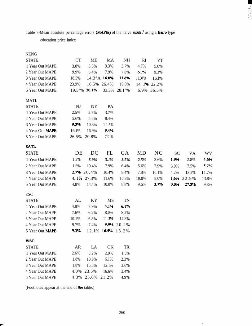
Table 7-Mean absolute percentage errors (MAPEs) of the naive rnodell using a Barro type

education price index

NENGSTATE1 Year Out MAPE2 Year Out MAPE3 Year Out MAPE4 Year Out MAPE5 Year Out MAPE

MATLSTATE1 Year Out MAPE2 Year Out MAPE3 Year Out MAPE4 Year Out MAPE5 Year Out MAPE

sAnSTATE1 Year Out MAPE

2 Year Out MAPE

3 Year Out MAPE4 Year Out MAPE5 Year Out MAPE

ESCSTATE1 Year Out MAPE2 Year Out MAPE3 Year Out MAPE4 Year Out MAPE

5 Year Out MAPE

WscSTATE1 Year Out MAPE2 Year Out MAPE3 Year Out MAPE4 Year Out MAPE5 Year Out MAPE

CT ME MA NH RI VT3.8% 3.5% 3.3% 3.7% 4.7% 5.0%9.9% 6.4% 7.9% 7.8% 6.7V0 9.3%

18.5% 14.3°A 16.OVO 13.6V0 11.OVO 16.l%23.9% 16.5% 26.4% 19.8% 14. lVO 22.2%19.5’% 20.lVO 33.3% 28.1’% 6.9% 36.5%

NJ NY PA2.5% 2.7% 3.7%5.6% 5.8% 8.4%9.39io 10.3% 1 1.5%

16.l% 16.9% 9.4V026.5% 20.8% 7.9’%

DE DC FL GA MD NC1.2% 8.9% 3.l% 3.5% 2.5% 3.6%

1.6% 19.4% 7.9% 6.4% 5.6% 7.9%

2.7V0 26 .4% 10.4% 8.4% 7.8% 10.1%4. lVO 27.3% 11.6% 10.8% 10.8% 8.0%4.8% 14.4% 10.0% 8.8% 9.6% 3.7V0

AL KY MS TN4.8% 3.9% 4.lVO 6.lVO7.6% 6.2% 8.0% 8.2%

10.1% 6.8% 11 .2% 14.8%9.7% 7.4% 9.9V0 20 .2%9.3V0 12 . l% 16.5V0 1 3 . 2 %

AR LA OK TX2.6% 5.2% 2.9% 1.3%1.8% 10.9% 6.l% 2.3%1.8% 15.5% 12.l% 3.6%4.0% 23.5% 16.6% 3.4%4.3% 25.6% 21.2% 4.9%

SC VA WV

1.9% 2.8% 4.6V0

3.9% 7.5% 5.7V0

4.2% 13.2% 1 1.7%1.6’%0 22 .9% 13.8%O.OYO 27.3V0 9.8%

(Footnotes appear at the end of the table.)

260

m-

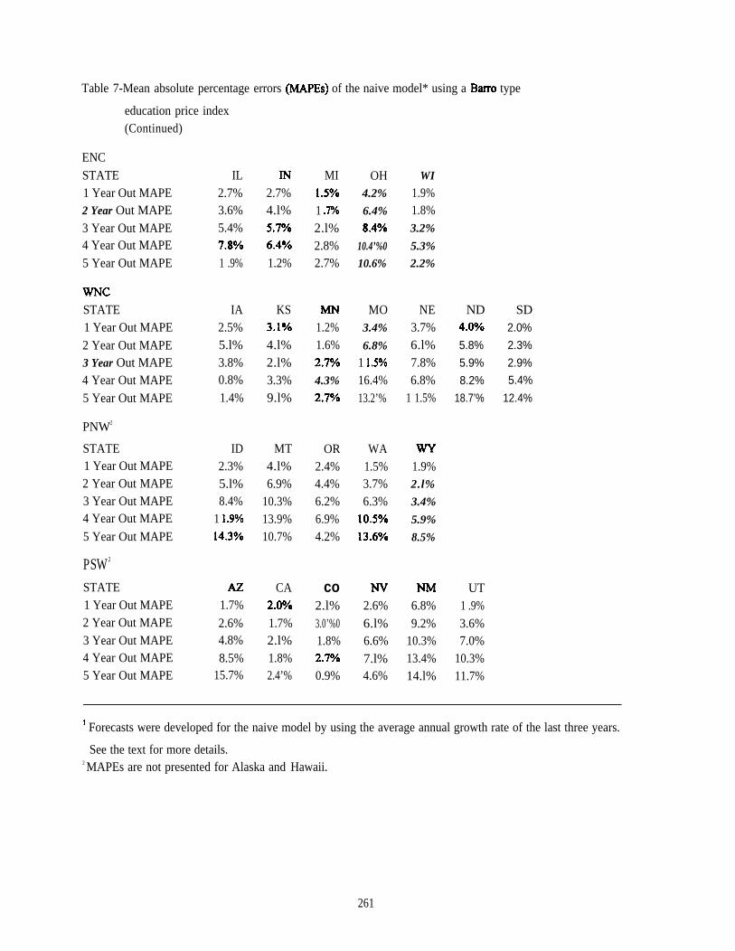
Table 7-Mean absolute percentage errors (MAPEs) of the naive model* using a Barro type

education price index(Continued)

ENCSTATE1 Year Out MAPE2 Year Out MAPE3 Year Out MAPE4 Year Out MAPE5 Year Out MAPE

WNcSTATE1 Year Out MAPE2 Year Out MAPE3 Year Out MAPE4 Year Out MAPE5 Year Out MAPE

PNW2

STATE1 Year Out MAPE2 Year Out MAPE3 Year Out MAPE4 Year Out MAPE

5 Year Out MAPE

PSW2

STATE1 Year Out MAPE2 Year Out MAPE3 Year Out MAPE4 Year Out MAPE5 Year Out MAPE

IL2.7%3.6%5.4%7.VXO1 .9%

IA2.5%5.l%3.8%0.8%1.4%

ID2.3%5.l%8.4%

1 1.9%14.3V0

M1.7%

2.6%4.8%8.5%

15.7%

ml2.7%4.l%5.7V06.4V01.2%

KS3.lVO4.l%2.l%3.3%9.l%

MT4.l%6.9%

10.3%13.9%10.7%

CA2.OVO1.7%2.l%1.8%2.4’%

MI1.5V01 .7V02.l%2.8%2.7%

1.2%1.6%2.7V0

4.3%

2.7’%0

OR2.4%4.4%6.2%6.9%4.2%

co2.l%3.0’%01.8%2.7V00.9%

OH4.2%

6.4%

8.4V0

10.4’%0

10.6%

MO3.4%

6.8%

1 1.5%016.4%13.2’%

WA1.5%3.7%6.3%

10.5VO13.6V0

Nv2.6%6.l%6.6%7.l%4.6%

WI

1.9%1.8%3.2%

5.3%

2.2%

NE3.7%6.l%7.8%6.8%

1 1.5%

1.9%2.l%

3.4%

5.9%

8.5%

6.8%9.2%

10.3%13.4%14.l%

ND SD4.oYio 2.0%

5.8% 2.3%

5.9% 2.9%

8.2% 5.4%

18.7’% 12.4%

UT1 .9%3.6%7.0%

10.3%11.7%

1 Forecasts were developed for the naive model by using the average annual growth rate of the last three years.

See the text for more details.2 MAPEs are not presented for Alaska and Hawaii.

261

. .,.,,.,.

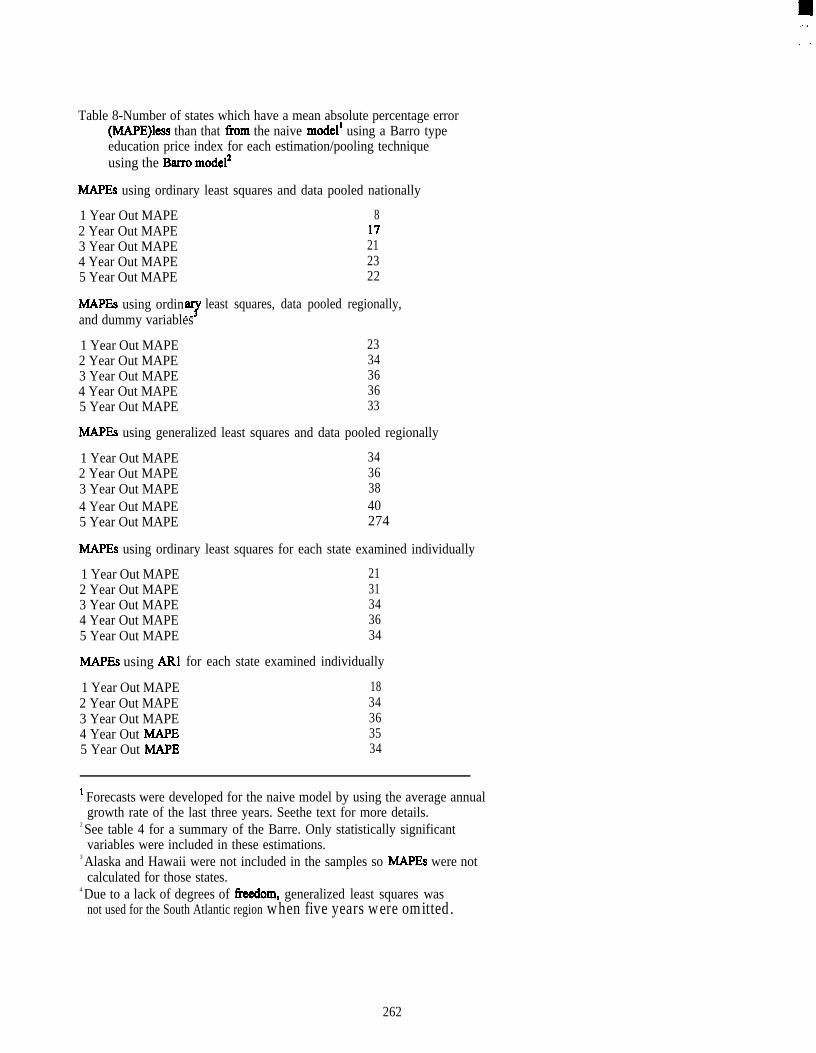
Table 8-Number of states which have a mean absolute percentage error(MAPE)less than that horn the naive modell using a Barro typeeducation price index for each estimation/pooling techniqueusing the Barro mode12

MAPEs using ordinary least squares and data pooled nationally

1 Year Out MAPE 82 Year Out MAPE 173 Year Out MAPE 214 Year Out MAPE 235 Year Out MAPE 22

MAPEs using ordinT

least squares, data pooled regionally,and dummy variables

1 Year Out MAPE 232 Year Out MAPE 343 Year Out MAPE 364 Year Out MAPE 365 Year Out MAPE 33

MAPEs using generalized least squares and data pooled regionally

1 Year Out MAPE 342 Year Out MAPE 363 Year Out MAPE 384 Year Out MAPE 405 Year Out MAPE 274

MAPEs using ordinary least squares for each state examined individually

1 Year Out MAPE2 Year Out MAPE3 Year Out MAPE4 Year Out MAPE5 Year Out MAPE

MAPEs using ARl

1 Year Out MAPE2 Year Out MAPE3 Year Out MAPE4 Year Out MAPE5 Year Out MAPE

2131343634

for each state examined individually

1834363534

1 Forecasts were developed for the naive model by using the average annualgrowth rate of the last three years. Seethe text for more details.

2 See table 4 for a summary of the Barre. Only statistically significantvariables were included in these estimations.

3 Alaska and Hawaii were not included in the samples so MAPEs were notcalculated for those states.

4 Due to a lack of degrees of fkeedom, generalized least squares wasnot used for the South Atlantic region when five years were omitted.

262

Table 9- Data Requirements for Forecasting the Barro Model by State

Are Forecasts Substitute

Available? If Needed

Personal Disposable Income

Population

National Price Deflator for Consumption

Expenditures

National Consumer Price Index

Average Daily Attendance

Sum of Revenue Receipts from State

and Federal Sources

Yes .-

Yes

Yes

Yes

Yes’

No

.-

.-

.-

.-

National Education Price Index No National Consumer Price Index

1 Average daily attendance forecasts computed using the state forecasts for fall enrollment.

263

. .

Table 10- Alternate specifications of the Forecasting model

Equation 1. Ordinary least squares and data pooled nationally

LCUREXPC = 130 + ~lLPCI + ~zLTPSL + ~~LADAPOP+ ~dGRA’DA + &LD + ~bso~ + ~7LTPSLS + p

Equation 2. Ordinary least squares, data pooled regionally, and dummy variables

LCUREXPC = ($ + &LPCI + &LTPSL + ~ADAPOP + ~4GlU4DA+ alDUMMY1 + . . . ...+ a@JMMY~ + w

Equation 3. Genemlized least Squares data pooled regionally

LCUREXPC = PO + ~lLPCI + ~zLTPSL + ~~LADAPOP + ~AGRADA + ~

Equation 4. Ordinary least squares with each state examined individually

LCUR.EXPC = PO + j31LPCI + ~zLTPSL + ~~LADAPOP + fIAGRADA + p

Equation 5. ARl with each state examined individually

LCUREXPC = PO + ~lLPCI + ~zLTPSL + ~~LADAPOP + ~4GRADA + p

Where:

LCUR.EXPC was current expenditures per student in ADA in 1965 dollars using the national consumer price index inlog form;

LPCI was disposable personal income per capita in 1965 dollars using the national price deflator for personalconsumption expenditures in log form;

LTPSL was the sum of state and local tax payments per capita in 1965 dollars using the national CPI in log form;

LADAPOP was the ratio of average daily attendance to the population;

GRADA was the change in average daily attendance;

LD was a dummy variable measuring states with a population density greater than 30;

SOUTH was a dummy variable for southern states;

LTPSLS was the product of LTPSL and the SOUTH variable; and

D~i was a dummy variable equal to 1 for the ith state in alphabetical order in the region. There were dummyvariables for each state in the region except the last one alphabetically.

264

Table 1 l-Comparison of the Barro model and the Forecasting model

Barro Model Forecasting Model

Differences in the Models

Price deflator Education price deflator’ National consumer pricefor dependent , indexvariable

State variable Sum of revenue receipts fkom Sum of state and local taxstate and federal sources per payments per capita in 1965capita in 1965 dollars using using the national CPI inthe national CPI in log form log form

Price variable Ratio of the average daily Ratio of the average dailyattendance to the population attendance to the populationmultiplied by ratio of the in log formeducation price indexl to thenational consumer price indexin log form

Differences in the Estimations of the Models

Estimationincludesstatisticallyinsignificantvariables

Yes

Results for both YesOrdinary LeastSquares and ARlpresented forcase when statesexaminedseparately

N02

No

1 Definition of the education price index is presented in the text.2 Statistically insignificant state dummy variables were included inestimations.

265

.,

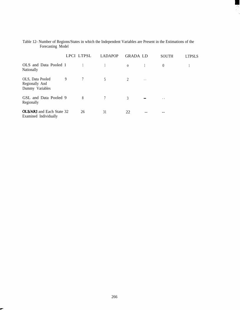
Table 12- Number of Regions/States in which the Independent Variables are Present in the Estimations of theForecasting Model

LPCI LTPSL

OLS and Data Pooled 1 1Nationally

OLS, Data Pooled 9 7Regionally AndDummy Variables

GSL and Data Pooled 9 8Regionally

OLS/ARl and Each State 32 26Examined Individually

LADAPOP

1

5

7

31

GRADA LD SOUTH LTPSLS

o 1 0 1

2 . .

3 .- . .

22 -- --

266

P’

Table 13-Number of states which have a MAPE less than that from the naive modell for eachestimation/pooling technique using the consumer price index for each estimation/poolingtechnique using the Forecasting mode12

MAPEs using ordinary least squares and data pooled nationally

1 Year Out MAPE 82 Year Out MAPE 203 Year Out MAPE 294 Year Out MAPE 305 Year Out MAPE 31

MAPEs using ordinary least squares, data pooled regionally, and dummy variables3

1 Year Out MAPE 182 Year Out MAPE 323 Year Out MAPE 354 Year Out MAPE 385 Year Out MAPE 38

MAPEs using generalized least squares and data pooled regionally- Alaska and Hawaiinot in the samples3

1 Year Out MAPE 332 Year Out MAPE 403 Year Out MAPE 414 Year Out MAPE 405 Year Out MAPE 264

MAPEs using generalized least squares and data pooled regionally- Alaska and Hawaii in the sampless

1 Year Out MAPE 332 Year Out MAPE 413 Year Out MAPE 404 Year Out MAPE 405 Year Out MAPE 284

MAPEs using ordinary least squares or AR1 with states examined individually

1 Year Out MAPE 162 Year Out MAPE 353 Year Out MAPE 374 Year Out MAPE 385 Year Out MAPE 38

1 Forecast were developed for the naive model by using the average annual growth rate of the lastthree years. See the text for more details.

2 See table 10 for a summary of the Forecasting model. Only statistically significant variables wereincluded in these estimations.

3 Alaska and Hawaii were not included in the samples so MAPEs were not calculated for those states.4 Due to a lack of degrees of ileedom, generalized least squares was not used for the

South Atlantic region when five years were omitted.s Alaska and Hawaii were included in the samples yet those MAPEs were not included in this count.

267

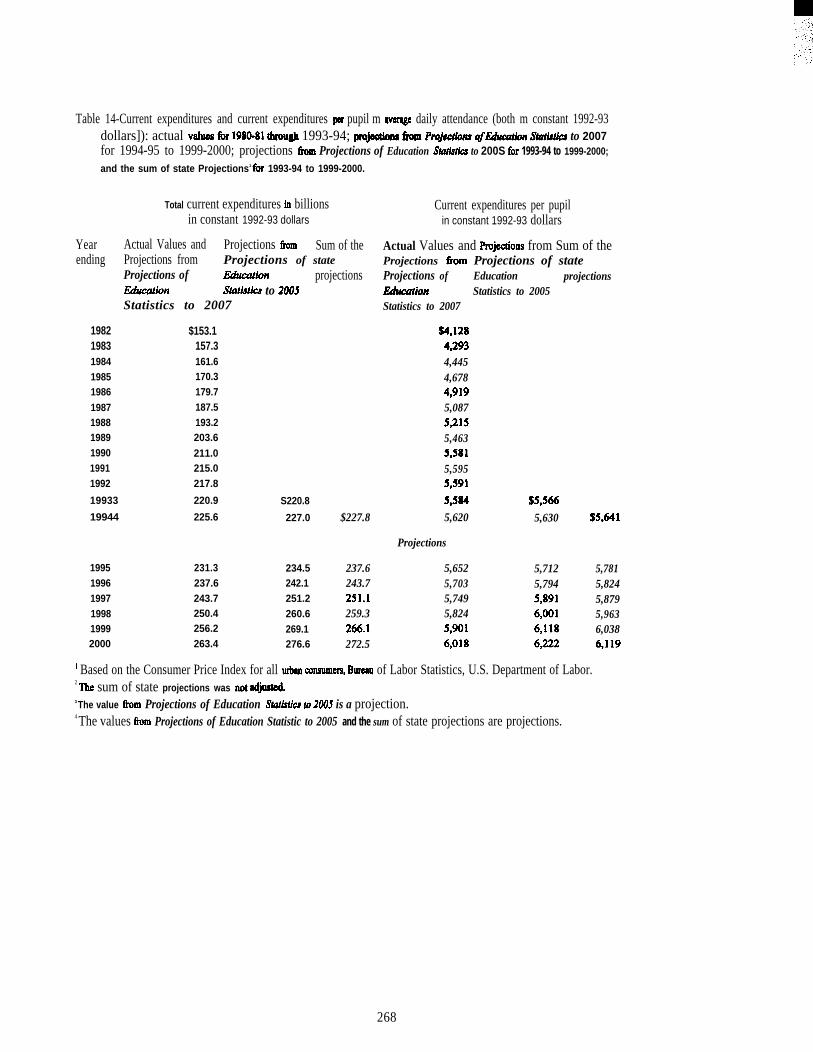
Table 14-Current expenditures and current expenditures pa pupil m awmge daily attendance (both m constant 1992-93dollars]): actual VtdM fw 198&81 tbmugh 1993-94; pmjwtioua ~ Projk@ons #&#u@ion Stdxics to 2007for 1994-95 to 1999-2000; projections fimn Projections of Education Statistia to 200S tir 1993-94 to 1999-2000;

and the sum of state Projectionsz fbr 1993-94 to 1999-2000.

Total current expenditures in billions Current expenditures per pupilin constant 1992-93 dollars in constant 1992-93 dollars

Year Actual Values and Projections tlom Sum of the Actual Values and Pr@ections from Sum of theending Projections from Projections of state Projections km Projections of state

Projections of lliucation projections Projections of Education projectionsILkation StatiWics to 200$Statistics to 2007

1982 $153.11983 157.3198419851986198719881989199019911992

19933

19944

161.6170.3179.7187.5193.2203.6211.0215.0217.8

220.9 S220.8

225.6 227.0

1995 231.3 234.51996 237.6 242.11997 243.7 251.21998 250.4 260.61999 256.2 269.12000 263.4 276.6

Utcation Statistics to 2005Statistics to 2007

$4,12842934,4454,6784,9195,0875J155,4635,5815,5955,591

s,im4 $5,X$6$227.8 5,620 5,630 !$5,641

Projections

237.6 5,652 5,712 5,781243.7 5,703 5,794 5,824251.1 5,749 5,891 5,879259.3 5,824 6,001 5,963266.1 5,901 6,118 6,038272.5 6,018 6222 6,119

1 Based on the Consumer Price Index for all urbau wnsumers, BurwJ of Labor Statistics, U.S. Department of Labor.2 ‘I13e sum of state projections was not ad@stcd.3 The value tim Projections of Education Statistiu @ 2005 is a projection.4 The values &om Projections of Education Statistic to 2005 and the sum of state projections are projections.

268

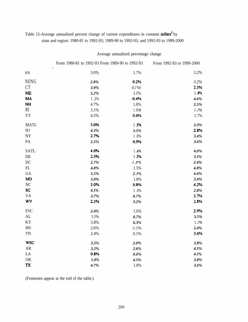
Table 15-Average annualized percent change of current expenditures in constant dollars2 by

us

NENGCT

RIVT

MATLNJNYPA

SATLDEDCFLGA

NCScVA

ESCALKYMSTN

WscARLAOKTx

state and region: 1980-81 to 1992-93; 1989-90 to 1992-93; and 1992-93 to 1999-2000

Average annualized percentage change

From 1980-81 to 1992-93 From 1989-90 to 1992-93t

3.0% 1.7%

2.8% 0.2V03.9% -0.1’%05.2% 1.l%1 .2% -0.4%04.7% 1.8%3.1% 1 .9?404.5% 0.6’XO

3.OVO 1 .5’XO4.3% 3.5%2.7V0 1 .0%2.5% 0.970

4.OVO2.5’%02.7%4.8%5.5%3.0%3.0704.l%3.7%2.3’XO

2.4%1.l%3.8%2.6%2.4%

3.5%3.2%0.8V01.8%4.7%

1 .4%1 .5’XO

-1 .9’%1.5%2.l%1.8%0.8’%01 .0%0.7%3.2%

1.6%0.7%6.3%

-1.1%0.1%

2.0%2.6%0.6%4.5%1.8%

From 1992-93 to 1999-2000

3.2%

3.2%2.3’%01 .4V04.6%2.5%1 .7%1.7%

3.3%2.8’%03.4%3.6%

4.0%3.l%2.4%4.8%4.4%3.4%4.2’XO2.8%3.WO2.8’XO

2.9’Mo3.5%

1 .7%2.4%3.6’%0

3.8%4.5%4.l%3.8%3.6%

(Footnotes appear at the end of the table.)

269

-,,,,.,,

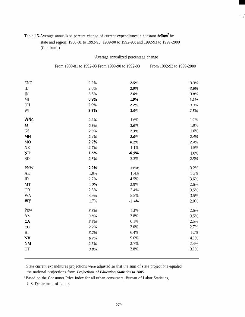
Table 15-Average annualized percent change of current expenditures] in constant dollars2 by

state and region: 1980-81 to 1992-93; 1989-90 to 1992-93; and 1992-93 to 1999-2000(Continued)

Average annualized percentage change

From 1980-81 to 1992-93 From 1989-90 to 1992-93 From 1992-93 to 1999-2000

ENCILINMIOHWI

WNcIAKS

MONE

SD

PNWAKIDMTORWA

PswAZCAcoHINv

UT

2.2%2.0%3.6%0.9’XO2.9%3.3’XO

2.3%0.9%2.9%2.4%2.7V02.7%1.6V02.8%

2.9’%01.8%2.7%1 .9’MO2.5%3.9%1.7%

3.3%3.8%3.3%2.2%3.2%6.7%2.5%3.0%

2.5%2.9%2.0%1.9V02.2%

3.9%

1.6%3.0%2.3%2.0%0.2%1.1%

-0.5Y03.3%

3.9’%01 .4%4.5%2.9%3.4%5.5%

-1 .4V0

1.l%2.8%0.l%2.0%6.4%9.0%2.7%2.8%

3.3%3.6%3.0%

3.3’%03.3%2.8%

1.9’%1.0%1.6%2.4%2.4%1.5%1.0%2.5%

3.2%1 .3%3.6%2.6%3.5%3.5%2.0%

2.6%3.5%2.5%2.7%1 .7%4.l%2.4%3.l%

1 State current expenditures projections were adjusted so that the sum of state projections equaledthe national projections from Projections of Education Statistics to 2005.

2 Based on the Consumer Price Index for all urban consumers, Bureau of Labor Statistics,U.S. Department of Labor.

270

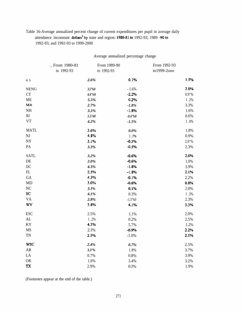
Table 16-Average annualized percent change of current expenditures per pupil in average daily

attendance inconstant dollars2by state and region: 1980-81to 1992-93; 1989 -90to1992-93; and 1992-93 to 1999-2000

, From 1980-81to 1992-93

u s

NENG

CTME

NHRIVT

MATLNJNYPA

SATLDEDCFLGAMDNCScVA

ESCALKYMSTN

WscARLAOKTx

Average annualized percentage change

From 1989-90 From 1992-93to 1992-93 to1999-2ooo

2.6% O.lvo

3.5’%0 - 1.6%4.4’%0 -2.2Y05.5% 0.2702.7% -1.8%3.5% -1.8Y03.1?40 -0.4’%04.2% -1.5%

3.6?40 0.0%4.8’%0 1 .7%3.170 -0.5%03.3% -0.5V0

3.2%2.0%4.3%2.5V04.3’MO3.0703.l%4.1%2.8%3.8V0

-0.670-0.6Y0-1.8Y0-1.8V0-0.lYO-0.6Y0

0.1’%00.3%

-1.3’%04.1’XO

2.5% 1.1%1 .2% 0.2%4.3’XO 5.7%2.l% -0.9Y02.5?40 -1.0%

2.4% 0.7%3.3’% 1.8%0.7% 0.8%1.6% 3.4%2.9% 0.l%

1.5V0

2.0’%00.9’%1 .2%3.3%1.6%0.6%1 .0%

1.8%0.9%2.0’%2.3%

2.O’XO1.0%3.9%2.lVO2.2%0.8’XO2.0%1 .3%2.3%3.3V0

2.0%2.5%1.2%2.2’XO2.lVO

2.5%3.7%3.9%3.2%1.9%

(Footnotes appear at the end of the table.)

271

❑

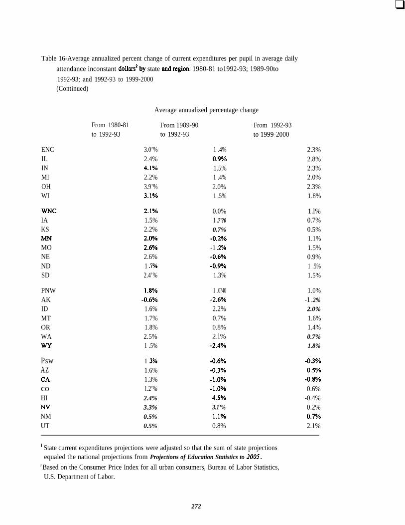
Table 16-Average annualized percent change of current expenditures per pupil in average daily

attendance inconstant dollars2by state andregion: 1980-81 to1992-93; 1989-90to

1992-93; and 1992-93 to 1999-2000(Continued)

Average annualized percentage change

From 1980-81to 1992-93

ENCILINMIOHWI

WNcIAKS

MONENDSD

PNWAKIDMTORWA

PswAZCAcoHINvNMUT

From 1989-90 From 1992-93to 1992-93 to 1999-2000

3.0’% 1 .4%2.4% 0.9%04.1%0 1.5%2.2% 1 .4%3.9’% 2.0%3.lVO 1 .5%

2.lVO1.5%2.2%2.OVO2.6V02.6%1 .7’%02.4’%

0.0%1 .7’?00.7%

-0.2%0-1 .2V0-0.6V0-0.9Y01.3%

1.8V0 1 .0?40-0.6Y0 -2.6V01.6% 2.2%1.7% 0.7%1.8% 0.8%2.5% 2.l%1 .5% -2.4Y0

1 .3’%01.6%1.3%1.2’%2.4%3.3%0.5%0.5%

-0.6Y0-0.3Y0

-1.OVO-1.OYO4.5V03.1’%

1.1’%00.8%

2.3%2.8%2.3%2.0%2.3%1.8%

1.l%0.7%0.5%1.1%1.5%0.9%1 .5%1.5%

1.0%-1 .2%2.0%

1.6%1.4%0.7%1.8%

-0.3Y00.5%0

-0.8Y00.6%

-0.4%0.2%0.7’%02.1%

1 State current expenditures projections were adjusted so that the sum of state projectionsequaled the national projections from Projections of Education Statistics to 200S.

2 Based on the Consumer Price Index for all urban consumers, Bureau of Labor Statistics,U.S. Department of Labor.

272

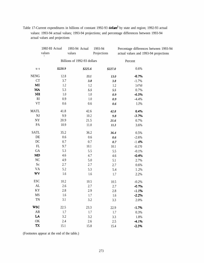
Table 17-Current expenditures in billions of constant 1992-93 dollars2 by state and region; 1992-93 actual

values: 1993-94 actual values; 1993-94 projections; and percentage differences between 1993-94actual values and projections

1992-93 Actual 1993-94 Actual 1993-94values values Projections

L

Billions of 1992-93 dollars

u s $220.9

NENG 12.8CT 3.7

1.25.31.0

RI 0.9VT 0.6

MATL 41.8NJ 9.9

NY 20.9PA 10.9

SATL 35.2DE 0.6DC 0.7FL 9.7

GA 5.34.6

NC 4.9Sc 2.7

VA 5.21.6

ESC 10.2AL 2.6KY 2.8MS 1.6TN 3.1

Wsc 22.5AR 1.7LA 3.2OK 2.4Tx 15.1

(Footnotes appear at the end of the table.)

$225.6

13.13.81.25.51.01.00.6

42.610.221.511.0

36.20.60.7

10.15.54.75.02.75.31.6

10.52.72.91.73.2

23.31.73.22.6

15.8

$227.0

13.03.81.25.50.90.90.6

42.89.8

21.611.3

36.40.60.7

10.15.54.65.12.75.41.7

10.52.72.81.63.3

22.91.73.32.5

15.4

Percentage differences between 1993-94actual values and 1993-94 projections

Percent

0.6%

-0.7Y0-1.7%

3.4’%00.7%

-6.5Y0-4.4%1.l%

0.4V0-3.7Y00.7%3.6%

0.5%-2.6%-1 .6’%0-0.170-0.1%-0.4Y02.7%0.6%1 .2%2.2%

-0.2%-0.7Y0-1.lVO-2.2Y02.0%

-1.7Y00.3%1.8%

-4.lVO-2.3V0

273

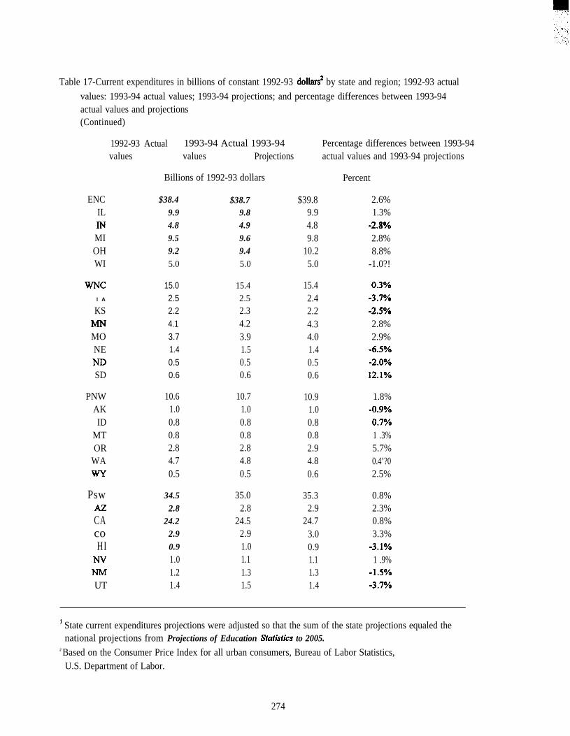
Table 17-Current expenditures in billions of constant 1992-93 dollars2 by state and region; 1992-93 actual

values: 1993-94 actual values; 1993-94 projections; and percentage differences between 1993-94actual values and projections(Continued)

1992-93 Actual 1993-94 Actual 1993-94 Percentage differences between 1993-94values values Projections actual values and 1993-94 projections

ENCILINMIOHWI

WNcI A

KS

MONE

SD

PNWAKID

MTOR

WA

PswMCAcoHI

Nv

UT

Billions of 1992-93 dollars

$38.49.94.89.59.25.0

15.02.52.24.13.71.40.50.6

10.61.00.80.82.84.70.5

34.52.8

24.22.90.91.01.21.4

$38.79.84.99.69.45.0

15.42.52.34.23.91.50.50.6

10.71.00.80.82.84.80.5

35.02.8

24.52.91.01.11.31.5

$39.89.94.89.8

10.25.0

15.42.42.24.34.01.40.50.6

10.91.00.80.82.94.80.6

35.32.9

24.73.00.91.11.31.4

Percent

2.6%1.3%

-2.8Y02.8%8.8%

-1.0?!

0.3V0“3.7’YO-2.5Y02.8%2.9%

-6.5Y0-2.OYO12.lVO

1.8%-0.9V0

0.7’%01 .3%5.7%0.4’?02.5%

0.8%2.3%0.8%3.3%

-3.lYO1 .9%

-1.5Y0-3.7V0

* State current expenditures projections were adjusted so that the sum of the state projections equaled thenational projections from Projections of Education Statktics to 2005.

2 Based on the Consumer Price Index for all urban consumers, Bureau of Labor Statistics,U.S. Department of Labor.

274

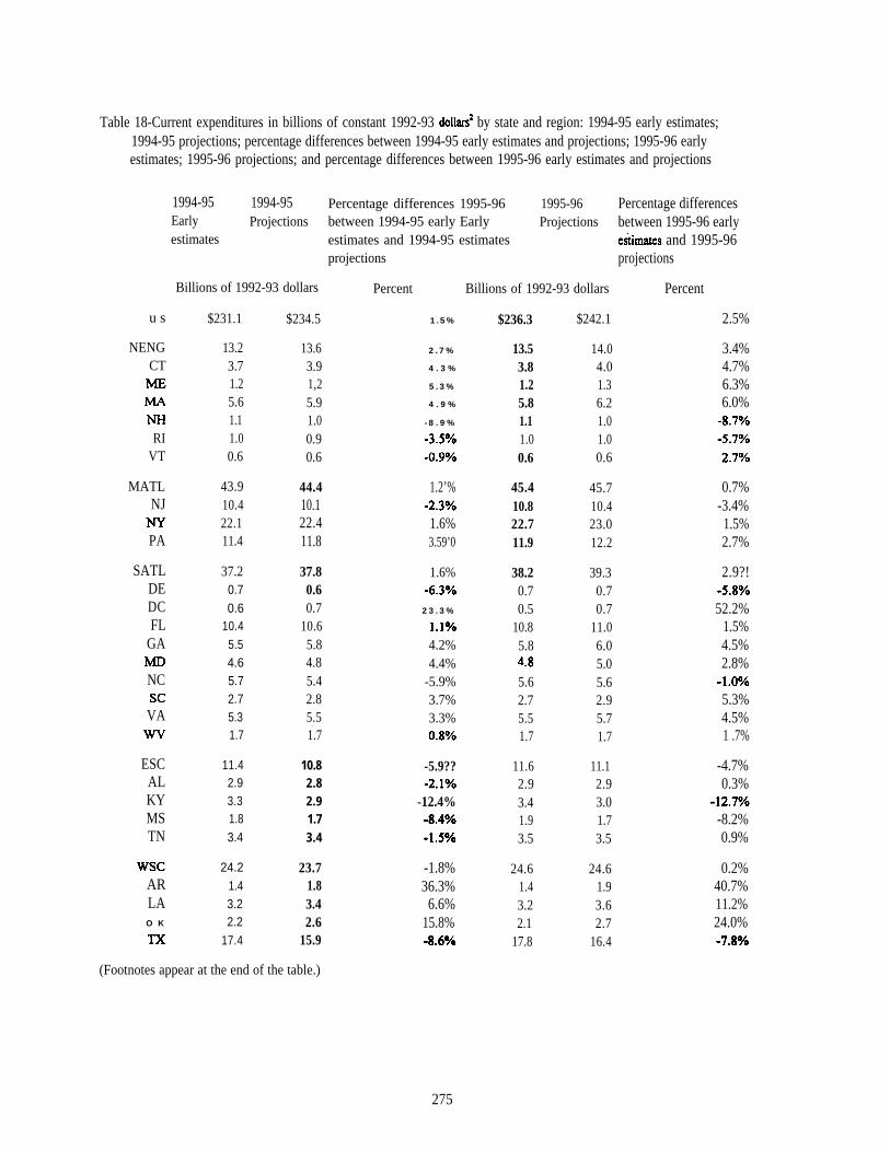
Table 18-Current expenditures in billions of constant 1992-93 dollars2 by state and region: 1994-95 early estimates;1994-95 projections; percentage differences between 1994-95 early estimates and projections; 1995-96 earlyestimates; 1995-96 projections; and percentage differences between 1995-96 early estimates and projections

u s

NENGCT

RIVT

MATLNJ

PA

SATLDEDCFL

GA

NCScVA

ESCALKYMSTN

WscARLAO K

Tx

1994-95 1994-95Early Projectionsestimates

Billions of 1992-93 dollars

$231.1

13.23.71.25.61.11.00.6

43.910.422.111.4

37.20.70.6

10.45.54.65.72.75.31.7

11.42.93.31.83.4

24.21.43.22.2

17.4

$234.5

13.63.91,25.91.00.90.6

44.410.122.411.8

37.80.60.7

10.65.84.85.42.85.51.7

10.82.82.91.73.4

23.71.83.42.6

15.9

Percentage differences 1995-96 1995-96between 1994-95 early Early Projectionsestimates and 1994-95 estimatesprojections

Percent Billions of 1992-93 dollars

1.5%

2.7%

4 . 3 %

5.3%

4 . 9 %

- 8 . 9 %

-3.5Y0

-0.9’YO

1.2’%-2.3Y0

1.6%3.59’0

1.6%-6.3Y0

23.3%

1.lVO4.2%4.4%

-5.9%3.7%3.3%0.8V0

-5.9??-2.lYO

-12.4%-8.4V0-1.YYO

-1.8%36.3%

6.6%15.8%-8.6’YO

$236.3

13.53.81.25.81.11.00.6

45.410.822.711.9

38.20.70.5

10.85.84.8

5.62.75.51.7

11.62.93.41.93.5

24.61.43.22.1

17.8

$242.1

14.04.01.36.21.01.00.6

45.710.423.012.2

39.30.70.7

11.06.05.05.62.95.71.7

11.12.93.01.73.5

24.61.93.62.7

16.4

Percentage differencesbetween 1995-96 earlyesdmates and 1995-96projections

Percent

2.5%

3.4%4.7%6.3%6.0%

-8.7Y0-5.7Y02.7V0

0.7%-3.4%1.5%2.7%

2.9?!-5.8Y052.2%

1.5%4.5%2.8%

-1.OVO5.3%4.5%1 .7%

-4.7%0.3%

-12.7Y0-8.2%0.9%

0.2%40.7%11.2%24.0%-7.8Y0

(Footnotes appear at the end of the table.)

275

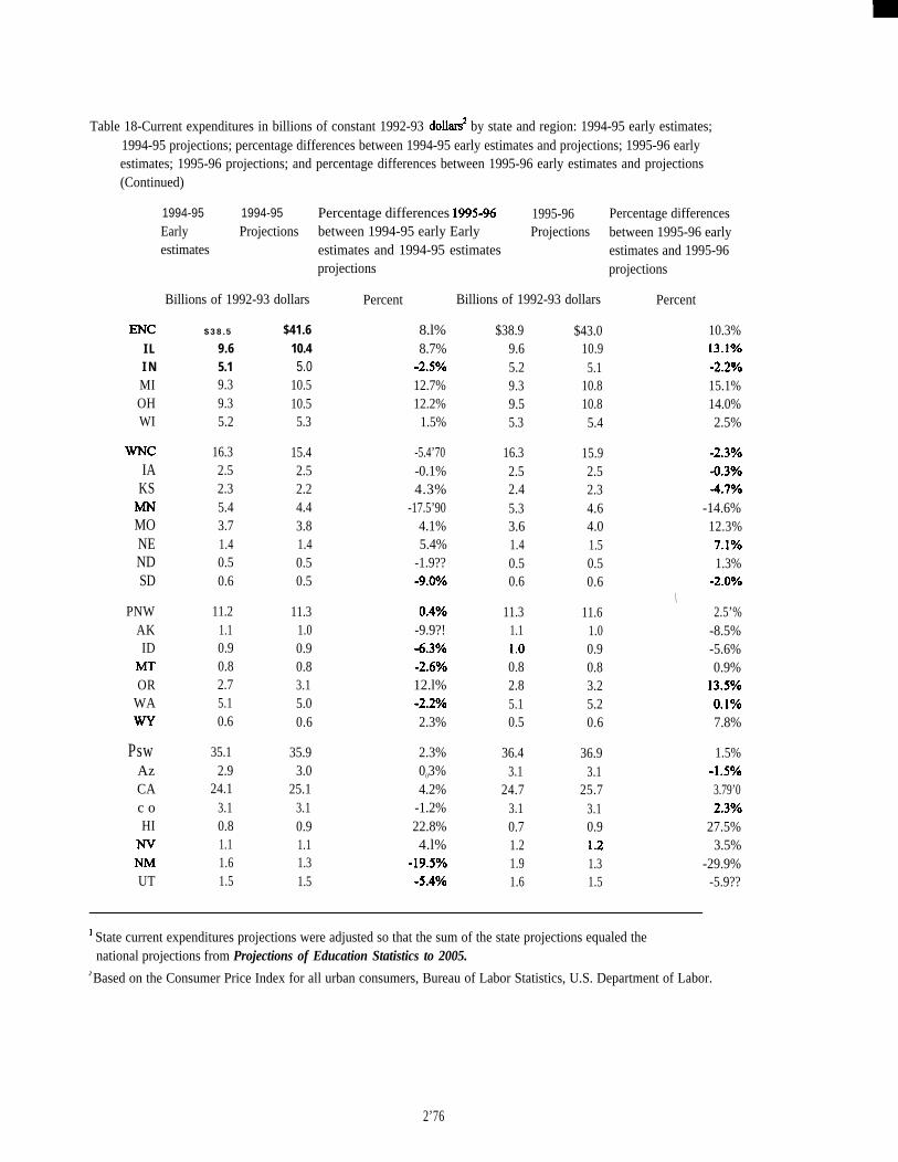
Table 18-Current expenditures in billions of constant 1992-93 dollars2 by state and region: 1994-95 early estimates;1994-95 projections; percentage differences between 1994-95 early estimates and projections; 1995-96 earlyestimates; 1995-96 projections; and percentage differences between 1995-96 early estimates and projections(Continued)

1994-95 1994-95Early Projectionsestimates

Billions of 1992-93 dollars

ENc $38.5 $41.6I L 9.6 10.4I N 5.1 5.0MI 9.3 10.5OH 9.3 10.5WI 5.2 5.3

WNcIA

KS

MONENDSD

16.32.52.35.43.71.40.50.6

15.42.52.24.43.81.40.50.5

PNW 11.2 11.3AK 1.1 1.0ID 0.9 0.9

0.8 0.8OR 2.7 3.1

WA 5.1 5.00.6 0.6

Psw 35.1 35.9Az 2.9 3.0CA 24.1 25.1c o 3.1 3.1HI 0.8 0.9

Nv 1.1 1.11.6 1.3

UT 1.5 1.5

Percentage differences 1995-96 1995-96between 1994-95 early Early Projectionsestimates and 1994-95 estimatesprojections

Percent Billions of 1992-93 dollars

8.l% $38.9 $43.08.7% 9.6 10.9

-2.5Y0 5.2 5.112.7% 9.3 10.812.2% 9.5 10.8

1.5% 5.3 5.4

-5.4’70 16.3 15.9-0.1% 2.5 2.54.3% 2.4 2.3

-17.5’90 5.3 4.64.1% 3.6 4.05.4% 1.4 1.5

-1.9?? 0.5 0.5-9.OYO 0.6 0.6

0.49’0 11.3 11.6-9.9?! 1.1 1.0-6.3Y0 1.0 0.9-2.6Y0 0.8 0.812.l% 2.8 3.2-2.2Y0 5.1 5.22.3% 0.5 0.6

2.3% 36.4 36.9003% 3.1 3.14.2% 24.7 25.7

-1.2% 3.1 3.122.8% 0.7 0.94.l% 1.2 1.2

-19.5Y0 1.9 1.3-5.4Y0 1.6 1.5

Percentage differencesbetween 1995-96 earlyestimates and 1995-96projections

Percent

10.3%13.lVO-2.2Y015.1%14.0%2.5%

-2.3Y0-0.3V0-4.7Y0

-14.6%12.3%7.1701.3%

“2.OYO\

2.5’%-8.5%-5.6%0.9%

13.5V0O.lvo7.8%

1.5%-1.5Y03.79’02.39’o

27.5%3.5%

-29.9%-5.9??

1 State current expenditures projections were adjusted so that the sum of the state projections equaled thenational projections from Projections of Education Statistics to 2005.

2 Based on the Consumer Price Index for all urban consumers, Bureau of Labor Statistics, U.S. Department of Labor.

2’76

MEDICAID FORECASTINGPRACTICES’Dan Williams

Baruch CollegeJanuary 27, 1998

COMPARING MEDICAJD FORECASTSApplied forecasting literature includes numerous

studies in which different approaches are comparedthrough simulated forecasting such as the M-competi-tion, the M-2 Competition, and the M-3 Competition(Makridakis, et. al., 1982; Makridakis et. al., 1989;Hibon and Makridakis, 1997). Less frequently, studiescompare different actual forecasts of the same data se-ries (&hley, 1988); however, because of the smallnumber of such multiple forecasts, there is limited op-portunity to evaluate sources of variation.

State government forecasting provides an opportu-nity for studying a large number of forecasts of sirnikwseries to determine the effects of cMTerent variables onforecasting practice. Often, many states forecast sirni-Iar series, such as tax revenue, nursing home bed need,prison population, or educational enrollment. Whilesome characteristics of these series dMer from state tostate other characteristics may be similar. For exam-pie, the unit of analysis maybe similar between states -each state might be interested in dollars of revenue, acount of children at each age cohort, and so forth.Also, the series in each state may experience the simi-lar social and political pertu.rbances at about the sametime. The study of these such forecasts may provideinsight about variables that aflkct applied forecasting.

This paper examines forecasting activities amongMedicaid agencies in the f@ United States, Wash-ing-ton, D. C., and five U.S. territories (American Sa-moa, Guam, Puerto Rico, Notiem Mariana Islands,and Virgin Islands). Most frequently, studies of state orlocal forecasting practice focus on revenue forecasting(Rodgers and Joyce, 1996; Bretschneider and Schroe-der, 1988; Bretschneider. et. al., 1989). There areseveral reasons why comparison of state Medicaidforecast practice may be better than comparison of staterevenue forecasting practices. First, there is no con-sistent reporting of state revenue estimates. Statesmake forecasts when it suits them and report them in areamer that is satisfactory to their governors or legis-latures. Collection of data through national organiza-tions such as the National Association of State BudgetOfficers is not so rigorous as to assure that reported

1 ‘Ilk r~h is supported by PSC CUNY grant number 666$$6,

data are comparable. In contrast, Medicaid agenciesmust report their expenditure estimates to the fderalgovernment using the ftierally specified HCFA-37form once a quarter beginning roughly 30 months be-fore the end of each fderal fiscal year.2

Second, determining the amcy of state revenueforecasts relies on the validity of state reported dMer-ences between planned and actual expenditure. Statesmay be politically motivated to repoti these &ta in afavorable manner. By con= Medicaid forecasts,can be compared with accounting data as reported on afederal report known as the HCFA-64. While thesedata may not be bias fhx,3 biases are likely to be smalland similar from state to state.

MEDICAID FORECASTING BACKGROUNDMedicaid is a federal and state fimded health care

financing program. The federal government contrib-utes 50% to 83’XO of the cost of the program in eachstate, with states contributing the balance. Medicaid isthe largest human seMces program in state budgets,accounting for 19.2’% of total state spending in 1995.It is second only to education in share of state generalfinds, and has the largest share of federal transferpayments to states (National Association of StateBudget Ofllcers, 1996). Medicaid is an entitlementprogram: once states establish rules about who is en-rolled and what is covered they are barred from refus-ing to enroll eligible individuals or from refbsing topay for covered semices due to funding shortfalls.Medicaid pays for health care through vendor pay-ments to health care suppliers (called “providers” bysome states). Beneficiaries present their Medicaidcards to enrolled suppliers who deliver semices andsubmit claims to state Medicaid agencies. The stateMedicaid agencies pay for these sewices based on“provider agreements,” which set payment conditions.As a result, the Medicaid agency is usually the last tofind out about the smite. For these reasons, Medicaidbudgeting is highly dependent on forecasting.

Because the Medicaid program is fiuuled Witii both

state and fderal funds, there are two levels of gover-nment who use Medicaid forecasts for budgeting. Prac-tices at these levels of government can be somewhat

2 The number of quartets from ffi reporting a fiscal y% to the end ofthat year has varied k time to time.‘ States may not anticipate rcwspective adjustments in the HCFA-37although they appear in HCFA-64. Another disadvantage of comparingstate forecasting practice using HCFA-37 data is that statea maybemore interested in their own budgets than in the reporting of their ex-pectations to the fdcral govemmcnt. So, the HCFA-37 may not capturethe atate’s best fbrecast.

277

Werent. In a typical state government, a Medicaidadministering agency makes a forecast that is submit-ted to an executive budget office for review. Some-times the executive budget office makes its own inde-pendent forecast which may be combined wi~ or sub-stituted for, the Medicaid agency’s forecast (JLARC,1997). This forecast is then submitted to the state leg-islature in the legislative budget process. The legisla-ture may make another forecast or may choose to relyon the executive forecast. There can be various mixedpractices, for example, a legislative agency may par-ticipate in selecting the executive forecast.

The fderal government uses the state forecasts ina ~erent way. The states submit their estimates tothe Health Care Financing Administration (HCFA),the federal agency responsible for administering theMedicaid grants to states, each quarter using a federalfo~ the HCFA-37 (formerly the HCFA-25). Fore-casts reported on this form are combined to producemtional estimates. The fderal government adjuststhese estimates: (a) to account for new f*ral policymaking that the states could not have known aboutwhen making their estimates; and (b) to correct forperceived patterns of errors occurring in past forecasts(llapnell, 1991). The fderal government uses thesecorrected forecasts to estimate federal Medicaid outlaysfor the next future fderal budget year. Estimates foryears beyond those reported in the HCFA-37 are madeby the HCFA OfEice of Actumy using algorithms de-veloped by a contractor prior to 1980 (Trapnell, 1991).In the fderal budgeting practice, HCFA budget esti-mates originating either from the states or the Office ofActuary are subject to scrutiny by OMB and CBO.

In the late 1980s and early 1990s Medicaid agen-cies experienced several years of significant forecasterror. In 1991 HCFA was criticized for unprecedentedoverages in the Medicaid budget (HHS NEWS, 1991;Executive Oilke of the President and Department ofHealth &Human SeMces, 1991). At that time, thef~ral government concluded that state forecastingwas a significant source of forecasting efior @X+SNEWS, 1991). Medicaid and related health care fore-casting and cost estimation have been the center ofcontinued disagreement and concern throughout the1990s (Ric~ 1991; Fkshei~ 1993; Doran, Roesenblatt,and Yarnamoto, 1994; MU of Technology Assess-men~ 1994; Hola.han and Liska, December, 1996; Rat-ner, 1997; scanlo~ 1997; Holahan and Liska, 1997),

EMPIRICAL STUDIES OF MEDICAID PRAC-mcE

“Forecasting Techniques and Budgetary Issues ofState Medicaid Programs” (McKusick, 1980) examinesthe forecasting practices of 10 state Medicaid pro-grams. Data are gathered from site visits. McKusickobserves, “Although each state’s estimating techniquesare unique, there are patterns that are common to mostmethodologies.” These common patterns include:●

●

●

●

●

●

●

●

●

●

States attempt to estimate demand for sexvice, andpay little attention to supply of service.Most state forecasts are prepared on a cash budg-eting basis although some forecast accruals andconvert to a cash basis.In many circumstances, reimbursement rate in-

crease decisions are known prior to budgeting andcan be used as an aid to expenditure forecasting.Many states have poor quality data sources, butthey compensate through inventive use of fore-casting techniques.Forecasting is understaffkxi in many states, leaving“many critical forecast issues. . . unanalyzed.”Few states relate economic conditions to enroll-ment. Where they do, such analyses may bc pri-marily produced for other governmental fimctions.State Medicaid budget estimates are “determinedby the political process,” with frequent reliance onsupplemental appropriations.States forecast no more than a two years horizon.States rely on trend analysis, rather than “lookingfor the underlying diving forces in medical costs.”Some state forecasts submitted to the HCFA areconsistent with their state budget estimates, whileothers are “the best guess of the analyst.”McKusick describes specific practices in each of

10 states (Caltiomia, Illinois, Maryland, Massachu-setts, Michigan, Pennsylvania, Rhode Island, Texas,Virginia and Wisconsin). Details are not summarizedhere. The matters he addresses include: the partici-pants in forecasting, the general forecasting approach(e.g., California divides the forecast into cument serv-ices and poli~ modifications), number of periodic ob-se~ations available to the forecast model, level of data(annual, monthly, etc.), sources of data, forecastingtechniques used, degree of data decomposition, fre-quency of forecasting, the state budget calendar, abilityto produce &ta reports for the fderal government,relative size of the Medicaid program (to other Medi-caid programs nationwide), breadth of Medicaid cover-age, and components of Medicaid coverage. Some ofthe techniques obsemd include: use of regression or

278

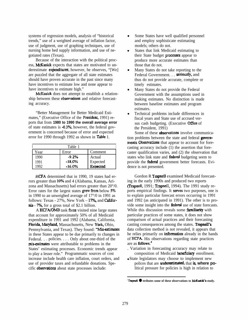
systems of regression models, analysis of “historicaltrends,” use of a weighted average of inflation factor,use of judgment, use of graphing techniques, use ofnursing home bed supply information, and use of ne-gotiated rates (Texas).

Because of the interaction with the political proc-ess, McKusick expects that states are motivated to un-derestimate ex&nditures; however, he observes, “[We]are puzzled that the aggregate of all state estimatesshould have proven accurate in the past since manyhave incentives to estimate low and none appear tohave incentives to estimate high.”

McKusick does not attempt to establish a relation-ship between these obsemations and relative forecast-ing accuracy.

“Better Management for Better Medicaid Esti-mates,” (Executive Office of the President 1991) re-ports that from 1980 to 1990 the overall average errorof state estimates is -0.30/o; however, the federal gov-ernment is concerned because of error and expectederror for 1990 through 1992 as shown in Table 1.

I Table 1 IYear Error Comment1990 -9.2Y0 Actual1991 -18.OYO Expected1992 -16.OYO Exmxted

HCFA determined that in 1990, 19 states had er-rors greater than 10’XO and 4 (Alabama, Kansas, Ari-zona and Massachusetts) had errors greater than 20°/0.Error rates for the largest states grew fkom below 5?40in 1990 to an unweighed average of 17°/0 in 1991 asfollows: Texas - 27%, New York – 17Yq and Californ-ia - 7Y0, for a gross total of $2.1 billion.

A HCFA/OMB task force visited nine large statesthat account for approximately 50% of all Medicaidexpenditure in 1991 and 1992 (Alabama, California,Flori~ Mar@@ Massachusetts, New York Ohio,Pennsylvania, and Texas). They found: “Mis-estimatesin these States appear to be due primarily to changes inFederal. . . policies. . . . Only about one-third of thernis-estimates were attributable to problems in theStates’ estimating processes. Economic trends appearto play a lesser role.” Programmatic sources of costincrease include health care inflation, court orders, anduse of provider taxes and refundable donations. Spe-cific obsemations about state processes include:

Some States have well qualified personneland employ sophisticate estimatingmodels; others do not.States that link Medicaid estimating totheir State budget prwesses appear toproduce more accurate estimates thanthose that do not.Many States do not take reporting to theFederal Government. . . seriously, andthus do not provide accurate, complete ortimely estimates.Many States do not provide the FederalGovernment with the assumptions used inmaking estimates. No distinction is madebetween baseline estimates and programestimates.Technical problems include differences infiscal years and State use of accrued ver-sus cash budgeting. (Executive Office ofthe President, 1991)Some of these obsemations involve communica-

tion problems between the state and federal gover-nments. Obsewations that appear to account for fore-casting accuracy include (1) the assertion that fore-caster qualification varies, and (2) the observation thatstates who link state and fderal budgeting seem toprovide the fderal government better forecasts. Evi-dence is not presented.

Gordon R Trapnell examined Medicaid forecast-ing in the early 1990s and produced two reports(’Ilapnell, 1991; Trapnell, 1994). The 1991 study re-ports empirical findings. It sexves two purposes, one isto explain particular forecast errors occurring in 1991and 1992 (as anticipated in 1991). The other is to pro-vide some insight into the fdera.1 use of state forecasts.While this discussion reveals some ftiliarity withparticular practices of some states, it does not showcomparison of actual practices and their forecastingcasting consequences among the states. Trapnell’sdata collection method is not revealed, it appears thathe relies primarily on idorrnation already in the handsof HCFA. His observations regarding state practicesare as follows:4. Variation in forecasting accuracy may relate to

composition of Medicaid beneficia~ enrollment.● State legislators may choose to implement new

polices that are underestimat~ that i% where po-litical pressure for policies is high in relation to

4 Trapnell ● ttributes some of these observations to McKusick*s study.

279

●

●

●

●

●

●

s

●

●

the determined costs.States may defer spending at the end of a state fis-cal year to ensure that state fiscal year estimatesare correct. This can happen because many statesbudget on a cash basis rather than an accrual ba-sis.Data available for forecasting in some states maybe of poor quality or may not be reconciled withactual expenditure experience.Past fderal action may discourage states horn re-vealing their true estimates. In particular, in 1982the f~eral government penalized states whoseactual expenditures exceeded their forecasts. As aconsequen~, states maybe motivated to overstatetheir estimates.There is wide variety in the sophistication of stateforecasting horn “trended forward total aggregatespending by type of seMce” to “fully specifiedeconometric model. . . . refitted quarterly.”Only a few states fully disaggregate data by thetype of seMce and type of beneficiary.Locus of responsibility varies amonp the states,with Medicaid agencies preparing some forecasts,while budget officials preparing others.There is “some correlation between how well offi-cials understood the programs and the details in-corporated in the cost estimates.”State forecasts improve as the horizon betweenforecast and the end of the fiscal year diminish.States may not reconcile state and federal fiscalyear reporting (most state fiscal years are fromJuly to June, while the federal fiscal year is fromOctober to September).Trapnell’s analysis of state variation is limited to

two paragraphs of his report in which he compares re-gional aggregate variation between the HCFA-37 andHCFA-64 reports. He finds that states in Region 1(states in each region are shown in Table 2) consis-tently underestimates its expenditures, states in Region2 generally overestimate expenditures and states in Re-gion 9 are usually very accurate. Trapnell’s reportmakes no effort to account for these variations in accu-racy. However, the most obvious characteristic of re-gions Trapnell mentions as having consistent patternsof accuracy are that they are dornimted by a singlestate. New York accounts for about 85°/0 of fderal ex-penditures in Region 2 and California accounts for asimilar amount in Region 9. In Region 1, Massachu-

setts accounts for about 60’XO of ftieral expenditures.It is likely that the explanation for the various fore-casting results in these three regions will be found atthese three states.

Table 2Region 1 Region 2

Connecticut New JerseyMaine New YorkMassachusetts Puerto RicoNew Hampshire Virgin IslandsRhode IslandVermont

Region 3 Region 4D.C. AlabamaDelaware FloridaMaryland GeorgiaPennsylvania KentuckyVirginia MississippiWest Virginia North Carolina

South CarolinaTennessee

Region 5 Region 6Illinois ArkansasIndiana LouisianaMichigan New MexicoMinnesota OklahomaOhio TexasWisconsin

“ Region 7 Region 8Iowa ColoradoKansas MontanaMissouri North DakotaNebraska South Dakota

UtahWyoming

Region 9 Region 10American Samoa AlaskaArizona IdahoCaltiornia OregonGuam Washingtonl-IawaiiNorthern MarianaNevada

Michele Insco of the Colorado state governmentconducted a Medicaid budget survey and circulated re-

S Massachusetts has two Medicaid agenciq the smaller of which isabout 2?zf0 of the program. ~s analysis excludes the small= agency.

280

suits to participating states in May, 1992 (hsco, 1992).This study consists of charts demonstrating factors thatmight a.flkct forecast accuracy or expenditure values.Some variables charted include: state populatio~ per-cent change in Medicaid expenditure fbm FY 91 toFY 92, characteristics of the Medicaid program irt-cluding various poli~ factors of current interest in1992, basis of accounting, and beginning/ending datesof state fiscal year. Some of the characteristics re-ported include the percent of poverty at which pregnantwomen and certain children meet eligibility criteria,experience with Boren Amendment lawsuits,G percent-age of births in the state covered by Medicai~ coverageof certain optional populations, etc. There is no ac-companying written repmt to interpret these charts. Byimplicatio~ these variables are thought to bear a rela-tionship to expenditures and forecast accuracy.

The Human Services Finance Officers sponsored asumy of Medicaid budget estimation methods byDeborah J. Lower (1993). Lower reports that her sur-vey is an extension of the Insco sumy and is aimed at“determining what techniques were being used in otherstates to assist them in responding to legislative andexecutive branch questions.” Lower suweyed the 50US States and D. C., and reports a response rate of 84%(43 states). Lower’s study fases on ident.@ing prac-tices rather than determining sources of variation.Lower does not attempt to evaluate the relationshipbetween these practices and forecast success. Practicesshe finds are as follows.General:● States use their own forecasts as compared with

contracting out forecasting fimctionso. Sta.fftime required to complete the HCFA-37

ranged ftom 0.1 to 15 FE and averaged at 1.6FIE. (The phrasing of this question appears tolimit the this response to completion of the form,and may exclude time required for forecasting.)

. The HCFA-37 may “be completed in differing cate-gories than state budget forecasts.

. Technical background of sticompleting theHCFA-37 or related forecasts includes actuarialscience, accounting, budge~ statistics, pro-@policy analysis, economics, management

“The130rcnAmadmmt. M language in Title XIX of the Social SecurityAct th8t allows states to psy institutional health cue providers f= dl-cicnt dclivay of health cam. It is widely held that the amdmcnt was@#xMIly pssstd to allow states to avoid paying excessive amounts tohospii and nursing homes. However, courts have intqntod it toprohibit st8tcs !lOm paying hospitals and nursing IaOrnes too little. TheBofcn Amdmcntwas mpe8kdin1997.

●

●

●

●

●

●

●

analysis and demographics.Budget office W ranged from 1 to 44 employeesand averaged at 7.8 FIE.Primary responsibility for the Medicaid budget iswith budget or finance agencies in 17 states andprogram or dzenti administrators or staff 25states.Twenty-six states report formal relationships be-tween budget and finance staff and program staff.Program staff have access to expenditure data in35 states.Some states report that program staff do not haveadequate technical skills for forecasting.States report that Medicaid accounts for 4% to52% of state budgets, averaging at 15.96Y0.Forty states report the existence of written guber-nato-rial guida&e in budget preparation.

Caseload Projections:●

●

●

●

●

●

●

●

●

●

●

●

Thirty-seven states use data concerning eligi-bility (enrolled beneficiaries).Thirty-one states evaluate population catego-ries.Twenty-seven states evaluate federal mandatesfor impact on enrollment.Twenty-three states use “program ~Ic in-formation.”Five states evaluate the impact of “retroactiveeligibility.’”Twenty-eight states report that they forecastbased on cash data (expenditures on date ofclaims payment).Eight states report that they forecast based onaccrual (seMce date) &ta.Four states report use of both cash and accrualdata.Six states report lack of access to “extractdata.”Lag time between seMce date and paymentdate is variable between states and betweenseMce categories.The predominant periodicity of data ismonthly.The average length of a forecasted data seriesis 5 years.

Utilization. Nineteen states report estimating utili=tion

directly horn enrolled beneficiaries.● Twelve states report using an intermediate

‘ Rctroutive eligibility is the a warding of eligibility fw ● period that isinthcpast.

281

determination of seMce recipients.● Eleven states report use of both techniques.● Eighteen states use seasonal adjustments for

some seMces.Price Level● States uses price indexes such as CPI or local

indexes.● States evaluate the impact of lawsuits.● Historical patterns may not be evaluated.. Thirty-seven states evaluate price level change

by seMce typ.● Twenty-one states evaluate price level change

by eligibility catego~.. Eight states evaluate price level change by

other demographic categories.Frequency of forecasts:. Sixteen states report updating forecasts quar-

terly.. Ten states report updating forecasts “as

needed.”Software Usage includes:. Spreadsheets (Lotus, Excel, Quattro Pro). Statistical software (SAS, SPSS)● Forecast software (Forecast Pro). Mainframe forecasting programs (five states)Program features:. Filleen states report no HMO enrollment.● Other states report enrollment from 553 to

384,377 (Lower does not provide bases forpercentage calculations).

● Twenty-two states report involvement inBoren Amendment lawsuits.

● Ofthirty-two states reporting data, the per-centage of births reimbursed through Medi-caid ranged from 14% to 56% and averaged at36.4%.

Data sources used by states to estimate impacts ofnew policies include:● Program information (41 states). Information from other states (40 states)

● Census data (36 states)● Insumnce company consultation (14 states). Providers, actuaries, health or research data,

and historical patterns.Difficulties states report include:● Last minute program and policy changes,● Accuracy of population growth estimates● Accuracy of utilization estimates.● Budgetary constraints (state restrictions vs.

federal mandates).

● Data validity.● Technological advancements.● Variation in lag between semice date and

payment date.. Retroactive adjustments.

It is diflicult to compare these empirical studiesbecause of the small number of agencies studied anddifferences in specific matters observed. Yet, sometopics persist. McKusick, Executive Oilice of thePresident (EOP), Insco, and Lower look into whetherforecasts concern cash expenditures or intermediateaccruals, and each finds variation in state practices.McKusic~ EOP, and Lower find variation in st.aH ca-pacities. McKusick and Trapnell find a relation be-tween Medicaid forecasting and the political ertviron-ment. McKusick, Trapnell, and Lower find variationin techniques used, degree of data disaggregation, dataquality, and locus of forecasting responsibility. Also,they find that many states attempt to account for policymaking that afkcts Medicaid expenditures. McKusickand EOP find that some states treat federal forecast re-porting differently than state purpose forecasting.

On most commonly discussed matters, findings areconsistent across the various studies. It is not possibleto detmninc change overtime. For example, McKu-sick’s data are too vague and his sample too small forcomparison with Lower.

NORMATIVE APPROACHES TO MEDICMDFORECASTING

Three HCFA guidelines for forecasting are exam-ined: (1) Charts from a presentation on forecasting, (2)normative guidelines in “Better Management for BetterMedicaid Estimates” (1991), and (3) HCFA-37 re-porting expectations.

HCFA (1990)8 recommends structuring the Medi-caid forecast using of the formula:

E(Y+l)=Px UXCor

E(y+l) = E(y) X(1+ AP) X (1+ AU) X (1 + AC)

where, E@+l) is the fhture year expenditure, P is theprojected price, U is the projected utilization,g C is the

8 ThCSC @i&lines arc demonstrated in ChlUtS and tablcq with limitednarrative discussion.9 With Madieai~ utilization can have aevcral meanings. HCFA 0ff3’S

two dcfiiitions: Suvicc unit per enrolled beneficiary and claims fic-queney, HCFA rocommcnds the earlier deftition. This utilization is acombination of two faetora: ratio of bcncficiarka using acrvicca(sometimes called “recipients”) to bcncficiarica enrolled and ratio of

282

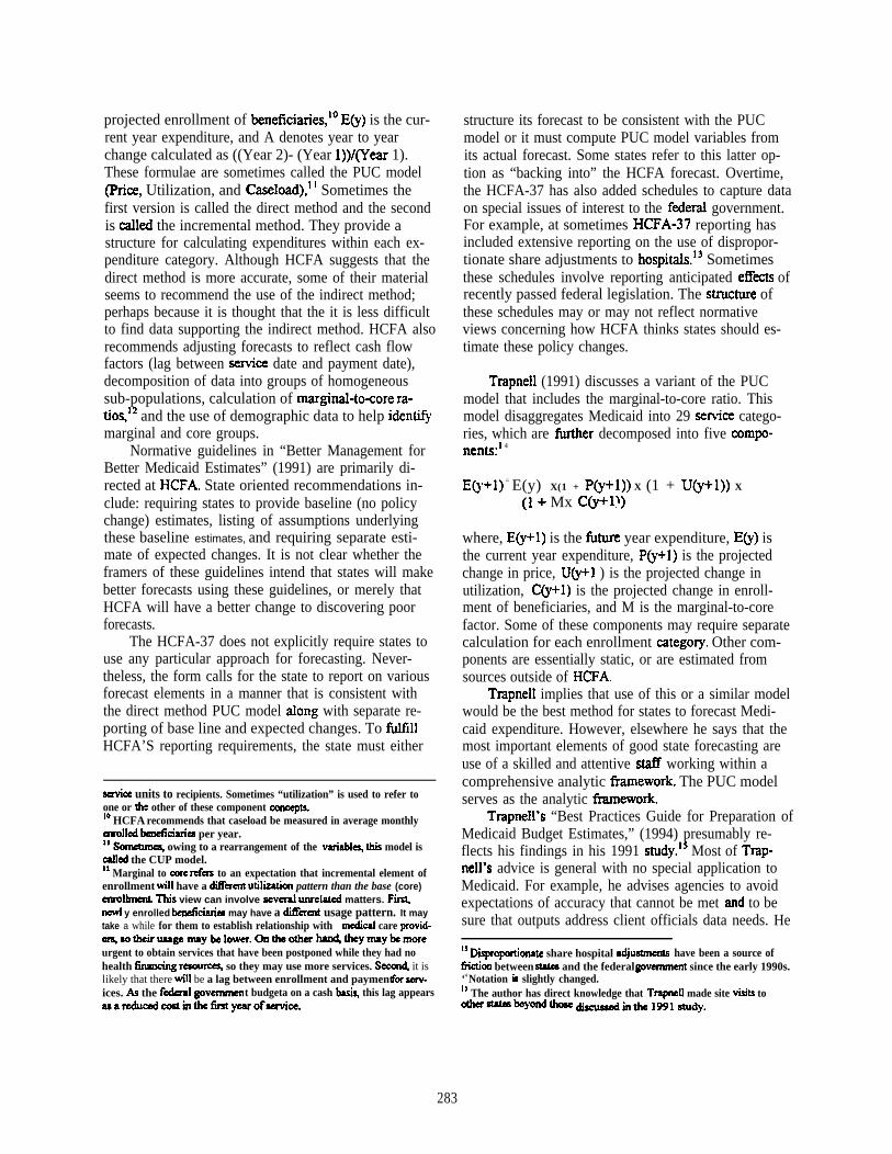
projected enrollment of beneficiaries,10 E~) is the cur-rent year expenditure, and A denotes year to yearchange calculated as ((Year 2)- (Year 1))/(Year 1).These formulae are sometimes called the PUC model(Rice, Utilization, and Caseload),l ] Sometimes thefirst version is called the direct method and the secondis calld the incremental method. They provide astructure for calculating expenditures within each ex-penditure category. Although HCFA suggests that thedirect method is more accurate, some of their materialseems to recommend the use of the indirect method;perhaps because it is thought that the it is less difficultto find data supporting the indirect method. HCFA alsorecommends adjusting forecasts to reflect cash flowfactors (lag between semice date and payment date),decomposition of data into groups of homogeneoussub-populations, calculation of marginal-to~ore ra-tios,]2 and the use of demographic data to help iden~marginal and core groups.

Normative guidelines in “Better Management forBetter Medicaid Estimates” (1991) are primarily di-rected at HCFA. State oriented recommendations in-clude: requiring states to provide baseline (no policychange) estimates, listing of assumptions underlyingthese baseline estimates, and requiring separate esti-mate of expected changes. It is not clear whether theframers of these guidelines intend that states will makebetter forecasts using these guidelines, or merely thatHCFA will have a better change to discovering poorforecasts.

The HCFA-37 does not explicitly require states touse any particular approach for forecasting. Never-theless, the form calls for the state to report on variousforecast elements in a manner that is consistent withthe direct method PUC model aIong with separate re-porting of base line and expected changes. To fultlllHCFA’S reporting requirements, the state must either

aavicc units to recipients. Sometimes “utilization” is used to refer toone or the other of these component concqxs.10 HCFA recommends that caseload be measured in average monthlyemolled bcnct%iaries per year.11s .

022wwM& owing to a rearrangement of the variableq this model iscallad the CUP model.12 Marginal to core refm to an expectation that incremental element ofenrollment will have a diikent utikation pattern than the base (core)enrollmti This view can involve acveml wrelated matters. F-ncwl y enrolled benefkities may have a dHerent usage pattern. It maytake a while for them to establish relationship with mcdicd care provid-~sotheiruaage may belower. Ontheother ha224theymaybemoreurgent to obtain services that have been postponed while they had nohealth ~g reaou~ so they may use more services. Secon4 it islikely that there will be a lag between enrollment and payment fw serv-

t budgeta on a cash bask this lag appearsices. A the f- govemrnenasareduced custinthefti yearofaemice.

structure its forecast to be consistent with the PUCmodel or it must compute PUC model variables fromits actual forecast. Some states refer to this latter op-tion as “backing into” the HCFA forecast. Overtime,the HCFA-37 has also added schedules to capture dataon special issues of interest to the ftieral government.For example, at sometimes HCFA-37 reporting hasincluded extensive reporting on the use of dispropor-tionate share adjustments to hospitals.13 Sometimesthese schedules involve reporting anticipated efkcts ofrecently passed federal legislation. The stmcture ofthese schedules may or may not reflect normativeviews concerning how HCFA thinks states should es-timate these policy changes.

Trapnell (1991) discusses a variant of the PUCmodel that includes the marginal-to-core ratio. Thismodel disaggregates Medicaid into 29 sexvice catego-ries, which are fbrther decomposed into five compo-nents:i 4

E(y+l) = E(y) X(1 + P(y+l)) X (1 + U(y+l)) X

(I+ Mx C@+l))

where, E(y+l) is the fhture year expenditure, E@) isthe current year expenditure, P(y+l) is the projectedchange in price, U(y+l ) is the projected change inutilization, C(y+l) is the projected change in enroll-ment of beneficiaries, and M is the marginal-to-corefactor. Some of these components may require separatecalculation for each enrollment categoxy. Other com-ponents are essentially static, or are estimated fromsources outside of HCFA.

Txapnell implies that use of this or a similar modelwould be the best method for states to forecast Medi-caid expenditure. However, elsewhere he says that themost important elements of good state forecasting areuse of a skilled and attentive staff working within acomprehensive analytic ffamework. The PUC modelserves as the analytic fkamework.

Trapnell’s “Best Practices Guide for Preparation ofMedicaid Budget Estimates,” (1994) presumably re-flects his findings in his 1991 study.ls Most of Trap-nell’s advice is general with no special application toMedicaid. For example, he advises agencies to avoidexpectations of accuracy that cannot be met ad to besure that outputs address client officials data needs. He

*3 Dkproportionate share hospital adjustmmts have been a source offi-iction between states and the federal govemmat since the early 1990s.‘4 Notation u slightly changed.1’ The author has direct knowledge that Trapnell made site tilts tooth=~beyondthose ~intil~l~dy.

283

recommends evaluating forecasts through productionof numerous outputs that can be compared with actu-al$ comparing forecasts with earlier forecasts of thesame series, and making frequent forecast updates. Herecommends usual forms of pm-forecasting such asdisaggmgating data ~d adjusting for non-reamingeven~ missing daQ and lag time between accrual ofliabilities and cash transactions. He recommends op-timizing the use of knowledge by such actions as es-tablishing a relationship with progmm ~, distin-guishing between matters that must be forecast andthose that can be know, and distinguishing between thenear fhture, about which forecasters may have specialknowledge, and the distant fhture, about which theyknow considerably less.

Trapnell raises considerable concern over dataused in Medicaid forecasting. This concern reflects alack of fhith in Medicaid data and health care data ingeneral. Data concerns include completeness, reliabil-ity, validity and timeliness of data. He suggests severalmethods of ver@ing data validity, by which he meansthat the dala is what it purports to be. Data can bevalidated by reconciling with accounting records, byexamining the process of its production when producedby the Medicaid agency, and by examining the docu-mentation of its production and meaning when pro-duced by others.

Trapnell recommends the use of an analytic modelto assure that the fcrecast addresses all elements of ex-penditure. The model he recommends is a anothervariant of the PUC model.

Trapnell lists nine special fwtures of Medicaidthat make forecasting Medicaid expenditures harderthan other health care expenditure forecasting theseare:1.2.

3.

4.

5.6.

7.

Criteria for Medicaid eligibility are very complex.Many beneficiaries are eligible and enrolled onlyfor short periods.Some individuals become eligible for Medicaid inpart because they have high medical bills, so theycan be expected to continue to have high medicalbills.Medicaid policy making leads to frequent changesin payment levels.Documentation of expenditures is incomplete.There are inconsistent definitions of data in ac-counting and claims processing.There are constant changes in the program result-ing from federal and state legislatio~ new regula-tions, administrative initiativ~ and court deci-sions.

8.

9.

The political process leads to a random patterns ofintementions in payment rates and other programfatures.Medicaid agencies need to be able to explain theirforecasts to officials and interest groups.Consequently, he recommends that the Medicaid

forecast should:1.2.3.4.

5.

6.

7.

●

●

●

●

Be easy to understand and test for reasonableness.Be easy to adjust for changes.Be easy to incorporate ad hoc adjustments.Be easy and inexpensive to re-estimate usingnewer data.Be easy to change to accommodate programchanges.Produce numerous outputs to compare with actualexperience.Produce outputs that fulfill forecast users’ needs.Trapnell also recommends that:Medicaid forecasting methodology should be ableto detect fkequent unexpected shocks to the expen-diture system,Forecasting should be insulated horn political in-terferenm,Staff should be assigned to forecasting as their iillmain work fiction, andThe loss finction that forecasters should minimizeis the consequences of forecast error. Trapnell as-sumes that there equally negative consequences forpositive and negative errors, thus, he recommendsa symmetrical loss fbnction.Trapnell does not recommend any specific fore-

casting technique. He recommends against the use ofcomplex econometric models or “black box” tech-niques, excessive reliance on high technology, or reli-ance on any single technology. Positive recommenda-tions include use of simple techniques, fitting tech-niques to the &ta and the mture of the problem, andallocating resources for forecasting based on criteria ofimportance and difficulty.

The National Association of State Budget Oflicers(NASBO) issued a brief guideline on Medicaid estima-tion practices (National Association of State BudgetOflkers, 1991). NASBO offers the general model:

“Simply pug a state’s expenditure on Medicaid isthe product of the number of people using itsseMces (caseload) and the cost of providing thoseseMces (price). Several variables must be accu-rately forecast for the overall estimate to be cor-rect: the economic environment in which theMedicaid program operates, the eligible popula-

284

1.

2.

3.

4.

5.

6.

7.

8.

9.

t.io~ the types and prices of setices used, the par-ticipation rate amcng eligible participants, policyinitiatives, and the fderal match rate.This guideline lists nine recommended practices:Include the budget agency, the Medicaid agency,and the legislative fiscal agency in the develop-ment of a Medicaid spending estimate. This is la-beled a “gheral practice” which seines consensusbuilding.Ensure that the economics of the spending esti-mate are consistent with those of the revenue esti-mate. This practice is of greater concern at turn-ing points when revenue and spending assump-tions may become disconnected.Ensure that the population assumptions used in theMedicaid estimate are consistent with overall statedemographic trends. Various state agenciesshould communicate to assure that estimates ofrelated coverage gToups are adequately coordi-nated.Maintain good data. Recommended data elementsinclude users, their attributes, and the semices theyuse.Establish. the price of seMces before the fiscal yearbegins. The aim is to remove uncertainty. “Ingeneral, states will find it easier to develop accu-rate spending estimates if the cost of semices is setlxfore the fiscal year begins. States that reimbursefor actual costs incurred are at a disadvantage inthis respect.”Account for caseload changes associated with out-reach efiorts. This concern involves the interac-tion between various programs and the possibilitythat outreach for one program will affect anotherprogram.Track federal and state legislation and regulations.This practice concerns the ikquent changes inpolicies that affkct Medicaid spending.Know the federal match rate*G and the likelihoodof it changing. This concern involves the distri-bution of costs between fderal and state govern-ments. Forecasting, in this sense, is oriented to-wards the costs to the state.Monitor the estimate. Even good estimates can bewrong. Medicaid agencies should produce

1’ “Match rate,” is one of several terms used to refer to the propotiion ofMedicaid mats paid by the fbl government. Other terms ase FMAPrate, FFP, ftil share, matck etc. This rate is published in the Fed-eral Register in Janumy or Febmary each year with an effkctive &ta ofthe following October 1. Federal Funding Information fbr States (FFIS),an 05shoot of the NASBO, monitors matching rates and forecastschanges prior to their oflkial publication in the Federal Register.

monthly or quarterly reports that compares Medi-caid spending with the original estimates. Devia-tions should be explained, so that forecasting canimprove over time.Recommendations 2 and 3 may improve accuracy

if the facilitate communication between forecasterswho have different perspectives on the state economy.Recommendation number 4 is similar to one of Trap-nell’s chief concerns, but Trapnell provides more ex-plicit advice concerning its implementation. Wherestates are able to comply with recommendation number5, they eliminate the need to forecast what they cartknow. Recommendation number 6 appears to be idio-syncratic to particular concerns of the early 1990s;however, it also seems to reflect Trapneil’s more gen-eral principle to maximize the use of knowledge.HCFA, Trapnell and NASBO all show considerableconcern over the impacts of policy making as discussedin recommendation 7. Recommendation number 8 in-volves monitoring, not forecasting. It also reflectsTrapnell’s principle to maximize use of knowledge.

The Congressional Budget Office uses of a modelsimilar to HCFA’S (Muse, 1993). Muse’s concern isnot to describe the forecasting of the ongoing program,but the method of estimating costs of program changes.The particular changes he is concerned about involvepreventive child health. He recommends the use of thefollowing model:]’

AT=ACXAPXAU+AA-O

where, A means “cha.qe in,” T is total payments, C ispopulation, P is price, U is utilization, A is adminis-trative costs or savings, and O is offsets. Muse’s nota-tion is confhing. I.fone assumes that AC, AP, and AUare ratios] 8 as discussed by HCFA or Trapnell, thenthis formula needs the modification of including thebase reimbursement in the right hand and the deletionof the change symbol on the left hand side of the for-mula; let BI = the base expenditure level for medicalcare and Bz = the base expenditure level for adminis-tration:

T=B1 X (l+AC) x (I+AP) X (l+AU) + B2 + AA -0or

AT=BIXACXAP XAU+AA-(O+BI)

If one assumes that AC, AP, and AU are numbers

17 Notation is modified,1’ AA would still be a fblly dimensional number.

285

. .

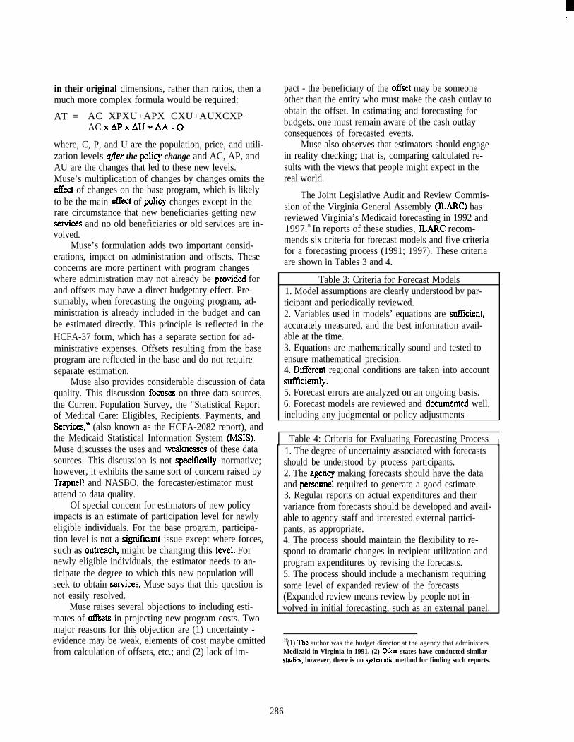
in their original dimensions, rather than ratios, then amuch more complex formula would be required:

AT = AC XPXU+APX CXU+AUXCXP+AC XAPXAU+AA-O

where, C, P, and U are the population, price, and utili-zation levels ajler the policy change and AC, AP, andAU are the changes that led to these new levels.Muse’s multiplication of changes by changes omits theeflkct of changes on the base program, which is likelyto be the main efkct of poliq changes except in therare circumstance that new beneficiaries getting newsetices and no old beneficiaries or old services are in-volved.

Muse’s formulation adds two important consid-erations, impact on administration and offsets. Theseconcerns are more pertinent with program changeswhere administration may not already be pro%ided forand offsets may have a direct budgetary effect. Pre-sumably, when forecasting the ongoing program, ad-ministration is already included in the budget and canbe estimated directly. This principle is reflected in theHCFA-37 form, which has a separate section for ad-ministrative expenses. Offsets resulting from the baseprogram are reflected in the base and do not requireseparate estimation.

Muse also provides considerable discussion of dataquality. This discussion fbcuses on three data sources,the Current Population Survey, the “Statistical Reportof Medical Care: Eligibles, Recipients, Payments, andSexvices,” (also known as the HCFA-2082 report), andthe Medicaid Statistical Information System (MSIS).Muse discusses the uses and wcxdcnesses of these datasources. This discussion is not spccitlcally normative;however, it exhibits the same sort of concern raised byTrapnell and NASBO, the forecaster/estimator mustattend to data quality.

Of special concern for estimators of new policyimpacts is an estimate of participation level for newlyeligible individuals. For the base program, participa-tion level is not a signifkant issue except where forces,such as outreac~ might be changing this level. Fornewly eligible individuals, the estimator needs to an-ticipate the degree to which this new population willseek to obtain seMces. Muse says that this question isnot easily resolved.

Muse raises several objections to including esti-mates of ofkts in projecting new program costs. Twomajor reasons for this objection are (1) uncertainty -evidence may be weak, elements of cost maybe omittedfrom calculation of offsets, etc.; and (2) lack of im-

pact - the beneficiary of the offket may be someoneother than the entity who must make the cash outlay toobtain the offset. In estimating and forecasting forbudgets, one must remain aware of the cash outlayconsequences of forecasted events.

Muse also observes that estimators should engagein reality checking; that is, comparing calculated re-sults with the views that people might expect in thereal world.

The Joint Legislative Audit and Review Commis-sion of the Virginia General Assembly (JLARC) hasreviewed Virginia’s Medicaid forecasting in 1992 and1997.19 In reports of these studies, JLARC recom-mends six criteria for forecast models and five criteriafor a forecasting process (1991; 1997). These criteriaare shown in Tables 3 and 4.

Table 3: Criteria for Forecast Models1. Model assumptions are clearly understood by par-ticipant and periodically reviewed.2. Variables used in models’ equations are tilcient,accurately measured, and the best information avail-able at the time.3. Equations are mathematically sound and tested toensure mathematical precision.4. Diil’erent regional conditions are taken into accountstdTlciently.5. Forecast errors are analyzed on an ongoing basis.6. Forecast models are reviewed and dmented well,including any judgmental or policy adjustments

I Table 4: Criteria for Evaluating Forecasting Process I1. The degree of uncertainty associated with forecastsshould be understood by process participants.2. The agen~ making forecasts should have the dataand pe~nnel required to generate a good estimate.3. Regular reports on actual expenditures and theirvariance from forecasts should be developed and avail-able to agency staff and interested external partici-pants, as appropriate.4. The process should maintain the flexibility to re-spond to dramatic changes in recipient utilization andprogram expenditures by revising the forecasts.5. The process should include a mechanism requiringsome level of expanded review of the forecasts.(Expanded review means review by people not in-volved in initial forecasting, such as an external panel.

199(1) ‘he author was the budget director at the agency that administersMedieaid in Virginia in 1991. (2) Other states have conducted similarstudi=, however, there is no @ematic method for finding such reports.

286

Excepting criterion 4 in Table 4, these criteriamight be applied to any forecasting problem. Most ap-pear to be a subset of more extensive criteria used inevaluating revenue forecasting (Joint Legislative Auditand Review Cogun.ission, 1991).

Many of these normative guidelines support thegoal of forecastkg accuracy. For example, JLARCrecommends that formulae be valid and NASBO,among many others, rec.ornmends the use of good data.Yet, many other recommendations concern other mat-ters. For example, Trapnell recommends against unre-alistic expectations of forecast results; similarly JLARCrecommends that forecast participants should under-stand the degree of forecast uncertainty.

RELATION TO REVENUE FORECASTINGRevenue forecasting literature suggests a tendency

for an asymmetrical forecasting loss fimction, favoringa cushion between total revenue and total expenditures(Rodgers and Joyce, 1996). The rationale is that thepenalty for overestimated revenue is greater than thepenalty for underestimated revenue. Similar reasoningwould have states overestimate expenditures in majorexpenditure categories such as Medicaid. Surplusesare less damaging and, in many states, can be repro-grammed at the end of the fiscal year to offset deficitselsewhere.

However, cushioning budgets through overestinla-tion of Medicaid expenditures differs from underesti-mation of revenue in one important respect. It changesthe locus of control over the cushion. Unappropriatedrevenue - which is the status of unexpected revenueresulting from greater receipts than budgeted - is, gen-erally, controlled by the central administrative agenciesor the legislature. over-appropriated finds, resultantfrom appropriating fimds to Medicaid agencies basedon overestimated forecasts, are controlled by line agen-cies. As there is a mtural distrust between central ad-ministrative agencies and line agencies, it is unlikelythat states would intentionally allow line agencies tocontrol surplus fimds,

Nevertheless, the line agencies, who submit theHCFA-37, maybe motivated to seek surplus funding asa cushion against their own forecast error. There wouldbe no advantage for these line agencies to make sepa-rate lower estimates for HCFA.

Trapnell argues that agencies might find differingbut equally negative consequences for overestimatingand underestimating expenditures. McKusick proposesthat there is lower penalty for underestimation. On the

other han~ Muse’s rationale for not counting offsets inestimating program changes suggests a higher penaltyfor underestimation.

The conflict concerning presence and direction ofbias can be e@ained by several factors. Firs~ McKu-sick’s study reported in 1980 reflects a relatively smallMedicaid program. With this small program, politicaldecision making may be more impotit than financialrisk, as is also suggested in some of Trapnell’s discus-sion. In their effort to maximize their distribution ofbenefits, elective officials may consider a small risk ofover expenditure to be less important than their abilityto distribute benefits to more people. Still, neitherMcKusick or Trapnell found empirical evidence of ac-tual underestimation.

SOME HYPOTHESESThese studies provide little explanation of relative

forecasting accuracy. However, they are a source formany hypotheses about Medicaid forecasting. In gen-eral these hypotheses are found by extrapolating theobjective of normative guidelines or the reasons for in-quiry in empirical studies. To a large degree, wherethere is expkmatoxy discussion, most of the views agreewith each other. In a few cases, as with the matter ofa-etriud loss fimction, there is disagreement.Where there is disagreement, the cited sources may notall support the form of the hypothesis ex--ressed here.Following are hypotheses that can be extracted fromthis body of literature:

1. States’ loss fi.mctions will be asymmetrical with apreference for overestimation (Trapnell, McKu-sick, Muse). McKusick proposes a preference forunderestimation. Trapnell offers conflictingviews, (1) he argues that the political environmentequally punishes over- and underestimation, (2) hepoints out that past f~eral behavior may create abias for overestimation, and (3) he proposes thatunderestimation bias arises from frequent selectionof policy initiatives that are underestimated.

2. States manipulate fiscal year end results to im-prove forecasting results within state budgeting.By implication states whose fiscal year ends coin-cide with federal fiscal year ends will appear to bemore accurate (’EOP, Trapnell, Insco).

3. Forecast models result in more accurate forecastswhen they:a) Account for delivery of medical care on serv-

ice date with lagged tradormation to cashpayment date (McKusick, Insco, Lower, Trap-

287

,. .,,. “ .,, ,

,.

b)

c)

d)

e)

f)

@

h)

i)j)

nell, Muse).Decompose data into homogeneous sewice andenrollment categories (McKusiclq Trapnell,Lower).Reflect the PUC model or an extended versionof the PUC model (HCF~ Trapnell, Muse,NASBO).Relate enrollment to economic conditions(McKusick).Relate seMce utilization with seMce supply(McKusick).Decompose series into baseline and policyevents (McKusic~ Trapnell, Lower, EOP,HCFA, NASBO, Muse, JLARC).Decompose utilization into recipients perbeneficiary and units of service per recipient(Lwer).Relate price estimates to price indexes (Lower,Trapncll).Account for fderal matching rates (NASBO).Account for regional variation (JLARC).

4. Forecasting accuracy is affkcted by:a)

b)

c)d)

e)

f)

g)h)i)

J)k)

Stmi) Skill (EOP, Lower, JLARC).ii) Quantity (McKusick, Lower, JLARC).iii) Dedication to the forecasting fiction, as

opposed to part-time forecasting (Trap-nell).

Forecaster understanding ofi) Forecast model assumptions (JLARC).ii) The Medicaid program (Trapnell).Forecaster access to program staff (Trapnell).Data:i) Quality (McKusick, Trapnell, Lower,

NASBO, Muse, JLARC),ii) Sources (Lower, Trapnell, Muse).iii) Periodicity (monthly, etc.) (McKusick,

Lower).iv) Series length (Lower).Setting rates prior to forecasting (McKusick,Trapnell, NASBO).Composition of the Medicaid program (Mc-Kusick, Trapnell, Insco, Lower),Update frequency (Trapnell, Lower).Length of forecast horizon (Trapnell).Decomposition of forecast into near fbture anddistant future (’Ikapnell).Whether seasonality is c.xarnined (Lower).Use of software:i) Spreadsheets (Low)er).ii) Statistical software (LOver).

1)m)

n)

o)

iii) Forecast sofhvare (Lower).Use of pre-forecast data editing (Trapnell).Insulation of forecasting from politics (Trap-nell).Allocation of forecasting resources to prob-lems (components) according to difficulty andimportance (’Ilapnell),Use and quality of forecast evaluation (Trap-nell, NASBO, JLARC).

5. Intra-governrnental forecasting factors that affkctforecasting accuracy include:a)

b)

c)

d)

Locus of primary forecasting responsibility -Medicaid agency or other state ageng (Mc-Kusick, Lower).Cooperation between forecasting bodies(Lower, NASBO, JLARC).Whether there is coordination between Medi-caid forecasting and other state forecasting(NASBO).Use of “expanded review” (JLARC).

6, Accuracy is improved when forecasting techniquesare:a) Simple (Trapnell).b) Not “black box” (Trapnell).c) Fit to the nature of the problem (Tkapnell).d) Fit to the quality of the data (Trapnell).e) Easy to use (Trapnell).f) Capable of detecting the effects of policy

shocks (Trapnell).7. Forecasting accuracy is not associated with the use

of any particular forecasting techniques (Trapnell).However, McKusick suggests the opposite, imply-ing that more sophisticated techniques may resultin greater accuracy.

8. When multi-stage forecasts are used, accuraq’ oflater stage forecasts depend on the accuracy ofearlier stage forecasts (Trapnell).

9. L,arge policy events a.tlect forecasting accuracy. Inparticular, forecasting accuracy is tiected by:a) Boren Amendment Lawsuits (Insco, Lower).b) Federal policies concerning pregnant women

and children (Insco, Lower).c) State initiatives involving Disproportionate

Share Hospitals (Trapnell, EOP).10. Perceived forecasting importance affects accuracy

and bias. In particular:a) The relative size of the Medicaid program to

other state programs affects accuracy. As theprogram increases in relative size, accuracybecomes more valued (McKusick, Lower).McKusick does not offer this view, instead it

288

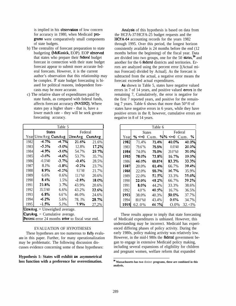
is implied in his obsemation of low concernfor accuracy in 1980, when Medicaid pro-gmms were comparatively small componentsof state budgets.

b) The centrality of forecast preparation to statebudgeting ‘@lcKusick, EOP). EOP obsewedthat states who prepare their fderal budgetforecast in connection with their state budgetforecast appear to submit more accurate fed-eral forecasts. However, it is the currentauthor’s observation that this relationship maybe complex. If state budget forecasting is bi-ased for political reasons, independent fore-casts may be more accurate.

c) The relative share of expenditures paid bystate funds, as compared with federal funds,affects forecast accuracy (NASBO). Wherestates pay a higher share - that is, have alower match rate – they will be seek greaterforecasting accuracy.

fialysis of this hypothesis is based on data fromthe HCFA-37/HCFA-25 budget requests and theHCFA-64 accounting records for the years 1982through 1995. Over this period, the longest horizonconsistently available is 24 months before the end (12months before the beginning) of the fiscal year. Dataare divided into two groups, one for the 50 states,20 andanother for the 6 fdera.1 districts and territories. Er-rors are analyzed using the percent error [(Actual mi-nus Forecast) divided by Actual]. As the forecast issubtracted from the actual, a negative error means theforecast exceeded actual expenditures.

A shown in Table 5, states have negative valuederrors in 7 of 14 years, and positive valued emors in theremaining 7, Cumulatively, the error is negative forthe first 7 reported years, and positive for the remain-ing 7 years. Table 6 shows that more than 50°/0 of

I states have negative errors in 6 years, while they havepositive errors in the 8; however, cumulative errors arenegative in 8 of 14 years.

Table 5 1States Federal

Year UnwAvg CurnAvg UnwAvg CumAvg1982 -4,7Y0 -4.7V0 21.6?40 21.6%1983 -5.3Y0 -5.070 12.8% 17.2!401984 -4.9V0 -5.OYO 54.7% 29.7V01985 -3.6Y0 -4.6Y0 53.7% 35.7%1986 -0.3?40 -3.7Y0 -0.4Yo 28.5%1987 8.l% -1.8’ZO -0.270 23.7%1988 8.9’%0 -0.2Y0 9.5’?40 21.7%1989 6.6% 0.6% 13.1’%0 20.6%1990 8.4?40 1.5% -2.8?40 18.0701991 23.8’Mo 3 .7’ZO 43.9% 20.6%1992 35.5?40 6.6% 43.2% 22.6’ZO1993 6.8V0 6.6’% 46.0% 24.6%1994 -6.2Y0 5.6% 78. l% 28.7V01995 -1.5Y0 5.l% 7.970 27,2%JnwAvg. = Unweighed average.;urWlvg. = Cumulative average.‘ercent error 24 months rxior to fiscal vear end.

EVALUATION OF HYPOTHESESThese hypotheses are too numerous to filly evalu-

ate in this paper. Further, for many operationalizationmay be problematic. The following discussion dis-cusses evidence concerning some of these hypotheses:

Hypothesis 1: States will exhibit an asymmetricalloss function with a preference for overestimation.

Table 6 IStates I Federal

Year ‘A <=0 Cum. YO ‘%0 <=0 Cum. YO I

1982198319841985198619871988198919901991199219931994

71.4%79.6’%74.0%78.OVO46,0V020.0%22.0%22.0%22.OVO

8.OVO4.0’%

38.0%80.0’%0

71.4%75.5%75.0%75.8%69.8?461.4%55.7%51.5’Ya48.2Ya44.2%40.5’?4a40.3%43.4%

40.0700.0?40

20.0’%016.7’%083.3?4066.7%16.7V033.3%66.7%33.3%16.7%50.OVO

0.0’%0

20.OVO20.OYO19.OVO33.37039.4V035.9%35.6?4039.2’?4038.6%36.5%37.7%34.7%

19951 62.0% 44.7YOI O.0% 32.<l%

These results appear to imply that state forecastingof Medicaid expenditures is unbiased. However, thisunderstanding may be incorrect. Medicaid has experi-enced differing phases of policy activity. During theearly 1980s, policy making activity was relatively low.However, in the mid-l 980s the fixleral government be-gan to engage in extensive Medicaid policy making,including several expansions of eligibility for childrenand pregnant women, welfare reform that expanded

10 Massachusetts has two distinct programs, these are combined in thisanalysis,

289

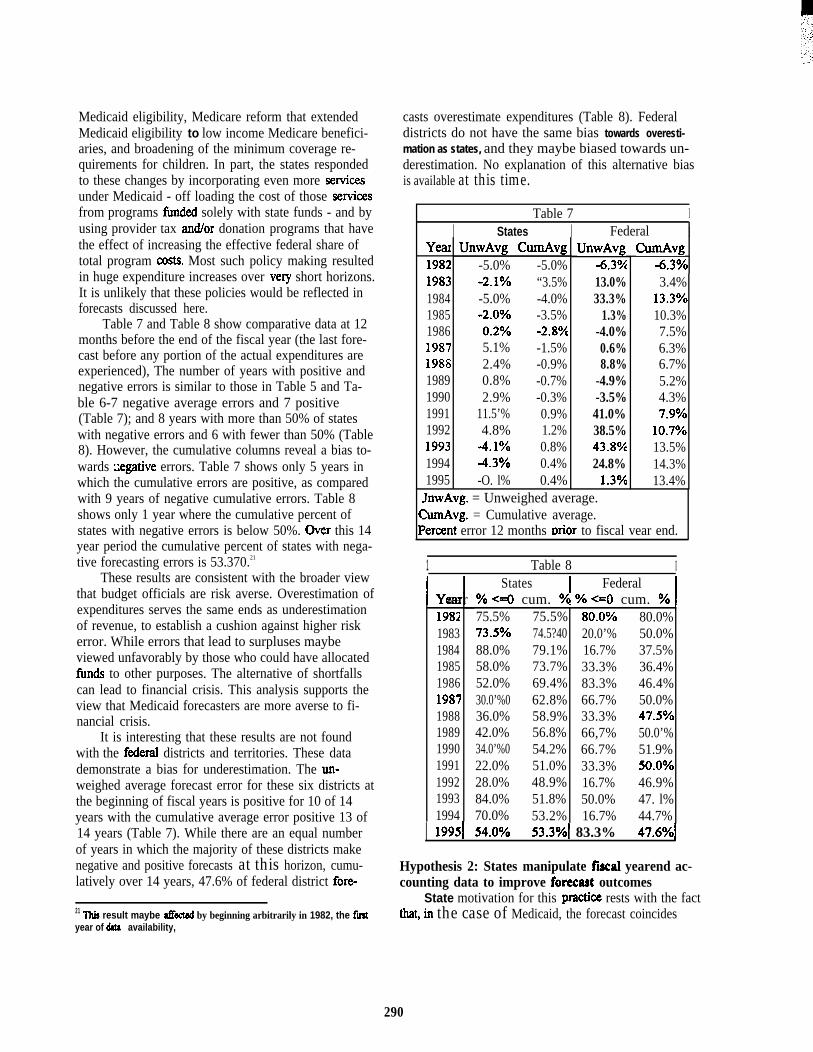
Medicaid eligibility, Medicare reform that extendedMedicaid eligibility to low income Medicare benefici-aries, and broadening of the minimum coverage re-quirements for children. In part, the states respondedto these changes by incorporating even more sewicesunder Medicaid - off loading the cost of those seMcesfrom programs fimded solely with state funds - and byusing provider tax and/or donation programs that havethe effect of increasing the effective federal share oftotal program costs. Most such policy making resultedin huge expenditure increases over ve~ short horizons.It is unlikely that these policies would be reflected inforecasts discussed here.

Table 7 and Table 8 show comparative data at 12months before the end of the fiscal year (the last fore-cast before any portion of the actual expenditures areexperienced), The number of years with positive andnegative errors is similar to those in Table 5 and Ta-ble 6-7 negative average errors and 7 positive(Table 7); and 8 years with more than 50% of stateswith negative errors and 6 with fewer than 50% (Table8). However, the cumulative columns reveal a bias to-wards fiegative errors. Table 7 shows only 5 years inwhich the cumulative errors are positive, as comparedwith 9 years of negative cumulative errors. Table 8shows only 1 year where the cumulative percent ofstates with negative errors is below 50%. Over this 14year period the cumulative percent of states with nega-tive forecasting errors is 53.370.21

These results are consistent with the broader viewthat budget officials are risk averse. Overestimation ofexpenditures serves the same ends as underestimationof revenue, to establish a cushion against higher riskerror. While errors that lead to surpluses maybeviewed unfavorably by those who could have allocatedfinds to other purposes. The alternative of shortfallscan lead to financial crisis. This analysis supports theview that Medicaid forecasters are more averse to fi-nancial crisis.

It is interesting that these results are not foundwith the fderal districts and territories. These datademonstrate a bias for underestimation. The un-weighed average forecast error for these six districts atthe beginning of fiscal years is positive for 10 of 14years with the cumulative average error positive 13 of14 years (Table 7). While there are an equal numberof years in which the majority of these districts makenegative and positive forecasts at this horizon, cumu-latively over 14 years, 47.6% of federal district fore-

21 Ibis result maybe afkted by beginning arbitrarily in 1982, the f~year of ti availability,

casts overestimate expenditures (Table 8). Federaldistricts do not have the same bias towards overesti-mation as states, and they maybe biased towards un-derestimation. No explanation of this alternative biasis available at this time.

Table 7 I

Yea19821983198419851986198719881989199019911992199319941995

I States I Federal IUnwAvg CurnAvg

-5.0%-2.lYO-5.0%-2.OYO0.2V05.1%2.4%0.8%2.9%

11.5’%4.8%

-4.lYO-4.3Y0-O. l%

-5.0%“3.5%-4.0%-3.5%-2.8%-1.5%-0.9%-0.7%-0.3%0.9%1.2%0.8%0.4%0.4%

UnwAvg-6.3%13.0%33.3%

1.3%-4.0%0.6%8.8%

-4.9%-3.5%41.0%38.5%43.8YQ24.8%

1.3Ya

CumAvg-6.3Y03.4%

13.3!X010.3%7.5%6.3%6.7%5.2%4.3%7.970

10.7VO13.5%14.3%13.4%

JnwAvg. = Unweighed average.hnAvg. = Cumulative average.>ercent error 12 months mior to fiscal vear end.

1 Table 8 I

II StatesI

FederalYear Yo <=0 cum. Yo 70 <=0 cum. Yo I1981198319841985198619871988198919901991199219931994

I75.5%73.5V088.0%58.0%52.0%30.0’%036.0%42.0%34.0’%022.0%28.0%84.0%70.0%

75.5% 80.OVO74.5?40 20.0’%79.1% 16.7%73.7% 33.3%69.4% 83.3%62.8% 66.7%58.9% 33.3%56.8% 66,7%54.2% 66.7%51.0% 33.3%48.9% 16.7%51.8% 50.0%53.2% 16.7%

80.0%50.0%37.5%36.4%46.4%50.0%47.57050.0’%51.9%50.07046.9%47. l%44.7%

I 53.3%1 83.3% 47.6V0

Hypothesis 2: States manipulate fiscal yearend ac-counting data to improve foreeast outcomes

State motivation for this practk rests with the factthat, in the case of Medicaid, the forecast coincides

290

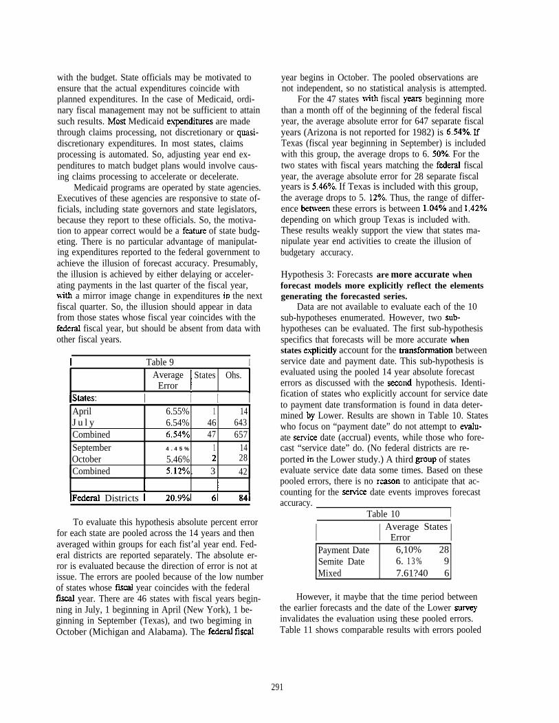
with the budget. State officials may be motivated toensure that the actual expenditures coincide withplanned expenditures. In the case of Medicaid, ordi-nary fiscal management may not be sufficient to attainsuch results. Most Medicaid expditures are madethrough claims processing, not discretionary or quasi-discretionary expenditures. In most states, claimsprocessing is automated. So, adjusting year end ex-penditures to match budget plans would involve caus-ing claims processing to accelerate or decelerate.

Medicaid programs are operated by state agencies.Executives of these agencies are responsive to state of-ficials, including state governors and state legislators,because they report to these officials. So, the motiva-tion to appear correct would be a future of state budg-eting. There is no particular advantage of manipulat-ing expenditures reported to the federal government toachieve the illusion of forecast accuracy. Presumably,the illusion is achieved by either delaying or acceler-ating payments in the last quarter of the fiscal year,With a mirror image change in expenditures in the nextfiscal quarter. So, the illusion should appear in datafrom those states whose fiscal year coincides with thefderal fiscal year, but should be absent from data withother fiscal years.

1 Table 9 IAverage

IStates Ohs.

Errori %lStates: I I I IApril 6.55% 1 14J u l y 6.54% 46 643Combined 6.54’?40 47 657September 4 . 4 5 % 1 14October 5.46% 2 28Combined 5.12’XO . 3 42

lFederal Districts I 20.9VOI 61 841

To evaluate this hypothesis absolute percent errorfor each state are pooled across the 14 years and thenaveraged within groups for each fist’al year end. Fed-eral districts are reported separately. The absolute er-ror is evaluated because the direction of error is not atissue. The errors are pooled because of the low numberof states whose fiscal year coincides with the federalfiscal year. There are 46 states with fiscal years begin-ning in July, 1 beginning in April (New York), 1 be-ginning in September (Texas), and two begiming inOctober (Michigan and Alabama). The ftieral fiscal

year begins in October. The pooled observations arenot independent, so no statistical analysis is attempted.

For the 47 states with fiscal yeaK beginning morethan a month off of the beginning of the federal fiscalyear, the average absolute error for 647 separate fiscalyears (Arizona is not reported for 1982) is 6.54Y0. IfTexas (fiscal year beginning in September) is includedwith this group, the average drops to 6. 50°/0. For thetwo states with fiscal years matching the fdera.1 fiscalyear, the average absolute error for 28 separate fiscalyears is 5.46?40. If Texas is included with this group,the average drops to 5. 12Y0. Thus, the range of differ-ence be~een these errors is between 1.04°/0 and 1.42°/0depending on which group Texas is included with.These results weakly support the view that states ma-nipulate year end activities to create the illusion ofbudgetary accuracy.

Hypothesis 3: Forecasts are more accurate whenforecast models more explicitly reflect the elementsgenerating the forecasted series.

Data are not available to evaluate each of the 10sub-hypotheses enumerated. However, two sub-hypotheses can be evaluated. The first sub-hypothesisspecifics that forecasts will be more accurate whenstates ex@icitly account for the trantiormation betweenservice date and payment date. This sub-hypothesis isevaluated using the pooled 14 year absolute forecasterrors as discussed with the seccmd hypothesis. Identi-fication of states who explicitly account for service dateto payment date transformation is found in data deter-mined by Lower. Results are shown in Table 10. Stateswho focus on “payment date” do not attempt to evahl-ate sewice date (accrual) events, while those who fore-cast “service date” do. (No federal districts are re-ported in the Lower study.) A third gToup of statesevaluate service date data some times. Based on thesepooled errors, there is no reason to anticipate that ac-counting for the sexvice date events improves forecastaccuracy.

Table 10 I

I I Average StatesError I

Payment Date 6,10% 28Semite Date 6. 1 3 % 9Mixed 7.61?40 6

However, it maybe that the time period betweenthe earlier forecasts and the date of the Lower suxveyinvalidates the evaluation using these pooled errors.Table 11 shows comparable results with errors pooled

291

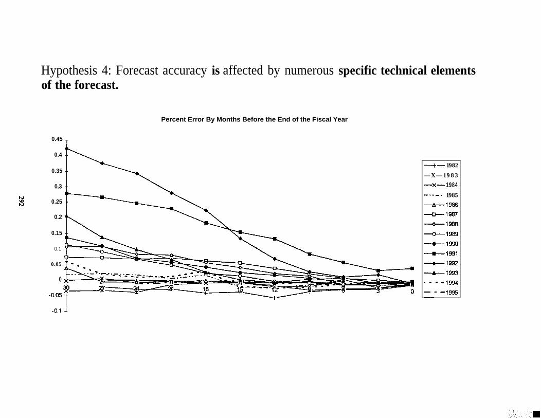
Hypothesis 4: Forecast accuracy is affected by numerous specific technical elementsof the forecast.

0.45

0.4

0.35

0.3

0.25

0.2

0.15

0.1

0.05

0.

T

Percent Error By Months Before the End of the Fiscal Year

+— 1982

— X — 1 9 8 3

—x— 1984-==-- 1985

~1988

~1987

~1988

-0.11

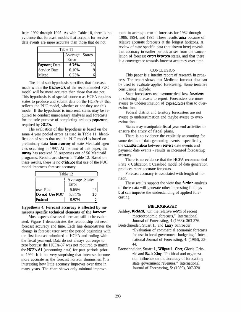
from 1992 through 1995. As with Table 10, there is noevidence that forecast models that account for servicedate events are more accurate than those that do not.

Table 11Average States

ErrorPaymen{ Date 5.7570 28Service Date 6.10% 9Mixed 6.23% 6

The third sub-hypothesis specifies that forecastsmade within the iia.mework of the recommended PUCmodel will be more accurate than those that are not.This hypothesis is of special concern as HCFA requiresstates to produce and submit data on the HCFA-37 thatreflects the PUC model, whether or not they use thismodel. If the hypothesis is incorrect, states may be re-quired to conduct unnecessary analyses and forecastsfor the sole purpose of completing arduous papenvorkrequired by HCFA.

The evaluation of this hypothesis is based on thesame 4 year pooled errors as used in Table 11. Identi-fication of states that use the PUC model is based onpreliminary data horn a sumey of state Medicaid agen-cies occurring in 1997. At the time of this paper, thesu.my has received 35 responses out of 56 Medicaidprograms. Results are shown in Table 12. Based onthese results, there is no mtidence that use of the PUCmodel improves forecast accuracy.

1 Table 12 I

I I Average States IError

use Puc 5.65% 13lDonot UsePUC I 5.81% 201[Federal I 8.97% 21

Hypothesis 4: Forecast accuracy is affected by nu-merous specific technical elements of the forecast

Most aspects discussed here are still to be evalu-ated. Figure 1 demonstrates the relationship betweenforecast accuracy and time. Each line demonstrates thechange in forecast error over the period beginning withthe first forecast submitted to HCFA and ending withthe fiscal year end. Data do not always converge tozero because the HCFA-37 was not required to matchthe HCFA-64 (accounting data) for past periods priorto 1992. It is not very surprising that forecasts becomemore accurate as the forecast horizon diminishes. It isinteresting how little accuracy improves over time inmany years. The chart shows only minimal improve-

ment in average error in forecasts for 1982 through1986, 1994, and 1995. These results tise because ofrelative accurate forecasts at the longest horizons. Areview of state specific data (not shown here) revealsthat accuracy in earlier periods arises from the cancel-lation of forecast emors beween states, and that thereis a convergence towards forecast accuracy over time.

CONCLUSIONThis paper is a interim report of research in prog-

ress. The report shows that Medicaid forecast data canbe used to evaluate applied forecasting. Some tentativeconclusions include:

State forecasters use asymmetrical loss fimctionsin selecting forecasts to report. Forecasters are moreaverse to underestimation of expmi.itures than to over-estimation.

Federal district and territory forecasters are notaverse to underestimation and maybe averse to over-estimation.

States may manipulate fiscal year end activities toensure the amcy of fiscal plans.

There is no evidence the explicitly accounting forsome details of data generating events - specifically,the t.ransfonnation between sewice date events andpayment date events - results in increased forecastingaccuracy.

There is no evidence that the HCFA recommendedPrice x Utilization x Caseload model of data generationproduces more accurate forecasts.

Forecast accuracy is associated with length of ho-rizon.

These results support the view that fMther analysisof these data will generate other interesting findingsthat can improve the understanding of applied fore-casting.

BIBLIOGIUPHYAshley, llichar~ “On the relative woti of recent

macroeconomic forecasts,” InternationalJournal of Forecasting, 4 (1988): 363-376.

Bretschneider, Stuart I., and Lany Schroeder,“Evaluation of commercial economic forecastsfor use in local government budgeting,” Inter-national Journal of Forecasting, 4: (1988), 33-44.

Bretschneider, Stuart I., Wilpen L. Gorr, Gloria Griz-zle and Earle Way, “Political and organiza-tion influence on the accuracy of forecastingstate government revenues,” InternationalJournal of Forecasting, 5: (1989), 307-320.

293

Doraq Phyllis A., Alice F. Roesenblatt, and Dale H.Yamamoto, “A Review of Premium Estimatesin the Health Security Am” MonographNumber Seven (Washington, DC: AmericanAcademy of Actuaries) April 1994.

Executive Ofike of the President and Department ofHealth & Human Sefices, “Better Manage-ment for Better Medicaid Estimates,” July 10,1991.

FirsheiK Jane~ “Forecasting Health Cmts: First, CrossYour Fingers,” Medicine & Health’s HealthReform hsigh~ December 6, 1993.

Heal Care Financing Administration, “ForecastingMedicaid Expenditures,” (unpublished)[1990].

HHS NEWS, “Administration Acts to Address Medi-caid Estimating Problems and Escalating CostIncreases,” July 10, 1991.

Hibou Michele and Spyros Makridakis, “M3-IJFCompetition first Results,” Conference Paper,17ti International Symposium on Forecasting,Barbados, June, 1997.

Holah.aq John and David Liska, “Reassessing theOutlook for Medicaid Spending Growth, (TheUrban Institute:http://www.urban. org/newfixhnf_a6.htrn),1997 (5/1/97).

Holahan, John and David Liska, “Where is MedicaidSpending Headed?” (The Urban Institute:Mtp://www.urban.org/entitlements/forecast.htm), December 1996 (5/1/97).

Joint Legislative Audit and Review Commission,“Revenue Forecasting in the ExecutiveBranch: Process and Models,” Semte Docu-ment No. 25, Richmond, 1991.

Joint Legislative Audit and Review Commission,“Review of the Virginia Medicaid Program,”Semte Document No. 27, Richmond, 1992.

Joint Legislative Audit and Review Commission,“Tecbnicd Report: Review of the MedicaidForecasting Methodology,” House DocumentNo. 5, Richmond, 1997.

Insco, Michele, “National Survey of States’ MedicaidBudget Experience” (unpublished) May, 1992.

Lower, Deborah J. “Medicaid Budget EstimationMethods: Results of a Smey of State Medi-caid Budget Officers,” Conference Paper,Human Services Finance Officers, September,1993.

Wdakis, S, A. hderso~ R. Carbone, R Fildes, M.Hibo~ R. Lewandowski, J. Newton, E.

Parzen, and R. Winkler, “The accuracy of ex-trapolation (time series) methods: results of aforecasting competition,” Journal of Fore-casting, 1 (1982): 111-153.

Makridakis, Spyros, Chris Chatfield, Michele Hibon,Michael Lawrence, Terence Mills, Keith Oral,and LeRoy F. Simmons, “The M.2-competition: A real-time judgmentally basedforecasting study,” International Journal ofForecasting, 5 (1989): 381-391.

McKusic~ David “Forecasting Techniques and Budg-etary Issues of State Medicaid Programs,”Falls Church, Virginia, September 30, 1980.

Muse, Donald N. “Estimating Costs and Savings fromPreventive Child Health Proposals,” TheGeorge Washington University, 1993.

National Association of State Budget Officers, “TheMedicaid Estimate,” [Washington, 1991].

National Association of State Budget Officers, “1995State Expenditure Report,” ~ashington),April, 1996.

OtWe of Technology Assessmen~ “Understanding Es-timates of the Impact of Health Reform on theFederal Budget,” published in CCHPulse:The Resource Guide to Health Care Reform(section 9076) 1994.

Ratner, Jonathan, “MEDICAID Decline in SpendingGrowth Due to a Combination of Factors,”Testimony Before the Committee on Finance,U.S. Senate, (Washington, DC: GAO), March4, 1997.

Rich, Spencer, “Bad Statistics Cited in Policy Miscal-culations,” Washington Post, August 6, 1991.

Rodgers, Robert and Philip Joyce, “The Effect of Un-deflorecasting on the Accuracy or RevenueForecasts by State Government,” Public Ad-ministration Review 56 (1996): 48-56.

Scanlon, William J. “MEDICAID Recent SpendingExperience an the Administration’s ProposedProgram Reform: Testimony Before the Sub-committee on Health and Environmen~Committee on Commerce., House of Repre-sentatives, (Washingto~ DC: GAO), March11, 1997.

Trapnell, Gordon R “Best Practices Guide for Prepa-ration of Medicaid Budget Estimates,” Actu-arial Research Corporation [1994].

Trapnell, Gordo~ “Assessment of Cment MedicaidForecasting Procedures,” Annandale, Vir-ginia, Actuarial Research corporatio~ June1991.

294

Consumer Health Accounts: What Can They Add to Medicare Policy Analysis?

R.M. Monaco, INFORUM, University of MarylandJ.H. Phelps, OHNS, office of the Actuary, HCFA1

Introduction”

Over the past few years the Office of the Actuaryof the Health care Financing Administration (HHS)and the Inforum group at the University of Marylandhave been investigating the relationships between thehealth care sector and the rest of the economy. Onepath of research has emphasized the fiscalconsequences of large spending increases for federalmedical programs, like Medicare. Beginning in 1995,outlays for hospital insurance (Medicare, part A)exceeded earmarked revenues and projections suggestthat outlays and revenues will continue to diverge byever-widening amounts. 2 Actuarial projections ofgrowth in Medicare part B. which is financed out ofgeneral revenues, also show growth faster than federaltax revenues. When Medicare spending rises fasterthan federal tax revenues, any or all of threeconsequences occur:

1. The federal deficit rises.

2. Other spending programs are cut so the deficit doesnot rise.

3. Payroll or other taxes are raised, so that otherspending programs can remain on their original fundingpaths without increasing the deficit.

All of these occurrences have macroeconomicconsequences, and influence the industrial structure ofemployment and output. Thus, in an indirect way,federal outlays related to medical care can have a largeinfluence on a wide variety of industries. In Monacoand Phelps {1995) we showed that a large increase inthe federal deficit from increases in Medicare spendingshills economic activity away from industries with highmeasured productivity, like manufacturing andagriculture, to industries with low measuredproductivity, like health care and business services. Inaddition, our research has shown that the combinedprojected social insurance deficits using SSA/HCFAmiddle-case scenarios over the next 50 years wouldrequire a pay-as-you-go payroll tax rate of 32 percentin 2050 to keep the federal budget balanced. This ismore than double the cunent rate (Monaco and Phelps(1997)).

Actuarial projections of Medicare spending risefor two distinct reasons (Monaco, Phelps, and Mulvey(1996)). First, in the short run (through about 201 1),the projected Medicare “deficit” is driven primarily byrapidly-rising spending per beneficiary. After 2011,actuarial projections of growth in spending perbeneficiary slows, but a rapid rise in the number ofbeneficiaries from retirement of the Baby Boomersresults in continued growth in Medicare spending.~ Therecent budget compromise has moved the projectedMedicare Part A trust fund insolvency date from 2001to 2007. This was done partly by reducing providerpayments per beneficiary--at least partially addressingthe first problem. However, the improvement in theoutlook of the Part A trust fund was accomplishedprimarily by reassigning home health liabilities fromPart A of the program to Part B. While this improvedPart A solvency, it did not reduce the projected overallMedicare deficit. Little was done to address the longer-term financing problems arising from the comingdemographic shift. Presumably, longer-term issues willbe addressed by the yet-to-be-appointed Medicarecommission. Thus, even with the recent reductions inthe near-term path of Medicare spending, it is clear thatMedicare policy will remain an important issuethroughout the next several years.

What Determines Medicare Spending?

The Medicare program was designed to cover asignificant portion of the cost of medical care for theelderly (over 64) and those with disabilities or end-stage renal disease. Broadly speaking, Part A ofMedicare covers hospital services, while Part B coversphysician services. Conceptually, Medicare is aninsurance program that, after some deductibles andcopayments paid by the beneficiary, directly reimbursesproviders for each kind of treatment.4 The importantpoint for our purpose is that the amount of Medicarespending in any year is not “capped” at any level.Given the reimbursement structure, Medicare outlaysare actually determined by the usage of coveredMedicare services by the beneficiary population. Inshort, Medicare outlays are determined by the demandfor medical services.

In most of our research, we have concentrated onanalyzing the economy-wide implications of projected

295

m-’

Medicare outlay paths without specifically forecastingthe Medicare outlay paths ourselves. Typically, wehave used projections of Medicare outlays from theOffice of the Actuary (HCFA), which we put into amodel as exogenous assumptions. We then ran themodel under different assumptions concerningfeedback between the health sector and the rest of theeconomy, and compared the results of the varioussimulations.

The model we’ve used and developed is acomprehensive, consistent, structural econometricmodel estimated on historical data from about 1960through 1994, with a simulation horizon of one to fiftyyears. In general, the model accounts for relationshipsamong macroeconomic variables such as governmentdeficits, interest rates, exchange rates, inflation, andunemployment, as well as the input-output relationshipsamong various industries that make up the economy.For example, the model accounts for the tendency oflarger government deficits to be accompanied by higherreal interest rates and exchanges rates, leading to lowerspending on autos, new houses, and agricultural goods(especially sensitive to exchange rates). It alsoaccounts for the reduction in the amount of steelproduction in the economy that accompanies thereduction in automobile and construction activity, aswell as the reduction in the output of the chemicalindustry as a result of the reduction in fertilizerdemand that accompanies the reduction in agriculturalproduction. 5

A key part of the model is the complete consumerdemand system, which estimates consumer spending by80 types of goods/services, allowing for income effects,demographic effects, own price, and cross-price effects(henceforth, goods and services will be called“goods”). We refer to a complete consumer demandsystem to emphasize that the system accounts for allconsumer spending, rather than just a part. Thetheoretical basis for the demand work is standardconsumer demand theory. Consumer demand theorybegins with a utility function, which translates amountsspent on each good into consumer satisfaction. As aquick review, the theory holds that consumers seek tomaximize their total utility by allocating spendingacross all goods subject to a budget constraint. Thetheory makes a few other key assumptions as well: (1)consumers prefer more of a good to less of a good, (2)consumers have complete preferences, that is, they cancompare and rank all combinations of goods, and (3)consumer preferences are transitive. In addition,assuming spending on all other goods remains thesame, additional equal amounts of spending on any

single good eventually yield a smaller and smalleramount of satisfaction. This last concept is thetraditional “diminishing marginal utility” assumption.b

In the typical empirical implementation of thecomplete demand system, the demand for medicalservices is treated no differently from other goods.Consumer spending for medical services is assumed tobe a function of the relative price of medical care andthe total income to be allocated, which includesgovernment cash and non-cash transfers. In most cases,other determinants are allowed as well. For example,in the demand system currently used by our macro-economic model, consumers decide how much hospitalservices, physician services, etc. they demand on thebasis of their income, the prices they must pay, and theage-structure of the population. Thus, we allow for thefact that older age groups tend to consume moremedical services, all other things equal.

In many implementations of complete consumerdemand systems, medical services spending is dividedinto several categories. In the current version of ourmodel, there are separate categories for hospitalservices, physician services, nursing home services, anddentists and other medical practitioners. Oneinnovation in our ongoing line of research allowedMedicare policy to affect the level of consumer demandfor medical care goods (Janoska ( 1997)). The viewembodied in our current consumer spending equationsis that a policy decision to raise or lower Medicarespending influences the consumer demand for m-edicalservices by raising or lowering the prices faced by agroup of consumers. Thus, when the impliedgovernment subsidy for medical care is made moregenerous, holding everything else equal, we reduce theprice of hospital services facing consumers. As aresult, Medicare beneficiaries typically tend toconsume more hospital services. Our estimatedparameters suggest that, as a generalization, the own-price elasticity across all of the medical servicescategories (after trying to account for the effect ofMedicare) is around 1, i.e. a 1 percent increase in theprice of medical services relative to all other goodsreduces demand by about 1 percent.

When a complete consumer demand system isembedded in a larger, comprehensive generalequilibrium model, the model can be used to generateforecasts of Medicare outlays, while simultaneouslyallowing for the feedback effects that rising Medicareoutlays generate on the rest of the economy (describedabove). The model can also be used to evaluateimpacts of other projections of Medicare spending by

296

overriding endogenous consumer health spending.With its endogenous demand system, the model canindicate of the path of Medicare spending over the nextfifty years, accounting for the rising number of peopleover age 64, the rising levels of income, and theassumed “generosity” of the Medicare program, whilesimultaneously allowing for the feedback betweenMedicare outlays and the rest of the economy.

t

Data Problems in Measuring the Medical ServicesSector

Simply applying consumer demand theory to theavailable national accounts consumer spending data isfairly straightforward and has proved very useful forpolicy analysis and forecasting in nonmedical areas.However, lately we and several other researchers havebegun to question whether the data typically used toestimate a system of complete demand equations meetthe requirements for a proper application of standardtheory. Questions have arisen especially in the area ofconsumer health spending, where the current structureof national account data emphasizes which providersreceive consumers’ dollars, rather than what actually isprovided. To consider the question more fully, it isuseful to consider briefly how the consumer spendingdata in the national accounts are derived.

Consumer spending data most often used byresearchers estimating complete consumer demandsystems appear in the published National Income andProduct Accounts (NIPA).7 The tables show thecomposition of consumer spending by type ofexpenditure; for example, consumer spending on newcars, used cars, food, clothes, jewelry, barbers’services. hospital services, physician services, dentistservices, etc. The data underlying these estimates ofconsumer spending by good/service are, for the mostpart, actually collected from the institutions receivingthe dollars, e.g. W-al-Mart, Home Depot, barbershops,hospitals, and nursing homes. These institutions areactually consumer-goods providers. The data in table2.4 (consumer spending by type of expenditure) isconstructed by knowing what these providers typicallysell, supplemented by information from other consumersurveys and trade association data.~

In most of the cases, data are only available fornominal spending. Few indicators of inflation-adjustedconsumer spending are available directly. For example,the “benchmark” estimate of consumer spending onphysician services in nominal dollars comes from theCensus of Service Industries. Between benchmarks,data are from an annual sutvey of services and from

HCFA data, and for quarterly data, supplemented by a“judgmental trend.”9 To calculate real consumerspending by type of expenditure, the nominal figuresare deflated by price indexes. For the vast majority ofthe expenditures, the relevant price indexes areconsumer prices. To calculate the “real” value ofconsumer spending on physician services, the nominalestimates prepared from the above-mentioned sourcesare divided by the consumer price index for physicianservices.

No data set is perfect. The key question in usingany data set is simply whether the data are good enoughto support the structure that will be built on them. Ourcurrent concern with the NIPA consumer spending dataas a support for consumer demand theory centers ontwo somewhat-related ideas. First, conceptually,medical services data in the NIPA, like almost allservices data in the NIPA, tell us where the consumerdollar is spent, not what the consumer dollar buys.Secondly, recent research has suggested that consumerprice indexes for medical care have substantiallyoverestimated the amount of inflation in medical care,and so have underestimated the amount of real servicesprovided by medical care practitioners.’” Each of theseproblems potentially has an enormous effect on thequality of the conclusions that can be obtained by ademand system approach to medical care consumption,and, by implication, to all consumer spending.

Spending on Consumer Goods versus Spending atConsumer-Goods Providers

The national accounts tell us where the consumerdollar for health goes -- which providers get the money.It does not, like data for some other goods,immediately tell us what consumers bought. In thissense, hospital services are treated the same way asbarbers’ services. In both cases, the “good” purchasedby the consumer is really measured by the spendingthat occurs in a particular kind of “store.” Thisdistinction poses problems for consumer demandtheory, which is almost always stated in terms of thedemand for distinct, separable goods and services thateach yield distinct bundles of satisfaction. Thus, theavailable data do not exactly match the requirements oftheory.

Pragmatically, when researchers apply consumerdemand theory to existing time-series of inflation-adjusted consumer spending by good, they generallyassume that using data on where consumers spend theirmoney is a close approximation to the kinds of goodsthat are actually bought. For the most part, this is true

297

ml-.

and we would not expect our price and incomeelasticities to be exceptionally sensitive to smalldeviations of the data from the “true” data. Commonsense allows us to be reasonably sure that substitutingspending at barbershops for the true “haircut” categorydoes little violence to the estimated price and incomeelasticities for haircuts. This is because, in general, wethink we have a fairly good idea of the type of serviceprovided in the barber’s shop. The possible range ofprices for haircuts, and the range of personalappearance services -- shaves, perms, pedicure,manicure, etc. -- is really quite narrow. We are willingto believe or assume that, given a constant consumerutility fimction, a real dollar of barbers’ servicesconveys a given amount of satisfaction over time. Inother words, we are willing to believe that thesatisfaction derived from any particular good purchasedat a barber’s shop is quite close to the average amountof satisfaction across all possible goods purchased at abarber’s shop. it

These implicit assumptions aren’t quite as tenablefor consumer spending data for hospital and physicianservices. Here the range of possible services is verywide. The range suggests that a dollar’s worth ofhospital spending may be associated with varyingdegrees of satisfaction, depending on exactly what thedollar bought. For example, a dollar’s worth ofsatisfaction may be quite large as part of a visit theemergency room to have a tetanus shot, or very small,as apart of a complicated operation. Thus, it is hard tobe content, as we are in the case of barbers’ services, toargue that the “average” amount of satisfaction from adollar spent on hospital services is reasonablyrepresentative of the satisfaction derived from a dollarspent on any arbitrary good purchased at a hospital.’2

Beyond these reservations, applying consumerdemand theory to the medical services categories in thenational accounts violates a basic part of the paradigm.In standard consumer theory, a good maybe asubstitute or complement with any other good,however, it may not be both. Yet because medicalservices data are largely shown by provider, aggregateconsumer spending on hospitals and physicians arealmost certainly both at the same time. For example,physicians work in hospitals, but bill separately. Thus,for an operation requiring a hospital stay, physiciansand hospitals are complements. However, there arealso cases in which a series of in-office visits can takethe place of a hospital stay; physicians and hospitals aresubstitutes. Similar kinds of examples can beconstructed across all of the categories of nationalincome account health spending. These problems

appear to be unique to the medical services categories,owing to the institutional arrangements that havedeveloped for paying for medical care. If barber shopsbilled each patron for using a chair and electricity, etc.,while the barber billed each patron for “haircutting,”we would have a similar situation to that of hospitalsand physicians.

The implication of the last issue is exceptionallyserious for good estimates of the price, income and age-structure relationships that underpin the standardconsumer demand approach. Shifts in treatmentregimes across national income account categories willmake it impossible to estimate reliable price, income,and age-structure relationships. To the extent thatempirical models rely on these parameters to help makeforecasts or are used in policy analysis, the analyses arebased on shaky ground.

The discussion of the last few paragraphs has beensomewhat abstract. However, the key points can bemade quite simply. For many services, nationalaccounts data substitute data measuring whereconsumer spending occurred in the place of what wasactually bought. When the establishment sells a narrowrange of goods, this is not a particularly significantproblem. As the range of goods and their priceswidens, the approximation worsens progressively. Therange of services provided by hospitals, physicians, andother medical care institutions is exceptionally wide, sothe approximation of provider spending to goodsspending needed for a proper application of consumerdemand theory is likely quite bad.

While some of these criticisms apply to almost allconsumer spending service accounts, two other featuresof medical care spending make this categorizationproblem especially serious. First, spending is anextremely large part of the total consumer spendingbundle; about 17 percent in 1996. Thus, because thehealth categories comprise a large portion of spending,forecasts and scenarios based on poor estimates of priceand income elasticities will be influential in the overalleconomic analysis. On a related note, because publicfunding of medical spending accounts for about a thirdof overall health care spending, and has an enormousinfluence on the government budget, accurate forecastsand robust estimates of the underlying demandparameters are essential to good policy making.

Better Estimates of Medical Prices

It has become popular recently to point out thelimitations of the current medical price indexes in the

298

consumer price index measurement program. The mostfindarnental issue facing the measurement of prices inthe health care sector is accounting for the changes inthe quality of the care provided. Conceptually, theinflation-adjusted spending figures and prices thatshould be the basis of price and income elasticities ofthe consumer demand approach should be “quality-adjusted.” Consider how the Bureau of Labor Statistics(BLS) would treat an innovation embodied in a newcar, such as more “bump resistant” bumpers. Becausethis improves the car, the CPI for new cars would belowered slightly, so that each nominal dollar spent on anew car would result in a slightly higher value for“real” new car spending than would have been the casewithout the adjustment. The BLS attempts to accountfor the improved quality of the car. 13 In general, whenthe “quality” of the good in question improves, weexpect that the price measures used to deflate thenominal purchases (the only available data) will becalculated in such a way as to make clear that the priceof a constant-quality good is lower.

Although measuring quality change for goods ishard, measuring quality change for many sewices isnearly impossible. For the medical services sector, thetask is made even more problematic because of thetendency to view prices from the perspective of who isproviding services rather than what services are beingprovided. Thus, there is a CPI for physician servicesand another for hospital services, but not one for, say,heart attacks. The major problem with even attemptingto measure quality change under the current structure ofthe CPI (and NIA consumer spending) in the medicalservices sector is that we would need to have some kindof outcomes data. But hospitals and physicians couldbe doing very different things over time, depending onthe disease incidence, the age-structure of thepopulation, and a host of other factors. Thus, the“outcomes” from a dollar’s worth of spending inhospitals would be nearly impossible to measure,because it depends on what was done at the hospital. Itis, however, the latter kind of CPI -- CPI adjusted foroutcomes quality -- which is most interesting andusefid from the point of view of consumer demandtheory .14

For many types of services the assumption of littleor no quality change is, to a first approximation,probably appropriate. In the case of barbers, we do nottake the trouble to inquire about whether the “haircut’”was successfid or not. We generally assume that theyare all successful (a haircut= a good haircut), or, moregenerally, that the probability of a satisfactory haircut isreasonably constant over time (90 percent of the

haircuts are good). Either is fine for time-seriesanalysis. But the probability of satisfaction from adollar spent on medical services of any type is probablyrising. At the very least, mortality data by diseasesuggests this is so. IS For example, between 1968 and1991, the age-sex-adjusted central death rate declinedfrom 1079 per hundred thousand to 778.9, a decline ofalmost 25 percent. Looking at the ten major causes ofdeath. the first and third (Heart disease and Vasculardisease) showed annual percentage declines during thisperiod of 2.2 and 4.3 percent respectively. Only thefifth and tenth leading causes (Respiratory and Other)showed any significant increase. The result of theseimprovements was that life expectancy at birth formales increased by 5,3 years and by 4.7 years forfemales. The data above offer the strong implicationthat, generally speaking, the probability of any dollarspent on hospital or physician services yieldingsatisfaction has risen over time. This is nothing morethan saying that medical care, per dollar spent, isgetting better: an inflation-adjusted dollar spent onhospital services for the treatment of a disease in 1990has a greater probability of yielding satisfaction than adollar spent in 1980 on the same disease.

To recapitulate, we can state the five major pointsin our argument.

1. Federal medical outlays depend on the consumerdemand for medical semices.

2. Comprehensive general equilibrium models --those incorporating macroeconomic feedbacks, as wellas the relationships among industrial sectors in theeconomy -- require a complete system of consumerspending. This type of model relies on nationalaccount data because it is complete and exhaustive ofconsumer spending.

3. There are serious problems applying the standardconsumer demand paradigm to the existing nationalaccounts data for medical services. Conceptually. thedata by providers is not appropriate for consumerdemand theo~. In addition, even if the data werecategorized in away useful for consumer demandtheory, lack of quality adjustment makes it nearlyimpossible to estimate good price and incomeelasticities. Together, these problems compromise thestability of estimated price and income elasticities forhealth-care components.

4. Inappropriate income and price elasticities -- evenin a model that captures all relevant feedbacks -- lead topoor forecasts of consumer demand for medical

299

services.

5. Poor forecasts of the consumer demand for medicalservices can lead to poor forecasts of federal medicalservices liabilities, and reduce the effectiveness of theeconomy-wide approach to analyzing federal medicalservices policy. We have concluded that our owneconomy-wide approach -- based on NIPA data --cannot be reasonably used to differentiate the separateeconomic effects of medical price changes and thequantity of medicai care used in the economy.

Another Approach to Accounting for ConsumerHealth Spending

As mentioned above, the national account data forconsumer spending on health services focuses onproviders. In contrast, what consumers typicallydemand is not hospital or physician services per se, buttreatment for a specific condition. The treatment pathcan be quite short and limited to a single provider, likea single trip to the general practitioner for animmunization or an antibiotic. However, the treatmentpath could be longer and much more complex, as in atreatment requiring initial in-office physician visits fordiagnosis, an in-patient hospital stay for an operation, aset of follow-up physician visits, and/or a stay in ashort-stay rehabilitation institution. To try to sidestepmany of the problems posed when the standardconsumer demand paradigm is applied to existingmedical services data in the national accounts, we cantry to recast the accounts by type of disease orcondition treated.

Looking at spending by condition treated ratherthan by where the medical services dollar is spentappears to resolve many of the issues discussed above.For example, treatment for diseases of the circulatorysystem is a fairly well-defined, if somewhat aggregatedconsumer good to which standard consumer theory canbe applied. It is sufficiently well-defined to avoid theproblem of being a substitute and complement with anyother good simultaneously. In short, it is a “good” in away that none of the consumer spending categories formedical services currently in the national accounts are.

Like Triplett (1997), we recommend developing amatrix that maps health spending by provider into thetreatments that completely exhaust consumer medicalcare spending (one category would likely be “all otherspending, not elsewhere classified.”). We would then

use the “treatments” data in the place of the currently-used provider data to estimate a complete consumerdemand system. This approach would lead to estimatesof the income and price elasticities of treatment fordisease X, where X could be a very aggregatedcategory (diseases of the circulatory system) or verydisaggregated (acute myocardial infarction). Theseelasticities would, in contrast to the currently estimatedprice and income elasticities, be economicallymeaningful.

Benefits of the “Treatments” Accounts

What benefits do we get from examining healthspending by disease categories rather than providercategories? First and foremost, the approach shouldyield more reliable estimates of important price andincome elasticities on which projections of consumermedical spending are based. Thus, it is likely thatgeneral equilibrium models would produce better (moreaccurate) forecasts of consumer health spending andMedicare liabilities than they currently can. Thepolicy-analysis potential of this treatments approach isquite broad, allowing evaluation of alternative changesin government subsidies of medical health demand bythe elderly. An additional advantage is that consumerhealth spending can be disaggregated into far moredetailed goods than the current groupings of providers(hospitals, nursing homes, physicians etc.)

Secondly, a treatments approach naturallyfacilitates splitting the nominal data into its price andquantity components. Estimating the quantity andquality of treatments is a daunting task, but thetreatments approach at least provides an outlet and aframework for incorporating current research abouttreatment efficacy into the national accounts. Severalrecent papers suggest that the conceptual and dataproblems are manageable with a treatments approach,although not easily so. Cutler et. al. (1996) discuss theissues with respect to acute myocardial infarctions(heart attacks), and show that after accounting for theimprovement in outcomes -- quality change -- the“price” of treatment has fallen by about one percent ayear since 1984. The flip side is that the “quantity” ofheart attack treatment has risen much more rapidly thanhad previously been thought.

The work of Cutler et. al. as well as those cited inGraboyes (1994) has several important implications: (1)Medicare spending has probably been more

300

“productive” than had previously been thought, (2) the“true” cost of living with respect to medical care isprobably much lower than ofilcial estimates suggest,and (3) measures of real economic activity like GDPhave probably been understated. The treatmentsapproach allows these implications to be incorporatedinto the national accounts data.

The possibility that a different framework forconsumer spending accounts might lead to a differentview of the role of medical care in the economy raisesbroader policy issues. Under the current situation,without knowing the treatment composition of medicalconsumption, it is difficult to account for the costs andbenefits of higher levels of medical spending. Thus itis difficult even to partially answer the most basicquestion posed in the early 1990’s health care reformdebates: what is the appropriate amount of health carespending in the economy? Consider only Medicarespending for the moment. When we are not sure whattreatments the elderly are demanding, it is hard todesign our policy to improve overall health with somecost effectiveness. Without some definition of the“quantity” of treatment and the cost per unit ofquantity, policy is reduced to the very indirectexpedient of targeting only the provider income flows -- largely the current situation.

But targeting provider income flows can be a poormechanism for enhancing the effectiveness of Medicarepolicy. The elderly obtain heart bypasses, hipreplacements and the like to treat their health problems.These health goods are composed of differentcombinations of inputs, like drugs, and providers’services (physicians’ services, inpatient and outpatienthospital services, nursing homes, and others).Medicare does not cover all types of health care costsequally. For example, Medicare does not typicallycover drugs purchased out of the hospital or nursinghome costs. Thus, when policy makers squeezeMedicare outlays by provider, they are increasing thedirect costs facing consumers differentially acrosstreatments that require different mixes of covered andnot-covered provider services. Without knowing thedifferent provider combinations that produce differenthealth goods, prices of more cost-effective treatmentpaths may be raised more than others. An interestingcorollary to this point is that programs that subsidizesome providers and not others are likely to induce anumber of distortions and be economically inefficient.

Focusing on provider payments without alsoconsidering the services provided implicitly promotesthe notion that provider income can be reduced without

reducing the volume of services per beneficiary.Generally, provider payments are made for servicesrendered. The reduction in provider payments meanseither the volume of services rendered will be reduced,or the cost per service rendered will be reduced. Only ifMedicare providers were reaping economic rent (excessprofits), would the reduction in “provider payments”not lead to a reduction in either the volume or quality ofservices rendered. The idea that we can reduceprovider payments without affecting services isinextricably bound up with the idea that Medicareproviders are earning “excess” income, which we canreduce without changing their behavior.’s If that is nottrue, then changing provider payments changesprovider behavior.

Whether cutting provider payments and services isa good idea or not depends on an assessment of thetotal costs and benefits of the Medicare program. Inother words, if the total costs of the last Medicare dollarspent were less than the total benefits, then cuttingprovider payments is not a good idea. The chiefdifficulty with applying this test to Medicare isdeveloping estimates of the total costs and benefits.Among the costs to be considered would be the effectof spending on the federal deficit, and the consequenteffects on interest rates, the value of the dollar,employment, and production. Also included would bethe forgone benefits of having not spent the dollar onother programs. Among the benefits to be consideredwould be reductions in mortality and morbidity, and,the investment benefits that accompany learning bydoing. Some of these costs and benefits can bedetermined only by looking at the medical sector;others require a comprehensive, economy-wide view.In either event, a better framework for evaluating themedical services sector will provide both bettereconomy-wide analyses as well as analyses of themedical care sector alone.

A crucial benefit of the treatments approach is thatit provides a natural conduit for considering diseaseincidence, treatment costs, and treatment efficacy. Forforecasting purposes, projecting disease incidence byage, the costs of each treatment, and the age structure ofthe population would take center stage. 17 For example,projections of a growing group of the very old shouldcorrespond with projections of higher demand fortreatment paths in which nursing homes area very largeinput. Thus, a consumer goods-based view of Medicarespending might encourage a broader view of federalmedical policy. If it were important to reduce futureMedicare spending, we might begin by actually raisingcurrent spending on targeted research at the disease

301

. .

treatment categories accounting for a high percentageof outlays. Or policies could be designed to encourageprevention or early detection. For example, diseases ofthe circulato~ system accounted for 18 percent ofinpatient hospital Medicare reimbursements in 1995.One policy might aim to reduce the incidence of suchdisease through diet, exercise, and regular tests whichmight result in early diagnosis and implementation ofpreventive steps.

The benefit of having a consumer treatmentapproach is to make these tradeoffs among diseasecategories explicit because we will now be able to seethe flow of subsidies to different diseases and theirdiffering outcomes.. This hardly eases the job of thepolicy maker. In fact, by explicitly acknowledging thedifferences across consumer health goods categories,policy making will probably get harder, because theconflicting resource requirements across treatmenttypes will be explicit. However, it is important toremember that these conflicts exist already; they aresimply more diff-icuh to see under the current datatreatment.

A Small Beginning

Recasting the accounts this way is not anexceptionally novel idea (see Triplett (1997) for relatedarguments) . Several researchers have distributed totalpersonal health care spending by disease/condition.The seminal work by Cooper and Rice (1976) hasbeen extended by Hodgson (1984, 1997)). Table 1shows the distribution of total U.S. personal health carespending over 18 aggregated ICD-9-CM categories for1980 and 1995. For a longer historical perspective,data are also presented for 1972, but, since they use anearlier ICD-7 coding system, the data are not strictlycomparable for all categories. It is also important tonote that the share of spending that was not allocatedvaries across all three time periods. The major sourceof unallocated costs comes from physicians and otherprofessional services and nursing home care.

The 18 ICD-9-CM categories show a fairly highdegree of concentration of spending and a high degreeof stability of spending shares and their trends overtime. Together, these five categories (Diseases of theNervous, Circulatory, and Digestive systems, Injuryand poisoning and Mental disorders) account for 55percent of all spending, with individual shares rangingfrom 8-to- 17 percent. Even a cursory look indicates

some interesting characteristics that suggestamenability to forecasting.

Circulatory system diseases has the largest share(16.9 percent in 1995) and the largest increase in share( 14.5 percent in 1972) of any of the top five categories.In 1980, the only year with separate over-65 data,approximately two-thirds of spending on circulatorydiseases go to the over 65 population, accounting foralmost 30 percent of the total spending for this group.’8On the other hand, the data for digestive diseases inTable 1 show a different picture. Digestive diseasesaccounted for a declining share of spending , from 14.8percent in 1972 to 11.4 percent in 1995. Digestivediseases are a somewhat special case, however, sincethey are heavily influenced by trends in dental spending(accounting for 48 percent of digestive-diseasespending in 1995). Only one-sixth of total spending ondigestive diseases was for the over-65 population. Thedifferent age characteristics of circulatory and digestivediseases suggest that spending growth for thesecategories will be decidedly different as the BabyBoomers age.

Relative price movements will also affect theevolution of spending in these categories. Relativeprices are affected by productivity (technology) andgovernment subsidies. It is interesting to note that theMedicare subsidy of physician and hospital services ismore important in circulatory diseases--where theseservices account for 65 percent of spending--thandigestive diseases where these services account for 44percent (see Table 2). The declining share of digestive-disease spending over the last 15 years might be partlyexplained by a relatively smaller Medicare subsidy forthe digestive-disease category.

Although there was some movement in nominalspending shares reflecting other underlying factors, therelative stability of shares during a period whenpersonal health spending had an annual growth rate ofnearly 10 percent is worth noting. Forecastingconsumer decisions requires that spending on diseasecategories first be deflated to constant dollars. Thisdeflation, along with adjustment for demographicchanges, should allow unique, disease-specific trends toemerge.

Table 2 displays input shares from the drug,hospital, and physician industries for the 18 diseasetreatment categories. The percentages accounted for by

302

these “inputs” vary greatly across treatment categories.

In 1995. hospitals accounted for only 20 percent oftotal spending on diseases of the nervous system, but 65percent of spending on neoplasms. Physicians played asmall role (10- 11 percent) for mental disorders anddiseases of the digestive system, but they accounted fora higher share of spending in diseases of the nervoussystem (32 percent) and the respiratory system (28.7percent). Th~ share of drug inputs varied from 1.5 to13 percent in 1995 and was substantially lower than in1972 and 1980 for most categories. Between 1972 and1995. drug input shares rose only for mental disordersand diseases of the digestive system. About half thecategories had declining drug shares of 3-5 percentagepoints. while in four categories, drug shares declinedby more than 10 percentage points. These declines arewhat would be predicted by the structure of theMedicare subsidy. Since spending on drugs is the least-subsidized input. treatment programs using morehospital and physician inputs present lower relativeprices to the consumer. Since some inputs are moreamenable to technological change (i.e. drugs) this typeof distortion may be having unintended dynamicconsequences.

Where Do We Go From Here?

While this preliminary picture is interesting, weclearly have a long way to go in the development ofconsumer health goods accounts. There are twodirections that can be simultaneously pursued. First,we can setup a set of accounts for 1992 through 1995making use of the large amount of data that are alreadyavailable. A key data source for this recent data on theover-65 population is HCFA’S Medicare CurrentBeneficiary Survey (MCBS). This is a rich data sourcethat was not available to researchers constructing theprevious data on spending by disease. Then we couldapply the Hodgson methodology, data from theNational Center for Health Statistics’ HospitalDischarge Survey, and the National Health Accountsproduced by HCFA to develop estimates of spendingby disease treatment for the under-65 population.Coincident with the development of nominal accountswould be work to begin developing price deflators fordisease categories. One very important question iswhich disease categorization scheme to use. Medicaredata are available at both the DRG (diagnosis relatedgroup) level, or the ICD-9 groupings. Data for the non-elderiy, however, are available only under the ICD-9definitions. The level of disaggregation for the diseasecategories is also important. Fortunately, if the health-consumption accounts are built from micro files, thereis a considerable amount of disaggregation available.

A more immediate route for developing disease-treatment accounts would simply begin from the threeavailable data points shown here. Rough estimates ofdeflators could be created using already existing studieswhere they are available. These preliminary time series

would be used in a complete consumer demand systemto estimate price and income elasticities and to forecastconsumer health spending. The resulting income andprice elasticities could then be compared with studiesusing the currently available NIPA data. While only afirst approximation, these elasticity estimates andforecasts would be quite interesting in themselves andhelp determine whether there is indeed an empiricalreason to more carefully develop other historicalseries.

Conclusion

In this paper, we have argued that if a traditionalconsumer demand approach is to be used to estimatekey parameters for forecasting and policy analysis, thecurrent NIPA data structure for health care spendingwill have to be changed. The issues involved appear tobe: (1) the current set of accounts do not measure“goods”, but where spending occurs, and (2) that focusmakes it difllcult to adequately adjust for quality inmedical care treatment. We have noted that otheranalysts have developed a disease-treatment data setwhich can serve as the basis for ongoing work, andprovide the examples to develop a richer dataenvironment. We believe that a disease-treatmentapproach in the NIPA would tie together severaldisparate strands of work on disease incidence, qualityof treatment, consumer health care spending, andfederal budget policy analysis. and improve theunderlying data structures on which federal medicalcare policy rest.

The issues of how health spending should grow iscritically important not only to policy makers, but tothe general public. How much life expectancy cancontinue to be increased and at what cost are essentialpieces of information for the public to make informeddecisions about how much to spend. Ultimately, thequestion of whether to build health consumptionaccounts rests on their potential contribution to theseissues.

End notes

1. This work was partially supported by HCFAContract 500-93-0007. We gratefully acknowledgeHCFA’S financial support as well as helpful commentsfrom Katie Levit, Mark Freeland and Art Sensenig of

303

the Office of National Health Statistics, HCFA andMargaret McCarthy of Inforum. This paper does notrepresent the position of the Health Care FinancingAdministration. Any errors are ours.

2. Board of Trustees, Federal Hospital InsuranceTrust Fund (1997), p 30.

3. Board of Trustees, Federal Hospital InsuranceTrust Fund (1997), p. 52

q. A clear, simple source explaining Medicarereimbursement is Waid ( 1997).

5. Monaco (1997) contains a description of themodel and a comparative discussion of this model type,known as an interindustry-macro (IM) model, macroand AGE-CGE models.

6. This is a caricature of consumer demand theory.See any undergraduate intermediate macroeconomicstextbook for a more rigorous treatment, like Nicholson(1988) or Pindyck and Rubinfeld (1989).

7. The standard data source is the Survey of CurrentBusiness. Detailed annual consumer spending tablesusually appear in the issues published just after annualrevisions. The nominal data appear in NIPA Table 2.4;“inflation-adjusted” data are shown in billions of chain-weighted 1992 dollars appear in table 2.5. The mostrecent annual numbers appear in the July 1997 issue ofthe Survey. Data are also available through the Internet(http://www.bea.com/).

8. In “benchmark” years this is true. In other years,and for quarterly data, consumer spending at thepublished detail level is “moved forward” by themovements in closely related data series that areavailable in a more timely fashion, like retail sales data

9. This information is taken from PersonalConsumption Expenditures, Methodology Papers: U.S.National Income and Product Accounts (June 1990), p23.

10. See The Boskin Commission Report and otherpapers on the overstatement of the CPI.

11. As a corollary, we are willing to believe that theaverage “price” of all possible goods purchased at abarber’s shop is reasonably representative of all prices

of all possible goods purchased at a barber’s shop.

12. Likewise, it is hard to argue that the average“price” for hospital services is representative of theprice of any arbitrary good purchased at a hospital.

13. There has been a veritable explosion of researchand commentary on measuring quality change in theCPI, partially brought on by the findings of the BoskinCommission. Some key papers on the issue includeMoulton (1996).

14. It is interesting to note that producer price indexesfor hospitals have recently been developed that attemptto price “treatments” as opposed to “room charges” asis done in the current CPI. The inflation rate forhospitals using the PPI measure is substantially lowerthan that using the CPI measure.

15. SSA Population Area Projections: 1996,Actuarial Study #110 p. 8-18.

16. This is the definition of economic rent.

17. Some of this work is already being done (seeOASDI Actuarial Note 107).

18. Hodgson (1984) developed a separatedissaggregation for people over age 65 for 1980, whichwill also soon be available for 1995, but the basic ideais amply illustrated with these numbers.

References

Advisory Council on Social Security, 1994-95 (1996),Final Report of the Technical Panel onAssumptions and Methods.

Board of Trustees, Federal Hospital Insurance TrustFund (1997) 1997 Annual Report of the Board ofTrustees of the Federal Hospital Insurance TrustFund. USGPO. Washington DC.

Board of Trustees, Federal Old-Age and SurvivorsInsurance and Disability Insurance Trust Funds(1997) 1997 Annual Report of the Board ofTrustees of the Fe&ral Olc-Age and SurvivorsInsurance and Disability Insurance Trwt Funds.USGPO. Washington DC.

304

Cooper, Barbara S. and Dorothy P. Rice (1976).“The Economic Cost of Illness Revisited, ” SocialSecurity Bulle/in (February). pp 21-36.

Cutler, David M., Mark McClellan, Joseph P.NewhouW, Dahlia Remler (1996), “Are MedicalPrices Declining?” NBER Working Paper 5750.

Graboyes, Rabert F. (1994), “Medical Care PriceIndexes, ” in Webb, Roy H., ed. Mzcroeconom”cData: A User’s Gui&. 3rd Ed., Federal ReserveBank of Richmond, pp. 70-82.

Hodgson, Thomas A. and Andrea Kopstein (1984).“Health Care Expenditures for Major Diseases in1980,” Health Care Financing Review. Volume5, Number 4 (Summer). pp. 1-12.

Janoska, Jeffry J. (1996). MOaWing PersonalConsumption and Government Transfers in aLong-Run Macroeconometric Forecasting Model.Unpublished Ph.D. Dissertation. University ofMaryland.

Janoska, Jeffry J. (1994a), “The PCE Equations:Revisions and Review, ” IA?FORUM WorkingPqer, Series 94 (4)

Janoska, Jeffry J. ( 1994b), “An Approach toModelling Medicare Benefits, ” INFORUMWorking Paper, Series 94 (10).

Levit, Katharine R., et. al. (1996), “National HealthExpenditures, 1994, ” Health Care FinancingReview, 17 (3), pp.205-242.

McCarthy, Margaret B. (1991), “LIFT: INFORUM’sModel of the U.S. Economy, ” Econonu”c SystemsResearch, 3 (3), pp. 15-36.

Moulton, Brent R., (1996), “Bias in the ConsumerPrice Index: What is the Evidence?” Journal ofEcononu”c Perspectives, 10 (4), Fall, pp. 159-178.

Momco, Ralph M. (1997), “A Brief Review ofAlternative Approaches to Inter-Sectoral PolicyAnalysis and Forecasting. ” Unpublishedmanuscript.

Fe&ral Forecasters Conference-1994. NCES 97-341, PP 235-248.

Monaco, Ralph M., and John Phelps (1995), “HealthCare Prices, The Federal Budget, And EconomicGrowth,” Health Afairs (Summer), pp. 248-259.

Nicholson, Walter (1997). IntermediateMacroeconomics and Its Application. 7th ed. TheDryden Press, Fort Worth.

Pindyck, Robert S., and Daniel L. Rubinfeld. (1989)Microecononu”cs. Macmillan PublishingCompany, New York.

Social Security Administration, Office of The ChiefActuary , ‘Social Security Area PopulationProjections: 1996, Actuarial Study No. 110.

Triplett, Jack E. (1997), What’s Different aboutHealth? Human Repair and Car Repair in NationalAccounts,” Unpublished manuscript.

Waid, Mary O. (1997) “Brief Summaries of Medicareand Medicaid, ” available at Internet sitehttp: //www.hcfa.gov/

Monaco, Ralph M., and John Phelps (1996), “BeyondTen Years: The Need to Lmok Further,” in U.S.Department of Education, National Center forEducational Statistics. me Eighth Fe&ralForecasters Conference-1996 and me Seventh

305

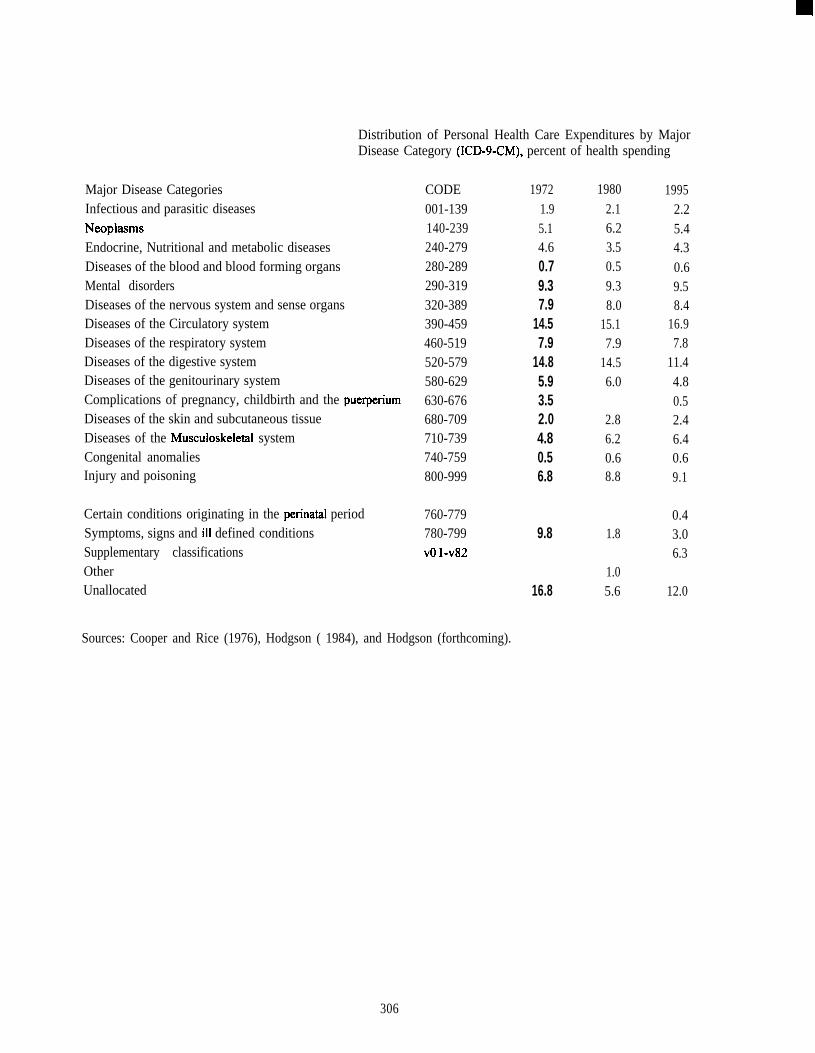
Distribution of Personal Health Care Expenditures by MajorDisease Category (ICD-9-CM), percent of health spending

Major Disease CategoriesInfectious and parasitic diseasesNeoplasmsEndocrine, Nutritional and metabolic diseasesDiseases of the blood and blood forming organsMental disordersDiseases of the nervous system and sense organsDiseases of the Circulatory systemDiseases of the respiratory systemDiseases of the digestive systemDiseases of the genitourinary systemComplications of pregnancy, childbirth and the puerperiumDiseases of the skin and subcutaneous tissueDiseases of the Musculoskeletal systemCongenital anomaliesInjury and poisoning

Certain conditions originating in the perinatal periodSymptoms, signs and ill defined conditionsSupplementary classificationsOtherUnallocated

CODE001-139140-239240-279280-289290-319320-389390-459460-519520-579580-629630-676680-709710-739740-759800-999

760-779780-799v() 1-v82

19721.95.14.60.79.37.9

14.57.9

14.85.93.52.04.80.56.8

9.8

16.8

19802.16.23.50.59.38.0

15.17.9

14.56.0

2.86.20.68.8

1.8

1.05.6

19952.25.44.30.69.58.4

16.97.8

11.44.80.52.46.40.69.1

0.43.06.3

12.0

Sources: Cooper and Rice (1976), Hodgson ( 1984), and Hodgson (forthcoming).

306

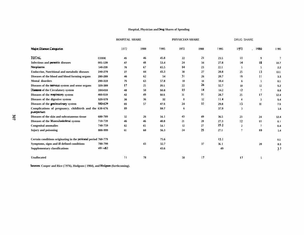
Hospital, Physician and Dmg Shares of Spending

HOSPITAL SHARE PHYSICIAN SHARE DRUG SHARE

hdajodheasefategories

TOTAL

Infectious and pamsitic diseases

Neoplasms

Endocrine, Nutritional and metabolic diseases

Diseases of the blood and blood forming organs

Mental disorders

Diseases of the nemous system and sense organs

Dkeases of the Circulatory system

Diseases of the mpiratory system

Diseases of the digestive system

Diseases of the genitourinary system

CODE

001-139

140-239

240-279

280-289

290-319

320-389

390459

460-519

520-579

580429

1972

45

47

76

27

46

75

17

48

42

36

65

Complications of pregnancy. childbirth and the 630-676 89pueq)erium

Diseases of the skin and subcutaneous tissue 680-709 32

Diseases of the Musculoskeletai system 710-739 46

Congenital anomalies 740-759 82

Injury and poisoning 800-999 61

Certain conditions originating in the perinatal period 760-779

Symptoms, signs and ill defined conditions 780-799

Supplementary classifications vO1-V82

Unallocated II

1980

46

48

67

44

62

63

25

50

49

36

57

26

46

65

60

43

78

I 995

45.8

53.4

65.5

43.3

54

57.8

20.1

50.8

50.5

32

47.5

59.7

34. I

40.8

54. I

56.3

75.6

32.7

43.6

1972

22

24

14

38

31

10

22

15

31

8

24

6

43

21

12

24

58

1980

21

34

23

27

26

10

26

18

31

1232

49

28

2725

37

17

I 995

23.5

27.8

22.1

20.8

20.7

10.4

32.7

14.2

28.711.4

29.837.9

36.527.325.2

27.1

15.1

36. I49

I 772 . 1980

II 9

14 18

5 5

25 13

16 II

6 5

10 12

12 7

25 17

4 3

13 II

3

23 24

12 11

2 7

7 10

20

17 5

I 995

7

10.7

2.2

13.1

3.3

8.1

5.2

8.8

12.4

5.4

7.5

1.6

12.4

8. I

0.4

1.4

0.1

8.3

;.7

SoUnxs: Cooper and Rice ( i 976), Hodgson ( 1984), and Hodgson (forthcoming).