Web of Knowledge Page 1 (Articles 1 -- 1)

[ 1 ]

Record 1 of 1Title: THE MICROSCOPIC-MACROSCOPIC SCALE TRANSFORMATION THROUGH A CHAOS SCENARIO IN THE FRACTAL SPACE-TIME THEORY Author(s): Munceleanu, GV (Munceleanu, G. V.); Paun, VP (Paun, V. -P.); Casian-Botez, I (Casian-Botez, I.); Agop, M (Agop, M.)Source: INTERNATIONAL JOURNAL OF BIFURCATION AND CHAOS Volume: 21 Issue: 2 Pages: 603-618 DOI: 10.1142/S021812741102888X Published: FEB 2011 Times Cited in Web of Science: 1 Total Times Cited: 1 Cited Reference Count: 29 Abstract: Considering that the particle movement takes place on fractal curves, the mathematical and physical aspects in fractal space-time theory are analyzed. In such context, the harmonic oscillator problem implies that the microscopic-macroscopic scale transition could be associated with an evolution scenario towards chaos. The splitting of the plasma plume, generated by laser ablation, into two patterns, has been successfully reproduced through a numerical simulation using the fractal hydrodynamic model. For the free time-dependent particle in a fractal space-time, the uniform movement is naturally obtained by a specific mechanism of vacuum polarization.Accession Number: WOS:000289468300018 Language: EnglishDocument Type: ArticleAuthor Keywords: Fractal space-time theory; microscopic-macroscopic scale transitionKeyWords Plus: HYDRODYNAMIC MODEL; LASER-ABLATION; RELATIVITYAddresses: [Munceleanu, G. V.] Alexandru Ioan Cuza Univ, Fac Phys, Iasi 700506, Romania [Paun, V. -P.] Univ Politehn Bucuresti, Fac Sci Appl, Dept Phys 1, Bucharest 060042, Romania [Casian-Botez, I.] Gh Asachi Tech Univ, Fac Elect Telecommun & Informat Technol, Iasi 700050, Romania [Agop, M.] Univ Sci & Technol Lille, Lab Phys Lasers Atomes & Mol, UMR 8523, F-59655 Villeneuve Dascq, France [Agop, M.] Gh Asachi Tech Univ, Dept Phys, Iasi 700050, RomaniaReprint Address: Munceleanu, GV (reprint author), Alexandru Ioan Cuza Univ, Fac Phys, Blvd Carol 1,11, Iasi 700506, RomaniaPublisher: WORLD SCIENTIFIC PUBL CO PTE LTD Publisher Address: 5 TOH TUCK LINK, SINGAPORE 596224, SINGAPORE Web of Science Category: Mathematics, Interdisciplinary Applications; Multidisciplinary SciencesSubject Area: Mathematics; Science & Technology - Other TopicsIDS Number: 749LL ISSN: 0218-1274 29-char Source Abbrev.: INT J BIFURCAT CHAOS ISO Source Abbrev.: Int. J. Bifurcation Chaos Source Item Page Count: 16

Web of Knowledge Page 1 (Articles 1 -- 1)

[ 1 ]

© 2012 Thomson Reuters Terms of Use Please give us your feedback on using Web of Knowledge.

Page 1 of 1Web of Knowledge [5.6] - Export Transfer Service

19.07.2012http://apps.webofknowledge.com/OutboundService.do

International Journal of Bifurcation and Chaos, Vol. 21 , No. 2 (2011) 603- 618 © World Scientific Publishing Company DOI: 10.1142/ S021812741102888X

THE MICROSCOPIC-MACROSCOPIC SCALE TRANSFORMATION THROUGH A CHAOS

SCENARIO IN THE FRACTAL SPACE-TIME THEORY

G. V. MUNCELEANU Faculty of Physics, "Al. I. Cuza " University, Blvd. Carol I No. 11, Iasi 700506, Romania

V.-P. PAUN Physics Department I,

Faculty of Applied Sciences, ~

Politehnica University of Bucharest, Bucharest 060042, Romania

paun@physics. pub. ro

I. CASIAN-BOTEZ Faculty of Electronics,

Telecommunication and Information Technology, "Gh. Asachi" Technical University,

Iasi 700050, Romania

M.AGOP Laboratoire de Physique des Lasers, Atomes et Molecules (UMR 8523) ,

Universite des Sciences et Technologies de Lille, Villeneuve d 'Ascq cedex 59655, France

Department of Physics, "Gh. Asachi" Technical University,

Iasi 700050, Romania

Received May 24, 2010

Considering that the particle movement t akes place on fractal curves, the mathematical and physical aspects in fractal space-time theory are analyzed. In such context , the harmonic oscil­lator problem implies that the microscopic-macroscopic scale transition could be associated with an evolution scenario towards chaos. The splitting of the plasma plume, generated by laser ablation, into two patterns, has been successfully reproduced through a numerical simu­lation using the fr act al hydrodynamic model. For the free time-dependent particle in a fractal space-time, the uniform movement is naturally obtained by a specific mechanism of vacuum polarization.

Keywords : Fractal space-time theory; microscopic-macroscopic scale transit ion.

603

604 G. V. Munceleanu et al.

1. Introduction

The complex dynamical systems which display chaotic behavior are recognized to acquire self­similarity and manifest strong fluctuations at all possible scales [Mandelbrot, 1982; Gouyet, 1992; Nottale, 1993]. Since the fractality appears as an universal property of the complex systems, it is necessary to construct a new physics, entitled fractal physics maybe, either through the non­differentiability property or through the transfi­nite sets, in the same manner as the Cantor set and its physical implications, in El Naschie's model [El Naschie et al., 1995; Weibel et al., 2005], for example. The mathematical procedures are in agreement with similar items [Olteanu et al., 2005; Cresson, 2005] and the support of relevant phys­ical processes is based on the references [N ottale et al., 2006; Celerier & Nottale, 2004]. Thus, both the scale relativity (SR) and the transfinite physics were developed. In the following, let us refer only to the SR Nottale's model i.e. to a continuous but nondifferentiable physical model. The SR uses the word "nondifferentiability" in its general meaning, denoting a set that shows struc­tures at all scales and is, thus, explicitly resolution­dependent.

The SR model is based both on the frac­tal space-time concept and on a generalization of Einstein's principle of relativity to scale transfor­mations. In other words, the SR model is built by completing the standard laws of classical physics (motion in space-time) by new scale laws. We can state that "the space-time resolutions are used as intrinsic variables, playing for the scale transforma­tion the same role as played by velocities for motion transformation" [Nottale, 1993; Nottale et al., 2006; Celerier & Nottale, 2004]. Also, in the present work, the harmonic oscillator problem is analyzed using a generalized Nottale 's model in its hydrodynamic version.

In fact, three scales of interaction of SR were developed:

(i) a "Galilean" version corresponding to the stan­dard fractals with constant fractal dimensions [Mandelbrot, 1982; Gouyet, 1992] and which involves quantum mechanics [Nottale, 1993; Nottale et al., 2006; Celerier & Nottale, 2004; Gottlieb et al., 2006; Agop et al., 2005; Agop et al., 2008b];

(ii) a special scale-relativistic version which implies the high energy physics [Nottale, 1993];

(iii) a "general scale-relativistic" version which implies the cosmology [Nottale, 1993, 1997; Agop et al. , 2007; Agop et al., 2008c].

In the accepted vision, the microscopic-macroscopic scale transition could be associated with an evolu­tion scenario towards chaos.

This paper is structured in eight sections, with the introduction as the first. In the second, the mathematical and physical aspects in fractal space­time are presented. The geodesics concept is the subject of Sec. 3 and, in Sec. 4, the hydrodynamic version in the fractal space-time is developed. In Sec. 5, the harmonic oscillator in fractal space-time is offered as an example and the hydrodynamic behavior of laser ablation plasma will be established in Sec. 6. Section 7 is devoted to the free particle in the fractal space-tim~ category and, finally, the conclusions are included in Sec. 8.

2. Mathematical and Physical Aspects in Fractal Space-Time

Let us suppose that the motion of particles takes place on continuous but nondifferentiable curves (fractal curves) with an arbitrary and constant fractal dimension, Dp. There is a diversity of fractal dimensions type, but Kolmogorov dimen­sion and Hausdorff dimension are most frequently used. For example, we present below the current definition of Hausdorff dimension [Olteanu~et al., 2005]. Let A C rytn and let C1, C2, ... be an open cover of it. More precisely, an open cover of A is defined by covers Ci such that A C LJ~1 Ci. Then, for every positive number s and E, let h~(A) = inf{Li diam(Ci) 8 I (Ci)i2'.0 is an open cover of A, diam (Ci)< E}, so that the s-dimensional Hausdorff measure of A is h8 (A) = limc:-.o h~(A).

It can be proved that there is a number DH(A) such that h8 (A) = oo if s < DH(A) and h8 = 0, ifs > DH(A). The number DH(A), the Hausdorff dimension of A, can be zero, infinite or a positive real number.

For the fixed fractal dimension type, we shall operate with it up to the end. In this paper, the Hausdorff's dimension is used.

The nondifferentiability, according with Cresson's mathematical procedures [Cresson, 2005] and Nottale's physical principles [Nottale, 1993; Nottale et al., 2006; Celerier & Nottale, 2004], implies the following:

(i) a continuous and a nondifferentiable curve (or almost nowhere differentiable) is explicitly

The Microscopic-Macroscopic Scale Transformation Through a Chaos Scenario 605

scale dependent, and its length tends to infinity, when the scale interval tends to zero. In other words, a continuous and non­differentiable space is fractal, in the general meaning given by Mandelbrot to this concept [Mandelbrot, 1982];

(ii) there is an infinity of fractal curves (geodesics) related to any couple of points (or starting from any point), and this is valid for all scales;

(iii) the breaking of local differential time reflec­tion invariance. The time-derivative of a func­tion F can be written two-fold:

(iv)

dF = lim F(t + dt) - F(t) dt dt---+D dt

= lim F(t) - F(t - dt). dt-->D dt

(1)

Both definitions are equal in the differen­tiable case. In the nondifferentiable situation, these definitions fail, since the limits are no longer defined. "In the framework of scale rel­ativity, the physics is related to the behav­ior of the function during the "zoom" oper­ation on time resolution 8t , here identified with the differential element dt ( "substitu­tion principle"), which is considered as an independent variable. The standard function F(t) is therefore replaced by a fractal func­tion F(t, dt) (for details see [Cresson, 2005]) explicitly dependent on the time resolution interval, whose derivative is undefined only at the unobservable limit dt ---t 0 [Nottale, 1993]. As a consequence, this leads us to define the two derivatives of the fractal function as explicit functions of the two variables t and dt

d+F = lim F(t + dt , dt) - F(t) dt dt-->D+ dt

(2a)

d_ F = lim F(t , dt) - F(t - dt, dt). dt dt---+D- dt

(2b)

The sign, +, corresponds to the forward pro­cess and, -, to the backward process; the differential of a fractal function F(t, dt) can be expressed as the sum of two differ­entials, one which is not scale-dependent , dF'(t) , and the other dependent on it , dF"(t) , therefore [Cresson, 2005]

dF ( t , dt) = dF' ( t) + dF" ( t, dt) . ( 3)

Particularly, the differential of the generalized coordinates, d±X(t, dt), can be decomposed as follows

where d±x(t) is the "classical part" and d±~(t , dt) is the "fractal part". Starting from here, multiplying by dt.__ 1 and using the substitutions

V _ d±X ± - dt )

d±X V± = dt '

d±~ li± =--

;:;o dt

we obtain the velocity field

(5a)

(5b)

(5c)

(6a,b)

( v) the fractal part of F, i.e. F", satisfies the relation [Cresson, 2005]

IF"(t) - F"(t') I ~it - t' l6 (7)

where 8 depends on the fractal dimen­sion Dp (for details see [Notta'le, 1993; Cresson, 2005]). Particularly, the differential of the "fractal part" of d±X, becomes

~(8a ,b)

or more, as an equality relation:

( d~~i) = ( ~) D1

F • (9a,b)

Written as

A ( dt ) ( D1

p ) - l d±~i = - - dt.

T T (lOa,b)

Equations (9a,b) imply the temporal scales 8t and T, and the length scale ,\, respectively. The significance of time dt and T results from Random Walk (Brownian motion) or its generalization, Levy motion [Nottale, 1993]. The differential time dt is identified by the resolution time ("substitution prin­ciple" [Nottale, 1993; Nottale et al., 2006; Celerier & Nottale, 2004]) , 8t = dt , while T

corresponds to the fractal-nonfractal tran­sition time. ,\ is a characteristic length, for example, of Planck's or de Broglie's type (for details see [Nottale, 1993]) ;

606 G. V. Munceleanu et al.

(vi) by the relation (10a,b) the velocity field becomes

. . . . ,\ ( T )1-(:tf-) V± = v± + u± = v± + -:; dt F .

(lla,b)

The transition scale T yields two distinct behaviors of the speed, depending on the res­olution at which it is considered, since V± ___, v~ when dt » T, and Vi___, u~ , when dt « T .

Obviously, the fractal dimension Dp also plays an important role in relations ( lla, b), but we shall consider this problem later on;

(vii) the local differential time reflection invariance is recovered by combining the two deriva­tives, d+/dt and d_ /dt, in the complex oper­ator [Nottale, 1993; Nottale et al., 2006; Celerier & Nottale, 2004]

We call this procedure "an extension by dif­ferentiability" (Cresson's extension - for details see [Cresson, 2005; Gottlieb et al., 2006]). Applying this operator to the "posi­tion vector" yields a complex speed

A dX V= ­

dt

= ! (d+X + d_X) _ !_ (d+X - d_ X) 2 dt 2 dt

V + +V_ .V +- V -2 - i 2

i - 2 [ ( v + - v _) + ( u+ - u_)]

= V-iU (13)

with

V ++ V_ 1 V =

2 = 2 [ ( V + + V _) + ( U+ + U_) ]

(14a) V+-V- 1

U = 2

= 2 [ ( V + - V - ) + ( U+ - U_ )]

(14b)

(viii)

(ix)

The real part , V, of the complex speed V, represents the standard classical speed, which is differentiable and independent of resolu­tion, while the imaginary part, U, is a new quantity arising from fractality, which is non­differentiable and resolution-dependent. In the usual classical limit , dt » T,

V+ =V_ =V,

U+ = U_ = 0

so that

V=v, U = O.

In the limit, dt « T ,

and

V+ =v-= 0,

u+~ u_ = u

V = u, U = O;

(15a)

(15b)

(16)

(17a)

(17b)

(18)

in order to t ake into consideration for the infinity of geodesics in the bundle, for their fractality and for the two valuedness of the derivative which all come from the non­differentiable geometry of the space-time con­tinuum, one therefore adopts a generalized statistical fluid like description, where instead of a classical deterministic speed or of a classi­cal fluid speed field, one uses a doublet of frac-

·:-.. tal functions of space coordinates anJ time which are also explicit functions of "resolu­tion time" [Nottale, 1993; Nottale et al., 2006; Celerier & Nottale, 2004]. Thus, the average values of the quantities must be considered in the previously mentioned sense [Nottale, 1993; Nottale et al., 2006; Celerier & Nottale, 2004]. Particularly, the average of d±X is

\d±X} = d±x (19)

with

(20a,b)

in such an interpretation, the "particles", are identified with the geodesics themselves. As a consequence, any measurement is interpreted as a sorting out (or selection) of the geodesics by the measuring device [Nottale, 1993].

Let us now assume that the movement curves (continuous, but nondifferentiable) are immersed in a three-dimensional space, and that x of components xi ( i = 1,"3) is the position vector of a point on the curve. Let us also consider a function f (X, t) and the

The Microscopic-Macroscopic Scale Transformation Through a Chaos Scenario 607

following Taylor series expansion, up to the second order:

of d± J = at dt + v f . d± x

1 82 f . . + 2 ()Xi()XJ d±Xid±X1

. (21a,b)

The relations (21a,b) are valid in any point of the space-time manifold and also for the points "X" on the fractal curve which we have selected in relations (21a,b). From here, the forward and backward aver­age values of this relation, take the form:

(22a,b)

We make the following stipulations: the mean val­ues of the function f and its derivates coincide with themselves and the differentials d±Xi and dt are independent. Therefore, the averages of their prod­ucts coincide with the product of average. Thus, Eqs. (22a,b) become:

of d±f = 8t dt + "V f (d±X )

1 321 . . + 2 8Xi8XJ (d±Xid±XJ) (23a,b)

or more, using Eqs. ( 4a, b) with the properties (20a,b),

of d±f = at dt + '\1 j d±X

1 32 f (d id j (dci dcJ ) ) + 2 ()Xi()XJ ±X ±X + '>± '> ± .

(24a,b)

Even the average value of the fractal coordinate, d~~ , is null [see ( 20a, b)], for the higher order of the fractal coordinate average, the situation can be dif­ferent. Let us focus on the mean (d~±d~~ ). If ii= j , t his average is zero due to the independence of de and d~j. So, using (lOa,b) we can write (see also [Cresson , 2005; Agop et al., 2008a, 2008b, 2008c]):

(25a,b)

with

. . { 1 if i = j 5i1 =

0 ifi-=/=j

and we had considered that

(d~~d~~) > 0 and dt > 0

(d~i_d~~ ) > 0 and dt < 0.

Then, Eqs. (24a,b) may be written under the form:

02 f .. A 2 ( dt) ( D2F ) - 1 ± . .JiJ _ - dt. ()Xi()XJ 2T T

(26a,b)

If we divide by dt, and neglect the terms which contain differential factors (for details on the method see [Gottlieb et al., 2006]) , Eqs. (26a,b) are reduced to:

d±f = of v VJ± >.2 (dt)(dF)-1 ~f

dt Ot + ± 2T T

~(27a,b)

with "V2 = 2=i 82 I 8X'f. These relations also allow us to define the operator,

d± 0 A 2 ( dt) ( D2

F ) - l -=-+V±"V± - - ~ dt Ot 2T T

(28a,b)

(see also [Agop et al., 2008b]). Under t hese circum­stances, let us calculate dj / dt. Taking into account Eqs. (12), (13) and (28a,b), we obtain:

df = ~ [(d+f d_f) - i (d+f - d_f)] dt 2 dt + dt dt dt

= - - + v + "V f + - - ~f 1 [ ( 0 j A 2

( dt ) ( D2

F ) - l )

2 Ot 2T T

( 0 j ). 2 ( dt ) ( D

2

F ) - l ) l + Ot + V - '\1 j - 2T -; ~j

608 G. V. Munceleanu et al.

i [ (a j ,\ 2

( dt ) ( D2

F )- l ) - - - + v + \7 f + - - b.f 2 at 2T 7

- ( ~~ + v - \7 f -~: ( ~) ( ,;F )- 1 1'f) l =af (V++V _ _ iV+-V- )v1

dt + 2 2

A2 (dt) (dF )-l -i- - b.f

27 7

a f A • >-2 ( dt ) ( D

2

F ) -1

= - + v . \7 f - i - - b.f. dt 27 7

(29)

This relation also allows us to define the fractal operator:

d a A >-2 ( dt ) ( D

2

F ) -1

dt = at + V . \7 - i 27 --; 6_. (30)

We now apply the principle of scale covariance (for details see [Nottale, 1993; Nottale et al. , 2006; Celerier & Nottale, 2004]), and postulate that the passage from classical (differentiable) mechanics to the "fractal" mechanics, which is considered here, can be implemented by replacing the standard time­derivative, d/ dt, by the complex operator dj dt (this result is the principle of scale covariance given by Nottale in [Nottale, 1993; Nottale et al., 2006; Celerier & Nottale, 2004]).

3. Geodesics in Fractal Space-Time

The inertial principle in its strong covariance form (Nottale 's principle [Nottale, 1993; Nottale et al., 2006; Celerier & Nottale, 2004]) is reduced to an equation of the N avier- Stokes type (geodesics equation) ,

AA A 2 ( 2 ) 1 dV av A A >- ( dt) D F - A

- = - + V · \7V - i - - b. V = 0 dt at 27 7

(31)

with an imaginary viscosity coefficient v

v = i A 2 ( dt) ( D2F )-1 27 7

(32)

This means that the local complex acceleration field , av/ at, the convective term , v . vv, and the dissipative one, b. V, reciprocally compensate at any point of the fractal curve. Moreover , the behavior of the fractal fluid is visco-elastic type or hysteretic type. Such results are in agreement with the opinions given in the books [Agop et al. , 2008a; Ferry & Goodnick, 1997]: the fractal fluid can be described by Kelvin- Voight or Maxwell rheological model with imaginary structure coefficient v. In the case of the irrotational motions:

\7 xV =O (33)

so that the speed field (13) can be expressed through the gradient of a scalar function <I>

(34)

named the scalar potential of the complex speed field: <I> = Re <I> + ilm <I>. Substituting Eq. (34) in Eq. (31) , we see

[ a<I> 1 2 . ,\

2 ( dt ) ( D

2

F ) - l l \7 - + -(\7¢) - i- - b.<I> = 0 at 2 27 7

(35)

and by an integration, a Bernoulli type equation

a.'f.. \ 2 ( d ) ( -2 )- 1

_'±' + ~(\7<I>) 2 - i~ _..!_ DF b.<I> = F(t'}' (36) at 2 27 7

with F(t) being a function which depends only on time. Particularly, for <I> of the form [Nottale, 1993]

. A 2 ( dt ) ( D

2F ) - l

<I> = -i- - ln w 27 7

(37)

where W is a new complex scalar function. For this condition, Eq. (36) takes the form

,\4 (dt) ( D~ ) - 2 ,\

2 (dt) (D2F )-l aw

- - b.w+ - - -472 7 2T 7 at

(38)

From here, "Schrodinger" type geodesics result for F(t) = 0, i.e.

~ (dt) (D~)-2 b.w + >-2 (dt) (D2

F)-1 aw = o. 472 7 27 7 at

(39)

The Microscopic-Macroscopic Scale Transformation Through a Chaos Scenario 609

Particularly, for the movement on fractal curves of the Peano's type, i.e. in the fractal dimension Dp = 2, and Compton's length and temporal scales,

.\=-n-2m0c '

n T=-­moc2'

(40a)

(40b)

Equation (55) takes the Schrodinger standard form

n2 aw - t::..w + in- =O. 2mo at ( 41)

4. Hydrodynamic Model in Fractal Space-Time

Replacing the complex speed field (34) in Eq. (31), and separating the real and imaginary parts, we obtain

8V mo at +mo V · \7V = -\7(Q) (42a)

oU .\ 2 ( dt) ( D2

F ) - l at + \7 (V . U) + 2T --:;- \7V = 0

(42b)

where Q is the fractal potential,

Q = - moU2 - mo .\2 (dt) (dF) -1 \7. U. (43) 2 2T T

The explicit form of the complex speed field is given by the expression

(44)

with p being the amplitude and S the phase. Then Eq. (34) with

,2 (d ) (-2 )- 1 . /\ t DF iS

<I>= -i- - ln(fae ) 2T T

( 45)

involves the complex velocity field components

.\2 (dt) (D2F)-l

V=- - \7S 2T T '

(46a)

.\2 (dt) (dF)-l U= - - \7lnp

2T T (46b)

while the fractal potential ( 43), is given by the simple expression

Q = - mo(dt)(D2F) -1 !:::.fa. T VP (47)

For other details see [Halbwachs, 1960; Wilhelm, 1970]. With Eqs. (46a,b) , Eq. (42b) takes the form:

(48)

or, by integration with p =/= 0

~ + \7 · (pV) = T(t) (49)

with T(t) a function which depends only on time. Equation (42a) corresponds to the momentum

conservation law, while~Eq. (49), with T(t) = 0, to the probability density conservation law. So equations:

mo ( 8

8~ + V · \7V) = -\7(Q) (50a)

~~ + \7 · (pV) = 0 (50b)

with Q given by ( 4 7) form the fractal hydro­dynamic equations in the fractal dimension Dp. The fractal potential ( 4 7) is induced by the non­differentiable space-time (for more details see [Agop et al., 2007]). Our results are more general ~ those of Nottale (the movements take place on fractal curves of Peano's type at Compton's space-time scale - i.e. the hydrodynamic model of quan­tum mechanics [Nottale, 1993; Nottale et al., 2006; Celerier & Nottale, 2004]).

The synchronization of the movements at the differentiable and non-differentiable scales implies V = - U. In such context , Eq. (50b) , through Eqs. ( 46a, b) , become a well-known differential equation for diffusion:

\7p = D!:::.. . Vt P

This equation becomes an important issue in the analysis of Brownian motion at any scale .

In an external potential U, the fractal hydro­dynamic equations become

mo ( 0

8~ + V · \7V) = - \7(Q + U) (51a)

~~ + \7 · (pV) = 0. (51b)

610 G. V. Munceleanu et al.

Two types of stationary states are distinguished:

(i) Dynamic states. For a/at= 0 and V-/= 0, i.e. at the differentiable scale, Eqs. (51a,b) give

V (mot - mo2U' - mo;: (~)(,JP) -\· U + U) ~ 0 (52a)

'V·(pV) = O (52b)

namely,

mo V 2 mo U 2 ,\

2 ( dt) ( v2

F )-1

------mo- - \7-U+U=E 2 2 2T T

(53a)

Consequently, the non-fractal inertia, mo V · 'VV, external force, -'VU and the fractal force, - \7 Q, are in balance at every field point -Eq. (52a). The sum of the nonfractal kinetic energy, m V 2 /2, external potential, U and frac­tal potential, Q, is invariant, i.e. equal to the integration constant E -/= E(r) - Eq. (53a).

pV = \7 x F. (53b)

E = (E) representQ. the total energy of the dynamic system. The probability fl.ow density pV has no sources - Eq. (52b), i.e. its stream­lines are closed - Eq. (53b).

(ii) Static states. For a/at = 0 and V = 0, i.e. at the nondifferentiable scale, Eqs. (10a,b) give

n ( mo U2

,\ 2

( dt) ( v2

p ) -1

) v ----mo- - \7-U+U =0 2 2T T

(54a)

i.e.

mo U 2 ,\ 2 ( dt) ( D2

F ) - l ----mo- - 'V·U+U=E.

2 2T T ~(54b)

Thus, the fractal force, - \7 Q and external force - 'VU are in balance at every field point -Eq. (54a). The sum of the external potential, U and fractal potential, Q, is invariant, i.e. equal to the integration constant E -/= E ( r) -Eq. (54b). E = (E) represents the total energy of the static system. Equation ( 51 b) is identi­cally satisfied.

As an illustration of the fractal hydrody­namic formalism, a static fractal system is further analyzed.

5. Harmonic Oscillator in Fractal -Space-Time

This model describes a particle of rest mass mo in a field of the form:

In a stationary state, the one-dimensional current density is constant through Eq. (52b ).

j(x) = p(x)V(x) = C = const. (56)

From here, by imposing the boundary conditions:

p(x = -oo) = p(x = +oo) = 0 (57)

we get C = 0, meaning that the velocity field V(x) is

V(x) = 0. (58)

From ( 58) and ( 46a) , we see that S is constant , i.e. the fluid particles are in phase. Therefore, at the macroscopic (differentiable) scale, we have a coherent fluid with a behavior of either suprafiu­idic or supraconductor type. Moreover, a momen­tum transfer does not exist on the velocity field

The Microscopic-Macroscopic Scale Transformation Through a Chaos Scenario 611

V(x). For a static state, the momentum conserva­tion law, with the restrictions (54b), becomes:

d\fi5 [ E ( fl )2

2] dx2 + 2moD2 - 2D x VP = O,

p(x = - oo) = p(x = +oo) = 0

D = A 2 ( dt) ( D2p )-1 2T T

(59a)

(59b)

(59c)

or further, by introducing the dimensional variable:

(60)

d\fi5 ( E 2) d( 2 + moDO - ( VP = O,

-oo ~ ( ~ +oo, p(( = -oo) = p(( = + oo) = 0.

(61a- c)

A solution p(() = Pn(() exists if and only if the total energy is quantified:

E = 2moDO ( n +}), n = 0, 1, 2,... (62)

The following probability density is found :

( ) - /fl_l_H2 (C)e- e Pn ( - V 2;[j 2nn! n <,, (63)

with the Hermite's polynomials of degree n [Nikiforov & Ouvarov, 1974].

For movement on fractal curves of the Peano's type, i.e. in the fractal dimension DF = 2, and Compton's length and temporal scales, i.e. for D = n/2m0 , from (62) and (63), the usual results of quantum mechanics are obtained. For DF < 2, from (59c), we get dt « T, i.e. the time resolution is much smaller than the fractal-nonfractal transition time, while for DF > 2, from (59c), we get dt » T, i.e. the time resolution is much greater than the fractal­nonfractal transition time. Now, using (63), we can build the one-dimensional fractal velocities field:

d ~[ Hn-1(() ] Ux = D dx(lnp) = vDO 2n Hn(() - ( (64)

respectively the fractal potential:

Q = _ 2m0D2

d2

(VP)=_ mou~ _ m Ddux n VP dx2 p 2 ° dx

= moD0(2n + 1 - e) (65)

where we used the relations [Nikiforov & Ouvarov, 1974]:

dH;((() = 2nHn-1(() (66a)

Hn(() - 2(Hn-1(() + 2(n - l)Hn-2(() = 0.

(66b)

Therefore:

(i) There is a nonzero velocity field, (64), gen­erated through a fractal process and hence a transfer of momentum.

(ii) The velocity field (64) "controls", through the fractal potential (65), "the flow regimes" of a fractal fluid.

(iii) The "observable" ~from the clasical quantum mechanics given Jnder the form of quantified energy:

En = Qn + U = 2moDO ( n + 1) (67)

allows the implementation of Reynold's criterium:

n = 0, 1, 2, ...

through the notations

1 2 En = 2m0Ve '

Ve= 4Rerl,

v=D

~

(68a,b)

(69a)

(69b)

(69c)

where Ve is a critical flow velocity, Re is a critical length through which the flow takes place, and v is a "viscosity" coefficient specific to the fractal fluid. There is a minimum value of the Reynolds number, n = 0, and which, through the notations:

6'.px = mo Ve,

~x=Re

(70a)

(70b)

introduces, for Peano's movements at Compton ' scale, i.e. for DF = 2 and D = n/2mo, a Heisen­berg's "egalitarian" relationship [Ballentine, 1998; Phillips, 2003]:

n ~Px~X = 2· (71)

For big Reynold's numbers, n < +oo, the flow regime of the fractal fluid becomes turbulent. In other words, the microscopic-macroscopic scale transition could be associated with an evolution

612 G. V. Munceleanu et al.

scenario towards chaos (equivalent to the Ruelle­Takens mechanism [Cristescu, 2008; Jackson, 1991]), through which a coherent fractal fluid, at microscopic scale, becomes turbulent (incoherent, normal) at macroscopic scale.

6 . The Hydrodynamic Behavior of Laser Ablation Plasma

In the usual theories of plasma physics, in which the charged particle movements take place on con­tinuous and differentiable curves (kinetic or bi-fluid type theories [Goldston & Rutherford, 1995]) , it is difficult to determine either the collision terms or source terms in connection with the elementary plasma processes (excitations, ionizations, recombi­nations, etc.). A new way to analyze the plasma dynamics is to consider that the charged parti­cle movements take place on continuous but non­differentiable curves, i.e. on fractals [Mandelbrot, 1982; Gouyet, 1992; Nottale, 1993; Nottale et al., 2006; Celerier & Nottale, 2004]. Then, the complex­ity of these dynamics is substituted by fractality. There are some fundamental arguments which can justify such hypothesis:

(i) by collision, the trajectory is no longer every­where differentiable. The "uncertainty" in tracking the particle is eliminated by means of the fractal approximation of motion;

(ii) the complex dynamical systems as plasma, which display chaotic behavior, are recognized to acquire self-similarity and manifest strong fluctuations at all possible scales [Nottale, 1993; El Naschie et al., 1995; Weibel et al., 2005].

For example, in laser ablation plasma [Gurlui et al. , 2008], the conductive behavior manifests at µs time scale, while the convective behavior, at ns time scale. In such context, every type of elementary process from plasma induces both spatial-temporal scales and the associated fractals. Moreover, the movement complexity is directly related to the frac­tal dimension: the fractal dimension increases as the movement becomes more complex [Mandelbrot, 1982; Gouyet, 1992]. Different definitions were given for the fractal dimension (Kolmogorov dimension, Hausdorff dimension, etc. [Gouyet , 1992]), but once we choose the fractal-type dimension in the study of motion we must work with it until the end. There­fore, considering that the complexity of the physical

processes from plasma is replaced by fractality (sit­uation in which the particle movements take place on fractal curves) then, it is no longer necessary to use notions as collision time, mean free path, etc., i.e. the whole classical "arsenal" of quantities from plasma physics [Goldston & Rutherford, 1995]. Then plasma will behave as a special collision-less fluid through geodesics in a fractal space-time [see Eqs. (50a,b)]. In the following, we shall analyze the dynamics of a laser plasma ablation. Let us rewrite the hydrodynamic equations of the scale relativ­ity, Eqs . (50a,b), for the two-dimensional case and Cartesian coordinates, in the following form:

on 0 0 ot + ox (nvx) + oy (nvy) = 0

"' o o 2 o op ot (nvx) + ox (nvx) + oy (nvxvy) = - ox

o o o 2 op ot (nvy) + ox (nvxvy) + oy (nvy) = - oy

(72a)

(72b)

(72c)

where we considered that the fractal potential ( 4 7) plays the role of the internal pressure p such that

1 VQ = -Vp,

p

p=nm.

(73a)

(73b)

The assumption is not singular, it was also used in [Gurlui et al., 2008]. By introducing th~ non­dimensional coordinates:

wt= t , (74a)

kx = x, (74b)

ky = y (74c)

Vxk (74d) - =Vx,

w Vyk _ - =Vy, w

(74e)

n (74f) n= -

no

and by admitting that the pressure variation is only due to concentration variation (we consider that the expansion process of the ablation plasma is isotherm) , that is:

(75)

with kB the Boltzmann constant and T the charge carriers temperature, Eqs. (72a)-(72c) become:

on o o ot + ox (nvx) + oy (nvy) = 0 (76a)

The Microscopic-Macroscopic Scale Transformation Through a Chaos Scenario 613

In expressions (76b) and (76c), we considered the scaling relation for the unit mass, (m= 1), kBTk2/w 2 := 1.

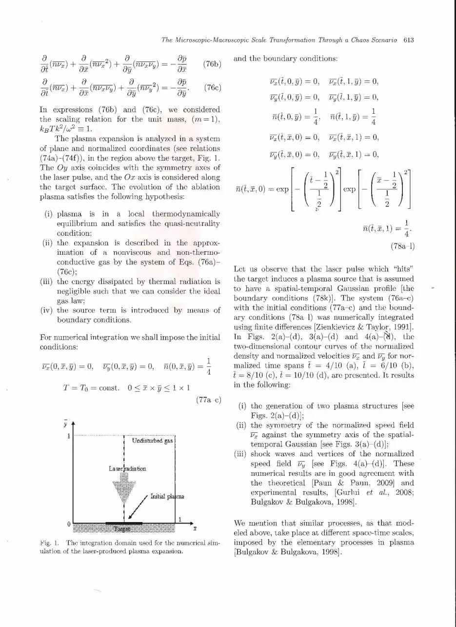
The plasma expansion is analyzed in a system of plane and normalized coordinates (see relations (74a)- (74f)), in the region above the target, Fig. 1. The Oy axis coincides with the symmetry axes of the laser pulse, and the Ox axis is considered along the target surface. The evolution of the ablation plasma satisfies the following hypothesis:

(i) plasma is in a local thermodynamically equilibrium and satisfies the quasi-neutrality condition;

(ii) the expansion is described in the approx­imation of a nonviscous and non-thermo­conductive gas by the system of Eqs. (76a)­(76c);

(iii) the energy dissipated by thermal radiation is negligible such that we can consider the ideal gas law;

(iv) the source term is introduced by means of boundary conditions.

For numerical integration we shall impose the initial conditions:

vx(O, x, y) = 0, vy(O, x, y) = 0, 1

n(O,x,y) = 4 T =To= const. 0:::; xx y:::; 1 x 1

(77a-c)

1 ...... ·· ·· ····· ....... ····•··· 1 UOOisturbed gas

• •

!/"~""~ 0 \'-~~--------... ~~~-1-;;._+

Fig. 1. The integration domain used for the numerical sim­ulation of the laser-produced plasma expansion.

and the boundary conditions:

Vx(t, 0, y) = 0, Vx(t, 1, y) = 0,

vy(t, 0, y) = 0, vy(t, 1, y) = 0,

n(t, o, y) = l' n(t, 1, y) = l vx(t ,x,0) = 0, vx(t,x, 1) = 0,

vy(t , x, 0) = 0, vy(t, x, 1) = 0,

n(i , x,o)~=[-(tj~)']cxp[-(xi~)'] n(t, x, 1) = l·

(78a-l)

Let us observe that the laser pulse which "hits" the target induces a plasma source that is assumed to have a spatial-temporal Gaussian profile [the boundary conditions (78k)]. The system (76a- c) with the initial conditions (77a-c) and the bound­ary conditions (78a- l) was numerically integrated using finite differences [Zienkievicz & Taylor, 1991].

·)\

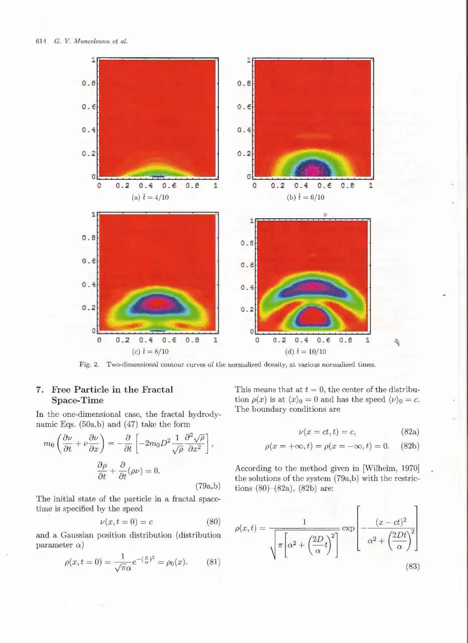
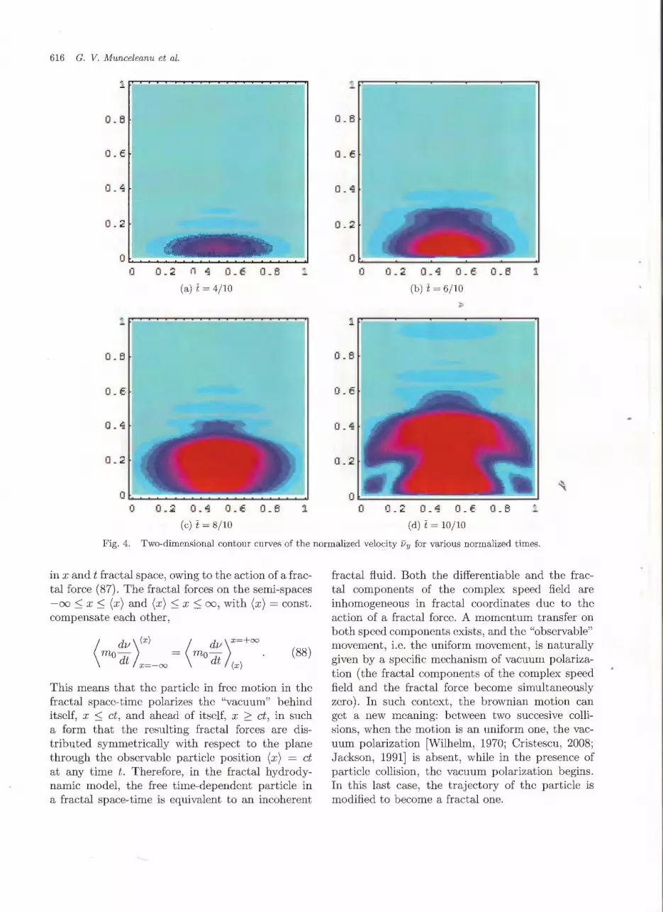
In Figs. 2(a)-(d), 3(a)-(d) and 4(a)-(81), the two-dimensional contour curves of the normalized density and normalized velocities Vx and Vy for nor­malized time spans t = 4/10 (a), t = 6/10 (b), t = 8/10 (c), t = 10/10 (d), are presented. It results in the following:

(i) the generation of two plasma structures [see Figs. 2(a)- (d)];

(ii) the symmetry of the normalized speed field Vx against the symmetry axis of the spatial­temporal Gaussian [see Figs. 3(a)-(d)];

(iii) shock waves and vertices of the normalized speed field Vy [see Figs. 4(a)- (d)]. These numerical results are in good agreement with the theoretical [Paun & Paun, 2009] and experimental results, [Gurlui et al., 2008; Bulgakov & Bulgakova, 1998].

We mention that similar processes, as that mod­eled above, take place at different space-time scales, imposed by the elementary processes in plasma [Bulgakov & Bulgakova, 1998].

614 G. V. Munceleanu et al.

(a) t = 4/10

IL B

0 0. 2 0 - i£ O . .S (L B

(c) t = 8/10

0

0 . .:3 0 .6

(b)t=6/10

1J.6 0.8

(d) t = 10/ 10

:1

Fig. 2. Two-dimensional contour curves of the normalized density, at various normalized times.

7. Free Particle in the Fractal Space-Time

In the one-dimensional case, the fractal hydrody­namic Eqs. (50a,b) and (47) take the form

mo ( [)z; + l/ av) = - !!__ [-2moD2 _1 32 VP] ' at ax at VP ax2

op a at + at (pv) = 0·

(79a,b)

The initial state of the particle in a fractal space­time is specified by the speed

v(x, t = 0) = c (80)

and a Gaussian position distribution (distribut ion parameter a)

1 ( x )2 p(x , t = 0) = r,;; e- o: = po(x) . (81) y7ra

This means that at t = 0, the center of the distribu­tion p(x) is at (x)o = 0 and has the speed (v)o = c. The boundary conditions are

v(x = ct, t) = c, (82a)

p(x = +oo, t) = p(x = - oo, t) = 0. (82b)

According to the method given in [Wilhelm, 1970] the solutions of the system (79a,b) with the restric­tions (80)- (82a), (82b) are:

(83)

The Microscopic-Macroscopic Scale Transformation Through a Chaos Scenario 615

(L Ei

(LB

!L 15

JJ - ~

o_ ~ 0_6 Q_B

(a) t = 4/10

(L ':'2 1L6

(c) t = 8/10

0 - :.:!

l o _~ Q _':'2 0. 6 O.B

(b) t = 6/10

(d) t = 10/10

Fig. 3. Two-dimensional contour curves of the normalized velocity !ix for various normalized times.

and

(84)

Equations (83) and (84) represent the fractal­hydrodynamic solution of the free motion of a particle at the differentiable scale. At the non­differentiable scale, the speed field of the particle

u(x t) = D8lnp = -2D x - ct (85)

' ox a 2 + ( 2: t y gets "felt" through the fractal potential

mou2 ou Q = --2- -moD ox

1 + 2m0 D 2 2 (86)

a2 + (2: t)

and the fractal force

F = - oQ = ox

4moD2(x - ct)

[ a2 + ( 2: t) r . (87)

While the observable motion of the particle is uni­form, (v) = c, the associated motions both at the differentiable scale - see Eq. (84) and at the non­differentiable one - see Eq. (85) are inhomogeneous

616 G. V. Munceleanu et al.

1L B

0 .6

0 - ·~

0 O. if· O.B

(a) t = 4/10

!L 8.

(d) t = 10/10

Fig. 4. Two-dimensional contour curves of the normalized velocity Dy for various normalized times.

in x and t fractal space, owing to the action of a frac­tal force ( 87) . The fractal forces on the semi-spaces -oo S x S (x/ and (x/ s x s oo, with (x/ = const. compensate each other,

\

dv )(x) _ \ dv )x=+= mo - - mo-

dt x=- = dt (x) (88)

This means that the particle in free motion in the fractal space-time polarizes the "vacuum" behind itself, x S ct, and ahead of itself, x ;::: ct, in such a form that the resulting fractal forces are dis­tributed symmetrically with respect to the plane through the observable particle position (x/ = ct at any time t. Therefore, in the fractal hydrody­namic model, the free time-dependent particle in a fractal space-time is equivalent to an incoherent

fractal fluid. Both the differentiable and the frac­tal components of the complex speed field are inhomogeneous in fractal coordinates due to the action of a fractal force. A momentum transfer on both speed components exists, and the "observable" movement , i.e. the uniform movement, is naturally given by a specific mechanism of vacuum polariza­tion (the fractal components of the complex speed field and the fractal force become simultaneously zero). In such context , the brownian motion can get a new meaning: between two succesive colli­sions, when the motion is an uniform one, the vac­uum polarization [Wilhelm, 1970; Cristescu, 2008; Jackson, 1991] is absent, while in the presence of particle collision, the vacuum polarization begins. In this last case, the trajectory of the particle is modified to become a fractal one.

The Micrnscopic-Macrnscopic Scale Transformation Thrnugh a Chaos Scenario 617

8. Conclusions

The main conclusions of the present paper are the fol owing:

(i) Considering that the motion of the par­ticles takes place on continuous but non­differentiable curves, i.e. on fractals with constant arbitrary fractal dimension Dp, mathematical and physical aspects are pre­sented.

(ii) It results in a Navier- Stokes-type equation with an imaginary viscosity coefficient, and from here, in the particular case of irrota­tional movement , a Schrodinger-type equation. The standard Schrodinger equation is obtained as a particular case of irrotational movement at Compton scale, with the constant fractal dimension Dp = 2.

(iii) Fractal hydrodynamic model results from a Navier-Stokes-type equation by separating the real and the imaginary parts of the complex speed field. The model is described through a momentum transport equation and a conser­vation law of the probability density.

(iv) Using the SR model in its hydrodynamic ver­sion, the harmonic oscillator is analyzed. The complex speed field of the fractal fluid proves to be essential: the zero value of the real (differentiable) part specifies the fractal fluid coherence (superconductor or super-fluid type behavior), while the nonzero value of the imag­inary (nondifferentiable or fractal) part selects, through the energy quantification condition, the stationary trajectory of the fractal fluid particles. Moreover, the momentum transfer is achieved only through the fractal component of the complex speed field of the fractal fluid and, the same fractal component , imposes totally the "observable" in the form of energy which is quantified. The "observable" from the clasi­cal quantum mechanics given under the form of quantified energy allows the implementa­tion of Reynold's criterium. In such a context, for a minimum value of the Reynolds number and Peano's movements at Compton scale, a Heisenberg's "egalitarian" relationship results. Moreover, for big Reynold's numbers, the flow regime of the fractal fluid becomes turbulent. In other words, the microscopic-macroscopic scale transition could be associated with an evolution scenario towards chaos (equivalent to the Ruelle- Takens mechanism), through

which a coherent fractal fluid , at microscopic scale, becomes turbulent (incoherent, normal) at macroscopic scale.

( v) The hydrodynamic behavior of a laser plasma ablation has been numerically simulated through the momentum and particle num­ber conservation laws. In these conditions, the splitting of the plasma plume into two patterns has been successfully reproduced.

(vi) For the free time-dependent particle in a frac­tal space-time, both the differentiable and the fractal components of the complex speed field are inhomogeneous in fractal coordinates due to the action of a fractal force. There exists a momentum transfer on both speed components and, the "observable" movement , i.e. the uni­form movement, it' naturally given by means of a specific mechanism of vacuum polariza­tion. More precisely, the particle in free motion in the fractal space-time polarizes the "vac­uum" behind itself and ahead of itself. The resulting fractal force field is distributed sym­metrically with respect to the plane through the observable particle position. On this plane, the fractal speed field and the fractal force are null for any time. In such a context, a new interpretation on the Brownian motion is possible.

References

Agop, M., Ioannou, P. D. & Nica, P. [2005] "Super­conductivity by means of the subquantum medium coherence," J. Math. Phys. 46.

Agop, M., Nica, P., Ioannou, P. D. , Malandraki, 0. & Gavanas-Pahomi, I. [2007] "El Naschie's epsilon (infinity) space-time, hydrodynamic model of scale relativity theory and some applications," Chaos Solit. Fract. 34, 1704- 1723.

Agop, M., Ioannou, P. D., Nica, P. E. & Paun, V. P. [2008a] The Fractal and its Implications in the Mate­rial Science (Athens University Press, Greece).

Agop, M., Nica, P., Ioannou, P. D. , Antici, A. & Paun, V. P. [2008b] "Fractal model of the atom and some properties of the matter through an extended model of scale relativity,'' Eur. Phys. J. D 49, 239- 248.

Agop, M., Nica, P. & Girtu, M. [2008c] "On the vacuum status in Weyl- Dirac theory,'' Gen. Relat. Gravit. 40, 35- 55.

Ballentine, L. E. [1998] Quantum Mechanics. A Modern Development (World Scientific, Singapore).

Bulgakov, A. V. & Bulgakova, N. M. [1998] "Gas­dynamic effects of the interaction between a pulsed laser-ablation plume and the ambient gas: Analogy

618 G. V. Munceleanu et al.

with an under expanded jet," J. Phys. D 31 , 693- 703.

Celerier , M. N. & Not t ale, L. [2004] "Quantum-classical transition in scale relativity," J. Phys. A: Math. Gen. 37, 931- 955.

Cresson, J. [2005] "Non-differentiable variational principles," J. Math. Anal. Appl. 307, 48- 64.

Cristescu, P. [2008] Nonlinear Dynamics and Chaos. Theoretical Fundaments and Applications (Academy Publishing House, Bucharest).

El Naschie, M. S. et al. [1995] Quantum Mechanics, Diffusion and Chaotic Fractals (Elsevier , Oxford).

Ferry, D. K. & Goodnick, S. M. [1997] Trans­port in Nanostructures (Cambridge University Press, Cambridge).

Goldston, R. J. & Rutherford , P. H. [1995] Introduction to Plasma Physics (CRC Press, Bristol).

Gottlieb , I ., Agop, M., Ciobanu, G. & Stroe, A. [2006] "El Naschie 's epsilon (infinity) space-time and new results in scale relativity theories," Chaos Solit. Fract. 30, 380- 398.

Gouyet , J . F. [1992] Physique et Structures Fractales (Masson, Paris).

Gurlui , S., Agop , M., Nica, P., Ziskind, M. & Focsa , C. [2008] "Experimental and theoretical investigations of a laser-produced aluminum plasma,'' Phys. Rev. E 78 , 026405 .

Halbwachs, F. [1960] Thorie Relativiste des Fluides Spin ( Gaut hier-Villars , Paris).

Jackson, E. A. [1991] Perspectives in Nonlinear Dynam­ics (Cambridge University Press, Cambridge).

Mandelbrot , B. [1982] The Fractal Geometry of Nature (Freeman, San Francisco).

Nikiforov, A. & Ouvarov, V. [1974] lments de la Thorie des Fonctions Spciales (Mir , Moskow).

Nottale, L. [1993] Fractal Space- Tim e and Microphysics: Towards a Theory of Scale Relativity (World Scien­tific, Singapore).

Nottale , L. [1997] "Scale-relativity and quantization of the universe. l. Theoretical fr amework," A stron. A strophys. 327, 867- 889.

Nottale, L., Celerier , M. N. & Lehner , T. [2006] "Non­abelian gauge field theory in scale relativity," J. Math. Phys. 47, 032203 (1- 19).

Olteanu, M., Paun, V. P. & Tanase, M. [2005] "Frac­tal analysis of zircaloy-4 fracture surface ," Revista de Chimie 56, 97- 100. ~

Paun, V. P. & Paun, M. A. [2009] "Theoretical model of polymer plasma laser ablation," Materiale Plastice 46 , 339- 340.

Phillips, A. C. [2003] Introduction to Quantum Mechan­ics (John Wiley and Sons, NY) .

Weibel, P. et al. [2005] Space-Time Physics and Fractal­ity (Springer, Vienna, NY).

Wilhelm, H. E. [1970] "Hydrodynamic model of quantum mechanics ," Phys. R ev. D l , 2278- 2285.

Zienkievicz, 0. C. & Taylor, R. L. [1991] The Finite Elem ent Method (McGraw-Hill , NY) .