Embed Size (px)
Citation preview

THE IMPACTS OF THE FEDERAL AID HIGHWAY PROGRAM
ON STATE AND LOCAL HIGHWAY EXPENDITURES
by
LEONARD SHERMAN
S.B., Massachusetts Institute of Technology(1971)
S.M., Massachusetts Institute of Technology(1971)
Submitted in partial fulfillment
of the requirements for the degree of
Doctor of Philosophy
at the
Massachusetts Institute of Technology
February, 1975A
Signature of Author. . . . . . .Department of Civil Engineepng, January 22, 1975
Certified by . . . . . . . . . . . . . . .Th9sis Supervisor
Accepted byI..I......Chairman, Departmental Committwon Graduate Studentsof the Department of Civil Engineering
A P F 17

2
ABSTRACT
THE IMPACTS OF THE FEDERAL AID HIGHWAY PROGRAM ON
STATE AND LOCAL HIGHWAY EXPENDITURES
by
LEONARD SHERMAN
Submitted to the Department of Civil Engineering onJanuary 22, 1975 in partial fulfillment of the
requirements for the degree of Doctor of Philosophy
This thesis investigates the impacts of the Federal Aid Highway Programon State and local highway expenditures. Our concern throughout theconduct of the research is to focus on this issue from a national policyperspective. Several recent events have led to an increasing interestin restructuring the Federal role in highway finance, most notably thecontroversy surrounding the passage of the 1973 Federal Aid Highway Actand the debate over post-Interstate System highway policy. Accordingly,the motivation of this research is a consideration of the design of andresponse to Federal Aid highway financing.
The starting point is a review of the mechanics of State and Federalhighway finance. Special attention is given to the unique aspects of theFederal Aid Highway Program (FAHP) and the attendant implications forempirical modelling. The thesis then proceeds to develop a theory ofState highway expenditure behavior. Our purpose here is to draw atten-tion to the premise that State highway expenditure behavior depends notonly on the level of available Federal grants-in-aid, but on the struc-tural characteristics of the grant program as well. The theoreticalmodels suggest that for the Interstate program, Federal grants havestimulated State expenditures that would most likely have not been madein the absence of the grant program. This behavior is contrasted withthe experience on the non-Interstate Federal Aid programs where thetheoretical models suggest that Federal grants have had a relativelyinsignificant impact on States' expenditure levels.
The theoretical hypotheses of State expenditure behavior are thenvalidated with econometric models designed to explore the factorsinfluencing States' total highway expenditure levels and the alloca-tion of States' highway budgets amongst alternative expenditure cate-gories. The models are estimated using a pooled data sample compris-ing the forty eight mainland States over a fourteen year analysisperiod.

3
Evaluation of the empirical results from the expenditure models suggestseveral basic policy recommendations for future Federal highway policy.Most notably, it is recommended that the U.S. Department of Transporta-tion undertake a grant consolidation program, eliminate existinggrant matching provisions, and restructure current apportionment factorsand Interstate Highway Trust Fund revenue mechanisms.
Thesis Supervisor: Marvin Lee Manheim
Professor of Civil EngineeringTitle:

4ACKNOWLEDGEMENTS
Throughout the course of this research, I have benfitted from theadvice, encouragement and assistance from many individuals. The contri-butions of Professor Marvin L. Manheim, my thesis advisor to the devel-opment of this study extend far beyond his valuable suggestions on par-ticular phases of the research. In a larger sense, he has been singlu-larly influential in stimulating my interest in the anlysis of trans-portation policy issues. Professors Paul Roberts, Wayne Pecknold,and Moshe Ben-Akiva, as members of my doctoral committee providedseveral valuable ideas and suggestions that aided in both the develop-ment of the theoretical analyses and in the writing of the final manu-
script. I would also like to express particular appreciation to Pro-fessor Richard Tresch of Boston College. I have benfitted greatly fromreading his own research in this field. And as a member of my doctoralcommittee, Professor Tresch's advice and encouragement have contributedgreatly to the development and presentation of the ideas in thisdissertation.
Several individuals in the U.S.Department of Transportation alsodeserve special mention for their role in assisting in the conductof this research. Ira Dye of the Office of Transportation PlanningAnalysis is gratefully acknowledged for his constant encouragementand for arranging the financial support by DOT that allowed this studyto be undertaken. Arrigo Mongini and George Wiggers, also in theOffice of Transportation Planning Analysis have been extremely helpfulin contributing numerous keen insights throughout the conduct of thisresearch. In addition I would like to express my appreciation to EdGladstone and Bill McCallum of the Federal Highway Administration forfreely giving of their time, advice and encouragement during the for-mative stages of this research.
To my friends and colleagues at M.I.T., in particular Frank Kop-pelman, Uzi Landau and Steve Lerman, I would like to express my thanksfor their constant help alon the way. Bronwyn Hall of the HarvardBureau of Economic Research must also be acknowledged for jer assis-tance in ironing out problems encountered in using the computer forthe econometric analysis phases of this research.
And finally, my thanks go to the numerous people who contributedgreatly to the preparation of the final document: Carol Walb, CharnaGarber, Charlotte Goldberg, Rebecca Lord and Shulamit Kahn.

5
TABLE OF CONTENTS
Page
TITLE PAGE...........................
ABSTRACT.............................
ACKNOWLEDGEMENTS.....................
TABLE OF CONTENTS....................
LIST OF FIGURES... ..............
LIST OF TABLES.................
CHAPTER I: Introduction and Summary..
I.1 Motivation for Research
1.2 Summary of Previous Studies
1.3 Modelling Strategy
1.4 Theoretical Models of State
1.5 The Empirical Study
1.6 Summary and Conclusions
1.7 Organization of the Thesis
Expenditure Behavior
CHAPTER II: The Mechanics of Highway Finance: AFactual Settin ........................
II.1 Introduction
11.2 Historical Development of the Federal AidHighway Program
i. The Early Federal Aid Highway Acts
ii. The Federal Aid Primary System
iii. The Federal Aid Secondary System
iv. Urban Extensions of the Primary andSecondary Systems
v. The Federal Aid Urban System
1
2
4
5
11
15
18
18
22
28
33
36
45
47
50
50
52
52
64
65
66
66

6
Page
vi. Traffic Operations Projects to IncreaseCapacity and Safety 69
vii. The Federal-Aid Interstate System 69
viii. Structural Revisions to the FAHP Incor-porated in the 1973 Federal-Aid HighwayAct 71
11.3 The Mechanics of the Interstate HighwayTrust Fund 74
i. Program Structure 74
Source of Federal Funds 74
Total Expenditure Levels 74
Expenditure Restrictions 77
Local Recipients of Federal Funds 79
Authorization Cycle 79
Apportionment Method 79
Matching Provisions 80
Sources of Local Matching Funds 80
ii. Time Lag Structure 87
iii. Aspects of Trust Fund Taxation 97
Definitions of the Revenue Terms 98
Income Redistributive Propertiesof the IHTF 100
Equity Considerations in Admini-stering the IHTF 112
II.4 Comparison of the Federal-Aid Highway ProgramWith the Federal Public TransportationAssistance Program 119
Sources of Federal Funds 119
Total Expenditure Levels 119
Authorization Cycle 120
Apportionment Method 120
Matching Provisions 121
Expenditure Restrictions 121
7
Page
Local Recipients of Federal Funds 122
Sources of Local Matching Funds 122
11.5 Summary and Conclusions 124
CHAPTER III: The Federal-Aid Highway Program: The Ana-lytics of Design and Response................ 129
III.1 Introduction 129
111.2 Fiscal Federalism - The Normative Aspects ofFederal Highway Grant Program Design 133
i. The Theory of Intergovernmental Grants 134
ii. Functional Grants as Solutions 138
iii. Practical Limitations of the ExternalBenefit Criterion 142
iv. Additional Goals of the Federal AidHighway Program 146
v. Theoretical Aspects of Policy Evaluation 150
111.3 The Analytics of State Responses to FederalGrants 153
i. The Basic Model 154
ii. Addition of a Conditional Matching Open-Ended Grant 156
iii. Analysis of Conditional Matching Close-Ended Grants 162
iv. Evaluation of Other Grant Program Structures 169
v. Summary of the Responses to AlternativeGrant Structures 174
vi. Qualifications of the Theoretical Analyses 181
111.4 The Analytics of State Responses to FederalGrants: The Benefit/Cost Investment Model 186
i. A Hypothetical Example 186
ii. A liagrammatic Description 193

8
Page
iii. Conclusions from the Benefit/CostInvestment Model 195
111.5 Observed Expenditure Patterns: The Impact ofthe ABC and Interstate Programs 198
i. Data Analysis of the ABC Highway Program 199
ii. Data Analysis of the Interstate HighwayProgram 203
111.6 Summary and Conclusions 208
CHAPTER IV: Development of the Total Expenditure Model.... 211
IV.1 Introduction 211
IV.2 Derivation of the Model 213
IV.3 Estimation Techniques for the Total Expen-diture Model 218
Error Component Analysis 222
IV.4 The Data Set and Modelling Considerations 229
i. The Socio-Economic Descriptors 231
ii. The Measurement of Highway Capital Stocks 239
iii. Descriptors of Financing Conventions andInstiutional Characteristics 247
iv. The Highway Grant Terms 248
v. The Price Deflators 251
IV.5 Research Strategy and Conseiderations forModel Interpretation 253
i. The Total Expenditure Model: Consider-ations for Model Interpretation 253
ii. Data Set Stratification 256
IV.6 Empirical Results 258
i. The Federal Grant Terms 263
ii. Differences in Grant Term CoefficientsBetween the Two Data Subsets 271

9
Page
iii. Interpretation of the Coefficient Estimatesof the Socio-Economic and InstitutionalDescirptor Variables
State Size Variables
The Income Measures
Institutional Characteristics
The Existing Inventory Measure
iv. The Deflated Data SEt
v. Tests of Equality Between Coefficients inthe Two Data Subsets
IV.7 Summary and Conclusions
CHAPTER V: Development of the Short Run Allocation Model..
V.1 Introduction
V.2 Derivation of the Short Run Allocation Model
V.3 Statistical Properties and EstimationProcedures
V.4 Modelling Considerations and Data Requirements
Equation 1 - The Interstate Construc-tion Share
Equation 2 - The Primary System Con-struction Share
Equation 3 - The Secondary System Con-
struction Share
Equation 4 - The Non-Federal-Aid Sys-stem Construction Share
Equation 5 - The Maintenance Expendi-ture Share
Equation 6 - The "Other" ExpendituresShare
V.5 Empirical Results - Parameter Estimates of theSRAM
V.6 Evaluation of the Elasticities and DerivativesFrom the Short Run Allocation Model
272
272
275
275
277
277
280
285
289
289
292
307
313
318
320
321
323
324
326
327
339
-

10
Page
V.7 Integration of the Results From the TotalTotal Expenditure Model and the Short RunAllocation Model: Long Run Responses 351
i. Socio-Economic Charactersistics 362
ii. Highway System Charactersistics 363
V.8 Summary 366
CHAPTER VI: Summary and Conclusions...................... 368
VI.1 Summary of the Thesis 368
VI.2 Policy Implications of the Empirical Findings 373
VI.3 Limitations of the Empirical Approach andDirections for Further Research 380
Bibliography............................................ 383
Biographical Summary ................................ 390
Appendix A: Estimated Parameter Values of the Long RunRevenue Policy Model...................... 391
Appendix B: Derivation of Derivatives and Elasticitiesfrom the Expenditure Models................427
Appendix C: Derivatives and Elasticities from theTwo Expenditure Models....................440

11
LIST OF FIGURES
Figure Title Page
1.3.1 State Highway Investment Behavior........... 29
1.4.1 The Total Expenditure Model ..................... 37
1.4.2 The Short Run Allocation Model................. .. 39
1.4.3 Elasticities of the Categorical Expenditures.... 42
11.2.1 State Expenditures on the Federal AidSystems......................................... 62
11.3.1 States Having Anti-Diversion Consti-tutional Amendments............................. 86
11.3.2 Frequency Distribution of InterstateObligations..................................... 90
11.3.3 Frequency Distribution of ABC Obligations ....... 91
11.3.4 Federal Aid Highway Program Lag Structure ....... 94
11.3.5 Interstate Highway Trust Fund Expendituresand Receipts.................................... 96
111.2.1 Internal and External Highway Benefitsand Costs.................................... 136
111.3.1 Highway Investment Indifference Curves.......... 155
111.3.2 Analysis of Conditional Matching Open-Ended Grants............... .............. 157
111.3.3 Grant Responses for Alternative PriceSubsidies....................................... 160
111.3.4 Analysis of Conditional Matching Close-Ended Grants.................................... 163
111.3.5 Affect of Grant Ceilings and PriceSubsidy Levels................................ 168

12
LIST OF FIGURES (Continued)
Figure Title Page
III.3.6 Analysis of Conditional, Non-MatchingClose-Ended Grants.............................. 170
III.3.7 Analysis of Responses to Grants for FunctionsNot Previously Undertaken by StateGovernments................................... 173
111.3.8 Summary of State Responses to AlternativeFederal Grant Structures........................ 175
111.4.1 Illustrative Example of the Benefit/CostInvestment Model.............................. 188
111.4.2 Diagrammatic Illustration of the Benefit/Cost Investment Model.......................... 194
IV.4.1 The Total Expenditure Model..................... 230
IV.4.2 Lorenz Curves................................... 237
IV.4.3 Depreciation Functions.......................... 246
IV.6.1 Estimation Results, Total ExpenditureModel Number SUl............................... 259
IV.6.2 Estimation Results, Total ExpenditureModel Number SU12............................... 260
IV.6.3 Estimation Results, Total ExpenditureModel Number SU6............................... 261
IV.6.4 Estimation Results, Total ExpenditureModel Number TUl2............................... 262
IV.6.5 Estimation Results, Total ExpenditureModel Number SU21.............................. 264
IV.6.6 Estimation Results, Total ExpenditureModel Number SU31............................. 265

LIST OF FIGURES (Continued)
Figure
IV.6.7
IV.6.8
IV.6.9
V.2.1
V.2.2
V.4.1
V.5.1
V.5.2
V.5.3
V.5.4
V.5.5
V.5.6
V.5.7
V.5.8
Title
Estimation Results, Total ExpenditureModel NumberS .........................
Estimation Results, Total ExpenditureModel Number 5D21.. ......................
Estimation Results, Total ExpenditureModel Number SD3l .........................
Constrained Estimation Form for theShort Run Allocation Model................
Corner Solutions in the SRAM...............
The Short Run Allocation Model.............
48 State Sample, OLS SRAM Product FormEstimation Results.........................
48 State Sample, GLS SRAM Product FormEstimation Results.............................
7 State Sample, OLS SRAM Product FormEstimationResults.....................
7 State Sample, GLS SRAM Product FormEstimationResults .......................
41 State Sample, OLS SRAM Product FormEstimation Results..................
41 State Sample, GLS SRAM Prodcut FormEstimation Results..........................0
48 State Sample OLS SRAM LExponential FormEstimation Results.....,...................
48 State Sample. GLS SRAM Exponential FormEstimationResults ........................
Page
256
267
268
300
304
316
329
330
331
332
333
334
335
336

14
LIST OF FIGURES (Continued)
Figure Title Paje
V.6.1 48 State Sample Short Run Model Derivatives..... 343
V.7.1 48 State Sample Long Run Model Derivatives...... 356
V.7.2 48 State Sample Long Run Model Elasticities.... 359

15
LIST OF TABLES
Table Title Page
11.2.1 Year in Which First State-Aid Law Passedand Highway Department Created.............. 54
11.2.2 Date of Authorization or Creation ofState Highway Systems........................... 58
11.2.3 Factors Employed in Apportioning FederalAid System Funds (Prior to Federal AidHighway Act of 1973) ....................... 67
11.2.4 Current Factors Employed in ApportioningFederal Aid System Funds...................68
11.3.1 Trust Fund Revenue Sources............ ...... 75
11.3.2 Interstate Highway Trust Fund Revenue BySource - Calendar Year 1970............... 76
11.3.3 Interstate Highway Trust Fund Receipts andAuthorizations................. .......... 78
11.3.4 Variable Matching Percentage for States WithMore Than Five Percent of Public Lands.......... 81
11.3.5 State Highway Finance: Highway Bond Sales,1961-1971...................................... 83
11.3.6 Distribution of Person Miles by Incomeand Type of Transport....................... 102
11.3.7 Distribution of Auto Travel Patterns byHousehold Income Levels.........................104
11.3.8 Relationship of Mode Choice and HouseholdIncome for Home-to-Work Trips................... 105
11.3.9 Relationship of Average Commute Time for Home-to-Work Trips by Household Income............... 106

16
LIST OF TABLES (Continued)
Table Title Page
11.3.10 Comparison of Estimated State Paymentsto the Highway Trust Fund with StateReceipts from the Highway Trust Fundand Federal Aid Apportionments; FiscalYears 1957-1970............................... 108
11.3.11 Distribution of 1968 Mileage of TravelOn and Off Federal Aid Systems byFunctional System in Urban Areas byPopulation Group.............................. 114
11.3.12 Incremental Costs of Rush Hour Travelby Various Modes.............................. 116
11.3.13 Total Federal Trust Fund ExpenditureAllocation versus Tax Payments.................. 118
111.3.1 Summary of Equilibrium Expenditure Patterns..... 158
11.3.2 Comparison of Equilibrium Points forAlternative Grant Structures Shown inFigure 111.3.4................................ 165
11.3.3 Summary of Grant Responses.................... 180
111.5.1 State Expenditures Over and Above MinimalMatching Requirements Expressed as aFraction of Total Expenditures on"ABC" Systems................................. 200
111.5.2 ABC System Expenditures/Grants: New York,1963........................................ 204
111.5.3 State Expenditures Over and Above MinimalMatching Requirements Expressed as aFraction of Total Expenditures onthe Interstate System.......................... 206
IV.4.1 Percent of Population Residing in Urban PlacesWith More Than 5000 Residents.................... 234

17
LIST OF TABLES (Continued)
Table Title Page
IV.4.2 Measures of Income Inequality, 1963............. .240
IV.4.3 Consumer Price Index........................... 252
IV.6.1 Direction of the Influence of theExplanatory Variables on Total StateHighway Expenditures...........................278
IV.6.2 Tests of Selected Subset CoefficientEqualities.................................... 284

18CHAPTER I
INTRODUCTION AND SUMMARY
I.1 Motivation for Research
This study is concerned with the impact of Federal aid financing on
the highway expenditures of State and local governments. Tne moti-
vations for this research are numerous. First, it is aimed at provi-
ding useful input to the ongoing debate over structural changes in the
Federal aid highway program. Although Federal responsibility for the
financing of highway facilities has been increasing in recent years,
both in terms of the extent of activity and the amounts of money
involved, the basic principles upon which the Federal aid highway
program operates was established over 50 years ago in the Federal-Aid
Act of 1916. For the first time proposals have been advanced which, in
one case will allow Federal monies to be used for non-highway urban
mass transit systems,I and in another, would establish non-modally
aligned block funding for a broad spectrum of transportation activities
(including non-capital expenditures).2 In order to evaluate the con-
sequences of these, and other program variants, it is first necessary
to assess the impacts of the existing Federal grant-in-aid program.
By any measure, the Federal aid highway program represents a large
expenditure of funds. Its magnitude, combined with its singular status
as a restricted trust fund, provide a second motivation for
As embodied in the Federal-Aid Highway Act of 1973.2As embodied in S.1693: the Special Transportation Revenue Sharing Actof 1969.

19focusing this analysis on the Federal aid highway program. Federal
expenditures for highways in 1970 amounted to $4.84 billion,I second
only to Federal welfare payments ($6.47 billion2). Moreover, Federal
highway outlays account for a large percentage of total (by all units
of government) highway expenditures,, averaging 27% nationwide, and
over 60% in some States (1970).3 Consequently, changes in the struc-
ture of the Federal aid highway program (e.g., amounts of Federal
money available, changes in the matching provisions, etc.) may cause
significant changes in State and local governmental highway invest-
ment behavior. Viewed in this perspective, the structure of the
Federal aid highway program is a significant policy tool with which
the U.S. Department of Transportation can influence the pattern of
highway investments. 4 To exploit this potential, an understanding
of the dynamics of State and local transportation investment be-
havior is essential.
A third motivation for focusing this investigation on the
Federal aid highway program as opposed to the broader question of
IFederal Highway Administration, HIGHWAY STATISTICS, 1970.
2Advisory Commission on Intergovernmental Relations, STATE-LOCALFINANCES: SIGNIFICANT FEATURES AND SUGGESTED LEGISLATION, 1972 ed.
3ibid.
4In this regard, the federal aid highway program has been used asa tool to counteract cyclical fluctuations in the Nation's economy.During the recession of the late 1950's, Congress appropriated$600 million (the so-called "D" funds) in addition to the appropri-ations for the Interstate and "ABC" programs, for the purpose ofstimulating governmental expenditures. For a description of theState response to the D fund program, see Friedlaender, A.F., "TheHighway Program as a Public Works Tool," pp. 93-101, in Ando, A.,

1 20intergovernmental fiscal relations (in all functional areas ), is that
it allows for a more detailed analysis of the complexities involved in
State and local investment decision-making behavior. There exists
ample evidence to suggest that States' expenditure responses to Federal
functional grants (e.g. highways, welfare, education, etc.) exhibit
more significant trade-offs amongst expenditures within a particular
function than between different functions. Federal grants for public
assistance provide one example. Since their inception in 1935, these
grants have been restricted to specific categories of needy people,2
leaving general welfare payments as the sole responsibility of States
and metropolitan areas. The experience has been that the States were
liberal in expanding the welfare programs in the Federally eligible
categories, and parsimonious in spending for general (non-aided) relief.3
et al., STUDIES IN ECONOMIC STABILIZATION, The Brookings Institution,1968.
In this thesis, we will be more concerned with the allocativeimpacts of the Federal aid highway program than with the use of Federalfunds in conjunction with a stabilization policy. We will raise theissue of whether Federal aid stimulates State expenditures (i.e. overand above the amounts required to simply match Federal funds).
IFor a general discussion on the characteristics of the variousfunctional Federal aid programs, see: Break, G.F., INTERGOVERNMENTALFISCAL RELATIONS IN THE UNITED STATES, The Brookings Institution, 1967;Maxwell, J.A.,, FINANCING STATE AND LOCAL GOVERNMENTS, The BrookingsInstitution, Revised Edition, 1969.
2There are currently five major Federal aid welfare programs: Old AgeAssistance, Aid to the Blind, Aid to the Permanently and TemporarilyDisabled, Aid for Dependent Children, and Medicaid.
3Maxwell, J.A.,"Federal Grant Elasticity and Distortion," National TaxJournal, Vol XXII , No. 4, pp. 550-552

Highways present perhaps an even more striking example where 21
State/local responses to Federal grants are more manifest in expen-
diture adjustments between particular highway categories, than in
overall adjustments to the State budget. Here too, Federal grants
are directed at designated types of highways,I leaving expenditures
on other highway-related activities to the discretion of the States.
Moreover, State restrictions on the use of their own trust fund
monies2 indicate that there is minimal interaction between investment
decisions in the highway "sector" and other sectors (e.g. welfare,
health, education, etc.) of the State budget.
In short a basic premise of this research is that investigation
of the impacts of the functional Federal grants in aid must explicitly
consider State/local expenditure responses within the aided function.
Thus, we will be more concerned with the magnitude of State highway
expenditures and the allocation of these expenditures amongst various
highway programs, than in attempting to trace the overall State/local
budget responses to Federal grants in terms of broadly defined
functions.
IFor example, Federal aid highway programs include capital grants forInterstate, Primary ("A"), Secondary ("B"), Urban Extension Roads("C").
2Twenty eight States have "anti-diversion" (State) constitutionalamendments. In all but four of the 50 states, gas tax and motorvehicle revenues are earmarked exclusively for highway relatedexpenditures.

1.2 Summary of Previous Studies 22
Whether we approach the subject from a normative or a postive
stance, the central issue is an analysis of the consequences of al-
ternative congressional actions. From a normative perspective, we
must know how the marketI reacts to various program structures so that
we can choose a policy which in some sense optimizes public sector
decision making. From a positive analysis stance, we must establish
a framework for predicting how the market will react to specific
policies (in particular, the existing program structure), so that we
can determine directions for incremental changes in program structure.
Thus, the central issue is a consideration of the design of, and the
response to Federal aid highway financing.
These questions have not gone totally unanswered in the lit-
erature, (although few researchers have chosen to focus their efforts
specifically on the highway sector). And yet, despite the formidable
array of recent statistical articles which purport to measure the
affects of federal grants on State/local spending, we do not as yet
have conclusive answers to such questions as: Have increasing levels
of Federal highway aid stimulated additional State/local spending, or
have Federal grants served mainly as a substitute for State expen-
ditures? How will the recently increased Federal share of "ABC"2
In this context, we make use of the term "market" to signify theinvestment pattern of State and local transportation decision-makingunits.
2The Federal-Aid Highway Act of 1970 stipulated that as of fiscal year1974, the Federal share of Primary, Secondary, and Urban Extension ("ABC")expenditures would increase from 50% of project cost to 70% of projectcost.

23road expenditures affect the allocation of highway investments in
Wisconsin? Will this behavior differ significantly from that of West
Virginia (or any other State for that matter)? If so, what factors --
social, economic, demographic, and political will temper their separate
reactions?
Our task would be relatively simple if we can address these
questions by simply adapting existing empirical studies to an investi-
gation of highway investment behavior. This is not the case however,
because neither of the two general approaches to estimating State/local
expenditure models advanced to date are appropriate for our purposes.
The first, and most common approach found in the literature has
been advanced by Sacks and Harris, Osman, and researchers.I The basic
method here is to estimate a model of State and Local expenditures in
a variety of functional categories, as a function of Federal grants and
socio-economic indicators. The National Tax Journal, which has served
as a forum for these articles since 1957, has published each new study
on the basis of the:
1) introduction of a new variable which apparentlyincreases the explanatory power of the models
Sacks, Seymour, and Richard Harris, "The Determinants of State andLocal Government Expenditures and Interfovernmental Flow of Funds,"National Tax Journal, Vol. XVII, No. 1Osman, J.W., "The Dual Impact of Federal Aid on State and LocalGovernment Expenditure," National Tax Journal, Vol XIX, No. 4Gabler, L.R., and J.I. Brest, "Interstate Variations in Per CapitaHighway Expenditures," National Tax Journal, Vol. XX, No. 1Fisher, Glenn W., "Interstate Variations in State and Local GovernmentExpenditures," National Tax Journal, Vol. XIV, No. 2

242) incorporation of different structural model forms -- e.g.
log-linear as opposed to linear
3) discussion of a new technique for including grants-in-aid as explanatory variables.
The basic problem with these studies is that they proceed with-
out an underlying model of individual State preferenczs. No account
is taken of the States' budget constraint, and as such, the essential
interdependence between functional activities (i.e. that a decision
to increase expenditures on one function must simultaneously by
compensated by reduced expenditure on others, or an increase in taxes)
is ignored. A second weakness with these approaches is their failure
to distinguish between long and short run State responses. In all but
O'Brien's study,1 a single year cross section of State expenditures
is regressed against explanatory variables (including Federal grants)
of the same year. This raises two immediate questions, both related
to inferring time series information from cross section data. First
we must question the validity of assuming (as the previously cited
studies implicity do) that States and localities react fully and
Kurnow, Ernst, "Determinants of State and Local Expenditures Reexamined",National Tax Journal, Vol. XVI, No. 3Fisher, Glenn W., "Determinants of State and Local Government Expen-ditures: A Preliminary Analysis," National Tax Journal Vol.XIX , No.3Bishop, George A., "Stimulative Versus Substitutive Effects of StateSchool Aid in New England," National Tax Journal, Vol.XVII , No.2Pogue, Thomas F., and L.G. Sgontz, "The Effect of Grants-in-Aid onState-Local Spending," National Tax Journal, Vol.XVIII, No. 1O'Brien, T., "Grants-in-Aid: Some Further Answers," National Tax Jour-nal, Vol. XXIV, No. 1Sharkansky, Ira, "Some More Thoughts About the Determinants of Govern-ment Expenditures," National Tax Journal, Vol.XXII , No. 4
1op cit

25immediately to changes in the explanatory variables. And second, we
must question the value of "one-shot" cross section models in light of
the likelihood of inter-temporal instability of the cross section
estimates.
These questions will be considered in greater detail in Chapter
V. We raise these issues here in order to stress the inadequate
treatment of the impact of Federal grants-in-aid on State and local
highway expenditures advanced to date. In summary, our basic objec-
tion to these studies (and at the same time, a starting point for the
methodology to be advanced by this study) are:
1) they fail to distinguish intra-(highway) functionallocation tradeoffs from the less significant inter-function State allocation decision-making process
2) they fail to account explicitly for the influence of aconstrained budget on allocation choices
3) no distinction is made between short and long run ex-penditure responses
4) a limited data set - usually a single year cross sectionis employed in the estimation of models.
Some of these objections are overcome in the second general
approach that has been taken in estimating the affects of Federal
grants-in-aid on State and local expenditures. The common theme of
the studies advanced by Henderson1, Gramlich2, and Tresch3 , is that
IHenderson, James M., LOCAL GOVERNMENT EXPENDITURES: A SOCIAL WELFAREANALYSIS, Unpublished Ph.D. Thesis, University of Minnesota, 1967.
2Gramlich, Edward M., "Alternative Federal Policies for StimulatingState and Local Expenditures: A Comparison of Their Effects,"National Tax Journal, Vol. XXI, No. 2.
3Tresch, Richard W., ESTIMATION OF STATE EXPENDITURE FUNCTION, 1954-1969, Unpublished Ph.D. Thesis, M.I.T., 1973.

States' expenditure decisions can be described in a manner analogous 26
to the (individual) consumer utility maximization framework. Thus,
the starting point of these analyses is the specification of the
States' utility function (in terms of the variety of functional activ-
ities, i.e. expenditure categories) and a budget constraint. The actual
demand relations for public good consumption which are empirically
estimated are derived from first order utility maximization conditions.
Our criticism here is not so much with the theoretical under-
pinnings of these models1, as with their treatment of the highway
expenditure question. Neither the Henderson2 or Gramlich3 study dis-
aggregate State and local expenditures by functional (in particular,
highway) category. As such, their results are not germane to the
questions which motivate the present study.
The Tresch thesis was the first study to employ both cross
It is important, however, to recognize that adoption of the State-as-utility-maximizer framework implies rather heroic assumptionson the political and administrative realities of State expenditurebehavior. In particular, the use of social indifference maps implythe existence of a well defined, consistent set of preferences forpublically provided goods. If we choose to regard these preferencesas belonging to a governmental body, then we must assume that thelegislature accurately expresses societal preferences. Furthermore,we must assume that the often conflicting preference orderings ofdifferent governmental agencies can be subsumed into one -- in somesense "final" -- utility mapping. See chapter III.
2Henderson's model is directed towards explaining the factors in-fluencing inter-county differences in per-capita total county govern-ment spending. His data set is a single year 3080 county crosssection.
3Gramlich uses a time series formulation on quarterly national account(all State aggregate) data. As such, his results explain neither
inter-function, nor inter-State expenditure behavior.

section and time series data in estimating State expenditures in a 27
variety of functional areas (including highways) within a utility
maximizing model framework. He correctly addresses the second and
fourth weaknesses (cited on page 25 ) of the previous studies by ex-
plicitly accounting for the influence of the States' budget constraint
on the provision of publically provided goods, and testing for the
stability of his cross section estimates over time. But he fails to
distinguish between intra and inter-function expenditure tradeoffs,
and ignores possible time lagged expenditure responses. These omis-
sions are particularly serious for the highway sector.I
The structure of Tresch's model "explicitly recognizes the
,2simultaneous nature of State expenditure decisions, whereas we have
argued that the States' highway budgeting and decision making insti-
tutions operate quite apart from other State functional expenditure
decisions. Because the underlying structure of his model assumes an
expenditure interaction which is not relevant, it is not surprising
for Tresch to conclude that "the transportation equation is most
notable for what is missing, rather than the single variable (per-
centage of State population living in urban areas) that entered
significantly."3
1Tresch focuses his research on State welfare expenditure behavior.Since these expenditures are financed from States' general taxrevenues (as are other non-highway expenditures), and Federal grantsare provided on a year-to-year basis (i.e. there is no "grace period"for grant obligation analogous to the highway program), his assumedstructure seems reasonable. The problem is that he applies thisstructure to the estimation of highway expenditure response.
2Tresch, op cit, page 21
3ibid, page 374. Variables that proved insignificant include: drivingage population, Federal Highway grants, population growth rates, allincome variables, and ratio of debt to total revenues.

281.3 Modelling Strategy
The basic premise of this research is that States' highway invest-
ment behavior can be separated from the overall State budgetary process.
In this context, it is useful to distinguish between State highway
revenue (or total expenditure) policy -- i.e. long range fiscal planning,
and allocation policy -- i.e. short range project programing. In the
simplest sense, we can say that policy decisions in the first category
determine the level of State highway expenditures over several years,
while the second policy determines the allocation of a (predetermined)
budget amongst alternative geographical areas and highway projects
within the State on a year-to-year basis.
Figure I.1 summarizes the hypothesized structure of highway
investment behavior that will be adopted in this study. The depicted
structure is recursive in nature, wherein the determination of highway
revenue is non-project specific, and allocation policy reflects project
selection given a fixed budget.
The fiscal planning policy model is based on the States' widespread
use of Needs Studies.I Perceived needs (expenditures), K are deter-
mined by design standards (d), traffic and socio-economic indicators
(A), institutional characteristics and financing conventions (I), and
the age and mix of the existing highway stock (K). Given the gap
Needs Studies develop a State's perceived highway expenditure levelnecessary to provide road service at a level consistent with currentstandards. All States have conducted Needs Studies, both for fiscalplanning purposes, and in conjunction with the FHWA's NationalHighway Needs Study.

29
STATE HIGHWAY INVESTMENT BEHAVIOR
{I} + REVENUE/FISCAL
{d} + {G}PLANNING POLICY
F]+{A} + KI {T},B3 + [R] +[ET]
{A}
{GF [{E}] ALLOCATIONPOLICY
{K} {I} {A}
NOTATION
* +
{dJ E
{A} E{I} {K} B
K*
GFGF
{T} B
B
[R)
(E9E
{GF} F
{E} B
vector of values of bracketed term
decision stage
desired value of variable
design criteria (standards)
socio-economic descriptorsinstitutional characteristics
mix and age of existing highway stock
desired highway plant ("needs")
total amount of Federal highway grants
highway-related State tax rates
amount of bond obligation assumed
highway-related revenue
total highway expenditures
program components of Federal aid
highway expenditures on each of several categories
Figure 1.3.1

30between perceived (desired) highway stock K , and available revenues --
determined by existing tax rates CT), tax base, (A), approved bond
issues B, and Federal grants, GF -- the State exercises its adopted
revenue policy by adjusting tax rates, seeking new bond issues, and
possibly effecting transfers to or from State general tax revenues.
These policy decisions ultamiately determine available highway revenues
R, and total State highway expenditures ET'
While the administrative and political realities of altering tax
rates and debt obligation inhibit quick adjustments to changes in costs
and demand 1, the project selection (programming) process operates on a
relatively short cycle time.2 In figure I.1, allocation policy is
reflected by the choices of expenditure levels (E), i.e. the component
categories (Interstate, Primary, Secondary, and maintenance, etc.) of
highway expenditure. These choices are influenced by the categorical
provisions of Federal aid (GF), the fixed State highway budget R
(as determined by revenue policy), and the traffic and socio-economic,
and institutional characteristics of the State.
The specification of the empirical models of total expenditure
and allocation policy that are empirically estimated in this thesis
follow the block recursive structure shown in figure I.1. In its
simplest form, the total expenditure model asserts that:
IBond approval is usually issued over a two to five year period. Theaverage duration between tax rate adjustments is even longer -- some-what over ten year during the 15 year period 1951-1965.
2We refer here to the time required to obligate funds for particularprojects (in response to changes in Federal aid, travel demand, etc.),not the construction time to complete individual projects.

31
(1) TOTAL STATE HIGHWAY GAP BETWEEN EXISTING AMOUNTS OFEXPENDITURES FROM = f AND DESIRED HIGHWAY , FEDERAL H/WOWN RESOURCES STOCK GRANTS REC'D.
The allocation model builds on the study of Treschl where the
States' highway investment demands for each expenditure category are
derived as first order conditions2 from a utility function and budget
constraint (where the budget constraint is determined in the revenue
policy model) specification. We argue in chapter III that adoption of
the utility maximization framework does not necessarily impose an un-
realistic assumption on the motivations of State highway investment
behavior. In fact, the fundamental premise of our model specification
is simply that States allocate their fixed highway budget so as to
maximize their derived benefits (utility)3 .
To state the allocational process formally, let Ei represent
State expenditure on category i; ET represent total expenditures from
the State's own resources; GF represent total Federal aid received by
the State. The model asserts that States allocate their budget so as
to maximize their utility, U:
lop cit2We refer to the optimization conditions that requires marginalutility to equal marginal cost for each investment alternative.
31t should be noted here that this study is largely limited toallocational problems, and questions of economic efficiency. Wewill not dwell on the distributional implications of specifichighway tax systems or investment decisions. Nor will we raisethe issue of whether the States' investment behavior trulyrepresent the preferences of a voting polity, or simply repre-sent a set of decisions made by an isolated bureaucratic agency.

32(2) max U = U(EI , E2,..., En)
subject to
Ei = ET + GF
We are not directly concerned with the utility function itself but
with first order maximization conditions which provide the investment
relations:1
(3)EXPENDITURES STATE SOCIO- TRANSPOR- FEDERAL TOTALDEVOTED TO = g ECONOMIC AND TATION AID FOR HIGHWAYCATEGORY i INSTITUTIONAL CHARAC- CATE- REVENUE
CHARACTERISTICS, TERISTICS, GORY i,
The essential structure of the revenue policy model and the
allocation policy model have been presented in this chapter in their
simplest form. We have ignored for the moment, specification of
appropriate dynamic structures, the distinction between the price and
income effects of Federal grants, and the specification of a capital
stock adjustment process. These details are left for later chapters.
Our purpose in briefly outlining the model structure here is to indi-
cate the differences in the approach that will be followed in this
thesis from the previous studies in this area.
IThe derivation of these first order condition relations requiresan assumption on the fom of the utility function. The derivationis discussed fully in chapter V.

331.4 Theoretical Models of State Expenditure Behavior
One of the major findings of this research is that both the
level and structure of Federal grant programs influence State expend-
iture behavior. It is useful to characterize a grant structure
according to the following provisions:
--categorical vs. non-categorical--matching vs. block funding--open-ended vs. close-ended
The first distinction relates to whether the grant is restricted to
expenditure on specific activities. The second classification dis-
tinguishes grants requiring specified matching funds from grants with
no matching provision. Finally, the open vs. close-ended classifica-
tion distinguishes grant programs with predetermined authorization
ceilings from those programs placing no limit on available Federal
Aid. The current Federal Aid Highway Program (FAHP) is an example
of categorical, matching close-ended grants. A transportation reve-
nue sharing program would exemplify non-categorical, close-ended
block funding.
While the empirical models employed in this research are
perfectly general (in the sense that they may be used to assess the
expenditure impacts of any grant structure) , the fact is that the
structure of the FAHP did not change over our analysis period (1957-
1970). For this reason, it is important to develop theoretical
models that enable the formulation of hypotheses describing the
expected State expenditure responses to various structural variants
of the FAHP.

Two theoretical models of State expenditure behavior are 34
advanced in this thesis -- one based on an application of consumer
allocation theory and the other based on a simple benefit/cost
investment criterion. Although these theoretical analyses apparently
differ with respect to their underlying assumptions, in fact the con-
clusions drawn from both approaches are quite similar. Both the
models draw attention to the rice and income effects introduced by
Federal grants, and proceed to demonstrate how State responses will
differ according to the presence of one or both of these grant charac-
teristics.
In simplest terms, a price effect refers to the allocational
responses to grants which effectively reduce the perceived price (or
benefit/cost ratio) of a particular aided function. An income effect
describes changes in expenditure patterns resulting from grants which
increase States' available resources, but do not alter the prices of
alternative highway facilities. The importance of the theoretical
models is to demonstrate the relationship between the structural
characteristics of a grant (e.g. matching vs. non-matching) and the
corresponding price and income effects of the grant in State expendi-
ture behavior. The major findings here are twofold. First, grants
providing price subsidies on specific highway categories will induce
a more significant reallocation of State highway expenditures (both
in terms of concentrating expenditures on the aided function and
increasing total expenditure levels) than grants (of like amount)
that serve solely as income subsidies. Second, it was shown that
grants which are ostensibly characterized by matching provisions may
in fact be (allocationally) equivalent to income subsidies. That is,

35the notion of marginality was introduced to distinguish between non-
binding matching grants and grants which effectivel serve as price
subsidies.
The latter finding is particularly germane to the evaluation of
the Federal Aid Highway Program. It is shown that although both the
ABC and Interstate programs are characterized by matching provisions,
ABC grants are not of sufficient magnitude to serve as price subsidies
at the States' investment margin. Accordingly, the theoretical models
indicate (and the emperical models validate) that changes in the level
of Interstate grants will have a greater allocational impact on the
States' highway investments than changes in the level of ABC grant
funding.
A complete typology of alternative Federal highway grant struc-
tures and the theoretical modelling framework to assess their relative
impacts is presented in chapter III.

1.5 The Empirical Study 36
The empirical models developed in this research attempt to
explain the factors influencing States' total highway expenditures
(the total expenditure model - TEM) and allocation decisions (the
short run allocation model - SRAM ), amongst alternative highway
expenditure categories. The data set employed in the estimation of
the empirical models consists of a fourteen year time series (1957-
1970) of a 48 State cross section.Thus the pooled time series/cross-
section data set yields 672 (14 years x 48 States) observations of
State highway expenditures, Federal grant availability, and socio-
economic, institutional and highway inventory descriptors.
While it would have been desirable to estimate separate expen-
diture models for each State (i.e. as forty eight separate time
series), lack of sufficient time series data precluded this approach.
Accordingly, both the total expenditure model and the allocation
model were estimated using the pooled (time series plus cross-section)
data set. In addition to the use of the full pooled data set, sev-
eral estimations were performed on selected subsets of the data --
for example singling out those States with conspicuously low Inter-
state expenditures over and above minimal matching requirements.
Several alternative specifications of the total expenditure
model were estimated using both price deflated and undeflated data.
The basic form of the TEM is presented in figure 1.2. The first eight
explanatory variables in the model correspond to the set of socio-
economic and institutional characteristics which influence a States'
perception of "desired" highway capacity (c.f. equation 1). The

37
THE TOTAL EXPENDITURE MODEL
RU= a0 + a 2*SPOP + a2*UFAC + a 3*PCY + a4*GINI + a 5*RLTOT
+ a6*TOLPCT + a7*BIPTCX + a 8*KSTK + ag*AVNIGP
+ a10*AVIGP + u
ere: Ru = State expenditures on highways exclusive ofFederal per capita grants
a 0= constant terms
a = estimated coefficients
SPOP = State population
UFAC = percent of population residing in urban areas
PCY = per capita State income
GINI = index of income inequality
KSTK = present discounted value of highway capital stockper capita
RLTOT = percent of total expenditures (all units ofgovernment) contributed by local (i.e. countyand municipal) governments
BIPTCX = percent of total capital expenditures providedfor by debt financing
AVNIGP = apportioned "ABC" grants (three year movingaverage) per capita
AVIGP = apportioned Interstate grants (three year movingaverage) per capita
u = error term
Figure 1.5.1
wh

38variable KSTK serves as a proxy for existing highway inventories.
Finally, the availability of Federal highway aid is represented by
AVNIGP and AVIGP -- a three year moving average of non-Interstate and
Interstate grants respectively.1
The short run allocation model actually consists of six dis-
tinct structural equations -- one for each expenditure category --
although the estimation technique employed explicitly accounts for
the joint interaction between shares.2 The estimated form of the
SRAM is reproduced in Figure 1.3. As indicated, the six shares con-
sidered in this analysis consist of expenditures on the Interstate
System, Primary System, Secondary System, non-Federal Aid System
construction, maintenance and a miscellaneous expenditure category.
The dependent variable in each of the equations of the SRAM
represents the share of total expenditures devoted to a particular
highway expenditure type. Similar to the total expenditure model,
the explanatory variables fall into three categories; socio-ecunumic
and highway system characteristics (SPOP, UFAC, GINI, PCY, KSTK,
PCCRMT, PCMF, KSTK), institutional characteristics (TOLPCT, RLTOT)
and the highway grant terms (AVIG, AVNIG, AVPG, AVSG and AVTG).
IThe use of three year moving averages was employed to account for twofactors. First, since Federal aid highway grants are actually avail-able for obligation over a three to three and one-half year period,inclusion of just a single years' grant would not accurately reflectthe multi-year grant availability. Second, the use of moving aver-ages partly accounts for the fact that States may not fully and im-mediately adjust to changes in Federal grant availability.
21n effect, the six equations are not independent. Since the sum ofthe shares must equal 1.0, an increase in expenditures on one cate-gory must be accompanied by a decrease in expenditures in one ormore of the remaining share categories ( in conformance with thebudget constraint).

THE SHORT RUN ALLOCATION MODEL
ESoal 1 a. 2 a1 T a14 a15 a 16SHARE 1: E= a SPP UFAC 2 KSTK %OLPCTaAVIGa5AVNIG
ET 1
SHARE 2: E aaSPOPa21UFACa 22KSTKa23AVPGa24AVIGa26
SHARE 3: SOa30P 31UFAC 32GINI33TSPMR 34PCCRMT 35AVSG 36AVIG 37
T
SHARE 4: EN 40UFAC 41 PCCRMT 42 RLTOT 43AVIG 4 4
SHARE 5: EM a a51 KSTKa52PCMFa 53RLTOT a54AVTGa55rE=Ta50
SHARE 6: E5 = a6 SPa61PCY a62KSTKa62RLTOT a63AvrGa64Tir 5
Figure I.5.1
w4

40EI = total State Interstate expenditures (State and Federal)
EP = total. Primary System expenditures
ES = total Secondary System expenditures
EN = non-Federal-Aid System construction expenditures
EM = maintenance expenditures
E= "other" expenditures (administration, grants to local govts.,miscellneous expendi Lures)
ET = total expenditures: sum of the above expenditures
SPOP = State population
UFAC = percent of population residing in urban areas
KSTK = present discounted value of highway capital stock
TOLPCT = percent of total State revenues raised on State-administeredtoll roads
AVIG = apportioned Interstate grants (three year moving average)
AVNIG = apportioned "ABC" grants (three year moving average)
AVPG = apportioned Primary System grants (three year moving average)
AVSG = apportioned Secondary System grants (three year moving average
AVTG = apportioned total grants (three year moving average)
GINI = index of income inequality
TSPMR = State rural primary system mileage
PCCRMT = percent of rural primary system mileage carrying more than10,000 ADT
PCMF percent of total primary system mileage carrying more than5,000 AD
RLTOT = percent of total expenditures (all units of govt.) contributedby local governments
PCY = State per capita income
aij = estimated coefficients
Figure 1.5.1 (contd.)

It should be clear that the total expenditure model and the 41
short run allocation model may be evaluated in a complementary fashion.
The TEM serves to predict the effect of Federal grants (among other
factors) on total State highway expenditures while the SRAM predicts
how the total budget will be allocated amongst alternative expenditure
categories. It is not our purpose here to provide a detailed descrip-
tion of the estimation results. However, a convenient means to sum-
marize the most important emperical findings is contained in figure 1.4.
The entries in this figure represent the elasticities of the expendi-
tures in each of the six highway categories with respect to each of
the variables in our analysis.' Perhaps the most striking finding
in light of our research objective to assess the expenditure impacts
of the Federal Aid Highway Program (FAHP) is that States have viewed
the Federal "ABC" grant program as a substitute for their own expen-
ditures as contrasted with Interstate grants which has served to
stimulate States' own highway expenditures. This is evident from
1Chapter VI derives the simple result that
TEjfXk = ET/Xk + rSj/Xk
where "Ej/Xk = elasticity of category jexpenditures w.r.t. variable Xk
nET/Xk = elasticity of total expendituresw.r.t. variable Xk (derived asa function of the estimatedparameters of the TEM)
lSj/Xk = elasticity of the share of ex-penditures devoted to categoryj w.r.t. variable Xk (derivedas a function of the estimatedparameters of the SRAM)

ELASTICITIES OF THE CATEGORICAL EXPENDITURES
Forty Eight State Sample
LONG RUN MODEL ELASTICITIES
INTERSTATEVARIABLE
SPOP
UFAC
PCY
GINI
KSTK
TSPMR
PCCRMT
PCMF
TOLPCT
RLTOT
AVIG
AVPG
AVSG
SHARE
PRIMARY
0.943
-0.198
0.623
-0.029
0.214
-0.031
-0.011
-0.001
0.023
0.028
-0.057
0.534
-0.045
SECONDARY
1.117
-0.287
0.623
0.302
0.127
0.277
0.026
-0.001
0.023
0.028
-0.074
-0.176
0.261
Figure 1.5.3
42
0.330
0.396
0.623
-0.029
-0.067
-0.031
-0.011
-0.001
-0.059
0.028
1.232
-0.070
-0.002

43
LONG RUN MODEL ELASTICITIES
VARIABLE
SPOP
UFAC
PCY
GINI
KSTK
TSPMR
PCCRMT
PCMF
TOLPCT
RLTOT
AVIG
AVPG
AVSG
SHARE
MAINT
0.497
-0.042
0.623
-0.029.
0.387
0.031
-0.011
0.007
0.923
-0.043
0.440
u 062
t001
NONFASYST.
1.662--
-0.890
0.623
-0.029
0.127
-0.031
0.183
-0.001
0.023
-0.489
0.198
-0.130
-0.026
Figure 1.5.3 (contd.)
OTHER
1. 987
-0.042
1.440
-0.029
0.034
-0.031
-0.011
-0.001
0.023
0.026
-0.146
-0.226
-0.066

the elasticities in figure 1.4 which indicate that a 1% increase in 44
Primary or Secondary grants leads to less than a 1% increase (.53% and
.26% respectively) in total expenditures on these systems while each
dollar increase in Interstate grants have tended to increase total
Interstate expenditures by more than the amount of the grant (elas-
ticity = 1.23). A more complete discussion of the impacts of the
FAHP (as well as other explanatory factors) in both total highway
expenditure and expenditure allocation is developed in Chapters IV
through VI. Suffice it to say here that the true value of the econo-
metric models is to allow us to isolate the effects of Federal grants
on State highway expenditures. Clearly there are factors other then
Federal grants -- socio-economic, demographic and institutional char-
acteristics -- that influence State highway expenditure behavior.
The total expenditure model arid the short run allocation model dev-
eloped in this thesis evaluate the influence of each of these factors
in States' highway expenditures.

451.6 Summary and Conclusions
This study develops a methodology for assessing the impacts of
the Federal Aid Highway Program on State expenditure behavior. Unlike
several previous studies in this area, the empirical work conducted in
this thesis builds upon a behavioral representation of State highway
investment decision making. As such, it has been possible to develop
several hypotheses, based on theoretical models, of the expected
State responses to numerous structural variants to the Federal Aid
Highway Program. Most importantly, it was shown that not only the
level, but the structure of a grant program influence State expendi-
ture behavior.
In general, the findings from the empirical research corrob-
orate the theoretical hypotheses. Interstate grants have been shown
to have a more significant impact on both the total expenditures and
allocation of States' highway budgets than the non-Interstate grant
programs. These results were reported in terms of the stimulatory
impact of the grants on States' own expenditure levels. The empir-
ical models clearly demonstrate that ABC grants have been viewed as
a substitute for expenditures the States would have undertaken in
the absence of grants. Contrastingly, the Interstate program has
been characterized by expenditure stimulation.
These results have important policy implications for the US
Department of Transportation. This research has shown that (for the
ABC program)) whereas the Federal government provides categorical
grants, presumably in those types of activities for which it per-

46ceives a national interest in stimulating expenditures (i.e. inducing
construction that may not have been undertaken in the absence of
grants), the net result may be the expansion of expenditures (or con-
traction through tax relief) in other (non-aided) areas in which the
Federal government has no officially stated interest. The major pol-
icy implications of this finding are twofold. First, if essentially
the same expenditure pattern as currently exists can be achieved with
grants devoid of categorical restrictions and specific matching pro-
visions, the administrative requirements of the FAHP are ineffective
and wasteful. Secondly, to the extent that the Federal Aid Highway
Program (and specifically the ABC component of that program) has not
achieved a significant reallocation of States' resources, it raises
the fundamental question of the objectives accomplished by the Federal
role in highway finance. While it may be argued that the chief rat-
ionale for the FAHP is to accelerate the construction of highway
systems that serve the national interest, the evidence developed in
this research indicates that at least some components of the FAHP
singularly fail to meet this objective.

1.7 Organization of the Thesis 47
This thesis has attempted to develop a series of econometric
models derived from an explicit representation of highway investment
decision making behavior. Accordingly, the elements of State highway
planning and programming procedures are presented in chapter II. The
intent here is to provide a factual setting for development of empir-
ical models. In this vein, the mechanics of Federal highway financing,
and a comparison of the highway program to the Federal role in other
modal areas are also discussed.
Chapter III sets forth a series of theoretical models which
address the question of the impacts of Federal grants-in-aid on State
and local transportation investments. We begin with models drawn from
consumer theory and applied to State highway investment behavior. We
choose to present these models for several reasons. First, as men-
tioned above, our State highway allocation models are based on con-
sumer theory. Second, this theory provides the basis for normative
statements on the design of Federal highway grant programs. And third,
consumer theory provides a convenient framework with which to evaluate
a wide variety of questions concerning State responses to Federal
grant availability. Thus, accepting the assumptions which the con-
sumer theory imposesl, we can investigate the differences in the
"idealized State" response to matching as opposed to block grants.
IThese assumptions will be itemized in full, and discussed in viewof the description of actual State highway planning and program-ming procedures presented in chapter II.

48
Similarly the analysis can be applied to the questions of "distortion"
(i.e. whether Federal matching grants cause unsubsidized highway serv-
ices to be neglected relative to subsidized activities), and the
effects of the grant program specificity (i.e. the allocational con-
sequences of restricting Federal grants to narrowly defined highway
categories). Next, a modelling framework based on a simple benefit/
cost investment criterion is presented to further clarify the dis-
tinction between the price and income effects characterizing Federal
highway grants. Chapter III concludes with an application of the
benefit/cost investment model to the Interstate and ABC grant programs.
Needless to say, we would like to assess the expenditure im-
pacts of the Federal Aid Highway Program with empirical analyses as
well. This is the purpose of chapters IV - VI. Chapter IV develops
an econometric model designed to explain the States' total expenditure
responses to the Federal Aid Highway Program. Because we are using
a pooled data set of time series and cross sectional observations,
careful attention must be given to the correct specification of
error variance - covariance matrix. A recent technique developed by
Theil and Goldberger is applied to our estimation problem to develop
generalized least squares estimates of the total expenditure model.
Chapter V develops an econometric model of the second dimension
of States' highway expenditure behavior, namely budget allocation. A
six category share model is estimated using data covering the forty
eight Mainland States over a fourteen year analysis period. Here too
special attention must be given to the proper econometric treatment
of the model structure. A generalized least squares technique is

49advanced to account for the joint interaction between expenditure
shares.
Chapter V also attempts to unite the empirical findings of the
SRAM with TEM developed in the previous chapter. In particular, the
analysis shows how to derive the elasticities'and derivatives of
highway expenditures as a function of the estimated parameters of the
total expenditure and short run allocation models. These emprirical
measures of the impacts of the Federal Aid Highway Program are compared
to the theoretical hypotheses of State highway expenditure behavior
advanced in chapter III.
Finally, chapter VI presents a summary of-the major findings
developed in this thesis. The policy implications of the theoretical
and empirical models are discussed and related to directions for future
fruitful research.

50
CHAPTER II
THE MECHANICS OF HIGHWAY FINANCE: A FACTUAL SETTING
II.1 Introduction
Any attempt to model the highway investment behavior of State
governments must take careful account of the institutional, political,
and administrative realities of the Federal-Aid Highway Program (FAHP).
The purpose of this chapter is to summaraize the major features of the
FAHP, and draw attention to the issues that will be addressed in the
theoretical and empirical analyses that follow.
Although not all of the material described in Chapter II is
directly required for the development of the empirical models of State
highway investment behavior, the presentation of a detailed description
of the FAHP provides a useful perspective for the evaluation of the
Federal highway programs in following chapters.
The Federal-Aid Highway Program has evolved in an incremental
fashion. Although the recently enacted Federal-Aid Highway Act of
1973 established several new Federal policies, the fundemental prin-
ciples upon which the FAHP operates were established in the germinal
highway legislation of 1916. Section 2 of this chapter traces the
historical development of the Federal-Aid Highway Program with partic-
ular emphasis on landmark legislation in the years 1916, 1921, 1944,
1956, and 1973. In each of these years, new Federal-Aid Systems were
incorporated into the FAHP starting with the Primary System in the

earliest acts, through the Interstate System of the 1956 act, to the
mass transit-inclusive Urban System of the 1973 act. Each Federal
Aid System is described in detail with respect to categorical restric-
tions, Federal matching provisions and authorization levels.
Section 3 focuses on the mechanics of the Interstate Highway
Trust Fund (IHTF). Particular attention is paid to tracing out the
flow of Federal funds from the point of initial Congressional authori-
zation to the actual receipt of funds by State Highway Departments.
In addition, this section includes a discussion of highway taxation
to show the various aspects of regressiveness and inequities inherent
in the IHTF revenue measures.
Section 4 presents a comparison of the FAHP to the Federal mass
transit assistance program in order to highlight the singular aspects
of the Interstate Highway Trust Fund. The IHTF is unique not only
by virtue of its magnitude of expenditures, but becuase of the mech-
anics of its operation as well. The comparison between the Federal
aid programs in these two modal areas is presented in terms of the
sources of Federal funds, total expenditure levels, authorization
cycles, apportionment methods, matching provisions, expenditure
restrictions, local recipients of Federal funds, and the sources of
local matching funds.
Chapter It concludes with a summary of findings, with particu-
lar emphasis on the major considerations for empirical models of
State expenditure response to the Federal-Aid Highway Program.

52
11.2 Historical Development of the Federal-Aid Highway Program
The Federal interest in transportation has its origin in
the Constitution, which enpowers the United States Government to
regulate interstate commerce, to provide for the general welfare
and the common defense, and to establish post roads. Obviously,
the evolution of the national transportation policy has undergone
innumerable changes since the original mandate of 1787, most
notably in the area of Federal highway policy.
Road development in the United States began slowly, with the
first major Federal highway capital investment program coming in
1916. At that time, Congress established the fundamental princi-
ples upon which the Federal-Aid Highway Program (FAHP) still oper-
ates today. These principles - namely that the States would act
as financial intermediaries in the planning, construction and main-
tenance of roads, receiving Federal aid in the form of matching
grants - have been refined in land-mark legislation in the years
1921, 1944, 1956, 1970, and 1973.
i. The Early Federal-Aid Highway Acts
The provision of roads in the United States was almost
entirely under local jurisdictional control before the turn of the
century. Although several States began organizing State Highway
Departments (SHD) in the early 1900's in response to a growing aware-
ness of the inadequacy of existing road networks in light of the
rising popularity of the automobile, a major stimulus for creation

53
of SHD's came with the passage of the Federal-Aid Road Act of 1916.
This act - the first Federal-aid highway legislation, stipu-
lated that each State seeking a grant was required to establish a
State Highway Department as well as meet Federal standards of road
construction and management. Although Federal aid under this Act
was minimal,1 the States responded immediately in establishing SHD's.
As shown in table 11.2.1 all States had legislated the creation of
State Highway Departments by 1917.
Four fundamental principles were established by the Federal-
Aid Road Act of 1916 which still dictate the operation of the FAHP:
1) The conditional, matching 2grant in aid would be the
sole instrument of Federal financial assistance for the
provision of highways.
2) Federal funds would be restricted to expenditure on
construction.
1. The total 1917 appropriation under this Act was only $5 million.By the time this appropriation was apportioned to the States,Delaware received scarcely more than $8000. Moreover, this aidwas restricted to the improvement of rural post roads. A Statecould receive no Federal funds for bridges greater than 20 feetin length, and were limited to a maximum of 10,000 Federal dollarsper road mile.
2. Conditional grants-in-aid refer to the requirement that funds arerestricted to particular categories of expenditure (e.g. ruralpost roads). Matching grants require States to furnish fundsfrom their own sources (in some fixed matching ratio) in order toqualify for Federal funds. A complete taxonomy of grant charac-teristics will be presented in chapter III.

54
YEAR IN WHICH FIRST STATE-AID LAW PASSED AND
HIGHWAY DEPARTMENT CREATED
YEAR DATE OF ESTABLISHMENT OF FIRST STATEFIRST HIGHWAY DEPARTMENTSTATE STATE-AIDLAW YEAR REMARKS
J-_PASSED
Al abamaArizonaArkansasCalifornia
Colorado
Connecticut
Delaware
FloridaGeorgiaIdahoIllinois
Indiana
Iowa
Kansas
Kentucky
LouisianaMaine
Maryland
Massachusetts
Michigan
Minnesota
MississippiMissouri
1911190919131895
1909
1895
1903
1915190819051905
1917
1904
1911
1912
19101901
1893
1892
1905
1905
19151907
1911190919131907
1909
1895
1903
1915191619131905
1917
1904
1917
1912
19101907
1898
1892
1901
1905
19161907
State Department of Engineering,Highway Commission created in 1911.
Originally to administer aid to coun-ties only.
Commission of 3 members; single com-missioner provided for in 1897.
Organization to administer State-aid;present organization created in 1917.
First commission provided for roadstudy; State Highway Departmentcreated in 1913.
Held unconstitutional same year;present organization created in 1919.
Iowa State College designated ascommission; in 1913 a 3-man commissionprovided.
State department with limited powersfor administration of Federal-aid.
Commissioner with advisory powers only;State Highway Department created in1920.
Present highway board created in 1921.Commissioner to supervise State-aidroads; law of 1913 establishedcommission.
Highway Division of geological survey;commission established 1908.
Preliminary commission for studies;in 1893 new commission established.
Highway committee appointed; StateReward Law in 1905.
Commission authorized in 1898; enactedinto law in 1905.
Engineer advisory to county officials;Hiqhway Commission created in 1913.
Table 11.2.1

55
YEAR IN WHICH FIRST STATE-AID LAW PASSED AND
HIGHWAY DEPARTMENT CREATED
YEAR DATE OF ESTABLISHMENT OF FIRST STATEFIRST RIGHWAY DEPARTMENT
STATE-AIDSTATE LAW YEAR REMARKS
PASSED
MontanaNebraskaNevadaNew Hampshire
New Jersey
New Mexico
New York
North Carolinaaorth Dakota
OhioOkiahomaOregonPennsyl vaniaRhode Island
South CarolinaSouth DakotaTennesseeTexasUtahVermontVirginiaWashingtonWest 'irniniaWisconsin
Wyoming
1913191119111903
1891
1909
1893
19011909
19041911191319031902
1917191119151917190918921898190519091911
1911
1913191119171903
1894
1909
1898
19151909
19041911191319031895
1917191319151917190918981906190519091907
1917
Commissioner appointed in 1905after study by engineer conission.
Aid to counties in 1891 underackninistration of board of agri-cul ture.
Territorial road commission; StateHighway Conmission created in 1912.
Appropriation for State-aid approvedby state engineer and surveyor.
"Good roads experiment station";State Highway Commission createdin 1913.
Advisory until 1910.
Report of Board of Public Roadsapproved by legislature, and acommissioner appointed.
Present department created in 1917.
Board provided for.Commissioner; a bureau provided in 1913.Work by geoloqical survey; commissioncreated in 1911
Source: U.S. Bureau of Public Roads-e-"HIGHWAY STATISTICS, Summary
Table 11.2.1
to 1945
(contd.)
56
3) The States would act as financial intermediaries in
the expenditure of Federal highway funds.
4) The States would be legal owners of Federal aid roads,
in that the responsibility for planning, constructing and
maintaining these roads would be "the duty of the States,
or their civil subdivisions, according to the laws of the
several States."'
The second major piece of Federal-aid Highway legislation
was passed in 1921, with the purposes of increasing the minimal
existing Federal authorizations, designating a primary system on
which all Federal aid would be spent, and establishing a floor on
minimal State appropriations. With passage of the Federal Road
Act of 1921, Congress established two more fundamental principles
(in addition to the four principles of the 1916 Act) which still
guide the FAHP:
5) Federal-aid would be accorded to specific road categories
on designated Federal-Aid Systems. Each Federal-Aid System
would be defined according to operating and design criteria
established by the Bureau of Public Roads.
6) Apportionment of national highway authorizations to the
States would be made according to a formula which weights the
1. Section 7, 39 Stat. 355

57
States' population, land area, and existing road mileage.
No State would receive less than .5% of the total yearly
authorization.
States were quick in responding to the Federal requirement
of designating a primary road system. As shown in Table 11.2.2
all States had designated their primary systems by 1924.
Al though the expenditure of Federal funds on secondary and
urban roads was permitted on a limited scale during the depression,
the official creation of the Federal-Aid Secondary and Federal-Aid
Urban systems was first stipulated in the Federal-Aid Road Act of
1944. The Federal-Aid Secondary (FAS) program provided matching
grants for "principal secondary and feeder roads, including farm-to-
market roads, rural free delivery mail, and public school bus routes."1
Federal-aid urban extension funds were provided for portions of
primary roads which passed through urban areas.
The 1944 Act served to establish what has since become known
as the "ABC"program. 2 The total Federal aid ABC authorization was
(and still is) divided in the ratio of 45 percent FAP, 30 percent
FAS, and 25 percent urban extension. Only minor modifications have
been made to the provisions of the ABC program as stipulated in 1944.
1. Federal-Aid Road Act of 1944.
2. "A" refers to the Federal Aid Primary (FAP) system, "B" theFAS system, and "C", urban extensions of FAP and FAS.

58
DATE OF AUTHORIZATION OR CREATION
OF STATE HIGHWAY SYSTEMS
STATE [YEAR REMARKS
AlabamaArizona
ArkansasCalifornia
Colorado
Connecticut
Delaware
Florida
GeorgiaIdaho
Illinois
Indiana
IowaKansas
Kentucky
LouisianaMaine
Maryland
MassachusettsMichigan
Minnesota
MississippiMissouriMontanaNebraska
19151910
19231902
1917
1913
1917
1915
19191915
1913
1917
19131918
1912
19211913
1908
18931913
1921
1924191719131921
Tentative State system laid out in 1910by State Highway Department.
Legislative enactment.Constitutional amendment empowered legis-
lature to establish State system; systemlaid out in 1910.
System of State routes for present andfuture improvement approved by legislature.
Map of trunk lines prepared in 1901 but notapproved by legislature until 1913.
System designated as a result of planningto expend Federal-aid funds.
State Highway Department authorized todesignate system; revised system adoptedby legislative enactment, 1923.
Legislative enactment.Legislature directed commission to desig-nate trunk highway system.
Law provided for the systematic laying out of16,000 miles of State-aid roads.
System of main market highways provided bylegislative enactment.
Inter-county road system designated.System designated as a result of planning
to expend Federal-aid funds.Primary system established by legislature as
"Inter-county seat system."
Complete system, including trunk lines, State-aid, and "3rd Class", roads designated.
State system established to be improved withstate bond issue. Roads classified about 1899.
Trunk-line system established limiting stateroad mileage in each county.
Trunk-line plan presented to legislature in1919; in effect May 1, 1921.
System designated as a result of planning toexpend Federal-aid funds.
Table 11.2.2

59
DATE OF AUTHORIZATION OR CREATION
OF STATE HIGHWAY SYSTEMS
STATE YEAR REMARKS
NevadaNew HampshireNew JerseyNew Mexico
New YorkNorth CarolinaNorth DakotaOhioOklahoma
Oregon
PennsylvaniaRhode IslandSouth Carolina
South DakotaTennesseeTexas
UtahVermont
Virginia
Washington
West VirginiaWisconsinWyoming
1917190519171912
19071915191719111913
1917
191119031917
191919151917
19121917
1918
1905
191719171919
I I
Certain roads designated "inter-county",later called "State highway."
State engineer's map adopted by legislature.
Map of State system included inof commissioner.
Authority granted dommission toState routes
annual report
designate
System designated as a result of planning toexpend Federal-aid funds.
Trunk road system provided for.Commission provided to plan system.System designated as a result of planning to
expend Federal-aid funds.Selected by commission.System designated as a result of planning to
expend Federal-aid funds.System designated as a result of planning to
expend Federal-aid funds.System in isolated units. Primary highway
designated by legislature in 1913.
Trunk highway system selected.
Source: U.S. Bureau of Public Roads
HIGHWAY STATISTICS, Summary to 1945
Table 11.2.2 (contd.)

60
"C" funds are now accorded to extensions of the secondary as
well as the primary system (1954 Federal-Aid Road Act). Further-
more, States now are allowed to transfer up to 201 percent of
their appropriation in any one Federal-Aid System to any other
System (1956 Federal-Aid Highway Act).
In historical perspective the 1944 Federal-Aid Road Act was
perhaps even more significant for its germinal role in establishing
the Interstate Highway System. Culminating six years of cooperative
study by the Bureau of Public Roads (BPR) and individual SHD's, the
1944 Act directed the BPR to designate a "National System of Inter-
state Highways." Although no special funds were appropriated at
this time, the Interstate network did become an established compo-
nent of the Federal-Aid System.
The Federal-Aid Highway Act of 1956 carried with it the most
sweeping reforms in the history of the Federal-Aid Highway Program.
Building on the six fundamental principles of FAHP operation estab-
lished in previous legislation, two final principles were added by
this landmark Act:
7) The National System of Interstate and Defense Highways would
be established as a distinct Federal Aid system with separate
authorizations, apportionment formulas, and matching ratios.
1. Changed to 40% by the Federal-Aid Highway Act of 1973.

61
8) The Interstate system as well as other Federal Aid
systems would be financed from the Interstate Highway Trust
Fund (IHTF). This Fund would be composed of excise taxes on
motor fuel, auto-related parts and oil, and truck use. Fur-
thermore, the IHTF would be restricted solely for the dis-
bursements of grants to States for the construction of roads
on the Federal-Aid System.
Since its inception in 1956, the Interstate program has domina-
ted the Federal-Aid Highway Program, with over $43 billion of Federal
funds obligated as of the end of calendar year 1972 (approximately
73% of the total Federal highway aid over this period). Although
the States' share of the Interstate program is at most 10 percent,
State funds devoted to Interstate construction represent a sizeable
fraction of total yearly SHD budgets as shown in figure 11.2.1. In
fact, in the mid-1960's, State expenditures on the Interstate system
exceeded expenditures on the ABC system.
More recently, Federal-aid legislation has given increased
emphasis (i.e. funding) to urban road systems. Without changing the
structure of the FAHP, new functional classes have been added to the
already existing ABC and Interstate programs. In particular, the
Federal Aid Highway Act of 1968 initiated the Traffic Operation Pro-
gram to Increase Capacity and Safety (TOPICS) funded at $100 million
per year. In the next highway bill (1970) Congress authorized funding
for the Urban (arterial) system which provided $100 million in addition

STATE EXPENDITURES ON THE FEDERAL AID SYSTEMS
375C-CI,
14
- r27NV- I20
0
c
o Iso
'75C> I
560 --4
ft 5 ll 'Ns 51 '60 'Vi '62 '65 'C4IC 68 '6 '61 'O '6 '70 YEAR
4
oce55
0
0 -4 -15 6 '~ 6 '5 '4 '6f '~ '6 6 61 '0 YA' /5 -4
F5I
Figure 11.2.1
62

63
to the extant urban extensions (of FAP and FAS) program. With
passage of the 1968 and 1970 Federal Aid Highway Acts, the over-
all level of funding for urban road systems increased from 25
percent to 33 percent of non-Interstate authorizations.1
The current Federal Aid Highway Program is administratively
structured in terms of several distinct Federal Aid Systems. Each
System is characterized by a separate biyearly authorization, and
a distinct set of factors employed in apportionment formulas. The
design and operating characteristics of each Federal Aid System are
broadly defined in various pieces of enabling legislation described
previously in this section.2 However, the legislative definitions
of the Federal Aid Systems are intended to provide only general
guidance as to the Congressional intent in stimulating the construc-
tion of particular class of roads. Ultimately the States, in coop-
eration with the Federal Highway Administration are responsible for
1. Prior to the 1968 Act, urban road funding (exclusive of Inter-state) was limited to the "C" program, where ABC authorizationswere divided on a 45/30/25% basis. For FY 1972 urban road systemauthorizations included $275 million for urban extensions, and$100 million for each TOPICS and urban arterial comprising 33%of the total $950 million non-interstate authorization.
2. Sections II.2.i through II.2.vii inmediately following will traceout the characteristics of the FAHP as of the end of calendaryear 1972, and thus are relevant for the empirical analysesfound in chapters III, IV and V (the empirical analyses coverthe period 1954-1970). Section II.2.viii outlines the changes inthe FAHP introduced by the Federal-Aid Highway Act of 1973.
64
the specific assignment of roads to a particular Federal Aid
System.
ii. The Federal Aid PrimarySystem (the "A" System)
The Federal Aid Primary (FAP), first established in 1921,
is the oldest of the Federal Aid Systems. The FAP is defined as
"an adequate system of connected main highways" not to "exceed 7
per centum of the total highway mileage of each ... State."1
Although the ultimate size of each State's FAP appears to have
been limited by law, this is not the case. Provision has been made
to increase the relative size of the FAP whenever the 7 percent
ceiling is approached. As a matter of practice, no State has had
to forfeit FAP grants because of the mileage restriction.
FAP authorizations are normally made from the Interstate
Highway Trust Fund every two years by two means: as a fixed percen-
tage of total ABC authorizations, and (possibly) as a supplemental
authorization. Forty five percent of the total ABC funds are dedi-
cated to the Primary System. In addition, Congress may authorize
funds over and above the ABC percentage Primary share.2
Apportionment of FAP authorizations to the States is derived
from the following formula:
1. 103(b), Subpart A, Title 23, U.S.C.
2. For example, in the Federal Aid Highway Act of 1970, Congressauthorized $1.1 billion for the ABC System (yielding $495 millionfor the FAP), as well as a supplemental $75 million FAP (rural)grant for each of fiscal years 1971 and 1972.

65
1) one third of the total apportioned on the basis of a
State's land area relative to the total U.S. land area
2) one third of the total apportioned on the basis of a
State's population relative to total U.S. population
3) one third of the total apportioned on the basis of a
State's rural postal route mileage relative to the U.S.
total of such mileage
4) no State to receive less than 0.5% of the total appor-
tionment
iii. The Federal Aid Secondary System (the "B" System)
The Federal Aid Secondary System includes farm-to-market
roads, rural mail routes, public school bus routes, local rural
roads, county roads, and township roads. As the legislative
guidelines indicate, the FAS consists of projects on a smaller
scale than the FAP. There is no mention of connectivity (as in the
legislative guidelines for FAP). The secondary system is intended
to provide a series of routes of secondary Statewide significance
linking markets to urban centers or to other FAS or FAP highways.
The method of authorization and apportionment for FAS is
very similar to the FAP System. Thirty percent of the total ABC
authorization from the IHTF is dedicated to the Secondary System.

66
Additional funds for rural sections of the FAS may be authorized.1
The apportionment formula is identical to the provisions of
the FAP formula, except that rural rather than total population is
used as an apportionment factor (see summary Tables 11.2.3, and
11.2.4).
iv. Urban Extensions of the Primary and Secondary Systems(the "C" System"
This system consists of projects on approved extensions of
the Federal Aid Secondary and Federal Aid Primary Systems in urban
areas. In practice, this System is merely an administrative classi-
fication, since urban roads can be Federally financed from "A,"
"B," or "C" funds. Federal funds for FAP/FAS urban extensions are
set at 25 percent of the total ABC authorization. Apportionment to
States is based on each State's relative population living in urban
places with population over 5000.
v. The Federal Aid Urban System (FAU)
The FAU program was established by the Federal Aid Highway Act
of 1970 as a distinct system of urban roads. That is the FAU and
"C" systems conform to different project selection criteria, authori-
zations, and apportionment factors. The FAU system is intended to be
"so located as to serve the major centers of activity, and designed
taking into consideration the highest traffic volume corridors, and
1. For example, the Federal Aid Highway Act of 1970 authorized $50million for this purpose.

67
FACTORS EMPLOYED IN
APPORTIONING FEDERAL AID SYSTEM FUNDS
(as of December 31, 1972)
1. FEDERAL AID PRIMARY ("A" FUNDS)*
One third on land area
One third on total State population
One third on rural postal route mileage
2. FEDERAL AID SECONDARY ("B" FUNDS)*
One third on land area
One third on rural State population
One third on rural postal route mileage
3. PRIMARY AND SECONDARY URBAN EXTENSIONS ("C" FUNDS)*
Population in urban places over 5000
4. FEDERAL AID URBAN SYSTEM
Population in urbanized areas over 50,000
5. TOPICS
Population in urban places over 5000
6. FEDERAL AID INTERSTATE
Federal share of the estimated cost of completing the
the Interstate System in each State
* No State to receive less than one half of one percent of thetotal ABC apportionment
Table 11.2.3

68
CURRENT FACTORS EMPLOYED IN
APPORTIONING FEDERAL-AID SYSTEM FUNDS1
Pursuant to the Federal-Aid Highway Act of 1973
1. FEDERAL AID PRIMARY ("A" FUNDS)*
One third on land**
One third on population of rural areas
One third on the mileage of intercity mail*;outes whereservice is performed by motor vehicles
2. FEDERAL AID SECONDARY"B"FUNDS***
Same as primary apportionment formula
*
3. PRIMARY AND SECONDARY URBAN EXTENSIONS ("C" FUNDS)
Population in urban places over 5000
4. FEDERAL AID URBAN SYSTEM
**
Population in urban places over 5000
5. FEDERAL AID INTERSTATE
Federal share of the estimated cost of completing theInterstate System in each State
* No State to receive less than one half of one percent of thetotal ABC apportionment
** Apportionment formula has changed from previous legislation
Table 11.2.4
69
the longest trips within such (urban) area."I
Authorizations from the IHTF are made every two years.2
Apportionment to States is on the basis of each State's relative
population living in urbanized areas (population over 50,000)
vi. Traffic Operations Projects to Increase Capacity and Safety
(TOPICS))3
The TOPICS program is intended to stimulate the construction
of projects "designed to reduce traffic congestion and to facilitate
the flow of traffic in the urban areas.4 Of all the Federal Aid
Systems, TOPICS projects are generally of the smallest scale. Exam-
ples of TOPICS improvements include grade separation of intersections,
widening of lanes, channelization of traffic, traffic control systems,
and loading and unloading ramps.
Authorization from the IHTF for TOPICS are made every two years.
Apportionments are made in the same basis as for the FAU system
(see Table 11.2.3).
vii. The Federal Aid Interstate System
The Interstate System (FAI) is different in several important
1. 103 (d), Subpart A, Title 23, United States Code.
2. For example, the 1970 Highway Act authorized $100 million foreach fiscal years 1972 and 1973
3. The TOPICS program was discontinued as of the beginning of fiscalyear 1974
4. 135 (a) Subpart A, Title 23, U.S.C. TOPICS was established bythe Federal Aid Highway Act of 1970

70
respects from the other components of the Federal Aid System.
First, the FAI is the only System that is close-ended in terms of
both total System mileage and required completion date. Current
legislation limits the mileage of the Interstate System to
41,200 miles,l and stipulates completion of the FAI by the end of
fiscal year 1979.2
Secondly, unlike the other Federal Aid Systems, the Bureau of
Public Roads played a major role in the selection of corridors for
future Interstate development. As early as 1944, a 41,000 mile
Interstate network (excluding urban sections) was established. Thus,
the major policy option exercised by the States was simply the pro-
gramming3 of Interstate investments on the approved network.
A third innovation of the Interstate System is in its method
of financing. The Federal/State matching ratio on the Interstate
is 90/10, compared with the 50/50 matching ratio on other Federal
Aid Systems. Interstate authorizations are established for the entire
1. As of December 31, 1972, total expenditures on completed Interstateprojects amounted to $49.3 billion, 65% of the 1972 estimatedcost of $76.3 billion for the entire Interstate system.
2. Future Federal Aid Highway Acts may extend this completion deadline.
3. In this context, programming refers to the scale of the projects(i.e. number of lanes), and the timing of Interstate investments.
4. The Federal Aid Highway Act of 1970 increased the Federal sharepayable on non-Interstate projects to 70% beginning with fiscalyear 1974. The new matching ratio also applies to funds unobli-gated from previous apportionments.

duraction of the FAI program. Thus unlike the biannual cycle for 71
other Federal Aid Systems, new Interstate Authorization levels are
set only when the duration of the Interstate program is extended.I
Finally, the method of Interstate apportionment differs from other
Federal Aid System apportionment in that it is based on the estimated
Federal share of the total cost to complete the FAI in each State,
rather than on State socio-economic characteristics (see table 11.2.3).
viii. Structural Revisions to the FAHP Incorporated in the
1973 Federal Aid Highway Act2
The Federal-Aid Highway Act of 1973, signed into law on
August 13 of that year introduced perhaps the most sweeping policy
revisions since the inception of the Federal-Aid Highway Program in
1916. The revisions reflected the increasing awareness on the part
of Congress and various interest groups of the shortcomings of the
FAHP (see Section III.2.iii). In fact, Congressional debate on the
proposed measures carried past the end of the 1972 legislative session
representing the first time in more than two decades that a highway
bill was not signed on a biennial basis.
The majority policy revisions incorporated into the Act are:
- diversion of gracts from the Interstate Highway Trust Fund
to urban mass transit facilities are allowed for the first
1. For example, the 1973 Highway Act established FAI authorizationsfor 6 years covering 1974 through 1979.
2. Public Law 93-87. An excellent description of the specifics ofthe 1973 Act is contained in the pamphlet HIGHWAYS, SAFETY ANDTRANSIT: AN ANALYSIS OF THE -FEDERAL AID HIGHWAY ACT OF 1973,.published by the Highway Users Federation for Safety and Mobility,Washington, D.C.

72
time beginning in fiscal year 1975
- greater emphasis is placed on the upgrading of non-Inter-state systems
- significant expansion of the Federal-Aid Urban System iscalled for
- for the first time States are directed to channel Federalurban planning monies directly to authorized metropolitanarea planning agencies
- grants designated for construction on the Interstate Systemmay, under certain conditions be used instead as mass transitaid
- a major realignment of the Federal-Aid highway systems iscalled for. In addition, three new systems are established:Priority Primary Routes, the Special Urban High Density jrafficProgram, and Economic Growth Center Development Highways
The most significant message imparted by the Federal-Aid Highway
Act of 1973 is the increased flexibility incorporated into the
Federal-Aid Highway Program. Although the Act did not go to the
extreme of dropping all categorical restrictions on the use of Federal
aid (as embodied in S. 1693 - the Special Transportation Revenue
Sharing Act of 1969), several features of the 1973 legislation allow
1. The major thrust of the Federal-Aid highway system realignment isto redesignate routes eligible for Federal assistance on the basisof anticipated future functional usage. The greatest change effectedby the Act will be on the Federal Aid Secondary System where the636,000 miles of the 1972 System is expected to be reduced to275,000 miles (as reported in the Federal Highway Administration'sReport on Functional Classification, 1972). The intent here isto concentrate Federal aid on those segments of the nation's roadnetwork with the greatest regional significance. For a concisedescription of the characteristics of the three new Federal-Aidsystems, see the Highway Users Federation pamphlet (oo. cit.)

73
the States greater latitude in tailoring the use of Federal highway
aid to neet the particular needs of their highway and transit
investment program. The diversion provisions on the use of FAHP
grants for mass transit, the increase in the allowed fund transfer
between non-Interstate systems from 20% to 40% (see Section II.2.i),
and the recent increase (stipulated by the 1970 Act) in the Federal
share payable in all non-Interstate systems from 50% to 70% of
total project cost, all signal a relaxation in the specificity of the
categorical restrictions which characterized previous FAP legislation.
Despite the numerous innovations introduced in the 1973 Federal-
Aid Hinhway Act, the Interstate !irghway Trust Fund (tt!TF) continues to
serve as the primary vehicle of Federal highway finance. The IHTF is
a unique Federal finance program, not only by virtue of its magnitude
of expenditures, but because of the mechanics of its operation as
well. The next section will detail the operation of the Trust Fund.

74
11.3. The Mechanics of the Interstate Iliqhway Trust Fund
i. Program Structure
It is convenient to summarize the program structure of the
Interstate Highway Trust Fund in terms of the following major
characteristics: source of Federal funds, total expenditure levels,
authorization cycle, apportionnent method, matching provisions,
expenditure restrictions, local recipients of Federal funds, and
3ources of local matching funds.
)ource of Federal Funds
Since the 1956 Highway Act, all Federal disbursements for
expenditures on the Federal-Aid Systems have been made from the
Interstate Highway Trust Fund (ITF). The IHTF is an institutional
iechanisrn designed to serve as the respository for all earmarked
Federal user charges associated with road use.
The major sources of IHTF revenue are shown in table 11.3.1.
3y far the greatest contribution to the Trust Fund comes from the ex-
cise tax on gasoline. In calendar year 1970, for example, highway-
related consumption yielded over $3.67 billion, or 70% of the total
IHTF revenues (see table 11.3.2).
IHTF revenues have been growing at an average rate of 9.2%
through the late 1960's (fiscal years 1966-1971), currently yielding
)ver $5.5 billion dollars.
Total Expenditure Levels
The Federal-Aid Highway Program represents by far the largest

75
TRUST FUND REVENUE SOURCES
SOURCES
Motor Fuel
Trucks, buses, and trailers
Inner tubes
Tread rubber
Truck and bus parts
Lubricating oil
Vehicle use
TAX RATE
4 per gallon
10% of manufacturers wholesale price
10 per pound
5 per pound
8% of the manufacturers wholesaleprice
6 per gallon
$3.00 per 1,000 lbs. (gross vehicleweight) for trucks weighing morethan 26,000 lbs.
Source: page 56, HIGHWAY STATISTICS 1970,
Federal Highway Administration
Table 11.3.1

76
INTERSTATE HIGHWAY TRUST FUND
REVENUE BY SOURCE
CALENDAR YEAR 1970
Source Inount(billions of dollars)
Motor Fuel
Trucks, buses andtrailers
Inner Tubes
:lotor Vehicle Use
Parts and Accessories
Lubricating Oil
Tread Rubber
$3.673
.655
.585
.141
.085
.065
*028
5.232
Percent of Total
70.1
12.4
11.2
2.89.
1 .69.
1 .39.
0.69.
1.00%
Source: Tables FE-205, FE-206HIGHWAY STATISTICS 1970,Federal Hiqhway Administration
Table 11.3.2

77
Federal public works grant program. In fact, of the more than 500
categorical grant programs administered by the Federal government,
the FAHP ranks second (to the welfare program) in expenditure of
funds. The latest FAHP authorization allows for a total expenditure
o01 $16.7 billion dollars (over the three year period 1974-1976)
divided among the Federal Aid Systems as follows: $8.75 million FAI,
$3.42 billion FAU, Urban High Density Routes and urban extensions of
FP/FAS, $1.19 billion FAS, and $2.127 billion FAP. Authorization
levels over the 10 year period 1961-1971 are shown in Table 11.3.3.
Expenditure Restrictions
Federal-Aid Highway Program funds are restricted to expendi-
ture on preliminary engineering,I right-of-way acquisition, and
construction of Federal-Aid Systen roads. Federal disbursements on
each Federal-Aid System are limited to the amounts specifically appor-
tioned with the exception that States may reapportion up to 40% of
their funds for any one System to any other System. 2
1. Preliminary engineering includes surveys and other elements of alocation study, and detailed designs and other plans, specifica-tions and estimates covering the construction on a selected location.
2. It's interesting to note that as of 1972, only 11 isolated casesof reapportionment have been exercised by the States. The reluc-tance to transfer funds among systems is partly explained by theflexibility in employing FAHP grants. For example, "C" projectsmay be funded from "A", "B", or "C" funds, without the need forformal reapportionment.

78
INTERSTATE HIGHWAY TRUST FUND
RECEIPTS AND AUTHORIZATIONS
1961-1971
REVENUES(in billionsof dollars)
2.799
2.956
3.293
3.539
3.670
3.924
4.455
4.428
4.690
5.469
5.725
AUTHORIZATIONS 1
(in billions ofdollars)
2.725
3.125
3.325
3.550
3.675
3.800
4.000
4.400
4.800
5.425
5.425
FISCAL CONTROL TOTALS{tin billions of dollars)
4.769
5.000
4.600
Sources: (1) pp. 11-153, FEDERAL LAWS, REGULATIONS
MATERIAL RELATING TO THE FEDERAL HIGHWAY
ADMINISTRATION, FHWA, 1971.
(2) TABLE 1, PROGRNI PROGRESS, FHWA memo dated
1/19/73
Table 11.3.3
Funds administered by the Bureau of Public Roads
YEAR
1961
1962
1963
1964
1965
1966
1967
1968
1969
1970
1971

79
Local Recipients of Federal Funds
The States are the sole recipients of Federal Highway capital
grants. No money is directly channeled to lower units of government,
although States are free to enter into agreement with their subdivi-
sions to financially cooperate on particular Federal-Aid projects.
In any event, the States maintain sole responsibility relative to
plans, specifications and estimates (PS & E), surveys, contract
awards, design, inspection, and construction of all projects on the
Federal -Aid Systems.
Authorization Cycle
FAHP funds for all Federal-Aid Systems except the FAI are
normally authorized every two years.1 These authorizations are
included in a biennial Highway Act enacted at least one-half year
before the States are allowed to use Federal funds. For example, the
Federal-Aid Highway Act of 1970, passed December 31, 1970, authorized
I11TF expenditures for fiscal years 1972 (beginninr July 1, 1971)
and 1973.
Interstate authorizations are determined for the duration of
the FAI program. The Federal-Aid Highway Act of 1973 authorized FAI
funding through FY 1979.
Apportionment Method
Apportionment refers to the amount of Federal Aid made avail-
able to each State for each of the Federal-Aid Systems. As shown in
1. The Federal-Aid Highway Act of 1973 departed from the biennialpattern of highway legislation. This Act authorized funds for threefiscal years.

80
Tables 11.2.3 and 11.2.4, each Federal-Aid System is associated
with a specific apportionment formula, expressed in terms of
State demographic and geographic characteristics. Ordinarily, the
apportionment of IHTF funds among States would be derived directly
from the approved authorization levels. However, between 1969 and
1973, the Office of Management and Budget (0MB) imposed restrictions
on Federal highway expenditure levels, in an effort to curb govern-
ment expenditures. Consequently, the amounts apportioned to the
States in these years were actually derived from the 0MB-imposed
Federal highway fiscal control totals. (see Table 11.3.3)
Matching Provisions
The Federal-Aid Interstate Systems is characterized by a
90/10 Federal/State matching ratio, All other Federal-Aid Systems
are subject to a 50/50 matching ratio. States Hith a large piblic
land holding are entitled to a larger Federal share of highway funds,
as determined by a "sliding scale" formula which increases the Federal
share in proportion to the amount of State land in the national
public domain. Thirteen States qualify for an increased Federal
highway share as shown in Table 11.3.4.
Sources of Local Matching Funds
Although all levels of government assume some responsibility
for collecting and disbursing funds for highway-related activities,
the States are by far the largest contributor in the FAIP. For
example, in calendar year 1970, the States' highway expenditures

81
VARIABLE MATCHING PERCENTAGE
FOR STATES WITH MORE THAN
FIVE PERCENT OF PUBLIC LAND
Federal Share Federal Share on otherState on Interstate Federal-Aid Systems
,laska -------- 95.00 (max)
Arizona 94.39 71.96
California 91.62 58.09
Colorado 91.31 56.57
Idaho 92.30 61.50
lontana 91.31 56.54
:evada 95.00 (ceiling 83.740.0level)837
:lew Mexico 92.58 62.91
Oregon 92.38 61.90
South Dakota 91.71 55.83
Utah 94.88 74.42
Uashington 90.71 53.54
Vyoning 92.87 64.36
Source: flurch, P.1., HIGHWAY REVENUE AND
EXPENDITURE POLICY IN THE UNITED STATES
Table 11.3.4
1. Other States subject to 90/10 Interstate share, and 50/50share on other Federal-Aid Systems.

82(10.55 billion), were greater than the combined highway expenditures of
the Federal government (4.96 billion), county governments (1.43 billion),
and municipal governments (2.39 billion).
3esides the sheer magnitude of their financial commitment to
the FAHP, the States play a central role in highway finance for two
more reasons. First, Federal grants-in-aid for highways are received,
programmed, and expended by States. In this context, Federal highway
"expenditures" can be considered as State highway revenue. Second,
all States have estab. ;hed some form of shared tax or grant-in-aid
mechanism with their civil subdivisions. As such, the State influ-
ences the expenditure pattern of the counties and municipalities.
State highway revenue derive from four major sources: Federal
highway grants, State taxes on motor fuel and motor vehicles, pro-
ceeds from bond sales, and appropriations from State general tax re
revenues.1 Motor fuel/vehicle tax revenue is the largest component
of State highway revenue, yielding about 60% (nationwide average) of
total SHD revenue in 1970. Highway bond sales represent varying
degrees of importance in different States. At one extreme are the
11 States that have not resorted to bond financing of either toll or
free roads (see Table 11.3.5) over the ten year period 1961-1970.
At the other extreme are 5 States which have established debt financing
1. In addition, several States derive revenue from the collection oftolls. For the purposes of this thesis, activities concerningtoll facility construction and operation will not be discussed.

83
STATE HIGHWAY FINANCE:
HIGHWAY BOND SALES, 1961-1971
Category I: States which have not issued bonds for toll or free roads
Arkansas
Colorado
Idaho
Iowa
Kansas
Category II: States which have
California
Illinois
Mi ssouri
iontana
levada
South Dakota
Utah
Wyoming
issued bonds solely for toll roadconstructi on
Indiana Texas
Louisiana Virginia
Category III: States which have issued (free and toll) hiqhwaybonds at irreqular intervals
Kentucky
Nai ne
Maryl and
Michigan
Minnesota
Oregon
Pennsylvania
South Carolina
Mitsissippi
Nebraska
New Hampshire
New Jersey
New riexi co
Washington
West Virgina
Wisconsin
Table 11.3.5
New York
North Carolina
North Dakota
Ohio
Oklahoma
Tennessee
Vermont
Alaska
Arizona
Florida
Georgia
Hawaii

84
STATE HIGHWAY FINANCE:
HIGHWAY BOND SALES, 1961-1971 (contd.)
Category IV: States which have issued free road bonds every year
Alabama
Connecticut
Del aware
Massachusetts
Rhode Island
Table 11.3.5 (contd.)

85
as a regular component of their highway finance program. These
States (see Table 11.3.5) have issued free road bonds in each of
the ten years 1961-1970. The remainder of the States have resorted
to bond financing on an irregular basis, presumably to meet perceived
short-term highway "needs" that could not be financed out of current
revenue sources.
Appropriations to State Highway Department programs from State
general tax revenues do not represent significant amounts of money,
nor are these transfers performed on a regular basis for the great
majority of the States. The notable exceptions to this rule are the
so-called general fund States: Delaware, New Jersey, New York and
Rhode Island. In these four States, all highway user tax revenues
are deposited in the State General Treasury, and thus technically all
appropriations for highway activities come from a non-earmarked
general fund. In practice, even in these States, yearly highway appro-
priations tend to nearly equal highway user tax revenues. For the
remainino States, all highway user revenues are set aside in State
Trust Funds, earmarked exclusively for highway-related expenditures.
Of the 46 "Trust Fund States" 28 States are subject to anti-diversion
Constitutional Amendments (see Figure 11.3.1). The remaininn States
have either established expenditure restrictions by State Statute or
simply through historical practice.

STATES HAVING ANTI-DIVERSION CONSTITUTIONAL AMENDMENTS
"*Fly
-States having anti-diversion constitutional amendments - 28
Figure 11.3.1
wat
I
1
Irv ar
--f I F-4 I
-1I LA I F-
I F--l I
-L r771If[_-
T
*. I t:!J f EfTEI rim H I FH r-H+r4'
IF-4 I RIL
V"lr
L wis
644mlj4 -1 1 go -THI
%Ora-
PAI P41.1a -Um I F-i I ILL
U-AT I F- wall= w DC L
7-L COL4-T V- IHIi =: I -i I I
I MH 1 -41 1 1
J 1-i I H.11 NCI -T L-
0 kX A121C sc
LA
t
-07mH

87
ii. TimeLag Structure
From the time that highway-related revenue is deposited in
the Federal Treasury account for the IHTF, to the time States
receive Federal reimbursements for completed work on Federal-Aid
Systems, Trust Fund monies pass through a series of stages at the
Federal and State level.
These stages can be defined as:
authorization - the Congressional allotment of Federal funds to
each of the Federal-Aid Systems
apportionment - the division of Federal funds on each of the
Federal-Aid Systems among each of the 50 states
obligation - a contracted agreement between a State and the
Federal governnent to commit funds to a particular
Federal-Aid System project
reimbursement - the actual transfer of Federal funds to a State
based upon a State's current billing of contracted
highway construction
In practice, there is a contracted stream of funds passing
between the IITF and the States. However, the actual reimbursement
from a given annual authorization nay take as long as 15 years.I In
order to trace the dynamics of the intergovernmental transfer of
highway funds, we represent the lag structure in five distinct steps.
1. That is, a State may receive a reimbursement from funds authorized15 years prior to the fund transfer.

88
Lag 1:Authorization-to-Aportionment
As previously noted, Congressional authorization of highway
funds precedes apportionment by at least six months.
Lai 2:_Apportionment-to-Programming
This lag relates to the time required by States to develop
highway programs for submittal to BPR review. The duration of this
lag is somewhat uncertain, varying for different project types, and
from State-to-State (for a given project type). Since the level of
Federal highway aid has been nrowing at a fairly steady rate since
the inception of the IHTF, States are well aware of the amounts of
rrants they can expect to receive. Accordingly, the States have tried
to "keep one step ahead" of the apportionment process by developing
programs containing enough projects to fully obligate their apportion-
ment levels.
In practice however, States have encountered varying degrees
of corrunity opposition to proposed projects. The result has been a
lag between the initial availability of Federal-Aid apportionments,
and subnittal of an approved program of Federal-Aid System projects.
Friedlaender has estimated that the apportionment-to-programming
lag was usually on the order of four to six weeks in the late 1950's.
In recent years, the increasing difficulty in negotiating community
1. Friedlaender, Ann, F., "The Federal Highway Program as a PublicWorks Tool," in Ando, A. et al, STUDIES IN ECONOMIC STABILIZATION,The Brookings Institute, 1968.

89
acceptance of highway projects has led to a significant increase in
the duration of the apportionment-to-programming lag. In fact, there
has been one case where a State,1 was unable to program its highway
apportionment before the deadline for obligating Federal funds was
reached.
Each State is given two years beyond the year for which funds
are authorized to obligate its highway apportionment. Figures 11.3.2
and II.3.3 show that most States are, in recent years programming
projects from previous years' apportionments. Figure 11.3.2 presents
the frequency distribution of State obligations for Interstate appor-
tionments. Midway through fiscal year 1973, four States were still
obligating 1971 funds, nine States were obligating 1972 funds, and
the remaining thirty eight States had obligated some portion of their
current apportionment.2 Taking the nation as a whole, only 17% of the
then current Interstate apportionment had been obligated by December 31,
1972.
Figure 11.3.3 shows the frequency distribution of ABC apportion-
ments obligated as of December 31, 1972. Relative to the Interstate
program, a higher percentage of current ABC apportionments have been
obligated. Only one State was still obligating 1971 funds, twelve
1. Actually, the "State" was ashington, D.C., which for the purposesof highway apportionments receives Federal funds in the same manneras States.
2. States always obligate their "oldest" apportionments first. Thus,any State obligating current apportionments has already completelyobligated its previous apportionments.

Frequency Distribution of Interstate Obligations
Number of States ObligatingVarious Percentages of TheirInterstate Annortionments
10
10 20 30 40percent
50 60 70obligated
80 90100 10 20 30 40 50 60 70 80 90100 10 20 30 40 50 60 70 80 90 100percent obligated percent obligated
1971 Apportionments 1972 Apportionments 1973 Apportionments
Figure 11.3.2
U.S.Average
9
8
7
6
5
4
3
2

Frequency Distribution of ABC Obligations
Number of States ObligatingVarious Percentages of TheirABC Apportionments
U.S. Average3 -------------
2A
8
1_________
27 _______________
NN
10 20 30 40 50 60 70 80 90 100 10 20 30 40 50 60 70 80percent obligated percent obligated
1971 Apportionments 1972 Apportionments
90 100.10 20 30 40 50 60 70 80 90 100percent obligated
1973 Apportionments
Figure 11.3.3
ko

92
States were obligating 1972 funds, and the remaining thirty nine
States were obligating current ABC apportionments. The U.S.
average of ABC apportionments obligated by mid-fiscal year 1973
was 32%. It may be concluded from these two figures that the appor-
tionment-to-programming lag is greater for the FAI program than for
the ABC program. Moreover, it is apparent that this lag has lengthened
significantly since Friedlaender's estinate in the late 1950's.
Several States have been unable to program potentially funded Federal-
Aid System projects for 2 1/2 years or loncier. The nationwide average
lag between apportionment and programming appears to he on the otder
of ten months.
Lag 3: Pronramming-to-Approval
Following a State's submission of a highway project to the
BPR, the District Engineer reviews the plans, specifications End
estimates detailed in the State aprlication. The review process can
take anywhere from one month to more than a year, depending on the
complexity and scale of the project. For example, a simple rural
resurfacing project may be approved within one or two morths, while
a large Interstate section with several complex drainage and [ridge
structure requirements would take several months to review.
The culmination of the BPR review is an approved project agree-
ment, allowinr States to obligate the use of Federal funds.
Lag 4: Obliiation-to-Contract Lag
An obligation does not involve an actual flow of funds. At
this point, a State has merely obtained the approval of the BPR to

93
seek bids on an approved project. The State now proceeds to enter
the project into its ongoing construction program. The State's
decision as to when to advertise a contract for construction is in-
fluenced by its capital budgeting status. Assuming a State advertises
a contract immediately upon signing a project agreement with the BPR,
there is usually a minimum of a three to four week period before
sealed Lids are opened. After the low bidder is determined, the
State must obtain the BPR's final approval on the contractor's quali-
fications. Thus, the minimum lag between initial BPR approval, and
the finel signing of a construction is typically on the order of one
month.
Lag 5: Contracts-to-Federal Reimbursement
ITF monies are disbursed to States on a reimbursement basis.
Thus, the final lag in this process involves the time required for the
contractors to mobilize their work force and submit the first month's
expense voucher, and for the State to verify that the work has been
done, and submit a record of expenses to the BPR office in Washington.
The lag here could be anywhere from one to two months.
Summary: La9 Structure on the Federal-Aid Highway Program
Figure 11.3.4 traces the FAHP lags from initial Congressional
authorization to the time that Federal funds actually enter the income
stream as construction expenditures. Two alternatives sequences are
shown, one with a total lag of one year, and the other with a two
year total lag. The major source of variation between these two lag

FEDERAL AID HIGHWAY PROGRAM LAG STRUCTURE
1- ~pzproximatJy -A yr
6 moa. II rI
Figure 11.3.4
I l. yrsI I I I I
z yrs
Leoendrnl AtlorisnrioM W[ A Inii'oV oj conract
A Eim1( ieam rsrnenf frm I HT
H Fh3rammir1 O f cc4-.F id &prem consfructoN ®...G Lae vou rae ,A )Fi flpoual oj AnS
r

95sequences is in the apportionment-to-programming lag, which may
take anywhere from one month to several years.
It should be noted that the total authorization-to-reimbursement
lag for those States who are still programming prior years' FAHP
funds, will generally be longer than the lag for States who are pro-
gramming current apportionments. In other words, States with a
relatively large unobligated portion of FAHP funds will not react
fully and immediately to changes in present FAHP apportionment levels.
Taking the nation as a whole, total highway obligations have
been running fairly close to the OMB-imposed fiscal control limitation
on IHF expenditure levels, as shown in figure 11.3.5. The total lag
between project approval (obligation), and Federal reimbursement is
represented by a horizontal line connecting the obligation and expen-
diture lines on figure 11.3.5. For example, at the point marked A,
this lag appears to be approximately 18 months.

96
FEDERAL-AID HIGHWAY PROGRAMINTERSTATE HIGHWAY TRUST FUND
EXPENDITURES AND RECEIPTS
Di
26
24
22
20
18
16
4
2
*IS71/65 FY 1q7o 7/1/70 FY --197-1 7/-1/71 F)Y -197Z 7/1/72 FY Y-Iq73 7/1/73
0=43, 847.1Source: FHWA Memo Dated 1/19/73,
"Progress of the FederalAid Highway Program"
Figure 11.3.5
Allars (millions)
.01elol --0 -
/.11
0

97
iii. Aspects of Trust Fund Taxation
The previous sections have detailed the mechanics of the
Feleral-Aid Highway Program as it has evolved since the early
1900's. While the focus of this chapter - in fact of the entire
thesis - is an investigation of how States react to the availability
of Federal highway grants, an underlying issue that deserves some
attention is the tz.xation conventions associated with the Interstate
Highway Trust Fund.
It is somewhat paradoxical that while the IHTF has come under
serious scholarly and Congressional scrutiny in recent years, the
use of Trusts Funds as a mechanism to finance transport facilities
has been introduced to other modal areas. In particular, the Airport
andi Airway Developnent Act of 19702 established tickeL tax-based
trist funds to finance the development of aviation facilities, and
sinilar proposals have been raised in regard to the inland waterway
system.
Perhaps the strongest argument in favor of a trust fund finan-
cing approach is in facilitating the orderly long-range planning and
implementation of public facilities by guaranteeing a stable level of
Federal financial assistance. Nonetheless, the practice of establish-
ing a set of earmarked user charges in the use of transport facilities
1. As manifest by the prolonged debate over passage of the 1973Federal-Aid Highway Act.
2. Public Law 91-258, Titles I and II, enacted May 21, 1970.

98
represents an intervention into the private market sector, and
carries with it impacts on equity, efficiency and redistribution of
income. This section will attempt to evaluate the economic consequen-
ces of the IHIF with particular attention paid to the aspects of
trust fund taxation.
Depending on one's viewpoint, the revenues raised for the
Interstate Highway Trust Fund are variously referred to as indirect
excise taxes, user charges, or prices for the use of the publically
provided road system. Some unambiguous definitions of these and
related key terms are essential if this analysis is to proceed on a
conmon ground. 1
De'initions of the Revenue Terms
Prices - a cost-based charge for the consumption of a scarceresource
User Charges - a revenue-raising levy, not necessarily based onthe real economic cost incurred in producing a(public) good
Taxes - a pure revenue measure which bears no explicit relationto the cost of providing public goods.2
In general, a tax is associated with a pure revenue objective,
an I evaluated in terms of its regressiveness/progressiveness (the
relative burdci of the levy on various income classes). User charges
1. The definitions presented here are drawn from "The Public FinanceAspects of the Transportation Sector," A Staff Paper prepared bythe Office of Policy and Plans Development, U.S. Department ofTransportation.
2. In fact, the inherent nature of a pure public good (e.g. nationaldefense) renders an explicit pricing system infeasible.

99
are cornonly associated with an equity goal - the concept that
users should pay a fair share for their consumption of a service and
prices are normally related to the concept of economic efficiency.
The importance of these distinctions between taxes, prices and user
charges is more than a mere semantic issue. The fundamental question
relates to goals of the Interstate Highway Trust Fund revenue measures.
For if the IHTF is to be viewed as a price system, then those prices
must be justified on the basis of Vie real costs incurred by an
individual user (driver) of the Federal-Aid Syteras. Conversely, if
the IHTF revenue measures are to serve as user charges, then a valid
concern is whether those charges meet an equity criterion. Finally,
to view the IHTF as a pure revenue mechanism raises the question of
the relative regressiveness of the revenue measures.
It would be difficult to argue the case for the IHTF as a
mechanism to foster efficient use of scarce highway resources. No
claim was originally made that the Trust Fund was to be financed
through a price (as previously defined) system.1 The revenue sources
(see Table 11.3.1) simply represented a pragmatic means to provide an
assured stream of revenues for highway construction.
Because the IHTF revenue sources have the properties of (excise)
1. Referring to Table 11.3.1, it is clear that the revenue sourcesof the IHTF do not fit our definition of prices. The levies ontires, tread rubber, oil, new trucks, buses and trailers, partsand accessories, gasoline, diesel and special fuels may be con-sidered as either user charges or (excise) taxes.

100
taxes and user charges, it is important to assess the impacts of the
program in terms of income redistribution and equity.
Income Redistributive Properties of the IHTF
The income redistributive properties of the IHTF can be viewed
in terms of either an individual driver, or in terms of the fifty
States. In the former case, we are concerned with the burden of the
IHTF revenue measures on an individual driver relative to his income.
In the latter case, the focus is on the amounts of FAHP aid received
by each State relative to their per capita income. In either case
the IHTF revenue measures may be defined as:
progressive - a wealthier individual (State) pays more (receivesless) in both absolute and proportional terms thana poorer individual (State)
proportional - a wealthier individual (State) pays more (receivesless) in only absolute terms than a poorer indivi-dual (State)
regressive - a wealthier individual (State) pays less than or anequal amount (receives more than or an equal amount) asa poorer individual (State).
In general, excise taxes tend to be proportional, or in some
casesI even regressive. This is true as long as consumption of an
item by individuals tends to grow less than proportionately with
1. Excise taxes will be regressive if the taxed item is an inferiorgood - i.e. an individual's consumption of the item decreases withincreasing income. For a general note on the regressivity ofexcise taxes see Due, J.F. and A.F. Friedlaender, GOVERNMENT FINANCE,Richard D. Irwin, Inc., Fifth Edition, 1973, page 384.

101
increases in personal income. Thus, for an evaluation of the
rergressivity of the IHTF revenue measures, in terms of the burden
on the individual driver, the issue is to determine the relative case
of the automobile (and thus the relative amount of the IHTF levy) by
individuals with differing income levels.
Ta!le 111.3.6 displays the distribution of person miles by
income class anr' type of transport based on a 1967 nationwide survey.
The survey was restricted to trips involving overnight stops away from
home and/or journeys in excess of 100 miles each way. Thus, we may
infer that the data is indicative of travel patterns for vacation ani
business travel rather than journey-to-work travel. The most striking
finding indicated by the table is that the percent of households in
each income class using auto for vacation or business travel tends
to decrease with increasing household income. Thus for example, while
auto accounted for 06% of the total person miles of travel by house-
holds with income $6000 - 7499, the corresponding figure for the
highest income group ($15,000 and over) is only 51.7%. The difference
in the intensity of auto usage between income groups for trips in
excess of 100 miles derives primarily from the marked increase in the
patronage of commercial air service by higher income households. The
choice of the air mode varies from a low of 8.5% of total person miles
of travel by the lowest household income category to a high of over
41% commercial air patronage1 by the highest income households.
1. The percentages reported here do not indicate the frequency withwhich one mode or another is chosen, but only the percent of totalmiles traveled on each mode. Thus one transcontinental car trip mayaccount for more mileage than dozensFf auto trips of a shorter distance.

102
Distribution of Person-Miles by Income
and Type of Transport
(For Overnioht Journeys and/or Trips in Excess of 100 Miles One Way)
Percent of Households in Each Income Class Choosing Each Mode
Source: Bureau of the Census, 1967 CENSUSOF TRANSPORTATION, Volume 1,July, 1970, pp. 35-36 (Table 12)
Table 11.3.6
Annual Household Primary Node of ravelIncome Auto Bus rain Coimercial Air Combinations and Other
Under $4000 79.0 6.1 4.4 8.5 2.0
$4000-5999 84.8 2.8 2.6 9.0 0.8
$6000-7499 86.0 1.0 1.9 9.4 1.7
$7500-9999 82.9 1.2 1.4 13.3 1.2
$l0,000-14,999 74.8 0.7 1.1 21.1 2.3
$15,000 and over 51.7 0.6 1.6 41.1 5.0
Income notreported 74.0 1.7 j25 18.6 3.2
All income groups 77.3 1.9 2.0 16.8 2.3

103
The data is indicative, if not conclusive of the phenomenon
that consumption of auto travel for relatively long trips may be
considered an inferior good. Further insight into this question is
provided by Table 11.3.7 which combines the modal split information
of Table 11.3.6 with data describing total person miles of travel
across all modes by income class. Tie last column of this table lists
the auto person-miles per household as a function of household income.
The pattern that emerges is that auto travel per household increases
yith income, but less than proportionately, except for the highest
income level where auto travel decreases sharply. Note that travel
by all modes increases uniformly with (column 4, Table 11.3.7)
income, indicative that vacation/business trips per se are superior
economic goods. Nonetheless, auto travel exhibits the characteristics
of decreasing patronage with increasing income.
Since the IHTF is (partly) financed through an excise tax on the
sale of casoline, the tax burden on an individual household is directly
re"ated to the intensity of auto usage. Given the above findings on
the pattern of auto usage for relatively long trips, it is clear that
IHTF taxation is regressive.
A similar pattern emerges for home-to-work auto trips. Data
supporting the contention that IHTF taxation is regressive with
respect to commuting is found in Tables 11.3.8 and 11.3.9. The
first table displays the modal split of home-to-work trips as a

Distribution of Auto Travel Patterns by Household Income Level
(For Overnight Journeys and/or Trips in Excess of 100 Miles One Way)
Source: Bureau of the Census, 1967
CENSUS OF TRANSPORTATION,
Volume 1, July, 1970, pp. 17, 35-46
Table 11.3.7
Annual Household Number of Number of Person-Miles Percentage of Auto PersonIncome Households Person-Miles Per Household Person-Miles Miles Per
(Millions) (Billions) Per Year by Auto Household
Under $4000 7.3 35.0 4790 79.0 3790
$4000-5999 6.8 46.0 6770 84.8 5740
$6000-7499 5.2 42.9 8270 36.0 7110
$7500-8999 6.5 58.6 9020 82.9 7490
$l0,000-14,999 5.7 65.9 11570 74.8 8660
$15,000 and over 2.6 34.8 13400 51.7 6920
Income not reported 4.0 28.6 7170 74.0 5300
All income groups 38.1 311.8 8180 77.0 6300
__

Relationship of Mode Choice and Household Income
for home-to-Work Trips
_,utombi_____Mode of Transportation
Automobil e ___
Annual Househol d Driver Passenrer Total Public Walking OtherIn comQ Transportation
Under $3000 25.5 20.1 45.7 12.8 11.9 29.6
$3000-3999 29.7 18.8 48.5 12.5 12.7 26.3
$4000-4999 34.7 21.4 56.1 11.6 7.0 25.3
$5000-5999 45.2 13.5 63.7 9.4 5.5 21.4
$6000-7499 46.4 20.3 67.2 6.9 5.3 20.6
$7500-9999 49.8 20.5 70.3 5.9 4.5 19.3
$10,000-14,999 54.9 19.2 74.1 5.1 2.9 17.9
$15,000 and over 58.8 16.4 75.2 6.5 3.3 15.0
All 48.4 19.1 67.5 7.2 5.0 20.3
Percent of employedjpersons in each household income groupby mode of home-to-work transportation (1%69)
Source: U.S. Department of Transportation, Federal Highway Administration,NATIONWIDE PERSONAL TRANSPORTATION STUDY, HOME-TO-WORK TRIPS ANDTRAVEL, Report No. 8, August, 1973.
Table 11.3.80m-

106
Relationship of Average Commute Time for
Hone-to-Work Auto Trips and Household Income
Annual Household
Income
Average Commute Time
(in minutes)
Figures represent 1970 data
Source: U.S. Department of Transportation,Federal Highway Administration,NATIONWIDE PERSONAL TRANSPORTATIONSURVEY, HOnE-TO-WORK TRIPS AND TRAVEL,Report No. 8, August, 1972
Table 11.3.9
Under $3000 18
$3000-3999 18
t4000-4999 20
$5000-5999 22
$0000-7499 19
$7500 -9999 20
$10,000-14,999 20
$15,000 and over 21
Pll income groups 20

107
function of income, based on a 1969-1970 nationwide survey.1 As
might be expected, the choice of auto for the journey-to-work tends
to increase as household income increases. However, it should be
noted that this increase is less than proportional: the range in
household income varies by a factor of more than five to one, while
auto patronage increase by only slightly more than two to one.
Sore indication of the average trip distance for journeys-to-
work by income groups is given by Table 11.3.9. The Nationwide
Personal Transportation Survey did not directly report on the varia-
tion in trip distance by income group. However, it is apparent from
the striking uniformity of corruting travel time across different
income groups, that travel distance for journeys-to-work cannot vary
appreciably across income classes.
The conclusion from these data is that the total auto mileage
devoted to journey-to-work trips (and thus the corresponding burden
imposed by the IHTF tax levies) increases less than proportionately
to increases in household income. Accordingly, with respect to this
trip purpose, the IHTF represents proportional tax system.
In addition to the income redistributive consequences of the
IHTF revenue measures on individual drivers, the FHAP effects on
explicit redistribution of income among States. We refer to the fact
1. The Uationwide Personal Transportation Survey conducted by theBureau of the Census.

Comparison of Estimated State Payments to the Highway Trust Fund with State Receipts fromthe Highway Trust Fund and Federal-Aid Apportionments, Fiscal Years 1957-1970
Estimated Pa entstothe H wa
rust und(Millions of Dollars)
Federal AidApportionments
For Each Dollar the StatePaidiito the Higwa TrustTrust fnd 75pto7/70,State was Apportioned
State PerCapita In-come 1963
Al abaaArizonaArkansasCaliforniaColoradoConnecticutDelawareFloridaGeorgiaIdahoIllinoisIndianaIowaKansasKentuckyLouisianaMaineMarylandMassachusettsMichiganMinnesotaMississippiMissouriMontanaNebraska
833451539
4,766561624143
1.5001 ,152
2242,3581,372
780674744800258768
1,0832,089
938555
1,258235448
1,006682539
4,102647692180
1,0321,008
3612,5081,188
747613930
1,124291799
1,0731,7781,157
6381,279
627463
$1.211.511.00
.861.151.111 .26
.69
.881.61.1.06
.87.96.91
1.251.401.131.04
.99
.851.231.151.022.671.03
166922201625**29932479*31132994*2141 **1878**20452911*2467229923981840183919572678*2774**25812365*14342360*22632273
Source: Federal Highway Administration, 1972 National Highway Needs Study Project C-i.
Table 11.3.10C)
State

Comparison of Estimated State Payments to the Highway Trust Fund with State Receipts fromthe Highway Trust Fund and Federal-Aid Apportionments, Fiscal Years 197-1970 (Continued)
Estimated Payments Federal Aid For Each Dollar the State State Perto the Highway Apportionments Paid into the Highwa Trust Capjgjncome
Trust Fund Fund 7/S to 7/7, State 1963(Millions of Dollars) was Aportioned
Nevada 155 352 $2.27 3235*New Hampshire 169 246 1.46 2343*New Jersey 1,514 1,238 .82 2960New Mexico 340 583 1.71 2048New York 2,897 2,718 .94 3009North Carolina 1,234 719 .58 1801**North Dakota 176 349 1.98 1999Ohio 2,442 2,689 1.10 2508*Oklahoma 776 668 .86 1990**Oregon 593 820 1.38 2471*Pennsylvania 2,424 2,311 .95 2437Rhode Island 185 251 1.36 2510*South Carolina 606 494 .82 1576**South Dakota 207 428 2.07 1908Tennessee 939 1,156 1.23 1772Texas 3,192 2,579 .81 2102**Utah 276 601 2.18 2210Vermont 110 320 2.91 2013Virginia 1,056 1,369 1.30 2093Washington 804 995 1.24 2618*West Virginia 394 804 2.04 1778Wisconsin 963 706 .73 2375Wyoming 147 469 3.19 2412** States with higher than average per capita income who are apportioned more than they contribute to
the Trust Fund** States with lower than average per capita income who are apportioned less than they contribute to the
Trust Fund
Table HI.3.10 (contd.)
a'0

110that the various apportionment formulas described in section 11.2,
determining the relative amounts of Federal-Aid System grants to be
given to the States result in several States contributing more to the
IHTF than they receive in the form of grants (and vice versa).
Table 11.3.10 indicates the extent of income redistribution
resulting from the Federal-Aid Highway Program apportionment formulas.
Of the thirty-one States which were apportioned more than they con-
tributed to the Trust Fund (over the period 1957-1970), fourteen
had higher than average per capita income.1 Conversely, the same
amount as they contributed to the IHTF, eight had a lower than average
per capita income. Both of these instances are examples of perverse
income distribution. It is not surprising to find that the formulas
used to apportion FAHP grants result in several cases (22 out of the 48'
mainland States) of States with higher than average per capita incomes
receiving proportionately higher income transfers in the form of highway
grants (and vice versa), since the enabling legislation did no
consider income distribution as an espoused goal of the Federal-Aid
Highway Program.2 None of the apportionment formulas described in
Tables 11.2.3 and 11.2.4 take account of per capita income, fiscal
capacity tax effort, or similar measures of State Wealth. Nonetheless,
as has been shown, the fact that a Federal grant program does not
l.The average per capita income in 1963 was $2287. Income data isshown for 1963 because this represents the meddle of the 1957-1970sample period for which apportionment data is presented.
2. For a good discussion of the debate over the selection of factorsto be incorporated into apportionment formulas, see Burch, P. op.cit.

111
address an explicit income redistribution goal, does not imply that
the program will be distributionally neutral.I
In summary, two aspects of the income redistributive impacts
of the Interstate Highway Trust Fund have been explored. First,
the excise taxes used to finance the IHTF tend to be regressive or
proportional, depending on individual drivers' trip purposes. Secondly,
the formulas employed in apportioning IHTF revenues among States
result in a mildly progressive redistribution of income. One more
point should be stressed with regard to the latter conclusion. The
low value of the correlation coefficient between per capita income
and apportionments (see footnote 1 below) reflects the fact that
there are nearly as many States exhibiting perverse income distribu-
tion with respect to the FAHP grants, as there are States emblematic
of the "commonly accepted" goals of income distribution. 2
1Taken as a whole, the FAHP appears to be mildly progressive. The
correlation coefficient between apportionments and per capita incomein 1970 was -0.1965. However, it is still the case that for morethan 20 States, the FAHP results in perverse income distribution.
2It should be noted that the Federal government does administer
several grant programs -- most notably the general revenue sharingprogram, and the welfare grant program -- which are structured toaccomplish explicit income distribution goals. Pursuant to the Stateand Local Fiscal Assistance Act of 1972 (general revenue sharing),States with lower per capita income and/or higher tax effort receiveproportionately higher Federal aid. And in the welfare grant programs,States with relatively large numbers of welfare recipients (and thuspresumably those States with relatively low per capita income), receiveproportionately higher amounts of Federal welfare assistance.

112Equity Considerations in Administering the IHTF
The issue of equity deserves some attention if for no other rea-
sen than that it has been the primary argument espoused by proponents
of continuing the trust fund approach to financing roads. This justi-
fication follows the general principle that those who use roads often
should ppy more than those who use them little. The obvious extension
of this principle -- often referred to as the benefit principle -- is
that those who do not use the road system (e.g. transit patrons) should
neither pay for, nor receive aid fron a highway trust fund. Although
the concept of equity inevitably involves the vagaries inherent in
deciding on what constitutes a "fair" distribution of the tax burden,
some general conclusions on the equity characteristics of the
Interstate Highway Trust Fund can nonetheless be established.
On an elementary level, it is indisputably true that the excise
tax on gasoline sales guarantees a rough measure of equity in that
those who drive more pay more. But the more sophisticated treatment
of equity examines both aspects of IHTF taxation: the distribution
of the tax burden and the distribution of benefits derived from the
IHTF. It is not s-fficient to conclude that the IHTF assures equity
based only on examination of the revenue side of the IHTF. Since
Federal highway grants are restricted to expenditure on roads comprising
the Federal Aid System, a more rigorous test of equity would require
that the tax burden assessed on individual users be distributed
according to the intensity of their use of the Federal-Aid System.
If all people drove in exactly the same proportion on the different
Federal-Aid highways as well as on roads off the Federal-Aid System,
113(FAS), then the policy of spreading the costs of the FAS over all
drivers would be justified. But as long as all drivers do not use the
various highway systems equally, inequities are bound to result. More
succintly, the driver who never uses the Federal-Aid System will effec-
tively subsidize a person who predominately does.
Table 11.3.11 provides evidence that drivers in different size
cities tend to make disproportionate use of roads on and off the Federal-
Aid Systems. The pattern that emerges is that the percent of travel
on all Federal-Aid Systems classified as principal and minor arterials
tends to decrease monotonically with increasing city size. For example,
while drivers in cities in the smallest population group devote 95.6%
and 86.1% of their vehicle miles to principal arterials and minor
arterials respectively on the Federal Aid System, the corresponding
figures for cities in the highest population group are only 80.7% and
66.7%. Thus for each mile driven (and thus for each Federal excise
tax dollar collected per vehicle mile), the population in smaller
cities get greater use from Federally financed roads than their coun-
terparts in larger cities.
In addition, there exists an equity issue with respect to the
relative use of roads within-the Federal-Aid System. In particular,
the Interstate System carries only 27.2% 1 of the total vehicle miles
on all Federal-Aid Systems in 1968, while accounting for 72% of the
total Federal apportionments in the same year. Accordingly, users
1As reported in the 1972 National Highway Needs Report (op cit)

Distribution of 1968 Mileage on Travel on and Off Federal"AidSystems by'Functional System in Urban Areas by Population Groups
114
Percent of Travel on Federal Aid Systems
Population Group
5,00010,00025,00050,000
100,000250,000500,000
1,000,000
Principal Arterial Systems
- 9,999- 24,999
49,999- 99,999- 249,999- 499,999- 999,999and over
95.694.293.391.086.487.983.880.7
Minor Arterial Systems
86.182.278.176.572.874.270.266.8
Source: Part II of the 1972 National Highway Needs Report,House Document No. 92-266 (Table 111-2, page 111-8)
Table 11.3.11

115of the Interstate System are heavily subsidized by drivers on the other
Federal-Aid Systems.
Two other examples of inequitable financing within the Federal
Aid Highway Program may be cited. Again, the rigorous test of equitable-
ness employed here relates the use of specific classes of highways
relative to the tax burden faced by specific types of highway users.
Along these lines, it has often been cited th&t peak-hour highway
users in urban areas are heavily subsidized by off-peak drivers. The
point was made as early as 1959 by Professor William Vickrey in testi-
fying before the Jiont Committee on Washington Metropolitan Problems.
Table 111.3.12 is condensed from Exhibit 51 of these hearings.
The data attempt to separate out the capital cost required in
implementing alternative transportation plans solely due to peak hour
traffic. The major finding here is that single occupant peak-hour
arivers require an incremental investment of $63 per round trip per
year (i.e., over and abive the investment required to provide adequate
capacity for off-peak auto use). While the exact figures reported
by Professor Vickrey might be subject to question, it is nonetheless
true that the IHTF revenue measures average costs over peak and off-
peak users alike, while peak users are responsible for the greater
share of the costs.I This is clearly an inequitable distribution
of the costs for the provision of urban highway facilities.
This issue also involves efficiency considerations, since thegasoline taxes do not serve as cost-based prices. In fact it maybe argued that the result has been as an overexpansion of urban high-ways, since it is not at all clear that peak-hour drivers would bewilling to pay the true social costs of their auto use.

Incremental Costs of Rush Hour Travel by Various Modes
Investment Costs Per Round Trip Per Person
Investment Per RoundTrip per Year ($)
Mode
Rate of CapitalCharge (percent)
Cost PerRound Trip
Operating CostsPer Round TripPer Person ($)
Totai CostsPer Round TripPer Person ($)
Express Bus
Rail
Private Automobile:1 PersonRoads and Vehicles
Out of Pocket OperatingCost
Parking
Total Auto I PersonTotal Auto 2 Persons
Source: Transportation Plan forWashington Metropolitanp. 478.
the National Capitol Region, Hearing Before the JointProblems, Congress of the United States, Eighty-Sixth
Committee onCongress, 1959,
Table 11.3.12
2.70
4.20
15
10
63.00
0.40
0.42
0.35
0.19
5 3.15
10.00
73.0036.50
8
0.75
0.61
3.15
0.30
1.00
4.452.23
0.80
3.951.98
0.30
0.20
0.500.25

117One final example of inequities inherent in the IHTF is provided
by the Federal Highway Administration's 1969 study on the Allocation of
Highway Cost Responsibility and Tax Payments. The major findings from
this tudy are summarized in Table 11.3.13. These data estimate the
total IHTF tax payments assessed on various highway users (automobiles,
buses, and trucks) as compared to the costs of providing the Federal
Aid Highway Systems attributable to each of these users. The apparent
conclusion from these data is that buses andmedium-sized trucks are
subsidizing automobile and heavy truck users of Federal-Aid roads.
Whether the subsidies (inequities) cited in this section are
desirable or not ultimately depends on value judgments as to the rela-
tive merits of different types of travel. Inevitably, the choice of
a financing mechanism for the provision of highways calls for compro-
mises and political_judgment. Thus for example, the explicit subsidy
of the Interstate System by drivers on the other FAS might be justified
on the basis of the particular importance of the Interstate System for
the national defense, and interstate commerce. While the other instances
of inequities inherent in the IHTF -- rural vis-a-vis urban, peak user
vis-a-vis off peak user and auto vis-a-vis turck users -- might be
harder to justify, the complexity involved in administering a
"perfectly equitable" user charge mechanism must be weighed in deciding
upon any changes that would reduce these inequities.
I The allocation of cost responsibility was based on the trafficvolume, vehicular weight and vehicle size of each of the highway userclasses. Heavier and/or larger vehicles require Ipecial structuralconsiderations in the design of highway facilities (thicker pavements,taller overhead structures, etc.).

118
Total Federal Trust Fund ExpenditureAllocation vs. Tax Payments 1969
Type of Vehicle Total Costs Allocated(Millions $)
Total TaxPayments(Millions $)
Ratio ofPayments toCosts
Automobiles
Buses
2 Axle-4 Tire Trucks
Other SingleUnit Trucks
Heavy TruckCombinations
Other
Total
2914
39
329
267
922
7
2742
59
546
480
702
11
4540
.94
1.51
1.66
1.80
0.76
1 .57
4540
Source: Allocation of Highway Cost Responsibility and Tax Payments1969, U.S. Department of Transportation, Federal HighwayAdministration, Bureau of Public Roads, p. 74, Table 25.
Table 11.3.13

119
11.4 Comparison of the Federal Aid Highway Program with theFederal Public Transportation Assistance Program
In order to provide further insight into some of the unique
aspects of the Federal-Aid Highway Program (FAHP) it is interesting
to compare its operation with the Federal Public Transportation
Assistance Program (FPTAP). The FPTAP differs in several important
respects from the FAHP. A convenient framework for comparing the
Federal roles in these two nodal areas is to summarize the FPTAP in
terms of the same program descriptions used to characterize the FAHP
(see Section I1.3.i).
Sources of Federal Funds
There is no FPTAP trust fund analogous to the previously
described Interstate Highway Trust Fund. Federal funds for transit
assistance derive from United States Treasury general tax revenues.
/n important consequence of this characteristic is that Federal authori-
zation levels are subject to Congress general budgetary review. Au-
thorizations in years of "tight money" may be limited. This is in
contrast to the IHTF whose financing is relatively automatic and
"painless", determined primarily by the total revenues accruing to the
Trust Fund.
Total Expenditure Levels
The magnitude of Federal financial effort in highway transpor-
tation dwarfs the FPTAP. Since the first Urban lass Transportation
Assistance Act (1964), Federal Transit grants have totaled $1.215
hillion (FY 1965-1971), only 3.85% of the total FAHP funds over the

120
same period. The most recent FPTAP bill, the Urban Mass Transpor-
tation Assistance Act of 1970 (as amended by Title III of the
Federal-Aid Highway Act of 1973) authorizes $6.1 billion through
fiscal year 1976.
uthorization Cycle
There is apparently no fixed authorization cycle in the FPTAP
analogous to the 2-year Federal highway authorization process. The
first significant Federal financial commitment to public transpor-
tation began with the Urban Mass Transportation Act of 1964 which
authorized funds for the three fiscal years 1965-1967. Public Law
0-562 provided additional grants for the two fiscal years 1968-1969.
Funds for the single FY 1970 were authorized by 701 of Public Law
90-448. Current authorizations derive from Public Law 91-152 which
provides funding for at least five years (FY 1972-1976).
Apportionment2ethod
Unlike the FAHP, Federal transit funds are not apportioned
anong States or local areas on a formula or other prespecified basis.
Federal grants are awarded on a project by project basis. A metro-
politan area or public transportation agency may apply for as many
Federal grants as it chooses. The only apportioning limitation is
that no State (i.e., the aggregate of all grant-receiving agencies or
municipalities in a State) may receive more than 12 1/2% of the
cumulative national level of grants obligated since the beginning of

121
FY 1971.1 An interesting consequence of this apportionment restric-
tion is that a State which embarks on an ambitious transit capital
improvement program may have to wait until other cities "catch up"
before qualifying for additional funding.
' tch i nProvisions
Grants for any type of qualifying public transportation project
are provided at a single matching rate -- a Federal share payable of
00% of the net project cost.2 UNet project cost is defined as the
estimated portion of the cost of a project which cannot be reasonably
financed from farebox revenues. It is clear that the stated matching
provisions give transit agencies the incentive to build relatively
high capital cost projects.
Expenditure Restrictions
Similar to the FAHP, the FPTAP is based upon Federal conditional,
matchin grants. In both programs, the conditional grants are
1. An exception is that any State which has received more than two-thirds of its grant limit may qualify for additional funding froma discretionary account which amounts to 15% of the total cumula-tive EPTAP authorization.
2. The initial determination of net project cost is made on the basisof estimates of total project cost and anticipated revenues derivedfrom engineering studies, studies of economic feasibility, anddata showing the nature and extent of the expected utilization ofthe project facilities and equipment. The actual amount of theFederal grant is determined at the completion of the project onthe basis of the actual net project cost. Further information onthe mechanics of Federal transit aid may be found in CAPITAL GRANTSFOR URBAN MASS TRANSPORTATION: INFORMATION FOR APPLICANTS, distribu-ted by the Urban Mass Transportation Administration (June, 1972).
122
restricted to financing capital expenditures. Grant-eligible public
transit projects include land acquisition, (re)-construction of
transit-related facilities, and the purchase of buses, rail rolling
stock, and related equipnent.
Local Recipients of Federal Funds
A fundamental difference between the FAHP and the FPTAP is
tat the latter deals with municipalities and transit line agencies.
The only State involvement with the acdiinistration of transit grants
is in a general advisory capacity. Applications by local governments
or transit agencies for Federal transit grants must be preceeded by
a State and local review process as stipulated 1by 0MB circular A-95
and other Federal proceedural requirements. In comparison, the FAHP
is administered exclusively through the States, with netropolitan
areas acting solely in an advisory/review capacity.
Sources of Local 1atching Funds
The definition of transit net project cost implies that local
agencies must provide some external (i.e. beyond operating revenues)
means of financing their share of Federally-aided public transportation
systems. Just as there is no established Trust Fund at the Federal
level, very few cities have chosen to enact Trust Funds at the local
level.1 The traditional means of local financing is through a two
1. An exception is found in Minnesota where the Twin Cities Metropoli-tan Transit Commission is empowered to set aside a levy of $1.00on all automobiles registered in Minneapolis-St. Paul for develop-ment and operation of mass transit systems.

123
layer bond issue: local property tax-supported bond issues for
fixed plant, and revenue bonds for the purchase of rolling stock.
However, there are several structural varients in the method of
transit financing in different metropolitan areas.
It is interesting to note that the necessity to obtain bond
issues to finance transit construction gives the local electorate
(where referenda are required to ratify bond issues) or State
legislatures virtual financial veto power. Several cases have
arisen where transit bondin9 referenda have been defeated (e.g.
Seattle (1969), Atlanta (1970), and New York (1972)), resulting in
at least a temporary delay in project construction. In contrast,
t:he FAHP is not characterized by an analogous veto process at the
State level. Although several States have provided for local veto
power over proposed highway projects, this control is not exercised
through restrictions on the use of public funds.

124
11.5 Summary and Conclusions
This chapter has provided a factual setting necessary for the
development of empirical models designed to assess the impacts of
the FAHP on State highway expenditure behavior. Of particular im-
portance is the finding that highway finance employs a trust fund
approach at both the Federal and State levels. The modelling im-
plication here is that the evaluation of alternative Federal highway
grant policies can proceed without a complete analysis of State
budgetary processes across functional areas outside the transport-
ation environment. In other words, since nearly all States finance
highway construction and maintenance from earmarked excise taxes,
we can restrict our modelling attention to how the FAHP affects long
range highway revenue policy, and short run highway programing
(allocation).
The highway financing environment stands in contrast to
financing conventions employed in the provision of other types of
State services (e.g. welfare assistance, health facilities, education
facilities) wherein all expenditures are made from a common budget.
In these areas, changes in Federal grants (e.g. for education) would
be expected to influence expenditure decisions on all functions
other than highways due to the effect of a State's budget constraint.1
1. For an empirical analysis of the interaction between expenditurebehavior on various State functional areas, see Tresch, R., op cit.

125The interaction between highway expenditure behavior and the perform-
ance of other State functions is minimal, and thus this research
will restrict the analysis to the highway sector. 1
A second major finding with regard to the development of
empirical models of expenditure behavior relates to the dynamics
of the Federal-Aid Highway Program. As discussed in Section 11.3,
Federal highway grants are available for abligation by States over
a period of up to three and one half years. This raises the issue
of a time lagged response to the FAHP -- i.e., States may not react
fully and immediately to the availability of any one year's highway
authorization. In fact, the amount of Federal highway grants
available to a State in one year is not simply that years' apportion-
ment. The empirical models presented later will employ a three
year moving average on Federal grants to account for this character-
istic of the FAHP.
A third major characteristic of highway finance which must
be accounted for in empirical models concerns the organization of
the FAHP into several distinct Federal-Aid Systems. The implication
here is that an important aspect of the highway expenditure behavior
is the decisions on the aliocation of a State's highway budget be-
tween alternative Federal Aid Systems (as well as expenditures on
1. Some interaction between highway and other functional areaexpenditure behavior may exist in those States with legis-lation limiting debt ceilings. In these cases, the decisionto sell binds for construction of a State University (forexample) might limit the debt service available for highwayconstruction. Since debt financing does not constitute amajor source of highway revenue for most States this type ofinteraction will be ignored.

other highway categories). Several previous studiesI have simply 127
attempted to model the effect of total Federal highway grant avail-
ability on total State highway expenditures. The problem with this
approach is that it fails to distinguish between the separate expend-
iture effects of Federal grants for each of the Federal-Aid Systems
(each characterized by distinct authorization levels, matching pro-
visions, etc.). The research strategy adopted in this thesis explicitly
accounts for the possibility of distinctly different State expenditure
responses to each of the major Federal-Aid System grants.
Finally, the discussion of highway finance presented in this
chapter serves to illustrate the two fundamental dimensions of State
highway investment behavior: revenue policy and allocation policy.
The former issue deals with the question of which factors influence
a State to raise a greater or lesser amount of (earmarked) highway
revenue. The second issue concerns the analysis of the factors that
determine how a State allocates its highway budget amongst candidate
expenditure categories. In this research the major focus is on the
effects of Federal grants on these two dimensions of State highway
expenditure behavior. Accordingly the empirical models presented
1. For example, O'Brien, T., op.cit., Gabler, L.R. and J.I.Brest, op cit.

128
in this research will explicitly deal with the behavioral bases for
long run re venue policy formulation and short run allocation policy
determination.I
1. The distinction between revenue policy as a "long run"phenomenon and allocation policy as a "short run" phenomenonderives from the fact that changes in the determinants ofState highway revenue (e.g. tax rates, bond sales, etc.)tend to be infrequent relative to the expression of aState's allocation policy (e.g., year-to-year capital budget-ing decisions.)

129
Chapter III
THE FEDERAL AID HIGHWAY PROGRAM: THE ANALYTICSOF DESIGN AND RESPTNSE
III.1 Introduction
Economists have developed an extensive set of theoretical
and analytical tools that have been applied with some measure
of success in analyzing the operation and performance of the
private sector. Attempts to extend these economic tools to the
analysis of the public sector cannot boast of similar success.
This is particularly true of recent research into the nature of
the impacts of Federal grants - in-aid on State and local
governments.
This chapter will set forth a series of theoretical
models that serve to illustrate the expected consequences of a
variety of Federal aid program structures. It should be
stressed at the outset that there are several obstacles to a
fruitful theoretical analysis of the impacts of the Federal aid
highway program.
An inmediate issue is whether to approach the analysis
from a normative (prescriptive) or positive (descriptive) per-
spective. Indeed, in studies of the private sector, the norma-
tive analysis of, for example an optimal pricing policy, is
often facilitated by rather simple assumptions on the objectives
of the economic agents in the system (for example, profit

130
maximization by a firm). Section 2 of this chapter discusses the
difficulty of inferring a set of goals guiding the Federal
government's role in highway finance. Despite the fact that the
Federal objectives in administering the highway grant program
are neither easily identifiable, non-conflicting or static,
Section two does attempt to develop a series of possible ra-
tionales for Federal participation in the provision of the
national highway system. For each rationale, the appropriate
design of the Federal aid highway program is presented.
Section three adopts a descriptive analytic framework.
A basic allocation model is presented based on the economic
theory of the consumer (i.e. the State is viewed as a consumer
of highway facilities), to develop the expected expenditure
responses of States to a variety of Federal-aid program struc-
tures. Needless to say, the results reported here are relevant
only to the extent that the assumptions underlying the alloca-
tion model accurately describe the decision-making calculus
employed by the States. Here too, an obstacle to fruitful
theoretical analysis is the lack of an easily identifiable set
of objectives defining the criteria by which States determine
the level and allocation of their transportation budget.
Nonetheless, section three proceeds on the basis of a somewhat
simplistic decsion rule: a State will allocate its transporta-
tion budget so as to maximize its perceived benefits (utility).

131
Qualifications to the analyses of State responses to a variety
of grant types (open and close ended, categorical and non-cate-
gorical, and matching and block type grants) are discussed in
subsection vi of section three.
Section four presents a different approach to analyzing
State responses to Federal grants. The concept of the benefit/
cost ratio of candidate highway projects is introduced as the
basic investment criterion used by States. Although the theo-
retical analyses of sections three and four apparently differ
with respect to their underlying assumptions, in fact the con-
clusions drawn from both approaches are quite similar. Both
sections draw attention to the price and income effects intro-
duced by Federal grants, and proceed to demonstrate how State
responses will differ according to the presence of one or
both of these grant characteristics.
Section five extends the analysis of the preceding
section with an investigation of historical grant and expendi-
ture levels of the Interstate and ABC highway programs. It is
shown that for the Interstate program, Federal grants have
stimulated State expenditures that would most likely have not
been made in the absence of the grant program. This result is
contrasted with the experience in the ABC program, where it is
shown that Federal grants have had a relatively insignificant
impact in determining total expenditure levels on an allocation

132
within the ABC system.
Section six summarizes the theoretical findings of
chapter three. The relationship between the response to Federal
grants, and the structural characteristics of the grants is
discussed. The similarity of findings between the consumer allo-
cation model (Section 3) and the benefit/cost investment model
(Section 4) are drawn, and related to the empirical evidence
presented in Section 5. Finally, the importance of validating
the theoretical findings in this chapter with econometric models
of succeeding chapters is stressed.

133111.2 Fiscal Federalism -- The Normative Aspects of Federal Highway
Grant Program Design
A logical starting point for an evaluation of the consequences
of the Federal Aid Highway Program (FAHP) is to consider the Federal
role in highway financing in the broader context of Fiscal Federalism.1
Viewed in this perspective, the immediate questions to be addressed
relate not so much to a detailed examination of the merits of one or
another apportionment formula or matching ratio, as to an ex ante
discussion of the justification for any Federal involvement in highway
finance. The distinction we wish to draw is simply this: proposed
changes to the existing structure of the FAMP may be called for because
the initial justification for the Federal role in highway finance is no
longer (or has never been) valid, or because the structure of the FAHP
is not compatible with the accepted goals of the Federal role in high-
way finance. The former issue is clearly normative. Although Congress-
ional debate over highway policy is not normally conducted at an abstract
level, it may be inferred that current Federal highway legislation does
recognize a need for Federal involvement in highway finance, and is in-
tended to, inter alia,-stimulate State expenditures on the Interstate
Highway System.
1. Fiscal Federalism is a generic title for the study of the dis-tribution of fiscal responsibilities in a decentralized- systemof governmental units. See Musgrave and Musgrave, PUBLIC FINANCEIN THEORY AND PRACTICE, McGraw-Hill Boook Company, 1973, chapters26,27, and Due and Friedlaender, GOVERNMENT FINANCE, Richard D.Irwin, Inc., 1973 (5th Edition), Chapter 19.

134
Accepting this policy statement for the moment, the often ex-
pressed criticisms that the current FAHP has stimulated State ex-
penditures on the Inter-State system beyond economically justifiable
levelsi is directed not so much against the provisions of the FAHP
as against the implicit national goals from which the FAHP is derived.
On the other hand, if the provisions of the FAHP did not stimu-
late Interstate Highway expenditures2 (again accepting this policy
for the moment), then there may be ample justification for realigning
the provisions of the FAHP. Thus the argument comes full circle.
there is a clear distinction between stated (or implicit) national
highway policy, and the characteristics of a particular highway
program designed to implement that policy. In the broadest sense,
the normative issue is to gain consensus on both of these aspects of
the Federal Aid Highway Program.
i. The Theory of Intergovernmental Grants
Theoretical considerations can give some indication of the ap-
propriate policy goals to be served by a program of intergovernmental
grants. In general, there are three factors inherent in a decentral-
ized system governmental jurisdictions that call for Federal fiscal
1. For example, see Testimony of Robert E. Gallamore, Director ofPolicy Development, Common Cause, Before the Subcommittee onRoads of the Senate Public Works Committee, February 15, 1973.
2. This would be the case if the States' Interstate Highway ex-penditures would have been at the same level in the absence ofFederal grants. In this instance, it may be argued that Federalfunds are primarily diverted to other expenditure categories in-cluding tax relief in which the Federal government has noofficially stated interest.

135
intervention. The first factor relates to the existence of signifi-
cant benefit spillovers, i.e., the incidence of benefits (or disbene-
fits) beyond the boundaries of the jurisdictions responsible for
financing public projects. In the case of highway investment, it is
clear that at least part of the benefits derived from the provision
of road services in any one State are enjoyed by residents of other
states. To the extent that one state provides an adequate system of
highways, adjoining states benefit from reduced over-the-road inter-
state transport costs, and increased personal mobility for vacation
and business travel.
The problem here is when some of the benefits are external, the
level of highway activity provided by any one state is likely to be
too small relative to the interests of the country as a whole, if
highways are financed locally, and decisions about the quantity to
produce are left solely in local hands. Formally, this problem can
be stated as follows. Consider a level of highway production Qi in
State i and the associated costs C%, and benefits B (internal bene-
fits) and Be (external benefits).1 In abstract terms, we represent
highway costs and benefits as continuous functions of the level of
highway production as shown in Figure 111.2.1. Borrowing the calculus
of economic production theory, the optimal scale of highway production
1. This example is solely for illustrative purposes. It is notnecessary at this time to distinguish between direct and in-direct benefits, nor between benefit incidence on subgroupswithin the population of a given state. The main thrust here issimply to investigate the allocative consequences of fragmentedjurisdictional highway investment ecision-making.

136
INTERNAL AND EXTERNAL HIGHWAY BENEFITS AND COSTS
,00 000A
.0
a-~
//
-
/
/
- A
-S -
Figure 111.2.1

137
in the absence of external incentives. Qi is determined as that point
where the marginal cost of highway production is equal to marginal
highway benefits. In particular, if each jurisdiction bases its in-
vestment decisions solely on the basis of benefits accruing to residents
within its boundaries, we have the optimal production scale condition:
1 1 (1)aQi aQi
Graphically, the optimal level of highway production is indicated by
the point Q. where the slope of the cost curve and benefit curve are
equal. Note that in this solution, no account has been taken of
the benefits accruing outside of State i.
If the residents of each jurisdiction were to base expenditure
decisions upon benefits to the entire country rather than to their
own areas alone, the optimal scale for provision of highways would
be guided by the condition:
aBT aBe 9BB aCi (2)
where BT = total highway benefits (BT = B + Be)
In this case, the optimal level of production is Q resulting in net
benefits, Bi(QI) - C(Qi) indicated by line segment cd (see figure
111.2.1). This latter solution results in an expansion of highway

138
production in State i from Qi to Q7 and more importantly, an increase
in net benefits from ab to cd.
Simply stated, the issue is this: in the absence of external
financial incentives, it is unrealistic to assume that individual
jurisdictions (e.g. states) will pursue a highway investment policy
that systematically accounts for benefits accruing beyond their
boundaries. In cases where significant benefit spillovers occur,
the consequences of this atomistic behavior is an underinvestment in
highway facilities.
ii. Functional Grants As Solutions
The above comments serve not only to outline a valid concern for
Federal intervention in highway finance, but serve to indicate the
appropriate structure for remedial Federal action. Short of an out-
right transfer of all highway investment activi es to the Federal
government,1 the Federal objective is to prov de a set of financial
incentives that will encourage lower level j isdictions to account
for benefit spillouts in their investmen -decisions. 2
To illustrate the mechanics of the appropriate program structure
to meet this objective, assume the federal government assumes a
1. By definition, a nationalized highway investment program wouldinternalize benefit spillouts effects.
2. Clearly, counteracting the adverse effects of benefit spilloutson state investment behavior is not the only objective of aFederal Aid Highway Program. In fact, there exist other, con-flicting federal objectives. These will be discussed in thefollowing sections.

139
(matching) share of the cost of the ith state's highway program as
determined by the ratio of external to total benefits accruing from
the provision of highways in State i. Returning to our initial model
of optimal highway production scale where State i considers only in-
ternal benefits in its investment calculus, we get the optimality
condition:
,C C C )
Q 1BT (3)
where C' = State i's share of the cost of highway production.11
Assume for the moment that the external benefits Be are some
fixed proportion of internal benefits Bij, i.e.:
Bi = f(Qi) (4)
Be = af(Q.)
then condition (3) reduces to
6T 'Bi jB Be B aci (5)
B i Qi BQi Bi Qg Qi
1. C1 represents the total cost of highway construction in State i.Ifthe federal government assumes a share of highway cost equal
Beto the ratio of external to total benefits, i.e., , the States'
highway cost is just -C (see figure 11I.2.1.).

140
But assumption (4) also implies:
B dB. "BB
(6)Bi i Q Q
Thus, optimality condition (3) takes the form:
- B1 Be SDBT Ci--- + - (7)
DQi 3Qi DQi qQi
The important conclusion that can be drawn from the above
derivation is that the consequences of a federal highway matching
grant program in situations where individual states consider only
internal benefits in their investment calculus is allocationally
equivalent to the highway production scale implied by states' ex-
penditure decisions (in the absence of grants) based upon benefits
accruing to the nation as a whole. Moreover, the production scale
implied by optimality condition (2) or (3) represents the most ef-
ficient level of highway production.1
Thus, to the extent that the provision of highways results in
significant benefit spillovers which are not accounted for in in-
dividual states' investment decisions, economic theory suggests a
justifiable federal policy role in highway finance intended to in-
crease the allocational-efficiency of highway investments. Moreover,
1. In the terms of figure 111.2.1, conditions (2) or (3) imply aproduction scale Q*. The net benefits associated with Q*,BT(Q*) - C(Q*) > BT(Q) - C(Q) V Q /

141
the economic theory dictates the appropriate program structure of
financial incentives designed to implement this policy. In parti-
cular, solely on the grounds of allocational efficiency,1 the federal
government should administer grants with the following program
characteristics.
conditional
The grants should be restricted to those classes of highways
that are characterized by significant external (interstate)
benefits.
matching ratios
The grants should be offered on a matching ratio basis. The
matching provisions are determined by the nationwide signifi-
cance of a particular highway class. Thus, for example, the
federal government should assume a larger share of the cost of
routes of major interstate importance than the share assumed
for highways of primarily local or regional significance.
open-ended
The grants should not be limited by a fixed grant ceiling. In
light of the theoretical considerations discussed above, open-
grants do not imply that States will expand their highway
1. It is again stressed that there are other criteria dictatingthe appropriate structure of the federal highway program. Someof these criteria will be discussed in the following sections.

142
investments arbitrarily. On the contrary the theory suggests
that open-ended grants with the appropriate] matching provisions
will encourage states to expand their highway investment pro-
gram only to the point where net (nationwide) benefits are
maximized.
iii. Practical Limitations of the External Benefit Criterion.
Although theoretical considerations point to the use of condi-
tional, open-ended, matching grants as a means to internalize
benefit spillouts,2 there are several limitations to the practicality
of this approach. Needless to say, the investment criteria discussed
in the previous section were somewhat simplistic. And cavalier re-
ferences to "benefits" quantified as a continuous function of "the
quantity of highways" ignores the facts that:
a) highway benefits cannot be quantified by a single measure;
b) nor can we make a neat distinction between benefits which are
internal or external to a given state;
c) the benefits derived from the provision of highways is not de-
finable over a continuum of the scale of highway investment;
d) The determination of internal and total highway benefits--
however measured--is exceedingly difficult; for any one state,
1. We refer here to an adjustment of the matching ratio to reflectthe ratio of external to total highway benefits.
2. These grants are often called "optimizing grants."

143
these measures are conditioned on the level of highway invest-
ment undertaken in adjoining states.
Taken together, these facts suggest that any practical applica-
tion of optimizing grants will of necessity involve compromises and
deviations from a rigid adherence to economic theory. The Federal
Aid Highway Program described in Chapter 2 may be viewed as one such
compromise. In light of the numerous criticisms that have been
levied against this program, it is necessary to question whether
the complaints constitute a general indictment of grants as an inter-
governmental fiscal device, or merely identify inherent structural
defects which must be balanced against the benefits of the FAHP.
It has been charged thatl there are too many separate highway
programs imposing excessively complex eligibility requirements and
using unduly complicated apportionment formulas. Others claim that
the FAHP has misdirected state and local expenditure allocation,
rigidified state budgetary processes, and curtailed local autonomy.
All of these charges are, to varying degrees, true. Take for
example the alleged distortion of the allocation of local funds
among different highway programs. Poorly designed grant programs
will have this effect--i.e., to the extent that the matching pro-
visions of the existing FAHP do not reflect the actual distribution
I See for example, Break, George F., INTERGOVERNMENTAL FISCALRELATIONS IN THE UNITED STATES, Brookings Institution, 1967,Chapter 3, for a good summary of arguments against federalcategorical grants.

143
these measures are conditioned on the level of highway invest-
ment undertaken in adjoining states.
Taken together, these facts suggest that any practical applica-
tion of optimizing grants will of necessity involve compromises and
deviations from a rigid adherence to economic theory. The Federal
Aid Highway Program described in Chapter 2 may be viewed as one such
compromise. In light of the numerous criticisms that have been
levied against this program, it is necessary to question whether
the complaints constitute a general indictment of grants as an inter-
governmental fiscal device, or merely identify inherent structural
defects which must be balanced against the benefits of the FAHP.
It has been charged thatl there are too many separate highway
programs imposing excessively complex eligibility requirements and
using unduly complicated apportionment formulas. Others claim that
the FAHP has misdirected state and local expenditure allocation,
rigidified state budgetary processes, and curtailed local autonomy.
All of these charges are, to varying degrees, true. Take for
example the alleged distortion of the allocation of local funds
among different highway programs. Poorly designed grant programs
will have this effect--i.e., to the extent that the matching pro-
visions of the existing FAHP do not reflect the actual distribution
1 See for example, Break, George F., INTERGOVERNMENTAL FISCALRELATIONS IN THE UNITED STATES, Brookings Institution, 1967,Chapter 3, for a good summary of arguments against federalcategorical grants.

144
of internal and external highway benefits, allocational inefficiencies
are bound to occur. However, properly designed grant programs will
have the opposite effect: these grants will simply serve to finance
a level of highway construction activity commensurate with the bene-
fits accruing to the notion as a whole. Related to this question is
the criticism that the FAHP has curtailed local autonomy. Here.too,
while this charge may be perfectly valid for the existing FAHP pro-
gram structure, an appropriately designed optimizing grant program2
will not shift state policy responsibilities to Washington, but
rather will remove the burden of state taxation for the financing of
benefits the states do not directly receive.
It is true of course that the present system of highway grants
does complicate the planning and administration of state highway in-
vestment programs. Grants are made available for some highway
activities (e.g., Interstate Highway construction) but not others
(e.g., road maintenance). Each grant comes with restrictions on road
1. This criticism stems partly from the assertion that federalhighway funds far exceed transit grant availability. Conse-quently, the local incentives for transit system improvementsare curtailed. This criticism does not indict federal grantsper se, but serves to underline the need for a realignment ofthe existing FAHP/transit grant program. If grants for bothof these modes were made available on an open-ended basis, suchthat each recipient could choose the extent of its own partici-pation in highway and transit programs, these criticisms wouldno longer be valid.
2. Implicit in this discussion is an equity issue. Since theintent of the optimizing grants is to finance the provision ofexternal highway benefits, these grants should be derived fromtaxes on states as determined by the net spill-in highway bene-fits they enjoy.
V

145
design standards, labor hiring practices, and planning and admini-
stration process guidelines. While economic theory may provide the
rationale for a federal highway grant program in simplistic terms,
it is undoubtedly true that in the inherently complex political and
social environment in which they operate, rjgid grant procedures,
carried out in isolation, no longer yield acceptable solutions.
In a tightly integrated society, where the consequences of
one functional grant program directly effect states' performance of
other functional activities and where actions taken in one locality
or state have widespread impact, a premium is placed on effective
fiscal cooperation among all levels of government. In light of the
issues raised in the preceeding pages, it is clear that while func-
tional grants are an important instrument for effecting highway in-
vestment allocational efficiency, there are numerous ancillary
consequences of a Federal grant program that must be considered as
well.
Ultimately the normative issues of grant program design must
explicitly account for the political and institutional consequences
of a system of intergovernmental grants. Although the allocative
impacts of specific highway grant programs will be the central focus
of this thesis, we will address the institutional questions in a
later chapter.

146
iv. Additional Goals of the Federal Aid Highway Program
In section III.2.ii, it was shown that a system of conditional,
open-ended, matching grants were the appropriate fiscal policy tool
to address the problem of benefit spillovers. There are other reasons
why the Federal government may desire to influence the investment
behavior of lower level governments. One example is the case of merit
goods1 -- that is those services deemed to be sufficiently meritorious
as to encourage the Federal government to offer incentives for their
provision. Implicit in the notion of merit goods is an element of
coercion. A Federal program of merit good incentives is intended to
redirect states' consumption oatterns in those instances where it is
considered that states systematically underestimate the value of the
services to themselves. 2
Putting it differently, merit goods may be considered as a
special case of Federal fiscal intervention to ensure a certain mini-
mum standard for the provision of public goods. 3 Arguments for merit
good subsidies have been frequently aired for non-transportation ser-
vices, particularly for health and old age care services (e.g.,
1. Musgrave and Musgrave, op.cit., page 612.
2. This stands in contrast to benefit spillover situations wherestates are assumed to systematically underestimate the value ofhighway services to the nation as a whole.
3. To be more specific, of a national consensus on the minimallyacceptable quality of a public service is achieved, Federal meritgood subsidies play the role of protecting the interests of theminority in a particular locality where majority decision pro-vides for a substandard level of public services.

147
Medicare, Medicaid, and Old Age Assistance programs). However, to
extend these arguments to the provision of highways is hardly defen-
sible as it would imply that over-the-road transport is an especially
meritorious means of travel relative to the service offered by com-
peting modes.
While this rationale for Federal fiscal intervention is not par-
ticularly relevant to the transportation sector,1 it should be noted
that conditional, close-ended, matching or block grants are best
suited to serve as merit good subsidies. This program structure as-
sures that the grants are selective (i.e., limited to specifically
identifiable merit goods) and supportife of only the minimum accept-
able level of merit good provision.
In addition to the fiscal objectives of correcting for benefit
spillovers, and subsidizing the provision of merit goods--both pri-
marily allocative objectives--the Federal government may wish to
pursue a grant program to meet explicit distributive goals. To be
sure, grant programs designed to meet reallocative goals are also
characterized by distributive consequences, and vice versa. However,
there is a clear distinction between grant programs whose rationale
is primarily allocative, and those whose rationale is primarily dis-
tributive.
1. On a limited scale one could present a case for highway grantsin the guise of merit good subsidies on the grounds that:-- safety considerations demand aicertain minimal level of highway
design standards--new modal technologies appear particularly promising, but local
authorities are adverse to experimenting with untried techniques.

148
In the latter case, the Federal government would pursue measures
which tend to equalize interstate fiscal strength without interfering
with their preferences among alternative public (e.g., highway) ser-
vices. 1 As in our previous discussion, the important point here is
that the design of a particular grant program is strongly related to
the adopted set of Federal objectives. In the instance where the
Federal goal is strictly distributive, the appropriate federal action
is the institution of unconditional, non-matching grants apportioned
on the basis of the differences between fiscal need and fiscal capa-
city among the states.2 Grants under the general heading of "revenue
sharing" have these program characteristics.
The advisability of these grants ultimately rests on the existence
of significant interstate differences in fiscal capacity and fiscal
needs. The highway sector presents a special case where the interstate
variations in fiscal strength are minimal, since both fiscal need and
fiscal capacity correlate positively to the level of automobile travel.
Given the existing method of gasoline taxation, states with relatively
1. That is, grants designed to meet distributional goals would notalter the perceived prices of specific public goods. This is incontrast to the previously discussed matching grants which playthe role of price subsidies for specific public goods.
2. This program calls for a measure of fiscal need--i.e., the costof providing a given level of (highway) services, and of fiscalcapacity--i.e., the tax rate required to raise a given level ofrevenue. The intent of this type of grant would simply be toequalize the tax rates required in various states to render agiven level of highway services.

149
high levels of automobile use (and presumably with correspondingly
high capital and maintenance investment requirements) will also enjoy
relatively high levels of available taxable income. This relationship
stands in contrast to government activities where the level of fiscal
need is inversely related to fiscal capacity.1 While it is simplistic
to presume that redistributive-oriented grant programs play no allo-
cative role (and vice versa2 ), there is little justification of
the need to structure the highway grant program to meet explicit fis-
cal equilization objectives.
1. Welfare assistance programs are one example. In this case thefiscal requirements of welfare programs are highest in thosestates and localities with the lowest fiscal capacities. Tosome extent this relationship holds for the provision of transitservices as well, in the sense that transit ridership (and theassociate of transit investment requirements) are inversely re-lated to income (see Wells, J.D. et al., ECONOMIC CHARACTERISTICSOF THE URBAN PUBLIC TRANSPORTATION INDUSTRY, Institute for De-fense Analyses, February, 1972, Chapter 4).
2. For example, federal aid highway apportionments in fiscal year1970 were mildly redistributive. The coefficient of correla-tion between apportionments and state per capita income was-0.1965.

150
v. Theoretical Aspects of Policy Evaluation
As is evident from the previous discussion, attempts to
address the normative issues of Federalhighway grant program
design along the lines of the underlying economic and institutional
structure of the national highway system are not particularly
fruitful. We have argued that the traditional rationales for Federal
fiscal intervention -- correction for benefit spillover, merit good
provision, and fiscal equalization -- are not demonstrably applica-
ble to the existing highway investment environment.
What is clear is that highway policy has developed as an
evolutionary process. The highway environment of the early 1900's,
when the initial federal-aid highway legislation was passed, was
characterized by significant benefit spillover and to some extent
merit good and fiscal equalization problems.I The policies that have
evolved since the Federal Road Act of 1916 (see Chapter 2) have
consisted primarily of additions to extant policy (e.g., new Federal-
Aid Systems, new institutional and planning requirements). The end
result has been an ever increasingly complex system of detailed
provisions governing the conduct of numerous federal aid grant programs.
1. See Burch, op.cit., for a good discussion of the evolution ofhighway investment policy.

151
Against this setting, it is extremely difficult to
extract an identifiable set of national highway investment goals.
From a normative standpoint, the design of the Federal Aid
Highway Program must confront two basic issues:
- can we achieve a consensus on the objectives ofthe Federal government's role in the provisionof highways?
- if these objectives can be achieved by the imple-mentation of a Federal grant-in-aid program, whatprogram design would Lest serve the Federal goals?
Political realities preclude a meaningful and conclusive
response to the first question. Policy formulation at the
Federal level is not a static process. Perceptions and priori-
ties change over time. Moreover, in any given year, Congressional
declarations of policy1 are expressed in vague terms, rather than
the operational statement of objectives required to pursue a
normative analysis of grant program design. In short, the
inherent complexity of the intergovernmental finance framework
discourages meaningful normative analysis.
Accordingly, the primary focus of this research is in the
framework of positive analysis -- a detailed investigation of the
consequences of the existing program structure, and an evaluation
1. As inferred from Federal highway legislation

152
of selected (incremental) changes to the existing structure.
A theoretical model of grant program design is presented in
the following section.

111.3 The Analytics of State Responses to Federal Grants 153
This section presents a basic model for use in analyzing how a
variety of highway grant programs could be expected to influence the
short run expenditure patterns of recipient governments. The analy-
sis framework focuses on the highway investment decision-making body
-- be it a State Highway Department (SHD), legislature, governor, or
a combination of these institutions. In any case, the decision-making
body is considered to represent a behavioral unit (BU) in the sense
that it exhibits a consistent set of preferences among alternative
transportation goods. The preference structure of the BU can be re-
presented by an indifference map among any combination of the trans-
portation goods.I Furthermore, we assume that the BU seeks to maxi-
mize the utilities inherent in that set of preferences, subject to
given prices and the resources available to it. The resources consist
of the sum total of all revenue earmarked for transportation expendi-
ture, plus the funds the BU receives from external sources in the form
of federal grants. Without loss of generality, resources may represent
funds dedicated solely to highway expenditure (i.e., a BU Highway
Trust Fund) or a multimodal trust fund. The analysis does presume
however that the budgetary and investment functions of the BU operate
1. The analysis is analogous to the consumer theory of an individual'sresource allocation. Thus we assume that our indifference mapsare convex to the origin and non-intersecting. These maps are notnecessarily assumed to represent the true preferences of thevoting polity, and thus do not derive from a "social welfare func-tion." Throughout the discussion, references to maximizing utilityare in the context of the utility of the. BU, whether or not thisutility truly reflects societal welfare.

154
independently of the BU's decision-making activities for non-transpor-
tation functions.
i. The Basic Model
Formally, the investment model takes the form:
max U = U(E , E2, ... E) (8)
nsubject to E. < R
i =1~
where U is the utility derived by the BU for a given allocation of
expenditures amongst transportation goods E1, FE2, ... EnI and R is
the total resource availability. For clarity, we focus the analysis
on the level of expenditure devoted to one specific hiphway category,
X, relative to the resources available for all non-X transportation
expenditures.
Thus in figure 111.3.1, we display the indifference map of the
BU, with the units of X on one axis (e.g. lane miles), and resources
for all other transportation uses, Y (in dollar terms) on the other.
Each indifference curve represents a distinct set of combinations of
X and Y for a given level of utility, i.e.,
U = U = U(X, Y) (9)
where Ui = i th level of utility.
1. These expenditure categories may represent distinct classes ofhighways, for example the various Federal Aid Systems.

155
HIGHWAY INVESTMENT INDIFFERENCE CURVES
Y4 -
0'
44
a ~ ;z;1 Cz9x3 4
Figure 111.3.1

156
Figure 111.3.1 depicts an indifference map at four distinct levels of
utility (U1 - UQ).
Given an initial resource level Y. , and the price of highway
commodity X, we can define a budget line B (in the absence of any
grants) as:
Y = Y. - pX (10)
Taken together, the indifference map and the budget lines define an
expansion (income-consumption) path of equilibrium resource allocation
(00' on figure 111.3.1). Each equilibrium point e = (x , y) satisfies
the condition of tangency between the budget line and indifference
curve:
9U = P
ii. Addition of a Conditional Matching Open-Ended (CMO) Grant.
Figure 111.3.2 reproduces the original, pre-grant equilibrium
point e2 = (x2, Y2). In this case, the RU is devoting y2Y2 dollars to
highway type X, and Oy2 dollars to all other highway expenditure cate-
gories. Assume now that the federal government has agreed to bear a
fixed percentage g bf the--costs of the local program for highway
commodity X. In terms of our initial expenditure model, a grant of this
type reduces the BU's perceived price of highway commodity X to the

157
ANALYSIS OF CONDITIONAL MATCHING OPEN-ENDED GRANTS
/
ej t
O0 K1 K j3 K
Figure 111.3.2
6z

158
level (1-g)p . This is shown in figure 111.3.2 by a shift in the bud-
get line from Y2J to Y2K. Note that the new budget line has pivoted
around 0oint Y2, reflecting the fact that a CMO grant does not in-
crease the resources available to the BU if no expenditures on high-
way commodity X are undertaken. Furthermore, it is easy to show that
the federal matching share g is represented on the figure by the
ratio L.
The equilibrium expenditure pattern along the post-grant budget
line B' is indicated by point e = (x, yb). More units of X have
been purchased, but at lower cost to the BU out of its own funds.
In particular, the post-grant expenditure pattern takes the form sum-
marized in Table 111.3.1
Table 111.3.1
Line Expenditure Descriptor
Units of X
Expenditure on X outof own funds
Expenditure on Y outof own funds
Grant money received
Total expenditure on X
Toti expenditure on Y
Pre-Grant Post-Grant
0x2x,Ox2 O2x
Y2y 2 Y2 y
-- y5Y2
y2 2 2 2 O
0y2 Oy2
Charge:Post-Grant minusPre-Grant
x2x2 (+
y Y 2
2 2
y2y2 (+
0Y2 OYf1. The post-grant price of X is = (1-g)p =(1-g) .
03 -OK x03-03Thus g= 1 OJ OK - wOJJK
K OK OTK'
1
2
3
4
5
6

159
From the last two lines in this table, it is clear that the
CMO grant has resulted in increases in total expenditures on both X
and Y. But reference to lines 2 and 3 of Table 111.3.1 indicates that
in terms of the allocation of the BU's own resources, expenditures on
X have decreased relative to the expenditure on non-aided highway
commodities (Y). In other words, the net result of the conditional
(on X) matching open-ended grant has been a shift of y2y' dollars
(formerly devoted to expenditure on highway commodity X) to expendi-
ture on non-X highway activities.
This is not necessarily the case however. The response of the
recipient government to the CMO grant will depend in general upon the
BU's expressed demand for highway goods, and in particular upon its
demand for the grant subsidized activity. More specifically, the
response will be a function of the B's price elasticity of demand
for the aided activity.
The generalized grant response is shown in figure 111.3.3 where
we have again indicated the initial pre-grant equilibrium point
e2"(x2, Y2), as well as the equilibria corresponding to CMO grants
with two different matching ratios.I These alternative- equilibria
trace out a price-consumption curve Y2Q describing expenditures on
X and Y for given grant matching ratios.2 In the declining portion
1. For clarity, the indifference curves have been omitted from thefigure. Budget line B2 in figure 111.3.3 is identical to B5 infigure 111.3.2.
2. Each point on the price-consumption curve represents apoint oftangency between a specific budget line and indifference curve.

160
GRANT RESPONSES FOR ALTERNATIVE PRICE SUBSIDIES
y
-PECR~eASIQ PICE AS PEPCEIJE>OY~Z ..0Q- Y TH E J
ERICE ELASTICITYoF "HI6'HWAY CeflOPfTY X
Figure 111.3.3

161
of the price consumption curve, the demand for highway commodity X is
price elastic: a decrease in price by g% (i.e., the federal share
of a grant for X) will result in a greater than g% increase in con-
sumption of X. In other words, federal grants in this region will
stimulate greater levels of expenditures on X from the BU's own resources.
This is clear from the comparison of the pre-grant equilibrium
point e2= 2y2) and the equilibrium point e'(x', y') resulting from
a CMO grant with matching ratio L (figure 111.3.3). In the latter
case, the BU's own expenditures on X have increased from y2Y2 to
yj'Y2-- the precise amount that expenditures on non-aided highway
activities have decreased. In fact, the equilibrium e' corresponds
to the unit-elastic point on the price consumption curve (see lower
portion of figure III.e.3). CMO grants with federal shares greater
than )L -- as represented by budget line B" -- will result in a sub-Ofstitution nf expenditures on X for Y. In this region of the price-
consump io: cui ve,the demand for highway commodity X is inelastic with
respect to post-grant price.
Summarily, the theoretical analysis indicates that conditional,
matching open-ended grants may result in a stimulation of the BU's
own allocation of resources to the aided highway function, or sub-
stitution of expenditures from the aided to non-aided functions de-
pending on the price elasticity of the subsidized commodity.

162
iii. Analysis of Conditional , Matching Close-Ended (CMC) Grants
The analysis of expenditure response to conditional, matching,
close-ended grants proceeds in a manner analogous to the previous
section. In this instance, we assume that the federal government
agrees to bear g% of the costs to provide highway commodity X up
to a fixed grant ceiling level. The graphical representation of this
grant structure is shown in figure 111.3.4, where the pre-grant
equilibrium point is indicated by e2=(x2 , y2 and the CMC grant has
a matching ratio of JK Suppose for example the federal government
has agreed to share in the cost of OxDI units of X--or equivalently
has invoked a grant ceiling of Y2Z1 dollars.1 The budget line facing
1. This equivalence can be demonstrated in terms of figure 111.3.4as follows:The total cost of OxDI units of X is given by line segment Z0ZI
If Y2Z = federal share of this total cost, then
2Z 1 Tg Z0 1
z0Y2 _ Qy2 z0z 1 -OzI
But Z% OK , and Z % Oi
Y2z1 O 1 Oz01 2 1D12 0KThus -- Z =Z Kz 0z1 Z1 1Oil<0 Z10OK O
Q.E.D.

163
ANALYSIS OF CONDITIONAL MATCHING CLOSE-ENDED GRANTS
z5
0AO
z2Z2
2,
I \ 4
Xt X2
I \?\\\ 3
Figure 111.3.4

164
the BU is given by Y2D1J1, with consumption of highway commodity X
beyond OXDl units costing the full market price 2 . Under these con-
ditions equilibrium resource allocation is indicated by point D0 where
the income consumption line intersects the budget line. Note that in
this case, where the break or "deflection"' point in the budget line
falls to the left of the income consumption path, the CMC grant, and
an unconditional non-matching, close-ended (UNC) grant of equivalent
magnitude (as indicated by budget line Z1DJ1 ) are allocationally
equivalent. Thus, in terms of figure 111.3.4, CMC grants with sta-
tutory ceilings up to Y2z2 dollars yield the same expenditures on
highway commodity X as equivalent dollar amount UNC grants.
Beyond this grant ceiling, CMC grants result in greater X
expenditures than an equal amount UNC grant, but less than an open-
ended matching grant with the same matching ratio as the CMC grant.
For example a CMC grant withceiling Y2Z3 yields the equilibrium point
D3, which involves a greater expenditure on highway commodity X than
the equilibrium point D' associated with the equivalent amount UNC
grant but less X expenditure than the equilibrium point D4 associated
with an equivalent matching ratio CMO grant (see Table 111.3.2).
For a given matchinq ratio, the grant ceiling ultimately reaches
a level at which it is no longer binding on resource allocation. In
particular, beyond the grant ceiling Y2Z4 where the CMC budget line
1. See Wilde, James A., "The Expenditure Effects of Grant-in-AidPrograms," NATIONAL TAX JOURNAL, VOL. XXI, Number 3.
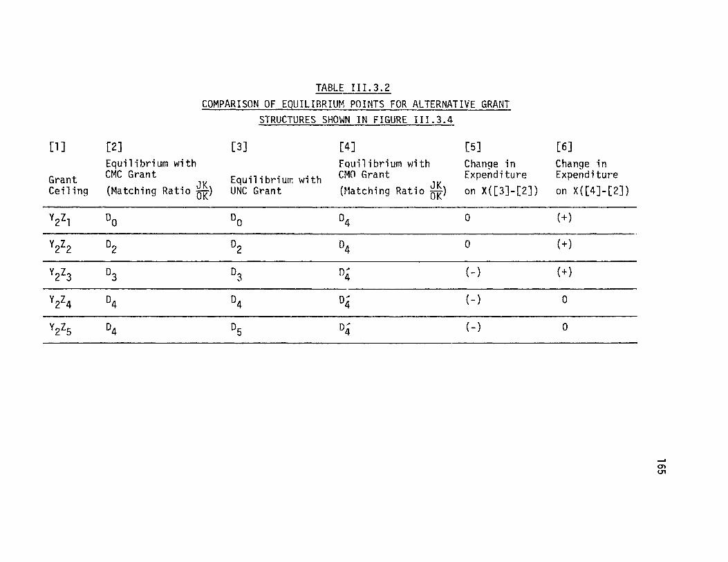
TABLE 111.3.2
COMPARISON OF EQUILIBRIUM POINTS FOR ALTERNATIVE GRANT
STRUCTURES SHOWN IN FIGURE 111.3.4
[1] [2]
Equilibrium with
Grant CMC Grant ,Ceiling (Matching Ratio O)
[3]
Equilibrium withUNC Grant
[4]
Equilibrium withCMO Grant
(Matching Ratio !)
[5]
Change inExpenditure
on X([3]-[2])
[6]
Change inExpenditure
on X([4]-[2])
Y2Z1 ODOD (+)y2zI D0 D90D40
Y2Z2 D2 D2 D 0 (+)
Y2Z3 D3 D3 04 (-)
y9294 D4D D4 (-) 0
Y2Z5 D4 D5 D4 () 0
atjCF)

166
intersects the price-consumption curve (point D4), CMC grants are al-
locationally equivalent to CMO grants. Thus increases in the grant
ceiling beyond the level Y2Z4 will in no way alter the highway expen-
diture pattern of recipient governments.
In general, the greater the federal matching share of expendi-
tures on highway commodity X, the greater is the upper limit on the
binding grant ceiling level. This relationship is shown schematically
by curve OP' in figure 111.3.5. The shaded area A. above OP' repre-
sents the region in which increases in the statutory grant ceiling for
a given matching ratio (for example moving from point III to
point IV ) will not alter the BU's allocation of resources between
X and y. Conversely, the area in B to the right of curve OP' re-
presents the region over which increases in the federal matching share
for a given grant ceiling (for example, movement from point III to
IV ) will not effect changes in the BU's consumption of X and Y.
Finally, the area C between curves OP' and OP' describes the region
over which changes in either the matching provisions, or the statutory
ceiling of a CMC grant will result in a reallocation of the BU's re-
sources amongst highway commodities X and Y. I The actual allocation
1. In terms of our schematic representation of the allocative impactsof CMC grants in figure 111.3.4, regions A , B , and C aredefined as follows:region A --break point in the budget line lies to the right of
the price-consumption curve Y 0region B --break point in the budget ling lies to the left of the
income-consumption curve 00'region C --break point in the budget line lies between the price-
consumption and income-consumption curves.

167
of the BU's resources between X and Y in this region is uniquely de-
fined by the deflection point in the post-CMC grant budget line.
The preceding analysis has served to demonstrate three distinct
response patterns to conditional, matching, close-ended grants. In one
pattern of CMC grant response, what is nominally conditional matching
aid, may in fact have only the influence of an unconditional block
grant. This behavior is manifest in region B of figure 111.3.5, and
is readily observable ex post facto in cases where the recipient govern-
ment devotes more than enough of its own resources to highway commodity
X than the amount required simply to match the federal highway grant.
The allocative impact of grants of this type is to induce a shift in
the resources the BU would have devoted to highway commodity X in the
absence of the CMC grant, to non-aided highway activities.
In those instances where the BU is observed to provide for expen-
ditures on X enabling them to qualify for only part of the total avail-
able federal grant, the CMC grant is allocationally equivalent to a
conditional, matching, open-ended arant. This behavior is represented
in figure 111.3.5 by region A , and may result in a greater or lesser
expenditure of theBU's own resources on highway commodity X, depending
on the price elasticity of the aided function at the pre-grant price
level.
Finally, the behavior response manifest in region C results in
a greater total expenditure on hiohway commodity X than equal amount
non-matching grants, but less than an open-ended grant with the same

168
AFFECT OF GRANT CEILINGS AND PRICE SUBSIDY LEVELS
OPPER LiuiTS oP8O1PWOM GRANT CEiLiAJ&.
...
I / 1~
Lit-FFPEVL rAThflMiA)& 5 HeIRE OFEMENtJiTARSS OJ Hi1HLJAyCOMoPtT X.
Figure 111.3.5
/ P/

169
matching ratio. Allocation of the BU's own resources between X and
Y in this situation again depends on the price elasticity of the BU's
demand for highway commodity X. This response pattern is readily
recognizable ex post facto where the BU just matches the full federal
CMC grant.
iv. Evaluation of Other Grant Program Structures
It should be evident that the analysis framework presented in
the three previous sections may be used to evaluate a wide range of
alternative grant program structures. For completeness, this section
will briefly evaluate the allocative consequences of two additional
cases: conditional, non-matching, close-ended (CNC) grants, and CMC
grants applied to situations where the BU has not previously allocated
any resources to the aided function.
The former case is illustrated in figure 111.3.6, with the pre-
grant equilibrium a point e2 (x2, Y2). Assume now that the federal
government introduces a non-matching grant of y3y4 dollars which is
restricted to expenditure on hgihway commodity X. This grant is re-
presented by budget line y3dJ, indicating that the CNC grant will
wholly finance up to OK1 units of X. Equilibrium in this case is at
point e =(x, y') (where the income-consumption curve 00' intersects
the budget line y3dJ), the allocational equivalent of an unconditional
non-matching grant of the same (y3y4) dollar amount. It follows that
the specificity characteristic of this CNC grant is not allocationally
significant: expenditures on X and Y are the same whether or not the
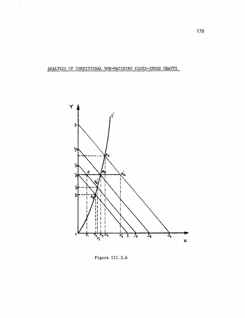
170
ANALYSIS OF CONDITIONAL NON-MATCHING CLOSE-ENDED GRANTS
C X '
Figure 111.3.6
171
grant is restricted to expenditure on X. This situation occurs wherever
the post-grant consumption of highway commodity X exceeds the statutory
grant ceiling--i.e., expenditures on X include the~BU's own resources.
Moreover, it is clear that this grant has increased expenditures on
non-aided highway functions by the amount y2yA. Thus although the grant
was nominally restricted to expenditure on X, a fraction -*was
y3y4actually diverted to other uses.
The response to CNC aid will be quite different in cases where the
grant ceiling is sufficiently large so as to cause the break point in
the post-grant budget line to fall to the right of the income-con-
sumption curve. For example, a CNC grant ceiling of y3y6 dollars will
produce budget line y3e434 with equilibrium occurring at the break point
e4. In this case, the BU shifts all of its pre-grant expenditures
on highway commodity X to the non-aided functions, using only federal
grant money for expenditure on the aided function. Thus CNC aid with a
sufficiently high grant ceiling results in a greater total expenditure
on highway commodity X than an equivalent amount unconditional grant.
This situation can be easily identified, since none of the BU's own
resources would be observed to support the aided highway function.
The analysis of conditional, matching grants (both open and close-
ended) presented in sections III.3.ii and III.3.iii assumed that the
BU's pre-grant equilibrium included positive levels of consumption of
highway commodity X, and other highway functions Y. This section con-
cludes with a discussion of the response to CMC and CMO grants in cases

172
where the BU has not previously allocated any resources to the aided
function.
In terms of figure 111.3.7, we assume an initial equilibrium at
e3=(O,y3). This solution obtains if the indifference curves (U1, ... U4)
are everywhere less steep than the budget line y3J, i.e.:
S9U9X < P V X > 0
3Y
Introduction of a conditional matching, open-ended grant is represented
by the budget line y3K, and yields a new equilibrium at e4=(x4, y4)i
Expenditures on highway commodity X in this case total y0y5 dollars.
Of this amount, yy3 dollars derive from the BU's own resources, re-
presenting a diversion of expenditures originally devoted to the non-
aided function. The remainder of the total post-grant expenditures on
X, y3y5 are supplied by the federal government.
If the grant had been of the CMC variety, equilibrium would occur
at either e4 or the break point in the CMC budget line, whichever comes
first. It should be noted that of all the grant structure/response
patterns discussed in the previous sections the case presented here is
the only one in which the post-grant reallocation of the BU's resources
always involves an increase in expenditures on the aided function
from the BU's own revenues
1. Assuming that the slope of the indifference curve 04 at y3 issteeper than the new budget line y3K.

173
ANALYSIS OF RESPONSES TO GRANTS FOR FUNCTIONS
NOT PREVIOUSLY UNDERTAKEN BY STATE GOVERNMENTS
Ye.
X6 7 K
Figure 111.3.7

v. Summary of the Responses to Alternative Grant Structures 17
In the preceding sections, an attempt has been made to
provide a descriptive theoretical framework for the analysis
of State Highway expenditure responses to alternative Federal-
Aid grant structures. While it is clear that the model
presented here presumes a degree of economic "rationality" that
ignores the administrative and political realities of State High-
way investment decision making, the analyses do advance a set
of hypotheses that may be modified to account for specific quali-
fications.1 To the extent that a relaxation of the underlying
assumptions do not alter the fundamantal logic of the models, these
analyses serve to place bounds on the expected pattern of State High-
way expenditure behavior.
Figure 111.3.8. a summarizes the relative impacts of alter-
native grant structures on State Highway expenditures. The horizon-
tal axis measures the magnitude of Federal grants, while the vertical
axis describes the post grant total (Federal + State) expenditures
on highway commodity X. It follows that point E describes the BU's
pre-grant expenditure level on X.
In comparing the responses to various grant programs, it is
useful to distinguish between two different behavioral patterns:
expenditure stimulation and expenditure substitution. The former
1 A discussion of the critical assumptions of the preceding analysesand possible modifications to the model results is presented atthe end of this section vi.

175
SUMMARY OF STATE RESPONSES TO ALTERNATIVE FEDERAL GRANT STRUCTURES
$I
TiTAL (sTare +FEDERAL) fKPeAJpiTU0A HIGH L)6AYCOMMODITY
EC: CMC grant response locusEI: CMO grant response locusEJ: UNC grant response locusEH: CNC grant response locus
Figure III.3.8.a
r
expenditurestimulation j
expenditurea substituion
'2
ToTAL AVAILABLEFEDERAL A(P
BXPENDITUARESor x and y
or I ~ 4W 0+01g
I
-. Sb
a
Figure III.3.8.b
I
A f1s,
If-E0 4

case obtains when the effect of the Federal grant is to increase 176
State expenditures on the aided highway function from own sources.
In other words, in these situations the State reallocates resources
from non-aided functions to expenditure on the aided highway cate-
gory. The contrary case, expenditure substitution obtains whenever
total post-grant expenditures on the aided function increase by
less than the amount of the Federal grant. The allocational con-
sequence here is a decrease in the level of State expenditures on
the aided function with a commensurate increase in expenditure
on non-aided functions. In terms of figure III.3.8.a, the expen-
diture stimulation and expenditure substitution response patterns
are indentified by the regions lying to the left and right respec-
tively of the line EF.
It is evident that of the four grant responses shown in figure
III.3.8.a only conditional matching (either open or close-ended) may
induce expedditure stimulation on the aided function. The curve
EG traces the expenditure response to succeeding by higher levels
of CMC grant funding (at a matching ratio of CD ). We assume thatAD
at the pre-grant price of highway commodity X (Af_ ),the BU was in theAC--
elastic portion of its demand for X.i For grant levels below OP.
dollars, the CMC grant is allocationally equivalent to the equiva-
lent amount UNC grants, (c.f. section III.3.iii) and thus curve EC
begins along the same locus as EJ in the expenditure substitution
1 This is indicated in figure III.3.8.b by the negative slope ofthe price consumption curve OB' at the pre-grant equilibrium Z0.

177region. Beyond the grant ceiling OP, the CMC grant yields equili-
bria at the break points along line segment Z5Z1 (figure III. 3. 8.b),
with expenditures on highway commodity X from the BU's own re-
sources increasing at the margin. When the grant ceiling reaches
the level 0P2, the BU's expenditures on highway commodity X net of
grants equals its pre-grant allocation to X (as indicated by point
Zl). Thus, above this level of Federal aid, the CMC grant serves
as an expenditure stimulant. Expenditures on X from the BU's own
revenues exceed their pre-grant level, ultimately reaching a maxi-
mum increase of G dollars at a grant ceiling of OP3. Beyond the
grant ceiling OP3, no further reallocation of expenditures between
highway commodity X1 and other functions Y occurs.
In a similar fashion, we can construct the curve EI to suggest
the locus of expenditure responses to conditional, matching, open-
ended grants with succeedingly higher matching ratios. In this case,
the higher the Federal matching ratio of the CMO grant, the greater
will be the amount of Federal money expended by the BU. Moreover,
since the BU was assumed to be initially in the elastic portion of
its demand for highway commodity X, expenditures on the aided func-
tion begin in the expenditure stimulation region above the threshold
line EF. Unitary price elasticity corresponds to aid OP3 (matching
ratio C), beyond which X expenditure substitution obtains at theAD
margin. Ultimately, beyond Federal aid levels of OP5 dollars

(matching ratio CE),the CMO grant yields an expenditure substitution 178
AE
response, with post-grant expenditures on X from the BU's own sources
falling below their pre-grant level. The limiting case here is a
CMO grant with a 100% Federal share--in other words a conditional
non-matching grant. Thus, as the Federal share payable approaches
100%, the curve El approaches the response locus EH associated
with conditional, non-matching close ended grants.
The response to unconditional block (i.e. non-matching) grants
exhibits the most significant expenditure substitution behavior.
In this case, a fraction of the UNC grants would be expected to be
devoted to highway commodity X as a direct substitute for the BU's
own X expenditures. The curve EJ traces the response locus to UNC
grants with succeedingly higher grant ceilings. This curve lies
entirely in the expenditure substitution response region, its slope
depending on the BU's marginal propensity to consume highway com-
modity X with higher levels of income.1 For UNC aid beyond the level
OP4 dollars, the BU substitutes its entire pre-grant expenditures
on X to non-aided activities Y, exclusively using Federal aid to
purchase highway commodity X.
1 The marginal propensity to consume (MPC) is defined as the inverseslope of the income-consumption curve AA'. Two limiting casesserve to place bounds on the UNC response locus Ed. If theincome-consumption curve is vertical (MPC=0), then each Federal-aiddollar is substituted one-for-one with the BU's own expenditureson X. The UNC grant response locus in this case is defined by EKin figure III.3.8.a. Conversely, if the MPC=co(income-consumptioncurve horizontal), then each Federal-aid dollar is fully expended onhighway commodity X with pre-grant X expenditures remaining fixed.
The case is represented by the UNC grant response locus EF.

179The expenditure response to conditional, non-matching, close-
ended grants is similar to the UNC grant response. As shown by
response locus EH, CNC grants are allocationally equivalent to UNC
grants below the funding level EP4 dollars. At that point, leakage
of grant money into non-aided highway activities (as measured by HIH2,
the vertical distance between EH and the 450 line OH) has reached
the level of pre-grant expenditures on highway commodity X (OE).
Further leakage is prevented as additional levels of CNC funding
is wholly devoted to X at the margin, and response locus EH diverges
from Ed.
Table 111.3.3 summarizes the most significant findings of the
preceding analysis. Of paramount importance is recognition of the
fact that changes in the structure of a Federal-aid grant program
may result in fundamental changes in the recipient government's
allocation of resources among alternative transportation commodities.
In this context our analysis framework can be used to address ques-
tions such as:
1) What is the least expensive means for the Federal government to
achieve a specified target expenditure by the recipients on
the aided highway functions?
2) For a given ceiling on Federal highway aid, which grant program
stipulations would be most favored by the recipient government?

Grant Response Pattern180
Response Locus(Figure III.3.8.a)
For relatively bigh matching ratios EI approaches EH at highand large grant ceilings, the allo- Federal grant levels
cative difference between condition-al matching and non-matching grantsare insignificant.
IL
Conditional close-ended matching Segment EG2 on responsegrants may be allocationally equi- locus EGvalent to unconditional block
2 grants for sufficiently low grantceilings. In these cases, thegrants result in expenditure sub-stitution on the aided function.
Only conditional matching grants Segment EI, on response(either open or close-ended) can locus EI.
3 be expectdd to increase expendi- Segment G3G on responsetures on the aided function by locus EGmore than the amount of the grant.
Unless the grant ceiling is not Response locus EG, andbinding, CMC grants have a lesser segment EG on responsestimulatory impact than a CMO locus EIgrant with the same matching ratio.
The specificity requirement on a Segment EHI on response5 conditional non-matching close- locus EH
ended grant may have no alloca-tive significant
6 Expenditure stimulation will be Not shownbreatest where CMO grants are ap-plied to highway functions notpreviously undertaken.
SUMMARY OF GRANT RESPONSES
Table 111.3.3

It is not surprising to note that the answers to these two 181
questions indicate a conflict in the preferences of the donor and
donee governments. If one of the goals of the Federal government
is to maximize the "return" on their grant (in terms of achieving
the greatest expenditure on the aided function for a given level
of Federal aid), they will always prescribe matching provisions
on their highway grant programs. The States, on the other hand,
would alwaysl find unconditional or block grants preferable to
conditional grants with the equivalent ceiling.
Another related finding of our theoretical analysis is that
under certain circumstances grant programs with categorical restric-
tions are allocationally equivalent to block grants (c.f. lines
1,2 and 5 of table 111.3.3). In these instances, the grant pro-
grams should be evaluated in terms of their income-redistributive
characteristics (e.g. whether they channel higher levels of aid
into poorer States), rather than in terms of their allocative ef-
ficiency characteristics. These issues will be discussed in greater
detail in section 111.4.
vi. Qualifications on the Theoretical Analyses
The validity of the theoretical findings derived in the pre-
ceding sections ultimately rests on the practicality of the under-
lying assumptions of our model. Basically, there are three crucial
assumptions upon which our theoretical analysis rests:
1 Except under certain restrictive conditions. See line 2 oftable 111.3.3.

1821) There is an identifiable behavioral unit at the State level
that expresses a consistent set of preferences among alterna-
tive transportation services.
2) These preferences may be represented by a map of continuous
indifference curves
3) Grant money receives no special treatment beyond the stipula-
tions made by the Federal government.
The first of these assumptions is perhaps the most difficult
to justify. Clearly, our reference to a "behavioral unit" ignores
the existence of the numerous political agencies and private forces
whose choices among alternative transportation projects often con-
flict. It is certainly true that on any given transportation pro-
ject, it would be simplistic to presume that a single individual
or a monolithic agency solely determines the investment decisions.
However, our model deals with overall budget behavior--that is,
decisions on the level of expenditure to be devoted to generic
transportation activities. We do not distinguish between the scale
or location of individual highway projects, but only between the
overall expenditure levels on aided and non-aided highway activities.
In this context, our assumption boils down to an assertion that a single
State agency (e.g. a State Highway Department/Commission or Depart-
ment of Transportation) sets forth an investment policy determining
the allocation of revenues amongst transportation investment alter-

natives in broad, generic categories. 1 183
It is nonetheless the case that in any given year, these cate-
gorical investments are comprised of a finite set of discrete pro-
jects whose individual cost may represent a sizable fraction of the
total investment. The implications here relate to the second as-
sumption of our analysis, that the indifference curves are continuous
functions of categorical highway expenditures. To the extent that
the demands for alternative highway commodities are expressed in
terms of discrete investment levels, the indifference curves will
be piecewise linear rather than continuous. We assume that this
qualification does not fundamentally alter the expenditure response
patterns indicated by our models.
The validity of the third assumption is not testable in any
empirical sense. However, there are two reasons to suspect that
the receipt of grant money may have the effect of shifting the
recipient government's indifference map. 2 The first reason is the
commonly held notion that it is "bad politics" to turn down a
Federal grant. This view argues that Federal grants are "some-
I For example, this policy might be expressed in terms of decisionsto spend a certain fraction of revenues on maintenance, another frac-tion on the State Primary Highway System, and a third fractionon the State Secondary Highway System. In some States these"decisions" are actually dictated by statute. In others, a Statehighway agency makes these decisions on a (multi-) year to (mlti-)year basis.
2 It should be noted that an indifference map describes the trade-offs amongst alternative goods irrespective of the prices of thosegoods. As discussed in the previous sections, changes in the pricesof the aided highway functions enter into our model through shiftsin the budget line, not the indifference map.

184thing special," or "free money," to be spent at all costs. Clearly,
if this is the case, the States will behave differently than our
models predict.
There is another possible explanation for a deviation from
our models'predictions which relates to "spin-off effects." Sup-
pose a State must choose between a major intercity freeway projectl
costong $100 million, and an arterial route costing $10 million.
After weighing the costs and benefits, assume the arterial route were
strongly preferred. At this point, however, the Federal government
offers to pay 90% of the freeway costs. With the costs equalized,
the State would choose between the two projects solely on the basis
of benefits. Let us assume that the State still prefers the arter-
ial project. If that were the extent of the decision, the grant offer
would be declined. However, this decision could be reversed by a
broader view of benefits. In a macro-economic context, the freeway
project has the advantage of bringing an additional $90 million into
the State's economy (which translates into increased income and
employment). Thus the macro-economic context for aid recipients
may be a vital factor in expenditure decisions and grant response.
The implication of the "free money" or "spin-off effect"
arguments is that Federal highway grants may induce a greater expen-
diture stimulation response than our models would predict. But
in order for this to be the case, we would have to observe the
IThis exapfple is placed in the setting of project selection, butthe same arguments apply to the broader question of overall bud-get allocation.

185States making expenditures on the aided highway functions less than
or just equal to amount required to match a full close-ended Federal
matching grant (see section III.3.v). Our model would appear to
be valid in cases where an expenditure substitution response is
associated with the Federal grant. In cases where our model pre-
dicts an expenditure stimulation response to a Federal highway
matching grant, the arguments advanced above indicate that the
model results may understate the expenditure levels on the aided
highway functions. As will be discussed in detail in section 111.4,
the majority of States exhibits an expenditure substitution response
to Federal highway grants.

186
111.4 The Analytics of State Responses to Federal Grants:The Benefit/Cost Investment Model
The previous section discussed the analytics of State
responses to Federal grants in terms of the allocation of
highway resources amongst alternative expenditure categories.
The basis of this discussion was that States allocate resources
so as to maximize their perceived benefits (utility).
The question of highway resource allocation can be
approached from a somewhat different perspective. In particular,
this section will present a benefit/cost investment model which
focuses on the level of resources raised from a States own
sources, in response to a variety of Federal highway grant
structures.1
i. A Hypothetical Example
Assume that a particular State has developed a set of
candidate highway projects, and is prepared to expend funds on
these projects up to the point where the benefit/cost ratio on
the "last" project is just equal to 1.0. More explicitly, we
assume that the State has ranked the projects in order of
1. For an application of this approach, see Miller, Edward,"The Economics of Matching Grants: The ABC Highway Program,"National Tax Journal, Vol. 27, No. 2, June, 1974.

187
decreasing benefit cost ratio as shown in figure 111.4.1.2
For the hypothetical values displayed in figure 111.4.1
the State is willing to expend a total of $10 million to imple-
ment projects 1 through 10. At this point, assume the Federal
government steps in and offers a grant of $G with the provision
that this grant must be matched dollar for dollar by the State
government (i.e. the matching rate is 50%). It may be argued
that there are three possible responses to the presence of the
Federal grant, depending on the size of the grant G:
Case I. $0< G 4$5M: Pure Income Effect
This case applies where the sum of the Federal grant G
and the State's matching share is less than the total amount the
State was apparently willing to expend on highways in the absence
of Federal grants. For example, assume the Federal grant
offered is $3.M After providing for the required matching
share, the State has expended $6.M This leaves a remainder of
2. It has often been noted that optimal project selection doesnot necessarily simply consist of those projects with thehighest benefit/cost ratios. (For example, see Pecknold,Wayne M., Evolution of Transport Systems: An Analysis of Time-Staged Investment Strategies Under Uncertainty, UnpublishedPh.D. Thesis, M.I.T. Department of Civil Engineering, 1970,and Newman, Lance, A Time-Staged Strategic Approach to Trans-portation System Planning, Unpublished S.M. Thesis, M.I.T.Department of Civil Engineering, 1972). In the presentationthat follows, we nonetheless make the assumption that Stateswill not choose to implement projects whose perceived B/Cratio is less than unity.

ILLUSTRATIVE EXAMPLE188
OF THE BENEFIT/COST INVESTMENTMODEL
Project No. B/C Total Cost (Millions of Dollars)
1.6
2.3
.7
10.0 - Cost of projects withB/C > 1.0
1.2
.6
.3
5.0 - Cost of projects with.5 .6 B/C( 1.0
.9
1.1
1.0
5.0 - Cost of projects withB/C 4.5
Figure III.4 1
1
2
Region I
10
7.6
6.9
1.0
11
12
Region 2
17
18
19
.97
.84
.50
.46
.41
Region 3
24 .23

189
projects costing $4M whose B/C ratio exceeds unity. Since, the
Federal grant has been exhausted there is no incentive to expand
the highway program beyond the previously determined level of
$10.M Thus, the net effect of the $3M Federal grant has been to
reduce the level of resources expended from the State's own
sources. Total highway expenditures remain unchanged, as the
State's own expenditures are reduced by just the amount of
Federal grant. This situation represents the case of a pure
income grant, where the close-ended grant is not of sufficient
magnitude to create a perceived price reduction at the margin.
As far as the State is concerned, the grant has had the effect
of providing an additional $3M of income to be expended on other
State services or "spent" on tax relief.
Admittedly, this conclusion presents a somewhat extreme
case. While the overall characterization of this type of grant
as an income subsidy remains valid, realistically it is not
necessarily the case that State expenditures on highways would be
reduced dollar for dollar by the amount of the Federal grant.
For one thing, it should again be noted that because of the
indivisibility and "lumpiness" of highway investments, the
presence of additional highway revenue might substantially alter
the project mix (and therefore the total expenditure level) of
an optimal highway investment program. Another mitigating
factor here is the restriction in most States against expenditure

190
of earmarked highway revenue on non-highway projects. The
consequence of this restriction (and particularly in the short
run where changes in State revenue raising sources - e.g. tax
rates, are not possible) is that at least part of the additional
revenue may be expended on the aided highway category, thus
increasing total expenditures on this function.
More importantly however, is the fact that any expansion
in total expenditures on the aided highway category results from
the chosen allocation the additional income derived from the
grant as opposed to any perceived price reduction on the aided
function. By the same token, it is likely that expenditures
on non-aided (highway) functions will be increased from the
additional income afforded by the grant.
Case II. $5M< G4$7 .5M Price Plus Income Effect
For the hypothetical situation depicted in figure 111.4.1,
once G exceeds the level of $5 million, the grant introduces both
a price and income effect on the State's allocation decisi3ns.1
1. A price effect refers to changes in the allocation of re-sources deriving from a change in the perceived price of oneor more expenditure items. Allocational shifts also derivefrom an income effect where the State allocates additionalincome on highway commodities whose perceived prices remainunchanged. A grant may introduce a pure income effect ora combination of a price effect and income effect. For amore detailed discussion of these concepts see Henderson J.M.and R.E. Quandt, Microeconomic Theory: A MathematicalApproach, McGraw-Hill Book Company, New York, 1958.

191
To see this, assume the Federal grant offered, G is $7 million.
Since the State was apparently willing to expend $10 million
from its own sources, it is clear that at least $5 million of
the grant will be used. At this point total expenditures amount
to $10 million, all projects with B/C greater than one have been
programmed, and $2 million of Federal grants remain available.
The remaining Federal grant has the effect of reducing the cost
of additional highway construction to the State by one-half.
In other words, the perceived B/C ratio of projects remaining
on the candidate list increase by a factor of two. Since the
B/C ratio of projects in Region 2 (see figure 111.4.1) fall in
the range 0.5 to 1, the availability of Federal grants increase
the perceived B/C ratio of these projects over unity.
Following the simple criterion that all projects with
(perceived) B/C 1 will be prograrrned, it is clear that the
State will employ the remaining Federal grant, bringing total
expenditures on the aided function to $14 million. Once the
entire Federal grant has been employed, there is no longer any
incentive for expansion of the highway program, since the State
must now bear the full cost of projects whose B/C ratio is less
than one.
While the net effect of this grant has been to increase
total expenditures, for a Federal investment of $7 million, total
expenditures increase by only $4 million (from $10 million in the

192
absence of grants to $14 million with the grant). The expendi-
ture increase derives from the price effect of the matching grant
at the margin (i.e. at the point where the State decides to
program projects in region 2 of figure IIM.4.1). It should also
be noted that total expenditures from the State's own sources
decrease from $10 million in the pre-grant situation to $7 million
in the post-grant situation. As in Case I, the saving in State
resources may be spent on other services, or translated into tax
reductions.
Case III G>$ 7 .5M: No Effect at the Margin
Following the same reasoning as presented in Case II, it
is clear that the State will not have an incentive to employ
Federal grants in excess of $7.5 million. Since all projects in
region 3 of figure 111.4.1 have a B/C ratio less than 0.5, the
availability of 50% Federal matching grants will not bring the
perceived B/C ratio of region 3 projects over one. Thus, for
this hypothetical example, the maximum grant level that will
willingly be employed by the State is $7.5M (this amount will
cover half the costs of all projects in region 1 and region 2).
At this grant level, total expenditures on the aided function
amount to $15M divided evenly between State and Federal funds.
This situation represents an increase in total expenditures by
$5M, but a decrease in State's own expenditures by $2.5

193
ii. A Diagrammatic Description
These three cases can be summarized diagrarnatically as
in figure 111.4.2. We assume that the State expresses a demand
for highway construction represented by the demand schedule
D1D1. Thus, for the full price of highway construction (i.e. in
the absence of grants), the State will purchase Q1 units of
highway at a total cost of ObcQ1 dollars. Case I of our previous
discussion is represented by the price line arsp. In particular,
50% matching grants are available up to a ceiling of Q0 highway
units. Beyond this level of highway expenditure, the State again
faces the full price of highways. As previously noted, the
State response to this grant is to maintain its previous produc-
tion scale of Q, units. Total expenditures from the State's own
sources is indicated in the figure by area OarQ1 (the full cost
borne by the State of highway construction up to the level Q).
This represents a decrease in State expenditures by Q0 rdQ1 dollars.
For the larger grant ceiling described in Case II, the
relevant price line is depicted by aefp, The response in this
instance is to expand production up to Q2 highway units at a
total cost to the State of OaeQ2 dollars. As in the previous
situation, State expenditures decrease from the pre-grant situa-
tion - in this case by the difference between areas abcd and
QadeQ2 '
Finally, the price line corresponding to Case III is
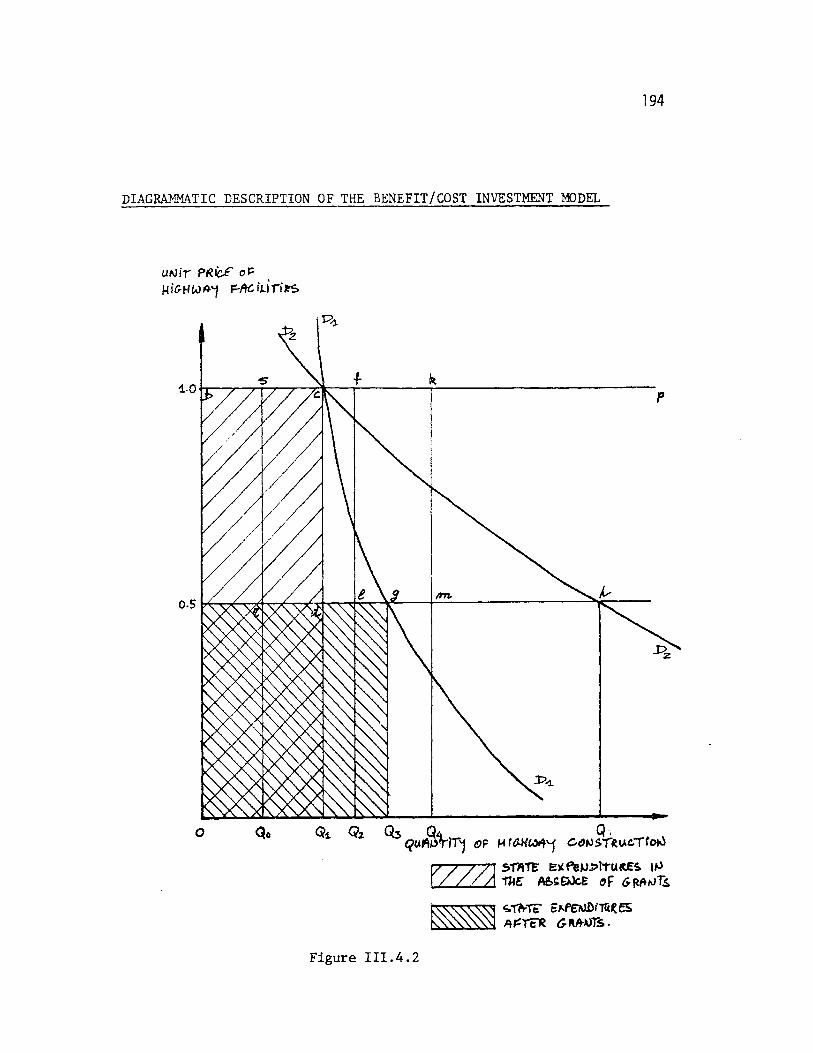
194
DIAGRAMMATIC DESCRIPTION OF THE BENEFIT/COST INVESTMENT MODEL
ufir PRfaC oFIGNLwI F-Acikrits
1 p4
e -C
P
'In A-
TZz
,trr'K VC i 4*
0 QQ( 3 PMWW+ 1 Cp0f4t~OiO Gi Qz Q ~~q(AA13?rTl OF HiR~n &MS s o
5TA~Tr EKftOPWUtES 10_ _E AbwkcZ oF &RSwT
-4TtWE~eEAPD(TI(&sArTCR aN6Ars.
Figure 111.4.2
0
/
/
7
/7
///
/
/7
7/
//
4-
/
- a -
firz z -m-4T T X V 'lr"r
ILlI I %
0

195
shown as amkp. Since this price line intersects the demand
schedule D1D,, the State will expand its highway program only as
far as Q 3 units, leaving Q3gmQ4 dollars of the Federal grant un-
expended. Total State expenditure in this case is OagQ3, a
decrease of abcd - QdgQ3 from the pre-grant situation.
M11. Conclusions From the Benefit/Cost Investment Model
An immediate conclusion that can be reached from the
preceding analysis is that:
Whereas the Federal government provides categoricalgrants presumably for those types of activities inwhich it perceives a national interest in stimula-ting expenditures (i.e. in inducing construction thatmay not have been undertaken in the absence of thegrant), the net result may be the expansion ofexpenditures (or contraction through tax relief) inother (non-aided) areas in which the Federal govern-ment has no officially stated interest.
This conclusion derives from the income effect of
close-ended matching grants, which under certain conditions such
as Case I of the preceding analysis, serve only as a non-cate-
gorical income subsidy to the States.1 In fact, in the preceding
hypothetical example, regardless of the ceiling of a 50% Federal
matching grant, post-grant State expenditures decrease from their
pre-grant level (and thus the savings incurred may be expended in
1. As described in Section 111.3, as long as the grant ceilingof a close-ended matching grant is low enough so as to benon-binding on the States investment calculus, the categoricalrestrictions of the grant are irrelevant. The allocationalconsequences of a grant of this type are identical to a simpleblock grant of like amount.

196
other areas).
This expenditure response pattern need not have been the
case however. As shown in figure 111.4.2 (and in the analysis
describing figure 111.4.1), the States demand for highway facili-
ties, expressed by the schedule D301 represents inelastic demand.
That is, a decrease in price by one-half results in less than a
doubling of total expenditures. It is entirely possible that a
State's expressed demand for highway construction may be elastic,
for example as depicted by the schedule D2D2 in figure 111.4.2.
In this case total State expenditures following the offer of a
50% Federal matching grant with a ceiling in excess of OahQ4
dollars exceed pre-grant expenditures by the amount QdhQ4 -
abcd (c.f. Section III.3.ii). However, regardless of the
elasticity properties of the State's expressed demand for highway
facilities, if the Federal grant in question has the properties
described in Section III.4.ii as Case I, the unambiguous conclu-
sion is that the categorical restrictions of the matching grant
are non-binding, resulting in a stimulation of State expenditures
on non-aided functions. For grants with ceilings sufficiently
large to fall into the categories described as Case II and
Case III, State expenditure response indeed depends on its
elasticity of demand for highway construction. For these cases,
elastic (inelastic) demand will result in a increase (decrease)

of State expenditures frpm their pre-grant levels.1 In the
next section, a brief analysis of actual highway expenditure
data will be presented to illustrate the conclusions discussed
above.
1. Several factors influence the price elasticity of a State'sdemand for highway construction including the level andgrowth in traffic on State roads, and tax capacity of theState (i.e. the propensity of the State to tap additionalrevenue sources or the willingness to increase levies onexisting revenue sources. In the context of the illustra-tive examples presented in this section, the price elasticityas expressed by the State's response to a Federal matchinggrant is determined solely by the number of projects inregion 2 of figure 111.4.1. Specifically, if in developinga list of mutually exclusive candidate projects for itshighway investment program, a State perceives numerousprojects marginally unattractive in benefit/cost terms (i.e.projects with B/C slightly less than one), then a relativelysmall Federal price subsidy may elicit a large expansion inthe State's highway investment program (representing priceelastic demand for highway facilities).
197

198
111.5 Observed Expenditure Patterns: The Impact of theABC and Interstate Programs
The analysis in Section 111.4 proceeded on the basis of a
State developing a highway investment program in the absence of
Federal highway grants, and then altering their investment
decisions in response to the offer of Federal matching grants.
Three possible response patterns were described (Cases I, II
and III), each dependent on the matching provisions and magni-
tude of the grant offer.
In examining data indicating the States' total expenditure
levels on Federal Aid System construction and Federal highway
grant availability, it is clear that we are merely observing
the States' expenditure responses to Federal highway grants
rather than - in any direct fashion - observing how expenditure
decisions changed due to the existence of Federal grants.
However, by simply comparing the magnitude of Federal
grant availability, and the level of expenditure from the State's
own resources (on Federal Aid Systems), it can be straightfor-
wardly inferred which of the three previously cited expenditure
response patterns obtain (c.f. Section III.4.ii).
For grants which have a pure income effect (Case r), we
should observe a State consistently expanding their own highway
expenditures beyond that level minimally required to match avail-
able Federal grants. In this case, the size of the grant is not

199
of sufficient magnitude to introduce a perceived price reduction
at the investment margin. By inference, this type of grant
simply provides additional non-categorical income to the State,
which may be expended on any highway function.
If on the other hand, the data indicate that State
expenditures consistently just equal the minimal amount required
to match available Federal grants, then a price plus income
effect may be inferred. In this case (Case II), the grant has
had the effect of stimulating additional expenditures on the
aided category, and increases in the size of the Federal grant
may be expected to further stimulate State expenditures. 1
Finally, if the data indicates that States consistently
do not exhaust all available Federal Aid, then it is clear that
Case III obtains. It should be noted that we can imediately
rule out the relevance of Case II since in only one isolated
instance has a State (actually, "State" in question was
Washington, D.C., who forfeited a portion of available Inter-
state aid in 1971) failed to obligate the entirety of available
Federal highway grants.
i. Data Analysis of the ABC Highway Program
Table 111.5.1 displays (for each of the 48 mainland
1. As opposed to (small) increases in Case I - type grants. wheretotal expenditures on the aided function would not be expectedto increase significantly.
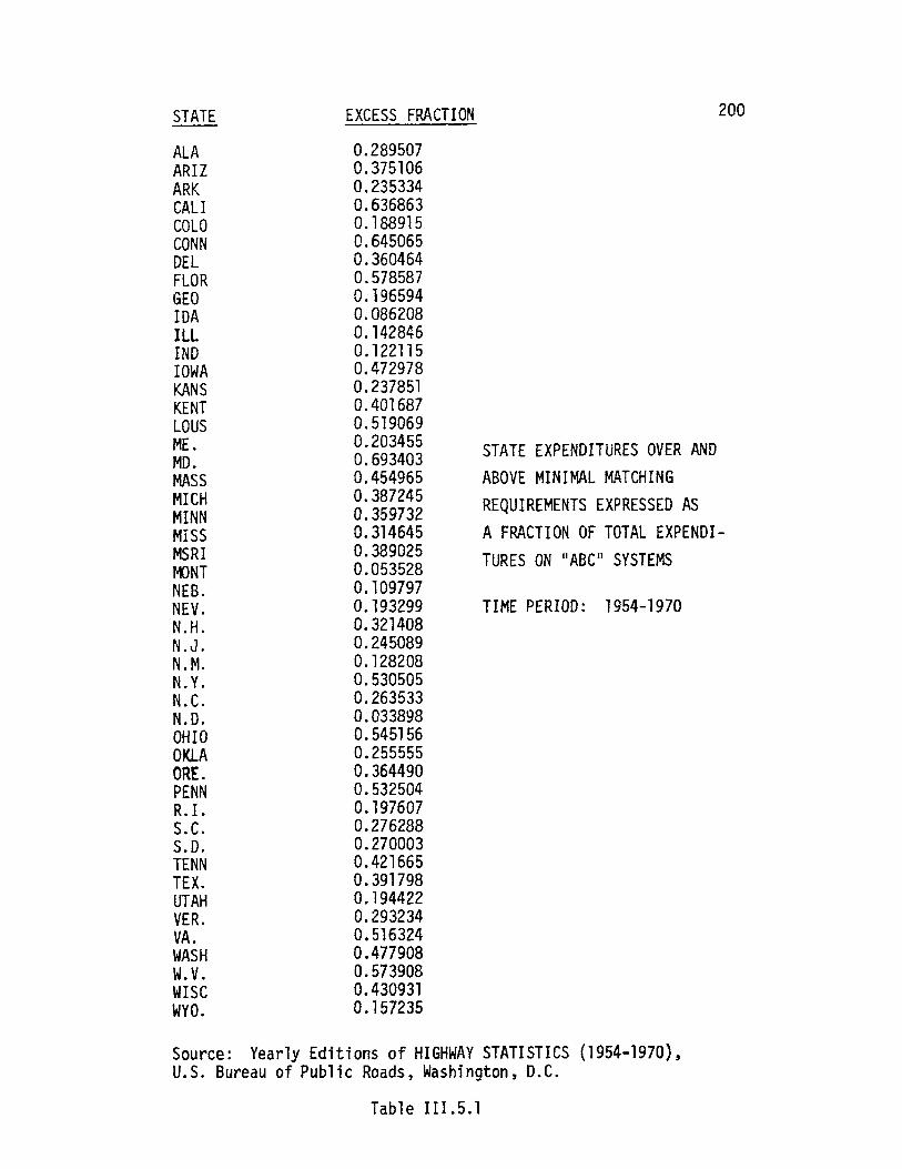
EXCESS FRACTIONSTATE
ALAARIZARKCALICOLOCONNDELFLORGEOIDAILLINDIOWAKAN SKENTLOUSME.MD.MASSMICHMINNMISSMSRIMONTNEB.NEV.N.H.N.J.N.M.N.Y.N.C.N.D.OHIOOKLAORE.PENNR.I.S.C.S.D.TENNTEX.UTAHVER.VA.WASHW.V.WISCWYo.
0.2895070.3751060.2353340.6368630.1889150.6450650.3604640.5785870.1965940.0862080.1428460.1221150.4729780.2378510.4016870.5190690.2034550.6934030.4549650.3872450.3597320.3146450.3890250.0535280.1097970.1932990.3214080.2450890.1282080.5305050.2635330.0338980.5451560.2555550.3644900.5325040.1976070.2762880.2700030.4216650.3917980.1944220.2932340.5163240.4779080.5739080.4309310.157235
TIME PERIOD: 1954-1970
Source: Yearly Editions of HIGHWAY STATISTICS (1954-1970),U.S. Bureau of Public Roads, Washington, D.C.
Table 111.5.1
STATE EXPENDITURES OVER AND
ABOVE MINIMAL MATCHING
REQUIREMENTS EXPRESSED AS
A FRACTION OF TOTAL EXPENDI-
TURES ON "ABC" SYSTEMS
200

201
States, over the time period 1954-1970) expenditures over
and above minimal matching requirements, expressed as a fraction
of total expenditures on "ABC" systems. More significantly, each
table entry is defined as:
ef = (ETPF) I[ 1 -F HPF (12)MF
ET
where: ef = excess fraction (i.e. the table entries)
ET = total expenditures by a given State overthe 17 year sample period on ABC Systems(State and Federal monies)
1MF = Federal matching share for a given State
PF= Payments of Federal ABC monies from theHighway Trust Fund to a given State overthe 17 year sample period
The term in brackets in equation (13) expresses the expen-
diture level from the States' own sources required to qualify for
receipt of PF Federal Aid dollars. Thus, the numerator expresses
1. As shown in figure , the Federal share payable is notequal for all States. The 13 Public Land States receiveABC grants with Federal shares payable ranging from 53.5%(Washington) to 95.0% (Alaska). The remaining States allare subject to 50/50 ABC grants. Additionally the Federalshare of grants to Public Land States change slightlfrom year to year in response to these States 'totalacreageof National Parks, Indian Reservations, etc. The data infigure 111.5.1 employed the Federal share payable in 1962 -the median year in the 17 year sample period.

202
the States' own excess expenditures beyond minimally required
matching monies.
The excess expenditure fractions in table 111.5.1 range
in value from 3.4% in North Dakota to 69.4% in Maryland. In
the latter case, of the total (State plus Federal monies ABC
system investment by Maryland, between 1954 and 1970 nearly
70% represented expenditures net of minimal matching require-
ments.
In fact, only three of the forty eight States (Idaho,
Montana and North Dakota) had excess expenditures totaling less
than 10% of the their total ABC expenditures. The inescapable
conclusion here is that for the great majority of States, the
ABC grant program has served the role of non-categorical
income subsidies. Neither the categorical restrictions, nor
the matching provisions have been allocationally significant.
In terms of the States' investment calculus, the determination
of total ABC system expenditures have been based on the full
cost of the marginal project rather than a price subsidized
(50%) cost. Inferentially, it makes little difference whether
the Federal share payable were 50% or some higher value - say
70%.l To see this, consider the example of New York's ABC
1. In fact, the Federal share payable on ABC systems wasincreased from 50% to 70% effective July 1, 1974.

203
system expenditure and grant availability in 1963 (table 111.5.2)
Given a 50% Federal matching share, it would cost New York
$60,315,000 to match the Federal payments made available. But
considering that New York was willing to expend over $200 million
on ABC system construction (from its own sources), it makes
little difference whether the first $60 million or the first $26
million went towards matching available Federal funds. Only the
price at the margin is important. Thus it is apparent that for
New York and most other States, we should expect increases in
ABC grants to have a relatively small impact (through an income
effect) on total ABC systems expenditures.
ii. Data Analysis of the Interstate Highway Program
As discussed in Section 11.2 , the Interstate highway
program differs in three important respects from the ABC
highway program. In magnitude, Federal grants for the Interstate
program exceeded ABC grants over the period 1954-1970 by
231%. Additionally, the basic Federal share payable for the
Interstate program amounts to 90% as compared to a 50% share
payable towards ABC projects. But perhaps the most fundamental
difference - at least in terms of States' expenditure responses
to Federal grants - is the fact that, unlike the ABC program,
the Interstate program represents a closed system. Total system
mileage and general corridor locations for the system were

204
ABC System ExpenditureslGrants
New York: 1963
(1000's of dollars)
50% Federal 70% FederalShare Share
Federal payments 60315
Required State matching funds 60315 25849
States' own expenditures 200964
"Excess expenditures" 140649 175115
Percentage excess expenditure 53.8% 67.0%
Table 111.5.2

205
determined years before the first Federal dollar was expended on
the system. Moreover, Federal Interstate grants are awarded
to the States on the basis of the relative cost to complete their
portion of the approved system, unlike ABC grants which are
fixed without regard to the level of investment chosen by the
State.
For these reasons, it may be inferred that States have
little incentive to expand Interstate highway construction sig-
nificantly beyond the level provided for by the Federal grants.
This expectation is borne out by the data in table 111.5.3 indi-
cating the States' expenditures over and above minimal matching
requirements, expressed as a fraction of total expenditures on
the Interstate system over the period 1954-1970 (refer to
equation 13). The excess expenditure fractions range from a
low value of 0l (North Dakota) to a high value of 37.7% in
Rhode Island. It is immediately clear that relative to expendi-
tures made on the ABC system, most States expend little more
than the minimally required amount necessary to qualify for
1. The negative value appearing for North Dakota indicates anerror in the data reported in HIGHWAY STATISTICS. Note thatan excess expenditure fraction less than zero would suggesta State not meeting its minimal matching requirement forthe receipt of Federal Funds. We shall assume that theexcess expenditures for North Dakota are essentially zero.

EXCESS FRACTION
ALAARIZARKCAL ICOLOCONNDELFLORGEOIDAILLINDIOWAKANSKENTLOUSME.MD.MASSMICHMINNMissMSRIMONTNEB.NEV.N.H.N.J.N. M.N. Y.N. C.N. 0.OHIO KLAORE.PENNR.I.S.C.S.D.TENNTEX.UTAHVER.VA.WASHW.V.WISCWYO.
0.0337060.1416950.0421720.2602110.0937790.1058660.1195800.1135270.1166680.0672190.0570980.1163340.1750110.0655200.0718060.0568500.0553360.0956720.1662040.1121190.0671620.0551570.0000280.0036780. 081 9410.0768830.0380500.0815530.0946870.071708
-0. 0433320.0285620.0971820.0922770.0428530.0936730.3769950.0251380.0472250. 0411910.1043520. 1746130.0263710. 0097040.1049550. 0968520.1508280.055882
TIME PERIOD: 1954-1970
Source: Yearly Editions of HIGHWAY STATISTICS (1954-1970),U.S. Bureau of Public Roads, Washington, D.C.
Table 111.5.3
STATE EXPENDITURES OVER AND
ABOVE MINIMAL MATCHING
REQUIREMENTS EXPRESSED AS
A FRACTION OF TOTAL EXPENDI-
TURES ON INTERSTATE SYSTEMS
STATE 206

207
receipt of Interstate grants. Fully thirty three out of the
forty eight States devote less than 10% of their total Interstate
investment towards expenditures beyond the minimal matching
requirement. And with the exception of California and
Rhode Island, all States exhibit an excess expenditure fraction
less than 20%.
Thus, it may safely be concluded that for the vast
majority of States, Interstate grants have been characterized
by a price and income effect. Following the analysis of Section
111.4., we may infer that Interstate grants have induced State
expenditures on projects that would not have been made in the
absence of grants. And by the same token, small increases in
the level or price subsidization of Interstate grants may be
expected to stimulate additional expenditures on the Interstate
system from the States' own resources.

208
III.6 Summaryand Conclusions
This chapter has attempted to define both the normative
and positive analytic issues involved in an investigation of the
Federal Aid Highway Program (FAHP). Two related findings merit
particular attention:
- the design of the FAHP should be related to the objec-tives the Federal government hopes to accomplish throughits grant program
- States' expenditure responses depend significantly onthe structural characteristics of Federal grants.
The former finding derives from the discussion in Section
2 on the normative aspects of the Federal Aid Highway Program.
Summarily, it should be noted that the selection of the appropri-
ate mathcing ratio - indeed the very choice of a Federal matching
grant as opposed to a block grant must be related to the perceived
fiscal problem the grant attempts to rectify. This type of per-
spective gives direction to arguments for and against alterations
to the existing FAHP. For example, it may be argued that the
stipulations in the 1973 Federal Aid Highway Act allowing for the
construction of mass transit facilities under the same grant
provisions as the Urban (highway) System1 is not the appropriate
form of transit aid.
The relevant issue here is that the primary rationale for
1. Close-ended categorical matching grants with a Federal sharepayable of 70%

209
Federal highway grants is entirely different from the rationale
fore transit aid. In the former case, the existence of signi-
ficant interstate benefit spillovers call for external financing
to move towards an efficient allocation of highway resources. In
the latter case, it is primarily the fiscal disparity between
different cities (i.e. the ability of a city to raise sufficient
revenue to provide for a given level of transit service) that
indicates the need for Federal financing. As discussed in Section
2, in the one instance, Federal matching grants are in order; in
the other, block funding is more appropriate.
The second major finding of this chapter is the relationship
between State expenditure responses, and structural characteris-
tics of Federal grants. It has been shown that categorical match-
ing grants will always stimulate greater expgnditure levels than
non-categorical block grants of like amount. In fact, Section 5
presented evidence that the ABC program has failed to serve as a
stimulus for additional construction on the aided systems. In
light of this finding it is important to question the objectives
of the ABC highway grant program. If the intent of Federal
grants for the ABC system was to "accelerate the construction of
Federal-aid highway systems .... since many of such highways or
portions thereof, are in fact inadequate to meet the needs of
local and interstate commerce"I, the program has apparently failed
1. Subpart A, Title 23, United States Code, Chapter 1, Section101(b): Declaration of Policy.

210
to do so. By the same token, the ABC grant program does not
appear to be necessary to ensure a minimal level of provision of
such systems (c.f. Section III.2.iv), since the great majority of
States invest funds far in excess of their minimal matching require-
ments. Indeed, the primary consequences of the ABC grant program
appears to be merely to have provided the States with additional
highway revenue - an outcome that could be achieved in a more
straightforward manner by the institution of non-categorical block
grants. 1
Needless to say, it is important to verify the theoretical
findings in this chapter with empirical evidence. The remaining
chapters of this thesis will discuss a series of econometric models
designed to assess the impacts of the Federal Aid Highway Program
on State highway expenditures.
1. Although this assertion reraises the initial question posedin this section: What are the objectives to be accomplishedby the FAHP.

CHAPTER IV 211
DEVELOPMENT OF THE TOTAL EXPENDITURE MODEL
IV.l Introduction
There are two fundamental dimensions of States' highway expendi-
ture behavior: long run revenue or total expenditure policy
formulation, and short run allocation (programming) determination.
The distinction between revenue policy as a "long-run" phenomenon
and allocation policy as a "short-run phenomenon derives from the
fact that changes in the determinants of State highway revenue(e.g.,
tax rates, bond sales, etc.) tend to be infrequent relative to the
expression of a State's allocation policy (e.g., year-to-year capital
budgeting decisions). The empirical models developed in this
research attempt to explain the factors influencing States' total
highway expenditures, and allocation decisions amongst alternative
highway expenditure categories. Naturally, the central focus of
the research is an evaluation of how Federal grants have affected
States' expenditure behavior.
In this chapter, the development of the total expenditure model
(TEM) is presented. Attempting to build on the common use of "Needs
Studies" as a long run fiscal planning device, Section 2 presents
a derivation of the TEM based on capacity utilization theory. The
major focus of this model is to trace States' total highway expenditure
responses to the presence of Federal highway grants.
Following the derivation of the model, Section 3 explores the
estimation problems inherent in the use of a pooled data set.

212While it would have been desirable to estimate the TEM for each State
individually -- as 48 separate time series -- lack of sufficient
historical data precluded this approach. Accordingly, we describe a
practical approach to estimating the model with both time series and
cross sectional data.
Section 4 describes the definitions and sources of data employed
in our TEM estimation. In many instances, data which would have been
desirable from a theoretical standpoint was not directly available.
The use of proxy information is fully described in this section. Next,
a short discussion is presented on considerations for interpreting
the empirical results. Hypotheses to be tested are discussed in terms
of the signs and magnitudes of specific parameter estimates.
Section 6 describes the actual estimation results of the total
expenditure model. Several alternative specifications are presented
and applied to an 2xperiment where the entire sample was divided into
two distinct subsets. The results convincingly demonstrate the States'
differing expenditure responses to the Interstate and ABC grant programs.
Finally, the major results and policy implications derived from
the estimation of the total expenditure model are set forth in
Section 7.

213IV.2 Derivation of the Model
It is convenient to conceptualize States' highway expenditure
behavior in terms of two dimensions:
1. decisions relating to the determination of the magnitudeof the States' highway budget in any given year, and
2. decisions relating to the allocation of that budget amongstalternative types of highway expenditure categories (e.g.Interstate, Primary System, maintenance, administration, etc.)
In fact, it may be argued that this analysis perspective is not
merely an artificial construct. While the administrative and political
realities of altering tax rates and debt obligation (and thus altering
total expenditure levels) inhibit quick adjustments to changes in
costs and demand,I the program selection (programming) process
operates on a relatively short cycle time.I
We focus here on the derivation of a model to explain the
derivation of a model to explain the first of the two dimensions of
State behavior: the determination of total highway expenditures.
An immediate starting point is an examination of the "Needs Study"
process. The highway needs process has been incorporated into the
U.S. Department of Transportation's biennial National Transportation
Studies, required of all States as of 1968. But prior to this time
to this time several States conducted explicit internal highway needs
studies for their own fiscal planning purposes at varying intervals.
In its simplest terms, a (highway) needs study involves the
Highway bond sales are usually issued over a two to five year period.The average duration between tax rate adjustments is ever longer.Over the fifteen-year period, 1951-1965, the average duration betweenthe States' tax rate adjustments was somewhat over ten years.

determination of the desired ("needed") level of highway physical 214
plant based on structural and functional deficiencies in existing
inventories, present and future design standards, traffic growth rates,
and anticipated highway functional classification. Highway needs
studies do not represent a radically innovative methodology to guide
States' investment behavior. In fact, conceptually the needs study
process may be considered as a specific application of the general
economic theory explaining the investment behavior of a behavioral
unit (be it a firm, industry or State Highway Department).
This is an important point, since we are attempting to model the
highway investment behavior of States, regardless of whether they
conducted explicit needs studies during the course of our analysis
period (1957 - 1970). The most general statement of the factors
influencing total highway investment behavior (of which a needs study
is one application) may be expressed by:
(1) Rt = f(Kt - Kt-)
where R = total revenues devoted tohighway expenditure(State plus Federal funds)
K* = desired capital stock inyear t
Kt-1 = actual capital stock at the
end of year t-l
Equation (1) asserts that the level of (total highway) investment
in a given year t is a function of the gap between a "desired level
of highway plant" at the end of year t and the existing level of
capital stock at the beginning of year t.

The conceptual basis of this investment relation has been 215
advanced under the general heading of "capacity utilization theories."
Most commonly, the dependent variable is expressed in terms of (a
firm's) investment in capital stock. In our application, we are
more interested in a State's total (capital plus non-capital)
highway investment. However, equation (1) remains perfectly general.
We would expect higher levels of total highway investment to be
associated with higher "gaps" between desired and existing highway
plant. Note that Rt in equation (1) is just the sum of the States'
own resources R and the amount of available Federal highwayt
grants Gt
(2) Rt = R0 + Gt tBut Gt is equal to the sum of unexpended Federal grants in years t-1,
t-2, . . . and Federal grants made available in year t:
(3) Gt = UBGt-1 +gt
where UBGt-1 = unexpended balance ofFederal grants as of theend of year t-l
gt = highway grants madeavailable in year t
Substituting equations (2) and (3) into equation (1) yields:
(4) Rt = f(K* - Kt-1 ) - (UBGt 1 +
which expresses the revenues raised for highway expenditure in a
For a good summary of the various applications of these theories,see Kuh, Edwin, CAPITAL STOCK GROWTH: A MICRO-ECONOMETRICAPPROACH, North Holland Publishing Company, 1971, especiallyChapter 2.

216
State in year t as a function of the gap between desired and actual
highway capital stock and Federal grants.
The capacity utilization theory expressed by equation (4) has a
clear relationship to the classical Needs Study Process of long run
fiscal planning. In effect, we are arguing that States adjust their
long run highway investment policy in response to their perception
of highway "needs" (K* in our terminology), the existing inventory
(Kt-I) of highways, and the available level of external funding
(Gt). Needless to say, the empirical measurement of "desired"
(and even actual) capital stock represents a formidable conceptual
problem.
Several factors influence a State's perception of highway needs1
(desired capital stock), including traffic and congestions levels,
demographic characteristics, and a variety of institutional char-
acteristics. Symbolically, we assume desired capital stock -- "needs" --
can be expressed as:
I It should be emphasized that our modelling framework does notassume that State highway expenditures will be adjusted to meetthe cost perceived highway needs from year to year. On the con-trary, the expenditure model employed here explicitly recognizesthe continuing existence of a "jap_" between perceived needs andactual highway capacity. It is the existence of this discrepancybetween desired and actual highway plantthat influences State de-cisions on the magnitude of total highway investment. Presumably,the greater the gap between "needs" and existing inventory in anygiven year, the greater will be the expenditures in that year.

(5) K = Kt (SEC, IC) 217
Where SEC= a vector of socio-economiccharacteristics of a State(e.g., urban density, pop-ulation, traffic conges-tion levels, per capitaincome, and various Stategrowth measures)
Where IC= a vector of institutionalcharacteristics describinga State's hi hway financingconventions e.g., the ex-tent of local participationin highway maintenance andconstruction, the extent oftoll road finance, and thedegree of debt-servicefinancing
Introducing equation (5) into (4) leads to the basic form of the
total investment model estimated in this study:
(6) Rt = f(Kt (SEC, IC) - Kt 1) - g(UBG + gt
where f and g are assumed to be linear functions of thearguments
Note that the last term above is written as a function, rather than the
simple sum of UBGt-1 and gt as in equation (4). The reason for the more
general specification here is to allow for an explicit test of the ef-
fect of Federal grants. In other word, equation (6) permits an assess-
ment of the impact of Federal grants on the level of total hig wa
expenditures derived from States' own sources. The major hypothesis
to be evaluated empirically is relative degree of expenditure stimulation
resulting from Interstate versus non-Interstate grants. In the hypo-
thetical model presented in Chapter III, preliminary data analysis in-
dicated that Interstate grant increases would most likely be associated
with increases in States' own expenditures. This behavior was contrast-

218
ed with the ABC grant program, where it was hypothesized that States
would view increases in ABC grants as a substitute for their own
expenditures on these Federal Aid Systems. The empirical results
presented in Section IV.6 will validate the theoretical hypotheses.

218%s
IV.3 Estimation Techniques for the Total Expenditure Model
While it would have been desirable to estimate the total
expenditure model (TEM) for each State individually (i.e. as
forty-eight separate time series), lack of sufficient historical
data precluded this approach. The specification of the TEM incor-
porated as many as twelve explantory variables (including the con-
stant term). Given only fourteen years in our analysis period (1957-
1970), individual State estimation is clearly infeasible.
Accordingly, the possibility of grouping our observations in
a pooled data set consisting of time series and cross-sectional
data merits special attention. One of the first investigations of
this problem was advanced by Theil and Goldberger,I who demonstrated
that the estimation of time series parameters can be designed to
incorporate additional information oabtainable from cross-sectional
data.
In principle, the reasons for pooling data ar - s mpl3: provided
that we cna take proper statistical account of individual regional
and/or time effects that may be present in the data, the use of
pooled data (by virtue of the large increase in available degrees
of freedom) yields more effecient model paramter estimates. In
our application, the use of pooled data increases the number of
available observations from 14 (years) to 672 (14 years x 48 States).
Theil, Henri, and A.S. Goldberger, "On Pure and Mixed StatisticalEstimation in Economics," International Economic Review, Volume II,No. 1, January, 1961

To clarify the statistical problems inherent in estimating 219
models employing pooled data, let us rewrite equation (6) of
Section IV.2 in matrix form to stress the fact that an observation
is specific to a particular State and year:
R0
R0
1R~'
(7) R0 = = X + u
0R
R0RNT
X - - X(K)ku11 11 11
XO) -.-. - X(K) u1T 1T 1T
+
O)x(K) uNINl ll kiNI
NT NTuNT

220
where:
N = number of States (48) in the sample
T = number of years (14) in the sample
K = number of explanatory variables in the model
R = a vector of observations (NTxI) of total highwayexpenditures from State n's own sources in year t
Thus we have observations on N (=48) States, n = 1, 2 . .,'N
taken over T (=14) years, t = 1, 2, . . . T. Our dependent variable
R is assumed to be explained by K truly exogenous varibales X.
The statistical properties of our parameter estimates B, and indeed
the very meaning of our model is determined by what we assume about
the properties of the residual vector U.
The standard assumptions of econometric theory (i.e. if ordinary
least squares (OLS) are to yield best linear unbiased parameter
estimates) are that the residuals are distributed with mean 0 and
variance a I. However, if a model is estimated with pooled data, there
are strong reasons to suggest that these assumptions are not valid.
When cross section and time series observations are combined in the
estimation of a regression equation, it is likely that certain
systematic shift effects are present in the data. Specifically,
we refer to the presence of factors not explicitly accounted for by
the included explanatory variables which nonetheless influence the
dependent variable.

221Two categories of "extraneous influences" may be present. One
relates to the presence of pure regional effects -- i.e. factors
outside the model which serve to determine the behavior of individual
States. Growth rate policies, political culture variables, "belief
in the future,"2 and auto/transit biases are examples of factors
that, although important in determining individual State expenditure
behavior, are difficult to explicitly model at the aggregate level of
analysis considered in this thesis. A second extraneous influence
relates to the presence of time dependent shifts -- i.e. those factors
which may affect all States at any given point in time, but vary
from year to year. The most obvious examples of this affect are
macro-economic influences: interest rates, degree of inflation/
regression, unemployment rates, etc.
A common method to account for these "extraneous influences" is
to introduce explicitly into the equation individual shift variables.
The rationale for this approach is that the observations contain an
additive effect specific to the individual State or year.
To account for such effects, dy variables corresponding to
1Kuh, Edwin, and J.R. Meyer, "How Extraneous are Extraneous Estimates,"The Review of Economics and Statistics, Volume 39 (November, 1957).
2The importance of this factor was discussed by Mead, Kirtland, DESIGNOF A STATE WIDE TRANSPORTATION SYSTEM PLANNING PROCESS: AN APPLICATIONTO CALIFORNIA, Unpublished Ph.D. thesis, M.I.T. Civil EngineeringDepartment.

each State or yearI may be explicitly introduced into the model. 222
The problem with this approach is that it reduces the degrees of
freedom by N without adding in any real sense to the explanatory
power of the model. Moreover, it is often found that the dummy
variable approach "overcompensates" for the individual effect by
drastically reducing the magnitude and significance of the
explanatory variables. 2
Error Component Analysis
Another technique to account for the.presence of individual State
and/or time shift effects is with error component analysis.3
Since we are assuming the presence of economic forces specific to
an individual State and/or year, not otherwise accounted for in our
model specification, it is reasonable to expect that these forces
"show up" in the residual term. To state this formally, we assume
1Obviously it would not be possible to introduce a specific dummyvariable for each State and for each year. The most common practiceis to focus on the presece of regional effects by introducingexplicit State dummy variables. For an example of this approach, seeBalestra, Pietro, and M. Nerlove, "Pooling Cross Section and TimeSeries Data in the Estimation of a Dynamic Model: The Demand forNatural Gas," Econometrica, Volume 34, Number 3 (July, 1966).
2This is particularly true of those variables that vary significantlyfrom State to State, but exhibit little variance in any givenState over time. The dummy variable approach was attempted in thisresearch and abandoned for the above reason. For a further discussionof this point, see Balestra and Nerlove, op. cit., especially pages590 - 593.
3Balestra and Nerlove, op. cit., Theil and Goldberger, op. cit.,Kuh, op. cit.

223each residual Unt may be decomposed into three statistically independent
components: an individual State effect 1n, a time shift effect
t , and a remainder vnt :(8) u nt Pn + t1 +
Since the residuals are assumed to tve zero mean, and the
components of untare independently distributed, it must also be
true that:
(9) E[pn] = E[6t] = E[vnt1 = 0
We further assume that there is no serial correlation among the
error components, and that they are independent from one State and
year to another:
E[v ntlin] = 0
(10) E[vnt6t] = 0
E[vn6t] = 0
E[vntvn't'10
2Ef lip,]
E[6t6tII 16
if n=n' and t=t'
otherwise
if n=n'
otherwise
if t=t'
otherwise
Accordingly, we may express the variance-covariance (an NTXNT matrix)
0 of the residuals (ant) by:
E[untuntw2
w 2
w 2
1
w2
w2-

224where:
S0 - 0
0 T 0
0 0
P = (12/IG2
= S/2
*6
Equation (11) follows directly from our assumption that the
covariance of all the cross products of the error components are
identically 0. Note that the variance-covariance matrix .11 has
a repetitive block structure. The diagonal blocks are T x T, and
represent the variance-covariance structure of the individual State
effect and remainder error component. The off-diagonal blocks, also
T x T are all diagonal matrices, whose single parameter T represents
the time shift effect.

It is clear from the form of equation (11) that the variance- 225
covariance of the residuals derived from estimation on pooled data
is not scalar. Accordingly, although ordinary least squares estimates
of the coefficients would be unbiased and consistent, they would
not be the most efficient (i.e. least variance estimators. In fact,
the best linear unbiased estimators are the generalized least squares
parameter estimates GLS which explicitly incorporate the non-scalar
variance-covariance matrix:
(12) GLS = (X'Q'X)'1 X'2'R0
A straightforward technique for deriving generalized least
square estimators where the error term structure assumes the form of
equation (8) has been advanced by Zellner.I Essentially, the
technique involves a two-step estimation procedure: first estimate
the model with ordinary least squares (OLS), and use the OLS residuals
and equation (11) to determine the parameters of J1. Second, a
generalized least squares estimation is performed by making the
appropriate transformation of the original data.
In our application, a simplified generalized least squares esti-
mation procedure was adopted. Specifically, no account was taken of
the separate time effect 6t . This error component was dropped for
two reasons. First, allowing for a time shift effect would "greatly
Zellner, A., "An Efficient Way of Estimating Seemingly UnrelatedRegressions and Tests for Aggregation Bias," Journal of the AmericanStatistical Association, Volume 57 (1962).

.226complicate the analysis without adding any essential generality."
It is obvious from the form of equation (11) that the development of
generalized least squares estimators requires inverting an NTXNT
matrix. Although the form of 2 inclusive of 6t is sparse (c.f.
equation (11)], the inverse matrix Q-1 does not assume or simple
pattern.2 In fact, inversion of a 672X672 matrix proves to be
unwieldy and expensive.
A second reason for dropping the individual time shift effect
is that when estimations were performed using time shift dummy
variables, the parameter estimates of these dummy variables did not
prove to be significant. In short, the most important "extraneous
influence" in our estimation problem was the presence of an
individual State shift effect.
The application of our simplified error component estimation
procedure was straightforward. Following the notation of equation
(11), we now assume that:
0 o - - 0(13) Q = a2 * *
0 0 01
Balestra and Nerlove, op.cit., p.504.
2That is, there was no simple (and inexpensive) way to invert

Remembering that each T x T matrix w is specified in terms of a 227
single parameter p, it may be shown that - can be estimated as a
function of OLS residual estimates:?
N T
(14) -_ n~ti - a2(=n=t= t'= t ' n=l t=l nt
N T (T-1) 62
where: Uj = OLS residuals for State nnt (=1,... ,N) in year t ,=l,...,T)
82 = estimated variance of the OLSregression
The actual estimation of generalized least squares (GLS) estimates
involves OLS estimation on suitably transformed data. The first step
is to determine the Choleski decomposition2 h of Q-1 defined as:
(15) h'h = -1
The original observations X and R are then premultiplied by the
Choleski decomposition matrix to define X and P
(16)( = hX
R = hR
Equation (1941 simply expresses the average value of all thoseelements of ulu' corresponding to where p appears in our assumedstructure of 02
2For an operational algorithm for determining Choleski darnos nmatrices, see Faddeev, D.K., and Fadeeva, V.N., COMPUTATIOAL M ODSOF LINEAR ALGEBRA, W.H. Freeman, San Francisco, 1963.

It follows directly that OLS estimation on the transformed data 228
yields GLS estimates of our model coefficients.1
In summary, the estimation of the total expenditure model
followed a simplified error component analysis which explicitly
allows for the presence of individual State shift effects in our
pooled data set. Once the structure and properties of the residuals
are specified [equation ( 8)], GLS estimation involves a straight-
forward application of a two-step procedure employing OLS residuals
to estimate the parameter of an assumed structure of the non-scalar
variance-covariance matrix.
I aOLS = (' '~'R= (X'h'hX)alX'h'hRoBut from (15), h'h =-1
Thus BOLS = (X'Q'lX)-lX'Q-IRO = SGLS

IV.4 The Data Set and Modelling Considerations
Returning to the basic form of the total expenditure model
derived in Section IV.2, we noted that States' own highway expenditures
were functionally related to perceived investment needs, existing
highway inventories and Federal grant availability:
(17)
While equation (17) suggests the basic explanatory relationship, the
problem remains to specify the socio-economic factor (SEC), and
institutional characteristic (IC) arguments of the highway needs term
Kt. Moreover, a practical means of representing existing inventories
Kt-1, and Federal grant availability must also be determined. This
section will discuss the definitions end sources of each of the
variables incorporated into the estimated total expenditure model.
Several alternative specifications of the total expenditure
model were estimated in this research using both deflated and
undeflated data. The basic form of the model is presente in
Figure IV.4.l. The first eight variables in the model correspond
to the set of socio-economic and institutional characteristics
which influence a State's perception of "desired" highway ca;acity.
The variable KSTK serves as a proxy for existing highway inventories
[i.e. the measure of Kt-i in (17)]. Finally, the availability of
That is, expenditure levels, Federal grants and per capitaincome variables were deflated by the consumer price index.
229

THE TOTAL EXPENDITURE MODEL 230
0 MFCR a0 + a1I*SPOP + a2 *UFAC + a3 *GPOP + a 4 *PCY
VMT
+ a 5 *GINI + a6 *RLTOT
+ a7 *TOLPCT + a8 *BIPTCX + a9 *KSTK
+ a10 *AVNIGP + a11 *AVIGP + U
where
R 0= State expenditures on highways exclusive of Federal percapita grants
a-ao = constant term
a1 = estimated coefficients
VMT = State vehicle miles of travel
SPOP = State Population
MFC = State motor fuel consumption
UFAC = percent of population residing in urban areas
GPOP = State population growth rate
PCY = per capita State income
GINI = index of income inequality
KSTK = present discounted value of highway capital stock per capita
RLTOT = percent of total expenditures (all units of government)contributed by local (i.e., county and municipal) governments
BIPTCX = percent of total capital expenditures provided for by debtfinancing
AVNIGP = apportioned "ABC" grants (three year moving average) percapita
AVIGP = apportioned Interstate grants (three year moving average)per capita
U = error termFigure IV.4.1

231Federal highway aid is represented by AVNIGP and AVIGP -- a three-year
moving average of non-Interstate and Interstate grants respectively.
i. The Socio-Economic Descriptors
Five variables were employed to describe the socio-economic
characteristics of each State: a basic State size variable (SPOP
or MFC or VMT), a measure of urbanization (UFAC), an indicator of
State growth (GPOP), and two income characteristics (per capita income
PCY, and income distribution GINI).
a. SPOP, MFC and VMT
It is reasonable to expect that, ceteris paribus, State
expenditures should increase with increasing levels of traffic demand.
For one thing, higher traffic levels will generate increasing levels
of earmarked State highway revenue. But more fundamentally, higher
levels of auto use require increased construction, maintenance
policing and aministrative expenses.
Three alternative measures of State size were employed as a
proxy for the scale of auto travel. The first indicator, State
population (SPOP), was derived from yearly editions of the Survey of
Buying Power.1 SPOP was entered into the model with a one year lag --
i.e. State expenditures during year t were related to population at
Sales Management, SURVEY OF BUYING POWER, 1950 - 1970 (YearlyEditions), Bell Brothers Publications.This publication is the only source of year-to-year, State-by-State socio-economic descriptor data. The Census Bureau doesnot publish population, income or growth indices for each Stateon a yearly basis. The Survey of Buying Power's data base isadjusted to conform with the decennial census data.

233the end of year t-l. Two alternative State size variables were also
tested in the TEM estimations. Vehicle miles of travel (VMT) is
perhaps the most direct measure each State's traffic levels. The
only source of this information is from yearly editions of the
Federal Highway Administrations HI3HWAY STATISTICS. Two problems
are encountered in the use of this data. First, the data itself is
not directly observed or collected, but estimated from gasoline sales
statistics, and assumptions on average vehicle mix (i.e. truck/auto
split) and gasoline consumption rates. Secondly, the data, is not
published on a yearly basis. Over the course of our fourteen year
analysis period, the FHWA published VMT data for only four years (1959,
1962, 1965 and 1968). For our purposes, intermediate (yearly)
values of the VMT data were determined by simple straight line
interpolation.
Motor fuel consumption (MFC), the third alternative State size
measure, was also derived from the FHWA Highway Statistics yearly
publications, The data was entered into the model net of fuel
deployed for agricultural, marine or aviation use. As with the two
previous measures, a simple one year lag was employed.
b. UFAC
The degree of urbanization (UFAC) is an important factor
in determining highway investment behavior (i.e. in terms of explaining
perceived highway investment needs K) for several reasons. First,
it is a measure of the "compactness" of a State as it serves to
distinguish between largely rural/agricultural/sparsely populated
States and densely populated urban/industrialized States (see
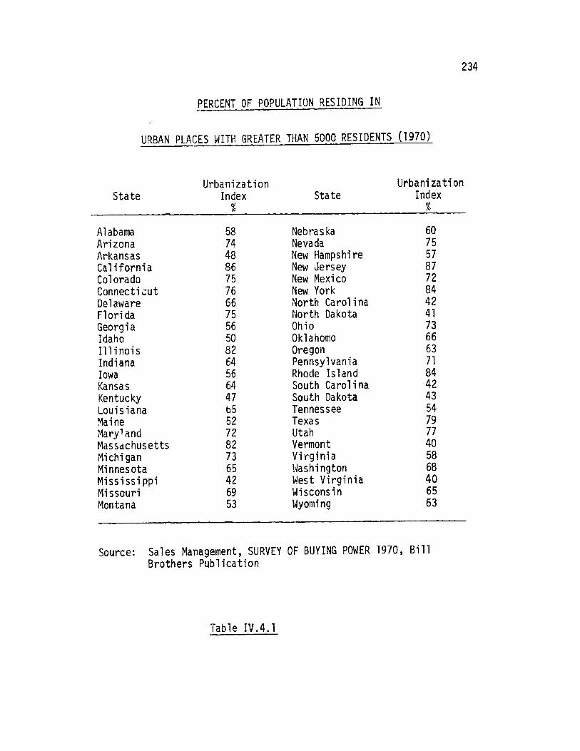
234
PERCENT OF POPULATION RESIDING IN
URBAN PLACES WITH GREATER. THAN 5000 RESIDENTS_(1970)
UrbanizationIndexState State
UrbanizationIndex
AlabamaArizonaArkansasCaliforniaColoradoConnecti cutDelawareFloridaGeorgiaIdahoIllinoisIndianaIowaKansasKentuckyLouisianaMaineMarylandMasSdchusettsMichiganMinnesotaMississippiMissouriMontana
587448867576667556508264566447b55272827365426953
NebraskaNevadaNew HampshireNew JerseyNew MexicoNew YorkNorth CarolinaNorth DakotaOhioOklahomoOregonPennsylvaniaRhode IslandSouth CarolinaSouth DakotaTennesseeTexasUtahVermontVirginiaWashingtonWest VirginiaWisconsinWyoming
Source: Sales Management, SUlBrothers Publication
RVEY OF BUYING POWER 1970, Bill
Table IV.4.1
607557877284424173666371844243547977405868406563
b-

235Table IV.4.1). Secondly, it serves to identify States with highly
concentrated urban areas where per lane mile construction costs are
relatively high.
On balance, we would expect the degree of urbanization to
negatively influence States' per capita highway expenditures.
There are two reasons for this. The first reason relates to the
indivisibility and "lumpiness" of highway investments. As a State's
population decentralizes (e.g. to previously unpopulated places),
the need for highway route mileage increases. However, even the
minimal provision of two lane rural roadways incurs a relatively
large capital outlay.I
Secondly, the more urbanized States have been subject to an
increasing presence of community opposition to urban roadway construc-
tion.
The urbanization index UFAC is defined as the percent of a
State's population residing in areas with greater than 5000 residents.
The data was derived from yearly editions of the Survey of Buying Power
and was entered into the TEM with a one year lag.
1That is, highway construction is charaterized by high fixed costs.Moreover, highway construction and maintenance rise less thanproportionately to increases in the number of lanes (for a givenroute distance).

236c. GPOP
As an indicator of the rate of State growth, a measure of
yearly population change was computed from the basic population
data described in Section IV.4.i.a. Ceteris paribus, one would
expect higher population growth rates to be associated with higher
highway investment levels. As it turned out, the population growth
rate data was characterized by extreme variability and proved to be
a poor explanator of highway investment behavior.
d. PCY and GINI
Two separate measures of State income--per capita income and
a measure of income inequality--were employed in the estimation of
the total expenditure model. Per capita income (PCY) is correlated
positively with auto usage (See Section II.3.ii), and thus we
should expect increasing State income to lead to increasing State
highway expenditure levels. PCY data was derived from yearly
editions of the Survey of Buying Power.
The GINI Index of Income Inequality is derived from Lorenz
income distribution curves.1 As shown in Figure IV.4.2, the Lorenz
curves describe the degree of homogeneity in household income within
a State. If each household earned exactly the State average income
level, then the Lorenz curve would be a straight line rising at 450
from the horizontal (i.e. 20% of the households earn 20% of total
income, 40% of households earn 40% of total income, etc.)
As the Lorenz curve plots the percentage of households, ranked
1Samuelson, Paul, ECONOMICS, McGraw-Hill Book Company, New York, 8thEdition, 1970.

237
LORENZ CURVES
Percent ofTotal StateIncome
IJA
-Lorenz Curves
Figure IV.4.2

238fromypoorest up on the horizontal axis and the percentage of income
they earn on the vertical axis, it is clear that as the degree of
income inequality increases, the Lorenz curves become increasingly
concave.
This suggests a measure of income inequality related to the area
between a Lorenz curve and the 450 (perfect income homogeity) line
(e.g. see the shaded area in Figure IV.4.2). In particular the GINI
Index of Income Inequality (GIII) is defined as
area bounded b a Lorenz curve(18) GIII = and the 45 line
area under the 450 line
The GINI index varies between 0 and 1 with higher index values indicat-
ing a greater degree of income inequality.
The actual GINI indices developed for this research were
constructed from piecewise linear Lorenz curves. The Survey of
Buying Power data described the number of households in each State
(and each year in the 14 year sample period) in each of five income
categories -- $0 - 2499, $2500 - 4999, $5000 - 7499, $7500 - $10,000
and $10,000 and over.
The GINI index serves to indicate two characteristics of the
States. First the GINI index provides a measure of the number of
low income households in each State. For a given level of per capita
income, a State with a high GINI index value would have a relatively
large number of low (and high) income households. Thus we are
accouting for the possibility that the average income level as well as
the distribution of income in a State will affect the level of auto

239usage (and thus ultimately affect the level of State highway expendi-
ture). The GIII also conveys a rough measure of regional characteris-
tics. From Table IV.4.2, which displays the GINI index for each of
the forty-eight mainland States in 1963 (the mid-year in our 14-year
sample period), southern/agricultural/rural States tend to have a
higher degree of income inequality than northern/industrial/urbanized
States.
ii. The Measurement of Highway Capital Stocks
The development of time series information on a State's
highway capital stock presents a formidable task. An imediate
problem is to select the units to describe the capital stock, and the
economic conventions to be employed in measuring the change in value
productivity of vintage stocks over time.
On theoretical grounds, it is clear that the best measure
of capital stock is output capacity. In terms of evaluating highway
investment behavior, it may be argued that a State's investment
decisions are based, at least in part, on the perceived gap between
the demand for existing highway service (e.g. vehicle miles of travel),
and the existing supply of the highway plant. Implicit in this
decision-making process is the notion of level of service. Herein
lies the problem in measuring highway physical plant. The capacity
of a highway system, and the quality of the output (i.e. level of
service) are inherently related. This relationship stands in contrast
to the capital stock measurement problem of manufacturing production
processes where output is normally of uniform quality. The only

240
MEASURES OF INCOME INEQUALITY1963
State Gini Index of Income Inequality
Oklahoma 43.1Florida 42.8Kentucky 42.5Alabama 42.3Louisiana 42.0Tennesee 41.9Texas 41.6Arizona 41.6Deleware 41.3Virginia 40.5New Mexico 40.2Iowa 40.2Mississippi 40.1Georgia 39,9North Carolina 39.8Oregon 39.7Vermont 39.1Minnesota 39.0Missouri 38.9Kansas 38.9Washington 38.7West Virginia 38.5South Dakota 38.4New York 38.4Nebraska 38.3Nevada 38.2Ohio 38.1Maine 37.8Pennsylvania 37.7Illinois 37.6Indiana 37.5Maryland 37.4Michigan 37.4Rhode Island 37.3South Carolina 37.3Colorado 37.3Massachusetts 37.2
Table IV.4.2

241
State Gini Index of Income Ineuality
North Dakota 37.0Idaho 37.0Wisconsin 36.8Arkansas 36.4Connecticut 36.1New Jersey 36.1New Hampshire 35.6Utah 35.2Montana 35.0Wyoming 34.8California 32.0
Table IV.4.2 (contd.)

242practical problem in capital stock measurement in this case is the
selection of an appropriate depreciation formulation to measure the
declining value productivity of older capital stocks.
From the above remarks, it is clear that a complete descrip-
tion of highway capital stock requires knowledge of the highway
system's value-in-use -- ie. a comprehensive inventory of the
physical (e.g. roadway width, surface quality, geometric design,
etc.) and operating characteristics (i.e. speeds over the roadway at
existing demand levels) of the highway system.
Unfortunately, this data is not available on a time series
basis. Moreover, for the few years in which comprehensive inventory
data exists,1 the data set is excessively unwieldy, as it represents
a large sample, section-by-section description of all State-adminis-
tered highway mileage. Considering the fact that this type of
information has been largely unavailable to State planners and
decision-makers on a year-to-year basis, the relevant question for
this analysis is to find a relevant proxy measure for value-in-use
highway capital stock, drawing on available time series data.
The primary source of highway mileage data examined in
this study is drawn from the yearly editions of Highway Statistics,
IHighway system inventory data has been collected as part of indivi-dual State Highway Needs Studies (HNS). The Federal governmentrequired HNS of all States as of 1968. Prior to the time, severalStates conducted HNS on their own at irregular intervals.

243published by the U.S. Bureau of Public Roads. Unfortunately, the
organization of this data does not lend itself inediately to
proxy measures of highway capital stock suitable for investment
analyses. The most important data gap is the lack of information on
the vintage distribution of the States' highway plant. Thus, it is
not immediately apparent how to depreciate the value-in-use of
existing capital. Moreover, yearly additions to States' highway
route mileage are reported in units of route mileage rathern than lane
mileage, with no distinction made between projects on new rights-of-
way, and projects designed to improve existing rights-of-way (e.g.
major resurfacing of existing mileage, lane widening, addition of new
lanes to existing ROW, etc.).
Clearly, any attempt to measure capital stock in terms of
capacity output requires data in lane mileage, rather than route
mileage terms. The data on total existing lane mileage is sketchy.
In all cases, the mileage figures are reported in discrete categories--
2 lanes, 3 lanes, and 4 lanes or more--so that the data are imprecise
in the highest lane category. Attempts to identify lane mileage figures
with specific Federal-Aid Systems is complicated by lack of data on
Federal Aid Secondary lane mileage. The lane mileage (LM) data is
broken down into Interstate LM, Federal-Aid Primary LM, and State
Primary System IM. The latter category includes portions of all of
the Federal Aid System mileage as well as State system mileage not
1For example, the number of vehicles per day that can be accomodated onthe State-administered road system at a given average speed.

incorporated on the Federal-Aid Systems. 244
In summary, attempts to employ mileage data as a proxy
measure of highway capital stock is complicated by a lack of
information on the vintage distribution of highway plant, and an
incomplete stratification of lane mileage by Federal and non-Federal-
Aid System.
Given the above-mentioned difficulties in applying mileage
data to the task of measuring capital stock, it is desirable to
investigate the use of historical capital expenditure data as a
proxy measure of existing highway stock. An immediate issue in
applying expenditure data is the proper accounting of the decline of
capital productivity over time. As it turns out, the proper treat-
ment of expenditure data as a capital stock proxy measure is far
less difficult than the use of the available mileage data. The
methodology for constructing highway capital stock measures requires
some attention to the choice of an appropriate depreciation
methodology.
Depreciation refers to the loss in value of a currently
held asset. Two types of depreciation functions are commonly found
in the literature: market value functions and efficiency loss
functions. The former measure indicates the decline in resale value
1The benefits of using physical measures of capital stock (i.e.elimination of price delator affects, and the ease of identifyingstock retirements) are obvious. Nonetheless, the investmentbehavior literature is replete with studies employing capitalexpenditure proxies of capital stock. The main reason for theuse of expenditure data is that it is generally more readilyavailable than physical measures of capital.

of fixed plant over time, while the latter measure reflects the 245
losses in efficiency due to wear on the fixed plant. The more
relegant measure for highway investment studies is the efficiency
loss function.
The techniques for deriving depreciated highway capital
stock measures in this study were based on methodology developed by
Jack Faucett Associates.1 The methodology involves applying an
efficiency loss depreciation function (ELDF) to the time series of
State highway expenditures. The Faucett study hypothesizes that the
efficiency loss of highway systems increases over time (i.e. as a
highway approaches the end of its service lifd2 The actual ELDF
employed takes the form of the lower segment of a rectangular
hyperbola:
(19) D(t) = SL tSL -at
where D(t) = percent of a highway system's remainingproductivity
t = the age of a highway
SL = the service life of a highway
a = a parameter of the effciency lossdepreciation function (Otacl)
This formula generates a family of depreciation functions
as a function of the parameter a (See Figure IV.4.3). Following the
conventions of the Jack Faucett study, a 20-year service life was
Jack Faucett Associates Inc., CAPITAL STOCK MEASURES FOR TRANSPORTA-TION, Volume 1, Report No. JACKFAU-71-04-1, 1971.
As manifested by the increasing level of required maintenance expendi-tures and/or the decreasing level of highway productivity (as measuredby vehicle capacity).

246
DEPRECIATION FUNCTIONS
percent ofremaining increasingproductivity values of a
D(t)
D(t) =SL-tSL-at
Figure IV.4.3

was assumed for State highway system construction expenditures, 247
and the ELDF parameter (a) was set to 0.8.
The efficiency loss depreciation function was applied to a
thirty-four year time series1 of State highway system expenditures to
generate the depreciated highway capital stock measures per capita
(KSTK)for each State and each year in the 14-year sample period.
iii. Descrigtors of Financing Conventions and InstitutionalCharacteristics
Three descriptors of State hiqhway financing conventions were
employed in this study: the extent of local participation in highway
finance (RLTOT)2, the importance of toll roads in generating State
highway revenues (TOLPCT)3, and the degree of debt service highway
financing (BIPTCX).
Since the dependent variable in the total expenditure model
exclusively measures State highway expenditures, we should expect
that higher degrees of local participation (as measured by RLTOT) in
the provision and maintenance of highway facilities will be
associated with lower expenditure levels from State resources. In
1The expenditure time series covered the period 1937 - 1970. Expen-diture data was derived from yearly editions of HIGHWAY STATISTICS.2RLTOT is defined as the ratio of municipal and county highway expendi-tures to total (all units of government) highway expenditures.
3TOLPCT is defined as the percentage of a Stage's highway revenuederived from highway tolls.
4BIPTCX is defined as the ratio of bond interest to State highwayconstruction expenditures.

other words, to the extent that a State delegates its highway 248
authority to lower units of government, State highway expenditures
should decrease.
The other two indicators of institutional characteristics,
TOLPCT and BIPTCX, reflect the degree of flexibility in the States'
highway finance program. For a given State gas tax rate, the
increasing use of toll road or debt service financing allows a State
greater opportunity to raise higher levels of highway revenue. Thus
we should expect TOLPCT and BIPTCX to positively influence State
highway expenditure levels.
Each of the three financing convention variables, RLTOT,
TOLPCT and BIPTCX, were derived from yearly editions of the FHWA's
HIGHWAY STATISTICS.
iv. The Highway Grant Terms
Two important characteristics distinguish the treatment of
the Federal highway grant terms in our total expenditure model from
previous empirical highway expenditure studies (See Section 1.3)
First, the Federal-Aid Highway Program was broken down into two
distinct components: Interstate System grants, and grants on the
non-Interstate ("ABC") Systems. The theoretical analyses of
Chapter III indicated the strong likelihood of differing State
expenditure responses to these two grant types. In fact, it
was hypothesized that the Interstate program grant structure would
most likely induce expenditure stimulation in contrast to the
hypothesized expenditure substitution response to ABC grants. The
modelling emplications of these hypotheses are twofold. First, it

was considered desirable to explicitly test these hypotheses by 250
separating out the two distinct grant types. Second, it was
considered likely that the simple inclusion of a total grant term
would "wash out" any empirically identifiable grant response.I
A second characteristic distinguishing this study from
previous research is in the treatment of the multi-year grant
availability problem. As discussed in Chapter II, Federal highway
grants are made available over a "grace period" extending from one-half
year before the beginning of the fiscal year of the authorization to
two years beyond the end of that fiscal year. The use of three year
movingaverages on the grant terms was employed to represent the
grace period FAHP feature. Moreover, the use of moving averages partly
accounts for the fact that States may not fully and immediately
adjust to changes in Federal highway grant availability.
The basic Federal grant data was obtained from yearly
editions of HIGHWAY STATISTICS. Apportionments for the years 1969
and 1970 were adjusted downward in accordance with the imposed
OMB fiscal control totals (See Section IV.2). The grant terms were
1All of the studies cited in the literature survey of Chapter Iincluded only a total highway grant term. Several estimations ofour TEM were conducted with a single total grant term. As expected,the estimated grant parameter was extremely small and had a largestandard error (See Section IV.6).
2Specifically, the three year moving averaged grant terms Gt werecomputed as
-1Gt= j(Gt+Gt-1 t-2) for t = 1954, . . ., 1970
where Gt = States' grant apportionments in year t.

251
expressed as averaged Interstate grants per capita (AVIGP) and
averaged non-Interstate grants per capita (AVNIGP).
v. Price Delflators
This study conducted estimations on both (price)
deflated and und2flated data. Specifically, all of the terms in
the total expenditure model whose units are expressed in dollars
were adjusted by the consumer price index (See Table IV.4.3)
according to the following relationship:
(20) d CPI
where: Vd = price deflated variable
V = value of variable in absoluteterms
CPI= consumer price index
In addition to deflating the dependent (highway expenditure)
variable, the following explanatory variables were deflated by the
Consumer Price Index: per capita income (DEFPCY), highway capital
stocks (DEFKSTK), Interstate grants (DEFIG), non-Interstate grants
(DEFNIG), and total grants (DEFTG).

252
Consumer Price Index
(1970 base)
Consumer Price Index
.689
.700
.725
.745.751.762.771.779.788.799.812.835.859.896.944
1.000
Source: U.S. Department of Transportation, 1974NATIONAL TRANSPORTATION STUDY: HIGHWAY PLANNINGPROGRAM MANUAL, Table 11-3
Table IV.4.3
Year
1955195619571958195919601961196219631964196519661967196819691970

253IV.5 Research Strategy and Considerations for Model Interpretation
i. The Total Expenditure Model: Considerations forModel Interpretation
As indicated in the previous section, the basic form of
the total expenditure model describes the relationship between
States' own per capita highway expenditures, and a set of variables
representing States' socio-economic and institutional characteristics
(serving as proxies for the "desired" level of highway inventories),
a measure of existing highway plant (with a one-year lag) and
measures of available Federal highway grants (divided into Interstate
and non-Interstate categories). Before presenting a discussion of
the emprical results, it is important to clarify the hypotheses
which the total expenditure model can address.
Consider first the estimated coefficients of the Federal
grant (per capita) terms (refer to Figure IV.4.1 ). Following the
discussion presented in Chapter III, it is clear that sign and
magnitude of these coefficient estimates will serve to distinguish
the substitution or stimulation effects of Federal highway grants.
To see this consider the following possible values of the grant
term (a ) coefficient estimates:1
The following comments are relevant to the analysis of both theInterstate and non-Interstate grant terms.

2541. a (- 1-9--
A value of a less than one would indicate that States
reduce their own highway expenditures by more than one
ddllar for each additional grant dollar received. This
type of behavior is highly improbable as it would imply
that Federal highway grants have served to reduce total
highway expenditures.
2. a9 = - 1.0
This case is symbolic of perfect expenditure substitution
wherein each additional dollar of Federal grants is
associated by exactly a one dollar reduction in the level
of the States' own expenditures. It follows that, in
this instance, total highway expenditures (State plus
Federal funds) do not change in response to changes in the
level of Federal grants.
3. - 1 ( a (0
Coefficient values in this range represent an expenditure
substitution response. Like the previous situation, States'
own expenditures decrease in response to increases in
Federal grants, but in this case not on a dollar for dollar
basis. In other words, a coefficient estimate in the
range - 1 to 0 indicates that total expenditures will

255
increase but by less thanI the amount of Federal grant
increases.
4. a > 0
This grant response is characteristic of expenditure
stimulation. In other words, each additional dollar of
Federal highway grant elicits an increase in States'
own expenditures. It is only for this range in
coefficient values (i.e. a 9-0) that total highway
expenditures can be expected to increase by more than
increases in the level of Federal grant funding.
A second hypothesis to which the total expenditure model
can be addressed is a test of the effect of the level of current
highway inventories on total highway expenditures.
It is commonly found that the higher the existing stock of
capital goods, the lower will be the current desired and actual level
of capital investment. While this behavior may pertain in our case,
it should be noted that the dependent variable in the empirical model
measures capital (i.e., highway construction expenditures) as well as
non-capital (e.g. maintenance, administration, highway police and
safety, etc.) expenditures. In general, non-capital expenditures
tend to increase with increasing levels of existing highway inventory.
Thus, the single coefficient of the existing inventory variable
1Except if a is identically 0 in which case, total expenditureswould incregse by exactly the amount of Federal grant increase.

256(KSTK) does not distinguish between capital and non-capital expenditure
responses to changes in KSTK. For this reason it is entirely
possible to obtain a positive coefficient estimate for the highway
inventory variable.
One final note of the form of the model pertains to the
interpretation of the parameter estimates of the socio-economic descriptor
variables. Since the dependent variable in our model is expressed
in terms of expenditures per capita, it is not necessarily true that
a negative coefficient on a socio-economic variable implies that
total expenditures decrease with increasing levels of that variable.
For example, a negative sign on the population variable (SPOP)
might indicate that highway expenditures do not increase at the same
rate as population increases (and thus per capita expenditures
decrease). Nonetheless, such a coefficient estimate may still imply
that total highway expenditures would increase in absolute terms
in response to population increases.
ii. Data Set Stratification
The theoretical analysis developed in Section III. 4
advanced the hypothesis that the stimulatory impacts of the Federal
Aid Highway Program would be greaest in those cases where States
expend little more than the minimally required highway matching
funds. It was for this reason that the TEM included separate
terms for Interstate and non-Interstate grants (the latter grant
type less binding than the former). But even within each grant
program there exists some variation in the extent to which States

257exceed minimal matching requirements. (For example, see Tables 111.5.1
and 111.5.3).
To further test the notion that (ceteris paribus) the
magnitude of Federal highway grants relative to State expenditure
levels plays an important role in influecning State investment behavior,
we divided our data set into two distinct groups. In particular,
one subset was defined as the seven States with conspicuously low
Interstate highway expenditures over and above minimal Interstate
System matching requirements. These seven States whose "excess"
Interstate expenditures amounted to less than 4% of their total
Interstate investment over the fourteen-year analysis period 1957 -
1970, were Alabama, Missouri, Montana, New Hampshire, North Carolina,
North Dakota, South Carolina, Cermont and Virginia (Table 111.5.3).
The second data subset set was comprised of the 41 remaining States.
Thus each of the alternative total expenditure model specifications
was estimated on the full pooled data set and two data subsets.
In terms of the estimated parameters of the TEM, the
hypothesis that States experiencing more binding Federal highway
grants exhibit stronger stimulatory expenditure responses would be
borne out if the coefficient of the Interstate grant term is larger
for the seven State sample than for the 41 State sample. The
empirical models do validate this hypothesis as will be described in
in the next section.

258IV.6 Empirical Results
In general, the empirical results of the total expenditure
model estimations corroborate the theoretical hypotheses advanced in
sections 111.5, and IV.4. A total of 34 alternative specifications
of the total expenditure model were estimated in this research,
representing the inclusion of different sets of variables the use
of both deflated and undeflated data, the representation of Federal
aid by a single total grant variable or as two terms stratified by
grant type, and the estimation of the model on the entire data sample
as well as two distinct data subsets. Appendix A presents a complete
listing of the estimation results. The purpose of this section is to
highlight the major findings of the model estimations, and integrate
the empirical results with the theoretical hypotheses advanced
earlier.
In the figures that follow, each regression run is described
by a four character model number 11 12 ni n2 where:
S - grant terms stratified by type (Interstate and
11 = non-Interstate)
IT - single total grant term
12 = U- undeflated data set
ID - price deflated data set
(1 - 48 State/14 year pooled sample
n, j 2 - 7 State/14 year pooled sample3 - 41 State/14 year pooled sample
n2 = 1,2, ... - model specification number
Figures IV.6.1 through IV.6.4 present the results of the
generalized least squares estimation of the TEM using undeflated
data on the full 48 State/14 year sample. In particular, Figure
IV.6.2 considers the addition of one explanatory variable -- the

ElltAIll.-RU3wULIS
TOTAL EXPENDITURE MODEL
GfRE RALlZEDt-LlASf-2LIARL
EzUjAIL.ELJi&t.b) 2L 5a~2l&)------ S~ I
FSTTIMAYF VA IJF
STANDFAR'l ERPR-
T-STATI STIC
rySrTrPT \IVAtIUF
STtNiDApfl CPPOR
T-ST\TTSTTC
-2 AL A --52IL --- S ------UEA----QY------G1N1L
9.A6 -0.650F-96 9.468 -0.601 0.019 '.635
5.58 0.732F-17 1.124 0.031 0.001 0.124
1.78 8.74 8.41 19.53 17.94 4.8
21- TOT-0.'31
0. o 36
8.96
TO. PC T0.457
0.069
6.62
A.YN IGP p-1.146
0.091
12.55
AVIOP(.6 19
0.0 43
14.39
Figure IV.6.1

E5 TJ M AL _U31LI-S
TOTAL EXPENDITURE MODEL
aQ !LS.3'1-Za1
.GENLAU2.-.LA-SQUAELS
E=.SAIS il L ii-=J&U2-=_ . _ . .
ESTIMATE VA LUE
STANDARD FPQ(IP
T-STATISTIC
cST IMATF VALUF
STANOAQD E2RAIR
'-STATISTIC
P LA-------ELY-----N
.9P -&.597E-06 10.639 -0.599 0.0117 0.613
5.55 0.796F-)7 1.206 0.03' 0.001 0.123
1.62 7.51 8.82 19.61 17.26 4.97
Q[LTQ T
.fl 37
8.95
TfL PCT0. 355
.0 'I
4.917
AVNIGP-1.123
0.097
11.61
AVIGP0.608
0.043
14. 14
arIP rx(0. 088
9.955
I.58
Figure IV.6.2r.-)a')C0
- - - - - - - - - - -
Wppmumm-pmmm

P.%LIt AI l-RLLLS
TOTAL EXPENDITURE MODEL
.DEL-UaALLb
G5,NF. ALILfEQ-LI Aall -. 5QUARfi
- .QSAK-- S1A 1 --------- - L----.-----------------1---
ESTIMATF VALUE 10.01 -0.137E-33 9360 -0.600 0.018 0.696
STAnAPf FPOqR 5.66 J0173F-04 1.12S 0.031 J.001 0.126
T-cTTTISrTTC 1. 77 7.91 8.30 19.16 17.73 4.81
RLTnT TOLPCT AVNIGP AVI~G
;ST!"A T E VALUF -0.3AG 3.410 -1.135 0.620
STtNPAP) F2P'R 0.036 .070 0.093 0.043
T-sTATISTIC .17 9.83 12.?? 14.25
Figure IV.6.3
N3-- A

EL.Ih1OL-SULL5
TOTAL EXPENDITURE MODEL
_!MQlEl . ,_ TU12
GENEBALILE EASI.S2UA&REi
-~ ~
ESTIMATF VALUE
STINOAnD FPRCR
T-STATISTIC
FSTIMATF VALIJF
STANDAPF EPROR
T--S TA'I STTC
-. ENU.AUL-SE E l UE!-
20.84 -0.314E-J6 16.553 -C.458 0.013 O.A-7
6.C4 C.844F-07 1.814 C.032 0.001 0.135
3.45 3.72 9.13 14.C7 12.79 2.950
PL TfT-0.418
I 3.t?
TOL PCT3.178
0. 098
1.83
AVTGP0.039
0.C35
1.11
BI pO.?59
0.056
4.40
Figure IV.6.4
N)
Nl")
on= mm No, am. 4pdw - A-6.206-d=6 .-a owl. -Aw-

263
degree of debt service financing to the basic set of nine right hand
side variables included in Figure IV.6.1.1 Figure IV.6.3 employs
vehicle miles of travel instead of population as the measure of State
size. And Figure IV.6.4 includes only a single Federal aid term -
total available highway grants, rather than the stratified grant terms
employed in the previous specifications.
The total expenditure model was also estimated for two
subsets of the full pooled data set. Specifically, Figure IV.6.5
presents the estimation results of one specification of the TEM for
the seven states with conspicuously minimal Interstate expenditures
over and above required matching funds (c.f. section IV.5). Figure
IV.6.6 presents the corresponding model estimation results for the
forty one other States.
The remaining estimation results derive from the use of price
deflated data on all variables whose units are expressed in dollar
terms. Specifically, Figures IV.6.7 through IV.6.8 represent the
basic nine variable specification (c.f. Figure IV.6.1) of the price
deflated TEM for the full pooled data set, the 7 State sample and the
41 State sample respectively. The most important empirical findings
from the total expenditure model are presented in summary fashion
below.
i. The Federal Grant Terms
The most striking finding from the total expenditure model
is that the ABC grant program has elicited a significant expenditure
1See section IV.4 for a definition of the variables listed in the
following fugures.

E511AI12 S.AL15
TOTAL EXPENDITURE MODEL
G E FNE R ALIZ.E -L EA.S!.5.UA dF -S AI ..-El_9.._nB-=.-ti216.-L..- ..5 - ..1 5 - - -- Q-.2 .2.
------------ -- - -- -- -- -- ------------
FSTIMATE VALUE
STANDAPO ERROR
T-C TATTST IC
FSTIMATF VALUF
ST ANDAP0 FFP1R
T-CTATISTIC
S iIMC22-2..---KU-UE AC.J ILL--
97.82 -0.668E-06 0.209 -1.340 0.006 .542
8.94 f.737E-06 fl.307 0.227 0.002 0.114
IC.90.91 0.69 5.90 3.66 4.74
_LTCT
-. e 127
1.41
TA PCT2.772
0.492
5.64
AVNIGP-0.310
0.161
1.92
C.657
0.061
10.75
Figure IV.6.5

Ei.lmAll2 NEEM5AIS
TOTAL EXPENDITURE MODEL
-!aJE LJVLa.AII31
.GENEtALtLLDLA.L-SQUARL&
F-STAT: Ffl0.964) = 241.3I SFF = 5.14 RSO = (794
rSTIMATF VALUE
STANOARD FRROR
T-STATTSTIC
ESTTMATF VALtIF
STANUAPD ERROR
T-STATIST TC
16.15
5.55
2.91
U 31-t *5?4-,1. r 4l~or41
12.75
-0.478F-06
.724E-07
6.60
TOL PCT0.368
3*171
5.21
Figure IV.6.6
N)-1,
..AIEAU..
-0.637
C.034
18.50
PC V
0.018
3.001
17.32
GIN?
0.693
0.122
5.67
S.?74
1.032
8.02
AYNIGP-0.856
0 e 114
7.51
0.439
C.057
7.68
a-* -ALJ6-.AJ6.w- .-.F- ---- o .-.

LUIA.MA12Ui_&L.2IS.
TOTAL EXPENDITURE MODEL
M-2DEL-N.-I DI
iENEAL.EDLSA._LQU A a
F-STAT: Ft 9.66?) r '48.72 SEE = 6.92- RSO = 0.772
FSTIMATE VALIJE
STANDARD ERPrlR
T-STAT!STIC
CCBSIA NI
[2.12
7.16
1669
--- j.El --.- _
-0.85TE-06
O.943E-07
9.039
ESTIMATE VALHE
STANDAP) FOPoFR
T-STATISTIC
Figure IV.6.7
n.LEa5.I&
8 .028
1.050
7.65
-0.738
0.040
18.66
12EEEfmlX.
0.O22
0.001
17.52
0.771
0.159
4.84
"LTT
-C.4?0
0.046
9.27
TPLPCT0.598
U.089
6.75
DEFGf-1.103
0.092
14.43
DE F IQ9.642
0.045
12.03
Am. AM Aw - -oubL426JON6 .w.'JWm.& Lmmd6 801,4 dw- am.& - -Jm&AL-WL own
_________-0- m-.- ---
-.0 W--ddmvmmmmmmmmp

E$LL IAIL26L..EiUUS.
TOTAL EXPENDITURE MODEL
L .fUELDAQ.SDJ21
GENEALJLEDL EA SIS.QUARE S
F-S TM:AFT9 l288) 28.00 SEE = 7.5 RS = 0 741
CONSTANT
FSTIMATF VALUE
STANPAPD ERROR
T-STATISTIC
FSTIMTF VALIuE
STANAPD ERROR
T-STATISTIC
121.10
9.36
12.93
RLTOT-o .185
06.nit
t.*81
Spnp
-0.623E-06
0.879E-06
3.71
TOLPCT3.590
0.532
7.15
Figure IV.6.8
tIFAC
-1.783
0.236
7.56
F PC Y
0.010
0.002
4.97
DEFKSTK
0.776
0.368
2.10
DE FNIG-0.295
0 .132
2.24
-1NL.
-0.679
0.099
6.87
0.666
0.058
11.50
. _k-0-A _-60- -_w _mm 4140 _1__ _ _ _ _ _ _-o b4MW Mmmvo nwapmbon&AA Mnnoit 9A 4 "
- - - - - - - - - - - - - - - - - - - - - - - - - -
-;A -Am L _ _ "- _ U_- -_A d-- _ -- wm- _ - -mm

JESILfAII l&.ES.ULIS
TOTAL EXPENDITURE MODEL
frQQL-h.&HjA31
JRALL IQE AS-iUARL
F-STAT: Ft 9.5641=236.03 SEE 6.60- RSQ =O.9L
ESTTMATF VALUE
STANDARD ERROR
T-STATISTIC
19.62
7.10
2.76
-0.648F-06
0.928E-07
6.98
.E.SKI&
8.696
1.065
8.16
ESTTMATE VALUE
STANDARD EPROR
T-STATISTIC
Figure IV.6.9
00
-0.778
0.044
17.64
.DEE.EC.
0.023
0.001
17.01
0.869
0.157
5.55
RLTCT-0.686
0.053
12.99
T1L9PCT0.444
0.091
4.87
DEFNIG-0.867
0.116
7.48
DEF IQ0.440
0.060
7.33
. wm. .mm _W .W m o
P--......-........_4- - -dm.40--..
.. .......... -ww.wm

269
substitution response amongst the States, as opposed to the Interstate
grant program which has been associated with expenditure stimulation.
Taking the nation as a whole, the coefficients of the non-Interstate
grant terms in all of the specifications employing undeflated data
fall in the range -1.123 to -1.146 (Figures IV.6.1-IV.6.3). In light
of the discussion in the previous section, where it was indicated
that grant coefficient values less than -1 represented highly
implausible behavior, each of these coefficients were tested for the
statistical significance of their difference from a value of exactly
-1.0.1 In none of the cases, did the coefficient values differ
significantly from a value of -1.0 (at the 5% significance level).
Thus for all practical purposes, the total expenditure model indicates
that the States exhibit a perfect expenditure substitution response
to Federal ABC grants. It is clear that this type of behavior does
not characterize the response to Interstate grants. Again referring
to figures IV.6.1 through IV.6.3, it can be seen that the Interstate
grant coefficients are all significantly greater than 0, ranging in
value from .608 to .630. Taking the nation as a whole, this would
indicate that an increase in Interstate grants by one dollar would
elicit an increase in State expenditures by approximately 60.
'The test involves the formulation of the following t statistic:
a - 1.0
9 where se is the standard error of the grant coefficient.se (a )
For example, using the values given in Figure IV.6.2 for the estimate
of the AVNIGP coefficient, t = 1.123-1.0- = 1.27 < 1.64 = t.05,662
(single tailed test) 0.097

270
The same behavioral pattern is evident from an examination
of the estimation results employing price deflated data (Figure
IV.6.7). In fact, the estimated values of the grant terms from
the deflated and undeflated data sets are remarkably similar. For
the full 48 State/14 year price deflated data set, the coefficients
of the non-Interstate grant terms were all slightly less (but not
significantly different) than -1.0, while the Interstate grant
coefficients assumed values around 0.60.
The inclusion of just a single grant term AVTGP representing
a three year moving average of total per capita highway grant
availability did not yield significant results. From Figure IV.6.4,
the estimated coefficient of the total grant term is 0.039 (indicating
mild expenditure stimulation) but this value is not significantly
different from 0 at the 5% significance level. These results are
not surpirsing in view of our findings that Interstate and ABC grants
have essentially opposite effects on State highway expenditure
behavior.
It is interesting to note that previous empirical studies
of State expenditure behavior have failed to distinguish between
different highwaygrant types. For example in a 1971 study by
O'BrienI employing a 48 State/9 year (1958-1966) pooled data set,
the estimated coefficient of total highway jrants was also found to
be mild by stimulative (0.067) but not significantly different from
O'Brien, Thomas, "Grants-In-Aid: Some Further Answers," NationalTax Journal, Vol. XXIV, No. 1 (March, 1971)

2710. The more interesting conclusion however is not that increasing
total Federal grant availability has induced higher State expenditure
levels, but that highway grants with significantly different
structural characteristics have been associated with significantly
different State expenditure responses.
ii. Differences in Grant Term Coefficients Between theTwo Data Subsets
It was hypothesized in chapter III of this research summary
that the potential of a grant to stimulate expenditures from States'
own sources is greatest in cases where the matching and appointment
provisions of a grant are "bindinq."1 To test this hypothesis, the
full sample of observations was divided into two groups (see IV.5.ii)
From Figures IV.6.5 and IV.6.6, it is evident that the seven States
exhibiting the lowest excess Interstate expenditures were more
sensitive to increases (or decreases) in Interstate grant funding
than the remaining forty-one States. Specifically the Interstate
grant coefficient for the seven State sample assumed a value of
.657 compared to a value of .439 for the remaining forty-one State
sample. 2
While all of these parameter estimates exemplify expenditure
stimulation, it appears that increases in Interstate grants to States
coming closest to minimally matching available Federal (Interstate)
aid will elicit a greater expenditure response than the response from
In the sense that State is found to minimally meet its requiredmatching expenditures.
2A similar pattern was indicated for the runs employing the datasubsets with deflated values (see Figures IV.6.8 and IV.6.9).

272
other States. Perhaps even more striking a result along these lines
is the difference in the non-Interstate (i.e. ABC) grant term
coefficients between the two data subsets. For example, comparing
Figures IV.6.5 and IV.6.6 the coefficient of the non-Interstate
grant term assumed values of -.31 (seven State sample) and -.86
(forty-one State sample). One of the reasons for the stronger
expenditure substitution response manifested by the forty-one State
sample is that, on average they were characterized by a higher
"excess fraction" (see section I11.5) of ABC System expenditures
than the States comprising the seven State sample. Referring to
Table 111.5.1, 33% of the total ABC System investment by the 41 State
sample represented expenditures over and above minimal ABC matching
requirements as compared to a figure of 29% for the seven State
sample.
iii. Interpretation of the Coefficient Estimates of the
and Institutional Descriptor Variables
a. State Size Variables
Results from the total expenditure model indicate that
per capita highway expenditures (from States' own sources) decrease
with increasing State population (SPOP) and urbanization (UFAC).
This pattern runs throughout the estimation results presented in
Figures IV.6.1 to IV.6.9. For example, the TEM estimation using
undeflated data on the full pooled data set indicates that (Figure
IV.6.1):
And thus, following the reasoning of Section III, would be more proneto view ABC grants as a substitute for their own ABC Systemexpenditures.

274
(21) R0PC = 9.96 - 0.65.10-6 SPOP - 0.60 UFAC + . . .
Thus, an increase in State population by one million or an
increase in urban density1 by one percent is associated with
approximately a 60t per capita decrease in State highway expenditures.
This does not imply that total (i.e. not per capita) highway
expenditures (R0) decrease with increasing population. We can express
total State highway expenditures R0 as:K
(22) R = RPC. SPOP = (a0 + 2 - a)SPOP + Iakk=2
where a = estimated constant term= estimated coefficient of
the population variable
The change in total (own) State highway expenditures with respect to
SPOP is qiven by:
K(23) D R = a + 2a * SP0p + lak
SPOP k=2
Thus the change in total expenditures with respect to SPOP will be
positive as long as:
K(24) a + 2a * SPOP + Yak> 0
k=2
Using the estimated coefficients in figure 4 and the average value
of the variable SPOP2 yields:
(25) a R = 9.96 - 2 *0.65 *10-6 . 0.38* 107 +- -. +3 SPOP
= 4.94 > 0
1Percent of a State's population residing in urban places greaterthan 5000 persons.
20ver the 14 year sample period, the 48 State average populationwas 3.8 million.

275This implies that population increases increase States' own highway
expenditures by $4.94 per person.
b. The Income Measures
Two separate measures of State income--per capita income
and a measure of income inequality--were employed in the estimation
of the total expenditure model. Per capita (State) income (PCY) is
correlated positively with auto usage and thus we should expect
increasing State income to lead to imcreasing State highway
expenditure levels. This hypothesis is borne out by the estimation
results. For example, referring to fiqure IV.6.1, an increase in per
capita income by one dollar would be associated with a 1.8* increase
in per capita State highway expenditures.
As discussed in section IV.4, the second income measure
employed in this study -- the GINI index of income inequality--
provides an indication of both the distribution of State income, and
a rough measure of regional characteristics.1 The estimation results
indicate that higher levels of income inequality are associated with
higher per apita State highway expenditures. For example, referring
to figure IV.6.1, an increase in the GINI index by one unit would
lead to a 61* per capita increase in State highway expenditures.
c. Institutional Characteristics
Three descriptors of State highway financing conventions
were employed in this study: the extent of local participation in
highway finance (RLTOT), the importance of toll roads in generating
1Namely that States with greater income inequality (higher levels ofGINI) tend to be Southern/rural/agricultural in nature.

276
State highway revenues (TOLPCT), and the degree of debt service
highway financing (BIPTCX).
Since the dependent variable in the total expenditure model
exclusively measures State highway expenditures, we should expect
that higher degrees of local participation (as measured by RLTOT) in
the provision and maintenance of highway facilities will be associated
with lower expenditure levels from State resources. In other words,
to the extent that a State delegates its highway authority to lower
units of government, State hiahway expenditures should decrease.
The other two indicators of institutional characteristics,
TOLPCT and BIPTCX reflect the degree of flexibility in the States'
highway finance program. For a given (State) gas tax rate, the
increasing use of toll road or debt service financing allows a State
greater opportunity to raise higher levels of highway revenue. Thus
we should expect TOLPCT and BIPTCX to positively influence State
highway expenditure levels.
These hypotheses were borne out by the estimation resilts
of the total expenditure model. For each percentage increase in the
ratio of local to total expenditures, State per capita highway
expenditures decrease by more than 304 (see Figure IV.6.1 - IV.6.4).
Increases in the percentage of toll road financing induce as much as
a 47t (per 1% increase in TOLPCT) increase in per capita State
highway expenditures. And the use of debt service financing was
associated with higher per capita highway expenditures--on the order
of a 64 increase for each percentage increase in BIPTCX (see Figure
IV.6.2).

277d. The Existing Inventory Measure
The estimation results indicate that higher levels of
existing inventory at the beginning of a year lead to higher levels
of expenditure on highways during that year. For example, referring
to figure IV.6.1, an increase in depreciated capital stock per
capita of $1.00 would lead to a $9.48 increase in State per capita
highway expenditures.
There are two explanations for this finding. First, the
higher the level of existing capital stocks, the higher will be the
required level of non-capital expenditures (e.g. maintenance, admini-
stration, highway police and safety etc.) to support the existing
facilities. Second, it may be hypothesized that the increasing
provision of highway facilities tends to divert and attract additional
auto ridership which in turn leads to higher levels of highway expen-
diture.
In summary, the estimation of the total expenditure model
generally confirmed the behavioral hypotheses advanced earlier.
Most significantly, it was shown that states have viewed the Federal
"ABC" grant program as a substitute for their own expenditures as
contrasted with the Interstate highway program which has served to
stimulate States' own highway expenditure levels. Table IV.6.1
summarizes the effects of each of the variables included in the TEM
on State highway expenditure levels.
iv. The Deflated Data Set
It is common practice in empirical studies dealing with
time series information to express all monetary data in real dollar

278
Variable
SPOP
UFAC
PCY
GINI
KSTK
RLTOT
TOLPCT
BIPTCX
AVNIGP
DIRECTION OF THE INFLUENCE OF THE EXPLANATORY VARIABLES
ON TOTAL STATE HIGHWAY EXPENDITURES
Direction of Influence on
Total State Highway Expenditures
+
+
+
+
+
+
AVIGP +
+: indicates that increasing levels of the variable are associated withincreased highway expenditure levels
-: indicates that increasing levels of the variable are associated withdecreased highway expenditure levels
Table IV.6.1

279terms for two reasons. First, price deflation converts expenditure
data to a common base, indicative of the fact that one dollar of
highway investment in 1957 differs from a one dollar investment in
(for example) 1970 in terms of corresponding physical output.
Secondly, price deflation introduces some notion of the price of the
provision of highway facilities in models where it is difficult or
infeasible to include an explicit price term.
In our application, the choice of an appropriate price
deflator was complicated by the fact that inflation rates differed
significantly among the various highway activities undertaken by
States. For example, over the last two decades price increases'
have been more rapid for Federal aid highway construction than for
maintenance and operational activities. 1 Moreover the structure of
the total expenditure model does not distinguish between individual
expenditure items; the dependent variable merely measures total
highway expenditures. As described in section IV.5, a somewhat
simplistic approach to price deflation was adopted in this research.
All data whose units are expressed in dollar terms were deflated by
the Consumer Price Index.
Examples of estimation results using deflated data are shown
in Figures IV.6.7 - IV.6.9.2 The results do not differ significantly
1Federal Highway Administration (FHWA) Notice HHO-34, "Highway Main-tenance and Operation Cost Trend Index," 12/14/72. FHWA Office ofHighway Operations, PRICE TRENDS FOR FEDERAL-AID HIGHWAY CONSTRUCTION,Second Quarter, 1973.
2These Figures correspond to the undeflated model runs shown inFigures IV.6.1, Iv.6.5 and IV.6.6 respectively.

280from the estimation runs on the undeflated data set. All of the
variables maintained the same sign and roughly the same magnitude,
the largest difference occurring in the coefficient of the population
variable. Most significantly, estimation of the TEM with the price
deflated data set again corroborated the basic finding that the ABC
grant program has been associated by expenditure substitution, while
the Interstate grant program has induced State expenditure stimula-
tion.1
v. Tests of Equality Between Coefficients in the TwoData Subsets
The empirical results reported in the previous paragraghs
have been based on the use of a pooled 48 State/14 year data set
as well as two data subsets comprising seven and forty one States
(over 14 years) respectively. This raises two related statistical
issues:
- the validity of pooling our seven State sample with theforty one State sample, and
- the significance of the difference between the estimatedcoefficients (taken as a whole) from the seven and fortyone State samples
In effect, while we have attempted to account for individual
State preferences by the GLS error component procedure (section IV.3),
it may nevertheless be the case that as a group, our seven State
sample exhibits significantly different behavior than the 41 State
IFor example, referring to Figure IV.6.7 representing estimation ofthe TEM on the 48 State deflated data set, the coefficient of theABC grant term (DEFNIG) was - 1.103, while the coefficient of theInterstate grant term (DEFIG) assumed the value . 642

281
sample. To state this premise formally we wish to test the null
hypothesis H0:
(26) 1 = B2
where: 6 = the set of regression coefficients
from a sample with T1 (=7 States x 14 years
= 98) observations
62 = the set of regression coefficients from
a second sample with T2 (=41 States x 14
years = 574) observations.
The null hypothesis leads directly to the specification of a
restricted model where no allowance is made for differing values
of 6.1 and s2
(27) Ro = 1R XIU1 = Xs + u
2 X ju2j
where i refers to the subset of T observations
on own expenditures R, explanatory variables Xi.1
and residual terms u.
In an obvious extension of (27), the unrestricted model with explicit
allowance for differing 61 and 62 may be written as:
In fact the restricted model (and notation) referred to here is justour original model specification presented in equation (17).

282
R0 X 0 8u
(28) R- = [; 0I VJ hR L 2 L2 2j
where u. = residuals from the unrestric-model
The test of the equality (in the statistical sense) between
H and B2 may be expressed by an F-statistic and is presented
here without proof:I
(u'u - u*'u*) / k- (29) F(k,T1+T2 -2k) = __________
u*I'u / (T1+T2 - 2k)
where k = the number of variables inour model
u'u = the sum of squared residualsfrom the restricted model
u*'u* = the sum of squared residualsfrom the unrestricted model
T. = number of observations insample i
F(k,T1+T2-2k) = the computed F-statisticwith parameters (degrees offreedom) k and T+T2-2k
In our application, construction of the relevant F-statistic
is straightfoward. The sum of squared residuals (SSR) from
Fisher, Franklin M., "Tests of Equality Between Sets ofCoefficients in Two Linear Regressions: An Expository Note,"Econometrica, Vol. 38, No. 2 (March, 1970)

283
the unrestricted model derives from summing the squared resid-
uals from the separate regression runs on the two data subsets.
Thus for example, referring to Figures IV.6.1, IV.6.5, and-IV.6.6,
where the Standard error of estimate (SEE) from the 48
State (restricted) sample, and the 7 and 41 State (unrestric-
ted) sample are 5.37, 6.57, and 5.14 respectively,1 the
corresponding F-statistic is computed as:
19450 - (4230 + 15164)
F(10,652) = 10 - 0.18
19394
652
Since this computed value of F is significantly less than the
critical value of the F distribution at the 5% significance
level (F 05 (l0,l000) = 1.84), we are unable to reject the
null hypothesis that 6l = g2. In other words, the practice
of pooling our observations -- at least in terms of com-
bining our 7 and 41 State sample for the given specification
of the TEM (Figure IV.6.1) on the undeflated data set appears
valid. The computed F-statistic for each of the alternative
specifications explored in this thesis is prsented in Table:
IV.6.2
1As presented in the Figures, the sum of squared residuals isequal to SEE squared times the number of observations in thesample.

284
TESTS OF SELECTED SUBSET COEFFICIENT EQUALITIES
(Table entries represent computed F-statisticsfor the model numbers appearing in Appendix A)
Undeflated Data
Model No. F-Stat
Deflated Data
Model No. F-Stat
Stratified Grant Terms SUlI 0.18* SDll 355SUl2 1.75* SD12 1.44*
Total Grant Term Only TUll 6.94 TDl 4.26
TUl2 4.93 TDl2 5.48
*not significant at the 5% level
Table IV.6.2

285
IV.7 Summary and Conclusions
The estimation results of the total expenditure model (TEM)
generally confirmed the previously advanced theoretical hypotheses
regarding the differing impacts of the Interstate and non-Interstate
gramt programs, the expected responses among States whose expenditures
are low relative to Federal grant availability, and the influence of
the socioeconomic and institutional characteristic variables.
While the data set used in calibrating the models describe condi-
tions over the fourteen year period 1957-1970, the empirical finding
may be interpreted in the broader sense of suggesting guidelines for
future Federal-Aid Highway Program (FAHP) policy. Toward this end, we
have shown that a major component of the FAHP has not been significantly
influential in stimulating State highway expenditures. To the extent
that States view a grant as a substitute for their own expenditures, one
must view the Federal-aid from the perspective of its value as a tax-
relief program rather than its merits in accomplishing an explicit
reallocational goal. Along these lines we have shown (see chapter II)
that the Interstate Highway Trust Fund is financed by non-progressive
excise taxes, and apportioned in a somewhat arbitrary fashion which
fails to accomplish a significant redistribution of State income.
In conjunction with the theoretical analyses of chapter III, the
empirical results of this chapter demonstrate that substitutive vs.
stimulative impacts of Federal aid (at least for aid in the form of
close-ended, conditional matching grants) depend critically on the level
of Federal grants in relation to State expenditures on the aided system.

286We have focused on the differing structural characteristics between
the Interstate and non-Interstate grant programs and the corresponding
differences in State expenditure responses. But these results have
general applicability. Close-ended, conditional matching grants whose
provisions are not binding on current or projected State expenditure
levels may be expected to be viewed as a substitute for States' own
i nvestments.
From a Federal policy stand points the empirical findings in this
chapter raise several important points. First, with our clearer
understanding of the dynamics of State expenditure responses to Federal-
aid, the fundemental issue of the objectives of the Federal Aid
Highway Program is called into question. In effect, the imposition of
Federal highway taxes and the pursuant distribution of categorical
highway grants represents an explicit expression of Federal policy.
It is not the intent of this research to argue the economic viability
of the Federal governments support for particular highway facilities.1
For example, our findings demonstrate the success of the Interstategrant program in "accelerating" the construction of Federal AidSystems (as measured by increasing State highway expenditurelevels), if in fact the intent of the this program was to stimulatehighway expenditures. However, it remains open to question whetherthe ensuing expenditure response to the Interstate grant programrepresents an economically viable investment of funds by benefit/cost or other relevant investment criteria. Our concern has beento merely trace expenditure responses, not to evaluate their economicconsequences, as this latter point has been adequately treatedin the literature. Se for example Friedlaender, Ann F., THEINTERSTATE HIGHWAY SYSTEM, North Holland Publishing Company,Amsterdam, 1965, especially chapter 3.

287
Suffice it to say that the restrictions on the use of Federal funds
for only certain types of facilities tends to identify those projects
whose provision is deemed to be in the national interest. Guaranteeing
a minimally acceptable provision of important transportation facilities
or stimulating road construction necessary for interstate commerce are
valid Federal objectives. But we have shown that for the ABC program,
the former objective may not be appropriate, and the second objective
is not being accomplished.
To be sure, the Federal Aid Highway Program is characterized by
other (non-allocational) consequences--ensuring adherence to Federal
labor and contracting regulations, promoting the implementation of
transportation planning and process guidelines, and redistributing
income. An in fact, we are arguing that greater attention needs
to be paid to these "ancillary" impacts in view of the failure of
specific components of the FAHP to effect a significant increase in
State highway expenditures. Our results indicate that restructuring
the FAHP with a relaxation of the specificity of the categorical
restrictions, and eliminating the built-in matching provisions would
not significantly alter State expenditure levels. In fact, over our
analysis period, the ABC program has effectively operated as a non-
categorical block grant system.
As described in section II.2.viii, the 1973 Highway Act has
incorporated several provisions designed to reduce the specificity of
the FAHP, most notably in terms of increasing the allowable fund
transfers between distinct Federal Aid Systems, and providing Urban
System aid for transit as well as highway construction. The logical

288
extension of the 1973 provisions would be to completely remove all
categorical and matching provisions from those components of the FAHP
where it is either not the intent or not a reasonable expectation
(given projected State expenditure levels and Federal grant availa-
bility) for Federal grnats to stimulate State expenditure levels.

289
CHAPTER V
DEVELOPMENT OF THE SHORT RUN ALLOCATION MODEL
V.1 Introduction
In this chapter, we present a model to explore the factors
influencing States' highway budget allocation. We have already
traced the impacts of Federal grants and socio-economic and
institutional characteristics on total highway expenditures. The
empirical analysis of chapter IV has been useful in verifying our
hypotheses on the substitution and stimulation effects of Federal
highway grants. Now w: turn our attention to the issue of the
determinants of expenditure levels devoted to specific types of
highway activities. Again, the central focus of the research is
the evaluation of how Federal grants have affected States' expenditure
behavior.
The short run allocation model (SRAM) developed here can be used
to asses for example the impacts of Interstate grants on Interstate
highway expenditures. Alternatively, we can investigate whether
increasing Federal highway grant availability on any of the Federal
and highway systems has been associated with increases or decreases
in highway maintenance or State highway system construction. In
short, the SRAM allows us to explore the dynamics of States'
expenditure behavior in terms of decisions relating to the allocation
of a fixed budget amongst alternative types of highway expenditures
categories (e.g. Interstate, Primary System, maintenance,
administration, etc.).

290Section 2 develops the derivation of the short run allocation
model, building on the consumer allocation theory presented in section
111.3. The derivation discusses the appropriate treatment of
alternative grant structures, and fixed State highway budget
constraints. The resulting estimatable equations take the form of a
share model with six distinct structural equations -- one for each
expenditure category. Section 3 discusses the statistical problems
inherent in estimating a share-type model. Essentially, since the
sum of the expenditure shares must equal 1.0, the six equations are
not independent. This section develops an estimation technique
which explicitly accounts for t'e joint interaction between shares.
Section 4 presents the definitions and sources of data employed
in the SRAM. Much of this data was also used in the estimation of
the total expenditure model (Chapter IV). Thus particular attention
will be given to data not previously described. The estimation
results from the SRAM are presented in section 5. As with the
empirical analysis of total expenditures, estimations of the SRAr
were performed on a full pooled 48 State/14 year data set as well as
two selected data subsets representing differing Interstate
expenditure behavior.
The empirical results from the SRAM are not easily or directly
interpretable. Accordingly, section 6 discusses the application of
derivatives and elasticities to explain State highway expenditure
behavior. This section presents a derivation of the derivative and
elasticity measures as functions of the estimated SRAM coefficients
and evaluates the behavioral implications of the actual results.

291An obvious extension of the previous section is to incorporate
the findings from the total expenditure model (TEM) into the empirical
analysis of allocation behavior. At this point we are able to
explain both dimensions of State highway expenditure behavior:
- decisions relating to the determination of the magnitude ofStates' highway budget in any given year, and
- decisions relating to the allocation of that budget amongstalternative highway activities.
Accordingly, section 7 presents the results from the TEM and SRAM in
terms of derivatives and elasticities of expenditures on each of the
six highway categories, as a function of the explanatory variables
employed in the analysis. The results of this analysis are
contrasted with the hypotheses advanced in the theoretical models of
State highway expenditure behavior developed in chapter III.
Finally, section 8 presents the conclusions and policy
irplications stemming from the empirical analyses developed in
Chapters IV and V.

292V.2 Derivation of the Short Run Allocation Model.
Before setting forth the analytical derivation of the short run
allocation model, it is important to describe the nature of the
decision environment we are attempting to model. It is convenient
to conceptualize States' highway expenditure behavior in terms of two
dimensions: the determination of total highway expenditure levels,
and decisions relating to the allocation of total expenditures
amongst broadly defined highway activities (e.g. Interstate
construction, maintenance, etc.) It should be clear at this point
that we are not attempting to explain the decision process governing
project selection at the aggregate level of analysis adopted in this
research. In modelling States' expenditure behavior, our data does
not distinguish between decisions to implement a construction or
maintenance project in a specific reqion within a State. Indeed, it
may well be argued that the complexity of individual project
evaluation -- from decisions relating to corridor determination to
detailed location studies and the formulation of specific construction
versus maintenance policies -- requires an analysis at a more
detailed level than that adopted in this research.
Nonetheless, the expression of States' investment behavior in
terms of generically defined highway activities remains a valid and
important analysis issue. This is particularly true from the
perspective of the Federal government. The Department of
Transportation administers several highway grant programs restricted
to use on a variety of broadly defined highway activities. Our
interest in developing the short run allocation model is to explain

293the impact of the FAHP on States' expenditure levels on aided and
non-aided highway activities rather than investigating the dynamics
of the decision process governing individual project selection.
In light of these observations, we may assert that States
allocate their fixed highway budget with consideration of existing
traffic levels, highway stock in place, socio-economic and
institutional characteristics, and available Federal aid, so as to
maximize their perceived benefits (utility).
The formal statement of this behavioral representation takes
the form:
(1) max U <J (E ,E2 ...Ent t' t'_t t)
nsubject to Z E? = Rt
where E = expenditures on highway category i inyear t
Ut = utility derived from the allocation ofexpenditures amongst the n highwayactivities
Rt = the available resources for highwayexpenditure in year t.
Although equation (1) is a perfectly general statement, the
representation of a State as a utility maximizer implies rather
heroic assumptions on the political and administrative realities of
State highway expenditure behavior. In particular, the use of
social indifference maps imply the existence of a well defined and
consistent set of preferences for publically provided goods.
Furthermore, we must assume that the often conflicting preference
orderings of different governmental agencies can be subsumed into

294one -- in some sense "final" -- utility mapping. These maps are not
necessarily assumed to represent the true preferences of the voting
polity, and thus do not derive from a "social welfare function".
Throughout the derivation, references to maximizing utility are
expressed in the context of the utility of a behavioral unit
("BU" -- a State Highway Department, Leislature, Department of
Transportation, etc. [see chapter III] ), whether or not this utility
truly reflects societal welfare1 . Finally, we must assume that the
existence of Federal highway grants alter a BU's resource allocation
strictly through price and/or income effects. In other words, we
ignore the possibility of shifts in the utility function due to
"spin-off effects" or "free money perceptions" introduced by highway
grants (see section III.3.vi).
1. Here again we emphasize the aggregate level of analysis adoptedI> this research. We do not attempt to trace the dynamics ofproject selection involving the resolution of conflictingpreferences among several decision-makers. Only the aggregatelevel of expenditures on all Interstate projects or maintenanceprojects are considered here. Moreover, the analysis is notnormative in the sense that no attempt is made to reflect societalpreferences.

295Accepting these provisions, we may proceed to derive estimatable
highway investment functions from our generalized utility speci-
fication. Specifically, we are not direcly concerned with the
utility function itself, but with the conditions under which this
function 4s maximized. Adopting a Cobb-Douglas utility function
specification and dropping the subscript t represting time (for
clarity), we may rewrite equation (1) as:
nmax U = U(E 1 , E2 ,...E ) = T En i=l
n(2) s.t. E R
where = parameters ("weights") of the utilityfunction
First order maximization conditionsI may be determined by the
Lagrange multiplier technique. Thus defining:
(3) TI = II- X( Z Ej - R) ,
the function U will be maximized when:
DU = al - =0
S = a - X = 0(4) rU
= E - R = 0
Forming the ratio of any two of the first n equations of (4) yields
1 The second order maximization conditions on the function U are
guaranteed by our assumption of utility funCtions convex to theorigin.

296
-or- E. - E. for i=l,...,n(5) a E 1 a j
Summing over the index i, we get
(6) Za.E. = E.= R1 (a. 3
Rearranging terms, we may write:
(7) E
E.a.
i=1
From (7) it is immediately apparent that at optimality, the States'
observed expenditure shares (the left hand side of equation 7) are a
function of their utility function parameters a. . In fact, for
the special case of utility functions homogeneous to degree one, the
model has the property that the parameters of the utility function
are just equal to the shares of each expenditure category
The basis for the development of estimatable investment
relations is that the parameters of the utility function, a.
represent "weights" -- i.e. the relative importance a State attaches
to expenditures on each of the highway categories. Thus we may
consider each a to be a function of several exogenous variables
describing traffic patterns, existing highway stock, socio-economic
1 Tresch (op.cit.), in his study of State expenditure behaviorestimated investment functions based on utility functionshomogeneous to degree one. We will not make any a prioriassumptions on the homogeneity properties of the States' utilityfunctions.

297and institutional characteristics, and Federal grant availability.Formally:
(8) = f (Z, U.) V
where Z = set of independent variables in function f
U = error term in f.
Using the functional representation of (8) in equation (7), we may
write the jth expenditure share s. as
(9) S. = E = f(zU)
Ef i (Z,9U )i=1
So far the derivation of the SRAM has centered on the rationale
for the general form of the model. Equation (9) represents the
basic structural equation of our model. The left hand side of the
equations are the directly observable highway expenditure shares in
each State and year. And the right hand side factors are a set of
exogenous explanatory variables. However as written, equation (9)
is highly non-linear, and therefore unsuitable for OLS or GLS
estimation. Rather than employing costly non-linear estimation
procedures, we may perform a simple transformation on our structural
equations to put them in the form of a linear system. Specifically,
we "normalize" each share s. by a selected share sk
(10) S. E. f.(Z,U.)
skEk k(Zk
Taking the logarithms of both sides of equation (10) leads to:
in i ) = in [ f.(Z,U.) ] - in [ fk(ZUk(k k

298The last step in our derivation requires an assumption on the
functional form of f.. In our research, the SRAM was estimated for
two alternative forms of f., product form:
(12) = LH Z 1 U.if.3 1 i
and exponential form:
(13) feji e j
i f.
It should be clear that substituting either of the two functional
forms of f. into equation (11) leads directly to an estimatable
specification of the short run allocation model:
(14) E,.Inl. n Z.. lnZ +U. - U
(E k J1 j E ki ki + a ki4j ick
(product form specification of f.)
-or-
(15) E.In = E .. Z.. - Z 3 k Zki + U.-U
(E k) i- 1 i i c ki ki J kiEJ isk
(exponential form specification of f.)
In this form, our n basic structural equations (see equation 9)
have been transformed into n-l log-linear equations. The variables
of the "normalizing share" k appear identically in each of the
remaining n-l equations. In order to determine a unique set of
parameter estimates for the kth share we must constrain the Bl
to be euqal in each of the remaining shares. This may be
accomplished by performing a constrained estimation as represented

by the matrix form in figure V.2.1.'
Two more problems must be addressed before proceeding to the
actual estimation of the short run allocation model. First of course
is the selection of the exogenous variables to be incorporated in the
analysis. The discussion has thus far been concerned only with the
form of the model. And in fact, the theory does not dictate which
variables should comprise the functions f.. Section V.4 will
discuss the a priori reasoning behind the specification of each of
our share equations.
The second analytical issue relates to the proper treatment of
Federal grants in constructing the dependent (share) variables. In
chapter III, we presented a detailed discussion on the price and/or
income effects associated with alternative types of Federal grants.
In terms of our empirical analysis, modelling alternative grant
structures requires the correct specification of the numerator and
denominator in our expenditure share terms. To see this, we may
rewrite the budget constraint of equation (1) of this section in
terms of prices and physical output measures, rather than in the
form of expenditures E. on alternative highway activities:
1 Figure V.2.1 is displayed for the exponential form specification.
299r fI

CONSTRAINED ESTIMATION FORM FOR THE SHORT RUN ALLOCATION MODEL
1 Z1 ,2 0 0 --- --- 0s i
in -Sk
s 2In -
n n-1s k
0 0 *-- 0
0
0 0
z k, Zk,2
Zk1 Zk,2
0 -- Z 1z -2 *-Zkl Z -k--
Figure V.2.1
06)CC
f
z 2,1 2,2 ------ . 01
$11
f12
2122
n-12
-1
k2
+
Ul-Uk
U2-Uk
t-i uk
CONSTRAINED ESTIMATION FORM FOR THE SHORT RUN ALLOCATION MODEL
--- e
0
0

(16) n = 0EE. =Z p.X. = R
i=1' i= 1 1
where P= price of highway activity i
X. = some physical output measure of highwayactivity i (e.g. lane miles)
R= states' own highway resources (i.e.exclusive of Federal grants)
Equation (16) expresses a budget constraint in the absence of
the availability of Federal grants, so that expenditures E and
resources R0 represent States' own funding. The introduction of a
Federal grant will alter the form of the budget constraint (and the
corresponding expenditure shares) in one of two ways, depending on
the structure of the grant.
Conditional Matching Grants - Open Ended
In this case the price of the aided category is reduced by the
Federal share payable. Assume for example that an open ended
matching grant is provided for highway commodity 1, with the Federal
government assuming g% of all expenditures on this function.
Budget constraint (16) now takes the form:1
This follows from tracing through the derivation presented inequations (2) through (7). Tresch (op.cit.) presents a gooddiscussion of these points in chapter 2 of his thesis.
301

(17) p1X (1-g) + pn X0302i=2
The first term in (17) represents States' own expenditures on the
aided category. Thus, the budget constraint is still satisfied
strictly in terms of States' own resources R0. It can be shown that
the derivation of our SRAM in this case would lead to a specification
of the numerator in the first expenditure share in terms of States'
own expendi tures. I
Block Grants - Close Ended
This type of grant does not alter States' perceived prices of
highway activities. However the total resources available to a
State are increased by the amount of the grant. Thus
(18) n n = R0 + GZ E. Z p.X.i=l 1 1il
where G = the level of Federal grant funding.
As is evident from equations (14) and (15), our normalizingprocedure renders the dependent variable in the estimatable SRAMequations in terms of a ratio between expenditure categories. Sincewe never deal explicitly with allocation shares, our task here isto determine the proper form for representing the share numerators-i.e. expenditures on each highway category. This task boils downto determining whether these expenditures should enter the modelexclusive or inclusive of Federal grants.

303Proper representation of expenditure shares in this case calls
for the specification of expenditures inclusive of-Federal grants.
The type of Federal highway grant encountered in this research,
close-ended conditional matching grants is, in a sense a hybrid of
our two above cases. We have detailed the argument (section 11I.3.V)
that as long as States exceed minimal grant matching requirements, a
close ended conditional matching grant is allocationally equivalent
to a like amount conditional block grant. Moreover, we have shown
that for the ABC program, and to a lesser extent for the Interstate
program as well, State expenditures have in fact far exceeded minimal
matching requirements (see figures 111.5.1 and 111.5.3).
Accordingly, we have chosen to model the dependent variables in the
SRAM as if Federal highway aid were provided on a conditional block
grant basis (i.e. States expenditures enter the model inclusive of
Federal grants).
For the Interstate grant program, our modellinq convention may
be somewhat suspect. In certain States, Interstate expenditures
have apparently been set at a level indicative of a "corner solution"
(see figure V.2.2). In other words, when State expenditures just
equal minimal grant matching requirements (as indicated in figure
V.2.2 by the tangency of utility curve UU1 at the break point in the
close-ended matching grant budget line R a R/ ), it is unclear
whether small changes in the level of Interstate grant funding would
result in States reacting along the locus of budget line R bR 1 (as2 2(as
our modelling convention assumes) or R bR2/

304
CORNER SOLUTIONS IN THE SRAM
LA
Figure V.2.2
305Fortunately our convention of modelling Interstate grants as
conditional block grants should not create any major problems. All
States have exceeded minimal Interstate matching requirements over
the course of our fourteen year study period. Although these
"excess" expenditures are often relatively small, it should be noted
that the Federal matching rate for the Interstate program -- as high
as 95% -- approaches conditional block funding (100%) in any event.
It is useful at this point to summarize our development of the
short run allocation model. The model is appealing for several
reasons. First it derives from an explicit representation of State
expenditure behavior that takes explicit account of the joint inter-
action between expenditure shares. The incorporation of a budget
constraint in our analysis recognizes the fact that the decision to
increase expenditures in one activity must be compensated with
reduced expenditures in at least one other activity. Second it
provides a convenient framework for evaluating any number of
allocation categories. For example, while we have not chosen to
divide our highway construction categories (e.g. Interstate, Primary,
Secondary Systems) into urban and ruralcomponents, dividing aggregate
categories into several subcategories is easily facilitated. Finally,
the SRAM takes explicit account of alternative grant structures.
In fact our adoption of a utility function with no a prioriassumptions on homogeneity properties guarantees that theexpenditure shares sum to one regardless of the parameterestimates of the SRAM.

306
Although our application was restricted to the representation of
Federal aid as conditional block grants, the analysis framework is
perfectly general in the way it treats differing grant structures.1
For example, Tresch (op.cit.) employed a model similar to the
SRAM to evaluate the impacts of open-ended conditional matchingWelfare grants.

307V.3 Statistical Properties and Estimation Procedures
In the derivation of the short run allocation model presented
in the previous section, care was taken to account for the joint
interaction between State highway allocation decisions. Specifically,
our explicit representation of a States' highway budget constraint
implies that the decision to increase highway expenditures on one
activity (share) must be "compensated" by a decrease in expenditures
devloted to at least one other activity. The choice of this analysis
framework places special requirements on both the manner in which the
individual structural equations enter the model, and the proper
estimation techniques to ensure efficient, unbiased parameter
estimates.
We have already briefly discussed the former issue. Because
the sum of a States' expenditure shares must equal 1.0, it is clear
that the individual share equations are not independent.
Operationally, this implies that it is not possible to separately
estimate each share equation. In fact, as displayed in figure
V.2.2, the entire set of expenditure shares are estimated in one
equation. This matrix representation of the SRAM ensures proper
treatment of the joint interaction between allocation decisions, and
provides a unique set of estimates for the coefficients of the
"normalizing share"
While the structure of the short run allocation model has
appealing theoretical properties, it is clear that our behavioral
assumptions create inherent problems in obtaining efficient and
unbiased parameter estimates. Specifically, in light of the inter-

308action between shares, it is generally not appropriate for the
estimation procedure to ignore these interrelationships as ordinary
least squares must necessarily do.)
To clarify the statistical problems inherent in estimating the
SRAM, it is convenient to rewrite the error term specification in
figure V.2.2 as Unts to emphasize the representation of our individual
observations in terms of a specific State, year and share. In this
notation:
n = 1, ...N = State number
t = 1, ...T =year
s -1, ...S = share number
In the pooled data set where the 48 States and 14 years are combined
in a single regression, the variance-covariance matrix of the
residual terms may be written as:
(19) = E[untsunts]
The "interrelationships" between shares imply a covariance betweenthe residuals of our individual structural equations. Thus thevariance-covariance matrix of the error terms is not scalar, andordinary least squares estimation is not appropriate.

309
~~1 C 12 Gs
21 22 2s
si s2 Wss
where: .. - an NTxNT matrix of variances andcovariances between the residualsof the N States over T years forshare i (i=1,...S)
= an NTxNT matrix of covariancesJ between the residuals of share i
and share j for N States and Tyears.
Following the discussion of the previous section, it is
reasonable to assume that within a State in a given year, errors
across expenditure categories (shares) are correlated. This
statement merely expresses in econometric terms the basic SRAM
premise that allocation decisions are interrelated. As a
computational necessity, we have been forced to qualify the above
statement by assuming that errors are independently distributed
across States and years and inter-share covariance terms are
distributed identically for all States and years:

310(20) ( %, if n=n' and t=t'
E[Untsun'nt's] = 0 if n/n' and/or tjt'
$ss if n=n' and t=t' and s=s'
While the simplification in the assumed error structure represented
by equation (20) may be questioned, it must be remembered that we are
dealing with an extremely large variance-covariance matrix. The
ultimate use of generalized least squares estimation requires the
inversion of the NTSxNTS matrix G. In our application where M=48,
T=14 and S=5, S1 (3360x3360) contained over 11 million elements. We
have attempted to model the most significant behavioral interactions
in keeping with an operation estimation procedure. 2
1 Actually, the short run allocation model incorporated six distinctexpenditure categories. But as discussed in section V.2, our"normalizing" procedure transforms transforms the basic structuralspecification into a single regression equation with S-1 shares
2 Perhaps the most dubious assumption inherent in equation (20) isthat within a given State, errors are distributed independentlyover time. It may also be hypothesized that (at least forbordering States) within a given year for a given share (particular-ly for the Interstate share), errors between States are correlated.We have actually tried to explicitly model these interactions.These experiments proved to be exceedingly expensive and impractical.

Substituting the assumptions inherent in equation (20) in 311
equation (19) yields the basic structure of the variance-covaraince
matrix of the SRAM residual terms. Using the notation of equation
(19) we may now assert the basic form of Q :
(21)
(22)
wss
wss
ss
0
0
Ess'
0
0
0 -
$ss
0 -
Ess'.
0
ss
-'-0
.0'0
0 * -ss
The development of generalized least squares parameter estimates,
given the assumed structure of the variance-covariance matrix
(equations 21 and 22) is straightforward. Following the procedure
outlined in section IV.3, we first perform an OLS estimation of the
short run allocation model. Using the OLS estimates of the residual
terms Unts, and the assumed structure of the variance covariance

312
matrix, we may derive the parameters of a by:
N T(23) $ss = unts s=1,..S
n=l t=1
1 N T(24) Yss' =untsunts
SS N T n =l t=l ^n s t ' s 1-2 , ... ,2S
The estimates of Sss and Ess, are then employed in determining
the Choleski decomposition of 2 (see equation (15) of chapter IV).
Finally, our original data set is transformed by the Choleski
decomposition matrix and another regression is performed to produce
generalized least squares parameter estimates.
In summary, we have attempted in this section to derive an
operational procedure for estimating efficient and unbiased
parameter estimates of the short run allocation model. Particular
attention has been given to the proper econometric treatment of the
assumed interaction between expenditures on individual highway
activities. The next section presents the actual specification of
variables employed in the SRAM that was estimated in this research.
Equations (23) and (24) express the average value of all elements
of Unts ts corresponding to where$s or s appear in our
assumed structure of Q.

313V.4 Modelling Considerations and Data Requirements
The short run allocation model consists of six distinct structural
equations corresponding to expenditures devoted to Interstate System
construction, Primary System construction, Secondary System construc-
tion, non-Federal-Aid System construction, maintenance activities
(an all road systems) and on "other" category capturing State
expenditures administration, highway police and safety, bond interest
and grants to local governments. These six shares are representative
of the three major Federally aided highway activities, and the three
major non-aided State highway functions. As such, we are able to
trace not only how a Federal grant effects expenditures on the aided
functions, but the resulting tradeoff and complementary allocation
responses among all major activities as well.
The dependent variable in each of the SRAM (structural)
equations represents the share of a State's total expenditures devoted
to a particular highway activity. The explanatory variables, as in
the total expenditure model (Chapter IV) fall into four categories:
socio-economic indicators (e.g. population and per capita income),
highway system characteristics (e.c. highway capital stocks and
congestion levels), institutional characteristics (e.g. local govern-
ment participation and toll road financing conventions), and Federal
grant availability.
The actual form of the short run allocation model is displayed in
Figure V.4.1 for the product form specification.1 Several
A similar specification of variables was also employed inestimating an exponential form model (c.f. equation 13).

characteristics of the SRAM are immediately apparent. First, we 314
have represented Federal highway grant availability in terms of each
of the major Federal-Aid-Systems - Interstate, Primary and Secondary.1
Contrastingly, the total expenditure model of the previous chapter
disaggregated grant availability only in terms of an Interstate and
non-Interstate designation. A second characteristic of the SRAM
is that individual constant terms have been incorporated in all but
one of the share equations. The exclusion of a constant from the
maintenance equation (which in fact was chosen as our "normalizing
share") was dictated by the fact that in a shares-type model
specification the matrix of explanatory variables will not be of
full column rank if a particular variable appears in each structural
equation.2
Finally, it should be noted that in estimating the short run
allocation model, the maintenance equation was chosen to normalize
each of the five remaining shares in the manner described by
equation (10). The choice of a particular normalizing share will
Grants for extensions of the Federal Aid Primary and SecondarySystems in urban areas ("C" funds) were added to terms representingPrimary-andSecondary System grant availability. This modellingconvention reflects the fact "C" funds may be used for eitherPrimary or Secondary system construction.
2 Thus it may also be noted that the population variable, SPOPappears in all but the share representing constructionexpenditures on non-Federal-Aid Systems (see Figure V.4.1).

315in general affect the empirical results.1 Ultimately, the mainten-
ance equation was selected as the normalizing share for no other
reason than that expenditure data on this function appeared to be
less reliable than for the remaining categories.2
Before presenting the estimation results derived from the
SRAM, it is useful to set forth a brief description of the variables
employed in each of the expenditure shares. Figure V.4.1 displays
the form of the entire set of SRAM equations.
Regardless of which equation is chosen as normalizing share, ourestimation procedures should provide efficient and inbiased para-meter estimates. Nonetheless, for a given data sample, we mayexpect small differences in the estimated model parametersdepending on the choice of a normalizing share.
2 Some variability exists in the States' data reporting conventions.A project considered to be a maintenance activity in one Statemight be reported as a construction expenditure by another State.

THE SHORT RUN ALLOCATION MODEL
E T
E p
a a,, a a a. aa 10SPOPIIUFACIz KSTK 13 TOLPCT 14AVIG 1 5 AVNIG 16
a 20SPOPa21UFACa22KSTKa23AVPGa24AVIGa26
- a SPOPa 31UFACa32GINIa33TSPMRa34PCCRMTa35AVSGa36AVIGa37ET 30
EN= a4UFACa41PCCRMTa42RLTOTa43AVIGa44L T 40
EM a SPOPa51 KSTKa52FPCMFa53RLTOTa 54AVTGa55E T 50
r = a6 SpP0 a61 PCY a62KSTKa62RLTOT a63AVGa64
T
Figure V.4.1
L&)
SHARE I:
SHARE 2:
SHARE 3:
SHARE 4:
SHARE 5:
SHARE 6:

E = total State Interstate expenditures (State and Federal) 317
E = total Primary System expenditures
ES = total Secondary System expenditures
EN = non-Federal-Aid System construction expenditures
EM = maintenance expenditures
E0 = "other" expenditures (administration, grants to local govts.,mi scel'Idneous expenditures)
ET = totai expenditures: sum of the above expenditures
SPOP = State population
UFAC = percent of population residing in urban areas
KSTK = present discounted value of highway capital stock
TOLPCT = percent of total State revenues raised on State-administeredtoll roads
AVIG = apportioned Interstate grants (three year moving average)
AVNIG = apportioned "ABC" grants (three year moving average)
AVPG = apportioned Primary System grants (three year moving average)
AVSG = apportioned Secondary System grants (three year moving average
AVTG = apportioned total grants (three year moving average)
GINI = index of income inequality
TSPMR = State rural primary system mileage
PCCRMT = percent of rural primary system mileage carrying more than10,000 ADT
PCMF percent of total primary system mileage carrying more than5,000 AUi
RLTOT = percent of total expenditures (all units of govt.) contributedby local governments
PCY = State per capita income
aij = estimated coefficients
Figure V.4.1 (contd.)

I318
Equation 1 - The Interstate Construction Share'
Six variables in addition to a constant term were employea in the
Interstate construction expenditure share equation. State size and
urban density are characterized by the variables SPOP and UFAC
respectively. With regard to the latter variable, we may expect
higher levels of urban density to positively influence Interstate
expenditure allocations, in light of the sharply increased costs of
urban versus rural highway construction of Interstate standards.2
A measure of existing highway stock in place is afforded by the
variable KSTK, derived accordina to the conventions Presented in
section IV.3. An institutional characteristic bearing particular
importance on a States' Interstate expenditure behavior is the
extent of toll road financing, TOLPCT. In the early years of the
Throughout the following presentation, unless otherwise indicatedthe definitions and sources of data employed in the SRAM are thesame as previously described in the development of the totalexpenditure model (see section IV.3).
2 The relatively high costs of urban Interstate construction stem fromthe marked difference between ROW acquisition costs in urban andrural areas. Moreover, Interstate expenditures are particularlysensitive to land costs, since this System's design standardsrequire more ROW than other highway systems.

Interstate program, several States chose to finance Interstate 319
highway construction through the use of revenue bonds based on toll
road operation. In fact the responsibility to construct and maintain
these Interstate route segments was often delegated to a quasi-public
Turnpike Authority.1 As such, all toll-financed Interstate
activities are not reported in our data as State expenditures.
Accordingly, we should expect the extent of toll-road financing
(TOLPCT) to negatively influence a States' allocation of resources
to construction on the Interstate System.
The final two variables in the Interstate equation reflect
Federal grant availability on the Interstate (AVIG) and non-Inter-
state (AVNIG) Systems. Results from the total expenditure model
(TEM) indicate that Interstate grants tend to stimulate State (total)
expenditures. The SRAM allows us to determine the extent to which
these grants have increased States' allocations specifically to
Interstate construction. The States' Interstate expenditure
response to the presence of non-Interstate grants may actually take
one of two directions. On the one hand, we might expect increasing
levels of non-Interstate grants to "draw away" resources that would
otherwise have been devoted to Interstate construction. However, as
we have shown in chapter IV, the ABC grant program has been viewed
by the States as a substitute for their own ABC expenditures. In
1 It should also be noted that toll-financed Interstate roads arenot eligible for Federal aid as stipulated by Title 23, UnitedStates Code, Section 301.
320
this perspective, increasing levels of ABC grants may "free up" State
resources that may be allocated on Interstate construction as well as
other State highway activities. In the SRAM, we will appeal to the
data to verify the latter hypothesis.
Equation 2 - The Primary System Construction Share
This equation contains the same socio-economic and highway
capital stock measures employed in the Interstate equation. However,
we should expect the States' Primary System expenditure responses to
these variables to differ from the expected responses expressed by
the Interstate share equation. For example, the urban density
measure should not exhibit as marked a positive influence on Primary
System expenditures because of the previously noted difference in
Primary System and Interstate System right of way requirements.
Federal aid availability in this equation was represented by two
terms -- the level of Primary System grants (AVPG) and the level of
Interstate System grants. The direct effect of Primary System
grants on State Primary System expenditures must be positive.1
1 Note that the dependent variables in the SRAM reflect total expen-diture levels inclusive of Federal arants. Even assuming thatStates need not raise their expenditure levels on the PrimarySystem to match increasing Federal Primary System grant availability(because current State expenditure levels far exceed minimalmatching requirements), it is extremely unlikely that States woulddecrease their own resource allocation to the Primary System by morethan the amount of Federal grant increases. This point will becomeclearer in section V.6 where elasticity measures are presented forthe SRAM. Suffice it to say here that we expect small increases inPrimary System grant availability - say 1% - to increase States'Primary System expenditure allocation, but most likely by an amountless than 1% (indicative of a substitutive grant response).

321The more irportant question is how these grants have influenced
States' own resource allocation on the Primary System. The empirical
results presented in the following sections will serve to verify our
previous hypotheses on the substitutive expenditure impacts of Primary
System grants. As for the States' Primary System expenditure res-
ponse to Interstate grants, we should expect a negative influence.
That is, our findings to this point suggest that the Interstate grant
program has increased State highway investment levels. The SRAM
estimation results will indicate the extent to which these increased
investment levels have come at the expense of resource allocation to
other State highway activities.
Equation 3 - The Secondary System Construction Share
Eioht variables (including the constant term) were used to
express the factors influencing States' Secondary System allocation
decisions. Since the relative importance of the Secondary System in
a State's highway network is greatest in the predominantly rural/
agricultural States,1 we should expect the population variable SPOP,
and the urban density measure UFAC to negatively influence Secondary
System expenditure allocation. By the same reasoning the GINI index
of income inequality (which was shown to be highest in rural/agricul-
tural States -- see figure IV.4.2) should relate positively to
Secondary System expenditure levels.
1 As noted in section II.2.iii, the Federal-Aid Secondary Systemcomprises farm-to-market roads, rural mail routes, public schoolbus routes, local rural roads, county roads, and township roads.

322In addition to these socio-economic indices, two descriptors of
the States' rural highway systems were included in the Secondary
System SRAM equation. The first, total State rural highway mileage
(TSPMR), indicates the scale of the existing rural highway network.
A second measure, PCCRMT provides a measure of the level of congestion
on the States' rural roads.2 Specifically, this variable represents
the percent of a State's rural highway mileage carrying more than
10,000 vehicles per day. We should expect hinher levels of rural
highway traffic to influence a State to increase Secondary System
construction expenditures.
1 This variable describes total State (i.e. exclusive of roads undercounty or municipal jurisdiction) highway mileage. Data werederived from yearly editions of the Federal Highway Administration'sHIGHWAY STATISTICS (op. cit.)
2 HIGHWAY STATISTICS (op. cit.) reports traffic volume data in termsof seven distinct ADT categories, ranqing from a State's mileagecarrying less than 5000 ADT to the number of miles bearing greaterthan 40000 ADT. The variable PCCRMT was derived from this sourceby dividing the rural mileage carrying greater than 10000 ADT, bytotal rural mileage.

323The final two variables in the Secondary System share equation
describe Federal grant availability for the Secondary (AVSG) and
Interstate (AVIG) Systems. The expected expenditure responses in
this instance should follow our discussion of hypothesized grant
response in the Primary System equation. Specifically, increased in
Federal Secondary aid should raise States' Secondary expenditures,
but by an amount less than a grant increase. Interstate grants on
the other hand may be expected to decrease States' Secondary
expenditure levels.
Equation 4 - The Non-Federal Aid System (MFAS) Construction Share
In addition to their construction of Interstate, Primary and
Secondary System highways, States also (wholly) finance the
construction of roads apart from the Federal-Aid System designation.
This activity represents a relatively minor expenditure of funds
(averaging less than 10% for our 48 State/14 year sample), and most
commonly represents rural highway construction. Four variables
(and a constant term) were included in this expenditure share.
Perhaps the most significant factor explaining the level of non-
Federal-Aid System expenditures is the degree of local highway
participation in highway finance (RLTOT). States differ markedly
in the extent to which counties and municipalities assume the
authority to construct and maintain local road networks. Since the
SRAM is structured strictly in terms of State activities, we would
expect RLTOT to negatively influence (State) expenditures on non-
Federal Aid System roads. The parameter estimate of the urban
density measure, UFAC should also be negative, reflecting the high

incidence of non-Federal Aid System construction in rural areas. 324
Our discussion so far provides the basis for the expected signs
of the parameter estimates of the two remaining variables included in
this expenditure share -- the degree of rural road congestion (PCCRMT)
and Federal Interstate grant availability (AVIG). Again noting the
relatively high incidence of NFAS construction in rural areas, we
should expect the presence of rural road congestion to induce higher
expenditure levels on this activity. Increases in Interstate grant
availability should, on the other hand decrease State expenditures on
NFAS construction, as States devote an increasing share of their
highway budget to expenditures on the aided function.
Equation 5 - The Maintenance Expenditure Share
The maintenance expenditure share contains five explanatory
variables -- State population (SPOP), depreciated highway capital
stocks (KSTK), a highway congestion measure (PCMF), the extent of
local participation in highway finance (RLTOT) and the level of total
Federal grant availability (AVTG). As in the previous share
equation, to the extent that a State delegates highway authority to
county and municipal governments, (State) maintenance expenditures
should decrease. That is, we should expect a negative coefficient
for the RLTOT term.
Although we might expect both of the highway system
characteristics variables, KSTK and PCMF to positively influence
States' maintenance expenditures, this response pattern need not
necessarily pertain. We refer here to the differing State policies
regarding the performance of highway maintenance activities. If all

States practiced a uniform maintenance policy,1 then increasing 325
congestion levels and/or increasing highway capital stocks would
increase highway maintenance requirements. But we may also observe
that some States adopt a highway policy favoring construction (as
opposed to maintenance) expenditures. Thus, relatively high levels
of existing capital stock actually (may) signal an explicit policy of
constructing highway facilities "at the expense" of maintenance
operations.2 Similarly, higher congestion levels may induce States
to increase construction expenditures rather than maintenance
operations. The SRAM allows for a specific test of these
conflicting hypotheses.
We have also included a term in the maintenance share equation
representing total Federal highway grant availability. The intent
here is to assess whether the presence of Federal aid has tended to
divert State expenditures from non-aided (i.e. maintenance) highway
activities.
For example, attempting to implement a specific policy to maintainuniform road surface quality. See Findakly, H.K., A DECISION MODELFOR INVESTMENT ALTERNATIVES IN HIGHWAY SYSTEMS, Unpublished ScDThesis, Department of Civil Engineering, Massachusetts Institute ofTechnology, September, 1972.
2 As reported in our data, a major resurfa project would berecorded as a construction expenditure. Maintenance expendituresare reported for patching, sealing and filling of road surfaces.

326Equation 6 - The "Other" Expenditures Share
The final share in our SRAM formulation captures expenditures on
all other State highway activities not included in the first five
equations. Specifically, this category is comprised of expenditures
on administration, highway police and safety, debt service payments,
and grants to local governments. Five variables (plus a constant
term) were incorporated in this SRAM equation. The first three,
SPOP, PCY and KSTK should all positively influence "other"
expenditures since States with relatively high populations, per capita
incomes and existing highway networks can be expected to support
relatively large highway-related administrative organizations ( e.g.
State Highway Departments and State Departments of Transportation).
As in our previous share equations, the delegation of highway
authority to lower units of government should decrease the
administrative requirements of State highway organizations. This
effect is captured in the variable RLTOT, which should be associated
with a negative coefficient estimate. Finally, a total Federal-aid
term was included (AVTG) to evaluate the impacts of Federal highway
grants on the performance of States' administrative and other
higheay activities.

327V.5 Empirical Results -- Parameter Estimates of the SRAM
As in the empirical analysis of the total expenditure model, lack
of sufficient time series data precluded statistically reliable State
by State estimation of the short run allocation model. Thus three
separate pooled data regressions were performed,1 corresponding to:
- the entire set of observations on the 48 States over 14
years (1957-1970).
- a subset of time series observations on the seven States
exhibiting the lowest level of Interstate expenditures over
and above minimum matching requirements, and
- the subset comprising observations on the 41 remaining
States over the 14 year period 1957-1970.
As described in section V.2, estimation of the SRAM was performed
for two alternative specifications of the individual structural (share)
equations - a product form model, and an exponential form model.
These data-set stratifications are similar to the modelling strategyfollowed in chapter IV. The seven States with conspicuously low"excess" Interstate expenditures were Missouri,'Montana,: NorthCarolina, North Dakota, South Carolina, Vermont and Virginia.
328The complete set of estimation results from the short run
aallocation model are reproduced in Figures V.5.1 - V.5.8. In these
figures, the results are displayed for each of the six expenditure
shares.I In each share equation, the figures indicate the individual
parameter estimates, standard errors and t-statistics in that order.
Figures V.5.1 and V.5.2 display the model parameters from the
product form specification on the full pooled data set using OLS and
GLS estimation respectively. The next four figures correspond to OLS
and GLS estimation of the two data subsets of the SRAM in the product
form specification. Finally, Figures V.5.7 and V.5.8 display the
respective OLS and GLS estimations of the exponential form SRAM on the
full pooled data set.
The empirical results from the short run allocation model are
most easily interpreted in terms of elasticities and derivatives of
the categorical expenditures with respect to the explanatory variables
incorporated in our analysis. This will be our task in the next two
sections of this chapter.
1 The notation used in the figures to denote expenditure shareequations is as follows: INT- Interstate construction, PRI - PrimarySystem construction, SEC - Secondary System construction, NON - non-Federal Aid System construction, MNT- maintenance, and OTH - allother expendi tures.

SHARE MODELESTIMATION RESULTS
SPECIFICATION: PRODUCT FORM MODEL
REGRESSION METHOD:F-STAT: F(37,3323)=25.97
ORDINARY LEAST SQUARES6 SEE= 1.037 RSQ= 0.200
CONSTANT SPOP UFAC KSTK TOLPCT AVIG AVNIG-0.36E 01 -0.14E 01 0.46E 00 -0.59E 00 -0.78E-01 0.98E 00 -0.27E-01
INT 0.15E 01 0.17E 00 0.17E 00 0.16E 00 0.28E-f1 0.33E 00 0.22E 00-2.51 -8.49 2.72 -3.76 -2.73 2.93 -0.12
CONSTANT SPOP UFAC KSTK AVPG AVIG-0.42E 01 -0.12E 01 -0.83E-C3 -0.40F 00 0.66E 00 0.13E 00
PRI 0.14E 01 0.16E 00 0.17E 00 0.16E 00 0.21E 00 0.33E 00-2.95 -7.48 -0.00 -2.55 3.07 0.38
CONSTANT SPOP UFAC 61I1 TSPMR PCCRMT AVSG AVIG-0.17E 01 -0.11E 01 -0.15E 00 -0.86E-01 0.26E 00 0.67E-02 0.45E 00 -0.58E-01
SEC 0.19E 01 0.13E 00 0.18E 00 0.32E 00 0.10E 00 0.42E-01 0.19E 00 0.34E 00-0.88 -7.87 -0.85 -0.27 2.49 0.16 2.35 -0.17
CONSTANT UFAC PCCRMT RLTOT AVIG-0.97E 01 -0.77E 00 0.21E 00 -0.49E 00 -0.89E-01
NON 0.12E 01 0.17E 00 0.34E-01 0.66E-01 0.50E 00-7.91 -4.38 6.20 -7.42 -0.18
SPOP KSTK PCMF RLTOT AVTG-0.86E 00 -0.14E 00 0.37E-01 -0.97E-UI 0.21E 00
MNT 0.10E 00 0.93E-01 0.30E-01 0.34E-01 0.49E 00-8.54 -1.55 1.22 -2.88 0.43
CONSTANT-0.10E 02
OTH 0.19E 01-5.41
SPOP-0.1OE 03.
0.15E 00-6.78
PCY0.94E 000.22E no
4.23
KSTK-0.75E 00
0.19E 00-3.95
Figure V.5.1CA)ro
RLTOT0. 11E-010.65 E-01
0.16
AVTG0.54E 000.51E 00
1.06
%J I L- %-f I 1 9 %.# V% I I w 1 11 6 1 4 'k %Lf S.F %0 %d I - I I %.R %-A L- L-

SHARE MODELESTIMATION RESULTS
SPECIFICATION: PRODUCT FORM MODEL
REGRESSION METHOD: GENERALIZED LEAST SQUARES
F-STAT: F(37,3323)=56.815 SEE= 0.!q7 RSQ= 0.354
CONSTANT SPOP UFAC KSTK TOLPCT AVIG AVNIG-0.70E 01 -0.15E 01 0.44E 00 -0.19E (0 -0.82E-01 0.12E 01 0.15E 00
INT 0.16E 01 0.24E 00 0.89E-01 0.19E 00 0.14E-01 0.25E 00 0.14E 00-4.52 --6.27 L.92 -1.03 -5.72 4.84 1.09
-CONSTANT SPOP UFAC KSTK AVPG AVIG-0.58E 01 -0.63E 00 -0.16E 00 0.86E-01 0.71E 00 -0.92E-01
PRI 0.14E 01 0.16E 00 0.74E-01 0.13E 00 0.99E-01 0.16E 00-4.12 -4.01 -2.10 0.69 7.14 -0.57
CONSTANT SPOP UFAC GINI TSPMR PCCRMT AVSG AVIG0.27E 01 -0.541 00 --0.24E 00 0.33E 00 0.31E 00 0.3EE-01 0.31E 00 -0.11E 00
SEC 0.17E 01 0.9E-01 0.78E-O1 0.14E CO 0.46E-01 0.18[-01 0.77E-01 0.81E-011.56 -7.94 -3.13 2.31 6.7-4 2.07 3.97 -1.34
CONSTANT UFAC PCCRMT RLTOT AVIG-0.48E 01 -0.85E 00 0.19E 00 -0.52E 00 0.23E 00
NON 0.12E 01 0.34E 00 0.60E-01 0.11E 00 0.36E 00-4.06 -2.48 3.21 -4.57 0.63
SPOP KSTK PCMF RLTOT AVTG-0.90E 000.23E 00
-3.91
0.26E 000.18E 00
1.46
0. 78E-020. 26E-01
0.30
-0. 71E-010. 23E-01
-3.10
KSTK-0.93E-010.71 E-01
-1.31
RLTOT AVTG-0,18E-02 -0.25E 000.22E-01 0.73E-01
-0.79 -3.44
Figure V.5.2
MNT
CONSTANT-0.14E 02
OTH 0.11E 01-8.02
SPOP0.23E 000.55E-01
4.18
PCy0.82E Co0. 85E-01
9.66
0.57E 000.37E 00
1.51
waL46)C0

SHARE MODELESTIMATION RESULTS
SPEC I F I CA TIOtN: PRODUCT FORM MODEL
REGRTS[9N METHOD:F-STAT: F(37, 453)=12.44
ORDINARY LEAST SQUARES9 SEE:= 0. 793 RSQ= 0. 468
CONSTANT-0.35E 01
INT 0.48E 01-0.74
CONS TANT-0.13E 01
PRI 0.47E 01-0.28
SPOP UFAC-0.18E 01 0.48E-0)0.34E 00 0.56E 00
-5.22 0.09
S POP-0.13E 01
0.33E 00-4.13
KSTK TOLPCT AVIG AVLN Q-0. 20F 00 0.31E-01 0,81E 00 0.30E 000.31E 00 0.60E-01 0.79E 00 0.47E 00
-0.64 0.52 1.03 0.64
UFAC KSTK AVPG AYIG0.58E 00 -0.iOE CO 0.64E 00 0.73E-020.56E 00 0.31E 00 0.44E 00 0.77E 00
1.04 -0.34 1.45 0.01
CCONSTANT0.35E 0]
SEC G.54E 010.64
SPOP-0.14E 01
0.36E 00-3.99
UFAC Giii0.14E 01 -0.28E 000.64E 00 0.95E 00
2.18 -0.29
TSPMR PCCRWIM0.]7E 01 -0.12E 000.77E 00 0.14E 00
2 23 -0.86
AVSG AVIQ-0.59E 00 -0.14E-010.79E 00 0.82E 00
-0.?5 -0.02
CONSTANT UFAC.0.34E 01 -0.t2E 01
NON C.51E 01 0.56E 000.6E -2.12
MNT
PCCRMT RTOT AVIG0.49E 00 -0.28E 00 -0.91E 000.10E 00 0.15E 00 0.13E 01
4.84 -1.93 -0.72
SPOP KSTK PCMF RLTOF AVTG-0.79E 00 0.50E-02 0.54E-01 -0.85E-01 0.18E-010.22E 00 0.13E 00 0.74E-91 0.76E-01 0.12E 01
-3.68 0.03 0.73 -1.13 0.02
CONSTANT SPOP0.18E 01 -0.10E 01
0TH 0.48E 01 0.29E 000.38 -3.53
PCY0.70E-010.60E 00
0.12
KSTK R .TOT0.27E 00 -0.55E-010.40E 00 0.14E 00
0.66 -0.38
Figure V.5.3
AVTG0.75E-010.12E 01
0.06
CoCO

SHARE MODELESTIMATIONRESULTS
SPECIFICATION: PRODUCT FORM MODEL
REGRESSION ME1HOD: GENERALIZED LEAST SQUARES
F-STAT: F(37, 453)=17.321 SEE= 1.039 RSO= 0.550
CONSTANT-0.94E 01
INT 0.64E 01-1.48
SPOP-0.16E 01
0.29E 00-5.37
CONSTANT-0.31E 01
PRI 0.62E 01-0.50
SPOP-0.80E 00
0.22E 00-3.63
UFAC0. 61E 000.26E 00
2.31
KSTK AVPG AVIG.19E 00 0.48E 00 -0.18E 00.18E 00 0.21E 00 0.38E 001.06 2.25 -0.49
CONSTANT0.80E 01
SEC 0.70E 011.15
SPOP-0.10E 010.19E 00
-5.59
UFAC0.97E 000.28E 00
3.51
GINI-0.19E 000.41E 00
-0.46
TSPMR0.13E 010.33E 00
3.94
PCCRMT AVSG AVIG-0.24E-01 -0.32E 00 -0.73E-010.60E-O1 0.34E 00 0.32E 00
-0.40 -0.94 -0.23
CONSTANT UFAC PCCRMT RkTOT AVIG0.24E 01 -0.62E 00 0.36E 00 -0.35E 00 -0.13E 01
NON 0.66E 01 0.11E 01 0.18E 00 0.25E 00 O.13E 010.36 -0.59 1.99 -1.38 -1.02
SPOP KSTK PCMF RLTO AVTG-0.69E 00 0.32E 00 0.12E 00 -0.58E-01 -0.62E-01
MNT 0.24E 00 0.18E 00 0.51E-01 0.48E-01 0.77E 00-2.84 1.78 2.42 -1.22 -0.08
-CONSTANT_.SPOP PCY_ 1 KYTK RLQTh_ AVT G0.97E 00 -0.32E 00 0.28E 00 0.45E 00 -0.94E-01 -0.22E 00
OTH 0.65E 01 0.15E 00 0.20E 00 0.16E 00 0.49E-01 0.43E 000.15 -2.21 1.37 2.87 -1.92 -0.51
Figure V.5.4
UFAC0.12E 000.33E 00
0.35
KSTK0.13E 000.23E 00
0.59
TOLPCT0. 22E-010. 36E-01
0.60
AVIG0.R1E 000.50E 00
1.62
AVNIG0.14U 000.29E 00
0.47

SHARE MODELEST IMATION RESULTS
SPECIFICATION: PRODUCT FORM MODEL
REGRESSION METHOD:F-STAT: F(37,2833)=19.81
ORDI'iARY LEAST SQUARES7 SEE= 1.058 RSO= 0.183
CONSTANT SPOP VFAC KSTK TOLPCT AVIG AVNIG-0.34E 01 -0.12E 01 0.32E 00 -0.57E 00 -0.13E 00 0.94E 00 -0.15E 00
INT 0.16E 01 0.20E 00 0.19E 00 0.18E 00 0.34E-01 0.37E 00 0.25E 00-2.16 -5.80 1.71 -3.09 -3.92 2.53 -0.60
CONSTANT SPOP UFAC KSTK AVPG AVIG-0.44E 01 -0.10E 01 -0.16E 00 -0.44E 00 0.68E 00 0.11E 00
PRI 0.15E 01 0.18E 00 0.19E 00 0.18E 00 0.24E 00 0.37E 00-2.88 -5.81 -0.85 -2.45 2.78 0.30
CONSTANT SPOP UFAC GINI TSPMR PCCRMT AVSG AVIG-0.23E 01 -0.94E 00 -0.44E 00 0.33E-01 0.25E 00 0.32E-01 0.56E 00 -0.93E-01
SEC 0.21E 01 0.15E 00 0.20E 00 0.34E 00 0.11E 00 0.46E-nl 0.22E 00 0.38E 00-1.10 -6.30 -2.14 0.10 2.18 0.70 2.59 -0.24
CONSTANT UFAC PCCRMT RLTOT AVIG-0.11E 02 -0.73E 00 0.1SE 00 -0.45E 00 0.73E-01
NON 0.13E 01 0.20E 00 0.36E-01 0.73E-01 0.56E 00-8.24 -3.70 5.07 -6.17 0.14
SPOP KSTK PCMF RLTOT AVTG-0.80E 00 -0.19E 00 0.23E-01 -0.56E-01 0.28E 00
tiNT 0.11E 00 0.10E 00 0.34E-01 0.37E-01 0.55E 00-7.05 -1.82 0.69 -1.51 0.51
CONSTANT SPOP PCY KSTK RLTOT AVTG-0.94E 01
OTH 0.21E 01-4.46
-0.90E 000.17E 00
-5.20
0.72E 000.24E 00
2.94
-0.77E 000.21E 00
-3.59
-0 .96E-030.73F-01
-0.01
0.59E 000.56E 00
1.05
Figure V.5.5 GaGaGa

SHARE MODELESTIMATION RESULTS
SPECIFICATION: PRODUCT FORM MODEL
REGRESSION METHOD: GENERALIZED LEAST SQUARES
F-STAT: F(37,2833)=49.481 SEE= 1.000 RSQ= 0.359
CONSTANT SPOP UFAC KST K TOLPCT AVIG AVNIG-0.79E 01 -0.11E 01 0.26E 00 -0.25E 00 -0.14E 00 0.11E 01 0.96E-01
INT 0.17E 01 0.22E 00 0.87E-01 0.18E 00 0.16E-01 0.25E 00 0.14E 00-4.71 -4.72 3.02 -1.37 -9.27 4.60 0.69
CONSTANT SPOP UFAC KSTK AVPG AIIG-0.70E 01 -0.53E 00 -0.30t 00 -0.53F-02 0.81E 00 -0.44E-f1
PRI 0.15E 01 0.16E 00 0.84E-01 0.14E 00 0.11E 00 0.18E 00-4.72 -4.2f: -3.62 -0.04 7.18 -0.25
CONSTANT SPOP UFAC GIUI TSPMR PCCPMT AVSG AVIG0z25E 01 -0.51F 00 -0.39F 00 0.38E 00 0.32E 00 0.40E-01 0.30F 00 -0.48F-01
SEC 0.19E 01 0.72E-01 0.SfE-01 0.15E 00 0.50E-01 0.20E-01 0.89E-01 0.93E-011.33 -7.07 -4.39 2.48 6.54 2.02 3.35 -0.52
CONSTANT UFAC PCCRMT RLTOT AVIG-0.47E 01 -. 71E 00 0.16E 00 -0.49E 00 0.48E 00
NON 0.12E 01 0.39E 00 0.66E-01 0.13E 00 0.45E 00-3.84 -1.82 2.51 -3.87 1.08
SPOP KSTK PCMF RLTOT AVTG-0-64E 00 0.12E 00 -0.40E-01 -0.21E-01 0.63E 00
MNT 0.21E 00 0.17E 00 0.26E-C1 0.23E--02 0.37E 00-3.05 0.74 -1.56 -0.92 1.69
CONSTANT SPOP PCY KSTK RLTQT AVTG-0.13E 02
OTH 0.19E 01-G.98
0.21E 0E00.64E-01
3.21
0.63E 000.90E-01
6.99
-0. 78E-010. 79E-01
-1.000.24E-01
-0.47
-0.12E 000. 91E-01
-1.34
wtW'
Figure V.5.6

SHAREMODELESTIMATION RESULTS
SPECIFICATION: EXPOPENTIAL FORM MODELREGRESSION METHOD:
F-STAT: F(37,3323)=23.745ORDINARY LEAST SQUARES
SEE= 1.046 RSO= 0.186
CONSTANT SPOP-0.29E 00 -0.32E-06
INT 0.20E 00 0.43E-07-1.44 -7.47
UFAC0.88E 000.32E 00
2.72
KST(K0.37E 000.17E 00
2.14
TOL PC',--0.66E 01
0.11E 01-6.07
AVIG AVNIG0.48E-08 -0.10E-070.13E-07 0.16E-07
0.36 -0.63
CONSTANT SPOP0.13E 00 -0.35E-06
PRI 0.20E 00 0.47E-070.65 -7.35
UFAC-0.59E 000.32E 00
-1.86
KSTK-0.59E-010.17E 00
-0.34
AVPG0. 29E-070. 23E-07
1.27
-0. 16E-080.13E-07
-0.12
CONSTANT SPOP UFAC GINi TSPMR PCCRMT AVSG AVIG-0.27E-01 -0.37E-06 -0.12E 01 -0.16E 00 0.14E-04 -0.30E 01 0.24E-07 0.15E-08
SEC 0.35E 00 0.4?E-07 0.33E 00 0.80E 00 0.79E-05 0.86E 90 0.2E-07 0.13E-07-0.08 -8.94 -3.73 -0.21 1.80 -3.54 0.86 0.11
CONISTANT UFAC ?CCRMT RLTOT AVIG-0.14E 31 -0.14E 01 0.33E 01 -0.55E 31 -0.95E-08
NON 0.20E 00 0.33E 00 0.81E 00 0.46E GO 0.13E-07-6.93 -4.22 4.01 -11.97 -0.72
^POP KSTK PCMF RLTOT AVTG-0.29E-0F -C.43E-O1 -0..39E 00 -0.13E 01 -C.22E-08
MNT 0.24E-07 0.10E 00 0.19E 00 0.24E 00 0.13E-07-12.14 -0.42 -2.05 -5.50 -0.17
CONSTANT $POP PCY K$TK RLTOT AVTG-0.41E 00 -0.33E-06
OTH 0.20E 00 0.34E-07-2.09 -9.78
0. 18E-030.81E-04
2.22
-0.32E 000.20E 00
-1.61
0.74E 000.47E 00
1.59
0. 21E-080.13E-07
0.16
Figure V.5.7WA
w,

SHARE MODELESTIMATION RESULTS
SPECIFICATION: EXPONENIAL FRM MODELREGRESSION METHOD: GENERALIZED LEAST SQUARES
F-SrAT: F(37,3323)=41.469 SEE= 1.003 RSQ= 0.285
CONSTANT SPOP UFAC KSTK TOLPCT AVIG AVNIG-0.45E 00 -0.18E-06 0.90E 00 0.62E 00 -0.67E 01 0.27E-07 0.13E-07
INT 0.20E 00 0.46E-07 0.18E 00 0.21E 00 0.64E 00 0.12E-07 0.13E-0/-2.28 -3.92 4.88 3.02 -10.49 2.34 1.04
CONSTANT SPOP UFAC KSTK AVPG AVIG0.59E 00 -0.13E-06 -0.72E 00 0.44E-01 0.46E-07 0.13E-07
PRI 0.21E 00 0.36E-07 0.15E 00 0.15E 00 0.14E-07 0.86E-082.88 -3.65 -4.70 0.28 3.37 1.51
CONSTANT SPOP UFAC GITJI TSPMR PCCRfIT AVSG AVIG-0.57E 00 -0.97E-07 -0.10E 01 0.40E 00 0.16E-04 -0.23E 01 0.26E-07 0.62E-08
SEC o.33E 00 0.14E-07 0.15E 00 0.36E 00 0.35E-05 0.35E 00 0.11E-07 0.27E-08-1.70 -7.04 -6.86 1.12 4.65 -6.56 2.45 2.29
CONSTANT UFAC PCCRMT RLTOT AVIC-0.58E 00 -0.98E 00 0.15E 01 -0.53E 01 0.24E-17
NON 0.19E 00 0.64E 00 0.14E 01 0.81E 00 0.13E-07-3.05 -1.S4 1.01 -6.56 1.78
SPOP KSTK PCMF RLTOT AVTG-0.15E-06 0.22E 00 -0.39E 00 -0.12E 01 0.20E-07
VINT 0.41E-07 0.19E 00 0.15E 00 0.17E 00 0.12E-07-3.56 1.15 -2.53 -Ii.83 1.75
CONSTANT SPOP PCY KSTK RVTOT AVTG-0.14E 01
OTH 0.19F 00-7.35
-0. 24E-070. 13E-07
-1.82
0.39E-030.31E-04
12.64
-0.51E 000. 79E-01
-6.46
0.46E 000.16E 00
2.83
0.36E-080.25E-08
1.44
Figure V.5.8

337However, several properties of the actual regression results
should be noted here. Our generalized least squares estimation
technique significantly improved the efficiency of the parameter
estimates. For example, comparing figures V.5.1 and V.5.2 the
Standard Error of Estimate (as noted by SEE in the figures) decreased
from 1.037 in the OLS estimation to 0.997 for GLS estimation. More
importantly, 25 of the 37 parameters in the SRAM had higher t-statistics
in the GLS estimation than in OLS estimation.
The signs of the parameter estimates proved to be generally
consistent with the a priori hypotheses advanced in section V.4. For
example, referring to the third share equation in Figure V.5.2, it
was found that a State's Secondary System expenditures tend to
decrease with population, urbanization and Interstate grant
availability, and increase with the level income inequality, rural
highway mileage and congestion levels, and Secondary System grant
availability.1 A full discussion of the implications of the entire
set of SRAM parameter estimates will be deferred to the next section.
Finally, it should be noted that the product form specification
of the SRAM provided somewhat more efficient parameter estimates than
the exponential form specification. Comparing Figures V.5.2 and
V.5.8, it may be seen that the F-statistics, Standard Error of
Estimate, R-squared, and 24 of the 37 paramters' t-statistics
1 These findings may be compared with our a priori hypotheses advancedin section V.4

338
were higher for the product form SRAM specification. For this
reason, further analysis of the exponential form SRAM was abandoned.
Estimations of the exponentail form model were not performed on ourtwo data subsets. Furthermore, the policy implications of theSRAM regression results found in the next two sections are all basedon the findings from the product form model.

V.6 Evaluation of the Elasticities and.Derivatives From theShort Run Allocation Model
The estimation results from the short run allocation model
are not immediately interpretable in a direct or simple fashion.
Our immediate concern is not with the estimation coefficients
themselves but with how the model predicts changes in expenditure
allocation with respect to the variables incorporated in the
analysis. A convenient way to describe these changes is with
derivatives and elasticities.
In our application, the derivative of an expenditure share
with respect to a variable in the SRAM may be defined as:
(25) = .( .a -2 af (Z,E)
axk 1Hk if,)
ax k
where s = expenditure share j
Xk = explanatory variable k
a = parameters of the utility function
f. = structural (share) equation in the SRAM
The second and third terms of this equation follow directly
from our derivation of the SRAM (c.f. equation 9). For our
purposes here, the form of equation (25) has two important
characteristics. First, it is clear that the derivatives are
expressed as a function of the parameter estimates of the short
run allocation model. And second, it may be seen that the
variables included in any one share will have an effect on the
derivatives (and elasticities) of all the shares in the SRAM.
339

340
Formally, this statement may be expressed as:
(26) S as.(26)s.~p = 0 * ki=.1 k
where S (=6) = number of shares in the SRAM
Equation (26) emphasizes the tradeoffs inherent in a State's
resource allocation decision process. Given a fixed budget, the
decision to increase expenditures on one activity must be
compensated by a decrease in the resources devoted to at least one
other highway function. For example if an increase in Interstate
grants stimulates additional State expenditures on Interstate
construction (as indicated by a positive derivative of the
Interstate share with respect to Interstate grants), then expendi-
tures on some other function(s) must decrease (as indicated, for
example, by a negative derivative of the non-Federal-Aid System
expenditure share with respect to Interstate grants). '
Appendix B develops a detailed derivation of the derivatives
and elasticities of the short run allocation model. Our purpose
here is to highlight the more significant policy implications of
the SRAM. It should be remembered that at this point we are
concerned only with allocation decisions.
The same comments apply to the interpretation of the SRAM
elasticities. The elasticities of the SRAM n are defined as= as. X
DXk s

341
from Figure V.6.1 that in the short run (i.e. fixed State budget),
a one dollar increase in Interstate grant availability is associated
with a $1.11 increase in total (State plus Federal) expenditures on
that system. However, it is also apparent that the same one
dollar increase in Interstate grants results in a decrease in
expenditures devoted to all other categories except maintenance.
Moreover, Figure v.6.1 indicates that Interstate grant increases
effect a more significant reallocation of State resources than
grants for the Primary and Secondary Systems. In particular, note
that the derivative of Secondary System expenditures with respect
to Secondary grants is only 1.04. If States matched Secondary
grants dollar for dollar, ithen we would expect to find a derivative
of 2.0. It appears then that in the short run, States only
minimally increase their own Secondary expenditures in response to
increasing Secondary System grant availability.
To a lesser extent, the States' short run reaction to
increases in Primary System grant availability is also character-
ized by less than a dollar for dollar matching response, as
indicated by the derivative value of 1.72. Both these findings
substantiate our earlier comments on the non-binding nature of
ABC grants. In particular, since States have been expending more
1We have previously noted that Secondary (and Primary) grants are
provided on a 50% Federal matching basis. In the Interstate
grant program, the Federal government assumes 90% of project costs.

342
In the next section, we will intergrate the results of the SRAM with
the total expenditure model to describe the impacts of Federal
grants and other factors on both total State highway expenditures
and interfunction allocation.
We begin our analysis of the SRAM with a presentation of the
model derivatives. Figure V.6.1 displays the derivatives from the
product form SRAM estimated (GLS) on the full 48 State/14 year
data set. Each column represents a highway activity, and the row
entries correspond to each of the explanatory variables in the
SRAM.I
The most striking finding from this figure is that changes
in the level of grants on a given Federal-Aid System affect not
onl the State's expenditures on that System, but significantly
alter the expenditure shares of other Federal-Aid Systems and the
remaining highway activities as well. For example, it is clear
See Figure V.4.1 for a definition of the explanatory variables.
The column headings are defined as INTERSTATE-Interstate System
construction expenditures, PRIMARY-Federal-Aid Primary System
construction expenditures, SECONDARY-Federal-Aid Secondary System
construction expenditures, NONFASYST-non-Federal-Aid System con-
struction expenditures, MAINT-maintenance expenditures, and
OTHER-administrative and other miscellaneous expenditures.

343
FORTY-EIGHT STATE SAMPLE
SHORT RUN MODEL DERIVATIVES
SHARE
VAR IADLE
SPOP
UFAC
PCY
GINI
KSTK
TSPMR
PCCRMT
P CM F
TO L PUT
R LTOT
AVIG
AVPG
AVSG
INTERSTATE
-0.105E 02
0.402E 08
-0.474E 04
-0.524E '7
-0.172E 08
-0.221E 03
-0.17?E 08
-0.398E 06
-0.103E 09
0.61E 07
0.111E 01
-0.317E 30
-0.17OE-01
PRIMARY
-0. 753E
-n.136E:
-0. 335E
-0. 371E
O.808E
-0. 157E
-0.122E
-0. 281E
0.287E
0.468E
-0.374E
0.172E
-0.354E
00
08
04
07
P7
03
08
06
08
07
00
01
00
SECONDARY
0.578E
-0. 100E
-0.170E
O.167E
0.940E
0.77E
0.147E
-0.142E
0.145E
0.237E
--C.iS7E
-0. 286E
0.1041"E
00
08
04
c8
06
03
08
06
08
07
cc
00
01
Figure V.6.1

344
FORTY-EIGHT STATE SAMPLE
SHORT RUN MODEL DERIVATIVES
SHARE
VARIlAnLE
SPOP
UFAC
PCY
GINI
KSTK
TSPMR
PCCRMT
IPMtF
TO L PUT
R L T OT
AVIG
APG
AVSG
I NTERSTATE
-0.105E 02
0.4O2E 08
-0.474C 04
-0.5241E '7
-0.172E 08
-0.221E 03
-0.172E 08
-0.398E 06
-0.103E 09
0.661E 07
0.111E 01
-0.317E 30
-0.17CE-01
PRIMARY
-0. 753E
-n.136-:
-0. 335E
-0.371E
O.808E
-0. 15 7E
-0.122E
-0. 281E
0.287E
0.468E
-0.374E
0. 172E
-0. 354E
00
08
04
07
..7
03
08
06
08
07
00
01
00
SECONDARY
0.578E
-0. 100E
-0.1 70E
0.167E
0.940E
0.737E
0.147E
-0. 142EE
0. 145E
0.237E
-C.1SIE
-0.286E
0. 1041E
00
08
04
c 8
06
C3
0 f
06
08
07
c0
00
01
Figure V.6.1 (contd.)

345
than the minimal matching requirements for these Systems, they
need not increase their own expenditures in order to satisfy the
matching requirements of additional ABC aid. And, in fact, our
results indicate that short run expenditure increases on the
Primary and Secondary Systems do not match (dollar for dollar)
increases in ABC grants.
Contrastingly, our SRAM results indicate that the short run
state response to increasing Interstate aid is to increase their
own expenditures by slightly more than the minimally required state
matching share. Referring to figure v.6.1, the derivative of total
(State plus Federal) Interstate expenditures with respect to
Interstate grants is 1.11. Thus, for each dollar increase in
Federal Interstate grant availability, we can expect (in the short
run) an eleven cent increase in State resources devoted to Inter-
state construction.
In addition to the direct effect of Federal aid, (that is the
effect of a Federal-Aid System grant on expenditures on the same
System), Federa'-aid also influences short run expenditures on
other highway activities. To begin with, Figure V.6.1 indicates
that each dollar increase in Interstate grant availability
induces a 37 cent and 20 cent decrease in short run expenditures
on the Primary and Secondary Systems respectively. Similarly,
increases in Primary (or Secondary) System grants result in a
decrease of States' resource allocation to the Interstate and

346
Secondary (or Primary) Systems. These "cross-derivatives"I are
useful in suggesting the complementary and substitutive allocation
characteristics manifest in States' highway expenditure behavior.
For example, Figure V.6.1 indicates that (in the short run):
-- Interstate grant increases induce greater decreases in
Primary System construction expenditures than in
Secondary System expenditures (i.e. States view
Interstate roads as a closer substitute for Primary
System roads than Secondary System roads).
-- Primary System grant increases have tended to draw
approximately equal resources from Secondary and
Interstate System expenditures. ("cross-derivatives"
equal to -.317 and -.286 respectively.)
-- Secondary System grant availability has had the least
reallocational impact of any of the Federal Aid
System grants. This is particularly true of the
effect Secondary grants on Interstate System expendi-
tures. From Figure V.6.1, it may be seen that each
dollar increase in Federal-Aid Secondary System grant
availability decreases States' Interstate expenditures
by less than two cents.
1 That is, the derivative of State expenditures on one activity
with respect to Federal grants on another highway activity.

347
-- Interstate grant increases have tended to increase
States' maintenance expenditures at the rate of
approximately five cents per grant dollar. This is an
interesting finding in light of the often expressed
hypothesis that Federal aid availability has resulted
in a decrease in States' expenditures on non-aided
activites,1 (e.g. maintenance). In fact, Interstate
grants have tended to accelerate Interstate construction,
which in turn has led to increasing maintenance require-
ments. Maintenance standards on the Interstate
System are measurably higher than on other road types.
This is because the Interstate System is designed for
higher driving speeds and thus require maintenance of
smooth roadys, wide rights-of-way and modern traffic
service devices (signs, lighting).
Several other findings concerning States' short run expendi-
ture behavior may be inferred from Figure V.6.1. In each of the
paragraphs below, the model implications are followed by the
relevant derivative from Figure V.6.1 in parentheses.
-- State maintenance expenditures increase with
increasing levels of existing highway inventory, KSTK
(.138 x 107), the level of highway congestion, PCMF
1For example, see Maxwell, J.A., "Federal Grant Elasticity andDistortion", National Tax Journal, Volume XXII, Number 4(December , 1969).

348
(.122 x 107) and the amount of Federal Interstate
grants (.495).
-- The share of the States' budget devoted to the non-
aided expenditure categories (non-FederalMid System
construction, maintenance and "other") tends to
decrease with increasing levels of any of the Federal
Aid System grants.1 This is particularly true of the
change in administration, highway police and safety
and other miscellaneous (i.e. "other") expenditures
in response to increases in the grant availability
on the Interstate (-.561), Primary (-.899) and
Secondary (-.637) Systems.
-- Increasing levels of urbanization tend to increase
State expenditures on the Interstate System
(.402 x 108) and decrease expenditures on the Primary
(-.136x108), Secondary (-l.OOxlO8) and non Federal-
Aid (-.118x108) Systems. The explanation here is that
the relatively large right of way requirements of the
Interstate System, and the high price of urban (versus
rural) land result in significantly higher Interstate
The important exception of the effect of Interstate grants onmaintenance expenditures has already been noted.

349
System costs in densely populated states. As might be
expected, State expenditures on the rural-oriented
road systems (the Secondary and non-Federal-Aid
Systems) decrease with higher levels of urbanization.
-- State expenditures on maintenance and non-Federal-Aid
System construction decrease with increasing levels of
local participation in highway finance (derivatives
equal -.146x108 and -.445x1&7 respectively.) These two
activities are commuonly delegated (to a greater or
lesser degree) to county and municipal highway
authorities. Thus to the extent tht lower govern-
mental agencies assume the financial responsibility for
maintenance and local road construction, State
expenditures on these activities decrease. By the same
token, the resources "freed up" by the delegation of
highway responsibility to lower governmental units
result in increasing State expenditure levels on those
functions under exclusive State control (as evidenced
by the positive derivatives of expenditures on the
Federal-Aid Systems with respect to RLTOT).
-- The SRAM results substantiate the hypothesis advanced
in section V.4 that the degree of toll road financing
(as measured by the variable TOLPCT) would negatively

350
influence States Interstate expenditures. In fact,
of all the expenditure categories in the SRAM, only
the Interstate share had a negative derivative
(-.103x109) with respect to TOLPCT.
In summary, this section has explored short run State highway
resource allocation behavior. The derivatives of the short run
allocation model generally corroborated the hypotheses advanced in
section V.4. Most notably, it was found that Primary and Secondary
System grants do not induce a dollar for dollar matching response
by the States in the short run. Here again we have drawn attention
to the fact that although the ABC grant program is characterized
by matching provisions, these provisions are not binding on States
allocation behavior. Contrastinoly, it was shown that the
Interstate grant program has induced States to expend slightly more
than the monomally required 10% State share, substantiating our
earlier coments on the more binding nature of the Interstate
grant program's matching provisions.
A more complete listing of the derivatives and elasticities
derived from the short run allocation model is presented in
Appendix C.1
The empirical results in this section were discussed in terms ofSRAM derivatives. The elasticities of the SRAM corroborate ourgeneral findings. In the next section where we investigate States'long run highway allocation behavior, our empirical results willbe evaluated both in terms of model derivatives and elasticities.

351
V.7 Integration of the Results from the Total Expenditure Modeland the Short Run Allocation Mode: Lon9 Run Responses
This section extends the analysis of the previous section by
considering the derivatives and elasticities of expenditures on each
of the six highway categories with respect to the variables employed
in both the short run allocation model and the total expenditure model.
We refer here to long run derivatives (or elasticities) since the
analysis allows for the influence of each of the variables on short
run allocation as well as total expenditure levels. For example,
the results of the short run analysis in section V.6 indicated that
the share of Interstate expenditures increases in response to increasing
Interstate grant levels. 1 But we have also seen from our total ex-
penditure model (Chapter IV) that Interstate grant increases have
tended to increase States' total expenditure levels. Thus to measure
the total effect of Interstate grants (or any other variable), we must
apply the predicted shifts in (short run) allocation shares to the
predicted change in (long run) total expenditures. In short, this
section attempts to integrate our findincs from the short run alloc-
ation model and the total expenditure model.
The two models of State highway expenditure behavior developed in
this thesis take the form:
More specifically, we have shown that Interstate grants have increa-sed short run State Interstate expenditures. Given the fixedbudget consumption of our short run analysis, it follows that theStates' share of resources devoted to Interstate construction hasincreased.

352short run allocation model (SRAM)
E. f-(27) s =R =
R gg
where s=
E. =
R =
f i
share of expenditures devoted to category j
expenditures on category j
total (State & Federal) expenditures
structural equation in the SRAM
total expenditure model (TEM)
(28) R0pc = o+ E8 Xmm
where R0 =
Xm
States per capita highway expendituresexclusive of Federal grants
TEM explanatory variables
m = TEM parameter estimates.
It may be noted that the dependent variable in the TEM (Rp) ispc
related to the form of the total expenditure term R in the short run
allocation model. The former represents States' own per capita
highway expenditures whereas the latter term is simply total highway
expenditures (inclusive of Federal payments). Thus, by definition:
(29) R = SPOP (R+pc + Fpc)
where SPOP = State population
Fpc = per capita Federal payments to the States.

353Assuming that States ultimately expend all Federal grants made
available, any differences between Federal highway payments Fp and
Federal highway grants can be attributed to short run, transient
responses. In the long run, it can be assumed that Federal payments
will eventually "settle down" to the rate of Federal grant availa-
bility. Thus in a long run static situation:
(30) FPC = GPC
where GPC = per capita Federal grant availability.
But per capita highway grants were included as an explanatory variable
in the total expenditure model. Thus employing the conventions of
equations (29) and (30) in equation (27), we can rewrite the total
expenditure model as:
(31) R = ( + ZmXm + (1+Gpc SPOP
exclusiveof grantterms
where R = total (inclusive of Federal grants)State highway expenditures
e = TEM parameter estimate of the Federalgrant terms
GPC= per capita Federal highway grants.
Equation (31) transforms our original TEM specification which served
to predict States' own per capita highway expenditures, into a form
which describes States total (inclusive of Federal grants) highway
Particularly if Federal grant availability does not significantlychange from year to year.

354expenditures R. In fact, the definition of R in equation (31) is
precisely the required form for interpretation of our allocation model.
Thus, rewriting equation (27), we get
(32) E= Six R
where s.= a highway expenditure share as defined in' the SRAM
and R = total State highway expenditures as definedby the transformation of the TEM representedby equation (30).
Finally, given the form of equation (32) we can define the long run
derivatives of our expenditure categories E. with respect to the
explanatory variables Xk:
(33) 3E
aXk
aR as.= s X + R
The corresponding long run
Xk9 Ei/Xk is simply:
3 Xk=. ~X F(34.) = _E xkTEAk axk r j
elasticity of E. with respect to variable
kXk (s R R )s.
_ i sj + R Xk3. k 3
as
ax
X 3E. RI k
X aR _sXk R Wak s. axk
3
- R/Xk + qsj/Xk
From the form of these equations, it is apparent that long run
expenditures on a particular highway category E increase in response3
to a change in an explanatory variable Xk if: 355
- the share of expenditures devoted to category j increased by
more than an attendant percentage decrease in total
expenditures,
- total expentirues increase (in percentage terms) by more than
an attendant decrease in the expenditure share devoted to
highway category j, or
- both total expenditures and the share of expenditures devoted
to category j increase.
Figure V.7.l1 displays the long run derivatives derived from the
two expenditure models. The interpretation of the derivatives of
expenditures with respect to the Federal grant variables deserve
particular attention since these results provide strong evidence on
the substitution/stimulation impacts of the Federal-Aid Highway
Program. It is apparent that of the three Federal grant programs
evaluated in this thesis, only the Interstate grant program had the
effect of increasing State expenditures by more than the minimally
required State matching share. Specifically, our results indicate
that each dollar increase in Interstate aid is associated with a
$1.57 increase in total Interstate expenditures, implying an increase
in States' own Interstate expenditures by 57t. In fact recalling
1 The derivatives in this Figure were derived from the parameterestimates of the "SUll" specification of the total expendituremodel (see Figure IV.6.1) and the GLS estimation of the SRAM(see Figure V.5.1).
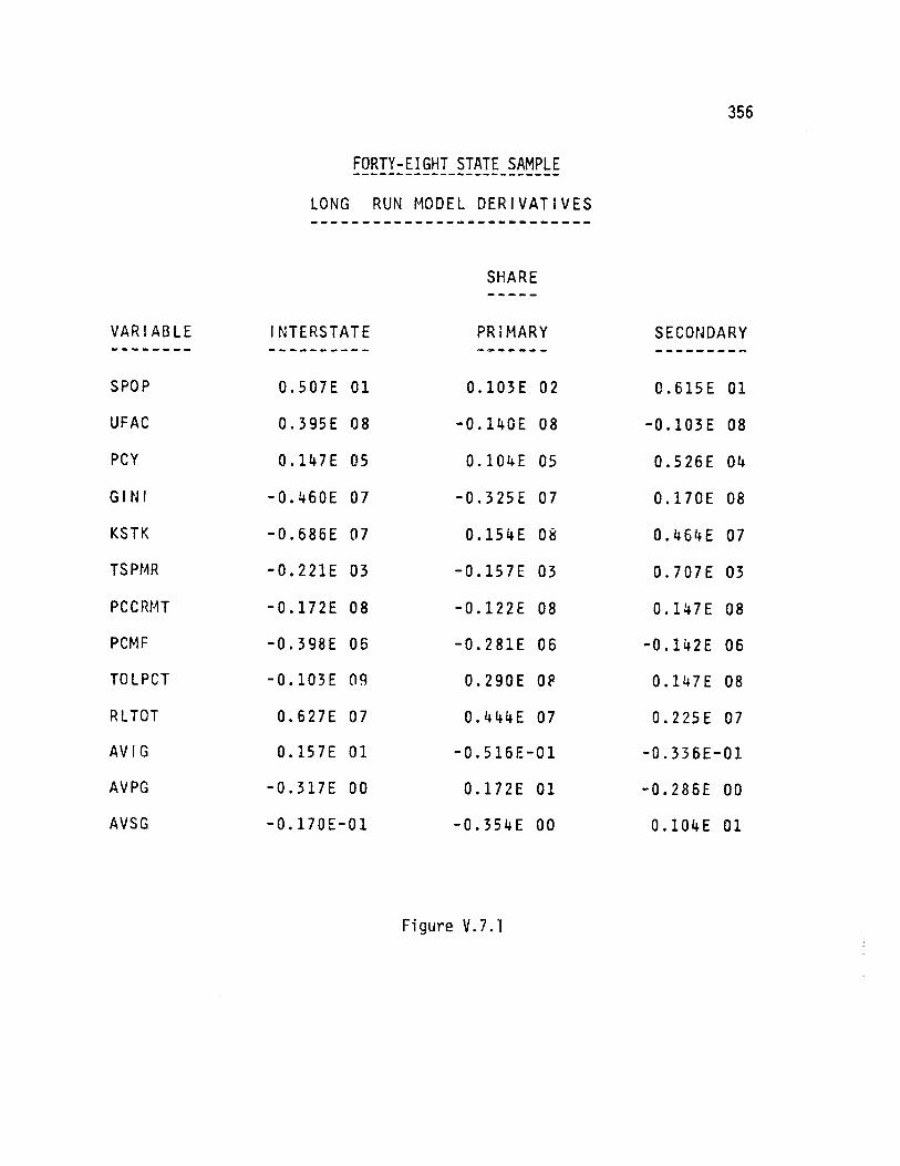
356
FORTY-EIGHT STATE SAMPLE
LONG RUN MODEL DERIVATIVES
SHARE
VARIABLE
SPOP
UFAC
PCY
GINI
KSTK
TS PMR
PCCRMT
PCMF
TOLPCT
RLTOT
AV I G
AV PG
AVSG
INTERSTATE
0.507E 01
0.395E 08
0.147E 05
-0.460E 07
-0.686E 07
-0.221E 03
-0.172E 08
-0.398E 06
-0.103E 09
0.627E 07
0.157E 01
-0.317E 00
-0. 170E-01
PRIMARY
0.103E 02
-0.140E 08
0.104E 05
-0.325E 07
0.154E 08
-0.157E 03
-0.122E 08
-0.281E 06
0.290E OF
0.444E 07
-0.516E-01
0.172E 01
-0.354E 00
SECONDARY
0.615E 01
-0.103E 08
0.526E 04
0.170E 08
0.464E 07
0.707E 03
0.147E 08
-0.142E 06
0.147E 08
0.225E 07
-0. 336E-01
-0.286E 00
0.104E 01
Figure V.7.1
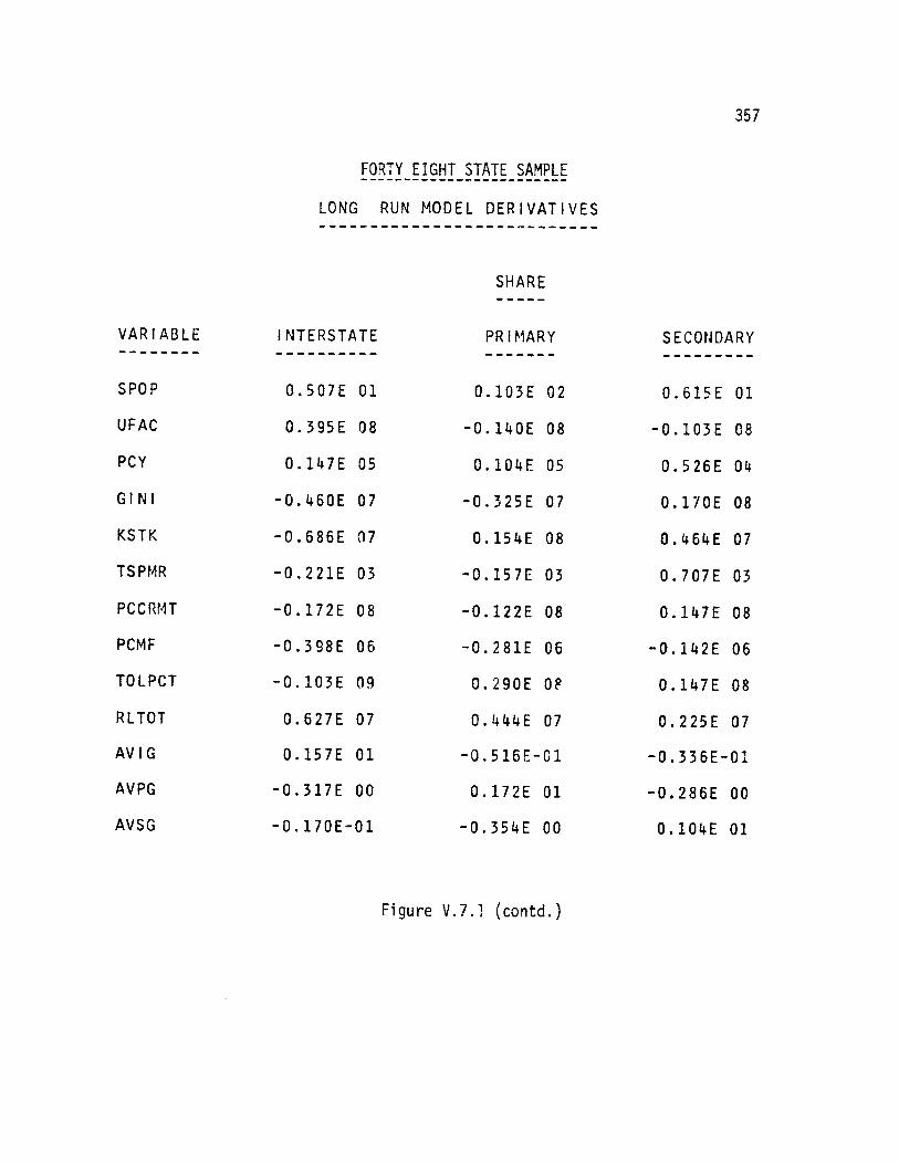
357
FORTY EIGHT STATE SAMPLE
LONG RUN MODEL DERIVATIVES
SHARE
VARIABLE
SPOP
UFAC
PCY
GI NI
KSTK
TSPMR
PCCRMT
PCMF
TOLPCT
RLTOT
AV I G
AVPG
AVSG
INTERSTATE
0.507E 01
0.395E 08
0.147E 05
-0.460E 07
-0.686E 07
-0.221E 03
-0.172E 08
-0.398E 06
-0.103E 09
0.627E 07
0.157E 01
-0.317E 00
-0. 170E-01
PRIMARY
0.103E 02
-0.140E 08
0.104E 05
-0.325E 07
0.154E 08
-0.157E 03
-0.122E 08
-0.281E 06
0.290E 08
0.44 4E 07
-0.516E-01
0.172E 01
-0.354E 00
SECONDARY
0.615E 01
-0.103E 08
0.526E 04
0.170E 08
0.46 4E 07
0.707E 03
0.147E 08
-0.142E 06
0.147E 08
0.225E 07
-0. 336E-01
-0.286E 00
0.104E 01
Figure V.7.1 (contd.)

358the results of our total expenditure model analysis, and the short run
allocation model analysis, our findings here are representative of a
State response to increasing Interstate aid wherein States increase
both their own total highway expenditures, and the share of those
expenditures devoted to Interstate construction.
This behavior stands in contrast to the States' response to
increasing Secondary System grant availability. Note from Figure
V.7.1 that the derivative of Secondary System expenditures with
respect to Secondary System grants is only 1.04. The implication
here is that each additional Federal Secondary System grant dollar
increases State expenditures by only four cents -- far less than the
increase that would pertain if States were matching increasing Federal
Aid on a dollar-for-dollar basis.I
In a similar fashion our results concerning the States' reaction
to increasing Primary System aid suggest a less than a dollar-for-
dollar expenditure matching response. The relevant derivative value
here indicates that each dollar increase in Primary System aid induces
only a 724 increase in States own expenditures on that System
(derivative value equal to 1.72). These results reflect our findings
from the empirical analysis of the total expenditure model (see
section IV.6). That is, the increases in Primary and Secondary
System expenditures in response to additions to grants on these
1 We again note that over our analysis period, Primary and SecondarySystem grants were provided on a 50% Federal, 50% State matchingbasis.

359
FORTY EIGHT STATE SAMPLE
LONG RUN MODEL ELASTICITIES
SHARE
!NT ERSTATE
0.330
0.396
0.623
-0.029
-0.067
-0.031
-0.011
-0. 001
-0.059
0. 028
1.232
-0. 070
-0.002
PRIMARY
0.943
-0.198
0.623
-0. 029
0.214
-0.031
-0.011
-0.001
0.023
0. 028
-0.057
0.534
-0.045
SECONDARY
1.117
-0.287
0.623
0.302
0.127
0.277
0. 026
-0. 001
0.023
0. 028
-0.074
-0.176
0.261
Figure V.7.2
VAR I ABLE
SPOP
UFAC
PCY
GINI
KSTK
TSPMR
PCCRMT
P CMF
TOLPCT
RLTOI
AVI G
AVPG
AVS G

360
FORTY EIGHT STATE SAMPLE
LONG RUN MODEL ELASTICITIES
SHARE
NONFASYST
1.662
-0.890
0.623
-0.029
0.127
-0. 031
0.183
-0. 001
0.023
-0. 489
0.198
-0. 130
-0.026
MAINT
0.407
-0.042
0.623
-0.029
0.387
-0.031
-0.011
0.007
0.023
-0.043
0.440
-0.062
0.001
OTHER
1.987
-0.042
1.440
-0.029
0.034
-0. 031
-0.011
-0.001
0.023
0.025
-0. 146
-0. 226
-0.066
Figure V.7.2 (contd.)
VARIABLE
SPOP
UFAC
PCY
G I N I
KSTK
TS PMR
PCCRMT
PCMF
TOLPCT
RLTOT
AVI G
AVPG
AVSG

361
Systems stem not from increases in States' own total expenditures,1
but from increases in the share of a States' resources devoted to
these Systems. Contrastingly, additional Interstate System aid has
had the effect of increasing both the States' total expenditures, and
the share of their expenditures devoted to Interstate construction.
The same general findings are evident from an examination of
Figure V.7.2 showing the long run elasticities from the two
expenditure models. It may be seen that a one percent increase in
Interstate grants leads to a 1.23% increase in long run State
Interstate expenditures. In other words, the fraction of total
expenditures representing Federal grant decreases with increasing
levels of Interstate aid. Conversely, the direct elasticities of
Primary and Secondary expenditures with respct to grants for these
Systems are less than one. These elasticities -- .53 for the
Primary System and .26 for the Secondary System indicate that Federal
grants comprise an increasingly larger fraction of total (State plus
zederal) expenditures on these Systems. Thus, on the Primary and
Secondary Systems, States' own expenditures have increased at approxi-
mately only one-half and one-fourth of the respective percentage
In fact, we have shown that the States' response to ABC grants ischaracterized by expenditure substitution. That is each additionalABC grant dollar is associated with a decrease in States' ownexpenditures by one dollar.

362
rate increases in Federal aid (for these Systems).1
The elasticities (or derivatives) of categorical highway
expenditures with respect to the other variables included in the
expenditure models generally conform with expected State behavior.
The indicated responses to each of these variables are summarized
below.
Socio-Economic Characteristics
As expected, increasing levels of State population (SPOP) and
per capita income (PCY) positively influence the expenditure levels
on all the highway categories. Highway travel within a State
increases with population and personal income. Therefore, we
should expect higher levels of SPOP and PCY to increase the States'
construction, maintenance and administrative expenditure requirements.2
It should be kept in mind in interpreting the results that elastici-
ties express percentage changes in the expenditure levels on each
highway category. Thus for example, while the elasticity of main-
tenance expenditures with respect to population increases (.497) is
1 Note that States' own Interstate expenditures have increased at agreater percentage rate than increases in Interstate aid. Thesefindings are all the more significant when it is recalled that forseveral years in our analysis period, States own Interstate expen-ditures exceeded their ABC System expenditures (see Figure 11.2.1)and the States' required matching share is lower on the Interstatethan on the Primary or Secondary Systems.
2 Moreover for a given gas tax rate, increasing highway travelprovides States with higher levels of earmarked highway revenue.
363greater than the corresponding elasticity for the Interstate System
(.3i0), in absolute terms increases in Interstate expenditures (in
response to changes SPOP) exceed those for highway maintenance.I
The measure of urbanization (UFAC) positively influenced Inter-
state System expenditures, reflecting the sharply increased cost of
Interstate highway construction in urban areas. The elasticity of
the remaining five shares with respect to UFAC were all negative, most
notably for the "lower order" (Sconary and non-Federal Aid) Systems.
GINI, the indicator of State income distribution had a positive
elasticity only for Secondary System expenditures. This result
reflects the fact that the rural States tend to have the greatest
degree of income inequality, and thus commit relatively higher
expenditure levels on the rural-oriented Secondary System.
Highway System Characteristics
Two measures of existing highway inventories (KSTK-depreciated
highway capital expenditures and TSPMR - State rural highway mileage)
and two indicators of highway congestion levels (PCCRMT--percent of
heavily traveled rural mileage and PCMF--percent of heavily traveled
total mileage) were incorporated in the analysis. As might be
expected, increasing levels of highway inventories positively
influenced maintenance and "other" (non-capital) expenditure levels.
In fact only Interstate expenditures exhibited a negative elasticity
1 As manifested by the corresponding derivative values (FigureV.7.1) of 5.07 for the Interstate category and 3.65 for themaintenance category.

364with respect to KSTK. Secondary System expenditures exhibited a
positive elasticity with repsect to rural highway mileage; again
indicating the rural orientation of the Secondary System.
Although the measures of highway congestion did not prove
particularly significant, the elasticities with respect to PCMF and
PCCRMT indicate reasonable expenditure responses. In particular
expenditures on the predominantly rural highway systems (Secondary
and non-Federal Aid Sustems) exhibited a positive elasticity with
respect to the level of rural highway congestion (PCCRMT). And
maintenance expenditures were positively influenced by the general
measure of State-wide concestion (PCMF).
Institutional Characteristics
The variable measuring the extent of local participation in
highway finance (RLTOT) exhibited neaative long run elasticities for
the non-Federal Aid System and maintenance expenditure categories.
Thus higher expenditure levels (presumably on highway maintenance
and non-Federal Aid System construction) by counties and municipali-
ties has the effect of "freeing up" (State) resources for the
performance of exclusive State highway functions (Federal
Aid System construction and administrative and other activities).
The second indicator of State highway financing conventions--the
extent of toll road financing (TOLPCT) did not appear to signifi-
cantly influence the allocation of State resources. However, the
results indicate that increasing use of toll roads has tended to
decrease Interstate expenditures while increasing the level of
expenditure on all other highway categories. As noted earlier,

365
this finding stems from the common State practice of delegating
Interstate System financing responsibility to quasi-public toll-
financed Turnpike Authorities.

366V.8 Summary
This chapter has presented an empirical analysis of the State
highway allocation behavior in both a short run and long run context.
The empirical model of short run highway allocation was derived from
a utility maximization representation of State expenditure behavior.
The model has the desirable property of explicitly accounting for State
budget constraints and thus focuses on the inherent tradeoffs States
must face in programing expenditures on alternative highway
activities. A generalized least square estimation technique was
developed to take proper statistical account of the joint interaction
between States highway expenditure shares.
The short run analysis explored allocation behavior under the
assumption that State budget levels were fixed. The results demon-
strated the relative importance of the Interstate grant program in
influencing States allocation decisions. The results from the short
run allocation model were then integrated with the empirical findings
of the total expenditure model (Chapter IV) to develop measures of
States' long run highway allocation behavior. The results demon-
strate that Federal grants for the Primary and Secondary Systems
have not significantly increased States' own expenditures on these
Systems. Specifically, it was shown that States have not had to
increase their own expenditures on a dollar-for-dollar matching basis
with increased Federal funding. This behavior contrasted with State
responses to the Interstate grant program, where it was shown that
increasing Federal aid has increased both total State expenditures
and the share of the States' budgets devoted to Interstate

367construction.
It was also shown that increases in Federal grant availability
have generally decreased State expenditures on non-aided activities.
One exception of interest was the finding that Interstate grant
increases have led to increases in States' maintenance expenditures,
indicative of the relatively large maintenance requirements associ-
ated with that system.
The predicted expenditure responses to changes in the State
socio-economic indicators, highway system characteristics and
institutional characteristics generally corroborated our a priori
hypotheses. The policy implications of our empirical findings
will be explored in the next chapter.

368
CHAPTER VI
SUMMARY AND CONCLUSIONS
VI.l Summary of the Thesis
This study has investigated the impacts of the Federal Aid
Highway Program on State highway expenditures. Our concern through-
out the conduct of the research has been to focus on this issue
from a national policy perspective. In simplest terms, the moti-
vation of the research was a consideration of the design of, and
response to Federal and highway financing.
Our starting point was a review of the mechanics of State and
Federal highway finance. Special attention was given to the
unique aspects of the Federal Aid Highway Program (FAHP) and
the attendant implications for empirical modelling. First, we took
note of the widespread use of earmarked Trust Funds at both the
Federal and State levels. This finding allowed us to restrict
our modelling attention solely to the dynamics of State higway
expenditure behavior.1 Second, our review of the highway finance
environment pointed out the significant differences between the
structural characteristics of the various Federal highway grant
programs--most notably between the Interstate and ABC highway
grant programs. The modelling implications here were twofold.
1 That is, unlike other State activities financed from general taxrevenues, we have been able to "separate out" highway expendi-ture decisions from the overall State budgetary process. Thismodelling convention is discussed in detail in Chapter II.

369
First, it became apparent that the models of State expenditure
behavior should explicitly account for the possibility of differ-
ing State responses to the availability of grants on the Inter-
state and ABC highway Systems.1 And second, the existence of
several distinct highway grant types suggested the importance of in-
vestigating the inherent tradeoffs States must face in programing
expenditures on alternative highway activities. In other words,
it was deemed important to trace the impact of the Federal Aid
Highway Program on both the total level of States' highway expendi-
tures and the allocation of State resources amongst Federally
aided and non-Federally aided highway activites.2
Following the review of the Federal and State highway finance
environment, we proceeded to develop a theory of State highway
expenditure behavior. Our purpose here was to draw attention
to the premise that State highway expenditure behavior depends
not only on the level of available Federal grants-in-aid, but on
the structural characteristics of the grant programs as well.
rowards this end, Chapter III started out with a normative dis-
This convention represents a departure from previous analytical
analyses in this area. None of the studies cited in the liter-ature review in Chapter I chose to evaluate the separate Stateexpenditure responses to grants on the different Federal AidHighway Systems. In section IV.6.1, we argue that failure toaccount for differing State responses to the Interstate vis-a-visABC highway grant programs obscures a fundamental characteristicof the Federal Aid Highway Program, and indeed yields misleadingresults.
2 Here too, our modelling convention differs from previous empirical
studies. As noted in Chapter I, the existing literature containmany examples of evaluations of States' total expenditure respon-ses to grants or States' allocation behavior. This thesis has at-tempted to present an integrated treatment of the impacts of theFAHP on both dimensions of State expenditure behavior.

370cussion of the considerations involved in designing a Federal
highway grant program to achieve specific national objectives. A
distinction was drawn between proposing changes to the existing
structure of the FAHP because the initial justification for the
Federal role in highway finance is no longer (or hasanever been)
valid, or because the structure of the FAHP is not compatible
with the accepted goals of the Federal role in highway finance.
While the normative analysis was not conclusive,1 the thesis does
argue that the issues involved in the design of a Federal grant
program are not simply a matter of political expediency. The
adoption of a revenue sharing program (for example) will have
significantly different allocational consequences than the pro-
vision of Federal aid on an open-ended categorical, matching grant
basis. Thus the normative analyis stresses the importance in
gaining a better understanding of the dynamics of State expendi-
ture responses to alternative Federal aid grant structures.
Accordingly, the remainder of Chapter III was devoted to the
development of a theory of State highway expenditure behavior. A
typology of alternative grant types was introduced, and evaluated
in terms of their impact in stimulating State expenditures on
aided functions or in effecting a substitution response wherein
States would reduce their own highway expenditures in response to
1 The normative analysis is limited by the difficulty in ascer-taining a unique, consensual national highway policy. Congres-sional debate is not normally conducted at an abstract (policy)level. Moreover, Federal highway objectives are not static.

371
increasing levels of Federal aid. Two modelling frameworks were
introduced, one based on an extension of consumer allocation theory,
and the other deriving from an application of a simple benefit/cost
investment criterion. Although these two models ostensibly differed
with respect to their underlying assumptions, in fact the conclu-
sions drawn from both approaches were quite similar. That is, both
analyses stressed the notion of price and income effects introduced
by Federal grants, and proceeded to demonstrate how State expendi-
ture responses differ according to the presence of one or both
of these grant characteristics. The theoretical models were then
used to investigate the historical grant and expenditure levels
on the Interstate and ABC highway programs. The theoretical analy-
ses suggested that for the Interstate program, Federal grants have
stimulated State expenditures that would most likely not have
been made in the absence of the grant program. This behavior was
contrasted with the experience in the ABC program, where it was
hypothesized that Federal grants have had a relatively insignificant
impact in determining States' total expenditure levels.
The theoretical models were useful in suggesting both the
appropriate framework for structuring the empirical models and the
expected empirical results. Our purpose in the remainder of the
thesis was to validate our theoretical hypotheses with econometric
models. Two models were advanced, treating in turn the impacts
of the FAHP on total State highway expenditures, and on the allocation
of States' highway budgets. The total expenditure model (TEM)
derived from a capacity utilization investment theory relating

372
States' highway investment levels to existing highway capital stocks,
proxy measures of desired highway capital stocks, and the availa-
bility of Federal aid. The empirical results strongly corroborated
the theoretical hypotheses regarding the differential impacts of
the Interstate and ABC highway grant programs.
The empirical model dealing with the second dimension of State
highway expenditure behavior--the short run allocation model (SRAM)
was derived from a utility maximization representation of State
decision making. The results demonstrated the differential im-
pacts of the various grant programs on States' short run budget
allocation amongst Federally aided and non-aided highway activities.
Finally, the empirical results from the short run alloca-
tion model were integrated with the findings of the total expendi-
ture model to develop measures of the States' long run highway
allocation behavior. These results were consistent with our a priori
hypotheses of State highway expenditure behavior.

373
VI.2 Policy Implications of the Empirical Findings
As the main focus of this thesis was to explore the impacts
of the FAHP on State expenditure behavior, we begin our discussion
here with the policy implications of estimation results of the Feder-
al grant terms included in the two expenditure models. We have
shown that the Interstate grant program has effected more signifi-
cant State expenditure responses than the ABC grant program.
Specifically, we have traced the responses to Federal grants in
terms of both States' total expenditure levels and short run
State budget allocation amongst aided and non-aided highway activi-
ties. For the former dimension of State behavior, the empirical
models have demonstrated that the Interstate programs have been
associated with increases in total (State plus Federal) expendi-
tures by more than the amount of increases in Federal Interstate
aid. Thus we concluded that the Interstate grant program has had
the effect of stimulating State highway expenditures.1 This response
pattern was contrasted with the ABC program, where the theoretical
and empirical models have demonstrated that States have substituted
their own highway expenditures for the receipt of increasing levels
of Federal ABC aid.
Regarding the second dimension of State highway expenditure
behavior, we have demonstrated that the various Federal grant pro-
grams have had a differential impact on States' allocation of their
1 Furthermore, we have shown that the resulting increase in States'total highway expenditures derive mainly from increasing resourceallocation to Interstate construction and maintenance activities(presumably in large measure in the Interstate system).

374
highway resources. Although all of the Federal highway grant
programs considered in this thesis were shown to stimulate States'
short run budget allocation to Federal-Aid System construction
activities, our results indicate that short run impacts of Primary
and Secondary System grants exhibit a less than dollar-for-dollar
matching response by the State.I Contrastingly, the Interstate
grant program was shown to increase States' short run Interstate
expenditures by more than the minimally required matching share.
In fact, based on our theoretical analyses (see Chapter III),
none of our empirical findings were unexpected. The empirical analy-
ses served to validate our a priori hypotheses, and placed dimen-
sions on the pattern of State responses to the FAFP. More important-
ly perhaps, the empirical research provides evidence which suggests
policy recomnendations for altering the present structure of the
Federal-Aid Highway Program.
Specifically, with our clearer understanding of the dynamics of
State expenditure responses to Federal aid, the fundamental issue
of the objectives of the Federal Aid Highway Program is called into
question. The imposition of Federal highway taxes and the pursuant
distribution of categorical grants represents an explicit expression
I Since the matching ratio of ABC aid over our analyses period was50% (except for the "public land States"; see Chapter II), ourresults indicate that even in the short run, States can "absorb"additional Federal aid without having to increase their ownexpenditures by the required State matching share. In Chapter II,we demonstrated that this response pattern could obtain only ifStates were histocially expending more than their minimallyrequired matching share on the Federal-Aid Systems.

375
of Federal policy. In particular, the restrictions on the use of
Federal funds for only certain types of facilities serves to iden-
tify those projects whose provision is deemed to be in the national
interest. It may well be argued that guaranteeing a minimally ac-
ceptable provision of important transportation facilities or stimu-
lating road construction necessary for interstate commerce are
valid Federal objectives. But we have shown that for the ABC pro-
gram, the former objective may not be appropriate, and the second
objective is not being accomplished. In short, our results indi-
cate that restructuring the Federal Aid Highway Program with a
relaxation of the specificity of the categorical restrictions, and
eliminating the built-in matching provisions would not significant-
ly alter State expenditure levels. Since the ABC program has
(over our analysis period) effectivejy operated as a non-categorical
block grant system, the detailed provisions (matching ratios,
categorical restructions, etc.) of the FAHP are unnecessary and
wasteful.
To be sure, the FAHP is characterized by other (non-allocation-
al) consequences--ensuring adherence to Federal labor and contracting
regulations, promoting the implementation of transportation planning
and process guidelines, and guaranteeing that Federally-funded
roads conform to certain safety standards. None of these "ancil-
lary" impacts are tied to the particular structure of the FAHP.
They are merely conditions States must satisfy in order to be eligible
for the receipt of Federal highway monies. Indeed, we are arguing

376
that greater attention needs to be paid to exploiting these
"ancillary" benefits in view of the failure of specific components
of the FAHP to achieve significant allocational goals.
We have already noted (section II.2.viii) that the Federal
Aid Highway Act of 1973 has incorporated several provisions de-
signed to reduce the specificity of the FAHP, most notably in terms
of increasing the allowable fund transfers between distinct Federal
Aid Systems, and providing Urban System aid for transit as well as
highway construction. The logical extension of the 1973 provisions
would be to completely remove all categorical and matching provisions
from those components of the FAHP where it is either not the intent
or not a reasonable expectation (given projected State expenditure
levels and Federal grant availability) for Federal grants to stimu-
late State expenditure levels.
As we noted in Chapter III, categorical matching grants are
most appropriate in situations where the Federal government perceives
a national interest in promoting investment on specific types of
highway facilities. Thus we argue that the criteria to be considered
in the design of the structure of the FAHP (specifically in terms
of the provision of categorical aid) is the existence of identifiable
investment needs1 on specific highway facilities. The analyses
I The Interstate System was a case where States would not haveheavily invested on this System in the absence of Federal cate-gorical grants. Moreover, it may be argued that the InterstateSystemis characterized by significant "benefit spillovers" (seeChapter III) due to its value in enhancing interstate commerceand national defense. Thus, grants for the Interstate System maybe viewed as a case where categorical aid was appropriate. Other
377
developed in this thesis suggest that categorical aid for broadly
defined functional highway classes, for example the Federal Aid
Primary System is not justified.
A related issue is the question of the advisability of the
existing taxation scheme and distribution formulas characterizing
the existing FAHP. We have shown that the gasoline excise tax
is at best proportional (for journey to work travel) and at worst
regressive (for vacation and business intercity travel). Moreover,
the analyses in Chapter II suggests that the apportionment formulas
currently in effect fail to accomplish a significant redistribution
of income from wealthier to poorer States. While the FAHP's
main objectives are not directly related to achieving more desirable
income redistribution,1 the generally recognized importance of
transport systems in promoting economic growthand regional develop-
ment suggests that more attention needs to be given to income dis-
tributive properties of FAHP apportionment formulas. In line with
our conclusion that the numerous highway categorical matching
instances where categorical grants might be appropriate includehigh risk/new technology projects where categorical "demonstration"grants serve to overcome States' reluctance to invest in un-tested technology, or, more generally any instance where theFederal government perceives a national interest in acceleratingexpenditures on specific project types (e.g., TOPICS, and the"Priority Primary Routes" designated in the 1972 Highway Act).
I There are more efficient Federal policies to achieve significantincome redistribution, for example direct transfer payments(Revenue Sharing) with income-based distribution formulas.

378
grants be consolidated into a block grant system, it is recommended
that the Department of Transportation give consideration to a
restructuring of the FAHP apportionment formulas. Towards this end,
the income and tax effort-based distribution formulas of the Federal
government's General Revenue Sharing program merit particular im-
portance.
The second aspect of income inequality inherent in the current
FAHP--the gasoline excise tax--also deserves DOT's attention in de-
veloping future Federal highway policy. The issue here involves
the income distribution characteristics, the revenue potential
and the price distortion characteristics of alternative taxation
schemes. While the gasoline tax possesses undesirable income dis-
tribution characteristics, it nonetheless represents an efficient
and relatively stable revenue source,2 and connotes a rough measure
of equity. 3 In order to mitigate its perverse income distribution,
DOT should consider supplementing the existing gasoline tax with
an excise tax on automobiles where the tax rate would be progressive-
ly higher for larger engine vehicles. This scheme would have the
I Since the FAHP apportionment formulas are currently administeredon a System-by-System basis, a grant consolidation program wouldrequire a change in apportionment policy in any event.
2 In the sense that demand for gasoline/auto travel is price in-elastic.
3 In the sense that the tax burden on an individual is proportionalto his usage of highway facilities.

379
merits of promoting progressive taxation and enhancing the Federal
government's objective of reducing gasoline consumption.
380
VI.3 Limitations of the Empirical Approach and Directions forFurther Research
The empirical analyses conducted in this thesis could be ex-
tended in several fruitful directions. First, more attention
could be given to investigating the specifics of the variation in
highway investment behavior between States. Data limitations
precluded the possibility of applying our expenditure models (the
short run allocation model and the total expenditure model) on a
State-by-State basis. While we did take proper statistical account
of interstate behavioral variation in the pooled data sample, more
research is necessary to investigate causal factors underlying
differences in State behavior. Along these lines, more attention
could be given to political and institutional factors. Does a
State's highway expenditure behavior change significantly after
it has formed a multimodal Department of Transportation? Are
there significant cultural and regional effects present--that
is for example, do Southern States express a different outlook on the
provision of public services that the New England States and is
so, why?1 Is there a difference in expenditure behavior that is
attributable to differing State political organization, as for
example between States where the Legislature exerts strong highway
policy influence and States where the Executive branch (Governor)
1 Some of these questions were examined in our highway expendituremodels through the use of "dummy variables." None of theseexperiments produced conclusive results.

381
assumes a major role in highway policy formation?
These are all important questions that can only be addressed
by adopting a more disaggregate analysis framework than the one
applied in this thesis. The approach we did adopt reflected a
focus on the highway investment issue from a national polic p2er-
spective.
A second area where future research would be fruitful involves
exploring the validity of the assumptions underlying our empirical
models. Our models have assumed States exhibit "rational economic
behavior" in the sense that allocation and expenditure decisions
are based on the desire to maximize States' perceived utility (or
benefit). While this view of the motivations for State decision-
making is quite general and non-restrictive, it would be instruc-
tive to conduct in-depth interviews with responsible State highway
officials to validate our assumptions. Such interviews would be
useful in both gaining further insight into the factors (variables)
to be included in future model development and checking the reason-
ableness of our empirical results.1
Finally, our modelling approach could be extended in a fore-
casting environment to assess the impacts of future Federal policy
alternatives. Along these lines, the policy recommendations ex-
pressed earlier in this chapter (grant consolidation and an alteration
1 The Federal Highway Administration has reviewed the majorempirical results developed in this research, and has indicatedgeneral agreement with our findings based on their own in-houseanalyses.
382
in the taxation and grant distribution characteristics of the
FAHP) as well as other alternative program variants could be
evaluated against baseline predictions of the consequences of con-
tinuing the existing FAHP.

BIBLIOGRAPHY 383
Advisory Commission on Intergovernmental Relations, STATE-LOCALFINANCES: SIGNIFICANT FEATURES AND SUGGESTED LEGISLATION, 1972Edition
Advisory Commission on Intergovernmental Relations, SPECIAL REVENUESHARING: AN ANALYSIS OF THE ADMINISTRATION'S GRANT CONSOLIDATIONPROPOSALS, December, 1971
Advisory Commission on Intergovernmental Relations, IMPACT OFFEDERAL PROGRAMS ON LOCAL GOVERNMENT, ORGANIZATION AND PLANNING,1962
Ainsworth, K.G., "Comments on Monypenny's Federal Grants-in -Aidto State Governments: A Political Analysis," National Tax Journal,Volume XIII, Number 3 (September, 1960)
Balestra, P., and M. Nerlove, "Pooling Cross Section and TimeSeries Data in the Estimation of a Dynamic Model: The Demand
for Natural Gas," Econometrica, Volume 34, Number 3
Barr, J.L. and O.A. Davis, "An Elementary Politidal and EconomicTheory of Expenditure of Local Governments," Southern Economic
Journal, Volume 34, Number 1 (October, 1966)
Birkhead, Guthrie S., METROPOLITAN ISSUES: SOCIAL, GOVERNMENTAL,FISCAL, Brookings Institution Reprint Number 61, Washington, D.C.,1962
Bishop, George A., "Stimulative Versus Substitutive Effects of StateSchool Aid in New England," National Tax Journal, Volume XVII, Number
2 (June, 1964)
Break, George F., INTERGOVERNMENTAL FISCAL RELATIONS IN THE UNITED
STATES, The Brookings Institution, (Studies of Government Finance),
Washington, D.C., 1967
Burch, P., HIGHWAY REVENUE AND EXPENDITURE POLICY IN THE UNITED STATES,Rutgers University Press, New Brunswick, New Jersey, 1962
Dearing, C.I., and W. Owen, NATIONAL TRANSPORTATION POLICY, The Brook-ings Institution, Washington D.C., 1949
DeGarmo, E. Paul, ENGINEERING ECONOMY, The MacMillan CompanyNew York,New York, 1960

384
Dorfman, Robert, PRICES AND MARKETS, Foundations of Modern EconomicsSeries, Prentice-Hall Inc., Englewood Cliffs, New Jersey, 1967
Dresch, S.P., "An 'Alternative' View of the Nixon Revenue SharingProgram," National Tax Journal, Volume XXIV, Number 2 (June, 1971)
Due, John F. and A.F. Friedlaender, GOVERNMENT FINANCE: ECONOMICSOF THE PUBLIC SECTOR, Richard D. Irwin Inc., Homewood, Illinois,
Fifth Edition, 1973
Faddeev, D.K. and V.N. Faddeeva, COMPUTATIONAL METHODS OF LINEAR
ALGEBRA, W. H. Freeman Inc., San Francisco, California, 1963
Ferman, Gerald, OUTPUT ANALYSIS: THE DISTRIBUTION OF GRANTS-IN-AID 1957-1967, Working Paper Number 10, Denter for the Study ofFederalism, Temple University, Philadelphia, Pennsylvania, 1974
Findakly, H.K., A DECISION MODEL FOR INVESTMENT ALTERNATIVES IN
HIGHWAY SYSTEMS, Unpublished ScD Thesis, Department of Civil
Engineering, Massachsuetts of Technology, September, 1972
Friedlaender, A. F., THE INTERSTATE HIGHWAY SYSTEM, North Holland
Publishing Co., Amsterdam, 1965
Friedlaender, A.F., "The Federal Highway Program as a Public Works
Tool," in Ando, A. et al, STUDIES IN ECONOMIC STABILIZATION, TheBrookings Institution, Washington, D.C., 1968
Gabler, L.R., and J.I. Brest, "Interstate Variations in Per CapitaHighway Expenditures," National Tax Journal, Volume XX, Number 1(March, 1967)
Gallamore, Robert E., (Reprint of) Testimony Before the Subcomit-tee on Roads of the Senate Public Works Committee, February 15, 1973
Gramlich, E.M., "Alternative Federal Policies for Stimulating State
and Local Expenditures: A Comparison of Their Effects," NationalTax Journal, Volume XXI, Number 1 (June 1968)
Haskell, M.A., "Notes and Memoranda: Federal Grants in Aid-TheirInfluence on State and Local Expenditures," Canadian Journal ofEconomics and Political Science, Volume XXX, Number 4 (November, 1964)

385
Haveman, R.H., and J. Margolis (editors) PUBLIC EXPENDIUTRES AND
POLICY ANALYSIS, Markham Publishing Company, Chicago, Illinois, 1970
Henderson, J.M. and R. E. Quandt, MICROECONONIC THEORY: A MATHE-
MATICAL APPROACH, McGraw-Hill Book Co., 1958
Highway Research Board, HIGHWAY FINANCING: 10 REPORTS, Highway
Research Record Number 20, 1963
Jack Faucett Associates Inc., CAPITAL STOCK MEASURES FOR TRANSPOR-
TATION, Report Number JACKFAU-71-04-1, Volumes I, II, and III,Chevy Chase, Maryland, June, 1972
Johnson, D.W.,.and C.M. Mohan, "Revenue Sharing and the Supply of
Public Goods," National Tax Journal, Volume XXIV, Number 2 (June, 1971)
Kuh, Edwin, CAPITAL STOCK GROWTH: A MICROECONOMETRIC APPROACH, North
Holland Publishing Co., Amsterdam, 1971
Kurnow, Ernest, "Determinants of State and Local Expenditures Recon-sidered," National Tax Journal, Volume XVI, Number 3 (September, 1963)
McFarland, W.F., ECONOMIC EFFICIENCY IN HIGHWAY EXPENDITURES, Unpub-lished PhD Thesis, Tulane University, New Orleans, Louisiana, 1970
McMahon, W.W. and C.M. Sprenkle, "A Theory of Earmarking," NationalTax Journal, Volume XXIII, Number 3 (September, 1970)
Maxwell, J.A., "Federal Grant Elasticity and Distortion," NationalTax Journal, Volume XXII, Number 4 (December, 1969)
Maxwell, J.A., FINANCING STATE AND LOCAL GOVERNMENTS, The BrookingsInstitute, Washington, D.C., 1969
Miller, Edward, "The Economics of Matching Grants: The ABC HighwayProgram," National Tax Journal, Volume XXVII, Number 2 (June, 1974)
Miller, Edward, "Short Run Responses to Changes in the Availability
of Federal Funds," Unpublished Department of Transportation Paper
(TPI-10), 1972
Miller, Edward, "Effects of Federal Grants in Aid on Local Expenditures,"Unpublished Department of Transportation Paper (TPI-10), 1972

386
Miller, Edward, "The Effects of the Revenue Sharing Pass Through inLarge Urban Areas," Unpublished Department of Transportation Paper(TPI-10) 1972
Miller, Edward, "Impacts of the ABC Program on Highway Investment,"Unpublished Department of Transportation Paper (TPI-10) 1972
Miller, Edward, "Differences in Returns by Road System," UnpublishedDepartment of Transportation Paper (TPI-10) 1972
Mogulof, M.B., "Regional Planning, Clearance, and Evaluation: A Lookat the A-95 Process," American Institute of Planners Journal, Volume37, Number 6 (November, 1971)
Monypenny, P., "Federal Grants-in-Aid to State Governments: A Politi-cal Analysis," National Tax Journal, Volume XIII, Number 1 (March, 1960)
Musgrave, R.A. and P.B. Musgrave, PUBLIC FINANCE IN THEORY ANDPRACTICE, McGraw-Hill Book Co., 1973
Musgrave, R.A..(editor), ESSAYS IN FISCAL FEDERALISM, The BrookingsInstitution, Washington, D.C., 1965
Neuman, Lance, A TIME STAGED STRATEGIC APPROACH TO TRANSPORTATIONSYSTEM PLANNING, Unpublished SM Thesis, Department of Civil Engineering,Massachusetts Institute of Technology, 1972
Oates, W.E., "The Dual Impact of Federal Aid on State and Local Govern-ment Expenditures: A Comment," National Tax Journal, Volume XXI,Number 4 (November, 1968)
O'Brien, T., "Grants-in-Aid:Some Further Answers," National Tax Jour-nal, Volume XXIV, Number 1 (March 1971)
Osman, Jack W., "The Dual Impact of Federal Aid on State and LocalGovernment Expenditure," National Tax Journal, Volume XIX, Number4 (December, 1966)
Osman, Jack W., "On the Use of Intergovernmental Aid as an Expendi-ture Determinant," National Tax Journal, Volume XXI, Number 4(December, 1968)
Pecknold, Wayne M., EVOLUTION OF TRANSPORT SYSTEMS: AN ANALYSIS OFTIME STAGED INVESTMENT STRATEGIES UNDER UNCERTAINTY, Unpublished PhDThesis, Department of Civil Engineering, Massachusetts Institute ofTechnology, 1970
387
Quandt, Richard E. and K.H. Young, "Cross-'Sectional Travel DemandModels: Estimates and Tests," Journal of Regional Science, VolumeIX, Number 2 (1969)
Roth, G.J., A SELF FINANCING ROAD SYSTEM, Institute for EconomicAffairs, London, 1966
Sacks, Seymour and R. Harris, "The Determination of State and LocalGovernment Expenditure and Intergovernmental Flow of Funds,"National Tax Journal, Volume XVII, Number 1 (March, 1964)
Scott, A.D., "The Evaluation of Federal Grants," Economica, VolumeXIX, Number, 76 (November, 1952)
Smerk, George M. , URBAN TRANSPORTATION; THE FEDERAL ROLE, IndianaUniversity Press, Bloomington, Indiana, 1965
Smith, A.H., "State Payments to Lcoal Governments in Wisconsin,"National Tax Journal, Volume XV, Number 3 (September, 1962)
Smith, D.L., "The Response of State and Local Governments to FederalGrants," National Tax Journal, Volume XXI, Number 3 (September, 1968)
Stanford Research Institute, BENEFIT/COST ANALYSIS OF HIGHWAY IMPROVE-MENT PROJECTS, SRI Project MU-7362, Stanford, California, December, 1969
Stockfisch, J.A., "Fees and Service Cahrges as a Source of CityRevenues," National Tax Journal, Volume XIII, Number 2 (June, 1970)
Strotz, R.H., "The Empirical Implications of a Utility Tree, Econo-metrica, Volume 25, Number 2
Teeples, R.K., "A Model of a Matching Grant-in-Aid Program WithExternal Tax Effects," National Tax Journal, Volume XXII, Number4 (December, 1969)
Theil, Henri, OPTIMAL DECISION RULES FOR GOVERNMENT AND INDUSTRY,North Holland Publishing Co., Amsterdam, 1964
Theil, Henri and A.S. Goldberger, "On Pure and Mixed StatisticalEstimation in Economics," International Economic Review, Volume 2,Number 1 (January, 1961)

388
U.S. Bureau of the Census, 1967 CENSUS OF TRANSPORTATION, Volume 1,National Travel Survey, Washington, D.C., July, 1970
U.S. Bureau of the Census, GOVERNMENTAL FINANCES IN 1953-1954(Yearly editions to 1969-1970), Washington, D.C.
U.S. Bureau of the Census, STATE GOVERNMENT FINANCES IN 1950 (Yearlyedition to 1970), Washington, D.C.
U.S. Bureau of Public Roads, HIGHWAY STATISTICS 1950 (Yearly editionsto 1970), Federal Highway Administration, U.S. Department of Transpor-tation, Washington, D.C.
U.S. Department of Transportation, Office of the Assistant SecretaryFor Policy and International Affairs, 1972 NATIONAL TRANSPORTATIONREPORT, Washington, D.C., 1972
U.S. Department of Transportation, NATIONWIDE PERSONAL TRANSPORTATIONSTUDY: HOME-TO-WORK TRIPS AND TRAVEL, Volume 8, Washington D.C.,
August, 1973
U.S. Department of Transportation, ALLOCATION OF HIGHWAY COST RESPON-
SIBILITY AND TAX PAYMENTS, Washington, D.C., 1969
U.S. Federal Highway Administration, FINANCIAL BACKGROUND FOR THE
1972 HIGHWAY NEEDS STUDY, Unpublished Report C-1, Washington, D.C., 1972
U.S. Federal Highway Administration, HIGHWAY FINANCE MANUAL, Washing-ton, D.C., 1972
Urban Mass Transportation Administration, CAPITAL GRANTS: FOR URBANMASS TRANSPORTATION: INFORMATION FOR APPLICANTS, Washington, D.C.,June, 1972
Wells, John D. et al, ECONOMIC CHARACTERISTICS OF THE URBAN PUBLICTRANSPORTATION INDUSTRY, Institute for Denfense Analyses, Arlington,Virginia, February, 1972
Wilde, J.A., "Grants-in-Aid: The Analytics of Design and Response,"National Tax Journal, Volume XXIV, Number 2 (June, 1971)
Wilde, J.A., "The Expenditure Effects of Grant-in-Aid Programs," Na-
tional Tax Journal, Volume XXI, Number 3 (November, 1968)

389
Winch, D.M., THE ECONOMICS OF HIGHWAY PLANNING, University of TorontoPress, Toronto, Ontario, 1963
Young, K.H., "The Synthesis of Time Series and Cross-Section Analyses:Demand for Air Transportation Service," Journal of the American
Statistical Association, Volume 67, Number 339
, "The Public Finance Aspects of the Transportation Sector, AStaff Paper Prepared by the Office of Policy and Plan Development,U.S. Department of Transportation, Washington, D.C., May, 1971
, FINANCING STATE AND LOCAL GOVERNMENTS, Proceedings of theMonetary Conference, Nantucket Island, Massachusetts, June 14-16, 1970
,Sales Management 's SURVERY OF BUYING POWER, (Yearly editions1950-1970), Bill Brothers Publications, New York, New York

390
Biographical Summary
Dr. Sherman was born in New York City on June 22, 1948. He pursuedundergraduate studies at the Massachusetts Institute of Technology,receiving a Bachelor of Science degreee in Aeronautical and Astro-nautical Engineering in February, 1971. Dr. Sherman received aMaster of Science degree in Transportation Systems Analysis fromM.I.T. in June, 1971. His S.M. thesis was entitled "The AirportAccess Problem: A Case Study Approach." Dr. Sherman remained atM.I.T. for his doctoral research, concentrating in the field oftransportation economics. He submitted his Ph.D. dissertation en-titled "The Impacts of the Federal Aid HIghway Program on State andLOcal Highway Expenditures," in January, 1975.
Dr. Sherman's research interests include a wide range of topicsrelating to transport economics. He is currently employed as aSenior Research Associate for Charles River Associates, Inc., wherehe is conducting research on Federal energy and environmental policyalternatives, and developing imporved methods for predicting urbantravel demand patterns. He has worked as a consultant to the govern-ment of Venezuela, assisting in the development of capital budgetingprocedures. Dr. Sherman has also consulted to the U. S. Departmentof Transportation in a variety of areas including developing proce-dures for assessing urban mobility, and assisting in the design ofthe National Transportation Study.

391
Appendix A
Estimated Parameter Values of the Long Run Revenue Policy Model

392
This appendix presents a complete listing of the regression runs
performed on the total expenditure model (TEM). In the figures that
follow, each regression run is described by a four character model
number, 1112nln2 where:
= 4
12
ni= {n2 =
S - grant terms stratified by type (Interstate andnon-Interstate
T - single grant term
U - undeflated data set
D - price deflated data set
1 - 48 State/14 year pooled data sample2 - 7 State/14 year pooled data sample
3 - 41 State/14 year pooled data sample
1,2,..., - model specification number

E3JAlL2ULESULLS
TOTAL EXPENDITURE MODEL
!QE_" .QLNhSU
SENE RAL1ZfLLLEAS.I2UARtS
E-:AIt.1- %k2tk12L55a&z------S LE--.2s3L---89502
a~--- aa~a -
F STI MA T E VALUE
STANPAPO ERRPP
T-STATISTIC
FSTrATE VALUE
STANflAP) E PPOR
T-STATTSTIC;
'.A6 -0.650E-06
5.58 0.732F-O7
1.78 8.74
R I. TOT-0.319
0.f'36
8.86
TO L PCT0.457
0.069
6.62
PrY C HNT
-0.601
0.031
19.53
0.018
0.001
17.94
9.468
Ie.24
8.41
A VNIGP-1.146
3.091
12.55
0.605
0.124
4.88
0.6 19
0.043
14.39
w~
-
m

EU AlL2E.ULUis
TOTAL EXPENDITURE MODEL
.ENERA2 IL.LAi QUAEl
F-STAT: F(10.661) = 238.10 SEE = x3 ~RS0 0 .182
CON STM'NT
ESTIMATE VALUE
STANDARD FP9PII
T-STATISTIC
FSTTMATF VALIIF
STANOARD EQRDR
T -STATISTIC
8.9P
5.55
1.62
RLTOT
J . 37
a03 7
SPOW
-0 .597E-06
0.796F-37
7.51
TOLPCT0.355
0. C8
4.3?
0.017
0.001
17.26
0.613
0.123
4.97
10 .639
1.206
8.8?
AVNIGP-1 *123
0.097
11.61
-00599
0.030
19.61
AVIGP
0.608
0.043
14.14
BI PTCX0. 088
0.055
1.58
ko
. " -.w .M WA.M-f mom .-~fi.A --_ _ _ -_ _ _ _ _ _6 _6 M M
- - - - - - - - - - -
-W - - -0..- -00 - qwft --M. om. -wpm
awmmlmmpwmompommom

EU.1_ ALL2 La.EaULIS
TOTAL EXPENDITURE MODEL
EQL.Na.sul3
GEN-rALIL.ED-LEAi.SQUARES
F-STAT: F(1066I1) 231 5FF = 5.-34 R&D = 0.781
CONISTANT cpnp. - ---- o- la -- -MO- ------
FSTIMATF VLIF
STANOAPD ERROR
T-STATISTIC
rSTIMATF VALUCf
STANARDF EROR
T-STATISTIC
6.73
5.70
1.18
RLTOT-0.333
0 r 36
9.1?
-0 .649E-96
0*728'-07
8.91
TOLPCT0.407
0.372
5.68
K STK IJFAC
0.018
0.001
17.98
&ILE.
0.656
0.125
5.24
q.872
t .t39
8.66
AVNIGP-1.146
0.091
12.61
-o .ss7
0.031
18.83
AVIGP0.607
0.043
14.08
GOP-3.402
3. 172
2.34
cLn
.d& M -1&d _6mw .. mum.- _ ._ - - - - _ _ - __ A&_-J6A
- - - - - - - - - - - - - - - - - - - - - - - - - - -
.- -MN.- - _

US Ilt ALi22-HEUL S
TOTAL EXPENDITURE MODEL
!QEt-tU~A' Ift
IEUEALELLLEAS1-iQUARLS
E= IiELi h -- 2 --- -- 5 1 --- 5 -- 2 3
CONSTANT-
C~STTMATF VAIIF
STANnAPI) FRPOR
T-STATISTIC
RSTYM-TF VALUIE
STANrAF9 ERROR
T-STATTSTIC
4.20
QLTDT
-I?47
0.037
6.68
-S pr-. 6CRE-06
O.758F-i7
8.02
TiLPCT
C. 784
0.086
3.29
12.852
1.193
10.76
AVNIGP
-1.179
0.093
12.71
ALLEAL -
-0.652
0.031
21.05
AVIGP
0.530
0.042
12.62
0.016
).001
15.51
B I PTAX
0.059
0.053
1012
0.20
0.120
6.9?
GPQP
-0,.508
0.164
3.10
- - - - - - - - - - - - - - - - - - - - - - - - - - - - - - - - - - - - - - - -
wiLw.EmwM- w1w -w-dmmo~ 49- -M 4M. At L.L.61 J9..w6 o64,64 .1p. -w. . . " ma.L-w. -.. . . -
mwmppmv

EiLLMALI22t-SaTS
TOTAL EXPENDITURE MODEL
ENE39AL LLL.DEAiIsQUA&LS
=SAI- L2Th kztL_2-4LI2 R--$UE &-5fl-___Z2--1
E[STIMATE VALUF
STA"FA' ERPPIP
T-STAT! STTC
ESTIMATP VALIIF
cTANOAP D EP PR
T-STATI 5TIr
CQ 2ArL--BE C.-.-E E---!EAC---_ 1---GL
7.93 -0 .153E-05 9.315 -0.602 '.018 0.659
5.67 C.l04F-)6 1.130 0.031 0.001 0.126
1.4" 7.49 8.24 19.17 17.62 17.62
PL TCT
-0.324
o. C 37
5.23
TfL PCTJ.401
V0071
8.84
AVNIGP-1. 11
0.093
5.68
AI!GP0.621
0,044
12.03
- - - - - - - - - - - - - - - - - - - - - - - - - - - - - - - - - - - - - - - - - - - - - - - - - - - - - - - - - - - - - - - - - - - - - -

TOTAL EXPENDITURE MODEL
G AF E1L.. .. suiEEALiLJEA ST_QUARE
F-STAT3!1 F( 9.h? = '50.79 SEE= ~R&QE2~iItI Aaaa4 =1 -.--. - -_2 _ _ _ _ -- -- _--"- - Ek
.C&N]iA.I_
ESTIMATE VALUE
STMPANA ERPOR
T-STATISTYC
PSTIMATE VALUE
STtNDAPD FRROR
T-STATISTIC
10.01
5.66
1.77
RLTOT-0.330
0.036
9.07
-0.137E-33
0.173F-04
7.9'
TOLPCT3.410
0.070
5.83
A5!K..
9.360
1 * 128I
8.30
AVNIGP-1.9135
0.093
12.22
.UEA.Q..
-0.600
0.031
19.16
0.018
0.001
17.73
AVIG0.620
0.043
14.25
0.606
0.126
4.81
.... Mo -- G kflI M- .O--.- -...4. - - .. MwoO- -W
... d-

TOTAL EXPE NDITURE MODEL
-MQQN.A..S21
ENESALIZEID-L EASiQUAR i
F-SrAr: E 9. RRI 2018 SF16 SEE 6.57
fllN A NT c pnp K CIK
FSTIMATE VALUE
STANDAPP ERRIR
T-CTATTST T
FSTIMATE VALIUE
STANQAP FPRfR
T-STATISTIC
97.82
8.94
1 0.95
RLTCT-0.127
x cqo
1.41
-0.668E-06
0.737E-06
0.91
T9LPCT2.772
0.492
5.64
RSO = 2m20
iFAC ECV . TMT
-1.340
0.227
5.90
0.006
0.002
3.66
0.209
0.307
0.69
AVNIGP-0.311)
0.161
1.92
-0.542
o.114
4.74
0.657
0.061
10.75
WA
1 x _ - - . _ _ -
-. - - - - - -- - - --. IN- _ - - - _ _ _
M

15LUAltl&ESiUUL
TOTAL EXPENDITURE MODEL
-I24LN-SU22
.G2 f3AU LL.EDLLAi1hS2UAES
E-STAT: FIC'. 87) = 15.24 SEE = 6.11 RSQ = .697
FSTIMATF VALUE
STANPAPf EPROR
T-STATISTIC
%-STIMTE VALUE
STANOArD FRROR
T-STATISTIC
73.5R -O.178E-O5 3.166 -0.616 0.003 -0.416
9.02 0.A65F-36 0.133 0.147 0.002 0.194
8.16 2.O 1.24 4.19 l.41 2.14
PL T'lT
-0.032
3.090
o.91
T')L PC T1.400
u.490
2.86
AVNIGP-0.379
0.208
1.8?
AVIGP0.571
0.091
6.26
9i PTCX0.484
0.491
0.99
a
.646 -;m .m6.&ibdl -U = _L _ _-m Wm__ _ _ _ _ __ _ _ _ _ _ __o _ _
- - - - - - - - - - - - - - - - - - - - - -
W-

TOTAL EXPENDITURE MODEL
.GENEALI LElA.IA QUAfli
F-STAT!F( fl.AS41 = 24t.3t SEE = 5 14 RSQ 0.794
--- ----- -- -- ----- - - -----
CONSTANT-
PSTIMATF VALUE
STANDARD FRROP
T-STATTSTIC
E STIMATE VALUE
STANDARD ERROR
T-STATISTTC
16.15
5.55
2.91
RLTOT--<.524
0 .C41
12.75
SPpp
-0.478E-06
2.724E-07
6.60
TOLPCT0.368
0.T71
5.21
.OJEAL.-
-0.637
0.034
18.50
0.018
0.001
17.32
KSTK-
8.?74
1.032
8.02
-0.856
0.114
7.51
0.693
0.122
5.67
0.439
0.057
7.68
-Pb
q U
."- .0- -.. I.-wo now.-ma-mm AN& JWMA-amx
a-

EULMA2N-REULIi
TOTAL EXPENDITURE MODFI
fQODL-Nia_.a2
GENE ALILE!LJEA.SSQUARfS
RSQ = 0.799
FSTIMATE VALUE
STANDAPD EfRlP
T-STATIST IC
L2N.IAN2I.
16.24
5.48
2.96
-0.5C8E-06
0.783E-37
6.49
ES T !NATF VALUE
STANDAPD EPROR
T-STATISTIC
10.050
1.125
8.93
-0.9631
0.034
18.53
3.018
0.001
16.99
RLTOT-2.534
0.043
12.32
0.683
0.121
5.65
TCL PCT0.393
0.086
4.55
AVNMI-GP-0.919
0.120
7.64
0.415
0.057
7.30
-0.05?
0.056
0.93
-ME-M- 4 A&= AlOWNEWO - 4M d aWW4 aNW- --- AML-OL-L-.dt-.d6-
- - - - - - - - - - - - - - - - - - - - - - - - - - - - - - - - - - - - - - -
-. U- . - --PON-- dL-.-401W d
...S

t~jMAUI.tLR3E.SU 15
TOTAL EXPENDITURE MODEL
fzESERAL QJZEJLEA2.1 UAEES
F-ST AT: Ff 8,66b3) z 2)l496 SE E _ .0 ERS z0.JZ Z
ESTIMATE VALUE
ST NPARD ERROP
T-STATISTIC
FSTIMATE VALUE
STANnAPD ERROR
T-STAT1STIC
-CO ANI-IiSEQ._M--K... EAINL...0-
24.1? -0.454E-06 13.640 -0.454 0.014 3.307
6.17 0.807E-07 1.655 0.033 0.001 0.138
3.90 5.62 8.24 13.69 13.01 2.21
RLTOT-0.488
0.038
12.84
TOLPCT0.482
3.378
6.14
A VT &P0.038
3 .03?
1.17
CD)
m.w_ _A -
- - - - - - - - - - - - - -

Ellbal N....ESals
TOTAL EXPENDITURE MODEL
LAUDE. TXUU12
.iGENEAL.LLEA I.5$QUARtS
E=IAIJ1.EU. LE..QA........ .--.-..--
ESTIMATF VALUE
STANDAPD FPRR
T-STATISTIC
20.84
6.34
3.45
-0.3 14E-)6
C.844F-OT
3.72
FSTIMATF VALIJF
STANDkPn EPROR
T-STA T ISTTC
16.553
1.814
9.13
-0.458
C .032
14.C7
0.013
0.001
t2.?9
0.337
0.135
2.50
RL TOT-0.418
0.C3g
13.6?
TOLPCT0.178
0.098
1.83
AVTGP0.039
0.035
1.11
B! PT c0.?59
0.056
4.40
0.
ampdolm- ---ad- 4 - -1dbAUW..m.m -

E5iLeAllMQmESULIS
TOTAL EXPENDITURE MODEL
EfELALuQ12Uf
' ENERALLLEDLWA AB
F-STAT: F( 9.662) = 199.56 SE E= 5.93 RSQ = 0.731
ESTIMATF VALIE
STANPARn FRROR
T-STATISTIC
E ST IMAlI E VA UE
STANDARD ERROp
T-STATISTIC
19.96
6.23
3.19
RLTfT-0.Sfl?
0.038
13.18
52- 2E------ESTK
-0.455E-)6 16.177
0.795E-7 1.756
5.72 9.21
TOLPCT0.388
0.081
4. 80
AVTGP-0.004
0.033
0.11
.JIEAL.
-0.461
0.033
12.96
0.015
0.001
13.30
.o 355
0.138
2.57
GPOP-0.543
0.191
2.85
4:0C:)
.- . t_ -- lgM SZo -mo-fd4mJ-rJ ---m--kfA-M 6&6L- -K LJPC.L
__-_.------... _.. _I_.W--
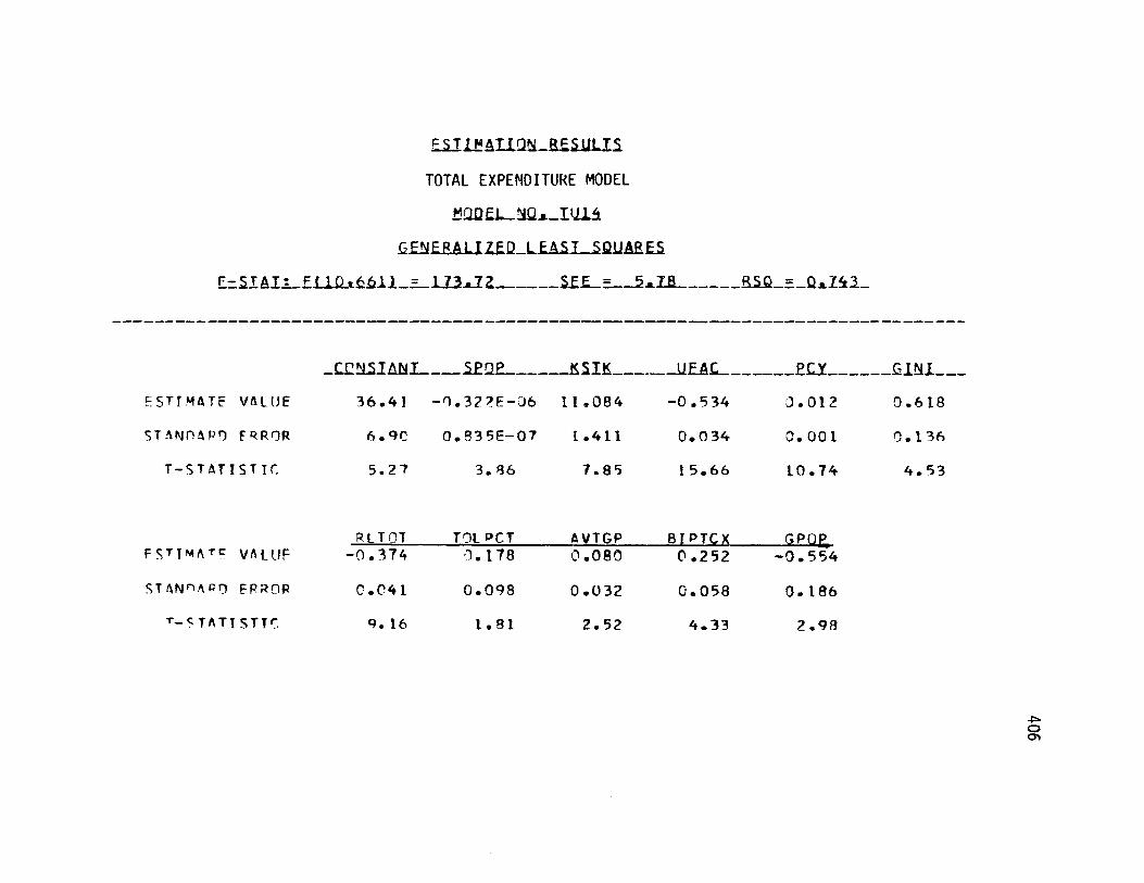
E5IefAlL.ESULT
TOTAL EXPENDITURE MODEL
.QDELQ..JUA
F-NEHAUSTLLESSQUARSi
F-STAT: F(10.6611 = 113.72 SEE = _5.7B RSO = 0.143
ESTIMATE VALAE
STANa)4P ERROR
T-STATISTIC
FSTIMATC VALUF
STANnAPQ ERROR
-S T A TI'ST r
_LN MAhl__ QI2__EI___UEA_---U0-----G- 8
36.41 -0.32?E-2i6 11.084 -0.534 0.012 0.618
6.9O 0.835E-07 1.411 0.034 0.001 0.136
5.27 3.86 7.85 15.66 10.74 4.53
RITOT-0.374
0.041
q,.16
TOL PCT11.178
0.098
1.81
AVTGP0.080
0.032
2.52
B IPT.X0.252
0.058
4.33
-0.554
0.186
2.98
4P'b0)
-M*-MoM Aw -dlkb..E-.dLIL-dg-MJ6 m dmmw-dr- AM =Mmp - dM-146 A. A6 mg--
- - - - - - - - - - - - - - - - - - - - - - - - - - - - - - - - - -
0 W-91-

LM A2 L&JUEUj.S
TOTAL EXPENDITURE MODEL
tullE l-N...-l02
.G.ENE A1.E LWAI.lQUA5E
F-STAT: Ff Ro R9) = I 9SFF = 7a1l RSQ = 0.9RD
STITMATF VA LUE
STNPAon FRRnRp
T-SrTATJSTIC
CNiIANI.
p9.12
11
8.81
3.31 7F-05
0.1 16E- J5
2.74
T 1MAT F VA LUF
ST ANFAPf ERROR
T -STATISTIC
.AVLi..
2.680
0.611
4.38
.ALUEA..
-1.331
Pi. 216
6.06
ml---
0.001
).002
0.42
RL T G0T
7. 6 r
2.9C6
-0.647
0.208
3.10
TOLPCT1.641
0. 189
8.67
0.725
* 101
7.15
0 l
, --, I -JL. Abdll;,JLAd Z -W.- Amin... LJ.AL3L bd.A ALIb-
- -- - -0- ,

iSIl!Ali~t-.ZLill
TOTAL EXPENDITURE MODEL
1ED2EL.-Z Iu22
UNERALl E LtA.iQUAfE
F-ATT F q pI= 1 56 SEE = 7m15
CPnp KS TKa~a~~-a- -a a~- - ~aa~ a - a~ --
rSTIMATF VALUE
STJANAFD F RP IR
T-STATISTIC
CSTIMATE VAL(UF
STANfAPD FRRIR
T-CTAT!STTC
101.40
9.79
10.35
RL T CT-13304
3.088
3.45
0.716E-06
'.338E-06
0.76
TOL PcT3.?90
0.546
6.03
RSO = 2
1fF AC PC v (INYV
-1.720
0.241
7.12
0.006
0.002
2.85
0.255
D0135
1 . 88
AVT GPC' .583
0.089
6.49
-0.416
0.218
1.91
BI pTn 0 085
0.096
0.89
0
-AL- - - - J-J6 -w- -- , -
.

TOTAL EXPENDITURE MODEL
M112111. 11!3
GESETAFMO*DUL48 aSM2I 5A37
c-STAT: F( 8.565) = ?43.48 5FF = 5.37 RSO = 0.775
FSTIMATF VALIF
STANPAPD ERR2P
T-STATISTIC
PS TIMATF VAlUt E
STANfnADO FQPOR
T-CTATISTIC
28.27 -G.357E-06 9.880 -0.528 0.015 0.458
5.60 J.739E-37 1.182 0.034 0.001 0.125
5.05 4.82 8.36 15.79 14.68 3.66
RL TOT--. 643
0. C4')
16.17
T JL PCT. 391
0.374
5.30
0.013
0.028
0.45
P-

TOTAL EXPENDITURE MODEL
MFDEL..Qa5U3Z
tE5ERAU Zt2.LEAS L.3SUA&ES
F-STAT! Fl 9.5641 = 21R.R5 5FF = S.34 RSO = 0.777
CTIMATF V ALLF
STANDAP ERRR
T-STAT!STIC
ESTYMATE VALIUE
STANDAR') EQPCR
T-STATISTTC
?6.46 -).322E-06 10.556 -0.529 0.015 0.482
1.6 J.788E-07 1.239 0.034 0.001 0.124
4.7? 4.38 8.52 15.80 14.19 3.88
RLTlT-0.617
044
14. OC
TOLPCTI0.315
0.990
3.49
AVTGP0.018
0 .032
0.56
fBIPTQ0.068
0.057
1.20
C
P-

Ej1ALL2-_RtES&LLis
TOTAL EXPENDITURE MODEL
- 2 1~L L2t-2 .5S9 =2 2---S-2x..
F I6MA TF V41 hF
'fTANI f9Q f t F;-IQ
T - T A fI 5T IC
LST IMAT E VA[III3
SI TAN f) A P' 9 FVfPP
T-S 1 t T J c j j
&CB~tat 5.L ..-- DttE1 L- EAffi----QEEBEL - -- GNI
12.1? -0.857F-06 8.028 -p.738 9.o? 0.771
7.16 Q.94 3F-07 1 .050 0.04J 0.001 0.159
1.69 9.09 7.65 18.66 17.52 4.84
jL I '31-C .4%0
0 .O4t
9.7
InI- PCT0. 598
U.089
6.75
OF FNI-1.103
0.092
14.43
DE F (0.642
0.045
17.03

E1A112lQLEiUJJ&
TOTAL EXPENDITURE MODEL
B-E12LWN...L.112
LfJERE ALU2E.LJE 5_QUARE
E-zMA~Lft12adt uIt3-2 fBl ---_L..-3k2t-----a&Q3&iL.
Cfl TAFJT
ESTIMATF VALUE
STANDARD ERRfP
T-STATISTIC
CSTIMATE VALUIE
STANDAPO E"ROP
T-STAT!STIC
n E FK ITK
11.33 -0.791F-06 11.286
7.04 0.101E-06 1.247
1.61 7.81 9.05
RL TDT-' . 395
0.047
8.40
TOLPCT3.421
0.112
3*75
DEFNJG-1.123
0.096
11.60
-0.730
0.039
18.81
DEFIG0.606
0.044
13.70
.ELE.LY.
0.022
0.001
16.95
RI l-PTCX-3.118
0.071
1.67
0.790
0.156
4.80
40b
- - - - - - - - - - - - - - - - - - -
--- -_ _ _.& -mw.
Nw.

EalL! Al12!LRESUi
TOTAL EXPENDITURE MODEL
LEN BALI ZEDIA&U1UABLS
F-STATz Fff0.AF 11 = 233.26 SFF = A.Rfl RSO = .-779
EST[MATF VALUE
STANDARD FPRPR
T-STATISTIC
8.3?
7.26
1.15
-0.361E-06
0.927F-07
9.28
flEEtESI&
10.389
1.167
8.90
DEFPCY GINI--. JA aa.---------. .U ..
-0.715
0.040
18.03
0.023
0.001
17.74
3.808
0.129
5.07
FSTIMATE VALIUE
STANDAPO FRROR
T-SrTATISTC
RLTfOT-0.442
0.046
qe.54
TOLPOT0.494
0.091
5.39
DEFNIG-16148
0.091
12.59
DEFIGo .607
0.044
13.67
GPOP-0.530
0.218
2.43
0-4L43
- - - - - - - - - - - - - - -
----m- ,-,-

E ilT 12UItEEULLS.
TOTAL EXPENDITURE MODEL
mF-TT l O EF L - 644
E=STAT: E~lo6601 3222.67 SEE = 6.44 RSO = 0.R802
ESTIMATE VALUF
STANDAPO ERROR
T-STATISTIC
-CC IANlI
33.23
7.64
4.34
-0 . 796E-06
0.963E-07
8.27
.2EEZI.
13.677
1.220
11.21
FSTIMATE VALUF
STANDARD FPQJR
T-STATI ST IC
-0.801
0.039
20.44
.DEELX.
0.020
0.001
15.03
1.040
0.153
6.8!
RLTOT
-1.323
r.047
6.98
TOLPCT
0.327
0.110
2.97
DEFNIG
-1.167
0.092
12.65
DEFIG
0.520
0.043
12.04
BI PTCX
0.087
0.067
1.30
GP9P
-0.619
0.207
2.99
.- 441; Jo. As.- -.t- .. .aA.. --b
_ j _ 4 0M_____ .----
-.0 mom-w..-wmm-wmmmmmwmw... Mwww

EiLLoAI1MLSES.uLu
TOTAL EXPENDITURE MODEL
ENERALZE-LEASit.SQUAREI
F-' TAT: Ft Qo AR) = 28m00fl SEE= 7.50 RSO = O 741. ZI- a 1 -- .na a--n-..-.- ABe- ---------- ee M
FSTIMATF VALUE
STANPAQD FRROR
T-STATISTIC
121.10
9.36
12.9
-0.623E-06
0.F79E-06
3.71
-12EK1&
0.776
0.368
2.10
ESTIMATE VALUE
STANPARO ERROR
T-STATIST IC
.IEA!L..
-1.783
0.236
7.56
0.010
0.002
4.97
-0.679
0.099
6.87
RLTOT-0.185
0.101
1. *83
TOLPCT3.590
0.502
7.15
DEFNIG-0.295
0.132
2.24
DEFl0.666
0.058
11.50
4C"
mvdmpM-dw-dw -.--W -mv-
.00 mmmlw.-M

TOTAL EXPENDITURE MODEL
NQELNQ(3-S 1222
GE&EBALLLQLA.SESQUA5E
F-STAT: Ff10. 871 = 17t73 5FF = 7.46
I A^r'
ESTIMATE VALUE
STANDARD FPROR
T-STATISTIC
%-STIMATF VALUE
STANDAPR F RP
T-STATISTIC
87.41
10.94
7.99
RLT.T0.092
0.10 q
0.84
-0. 179E-05
0 a 106F-05
1.68
TOLPCT1.789
0.456
3.76
RSO = 0.77
- r- Dr v r TM T
0.005
0.002
?.07
0.056
O .16c:
0.34
OFFNIG-0.433
0.206
2.10
-0.419
0.231
1.82
-0.859
0*176
4.88
9 FF It;0.624
0.087
7.17
B! PTQX0.492
0.549
0.90
-Jb
a)
-.- a-m-AL a;- -- I J A- dM6Jd-JL -go- - ' ' MIL -AL- Aw M J06 Jklw- - %up ..m - -wm w
I--ELuC NI .

ESIlfAlItLRE.SULIS
TOTAL EXPENDITURE MODEL
2iE 9iEALEQWi S UA t
F-STAT: F( 9.5641 = 236.03 SEE = 6.60- RSO = 0.790
rfnlNczTANT
ESTTMATE VALIE
STANPARD ERROR
T-STATISTIC
ESTTMATE VLUE
STANDAPO FPRFR
T-STATIST IC
19.62
7.10
2.76
RLTCT-0.686
0.053
12.99
-0.648F-06
0.928E-37
6.98
TDLPCT0.444
0.091
4.87
nF FKI C TKt
-0.778
0.044
17.64
I)EE-ec.
0.023
0.001
17.01
&nfa _
0.869
0*157
5.55
8.696
1 .065
8.16
DEFNIG-0.867
0.116
7.48
DE F IQ0.440
0.060
7.33
4'zb
.immommaw-11116-d6w 6 A I ' -at A -M - .- mm A& 3bK -ML. -- "-Mo-mmw _,-
-----
om
11FCar

TOTAL EXPENDITURE MODEL
tQ0F EL..NA SD2
GENERALLIED-EASE-SiLAEAES
F-STAT: F(10.5631 = ?16A5 SEE = 6.55 RSO = 0.794
ESTIMATE VALUE
STANPAP Y FRROR
T-STATISTIC
CDNSJ.AU
195
7.C4
2.78
-0.676E-06
0.101E-06
6.72
ESTIMATE VALUF
STANDAPD ERROR
T-STATISTIC
DEEEKSI&
10.153
1. 152
8.81
SUEAC.-
-0.771
0.044
17.60
DEER.YZ
0.023
0.001
16.57
0.861
0.155
5.55
-0.*697
0.056
12.44
TOL PCT0.468
0.111
4.21
DEFNIG-0 .908
0.122
7.44
DEF IG0.415
0.060
6.94
81 PTCX-0.053
0.072
0.73
4 :b..- j00
- - - - - - - - - - -
M -.- d- -_-__.NM-_d-----
go

F-STAT: Ft R 6631
Eii L1fAUlQ!LBE&ULLS
TOTAL EXPENDITURE MODEL
= 21533 SEE = ltl -R&SQ _fQAZ Z_
ClNSTANT DE FKSTK.
ESTIMATE VALuE
STANDAP) EPQPR
T-STATISTIC
ESTIMATE VALUE
STANDARD ERROR
T-STATISTIC
30.59
7.81
3.92
RLTOT-0.638
0.048
13.27
-0.62 OE-06
0. 102E-06
6.06
TOLPCT0.576
0.100
5.76
SPOP UFAC. OE EPC-Y
14.757
1.711
8.62
-GINI
-0.551
0.042
13.11
0.018
0.001
12.92
0.359
0.175
2.04
DEFTG0.017
0.033
0.52
Imw - - -
- - - - - - - - - - - - - - - -
- N . - - --Z= L -m-- -A -11 - -_ _ _ _ _ _ _ .P A AL --- A M.=. -0 -.-96an A- w
-P

FiE LALTDL&E&LuLIS
TOTAL EXPENDITURE MODEL
.MDELJ.Q.STJ2LZ
2ENEaRAU..2 L l.SzJAafia
F-STAT Ff 9.aA2) = 203mA SFF = 7.o46 RSO = 0.734
CONSTANT
ESTIMATE VALUE
STANDARD FRPOR
T-STATISTIC
E~STIMATE VALUF
STANDARD ERROR
T-STATISTIC
25.83
7.68
3.36
RLTOT-0.551
0.050
10.99
SP
-0.441E-96
0. 108E-06
4.08
TOLPCT0. 222
0.124
1.79
.JIEA.-0.561
0.041
13.55
QEELCY
0.017
0.001
12.17
2EFK&T
15.012
1.784
8.97
DEFTGo .044
0.035
1.27
0.427
0.172
2.48
BPTCX0.331
0.076
4.38
____-__- ~ ~ _ _ _dwSio " _ __OL -0 . L
0

fEUlLAUI.tL-&SULlS
TOTAL EXPENDITURE MODEL
mDDEL.5a. t1113
(&NERAJLIEDLE A .LSQUAR&E
F-STAT: F i q*s i = 1, 9S76 SEF = .S7-- a a _ -a6 __. .6w A .
CONSTANT
ESTIMATE VALUE
STANPAPD FPROR
T-STATISTIC
ESTIMATE VALUE
STANPARD ERROR
T-STATISTIC
24.98
7.98
3.13
RLTOT-0.657
o.048
13.57
spnp
-0.622E-06
0. 102E-06
6.12
1TOLPCT0.496
0. 103
4.81
RSC = n.777
IFAr
-0.529
0.042
12.49
* P.EERC.
0.019
0.001
13.19
DFFKSTK
15.419
1.712
9.00
DEFTG0.004
0.032
0.13
0.447
0.176
2.54
GPOP-n .659
0.243
2.72
4 :Ib
- - - - - - - - - - -
_-_ _-- - i ----- -.
om

EU1leA112N-EULUS
TOTAL EXPENDITURE MODEL
GENELALILQEDEASL.SQUAES
F-STAlv El t61I -= FF3.22 -SEE = 7f3 -RSU-= O4
ESTIMATE VALUE
STANDAR ERROR
T-STAT1STIC
LDtSIAUI
45.66
A.71
5.24
-0.45 3F-06
0. 106E-06
4.27
11.789
1.437
8.20
FSTIMATE VALUE
STANDARD EPROR
T-STATISTIC
UEAQ.
-0.655
0.043
15.13
0.015
0.002
10.61
0.791
0.173
4.58
-L L-0.489
0.052
9.44
TJOL PC T0.212
0.124
1.71
DEFTG0.067
0.032
2.08
81 PTCX0.315
0.074
4.24
GPOP-0. 736
0.236
3.12
N3b
Aso. A.d
.W.mo__..Go0-
ft

TOTAL EXPENDITURE MODl.
MODEL N Z.D21
F S IETEtALlEDUIL.SQ2U A R.2
F - a I L 1B1 -12 l_. .. 3 E.2-.- 2.
-------------------------- ---------------------
ESTIMATE VALUE
STANDARD ERROR
T-STATISTIC
CCNiiAI
Q4.63
13.92
6.80
0.224E-05
0. t4E-05
1.58
ESTIMATE VALUE
STANDAPD ERROR
T-ST&TISTIC
DfFFKSTK
2.180
0.671
3.25
iFAC-
-1.09 7
0.250
4.40
DEEPCY
0.003
0.002
1.07
-0.619
0.271
2.28
RLTOT-0.?86
0.116
2.45
TOL PCT1.322
0.129
10.25
DEFTG0.563
o .094
6.00
4-)z
E.IlaI.ON-REULI5
- _-. __ _ __J-.__ _ ---jL o

ESily.All -REULIS
TOTAL EXPENDITURE MODEL
BUDELNO_.-XI22
fiENE ALLE ASflUARU
F-cZTAT! Ft Q. RAI = 16A CFF = A. 92 RSO = nA?9a~.~-a ~ Mad-a aa n~a~
ESTIMATE VALUE
STANDARD ERROR
T-STATISTIC
ESTIMATE VALUE
STANDARD ERROR
T-STAT!STIC
QaI AIs2 an EEKU uE cD e x---1-h~
107.32 0.109E-05 0.372 -1.870 0.009 -0.381
11.0C 0.117E-05 0.140 0.275 0.002 0.278
9.10 0.93 2.66 6.81 3.50 1.37
RLTOT-0.368
0.110
3.36
TOLPCT3.578
0.657
5.45
DEF3G0.580
0.086
6.76
BIPTC0.057
0.127
0.45
W-mm...kw

s ATIhl-NA_.EULI
TOTAL EXPENDITURE MODEL
2DfEL_.JTD31
fGLNERALI.E LFAS L ._ QUARES
E-AIA.L 1...23DQ. FF = 6AR
DEF KSTK-
RQS = (1.772Am - --- _ .- .r --- - = - _
UFAC- OE EPCY
FSTIMATF VALuE
STANDAPO ERROR
T-STATISTIC
ESTIMATE VALUE
STANDARD EPROP
T-STATISTIC
34.84
7.15
4.87
SL T nT-O.8 34
0.058
16.40
-0.498E-06
0.948E-07
5.25
.10LC-T
0.479
0.095
5.05
DEFTG0.001
o.029
0.04
4'-:1
10.351
1.217
8.51
GINI
-0.643
0.043
15.00
0.019
0.001
14.41
0.574
0.160
3.59
.. J6 _ M _ _ _..._ . _ _ _ __~JA 16 oaw o__
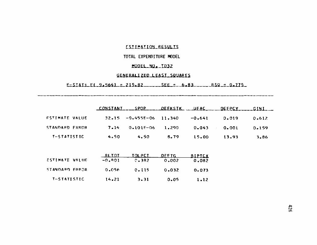
EI5!IALLHLRtiULT
TOTAL EXPENDITURE MODEL
. D E LN.a2
G EBE~lZ LE A SI QMA
CFE =
C fmcT AN T oP nE cK rTK UFAC nFFPrY rl NT-a& ~~ ~ a~ a.- - - ..
FSTTMATE VALUE
STANTARD ERROR
T-STATISTIC
ESTIMATE VALUF
STANDAI) ERRPOR
T-STATISTIC
32.15
7.14
4.50
OR LTO T-0.OA1
0.056
14.21
-0.455F-06
0.101E-06
4.50
T...L PC T%.382
0.115
3.31
F-TAT:AT Ft Q.AA4I = 2t 2 RQ = 0 77S
-0.641
0.043
15.00
0.019
0.001
13.93
11.340
1.290
8.79
DEFTG0.002
0.032
0.05
0.612
0.159
3.86
0.082
0.073
[.12
4N)
L- A *= I-10--I-L- -ZX2 %Jxa :-- - _ _ _.. .. aj__ L._ .- _ 0 ]" jLdj~d- - .I j L
.-- - -..&Xaj

427
Appendix B
Derivation of Derivatives and Elasticities
from the Expenditure Mndels

428
This appendix sets forth the derivation of derivatives and
elasticities from the long run revenue policy model, and the short
run allocation model. Moreover, it will be shown how the results
from these two models can be combined to indicate the total change-
on both revenue and allocation- resulting from changes in the level
of the explanatory variables.
The short run allocation model takes the form
If(1) .=E. = f
where S. = share of expenditure devoted to category j
E = expenditures on category j
R = E = total expenditures (State and FederalI funds)
f. = f(X) = n XJk or iejk Xkkej k
We wish to derive the form of both the derivative of E. with
respect to Xk ,DE. , and the elasticity of E. with respect to
k kE
3 XkX ks'n E /X k
From (1) we get
(2) = R j = R(X) jL.
i f (X)

429
But R(X) is related to the estimated form of the long run
revenue policy model.
The long run revenue policy model takes the form:
(3) Rown, -pc a + I RMXmm
where Rown,.pc = total per capita expenditures from statesown sources (i.e. exclusive of Federalpayments to the States, F).
a= estimated coefilcients
Thus, R own, pcin (3) is related to R in (2) by:
(4) R = SPOP *(Rown,p + FPC)
where SPOP state population
Fpc = Federal highway payments per capita
Assuming a long run static solution1 whereby
F = GPCwhere Gpc = per capita highway grants,
1. Assuming that the states ultimately expend all Federal grantsmade available, differences between GPC and FPC can be
attributed to short run, transient responses. In the longrun, it can be assumed that Federal payments will eventually"settle down" to the rate of Federal grant availability.
(5)

430
the long run revenue policy model can be rewritten as:
(6) R += (s+mXm+ (1 + ) Gpc )*SPOP
Returning to equation (2) we can now define the derivative of
E with respect to Xk as:
(7) @E .
Xk= Si
j kX+ R s.
ak
The corresponding elasticity is simply:
(8) Ej/Xk
XkE.
3
SaE
ax k
R Xk
x =E.
ax
ak
xk
3TR
) = XkR
a RaX k
Xk
3
as.
aXk
- R/Xk + Sj/Xk

431
The Product Form Model
In this case, the specification of each share takes the form:
T1 Xkjk Ej n
(9) s. = = ~dj
where: n = share numerator
d = share denominator
k = estimated share modeljk coefficients
Assume variable Xp appears in the share numerator and one or more
of the fi in the share denominator. The derivative of the numera-
tor with respect to Xp takes the form:
aa- &1jkj n
(10) = Jpp Xk jk Xp kjp
kfp
By the same reasoning, the derivative of the share denominator
with respect to XP is:

432
(11) - I.p i p
Using these results, we can now derive:
2 as. and(12) = d - n - p
=(Y Gd-n - n f
= s~ (1 - s) p
p
a.- sI Y s
i/jI
Returning to equation (7), the derivative of expenditures on
category i with respect to variable Xp is:
(13) aE = s n + {sR (1 - sQ )pp - s4 i }
But from (6),
If the variable in question X = SPOP, then apop= 0+
2 S SPOP

(14) 3E
Thus, we can
with respect
(15) KE.axP
= SPOP
now state the final
to variable X :
= SPOP +
The corresponding elasticity for
simply:
(16) /X p X SPOP
R
form of the derivative of E
{ s~ (I - s.) S.
-s Ot 8 Ps }
i hj
the product form model is
+ (1-s.) S. - a s3 Jp iPi
Ivi
Special Cases: The Product Form Model
In the derivation of the derivatives and elasticities of the
expenditure models, on the preceding pages, it was assumed that
the explanatory variables X enter into the allocation model as
given in equation (9). In the actual estimated form of the
models, there were two exceptions to this specification.
The first concerns the highway grant variables, which enter
several of the expenditure shares as either specific grant types
(e.g. Interstate, Primary, Secondary) or as aggregates across
433

434
grant categories (e.g. total non-Interstate grants, total grants).
We are interested in deriving the derivatives and elasticities of
expenditures with respect to each of the categorical grant types.
Since the derivation in this instance follows the same reasoning
as in the preceding section, the results are presented without
a detailed derivation.
Let G I
G,
G s
GNI
GT
- Interstate grants
- Primary grants
- Secondary grants
- Gp + GS = non-Interstate grants
- Total Grants
From equation (6), it is clear that:
-A
(17) -G = (1 + ) SPOP, for g = I, P, S
Using this result in equation (7), the derivatives of expenditures
with respect to grant terms take the form:
(18)aE.
-tag = s.'(l + 6 )-SPOP + R { s -() -s
g + yAjNI+ G -
G ) s }
A
(OXj &* GNIczNI

435
for g = I, P, S
and = 0 if g=I{l ifg= P or S
The corresponding derivatives follow directly from equation (18):
(19) (E /G (1 + 0g ) G SPOP + (1 -s
R
+ G + taT -
NI T
GG(ig + 6i aiNI + aiT)sii j NI
The second exception to the general derivation of elasti-
cities and derivatives concerns the population variable, SPOP.
This variable appears in several of the expenditure shares in
both direct form, and as the denominator of the variable measuring
capital per capita (KSTK). In this case, we can rewrite
equation (9) as:
S jSPOP- CAPTL jKSTK X jk XAk(20) S(Xk
SPOP i (SPOP A iKSTK X i-- XkI k
where: CAPTL = highway capital stocks

436
The derivative and elasticity of share s with respect to SPOP
can be written respectively as:
as. = LIISPOPI~2KSTK) s (l -si) -SPOP
&iSPOP - &iKSTK
3 13 SPOP
(22) 3Is /SPOP
As noted in
of total expenditures,
(1i s) (&jSPOP ~ &IjKSTK)
. s i(iSPOP - &iKSTK)
itj
the footnote on page , the derivative
R with respect to population is:
- +2U SPOP(23)
Thus we can now state the form of the 'derivative and elasticity
of E with respect to SPOP:
(24) = Si( + 2 SPOP SPOP) +
14is.{(jSPOP 7 SjKSTK) (1 - s ) -
.. i SPOP ~ -iKSTK)5i}
(21)

437
SOP A A(25) TE./SPOP = - o ( + 2$Spop) +
(&jSPOP - JKSTK) (1 - -
j (&iSPOP - CiKSTK)*Si
The Exponential Form Model
The derivatives and elasticities from the exponential
form allocation model differ from the previously presented results
of the product form model. In this case, each share is specified
as:
(26) s. = k a
IIe
'i hei
Following the same reasoning as expressed in equations (10)
through (12), the derivative of expenditure share j with respect
to a particular variable Xp is given by:
(27) as. = A s (1 - s) - saxJip 3 3j S.
The corresponding elasticity is simply:
(28) rsx = j X ( - s ) - Xp{j .S

438
Substitutin these results in equations (7) and (8), we get the
derivative and elasticity of E with respect to X for the exponen-
tial form allocation model:
(29) = OP + R{& s (1 - si) - s a s}
pp JjL
(30) X SPOP + 0.X (1 - sj) - aX s
R
Special Cases: The Exponential Form Model
As in the product type allocation model, the general form
of the derivatives and elasticities for the exponential form allo-
cation model do not apply in the case of the population variable
and the highway grant terms. The derivatives and elasticities
from the exponential model, for these special cases are presented
below.
(31) = (1 + ) SPOP + R{ s (1 - s ) (a. +
gg
6 i JfNI + aJT) - si(ig + YiNI + iT
1The notation used here is identical to the definitions given inthe section "Special Cases: The Product Form Model."

439
= -) SPOP + G {(1 - s.) (. +
S ajNI + &jT ig5
for g = I, P, S
and 6, 0 if g1Iand 6~ ={ 1 i gII1 if g0I
= s O +C 2SPOP SPOP) +
ReKSTK-s6.{(1-s.) (&jSPOP-
+ 5SiNI jI+ &iT) s }
LjKSTK) -SPOP
iSPOP _ i S K )
SPOP + P= T(0 + 20po SPOP) +
KSTK { 3(1 - s ) (jSPOP SPOP -
aSPOP S -aiKSTK) si
5jIKSTK) -
(32)T'E /G
(33) aE.i
(34)TE /SPOP

440
Appendix C
Derivatives and Elasticities from the
Two Expenditure Models

441
This appendix contains the derived elasticities and derivatives
from the expenditure models described in Chapters IV and V. On the
pages that follow, the tables are titled "Short Run" or "Long Run"
Elasticities (or Derivatives). The short run measures pertain to the
short run expenditure model (SRAM), where by definition the States'
budgets are fixed. The long run elasticities and derivatives reflect
the empirical analysis integrating the results of the SRAM and TEM,
and thus describe States' long run expenditure responses to Federal
grants (inter alia) where budget levels can change.
The derivatives and elasticites are presented for both the
product form and exponential form of the SRAM (see Chapter V.).

442
PRODUCT FORM SPECIFICATION OF THE SRAMFORTY EIGHT STATE SAMPLE
SHORT RUN MODEL ELASTICiTIES
SHAR E
VARI ABLE
SPOP
UFAC
PCY
G I N I
KS TK
TS PMR
PCCRMT
PCM F
TOLPCT
RLTOT
AVI G
AV PG
AVSG
INTERSTATE
-0.682
0.402
-0.201
-0.033
-0.169
-0.031
-0.011
-0.001
-0.059
0.029
0.873
-0.070
-0.002
PRI MARY
0.069
0.192
-0. 201
-0.033
0. 112
-0.031
-0. 011
-0.001
0.023
0. 029
-0.416
0. 534
-0.045
SECONDARY
0.105
-0.280
-0.201
0.298
0.026
0.277
0.026
-0.001
0.023
0.029
-0.433
-0.176
0.261

443
PRODUCT FORM SPECIFICATION OF THE SRAMFORTY EIGHT STATE SAMPLE
SHORT RUN MODEL ELASTICITIES
SHARE
NONFASYST
0.650
-0.884
-0.201
-0.033
0.026
-0.031
0. 183
-0.001
0.023
-0.488
-0.161
-0.130
-0.026
MAI NT
-0.515
-0.036
-0.201
-0.033
0.285
-0.031
-0.011
0.007
0.023
-0.041
0. 082
-0.062
0. 001
OTHER
0.975
-0.036
0.616
-0.033
-0.068
-0.031
-0.011
-0.001
0.023
0.028
-0.505
-0.226
-0.066
VARI ABLE
SPOP
UFAC
PCY
GiNI
KSTK
TS PMR
PCCRMT
PCMF
TOLPCT
RLTOT
AVI G
AVPG
AVSG

444PRODUCT FORM SPECIFICATION OF THE SRAM
SEVEN STATE SAMPLE
SHORT RUN MODEL ELASTICITIES
SHAR E
VARIABLE
SPOP
UFAC
PCY
GI NI
KSTK
TS PMR
PCCRMT
PCM F
TOLPCT
RLTOT
AVIG
AVPG
AVSG
INTERSTATE
-0.573
-0.128
-0.049
0.022
-0.077
-0.150
-0.014
-0.021
0.015
0.189
0.774
-0.016
0.084
PRIMARY
0.126
0.366
-0.049
0. 022
-0.021
-0.150
-0. 014
-0.021
-0.006
0.189
-0.217
0. 379
0.035
SECONDARY
0.085
0.726
-0.049
-0.168
-0.211
1.150
-0.038
-0.021
-0.006
0. 189
-0.759
-0.105
-0.282

445
PRODUCT FORM SPECIFICATION OF THE SRAMSEVEN STATE SAMPLE
SHORT RUN MODEL ELASTI C ITI ES
SHARE
VARIABLE NONFASYST MAINT OTHER
spop 1-122 0.114 0.347
UFAC -0.867 -0.245 -0.245
PCY -0.049 -0.049 0.232
GINI 0.022 0.022 0.022
KSTK -0.211 0.110 0.238
TS PMR -0.150 -0.150 -0.150
PCCRMT 0.348 -0.014 -0.014
PCMF -0.021 0.103 -0.021
TOLPCT -0.006 -0.006 -0.006
RLTOT -0.161 0.131 -0.750
AVIG -0.962 -0.076 -0.186
AVPG - -0.375 -0.117 -0.149
AVSG -0.115 0.028 0.010

446PRODUCT FORM SPECIFICATION OF THE SRAM
FORTY ONE STATE SAMPLE
SHORT RUN MODEL ELASTICITIES
SHARE
INTERSTATE
-0.406
0.314
-0.162
-0.037
-0.174
-0.032
-0.010
0.005
-0.104
0. 024
0.781
-0.124
0.112
PRIMARY
-0. 117
-0.254
-0.162
-0.037
0.070
-0.032
-0.010
0.005
0.041
0.024
-0.397
0.617
-0.157
SECONDARY
-0.102
-0.339
-0.162
0. 343
0. 075
0. 292
0. 030
0. 005
0. 041
0. 024
-0.401
-0. 193
0. 140
VARIABLE
SPOP
UFAC
PCY
GINI
KSTK
TSPMR
PCCRMT
PCMF
TOLPCT
RLTOT
AVIG
AVPG
AVSG

447
PRODUCT FORM SPECIFICATION OF THE SRAMFORTY ONE STATE SAMPLE
SHORT RUN MODEL ELASTiCITIES
SHARE
VARIABLE
SPOP
UFAC
PCY
GINI
KSTK
TS PMR
PCCRMT
PCMF
TOLPCT
RLTOT
AVI G
AVPG
AVSG
NONFASYST
0.406
-0.663
-0. 162
-0.037
0.075
-0.032
0.155
0.005
0.041
-0.472
-0.006
-0.096
0.221
MAINT
-0.361
0.050
-0.162
-0.037
0.200
-0.032
-0.010
-0.035
0.041
0.003
0. 102
-0.066
0.338
OTHER
0.690
0.050
0.465
-0.037
-0.003
-0.032
-0. 010
0. 005
0.041
0. 012
-0.441
-0. 217
-0. 253

448
PRODUCT FORM SPECIFICATION OF THE SRAM
FORTY EIGHT STATE SAMPLE
SHORT RUN MODEL DERIVATIVES
SHARE
INTERSTATE
-.105E 02
0.402E08
-0.474E 04
-0.524E 07
-0.172E 08
-0.221E 03
-0.172E 08
-0.398E 06
-0.103E 09
0.661E 07
0.111E 01
-0.317E 00
-0.170E-01
PRIMPRY
-.753E 00
-0.136E08
-0.335E 04
-0.371E 07
0.808E 07
-0.157E 03
-0.122E 08
-0.281E 06
0.287E 08
0.468E 07
-0.374E 00
O.172E 01
-0.354E 00
SECONDARY
0.578E 00
-0.100E 08
-0.170E 04
0.167E 08
0.940E 06
0.707E 03
0.147E 08
-0.142E 06
0.145E 08
0.237E 07
-0.197E 00
-0.286E 00
0.104E 01
VARIABLE
SPOP
UFAC
PCY
GINI
KSTK
TSPMR
PCCRMT
PCMF
TOLPCT
RLTOT
AVIG
AVPG
AVSG

449
PRODUCT FORM SPECIFICATION OF THE SRAMFORTY EIGHT STATE SAMPLE
SHORT RUN MODEL DERIVATIVES
SHARE
VAR I ABLE
SPOP
-J FA C
PCY
GINI
KSTK
TSPMR
PCCRMT
P CM F
TOLPCT
RLTOT
AVIG
AVPG
AVSG
NON FASYST
0.134E 01
-0.118E 08
-0.f633 E 03
-C.701E 06
0.351E 06
-0.296E 02
0.379E 08
-0.531E 05
0.-41E 07
-0.146E 08
-0. 273E-01
-0. 71E-01
-0.390E-01
MAINT
-0.378E 01
-0.169E 07
-0.226E lL4
-0.250E 07
0.138E 08
-0.106E 03
-0.821E 07
0.122E 07
0.193E 08
-0.445E 07
0. 495E- 01
-0.135E 00
0.774 E -02
OT H E R
0. 131E
-0. E10E
0.127E
-0. 4558E
-0. 601E
-0. 193E
-0. 150E
-0.347E
0.35 4E
0.5143E
-0.561E
-0. 3 99 E
-0. 637E
02
07
05
07
07
03
08
06
08
07
00
00
00

450PRODUCT FORM SPECIFICATION OF THE SRAM
SEVEN STATE SAMPLE
SHORT RUN MODEL DERIVATIVES
SHARE
VARIABLE INTERSTATE PRIMARY SECONDARY
SPOP -0.930E 01 0.150E 01 -.553E 00
U5AC -0.114E 08 0.238E 08 0.259E 08
PCY -0,888E 03 -0.649E 03 -0.356E 03
GIN! 0.231E 07 0,..69E 07 -0.710E 07
KSTK -0.481E 07 -0.957E 06 -0.52E 07
TSPMR -0.870E 03 -0.636E 03 O.268E 04
PCCRMT -0.412E 08 -0.301E 08 -0.448E 08
PcMP -0.102E 08 -0.746E 07 -0.409E 07
TOLPCT 0.525E 08 -0.155E 08 -0.851E 07
RLTOT 0.365E 08 0.267E 08 0.146E 08
AVIG 0.9572 00 -0.196E 00 -0.376E 00
AVPG -0.679E-01 0.118E 01 -0.179E 00
AVSG p.645E '0 0.194E 00 -O.66E 00

451
PRODUCT FORM SPECIFICATION OF THE SRAMSEVEN STATE SAMPLE
Si-ORT RUN ICDEL DERIVATIVES
SHARE
VARIABLE
SPOP
UFAC
PCY
G1 N
KS TK
TS PMR
PCCAIT
P CM F
TULPCT
R L T
AVIG
AV PG
AVSG
ON FAS Y.ST
0.29 E
-0. 124E
-0. 143E
O.371E
-0. 213E
-0.140E
0.165E
-3.164E
~-O.500E
-O.191E
-0.257E
-0 .142 E
MAINT
01
08
03
06
07
03
09
07
07
07
00
00
00
0.109E 01
-0.129E 08
-0.524E 03
0.136E 07
0.407E 07
-0.5i14E 03
-0.243E 08
0.295E 08
-0.123E 08
0.149E 08
-0.53 2E-01
-C.295E 00
0.126E 00
C THE R
0.340E 01
-0.132E 08
0.255E 04
0.139E 07
0.899E 07
-0.526E 03
-0.249E 08
-0.517E 07
-0.128E 08
-0.874E 08
-0.139E 00
-0.384E 00
0. 465E-01

452
PRODUCT FORM SPECIFICATION OF THE SRAM
FORTY ONE STATE SAMPLE
SHORT RUN MODEL DERIVATIVES
SHARE
INTERSTATE.
0.799E 00
-0.865E 07
-0.509E 03
-0.799E 06
0.106E 07
-0.300E 02
0.293E 08
0.243E 06
0.864E 07
-0.139E 08
-0.908E-03
-0.566E-01
-0.644E-02
PRIMARY
-0.252E 01
0.232E 07
-0.181E 04
-0.284E 07
0.997E 07
-0.106E 03
-0.666E 07
-0.586E 07
0.307E 08
0.266E 06
0.594E-01
-0.133E 00
0.398E-01
SECONDARY
0.972E 01
0.468E 07
0.104E 05
-0.571E 07
-0.306E 06
-0.214E 03
-0.134E 08
0.174E 07
0.618E 08
0.254E 07
-0.517E 00
-0.915E 00
-0.556E 00
VARIABLE
SPOP
UFAC
PCY
GINI
KSTK
TSPMR
PCCRMT
PCMF
TOLPCT
RLTOT
AVIG
AVPG
AVSG
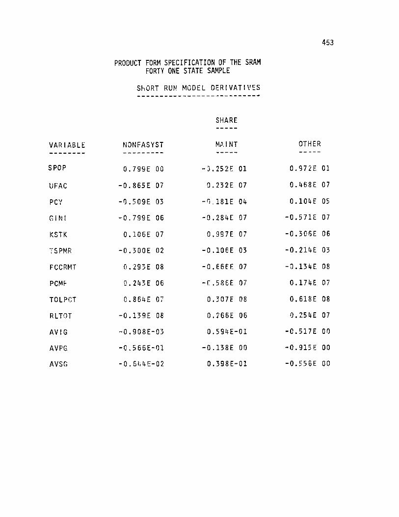
453
PRODUCT FORM SPECIFICATION OF THE SRAMFORTY ONE STATE SAMPLE
ShORT RUN MODEL DERIVATIVES
SHARE
VARIABLE
SPOP
UFAC
PCY
GINI
KSTK
TSPMR
FCCRMT
PCMF
TOLPCT
RLTOT
AVIG
AVPG
AVSG
NONFASYST
0.799E 00
-0.865E 07
-0.509E 03
-0.799E 06
0.106E 07
-0.300E 02
0.293E 08
O.243E 06
O.864E 07
-O.139E 08
-0 .908E-03
-C.566E-01
-0.6L- 4E-02
MAINT
-J.252E 01
0.232E 07
-0.181E 04
-0.284E 07
O.997E 07
-0.106E 03
-0.66FE 07
-C .586E 07
O.307E 08
0.266E 06
0.59 4E-01
-0.138E 00
0.398E-01
OTHER
0.972E
0.468E
0.IO4E
-0.571E
-0. 306E
-0. 214E
-3.134 E
0.174 E
O.618E
0. 254E
-0.517E
-0.915E
-. 5S6E
01
07
05
07
06
03
08
07
08
07
00
00
00
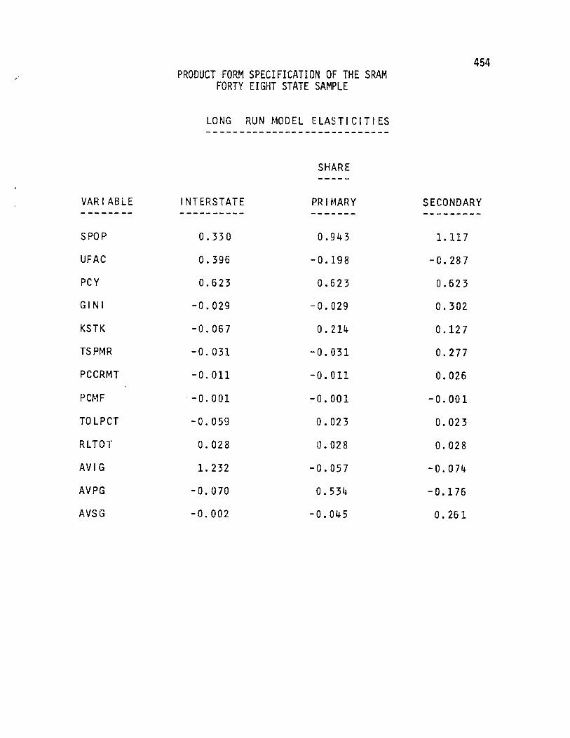
454PRODUCT FORM SPECIFICATION OF THE SRAM
FORTY EIGHT STATE SAMPLE
LONG RUN MODEL ELASTICITIES
SHARE
VARIABLE
SPOP
UFAC
PCY
GINI
KSTK
TSPMR
PCCRMT
PCMF
TOLPCT
RLTOT
AVI G
AVPG
AVS G
INTERSTATE
0.330
0.396
0.623
-0.029
-0.067
-0. 031
-0. 011
-0.001
-0. 059
0.028
1.232
-0. 070
-0.002
PRIMARY
0.943
-0.198
0.623
-0.029
0. 214
-0. 031
-0.011
-0. 001
0.023
0.028
-0.057
0.534
-0.045
SECONDARY
1.117
-0.287
0.623
0.302
0.127
0.277
0.026
-0.001
0.023
0.028
-0.074
-0.176
0.261

455
PRODUCT FORM SPECIFICATION OF THE SRAMFORTY EIGHT STATE SAMPLE
LONG RUN MODEL ELASTICITIES
SHARE
NONFASYST
1.662
-0.890
0.623
-0.029
0.127
-0.031
0.183
-0.001
0.023
-0.489
0.198
-0.130
-0.026
OTHERMAINT
0,497
-0.042
0.623
-0.029
0.387
-0.031
-0.011
0.007
0.023
-0.043
0.440
-0.062
0.001
1.987
-0.042
1. 440
-0.029
0.034
-0.031
-0.011
-0.001
0. 023
0.026
-0. 146
-0.226
-0.066
VARIABLE
SPOP
UFAC
PCY
GINI
KSTK
TSPMR
PC C RMT
PCMF
TOLPCT
RLTOT
AVI G
AVPG
AVS G

456PRODUCT FORM SPECIFICATION OF THE SRAM
SEVEN STATE SAMPLE
LONG RUN MODEL ELASTICITIES
SHARE
VARIABLE
SPOP
UFAC
PCY
GINI
KSTK
TS PMR
PCCRMT
PCMF
TOLPCT
RLTOT
AVI G
AVPG
AVSG
INTERSTATE
1. 326
-0.139
0.188
0.018
-0.075
-0.150
-0.014
-0. 021
0.016
0.189
1.159
0.031
0.110
PRIMARY
2.026
0.355
0.188
0.018
-0.019
-0.150
-0. 014
-0.021
-0.006
0.189
0.168
0.425
0.061
SECONDARY
1.985
0.715
0.188
-0.172
-0.209
1.150
-0.038
-0.021
-0.006
0.189
-0.374
-0.058
-0.256

457
PRODUCT FORM SPECIFICATION OF THE SRAMSEVEN STATE SAMPLE
LONG RUN MODEL ELASTICITIES
SHARE
NONFASYST
3.021
-0.878
0.188
0.018
-0.209
-0.150
0.348
-0. 021
-0.006
-0.162
-0.576
-0.328
-0.089
MAINT
2. 014
-0.256
0.188
0. 018
0.113
-0.150
-0.014
0.103
-0.006
0.131
0.310
-0.071
0. 054
OTlER
2.247
-0.256
0.468
0.018
0. 240
-0.150
-0.014
-0.021
-0.006
-0.750
0. 200
-0.103
0. 036
VARIABLE
S POP
UFAC
PCY
GINI
KSTK
TSPMR
PCCRMT
PCMF
TOLPCT
RLTOT
AVIG
AVPG
AVSG

458PRODUCT FORM SPECIFICATION OF THE SRAM
FORTY ONE STATE SAMPLE
LONG RUN MODEL ELASTICITIES
SHARE
INTERSTATE
0. 754
0.307
0.690
-0. 033
-0.086
-0. 032
-0. 010
0.005
-0.104
0.021
1.098
-0. 115
0.115
PRIM ARY
1. 042
-0. 261
0.690
-0. 033
0.157
-0.032
-0. 010
0. 005
0.041
0. 021
-0. 080
0.626
-0.154
SECONDARY
1.057
-0.346
0. 690
0. 348
0.162
0.292
0.030
0.005
0.041
0.021
-0. 084
-0.184
0.144
VARIABLE
SPOP
UFAC
PCY
GINI
KSTK
TSPMR
PCCRMT
PCMF
TOLPCT
RLTOT
A V I G
AVPG
AVSG

459
PRODUCT FORM SPECIFICATION OF THE SRAMFORTY ONE STATE SAMPLE
LONG RUN MODEL ELASTICITIES
SHARE
VAR I A BLE
SPOP
UFAC
PCY
G I N I
KSTK
TSPMR
PCCRMT
PCM F
TOLPCT
RLTOT
AVI G
AVPG
AVSG
NONFASYST
1.565
-0.670
0.690
-0.033
0.162
-0. 032
0.155
0.005
0. 041
-0.475
0.312
-0.087
0.224
MA I NT
0.799
0. 043
0.690
-0.033
0.287
-0.032
-0.010
-0.035
0. 041
-0.0Oo
0.419
-0.057
0. 341
0 TH ER
1.850
0.043
1.318
-0.033
0.084
-0. 032
-0. 010
0.005
0.041
0.009
-0.124
-0.208
-0.249

460PRODUCT FORM SPECIFICATION OF THE SRAM
FORTY EIGHT STATE SAMPLE
LONG RUN MODEL DERIVATIVES
SHARE
VARIABLE
SPOP
UFAC
PCY
GiNI
KSTK
TSPMR
PCCRMT
PCMF
TOLPCT
RLTOT
AV I G
AVPG
AVSG
INTERSTATE
0.507E 01
0.395E 08
0.147E 05
-0.460E 07
-0.686E 07
-0.221E 03
-0.172E 08
-0.398E 06
-0.103E 09
0.627E 07
0.157E 01
-0.317E 00
-0. 170E-01
PRIMARY
0.103E 02
-0.140E 08
0.104E 05
-0.325E 07
0.154E 08
-0.157E 03
-0.122E 08
-0.281E 06
0.290E 08
0.444E 07
-0.5 16E-01
O.172E 01
-0.354E 00
SECONDARY
O.615E 01
-0.103E 08
0.526E 04
0.170E 08
0.464E 07
O.707E 03
0.147E 08
-0.142E 06
0.147E 08
0.225E 07
-0.336E-01
-0.286E 00
0.1O4E 01

461
PRODUCT FORM SPECIFICATION OF THE SRAMFORTY EIGHT STATE SAMPLE
LONG RUN MODEL DERIVATIVES
SHARE
VARIABLE
SPOP
UFAC
PCY
GINI
KSTK
TSPMR
PCC.RMT
PCMF
TOLPCT
RLTOT
AV I G
AV PG
AVSG
NONFASYST
O.342E 01
-0.119E 08
0.196E 04
-0.614 E 06
0.173E 07
-0.296E 02
0.379E 08
-0.531E 05
0.543E 07
-0.147E 08
0. 33 6E-01
-0. 791E-01
-0.390E-01
MAINT
0.365E 01
-0.201E 07
0.701E 04
-0.219E 07
0.188E 08
-0.106E 03
-0.821E 07
0.122F 07
0.196E 08
-0. 461E 07
0.267E 00
-0.135E 00
0. 774E-02
OTHER
0.267E 02
-0.368E 07
0.297E 05
-0.402E 07
0.302E 07
--0.193E 03
-0.J50E 08
-0.347E 06
0.358E 08
0.513E 07
-0.162E 00
-0.899E 00
-0.5&7F 00

462PRODUCT FORM SPECIFICATION OF THE SRAM
SEVEN STATE SAMPLE
LONG RUN MODEL DERIVATIVES
SHARE
VARIABLE INTERSTATE PRIMARY SECONDARY
SPOP 0.215E 02 0.240E 02 .129E 02
UFAC -0.L24E 08 0.231E 08 O.255E 08
PCY 0.342E 04 0.250E 04 0.137E 04
GIN, 0.191E 07 0.140E 07 -0.726E 07
KSTK -0.466E 07 -0.8h6E 06 -0.523E 07
TSPIR -0.870E 03 -0.636E 03 O.268E 04
PCCRMT -0.412E 08 -0.301E 08 -0.448E 08
PCMF -0.102E 08 -0.746E 07 -0.409E 07
TOLPCT 0.546E 08 -0.140E 08 -0.770E 07
RLTOT 0.36 4E 08 0.266E 08 0.146E 08
AVIG 0.143E 01 0.152E 00 -0.185E 00
AVPG 0.130E 00 0.132E 01 -0.996E-01
AVSG 0.843E 00 0.339E 00 -0.787E 00

463
PRODUCT FORM SPECIFICATION OF THE SRAMSEVEN STATE SAMPLE
LONG RUN MODEL DERIVATIVES
SHARE
VARIABLE NONFASYST MAINT OTHER
SPOP 0.789E 01 0.193E 02 0.220E 02
UFAC -0.126E 08 -0.135E 08 -0.138E 08
PCY 0.531E 03 0.202E 04 0.516E 04
GINI 0.308E 06 0.113E 07 0.116E 07
KSTK -0.210E 07 0.416E 07 0.908E 07
TSPMR -0.140E 03 -0.5l14E 03 -0.526E 03
PCCRMT 0.165E 09 -0.2L43E 08 -0.249E 08
PCMF -0.164E 07 0.295E 08 -0.617E 07
TOLPCT -0.309E 07 -0.113E 08 -0.116E 08
RLTOT -0.5C2E- 07 0.14 9E 08 -0.875E 08
AVIG -0.115E 00 0.226E 00 0.149E 00
AVPG --0.225E 00 -0.178E 00 -0.264E 00
AVSG -0.110E 00 0.243E 00 0.166E 00

464PRODUCT FORM SPECIFICATION OF THE SRAM
FORTY ONE STATE SAMPLE
LONG RUN MODEL DERIVATIVES
SHARE
VARIABLE
SPOP
UFAC
PCY
GINI
KSTK
TSPMR
PCCRMT
PCv=
TOLPCT
ALTOT
AV I G
AV PG
AVSG
INTERSTATE
0.115E
0.311 F
0. 168E
-0. 540E
-0.944E
-0. 233E
-0. 145E
0. 189E
-0.1.72E
0. 479E
1.140E
-0. 526E
-0. 137E
02
08
05
07
C7
03
03
07
09
07
01
00
00
PRIMARY
0.112E 02
-0.186E 08
0.118E 05
-0.380E 07
0.121E 08
-0.164E 03
-0.102E 08
0.133E 07
0,475E 08
0.337E 07
-0. 719E-01
0.202E 01
-0.318E 00
SECONDARY
0.566E 01
-0.123E 08
0.589E 04
0.202E 08
0.622E 07
O.748E 03
0.156E 08
0.661E 06
0.237E 08
0168E 07
-0.3 74E-01
-0.295E 00
0.106E 01

465
PRODUCT FORM SPECIFICATION OF THE SRAMFORTY ONE STATE SAMPLE
LONG RUN MODEL DERIVATIVES
SHARE
VARIABLE
SPOP
UFAC
PCY
G I N I
KSTK
TSPMR
PCCRMT
PCMF
TOLPCT
RLTOT
AVIG
AV PG
AVSG
NOIFASYST
0.308E 01
-0.874E 07
0.216E 04
-0.696E 06
0.229E 07
-0.300E 02
0.293E 08
0. 243E 06
0.870E 07
-0.140E 08
0. 511E-01
-0. 514E-01
-0. 123E-02
MA NT
0.558E 01
0.199E 07
0.768E 0 (
-0.2 47E 07
0.14 3E 08
-0.106E 03
-0.666E 07
-0.586E 07
0.309E 08
-0.993E 04
0.?L44E 00
-C.120E 00
0.5 83E-01
OTHER
0. 260E
0.400E
0.295E
-0. 498E
0.8 48E
-0.214E
-0.134E
0.174E
0. 622E
0. 198E
-0. 145E
-0. 878E
-0. 519E
02
07
05
07
07
03
08
07
08
07
00
00
00

466EXPONENTIAL FORM SPECIFICATION OF THE SRAM
FORTY EIGHT STATE SAMPLE
SHORT RUN MODEL ELASTICITIES
SHARE
VARIABLE
SPOP
UFAC
PCY
GINi
KSTK
TSPMR
PCCRMT
PCMF
TOLPCT
RLTOT
AVI G
AVPG
AVSG
INTERSTATE
-0. 469
0.554
-0. 242
-0. 015
0.314
-0.014
0.007
0.008
-0.164
0.065
0.554
-0.057
0.012
PRIMARY
-0.018
-0.415
-0.242
-0.015
-09.026
-0. 014
0.007
06008
0. 064
06065
-0.108
0.379
-0.058
SECONDARY
0.087
-0.579
-0. 242
0.138
-0.051
0.121
-0.082
0.008
0. 064
0.065
-0.435
-0.229
0.031

467EXPONENTIAL FORM SPECIFICATION OF THE SRAM
FORTY EIGHT STATE SAMPLE
SHORT RUN MODEL ELASTICITIES
SHAR E
NONFASYST
0.308
-0.569
-0.242
-0.015
-0.051
-0. 014
0.063
0. 008
0.064
-1.345
0.404
0.086
0.071
MAl NT
-0.157
0.017
-0.242
-0.015
0.077
-0.014
0.007
-0.0 54
0.064
-0.248
0.230
0.038
0.051
OTHER
0.554
0.017
0.740
-0.015
-0.351
-0. 014
0.007
0. 008
0.064
0.188
-0. 555
-0.182
-0.039
VARIABLE
SPOP
UFAC
PCY
GINI
KS TK
TS PMR
PCCRMT
PCMF
TOLPCT
RLTOT
AVI G
AVPG
AVSG

468EXPONENTIAL FORM SPECIFICATION OF THE SRAM
FORTY EIGHT STATE SAMPLE
SHORT RUN MODEL DERIVATIVES
SHAR
VARIABLE
SPOP
UPAC
PCY
GINI
KSTK
TSPMR
PCCRMT
PCM F
TOLPCT
RLTOT
AVI G
AV PG
AVSG
INTERSTATE
-0. 721E
O .553E
-0. 570E
-0. 243E
0. 319E
-0.968E
0.106E
0.315E
-0. 236E
0.145E
O.704E
-0. 258E
3.136E
01
08
04
07
08
02
08
37
09
0?
00
00
00
PRIMARY
-0.191E 00
-0. 293E 08
-0.403E 04
-0.172E 07
-0.187E 07
-0.685E 02
0,747E 07
0.223E 07
0.79Y 08
0.103E 08
-0.9 71E-01
0.122E 01
-0.456E 00
SECONDARY
0.477E
-0.207E
-0. 204E
0. 776E
-0. 188E
0.309E
-0. 453E
0.113E
0. 401E
0.522E
-0.198E
-0. 372E
0.322E
00
08
04
07
07
03
08
07
08
07
00
00
00

469
EXPONENTIAL FORM SPECIFICATION OF THE SRAMFORTY EIGHT STATE SAMPLE
SHORT RUN MODEL DERI VATI VES
SHARE
VARIABLE
S POP
UFAC
PCY
GINI
KSTK
TS PMR
PCCRMT
PCMF
TOLPCT
RLTOT
AVI
AVPG
AVS G
NONFASYST
0. 633E 00
-0.760E 07
-0. 761E 03
-0.325E 06
-0.700E 06
-0.129E 02
0.130E 08
0.421E 06
0.150E 08
-0. 404E 08
0.6 86E-01
0. 524E-01
0.105E 00
MAINT
-0.115E 01
0.825E 06
-0.272E 04
-0.116E 07
0.373E 07
-0.462E 02
0.504E 07
-0.968E 07
0.535E 08
-0.266E 08
0.139E 00
0. 817E-01
0.270E 00
OTHER
0. 744E
0. 151E
0.152E
-0. 212E
-0. 312E
-0. 846E
0.922E
0.275E
0.0 979E
0. 369E
-0. 617E
-0. 72 3E
-0. 377E
01
07
05
07
08
02
07
07
08
08
00
00
00

470EXPONENTIAL FORM SPECIFICATION OF THE SRAM
FORTY EIGHT STATE SAMPLE
LONG RUN MODEL ELASTICITIES
SHARE
VARI ABLE
SPOP
UFAC
PCY
GINI
KSTK
TS PMR
PCCRMT
PCMF
TOLPCT
RLTOT
AVIG
AVPG
AVSG
I NTh.RSTATE
0.543
0.547
0.583
-0.011
0.415
-0. 014
0.007
0.008
-0.263
J. 063
0.913
-0. 057
0.012
PR IMARY
0.994
-0. 421
0. 583
-0.011
0. 076
-0.014
0.007
0.008
0. 064
0. 063
0. 251
0. 379
-0.058
SECONDARY
1.098
-0.586
0.583
0.142
0.050
0.121
-0.082
0.008
0.064
0.063
-0.076
-0. 229
0.081
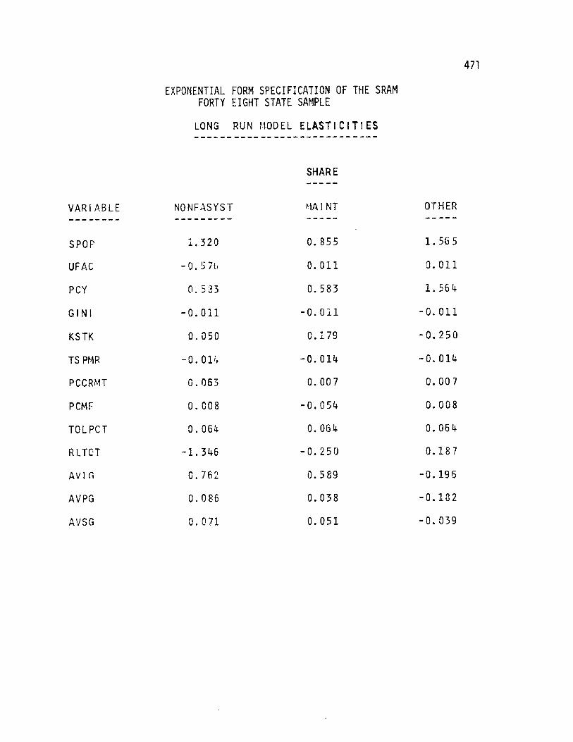
471
EXPONENTIAL FORM SPECIFICATION OF THE SRAMFORTY EIGHT STATE SAMPLE
LONG RUN MODEL ELASTICITIES
SHARE
VARIABLE
SPOP
UFAC
PCY
GINI
KSTK
TS PMR
PCCRMT
PCMF
TOLPCT
R LTCT
AVI G
A V PG
AVSG
NONFASYST
1.320
-0.57T
0.533
-0.011
0. 050
-0. 014 i
0.063
0.008
0.064
-1. 346
0.762
0.086
0.071
MAI NT
0.855
0. 011
0. 583
-0. 011
0.179
-0. 014
0.007
-0.054
0. 064
-0. 250
0.589
0.038
0.051
OTHER
1.565
0.011
1.564
-0.011
-0.250
-0. 014
0.007
0.008
0.064
0.18 7
-0.196
-0. 182
-0.039

472
EXPONENTIAL FORM SPECIFICATION OF THE SRAMFORTY EIGHT STATE SAMPLE
LONG RUN MODEL DERIVATIVES
SHARE
VARIABLE INTERSTATE PR IMARY SECONDARY
SPOP 0.836E 01 0.108E 02 0.605E 01
UFAC 0.547E 08 -0.298E 08 -0. 210E 08
PCY O.137E 05 O.972E 04 0.492E 04
GINI -0.178E 07 -0.126E 07 0.799E 07
KSTK 0.423E 08 0.545E 07 0.183E 07
TSPMR -0.968E 02 -0.685E 02 0.309E 03
PCCRMT 0.106E 08 0. 747E 07 -0. 453E 08
PCMF 0.315E 07 0.223E 07 0.113E 07
TOLPCT -0.285E 09 0.797E 08 0.403E 08
RLTOT 0.142E 08 0o.101E 08 0.510E 07
AVIG 0.116E 01 0.226E 00 -0. 347E-01
AVPG -0. 258E 00 0.122E 01 -0.372E 00
AVSG 0.136E 00 -0.456E 00 0.322E 00

473
EXPONENTIAL FORM SPECIFICATION OF THE SRAMFORTY EIGHT STATE SAMPLE
LONG RUN MODEL DERIVATIVES
SHARE
VARI ABLE
S PO F
UFAC
PCY
GI NI
KSTK
TSPMR
PCCRMT
PCMF
TOLPCT
RLTOT
AVI G
AVPG
AVSG
NONFASYST
0. 271E
-0.769E
01
07
0.184E 04
-0.238E 06
0.681E 06
-0.129E 02
O.130E 08
0.421E 06
0.150E 08
-0.404E 08
0.129E 00
0. 524E-01
0.105E 00
MA INT
0. 628E 01
0.512E 06
0.656E 04
-0.851E 06
0.867E 07
-0.462E 02
0.50L4E 07
-0.968E 07
0.537E 08
-0.268E 08
0.357E 00
0. 817E-01
0.270E 00
OTHER
0. 211E
0.9 38E
0.322E
-0. 156E
-0. 222E
-0.846E
0.922E
0. 275E
0.9 84E
0. 366E
-0. 218E
-0. 723E
-0. 377E
02
06
05
07
08
02
07
07
08
08
00
00
00


