Matias Sevel RasmussenTor JustesenAnders DohnJesper LarsenMay 2010

Report 11.2010

DTU Management Engineering

The Home Care Crew Scheduling Problem: Preference-Based Visit Clus-tering and Temporal Dependencies

The Home Care Crew Scheduling Problem:

Preference-Based Visit Clustering and Temporal

Dependencies

Matias Sevel Rasmussen∗ Tor Justesen Anders DohnJesper Larsen

Department of Management EngineeringTechnical University of Denmark

May, 2010

Abstract

In the Home Care Crew Scheduling Problem a staff of caretakershas to be assigned a number of visits to patients’ homes, such that theoverall service level is maximised. The problem is a generalisation ofthe vehicle routing problem with time windows. Required travel timebetween visits and time windows of the visits must be respected. Thechallenge when assigning visits to caretakers lies in the existence ofsoft preference constraints and in temporal dependencies between thestart times of visits.

We model the problem as a set partitioning problem with sideconstraints and develop an exact branch-and-price solution algorithm,as this method has previously given solid results for classical vehiclerouting problems. Temporal dependencies are modelled as generalisedprecedence constraints and enforced through the branching. We in-troduce a novel visit clustering approach based on the soft preferenceconstraints. The algorithm is tested both on real-life problem instancesand on generated test instances inspired by realistic settings. The useof the specialised branching scheme on real-life problems is novel. Thevisit clustering decreases run times significantly, and only gives a lossof quality for few instances. Furthermore, the visit clustering allows usto find solutions to larger problem instances, which cannot be solvedto optimality.

∗Corresponding author: Email: mase@man.dtu.dk. Address: Department of Man-agement Engineering, Technical University of Denmark, Produktionstorvet, Building 424,DK-2800 Kgs. Lyngby, Denmark. Tel.: +45-45254442. Fax: +45-45933435.

1

Keywords: Home care, Health care, Home health care, Crew schedul-ing, Vehicle routing, Vehicle routing with time windows, Visit clustering,Clustering, Preferences, Generalised precedence constraints, Temporal de-pendency, Temporal dependencies, Synchronisation, Real-life application,Branch-and-price, Column generation, Dantzig-Wolfe decomposition, Setpartitioning, Scheduling, Routing, Integer programming

1 Introduction

The Home Care Crew Scheduling Problem (HCCSP) described in this paperhas its origin in the Danish health care system. The home care service wasintroduced in 1958 and since then, there has been a constant increase in thenumber of services offered. The primary purpose is to give senior citizensand disabled citizens the opportunity to stay in their own home for as longas possible. The HCCSP is the problem of scheduling caretakers in a waythat maximises the service level, possibly even at a reduced cost.

When a citizen applies for home care service, a preadmission assessmentis initiated. The result of the assessment is a list of granted services. Theservices may include cleaning, laundry assistance, preparing food, and sup-port for other everyday tasks. They may also include assistance with respectto more personal needs, e.g. getting out of bed, bathing, dressing, and dosingmedicine. As a consequence of the variety of services offered, people withmany different competences are employed as caretakers.

Given a list of services for each of the implicated citizens, a long-termplan is prepared. In the long-term plan, each service is assigned to specifictime windows, which are repeated as frequently as the preadmission assess-ment prescribes. The citizens are informed of the long-term plan, and hencethey know approximately when they can expect visits from caretakers. Fromthe long-term plan, a specific schedule is created on a daily basis. In thedaily problem, caretakers are assigned to visits. A route is built for eachcaretaker, respecting the competence requirements and time window of eachvisit and working hours of the caretaker.

In the following, we restrict ourselves to looking at the daily schedul-ing problem only. The problem is a crew scheduling problem with strongties to vehicle routing with time windows. However, we have a number ofcomplicating issues that differentiates the problem from a traditional vehi-cle routing problem. One complication is the multi-criteria nature of theobjective function. It is, naturally, important to minimise the overall oper-ation costs. However, the operation costs are not very flexible in the dailyscheduling problem. More important is it to maximise the level of servicethat can be provided. The service level depends on a number of differentfactors. Often, it is impossible to fit all visits into the schedule in theirdesignated time windows. Hence, some visits may have to be rescheduled

2

or cancelled. In our solutions, a visit is either scheduled within the givenrestrictions or marked as uncovered. The manual planner will deal withuncovered visits appropriately. The main priority is to leave as few visitsuncovered as possible. Also, all visits are associated with a priority and it isimportant to only reschedule and cancel less significant visits. Furthermore,it is important to service each citizen from a small subgroup of the wholeworkforce (the so-called preferred caretakers), as this establishes confidencewith the citizen. Another complication compared to traditional vehicle rout-ing, is that we have temporal dependencies between visits. The temporaldependencies constrain and interconnect the routes of the caretakers.

HCCSP generalises the Vehicle Routing Problem with Time Windows(VRPTW) for which column generation solution algorithms have proven suc-cessful, see Kallehauge et al. (2005). Therefore, we model HCCSP as a SetPartitioning Problem (SPP) with side constraints and develop a branch-and-price solution algorithm. Temporal dependencies are modelled by a singletype of constraints: generalised precedence constraints. These constraintsare enforced through the branching. Different visit clustering schemes aredevised for the problem. The schemes are based on the existence of soft pref-erence constraints. The visit clustering schemes for the exact branch-and-price framework are novel. The visit clustering will naturally compromiseoptimality, but will allow us to solve larger instances. We will compare thedifferent visit clustering schemes by testing them both on real-life probleminstances and on generated test instances inspired by realistic settings. Toour knowledge, we are the first to enforce generalised precedence constraintsin the branching for real-life problems. The contribution of this paper ishence twofold. Firstly, we devise visit clustering schemes for the problem,and secondly, we enforce generalised precedence constraints in the branchingfor the first time for real-life problems.

Optimisation methods for crew scheduling are widely used and describedin the literature, especially regarding air crew scheduling. However, whenit comes to scheduling of home care workers the literature is sparse. Thiswork builds on top of two recent Master’s theses, Lessel (2007) and Thomsen(2006). The most recent of these, Lessel (2007), uses a two-phase approachwhich first groups the visits based on geographical position, competences,and preferences. A caretaker is associated to each group and the secondphase considers each group as a Travelling Salesman Problem with TimeWindows (TSPTW).

The other thesis, Thomsen (2006), treats the problem as a Vehicle Rout-ing Problem with Time Windows and Shared Visits (VRPTWSV) and usesan insertion heuristic to feed a tabu search with initial solutions. The modelsand solution methods in Lessel (2007) and Thomsen (2006) can only handleconnected visits where two caretakers are at the same time at the citizen.

With offset in the Swedish home care system, Eveborn et al. (2006) de-scribe a system in operation. They use a Set Partitioning Problem model

3

and solve the problem heuristically by using a repeated matching approach.The matching combines caretakers with visits. Eveborn et al. (2006) re-port that the travelling time savings in a moderate guess are 20% and thatthe time savings on the planning correspond to 7% of the total workingtime. Bredstrom and Ronnqvist (2008) show a mathematical model thatcan handle synchronisation constraints and precedence constraints betweenpairs of visits. The model is a VRPTW with the additional synchronisa-tion and precedence constraints that tie the routes together. They solvethe model using a heuristic. Bredstrom and Ronnqvist (2007) develop abranch-and-price algorithm to solve the model of Bredstrom and Ronnqvist(2008), but without the precedence constraints. The model is decomposedto an SPP and the integrality requirement on the binary decision variablesis relaxed. Also, the synchronisation constraints are removed from the SPP.Instead, integrality and synchronisation are handled by the branching, andto our knowledge they are the first to use a non-heuristic solution approachto home care problems. Their subproblem is an Elementary Shortest Pathwith Time Windows (ESPPTW).

Bertels and Fahle (2006) use a combination of linear programming, con-straint programming and metaheuristics for solving what they call the HomeHealth Care Problem. However, they do not incorporate connected visits,which makes their approach less interesting for our situation. Begur et al.(1997) describe a decision support system (DSS) in use in the United States.The DSS provides routes for caretakers by using GIS systems. Their model isa Vehicle Routing Problem (VRP) without time windows and without sharedvisits, which again is not suitable for our needs. Cheng and Rich (1998) de-scribe the Home Health Care Routing and Scheduling Problem which theymodel as a Vehicle Routing Problem with Time Windows (VRPTW). Theydistinguish between full-time and part-time caretakers. They use a two-phase heuristic approach, in which they first find an initial solution usinga greedy heuristic. Next, the solution is improved using local search. Themodel does not include temporal connections between visits.

Related to the HCCSP is the Manpower Allocation Problem with TimeWindows (MAPTW). A demanded number of servicemen must be allocatedto each location within the time windows. Primarily the number of usedservicemen must be minimised, and secondarily the used travel time. Thejobs have different locations, skill requirements, and time windows. Thisproblem is dealt with by Lim et al. (2004). More closely related to HCCSPis the Manpower Allocation Problem with Time Windows and job-TeamingConstraints (MAPTWTC). Li et al. (2005) present a construction heuristiccombined with simulated annealing for solving MAPTWTC instances. Theirmodel adds synchronisation constraints to the model of Lim et al. (2004),but does not include precedence constraints. MAPTWTC is also solved inDohn et al. (2009a), again with multiple teams cooperating on tasks. Anexact solution approach is introduced. They decompose to a set partitioning

4

problem and develop a branch-and-price algorithm. The subproblem in thecolumn generation is an ESPPTW.

The HCCSP can be seen as a VRPTW, but with the addition of thecomplicating connections between visits, and with another objective thanthe regular minimisation of total distance. When only synchronised visitsare considered as connection type, the problem can be referred to as sharedvisits, yielding the VRPTWSV. The literature on VRPTW is huge. We referto Kallehauge et al. (2005) and Cordeau et al. (2002). Recently, a variantof VRPTW very similar to the HCCSP has been described in Dohn et al.(2009b). The authors formalise the concept of temporal dependencies in theVehicle Routing Problem with Time Windows and Temporal Dependencies(VRPTWTD) and investigate the effectiveness of different formulations andsolution approaches.

The remainder of the paper is organised as follows. In Section 2, wepresent an IP formulation of HCCSP. In Section 3, we introduce a decom-posed version of this formulation. In Section 4, we present the specialisedbranching scheme used. Section 5 introduces clustering of visits and othermethods to decrease the solve time of the pricing problem. Real-life andgenerated test instances are described in Section 6. In Section 7, we presentresults from test runs on these instances. Finally, in Section 8 we concludeon our work and suggest topics for future research.

2 Problem formulation

The set of caretakers is denoted K, and the set of visits at the citizensis denoted C = {1, . . . , n − 1}. For each visit i ∈ C a time window isdefined as [αi, βi], where αi ≥ 0 and βi ≥ 0 specify the earliest respectivelylatest possible start time of the visit. For algorithmic reasons, we introduceartificial visits 0k and nk as the start visit respectively end visit for caretakerk ∈ K, and we define N k = C ∪ {0k, nk} as the set of all potential visits forcaretaker k. The duty length for each caretaker k ∈ K is given by the timewindow [α0k , β0k ] = [αnk , βnk ], i.e. caretaker k ∈ K cannot start his or herduty before time α0k ≥ 0 and must have finished his or her last visit beforetime β0k ≥ 0. The travel distance between a pair of visits (i, j) is givenby the parameter skij . The parameter depends on k ∈ K as the caretakersuse different means of transportation. If it is not possible to travel directlybetween visits i and j for caretaker k, then skij = ∞. We define skii = ∞,∀k ∈ K,∀i ∈ N k. The parameter skij includes the duration (service time)of visit i. Travelling between any two visits i and j gives rise to the costsckij dependent on the caretaker k ∈ K. For any combination of i ∈ C andk ∈ K the parameter ρki = 1 if k can be assigned to visit i, ρki = 0 otherwise.Also, for any combination of i ∈ C and k ∈ K the preference parameterδki ∈ R gives the cost for letting caretaker k handle visit i. A negative cost

5

t ime

(a) Synchronisation.

t ime

(b) Overlap.

t ime

(c) Minimum difference.

t ime

(d) Maximum difference.

t ime

(e) Min+max difference.

Figure 1: Five types of temporal dependencies. Each of the five subfiguresshows the time windows of two visits i (top) and j (bottom) with a temporaldependency between them. Assuming some start time for visit i, the dottedline shows the earliest feasible start time for visit j, and the dashed dottedline shows the latest feasible start time. For synchronisation (a) the twolines coincide, and are drawn as one full line.

means that we would like caretaker k to handle visit i, whereas a positivecost means that we would prefer not to let caretaker k handle visit i. Theparameter γi is the priority of visit i ∈ C, the higher, the more important.

As described in Section 1, visits may be temporally dependent due todifferent home care needs. In order to make it easier for the manual plannerto assign substitutes to the uncovered visits, it is required that visits, whichhave a temporal dependency to an uncovered visit, still respect the temporaldependency. In other words, a temporal dependency is still respected evenif one of the visits is uncovered. Five types of temporal dependencies areoften seen in practice. The five types can be seen in Figure 1. These tem-poral dependencies can be modelled by introducing generalised precedenceconstraints of the form

σi + pij ≤ σj ,

where σi denotes the start time of visit i, and pij ∈ R quantifies the requiredgap. The set of pairs of visits (i, j) ∈ C×C for which a generalised precedenceconstraint exists is denoted P.

As can be seen, this constraint simply implies that j starts minimum pijtime units after i. An often encountered example of a temporal dependencyis that of synchronisation, see Figure 1(a), where two visits are required tostart at the same time. The way to handle this is to add both (i, j) and(j, i) to P with pij = pji = 0. As also described by Dohn et al. (2009b),Table 1 shows how to model all the temporal dependencies of Figure 1 with

6

generalised precedence constraints. It can be seen that (a), (b) and (e) eachrequires two generalised precedence constraints, whereas (c) and (d) onlyneed one each.

Temporal dependency pij pji

(a) Synchronisation 0 0(b) Overlap −durj −duri

(c) Minimum difference diffmin N/A(d) Maximum difference N/A −diffmax

(e) Minimum+maximum difference diffmin −diffmax

Table 1: Values for pij for the five temporal dependencies of Figure 1. duriis the service time of visit i, diffmin is the minimum difference required anddiffmax is the maximum difference required.

2.1 Integer programme

To model the problem, three sets of decision variables are defined: the bi-nary routing variables xkij , the scheduling variables tki ∈ Z+ and the binarycoverage variables yi. xkij = 1 if caretaker k ∈ K goes directly from visiti ∈ N k to j ∈ N k, and xkij = 0 otherwise. The scheduling variable tki is thetime the caretaker k ∈ K starts handling visit i ∈ N k. tki = 0 if caretaker kis not assigned to visit i. yi = 1 if visit i ∈ C is not covered by any caretakerand yi = 0 otherwise. The weights w1, w2 and w3 are used to control theobjective function.

HCCSP can now be formulated as the integer programme given be-low. The formulation is very similar to the formulation in Bredstrom andRonnqvist (2007).

7

minw1

∑k∈K

∑i∈Nk

∑j∈Nk

ckijxkij + w2

∑k∈K

∑i∈C

∑j∈Nk

δki x

kij+ w3

∑i∈C

γiyi (1)

s.t.∑k∈K

∑j∈Nk

xkij + yi = 1 ∀i ∈ C (2)

∑j∈Nk

xkij ≤ ρk

i ∀k ∈ K,∀i ∈ C (3)

∑j∈Nk

xk0k,j = 1 ∀k ∈ K (4)

∑i∈Nk

xki,nk = 1 ∀k ∈ K (5)

∑i∈Nk

xkih −

∑j∈Nk

xkhj = 0 ∀k ∈ K,∀h ∈ C (6)

αi

∑j∈Nk

xkij ≤ tki ≤ βi

∑j∈Nk

xkij ∀k ∈ K,∀i ∈ C ∪ {0k} (7)

αnk ≤ tknk ≤ βnk ∀k ∈ K (8)

tki + skijx

kij ≤ tkj + βi(1− xk

ij) ∀k ∈ K,∀i, j ∈ N k (9)

αiyi +∑k∈K

tki + pij ≤∑k∈K

tkj + βjyj ∀(i, j) ∈ P (10)

xkij ∈ {0, 1} ∀k ∈ K,∀i, j ∈ N k (11)

tki ∈ Z+ ∀k ∈ K,∀i ∈ N k (12)yi ∈ {0, 1} ∀i ∈ C (13)

The objective (1) is multi-criteria. Often, minimising uncovered visits(the third term) is prioritised over maximising caretaker-visit preferences(the second term), which again is prioritised over minimising the total trav-elling costs (the first term). This can be accomplished by setting w1 = 1,w2 =

∑k∈K

∑i∈N k

∑j∈N k c

kij and w3 = w2|C|maxk∈K,i∈C δki . Constraints

(2) ensure that each visit is covered exactly once or left uncovered, and care-takers can only handle allowed visits (3). Constraints (4)–(6) ensure thatthe caretakers begin at the start visit, end at the end visit, and that routesare not segmented. Constraints (7) and (8) control that time windows arerespected. Furthermore, Constraints (7) set tki = 0 when k does not visit i.Travelling distances are respected due to Constraints (9). Constraints (10)are the generalised precedence constraints. The y-variable terms ensurethat generalised precedence constraints are respected even when visits arecancelled. Finally, Constraints (11)–(13) set the domains of the decisionvariables.

The HCCSP formulation can be seen as a generalisation of an uncapac-itated, multiple-depot VRPTW. The aim is to push flow for each caretakerfrom start visit to end visit through as many profitable nodes as possible

8

while respecting time windows and minimising costs. Also, it is only allowedfor one caretaker to go through each node.

The HCCSP generalises the Travelling Salesman Problem (TSP). TSP iswell-known to be NP-hard as its decision problem version is NP-complete,see Problem ND22 in Garey and Johnson (1979). Therefore, also HCCSP isNP-hard, and we can therefore not expect to solve the problem efficiently,i.e. in polynomial time. The NP-hardness of the HCCSP is the reason whywe develop a branch-and-price solution algorithm.

3 Decomposition

We will Dantzig-Wolfe decompose the HCCSP described in the previous sec-tion and model it as a set partitioning problem with side constraints. Thenwe will solve the model using dynamic column generation in a branch-and-price framework. This approach has presented superior results on VRPTWand the similarities to HCCSP are strong enough to suggest the same ap-proach here. There is a vast amount of literature on column generation basedsolution methods for VRPTW, see e.g. Kallehauge et al. (2005) for a recentliterature review and an introduction to the method. In a branch-and-priceframework the problem is split into two problems, a master problem and asubproblem. The subproblem generates feasible caretaker schedules, whichare then subsequently combined in a feasible way in the master problem. Inthe master problem, given a large set of feasible schedules to choose from,one schedule is chosen for each caretaker. Given a set of caretakers K, eachcaretaker must choose a schedule from the set Rk, which is the set of poten-tial schedules for caretaker k. Together, the schedules must cover as manyvisits as possible from the set C.

A feasible schedule r for a caretaker k ∈ K is defined as a route startingat 0k and ending at nk and respecting all constraints in the IP formulationfrom Section 2.1 which do not link multiple routes. The schedule includesthe starting times of the visits. The parameter ckr gives the cost for caretakerk ∈ K for schedule r ∈ Rk, and ci = w3γi gives the cost for leaving visiti ∈ C uncovered. The binary parameter akir = 1 if visit i is included inschedule r for caretaker k and akir = 0 otherwise. Moreover, tkir is the starttime of visit i in schedule r for caretaker k, if i is included in r for k. If i isnot included in r for k, tkir = 0.

3.1 Master problem

We introduce the binary decision variable λkr where λkr = 1 if schedule r ∈ Rkis chosen for caretaker k ∈ K, and λkr = 0 otherwise. Furthermore, weintroduce the binary decision variable Λi where Λi = 1 if visit i ∈ C isuncovered, and Λi = 0 otherwise. HCCSP can now be solved by finding aminimum cost combination of schedules such that all constraints are fulfilled.

9

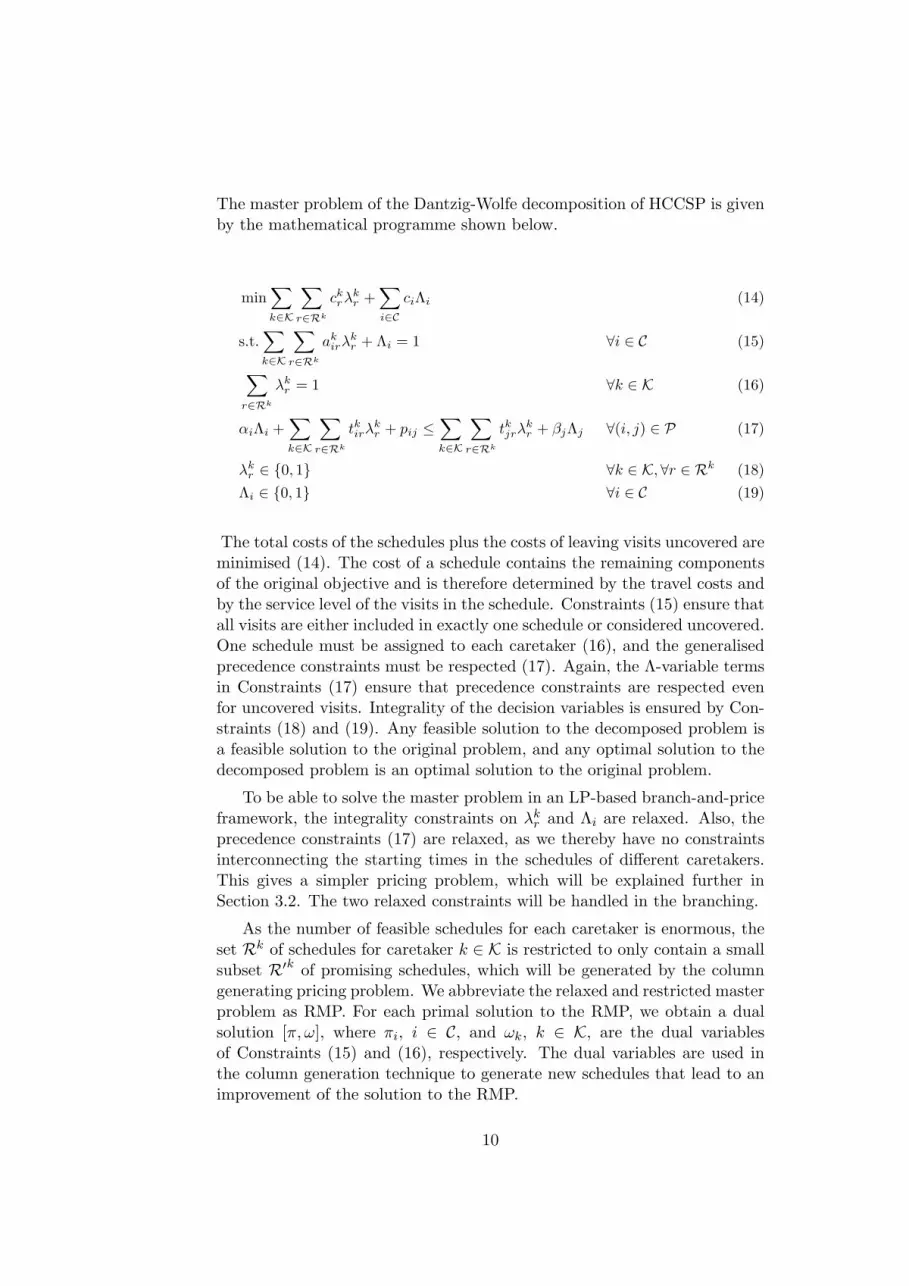
The master problem of the Dantzig-Wolfe decomposition of HCCSP is givenby the mathematical programme shown below.

min∑k∈K

∑r∈Rk

ckrλkr +

∑i∈C

ciΛi (14)

s.t.∑k∈K

∑r∈Rk

akirλ

kr + Λi = 1 ∀i ∈ C (15)

∑r∈Rk

λkr = 1 ∀k ∈ K (16)

αiΛi +∑k∈K

∑r∈Rk

tkirλkr + pij ≤

∑k∈K

∑r∈Rk

tkjrλkr + βjΛj ∀(i, j) ∈ P (17)

λkr ∈ {0, 1} ∀k ∈ K,∀r ∈ Rk (18)

Λi ∈ {0, 1} ∀i ∈ C (19)

The total costs of the schedules plus the costs of leaving visits uncovered areminimised (14). The cost of a schedule contains the remaining componentsof the original objective and is therefore determined by the travel costs andby the service level of the visits in the schedule. Constraints (15) ensure thatall visits are either included in exactly one schedule or considered uncovered.One schedule must be assigned to each caretaker (16), and the generalisedprecedence constraints must be respected (17). Again, the Λ-variable termsin Constraints (17) ensure that precedence constraints are respected evenfor uncovered visits. Integrality of the decision variables is ensured by Con-straints (18) and (19). Any feasible solution to the decomposed problem isa feasible solution to the original problem, and any optimal solution to thedecomposed problem is an optimal solution to the original problem.

To be able to solve the master problem in an LP-based branch-and-priceframework, the integrality constraints on λkr and Λi are relaxed. Also, theprecedence constraints (17) are relaxed, as we thereby have no constraintsinterconnecting the starting times in the schedules of different caretakers.This gives a simpler pricing problem, which will be explained further inSection 3.2. The two relaxed constraints will be handled in the branching.

As the number of feasible schedules for each caretaker is enormous, theset Rk of schedules for caretaker k ∈ K is restricted to only contain a smallsubset R′k of promising schedules, which will be generated by the columngenerating pricing problem. We abbreviate the relaxed and restricted masterproblem as RMP. For each primal solution to the RMP, we obtain a dualsolution [π, ω], where πi, i ∈ C, and ωk, k ∈ K, are the dual variablesof Constraints (15) and (16), respectively. The dual variables are used inthe column generation technique to generate new schedules that lead to animprovement of the solution to the RMP.

10

3.2 Pricing problem

The pricing problem is used to find the feasible schedule with the most neg-ative reduced cost (if any exists). As the caretakers have different workinghours and competences, the pricing problem is split into |K| independentpricing problems. The pricing problem is an Elementary Shortest PathProblem with Time Windows (ESPPTW), which has been proved NP-hardin Dror (1994). The pricing problem for a caretaker k ∈ K is formulated asan integer programme below. Any feasible solution to the pricing problemwith negative cost represents a column with negative reduced cost in theRMP.

min∑

i∈Nk

∑j∈Nk

(w1c

kij + w2δ

ki − πi

)xij − ωk (20)

s.t.∑

j∈Nk

x0k,j = 1 (21)

∑i∈Nk

xi,nk = 1 (22)

∑i∈Nk

xih −∑

j∈Nk

xhj = 0 ∀h ∈ Ck (23)

αi

∑j∈Nk

xij ≤ ti ≤ βi

∑j∈Nk

xij ∀i ∈ Ck ∪ {0k} (24)

αnk ≤ tnk ≤ βnk (25)

ti + skijxij ≤ tj + βi(1− xij) ∀i, j ∈ N k (26)

xij ∈ {0, 1} ∀i, j ∈ N k (27)

ti ∈ Z+ ∀i ∈ N k (28)

Here, we have introduced the decision variables xij and ti which are thesame as in (1)–(13), without the k index. For a given k ∈ K, the subset ofvisits Ck = {i ∈ C : ρki = 1} is the set of visits allowed for k. Moreover,N k = Ck ∪ {0k, nk}, and we define δk

0k= δk

nk= π0k = πnk = 0.

The relatively simple expression (20) for the reduced costs of a columnis one of the reasons why the generalised precedence constraints are relaxed.One could, as done in van den Akker et al. (2006) and in Dohn et al. (2009b)have kept the generalised precedence constraints in the RMP. This wouldhave implied a more complicated pricing problem, as the pricing problemthen incorporates a means of adjusting the starting times in a schedulebased on the dual variables. In van den Akker et al. (2006) they do notsolve their pricing problem by an exact method, but use a heuristic method.Benchmark results from Dohn et al. (2009b) show that in many cases it isas good to relax the generalised precedence constraints, as to keep them inthe master problem.

11

We solve the pricing problem with a labelling algorithm built on ideasfrom Chabrier (2006) and Feillet et al. (2004).

4 Branching

The generalised precedence constraints and the integrality constraints thatwere relaxed from the master problem are handled in the branching partof the branch-and-price algorithm. To handle both types of constraints, weneed to present two branching methods. One to handle the violation of anintegrality constraint and another to handle the violation of a precedenceconstraint. The branching scheme used to handle precedence constraintviolations is a time window branching scheme. This also enforces integralityto a certain point as shown in Gelinas et al. (1995). Nonetheless, one cannotsolely rely on time window branching to enforce integrality, so we use anadditional branching scheme to force the solution to integrality. First, wewill present a preprocessing technique.

4.1 Preprocessing of time windows

The visits C can be grouped according to how they are connected by gen-eralised precedence constraints. Define the directed temporal dependencygraph G = (V,A) by V = C and A = P. The graph G consists of one ormore sub-graphs, which corresponds to the connected components in theundirected version of G. An example of such a graph is shown in Fig-ure 2(a). From the existing generalised precedence constraints, additional

•

••

••

•

••

•

•

•

•• •

??�����

""EEEE

EEEE

E

**TTTTTTT

��???

????

????

???

11ccccccc

RR%%%%%yysss

aaDDD

(a) Example of a temporal dependencygraph.

•

••

••

•

••

•

•

•

•• •

??�����

""EEEE

EEEE

E

**TTTTTTT

��???

????

????

???

11ccccccc

RR%%%%%yysss

aaDDDnn

22

**

(b) The same graph expanded with de-rived arcs.

Figure 2: A temporal dependency graph.

derived generalised precedence constraints can be found. In every subgraphwith three or more nodes, we look for triples i, j, k ∈ C where (i, j), (j, k) ∈ Pwith i 6= j, j 6= k, k 6= i. If (i, k) /∈ P, then the pair is added to P withpik = pij+pjk. If (i, k) ∈ P the offset is updated to pik := max{pik, pij+pjk}in order to get the tightest constraint. The process is repeated until no fur-ther constraints can be derived or tightened. The example will now lookas in Figure 2(b). This derivation of generalised precedence constraints will

12

make it possible to reduce more time windows, as there will be a greaternumber of precedence constraints on which to perform the following pair-wise reduction technique.

If two visits i, j ∈ C are connected via a (possibly derived) generalisedprecedence constraint (i, j) ∈ P, it might be possible to tighten the timewindows of i and j, such that [α′i, β

′i] = [αi,min{βi, βj − pij}] and [α′j , β

′j ] =

[max{αj , αi + pij}, βj ] are the new time windows as illustrated in Figure 3.This preprocessing is repeated until no time windows are tightened. The

preprocessing technique can be used in every node of the branch-and-boundtree. It should be noted that this time window reduction can only be carriedout, because it is required that also temporal dependencies with cancelledvisits must be respected. If this was not the case, then the cancellation ofa visit i with (i, j) ∈ P would lead to the time window of j being “reset”(assuming it was previously reduced by preprocessing).

t imep

ijp

ij

(a) Before preprocessing.

t imep

ijp

ij

(b) After preprocessing.

Figure 3: Adjustment of time windows in accordance to a generalised prece-dence constraint. Each of the subfigures shows the time windows of twovisits i (top) and j (bottom).

4.2 Branching on generalised precedence constraints

A generalised precedence constraint (i, j) ∈ P is violated if there existspositive variables λk1

r1 > 0 and λk2r2 > 0 (the relaxation allows for k1 = k2

and r1 = r2, but we will prevent that in the subproblem) in the solution tothe RMP for which

tk1i,r1

+ pij � tk2j,r2

.

Therefore, to remedy this, we will alter the time windows in the branches.In the left branch the time window of visit i is set to [αi, tsplit − 1], wheretsplit is the split time. In the right branch the time window of visit i is set to[tsplit, βi]. The preprocessing technique described in the previous section isused again, which will result in the time window of visit j in the right branchbeing changed to [tsplit + pij , βj ]. All previously generated schedules violat-ing these new time windows are removed. The split time is selected suchthat tk2

j,r2− pij + 1 ≤ tsplit ≤ tk1

i,r1. Hence, the branching scheme divides the

13

solution space into two sets, where the solution that violates the precedenceconstraint for (i, j) becomes infeasible in each of them. Synchronisationconstraints are often seen in home care instances. The branching schemesuggested here combined with preprocessing of time windows is as strong asthe scheme tailored for synchronisation described in Ioachim et al. (1999).This is elaborated in Dohn et al. (2009b), where it is also described howto pick the best split time in the given interval. An illustration of the gen-eralised precedence constraint branching scheme can be found in Figure 4.

t ime

(a) Parent node.

t ime

(b) Left child node.

t ime

(c) Right child node.

Figure 4: Example of the branching applied when a generalised precedenceconstraint is violated. Each of the subfigures shows the time windows oftwo visits i (top) and j (bottom), and the start times of the visits in anRMP solution. The violated constraint for (i, j) has pij = 2. The dottedline shows the chosen split time, and the distance between the ticks on thetime line is two time units.

4.3 Integer branching

In the following, we will let Ak denote the |C| × |R′k|-matrix where theelements are given by the parameter akir for a given caretaker k ∈ K, i.e. eachcolumn in Ak represents a schedule r ∈ R′k. Now, consider the structure ofthe constraint matrix of the RMP which is shown in Figure 5. For clarity,we only show ones of the constraint matrix and introduce m = |K| andn = n− 1.

λk11 · · · λk1

|R′k1 | · · · λkm1 · · · λkm

|R′km | Λ1 · · · Λn

1 1... Ak1 · · · Akm

. . .n 1k1 1 · · · 1...

. . .km 1 · · · 1

Figure 5: Constraint matrix for the RMP.

14

We observe that the RMP has strong integer properties due to the gen-eralised upper bound constraints (16) for each caretaker, see e.g. Rezanovaand Ryan (2010) for further details and references. That is, for all caretakersk ∈ K, their submatrix of the constraint matrix is perfect. Consequently,fractionality in the LP solutions will never appear within one caretaker’sblock of schedules. Any fractions in the RMP can therefore only occur be-tween blocks of columns, belonging to different caretakers. Hence, if theLP solution is fractional, it is because two or more caretakers compete forone or more visits in their schedules. Let i ∈ C denote a visit for whichcaretaker k ∈ K is competing with one or more other caretakers. Since thevisit can only be handled by one caretaker, then in an integer solution eitherk handles i or k does not handle i.

We will exploit the strong integer properties of the constraint matrix ofthe RMP to apply a so-called constraint branching strategy, see Ryan andFoster (1981). We introduce the sum Ski =

∑r∈R′k a

kirλ

kr . If a fractional

solution occurs, the constraint branching strategy is now to find a visit-caretaker pair (i, k) of a visit i ∈ C and a caretaker k ∈ K for which 0 <Ski < 1. In the 1-branch visit i is forced to be handled by k and in the0-branch prohibit visit i from being handled by k. Notice that since atleast one of the unique λkr is fractional then at least one sum Ski is alsofractional. This can be shown by a contradiction argument, see Dohn andKolind (2006).

Whenever the sum Ski is fractional for two or more visit-caretaker pairs(i, k), we have to select one of these as the candidate for branching in thenode. If Ski is close to 1, forcing Ski = 1 will probably not change the solutiondrastically, so only a small increase in the lower bound can be expected inthis branch. On the other hand, as the LP solution suggests that caretakerk should handle i in an optimal solution, ruling out this option (Ski = 0)is likely to cause a major increase in the lower bound. If Ski is close to0, a similar line of reasoning also shows a skewed branching. In order tokeep the branch-and-bound tree balanced, we select the “most fractional”candidate, i.e. the candidate closest to one half. More formally, we select(i∗, k∗) = arg min(i,k)∈C×K:0<Ski <1

∣∣Ski − 12

∣∣.5 Clustering of visits and arc removal

The HCCSP exhibits a structural feature that can be used to group orcluster visits. HCCSP has, as opposed to VRPTW, a preference parameterfor each caretaker-visit combination. Moreover, test runs have suggestedthat the ESPPTW solver is a bottleneck in the branch-and-price algorithm.Therefore, we have developed schemes that reduce the sizes of the ESPPTWnetworks, which will in turn decrease the running time of the algorithm.For some larger instances, visit clustering is even needed to find feasible

15

solutions.When no reduction of the ESPPTW networks is used, every caretaker

k ∈ K can visit every i ∈ C where ρki = 1. However, in a good solution(assuming the objective function weights are set as suggested in Section 2.1),a caretaker k will only handle visits i where δki is favourable. Therefore, wehave devised three ways of clustering visits for a caretaker according to thepreference parameter δki , thereby effectively reducing the network sizes foreach caretaker. Again, let Ck = {i ∈ C : ρki = 1}. All schemes operate witha cluster of visits Ck ⊆ Ck for a caretaker. The first scheme only puts visitsin the cluster, when it is directly profitable, i.e. Ck = {i ∈ Ck : δki < 0}.

In the second scheme preference parameters for caretaker k are orderednon-decreasingly as δki1 ≤ · · · ≤ δ

kiξ≤ · · · ≤ δki|Ck| with ties broken arbitrarily.

Define the set ∆kξ = {δki1 , . . . , δ

kiξ} given the parameter ξ. The second scheme

then defines the cluster as Ck = {i ∈ Ck : δki ∈ ∆kξ}. The cluster contains

the ξ most profitable visits.The two first clustering schemes do not guarantee that all visits are in

a cluster. Therefore, all remaining visits i ∈ C\⋃k∈K Ck are added to all

clusters.The third scheme seeks to exploit the integer properties of the problem

described in Section 4.3. If the caretakers cannot compete for visits, the LPsolutions will be naturally integer, and hence the run times will decreasesignificantly. Therefore, we make the visit clusters pairwise disjoint, i.e.∀k1, k2 ∈ K, k1 6= k2 : Ck1 ∩ Ck2 = ∅. Again, the preference parameters foreach caretaker are ordered non-decreasingly. Hereafter, the scheme iteratesover the caretakers in a round-robin fashion and puts the most profitablevisit in the caretaker’s cluster (if it is not already put in another caretaker’scluster). Suppose visit j is already in Ck for caretaker k, then there are twoconditions under which another visit i is not permitted in the cluster. If icannot be carried out before j, and also j cannot be carried out before i,then the visits can never be scheduled in the same route. This is detectedwhenever αi + skij > βj ∧ αj + skji > βi. The second condition is when thereis a temporal dependency, which disallows any route with both visits. Thisis the case when (i, j), (j, i) ∈ P and −skji < pij ∧ −skij < pji.

The use of clustering will sacrifice optimality, and later we will lookinto how big the gap to optimality is, and compare it against the benefitof improved run time. The closest to this idea we have seen in the VRPliterature is the petal method, see e.g. Foster and Ryan (1976), which clustersthe visits based on geographical position.

5.1 Expansion of visit clusters

The clustering of visits can lead to visits being uncovered not because itis optimal, but due to the clustering. Hopefully, these are only a very few

16

visits. In order to remedy this, the clusters are made dynamic, in the sensethat expansion of the clusters is allowed. For any branch-and-bound node,uncovered visits can be detected, by looking at the LP optimal solution.If there are uncovered visits, they are added to all clusters, and the LPproblem is solved again. We suggest two versions of the cluster expansion.Either cluster expansion can happen only in the root node, or it can happenin any node of the branch-and-bound tree. Especially the latter adds a twistof unpredictability (though still deterministic) to the problem, because theproblem basically can be changed anywhere in the branch-and-bound tree.It can happen that the lower bound for a child is lower than the lower boundfor its parent, which is avoided when expansion is only allowed in the rootnode.

5.2 Removal of idle arcs

We will here present another method to reduce the network sizes. Thetime where the caretaker is neither visiting a citizen nor travelling is calledidle time. This is time where the caretaker is basically just waiting for thetime window of the next visit to open. Therefore, another means to reducethe sizes of the ESPPTW networks, is to remove arcs where the minimumidle time φkij = αj − (βi + skij) between two visits is high. Again, proof ofoptimality is sacrificed, but in a good solution, we probably would not seethe use of many arcs with large idle time.

6 Test instances

We have had access to four authentic test instances from two Danish mu-nicipalities. These are named hh, ll1, ll2 and ll3. Based on the authenticinstances we have generated 60 extra instances. These instances are con-structed by generating new sets of generalised precedence constraints foreach of the four authentic instances, while still keeping the original setsof caretakers and visits and original travelling times. The new generalisedprecedence constraint sets are based on the five types of temporal depen-dencies from Figure 1, and we have created five sets named td0–4. Thegeneralised precedence constraints in the set td0 are of the temporal de-pendency type synchronisation (a). The set td1 is of the type overlap (b).The set td2 consists of the types minimum difference (c) and maximum dif-ference (d). When values are drawn randomly, these categories collapse toone. The set td3 is of type minimum+maximum difference (e). Finally, td4is a random combination of the other four types. Three sets of generalisedprecedence constraints were generated for each of these fives sets: Sets A,B, and C, where the number of generalised precedence constraints approx-imately is, respectively, 10%, 20%, and 30% of the number of visits. Thesets of generalised precedence constraints were generated as in Dohn et al.

17

(2009b). Characteristics for these test instances can be seen in Table 2. Thenotation td[0-4] expands to td0, td1, td2, td3, and td4. It is compacted inthe table, because the instances share the same characteristics.

Furthermore, Bredstrom and Ronnqvist (2007) have very kindly given usaccess to their 30 data instances. These data instances are generated basedon realistic settings and only contain synchronisation constraints. All visitshave the same priority, and no visits are excluded for any of the caretakers,i.e. ρki = 1,∀i ∈ C,∀k ∈ K. The preference parameter δki is drawn randomlybetween −10 and 10. For all of the instances, all caretakers in that instancehave the same duty hours. Characteristics for these test instances can alsobe seen in Table 2. Again, br-[06-08][S,M,L]-td0 means that for each ofbr-06, br-07, and br-08, there are three instances: One with small (S) timewindows, one with medium (M) time windows, and one with large (L) timewindows.

hh

ll1

ll2

ll3

hh-t

d[0

-4]-A

hh-t

d[0

-4]-B

hh-t

d[0

-4]-C

ll1-t

d[0

-4]-A

ll1-t

d[0

-4]-B

ll1-t

d[0

-4]-C

ll2-t

d[0

-4]-A

ll2-t

d[0

-4]-B

ll2-t

d[0

-4]-C

ll3-t

d[0

-4]-A

ll3-t

d[0

-4]-B

ll3-t

d[0

-4]-C

br-

[01-0

5][S,M

,L]-td

0

br-

[06-0

8][S,M

,L]-td

0

br-

[09-1

0][S,M

,L]-td

0

|K| 15 8 7 6 15 15 15 8 8 8 7 7 7 6 6 6 4 10 16|C| 150 107 60 61 150 150 150 107 107 107 60 60 60 61 61 61 20 50 80|P| 6 0 0 0 16 30 46 10 22 32 6 12 18 6 12 18 4 10 16

Table 2: Characteristics for the test instances. |K| is number of caretakers,|C| is number of visits and |P| is number of generalised precedence con-straints.

7 Computational results

The aim in this section is to compare the different visit clustering techniquespresented in Section 5. We will also try to measure the effects of removalof idle time arcs and cluster expansion. Using clustering will sacrifice opti-mality, and we will here investigate how big the gap to optimality is, andcompare it against the benefit of improved run time.

We measure three quality parameters, which are also the terms of theobjective function: uncovered visits, caretaker-visit preferences, and totaltravel costs. The weights of the objective function are set as suggested inSection 2.1, so a hierarchical ordering is obtained. We seek to minimise thenumber of uncovered visits and maximise the preference level of the solution.The total travel costs are measured in minutes for all caretakers for thewhole daily schedule. We subtract the durations of the visits in the total

18

travel time, hence giving preference to longer visits, and thereby maximisingthe so-called face-to-face time. More formally, we define the travel cost asckij = skij−2 ·duri. Hence, if it were only possible to cover either visit i or thetwo visits j and h, coverage of visit i is preferred, whenever γi ≥ γj +γh andduri > durj + durh, assuming the travel time for both options is the same.Minimising the total travel costs are not as important as minimising the twoother measurements, but low travel costs are naturally preferred. In orderto be able to make comparisons this third measure is ignored, when we areperforming tests on the instances from Bredstrom and Ronnqvist (2007).

The algorithm is implemented in the branch-and-cut-and-price frame-work from COIN-OR, see Lougee-Heimer (2003), using the COIN-OR open-source LP solver CLP. All tests are run on 2.2 GHz processors. As anoutcome of preliminary tests, we return up to five negative reduced costcolumns per caretaker per iteration. For all of the test runs we have seta time out limit of one hour. The implementation of the ESPPTW solverensures that generalised precedence constraints, that make two visits mutu-ally exclusive, are respected within the individual routes. This tightens thelower bounds and reduces the number of branch-and-bound nodes.

We have grouped the instances into 35 test groups based on their size,the type of temporal dependency included, and the number of temporaldependencies. The test groups can be seen in Table 3. For each of thesegroups, 13 different settings for the algorithm are compared. The settingsare written as CS-RA-ER, abbreviating clustering scheme, removal of arcs,and expansion in root only, respectively. CS = 0 corresponds to no use ofvisit clustering. CS = 1 gives all-preferred clusters, i.e. clusters for care-taker k where δki < 0 for all visits i in the cluster, as described in Section 5.CS = 2 gives fixed-size clusters of a fixed size ξ. CS = 3 gives pair-wise dis-joint clusters. Before the preference parameters are sorted they are shuffledrandomly in order to make the tie-breaking arbitrary. The setting RA is abinary parameter, which is 1, if we remove arcs based on idle time, and 0otherwise. The setting ER is also a binary parameter, which is 1, if we onlyallow cluster expansion in the root node of the branch-and-bound tree, and0 if cluster expansion is allowed in every node of the branch-and-bound tree.Thus, the settings 0-0-0 (as well as the redundant settings 0-0-1) give theoptimal solution. However, some of the instances are not possible to solveto optimality within the time limit, they can only be solved using clustering.For CS = 2, we use a fixed cluster size ξ = 12. With a fixed cluster size of 12,the pricing problems (at least initially, before cluster expansion) are solvedvery fast. When arcs are removed, the largest allowed minimum idle timeφkij is set to 10 minutes, both based on preliminary tests. The abbreviationBR is used when we show results from Bredstrom and Ronnqvist (2007).

In Table 3 the comparison is shown. The numbers are averages over allinstances in the test group. In total, we have 1190 test runs, which givesa good statistical foundation. Let T and Z denote the run time and the

19

objective value, respectively, of a given test run, and let Tref and Zref denotethe run time and the objective value of a reference solution, respectively. Thetime difference is then calculated as T/Tref in percent, and the objective gapis calculated as |(Z − Zref)/Zref| in percent. When the objective is betterthan the reference objective a minus sign is added. The reference settingsare the leftmost, in most cases it will be the settings 0-0-0, which is a veryintuitive reference. All the instances in the test groups [hh,ll1] and [hh,ll1]-td[0-4]-[A,B,C] have not been possible to solve to optimality. Any attempthas, when the one hour time out limit is reached, ended up with around70% or more of the visits uncovered in the best solution in the branch-and-bound tree. Therefore, the reference settings for these test groups willbe 1-0-0. When using relative gaps for comparison, one should be careful,because relative gaps are highly dependent on the objective measure. In ourcase we have a very high penalty on uncovered visits, so a single uncoveredvisit as opposed to no uncovered visits would lead to a large gap. Also, forall instances based on ll1, there will be eight visits that are impossible tocover, as they cannot be completed within the working hours of any of thecaretakers. This fixed cost for all generated routes makes the gaps smaller.

As mentioned earlier, the dynamic expansion of visit clusters makes thealgorithm behave somewhat unpredictable. In the cases where we see thetime difference being close to 100% and the objective gap at the same timebeing close to 0%, it is very likely that the clusters are expanded to nearlythe entire set Ck, thereby getting close to CS = 0. On the other hand, whenthe gap is small and the time difference significantly below 100%, then agood initial clustering is used. With regard to the time-quality trade-off,the all-preferred (CS = 1) and the fixed-size (CS = 2) clustering schemesboth have instance groups where they are performing best. If dynamiccluster expansion was not used, then it would be expected that the fixed-size clustering scheme would be the fastest on larger instances (e.g. instancesbased on hh or ll1), as the cluster size is kept small. This does not happen,though, due to the clusters being expanded aggressively. The aggressiveexpansion happens when a lot of visits are uncovered and therefore addedto every caretaker’s cluster. For the hh and ll1 instance groups, we thereforesee that the fixed-size clustering is slower, but better than the all-preferredclustering. In some test runs with the fixed-size clustering scheme in thetest groups [ll2,ll3]-td0-A and [ll2,ll3]-td3-B, the initial clustering has leadto very large branch-and-bound trees. This is visible in the averages. For thepair-wise disjoint clustering scheme the picture is more clear. As expectedit is very fast, but it does not come without a price, as the solution qualitiesfor this scheme generally are the worst.

Focusing on the impact of removal of idle time arcs (RA), Table 3 doesnot disclose much. It it very hard to find a pattern in the impact of thissetting. Removal of idle time arcs may reduce the ESPPTW networks,but the removal could also lead to more visits being uncovered in the LP

20

SettingsGroup 0-0-0 1-0-0 1-0-1 1-1-0 1-1-1 2-0-0 2-0-1 2-1-0 2-1-1 3-0-0 3-0-1 3-1-0 3-1-1 BR

Time difference (%)br-[01-05] 100 39 96 48 52 47 54 60 57 6 4 6 5 192br-[06-08] 100 60 58 48 55 11 20 13 57 1 1 1 1 157br-[09-10] 100 81 81 87 87 21 50 11 27 1 1 1 0 144[hh,ll1] N/A 100 87 70 106 105 104 48 45 8 5 5 4 N/A[hh,ll1]-td0-A N/A 100 246 99 322 1395 1384 1872 1770 77 35 66 36 N/A[hh,ll1]-td0-B N/A 100 44 102 43 540 1362 160 1235 30 23 30 18 N/A[hh,ll1]-td0-C N/A 100 45 72 88 266 645 168 971 63 41 56 42 N/A[hh,ll1]-td1-A N/A 100 100 74 74 138 155 110 235 47 45 43 38 N/A[hh,ll1]-td1-B N/A 100 78 89 75 161 126 123 133 40 34 38 33 N/A[hh,ll1]-td1-C N/A 100 89 97 109 101 123 89 104 56 37 48 29 N/A[hh,ll1]-td2-A N/A 100 97 89 80 29 29 39 36 5 5 5 6 N/A[hh,ll1]-td2-B N/A 100 2788 216 253 121 124 100 91 15 15 15 13 N/A[hh,ll1]-td2-C N/A 100 115 107 848 211 173 140 133 81 52 75 58 N/A[hh,ll1]-td3-A N/A 100 43 91 90 510 440 258 247 5 4 6 5 N/A[hh,ll1]-td3-B N/A 100 58 201 177 15 17 17 16 3 2 2 1 N/A[hh,ll1]-td3-C N/A 100 104 104 104 11 8 8 5 1 1 2 1 N/A[hh,ll1]-td4-A N/A 100 61 50 176 103 106 71 64 18 11 19 12 N/A[hh,ll1]-td4-B N/A 100 207 67 119 351 351 106 90 8 5 11 7 N/A[hh,ll1]-td4-C N/A 100 99 16 60 102 102 15 24 4 3 4 2 N/A[ll2,ll3] 100 15 15 17 19 8 29 6 29 0 0 0 0 N/A[ll2,ll3]-td0-A 100 14 16 37 71 2014 2014 1310 2014 1 1 1 1 N/A[ll2,ll3]-td0-B 100 40 38 42 42 1 1 1 1 0 0 0 0 N/A[ll2,ll3]-td0-C 100 31 29 30 29 3 3 3 3 2 1 2 2 N/A[ll2,ll3]-td1-A 100 98 98 20 24 19 24 11 16 0 0 0 0 N/A[ll2,ll3]-td1-B 100 65 63 21 34 20 4 5 5 0 0 0 0 N/A[ll2,ll3]-td1-C 100 94 94 91 91 1 1 1 0 0 0 0 0 N/A[ll2,ll3]-td2-A 100 12 12 11 11 1 17 1 11 0 0 0 0 N/A[ll2,ll3]-td2-B 100 12 12 83 77 98 98 98 94 0 0 0 0 N/A[ll2,ll3]-td2-C 100 7 8 11 10 66 62 79 76 1 1 1 1 N/A[ll2,ll3]-td3-A 100 97 97 89 97 1 97 1 96 0 0 0 0 N/A[ll2,ll3]-td3-B 100 21 22 12 12 940 1971 463 1970 0 0 1 1 N/A[ll2,ll3]-td3-C 100 97 97 97 97 1 1 0 0 0 0 0 0 N/A[ll2,ll3]-td4-A 100 99 98 102 102 79 98 45 11 0 0 0 0 N/A[ll2,ll3]-td4-B 100 99 99 82 79 0 0 0 0 0 0 0 0 N/A[ll2,ll3]-td4-C 100 93 93 50 92 0 0 0 0 0 0 0 0 N/AAvg. (0-0-0) 100 56 59 52 57 175 239 111 235 1 1 1 1 N/AAvg. (1-0-0) N/A 100 180 115 157 704 884 480 884 14 10 13 10 N/A

Objective gap (%)br-[01-05] 0 204 203 205 205 3 3 5 4 806 937 1070 1201 0br-[06-08] 0 0 0 0 0 121 147 93 147 524 747 526 776 0br-[09-10] 0 0 0 -1 -1 155 179 158 179 289 914 292 914 6[hh,ll1] N/A 0 26 26 26 0 0 3 3 75 83 83 90 N/A[hh,ll1]-td0-A N/A 0 4 -6 4 -20 -13 -19 -11 7 32 7 32 N/A[hh,ll1]-td0-B N/A 0 18 7 18 -7 0 -5 2 23 44 23 54 N/A[hh,ll1]-td0-C N/A 0 21 10 24 3 7 -1 6 15 40 32 53 N/A[hh,ll1]-td1-A N/A 0 0 -2 -2 -29 -2 -27 0 -4 4 6 13 N/A[hh,ll1]-td1-B N/A 0 19 0 28 -9 2 -9 6 15 34 17 36 N/A[hh,ll1]-td1-C N/A 0 20 0 20 -14 16 -10 12 20 35 20 35 N/A[hh,ll1]-td2-A N/A 0 2 4 4 15 15 -8 -8 14 14 46 46 N/A[hh,ll1]-td2-B N/A 0 2 6 6 -4 -2 -2 0 31 33 39 39 N/A[hh,ll1]-td2-C N/A 0 2 6 6 -6 2 -4 4 11 36 15 42 N/A[hh,ll1]-td3-A N/A 0 9 2 9 0 0 -2 -2 59 61 61 63 N/A[hh,ll1]-td3-B N/A 0 0 2 2 0 0 2 2 58 63 60 72 N/A[hh,ll1]-td3-C N/A 0 18 2 20 2 5 2 5 11 16 20 27 N/A[hh,ll1]-td4-A N/A 0 5 -5 5 12 5 -2 5 34 43 34 46 N/A[hh,ll1]-td4-B N/A 0 13 0 11 2 11 2 11 37 59 39 63 N/A[hh,ll1]-td4-C N/A 0 16 -2 10 2 8 0 2 18 54 18 66 N/A[ll2,ll3] 0 0 0 0 0 456 570 456 570 1710 1710 3990 3990 N/A[ll2,ll3]-td0-A 0 0 0 0 0 174 174 0 35 626 626 764 764 N/A[ll2,ll3]-td0-B 0 0 0 0 0 246 246 246 246 369 390 635 717 N/A[ll2,ll3]-td0-C 0 0 0 0 0 153 153 153 153 170 204 255 408 N/A[ll2,ll3]-td1-A 0 0 0 0 0 456 570 456 570 1597 1597 2052 2052 N/A[ll2,ll3]-td1-B 0 0 0 0 0 343 570 115 570 1711 2508 1597 3078 N/A[ll2,ll3]-td1-C 0 0 0 0 0 229 570 570 798 1483 2053 1711 2167 N/A[ll2,ll3]-td2-A 0 0 0 0 0 456 570 0 114 2622 2622 5015 5015 N/A[ll2,ll3]-td2-B 0 0 0 0 0 103 103 21 21 185 185 451 451 N/A[ll2,ll3]-td2-C 0 0 0 0 0 68 68 0 0 442 442 664 664 N/A[ll2,ll3]-td3-A 0 0 0 0 0 0 114 456 570 2622 2622 3534 3534 N/A[ll2,ll3]-td3-B 0 0 0 0 0 1 114 1 114 2508 2508 2964 2964 N/A[ll2,ll3]-td3-C 0 0 0 0 0 1 1 1 1 1711 1711 2395 2395 N/A[ll2,ll3]-td4-A 0 0 0 0 0 266 266 266 266 1012 1012 2077 2077 N/A[ll2,ll3]-td4-B 0 0 0 0 0 266 266 266 266 1119 1119 1970 1970 N/A[ll2,ll3]-td4-C 0 0 0 0 0 266 266 266 266 959 959 2343 2343 N/AAvg. (0-0-0) 0 11 11 11 11 198 261 186 257 1182 1309 1806 1973 N/AAvg. (1-0-0) N/A 0 5 1 5 100 137 93 135 647 722 988 1086 N/A

Table 3: Comparison of different settings for the algorithm for the testgroups. Settings are written as CS-RA-ER. Test groups br-[x-x][S,M,L]-td0are shortened to br-[x-x]. The average ‘Avg. (0-0-0)’ uses the settings 0-0-0 as reference settings and does not include the test groups [hh,ll1] and[hh,ll1]-td[0-4]-[A,B,C], as test runs are not carried out in these groups withthe settings 0-0-0. The average ‘Avg. (1-0-0)’ uses the settings 1-0-0 asreference settings and includes all test groups, but not the settings 0-0-0.

21

solution and therefore added to all caretaker’s clusters. This would increasethe network sizes.

The table shows that when cluster expansion is allowed in every node inthe branch-and-bound tree (ER = 0), the solution quality tends to be justbetter than when expansion is only allowed in the root node (ER = 1). Thisis expected, but still, if many visits are uncovered in the root LP solution,this could lead to large clusters, and thereby better solution quality.

Looking at the numbers for the test groups ending with A, B, and C,there does not seem to be a correlation between the performance of thedifferent clustering schemes and the number of generalised precedence con-straints for an instance. None of the clustering schemes stand out with aconsequently good or bad performance in either size A, B, or C. Likewise,there does not seem to be a correlation between the type of temporal de-pendency and the performance of the schemes. This is also sensible, as theclustering is preference-based and as such independent of types and numbersof temporal dependencies.

If we compare our results against the results from Bredstrom and Ronnqvist(2007), we are significantly faster in all test groups. We are able to verifytheir optimal solution values for the groups br-[01-05][S,M,L]-td0 and br-[06-08][S,M,L]-td0, and we are able to improve the best known solution valuesfor the group br-[09-10][S,M,L]-td0 by 6% on average. For some instances wecan prove optimality of the improved solutions. The settings 1-1-0 and 1-1-1give better solution quality on average for the group br-[09-10][S,M,L]-td0than the setting 0-0-0. This is possible, because we reach the time out limiton some test runs, and therefore the returned solution is not necessarilyoptimal, but only the best solution in the branch-and-bound tree at timeout.

Table 4 shows detailed statistics for individual test runs. The test runsshown here are chosen, because they are representative for the numbers fromTable 3. It should be noted, that we have integerised the preference param-eter in the instances from Bredstrom and Ronnqvist (2007), by scaling itwith a factor of 104. In the process some rounding took place, and further-more the results reported in Bredstrom and Ronnqvist (2007) are rounded.Therefore, reported numbers for the settings 0-0-0 and BR in Table 4 willnot necessarily match on all digits. Also, one should keep in mind that ourlower bounds are tighter.

The detailed statistics for the test runs show that there is a clear con-nection between the run times and the sizes of the branch-and-bound trees,which is intuitively very sensible and expected. It should here be noticedthat Bredstrom and Ronnqvist (2007) use significantly fewer branch-and-bound nodes than our algorithm. This is most probably due to their branch-ing candidate selection which seems to perform very well.

Overall it can be said, that, as expected, run times can be decreasedby using visit clustering, but this implies a decreased solution quality. It

22

Test

case

Sett

ings

Root

LP

valu

e

Ob

jecti

ve

valu

e

Uncovere

dvis

its

B&

Bnodes

B&

Bdepth

Subpro

ble

ms

solv

ed

Genera

ted

colu

mns

LP

solv

eti

me

(s)

Subpro

ble

mti

me

(s)

Runnin

gti

me

(s)

br-05S-td0 0-0-0 -76277.00 -76277 0 11 4 284 687 0.31 0.17 0.60br-05S-td0 1-0-0 -71289.00 923612 1 3 1 64 124 0.02 0.02 0.05br-05S-td0 1-1-0 -71289.00 923612 1 3 1 88 154 0.04 0.02 0.07br-05S-td0 1-0-1 -71289.00 923612 1 3 1 64 124 0.02 0.03 0.05br-05S-td0 1-1-1 -71289.00 923612 1 3 1 88 154 0.03 0.02 0.07br-05S-td0 2-0-0 -76277.00 -76277 0 9 3 200 436 0.12 0.08 0.26br-05S-td0 2-1-0 -76277.00 -76277 0 9 3 152 366 0.11 0.06 0.22br-05S-td0 2-0-1 -76277.00 -76277 0 9 3 200 436 0.14 0.06 0.28br-05S-td0 2-1-1 -76277.00 -76277 0 9 3 152 366 0.12 0.06 0.22br-05S-td0 3-0-0 933849.00 933849 1 1 0 16 38 0.00 0.00 0.01br-05S-td0 3-1-0 933849.00 933849 1 1 0 16 34 0.00 0.00 0.01br-05S-td0 3-0-1 933849.00 933849 1 1 0 16 38 0.00 0.00 0.02br-05S-td0 3-1-1 933849.00 933849 1 1 0 16 34 0.00 0.01 0.02br-05S-td0 BR -76290.00 -76290 0 1 - 139 - - - 0.64br-06M-td0 0-0-0 -380509.00 -379854 0 353 33 8989 8941 54.91 35.10 107.18br-06M-td0 1-0-0 -380509.00 -379854 0 419 58 10284 8359 34.44 26.10 72.35br-06M-td0 1-1-0 -379287.00 -378589 0 431 48 10904 8148 32.17 26.71 70.64br-06M-td0 1-0-1 -380509.00 -379854 0 419 58 10284 8359 34.38 26.32 72.53br-06M-td0 1-1-1 -379287.00 -378589 0 431 48 10904 8148 32.17 26.49 69.67br-06M-td0 2-0-0 -376764.00 649853 1 77 38 1910 1399 2.67 4.16 8.22br-06M-td0 2-1-0 -374594.00 -332648 0 109 54 2520 1701 4.04 5.23 11.37br-06M-td0 2-0-1 -376764.00 641531 1 91 40 2240 1642 2.83 4.49 8.95br-06M-td0 2-1-1 -374594.00 653339 1 177 43 4070 2254 5.11 7.72 15.67br-06M-td0 3-0-0 -362005.00 686191 1 51 25 1060 530 0.22 1.73 2.42br-06M-td0 3-1-0 -352443.00 -301188 0 33 16 840 464 0.14 1.41 1.87br-06M-td0 3-0-1 -362005.00 1662244 2 47 13 880 436 0.20 1.31 1.81br-06M-td0 3-1-1 -352443.00 3680521 4 31 15 520 282 0.08 0.81 1.12br-06M-td0 BR -386860.00 -379880 0 101 - 1861 - - - 247.88hh 1-0-0 6851842.00 6851850 5 187 21 16755 12032 27.74 587.64 639.90hh 1-1-0 6851859.00 6851867 5 141 15 11910 9090 17.65 422.74 458.90hh 1-0-1 6851842.00 6851850 5 171 19 15915 11629 22.73 517.76 564.61hh 1-1-1 6851859.00 6851867 5 139 15 11640 8792 19.51 613.39 694.34hh 2-0-0 6858829.00 6858843 5 167 21 16890 20070 42.30 549.17 617.44hh 2-1-0 7860857.00 7860868 6 121 21 6630 6896 17.90 235.45 266.05hh 2-0-1 6858829.00 6858843 5 167 21 16305 19558 43.97 569.96 639.66hh 2-1-1 7860857.00 7860868 6 115 21 5880 6012 13.21 186.02 209.15hh 3-0-0 11869075.00 10870068 9 23 11 1650 1594 1.06 45.22 48.64hh 3-1-0 12871112.00 11872103 10 21 10 1080 1012 0.48 29.91 31.94hh 3-0-1 11869075.00 13869078 10 21 10 1140 1223 0.60 29.90 32.29hh 3-1-1 12871112.00 14871115 11 19 9 810 855 0.36 22.95 24.50ll1-td1-B 1-0-0 36920146.00 37926295 17 21 10 952 1487 2.05 31.07 35.56ll1-td1-B 1-1-0 36920146.00 37926294 17 17 8 992 1494 2.08 23.22 26.91ll1-td1-B 1-0-1 36920146.00 44921229 18 25 12 792 1128 1.43 21.31 24.26ll1-td1-B 1-1-1 36920146.00 48924236 19 27 13 888 1230 1.80 18.80 22.20ll1-td1-B 2-0-0 33245315.00 35937179 15 65 32 2216 3688 33.05 86.91 128.25ll1-td1-B 2-1-0 33245315.00 34937306 17 51 25 1856 3524 28.04 60.63 95.23ll1-td1-B 2-0-1 33245315.00 40932305 17 39 19 1448 2962 21.55 65.10 94.11ll1-td1-B 2-1-1 33245315.00 41932341 18 73 36 2104 3535 32.74 65.87 106.49ll1-td1-B 3-0-0 38767254.00 39934260 16 17 8 856 1074 0.88 15.47 17.73ll1-td1-B 3-1-0 38767255.33 39934260 16 21 10 816 1035 1.02 13.13 15.56ll1-td1-B 3-0-1 38767254.00 48931257 19 19 9 552 825 0.53 8.86 10.31ll1-td1-B 3-1-1 38767255.33 48932218 19 25 12 576 721 0.58 8.39 9.96ll2-td4-C 0-0-0 940394.00 940400 1 341 22 15393 29336 204.53 103.45 333.50ll2-td4-C 1-0-0 940394.00 940400 1 153 14 6279 8202 29.95 19.74 56.44ll2-td4-C 1-1-0 940398.75 940400 1 27 7 938 1488 4.19 3.10 8.33ll2-td4-C 1-0-1 940394.00 940400 1 153 14 6202 8114 29.61 19.24 55.40ll2-td4-C 1-1-1 940398.75 940400 1 27 7 854 1331 3.88 2.83 7.72ll2-td4-C 2-0-0 940412.00 4941459 2 3 1 203 582 0.31 0.79 1.26ll2-td4-C 2-1-0 940415.00 4941423 2 3 1 203 553 0.23 0.70 1.09ll2-td4-C 2-0-1 940412.00 4941459 2 3 1 203 582 0.31 0.79 1.25ll2-td4-C 2-1-1 940415.00 4941423 2 3 1 203 553 0.25 0.67 1.09ll2-td4-C 3-0-0 3949532.00 3949532 4 1 0 84 233 0.03 0.22 0.30ll2-td4-C 3-1-0 25951558.00 25951558 8 1 0 56 152 0.01 0.14 0.21ll2-td4-C 3-0-1 3949532.00 3949532 4 1 0 84 233 0.02 0.23 0.31ll2-td4-C 3-1-1 25951558.00 25951558 8 1 0 56 152 0.02 0.15 0.22

Table 4: Key statistics for selected test runs. Settings are written as CS-RA-ER.

23

is difficult to point out the best settings as well as to quantify the speedgain/quality loss trade-off. As mentioned earlier, it is seen that the pair-wisedisjoint clustering is by no doubt the fastest, but if quality is also taken intoaccount, the all-preferred clustering scheme tends to perform best. Settingswith CS = 1 have at least equally good and in most cases much better runtimes when compared to the settings 0-0-0 and do only have a significantloss in quality for the test group br-[01-05][S,M,L]-td0. The loss in qualityis due to three out of 15 instances in the group having a single uncoveredvisit in the solutions with CS = 1. Focusing on the all-preferred clusteringscheme, it seems to be slightly better for the solution quality to allow clusterexpansion in every node of the branch-and-bound tree.

Lastly, it should be mentioned that we have also compared our solu-tions of hh, ll1, ll2, and ll3 with the current practice. Current practice isbased partly on an automated heuristic and partly on manual planning. Un-fortunately, it is not straight forward to make a comparison. It is clearlyindicated, though, that we are able to enhance the service level. There is asignificant decrease in the number of uncovered visits and a truly dramaticdecrease in the number of necessary constraint adjustments. Constraint ad-justments are another way of dealing with an uncovered visit, so that it ispossible to fit the visit into the schedule anyway. Possible options are to:reduce the duration of the visit, extend the time window of the visit or ex-tend the work shift of one of the caretakers. This is done a lot in practice,and it makes comparison very difficult. However, any of these adjustmentswill naturally decrease the overall quality of the schedule. In the presentedsolution method, we have chosen to keep all the original constraints intact,and let the constraint adjustment be a manual post-processing task. Thisdecision is supported by the fact that it is hard to put a quantitative penaltyon all possible adjustments before solving.

8 Conclusion and future work

Initiated by the method’s successful use in the VRPTW context, we haveformulated the Home Care Crew Scheduling Problem as a set partitioningproblem with side constraints and developed a branch-and-price solution al-gorithm. All temporal dependencies are modelled as generalised precedenceconstraints, and these constraints are enforced through the branching. Toour knowledge, we are the first to enforce generalised precedence constraintsin the branching for real-life problems. Based on the preference parame-ters, we have devised different visit clustering schemes. The visit cluster-ing schemes for the exact branch-and-price framework are novel. We havecompared the visit clustering schemes in order to survey how much theydecrease run times, and how much they compromise optimality. The visitclustering schemes have been tested both on real-life problem instances and

24

on generated test instances inspired by realistic settings. The tests haveshown that by using clusters with only preferred visits, run times were sig-nificantly decreased, while there was only a loss of quality for few instances.The clustering schemes have allowed us to find solutions to instances thatcould not be solved to optimality. Summarised, our main contributions are:Development of visit clustering schemes for the Home Care Crew Schedul-ing Problem, and enforcement of generalised precedence constraints in thebranching for real-life problems.

We see a number of directions in which future work on this problemcould go. One direction is improvement of the algorithm presented in thispaper. New visit clustering schemes could be devised accompanied by clusterexpansion schemes. For the clustering scheme with a fixed cluster size, itcould be interesting to look into what determines a good cluster size for agiven instance. It might be possible to express the cluster size as a functionof number of visits and number of caretakers.

Other very interesting and yet unexplored planning problems in homecare are long-term planning and disruption management. In the long-termplanning problem, the goal is to present a plan that spans e.g. half a year.The long-term problem does not decide how the visits should be assignedto the specific caretakers, but only how to distribute the visits optimally onthe weekdays and possibly in time windows.

In a disruption management or recovery situation the original plan hasbecome infeasible due to unforeseen circumstances. Therefore, reschedulingof the caretakers for the remains of the planning period (most likely the restof the day) must take place. The goal of the rescheduling is to provide anew, feasible plan very fast, i.e. within minutes, with as few alterations tothe original plan as possible. In many cases the disruption will only directlyinfluence a smaller subset of the caretakers, and an approach could be in-spired by what Rezanova and Ryan (2010) do for train driver rescheduling.

References

S. Begur, D. Miller, and J. Weaver. An integrated spatial dss for schedulingand routing home-health-care nurses. Interfaces, 27(4):35–48, 1997.

S. Bertels and T. Fahle. A hybrid setup for a hybrid scenario: combiningheuristics for the home health care problem. Computers and OperationsResearch, 33(10):2866–2890, 2006.

D. Bredstrom and M. Ronnqvist. A branch and price algorithm for thecombined vehicle routing and scheduling problem with synchronizationconstraints. Technical report, Department of Finance and ManagementScience, Norwegian School of Economics and Business Administration,2007.

25

D. Bredstrom and M. Ronnqvist. Combined vehicle routing and schedul-ing with temporal precedence and synchronization constraints. EuropeanJournal of Operational Research, 191(1):19–31, 2008.

A. Chabrier. Vehicle routing problem with elementary shortest path basedcolumn generation. Computers and Operations Research, 33(10):2972–2990, 2006.

E. Cheng and J. L. Rich. A home health care routing and scheduling prob-lem. Technical report, Department of CAAM, Rice University, 1998.

J.-F. Cordeau, G. Desaulniers, J. Desrosiers, M. M. Solomon, and F. Soumis.Vrp with time windows. In P. Toth and D. Vigo, editors, The VehicleRouting Problem, chapter 7, pages 176–213. Society for Industrial andApplied Mathematics, 2002.

A. Dohn and E. Kolind. A practical branch and price approach to the crewscheduling problem with time windows. Master’s thesis, Informatics andMathematical Modelling, Technical University of Denmark, 2006.

A. Dohn, E. Kolind, and J. Clausen. The manpower allocation problem withtime windows and job-teaming constraints: A branch-and-price approach.Computers and Operations Research, 36(4):1145–1157, 2009a.

A. Dohn, M. S. Rasmussen, and J. Larsen. The vehicle routing problem withtime windows and temporal dependencies. Technical report, Departmentof Management Engineering, Technical University of Denmark, 2009b.

M. Dror. Note on the complexity of the shortest path models for columngeneration in vrptw. Operations Research, 42(5):977–8, 1994.

P. Eveborn, P. Flisberg, and M. Ronnqvist. Laps care—an operationalsystem for staff planning of home care. European Journal of OperationalResearch, 171(3):962–976, 2006.

D. Feillet, P. Dejax, M. Gendreau, and C. Gueguen. An exact algorithm forthe elementary shortest path problem with resource constraints: applica-tion to some vehicle routing problems. Networks, 44(3):216–29, 2004.

B. A. Foster and D. M. Ryan. An integer programming approach to thevehicle scheduling problem. Operational Research Quarterly, 27(2):367–384, 1976.

M. Garey and D. Johnson. Computers and Intractability: A Guide to theTheory of NP-Completeness. W.H. Freeman and Co., New York, 1979.

S. Gelinas, M. Desrochers, J. Desrosiers, and M. Solomon. A new branch-ing strategy for time constrained routing problems with application tobackhauling. Annals of Operations Research, 61:91–109, 1995.

26

I. Ioachim, J. Desrosiers, F. Soumis, and N. Belanger. Fleet assignment androuting with schedule synchronization constraints. European Journal ofOperational Research, 119(1):75–90, 1999.

B. Kallehauge, J. Larsen, O. B. Madsen, and M. Solomon. The vehiclerouting problem with time windows. In G. Desaulniers, J. Desrosiers, andM. M. Solomon, editors, Column Generation, GERAD 25th anniversaryseries, chapter 3, pages 67–98. Springer, New York, 2005.

C. R. Lessel. Ruteplanlægning i hjemmeplejen. Master’s thesis, Informaticsand Mathematical Modelling, Technical University of Denmark, 2007.

Y. Li, A. Lim, and B. Rodrigues. Manpower allocation with time windowsand job-teaming constraints. Naval Research Logistics, 52(4):302–311,2005.

A. Lim, B. Rodrigues, and L. Song. Manpower allocation with time windows.Journal of the Operational Research Society, 55(11):1178–1186, 2004.

R. Lougee-Heimer. The common optimization interface for operations re-search: Promoting open-source software in the operations research com-munity. IBM Journal of Research and Development, 47(1):57–66, 2003.

N. J. Rezanova and D. M. Ryan. The train driver recovery problem-a setpartitioning based model and solution method. Computers and OperationsResearch, 37(5):845–856, 2010.

D. M. Ryan and B. Foster. An integer programming approach to scheduling.Computer Scheduling of Public Transport. Urban Passenger Vehicle andCrew Scheduling. Proceedings of an International Workshop, pages 269–280, 1981.

K. Thomsen. Optimization on home care. Master’s thesis, Informatics andMathematical Modelling, Technical University of Denmark, 2006.

J. van den Akker, J. Hoogeveen, and J. van Kempen. Parallel machinescheduling through column generation: Minimax objective functions. Lec-ture Notes in Computer Science, 4168:648–659, 2006.

27

In the Home Care Crew Scheduling Problem a staff of caretakers has to be assigned anumber of visits to patients’ homes, such that the overall service level is maximised. Theproblem is a generalisation of the vehicle routing problem with time windows. Requiredtravel time between visits and time windows of the visits must be respected. The challengewhen assigning visits to caretakers lies in the existence of soft preference constraints andin temporal dependencies between the start times of visits.

We model the problem as a set partitioning problem with side constraints and developan exact branch-and-price solution algorithm, as this method has previously given solidresults for classical vehicle routing problems. Temporal dependencies are modelled asgeneralised precedence constraints and enforced through the branching. We introduce anovel visit clustering approach based on the soft preference constraints. The algorithmis tested both on real-life problem instances and on generated test instances inspiredby realistic settings. The use of the specialised branching scheme on real-life problemsis novel. The visit clustering decreases run times significantly, and only gives a loss ofquality for few instances. Furthermore, the visit clustering allows us to find solutions tolarger problem instances, which cannot be solved to optimality.

ISBN 978-87-90855-80-2

DTU Management Engineering

Department of Management Engineering

Technical University of Denmark

Produktionstorvet

Building 424

DK-2800 Kongens Lyngby

Denmark

Tel. +45 45 25 48 00

Fax +45 45 93 34 35

www.man.dtu.dk