The effective diffusivities in porous media with and without nonlinear reactions

Chemical Engineering Science 62 (2007) 1466–1476www.elsevier.com/locate/ces

The effective diffusivities in porous media with and without nonlinearreactions

Mitra Dadvara, Muhammad Sahimib,∗aDepartment of Chemical Engineering, Amir Kabir University of Technology, Tehran 15875, Iran

bMork Family Department of Chemical Engineering & Materials Science, University of Southern California, Los Angeles, CA 90089-1211, USA

Received 8 September 2006; received in revised form 13 November 2006; accepted 3 December 2006Available online 12 December 2006

Abstract

The question of whether effective diffusivities in porous materials under reactive and nonreactive conditions are equal is addressed. Previousstudies had considered the problem with first-order reactions. We study the issue with two nonlinear reactions—a second-order reaction andone governed by the Michaelis–Menten kinetics. Pore network and continuum models of porous media are utilized to estimate the effectivediffusivities under reactive and nonreactive conditions. We show that the two effective diffusivities are significantly different. The differenceis due to the heterogeneities of the porous material, and the fluctuations that they cause in the spatially varying local concentrations anddiffusivities, and can be as large as a few orders of magnitude. Theoretical analysis of diffusion and reactions in porous media is also presentedthat supports the results of the simulations. In particular, it is shown that the results of pore network simulations cannot be fitted to the classicalcontinuum equation of diffusion and reaction, and that a more complex continuum equation should be used for this purpose.� 2006 Published by Elsevier Ltd.

Keywords: Porous media; Diffusion and nonlinear reaction; Pore network model; Simulation

1. Introduction

Diffusion-controlled reaction (DCR) processes have broadapplications, and appear in a wide variety of important phe-nomena in biology, chemistry, and engineering sciences. Forexample, the DRC processes are of fundamental importance tothe kinetics of the growth of polymer chains, colloids, crys-tal growth, and biophysical and biological systems. Successfuldesign of new catalysts and membrane reactors—important in-dustrial problems—requires accurate estimates of the effectivediffusivity of the reacting and nonreacting species within thecatalyst support’s and the reactor’s pore space. It is this prob-lem that is of interest to us in the present paper. Keil (1999)provides a survey of some of the more recent works in thisactive area of research.

To model diffusion and reaction in a porous material, thepore space is often represented by a continuum, characterized

∗ Corresponding author. Tel.: +1 213 740 2064; fax: +1 213 740 8053.E-mail address: [email protected] (M. Sahimi).

0009-2509/$ - see front matter � 2006 Published by Elsevier Ltd.doi:10.1016/j.ces.2006.12.002

by a set of effective properties (such as diffusivity, permeability,etc.), so that the governing equation for the concentration C ofa reacting species within the pore space is given by

�C

�t+ De∇2C + R = 0, (1)

where R is the reaction rate which depends on the concen-trations of all the species involved in the reaction, and De isthe effective diffusivity which is a strong function of the porespace’s heterogeneity and, possibly, the reactants’ concentra-tions. Although this approach is widely popular (Sahimi et al.,1990; Keil, 1999), at least one aspect of it merits investigationwhich is related to the fundamental question of whether theeffective diffusivities, measured or estimated in the presenceand absence of a chemical reaction, are equal. We denote thetwo diffusivities by De and D0, respectively. If the two diffu-sivities are not equal, then the effective diffusivity De used inEq. (1) should be the one that has been measured or estimatedunder reactive conditions. This important question has beenstudied for decades, but conflicting results have been reportedin the literature.

http://www.elsevier.com/locate/ces

mailto:[email protected]

M. Dadvar, M. Sahimi / Chemical Engineering Science 62 (2007) 1466–1476 1467

Otani and Smith (1966) reported that De was only about20% of D0 in the DCR system that they studied. Wakao et al.(1969) measured D0 of hydrogen using a Wicke–Kallenbachapparatus, and estimated De from reaction–rate data for theconversion of para to ortho hydrogen, measured in a packed-bed reactor. They reported that the value of D0 was three timeslarger than De. Toei et al. (1973) carried out similar experimentsfor the hydrogenation of ethylene. Although they reported thatDe, measured on a single particle, was consistent with D0, thediffusivity measured in a packed-bed reactor was not. Park andKim (1984) compared the diffusivity that had been measuredusing a transient adsorption technique with one obtained fromrate data for the isomerization of cyclopropane, and reported asignificant difference between D0 and Dr

e . On the other hand,Rao and Smith (1964) studied the ortho–para hydrogen reactionand reported good agreement between D0 and De, a conclusionthat was also reached by Balder and Petersen (1968) basedon diffusion and reaction–rate data for the hydrogenolysis ofcyclopropane.

The apparent difference between D0 and De can, of course,be attributed to the difficulties in estimating the parameters ofthe models used to extract the diffusivities from experimentaldata. Some of such difficulties were described by McGreavyand Siddiqui (1980) and Baiker et al. (1982). But, the diffi-culties may also be due to deeper reasons than problems withthe measurements. For example, suppose that the porous ma-terial is bidisperse, i.e., it has been formed by aggregation ofsmaller microparticles. Then, the material contains a networkof macropores coupled to the network of the micropores. Rep-resenting such a porous material by a single continuum charac-terized by a single effective diffusivity (reactive or not) cannotbe rigorously justified, both theoretically (Hughes and Sahimi,1993a,b) and experimentally. For example, under nonreactiveconditions, a steady-state measurement of the diffusivity us-ing a Wicke–Kallenbach experiment would be dominated bydiffusion within the macropores’ network, whereas the micro-pores contribute significantly to unsteady-state measurements(and the reaction data under reactive conditions).

Since experiments have not provided a definitive evidencefor or against the equality of D0 and De, it is of consider-able interest to investigate whether there is any theoretical ba-sis for the experimental data that indicate that the diffusiv-ity under reactive conditions may be different from D0. Thisquestion has been addressed by two different approaches. Oneis based on the volume-averaging technique (see, for exam-ple, Whitaker, 1986, 1999, and references therein) according towhich the concentrations of the reactants are averaged over arepresentative volume element. This approach was developedby Ryan et al. (1980) for DCR processes in porous media. Thevolume-averaged DCR equations are then solved numericallyfor spatially periodic porous media, or more sophisticated mod-els. Ryan et al. (1980) argued that, with a first-order reaction,the effective diffusivity should be independent of the chemicalreaction rate.

The second approach is based on utilizing pore network mod-els of porous media (for reviews and extensive discussions see,for example, Sahimi et al., 1990; Sahimi, 1993, 1995; Rieck-

mann and Keil, 1997, 1999; Keil, 1999), an approach that wasoriginally developed by Mohanty et al. (1982). On the ana-lytical side, Sahimi (1988) developed an effective-medium ap-proximation (EMA) for DCR processes in pore networks witha first-order reaction, and reported weak dependence of theeffective diffusivity on the reaction rate, unless the pore networkis very heterogeneous or is near its percolation threshold—thepoint at which it loses it macroscopic connectivity.

One may also combine the pore network model with MonteCarlo simulations. For example, Sharratt and Mann (1987) sim-ulated diffusion and first-order reaction in a two-dimensional(2D) pore network model, and Patwardhan and Mann (1991)applied the same model to the Wicke–Kallenbach diffusionmeasurements. The network’s nodes were assumed to have neg-ligible volumes, so that the numerical simulations reduced tofinding the solution of a set of linear equations governing theconcentrations at the network’s nodes, each describing a DCRin a single pore with a linear reaction (see below). The over-all rate of reaction within the pore network, expressed as aneffectiveness factor, was then calculated and compared withthe solution of the continuum model, Eq. (1). Estimates of De

were obtained by matching the effectiveness factor obtainedfrom the continuum model to the simulation result. Sharrattand Mann reported that the effective diffusivity varied withthe reaction rate. McGreavy et al. (1992) modeled a chromato-graphic reactor using the model of Sharratt and Mann (1987),and Hollewand and Gladden (1992) applied the basic approachof Sharratt and Mann (1987) to a simple-cubic network andanother 3D network with random connectivity. The results ofboth groups supported the view that the effective diffusivitydepends on the reaction rate. On the other hand, Zhang andSeaton (1994) used a pore network model and reached theopposite conclusion, namely, that the diffusivities D0 and De

are equal.The difference between the results of Zhang and Seaton

(1994) and those of Sharratt and Mann (1987), McGreavyet al. (1992), and Hollewand and Gladden (1992) was explained(Zhang and Seaton, 1994) by attributing it to the use of differentprocedures for fitting the continuum model to the simulationresults. Sharratt and Mann (1987) and Hollewand and Gladden(1992) fitted the effectiveness factor from the continuum modelto the estimate obtained from the simulations. The approach ofMcGreavy et al. (1992) was similar in spirit to that of thesetwo groups, in that they also used a macroscopic measure ofthe network’s performance by fitting the effectiveness factor tothe moments of the reactor’s residence time distribution.

We emphasize that all the theoretical and simulations worksdescribed above were for linear reactions. Rieckmann and Keil(1997, 1999), Wood et al. (2002), and Dadvar and Sahimi(2001, 2002, 2003) did study diffusion and nonlinear reactionsin pore networks, but did not investigate the question of theequality (or inequality) of D0 and De. In fact, with one excep-tion (L’Heureux, 2004), there have been no theoretical workand accurate computer simulations to study the question of theequality of D0 and De for nonlinear reactions. Given the uncer-tainty in drawing a definitive conclusion for linear reactions, itis even more imperative to study the problem when nonlinear

1468 M. Dadvar, M. Sahimi / Chemical Engineering Science 62 (2007) 1466–1476

reactions occur in a porous material, as they are, in fact, muchmore common in practical situations.

The goal of the present paper is to study the question ofequality of D0 and De in a porous material in which a nonlin-ear reaction occurs. We use both pore network and continuummodels to study the problem, and consider two nonlinear reac-tions. One is a second-order reaction, while the kinetics of thesecond reaction follows the Michaelis–Menten (MM) model.Hence, we consider

R = −kC2, R = − k1C

1 + k2C, (2)

where k, k1, and k2 are the kinetic constants. The MM kinet-ics is quite common among enzymatic reactions for producingdrugs, foodstuff, and even ethanol (see, for example, Dadvarand Sahimi, 2001, 2002, 2003, and references therein). Weshow that the effective diffusivities computed with and withoutthe nonlinear reactions are numerically very different. We alsodescribe a theoretical analysis of the problem for both linearand nonlinear reactions which sheds light on the reasons as towhy the two diffusivities cannot, in general, be equal.

The plan of this paper is as follow. In the next section we de-scribe the pore network model that we used to estimate the ef-fective diffusivities under reactive and nonreactive conditions.Section 3 describes how the pore network simulations, in con-junction with the continuum model, Eq. (1), are used for esti-mating the effective diffusivity under reactive conditions. Theresults are presented and discussed in Section 4. The theoreti-cal analysis of the problem is described in Section 5, while thepaper is summarized in the last section.

2. The effective diffusivity from the pore network model

Any porous medium can, in principle, be mapped onto anequivalent network of pore throats (bonds) and pore bodies(nodes). For brevity, we refer to pore throats and pore bod-ies simply as pores and nodes. We assume that no significantreaction occurs in the nodes; they simply represent the junc-tions at which the pores are connected to each other. We use asimple-cubic network that has a coordination number (the num-ber of bonds that are connected to each node) of 6. To study theeffect of the connectivity, we also use networks with an aver-age coordination number Z which we construct by randomiz-ing the simple-cubic network. That is, we select at random afraction pb of the bonds (pores) given by

pb = 1 − 16Z, (3)

and remove them from the network.The pores are assumed to be cylindrical with smooth inter-

nal surface, to each of which we assign an effective radius. Itwill not pose any computational difficulty if the pores have asheet-like structure or contain converging–diverging segments.However, we ignore the effect of the pores’ shape as it has nostrong effect on the main goal of the paper, namely, computingthe effective diffusivities under reactive and nonreactive condi-tions. The pores’ effective radii are distributed according to a

-7 -3.5 0

0

0.5

1

1.5

ln(r)

f(r)

× 1

02

Base Case, ra

ra × 5

ra / 5

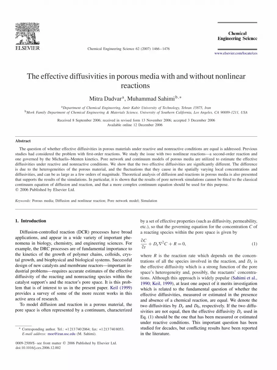
Fig. 1. Three PSDs used in the study.

pore size distribution (PSD) f (r), given by

f (r) = r − rmin

(ra − rmin)2

exp

[−1

2

(r − rmin

ra − rmin

)2]

, (4)

where ra and rmin are the average and minimum pore radius,respectively. We use a typical value of ra reported in the lit-erature for catalyst particles. We also consider PSDs with anaverage pore size five times smaller and larger than the basecase ra , in order to understand its effect on the effective diffu-sivities. Fig. 1 shows the three PSDs that we used in the simu-lations. Using Eq. (4), we also constructed bimodal PSDs thatwill be described in Section 4, where we present the results.One may select the pores’ lengths l from a statistical distribu-tion, but in the absence of any experimental data, we assume lto be constant.

Let us point out that, the pore network of a real catalyst par-ticle has the dimensions of the particle itself. Thus, the actualpore network has a very large number of pores. Simulation ofsuch a pore network, with the appropriate PSD and porosity, isdifficult, if not impossible. To avoid this problem, Sharratt andMann (1987) used a pore network of the same size as a realcatalyst particle, with a realistic PSD but with a low porosity.In our simulations, we use a large network, while maintainingrealistic values for the pore sizes. Thus, we simulate a networkwhich is small compared to the actual pore network of a cat-alyst, but has realistic local structure. We also generate manyrealizations of the network, and average the results over all ofthem. The macroscopic properties of pore networks become in-dependent of their linear size, once they are larger than a certainsize. Therefore, the approach that we take should be reasonable.

We now describe the pore-level diffusion–reaction phe-nomena, assuming that steady-state conditions are prevailing.Since we are mainly interested in the macroscopic properties,only the variations of C in the pores’ axial direction, say thex-direction, are significant. Thus, if we consider a pore ofradius r and write a mass balance for a shell of thickness �x


between axial positions x and x + �x, we obtain

Dp(�)d2C

dx2− 2

raR = 0, (5)

where Dp is the diffusivity in the pore, and a is the surfacearea per unit weight of the particle. Here, � = RM/r , whereRM is the molecular radius of the reactants which may, ingeneral, be comparable with the pore radius r. This gives rise tothe phenomenon of hindered diffusion (Deen, 1987), wherebymolecular diffusion in a porous medium is restricted by therelatively large molecules being excluded from parts of the porespace, a phenomenon that has also been studied by the porenetwork models (Sahimi and Jue, 1989; Sahimi, 1992; Zhangand Seaton, 1992). Therefore, the �-dependence of Dp must betaken into account. At the pore level, Brenner and Gajdos (1977)and others (see Deen, 1987, and references therein) studiedhindered diffusivity of spherical molecules in cylindrical pores,and showed that for ��0.3 one has

Dp = D∞[1 + 1.125� ln � + 0.416� + 2.25�2 ln � + O(�3)],(6)

where D∞ is the molecular diffusivity in the bulk.In any event, using, for example, the expression for the reac-

tion rate R according to the MM kinetics, Eq. (5) is rewritten as

Dp

d2C

dx2− 2

ra

k1C

1 + k2C= 0. (7)

If we now introduce the dimensionless variables, C = C/C0,and z = x/l, where l is the pore length, and delete the bar signfor convenience, we obtain

d2C

dz2− �2

p

C

1 + �C= 0, (8)

where

� = k2C0, �2p = 2l2k1

raDp

. (9)

Here, �p is a pore-level Thiele modulus, which is different fromthat of the particle (pore network) at the macroscopic scale.The diffusion–reaction equation with a second-order reactioncan be rewritten in dimensionless form in a similar manner.Eq. (8) must be solved subject to the boundary conditions that,C(z=0)=Cz0 at one end of the pore, and C(z=1)=Cz1 at theother end of the pore. As it has no known analytical solution,Eq. (8) must be solved numerically.

Since no chemical reaction occurs at the nodes, the total fluxof the reactants that enter a node must be equal to their fluxleaving the node. Therefore, for any node i in the network’sinterior (not on the boundary) we must have∑{ij}

Jij Sij = 0, (10)

where Jij is the flux of the species in pore ij, Sij = �r2ij is the

cross-sectional area of pore ij, and the sum is over all the pores

ij that are connected to node i. The flux Jij is given by

Jij = −Dp

dC

dx= Dp

l�C, (11)

where �C = C(x = 0) − C(x = l) is the difference betweenthe concentrations at the pore’s two ends. Due to nonlinearityof Eq. (8) (and its counterpart for the case of a second-orderreaction), one cannot derive an analytical expression for theflux Jij and, hence, one must resort to numerical simulation.

Thus, consider the numerical solution of Eq. (8) within apore. Since steady-state conditions are prevailing and the pore-level diffusion–reaction problem is 1D, the simplest and mostefficient numerical method for solving Eq. (8) is the standardfinite-difference (FD) approximation. Suppose that for everypore we use three grid points, two at the pore’s ends, whichcoincide with the nodes to which the pore is connected, and onein the middle of the pore. Writing down the FD approximationto Eq. (8) at the middle point and rearranging the equation yield

2�C21 + [2 − �(Cz0 + Cz1) + �2

p�z2]C1 − (Cz0 + Cz1) = 0,

(12)

where C1 is the concentration in the middle grid point, and�z = 1

2 . Eq. (12), a second-order algebraic equation, can besolved explicitly for C1. Since the net flux Jij in the pore isthe same as the flux between one end of the pore and the gridpoint in its middle, the implication is that, when only one FDgrid point is inserted inside the pore (in the middle), Jij can beexpressed explicitly in terms of the concentrations at the twonodes to which the pore is connected (i.e., in terms of Cz0 andCz1), although, unlike the linear kinetics case and due to non-linearity of the solution of Eq. (12), the resulting expressionis still nonlinear in the nodal concentrations Cz0 and Cz1 (seealso below). Our preliminary numerical simulations indicatedthat, using three FD points for each pore provides accurate so-lution of the nonlinear diffusion–reaction equation throughoutthe network and, therefore, in the computations reported belowwe also used three FD points for every pore. We found the sameto be true for the case in which the reaction is second order.

We computed two effective diffusivities using the pore net-work model. One is in the absence of any reaction. In this limit,the flux Jij in the pore ij is given by Jij =Dp(Cx=0 −Cx=l )/ l.When this expression is substituted in Eq. (10), it results in aset of simultaneous linear equations that governs the nodal con-centrations, which we solve using the conjugate-gradient (CG)method. The boundary conditions are a fixed concentration dif-ference �C imposed in the x-direction, and periodic boundaryconditions in the y- and z-directions. We then compute, usingthe solution of the set, the total flux J through the network.Given the imposed concentration difference, the effective dif-fusivity D0, in the absence of a reaction, is then computedreadily, D0 = J/(L�C), where L is the pore network’s length.

The second diffusivity that we compute is in the presence ofthe nonlinear reactions. Together, Eqs. (10)–(12) yield a set ofnonlinear algebraic equations that govern the nodal concentra-tions, which we solve using a combination of the Newton andthe CG methods. In this case, a fixed concentration is imposedon the x = 0 face of the network, while a zero-flux boundary


condition is imposed at the x = 12L face. Periodic boundary

conditions are imposed in the y- and z-directions. After com-puting the concentration profile throughout the network, thenetwork effective diffusivity De in the presence of a reaction iscomputed by calculating the total flux of the reactants throughthe network. The total flux is the sum of the individual fluxesin all the pores that are aligned in the macroscopic (x) directionand are distributed between two neighboring yz planes (understeady-state condition, it does not matter which two planes areselected). The flux in each pore is computed by the usual ex-pression for the diffusive flux (Bird et al., 2002, p. 555) exceptthat, unlike the nonreactive case, the concentration profile nowcontains the effect of the nonlinear reactions, since the pro-file was computed by solving Eqs. (10)–(12) in each pore andthroughtout the network (see above). Having computed the to-tal flux and the boundary conditions, the effective diffusivityunder reaction condition is readily computed.

All the results were obtained using L×L×L networks, withL= 40, where L is measured in units of the pore’s length l. Wealso averaged the results over 10 realizations.

3. The effective diffusivity from the continuum model

In our opinion, pore network modeling provides the mostaccurate way of investigating whether the effective diffusivi-ties under reactive and nonreactive conditions are equal, as thesimulations are unambiguous and the effects of the PSD andpore connectivity are directly taken into account (see also thediscussion in Section 5).

However, we also computed the effective diffusivities, un-der reactive condition, by fitting the macroscale continuumdiffusion–reaction equation to the simulation results. The ideais that, if the pore network is a true representation of a porousmaterial, and if the material is macroscopically homogeneous,then one should be able to represent (fit) the concentration pro-file obtained from the network simulation by the classical con-tinuum diffusion–reaction equation (Bird et al., 2002). Thus,consider, for example, the case of the second-order irreversiblereaction in a semi-infinite slab, for which Eq. (1), under steady-state condition, becomes

De

d2C

dx2− kC2 = 0, (13)

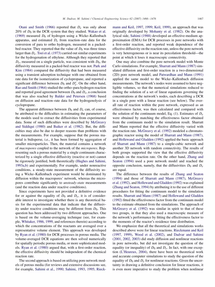
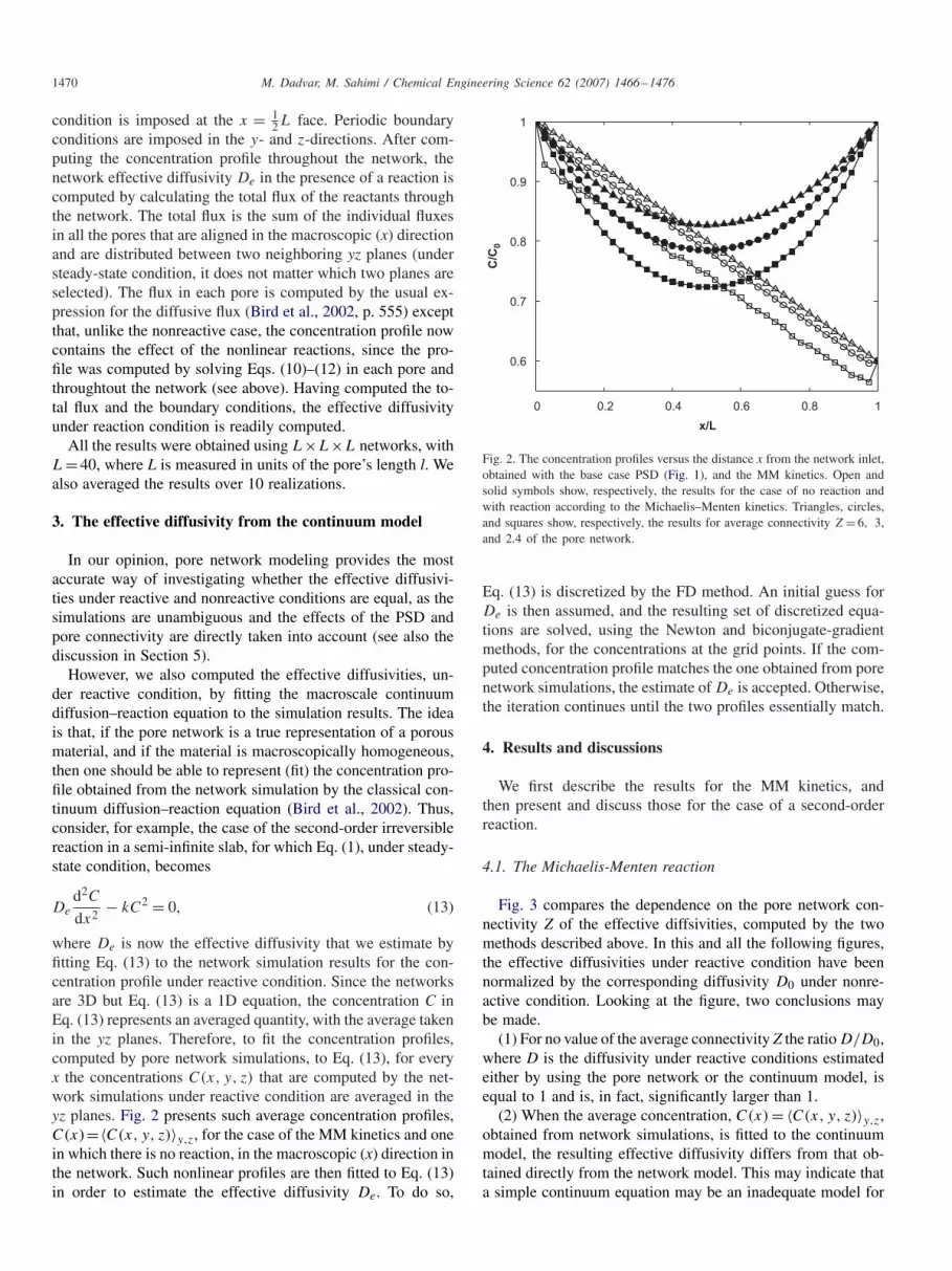
where De is now the effective diffusivity that we estimate byfitting Eq. (13) to the network simulation results for the con-centration profile under reactive condition. Since the networksare 3D but Eq. (13) is a 1D equation, the concentration C inEq. (13) represents an averaged quantity, with the average takenin the yz planes. Therefore, to fit the concentration profiles,computed by pore network simulations, to Eq. (13), for everyx the concentrations C(x, y, z) that are computed by the net-work simulations under reactive condition are averaged in theyz planes. Fig. 2 presents such average concentration profiles,C(x)=〈C(x, y, z)〉y,z, for the case of the MM kinetics and onein which there is no reaction, in the macroscopic (x) direction inthe network. Such nonlinear profiles are then fitted to Eq. (13)in order to estimate the effective diffusivity De. To do so,

0 0.2 0.4 0.6 0.8 1

0.6

0.7

0.8

0.9

1

x/L

C/C

0

Fig. 2. The concentration profiles versus the distance x from the network inlet,obtained with the base case PSD (Fig. 1), and the MM kinetics. Open andsolid symbols show, respectively, the results for the case of no reaction andwith reaction according to the Michaelis–Menten kinetics. Triangles, circles,and squares show, respectively, the results for average connectivity Z = 6, 3,and 2.4 of the pore network.

Eq. (13) is discretized by the FD method. An initial guess forDe is then assumed, and the resulting set of discretized equa-tions are solved, using the Newton and biconjugate-gradientmethods, for the concentrations at the grid points. If the com-puted concentration profile matches the one obtained from porenetwork simulations, the estimate of De is accepted. Otherwise,the iteration continues until the two profiles essentially match.

4. Results and discussions

We first describe the results for the MM kinetics, andthen present and discuss those for the case of a second-orderreaction.

4.1. The Michaelis-Menten reaction

Fig. 3 compares the dependence on the pore network con-nectivity Z of the effective diffsivities, computed by the twomethods described above. In this and all the following figures,the effective diffusivities under reactive condition have beennormalized by the corresponding diffusivity D0 under nonre-active condition. Looking at the figure, two conclusions maybe made.

(1) For no value of the average connectivity Z the ratio D/D0,where D is the diffusivity under reactive conditions estimatedeither by using the pore network or the continuum model, isequal to 1 and is, in fact, significantly larger than 1.

(2) When the average concentration, C(x) = 〈C(x, y, z)〉y,z,obtained from network simulations, is fitted to the continuummodel, the resulting effective diffusivity differs from that ob-tained directly from the network model. This may indicate thata simple continuum equation may be an inadequate model for


1.5 3 4.5 6

1.5

2

2.5

3

3.5

4

Z

D / D

0

Fig. 3. The effective diffusivities obtained by pore network simulations(circles), and by fitting the average concentration profiles in the pore networkto the continuum model (triangles). Z is the network’s average connectivity.The PSD is the base case (Fig. 1), and the reaction follows the MM kinetics.

1.5 3 4.5 6

0

4

8

12

Z

D / D

0

Fig. 4. Effect of the average pore size ra on the effective diffusivity. Trianglesand squares with solid curves show the results, computed by using the porenetwork model and the MM kinetics, when ra is, respectively, five timeslarger and smaller than that of the base case PSD (see Fig. 1), while dashedcurves show the results obtained by fitting the average concentration profilesin the pore network to the continuum model. Z is the network’s averageconnectivity.

representing detailed numerical results obtained from a networkmodel (see also Section 5).

To check whether the differences in Fig. 3 are possibly dueto the particular PSD and its average pore size that we used,we repeated (as mentioned above) the simulations for twoother PSDs (see Fig. 1) with average pore sizes that were fivetimes larger and smaller than the base case used for the resultsshown in Fig. 3. Fig. 4 compares the diffusivities under reactive

-8 -4

0

2

4

6

8

10

ln(r)

f(r)

×10

-2

Fig. 5. Two bimodal PSDs used in the simulations. Continuous and dashedcurves show, respectively, the PSDs for p = 0.5 and 0.8, where p is thefraction of the macropores.

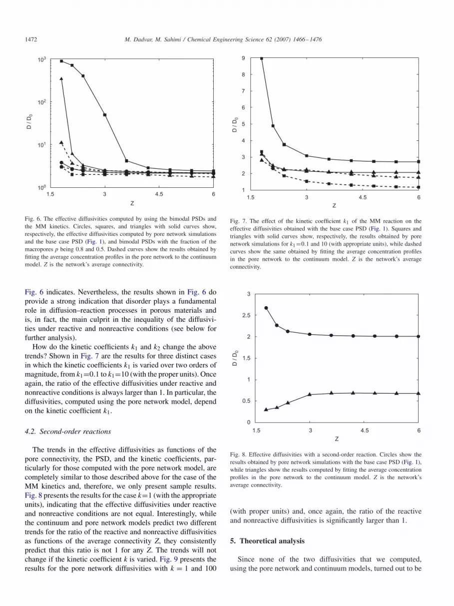
conditions, computed with the three PSDs. Once again, for allthe cases, the ratio of the diffusivities under reactive and non-reactive conditions is significantly larger than 1. In addition,similar to the results shown in Fig. 3, the estimated reactivediffusivities obtained from the network and continuum modelsare different.

Some catalyst particles possess a bimodal PSD, indicatingthe existence of micropores on the one hand, and meso- ormacropores on the other hand. The question, then, is whethera bimodal PSD changes the trends seen in Figs. 3 and 4. Al-though as Hughes and Sahimi (1993a,b) pointed out, such ma-terials are more accurately and rigorously modeled with twocoupled networks, one each for each type of the pore, as apreliminary step for addressing the question, we simulated thereaction–diffusion process in a pore network in which a frac-tion p of the pores followed the PSD (4) with the same aver-age pore size as the base case considered above (the meso- ormacropores), while the rest of the pore sizes were distributedaccording to Eq. (4) but with an average pore size that was 1

100of the base case, and a minimum pore size rmin that was 1

50of the base case. Hence, the two PSDs, representing two dis-tinct types of pores, were completely separated with no over-lap. We considered two cases with p = 0.5 and 0.8, with thecorresponding PSDs shown in Fig. 5.

Fig. 6 presents the results obtained with the continuummodel, and compares them with those obtained directly fromnetwork simulations. In this case, the ratio D/D0 for both thenetwork and continuum diffusivities can be as high as 103.Such large differences might partly be due to the inadequacyof representing the pore space by a single pore network, ratherthan two coupled networks (Hughes and Sahimi, 1993a,b). Inother words, had we used two coupled networks to representthe bidisperse porous material, the differences between thetwo effective diffusivities might not have been as large as what


1.5 3 4.5 6

103

102

101

100

Z

D /

D0

Fig. 6. The effective diffusivities computed by using the bimodal PSDs andthe MM kinetics. Circles, squares, and triangles with solid curves show,respectively, the effective diffusivities computed by pore network simulationsand the base case PSD (Fig. 1), and bimodal PSDs with the fraction of themacropores p being 0.8 and 0.5. Dashed curves show the results obtained byfitting the average concentration profiles in the pore network to the continuummodel. Z is the network’s average connectivity.

Fig. 6 indicates. Nevertheless, the results shown in Fig. 6 doprovide a strong indication that disorder plays a fundamentalrole in diffusion–reaction processes in porous materials andis, in fact, the main culprit in the inequality of the diffusivi-ties under reactive and nonreactive conditions (see below forfurther analysis).

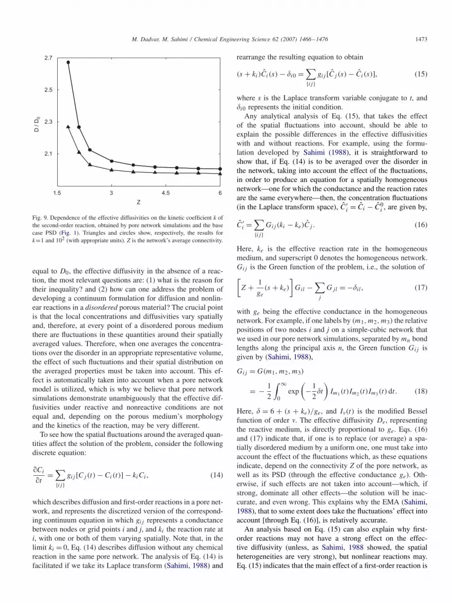
How do the kinetic coefficients k1 and k2 change the abovetrends? Shown in Fig. 7 are the results for three distinct casesin which the kinetic coefficients k1 is varied over two orders ofmagnitude, from k1=0.1 to k1=10 (with the proper units). Onceagain, the ratio of the effective diffusivities under reactive andnonreactive conditions is always larger than 1. In particular, thediffusivities, computed using the pore network model, dependon the kinetic coefficient k1.

4.2. Second-order reactions

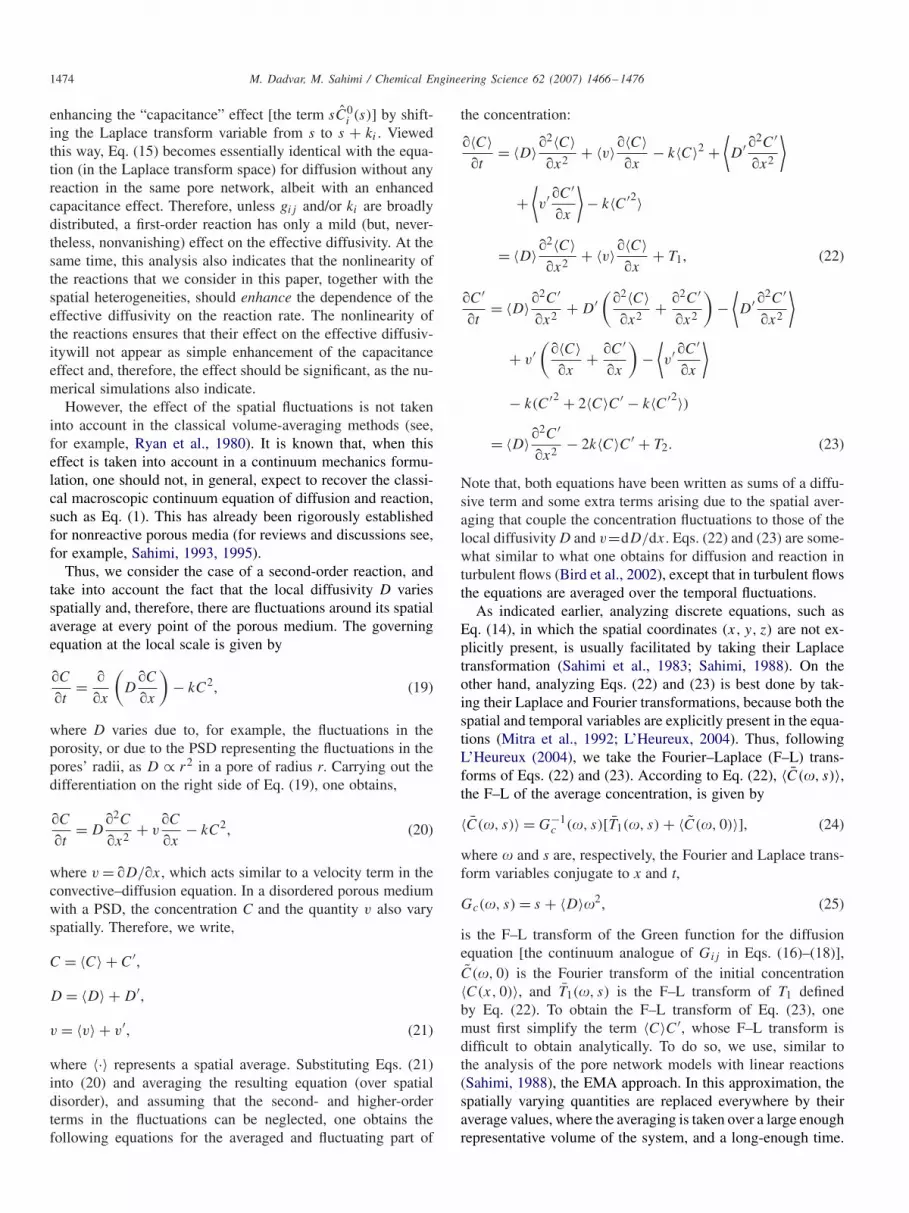
The trends in the effective diffusivities as functions of thepore connectivity, the PSD, and the kinetic coefficients, par-ticularly for those computed with the pore network model, arecompletely similar to those described above for the case of theMM kinetics and, therefore, we only present sample results.Fig. 8 presents the results for the case k=1 (with the appropriateunits), indicating that the effective diffusivities under reactiveand nonreactive conditions are not equal. Interestingly, whilethe continuum and pore network models predict two differenttrends for the ratio of the reactive and nonreactive diffusivitiesas functions of the average connectivity Z, they consistentlypredict that this ratio is not 1 for any Z. The trends will notchange if the kinetic coefficient k is varied. Fig. 9 presents theresults for the pore network diffusivities with k = 1 and 100

1.5 3 4.5 6

1

2

3

4

5

6

7

8

9

Z

D / D

0

Fig. 7. The effect of the kinetic coefficient k1 of the MM reaction on theeffective diffusivities obtained with the base case PSD (Fig. 1). Squares andtriangles with solid curves show, respectively, the results obtained by porenetwork simulations for k1=0.1 and 10 (with appropriate units), while dashedcurves show the same obtained by fitting the average concentration profilesin the pore network to the continuum model. Z is the network’s averageconnectivity.

1.5 3 4.5 6

0

0.5

1

1.5

2

2.5

3

Z

D / D

0

Fig. 8. Effective diffusivities with a second-order reaction. Circles show theresults obtained by pore network simulations with the base case PSD (Fig. 1),while triangles show the results computed by fitting the average concentrationprofiles in the pore network to the continuum model. Z is the network’saverage connectivity.

(with proper units) and, once again, the ratio of the reactiveand nonreactive diffusivities is significantly larger than 1.

5. Theoretical analysis

Since none of the two diffusivities that we computed,using the pore network and continuum models, turned out to be


1.5 3 4.5 6

2.1

2.3

2.5

2.7

Z

D /

D0

Fig. 9. Dependence of the effective diffusivities on the kinetic coefficient k ofthe second-order reaction, obtained by pore network simulations and the basecase PSD (Fig. 1). Triangles and circles show, respectively, the results fork=1 and 102 (with appropriate units). Z is the network’s average connectivity.

equal to D0, the effective diffusivity in the absence of a reac-tion, the most relevant questions are: (1) what is the reason fortheir inequality? and (2) how can one address the problem ofdeveloping a continuum formulation for diffusion and nonlin-ear reactions in a disordered porous material? The crucial pointis that the local concentrations and diffusivities vary spatiallyand, therefore, at every point of a disordered porous mediumthere are fluctuations in these quantities around their spatiallyaveraged values. Therefore, when one averages the concentra-tions over the disorder in an appropriate representative volume,the effect of such fluctuations and their spatial distribution onthe averaged properties must be taken into account. This ef-fect is automatically taken into account when a pore networkmodel is utilized, which is why we believe that pore networksimulations demonstrate unambiguously that the effective dif-fusivities under reactive and nonreactive conditions are notequal and, depending on the porous medium’s morphologyand the kinetics of the reaction, may be very different.

To see how the spatial fluctuations around the averaged quan-tities affect the solution of the problem, consider the followingdiscrete equation:

�Ci

�t=

∑{ij}

gij [Cj (t) − Ci(t)] − kiCi , (14)

which describes diffusion and first-order reactions in a pore net-work, and represents the discretized version of the correspond-ing continuum equation in which gij represents a conductancebetween nodes or grid points i and j, and ki the reaction rate ati, with one or both of them varying spatially. Note that, in thelimit ki = 0, Eq. (14) describes diffusion without any chemicalreaction in the same pore network. The analysis of Eq. (14) isfacilitated if we take its Laplace transform (Sahimi, 1988) and

rearrange the resulting equation to obtain

(s + ki)Ci(s) − �i0 =∑{ij}

gij [Cj (s) − Ci(s)], (15)

where s is the Laplace transform variable conjugate to t, and�i0 represents the initial condition.

Any analytical analysis of Eq. (15), that takes the effectof the spatial fluctuations into account, should be able toexplain the possible differences in the effective diffusivitieswith and without reactions. For example, using the formu-lation developed by Sahimi (1988), it is straightforward toshow that, if Eq. (14) is to be averaged over the disorder inthe network, taking into account the effect of the fluctuations,in order to produce an equation for a spatially homogeneousnetwork—one for which the conductance and the reaction ratesare the same everywhere—then, the concentration fluctuations(in the Laplace transform space), C′

i = Ci − C0i , are given by,

C′i =

∑{ij}

Gij (ki − ke)Cj . (16)

Here, ke is the effective reaction rate in the homogeneousmedium, and superscript 0 denotes the homogeneous network.Gij is the Green function of the problem, i.e., the solution of[Z + 1

ge

(s + ke)

]Gil −

∑j

Gjl = −�il , (17)

with ge being the effective conductance in the homogeneousnetwork. For example, if one labels by (m1, m2, m3) the relativepositions of two nodes i and j on a simple-cubic network thatwe used in our pore network simulations, separated by mn bondlengths along the principal axis n, the Green function Gij isgiven by (Sahimi, 1988),

Gij = G(m1, m2, m3)

= − 1

2

∫ ∞

0exp

(−1

2�t

)Im1(t)Im2(t)Im3(t) dt . (18)

Here, � = 6 + (s + ke)/ge, and I�(t) is the modified Besselfunction of order �. The effective diffusivity De, representingthe reactive medium, is directly proportional to ge. Eqs. (16)and (17) indicate that, if one is to replace (or average) a spa-tially disordered medium by a uniform one, one must take intoaccount the effect of the fluctuations which, as these equationsindicate, depend on the connectivity Z of the pore network, aswell as its PSD (through the effective conductance ge). Oth-erwise, if such effects are not taken into account—which, ifstrong, dominate all other effects—the solution will be inac-curate, and even wrong. This explains why the EMA (Sahimi,1988), that to some extent does take the fluctuations’ effect intoaccount [through Eq. (16)], is relatively accurate.

An analysis based on Eq. (15) can also explain why first-order reactions may not have a strong effect on the effec-tive diffusivity (unless, as Sahimi, 1988 showed, the spatialheterogeneities are very strong), but nonlinear reactions may.Eq. (15) indicates that the main effect of a first-order reaction is


enhancing the “capacitance” effect [the term sC0i (s)] by shift-

ing the Laplace transform variable from s to s + ki . Viewedthis way, Eq. (15) becomes essentially identical with the equa-tion (in the Laplace transform space) for diffusion without anyreaction in the same pore network, albeit with an enhancedcapacitance effect. Therefore, unless gij and/or ki are broadlydistributed, a first-order reaction has only a mild (but, never-theless, nonvanishing) effect on the effective diffusivity. At thesame time, this analysis also indicates that the nonlinearity ofthe reactions that we consider in this paper, together with thespatial heterogeneities, should enhance the dependence of theeffective diffusivity on the reaction rate. The nonlinearity ofthe reactions ensures that their effect on the effective diffusiv-itywill not appear as simple enhancement of the capacitanceeffect and, therefore, the effect should be significant, as the nu-merical simulations also indicate.

However, the effect of the spatial fluctuations is not takeninto account in the classical volume-averaging methods (see,for example, Ryan et al., 1980). It is known that, when thiseffect is taken into account in a continuum mechanics formu-lation, one should not, in general, expect to recover the classi-cal macroscopic continuum equation of diffusion and reaction,such as Eq. (1). This has already been rigorously establishedfor nonreactive porous media (for reviews and discussions see,for example, Sahimi, 1993, 1995).

Thus, we consider the case of a second-order reaction, andtake into account the fact that the local diffusivity D variesspatially and, therefore, there are fluctuations around its spatialaverage at every point of the porous medium. The governingequation at the local scale is given by

�C

�t= �

�x

(D

�C

�x

)− kC2, (19)

where D varies due to, for example, the fluctuations in theporosity, or due to the PSD representing the fluctuations in thepores’ radii, as D ∝ r2 in a pore of radius r. Carrying out thedifferentiation on the right side of Eq. (19), one obtains,

�C

�t= D

�2C

�x2+ v

�C

�x− kC2, (20)

where v = �D/�x, which acts similar to a velocity term in theconvective–diffusion equation. In a disordered porous mediumwith a PSD, the concentration C and the quantity v also varyspatially. Therefore, we write,

C = 〈C〉 + C′,

D = 〈D〉 + D′,

v = 〈v〉 + v′, (21)

where 〈·〉 represents a spatial average. Substituting Eqs. (21)into (20) and averaging the resulting equation (over spatialdisorder), and assuming that the second- and higher-orderterms in the fluctuations can be neglected, one obtains thefollowing equations for the averaged and fluctuating part of

the concentration:

�〈C〉�t

= 〈D〉�2〈C〉�x2

+ 〈v〉�〈C〉�x

− k〈C〉2 +⟨D′ �2C′

�x2

⟩

+⟨v′ �C′

�x

⟩− k〈C′2〉

= 〈D〉�2〈C〉�x2

+ 〈v〉�〈C〉�x

+ T1, (22)

�C′

�t= 〈D〉�

2C′

�x2+ D′

(�2〈C〉�x2

+ �2C′

�x2

)−

⟨D′ �2C′

�x2

⟩

+ v′(

�〈C〉�x

+ �C′

�x

)−

⟨v′ �C′

�x

⟩

− k(C′2 + 2〈C〉C′ − k〈C′2〉)

= 〈D〉�2C′

�x2− 2k〈C〉C′ + T2. (23)

Note that, both equations have been written as sums of a diffu-sive term and some extra terms arising due to the spatial aver-aging that couple the concentration fluctuations to those of thelocal diffusivity D and v=dD/dx. Eqs. (22) and (23) are some-what similar to what one obtains for diffusion and reaction inturbulent flows (Bird et al., 2002), except that in turbulent flowsthe equations are averaged over the temporal fluctuations.

As indicated earlier, analyzing discrete equations, such asEq. (14), in which the spatial coordinates (x, y, z) are not ex-plicitly present, is usually facilitated by taking their Laplacetransformation (Sahimi et al., 1983; Sahimi, 1988). On theother hand, analyzing Eqs. (22) and (23) is best done by tak-ing their Laplace and Fourier transformations, because both thespatial and temporal variables are explicitly present in the equa-tions (Mitra et al., 1992; L’Heureux, 2004). Thus, followingL’Heureux (2004), we take the Fourier–Laplace (F–L) trans-forms of Eqs. (22) and (23). According to Eq. (22), 〈C(�, s)〉,the F–L of the average concentration, is given by

〈C(�, s)〉 = G−1c (�, s)[T1(�, s) + 〈C(�, 0)〉], (24)

where � and s are, respectively, the Fourier and Laplace trans-form variables conjugate to x and t,

Gc(�, s) = s + 〈D〉�2, (25)

is the F–L transform of the Green function for the diffusionequation [the continuum analogue of Gij in Eqs. (16)–(18)],C(�, 0) is the Fourier transform of the initial concentration〈C(x, 0)〉, and T1(�, s) is the F–L transform of T1 definedby Eq. (22). To obtain the F–L transform of Eq. (23), onemust first simplify the term 〈C〉C′, whose F–L transform isdifficult to obtain analytically. To do so, we use, similar tothe analysis of the pore network models with linear reactions(Sahimi, 1988), the EMA approach. In this approximation, thespatially varying quantities are replaced everywhere by theiraverage values, where the averaging is taken over a large enoughrepresentative volume of the system, and a long-enough time.


Thus, one replaces 〈C〉 by a constant value C0 (similar to theabove analysis for first-order reactions).We then obtain

C′(�, s) = G−1(�, s)T2(�, s), (26)

where G(�, s)=Gc(�, s)+2kC0. Therefore, in the space–timedomain, the fluctuating part of the concentration is given by

C′(x, t) =∫ t

0

∫G−1(x − x′, t − t ′)T2(x

′, t ′) dx′ dt ′

= G−1(x − x′, t − t ′) ∗ T2(x′, t ′), (27)

where ∗ denotes the convolution operator. To make furtherprogress, we need to express the various terms of T1 and T2in terms of the average concentration and its derivatives. Theanalysis for doing so is tedious. Using Eq. (27) one can show,for example, that (L’Heureux, 2004)

⟨v′ �C′

�x

⟩= �G−1(x − x′, t − t ′)

�x

∗[〈v′2〉�〈C(x′)〉

�x′ + 〈v′D′〉�2〈C(x′)〉�x′2

](28)

and⟨D′ �2C′

�x2

⟩= �2G−1(x − x′, t − t ′)

�x2

∗[〈D′v′〉�〈C(x′)〉

�x′ + 〈D′2〉�2〈C(x′)〉�x′2

]. (29)

All other terms can also be determined, so that they are rewrittenin terms of the average concentration and its derivatives. Tobe utilized in Eqs. (24) and (26), we must then take their F–Ltransforms.

However, expressing T1 and T2 in terms of the average con-centration and its derivatives, by such equations as (28) and(29), is necessary but not sufficient for deriving the final equa-tion that governs the average concentration. As Eqs. (28) and(29) indicate, the various terms involve the Green functionwhich, in turn, depends on the average 〈D〉, and the statisti-cal distribution of the fluctuations D′. Therefore, we must alsospecify the statistical distribution of the fluctuations D′, so thatall the terms involving the averages of D, v and their fluctua-tions and, hence, the Green function, can be explicitly evalu-ated. In the present paper, porous media at small length scalesare of interest. As Knackstedt et al. (2001) demonstrated, evenat such small length scales the porosity may fluctuate strongly.Moreover, the local diffusivity D fluctuates due to the varia-tions in the pore sizes, so that even in the absence of porosityfluctuations, one still hasfluctuations in D, C, and v. Thus, if,for example, h(D) is the distribution of the local D, then, as-suming that, D = ar2, where a is a constant, h(D) can easilybe determined given the PSD f (r), since h(D) dD = f (r) dr .Let us then assume that the fluctuations D′ follow a statisticaldistribution (usually taken to be Gaussian) with zero average,

and a correlation function C(x) defined by

C(x) = 〈D′(x′)D′(x + x′)〉, (30)

where the averaging is performed over all x′.One can then determine all the terms that contribute to

the governing equation for the average concentration. Whenthis is done (the procedure for which is tedious), one obtains(L’Heureux, 2004)

�〈C〉�t

= De

�2〈C〉�x2

+ 〈v〉�〈C〉�x

− k〈C〉2 − (c1 + c2)

(�2〈C〉�x2

)2

− c3

(�〈C〉�x

)2

+ c2�3〈C〉�x3

�〈C〉�x

, (31)

where De is the effective diffusivity in the porous medium underreactive conditions, and c1, c2, and c3 are constants. They, aswell as De, depend on the statistics of the distribution h(D) ofthe local diffusivities (hence the PSD), the correlation functionC(r), and the reaction rate constant k. According to Eq. (31), thegoverning equation for the average concentration of diffusingreactants in a disordered porous medium with second-orderreaction is much more complex than Eq. (13), hence explainingwhy,

(1) the effective diffusivities under reactive and nonreactiveconditions are not equal;

(2) the averaged concentration profiles computed by pore net-work simulations cannot be simply fitted to Eq. (13); and,therefore,

(3) the effective diffusivities that we computed by using porenetwork simulations, and by fitting the average concentra-tion profiles in the pore network model to Eq. (13), are notequal.

6. Summary

Extensive numerical simulations of diffusion and nonlinearreactions in porous materials were carried, using a 3D porenetwork model of the pore space. A second-order reaction andone according to the Michaelis–Menten kinetics were consid-ered, and the pore size distribution, pore connectivity, and thereaction rate coefficients were varied in order to study theireffect on the effective diffusivities. The results of thesimulations were also fitted to the classical continuumdiffusion–reaction equation, typically used for modelingthe phenomenon at the macroscale. We found, in all thecases considered, that the effective diffusivities under reac-tive and nonreactive conditions are not equal, and that inmany cases they differ greatly. Theoretical analysis was alsopresented that supported the conclusion reached by the nu-merical simulations. The analysis indicated that the hetero-geneity of the pore space, coupled with the nonlinear kinet-ics of the reactions, give rise to strong fluctuations in theconcentration distribution. Such fluctuations are the sourceof the inequality of the effective diffusivities under reac-tive and nonreactive conditions. The analysis also indicated


that the concentration profiles that one obtains from porenetwork simulations cannot be fitted to the classical continuumequation of diffusion and nonlinear reactions. More complexcontinuum models, such as Eq. (31) for second-order reactions,that do take into account the effect of the spatial fluctuations,are needed for this purpose.

Acknowledgment

The work of M.D. was supported in part by the NIOC.

References

Baiker, A., New, M., Richan, W., 1982. Determination of intraparticle diffusioncoefficients in catalyst pellets—a comparative study of measuring methods.Chemical Engineering Science 37, 643.

Balder, J.R., Petersen, E.E., 1968. Application of the single pellet reactor fordirect mass transfer studies. Journal of Catalysis 11, 195.

Bird, R.B., Stewart, W.E., Lightfoot, E.N., 2002. Transport Phenomena,second ed. Wiley, New York.

Brenner, H., Gajdos, L.J., 1977. The constrained Brownian movement ofspherical particles in cylindrical pores of comparable radius. Journal ofColloids and Interface Science 58, 312.

Dadvar, M., Sahimi, M., 2001. Pore network model of deactivation ofimmobilized glucose isomerase in packed-bed reactors. I: two-dimensionalsimulations at the particle level. Chemical Engineering Science 56, 1.

Dadvar, M., Sahimi, M., 2002. Pore network model of deactivationof immobilized glucose isomerase in packed-bed reactors. II: three-dimensional simulations at the particle level. Chemical Engineering Science57, 939.

Dadvar, M., Sahimi, M., 2003. Pore network model of deactivation ofimmobilized glucose isomerase in packed-bed reactors. III: multiscalemodeling. Chemical Engineering Science 58, 4935.

Deen, W.M., 1987. Hindered transport of large molecules in liquid-filledpores. A.I.Ch.E. Journal 33, 1409.

Hollewand, M.P., Gladden, L.F., 1992. Modelling of diffusion and reactionin porous catalysts using a random three-dimensional network model.Chemical Engineering Science 47, 1761.

Hughes, B.D., Sahimi, M., 1993a. Diffusion in disordered systems withmultiple families of transport paths. Physical Review Letters 70, 2581.

Hughes, B.D., Sahimi, M., 1993b. Stochastic transport in heterogeneous mediawith multiple families of transport paths. Physical Review E 48, 2776.

Keil, F.J., 1999. Diffusion and reaction in porous networks. Catalysis Today53, 245.

Knackstedt, M.A., Sheppard, A.P., Sahimi, M., 2001. Pore network modelingof two-phase flow in porous rock: the effect of correlated heterogeneity.Advances in Water Resources 24, 257.

L’Heureux, I., 2004. Stochastic reaction–diffusion phenomena in porous mediawith nonlinear kinetics: effects of quenched porosity fluctuations. PhysicalReview Letters 93, 180602.

McGreavy, C., Siddiqui, M.A., 1980. Consistent measurement of diffusioncoefficients for effectiveness factors. Chemical Engineering Science 35, 3.

McGreavy, C., Andrade Jr., J.S., Rajagopal, K., 1992. Consistent evaluationof effective diffusion and reaction in pore networks. Chemical EngineeringScience 47, 2751.

Mitra, P.P., Sen, P.N., Schwartz, L.M., Le Doussal, P., 1992. Diffusionpropagator as a probe of the structure of porous media. Physical ReviewLetters 68, 3555.

Mohanty, K.K., Ottino, J.M., Davis, H.T., 1982. Reaction and transportin disordered media: introduction of percolation concepts. ChemicalEngineering Science 37, 905.

Otani, S., Smith, J.M., 1966. Effectiveness of large catalyst pellets—an experimental study. Journal of Catalysis 5, 332.

Park, S.H., Kim, Y.G., 1984. The effect of chemical reaction on effectivediffusivity within biporous catalysts—I. Chemical Engineering Science 39,533.

Patwardhan, A.V., Mann, R., 1991. Effective diffusivity and tortuosity inWicke–Kallenbach experiments: direct interpretation using a stochasticpore network. In: The 1991 Institution of Chemical Engineers ResearchEvent. Institution of Chemical Engineers, Rugby, p. 91.

Rao, M.R., Smith, J.M., 1964. Diffusion and reaction in porous glass.A.I.Ch.E. Journal 10, 293.

Rieckmann, C., Keil, F.J., 1997. Multicomponent diffusion and reaction inthree-dimensional networks: general kinetics. Industrial and EngineeringChemistry Research 36, 3275.

Rieckmann, C., Keil, F.J., 1999. Simulation and experiment ofmulticomponent diffusion and reaction in three-dimensional networks.Chemical Engineering Science 54, 3485.

Ryan, D., Carbonell, R.G., Whitaker, S., 1980. Effective diffusivities forcatalyst pellets under reactive conditions. Chemical Engineering Science35, 10.

Sahimi, M., 1988. Diffusion-controlled reactions in disordered porousmedia—I. Uniform distribution of reactants. Chemical Engineering Science43, 2981.

Sahimi, M., 1992. Transport of macromolecules in porous media. Journal ofChemical Physics 96, 4718.

Sahimi, M., 1993. Flow phenomena in rocks: from continuum models tofractals, percolation, cellular automata, and simulated annealing. Reviewsof Modern Physics 65, 1393.

Sahimi, M., 1995. Flow and Transport in Porous Media and Fractured Rock.VCH, Weinheim.

Sahimi, M., Jue, V.L., 1989. Diffusion of large molecules in porous media.Physical Review Letters 62, 629.

Sahimi, M., Hughes, B.D., Scriven, L.E., Davis, H.T., 1983. Stochastictransport in disordered systems. Journal of Chemical Physics 78, 6849.

Sahimi, M., Gavalas, G.R., Tsotsis, T.T., 1990. Statistical and continuummodels of fluid–solid reactions in porous media. Chemical EngineeringScience 45, 1443.

Sharratt, P.N., Mann, R., 1987. Some observations on variation of tortuositywith Thiele modulus and pore size distribution. Chemical EngineeringScience 42, 1565.

Toei, R., Okazaki, M., Nakanishi, K., Kondo, Y., Hayashi, M., Shiozaki, Y.,1973. Effective diffusivity of a porous catalyst with and without chemicalreaction. Journal of Chemical Engineering of Japan 6, 50.

Wakao, N., Kimura, H., Shibata, M., 1969. Kinetic studies and effectivediffusivities in para to ortho hydrogen conversion reaction. Journal ofChemical Engineering of Japan 2, 51.

Whitaker, S., 1986. Local thermal equilibrium: an application to packed bedcatalytic reactor design. Chemical Engineering Science 41, 2029.

Whitaker, S., 1999. The Method of Volume Averaging. Kluwer, Dordrecht.Wood, J., Gladden, L.F., Keil, F.J., 2002. Modelling diffusion and reaction

by capillary condensation using three-dimensional pore network. Part 2.Dusty gas model and general reaction kinetics. Chemical EngineeringScience 57, 3047.

Zhang, L., Seaton, N.A., 1992. Prediction of the effective diffusivity in porenetworks close to a percolation threshold. A.I.Ch.E. Journal 38, 1816.

Zhang, L., Seaton, N.A., 1994. The application of continuum equations todiffusion and reaction in pore networks. Chemical Engineering Science49, 41.

Documents

The effective diffusivities in porous media with and without nonlinear reactions