The Demand for Mortgages under Macro Volatility:

The Argentine Case

Sebastián Auguste Ricardo Bebczuk Ramiro Moya

Inter-American Development Bank

Department of Research and Chief Economist

TECHNICAL NOTES

No. IDB-TN-284

November 2011

The Demand for Mortgages under Macro Volatility:

The Argentine Case

Sebastián Auguste Ricardo Bebczuk

Ramiro Moya

Inter-American Development Bank

2011

http://www.iadb.org The Inter-American Development Bank�Technical Notes encompass a wide range of best practices, project evaluations, lessons learned, case studies, methodological notes, and other documents of a technical nature. The information and opinions presented in these publications are entirely those of the author(s), and no endorsement by the Inter-American Development Bank, its Board of Executive Directors, or the countries they represent is expressed or implied. This paper may be freely reproduced.

1

Abstract1

This paper analyzes mortgage loan demand in Argentina using a new survey administered in the Buenos Aires Metropolitan Area. It is found that recurring macro volatility and violation of financial property rights have increased demand for real estate as an investment, which in turn raises house prices and makes it more difficult for consumer households to meet minimum income requirements for obtaining a mortgage. Affordability thus seems to offer a better explanation than standard supply side constraints for the small size of the mortgage market in Argentina. Overall, the findings suggest that the shallow mortgage market has not posed a major impediment to home ownership rate in Argentina and that the small (and shrinking) mortgage market has more to do with lack of demand than credit supply constraints. JEL classifications: G21, R21, R31 Keywords: Housing, Mortgage market, Macro volatility, Argentina

1 Sebastián Auguste and Ramiro Moya are affiliated with the Fundación de Investigaciones Económicas Latinoamericanas (FIEL). Ricardo Bebczuk is affiliated with the Centro de Estudios Distributivos, Laborales y Sociales (CEDLAS). The authors thank Arturo Galindo, Alessandro Rebucci, Frank Warnock, Veronica Warnock, and IDB participants in the Housing Finance Seminar for helpful comments and criticisms. Corresponding author: sauguste@umich.edu.

2

1. Introduction The mortgage market in Argentina quickly expanded during the 1990s as a result of the

economic boom, market-oriented reforms in the financial sector, and an upgrading to

international best practices in the mortgage regulatory framework. The stock of mortgage loans

increased from 0.9 to 6 percent of GDP between 1990 and 2000. Mortgage loans became an

important product for banks (36 percent of their loan portfolio) and for new homeowners (30

percent of new titles were mortgage-financed). Whereas the stock of total credit to the private

sector increased by two-and-a-half times over the 1990s, the stock of mortgage loans increased

fivefold.2

Macroeconomic conditions changed dramatically by the end of 2001, however, when

Argentina was hit by a massive financial crisis (after three years of stagnation). In December of

2001 a sovereign default was announced, and in January 2002 the currency board was

abandoned. The local currency drastically devaluated from one peso per US dollar to almost four

per dollar in a few months. The devaluation produced widespread balance sheet effects in a

highly dollarized economy, and several emergency measures were taken. Deposits in foreign

currency were “pesified” at 1.4 pesos per dollar (well below the market rate, implying large

losses for depositors) and banking loans in foreign currency were pesified at one peso per dollar

(implying large gains for debt holders).

3

The exit of the crisis was V-shaped, favored by the international context and the boom in

commodity prices. Between 2009 and 2002 the economy grew at an impressive annual rate of

7.5 percent, whereas construction grew 16 percent annually. Housing prices in US dollars

bounced back and even surpassed the 1990s levels, at the time that real incomes and employment

In this period, mortgage loans were pesified as well, and

foreclosures were temporarily suspended. Real GDP and private consumption plummeted 10.9

percent and 14.4 percent, respectively, in 2002 alone, down 18.4 percent and 21.4 percent,

respectively, from their pre-crisis peak in 1998. Argentina’s crisis was reflected in the value of

local assets in US dollars. The Merval index (which reflects the value of major companies listed

on the Buenos Aires Stock Exchange) fell drastically, and real estate prices in US dollars

plunged by 50 percent on average in Buenos Aires City.

2 The paper mainly deals with mortgage housing finance through the banking system. However, at some points in the document, reference will be made to other forms of public or private housing finance. 3 For a description of the Argentine crisis see Auguste et al. (2006). Agarwal, Chomsisengphet and Hassler (2005) describe the housing finance policies implemented during the crisis.

3

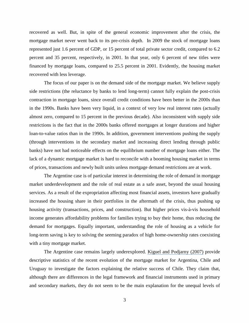
recovered as well. But, in spite of the general economic improvement after the crisis, the

mortgage market never went back to its pre-crisis depth. In 2009 the stock of mortgage loans

represented just 1.6 percent of GDP, or 15 percent of total private sector credit, compared to 6.2

percent and 35 percent, respectively, in 2001. In that year, only 6 percent of new titles were

financed by mortgage loans, compared to 25.5 percent in 2001. Evidently, the housing market

recovered with less leverage.

The focus of our paper is on the demand side of the mortgage market. We believe supply

side restrictions (the reluctance by banks to lend long-term) cannot fully explain the post-crisis

contraction in mortgage loans, since overall credit conditions have been better in the 2000s than

in the 1990s. Banks have been very liquid, in a context of very low real interest rates (actually

almost zero, compared to 15 percent in the previous decade). Also inconsistent with supply side

restrictions is the fact that in the 2000s banks offered mortgages at longer durations and higher

loan-to-value ratios than in the 1990s. In addition, government interventions pushing the supply

(through interventions in the secondary market and increasing direct lending through public

banks) have not had noticeable effects on the equilibrium number of mortgage loans either. The

lack of a dynamic mortgage market is hard to reconcile with a booming housing market in terms

of prices, transactions and newly built units unless mortgage demand restrictions are at work.

The Argentine case is of particular interest in determining the role of demand in mortgage

market underdevelopment and the role of real estate as a safe asset, beyond the usual housing

services. As a result of the expropriation affecting most financial assets, investors have gradually

increased the housing share in their portfolios in the aftermath of the crisis, thus pushing up

housing activity (transactions, prices, and construction). But higher prices vis-à-vis household

income generates affordability problems for families trying to buy their home, thus reducing the

demand for mortgages. Equally important, understanding the role of housing as a vehicle for

long-term saving is key to solving the seeming paradox of high home-ownership rates coexisting

with a tiny mortgage market.

The Argentine case remains largely underexplored. Kiguel and Podjarny (2007) provide

descriptive statistics of the recent evolution of the mortgage market for Argentina, Chile and

Uruguay to investigate the factors explaining the relative success of Chile. They claim that,

although there are differences in the legal framework and financial instruments used in primary

and secondary markets, they do not seem to be the main explanation for the unequal levels of

4

development among the three countries. On the contrary, the most important variables in

explaining the differences are macroeconomic conditions. These include the following:

1. A stable currency to finance long-term fixed-rate loans or, in the presence

of double-digit inflation, indexation, loans in hard currencies, or other

adjustment mechanisms that allow for long-term contracts.

2. For the first condition to work well in practice, the economy must

maintain a certain level of macroeconomic stability, especially regarding

the exchange rate, price levels and interest rates.

3. The existence of mechanisms for flexible and standardized mortgage

origination (primary market) and institutional investors to provide a long-

term horizon financing to feed the secondary market.

4. Potential mortgage holders, especially employees, must be able to meet

the credit requirements to qualify for a loan, a situation sometimes

difficult to achieve in an environment where the ratio of housing prices to

wages is high and nominal interest rates are high as well.

Their conclusions are based on descriptive macro statistics and a simulation exercise on the

behavior of payment-to-income ratio that a hypothetical mortgage holder should have to pay

under a standard fixed rate loan in each country according to its macro volatility history.4

Cristini and Moya (2004) analyze the deepening of the mortgage market in the 1990s

compared to the failure of the 1980s, concluding that the rapid takeoff is due to both

macroeconomic stability and the development of legal and market institutions. Banzas and

Fernández (2007) describe the Argentine case including the 2001/2002 crisis. Using household

survey (EPH) data for 2007, they perform a simple affordability exercise and find that, in spite of

the more favorable conditions offered by banks, almost 60 percent of the population does not

satisfy the minimum requirements for obtaining a mortgage loan.

5

4 In a 10-year loan indexed to CPI with an initial loan payment-to-income ratio of 30 percent, the probability that the ratio goes above 40 percent for 12 consecutive months is 53 percent in Argentina and just 3 percent in Chile, which means that in a standard mortgage contract, an Argentine household faces greater risk of experiencing difficulties in repayment.

5 In the exercise they use prices for the cheapest neighborhoods of Buenos Aires City, and they generously correct family income upwards to compensate for underreporting. Their results should thus be interpreted as a lower bound, i.e., the percentage of excluded families may exceed 60 percent.

5

Cristini and Moya (2008) analyze housing across Latin America and find, inter alia, that

the region has high ownership at the expense of quality. Cristini and Iaryczower (1997),

evaluating the public housing finance system FONAVI based on a simulation exercise using

household survey (EPH) microdata, find that the implicit subsidy (from 20 to 80 percent,

depending on the province) is too high and unequally distributed. Although the decentralization

of the 1990s helped to improve efficiency, there are still middle-income households receiving the

subsidy. Gaba et al. (2003) explore the possibility of introducing an indexation system similar to

Chile’s, and Delgobbo (2000) evaluates the competitive effects of the creation of a secondary

institution by one of the most important mortgage banks in Argentina.6

These papers are based either on macro data or household survey data, as micro data on

housing finance are nearly nonexistent. An exception is Agarwal, Chomsisengphet and Hassler

(2005), who also study the 2001/2002 crisis in Argentina. These authors use a unique loan-level

data set to empirically assess the impact of the currency devaluation and the economic response

policies on prepayment and default patterns of residential mortgages as a consequence of the

previously mentioned pesification of bank loans and deposits.

For the present research work, we exploit for the first time a preexisting living conditions

survey including some limited data on housing finance and, especially, a unique survey

conducted for this study. This information is particularly suitable for exploring the state of the

housing finance system (with primary but not exclusive emphasis on the mortgage market) and

the demand drivers behind it.

The remainder of the paper is structured as follows. Section 2 briefly describes the

housing and housing finance system in Argentina. Section 3 provides a discussion on the recent

evolution of the Argentine mortgage market. Section 4 describes the novel micro-data used and

reports the main findings, and Section 5 offers concluding remarks.

6 Warnock and Warnock (2008) provide cross-country evidence of the variables affecting mortgage depth, where Argentina is included, finding that countries with stronger legal rights (through collateral and bankruptcy laws), deeper credit information systems, and a more stable macroeconomic environment have deeper housing finance systems. Across developed countries, which tend to have low macroeconomic volatility and relatively extensive credit information systems, variation in the strength of legal rights helps explain the extent of housing finance.

6

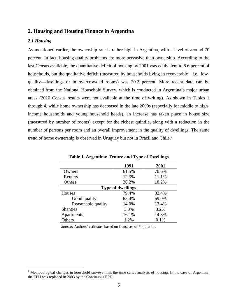
2. Housing and Housing Finance in Argentina 2.1 Housing As mentioned earlier, the ownership rate is rather high in Argentina, with a level of around 70

percent. In fact, housing quality problems are more pervasive than ownership. According to the

last Census available, the quantitative deficit of housing by 2001 was equivalent to 8.6 percent of

households, but the qualitative deficit (measured by households living in recoverable—i.e., low-

quality—dwellings or in overcrowded rooms) was 20.2 percent. More recent data can be

obtained from the National Household Survey, which is conducted in Argentina’s major urban

areas (2010 Census results were not available at the time of writing). As shown in Tables 1

through 4, while home ownership has decreased in the late 2000s (especially for middle to high-

income households and young household heads), an increase has taken place in house size

(measured by number of rooms) except for the richest quintile, along with a reduction in the

number of persons per room and an overall improvement in the quality of dwellings. The same

trend of home ownership is observed in Uruguay but not in Brazil and Chile.7

Table 1. Argentina: Tenure and Type of Dwellings

1991 2001 Owners 61.5% 70.6% Renters 12.3% 11.1% Others 26.2% 18.2%

Type of dwellings Houses 79.4% 82.4% Good quality 65.4% 69.0% Reasonable quality 14.0% 13.4% Shanties 3.3% 3.2% Apartments 16.1% 14.3% Others 1.2% 0.1%

Source: Authors’ estimates based on Censuses of Population.

7 Methodological changes in household surveys limit the time series analysis of housing. In the case of Argentina, the EPH was replaced in 2003 by the Continuous EPH.

7

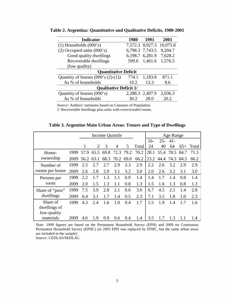
Table 2. Argentina: Quantitative and Qualitative Deficits, 1980-2001

Indicator 1980 1991 2001 (1) Households (000’s) 7,572.3 8,927.3 10,075.8 (2) Occupied units (000’s) 6,798.3 7,743.5 9,204.7 Good quality dwellings 6,198.7 6,281.9 7,628.2 Recoverable dwellings (low quality)

599.6 1,461.6 1,576.5

Quantitative Deficit Quantity of houses (000’s (2)-(1)) 774.1 1,183.8 871.1 As % of households 10.2 13.3 8.6

Qualitative Deficit 1/ Quantity of houses (000’s) 2,288.3 2,497.9 2,036.3 As % of households 30.2 28.0 20.2

Source: Authors’ estimates based on Censuses of Population. 1/ Recoverable dwellings plus units with overcrowded rooms.

Table 3. Argentine Main Urban Areas: Tenure and Type of Dwellings

Income Quintile

Total

Age Range

1 2 3 4 5 16-24

25-40

41-64 65+ Total

Home-ownership

1999 57.9 65.5 69.8 72.3 79.2 70.2 28.1 55.4 78.5 84.7 71.3 2009 56.2 63.1 68.3 70.2 69.0 66.2 23.2 44.4 74.3 84.5 66.2

Number of rooms per house

1999 2.5 2.7 2.7 2.9 3.3 2.9 2.2 2.6 3.2 2.9 2.9 2009 2.6 2.8 2.9 3.1 3.2 3.0 2.0 2.6 3.2 3.1 3.0

Persons per room

1999 2.2 1.7 1.3 1.1 0.9 1.4 1.4 1.7 1.4 0.8 1.4 2009 2.0 1.5 1.3 1.1 0.8 1.3 1.5 1.6 1.3 0.8 1.3

Share of “poor” dwellings

1999 7.5 3.9 2.8 2.1 0.6 3.0 6.7 4.5 2.1 1.4 2.8 2009 6.4 3.1 1.7 1.4 0.5 2.3 7.1 3.5 1.8 1.0 2.3

Share of dwellings of low-quality materials

1999 4.3 2.4 1.6 1.0 0.4 1.7 1.5 1.9 1.4 1.7 1.6

2009 4.6 1.9 0.9 0.6 0.4 1.4 3.5 1.7 1.3 1.1 1.4 Note: 1999 figures are based on the Permanent Household Survey (EPH) and 2009 on Continuous Permanent Household Survey (EPHC) (in 2003 EPH was replaced by EPHC, but the same urban areas are included in the sample) Source: CEDLAS/SEDLAC.

8

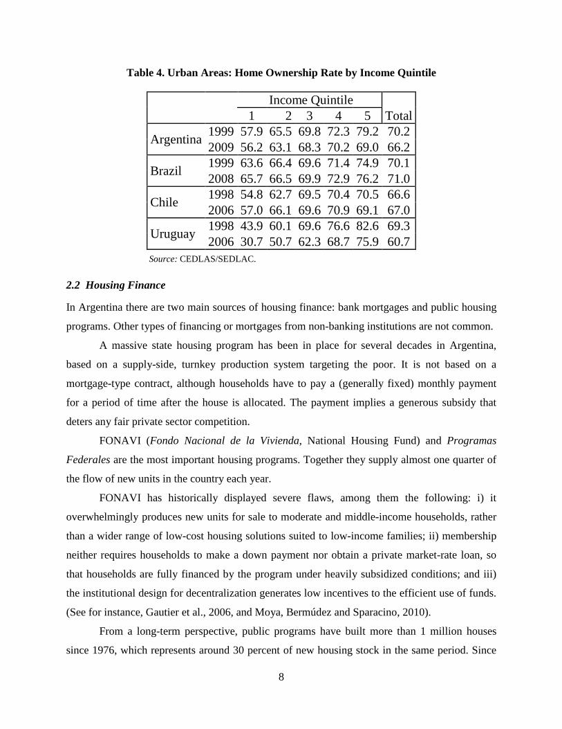
Table 4. Urban Areas: Home Ownership Rate by Income Quintile

Income Quintile Total 1 2 3 4 5

Argentina 1999 57.9 65.5 69.8 72.3 79.2 70.2 2009 56.2 63.1 68.3 70.2 69.0 66.2

Brazil 1999 63.6 66.4 69.6 71.4 74.9 70.1 2008 65.7 66.5 69.9 72.9 76.2 71.0

Chile 1998 54.8 62.7 69.5 70.4 70.5 66.6 2006 57.0 66.1 69.6 70.9 69.1 67.0

Uruguay 1998 43.9 60.1 69.6 76.6 82.6 69.3 2006 30.7 50.7 62.3 68.7 75.9 60.7

Source: CEDLAS/SEDLAC. 2.2 Housing Finance In Argentina there are two main sources of housing finance: bank mortgages and public housing

programs. Other types of financing or mortgages from non-banking institutions are not common.

A massive state housing program has been in place for several decades in Argentina,

based on a supply-side, turnkey production system targeting the poor. It is not based on a

mortgage-type contract, although households have to pay a (generally fixed) monthly payment

for a period of time after the house is allocated. The payment implies a generous subsidy that

deters any fair private sector competition.

FONAVI (Fondo Nacional de la Vivienda, National Housing Fund) and Programas

Federales are the most important housing programs. Together they supply almost one quarter of

the flow of new units in the country each year.

FONAVI has historically displayed severe flaws, among them the following: i) it

overwhelmingly produces new units for sale to moderate and middle-income households, rather

than a wider range of low-cost housing solutions suited to low-income families; ii) membership

neither requires households to make a down payment nor obtain a private market-rate loan, so

that households are fully financed by the program under heavily subsidized conditions; and iii)

the institutional design for decentralization generates low incentives to the efficient use of funds.

(See for instance, Gautier et al., 2006, and Moya, Bermúdez and Sparacino, 2010).

From a long-term perspective, public programs have built more than 1 million houses

since 1976, which represents around 30 percent of new housing stock in the same period. Since

9

2003 the rate of public housing construction has increased and new programs have proliferated.

In line with these developments, federal expenditure on housing has almost doubled, increasing

from 0.45 percent of GDP in 1990s to 0.7 percent in the 2000s. Many of these recent federal

initiatives continue to display some of the crucial weaknesses of the old system. In particular,

they have failed, as in other Latin American programs, to replace turnkey production with direct

demand-subsidy programs that use private developers and lenders to build new units for

moderate-income households much more effectively.

Figure 1 displays the flow of government housing resources and that of housing

mortgages supplied by the banking system, both in percentage of GDP, which indicates the

growing role of public housing programs relative to commercial mortgage financing.

Figure 1. Flow of Housing State Programs and Bank Housing Mortgages, 1994-2008 (% of GDP)

0.0%

0.2%

0.4%

0.6%

0.8%

1.0%

1.2%

1.4%

1.6%

1.8%

1994

1995

1996

1997

1998

1999

2000

2001

2002

2003

2004

2005

2006

2007

2008

(e)

State Housing programs

New mortgage loans (residential and commercial)

10

While government housing programs have not promoted the development of the

mortgage market, they do not seem to have hurt it significantly, since massive public housing

programs are intended for a population segment of little interest to the mortgage market.8

As for

direct interventions in the latter market, they have been very small in scale, and thus they did not

have any perceptible effect on market size or structure.

2.3 Mortgage Market All indicators confirm that this market, despite an incipient but still trifling takeoff in the 1990s,

remains largely undeveloped even after the post-crisis economic recovery.

Historically the mortgage market was very small in Argentina. In the 1970s and 1980s it

was dominated by public banks. A moderate and short-lived boom in mortgage loans took place

in the mid-1990s in response to proper macroeconomic and institutional conditions. Total

mortgage loans jumped from 1.8 percent of GDP in 1993 to a maximum of 6.2 percent of GDP

in 2001. Mortgage loans for housing increased from 2 percent to 4 percent of GDP in the same

period.

As a consequence of the 2001-2002 crisis, private credit dropped from 20.1 percent of

GDP in 2001 to 11.4 percent in 2009, whereas mortgage loans fell from 6.2 percent to 1.6

percent of GDP (from 4 percent to 1 percent in the case of housing loans). Likewise, the stock of

mortgage loans represented 31 percent of the total stock of credit to the private sector in 2001

and only 14.5 percent in 2009 (see Figure 1). This clearly indicates that mortgages were hit even

harder than private credit as a whole.

8 Nevertheless, recent estimates from a survey on this topic indicate that some filtering might be happening. In fact, although 41 percent of beneficiaries belong to households in the lowest two income deciles, 11 percent display incomes comparable to the highest 20 percent of the distribution. This filtering seems to be more important among FONAVI´s beneficiaries than the more recent programs (the so called Programas Federales). See Moya, Bermúdez and Sparacino (2010).

11

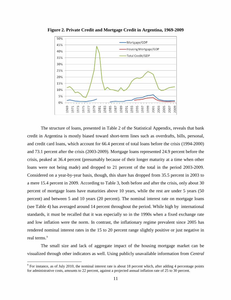
Figure 2. Private Credit and Mortgage Credit in Argentina, 1969-2009

The structure of loans, presented in Table 2 of the Statistical Appendix, reveals that bank

credit in Argentina is mostly biased toward short-term lines such as overdrafts, bills, personal,

and credit card loans, which account for 66.4 percent of total loans before the crisis (1994-2000)

and 73.1 percent after the crisis (2003-2009). Mortgage loans represented 24.9 percent before the

crisis, peaked at 36.4 percent (presumably because of their longer maturity at a time when other

loans were not being made) and dropped to 21 percent of the total in the period 2003-2009.

Considered on a year-by-year basis, though, this share has dropped from 35.5 percent in 2003 to

a mere 15.4 percent in 2009. According to Table 3, both before and after the crisis, only about 30

percent of mortgage loans have maturities above 10 years, while the rest are under 5 years (50

percent) and between 5 and 10 years (20 percent). The nominal interest rate on mortgage loans

(see Table 4) has averaged around 14 percent throughout the period. While high by international

standards, it must be recalled that it was especially so in the 1990s when a fixed exchange rate

and low inflation were the norm. In contrast, the inflationary regime prevalent since 2005 has

rendered nominal interest rates in the 15 to 20 percent range slightly positive or just negative in

real terms.9

The small size and lack of aggregate impact of the housing mortgage market can be

visualized through other indicators as well. Using publicly unavailable information from Central

9 For instance, as of July 2010, the nominal interest rate is about 18 percent which, after adding 4 percentage points for administrative costs, amounts to 22 percent, against a projected annual inflation rate of 25 to 30 percent.

12

de Deudores (the credit register administered by the Central Bank) over 2002-2009, Table 5 in

the Statistical Appendix indicates the following:

• Housing mortgage loans have steadily increased over time as a share of total

mortgages but still account for only between 28 and 50 percent of total

mortgages (both in terms of volumes and number of borrowers), the rest being

mortgages granted to enterprises;

• The banking system has only 158,000 housing mortgage clients in 2009

(down from 182,000 in 2002). For a country where more than three million

households do not own a house, this figure looks quite insignificant.

• The average loan size is remarkably low compared to home values. While

loans have moved from US$6,000 in 2002 to US$14,000 in 2007-2009, the

average value of urban houses, with obvious differences by location, has been

between US$30,000 and US$60,000. This would mean that actual loan-to-

value ratios are quite low and/or some loans are used for home remodeling

and improvements (or to cover other expenses not related to housing) rather

than to buy a new home.

As an additional proof of the low penetration of housing mortgages, Table 6 displays the

number of new property titles in Buenos Aires City, the country’s richest district in per capita

GDP terms. The percentage of mortgage-related titles reached its peak in 1994 (34.7 percent). In

general, the figure for 1991-2000 (29.5 percent), while already low, is more than four times

higher than the 2003-2009 level of 6.7 percent.

The configuration of the mortgage market by bank in 2002 and 2009 appears in Tables

7A and 7B. In both cases, substantial concentration in only a few institutions is observed. The

top five banks account for 76.2 percent of total volume in 2002 and 86.6 percent in 2009, while

for the top 10 the cumulative share exceeds 95 percent. No change is found when looking at the

number of borrowers instead of loan volume. The two largest public banks (Banco Nación and

Banco de la Provincia de Buenos Aires), the private and foreign-owned Santander Río and

BBVA Francés, and Banco Hipotecario (with both private and public sector ownership) have

13

appeared in the top five on both dates. The last column of both tables shows that the average loan

size has shrunk from US$27,350 to US$12,400 between 2002 and 2009.10

3. Key Stylized Facts about Mortgage Financing in Argentina In order to make sense of the current state of housing finance in Argentina, with an emphasis on

mortgage finance, a number of stylized facts from the 1990s and the 2000s must be highlighted.

Furthermore, these observations provide evidence to support or reject the demand-driven

hypothesis advanced in this paper.

3.1 Mortgage Regulation and Other Government Interventions Since the mid-1990s, mortgage regulation in Argentina has been friendly or at least innocuous,

leaving the private sector broad flexibility in designing its products. In the 1990s overall and

mortgage-specific banking regulations were upgraded in Argentina to adapt to the best

international practices, a credit bureau (Central de Deudores) was created, the legal framework

was amended to facilitate the issuance of mortgage-backed assets and some public banks were

privatized. These changes, within a stable macroeconomic environment and the dollar as a unit

of value for long-term saving and lending (legally set as a currency board), were instrumental to

a modest mortgage market boom. As regulations did not substantially change between the 1990s

and 2000s—if anything, they were in some aspects improved in some aspects—no regulatory

overkill can explain the collapse of the mortgage market in the last decade.11,12

10 It can be seen that, as of 2009, Banco Nación and Banco de la Provincia de Buenos Aires offer larger loans (US$18,800 and US$15,700, respectively) than other institutions. In terms of policy implications, this may involve selection of high-income clients (contrary to the educated prior regarding the role of public banks in targeting lower income groups) and/or to higher loan-to-value ratios.

For the sake of

exposition, the regulatory framework will be divided into several areas, which immediately

follow.

11 At any rate, the prohibition of inflation-indexed contracts appears as the only major regulatory constraint on the mortgage market. Given the fact that the lack of indexation entails a macro-level policy rather than a mortgage-specific one, it remains to be seen whether an indexation regime would remove the current reluctance of banks and potential clients to enter the mortgage market on a massive scale, which would require all key relative prices to be credibly anchored in the long-run. 12 At present, banks offer fixed, variable and mixed interest rates and have launched some innovative products in terms of long-term adjustment (for example, Banco Nación has a line where the interest rate adjusts to wage increases, and payments have a cap in terms of client income). However, this varied menu has not increased the demand for mortgages, nor has the zero to negative real interest rate. This is consistent with the fact that the interest rate, especially the short-term one, is the only risk factor in a mortgage contract. Real income and unemployment risk may likely play a larger effect on the decision to apply for such a loan.

14

3.1.1 Securitization and Other Capital Market-Related Reforms Law 24.441 (Law of Housing Finance and Construction), passed in 1994, established new

instruments to facilitate housing finance through capital markets. Following international best

practices, the norm set up the legal framework for the securitization of mortgage bank loans via

the issuance of financial trusts (fideicomisos financieros). Likewise, it authorized the issuance of

Letras Hipotecarias (mortgage-backed securities). These reforms were followed in 2000 with the

creation of Banco de Crédito y Securitización (BACS), a second-tier institution to promote these

transactions, owned by Banco Hipotecario (70 percent), International Financial Corporation (20

percent), IRSA (an Argentine listed company, with a 5.1 percent share), and Quantum Industrial

Partners (a foreign investment fund, owning the remaining 4.9 percent). Once the economy

stabilized after the 2001-2002 crisis, BACS initiated its operations with the issuance of Cédulas

Hipotecarias (mortgage-backed securities). These favorable changes for the securitization

process were accompanied by better macroeconomic conditions than in the past and by the

inception of the private pension system in 1994, which was thought to fuel a large demand for

such long-term securities. To further foster securitization, in July 1997 the Central Bank issued,

through Comunicación “A” 2563, an Origination Manual for Mortgage Loans aimed at

standardizing loans so as to increase the critical mass of those eligible for securitization.

The outcome, however, has not lived up to expectations. Financial trusts have never taken

off, with a stock of 0.5 percent of GDP and just 4.5 percent of total bank loans securitized on

average for 2000-2009 (see Table 8A). These values are even lower in recent years: in 2009, for

example, they were 0.3 percent and 2.8 percent, respectively. Mortgages account for an equally

decreasing share of these trusts, from a maximum of 78.4 percent in 2002 to 19.2 percent in

2009. Housing mortgages, in turn, represent about 50 percent of total mortgage-based financial

trusts. Table 8B shows the small volume of securitized total mortgages (10.7 percent in 2000-

2009) and housing mortgages (17.6 percent). Cédulas Hipotecarias represented 11 percent of

total mortgage-based trusts over 2000-2008, but jumped to 77.8 percent in 2009 thanks to the use

of retirement funds now administered by the government and previously managed by the private

pension funds, which were nationalized in 2008.13

13 Another failed initiative from the Central Bank has been the promotion of a swaps market, which would allow banks to transfer to other investors their long-term, fixed interest rate loans—such as most mortgages, at least in their first years—to match their floating interest rate obligations. In spite of the Central Bank auctions, the interbank swaps market has not traded more than US$1.2 billion per year since 2006. Delfiner (2010) lists a number of reasons

15

3.1.2 Foreclosure Procedures Law 24.441 additionally created a special out-of-court foreclosure settlement which, unlike the

regular judicial course of action, includes a precise and short (60 days) timeline from the moment

the mortgage becomes non-performing to the point at which the property is transferred to the

creditor on an expedited basis. In practice, according to market sources, this reform was of

limited help in accelerating repossession procedures, which still last approximately two to four

years.

However, a noticeable step backward for creditor rights was the suspension of

foreclosure proceedings in the aftermath of the 2002 crisis. By Law 25.563, passed in February

2002, the Congress suspended all mortgage foreclosures for 180 days. This legal step was

intended to cope with the financial distress of those borrowers with dollar-denominated liabilities

and peso-denominated incomes, whose ability to repay was seriously impaired by the steep peso

devaluation after the abandonment of the Convertibility Plan. After several extensions of this

norm, Law 26.167 of 2006 prohibited any foreclosure on houses for unpaid loans under

AR$100,000 at origination, applying it to mortgages finalized between January 1, 2001 and

September 11, 2003. In 2003 a new mechanism (Sistema de Refinanciación Hipotecaria, Law

25.798, passed in November 2003) was put in place to alleviate the situation of delinquent

mortgage borrowers with debts under AR$100,000 at origination, whereby past-due loans were

transferred to a trust administered by Banco Nación. In this case the beneficiaries were not only

bank borrowers but also those indebted with non-bank, informal intermediaries (which are

estimated to constitute 40 percent of all failed mortgage borrowers). The trust was commissioned

to recover unpaid loans under benign conditions for borrowers, while canceling past-due services

with government bonds.14

At the same time, loans were pesified at the pre-crisis exchange rate of 1 peso per US

dollar, while bank liabilities were allowed to keep track of the official exchange rate, initially set

at $1.4 peso per dollar. Later in 2002 debts were adjusted by a wage-linked index (Coeficiente de

Variación Salarial). Law 26.167 of 2006 finally determined that the amount of debt should be

the lowest between the above indexed value and the original outstanding debt converted at the $1

for this disappointing situation, including: i) institutional and economic instability; ii) lack of interested investors, as most banks are on the same side of the market, and of specialized market makers, with the sole exception of the Central Bank; and iii) the short-term bias of banks’ assets and liabilities, which undermine the demand for long-term derivatives such as swaps and hinders the development of a term structure of interest rates.

16

per US dollar exchange rate plus 30 percent of the wedge between the market exchange rate and

the $1 peso per dollar parity, plus 2.5 percent annual interest.

In terms of policy implications, these actions provided relief for many households, but it

represented a violation of creditor rights, which has undermined the willingness of depositors to

invest in the banking system and the willingness of banks to make mortgage loans.15

3.1.3 Mortgage Affordability-Related Regulatory Measures In August 2006, the Central Bank issued Comunicación “A” 4551 allowing banks to lend up to

100 percent of the value of the property whenever this value does not exceed AR$200,000, and

up to 90 percent when the value ranges from AR$200,001 to AR$300,000. Previously, the

regulatory upper limit for all mortgages was 70 percent. This norm was designed to ease access

to credit by households unable to save enough for the down payment. As we found in interviews

with bankers, however, this reform was inconsequential, as the maximum loan-to-value ratio

found in the market has remained around 70 percent. This stems from the fact that the actual

binding constraint is insufficient affordability to Argentine households, as shown earlier in the

document.

3.1.4 Mortgage Affordability-Related Direct State Interventions In recent years, the government has sought to promote the development of the mortgage market

through more direct interventions seeking to confront the affordability problem. Two initiatives

are worth mentioning. In August 2006, the “Plan Inquilinos” (“Renters Plan”). The goal was to

confront the affordability constraint by enabling renters to buy a house with similar

characteristics to the one they were living in while paying a monthly amount no higher than their

monthly rent. However, the only pecuniary support from the government was the reimbursement

of the 21 percent value added tax on the materials bought to build a new house. The plan failed

as a result of the wedge between monthly payment and rent, which is at the heart of the

affordability issue.16

15 Nevertheless, it must be noted that banks, even before the crisis, were reluctant to go forward with foreclosure procedures, and were and still are more inclined to exhaust out-of-court debt renegotiation. 16 According to Reporte Inmobiliario, a business magazine specialized in real estate, only 3,049 mortgages were granted under this scheme. The same publication asserts “It could have had some impact if people were flexible enough to move to less expensive locations. But this is not the usual choice, and thus many prefer remaining as tenants.”

17

In May 2009 the government launched a housing finance plan backed by retirement funds

maintained by Administración Nacional de la Seguridad Social (ANSES), with Banco

Hipotecario acting as the direct, first-tier lender. Despite this allegedly softer funding source, the

fixed interest rate was set at 10 percent for new construction, 13.95 percent for purchase of new

homes and 15.95 percent for existing houses. When administrative expenses were included these

figures went up to 14 percent, 18 percent and 20 percent, respectively. The program did not have

any noticeable impact on the mortgage market as a whole.

3.1.5 Pro-Informal Borrowers’ Regulatory Measures Comunicación “A” 4551 of 2006 also allowed banks to use credit scoring to accept or reject

mortgage loan applications under AR$200,000 instead of requiring formal income

documentation. This was thought to ease the access to credit to informal workers. In practice,

this caused no major change in the pool of borrowers. Banks, according to interviews, were

already lending to partially informal workers. In such cases, the bank would set a higher

payment-to-income ratio (for example, up to 50 percent of formal income) to account for the

undocumented income (estimated via documented wealth or bank movements). However, fully

informal workers did not gain access to this market after the measure was put in place.

3.2. Portfolio Choices, Affordability and Ownership In the 2001/2002 crisis deposits were frozen and partially confiscated, but this was not the only

episode of deposit confiscation in Argentina; in 1990 large deposits were compulsorily

exchanged for government bonds. Since Argentine economic history displays recurring banking

and currency crises, it is not surprising that a distinctive feature of the Argentine financial

environment is savers’ have grown to deeply distrust formal financial intermediaries.

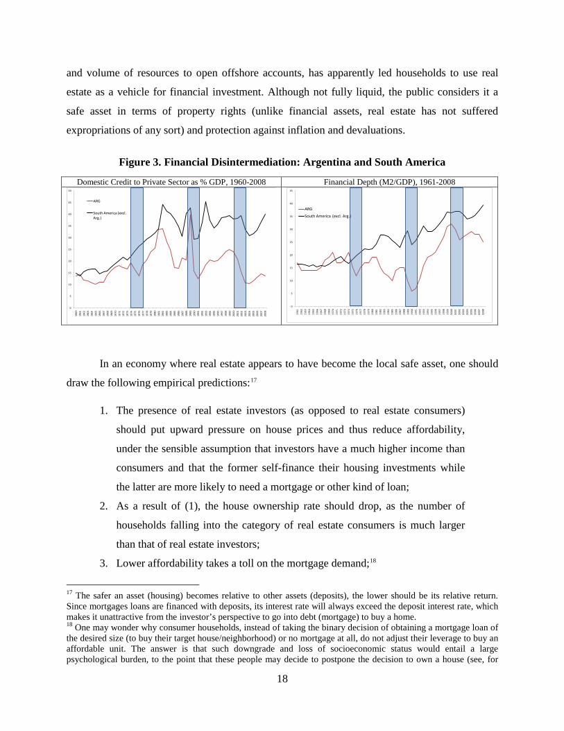
An eloquent testimony to this phenomenon is the evolution of domestic credit to the

private sector, as shown in Figure 3. In 1960, it represented 14 percent of GDP in Argentina and

17 percent, on average, in the rest of South America. At present, however, those values are about

12 percent and 40 percent, respectively. Even during the flourishing 1990s, private credit to GDP

did not exceed 25 percent.

The lack of reliance on banks means that savings are held in other assets. Lack of

confidence, coupled with the lack of capital market alternatives open to the average investor

(stocks, bonds, and derivatives), and the fact that not everybody has the financial sophistication

18

and volume of resources to open offshore accounts, has apparently led households to use real

estate as a vehicle for financial investment. Although not fully liquid, the public considers it a

safe asset in terms of property rights (unlike financial assets, real estate has not suffered

expropriations of any sort) and protection against inflation and devaluations.

Figure 3. Financial Disintermediation: Argentina and South America

Domestic Credit to Private Sector as % GDP, 1960-2008 Financial Depth (M2/GDP), 1961-2008

0

5

10

15

20

25

30

35

40

45

50

1960

1961

1962

1963

1964

1965

1966

1967

1968

1969

1970

1971

1972

1973

1974

1975

1976

1977

1978

1979

1980

1981

1982

1983

1984

1985

1986

1987

1988

1989

1990

1991

1992

1993

1994

1995

1996

1997

1998

1999

2000

2001

2002

2003

2004

2005

2006

2007

2008

ARG

South America (excl. Arg.)

0

5

10

15

20

25

30

35

40

45

1961

1962

1963

1964

1965

1966

1967

1968

1969

1970

1971

1972

1973

1974

1975

1976

1977

1978

1979

1980

1981

1982

1983

1984

1985

1986

1987

1988

1989

1990

1991

1992

1993

1994

1995

1996

1997

1998

1999

2000

2001

2002

2003

2004

2005

2006

2007

2008

ARG

South America (excl. Arg.)

In an economy where real estate appears to have become the local safe asset, one should

draw the following empirical predictions:17

1. The presence of real estate investors (as opposed to real estate consumers)

should put upward pressure on house prices and thus reduce affordability,

under the sensible assumption that investors have a much higher income than

consumers and that the former self-finance their housing investments while

the latter are more likely to need a mortgage or other kind of loan;

2. As a result of (1), the house ownership rate should drop, as the number of

households falling into the category of real estate consumers is much larger

than that of real estate investors;

3. Lower affordability takes a toll on the mortgage demand;18

17 The safer an asset (housing) becomes relative to other assets (deposits), the lower should be its relative return. Since mortgages loans are financed with deposits, its interest rate will always exceed the deposit interest rate, which makes it unattractive from the investor’s perspective to go into debt (mortgage) to buy a home.

18 One may wonder why consumer households, instead of taking the binary decision of obtaining a mortgage loan of the desired size (to buy their target house/neighborhood) or no mortgage at all, do not adjust their leverage to buy an affordable unit. The answer is that such downgrade and loss of socioeconomic status would entail a large psychological burden, to the point that these people may decide to postpone the decision to own a house (see, for

19

4. Higher house prices, if also higher in terms of construction costs, should also

encourage new construction; and

5. Larger supply, combined with the lower expected return on a safe asset,

should diminish the rental value of housing.

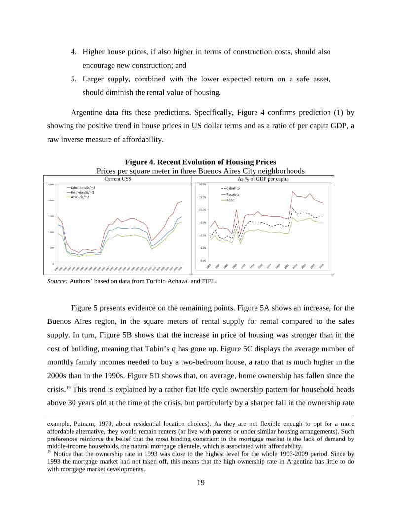
Argentine data fits these predictions. Specifically, Figure 4 confirms prediction (1) by

showing the positive trend in house prices in US dollar terms and as a ratio of per capita GDP, a

raw inverse measure of affordability.

Figure 4. Recent Evolution of Housing Prices

Prices per square meter in three Buenos Aires City neighborhoods Current US$ As % of GDP per capita

0

500

1,000

1,500

2,000

2,500

Caballito u$s/m2Recoleta u$s/m2ABSC u$s/m2

0.0%

5.0%

10.0%

15.0%

20.0%

25.0%

30.0%

Caballito

Recoleta

ABSC

Source: Authors’ based on data from Toribio Achaval and FIEL.

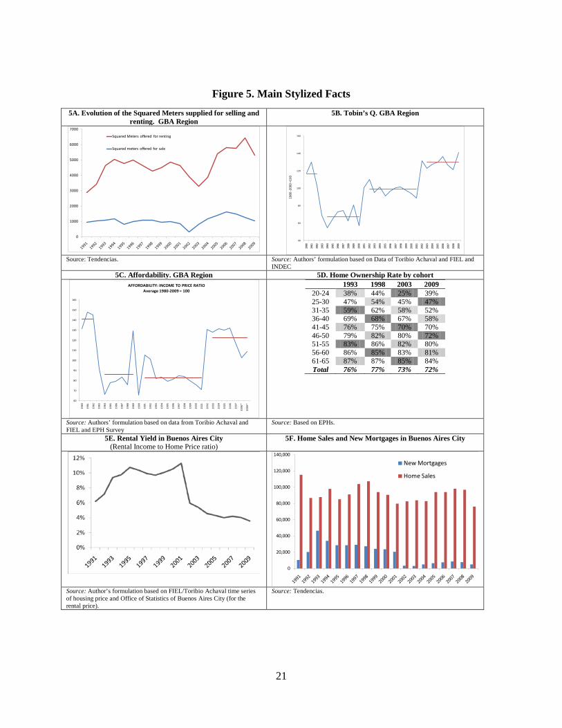
Figure 5 presents evidence on the remaining points. Figure 5A shows an increase, for the

Buenos Aires region, in the square meters of rental supply for rental compared to the sales

supply. In turn, Figure 5B shows that the increase in price of housing was stronger than in the

cost of building, meaning that Tobin’s q has gone up. Figure 5C displays the average number of

monthly family incomes needed to buy a two-bedroom house, a ratio that is much higher in the

2000s than in the 1990s. Figure 5D shows that, on average, home ownership has fallen since the

crisis.19

example, Putnam, 1979, about residential location choices). As they are not flexible enough to opt for a more affordable alternative, they would remain renters (or live with parents or under similar housing arrangements). Such preferences reinforce the belief that the most binding constraint in the mortgage market is the lack of demand by middle-income households, the natural mortgage clientele, which is associated with affordability.

This trend is explained by a rather flat life cycle ownership pattern for household heads

above 30 years old at the time of the crisis, but particularly by a sharper fall in the ownership rate

19 Notice that the ownership rate in 1993 was close to the highest level for the whole 1993-2009 period. Since by 1993 the mortgage market had not taken off, this means that the high ownership rate in Argentina has little to do with mortgage market developments.

20

of younger households. For instance, in 1998, 54 percent of household heads between 25 and 30

years old were owners, and just 45 percent in 2003 (47 percent in 2009). Jointly breaking down

figures by income and age (results available from the authors), the ownership rate dropped

particularly for young middle income households (deciles 6-8 by total household income). These

are the households that should be a priori more affected by affordability issues; households at the

extremes of the income distribution, and individuals at the extremes of the age distribution,

should be more immune to these housing market trends.20

Finally, 5E shows that the rental yield has fallen significantly after the crisis, and 5F

shows that new mortgage loans have not followed the increase in home sales.

20 We also tested whether household formation changed in the after crisis period. Our prior belief was that young people would emancipate at older age as housing become less affordable after the crisis. Simple test for average household formation rate does not show a significant difference. The lack of change might be explained by the relative fall of rental price. A deeper analysis, which is out of the scope of this paper, should take into account emancipation rates by income groups, since it is likely that affordability hit harder in middle income households.

21

Figure 5. Main Stylized Facts

5A. Evolution of the Squared Meters supplied for selling and renting. GBA Region

5B. Tobin’s Q. GBA Region

0

1000

2000

3000

4000

5000

6000

7000

Squared Meters offered for renting

Squared meters offered for sale

40

60

80

100

120

140

160

1980

1981

1982

1983

1984

1985

1986

1987

1988

1989

1990

1991

1992

1993

1994

1995

1996

1997

1998

1999

2000

2001

2002

2003

2004

2005

2006

2007

2008

2009

1980

-200

9 =1

00

Source: Tendencias. Source: Authors’ formulation based on Data of Toribio Achaval and FIEL and

INDEC 5C. Affordability. GBA Region 5D. Home Ownership Rate by cohort

60

70

80

90

100

110

120

130

140

150

160

1980

1981

1982

1983

1984

1985

1986

1987

1988

1989

1990

1991

1992

1993

1994

1995

1996

1997

1998

1999

2000

2001

2002

2003

2004

2005

2006

2007

2008

*

2009

*

AFFORDABILITY: INCOME TO PRICE RATIOAverage 1980-2009 = 100

1993 1998 2003 2009 20-24 38% 44% 25% 39% 25-30 47% 54% 45% 47% 31-35 59% 62% 58% 52% 36-40 69% 68% 67% 58% 41-45 76% 75% 70% 70% 46-50 79% 82% 80% 72% 51-55 83% 86% 82% 80% 56-60 86% 85% 83% 81% 61-65 87% 87% 85% 84% Total 76% 77% 73% 72%

Source: Authors’ formulation based on data from Toribio Achaval and FIEL and EPH Survey

Source: Based on EPHs.

5E. Rental Yield in Buenos Aires City (Rental Income to Home Price ratio)

5F. Home Sales and New Mortgages in Buenos Aires City

0

20,000

40,000

60,000

80,000

100,000

120,000

140,000

New Mortgages

Home Sales

Source: Author’s formulation based on FIEL/Toribio Achaval time series of housing price and Office of Statistics of Buenos Aires City (for the rental price).

Source: Tendencias.

22

To explore the affordability hypothesis in greater depth we finish this section by running

a simple simulation exercise based on microdata from household surveys.21

We estimate whether

the family has enough income to obtain a mortgage necessary to buy a typical house for its type

(according to family size and income decile) in 1999 and 2009. We adopt the following

assumptions:

1. As we only have prices for relatively expensive neighborhoods of Buenos

Aires City, we assume that the observed prices are those of houses for

families in the top income decile, and then we re-compute house prices for

other income deciles using expenditure on housing (rent) by decile based

on microdata from the 1997 Household Expenditure Survey. Prices by

decile are computed for 1999 and 2009.22

2. Households with housing needs are non-owners (i.e., renters and

occupants) and owners living in houses of very low quality. The latter are

those who own houses in the lowest 10 percent of the distribution of a

quality index we constructed using factor analysis and five attributtes

available in both surveys: the quality of floors, the existence of both

running water and a bathroom inside the house, a flush toilet with some

flushing mechanism and a connection to public sewerage.

3. Qualified households are those able to pay the installment-to-income ratio

required by banking institutions. In the baseline simulation we only use

formal income but we also perform simulations with a more flexible

definition, adding to formal income 50 percent of informal income.23

The main results of our simulation exercise are shown in Table 5. As is clear, the share of

potential borrowers collapsed in 2009 compared to 1999, explained mainly by a large increase in

the relative price of housing to household income. For example, under a flexible definition of

income, and considering a 15-year mortgage at a nominal interest rate of 8 percent,24

21 This approach was followed in Gautier et al. (2006).

with an 80

percent LTV and installment payments no greater than 30 percent of total income, the market

22 In both cases we use the last sample of the year, that is, the second semester of 1999 and the last quarter of 2009. 23 Technically the survey only identifies whether the worker contributes to the Social Security System or not. 24 Other costs amount to 2 percentage points of the loan, which means that the effective interest rate reaches 10 percent annually for this case.

23

size (“would-be borrowers”) collapsed from 30 percent in 1999 to just 7 percent in 2009. If

instead we only take into account verifiable income (formal income), only 3.7 percent of

households in 1999 and just 0.9 percent in 2009 would be able to obtain a mortgage in 2009 (in

spite of a fall in informality from 52 percent in 1999 to 44 percent in 2009).

Table 5. Mortgage Loans Potential Demand LTV 80% and installment ratio less than 30%

Nominal interest rate 1999 2009

Loan Term (years) 6.0% 8.0% 12.0% 14.0% 6.0% 8.0% 12.0% 14.0%

Market size (% of total households) 10 13.0% 10.2% 5.5% 4.4% 2.0% 1.0% 1.0% 1.0% 15 40.0% 30.0% 13.6% 11.4% 8.8% 7.0% 4.0% 3.0% 25 50.0% 40.0% 17.0% 13.6% 15.7% 10.9% 4.9% 3.0%

Market size with formal income only (% of total households) 10 2.2% 1.6% 0.7% 0.7% 0.9% 0.9% 0.0% 0.0% 15 6.9% 3.7% 1.6% 0.7% 1.9% 0.9% 0.9% 0.0% 25 19.4% 8.6% 2.2% 1.6% 1.9% 1.9% 0.9% 0.9%

Households with housing problems who could afford a loan (%) 10 1.6% 0.9% 0.5% 0.5% 0.4% 0.4% 0.0% 0.0% 15 12.0% 3.6% 0.9% 0.9% 0.7% 0.4% 0.4% 0.4% 25 23.1% 12.0% 1.6% 0.9% 1.8% 0.7% 0.4% 0.4%

Source: Authors’ estimates based on EPH (1999 and 2009) and ENGH (1997).

Another exercise is to simulate what would have happened if interest rates were lower

(for instance, if indexation is allowed). At a 25-year loan term, an interest rate reduction from 12

percent to 6 percent, and taking into account a flexible definition of income, the potential market

would increase from 4.9 percent to 16 percent of households. If the LTV falls from the 80

percent used in Table 5 to 60 percent, around 50 percent of households would be eligible for a

loan.25

Any of these credit market conditions would only benefit a tiny fraction of households

suffering a housing deficit (not owners or low quality owners), given that they are concentrated

in the lowest income strata.

3.3. Quality and Ownership Given that both ownership rates and quality tend to rise pari passu with income, problems in the

housing financial market should be more evident in young households (who depend more on

25 Results are available from the authors.

24

financing). Several studies, notably Ortaló-Magné and Rady (1998),26 and Chiuri and Japelli

(2003),27

In this section, we test whether, after controlling for demographic factors, proxies for

income (permanent and transitory) and household location, the change in market conditions after

the crisis affected the timing of home purchase and the quality of housing. We follow the Chiuri

and Jappelli approach, estimating a probit model for ownership explained by demographic

variables (age, squared age and cubic age; family size; marital status), income proxies (years of

education as permanent income proxy; income decile as current income), a dummy for location

and a control for housing quality. We use the EPH surveys for 2009 (post-crisis) and 1999 (pre-

crisis).

analyze ownership over the life cycle.

28 We additionally construct a Housing Quality Index using factor analysis based on five

attributes available in both surveys: the quality of floors, the existence of both running water and

a bathroom inside the house, a flush toilet with some flushing mechanism and a connection to

public sewerage.29

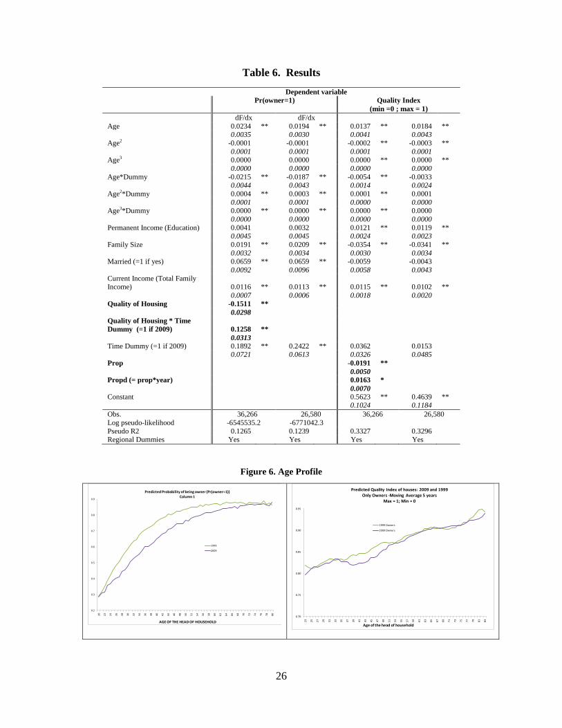
The results of this simple econometric exercise are displayed in Table 6. We merge both

samples (1999 and 2009) in one database and then run a Probit regression for ownership

(columns 1 and 2) and a OLS regression for quality (columns 3 and 4). In the first column we

include quality as a regressor but not in the second to estimate the correlation between quality

and ownership. The interacting dummy with quality is the time dummy (taking 1 for 2009 data).

A similar approach is used for quality, as we include in column 3 a dumy for onwership and we

exclude this variable in column 4.

Column 1 shows that onwership and quality are negatively correlated. The interacting

dummy for 2009 shows a positive and significant effect, which means the trade-off between

26 One important conclusion from Ortaló-Magné and Rady (1999) is that increases in the incomes of the youngest provoke a higher demand for small apartments, leading to capital gains for current owners, which allow them to go up on the property ladder (upsizing). Another implication is that during booms the average age of first-time buyers drops and vice versa. 27 They use a large international dataset to study the determinants of housing tenure in 14 countries, with a dataset of 400,000 observations. Individual information is merged with country panel data on indicators of access to housing finance markets (the ratio of mortgage lending to GDP and the down payment ratio). The authors then proceed to estimate the age profile of home ownership controlling for individual country effects, time (or cohort) effects, demographic variables, proxies for permanent income and mortgage market indicators. They find evidence consistent with the hypothesis that mortgage market imperfections affect the age profile of home ownership, forcing the youngest to save and postpone home purchase for later; however, this effect is to some extent attenuated and then reversed at older ages. 28 EPH is representative of the urban areas for the entire country: it covers 32 urban areas, and it is a stratified sample, with 16,300 and 24,700 observations for each period, respectively. 29 Flush toilet has the highest weight and having a bathroom inside the lowest.

25

qualtiy and ownership is lower in 2009 (but still negative). The lower cofficient for 2009 means

that a household has to sacrifice more quality to obtain ownership than in 1999. A symmetric

result is found for the regression in columns 3 and 4. A difference between both regression is in

education, a variable we use to proxy permanent income. More education is associated with

better quality of homes, but not with ownership (i.e., more educated people prefer to live in a

good quality house even when they have to rent).

The ownership rate in the 2009 sample is significantly lower than in 1999. As is standard

in the literature, we find that younger households are less likely to be owners, and the probability

of ownership increases with age. Comparing 2009 with 1999, we find that the life cyle of

ownership is flatter, that is, in 2009 not only younger households were less likely to have a

house, but also the increase in the probability with age is lower.

Both results together imply that the ownership rate pattern is different now than 10 years

ago. In fact, the 2009 pattern fits the life-cycle pattern better today than a decade ago, which is

by itself evidence of less affordable houses. Now more than before, at any age the probability of

being owner is lower but increasing over time. Also, while it was formerly possible to sacrifice

some quality in order to own a home, this trade-off is now less easily available, so that owning a

home of similar quality home is less likely now than before.

The quality index grows with age, again fitting the life-cycle pattern. When we focus

only on the subsample of owners, patterns are not different between the current and the past

decade. This seems to be evidence that the quality trade-off did not change. Instead, what did

change is that the likelihood of being an owner is lower regardless of the quality of the unit.

26

Table 6. Results

Dependent variable Pr(owner=1) Quality Index (min =0 ; max = 1)

dF/dx dF/dx Age 0.0234 ** 0.0194 ** 0.0137 ** 0.0184 **

0.0035 0.0030 0.0041 0.0043 Age2 -0.0001 -0.0001 -0.0002 ** -0.0003 **

0.0001 0.0001 0.0001 0.0001 Age3 0.0000 0.0000 0.0000 ** 0.0000 **

0.0000 0.0000 0.0000 0.0000 Age*Dummy -0.0215 ** -0.0187 ** -0.0054 ** -0.0033 0.0044 0.0043 0.0014 0.0024 Age2*Dummy 0.0004 ** 0.0003 ** 0.0001 ** 0.0001 0.0001 0.0001 0.0000 0.0000 Age3*Dummy 0.0000 ** 0.0000 ** 0.0000 ** 0.0000

0.0000 0.0000 0.0000 0.0000 Permanent Income (Education) 0.0041 0.0032 0.0121 ** 0.0119 **

0.0045 0.0045 0.0024 0.0023 Family Size 0.0191 ** 0.0209 ** -0.0354 ** -0.0341 **

0.0032 0.0034 0.0030 0.0034 Married (=1 if yes) 0.0659 ** 0.0659 ** -0.0059 -0.0043

0.0092 0.0096 0.0058 0.0043 Current Income (Total Family Income) 0.0116 ** 0.0113 ** 0.0115 ** 0.0102 **

0.0007 0.0006 0.0018 0.0020 Quality of Housing -0.1511 **

0.0298 Quality of Housing * Time Dummy (=1 if 2009) 0.1258 **

0.0313 Time Dummy (=1 if 2009) 0.1892 ** 0.2422 ** 0.0362 0.0153

0.0721 0.0613 0.0326 0.0485 Prop -0.0191 **

0.0050 Propd (= prop*year) 0.0163 *

0.0070 Constant 0.5623 ** 0.4639 **

0.1024 0.1184 Obs. 36,266 26,580 36,266 26,580 Log pseudo-likelihood -6545535.2 -6771042.3 Pseudo R2 0.1265 0.1239 0.3327 0.3296 Regional Dummies Yes Yes Yes Yes

Figure 6. Age Profile

0.2

0.3

0.4

0.5

0.6

0.7

0.8

0.9

20 22 24 26 28 30 32 34 36 38 40 42 44 46 48 50 52 54 56 58 60 62 64 66 68 70 72 74 76 78 80

1999

2009

Predicted Probability of being owner (Pr(owner=1))Column 1

AGE OF THE HEAD OF HOUSEHOLD 0.70

0.75

0.80

0.85

0.90

0.95

23 25 27 29 31 33 35 37 39 41 43 45 47 49 51 53 55 57 59 61 63 65 67 69 71 73 75 77 79 81 83

1999 Owners

2009 Owners

Predicted Quality Index of houses: 2009 and 1999Only Owners -Moving Average 5 years

Max = 1; Min = 0

Age of the head of household

27

4. Analytical Model and Results 4.1 Data Used We focus our analysis on the Buenos Aires Metropolitan Region (Area Metropolitana de Buenos

Aires, AMBA), which comprises the autonomous city of Buenos Aires and the 24 municipalities

in the suburbs (usually known as Greater Buenos Aires, GBA), representing approximately one

third of Argentina’s population. We use four different sources of microdata: the Household

Consumption Survey, the national Household Survey (Encuesta Permanente de Hogares, EPH),

SIEMPRO (Sistema de Información, Evaluación y Monitoreo de Programas Sociales) and our

own specially designed survey (see Appendix for methodological details).

The Household Consumption Survey, a national-level survey that collects detailed

information on household consumption, is conducted every 10 years and used by the

Office of Statistics to construct the Consumer Price Index.30

Our survey was conducted telephonically by randomly sampling over the universe of

fixed telephone lines in AMBA; the sample consists of 1,600 households. Results on ownership

rate and mean household characteristics are reassuringly consistent with EPH statistics. We

repeated some SIEMPRO questions so as to be able to have updated information on key

household characteristics, and we additionally included a new set of questions aimed at having a

better grasp of housing finance and financial constraints in Argentina. For the latter, we follow

the direct method, as developed originally by Jappelli (1990)

EPH is a household survey for the

main urban centers which includes information about housing ownership and quality of housing,

available for GBA since 1974. SIEMPRO, a living conditions survey which was carried out in

1997 and 2001, contains information about ownership, quality of housing and financing of

housing (if the house was bought with financing, and the source of financing) for the entire

country.

31

30 In our simulations we use the 1997 Survey since the micro data of the 2006 Survey are not publicly available.

—or the similar approach used by

Feder et al. (1989 and 1990). The approach of directly asking respondents about their rationing

status was further refined by Baydas, Meyer and Aguilera-Alfred (1994), Zeller (1994), Kochar

(1997), and Mushinski (1999). In this approach individuals can be classified into the following

categories: i) unconstrained (either those not interested in applying for a mortgage or receiving

31 Jappelli (1990) used the following question to determine credit rationing: “Was there any time in the past few years that you (or your husband/wife) thought of applying for credit at a particular place but changed your mind because you thought you might be turned down?”

28

the full loan amount requested), and ii) constrained (those manifesting an unmet demand for

credit).

Table 7 compares our results (2010) and SIEMPRO results for AMBA (1997 and 2001).

Our survey shows that ownership of both buildings and land has fallen over time (as suggested

by the EPH survey as well), whereas ownership of just the building (usually building an auxiliary

house in the house of a relative) has increased. Both trends were also observed between 1997 and

2001 according to SIEMPRO. We also observe an increase in the share of households renting

(16.1 percent in 2010 compared to 12 percent in 2001) and a decrease in households occupying

without paying rent. Squatting (unlawful settlement without title on land) increased between

2001 and 199732 and again between 2010 and 2001, which represents a worrisome trend.33

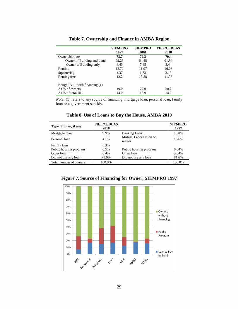
In regard to how households financed ownership, in 2010 only 20.2 percent of owners

used any type of financing (including public housing programs and non-mortgage financing).

This ratio is significantly higher than in 2001.

Table 8 classifies households by type of financing

for 2010. Only 10 percent of the owners resorted to mortgages (including both private and public

banks), while personal loans (4 percent), loans from relatives (6 percent), and even public

housing programs (0.5 represented) were equally negligible sources of finance. As a result, 79

percent did not use any loans at all, and over 90 percent of these households used their own

savings to pay for housing.34

32 According to SIEMPRO the increase in squatting between 1997 and 2001 occurred in all regions and not only AMBA.

SIEMPRO 1997 includes a question about source of financing, but

with less accurate classification (for instance, it does not discriminate between mortgage loans

and other type of loans). According to this survey, 0.64 percent of owners were financed through

public housing programs, similar to the 2010 ratio (this low share of public programs in AMBA

is due to the regional distribution of these programs, which are more important in other regions

of the country, as shown in Figure 7.).

33 At the time of writing (December 2010), squatting has been widespread in AMBA region, with social conflicts and fights between neighbors and squatters. One of the most notorious was the appropriation of Indoamerican Park in the city of Buenos Aires by 8,000 peoples who attempted to settle there; three squatters were killed during the conflict. 34 Of these 888 unleveraged households, only 3 households received their house from a government program and 100 inherited their houses.

29

Table 7. Ownership and Finance in AMBA Region

SIEMPRO 1997

SIEMPRO 2001

FIEL/CEDLAS 2010

Ownership rate 73.7 72.3 70.4 Owner of Building and Land 69.28 64.88 61.94 Owner of Building only 4.43 7.45 8.44 Renting 12.72 11.97 16.06 Squattering 1.37 1.83 2.19 Renting free 12.2 13.88 11.38 Bought/Built with financing (1) As % of owners 19.0 22.0 20.2 As % of total HH 14.0 15.9 14.2

Note: (1) refers to any source of financing: mortgage loan, personal loan, family loan or a government subsidy.

Table 8. Use of Loans to Buy the House, AMBA 2010

Type of Loan, if any FIEL/CEDLAS 2010

SIEMPRO 1997

Mortgage loan 9.9% Banking Loan 13.0%

Personal loan 4.1% Mutual, Labor Union or realtor 1.76%

Family loan 6.3% Public housing program 0.5% Public housing program 0.64% Other loan 0.4% Other loan 3.64% Did not use any loan 78.9% Did not use any loan 81.6% Total number of owners 100.0% 100.0%

Figure 7. Source of Financing for Owner, SIEMPRO 1997

30

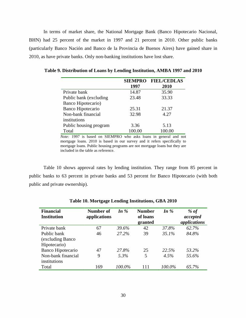
In terms of market share, the National Mortgage Bank (Banco Hipotecario Nacional,

BHN) had 25 percent of the market in 1997 and 21 percent in 2010. Other public banks

(particularly Banco Nación and Banco de la Provincia de Buenos Aires) have gained share in

2010, as have private banks. Only non-banking institutions have lost share.

Table 9. Distribution of Loans by Lending Institution, AMBA 1997 and 2010

SIEMPRO

1997 FIEL/CEDLAS

2010 Private bank 14.87 35.90 Public bank (excluding Banco Hipotecario)

23.48 33.33

Banco Hipotecario 25.31 21.37 Non-bank financial institutions

32.98 4.27

Public housing program 3.36 5.13 Total 100.00 100.00

Note: 1997 is based on SIEMPRO who asks loans in general and not mortgage loans. 2010 is based in our survey and it refers specifically to mortgage loans. Public housing programs are not mortgage loans but they are included in the table as reference.

Table 10 shows approval rates by lending institution. They range from 85 percent in

public banks to 63 percent in private banks and 53 percent for Banco Hipotecario (with both

public and private ownership).

Table 10. Mortgage Lending Institutions, GBA 2010

Financial Institution

Number of applications

In % Number of loans granted

In % % of accepted

applications Private bank 67 39.6% 42 37.8% 62.7% Public bank (excluding Banco Hipotecario)

46 27.2% 39 35.1% 84.8%

Banco Hipotecario 47 27.8% 25 22.5% 53.2% Non-bank financial institutions

9 5.3% 5 4.5% 55.6%

Total 169 100.0% 111 100.0% 65.7%

31

4.2. Demand for Mortgage Loans in Argentina: New Survey Evidence As observed loan volumes are not directly informative of the underlying demand and supply

forces, a household survey is a highly useful tool for revealing preferences and impediments to

demand. In this section we report findings on self-reported demand for mortgages and seek to

identify some sociodemographic factors behind the decision to apply for a loan and the reasons

why some households are excluded from this kind of credit.35

We classify households into two groups. The first consists of households with a demand

for mortgages, which include some that have applied to a loan and others that have not. Among

those that actually applied, some obtained the loan (with a subset getting as much as they wanted

to) and others were rejected. Financially constrained households are defined as those with a

revealed demand for a mortgage that either decided not to ask for a loan or that applied and were

turned down. The second group consists of households without a demand for mortgages,

including those stating they did not need or did not want loan.

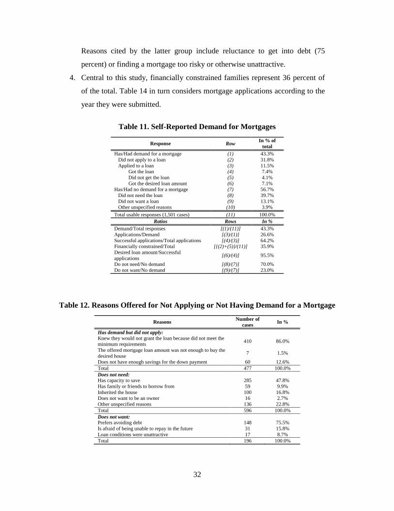
The results, displayed in Table 11 and Table 12, seem to defy common sense but are in

reality very much in line with other enterprise credit surveys (see, for example, Bebczuk, 2010).

The following results are of particular interest: 1. Only 43 percent of households want mortgage loans, and only 27 percent

applied for them.

2. Suggesting a great deal of self-selection, 64 percent of these applications were

successful, and 95 perceived of successful applicants obtained as much credit

as they asked for. The main reason for not applying, according to 84 percent

of this subset of households, is potential failure to not meet banks’ minimum

requirements. In other words, affordability seems to be a major issue in the

Argentine mortgage market.

3. As discussed in Table 13, of the 57 percent of households not interested in

obtaining a mortgage, 70 percent said they did not need one. Reasons for not

needing a mortgage include being able to save (48 percent), having inherited a

house (17 percent), or not wanting a mortgage for other reasons (23 percent).

35 For this section we limit the analysis to those households with information on all questions, which reduces the sample size to 1,501. The 99 missing households do not have any particular pattern and are considered as missing at random.

32

Reasons cited by the latter group include reluctance to get into debt (75

percent) or finding a mortgage too risky or otherwise unattractive.

4. Central to this study, financially constrained families represent 36 percent of

of the total. Table 14 in turn considers mortgage applications according to the

year they were submitted.

Table 11. Self-Reported Demand for Mortgages

Response Row In % of total

Has/Had demand for a mortgage (1) 43.3% Did not apply to a loan (2) 31.8% Applied to a loan (3) 11.5% Got the loan (4) 7.4% Did not get the loan (5) 4.1% Got the desired loan amount (6) 7.1% Has/Had no demand for a mortgage (7) 56.7% Did not need the loan (8) 39.7% Did not want a loan (9) 13.1% Other unspecified reasons (10) 3.9% Total usable responses (1,501 cases) (11) 100.0%

Ratios Rows In % Demand/Total responses [(1)/(11)] 43.3% Applications/Demand [(3)/(1)] 26.6% Successful applications/Total applications [(4)/(3)] 64.2% Financially constrained/Total [{(2)+(5)}/(11)] 35.9% Desired loan amount/Successful applications [(6)/(4)] 95.5%

Do not need/No demand [(8)/(7)] 70.0% Do not want/No demand [(9)/(7)] 23.0%

Table 12. Reasons Offered for Not Applying or Not Having Demand for a Mortgage

Reasons Number of cases In %

Has demand but did not apply: Knew they would not grant the loan because did not meet the minimum requirements 410 86.0%

The offered mortgage loan amount was not enough to buy the desired house 7 1.5%

Does not have enough savings for the down payment 60 12.6% Total 477 100.0% Does not need: Has capacity to save 285 47.8% Has family or friends to borrow from 59 9.9% Inherited the house 100 16.8% Does not want to be an owner 16 2.7% Other unspecified reasons 136 22.8% Total 596 100.0% Does not want: Prefers avoiding debt 148 75.5% Is afraid of being unable to repay in the future 31 15.8% Loan conditions were unattractive 17 8.7% Total 196 100.0%

33

Table 13. Reasons Offered for Not Applying or Not Having a Demand for a Mortgage by type of tenant

Response (in number of cases) Total Owns Rents Occupies

without rent Has/Had demand for a mortgage 650 353 180 117 Did not apply to a loan 477 242 140 95 Applied to a loan 173 111 40 22 Got the loan 111 89 0 0 Did not get the loan 62 22 40 22 Has/Had no demand for a mortgage 851 674 77 100

Did not need the loan 596 489 38 69 Did not want a loan 196 147 31 18 Other unspecified reasons 59 38 8 13 Total usable responses 1,501 1,027 257 217

The total of 173 applications were more or less evenly distributed over three subperiods:

before 1991 (36 percent), between 1991 and 2001 (27 percent) and between 2002 and 2010 (33

percent). Accepted applications dropped from 90 percent in the first sub-period to 70 percent in

the second, during the Convertibility Plan, to a record low of 33 percent in the post-

Convertibility era. We asked the main reason for the loan rejection, as shown in Table 14b,

finding that the most common reason is lack of income. The lower approval rate in the 2000s is

not due to bank refusal; on the contrary, lack of income is the main reason in the 2000s even

more than in the 1990s, probably influenced by successive official announcements of seemingly

accessible mortgage plans for lower income families, which encouraged some of them to apply

for otherwise unaffordable loans.

Although the survey asks about both past demand (by those who are presently

homeowners) and current demand (by those who are not yet owners), it is interesting to note in

Table 14a that the latter group displays higher demand than present owners seem to have had in

the past. Specifically, 70 percent of renters and 54 percent of occupants without rent, but only 34

percent of owners, express demand for mortgages. However, the percentage of applicants is not

that different: 16 percent of renters and 10 percent of occupants without rent asked for a loan,

compared to 11 percent in the case of owners. This means that, despite the differences in

demand, self-exclusion prevents many potential borrowers from tapping the banking system.

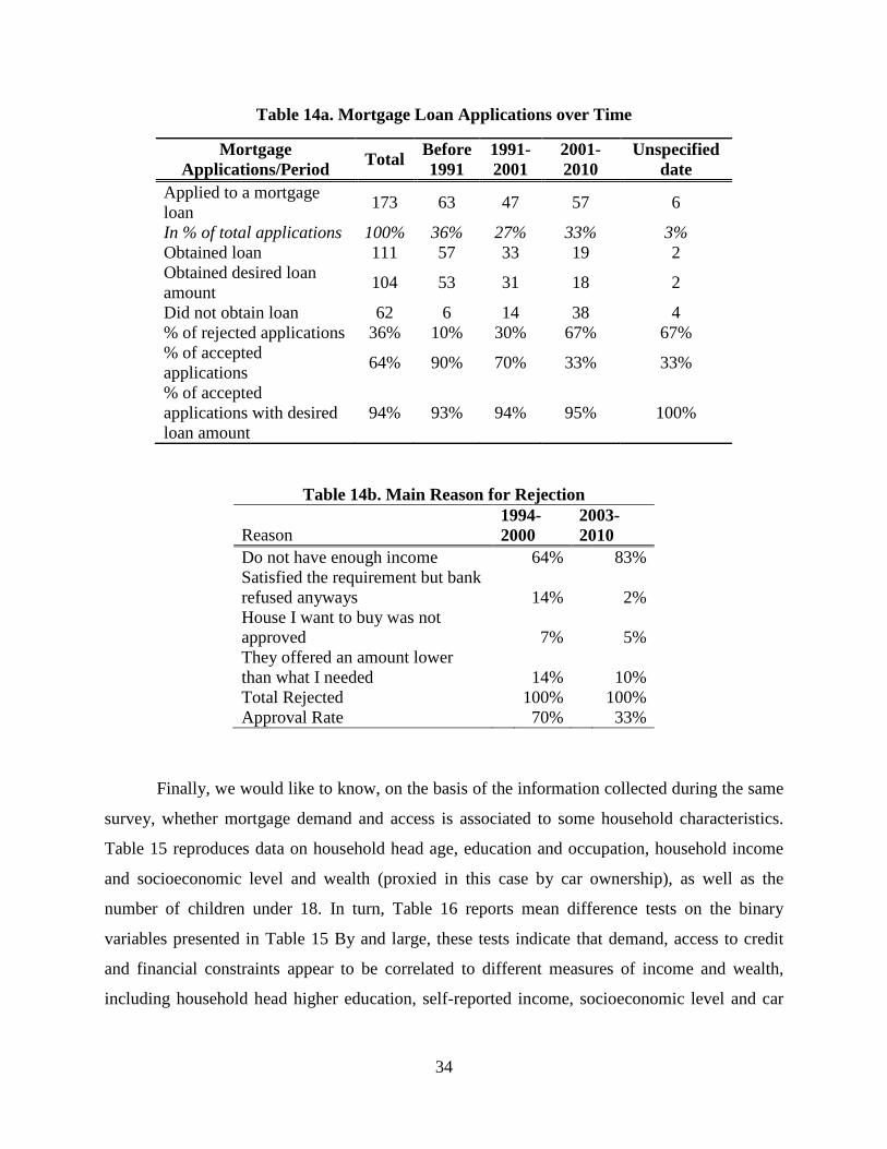
34

Table 14a. Mortgage Loan Applications over Time

Mortgage Applications/Period Total Before

1991 1991-2001

2001-2010

Unspecified date

Applied to a mortgage loan 173 63 47 57 6

In % of total applications 100% 36% 27% 33% 3% Obtained loan 111 57 33 19 2 Obtained desired loan amount 104 53 31 18 2

Did not obtain loan 62 6 14 38 4 % of rejected applications 36% 10% 30% 67% 67% % of accepted applications 64% 90% 70% 33% 33%

% of accepted applications with desired loan amount

94% 93% 94% 95% 100%

Table 14b. Main Reason for Rejection

Reason 1994-2000

2003- 2010

Do not have enough income

64%

83% Satisfied the requirement but bank refused anyways

14%

2%

House I want to buy was not approved

7%

5%

They offered an amount lower than what I needed

14%

10%

Total Rejected

100%

100% Approval Rate

70%

33%

Finally, we would like to know, on the basis of the information collected during the same

survey, whether mortgage demand and access is associated to some household characteristics.

Table 15 reproduces data on household head age, education and occupation, household income

and socioeconomic level and wealth (proxied in this case by car ownership), as well as the

number of children under 18. In turn, Table 16 reports mean difference tests on the binary

variables presented in Table 15 By and large, these tests indicate that demand, access to credit

and financial constraints appear to be correlated to different measures of income and wealth,

including household head higher education, self-reported income, socioeconomic level and car

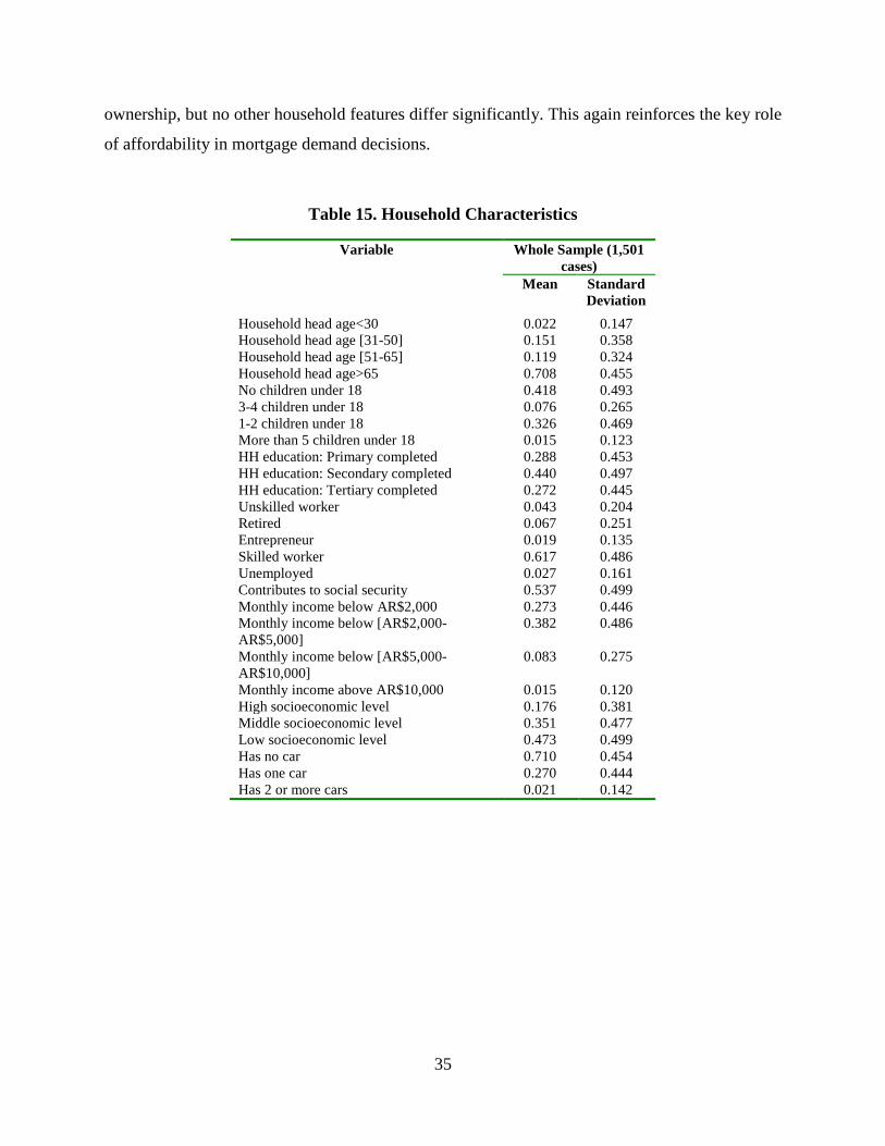
35

ownership, but no other household features differ significantly. This again reinforces the key role

of affordability in mortgage demand decisions.

Table 15. Household Characteristics

Variable Whole Sample (1,501 cases)

Mean Standard Deviation

Household head age<30 0.022 0.147 Household head age [31-50] 0.151 0.358 Household head age [51-65] 0.119 0.324 Household head age>65 0.708 0.455 No children under 18 0.418 0.493 3-4 children under 18 0.076 0.265 1-2 children under 18 0.326 0.469 More than 5 children under 18 0.015 0.123 HH education: Primary completed 0.288 0.453 HH education: Secondary completed 0.440 0.497 HH education: Tertiary completed 0.272 0.445 Unskilled worker 0.043 0.204 Retired 0.067 0.251 Entrepreneur 0.019 0.135 Skilled worker 0.617 0.486 Unemployed 0.027 0.161 Contributes to social security 0.537 0.499 Monthly income below AR$2,000 0.273 0.446 Monthly income below [AR$2,000-AR$5,000]

0.382 0.486

Monthly income below [AR$5,000-AR$10,000]

0.083 0.275

Monthly income above AR$10,000 0.015 0.120 High socioeconomic level 0.176 0.381 Middle socioeconomic level 0.351 0.477 Low socioeconomic level 0.473 0.499 Has no car 0.710 0.454 Has one car 0.270 0.444 Has 2 or more cars 0.021 0.142

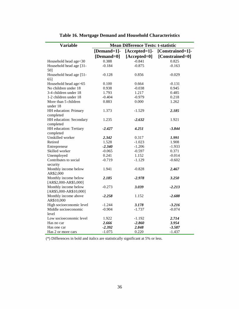
36

Table 16. Mortgage Demand and Household Characteristics

Variable Mean Difference Tests: t-statistic

[Demand=1]-[Demand=0]

[Accepted=1]-[Accepted=0]

[Constrained=1]-[Constrained=0]

Household head age<30 0.388 -0.841 0.825 Household head age [31-50]

-0.184 -0.875 -0.163

Household head age [51-65]

-0.128 0.856 -0.029

Household head age>65 0.100 0.664 -0.131 No children under 18 0.938 -0.038 0.945 3-4 children under 18 1.793 1.217 0.485 1-2 children under 18 -0.404 -0.979 0.218 More than 5 children under 18

0.883 0.000 1.262

HH education: Primary completed

1.373 -1.529 2.185

HH education: Secondary completed

1.235 -2.632 1.921

HH education: Tertiary completed

-2.427 4.251 -3.844

Unskilled worker 2.342 0.317 1.991 Retired 1.528 -1.023 1.908 Entrepreneur -2.340 -1.206 -1.933 Skilled worker -0.065 -0.597 0.371 Unemployed 0.241 1.152 -0.014 Contributes to social security

-0.719 -1.129 -0.602

Monthly income below AR$2,000

1.941 -0.828 2.467

Monthly income below [AR$2,000-AR$5,000]

2.185 -2.978 3.250

Monthly income below [AR$5,000-AR$10,000]

-0.273 3.039 -2.213

Monthly income above AR$10,000

-2.258 1.152 -2.688

High socioeconomic level -1.244 3.178 -3.216 Middle socioeconomic level

-0.904 -1.737 -0.074

Low socioeconomic level 1.922 -1.192 2.714 Has no car 2.666 -2.860 3.954 Has one car -2.392 2.848 -3.587 Has 2 or more cars -1.075 0.220 -1.437

(*) Differences in bold and italics are statistically significant at 5% or less.

37

To close, we run in Table 17 a Heckman estimation to control for endogeneity bias via a

two-step regression, where the first stage estimates a demand (or selection) equation and an

access (or financial constraint) equation in the second stage.36

To ensure the correspondence

between demand and household characteristics, we restrict the analysis to households that

became owners since 2002 onwards or still do not own a house. Although we tried several

specifications, the only variables that proved to be robustly significant were a high

socioeconomic level (with the expected positive sign) in the access equation and tertiary

education and no car ownership, with negative and positive loadings respectively, in the demand

equation. This econometric evidence confirms the preliminary verdict from the previous

descriptive statistics.

Table 17. Access and Demand for Mortgage Loans Heckman Two-Stage Estimation

Access (financial constraint) equation High socioeconomic level -0.154 (-2.26) Low socioeconomic level -0.034 (-0.65) Constant 1.299 (6.04) Selection (demand) equation Tertiary education completed -0.234 (-1.84) No car ownership 0.287 (2.13) Constant 0.042 (0.32)

Wald test (p-value) 5.22 (0.073)

Number of observations 448 Censored observations 196 Uncensored observations 252

36 For a previous application of this methodology to study credit constraints for firms, see Bigsten, Collier and Dercon (2000).

38

5. Conclusions and Policy Implications This paper has studied housing finance in Argentina, with an emphasis on demand for mortgage

loans and developments following the 2001-2002 crisis. Both macro data and survey information

were employed, including the results of the survey especially designed for this study. By

analyzing the demand for mortgage loans we uncovered that in addition to the standard financial

disintermediation argument (supply side) to explain mortgage market underdevelopment in

volatile economies, demand plays a very important role as well. The main findings are the

following:

1. Despite the shrinking size of the mortgage market after the crisis, housing

prices and construction has boomed in Argentina.

2. The contraction of the mortgage market in the 2000s compared to the 1990s

cannot be attributed to inadequate regulations or lack of loanable resources in

the banking system.

3. On the contrary, market developments are consistent with a lack of demand

for mortgages, which have become unaffordable for a large percentage of the

population.

4. In turn, diminished affordability is associated with segmentation among

buyers: as housing has become a safe asset (in the sense of being

expropriation-free when compared to bank deposits and other financial

assets), investors’ strong demand prevents households in search of a residence

from being eligible for a mortgage loan.

5. While middle-income households prefer renting to moving to a worse quality

unit or a worse location, low income households accept such a trade-off.

6. Regardless of the lack of a dynamic mortgage market, home ownership

continues to be around 70 percent, although the rate has declined since the

1990s.

7. The high ownership rate reflects widespread use of own funds to buy a house,

willingness to reduce the dwelling quality in order to own and government

assistance via housing programs targeting low to middle-income households.

Other recent interventions in the mortgage market were mostly ineffectual.

39

8. Ownership rate is considerably lower in middle income households with

young heads;

9. The survey carried out for this study confirmed many of these statements,

showing in particular that the demand for external finance is extremely low. These results show that, in the face of the acute affordability problem, policies aimed at

fostering the supply side of mortgages, as the Government has tried to do in recent years by

providing loanable funds to the banking system, are bound to turn out ineffective. Even the

current environment of low real interest rates is unlikely to overcome the lack of demand; our

exercises on affordability attest to the fact that a very small portion of households would be

eligible for a mortgage, even under favorable interest rate levels and lax LTV requirements. On

the other hand, public housing programs are not suitable for a large percentage of the population.

The apparent major constraint from the demand (vis-à-vis the supply) side calls for a different set

of policies. Policies designed to increase the amount of urban land with proper infrastructure

would increase the supply of housing, particularly for the poor, and relax the affordability

problem. Moreover, policies that foster the market for rental housing could address investors’

desire to buy housing and increase non-owners’ likelihood of renting a high-quality unit. Finally,

if further promotion of the mortgage market is needed, conditions must be made more favorable

for demand; in particular, the affordability issue is likely to persist in the medium run (at least

until conventional financial assets are again massively accepted by local investors as a store of

value). Those can be achieved through the introduction of new instruments or demand subsidies

to complement, or even partly substitute for, ongoing government housing programs. Of course,

this must be weighed against the resulting fiscal burden and the opportunity costs in terms of

other badly needed social expenditures.

40

References Agarwal, S., S. Chomsisengphet and O. Hassler. 2005. “The Impact of the 2001 Financial Crisis

and the Economic Policy Responses on the Argentine Mortgage Market.” Journal of

Housing Economics 14(3): 242-270.

Auguste, S. et al. 2006. “Cross-Border Trading as a Mechanism for Implicit Capital Flight:

ADRs, CEDEARs, and the Argentine Crisis.” Journal of Monetary Economics 53(7):

1259-1295.

Banzas, A., and L. Fernández. 2007. “El Financiamiento a la Vivienda en Argentina: Historia

Reciente, Situación Actual y Desafíos.” Documento de Trabajo 18. Buenos Aires,

Argentina: Centro de Economía y Finanzas para el Desarrollo de la Argentina

(CEFIDAR).

Baydas, M.M., R.L. Meyer and N. Aguilera-Alfred. 1994. “Discrimination against Women in

Formal Credit Markets: Reality or Rhetoric?” World Development 22(7): 1073-1082.

Bebczuk, R. 2010. “Acceso al Financiamiento de las PYMES en Argentina: Estado de Situación

y Propuestas de Política.” Serie Financiamiento del Desarrollo 227. Santiago, Chile:

United Nations Ecomomic Commission for Latin America and the Caribbean.

Bebczuk, R., J.M. Fanelli and J. Pradelli. 2003. “Determinants and Consequences of Financial

Constraints Facing Firms in Argentina.” In: A. Galindo and F. Schiantarelli, compilers.

Credit Constraints and Investment in Latin America. Washington, DC, United States:

Inter-American Development Bank.

Bigsten, A., P. Collier and S. Dercon. 2000. “Credit Constraints in Manufacturing Enterprises in

Africa.” Working Paper. Oxford, United Kingdom: University of Oxford, Centre for the

Study of African Economies.

Central Bank of Argentina. Various dates. Comunicaciones “A”. Buenos Aires, Argentina:

Central Bank of Argentina.

Chiquier, L., and M. Lea. 2009. Housing Finance Policy in Emerging Economies. Washington,

DC, United States: World Bank.

Chiuri, M.C., and T. Japelli. 2003. “Financial Market Imperfections and Home Ownership: A

Comparative Study.” European Economic Review 47: 857–875.

41

Cristini, M., and M. Iaryczower. 1997. “Un Análisis Económico de las Políticas de Vivienda en

la Argentina: El FO.NA.VI.” Buenos Aires, Argentina: Asociación Argentina de

Economía Política. Available at: http://www.aaep.org.ar/espa/anales/pdf/cristini_iaryczower.pdf

Cristini, M., and R. Moya. 2004. “Las Instituciones del Financiamiento de la Vivienda en

Argentina.” Research Department Working Paper 498. Washington, DC, United States:

icano de Desarrollo, Washington, D.C. 2004.

Cristini, M., and R. Moya. 2008. “Ciudades y Calidad de Vida en América Latina y el Caribe:

Evolución Histórica y Comparación Internacional.” Background paper for 2009

Development in the Americas Beyond Facts: Understanding Quality of Life. Washington,

DC, United States: Inter-American Development Bank.

Cuenin, F., and R. Moya. 2010. “Housing Policy Matters for the Poor.” Washington, DC, United

States: Inter-American Development Bank. Mimeographed document.

Delfiner, M. 2010. “El Mercado de Derivados en Argentina.” In: R. Bebczuk, editor. Progresos

en Finanzas. Buenos Aires, Argentina: Asociación Argentina de Economía

Política/Editorial Temas.

Delgobbo, A. 2000. “Balance sobre la Conformación de un Mercado de Hipotecas Titulizadas en

Argentina.” Buenos Aires, Argentina: Ministerio de Economía, Secretaría de Defensa de

la Competencia y del Consumidor.

Duca, J.V., and S.S. Rosenthal. 1994. “Borrowing Constraints and Access to Owner-Occupied

Housing.” Regional Science and Urban Economics 24(3): 301-322.

Feder, G. et al. 1989. “Agricultural Credit and Farm Performance in China.” Journal of

Comparative Economics 13: 508-526.

Feder, G. et al. 1990. “The Relationship between Credit and Productivity in Chinese Agriculture:

A Microeconomic Model of Disequilibrium.” American Journal of Agricultural

Economics 72: 1151-1157.

Fisher, L.M., and A.J. Jaffe. 2003. “Determinants of International Home Ownership Rates.

Housing Finance International 18(1): 34-42.

Gaba, E. et al. 2003. “Indexación en Chile y su Posible Aplicación en Argentina.” Serie de

Estudios Económicos. Buenos Aires, Argentina: BBVA Banco Francés.

42

Galindo, A., and E. Lora. 2005. “Foundations of Housing Finance.” In: Unlocking Credit: The

Quest for Deep and Stable Bank Lending. Baltimore, United States: Inter-American

Development Bank/Johns Hopkins University Press.

Gautier, M. et al. 2006. “Review of Argentina’s Housing Sector: Options for Affordable Housing

Policy.” Policy Research Working Paper. Washington, DC, United States: World Bank.

Gwin, C.R., and S.E. Ong. 2008. “Do We Really Understand Homeownership Rates? An

International Study.” International Journal of Housing Markets and Analysis 1(1): 52-67.

Hassler, O. 2007. “Instruments for Improving the Soundness and Depth of Housing Finance.”

Presentation at the Central Bank of Argentina, Buenos Aires, Argentina.

Jappelli, T. 1990. “Who Is Credit Constrained in the U.S. Economy.” Quarterly Journal of

Economics 105: 219-234.

Kiguel, M.A., and E. Podjarny. 2007. “Impacto de Factores Macro y Microeconómicos en el

Desarrollo del Mercado de Hipotecas: Reflexiones Basadas en Argentina, Chile y

Uruguay.” Serie de Estudios Económicos y Sociales CSC 07-010. Washington, DC,

United States: Inter-American Development Bank.

Kochar, A. 1997. “An Empirical Investigation of Rationing Constraints in Rural Credit Markets

in India.” Journal of Development Economics 53: 339-371.

Moya, R., G. Bermúdez and A. Sparacino. 2010. “¿Están los Programas de Vivienda Llegando a

los Pobres? El Caso Argentino.” Washington, DC, United: Inter-American Development

Bank. Mimeographed document.

Mushinski, D.W. 1999. “An Analysis of Offer Functions of Banks and Credit Unions in

Guatemala.” Journal of Development Studies 36: 88-112.

Ortalo-Magné, F., and S. Rady. 1999. “Boom in, Bust Out: Young Households and the Housing

Price Cycle.” European Economic Review (4-6): 755-766.

----. 2006. “Housing Market Dynamics: On the Contribution of Income Shocks and Credit

Constraints.” Review of Economic Studies 73(2): 459-485.

Putnam, S.H. 1979. Urban Residential Location Models. New York, United States: Springer.

Sanders, A.B. 2005. “Barriers to Homeownership and Housing Quality: The Impact of the

International Mortgage Market.” Journal of Housing Economics 14: 147-152

Warnock, V.C., and F.E. Warnock. 2008. “Markets and Housing Finance.” Journal of Housing

Economics 17(3): 239-251.

43

Zeller, M. 1994. “Determinants of Credit Rationing: A Study of Informal Lenders and Formal

Credit Groups in Madagascar.” World Development 22: 1895-1907.