Embed Size (px)
Citation preview
arX
iv:0
812.
3538
v4 [
q-fi
n.ST
] 7
Sep
201
0
Estimation of the instantaneous volatility
Alexander Alvarez ∗, Fabien Panloup†, Monique Pontier ‡, Nicolas Savy §
September 8, 2010
Abstract
This paper is concerned with the estimation of the volatility process in a stochastic volatility
model of the following form: dXt = atdt + σtdWt, where X denotes the log-price and σ is a
càdlàg semi-martingale. In the spirit of a series of recent works on the estimation of the cumulated
volatility, we here focus on the instantaneous volatility for which we study estimators built as
finite differences of the power variations of the log-price. We provide central limit theorems with
an optimal rate depending on the local behavior of σ. In particular, these theorems yield some
confidence intervals for σt.
Keywords: Central limit theorem, Power variation, semimartingale.AMS Classification (2000): Primary 60F05; Secondary 91B70, 91B82.
1 Introduction
The financial market objects offering a great complexity of modelling, the development and thestudy of financial models has attracted a lot of attention in recent years. For such models, a keyparameter is the volatility, which is of paramount importance. The fact that the volatility is notconstant has been observed for a long time. Thus, since the famous but too stringent Black andScholes model, many stochastic volatility models have been introduced. Among them, models wherejumps occur are now widely spread in the literature (see e.g. [9] for a review and [10] for a list of recentstudies on this topic), mainly because there are able to fit skews and smiles that can not be capturedby continuous models.In this paper, we deal with the following kind of model:
Xt = x+
∫ t
0asds+
∫ t
0σsdWs ∀t ≥ 0,
where W is a Brownian motion and σ is a càdlàg semi-martingale (assumptions will be made precise inthe next section). At this stage, one can remark the main restriction of our model: jumps only occurin the volatility but not in the price. This restriction will be explained in the sequel.When such a model is discretely observed, a (now) classical tool for the estimation of the volatility is
∗La Habana University, [email protected]†Institut de Mathématiques de Toulouse et INSA Toulouse, [email protected]‡Institut de Mathématiques de Toulouse et Université de Toulouse, [email protected]§Institut de Mathématiques de Toulouse et Université de Toulouse, [email protected]
1

to make use of the power variations of order p (see next section for details) that have some convergenceproperties to the cumulated volatility process:
∫ t0 |σs|pds (when p = 2, this type of result is only
the convergence of the quadratic variations to the angle bracket of the continuous semi-martingaleX). The study of such estimators of the integrated volatility and its use for the detection of jumpshave been deeply studied in the last years (see for instance [7, 8, 23] for the continuous setting,[1, 2, 18, 19, 24, 23, 3, 15] for the discontinuous setting and the more recent papers [16, 22, 20]).Unlike these works, the aim of this paper is to estimate rather the instantaneous volatility. Then,the natural idea is to study estimators which are built as “derivatives” of the power variations. Moreprecisely, the proposed estimator of the instantaneous volatility is a normalized relative increment ofcumulative volatility estimator, this relative increment being taken on a smaller and smaller interval.We provide some central limit theorems for the σt-estimator and we exhibit an optimal rate dependingon the local behavior of σ. More precisely, if a Brownian component exists in σ, the best rate is of ordern1/4 and otherwise, it depends on the intensity of jumps. In particular, when the jump componenthas finite-variation, the optimal rate is of order n1/3. These central limits lead in particular to someconfidence intervals for σt and to an asymptotic control of the relative error between the estimatorand σt.When jumps occur in the log-price X, it seems that we could extend some of the previous announcedresults by exploiting the fact that convergence properties for the power variations to the cumulatedvolatility still hold when p < 2. However, this extension generates some technicalities which are out ofours objectives.The paper is organized as follows. In Section 2, we introduce the model we deal with, we present thedifferent assumptions for this study and we state our main theorems: Central Limit Theorems for theinstantaneous volatility. Section 3 is the proof of these theorems. From Theorem 3, we easily deducea confidence interval for the instantaneous volatility, this is shown in Section 4. Moreover, we stressthe fact that the confidence interval length increases with p. Finally, the volatility estimator is testedon some simulations in Section 5.
2 Setting and Main Results
We consider a stochastic process (Xt)t≥0 defined on a filtered probability space by:
dXt = atdt+ σtdWt, t ≥ 0, (1)
where W is an (Ft)-adapted Wiener process on (Ω,F , (Ft),P) which satisfies the usual conditions,a : R+ → R and σ are some càdlàg (Ft)-adapted processes. Furthermore, σ is assumed to be a positiveprocess.Let T be a positive number and assume that X is observed at times i∆n for all i = 0, 1, . . . , [ T∆n
]. Inthe sequel, we will assume that ∆n −−−−−→
n→+∞0.
In this paper, we want to estimate σt using the asymptotic properties of the observed discrete incre-ments of X. For p > 0, we denote by B(p,∆n), the process of power variations of order p, i.e. thestochastic process defined by
B(p,∆n)t :=
[t/∆n]∑
i=1
|∆ni X|p , t ∈ [0, T ]
where ∆ni X := Xi∆n −X(i−1)∆n
.
2

The sequence (B(p,∆n)t)n is now classically known as an estimator of∫ t0 σ
psds. We are going to
recall some existing results about the convergence of this sequence but before, we want to precise theassumptions on σ that will be necessary throughout the paper. We introduce the following assumptionsdepending on parameter q ∈ [1, 2] which is related to the behavior of the small jumps of (σt):
(H1q) : σ is a positive càdlàg semimartingale such that σt = |Yt| where (Yt) satisfies:
dYs = bsds+ η1(s)dWs + η2(s)dW2s
+
∫
R
y1|y|≤1(µ(ds, dy)− ν(ds, dy)) +
∫
R
y1|y|>1µ(ds, dy),
where b, η1, η2 are adapted càdlàg processes, µ denotes a random measure on R+ × R withpredictable compensator ν satisfying: ν(dt, dy) = dtFt(dy) and (
∫(1∧ |y|q)Ft(dy))t≥0 is a locally
bounded predictable process.
The above assumption on the predictable compensator imply that (σt) is quasi-left continuous and thatthe jump component has locally-finite q-variation. In order to obtain our main results, we actuallyneed to introduce a little more constraining control of the jump component:
(H2q) : For every T > 0,
limε→0
supt∈[0,T ]
∫
|y|≤ε|y|qFt(dy) = 0 a.s.
As an example, if (Yt) is a solution to the following SDE:
dYt = b(Yt−)dt+ ς1(Yt−)dWt + ς2(Yt−)dW2t κ(Yt−)dZt, (2)
where b : R → R, ς : R 7→ R, ς2 : R 7→ R and κ : R 7→ R are some continuous functions withsublinear growth, (Wt)t≥0 is a Brownian motion and (Zt)t≥0 is a centered purely discontinuous Lévyprocess independent of (Wt)t≥0 with Lévy measure π satisfying
∫(|y|q ∧ 1)π(dy) <∞, q ∈ [1, 2], then
Assumptions (H1q) and (H2
q) hold.
Before going further, we also need to remind the definition of stable convergence that we denote by
L − s. We say that a sequence of random variables (Yn) converges stably to Y or YnL−s⇒ Y , if
there exists an extension (Ω, F , P) of (Ω,F ,P) and a random variable Y defined on (Ω, F , P) suchthat for every bounded measurable random variable H, for every bounded continuous function f ,E [Hf(Yn)] → E[Hf(Y )] when n→ +∞ where E denotes the expectation on the extension.
Now, we can recall two results (adapted to our context) about the asymptotic properties of (B(p,∆n)t)n,from Lépingle [17] (see also [15], Theorem 2.4) and Aït Sahalia and Jacod [3, Theorem 2] respectively.On the same topic, we can also quote [6, 8].
Proposition 1. Assume (H22). Let p be a positive number and set mp := E [|U |p] where U ∼ N (0, 1).
Then, locally uniformly in t,
∆1− p
2n B(p,∆n)t
P−−−−−→n→+∞
mpA(p)t with A(p)t =
∫ t
0σpsds.
3

Proposition 2. Let p ≥ 2 and assume Assumption 1 of [3]. Then, the sequence of continuous processes(Y (n, p))n∈N defined for any n ∈ N by
Y (n, p)t :=1√∆n
(∆
1− p
2n B(p,∆n)t −mpA(p)t
), t ≥ 0,
converges stably to a random variable Y (p) on an extension (Ω, F , (Ft), P) of the original filtered space(Ω,F , (Ft),P) such that, for any t ≥ 0, conditionally on F , Y (p)t is a centered Gaussian variable withvariance E[Y (p)2t | F ] = (m2p −m2
p)A(2p)t.
Looking at these results, it is natural to try to estimate σpt by the following statistic: (Σ(p,∆n, hn)t)defined for every t ≤ T with T = T − h1 by:
Σ(p,∆n, hn)t :=∆
1− p
2n
(B(p,∆n)t+hn − B(p,∆n)t
)
mphn. (3)
Actually, this estimator is the mean of p-variations in a window of length hn where (hn) is assumed tobe a non-increasing sequence of positive numbers such that hn tends to 0.
We are now able to state our main results.
Theorem 3. Let p = 2 or p ≥ 3 and let (Xt) be a stochastic process solution to (1). Assume (H12)
and (H22). Assume that ∆n = o(hn). Then,
(i) If hn/√∆n → 0, ∀t ∈ [0, T ],
√hn∆n
(Σ(p,∆n, hn)t − σpt )L−s−−−−−→
n→+∞
√ϕ1(p, t, σ) U, (4)
where, conditionally on F , U is a standard Gaussian random variable and ϕ1(p, t, σ) =m2p−m2
p
m2p
σ2pt .
(ii) If√∆n/hn → β ∈ R+, ∀t ∈ [0, T ],
1√hn
(Σ(p,∆n, hn)t − σpt )L−s−−−−−→
n→+∞
√β2ϕ1(p, t, σ) + ϕ2(p, t) U, (5)
where ϕ1(p, t, σ) and U are defined as before and,
ϕ2(p, t) =p2
3 (σt)2p−2‖η‖2(t)) with ‖η‖2(t) = η21(t) + η22(t).
Note that when the drift term a is null, the result is valid even if 2 < p < 3. Otherwise, the driftcontributes in a bias for the estimator that is not negligible in case 2 < p < 3.In the second result, we assume that there is no Brownian component in the volatility, i.e. thatη1 = η2 = 0 and that the jump component has locally q-finite variation. In this case, we show that wecan alleviate the constraint on the sequence (hn) (see also Remark 5).
Theorem 4. Let p = 2 or p ≥ 3. and let (Xt) be a stochastic process solution to (1). Assume (H1q)
and (H2q) with q ∈ [1, 2] and suppose that η1 = η2 = 0. Assume that ∆n = o(hn). Then,
(i) If q ∈ (1, 2], if lim supn→+∞ h1/2+1/qn /
√∆n < +∞, ∀t ∈ [0, T ],
√hn∆n
(Σ(p,∆n, hn)t − σpt )L−s−−−−−→
n→+∞
√ϕ1(p, t, σ)U, (6)
4

where ϕ1(p, t, σ) and U are defined as in Theorem 3.(ii) Assume that q = 1. If limn→+∞ h3n/∆n = 0, (6) holds.If limn→+∞ h3n/∆n = β ∈ R
∗+ and if (
∫0<|y|≤1 yFt(dy))t≥0 is càglàd (left-continuous with right limits),
then, ∀t ∈ [0, T ],
√hn∆n
(Σ(p,∆n, hn)t − σpt )L−s−−−−−→
n→+∞
√ϕ1(p, t, σ)U +
β
2pσp−1
t
(bt − lim
sցt
∫
0<|y|≤1yFs(dy)
). (7)
Following Tauchen and Todorov [21] and according to concrete data, pure jump volatility process couldbe a more convenient model. In such a case, it seems that the right theorem to be applied is Theorem 4.In cases (i) in both Theorems, we get for all t > 0,
√hn∆n
(Σ(p,∆n, hn)t
σpt− 1
)L−s−−−−−→
n→+∞
√m2p −m2
p
mpU, (8)
where U ∼ N (0, 1) and U is independent of Ft. This result is enough to obtain an estimation of σptand to obtain a confidence interval for it, together the convergence rate.
Remark 5. It must be stressed here that the convergence rate depends on the balance between thefrequency of observations and the length hn of the window. Hence, the following considerations justifythe choice of a “good pair" (hn,∆n): let p = 2 or p ≥ 3 and assume ∆n = o(hn). Consideringthe window width hn, rn := hn
∆ncorresponds to the number of observations on the interval [t, t + hn].
Suppose ∆n = 1n and rn := nρ, 0 < ρ < 1, then hn = nρ−1. In this scheme, assuming (H1
2), (H22),
Theorem 3 yields the following convergence rates:
(i) ρ < 12 yields a convergence rate of order nρ/2,
(ii) ρ ≥ 12 yields a convergence rate of order n(1−ρ)/2.
In case η1 = η2 = 0, under Hypotheses (H1q) and (H2
q) with 1 ≤ q ≤ 2, Theorem 4 yields the followingconvergence rates:
(i) if 1 < q ≤ 2, ρ ≤ 22+q , yields a convergence rate of order nρ/2,
(ii) the same convergence rate occurs in case q = 1, ρ ≤ 23 ; the best convergence rate is of order n1/3,
obtained for ρ = 2/3. As an example in such a case, let us choose rn = n2/3 ∼ 300. It means 300data which can be the daily observations and globally n = 3003/2 ∼ 5200. This may correspond toa realistic data set.
3 Proofs
In every proofs C or Cp are constants which can change from a line to another. In order to makethe notations easier to handle, we will denote by:
Dnt =
i ∈ N,
[t
∆n
]+ 1 ≤ i ≤
[t+ hn∆n
], Cn,i = u ∈ R, (i− 1)∆n ≤ u ≤ i∆n ,
Cn,it = u ∈ R, (i− 1)∆n ∨ t ≤ u ≤ i∆n , Cn,it,s = u ∈ R, (i− 1)∆n ∨ t ≤ u ≤ s .
5

3.1 Decomposition of the error
Following [15], we first decompose Σ(p,∆n, hn)t − σpt as follows:
Σ(p,∆n, hn)t − σpt =Z
(n,p)t+hn
− Z(n,p)t
mphn+( 1
rn
∑
Dnt
σpi∆n− σpt
), (9)
where rn = hn/∆n and
Z(n,p)t := ∆
1− p
2n B(p,∆n)t −mp
[t/∆n]∑
i=1
∆nσpi∆n
.
On the one hand, denoting by Eni−1 [∗] the conditional expectation with respect to F(i−1)∆n
, one can
notice that Eni−1
[∣∣∣σ(i−1)∆n
∆ni W√∆n
∣∣∣p]
= σp(i−1)∆nmp, and it is easy to checks that
Z(n,p)t+hn
− Z(n,p)t
hn= Λn1 (t) + Λn2 (t) + Λn3 (t),
with
Λn1 (t) :=∆n
hn
∑
i∈Dnt
(∣∣∣∣∆ni X√∆n
∣∣∣∣p
−∣∣∣∣σ(i−1)∆n
∆niW√∆n
∣∣∣∣p
− Eni−1
[∣∣∣∣∆niX√∆n
∣∣∣∣p
−∣∣∣∣σ(i−1)∆n
∆niW√∆n
∣∣∣∣p])
,
Λn2 (t) :=∆n
hn
∑
i∈Dnt
σp(i−1)∆n
(∣∣∣∣∆niW√∆n
∣∣∣∣p
−mp
),
Λn3 (t) :=∆n
hn
∑
i∈Dnt
(Eni−1
[∣∣∣∣∆ni X√∆n
∣∣∣∣p]
−mpσp(i−1)∆n
)+
∆n
hnmp
(σp[(t+hn)/∆n]
− σp[t/∆n]
).
On the other hand, let us now decompose the second part of (9). Itô’s formula applied to x → |x|pwith p ≥ 1 yields for every i ≥ [t/∆n] + 1:
|Yi∆n |p = |Yt|p +Ai∆n −At +Mi∆n −Mt, with,
Mt =
∫ t
0p sgn(Ys)|Ys|p−1η1(s)dWs +
∫ t
0p sgn(Ys)|Ys|p−1η2(s)dW
2s ,
At =
∫ t
0θsds +
∫ t
0
∫
|y|≤1p sgn(Ys)|Ys− |p−1(µ− ν)(ds, dy)
+∑
0<s≤t
(|Ys− +∆Ys|p − |Ys−|p − p sgn(Ys)|Ys−|p−1∆Ys1|∆Ys|≤1
),
and
θs = p sgn(Ys)|Ys|p−1bs +p(p− 1)
2|Ys|p−2‖η‖2(s).
Then, it follows that1
rn
∑
i∈Dnt
σpi∆n− σpt = Λn4 (t) + Λn5 (t), with,
Λn4 (t) =1
rn
∑
i∈Dnt
([(t+ hn)/∆n]− i+ 1)(Mi∆n −M(i−1)∆n∨t)
Λn5 (t) =1
rn
∑
i∈Dnt
([(t+ hn)/∆n]− i+ 1)(Ai∆n −A(i−1)∆n∨t).
6

3.2 Preliminary Lemmas
In this section, we establish a series of useful lemmas for the sequel of the proof. First, we show inLemma 6 that it is enough to prove the main results under (H2
q) and the following assumption:
(SH)q a,b, η1, η2, and∫ .0
∫(|y|q∧1)Fs(dy)ds are bounded and there existsM > 0 such that Fs([−M,M ]c) =
0 a.s. ∀s ≥ 0.
Lemma 6. Assume that the conclusions of Theorem 3 and 4 hold for every (X,σ) satisfying (SH)qand (H2
q) (with q ∈ [1, 2] depending on the statement). Then, the conclusions hold for every (X,σ)satisfying (H1
q) and (H2q) with q ∈ [1, 2].
The proof of this lemma is based on a classical localization procedure and is done in the Appendix (seeSection 6).As a consequence of the preceding lemma, we now work under (SH)q. In the following preliminaryresult, we state a series of useful properties on σ under this assumption.
Lemma 7. Assume (SH)2.
(i) For every T > 0 and every r > 0,
E
[sup
0≤t≤T(σt)
r
]<∞. (10)
(ii) For every 0 ≤ s ≤ t ≤ T such that |t − s| ≤ 1, it exists a deterministic constant CT > 0 suchthat:
E [|σt − σs|r | Fs] ≤ CT |t− s|1∧ r2 , ∀r > 0. (11)
E
[∣∣∣∣∫ t
sσudWu
∣∣∣∣q]
≤ CT |t− s| q2 , ∀q > 0. (12)
E
[∣∣∣∣∫ t
s(σu − σs)dWu
∣∣∣∣q]
≤ CT |t− s|q∧( q2+1), ∀q > 0. (13)
The proof of this lemma is based on standard tools and is also done in the appendix (see Section 6).
Finally, the last preliminary result is a corollary of a result by [11] on the stable-CLT for martingaleincrements adapted to our specific framework (in our case, the subset of concerned σ-fields are notordered by the inclusion relation).
Lemma 8. Let (Ω,F ,P) denote a probability space. For n ≥ 1, let ζn2 , ζn3 , . . . , ζ
nkn
denote some mar-
tingale increments with respect to the sub-σ-fields of F Fn,1 ⊂ Fn,2 ⊂ . . . ⊂ Fn,kn. Set Sn =∑kn
i=2 ζni
and G = ∩n≥1Fn,1. Assume that n → Fn,kn is a non-increasing sequence of σ-fields such that∩n≥1Fn,kn = G. Then, if the following conditions hold:
(i) There exists a G-measurable random variable η such that
kn∑
i=2
E[(ζni )2/Fn,i−1]
P−→ η as n→ +∞, (14)
7

(ii) For every ε > 0,kn∑
i=2
E[(ζni )21|ζni |2≥ε/Fn,i−1]
P−→ 0 as n→ +∞, (15)
then, (Sn) converges stably to S where S is defined on an extension (Ω, F , P) and such that conditionallyon F , the distribution of S is a centered Gaussian law with variance η.
Proof. First, we prove the lemma when the convergence in (14) and (15) holds a.s. Then, the randomvariable η being ∩n≥1Fn,1-measurable, we deduce from Corollary 2 of [11] that for every boundedG-measurable random variable Z, for every bounded continuous function f
E[Zf(Sn)]n→+∞−−−−−→
∫
R
E[Zf(√ηu)]
1√2π
exp(−u2
2)du. (16)
Now, let Y denote a bounded F-measurable random variable. Since Sn is Fn,kn-measurable,
|E[Y f(Sn)]− E[E[Y/G]f(Sn)]| = |E[(E[Y/Fn,kn ]− E[Y/G])f(Sn)]| ≤ CE[|E[Y/Fn,kn ]− E[Y/G]|].
Under the assumptions of the lemma, n → Fn,kn is a non-increasing sequence and G = ∩n≥1Fn,kn .Thus, by the convergence theorem for reverse martingales,
E[Y/Fn,kn ]n→+∞−−−−−→ E[Y/G] a.s.
The function f and the random variable Y being bounded, it follows from the dominated convergenceTheorem that
E[Y f(Sn)]− E[E[Y/G]f(Sn)] n→+∞−−−−−→ 0.
Finally, since E[Y/G] is a bounded G-measurable random variable, we deduce from (16) that for everybounded continuous function f ,
E[Y f(Sn)]n→+∞−−−−−→
∫E[E[Y/G]f(√ηu)]e
−u2
2√2πdu =
∫E[Y f(
√ηu)]
e−u2
2√2π
du = E[Y f(S)],
where S is defined on an extension (Ω, F , P) and such that conditionally on F , the distribution of S isa centered Gaussian distribution with variance η.Assume now that the convergence in (14) and (15) only holds in probability. Following carefully thepreceding proof, we observe that we only have to prove that (16) still holds: let Z denote a boundedG-measurable random variable and let f be a bounded continuous function. Then, n → E[Zf(Sn)] isa bounded sequence. Let (E[Zf(Snk
)])k denote a convergent subsequence . Using that it is enoughto assume (15) for a countable family (εk) and the fact that the convergence in probability impliesthe a.s convergence of a subsequence, it follows from a diagonalization procedure that there exists asubsequence (mk) of (nk) such that (14) and (15) hold a.s. Then, a second application of Corollary 2of [11] yields for any subsequence (mk):
limk→+∞
E[Zf(Smk)] =
∫E[Zf(
√ηu)]
e−u2
2√2π
du.
This concludes the proof of the lemma.
8

3.3 The CLTs for the Brownian martingale terms
In this section, we focus on the main terms of the decomposition which satisfy a central limittheorem.
Proposition 9. Assume that ∆n = o(hn) and (SH)2.
(i). Then,
ρn (Λn2 (t) + Λn4 (t))
L−s−−−−−→n→+∞
f(t, p)U, (17)
where U ∼ N (0, 1), U is independent of Ft and
(f2(t, p), ρn) =
(ϕ1(p, t, σ),
√rn)
if hn = o(√∆n),(
β2ϕ1(p, t, σ) + ϕ2(p, t),1√hn
)if
√∆n
hn→ β ∈ R
∗+,(
13p
2(σt)2p−2‖η‖2(t), 1√
hn
)if
√∆n
hn→ 0.
(18)
(ii). In case of pure jump process, meaning we assume that η1 = η2 = 0, then, Λ4 = 0 and, for everyt ∈ [0, T ], √
hn∆n
Λn2 (t)L−s−−−−−→
n→+∞f(t, p)U, (19)
with f2(t, p) = ϕ1(p, t, σ).
Proof. Actually, in case (ii), the proof is easier since it only deals with Λn2 , and is more or less includedin what follows.
Let t > 0. Let (ξni ), i = [t/∆n]+2, . . . , [(t+hn)/∆n], n ≥ 1 be the sequence of martingale incrementsdefined by: ξn = ξn,1i + ξn,2i with
ξn,1i :=ρnrn
(∣∣∣∣σ(i−1)∆n
∆niW√∆n
∣∣∣∣p
− Eni−1
[∣∣∣∣σ(i−1)∆n
∆niW√∆n
∣∣∣∣p])
, (20)
ξn,2i :=ρnrn
([(t+ hn)/∆n]− i+ 1)(Mi∆n −M(i−1)∆n∨t). (21)
We first notice that∑[ t+hn
∆n]
i=[ t∆n
]+2(ξn,1i + ξn,2i ) = ρn(Λ
n2 (t) + Λn4 (t)) − εn where εn = ξn
[ t∆n
]+1→ 0 in
probability. Second, let us show that Lemma 8 can be applied to the sequence (ξni ). Set kn :=[(t + hn)/∆n] − [t/∆n]. For every i ∈ 2, . . . , kn, set ζi,n = ξ[t/∆n]+i which is (Fn,i)-adapted whereFn,i := F(i+[t/∆n])∆n
for every i ∈ 1, . . . , kn − 1 and Fn,kn := Ft+hn . We observe that the sequencen → Fn,kn = Ft+hn is nonincreasing and that ∩n≥1Fn,1 = ∩n≥1Fn,kn = Ft since the filtration (Ft)is right-continuous. Then, we deduce from Lemma 8 that in order to prove the proposition, it is nowenough to check Conditions (14) and (15). These conditions will follow from the two following lemmas.
Lemma 10. Let f(t, p) defined by (18), then
[ t+hn∆n
]∑
i=[ t∆n
]+2
Eni−1
[(ξn,1i + ξn,2i )2
]P−−−−−→
n→+∞f2(t, p).
9

Proof. Three sums have to be computed:
[ t+hn∆n
]∑
i=[ t∆n
]+2
Eni−1
[(ξn,1i )2
],
[ t+hn∆n
]∑
i=[ t∆n
]+2
Eni−1
[(ξn,2i )2
],
[ t+hn∆n
]∑
i=[ t∆n
]+2
Eni−1
[ξn,1i ξn,2i
].
(i) First
Eni−1
[(ξn,1i
)2]=
(ρnrn
)2
(m2p −m2p)(σ(i−1)∆n
)2p, (22)
and since σ is càd,
1
rn
[ t+hn∆n
]∑
i=[ t∆n
]+2
σ2p(i−1)∆n−−−−−→n→+∞
σ2pt a.s.
Thus, by the definition of ρn,
[ t+hn∆n
]∑
i=[ t∆n
]+2
Eni−1
[(ξn,1i )2
]P−−−−−→
n→+∞
(m2p −m2p)σ
2pt if hn = o(
√∆n),
β2(m2p −m2p)σ
2pt if
√∆n/hn → β ∈ R
∗+,
0 if√∆n/hn → 0.
(23)
(ii) Second,
Eni−1
[(ξn,2i
)2]=
(ρn([(t+ hn)/∆n]− i+ 1)
rn
)2 ∫
Cn,it
Eni−1 [ψs] ds,
with ψs = p2|Ys|2p−2[η21(s) + η22(s)]. One observes that
E
[ t+hn∆n
]∑
i=[ t∆n
]+2
(ρn([(t+ hn)/∆n]− i+ 1)
rn
)2∣∣∣∣∣
∫
Cn,it
(Eni−1 [ψs]− ψt)ds
∣∣∣∣∣
,
≤ ∆n
[ t+hn∆n
]∑
i=[ t∆n
]+2
(ρn([(t+ hn)/∆n]− i+ 1)
rn
)2
E
[sup
s∈[t,t+hn]|ψs − ψt|
],
≤ Cρ2nhnE
[sup
s∈[t,t+hn]|ψs − ψt|
].
The function ψ is càd. Therefore, using (10) and the fact that η1 and η2 are bounded, we deduce fromthe dominated convergence theorem that for every t ∈ [0, T ],
E
[sup
s∈[t,t+hn]|ψs − ψt|
]−−−−−→n→+∞
0. (24)
It follows from the definition of ρn that
[ t+hn∆n
]∑
i=[ t∆n
]+2
(Eni−1
[(ξn,2i )2
]−(ρn([(t+ hn)/∆n]− i+ 1)
rn
)2
∆nψt
)P−−−−−→
n→+∞0.
10

Thus, since
1
hn
[ t+hn∆n
]∑
i=[ t∆n
]+2
(([(t+ hn)/∆n]− i+ 1)
rn
)2
∆n −−−−−→n→+∞
1
3,
we obtain that the order of∑[ t+hn
∆n]
i=[ t∆n
]+2Eni−1
[(ξn,2i )2
]is 1
3ρ2nhnψt thus
[ t+hn∆n
]∑
i=[ t∆n
]+2
Eni−1
[(ξn,2i )2
]P−−−−−→
n→+∞
0 if hn = o(
√∆n)
ψt
3 if√∆n/hn → β ∈ R+.
(25)
(iii) Finally, we consider the cross products Eni−1
[ξn,1i ξn,2i
]. First of all, it is easily seen that, W and
W 2 being independent, only the term in W of M will play a role. Thus we have:
Eni−1
[ξn,1i ξn,2i
]
= αi,n(t)σp(i−1)∆n
Eni−1
[∫
Cn,it
pσp−1s η1(s)dWs
(|∆n
iW |p − Eni−1 [|∆n
iW |p])]
with αi,n(t) = (ρn/rn)2∆
−p/2n ([(t+ hn)/∆n]− i+ 1). Now, by Itô’s formula,
|∆niW |p = p
∫
Cn,i
sgn(Ws −W(i−1)∆n)|Ws −W(i−1)∆n
|p−1dWs +p(p− 1)
2
∫
Cn,i
|Ws −W(i−1)∆n|p−2ds.
Then, we have Eni−1
[ξn,1i ξn,2i
]= T n,1i + T n,2i with
T n,1i = p2αi,n(t)σp(i−1)∆n
∫
Cn,it
Eni−1
[σp−1s η1(s) sgn(Ws −W(i−1)∆n
)|Ws −W(i−1)∆n|p−1
]ds,
T n,2i =p2(p− 1)
2αi,n(t)σ
p(i−1)∆n
Eni−1
[∫
Cn,i
|Ws −W(i−1)∆n|p−2ds
∫
Cn,it
σp−1s η1(s)dWs
].
First, let us focus on T n,2i . By an integration by parts, one obtains that:
Eni−1
[∫
Cn,it
|Ws −W(i−1)∆n∨t|p−2ds
∫
Cn,it
σp−1s η1(s)dWs
]
=
∫
Cn,it
Eni−1
[(∫
Cn,it,s
σp−1u η1(u)dWu
)|Ws −W(i−1)∆n∨t|p−2
]ds
=
∫
Cn,it
Eni−1
[∫
Cn,it,s
(σp−1u η1(u)− σp−1
t η1(t))dWu.|Ws −W(i−1)∆n∨t|p−2
]ds,
where in the last line we used that for every s ∈ [(i− 1)∆n, i∆n],
Eni−1
[(Ws −W(i−1)∆n∨t)|Ws −W(i−1)∆n∨t|p−2
]= 0.
11

Then, using Cauchy-Schwarz inequality
Eni−1
[(∫
Cn,it,s
(σp−1u η1(u)− σp−1
t η1(t))dWu
)|Ws −W(i−1)∆n∨t|p−2
]
≤
√√√√√Eni−1
(∫
Cn,it,s
(σp−1u η1(u)− σp−1
t η1(t))dWu
)2.√
Eni−1
[|Ws −W(i−1)∆n∨t|2p−4
],
≤
√√√√∫
Cn,it,s
Eni−1
[(sup
u∈[t,t+hn]
∣∣∣σp−1u η1(u)− σp−1
t η1(t)∣∣∣2)]
du. (s− (i− 1)∆n)(p−2)/2.
Then (10) yields:
E
[|T n,2i |
]≤ Cαi,n(t)E
[sup
u∈[t,t+hn]
∣∣∣σp−1u η1(u)− σp−1
t η1(t)∣∣∣2] 1
2 ∫
Cn,it
(s− (i− 1)∆n)p−12 ds,
≤ Cρ2n
√∆n
r2n([(t+ hn)/∆n]− i+ 1)E
[sup
u∈[t,t+hn]
∣∣∣σp−1u η1(u)− σp−1
t η1(t)∣∣∣2] 1
2
.
Thus, an argument similar to (24) yields:
[ t+hn∆n
]∑
i=[ t∆n
]+2
T n,2iP−−−−−→
n→+∞0. (26)
Second, we focus on T n,1i . Using again that σ and η are càd, one obtains that
[ t+hn∆n
]∑
i=[ t∆n
]+2
[T n,1i − p2αi,n(t)σ
2p−1t η1(t)
∫
Cn,it
Eni−1
[sgn(Ws −W(i−1)∆n
)|Ws −W(i−1)∆n|p−1
]ds
]P−−−−−→
n→+∞0.
Then, since Eni−1
[sgn(Ws −W(i−1)∆n
)|Ws −W(i−1)∆n|p−1
]= 0 we deduce that
[ t+hn∆n
]∑
i=[ t∆n
]+2
T n,1iP−−−−−→
n→+∞0.
then with (26) that
[ t+hn∆n
]∑
i=[ t∆n
]+2
Eni−1
[ξn,1i ξn,2i
]P−−−−−→
n→+∞0. (27)
Thus, by (23), (25) and (27), we obtain that,
[ t+hn∆n
]∑
i=[ t∆n
]+2
Eni−1
[(ξn,1i + ξn,2i )2
]P−−−−−→
n→+∞f2(t, p).
12

Lemma 11. The following Lindeberg condition holds:
[ t+hn∆n
]∑
i=[ t∆n
]+2
Eni−1
[(ξn,1i + ξn,2i )21|ξn,1
i +ξn,2i |2≥ε
]−−−−−→n→+∞
0 a.s. ∀ε > 0. (28)
Proof. Let us prove (28). We derive from the Cauchy-Schwarz and Chebyshev inequalities that,
Eni−1
[(ξn,1i + ξn,2i
)21|ξn,1
i +ξn,2i |2≥ε
]≤ E
ni−1
[(ξn,1i + ξn,2i
)4] 12 [
P
[|ξn,1i + ξn,2i |2 ≥ ε
∣∣∣ F(i−1)∆n
]] 12,
≤ 8
ε
(Eni−1
[(ξn,1i
)4]+ E
ni−1
[(ξn,2i
)4]).
On the one hand, using (20),
Eni−1
[(ξn,1i
)4]=ρ4nr4nσ4p(i−1)∆n
E[(|U |p −mp)
4],
and since σ is locally bounded, we obtain that there exists C(ω) such that for all t ≥ 0,
[ t+hn∆n
]∑
i=[ t∆n
]+2
Eni−1
[(ξn,1i )4
]≤ C(ω)
ε
[ t+hn∆n
]∑
i=[ t∆n
]+2
ρ4nr4n
=C(ω)
ε
ρ4nr3n.
If hn = o(√∆n) (resp.
√∆n = O(hn)), ρ
4n/r
3n = 1/rn (resp. ρ4n/r
3n = ∆
3/2n /h5n). Thus,
∑[ t+hn∆n
]
i=[ t∆n
]+2Eni−1
[(ξn,1i )4
]−−−−−→n→+∞
0 a.s.
On the other hand, using (21)
E
[ t+hn∆n
]∑
i=[ t∆n
]+2
Eni−1
[(ξn,2i
)4] =
(ρnrn
)4
([(t+ hn)/∆n]− i+ 1)4 E[(Mi∆n −M(i−1)∆n∨t)
4]
≤[ t+hn
∆n]∑
i=[ t∆n
]+2
(ρnrn
)4
([(t+ hn)/∆n]− i+ 1)4 E
(∫
Cn,it
ψ(s)ds
)2 .
≤[ t+hn
∆n]∑
i=[ t∆n
]+2
(ρnrn
)4
([(t+ hn)/∆n]− i+ 1)4 ∆n
∫
Cn,it
E[ψ(s)2
]ds.
Since ψ(s) ≤ C|σt|2p−2, it follows from (10) that sups∈[0,T ] E[ψ(s)2
]< +∞. Now,
[ t+hn∆n
]∑
i=[ t∆n
]+2
(ρnrn
)4
([(t+ hn)/∆n]− i+ 1)4∆2n ≤ Cρ4nrn∆
2n,
and one checks that this right-hand member tends to 0 in every cases. It follows that the Lindebergcondition is fulfilled.
These two lemmas conclude the proof of Proposition 9.
13

3.4 The remainder terms
We focus on Λn5 (t), recalling:
Λn5 (t) =1
rn
∑
i∈Dnt
([(t+ hn)/∆n]− i+ 1)(Ai∆n −A(i−1)∆n∨t).
We obtain the following results of convergence in probability.
Proposition 12. Assume (SH)q and (H2q) with q ∈]1, 2]. Then, for every t ∈ [0, T ]:
1
h1/qn
Λn5 (t)P−−−−−→
n→+∞0. (29)
Assume that the previous assumptions hold with q = 1 and that(∫
0<|y|≤1 yFt(dy))t≥0
is càglàd. Let
(θ0t ) be defined by
θ0t := pσp−1t
(bt − lim
sցt
∫
0<|y|≤1yFs(dy)
)+p(p− 1)
2σp−2t ‖η‖2(t), (30)
Then for every t ∈ [0, T ],1
hnΛn5 (t)
P−−−−−→n→+∞
θ0t2. (31)
Remark 13. Note that Assumption (H2q) is only necessary at this stage of the proof where a kind of
regularity of the small jumps is needed.
Proof. It will be useful to notice that, for every ǫ > 0, At = Lǫ(t) +Mǫ(t) +N ǫ(t), with
Lǫ(t) =∫ t
0
(θs −
∫
ǫ≤|y|≤1p|Ys|p−1yFs(dy)
)ds,
Mǫ(t) =
∫ t
0
∫
|y|≤ǫp|Ys− |p−1y(µ− ν)(ds, dy) +
∑
0<s≤tHgp(Ys−,∆Ys)1[|∆Ys|≤ǫ],
N ǫ(t) =∑
0<s≤t(|Ys− +∆Ys|p − |Ys−|p) 1|∆Ys|>ǫ.
where gp(x) = |x|p and for every f : R → R,
Hf (x, y) = f(x+ y)− f(x)− f ′(x)y. (32)
With these notations, the above proposition is a consequence of the following lemma.
Lemma 14. Assume (SH)q with q ∈ [1, 2]. Then,(i) For every ε > 0, there exists a.s. n0(ω) such that for every n ≥ n0(ω),
1
rn
∑
i∈Dnt
([t+ hn∆n
]− i+ 1
)(N ε
i∆n−N ε
(i−1)∆n∨t) = 0.
14

(ii) Assume moreover (H2q) with q ∈ [1, 2]. For every δ > 0, there exists, εδ > 0 such that for every
ε ≤ εδ:
P
1
rn
∣∣∣∑
i∈Dnt
([t+ hn∆n
]− i+ 1
)(Mε
i∆n−Mε
(i−1)∆n∨t)∣∣∣ > δh1/qn
−−−−−→
n→+∞0.
(iii) For every ε > 0, we have almost surely
lim supn→+∞
1
hn
1
rn
∑
i∈Dnt
([t+ hn∆n
]− i+ 1
) ∣∣∣Lεi∆n−Lε(i−1)∆n∨t
∣∣∣
< +∞. (33)
Assume moreover that (SH)1 and (H21) hold and that
(∫0<|y|≤1 yFt(dy)
)t≥0
is càglàd. Then, almost
surely,
lim supε→0
lim supn→+∞
1
hn
1
rn
∑
i∈Dnt
([t+ hn∆n
]− i+ 1
)(Lεi∆n
− Lε(i−1)∆n∨t
)=θ0t2. (34)
Proof. (i) Let T εt denote the random time defined by T εt (ω) := infs > t, |∆Ys| ≥ ε. For every δ > 0,
P [t ≤ T εt ≤ t+ δ] ≤ E
∑
t≤s≤t+δ1|∆Ys|≥ε
≤ E
[∫ t+δ
t
∫
|y|≥εFs(dy)ds
].
Under (SH)2,
∫
|y|≥εFs(dy) ≤ ε−2
∫
|y|≥ε|y|2Fs(dy) ≤ ε−2 sup
s∈[0,T ]
∫|y|2Fs(dy) ≤M/ε2.
It follows from the dominated convergence theorem that P [T εt = t] = 0. Thus, a.s., there exists n0(ω)such that Tt(ω) > t+ hn for every n ≥ n0(ω). The result follows.
(ii) On the one hand, by the Doob inequality for discrete martingales, we have for every q ∈ (1, 2],
E
∣∣∣∑
i∈Dnt
([(t+ hn)/∆n]− i+ 1)
∫
Cn,it
∫
|y|≤εp(σs−)
p−1y(µ − ν)(ds, dy)∣∣∣q
≤ E
∣∣∣∑
i∈Dnt
([(t+ hn)/∆n]− i+ 1)2∫
Cn,it
∫
|y|≤εp2σ2p−2
s y2ν(ds, dy)∣∣∣q
2
.
Then, using that (∑ |ui|)q/2 ≤∑ |ui|q/2 (since q/2 ≤ 1) and Jensen’s inequality, we obtain:
E
∣∣∣∑
i∈Dnt
([t+ hn∆n
]− i+ 1
)∫
Cn,it
∫
|y|≤εp(σs−)
p−1y(µ− ν)(ds, dy)∣∣∣q
≤ C∑
i∈Dnt
([t+ hn∆n
]− i+ 1
)q∆
q
2−1
n
∫
Cn,it
E
[∫
|y|≤εσ(p−1)qs |y|qFs(dy)
]ds.
15

Using Assumption (SH)q, we derive from Cauchy-Schwarz’s inequality, (10), Assumption (H2q) and
the dominated convergence Theorem that:
sups∈[0,T ]
E
[∫
|y|≤εσ(p−1)qs |y|qFs(dy)
]−−−→ε→0
0.
Thus, using that ∑
i∈Dnt
([(t+ hn)/∆n]− i+ 1)q ≤ Crq+1n ,
it follows that for every q ∈ [1, 2], for every η > 0, there exists ε1η > 0 such that for every ε ≤ ε1η ,
E
∣∣∣ 1rn
∑
i∈Dnt
([t+ hn∆n
]− i+ 1
)∫
Cn,it
∫ ε
−εpσp−1
s−y(µ− ν)(ds, dy)
∣∣∣
≤ Cηh1/qn . (35)
On the other hand, by the Taylor formula, we have
|Hgp(x, y)| ≤ C(|x|p−2|y|2 + |y|2p
),
when p ≥ 2. Then, using that (H2q) implies (H2
2) and (H22p), we obtain that for every η > 0, there
exists ε0 > 0 such that for every ε ≤ ε2η,
E
∑
s∈Cn,it
|Hgp(Y −s ,∆Ys)|1|∆Ys|≤ε
≤ Cη∆n.
Thus, for every η > 0, there exists ε2η such that for every ε ≤ ε2η,
E
∣∣∣ 1rn
∑
i∈Dnt
([(t+ hn)/∆n]− i+ 1)Hgp(Y −s ,∆Ys)1|∆Ys|≤ε
∣∣∣
≤ Cρrn∆n. (36)
Therefore, (ii) follows from (35) and (36).
(iii) Since θs, Ys and∫ǫ≤|y|≤1 yFs(dy) are locally bounded, there exists almost surely CT (ω) such that
for every t ∈ [0, T ], for every n ≥ 1, |Lǫi∆n− Lǫ(i−1)∆n∨t| ≤ CT (ω)∆n. Assertion (33) follows. By
construction and under the assumptions on σ and b, (θ0s) is càd. Then,
Lǫi∆n− Lǫ(i−1)∆n∨t = θ0t∆n +Rni (ε, t) + oω,t(∆n),
with Rni (ε, t) = −pσp−1t
∫Cn,it
∫|y|≤ε yFs(dy)ds. Then, since
1
hn
1
rn
∑
i∈Dnt
([(t+ hn)/∆n]− i+ 1)∆n
−−−−−→
n→+∞1
2,
it follows that
lim supn→+∞
1
hn
∣∣∣ 1rn
∑
i∈Dnt
([(t+ hn)/∆n]− i+ 1)(Lεi∆n
− Lε(i−1)∆n∨t
)− θ0t
2
∣∣∣
≤ lim supn→+∞
1
hnrn
∑
i∈Dnt
([(t+ hn)/∆n]− i+ 1)|Rni (ε, t)|,
≤ Cσp−1t sup
s∈[0,T ]
∫
|y|≤ε|y|Fs(dy).
16

Finally, we deduce (34) from (H21).
Lemma 15. Assume (SH)2. Then, there exists Cp > 0 such that for all t
supt∈[0,T ]
E[(Λn1 (t))
2]≤ Cp
∆1+ 1
pn
hn.
As a consequence, for every t ∈ [0, T ],
√hn∆n
Λn1 (t)L2
−−−−−→n→+∞
0.
Proof. Set σni = σi∆n . Then, by a martingale argument, we have
E[(Λn1 (t))
2]≤ ∆2
n
h2n
∑
i∈Dnt
E
[(∣∣∣∣∆ni X√∆n
∣∣∣∣p
−∣∣∣∣σni−1
∆niW√∆n
∣∣∣∣p)2
],
≤ ∆2−pn
h2n
∑
i∈Dnt
E
[(|∆n
i X|p −∣∣σni−1∆
niW
∣∣p)2].
As dXt = atdt+ σtdWt, we have ∆ni X = σ(i−1)∆n
∆niW + χni , with
χni =
∫
Cn,i
(σs − σ(i−1)∆n)dWs +
∫
Cn,i
asds.
Using a Taylor expansion of g(x) = |x|p on the interval [σ(i−1)∆n∆niW ;∆n
iX], we have :
∣∣|∆ni X|p − |σ(i−1)∆n
∆niW |p
∣∣ ≤ supx∈[σ(i−1)∆n∆
ni W ;∆n
i X]|g′(x)| |χni |.
But |g′(x)| = O(|x|p−1) thus using the relation |x+ y|p ≤ Cp(|x|p + |y|p) with Cp a constant, we have
supx∈[σ(i−1)∆n∆
ni W ;∆n
i X]|g′(x)| ≤ Cp(|σ(i−1)∆n
∆niW |p−1 + |χni |p−1),
∣∣|∆niX|p − |σ(i−1)∆n
∆niW |p
∣∣ ≤ Cp(|σ(i−1)∆n∆niW |p−1|χni | + |χni |p).
Finally there is a constant Cp such that, for all t ≥ 0:
E[(Λn1 (t))
2]
≤ Cp∆2−pn
h2n
∑
i∈Dnt
E[|χni |2|σ(i−1)∆n
∆niW |2p−2 + |χni |2p
],
≤ Cp∆2−pn
h2n
∑
i∈Dnt
[(E[|χni |2p
]) 1p(E[|σ(i−1)∆n
∆niW |2p
]) p−1p + E
[|χni |2p
]]. (37)
First of all, the independence between σ(i−1)∆nand ∆n
iW and (10) yield:
E[|σ(i−1)∆n
∆niW |2p
]= ∆p
nm2p E[|σ(i−1)∆n
|2p]≤ Cp∆
pn.
17

So it remains to give a majoration of E[|χni |2p
]. Since a is bounded by M ,
E[|χni |2p
]≤ Cp.
(E
[∣∣∣∣∫
Cn,i
(σs − σ(i−1)∆n)dWs
∣∣∣∣2p]+ (M∆n)
2p
).
Now, using inequality (13) and since p ≥ 1, E[|χni |2p
]≤ Cp.
(∆p+1n +∆2p
n
)≤ C.∆p+1
n . Thus (37)
becomes:
E[(Λn1 (t))
2]≤ Cp.
∆2−pn
h2n
∑
i∈Dnt
[(∆p+1
n )1p∆p−1
n +∆p+1n
]≤ C
hn
[∆
1+ 1p
n +∆2n
],
the constant Cp does not depend on t and as p ≥ 2, we have,
supt∈[0,T ]
E[(Λn1 (t))
2]≤ Cp
∆1+ 1
pn
hn,
which ends the proofs.
Proposition 16. Assume (SH)2. Then,
E
[∣∣∣∣Eni−1
[∣∣∣∣∆niX√∆n
∣∣∣∣p]
−mp|σ(i−1)∆n|p∣∣∣∣]≤
C∆
12n if p = 2
C∆p−22
∧ 12
n if p > 2.(38)
As a consequence, if p = 2 or p ≥ 3, ‖Λn3 (t)‖1 ≤ C√∆n and,
max
(√hn∆n
,
√1
hn
)Λn3 (t)
L1
−−−−−→n→+∞
0.
Proof. We begin the proof by the following remark. Scaling and independence properties of the Brow-nian motion and the Ito’s formula yield
mp =p(p− 1)
2∆p
2n
∫
Cn,i
Eni−1
[|Ws −W(i−1)∆n
|p−2]ds.
Keeping in mind this representation of mp, we decompose the integrand of (38) as follows:
Eni−1
[∣∣∣∣∆ni X√∆n
∣∣∣∣p]
−mp|σ(i−1)∆n|p = An1,i +An2,i where
An1,i = Eni−1
[∣∣∣∣∆niX√∆n
∣∣∣∣p]
− p(p− 1)
2∆p
2n
∫
Cn,i
Eni−1
∣∣∣∣∣
∫ s
(i−1)∆n
σudWu
∣∣∣∣∣
p−2
σ2s
ds,
An2,i =p(p− 1)
2∆p
2n
∫
Cn,i
Eni−1
∣∣∣∣∣
∫ s
(i−1)∆n
σudWu
∣∣∣∣∣
p−2
σ2s − σp(i−1)∆n
∣∣∣∣∣
∫ s
(i−1)∆n
dWu
∣∣∣∣∣
p−2 ds.
Then, the result is a consequence of Lemmas 17 and 18 corresponding to An1,i and An2,i respectively.
18

Lemma 17. Assume (SH)2. Then,
E[|An1,i|
]≤C.∆n if p = 2,
C.∆(p2−1)∧ 1
2n if p > 2.
(39)
Proof. First, we use Itô’s formula to develop Ani :
∣∣∣∣∆ni X√∆n
∣∣∣∣p
=
∫
Cn,i
p.sgn(Xs −X(i−1)∆n)|Xs −X(i−1)∆n
|p−1
∆p
2n
asds
+1
2p(p− 1)
∫
Cn,i
|Xs −X(i−1)∆n|p−2
∆p
2n
σ2sds+Mni ,
with Eni−1 [M
ni ] = 0. It follows that:
An1,i = Eni−1
[∫
Cn,i
p.sgn(Xs −X(i−1)∆n)|Xs −X(i−1)∆n
|p−1
∆p
2n
asds
]
+1
2p(p− 1)Eni−1
[∫
Cn,i
Rni (s)σ2sds
],
with Rni (s) :=|Xs−X(i−1)∆n |p−2
∆p2n
− |∫ s
(i−1)∆nσudWu|p−2
∆p2n
. Now, using that a is bounded, we have
E[|Xs −X(i−1)∆n
|p−1|as|]≤ C
(s− (i− 1)∆n)
p−1 + E
∣∣∣∣∣
∫ s
(i−1)∆n
σudWu
∣∣∣∣∣
p−1
≤ C(s− (i− 1)∆n)p−1 + C(s− (i− 1)∆n)
1∨ p−12 ,
owing to Inequality (12). Hence, for every p ≥ 2,
E
[∫
Cn,i
p|Xs −X(i−1)∆n
|p−1
∆p
2n
|as|ds]≤ C∆
12∨(2− p
2)
n .
Now, we observe that Rni (s) = 0 when p = 2 so the proof is ended in this case.
When p > 2, recall that for every q > 0 and ∀(u, v) ∈ R2,
∣∣|u|q − |v|q∣∣ ≤
|u− v|q if q ≤ 1
Cq(|u− v||u|q−1 + |u− v|q
)if q > 1,
(40)
applying it with q = p− 2 yields
|Rni (s)| ≤
1
∆p2n
|∫ s(i−1)∆n
audu|p−2 if p ≤ 3
C. 1
∆p2n
(∣∣∣∫ s(i−1)∆n
audu∣∣∣ .∣∣∣∫ s(i−1)∆n
σudWu
∣∣∣p−3
+∣∣∣∫ s(i−1)∆n
audu∣∣∣p−2)
if p > 3.(41)
First, let p ∈ (2, 3]. Since a is uniformly bounded,
|Rni (s)| ≤ C∆− p
2n
[(s− (i− 1)∆n)
p−2].
19

Then, E[σ3s]
uniformly bounded, Cauchy-Schwarz and inequality (12) yield
E
[∫
Cn,i
|Rni (s)σ2s |ds]≤ C∆
p
2−1
n . (42)
Assume now that p > 3. First, for all s ∈ [(i − 1)∆n, i∆n], we derive from a bounded and Cauchy-Schwarz inequality that
E
∣∣∣∣∣
∫ s
(i−1)∆n
audu
∣∣∣∣∣
∣∣∣∣∣
∫ s
(i−1)∆n
σudWu
∣∣∣∣∣
p−3
σ2s
≤ C(s− (i− 1)∆n)E
∣∣∣∣∣
∫ s
(i−1)∆n
σudWu
∣∣∣∣∣
2(p−3)
12
E[∣∣σ4s
∣∣] 12 .
Therefore, using inequalities (12) and (10), we have:
E
∣∣∣∣∣
∫ s
(i−1)∆n
audu
∣∣∣∣∣ σ2s
∣∣∣∣∣
∫ s
(i−1)∆n
σudWu
∣∣∣∣∣
p−3 ≤ C.(s − (i− 1)∆n)
p−32
+1.
Thus, we derive from (41), the preceding inequality and (42) that when p > 3,
E
[∫
Cn,i
|Rni (s)σ2s |ds]≤ C
∆p
2n
∫
Cn,i
[(s− (i− 1)∆n)
p−2 + (s− (i− 1)∆n)p−12
]ds ≤ C.∆
12n .
We now focus on An2,i.
Lemma 18. Assume (SH)2. Then,
E[|An2,i|
]≤
C.∆
12n if p = 2,
C.∆(p2−1)∧ 1
2n if p > 2.
(43)
Proof. In case p = 2 we deal with 1∆n
∫Cn,i
(σ2s − σ2(i−1)∆n
)ds. Hence by Cauchy-Schwarz, (10) and
(11), we deduce that,
E
[1
∆n
∣∣∣∣∫
Cn,i
(σ2s − σ2(i−1)∆n
)ds
∣∣∣∣]≤ C
1
∆n
∫
Cn,i
[E[|σs − σ(i−1)∆n
|2]] 1
2 ≤ C∆12n . (44)
When p > 2, first,
1
∆p
2n
∫
Cn,i
Eni−1
σ2s
∣∣∣∣∣
∫ s
(i−1)∆n
σudWu
∣∣∣∣∣
p−2
− σp(i−1)∆n
∣∣∣∣∣
∫ s
(i−1)∆n
dWu
∣∣∣∣∣
p−2 ds = Bn
1,i +Bn2,i with,
Bn1,i =
1
∆p
2n
∫
Cn,i
Eni−1
(σ2s − σ2(i−1)∆n
)
∣∣∣∣∣
∫ s
(i−1)∆n
σudWu
∣∣∣∣∣
p−2 ds,
Bn2,i =
σ2(i−1)∆n
∆p
2n
∫
Cn,i
Eni−1
∣∣∣∣∣
∫ s
(i−1)∆n
σudWu
∣∣∣∣∣
p−2
−∣∣∣∣∣
∫ s
(i−1)∆n
σ(i−1)∆ndWu
∣∣∣∣∣
p−2 ds.
20

Let us focus on Bn1,i and let q > 1 and r > 1 satisfying 1
q + 1r = 1 and r > 2 ∨ 2
p−2 . Using Hölderinequality, we have
E
∣∣∣σ2s − σ2(i−1)∆n
∣∣∣ .∣∣∣∣∣
∫ s
(i−1)∆n
σudWu
∣∣∣∣∣
p−2 ≤
(E
[∣∣∣σ2s − σ2(i−1)∆n
∣∣∣q])1
q
.
E
∣∣∣∣∣
∫ s
(i−1)∆n
σudWu
∣∣∣∣∣
r(p−2)
1r
.
Then, on the one hand, applying again Holder’s inequality applied with p = 2/q(> 1) and q = q/(q−2),we derive from (10) and (11),
E
[|σ2s − σ2(i−1)∆n
|q] 1
2q ≤ CE[|σs − σ(i−1)∆n
|2] 12 ≤ C(s− (i− 1)∆n)
12 ,
On the other hand, using (12),
E
∣∣∣∣∣
∫ s
(i−1)∆n
σudWu
∣∣∣∣∣
r(p−2)
1r
≤ C(s− (i− 1)∆n)p−22 .
Thus,
E
∣∣∣σ2s − σ2(i−1)∆n
∣∣∣ .∣∣∣∣∣
∫ s
(i−1)∆n
σudWu
∣∣∣∣∣
p−2 ≤ C.(s − (i− 1)∆n)
p−22
+ 12 . (45)
Hence, we have
E[∣∣Bn
1,i
∣∣] ≤ C∆12n . (46)
We now study Bn2,i. Set Mn
s =∫ s(i−1)∆n
(σu − σ(i−1)∆n)dWu. By (40),
∣∣∣∣∣∣
∣∣∣∣∣
∫ s
(i−1)∆n
σudWu
∣∣∣∣∣
p−2
−∣∣∣∣∣
∫ s
(i−1)∆n
σ(i−1)∆ndWu
∣∣∣∣∣
p−2∣∣∣∣∣∣
≤
|Mn
s |p−2 if p ≤ 3
C.
(|Mn
s |.∣∣∣∫ s(i−1)∆n
σ(i−1)∆ndWu
∣∣∣p−3
+ |Mns |p−2
)if p > 3.
(47)
Hence, if p ≤ 3, it follows from (13) and Cauchy-Schwarz inequality that
E[∣∣Bn
2,i
∣∣] ≤ C
∆p
2n
∫ i∆n
(i−1)∆n
E
[|Mn
s |2(p−2)] 1
2.E[|σ(i−1)∆n
|4] 12 ds,
≤ C
∆p
2n
∫ i∆n
(i−1)∆n
[(s− (i− 1)∆n)2(p−2)]
12 ds ≤ C∆
p
2−1
n . (48)
Assume now that p > 3. According to (47), we have two terms to manage with. On the one hand, byCauchy-Schwarz and (13), we have
E
σ2(i−1)∆n
|Mns |.∣∣∣∣∣
∫ s
(i−1)∆n
σ(i−1)∆ndWu
∣∣∣∣∣
p−3
≤(E[|Mn
s |2]) 1
2 (s − (i− 1)∆n)p−32 E
[|σ(i−1)∆n
|2(p−1)] 1
2 ≤ C(s− (i− 1)∆n)p−12 .
21

On the other hand, Cauchy-Schwarz and (13) applied with q = 2(p − 2) ≥ 2 yield
E
[σ2(i−1)∆n
|Mns |p−2
]≤(E
[σ4(i−1)∆n
]) 12.(E
[|Mn
s |2(p−2)]) 1
2 ≤ C(s− (i− 1)∆n)p−12 .
Thus, it follows that when p > 3,
E[|Bn
2,i|]≤ C.∆
12n . (49)
Finally, we derive the lemma from (46), (48), (49).
3.5 Proof of main Theorems, a synthesis
Gathering the previous steps, Theorems 3 and 4 are now consequences of the classical followinglemma:
Lemma 19. Let (Xn) and (Yn) be some sequences of random variables defined on (Ω,F ,P) with valuesin a Polish space E. Assume that (Xn) converges L− s to X and that (Yn) converges in probability toY . Then, the sequence of random variables (Zn = Xn + Yn) converges L− s to X + Y .
Indeed, focus for instance on statements (4) and (6). By Lemma 6, it is enough to prove theseconvergences under (SH)q and (H2
q). Then, on the one hand, using Proposition 12 (and the fact
that supn≥1(√hn/∆n)h
1/qn < +∞ under the assumptions), Lemma 15 and Proposition 16 with p ∈
1/2 ∪ [3,+∞[, we deduce respectively that√hn∆n
Λn5 (t)P−−−−−→
n→+∞0,
√hn∆n
Λn1 (t)P−−−−−→
n→+∞0,
√hn∆n
Λn3 (t)P−−−−−→
n→+∞0 since ∆
p−22
∧ 12
n = ∆12n if p ≥ 3.
On the other hand, under the assumptions of Theorems 3(i) and 4(i), one deduces from Proposition9(i) and (ii) respectively that,
√hn∆n
(Λn2 (t) + Λn4 (t))L−s−−−−−→
n→+∞f(t, p)U, (50)
Therefore, (4) and (6) follow from Lemma 19 applied with Y = 0 and from the decomposition of theerror stated in Section 3.1. Using Proposition 9(i) when
√∆n/hn → β ∈ R+, the same ideas lead to
(5). Finally, applying Lemma 19 with Y = θ0. , (7) follows from Proposition 9(ii) and from the factthat
1
hnΛn5 (t)
P−−−−−→n→+∞
θ0t (see Proposition 12).
4 Asymptotic confidence interval
Actually, Theorems 3 and 4 allow us to build a confidence region to estimate for all t parameterσt. Since the variance limits in their second part depend on the unknown parameters η1(t) and η2(t),
we focus on their first part (i) when hn/√∆n (respectively lim supn→+∞ h
1/2+1/qn /
√∆n < +∞). This
confidence region could be defined as follows:σt,
√rn|Σ(p,∆n, hn)t − σpt |√
ϕ1(p, t, σt)≤ 1.96
,
22

and according to (4) or (6) with, for instance, asymptotic probability 0.95, we get:
P
√rn|Σ(p,∆n, hn)t − σpt |mp
σpt
√m2p −m2
p
≤ 1.96
−−−−−→
n→+∞0.95.
Thus, with 0.95 asymptotic confidence,
σpt ∈
mp
√rnΣ(p,∆n, hn)t
mp√rn + 1.96
√m2p −m2
p
,mp
√rn Σ(p,∆n, hn)t
mp√rn − 1.96
√m2p −m2
p
. (51)
The confidence interval length is about r− 1
2n . Actually, the most interesting point is that we obtain an
asymptotic confidence interval for the relative error:
P
∣∣∣∣Σ(p,∆n, hn)t
σpt− 1
∣∣∣∣ ≤1.96
√m2p −m2
p
mp√rn
−−−→
n→∞0.95.
Remark 20. Finally, to compare this result with respect to p, we have to compare asymptotic confidenceintervals of σt, depending on p, namely
σt ∈
mp
√rnΣ(p,∆n, hn)t
mp√rn + 1.96
√m2p −m2
p
1p
,
mp
√rnΣ(p,∆n, hn)t
mp√rn − 1.96
√m2p −m2
p
1p
,
This interval length is about r− 1
2n
√m2p−m2
p
pmp, and this length order is unhappily increasing with p, so it
could be not so good to use p > 2.
5 Simulations
In this section, we want to test numerically the volatility estimator. In order to be able to comparethe estimations with the true volatility, we do not use some real datas but get our observations fromquasi-exact simulations of toy models (by quasi-exact, we mean simulations of the process using anEuler scheme with a very small time-discretization step).
5.1 A numerical test in a continuous stochastic volatility model
In this part, we consider the stochastic volatility model proposed in [13] where the volatility isan Ornstein-Uhlenbeck process. Denote the price by (St) and by (σt) the (non-negative) stochasticvolatility. Set Xt := log(St) and vt := σ2t . The model is defined by:
dXt = (r − 1
2σ2t )dt+ σ(t)dW 1
t
dvt = a(m− vt)dt+ β(ρdW 1t +
√1− ρ2dW 2
t ),
where r, a, β and m are some positive parameters, ρ ∈ [−1, 1] and the processes W 1 and W 2 areindependent one-dimensional Brownian motions.
23
We set X0 = log(50), v0 = m and simulate quasi-exactly (Xt, vt) at times 0, 1/n, 2/n, . . . , 1 with thefollowing parameters:
r = 0.05, ρ = 0, a = 1, m = 0.05, and β = 0.05.
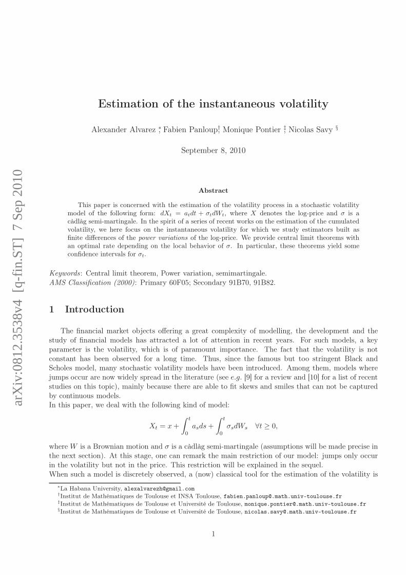
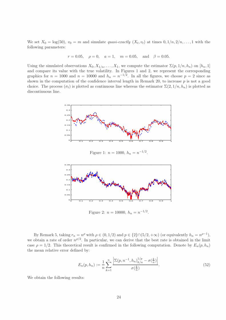
Using the simulated observations X0,X1/n, . . . ,X1, we compute the estimator Σ(p, 1/n, hn) on [hn, 1]and compare its value with the true volatility. In Figures 1 and 2, we represent the correspondinggraphics for n = 1000 and n = 10000 and hn = n−1/2. In all the figures, we choose p = 2 since asshown in the computation of the confidence interval length in Remark 20, to increase p is not a goodchoice. The process (σt) is plotted as continuous line whereas the estimator Σ(2, 1/n, hn) is plotted asdiscontinuous line.
0 0.1 0.2 0.3 0.4 0.5 0.6 0.7 0.8 0.9 10
0.05
0.1
0.15
0.2
0.25
0.3
0.35
Figure 1: n = 1000, hn = n−1/2.
0 0.1 0.2 0.3 0.4 0.5 0.6 0.7 0.8 0.9 10
0.05
0.1
0.15
0.2
0.25
0.3
0.35
Figure 2: n = 10000, hn = n−1/2.
By Remark 5, taking rn = nρ with ρ ∈ (0, 1/2) and p ∈ 2∩(5/2,+∞) (or equivalently hn = nρ−1),we obtain a rate of order nρ/2. In particular, we can derive that the best rate is obtained in the limitcase ρ = 1/2. This theoretical result is confirmed in the following computation. Denote by En(p, hn)the mean relative error defined by:
En(p, hn) :=1
n
n∑
k=1
∣∣∣Σ(p, n−1, hn)1/pk/n − σ( kn )
∣∣∣σ( kn)
. (52)
We obtain the following results:
24

En(2, n−0.4) En(2, n
−0.5) En(2, n−0.6)
n = 103 18,9% 16,6% 18,6%
n = 104 12,2% 11,0% 12,3%
En(4, n−0.4) En(4, n
−0.5) En(4, n−0.6)
n = 103 20,3% 17,5% 19,2%
n = 104 13,0% 11,9% 12,9%
Here, Remark 20 is confirmed by the fact: the estimations seem to be better with p = 2 than withp = 4.
5.2 A numerical test in a jump model
In this last part, we assume that the volatility is a jump process solution to a SDE driven by a
tempered stable subordinator (Z(λ,β)t ) with Lévy measure π(dy) = 1y>0 exp(−λy)/y1+βdy. This model
can be viewed as a particular case of the Barndorff-Nielsen and Shephard model [5] (for other jumpvolatility models see e.g. [9, 12]):
dXt = (r − 1
2σ2(t))dt+ σ(t)dW 1
t
dvt = −µvtdt+ dZ(λ,β)t
with the following choice of parameters:
r = 0.05, µ = 1, λ = 1 and β = 1/2.
This concerns Example (2) in Section 1 where Hypotheses (H1q) and (H2
q) hold for any q ≥ βand Theorem 4 can be applied. As in the preceding example, we simulate (Xt, vt) on the interval[0, 1] with X0 = log(50) and v0 = 0.05. In order to compare the two types of models, we chose somesimilar parameters. The main difference between these two models comes from the variations which arestronger in the first case. We obtain a quasi-exact sequel (Xk/n, vk/n) with k ∈ 0, . . . , n. In Figures
3 and 4, we represent the estimated and true volatilities for some different choices of hn = n−1/2,n = 103 and n = 104.
0 0.1 0.2 0.3 0.4 0.5 0.6 0.7 0.8 0.9 10
0.05
0.1
0.15
0.2
0.25
0.3
Figure 3: n = 1000, hn = n−1/2.
For these computations, we obtain the following mean relative errors:
25

0 0.1 0.2 0.3 0.4 0.5 0.6 0.7 0.8 0.9 10
0.05
0.1
0.15
0.2
0.25
0.3
Figure 4: n = 10000, hn = n−1/2.
En(2, n−0.4) En(2, n
−0.5) En(2, n−0.6)
n = 103 13,2% 8,3% 6,3%
n = 104 9,1% 5,5% 3,2%
En(4, n−0.4) En(4, n
−0.5) En(4, n−0.6)
n = 103 15,5% 11,0% 8,8%
n = 104 10,1% 6,6% 3,9%
It seems the best result is obtained with hn = n−0.6, according to Remark 5 in case η1 = η2 = 0: thebest convergence rate is obtained with ρ = 2/3.
6 Appendix
Proof of Lemma 6: Since the arguments are almost the same for each statement of the main results,we only prove (4) (with p ∈ 2 ∪ [3,+∞) and t ≥ 0.)Let (X,σ) satisfy (H1
q) and (H2q). Then, there exists a sequence (TM )M≥1 of stopping times increasing
to ∞ such that the processes (at), (bt), (η1(t)), (η2(t)) and (∫(1∧ |y|q)Ft(dy)) are bounded on [0, TM ].
Since (∫|y|≥1 yFs(dy))s≥0 is locally bounded, we can also assume that |∆Yt| ≤M on [0, TM ]. Then, let
XM , σM be defined by XM = Xt∧TM and σM = |YM | where
YMt =
∫ t∧TM
0bsds+
∫ t∧TM
0η1(s)dW
1s +
∫ t∧TM
0η2(s)dW
2s
+
∫ t∧TM
0
∫
|y|≤1y(µ− ν)(ds, dy) +
∫ t∧TM
0
∫
1≤|y|≤Myµ(ds, dy).
By construction, (XM , YM ) satisfies (SH)q and (H2q) for everyM ∈ N. It follows from the assumptions
of the proposition that for every M ∈ N,
√rn(ΣM (p,∆n, hn)t − (σMt )p
))
L−s−−−−−→n→+∞
√ϕ1(p, t, σ)U, (53)
where ΣM is the statistic related to (XM , σM ) as in (3), U ∼ N (0, 1) and U is independent of Ft. Letus now prove (4). Let g be a bounded continuous function on R and let H be a bounded F-measurable
26

random variable. Then, for all M ∈ N,
E [Hg(√rn(Σ(p,∆n, hn)t − (σt)
p)]− E[g(√ϕ1(p, t, σ)U)] =
E [Hg (√rn(Σ(p,∆n, hn)t − σpt ))]− E
[Hg
(√rn(Σ
M (p,∆n, hn)t − (σMt )p))]
+ E[Hg
(√rn(Σ
M (p,∆n, hn)t − (σMt )p))]
− E[Hg
(√ϕ1(p, t, σM )U
)]
+ E[Hg
(√ϕ1(p, t, σM )U
)]− E[Hg
(σt,√ϕ1(p, t, σ)U
)].
Set BM = ω, t+h1 < TM (ω). By construction, on BM , σMt = σt and ΣM (p,∆n, hn)t = Σ(p,∆n, hn)tfor every n ∈ N. Thus, uniformly in n, the first and third right-hand side terms are bounded by2‖g‖∞‖H‖∞P [Bc
M ] for every M ∈ N. Then, since Assumption (H1q) implies that TM → +∞ a.s,
P [BcM ] → 0 as M → +∞. Now, by (53), for every M ∈ N,
E[Hg
(√rn(Σ
M (p,∆n, hn)t − (σMt )p))]
−−−−−→n→+∞
E[Hg
(√ϕ1(p, t, σM )U
)]
and the result follows.
Proof of Lemma 7 (i). Let us prove (10). Thanks to Jensen’s inequality, we can only consider thecase r ≥ 2. Since the jumps of Y are bounded, we can compensate the big jumps and write
Yt =
∫ t
0budu+
∫ t
0η1(s)dWs +
∫ t
0η2(s)dW
2s +
∫ t
0
∫
R
y(µ− ν)(ds, dy),
where bt = bt +∫|y|>1 yFt(dy). Then, using (SH)2 and Burkholder-Davis-Gundy inequality, we have
for every r ≥ 2:
E
[supt∈[0,T ]
|σt|r]≤ C
(T r + T r/2 + E
[supt∈[0,T ]
(∫ t
0
∫
R
y2µ(ds, dy)
)r/2]),
where C is a deterministic constant. Let us focus on the last term of the right-hand side. We canwrite:
E
[supt∈[0,T ]
(∫ t
0
∫
R
y2µ(ds, dy)
) r2
]
≤ CE
[supt∈[0,T ]
(∫ t
0
∫
R
y2(µ− ν)(ds, dy)
) r2
]+ CE
[(∫ T
0
∫
R
y2ν(ds, dy)
) r2
]
≤ C
(E
[(∫ T
0
∫
R
y4µ(ds, dy)
) r4
]+ T
r2
),
where in the last inequality, we again used Burkholder-Davis-Gundy inequality and (SH)2. Set k0 =mink ∈ N, r ≤ 2k. By an iteration, we obtain
E
[supt∈[0,T ]
(∫ t
0
∫
R
y2µ(ds, dy)
)r/2]≤ C
E
(∫ T
0
∫
R
y2k0µ(ds, dy)
)r/2k0+ C
k0∑
i=1
T r/2k
.
27

Using that |u+ v|ρ ≤ |u|ρ + |v|ρ when ρ ≤ 1, we have
E
[supt∈[0,T ]
(∫ t
0
∫
R
y2k0µ(ds, dy)
)r/2k0]≤ E
[(∫ T
0
∫
R
yrµ(ds, dy)
)]≤ CT ,
and the result follows.(ii). For (11), when r ≥ 2, we obtain by a similar approach:
E [|σt − σs|r | Fs] ≤ CT (|t− s|r + |t− s|r/2) + |t− s|),
where CT is a deterministic constant. This yields the result when r ≥ 2. When r < 2 the result followsfrom the Jensen inequality. Let us prove (12). If 0 < q < 2, using Jensen inequality and the concavityof the map x 7→ xq/2, we have
E
[∣∣∣∣∫ t
sσudWu
∣∣∣∣q]
≤ E
[∣∣∣∣∫ t
sσudWu
∣∣∣∣2] q
2
≤(∫ t
sE
[sups≤u≤t
σ2u
]du
)q/2≤ C(t− s)
q
2 ,
owing to (10). When q ≥ 2, we first derive from Burkholder-Davis-Gundy inequality that
E
[∣∣∣∣∫ t
sσudWu
∣∣∣∣q]
≤ CE
[∣∣∣∣∫ t
sσ2udu
∣∣∣∣q/2].
Then, Jensen inequality and the convexity of the map x 7→ xq/2 yield
(1
t− s
∫ t
sσ2udu
)q/2≤ 1
t− s
∫ t
sσqudu,
Thus,
E
[∣∣∣∣∫ t
sσ2udu
∣∣∣∣q/2]≤ (t− s)q/2−1
∫ t
sE [σqu] du,
and (12) again follows from (10).Finally, let us prove (13). With similar arguments as previously, we obtain:
E
[∣∣∣∣∫ t
s(σu − σs)dWu
∣∣∣∣q]
≤ C
(∫ ts E[|σu − σs|2
]du)q/2
if q ∈ (0, 2]
(t− s)q/2−1∫ ts E [|σu − σs|q] du if q ≥ 2,
and (13) follows from (11).
Acknowledgements. We are deeply grateful to the listeners of our presentations and to Jean Jacodfor their valuable advices.
References
[1] Yacine Aït-Sahalia. Disentangling diffusion from jumps. Journal of Financial Economics, 74:487–528, 2004.
28
[2] Yacine Aït-Sahalia and Jean Jacod. Volatility estimators for discretely sampled Lévy processes.Ann. Statist., 35(1):355–392, 2007.
[3] Yacine Aït-Sahalia and Jean Jacod. Testing for jumps in a discretely observed process. Ann.Statist., 37(1):184–222, 2009.
[4] Alexander Alvarez. Modélisation de séries financières, estimations, ajustement de modèles et testsd’hypothèses. PhD thesis, Université de Toulouse, 2007.
[5] Ole E. Barndorff-Nielsen. Modelling by Lévy processes. In Selected Proceedings of the Sympo-sium on Inference for Stochastic Processes (Athens, GA, 2000), volume 37 of IMS Lecture NotesMonogr. Ser., pages 25–31. Inst. Math. Statist., Beachwood, OH, 2001.
[6] Ole E. Barndorff-Nielsen, Svend Erik Graversen, Jean Jacod, Mark Podolskij, and Neil Shephard.A central limit theorem for realised power and bipower variations of continuous semimartingales,in From Stochastic Analysis to Mathematical Finance, the Shiryaev Festschrift, Y. Kabanov, R.Liptser, J. Stoyanov eds, Springer-Verlag, Berlin, 33–68, 2006.
[7] Ole E. Barndorff-Nielsen and Neil Shephard. Econometric analysis of realized volatility and its usein estimating stochastic volatility models. J. R. Stat. Soc. Ser. B Stat. Methodol., 64(2):253–280,2002.
[8] Ole E. Barndorff-Nielsen and Neil Shephard. Econometrics of Testing for Jumps in FinancialEconomics Using Bipower Variation, Journal of Financial Econometrics 4, 1-30, 2006.
[9] Rama Cont and Peter Tankov. Financial modelling with jump processes. Chapman & Hall/CRCFinancial Mathematics Series. Chapman & Hall/CRC, Boca Raton, FL, 2004.
[10] Fulvio Corsi, Davide Pirino, and Roberto Renò. Volatility forecasting: the jumps do matter.Preprint, 2008.
[11] G. K. Eagleson. Martingale convergence to mixtures of infinitely divisible laws. Ann. Probability,3 no. 3:557–562, 1975.
[12] Fernando Espinosa and Josep Vives. A volatility-varying and jump-diffusion Merton type modelof interest rate risk. Insurance Math. Econom., 38(1):157–166, 2006.
[13] Jean-Pierre Fouque, George Papanicolaou, and K. Ronnie Sircar. Derivatives in financial marketswith stochastic volatility. Cambridge University Press, Cambridge, 2000.
[14] Peter Hall and Christopher C. Heyde. Martingale limit theory and its application. Academic PressInc. [Harcourt Brace Jovanovich Publishers], New York, 1980.
[15] Jean Jacod. Asymptotic properties of realized power variations and related functionals of semi-martingales. Stochastic Process. Appl., 118(4):517–559, 2008.
[16] Jean Jacod, Mark Podolskij, and Mathias Vetter. Limit theorems for moving averages of discretizedprocesses plus noise - madpn-3. Preprint.
[17] Dominique Lépingle. La variation d’ordre p des semi-martingales. Z. Wahrscheinlichkeitstheorieund Verw. Gebiete, 36(4):295–316, 1976.
[18] Cecilia Mancini. Disentangling the jumps of the diffusion in a geometric jumping Brownian.Giornale dell’Istituto Italiano degli Attuari, LXIV:19–47, 2001.
29

[19] Cecilia Mancini. Estimating the integrated volatility in stochastic volatility models with Lévytype jumps. Technical report, Universita di Firenze, 2004.
[20] Christian Y. Robert and Mathieu Rosenbaum. Volatility and covariation estimation when mi-crostructure noise and trading times are endogenous to appear in Mathematical Finance, 2009.
[21] Viktor Todorov and George Tauchen. Volatility jumps. Preprint, 2008.
[22] Almuut E.D. Veraart. Inference for the jump part of quadratic variation of Ito semimartingales.Econometric Theory (26-02), 331–368, 2010.
[23] Jeannette H. C. Woerner. Estimation of integrated volatility in stochastic volatility models. Appl.Stoch. Models Bus. Ind., 21(1):27–44, 2005.
[24] Jeannette H. C. Woerner. Power and multipower variation: inference for high frequency data. InStochastic finance, pages 343–364. Springer, New York, 2006.
30


