The Communication Complexity of Optimization - NSF PAR

The Communication Complexity of Optimization

Santosh S. Vempala∗ Ruosong Wang† David P. Woodruff‡

Abstract

We consider the communication complexity of a numberof distributed optimization problems. We start with theproblem of solving a linear system. Suppose there is acoordinator together with s servers P1, . . . , Ps, the i-thof which holds a subset A(i)x = b(i) of ni constraintsof a linear system in d variables, and the coordinatorwould like to output an x ∈ Rd for which A(i)x = b(i)

for i = 1, . . . , s. We assume each coefficient of each con-straint is specified using L bits. We first resolve the ran-domized and deterministic communication complexityin the point-to-point model of communication, showingit is eΘ(d2L + sd) and eΘ(sd2L), respectively. We ob-tain similar results for the blackboard communicationmodel. As a result of independent interest, we showthe probability a random matrix with integer entries in−2L, . . . , 2L is invertible is 1− 2−Θ(dL), whereas pre-viously only 1− 2−Θ(d) was known.

When there is no solution to the linear system, anatural alternative is to find the solution minimizingthe ‘p loss, which is the ‘p regression problem. Whilethis problem has been studied, we give improved upperor lower bounds for every value of p ≥ 1. One takeawaymessage is that sampling and sketching techniques,which are commonly used in earlier work on distributedoptimization, are neither optimal in the dependence ond nor on the dependence on the approximation ε, thusmotivating new techniques from optimization to solvethese problems.

Towards this end, we consider the communicationcomplexity of optimization tasks which generalize linearsystems, such as linear, semidefinite, and convex pro-gramming. For linear programming, we first resolve thecommunication complexity when d is constant, showingit is eΘ(sL) in the point-to-point model. For general d

and in the point-to-point model, we show an eO(sd3L)

upper bound and an eΩ(d2L + sd) lower bound. In fact,we show if one perturbs the coefficients randomly bynumbers as small as 2−Θ(L), then the upper bound iseO(sd2L)+poly(dL), and so this bound holds for almost

∗Georgia Tech. Email: [email protected].†Carnegie Mellon University. Email:

[email protected].‡Carnegie Mellon University. Email: [email protected].

all linear programs. Our study motivates understand-ing the bit complexity of linear programming, whichis related to the running time in the unit cost RAMmodel with words of O(log(nd)) bits, and we give thefastest known algorithms for linear programming in thismodel.

1 Introduction

Large-scale optimization problems often cannot fit intoa single machine, and so they are distributed acrossa number s of machines. That is, each of serversP1, . . . , Ps may hold a subset of constraints that itis given locally as input, and the goal of the serversis to communicate with each other to find a solutionsatisfying all constraints. Since communication is oftena bottleneck in distributed computation, the goal of theservers is to communicate as little as possible.

There are several different standard communicationmodels, including the point-to-point model and theblackboard model. In the point-to-point model, eachpair of servers can talk directly with each other. Thisis often more conveniently modeled by looking at thecoordinator model, for which there is an extra servercalled the coordinator, and all communication mustpass through the coordinator. This is easily seen tobe equivalent, from a total communication perspective,to the point-to-point model up to a factor of 2, forforwarding messages from server Pi to server Pj , anda term of log s per message to indicate which serverthe message should be forwarded to. Another model ofcomputation is the blackboard model, in which there is ashared broadcast channel among all the s servers. Whena server sends a message, it is visible to each of the others − 1 servers and determines who speaks next, basedupon an agreed upon protocol. We mostly considerrandomized communication, in which for every input,we require the coordinator to output the solution to theoptimization problem with high probability. For linearsystems we also consider deterministic communicationcomplexity.

A number of recent works in the theory communityhave looked at studying specific optimization problemsin such communication models, such as principal com-ponent analysis [35, 39, 13] and kernel [8] and robust

1733Copyright © 2020 by SIAM

Unauthorized reproduction of this article is prohibited

Dow

nloa

ded

12/3

0/20

to 4

5.17

.162

.35.

Red

istri

butio

n su

bjec

t to

SIA

M li

cens

e or

cop

yrig

ht; s

ee h

ttps:

//epu

bs.si

am.o

rg/p

age/

term

s

variants [59, 23], computing higher correlations [35], ‘pregression [55, 23] and sparse regression [15], estimatingthe mean of a Gaussian [61, 28, 15], database problems[31, 58], clustering [17], statistical [56], graph problems[43, 56] and many, many more.

There are also a large number of distributed learn-ing and optimization papers, for example [7, 61, 63, 1,14, 40, 60, 19, 44, 26, 24, 25, 32, 47, 46, 62, 4, 34].With a few exceptions, these works do not study generalcommunication complexity, but rather consider specificclasses of algorithms. Namely, a number of these worksonly allow gradient and Hessian computations in eachround, and do not allow arbitrary communication. An-other aspect of these works is that they typically donot count total bit complexity, but rather only countnumber of rounds, whereas we are interested in totalcommunication. In a number of optimization problems,the bit complexity of storing a single number in anintermediate computation may be as large as storingthe entire original optimization problem. It is there-fore infeasible to transmit such a number. While onecould round this number, the effect of rounding is oftenunclear, and could destroy the desired approximationguarantee. One exception to the above is the work of[52], which studies the problem in which there are twoservers, each holding a convex function, who would liketo find a solution so as to minimize the sum of the twofunctions. The upper bounds are in a different com-munication model than ours, where the functions areadded together, while the lower bounds only apply to arestricted class of protocols.

Noticeably absent from previous work is the com-munication complexity of solving linear systems, whichis a fundamental primitive in many optimization tasks.Formally, suppose there is a coordinator together withs servers P1, . . . , Ps, the i-th of which holds a subsetA(i)x = b(i) of ni constraints of a d-dimensional lin-ear system, and the coordinator would like to outputan x ∈ Rd for which A(i)x = b(i) for i = 1, . . . , s.We further assume each coefficient of each constraintis specified using L bits. The first question we ask isthe following.

Question 1.1. What is the communication complexityof solving a linear system?

When there is no solution to the linear system,a natural alternative is to find the solution minimiz-ing the ‘p loss, which is the ‘p regression problemminx∈Rd kAx − bkp, where for an n-dimensional vector

y, kykp = (Pni=1 |yi|p)

1/pis its ‘p norm.

In the distributed ‘p regression problem, each serverhas a matrix A(i) ∈ Rni×d and a vector b(i) ∈ Rni ,and the coordinator would like to output an x ∈ Rd

so that kAx− bkp is approximately minimized, namely,that kAx − bkp ≤ (1 + ε) minx0 kAx0 − bkp. Note thathere A ∈ Rn×d is the matrix obtained by stackingthe matrices A(1), . . . , A(s) on top of each other, wheren =

Psi=1 ni. Also, b ∈ Rn is the vector obtained by

stacking the vectors b(1), . . . , b(s) on top of each other.We assume that each entry of A and b is an L-bit integer,and we are interested in the randomized communicationcomplexity of this problem.

While previous work [41, 55] has looked at thedistributed ‘p regression problem, such work is basedon two main ideas: sampling and sketching. Suchtechniques reduce a large optimization problem to amuch smaller one, thereby allowing servers to sendsuccinct synopses of their constraints in order to solvea global optimization problem.

Sampling and sketching are the key techniques ofrecent work on distributed low rank approximation[55, 35] and regression algorithms. A natural ques-tion, which will motivate our study of more complexoptimization problems below, is whether other tech-niques in optimization can be used to obtain morecommunication-efficient algorithms for these problems.

Question 1.2. Are there tractable optimization prob-lems for which sampling and sketching techniques aresuboptimal in terms of total communication?

To answer Question 1.2 it is useful to study opti-mization problems generalizing both linear systems and‘p regression for certain values of p. Towards this end,we consider the communication complexity of linear,semidefinite, and convex programming. Formally, in thelinear programming problem, suppose there is a coor-dinator together with s servers P1, . . . , Ps, the i-th ofwhich holds a subset A(i)x ≤ b(i) of ni constraints of ad-dimensional linear system, and the coordinator, whoholds a vector c ∈ Rd, would like to output an x ∈ Rdfor which cTx is maximized subject to A(i)x ≤ b(i) fori = 1, . . . , s. We further assume each coefficient of eachconstraint, as well as the objective function c, is speci-fied using L bits.

Question 1.3. What is the communication complexityof solving a linear program?

One could try to implement known linear program-ming algorithms as distributed protocols. The mainchallenge here is that known linear programming al-gorithms operate in the real RAM model of computa-tion, meaning that basic arithmetic operations on realnumbers can be performed in constant time. This isproblematic in the distributed setting, since it mightmean real numbers need to be communicated among the



Dow

nloa

ded

12/3

0/20

to 4

5.17

.162

.35.

Red

istri

butio

n su

bjec

t to

SIA

M li

cens

e or

cop

yrig

ht; s

ee h

ttps:

//epu

bs.si

am.o

rg/p

age/

term

s

servers, resulting in protocols that could have infinitecommunication. Thus, controlling the bit complexity ofthe underlying algorithm is essential, and this motivatesthe study of linear programming algorithms in the unitcost RAM model of computation, meaning that a word isO(log(nd)) bits, and only basic arithmetic operations onwords can be performed in constant time. Such a modelis arguably more natural than the real RAM model. Ifone were to analyze the fastest linear programming al-gorithms in the unit cost RAM model, their time com-plexity would blow up by poly(dL) factors, since theintermediate computations require manipulating num-bers that grow exponentially large or small. Surpris-ingly, we are not aware of any work that has addressedthis question:

Question 1.4. What is the best possible running timeof an algorithm for linear programming in the unit costRAM model?

As far as time complexity is concerned, it is noteven known if linear programming is inherently moredifficult than just solving a linear system. Indeed, a longline of work on interior point methods, with the currentmost recent work of [20], suggests that solving a linearprogram may not be substantially harder than solvinga linear system. One could ask the same question forcommunication.

Question 1.5. Is solving a linear program inherentlyharder than solving a linear system? What about justchecking the feasibility of a linear program versus thatof a linear system?

Recent Independent Work. A recent indepen-dent work [5] also studies solving linear programs inthe distributed setting, although their focus is to studythe tradeoff between round complexity and communi-cation complexity in low dimensions, while our focus isto study the communication complexity in arbitrary di-mensions. Note, however, that we also provide nearlyoptimal bounds for constant dimensions for linear pro-gramming in both coordinator and blackboard models.

1.1 Our Contributions We make progress on an-swering the above questions, with nearly tight boundsin many cases. For a function f , we let eO(f) =

f polylog(sndL/ε) and similarly define eΘ and eΩ.

1.1.1 Linear Systems We begin with linear sys-tems, for which we obtain a complete answer for bothrandomized and deterministic communication, in bothcoordinator and blackboard models of communication.

Theorem 1.1. In the coordinator model, the random-ized communication complexity of solving a linear sys-tem is eΘ(d2L + sd), while the deterministic communi-

cation complexity is eΘ(sd2L). In the blackboard model,both the randomized communication complexity and thedeterministic communication complexity are eΘ(d2L+s).

Theorem 1.1 shows that randomization provablyhelps for solving linear systems. The theorem also showsthat in the blackboard model the problem becomessubstantially easier.

1.1.2 Approximate Linear Systems, i.e., ‘p Re-gression We next study the ‘p regression problem inboth the coordinator and blackboard models of com-munication. Finding a solution to a linear system isa special case of ‘p regression; indeed in the case thatthere is an x for which Ax = b we must return such anx to achieve (1 + ε) relative error in objective functionvalue for ‘p regression. Consequently, our lower boundsfor linear systems apply also to ‘p regression for anyε > 0.

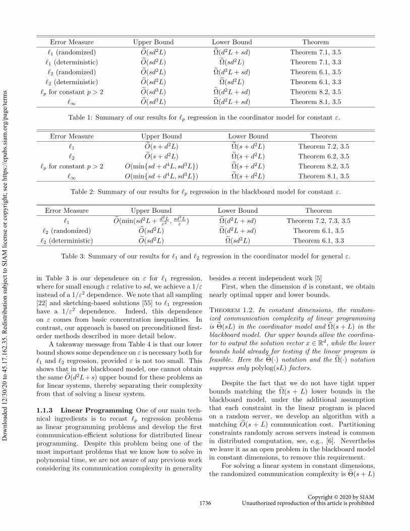
We first summarize our results in Table 1 andTable 2 for constant ε. We state our results primarily forrandomized communication. However, in the case of ‘2

regression, we also discuss deterministic communicationcomplexity.

One of the main takeaway messages from Table 1is that sampling-based approaches, namely those basedupon the so-called Lewis weights [22], would requireΩ(dp/2) samples for ‘p regression when p > 2, and thuscommunication. Another way for solving ‘p regressionfor p > 2 is via sketching, as done in [55], but thenthe communication is Ω(n1−2/p). Our method, whichis deeply tied to linear programming, discussed morebelow, solves this problem in eO(sd3L) communication.Thus, this gives a new method, departing from samplingand sketching techniques, which achieves much bettercommunication. Our method involves embedding ‘pinto ‘∞, and then using distributed algorithms for linearprogramming to solve ‘∞ regression.

As with linear systems, one takeaway message fromthe results in Table 2 is that the problems have signif-icantly more communication-efficient upper bounds inthe blackboard model than in the coordinator model.Indeed, here we obtain tight bounds for ‘1 and ‘2 re-gression, matching those that are known for the easierproblem of linear systems.

We next describe our results for non-constant ε inboth the coordinator model and the blackboard model.Here we focus on ‘1 and ‘2, which illustrate severalsurprises.

One of the most interesting aspects of the results



Dow

nloa

ded

12/3

0/20

to 4

5.17

.162

.35.

Red

istri

butio

n su

bjec

t to

SIA

M li

cens

e or

cop

yrig

ht; s

ee h

ttps:

//epu

bs.si

am.o

rg/p

age/

term

s

Error Measure Upper Bound Lower Bound Theorem

‘1 (randomized) eO(sd2L) eΩ(d2L + sd) Theorem 7.1, 3.5

‘1 (deterministic) eO(sd2L) eΩ(sd2L) Theorem 7.1, 3.3



‘p for constant p > 2 eO(sd3L) eΩ(d2L + sd) Theorem 8.2, 3.5

‘∞ eO(sd3L) eΩ(d2L + sd) Theorem 8.1, 3.5

Table 1: Summary of our results for ‘p regression in the coordinator model for constant ε.


‘1eO(s + d2L) eΩ(s + d2L) Theorem 7.2, 3.5

‘2eO(s + d2L) eΩ(s + d2L) Theorem 6.2, 3.5

‘p for constant p > 2 O(minsd + d4L, sd3L) eΩ(s + d2L) Theorem 8.2, 3.5

‘∞ O(minsd + d4L, sd3L) eΩ(s + d2L) Theorem 8.1, 3.5

Table 2: Summary of our results for ‘p regression in the blackboard model for constant ε.


‘1eO(min(sd2L + d2L

ε2 , sd3Lε ) eΩ(d2L + sd) Theorem 7.2, 7.3, 3.5



Table 3: Summary of our results for ‘1 and ‘2 regression in the coordinator model for general ε.

in Table 3 is our dependence on ε for ‘1 regression,where for small enough ε relative to sd, we achieve a 1/εinstead of a 1/ε2 dependence. We note that all sampling[22] and sketching-based solutions [55] to ‘1 regressionhave a 1/ε2 dependence. Indeed, this dependenceon ε comes from basic concentration inequalities. Incontrast, our approach is based on preconditioned first-order methods described in more detail below.

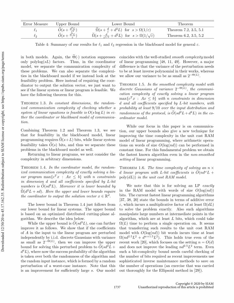
A takeaway message from Table 4 is that our lowerbound shows some dependence on ε is necessary both for‘1 and ‘2 regression, provided ε is not too small. Thisshows that in the blackboard model, one cannot obtainthe same eO(d2L+s) upper bound for these problems asfor linear systems, thereby separating their complexityfrom that of solving a linear system.

1.1.3 Linear Programming One of our main tech-nical ingredients is to recast ‘p regression problemsas linear programming problems and develop the firstcommunication-efficient solutions for distributed linearprogramming. Despite this problem being one of themost important problems that we know how to solve inpolynomial time, we are not aware of any previous workconsidering its communication complexity in generality

besides a recent independent work [5]First, when the dimension d is constant, we obtain

nearly optimal upper and lower bounds.

Theorem 1.2. In constant dimensions, the random-ized communication complexity of linear programmingis eΘ(sL) in the coordinator model and eΩ(s + L) in theblackboard model. Our upper bounds allow the coordina-tor to output the solution vector x ∈ Rd, while the lowerbounds hold already for testing if the linear program isfeasible. Here the eΘ(·) notation and the eΩ(·) notationsuppress only polylog(sL) factors.

Despite the fact that we do not have tight upperbounds matching the eΩ(s + L) lower bounds in theblackboard model, under the additional assumptionthat each constraint in the linear program is placedon a random server, we develop an algorithm with amatching eO(s + L) communication cost. Partitioningconstraints randomly across servers instead is commonin distributed computation, see, e.g., [6]. Neverthelsswe leave it as an open problem in the blackboard modelin constant dimensions, to remove this requirement.

For solving a linear system in constant dimensions,the randomized communication complexity is eΘ(s + L)



Dow

nloa

ded

12/3

0/20

to 4

5.17

.162

.35.

Red

istri

butio

n su

bjec

t to

SIA

M li

cens

e or

cop

yrig

ht; s

ee h

ttps:

//epu

bs.si

am.o

rg/p

age/

term

s


‘1eO(s + d2L

ε2 ) eΩ(s + dε + d2L) for s > Ω(1/ε) Theorem 7.2, 3.5, 5.1

‘2eO(s + d2L

ε ) eΩ(s + dε1/2

+ d2L) for s > Ω(1/√ε) Theorem 6.2, 3.5, 5.2

Table 4: Summary of our results for ‘1 and ‘2 regression in the blackboard model for general ε.

in both models. Again, the eΘ(·) notation suppressesonly polylog(sL) factors. Thus, in the coordinatormodel, we separate the communication complexity ofthese problems. We can also separate the complexi-ties in the blackboard model if we instead look at thefeasibility problem. Here instead of requiring the coor-dinator to output the solution vector, we just want tosee if the linear system or linear program is feasible. Wehave the following theorem for this.

Theorem 1.3. In constant dimensions, the random-ized communication complexity of checking whether asystem of linear equations is feasible is O(s logL) in ei-ther the coordinator or blackboard model of communica-tion.

Combining Theorem 1.2 and Theorem 1.3, we seethat for feasibility in the blackboard model, linearprogramming requires eΩ(s+L) bits, while linear system

feasibility takes eO(s) bits, and thus we separate theseproblems in the blackboard model as well.

Returning to linear programs, we next consider thecomplexity in arbitrary dimensions.

Theorem 1.4. In the coordinator model, the random-ized communication complexity of exactly solving a lin-ear program maxcTx : Ax ≤ b with n constraintsin dimension d and all coefficients specified by L-bitnumbers is eO(sd3L). Moreover it is lower bounded byeΩ(d2L + sd). Here the upper and lower bounds requirethe coordinator to output the solution vector x ∈ Rd.

The lower bound in Theorem 1.4 just follows fromour lower bound for linear systems. The upper boundis based on an optimized distributed cutting-plane al-gorithm. We describe the idea below.

While the upper bound is eO(sd3L), one can furtherimprove it as follows. We show that if the coefficientsof A in the input to the linear program are perturbedindependently by i.i.d. discrete Gaussians with varianceas small as 2−Θ(L), then we can improve the upperbound for solving this perturbed problem to eO(sd2L +d4L), where now the success probability of the algorithmis taken over both the randomness of the algorithm andthe random input instance, which is formed by a randomperturbation of a worst-case instance. Note that thisis an improvement for sufficiently large s. Our model

coincides with the well-studied smooth complexity modelof linear programming [48, 11, 49]. However, a majordifference is that the variance of the perturbation needsto be at least inverse polynomial in their works, whereaswe allow our variance to be as small as 2−Θ(L).

Theorem 1.5. In the smoothed complexity model withdiscrete Gaussians of variance 2−Θ(L), the communi-cation complexity of exactly solving a linear programmaxcTx : Ax ≤ b with n constraints in dimensiond and all coefficients specified by L-bit numbers, withprobability at least 9/10 over the input distribution and

randomness of the protocol, is eO(sd2L+d4L) in the co-ordinator model.

While our focus in this paper is on communica-tion, our upper bounds also give a new technique forimproving the time complexity in the unit cost RAMmodel of linear programming, where arithmetic opera-tions on words of size O(log(nd)) can be performed inconstant time. For this fundamental problem we obtainthe fastest known algorithm even in the non-smoothedsetting of linear programming.

Theorem 1.6. The time complexity of solving an n ×d linear program with L-bit coefficients is eO(ndωL +poly(dL)) in the unit cost RAM model.

We note that this is for solving an LP exactlyin the RAM model with words of size O(log(nd))bits. The current fastest linear programming algorithms[37, 38, 20] state the bounds in terms of additive errorε, which incurs a multiplicative factor of at least Ω(dL)to solve the problem exactly. Also such algorithmsmanipulate large numbers at intermediate points in thealgorithm, which are at least L bits, which could takeΩ(L) time to perform a single operation on. It seemsthat transferring such results to the unit cost RAMmodel with O(log(nd)) bit words incurs time at leastΩ(nd2.5L2 + dw+1.5L2). This holds true even of therecent work [20], which focuses on the setting n = O(d)and does not improve the leading nd2.5L2 term. Evensuch a bit-complexity bound needs careful checking ofthe number of bits required as recent improvements usesophisticated inverse maintenance methods to save onthe number of operations (an exercise that was carriedout thoroughly for the Ellipsoid method in [29]).



Dow

nloa

ded

12/3

0/20

to 4

5.17

.162

.35.

Red

istri

butio

n su

bjec

t to

SIA

M li

cens

e or

cop

yrig

ht; s

ee h

ttps:

//epu

bs.si

am.o

rg/p

age/

term

s

1.1.4 Implications for Convex Optimizationand Semidefinite Programming Our upper boundsalso extend to more general convex optimization prob-lems. For these, we must modify the problem statementto finding an ε-additive approximation rather than theexact solution. We obtain the following upper boundfor a convex program in Rd.Theorem 1.7. The communication complexity of solv-ing the convex optimization problem mincTx : x ∈TiKi for convex sets Ki ⊆ RBn, one per server,

to within an additive error ε, i.e., finding a pointy s.t. cT y ≤ OPT + ε and y ∈

TiKi + εBn is

O(sd2 log(Rd/ε) log d).

If the objective function is not known to all servers,we incur an additional O(sdL) communication. Forsemidefinite programs with d × d symmetric matri-ces and n linear constraints this gives a bound ofeO(sd4 log(1/ε)). Note that we can simply send all theconstraints to one server in O(nd2L) communication, sothis is always an upper bound.

1.2 Our Techniques

1.2.1 Linear Systems To solve linear systems in thedistributed setting, the coordinator can go through theservers one by one. The coordinator and all serversmaintain the same set C of linearly independent linearequations. For each server Pi, if there is a linearequation stored by Pi that is linearly independent withlinear equations in C, then Pi sends that linear equationto all other servers and adds that linear equation intoC. In the end, C will be a maximal set of linearlyindependent equations, and thus the coordinator cansimply solve the linear equations in C. This protocolis deterministic and has communication complexityO(sd2L) in the coordinator model and O(s + d2L) inthe blackboard model, since at most d linear equationswill be added into the set C.

In fact, the preceding protocol is optimal for de-terministic protocols, even just for testing the feasibil-ity of linear systems. To prove lower bounds, we firstprove the following new theorem about random matriceswhich may be of independent interest.

Theorem 1.8. (Informal version of Theorem 3.1)Let R be a d × d matrix with i.i.d. random integerentries in −2L, . . . , 2L. The probability that R isinvertible is 1− 2−Θ(dL).

The previous best known probability bound was only1 − 2−Θ(d) [50, 12]; we stress that the results of [12]are not sufficient1 to prove our stronger bound with the

1We have verified this with Philip Matchett Wood, who is an

extra factor of L in the exponent, which is crucial forour lower bound.

With Theorem 1.8, in Lemma 3.2, we use theprobabilistic method to construct a set of |H| = 2Ω(d2L)

matrices H ⊆ Rd×d with integral entries in [−2L, 2L],such that for any S, T ∈ H, S−1ed 6= T−1ed, where edis the d-th standard basis vector.

Now consider any deterministic protocol for testingthe feasibility of linear systems. Suppose the linearsystem on the i-th server is Hix = ed for some Hi ∈ H,then the entire linear system is feasible if and only ifH1 = H2 = . . . = Hs. This is equivalent to theproblem in which each server receives a binary stringof length log(|H|), and the goal is to test whetherall strings are the same or not. In the coordinatormodel, a deterministic lower bound of Ω(s log(|H|)) forthis problem can be proved using the symmetrizationtechnique in [43, 57], which gives an optimal Ω(sd2L)lower bound. An optimal Ω(s+d2L) deterministic lowerbound can also be proved in the blackboard model.More details can be found in Section 3.3.

For solving linear systems, an Ω(d2L) lower boundholds even for randomized algorithms in the coordinatormodel. When there is only a single server which holds alinear system Hx = ed for some H ∈ H, in order for thecoordinator to know the solution x = H−1ed, standardinformation-theoretic argument shows that log(|H|) bitsof communication is necessary, which gives an Ω(d2L)lower bound. This idea is formalized in Section 3.4. Anatural question is whether the O(sd2L) upper boundis optimal for randomized protocols.

We first show that in order to test feasibility, itis possible to achieve a communication complexity ofO(sd2 log(dL)), which can be exponentially better thanthe bound for deterministic protocols. The idea isto use hashing. With randomness, the servers canfirst agree on a random prime number p, and testthe feasibility over the finite field Fp. It suffices tohave the prime number p randomly generated fromthe range [2,poly(dL)], and thus the L factor in thecommunicataion complexity of deterministic protocolscan be improved to log p = log(dL). However, it isstill unclear if solving linear systems in the coordinatormodel will require Ω(sd2L) bits of communication forrandomized protocols.

Quite surprisingly, we show that O(sd2L) is not theoptimal bound for randomized protocols, and the opti-mal bound is eΘ(d2L + sd). In the deterministic pro-

author of [12]. The issue is that in their Corollary 1.2, theyhave an explicit constraint on the cardinality of the set S, i.e.,|S| = O(1). In their Theorem 2.2, it is assumed that |S| = no(n).Thus, as far as we are aware, there are no known results sufficientto prove our singularity probability bound.



Dow

nloa

ded

12/3

0/20

to 4

5.17

.162

.35.

Red

istri

butio

n su

bjec

t to

SIA

M li

cens

e or

cop

yrig

ht; s

ee h

ttps:

//epu

bs.si

am.o

rg/p

age/

term

s

tocol with communication complexity O(sd2L), mostcommunication is wasted on synchronizing the set C,which requires the servers to send linear equations toall other servers. In our new protocol, only the coordi-nator maintains the set C. The issue now, however, isthat the servers no longer know which linear equationthey own is linearly independent with those equationsin C. On the other hand, each server can simply gener-ate a random linear combination of all linear equationsit owns. We can show that if a server does have a lin-ear equation that is linearly independent with those inC, with constant probability, the random linear com-bination is also linearly independent with those in C,and thus the coordinator can add the random linearcombination into C. Notice that taking random linearcombinations to preserve the rank of a matrix is a spe-cial case of dimensionality reduction or sketching, whichcomes up in a number of applications, see, for examplecompressed sensing [16, 10], data streams [3], and ran-domized numerical linear algebra [54]. Here though, acrucial difference is that we just need the fact that if aset of vectors S is not contained in the span of anotherset of vectors V , then a random linear combination ofthe vectors in S is also not in the span of V with highprobability. This allows us to adaptively take as few lin-ear combinations as possible to solve the linear system,enabling us to achieve much lower communication thanwould be possible by just sketching the linear systemsat each server and non-adaptively combining them.

If we implement this protocol naıvely, then the com-munication complexity will be eO(d2L + sdL), since atmost d linear equations will be added into C, and thereis an eO(dL) communication complexity associated witheach of them. Furthermore, even if a server does nothave any linear equation that is linearly independentwith C, it still needs to send random linear combinationsto the coordinator, which would require eO(sdL) com-

munication. To improve this further to eO(sd), we canstill use the hashing trick mentioned before. If a servergenerates a random linear combination, it can first testwhether the linear combination is linearly independentwith C over the finite field p, for a random prime p cho-sen in [2,poly(dL)]. This will reduce the communication

complexity to eO(d) for each test. If the linear equationis indeed linearly independent with C, then the serversends the original linear equation (without taking theresidual modulo p) to the coordinator. Again the totalcommunication complexity for sending the original lin-ear equations is upper bounded by O(d2L). Thus, thetotal communication complexity is upper bounded byeO(d2L + sd). See Section 4.2 for details.

By a reduction from the OR of s − 1 copies ofthe two-server set-disjointness problem to solving linear

systems, we can prove an extra eΩ(sd) lower bound,which holds even for testing feasibility of linear systems.Here the idea is to interpret vectors in 0, 1d ascharacteristic vectors of subsets of [d]. One of theservers will fix the solution of the linear system to bea predefined vector x. Each server Pi has a singlelinear equation aTi x = 1. By interpreting vectors assets, aTi x = 1 implies the set represented by ai and xare intersecting. Thus, the servers are actually solvingthe OR of s− 1 copies of the two-server set-disjointnessproblem, which is known to have eΩ(sd) communicationcomplexity [43, 56]. This lower bound is formally givenin Section 3.4.

1.2.2 Linear Regression For an ‘2 regression in-stance minx kAx− bk2, the optimal solution can be cal-culated using the normal equations, i.e., the optimalsolution x satisfies ATAx = AT b. This already givesa simple yet nearly optimal deterministic protocol for‘2 regression in the coordinator model: the coordina-tor calculates ATA and AT b using only eO(sd2L) bitsof communication by collecting the covariance matricesfrom each server and summing them up. The eO(sd2L)communication complexity matches our lower boundfor solving linear systems for deterministic protocols inthe coordinator model. However, when implementedin the blackboard model, the communication complex-ity of this protocol is still eO(sd2L). To improve thisbound, we first show how to efficiently obtain approxi-mations to leverage scores in both models. Our proto-col is built upon the algorithm in [21], but implementedin a distributed manner. The resulting algorithm haseO(sd2L) communication complexity in the coordinator

model but only eO(s + d2L) communication complexityin the blackboard model. With approximate leveragescores, the coordinator can then sample eO(d/ε2) rowsof the matrix A to obtain a subspace embeeding, at whichpoint it will be easy to calculate a (1 + ε)-approximatesolution to the ‘2 regression problem. The number ofsampled rows can be further improved to eO(d/ε) usingSarlos’s argument [45] since solving ‘2 regression doesnot necessarily require a full (1 + ε) subspace embed-ding, which results in a protocol with communicationcomplexity eO(s+ d2L/ε) in the blackboard model. Fulldetails can be found in Section 6.

One may wonder if the dependence on 1/ε is neces-sary for solving ‘2 regression in the blackboard model.In Section 5, we show that some dependence on 1/ε isactually necessary. We show an Ω(d/

√ε) lower bound

whenever s > Ω(1/√ε). The hardness follows from

the fact that if the matrix A satisfies A(i) = I forall i ∈ [s], then the optimal solution is just the aver-age of b(1), b(2), . . . , b(s). Thus, if we can get sufficiently



Dow

nloa

ded

12/3

0/20

to 4

5.17

.162

.35.

Red

istri

butio

n su

bjec

t to

SIA

M li

cens

e or

cop

yrig

ht; s

ee h

ttps:

//epu

bs.si

am.o

rg/p

age/

term

s

good approximation to the ‘2 regression problem, thenwe can actually recover the sum of b(1), b(2), . . . , b(s),at which point we can resort to known communicationcomplexity lower bound in the blackboard model [43].This argument will also give an Ω(d/ε) lower boundfor (1 + ε)-approximate ‘1 regression in the blackboardmodel, whenever s > Ω(1/ε). Details can be found inSection 5.

For ‘1 regression, we can no longer use the normalequations. However, we can obtain approximations to‘1 Lewis weights by using approximations to leveragescores, as shown in [22]. With approximate ‘1 Lewisweights of the A matrix, the coordinator can then obtaina (1 + ε) ‘1 subspace embedding by sampling eO(d/ε2)rows. This will give an O(sd2L + d2L/ε2) upper boundfor (1 + ε)-approximate ‘1 regression in the coordinatormodel, and an O(s+d2L/ε2) upper bound in the black-board model. It is unclear if the number of sampledrows can be further reduced since there is no known‘1 version of Sarlos’s argument. A natural question iswhether the 1/ε2 dependence is optimal. We show thatthe dependence on ε can be further improved to 1/ε,by using optimization techniques, or more specifically,first-order methods. Despite the fact that the objectivefunction of ‘1 regression is neither smooth nor strongly-convex, it is known that by using Nesterov’s Acceler-ated Gradient Descent and smoothing reductions [42],one can solve ‘1 regression using only O(1/ε) full gra-dient calculations. On the other hand, the complexityof first-order methods usually has dependences on var-ious parameters of the input matrix A, which can beunbounded in the worst case. Fortunately, recent devel-opments in ‘1 regression [27] show how to preconditionthe matrix A by simply doing an ‘1 Lewis weights sam-pling, and then rotating the matrix appropriately. Bycarefully combining this preconditioning procedure withAccelerated Gradient Descent, we obtain an algorithmfor (1 + ε)-approximate ‘1 regression with communica-

tion complexity eO(sd3L/ε) in the coordinator model,which shows it is indeed possible to improve the ε de-pendence for ‘1 regression. More details can be foundin Section 7.

For general ‘p regression, if we still use Lewisweights sampling, then the number of sampled rowsand thus the communication complexity will be Ω(dp/2).Even worse, when p = ∞, Lewis weights sampling willrequire an unbounded number of samples. However,‘∞ regression can be easily formulated as a linearprogram, which we show how to solve exactly in thedistributed setting. Inspired by this approach, wefurther develop a general reduction from ‘p regressionto linear programming. Our idea is to use the max-stability of exponential random variables [2] to embed

‘p into ‘∞, write the optimization problem in ‘∞ asa linear program and then solve the problem usinglinear program solvers. However, such embeddingsbased on exponential random variables usually produceheavy-tailed random variables and makes the dilationbound hard to analyze. Here, since our goal is justto solve a linear regression problem, we only needthe dilation bound for the optimal solution of theregression problem. In Section 8, we show that (1 + ε)-approximate ‘p regression can be reduced to solving a

linear program with eO(d/ε2) variables, which implies acommunication protocol for ‘p regression without theΩ(dp/2) dependence.

1.2.3 Linear and Convex Programs We adapttwo different algorithms from the literature for efficientcommunication and implement them in the distributedsetting. The first is Clarkson’s algorithm, which worksby sampling O(d2) constraints in each iteration andfinds an optimal solution to this subset; the samplingweights are maintained implicitly. In each iterationthe total communication is O(d3L) for gathering the

constraints and an additional eO(sd2L) per round tosend the solution to this subset of constraints to allservers. This solution is used to update the samplingweights. Clarkson’s algorithm has the nice guaranteethat it needs only O(d log n) rounds with high probabil-ity. A careful examination of this algorithm shows thatthe bit complexity of the computation (not the commu-nication) is dominated by checking whether a proposedsolution satisfies all constraints, i.e., computing Ax fora given x. We show this can be done with time com-plexity eO(ndωL) in the unit cost RAM model and thisis the leading term of the claimed time bound.

Notice that the eO(sd3L) term in the communicationcomplexity of Clarkson’s algorithm comes from the factthat the protocol needs to send an optimal solution x∗

of a linear program with size O(d2) × d for a totalof O(d log n) times. However, when each server Pireceives x∗, all Pi will do is to check whether x∗ satisfiesthe constraints stored on Pi or not. Notice that hereentries in the constraints have bit complexity L, whereasthe solution vector x∗ has bit complexity eO(dL) foreach entry. Intuitively, for most linear programs, wedon’t need such a high precision for the solution vectorx∗. This leads to the idea of smoothed analysis. Weshow that if the coefficients of A in the input to thelinear program are perturbed independently by i.i.d.discrete Gaussians with variance as small as 2−Θ(L),then we can improve the upper bound for solving thisperturbed problem to eO(sd2L + d4L). The reason hereis that with Gaussian noise, we can round each entryof the solution vector x∗ to have bit complexity eO(L),



Dow

nloa

ded

12/3

0/20

to 4

5.17

.162

.35.

Red

istri

butio

n su

bjec

t to

SIA

M li

cens

e or

cop

yrig

ht; s

ee h

ttps:

//epu

bs.si

am.o

rg/p

age/

term

s

which would suffice for verifying whether x∗ satisfies theconstraints or not, for most linear programs. Detailsregarding Clarkson’s algorithm can be found in Section10. The smoothed analysis model and running time ofClarkson’s lgorithm in the unit cost RAM model can befound in the full version [53].

One minor drawback of Clarkson’s algorithm is ithas a dependence on log n. In constant dimensions, oureΩ(s + L) lower bound in the blackboard model holdsonly when n = 2Ω(L), in which case the communicationcomplexity of Clarkson’s algorithm will be eO(sL+L2).

Under the additional assumption that each con-straint in the linear program is placed on a randomserver, we develop an algorithm with communicationcomplexity eO(s + L) in the blackboard model. Toachieve this goal, we modify Seidel’s classical algorithmand implement it in the distributed setting. Seidel’s al-gorithm benefits from the additional assumption fromtwo aspects. On the one hand, Seidel’s classical al-gorithm needs to go through all the constraints in arandom order, which can be easily achieved now sinceall constraints are placed on a random server. On theother hand, Seidel’s classical algorithm needs to makea recursive call each time it finds one of d constraintsthat determines the optimal solution, and will makePni=1 d/i = Θ(d log n) recursive calls in expectation.

To implement Seidel’s algorithm in the distributed set-ting, each time we find one of the d constraints thatdetermines the optimal solution, the current server alsoneeds to broadcast that constraint. Thus, naıvely weneed to broadcast O(d log n) constraints during the ex-ecution, which would result in O(s + L log n) commu-nication. Under the additional assumption, with goodprobability, the first server P1 stores at least Ω(n/s)constraints. Since the first server P1 does not needto make any recursive calls or broadcasts, the totalnumber of recursive calls (and thus broadcasts) will bePni=Ω(n/s) d/i = Θ(d log s). The formal analysis is given

in the full version.For convex programming, we have to use a more

general algorithm. We use a refined version of theclassical center-of-gravity method. The basic idea isto round violated constraints that are used as cuttingplanes to O(d log d) bits. We optimize over the ellipsoidmethod in the following two ways. First, we roundthe violated constraint sent in each iteration by locallymaintaining an ellipsoid to ensure the rounding errordoes not affect the algorithm. Roughly speaking, eachserver maintains a well-rounded current feasible set, andthe number of bits needed in each round is thus onlyeO(d). Secondly, we use the center of gravity method tomake sure the volume is cut by a constant factor ratherthan a (1 − 1/d) factor in each iteration, even when

constraints are rounded. See Section 11 for details.

2 Preliminaries

2.1 Notation For m matrices A(1) ∈ Rd×n1 , A(2) ∈Rd×n2 , . . . , A(m) ∈ Rd×nm , we use [A(1) A(2) · · · A(m)]to denote the matrix in Rd×(n1+n2+···+nm) whose firstn1 columns are the same as A(1), the next n2 columnsare the same as A(2), . . . , and the last nm columns arethe same as A(m).

For a matrix A ∈ Rn×d, we use span(A) = Ax |x ∈ Rd to denote the subspace spanned by the columnsof the matrix A. For a set of vectors S ⊆ Rd, we usespan(S) to denote the subspace spanned by the vectorsin S. For a set of linear equations C, we also span(C)to denote all linear combinations of linear equations inC. We use Ai to denote the i-th column of A and Ai

to denote the i-th row of A. We use A† to denote theMoore-Penrose inverse of A. We use rank(A) to denotethe rank of A over the real numbers and rankp(A) todenote the rank of A over the finite field Fp.

For a vector x ∈ Rd, we use kxkp =Pdi=1 |xi|p

1/p

to denote its ‘p norm. For two vectors x and y, we usehx, yi to denote their inner product.

For matrices A and B, we say A ≈κ B if and onlyif 1κB A κB, where refers to the Lowner partial

ordering of matrices, i.e., A B if B − A is positivesemi-definite.

2.2 Models of Computation and Problem Set-tings We study the distributed linear regression prob-lem in two distributed models: the coordinator model(a.k.a. the message passing model) and the blackboardmodel. The coordinator model represents distributedcomputation systems with point-to-point communica-tion, while the blackboard model represents those wheremessages can be broadcasted to each party.

In the coordinator model, there are s ≥ 2 serversP1, P2, . . . , Ps, and one coordinator. These s servers candirectly send messages to the coordinator through a two-way private channel. The computation is in terms ofrounds: at the beginning of each round, the coordinatorsends a message to some of the s servers, and theneach of those servers that have been contacted by thecoordinator sends a message back to the coordinator.

In the alternative blackboard model, the coordinatoris simply a blackboard where the s servers P1, P2, . . . , Pscan share information; in other words, if one serversends a message to the coordinator/blackboard then theother s − 1 servers can see this information withoutfurther communication. The order for the serversto send messages is decided by the contents of theblackboard.



Dow

nloa

ded

12/3

0/20

to 4

5.17

.162

.35.

Red

istri

butio

n su

bjec

t to

SIA

M li

cens

e or

cop

yrig

ht; s

ee h

ttps:

//epu

bs.si

am.o

rg/p

age/

term

s

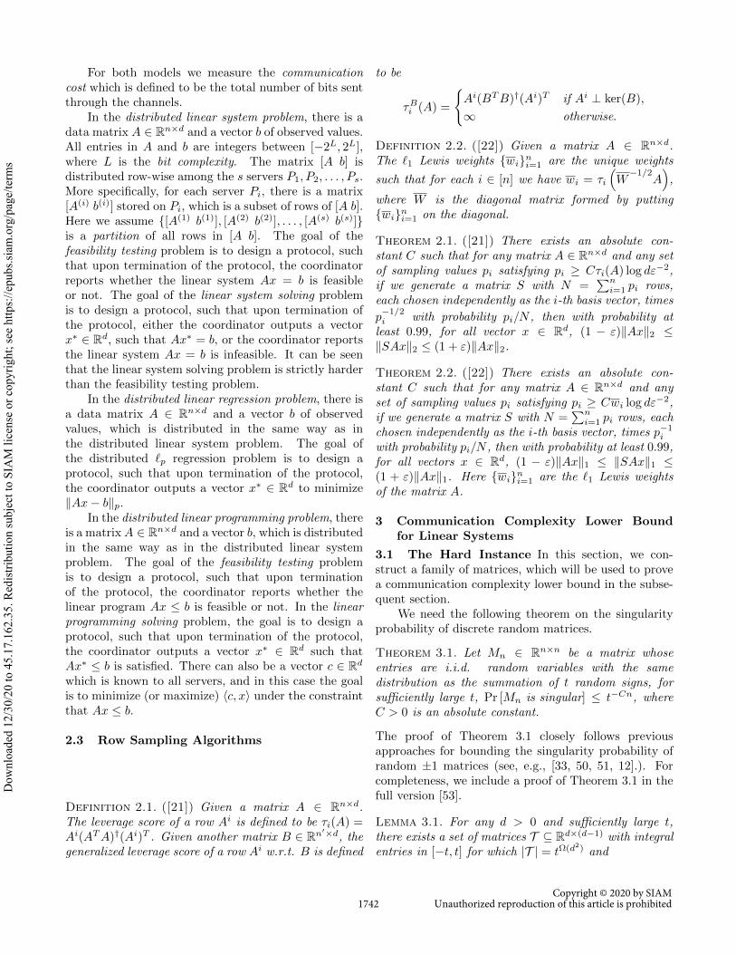
For both models we measure the communicationcost which is defined to be the total number of bits sentthrough the channels.

In the distributed linear system problem, there is adata matrix A ∈ Rn×d and a vector b of observed values.All entries in A and b are integers between [−2L, 2L],where L is the bit complexity. The matrix [A b] isdistributed row-wise among the s servers P1, P2, . . . , Ps.More specifically, for each server Pi, there is a matrix[A(i) b(i)] stored on Pi, which is a subset of rows of [A b].Here we assume [A(1) b(1)], [A(2) b(2)], . . . , [A(s) b(s)]is a partition of all rows in [A b]. The goal of thefeasibility testing problem is to design a protocol, suchthat upon termination of the protocol, the coordinatorreports whether the linear system Ax = b is feasibleor not. The goal of the linear system solving problemis to design a protocol, such that upon termination ofthe protocol, either the coordinator outputs a vectorx∗ ∈ Rd, such that Ax∗ = b, or the coordinator reportsthe linear system Ax = b is infeasible. It can be seenthat the linear system solving problem is strictly harderthan the feasibility testing problem.

In the distributed linear regression problem, there isa data matrix A ∈ Rn×d and a vector b of observedvalues, which is distributed in the same way as inthe distributed linear system problem. The goal ofthe distributed ‘p regression problem is to design aprotocol, such that upon termination of the protocol,the coordinator outputs a vector x∗ ∈ Rd to minimizekAx− bkp.

In the distributed linear programming problem, thereis a matrix A ∈ Rn×d and a vector b, which is distributedin the same way as in the distributed linear systemproblem. The goal of the feasibility testing problemis to design a protocol, such that upon terminationof the protocol, the coordinator reports whether thelinear program Ax ≤ b is feasible or not. In the linearprogramming solving problem, the goal is to design aprotocol, such that upon termination of the protocol,the coordinator outputs a vector x∗ ∈ Rd such thatAx∗ ≤ b is satisfied. There can also be a vector c ∈ Rdwhich is known to all servers, and in this case the goalis to minimize (or maximize) hc, xi under the constraintthat Ax ≤ b.

2.3 Row Sampling Algorithms

Definition 2.1. ([21]) Given a matrix A ∈ Rn×d.The leverage score of a row Ai is defined to be τi(A) =Ai(ATA)†(Ai)T . Given another matrix B ∈ Rn0×d, thegeneralized leverage score of a row Ai w.r.t. B is defined

to be

τBi (A) =

(Ai(BTB)†(Ai)T if Ai ⊥ ker(B),

∞ otherwise.

Definition 2.2. ([22]) Given a matrix A ∈ Rn×d.The ‘1 Lewis weights wini=1 are the unique weights

such that for each i ∈ [n] we have wi = τi W−1/2

A ,

where W is the diagonal matrix formed by puttingwini=1 on the diagonal.

Theorem 2.1. ([21]) There exists an absolute con-stant C such that for any matrix A ∈ Rn×d and any setof sampling values pi satisfying pi ≥ Cτi(A) log dε−2,if we generate a matrix S with N =

Pni=1 pi rows,

each chosen independently as the i-th basis vector, times

p−1/2i with probability pi/N , then with probability at

least 0.99, for all vector x ∈ Rd, (1 − ε)kAxk2 ≤kSAxk2 ≤ (1 + ε)kAxk2.

Theorem 2.2. ([22]) There exists an absolute con-stant C such that for any matrix A ∈ Rn×d and anyset of sampling values pi satisfying pi ≥ Cwi log dε−2,if we generate a matrix S with N =

Pni=1 pi rows, each

chosen independently as the i-th basis vector, times p−1i

with probability pi/N , then with probability at least 0.99,for all vectors x ∈ Rd, (1 − ε)kAxk1 ≤ kSAxk1 ≤(1 + ε)kAxk1. Here wini=1 are the ‘1 Lewis weightsof the matrix A.

3 Communication Complexity Lower Boundfor Linear Systems

3.1 The Hard Instance In this section, we con-struct a family of matrices, which will be used to provea communication complexity lower bound in the subse-quent section.

We need the following theorem on the singularityprobability of discrete random matrices.

Theorem 3.1. Let Mn ∈ Rn×n be a matrix whoseentries are i.i.d. random variables with the samedistribution as the summation of t random signs, forsufficiently large t, Pr [Mn is singular] ≤ t−Cn, whereC > 0 is an absolute constant.

The proof of Theorem 3.1 closely follows previousapproaches for bounding the singularity probability ofrandom ±1 matrices (see, e.g., [33, 50, 51, 12].). Forcompleteness, we include a proof of Theorem 3.1 in thefull version [53].

Lemma 3.1. For any d > 0 and sufficiently large t,there exists a set of matrices T ⊆ Rd×(d−1) with integralentries in [−t, t] for which |T | = tΩ(d2) and



Dow

nloa

ded

12/3

0/20

to 4

5.17

.162

.35.

Red

istri

butio

n su

bjec

t to

SIA

M li

cens

e or

cop

yrig

ht; s

ee h

ttps:

//epu

bs.si

am.o

rg/p

age/

term

s

1. For any T ∈ T , rank(T ) = d− 1;

2. For any S, T ∈ T such that S 6= T , span([S T ]) =Rd.

Proof. We use the probabilisitic method to prove the ex-istence. The proof can be found in the full version [53].

The following lemma can be easily proved usingLemma 3.1. See the full version [53] for the formal proof.

Lemma 3.2. For any d > 0 and sufficiently large t,there exists a set of matrices H ⊆ Rd×d with integralentries in [−t, t] for which |H| = tΩ(d2) and

1. For any T ∈ H, T is non-singular;

2. For any S, T ∈ H, S−1ed 6= T−1ed, where ed is thed-th standard basis vector.

3.2 Deterministic Lower Bound for the EqualityProblem In this section, we prove our deterministiccommunication complexity lower bound for the Equalityproblem in the coordinator model, which will be used asan intermediate problem in Section 3.3. In the Equalityproblem, each server Pi receives a binary string ti ∈0, 1n. The goal is to test whether t1 = t2 = . . . = ts.We will prove an Ω(sn) lower bound for deterministiccommunication protocols. The case s = 2 has a well-known Ω(n) lower bound.

Lemma 3.3. (See, e.g., [36, p11]) Any deterministicprotocol for solving the Equality problem with s = 2requires Ω(n) bits of communication.

Our plan is to reduce the case s = 2 to the cases > 2, using the symmetrization technique [43, 57]. Inthe full version [53], we prove the following theorem.

Theorem 3.2. Any deterministic protocol for solvingthe Equality problem with s servers in the coordinatormodel requires Ω(sn) bits of communication.

3.3 Deterministic Lower Bound for TestingFeasibility of Linear Systems In this section, wepresent our deterministic communication complexitylower bound for testing the feasibility of linear systems,in the coordinator model and the blackboard model.The proof can be found in the full version [53].

Theorem 3.3. For any deterministic protocol P,

• If P can test whether Ax = b is feasible or notin the coordinator model, then the communicationcomplexity of P is Ω(sd2L);

• If P can test whether Ax = b is feasible or notin the blackboard model, then the communicationcomplexity of P is Ω(s + d2L);

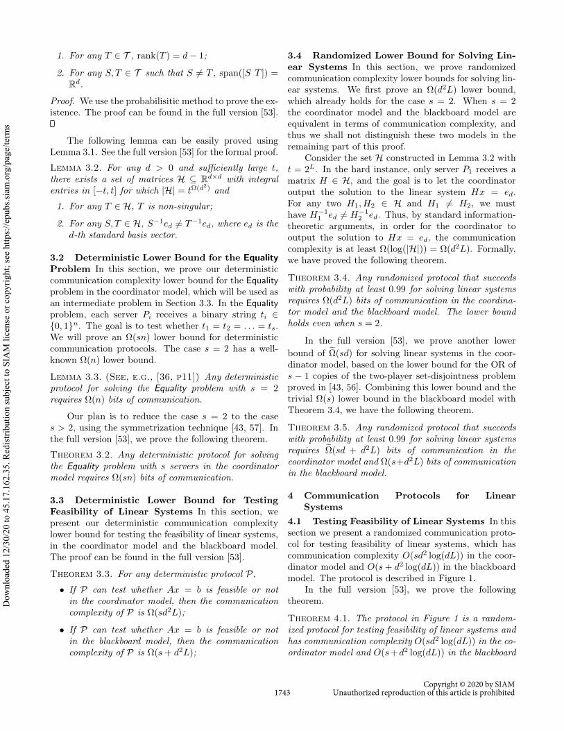
3.4 Randomized Lower Bound for Solving Lin-ear Systems In this section, we prove randomizedcommunication complexity lower bounds for solving lin-ear systems. We first prove an Ω(d2L) lower bound,which already holds for the case s = 2. When s = 2the coordinator model and the blackboard model areequivalent in terms of communication complexity, andthus we shall not distinguish these two models in theremaining part of this proof.

Consider the set H constructed in Lemma 3.2 witht = 2L. In the hard instance, only server P1 receives amatrix H ∈ H, and the goal is to let the coordinatoroutput the solution to the linear system Hx = ed.For any two H1, H2 ∈ H and H1 6= H2, we musthave H−1

1 ed 6= H−12 ed. Thus, by standard information-

theoretic arguments, in order for the coordinator tooutput the solution to Hx = ed, the communicationcomplexity is at least Ω(log(|H|)) = Ω(d2L). Formally,we have proved the following theorem.

Theorem 3.4. Any randomized protocol that succeedswith probability at least 0.99 for solving linear systemsrequires Ω(d2L) bits of communication in the coordina-tor model and the blackboard model. The lower boundholds even when s = 2.

In the full version [53], we prove another lower

bound of eΩ(sd) for solving linear systems in the coor-dinator model, based on the lower bound for the OR ofs − 1 copies of the two-player set-disjointness problemproved in [43, 56]. Combining this lower bound and thetrivial Ω(s) lower bound in the blackboard model withTheorem 3.4, we have the following theorem.

Theorem 3.5. Any randomized protocol that succeedswith probability at least 0.99 for solving linear systemsrequires eΩ(sd + d2L) bits of communication in thecoordinator model and Ω(s+d2L) bits of communicationin the blackboard model.

4 Communication Protocols for LinearSystems

4.1 Testing Feasibility of Linear Systems In thissection we present a randomized communication proto-col for testing feasibility of linear systems, which hascommunication complexity O(sd2 log(dL)) in the coor-dinator model and O(s + d2 log(dL)) in the blackboardmodel. The protocol is described in Figure 1.

In the full version [53], we prove the followingtheorem.

Theorem 4.1. The protocol in Figure 1 is a random-ized protocol for testing feasibility of linear systems andhas communication complexity O(sd2 log(dL)) in the co-ordinator model and O(s+d2 log(dL)) in the blackboard



Dow

nloa

ded

12/3

0/20

to 4

5.17

.162

.35.

Red

istri

butio

n su

bjec

t to

SIA

M li

cens

e or

cop

yrig

ht; s

ee h

ttps:

//epu

bs.si

am.o

rg/p

age/

term

s

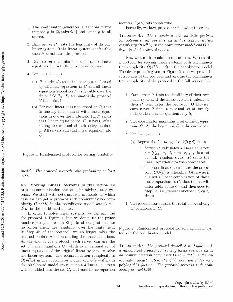
1. The coordinator generates a random primenumber p in [2,poly(dL)] and sends p to allservers.

2. Each server Pi tests the feasibility of its ownlinear system. If the linear system is infeasiblethen Pi terminates the protocol.

3. Each server maintains the same set of linearequations C. Initially C is the empty set.

4. For i = 1, 2, . . . , s

(a) Pi checks whether the linear system formedby all linear equations in C and all linearequations stored on Pi is feasible over thefinite field Fp. Pi terminates the protocolif it is infeasible.

(b) For each linear equation stored on Pi thatis linearly independent with linear equa-tions in C over the finite field Fp, Pi sendsthat linear equation to all servers, aftertaking the residual of each entry modulop. All servers add that linear equation intoC.

Figure 1: Randomized protocol for testing feasibility

model. The protocol succeeds with probability at least0.99.

4.2 Solving Linear Systems In this section wepresent communication protocols for solving linear sys-tems. We start with deterministic protocols, in whichcase we can get a protocol with communication com-plexity O(sd2L) in the coordinator model and O(s +d2L) in the blackboard model.

In order to solve linear systems, we can still usethe protocol in Figure 1, but we don’t use the primenumber p any more. In Step 4a of the protocol, weno longer check the feasibility over the finite field.In Step 4b of the protocol, we no longer takes theresidual modulo p before sending the linear equations.At the end of the protocol, each server can use theset of linear equations C, which is a maximal set oflinear equations of the original linear system, to solvethe linear system. The communication complexity isO(sd2L) in the coordinator model and O(s + d2L) inthe blackboard model since at most d linear equationswill be added into the set C, and each linear equation

requires O(dL) bits to describe.Formally, we have proved the following theorem.

Theorem 4.2. There exists a deterministic protocolfor solving linear systems which has communicationcomplexity O(sd2L) in the coordinator model and O(s+d2L) in the blackboard model.

Now we turn to randomized protocols. We describea protocol for solving linear systems with communica-tion complexity eO(d2L + sd) in the coordinator model.The description is given in Figure 2, and we prove thecorrectness of the protocol and analyze the communica-tion complexity of the protocol in the full version [53].

1. Each server Pi tests the feasibility of their ownlinear system. If the linear system is infeasiblethen Pi terminates the protocol. Otherwise,each server Pi finds a maximal set of linearlyindependent linear equations, say Si.

2. The coordinator maintains a set of linear equa-tions C. At the beginning C is the empty set.

3. For i = 1, 2, . . . , s

(a) Repeat the followings for O(log d) times

i. Server Pi calculates a linear equationc =

Pt∈Si rt · t, here rtt∈Si is a set

of i.i.d. random signs. Pi sends thelinear equation c to the coordinator.

ii. The coordinator terminates the proto-col if C∪c is infeasible. Otherwise ifc is not a linear combination of thoselinear equations in C, then the coordi-nator adds c into C, and then goes toStep 3a, i.e., repeats another O(log d)times.

4. The coordinator obtains the solution by solvingall equations in C.

Figure 2: Randomized protocol for solving linear sys-tems in the coordinator model

Theorem 4.3. The protocol described in Figure 2 isa randomized protocol for solving linear systems whichhas communication complexity eO(sd + d2L) in the co-

ordinator model. Here the eO(·) notation hides onlypolylog(dL) factors. The protocol succeeds with prob-ability at least 0.99.



Dow

nloa

ded

12/3

0/20

to 4

5.17

.162

.35.

Red

istri

butio

n su

bjec

t to

SIA

M li

cens

e or

cop

yrig

ht; s

ee h

ttps:

//epu

bs.si

am.o

rg/p

age/

term

s

5 Communication Complexity Lower Boundsfor Linear Regression in the BlackboardModel

In this section, we prove communication complexitylower bounds for linear regression in the blackboardmodel.

We first define the k-XOR problem and the k-MAJ problem. In the blackboard model, each serverPi receives a binary string xi ∈ 0, 1d. In the k-XORproblem, at the end of a communication protocol, thecoordinator correctly outputs the coordinate-wise XORof these vectors, for at least 0.99d coordinates. In the k-MAJ problem, at the end of a communication protocol,the coordinator correctly outputs the coordinate-wisemajority of these vectors, for at least 0.99d coordinates.

We need the following lemma for our lower boundproof, whose proof can be found in the full version [53].

Lemma 5.1. Any randomized communication protocolthat solves the k-XOR problem or the k-MAJ problemand succeeds with probability at least 0.99 has commu-nication complexity Ω(dk).

In the full version [53], we give a reduction fromk-MAJ to (1 + ε)-approximate ‘1 regression in theblackboard model, and prove an Ω(d/ε) lower boundwhen s > Ω(1/ε). We also give a reduction from k-XORto (1 + ε)-approximate ‘2 regression in the blackboardmodel, and prove an Ω(d/

√ε) lower bound when s >

Ω(1/√ε). These reductions, together with Lemma 5.1,

lead to the following theorems.

Theorem 5.1. When s > Ω(1/ε), any randomizedprotocol that succeeds with probability at least 0.99 forsolving (1+ε)-approximate ‘1 regression requires Ω(d/ε)bits of communication in the blackboard model.

Theorem 5.2. When s > Ω(1/√ε), any randomized

protocol that succeeds with probability at least 0.99for solving (1 + ε)-approximate ‘2 regression requiresΩ(d/

√ε) bits of communication in the blackboard model.

6 Communication Protocols for ‘2 Regression

In this section, we design distributed protocols forsolving the ‘2 regression problem.

6.1 A Deterministic Protocol In this section, wedesign a simple deterministic protocol for ‘2 regressionin the distributed setting with communication complex-ity eO(sd2L) in the coordinator model.

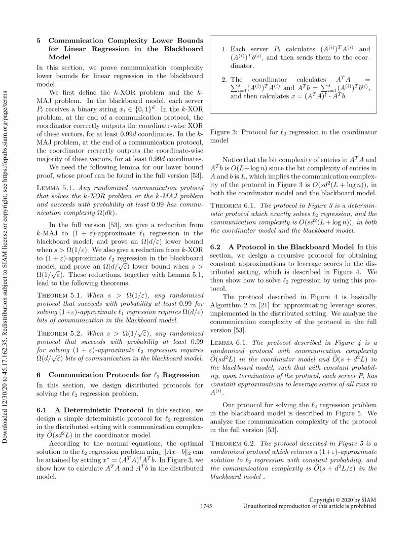
According to the normal equations, the optimalsolution to the ‘2 regression problem minx kAx−bk2 canbe attained by setting x∗ = (ATA)†AT b. In Figure 3, weshow how to calculate ATA and AT b in the distributedmodel.

1. Each server Pi calculates (A(i))TA(i) and(A(i))T b(i), and then sends them to the coor-dinator.

2. The coordinator calculates ATA =Psi=1(A(i))TA(i) and AT b =

Psi=1(A(i))T b(i),

and then calculates x = (ATA)† ·AT b.

Figure 3: Protocol for ‘2 regression in the coordinatormodel

Notice that the bit complexity of entries in ATA andAT b is O(L+log n) since the bit complexity of entries inA and b is L, which implies the communication complex-ity of the protocol in Figure 3 is O(sd2(L + log n)), inboth the coordinator model and the blackboard model.

Theorem 6.1. The protocol in Figure 3 is a determin-istic protocol which exactly solves ‘2 regression, and thecommunication complexity is O(sd2(L+ log n)), in boththe coordinator model and the blackboard model.

6.2 A Protocol in the Blackboard Model In thissection, we design a recursive protocol for obtainingconstant approximations to leverage scores in the dis-tributed setting, which is described in Figure 4. Wethen show how to solve ‘2 regression by using this pro-tocol.

The protocol described in Figure 4 is basicallyAlgorithm 2 in [21] for approximating leverage scores,implemented in the distributed setting. We analyze thecommunication complexity of the protocol in the fullversion [53].

Lemma 6.1. The protocol described in Figure 4 is arandomized protocol with communication complexityeO(sd2L) in the coordinator model and eO(s + d2L) inthe blackboard model, such that with constant probabil-ity, upon termination of the protocol, each server Pi hasconstant approximations to leverage scores of all rows inA(i).

Our protocol for solving the ‘2 regression problemin the blackboard model is described in Figure 5. Weanalyze the communication complexity of the protocolin the full version [53].

Theorem 6.2. The protocol described in Figure 5 is arandomized protocol which returns a (1+ε)-approximatesolution to ‘2 regression with constant probability, andthe communication complexity is eO(s + d2L/ε) in theblackboard model .



Dow

nloa

ded

12/3

0/20

to 4

5.17

.162

.35.

Red

istri

butio

n su

bjec

t to

SIA

M li

cens

e or

cop

yrig

ht; s

ee h

ttps:

//epu

bs.si

am.o

rg/p

age/

term

s

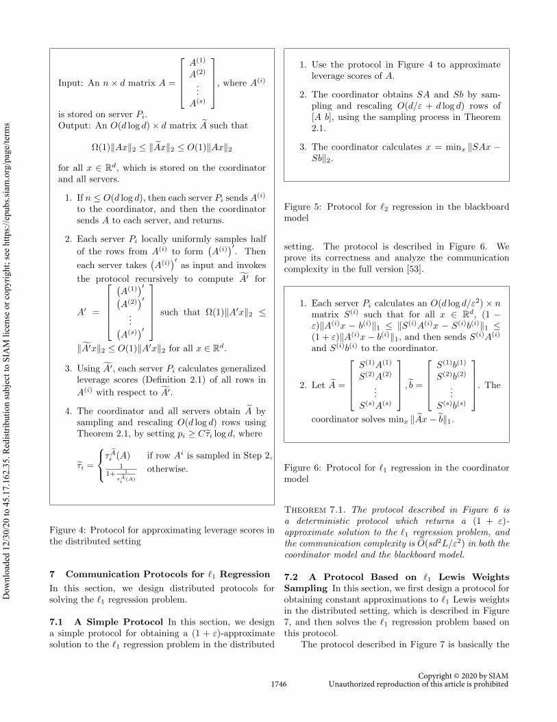
Input: An n× d matrix A =

A(1)

A(2)

...A(s)

, where A(i)

is stored on server Pi.Output: An O(d log d)× d matrix eA such that

Ω(1)kAxk2 ≤ k eAxk2 ≤ O(1)kAxk2

for all x ∈ Rd, which is stored on the coordinatorand all servers.

1. If n ≤ O(d log d), then each server Pi sends A(i)

to the coordinator, and then the coordinatorsends A to each server, and returns.

2. Each server Pi locally uniformly samples half

of the rows from A(i) to form A(i) 0. Then

each server takes A(i) 0as input and invokes

the protocol recursively to compute fA0 for

A0 =

A(1) 0

A(2) 0

...

A(s) 0

such that Ω(1)kA0xk2 ≤

kfA0xk2 ≤ O(1)kA0xk2 for all x ∈ Rd.

3. Using fA0, each server Pi calculates generalizedleverage scores (Definition 2.1) of all rows in

A(i) with respect to fA0.

4. The coordinator and all servers obtain eA bysampling and rescaling O(d log d) rows usingTheorem 2.1, by setting pi ≥ Ceτi log d, where

eτi =

τeAi (A) if row Ai is sampled in Step 2,

11+ 1

τeAi

(A)

otherwise.

Figure 4: Protocol for approximating leverage scores inthe distributed setting

7 Communication Protocols for ‘1 Regression

In this section, we design distributed protocols forsolving the ‘1 regression problem.

7.1 A Simple Protocol In this section, we designa simple protocol for obtaining a (1 + ε)-approximatesolution to the ‘1 regression problem in the distributed

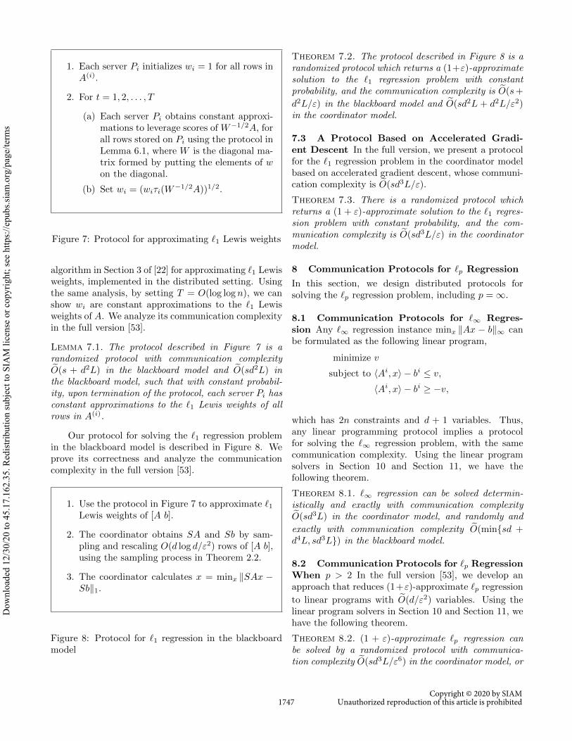
1. Use the protocol in Figure 4 to approximateleverage scores of A.

2. The coordinator obtains SA and Sb by sam-pling and rescaling O(d/ε + d log d) rows of[A b], using the sampling process in Theorem2.1.

3. The coordinator calculates x = minx kSAx −Sbk2.

Figure 5: Protocol for ‘2 regression in the blackboardmodel

setting. The protocol is described in Figure 6. Weprove its correctness and analyze the communicationcomplexity in the full version [53].

1. Each server Pi calculates an O(d log d/ε2)× nmatrix S(i) such that for all x ∈ Rd, (1 −ε)kA(i)x − b(i)k1 ≤ kS(i)A(i)x − S(i)b(i)k1 ≤(1 + ε)kA(i)x− b(i)k1, and then sends S(i)A(i)

and S(i)b(i) to the coordinator.

2. Let eA =

S(1)A(1)

S(2)A(2)

...S(s)A(s)

,eb =

S(1)b(1)

S(2)b(2)

...S(s)b(s)

. The

coordinator solves minx k eAx−ebk1.

Figure 6: Protocol for ‘1 regression in the coordinatormodel

Theorem 7.1. The protocol described in Figure 6 isa deterministic protocol which returns a (1 + ε)-approximate solution to the ‘1 regression problem, andthe communication complexity is eO(sd2L/ε2) in both thecoordinator model and the blackboard model.

7.2 A Protocol Based on ‘1 Lewis WeightsSampling In this section, we first design a protocol forobtaining constant approximations to ‘1 Lewis weightsin the distributed setting, which is described in Figure7, and then solves the ‘1 regression problem based onthis protocol.

The protocol described in Figure 7 is basically the



Dow

nloa

ded

12/3

0/20

to 4

5.17

.162

.35.

Red

istri

butio

n su

bjec

t to

SIA

M li

cens

e or

cop

yrig

ht; s

ee h

ttps:

//epu

bs.si

am.o

rg/p

age/

term

s

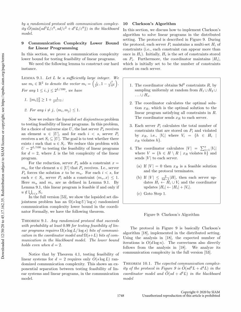
1. Each server Pi initializes wi = 1 for all rows inA(i).

2. For t = 1, 2, . . . , T

(a) Each server Pi obtains constant approxi-mations to leverage scores of W−1/2A, forall rows stored on Pi using the protocol inLemma 6.1, where W is the diagonal ma-trix formed by putting the elements of won the diagonal.

(b) Set wi = (wiτi(W−1/2A))1/2.

Figure 7: Protocol for approximating ‘1 Lewis weights

algorithm in Section 3 of [22] for approximating ‘1 Lewisweights, implemented in the distributed setting. Usingthe same analysis, by setting T = O(log log n), we canshow wi are constant approximations to the ‘1 Lewisweights of A. We analyze its communication complexityin the full version [53].

Lemma 7.1. The protocol described in Figure 7 is arandomized protocol with communication complexityeO(s + d2L) in the blackboard model and eO(sd2L) inthe blackboard model, such that with constant probabil-ity, upon termination of the protocol, each server Pi hasconstant approximations to the ‘1 Lewis weights of allrows in A(i).

Our protocol for solving the ‘1 regression problemin the blackboard model is described in Figure 8. Weprove its correctness and analyze the communicationcomplexity in the full version [53].

1. Use the protocol in Figure 7 to approximate ‘1

Lewis weights of [A b].

2. The coordinator obtains SA and Sb by sam-pling and rescaling O(d log d/ε2) rows of [A b],using the sampling process in Theorem 2.2.

3. The coordinator calculates x = minx kSAx −Sbk1.

Figure 8: Protocol for ‘1 regression in the blackboardmodel

Theorem 7.2. The protocol described in Figure 8 is arandomized protocol which returns a (1+ε)-approximatesolution to the ‘1 regression problem with constantprobability, and the communication complexity is eO(s+

d2L/ε) in the blackboard model and eO(sd2L + d2L/ε2)in the coordinator model.

7.3 A Protocol Based on Accelerated Gradi-ent Descent In the full version, we present a protocolfor the ‘1 regression problem in the coordinator modelbased on accelerated gradient descent, whose communi-cation complexity is eO(sd3L/ε).

Theorem 7.3. There is a randomized protocol whichreturns a (1 + ε)-approximate solution to the ‘1 regres-sion problem with constant probability, and the com-munication complexity is eO(sd3L/ε) in the coordinatormodel.

8 Communication Protocols for ‘p Regression

In this section, we design distributed protocols forsolving the ‘p regression problem, including p =∞.

8.1 Communication Protocols for ‘∞ Regres-sion Any ‘∞ regression instance minx kAx − bk∞ canbe formulated as the following linear program,

minimize v

subject to hAi, xi − bi ≤ v,

hAi, xi − bi ≥ −v,

which has 2n constraints and d + 1 variables. Thus,any linear programming protocol implies a protocolfor solving the ‘∞ regression problem, with the samecommunication complexity. Using the linear programsolvers in Section 10 and Section 11, we have thefollowing theorem.

Theorem 8.1. ‘∞ regression can be solved determin-istically and exactly with communication complexityeO(sd3L) in the coordinator model, and randomly and

exactly with communication complexity eO(minsd +d4L, sd3L) in the blackboard model.

8.2 Communication Protocols for ‘p RegressionWhen p > 2 In the full version [53], we develop anapproach that reduces (1+ε)-approximate ‘p regression

to linear programs with eO(d/ε2) variables. Using thelinear program solvers in Section 10 and Section 11, wehave the following theorem.

Theorem 8.2. (1 + ε)-approximate ‘p regression canbe solved by a randomized protocol with communica-tion complexity eO(sd3L/ε6) in the coordinator model, or



Dow

nloa

ded

12/3

0/20

to 4

5.17

.162

.35.

Red

istri

butio

n su

bjec

t to

SIA

M li

cens

e or

cop

yrig

ht; s

ee h

ttps:

//epu

bs.si

am.o

rg/p

age/

term

s

by a randomized protocol with communication complex-ity eO(minsd3L/ε6, sd/ε2 + d4L/ε8) in the blackboardmodel.

9 Communication Complexity Lower Boundfor Linear Programming

In this section, we prove a communication complexitylower bound for testing feasibility of linear programs.

We need the following lemma to construct our hardinstance.

Lemma 9.1. Let L be a sufficiently large integer. We

use mi ∈ R2 to denote the vector mi = i2L

, 1− i2

2·4L .

For any 1 ≤ i, j ≤ 2L/100, we have

1. kmik22 ≥ 1 + 124L+2 ;

2. For any i 6= j, hmi,mji ≤ 1.

Now we reduce the lopsided set disjiontness problemto testing feasibility of linear programs. In this problem,for a choice of universe size U , the last server Ps receivesan element u ∈ [U ], and for each i < s, server Pireceives a set Si ⊆ [U ]. The goal is to test whether thereexists i such that u ∈ Si. We reduce this problem withU = 2L/100 to testing the feasibility of linear programsfor d = 2, where L is the bit complexity of the linearprogram.

For the reduction, server Ps adds a constraint x =mu, for the element u ∈ [U ] that Ps receives. I.e., serverPs forces the solution x to be mu. For each i < s, foreach v ∈ Si, server Pi adds a constraint hmv, xi ≤ 1.Here mu and mv are as defined in Lemma 9.1. ByLemma 9.1, this linear program is feasible if and only ifu /∈

Si<s Si.

In the full version [53], we show the lopsided set dis-jointness problem has an Ω(s logU/ log s) randomizedcommunication complexity lower bound in the coordi-nator Formally, we have the following theorem.

Theorem 9.1. Any randomized protocol that succeedswith probability at least 0.99 for testing feasibility of lin-ear programs requires Ω(s logL/ log s) bits of communi-cation in the coordinator model and Ω(s+L) bits of com-munication in the blackboard model. The lower boundholds even when d = 2.

Notice that by Theorem 4.1, testing feasibility oflinear systems for d = 2 requires only O(s logL) ran-domized communication complexity. This shows an ex-ponential separation between testing feasibility of lin-ear systems and linear programs, in the communicationmodel.

10 Clarkson’s Algorithm

In this section, we discuss how to implement Clarkson’salgorithm to solve linear programs in the distributedsetting. The protocol is described in Figure 9. Duringthe protocol, each server Pi maintains a multi-set Hi ofconstraints (i.e., each constraint can appear more thanonce in Hi). Initially, Hi is the set of constraints storedon Pi. Furthermore, the coordinator maintains |Hi|,which is initially set to be the number of constraintsstored on each server.

1. The coordinator obtains 9d2 constraints R, bysampling uniformly at random from H1 ∪H2 ∪. . . ∪Hs.

2. The coordinator calculates the optimal solu-tion xR, which is the optimal solution to thelinear program satisfying all constraints in R.The coordinator sends xR to each server.

3. Each server Pi calculates the total number ofconstraints that are stored on Pi and violatedby xR, i.e., |Vi| where Vi = h ∈ Hi |xR violates h.

4. The coordinator calculates |V | =Psi=1 |Vi|

where V = h ∈ H \ R | xR violates h andsends |V | to each server.

(a) If |V | = 0 then xR is a feasible solutionand the protocol terminates.

(b) If |V | ≤ 29d−1 |H|, then each server up-

dates Hi ← Hi ∪ Vi and the coordinatorupdates |Hi| ← |Hi|+ |Vi|.

(c) Goto Step 1.

Figure 9: Clarkson’s Algorithm

The protocol in Figure 9 is basically Clarkson’salgorithm [18], implemented in the distributed setting.Using the analysis in [18], the expected number ofiterations is O(d log n). The correctness also directlyfollows from the analysis in [18]. We analyze itscommunication complexity in the full version [53].

Theorem 10.1. The expected communication complex-ity of the protocol in Figure 9 is eO(sd3L + d4L) in the

coordinator model and eO(sd + d4L) in the blackboardmodel



Dow

nloa

ded

12/3

0/20

to 4

5.17

.162

.35.

Red

istri

butio

n su

bjec

t to

SIA

M li

cens

e or

cop

yrig

ht; s

ee h

ttps:

//epu

bs.si

am.o

rg/p

age/

term

s

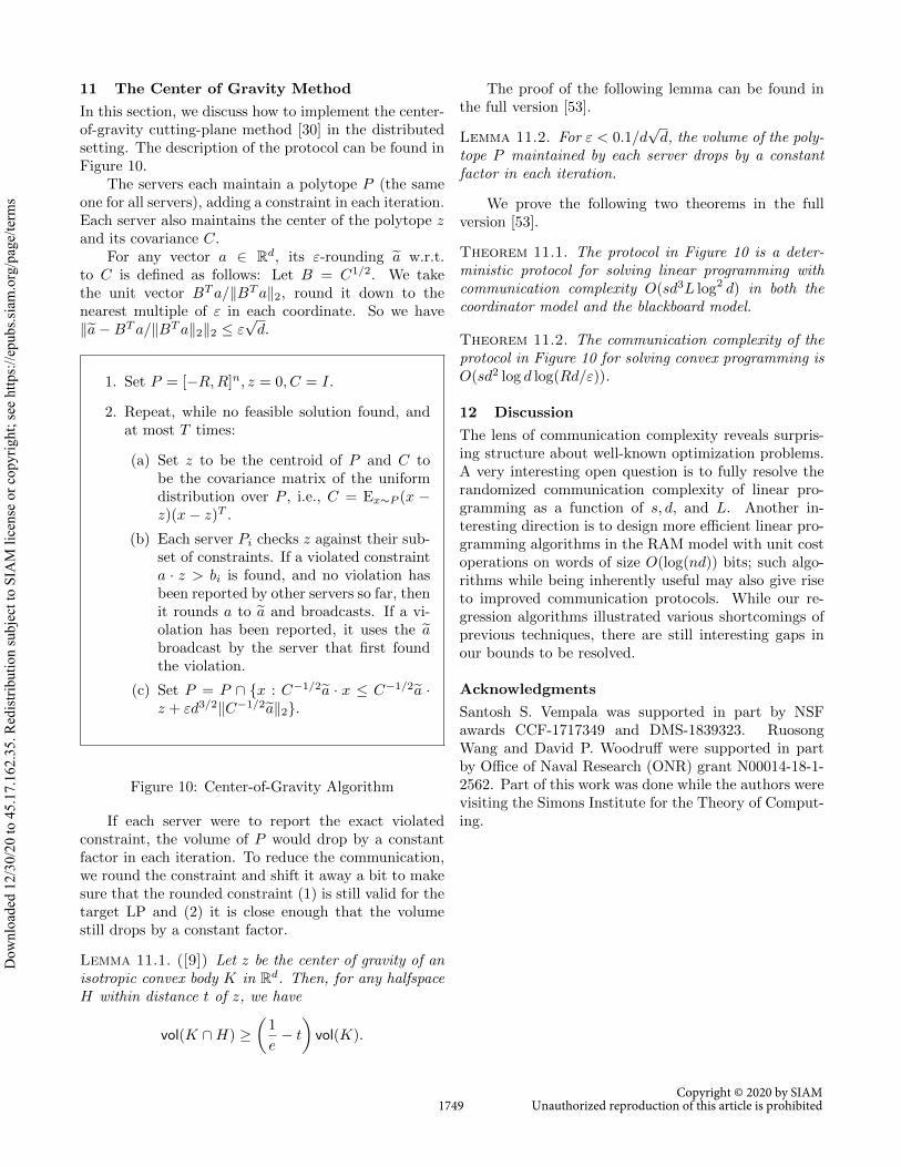
11 The Center of Gravity Method

In this section, we discuss how to implement the center-of-gravity cutting-plane method [30] in the distributedsetting. The description of the protocol can be found inFigure 10.

The servers each maintain a polytope P (the sameone for all servers), adding a constraint in each iteration.Each server also maintains the center of the polytope zand its covariance C.

For any vector a ∈ Rd, its ε-rounding ea w.r.t.to C is defined as follows: Let B = C1/2. We takethe unit vector BTa/kBTak2, round it down to thenearest multiple of ε in each coordinate. So we havekea−BTa/kBTak2k2 ≤ ε

√d.

1. Set P = [−R,R]n, z = 0, C = I.

2. Repeat, while no feasible solution found, andat most T times:

(a) Set z to be the centroid of P and C tobe the covariance matrix of the uniformdistribution over P , i.e., C = Ex∼P (x −z)(x− z)T .

(b) Each server Pi checks z against their sub-set of constraints. If a violated constrainta · z > bi is found, and no violation hasbeen reported by other servers so far, thenit rounds a to ea and broadcasts. If a vi-olation has been reported, it uses the eabroadcast by the server that first foundthe violation.

(c) Set P = P ∩ x : C−1/2ea · x ≤ C−1/2ea ·z + εd3/2kC−1/2eak2.

Figure 10: Center-of-Gravity Algorithm

If each server were to report the exact violatedconstraint, the volume of P would drop by a constantfactor in each iteration. To reduce the communication,we round the constraint and shift it away a bit to makesure that the rounded constraint (1) is still valid for thetarget LP and (2) it is close enough that the volumestill drops by a constant factor.

Lemma 11.1. ([9]) Let z be the center of gravity of anisotropic convex body K in Rd. Then, for any halfspaceH within distance t of z, we have

vol(K ∩H) ≥ 1

e− t vol(K).

The proof of the following lemma can be found inthe full version [53].

Lemma 11.2. For ε < 0.1/d√d, the volume of the poly-

tope P maintained by each server drops by a constantfactor in each iteration.

We prove the following two theorems in the fullversion [53].

Theorem 11.1. The protocol in Figure 10 is a deter-ministic protocol for solving linear programming withcommunication complexity O(sd3L log2 d) in both thecoordinator model and the blackboard model.

Theorem 11.2. The communication complexity of theprotocol in Figure 10 for solving convex programming isO(sd2 log d log(Rd/ε)).

12 Discussion

The lens of communication complexity reveals surpris-ing structure about well-known optimization problems.A very interesting open question is to fully resolve therandomized communication complexity of linear pro-gramming as a function of s, d, and L. Another in-teresting direction is to design more efficient linear pro-gramming algorithms in the RAM model with unit costoperations on words of size O(log(nd)) bits; such algo-rithms while being inherently useful may also give riseto improved communication protocols. While our re-gression algorithms illustrated various shortcomings ofprevious techniques, there are still interesting gaps inour bounds to be resolved.

Acknowledgments

Santosh S. Vempala was supported in part by NSFawards CCF-1717349 and DMS-1839323. RuosongWang and David P. Woodruff were supported in partby Office of Naval Research (ONR) grant N00014-18-1-2562. Part of this work was done while the authors werevisiting the Simons Institute for the Theory of Comput-ing.



Dow

nloa

ded

12/3

0/20

to 4

5.17

.162

.35.

Red

istri

butio

n su

bjec

t to

SIA

M li

cens

e or

cop

yrig

ht; s

ee h

ttps:

//epu

bs.si

am.o

rg/p

age/

term

s

References

[1] Alekh Agarwal, Olivier Chapelle, Miroslav Dudık,and John Langford. A reliable effective terascalelinear learning system. Journal of Machine LearningResearch, 15(1):1111–1133, 2014.

[2] Alexandr Andoni. High frequency moments via max-stability. In Acoustics, Speech and Signal Processing(ICASSP), 2017 IEEE International Conference on,pages 6364–6368. IEEE, 2017.

[3] Alexandr Andoni et al. Eigenvalues of a matrix in thestreaming model. In Proceedings of the twenty-fourthannual ACM-SIAM symposium on Discrete algorithms,pages 1729–1737. Society for Industrial and AppliedMathematics, 2013.

[4] Yossi Arjevani and Ohad Shamir. Communicationcomplexity of distributed convex learning and opti-mization. In Advances in Neural Information Process-ing Systems 28: Annual Conference on Neural Infor-mation Processing Systems 2015, December 7-12, 2015,Montreal, Quebec, Canada, pages 1756–1764, 2015.

[5] Sepehr Assadi, Nikolai Karpov, and Qin Zhang. Dis-tributed and streaming linear programming in low di-mensions. In Proceedings of the 38th ACM SIGMOD-SIGACT-SIGAI Symposium on Principles of DatabaseSystems, pages 236–253. ACM, 2019.

[6] Sepehr Assadi and Sanjeev Khanna. Randomized com-posable coresets for matching and vertex cover. In Pro-ceedings of the 29th ACM Symposium on Parallelismin Algorithms and Architectures, SPAA 2017, Wash-ington DC, USA, July 24-26, 2017, pages 3–12, 2017.

[7] Maria-Florina Balcan, Avrim Blum, Shai Fine, andYishay Mansour. Distributed learning, communicationcomplexity and privacy. In COLT 2012 - The 25thAnnual Conference on Learning Theory, June 25-27,2012, Edinburgh, Scotland, pages 26.1–26.22, 2012.

[8] Maria-Florina Balcan, Yingyu Liang, Le Song,David P. Woodruff, and Bo Xie. Communication ef-ficient distributed kernel principal component analy-sis. In Proceedings of the 22nd ACM SIGKDD Inter-national Conference on Knowledge Discovery and DataMining, San Francisco, CA, USA, August 13-17, 2016,pages 725–734, 2016.

[9] D. Bertsimas and S. Vempala. Solving convex pro-grams by random walks. J. ACM, 51(4):540–556, 2004.

[10] P Bickel, P Diggle, S Fienberg, U Gather, I Olkin, andS Zeger. Springer series in statistics. 2009.

[11] Avrim Blum and John Dunagan. Smoothed analysisof the perceptron algorithm for linear programming.In Proceedings of the thirteenth annual ACM-SIAMsymposium on Discrete algorithms, pages 905–914.Society for Industrial and Applied Mathematics, 2002.

[12] Jean Bourgain, Van H Vu, and Philip Matchett Wood.On the singularity probability of discrete random ma-trices. Journal of Functional Analysis, 258(2):559–603,2010.

[13] Christos Boutsidis, David P. Woodruff, and PeilinZhong. Optimal principal component analysis in dis-

tributed and streaming models. In Proceedings of the48th Annual ACM SIGACT Symposium on Theory ofComputing, STOC 2016, Cambridge, MA, USA, June18-21, 2016, pages 236–249, 2016.

[14] Stephen P. Boyd, Neal Parikh, Eric Chu, Borja Peleato,and Jonathan Eckstein. Distributed optimization andstatistical learning via the alternating direction methodof multipliers. Foundations and Trends in MachineLearning, 3(1):1–122, 2011.

[15] Mark Braverman, Ankit Garg, Tengyu Ma, Huy L.Nguyen, and David P. Woodruff. Communicationlower bounds for statistical estimation problems via adistributed data processing inequality. In Proceedingsof the 48th Annual ACM SIGACT Symposium onTheory of Computing, STOC 2016, Cambridge, MA,USA, June 18-21, 2016, pages 1011–1020, 2016.

[16] Emmanuel J Candes and Terence Tao. Decoding bylinear programming. IEEE Transactions on Informa-tion Theory, 51(12):4203–4215, 2005.

[17] Jiecao Chen, He Sun, David P. Woodruff, and QinZhang. Communication-optimal distributed cluster-ing. In Advances in Neural Information ProcessingSystems 29: Annual Conference on Neural Informa-tion Processing Systems 2016, December 5-10, 2016,Barcelona, Spain, pages 3720–3728, 2016.

[18] Kenneth L Clarkson. Las vegas algorithms for linearand integer programming when the dimension is small.Journal of the ACM (JACM), 42(2):488–499, 1995.

[19] Kenneth L. Clarkson and David P. Woodruff. Numer-ical linear algebra in the streaming model. In Proceed-ings of the 41st Annual ACM Symposium on Theoryof Computing, STOC 2009, Bethesda, MD, USA, May31 - June 2, 2009, pages 205–214, 2009.

[20] M. B. Cohen, Y. Tat Lee, and Z. Song. Solving LinearPrograms in the Current Matrix Multiplication Time.In STOC, 2019.

[21] Michael B Cohen, Yin Tat Lee, Cameron Musco,Christopher Musco, Richard Peng, and Aaron Sidford.Uniform sampling for matrix approximation. In Pro-ceedings of the 2015 Conference on Innovations in The-oretical Computer Science, pages 181–190. ACM, 2015.

[22] Michael B Cohen and Richard Peng. ‘p row sam-pling by lewis weights. In Proceedings of the forty-seventh annual ACM symposium on Theory of com-puting, pages 183–192. ACM, 2015.

[23] Graham Cormode, Charlie Dickens, and David P.Woodruff. Leveraging well-conditioned bases: Stream-ing and distributed summaries in minkowski p-norms.In Proceedings of the 35th International Conferenceon Machine Learning, ICML 2018, Stockholmsmassan,Stockholm, Sweden, July 10-15, 2018, pages 1048–1056,2018.

[24] Andrew Cotter, Ohad Shamir, Nati Srebro, andKarthik Sridharan. Better mini-batch algorithms viaaccelerated gradient methods. In Advances in neu-ral information processing systems, pages 1647–1655,2011.

[25] Ofer Dekel, Ran Gilad-Bachrach, Ohad Shamir, and



Dow

nloa

ded

12/3

0/20

to 4

5.17

.162

.35.

Red

istri

butio

n su

bjec

t to

SIA

M li

cens

e or

cop

yrig

ht; s

ee h

ttps:

//epu

bs.si

am.o

rg/p

age/

term

s

Lin Xiao. Optimal distributed online prediction usingmini-batches. Journal of Machine Learning Research,13(Jan):165–202, 2012.

[26] John C Duchi, Alekh Agarwal, and Martin J Wain-wright. Dual averaging for distributed optimization:Convergence analysis and network scaling. IEEETransactions on Automatic control, 57(3):592–606,2012.

[27] David Durfee, Kevin A Lai, and Saurabh Sawlani.‘1 regression using lewis weights preconditioning andstochastic gradient descent. In Conference On Learn-ing Theory, pages 1626–1656, 2018.

[28] Ankit Garg, Tengyu Ma, and Huy L. Nguyen. Oncommunication cost of distributed statistical estima-tion and dimensionality. In Advances in Neural In-formation Processing Systems 27: Annual Conferenceon Neural Information Processing Systems 2014, De-cember 8-13 2014, Montreal, Quebec, Canada, pages2726–2734, 2014.

[29] M. Grotschel, L. Lovasz, and A. Schrijver. Geometricalgorithms and combinatorial optimization. Springer,1988.

[30] B. Grunbaum. Partitions of mass-distributions andconvex bodies by hyperplanes. Pacific J. Math.,10:1257–1261, 1960.

[31] Dirk Van Gucht, Ryan Williams, David P. Woodruff,and Qin Zhang. The communication complexity of dis-tributed set-joins with applications to matrix multipli-cation. In Proceedings of the 34th ACM Symposiumon Principles of Database Systems, PODS 2015, Mel-bourne, Victoria, Australia, May 31 - June 4, 2015,pages 199–212, 2015.

[32] Martin Jaggi, Virginia Smith, Martin Takac, JonathanTerhorst, Sanjay Krishnan, Thomas Hofmann, andMichael I Jordan. Communication-efficient distributeddual coordinate ascent. In Advances in neural infor-mation processing systems, pages 3068–3076, 2014.

[33] Jeff Kahn, Janos Komlos, and Endre Szemeredi. Onthe probability that a random±1-matrix is singu-lar. Journal of the American Mathematical Society,8(1):223–240, 1995.

[34] Daniel M Kane, Roi Livni, Shay Moran, and AmirYehudayoff. On communication complexity of classi-fication problems. arXiv preprint arXiv:1711.05893,2017.

[35] Ravi Kannan, Santosh Vempala, and David P.Woodruff. Principal component analysis and highercorrelations for distributed data. In Proceedings ofThe 27th Conference on Learning Theory, COLT 2014,Barcelona, Spain, June 13-15, 2014, pages 1040–1057,2014.

[36] Eyal Kushilevitz and Noam Nisan. CommunicationComplexity. Cambridge University Press, New York,NY, USA, 1997.

[37] Yin Tat Lee and Aaron Sidford. Path finding methodsfor linear programming: Solving linear programs ino(vrank) iterations and faster algorithms for maximumflow. In 55th IEEE Annual Symposium on Foundations

of Computer Science, FOCS 2014, Philadelphia, PA,USA, October 18-21, 2014, pages 424–433, 2014.

[38] Yin Tat Lee and Aaron Sidford. Efficient inverse main-tenance and faster algorithms for linear programming.In IEEE 56th Annual Symposium on Foundations ofComputer Science, FOCS 2015, Berkeley, CA, USA,17-20 October, 2015, pages 230–249, 2015.

[39] Yingyu Liang, Maria-Florina Balcan, Vandana Kan-chanapally, and David P. Woodruff. Improved dis-tributed principal component analysis. In Advancesin Neural Information Processing Systems 27: AnnualConference on Neural Information Processing Systems2014, December 8-13 2014, Montreal, Quebec, Canada,pages 3113–3121, 2014.

[40] Dhruv Mahajan, S Sathiya Keerthi, S Sundararajan,and Leon Bottou. A parallel sgd method with strongconvergence. arXiv preprint arXiv:1311.0636, 2013.

[41] Xiangrui Meng and Michael W. Mahoney. Low-distortion subspace embeddings in input-sparsity timeand applications to robust linear regression. In Sympo-sium on Theory of Computing Conference, STOC’13,Palo Alto, CA, USA, June 1-4, 2013, pages 91–100,2013.

[42] Yu Nesterov. Smooth minimization of non-smoothfunctions. Mathematical programming, 103(1):127–152, 2005.

[43] Jeff M Phillips, Elad Verbin, and Qin Zhang. Lowerbounds for number-in-hand multiparty communicationcomplexity, made easy. In Proceedings of the twenty-third annual ACM-SIAM symposium on Discrete Algo-rithms, pages 486–501. SIAM, 2012.

[44] Peter Richtarik and Martin Takac. Distributed coor-dinate descent method for learning with big data. TheJournal of Machine Learning Research, 17(1):2657–2681, 2016.

[45] Tamas Sarlos. Improved approximation algorithms forlarge matrices via random projections. In Foundationsof Computer Science, 2006. FOCS’06. 47th AnnualIEEE Symposium on, pages 143–152. IEEE, 2006.

[46] Ohad Shamir and Nathan Srebro. Distributed stochas-tic optimization and learning. In Communication,Control, and Computing (Allerton), 2014 52nd AnnualAllerton Conference on, pages 850–857. IEEE, 2014.

[47] Ohad Shamir, Nati Srebro, and Tong Zhang.Communication-efficient distributed optimization us-ing an approximate newton-type method. In Inter-national conference on machine learning, pages 1000–1008, 2014.

[48] Daniel Spielman and Shang-Hua Teng. Smoothedanalysis of algorithms: Why the simplex algorithmusually takes polynomial time. In Proceedings ofthe thirty-third annual ACM symposium on Theory ofcomputing, pages 296–305. ACM, 2001.

[49] Daniel A Spielman and Shang-Hua Teng. Smoothedanalysis of termination of linear programming algo-rithms. Mathematical Programming, 97(1-2):375–404,2003.

[50] Terence Tao and Van Vu. On random±1 matrices:



Dow

nloa

ded

12/3

0/20

to 4

5.17

.162

.35.

Red

istri

butio

n su

bjec

t to

SIA

M li

cens

e or

cop

yrig

ht; s

ee h

ttps:

//epu

bs.si

am.o

rg/p

age/

term

s

singularity and determinant. Random Structures &Algorithms, 28(1):1–23, 2006.

[51] Terence Tao and Van Vu. On the singularity prob-ability of random bernoulli matrices. Journal of theAmerican Mathematical Society, 20(3):603–628, 2007.

[52] John N Tsitsiklis and Zhi-Quan Luo. Communicationcomplexity of convex optimization. Journal of Com-plexity, 3(3):231–243, 1987.

[53] Santosh S Vempala, Ruosong Wang, and David PWoodruff. The communication complexity of optimiza-tion. arXiv preprint arXiv:1906.05832, 2019.

[54] David P Woodruff et al. Sketching as a tool fornumerical linear algebra. Foundations and Trends R

in Theoretical Computer Science, 10(1–2):1–157, 2014.[55] David P. Woodruff and Qin Zhang. Subspace embed-

dings and ‘p-regression using exponential random vari-ables. In COLT 2013 - The 26th Annual Conferenceon Learning Theory, June 12-14, 2013, Princeton Uni-versity, NJ, USA, pages 546–567, 2013.

[56] David P. Woodruff and Qin Zhang. When distributedcomputation is communication expensive. In Dis-tributed Computing - 27th International Symposium,DISC 2013, Jerusalem, Israel, October 14-18, 2013.Proceedings, pages 16–30, 2013.

[57] David P Woodruff and Qin Zhang. An optimal lowerbound for distinct elements in the message passingmodel. In Proceedings of the twenty-fifth annual ACM-SIAM symposium on Discrete algorithms, pages 718–733. Society for Industrial and Applied Mathematics,2014.

[58] David P. Woodruff and Qin Zhang. Distributed statis-tical estimation of matrix products with applications.In Proceedings of the 37th ACM SIGMOD-SIGACT-SIGAI Symposium on Principles of Database Systems,Houston, TX, USA, June 10-15, 2018, pages 383–394,2018.

[59] David P. Woodruff and Peilin Zhong. Distributedlow rank approximation of implicit functions of amatrix. In 32nd IEEE International Conference onData Engineering, ICDE 2016, Helsinki, Finland, May16-20, 2016, pages 847–858, 2016.

[60] Tianbao Yang. Trading computation for communica-tion: Distributed stochastic dual coordinate ascent. InAdvances in Neural Information Processing Systems,pages 629–637, 2013.

[61] Yuchen Zhang, John C. Duchi, and Martin J. Wain-wright. Communication-efficient algorithms for statis-tical optimization. Journal of Machine Learning Re-search, 14(1):3321–3363, 2013.

[62] Yuchen Zhang and Xiao Lin. Disco: Distributedoptimization for self-concordant empirical loss. InInternational conference on machine learning, pages362–370, 2015.

[63] Martin Zinkevich, Markus Weimer, Alexander J.Smola, and Lihong Li. Parallelized stochastic gradi-ent descent. In Advances in Neural Information Pro-cessing Systems 23: 24th Annual Conference on NeuralInformation Processing Systems 2010. Proceedings of a

meeting held 6-9 December 2010, Vancouver, BritishColumbia, Canada., pages 2595–2603, 2010.



Dow

nloa

ded

12/3

0/20

to 4

5.17

.162

.35.

Red

istri

butio

n su

bjec

t to

SIA

M li

cens

e or

cop

yrig

ht; s

ee h

ttps:

//epu

bs.si

am.o

rg/p

age/

term

s

Documents

The Communication Complexity of Optimization - NSF PAR