The Acoustics Module User's Guide - COMSOL Documentation

Acoustics ModuleUser’s Guide

C o n t a c t I n f o r m a t i o n

Visit the Contact COMSOL page at www.comsol.com/contact to submit general inquiries, contact Technical Support, or search for an address and phone number. You can also visit the Worldwide Sales Offices page at www.comsol.com/contact/offices for address and contact information.

If you need to contact Support, an online request form is located at the COMSOL Access page at www.comsol.com/support/case. Other useful links include:

• Support Center: www.comsol.com/support

• Product Download: www.comsol.com/product-download

• Product Updates: www.comsol.com/support/updates

• COMSOL Blog: www.comsol.com/blogs

• Discussion Forum: www.comsol.com/community

• Events: www.comsol.com/events

• COMSOL Video Gallery: www.comsol.com/video

• Support Knowledge Base: www.comsol.com/support/knowledgebase

Part number: CM020201

A c o u s t i c s M o d u l e U s e r ’ s G u i d e © 1998–2020 COMSOL

Protected by patents listed on www.comsol.com/patents, and U.S. Patents 7,519,518; 7,596,474; 7,623,991; 8,457,932; 9,098,106; 9,146,652; 9,323,503; 9,372,673; 9,454,625; 10,019,544; 10,650,177; and 10,776,541. Patents pending.

This Documentation and the Programs described herein are furnished under the COMSOL Software License Agreement (www.comsol.com/comsol-license-agreement) and may be used or copied only under the terms of the license agreement.

COMSOL, the COMSOL logo, COMSOL Multiphysics, COMSOL Desktop, COMSOL Compiler, COMSOL Server, and LiveLink are either registered trademarks or trademarks of COMSOL AB. All other trademarks are the property of their respective owners, and COMSOL AB and its subsidiaries and products are not affiliated with, endorsed by, sponsored by, or supported by those trademark owners. For a list of such trademark owners, see www.comsol.com/trademarks.

Version: COMSOL 5.6

www.comsol.com/patents/

https://www.comsol.com/comsol-license-agreement/

http://www.comsol.com/contact/

http://www.comsol.com/contact/offices/

http://www.comsol.com/support/case/

http://www.comsol.com/support/

http://www.comsol.com/product-download/

http://www.comsol.com/support/updates/

https://www.comsol.com/trademarks/

http://www.comsol.com/blogs/

http://www.comsol.com/community/

http://www.comsol.com/events/

http://www.comsol.com/video/

http://www.comsol.com/support/knowledgebase/

C o n t e n t s

C h a p t e r 1 : I n t r o d u c t i o n

Acoustics Module Capabilities 25

What Can the Acoustics Module Do? . . . . . . . . . . . . . . . 25

What Are the Application Areas? . . . . . . . . . . . . . . . . 27

Which Problems Can You Solve?. . . . . . . . . . . . . . . . . 29

Fundamental of Acoustics 31

Acoustics Explained . . . . . . . . . . . . . . . . . . . . . . 31

Mathematical Models for Acoustic Analysis . . . . . . . . . . . . . 32

Damping . . . . . . . . . . . . . . . . . . . . . . . . . . 34

Artificial Boundaries. . . . . . . . . . . . . . . . . . . . . . 36

Acoustics Module Physics Interface Guide 38

Common Physics Interface and Feature Settings and Nodes . . . . . . 44

Where Do I Access the Documentation and Application Libraries? . . . . 44

Overview of the User’s Guide 49

C h a p t e r 2 : P r e s s u r e A c o u s t i c s I n t e r f a c e s

The Pressure Acoustics, Frequency Domain Interface 56

Domain, Boundary, Edge, Point, and Pair Nodes for the Pressure

Acoustics, Frequency Domain Interface . . . . . . . . . . . . . 61

Pressure Acoustics . . . . . . . . . . . . . . . . . . . . . . 63

Poroacoustics . . . . . . . . . . . . . . . . . . . . . . . . 70

Narrow Region Acoustics . . . . . . . . . . . . . . . . . . . 78

Anisotropic Acoustics . . . . . . . . . . . . . . . . . . . . . 81

Background Pressure Field . . . . . . . . . . . . . . . . . . . 82

Initial Values . . . . . . . . . . . . . . . . . . . . . . . . 85

Monopole Domain Source . . . . . . . . . . . . . . . . . . . 85

Dipole Domain Source . . . . . . . . . . . . . . . . . . . . 86

C O N T E N T S | 3

4 | C O N T E N T S

Heat Source . . . . . . . . . . . . . . . . . . . . . . . . 86

Sound Hard Boundary (Wall) . . . . . . . . . . . . . . . . . . 87

Axial Symmetry . . . . . . . . . . . . . . . . . . . . . . . 87

Normal Acceleration . . . . . . . . . . . . . . . . . . . . . 87

Normal Velocity . . . . . . . . . . . . . . . . . . . . . . . 88

Normal Displacement . . . . . . . . . . . . . . . . . . . . . 88

Sound Soft Boundary . . . . . . . . . . . . . . . . . . . . . 89

Pressure . . . . . . . . . . . . . . . . . . . . . . . . . . 89

Impedance . . . . . . . . . . . . . . . . . . . . . . . . . 90

Symmetry . . . . . . . . . . . . . . . . . . . . . . . . . 95

Periodic Condition . . . . . . . . . . . . . . . . . . . . . . 95

Matched Boundary . . . . . . . . . . . . . . . . . . . . . . 97

Exterior Field Calculation . . . . . . . . . . . . . . . . . . . 98

Port . . . . . . . . . . . . . . . . . . . . . . . . . . . 101

Circular Port Reference Axis . . . . . . . . . . . . . . . . . 107

Lumped Port . . . . . . . . . . . . . . . . . . . . . . . 107

Thermoviscous Boundary Layer Impedance . . . . . . . . . . . . 110

Plane Wave Radiation . . . . . . . . . . . . . . . . . . . . 112

Spherical Wave Radiation . . . . . . . . . . . . . . . . . . 113

Cylindrical Wave Radiation . . . . . . . . . . . . . . . . . . 113

Incident Pressure Field. . . . . . . . . . . . . . . . . . . . 114

Interior Sound Hard Boundary (Wall) . . . . . . . . . . . . . . 117

Interior Normal Acceleration . . . . . . . . . . . . . . . . . 117

Interior Normal Velocity . . . . . . . . . . . . . . . . . . . 118

Interior Normal Displacement. . . . . . . . . . . . . . . . . 118

Interior Impedance/Pair Impedance . . . . . . . . . . . . . . . 119

Interior Perforated Plate/Pair Perforated Plate. . . . . . . . . . . 120

Continuity . . . . . . . . . . . . . . . . . . . . . . . . 122

Line Source . . . . . . . . . . . . . . . . . . . . . . . . 122

Line Source on Axis. . . . . . . . . . . . . . . . . . . . . 125

Monopole Point Source . . . . . . . . . . . . . . . . . . . 126

Dipole Point Source. . . . . . . . . . . . . . . . . . . . . 128

Quadrupole Point Source . . . . . . . . . . . . . . . . . . 129

Point Sources (for 2D Components) . . . . . . . . . . . . . . 132

Circular Source (for 2D Axisymmetric Components) . . . . . . . . 134

Pressure (Point Condition) . . . . . . . . . . . . . . . . . . 135

The Pressure Acoustics, Transient Interface 136

Domain, Boundary, Edge, and Point Nodes for the Pressure

Acoustics, Transient Interface . . . . . . . . . . . . . . . 138

Transient Pressure Acoustics Model . . . . . . . . . . . . . . 139

Nonlinear Acoustics (Westervelt) Contributions. . . . . . . . . . 140

Background Pressure Field (for Transient Models) . . . . . . . . . 143

Incident Pressure Field (for Transient Models). . . . . . . . . . . 144

The Gaussian Pulse Source Type Settings. . . . . . . . . . . . . 145

Normal Acceleration . . . . . . . . . . . . . . . . . . . . 146

Normal Velocity . . . . . . . . . . . . . . . . . . . . . . 147

Normal Displacement . . . . . . . . . . . . . . . . . . . . 147

Exterior Field Calculation (for Transient Models) . . . . . . . . . 147




The Pressure Acoustics, Boundary Mode Interface 151

Initial Values . . . . . . . . . . . . . . . . . . . . . . . 152

Boundary, Edge, Point, and Pair Nodes for the Pressure Acoustics,

Boundary Mode Interface . . . . . . . . . . . . . . . . . 153

The Pressure Acoustics, Boundary Elements Interface 154

Domain, Boundary, Edge, and Pair Nodes for the Pressure

Acoustics, Boundary Elements Interface . . . . . . . . . . . . 161

Pressure Acoustics . . . . . . . . . . . . . . . . . . . . . 161

Background Pressure Field . . . . . . . . . . . . . . . . . . 163

Initial Values . . . . . . . . . . . . . . . . . . . . . . . 163

Sound Hard Boundary (Wall) . . . . . . . . . . . . . . . . . 163

Normal Acceleration . . . . . . . . . . . . . . . . . . . . 164

Normal Velocity . . . . . . . . . . . . . . . . . . . . . . 164

Normal Displacement . . . . . . . . . . . . . . . . . . . . 165

Sound Soft Boundary . . . . . . . . . . . . . . . . . . . . 165

Pressure . . . . . . . . . . . . . . . . . . . . . . . . . 165

Impedance . . . . . . . . . . . . . . . . . . . . . . . . 165

Exclude Boundary . . . . . . . . . . . . . . . . . . . . . 166




C O N T E N T S | 5

6 | C O N T E N T S


Continuity . . . . . . . . . . . . . . . . . . . . . . . . 169

The Pressure Acoustics, Time Explicit Interface 170

Domain, Boundary, Edge, and Point Nodes for the Pressure

Acoustics, Time Explicit Interface . . . . . . . . . . . . . . 173

Pressure Acoustics, Time Explicit Model . . . . . . . . . . . . . 173

Background Acoustic Field . . . . . . . . . . . . . . . . . . 176

Initial Values . . . . . . . . . . . . . . . . . . . . . . . 178

Mass Source . . . . . . . . . . . . . . . . . . . . . . . 178

Heat Source . . . . . . . . . . . . . . . . . . . . . . . 178

Volume Force Source . . . . . . . . . . . . . . . . . . . . 179



Pressure . . . . . . . . . . . . . . . . . . . . . . . . . 180

Symmetry . . . . . . . . . . . . . . . . . . . . . . . . 180

Normal Velocity . . . . . . . . . . . . . . . . . . . . . . 180

Impedance . . . . . . . . . . . . . . . . . . . . . . . . 181

Exterior Field Calculation . . . . . . . . . . . . . . . . . . 181



Material Discontinuity . . . . . . . . . . . . . . . . . . . . 183

Continuity . . . . . . . . . . . . . . . . . . . . . . . . 183

General Flux/Source . . . . . . . . . . . . . . . . . . . . 184

General Interior Flux . . . . . . . . . . . . . . . . . . . . 184

Modeling with the Pressure Acoustics Branch (FEM-Based

Interfaces) 186

Meshing (Resolving the Waves) . . . . . . . . . . . . . . . . 186

Lagrange and Serendipity Shape Functions . . . . . . . . . . . . 188

Time Stepping in Transient Models . . . . . . . . . . . . . . . 189

Frequency Domain, Modal and AWE . . . . . . . . . . . . . . 191

Solving Large Acoustics Problems Using Iterative Solvers. . . . . . . 192

Perfectly Matched Layers (PMLs) . . . . . . . . . . . . . . . . 198

Postprocessing Variables . . . . . . . . . . . . . . . . . . . 203

Evaluating the Acoustic Field in the Exterior: Near- and Far-Field . . . 208

Dedicated Acoustics Plots for Postprocessing . . . . . . . . . . . 210

About the Material Databases for the Acoustics Module . . . . . . . 216

Specifying Frequencies: Logarithmic and ISO Preferred . . . . . . . 216

Modeling with the Pressure Acoustics Branch (BEM-Based

Interface) 217

When to Use BEM . . . . . . . . . . . . . . . . . . . . . 217

Selections: Infinite Void and Finite Voids . . . . . . . . . . . . . 218

Solvers for BEM Models . . . . . . . . . . . . . . . . . . . 219

Meshing BEM Models . . . . . . . . . . . . . . . . . . . . 219

Postprocessing BEM Results. . . . . . . . . . . . . . . . . . 220

Modeling with the Pressure Acoustics Branch (DG-FEM-Based

Interface) 222

Meshing, Discretization, and Solvers . . . . . . . . . . . . . . 222

Postprocessing: Variables and Quality . . . . . . . . . . . . . . 222

Absorbing Layers . . . . . . . . . . . . . . . . . . . . . . 222

Storing Solution on Selections for Large Models . . . . . . . . . . 223

Assemblies and Pair Conditions . . . . . . . . . . . . . . . . 223

Theory Background for the Pressure Acoustics Branch 224

The Governing Equations. . . . . . . . . . . . . . . . . . . 224

Pressure Acoustics, Frequency Domain Equations . . . . . . . . . 228

Pressure Acoustics, Transient Equations . . . . . . . . . . . . . 231

The Nonlinear Westervelt Equation . . . . . . . . . . . . . . 232

Pressure Acoustics, Boundary Mode Equations . . . . . . . . . . 233

Theory for the Plane, Spherical, and Cylindrical Radiation Boundary

Conditions . . . . . . . . . . . . . . . . . . . . . . . 234

Theory for the Exterior Field Calculation: The Helmholtz-Kirchhoff

Integral . . . . . . . . . . . . . . . . . . . . . . . . 237

Theory for the Boundary Impedance Models 241

Impedance Conditions . . . . . . . . . . . . . . . . . . . . 241

RCL Models. . . . . . . . . . . . . . . . . . . . . . . . 242

Physiological Models . . . . . . . . . . . . . . . . . . . . 244

Waveguide End Impedance Models . . . . . . . . . . . . . . . 252

Porous Layer Models . . . . . . . . . . . . . . . . . . . . 253

Characteristic Specific Impedance Models . . . . . . . . . . . . 254

C O N T E N T S | 7

8 | C O N T E N T S

Theory for the Interior Impedance Models 256

Interior Perforated Plate Models . . . . . . . . . . . . . . . . 256

Theory for the Equivalent Fluid Models 262

Introduction to the Equivalent Fluid Models. . . . . . . . . . . . 262

About the Pressure Acoustics Fluid Models . . . . . . . . . . . . 264

About the Poroacoustics Models . . . . . . . . . . . . . . . . 266

About the Narrow Region Acoustics Models . . . . . . . . . . . 280

Theory for the Perfectly Matched Layers in the Time

Domain 286

Introduction to Perfectly Matched Layers . . . . . . . . . . . . 286

Perfectly Matched Layers in the Time Domain . . . . . . . . . . . 287

References for the Pressure Acoustics Branch 288

C h a p t e r 3 : E l a s t i c W a v e s I n t e r f a c e s

The Solid Mechanics (Elastic Waves) Interface 294

The Poroelastic Waves Interface 296

Domain, Boundary, and Pair Nodes for the Poroelastic Waves

Interfaces . . . . . . . . . . . . . . . . . . . . . . . 298

Poroelastic Material . . . . . . . . . . . . . . . . . . . . . 298

Porous, Free . . . . . . . . . . . . . . . . . . . . . . . 305

Initial Values . . . . . . . . . . . . . . . . . . . . . . . 306

Fixed Constraint . . . . . . . . . . . . . . . . . . . . . . 306

Periodic Condition . . . . . . . . . . . . . . . . . . . . . 306

Porous, Pressure . . . . . . . . . . . . . . . . . . . . . . 307

Prescribed Displacement . . . . . . . . . . . . . . . . . . . 307

Prescribed Velocity . . . . . . . . . . . . . . . . . . . . . 308

Prescribed Acceleration . . . . . . . . . . . . . . . . . . . 309

Roller . . . . . . . . . . . . . . . . . . . . . . . . . . 310

Septum Boundary Load . . . . . . . . . . . . . . . . . . . 310

Symmetry . . . . . . . . . . . . . . . . . . . . . . . . 311

The Elastic Waves, Time Explicit Interface 312

Domain, Boundary, Edge, Point, and Pair Nodes for the Elastic

Waves, Time Explicit Interface . . . . . . . . . . . . . . . 314

Elastic Waves, Time Explicit Model . . . . . . . . . . . . . . . 315

Damping . . . . . . . . . . . . . . . . . . . . . . . . . 319

Initial Values . . . . . . . . . . . . . . . . . . . . . . . 320

Body Load . . . . . . . . . . . . . . . . . . . . . . . . 320

Axial Symmetry . . . . . . . . . . . . . . . . . . . . . . 321

Free. . . . . . . . . . . . . . . . . . . . . . . . . . . 321

Fixed . . . . . . . . . . . . . . . . . . . . . . . . . . 321


Boundary Load . . . . . . . . . . . . . . . . . . . . . . 322

Low-Reflecting Boundary . . . . . . . . . . . . . . . . . . . 322

Symmetry . . . . . . . . . . . . . . . . . . . . . . . . 323

Antisymmetry . . . . . . . . . . . . . . . . . . . . . . . 323


Continuity . . . . . . . . . . . . . . . . . . . . . . . . 323



Modeling with the Elastic Waves Branch 325

Meshing and Solving Wave Problems Solved with Solid Mechanics . . . 325

Meshing Poroelastic Waves Models . . . . . . . . . . . . . . . 326

Solving Large Poroelastic Wave Models . . . . . . . . . . . . . 326

Meshing and Solving Elastic Waves, Time Explicit Models. . . . . . . 327

Absorbing Layers in Elastic Waves, Time Explicit . . . . . . . . . . 328

Computing the Displacement in the Elastic Waves, Time Explicit. . . . 329

Theory for the Poroelastic Waves Interfaces 331

Elastic Waves Introduction . . . . . . . . . . . . . . . . . . 331

Poroelastic Waves Theory . . . . . . . . . . . . . . . . . . 332

Boundary Conditions for Poroelastic Waves . . . . . . . . . . . 337


References for the Poroelastic Waves Interfaces . . . . . . . . . . 341

Theory for the Elastic Waves, Time Explicit Interface 343

Governing Equations . . . . . . . . . . . . . . . . . . . . 343

References for the Elastic Waves, Time Explicit Interface . . . . . . 343

C O N T E N T S | 9

10 | C O N T E N T S

C h a p t e r 4 : A c o u s t i c - S t r u c t u r e I n t e r a c t i o n I n t e r f a c e s

The Acoustic-Solid Interaction, Frequency Domain Interface 346

The Acoustic-Solid Interaction, Transient Interface 349

The Acoustic-Piezoelectric Interaction, Frequency Domain

Interface 352

The Acoustic-Piezoelectric Interaction, Transient Interface 355

The Acoustic-Poroelastic Waves Interaction Interface 358

The Acoustic-Solid-Poroelastic Waves Interaction Interface 360

The Acoustic-Solid Interaction, Time Explicit Interface 362

The Acoustic-Shell Interaction, Frequency Domain Interface 365

The Acoustic-Shell Interaction, Transient Interface 368

Modeling with the Acoustic-Structure Interaction Branch 371

Prestressed Acoustic-Structure Interaction . . . . . . . . . . . . 371

Solving Large Acoustic-Structure Interaction Models . . . . . . . . 372

Configuration of Perfectly Matched Layers (PMLs) for

Acoustic-Structure Interaction Models . . . . . . . . . . . . 373

C h a p t e r 5 : A e r o a c o u s t i c s I n t e r f a c e s

The Linearized Euler, Frequency Domain Interface 377

Domain, Boundary, and Pair Nodes for the Linearized Euler,

Frequency Domain Interface . . . . . . . . . . . . . . . . 380

Linearized Euler Model . . . . . . . . . . . . . . . . . . . 381

Rigid Wall . . . . . . . . . . . . . . . . . . . . . . . . 384

Initial Values . . . . . . . . . . . . . . . . . . . . . . . 385

Axial Symmetry . . . . . . . . . . . . . . . . . . . . . . 385

Domain Sources . . . . . . . . . . . . . . . . . . . . . . 385

Background Acoustic Fields . . . . . . . . . . . . . . . . . . 386

Pressure (Isentropic) . . . . . . . . . . . . . . . . . . . . 387

Prescribed Acoustic Fields . . . . . . . . . . . . . . . . . . 387

Acoustic Impedance (Isentropic) . . . . . . . . . . . . . . . . 388

Symmetry . . . . . . . . . . . . . . . . . . . . . . . . 389

Impedance and Interior Impedance . . . . . . . . . . . . . . . 389

Moving Wall . . . . . . . . . . . . . . . . . . . . . . . 390

Interior Wall . . . . . . . . . . . . . . . . . . . . . . . 391

Asymptotic Far-Field Radiation . . . . . . . . . . . . . . . . 391

Outflow Boundary . . . . . . . . . . . . . . . . . . . . . 392

Continuity . . . . . . . . . . . . . . . . . . . . . . . . 392

The Linearized Euler, Transient Interface 394

Domain, Boundary, and Pair Nodes for the Linearized Euler,

Transient Interface . . . . . . . . . . . . . . . . . . . . 396

Initial Values . . . . . . . . . . . . . . . . . . . . . . . 397

Moving Wall . . . . . . . . . . . . . . . . . . . . . . . 397

The Linearized Navier–Stokes, Frequency Domain Interface 399

Domain, Boundary, and Pair Nodes for the Linearized Navier–Stokes,

Frequency Domain and Transient Interfaces . . . . . . . . . . 403

Linearized Navier–Stokes Model . . . . . . . . . . . . . . . . 404

Domain Sources . . . . . . . . . . . . . . . . . . . . . . 409

First-Order Material Parameters . . . . . . . . . . . . . . . . 409


Initial Values . . . . . . . . . . . . . . . . . . . . . . . 410

Axial Symmetry . . . . . . . . . . . . . . . . . . . . . . 411

Wall . . . . . . . . . . . . . . . . . . . . . . . . . . 411

Pressure (Adiabatic). . . . . . . . . . . . . . . . . . . . . 412

Symmetry . . . . . . . . . . . . . . . . . . . . . . . . 413

Interior Wall . . . . . . . . . . . . . . . . . . . . . . . 413

Interior Normal Impedance . . . . . . . . . . . . . . . . . . 414

No Slip . . . . . . . . . . . . . . . . . . . . . . . . . 415

Slip . . . . . . . . . . . . . . . . . . . . . . . . . . . 415


Prescribed Pressure. . . . . . . . . . . . . . . . . . . . . 417

C O N T E N T S | 11


No Stress . . . . . . . . . . . . . . . . . . . . . . . . 417

Boundary Stress . . . . . . . . . . . . . . . . . . . . . . 417

Normal Impedance . . . . . . . . . . . . . . . . . . . . . 418

Isothermal . . . . . . . . . . . . . . . . . . . . . . . . 418

Adiabatic . . . . . . . . . . . . . . . . . . . . . . . . . 419

Prescribed Temperature . . . . . . . . . . . . . . . . . . . 419

Heat Flux. . . . . . . . . . . . . . . . . . . . . . . . . 419

Continuity . . . . . . . . . . . . . . . . . . . . . . . . 420

The Linearized Navier–Stokes, Transient Interface 421

The Linearized Potential Flow, Frequency Domain Interface 424

Domain, Boundary, Edge, Point, and Pair Nodes for the Linearized

Potential Flow, Frequency Domain Interface . . . . . . . . . . 426

Linearized Potential Flow Model . . . . . . . . . . . . . . . . 427

Initial Values . . . . . . . . . . . . . . . . . . . . . . . 427


Velocity Potential. . . . . . . . . . . . . . . . . . . . . . 428

Normal Mass Flow . . . . . . . . . . . . . . . . . . . . . 429

Plane Wave Radiation . . . . . . . . . . . . . . . . . . . . 429

Incident Velocity Potential . . . . . . . . . . . . . . . . . . 430



Normal Velocity . . . . . . . . . . . . . . . . . . . . . . 431

Impedance, Interior Impedance, and Pair Impedance . . . . . . . . 432

Vortex Sheet . . . . . . . . . . . . . . . . . . . . . . . 432


Continuity . . . . . . . . . . . . . . . . . . . . . . . . 433

Mass Flow Edge Source . . . . . . . . . . . . . . . . . . . 434

Mass Flow Point Source . . . . . . . . . . . . . . . . . . . 434

Mass Flow Circular Source . . . . . . . . . . . . . . . . . . 434

Mass Flow Line Source on Axis . . . . . . . . . . . . . . . . 435

Axial Symmetry . . . . . . . . . . . . . . . . . . . . . . 435

The Linearized Potential Flow, Transient Interface 436

Domain, Boundary, Edge, Point, and Pair Nodes for the Linearized

Potential Flow, Transient Interface . . . . . . . . . . . . . . 437

The Linearized Potential Flow, Boundary Mode Interface 439

Boundary, Edge, Point, and Pair Nodes for the Linearized Potential

Flow, Boundary Mode Interface . . . . . . . . . . . . . . . 440

The Compressible Potential Flow Interface 442

Domain, Boundary, and Pair Nodes for the Compressible Potential

Flow Interface . . . . . . . . . . . . . . . . . . . . . 443

Compressible Potential Flow Model. . . . . . . . . . . . . . . 444

Initial Values . . . . . . . . . . . . . . . . . . . . . . . 445

Slip Velocity . . . . . . . . . . . . . . . . . . . . . . . . 445

Symmetry . . . . . . . . . . . . . . . . . . . . . . . . 445

Normal Flow . . . . . . . . . . . . . . . . . . . . . . . 445

Mass Flow . . . . . . . . . . . . . . . . . . . . . . . . 446

Mean Flow Velocity Potential . . . . . . . . . . . . . . . . . 446


Interior Wall (Slip Velocity) . . . . . . . . . . . . . . . . . . 446

Modeling with the Aeroacoustics Branch 448

Selecting an Aeroacoustics Interface . . . . . . . . . . . . . . 448

Meshing . . . . . . . . . . . . . . . . . . . . . . . . . 449

Stabilization . . . . . . . . . . . . . . . . . . . . . . . . 450

Solver Suggestions for Large Aeroacoustic Models . . . . . . . . . 451

Absorbing Layers for the Linearized Euler, Transient Interface . . . . 452


Time Stepping in Transient Models . . . . . . . . . . . . . . . 454

Mapping Between Fluid Flow and Acoustics Mesh . . . . . . . . . 454

Coupling to Turbulent Flows (Eddy Viscosity) . . . . . . . . . . . 457

Eigenfrequency Studies . . . . . . . . . . . . . . . . . . . 457

Suppressing Constraints on Lower Dimensions . . . . . . . . . . 458


Theory Background for the Aeroacoustics Branch 462

General Governing Equations . . . . . . . . . . . . . . . . . 463

Linearized Navier–Stokes . . . . . . . . . . . . . . . . . . 466

Linearized Euler . . . . . . . . . . . . . . . . . . . . . . 467

Scattered Field Formulation for LE and LNS . . . . . . . . . . . 470

Linearized Potential Flow. . . . . . . . . . . . . . . . . . . 471

Compressible Potential Flow . . . . . . . . . . . . . . . . . 474



References for the Aeroacoustics Branch Interfaces 477

C h a p t e r 6 : T h e r m o v i s c o u s A c o u s t i c s I n t e r f a c e s

The Thermoviscous Acoustics, Frequency Domain Interface 480

Domain, Boundary, and Pair Nodes for the Thermoviscous Acoustics,

Frequency Domain Interface . . . . . . . . . . . . . . . . 486

Thermoviscous Acoustics Model . . . . . . . . . . . . . . . . 487


Heat Source . . . . . . . . . . . . . . . . . . . . . . . 492

Initial Values . . . . . . . . . . . . . . . . . . . . . . . 492

Axial Symmetry . . . . . . . . . . . . . . . . . . . . . . 493

Wall . . . . . . . . . . . . . . . . . . . . . . . . . . 493

Pressure (Adiabatic). . . . . . . . . . . . . . . . . . . . . 494

Symmetry . . . . . . . . . . . . . . . . . . . . . . . . 495

Port . . . . . . . . . . . . . . . . . . . . . . . . . . . 495


Interior Wall . . . . . . . . . . . . . . . . . . . . . . . 503

Interior Normal Impedance . . . . . . . . . . . . . . . . . . 504

Interior Velocity . . . . . . . . . . . . . . . . . . . . . . 504

Interior Temperature Variation . . . . . . . . . . . . . . . . 505

No Slip . . . . . . . . . . . . . . . . . . . . . . . . . 506

Slip . . . . . . . . . . . . . . . . . . . . . . . . . . . 507

Velocity . . . . . . . . . . . . . . . . . . . . . . . . . 508

No Stress . . . . . . . . . . . . . . . . . . . . . . . . 509

Boundary Stress . . . . . . . . . . . . . . . . . . . . . . 509

Normal Impedance . . . . . . . . . . . . . . . . . . . . . 509

Isothermal . . . . . . . . . . . . . . . . . . . . . . . . 510

Adiabatic . . . . . . . . . . . . . . . . . . . . . . . . . 510

Temperature Variation . . . . . . . . . . . . . . . . . . . 511

Heat Flux. . . . . . . . . . . . . . . . . . . . . . . . . 511

The Thermoviscous Acoustics, Transient Interface 512


Transient Interface . . . . . . . . . . . . . . . . . . . . 515


Nonlinear Thermoviscous Acoustics Contributions . . . . . . . . . 517


The Thermoviscous Acoustics, Boundary Mode Interface 521


Boundary Mode Interface . . . . . . . . . . . . . . . . . 524


The Acoustic-Thermoviscous Acoustic Interaction, Frequency

Domain Interface 527

The Thermoviscous Acoustic-Solid Interaction, Frequency


The Thermoviscous Acoustic-Shell Interaction, Frequency


Modeling with the Thermoviscous Acoustics Branch 535

Meshing the Boundary Layer . . . . . . . . . . . . . . . . . 535

Solver Suggestions for Large Thermoviscous Acoustics Models . . . . 536


Transient Solver Settings . . . . . . . . . . . . . . . . . . . 540


Suppressing Constraints on Lower Dimensions . . . . . . . . . . 544

Theory Background for the Thermoviscous Acoustics Branch 546

The Viscous and Thermal Boundary Layers . . . . . . . . . . . . 547

General Linearized Compressible Flow Equations . . . . . . . . . 548

Acoustic Perturbation and Linearization . . . . . . . . . . . . . 549

Scattered Field Formulation and Background Acoustic Fields . . . . . 554

Formulation for Eigenfrequency Studies . . . . . . . . . . . . . 555

Formulation for Mode Analysis in 2D and 1D Axisymmetry. . . . . . 557

Formulation for the Boundary Mode Interface . . . . . . . . . . . 558

References for the Thermoviscous Acoustics, Frequency Domain

Interface. . . . . . . . . . . . . . . . . . . . . . . . 559



C h a p t e r 7 : U l t r a s o u n d I n t e r f a c e s

The Convected Wave Equation, Time Explicit Interface 562

Domain, Boundary, Edge, Point, and Pair Nodes for the Convected

Wave Equation Interface . . . . . . . . . . . . . . . . . 564

Convected Wave Equation Model . . . . . . . . . . . . . . . 565

Domain Sources . . . . . . . . . . . . . . . . . . . . . . 568

Sound Hard Wall . . . . . . . . . . . . . . . . . . . . . . 569

Initial Values . . . . . . . . . . . . . . . . . . . . . . . 569

Normal Velocity . . . . . . . . . . . . . . . . . . . . . . 569

Pressure . . . . . . . . . . . . . . . . . . . . . . . . . 570

Symmetry . . . . . . . . . . . . . . . . . . . . . . . . 570

Acoustic Impedance. . . . . . . . . . . . . . . . . . . . . 570

Interior Wall . . . . . . . . . . . . . . . . . . . . . . . 571




The Nonlinear Pressure Acoustics, Time Explicit Interface 574

Domain, Boundary, Edge, and Point Nodes for the Nonlinear

Pressure Acoustics, Time Explicit Interface. . . . . . . . . . . 577

Nonlinear Pressure Acoustics, Time Explicit Model . . . . . . . . . 577

Initial Values . . . . . . . . . . . . . . . . . . . . . . . 578

Mass Source . . . . . . . . . . . . . . . . . . . . . . . 579

Heat Source . . . . . . . . . . . . . . . . . . . . . . . 579

Volume Force Source . . . . . . . . . . . . . . . . . . . . 580



Pressure . . . . . . . . . . . . . . . . . . . . . . . . . 580

Symmetry . . . . . . . . . . . . . . . . . . . . . . . . 581

Normal Velocity . . . . . . . . . . . . . . . . . . . . . . 581

Impedance . . . . . . . . . . . . . . . . . . . . . . . . 581




Continuity . . . . . . . . . . . . . . . . . . . . . . . . 583



Modeling with the Convected Wave Equation Interface 585

Meshing, Discretization, and Solvers . . . . . . . . . . . . . . 585

Postprocessing: Variables and Quality . . . . . . . . . . . . . . 587

Absorbing Layers . . . . . . . . . . . . . . . . . . . . . . 587

Stabilizing Physical Instabilities (Filtering) . . . . . . . . . . . . . 589

Storing Solution on Selections for Large Models . . . . . . . . . . 589

Assemblies and Pair Conditions . . . . . . . . . . . . . . . . 589

Modeling with the Nonlinear Pressure Acoustics, Time

Explicit Interface 591

Solving Highly Nonlinear Problems . . . . . . . . . . . . . . . 591

Adaptive Mesh Refinement . . . . . . . . . . . . . . . . . . 592

Theory for the Convected Wave Equation Interface 593

Governing Equations of the Convected Wave Equation . . . . . . . 593

Boundary Conditions . . . . . . . . . . . . . . . . . . . . 595

The Lax–Friedrichs Flux . . . . . . . . . . . . . . . . . . . 596

Theory for the Nonlinear Pressure Acoustics, Time Explicit

Interface 597

Governing Equations for Nonlinear Pressure Acoustics, Time Explicit . . 597

References for the Ultrasound Interface 598

C h a p t e r 8 : G e o m e t r i c a l A c o u s t i c s I n t e r f a c e s

The Ray Acoustics Interface 600

Domain, Boundary, and Global Nodes for the Ray Acoustics

Interface. . . . . . . . . . . . . . . . . . . . . . . . 607

Medium Properties . . . . . . . . . . . . . . . . . . . . . 608

Wall . . . . . . . . . . . . . . . . . . . . . . . . . . 610

Axial Symmetry . . . . . . . . . . . . . . . . . . . . . . 616

Accumulator (Boundary) . . . . . . . . . . . . . . . . . . . 617




Ray Properties . . . . . . . . . . . . . . . . . . . . . . . 620

Release . . . . . . . . . . . . . . . . . . . . . . . . . 621

Sound Pressure Level Calculation . . . . . . . . . . . . . . . 627

Accumulator (Domain) . . . . . . . . . . . . . . . . . . . 628

Nonlocal Accumulator. . . . . . . . . . . . . . . . . . . . 629

Release from Boundary . . . . . . . . . . . . . . . . . . . 630

Release from Symmetry Axis . . . . . . . . . . . . . . . . . 635

Background Velocity . . . . . . . . . . . . . . . . . . . . 636

Auxiliary Dependent Variable . . . . . . . . . . . . . . . . . 636

Release from Edge . . . . . . . . . . . . . . . . . . . . . 637

Release from Point . . . . . . . . . . . . . . . . . . . . . 637

Release from Point on Axis . . . . . . . . . . . . . . . . . . 637

Release from Grid . . . . . . . . . . . . . . . . . . . . . 638

Release from Grid on Axis . . . . . . . . . . . . . . . . . . 641

Release from Data File. . . . . . . . . . . . . . . . . . . . 642

Ray Continuity. . . . . . . . . . . . . . . . . . . . . . . 643

Ray Termination . . . . . . . . . . . . . . . . . . . . . . 644

Ray Detector . . . . . . . . . . . . . . . . . . . . . . . 645

Modeling with the Ray Acoustics Interface 647

Mixed Diffuse and Specular Wall Conditions . . . . . . . . . . . 647

Assigning Directivity to a Source . . . . . . . . . . . . . . . . 648

Impulse Response Plot and Receiver Dataset . . . . . . . . . . . 648

Stopping Rays for a Given Condition . . . . . . . . . . . . . . 655

Mesh Guidelines . . . . . . . . . . . . . . . . . . . . . . 655

Nonlocal Couplings . . . . . . . . . . . . . . . . . . . . . 658

Using Ray Detectors . . . . . . . . . . . . . . . . . . . . 659

Other Results Plots, Datasets, and Derived Values . . . . . . . . . 660

Theory for the Ray Acoustics Interface 662

Introduction to Ray Acoustics . . . . . . . . . . . . . . . . . 662

Initial Conditions: Direction. . . . . . . . . . . . . . . . . . 663

Material Discontinuity Theory . . . . . . . . . . . . . . . . . 665

Intensity and Wavefront Curvature . . . . . . . . . . . . . . . 666

Intensity and Phase Reinitialization . . . . . . . . . . . . . . . 671

Wavefront Curvature Calculation in Graded Media . . . . . . . . . 673

Attenuation Within Domains . . . . . . . . . . . . . . . . . 678

Ray Termination Theory . . . . . . . . . . . . . . . . . . . 680

Accumulator Theory: Domains . . . . . . . . . . . . . . . . 682

Accumulator Theory: Boundaries . . . . . . . . . . . . . . . 683

Sound Pressure Level Calculation Theory . . . . . . . . . . . . 685

References for the Ray Acoustics Interface . . . . . . . . . . . . 686

The Acoustic Diffusion Equation Interface 687

Domain, Boundary, and Global Nodes for the Acoustic Diffusion

Equation Interface . . . . . . . . . . . . . . . . . . . . 690

Acoustic Diffusion Model. . . . . . . . . . . . . . . . . . . 691

Room . . . . . . . . . . . . . . . . . . . . . . . . . . 691

Wall . . . . . . . . . . . . . . . . . . . . . . . . . . 692

Inward Energy Flux . . . . . . . . . . . . . . . . . . . . . 693

Initial Values . . . . . . . . . . . . . . . . . . . . . . . 694

Fitted Domain . . . . . . . . . . . . . . . . . . . . . . . 694

Domain Source . . . . . . . . . . . . . . . . . . . . . . 694

Room Coupling . . . . . . . . . . . . . . . . . . . . . . 695

Mapped Room Coupling . . . . . . . . . . . . . . . . . . . 695

Destination Selection . . . . . . . . . . . . . . . . . . . . 696

Point Source . . . . . . . . . . . . . . . . . . . . . . . 696

Modeling with the Acoustic Diffusion Equation Interface 697

The Eigenvalue Study Type . . . . . . . . . . . . . . . . . . 697

Combined Stationary and Time Dependent Study . . . . . . . . . 697

Theory for the Acoustic Diffusion Equation Interface 698

Statistical Model of Reverberation Time . . . . . . . . . . . . . 698

The Acoustic Diffusion Equation . . . . . . . . . . . . . . . . 699

References for the Acoustic Diffusion Equation Interface. . . . . . . 705

C h a p t e r 9 : P i p e A c o u s t i c s I n t e r f a c e s

The Pipe Acoustics Frequency Domain and Transient

Interfaces 710

The Pipe Acoustics, Frequency Domain Interface. . . . . . . . . . 710

The Pipe Acoustics, Transient Interface . . . . . . . . . . . . . 712

Edge, Boundary, Point, and Pair Nodes for the Pipe Acoustics



Interfaces . . . . . . . . . . . . . . . . . . . . . . . 713

Initial Values . . . . . . . . . . . . . . . . . . . . . . . 714

Fluid Properties . . . . . . . . . . . . . . . . . . . . . . 714

Pipe Properties . . . . . . . . . . . . . . . . . . . . . . 715

Volume Force . . . . . . . . . . . . . . . . . . . . . . . 716

Closed. . . . . . . . . . . . . . . . . . . . . . . . . . 716

Pressure . . . . . . . . . . . . . . . . . . . . . . . . . 717

Velocity . . . . . . . . . . . . . . . . . . . . . . . . . 717

End Impedance . . . . . . . . . . . . . . . . . . . . . . 718

Theory for the Pipe Acoustics Interfaces 720

Governing Equations . . . . . . . . . . . . . . . . . . . . 720

Theory for the Pipe Acoustics Boundary Conditions . . . . . . . . 724

Solving Transient Problems . . . . . . . . . . . . . . . . . . 727

Cutoff Frequency. . . . . . . . . . . . . . . . . . . . . . 728

Flow Profile Correction Factor . . . . . . . . . . . . . . . . 728

References for the Pipe Acoustics Interfaces . . . . . . . . . . . 729

C h a p t e r 1 0 : M u l t i p h y s i c s C o u p l i n g s

Coupling Features 732

Acoustic-Structure Boundary . . . . . . . . . . . . . . . . . 732

Thermoviscous Acoustic-Structure Boundary . . . . . . . . . . . 734

Aeroacoustic-Structure Boundary . . . . . . . . . . . . . . . 736

Acoustic-Thermoviscous Acoustic Boundary . . . . . . . . . . . 737

Acoustic-Porous Boundary . . . . . . . . . . . . . . . . . . 738

Porous-Structure Boundary . . . . . . . . . . . . . . . . . . 739

Background Potential Flow Coupling . . . . . . . . . . . . . . 739

Background Fluid Flow Coupling . . . . . . . . . . . . . . . . 740

Acoustic FEM-BEM Boundary . . . . . . . . . . . . . . . . . 742

Acoustic-Pipe Acoustic Connection. . . . . . . . . . . . . . . 742

Acoustic-Structure Boundary, Time Explicit. . . . . . . . . . . . 743

Pair Acoustic-Structure Boundary, Time Explicit . . . . . . . . . . 744

Lorentz Coupling. . . . . . . . . . . . . . . . . . . . . . 745

Predefined Multiphysics Interfaces 747

Modeling with Multiphysics Couplings 749

Use Selections . . . . . . . . . . . . . . . . . . . . . . . 749

The Override Behavior . . . . . . . . . . . . . . . . . . . 750

The Solvers . . . . . . . . . . . . . . . . . . . . . . . . 750

Perfectly Matched Layers (PMLs) . . . . . . . . . . . . . . . . 751

C h a p t e r 1 1 : S t r u c t u r a l M e c h a n i c s w i t h t h e A c o u s t i c s

M o d u l eVibroacoustic Applications . . . . . . . . . . . . . . . . . . 754

The Solid Mechanics Interface . . . . . . . . . . . . . . . . . 754

The Piezoelectricity Interface . . . . . . . . . . . . . . . . . 754

Acoustic-Structure Multiphysics Interaction. . . . . . . . . . . . 755

C h a p t e r 1 2 : S t u d y T y p e s

Acoustics Module Study Types 758

Stationary Study . . . . . . . . . . . . . . . . . . . . . . 759

Frequency Domain Study . . . . . . . . . . . . . . . . . . . 759

Eigenfrequency Study . . . . . . . . . . . . . . . . . . . . 760

Mode Analysis Study . . . . . . . . . . . . . . . . . . . . 762

Boundary Mode Analysis . . . . . . . . . . . . . . . . . . . 763

Time Dependent Study . . . . . . . . . . . . . . . . . . . 763

Frequency Domain, Modal and Time-Dependent, Modal Studies . . . . 764

Ray Tracing . . . . . . . . . . . . . . . . . . . . . . . . 764

Modal Reduced Order Model . . . . . . . . . . . . . . . . . 765

Additional Analysis Capabilities . . . . . . . . . . . . . . . . 765

Mapping . . . . . . . . . . . . . . . . . . . . . . . . . 765



C h a p t e r 1 3 : A c o u s t i c P r o p e r t i e s o f F l u i d s

Material Properties 768

The Bulk Viscosity 772

The Value of the Bulk Viscosity . . . . . . . . . . . . . . . . 772

Attenuation and Loss Models 775

Loss Mechanisms . . . . . . . . . . . . . . . . . . . . . . 775

The Atmosphere and Ocean Attenuation Models . . . . . . . . . 776

Boundary Layer vs. Bulk Losses . . . . . . . . . . . . . . . . 777

References for The Acoustic Properties of Fluids 779

C h a p t e r 1 4 : G l o s s a r y

Glossary of Terms 782

1

I n t r o d u c t i o n

The Acoustics Module is an optional package that extends the COMSOL Multiphysics® environment with customized interfaces and functionality optimized for the analysis of acoustics and vibration problems.

This module solves problems in the general areas of acoustics, acoustic-structure interaction, aeroacoustics, thermoviscous acoustics, linear ultrasound, pressure and elastic waves in porous materials, vibrations, and geometrical acoustics. The physics interfaces included are fully multiphysics enabled, making it possible to couple them to any other physics interface in COMSOL Multiphysics. Explicit demonstrations of these capabilities are supplied with the product in a library (the Acoustics Module Application Library) of ready-to-run models and applications that make it quicker and easier to get introduced to discipline-specific problems. One example being a model of a loudspeaker involving both electromechanical and acoustic-structural couplings.

This chapter is an introduction to the capabilities of the Acoustics Module and gives a short introduction to the fundamentals of acoustics. A summary of the physics interfaces and where you can find documentation and model examples is also included. The last section is a brief overview with links to each chapter in this guide.

23

24 | C H A P T E R

In this chapter:

• Acoustics Module Capabilities

• Fundamental of Acoustics

• Acoustics Module Physics Interface Guide

• Overview of the User’s Guide

1 : I N T R O D U C T I O N

A c ou s t i c s Modu l e C apab i l i t i e s

In this section:

• What Can the Acoustics Module Do?

• What Are the Application Areas?

• Which Problems Can You Solve?

What Can the Acoustics Module Do?

The Acoustics Module is a collection of physics interfaces for COMSOL Multiphysics adapted to a broad category of acoustics simulations in fluids and solids. This module is useful even if you are not familiar with computational techniques. It can serve equally well as an excellent tool for educational purposes.

The Acoustics Module also includes many specialized formulations and material models that can be used for dedicated application areas like thermoviscous acoustics used in miniature transducers and mobile devices or Biot’s equations for modeling poroelastic waves. It also includes many predefined couplings between physics, called Multiphysics couplings, to model, for example, vibroacoustic problems.

The module supports time-harmonic (frequency domain), eigenfrequency, modal, and transient studies for all fluids (depending on the acoustic equations solved) as well as static, transient, eigenfrequency, modal, and frequency-response for the analyses of wave propagation in structures.

The multiphysics environment is further extended as the module combines several dedicated numerical methods, including the finite element method (FEM), the boundary element method (BEM), ray tracing, and the discontinuous Galerkin finite elements method (dG-FEM).

The available physics interfaces include the following functionality:

• Pressure acoustics: model the propagation of sound waves (pressure waves) in the frequency domain solving the Helmholtz equation or in the time domain solving the scalar wave equation. Pressure acoustics comes in different flavors depending on the numerical formulation used. This includes finite element (FEM) based interfaces for frequency and transient models, a boundary element (BEM) based interface only used in the frequency domain, and a discontinuous Galerkin (dG-FEM) formulation based interface used for transient simulations. The Acoustics Module has built-in

A C O U S T I C S M O D U L E C A P A B I L I T I E S | 25

26 | C H A P T E R

couplings between BEM and FEM that allows for modeling hybrid FEM-BEM problems.

• Acoustic-structure interaction: combine pressure waves in the fluid with elastic waves in the solid. The physics interfaces provide predefined multiphysics couplings at the fluid-solid interface.

• Boundary mode acoustics: find propagating and evanescent modes in ducts and waveguides.

• Thermoviscous acoustics: model the detailed propagation of sound in geometries with small length scales. This is acoustics including thermal and viscous losses explicitly. Also known as visco-thermal acoustics, thermo acoustics, or linearized compressible Navier-Stokes. In the time domain nonlinear effects can be included.

• Aeroacoustics: model the influence a background mean flow has on the propagation of sound waves in the flow, so-called, flow borne noise/sound. Interfaces exist to solve the linearized potential flow, the linearized Euler equations, and the linearized Navier-Stokes equations in both time and frequency domain.

• Compressible potential flow: determine the flow of a compressible, irrotational, and inviscid fluid.

• Solid mechanics and elastic waves: solve structural mechanics problems and the propagation of elastic waves in solids.

• Piezoelectricity: model the behavior of piezoelectric materials in a multiphysics environment solving for the electric field and the coupling to the solid structure.

• Poroelastic waves: in porous materials model the coupled propagation of elastic waves in the solid porous matrix and the pressure waves in the saturation fluid. Biot’s equations are solved here. Includes options to include both thermal and viscous losses.

• Ultrasound: in ultrasound problems transient propagation is important and it is also important to be able to solve models with many wavelengths. These interfaces are based in the discontinuous Galerkin or dG-FEM formulation.

• Acoustic diffusion equation: solve a diffusion equation for the acoustic energy density distribution for systems of coupled rooms in room acoustic applications.

• Ray acoustics: compute trajectories and intensity of acoustic rays in room acoustic as well as underwater acoustic applications. Determine the impulse response with dedicated features in postprocessing.

• Pipe acoustics: use this physics interface to model the propagation of sound waves in pipe systems including the elastic properties of the pipe. The equations are


formulated in 1D for fast computation and can include a stationary background flow.

All the physics interfaces include a large number of boundary conditions. For the pressure acoustics applications, you can choose to analyze the scattered wave in addition to the total wave. Impedance conditions can be used to mimic a specific acoustic behavior at a boundary, for example, the acoustic properties of the human ear or a mechanical system approximated by a simple RCL circuit. Perfectly matched layers (PMLs) and absorbing layers provide accurate simulations of open pipes and other models with unbounded domains. The modeling domain includes support for several types of damping and losses that occur in porous materials (poroacoustics) or that are due to viscous and thermal losses (narrow region acoustics). For results evaluation of pressure acoustics models, you can compute the exterior acoustic field (phase and magnitude) and plot it in predefined radiation pattern plots.

What Are the Application Areas?

The Acoustics Module can be used in all areas of engineering and physics to model the propagation of sound waves in fluids. The module also includes several multiphysics interfaces because it is common for many application areas involving sound to also have interaction between fluid and solid structures, have electric fields in piezoelectric materials, have heat generation, or require modeling of electro-acoustic transducers.

Figure 1-1: An application example is the modeling of mufflers. Here a plot from the Absorptive Muffler model from the COMSOL Multiphysics Applications Libraries.


28 | C H A P T E R

Typical application areas for the Acoustics Module include:

• Automotive applications such as mufflers, particulate filters, and car interiors.

• Sound scattering, absorption, and sound emission problems.

• Civil engineering applications such as characterization of sound insulation and sound scatterers. Vibration control and sound transmission problems. Pipe acoustics for HVAC type of systems.

Figure 1-2: Modeling a transducer is a true multiphysics application, comprising thermoviscous acoustics, electrostatics, and a membrane. Here the displacement of the microphone diaphragm from the Brüel & Kjær 4134 Condenser Microphone model from the Acoustics Module Applications Library.

• Modeling of loudspeakers, microphones, and other transducers. Transducers are devices for transformation of one form of energy to another (electrical, mechanical, or acoustical). This type of problem is common in acoustics and is a true multiphysics problem involving electric, structural, and acoustic interfaces.

• Mobile applications such as feedback analysis, optimized transducer placement, and directivity assessment.

• Aeroacoustics for jet engine noise, muffler systems with nonisothermal flow, and flowmeters.


• Ultrasound piezoelectric transducers.

• Musical instruments.

• Bioacoustic applications with ultrasound and more.

• Underwater acoustics and sonar applications.

• Pressure waves in geophysics.

• Room acoustics using the ray tracing method or an acoustic diffusion equation approach.

• Advanced multiphysics applications such as photoacoustics, optoacoustics, thermoacoustic cooling, acoustofluidics, acoustic streaming and radiation, and combustion instabilities.

Using the full multiphysics couplings within the COMSOL Multiphysics environment, you can couple the acoustic waves to, for example, an electromagnetic analysis or a structural analysis for acoustic-structure interaction. The module smoothly integrates with all of the COMSOL Multiphysics functionality.

Which Problems Can You Solve?

The Acoustics Module interfaces handle acoustics in fluids (both quiescent and moving background flows) and solids. The physics interfaces for acoustics in fluids support transient, eigenfrequency, frequency domain, mode analysis, and boundary mode analysis in pressure acoustics and linearized potential flow. Thermoacoustic problems, that involve thermal and viscous losses, have support for eigenfrequency and frequency domain analysis. The study of elastic and poroelastic waves in solids also has support for eigenfrequency and frequency domain analysis. The physics interfaces for solids support static, transient, eigenfrequency, and frequency response analysis. Further, by using the predefined couplings between fluid and solid interfaces, you can solve problems involving acoustic-structure interaction including the coupling to piezoelectric materials.

All categories are available as 2D, 2D axisymmetric, and 3D models, with the following differences.

• The Acoustic-Shell Interaction interfaces are supported in 2D axisymmetric and 3D, and also require the addition of the Structural Mechanics Module.

• The Pipe Acoustics interfaces exist on edges in 2D and 3D.


30 | C H A P T E R

• In 2D, the module has in-plane physics interfaces for problems with a planar symmetry as well as axisymmetric physics interfaces for problems with a cylindrical symmetry.

• Use the fluid acoustics interfaces with 1D and 1D axisymmetric geometries.

When using the axisymmetric models, the horizontal axis represents the r direction and the vertical axis the z direction. The geometry is in the right half plane; that is, the geometry must be created and is valid only for positive r.


Fundamen t a l o f A c ou s t i c s

This section includes a brief introduction to acoustics and provides a short introduction to the mathematical formulation of the governing equations. It also introduces some important concepts like damping and the use of artificial boundaries.

In this section:

• Acoustics Explained

• Mathematical Models for Acoustic Analysis

• Damping

• Artificial Boundaries

Acoustics Explained

Acoustics is the physics of sound. Sound is the sensation, as detected by the ear, of very small rapid changes in the air pressure above and below a static value. This static value is the atmospheric pressure (about 100,000 pascals), which varies slowly. Associated with a sound pressure wave is a flow of energy — the intensity. Physically, sound in air is a longitudinal wave where the wave motion is in the direction of the movement of energy. The wave crests are the pressure maxima, while the troughs represent the pressure minima.

Sound results when the air is disturbed by some source. An example is a vibrating object, such as a speaker cone in a sound system. It is possible to see the movement of a bass speaker cone when it generates sound at a very low frequency. As the cone moves forward it compresses the air in front of it, causing an increase in air pressure. Then it moves back past its resting position and causes a reduction in air pressure. This process continues, radiating a wave of alternating high and low pressure propagating at the speed of sound.

The propagation of sound in solids happens through small-amplitude elastic oscillations of its shape. These elastic waves are transmitted to surrounding fluids as ordinary sound waves. The elastic sound waves in the solid are the counterpart to the pressure waves or compressible waves propagating in the fluid.

F U N D A M E N T A L O F A C O U S T I C S | 31

32 | C H A P T E R

Mathematical Models for Acoustic Analysis

Standard acoustic problems involve solving for the small acoustic pressure variations p on top of the stationary background pressure p0. Mathematically this represents a linearization (small parameter expansion) around the stationary quiescent values.

The governing equations, for a compressible lossless (no thermal conduction and no viscosity) fluid flow problem, are the momentum equation (Euler’s equation) and the continuity equation. These are given by:

where ρ is the total density, p is the total pressure, and u is the velocity field. In classical pressure acoustics all thermodynamic processes are assumed reversible and adiabatic, known as an isentropic process. The small parameter expansion is performed on a stationary fluid of density ρ0 (SI unit: kg/m3) and at pressure p0 (SI unit: Pa) such that:

where the subscript 1 represent the small acoustic variations (sometimes these are denoted with a prime instead). Inserting these into the governing equations and only retaining terms linear in the small perturbation variables yields

One of the dependent variables, the density, is removed by expressing it in terms of the pressure using the density differential (linearization)

∂u∂t------ u ∇⋅( )u+

1ρ---∇p–=

∂ρ∂t------ ∇ ρu( )⋅+ 0=

p p0 p1+=

ρ ρ0 ρ1+=

u 0 u1+=

with

p1 p0«

ρ1 ρ0«

u1 c«

∂u1∂t

--------- 1ρ0------∇p1–=

∂ρ1∂t

--------- ρ0 ∇ u1⋅( )+ 0=

ρ1∂ρ0∂p---------

sp1

1

cs2

-----p1= =


where cs is recognized as the (isentropic) speed of sound (SI unit: m/s) at constant entropy s. It should be noted that this equation is valid for constant valued (not space dependent) background density ρ0 and background pressure p0. The subscripts s and 0 are dropped in the following. From the above expression it also follows that another requirement for linear acoustics (the perturbation approximation) to be valid is that

Finally, rearranging the equations (divergence of momentum equation inserted into the continuity equation) and dropping the subscript 1 yields the wave equation for sound waves in a lossless medium

(1-1)

The speed of sound is related to the compressibility of the fluid where the waves are propagating. The combination ρ c

2 is called the bulk modulus, commonly denoted K (SI unit: N /m2).

A special case is a time-harmonic wave, for which the pressure varies with time as

where ω = 2π f (SI unit: rad/s) is the angular frequency and f (SI unit: Hz) is denoting the frequency. Assuming the same harmonic time-dependence for the source terms, the wave equation for acoustic waves reduces to an inhomogeneous Helmholtz equation:

(1-2)

where the ratio ω/c is recognized as the wave number k. This equation can also be treated as an eigenvalue PDE to solve for eigenmodes and eigenfrequencies.

Typical boundary conditions for the wave equation and the Helmholtz equation are:

• Sound-hard boundaries (walls)

• Sound-soft boundaries

• Impedance boundary conditions

• Radiation boundary conditions

p1 ρ0cs2

«

1

c2---- ∂2p

∂t2--------- ∇– ∇p( )⋅ 0=

p x t,( ) p x( ) eiωt=

∇ ∇p( )⋅ ω2

c2------p+ 0=


34 | C H A P T E R

A detailed derivation of the governing equations is given in Theory Background for the Pressure Acoustics Branch. For the propagation of compressional (acoustic) waves in a viscous and thermally conducting fluid the theory is presented in Theory Background for the Thermoviscous Acoustics Branch and for acoustics in moving media (aeroacoustics) in Theory Background for the Aeroacoustics Branch.

Damping

Fluids like air or water — by far the most common media in acoustics simulations — exhibit practically no internal damping (so-called bulk attenuation) over the number of wavelengths that can be resolved with the finite element method and in the audio frequency range. However, in ultrasound applications or when using ray tracing to model room and underwater acoustics, these become important.

In smaller systems, damping takes place through interaction with solids, either because of friction between the fluid and a porous material filling the domain, or because acoustic energy is transferred to a surrounding solid where it is absorbed. In systems with small length scales, significant losses can occur in the viscous and thermal acoustic boundary layer at walls.

A T M O S P H E R E A N D O C E A N A T T E N U A T I O N

When performing ray acoustics simulations or modeling ultrasound applications, the bulk or internal attenuation of atmospheric air or the ocean sew water can be modeled using the built-in Atmosphere attenuation or the Ocean attenuation models. Both models are semi analytical and fitted to extensive experimental data. The atmosphere model complies with the ANSI standard.

P O R O U S A B S O R B I N G M A T E R I A L S

For frequency-domain modeling, the most convenient and compact description of a damping material (where material here refers to the homogenization of a fluid and a porous solid) is given by its complex wave number k and complex impedance Z, both functions of frequency. Knowing these properties, define a complex speed of sound as cc = ω/k and a complex density as ρc = kZ/ω. Defining ρc and cc results in a so-called equivalent-fluid model or fluid model.

For further details about material properties and attenuation models see the Acoustic Properties of Fluids chapter.


It is possible to directly measure the complex wave number and impedance in an impedance tube in order to produce curves of the real and imaginary parts (the resistance and reactance, respectively) as functions of frequency. These data can be used directly as input to COMSOL Multiphysics interpolation functions to define k and Z.

Sometimes acoustic properties cannot be obtained directly for a material you want to try in a model. In that case you must resort to knowledge about basic material properties independent of frequency. Several empirical or semi-empirical models exist in COMSOL Multiphysics and can estimate the complex wave number and impedance as function of material parameters. These models are defined in the Poroacoustics domain feature of the Pressure Acoustics interfaces — for example, the Johnson-Champoux-Allard model and the Delany-Bazley-Miki models; the latter uses frequency and flow resistivity as input.

B O U N D A R Y L A Y E R A B S O R P T I O N ( T H E R M O V I S C O U S A C O U S T I C S )

In systems of small dimensions (or at low frequencies) the size of the acoustic boundary layer (the viscous and thermal acoustic penetration depth) that exists at all walls can become comparable to the physical dimensions of the modeled system. In air the boundary layer thickness is 0.22 mm at 100 Hz. This is typically the case inside miniature transducers, condenser microphones, in MEMS systems, in tubing for hearing aids, or in narrow gaps of vibrating structures.

For such systems, it is often necessary to use a more detailed model for the propagation of the acoustics waves. This model is implemented in the Thermoviscous Acoustics interface. In simple cases for sound propagating in long ducts of constant cross sections, the losses occurring at the boundaries can be smeared out on the fluid using one of the fluid models of the Narrow Region Acoustics domain feature. For geometries with curved surfaces and non-constant cross sections an alternative is to use

The Acoustics Module includes a series of fluid models that are described in Pressure Acoustics and Theory for the Equivalent Fluid Models. In addition, The Poroelastic Waves Interface can be used for detailed modeling of the propagation of coupled pressure and elastic waves in porous materials.


36 | C H A P T E R

the Thermoviscous Boundary Layer Impedance boundary condition, also available in Pressure Acoustics.

D A M P I N G A T B O U N D A R I E S

The losses associated with the acoustic field often stem from the interaction with boundaries, for example, when interacting with a rubber material. In this case, it may be necessary to include the acoustic-structure interaction using the appropriate multiphysics coupling. Another way of including the losses is to use an impedance boundary condition. The Acoustics Module provides a series of impedance models to model, for example, the human ear, human skin, or a simple mechanical lumped RCL system.

Artificial Boundaries

In most cases, the acoustic wave pattern that is to be simulated is not contained in a closed cavity. That is, there are boundaries in the model that do not represent a physical wall or limit of any kind. Instead, the boundary condition has to represent the interaction between the wave pattern inside the model and everything outside. Conditions of this kind are generically referred to as artificial boundary conditions (ABCs).

Such conditions should ideally contain complete information about the outside world, but this is not practical. After all, the artificial boundary was introduced to avoid spending degrees of freedom (DOFs) on modeling whatever is outside. The solution lies in trying to approximate the behavior of waves outside the domain using only information from the boundary itself. This is difficult in general for obvious reasons.

One particular case that occurs frequently in acoustics concerns boundaries that can be assumed to let wave energy propagate out from the domain without reflections. This leads to the introduction of a particular group of artificial boundary conditions known as nonreflecting boundary conditions (NRBCs), of which two kinds are available in this module: matched boundary conditions and radiation boundary conditions.

More details on the detailed acoustic model for viscous and thermal losses are described in Thermoviscous Acoustics Interfaces. See the boundary layer absorption fluid models in Narrow Region Acoustics for simplified modeling in uniform waveguide structures or the Thermoviscous Boundary Layer Impedance boundary condition.


Another way to model an open nonreflecting boundary is to add a so-called perfectly matched layer (PML) domain or an absorbing layer domain. These domains use two different techniques to dampens all outgoing waves with no or minimal reflections. See, for example, Perfectly Matched Layers (PMLs) for more information.


38 | C H A P T E R

A c ou s t i c s Modu l e Ph y s i c s I n t e r f a c e Gu i d e

The Acoustics Module extends the functionality of the physics interfaces of the COMSOL Multiphysics base package. The details of the physics interfaces and study types for the Acoustics Module are listed in the table below.

In the COMSOL Multiphysics Reference Manual:

• Studies and Solvers

• The Physics Interfaces

• For a list of all the core physics interfaces included with a COMSOL Multiphysics license, see Physics Interface Guide.

PHYSICS INTERFACE ICON TAG SPACE DIMENSION

AVAILABLE STUDY TYPE

Acoustics

Pressure Acoustics

Pressure Acoustics, Frequency Domain1

acpr all dimensions eigenfrequency; frequency domain; frequency domain, modal; mode analysis (2D and 1D axisymmetric models only); boundary mode analysis (3D and 2D axisymmetric models only)

Pressure Acoustics, Transient

actd all dimensions eigenfrequency; frequency domain; frequency domain, modal; time dependent; time dependent, modal; mode analysis (2D and 1D axisymmetric models only)

Pressure Acoustics, Boundary Mode

acbm 3D, 2D axisymmetric

mode analysis


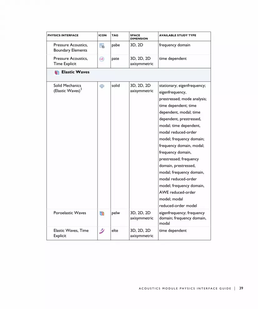
Pressure Acoustics, Boundary Elements

pabe 3D, 2D frequency domain

Pressure Acoustics, Time Explicit

pate 3D, 2D, 2D axisymmetric

time dependent

Elastic Waves

Solid Mechanics (Elastic Waves)1

solid 3D, 2D, 2D axisymmetric

stationary; eigenfrequency;

eigenfrequency,

prestressed; mode analysis;

time dependent; time

dependent, modal; time

dependent, prestressed,

modal; time dependent,

modal reduced-order

model; frequency domain;

frequency domain, modal;

frequency domain,

prestressed; frequency

domain, prestressed,

modal; frequency domain,

modal reduced-order

model; frequency domain,

AWE reduced-order

model; modal

reduced-order model

Poroelastic Waves pelw 3D, 2D, 2D axisymmetric

eigenfrequency; frequency domain; frequency domain, modal

Elastic Waves, Time Explicit

elte 3D, 2D, 2D axisymmetric

time dependent



A C O U S T I C S M O D U L E P H Y S I C S I N T E R F A C E G U I D E | 39

40 | C H A P T E R

Acoustic-Structure Interaction

Acoustic-Solid Interaction, Frequency Domain3

— 3D, 2D, 2D axisymmetric


Acoustic-Solid Interaction, Transient3


eigenfrequency; frequency domain; frequency domain, modal; time dependent; time dependent, modal

Acoustic-Shell Interaction, Frequency Domain2,3

— 3D, 2D axisymmetric


Acoustic-Shell Interaction, Transient2, 3

— 3D, 2D axisymmetric


Acoustic-Piezoelectric Interaction, Frequency Domain3



Acoustic-Piezoelectric Interaction, Transient3



Acoustic-Solid-Poroelastic Waves Interaction3



Acoustic-Poroelastic Waves Interaction3



Acoustic-Solid Interaction, Time Explicit

— 3D, 2D time domain

Aeroacoustics

Linearized Euler, Frequency Domain

lef 3D, 2D, 2D axisymmetric, 1D

frequency domain; eigenfrequency




Linearized Euler, Transient

let 3D, 2D, 2D axisymmetric, 1D

time dependent

Linearized Potential Flow, Frequency Domain

ae all dimensions frequency domain; mode analysis (2D and 1D axisymmetric models only)

Linearized Potential Flow, Transient

aetd all dimensions frequency domain; time dependent; mode analysis (2D and 1D axisymmetric models only)

Linearized Potential Flow, Boundary Mode

aebm 3D, 2D axisymmetric

mode analysis

Compressible Potential Flow

cpf all dimensions stationary; time dependent

Linearized Navier-Stokes, Frequency Domain

lnsf 3D, 2D, 2D axisymmetric, 1D

frequency domain; eigenfrequency

Linearized Navier-Stokes, Transient

lnst 3D, 2D, 2D axisymmetric, and 1D

time dependent

Thermoviscous Acoustics

Thermoviscous Acoustics, Frequency Domain

ta all dimensions eigenfrequency; frequency domain; frequency domain, modal; mode analysis (2D and 1D axisymmetric models only)

Thermoviscous Acoustics, Transient

tatd all dimensions time dependent

Thermoviscous Acoustics, Boundary Mode

tabm 3D, 2D axisymmetric

mode analysis

Acoustic-Thermoviscous Acoustic Interaction, Frequency Domain3


eigenfrequency; frequency domain; frequency domain, modal; boundary mode analysis (3D and 2D axisymmetric only); mode analysis (2D only)




42 | C H A P T E R

Thermoviscous Acoustic-Solid Interaction, Frequency Domain3


eigenfrequency; frequency domain; frequency domain, modal; mode analysis (2D only)

Thermoviscous Acoustic-Shell Interaction, Frequency Domain2,3

— 3D eigenfrequency; frequency domain; frequency domain, modal

Ultrasound

Convected Wave Equation, Time Explicit

cwe 3D, 2D, 2D axisymmetric

time dependent

Nonlinear Acoustics, Time Explicit

nate 3D, 2D, 2D axisymmetric

time dependent

Geometrical Acoustics

Ray Acoustics rac 3D, 2D, 2D axisymmetric

ray tracing; time dependent

Acoustic Diffusion Equation

ade 3D eigenvalue; stationary; time dependent

Pipe Acoustics

Pipe Acoustics, Frequency Domain

pafd 3D, 2D eigenfrequency; frequency domain

Pipe Acoustics, Transient

patd 3D, 2D time dependent




Structural Mechanics

Solid Mechanics1 solid 3D, 2D, 2D axisymmetric

stationary; eigenfrequency; eigenfrequency, prestressed; mode analysis; time dependent; time dependent, modal; time dependent, prestressed, modal; time dependent, modal reduced-order model; frequency domain; frequency domain, modal; frequency domain, prestressed; frequency domain, prestressed, modal; frequency domain, modal reduced-order model; frequency domain, AWE reduced-order model

Piezoelectricity3 — 3D, 2D, 2D axisymmetric

stationary; eigenfrequency; eigenfrequency, prestressed; time dependent; time dependent, modal; time dependent, prestressed, modal; frequency domain; frequency domain, modal; frequency domain, prestressed; frequency domain, prestressed, modal; small-signal analysis, frequency domain




44 | C H A P T E R

Common Physics Interface and Feature Settings and Nodes

There are several common settings and sections available for the physics interfaces and feature nodes. Some of these sections also have similar settings or are implemented in the same way no matter the physics interface or feature being used.

In each module’s documentation, only unique or extra information is included; standard information and procedures are centralized in the COMSOL Multiphysics Reference Manual.

Where Do I Access the Documentation and Application Libraries?

A number of internet resources have more information about COMSOL, including licensing and technical information. The electronic documentation, topic-based (or

Magnetostriction,3,4 — 3D, 2D, 2D axisymmetric

stationary; eigenfrequency; time dependent; frequency domain; small-signal analysis, frequency domain; eigenfrequency, prestressed; frequency domain, prestressed

1 This physics interface is included with the core COMSOL package but has added functionality for this module.2 Requires both the Structural Mechanics Module and the Acoustics Module.3 This physics interface is a predefined multiphysics coupling that automatically adds all the physics interfaces and coupling features required.4 Requires the addition of the AC/DC Module.



In the COMSOL Multiphysics Reference Manual see Table 2-4 for links to common sections and Table 2-5 to common feature nodes. You can also search for information: press F1 to open the Help window or Ctrl+F1 to open the Documentation window.


context-based) help, and the application libraries are all accessed through the COMSOL Desktop.

T H E D O C U M E N T A T I O N A N D O N L I N E H E L P

The COMSOL Multiphysics Reference Manual describes the core physics interfaces and functionality included with the COMSOL Multiphysics license. This book also has instructions about how to use COMSOL Multiphysics and how to access the electronic Documentation and Help content.

Opening Topic-Based HelpThe Help window is useful as it is connected to the features in the COMSOL Desktop. To learn more about a node in the Model Builder, or a window on the Desktop, click to highlight a node or window, then press F1 to open the Help window, which then displays information about that feature (or click a node in the Model Builder followed by the Help button ( ). This is called topic-based (or context) help.

If you are reading the documentation as a PDF file on your computer, the blue links do not work to open an application or content referenced in a different guide. However, if you are using the Help system in COMSOL Multiphysics, these links work to open other modules, application examples, and documentation sets.

To open the Help window:

• In the Model Builder, Application Builder, or Physics Builder click a node or window and then press F1.

• On any toolbar (for example, Home, Definitions, or Geometry), hover the mouse over a button (for example, Add Physics or Build All) and then press F1.

• From the File menu, click Help ( ).

• In the upper-right corner of the COMSOL Desktop, click the Help ( ) button.


46 | C H A P T E R

Opening the Documentation Window

T H E A P P L I C A T I O N L I B R A R I E S W I N D O W

Each model or application includes documentation with the theoretical background and step-by-step instructions to create a model or application. The models and applications are available in COMSOL Multiphysics as MPH files that you can open for further investigation. You can use the step-by-step instructions and the actual models as templates for your own modeling. In most models, SI units are used to describe the relevant properties, parameters, and dimensions, but other unit systems are available.

Once the Application Libraries window is opened, you can search by name or browse under a module folder name. Click to view a summary of the model or application and its properties, including options to open it or its associated PDF document.

To open the Help window:

• In the Model Builder or Physics Builder click a node or window and then press F1.

• On the main toolbar, click the Help ( ) button.

• From the main menu, select Help>Help.

To open the Documentation window:

• Press Ctrl+F1.

• From the File menu select Help>Documentation ( ).

To open the Documentation window:

• Press Ctrl+F1.

• On the main toolbar, click the Documentation ( ) button.

• From the main menu, select Help>Documentation.

The Application Libraries Window in the COMSOL Multiphysics Reference Manual.


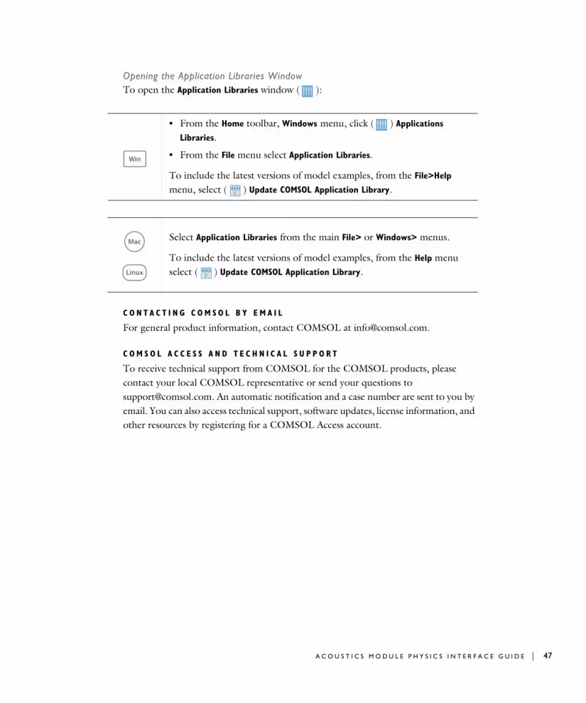
Opening the Application Libraries WindowTo open the Application Libraries window ( ):

C O N T A C T I N G C O M S O L B Y E M A I L

For general product information, contact COMSOL at [email protected].

C O M S O L A C C E S S A N D T E C H N I C A L S U P P O R T

To receive technical support from COMSOL for the COMSOL products, please contact your local COMSOL representative or send your questions to [email protected]. An automatic notification and a case number are sent to you by email. You can also access technical support, software updates, license information, and other resources by registering for a COMSOL Access account.

• From the Home toolbar, Windows menu, click ( ) Applications

Libraries.

• From the File menu select Application Libraries.

To include the latest versions of model examples, from the File>Help menu, select ( ) Update COMSOL Application Library.

Select Application Libraries from the main File> or Windows> menus.

To include the latest versions of model examples, from the Help menu select ( ) Update COMSOL Application Library.


48 | C H A P T E R

C O M S O L O N L I N E R E S O U R C E S

COMSOL website www.comsol.com

Contact COMSOL www.comsol.com/contact

COMSOL Access www.comsol.com/access

Support Center www.comsol.com/support

Product Download www.comsol.com/product-download

Product Updates www.comsol.com/support/updates

COMSOL Blog www.comsol.com/blogs

Discussion Forum www.comsol.com/community

Events www.comsol.com/events

COMSOL Application Gallery www.comsol.com/models

COMSOL Video Gallery www.comsol.com/video

Support Knowledge Base www.comsol.com/support/knowledgebase


https://www.comsol.com

https://www.comsol.com/contact/

https://www.comsol.com/access

https://www.comsol.com/support/

https://www.comsol.com/product-download/

https://www.comsol.com/support/updates

https://www.comsol.com/blogs/

https://www.comsol.com/community

https://www.comsol.com/events/

http://www.comsol.com/models/

http://www.comsol.com/video/

http://www.comsol.com/support/knowledgebase/

Ove r v i ew o f t h e U s e r ’ s Gu i d e

The Acoustics Module User’s Guide gets you started with modeling acoustics using COMSOL Multiphysics. The information in this guide is specific to the Acoustics Module. Instructions on how to use COMSOL in general are included with the COMSOL Multiphysics Reference Manual.

As detailed in the section Where Do I Access the Documentation and Application Libraries? this information can also be searched from the COMSOL Multiphysics software Help menu.

Good practices as well as some tips and tricks are located in dedicated modeling sections under each branch. They are:

• Modeling with the Pressure Acoustics Branch (FEM-Based Interfaces)

• Modeling with the Pressure Acoustics Branch (BEM-Based Interface)

• Modeling with the Pressure Acoustics Branch (DG-FEM-Based Interface)

• Modeling with the Elastic Waves Branch

• Modeling with the Acoustic-Structure Interaction Branch

• Modeling with the Aeroacoustics Branch

• Modeling with the Thermoviscous Acoustics Branch

• Modeling with the Convected Wave Equation Interface

• Modeling with the Nonlinear Pressure Acoustics, Time Explicit Interface

• Modeling with the Ray Acoustics Interface

• Modeling with the Acoustic Diffusion Equation Interface

• Modeling with Multiphysics Couplings

Dedicated theory sections also exist under each branch. Here the physics and mathematics of the governing equations and selected boundary conditions are discussed.

O V E R V I E W O F T H E U S E R ’ S G U I D E | 49

50 | C H A P T E R

T A B L E O F C O N T E N T S , G L O S S A R Y , A N D I N D E X

To help you navigate through this guide, see the Contents, Glossary, and Index.

T H E P R E S S U R E A C O U S T I C S B R A N C H

The Pressure Acoustics Interfaces chapter describes the following interfaces:

The Pressure Acoustics, Frequency Domain Interface is the core physics interface which models the sound waves in the frequency domain and The Pressure Acoustics, Transient Interface is the core physics interface which models the sound waves in the time domain with the possibility to include nonlinear effects. The Pressure Acoustics, Boundary Mode Interface solves for modes that propagate through a cross section of your geometry.

The Pressure Acoustics, Boundary Elements Interface uses the boundary element (BEM) method to solve the Helmholtz equation in the frequency domain. It is well suited for radiation and scattering problems and can be seamlessly coupled to structures and the finite element based The Pressure Acoustics, Frequency Domain Interface.

The Pressure Acoustics, Time Explicit Interface uses the discontinuous Galerkin (dG-FEM) formulation to solve transient models using a time explicit method. The interface can solve large problems as the method is very computationally efficient.

T H E E L A S T I C W A V E S B R A N C H

The Elastic Waves Interfaces chapter describes the following interfaces:

The Solid Mechanics (Elastic Waves) Interface is a shortcut to add the Solid Mechanics interface which is used to compute the displacement field in solids with propagating elastic waves.

The Poroelastic Waves Interface is used to compute the displacement field and acoustic pressure fluctuation in porous materials with propagating poroelastic waves.

The Elastic Waves, Time Explicit Interface uses the discontinuous Galerkin (dG-FEM) formulation to solve transient linear elastic wave models using a time explicit method. The interface can solve large problems as the method is very computationally efficient.

T H E A C O U S T I C - S T R U C T U R E I N T E R A C T I O N B R A N C H

The Acoustic-Structure Interaction Interfaces chapter describes the following interfaces:


The Acoustic-Solid Interaction, Frequency Domain Interface is a combination of pressure acoustics and solid mechanics with predefined couplings and The Acoustic-Solid Interaction, Transient Interface is a combination of transient pressure acoustics and solid mechanics with predefined couplings.

The Acoustic-Shell Interaction, Frequency Domain Interface and The Acoustic-Shell Interaction, Transient Interface requires a Structural Mechanics Module license. This multiphysics interface combines the Pressure Acoustics, Frequency Domain (or the Pressure Acoustics, Transient) interface, the Shell interface, and the Acoustic-Structure Boundary multiphysics coupling. The physics interface is available for 2D axisymmetric and 3D geometries.

The Acoustic-Piezoelectric Interaction, Frequency Domain Interface is a combination of Pressure Acoustics, Frequency Domain; solid Mechanics; Electrostatics; Acoustic-structure boundary; Piezoelectric Effect. The Acoustic-Piezoelectric Interaction, Transient Interface combines Pressure Acoustics, Transient; Solid Mechanics; Electrostatics; Acoustic-structure boundary; Piezoelectric Effect.

The Acoustic-Poroelastic Waves Interaction Interface combines Pressure Acoustics, Frequency Domain and Poroelastic Waves together with the Acoustic-Porous Boundary multiphysics coupling.

The Acoustic-Solid-Poroelastic Waves Interaction Interface combines Pressure Acoustics, Frequency Domain and Solid Mechanics together with the Acoustic-Structure Boundary and Acoustic-Porous Boundary multiphysics coupling.

The Acoustic-Solid Interaction, Time Explicit Interface combines Pressure Acoustics, Time Explicit and Elastic Waves, Time Explicit together with the Acoustic-Structure Boundary, Time Explicit multiphysics coupling.

T H E A E R O A C O U S T I C S B R A N C H

The Aeroacoustics Interfaces chapter describes the following interfaces:

The Linearized Euler, Frequency Domain Interface and The Linearized Euler, Transient Interface models the acoustic variations in density, velocity, and pressure in the presence of a stationary background mean-flow that is well approximated by an ideal gas flow. This physics interface is used for aeroacoustic simulations that can be described by the linearized Euler equations.

The Linearized Navier–Stokes, Frequency Domain Interface and The Linearized Navier–Stokes, Transient Interface models the acoustic variations in pressure, velocity, and temperature in the presence of any stationary isothermal or nonisothermal


52 | C H A P T E R

background mean flow. This physics interface is used for aeroacoustic simulations that can be described by the linearized Navier-Stokes equations.

The Linearized Potential Flow, Frequency Domain Interface models acoustic waves in potential flow in the frequency domain and The Linearized Potential Flow, Transient Interface models acoustic waves in potential flow in the time domain. The Linearized Potential Flow, Boundary Mode Interface solves for modes that propagate through a cross section of your geometry.

The Compressible Potential Flow Interface models irrotational flow used as input for the background flow in the linearized potential flow interfaces.

T H E T H E R M O V I S C O U S A C O U S T I C S B R A N C H

The Thermoviscous Acoustics Interfaces chapter describes The Thermoviscous Acoustics, Frequency Domain Interface and The Thermoviscous Acoustics, Transient Interface which are necessary when modeling acoustics accurately in geometries with small dimensions. Near walls, viscosity and thermal conduction become important because they create a viscous and a thermal boundary layer where losses are significant. Nonlinear effects can be modeled on the time domain. The Thermoviscous Acoustics, Boundary Mode Interface is used to identify propagating and nonpropagating modes in waveguides and ducts of small dimensions, including thermal and viscous losses.

The Acoustic-Thermoviscous Acoustic Interaction, Frequency Domain Interface combines the Thermoviscous Acoustics, Frequency Domain and Pressure Acoustics, Frequency Domain interfaces together with the Acoustic-Thermoviscous Acoustic Boundary multiphysics coupling.

The Thermoviscous Acoustic-Solid Interaction, Frequency Domain Interface is also described here. This physics interface combines the Thermoviscous Acoustics, Frequency Interface domain and Solid Mechanics Interface together with the Thermoviscous Acoustic-Structure Boundary multiphysics coupling.

The Thermoviscous Acoustic-Shell Interaction, Frequency Domain Interface requires a Structural Mechanics Module license. The multiphysics interface combines the Thermoviscous Acoustics, Frequency domain Interface and the Shell Interface together with the Thermoviscous Acoustic-Structure Boundary multiphysics coupling.

U L T R A S O U N D

The Ultrasound Interfaces chapter describes the following interfaces:


The Convected Wave Equation, Time Explicit Interface uses the discontinuous Galerkin (dG-FEM) formulation to model the propagating of linear ultrasound waves in the time domain, including the effects of a stationary background flow.

The Nonlinear Pressure Acoustics, Time Explicit Interface uses the discontinuous Galerkin (dG-FEM) formulation to model the propagation of nonlinear high amplitude pressure waves in fluids including dissipation effects.

T H E G E O M E T R I C A L A C O U S T I C S B R A N C H

The Geometrical Acoustics Interfaces includes The Ray Acoustics Interface, used to compute the trajectories, phase, and intensity of acoustic rays, and The Acoustic Diffusion Equation Interface, which solves a diffusion equation for the acoustic energy density. The theory is also discussed for both physics interfaces.

T H E P I P E A C O U S T I C S B R A N C H

The Pipe Acoustics Frequency Domain and Transient Interfaces have the equations and boundary conditions for modeling the propagation of sound waves in flexible pipe systems. The equations are formulated in a general way to include the possibility of a stationary background flow. There are two interfaces, one for transient analysis and one for frequency domain studies.

T H E M U L T I P H Y S I C S C O U P L I N G S

The Multiphysics Couplings chapter describes all the multiphysics couplings available with the Acoustics Module. These are the built-in conditions that can couple the physics together; for example, the Acoustic-Structure Boundary couples pressure acoustics to any solid boundary.

S T R U C T U R A L M E C H A N I C S W I T H T H E A C O U S T I C S M O D U L E

The Structural Mechanics with the Acoustics Module chapter provides information about The Solid Mechanics Interface used for modeling, for example, the structural part of acoustic-structure interaction. This is an extension of the Solid Mechanics interface in COMSOL Multiphysics, and you find it under the Structural Mechanics branch, or using the shortcut The Solid Mechanics (Elastic Waves) Interface under the Elastic Waves branch.

The Piezoelectricity Interface interface is also shortly presented. It combines Solid Mechanics and Electrostatics together with the constitutive relationships required to model piezoelectrics. Both the direct and inverse piezoelectric effects can be modeled and the piezoelectric coupling can be formulated using either the strain-charge or stress-charge forms.


54 | C H A P T E R

The theory for the solid mechanics interface as well as for the Piezoelectricity interface is found in the Structural Mechanics Module User’s Guide.


2

P r e s s u r e A c o u s t i c s I n t e r f a c e s

This chapter describes the Acoustics Module background theory and physics interfaces found under the Pressure Acoustics branch ( ).

• The Pressure Acoustics, Frequency Domain Interface

• The Pressure Acoustics, Transient Interface

• The Pressure Acoustics, Boundary Mode Interface

• The Pressure Acoustics, Boundary Elements Interface

• The Pressure Acoustics, Time Explicit Interface

• Modeling with the Pressure Acoustics Branch (FEM-Based Interfaces)

• Modeling with the Pressure Acoustics Branch (BEM-Based Interface)

• Modeling with the Pressure Acoustics Branch (DG-FEM-Based Interface)

• Theory Background for the Pressure Acoustics Branch

• Theory for the Boundary Impedance Models

• Theory for the Interior Impedance Models

• Theory for the Equivalent Fluid Models

• Theory for the Perfectly Matched Layers in the Time Domain

• References for the Pressure Acoustics Branch

55

56 | C H A P T E R

Th e P r e s s u r e A c ou s t i c s , F r e qu en c y Doma i n I n t e r f a c e

The Pressure Acoustics, Frequency Domain (acpr) interface ( ), found under the Pressure Acoustics branch ( ) when adding a physics interface, is used to compute the pressure variations for the propagation of acoustic waves in fluids at quiescent background conditions. It is suited for all frequency-domain simulations with harmonic variations of the pressure field.

The physics interface can be used for linear acoustics described by a scalar pressure variable. It includes domain conditions to model losses in a homogenized way, so-called equivalent fluid models, for porous materials as well as losses in narrow regions (waveguides or slits). The plane wave attenuation behavior of the acoustic waves may also be entered as a user-defined quantity, or based on the losses in the atmosphere or ocean. Effective anisotropic material properties can be modeled with an effective anisotropic density formulation. Domain features also include background acoustic fields, as well as monopole and dipole domain sources.

The physics interface solves the Helmholtz equation in the frequency domain for given frequencies, or as an eigenfrequency or mode analysis study. The harmonic variation of all fields and sources is given by using the +iω convention.

An acoustics model can be part of a larger multiphysics model that describes, for example, the interactions between structures and acoustic waves. This physics interface is suitable for modeling acoustics phenomena that do not involve fluid flow (convective effects).

The sound pressure p, which is solved for in pressure acoustics, represents the acoustic variations (or acoustic perturbations) to the ambient pressure. In the absence of flow, the ambient pressure pA is simply the static absolute pressure.

The governing equations and boundary conditions are formulated using the total pressure pt with a so-called scattered field formulation. In the presence of a Background Pressure Field defining a background pressure wave pb (this could, for example, be a plane wave), the total acoustic pressure pt is the sum of the pressure solved for p (which is then equal to the scattered pressure ps) and the background

eiωt

2 : P R E S S U R E A C O U S T I C S I N T E R F A C E S

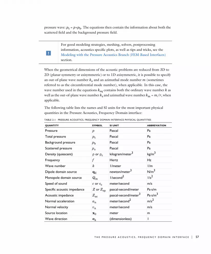
pressure wave: pt = p+pb. The equations then contain the information about both the scattered field and the background pressure field.

When the geometrical dimensions of the acoustic problems are reduced from 3D to 2D (planar symmetry or axisymmetric) or to 1D axisymmetric, it is possible to specify an out-of-plane wave number kz and an azimuthal mode number m (sometimes referred to as the circumferential mode number), when applicable. In this case, the wave number used in the equations keq contains both the ordinary wave number k as well as the out-of-plane wave number kz and azimuthal wave number km = m/r, when applicable.

The following table lists the names and SI units for the most important physical quantities in the Pressure Acoustics, Frequency Domain interface:

For good modeling strategies, meshing, solvers, postprocessing information, acoustics specific plots, as well as tips and tricks, see the Modeling with the Pressure Acoustics Branch (FEM-Based Interfaces) section.

TABLE 2-1: PRESSURE ACOUSTICS, FREQUENCY DOMAIN INTERFACE PHYSICAL QUANTITIES

QUANTITY SYMBOL SI UNIT ABBREVIATION

Pressure p Pascal Pa

Total pressure pt Pascal Pa

Background pressure pb Pascal Pa

Scattered pressure ps Pascal Pa

Density (quiescent) ρ or ρc kilogram/meter3 kg/m3

Frequency f Hertz Hz

Wave number k 1/meter 1/m

Dipole domain source qd newton/meter3 N/m3

Monopole domain source Qm 1/second2 1/s2

Speed of sound c or cc meter/second m/s

Specific acoustic impedance Z or Zsp pascal-second/meter Pa·s/m

Acoustic impedance Zac pascal-second/meter3 Pa·s/m3

Normal acceleration an meter/second2 m/s2

Normal velocity vn meter/second m/s

Source location x0 meter m

Wave direction ek (dimensionless) 1

T H E P R E S S U R E A C O U S T I C S , F R E Q U E N C Y D O M A I N I N T E R F A C E | 57

58 | C H A P T E R

In the following descriptions of the functionality in this physics interface, the subscript c in ρc and cc (the density and speed of sound, respectively) denotes that these can be complex-valued quantities in models with damping.

When this physics interface is added, these default nodes are also added to the Model

Builder — Pressure Acoustics Model, Sound Hard Boundary (Wall), and Initial Values.

Then, from the Physics toolbar, add other nodes that implement, for example, boundary conditions and point conditions. You can also right-click Pressure Acoustics,

Frequency Domain to select physics features from the context menu.

S E T T I N G S

The Label is the default physics interface name.

The Name is used primarily as a scope prefix for variables defined by the physics interface. Refer to such physics interface variables in expressions using the pattern <name>.<variable_name>. In order to distinguish between variables belonging to different physics interfaces, the name string must be unique. Only letters, numbers, and underscores (_) are permitted in the Name field. The first character must be a letter.

The default Name (for the first physics interface in the model) is acpr.

E Q U A T I O N

Expand the Equation section to see the equations solved for with the Equation form specified. The default selection for Equation form is Study controlled. The available studies are selected under Show equations assuming.

• For Study controlled, the scaling and nonreflecting boundary settings are optimized for the numerical performance of the different solvers and study types.

• For Frequency domain, enter the settings as described in Scaling Factor and Nonreflecting Boundary Condition Approximation.

P H Y S I C S S Y M B O L S

Select to Enable physics symbols (selected per default). This shows the physics symbols, like for example, normals or symmetry planes in the Graphics window when applicable.

Physics Nodes — Equation Section in the COMSOL Multiphysics Reference Manual


P R E S S U R E A C O U S T I C S E Q U A T I O N S E T T I N G S

In this section you can add out-of-plane information defining an out-of-plane wave number kz or an azimuthal wave number km = m/r through the mode number m. Add if applicable:

• For 1D axisymmetric components, the default Out-of-plane wave number kz (SI unit: rad/m) is 0 rad/m. The default Azimuthal mode number m (dimensionless) is 0. The pressure has the form:

• For 2D axisymmetric components, the default Azimuthal mode number m (dimensionless) is 0. The pressure has the form:

• For 2D components, the default Out-of-plane wave number kz (SI unit: rad/m) is 0 rad/m. The pressure has the form:

Note that when performing a mode analysis study in 2D (solving for the out-of-plane wave number) the Out-of-plane wave number property is not used as this is now the variable solved for.

Scaling Factor and Nonreflecting Boundary Condition ApproximationFor all component dimensions, and if required, click to expand the Equation section, then select Frequency domain as the Equation form and enter the settings as described below.

The default Scaling factor Δ is 1/ω2 and Nonreflecting boundary condition approximation is Second order. These values correspond to the equations for a Frequency Domain study when the equations are study controlled.

To get the equations corresponding to an Eigenfrequency study, change the Scaling

factor Δ to 1 and the Nonreflecting boundary conditions approximation to First order.

G L O B A L P O R T S E T T I N G S

Select to enable the Activate port sweep option (not selected per default). This option is used to compute the full scattering matrix when Port conditions are used. For more details see The Port Sweep Functionality subsection. The section only exists for 3D and 2D axisymmetry.

p r ϕ z, ,( ) p r( )e i kzz mϕ+( )–=

p r ϕ z, ,( ) p r z,( )e imϕ–=

p x y z, ,( ) p x y,( )e ikzz–=


60 | C H A P T E R

Select the Mode shape normalization as Amplitude normalized (the default) or Power

normalized. This setting controls if the mode shapes are normalized to have a unit maximum amplitude or carry unit power. The selection determines how the scattering matrix is to be interpreted.

S O U N D P R E S S U R E L E V E L S E T T I N G S

The zero level on the dB scale varies with the type of fluid. That value is a reference pressure that corresponds to 0 dB. This variable occurs in calculations of the sound pressure level Lp based on the root mean square (rms) pressure prms, such that

where pref is the reference pressure and the star (*) represents the complex conjugate. This is an expression valid for the case of harmonically time-varying acoustic pressure p.

Select a Reference pressure for the sound pressure level based on the fluid type:

• Use reference pressure for air to use a reference pressure of 20 μPa (20·10−6 Pa).

• Use reference pressure for water to use a reference pressure of 1 μPa (1·10−6 Pa).

• User-defined reference pressure to enter a reference pressure pref, SPL (SI unit: Pa). The default value is the same as for air, 20 μPa.

T Y P I C A L W A V E S P E E D

Enter a value or expression for the Typical wave speed for perfectly matched layers cref (SI unit m/s). The default is 343 m/s.

D I S C R E T I Z A T I O N

From the list select the element order and type (Lagrange or serendipity) for the Pressure, the default is Quadratic Lagrange.

To see all settings in this section, click the Show More Options button ( ) and select Advanced Physics Options in the Show More Options dialog box.

Lp 20prmspref---------- log= with prms

12--- p p∗=

Choosing between Lagrange and Serendipity Shape Functions has influence on the number of DOFs solved for and on stability for a distorted mesh.


D E P E N D E N T V A R I A B L E S

This physics interface defines one dependent variable (field), the Pressure p. If required, edit the name, which changes both the field name and the dependent variable name. If the new field name coincides with the name of another pressure field in the model, the interfaces share degrees of freedom and dependent variable name. The new field name must not coincide with the name of a field of another type, or with a component name belonging to some other field.

Domain, Boundary, Edge, Point, and Pair Nodes for the Pressure Acoustics, Frequency Domain Interface

The Pressure Acoustics, Frequency Domain Interface has Domain, Boundary, Edge, Point, and Pair nodes, listed in alphabetical order, available from the Physics ribbon toolbar (Windows® users), Physics context menu (macOS or Linux® users), or right-click to access the context menu (all users). Continuity in the total pressure is the default condition on interior boundaries.

The Pressure Acoustics, Transient Interface also shares these nodes, with some additional features described in Domain, Boundary, Edge, and Point Nodes for the Pressure Acoustics, Transient Interface.

The Pressure Acoustics, Boundary Mode Interface also shares these nodes, with one additional feature described in Boundary, Edge, Point, and Pair Nodes for the Pressure

• Domain, Boundary, Edge, Point, and Pair Nodes for the Pressure Acoustics, Frequency Domain Interface


Eigenmodes of a Room: Application Library path COMSOL_Multiphysics/

Acoustics/eigenmodes_of_room

Acoustic Levitator: Application Library path Acoustics_Module/

Nonlinear_Acoustics/acoustic_levitator. This model also requires the Particle Tracing Module.


62 | C H A P T E R

Acoustics, Boundary Mode Interface. For the Pressure Acoustics, Boundary Mode interface, apply the feature to boundaries instead of domains for 3D components.

In general, to add a node, go to the Physics toolbar, no matter what operating system you are using. Subnodes are available by clicking the parent node and selecting it from the Attributes menu.

• Anisotropic Acoustics

• Axial Symmetry

• Background Pressure Field

• Circular Source (for 2D Axisymmetric Components)

• Continuity

• Cylindrical Wave Radiation

• Dipole Point Source

• Dipole Domain Source

• Exterior Field Calculation

• Heat Source

• Impedance

• Incident Pressure Field

• Interior Normal Acceleration

• Interior Normal Displacement

• Interior Normal Velocity

• Interior Impedance/Pair Impedance

• Interior Perforated Plate/Pair Perforated Plate

• Interior Sound Hard Boundary (Wall)

• Initial Values

• Line Source

• Line Source on Axis

• Lumped Port

• Matched Boundary

• Monopole Point Source

• Monopole Domain Source

• Narrow Region Acoustics

• Normal Acceleration

• Normal Displacement

• Normal Velocity

• Quadrupole Point Source

• Periodic Condition

• Plane Wave Radiation

• Point Sources (for 2D Components)

• Poroacoustics

• Port

• Pressure Acoustics

• Pressure

• Pressure (Point Condition)

• Sound Hard Boundary (Wall)

• Sound Soft Boundary

• Spherical Wave Radiation

• Symmetry

• Thermoviscous Boundary Layer Impedance


Pressure Acoustics

The Pressure Acoustics node adds the equations for time-harmonic (frequency domain) and eigenfrequency acoustics modeling of classical acoustics. In the Settings window, define the properties for the acoustics model and model inputs including the absolute background pressure and temperature.

M O D E L I N P U T S

Select, User defined (the default), Common model input, or an input from another physics interface, if applicable.

The values of the quiescent (or background) Temperature T (SI unit: K) and Absolute

pressure pA (SI unit: Pa) are entered in the Model Inputs section if required by the material properties (other inputs like relative humidity or salinity can also appear). The values of the model inputs can influence the material properties like, for example, the density and speed of sound, depending on their definition in the Materials node. In

For axisymmetric components, COMSOL Multiphysics takes the axial symmetry boundaries (at r = 0) into account and automatically adds an Axial Symmetry node to the component that is valid on the axial symmetry boundaries only.

In the COMSOL Multiphysics Reference Manual, see Table 2-4 for links to common sections and Table 2-5 for common feature nodes. You can also search for information: press F1 to open the Help window or Ctrl+F1 to open the Documentation window.

The advanced fluid models are defined using individual physics feature nodes: Poroacoustics, Narrow Region Acoustics, and Anisotropic Acoustics. In the time domain nonlinear effects can be included using the Nonlinear Acoustics (Westervelt) Contributions node.

For details about some of the available fluid models, see Theory for the Equivalent Fluid Models.

For more information about using variables during the results analysis, see Postprocessing Variables.


64 | C H A P T E R

general, if the model includes a material property that depends on a model input, the corresponding text field will be enabled.

If Ideal gas is selected as the Fluid model, both the Temperature T and Absolute pressure pA fields are enabled. In this case this input option is always available.

In addition, the Temperature T and Absolute pressure pA can be picked up from another physics interface where the fields have been calculated. For example, select a temperature field defined by a Heat Transfer interface or a Nonisothermal Flow interface (if any). Or, if applicable, select a pressure as defined by a Fluid Flow interface present in the model. For example, select Absolute pressure (spf) to use the absolute pressure defined by a Laminar Flow interface spf.

The input to the Model Inputs fields influences the value of the material parameters in the model. Typically, the density ρ and the speed of sound c in the model depend on the absolute pressure and/or the temperature. Picking up any of those from another physics interface typically results in space dependent quantities ρ = ρ(x) and c = c(x).

P R E S S U R E A C O U S T I C S M O D E L

To define the properties of the fluid, select a Fluid model from the list:

• Linear elastic (the default) for defining the classical lossless fluid: Go to Linear Elastic Fluid Model.

• User-defined attenuation for defining losses through an attenuation coefficient: Go to User-Defined Attenuation Fluid Model.

• Atmosphere attenuation defines the standard attenuation of atmospheric (moist) air: Go to Atmosphere Attenuation Fluid Model.

• Ocean attenuation defines attenuation in the seawater of the ocean: Go to Ocean Attenuation Fluid Model.

Details about the Model Input and the Default Model Inputs are found in the Global and Local Definitions chapter of the COMSOL Multiphysics Reference Manual.

Detailed aeroacoustic or convected acoustic models that take into account the full background flow (including the movement of the fluid) are available under the Aeroacoustics Interfaces.


• Viscous, Thermally conducting, and Thermally conducting and viscous defines the classical thermoviscous attenuation model: Go to Thermally Conducting and/or Viscous Fluid Model.

• General dissipation defines losses through the sound diffusivity: Go to General Dissipation Fluid Model.

• Ideal gas to define the properties of an ideal gas: Go to Ideal Gas Fluid Model.

Linear Elastic Fluid ModelLinear elastic is the default. When the material parameters are real values, this corresponds to a lossless compressible fluid. From the Specify list, select Density and

speed of sound (the default), Impedance and wave number, or Bulk modulus and density. To add user-defined losses, in a general way, specify the properties as complex-valued data.

For each of the following, the default values (when applicable), are taken From material or for User defined, enter other values or expressions.

• For Density and speed of sound, define the Speed of sound c (SI unit: m/s) and Density ρ (SI unit: kg/m3).

• For Impedance and wave number, define the Characteristic acoustic impedance Z (SI unit: Pa·s/m) and enter a Wave number k (SI unit: rad/m).

• For Bulk modulus and density, define the Effective bulk modulus K (SI unit: Pa) and Density ρ (SI unit: kg/m3). Selecting User defined is well suited for entering the

The theory for the fluid models is in the section Theory for the Equivalent Fluid Models.

The fluid models represent different bulk loss or attenuation mechanisms (applied in a homogenized way) or ways of defining the properties of the fluid. Some of these models are sometimes referred to as equivalent fluid models. The loss model can be a theoretical model or a model based on measurement data for the attenuation in the fluid like the atmosphere or the ocean.

Losses in porous materials are defined in Poroacoustics. Thermoviscous boundary layer losses in narrow regions of constant cross section (like waveguides) can be modeled using Narrow Region Acoustics.


66 | C H A P T E R

properties of a user-defined porous material fluid model. Predefined porous models exist in the Poroacoustics domain feature.

User-Defined Attenuation Fluid ModelThe User-defined attenuation model adds a user-defined attenuation to the fluid. This data is typically based on experimental data for the attenuation coefficient α. Adding attenuation makes the wave number k complex valued. For example, a plane wave p(x) moving in the x direction is attenuated according to

When the attenuation is defined in Np per unit length, the wave has a spatial exponential decay governed by the attenuation coefficient.

The default Speed of sound c (SI unit: m/s) and Density ρ (SI unit: kg/m3) are taken From material. For User defined, enter other values or expressions for one or both options.

Select an Attenuation type: Attenuation coefficient, Np per unit length (the default) to define an attenuation coefficient α in Np/m (nepers per meter), Attenuation coefficient,

dB per unit length to define an attenuation coefficient α in dB/m (decibel per meter), or Attenuation coefficient, dB per wavelength to define an attenuation coefficient α in dB/λ (decibel per wavelength). For any selection, enter a value or expression in the Attenuation coefficient α field.

Atmosphere Attenuation Fluid ModelThe Atmospheric attenuation model defines attenuation in atmospheric air that follows the ANSI standard S1.26-2014, see Ref. 6 (Appendix B), 43, 44, and 45 for details.

k ωc---- iα–=

p x( ) e ikx– e i ω c⁄( )x– e αx–= =

Do not confuse the attenuation coefficient α with the attenuation constant m most often defined in room acoustics (it is also known as the intensity attenuation coefficient). The two are simply related through 2α = m. The difference stems from how the intensity scales in the propagation direction: I(x) = I0·exp(-2αx) = I0·exp(-mx).

User-Defined Attenuation Fluid Model


The model describes attenuation due to thermal and viscous effects (primarily pure air), the relaxation processes for nitrogen and oxygen, and the dependency on atmospheric pressure (absolute pressure), temperature, and relative humidity. The attenuation in air is important for propagation over large distances and for high frequency processes. This also means that the attenuation effect is more important in ray tracing simulations where propagation can be simulated over much larger distances, see The Ray Acoustics Interface.

When the model is selected the Model Input section includes inputs for the Temperature

T (SI unit: K), the Absolute pressure pA (SI unit: Pa), and the Relative humidity (SI unit: 1). In the Pressure Acoustic Model section the default Speed of sound c (SI unit: m/s) and Density ρ (SI unit: kg/m3) are taken From material. For User defined, enter other values or expressions for one or both options.

Ocean Attenuation Fluid ModelThe Ocean attenuation model defines attenuation in seawater of the ocean. The model is based on a semianalytical model with parameters that are based on extensive measurement data. It includes effects due to viscosity in pure water, the relaxation processes of boric acid and magnesium sulfate, as well as depth, temperature, practical salinity, and pH value. For further details, see Ref. 46, 47, 48, 49, and 50. The ocean attenuation model is important in ray tracing simulations where propagation can be simulated over much larger distances, see The Ray Acoustics Interface.

When the model is selected, the Model Input section includes inputs for the Temperature

T (SI unit: K), the Depth D (SI unit: m), and the Practical salinity Sp (SI unit: 1); the default is 35. In the Pressure Acoustic Model section, the default Speed of sound c (SI unit: m/s) and Density ρ (SI unit: kg/m3) are taken From material. For User defined, enter other values or expressions for one or both options. Enter a value for the pH value pH (SI unit: 1); the default is 8.

φ

The Practical salinity is defined on the Practical Salinity Scale. It represents a specific way of measuring salinity through electric conductivity. Practical salinity is a unit-less quantity, although it can be thought of as given in units of g/kg. The default value for the Practical salinity Sp is 35. For details see Ref. 55.


68 | C H A P T E R

Thermally Conducting and/or Viscous Fluid ModelThe Viscous, the Thermally conducting, and the Thermally conducting and viscous fluid models essentially add the same attenuation model. Here, the attenuation is due to bulk viscous and/or thermal losses. This type of model is relevant in highly viscous fluids or thermally conducting fluids when acoustic waves are traveling over large distances (relative to the wavelength). This is not a model for viscous and thermal boundary layer losses in narrow regions (see Narrow Region Acoustics). The models define the classical thermoviscous attenuation αtv properties of a fluid and can be applied in cases when, for example, relaxation processes are not important. The classical thermoviscous amplitude attenuation is given by

In atmospheric air or salt water where relaxation processes are important use the Atmosphere attenuation or the Ocean attenuation model as they capture these effects and also their dependency on, for example, relative humidity or salinity.

For each of the following (when applicable), the default values are taken From material. For User defined, enter other values or expressions for any or all options.

• Speed of sound c (SI unit: m/s).

• Density ρ (SI unit: kg/m3).

• Heat capacity at constant pressure Cp (SI unit: J/(kg·K)).

• Ratio of specific heats γ (dimensionless).

• Thermal conductivity k (SI unit: W/(m·K)).

For a discussion about air and water materials as commonly used in acoustics, the attenuation in (sea) water and (humid) air, and other material properties, see the Acoustic Properties of Fluids chapter of this manual.

αtvω2

2ρc3------------ 4

3---μ μB

k γ 1–( )Cp

--------------------+ + =


• Dynamic viscosity μ (SI unit: Pa·s).

• Bulk viscosity μB (SI unit: Pa·s).

General Dissipation Fluid ModelFor General dissipation enter the Speed of sound c (SI unit: m/s), the Density ρ (SI unit: kg/m3), and the Sound diffusivity δ (SI unit: m2/s). By default they are taken From

material and for User defined enter other values or expressions.

The sound diffusivity is automatically calculated for the classical thermoviscous case using either the Viscous, Thermally conducting or the Thermally conducting and viscous options (see below). For nonideal fluids like tissue, the sound diffusivity is measured directly instead and can be entered with the General dissipation.

Ideal Gas Fluid ModelFor Ideal Gas, you can edit the Model Inputs section. For each of the following, the default values are taken From material. For User defined, enter other values or expressions for any or all options.

• Select a Gas constant type: Specific gas constant Rs (SI unit: J/(kg·K) (the default) or Mean molar mass Mn (SI unit: kg/mol). For Mean molar mass, the molar gas constant (universal gas constant) R = 8.314 J/(mol·K) is used as the built-in physical constant.

• From the Specify Cp or γ list, select Heat capacity at constant pressure Cp (SI unit: J /(kg·K)) (the default) or Ratio of specific heats γ. For common diatomic gases such as air, γ = 1.4 is the standard value.

It is possible to assess the magnitude of the losses due to thermal conduction and viscosity, that is, the power dissipation density (SI unit: W/m3). This is done during the analysis process by plotting the variables for:

• Viscous power dissipation density (acpr.diss_visc)

• Thermal power dissipation density (acpr.diss_therm)

• Combined total power dissipation density (acpr.diss_tot)

• Viscous Fluid Model

• Thermally Conducting Fluid Model

• Thermally Conducting and Viscous Fluid Model


70 | C H A P T E R

Poroacoustics

The Poroacoustics node defines a fluid domain with a porous material modeled in a homogenized way using a so-called equivalent fluid model. Several models exist to define the attenuation and dispersion experienced by the pressure waves as they propagate in the porous domain. The different models are described below.

P O R O A C O U S T I C S M O D E L

Select a Poroacoustics model: Delany-Bazley-Miki (the default), Zwikker-Kosten, Attenborough, Wilson, Johnson-Champoux-Allard, Johnson-Champoux-Allard-Lafarge, Johnson-Champoux-Allard-Pride-Lafarge, Three-parameter approximation JCAL model, Williams EDFM, or Wood.

F L U I D P R O P E R T I E S

Enter the properties of the saturating fluid that is inside of the porous material. These settings are common to most porous models. By default the Fluid material uses the Domain material.

The following properties are available based on the Poroacoustics model selected above. The default values are taken From material. For User defined enter a different value or expression.

• Speed of sound c (SI unit: m/s) of the saturating fluid.

• Density ρf (SI unit: kg/m3) of the saturating fluid (the fluid density).

If any other than the default Delany-Bazley-Miki is selected, the following properties are also required, depending on the selection. These material parameters are necessary as the more advanced models include the losses associated with viscosity and thermal conduction in a more or less detailed way:


• Ratio of specific heats γ (dimensionless).


About the Poroacoustics Models



• Fluid bulk modulus Kf (SI unit: Pa).

P O R O U S M A T R I X P R O P E R T I E S

In this section, enter the properties that describe the porous material. By default the Porous elastic material uses the Domain material (the material defined for the domain). Select another material as needed. For example, create your own material that contains the properties of a given porous material and refer to it here. Here you also select if you want to use a rigid frame approximation or a limp frame approximation for the porous material (where applicable). The poroacoustic model defines complex-valued frequency-dependent expressions for both the bulk modulus and the equivalent density.

Based on the Poroacoustics model selected, enter the following settings for the porous matrix.

Delany-Bazley-MikiThe Delany-Bazley-Miki model is an empirical model used to describe fibrous materials such as rockwool or glass fiber. The model can be used for materials with a porosity, εp, close to one. For Delany-Bazley-Miki, the Flow resistivity Rf (SI unit: Pa·s/m2) uses values From material. For User defined, enter a value or expression.

Select an option from the Constants list: Delany-Bazley (the default), Miki, Qunli, Mechel, glass fiber, low X, Mechel, glass fiber, high X, Mechel, rock fiber, low X, Mechel, rock fiber, high X, Komatsu, Modified Allard and Champoux, or User defined. For

The implemented poroacoustics models are all applicable for any fluid, except the empirically determined Delany-Bazley-Miki model, which applies only to air. See Ideal Gas and General Fluid Options for details.

• Delany-Bazley-Miki

• Zwikker-Kosten

• Attenborough

• Wilson

• Johnson-Champoux-Allard

• Johnson-Champoux-Allard-Lafarge

• Johnson-Champoux-Allard-Pride-Lafarge

• Three-Parameter Approximation JCAL Model

• Williams Effective Density Fluid Model (EDFM)

• Wood


72 | C H A P T E R

User defined enter values in the C1 to C8 fields. The models are empirical and based on fitting to measured data. This means the models have different regions of applicability with respect to the flow resistivity Rf, the frequency f, the material type, and the parameter X defined as

All the models are applicable for materials with a porosity εp close to 1. The model informations are listed in Table 2-2. See also Ref. 23 and the relevant section in About the Poroacoustics Models for further details.

Xf ρf⋅Rf

-----------=


Zwikker-KostenThe Zwikker-Kosten model is a two-parameter semiempirical model. It is one of the earliest equivalent fluid models for porous materials. The model assumes that the pores

TABLE 2-2: DELANY-BAZLEY-MIKI MODEL OPTIONS AND APPLICABILITY

MODEL NAME APPLICABILITY

Delany-Bazley Glass and rock wool with:

Miki Glass and rock wool with:

Qunli Porous plastic and open foams:

Mechel, glass fiber, low X Glass fiber:

Mechel, glass fiber, high X Glass fiber:

Mechel, rock fiber, low X Rock fiber:

Mechel, rock fiber, high X Rock fiber:

Komatsu Glass and rock wool:

Modified Allard and Champoux

0.01 X 1≤ ≤

103 Rf 50 103⋅ Pasm 2–≤ ≤

0.01 X 1≤ ≤

103 Rf 50 103⋅ Pasm 2–≤ ≤

200 f 2000 Hz≤ ≤

3 103⋅ Rf 24 103⋅ Pasm 2–≤ ≤

X 0.025≤

X 0.025≥

X 0.025≤

X 0.025≥

6 103⋅ Rf 73 103⋅ Pasm 2–≤ ≤

45 f 11 103 Hz⋅≤ ≤

Flow resistivity Rf is easy to measure and is independent of frequency.

Absorptive Muffler: Application Library path Acoustics_Module/

Automotive/absorptive_muffler


74 | C H A P T E R

are cylinder-like with an effective hydraulic radius Hr. See Ref. 15 and About the Poroacoustics Models for further details.

For Zwikker-Kosten, select a Porous matrix approximation: Rigid (the default) or Limp. Then based on your choice, the default value for each of the following parameters is taken From material. For User defined, enter another value or expression.

• Porosity εp (dimensionless).

• Hydraulic radius of pores Hr (SI unit: m).

• Drained density of porous material ρd (SI unit: kg/m3).

AttenboroughThe Attenborough model is also based on the cylindrical-like pore assumption. It is a so-called four-parameter semiempirical model. The model is an extension of the Zwikker-Kosten model and has two additional input parameters. It accounts for the tortuosity (high frequency limit) τ∞, which is related to the orientation of the pores relative to the propagation direction. The hydraulic diameter of the pores is replaced by an expression that included the flow resistivity Rf and a fitting parameter b (this parameter is related to the anisotropy of the pore distribution). See Ref. 9, Ref. 16, and About the Poroacoustics Models for details.

For Attenborough, select a Porous matrix approximation: Rigid (the default) or Limp. Then based on your choice, the default value for most of the following parameters is taken From material. For User defined, enter another value or expression.


• Flow resistivity Rf (SI unit: Pa·s/m2).

• Tortuosity factor (high frequency limit) τ∞ (dimensionless). The default is 1.

• Fitting parameter b (dimensionless). The default is 1.


WilsonThe Wilson model is a generalization of the semianalytical models for porous materials with constant cross section and parallel pores. This model is intended to match the middle frequency behavior of a porous material. See Ref. 17, Ref. 9, Ref. 18, and About the Poroacoustics Models for further details.


For Wilson, select a Porous matrix approximation: Rigid (the default) or Limp. Then based on your choice, the default value for the following parameters is taken From

material. For User defined, enter another value or expression.


• Bulk modulus infinite frequency limit (SI unit: Pa).

• Density infinite frequency limit (SI unit: kg/m3).

• Entropy-mode relaxation time τent (SI unit: s).

• Vorticity-mode relaxation time τvor (SI unit: s).

Johnson-Champoux-AllardThe Johnson-Champoux-Allard (or JCA model) is a five-parameter semiempirical model for describing a large range of porous materials with rigid (or limp) frames. As input, the model requires the viscous Lv and thermal Lth characteristic lengths (sometimes denoted Λ and Λ'). These replace the hydraulic radius used in simpler models and account for the thermal and viscous losses that appear at the acoustic boundary layer at pore walls. See About the Poroacoustics Models for details.

For Johnson-Champoux-Allard, select a Porous matrix approximation: Rigid (the default) or Limp. Then based on your choice, the default value for most of the following parameters is taken From material. For User defined, enter another value or expression.


• Flow resistivity Rf (SI unit: Pa·s/m2).

• From the Specify list:

- Select Viscous characteristic length (the default) to directly enter an expression for Lv (SI unit: m). The default expression is sqrt(acpr.mu*acpr.tau*8/(acpr.Rf*acpr.epsilon_p)), which corresponds to s = 1.

- Select Viscous characteristic length parameter to enter a value for s (dimensionless) (the default is 1).

• Thermal characteristic length Lth (SI unit: m). The default expression is 2*acpr.Lv.

K∞

ρ∞

Approximate expressions for the two relaxation times that are based on intrinsic material properties are given in the theory section for the Wilson model.


76 | C H A P T E R



Johnson-Champoux-Allard-LafargeThe Johnson-Champoux-Allard-Lafarge (or JCAL model) is an extension to the JCA model. It introduces corrections to the bulk modulus thermal behavior at low frequencies which is not captured by the JCA model. It introduces the static thermal permeability parameter and, thus, has one more parameter than the JCA model. It is a six-parameter semiempirical model. See Ref. 13, Ref. 9, and About the Poroacoustics Models for further details.

For Johnson-Champoux-Allard-Lafarge, the settings are the same as for Johnson-Champoux-Allard with the addition of the Static thermal permeability (SI unit: m2) setting.

Johnson-Champoux-Allard-Pride-LafargeThe Johnson-Champoux-Allard-Pride-Lafarge (or JCAPL model) further extends the JCAL models by introducing a static viscous τ0 and thermal τ'0 tortuosity.

For Johnson-Champoux-Allard-Pride-Lafarge, the settings are the same as for Johnson-Champoux-Allard plus these additional parameters:

• Static viscous tortuosity τ0 (dimensionless). The default is 1.

• Static thermal tortuosity τ'0 (dimensionless). The default is 1.

• Static thermal permeability (SI unit: m2).

Three-Parameter Approximation JCAL ModelThe Three-parameter approximation JCAL model represents an approximation to the JCAL model. Instead of requiring 6 parameters as input for the porous matrix it only requires three. The porosity as well as two parameters that relate to the topology of the pores are needed (their size and distribution). Two different approximation methods exist for the density and bulk modulus. Select the Density and bulk modulus

approximation to either Johnson-Champoux-Allard-Pride-Lafarge (the default) or Padé

approximation. Then if necessary enter the values for (default is From material):


The Johnson-Champoux-Allard (JCA) model with a rigid (motionless) frame (skeleton) is sometimes referred to as a Biot equivalent fluid model with a rigid porous matrix.

κ'0

κ'0

κ'0


• Median pore size (SI unit: m).

• Standard deviation in pore size distribution σs (dimensionless).

Details about the model can be found in Ref. 56, 57, 58, 59, and 60.

Williams Effective Density Fluid Model (EDFM)Williams EDFM is an effective density fluid model (EDFM) used to model the propagation of acoustic waves in sediments. The model assumes that the bulk and shear moduli of the frame of the porous material are negligible, meaning that the porous frame is limp. See Ref. 24 and About the Poroacoustics Models for further details.

The Porous Matrix Properties (the properties for the sediment) for Williams EDFM have the default values taken From material. For User defined, enter another value or expression:

• Grain density ρgr (SI unit: kg/m3).

• Grain bulk modulus Kgr (SI unit: Pa).



• Permeability κp (SI unit: m2).

• Hydraulic radius of pores Hr (SI unit: m).

WoodThe Wood model is used for a fluid mixture or a fluid suspension (solid inclusions completely surrounded by fluid). The Woods formula for the sound velocity is determined by using the effective bulk modulus of the suspension and the volume average density. As the Williams EDFM, this model gives effective values for the mixture. This model is exact for low frequencies, when the wavelength is much larger than the size of the inclusions. See Ref. 25 and About the Poroacoustics Models for further details.

The Porous Matrix Properties (the properties for the inclusions) for the Wood model are entered in the Inclusion properties table. For each Inclusion (any number of inclusions can be added, the number is automatically incremented) enter the Volume fraction, the Bulk modulus, and the Density. Add a new row (inclusion) by clicking the plus sign below the table. The table may be saved or loaded from a file.

s


78 | C H A P T E R

Narrow Region Acoustics

The Narrow Region Acoustics node defines a fluid model for viscous and thermal boundary-layer-induced losses in channels and ducts of constant cross section. The losses due to the viscous and thermal dissipation in the acoustic boundary layer are homogenized and smeared on the fluid. This equivalent-fluid model can be used in long tubes of constant cross section (or only in a slowly varying cross section) instead of a fully detailed thermoviscous acoustics model. This type of model has a low computational cost compared to a thermoviscous acoustic model. The models are applicable for all fluids, that is, both gases and liquids. In the case of waveguides of varying thicknesses or in general other structures with curved surfaces, an alternative is to use the Thermoviscous Boundary Layer Impedance condition.

D U C T P R O P E R T I E S

Select a Duct type: Wide duct approximation (the default), Very narrow circular duct

(isothermal), Slit, Circular duct, Rectangular duct, Equilateral triangular duct, or User

defined.

• For Wide duct approximation enter a Hydraulic diameter Hd (SI unit: m).

This model can be used in ducts of any cross section as long as the hydraulic diameter of the duct (four times the cross-section area divided by circumference) is much larger than the viscous boundary layer thickness.

• For Very narrow circular duct (isothermal) enter the duct Radius a (SI unit: m).

This model is only valid for very narrow circular ducts where isothermal conditions apply. The radius of the duct has to be much smaller than the thickness of the thermal boundary layer. For this model it is assumed that the compressibility (bulk modulus) of the fluid also takes the isothermal value.

About the Narrow Region Acoustics Models

The Slit, Circular duct, Rectangular duct, and Equilateral triangular duct

models are applicable as long as the cross-section dimension is much smaller than the wavelength and the boundary layer thickness is smaller than the wavelength. The cross-section parameter can be a slowly varying function of space. These are known as a low reduced frequency (LRF) model.


• For Slit enter the slit Height h (SI unit: m). Use this model in narrow slit domains to include the damping and attenuation that occurs here because of the losses in the viscous and thermal boundary layer.

• For Circular duct enter the duct Radius a (SI unit: m). This model is useful for modeling the damping and attenuation that occurs when acoustic waves propagate in all tubing systems of small cross-section dimensions.

• For Rectangular duct enter the duct Side lengths W and H (SI unit: m). Use this model for waveguides and ducts with a rectangular cross section. Also see Advanced Physics Options for additional settings.

• For Equilateral triangular duct enter the duct Side length d (SI unit: m). Use this model for waveguides and ducts with an equilateral triangular cross section.

h

a

W

H

d


80 | C H A P T E R


Based on your selection in Duct Properties, different fluid properties need to be entered.

For User defined, enter the value for the Complex wave number kc (SI unit: rad/m) and (specific characteristic) Complex acoustic impedance Zc (SI unit: Pa·s/m). These values can be used to model the propagation in ducts of arbitrary cross sections.

For the other duct types, several other fluid properties are needed. The default values for the following are taken From material.

• Speed of sound c (SI unit: m/s)

• Density ρ (SI unit: kg/m3)

• Ratio of specific heats γ (SI unit: 1). In many liquids the value of γ is close to 1, the exact value can be derived from the expression where the (isobaric) coefficient of thermal expansion αp and the isothermal compressibility βT is used.

• Dynamic viscosity μ (SI unit: Pa·s)

The following are available for Wide duct approximation, Slit, Circular duct, Rectangular duct, and Equilateral triangular duct:

• Heat capacity at constant pressure Cp (SI unit: J/(kg·K))

• Thermal conductivity k (SI unit: W/(m·K))

A D V A N C E D P H Y S I C S O P T I O N S

To display this section, click the Show More Options button ( ), select Advanced

Physics Options and choose Rectangular duct as the Duct type.

To determine the complex propagation constants for a waveguide, of arbitrary cross section, use The Thermoviscous Acoustics, Boundary Mode Interface. Apply it on the cross-section geometry of the waveguide. The interface solves for the propagating modes and includes all losses in detail. The complex wave number kc is then given by the plane wave mode solved for. This is the variable tabm.kn. The predefined variable tabm.Zc gives the (lumped) specific characteristic complex impedance Zc. Search for the mode nearest to the (lossless) plane wave mode.

1 αp2T( ) βTρCp( )⁄–( ) 1–


The Number of terms for the sum N (used to describe the rectangular duct model) can be set. The default is N = 100 and should cover most cases, see under Slits, Circular Ducts, Rectangular Ducts, and Equilateral triangular Ducts.

Anisotropic Acoustics

The Anisotropic Acoustics node is used to define a fluid with properties that can be modeled with an effective anisotropic density. The feature can be used to model metamaterials in a homogenized manner or when modeling fibrous materials with anisotropic properties. The material properties are defined through an effective bulk modulus K and an effective density tensor ρ. The density variable can be defined as being isotropic (a scalar), a diagonal tensor, or a symmetric tensor. The resulting (generalized) Helmholtz equation solved in the frequency domain is then

where it should been emphasized that is here a tensor. The resulting system will have principal speeds of sound that are (square root of) the eigenvalues and directions that are the eigenvectors of the quantity .

• Lumped Receiver Connected to Test Setup with a 0.4-cc Coupler: The Application Library path Acoustics_Module/Electroacoustic_Transducers/

lumped_receiver_04cc

• Generic 711 Coupler — An Occluded Ear-Canal Simulator: The Application Library path Acoustics_Module/

Tutorials,_Thermoviscous_Acoustics/generic_711_coupler

The Narrow Region Acoustics models are so-called equivalent fluid models that have a non-trivial (nonlinear) dependency on the frequency. This means that performing an eigenfrequency analysis should be considered carefully, see Eigenfrequency Study. Moreover, the linearization process (linearization with respect to the frequency) of the underlying mathematical models can cause numerical problems (an error message is thrown). For the Rectangular duct one remedy is to decrease the number of terms used in the sum, for the Circular duct it can be necessary to switch to another model, like the Very narrow circular duct (isothermal).

∇ ρ 1– ∇pt qd–( )–( )ω2pt

K------------–⋅ Qm=

ρ 1–

c2 ρ 1– K=


82 | C H A P T E R

C O O R D I N A T E S Y S T E M S E L E C T I O N

Select the Coordinate system in which the density tensor is defined. The default is the Global coordinate system.

A N I S O T R O P I C A C O U S T I C S

Enter the Effective bulk modulus K (SI unit: Pa) taken From material. For User defined enter other values or expressions for any or all options.

Enter the Effective density ρ (SI unit: kg/m3) taken From material. For User defined enter other values or expressions for any or all options. Also select the representation for the density tensor either Isotropic (the default), Diagonal, or Symmetric.

Background Pressure Field

Add a Background Pressure Field node to model a background/incident pressure wave to study the scattered pressure field ps, which is defined as the difference between the total acoustic pressure pt and the background pressure field pb:

This feature sets up the equations in a so-called scattered field formulation where the dependent variable is the scattered field p = ps. In a model where the background pressure field is not defined on all acoustic domains (or it is different), continuity is automatically applied in the total field pt on interior boundaries between domains.

The background pressure field has built-in options for plane waves, spherical waves, and cylindrical waves. It can also be defined by a user defined analytical expression, that is a function of space, or it can be given by the solution to another acoustics problem.

Coordinate systems with directions which change with time should not be used.

Acoustic Cloaking: The Application Library path Acoustics_Module/

Tutorials,_Pressure_Acoustics/acoustic_cloaking

pt pb ps+=

For a Frequency Domain study type, the frequency of the background pressure field is the same as for the dependent variable p.


B A C K G R O U N D P R E S S U R E F I E L D

Select a Background pressure field type: Plane wave (the default), Cylindrical Wave, Spherical Wave, or User defined. For 2D axisymmetric models, it is possible to expand the plane wave in their cylindrical harmonics.

To set up and calculate the intensity variables for both the total, background, and scattered acoustic fields select Calculate background and scattered field intensity at the bottom of the settings window. This requires an additional input of the Density ρ (SI unit: kg/m3) for the defined background pressure field. Selecting this option will also define the velocity variables for the various fields.

Plane WaveThe Plane wave option defines the background pressure field pb of the type:

where p0 is the wave amplitude, k is the wave vector with amplitude ks = ω/c and wave direction vector ek, and x is the location on the boundary.

For Plane wave enter values for the Pressure amplitude p0 (SI unit: Pa), the Speed of

sound c (SI unit: m/s) of the fluid defining the field, either From material or User

defined, enter a Wave direction ek (dimensionless), and a Phase (SI unit: rad).

In 2D axisymmetric models, the incident fields take a slightly different form due to the geometrical restrictions. Only the z-component for the Wave direction ek can be entered. Per default, the wave can only travel in the axial direction since this is the only axisymmetric form of a plane wave.

By selecting Enable plane wave expansion, the plane wave is expanded in its cylindrical harmonics and a general Wave direction ek can be selected. This sets up a wave of the form:

For exciting waveguide structures with a given wave type it is recommended to use the Port or Lumped Port conditions, instead of a background pressure field. If still used, the feature should be backed by a PML or radiation condition to model an infinite waveguide.

pb p0ei k x⋅( )– p0e

iksx e⋅ k

ek

-------------- –

= =

φ

pi eiφ2sign(m)imJm ksx ek er⋅( )er⋅( )

ek----------------------------------------–

iksx ek ez⋅( )ez⋅( )

ek----------------------------------------–

exp=


84 | C H A P T E R

where m is the Azimuthal mode number specified in the Pressure Acoustics Equation Settings. To expand the solution, it is necessary to run a Parametric Sweep over the mode number from 0 up to the desired resolution.

Cylindrical WaveThe Cylindrical Wave option defines the background pressure field pb as a predefined cylindrical wave:

where p0 is the amplitude given at the reference distance rref = 0.548/ks (the distance where the Hankel function is one), ks = ω/c is the wave number, is the Hankel function of the second kind (representing an outgoing cylindrical wave), rs is the distance from the source axis, esa is the direction of the source axis, x0 is a point on the source axis, and x is the location on the boundary.

For Cylindrical Wave, enter a Pressure amplitude at reference distance p0 (SI unit: Pa), the Speed of Sound c (SI unit: m/s) of the fluid defining the field, either From material or User defined, enter a Source Location x0 (SI unit: m), a Source Axis esa (the vector does not need to be normalized), and a Phase (SI unit: rad).

In 2D axisymmetric models, the incident fields take a slightly different form due to the geometrical restrictions. Neither source location nor axis is needed as the source is always located on the z-axis.

Spherical WaveThe Spherical Wave option defines the background pressure field pb as a predefined spherical wave (only for 2D axisymmetric and 3D):

where p0 is the amplitude given at the reference distance of 1 m, ks = ω/c is the wave number, rs is the distance from the source, x0 is the source location of the spherical wave, and x is the location on the boundary.

An example using the Enable plane wave expansion functionality can be found online in the Application Gallery. The model Plane Wave Scattering off a 2D Axisymmetric Object: Plane Wave Expansion Approach is found at www.comsol.com/model/51311

pb p0eiφH02( )

ksrs( )= rsx x0–( ) esa×

esa-------------------------------------=

Hm2( )

φ

pb p0eiφrrefrs

--------e iksrs–= rref 1 m= rs x x0–=


https://www.comsol.com/model/51311

For Spherical Wave, enter a Pressure amplitude at reference distance p0 (SI unit: Pa), the Speed of Sound c (SI unit: m/s) of the fluid defining the field, either From material or User defined, enter a Source Location x0 (SI unit: m), and a Phase (SI unit: rad).

In 2D axisymmetric models, the incident fields take a slightly different form due to the geometrical restrictions. Only enter the Source Location, z coordinate z0 (SI unit: m) since the source is always located on the z-axis in a 2D axisymmetric model.

User DefinedFor the User defined option, enter an expression for the Background pressure field pb (SI unit: Pa).

Initial Values

The Initial Values node adds an initial value for the pressure. In the time domain, it also adds an initial value for the pressure time derivative. The initial values can serve as an initial guess for a nonlinear solver or describe the initial state that will then evolve in time. If more than one initial value is needed, from the Physics toolbar, click to add more Initial Values nodes.

I N I T I A L V A L U E S

Enter a value or expression for the initial values for the Pressure p (SI unit: Pa) and, in the time domain, also for the Pressure, first time derivative, ∂p/∂t (SI unit: Pa/s).

Monopole Domain Source

Use the Monopole Domain Source node to add a domain source term Qm to the governing equation. A monopole domain source added to a domain has a uniform strength in all directions. In advanced models, this source term can, for example, be

φ

For both the cylindrical and the spherical wave options the source and/or source axis should be located outside the domain where the background pressure field feature is defined.

• Acoustic Cloaking: Application Library path Acoustics_Module/


• Acoustic Scattering off an Ellipsoid: Application Library path Acoustics_Module/Tutorials,_Pressure_Acoustics/acoustic_scattering


86 | C H A P T E R

used to represent a domain heat source causing pressure variations or a user defined nonlinear contribution to the equations in the time domain. Add this node from the More submenu.

M O N O P O L E S O U R C E

Enter a Monopole domain source Qm (SI unit: 1/s2).

Dipole Domain Source

Use the Dipole Domain Source node to add the domain source term qd to the governing equation. This source represents a domain volumetric force. This source is typically stronger in two opposite directions. In advanced models, this term can, for example, be used to represent a uniform constant background flow convecting the sound field. Add this node from the More submenu.

D I P O L E S O U R C E

Enter coordinates for the Dipole domain source qd (SI unit: N/m3). These are the individual components of the dipole source vector.

Heat Source

Use the Heat Source feature to add a domain heat source that generates sound. If a fluid is heated and cooled rapidly, thermal expansion and contraction will generate acoustic waves. This could be a source representing a pulsating laser beam or a flame source in a combustion simulation. The feature adds a monopole domain source to the right-hand side defined as

where the (isobaric) coefficient of thermal expansion αp is defined in terms of the speed of sound c, heat capacity at constant pressure Cp, ambient temperature T (this value is taken from the model inputs and can be space dependent), and ratio of specific heats γ.

D O M A I N H E A T S O U R C E

Specify the Heat source strength Qheat (SI unit: W/m3).

Qmαp

ρCp----------iωQheat= (frequency domain)

Qmαp

ρCp----------

∂Qheat∂t

----------------= (time domain)

αp1c---

Cp γ 1–( )T

------------------------=



Enter the additional fluid properties necessary to define the heat source. Enter the Heat

capacity at constant pressure Cp (SI unit: J/(kg·K)) and the Ratio of specific heats γ (dimensionless). The default for both is From material. Select User defined to enter a value or expression directly.

Sound Hard Boundary (Wall)

The Sound Hard Boundary (Wall) adds a boundary condition for a sound hard boundary or wall, which is a boundary at which the normal component of the acceleration (and thus the velocity) is zero:

For zero dipole domain source (qd = 0) and constant fluid density ρc, this means that the normal derivative of the pressure is zero at the boundary:

Sound-hard boundaries are available for all study types. Note that mathematically this condition is identical to the Symmetry condition.

Axial Symmetry

The Axial Symmetry node is a default node added for all 2D and 1D axisymmetric components. The boundary condition is active on all boundaries on the symmetry axis.

Normal Acceleration

The Normal Acceleration adds an inward normal acceleration an:

Alternatively, specify the acceleration a0 of the boundary. The part in the normal direction is used to define the boundary condition:

n–1ρc-----– ∇pt qd–( )

⋅ 0=

n∂∂pt 0=

n–1ρc-----– ∇pt qd–( )

⋅ an=

n–1ρc-----– ∇pt qd–( )

⋅ n– a⋅ 0=


88 | C H A P T E R

This feature represents an external source term. It can also be used to manually couple acoustics with a structural analysis for modeling acoustic-structure interaction.

N O R M A L A C C E L E R A T I O N

Select a Type: Inward Acceleration (the default) or Acceleration.

• For Inward Acceleration enter the value of the Inward acceleration an (SI unit: m/s2). Use a positive value for inward acceleration or a negative value for outward acceleration.

• For Acceleration enter values for the components of the Acceleration a0 (SI unit: m/s2).

Normal Velocity

The Normal Velocity adds an inward normal velocity vn, which is assumed to be harmonically oscillating:

Alternatively, specify the acceleration v0 of the boundary. The part in the normal direction is used to define the boundary condition:


N O R M A L V E L O C I T Y

Select a Type: Inward Velocity (the default) or Velocity.

• For Inward Velocity enter the value of the Inward velocity vn (SI unit: m/s). Use a positive value for inward velocity or a negative value for outward velocity.

• For Velocity enter values for the components of the Velocity v0 (SI unit: m/s).

Normal Displacement

The Normal Displacement adds an inward normal displacement dn, which is assumed to be harmonically oscillating:

n–1ρc-----– ∇pt qd–( )

⋅ iωvn=

n–1ρc-----– ∇pt qd–( )

⋅ iωn– v⋅ 0=


Alternatively, specify the acceleration d0 of the boundary. The part in the normal direction is used to define the boundary condition:


N O R M A L D I S P L A C E M E N T

Select a Type: Inward Displacement (the default) or Displacement.

• For Inward Displacement enter the value of the Inward displacement dn (SI unit: m). Use a positive value for inward displacement or a negative value for outward displacement.

• For Displacement enter values for the components of the Displacement d0 (SI unit: m).

Sound Soft Boundary

The Sound Soft Boundary adds a boundary condition for a sound soft boundary, where the acoustic pressure vanishes: pt = 0. It is an appropriate approximation for a liquid-gas interface and in some cases for external waveguide ports. For modeling detailed port behavior use the Port condition.

C O N S T R A I N T S E T T I N G S

To display this section, click the Show More Options button ( ) and select Advanced

Physics Options.

Pressure

The Pressure node creates a boundary condition that acts as a pressure source at the boundary, which means that a constant acoustic pressure p0 is specified and maintained at the boundary: pt = p0. In the frequency domain, p0 is the amplitude of a harmonic pressure source. The node is also available from the Pairs submenu as an option at interfaces between parts in an assembly.

n–1ρc-----– ∇pt qd–( )

⋅ iω( )2dn=

n–1ρc-----– ∇pt qd–( )

⋅ iω( )–2n d⋅ 0=


90 | C H A P T E R

P R E S S U R E

Enter the value of the Pressure p0 (SI unit: Pa).



Physics Options.

Impedance

The Impedance node adds an impedance boundary condition with the option to select between several built-in impedance models and engineering relations. The impedance condition is a generalization of the sound-hard and sound-soft boundary conditions:

In the Pressure Acoustics, Transient interface using a Time Dependent study, the impedance boundary condition is the following:

Here, Zi is the specific acoustic input impedance of the external domain and it has the SI unit Pa·s/m — a pressure divided by a velocity. From a physical point of view, the acoustic input impedance is the ratio between the local pressure and local normal particle velocity. The Impedance boundary condition is a good approximation of a locally reacting surface — a surface for which the normal velocity at any point depends only on the pressure at that exact point.

For plane waves, the specific acoustic impedance Zi is related to the acoustic impedance Zac (ratio of average surface pressure and flow rate) and the mechanical impedance Zmech (ratio of force and velocity) via the area A of the boundary, according to

This relation only defines the relation between average or lumped impedance values at a surface.

All built-in impedance models only exist in the frequency domain. The only exception is the User defined impedance, which can be applied also in the time domain. In the frequency domain, the impedance can be any complex-valued number and thus models

n–1ρc-----– ∇pt qd–( )

⋅iωpt

Zi-----------–=

n–1ρ---– ∇pt qd–( )

⋅ 1Zi-----

∂pt∂t--------=

Zmech AZi A2Zac= =


a surface that is both resistive and reactive. In the time domain, only resistive (real-valued impedance) effects can be included.

I M P E D A N C E

A number of different types of impedance boundary conditions are included to address standard situations in many typical applications of pressure acoustics:

• Simple RCL models define lumped-parameter circuits describing, for example, the mechanical response of a microphone diaphragm. This model is only fully valid for plane waves at normal incidence.

• A set of physiological models enable easy modeling of the surface impedance of human skin and the acoustic loads of the human ear and eardrum. The ear and eardrum models are based on lumped models and only really valid for plane waves at normal incidence. They can be used as engineering approximations in other cases.

In the two opposite limits Zi → ∞ and Zi → 0, this boundary condition is identical to the Sound Hard Boundary (Wall) condition and the Sound Soft Boundary condition, respectively.

COMSOL Multiphysics supports the use of the rayl unit when specifying a value of the impedance (1 rayl = 1 Pa·s/m). Two variants exist: [rayl] and [rayl_cgs]. The latter is the definition of the unit in the cgs unit system. Notice that inconsistent definitions give: 1[rayl_cgs] = 10[rayl] = 10[Pa*s/m].

On an impedance boundary, postprocessing variables exist to evaluate the equivalent absorption coefficient. They are the absorption coefficient for normal incidence acpr.imp1.alpha_n and for random incidence acpr.imp1.alpha_ran (here given for the impedance feature imp1).

Notice that the Impedance boundary condition cannot directly be combined with a source like Normal Acceleration. In cases where such a behavior is desired, modeling a source impedance, this can be achieved by coupling the boundary to an Electrical Circuit model. See, for example, the Lumped Loudspeaker Driver model under Electroacoustic Transducers in the Application Library.


92 | C H A P T E R

• The waveguide end impedances define simplified models of the acoustic losses at the end of pipes and ducts. Like for the RCL impedance, this model is only valid for plane waves at normal incidence at the end of waveguides. It is not valid when higher order modes start to propagate.

• A porous layer backed by a sound-hard wall model can be defined.

• Simple wave-type specific characteristic impedance models exist to address open boundaries in a simplified way.

• An option to define the impedance through the absorption coefficient of the surface.

The ear impedance, skin impedance, and RCL models provide tools for engineers to add realistic acoustic loads when, for example, developing and simulating headphones, hearing aids, headsets, and other mobile devices.

Choose an Impedance model — User defined (the default), RCL, Physiological, Waveguide

end impedance, Porous layer, Characteristic specific impedance, or Absorption Coefficient.

User DefinedAllows the user to enter any expression and is the only impedance model that applies to time-dependent models. It is advantageous to enter complicated user-defined models as a variable under the Definitions node or use an interpolation function for measured data.

Enter the value of the Impedance Zi (SI unit: Pa·s/m). The default value is set to the characteristic-specific impedance of air: 1.2 kg/m3·343 m/s.

RCLThe RCL model includes all possible circuits involving a source of damping (a resistor Rac), an acoustic mass or inertance (an inductor Lac), and a source of acoustic compliance (a capacitor Cac). The circuit elements are entered in acoustic units. These can be used as a simple model of, for example, the input impedance of a microphone, a loudspeaker cone, or other electromechanical applications. Other applications include general transmission line/circuit models with applications in materials with exotic acoustic properties. More advanced circuit models may be entered manually in the User defined option or by coupling to an Electric Circuit model (this requires the AC/DC Module).

The theory for the impedance models is discussed in detail in Theory for the Boundary Impedance Models.


Choose an option from the list: Serial coupling RCL, Parallel coupling RCL, Parallel LC in

series with R, Parallel RC in series with L, Parallel RL in series with C, Serial RC in parallel

with L, Serial LC in parallel with R, or Serial RL in parallel with C.

Notice the matching diagram and Equation section information for each choice. Then enter the following:

• Equivalent acoustic resistance Rac (SI unit: kg/(m4·s)).

• Equivalent acoustic compliance Cac (SI unit: m4·s2/kg).

• Equivalent acoustic inertance Lac (SI unit: kg/m4).

PhysiologicalThis is a set of simple models to address applications involving interactions of acoustics with the human body. The models comprise human skin, the impedance of the entire human ear including or excluding the pinna, the outward radiation impedance caused by the pinna, and the inward impedance experienced at the ear drum comprising the drum and the entire inner ear. For the two models of the human ear (with/without pinna), the pressure at the ear drum is automatically calculated. The variable has the form acpr.imp1.p_ear_drum and is available for postprocessing.

The whole-ear models are based on the geometry of the ear canal and pinna of a specific ear (see Ref. 28-30), but person-to-person variations are to be expected. For applications where a specific ear canal geometry can be obtained, better results are expected by explicitly modeling this and applying the eardrum impedance at the end.

Choose an option from the list: Human skin, Outward human ear radiation, Human ear

drum, Human ear without pinna, or Human ear, full. Then select either From material (the default) or User defined for the following, as required:

• Ratio of specific heats γ (SI unit: 1).




Generic 711 Coupler — An Occluded Ear-Canal Simulator: Application Library path Acoustics_Module/



94 | C H A P T E R

When the From material option is selected, remember to add a material under the Materials node and assign it to the specific boundary. The boundary will not automatically assume the physical properties of the domain.

Waveguide End ImpedanceThis is a set of idealized models for the acoustic losses at the end of pipes opening into vast domains. The models consider both square and circular cross sections, as well as flanged and unflanged pipe ends. These models are based on a plane wave assumption (propagation below the cutoff frequency).

Choose an option from the list: Flanged pipe, circular (the default), Flanged pipe,

rectangular, Unflanged pipe, circular (low ka limit), or Unflanged pipe, circular. Then enter the following as required:

• Inner radius a (SI unit: m) or

• Inner width wi (SI unit: m) and Inner height hi (SI unit: m).

Porous LayerThis choice models the acoustic losses of a normally incident field on a porous layer of user-defined thickness d backed by a sound-hard wall. Use this boundary condition as an alternative to modeling the porous layer explicitly using the Poroacoustics feature. All material models from Poroacoustics are implemented in this feature.

Enter the Thickness of porous layer d (Si unit: m) and select a Poroacoustic model. The rest of the settings are the same as for Poroacoustics.

Characteristic Specific ImpedanceThis is a set of models describing the characteristic impedance associated with three basic wave types: plane wave, cylindrical wave, and spherical wave. Although mostly of academic interest, these serve as good first-order and wave-type specific boundary-condition models of infinite domains (open boundaries). They can be applied to all cases where the tangential components of the acoustic field at the boundary may be ignored, that is when the angle of incidence is well defined and the wave direction is well known. Use the radiation conditions (Plane Wave Radiation, Spherical Wave Radiation, or Cylindrical Wave Radiation) if a nonreflecting open boundary is modeled.

Open Pipe: Application Library path Acoustics_Module/

Verification_Examples/open_pipe


Select a Wave type: Plane wave (the default), Cylindrical wave, or Spherical wave. Then enter the Wave direction ek for the plane wave (default is normal to the surface); the Radiating field source location r0 and Radiating field source axis rac for the cylindrical wave; or the Radiating field source location r0 for the spherical wave.

Absorption CoefficientWith this option the specific impedance of a boundary is defined through the normal incidence absorption coefficient αn (SI unit: 1) of the boundary. Since the absorption coefficient carries no phase information, it is also possible to define the phase of the associated reflection coefficient. If no phase is entered the impedance will be purely resistive (no reactive component is defined). This is typically an acceptable approximation at higher frequencies and it is also the assumption in ray tracing models. Sometimes surfaces are only specified through an absorption coefficient and in such cases using the Absorption coefficient option can be a first good approximation.

Enter the Normal incidence absorption coefficient αn (SI unit: 1) and the Phase (SI unit: rad).

Symmetry

The Symmetry node adds a boundary condition where there is symmetry in the pressure. Use this condition to reduce the size of a model by cutting it in half where there are symmetries. In pressure acoustics, this boundary condition is mathematically identical to the Sound Hard Boundary (Wall) condition.

Periodic Condition

The Periodic Condition node adds a periodic boundary condition that can be used to reduce the model size by using symmetries and periodicities in the geometry and physics interfaces being modeled. This feature works well for cases like opposing parallel boundaries. In other cases, use a Destination Selection subnode to control the destination. By default, it contains the selection that COMSOL Multiphysics identifies.

P E R I O D I C I T Y S E T T I N G S

Select a Type of periodicity: Continuity (the default), Antiperiodicity, Floquet periodicity (Bloch periodicity), or Cyclic symmetry.

• For Floquet periodicity, also known as Bloch periodicity, enter a k-vector for Floquet

periodicity kF (SI unit: rad/m) for the x, y, and z coordinates (3D components), the


96 | C H A P T E R

r and z coordinates (2D axisymmetric components), or x and y coordinates (2D components).

This condition is used to model infinite periodic structures with nonnormal incident pressure fields or excitations. Use it to model, for example, a large perforated plate with an oblique incident wave with wave vector k (and set kF = k) by only analyzing one hole or one subset of holes that is periodic.

• For Cyclic symmetry select a Sector angle: Automatic (the default) or User defined. For User defined enter a value for θS (SI unit: rad). Enter an Azimuthal mode number m (dimensionless).

This condition is used to model any geometry that has a cyclic periodic structure such as a microphone or a loudspeaker driver. Setting the azimuthal mode number determines what mode is analyzed. The response of the full system to an external excitation is in general a linear combination of many different modes.

In the time domain, both the Cyclic symmetry and the Floquet periodicity boundary conditions reduce to the continuity condition.


To display this section, select Advanced Physics Options in the Show More Options dialog box.

To optimize the performance of the Floquet periodicity and the Cyclic

symmetry conditions, it is recommended that the source and destination meshes are identical. This can be achieved by first meshing the source boundary or edge and then copying the mesh to the destination boundary or edge. When the Periodic Condition stretches across regions with a mix of default material models, PMLs, background pressure fields, or background acoustic fields, it is recommended to add one Periodic

Condition for each set of such boundaries.

The Porous Absorber model uses Floquet periodic boundary conditions to model an infinite porous absorber used for sound proofing. The Application Library path is Acoustics_Module/

Building_and_Room_Acoustics/porous_absorber


E X C L U D E D E D G E S


E X C L U D E D P O I N T S


O R I E N T A T I O N O F S O U R C E


Matched Boundary

The Matched Boundary node adds a matched boundary condition. Like the radiation boundary conditions, it belongs to the class of nonreflecting boundary conditions (NRBCs). The Incident Pressure Field subnode is available if required.

Properly set up, the matched boundary condition allows one mode with wave number k1 (set k2 = k1), or two modes with wave numbers k1 and k2, to leave the modeling domain with minimal reflections. The equation is given by

Here, , for a given point on the boundary, refers to the Laplace operator in the tangential plane at that point, while pi is the amplitude of an optional incoming plane wave with wave vector k. In addition to pi, specify the propagation direction nk, whereas the wave number is defined by keq = ω/cc in 3D and 2D.

• See Orientation of Source and Destination in the COMSOL Multiphysics Reference Manual.

• See Excluded Surfaces, Excluded Edges, and Excluded Points in the COMSOL Multiphysics Reference Manual.

n–1ρc-----– pt qd–∇( )

⋅i ω

cc---- 2

k1k2+ p iΔ||p+

ρc k1 k2+( )-------------------------------------------------------------+

i ωcc---- 2

k1k2+ pi iΔ|| pi+

ρc k1 k2+( )---------------------------------------------------------------- n 1

ρc----- pi∇⋅+=

Δ||


98 | C H A P T E R

The matched boundary condition is useful for modeling acoustic waves in ducts and waveguides at frequencies below the cutoff frequency for the second excited transverse mode. In such situations, set k1 = ω/cc and k2 = ω1/cc, where ω1 = 2π f1, and f1 is the cutoff frequency for the first excited mode. In general, if several modes exist use the Port boundary condition. The cutoff frequency or wave number may be found using a Boundary Mode Acoustics model. When k1 = k2 = ω/cc, the matched boundary condition reduces to the time-harmonic plane-wave radiation boundary condition.

M A T C H E D B O U N D A R Y

From the Match list, select One mode (the default) or Two modes. Then enter a Wave

number (SI unit rad/m) based on the selection: k1 for One mode and k1 and k2 for Two

modes.

Exterior Field Calculation

Use the Exterior Field Calculation node to apply the source boundaries for the exterior field transformation set up by the Helmholtz-Kirchhoff integral. You also specify a name for the acoustic exterior field variable used in subsequent postprocessing. The feature allows the calculation and visualization of the pressure field outside the computational domain at any distance including amplitude and phase. Note that the feature only operates on the scattered field variables and is thus also well suited for analyzing the results of a scattering problem.

The exterior field boundary should be continuous and needs to enclose all sources and scatterers. The feature should be applied on an exterior boundary, a boundary on the inside of a PML, or an interior boundary where the normal direction is continuous along the boundary. If an interior boundary is used, the material properties should be continuous across the boundary. In the latter case, the advanced physics option Reverse

normal direction check box should be marked if the normal is pointing inward (see below).

On exterior radiation boundaries and on the inside boundary of a PML the normals are always automatically adjusted. In all other cases the direction of the normals can be visualized with an arrow surface or line plot in postprocessing.

keq2 ω

cc---- 2

kz2

–=


E X T E R I O R F I E L D C A L C U L A T I O N

Enter an Exterior field variable name for the exterior field acoustic pressure field (the default is pext).

If required, add a condition for one of the Cartesian coordinate planes (with a possible offset) to model either a symmetry condition in the plane (which is the same as an infinite sound hard boundary) or an antisymmetry condition in the plane (which is the same as an infinite sound soft boundary). The infinite sound hard boundary option is especially useful when modeling system with an infinite baffle configuration.

For each of these planes, select the type for the condition to be applied in the x = x0, y = y0, or z = z0 planes. Select the type of condition: Off (the default), Symmetry/Infinite

sound hard boundary, or Antisymmetric/Infinite sound soft boundary. Then enter the value for the plane location x0, y0, or z0 (the default is 0 m). This allows an offset of the infinite condition planes along the main coordinate axes.

When one of the conditions is enabled the infinite plane, where it applies, is rendered and can be visualized in the Graphics window. This rendering can be turned off in the Physics Symbol section by clearing the check box Show physics symbols.

Select a Type of integral: Full integral (the default) to compute The Helmholtz-Kirchhoff Integral Representation or the Far-field integral approximation

for r → ∞ to compute the value in The Far-Field Limit.

The exterior field pressure is evaluated using the exterior field operator (the name is defined in the Exterior field variable name input field, the default is pext).

To evaluate the pressure in a point (x0,y0,z0), simply write pext(x0,y0,z0). To evaluate the sound pressure level in the same point, it is advantageous to use the subst() operator and write, for example, subst(acpr.efc1.Lp_pext,x,x0,y,y0,z,z0).

An example of this is given in the Loudspeaker Driver — Frequency-Domain Analysis tutorial model from the Acoustics Application Libraries.


100 | C H A P T E R

A D V A N C E D S E T T I N G S


Physics Options.

The option Use polynomial-preserving recovery for the normal gradient on interior

boundaries is selected per default on interior boundaries. This means that the exterior field feature automatically uses the polynomial-preserving recovery operator ppr() to get an enhanced evaluation of the normal derivative of the pressure. This increases the precision of the exterior field calculation. If you click to clear this check box this removes all instances of the operator from the equations.

The option Reverse normal direction on interior boundaries allows reversing the normal used in the Helmholtz-Kirchhoff integral. To get the correct phase the normal has to point inward. Typically, if the exterior field is calculated in an interior boundary to the

In older versions of COMSOL Multiphysics the Exterior Field Calculating feature was called Far-Field Calculation. The Exterior Field Calculating has an improved GUI and uses the full integral as default. In acoustics the amplitude and phase of the pressure signal are in most cases necessary and evaluation is often not performed in the true far field (beyond the Rayleigh radius of radiating bodies).

The ppr() operator is not added when the exterior field calculation is performed on an external boundary or a boundary adjacent to a perfectly matched layer (PML) domain. In the latter case, the down() or up() operator is automatically added in order to retrieve values of variables from the physical domain only.

In these cases, use a single boundary layer mesh on the inside of the outer boundary or on the inside of the PML to enhance the precision of the exterior field calculation.


physics (not a boundary next to a PML), the normals will point outward and the option should be used.

Port

The Port boundary condition is used to excite and absorb acoustic waves that enter or leave waveguide structures, like a duct or channel, in an acoustic model. A given port condition supports one specific propagating mode. To provide the full acoustic description, combine several port conditions on the same boundary. Make sure that all propagating modes in the studied frequency range are included (all modes that have a cutoff frequency in the frequency range). By doing this, the combined port conditions provide a superior nonreflecting or radiation condition for waveguides to, for example, the Plane Wave Radiation condition or a perfectly matched layer (PML) configuration. The same port boundary condition feature should not be applied to several waveguide inlets/outlets. The port condition supports S-parameter (scattering parameter) calculation but it can also be used as a source to just excite a system. The Port boundary condition exist for 3D, 2D, and 2D axisymmetric models.

On a given boundary, a combination of ports will define the total acoustic field (sum of incident and outgoing waves) as

• Evaluating the Acoustic Field in the Exterior: Near- and Far-Field

• Several dedicated acoustics plots rely on the exterior field calculation, see Dedicated Acoustics Plots for Postprocessing

• ppr and pprint and up and down (operators) in the COMSOL Multiphysics Reference Manual

• Acoustic Scattering off an Ellipsoid: Application Library path Acoustics_Module/Tutorials,_Pressure_Acoustics/acoustic_scattering

• Duct with Right-Angled Bend: Application Library path Acoustics_Module/Tutorials,_Pressure_Acoustics/duct_right_angled_bend

• Absorptive Muffler: Application Library path Acoustics_Module/


• Muffler with Perforates: Application Library path Acoustics_Module/

Automotive/perforated_muffler


102 | C H A P T E R

where the summation “i” is over all ports on the given boundary “bnd”, Sij is the scattering parameter, Ain is the amplitude of the incident field (at port “j”), φ is the phase of the incident field, and pi is the mode shape of the i-th port. The mode shape pi is normalized to have either a unit maximum amplitude or a unit power (see the normalization option in the Global Port Settings section). This means that the scattering parameter Sij defines the amplitude of mode i when a system is exited at port j (with mode j). This corresponds to a multi-mode expansion of the solution on the given port. The scattering parameters are automatically calculated when an acoustic model is set up with just one port exciting the system. To get the full scattering matrix The Port Sweep Functionality can be used.

P O R T P R O P E R T I E S

Enter a unique Port name. Only nonnegative integer numbers can be used as Port name as it is used to define the elements of the S-parameter matrix. The numeric port names are also required for port sweep functionality. The port name is automatically incremented by one every time a port condition is added.

Select a Type of port: User defined (the default), Numeric, Circular, Rectangular or Slit. Depending on the selection different options appear in the Port Mode Settings section (see below). Use the Circular and Rectangular for ports with the given cross section in 3D, the Circular option in 2D axisymmetry, and the Slit (plane wave mode) option in 2D. If the port has a different cross section, then either use the User defined option or the Numeric port.

pt Aineiφ Sij δij+( )pii bnd∈=

Only one port should be excited at a time if the purpose is to compute S-parameters. The S-parameters are defined as acpr.S11, acpr.S21, etc. and can be used in postprocessing.

In other cases, having more than one port exciting the system might be wanted, but the S-parameter variables cannot be correctly computed. So when several ports are excited, the S-parameter output is turned off.


P O R T M O D E S E T T I N G S

Depending on the option selected for the Type of port (see above):

• For User defined enter user defined expressions for the Mode shape pn and the Mode

wave number kn (SI unit: rad/m). The modes shape will automatically be scaled before it is used in the port condition. The normalized mode shape can be visualized by plotting acpr.port1.pn (here for Port 1 etc.). Use the user defined option to enter a known analytical expression or to use the solution from The Pressure Acoustics, Boundary Mode Interface. The solutions from the boundary mode analysis can be referenced using the withsol() operator.

• The Numeric port option is used for waveguide cross sections that are neither circular nor rectangular. In this case, a boundary mode problem is solved on the port face to compute the desired propagating mode. This option requires the use of a Boundary Mode Analysis step in the study. It should be placed before the Frequency

Domain step. In the study, add one Boundary Mode Analysis step for each Numeric port and make sure to reference the proper Port name in the study step.

Select the Mode wave number from option to decide how the mode wave number kn is determined:

- In general for a model with losses, use the default Out-of-plane wave number option; then the wave number is taken from the Boundary Mode Analysis step. In this case, it is not possible to perform a frequency sweep in the Frequency Domain study step. Only one frequency can be used and it should correspond to the Mode

analysis frequency entered in the Boundary Mode Analysis step(s). One option is to add a Parametric Sweep and define a parameter for the frequency used in both the steps. In this case, care should be taken when setting up the search criteria in the mode analysis.

- For a model without any losses, select the Computed lossless mode cutoff frequency option. In this case, a frequency sweep is possible. The Boundary Mode Analysis should only be carried out at the highest frequency in the sweep. The wave number is computed analytically for all the other frequencies.


104 | C H A P T E R

• The Circular port option is used for a port with a circular cross section. Enter the Mode number, azimuthal m and the Mode number, radial n to define the mode captured by the port. In 3D, also right-click the Port condition to add the Circular Port Reference Axis when the Circular port type is selected. The cutoff frequency of the mode can be evaluated in postprocessing using the variable acpr.port1.fc (here for Port 1 etc.).

Figure 2-1: The first 6 modes (m,n) of a waveguide with circular cross section.

When the Numeric port option is used and the boundary mode analysis is run, the boundary conditions from the Pressure Acoustics model are automatically inherited in the boundary problem. For this automatic procedure, there is only support for the Sound Hard Boundary (Wall), Symmetry, Pressure, and Sound Soft conditions. If you need more complex behavior, use the Pressure Acoustics, Boundary Mode physics interface in combination with the User defined port type.

When running a frequency domain sweep, in a model that uses either the Circular or the Rectangular port options, you can get a solver warning: New constraint force nodes detected: These are not stored.

This warning can be disregarded. The reason for the warning is that certain constraints, in underlying equations, only are activated when the frequency is above the mode cutoff frequency.

(0,0) (1,0) (0,1) (1,1) (2,0) (0,2)


• The Rectangular port option, only available in 3D, is used for a port with a rectangular cross section. Enter the Mode number, longest side m and the Mode

number, shortest side n to define the mode captured by the port.

Figure 2-2: The first 6 modes (m,n) of a waveguide of rectangular cross section.

• The Slit port option is only valid in 2D geometries. Enter the Mode number m to define the mode captured by the port.

I N C I D E N T M O D E S E T T I N G S

Activate if the given port is excited by an incident wave of the given mode shape. For the first Port condition added in a model, the Incident wave excitation at this port is set to On. For subsequent conditions added, the excitation is set to Off per default. If more than one port in a model is excited the S-parameter calculation is not performed.

When the Incident wave excitation at this port is set to On, then select how to define the incident wave. Set Define incident wave to Amplitude (the default) or Power.

• For Amplitude enter the amplitude Ain (SI unit: Pa) of the incident wave. This is in general defined as the maximum amplitude for a given mode shape.

• For Power enter the power Pin (SI unit: W) of the incident wave. This is in general defined as the RMS power of the incident wave.

• For both options enter the phase φ (SI unit: rad) of the incident wave. This phase contribution is multiplied with the amplitude defined by the above options. The Amplitude input can be a complex number.

(0,0) (1,0) (0,1) (1,1) (2,0) (0,2)

The cutoff frequency of the port modes can be evaluated in postprocessing using the variable acpr.port1.fc (here for Port 1 etc.).


106 | C H A P T E R

Note that when the Activate port sweep option is selected at the physics level, the options in the Incident Mode Settings section are deactivated. This is because this option automatically sends in a mode of unit amplitude, sweeping through one port at a time.



Physics Options.

T H E P O R T S W E E P F U N C T I O N A L I T Y

The port sweep functionality is used to reconstruct the full scattering matrix Sij by automatically sweeping the port excitation through all the ports included in the model. When the port sweep is activated, the options in the Incident Mode Settings in the port conditions are deactivated and COMSOL controls which port that is excited with an incident mode.

The port sweep functionality is activated at the main physics interface level by selecting Activate port sweep in the Global Port Settings section. Enter the Sweep parameter

name, the default is PortName. Create a parameter with the same name under Global

Definitions>Parameters 1. This is the name of the parameter to be used in a parametric

All ports with incident wave excitation turned off have an arrow symbol, added in the Graphics window, that points outward. When incident wave excitation is turned on, the arrow symbol points inward.

If a waveguide is cut with one or several symmetry planes, care should be taken when setting up the port modes and when postprocessing.

For the Circular and Rectangular options make sure to only select modes that are actually symmetric according to the symmetry planes.

When postprocessing, remember that absolute values like, for example, the outgoing power at port 1, acpr.port1.P_out, needs to be multiplied with an appropriate factor. Multiplication with two if one symmetry plane is used etc.

The port condition is in general not compatible with the Background Pressure Field domain feature. Combining the two will generate unphysical results if placed next to each other.


sweep, here it should represent the Port name integer values (defined when adding the port conditions). Add a parametric sweep study step and run the sweep over the PortName parameter with an integer number of values representing all the ports in the model. Once the model is solved the full scattering matrix can be evaluated using the defined global variables acpr.S11, acpr.S21, acpr.S12 etc. The transmission loss (TL) between two given ports is also computed, for example, the variable for the TL loss from port 1 to 2 is given by acpr.TL_12.

If only two ports are added to the Pressure Acoustics model, COMSOL also automatically computes the transfer matrix of the system (variables acpr.T11, acpr.T12, acpr.T21, acpr.T22) and the impedance matrix of the system (acpr.Z11, acpr.Z12, acpr.Z21, acpr.Z22). These expressions are only true if plane wave modes are used.

Circular Port Reference Axis

The Circular Port Reference Axis is necessary when the port type is set to Circular in the Port feature. Select two points in the geometry to define the azimuthal reference axis for the port mode orientation.

Lumped Port

The Lumped Port feature connects a waveguide or duct inlet/outlet to a lumped representation element. This can be an Electrical Circuit, a two-port network defined through a transfer matrix, or a lumped representation of a waveguide. Basically, it couples the end of a waveguide to an exterior system that has a given lumped representation. Several representations and sources exist to describe the lumped system as well as excite the system. When using the lumped port representation, it is assumed that only plane waves propagate in the acoustic waveguide.

Use the Global Matrix Evaluation under Derived Values to evaluate the full scattering matrix acpr.S.


108 | C H A P T E R

L U M P E D P R O P E R T I E S

Select the type of lumped representation connected to the port by selecting the Connection type as Circuit, Two-port (the default), Waveguide. The selection made here influences the settings and options in the Connection Type section (see below).

• The Circuit option is used to connect the port boundary to a an Electrical Circuit interface (this requires the AC/DC module). The connection is set up by adding the External I vs. U element in the circuit model and selecting the lumped port as the Electric potential, for example, Voltage from lumped port (acpr/lport1). The feature automatically introduces a unit transformation from electric to acoustic units. The classical equivalence between the voltage V (SI units: V) and the pressure p (SI unit: Pa) as well as the current I (SI unit: A) and the volume velocity Q (SI unit: m3/s) is made.

• For the Two-port option it is assumed that the port boundary is connected to a two-port system described through a transfer matrix T. See the Connection Type section for details.

• For the Waveguide option it is assumed that the port boundary is extended with a waveguide of constant and identical cross section. The connection is equivalent to the two-port as the waveguide is defined through the appropriate transfer matrix T, of a waveguide. See the Connection Type section for details.

For the Two-port and the Waveguide options also select the Exterior condition as Circuit, Ideal source (the default), Impedance, or Port. The selection made here influences what section is visible in the user interface. When Port is selected enter the Port name, similar to the Port condition. See below for a description of the options.

Two electroacoustic tutorial models that couple a circuit (lumped representation of a microspeaker) to an acoustic domain using the Lumped

Port and the Circuit option are:

• Lumped Receiver Connected to Test Setup with a 0.4-cc Coupler: Application Library path Acoustics_Module/Electroacoustic_Transducers/

lumped_receiver_04cc

• Lumped Receiver with Full Vibroacoustic Coupling: Application Library path Acoustics_Module/Electroacoustic_Transducers/

lumped_receiver_vibroacoustic


C O N N E C T I O N T Y P E

This section is visible if Two-port or Waveguide is selected as the Connection type.

• For Two-port, select the Two-port representation as Acoustic (the default) or Electroacoustic. The selection indicates if the transfer matrix is from acoustic to acoustic variables or from electric to acoustic variables. The first can be used to include a transfer matrix of an acoustic sub-system, for example, extracted using the Port condition. The latter should, for example, be used if the transfer matrix represents a transducer with electric inputs and acoustic outputs.

Enter expressions, for example, calling interpolation functions that depend on frequency, for the elements of the transfer matrix T11, T12, T21, and T22.

For the Acoustic option, you can choose to invert the transfer matrix by selecting Invert transfer matrix direction. This option will invert and correct the signs of the transfer matrix T behind the scene.

• For Waveguide, select the Waveguide model as Automatic (the default) or User defined. The Automatic option will use the cross-section data and fluid properties of the boundary for the model. If User defined is selected, enter values for the Wave number k, the Specific characteristic acoustic impedance Z. For both options, enter the Waveguide length L (SI unit: m) modeled with the lumped representation.

S O U R C E S E T T I N G S

This section is visible if Ideal source is selected as the Exterior condition.

Select the Input source as Average pressure (the default) or Volume flow. Enter values for the average pressure pav,in or the volume flow Qin. These represent ideal sources equivalent to an ideal voltage or ideal current source.

I M P E D A N C E S E T T I N G S

This section is visible if Impedance is selected as the Exterior condition.

In this case the lumped port is not active and an impedance condition can be applied to terminate the lumped representation. This could, for example, be the acoustic impedance of a microphone membrane. Select the Impedance model as User defined (the default), RCL, or Waveguide end impedance.

• For the User defined option select the input format as an Acoustic impedance Zac (SI unit: kg/m4·s) or an Impedance Z (SI unit: Pa·s/m). If the electroacoustic representation is used for the two-port enter the Electric impedance Z (SI unit: Ω).

• The RCL and Waveguide end impedance options have the same options as the Impedance boundary condition.


110 | C H A P T E R


This section is visible if Port is selected as the Exterior condition.

With this option the exterior behavior of the lumped system is like a Port condition with only plane wave modes propagating. The system can be excited if Incident wave

excitation at this port is turned On. Enter the amplitude Ain and phase φ of the incident wave. The units depend on the representation used. For this option, the scattering parameter acpr.S11, acpr.S21 etc. of the system is also computed automatically.

Thermoviscous Boundary Layer Impedance

The Thermoviscous Boundary Layer Impedance condition adds the losses due to thermal and viscous dissipation in the acoustic boundary layers at a wall. The condition is sometimes known simply as the BLI model. The losses are included in a locally homogenized manner, where the losses are integrated through the boundary layers analytically. The condition is applicable in cases where boundary layers are not overlapping. That is, it is not applicable in a very narrow waveguide (with dimensions comparable to the boundary layer thickness) or on very curved boundaries. Other than that, there are no restrictions on the shape of the geometry. This is in contrast to the Narrow Region Acoustics feature which is applicable only in waveguides of constant cross section, but also applicable for all frequencies, that is, also the very narrow case where boundary layers are overlapping. The thickness of the viscous and thermal boundary layers is given by

where ω is the angular frequency, μ the dynamic viscosity, ρ the density, k the coefficient of thermal conductivity, and Cp the (specific) heat capacity at constant pressure.

The Thermoviscous Boundary Layer Impedance condition adds an impedance-like boundary condition by defining the inward normal velocity -n·v at the boundary in terms of the pressure and its tangential derivatives:

where Tbnd is a possible boundary temperature variation source, vn is a possible normal velocity source, and is a possible tangential velocity source (normal and tangential components are computed from a velocity vector). The expression implemented is a

δv2μωρ-------= δth

2kωρCp---------------=

n v⋅– iω TbndαpTρCp-----------– pt

δthαp1 i+--------------– vn–

δv1 i+----------- ∇|| v||

0 1iωρ----------Δ||pt+⋅

+=

v||0


generalization of the expression presented in Ref. 53 including boundary temperature and velocity sources. Velocity sources are presented in Ref. 54 but without including the thermal effects. The general idea of the boundary layer impedance formulation can be found in Pierce, Ref. 5 (see equation 10-4.12 in section 10-4 about the Acoustic Boundary-Layer Theory).

M O D E L I N P U T

Enter a value for the (equilibrium or boundary) Temperature T (SI unit: K). This field is always necessary as the temperature enters the expression for the boundary condition. This corresponds to the equilibrium temperature T0 in the thermoviscous interfaces.


Select a Coordinate system: Global coordinate system (default) or Boundary boundary

System 1 (sys1). If more coordinate systems are present in the model they will also show in the list. The option is used for entering the velocity vector.

M E C H A N I C A L C O N D I T I O N

Select the Mechanical condition that applies for the wall/boundary: No slip (default), Slip, Velocity, or Normal velocity (slip). These options give most of the relevant mechanical conditions that can be set up using the The Thermoviscous Acoustics, Frequency Domain Interface.

• No slip, default condition at a wall that is not moving.

• Slip, condition at a wall that is not moving and where the viscous boundary layer effects are disregarded.

• Velocity, a moving/vibrating wall where the viscous boundary layer effects are taken into account. A pure tangential wall movement will, for example, generate sound. This is not the case in the lossless case.

• Normal velocity (slip), a moving/vibrating wall where viscous boundary layer effects are disregarded, only the normal component of the wall movement will contribute to the sound generation.

The boundary layer impedance is used in the tutorial Piezoelectric MEMS Speaker. Application Library path: Acoustics_Module/

Electroacoustic_Transducers/piezo_mems_speaker


112 | C H A P T E R

T H E R M A L C O N D I T I O N

Select the Thermal condition that applies for the wall/boundary: Isothermal (default), Adiabatic, or Temperature variation. These options give most of the relevant thermal conditions that can be set up using the The Thermoviscous Acoustics, Frequency Domain Interface.

• Isothermal, default condition at a solid wall. Since the thermal conductivity of solids are orders of magnitude larger than fluids the isothermal condition for the fluid is a good approximation in most cases.

• Adiabatic, condition at a wall where the thermal boundary effects are disregarded.

• Temperature variation, applies a fluctuating temperature condition at the boundary.


Select where the Fluid material is taken from. The default is the Boundary material (remember to assign a material to the boundary if this option is used) or select a specific material if desired.

Enter the necessary material properties for the Speed of sound c, Density ρ, Heat capacity

at constant pressure Cp, Ratio of specific heats γ, Thermal conductivity k, and the Dynamic viscosity μ. Per default they are taken From material. For User defined enter a value for the property.

Plane Wave Radiation

The Plane Wave Radiation node adds a radiation boundary condition for a plane wave. If required, add an Incident Pressure Field to model an incoming wave. This radiation condition allows an outgoing plane wave to leave the modeling domain with minimal reflections, when the angle of incidence is near normal. Add this node from the Radiation Conditions submenu.

The plane wave type is suitable for modeling open boundaries and ports (in the plane-wave regime only). The condition can be used for waveguide structures as long as they are only interesting in the plane-wave region, but in general the Port boundary condition should be used. When using the radiation condition on an open far-field boundary, it is recommended to construct the boundary such that the incidence angle is near to normal. This of course requires a priori knowledge of the problem and the solution. See the theory section Theory for the Plane, Spherical, and Cylindrical


Radiation Boundary Conditions for details about the equations and the formulation of this nonreflecting boundary condition.

• An estimate of the reflection coefficient Rs, for the spurious waves reflecting off the plane wave radiation boundary, is, for incident plane waves at angle θ, given by the expression:

where N is the order of the boundary condition (here 1 or 2). So at normal incidence (θ = 0), there are no spurious reflections, while, for example, at an incidence angle of 30o for N = 2 (plane wave radiation in the frequency domain), the amplitude of the spurious reflected wave is 0.5 % of the incident.

Spherical Wave Radiation

The Spherical Wave Radiation node adds a radiation boundary condition for a spherical wave, for which you define the source location. If required, add an Incident Pressure Field to model an incoming wave. This radiation condition allows an outgoing spherical wave to leave the modeling domain with minimal reflections. The geometry of the modeling domain should be adapted to have the outgoing spherical waves coincide with the boundary, in order to minimize spurious reflections. Add this node from the Radiation Conditions submenu.

See Theory for the Plane, Spherical, and Cylindrical Radiation Boundary Conditions for details about the equations and the formulation of this nonreflecting boundary condition.

S P H E R I C A L W A V E R A D I A T I O N

Enter coordinates for the Radiating field source location r0 (SI unit: m) for 3D and 2D models. In a 2D axisymmetric model, enter the Radiating field source location, z

coordinate z0 (SI unit: m).

Cylindrical Wave Radiation

The Cylindrical Wave Radiation node adds a radiation boundary condition for a cylindrical wave, for which you define the source location and the source axis direction. If required, add an Incident Pressure Field to model an incoming wave. This radiation condition allows an outgoing cylindrical wave to leave the modeling domain with minimal reflections. The geometry of the modeling domain should be adapted to have

Rsθ 1–cosθ 1+cos

----------------------N

=


114 | C H A P T E R

the outgoing cylindrical waves coincide with the boundary, in order to minimize spurious reflections. Add this node from the Radiation Conditions submenu.

See Theory for the Plane, Spherical, and Cylindrical Radiation Boundary Conditions for details about the equations and the formulation of this nonreflecting boundary condition.

C Y L I N D R I C A L W A V E R A D I A T I O N

Enter coordinates for the Radiating field source location r0 (SI unit: m) and the Radiating field source axis direction raxis (dimensionless).

Incident Pressure Field

The Incident Pressure Field node is a subnode to all nonreflecting boundary conditions (plane, cylindrical, spherical wave radiation, and matched boundary). From the Physics toolbar, add to Matched Boundary, Plane Wave Radiation, Spherical Wave Radiation, or Cylindrical Wave Radiation nodes. In the frequency domain, four options exist for the Pressure field type: Plane wave, Cylindrical wave, Spherical wave, and User defined.

To set up and calculate the intensity variables for both the total, incident, and reflected acoustic fields at the boundary select Calculate incident and reflected field intensity at the bottom of the settings window. This requires and additional input of the Density ρ (SI unit: Pa) for the defined incident pressure field. The variables are available in postprocessing the results.

The Incident Pressure Field has built-in functionality to perform a plane wave expansion. This allows modeling scattering problems involving 2D axisymmetry using a 2D axisymmetric, model even though a plane wave is not in general axisymmetric.

Acoustic Cloaking: Application Library path Acoustics_Module/


When calculating, for example, a transfer function, use the defined variable acpr.p_i for the incident field value on the boundary. This variable also contains phase information that can be difficult to assess otherwise.


I N C I D E N T P R E S S U R E F I E L D

From the Incident pressure field type list, select Plane wave (the default), Cylindrical

wave, Spherical wave, or User defined to define the incident pressure field type.

Plane WaveIf the incident pressure field pi is a predefined plane wave, it is of the type:

where p0 is the wave amplitude, k is the wave vector with amplitude ks = ω/c and wave direction vector ek, and x is the location on the boundary.

For Plane Wave, enter a Pressure amplitude p0 (SI unit: Pa), the Speed of Sound c (SI unit: m/s) of the medium defining the incident wave, the Wave direction ek (SI unit: m), and a Phase (SI unit: rad).

In 2D axisymmetric models, the incident fields take a slightly different form due to the geometrical restrictions. Only the z-component for the Wave direction ek can be entered. Per default, the wave can only travel in the axial direction, since this is the only axisymmetric form of a plane wave.

By selecting Enable plane wave expansion, the plane wave is expanded in its cylindrical harmonics and a general Wave direction ek can be selected. This sets up a wave of the form:

where m is the Azimuthal mode number specified in the Pressure Acoustics Equation Settings. To expand the solution, it is necessary to run a Parametric Sweep over the mode number from 0 up to the desired resolution.

Cylindrical WaveIf the incident pressure field pi is a predefined cylindrical wave, it is of the type:

When a perfectly matched layer (PML) is present in the model, do not apply incident fields on its outer boundaries. The PML is applied to absorb waves that move out of the computational domain. Defining an incident field on its boundary will lead to unphysical results.

pi p0ei k x⋅( )– p0e

iksx e⋅ k

ek

-------------- –

= =

φ

pi eiφ2sign(m)imJm ksx ek er⋅( )er⋅( )

ek----------------------------------------–

iksx ek er⋅( )er⋅( )

ek----------------------------------------–

exp=


116 | C H A P T E R

where p0 is the amplitude given at the reference distance rref = 0.548/ks (the distance where the Hankel function is one), ks = ω/c is the wave number, is the Hankel function of the second kind (representing an outgoing cylindrical wave), rs is the distance from the source axis, esa is the direction of the source axis, x0 is a point on the source axis, and x is the location on the boundary.

For Cylindrical wave, enter a Pressure amplitude at reference distance p0 (SI unit: Pa), the Speed of sound c (SI unit: m/s) of the medium defining the incident wave, a Source

location x0 (SI unit: m), a Source axis esa (the vector is automatically normalized), and a Phase (SI unit: rad).

In 2D axisymmetric models, the incident fields take a slightly different form due to the geometrical restrictions. No source location nor axis is needed, as the source is always located on the z-axis.

Spherical WaveIf the incident pressure field pi is a predefined spherical wave (only for 2D axisymmetric and 3D), it is of the type:

where p0 is the amplitude given at the reference distance of 1 m, ks = ω/c is the wave number, rs is the distance from the source, x0 is the source location of the spherical wave, and x is the location on the boundary.

For Spherical wave, enter a Pressure amplitude at reference distance p0 (SI unit: Pa), the Speed of sound c (SI unit: m/s) of the medium defining the incident wave, a Source

location x0 (SI unit: m), and a Phase (SI unit: rad).

In 2D axisymmetric models, the incident fields take a slightly different form due to the geometrical restrictions. Only enter the z-coordinate for the Source location z0 (SI unit: m) since the source is always located on the z-axis in a 2D axisymmetric model.

pi p0H02( ) ksrs( )= rs

x x0–( ) esa×esa

-------------------------------------=

Hm2( )

φ

pi p0rrefrs

--------e iksrs–= rref 1 m= rs x x0–=

φ

For both the cylindrical and the spherical wave options, the source and/or source axis should be located outside the computational domain where the radiation condition is applied. The fields should be incident on the radiation boundary.


User DefinedIf User defined is selected, enter the expression for the Incident pressure field pi (SI unit: Pa) as a function of space.

Interior Sound Hard Boundary (Wall)

The Interior Sound Hard Boundary (Wall) node adds a boundary condition for a sound hard boundary or wall on interior boundaries. Add this node from the Interior

Conditions submenu. A sound-hard boundary is a boundary at which the normal component of the acceleration is zero:

This is applied to the two sides of the boundary (the up and down sides). For zero dipole source qd and constant fluid density ρc, this means that the normal derivative of the pressure is zero at the boundary. On an interior sound hard boundary, the pressure is not continuous but is treated as a so-called slit feature.

Interior Normal Acceleration

The Interior Normal Acceleration node adds a normal acceleration on an interior boundary and ensures that the pressure is noncontinuous. Add this node from the Interior Conditions submenu. The pressure has a so-called slit condition on this boundary. This boundary condition can be used to model sources as, for example, the movement of a speaker cone modeled as a boundary. The condition adds the normal part of an acceleration a0:

Alternatively, specify the inward acceleration an. The normal of the boundary is interpreted as pointing outward.

n–1ρc-----– pt qd–∇( )

up

⋅ 0= n–1ρc-----– pt qd–∇( )

down

⋅ 0=

n–1ρc-----– ∇pt qd–( )

up

⋅ n a⋅ 0= n–1ρc-----– ∇pt qd–( )

down

⋅ n a⋅ 0=

n–1ρc-----– ∇pt qd–( )

up

⋅ an= n–1ρc-----– ∇pt qd–( )

down

⋅ an=


118 | C H A P T E R

I N T E R I O R N O R M A L A C C E L E R A T I O N

Select a Type: Acceleration (the default) or Normal acceleration.


• For Normal acceleration enter the value of the Normal acceleration an (SI unit: m/s2) in the normal direction. The normal is depicted as a red arrow in the graphics window on the selected boundary.

Interior Normal Velocity

The Interior Normal Velocity node adds a normal velocity on an interior boundary and ensures that the pressure is noncontinuous here. Add this node from the Interior

Conditions submenu. The pressure has a so-called slit condition on this boundary. The condition is very similar to the Interior Normal Acceleration condition, simply having the acceleration given by iω times the velocity.

I N T E R I O R N O R M A L V E L O C I T Y

Select a Type: Velocity (the default) or Normal velocity.

• For Velocity enter values for the components of the Velocity v0 (SI unit: m/s2).

• For Normal velocity enter the value of the Normal velocity vn (SI unit: m/s2) in the normal direction. The normal is depicted as a red arrow in the graphics window on the selected boundary.

Interior Normal Displacement

The Interior Normal Displacement node adds a normal displacement on an interior boundary and ensures that the pressure is noncontinuous. Add this node from the Interior Conditions submenu. The pressure has a so-called slit condition on this boundary. The condition is very similar to the Interior Normal Acceleration condition, simply having the acceleration given by (iω)2 times the displacement.

• Cylindrical Subwoofer: Application Library path Acoustics_Module/

Tutorials,_Pressure_Acoustics/cylindrical_subwoofer

• Lumped Loudspeaker Driver: Application Library path Acoustics_Module/Electroacoustic_Transducers/lumped_loudspeaker_driver


I N T E R I O R N O R M A L D I S P L A C E M E N T

Select a Type: Displacement (the default) or Normal displacement.

• For Displacement enter values for the components of the Displacement d0 (SI unit: m/s2).

• For Normal displacement enter the value of the Normal displacement dn (SI unit: m/s2) in the normal direction. The normal is depicted as a red arrow in the graphics window on the selected boundary.

Interior Impedance/Pair Impedance

The Interior Impedance and Pair Impedance nodes add an impedance boundary condition on interior boundaries or boundaries between the parts of pairs. Add the Interior Impedance node from the Interior Conditions submenu. This condition is a generalization of the sound-hard and sound-soft boundary conditions. The condition corresponds to a transfer impedance condition, relating the pressure drop across the boundary to the velocity at the boundary. In the frequency domain, it imposes the following equations:

For a Time Dependent study (time domain), the boundary condition uses the following equations:

On pair (interior) impedance conditions, the up and down, which refers to the up and down sides of an interior boundary, is replaced by a dst and src subscript in the equation display. These refer to the destination and source faces in the pair. In the pair feature the normal on the left-hand side in the equation refers to the destination normal direction ndst.

pt,down pt,up–

n–1ρc-----– ∇pt qd–( )

up

⋅ pt,down pt,up–( ) i– ωZi

---------=

n–1ρc-----– ∇pt qd–( )

down

⋅ pt,down pt,up–( ) i– ωZi

---------=

n–1ρ---– pt qd–∇( )

up

⋅ 1Zi---- ∂

∂t---- pt,up pt,down–( )=

n–1ρ---– pt qd–∇( )

down

⋅ 1Zi---- ∂

∂t---- pt,up pt,down–( )=


120 | C H A P T E R

Zi is the transfer impedance, which from a physical point, is the ratio between pressure drop and normal particle velocity.

I N T E R I O R I M P E D A N C E / P A I R I M P E D A N C E

Enter the value of the Impedance Zi (SI unit: Pa·s/m). The default is 0 Pa·s/m.

Interior Perforated Plate/Pair Perforated Plate

The Interior Perforated Plate and Pair Perforated Plate nodes provide the possibility of specifying the characteristic properties for a perforated plate. Add the Interior

Perforated Plate node from the Interior Conditions submenu.

COMSOL Multiphysics has three Model types for calculating the transfer impedance of a perforated plate. The following options are available:

• Thin plate (the default), the model where the losses due to heat conduction are negligible.

• Thick plate, the model that takes the thermal effects into account.

• Asymptotic (legacy) model, the model available in COMSOL Multiphysics version 5.2a and earlier.

A detailed description of the implemented models can be found in the Theory for the Interior Impedance Models section. The model properties are divided into two groups as shown below.

I N T E R I O R P E R F O R A T E D P L A T E / P A I R P E R F O R A T E D P L A T E

• Hole diameter dh (SI unit: m). The default is 1 mm (10−3 m).

• Plate thickness tp (SI unit: m). The default is 1.5 mm (1.5·10−3 m).

• Area porosity σ, that is, the holes’ fraction of the boundary surface area, a dimensionless number between 0 and 1. The default is 0.1, which means 10% of the plate area consists of holes.

In the two opposite limits Zi → ∞ and Zi → 0, this boundary condition is identical to the Sound Hard boundary condition and the Sound Soft boundary condition, respectively. Additional information is found in Identity and Contact Pairs in the COMSOL Multiphysics Reference Manual.


• End correction to the resistance δresist and the reactance δreactt (SI unit: m). The default built-in sets δresist = δresist = 4dh/3π. Otherwise, select the user defined.

• Hole-hole interaction fint, a dimensionless function that accounts for the influence of the porosity on the end correction. The default is the built-in Fok function (using eight terms):

.

• Discharge coefficient (linear) , that is, a dimensionless coefficient related to the rate of the real flow through a hole to the theoretical flow. The default is 1.

Enable the Include nonlinear effects check box to include the nonlinear contribution to the resistance at high sound pressure levels. The following parameters become available:

• Scaling factor fnl, a dimensionless. Default is 1.

• Discharge coefficient (nonlinear) , which has the same meaning as . The default is 0.76.

Enable User-defined contribution check box to, for example, include the effects of a mean flow on the impedance. The following parameters become available:

• User-defined resistance θ(user) , a contribution to the resistive part of the impedance,

dimensionless. The default is 0.

• User-defined resistance χ(user) , a contribution to the reactive part of the impedance,

dimensionless. The default is 0.


Select the Fluid material from Boundary material (the default) or select a material from the list. If Boundary material is selected, you need to add a material to the given boundary under the Materials node.

Select the material properties either From material (the default) or User defined:

• Density ρ (SI unit: kg/m3).



• Ratio of specific heats γ (SI unit: 1). Only for the Thick plate model.

fint an σ( )n

n 0=

8

=

CDlin( )

CDnl( ) CD

lin( )


122 | C H A P T E R

• Heat capacity at constant pressure Cp (SI unit: J/(kg·K)). Only for the Thick plate model.

• Thermal conductivity k (SI unit: W/(m·K)). Only for the Thick plate model.

Continuity

Continuity is available as an option at interfaces between parts in an assembly, from the Pairs submenu. The condition gives continuity in total pressure and in the normal acceleration over the pair:

Subscripts src and dest in the equation refer to the source and destination in the pair; that is, the two sides in the pair.



Physics Options.

Line Source

Use the Line Source node to add a source on a line/edge in 3D components. This type of source corresponds to a radially vibrating cylinder in the limit where its radius tends to zero. The line source adds a source term to the right-hand side of the governing Helmholtz equation such that:

The transfer impedance models from the list above are only valid for the perforates with round holes. For other types of perforates — with squared or slit-shaped holes — the values of some parameters can considerably differ from that of the suggested built-in perforates. It is recommended that you use the Interior Impedance/Pair Impedance condition to enter a user-defined model in such a case. The user-defined impedance can be obtained from a thermoviscous acoustic submodel (see The Thermoviscous Acoustics, Frequency Domain Interface) as demonstrated in the Acoustic Muffler with Thermoviscous Acoustic Impedance Lumping model.

pt,src pt,dest=

n–1ρc----- pt qd–∇( )

src–

1ρc-----– pt qd–∇( )

dest

–⋅ 0=


https://www.comsol.com/model/acoustic-muffler-with-thermoviscous-acoustic-impedance-lumping-10536

https://www.comsol.com/model/acoustic-muffler-with-thermoviscous-acoustic-impedance-lumping-10536

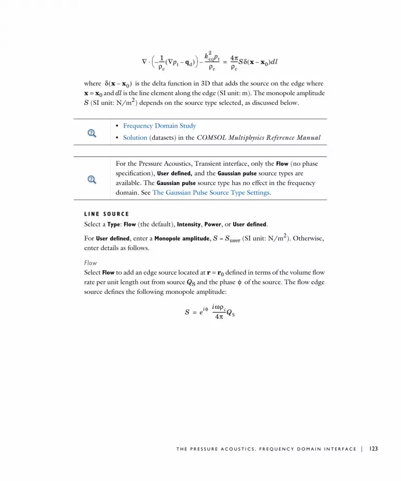
where is the delta function in 3D that adds the source on the edge where x = x0 and dl is the line element along the edge (SI unit: m). The monopole amplitude S (SI unit: N/m2) depends on the source type selected, as discussed below.

L I N E S O U R C E

Select a Type: Flow (the default), Intensity, Power, or User defined.

For User defined, enter a Monopole amplitude, S = Suser (SI unit: N/m2). Otherwise, enter details as follows.

FlowSelect Flow to add an edge source located at r = r0 defined in terms of the volume flow rate per unit length out from source QS and the phase of the source. The flow edge source defines the following monopole amplitude:

∇ 1ρc-----– ∇pt qd–( )

⋅keq

2 ptρc

-------------–4πρc------Sδ x x0–( )dl=

δ x x0–( )

• Frequency Domain Study

• Solution (datasets) in the COMSOL Multiphysics Reference Manual

For the Pressure Acoustics, Transient interface, only the Flow (no phase specification), User defined, and the Gaussian pulse source types are available. The Gaussian pulse source type has no effect in the frequency domain. See The Gaussian Pulse Source Type Settings.

φ

S eiφ iωρc4π

------------QS=


124 | C H A P T E R

A flow edge source with the strength QS represents an area flow out from the source (the source is a very thin cylinder with a surface that pulsates).

• Enter a Volume flow rate per unit length out from source, QS (SI unit: m2/s) for the source-strength amplitude in the field.

• Enter a Phase (SI unit: rad).

IntensitySelect Intensity to add an edge source located at r = r0 defined in terms of the source intensity radiated Irms and the phase of the source. Set a desired free space reference intensity (RMS) Irms at a specified distance dsrc from the source. In a homogeneous medium, the specified intensity is obtained when the edge is a straight line (this is the reference). With other objects and boundaries present, or if the edge is curved, the actual radiated intensity is different. This source type defines the following monopole amplitude:

where Ledge is the length of the source line (automatically determined) and dsrc is the distance from the source where free space reference intensity (RMS) Irms is specified. Enter values or expressions for:

• Free space reference intensity (RMS), Irms (SI unit: W/m2).

• Distance from source center dsrc (SI unit: m).

• Phase (SI unit: rad).

PowerSelect Power to add an edge source located at r = r0 specified in terms of the source’s reference RMS strength by stating the total power Prms a straight line source would radiate into a homogeneous medium. This source type defines the following monopole amplitude:

When defining a Solution dataset and plotting the results, specify a nonzero phase to produce a nonzero result when visualizing the resulting pressure field using the default value (0) in the Solution at

angle (phase).

φ

φ

φ

S eiφ dsrcLedge-------------- 2Irefρccc=

φ


where Ledge is the length of the source line (automatically determined) and Prms denotes the free space reference RMS power (in the reference homogeneous case) per unit length measured in W/m. Enter values or expressions for:

• Free space reference power (RMS), Prms (SI unit: W).


Line Source on Axis

Use the Line Source on Axis node to add a line source on the axis of symmetry in 2D axisymmetric components. This type of source corresponds a radially vibrating cylinder in the limit where its radius tends to zero. The line source adds a source term to the right-hand side of the governing Helmholtz equation such that:

where is the delta function in 3D that adds the source on the axis of symmetry where z = z0 and r = 0, and dz is the line element along the z-axis (SI unit: m). The monopole amplitude S (SI unit: N/m2) depends on the source type selected and is the same as discussed in the 3D case for a Line Source.

L I N E S O U R C E O N A X I S

Select a Type: Flow (the default), Intensity, Power, or User defined. See the options and expression for Line Source. The sources are the same but in 2D axisymmetric components they are only applicable on the symmetry axis at r = 0.

S eiφ

Ledge-------------

ρcccPrms2π

----------------------=

φ

∇ 1ρc-----– ∇pt qd–( )

⋅keq

2 ptρc

-------------–4πρc------Sδ z z0–( )dz=

δ z z0–( )



• Solution (datasets) in the COMSOL Multiphysics Reference Manual


126 | C H A P T E R

Monopole Point Source

Use the Monopole Point Source node to add a monopole point source in 3D components on any point and in 2D axisymmetric components on points on the axis of symmetry. This is a source that is uniform and equally strong in all directions. A monopole represents a radially pulsating sphere in the limit where the radius tends to zero. The monopole point source adds a point source term to the right-hand side of the governing Helmholtz equation such that:

where is the delta function in three dimensions and adds the source at the point where x = x0. The monopole amplitude S (SI unit: N/m2) depends on the source type selected, as discussed below.

M O N O P O L E P O I N T S O U R C E

Select a Type: Flow (the default), Intensity, Power, or User defined.

For User defined enter a Monopole amplitude, S = Suser (SI unit: N/m).

FlowSelect Flow to add an monopole point source located at x = x0 defined in terms of the volume flow rate out from source QS and the phase of the source. The source defines the following monopole amplitude:

Enter values or expressions for:

• Volume flow rate out from source, QS (SI unit: m3/s).


∇ 1ρc-----– ∇pt qd–( )

⋅keq

2 ptρc

-------------–4πρc------Sδ x x0–( )=

δ x x0–( )


φ

S eiφiωρc4π

------------QS=

φ


IntensitySelect Intensity to define the source in terms of the free space reference RMS intensity Irms it radiates. In a homogeneous medium, the specified intensity is obtained (the reference), but with other objects and boundaries present the actual intensity is different. The source defines the following monopole amplitude:

where dsrc is the distance from the source where the intensity Irms is specified and is the phase of the source. Enter values or expressions for:




PowerWhen Power is selected, specify the source’s reference RMS strength by stating the power it radiates. In a homogeneous medium, the specified power is obtained (the reference), but with other objects and boundaries present the actual power is different. The source defines the following monopole amplitude:

where Pref denotes the radiated RMS power per unit length measured in W/m. Enter values or expressions for:

• Free space reference power (RMS), Prms (SI unit: W).


S eiφdsrc 2ρcccIrms=

φ

φ

S eiφ ρcccPrms2π

----------------------=

φ

Bessel Panel: Application Library path Acoustics_Module/

Tutorials,_Pressure_Acoustics/bessel_panel

Hollow Cylinder: Application Library path Acoustics_Module/

Vibrations_and_FSI/hollow_cylinder

Point sources in 2D components also exist. They actually correspond to infinite out-of-plane line sources, see Point Sources (for 2D Components).


128 | C H A P T E R

Dipole Point Source

Use the Dipole Point Source node to add a dipole point source. A dipole is mathematically a source that corresponds to two monopoles close to each other that are completely out of phase. Dipoles appear when there are fluctuating forces in the medium; for example, a small object that vibrates back and forth. A complex acoustic source may be expanded and approximated by a collection of point sources (Monopole Point Source, Dipole Point Source, and Quadrupole Point Source). The dipole point source adds a point source term to the right-hand side of the governing Helmholtz equation such that:

where δ(x − x0) is the delta function in three dimensions and adds the source at the point where x = x0. The dipole moment vector D (SI unit: N) depends on the source type selected, as discussed below. In 2D axisymmetric models, the dipole point source is only added to the z-axis, such that x0 = (0,0,z). See Ref. 5 for details.

Figure 2-3: Schematic illustration of a dipole source.

D I P O L E P O I N T S O U R C E

Select a Type: Power (the default) or User defined.

User DefinedFor User defined enter a Dipole moment vector D (SI unit: N). In 2D axisymmetric components enter the z-component only.

PowerThe Power option defines the following dipole moment vector in terms of the free space reference power, the dipole direction, and the source phase

∇ 1ρc-----– ∇pt qd–( )

⋅keq

2 ptρc

-------------–4πρc------D ∇δ x x0–( )⋅=


Enter the following:

• Free space reference power (RMS), Prms (SI unit: W). In a homogeneous medium, the specified power is radiated (the reference), but with other objects and boundaries present the actual power is different.

• The source Phase (SI unit: rad).

• Dipole moment direction eD. Defines the direction of the dipole moment vector. In 2D axisymmetric components the direction is aligned along the z-axis such that eD = ez.

Quadrupole Point Source

Use the Quadrupole Point Source node to enter a quadrupole point source. A quadrupole is mathematically a source that corresponds to two dipoles close to each other. A complex acoustic source may be expanded and approximated by a collection of point sources (Monopole Point Source, Dipole Point Source, and Quadrupole Point Source). The quadrupole point source adds a point source term to the right-hand side of the governing Helmholtz equation such that:

where is the delta function in three dimensions and adds the source at the point where x = x0. The quadrupole D-vector D (SI unit: N) and the quadrupole d-vector d (SI unit: m) depend on the source type selected, as discussed below. In 2D axisymmetric models, the quadrupole point source is only added to the z-axis, such that x0 = (0,0,z) and only orientations along the axis are possible. Two types of predefined quadrupole sources exist, a Power (longitudinal) and a Power (lateral) configuration. In the longitudinal source, the D and d vectors are parallel and point in the same direction. In the lateral configuration, the D and d vectors are perpendicular to each other (see Ref. 5 for details).

D D eiφ eDeD---------= D 2 3ρccc

3Prms

2πω2--------------------------=

φ


∇ 1ρc-----– ∇pt qd–( )

⋅keq

2 ptρc

-------------–4πρc------ D ∇⋅( ) d ∇⋅( )δ x x0–( )=

δ x x0–( )


130 | C H A P T E R

Q U A D R U P O L E P O I N T S O U R C E

Select a Type: Power (longitudinal) (the default), Power (lateral), or User defined. The lateral options do not exist in 2D-axisymmetric models.

User DefinedFor User defined enter the Quadrupole d vector (SI unit: m) and Quadrupole D vector (SI unit: N). In 2D axisymmetric models enter a Quadrupole amplitude Q (SI unit: N⋅m) as both the D and d vectors are pointed along the z-axis.

Figure 2-4: Schematic illustration of the user-defined quadrupole point source.

Power (Longitudinal)The Power (longitudinal) defines the following values for the two quadrupole vectors




ed eD= Q d DT⋅ Qeiφ ed eD⋅( )= =

Q2 5ρcccPrms

2πk4--------------------------=

φ


• Quadrupole direction, (dimensionless). In a 2D axisymmetric model, the direction is along the z-axis.

Figure 2-5: Schematic illustration of the longitudinal power quadrupole point source.

Power (Lateral)The Power (lateral), not defined in 2D axisymmetric components, defines the following values for the two quadrupole vectors:




• Quadrupole normal, n (dimensionless). This is the normal to the plane in which the quadrupole is located.

e'D

ed n eD×= Q d DT⋅ Qeiφ ed eD⋅( )= =

Q2 15ρcccPrms

2πk4------------------------------=

φ


132 | C H A P T E R

• Quadrupole direction, (dimensionless). The projection of this vector onto the plane (defined by the normal n) defines the direction of the dipole D-vector.

Figure 2-6: Schematic illustration of lateral quadrupole point source.

Point Sources (for 2D Components)

For 2D components, the monopole, dipole, and quadrupole point sources also exist. All the sources actually correspond to an infinite line source in the out-of-plane direction. The monopole is uniform and equally strong in all the in-plane directions — an infinitely long pulsating cylinder. The dipole source represents an infinitely long cylinder moving back and forth. The quadrupole represents two dipoles close to each other.

The point sources add the following point source term to the right-hand side of the governing Helmholtz equation — for monopole, dipole, and quadrupole point sources, respectively:

where δ(x − x0) is the delta function in 2D and adds the source at the point where (x,y) = x = x0. The monopole amplitude S (SI unit: N/m2), the dipole moment vector D (SI unit: N/m), and the quadrupole d vector (SI unit: m) and D vectors (SI unit: N/m) depend on the source type selected.

e'D


4πρc------Sδ x x0–( ) 4π

ρc------D ∇δ x x0–( )⋅ 4π

ρc------ D ∇⋅( ) d ∇⋅( )δ x x0–( )


M O N O P O L E P O I N T S O U R C E ( 2 D C O M P O N E N T S )

Select a Type: Flow (the default), Intensity, Power, or User defined. For User defined enter a Monopole amplitude, Suser (SI unit: N/m).

FlowSelect Flow to add a monopole point source located at r = r0 defined in terms of the volume flow rate per unit length out from source QS and the phase of the source. The source defines the following monopole amplitude:


• Volume flow rate out from source, QS (SI unit: m3/s).


IntensitySelect Intensity to define the source in terms of the free space reference RMS intensity Irms it radiates. In a homogeneous medium, the specified intensity is obtained (the reference), but with other objects and boundaries present, the actual intensity is different. The source defines the following monopole amplitude:

where dsrc is the distance from the source where the intensity Irms is specified and is the phase of the source. Enter values or expressions for:




PowerWhen Power is selected, specify the source’s reference RMS strength by stating the power per unit length it radiates. In a homogeneous medium, the specified power is obtained (the reference), but with other objects and boundaries present, the actual source power is different. The source defines the following monopole amplitude:

φ

S eiφiωρc4π

------------QS=

φ

S eiφ 2ρcωIrmsdsrc2π

---------------------------------=

φ

φ

S eiφ 2ρcωPrms

2π( )2-------------------------=


134 | C H A P T E R

where Prms denotes the free space RMS reference power per unit length measured in W/m and is the phase of the source. Enter values or expressions for:

• Free space reference power (RMS) per unit length, Prms (SI unit: W/m).


D I P O L E P O I N T S O U R C E ( 2 D C O M P O N E N T S )

Enter a user defined Dipole-moment vector, D (SI unit: N/m).

Q U A D R U P O L E P O I N T S O U R C E ( 2 D C O M P O N E N T S )

Enter a user defined Quadrupole d vector, d (SI unit: m), and a user defined Quadrupole

D vector, D (SI unit: N/m).

Circular Source (for 2D Axisymmetric Components)

Use the Circular Source node to add a source in a 2D axisymmetric component on points off the axis of symmetry. Such points correspond to circular sources or ring sources. This type of source is, for example, used to mimic source terms from rotors. The circular source adds a point source term to the right-hand side of the governing Helmholtz equation such that:

where is the delta function that adds the source at the point where x = x0 and rdϕ is the line element around the circular source (SI unit: m). The monopole amplitude S (SI unit: N/m2) depends on the source type selected, as discussed below.

φ

φ


∇ 1ρc-----– ∇pt qd–( )

⋅keq

2 ptρc

-------------–4πρc------Sδ x x0–( )rdϕ=

δ x x0–( )

For the Pressure Acoustics, Transient interface the Flow (no phase specification), User defined, and the Gaussian pulse source types are available. The Gaussian pulse source type has no effect in the frequency domain. See The Gaussian Pulse Source Type Settings.


C I R C U L A R S O U R C E

Select a Type: Flow (the default) or User defined. For User defined enter a Monopole

amplitude, S = Suser (SI unit: N/m2).

FlowWhen Flow is selected the source is defined in terms of the volume flow rate QS per unit length out form the source. The flow circular source defines the following monopole amplitude:


• Volume flow rate per unit length out from source, QS (SI unit: m2/s).


Pressure (Point Condition)

Use the Pressure condition on points to define pressure monopole-like sources with a specific pressure. The condition is, for example, useful when setting up room acoustic models where a prescribed pressure is needed (ideal pressure source). The condition acts as a constraint.

P R E S S U R E

Enter a value or expression for the Pressure p0 (SI unit: Pa). In the time domain, the expression should depend on time.

S eiφ iωρc4π

------------QS=

φ


136 | C H A P T E R

Th e P r e s s u r e A c ou s t i c s , T r a n s i e n t I n t e r f a c e

The Pressure Acoustics, Transient (actd) interface ( ), found under the Acoustics>Pressure Acoustics branch ( ) when adding a physics interface, is used to compute the pressure variation when modeling the propagation of acoustic waves in fluids at quiescent background conditions. It is suited for time-dependent simulations with arbitrary time-dependent fields and sources.

The physics interface can be used to model linear and nonlinear acoustics that can be well described by the scalar pressure variable. Domain conditions include the Nonlinear Acoustics (Westervelt) Contributions to include nonlinear effects, the Anisotropic Acoustics feature to model fluids with an effective anisotropic density, and the Background Pressure Field (for Transient Models) for defining a background acoustic field to model scattering problems or defining incident waves. User-defined sources can also be added via the Monopole Domain Source or the Dipole Domain Source. For open problems, Perfectly Matched Layers (PMLs) can be applied, also in the time domain for Pressure Acoustics, as efficient nonreflecting boundary conditions.

The physics interface solves the scalar wave equation in the time domain. Studies for performing time-dependent modal and modal reduced-order models also exist. The physics interface also solves in the frequency domain with the available boundary conditions.


Builder — Transient Pressure Acoustics Model, Sound Hard Boundary (Wall), and Initial

Values. Then, from the Physics toolbar, add other nodes that implement, for example, boundary conditions and source. You can also right-click Pressure Acoustics, Transient

to select physics features from the context menu.

For good modeling strategies, meshing, solvers, postprocessing information, acoustics specific plots, as well as tips and tricks, see the Modeling with the Pressure Acoustics Branch (FEM-Based Interfaces) section.


S E T T I N G S



The default Name (for the first physics interface in the model) is actd.

T Y P I C A L W A V E S P E E D F O R P E R F E C T L Y M A T C H E D L A Y E R S

Enter a value or expression for the Typical wave speed for perfectly matched layers cref (SI unit m/s). The default is 343 m/s. It is important to set this speed correctly as the performance of the Perfectly Matched Layers (PMLs) in the time domain depends only on the wave speed and not the wavelength. For further details see the Time Domain Perfectly Matched Layers section.

T R A N S I E N T S O L V E R S E T T I N G S

Enter the Maximum frequency to resolve in the model. The default frequency is set to 1000[Hz] but should be changed to reflect the frequency content of the sources used in the model. Select the Time stepping (method) as Fixed (preferred) the default and recommended or Free. The Free option is in general not recommended for wave problems. The generated solver will be adequate in most situations if the computational mesh also resolves the frequency content in the model. Note that any changes made to these settings (after the model is solved the first time) will only be reflected in the solver if Show Default Solver or Reset Solver to Defaults is selected in the study. It is also important to Reset Solver to Defaults if the Nonlinear Acoustics (Westervelt) Contributions feature is added as special handling of the nonlinear term is enabled. For highly nonlinear problems set up with user-defined terms, manual tuning of the solver may be necessary. In nonlinear models the maximum frequency to resolve should be selected based on the number of harmonics to be resolved.

Further details on Time Stepping in Transient Models in the Modeling with the Pressure Acoustics Branch (FEM-Based Interfaces) section.

The remainder of the Settings window is shared with The Pressure Acoustics, Frequency Domain Interface.

T H E P R E S S U R E A C O U S T I C S , T R A N S I E N T I N T E R F A C E | 137

138 | C H A P T E R

Domain, Boundary, Edge, and Point Nodes for the Pressure Acoustics, Transient Interface

The Pressure Acoustics, Transient Interface shares most of its nodes with The Pressure Acoustics, Frequency Domain Interface, except the following:

• Domain, Boundary, Edge, and Point Nodes for the Pressure Acoustics, Transient Interface


• Theory for the Perfectly Matched Layers in the Time Domain

• Transient Gaussian Explosion: Application Library path Acoustics_Module/Tutorials,_Pressure_Acoustics/gaussian_explosion

• Gaussian Pulse Absorption by Perfectly Matched Layers: Pressure Acoustics, Transient: Application Library path Acoustics_Module/

Tutorials,_Pressure_Acoustics/gaussian_pulse_perfectly_matched_layers

• Nonlinear Acoustics — Modeling of the 1D Westervelt Equation: Application Library path Acoustics_Module/Nonlinear_Acoustics/

nonlinear_acoustics_westervelt_1d

• Nonlinear Acoustics (Westervelt) Contributions

• Background Pressure Field (for Transient Models)

• Exterior Field Calculation (for Transient Models)

• Incident Pressure Field (for Transient Models)





• Normal Velocity


• Transient Pressure Acoustics Model

• The Gaussian Pulse Source Type Settings

Domain, Boundary, Edge, Point, and Pair Nodes for the Pressure Acoustics, Frequency Domain Interface


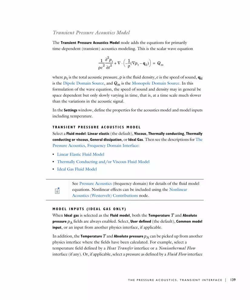
Transient Pressure Acoustics Model

The Transient Pressure Acoustics Model node adds the equations for primarily time-dependent (transient) acoustics modeling. This is the scalar wave equation

where pt is the total acoustic pressure, ρ is the fluid density, c is the speed of sound, qd is the Dipole Domain Source, and Qm is the Monopole Domain Source. In this formulation of the wave equation, the speed of sound and density may in general be space dependent but only slowly varying in time, that is, at a time scale much slower than the variations in the acoustic signal.

In the Settings window, define the properties for the acoustics model and model inputs including temperature.

T R A N S I E N T P R E S S U R E A C O U S T I C S M O D E L

Select a Fluid model: Linear elastic (the default), Viscous, Thermally conducting, Thermally

conducting or viscous, General dissipation, or Ideal Gas. Then see the descriptions for The Pressure Acoustics, Frequency Domain Interface:

• Linear Elastic Fluid Model

• Thermally Conducting and/or Viscous Fluid Model

• Ideal Gas Fluid Model

M O D E L I N P U T S ( I D E A L G A S O N L Y )

When Ideal gas is selected as the Fluid model, both the Temperature T and Absolute

pressure pA fields are always enabled. Select, User defined (the default), Common model

input, or an input from another physics interface, if applicable.

In addition, the Temperature T and Absolute pressure pA can be picked up from another physics interface where the fields have been calculated. For example, select a temperature field defined by a Heat Transfer interface or a Nonisothermal Flow interface (if any). Or, if applicable, select a pressure as defined by a Fluid Flow interface

1

ρc2---------

∂2pt

∂t2----------- ∇ 1

ρ--- pt qd–∇( )–

⋅+ Qm=

See Pressure Acoustics (frequency domain) for details of the fluid model equations. Nonlinear effects can be included using the Nonlinear Acoustics (Westervelt) Contributions node.


140 | C H A P T E R

present in the model. For example, select Absolute pressure (spf) to use the absolute pressure defined by a Laminar Flow interface spf.

Nonlinear Acoustics (Westervelt) Contributions

The propagation of finite-amplitude pressure waves cannot be described by the linear acoustic wave equation (small perturbation assumption) and requires solving the full nonlinear second-order wave equation. The latter allows a simplification when cumulative nonlinear effects dominate local nonlinear effects, for example, when the propagation distance is greater than the wavelength. The simplified equation is referred to as the Westervelt equation and reads

,

where δ is the diffusivity of sound and β is the coefficient of nonlinearity. In general, the linear assumption is only valid when

which has a value of approximately 1.5·105 Pa for air and 2·109 Pa for water. So, whenever the acoustic pressure is say a factor 100 less than these values, the linear assumption holds. When this is not the case, the Nonlinear Acoustics (Westervelt)

Contributions feature should be added.

The Nonlinear Acoustics (Westervelt) Contributions node adds the nonlinear contribution (first term on the right-hand side) to the Transient Pressure Acoustics

Model. That is, the linear acoustic wave equation transforms to the nonlinear Westervelt equation. To add the dissipation term (last term on the left-hand side) select, for

The Nonisothermal Flow interface requires the addition of the Heat Transfer Module or CFD Module.


1

ρc2---------

∂2pt

∂t2----------- ∇ 1

ρ--- pt qd–∇( )–

δρc2---------

∂ pt∇∂t

------------–

⋅+β

ρ2c4-----------

∂2pt2

∂t2------------ Qm+=

p ρc2«


example, the General dissipation as the Fluid model in the Transient Pressure Acoustics Model.

N O N L I N E A R A C O U S T I C S ( W E S T E R V E L T )

Specify the coefficient of nonlinearity. The available options are From parameter of

nonlinearity (the default), From ratio of specific heats (for gases), and User defined.

• For the option From parameter of nonlinearity enter the value of the Parameter of

nonlinearity, B/A. The coefficient of nonlinearity is defined as follows

The parameter of nonlinearity quantifies the effect of nonlinearity on the local speed of sound in the fluid. It is expressed as c = c0 + (B/2A)u in the first-order terms, where u is the acoustic particle velocity.

The resulting equation is nonlinear and therefore does not allow the application of the superposition principle. In particular, the Background Pressure Field (for Transient Models) cannot be defined together with the Nonlinear Acoustics (Westervelt) Contributions feature.

The presence of the Nonlinear Acoustics (Westervelt) Contributions node changes the default solver settings for the proper treatment of nonlinearities. It is therefore required to Reset Solver to Defaults whenever the feature is added to or removed from the model.

The frequency spectrum of a nonlinear wave model contains not only the center frequency f0 but also the harmonics N·f0, N = 1,2,3,… generated. The Maximum frequency to resolve in the Transient Solver Settings section should be specified to resolve a desired number of harmonics to achieve a certain precision. This is especially important for shock waves, where the number of harmonics to resolve can exceed 10.

• For the theory background of this nonlinear feature, see Pressure Acoustics, Transient Equations.

β 1 B2A-------+=


142 | C H A P T E R

• For the option From ratio of specific heats (for gases) enter the Ratio of specific heats, γ. This option is valid for perfect gases under isentropic conditions. Here,

B/A = γ − 1, which yields

• Choose the User defined option to specify β explicitly.

S H O C K - C A P T U R I N G S T A B I L I Z A T I O N

To display this section, click the Show More Options button ( ) and select Stabilization. Select Enable q-Laplacian relaxation to add some artificial nonlinear damping to the model (it is turned off per default). This is typically only necessary in highly nonlinear models. The dissipative term of physical origin will often balance the shock formation (remember to define the appropriate Fluid model in the Transient Pressure Acoustics Model). The effective diffusivity is tuned with the stabilization by adding an extra term that reads

The highest artificial damping is achieved where the acoustic pressure increases or decreases the most rapidly. It reaches its maximal values where the pressure endures discontinuities, that is, where shocks arise. Thus, this technique provides a shock-capturing stabilization.

Specify the q-Laplacian exponent q and the q-Laplacian factor κ to get the desirable amount of artificial damping. Note that the damping must not be too high nor too low. The particular values of q and κ depend on the material and the input signal frequency. The two parameters that control the stabilization require manual tuning. A suggested approach is to use a simple 1D model to tune the parameters based on fluid material properties and frequency content. Use, for example, the Nonlinear Acoustics — Modeling of the 1D Westervelt Equation model from the application library to do so.

β γ 1+2

------------=

δκ 1t∂

∂ p∇q 1–

– –

Nonlinear Acoustics — Modeling of the 1D Westervelt Equation: Application Library path Acoustics_Module/Nonlinear_Acoustics/



Background Pressure Field (for Transient Models)

Add a Background Pressure Field node to model an background/incident pressure wave to study the scattered pressure field ps, which is defined as the difference between the total acoustic pressure pt and the background pressure field pb:

This feature sets up the equations in a so-called scattered field formulation where the dependent variable is the scattered field p = ps. In a model where the background pressure field is not defined on all acoustic domains (or it is different), continuity is automatically applied in the total field pt on interior boundaries between domains.


Select the Pressure field type as Plane wave (monochromatic) (the default), Modulated

Gaussian pulse, or User defined.

• For Plane wave (monochromatic) enter a value for the Pressure amplitude p0 of the wave, select the Speed of sound as User defined (enter a value for c) or From material, enter a Wave direction vector ek, enter the Signal frequency f0 of the wave, and a possible Phase .

These settings defined a background pressure field pb as a plane propagating wave of the type:

• For Modulated Gaussian pulse enter a value for the Pressure amplitude p0 of the wave, select the Speed of sound as User defined (enter a value for c) or From material, enter a Wave direction vector ek and enter the Signal emitting plane coordinate x0. The latter two options define the initial location of the pulse and the propagation direction. When modeling scattering problems, the initial location should be placed outside the computational domain. Next define the frequency content of the Gaussian pulse. Select the Gaussian pulse bandwidth as Full width at half maximum,

power (the default), Full width at half maximum, amplitude, Full duration at half

maximum, power, Full duration at half maximum, amplitude, or Standard deviation.

If the chosen fluid model has no dissipation (Linear elastic (the default) or Ideal Gas), a default sound dissipation δ = 2·10-5 m2/s will be used in the artificial damping term.

pt pb ps+=

φ

pb x t,( ) p0 2πf0 tx ek⋅c ek--------------–

φ+ sin=


144 | C H A P T E R

For the first two options enter a frequency bandwidth Δf and for the latter a time window Δt. Finally, enter the carrier Signal frequency (for time dependent studies) f0.

These settings defined a background pressure field pb as a propagating modulated Gaussian pulse of the type:

where the standard deviation σ of the Gaussian G(x,t) depends on the bandwidth option selected. The modulated Gaussian pulse option only gives contributions when a time dependent model is solved. It has the advantage of having a defined frequency content and can be used for limited bandwidth simulations. In combination with the Exterior Field Calculation (for Transient Models) and an FFT study, the broadband scattering characteristics of an object can be analyzed.

• For User defined enter an analytical expression that can be a function of both space and time or use a solution from a previous study.


To display this section, when the Plane wave (monochromatic) option is selected, click the Show More Options button ( ) and select Advanced Physics Options in the Show

More Options dialog box.

Click to select the Use ramp function option (selected per default). With this option turned on, a ramp is automatically added to smoothly increase the background pressure field amplitude over the first period T = 1/f0. This option ensures numerical stability.

Incident Pressure Field (for Transient Models)

The Incident Pressure Field node is a subnode to all nonreflecting boundary conditions (plane, cylindrical, spherical wave radiation, and matched boundary). From the Physics toolbar, add to Matched Boundary, Plane Wave Radiation, Spherical Wave Radiation, or Cylindrical Wave Radiation nodes. Three options exist for transient models: Plane

weave (monochromatic) (the default), Modulated Gaussian pulse, and User Defined.

Plane Wave (Monochromatic)The same options apply as for the incident fields as for the Background Pressure Field (for Transient Models) feature.

pb x t,( ) p0G x t,( ) 2πf0 tx ek⋅c ek--------------–

sin=


Modulated Gaussian pulseThe same options apply as for the incident fields as for the Background Pressure Field (for Transient Models) feature.

User DefinedIf you are in the Pressure Acoustics, Transient interface, the incident pressure field is only of the user-defined type. In this case, the incident pressure field needs to be defined as a traveling wave of the form

where ω is the angular frequency and k is the wave vector. The function f is any function, for example, a sine function. This spatial and temporal dependency is a requirement for the radiation boundary condition to work properly.

The Gaussian Pulse Source Type Settings

For the Pressure Acoustics, Transient interface, you can in addition to the User Defined and Flow option select a predefined Gaussian pulse as a source Type for the Line Source, Line Source on Axis, Monopole Point Source, Point Sources (for 2D Components), and Circular Source (for 2D Axisymmetric Components) features. This type adds a source with a Gaussian time profile defined in terms of its amplitude A, its frequency bandwidth f0, and the pulse peak time tp. Using this source type results in solving a wave equation of the type:

where S is the source strength.

In 3D components (for Line Source), 2D axisymmetric components (for Line Source on Axis and Circular Source (for 2D Axisymmetric Components)), and 2D components (for Point Sources (for 2D Components)), all of which are effectively line sources, enter the following values or expressions:

• The value of the pulse Amplitude A (SI unit: m2/s).

• Frequency bandwidth f0 (SI unit: Hz).

• Pulse peak time tp (SI unit: s) for the duration of the pulse.

f ωt k x⋅–( )

1

ρc2---------

∂2pt

∂t2----------- ∇ 1

ρ--- pt qd–∇( )–

⋅+4πρ

------Sδ x x0–( )=

S ρ4π------ ∂

∂t----- Ae

π2f02 t tp–( )2–[ ] A– ρπ

2---f0

2 t tp–( )e π2f02 t tp–( )2–

= =


146 | C H A P T E R

In 3D and 2D axisymmetric components for the Monopole Point Source, enter the following values or expressions:

• The value of the pulse Amplitude A (SI unit: m3/s).

• Frequency bandwidth f0 (SI unit: Hz).

• Pulse peak time tp (SI unit: s) for the duration of the pulse.

Normal Acceleration

The Normal Acceleration adds an inward normal acceleration an(t). Mathematically, the condition adds the boundary condition:

Alternatively, specify the acceleration a0 of the boundary. The part in the normal direction is used to define the boundary condition:






Transient Gaussian Explosion: Application Library path Acoustics_Module/Tutorials,_Pressure_Acoustics/gaussian_explosion

n–1ρ0------– ∇p qd–( )

⋅ an t( )=

n–1ρ---– ∇p qd–( )

⋅ n– a⋅ 0 t( )=

In transient models all sources need to be functions of time t in order to represent an acoustic signal. This can, for example, be a harmonic sine wave defined as sin(omega*t) or any other signal.


Normal Velocity

The Normal Velocity adds an inward normal velocity vn(t) or specify the acceleration v0(t) of the boundary. The part in the normal direction is used to define the boundary condition. The condition is very similar to the Normal Acceleration condition having the acceleration given by the time derivative of the velocity an(t) = ∂vn(t)/∂t. This feature represents an external source term. It can also be used to manually couple acoustics with a structural analysis for modeling acoustic-structure interaction.





Normal Displacement

The Normal Displacement adds an inward normal displacement dn(t) or specify the acceleration d0(t) of the boundary. The part in the normal direction is used to define the boundary condition. The condition is very similar to the Normal Acceleration condition having the acceleration given by the double time derivative of the displacement an(t) = ∂2dn(t)/∂t2. This feature represents an external source term. It can also be used to manually couple acoustics with a structural analysis for modeling acoustic-structure interaction.





Exterior Field Calculation (for Transient Models)

The Exterior Field Calculation feature adds the equations necessary to postprocess the exterior field to the computational domain for open problems. The feature is the same as the Exterior Field Calculation in The Pressure Acoustics, Frequency Domain


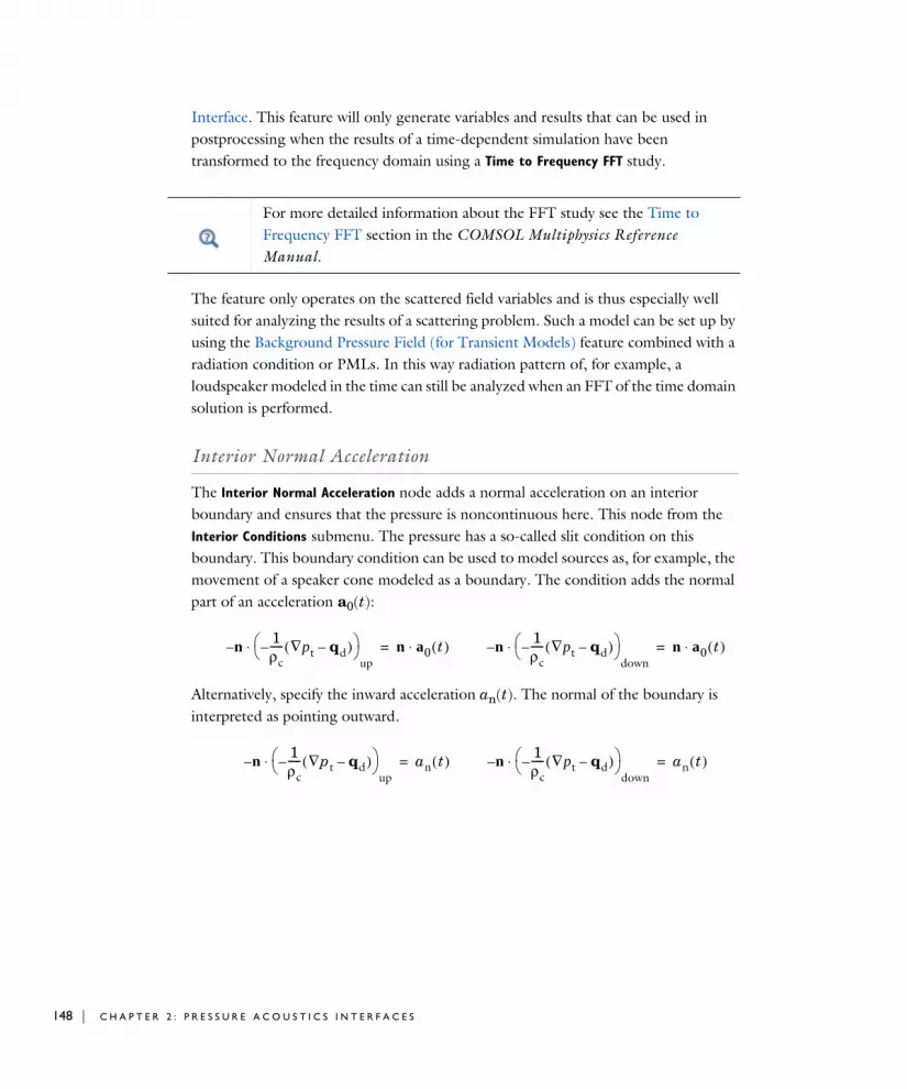
148 | C H A P T E R

Interface. This feature will only generate variables and results that can be used in postprocessing when the results of a time-dependent simulation have been transformed to the frequency domain using a Time to Frequency FFT study.

The feature only operates on the scattered field variables and is thus especially well suited for analyzing the results of a scattering problem. Such a model can be set up by using the Background Pressure Field (for Transient Models) feature combined with a radiation condition or PMLs. In this way radiation pattern of, for example, a loudspeaker modeled in the time can still be analyzed when an FFT of the time domain solution is performed.


The Interior Normal Acceleration node adds a normal acceleration on an interior boundary and ensures that the pressure is noncontinuous here. This node from the Interior Conditions submenu. The pressure has a so-called slit condition on this boundary. This boundary condition can be used to model sources as, for example, the movement of a speaker cone modeled as a boundary. The condition adds the normal part of an acceleration a0(t):

Alternatively, specify the inward acceleration an(t). The normal of the boundary is interpreted as pointing outward.

For more detailed information about the FFT study see the Time to Frequency FFT section in the COMSOL Multiphysics Reference Manual.

n–1ρc-----– ∇pt qd–( )

up

⋅ n a⋅ 0 t( )= n–1ρc-----– ∇pt qd–( )

down

⋅ n a⋅ 0 t( )=

n–1ρc-----– ∇pt qd–( )

up

⋅ an t( )= n–1ρc-----– ∇pt qd–( )

down

⋅ an t( )=





• For Normal acceleration enter the value of the Normal acceleration an (SI unit: m/s2) in the normal direction. The normal is depicted as a red arrow in the graphics window on the selected boundary.


The Interior Normal Velocity node adds a normal velocity on an interior boundary and ensures that the pressure is noncontinuous. Add this node from the Interior Conditions

submenu. The pressure has a so-called slit condition on this boundary. The condition is very similar to the Interior Normal Acceleration condition having the acceleration given by the time derivative of the velocity.


Select a Type: Velocity (the default) or Nromal velocity.

• For Velocity enter values for the components of the Velocity v0 (SI unit: m/s2).

• For Normal velocity enter the value of the Normal velocity vn (SI unit: m/s2) in the normal direction. The normal is depicted as a red arrow in the graphics window on the selected boundary.


The Interior Normal Displacement node adds a normal displacement on an interior boundary and ensures that the pressure is noncontinuous. Add this node from the Interior Conditions submenu. The pressure has a so-called slit condition on this boundary. The condition is very similar to the Interior Normal Acceleration condition having the acceleration given by the double time derivative of the displacement.

In transient models all sources need to be functions of time t in order to represent an acoustic signal. This can, for example, be a harmonic sine wave defined as sin(omega*t) or any other signal.


150 | C H A P T E R



• For Displacement enter values for the components of the Displacement d0 (SI unit: m/s2).

• For Normal displacement enter the value of the Normal displacement dn (SI unit: m/s2) in the normal direction. The normal is depicted as a red arrow in the graphics window on the selected boundary.


Th e P r e s s u r e A c ou s t i c s , Bounda r y Mode I n t e r f a c e

The Pressure Acoustics, Boundary Mode (acbm) interface ( ), found under the Acoustics>Pressure Acoustics branch ( ) when adding a physics interface, is used to compute and identify propagating and nonpropagating modes in waveguides and ducts by performing a boundary mode analysis on a given boundary. The study is useful, for example, when specifying sources at inlets or analyzing transverse acoustic modes in ducts. It is available for 3D and 2D axisymmetric component models.

The physics interface solves the Helmholtz eigenvalue equation on boundaries, searching for the out-of-plane wave numbers at a given frequency.


Builder: Pressure Acoustics Model, Sound Hard Boundary (Wall), and Initial Values. Then, from the Physics toolbar, add other nodes that implement, for example, boundary conditions and sources. You can also right-click Pressure Acoustics, Boundary Mode to select physics features from the context menu.

S E T T I N G S



The default Name (for the first physics interface in the model) is acbm.

T H E P R E S S U R E A C O U S T I C S , B O U N D A R Y M O D E I N T E R F A C E | 151

152 | C H A P T E R

E Q U A T I O N


See the settings for Sound Pressure Level Settings for the Pressure Acoustics, Frequency Domain interface.


This physics interface defines one dependent variable (field), the Pressure p. The name can be changed but the names of fields and dependent variables must be unique within a model.


From the list select the element order and type (Lagrange or serendipity) for the Pressure, the default is Quadratic Lagrange.

Initial Values

The Initial Values node adds initial values for the sound pressure. Add more Initial

Values nodes from the Physics toolbar.

For 2D axisymmetric components, the Azimuthal mode number m is by default 0. It is an integer entering the axisymmetric expression for the pressure:

Change the value as needed. Also see Physics Nodes — Equation Section in the COMSOL Multiphysics Reference Manual.

p r z ϕ, ,( ) p r( ) ei kzz mϕ+( )–

=

• Initial Values

• Boundary, Edge, Point, and Pair Nodes for the Pressure Acoustics, Boundary Mode Interface

• Pressure Acoustics, Boundary Mode Equations



Enter a value or expression for the Pressure p (SI unit: Pa) initial value.

Boundary, Edge, Point, and Pair Nodes for the Pressure Acoustics, Boundary Mode Interface

Special postprocessing variables exist for the Boundary Mode Acoustics interface. They are described in Pressure Acoustics, Boundary Mode Variables.

Eigenmodes in a Muffler: Application Library path Acoustics_Module/

Automotive/eigenmodes_in_muffler

Except for Initial Values, The Pressure Acoustics, Boundary Mode Interface shares all of its feature nodes with the Pressure Acoustics, Frequency Domain interface. See Domain, Boundary, Edge, Point, and Pair Nodes for the Pressure Acoustics, Frequency Domain Interface.

Also, for the Pressure Acoustics, Boundary Mode interface, apply the features to boundaries instead of domains for 3D components.

T H E P R E S S U R E A C O U S T I C S , B O U N D A R Y M O D E I N T E R F A C E | 153

154 | C H A P T E R

Th e P r e s s u r e A c ou s t i c s , Bounda r y E l emen t s I n t e r f a c e

The Pressure Acoustics, Boundary Elements (pabe) interface ( ), found under the Pressure Acoustics branch ( ) when adding a physics interface, is used to compute the pressure variation for the propagation of acoustic waves in gases and liquids. It is suited for all frequency-domain simulations with harmonic variations of the pressure field. The formulation is based on the boundary element method (BEM) and the interface is available in 2D and 3D. The physics interface solves Helmholtz equation for constant-valued material properties and uses the pressure as the dependent variable.

The interface is fully multiphysics enabled and can be coupled seamlessly with the physics interfaces that are based on the finite element method (FEM). This includes coupling to vibrating structures with the Acoustic-Structure Boundary multiphysics coupling, to FEM acoustic domains, with the Acoustic FEM-BEM Boundary multiphysics coupling, to thermoviscous acoustic domains with the Acoustic-Thermoviscous Acoustic Boundary multiphysics coupling, and to poroelastic waves domains with the Acoustic-Porous Boundary multiphysics coupling. This approach allows modeling in a FEM-BEM framework, using the strength of each formulation adequately. The BEM-based interface is especially well suited for radiation and scattering problems.

The advantage of the boundary element method is that only boundaries need to be meshed and the degrees of freedom (DOFs) solved for are restricted to the boundaries. This introduces some clear ease-of-use for handling complex geometries. However, the BEM technique results in fully populated or dense matrices that need dedicated numerical methods. The BEM method is so to speak more expensive per DOF than the FEM method but has fewer DOFs. Assembling and solving these can be very demanding. This means that when solving acoustic models of small and medium size, The Pressure Acoustics, Frequency Domain Interface will often be faster than solving the same problem with the BEM interface. The challenge for the FEM interface is to set up open boundaries, for example, using PMLs, in an efficient way. When the geometries are complex or two structures are far apart, large air domains need to be meshed. This costs a lot on the computational side as the frequency is increased.

For acoustically large models (problems that contain many wavelengths, at high frequency or for large domains) the stabilized formulation option (see Stabilization)


ensures efficient convergence at the cost of some additional degrees of freedom. For low to medium frequencies (small to medium models), running without stabilization is more efficient. The stabilized formulation only gives a benefit in computing time for the acoustically large models.

The governing Helmholtz equation defined by the Pressure Acoustics, Boundary Element interface is given by:

(2-1)

where pt is the total acoustic pressure, keq is the wave number, ρc is the density, and cc is the speed of sound. The subscript “c” denotes that these can be complex-valued quantities in models with damping. The governing equations and boundary conditions are formulated using the total pressure pt with a so-called scattered field formulation. In the presence of a Background Pressure Field defining a background pressure wave pb (this could, for example, be a plane wave), the total acoustic pressure pt is the sum of the pressure solved for p (which is then equal to the scattered pressure ps) and the

For good modeling strategies, meshing, solvers, postprocessing information, as well as tips and tricks, see the Modeling with the Pressure Acoustics Branch (BEM-Based Interface) section.

• Head and Torso HRTF Computation. Application Library path: Acoustics_Module/Tutorials,_Pressure_Acoustics/head_torso_hrtf

• Spherical Scatterer: BEM Benchmark. Application Library path: Acoustics_Module/Verification_Examples/

spherical_scatterer_bem_benchmark

1ρc-----∇2pt–

keq2

ρc--------pt– 0=

pt p pb+= keq2 ω

cc---- 2

=

T H E P R E S S U R E A C O U S T I C S , B O U N D A R Y E L E M E N T S I N T E R F A C E | 155

156 | C H A P T E R

background pressure wave: pt = p+pb. The equations then contain the information about both the scattered field and the background pressure field.


Builder — Pressure Acoustics, Sound Hard Boundary (Wall), and Initial Values.

Then, from the Physics toolbar, add other nodes that implement boundary conditions. You can also right-click Pressure Acoustics, Boundary Elements to select physics features from the context menu. Infinite conditions like a symmetry plane or an infinite sound hard boundary are defined in the Symmetry/Infinite Boundary Condition section.

The boundary element method (BEM) used in the Pressure Acoustics, Boundary Element interface is based on the direct method with Costabels symmetric coupling. The adaptive cross approximation (ACA) fast summation method is used for solving the resulting linear system. This method uses partial assembly of the matrices where the effect of the matrix vector multiplication is computed. The default iterative solver used is GMRES. With the built-in multiphysics couplings, it is easy and seamless to set up problems that combine FEM- and BEM-based physics. When solving these coupled models, the default approach is to use hybridization with the ACA for BEM and an appropriate preconditioner for the FEM part of the problem (direct or multigrid).

More details about the BEM formulation can be found in The PDE, Boundary Elements Interface documentation in the COMSOL Multiphysics Reference Manual.

For a tutorial that uses a BEM-FEM coupling to model an acoustic problem see the Bessel Panel. Application Library path Acoustics_Module/

Tutorials,_Pressure_Acoustics/bessel_panel

• Domain, Boundary, Edge, and Pair Nodes for the Pressure Acoustics, Boundary Elements Interface


Physics Nodes — Equation Section in the COMSOL Multiphysics Reference Manual


S E T T I N G S



The default Name (for the first physics interface in the model) is pabe.

E Q U A T I O N

Expand the Equation section to see the equations solved for with the Equation form specified. The default selection is Equation form is set to Study controlled. The available studies are selected under Show equations assuming. If Frequency domain is selected as the Equation form the Frequency of the study can be either taken From solver or User

defined.


Select the Enable physics symbols check box to display the infinite boundary condition lines or planes in the geometry.









12--- p p∗=


158 | C H A P T E R

S Y M M E T R Y / I N F I N I T E B O U N D A R Y C O N D I T I O N

In this section you can specify infinite boundary conditions for the boundary element problem. These are conditions that are not added on a boundary but apply to a line in 2D or a plane in 3D. The planes where the conditions are applied are visualized if the Enable physics symbols is turned on (the default) in the Physics Symbols section.

For pressure acoustics a symmetry condition is mathematically equivalent to a sound hard boundary, and an antisymmetry condition is equivalent to a sound soft boundary. In this way you can include a Symmetry/Infinite sound hard boundary or an Antisymmetry/Infinite sound soft boundary along “infinite lines” (in 2D) or “infinite planes” in (3D). Only one condition per Cartesian direction can be applied.

For the infinite conditions to be mathematically valid it is important that all sources and BEM boundaries are located on the same side of (or on) the infinite conditions. The condition can, for example, not be used as an infinite baffle with sound radiating through a hole. In this case, the propagation domain is on a different side than the source.

An important aspect is how the results are visualized, specifically when setting the Parameter Bounds in the grid dataset. Say the condition represents a symmetry plane then visualize the solution in the entire domain. On the other hand if the condition represents an infinite sound hard boundary, like the ground or an infinite baffle, then only visualize the solution above that plane by setting the Parameter Bounds in the Grid

3D or Grid 2D dataset in Results.

Choose an option from the Condition for the x = x0 plane, Condition for the y = y0

plane, and Condition for the z = z0 plane lists (when applicable). In 2D, these are out-of-plane surfaces. Choose one of the following options:

• Off, for no symmetry (the default)

• Symmetric/Infinite sound hard boundary

• Antisymmetric/Infinite sound soft boundary

Then enter the value for the plane location x0, y0, or z0 (the default is 0 m). This allows an offset of the infinite condition planes along the main coordinate axes.

F A R - F I E L D A P P R O X I M A T I O N


Physics Options.

These settings are used for matrix assembly and postprocessing. They allow characterization of interactions occurring in the boundary element method as


near-field or far-field interactions. While the near-field interactions are represented explicitly, the far-field interactions can be represented in an approximate way. This approach results in considerable memory and performance improvements when used in combination with iterative solvers using matrix-free format or during postprocessing. The near-field part of the stiffness matrix is used as input by the Direct and Sparse Approximate Inverse preconditioners.

The Use far-field approximation check box is selected by default in order to accelerate the solution process. If the check box is cleared, the solution will be slightly more accurate but the computational time and memory consumption may become prohibitively high.

The Approximation type can be either ACA+ or ACA. These alternatives correspond to two different versions of the adaptive-cross-approximation (ACA) method, which is a fast matrix multiplication method based on far-field approximations.

C O N D I T I O N A T I N F I N I T Y

In this section, you specify the condition to apply at infinity for an unbounded problem. For the Helmholtz equation, solved here, choose to specify an Outgoing wave (the default) or an Incoming wave. In almost all cases the Outgoing wave option should be selected.

Q U A D R A T U R E

The quadrature settings are by default set to Automatic. This means that the quadrature integration order values will follow the element order selection in the Discretization section. Higher element orders automatically generate higher values for the quadrature integration orders.

More details are found under Far-Field Approximation Settings in The PDE, Boundary Elements Interface documentation in the COMSOL Multiphysics Reference Manual.

More details are found under Quadrature in The PDE, Boundary Elements Interface documentation in the COMSOL Multiphysics Reference Manual.


160 | C H A P T E R

S T A B I L I Z A T I O N

To display this section, click the Show More Options button ( ) and select Stabilization in the Show More Options dialog box.

For acoustically large models (problems that contain many wavelengths, at high frequency or for large domains) enable the Stabilized formulation option to ensure efficient convergence at the cost of some additional degrees of freedom.

When Stabilized formulation is selected, an edit field for the Stabilization parameter is enabled with the default value sqrt(abs(pabe.k[m])). This is a parameter that should scale inversely with the wavelength. The default gives good performance in most cases.

P O S T P R O C E S S I N G S E T T I N G S


Physics Options in the Show More Options dialog box.

This setting controls the interpolation that is done close to boundaries (typically in the last mesh element) between variables on boundaries (these are the variables solved for in BEM based interfaces) and their value evaluated with the kernel in the domains. Numerically the kernel evaluation is prone to errors near the boundaries while the DOFs solved for are exact on the boundaries. Using an interpolation in the inner mesh element removes singularities in the results when postprocessing values in the domain near a boundary.

Enter an expression for the Interpolation distance from boundary. The entered value defines the distance beyond which the kernel evaluation is used. The default is 0.5*h which gives reasonable results. This default corresponds to half the mesh size h. If the value is set to 0 no interpolation is done.


From the Dependent variable/Normal boundary flux list, choose from predefined options for the boundary element discretization order for the dependent variable and the normal boundary flux. The predefined options represent the suitable combinations of element orders such as Quadratic/Linear (the default).

See also Postprocessing BEM Results in the Modeling with the Pressure Acoustics Branch (BEM-Based Interface) section.


The settings under Value types when using splitting of complex variables are important for sensitivity and optimization computations. See the description of the built-in operators fsens and fsensimag.


This physics interface defines one dependent variable (field), the Pressure p. If required, edit the name, which changes both the field name and the dependent variable name. The new field name must not coincide with the name of a field of another type, or with a component name belonging to some other field.

Domain, Boundary, Edge, and Pair Nodes for the Pressure Acoustics, Boundary Elements Interface

The Pressure Acoustics, Boundary Elements Interface has the following domain and boundary conditions (in alphabetic order):

Pressure Acoustics

The Pressure Acoustics node adds the equations for solving the Helmholtz equation, defined by Equation 2-1, in the frequency domain using the boundary element method. The material properties have to be constant valued for each Pressure Acoustics node added.

Each Pressure Acoustics node adds the necessary BEM equations to the adjacent boundaries of the selection (with the material properties defined). The domain features in the BEM interface can be applied to all types of domain selections: solid domains, finite voids, and the infinite void. Only the exterior boundaries of the selections as well

• Background Pressure Field

• Continuity

• Impedance

• Initial Values







• Normal Velocity

• Pressure

• Pressure Acoustics




162 | C H A P T E R

as applied interior boundary conditions need to be meshed. Finite voids are selections of domains that have no solids in the geometry but are only defined by a closed set of boundaries. The Infinite void represents the exterior most infinite domain. This selection is the typical used for radiation or scattering problems. Remember that the materials defined in the Materials node need to be applied to the same selections.

In the Settings window, define the properties for the acoustics model and model inputs including the absolute background pressure and temperature.


The values of the quiescent (or background) Temperature T (SI unit: K) and Absolute

pressure pA (SI unit: Pa) are entered in the Model Inputs section. The values of the model inputs can influence the material properties like, for example, the density and speed of sound, depending on their definition in the Materials node. In the BEM formulation these two values have to be constant valued for each Pressure Acoustics node added.


To define the properties of the bulk fluid, select a Fluid model from the list: Linear elastic (the default), Linear elastic with attenuation, Viscous, Thermally conducting, Thermally

conducting and viscous, or Ideal gas. The settings for the fluid models are the same as for Pressure Acoustics in The Pressure Acoustics, Frequency Domain Interface.

See also Selections: Infinite Void and Finite Voids in the Modeling with the Pressure Acoustics Branch (BEM-Based Interface) section.

The fluid models represent different bulk loss or attenuation mechanisms (applied in a homogenized way) or ways of defining the fluid properties of the fluid. Some of these models are sometimes referred to as an equivalent fluid model. The loss model can be a theoretical model or a model based on measurement data for the attenuation in the fluid.

The theory for the fluid models is in the section Theory for the Equivalent Fluid Models.


Background Pressure Field

Add a Background Pressure Field node to add a background pressure wave to model scattering problems solving for the scattered pressure field ps. The total field pt is the sum of the scattered field and the background pressure field pb:

This feature sets up the equations in a so-called scattered field formulation where the dependent variable is the scattered field p = ps. When added, the background pressure field is applied everywhere; it has a locked selection set to all.

In models solved with the boundary element method, it is important that the defined Background Pressure Field is an exact solution to the governing equation. If this is not the case, the results will be unphysical. This means that setting up a user-defined field needs careful consideration.


Select a Background pressure field type: Plane wave (the default), Cylindrical Wave, Spherical Wave, or User defined. Most of the options and settings here are the same as for the Background Pressure Field in The Pressure Acoustics, Frequency Domain Interface.

The only difference lies in the definition of the material properties for the background field. In the BEM interface define a Wave number either picked up from a Pressure Acoustics model in the physics tree (the default), for example, Wave number (pabe/

bpam1), or defined From speed of sound. This option ensures that the background field is a solution to the governing equation. If several material models are added, they must have the same speed of sound, to ensure that the background pressure field is a solution to the underlying Helmholtz equation.

Initial Values

The Initial Values node adds an initial value for the pressure.


The Sound Hard Boundary (Wall) adds a boundary condition for a sound hard boundary or wall, which is a boundary at which the normal component of the acceleration (and thus the velocity) is zero:

pt pb ps+=


164 | C H A P T E R

To apply a sound hard boundary condition to an infinite plane in the boundary element model, see the Symmetry/Infinite Boundary Condition functionality.

Normal Acceleration

The Normal Acceleration adds a source at an exterior boundary defined by the inward normal acceleration an or alternatively given through an acceleration a0:





Normal Velocity

The Normal Velocity adds a source at an exterior boundary defined by the inward normal velocity vn or alternatively given through a velocity v0:





n 1ρc-----∇pt–

⋅– 0=

n 1ρc-----∇pt–

⋅– an n a0⋅–= =

n 1ρc-----∇pt–

⋅– iωvn iω n v0⋅( )–= =


Normal Displacement

The Normal Displacement adds a source at an exterior boundary defined by the inward normal displacement dn or alternatively given through a displacement d0:





Sound Soft Boundary

The Sound Soft Boundary adds a boundary condition for a sound soft boundary, where the acoustic pressure vanishes: pt = 0. It is an appropriate approximation for a liquid-gas interface and in some cases for external waveguide ports. To apply a sound soft condition to an infinite plane in the boundary element model, see the Symmetry/Infinite Boundary Condition functionality.

Pressure

The Pressure node creates a boundary condition that acts as a pressure source at the boundary, which means that a constant acoustic pressure p0 is specified and maintained at the boundary: pt = p0. The pressure can be a complex number and thus includes phase information.

P R E S S U R E

Enter the value of the Pressure p0 (SI unit: Pa).

Impedance

The Impedance node adds an impedance boundary condition with the option to select between several built-in impedance models and engineering relations. All the options

n 1ρc-----∇pt–

⋅– iω( )2dn iω( )2n d0⋅–= =


166 | C H A P T E R

are the same as for the Impedance condition of The Pressure Acoustics, Frequency Domain Interface. All the settings and models are described there.

Exclude Boundary

The Exclude Boundary feature is used to remove boundaries from the boundary element problem. The selected boundaries will neither contribute to the assembly of the BEM problem nor to the solution. The condition can be used to set up models where the BEM interface is used as an ideal infinite domain in an infinite baffle (infinite half space) setup when coupled to the Pressure Acoustics, Frequency Domain. In these models, all boundaries of the FEM problem need to be excluded, except for the ones in the multiphysics coupling.


The Interior Sound Hard Boundary (Wall) sets up a wall condition on an interior boundary. Add this node from the Interior Conditions submenu. The pressure is discontinuous across this boundary.

When postprocessing and plotting variables on boundaries with interior conditions, the boundary variables (with extension _bnd) give the average value of the two sides. Use the up (_up) and down (_down) variants to depict the values on both sides of the boundary.

For a tutorial that uses a BEM-FEM coupling and the Exclude Boundary feature to model an acoustic problem in an infinite baffle setup see the tutorial Piezoelectric Tonpilz Transducer with a Prestressed Bolt. Application Library path Acoustics_Module/Piezoelelctric_Devices/

tonpilz_transducer_prestressed

See also Postprocessing BEM Results in the Modeling with the Pressure Acoustics Branch (BEM-Based Interface) section.

In the BEM formulation, interior conditions cannot intersect other (exterior) conditions. It is recommended that this type of model is set up by using FEM in the region around the interior condition and BEM outside of that region.



The Interior Normal Acceleration sets up an interior source that can be used to model a thin vibrating structure, for example, a loudspeaker diaphragm. Add this node from the Interior Conditions submenu. The pressure is discontinuous across this boundary.

The pressure is discontinuous across this boundary. Use the up and down version of the postprocessing variables to visualize quantities on the two sides of the boundary, for example, the up side total pressure is pabe.p_t_up.




• For Normal acceleration enter the value of the Normal acceleration an (SI unit: m/s2) in the normal direction.


Select Show physics symbols to show the normal direction as a symbol (red arrow) in the Graphics window (selected per default).


The Interior Normal Velocity sets up an interior source that can be used to model a thin vibrating structure, for example, a loudspeaker diaphragm. Add this node from the Interior Conditions submenu.




168 | C H A P T E R


Select a Type: Velocity (the default) or Normal velocity.


• For Normal velocity enter the value of the Normal velocity vn (SI unit: m/s) in the normal direction.




The Interior Normal Displacement sets up an interior source that can be used to model a thin vibrating structure, for example, a loudspeaker diaphragm. Add this node from the Interior Conditions submenu.







• For Normal displacement enter the value of the Normal displacement dn (SI unit: m) in the normal direction.



Continuity

For details see the Continuity condition in The Pressure Acoustics, Frequency Domain Interface.



170 | C H A P T E R

Th e P r e s s u r e A c ou s t i c s , T ime Exp l i c i t I n t e r f a c e

The Pressure Acoustics, Time Explicit (pate) interface ( ), found under the Acoustics>Pressure Acoustics branch ( ) when adding a physics interface, is used to compute the pressure variation when modeling the propagation of acoustic waves in fluids at quiescent background conditions. The interface is used to solve large transient linear acoustic problems containing many wavelengths. It is suited for time-dependent simulations with arbitrary time-dependent sources and fields. The interface includes a Background Acoustic Field option for modeling of scattering problems. Absorbing layers are used to set up effective nonreflecting-like boundary conditions. The exterior field can be calculated by combining the Exterior Field Calculation feature with a Time to Frequency FFT study step. The interface exists in 2D, 2D axisymmetric, and 3D.

The interface is based on the discontinuous Galerkin method (dG-FEM) and uses a time-explicit solver. The method is very memory lean and is well suited for cluster computing. Application areas include the transient propagation of audio pulses in room acoustics or modeling scattering phenomena involving large objects relative to the wavelength.

If the acoustic waves propagate in a background flow (for example, inside a flowmeter), then use The Convected Wave Equation, Time Explicit Interface.

For modeling acoustic structure interaction (ASI) the Pressure Acoustics, Time Explicit interface can be combined with The Elastic Waves, Time Explicit Interface using the Acoustic-Structure Boundary, Time Explicit multiphysics coupling.

The interface solves the linearized Euler equations assuming an adiabatic equation of state. The dependent variables are the acoustic pressure and the acoustic velocity perturbations. Bulk losses (volume attenuation) can be included in the interface using the classical expression for thermal and viscous attenuation or a general dissipation term.

Losses at boundaries can be modeled with impedance conditions. The built-in option includes frequency independent resistive losses. By combining the interface with a user defined Boundary ODEs and DAEs mathematics interface general frequency dependent conditions can be formulated also for the time domain.



Builder — Pressure Acoustics Time Explicit Model, Sound Hard Boundary (Wall), and Initial

Values. Then, from the Physics toolbar, add other nodes that implement, for example, boundary conditions and source. You can also right-click Pressure Acoustics, Time

Explicit to select physics features from the context menu.

S E T T I N G S



The default Name (for the first physics interface in the model) is pate.

F I L T E R P A R A M E T E R S F O R A B S O R B I N G L A Y E R S


Physics Options. In the Filter Parameters for Absorbing Layers section you can change and control the values set for the filter used in the Absorbing Layers. The values of the filter parameters defined here are used in all absorbing layers added to the model and they override the value of filter parameters enabled in the material model (Pressure Acoustics, Time Explicit Model). The default values of the filter parameters α, ηc, and

For good modeling strategies, meshing, solvers, postprocessing information, acoustics specific plots, as well as tips and tricks, see the Modeling with the Pressure Acoustics Branch (DG-FEM-Based Interface) section.

Domain, Boundary, Edge, and Point Nodes for the Pressure Acoustics, Time Explicit Interface

For a tutorial example that uses the interface to model a scattering problem see the Submarine Scattering: Time-Domain Simulation and FFT tutorial in the COMSOL Application Gallery: https://www.comsol.com/model/55921

T H E P R E S S U R E A C O U S T I C S , T I M E E X P L I C I T I N T E R F A C E | 171


172 | C H A P T E R

s are set to 0.1, 0.01, and 2, respectively. Inside the absorbing layer it is important to use a filter that is not too aggressive since this will result in spurious reflections.


The settings selected here are only used if the transient solution solved is transformed into the frequency domain using the Time to Frequency FFT study. The zero level on the dB scale varies with the type of fluid. That value is a reference pressure that corresponds to 0 dB. This variable occurs in calculations of the sound pressure level Lp based on the root mean square (rms) pressure prms, such that





User-defined reference pressure to enter a reference pressure pref, SPL (SI unit: Pa). The default value is the same as for air, 20 μPa.


In this section you can select the discretization for the Acoustic pressure and Acoustic

velocity. Per default both are set to Quartic (4th order). Using quartic elements together with a mesh size equal to approximately half the wavelength to be resolved, leads to the best performance when using the DG method. For further details see the Meshing, Discretization, and Solvers section.


The dependent variables are the Acoustic pressure, and the Acoustic velocity. The names can be changed, but the names of fields and dependent variables must be unique within

For general information about the filter see the Filter Parameters section under Wave Form PDE in the COMSOL Multiphysics Reference Manual.


12--- p p∗=


a model. The name for the Acoustic velocity, components can also be selected individually.

Domain, Boundary, Edge, and Point Nodes for the Pressure Acoustics, Time Explicit Interface

The Pressure Acoustics, Time Explicit Interface has the following domain and boundary conditions listed in alphabetic order, available from the Physics ribbon toolbar (Windows users), Physics context menu (Mac or Linux users), or right-click to access the context menu (all users). Continuity in velocity and pressure is the default condition on interior boundaries. If a boundary separates two different materials the Material Discontinuity or Continuity (the pair version of material discontinuity) condition has to be applied to ensure the continuity in velocity and pressure.

Pressure Acoustics, Time Explicit Model

The Pressure Acoustics, Time Explicit Model node adds the equations to model the transient propagation of linear acoustics waves based on the dG-FEM time explicit method. For the time explicit method used, the governing equations are formulated as a first order system, in terms of the linearized continuity equation and the linearized momentum equation, as

• Background Acoustic Field

• Continuity

• Exterior Field Calculation

• General Flux/Source

• General Interior Flux

• Heat Source

• Impedance



• Initial Values

• Mass Source

• Material Discontinuity

• Normal Velocity

• Pressure

• Pressure Acoustics, Time Explicit Model



• Symmetry

• Volume Force Source


174 | C H A P T E R

(2-2)

where t is time, pt is the total acoustic pressure, ut is the total acoustic velocity, ρ is the fluid density, c is the speed of sound, and I is the unit matrix. Domain sources like a Mass Source, Heat Source, or Volume Force Source can be defined through the right hand sides Qm and qd. These two source terms represent the same quantities as the Monopole Domain Source and the Dipole Domain Source in The Pressure Acoustics, Frequency Domain Interface and The Pressure Acoustics, Transient Interface.

The dependent variables are the acoustic pressure p and the acoustic velocity u (sometimes called particle velocity or perturbation velocity). The equations are formulated in the total fields pt and ut which is the sum of the scattered field (the dependent variable solved for) and a possible background field pb and ub. The background field can be set up using the Background Acoustic Field feature.

The equations solved are the linearized Euler equations in a quiescent setting. The equations are easily combined to generate the scalar wave equation solved in The Pressure Acoustics, Transient Interface as discussed in Theory Background for the Pressure Acoustics Branch.

In the formulation of the wave equation, the speed of sound c and density ρ may in general be space dependent but only slowly varying in time, that is, at a time scale much slower than the variations in the acoustic signal.

In the Settings window, define the properties for the acoustics model and model inputs including temperature.

1

ρc2---------

∂pt∂t-------- ∇ ut⋅+ Qm=

ρ∂ut∂t

--------- ∇ ptI( )⋅+ qd=

The equations solved in the Pressure Acoustics, Time Explicit interface are closely related to the equations solved in The Convected Wave Equation, Time Explicit Interface. There is no background flow option in the Pressure Acoustics, Time Explicit interface but, on the other hand, it uses a scattered field formulation that allows solving scattering problems. For nonlinear acoustic problems The Nonlinear Pressure Acoustics, Time Explicit Interface should be used.



Select a Fluid model: Linear elastic (the default), Viscous, Thermally conducting, Thermally

conducting and viscous, General dissipation, or Ideal gas.

• If Linear elastic is selected enter the speed of sound c and the density ρ.

• If Viscous, Thermally conducting, or Thermally conducting and viscous is selected enter the fluid properties (see the Transient Pressure Acoustics Model for details). These three options will define the sound diffusivity δ through the classical material properties. The options are equivalent to defining the classical thermoviscous attenuation factor atv in the frequency domain.

• If General dissipation is selected enter the speed of sound c, the density ρ, and the sound diffusivity δ. This option can be used for modeling fluids with measured damping properties. The relation between the sound diffusivity δ and the equivalent (plane wave) attenuation coefficient α, at a given frequency f, is given by the expression

where ω = 2πf and c is the speed of sound.

• If Ideal gas is selected enter the combination of material properties defining the gas.

For all options, the default is to use the material property values from From material, select User defined from the list to enter a user-defined value or expression in the text field that appears. For numerical stability reasons it is recommended to use physical values of attenuation properties.

Selecting any of the dissipations models will modify the governing Equation 2-2 by adding a right hand side to the momentum equation defined as

(2-3)

This term has a small cost on the computation time when solving the model. The term has to be evaluated at every time-step taken by the solver.

L A X - F R I E D R I C H S F L U X P A R A M E T E R S

To display this section, click the Show More Options button ( ) and select Stabilization in the Show More Options dialog box. In this section, you specify the value of the Lax-Friedrichs flux parameter τLF (default value: 0.2). This value controls the numerical flux between the elements (nodal discontinuous Lagrange elements) used with the discontinuous Galerkin (DG) method. The numerical flux defines how

α δω2

2c3----------=

qd ρδ∇ ∇u( )⋅ ρδ uΔ= =


176 | C H A P T E R

adjacent elements are connected and how continuous p and u are. Different definitions of the numerical flux lead to different variants of the DG method. The flux implemented here is the so-called global Lax-Friedrichs numerical flux. The value of the parameter τLF should be between 0 and 0.5. For τLF = 0 a so-called central flux is obtained. Setting τLF = 0.5 gives a maximally dissipative global Lax-Friedrichs flux.

F I L T E R P A R A M E T E R S


Physics Options in the Show More Options dialog box. By default, the filter parameters α, ηc, and s are not active. Select the Activate check box to activate the filter. The filter provides higher-order smoothing for the DG formulation. Inside absorbing layers the settings given here are overridden by the Filter Parameters for Absorbing Layers.

Background Acoustic Field

Add a Background Acoustic Field node to model a background/incident pressure wave to study the scattered pressure fields ps and us. The scattered fields are defined as the difference between the total acoustic fields pt and ut and the background acoustic field pb and ub:

This feature sets up the equations in a so-called scattered field formulation where the dependent variable is the scattered field (p = ps and u = us). In a model where the background acoustic field is not defined on all acoustic domains (or it is different) continuity is automatically applied in the total fields pt and ut on interior boundaries between domains.

For general information about the numerical flux see the Numerical Flux section under Wave Form PDE in the COMSOL Multiphysics Reference Manual.

For more detailed information about the filter see the Filter Parameters section under Wave Form PDE in the COMSOL Multiphysics Reference Manual.

pt pb ps+=

ut ub us+=


B A C K G R O U N D A C O U S T I C F I E L D

Select the Pressure field type as Plane wave (monochromatic) (the default) or User

defined.

• For Plane wave (monochromatic) enter a value for the Pressure amplitude p0 of the wave, select the Speed of sound and Density as User defined (enter a value for c or ρ) or From material, enter a Wave direction vector ek, enter the Signal frequency f0 of the wave, and a possible Phase .

These settings defined a background acoustic field as a plane propagating wave of the type:

• For Modulated Gaussian pulse enter a value for the Pressure amplitude p0 of the wave, select the Speed of sound as User defined (enter a value for c) or From material, enter a Wave direction vector ek and enter the Signal emitting plane coordinate x0. The latter two options define the initial location of the pulse and the propagation direction. When modeling scattering problems the initial location should outside the computational domain. Next define the frequency content of the Gaussian pulse. Select the Gaussian pulse bandwidth as Full width at half maximum, power (the default), Full width at half maximum, amplitude, Full duration at half maximum, power, Full duration at half maximum, amplitude, or Standard deviation. For the first two options enter a frequency bandwidth Δf and for the latter a time window Δt. Finally, enter the carrier Signal frequency (for time dependent studies) f0.

These settings defined a background pressure field pb as a propagating modulated Gaussian pulse of the type:

where the standard deviation σ of the Gaussian G(x,t) depends on the bandwidth option selected. The modulated Gaussian pulse option only gives contributions when a time dependent model is solved. It has the advantage of having a defined frequency content and can be used for limited bandwidth simulations. In combination with the Exterior Field Calculation and an FFT study the broadband scattering characteristics of an object can be analyzed.

• For User defined enter an analytical expression that can be function of both space and time or use a solution from a previous study.

φ

pb x t,( ) p0 2πf0 tx ek⋅c ek--------------–

φ+ sin= ub x t,( )

pbρc------

ekek--------=

pb x t,( ) p0G x t,( ) 2πf0 tx ek⋅c ek--------------–

sin= ub x t,( )

pbρc------

ekek--------=


178 | C H A P T E R


To display this section, when the Plane wave (monochromatic) option is selected, click the Show More Options button ( ) and select Advanced Physics Options in the Show

More Options dialog box.

Click to select the Use ramp function option (selected per default). With this option turned on, a ramp is automatically added to smoothly increase the background pressure field amplitude over the first period T = 1/f0. This option ensures numerical stability.

Initial Values

The Initial Values node adds initial values for the acoustic pressure and the acoustic velocity that can serve as an initial state for the solver. If more than one initial value is needed, from the Physics toolbar click to add more Initial Values nodes.


Enter a value or expression for the initial values for the Pressure p (SI unit: Pa) and the Acoustic velocity, u (SI unit: m/s).

Mass Source

The Mass Source sets up the right-hand side of the continuity equation, in Equation 2-2, in terms of a mass rate of change. This is a monopole-like source that acts uniformly in all directions.

M A S S S O U R C E

Enter the Mass source M (SI unit: kg/(m3·s)).

Heat Source

The Heat Source sets up the right-hand side of the continuity equation, in Equation 2-2, in terms of a heat density source. This is a monopole-like source that acts uniformly in all directions.

Qm1ρ---M=

Qmαp

ρCp----------Qheat=


where αp is the (isobaric) coefficient of thermal expansion, ρ is the density, Cp is the heat capacity at constant pressure, and Qheat is the heat source.

M O D E L I N P U T

Enter the ambient Temperature T, the default is 293.15[K].

H E A T S O U R C E

Enter the Heat Source Qheat (SI unit: W/m3).


Enter the Heat capacity at constant pressure Cp and the Ratio of specific heats γ either selected From material or User defined. The ratio of specific heats is used to calculate the coefficient of thermal expansion through the thermodynamic relation

Volume Force Source

The Volume Force Source sets up the right-hand side of the momentum equation, in Equation 2-2, in terms of a volumetric force. This is a dipole-like source that acts differently in two directions.

V O L U M E F O R C E S O U R C E

Enter the Volume force source F (SI unit: N/m3).


The Sound Hard Boundary (Wall) adds a boundary condition for a sound hard boundary or wall, which is a boundary at which the normal component of the velocity is zero (a slip condition)

Note that this condition is not identical to the Symmetry condition. The condition is also available from the Pairs submenu, as an option at interfaces between parts in an assembly. This effectively introduces a condition similar to the Interior Sound Hard Boundary (Wall) but used on an assembly.

αp1c---

Cp γ 1–( )T

------------------------=

qd F=

n– u⋅ 0=


180 | C H A P T E R

Sound Soft Boundary

The Sound Soft Boundary conditions adds a boundary condition for a sound soft boundary, where the acoustic pressure vanishes pt = 0. It is an appropriate approximation, for example, for a liquid-gas interface or in some cases for external waveguide ports.

Pressure

The Pressure node creates a boundary condition that acts as a pressure source at the boundary. The total acoustic pressure is given at the boundary pt = p0(t).

P R E S S U R E

Enter an expression for the Pressure p0(t) (SI unit: Pa). The input can be any analytical function or interpolation data that can be function of both time and space.

Symmetry

The Symmetry node adds a boundary condition imposing symmetry in the pressure and velocity field. Use this condition to reduce the size of a model by cutting it in half where there are known symmetries. The condition implies symmetry in the acoustic fields

Normal Velocity

The Normal Velocity condition adds a source specified in terms of an inward normal velocity vn(t) or velocity v0(t) of the boundary. The component in the normal direction is used to define the boundary condition. This feature represents an external source term like a vibrating surface. The condition is also available from the Pairs submenu, as an option at interfaces between parts in an assembly. This effectively introduces a condition similar to the Interior Normal Velocity but used on an assembly.



• For Inward Velocity enter the value of the Inward velocity vn (SI unit: m/s).


n ut⋅ 0=


Impedance

The Impedance condition adds a boundary condition defining the relation between the local total acoustic pressure pt and the normal acoustic velocity n·ut, that is, the specific acoustic impedance Zi. The condition specifies the normal velocity

This condition can be used to model the properties of artificial boundaries by adding constant resistive losses (no reactive components can be added). When the impedance is set equal to the characteristic specific impedance of a propagating plane wave ρc, the condition represent the simplest nonreflecting boundary condition. This is also the default value of the impedance when the condition is added.

The acoustic impedance condition (with the default value ρc) should be used at the outer boundary when Absorbing Layers are used in a model.

I M P E D A N C E

Enter a value or expression for the Impedance Zi (SI unit: Pa·s/m). The default expression is pate.c*pate.rho which is the characteristic specific impedance ρc of a propagating plane wave.

Exterior Field Calculation

The Exterior Field Calculation feature adds the equations necessary to postprocess the exterior field to the computational domain for open problems. The feature is the same as the Exterior Field Calculation in The Pressure Acoustics, Frequency Domain

n ut⋅ptZi-----–=

As mentioned, the built-in impedance boundary condition only supports frequency independent resistive impedances (they can be space dependent). To model more advanced general user-defend frequency dependent impedance conditions, combine the Normal Velocity boundary condition with the boundary version of The ODE and DAE Interfaces (see Distributed ODEs and DAEs). The time explicit formulation and solver are compatible with solving ODEs on boundaries.

For an example, see the COMSOL Application Gallery tutorial: Full Wave Time Domain Room Acoustics with Frequency Dependent Impedance. Found at: https://www.comsol.com/model/90551


http://www.comsol.com/model/90551

182 | C H A P T E R

Interface. This feature will only generate variables and results that can be used in postprocessing when the results of a time-dependent simulation have been transformed to the frequency domain using a Time to Frequency FFT study.

The feature only operates on the scattered field variables and is thus especially well suited for analyzing the results of a scattering problem. Such a model can be set up by using the Background Acoustic Field feature combined with the Absorbing Layers. Since the time explicit formulation is very memory lean, scattering problems that cannot be solved in the frequency domain can be handled with a time domain approach and an FFT.


The Interior Sound Hard Boundary (Wall) node, found under the Interior Conditions

submenu, adds the boundary condition for a sound hard boundary or wall on interior boundaries. The condition reads

The condition ensures that the total normal velocity is zero on both the up and down side of the boundary, while applying a slit on the pressure (the pressure is discontinuous across the boundary).


The Interior Normal Velocity node, found under the Interior Conditions submenu, adds the boundary condition for a moving interior boundary. This can, for example, represent a thin vibrating structure or s speaker membrane. The condition reads

For more detailed information about the FFT study see the Time to Frequency FFT section in the COMSOL Multiphysics Reference Manual.

Submarine Scattering: Time Domain Simulation and FFT: In the COMSOL Application Gallery www.comsol.com/model/55921

ut,up n⋅ 0=

ut,down n⋅ 0=



The condition ensures that the total normal velocity is defined on both the up and down side of the boundary, while applying a slit on the pressure (the pressure is discontinuous across the boundary).


Select the Type: Velocity (default) or Normal velocity and specify either the Velocity (vector) v0 or the normal component through the Normal velocity vn.

Material Discontinuity

The Material Discontinuity node, found under the Interior Conditions submenu, adds an interior boundary condition to handle jumps in material properties. As the interface is based on the discontinuous Galerkin method special handling is necessary when a jump exists in the specific characteristic impedance Z0 = ρc of the medium.

The condition implements continuity in total pressure and in the normal velocity over the interior boundary:

Subscripts “up” and “down” in the equation refer to the up and down sides of the interior boundary, relative to the normal n.

Continuity

The Continuity node, exists as an option at interfaces between parts in an assembly, from the Pairs submenu. The condition is similar to the Material Discontinuity condition that applies to interior boundaries. The difference is that the Continuity condition should also be applied when the same material exists on both sides of a pair. The advantage of using a pair feature is that the mesh does not need to be conforming on the two sides of the interface (the two parts pf the assembly). This is especially advantageous for the time explicit discontinuous Galerkin method as the time step depends on mesh size and local speed of sound.

The condition implements continuity in total pressure and in the normal velocity over the pair:

ut,up n⋅ v0 t( ) n⋅ vn t( )–= =

ut,down n⋅ v0 t( ) n⋅ vn t( )–= =

pt, up pt, down=

n ut, up⋅ n ut, down⋅=


184 | C H A P T E R

Subscripts “src” and “dst” in the equation refer to the source and destination in the pair; that is, the two sides in the pair.

General Flux/Source

The General Flux/Source node, found under the More submenu, adds the most general boundary condition for the Pressure Acoustics, Time Explicit model, as it is formulated (in the conservative form) for the discontinuous Galerkin method (dG). The condition defines the normal flux gp and gu at an exterior boundary, given by

where u = (u, v, w) and n = (nx, ny, nz) in 3D and 2D, or n = (nr, nϕ, nz) in 2D axisymmetric. Note that this condition is expressed in terms of the dependent variables and not the total fields. Care should be taken when using this advanced condition as the method is sensitive to proper formulation of boundary conditions. Only one characteristic can enter the domain at any boundary at the time, meaning that it is easy to overspecify the problem. Use the mesh normals (nxmesh, nymesh, and nzmesh; or nrmesh, nphimesh, and nzmesh) in the expression you define.

G E N E R A L F L U X / S O U R C E

Enter the expression for the components of the Flux vector gp and gu.

General Interior Flux

The General Interior Flux node, found under the More submenu, adds the most general interior boundary condition for the Pressure Acoustics, Time Explicit model, as it is formulated (in the conservative form) for the discontinuous Galerkin method (dG).

pt, src pt, dst=

nsrc ut, src⋅ ndst ut, dst⋅–=

For more details on using assemblies and the pair features see Assemblies and Pair Conditions in the Modeling with the Pressure Acoustics Branch (DG-FEM-Based Interface) section.

n Γp⋅– n u⋅ gp= =

n Γu⋅–

n1p

n2p

n3p

gu= =


The condition defines the normal flux gp and gu at an interior boundary. It should include any necessary numerical flux (as it overrides the Lax-Friedrichs flux). Care should be taken when using this advanced condition as the method is sensitive to proper formulation of boundary conditions.

G E N E R A L I N T E R I O R F L U X



186 | C H A P T E R

Mode l i n g w i t h t h e P r e s s u r e A c ou s t i c s B r an c h ( FEM -Ba s e d I n t e r f a c e s )

This section contains good practices and modeling tips and tricks for the finite element method (FEM) based interfaces of the Pressure Acoustics Branch: The Pressure Acoustics, Frequency Domain Interface, The Pressure Acoustics, Transient Interface, and The Pressure Acoustics, Boundary Mode Interface. In this section:

• Meshing (Resolving the Waves)

• Lagrange and Serendipity Shape Functions

• Time Stepping in Transient Models

• Frequency Domain, Modal and AWE

• Solving Large Acoustics Problems Using Iterative Solvers

• Perfectly Matched Layers (PMLs)

• Postprocessing Variables


• Dedicated Acoustics Plots for Postprocessing

• About the Material Databases for the Acoustics Module

• Specifying Frequencies: Logarithmic and ISO Preferred

Meshing (Resolving the Waves)

Solutions to acoustic problems are wavelike. The waves are characterized by a wavelength λ in space, whose value depends on the frequency and speed of sound c in the medium according to λ = c/f. This wavelength has to be resolved by the mesh.

To represent a wave on a discrete grid (the mesh), it is obvious that the mesh elements must be smaller than the wavelength in order to resolve the wave. That is, there needs to be several degrees of freedom (DOFs) per wavelength in the direction of propagation. In reality, the lower limit for a fully reliable solution lies at about ten to twelve degrees of freedom per wavelength.

Because the direction of propagation is generally not known beforehand, it is good practice to aim for an isotropic mesh with about twelve DOFs per wavelength on


average, independently of the direction. Therefore, the number of DOFs in a sufficiently resolved mesh is about:

• 1728 = 123 times the model volume measured in wavelengths cubed in 3D.

• 144 = 122 times the model area measured in wavelengths squared in 2D.

• 12 times the model length measured in wavelengths in 1D.

Before starting a new model, try to estimate the required number of DOFs using these guidelines. The maximum number of DOFs that can be solved for differs between computer systems. See Solving Large Acoustics Problems Using Iterative Solvers for solver suggestions.

U S I N G L A G R A N G E A N D S E R E N D I P I T Y E L E M E N T S

When creating an unstructured mesh for use with the default 2nd-order Lagrange elements or 2nd-order serendipity elements (see Lagrange and Serendipity Shape Functions), set the maximum element size hmax to about λ/5 or smaller. Because all elements in the constructed mesh are smaller than hmax, the limit is set larger than the actual required element size. Note that for specific engineering purposes it is sometimes possible to use a coarser mesh. This is, for example, the case if only the sound pressure level (SPL) is of interest as a result, and not the exact phase pf the pressure (correct balance between real and imaginary part of the pressure variable in the frequency domain). In general mesh a mesh sensitivity analysis should be carried out to investigate the sensitivity on the solutions parameters of interest. The mesh should also resolve important geometric features and possible gradients in the material parameters and model inputs. Geometric features are, for example, curved surfaces or narrow gaps which need to be resolved adequately. Another important example is if a thin structure is present (possibly modeled as a boundary using an interior condition). In this case it is important to have a fine mesh near the edge of the structure to resolve gradients in the pressure.

Unstructured meshes are generally better than structured meshes for wave problems where the direction of wave propagation is not known everywhere in advance. The reason is that in a structured mesh, the average resolution typically differs significantly between directions parallel to the grid lines and directions rotated 45 degrees about one of the axes.

M O D E L I N G W I T H T H E P R E S S U R E A C O U S T I C S B R A N C H ( F E M - B A S E D I N T E R F A C E S ) | 187

188 | C H A P T E R

M E S H I N G T H E P E R F E C T L Y M A T C H E D L A Y E R ( P M L )

When using a perfectly matched layer (PML) to truncate the computational domain, it is good practice to use a structured mesh inside the PML region. In 3D models, use a Swept mesh inside the PML and in 2D models use a Mapped mesh. Use at least 5 elements in the thickness when using rational PML scaling and 8 elements when using the default polynomial scaling in the PML. Again, make sure the check for mesh convergence by adding more layers.

When creating the geometry for your model, use the Layers option to create the geometry of your PML layer or domain. This will ensure that it is suited for proper meshing using a structured mesh.

Lagrange and Serendipity Shape Functions

In most of the physics interfaces in the Acoustics Module and specifically in the Pressure Acoustics interfaces, you can choose between two families of shape functions: Lagrange and serendipity. The current default is to use Lagrange shape functions.

When using a structured mesh it may be advantageous to switch to the serendipity elements as they generate significantly fewer degrees of freedom (DOFs). The accuracy is in most cases almost as good as for the Lagrange elements. The Lagrange elements are however less sensitive to strong mesh distortions.

Meshing in the COMSOL Multiphysics Reference Manual

Acoustic Scattering off an Ellipsoid: Application Library path Acoustics_Module/Tutorials,_Pressure_Acoustics/acoustic_scattering

Structured Meshes in the COMSOL Multiphysics Reference Manual


The serendipity shape functions differs from the Lagrange shape functions only for the following element shapes:

• 2D: Quadrilateral elements of discretization order higher than 1.

• 3D: Hexahedral, prism, and pyramid elements of discretization order higher than 1.

When coupling two physics interfaces that have the same DOFs like, for example, displacement, the same type of shape functions should be used in both interfaces to ensure conformity. Since there is no difference between the two families of shape functions in 1D, this is not an issue when connecting edges.

Time Stepping in Transient Models

When solving transient models, first decide on the maximal frequency you want to resolve, say fmax. This frequency translates to a minimal wavelength λmin = c/fmax and in turn to a maximum element size hmax < λmin/5 as discussed in Meshing (Resolving the Waves).

The value of this maximum frequency should also be entered into the Maximum

frequency to resolve field in the Transient Solver Settings section at the top physics level. Here it is also possible to select the Time stepping (method) as either Fixed (preferred) or Free. It is recommended to use the Fixed (preferred) method as this method is best suited for wave propagation problems. Using these settings the generated solver will be adequate in most situations if the computational mesh also resolves the frequency content in the model, see Meshing (Resolving the Waves). The auto generated suggestion is good for all linear and weakly nonlinear problems. If the model studied exhibits high nonlinearities the solver may need manual setup and tuning.

The logic for the automatic choice made is as follows. The mesh resolution imposes a restriction on the time-step size Δt taken by the solver. The relationship between mesh size and time-step size is closely related to the Courant number given by the Courant-Friedrichs-Lewy (CFL) condition (Ref. 33), which is defined as


• The Lagrange Element (shlag)

• The Nodal Serendipity Element (shnserp)


190 | C H A P T E R

where c is the speed of sound and h is the mesh size. This nondimensional number can be interpreted as the fraction of an element the wave travels in a single (solver) time step. The Courant number around 1 would correspond to the same resolution in space and time if the discretization errors were of the same size; however, that is normally not the case.

By default, COMSOL Multiphysics uses the implicit second-order accurate method generalized-α to solve transient acoustics problems. In space, the default is 2nd-order Lagrange elements. Generalized-α introduces some numerical damping of high frequencies but much less than the BDF method.

The temporal discretization errors for generalized-α are larger than the spatial discretization errors when 2nd-order elements are used in space. The limiting step size, where the errors are of roughly the same size, can be found somewhere at CFL < 0.2. You can get away with a longer time step if the forcing does not make full use of the mesh resolution; that is, if high frequencies are absent from the outset.

The condition on the Courant number is, for a time implicit method, not necessary for stability reasons of the method, but it is used to give a good estimate for accuracy. Basically, you want to ensure the same numerical resolution in time and space. Defining an good time step for a model with proper spatial resolution.

When the excitation contains all the frequencies the mesh can resolve, there is no point in using an automatic time-step control which can be provided by the time-dependent solver (the Free option). The tolerances in the automatic error control are difficult to tune when there is weak but important high-frequency content. Instead, you can use your knowledge of the typical mesh size, speed of sound, and Courant number to calculate and prescribe a fixed time step. This is exactly the default behavior when the Fixed (preferred) method is chosen in the Transient Solver Settings section. The Free option corresponds to the automatic time-step control but with some tighter controls of the allowed time-steps. This latter option is still in general not recommended as the fixed time stepping option typically yields much better results (and is faster).

CFL cΔth

---------=

Time Dependent in the COMSOL Multiphysics Reference Manual.


The internal time step generated by the Fixed (preferred) option and the entered Maximal frequency to resolve is set by assuming that the user has generated a mesh that properly resolves the same maximal frequency (minimal wavelength). The following step is generated

Assuming that N is between 5 and 6 and the Courant number is roughly 0.1, these values give a good margin of safety. To check that the accuracy is acceptable, it is recommended that you run a short sequence of typical excitations with progressively smaller time steps (larger fmax) and check the convergence.

Frequency Domain, Modal and AWE

When solving models in the frequency domain and performing a large frequency sweep, it can sometimes be useful to use the Frequency Domain, Modal study or the Asymptotic waveform evaluation (AWE) option in the normal Frequency Domain study. Both approaches can significantly speed up the solution time when sweeping over many frequencies.

Δ thmaxCFL

c------------------------ CFL

fmaxN--------------- 1

60fmax-----------------≈= =

If a Multiphysics coupling is used to couple, for example, acoustics with structural interfaces, the correct time-stepping method will be used and it will be based on the settings in the acoustics interface.

When several acoustics interfaces are present in a model, the logic for the time step is to use the minimal time step dictated by the contributing physics.

Some physics, like Electrostatics (present when modeling piezoelectric problems), suggest a BDF time stepping method to be used. If this physics is present, the BDF method will be used but the maximal time steps will be taken from the acoustics suggestions. In this case go to the Time-Dependent Solver node and change the Method in the Time Stepping section to Generalized alpha. All other settings will be correct.

Transient Gaussian Explosion: Application Library path Acoustics_Module/Tutorials,_Pressure_Acoustics/gaussian_explosion


192 | C H A P T E R

For the Frequency Domain, Modal consider:

• The modal solver requires that the eigenfrequencies and modes can be easily found for up to twice the maximal study frequency. If a model contains many resonances in the desired frequency range, this may not be a good idea.

• Note that since the modal solver assumes linear perturbation, all sources should be declared using the linper() operator.

For the Asymptotic waveform evaluation consider:

• When using the AWE option under Study Extensions in the Frequency Domain study, it is necessary to enter an AWE expression. This is an expression that represents the response of the system. It needs to be a global expression. This can for example be the sound pressure level (SPL) evaluated using an integration or average operator. Integration in a point will give the SPL in that point.

Solving Large Acoustics Problems Using Iterative Solvers

This section has some guidance for solving large acoustics problems. For smaller problems using a direct solver like MUMPS is often the best choice. For larger problems, especially in 3D, the only option is often to use an iterative method such as multigrid.

• Direct Solver Tuning

• Automatically Generated Iterative Solver Suggestions

• Complex Shifted Laplacian for Very Large Frequency Domain Models

• Domain Decomposition for Helmholtz on Clusters

Both solvers are used and discussed in the tutorial: Helmholtz Resonator Analyzed with Different Frequency Domain Solvers: Application Library path Acoustics_Module/Tutorials,_Pressure_Acoustics/

helmholtz_resonator_solvers

See also the sections Frequency Domain Study and Frequency Domain, Modal and Time-Dependent, Modal Studies in the Study Types chapter.


• Manual Setup of GMG Solver Suggestions and Theory

D I R E C T S O L V E R T U N I N G

When using the default direct solver MUMPS, one option to reduce computation time and decrease the memory consumption, is to enable the option Block low rank

factorization on the Direct solver node. This can for many pressure acoustics problems reduce both memory and computation time by about 20 % to 25 %. This option is not default, as it is not efficient for all types and combinations of boundary conditions. For example, it is not suited for models with non-local couplings, like models with periodic conditions.

A U T O M A T I C A L L Y G E N E R A T E D I T E R A T I V E S O L V E R S U G G E S T I O N S

If the direct solver runs out of memory a simple first approach is to enable and use one of the auto generated iterative solver suggestions. A good starting point for this is to right-click the study node and select Show Default Solver, then expand the Solver

Configuration tree under Stationary Solver or Time-Dependent Solver. Predefined iterative solver suggestions are automatically generated. Per default, for a pure Pressure Acoustics, Frequency Domain model, a direct solver is used and four iterative solvers are suggested (disabled). To turn on one of these, right-click the solver and select Enable (or press F4). The four suggestions are:

1 Suggested Iterative Solver (GMRES with GMG): uses the GMRES iterative solver with a geometric multigrid (GMG) preconditioner. This method is typically faster than the direct solver and uses less memory for medium to large 3D models. For details see Manual Setup of GMG Solver Suggestions and Theory.

In large models with structured mesh you can save DOFs by changing the default Lagrange elements to serendipity elements. For more information see Lagrange and Serendipity Shape Functions.

For further details see the Direct section in the in the COMSOL Multiphysics Reference Manual.

For an example that uses the Block low rank factorization see: Test Bench Car Interior. Application Library path: Acoustics_Module/Automotive/

test_bench_car_interior


194 | C H A P T E R

2 Suggested Iterative Solver (FGMRES with GMG): uses the FGMRES iterative solver with a geometric multigrid (GMG) preconditioner. This method is more robust than GMRES, especially for problems that exhibit sharp resonances. If the GMRES suggestion does not converge try the FGMRES suggestion instead. For details see Manual Setup of GMG Solver Suggestions and Theory.

3 Suggested Iterative Solver (Shifted Laplace): For increasing frequencies, the first two suggested iterative solvers, described above, will eventually stop converging. One solution is to use the complex shifted Laplacian (CSL or SL) method for the multigrid preconditioner. The SL method will in general speed up convergence for larger models. For details see Complex Shifted Laplacian for Very Large Frequency Domain Models.

4 Suggested Iterative Solver (Domain Decomposition): This last suggestion is for solving very large models that need to run in a cluster (using a distributed architecture). The performance of the method will be best when used on several nodes. For details see Domain Decomposition for Helmholtz on Clusters.

If PMLs are present in the model solved with an iterative method, it is necessary to use the Polynomial scaling option (the default) and the recommended 8 mesh layers. This option will ensure proper convergence of the iterative methods. See the Perfectly Matched Layers (PMLs) section for further details.

For models that run with a very fine frequency step (with a linear frequency distribution) the Reuse solution from previous step option is good. The default Auto (or Yes) options will help convergence by providing a good initial guess for the iterative solvers. However, in models with large spacing in the solved frequencies and where frequencies are given on a logarithmic axis the option should be set to Off. This will speed up convergence.

For an example that solves a pressure acoustics model using an iterative solver see: Baffled Membrane. Application Library path: Acoustics_Module/Tutorials,_Pressure_Acoustics/baffled_membrane


C O M P L E X S H I F T E D L A P L A C I A N F O R V E R Y L A R G E F R E Q U E N C Y D O M A I N

M O D E L S

When the frequency in the solved problem increases, the first two suggested iterative solvers, described above, will eventually stop converging. One solution is to use the complex shifted Laplacian (CSL or SL) method for the multigrid preconditioner. The SL method will in general speed up convergence for larger models. One exception, where the SL method will not help, is in models solved near resonances with low damping from the boundaries. Here, the default GMG suggestion described above will most likely work better. For a pure Pressure Acoustics model the SL solver suggestion is set up automatically with appropriate settings.

Manual Setup of the SL SolverTo set up the SL method manually, expand the solver tree and select the Multigrid node under the first iterative suggestion (enable the suggestion). Select the Prefer the free

matrix format check box and then select the Shifted Laplace contribution check box. Now select the Physics (a pressure acoustics interface present in the list) and select the Manual option for the Add weak contributions. In the Weak expression field, enter the following term:

shift*acpr.p_t*test(p)*(-i*abs(acpr.k[m])^1.5)*acpr.delta/acpr.rho_c

where shift is a parameter between −1 and 1 (start with 0.5). This parameter acts as a relaxation factor. If the physics interface tag is different from acpr, update the expression to match the physics interface tag. The added weak term does not modify the solution of the original problem. It is only used on the multigrid levels to help with convergence.

The same should be done by selecting the Shifted Laplace contribution on multigrid

levels check box. Then select the Manual option and add the same term as Weak

expression.

The first option, Shifted Laplace contribution, adds the SL contribution only on the fine level used for the smoothers. The second option, Shifted Laplace contribution on

multigrid levels, adds the SL contributions also on all multigrid levels.

To further improve the method at very high frequencies the Hierarchy generation

method option (on the multigrid mode) can be changed from the default Lower

element order first (any) to Coarsen mesh. Then enter an appropriate Mesh coarsening

factor. For acoustics models meshed with λ/N the coarsening can be up to about N. Typically use N = 5 and set a coarsening factor between 2 and 4.


196 | C H A P T E R

The default iterative solver is GMRES which can become memory consuming for large problems. When the problem requires many iterations to be solved, it is typically necessary to increase the Number of iterates before restart to say 1000. In this case the iterative solver can be changed to TFQMR. This solver will typically require more iterations to reach convergence, but it is more memory lean.

Another memory saving option is to use the Block low rank factorization option for the Direct solver (when using MUMPS) under the Coarse Solver node. Expand the multigrid solver node to locate it.

D O M A I N D E C O M P O S I T I O N F O R H E L M H O L T Z O N C L U S T E R S

For very large models that can be solved on clusters with many nodes you can set up a special version of domain decomposition for Helmholtz equation. The method can be set up to use multigrid with the complex shifted Laplacian method as well as absorbing boundaries for the domains.

M A N U A L S E T U P O F G M G S O L V E R S U G G E S T I O N S A N D T H E O R Y

The underlying equation the problems solved in pressure acoustics is the Helmholtz equation. For high frequencies (or wave numbers) the matrix resulting from a finite-element discretization becomes highly indefinite. In such situations, it can be problematic to use geometric multigrid (GMG) with simple smoothers such as Jacobi or SOR (the default smoother). Fortunately, there exist robust and memory-efficient approaches that circumvent many of the difficulties associated with solving the Helmholtz equation using geometric multigrid.

For further details see Complex Shifted Laplacian for Large Helmholtz Problems section in the in the COMSOL Multiphysics Reference Manual.

For an example that solves a pressure acoustics model using the shifted Laplacian solver see the COMSOL Application Gallery model entry: https://www.comsol.com/model/15013

For further details see Complex Shifted Laplacian for Large Helmholtz Problems section in the in the COMSOL Multiphysics Reference Manual.


http://www.comsol.com/model/15013

When using a geometric multigrid as a linear system solver together with simple smoothers, the Nyquist criterion must be fulfilled on the coarsest mesh. If the Nyquist criterion is not satisfied, the geometric multigrid solver might not converge. One way to get around this problem is to use GMRES or FGMRES as a linear system solver with geometric multigrid as a preconditioner. This is the strategy used in the default iterative solver suggestions.

As a good starting point for setting up the solver manually is to select Show Default

Solver on the main study node and expand the tree. Go to the Stationary Solver and add an Iterative solver node, per default it uses the GMRES method. The default preconditioner is the incomplete LU (see the subnode to the Iterative node), right-click the Iterative solver node and select Multigrid. Even if the Nyquist criterion is not fulfilled for the coarse meshes of the multigrid preconditioner, such a scheme is more likely to converge. For problems with high frequencies this approach might, however, lead to a large number of iterations. Then it can be advantageous to use either:

• Geometric multigrid as a linear system solver (set the Solver selection to Use

preconditioner) with GMRES as a smoother. Under the Multigrid node right-click the Presmoother and Postsmoother nodes and select the Krylov Preconditioner with the Solver selection to GMRES.

• FGMRES as a linear system solver (set the Solver selection to FGMRES) with geometric multigrid as a preconditioner (where GMRES is used as a smoother, as above).

Using GMRES or FGMRES as an outer iteration and smoother removes the requirements on the coarsest mesh. When GMRES is used as a smoother for the multigrid preconditioner, FGMRES must be used for the outer iterations because such a preconditioner is not constant (see Ref. 34).

Use GMRES as a smoother only if necessary because GMRES smoothing is very time- and memory-consuming on fine meshes, especially for many smoothing steps.

When solving large acoustics problems, the following options, in increasing order of robustness and memory requirements, can be of use:

• If the Nyquist criterion is fulfilled on the coarsest mesh, try to use geometric multigrid as a linear system solver (set Multigrid as preconditioner and set the linear system solver to Use preconditioner) with default smoothers. The default smoothers are fast and have small memory requirements.


198 | C H A P T E R

• An option more robust than the first point is to use GMRES as a linear system solver with geometric multigrid as a preconditioner (where default SOR smoothers are used). GMRES requires memory for storing search vectors. This option can sometimes be used successfully even when the Nyquist criterion is not fulfilled on coarser meshes. Because GMRES is not used as a smoother, this option might find a solution faster than the next two options even if a large number of outer iterations are needed for convergence.

• If the above suggestion does not work, try to use geometric multigrid as a linear system solver with GMRES as a smoother.

• If the solver still has problems converging, try to use FGMRES as a linear system solver with geometric multigrid as a preconditioner (where GMRES is used as a smoother).

• Try to use as many multigrid levels as needed to produce a coarse mesh for which a direct method can solve the problem without using a substantial amount of memory.

• If the coarse mesh is still too fine for a direct solver, try using an iterative solver with 5–10 iterations as coarse solver.

Perfectly Matched Layers (PMLs)

The perfectly matched layer (PML) is a domain or layer (sometimes called sponge layer) that is added to an acoustic model to mimic an open and nonreflecting infinite domain. It sets up a perfectly absorbing domain as an alternative to nonreflecting boundary conditions. The PML works with all types of waves, not only plane waves. It is also efficient at very oblique angles of incidence. In the frequency domain the PML imposes a complex-valued coordinate transformation to the selected domain that effectively makes it absorbing at a maintained wave impedance, and thus eliminating reflections at the interface. In the time domain, additional equations are solved in the PML for the inverse Laplace transformed equations.

A Perfectly Matched Layers ( ) is added to the model in the Definitions node in the component where the physics is solved. In the frequency domain the PMLs can be used for the Pressure Acoustics, Acoustic-Structure Interaction, Aeroacoustics, and

Studies and Solvers and Multigrid in the COMSOL Multiphysics Reference Manual


Thermoviscous Acoustics interfaces. In the time domain the PMLs only exist for the Pressure Acoustics, Transient interface.

In this section:

• Geometry of the PML Layer

• Geometry Type (User Defined Option)

• Meshing the PMLs

• Coordinate Stretching, Scaling, and Curvature

• Limitations of the Perfectly Matched Layers

• Time Domain Perfectly Matched Layers

G E O M E T R Y O F T H E P M L L A Y E R

When creating the geometry for your model, it is advantageous to use the Layers feature in the geometry to create the PML domains. This ensures that the geometry is suited for a structured mesh. The physical thickness of the layers is not important in frequency domain models. Here a real stretching is applied to mathematically scale the thickness relative to the wavelength. The thickness should however be such that the mesh is more or less regular (avoid too thin mesh elements). In the time domain the thickness is important, see Time Domain Perfectly Matched Layers for details.

If the PML is located close to a radiating source or a scatterer, evanescent wave components can interact with the PML stretching and generate unphysical reflections. This can be avoided by tuning the Coordinate Stretching, Scaling, and Curvature parameters. To further prevent this, it is also recommended to place the PML more than λ/8 away from these surfaces, but it is not necessary, if the PML parameters are tuned correctly.

G E O M E T R Y T Y P E ( U S E R D E F I N E D O P T I O N )

When setting up a PML, you select the geometry type of the layer. This is only related to hoe the layer looks in the geometry. Typically, the predefined options Cartesian, Cylindrical, or Spherical can apply in most situations. Using these, COMSOL will automatically detect the layer thickness and define the local coordinates inside the PML. In some cases the automatic detection can fail (this can, for example, happen for certain imported CAD geometries). The automatic detection also fails if the domain is not the outer most entity in the geometry.

A workaround, when the automatic detection fails, is then to use the User defined geometry type. This advanced option makes it possible to define the local Distance functions and layer Thickness manually. For example, for a spherical PML geometry


200 | C H A P T E R

the typical distance function is sqrt(x^2+y^2+z^2)-r0, where r0 is the radius of the inner domain. The user-defined option can also be used for special layer shapes.

To verify that the geometry detection is correct, or a user defined geometry type is set up correctly, it can be useful to plot the normalized distance functions of the PMLs. The values should lie be between 0 and 1. Select Get Initial Value on the study (it is not necessary to solve) and then plot the variable <tag>.sDist<i>, where <tag> is the PML tag (pml1, pml2, etc.) and a number <i> (1, 2, etc.) is added if several stretching functions are used in the PML, for example in a corner.

M E S H I N G T H E P M L S

Optimal behavior of the PML is achieved when the mesh inside the PML domain is structured. Use a mapped mesh in 2D models and a swept mesh in 3D models. Use at least 8 layers when using the default polynomial stretching option. As a good starting point for the rational stretching use 5 or 6 mesh layers inside the PML.

C O O R D I N A T E S T R E T C H I N G , S C A L I N G , A N D C U R V A T U R E

The choice of the Coordinate stretching type and the PML scaling factor and the PML

curvature parameter depends on the problem at hand. A detailed description is given in the PML Implementation section of the COMSOL Multiphysics Reference Manual. In general, the Rational stretching option is used for open radiation problems for propagating waves (it is efficient for many angles of incidence). The Polynomial stretching option is good for systems with a mix of different wave types, for example, in multiphysics problems involving structural and acoustic waves, or problems containing a combination of propagating and evanescent waves. For the polynomial stretching type, the PML scaling curvature parameter can in general be increase to a

Infinite Elements, Perfectly Matched Layers, and Absorbing Layers in the COMSOL Multiphysics Reference Manual

In the following model a user defined geometry type is used: Headphone on an Artificial Ear: Application Library path Acoustics_Module/

Electroacoustic_Transducers/headphone_artificial_ear

The following is a good tutorial model on the use of perfectly matched layers (PMLs): Acoustic Scattering off an Ellipsoid: Application Library path Acoustics_Module/Tutorials,_Pressure_Acoustics/acoustic_scattering


value between 3 and 5 for better performance at low frequencies. Note that when solving a model using an iterative solver the Polynomial scaling should always be used to ensure convergence.

The polynomial stretching should also be used at the end of waveguides. However, in pressure acoustics models you should use the Port condition as the waveguide termination as is provides a superior nonreflecting condition.

There is also a User Defined coordinate stretching type which allow users to define advanced stretching functions to handle special cases. The stretching can in this way be optimized to a special problem.

To ensure that the PML is working optimally, it is good practice to make a mesh convergence test by refining (adding more layers to) the structured mesh in the PML domain. This is especially important at low frequencies, where evanescent waves may interact with the PML and give erroneous solutions.

The behavior of the PMLs at low frequencies is discussed in the following model. Plotting the total radiated power can be a good indicator of possible issues. Lumped Loudspeaker Driver: Application Library path Acoustics_Module/Electroacoustic_Transducers/lumped_loudspeaker_driver


The PMLs damp a certain wavelength existing in the system. The wavelength is deducted from the frequency and a reference wave speed cref. The wave speed is defined in the Typical Wave Speed section. Set cref equal to the speed of sound of the material in the PML.

When multiple physics and materials are involved, be cautious. Depending on the configuration, use several PMLs and PML domains or a single PML. For details, see Configuration of Perfectly Matched Layers (PMLs) for Acoustic-Structure Interaction Models.


202 | C H A P T E R

L I M I T A T I O N S O F T H E P E R F E C T L Y M A T C H E D L A Y E R S

When a model contains a Background Pressure Field and PMLs, certain configurations will create incompatibilities that lead to erroneous behavior. The problem arises if a domain with a background pressure field is next to a domain without the feature (for example when setting up absorption problems) and the two domains have a common PML attached to them. Meaning that the PML next to the background pressure field touches the PML next to the domain without the background pressure field. In this case, there is an incompatibility at the common edge of the PMLs. In one PML domain the pressure DOF is interpreted as a scattered field, while it is the total field in the other. Note that you can set up models that contain this feature configuration as long as the PMLs do not touch.

T I M E D O M A I N P E R F E C T L Y M A T C H E D L A Y E R S

In the time domain the PML does not include a real stretching component. This means that the geometrical thickness, of the layer in the geometry, needs to be set adequately. When meshing the PMLs for time domain simulations, it is recommended to use a structured mesh in the same way as in the frequency domain. Use at least 8 mesh layers for the rational scaling and 6 for the polynomial scaling and the same mesh element size as that in the adjacent physical domain (a detailed investigation is available in Ref. 41).

The recommended values of the PML scaling factor and the PML scaling curvature parameter are 1, 3 and 1, 1 for the Polynomial and the Rational stretching types, respectively. For the Polynomial stretching, the PML scaling factor equal to 1 corresponds to the theoretical reflection coefficient R0 = 10-3 from the interface between the physical domain and the PML for a plane wave.

When a perfectly matched layer (PML) is present in the model do not apply an Incident Pressure Field on its outer boundaries. The PML is applied to absorb waves that move out of the computational domain. Defining an incident field on its boundary will lead to unphysical results.


Note that the absence of a real stretching makes the time domain PMLs unable to efficiently absorb evanescent waves.

Postprocessing Variables

Several specialized variables specific to acoustics are predefined in the Acoustics Module and can be used when analyzing the results of an acoustic simulation. The variables are available from the expression selection menus when plotting.

In this section:

• Intensity Variables

• Power Dissipation Variables

• Pressure Acoustics, Boundary Mode Variables

I N T E N S I T Y V A R I A B L E S

The propagation of an acoustic wave is associated with a flow of energy in the direction of the wave motion, the intensity vector I. The sound intensity in a specific direction (through a specific boundary) is defined as the time average of (sound) power per unit area in the direction of the normal to that area.

In the settings for the Perfectly Matched Layer it is important that if you change the Typical wavelength from option to User defined, then it is not the actual wavelength that should be entered but rather the speed of sound per Hertz. For example, if User defined is selected in a normal air domain, then enter 343[m/s]/1[Hz]. The reason is that in the time domain the PML is not related to wavelength but to speed of sound. Transient signals typically include many Fourier frequency components.

See Theory for the Perfectly Matched Layers in the Time Domain for details about the implementation.


• Results Analysis and Plots

• Operators, Functions, and Constants


204 | C H A P T E R

Knowledge of the intensity is important when characterizing the strength of a sound source — that is, the power emitted by the source. The power is given by the integral of n·I on a surface surrounding the source, where n is the surface normal. The intensity is also important when characterizing transmission phenomena, for example, when determining transmission loss, insertion loss curves, or absorption.

The acoustic intensity vector I (SI unit: W/m2) is defined as the time average of the instantaneous rate of energy transfer per unit area (sound power) pu, such that

(2-4)

where p is the pressure and u the particle velocity.

Frequency DomainIn the frequency domain (harmonic time dependence), the time averaging integral Equation 2-4 reduces to

(2-5)

where denotes complex conjugation. In the frequency domain the velocity is readily expressed in terms of the pressure as . Using the specific characteristic acoustic impedance for plane waves, the intensity can also be expressed in terms of the root mean square (RMS) pressure as

In the Pressure Acoustics, Frequency Domain interface the general formulation, valid for all types of waves given in Equation 2-5, is used to define the intensity.

When using the scattered field formulation, by adding a Background Pressure Field feature, the intensity variables for the total, background, and scattered fields are available in postprocessing if the Calculate background and scattered field intensity option is selected.

Time DomainFor time-dependent problems, the equivalent quantity is the instantaneous value of the intensity, defined as

I 1T---- pu td

0

T

=

I 12---Re pu∗( ) 1

4--- pu∗ p∗u+( )= =

∗u 1– iωρ( )⁄ ∇p=

I 12---pp∗

ρc----------=

iinst pu=


This expression is difficult to recover in pressure acoustics and would require the solution of an additional PDE to calculate the velocity from the pressure dependent variable. Only the intensity I (time averaged) is available as postprocessing variable in the frequency domain and can be selected from the expressions menus when plotting. The instantaneous intensity does exists as a postprocessing variable in transient interfaces such as Linearized Euler, Linearized Navier-Stokes, or Thermoviscous Acoustics where the velocity is solved for explicitly, see Modeling with the Aeroacoustics Branch or Modeling with the Pressure Acoustics Branch (FEM-Based Interfaces) for details.

Postprocessing VariablesThe variables are defined in Table 2-3, Table 2-4, and Table 2-5. In the variable names, phys_id represents the interface name, for example, acpr for a Pressure Acoustics, Frequency Domain interface.

TABLE 2-3: INTENSITY VARIABLES IN 3D

VARIABLE DESCRIPTION

phys_id.I_mag Magnitude of the intensity vector (frequency domain only)

phys_id.Ix x-component of the intensity vector (frequency domain only)

phys_id.Iy y-component of the intensity vector (frequency domain only)

phys_id.Iz z-component of the intensity vector (frequency domain only)

TABLE 2-4: INTENSITY VARIABLES IN 2D AXISYMMETRIC



phys_id.Ir r-component of the intensity vector (frequency domain only)








• Results Analysis and Plots

• Expressions and Predefined Quantities


206 | C H A P T E R

P O W E R D I S S I P A T I O N V A R I A B L E S

Common to the Pressure Acoustics fluid models (also porous materials) and The Thermoviscous Acoustics, Frequency Domain Interface is that all the interfaces model some energy dissipation process, which stem from viscous and thermal dissipation processes. The amount of dissipated energy can be of interest as a results analysis variable or as a source term for a multiphysics problem. An example could be to determine the amount of heating in the human tissue when using ultrasound. In the Acoustics Module special variables exist for the dissipation.

• For the case of a plane wave propagating in the bulk of a fluid (the general thermal and viscous fluid models described in Thermally Conducting and Viscous Fluid Model) the dissipation is

and in the frequency domain after averaging over one period

(2-6)

where * in Equation 2-6 is the complex conjugate operator.

• In addition, an approximate expression for the dissipated energy density from a propagating plane wave exists for the Narrow Region Acoustics, the Poroacoustics models and attenuation in Pressure Acoustics. This total dissipated power density Qpw is defined by

where is the magnitude of the intensity vector I, and k is the wave number. This expression is an approximation and is only valid for traveling plane waves (or waves that are close to plane); however, it has many uses as a first estimate of the dissipation since it is easy to calculate in many different situations. The expression is, for example, not valid for standing waves in resonant systems. When the above expression is not valid, the dissipated energy should be calculated using an energy balance approach.

Δ 1

ρc2( )2

---------------- μ 43---

μbμ------+

k γ 1–( )Cp

--------------------+∂p∂t------ 2

=

Δ 1

ρc2( )2

---------------- μ 43---

μbμ------+

k γ 1–( )Cp

--------------------+ω2

2------pp∗=

Qpw 2 I imag k( )–=

I


The power dissipation variables are defined in Table 2-6. In the variable names, phys_id represents the name (acpr, for example, for a pressure acoustics interface).

P R E S S U R E A C O U S T I C S , B O U N D A R Y M O D E V A R I A B L E S

A series of special variables exist for postprocessing after solving a boundary mode acoustics problem. They include in-plane and out-of-plane components of the velocity v and acceleration a.

The in-plane (ip) and out-of-plane (op) components to the acceleration and velocity are defined as

where n is the normal to the surface being modeled. The velocity and acceleration are defined in terms of the gradient of the pressure p as follows

and

where kn is the out-of-plane wave number solved for, m is a possible radial wave mode number, and is the tangential derivative along the boundary.

TABLE 2-6: POWER DISSIPATION VARIABLES


phys_id.diss_therm Thermal power dissipation density

phys_id.diss_visc Viscous power dissipation density

phys_id.diss_tot Total thermal and viscous power dissipation density

phys_id.Q_pw Plane-wave total dissipated power density

aip a a n⋅( )n–=

vip v v n⋅( )n–=

aop a n⋅( )n=

vop v n⋅( )n=

∇p ∇||p iknpn–= in 3D

∇p ∇||p iknp nr 0 nz, ,( )– p 0 imr-----– 0, ,

+= in 2D axisymmetry

v iωρ-------∇p= and a iωv=

∇||


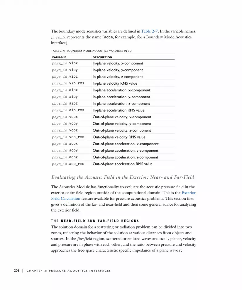
208 | C H A P T E R

The boundary mode acoustics variables are defined in Table 2-7. In the variable names, phys_id represents the name (acbm, for example, for a Boundary Mode Acoustics interface).

Evaluating the Acoustic Field in the Exterior: Near- and Far-Field

The Acoustics Module has functionality to evaluate the acoustic pressure field in the exterior or far-field region outside of the computational domain. This is the Exterior Field Calculation feature available for pressure acoustics problems. This section first gives a definition of the far- and near-field and then some general advice for analyzing the exterior field.

T H E N E A R - F I E L D A N D F A R - F I E L D R E G I O N S

The solution domain for a scattering or radiation problem can be divided into two zones, reflecting the behavior of the solution at various distances from objects and sources. In the far-field region, scattered or emitted waves are locally planar, velocity and pressure are in phase with each other, and the ratio between pressure and velocity approaches the free-space characteristic specific impedance of a plane wave rc.

TABLE 2-7: BOUNDARY MODE ACOUSTICS VARIABLES IN 3D


phys_id.vipx In-plane velocity, x-component

phys_id.vipy In-plane velocity, y-component

phys_id.vipz In-plane velocity, z-component

phys_id.vip_rms In-plane velocity RMS value

phys_id.aipx In-plane acceleration, x-component

phys_id.aipy In-plane acceleration, y-component

phys_id.aipz In-plane acceleration, z-component

phys_id.aip_rms In-plane acceleration RMS value

phys_id.vopx Out-of-plane velocity, x-component

phys_id.vopy Out-of-plane velocity, y-component

phys_id.vopz Out-of-plane velocity, z-component

phys_id.vop_rms Out-of-plane velocity RMS value

phys_id.aopx Out-of-plane acceleration, x-component

phys_id.aopy Out-of-plane acceleration, y-component

phys_id.aopz Out-of-plane acceleration, z-component

phys_id.aop_rms Out-of-plane acceleration RMS value


Moving closer to the sources into the near-field region, pressure and velocity gradually slide out of phase. This means that the acoustic field contains energy that does not travel outward or radiate. These evanescent wave components are effectively trapped close to the source. Looking at the sound pressure level, local maxima and minima are apparent in the near-field region.

Naturally, the boundary between the near-field and far-field regions is not sharp. A general guideline is that the far-field region is that beyond the last local energy maximum, that is, the region where the pressure amplitude drops monotonously at a rate inversely proportional to the distance R from any source or object.

A similar definition of the far-field region is the region where the radiation pattern — the locations of local minima and maxima in space — is independent of the distance to the wave source. This is equivalent to the criterion for Fraunhofer diffraction in optics, which occurs for Fresnel numbers, F = a2/λ R, much smaller than 1. For engineering purposes, this definition of the far-field region can be applied:

(2-7)

In Equation 2-7, a is the radius of a sphere enclosing all objects and sources, λ is the wavelength, and k is the wave number. Another way to write the expression leads to the useful observation that the size of the near-field region expressed in source-radius units is proportional to the dimensionless number k a, with a prefactor slightly larger than one. This relation is known as the Rayleigh radius R0 = S/λ, where S is the source area, for example for a piston.

Knowing the extent of the near-field region is useful when applying radiation boundary conditions because these are accurate only in the far-field region. PMLs, on the other hand, can be used to truncate a domain already inside the near-field region.

T H E H E L M H O L T Z - K I R C H H O F F I N T E G R A L R E P R E S E N T A T I O N

In many cases, solving the acoustic Helmholtz equation everywhere in the domain where results are requested is neither practical nor necessary. For homogeneous media, the solution anywhere outside a closed surface containing all sources and scatterers can be written as a boundary integral in terms of quantities evaluated on the surface. To evaluate this Helmholtz-Kirchhoff integral, it is necessary to know both Dirichlet and Neumann values on the surface. Applied to acoustics, this means that if the pressure and its normal derivative is known on a closed surface, the acoustic field can be calculated at any point outside, including amplitude and phase. This functionality is included in the Exterior Field Calculation feature. The feature has two options for the

R 8a2

λ----------> 8

2π------ka2=


210 | C H A P T E R

evaluation, one full integral (the default) and one that only looks in the extreme far field. See the section Theory for the Exterior Field Calculation: The Helmholtz-Kirchhoff Integral for further details.

F U L L I N T E G R A L

To evaluate the full Helmholtz-Kirchhoff integral, use the default Full integral option in the Type of integral options. The full Helmholtz-Kirchhoff integral gives the pressure (including phase) at any point at a finite distance from the source surface. This is necessary in many acoustic applications, for example, when analyzing the sensitivity of transducers. Note that numerical integration tends to lose accuracy at very large distances. See Exterior Field Calculation.

T H E F A R - F I E L D L I M I T

In many scattering applications, the quantity of interest is the far-field radiation pattern, which can be defined as the limit of r | p | when r goes to infinity in a given direction. To evaluate the pressure in the far-field limit set the Type of integral to Far-field integral approximation for r → ∞ in the settings for the exterior field variables. With this option, only the direction of the evaluation point r is of interest not the distance |r|. See Exterior Field Calculation.

E X T E R I O R F I E L D O P E R A T O R

The exterior field pressure is evaluated using the exterior field operator. The name is defined in the Exterior field variable name input field and the default is pext.

The exterior field pressure can be evaluated in a given point (x0,y0,z0) by simply writing pext(x0,y0,z0). To evaluate the sound pressure level in the same point, it is advantageous to use the subst() operator and, for example, write subst(acpr.efc1.Lp_pext,x,x0,y,y0,z,z0).

These evaluations are automatically carried out in the dedicated postprocessing features presented in the section below.

Dedicated Acoustics Plots for Postprocessing

Dedicated acoustics postprocessing functionality exists to plot responses, transfer functions, directivity patterns and more. They require the Acoustics Module license.

For an example, see Loudspeaker Driver: Application Library path Acoustics_Module/Electroacoustic_Transducers/loudspeaker_driver.


In this section:

• Radiation Pattern Plots (Spatial Response)

• Grid and Parametrized Datasets

• Octave Band Plots

• Directivity Plots

R A D I A T I O N P A T T E R N P L O T S ( S P A T I A L R E S P O N S E )

Evaluating and plotting the acoustic pressure around radiating objects and sources is essential for the development of several acoustic devices. This is known as the spatial response or the radiation pattern. Application areas range from underwater acoustic transducers and loudspeakers, to determining the spatial sensitivity of microphone systems (for example, using reciprocity). Using the Exterior Field Calculation feature can help to reduce the computational domain while still being able to determine the pressure and thus the spatial response in the exterior field (near-field to far-field). The Radiation Pattern plots are specially designed for easy evaluation of the exterior field variables, that is, the acoustic exterior pressure and the exterior field sound pressure level.

In the radiation pattern plots, the exterior field variable (pressure or sound pressure level) is represented in a polar plot for a selected number of angles. Data is retrieved on an evaluation circle in 2D, 2D axial symmetry, or 3D. The angle interval and the number of angles can be manually specified. The evaluation circle origin, orientation, and radius can be specified as well as the reference direction. The evaluation circle can be visualized using a Preview Evaluation Plane functionality. There is also a built-in


212 | C H A P T E R

option to calculate the Beam Width of the plotted data. The data is stored in a table that can be plotted using the Table Graph option.

Figure 2-7: Example of a 2D and 3D radiation pattern plot from the Bessel Panel tutorial model.

The 3D radiation pattern plots create a 3D polar plot (or bubble plot) where the data is evaluated on a sphere. Here, you can specify a separate expression for the surface color. In the 3D radiation pattern plots, the directivity can also be calculated by enabling the Compute directivity option. The result is given in a table and is calculated as the maximum power relative to the average power. The table comprises the maximal radiation direction (polar angles), the directivity, and the directivity given in dB (also known as the directivity index).

The main advantage with the radiation pattern plot, as compared to making a line graph, is that the circle/sphere that you use for defining the plot directions, is not part of your geometry for the solution. Thus, the number of plotting directions is decoupled from the discretization of the solution domain.

Variables defined by the Exterior Field Calculation feature like, for example, the pressure acpr.efc1.pext or sound pressure level acpr.efc1.Lp_pext are globally defined variables and can be directly evaluated in the Radiation Pattern plot and Directivity plot. The values plotted only make physical sense if they are evaluated outside of the Exterior Field Calculation boundary.

To visualize, for example, the sound pressure level inside of the Exterior Field

Calculation boundary plot the expression: at2(x,y,acpr.Lp) in 2D,


at2(r,z,acpr.Lp) in 2D axisymmetry, or at3(x,y,z,acpr.Lp) in 3D. The at2() and at3() operators ensure the variables are globally defined.

G R I D A N D P A R A M E T R I Z E D D A T A S E T S

Another way of evaluating and depicting the exterior field is by using either the Grid

2D , the Grid 3D , the Parametrized Curve 2D and 3D, or the Parametrized Surface

Default exterior field plots (that use the radiation pattern plots) are automatically added to any model that uses exterior field calculation feature, when Generate default plots is selected (the default) on the study node.

In a 3D Radiation Pattern plot, the definition of the polar angle θ and the azimuthal angle follows the spherical coordinate system typically used in physics.

To help visualize the angles, assuming the center is at the origin, simply plot the following expressions:

• Polar angle θ: acos(z/sqrt(x^2+y^2+z^2))

• Azimuthal angle : atan2(y,x)

• For a 3D example, see Bessel Panel: Application Library path Acoustics_Module/Tutorials,_Pressure_Acoustics/bessel_panel.

• For a 2D axisymmetric example, see Cylindrical Subwoofer: Application Library path Acoustics_Module/

Tutorials,_Pressure_Acoustics/cylindrical_subwoofer.


• Radiation Pattern and Results Analysis and Plots in the COMSOL Multiphysics Reference Manual

ϕ r θ ϕ, ,( )

ϕ


214 | C H A P T E R

datasets. All of these datasets allow the evaluation of global quantities, like the exterior field variables, outside of the computational domain (outside of the mesh).

O C T A V E B A N D P L O T S

A dedicated Octave Band ( ) plot exists to plot frequency response, transfer functions, transmission loss, and insertion loss curves. The plot has several built-in acoustics specific features like predefined weighting (Z, A, C, and User defined) as well as the possibility to plot the response in octaves, 1/3 octaves, 1/6 octaves, or as a continuous response.

Figure 2-8: Sensitivity curve plotted as 1/3 octave bands and a continuous curve. From the Loudspeaker Driver model in the Application Library.

The exterior field is depicted in several ways in the model Piezoelectric Tonpilz Transducer: Application Library path Acoustics_Module/

Piezoelectric_Devices/tonpilz_transducer.

For details see Octave Band in the Results Analysis and Plots chapter in the COMSOL Multiphysics Reference Manual.

The predefined Z, A, and C weightings are defined in IEC 61672-1. See IEC 61672-1 Electroacoustics - Sound level meters - Part 1: Specifications for details.


D I R E C T I V I T Y P L O T S

Another acoustics specific plot, especially used for loudspeakers, is the dedicated Directivity ( ) plot. The plot allows audio engineers to depict the spatial response of a loudspeaker as function of both frequency and spatial angle in a contour-like plot. Representing the spatial response in this manner is a very common in the loudspeaker industry. Measured data is often also represented in the same manner. The plot includes many options to format the plot to achieve maximal insight into the modeled data, for example, linear and logarithmic frequency axis scaling options, easy switch of the x- and y-axis (frequency and polar angle axis), as well as options to normalize the data with respect to a given angle or the maximal value.

Figure 2-9: Example of the directivity plot from the Lumped Loudspeaker driver model in the Application Library.

For examples that use an Octave Band plot, see:

• Absorptive Muffler: Application Library path Acoustics_Module/


• The Brüel & Kjær 4134 Condenser Microphone: Application Library path Acoustics_Module/Electroacoustic_Transducers/bk_4134_microphone.

For details see Directivity in the Results Analysis and Plots chapter in the COMSOL Multiphysics Reference Manual.


216 | C H A P T E R

About the Material Databases for the Acoustics Module

The Acoustics Module includes two material databases: Liquids and Gases, with temperature-dependent fluid dynamic and thermal properties, and a Piezoelectric Materials database with over 20 common piezoelectric materials.

Specifying Frequencies: Logarithmic and ISO Preferred

When solving a model in the frequency domain, you need to specify the Frequencies to solve for in the Frequency Domain study step. Several built-in options exist when selecting the Range ( ). Specifically for acoustics modeling the Entry method has the Logarithmic and the ISO preferred frequencies. The latter option is only available with the Acoustics Module and is activated by clicking the Show More Options button ( ) and selecting Advanced Physics Options in the Show More Options dialog box. For ISO

preferred frequencies, select a start and stop frequency and the interval (Octave, 1/3 Octave, 1/6 Octave, 1/12 Octave, and 1/24 Octave). The 1/3 octave preferred frequencies are defined based on ISO 266. They are extended to frequencies based on the preferred numbers of ISO 3 (series R20, R40, and R80).

Lumped Loudspeaker Driver. Application Library path: Acoustics_Module/Electroacoustic_Transducer/lumped_loudspeaker_driver

For detailed information about Materials, the Liquids and Gases Materials Library, and the Piezoelectric Materials Library see the COMSOL Multiphysics Reference Manual.

For a discussion about the air and water materials as commonly used in acoustics, as well as attenuation models, and other material properties see the Acoustic Properties of Fluids chapter of this manual.


Mode l i n g w i t h t h e P r e s s u r e A c ou s t i c s B r an c h ( BEM -Ba s e d I n t e r f a c e )

This section contains good practices and modeling tips and tricks for the boundary element method (BEM) based interface of the Pressure Acoustics Branch: The Pressure Acoustics, Boundary Elements Interface.

In this section:

• When to Use BEM

• Selections: Infinite Void and Finite Voids

• Solvers for BEM Models

• Meshing BEM Models

• Postprocessing BEM Results

When to Use BEM

Solving acoustics problems using the boundary element method (BEM) can be very advantageous compared to the finite element method (FEM) for some types of problems. For others problems, FEM has its advantages. The recommended approach is to use the BEM and FEM methods where they apply best and also to combine them. Since the BEM interface is fully enabled with multiphysics capabilities, it can be coupled seamlessly with the physics interfaces that are based on FEM. This functionality includes coupling to vibrating structures with the Acoustic-Structure Boundary multiphysics coupling and to other acoustic domains with the Acoustic FEM-BEM Boundary multiphysics coupling. This approach enables modeling in a FEM-BEM framework, using the strength of each formulation adequately. The BEM-based interface is especially well suited for radiation and scattering problems.

The advantage of the boundary element method is that only boundaries need to be meshed and the DOFs solved for are restricted to the boundaries. This introduces some clear ease-of-use for handling complex geometries. However, the BEM technique results in fully populated or dense matrices that need dedicated numerical methods. Assembling and solving these matrices can be very demanding. This means that when solving acoustic models of small and medium size, The Pressure Acoustics, Frequency Domain Interface will often be faster than solving the same problem with the BEM interface.

M O D E L I N G W I T H T H E P R E S S U R E A C O U S T I C S B R A N C H ( B E M - B A S E D I N T E R F A C E ) | 217

218 | C H A P T E R

The challenge with using the FEM interface is to set up open boundaries in an efficient way, for example, by using PMLs. When PMLs cannot easily be placed snugly around radiating structures or two structures are far apart, large air domains need to be meshed. This costs a lot on the computational side, as the frequency is increased. These problems are well suited for the BEM interface, as only the boundary of the radiating structure needs to be meshed.

Interior problems can be solved with the BEM interface, but typically it is much more efficient to solve these problems using the FEM-based interfaces. Remember also that an iterative solver will struggle to solve interior problems, with no or little damping, when resonances appear. If you are close to an eigenfrequency with a high Q, the solution will also be very mesh sensitive.

Note also that at very low frequencies, the BEM method may “break down” for interior problems and give inaccurate results. This is in practice not an issue, as this kind of problem should be solved with The Pressure Acoustics, Frequency Domain Interface.

Selections: Infinite Void and Finite Voids

For modeling with BEM, a geometry model can have multiple domains and multiple finite voids. However, there can be only one infinite void.

• A domain corresponds to a finite region where the geometry model is of the type solid. The geometry in most models based on FEM consists of domains only.

• Any other finite region is a finite void. A finite void can be created as a geometric primitive of type curve (in 2D) or surface (in 3D), for example, or by a Boolean difference operation, subtracting a closed domain from the model geometry.

• The infinite void is the single unbounded region surrounding the geometry model. This is the typical region selected when modeling scattering or radiation problems with the Pressure Acoustics, Boundary Elements interface.

• If the model contains finite voids and an infinite void, those volumetric regions appear in the domain selection lists for the BEM interface and in the Selection List window as Finite void 1, and so on, and as Infinite void.

• It is important to also assign the materials under the Materials node to the appropriate selections of the Pressure Acoustics model. Note that material parameters need to be constant for each applied Pressure Acoustics model.

• Assigning the Pressure Acoustics model to a selection adds the necessary equations to the exterior boundaries of the selections. Only these boundaries need to be


meshed. The condition at infinity (of the infinite void) is selected in the Condition at Infinity section. The typical and default is an outgoing wave condition.

Solvers for BEM Models

The default for The Pressure Acoustics, Boundary Mode Interface is to use an iterative solver for 3D models and a direct dense matrix solver for 2D problems. If the Far-Field Approximation is turned off, the direct dense matrix solver will be used in all situations. The dense matrix solver is adequate for small BEM problems but quickly runs out of memory for increasing number of DOFs.

When the Stabilized formulation is used a different solver suggestion is generated. Make sure to reset the solver to default if changes are made. The solver uses PARDISO as a direct preconditioner and GMRES as the iterative method.

The boundary element method (BEM) used in the Pressure Acoustics, Boundary Elements interface is based on the direct method with Costabel’s symmetric coupling. The adaptive cross approximation (ACA) fast summation method is used for solving the resulting linear system. This method uses partial assembly of the matrices where the effect of the matrix vector multiplication is computed. The default iterative solver used is GMRES.

For multiphysics problems that combine BEM and FEM interfaces and are set up with one of the multiphysics couplings; the default approach is to use hybridization with ACA for BEM and an appropriate preconditioner for the FEM part of the problem (direct or multigrid). Several solver suggestions are given for the multiphysics FEM-BEM problems.

Meshing BEM Models

When solving an acoustics problem with the boundary element method, the same restrictions exist on the mesh as for the finite-element-based interfaces. In general, the mesh should resolve the wavelength with 5 to 6 elements. The mesh should also resolve small details and curved surfaces adequately. For exterior problems, the mesh can in practice be slightly coarser and it typically suffices to use 4 elements per

Further details about the BEM formulation are found in The PDE, Boundary Elements Interface documentation in the COMSOL Multiphysics Reference Manual.


220 | C H A P T E R

wavelength. Using a structured quad surface mesh will result in fewer degrees of freedom and should be used if possible.

Postprocessing BEM Results

When solving a problem with The Pressure Acoustics, Boundary Elements Interface, the resulting solution will consist of the dependent variables on boundaries. Evaluating the solution in a domain is based on a kernel evaluation.

On boundaries, dependent variables exist for the pressure p, up and down pressure-dependent variables on interior boundaries (pabe.p_up and pabe.p_down), as well as a normal flux variable pabe.pbam1.bemflux.

The Pressure Acoustics, Boundary Elements Interface sets up predefined postprocessing variables that combine the properties of the boundary variables, when needed, with variables based on the kernel evaluation.

Domain EvaluationThe BEM solution can in general be evaluated in domains using the Grid 2D and Grid 3D datasets. This sets up an underlying grid for the kernel evaluation of the solution. The grid dataset can, for example, be selected as the input Dataset for a slice plot. A grid dataset and a multislice plot are generated and used in the default plots when a BEM model is solved. Note also that the kernel-based variables can be evaluated on domains that are meshed.

All the Dedicated Acoustics Plots for Postprocessing that exist for the FEM interfaces can be used with the variables defined by the BEM solution. This is, for example, the Radiation Pattern plot or the Directivity plot used for analyzing the spatial radiation pattern of a transducer or a scattered field.

The BEM solution can be evaluated at a given coordinate using the at3_spatial(...) operator. In a 3D model you can evaluate the sound pressure level in the point (x,y,z) = (1 m,0,0) by typing: at3_spatial(1[m],0,0,pabe.Lp,’minc’).

This can, for example, be used to normalize the data in a Radiation Pattern plot by typing: pabe.Lp-at3_spatial(1[m],0,0,pabe.Lp,’minc’)


Boundary EvaluationWhen evaluating the solution on boundaries, the plot lists are populated with special boundary variables in a Boundary variables submenu located under, for example, the Pressure and sound pressure level or Acceleration and velocity menu. The boundary variables have a “_bnd” added to their names. For example, the total acoustic pressure on a boundary is pabe.p_t_bnd. On interior boundaries, there are also up and down variants of the variables, with “_up” and “_down” added, respectively. On interior boundaries (where an interior boundary condition has been added), the boundary variable is the average of the up and down variables.

The boundary variables should be used when plotting on surfaces, as they do not rely on the kernel evaluation but are directly related to the DOFs solved for in the BEM problem.


222 | C H A P T E R

Mode l i n g w i t h t h e P r e s s u r e A c ou s t i c s B r an c h (DG - FEM -Ba s e d I n t e r f a c e )

This section contains good practices and modeling tips and tricks for the discontinuous Galerkin finite element method (dG-FEM) based interface of the Pressure Acoustics Branch: The Pressure Acoustics, Time Explicit Interface. In this section:

• Meshing, Discretization, and Solvers

• Postprocessing: Variables and Quality

• Absorbing Layers

• Storing Solution on Selections for Large Models

• Assemblies and Pair Conditions

Meshing, Discretization, and Solvers

The same considerations for the mesh, discretization, and solvers apply for the Pressure Acoustics, Time Explicit interface as for The Convected Wave Equation, Time Explicit Interface. Details are found in Meshing, Discretization, and Solvers under the modeling section for that physics. The interface is supported on all mesh types and for all combinations of mesh.

Postprocessing: Variables and Quality

The same considerations for postprocessing apply for the Pressure Acoustics, Time Explicit interface as for The Convected Wave Equation, Time Explicit Interface. Details are found in Postprocessing: Variables and Quality under the modeling section for that physics.

Absorbing Layers

The same considerations for the absorbing layers and their setup apply for the Pressure Acoustics, Time Explicit interface as for The Convected Wave Equation, Time Explicit Interface. Details are found in Absorbing Layers under the modeling section for that physics.


Storing Solution on Selections for Large Models

The same considerations for storing data apply for the Pressure Acoustics, Time Explicit interface as for The Convected Wave Equation, Time Explicit Interface. Details are found in Storing Solution on Selections for Large Models under the modeling section for that physics.

Assemblies and Pair Conditions

The same considerations for using assemblies and pair condition apply for the Pressure Acoustics, Time Explicit interface as for The Convected Wave Equation, Time Explicit Interface. Details are found in Assemblies and Pair Conditions under the modeling section for that physics.

M O D E L I N G W I T H T H E P R E S S U R E A C O U S T I C S B R A N C H ( D G - F E M - B A S E D I N T E R F A C E ) | 223

224 | C H A P T E R

Th eo r y Ba c k g r ound f o r t h e P r e s s u r e A c ou s t i c s B r an c h

This section describes the governing equations and the mathematical formulation of the governing equations as used in the Pressure Acoustics branch of the Acoustics Module. Details are also given regarding some of the boundary conditions, including the radiation boundary conditions as well as the exterior field calculation feature. The section starts with a general introduction to the governing equations used in pressure acoustics.

In this sections:

• The Governing Equations

• Pressure Acoustics, Frequency Domain Equations

• Pressure Acoustics, Transient Equations

• The Nonlinear Westervelt Equation

• Pressure Acoustics, Boundary Mode Equations

• Theory for the Plane, Spherical, and Cylindrical Radiation Boundary Conditions

• Theory for the Exterior Field Calculation: The Helmholtz-Kirchhoff Integral

The Governing Equations

Pressure acoustic problems involve solving for the small acoustic pressure variations p (also named p’ or p1) on top of the stationary background pressure p0. Mathematically, this represents a linearization (small parameter expansion) of the dependent variables around the stationary quiescent values.

The governing equations for a compressible lossless (no thermal conduction and no viscosity) fluid flow problem are the mass conservation equation (continuity equation), the momentum conservation equation (Euler's equation), and the energy equation (entropy equation). These are given by:


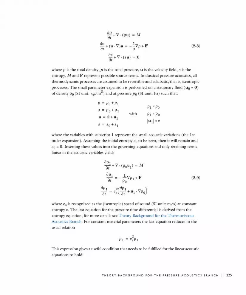
(2-8)

where ρ is the total density, p is the total pressure, u is the velocity field, s is the entropy, M and F represent possible source terms. In classical pressure acoustics, all thermodynamic processes are assumed to be reversible and adiabatic, that is, isentropic processes. The small parameter expansion is performed on a stationary fluid (u0 = 0) of density ρ0 (SI unit: kg/m3) and at pressure p0 (SI unit: Pa) such that:

where the variables with subscript 1 represent the small acoustic variations (the 1st order expansion). Assuming the initial entropy s0 to be zero, then it will remain and s0 = 0. Inserting these values into the governing equations and only retaining terms linear in the acoustic variables yields

(2-9)

where cs is recognized as the (isentropic) speed of sound (SI unit: m/s) at constant entropy s. The last equation for the pressure time differential is derived from the entropy equation, for more details see Theory Background for the Thermoviscous Acoustics Branch. For constant material parameters the last equation reduces to the usual relation

This expression gives a useful condition that needs to be fulfilled for the linear acoustic equations to hold:

∂ρ∂t------ ∇ ρu( )⋅+ M=

∂u∂t------ u ∇⋅( )u+

1ρ---∇p– F+=

∂s∂t----- ∇ su( )⋅+ 0=

p p0 p1+=

ρ ρ0 ρ1+=

u 0 u1+=

s s0 s1+=

with

p1 p0«

ρ1 ρ0«

u1 c«

∂ρ1∂t

--------- ∇ ρ0u1( )⋅+ M=

∂u1∂t

--------- 1ρ0------∇p1– F+=

∂p1∂t

--------- cs2 ∂ρ1

∂t--------- u1 ρ0∇⋅+ =

p1 cs2ρ1=

T H E O R Y B A C K G R O U N D F O R T H E P R E S S U R E A C O U S T I C S B R A N C H | 225

226 | C H A P T E R

The subscript “s” is dropped in the following along with the subscript “0” on the background density ρ0. Finally, rearranging Equation 2-9, renaming the source terms, and dropping the subscript “1” yields the wave equation for pressure waves in a lossless medium

. (2-10)

Here ρ (SI unit: kg/m3) refers to the density, and c (SI unit: m/s) denotes the speed of sound. In this general formulation of the scalar wave equation, the speed of sound and density may in general be space dependent, for example, through their dependency on the background temperature. The equation includes two optional source terms:

• The monopole domain source Qm (SI unit: 1/s2). This source corresponds to a mass source on the right-hand side of the continuity equation.

• The dipole domain source qd (SI unit: N/m3). This source corresponds to a domain force source on the right-hand side of the momentum equation.

The combination ρc2 is called the adiabatic bulk modulus, commonly denoted Ks (SI unit: Pa). The bulk modulus is equal to the one over the adiabatic compressibility coefficient βs = 1/Ks = 1/ρc2(SI unit: 1/Pa).

In Equation 2-10 both the speed of sound c = c(x) and the density ρ = ρ(x) may be dependent on the spatial coordinates x while they are independent of time, or only slowly varying in time (that is, at a time scale much slower than the variations in the acoustic signal). If both domain sources are set to zero and the density is constant in space, you can recover the standard wave equation

An important special case is a time-harmonic wave, for which the pressure varies with time as

p1 ρ0cs2

«

1

ρc2--------

t2

2

∂∂ p ∇ 1

ρ---– ∇p qd–( )

⋅+ Qm=

∂2p

∂t2--------- c2∇2p=

Some classical references on acoustics for further reading are found in Ref. 4, Ref. 5, Ref. 6, Ref. 7, and Ref. 8.


where ω = 2πf (rad/s) is the angular frequency and f (SI unit: Hz) is the frequency. Assuming the same harmonic time dependence for the source terms, the wave equation for acoustic waves reduces to an inhomogeneous Helmholtz equation

. (2-11)

In this equation, the subscript “c” on the density and the speed of sound refers to that they may be complex valued. Lossy media, like porous materials or highly viscous fluids, can be modeled by using the complex-valued speed of sound and density. A selection of such fluid models is available in The Pressure Acoustics, Frequency Domain Interface. The attenuation in these fluid models is frequency dependent in different ways, depending on the physical origin of the damping. A description of the different fluid models is given in Theory for the Equivalent Fluid Models.

In the time domain, only certain frequency dependencies can be modeled, which limits the number of fluid models that can be used in The Pressure Acoustics, Transient Interface. One way to model damping in the time domain is to introduce an additional term of first order in the time derivative to account for attenuation of the sound waves

(2-12)

The damping term in Equation 2-12 is absent from the standard PDE formulations in the Pressure Acoustics, Transient interface, but it corresponds to a monopole domain source proportional to the time derivative of the pressure. This approach is, however, not used in the viscous and thermally conducting fluid models that contain damping for transient acoustics (see Viscous Fluid Model, Thermally Conducting Fluid Model, and Thermally Conducting and Viscous Fluid Model). The physical origin of the damping corresponds here to a dipole-like source.

p x t,( ) p x( ) eiωt

=

∇ 1ρc-----– ∇p qd–( )

⋅ ω2pρc cc

2-------------– Qm=

1

ρ c2--------

t2

2

∂∂ p da t∂

∂p– ∇ 1

ρ---– ∇p qd–( )

⋅+ Qm=

Even when sound waves propagate in a lossless medium, attenuation can occur by interaction with the surroundings at the system boundaries. In particular, this applies to the impedance boundary conditions.


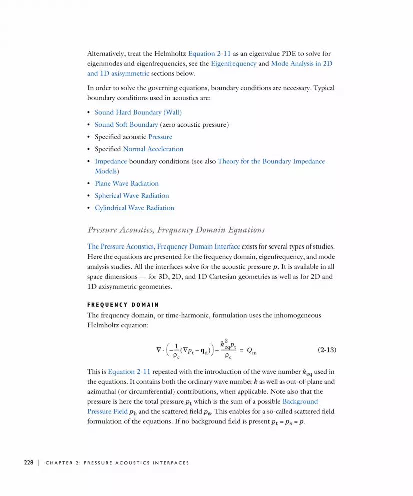
228 | C H A P T E R

Alternatively, treat the Helmholtz Equation 2-11 as an eigenvalue PDE to solve for eigenmodes and eigenfrequencies, see the Eigenfrequency and Mode Analysis in 2D and 1D axisymmetric sections below.

In order to solve the governing equations, boundary conditions are necessary. Typical boundary conditions used in acoustics are:


• Sound Soft Boundary (zero acoustic pressure)

• Specified acoustic Pressure

• Specified Normal Acceleration

• Impedance boundary conditions (see also Theory for the Boundary Impedance Models)


• Spherical Wave Radiation

• Cylindrical Wave Radiation

Pressure Acoustics, Frequency Domain Equations

The Pressure Acoustics, Frequency Domain Interface exists for several types of studies. Here the equations are presented for the frequency domain, eigenfrequency, and mode analysis studies. All the interfaces solve for the acoustic pressure p. It is available in all space dimensions — for 3D, 2D, and 1D Cartesian geometries as well as for 2D and 1D axisymmetric geometries.

F R E Q U E N C Y D O M A I N

The frequency domain, or time-harmonic, formulation uses the inhomogeneous Helmholtz equation:

(2-13)

This is Equation 2-11 repeated with the introduction of the wave number keq used in the equations. It contains both the ordinary wave number k as well as out-of-plane and azimuthal (or circumferential) contributions, when applicable. Note also that the pressure is here the total pressure pt which is the sum of a possible Background Pressure Field pb and the scattered field ps. This enables for a so-called scattered field formulation of the equations. If no background field is present pt = ps = p.

∇ 1ρc-----– ∇pt qd–( )

⋅keq

2 ptρc

-------------– Qm=


In this equation, p = p (x,ω) = p(x)eiωt (the dependence on ω is henceforth not explicitly indicated). Compute the frequency response by doing a parametric sweep over a frequency range using harmonic loads and sources.

When there is damping, ρc and cc are complex-valued quantities. The available damping models and how to apply them is described in the sections Pressure Acoustics and Theory for the Equivalent Fluid Models.

Equation 2-13 is the equation that the software solves for 3D geometries. In lower-dimensional and axisymmetric cases, restrictions on the coordinate dependence mean that the equations differ from case to case. Here is a brief summary of the situation.

2DIn 2D, the pressure is of the form

which inserted in Equation 2-13 gives

(2-14)

The out-of-plane wave number kz can be set on the Pressure Acoustics page. By default its value is 0. In the mode analysis study −ikz is used as the eigenvalue λ.

2D AxisymmetryFor 2D axisymmetric geometries the independent variables are the radial coordinate r and the axial coordinate z. The only dependence allowed on the azimuthal coordinate

is through a phase factor,

(2-15)

where m denotes the azimuthal mode number. The mode number defines an azimuthal wave number km = m/r. Because the azimuthal coordinate is periodic, m must be an integer. Just like kz in the 2D case, m can be set in the Settings window for Pressure Acoustics.

As a result of Equation 2-15, the equation to solve for the acoustic pressure in 2D axisymmetric geometries becomes

p x( ) p x y,( )e i– kz z=

∇ 1ρc----- pt qd–∇( )–

⋅keq

2

ρc-------- pt– Qm=

keq2 ω2

cc2

------- kz2

–=

ϕ

p r ϕ z, ,( ) p r z,( )e imϕ–=


230 | C H A P T E R

1D AxisymmetryIn 1D axisymmetric geometries,

leading to the radial equation

where both the azimuthal wave number km and the axial wave number kz, appear as parameters.

1DThe equation for the 1D case is obtained by letting the pressure depend on a single Cartesian coordinate x:

E I G E N F R E Q U E N C Y

In the eigenfrequency formulation, the source terms are absent; the eigenmodes and eigenfrequencies are solved for:

(2-16)

The eigenvalue λ introduced in this equation is related to the eigenfrequency f, and the angular frequency ω, through λ = i2πf = iω. Because they are independent of the

r∂∂ r

ρc-----– r∂

∂p qr– r

z∂∂ 1

ρc-----–

z∂∂p qz– keq

2

ρc--------rp–+ rQm=

keq2 ω

cc------ 2

km2

–= kmmr-----=

p r φ z, ,( ) p r( )e i kz z mϕ+( )–=

r∂∂ r

ρc-----– r∂

∂p qr– keq

2

ρc--------rp– rQm=

keq2 ω

cc------ 2

km2

– kz2

–= kmmr-----=

xdd 1

ρc-----

xddp qd– –

keq2

ρc-------- p– Qm=

keq2 ω

cc------ 2

=

∇ 1ρc-----– ∇p

⋅ λ2 pρc cc

2-----------+ 0=


pressure, the solver ignores any dipole and monopole sources unless a coupled eigenvalue problem is being solved.

Equation 2-16 applies to the 3D case. The equations solved in eigenfrequency studies in lower dimensions and for axisymmetric geometries are obtained from their time-harmonic counterparts, given in the previous subsection, by the substitution ω2 → −λ2.

Switch between specifying the eigenvalues, the eigenfrequencies, and the angular frequencies by selecting from the Eigenvalue transformation list in the solver sequence’s Settings window for Eigenvalue.

M O D E A N A L Y S I S I N 2 D A N D 1 D A X I S Y M M E T R I C

See Mode Analysis Study in the Pressure Acoustics, Boundary Mode Equations section. The mode analysis study type is only available for the Pressure Acoustics, Frequency Domain interface in 2D and 1D axisymmetric components, where the solver solves for the eigenvalues λ = −ikz for a given frequency. Here kz is the out-of-plane wave number of a given mode and the resulting pressure field p represents the mode on the cross section of an infinite waveguide or duct.

Pressure Acoustics, Transient Equations

Use the Time Dependent study type to model transient acoustic phenomena in a stationary fluid and to solve the wave equation

for the acoustic pressure, p = p(x, t). Here c is the speed of sound and ρ denotes the equilibrium density, while qd and Qm are dipole and monopole sources, respectively. The density and speed of sound can both be nonconstant in space. In contrast, they are assumed to vary with time on scales much larger than the period for the acoustic waves and are therefore considered time independent in the previous equation. This physics interface is available for 3D, 2D, and 1D Cartesian geometries as well as for 2D and 1D axisymmetric geometries.

Vibrations of a Disk Backed by an Air-Filled Cylinder: Application Library path Acoustics_Module/Verification_Examples/coupled_vibrations

1ρc2---------∂2p

∂t2--------- ∇ 1

ρ--- p qd–∇( )–

⋅+ Qm=


232 | C H A P T E R

The Nonlinear Westervelt Equation

To extend the validity of the small perturbation wave equation to finite amplitude waves, nonlinear effects need to be taken into account. The first idea is to expand the density pressure relation to second order to include the effect of finite amplitude waves. This gives

(2-17)

where we have kept the subscript “1” to highlight the acoustic perturbation quantities and a subscript “0” for the quiescent quantities. See Ref. 6 and 42 for details. The quantity B/A is the parameter of nonlinearity (see Ref. 51). This expression basically means that the different parts of the acoustic pressure wave travel at different speeds.

Inserting the above into the governing Equation 2-8 (retaining the dissipative terms) will lead to the full nonlinear second-order wave equation. This is the nonlinear equivalent to Equation 2-9 (or actually the nonlinear equivalent to the full equations of thermoviscous acoustics). Next assume that boundary layer effects can be disregarded and cumulative nonlinear effects dominate local nonlinear effects, for example, when the propagation distance is greater than the wavelength. This leads to the well-known Westervelt equation (see Ref. 42)

(2-18)

Here we have eliminated the density fluctuations and then removed the subscripts. Hence, pt is the (total) acoustic pressure, ρ is the quiescent density, δ is the diffusivity of sound, and β is the coefficient of nonlinearity (related to the parameter of nonlinearity B/A).

The Westervelt equation supports the propagation of shocks. Shocks can be hard to capture numerically and require the addition of stabilization. This can, for example, be done by adding diffusivity near the shock location. One method (used in COMSOL) is to add an effective diffusivity term that reads

The highest artificial damping is achieved where the acoustic pressure increases or decreases the most rapidly. It reaches its maximal values where the pressure endures

p1 c02ρ1

c02

ρ0------ B

2A-------ρ1

2 …+ +=

1

ρc2---------

∂2pt

∂t2----------- ∇ 1

ρ--- pt qd–∇( )–

δρc2---------

∂ pt∇∂t

------------–

⋅+β

ρ2c4-----------

∂2pt2

∂t2------------ Qm+=

δκ 1t∂

∂ p∇q 1–

– –


discontinuities, that is, where shocks arise. Thus this technique provides a shock-capturing stabilization. See Ref. 52 for more details. Specify the so-called q-Laplacian exponent q and the so-called q-Laplacian factor κ to get the desirable amount of artificial damping. Note that the damping must not be too high nor too low. The particular values of q and κ depend on the material and the input signal frequency. The two parameters that control the stabilization require manual tuning. A suggested approach is to use a simple 1D model to tune the parameters based on fluid material properties and frequency content.

Pressure Acoustics, Boundary Mode Equations

When an acoustic wave of a given angular frequency ω is fed into a waveguide or a duct, only a finite set of shapes, or modes, for the transverse pressure field can propagate over long distances inside the structure. The higher the frequency, the higher the number of sustainable modes.

Take, as an example, a uniform straight duct whose axis is in the z direction. The acoustic field in such a duct can be written as a sum of the form

The constant kzj is the axial wave number of the jth propagating transverse mode, pj(x, y). These transverse modes and their associated axial wave numbers are solutions to an eigenvalue problem defined on the duct’s cross section. The mode analysis capabilities in The Pressure Acoustics, Boundary Mode Interface makes it possible to solve such eigenvalue problems. The physics interface is available for 3D Cartesian and 2D axisymmetric geometries and solves for the transverse eigenmodes for the acoustic pressure p and the associated propagation constants kz. The Mode Analysis Study is briefly discussed.

M O D E A N A L Y S I S S T U D Y

The eigenvalue solver computes a specified number of solutions {pj, λj} to the equation

Nonlinear Acoustics — Modeling of the 1D Westervelt Equation: Application Library path Acoustics_Module/Nonlinear_Acoustics/


p x( ) pj x y,( )e ikzjz–

j 0=

N

=


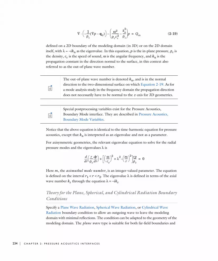
234 | C H A P T E R

(2-19)

defined on a 2D boundary of the modeling domain (in 3D) or on the 2D domain itself, with λ = −ikn as the eigenvalue. In this equation, p is the in-plane pressure, ρc is the density, cc is the speed of sound, ω is the angular frequency, and kn is the propagation constant in the direction normal to the surface, in this context also referred to as the out-of-plane wave number.

Notice that the above equation is identical to the time-harmonic equation for pressure acoustics, except that kn is interpreted as an eigenvalue and not as a parameter.

For axisymmetric geometries, the relevant eigenvalue equation to solve for the radial pressure modes and the eigenvalues λ is

Here m, the azimuthal mode number, is an integer-valued parameter. The equation is defined on the interval r1 < r < r2. The eigenvalue λ is defined in terms of the axial wave number kz through the equation λ = −ikz

Theory for the Plane, Spherical, and Cylindrical Radiation Boundary Conditions

Specify a Plane Wave Radiation, Spherical Wave Radiation, or Cylindrical Wave Radiation boundary condition to allow an outgoing wave to leave the modeling domain with minimal reflections. The condition can be adapted to the geometry of the modeling domain. The plane wave type is suitable for both far-field boundaries and

∇ 1ρc----- p qd–∇( )–

⋅ ω2

ρccc2

-----------kn

2

ρc-----–

p– Qm=

The out-of-plane wave number is denoted kn, and is in the normal direction to the two-dimensional surface on which Equation 2-19. As for a mode analysis study in the frequency domain the propagation direction does not necessarily have to be normal to the z-axis for 3D geometries.

Special postprocessing variables exist for the Pressure Acoustics, Boundary Mode interface. They are described in Pressure Acoustics, Boundary Mode Variables.

rdd r

ρc-----

rddp

ω

cc------ 2

λ2 mr----- 2

–+rpρc-----+ 0=


ports (for plane waves only). For general radiation boundary conditions for waveguides (supporting multi-modes) it is recommended to use the Port boundary condition.

Radiation boundary conditions are available for all types of studies. For the frequency-domain study, Givoli and Neta’s reformulation of the Higdon conditions (Ref. 1) for plane waves has been implemented to the second order. For cylindrical and spherical waves, COMSOL Multiphysics uses the corresponding 2nd-order expressions from Bayliss, Gunzburger, and Turkel (Ref. 2). The Transient, Mode analysis, and Eigenfrequency studies implement the same expansions to the first order.

The first-order radiation boundary conditions in the frequency domain read

where k is the wave number and κ ( r ) is a function whose form depends on the wave type:

• Plane wave: κ( r ) = 0

• Cylindrical wave: κ( r ) = 1 / (2 r)

• Spherical wave: κ( r ) = 1 / r

In the cylindrical and spherical wave cases, r is the shortest distance from the point r = (x, y, z) on the boundary to the source. The right-hand side of the equation represents an optional incoming pressure field pi (see Incident Pressure Field).

The second-order radiation boundary conditions in the frequency domain are defined below. In these equations, at a given point on the boundary denotes the Laplace operator in the tangent plane at that particular point.

P L A N E W A V E

In the notation of Givoli and Neta (Ref. 1), the above expressions correspond to the parameter choices C0 = C1 = C2 = ω/k. For normally incident waves, this gives a vanishing reflection coefficient.

n–1ρc-----– ∇pt qd–( )

⋅ ik κ r( )+( ) pρc-----+ ik κ r( )+( )

piρc----- n

∇piρc

--------- ⋅+=

Δ||

n–1ρc-----– pt qd–∇( )

⋅ i kρc-----p i

2kρc------------Δ|| p+ +

i2kρc------------Δ|| pi i k

ρc-----pi n 1

ρc----- pi∇⋅+ +=


236 | C H A P T E R

C Y L I N D R I C A L W A V E

The cylindrical wave boundary condition is based on a series expansion of the outgoing wave in cylindrical coordinates (Ref. 2), and it assumes that the field is independent of the axial coordinate. Specify the axis of this coordinate system by giving an orientation (nx, ny, nz) and a point (x0, y0, z0) on the axis. In axisymmetric geometries, the symmetry axis is the natural and only choice.

S P H E R I C A L W A V E

Use a spherical wave to allow a radiated or scattered wave — emanating from an object centered at the point (x0, y0, z0) that is specified — to leave the modeling domain without reflections. The boundary condition is based on an expansion in spherical coordinates from Bayliss, Gunzburger, and Turkel (Ref. 2), implemented to the second order.

T R A N S I E N T A N A L Y S I S

The transient radiation boundary condition is the first-order expression

n–1ρc-----– pt qd–∇

⋅ =

ikeq12r------ 1

8r 1 ikeqr+( )---------------------------------–+

pi p–( )ρc

------------------ n 1ρc----- pi∇⋅

rΔ||pi rΔ||p–( )2 1 ikeqr+( )ρc-------------------------------------+ +

n–1ρc-----– pt qd–∇( )

ikeq1r---+

pρc-----

rΔ||p2ρc ikeqr 1+( )------------------------------------–+⋅

rΔ||pi2ρ0c ikeqr 1+( )---------------------------------------– ikeq

1r---+

piρc----- n 1

ρc----- pi∇⋅+ +=

n–1ρ---– ∇pt qd–( )

⋅ 1ρ--- 1

c---

t∂∂p κ r( ) p+

+1ρ--- 1

c---

t∂∂pi κ r( ) pi n pi∇⋅+ +

=


where κ ( r ) is the same wave-type dependent function as for the eigenfrequency case and pi the optional Incident Pressure Field.

Theory for the Exterior Field Calculation: The Helmholtz-Kirchhoff Integral

The Acoustics Module has functionality to evaluate the acoustic pressure field in the exterior field region of the model (outside the computational domain). This section gives the relevant definitions and mathematical background as well as some general advice for analyzing the exterior field. Details about how to use the exterior field functionality is described in Exterior Field Calculation and in the modeling section Evaluating the Acoustic Field in the Exterior: Near- and Far-Field.

T H E H E L M H O L T Z - K I R C H H O F F I N T E G R A L R E P R E S E N T A T I O N

In many cases, solving the acoustic Helmholtz equation everywhere in the domain where results are requested is neither practical nor necessary. For homogeneous media, the solution anywhere outside a closed surface containing all sources and scatterers can be written as a boundary integral in terms of quantities evaluated on the surface. To evaluate this Helmholtz-Kirchhoff integral, it is necessary to know both Dirichlet and Neumann values on the surface. Applied to acoustics, this means that if the pressure and its normal derivative (which is related to the normal velocity) is known on a closed surface, the acoustic field can be calculated at any point outside.

In general, the solution p to Helmholtz’ equation

An estimate of the reflection coefficient Rs for spurious waves off the plane wave radiation boundary, for incident plane waves at angle θ is given by the expression:

where N is the order of the boundary condition (here 1 or 2). So at normal incidence (θ = 0) there are no spurious reflections, while, for example, at an incidence angle of 30o for N = 2 (plane wave radiation in the frequency domain) the amplitude of the spurious reflected wave is 0.5 % of the incident.

Rsθ 1–cosθ 1+cos

----------------------N

=

∇ p∇⋅– k2 p– 0=


238 | C H A P T E R

in the homogeneous domain exterior to a closed surface, S, can be explicitly expressed in terms of the values of p and its normal derivative on S:

Here the coordinate vector r parameterizes S. The unit vector n is the outward normal to the exterior infinite domain; thus, n points into the domain that S encloses. The function G (R, r) is a Green’s function satisfying

This essentially means that the Green’s function, seen as a function of r, is an outgoing traveling wave excited by a simple source at R. In 3D, the Green’s function is therefore:

In 2D, the Green’s function contains a Hankel function instead of the exponential:

Inserting the 3D Green’s function in the general representation formula gives:

(2-20)

while in 2D, the Hankel function leads to a slightly different expression:

(2-21)

For axially symmetric geometries, the full 3D integral must be evaluated. The Acoustics Module uses an adaptive numerical quadrature in the azimuthal direction on a fictitious revolved geometry in addition to the standard mesh-based quadrature in the rz-plane.

The default in the Exterior Field Calculation feature is to evaluate the full Helmholtz-Kirchhoff integral given in Equation 2-20 and Equation 2-21.

p R( ) G R r,( ) p r( )∇ G R r,( ) p r( )∇–( ) n⋅ SdS=

∇ G R r,( )∇⋅– k2G R r,( )– δ 3( ) R r–( )=

G R r,( ) e ik r R––

4π r R–-----------------------=

G R r,( ) i4---H0

2( ) k r R–( )=

p R( ) 14π------ e ik r R––

r R–---------------------- p r( )∇ p r( ) 1 ik r R–+( )

r R– 2------------------------------------ r R–( )+

n Sd⋅S=

p R( ) i4---– H0

2( ) k r R–( ) p r( )∇ kp r( )H1

2( ) k r R–( )r R–

------------------------------------ r R–( )+

n Sd⋅S=


T H E F A R - F I E L D L I M I T

The full Helmholtz-Kirchhoff integral gives the pressure at any point at a finite distance from the source surface, but the numerical integration tends to lose accuracy at very large distances. At the same time, in some applications, the quantity of interest is the far-field radiation pattern, which can be defined as the limit of r | p | when r goes to infinity in a given direction.

Taking the limit of Equation 2-20 when | R | goes to infinity and ignoring the rapidly oscillating phase factor, the far field, pfar is defined as

Because Hankel functions asymptotically approach an exponential, the limiting 2D integral is remarkably similar to that in the 3D case:

For axially symmetric geometries, the azimuthal integral of the limiting 3D case can be handled analytically, which leads to a rather complicated expression but avoids the numerical quadrature required in the general case. For zero azimuthal mode number m = 0, the expression is:

(2-22)

In this integral, r and z are the radial and axial components of r, while R and Z are the radial and axial components of R.

To evaluate the pressure in the far-field limit according to the equations in this section, set the Type of integral option to the Far-field integral approximation for r → ∞ option

pfar R( ) 14π------– e

ikr R⋅R

-----------p r( )∇ ikp r( ) R

R-------–

n⋅ SdS=

The relevant quantity is | pfar| rather than pfar because the phase of the latter is undefined. For the same reason, only the direction of R is important, not its magnitude.

pfar R( ) 1 i–

4 πk-------------- e

ikr R⋅R

-----------p r( )∇ ikp r( ) R

R-------–

n⋅ SdS=

pfar R( ) 12---– re

ikzZR-------

J[ 0krR

R----------- p r( )∇ n⋅ –

S≅

ikp r( )R

----------------- inr RJ1krR

R----------- nzZJ0

krRR

----------- +

dS


240 | C H A P T E R

in the Exterior Field Calculation section in the Settings window for the feature. See Exterior Field Calculation.

T H E E L K E R N E L E L E M E N T

These integrals can be implemented as integration coupling variables in COMSOL Multiphysics. However, such an approach is very inefficient because then the simple structure of the integration kernels cannot be exploited. In the Acoustics Module, convolution integrals of this type are therefore evaluated in optimized codes that hides all details from the user.


Th eo r y f o r t h e Bounda r y Impedan c e Mode l s

In this section:

• Impedance Conditions

• RCL Models

• Physiological Models

• Waveguide End Impedance Models

• Porous Layer Models

• Characteristic Specific Impedance Models

Impedance Conditions

An impedance boundary condition relates the acoustic pressure and the acoustic velocity to each other at a given point. This relationship is provided by knowledge about the conditions on the boundary, for example, a specific material or an acoustically active boundary. Therefore, an impedance boundary condition can be used to impose the properties of the boundary without modeling it explicitly. Impedance boundary conditions thus generalize the sound-hard and sound-soft boundary conditions to address a large number of cases between these two extremes.

Mathematically, a specific acoustic impedance Zi is defined on some cross section as the ratio between the acoustic pressure p and the acoustic velocity perpendicular to the area (the normal velocity)

.

In Pressure Acoustics, Frequency Domain, this boundary condition is imposed as

(2-23)

while in the Pressure Acoustics, Transient interface using a Time Dependent study, the impedance boundary condition is the following:

v⊥

Zipv⊥------=

n–1ρc-----– ∇pt qd–( )

⋅iωptZi

-----------–=

T H E O R Y F O R T H E B O U N D A R Y I M P E D A N C E M O D E L S | 241

242 | C H A P T E R

(2-24)

Here Zi is the acoustic input impedance of the external domain and it has the unit of a specific acoustic impedance. The specific acoustic impedance Zi (SI unit: Pa·s/m) is related to the acoustic impedance Zac (ratio of pressure and flow rate, SI unit: Pa·s/m3) and the mechanical impedance Zmech (ratio of force and velocity, SI unit: N·s/m) via the area A of the boundary, according to

(2-25)

Impedance boundary conditions only relate the normal velocity (the velocity perpendicular to the boundary) to the pressure, but do not consider the tangential velocity (component parallel to the boundary). This is due to the mathematical construction of the governing equation and the fact that pressure acoustics solves only for the scalar pressure. Put differently, the impedance boundary condition only applies to the normal component of the incident field. Thus, by applying an impedance boundary condition this tangential velocity component is ignored altogether. For this reason, impedance boundary conditions are in most cases low-order approximations to the actual boundary properties. In cases where this is unacceptable, it is consequently better to either model the boundary explicitly or use a higher-order model, such as for instance the Plane Wave Radiation at an open boundary.

RCL Models

Circuit models are used as low-order models of acoustically active boundaries specifying the input impedance of the external domain. For example, modeling mechanical properties of a loudspeaker cone, a microphone diaphragm, or biological tissue, as experienced by the incident wave. For such boundaries, the pressure and velocity are modulated in response to the behavior of the boundary.

An RCL model is intended to provide a simple model to represent the frequency-dependent mechanical properties of a system that typically has some loss, a mass, and a compliance. The option includes all combinations of a three-element circuit consisting of an acoustic damper (acoustic resistance, a resistor Rac), an acoustic mass (acoustic inertance, an inductor Lac) and an acoustic compliance (a capacitor Cac), which are the simplest resonating acoustic circuits. While full circuit models tend to be more sophisticated (see for example Ref. 26), one can typically identify a simple core circuit responsible for the basic response which consists of such three elements.

n–1ρc-----– ∇p qd–( )

⋅ 1Zi-----

∂pt∂t--------=

Zmech AZi A2Zac= =


The acoustic impedance Zac is related to the specific impedance Zi implemented in the weak equations Equation 2-23 and Equation 2-24 by the area of the boundary A as

.

C I R C U I T M O D E L O P T I O N S

A schematic illustration is provided for each circuit in the Equation Display window.

Serial coupling of Rac, Cac and Lac

Parallel coupling of Rac, Cac and Lac

Parallel coupled Lac and Cac in series with Rac

Parallel coupled Rac and Cac in series with Lac

Parallel coupled Rac and Lac in series with Cac

Serial coupled Rac and Cac in parallel with Lac

Serial coupled Lac and Cac in parallel with Rac

Serial coupled Rac and Lac in parallel with Cac

Zi AZac=

Zac Rac iωLac1

iωCac---------------+ +=

Zac iωCac1

Rac-------- 1

iωLac---------------+ +

1–=

Zac Rac iωCac1

iωLac---------------+

1–+=

Zac iωLac1

Rac-------- iωCac+

1–+=

Zac1

iωCac--------------- 1

Rac-------- 1

iωLac---------------+

1–+=

Zac1

iωLac--------------- 1

iωCac--------------- Rac+ 1–

+1–

=

Zac1

Rac-------- iωLac

1iωCac---------------+

1–+

1–=

Zac iωCac iωLac Rac+( ) 1–+[ ]

1–=


244 | C H A P T E R

L I M I T A T I O N S

A circuit model is one-dimensional and considers only changes in the direction normal to the boundary; any variations across the boundary are ignored. Therefore, circuit models provide good results at low frequencies with wavelengths substantially larger than the dimensions of the boundary.

A C O U S T I C A L O R M E C H A N I C A L C I R C U I T S

It is sometimes advantageous to use circuit models in mechanical units rather than acoustical units. In these cases, the overall structure of the impedance boundary condition equation does not change, but the numerical value of the parameters do. The mechanical impedance Zmech (the ratio of force F and velocity v) and the acoustic impedance Zac are related via the boundary surface area A by the expression

.

Physiological Models

The physiological models are simple equivalent circuit models for parts of the human body which typically are of importance in acoustical applications, namely the skin, the full human ear, the eardrum and inner ear, and the acoustic impedance from the ear’s pinna. These models are good approximations to the active, acoustical properties of these body parts with particular relevance for development of hearing aids, mobile devices, and head phones.

H U M A N S K I N M O D E L

This model has been developed as a lowest-order, reasonable approximation to experimental data in Ref. 27 (see their Figure 9). It consists of a simple serial RCL circuit applied on a transducer area of At, and has the impedance

with At = 1.5 cm2, Rs = 9.0 N s m-1, Ls = 0.53·10-3 N s2·m-1 and Cs = 5.3·10-6 m N-1.

M O D E L S R E L A T E D T O T H E H U M A N E A R

Four models related to the human ear have been included. These detailed and experimentally-verified circuit models describe parts of the human ear, as well as the entire human ear, see Ref. 28 to 30 for further details.

Zmech A2Zac=

ZiRsAt------

iωLsAt

------------ 1iωCsAt-------------------+ +=


Outward human ear radiationThis impedance describes the acoustic radiation losses from the pinna (also known as the auricle, this is the visible part of the ear which is exterior to the head), see Figure 2-10. For cases where you model the ear canal explicitly using pressure acoustics, this boundary condition describes the acoustic losses from the outward acoustic radiation from the ear canal and into the surrounding air.

(2-26)

where Rpar = 7.0·106 N·s·m-5, Lpar = 100 N·s2·m-5, Cpar = 1.7·10-12 m5 N-1, Q = 6, R1 = R2 = Rpar, R3 = 2Rpar, ω1 = 6000·2π Hz, ω1 = 9000·2π Hz, and ω1 = 13000·2π Hz.

Figure 2-10: Illustration of outward human ear radiation.

Human ear drum impedanceThis model describes the impedance of the human ear drum and the entire inner ear, that is, the acoustic impedance experienced in the ear canal when looking into the ear

Zrad Ypar Yk

k 1=

3

+

1–

,=

Ypar1

Rpar---------- 1

iωLpar----------------- iωCpar+ += Yk Rk 1 iQ ω

ωk------

ωk

ω------–+

=


246 | C H A P T E R

drum, see Figure 2-11. The model equations are given in Equation 2-27 and Equation 2-28, and the parameter values in Table 2-8.

Figure 2-11: Illustration of human eardrum impedance.

(2-27)

Zeardrum Zcavk11Zsc k12+

k21Zsc k22+--------------------------------+= K

k11 k12

k21 k22

=

k111

AD-------- 1 YmiZdm+( )= k12

ZdmiAD

----------- 1YmiZincusZdm

Zdmi-----------------------------------+

=

k21YacAD-------- 1 YmiZdm+( ) ADYmi+=

k22YacZdmi

AD-------------------- 1

YmiZincusZdmZdmi

-----------------------------------+ AD 1 YmiZincus+( )+=

AD ω( )A ω( ) if ω ωAph<

A ω( ) eiΦA ω( ) if ω ωAph≥

= ΦA ω( ) sAphω

ωAph------------ log ϕA+=

A ω( )A0 A∞+

1 ωωA------- 2

–iω

QAωA---------------+

----------------------------------------------- A∞–=

Zcav Ytcav1

Zada1

Yant----------+

----------------------------+

1–

= Ytcav Rtcav1

iωCtcav-------------------+

1–=


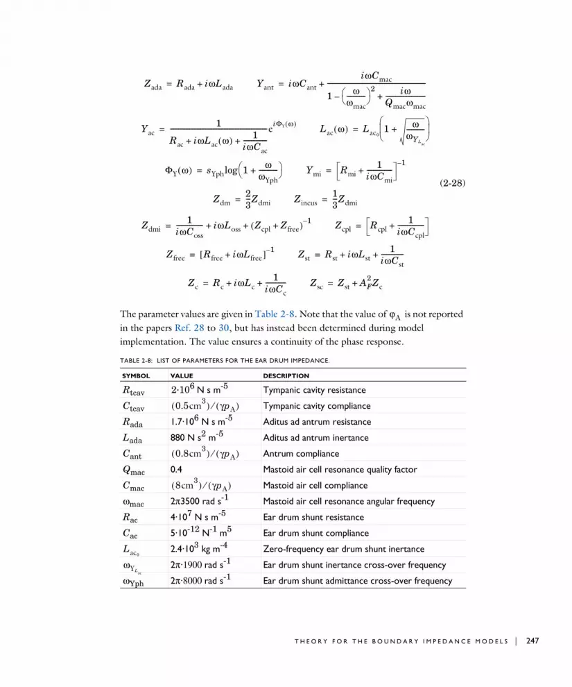
(2-28)

The parameter values are given in Table 2-8. Note that the value of is not reported in the papers Ref. 28 to 30, but has instead been determined during model implementation. The value ensures a continuity of the phase response.

TABLE 2-8: LIST OF PARAMETERS FOR THE EAR DRUM IMPEDANCE.

SYMBOL VALUE DESCRIPTION

Rtcav 2·106 N s m-5 Tympanic cavity resistance

Ctcav Tympanic cavity compliance

Rada 1.7·106 N s m-5 Aditus ad antrum resistance

Lada 880 N s2 m-5 Aditus ad antrum inertance

Cant Antrum compliance

Qmac 0.4 Mastoid air cell resonance quality factor

Cmac Mastoid air cell compliance

ωmac 2π3500 rad s-1 Mastoid air cell resonance angular frequency

Rac 4·107 N s m-5 Ear drum shunt resistance

Cac 5·10-12 N-1 m5 Ear drum shunt compliance

2.4·103 kg m-4 Zero-frequency ear drum shunt inertance

2π·1900 rad s-1 Ear drum shunt inertance cross-over frequency

ωYph 2π·8000 rad s-1 Ear drum shunt admittance cross-over frequency

Zada Rada iωLada+= Yant iωCantiωCmac

1 ωωmac------------ 2

–iω

Qmacωmac-------------------------+

--------------------------------------------------------------+=

Yac1

Rac iωLac ω( ) 1iωCac---------------+ +

-------------------------------------------------------------eiΦY ω( )= Lac ω( ) Lac0

1 ωωYLac

-----------+

=

ΦY ω( ) sYph 1 ωωYph------------+

log= Ymi Rmi1

iωCmi----------------+

1–=

Zdm23---Zdmi= Zincus

13---Zdmi=

Zdmi1

iωCoss----------------- iωLoss Zcpl Zfree+( ) 1–

+ += Zcpl Rcpl1

iωCcpl-----------------+=

Zfree Rfree iωLfree+[ ] 1–= Zst Rst iωLst

1iωCst--------------+ +=

Zc Rc iωLc1

iωCc-------------+ += Zsc Zst AF

2 Zc+=

ϕA

0.5cm3( ) γpA( )⁄

0.8cm3( ) γpA( )⁄

8cm3( ) γpA( )⁄

Lac0

ωYLac


248 | C H A P T E R

Human ear without pinnaThis model accounts for the acoustic losses associated with the ear canal and the entire human ear, see Figure 2-12. It does not include the radiation losses associated with the pinna, the visible part of the ear which is external to the head.

sYph 1.4 Ear drum shunt admittance decay slope

A0 38 mm2 Effective ear drum area, low frequency limit

2 mm2 Effective ear drum area, infinite frequency limit

ωA 2π·2200 rad s-1 Effective ear drum area resonance angular frequency

QA 1.3 Effective ear drum area resonance quality factor

sAph -1.2 Effective ear drum area high-frequency decay slope

ωAph 2π·1500 rad s-1 Effective ear drum area cross-over frequency

-0.8038 Effective ear drum area lag phase constant

Rmi 1 N s m-1 Mechanical resistance of incudomalleal joint

Cmi 0.04 mm N-1 Mechanical compliance of incudomalleal joint

Coss 3·10-3 m N-1 Mechanical compliance of ossicles

Loss 7·10-3 g Mechanical inertance of ossicles

Ccpl 0.5·10-3 m N-1 Mechanical compliance of ossicles-drum coupling

Rcpl 0.08 N s m-1 Mechanical resistance of ossicles-drum coupling

Rfree 0.02 N s m-1 Mechanical resistance of peripheral parts of the drum

Lfree 12·10-3 g Mechanical inertance of peripheral parts of the drum

Rst 18·10-3 N s m-1 Mechanical resistance of stapes

Lst 3·10-3 g Mechanical inertance of stapes

Cst 1.2·10-3 m N-1 Mechanical compliance of stapes

Rc 70·10-3 N s m-1/ AF

2Resistance of cochlea

Lc 10·10-3 g / AF2 Inertance of cochlea

Cc 11·10-3 m N-1·AF2 Compliance of cochlea

AF 3 mm2 Stapes footplate area

TABLE 2-8: LIST OF PARAMETERS FOR THE EAR DRUM IMPEDANCE.

SYMBOL VALUE DESCRIPTION

A∞

ϕA


(2-29)

Here, Zeardrum is the eardrum impedance defined in Equation 2-28 and Tij are the components of the transfer matrix T that describes the ear canal as a two-port. The ear canal is treated as Ntot small segments each with length Δk and radius rk so its full two port T is given by

. (2-30)

where

(2-31)

In these expressions, γ is the ratio of specific heats, Γk is the propagation constant (“wave number”) of the kth ear canal segment which has the segment-specific attenuation αk,

is the segment-specific Womersley number, and

Zear w/o pinna

T11T12

Zeardrum--------------------+

T21T22

Zeardrum--------------------+

-------------------------------------=

TT11 T12

T21 T22

ΓkΔk( )cosh ΓkΔk( )Ztwksinh

ΓkΔk( )sinhZtwk

------------------------------- ΓkΔk( )coshk 1=

Ntot

∏= =

Ztwk

ρc

πrk2

---------= Γk 3αk iωc----+=

αkωc---- 1

2Wok

-------------------ζ11

Wok2

-----------ζ21

Wok3 2

-------------------ζ3+ +=

ζ1 1 γ 1–

Pr-----------+= ζ2 1 γ 1–

Pr----------- γ 1– γ 1–( )2

+2Pr

-------------------------------------–+=

ζ278--- γ 1–

Pr----------- γ 1– γ 1–( )2

+2Pr

-------------------------------------–4 γ 1–( )2 4 γ 1–( )3 γ 1–( )–+

8Pr32---

---------------------------------------------------------------------------+ +=

Wokρωrk

2

μ-------------=

PrCpμ

k----------=


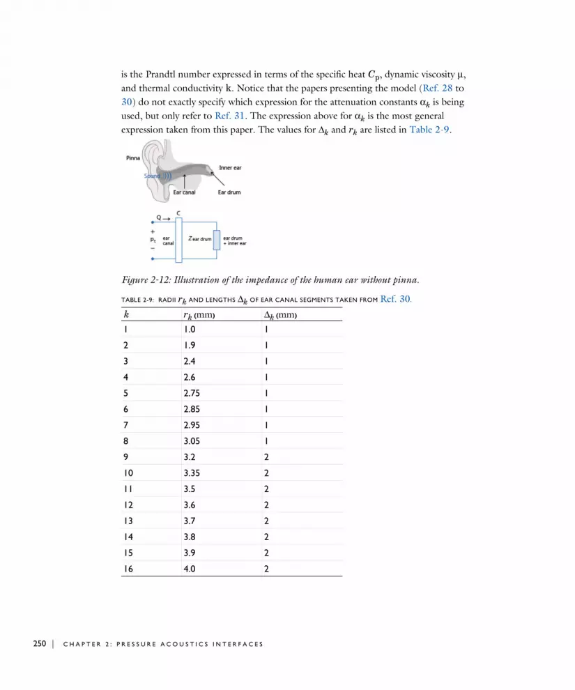
250 | C H A P T E R

is the Prandtl number expressed in terms of the specific heat Cp, dynamic viscosity μ, and thermal conductivity k. Notice that the papers presenting the model (Ref. 28 to 30) do not exactly specify which expression for the attenuation constants αk is being used, but only refer to Ref. 31. The expression above for αk is the most general expression taken from this paper. The values for Δk and rk are listed in Table 2-9.

Figure 2-12: Illustration of the impedance of the human ear without pinna.

TABLE 2-9: RADII rk AND LENGTHS Δk OF EAR CANAL SEGMENTS TAKEN FROM Ref. 30.

k rk (mm) Δk (mm)

1 1.0 1

2 1.9 1

3 2.4 1

4 2.6 1

5 2.75 1

6 2.85 1

7 2.95 1

8 3.05 1

9 3.2 2

10 3.35 2

11 3.5 2

12 3.6 2

13 3.7 2

14 3.8 2

15 3.9 2

16 4.0 2


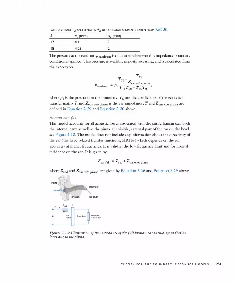
The pressure at the eardrum peardrum is calculated whenever this impedance boundary condition is applied. This pressure is available in postprocessing, and is calculated from the expression

,

where pt is the pressure on the boundary, Tij are the coefficients of the ear canal transfer matrix T and Zear w/o pinna is the ear impedance; T and Zear w/o pinna are defined in Equation 2-29 and Equation 2-30 above.

Human ear, fullThis model accounts for all acoustic losses associated with the entire human ear, both the internal parts as well as the pinna, the visible, external part of the ear on the head, see Figure 2-13. The model does not include any information about the directivity of the ear (the head related transfer functions, HRTFs) which depends on the ear geometry at higher frequencies. It is valid in the low frequency limit and for normal incidence on the ear. It is given by

where Zrad and Zear w/o pinna are given by Equation 2-26 and Equation 2-29 above.

Figure 2-13: Illustration of the impedance of the full human ear including radiation losses due to the pinna.

17 4.1 2

18 4.25 2

TABLE 2-9: RADII rk AND LENGTHS Δk OF EAR CANAL SEGMENTS TAKEN FROM Ref. 30.

k rk (mm) Δk (mm)

peardrum pt

T22T12

Zear w/o pinna--------------------------------–

T11T22 T12T21–------------------------------------------------=

Zear full Zrad Zear w/o pinna+=


252 | C H A P T E R

The pressure at the eardrum peardrum is calculated whenever this impedance boundary condition model is applied. This pressure is calculated from Zear full using the expression

.

Waveguide End Impedance Models

Tubes and ducts are acoustic waveguides, and there are acoustic radiation losses when such a waveguide opens into a large domain. Idealized models for these losses have been implemented as boundary impedance models. Thus, instead of explicitly modeling the large domain, an appropriate impedance model Zend can be applied with Zi = Zend. These models all assume that the domain is infinitely big, that the propagation is in the direction of the waveguide axis, and that the propagating mode is a plane wave. As with all other impedance boundary models, only the boundary-normal velocity component is taken into account.

In the following the term ρc takes different values depending on when the impedance condition is applied. Specifically, for models with damping they are equal to the complex valued quantities ρccc, while when applied on an Anisotropic Acoustic domain the normal direction variables are used ρncn.

Flanged pipe, circularFor a pipe of a user-specified radius a, the acoustic losses are given by (see Ref. 6)

where J1(x) is the Bessel function of the first kind of order 1, H1(x) is the Struve function, and k is the wave number of the wave. This expression is also known as the impedance from a baffled piston.

Flanged pipe, rectangularFor a rectangular duct of user-specified inner width wi and inner height hi, the acoustic losses are given by (see Ref. 5)

peardrum pt 1Zrad

Zear full-----------------–

T22

T12Zear full-----------------–

T11T22 T12T21–--------------------------------------------=

Zend ρc 12J1 2ka( )

2ka--------------------------– i

2H1 2ka( )2ka

---------------------------+ = k ω

c----=


.

This relationship applies provided the following requirements are satisfied

.

Unflanged pipe, circular (low ka limit)For an unflanged circular pipe of a user-specified radius a in the limit of small radius (low ka), the pipe end impedance is given by the classical expression (see Ref. 6)

.

Unflanged pipe, circularFor an unflanged pipe of any user-specified radius a relative to the wave number k, an approximate end impedance is given in Ref. 32. It is

where δ(ka) is a tabulated function reproducing the curve in Fig. 2 in Ref. 32 (where δ(ka) is referred to by l/a).

Porous Layer Models

A boundary impedance model is implemented to specifically handle cases investigating the acoustical properties of a porous layer of a given thickness d backed by a sound-hard wall. This can be applied instead of explicitly modeling the porous layer, as long as the incident acoustic field is normal to the boundary; as for all the other

Zendρc

2πwihi------------------ wihi( )2k2 ik wihi( )

32---f

wihi------ += k ω

c----=

f x( ) 2x

12---sinh 1– 1

x--- 2x

12---–

sinh 1– x( ) 23--- x

32---

x

32---–

x x 1–+( )

32---

–++ +=

wi hi≥ kwi 1« khi 1«

Zend ρc ka( )2

4-------------- i0.6133ka+= k ω

c----= ka 1«

Zend ρc1 R+1 R–--------------= R R e2ikaδ ka( )

–= k ωc----=

Re

ka( )2

2--------------–

1 ka( )4

6-------------- 1

e0.5772ka------------------------ log 19

12------+

+ if ka 1<

πkae ka– 1 332------ 1

ka( )2--------------+ if 1 ka 3.83< <

=


254 | C H A P T E R

boundary impedance models, the tangential components of the acoustic field are ignored by this model.

For a porous layer with a user-specified thickness d, the impedance from the porous layer backed by a sound-hard wall is given by (see Ref. 9)

.

Here ρc and cc are the equivalent fluid descriptions of the porous model. This impedance model applies to any type of porous model which can be written as an equivalent fluid model. All porous models implemented in COMSOL are available for this impedance boundary condition. See details of the poroacoustics equivalent fluid models in the section Theory for the Equivalent Fluid Models.

Characteristic Specific Impedance Models

For well-defined wave types in infinite domains, an impedance condition exists in every point whereby the pressure and normal velocity are related. Thus, these impedances can be imposed on a boundary to model an infinite, open domain in cases where the wave source inside the domain is either a direction (plane wave), a point (spherical wave) or a line (cylindrical wave). However, be aware that only the boundary-normal component of the velocity is used in the impedance boundary condition while the tangential component is ignored; in cases of nonnegligible tangential components it is recommended to instead use the options Plane Wave Radiation, Spherical Wave Radiation, and Cylindrical Wave Radiation.

Plane waveThe impedance is given by

,

see Ref. 6. This is given solely by material parameters and has no user input.

Spherical waveThis impedance corresponds to the wave from a point source. It is calculated from the expression (given in Ref. 6)

Zi iρccc kd( )cot–= k ωcc----=

Zi ρccc=

Ziρccc

1 1ikrb-----------+

---------------------= rb x0 x–= k ωcc----=


where x0 is the user-specified location of the point source generating the spherical waves, x is the position of the boundary, and rb is the distance between the two.

Cylindrical waveThis classic infinite-domain wave impedance from an acoustic line source with the user-specified direction and position x0 is presented in, for example, Ref. 6. The expression for the impedance is

where is the Hankel function of the second kind of order m given in terms of the Bessel functions of order m of the first and second kind, Jm(x) and Ym(x), respectively. Notice that the source axis vector esa is automatically normalized in this implementation.

n0

Zi iρcccH0

2( ) krb( )

H12( ) krb( )

-------------------------= k ωcc----=

rb x0 x–( ) x0 x–( ) esa⋅{ }esa–x0 x–( ) esa×

esa-------------------------------------= =

Hm2( ) x( ) Jm x( ) iYm x( )–=


256 | C H A P T E R

Th eo r y f o r t h e I n t e r i o r Impedan c e Mode l s

In this section:

• Interior Perforated Plate Models

Interior Perforated Plate Models

The transfer impedance of an interior boundary is defined as the ratio of the pressure drop across the boundary to the velocity on the boundary:

(2-32)

The resulting value of Zi can be treated as a superposition of several contributions which are derived separately. Note that the theory below is only valid for the perforates with circular-shaped holes. Other types of holes can lead to significantly different results, which will make the models that are considered here inadequate and unreliable.

T R A N S F E R I M P E D A N C E O F A H O L E

Let the z-coordinate axis be directed along the axis of a cylindrical hole of the height tp (see Figure 2-14). Let the variation of the pressure and the velocity along the z-axis have the following pattern:

(2-33)

The substitution of Equation 2-33 into Equation 2-32 results in

,

where Zc is the characteristic impedance and kc is the complex wave number defined according to the low reduced frequency (LRF) models from the Narrow Region Acoustics for Slits, Circular Ducts, Rectangular Ducts, and Equilateral triangular Ducts. That is,

ZiΔptvn

---------pt,up pt,down–

vn-----------------------------------= =

p z( ) peikcz– v z( ), ve

ikcz–= =

Zip z tp+( ) p z( )–

vn z tp 2⁄+( )---------------------------------------- p z( )

vn z( )------------- e

ikctp– 2⁄e

ikctp 2⁄–( ) 2iZc

kctp2

----------sin–= = =


.

Figure 2-14: To the derivation of the transfer impedance of a one-hole perforate.

The expression for the normalized transfer impedance of an orifice reads

. (2-34)

For thinner plates ( ) the approximation is valid, which yields

. (2-35)

Note that Equation 2-35 coincides with the expression that follows from Crandall’s formula for an infinite tube with the circular cross section (see Ref. 35). Equation 2-34 accounts for both viscous and thermal effects inside the hole, while the simplified Equation 2-35 contains the viscous part only (thermal effects are negligible for the thin plate limit).

Zc ρc γ γ 1–( )ϒth–[ ]ϒv( )12---–

kc, ωc---- γ γ 1–( )ϒth–[ ] 1

ϒv------

12---

= =

z

tp

dh

ziZiρc------

2ikctp

2---------- sin

γ γ 1–( )ϒth–[ ]ϒv

-------------------------------------------------–= =

ktp 1« k, ω c⁄=kctp

2---------- sin

kctp2

----------≈

ziZiρc------ iω

c------–

tpϒv------= =

T H E O R Y F O R T H E I N T E R I O R I M P E D A N C E M O D E L S | 257

258 | C H A P T E R

V E N A C O N T R A C T A A N D A R E A P O R O S I T Y

Equation 2-34 and Equation 2-35 are exact if the streamlines of a flow through the hole are parallel to the z-axis throughout the orifice area. In reality, there is a radial component of the flow, which leads to the reduction (contraction) of this area. The minimum area where the streamlines remain parallel to the z-axis is called vena contracta. The flow velocity at the vena contracta is also different from that of the ideal flow. A coefficient that accounts for these effects is called the discharge coefficient, CD. The value of the discharge coefficient can be obtained from measurements as function of the plate thickness and the orifice shape and diameter.

Another parameter that used to express the interior impedance of a perforate is the porosity, σ. The holes are usually uniformly distributed over the plate, and the porosity accounts for the distribution as the ratio of the hollow area to the area of the plate. Depending on the pattern used when the holes are strewn over the plate, the porosity is defined as follows

for a square and a triangular pattern, respectively. The parameter a determines the hole spacing.

The resulting expression for the interior impedance of a perforate comes out from dividing zi by the product σCD:

. (2-36)

Either Equation 2-34 or Equation 2-35 can be used for the substitution for zi in Equation 2-36. The resulting models will further be referred to as the thick and the thin plate models, respectively.

E N D C O R R E C T I O N A N D H O L E - H O L E I N T E R A C T I O N

The subscript “orifice” in Equation 2-36 means that the expression accounts for the transfer impedance of a perforate caused by the presence of the holes; that is, a piston of fluid of the length tp. However, the actual mass of fluid affected by an incident wave is larger than that inside the hole. The effective mass of the fluid can be taken into account by the piston which is on each side longer by δ than the initial one (see Figure 2-15). This results in adding two extra terms (for each side of the perforate) of

σπdh

2

4a2----------= and σ

πdh2

2 3a2-----------------=

zorifice

ziσCD------------=


the form Equation 2-35 with tp replaced by δ. The choice of Equation 2-35 is due to the absence of highly conducting walls in the end corrections area.

If two holes are located relatively close to one another, the actual masses of the attached fluid can become overlapped. This makes the total mass less than just the sum of those for the separate hole. In order to take the hole-hole interaction into account, the end

Figure 2-15: To the definition of end corrections.

correction is reduced by a factor fint. The last is a function of the porosity and the most often expressed by the Fok function:

.

The end correction is usually considered as a function of the hole diameter and can in practice be different for the resistive and the reactive parts of the transfer impedance. For this reason, it is useful to split δ into two parts: δresist and δreact. The resulting term that accounts for the end correction and the hole-hole interaction reads

. (2-37)

Actual affected mass of fluid

Equivalentpiston

δ

ψ σ( ) an σ( )n

n 0=

N

=

zend Re iωcσCD---------------

2δresistϒv

----------------fint – iIm iω

cσCD---------------

2δreactϒv

----------------fint –=


260 | C H A P T E R

N O N L I N E A R A N D M E A N F L O W E F F E C T S

At medium and high sound pressure levels, the displacement of acoustic particles becomes comparable to the diameter of the holes. This causes flow separation and vortex shedding at the entrance and the exit of the hole. This results in the acoustic energy dissipation and increases the acoustic resistance of the perforate Ref. 36. That is, an extra resistance term should be added to the resulting transfer impedance expression.

Different forms of the contribution to the resistance are similar in the following sense:

• The resistance term is directly proportional to the acoustic particle velocity, which makes it nonlinear;

• The term is frequency dependent through the acoustic particle velocity.

The expression incorporated into the Interior Perforated Plate boundary condition reads

, (2-38)

where fnl is a correction factor (equals 1 by default) and vn is the acoustic particle velocity component normal to the plate. Other expressions for the nonlinear resistance term can be found in Ref. 36.

The presence of a mean flow also changes of the transfer impedance. In order to account for these and other possible effects, the Interior Perforated Plate boundary condition feature includes an option to enable user-defined resistance and reactance:

. (2-39)

Equation 2-37 is only acceptable if the media is the same on both sides of the perforate. If the plate is backed by a porous layer on one side, the values of δ and fint can differ significantly from those on the other side. For example, the interaction between holes is hampered by porous media, which results in neglecting of fint on one side of the plate and leads to the following correction factor: (δ + 1)fint.

znl1 σ2

–

σ2CD2

---------------fnl2c------ vn=

zuser θ user( ) iχ user( )+=


Relative to the mean flow, the contribution of a grazing or a bias flow to the resistance can be expressed through the flow Mach number as shown in Ref. 37.

Combining the expressions Equation 2-36–Equation 2-39 together yields the full expression for the transfer impedance of a perforate for the thick

and the thin

plate models. The discharge coefficient CD is taken different for the linear and the nonlinear parts for the sake of flexibility.

Ziρc------

2ikctp

2---------- sin

γ γ 1–( )ϒth–[ ]ϒv

------------------------------------------------- Re iωcσCD

lin( )--------------------

2δresistϒv

----------------fint

– iIm iωcσCD

lin( )--------------------

2δreactϒv

----------------fint

1 σ2–

σCDnl( )( )

2-----------------------+

fnl2c------ vn θ user( ) iχ user( )

+ +

––=

Ziρc------ Re iω

cσCDlin( )

--------------------tp 2+ δresist

ϒv----------------------------fint

iIm iωcσCD

lin( )--------------------

tp 2+ δreactϒv

---------------------------fint

1 σ2–

σCDnl( )( )

2-----------------------+

fnl2c------ vn θ user( ) iχ user( )

+ +

––=


262 | C H A P T E R

Th eo r y f o r t h e Equ i v a l e n t F l u i d Mode l s

In this section:

• Introduction to the Equivalent Fluid Models

• About the Pressure Acoustics Fluid Models

• About the Poroacoustics Models

• About the Narrow Region Acoustics Models

Introduction to the Equivalent Fluid Models

It is possible to define the properties of a fluid in several ways in pressure acoustics. In a Pressure Acoustics domain feature attenuation properties for the bulk fluid may be specified. Acoustic losses in porous materials are modeled by homogenizing the porous matrix and saturating fluid, and are defined by the Poroacoustics domain feature (frequency domain only). The viscous and thermal losses that occur in the acoustic boundary layer can be modeled in a homogenized way using the Narrow Region Acoustics domain feature (frequency domain only). The different ways of defining the properties of a fluid are called fluid models. They are also often referred to as equivalent fluid models.

Losses and damping occur when acoustic waves propagate in a porous material (where material refers to the homogenization of a fluid and a porous solid) because of bulk viscous and thermal properties, or because of thermal and viscous losses in the acoustic boundary layer at walls in narrow ducts. The purpose of the fluid model is to mimic a special loss behavior by defining a complex-valued density ρc and speed of sound cc. These are often frequency dependent.

In a Pressure Acoustics domain feature, the default Linear elastic fluid model (see Linear Elastic Fluid Model) enables you to specify a linearly elastic fluid using either the density ρ and speed of sound c, the impedance Z and wave number k, or the equivalent bulk modulus K and the density ρ. When any of these material parameters are complex-valued, damping is introduced.

It is always necessary to specify a set of two parameters (for example Z and k) or conditions in order to calculate the complex speed of sound and complex density


needed to specify a fluid model. The choice of parameters typically depend on the application and which equivalent fluid is being modeled. For example:

• It is possible to determine the complex wave number k and impedance Z from directly measuring it in an impedance tube in order to produce curves of the real and imaginary parts (the resistance and reactance, respectively) as functions of frequency. These data can be used directly as input to COMSOL Multiphysics interpolation functions to define k and Z.

• The option to define the equivalent bulk modulus K and density ρ is often used when characterizing the propagation of acoustic waves in a porous material. These parameters may be determined from measurements or by defining an analytical model expression.

The linear elastic fluid model enables the user to enter any desired fluid models with the desired combination of fluid properties. It is the most general fluid model. You may enter any user-defined analytical expressions for your favorite equivalent fluid model or use measurement data to represent the lossy behavior of the fluid.

P R O P A G A T I O N I N G E N E R A L F L U I D W I T H B U L K L O S S E S

The options are (see About the Pressure Acoustics Fluid Models and the settings for the Pressure Acoustics node):

• Linear elastic: define density and speed of sound, impedance and wave number, or equivalent bulk modulus and density.

• Linear elastic with attenuation: define an attenuation parameter for the fluid.

• Ideal gas is also available but not described here. This fluid model is used to specify the fluid properties by selecting a gas constant type and selecting between entering the heat capacity at constant pressure or the ratio of specific heats. See Ideal Gas Fluid Model for details.

• Viscous and/or thermally conducting fluids (bulk losses): the losses are due to viscous losses, thermal conduction, or the combined thermal conduction and viscous losses in the bulk of the fluid.

P R O P A G A T I O N I N P O R O U S M A T E R I A L S

A series of fluid models exist for describing the propagation of pressure waves in porous materials. These range from fully empirical models to semianalytical/empirical models with varying degree of complexity. See Poroacoustics and About the Poroacoustics Models for more detail.

T H E O R Y F O R T H E E Q U I V A L E N T F L U I D M O D E L S | 263

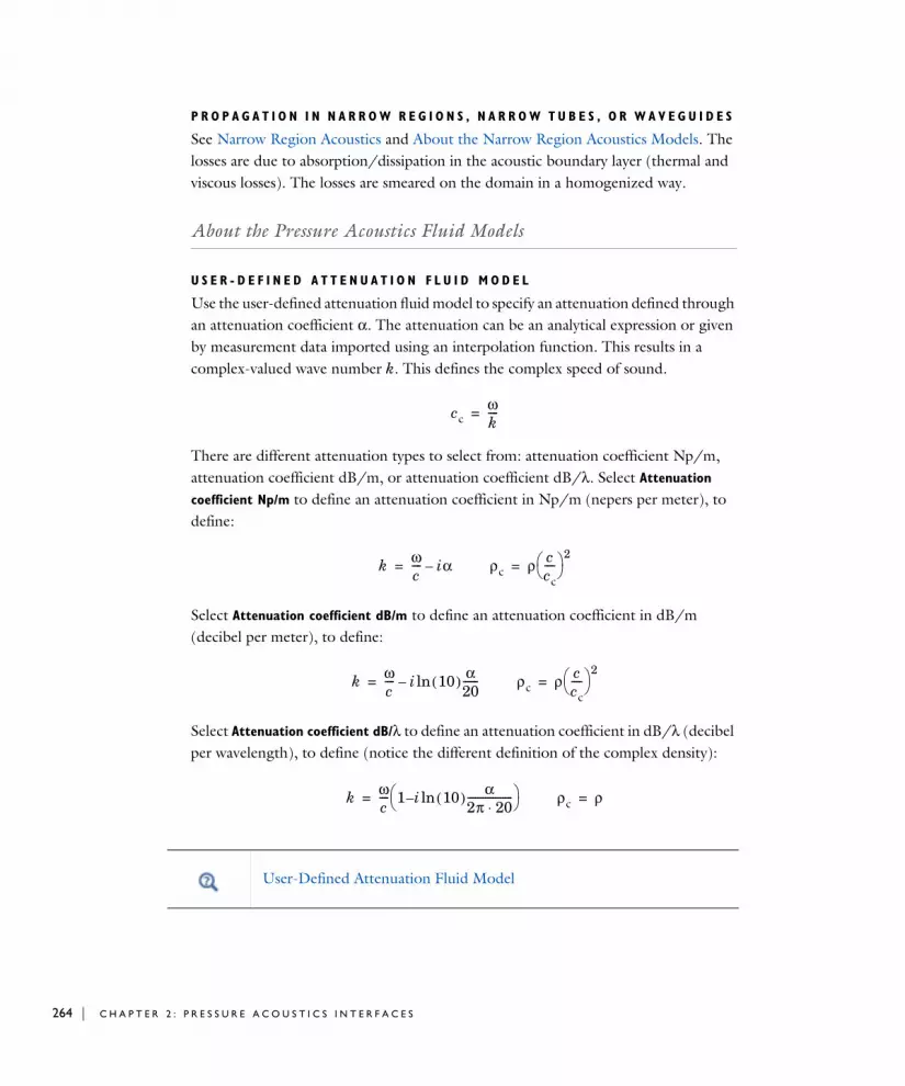
264 | C H A P T E R

P R O P A G A T I O N I N N A R R O W R E G I O N S , N A R R O W T U B E S , O R W A V E G U I D E S

See Narrow Region Acoustics and About the Narrow Region Acoustics Models. The losses are due to absorption/dissipation in the acoustic boundary layer (thermal and viscous losses). The losses are smeared on the domain in a homogenized way.

About the Pressure Acoustics Fluid Models

U S E R - D E F I N E D A T T E N U A T I O N F L U I D M O D E L

Use the user-defined attenuation fluid model to specify an attenuation defined through an attenuation coefficient α. The attenuation can be an analytical expression or given by measurement data imported using an interpolation function. This results in a complex-valued wave number k. This defines the complex speed of sound.

There are different attenuation types to select from: attenuation coefficient Np/m, attenuation coefficient dB/m, or attenuation coefficient dB/λ. Select Attenuation

coefficient Np/m to define an attenuation coefficient in Np/m (nepers per meter), to define:

Select Attenuation coefficient dB/m to define an attenuation coefficient in dB/m (decibel per meter), to define:

Select Attenuation coefficient dB/λ to define an attenuation coefficient in dB/λ (decibel per wavelength), to define (notice the different definition of the complex density):

ccωk----=

k ωc---- iα–= ρc ρ c

cc---- 2

=

k ωc---- i 10( ) α

20------ln–= ρc ρ c

cc---- 2

=

k ωc---- 1 i 10( ) α

2π 20⋅------------------ln–

= ρc ρ=

User-Defined Attenuation Fluid Model


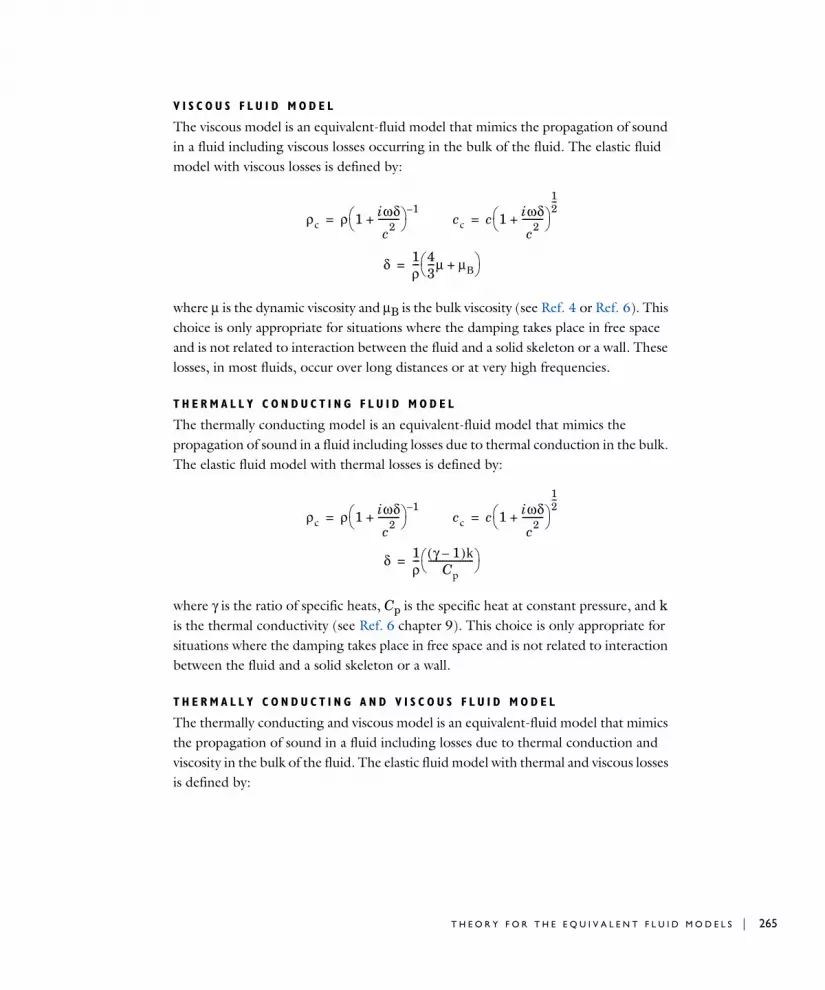
V I S C O U S F L U I D M O D E L

The viscous model is an equivalent-fluid model that mimics the propagation of sound in a fluid including viscous losses occurring in the bulk of the fluid. The elastic fluid model with viscous losses is defined by:

where μ is the dynamic viscosity and μB is the bulk viscosity (see Ref. 4 or Ref. 6). This choice is only appropriate for situations where the damping takes place in free space and is not related to interaction between the fluid and a solid skeleton or a wall. These losses, in most fluids, occur over long distances or at very high frequencies.

T H E R M A L L Y C O N D U C T I N G F L U I D M O D E L

The thermally conducting model is an equivalent-fluid model that mimics the propagation of sound in a fluid including losses due to thermal conduction in the bulk. The elastic fluid model with thermal losses is defined by:

where γ is the ratio of specific heats, Cp is the specific heat at constant pressure, and k is the thermal conductivity (see Ref. 6 chapter 9). This choice is only appropriate for situations where the damping takes place in free space and is not related to interaction between the fluid and a solid skeleton or a wall.

T H E R M A L L Y C O N D U C T I N G A N D V I S C O U S F L U I D M O D E L

The thermally conducting and viscous model is an equivalent-fluid model that mimics the propagation of sound in a fluid including losses due to thermal conduction and viscosity in the bulk of the fluid. The elastic fluid model with thermal and viscous losses is defined by:

ρc ρ 1 iωδc2

---------+ 1–

= cc c 1 iωδc2

---------+

12---

=

δ 1ρ--- 4

3---μ μB+ =

ρc ρ 1 iωδ

c2---------+

1–= cc c 1 iωδ

c2---------+

12---

=

δ 1ρ--- γ 1–( )k

Cp-------------------- =


266 | C H A P T E R

where μ is the dynamic viscosity and μB is the bulk viscosity, γ is the ratio of specific heats, Cp is the specific heat at constant pressure, and k is the thermal conductivity (see Ref. 6 chapter 9). This choice is only appropriate for situations where the damping takes place in free space and is not related to interaction between the fluid and a solid skeleton or a wall.

About the Poroacoustics Models

The Poroacoustics node introduces several fluid models for modeling the propagation of acoustic waves in porous materials. After some general remarks about fluid models and the rigid and limp regime approximations, these models are discussed in this section:

• Porous Fluid Models

• Delany-Bazley-Miki

• Zwikker-Kosten

• Attenborough

• Wilson

• Johnson-Champoux-Allard (JCA)

• Johnson-Champoux-Allard-Lafarge (JCAL)

• Johnson-Champoux-Allard-Pride-Lafarge (JCAPL)

• Williams EDFM (equivalent density fluid model)

• Wood (fluid suspension Model)

P O R O U S F L U I D M O D E L S

The poroacoustics fluid models are equivalent fluid models that mimic the behaviors of a full Poroelastic Material model, which is defined by Biot’s theory. A poroacoustics

ρc ρ 1 iωδc2

---------+ 1–

= cc c 1 iωδc2

---------+

12---

=

δ 1ρ--- 4

3---μ μB+ γ 1–( )k

Cp--------------------+

=

Thermally Conducting and/or Viscous Fluid Model


fluid model is based on describing the frequency-dependent effective fluid density ρ(ω) and the effective fluid bulk modulus K(ω) of the combined equivalent fluid-solid system (saturating fluid and porous matrix). The description of these models includes the losses associated with the propagation of acoustic waves in porous materials. An equivalent fluid model is computationally less demanding than the full poroelastic model. However, it is only physically correct for certain choices of material parameters. Most poroacoustic models are only valid in the rigid or limp porous matrix approximations.

Limp and Rigid Porous Matrix ModelsIn the rigid porous matrix limit, the matrix is assumed to be so stiff that it does not move (sometimes referred to as a motionless skeleton model). In this case it is assumed that in Biot’s theory u = 0, which yields a wave equation with complex density and bulk modulus. In a rigid porous material the Biot-Willis coefficient is equal to the porosity αB = εP. All the poroacoustic fluid models are based on defining the rigid effective density ρrig (see Ref. 9).

The limp porous matrix limit is the opposite of the rigid assumption. It is used to model materials where the stiffness of solid phases (the porous matrix) is so weak that it cannot support free, structure-borne wave propagation (neither longitudinal nor transverse). That is, the stiffness (in vacuo bulk stiffness) is very small compared to air such that the solid phase motion becomes acoustically significant. If it is light enough, the solid phase still moves because it is “dragged along” by the fluid motion; a limp porous material model is also an equivalent fluid model because it only features a single longitudinal wave type. Typically, the limp assumption can be applied to very light weight fibrous materials (less than 10 kg/m3) if these are not stiffened by the injection of binder material. In the limp case, it is assumed that the stress tensor vanishes and that in Biot’s theory, the Biot-Willis coefficient is αB = 1. The limp density is related to the rigid density by a mixture model (see Ref. 10)

where ρf is the fluid density, ρd is the drained porous matrix density, ρav is the average effective density, and ρlimp is the resulting effective limp density.

Fluid ParametersDefining the equivalent density and bulk modulus results in the usual complex-valued speed of sound and density (the propagation parameters):

ρlimpρrigρav ρf

2–

ρav ρrig 2ρ– f+-----------------------------------= ρav ρd εpρf+=


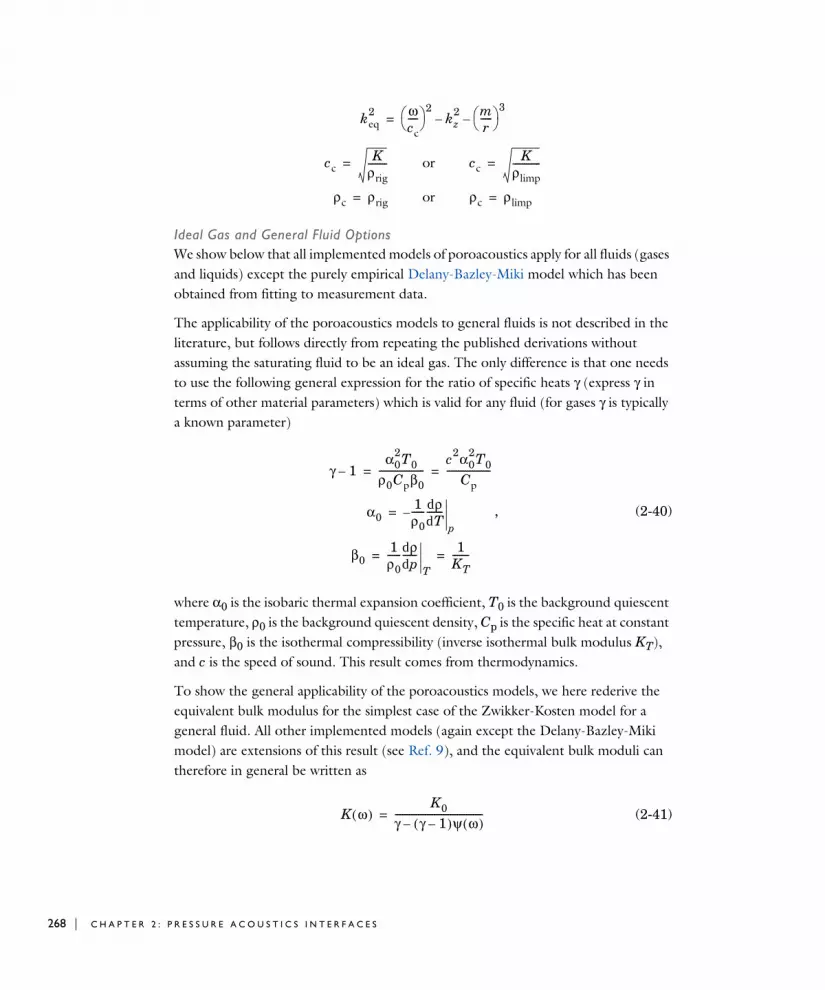
268 | C H A P T E R

Ideal Gas and General Fluid OptionsWe show below that all implemented models of poroacoustics apply for all fluids (gases and liquids) except the purely empirical Delany-Bazley-Miki model which has been obtained from fitting to measurement data.

The applicability of the poroacoustics models to general fluids is not described in the literature, but follows directly from repeating the published derivations without assuming the saturating fluid to be an ideal gas. The only difference is that one needs to use the following general expression for the ratio of specific heats γ (express γ in terms of other material parameters) which is valid for any fluid (for gases γ is typically a known parameter)

, (2-40)

where α0 is the isobaric thermal expansion coefficient, T0 is the background quiescent temperature, ρ0 is the background quiescent density, Cp is the specific heat at constant pressure, β0 is the isothermal compressibility (inverse isothermal bulk modulus KT), and c is the speed of sound. This result comes from thermodynamics.

To show the general applicability of the poroacoustics models, we here rederive the equivalent bulk modulus for the simplest case of the Zwikker-Kosten model for a general fluid. All other implemented models (again except the Delany-Bazley-Miki model) are extensions of this result (see Ref. 9), and the equivalent bulk moduli can therefore in general be written as

(2-41)

keq2 ω

cc---- 2

kz2

–mr----- 3

–=

ccK

ρrig--------= or cc

Kρlimp------------=

ρc ρrig= or ρc ρlimp=

γ 1–α0

2T0ρ0Cpβ0--------------------

c2α02T0

Cp-------------------= =

α01ρ0------ dρ

dT-------

p–=

β01ρ0------dρ

dp------

T

1KT-------= =

K ω( )K0

γ γ 1–( )ψ ω( )–--------------------------------------=


for any of these models, where the frequency response Ψ(ω) is specific to each model. Consequently, the following derivation is sufficient to show the general result.

Derivation of the Equivalent Bulk Modulus Valid for Any Fluid in the Zwikker-Kosten TheoryIn general, the (isentropic) bulk modulus is given by

. (2-42)

A relationship between the pressure p and the density ρ is needed to define the effective bulk modulus, and the equation of state provides such a relationship. Instead of relying on the ideal gas equation, we here use the following general equation of state

(2-43)

which merely stipulates that the density ρ is a function of both pressure p and temperature T. The temperature-dependence is nonnegligible since we are dealing with small pores, and acoustics in porous materials belong to thermoviscous acoustics (see Thermoviscous Acoustics Interfaces). Assuming the acoustic fields are small harmonic perturbations (denoted by a subscript 1) about a quiescent reference state (denoted by subscript 0)

(2-44)

and Taylor-expanding the general equation of state Equation 2-43 to first order, we find

(2-45)

where βT is the isothermal compressibility.

In order to calculate the effective bulk modulus from Equation 2-42 using the equation of state Equation 2-45, a relationship between T1 and p1 is derived from the linearized energy equation (see Theory Background for the Thermoviscous Acoustics Branch)

K0 ρdpdρ------=

ρ ρ p T,( )=

ρ ρ0 ρ1eiωt+=

p p0 p1eiωt+=

T T0 T1eiωt+=

ρ1 ρ0 βTp1 α0T1–( )=


270 | C H A P T E R

(2-46)

where Dth is the thermal diffusivity, k is the thermal conductivity, and Q is a volumetric heat source. To proceed with the solution of this equation, it is generally assumed that (i) the pore can be modeled as a hollow cylinder, (ii) the contributions from radial variations dominate over axial variations so it suffices to solve the radial problem while assuming no axial variations Ref. 9, and (iii) the pore radius is much smaller than the wavelength, whereby the pressure does not change noticeably across the radius. By these assumptions the pressure p1 can be treated as a constant in Equation 2-46 and the equation has only radial variations:

The cross-sectional average solution under these assumptions, and with the boundary condition of zero acoustic temperature T1 on the pore walls at r = R, is

. (2-47)

Here

(2-48)

where Wo is the Womersley number (see the note below), and Pr is the Prandtl number, measuring the relative width of the viscous boundary layer thickness to the thermal boundary layer thickness.

With the solution from Equation 2-47, the pressure can now be expressed as a function of the density using the first-order equation of state Equation 2-45:

(2-49)

0 iωDth---------–∇2

T1

α0T0k

-------------iωp1Qk----+ +=

Dthk

ρ0Cp-------------=

T1∇2 1r---

r∂∂ T1

r2

2

∂∂ T1+→

T1(r)α0T0ρ0Cp-------------p1

Qρ0Cp------------- 1

iω------+ 1 2

Wo Pr i–----------------------------

J1 Wo Pr i–( )

J0 Wo Pr i–( )----------------------------------------–=

WoR2ωρ0

μ------------------= Pr μ

ρDth-------------=

p1 ρ1( )

ρ1Qα0Cp

----------- 1 2Wo Pr i–----------------------------

J1 Wo Pr i–( )

J0 Wo Pr i–( )----------------------------------------–+

ρ0 βTα0

2T0ρ0Cp------------- 1 2

Wo Pr i–----------------------------

J1 Wo Pr i–( )

J0 Wo Pr i–( )----------------------------------------––

----------------------------------------------------------------------------------------------------------------------------=


From this we obtain the following expression for the equivalent bulk modulus (see Equation 2-42)

(2-50)

where the ratio of specific heats γ is defined in Equation 2-40 for a general fluid and K0 is the isentropic bulk modulus of the fluid. This formula Equation 2-50 is mathematically equivalent to the normal Zwikker-Kosten formula for the equivalent bulk modulus (see Ref. 15), but it has been derived for a general fluid and not just an ideal gas.

We emphasize that from this result for a general fluid follows the general formula Equation 2-41, in this particular case with

(2-51)

with the Womersley number Wo containing the frequency dependence.

D E L A N Y - B A Z L E Y - M I K I

The Delany-Bazley-Miki model is an equivalent fluid model that mimics the bulk losses in certain porous/fibrous materials. The model represents a porous medium with the following complex propagation constants:

K ω( ) ρ0dp1dρ1---------

K0

γ γ 1–( ) 1 2Wo Pr i–----------------------------

J1 Wo Pr i–( )

J0 Wo Pr i–( )----------------------------------------––

--------------------------------------------------------------------------------------------------------------= =

ψ ω( ) 1 2Wo Pr i–----------------------------

J1 Wo Pr i–( )

J0 Wo Pr i–( )----------------------------------------–=

The Womersley number Wo measures the influence of viscous effects relative to the oscillation frequency ω. For viscosity dominates and the velocity profile is the well-known Poiseuille parabola, while in the Helmholtz regime for the velocity profile is plug-like with a very small boundary layer close to the walls.

Wo 1«

Wo 1»

kcωc---- 1 C1X

C2–iC3X

C– 4–+[ ]=

Zc ρfc 1 C5XC6–

iC7XC– 8–+[ ]=

Xf ρf⋅Rf

-----------=


272 | C H A P T E R

where ρf is the fluid density, f is the frequency, and Rf is the flow resistivity. Several predefined sets of the coefficients Ci exist. They are the classic Delany-Bazley model, the Miki model (see Ref. 9, section 2.5 and ), the Qunli, several variants of the Mechel model for different configurations, the Komatsu model, and a so-called Modified Champoux and Allard model. These are all empirical models based on fitting the two complex functions to measured data for the complex wave number kc and complex specific acoustic impedance Zc. All the models are applicable for materials with a porosity εp close to 1. The applicability of the different model parameters is listed in Table 2-10. See also Ref. 23 for further details.



Delany-Bazley Glass and rock wool with:

Miki Glass and rock wool with:

The validity of the model using the Miki parameters is not well-established for X< 0.01, but the model is slightly better behaved mathematically below this limit using the Miki parameters rather than the Delany-Bazley parameters, see Ref. 22.

Qunli Porous plastic and open foams:

Mechel, glass fiber, low X Glass fiber:

Mechel, glass fiber, high X Glass fiber:

Mechel, rock fiber, low X Rock fiber:

Mechel, rock fiber, high X Rock fiber:

0.01 X 1≤ ≤

103 Rf 50 103⋅ Pasm 2–≤ ≤

0.01 X 1≤ ≤

103 Rf 50 103⋅ Pasm 2–≤ ≤

200 f 2000 Hz≤ ≤

3 103⋅ Rf 24 103⋅ Pasm 2–≤ ≤

X 0.025≤

X 0.025≥

X 0.025≤

X 0.025≥


Z W I K K E R - K O S T E N

Zwikker-Kosten is one of the earliest equivalent fluid models for porous materials (Ref. 15). It is a rigid frame model defined by the complex (rigid) density

where Hr is the hydraulic radius of the pores (for straight cylindrical pores Hr = a = radius) and Wo is the Womersley number (see Equation 2-48 and the note below). Wo is related to the ratio between viscous penetration depth δv and the hydraulic radius. δv gives the scale of the viscous boundary layer thickness (see Theory Background for the Thermoviscous Acoustics Branch for details). The bulk modulus is given by

where pA denotes the ambient pressure, ρf the fluid density, γ the ratio of specific heat, Pr the Prandtl number, µ the dynamic viscosity, Cp the heat capacity at constant pressure, and k the coefficient of thermal conduction. J0 and J1 are Bessel functions of the first kind. The factor γ pA is the isentropic bulk modulus (K0 = γ pA). The free parameters of the pores are the porosity εP and the hydraulic radius Hr.

A T T E N B O R O U G H

The Attenborough model is also based on the cylindrical-like pore assumption. It is a so-called four parameter semi-empirical model. The model is an extension of the Zwikker-Kosten model and adds two more input parameters. It accounts for the tortuosity (high frequency limit) , which is related to the orientation of the pores relative to the propagation direction. The hydraulic diameter of the pores is replaced

Komatsu Glass and rock wool:

Modified Champoux and Allard



6 103⋅ Rf 73 103⋅ Pasm 2–≤ ≤

45 f 11 103 Hz⋅≤ ≤

ρrigρfεP----- 1

1 2Wo i–------------------

J1 Wo i–( )

J0 Wo i–( )------------------------------–

-----------------------------------------------------------= WoωρfHr

2

μ----------------- 2

Hrδv------= =

KγpAεP

--------- 1

1 γ 1–( ) 2Wo iPr–------------------------

J1 Wo iPr–( )

J0 Wo iPr–( )------------------------------------+

----------------------------------------------------------------------------------------= PrCpμ

k----------=

τ∞


274 | C H A P T E R

by an expression that includes the flow resistivity Rf, and a fitting parameter b, (this parameter is related to the anisotropy of the pores). See Ref. 9 and Ref. 16. The equivalent density and bulk modulus are defined as

and

where pA denotes the ambient pressure, ρf the fluid density, γ the ratio of specific heat, Pr the Prandtl number, µ the dynamic viscosity, Cp the heat capacity at constant pressure, and k the coefficient of thermal conduction. J0 and J1 are Bessel functions of the first kind. The variable s' (anisotropy factor) is derived from other material parameters and is related to the Womersley number (see Equation 2-48):

Here, ω denotes the angular frequency. The four parameters needed (when the fluid is air at room temperature) are the porosity εP, the tortuosity τ∞, flow resistivity Rf, and the fitting parameter b (dimensionless, close to 1). The fitting parameter b is tabulated for certain well-defined pore cross-sections in Table 2-11.

In this way, the hydraulic radius of the Attenborough model is formulated in terms of measurable intrinsic properties of the porous material which alleviates the need to know the pore radii.

The viscous characteristic length of the model Lv can also be defined by

TABLE 2-11: FITTING FACTOR b FOR DIFFERENT CROSS-SECTIONAL GEOMETRIES (SEE Ref. 9)

CROSS-SECTIONAL SHAPE b

Circle 1

Square 1.07

Equilateral triangle 1.11

Rectangular slit 0.81

ρrigρfεP-----

τ∞

1 2s' i–-------------

J1 s' i–( )

J0 s' i–( )-------------------------–

------------------------------------------------=

KγpAεP

--------- 1

1 γ 1–( ) 2s' Pr i–-----------------------

J1 s' Pr i–( )

J0 s' Pr i–( )-----------------------------------+

--------------------------------------------------------------------------------------= PrCpμ

k----------=

s' b8ωρfτ∞

εPRf-------------------=


with δv the viscous penetration depth. This length is related to the pores’ circular cross section radius R (for a cylinder) and the thickness of the viscous boundary layer. The parameter b = 1/s, where s is the viscous characteristic length parameter. See the following models:

• Johnson-Champoux-Allard (JCA)

• Johnson-Champoux-Allard-Lafarge (JCAL)

• Johnson-Champoux-Allard-Pride-Lafarge (JCAPL)).

Note that the tortuosity is related to the angle θ between the cylindrical pores and the direction of propagation of the wave, by

W I L S O N

The Wilson model is a generalization of the analytical models for porous materials with constant cross section and parallel pores. This model is intended to match the middle frequency behavior of a porous material (see Ref. 9, Ref. 17, and Ref. 18). It is not a good model for ω tending to 0 or infinity. The equivalent density and bulk modulus are given by

where τvor denotes the vorticity-mode relaxation time, τent the entropy-mode relaxation time, ρ∞ the infinity frequency limit for the density, K∞ the infinity frequency limit for the bulk modulus, and γ is the ratio of specific heats. These are the four free parameters. With appropriate choices for the relaxation parameters, the Wilson model can be fitted to mimic all the models described here. For example, setting τvor = 2.54/Rf and τent = 3.75/Rf, the equations mimic the Delany-Bazley model (see Cox and D’Antonio Sec. 5.4.4, Ref. 18).

Lv b8μτ∞εPRf------------- s' μ

ωρf--------- s'

δv

2-------= = =

τ∞1

cos2 θ( )-------------------=

ρrig ρ∞1 iωτvor+( )1 2⁄

1 iωτvor+( )1 2⁄ 1–------------------------------------------------=

K K∞1 iωτent+( )1 2⁄

1 iωτent+( )1 2⁄ γ 1–+---------------------------------------------------------=


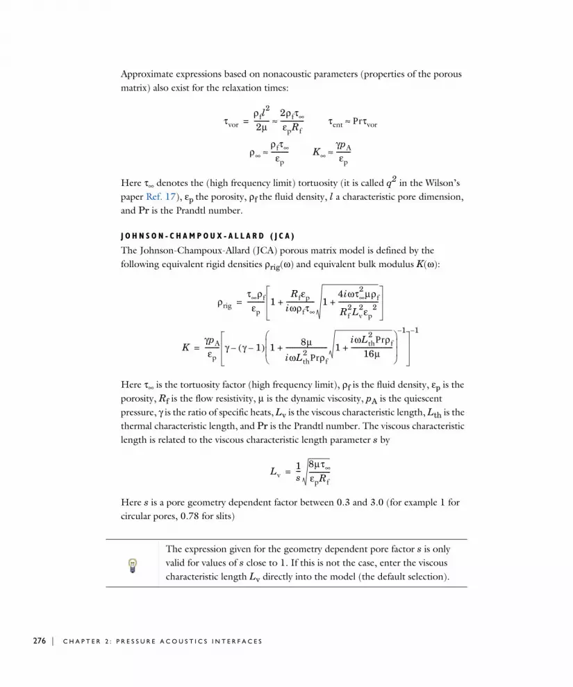
276 | C H A P T E R

Approximate expressions based on nonacoustic parameters (properties of the porous matrix) also exist for the relaxation times:

Here τ∞ denotes the (high frequency limit) tortuosity (it is called q2 in the Wilson’s paper Ref. 17), εp the porosity, ρf the fluid density, l a characteristic pore dimension, and Pr is the Prandtl number.

J O H N S O N - C H A M P O U X - A L L A R D ( J C A )

The Johnson-Champoux-Allard (JCA) porous matrix model is defined by the following equivalent rigid densities ρrig(ω) and equivalent bulk modulus K(ω):

Here τ∞ is the tortuosity factor (high frequency limit), ρf is the fluid density, εp is the porosity, Rf is the flow resistivity, μ is the dynamic viscosity, pA is the quiescent pressure, γ is the ratio of specific heats, Lv is the viscous characteristic length, Lth is the thermal characteristic length, and Pr is the Prandtl number. The viscous characteristic length is related to the viscous characteristic length parameter s by

Here s is a pore geometry dependent factor between 0.3 and 3.0 (for example 1 for circular pores, 0.78 for slits)

τvorρfl

2

2μ----------

2ρfτ∞εpRf

---------------≈= τent Prτvor≈

ρ∞ρfτ∞

εp-----------≈ K∞

γpAεp

---------≈

ρrigτ∞ρf

εp----------- 1

Rfεpiωρfτ∞------------------ 1

4iωτ∞2 μρf

Rf2Lv

2εp2

-------------------------++=

KγpAεp

--------- γ γ 1–( ) 1 8μ

iωLth2 Prρf

-------------------------- 1iωLth

2 Prρf16μ

--------------------------++

1–

–

1–

=

Lv1s---

8μτ∞εpRf-------------=

The expression given for the geometry dependent pore factor s is only valid for values of s close to 1. If this is not the case, enter the viscous characteristic length Lv directly into the model (the default selection).


J O H N S O N - C H A M P O U X - A L L A R D - L A F A R G E ( J C A L )

The Johnson-Champoux-Allard-Lafarge (JCAL) model introduces corrections to the bulk modulus thermal behavior at low frequencies that is not captured by the JCA model (see Ref. 13). The equivalent density is the same as in the JCA model. The correction is to the bulk modulus and is given by

with the introduction of the new parameter, k’0, which is the static thermal permeability (SI unit: m2). For measurements and details of this parameter see Ref. 11 and Ref. 12 for examples.

J O H N S O N - C H A M P O U X - A L L A R D - P R I D E - L A F A R G E ( J C A P L )

The Johnson-Champoux-Allard-Pride-Lafarge (JCAPL) model further extends the JCAL models by introducing a static viscous τ0 and thermal τ'0 tortuosity, which both introduce low frequency corrections to the JCAL and JCA models. See Ref. 14 and Ref. 9.

This model has the complex rigid density given by:

The viscous Lv and thermal Lth characteristic lengths are also sometimes denoted by Λ and Λ’, respectively.

Porous Absorber: Application Library path Acoustics_Module/

Building_and_Room_Acoustics/porous_absorber

KγpAεp

--------- γ γ 1–( ) 1εpμ

iωk'0Prρf------------------------- 1

4iω k'0( )2Prρf

μLth2 εp

2------------------------------------++

1–

–

1–

=

ρrigρfτ ω( )

εp-----------------=

τ ω( ) τ∞ 1 1iω------F ω( )+= F ω( ) 1 P– P 1 M

2P2----------iω++=

iωiωρfk0τ∞

μεp------------------------= M

8k0τ∞

εpLv2

----------------=

P M4 τ0 τ∞ 1–⁄( )---------------------------------

2k0τ∞2

εpLv2 τ0 τ∞–( )

-----------------------------------= =


278 | C H A P T E R

where the new parameter is the static viscous tortuosity τ0 (dimensionless). The viscous permeability is defined as k0 = μ/Rf (SI unit: m2).

The complex bulk modulus K is given by:

where the new parameter is the static thermal tortuosity τ'0 (dimensionless).

W I L L I A M S E D F M ( E Q U I V A L E N T D E N S I T Y F L U I D M O D E L )

The Williams EDFM model is a so-called equivalent density fluid model. The model is derived under the assumption that the bulk and shear moduli of the frame of the porous material are negligible, see Ref. 24 for further details. This is why the model pertains to sediments. The effective bulk modulus Keff and an effective density ρeff defined my the model are given by

In Ref. 9 (equation 5.32), P is called b, k0 is called q0, and Pr is called B2.

KγpAεp

--------- 1β ω( )------------=

β ω( ) γ γ 1–( ) 1 1iω'-------F'˜

ω( )+1–

– γ γ 1–( )τ'˜ ω( )1–

–= =

F'˜ ω( ) 1 P'– P' 1 M'

2P'2-----------iω'++= iω'

iωρfPrk'0μεp

-------------------------=

M'8k'0

εpLth2

--------------= P' M'4 τ'0 1–( )----------------------=

In Ref. 9 (equation 5.35), is called α '(ω), and P’ = 1.

The JCA model is recovered by setting M' = P = P' = 1 and the JCAL is recovered by setting P = P' = 1.

τ'˜ ω( )


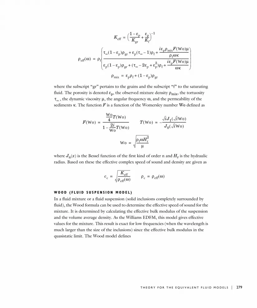
where the subscript “gr” pertains to the grains and the subscript “f” to the saturating fluid. The porosity is denoted εp, the observed mixture density ρmix, the tortuosity

, the dynamic viscosity μ, the angular frequency ω, and the permeability of the sediments κ. The function F is a function of the Womersley number Wo defined as

where Jn(x) is the Bessel function of the first kind of order n and Hr is the hydraulic radius. Based on these the effective complex speed of sound and density are given as

W O O D ( F L U I D S U S P E N S I O N M O D E L )

In a fluid mixture or a fluid suspension (solid inclusions completely surrounded by fluid), the Wood formula can be used to determine the effective speed of sound for the mixture. It is determined by calculating the effective bulk modulus of the suspension and the volume average density. As the Williams EDFM, this model gives effective values for the mixture. This result is exact for low frequencies (when the wavelength is much larger than the size of the inclusions) since the effective bulk modulus in the quasistatic limit. The Wood model defines

Keff1 εp–

Kgr--------------

εpKf------+

1–

=

ρeff ω( ) ρf

τ∞ 1 εp–( )ρgr εp τ∞ 1–( )ρfiεpρmixF Wo( )μ

ρfωκ-----------------------------------------+ +

εp 1 εp–( )ρgr τ∞ 2εp– εp2

+( )ρfiεpF Wo( )μ

ωκ------------------------------+ +

------------------------------------------------------------------------------------------------------------------------

=

ρmix εpρf 1 εp–( )ρgr+=

τ∞

F Wo( )

Wo4

---------T Wo( )

1 2iWo---------T Wo( )–

-------------------------------------= T Wo( )iJ1 iWo( )

J0 iWo( )---------------------------------–=

WoρfωHr

2

μ-----------------=

ccKeff

ρeff ω( )-----------------= ρc ρeff ω( )=


280 | C H A P T E R

where θf, Kf, and ρf, are the fluid’s volume fraction, adiabatic bulk modulus, and density, respectively; and θi, Ki, and ρi, are the inclusion’s volume fractions, adiabatic bulk moduli, and densities, respectively. And again the complex speed of sound and density are defined as

About the Narrow Region Acoustics Models

The Narrow Region Acoustics fluid models are used to mimic the thermal and viscous losses that exist in narrow tubes where the tube cross-section length-scale is comparable to the thermal and viscous boundary layer thickness (boundary-layer absorption). It is essential to include these losses in order to get correct results.

These models are commonly used in situations where solving a full detailed thermoviscous acoustic model is computationally costly; for example when analyzing long narrow ducts/tubes of constant cross section. Here it is possible to add or smear the losses associated with the boundary layer onto the bulk of the fluid: an equivalent fluid model. For many geometries, analytical expressions exist for the losses associated with the acoustic boundary layers. The models can be applied under different assumptions. The models and assumptions are discussed in this section.

1Keff---------

θfKf------

θiKi-----

i

N

+=

ρeff θfρf θiρi

i

N

+=

ccKeffρeff---------= ρc ρeff=

In more complex geometries where thermal and viscous losses are important, see The Thermoviscous Acoustics, Frequency Domain Interface, which is more fundamental and detailed.

Narrow Region Acoustics


Several fluid models exist:

• The wide duct approximation can be used for any duct cross section in the limit where the duct width is significantly larger than the acoustic boundary layer thickness. See Wide Ducts.

• The very narrow circular ducts (isothermal) can only be used when the duct width is so small that isothermal conditions apply. This is when the duct width is much smaller than the acoustic thermal boundary layer thickness. See Very Narrow Circular Ducts (Isothermal).

• The slit, circular duct, rectangular duct, and equilateral triangular duct models are based on an analytical solution of the thermoviscous acoustic equations in the limit where the acoustic wavelength is much larger than both the duct cross section (below the cutoff frequency) and the boundary layer thickness. This is the case in most engineering applications. See Slits, Circular Ducts, Rectangular Ducts, and Equilateral triangular Ducts.

• Finally, selecting the user defined option enables you to enter expressions for the complex wave number and the complex acoustic impedance. These may be analytical expressions, interpolated values, or values extracted from a detailed boundary mode analysis using the full formulation of The Thermoviscous Acoustics, Boundary Mode Interface.

W I D E D U C T S

For a relatively wide duct, the losses introduced in the acoustic boundary layer may be studied by adding these as an effective wall shear force. This approach is used in Blackstock (Ref. 6) and results in equivalent fluid complex wave number kc defined by

(2-52)

where Hd is the hydraulic diameter of the duct, S is the duct cross-section area, C is the duct circumference, μ is the dynamic viscosity, ρ is the fluid density, γ is the ratio of specific heats, Cp is the specific heat at constant pressure, k is the fluid thermal conductivity, and Pr is the Prandtl number. For a cylindrical duct, Hd = 2a where a is the radius.

kcωc---- 1

1 B πiω------–

----------------------------- ωc---- 1 B

2---- π

iω------+

≅=

B 4Hd------- μ

πρ------ 1 γ 1–

Pr-----------+

= PrμCp

k----------= Hd 4S

C----=


282 | C H A P T E R

The approximation in Equation 2-52 is only valid for systems where the effective radius Hd/2 is larger than the boundary layer, but not so small that mainstream thermal and viscous losses are important. Thus requiring

where δv is the characteristic thickness of the viscous boundary layer (the viscous penetration depth), c is the speed of sound, and ω is the angular frequency. The complex wave number is related to the complex density and speed of sound by the equation (assuming a real valued bulk modulus)

V E R Y N A R R O W C I R C U L A R D U C T S ( I S O T H E R M A L )

In the other limit where the duct diameter is sufficiently small or the frequency sufficiently low, the thermal boundary layer thickness becomes much larger than the duct cross section a. This is the case when

where δth is the characteristic thickness of the thermal boundary layer (thermal penetration depth), ρ is the density, Cp is the heat capacity at constant pressure, and k is the fluid thermal conductivity. In this case see Pierce (Ref. 5); the system may be seen as isothermal and the acoustic temperature variation is zero everywhere in the duct T = 0. The fluid complex wave number kc is then defined by

(2-53)

where cT is the isothermal speed of sound, a is the duct radius, µ is the dynamic viscosity, and ω is the angular frequency. The theory is derived for ducts of circular cross section — the model is therefore only applicable for systems with small variations away from a circular cross section. The complex wave number is related to the complex density and speed of sound by the equation (here the bulk modulus is defined in the isothermal limit)

δvHd2

------- c2

ω2------ 1

δv-----< < δv

2μωρ-------=

ccωkc-----= ρc ρ c

cc---- 2

=

a δth«ωρa2Cp

2k--------------------- 1«

kcωcT------ 4μ

ρωa2--------------

12---

i–4μω

ρcT2 a2

----------------

12---

= cTcγ

------=


S L I T S , C I R C U L A R D U C T S , R E C T A N G U L A R D U C T S , A N D E Q U I L A T E R A L

T R I A N G U L A R D U C T S

The slit, circular duct, rectangular duct, and equilateral triangular duct models are based on the so-called low reduced frequency (LRF) model that describes the propagation of acoustic waves in small waveguides (ducts and slits) including thermal and viscous losses. Details about these models are in Ref. 19, Ref. 20, and Ref. 21. The models cover the range from fully isothermal conditions (very low frequencies or very narrow tubes) to large ducts where the boundary layer only represents a fraction of the duct size. The models apply as long as the cross section of the duct is much smaller than the acoustic wavelength (the model is below the cutoff frequency) and when the cross section is constant or only very slowly varying.

In a narrow waveguide the complex wave number, kc, and complex specific acoustic impedance, Zc, are given by

where Υv and Υth are the mean value (cross section averaged) of the scalar viscous and thermal field functions, respectively. The functions are geometry and material-dependent functions (specified below) and γ is the ratio of specific heats. The fluid density ρ, the speed of sound is c, and the angular frequency ω define the free space wave number k0 and the specific acoustic impedance Z0. The subscripts “v” and “th” stand for viscous and thermal (heat) fields, respectively. Once these are known, the complex speed of sound and complex density are given by

The values of the Υj functions can be derived by solving the full set of linearized Navier-Stokes equations (the equations solved by the thermoviscous acoustics interfaces, see Theory Background for the Thermoviscous Acoustics Branch) by

ccωkc-----= ρc ρ

cTcc------

2=

kc2 k0

2 γ γ 1–( )ϒth–

ϒv--------------------------------- = k0

ωc----=

Zc2 Z0

2

ϒv γ γ 1–( )ϒth–( )--------------------------------------------= Z0 ρc=

ccωkc-----=

ρckcZc

ω------------

k0Z0ω

------------- 1ϒv------ ρ

ϒv------= = =


284 | C H A P T E R

splitting these into an isentropic (adiabatic), a viscous, and a thermal part. Doing this introduces the viscous and the thermal wave numbers for the system

The equations may be solved analytically under the following assumptions used for the LRF models:

• The viscous and thermal wave numbers must be much larger than the acoustic wave number (the acoustic wavelength must be much larger than the boundary layer thickness):

• The cross section of the waveguide must be much smaller than the acoustic wavelength (the model is below the cutoff frequency).

• The cross section of the waveguide must be constant or at most slowly varying in the propagation direction.

• The length of the waveguide in the propagation direction should be larger than the boundary layer thickness.

The resulting analytical expressions, for the viscous and thermal Υ functions, are for the given geometry (these results are reviewed in Ref. 19):

• Slit of height h

• Circular duct of radius a

• Rectangular duct of side lengths W and H

kv2 iωρ

μ---–= kth

2 iωρCp

k----------–=

kjk0------ 1» λ0 δj»

ϒj 1kjh 2⁄( )tan

kjh 2⁄-------------------------------–=

ϒiJ2 kja( )J0 kja( )--------------------–=


• Equilateral triangular duct of side length d

User DefinedThe user defined option in the Narrow Region Acoustics domain feature can be used to define a LRF model for a waveguide of an arbitrary cross sections. Enter values for the complex wave number kc and the characteristic complex impedance Zc. This can be a user defined analytical expression or values derived from a mode analysis study.

ϒi kj2 αmm'( ) 2– 1

αmW 2⁄( )tanαmW 2⁄

------------------------------------– βmm'( ) 2– 1

βmH 2⁄( )tanβmH 2⁄

-----------------------------------– +

m 0=

∞

=

m' m 1 2⁄+( )π=

αm kj2 2m'

W---------- –= βm kj

2 2m'H

---------- –=

ϒi 1 3

32--- kjl( ) 3

2--- kjl( )–tan

32--- kjl( ) 2 3

2--- kjl( ) tan

--------------------------------------------------------–= l d2 3-----------=

To determine the complex propagation constants for a waveguide, of arbitrary cross section, use The Thermoviscous Acoustics, Boundary Mode Interface. Apply it on the cross-section geometry of the waveguide. The interface solves for the propagating modes and includes all losses in detail. The complex wave number kc is then given by the plane wave mode solved for. This is the variable tabm.kn. The predefined variable tabm.Zc gives the (lumped) complex characteristic impedance Zc. Search for the mode nearest to the (lossless) plane wave mode.


286 | C H A P T E R

Th eo r y f o r t h e P e r f e c t l y Ma t c h ed L a y e r s i n t h e T ime Doma i n

In this section:

• Introduction to Perfectly Matched Layers

• Perfectly Matched Layers in the Time Domain

Introduction to Perfectly Matched Layers

The concept of a perfectly matched layer (PML) as an absorbing boundary condition was introduced by Bérenger (Ref. 38) with regard to the system of Maxwell’s equations. The PML provided absorption of propagating waves without introducing reflections from the interface between the PML and the physical domain. This made the PML technique attractive for treating open domain problems for acoustic, elastic, and electromagnetic wave propagation.

Bérenger’s PML formulation is usually referred to as the split PML, because the unknowns are split into a sum of nonphysical components in PML domains. Another formulation that does not require splitting the variables is based on the coordinate transformation in PML domains, where the real coordinate is mapped onto the complex plane:

. (2-54)

For example, the mapping Equation 2-54 will transform the 1D Helmholtz equation as follows:

. (2-55)

x f x( )= C∈

iω( )2

c2--------------p 1

f' x( )-----------–

x∂∂ 1

f' x( )-----------

x∂∂p

0=



Perfectly Matched Layers in the Time Domain

For the sake of brevity, consider the 1D Equation 2-55. In order to derive the PML formulation in the time domain, the following steps are taken (Ref. 39). First, consider a special form of the mapping Equation 2-54:

, (2-56)

which yields .

Then, taking Equation 2-56 into account, multiply Equation 2-55 by 1+σ(x)/iω. Equation 2-55 transforms to the following form:

. (2-57)

The transformation to the time domain is performed according to the rule . Its direct application to Equation 2-57 would result in a time integral

of p. To avoid this, an auxiliary variable u is introduced:

. (2-58)

Equation 2-57 and Equation 2-58 yield a system of partial differential equations in the time domain equivalent to the frequency domain Equation 2-55:

(2-59)

The derivation of the model in 3D space, where more auxiliary variables are required, is given in Ref. 39.

In the axisymmetric cases, the coordinate stretching in PML domains is expressed in curvilinear coordinates. A thorough study of the use of PMLs for such problems in the frequency and the time domains is given in Ref. 40.

x x 1iω------ σ ξ( ) ξd

x0

x

+=

dx f' x( )dx 1 σ x( ) iω⁄+( )dx= =

iω( )2

c2-------------- iωσ

c2----------+

px∂

∂ 1

1 σiω------+

----------------x∂

∂p

– 0=

iωp p∂ t∂⁄→

1

1 σiω------+

----------------x∂

∂px∂

∂p σσ iω+----------------

x∂∂p

–x∂

∂p u+= =

1

c2-----

t2

2

∂∂ p σ

t∂∂p

+

x∂∂ u

x∂∂p

+ – 0=

t∂∂u σ u

x∂∂p

+ + 0.=

T H E O R Y F O R T H E P E R F E C T L Y M A T C H E D L A Y E R S I N T H E T I M E D O M A I N | 287

288 | C H A P T E R

Re f e r e n c e s f o r t h e P r e s s u r e A c ou s t i c s B r an c h

1. D. Givoli and B. Neta, “High-order Non-reflecting Boundary Scheme for Time-dependent Waves,” J. Comput. Phys., vol. 186, pp. 24–46, 2004.

2. A. Bayliss, M. Gunzburger, and E. Turkel, “Boundary Conditions for the Numerical Solution of Elliptic Equations in Exterior Regions,” SIAM J. Appl. Math., vol. 42, no. 2, pp. 430–451, 1982.

3. A.B. Bauer, “Impedance Theory and Measurements on Porous Acoustic Liners,” J. Aircr., vol. 14, pp. 720–728, 1977.

4. S. Temkin, Elements of Acoustics, Acoustical Society of America, 2001.

5. A.D. Pierce, Acoustics: An Introduction to its Physical Principles and Applications, Acoustical Society of America (second print), 1991.

6. D.T. Blackstock, Fundamentals of Physical Acoustics, John Wiley & Sons, 2000.

7. P.M. Morse and K.U. Ignard, Theoretical Acoustics, Princeton University Press, 1986.

8. L.D. Landau and E.M. Lifshitz, Fluid Mechanics, Course of Theoretical Physics, Volume 6, Butterworth-Heinemann, 2003.

9. J.F. Allard and N. Atalla, Propagation of Sound in Porous Media, Modeling Sound Absorbing Materials, 2nd Edition, John Wiley & Sons, 2009.

10. R. Panneton, “Comment on the Limp Frame Equivalent Fluid Model for Porous Media,” J. Acoust. Soc. Am., vol. 122, no. 6, pp. EL217–EL222, 2007.

11. M. Sadouki, M. Fellah, Z.E. Fellah, E. Ogam, N. Sebaa, F.G. Mitri, and C. Depollier, “Measuring static thermal permeability and inertial factor of rigid porous materials,” J. Acoust. Soc. Am., vol. 130, p. 2627, 2011.

12. X. Olny and R. Panneton, “Acoustical determination of the parameters governing thermal dissipation in porous media,” J. Acoust. Soc. Am., vol. 123, 814–824, 2008.

13. D. Lafarge, P. Lemarinier, J.-F. Allard, and V. Tarnow, “Dynamic compressibility of air in porous structures at audible frequencies,” J. Acoust. Soc. Am., vol. 102, no. 4, pp. 1994–2006, 1997.


14. S.R. Pride, F.D. Morgan, and A.F. Gangi, “Drag forces of porous-medium acoustics,” Phys. Rev. B, vol. 47, pp. 4964–4978, 1993.

15. C. Zwikker and C. W. Kosten, Sound Absorbing Materials, Elsevier Publishing, New York, 1949.

16. K. Attenborough, “On the acoustic slow wave in air filled granular media,” J. Acoust. Soc. Am., vol. 81, no. 1, pp. 93–102, 1987.

17. K. Wilson, “Relaxation-matched modeling of propagation through porous media, including fractal pore structure,” J. Acoust. Soc. Am., vol. 94, no. 2, pp. 1136–1145, 1993.

18. T.J. Cox and P. D’Antonio, Acoustic Absorbers and Diffusers, Taylor and Francis, 2nd ed., 2009. http://apmr.matelys.com/index.html.

19. R. Kampinga, Viscothermal Acoustics Using Finite Elements, Analysis Tools for Engineers, PhD thesis, University of Tweente, The Netherlands, 2010.

20. M.R. Stinson, “The propagation of plane sound waves in narrow and wide circular tubes, and generalization to uniform tubes of arbitrary cross-sectional shapes,” J. Acoust. Soc. Am., vol. 89, pp. 550, 1990.

21. H. Tijdeman, “On the propagation of sound waves in cylindrical tubes,” J. Sound Vib., vol. 39, pp 1, 1975.

22. Y. Miki, “Acoustical properties of porous materials - modifications of Delany-Bazley models,” J. Acoust. Soc. Jpn (E), vol. 11, no. 1, 1990.

23. D. Oliva and V. Hongisto, “Sound absorption of porous materials – Accuracy of prediction methods,” Appl. Acoust., vol. 74, issue 12, pp. 1473–1479, 2013.

24. K. L Williams, “An effective density fluid model for acoustic propagation in sediments derived from Biot theory,” J. Acoust. Soc. Am., vol. 110, pp. 2276, 2001.

25. A. B. Wood, A Textbook of Sound, The Macmillan company, New York, 1941.

26. W. M. Leach, Jr, Electroacoustics & Audio Amplifier Design, Kendall Hunt publishing company, 2010.

27. B. Håkansson, P. Carlsson, and A. Tjellström, “The mechanical point impedance of the human head, with and without skin penetration”, J. Acoust. Soc. Am., vol. 80, issue 4, pp.1065–1075 (1986).

R E F E R E N C E S F O R T H E P R E S S U R E A C O U S T I C S B R A N C H | 289

http://apmr.matelys.com/index.html

290 | C H A P T E R

28. H. Hudde and A. Engel, “Measuring and modeling basic properties of the human middle ear and ear canal. Part I: Model structure and measure techniques”, ACOUSTICA acta acoustica, vol. 84, pp. 720–738 (1998).

29. H. Hudde and A. Engel, “Measuring and modeling basic properties of the human middle ear and ear canal. Part II: Ear canal, middle ear cavities, eardrum, and ossicles”, ACOUSTICA acta acoustica, vol 84, pp. 894–913 (1998).

30. H. Hudde and A. Engel, “Measuring and modeling basic properties of the human middle ear and ear canal. Part III: Eardrum impedances, transfer functions and model calculations”, ACOUSTICA acta acoustica, vol. 84, pp. 1091–1109 (1998).

31. D.H. Keefe, “Acoustical wave propagation in cylindrical ducts: Transmission line parameter approximations for isothermal and nonisothermal boundary conditions”, J. Acoust. Soc. Am., vol. 75, issue 1, pp. 58–62 (1984).

32. H. Levine and J. Schwinger, “On the radiation of sound from an unflanged circular pipe”, Phys. Rev., vol. 73, no. 4, pp. 383–406 (1948).

33. R. Courant, K.O. Friedrichs, and H. Lewy, “On the Partial Difference Equations of Mathematical Physics,” IBM Journal, vol. 11, pp. 215–234, 1956.

34. Y. Saad, “A Flexible Inner-outer Preconditioned GMRES Algorithm,” SIAM J. Sci. Statist. Comput., vol. 14, pp. 461–469, 1993.

35. M.R. Stinson and E.A.G. Shaw, “Acoustic impedance of small, circular orifices in thin plates,” J. Acoust. Soc. Am., vol. 77, issue 6, pp. 2039–2042, 1985.

36. M.A. Temiz, J. Tournadre, and I.L. Arteaga, “Non-linear acoustic transfer impedance of micro-perforated plates with circular orifices,” J. Sound and Vibration, vol. 366, pp. 418–428, 2016.

37. T. Elnady, “Modelling and characterization of perforates in lined ducts and mufflers,” PhD Thesis, The Royal Institute of Technology (KTH), 2004.

38. J.-P. Bérenger, “A perfectly matched layer for the absorption of electromagnetic waves,” J. Comp. Phys., vol. 114, issue 2, pp. 185–200, 1994.

39. B. Kaltenbacher, M. Kaltenbacher, and I. Sim, “A modified and stable version of a perfectly matched layer technique for the 3-d second order wave equation in time domain with an application to aeroacoustics,” J. Comp. Phys., vol. 235, pp. 407–422, 2013.

40. F. Collino and P. Monk, “The perfectly matched layer in curvilinear coordinates,” SIAM J. Sci. Comput., vol. 19, number 6, pp. 2061–2090, 1998.


41. M. Kaltenbacher, Numerical Simulation of Mechatronic Sensors and Actuators, 3rd edn., Springer: Berlin, 2015.

42. M.F. Hamilton and D.T. Blackstock, eds., Nonlinear Acoustics, Academic Press, San Diego, CA, 1998.

43. H.E. Bass, L.C. Sutherland, A.J. Zuckerwar, D.T. Blackstock, and D.M. Hester, “Atmospheric absorption of sound: Further developments,” J. Acoust. Soc. Am., vol. 97, pp. 680-683, 1995; “Erratum,” J. Acoust. Soc. Am., vol. 99, p. 1259. 1996.

44. ANSI S1.26-2014 (supersedes ANSI S1.26-1995) “American National Standard method for calculation of the absorption of sound by the atmosphere” (Acoustical Society of America, New York, 2014).

45. National Physics Lab (NPL), “NPL Acoustics: Calculation of absorption of sound by the atmosphere,” http://resource.npl.co.uk/acoustics/techguides/absorption/

46. R.E. Francois and G.R. Garrison, “Sound absorption based on ocean measurements: Part I: Pure water and magnesium sulfate contributions,” J. Acoust. Soc. Am., vol. 72, pp. 896–907, 1982.

47. R.E. Francois and G.R. Garrison, “Sound absorption based on ocean measurements: Part II: Boric acid contribution and equation for total absorption,” J. Acoust. Soc. Am., vol. 72, pp. 1879–1890, 1982.

48. M.A. Ainslie and J.G. McColm, “A simplified formula for viscous and chemical absorption in sea water,” J. Acoust. Soc. Am., vol. 103, pp. 1671–1672, 1998.

49. F. H. Fisher and V.P. Simmons, “Sound absorption in seawater,” J. Acoust. Soc. Am., vol. 62, pp. 558–564, 1977.

50. National Physics Lab (NPL), “Calculation of absorption of sound in seawater,” http://resource.npl.co.uk/acoustics/techguides/seaabsorption/

51. M.F. Hamilton and D.T. Blackstock, “On the coefficient of nonlinearity in nonlinear acoustics”, J. Acoust. Soc. Am., vol. 83, pp. 74–77, 1988.

52. V. Nikolic, On Certain Mathematical Aspects of Nonlinear Acoustics: Well-Posedness, Interface Coupling, and Shape Optimization, PhD thesis, University of Klagenfurt (2015).

53. M. Berggren, A. Bernland, and D. Noreland, “Acoustic Boundary Layers as Boundary Condition,” J. Comp. Phys., vol. 371, pp. 633-650, 2018.

R E F E R E N C E S F O R T H E P R E S S U R E A C O U S T I C S B R A N C H | 291

http://resource.npl.co.uk/acoustics/techguides/absorption/

http://resource.npl.co.uk/acoustics/techguides/seaabsorption/

292 | C H A P T E R

54. J. S. Bach and H. Bruus, “Theory for Acoustics with Viscous Boundary Layers and Streaming in Curved Elastic Cavities,” J. Acoust. Soc. Am., vol. 144, pp. 766-784 2018.

55. IOC, SCOR and IAPSO, 2010: The international thermodynamics equation of seawater - 2010: Calculation and use of thermodynamic properties. Intergovernmental Oceanographic Commission, Manuals and Guides No. 56, UNESCO (English), 196 pp.

56. Horoshenkov, Hurrell, and Groby, “A three-parameter analytical model for the acoustical properties of porous media,” J. Acoust. Soc. Am., vol. 145 (4), pp. 2512-2517, 2019

57. Horoshenkov, Groby, and Dazel, “Asymptotic limits of some models for sound propagation in porous media and the assignment of the pore characteristic lengths,” J. Acoust. Soc. Am., vol. 139 (5), pp. 2463-2474, 2016.

58. Horoshenkov, Attenborough, and Chandler-Wilde, “Padé approximants for the acoustical properties of rigid frame porous media with pore size distributions,” J. Acoust. Soc. Am., vol. 104, pp. 1198-1209, 1998.

59. Horoshenkov, Hurrell, and Groby, “Erratum: A three-parameter analytical model for the acoustical properties of porous media [J. Acoust. Soc. Am. 145(4), 2512–2517 (2019)]”, J. Acoust. Soc. Am., vol 147 (1), p. 146, 2020

60. Horoshenkov, Groby, and Dazel, “Erratum: Asymptotic limits of some models for sound propagation in porous media and the assignment of the pore characteristic lengths [J. Acoust. Soc. Am. 139(5), 2463–2474 (2016)]”, J. Acoust. Soc. Am., vol 147 (1), p. 205, 2020


3

E l a s t i c W a v e s I n t e r f a c e s

This chapter describes the Acoustics Module background theory and physics interfaces found under the Elastic Waves branch ( ).

• The Solid Mechanics (Elastic Waves) Interface

• The Poroelastic Waves Interface

• The Elastic Waves, Time Explicit Interface

• Modeling with the Elastic Waves Branch

• Theory for the Poroelastic Waves Interfaces

• Theory for the Elastic Waves, Time Explicit Interface

293

294 | C H A P T E R

Th e S o l i d Me chan i c s ( E l a s t i c Wav e s ) I n t e r f a c e

The Solid Mechanics (Elastic Waves) interface ( ), found under the Acoustics>Elastic

Waves branch ( ) when adding a physics interface, is a shortcut to add the Solid Mechanics interface which is used to compute the displacement field in solids with propagating elastic waves. The Solid Mechanics interface supports studies in many forms, specifically the dynamic Navier’s equation is solved in the solid in the frequency domain. Dedicated Multiphysics Couplings exist to couple fluid, solid, and porous domains.


Builder — Linear Elastic Material, Free, and Initial Values. For 2D axisymmetric components an Axial Symmetry node is also added. Features and boundary conditions are described in the Solid Mechanics documentation.

T H E P O R T C O N D I T I O N

The Solid Mechanics interface has functionality and features that are specifically tailored for elastic wave applications. The Port condition allows to set up conditions at the inlet/outlet of elastic wave guide structures that are mathematically consistent. Use the Port to set up non-reflecting conditions, that perform better than a PML, as every propagating modes are captured explicitly.

S O L V I N G E L A S T I C W A V E P R O B L E M S I N T H E T I M E D O M A I N

When solving elastic wave problems with the Solid Mechanics interface in the time domain it is important to make changes to the Transient Solver Setting section. Expand the section and select the check-box Maximum frequency to resolve, then enter the

For information about meshing see Meshing and Solving Wave Problems Solved with Solid Mechanics in the Modeling with the Elastic Waves Branch section.

See the tutorial Mechanical Multiport System: Elastic Wave Propagation in a Small Aluminum Plate. Application Library path: Acoustics_Module/Elastic_Waves/mechanical_multiport_system

3 : E L A S T I C W A V E S I N T E R F A C E S

maximum frequency to resolve in the model fmax,sol. The maximum frequency is dictated by the frequency content of the source as well as the eigenmodes of the structure that can be excited. Setting this correctly will results in a transient solver tuned specifically for modeling wave problems.

T H E S O L I D M E C H A N I C S ( E L A S T I C W A V E S ) I N T E R F A C E | 295

296 | C H A P T E R

Th e Po r o e l a s t i c Wav e s I n t e r f a c e

The Poroelastic Waves (pelw) interface ( ), found under the Acoustics>Elastic Waves

branch ( ) when adding a physics interface, is used to compute the displacement field and acoustic pressure fluctuation in porous materials with propagating poroelastic waves. Dedicated Multiphysics Couplings exist that define the couplings between fluid, solid, and porous domains.

Examples of applications include the propagation of elastic waves in rocks and soils, modeling the acoustic attenuation properties of particulate filters, characterizing sound absorbers and liners, or modeling the porous foams in headphones. The physics interface is valid for modeling the propagation of the coupled linear elastic and linear acoustic waves in the frequency domain. Harmonic variations of the displacement field and the sources are assumed. In the porous domains, Biot’s equations are solved accounting for the coupled propagation of elastic waves in the elastic porous matrix and pressure waves in the saturating pore fluid. This includes the damping effect of the pore fluid due to viscous losses only (the Biot model), typically with a saturating liquid like water or oil, or the combined effect of viscous and thermal losses (the Biot-Allard model), typically when the saturating fluid is air.

When the Poroelastic Waves interface is added, these default nodes are also added to the Model Builder: Poroelastic Material, Porous, Free, and Initial Values. For 2D axisymmetric components, an Axial Symmetry node is also added.

Then, from the Physics toolbar, add other nodes that implement, for example, boundary conditions and sources. You can also right-click Poroelastic Waves to select physics features from the context menu.

S E T T I N G S


• For information about modeling strategies and meshing see Meshing Poroelastic Waves Models and Solving Large Poroelastic Wave Models in the Modeling with the Elastic Waves Branch section.

• See the Theory for the Poroelastic Waves Interfaces for details about the governing equations. The specifics of the Biot and the Biot-Allard models are also discussed here.



The default Name (for the first physics interface in the model) is pelw.

The rest of the physics interface settings are the same as for The Pressure Acoustics, Frequency Domain Interface and The Solid Mechanics Interface.

• Acoustics of a Particulate-Filter-Like System: Application Library path Acoustics_Module/Automotive/acoustics_particulate_filter

• Acoustic Reflections off a Water-Sediment Interface: Application Library path Acoustics_Module/Underwater_Acoustics/

reflections_water_sediment

• Headphone on an Artificial Ear: Application Library path Acoustics_Module/Electroacoustic_Transducers/headphone_artificial_ear

T H E P O R O E L A S T I C W A V E S I N T E R F A C E | 297

298 | C H A P T E R

Domain, Boundary, and Pair Nodes for the Poroelastic Waves Interfaces

The Poroelastic Waves Interface has these domain, boundary, and pair nodes available from the Physics ribbon toolbar (Windows users), Physics context menu (Mac or Linux users), or right-click to access the context menu (all users)

Poroelastic Material

Use the Poroelastic Material node to define the poroelastic material and fluid properties, that is the properties of the porous matrix and the saturating fluid.The

• Added Mass1

• Boundary Load1

• Fixed Constraint

• Free1

• Initial Stress and Strain1

• Initial Values


• Poroelastic Material

• Porous, Free

• Porous, Pressure

• Prescribed Acceleration

• Prescribed Displacement

• Prescribed Velocity

• Rigid Connector1

• Roller

• Septum Boundary Load

• Spring Foundation1

• Symmetry

• Thin Elastic Layer1

1 These features are described for the Solid Mechanics interface in the Structural Mechanics Module User’s Guide




subnode is available from the context menu (right-click the parent node) or from the Physics toolbar, Attributes menu.

P O R O E L A S T I C M O D E L

Select the Model used to describe the losses to include in the porous material:

• Biot (viscous losses), this model is primarily used in earth sciences when the saturating fluid is a liquid like water or oil. The model is based on Biot’s original work and only includes the effects of viscous losses in the pores.

• Biot-Allard (thermal and viscous losses), this model is intended for simulating porous materials where the saturating fluid is air. This is for modeling sound absorbers, liners, foams used in headphones and loudspeakers, cloth and much more.

When selecting a specific model, the required material input will change in order to align with the data normally available for the intended applications.

P O R O U S M A T R I X P R O P E R T I E S

The default Porous elastic material uses the Domain material (the material defined for the domain). This setting should be different from the one for the Fluid material selected in the Fluid Properties section. Typically, select another material directly (a material defined in the Materials node) for the porous elastic material and use the default Domain material option for the Fluid material.

Select a Porous model: Drained matrix, isotropic; Drained matrix, orthotropic; or Drained

matrix, anisotropic. Then enter or select the settings as described.

• Porous Model Drained Matrix, Isotropic

• Porous Model for Drained Matrix, Orthotropic

• Porous Model for Drained Matrix, Anisotropic

• Porous Matrix Parameters for Biot (viscous losses) Model

• Porous Matrix Parameters for Biot-Allard (thermal and viscous losses) Model

Three different waves can propagate in a poroelastic material; fast pressure waves, slow pressure waves, and shear waves. Their speed can be evaluated through the variables pelw.cp_fast, pelw.cp_slow, and pelw.cs_poro, respectively. These should not be confused with the material properties for the constituting solid (pelw.cp and pwel.cs) and fluid (pelw.c). All three poroelastic wave types should be resolved by the computational mesh.


300 | C H A P T E R

Porous Model Drained Matrix, IsotropicIf Drained matrix, isotropic is selected from the Porous model list, select a pair of elastic properties to describe an isotropic drained porous material. The drained parameters are also sometimes referred to as the in vacuo elastic parameters; they are in principle measured without the presence of the saturating fluid. From the Specify list, select:

• Young’s modulus and Poisson’s ratio to specify drained Young’s modulus (elastic modulus) Ed (SI unit: Pa) and Poisson’s ratio νd (dimensionless). For an isotropic material, Young’s modulus is the spring stiffness in Hooke’s law, which in 1D form is σ = Edε, where σ is the stress and ε is the strain. Poisson’s ratio defines the normal strain in the perpendicular direction, generated from a normal strain in the other direction and follows the equation ε⊥ = −υε||

• Shear modulus and Poisson’s ratio (the default for the Biot-Allard model) to specify drained shear modulus Gd (SI unit: Pa) and Poisson’s ratio νd (dimensionless).

• Young’s modulus and Shear modulus to specify drained Young’s modulus (elastic modulus) Ed (SI unit: Pa) and drained shear modulus Gd (SI unit: Pa).

• Bulk modulus and shear modulus (the default for the Biot model) to specify the drained bulk modulus Kd (SI unit: Pa) and the drained shear modulus Gd (SI unit: Pa). The bulk drained modulus is a measure of the solid porous matrix’s resistance to volume changes. The shear modulus is a measure of the solid porous matrix’s resistance to shear deformations.

• Lamé parameters to specify the drained Lamé parameters λd (SI unit: Pa) and μd (SI unit: Pa).

• Pressure-wave and shear-wave speeds to specify the drained pressure-wave speed cp (SI unit: m/s) and the shear-wave speed cs (SI unit: m/s).

For each pair of properties, select from the applicable list to use the value From material or enter a User defined value or expression. Each of these pairs define the drained elastic properties and it is possible to convert from one set of properties to another.

Porous Model for Drained Matrix, OrthotropicWhen Drained matrix, orthotropic is selected from the Porous model list, the material properties of the solid porous matrix vary in orthogonal directions only.

The default properties take values From material. For User defined, enter values or expressions for the drained Young’s modulus E (SI unit: Pa), the drained Poisson’s ratio ν (dimensionless), and the drained Shear modulus G (SI unit: Pa).


Porous Model for Drained Matrix, AnisotropicWhen Drained matrix, anisotropic is selected from the Porous model list, the material properties of the solid porous matrix vary in all directions, and the stiffness comes from the symmetric Elasticity matrix, D (SI unit: Pa). The default uses values From material. For User defined enter values in the 6-by-6 symmetric matrix that displays.

Porous Matrix Parameters for Biot (viscous losses) ModelEnter the following (remaining) parameters necessary to define the properties of a Biot

(viscous losses) porous material model. The defaults use values From material. For User

defined enter other values or expressions as needed.

• Bulk modulus and shear modulus (the default for the Biot model as described above) to specify the drained bulk modulus Kd (SI unit: Pa) and the drained shear modulus Gd (SI unit: Pa).

• Drained density of porous material to specify the drained density of the porous material in vacuum ρd (SI unit: kg/m3). The drained density ρd is equal to (1 − εp) ρs where ρs is the density of the solid material from which the matrix is made and εp is the porosity.

• Permeability to specify the permeability of the porous material κp (SI unit: m2). The permeability is a measure of the ability of the porous material to let fluid pass through it. It hence gives some measure of the pore size and thus correlates to the viscous damping experienced by pressure waves propagating in the saturating fluid.

• Porosity to specify the porosity of the material εp (dimensionless). It defines the amount of void volume inside the porous matrix and takes values between 0 (no porous material only fluid) and 1 (fully solid material no fluid).

• Biot-Willis coefficient to specify the Biot-Willis coefficient αB (dimensionless). This coefficient relates the bulk modulus (compressibility) of the drained porous matrix to a block of solid material. It is defined as

where Kd is the drained bulk modulus and Ks is the bulk module of a block of solid material (made of the matrix material). The drained bulk modulus is related to the stiffness of the porous matrix, while the solid bulk modulus is related to the compressibility of the material or grains from which the porous matrix is made. The Biot-Willis coefficient is bound by . A rigid porous matrix (Voigt upper

αB 1KdKs-------–=

εp αB 1≤ ≤


302 | C H A P T E R

bound) has αB = εp and a soft or limp porous matrix (Reuss lower bound) has αB = 1.

• Tortuosity factor (high frequency limit) or the structural form factor (dimensionless). This is a purely geometrical factor that depends on the microscopic geometry and distribution of the pores inside the porous material. It is independent of the fluid and solid properties and is normally >1. The default is 2. The more complex the propagation path through the material, the higher is the absorption. The tortuosity partly represents this complexity.

Porous Matrix Parameters for Biot-Allard (thermal and viscous losses) ModelEnter the following (remaining) parameters necessary to define the properties of a Biot-Allard (thermal and viscous losses) porous material model. The defaults use values From material. For User defined enter other values or expressions as needed.

• Shear modulus and Poisson’s ratio (the default for the Biot-Allard model as described above) to specify drained shear modulus Gd (SI unit: Pa) and Poisson’s ratio νd (dimensionless).

• Drained density of porous material to specify the drained density of the porous material in vacuum ρd (SI unit: kg/m3). The drained density ρd is equal to (1 − εp) ρs where ρs is the density of the solid material from which the matrix is made and εp is the porosity.

• Porosity to specify the porosity of the material εp (dimensionless). It defines the amount of void volume inside the porous matrix and takes values between 0 (no porous material only fluid) and 1 (fully solid material no fluid).

• Flow resistivity to specify the (static) flow resistivity of the porous material Rf (SI unit: Pa·s/m2). The flow resistivity is a measure of the ability of the porous material to let fluid pass through it. It hence gives some measure of the pore size and thus correlates to the viscous damping experienced by pressure waves propagating in the saturating fluid. The flow resistivity is also sometimes denoted σ (using the unit N·s/m4) and it is related to the permeability through κp = μ/Rf.

• Isotropic structural loss factor to specify the loss factor of the porous matrix ηs (dimensionless). This value introduces the damping due to losses in the porous structure by transform the elastic moduli into complex valued quantities. This quantity can be frequency dependent if necessary.

• Tortuosity factor (high frequency limit) or the structural form factor τ∞ (dimensionless). This is a purely geometrical factor that depends on the microscopic geometry and distribution of the pores inside the porous material. It is independent of the fluid and solid properties and is normally >1. The default is 2. The more

τ∞


complex the propagation path through the material, the higher the absorption. The tortuosity partly represents this complexity.

• Viscous characteristic length to specify the viscous length scale Lv (SI unit: m). This value is sometimes denoted Λ and replaces the hydraulic radius used in simpler models to account for the viscous losses that appear in the acoustic boundary layer at pore walls.

• Thermal characteristic length to specify the thermal length scale Lth (SI unit: m). This value is sometimes denoted Λ’ and replaces the hydraulic radius used in simpler models to account for the thermal losses that appear in the acoustic boundary layer at pore walls.

• Biot-Willis coefficient how to calculate the Biot-Willis coefficient αB by selecting From material, Rigid assumption (the default), General model, or User defined. This coefficient relates the bulk modulus (compressibility) of the drained porous matrix to a block of solid material.

- From material to pick up the value from the domain material.

- Rigid assumption (the default) and the model defines a rigid porous matrix (Voigt upper bound) where αB = εp.

- General model to define the Biot-Willis coefficient αB according to its general definition

where Kd is the drained bulk modulus and Ks is the bulk module of the skeleton material (bulk modulus of a block of solid material made of the matrix material). When this option is selected also enter the Bulk modulus of skeleton material Ks (taken from material as default). The drained bulk modulus Kd is related to the stiffness of the porous matrix, while the skeleton bulk modulus Ks is related to the compressibility of the material or grains from which the porous matrix is made. The Biot-Willis coefficient is bound by . A rigid porous matrix (Voigt upper bound) has αB = εp and a soft or limp porous matrix (Reuss lower bound) has αB = 1.

- User defined enter a value for the Biot-Willis coefficient αB (dimensionless). In the limp limit when αB = 1 it is recommended to use the Poroacoustics feature of The Pressure Acoustics, Frequency Domain Interface instead of the Poroelastic Waves interface. In poroacoustics the limp limit, when the structure is so “fluffy” that it moves with the fluid, has the assumption Kd = 0 and αB = 1 included explicitly.

αB 1KdKs-------–=

εp αB 1≤ ≤


304 | C H A P T E R


The default Fluid material uses the Domain material. This is the material defined for the domain in the Materials node.

Define the properties of the saturating fluid in terms of its density, viscosity and compressibility but also the viscosity model. The defaults use values for the material parameters are From material. For User defined enter other values or expressions as needed.

• Fluid Parameters for Biot (Viscous Losses) Model

• Fluid Parameters for Biot-Allard (Thermal and Viscous Losses) Model

Fluid Parameters for Biot (Viscous Losses) Model• Density defines the density of the saturating fluid ρf (SI unit: kg/m3).

• Dynamic viscosity to define the dynamic viscosity of the saturating fluid μf (SI unit: Pa·s). The parameter is important for the amount of viscous damping experienced by the acoustic waves.

• Compressibility of the saturating fluid χf (SI unit: 1/Pa). Remember that the fluid compressibility χf is related to the fluid bulk modulus Kf (SI unit: Pa) and the speed of sound c, through the relation

The compressibility of the fluid also enters the expression for Biot’s module M, given by

It should be noted that Biot-Willis coefficient αB only depends on the properties of the porous matrix while Biot’s module M depends on both fluid and porous matrix properties.

Select a Viscosity Model, either Biot’s low frequency range or Biot’s high frequency range.

• Biot’s low frequency range models damping at low frequencies where the acoustic boundary layer (the viscous penetration depth) is assumed to span the full width of the pores. This is also the so-called Poiseuille limit.

• For Biot’s high frequency range also select Specify as Reference frequency or Characteristic pore size. Either enter a Reference frequency fr (SI unit: Hz) or a

χf1Kf------ 1

c2ρf

----------= =

MKs

1 εp–KdKs------- εp+ Ksχf–

----------------------------------------------------= KsKd

1 αB–----------------=


Characteristic pore size a (SI unit: m). This model implements a correction factor to the viscosity that accounts for the relative scale difference between a typical pore diameter and the acoustic boundary layer thickness. The modified viscosity is of the form

where fr is the reference frequency and a is a characteristic size of the pores. The expression for fr is one typically used in literature but it is often measured or empirically determined. The expression for fr corresponds to finding the frequency at which the viscous boundary layer thickness is of the scale a.

Fluid Parameters for Biot-Allard (Thermal and Viscous Losses) Model• Density to define the density of the saturating fluid ρf (SI unit: kg/m3).

• Dynamic viscosity to define the dynamic viscosity of the saturating fluid μf (SI unit: Pa·s). The parameter is important for the amount of viscous damping experienced by the acoustic waves.

• Ratio of specific heats to define the ratio of specific heats (adiabatic index) of the saturating fluid γ (dimensionless).

• Heat capacity at constant pressure to define the (specific) heat capacity at constant pressure of the saturating fluid Cp (SI unit: J/(kg·K)).

• Thermal conductivity to define the thermal conductivity of the saturating fluid k (SI unit: W/(m·K)). The parameter is important for the amount of thermal damping experienced by the acoustic waves.

Porous, Free

The Porous, Free node is the default boundary condition for The Poroelastic Waves Interface. It means that there are no constraints and no loads acting on the porous matrix, and a sound-soft boundary for the fluid pressure.

μf μfFffr---

= frμf

2πa2ρf

------------------=

See High Frequency Correction (Biot Model) for more details.

Porous, Free (Sound-Soft Boundary) Theory


306 | C H A P T E R

Initial Values

The Initial Values node adds initial values for the pressure and displacement field. Add more Initial Values nodes from the Physics toolbar.


Enter a value or expression for the Pressure p (SI unit: Pa) and Displacement field u (SI unit: m) initial values. The default is 0 Pa for the pressure and 0 m for the displacement field.

Fixed Constraint

The Fixed Constraint node adds a condition that makes the porous matrix fixed (fully constrained); that is, the displacements are zero in all directions. This boundary condition also sets an impervious (sound-hard) boundary for the fluid pressure.

Periodic Condition

The Periodic Condition node adds a periodic boundary condition that can be used to reduce the model size by using symmetries and periodicities in the geometry and physics interfaces being modeled. The condition is found under the Connections submenu.


Select a Type of periodicity: Continuity (the default), Antiperiodicity, Floquet periodicity (Bloch periodicity), or Cyclic symmetry, or User defined.

Fixed (Sound-Hard Boundary) Equations

For details see the Periodic Condition description in Pressure Acoustics.


Porous, Pressure

The Porous, Pressure node creates a boundary condition that acts as a pressure source at the boundary, which means a constant acoustic pressure p = p0 is specified. In the frequency domain, p0 is the amplitude of a harmonic pressure source.

P R E S S U R E

Enter the value of the Pressure p0 (SI unit: Pa) at the boundary.




Prescribed Displacement

The Prescribed Displacement node adds a condition where the displacements are prescribed in one or more directions to the porous matrix boundary.

If a displacement is prescribed in one direction, this leaves the porous matrix free to deform in the other directions. Also define more general displacements as a linear combination of the displacements in each direction.

• If a prescribed displacement is not activated in any direction, this is the same as a Free constraint.

• If a zero displacement is applied in all directions, this is the same as a Fixed Constraint for the porous matrix and a Sound Hard Wall for the fluid.

P R E S C R I B E D D I S P L A C E M E N T

Define the prescribed displacements using a Standard notation or a General notation.

Pressure Equations


308 | C H A P T E R

Standard NotationTo define the displacements individually, click the Standard notation button (the default).

General NotationTo specify the displacements using a General notation that includes any linear combination of displacement components, click the General notation button.

Enter values in the H matrix and R vector fields. For the H matrix, also select an Isotropic, Diagonal, Symmetric, or Full matrix and enter values as needed.




Prescribed Velocity

The Prescribed Velocity node adds a boundary condition where the velocity of the porous matrix is prescribed in one or more directions. With this boundary condition it is possible to prescribe a velocity in one direction, leaving the porous matrix free in the other directions. The condition is found under the More Constraints submenu.

To define a prescribed displacement for each space direction (x, y, and z for 3D), select one or more of the Prescribed in x direction, Prescribed in y

direction, and Prescribed in z direction check boxes. Then enter a value or expression for the prescribed displacements u0, v0, or w0 (SI unit: m).

For 2D axisymmetric components and to define a prescribed displacement for each space direction (r and z), select one or both of the Prescribed in r

direction and Prescribed in z direction check boxes. Then enter a value or expression for the prescribed displacements u0 or w0 (SI unit: m).

Prescribed Displacement Equations



P R E S C R I B E D V E L O C I T Y

Prescribed Acceleration

The Prescribed Acceleration node adds a boundary condition, where the acceleration of the porous matrix is prescribed in one or more directions. With this boundary condition, it is possible to prescribe a acceleration in one direction, leaving the porous matrix free in the other directions. The condition is found under the More Constraints submenu.



To define a porous, prescribed velocity for each space direction (x, y, and z for 3D), select one or all of the Prescribed in x direction, Prescribed in y

direction, and Prescribed in z direction check boxes. Then enter a value or expression for the components vx, vy, and vz (SI unit: m/s).

For 2D axisymmetric components and to define a prescribed velocity for each space direction (r and z), select one or both of the Prescribed in r

direction and Prescribed in z direction check boxes. Then enter a value or expression for vr and vz (SI unit: m/s).

Prescribed Velocity Equations



310 | C H A P T E R

P R E S C R I B E D A C C E L E R A T I O N

Roller

The Roller node adds a roller (sliding wall) constraint as the boundary condition; that is, the porous matrix displacement is zero in the direction perpendicular (normal) to the boundary, but the porous matrix is free to move in the tangential direction. This boundary condition also sets an impervious (sound-hard) boundary for the fluid pressure. The condition is found under the More Constraints submenu.




Septum Boundary Load

Add a Septum Boundary Load to boundaries for a pressure acting on the porous matrix through a septum layer.

To define a porous, prescribed acceleration for each space direction (x, y, and z for 3D), select one or all of the Prescribed in x direction, Prescribed

in y direction, and Prescribed in z direction check boxes. Enter a value or expression for the prescribed acceleration ax, ay, and az (SI unit: m/s2).

For 2D axisymmetric components and to define a porous, prescribed acceleration for each space direction (r and z), select one or both of the Prescribed in r direction and Prescribed in z direction check boxes. Then enter a value or expression for the prescribed acceleration ar and az (SI unit: m/s2).

Prescribed Acceleration Equations

Roller Equations


S E P T U M B O U N D A R Y L O A D

Enter a Surface density ρsep (SI unit: kg/m3). Enter coordinates for the Load FA (SI unit: N/m2).

Symmetry

The Symmetry node adds a boundary condition where there is symmetry in the pressure and displacement field. Use this condition to reduce the size of a model by cutting it in half where there are symmetries. The condition is found under the More

Constraints submenu.




Septum Boundary Load Equations


312 | C H A P T E R

Th e E l a s t i c Wav e s , T ime Exp l i c i t I n t e r f a c e

The Elastic Wave, Time Explicit interface ( ), found under the Acoustics>Elastic Waves

branch ( ) when adding a physics interface, is used to model the transient propagation of elastic waves in linear elastic materials. It is used to compute the velocity and strain field in solids with propagating elastic waves. It is suited for time-dependent simulations with arbitrary time-dependent sources and fields. In general, the interface is suited for modeling the propagation of elastic waves over large distances relative to the wavelength, for example, ultrasound propagation for nondestructive testing (NDT), or seismic waves. The interface includes absorbing layers that are used to set up effective nonreflecting like boundary conditions (sponge layers). The interface exists in 2D (generalized plane strain), 2D axisymmetric, and 3D.

The interface is based on the discontinuous Galerkin (dG or dG-FEM) method and uses a time explicit solver. The method is very memory efficient and can solve problems with many million degrees of freedom (DOFs). The method is also well suited for distributed computing on clusters.

The Elastic Waves, Time Explicit interface can be coupled to the The Pressure Acoustics, Transient Interface and The Nonlinear Pressure Acoustics, Time Explicit Interface, using either the Acoustic-Structure Boundary, Time Explicit or the Pair Acoustic-Structure Boundary, Time Explicit multiphysics couplings.

The interface solves the equations of linear elasticity in the velocity-strain formulation. The dependent variables are the structural velocity v (SI unit: m/s) and the strain E (SI unit: 1). Structural damping can be introduced using a Rayleigh damping model. The displacement u (SI unit: m) can be computed by solving additional equations, see Computing the Displacement in the Elastic Waves, Time Explicit.

When the Elastic Wave, Time Explicit interface is added, these default nodes are also added to the Model Builder: Elastic Wave, Time Explicit Model, Free, and Initial Values.

Then, from the Physics toolbar, add other nodes that implement, for example, boundary conditions and sources. You can also right-click Elastic Wave, Time Explicit to select physics features from the context menu.

S E T T I N G S




The default Name (for the first physics interface in the model) is elte.



Physics Options in the Show More Options dialog box. In the Filter Parameters for

Absorbing Layers section you can change and control the values set for the filter used in the Absorbing Layers in Elastic Waves, Time Explicit. The values of the filter parameters defined here are used in all absorbing layers added to the model and they override the value of filter parameters enabled in the material model (Elastic Waves, Time Explicit Model). The default values of the filter parameters α, ηc, and s are set to 0.2, 0.01, and 2, respectively. Inside the absorbing layer, it is important to use a filter that is not too aggressive since this will result in spurious reflections.


In this section you can select the discretization for the Structural velocity and Strain

tensor, Voigt notation. Per default both are set to Quartic (4th order). Using quartic elements together with a mesh size equal to approximately half the wavelength to be resolved, leads to the best performance when using the dG method.

• Isotropic-Anisotropic Sample: Elastic Wave Propagation. The Application Library path: Acoustics_Module/Elastic_Waves/

isotropic_anisotropic_sample

• Ground Motion After Seismic Event: Scattering off a Small Mountain. The Application Library path: Acoustics_Module/

Elastic_Waves/ground_motion_seismic_event

• Propagation of Seismic Waves Through Earth. The Application Library path: Acoustics_Module/Elastic_Waves/seismic_waves_earth


T H E E L A S T I C W A V E S , T I M E E X P L I C I T I N T E R F A C E | 313

314 | C H A P T E R


The dependent variables (field variables) are the Structural velocity and Structural

velocity, components, and the Strain tensor, Voigt notation and Strain tensor, Voigt

notation, components. The names can be changed, but the names of fields and dependent variables must be unique within a model.

Domain, Boundary, Edge, Point, and Pair Nodes for the Elastic Waves, Time Explicit Interface

The Elastic Waves, Time Explicit Interface has these domain, boundary, edge, and pair nodes, listed in alphabetical order, available from the Physics ribbon toolbar (Windows users), Physics context menu (Mac or Linux users), or right-click to access the context menu (all users). Continuity in velocity and stress is the default condition on interior boundaries. If a boundary separates two different materials the Material Discontinuity or Continuity (the pair version of material discontinuity) condition has to be applied to ensure the continuity in velocity and stress.

• For information about modeling strategies, meshing, the absorbing layer and more, see Modeling with the Elastic Waves Branch.

• For the theoretical background of the model solved, see Theory for the Elastic Waves, Time Explicit Interface.


• Axial Symmetry

• Antisymmetry

• Body Load

• Boundary Load

• Continuity

• Damping

• Elastic Waves, Time Explicit Model

• Initial Values

• Fixed

• Free



• Low-Reflecting Boundary



• Symmetry


Elastic Waves, Time Explicit Model

The Elastic Waves, Time Explicit Model node adds the equations for modeling the propagation of linear elastic waves. Define the properties of a general isotropic or anisotropic material. The model solves the governing equations for a general liner elastic material in a velocity-strain formulation

where v is the velocity, ρ the density, S the stress tensor, E the strain tensor, C is the elasticity tensor (or stiffness tensor), and Fv is a possible body force. The equations are valid for both isotropic and anisotropic material data. Bulk dissipation can be added by using the Damping subnode.


The Global coordinate system is selected by default. The Coordinate system list contains all applicable coordinate systems in the component. The coordinate system is used for interpreting directions of orthotropic and anisotropic material data and when stresses or strains are presented in a local system.

L I N E A R E L A S T I C M A T E R I A L

Define the Solid model representation of the material. Choose:

• Isotropic for a linear elastic material that has the same properties in all directions.

• Orthotropic for a linear elastic material that has different material properties in orthogonal directions, so that its stiffness depends on the properties Ei, νij, and Gij.


ρ∂v∂t------ ∇ S⋅– Fv=

∂E∂t------- 1

2--- ∇v ∇v( )T

+[ ]– 0=

S C:E=



316 | C H A P T E R

• Anisotropic for a linear elastic material that has different material properties in different directions, and the stiffness comes from the symmetric elasticity matrix, D

If orthotropic or anisotropic is selected then also select the Material data ordering to Voigt (the default) or Standard notation. This option defines what numbering and notation is used for entering user defined material data and when defining material properties in the Materials node.

Specification of Elastic Properties for Isotropic MaterialsFor an Isotropic Solid model, from the Specify list select a pair of elastic properties for an isotropic material — Young’s modulus and Poisson’s ratio, Young’s modulus and shear

modulus, Bulk modulus and shear modulus, Lamé parameters, or Pressure-wave and

shear-wave speeds. For each pair of properties, select from the applicable list to use the value From material or enter a User defined value or expression.

Each of these pairs define the elastic properties and it is possible to convert from one set of properties to another according to Table 3-1.

The individual property parameters are:

• Young’s modulus (elastic modulus) E.

TABLE 3-1: EXPRESSIONS FOR THE ELASTIC MODULI.

DESCRIPTION VARIABLE D(E,ν) D(E,G) D(K,G) D(λ,μ)Young’s modulus

E = E E

Poisson’s ratio

ν = ν

Bulk modulus

K = K

Shear modulus

G = G G μ

Lamé parameter λ

λ = λ

Lamé parameter μ

μ = G G μ

Pressure- wave speed

cp =

Shear-wave speed

cs =

9KG3K G+------------------- μ3λ 2μ+

λ μ+--------------------

E2G-------- 1– 1

2--- 1 3G

3K G+-------------------–

λ2 λ μ+( )---------------------

E3 1 2ν–( )------------------------ EG

3 3G E–( )--------------------------- λ 2μ

3-------+

E2 1 ν+( )---------------------

Eν1 ν+( ) 1 2ν–( )

--------------------------------------- G E 2G–( )3G E–

---------------------------- K 2G3

--------–

E2 1 ν+( )---------------------

E 1 ν–( )ρ 1 ν+( ) 1 2ν–( )------------------------------------------ G 4G E–( )

ρ 3G E–( )---------------------------- K 4G 3⁄+

ρ-------------------------- λ 2μ+

ρ----------------

E2ρ 1 ν+( )------------------------- G ρ⁄ G ρ⁄ μ ρ⁄


• Poisson’s ratio ν.

• Shear modulus G.

• Bulk modulus K.

• Lamé parameter λ and Lamé parameter μ.

• Pressure-wave speed (longitudinal wave speed) cp.

• Shear-wave speed (transverse wave speed) cs. This is the wave speed for a solid continuum. In plane stress, for example, the actual speed with which a longitudinal wave travels is lower than the value given.

Specification of Elastic Properties for Orthotropic MaterialsWhen Orthotropic is selected from the Solid model list, the material properties vary in orthogonal directions only. The Material data ordering can be specified in either Standard or Voigt notation. When User defined is selected in 3D, enter three values in the fields for Young’s modulus E, Poisson’s ratio ν, and the Shear modulus G. This defines the relationship between engineering shear strain and shear stress. It is applicable only to an orthotropic material and follows the equation

Specification of Elastic Properties for Anisotropic MaterialsWhen Anisotropic is selected from the Solid model list, the material properties vary in all directions, and the stiffness comes from the symmetric Elasticity matrix, D. The Material data ordering can be specified in either Standard or Voigt notation. When User

defined is selected, a 6-by-6 symmetric matrix is displayed.

DensityThe default Density ρ uses values From material. For User defined enter another value or expression. If any material in the model has a temperature dependent mass density, and From material is selected, the Volume reference temperature list will appear in the Model

εijτijGij--------=

νij is defined differently depending on the application field. It is easy to transform among definitions, but check which one the material uses.

Note that the 6-by-6 Elasticity matrix, D has to be complete regardless of the spatial dimension of the problem. This is due to the generalized plane strain formulation of the governing equations solved in 2D.


318 | C H A P T E R

Input section. As a default, the value of Tref is obtained from a Common model input. You can also select User defined to enter a value or expression for the reference temperature locally.

L A X – F R I E D R I C H S F L U X P A R A M E T E R

To display this section, click the Show More Options button ( ) and select Stabilization in the Show More Options dialog box. In this section, you specify the value of the Lax–Friedrichs flux parameter τLF (default value: 0.2). This value controls the numerical flux between the elements (nodal discontinuous Lagrange elements) used with the discontinuous Galerkin (dG) method. The numerical flux defines how adjacent elements are connected and how continuous v and E are. Different definitions of the numerical flux lead to different variants of the dG method. The flux implemented here is the so-called global Lax–Friedrichs numerical flux. The value of the parameter τLF should be between 0 and 0.5. For τLF = 0 a so-called central flux is obtained. Setting τLF = 0.5 gives a maximally dissipative global Lax–Friedrichs flux.



Physics Options in the Show More Options dialog box. By default, the filter parameters α, ηc, and s are not active. Select the Activate check box to activate the filter. The filter provides higher-order smoothing for the dG formulation and can be used to stabilize the solution. Inside absorbing layers the settings given here are overridden by the Filter Parameters for Absorbing Layers.

Enter values for the filter parameters in the corresponding text fields (default values: 36, 0.6, and 3). α must be positive and lie between 0 and 36. α = 0 means no dissipation and α = 36 means maximal dissipation. ηc should be between 0 and 1, where 0 means maximal filtering and 1 means no filtering (even if filtering is active). The s parameter should be larger than 0 and controls the order of the filtering (a



dissipation operator of order 2s). For s = 1, you get a filter that is related to the classical 2nd-order Laplacian. A larger s gives a more pronounced low-pass filter.

E S T I M A T E O F M A X I M U M W A V E S P E E D


Physics Options in the Show More Options dialog box. The maximum wave speed enters the expression for the cell wave time scale used by the solver to estimate a stable internal time step. Select Automatic (the default) or User defined. With the Automatic option the maximum speed is set equal to the pressure wave speed, for User defined enter another value for cmax. The estimate for isotropic materials is correct, but for certain configurations of anisotropic materials it can be necessary to enter a larger value to ensue numerical stability.

Damping

Use the Damping subnode to add Rayleigh damping to the material model. The only option for the Damping type is Rayleigh damping.

In this damping model, the damping parameter ξ is expressed in terms of the mass m and the stiffness k as

That is, Rayleigh damping is proportional to a linear combination of the stiffness and mass; there is no direct physical interpretation of the mass damping parameter αdM and the stiffness damping parameter βdM.

This feature adds aright hand side to the momentum equation of the form:

D A M P I N G S E T T I N G S

Select Input parameters — Alpha and beta — to enter the damping parameters explicitly, or Damping ratios to derive the damping parameters from the damping ratio at two frequencies.


ξ αdMm βdKk+=

αdMρv– βdK ∇ ∂S∂t-------⋅

+


320 | C H A P T E R

When Alpha and beta is selected, enter the Mass damping parameter αdM and the Stiffness damping parameter βdK.

When Damping ratios is selected, enter two frequencies, f1 and f2, and the corresponding damping ratios ζ1 and ζ2 at these frequencies. The Rayleigh damping parameters are computed as


When the Damping subnode is added filtering is automatically enabled on the selected domains. To display the section, click the Show More Options button ( ) and select Advanced Physics Options in the Show More Options dialog box. The filtering is added in order to stabilize the underlying equations. This is necessary because damping is added as a right-hand-side contribution to the governing equations in the dG-FEM formulation. In general, the values for the damping parameters should represent physical behavior. If unrealistically large values are entered, the method becomes unstable even with the filtering turned on. Note that if only very small amounts of damning are added, the filter will contribute with an additional small amount of numerical damping.

Initial Values

The Initial Values node adds initial values for the velocity field and strain field that can serve as an initial condition for a transient simulation or as an initial guess for a nonlinear analysis. In addition to the default Initial Values node always present in the interface, you can add more Initial Values nodes if needed.

Body Load

The Body Load nodes adds a general volumetric load to the selected domain. The feature can be used to approximate sources of complex external processes.

αdM 4πf1f2ς1f2 ς2f1–

f22 f1

2–

---------------------------=

βdKς2f2 ς1f1–

π f22 f1

2–( )

---------------------------=


F O R C E

Select a Load type — Force per unit volume, Total force, or for 2D components, Force

per unit area.

Then enter values or expressions for the components in the matrix based on the selection and the space dimension. These can be general time dependent expressions or data from interpolation functions.

Axial Symmetry

In a 2D axisymmetric geometry the Axial Symmetry condition is automatically added on the axis of symmetry at r = 0. On this boundary the radial component of the velocity is set equal to zero as well as the tangential component of the traction:

Free

The Free node is the default boundary condition. It means that there are no constraints and no loads acting on the boundary. When the physics interfaces is added, a default Free node is added. If you look at the selections for this node, it will show all boundaries which do not have any boundary conditions applied.

Fixed

The Fixed node adds a condition that makes the geometric entity fixed; that is, the velocities are zero in all directions on the selected geometrical entities.

Prescribed Velocity

The Prescribed Velocity node adds a boundary condition where the velocity is prescribed in one or more directions. It is possible to prescribe a velocity in one or more directions, leaving the solid fixed in the other directions (the default 0 value).

For Total force COMSOL Multiphysics divides the total force by the volume of the domains where the load is active. For 2D components, and if Force per unit area is selected, the body load as force per unit volume is then the value of F divided by the thickness.

er v⋅ 0=

er Sn× 0=


322 | C H A P T E R


Enter the velocity vector v0 components. These can be general time dependent expressions or data from interpolation functions.

Boundary Load

Use a Boundary Load to apply tractions or pressure to boundaries.

F O R C E

Select a Load type — Force per unit area, Pressure, Total force, or for 2D components, Force per unit length. Then enter values or expressions for the components in the matrix based on the selection and the space dimension.

• For Force per unit length, the boundary load as force per unit area is the value of F divided by the thickness.

• For Total force, COMSOL Multiphysics divides the total force by the area of the surfaces where the load is active.

• For Pressure, a scalar input is given, and the orientation of the load is given by the normal to the boundary. The pressure is positive when directed toward the solid. In a geometrically nonlinear analysis, the current surface normal and area are used.

Low-Reflecting Boundary

Use the Low-Reflecting Boundary node to let elastic waves pass out from the model with minimal reflections. As a default, it takes material data from the domain in an attempt to create a perfect impedance match for both pressure waves and shear waves. The condition is sensitive to the direction of the incoming wave and works best for normal incidence.

The Low-Reflecting Boundary should be used in combination with the Absorbing Layers in Elastic Waves, Time Explicit to create efficient absorbing conditions (sponge layers) that work for most angles of incidence. The condition should be added at the outside of the absorbing layer.


D A M P I N G

Select a Damping type — P and S waves or User defined. For User defined enter values or expressions for the Mechanical impedance di. The defaults for all values are 0.5*elte.rho*(elte.cp+elte.cs) (on the diagonal for).

Symmetry

The Symmetry node adds a boundary condition that represents symmetry in the geometry and in the loads. A symmetry condition is free in the plane and fixed in the out-of-plane direction.

Antisymmetry

The Antisymmetry node adds a boundary condition for an antisymmetry boundary. An antisymmetry condition is fixed in the plane and free in the out-of-plane direction.


The Material Discontinuity node adds an interior boundary condition to handle jumps in material properties. As the interface is based on the discontinuous Galerkin method special handling is necessary when a jump exists in the material properties.

The condition implements continuity in velocity and normal stress over the interior boundary:


Continuity

The Continuity node, exists as an option at interfaces between parts in an assembly, from the Pairs submenu. The condition is similar to the Material Discontinuity condition that applies to interior boundaries. The difference is that the Continuity

See the Low-Reflecting Boundary Condition in the theory chapter of the Structural Mechanics Module User’s Guide.

vdown vup– 0=

Sdown Sup–( )n 0=


324 | C H A P T E R

condition should also be applied both when the same material exists on the two sides of a pair and when the material is different. The advantage of using a pair feature is that the mesh does not need to be conforming on the two sides of the interface (the two parts of the assembly). This is especially advantageous for the time explicit discontinuous Galerkin method as the time step depends on mesh size and local speed of sound.

The condition implements continuity in velocity and in the normal stress over the pair:

Subscripts “src” and “dest” in the equation refer to the source and destination in the pair; that is, the two sides in the pair.

General Flux/Source

The General Flux/Source node, found under the More submenu, adds the most general boundary condition for the elastic waves equation, as it is formulated (in the conservative form) for the discontinuous Galerkin method (dG). The condition defines the normal flux g at an exterior boundary. Care should be taken when using this advanced condition as the method is sensitive to proper formulation of boundary conditions. Only one characteristic can enter the domain at any boundary at the time, meaning that it is easy to over-specify the problem.


Enter the expression for the components of the Flux vector g.


The General Interior Flux node, found under the More submenu, adds the most general interior boundary condition for the Elastic Waves, Time Explicit model, as it is formulated (in the conservative form) for the discontinuous Galerkin method (dG). The condition defines the normal flux g at an interior boundary. It should include any necessary numerical flux (as it overrides the Lax–Friedrichs flux). Care should be taken when using this advanced condition as the method is sensitive to proper formulation of boundary conditions.



vsrc vdst=

Ssrcnsrc Sdstndst–=


Mode l i n g w i t h t h e E l a s t i c Wav e s B r an c h

In this section:

• Meshing and Solving Wave Problems Solved with Solid Mechanics

• Meshing Poroelastic Waves Models

• Solving Large Poroelastic Wave Models

• Meshing and Solving Elastic Waves, Time Explicit Models

• Absorbing Layers in Elastic Waves, Time Explicit

• Computing the Displacement in the Elastic Waves, Time Explicit

Meshing and Solving Wave Problems Solved with Solid Mechanics

In solids several waves propagate depending on the configuration of the model. The wave with the shortest wavelength (the slowest wave) needs to be resolved with 5 to 6 mesh elements. In general geometry details also need to be resolved by the mesh. For thin structures use at least two mesh elements in the thickness.

In the bulk, the pressure wave is typically the fastest wave and the shear wave is the slowest wave. The wave speeds can be evaluated through the variables solid.cp and solid.cs. They can be evaluated before solving a model fully, by using the Get Initial

Value on the study, and then plot the variables or evaluate them in a point. If a free surface or a material discontinuity is present in the model interfacial waves will also propagate. For example, the classical estimate for the Rayleigh wave speed vR is

where ν is the Poisson’s ratio and cs is shear wave speed.

When solving elastic wave problems with the Solid Mechanics interface in the time domain, it is important to make changes to the Transient Solver Setting section (top interface node). Expand the section and select the check-box Maximum frequency to

resolve, then enter the maximum frequency to resolve in the model fmax,sol (remember to reset the solver if changes are made to this section). The maximum frequency is dictated by the frequency content of the source as well as the eigenmodes of the

vRcs------ 0.87 1.12ν+

1 ν+---------------------------------≈

M O D E L I N G W I T H T H E E L A S T I C W A V E S B R A N C H | 325

326 | C H A P T E R

structure that can be excited. Setting this correctly will results in a transient solver tuned specifically for modeling wave problems.

Meshing Poroelastic Waves Models

Three different waves can propagate in a poroelastic material; fast pressure waves, slow pressure waves, and shear waves. Their speed can be evaluated through the variables pelw.cp_fast, pelw.cp_slow, and pelw.cs_poro, respectively. These should not be confused with the material properties for the constituting solid (pelw.cp and pwel.cs) and the fluid in the pores (pelw.c). The wave speed values can be evaluated before solving a model fully, by using the Get Initial Value on the study. Then plot the variables or evaluate them in a point.

All three poroelastic wave types should be resolved by the computational mesh. This means that the minimum mesh size is given by the wavelength of the slowest wave (the shortest wavelength) divided by 5 to 6. The mesh should of course also resolve geometry details such as highly curved boundaries and narrow regions. In general a mesh convergence study is always recommended.

Solving Large Poroelastic Wave Models

Large poroelastic waves models and especially large multiphysics models, that involve poroelastic waves physics, can be solved using an iterative solver (see the application library example below). For iterative approaches using tight tolerances is recommended. The preconditioner can be either the multigrid (geometric multigrid or GMG) solving for both pressure and displacement (as in the example). An alternative is to use hybridization and a direct preconditioner for the pressure DOFs

The correct setup of the solver (specifying the maximum frequency) when using the Solid Mechanics interface, to model transient wave problems, is done to ensure adequate resolution in time and space. The transient solver is based on the time implicit method. This is in contrast to the time explicit based physics interface, where the internal time step needs to ensure stability of the method.


and another direct preconditioner for the displacement DOFs. Both should use PARDISO as the direct solver.

Meshing and Solving Elastic Waves, Time Explicit Models

Meshing and solution time are closely linked when modeling physics based on the discontinuous Galerkin (dG) time explicit method. The computational mesh has to resolve the shortest wavelength in the model (the slowest wave), while it is the fastest wave speed and the smallest mesh element that dictate the internal time step of the solver.

In general, the maximal mesh size hmax is dictated by the smallest wavelength (the slowest wave) such that

where fmax is the maximal frequency to resolve in the model, given by the frequency content of the source, and cmin is the slowest waves speed in the model. This is typically the shear wave speed cs, but for problems with a free interface or a material discontinuities, interfacial waves also exist. For example, the classical estimate for the Rayleigh wave speed vR is

where ν is the Poisson’s ratio and cs is shear wave speed.

Internally, the time step taken by the time explicit method is given by the global minimum of the local mesh size relative to the maximal local wave speed. This is also known as the cell wave time scale, the value can be visualized by plotting the variable elte.wtc. This means that small mesh elements should be avoided, see Meshing, Discretization, and Solvers for the Convected Wave Equation documentation, for more details.

The maximal wave speed used to predict the cell wave time scale uses the pressure wave speed cp as default. The value is exact for isotropic materials but is an estimate for

Headphone on an Artificial Ear: Application Library path Acoustics_Module/Electroacoustic_Transducers/headphone_artificial_ear

hmaxcmin

1.5 f⋅ max----------------------- to

cmin2 f⋅ max------------------=

vRcs------ 0.87 1.12ν+

1 ν+---------------------------------≈


328 | C H A P T E R

materials anisotropic properties. For anisotropic materials it can be necessary to use a larger value to ensure stability of the numerical method. This can be done in the Estimate of Maximum Wave Speed section for each material model. To display this section, click the Show More Options button ( ) and select Advanced Physics Options in the Show More Options dialog. Select Automatic (the default) or User defined. With the Automatic option the maximum speed is set equal to the pressure wave speed, for User defined enter another value for cmax (a larger value may be needed for stability).

When several materials are used in a model, the use of assemblies and pair features is recommended (Continuity and Pair Acoustic-Structure Boundary, Time Explicit). The advantage of using a pair feature is that the mesh does not need to be conforming on the two sides of the interface (the two parts pf the assembly). This is especially advantageous for the time explicit discontinuous Galerkin method as the time step depends on mesh size and local speed of sound.

If material properties result in large variations of the local cell wave time scale, then it can be advantageous to use the Adam-Bashforth 3 (local) method instead of the default Runge-Kutta method.

Absorbing Layers in Elastic Waves, Time Explicit

The Elastic Waves, Time Explicit Interface includes so-called absorbing layers, also often referred to as sponge layers. The layers work by combining three techniques: a scaling system, filtering, and a low-reflecting condition.

The layers are set up by adding the Absorbing Layer under the Definitions node. This adds a special scaled system. The scaling effectively slows down the propagating waves and ensures that they “align up” (normal) toward the outer boundary. This means that the waves will hit the outer boundary in a closer to normal direction. Filtering attenuates and filters out high frequency components of the wave. The filter parameters are controlled under the Filter Parameters for Absorbing Layers section at the main physics level. Finally, at the outer boundary of the layer add a Low-Reflecting Boundary condition, which will work well to remove all remaining waves, as normal incidence has been ensured.



The physical thickness of the layer should be such that it contains 2 to 3 mesh elements. This in practice means that it should roughly have a thickness equal to the largest wavelength resolved in the model. You want to avoid to create small mesh elements in the absorbing layers. These can potentially slow down the solution procedure since the internal time stepping is controlled by the mesh size.

For the Absorbing Layers select the Type (Cartesian, Cylindrical, Spherical, or User defined) under the Geometry section. Enter values for the Physical Width and Pole Distance under the Scaling section.

For the layers to work optimally, the filter should not be too aggressive. Moreover, the scaled coordinates in the layer domain should also vary smoothly. To inspect the scaled system you can, for example, plot the coordinate variables x_absorb_ab1, y_absorb_ab1, and z_absorb_ab1. In 2D axisymmetry, they are r_absorb_ab1 and z_absorb_ab1. Note that the variables are not in the plot menu under the Replace

Expression.

Using the absorbing layers with the three combined techniques will enable the reduction of spurious reflections by a factor between 100 and 1000 compared to the incident amplitude.

Computing the Displacement in the Elastic Waves, Time Explicit

The Elastic Waves, Time Explicit interface solves for the velocity v and the strain E. It is sometimes useful to also compute the displacement u. This comes at an additional computational cost as an additional equation needs to be solved. The cost depends on

For more details on the Geometry and Scaling see the Infinite Elements, Perfectly Matched Layers, and Absorbing Layers section in the COMSOL Multiphysics Reference Manual.

• Isotropic-Anisotropic Sample: Elastic Wave Propagation. The Application Library path: Acoustics_Module/Elastic_Waves/

isotropic_anisotropic_sample

• Ground Motion After Seismic Event: Scattering off a Small Mountain. The Application Library path: Acoustics_Module/



330 | C H A P T E R

where the displacement evaluation is required, in a point, on an edge, on a boundary, or in a domain. In all cases the simple ODE related the displacement and the velocity:

If the displacement is required on a space dimension lower than the current, use one of the ODE and DAE Interfaces applied to the selection needed. The time explicit interface and solver support solving ODEs also.

If the displacement field is needed in a domain of the current space dimension, then add a Wave Form PDE interface to the desired selection. Set the Damping or Mass

Coefficient da to 1, the Conservative Flux Γ to 0, and as Source Term f to the velocity field. Finally, also set the Estimate of Maximum Wave Speed Ws to the same value as in the Elastic Waves interface, typically elte.cp.

dudt-------- v=

For an example where an ODE is used to compute the displacement in a point see the tutorial Ground Motion After Seismic Event: Scattering off a Small Mountain. The Application Library path: Acoustics_Module/



Th eo r y f o r t h e Po r o e l a s t i c Wav e s I n t e r f a c e s

The Poroelastic Waves Interface theory is described in this section:

• Elastic Waves Introduction

• Poroelastic Waves Theory

• Boundary Conditions for Poroelastic Waves


• References for the Poroelastic Waves Interfaces

Elastic Waves Introduction

The most general linear relation (more details are found in the Structural Mechanics Theory section of the Structural Mechanics Module User’s Guide) between the stress and strain tensors in solid materials can be written as

here, σ is the Cauchy’s stress tensor, ε is the strain tensor, and cijkl is a fourth-order elasticity tensor. For small deformations, the strain tensor is defined as

where u represents the displacement vector.

The elastic wave equation is then obtained from Newton’s second law

here, ρ is the medium density, and s0 and F represent source terms.

An important case is the time-harmonic wave, for which the displacement varies with time as

σij cijklεkl=

ε u( ) 12--- ∇u ∇uT+( )=

ρ ∂2

∂t2--------u ∇ σ u( ) s0–( )⋅– F=

u x t,( ) u x( ) eiωt=

T H E O R Y F O R T H E P O R O E L A S T I C W A V E S I N T E R F A C E S | 331

332 | C H A P T E R

with f (SI unit: Hz) denoting the frequency and ω = 2π f (SI unit: rad/s) the angular frequency. Assuming the same time-harmonic dependency for the source terms s0 and F, the wave equation for linear elastic waves reduces to an inhomogeneous Helmholtz equation:

(3-1)

Alternatively, treat this equation as an eigenvalue PDE to solve for eigenmodes and eigenfrequencies as described in the Structural Mechanics Module User’s Guide in the Structural Mechanics Modeling chapter under Eigenfrequency Analysis. Also add damping as described in Mechanical Damping and Losses.

Poroelastic Waves Theory

In his seminal work, Biot extended the classical theory of linear elasticity to porous media saturated with fluids (Ref. 1, Ref. 2, and Ref. 3).

In Biot’s theory, the bulk moduli and compressibilities are independent of the wave frequency, and can be treated as constant parameters. The porous matrix is described by linear elasticity and damping is introduced by considering the viscosity of the fluid in the pores, which can be frequency dependent. This description is adequate for the propagation of poroelastic waves in soils and rocks where the saturating fluid is a liquid, like oil or water. This formulation is referred to as the Biot model (this is in some sense the classical formulation).

• High Frequency Correction (Biot Model)

When the considered porous material is saturated by a gas, like air, thermal losses need to be included in order to properly model its behavior. This is the case when modeling sound absorbers, car cabin liners, or foams used in headsets or loudspeakers. The formulation of the equations where both the thermal and viscous losses are included is sometimes referred to as Biot-Allard model. In this case both the viscosity and the fluid compressibility are considered to be frequency dependent and complex valued (Ref. 7, Ref. 8, Ref. 9, Ref. 10, and Ref. 11).

• Biot-Allard Model (Viscous and Thermal Losses)

Consider Biot’s expressions for poroelastic waves (Ref. 3, Ref. 4, and Ref. 6)

ρ– ω2u ∇ σ u( ) s0–( )⋅– F=


(3-2)

Here, u is the displacement of the porous material, σ is the total stress tensor (fluid and porous material), w is the fluid displacement with respect to the porous matrix, ρf and μf are the fluid’s density and viscosity, τ is the tortuosity, εp is the porosity, pf is the fluid pore pressure, κ is the permeability and ρav the average density. The average density is the total density (porous material plus pore fluid) ρav = ρd + εpρf.

Assuming a time-harmonic dependency for the variables, u(x,t) = u(x)eiωt, w(x,t) = w(x)eiωt, the time derivatives can be removed, so the system in Equation 3-2 becomes

(3-3)

Here, the complex density ρc(ω) (Ref. 5) accounts for the tortuosity, porosity, and fluid density, and the viscous drag on the porous matrix

(3-4)

H I G H F R E Q U E N C Y C O R R E C T I O N ( B I O T M O D E L )

At low frequencies or for small pore sizes, the flow profile inside the pores can be assumed to be Poiseuille like. In this case, the viscosity in Equation 3-4 effectively has a constant value. For increasing frequency, the profile changes and a frequency-dependent correction factor needs to be taken into account. This is done by selecting the Biot’s high frequency range option from the Viscosity model list. In this case Equation 3-4 is implemented with a frequency-dependent viscosity μc(f) (Ref. 2, Ref. 3, Ref. 5)

Here, fr is a reference frequency (SI unit: Hz), which determines the low-frequency range f << fr and the high-frequency range f >> fr.

ρav∂2

∂t2--------u ρf

∂2

∂t2--------w ∇ σ⋅–+ 0=

ρf∂2

∂t2--------u

μfκ----- ∂

∂t-----w τ

εp-----ρf

∂2

∂t2--------w ∇pf+ + + 0=

ρav– ω2u ρfω2w ∇– σ⋅+ 0=

ρ– fω2u ω2ρc– ω( )w ∇pf+ 0=

ρc ω( ) τεp-----ρf

μfiωκ----------+=

μc f( ) μf Fcffr---

⋅=


334 | C H A P T E R

The reference frequency fr can be interpreted as the limit when viscous forces equal inertial forces in the fluid motion. In a pore with characteristic size a, this happens when the viscous penetration depth is equal to the pore radius.

In the low-frequency limit, viscous effects dominate, while in the high-frequency limit, inertial effects dominate fluid motion in the pores (losses occur in the viscous boundary layer). In Biot’s low frequency range, ω → 0 and Fc = 1.

In order to account for a frequency dependence on the viscous drag, Biot defined the operator Fc(Θ) as

where, T(Θ) is related to the Kelvin functions Ber(Θ) and Bei(Θ)

and J0 and J1 are Bessel functions of the first kind. This expression can be recognized as the loss terms in Zwikker-Kosten like equivalent fluid models (Derivation of the Equivalent Bulk Modulus Valid for Any Fluid in the Zwikker-Kosten Theory) or the loss models for cylindrical waveguides in the narrow region acoustics or LRF models (About the Narrow Region Acoustics Models) models.

U - P F O R M U L A T I O N

The formulation in terms of the displacements u and w is not optimal from the numerical viewpoint, since it requires to solve for two displacement fields (Ref. 7, Ref. 8, Ref. 9). The Poroelastic Waves interface solves for the fluid pore pressure variable pf instead of the fluid displacement field w.

The second row in Equation 3-3 is simplified to

so the first row in Equation 3-3 becomes

δvμf

2πfrρf---------------- a fr

μf

2πa2ρf

------------------= = =

Fc Θ( ) 14--- ΘT Θ( )

1 2iT Θ( ) Θ⁄+-------------------------------------- =

T Θ( ) Ber' Θ( ) iBei' Θ( )+Ber Θ( ) iBei Θ( )+----------------------------------------------- i– J– 1 i– Θ( )

J0 i– Θ( )--------------------------------------= =

w 1ω2ρc ω( )---------------------- ∇pf ρfω2– u( )=


(3-5)

The total stress tensor σ is then divided into the contributions from the elastic porous (drained) matrix and from the pore fluid

here, the identity tensor I means that the pore pressure pf only contributes to the diagonal of the total stress tensor σ. The parameter αB is the so-called Biot-Willis coefficient. The drained, elastic stress tensor is written as σd = c:ε when ε is the strain tensor of the porous matrix, and the elasticity tensor c contains the drained porous matrix’s elastic properties (see the Linear Elastic Material feature in the Structural Mechanics Module User’s Guide).

Finally, arrange Equation 3-5 in terms of the variables u and p:

(3-6)

The next Biot’s equation comes from taking the divergence of the second row in Equation 3-3, previously divided by −ρc(ω)

(3-7)

Using the expressions for the volumetric strain εvol = ∇·u and fluid displacement (Ref. 3, Ref. 4),

Biot’s modulus M is calculated from the porosity εp, fluid compressibility χf, Biot-Willis coefficient αB and the drained bulk modulus of the porous matrix Kd

(3-8)

so Equation 3-7 simplifies to

(3-9)

ρav– ω2uρf

ρc ω( )--------------– ∇pf ρf– ω2u( ) ∇– σ⋅ 0=

σ u pf,( ) σd u( ) αB– pfI=

ρavρf

2

ρc ω( )--------------–

– ω2u ∇– σd u( ) αB– pfI( )⋅ρf

ρc ω( )--------------∇pf=

ω2∇ρf

ρc ω( )--------------u ⋅ ω2∇ w⋅+ ∇+

1ρc ω( )--------------–

∇pf⋅ 0=

∇– w⋅pfM----- αBεvol+=

1M----- εpχf

αB εp–

Kd------------------ 1 αB–( )+=

ω2∇ρf

ρc ω( )--------------u ⋅ ω2 1

M-----pf αBεvol+ – ∇ 1

ρc ω( )--------------–

∇pf⋅+ 0=


336 | C H A P T E R

and Biot’s wave equations (Equation 3-6 and Equation 3-9) can be written in terms of the variable u and pf as

(3-10)

Further arranging the first row in Equation 3-10 to fit the formulation in the Elastic Waves interface (Equation 3-1) gives

(3-11)

The body load F depends on the angular frequency and the gradient of fluid pressure and the fluid pressure acts as a spherical contribution to the diagonal of Cauchy stress tensor

Arranging the second row in Equation 3-10 to fit the implementation of the Pressure Acoustics, Frequency Domain interface gives (see Theory Background for the Pressure Acoustics Branch)

(3-12)

The monopole domain source Qm (SI unit: 1/s2) and the dipole domain source qd (SI unit: N/m3) depend on the angular frequency ω, the displacement of the porous matrix u, the fluid density and Biot-Willis coefficient αB

ω– 2 ρavρf

2

ρc ω( )--------------–

u ∇– σd u( ) αB– pfI( )⋅ρf

ρc ω( )--------------∇pf=

ω2

M-------– pf ∇ 1

ρc ω( )--------------– ∇pf ω2ρfu–( )⋅+ ω2αBεvol=

The saturated (also called Gassmann) modulus can be obtained from the drained bulk modulus Kd, Biot modulus M, and Biot-Willis coefficient αB as Ksat = Kd + αB

2M (Ref. 5).

ω2– ρavρf

2

ρc ω( )--------------–

u ∇ σd u( ) s0–( )⋅– F=

Fρf

ρc ω( )--------------∇pf=

s0 αBpfI=

ω2

M-------– pf ∇ 1

ρc ω( )-------------- ∇pf qd–( ) –⋅+ Qm=


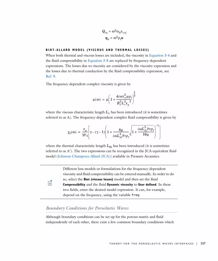
B I O T - A L L A R D M O D E L ( V I S C O U S A N D T H E R M A L L O S S E S )

When both thermal and viscous losses are included, the viscosity in Equation 3-4 and the fluid compressibility in Equation 3-8 are replaced by frequency-dependent expressions. The losses due to viscosity are considered by the viscosity expression and the losses due to thermal conduction by the fluid compressibility expression, see Ref. 9.

The frequency-dependent complex viscosity is given by

where the viscous characteristic length Lv has been introduced (it is sometimes referred to as Λ). The frequency-dependent complex fluid compressibility is given by

where the thermal characteristic length Lth has been introduced (it is sometimes referred to as Λ’). The two expressions can be recognized in the JCA equivalent fluid model (Johnson-Champoux-Allard (JCA)) available in Pressure Acoustics.

Boundary Conditions for Poroelastic Waves

Although boundary conditions can be set up for the porous matrix and fluid independently of each other, there exist a few common boundary conditions which

Qm ω2αBεvol=

qd ω2ρfu=

μ ω( ) μ 14iωτ∞

2 μρf

Rf2Lv

2εp2

-------------------------+

12---

=

χf ω( )εp

γpA--------- γ γ 1–( ) 1 8μ

iωLth2 Prρf

-------------------------- 1iωLth

2 Prρf16μ

--------------------------++

1–

–=

Different loss models or formulations for the frequency-dependent viscosity and fluid compressibility can be entered manually. In order to do so, select the Biot (viscous losses) model and then set the fluid Compressibility and the fluid Dynamic viscosity to User defined. In these two fields, enter the desired model expression. It can, for example, depend on the frequency, using the variable freq.


338 | C H A P T E R

deserve special attention. The following sections refer to the boundary conditions for the system written in Equation 3-11 and Equation 3-12. See derivation in Ref. 7, Ref. 8, and Ref. 9.

P O R O U S , F R E E ( S O U N D - S O F T B O U N D A R Y ) T H E O R Y

The Porous, Free boundary condition is the default for the porous matrix. It means that the displacement of the porous matrix in Equation 3-11 is unconstrained, so it can move freely without experiencing any loads.

The sound soft boundary condition for acoustics creates a boundary condition for Equation 3-12 where the acoustic pressure vanishes, so it sets pf = 0.

F I X E D ( S O U N D - H A R D B O U N D A R Y ) E Q U A T I O N S

For simulating a poroelastic medium bounded by a rigid impervious wall, impose a Fixed Constraint node for the porous matrix displacement in Equation 3-11, u = 0, and a sound-hard boundary condition for the pore pressure in Equation 3-12:

P R E S S U R E E Q U A T I O N S

For a given fluid pressure p0 on the boundary, set the pressure in Equation 3-12 to . Since the fluid pressure is set to p0, the normal stress on the porous matrix

in Equation 3-11 reduces to

For a rigid porous matrix αB = εp, the load is equivalent to

and for a soft porous matrix αB = 1, there is no load since

P R E S C R I B E D D I S P L A C E M E N T E Q U A T I O N S

For a prescribed displacement u0 at the boundary, set the displacement of the porous matrix in Equation 3-11 as u = u0 and assume a sound-hard (impervious) boundary for the fluid pressure in Equation 3-12:

n 1ρc ω( )-------------- ∇pf ρf– ω2u( ) ⋅ 0=

pf p0=

n σd u( )⋅ n αB 1–( )p0=

n σd u( )⋅ n εp 1–( )p0=

n σd u( )⋅ 0=


P R E S C R I B E D V E L O C I T Y E Q U A T I O N S

For a prescribed velocity v0 at the boundary, set the displacement of the porous matrix in Equation 3-11 as

and assume a sound-hard (impervious) boundary condition for the fluid pressure in Equation 3-12

P R E S C R I B E D A C C E L E R A T I O N E Q U A T I O N S

For a prescribed acceleration a0 at the boundary, set the displacement of the porous matrix in Equation 3-11 as

and assume a sound-hard (impervious) boundary condition for the fluid pressure in Equation 3-12

R O L L E R E Q U A T I O N S

The roller, or sliding wall boundary, means that the boundary is impervious (sound-hard) to fluid displacements, but it allows tangential displacements of the porous matrix.

The normal displacement of the porous matrix in Equation 3-11 is constrained, but the porous matrix is free to move in the tangential direction

The impervious (sound hard) boundary condition for the fluid pressure in Equation 3-12 is obtained from

n 1ρc ω( )-------------- ∇pf ρf– ω2u( ) ⋅ 0=

u 1iω------v0=

n 1ρc ω( )-------------- ∇pf ρf– ω2u( ) ⋅ 0=

u 1ω– 2

----------a0=

n 1ρc ω( )-------------- ∇pf ρf– ω2u( ) ⋅ 0=

n u⋅ 0=


340 | C H A P T E R

S E P T U M B O U N D A R Y L O A D E Q U A T I O N S

For a prescribed load FA at the boundary, suppose that one side of the septum is fixed to the porous matrix and the other side bears the load.

A septum is a very limp and thin impervious layer with surface density ρsep. Since the septum can be seen as a boundary mass density, this boundary condition is achieved by setting an effective load FS = FA + ρsepω2u on the porous matrix, so the normal stress in Equation 3-11 reduces to

and a sound-hard (impervious) boundary condition is applied for the fluid pressure in Equation 3-12


Other well known formulations of the poroelastic waves equations exist which use other parameters and variables in their definition (see Ref. 10). To help users that are familiar with these formulations, some of the most common parameters have been added as postprocessing variables under the Biot-Allard coefficients menu (when clicking the Replace Expressions button in plots). The variables included are:

TABLE 3-2: BIOT-ALLARD COEFFICIENTS

COMSOL NAME DEFINITIONS NAME

pelw.rho11 Mass coefficient (11)

pelw.rho22 Mass coefficient (22)

pelw.rho12 Inertial interaction mass coefficient (12)

pelw.rho11_c Complex mass coefficient (11)

pelw.rho22_c Complex mass coefficient (11)

pelw.rho12_c Complex inertial interaction mass coefficient (12)

pelw.A_c See Ref. 10 Complex elastic coefficient

n 1ρc ω( )-------------- ∇pf ρf– ω2u( ) ⋅ 0=

n σd u( ) αBpfI–( )⋅ FS=

n 1ρc ω( )-------------- ∇pf ρf– ω2u( ) ⋅ 0=

ρ11 ρd ρ12–=

ρ22 εpρf ρ12–=

ρ12 ρ– a εpρf τ∞ 1–( )–= =

ρ11 ρ11 b ω( ) iω( )⁄+=

ρ22 ρ22 b ω( ) iω( )⁄+=

ρ12 ρ12 b ω( ) iω( )⁄–=


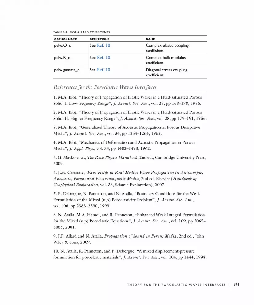
References for the Poroelastic Waves Interfaces

1. M.A. Biot, “Theory of Propagation of Elastic Waves in a Fluid-saturated Porous Solid. I. Low-frequency Range”, J. Acoust. Soc. Am., vol. 28, pp 168–178, 1956.

2. M.A. Biot, “Theory of Propagation of Elastic Waves in a Fluid-saturated Porous Solid. II. Higher Frequency Range”, J. Acoust. Soc. Am., vol. 28, pp 179–191, 1956.

3. M.A. Biot, “Generalized Theory of Acoustic Propagation in Porous Dissipative Media”, J. Acoust. Soc. Am., vol. 34, pp 1254–1264, 1962.

4. M.A. Biot, “Mechanics of Deformation and Acoustic Propagation in Porous Media”, J. Appl. Phys., vol. 33, pp 1482–1498, 1962.

5. G. Mavko et al., The Rock Physics Handbook, 2nd ed., Cambridge University Press, 2009.

6. J.M. Carcione, Wave Fields in Real Media: Wave Propagation in Anisotropic, Anelastic, Porous and Electromagnetic Media, 2nd ed. Elsevier (Handbook of Geophysical Exploration, vol. 38, Seismic Exploration), 2007.

7. P. Debergue, R. Panneton, and N. Atalla, “Boundary Conditions for the Weak Formulation of the Mixed (u,p) Poroelasticity Problem”, J. Acoust. Soc. Am., vol. 106, pp 2383–2390, 1999.

8. N. Atalla, M.A. Hamdi, and R. Panneton, “Enhanced Weak Integral Formulation for the Mixed (u,p) Poroelastic Equations”, J. Acoust. Soc. Am., vol. 109, pp 3065–3068, 2001.

9. J.F. Allard and N. Atalla, Propagation of Sound in Porous Media, 2nd ed., John Wiley & Sons, 2009.

10. N. Atalla, R. Panneton, and P. Debergue, “A mixed displacement-pressure formulation for poroelastic materials”, J. Acoust. Soc. Am., vol. 104, pp 1444, 1998.

pelw.Q_c See Ref. 10 Complex elastic coupling coefficient

pelw.R_c See Ref. 10 Complex bulk modulus coefficient

pelw.gamma_c See Ref. 10 Diagonal stress coupling coefficient

TABLE 3-2: BIOT-ALLARD COEFFICIENTS

COMSOL NAME DEFINITIONS NAME


342 | C H A P T E R

11. N. Atalla, F. Sgard, and C.K. Amedin, “On the modeling of sound radiation from poroelastic materials”, J. Acoust. Soc. Am., vol. 120, pp 1990, 2006.


Th eo r y f o r t h e E l a s t i c Wav e s , T ime Exp l i c i t I n t e r f a c e

The Elastic Waves, Time Explicit Interface theory is described in this section:

• Governing Equations

• References for the Elastic Waves, Time Explicit Interface

Governing Equations

The model solves the governing equations for a general linear elastic material in a velocity-strain formulation

where v is the velocity, ρ the density, S the stress tensor, E the strain tensor, C is the elasticity tensor (or stiffness tensor), and Fv is a possible body force. The equations are valid for both isotropic and anisotropic material data.

References for the Elastic Waves, Time Explicit Interface

1. J.S. Hesthaven and T. Warburton, Nodal Discontinuous Galerkin Methods: Algorithms, Analysis, and Applications, Springer, 2008.

ρ∂v∂t------ ∇ S⋅– Fv=

∂E∂t------- 1

2--- ∇v ∇v( )T

+[ ]– 0=

S C:E=

T H E O R Y F O R T H E E L A S T I C W A V E S , T I M E E X P L I C I T I N T E R F A C E | 343

344 | C H A P T E R

4

A c o u s t i c - S t r u c t u r e I n t e r a c t i o n I n t e r f a c e s

This chapter describes the physics interfaces found under the Acoustic-Structure

Interaction branch ( ).

• The Acoustic-Solid Interaction, Frequency Domain Interface

• The Acoustic-Solid Interaction, Transient Interface

• The Acoustic-Piezoelectric Interaction, Frequency Domain Interface

• The Acoustic-Piezoelectric Interaction, Transient Interface

• The Acoustic-Poroelastic Waves Interaction Interface

• The Acoustic-Solid-Poroelastic Waves Interaction Interface

• The Acoustic-Solid Interaction, Time Explicit Interface

• The Acoustic-Shell Interaction, Frequency Domain Interface

• The Acoustic-Shell Interaction, Transient Interface

• Modeling with the Acoustic-Structure Interaction Branch

345

346 | C H A P T E R

Th e A c ou s t i c - S o l i d I n t e r a c t i o n , F r e qu en c y Doma i n I n t e r f a c e

The Acoustic-Solid Interaction, Frequency Domain multiphysics interface ( ), found under the Acoustics>Acoustic-Structure Interaction branch ( ) when adding a physics interface, combines the Pressure Acoustics, Frequency Domain and Solid Mechanics interfaces to connect the acoustics pressure variations in the fluid domain with the structural deformation in the solid domain. It can, for example, be used to determine the transmission of sound through an elastic structure or solve for the coupled vibroacoustics phenomena present in a loudspeaker.

Acoustic-structure interaction or ASI refers to a multiphysics phenomenon where the acoustic pressure causes a fluid load on the solid domain, and the structural acceleration acts on the fluid domain as a normal acceleration across the fluid-solid boundary.

A dedicated multiphysics coupling condition is readily defined for the fluid-solid boundary and sets up the fluid loads on the solid domain and the effect of the structural accelerations on the fluid.

The physics interface is available for 3D, 2D, and 2D axisymmetric geometries and has the capability to model pressure acoustics and solid mechanics in the frequency domain, including a special acoustic-solid boundary condition for the fluid-solid interaction.

When a predefined Acoustic-Solid Interaction, Frequency Domain interface is added from the Acoustics>Acoustic-Structure Interaction branch of the Model Wizard or the Add

Physics windows, the Pressure Acoustics, Frequency Domain and Solid Mechanics interfaces are added to the Model Builder.

In addition, the Multiphysics Couplings node is added, which automatically includes the Acoustic-Structure Boundary multiphysics coupling.

See The Multiphysics Branch and Multiphysics Modeling Workflow in the COMSOL Multiphysics Reference Manual.

4 : A C O U S T I C - S T R U C T U R E I N T E R A C T I O N I N T E R F A C E S

S E T T I N G S F O R P H Y S I C S I N T E R F A C E S A N D M U L T I P H Y S I C S C O U P L I N G S

When a predefined multiphysics interface is used, for example Acoustic-Solid

Interaction, Frequency Domain, the Selection on the multiphysics coupling is automatically set to All boundaries. In this way, the multiphysics coupling is automatically active on all boundaries with Pressure Acoustics, Frequency Domain on one side and Solid Mechanics on the other.

However, if physics interfaces are added one at a time, followed by the multiphysics couplings, these modified settings are not automatically included.

For example, if the single interfaces are added, COMSOL Multiphysics adds an empty Multiphysics Couplings node. You can choose the available multiphysics couplings, but you need manually to select on which boundaries they need to be applied, or select All

boundaries to recover the predefined behavior.

P H Y S I C S I N T E R F A C E S A N D M U L T I P H Y S I C S C O U P L I N G S

Multiphysics CouplingThe Acoustic-Structure Boundary multiphysics coupling is described in the Multiphysics Couplings chapter.

Physics Interface FeaturesPhysics nodes are available from the Physics ribbon toolbar (Windows users), Physics context menu (Mac or Linux users), or right-click to access the context menu (all users).

Multiphysics couplings are available from the context menu (right-click the Multiphysics Couplings node) or from the Physics toolbar, Multiphysics menu.

Use the online help in COMSOL Multiphysics to locate and search all the documentation. All these links also work directly in COMSOL Multiphysics when using the Help system.


T H E A C O U S T I C - S O L I D I N T E R A C T I O N , F R E Q U E N C Y D O M A I N I N T E R F A C E | 347

348 | C H A P T E R

• The available physics features for The Pressure Acoustics, Frequency Domain Interface are listed in the section Domain, Boundary, Edge, Point, and Pair Nodes for the Pressure Acoustics, Frequency Domain Interface.

• The available physics features for The Solid Mechanics Interface are listed in the Structural Mechanics Module User’s Guide.

• Theory section in the Structural Mechanics Module User’s Guide


Acoustic-Structure Interaction: Application Library path Acoustics_Module/Tutorials,_Pressure_Acoustics/acoustic_structure

Suggestions for setting up the solvers for solving large acoustic-structure interaction problems are given in Solving Large Acoustic-Structure Interaction Models in the Modeling with the Acoustic-Structure Interaction Branch section.


Th e A c ou s t i c - S o l i d I n t e r a c t i o n , T r a n s i e n t I n t e r f a c e

The Acoustic-Solid Interaction, Transient multiphysics interface ( ), found under the Acoustics>Acoustic-Structure Interaction branch ( ) when adding a physics interface, combines the Pressure Acoustics, Transient and Solid Mechanics interfaces to connect the acoustics pressure variations in the fluid domain with the structural deformation in the solid domain. It can, for example, be used to determine the transmission of sound through an elastic structure or solve for the coupled vibroacoustics phenomena present in a loudspeaker.

Acoustic-structure interaction or ASI refers to a multiphysics phenomenon where the acoustic pressure causes a fluid load on the solid domain, and the structural acceleration acts on the fluid domain as a normal acceleration across the fluid-solid boundary.

Special physics interface conditions are readily defined at the fluid-solid boundary and set up the fluid loads on the solid domain and the effect of the structural accelerations on the fluid. The physics interface allows for transient studies but also solves in the frequency domain with the available boundary conditions.

When a predefined Acoustic-Solid Interaction, Transient interface is added from the Acoustics>Acoustic-Structure Interaction branch of the Model Wizard or the Add Physics windows, the Pressure Acoustics, Transient and Solid Mechanics interfaces are added to the Model Builder.



For modeling of acoustic-structure interaction in the frequency domain, The Acoustic-Solid Interaction, Frequency Domain Interface contains additional functionality that is not applicable for modeling in the time domain.

T H E A C O U S T I C - S O L I D I N T E R A C T I O N , T R A N S I E N T I N T E R F A C E | 349

350 | C H A P T E R


When the predefined multiphysics interface is used, the Selection on the multiphysics coupling is automatically set to All boundaries. In this way, the multiphysics coupling is automatically active on all boundaries with Pressure Acoustics, Transient on one side and Solid Mechanics on the other.












• The available physics features for The Pressure Acoustics, Transient Interface are listed in the section Domain, Boundary, Edge, and Point Nodes for the Pressure Acoustics, Transient Interface.



• Theory section in the Structural Mechanics User’s Guide


T H E A C O U S T I C - S O L I D I N T E R A C T I O N , T R A N S I E N T I N T E R F A C E | 351

352 | C H A P T E R

Th e A c ou s t i c - P i e z o e l e c t r i c I n t e r a c t i o n , F r e qu en c y Doma i n I n t e r f a c e

The Acoustic-Piezoelectric Interaction, Frequency Domain multiphysics interface ( ), found when adding a physics interface under the Acoustics>Acoustic-Structure

Interaction branch ( ), combines the Pressure Acoustics, Frequency Domain, Solid Mechanics, and Electrostatics interfaces to connect and solve for the acoustic pressure variations in fluids with the structural deformation in both solids and piezoelectric solid domains. The physics interface also includes features from Electrostatics to solve for the electric field in the piezoelectric material. It may be used for modeling piezoelectric transducers for sonar or medical applications and, for example, enhancing the impedance matching layers as well as the far-field radiation patterns of the transducer.

The Helmholtz equation is solved in the fluid domain and the structural equations in the solid together with the constitutive relationships required to model piezoelectrics. Both the direct and inverse piezoelectric effects can be modeled, and the piezoelectric coupling can be formulated using the strain-charge or stress-charge forms.

When a predefined Acoustic-Piezoelectric Interaction, Frequency Domain interface is added from the Acoustics>Acoustic-Structure Interaction branch ( ) of the Model

Wizard or the Add Physics windows, the Pressure Acoustics, Frequency Domain, Solid

Mechanics, and Electrostatics interfaces are added to the Model Builder.

In addition, the Multiphysics Couplings node is added, which automatically includes the Acoustic-Structure Boundary and Piezoelectric Effect multiphysics couplings.


The equations solved in the solid and fluid domains can be found in the Structural Mechanics Module User’s Guide and in Theory Background for the Pressure Acoustics Branch, respectively.



When the predefined multiphysics interface is used, the Selection on the Acoustic-Structure Boundary multiphysics coupling is automatically set to All boundaries. In this way, the multiphysics coupling is automatically active on all boundaries with Pressure Acoustics, Frequency Domain on one side and Solid Mechanics on the other. Similarly, the Selection on the Piezoelectric Effect multiphysics coupling is automatically set to All domains and active in all valid domains.


For example, if the single interfaces are added, COMSOL Multiphysics adds an empty Multiphysics Couplings node. You can choose the available multiphysics coupling, but you need manually to select on which boundaries or domains they need to be applied, or select All boundaries or All domains to recover the predefined behavior.


Multiphysics CouplingsThe Acoustic-Structure Boundary multiphysics coupling is described in the Multiphysics Couplings chapter. The Piezoelectric Effect is described for The Piezoelectricity Interface.

Piezoacoustic Transducer: Application Library path Acoustics_Module/

Piezoelectric_Devices/piezoacoustic_transducer



T H E A C O U S T I C - P I E Z O E L E C T R I C I N T E R A C T I O N , F R E Q U E N C Y D O M A I N I N T E R F A C E | 353

354 | C H A P T E R



• The available physics features for The Solid Mechanics Interface that are described in the Structural Mechanics Module User’s Guide.

• The available physics features for The Electrostatics Interface are listed in the section Domain, Boundary, Edge, Point, and Pair Nodes for the Electrostatics Interface in the COMSOL Multiphysics Reference Manual.

• Some additional piezoelectric features for the Solid Mechanics and Electrostatics interfaces are described for The Piezoelectricity Interface.



• Theory of Electrostatics in the COMSOL Multiphysics Reference Manual



Th e A c ou s t i c - P i e z o e l e c t r i c I n t e r a c t i o n , T r a n s i e n t I n t e r f a c e

The Acoustic-Piezoelectric Interaction, Transient multiphysics interface ( ), found when adding a physics interface under the Acoustics>Acoustic-Structure Interaction

branch ( ), combines the Pressure Acoustics, Transient and Piezoelectricity interfaces to connect and solve for the acoustic pressure variations in fluids with the structural deformation in both solids and piezoelectric solid domains. The physics interface also includes features from Electrostatics to solve for the electric field in the piezoelectric material. Examples include modeling piezoelectric transducers for sonar or medical applications and, for example, enhancing the impedance matching layers.

The pressure wave equation is solved in the fluid domain and the structural dynamic equations in the solid together with the constitutive relationships required to model piezoelectrics. Both the direct and inverse piezoelectric effects can be modeled, and the piezoelectric coupling can be formulated using the strain-charge or stress-charge forms.

When a predefined Acoustic-Piezoelectric Interaction, Transient interface is added from the Acoustics>Acoustic-Structure Interaction branch of the Model Wizard or the Add

Physics windows, the Pressure Acoustics, Frequency Domain, Solid Mechanics, and Electrostatics interfaces are added to the Model Builder.

In addition, the Multiphysics Couplings node is added, which automatically includes the Acoustic-Structure Boundary and Piezoelectric Effect multiphysics couplings.


When the predefined multiphysics interface is used, the Selection on the Acoustic-Structure Boundary multiphysics coupling is automatically set to All boundaries. In this way, the multiphysics coupling is automatically active on all boundaries with Pressure Acoustics, Frequency Domain on one side and Solid Mechanics on the other. Similarly, the Selection on the Piezoelectric Effect multiphysics coupling is automatically set to All domains and active in all valid domains.


T H E A C O U S T I C - P I E Z O E L E C T R I C I N T E R A C T I O N , T R A N S I E N T I N T E R F A C E | 355

356 | C H A P T E R


For example, if the single interfaces are added, COMSOL Multiphysics adds an empty Multiphysics Couplings node. You can choose the available multiphysics couplings, but you need manually to select on which boundaries or domains they need to be applied, or select All boundaries or All domains to recover the predefined behavior.


Multiphysics CouplingsThe Acoustic-Structure Boundary multiphysics coupling is described in the Multiphysics Couplings chapter. The Piezoelectric Effect is shortly described in The Piezoelectricity Interface.








• The available physics features for The Electrostatics Interface are listed in the section Domain, Boundary, Edge, Point, and Pair Nodes for the Electrostatics Interface in the COMSOL Multiphysics Reference Manual.

• Some additional piezoelectric features for the Solid Mechanics and Electrostatics interfaces are described for The Piezoelectricity Interface.


• Theory of Electrostatics in the COMSOL Multiphysics Reference Manual


T H E A C O U S T I C - P I E Z O E L E C T R I C I N T E R A C T I O N , T R A N S I E N T I N T E R F A C E | 357

358 | C H A P T E R

Th e A c ou s t i c - P o r o e l a s t i c Wav e s I n t e r a c t i o n I n t e r f a c e

The Acoustic-Poroelastic Waves Interaction multiphysics interface ( ) combines Pressure Acoustics, Frequency Domain and Poroelastic Waves together with the Acoustic-Porous Boundary multiphysics coupling.

When a predefined Acoustic-Poroelastic Waves Interaction interface is added from the Acoustics>Acoustic-Structure Interaction branch ( ) of the Model Wizard or the Add

Physics windows, the Poroelastic Waves and Pressure Acoustics, Frequency Domain interfaces are added to the Model Builder.

In addition, the Multiphysics Couplings node is added, which automatically includes the Acoustic-Porous Boundary multiphysics coupling.


When the predefined multiphysics interface is used, for example Acoustic-Poroelastic

Waves Interaction, the Selection on the multiphysics coupling is automatically set to All

boundaries. In this way the multiphysics coupling is automatically active on all boundaries with Pressure Acoustics, Frequency Domain on one side and Poroelastic Waves

on the other.

However, if physics interfaces are added one at a time, followed by the multiphysics coupling, these modified settings are not automatically included.

For example, if single Poroelastic Waves and Pressure Acoustics, Frequency Domain interfaces are added, COMSOL Multiphysics adds an empty Multiphysics Couplings node. You can choose the available multiphysics couplings, but you need manually to



select on which boundaries they need to be applied, or select All boundaries to recover the predefined behavior


Multiphysics CouplingThe Acoustic-Porous Boundary multiphysics coupling is described in the Multiphysics Couplings chapter.


• The available physics features for The Poroelastic Waves Interface are listed in the section Domain, Boundary, and Pair Nodes for the Poroelastic Waves Interfaces.





T H E A C O U S T I C - P O R O E L A S T I C W A V E S I N T E R A C T I O N I N T E R F A C E | 359

360 | C H A P T E R

Th e A c ou s t i c - S o l i d - P o r o e l a s t i c Wav e s I n t e r a c t i o n I n t e r f a c e

The Acoustic-Solid-Poroelastic Waves Interaction multiphysics interface ( ) combines Pressure Acoustics, Frequency Domain, Solid Mechanics, and Poroelastic Waves together with the Acoustic-Structure Boundary, Porous-Structure Boundary, and Acoustic-Porous Boundary multiphysics couplings.

When a predefined Acoustic-Solid-Poroelastic Waves Interaction interface is added from the Acoustics>Acoustic-Structure Interaction branch ( ) of the Model Wizard or the Add Physics windows, the Pressure Acoustics, Frequency Domain, Solid Mechanics, and Poroelastic Waves interfaces are added to the Model Builder.

In addition, the Multiphysics Couplings node is added, which automatically includes the Acoustic-Porous Boundary, Porous-Structure Boundary, and Acoustic-Structure Boundary multiphysics couplings.


When a predefined multiphysics interface is used, for example Acoustic-Solid-Poroelastic

Waves Interaction, the Selection on the multiphysics couplings is automatically set to All

boundaries. In this way, the relevant multiphysics couplings are automatically active on all relevant boundaries connecting two physics.


For example, if single Poroelastic Waves and Pressure Acoustics, Frequency Domain interfaces are added, COMSOL Multiphysics adds an empty Multiphysics Couplings node. You can choose the available multiphysics couplings, but you need manually to



select on which boundaries they need to be applied, or select All boundaries to recover the predefined behavior.


Multiphysics CouplingsThe Acoustic-Porous Boundary, Porous-Structure Boundary, and Acoustic-Structure Boundary multiphysics couplings are described in the Multiphysics Couplings chapter.


• The available physics features for The Poroelastic Waves Interface are listed in the section Domain, Boundary, and Pair Nodes for the Poroelastic Waves Interfaces.






T H E A C O U S T I C - S O L I D - P O R O E L A S T I C W A V E S I N T E R A C T I O N I N T E R F A C E | 361

362 | C H A P T E R

Th e A c ou s t i c - S o l i d I n t e r a c t i o n , T ime Exp l i c i t I n t e r f a c e

The Acoustic-Solid Interaction, Time Explicit multiphysics interface ( ) combines Pressure Acoustics, Time Explicit and Elastic Waves, Time Explicit together with the Acoustic-Structure Boundary, Time Explicit multiphysics coupling. The physics interface is available for 3D and 2D geometries.

Acoustic-structure interaction or ASI refers to a multiphysics phenomenon where the acoustic pressure causes a fluid load on the solid domain, and the structural acceleration acts on the fluid domain as a normal acceleration across the fluid-solid boundary. The Acoustic-Solid Interaction, Time Explicit interface can, for example, be used to determine the transmission of sound through an elastic structure or solve for the coupled vibroacoustics phenomena present in an ultrasonic transducer or flowmeter.

The discontinuous Galerkin time explicit method enables efficient computation of acoustically large models (containing many wavelengths) in the time domain. The formulation of the governing equations, effectively requires the acoustics pressure and velocity variations in the fluid domain to be coupled with the structural velocity and strain variations in the solid domain.

A dedicated multiphysics coupling condition is readily defined for the fluid-solid boundary and sets up the continuity in velocity and normal stress.

When a predefined Acoustic-Solid Interaction, Time Explicit interface is added from the Acoustics>Acoustic-Structure Interaction branch of the Model Wizard or the Add Physics windows, the Pressure Acoustics, Time Explicit and Elastic Waves, Time Explicit interfaces are added to the Model Builder. In addition, the Multiphysics Couplings node is added, which automatically includes the Acoustic-Structure Boundary, Time Explicit multiphysics coupling.




When a predefined multiphysics interface is used, for example Acoustic-Structure

Boundary, Time Explicit, the Selection on the multiphysics coupling is automatically set to All boundaries. In this way, the multiphysics coupling is automatically active on all boundaries with Pressure Acoustics, Time Explicit on one side and Elastic Waves, Time

Explicit on the other.





Multiphysics CouplingsThe Acoustic-Structure Boundary, Time Explicit multiphysics coupling is described in the Multiphysics Couplings chapter. Note that a pair version of the multiphysics coupling exists that can be used for assemblies: Pair Acoustic-Structure Boundary, Time Explicit.



T H E A C O U S T I C - S O L I D I N T E R A C T I O N , T I M E E X P L I C I T I N T E R F A C E | 363

364 | C H A P T E R


• The available physics features for The Pressure Acoustics, Time Explicit Interface are listed in the section Domain, Boundary, Edge, and Point Nodes for the Pressure Acoustics, Time Explicit Interface.

• The available physics features for The Elastic Waves, Time Explicit Interface are listed in the section Domain, Boundary, Edge, Point, and Pair Nodes for the Elastic Waves, Time Explicit Interface.



• Theory for the Elastic Waves, Time Explicit Interface


Th e A c ou s t i c - S h e l l I n t e r a c t i o n , F r e qu en c y Doma i n I n t e r f a c e

The Acoustic-Shell Interaction, Frequency Domain multiphysics interface ( ), found under the Acoustics>Acoustic-Structure Interaction branch ( ) when adding a physics interface, combines features from the Pressure Acoustics, Frequency Domain and Shell interfaces to connect the acoustics pressure variations in the fluid domain with the structural deformation of a shell boundary. It may for example be used for determining the transmission of sound through a thin elastic structure such as a car hood and analyzing the vibroacoustics of a loudspeaker cone.

Acoustic-structure interaction or ASI refers to a multiphysics phenomenon where the acoustic pressure causes a fluid load on the solid surface, and the structural acceleration acts on the fluid domain as a normal acceleration across the fluid-structure boundary.

Special physics interface conditions are readily defined at the fluid-shell boundary and set up the fluid loads on the shell boundary and the effect of the structural accelerations on the fluid. The physics interface is available for 3D and 2D axisymmetric geometries, and it is capable of modeling the coupled pressure acoustics and shell vibrations in the frequency domain.

When a predefined Acoustic-Shell Interaction, Frequency Domain interface is added from the Acoustics>Acoustic-Structure Interaction branch of the Model Wizard or the Add

Physics windows, the Pressure Acoustics, Frequency Domain and Shell interfaces are added to the Model Builder.

In addition, the Multiphysics Couplings node is added, which automatically includes the multiphysics coupling Acoustic-Structure Boundary.


When a predefined multiphysics interface is used, for example Acoustic-Shell Interaction,

Frequency Domain, the Selection on the multiphysics coupling is automatically set to All

boundaries. In this way, the multiphysics coupling is automatically active on all Shell boundaries with Pressure Acoustics, Frequency Domain on one side or both sides.

This physics interface requires a Structural Mechanics Module license. For theory and physics interface feature descriptions relating to the Shell interface, see the Structural Mechanics Module User’s Guide.

T H E A C O U S T I C - S H E L L I N T E R A C T I O N , F R E Q U E N C Y D O M A I N I N T E R F A C E | 365

366 | C H A P T E R


For example, if single Shell and Pressure Acoustics, Frequency Domain interfaces are added, COMSOL Multiphysics adds an empty Multiphysics Couplings node. You can choose the available multiphysics couplings, but you need manually to select on which boundaries they need to be applied, or select All boundaries to recover the predefined behavior.





• The available physics features for Results Evaluation are listed in the section Domain, Boundary, Edge, Point, and Pair Nodes for the Shell and Plate Interfaces in the Structural Mechanics Module User’s Guide.






• Theory for the Shell and Plate Interfaces in the Structural Mechanics Module User’s Guide

T H E A C O U S T I C - S H E L L I N T E R A C T I O N , F R E Q U E N C Y D O M A I N I N T E R F A C E | 367

368 | C H A P T E R

Th e A c ou s t i c - S h e l l I n t e r a c t i o n , T r a n s i e n t I n t e r f a c e

The Acoustic-Shell Interaction, Transient multiphysics interface ( ), found under the Acoustics>Acoustic-Structure Interaction branch ( ) when adding a physics interface, combines features from the Pressure Acoustics, Transient and Shell interfaces to connect the acoustics pressure variations in the fluid domain with the structural deformation of a shell boundary. It may for example be used for determining the transmission of sound through a thin elastic structure such as a car hood and analyzing the vibroacoustics of loudspeaker cone.

Acoustic-structure interaction refers to a multiphysics phenomenon where the acoustic pressure causes a fluid load on the solid surface, and the structural acceleration affects the fluid domain as a normal acceleration across the fluid-structure boundary.

Special physics interface conditions are readily defined at the fluid-shell boundary and set up the fluid loads on the shell boundary and the effect of the structural accelerations on the fluid. The physics interface is only available for 3D geometries, and it is capable of modeling the coupled pressure acoustics and shell vibrations in the time domain.

When a predefined Acoustic-Shell Interaction, Transient interface is added from the Acoustics>Acoustic-Structure Interaction branch of the Model Wizard or the Add Physics windows, the Pressure Acoustics, Transient and Shell interfaces are added to the Model Builder.



When a predefined multiphysics interface is used, for example Acoustic-Shell Interaction,

Transient, the Selection on the multiphysics coupling is automatically set to All

boundaries. In this way, the multiphysics coupling is automatically active on all Shell boundaries with Pressure Acoustics, Transient on one side or both sides.

This physics interface requires a Structural Mechanics license. For theory and physics interface feature descriptions relating to the Shell interface, see the Structural Mechanics Module User’s Guide.



For example, if single Shell and Pressure Acoustics, Transient interfaces are added, COMSOL Multiphysics adds an empty Multiphysics Couplings node. You can choose the available multiphysics couplings, but you need manually to select on which boundaries they need to be applied, or select All boundaries to recover the predefined behavior.





• The available physics features for Results Evaluation are listed in the section Domain, Boundary, Edge, Point, and Pair Nodes for the Shell and Plate Interfaces in the Structural Mechanics Module User’s Guide.




T H E A C O U S T I C - S H E L L I N T E R A C T I O N , T R A N S I E N T I N T E R F A C E | 369

370 | C H A P T E R




Mode l i n g w i t h t h e A c ou s t i c - S t r u c t u r e I n t e r a c t i o n B r an c h

In this section:

• Prestressed Acoustic-Structure Interaction

• Solving Large Acoustic-Structure Interaction Models

• Configuration of Perfectly Matched Layers (PMLs) for Acoustic-Structure Interaction Models

Prestressed Acoustic-Structure Interaction

When modeling transducers like microphones or ultrasound horns there are often parts of the structure, like the diaphragm or a bolt, that are under tension or prestressed. In these cases, it is essential to include this effect when modeling the transducer. A prestressed part will shift the resonance frequency of the mechanical system and thus the overall vibroacoustic behavior will change.

Such prestressed acoustic-structure interaction models can be set up and solved fully coupled including all effects. The procedure is as follows:

1 Set up the model including all relevant physics.

2 Couple the physics using the required multiphysics couplings.

3 All acoustic sources, structural loads, and any forcing that are nonstatic, should be defined using the linper() operator. This will ensure that they are used only in the frequency-domain part of the study (that one is set to linear perturbation).

4 Add a Prestressed Analysis, Frequency Domain study.

• Piezoelectric Tonpilz Transducer with a Prestressed Bolt: Application Library path Acoustics_Module/Piezoelectric_Devices/

tonpilz_transducer_prestressed.

• The Brüel & Kjær 4134 Condenser Microphone: Application Library path Acoustics_Module/Electroacoustic_Transducers/

bk_4134_microphone.

M O D E L I N G W I T H T H E A C O U S T I C - S T R U C T U R E I N T E R A C T I O N B R A N C H | 371

372 | C H A P T E R

5 Note that in the Stationary step the acoustics physics interfaces have an orange warning triangle under the Physics and Variables Selection. This simply means that they will not be used in the stationary study since acoustics is not supporting the study type. Therefore the Solve for this field will automatically not be marked under the Dependent Variables in the Solver Configurations.

6 Note also that the Include geometric nonlinearity box is checked in the Frequency-Domain, Perturbation step. If it is not checked, the prestress effect is lost.

7 Solve the model for the desired frequencies.

A prestressed type of analysis can also be done on pure structural problems in the frequency domain and when searching for eigenfrequencies of structures.

Solving Large Acoustic-Structure Interaction Models

In models that involve acoustic-structure interaction, the strategy for solving large problems involves solving the system in a segregated way. That is, the system is not solved fully coupled in one step but iterations are used solving one physics interface at a time.

To set up such a solver right-click on the Stationary Solver step and select Segregated. In the first Segregated Step solve for the structural dependent variables (displacement). Set up a second segregated step where you select the pressure dependent variable. Under each of the steps select the solver of choice for solving the single physics interface problem. For example, in the case where only a small structural domain is included, use an iterative multigrid approach for the acoustics (see Solving Large Acoustics Problems Using Iterative Solvers) and a direct solver for the structure.

This strategy is only readily applicable when the coupling between the solid and the acoustic domain is done via Neumann conditions; this is the case for all models where the acoustic domain uses Pressure Acoustics. In, for example, models with thermoviscous acoustic-structure interaction, the coupling is based on a Dirichlet condition (a pointwise constraint) and required reformulating the continuity condition using weak constraints. Nor does this approach work for models coupling

See also Prestressed Structures, Pretensioned Bolts, and Mechanical Damping and Losses in the Structural Mechanics Module User’s Guide


piezoelectric domains, structures, and acoustics; here a fully coupled approach is necessary.

Configuration of Perfectly Matched Layers (PMLs) for Acoustic-Structure Interaction Models

Care should be taken when setting up perfectly matched layers (PMLs) in models that include fluid domains and solid domains. In general models with several different materials, that being different solids or different fluids.

Two configurations exist for the PMLs in these systems:

• The PML regions of two physics (or two different material models) are adjacent and in contact. In this case, a single PML feature should be used for the two PML domains. Set the Typical wavelength from to User defined and enter a value based on the longest wavelength. For example, for an air-steel system enter: 5770[m/s]/freq

The shorter wavelengths should be captured by increasing the mesh resolution or increasing the PML scaling curvature parameter. This will ensure optimal damping of all wavelengths in the system. In any case, control the convergence of the results by increasing the number of mesh layers in the PML.

• The PML regions of two physics (or two different material models) do not touch. In this case, use one PML feature for each PML domain. Keep the default setting of Typical wavelength from to Physics interface and select the relevant physics interface under Physics.

The reason that two PML features cannot be used when the PML domains a adjacent to each other is that the scaling inside the PMLs will differ (because of different speed

Studies and Solvers and Multigrid in the COMSOL Multiphysics Reference Manual

• Infinite Elements, Perfectly Matched Layers, and Absorbing Layers in the COMSOL Multiphysics Reference Manual.

• See Perfectly Matched Layers (PMLs) in Modeling with the Pressure Acoustics Branch (FEM-Based Interfaces) in the Acoustics Module User’s Guide.

M O D E L I N G W I T H T H E A C O U S T I C - S T R U C T U R E I N T E R A C T I O N B R A N C H | 373

374 | C H A P T E R

of sounds). This will lead to an unphysical situation at the interface between the two PMLs which results in errors in the solution. Spurious waves may be generated.

See the Acoustic-Structure Interaction with a Perfectly Matched Layer (PML) model in the Application Gallery on the COMSOL website. It is located here: https://www.comsol.com/model/acoustic-structure-interaction-with-a-perfectly-matched-layer-pml-23521


https://www.comsol.com/model/acoustic-structure-interaction-with-a-perfectly-matched-layer-pml-23521

https://www.comsol.com/model/acoustic-structure-interaction-with-a-perfectly-matched-layer-pml-23521

5

A e r o a c o u s t i c s I n t e r f a c e s

This chapter describes the physics interfaces found under the Aeroacoustics branch .

The aeroacoustic branch has physics interfaces to solve the fully linearized acoustic equation for several physical conditions, they are: the linearized Euler (LE) equations, the linearized Navier–Stokes (LNS) equations, and the linearized potential flow (LPF) equations. These equations are also referred to as convected acoustics.

In this chapter:

• The Linearized Euler, Frequency Domain Interface

• The Linearized Euler, Transient Interface

• The Linearized Navier–Stokes, Frequency Domain Interface

• The Linearized Navier–Stokes, Transient Interface

• The Linearized Potential Flow, Frequency Domain Interface

• The Linearized Potential Flow, Transient Interface

• The Linearized Potential Flow, Boundary Mode Interface

• The Compressible Potential Flow Interface

375

376 | C H A P T E R

• Modeling with the Aeroacoustics Branch

• Theory Background for the Aeroacoustics Branch

• References for the Aeroacoustics Branch Interfaces

5 : A E R O A C O U S T I C S I N T E R F A C E S

Th e L i n e a r i z e d Eu l e r , F r e qu en c y Doma i n I n t e r f a c e

The Linearized Euler, Frequency Domain (lef) interface ( ), found under the Acoustics>Aeroacoustics branch ( ) when adding a physics interface, is used to compute the acoustic variations in density, velocity, and pressure in the presence of a stationary background mean-flow that is well approximated by an ideal gas flow. The physics interface is used for aeroacoustic simulations that can be described by the linearized Euler equations.

The equations defined by the Linearized Euler, Frequency Domain interface are the linearized continuity, momentum (Euler), and energy equations. The physics interface solves for the acoustic variations in the density ρ, velocity field u, and pressure p. The equations are formulated in the frequency domain and assume harmonic variation of all sources and fields. The harmonic variation of all fields and sources is given by eiωt using the +iω convention. The background mean flow can be any stationary gas flow that is well approximated by an ideal gas. The coupling between the acoustic field and the background flow does not include any predefined flow induced noise. Even though the equations do not include any loss mechanisms, only acoustic modes exist in the frequency domain as the driving frequency is predefined and real valued.

Coupling between a background mean flow, computed from a Fluid Flow model, and the Linearized Euler model is handled by the Background Fluid Flow Coupling multiphysics coupling and the dedicated Mapping study. Details are also found in the Mapping Between Fluid Flow and Acoustics Mesh section.

The equations are implemented in the so-called scattered field formulation. All equations and boundary conditions are formulated in the total acoustic fields (ρt, ut, pt). The total fields are in the presence of the Background Acoustic Fields feature the sum of the background (ρb, ub, pb) and the scattered field (ρ, u, p):

For modeling tips and tricks and good practice, see the Modeling with the Aeroacoustics Branch section.

ρt ρ ρb+= ut u ub+= pt p pb+=

T H E L I N E A R I Z E D E U L E R , F R E Q U E N C Y D O M A I N I N T E R F A C E | 377

378 | C H A P T E R

The scattered field variables are the variables solved for, that is, the dependent variables. When no background acoustic field is present, the total field is simply equal to the scattered field


Builder — Linearized Euler Model, Rigid Wall, and Initial Values. For axisymmetric components an Axial Symmetry node is also added.

Then, from the Physics toolbar, add other nodes that implement, for example, boundary conditions and sources. You can also right-click Linearized Euler, Frequency

Domain to select physics features from the context menu.

S E T T I N G S



The default Name (for the first physics interface in the model) is lef.


See Sound Pressure Level Settings for the Pressure Acoustics, Frequency Domain interface. Only Use reference pressure for air or User-defined reference pressure are available selections.


See Typical Wave Speed for the Pressure Acoustics, Frequency Domain interface.


This physics interface defines these dependent variables (fields), the Density rho, Velocity field u and its components, and Pressure p. The name can be changed but the names of fields and dependent variables must be unique within a model.



ρt ρ= ut u= pt p=


Select the Stabilization Method — No stabilization applied, Galerkin least squares (GLS)

stabilization (the default), Streamline upwind Petrov-Galerkin (SUPG) stabilization, or Streamline diffusion (legacy method). When stabilization is selected enter a value for the Stabilization constant αstab (dimensionless). The default value is 1e-5 and should typically have a numerical value between 1e-3 and 1e-7. In cases where there is no background flow, set the value to the lower limit 1e-7.

The default GLS stabilization is the most efficient stabilization method as it operates on the convective, reactive, and diffusive parts of the governing equations. This is also the default method and the method suggested for most applications. The stabilization constant αstab can be tuned depending on the problem solved, the nature of the background mean flow, and on the computational mesh.

If the stabilization is turned off, it is probably necessary to change the discretization to ensure a stable numerical scheme; set the order of the density one order lower than the velocity and pressure dependent variables, for example, using a P1-P2-P2 discretization.


From the list select the element order and type (Lagrange or serendipity) the default is Linear for all the dependent variables.

• Stabilization in the Modeling with the Aeroacoustics Branch section.

Choosing between Lagrange and Serendipity Shape Functions has influence on the number of DOFs solved for and on stability for distorted meshes.

• Domain, Boundary, and Pair Nodes for the Linearized Euler, Frequency Domain Interface



380 | C H A P T E R

Domain, Boundary, and Pair Nodes for the Linearized Euler, Frequency Domain Interface

The Linearized Euler, Frequency Domain Interface has these domain, boundary, and pair nodes and subnodes, listed in alphabetical order, available from the Physics ribbon toolbar (Windows users), Physics context menu (Mac or Linux users), or right-click to access the context menu (all users).

For a tutorial and benchmark model, solving the linearized Euler equations in both the frequency and the time domains, see the Application Gallery model: Point Source in 2D Jet: Radiation and Refraction of Sound Waves Through a 2D Shear Layer

https://www.comsol.com/model/point-source-in-2d-jet-radiation-and-refraction-of-sound-waves-through-a-2d-shea-16685

The model requires the Acoustics Module and the CFD Module.


• Acoustic Impedance (Isentropic)

• Asymptotic Far-Field Radiation

• Axial Symmetry

• Background Acoustic Fields

• Continuity

• Domain Sources

• Impedance and Interior Impedance

• Initial Values

• Interior Wall

• Linearized Euler Model

• Moving Wall

• Outflow Boundary

• Periodic Condition1

• Prescribed Acoustic Fields

• Pressure (Isentropic)

• Rigid Wall

• Symmetry

1Described for the Thermoviscous Acoustics, Frequency Domain interface




Linearized Euler Model

Use the Linearized Euler Model to set up the governing equations, define the background mean flow, the ideal gas fluid properties, and select gradient term suppression stabilization (advanced physics option), if needed. The governing equations solved are (in the time domain):

(5-1)

where ρt, ut, and pt are the acoustic perturbations to the density, velocity, and pressure, respectively. The subscript “t” refers to the fact that the acoustic variables are the total fields, that is, the sum of possible Background Acoustic Fields and the scattered fields.

In the frequency domain, the time derivatives of the dependent variables is replaced by multiplication with iω. The variables with a zero subscript are the background mean flow values, γ is the ratio of specific heats. The right-hand-side source terms Sc, Sm, and Se are zero per default. They can be defined in the Domain Sources node. Details about the physics solved and references are found in the Theory Background for the Aeroacoustics Branch section.


In order to model the influence of the background mean flow on the propagation of the acoustic waves in the fluid, the background mean flow temperature T0, absolute pressure p0, and velocity field u0 need to be defined.

Select User defined (the default), Common model input, or a variable defined by a flow simulation performed using the CFD Module. By default, they are set to the quiescent


∂ρt∂t-------- ∇ ρtu0 ρ0ut+( )⋅+ Sc=

∂ut∂t-------- ut

ρtρ0------u0+ ∇⋅

u0 u0 ∇⋅( )ut1ρ0------∇pt+ + + Sm=

∂pt∂t-------- ut ∇p0 ptγ ∇ u0⋅( ) u0 ∇pt γp0 ∇ ut⋅( )+⋅+ +⋅+ Se=


382 | C H A P T E R

background conditions of air. All the background flow parameters can also be constants or analytical expressions functions of space.

Enter User defined values for the Background mean flow temperature T0 (SI unit: K), Background mean flow pressure p0 (SI unit: Pa), and Background mean flow velocity u0 (SI unit: m/s). The defaults are 293.15 K, 1 atm, and 0 m/s, respectively.

Note that the Background mean flow density also needs to be defined or entered in the Fluid Properties section below.


Select an option for the Background mean flow density ρ0 (SI unit: kg/m3) — Ideal gas (the default), From material, User defined (default value 1.2 kg/m3), or it can be picked up from a flow interface, for example, from a High Mach Number Flow model as Density (hmnf/fluid1). As the flow is assumed to be an ideal gas, the background density ρ0 is readily defined as

where Rs is the specific gas constant.

Define the remaining fluid properties necessary. Select the Gas constant type: Specific

gas constant (the default) or Mean molar mass. The defaults take values From material or for User defined enter another value or expression:

• Specific gas constant Rs (SI unit: J/(kg·K)). The default is 287.058 J/(kg·K)).

• Mean molar mass Mn (SI unit: g/mol). The default is 28.97 g/mol), which calculates Rs = R/Mn, where R is the gas constant.

When modeling aeroacoustics it is important how the Mapping Between Fluid Flow and Acoustics Mesh is done from a numerical perspective.


ρ0p0

RsT0-------------=


Select an option from the Specify Cp or γ list: Ratio of specific heats (the default) or Heat

capacity at constant pressure. The defaults take values From material or for User defined enter another value or expression:

• Ratio of specific heats γ (dimensionless). The default is 1.4.

• Heat capacity at constant pressure Cp (SI unit: J/(kg⋅K)). The default is 1005.4 J/(kg·K)), which calculates γ = Cp /(Cp − Rs).

G R A D I E N T T E R M S U P P R E S S I O N S T A B I L I Z A T I O N

When the linearized Euler (LE) equations are solved in the time domain (or in the frequency domain with an iterative solver), linear physical instability waves can develop, the so-called Kelvin-Helmholtz instabilities. They are instabilities that grow exponentially because no losses exist in the LE equations (no viscous dissipation and no heat conduction). They are also naturally limited by nonlinearities in the full Navier–Stokes flow equations. The terms responsible for the instabilities are typically the reactive terms in the governing equations. It has been shown that in some problems the growth of these instabilities can be limited, while the acoustic solution is retained, by canceling terms involving gradients of the mean flow quantities. This is known as gradient terms suppression (GTS) stabilization.

More details are available in Ref. 9, Ref. 10, Ref. 11, and in the Theory Background for the Aeroacoustics Branch section.

All the aeroacoustic specific terms can be disabled. They are grouped into Reactive terms and Convective terms. Select the following check boxes to activate the applicable gradient term suppression (GTS):

Reactive terms• Suppression of mean flow density gradients

This option sets the following reactive term in the continuity equation to zero:

• Suppression of mean flow velocity gradients

This option sets the following reactive terms in the three governing equations to zero:

ut ∇ρ0⋅ 0=

ρt ∇ u0⋅( ) 0= utρtρ0------u0+ ∇⋅

u0 0= γpt ∇ u0⋅( ) 0=


384 | C H A P T E R

• Suppression of mean flow pressure gradients

This option sets the following term in the energy equation to zero:

Convective terms• Suppression of all convective terms

This option removes all the convective terms in the governing equations. This is a drastic measure as it removes the convective influence of the flow. It should be considered carefully before doing this. This option removes all terms of the type:

Rigid Wall

The Rigid Wall condition is used to model a rigid wall, corresponding to the sound hard wall condition in Pressure Acoustics. In the case of lossless flows, this reduces to the slip condition where n is the surface normal.




E X C L U D E D E D G E S / P O I N T S


Physics Options in the Show More Options dialog box. See Suppressing Constraints on Lower Dimensions for details.

ut ∇⋅ p0 0=

u0 ∇⋅( ) …( ) 0=

ut n⋅ 0=

On highly curved surfaces, it may be necessary to switch the Constraint

method from the default Elemental to Nodal in order to avoid locking effects.

For systems with a trailing edge on an airfoil or with an edge singularity between a liner and a rigid wall, the exclude edges and points functionality can be used to set up an appropriate Kutta condition. See Suppressing Constraints on Lower Dimensions.


Initial Values

The Initial Values node adds initial values for the density, the velocity field, and pressure. Add more Initial Values nodes from the Physics toolbar.


Enter a value or expression for the initial values of the Density rho (SI unit: kg/m3), the Velocity field u (SI unit: m/s), and the Pressure p (SI unit: Pa).

Axial Symmetry

In a 2D axisymmetric geometry the Axial Symmetry condition is automatically added on the axis of symmetry at r = 0. On this boundary the radial component of the total velocity is set equal to zero

Domain Sources

Add a Domain Sources node to define the mass source, and momentum and energy source types. This domain feature adds the right-hand side Sc , Sm, and Se to the governing Equation 5-1 defined through different options

where M is a mass source, A is an acceleration source, F is a volume force source, prc is a pressure rate of change source, and Q is a volumetric heat source. Notice that the mass source term enters both the momentum and the energy equations in a consistent way. The Domain Sources can be used to create any user defined source by entering expressions into the fields. The sources can for example be point-like Gaussian sources to model an idealized single vortex or two interacting vortices.

D O M A I N S O U R C E S

Enter a Mass source M (SI unit: kg/(m3·s)).

ut 0= ut ut vt wt, ,( )=

Sc M=

Sm Au0M

ρ0------------–= or Sm

1ρ0------ F u0M–( )=

Se prcγp0M

ρ0---------------+= or Se γ 1–( )Q

γp0Mρ0

---------------+=


386 | C H A P T E R

Select a Momentum source type: Acceleration (the default) or Volume force. For Acceleration enter vector expressions or values for the Acceleration source A (SI unit: m/s2). For Volume force enter vector expressions or values for the Volume force source F (SI unit: N/m3).

Select an Energy source type: Pressure rate of change (the default) or Heat source. For Pressure rate of change enter an expression or value for the Pressure rate of change

source prc (SI unit: Pa/s). For Heat source enter vector expressions or values for the Heat source Q (SI unit: W/m3).

Background Acoustic Fields

The Background Acoustic Fields makes it possible to define a background field in a domain. This condition can be used to model scattering problems or as an inlet-like condition. In the latter case, when a perfectly matched layer is also present, you can set up a model with an incident field that also lets any reflected waves leave the computational domain. The feature is similar to the Background Pressure Field feature in Pressure Acoustics and the Background Acoustic Fields in Thermoviscous Acoustics.

This condition defines the background fields at the domain level (ρb, ub, pb). The total acoustic field is now the sum of the scattered field (the dependent variables solved for) and the background field, such that

On interior boundaries continuity in the total field is automatically applied. All boundary conditions are expressed in terms if the total fields.

B A C K G R O U N D A C O U S T I C F I E L D S


• Background acoustic density ρb (SI unit: kg/m3).

• Background acoustic velocity ub (SI unit: m/s).

• Background acoustic pressure pb (SI unit: Pa).

ρt ρ ρb+= ut u ub+= pt p pb+=

Several predefined variables exist for the total, background, and scattered field: the temperature, the entropy, the intensity, and the sound pressure level. They are located in the plot menu group Background and scattered

fields, when postprocessing.


Pressure (Isentropic)

The Pressure (Isentropic) node is used for prescribing a pressure pp at a boundary assuming the isentropic relation between pressure and density (adiabatic relation). This means defining

P R E S S U R E

Enter a value or expression for the prescribed pressure pp (SI unit: Pa).







Prescribed Acoustic Fields

The Prescribed Acoustic Fields condition makes it possible to prescribe one or more of the dependent variables at a boundary. When specifying (constraining) the dependent variables for the linearized Euler equations, it is necessary to not underconstrain the system. Typically, this requires defining both the density and pressure, defining the velocity, or defining all three at the same time.

P R E S C R I B E D V A L U E S F O R A C O U S T I C V A R I A B L E S

By default no check boxes are selected. Click to select the following check boxes as needed.

• Prescribed density ρp (SI unit: kg/m3).

pt pp= ρtpp

c02

------=

For systems that can be assumed isentropic, where the acoustic changes in the entropy are zero, enter an expression for the pressure p_user and the density p_user/lef.c0^2. This corresponds to the classical relation

. This is also achieved using the Pressure (Isentropic) condition.p c02ρ=


388 | C H A P T E R

• Prescribed velocity (SI unit: m/s). If this check box is selected, choose one or more of these additional check boxes: Prescribed in x direction upx, Prescribed in y direction upy, or Prescribed in z direction upz (for 3D components); or Prescribed in r direction upr and Prescribed in z direction upz (for 2D axisymmetric components).

• Prescribed pressure pp (SI unit: Pa).







Acoustic Impedance (Isentropic)

The Acoustic Impedance (Isentropic) adds a simple acoustic impedance assuming isentropic (adiabatic) behavior for the fields. This condition should be used with care as it is not necessary that the solution is isentropic near a boundary. The Ingard-Myers type impedance condition is defined by the Impedance and Interior Impedance conditions. The isentropic impedance conditions reads:

In transient models, use this boundary condition in combination with the Absorbing Layers for the Linearized Euler, Transient Interface to create efficient nonreflection conditions.

I M P E D A N C E

Enter an expression or value for the Impedance Zi (SI unit: Pa·s/m). The default value is set to let.rho0*let.c0, which is the specific characteristic impedance of a plane propagating wave.




ptn ut⋅-------------- Zi= pt c0

2ρt=





Symmetry

The Symmetry node adds a symmetry condition at a boundary; it acts the same as the Rigid Wall condition.







Impedance and Interior Impedance

Use the Impedance or Interior Impedance condition to specify an acoustic impedance on an exterior boundary or as a transfer impedance on an interior boundary. The impedance can be any expression and can, for example, be a function of the frequency (freq). The condition can be used to model a porous lining in a duct or specifying an outlet impedance. The condition is based on the Ingard-Myers condition, see Ref. 1 and About the Impedance Boundary Condition located in the Theory Background for the Aeroacoustics Branch section. The condition is a so-called low frequency approximation; the viscous boundary layer of the background flow is assumed infinitely thin at the impedance wall.

I M P E D A N C E ( I N G A R D - M Y E R S ) / I N T E R I O R I M P E D A N C E ( I N G A R D - M Y E R S )

Enter the value of the Normal impedance Zn (SI unit: Pa·s/m). This can be an analytical expression or data provided through an interpolation function. Click to select the Grazing flow conditions check box, if the impedance is at a boundary with no normal velocity component for the background flow, u0·n = 0. This simplifies the equations that are solved for in the boundary condition.


390 | C H A P T E R







Moving Wall

The Moving Wall condition is used to model a vibrating wall with harmonic variations. The condition is a variant of the Ingard-Myers condition used for the Impedance. See Ref. 1 and About the Moving Wall Boundary Condition located in the Theory Background for the Aeroacoustics Branch section for further details.

M O V I N G W A L L

Select a Displacement: Inward normal displacement vn (SI unit: m) (the default), Displacement field vw (SI unit: m), Inward normal velocity un (SI unit: m/s), or Velocity

field uw(SI unit: m/s). Then enter values or expressions based on the selection.







For systems with a trailing edge on an airfoil or with an edge singularity between a liner and a rigid wall, the exclude edges and points functionality can be used to set up an appropriate Kutta condition. See Suppressing Constraints on Lower Dimensions.


Interior Wall

The Interior Wall boundary condition is used to model a wall condition on an interior boundary. It is similar to the Rigid Wall boundary condition available on exterior boundaries except that it applies on both sides (up and down) of an interior boundary. It allows discontinuities (in density, velocity, and pressure) across the boundary. Use the Interior Wall boundary condition to avoid meshing thin structures by applying this slip-like condition on interior curves and surfaces instead.

Asymptotic Far-Field Radiation

Use the Asymptotic Far-Field Radiation node to prescribe open nonreflecting radiation conditions. The boundary condition is based on the asymptotic behavior of the acoustic waves in the far field. The condition is also known as the condition of Tam and Dong (see Ref. 17). The condition applies at boundaries far from a compact acoustic source. The waves must be assumed spherical in 3D (and 2D axisymmetric) or cylindrical in 2D. This means that the condition is valid in the limit where

where r is the distance from the source located at r0 and k is the wave number. The condition is formulated for the scattered field only, in problems involving an Background Acoustic Fields feature. The condition of Tam and Dong reads:

where η = 1 in the 3D (and 2D axisymmetric) spherical case and η = 2 in the 2D cylindrical case. In the frequency domain the time derivative is replaced by a multiplication with iω.

The acoustic perturbations behave differently than the entropy and vorticity waves. The acoustic waves propagate in all directions at the speed of sound (corrected by the background flow) while the entropy and vorticity waves are only convected by the background flow. The linearized Euler equations support both these waves so both have to be taken care off. At boundaries where the background flow leaves the

kr 1» r r r0–= k ωc0-----=

1V θ( )------------ ∂

∂t----- ∂

∂r----- 1

ηr------+ + U 0= U

ρup

=

V θ( ) u0 er c02 u0 eθ u0 eφ⋅+⋅( )–+⋅=


392 | C H A P T E R

computational domain, add the Outflow Boundary subfeature. A default Outflow Boundary node is added with a cleared selections.

When using the Asymptotic Far-Field Radiation condition careful meshing near the boundary needs to be considered as gradients of the degrees of freedom enter the equation. Because of this challenge, using the absorbing layers (ALs) in the time domain or the perfectly matched layers (PMLs) in the frequency domain is often more adequate and results in more accurate solution.

A S Y M P T O T I C F A R - F I E L D R A D I A T I O N

Enter a Source location r0 (SI unit: m).

Outflow Boundary

A default Outflow Boundary subnode is added to the Asymptotic Far-Field Radiation. The outflow condition has to be added where the background mean flow leaves the computational domain to ensure that vorticity and entropy waves are not created here.

When solving, the interface can return an error if the condition is added where there is no background mean flow, u0 = 0. Here certain terms evaluate to zero. Adding the condition at boundaries where the background mean flow enters the computational domain can result in unphysical results.

Continuity

Continuity is available as an option at interfaces between parts in a pair. This condition gives continuity in all the dependent variables: density, velocity, and pressure. It corresponds to a situation where the boundary has no direct effect on the acoustic fields (subscripts “src” and “dest” in the equation refers to the source and destination, the two sides of the pair):

Details about Absorbing Layers for the Linearized Euler, Transient Interface are found in the Modeling with the Aeroacoustics Branch section.

Usrc Udest– 0,= U ρt ut pt, ,( )T=


P A I R S E L E C T I O N

Select an identity pair. A pair is automatically created in the geometry when Create pairs is checked in the Form Union/Assembly step.





394 | C H A P T E R

Th e L i n e a r i z e d Eu l e r , T r a n s i e n t I n t e r f a c e

The Linearized Euler, Transient (let) interface ( ), found under the Acoustics>Aeroacoustics branch ( ) when adding a physics interface, is used to compute the acoustic variations in density, velocity, and pressure in the presence of a stationary background mean-flow that is well approximated by an ideal gas flow. The physics interface is used for aeroacoustic simulations that can be described by the linearized Euler equations.

The equations defined by the Linearized Euler, Transient interface are the linearized continuity, momentum (Euler), and energy equations. The physics interface solves for the acoustic variations in the density ρ, velocity field u, and pressure p. The equations are formulated in the time domain. The background mean flow can be any stationary gas flow that is well approximated by an ideal gas. The coupling between the acoustic field and the background flow does not include any predefined flow induced noise. As the equations do not include any loss mechanisms, nonacoustic modes and instabilities can be modeled in the time domain.

The equations are defined using a scattered-field formulation just as in The Linearized Euler, Frequency Domain Interface and allows the use of Background Acoustic Fields. Open nonreflecting conditions are set up with the Absorbing Layers for the Linearized Euler, Transient Interface.

Coupling between a background mean flow, computed from a Fluid Flow model, and the Linearized Euler model is handled by the Background Fluid Flow Coupling multiphysics coupling and the dedicated Mapping study. Details are also found in the Mapping Between Fluid Flow and Acoustics Mesh section


Builder — Linearized Euler Model, Rigid Wall, and Initial Values. For axisymmetric components an Axial Symmetry node is also added.

For modeling tips and tricks and good practice, see the Modeling with the Aeroacoustics Branch section.


Then, from the Physics toolbar, add other nodes that implement, for example, boundary conditions and sources. You can also right-click Linearized Euler to select physics features from the context menu.

S E T T I N G S



The default Name (for the first physics interface in the model) is let.


See Stabilization in the frequency domain interface for details.

D A M P I N G P A R A M E T E R S F O R A B S O R B I N G L A Y E R S


Physics Options in the Show More Options dialog box. In the Damping Parameters for

Absorbing Layers section you can change and control the values of the artificial damping added in the Absorbing Layers for the Linearized Euler, Transient Interface. Enter a value for the Numerical viscosity parameter μnum (default value is 100 Pa·s) and the Numerical viscosity curvature n (default value is 2).


Enter the Maximum frequency to resolve in the model. The default frequency is set to 1000[Hz] but should be changed to reflect the frequency content of the sources used in the model. Select the Time stepping (method) as Fixed (preferred) the default and recommended or Free. The Free option is in general not recommended for wave problems. The generated solver will be adequate in most situations if the computational mesh also resolves the frequency content in the model. Note that any changes made to these settings (after the model is solved the first time) will only be reflected in the solver if Show Default Solver or Reset Solver to Defaults is selected in the study.

Details about Time Stepping in Transient Models are found in the Modeling with the Aeroacoustics Branch section.

T H E L I N E A R I Z E D E U L E R , T R A N S I E N T I N T E R F A C E | 395

396 | C H A P T E R


See Discretization in the frequency domain interface for details.


This physics interface defines these dependent variables (fields), the Density rho, Velocity field u and its components, and Pressure p. The name can be changed but the names of fields and dependent variables must be unique within a model.

Domain, Boundary, and Pair Nodes for the Linearized Euler, Transient Interface

The Linearized Euler, Transient Interface has these nodes, listed in alphabetical order, available from the Physics ribbon toolbar (Windows users), Physics context menu (Mac or Linux users), or right-click to access the context menu (all users).

• Domain, Boundary, and Pair Nodes for the Linearized Euler, Transient Interface




This physics interface shares some of its node settings with The Linearized Euler, Frequency Domain Interface.

Initial Values

The Initial Values node adds initial values for the density, the velocity field, pressure, and the first time derivatives for each variable. Add more Initial Values nodes from the Physics toolbar.


Enter a value or expression for the initial values of the:

• Density rho (SI unit: kg/m3).

• Velocity field u (SI unit: m/s).

• Pressure p (SI unit: Pa).

Moving Wall

The Moving Wall condition can in the time domain only be defined in terms of the normal displacement. It is used to define a vibrating or moving wall. The displacement can be any time-dependent expression. The condition can, for example, be used to model an actuator creating sound in a gas flowmeter.

M O V I N G W A L L

Enter a Normal displacement vn (SI unit: m).

• Acoustic Impedance (Isentropic)1

• Asymptotic Far-Field Radiation1

• Axial Symmetry1

• Background Acoustic Fields1

• Continuity1

• Domain Sources1

• Initial Values

• Interior Wall1

• Linearized Euler Model1

• Moving Wall

• Rigid Wall1

• Prescribed Acoustic Fields1

• Pressure (Isentropic)1

• Symmetry1

1This feature is described in the Linearized Euler, Frequency Domain interface.

T H E L I N E A R I Z E D E U L E R , T R A N S I E N T I N T E R F A C E | 397

398 | C H A P T E R








Th e L i n e a r i z e d Na v i e r– S t o k e s , F r e qu en c y Doma i n I n t e r f a c e

The Linearized Navier–Stokes, Frequency Domain (lnsf) interface ( ), found under the Acoustics>Aeroacoustics branch ( ) when adding a physics interface, is used to compute the acoustic variations in pressure, velocity, and temperature in the presence of any stationary isothermal or nonisothermal background mean flow. The physics interface is used for aeroacoustic simulations that can be described by the linearized Navier–Stokes equations.

The equations are formulated in the frequency domain and assume harmonic variation of all sources and fields. The equations include viscous losses and thermal conduction as well as the heat generated by viscous dissipation, if relevant. The coupling between the acoustic field and the background flow does not include any predefined flow induced noise.

The equations defined by the Linearized Navier–Stokes, Frequency Domain interface are the linearized continuity, momentum (Navier–Stokes), and energy equations. The physics interface solves for the acoustic variations in the pressure p, velocity field u, and temperature T. The harmonic variation of all fields and sources is given by using the +iω convention. The equations are formulated in the frequency domain for any fluid including losses due to viscosity and thermal conduction. The background mean flow can be any stationary flow.

The Linearized Navier–Stokes, Frequency Domain interface is formulated in the so-called scattered-field formulation where the total acoustic field (subscript t) is the sum of the scattered field (the field solved for p, u, and T) and a possible background acoustic field (subscript “b”), such that

All governing equations and boundary conditions are formulated in the total field variables. When no Background Acoustic Fields feature is present (the background field values are zero per default) the total field is simply the field solved for

Coupling the interfaces to structures enables detailed vibration analysis of structures in the presence of flow, such as FSI in the frequency domain. The coupling in the

eiωt

pt p pb+= ut u ub+= Tt T Tb+=

pt p= ut u= Tt T=

T H E L I N E A R I Z E D N A V I E R – S T O K E S , F R E Q U E N C Y D O M A I N I N T E R F A C E | 399

400 | C H A P T E R

frequency domain and time domain is readily performed using the predefined Aeroacoustic-Structure Boundary multiphysics coupling feature.

Coupling between a background mean flow, computed from a Fluid Flow model, and the Linearized Euler model is handled by the Background Fluid Flow Coupling multiphysics coupling and the dedicated Mapping study. Details are also found in the Mapping Between Fluid Flow and Acoustics Mesh section


Builder — Linearized Navier–Stokes Model, Wall, and Initial Values. For axisymmetric components, an Axial Symmetry node is also added.

Then, from the Physics toolbar, add other nodes that implement, for example, boundary conditions and sources. You can also right-click Linearized Navier–Stokes,


S E T T I N G S



The default Name (for the first physics interface in the model) is lnsf.

For modeling tips and tricks and good practice see the Modeling with the Aeroacoustics Branch section.

The Helmholtz Resonator with Flow: Interaction of Flow and Acoustics tutorial model gives an example of how to model the detailed interaction between flow and acoustics. The model requires both the Acoustics Module and the CFD Module. The Application Library path is: Acoustics_Module/Aeroacoustics_and_Noise/helmholtz_resnoator_with_flow


E Q U A T I O N

Expand the Equation section to see the equations solved for with the Equation form specified. The default selection is Equation form is set to Study controlled. The available studies are selected under Show equations assuming.

• For Study controlled, the scaling of the equations is optimized for the numerical performance of the different solvers and study types.

• For Frequency domain you can manually enter the scaling parameter Δ under Linearized Navier–Stokes Equation Settings section.

L I N E A R I Z E D N A V I E R – S T O K E S E Q U A T I O N S E T T I N G S

Click to select Adiabatic formulation to use an adiabatic equation of state and disable the temperature degree of freedom for the linearized Navier–Stokes equations. This formulation is applicable when the thermal losses can be disregarded, this is often the case in liquids like water. In gases, like air, on the other hand the full formulation is necessary. When Adiabatic formulation is selected, all temperature conditions and options are disabled in the user interface.

For all component dimensions, and if required, click to expand the Equation section, then select Frequency domain as the Equation form and enter the settings as described below.

The default Scaling factor Δ is 1/(iω). This value correspond to the equations for a Frequency Domain study when the equations are study controlled. To get the equations corresponding to an Eigenfrequency study, change the Scaling factor Δ to 1. Changing the scaling factor influences the coupling to other physics.


See Sound Pressure Level Settings for the Pressure Acoustics, Frequency Domain interface.


See Typical Wave Speed for the Pressure Acoustics, Frequency Domain interface.


This physics interface defines these dependent variables (fields), the Pressure p, Velocity

field u and its components, and Temperature variation T. The name can be changed but the names of fields and dependent variables must be unique within a model.


402 | C H A P T E R



Select the Stabilization Method — No stabilization applied, Galerkin least squares (GLS)

stabilization (the default), Streamline upwind Petrov-Galerkin (SUPG) stabilization, or Streamline diffusion (legacy method). When stabilization is selected enter a value for the Stabilization constant αstab (dimensionless). The default value is 1e-2 and should typically have a numerical value between 1 and 1e-3.

The default GLS stabilization is the most efficient stabilization method as it operates on the convective, reactive, and diffusive parts of the governing equations. This is also the default method and the method suggested for most applications. The stabilization constant αstab can be tuned depending on the problem solved, the nature of the background mean flow, and on the computational mesh.


From the list select the element order and type (Lagrange or serendipity) the default is Linear for all the dependent variables.

• Stabilization in the Modeling with the Aeroacoustics Branch section.

Choosing between Lagrange and Serendipity Shape Functions has influence on the number of DOFs solved for and on stability for distorted mesh.


• Domain, Boundary, and Pair Nodes for the Linearized Navier–Stokes, Frequency Domain and Transient Interfaces



Domain, Boundary, and Pair Nodes for the Linearized Navier–Stokes, Frequency Domain and Transient Interfaces

The Linearized Navier–Stokes, Frequency Domain Interface has these domain, boundary, and pair nodes, listed in alphabetical order, available from the Physics ribbon toolbar (Windows users), Physics context menu (Mac or Linux users), or right-click to access the context menu (all users).

As a tutorial model showcasing acoustic-structure interaction in the presence of flow, that is FSI in the frequency domain, see the Application Gallery model: Vibrating Plate in a 2D Viscous Parallel Plate Flow.

https://www.comsol.com/model/vibrating-plate-in-a-2d-viscous-parallel-plate-flow-18871

An advanced example of a Coriolis flowmeter is found in the Application Gallery: Coriolis Flowmeter: FSI Simulation in the Frequency Domain.

https://www.comsol.com/model/coriolis-flow-meter-fsi-simulation-in-the-frequency-domain-51831

Both the models solve the linearized Navier–Stokes equations coupled to solid mechanics in the presence of flow. The model requires both the Acoustics Module and the CFD Module.



https://www.comsol.com/model/vibrating-plate-in-a-2d-viscous-parallel-plate-flow-18871

https://www.comsol.com/model/coriolis-flow-meter-fsi-simulation-in-the-frequency-domain-51831

404 | C H A P T E R

Linearized Navier–Stokes Model

The Linearized Navier–Stokes Model sets up the governing equations, defines the background mean flow, fluid properties, and the compressibility and thermal expansion properties of the fluid. The governing equations solved are the continuity, momentum, and energy equations:

(5-2)

where pt, ut, and Tt are the acoustic perturbations to the pressure, velocity, and temperature, respectively. The subscript “t” refers to the fact that the acoustic variables are the total fields, that is, the sum of possible Background Acoustic Fields and the scattered fields.

• Adiabatic

• Axial Symmetry


• Boundary Stress

• Continuity

• Domain Sources

• First-Order Material Parameters

• Heat Flux

• Initial Values

• Interior Normal Impedance

• Interior Wall

• Isothermal

• Linearized Navier–Stokes Model


• Prescribed Pressure

• Prescribed Temperature


• Pressure (Adiabatic)

• No Stress

• Normal Impedance

• No Slip

• Slip

• Symmetry

• Wall


∂ρt∂t-------- ∇ ρ0ut ρtu0+( )⋅+ M=

ρ0∂ut∂t-------- ut ∇⋅( )u0 u0 ∇⋅( )ut+ + ρt u0 ∇⋅( )u0+ ∇ σ F u0M–+⋅=

ρ0Cp∂Tt∂t

--------- ut ∇⋅( )T0 u0 ∇⋅( )Tt+ + ρCp u0 ∇⋅( )T0+

α– pT0∂pt∂t-------- ut ∇⋅( )p0 u0 ∇⋅( )pt+ + αpTt u0 ∇⋅( )p0– ∇ k∇Tt( ) Φ Q+ +⋅=


In the frequency domain, the time derivatives of the dependent variables are replaced by multiplication with iω. The stress tensor is σ and Φ is the viscous dissipation function. The right-hand-side source terms M, F, and Q are initially zero; they can be defined using the Domain Sources feature. The variables with a zero subscript are the background mean flow values. The material parameters are defined below. Details about the physics and references are found in the Theory Background for the Aeroacoustics Branch section.

The constitutive equations are the stress tensor and the linearized equation of state, while the Fourier heat conduction law is readily included in the above energy equation,

(5-3)

when Adiabatic formulation is selected in the Linearized Navier–Stokes Equation Settings section the equation of state reduces to

The linearized viscous dissipation function is defined as

(5-4)


In order to model the influence of the background mean flow on the propagation of the acoustic waves in the fluid, the background mean flow temperature T0, absolute pressure p0, and velocity field u0 need to be defined. The density is defined in the Fluid

Properties section below, and is per default taken from the material. It is thus a function of the model inputs, that is, the background pressure and temperature. Select User

defined (the default) or Common model input. For User defined enter values for:

• Background mean flow temperature T0 (SI unit K). The default is 293.15 K.

σ ptI– μ ∇ut ∇ut( )T+( ) μB

23---μ–

∇ ut⋅( )I+ +=

ρt ρ0 βTpt αpTt–( )=

ρt ρ0βspt ρ0βTγ

------pt= =

Φ ∇ut:τ u0( ) ∇u0:τ ut( )+=

τ ut( ) μ ∇ut ∇ut( )T+( ) μB

23---μ–

∇ ut⋅( )I+=

τ u0( ) μ ∇u0 ∇u0( )T+( ) μB

23---μ–

∇ u0⋅( )I+=


406 | C H A P T E R

• Background mean flow pressure p0 (SI unit: Pa). The default is 1 atm.

• Background mean flow velocity u0 (SI unit: m/s). The defaults are 0 m/s.


The defaults for the following are taken From material. For User defined edit the default values:

• Background mean flow density ρ0(p0, T0) (SI unit: kg/m3). The Ideal gas option can also be selected as the density formulation.


• Bulk viscosity μB (SI unit: Pa·s).



T H E R M A L E X P A N S I O N A N D C O M P R E S S I B I L I T Y

The Thermal Expansion and Compressibility section is displayed if From material or User

defined is selected as the Background mean flow density under the Fluid Properties section. For the Ideal gas option the parameters are readily defined.

Select an option from the Coefficient of thermal expansion αp list — From material, From

background mean flow density, From speed of sound (the default), or User defined.

When modeling aeroacoustics it is important how the Mapping Between Fluid Flow and Acoustics Mesh is done from a numerical perspective. The Background Fluid Flow Coupling multiphysics coupling handles this in an automated manner.

Physically the Coupling to Turbulent Flows (Eddy Viscosity) is also important to model the attenuation of acoustics waves due to turbulence.


For a discussion about the air and water materials as commonly used in acoustics and other material properties, such as the bulk viscosity, see the Acoustic Properties of Fluids chapter of this manual.


Select an option from the Isothermal compressibility βT list — From background mean

flow density, From isentropic compressibility, From speed of sound (the default), or User

defined.

The different options for defining the (isobaric) coefficient of thermal expansion and the isothermal compressibility stem from their respective thermodynamic definitions:

• For the From speed of sound (the default for both) options the values for the Speed

of sound c0 (SI unit: m/s) and Ratio of specific heats γ (dimensionless) are taken From

material. For User defined enter a different value or expression. The From speed of

sound option is typically preferred (and the default) as the speed of sound and the ratio of specific heats are material properties often more readily available (see definition above).

• For the From background mean flow density the values are computed from the density expression (see definition above). This option is only valid if the density material property has the built in dependency on pressure p0 and temperature T0. This is not always the case.

• For the From material the coefficient of thermal expansion is taken from the materials node. Not all materials have this property defined. If this is the case a small warning cross will appear on the materials node.

• For the From isentropic compressibility option the values for the Isentropic

compressibility βs (SI unit: 1/Pa) and Ratio of specific heats γ (dimensionless) are taken From material (the default). For User defined enter a different values or expressions.

• For User defined enter a value or expression for the isobaric coefficient of thermal expansion αp (SI unit: 1/K) and/or the isothermal compressibility βT (SI unit: 1/Pa).

V I S C O U S D I S S I P A T I O N F U N C T I O N

Select the Include viscous dissipation function check box if you want to include the heat source generated by the viscous losses. The viscous dissipation function Φ is defined in Equation 5-4.

αp1ρ0------–

∂ρ0∂T0----------

p

1c0-----

Cp γ 1–( )T0

------------------------= =

βT1ρ0------

∂ρ0∂p0---------

T

1ρ0------ γ

c02

----- γβs= = =


408 | C H A P T E R

G R A D I E N T T E R M S U P P R E S S I O N S T A B I L I Z A T I O N

When the linearized Navier–Stokes (LNS) equations are solved in the time domain (or in the frequency domain with an iterative solver), linear physical instability waves can develop, the so-called Kelvin-Helmholtz instabilities. They are instabilities that can grow, but to less degree than in the linearized Euler equations because losses are present in the LNS equations. They are further naturally limited by nonlinearities in the full Navier–Stokes flow equations. The terms responsible for the instabilities are typically the reactive terms in the governing equations. It has been shown that in some problems the growth of these instabilities can be limited, while the acoustic solution is retained, by canceling terms involving gradients of the mean-flow quantities. This is known as gradient terms suppression (GTS) stabilization.

The GTS option can also be used to alter the governing equations to fit a desired formulation of the linearized Navier–Stokes equations. This can be relevant in certain applications.

All the aeroacoustic specific terms can be disabled. They are grouped into Reactive terms and Convective terms. Select the following check boxes to activate the applicable gradient term suppression (GTS):

Reactive terms• Suppression of mean flow pressure gradients

This option sets the following term to zero:

• Suppression of mean flow velocity gradients


• Suppression of mean flow temperature gradients


• Suppression of mean flow density gradients


ut ∇p0⋅ 0= u0 ∇p0⋅ 0=

∇ u0⋅ 0= ut ∇u0⋅ 0= u0 ∇u0⋅ 0=

ut ∇T0⋅ 0= u0 ∇T0⋅ 0=

ut ∇⋅ ρ0 0=


Convective terms• Suppression of all convective terms

This option removes all the convective terms in the governing equations. This is a drastic measure as it removes the convective influence of the flow. It should be considered carefully before doing this. This option removes all terms of the type:

Domain Sources

Add a Domain Sources node to define the mass source, volume force source, and heat source, the right-hand-side of Equation 5-2. These can, for example, model varying thermal sources in a combustion chamber or a pulsating laser. Notice that the mass source term enters both the continuity and the momentum equation, this results from a consistent derivation of the governing equations. A mass source term will, when convected also result in a momentum source.


Enter values or expressions for the following:

• Mass source M (SI unit: kg/(m3·s)).

• Volume force source F (SI unit: N/m3).

• Heat source Q (SI unit: W/m3).

First-Order Material Parameters

To display this node in the context menu, click the Show More Options button ( ) and select Advanced Physics Options in the Show More Options dialog box.

Use the First Order Material Parameters node to include subtle (acoustic) variations in the material parameters due to the acoustic variations of the dependent variables. The selected material parameters vary according to a linearization about their background values (at pressure p0 and temperature T0). The viscosity μ is, for example, replaced by:

u0 ∇⋅( ) …( ) 0=

μ μ p∂μ∂p------

T0

T ∂μ∂T-------

p0

+ +→


410 | C H A P T E R

F I R S T - O R D E R M A T E R I A L P A R A M E T E R S

By default, no check boxes are selected. Click to select the following check boxes as needed.

• Derivatives of dynamic viscosity ∂μ/∂p (SI unit: s) and ∂μ/∂T (SI unit: kg/(m·s·Κ)).

• Derivatives of bulk viscosity ∂μB/∂p (SI unit: s) and ∂μB/∂T (SI unit: kg/(m·s·Κ)).

• Derivatives of heat capacity at constant pressure ∂Cp/∂p (SI unit: m3/(kg·K)) and ∂Cp/∂T (SI unit: m2/(s2·K2)).

• Derivatives of thermal conduction ∂k/∂p (SI unit: m2/(s·K)) and ∂k/∂T (SI unit: m·kg /(s2·K2)).

• Derivatives of coefficient of thermal expansion ∂αp/∂p (SI unit: m·s2/(kg·K)) and ∂αp/∂T (SI unit: 1/K2).

V I S C O U S D I S S I P A T I O N F U N C T I O N

Select the Include viscous dissipation function check box to include the effects of the redefined material parameters on the viscous dissipation function.


When the Background Acoustic Fields feature is added to a domain, it is possible to define the value of the background acoustic field variables pb, ub, and Tb. Using this feature, it is possible to set up scattering problems as well as defining acoustic fields at an inlet of a waveguide (using a small domain at the inlet).


Enter expressions for the Background acoustic pressure pb, the Background acoustic

velocity ub, and the Background temperature variation Tb. These can be analytical expressions or values of dependent variables solved in a previous study that defines the background field.

Initial Values

The Initial Values node adds initial values for the pressure, the velocity field, and temperature. Add more Initial Values nodes from the Physics toolbar.


Enter a value or expression for the initial values of the Pressure p (SI unit: Pa), the Velocity field u (SI unit: m/s), and the Temperature T (SI unit: K).


Axial Symmetry


Wall

The Wall condition is the most common condition at solid surfaces. This condition contains both a mechanical and a thermal selection. The default is a no-slip and isothermal condition applicable in most cases. More advanced conditions at boundaries can be set up by combining any of the Mechanical and Thermal conditions available.

The Wall condition is also the default condition added when the physics interface is set up. Note that, the selections in this default condition can be changed (they are not locked to all boundaries). When used together with a perfectly matched layer (PML) it is recommended to use the no-slip option at the outer boundary of the layer. Specifically, using the slip condition in combination with a rational scaling in the PML will lead to a singularity and an error.

The no-slip condition is the origin of the viscous boundary layer and the isothermal condition is the origin of the thermal boundary layer. It is within these acoustic boundary layers that the main dissipation happens. In some applications like for example, in large muffler systems, it is often not necessary to model these loss effects and thus switching to slip and adiabatic can be a good approximation. This also means that the mesh does not need to resolve the acoustic boundary layer which can save DOFs.

M E C H A N I C A L

Select a Mechanical condition — No slip (the default) or Slip. See the No Slip and Slip conditions for further details.

T H E R M A L

Select a Thermal condition — Isothermal (the default) or Adiabatic. See the Isothermal and Adiabatic conditions for further details.



412 | C H A P T E R




If Slip is selected for the Mechanical condition and Use weak constraints is enabled then the default discontinuous Galerkin (penalty like) formulation is switched to a Lagrange multiplier formulation instead. See the Slip condition for details. For the No-slip and Isothermal selections a weak formulation is used instead of a pointwise constraint.




Pressure (Adiabatic)

Add a Pressure (Adiabatic) node to give a pressure boundary condition with adiabatic conditions for the temperature. The condition is given by

where pp is the desired pressure at the boundary, σ is the stress tensor, and n the surface normal. This is a good approximation when prescribing a pressure at an inlet or outlet.

P R E S S U R E ( A D I A B A T I C )

Enter a value or expression for the Pressure pp (SI unit: Pa).







pt pp= σn ppn= n– k∇– Tt( )⋅ 0=


Symmetry

The Symmetry node adds a boundary condition that represents symmetry. It corresponds to the Slip condition for the mechanical degrees of freedom and the Adiabatic condition for the temperature variation. The symmetry condition should only be applied to flat surfaces.







Interior Wall

The Interior Wall boundary condition is used to model a wall condition on an interior boundary. It is similar to the Wall boundary condition available on exterior boundaries except that it applies on both sides (up and down) of an interior boundary. It allows discontinuities (in pressure, velocity, and temperature) across the boundary. Use the Interior Wall boundary condition to avoid meshing thin structures by applying this slip-like condition on interior curves and surfaces instead.

M E C H A N I C A L


T H E R M A L





If Slip is selected for the Mechanical condition and Use weak constraints is enabled then the default discontinuous Galerkin (penalty like) formulation is switched to a Lagrange


414 | C H A P T E R

multiplier formulation instead. For the No-slip and Isothermal selections a weak formulation is used instead of a pointwise constraint.




Interior Normal Impedance

Use the Interior Normal Impedance node to apply a transfer impedance condition on an interior boundary. The condition relates the normal stress at the two sides of the boundary (up and down) to the normal velocity via the normal transfer impedance Zn. The condition allows discontinuities (a slit) in pressure and temperature depending on the condition chosen for the temperature.

M E C H A N I C A L

Enter a value or expression for the Normal impedance Zn (SI unit: Pa⋅s/m). This is the transfer impedance of the interior boundary.

Select a condition for the Tangential velocity — Slip (the default) or No slip. The No Slip option will apply an additional constraint for the velocity in the tangential direction on the two sides of the interior boundary.

T H E R M A L

Select a Thermal condition — Isothermal (the default) or Adiabatic.




σup σdown–( )n Zn ut n⋅( )n=

σ ptI– μ ut∇ ut∇( )T+( ) 2μ3

------- μB– ∇ ut⋅( )I–+=

Znpt,down pt,up–

ut n⋅-----------------------------------=





No Slip

The No Slip sets up a no-slip condition for the flow on a hard wall:







Slip

Add a Slip node to define slip for the velocity defined by

where σ is the stress tensor. The last equation expresses that no tangential stress exists at that boundary.

This results in a so-called no-penetration condition where no viscous boundary layer is created. This condition can be used at boundaries where it is not necessary to model the losses in the viscous boundary layer. Used together with the Adiabatic condition, no acoustic boundary layer is modeled.

ut 0=

Mechanical and thermal boundary conditions contribute with each other such that a condition can be set on the velocity and temperature simultaneously. Thermal type conditions override each other and the same is true for mechanical type conditions.

n ut⋅ 0=

σn σn n⋅( )n– 0,= σn σn=


416 | C H A P T E R

When running a model with a perfectly matched layer (PML), it is recommended not to combine a Slip condition with a rational scaling in the PML, as this will lead to a singularity and an error.

Per default, the Slip condition uses a so-called discontinuous Galerkin or penalty formulation to prevent locking problems on curved surfaces.




Select Use weak constraints if you want to switch from the default discontinuous Galerkin (penalty like) formulation to a Lagrange multiplier formulation for the slip condition (this formulation is not suited for an iterative solver). The Lagrange multiplier formulation also prevents locking problems.




Prescribed Velocity

Add a Prescribed Velocity node to define the velocity at a boundary.


Select the components to prescribe and enter a value for the Prescribed in the direction

(SI unit: m/s).








Prescribed Pressure

Add a Prescribed Pressure node to prescribe the pressure at a boundary (using a constraint).

P R E S C R I B E D P R E S S U R E

Enter a Pressure pp (SI unit: Pa).







No Stress

Use the No Stress node to set the total surface stress equal to zero:

Boundary Stress

Use the Boundary Stress node to define the total surface (boundary) stress through a stress tensor, a traction force, or a pressure. Add this node from the Mechanical

submenu. The stress condition reads

where is a symmetric stress tensor, the product defines a traction force. The traction condition reads

where Ftr is the surface traction force. The pressure condition reads

ptI– μ ut∇ utT∇+( ) 2μ

3------- μB– ∇ ut⋅( )I–+ n 0=

ptI– μ ut∇ ut∇( )T+( ) 2μ3

------- μB– ∇ ut⋅( )I–+ n σpn=

σp σpn

ptI– μ ut∇ ut∇( )T+( ) 2μ3

------- μB– ∇ ut⋅( )I–+ n Ftr=


418 | C H A P T E R

where pbnd is the pressure applied to the boundary (acting in the normal direction).

S T R E S S

Select a Stress type — Stress tensor, Traction (the default), or Pressure. For Stress tensor enter the (symmetric) Stress tensor (SI unit: N/m2) components, for Traction enter the traction force Ftr (SI unit: N/m2) components, and for Pressure enter the boundary pressure pbnd (SI unit: Pa).

Normal Impedance

Use the Normal Impedance node to specify a normal impedance Zn on a boundary. This feature is useful outside the viscous boundary layer, as this condition mimics the behavior of a corresponding Pressure Acoustics Model with a normal impedance condition. The boundary condition reads:

M E C H A N I C A L

Enter a value or expression for the Normal impedance Zn (SI unit: Pa⋅s/m).

Select a condition for the Tangential velocity — Slip (the default) or No slip. The No Slip option will apply an additional constraint for the velocity in the tangential direction on the boundary.

Isothermal

The Isothermal node sets up an isothermal condition:

This is a good approximation on solid walls, as heat conduction is typically much higher in solids than in fluids.




ptI– μ ut∇ ut∇( )T+( ) 2μ3

------- μB– ∇ ut⋅( )I–+ n pbndn–=

σp

ptI– μ ut∇ utT∇+( ) 2μ

3------- μB– ∇ ut⋅( )I–+ n Zn ut n⋅( )n–=

Tt 0=





Adiabatic

Add an Adiabatic node to set up an adiabatic condition for the temperature, that is, the natural condition for the temperature

Prescribed Temperature

Add a Prescribed Temperature node to define the temperature variation Tp at a boundary.

P R E S C R I B E D T E M P E R A T U R E

Enter a value or expression for the Temperature Tp (SI unit: K).







Heat Flux

Add a Heat Flux node to define the inward normal heat flux qn at a boundary:

H E A T F L U X

Enter a value or expression for the Inward normal heat flux qn (SI unit: W/m2).

n– k∇– Tt( )⋅ 0=

n– k– ∇Tt( )⋅ qn=


420 | C H A P T E R

Continuity

Continuity is available as an option at interfaces between parts in a pair. This condition gives continuity in all the dependent variables: pressure, velocity, and temperature. It corresponds to a situation where the boundary has no direct effect on the acoustic fields (subscripts “src” and “dest” in the equation refers to the source and destination, the two sides of the pair):

Usrc Udest– 0,= U pt ut Tt, ,( )T=


Th e L i n e a r i z e d Na v i e r– S t o k e s , T r a n s i e n t I n t e r f a c e

The Linearized Navier–Stokes, Transient (lnst) interface ( ), found under the Acoustics>Aeroacoustics branch ( ) when adding a physics interface, is used to compute the acoustic variations in pressure, velocity, and temperature in the presence of any stationary isothermal or nonisothermal background mean-flow. The physics interface is used for aeroacoustic simulations that can be described by the linearized Navier–Stokes equations.

The equations are formulated in the time domain and include viscous losses and thermal conduction as well as the heat generated by viscous dissipation, if relevant. The coupling between the acoustic field and the background flow does not include any predefined flow induced noise.

The equations defined by the Linearized Navier–Stokes, Transient interface are the linearized continuity, momentum (Navier–Stokes), and energy equations. The physics interface solves for the acoustic variations in the pressure, velocity, and temperature. The equations are formulated in the time domain for any fluid including losses due to viscosity and thermal conduction. The background mean flow can be any stationary flow.

The governing equations are defined using a scattered field formulation just as in The Linearized Navier–Stokes, Frequency Domain Interface and can use Background Acoustic Fields feature.


Builder — Linearized Navier–Stokes Model, Wall, and Initial Values. For axisymmetric components, an Axial Symmetry node is also added. Then, from the Physics toolbar, add other nodes that implement, for example, boundary conditions and sources. You can also right-click Linearized Navier–Stokes, Transient to select physics features from the context menu.

Coupling between a background mean flow, computed from a Fluid Flow model, and the Linearized Euler model is handled by the Background Fluid Flow Coupling

T H E L I N E A R I Z E D N A V I E R – S T O K E S , T R A N S I E N T I N T E R F A C E | 421

422 | C H A P T E R

multiphysics coupling and the dedicated Mapping study. Details are also found in the Mapping Between Fluid Flow and Acoustics Mesh section

S E T T I N G S



The default Name (for the first physics interface in the model) is lnst.



For modeling tips and tricks and good practice see the Modeling with the Aeroacoustics Branch section.


The Stabilization, Dependent Variables, and Discretization settings are the same as for The Linearized Navier–Stokes, Frequency Domain Interface.


For boundary conditions and domain conditions see:

• Domain, Boundary, and Pair Nodes for the Linearized Navier–Stokes, Frequency Domain and Transient Interfaces


T H E L I N E A R I Z E D N A V I E R – S T O K E S , T R A N S I E N T I N T E R F A C E | 423

424 | C H A P T E R

Th e L i n e a r i z e d Po t e n t i a l F l ow , F r e qu en c y Doma i n I n t e r f a c e

The Linearized Potential Flow, Frequency Domain (ae) interface ( ), found under the Acoustics>Aeroacoustics branch ( ) when adding a physics interface, is used to compute the acoustic variations in the velocity potential in the presence of an inviscid and irrotational background mean flow, that is, a potential flow. The physics interface is used for aeroacoustic simulations that can be described by the linearized compressible potential flow equations.

The equations are formulated in the frequency domain and assume harmonic variation of all sources and fields. The physics interface is limited to flows with a Mach number Ma < 1, partly due to limitations in potential flow and partly due to the acoustic boundary settings needed for supersonic flow. The coupling between the acoustic field and the background flow does not include any predefined flow-induced noise.


Builder — Aeroacoustics Model, Sound Hard Boundary (Wall), and Initial Values. For axisymmetric components an Axial Symmetry node is also added.

Then, from the Physics toolbar, add other nodes that implement, for example, boundary conditions and sources. You can also right-click Linearized Potential Flow,


S E T T I N G S



The default Name (for the first physics interface in the model) is ae.


L I N E A R I Z E D P O T E N T I A L F L O W E Q U A T I O N S E T T I N G S


The settings are the same as Sound Pressure Level Settings for the Pressure Acoustics, Frequency Domain interface.


The settings are the same as Typical Wave Speed for the Pressure Acoustics, Frequency Domain interface.


This physics interface defines one dependent variable (field), the Velocity potential phi. The name can be changed but the names of fields and dependent variables must be unique within a model.


From the list select the element order and type (Lagrange or serendipity) for the velocity potential, the default is Quadratic Lagrange.

For 1D axisymmetric components, the Azimuthal wave number m (dimensionless) is 0 by default. The Out-of-plane wave number kz (SI unit: rad/m) is 0 rad/m by default.

For 2D components, the Out-of-plane wave number kz (SI unit: rad/m) is 0 rad/m by default.

For 2D axisymmetric components the Azimuthal wave number m (dimensionless) is 0 by default.


• Domain, Boundary, Edge, Point, and Pair Nodes for the Linearized Potential Flow, Frequency Domain Interface


T H E L I N E A R I Z E D P O T E N T I A L F L O W , F R E Q U E N C Y D O M A I N I N T E R F A C E | 425

426 | C H A P T E R

Domain, Boundary, Edge, Point, and Pair Nodes for the Linearized Potential Flow, Frequency Domain Interface

The Linearized Potential Flow, Frequency Domain Interface has these domain, boundary, edge, point and pair nodes, listed in alphabetical order, available from the Physics ribbon toolbar (Windows users), Physics context menu (Mac or Linux users), or right-click to access the context menu (all users).

• Flow Duct: Application Library path Acoustics_Module/Aeroacoustics_and_Noise/flow_duct

• Doppler Shift: Application Library path Acoustics_Module/Aeroacoustics_and_Noise/doppler_shift


• Continuity

• Initial Values

• Impedance, Interior Impedance, and Pair Impedance


• Linearized Potential Flow Model

• Mass Flow Circular Source

• Mass Flow Edge Source

• Mass Flow Point Source

• Normal Mass Flow

• Normal Velocity





• Velocity Potential

• Vortex Sheet

For axisymmetric components, COMSOL Multiphysics takes the axial symmetry (at r = 0) into account and automatically adds an Axial

Symmetry node to the component that is valid on the axial symmetry edges/points only.


Linearized Potential Flow Model

The Linearized Potential Flow Model node adds the equations for frequency domain aeroacoustics modeling. You here need to enter the material properties as well as the background mean flow information.

L I N E A R I Z E D P O T E N T I A L F L O W M O D E L

The default values for the Density ρ0 (SI unit: kg/m3) and the Mean flow speed of sound c0 (SI unit: m/s) are taken From material. For User defined, enter other values or expressions. For example, this could be to select the values taken from a simulation run using The Compressible Potential Flow Interface.

Also enter values or expressions for the Mean flow velocity V (SI unit: m/s).

Initial Values

The Initial Values node adds initial values for the velocity potential. For The Linearized Potential Flow, Transient Interface it also adds initial values for the velocity potential, first time derivative. If needed, add more Initial Values nodes from the Physics toolbar or the main physics interface node’s context menu.


It is important to know that the velocity field needs to be a solution to a compressible potential flow simulation. It has to be an irrotational and inviscid flow, for example, a constant flow field V is of this type. Any other type of flow yields nonphysical solutions for this formulation of the governing equations.

Coupling between the flow form The Compressible Potential Flow Interface interface to the linearized potential flow model can be set up using the Background Potential Flow Coupling coupling found under the Multiphysics Couplings node. The feature appears when both physics interfaces are present in a model.


428 | C H A P T E R


Enter a value or expression for the initial value of the Velocity potential phi (SI unit: m2/s).

For The Linearized Potential Flow, Transient Interface also enter a Velocity potential,

first time derivative, (SI unit: m2/s2).


Use the Sound Hard Boundary (Wall) condition to model rigid boundary surfaces or walls. It prescribes a vanishing normal component of the particle velocity at the boundary. Multiplied by the density, it can equivalently be expressed as a no-flow condition:

The sound-hard boundary condition is available for all study types. The equation above applies to the time-domain calculations in The Linearized Potential Flow, Transient Interface; to obtain the corresponding condition for frequency domain, simply replace ∂/∂t by iω.

In The Linearized Potential Flow, Boundary Mode Interface the no-flow or wall condition, known as sound hard, sets the normal acceleration — and thus also the normal velocity — to zero at the edge.

Velocity Potential

Use the Velocity Potential node when coupling two Linearized Potential Flow, Frequency Domain interfaces together because it can sometimes be necessary to set the velocity potential: .

V E L O C I T Y P O T E N T I A L

Enter a Velocity potential (SI unit: m2/s).

φ t∂⁄∂

n– ρ0 φ Vρ0

c02

------t∂

∂φ V φ∇⋅+ –∇

⋅ 0=

n– ρ0 φ∇ Vρ0

c02

------ iωφ φ∇ V⋅( )+( )–

⋅ 0=

φ φ0=

φ0





Normal Mass Flow

Use the Normal Mass Flow node to set the inward mass flow boundary condition.

For The Linearized Potential Flow, Frequency Domain Interface, the natural boundary condition for the total wave has the meaning of a mass flow through the boundary surface:

For The Linearized Potential Flow, Boundary Mode Interface, the natural edge condition for the total wave has the meaning of normal mass flow.

N O R M A L M A S S F L O W

Enter an Inward mass flow mn (SI unit: kg/(m2·s)).

Plane Wave Radiation

The Plane Wave Radiation is a class of nonreflecting boundary conditions, which assume that there is an outgoing plane wave, and optionally also an incoming exciting wave.

For transient analysis the boundary condition is

n– ρ0 φ∇ Vρ0

c02

------t∂

∂φ V φ∇⋅+ –

⋅ mn=

n– ρ0 φ∇ Vρ0

c02

------ iωφ φ∇ V⋅( ) λ φVn+ +( )–

⋅ mn=

n– ρ0 φ∇ Vρ0

c02

------t∂

∂φ φ∇ V⋅( )+ –

ρ0kn t∂∂φ

– n Vρ0

c02

------t∂

∂φ kn t∂∂φ n V⋅–

⋅–⋅ =

ρ0 t∂∂ φ0kk n nk⋅( ) n V

ρ0

c02

------kk t∂∂φ0nk V ρ0kn t∂

∂φ0– n Vρ0

c02

------ kn t∂∂φ0 n V⋅

⋅+⋅⋅–

kk1

c0 V nk⋅+---------------------------= kn

1c0 V n⋅+------------------------=


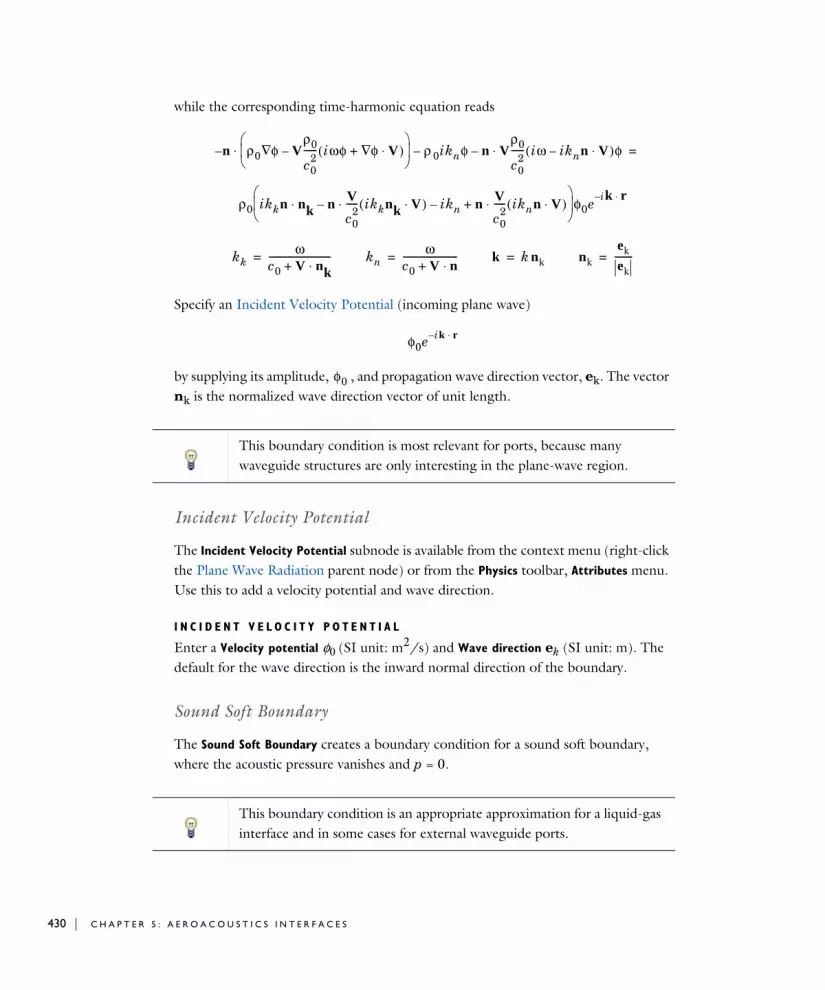
430 | C H A P T E R

while the corresponding time-harmonic equation reads

Specify an Incident Velocity Potential (incoming plane wave)

by supplying its amplitude, , and propagation wave direction vector, ek. The vector nk is the normalized wave direction vector of unit length.

Incident Velocity Potential

The Incident Velocity Potential subnode is available from the context menu (right-click the Plane Wave Radiation parent node) or from the Physics toolbar, Attributes menu. Use this to add a velocity potential and wave direction.

I N C I D E N T V E L O C I T Y P O T E N T I A L

Enter a Velocity potential φ0 (SI unit: m2/s) and Wave direction ek (SI unit: m). The default for the wave direction is the inward normal direction of the boundary.

Sound Soft Boundary

The Sound Soft Boundary creates a boundary condition for a sound soft boundary, where the acoustic pressure vanishes and p = 0.

n– ρ0 φ∇ Vρ0

c02

------ iωφ φ∇ V⋅+( )–

ρ 0iknφ– n Vρ0

c02

------ iω iknn V⋅–( )φ⋅–⋅ =

ρ0 ikkn nk n Vc0

2----- ikknk V⋅( ) ikn– n V

c02

----- iknn V⋅( )⋅+⋅–⋅

φ0ei– k r⋅

kkω

c0 V nk⋅+---------------------------= kn

ωc0 V n⋅+------------------------= k k nk= nk

ekek--------=

φ0e ik r⋅–

φ0

This boundary condition is most relevant for ports, because many waveguide structures are only interesting in the plane-wave region.

This boundary condition is an appropriate approximation for a liquid-gas interface and in some cases for external waveguide ports.





Periodic Condition

The Periodic Condition node adds a periodic boundary condition that can be used to reduce the model size by using symmetries and periodicities in the geometry and physics interfaces being modeled. This feature works well for cases like opposing parallel boundaries. In other cases, use a Destination Selection subnode to control the destination. By default, it contains the selection that COMSOL Multiphysics identifies.


Select a Type of periodicity: Continuity (the default) or Antiperiodicity.







Normal Velocity

Use the Normal Velocity node in time-harmonic analysis to specify the velocity component normal to the boundary:

Here vn denotes the outward normal velocity at the boundary surface, which is specified in the vn text field.

See Orientation of Source and Destination in the COMSOL Multiphysics Reference Manual.

n ρ0 φ∇ Vρ0

c02

------ iωφ V φ∇⋅+( )–

⋅ ρ0 vn1iω------V ∇⋅ vn+

=


432 | C H A P T E R


Enter a Normal velocity vn (SI unit: m/s).

Impedance, Interior Impedance, and Pair Impedance

Use the Impedance, Interior Impedance, or Pair Impedance node in time-harmonic analysis to define the input impedance of an external domain, at an interior boundary, or at the boundary between parts in an assembly as the ratio of pressure (or pressure drop) to normal velocity, Zi = p/(n · v) at the boundary. The associated impedance boundary condition is

On pair (interior) impedance conditions the up/down, that refers to the up and down side of an interior boundary, is replaced by a 1 and 2 index in the equation display. These refer to the two faces in the pair.

I M P E D A N C E / I N T E R I O R I M P E D A N C E / P A I R I M P E D A N C E

Enter an input Impedance Zi (SI unit: Pa·s/m).

Vortex Sheet

Use the Vortex Sheet boundary condition to model a shear layer that separates a stream from the free velocity field. Because the velocity potential is discontinuous over this boundary. Vortex sheets are only applicable on interior boundaries or between assemblies.

The equations defining the vortex sheet boundary condition are

where w denotes the outward normal displacement (SI unit: m) of the vortex sheet surface. The condition ensures continuity in the normal stress (the pressure) and the normal displacement, while allowing for a slit (jump) in the tangential component of the total velocity.

n– ρ0 φ∇ρ0

c02

------ iω φ V φ∇⋅+( )V–

⋅ ρ0pZi----- 1

iω------ V ∇⋅( ) p

Zi-----+

= i up down,=

n ρ0 φ∇ Vρ0

c02

------ iωφ V φ∇⋅+( )–

⋅i

ρ0 iω V ∇⋅+( ) w[ ]i= i up down,=

pup pdown= wup wdown–=


On pair (interior) vortex sheet conditions the up/down, that refers to the up and down side of an interior boundary, is replaced by a 1 and 2 index in the equation display (referring to the two faces in the pairs).

This boundary condition adds and additional degree of freedom ae.vs1.w (here using the default name for the physics interface and boundary condition) which is solved for.


For The Linearized Potential Flow, Frequency Domain Interface and The Linearized Potential Flow, Transient Interface, use the Interior Sound Hard Boundary (Wall) condition to model interior rigid boundary surfaces, or walls. It prescribes a vanishing normal component of the particle velocity at the boundary. Multiplied by the density, it can equivalently be expressed as a no-flow condition:

The up/down refers to the up and down side of an interior boundary. The sound-hard boundary condition is available for all analysis types. The equation above applies to the time domain calculations in the Linearized Potential Flow, Transient interface; to obtain the corresponding condition for the frequency domain, simply replace ∂/∂t with iω.

Continuity

Continuity is available as an option at interfaces between parts in a pair. This condition gives continuity in the velocity potential as well as continuity in the mass flow. It corresponds to a situation where the boundary has no direct effect on the acoustic velocity potential field (subscripts 1 and 2 in the equation refer to the two sides of the pair):




n– ρ0 φ Vρ0

c02

------t∂

∂φ V φ∇⋅+ –∇

⋅i

0= i up down,=

n ρ0 φ∇ Vc0

2----- iω V ∇⋅+( )φ–

1

ρ0 φ∇ Vc0

2----- iω V ∇⋅+( )φ–

2

–⋅ 0=


434 | C H A P T E R

Mass Flow Edge Source

For 3D components, use a Mass Flow Edge Source to specify the mass flow rate on an edge:

In the time domain, factors iω are replaced by partial time derivatives, ∂/∂t.

M A S S F L O W E D G E S O U R C E

Enter a Mass flow rate m' (SI unit: kg/(m2·s)) and enter a Phase θ (dimensionless).

Mass Flow Point Source

Add a Mass Flow Point Source node to specify the mass flow rate on a point:


M A S S F L O W P O I N T S O U R C E

Enter a Mass flow rate m' (SI unit: kg/s for 3D and 2D axisymmetric components; kg/(m·s) for 2D components).

Enter a Phase θ (dimensionless).

Mass Flow Circular Source

For 2D axisymmetric components, use a Mass Flow Circular Source node to add a circular source located at x = x0:

ρ0

c02

------iω iωφ V ∇φ⋅+( )– ∇ ρ0 φ∇ Vρ0

c02

------ iωφ V φ∇⋅+( )–

⋅+ m'eiθδ x x0–( )dl=

ρ0

c02

------iω iωφ V ∇φ⋅+( )– ∇ ρ0 φ∇ Vρ0

c02

------ iωφ V φ∇⋅+( )–

⋅+ m'eiθδ x x0–( )=

Doppler Shift: Application Library path Acoustics_Module/Aeroacoustics_and_Noise/doppler_shift

ρ0

c02

------iω iωφ V ∇φ⋅+( )– ∇ ρ0 φ∇ Vρ0

c02

------ iωφ V φ∇⋅+( )–

⋅+ m'eiθδ x x0–( )rdϕ=



M A S S F L O W C I R C U L A R S O U R C E

Enter a Mass flow rate m' (SI unit: kg/(m⋅s) and enter a Phase θ (dimensionless).

Mass Flow Line Source on Axis

For 2D axisymmetric components, use a Mass Flow Line Source on Axis node to add a line source along the symmetry axis:


M A S S F L O W L I N E S O U R C E O N A X I S

Enter a Mass flow rate m' (SI unit: kg/(m·s)) and enter a Phase θ (dimensionless).

Axial Symmetry

The Axial symmetry feature is a default node added for all axisymmetric components. The boundary condition is active on all boundaries on the symmetry axis.

ρ0

c02

------iω iωφ V ∇φ⋅+( )– ∇ ρ0 φ∇ Vρ0

c02

------ iωφ V φ∇⋅+( )–

⋅+ m'eiθδ x x0–( )dz=


436 | C H A P T E R

Th e L i n e a r i z e d Po t e n t i a l F l ow , T r a n s i e n t I n t e r f a c e

The Linearized Potential Flow, Transient (aetd) interface ( ), found under the Acoustics>Aeroacoustics branch ( ) when adding a physics interface, is used to compute the acoustic variations in the velocity potential in the presence of an inviscid and irrotational background mean flow — that is, a potential flow. The physics interface is used for aeroacoustic simulations that can be described by the linearized compressible potential flow equations.

The equations are formulated in the time domain. The physics interface is limited to flows with a Mach number Ma < 1, partly due to limitations in potential flow and partly due to the acoustic boundary settings needed for supersonic flow. The coupling between the acoustic field and the background flow does not include any predefined flow-induced noise.


Builder — Linearized Potential Flow Model, Sound Hard Boundary (Wall), and Initial

Values. For axisymmetric components an Axial Symmetry node is also added.


Transient to select physics features from the context menu.

S E T T I N G S



The default Name (for the first physics interface in the model) is aetd.


Enter the Maximum frequency to resolve in the model. The default frequency is set to 1000[Hz] but should be changed to reflect the frequency content of the sources used in the model. Select the Time stepping (method) as Fixed (preferred) the default and


recommended or Free. The Free option is in general not recommended for wave problems. The generated solver will be adequate in most situations if the computational mesh also resolves the frequency content in the model. Note that any changes made to these settings (after the model is solved the first time) will only be reflected in the solver if Show Default Solver or Reset Solver to Defaults is selected in the study.

Domain, Boundary, Edge, Point, and Pair Nodes for the Linearized Potential Flow, Transient Interface

The Linearized Potential Flow, Transient Interface has these domain, boundary, edge, point, and pair nodes, listed in alphabetical order and described for The Linearized Potential Flow, Frequency Domain Interface. The nodes are available from the Physics ribbon toolbar (Windows users), Physics context menu (Mac or Linux users), or right-click to access the context menu (all users).


The remainder of the settings are shared with The Linearized Potential Flow, Frequency Domain Interface.

• Domain, Boundary, Edge, Point, and Pair Nodes for the Linearized Potential Flow, Transient Interface



T H E L I N E A R I Z E D P O T E N T I A L F L O W , T R A N S I E N T I N T E R F A C E | 437

438 | C H A P T E R

• Continuity

• Initial Values



• Mass Flow Point Source

• Mass Flow Circular Source

• Mass Flow Edge Source








Th e L i n e a r i z e d Po t e n t i a l F l ow , Bounda r y Mode I n t e r f a c e

The Linearized Potential Flow, Boundary Mode (aebm) interface ( ), found under the Acoustics>Aeroacoustics branch ( ) when adding a physics interface, is used to compute eigenmodes and out-of-plane wave numbers for the linearized compressible potential flow equations. This study is used, for example, when specifying sources at inlets or analyzing transverse acoustic modes in ducts.

The physics interface solves an eigenvalue equation on boundaries, searching for the out-of-plane wave numbers at a given frequency.


Builder — Linearized Potential Flow Model, Sound Hard Boundary (Wall), and Initial

Values. For 2D axisymmetric models an Axial Symmetry node is also added.


Boundary Mode to select physics features from the context menu.

S E T T I N G S



The default Name (for the first physics interface in the model) is aebm.

This physics interface is limited to flows with a Mach number Ma < 1, partly due to limitations in the potential flow formulation and partly due to the acoustic boundary settings needed for supersonic flow.

T H E L I N E A R I Z E D P O T E N T I A L F L O W , B O U N D A R Y M O D E I N T E R F A C E | 439

440 | C H A P T E R

L I N E A R I Z E D P O T E N T I A L F L O W E Q U A T I O N S E T T I N G S

For 2D axisymmetric components, the Azimuthal mode number m (dimensionless) is 0 by default. It is an integer entering the axisymmetric expression for the velocity potential:


The settings are the same as Sound Pressure Level Settings for the Pressure Acoustics, Frequency Domain interface.


This physics interface defines one dependent variable (field), the Velocity potential phi. The name can be changed but the names of fields and dependent variables must be unique within a model.


From the list select the element order and type (Lagrange or serendipity) the default is Quadratic Lagrange.

Boundary, Edge, Point, and Pair Nodes for the Linearized Potential Flow, Boundary Mode Interface

The Linearized Potential Flow, Boundary Mode Interface has these boundary, edge, point, and pair nodes, listed in alphabetical order, available from the Physics ribbon

φ r z ϕ, ,( ) φ r( ) ei kzz mϕ+( )–

=


• Boundary, Edge, Point, and Pair Nodes for the Linearized Potential Flow, Boundary Mode Interface


Flow Duct: Application Library path Acoustics_Module/Aeroacoustics_and_Noise/flow_duct


toolbar (Windows users), Physics context menu (Mac or Linux users), or right-click to access the context menu (all users).

These features are described for The Linearized Potential Flow, Frequency Domain Interface. The only difference for the Linearized Potential Flow, Boundary Mode interface is that you apply the features to boundaries instead of domains for 3D components. In the Linearized Potential Flow Model you can enter a Unit normal that defines the positive propagation direction.

In general, to add a node, go to the Physics toolbar, no matter what operating system you are using.

• Continuity

• Initial Values







T H E L I N E A R I Z E D P O T E N T I A L F L O W , B O U N D A R Y M O D E I N T E R F A C E | 441

442 | C H A P T E R

Th e Comp r e s s i b l e Po t e n t i a l F l ow I n t e r f a c e

The Compressible Potential Flow (cpf) interface ( ), found under the Acoustics>Aeroacoustics branch ( ), is used to compute the velocity potential and density in a compressible potential flow model. Derived values include the associated pressure, velocity, and temperature in the flow. In a compressible potential flow model, the flow is assumed to be represented by an ideal barotropic, irrotational fluid at constant entropy, that is, the fluid is also inviscid. The physics interface is used for modeling the background mean flow used as input to The Linearized Potential Flow, Frequency Domain Interface or The Linearized Potential Flow, Transient Interface.


Builder — Compressible Potential Flow, Slip Velocity, and Initial Values. For axisymmetric models an Axial Symmetry node is also added.

Then, from the Physics toolbar, add other nodes that implement, for example, boundary conditions and sources. You can also right-click Compressible Potential Flow

to select physics features from the context menu.

S E T T I N G S



The default Name (for the first physics interface in the model) is cpf.

The potential flow formulation for steady compressible flow is in general not suited for modeling shocks. In the region after a shock the flow is typically rotational, hence it is only suited for problems with a Mach number Ma < 1.


R E F E R E N C E V A L U E S

Edit or enter the values as needed:

• Reference pressure pref (SI unit: Pa). The default is 1 atm.

• Reference density ρref (SI unit: kg/m3). The default is 1.2 kg/m3.

• Reference velocity νref (SI unit: m/s).

• Reference force potential Ψref (SI unit: J/kg).


This physics interface defines two dependent variables (field), the Mean flow velocity

potential Phi and the Density rho. The name can be changed but the names of fields and dependent variables must be unique within a model.


Select the discretization order for the Mean flow velocity potential and the Density dependent variables. The default is Quadratic for both.

Domain, Boundary, and Pair Nodes for the Compressible Potential Flow Interface

The Compressible Potential Flow Interface has these domain, boundary, and pair nodes, listed in alphabetical order, available from the Physics ribbon toolbar (Windows

• Domain, Boundary, and Pair Nodes for the Compressible Potential Flow Interface


Flow Duct: Application Library path Acoustics_Module/Aeroacoustics_and_Noise/flow_duct

T H E C O M P R E S S I B L E P O T E N T I A L F L O W I N T E R F A C E | 443

444 | C H A P T E R

users), Physics context menu (Mac or Linux users), or right-click to access the context menu (all users).

Compressible Potential Flow Model

The Compressible Potential Flow Model node adds equations for time-dependent or stationary modeling of compressible potential flow. The model will solve for the mean flow velocity potential and the density. The pressure and the velocity field are defined from these dependent variables.

C O M P R E S S I B L E P O T E N T I A L F L O W M O D E L

For the Ratio of specific heats γ (dimensionless) select From material (the default) or User defined. For the User defined option, the default value is 1.4.

Enter a Force potential ψ (SI unit: J/kg). To model a domain force or domain source acting on the fluid.

Select the Calculate temperature option it you need to also calculate the temperature field in the fluid. If this is selected, you also need to specify the Specific gas constant Rs (SI unit: J/(kg·K)). Select From material (the default) or User defined. Enabling this calculates the temperature according to

• Compressible Potential Flow Model

• Initial Values

• Interior Wall (Slip Velocity)

• Mass Flow

• Mean Flow Velocity Potential

• Normal Flow


• Slip Velocity

• Symmetry




where pA is the pressure and ρ the density in the fluid.

Depending on the material selected in the Materials node for the fluid (typically Air) the Model Inputs may be active. Per default the Absolute pressure is taken from the model itself (unavailable). If the Calculate temperature option is enabled the Temperature is also taken from the model (unavailable). This will give a physically consistent solution. In both cases, you can click the Make All Model Inputs Editable icon to enter a user defined expression.

Initial Values

The Initial Values node adds initial values for the mean flow velocity potential and density variables. Add more Initial Values nodes from the Physics toolbar.


Enter a value or expression for the initial values Mean flow velocity potential Phi (SI unit: m2/s). Enter a Density rho (SI unit: kg/m3) the default is the reference density cpf.rhoref.

Slip Velocity

The Slip Velocity node is the natural condition at a boundary impervious to the flow, meaning that the velocity normal to the boundary is zero. By multiplying with the density, this condition can alternatively be expressed as a vanishing mass flow through the boundary

Symmetry

The Symmetry condition is applied at planes where the model has symmetries. Using the intrinsic symmetries of a problem is a simple way to reduce the model size.

Normal Flow

The Normal Flow node implies that the flow is normal to the boundary and thus that the tangential velocity is zero. This corresponds to a constant velocity potential along

TpA

ρRs----------=

n– ρ∇Φ⋅ 0=


446 | C H A P T E R

the boundary. Because the velocity potential is determined only up to a constant, imposing this condition fixes the arbitrary constant to zero where .

Mass Flow

The Mass Flow node specifies the mass flow through the boundary. The mass flow is given by the product of the normal velocity vn and the density at the boundary ρbnd. This results in a flux condition given by

M A S S F L O W

Enter the Normal velocity vn (SI unit: m/s) and Fluid density at the boundary ρbnd (SI unit: kg/m3). The defaults are cpf.vref and cpf.rhoref, respectively. The values given in the Reference Values.

Mean Flow Velocity Potential

Use the Mean Flow Velocity Potential condition to prescribe the flow potential Φ at a boundary, Φ = Φ0. This condition can be used to set up theoretical flow conditions at a boundary or couple to other physics interfaces.

M E A N F L O W V E L O C I T Y P O T E N T I A L

Enter the Mean flow velocity potential Φ0 (SI unit: m2/s).

Periodic Condition

Use the Periodic Condition to define periodicities between boundaries in the model. From the Type of periodicity menu select Continuity (default) or Antiperiodicity.

Interior Wall (Slip Velocity)

The Interior Wall (Slip Velocity) is used to set up interior walls on interior boundaries. This simplifies modeling and meshing steps as the wall does not need to have a

φ 0=

Setting the Normal Flow condition on two or more disjoint boundaries can result in the wrong features unless symmetry implies that the velocity potential is equal on the boundaries in question.

n– ρ∇Φ⋅ vnρbnd=


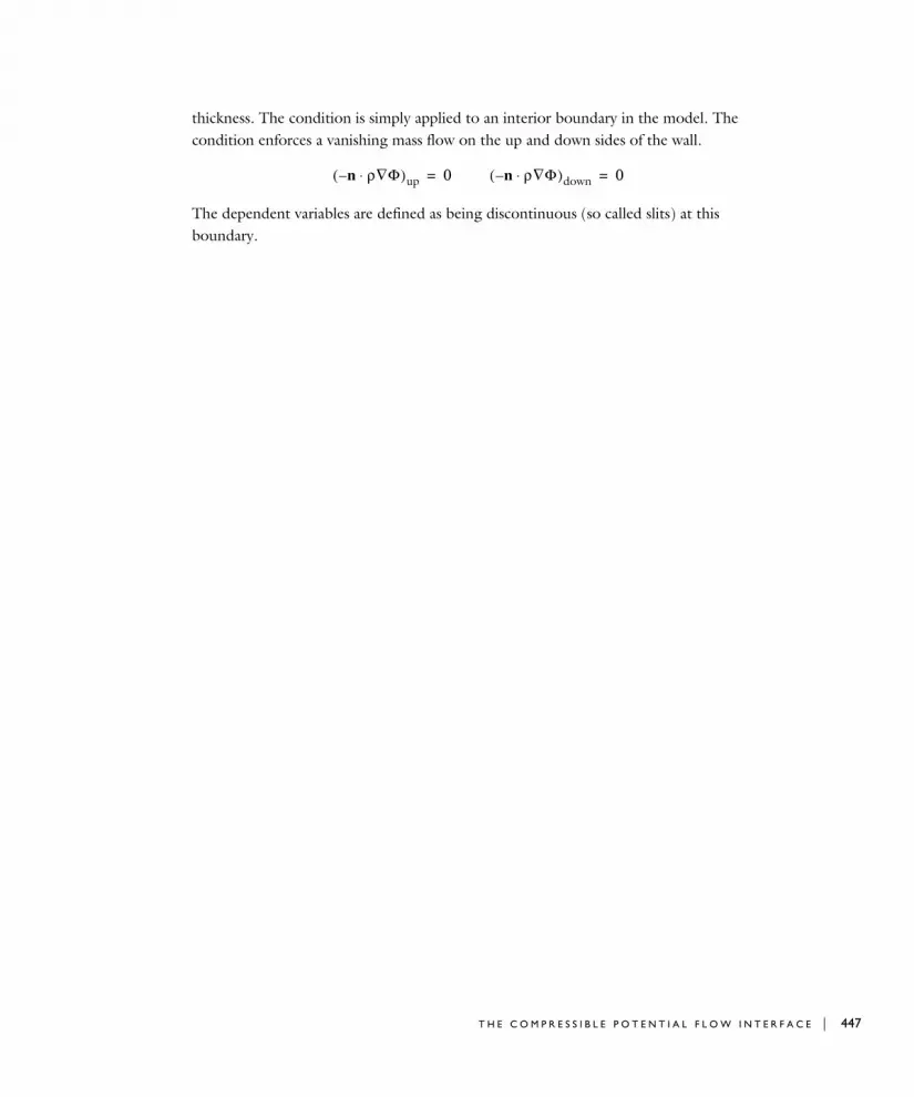
thickness. The condition is simply applied to an interior boundary in the model. The condition enforces a vanishing mass flow on the up and down sides of the wall.

The dependent variables are defined as being discontinuous (so called slits) at this boundary.

n– ρ∇Φ⋅( )up 0= n– ρ∇Φ⋅( )down 0=


448 | C H A P T E R

Mode l i n g w i t h t h e A e r o a c ou s t i c s B r an c h

In this section:

• Selecting an Aeroacoustics Interface

• Meshing

• Stabilization

• Solver Suggestions for Large Aeroacoustic Models

• Absorbing Layers for the Linearized Euler, Transient Interface


• Time Stepping in Transient Models

• Mapping Between Fluid Flow and Acoustics Mesh

• Coupling to Turbulent Flows (Eddy Viscosity)

• Eigenfrequency Studies

• Suppressing Constraints on Lower Dimensions


Selecting an Aeroacoustics Interface

When modeling a muffler with an internal nonisothermal flow, a jet engine, or a flow sensor you should consider which physics interface to use. The influence the background mean flow has on the acoustic behavior in an aeroacoustic model can be modeled in several ways. The effects that need to be included typically depend on the Mach number (Ma). A rule of thumb says that for a Mach number below 0.1 (Ma < 0.1) the convective effects of the background flow need not to be included, above they do. Other considerations are of course also important; for example, whether viscous and thermal losses are important, if the background flow has large gradients, or if the flow is turbulent or has vorticity.

• Mach number less than 0.1 (Ma < 0.1)

In this situation the convective flow effects can normally be neglected and Pressure Acoustics can be used. Only the background temperature distribution T = T(x) and background pressure distribution pA = pA(x) need to be included. This can be done


directly in the Pressure Acoustics interface as a Model Inputs. The effects are included by making sure that the material properties depend on the local pressure and temperature; the spatial variations in the speed of sound is c = c(pA,T) = c(x) and in the density ρ = ρ(pA,T) = ρ(x), respectively.

• Mach number greater than 0.1 (Ma > 0.1):

In this case the convective effects of the flow can probably not be neglected. Modeling this type of system requires the use of one of the Aeroacoustics interfaces: linearized potential flow, linearized Euler, or linearized Navier–Stokes. The choice depends on the assumptions about the flow that can be made.

Meshing

When solving a model using one of the Aeroacoustic interfaces, it is important to remember that this is a wave problem. This means that the wavelength should be resolved by an appropriate number of mesh elements. Using the same guidelines as for Pressure Acoustics is reasonable, that is, a first good mesh should use at least 5 elements per wavelength for second order shape functions. In the linearized Euler interface, the default shape functions are first order and here using at least 15 to 20 elements per wavelength is a first good choice.

The Background FlowAnother important parameter to consider is resolving details in the background mean flow field. The acoustic mesh should capture gradients that exist in the background flow as these have a large influence on the acoustic propagation. Waves may, for example, be reflected and refracted in shear layers.

Note that when the background mean flow velocity u0 is set to zero, the linearized Navier–Stokes equations reduce to the thermoviscous acoustic equations. However, in thermoviscous acoustics the default discretization is P1, P2, P2 and no stabilization is applied.

Meshing guidelines for the Pressure Acoustics interface is given in Meshing (Resolving the Waves) under the Modeling with the Pressure Acoustics Branch (FEM-Based Interfaces) section.

M O D E L I N G W I T H T H E A E R O A C O U S T I C S B R A N C H | 449

450 | C H A P T E R

Meshing the Acoustic Boundary Layers in LNSThe Linearized Navier–Stokes interfaces just as the Thermoviscous Acoustics interface captures the physics of the acoustic boundary layer. When no-slip and isothermal conditions are used on walls a viscous and a thermal boundary layer will exist. In order for the solution to be well behaved and capture losses correctly, it is important to mesh this layer, for example, by using a boundary layer mesh. If the model is large using a single boundary layer mesh, with the approximate extend of the acoustic boundary layer, is the minimum requirement for a good solution.

Resolving Vorticity and Physics in LE and LNSIn the LE and LNS interfaces the GLS stabilization is very efficient and can ensure smooth and converged solution even without resolving details like vorticity generation (the propagation of vorticity waves). If these are important processes in the model the mesh should of course be able to resolve these details. Either refine the mesh or switch to (P2, P2, P2) discretization (keep the stabilization turned on). For LNS models these phenomena are typically generated at walls where the no-slip condition generates vorticity when an acoustic wave is interacting with the background flow.

Stabilization

When solving the linearized Euler (LE) and linearized Navier–Stokes (LNS) equations using the finite element method (the standard Galerkin formulation). It can be shown that the method looses its good approximation characteristics when convective terms are present and when these terms locally dominate (Ref. 19). This can lead to spurious numerical oscillations. To remedy these oscillations stabilization is used.

T H E S T A B I L I Z A T I O N M E T H O D S

In the linearized Navier–Stokes (LNS) and linearized Euler (LE) interfaces two stabilization methods are implemented. The Galerkin least squares (GLS) and the streamline upwind Petrov-Galerkin (SUPG) stabilization. It is in general recommended to use the GLS method. The SUPG method is implemented for completeness and can be used by experienced users. There is also the option to not use

It can be shown that if the cell Péclet number has a value larger than one Pec > 1 the solution will oscillate. In the linearized Navier–Stokes interface the variables lnsf.CellPe_th and lnsf.CellPe_v can be plotted to assess the characteristic number when comparing convection to viscous and thermal diffusion, respectively.


stabilization or to use the legacy method from version 5.2a and older. The legacy method for the LE interface is based on the implementation discussed in Ref. 10.

The implementation of the GLS stabilization methods follows the one discussed in Ref. 14, 19, 21, and 23. A general overview about stabilization methods can be found in Ref. 22. The GLS method combines stability and accuracy and the method order of accuracy is O(h2p+1) where p is the shape function order and h is the local mesh size. The SUPG method has an accuracy order of O(hp+1/2) for convection dominated problems and O(hp+1) for diffusion dominated problems.

The default discretization for the LNS and LE interface is to use linear elements for all the dependent variables (P1-P1-P1). This effectively removes the stabilization on the diffusive parts of the equation. The GLS method is still superior to the SUPG method as it also stabilizes the reactive terms. These are the terms where gradients of the background fields enter. If no stabilization is used then set a (P1-P2-P2) discretization for the dependent variables as it ensures a more stable numerical scheme.

Solver Suggestions for Large Aeroacoustic Models

Studying aeroacoustic applications often lead to very large models that can contain many degrees of freedom (DOFs). Different steps can be taken to reduce the size of the models, for example, consider the use of slip instead of no-slip conditions in the LNS interface (avoiding the details in the acoustic boundary layer) or consider the choice between Lagrange and Serendipity Shape Functions.

The equation residuals can be visualized in the LE and the LNS interfaces by plotting, for example, lnsf.res_e (equation residual for the energy equation), lnsf.res_mx (equation residual for the momentum equation x-component), lnsf.res_my, lnsf.res_mz, and lnsf.res_e (equation residual for the energy equation).

See for example the model Point Source in 2D Jet: Radiation and refraction of sound waves through a 2D shear layer found in the Model Gallery: www.comsol.com/model/point-source-in-2d-jet-radiation-and-refraction-of-sound-waves-through-a-2d-shea-16685



452 | C H A P T E R

When a model reaches a size where it can no longer fit in memory (when solved using the default direct solver) or if the solution procedure is slow with a direct solver, then it can be advantageous to switch to an iterative solver approach.

For the Linearized Navier–Stokes interfaces iterative solver suggestions are automatically generated when the default solver is generated. These can be seen by expanding the Solver Configuration tree under Stationary Solver or Time-Dependent

Solver. Per default a direct solver is used and two iterative solvers are suggested and disabled. To turn on one of these approached right-click the solver and select Enable (or press F4). The first suggestion (GMRES with Direct Precon.) uses an iterative solver with a direct preconditioner. This method is typically faster than the direct solver and uses 20% less memory. The second suggestion (GMRES with DD) uses an iterative solver with the domain decomposition method. This method is very robust (also for multiphysics applications) and very memory efficient, but it can be slow.

For the Linearized Euler interfaces the default solver is PARDISO, which is also the most robust option. Iterative solver will often struggle for the linearized Euler equations because there is not dissipation involved and instabilities are inherent.

S O L V I N G I N T H E A D I A B A T I C C A S E

In certain cases, it is a good assumption to not include thermal conduction in the model and treat all processes as adiabatic (isentropic). This is, for example, relevant for fluids where the thermal boundary layer is much thinner than the viscous, like in water. Not solving for the temperature field T also saves some degrees of freedom (DOFs).

This is achieved by selecting the Adiabatic formulation option under the Linearized Navier–Stokes Equation Settings section. When Adiabatic formulation is selected all temperature options and conditions are disabled in the user interface.

Absorbing Layers for the Linearized Euler, Transient Interface

The Linearized Euler, Transient Interface includes so-called absorbing layers, also often referred to as sponge layers. The layers work by combining three techniques: a scaling system, damping, and a simple nonreflecting condition.

Further details on solving large models can be found in the Solver Suggestions for Large Thermoviscous Acoustics Models section. These suggestions also apply to the linearized Navier–Stokes physics.


The layers are set up by adding the Absorbing Layer under the Definitions node. This adds a special scaled system. The scaling effectively slows down the propagating waves and ensures that they “align up” (normal) toward the outer boundary. This means that the waves will hit the outer boundary in a closer to normal direction. Damping in the form of artificial numerical viscosity, is automatically applied in the layer in a matched manner (increasing from zero at the boundary to the physical domain). The artificial viscosity attenuates or damps high-frequency components of the wave in the layer. The amount of damping is controlled under the Damping Parameters for Absorbing Layers section at the main physics level. Finally, at the outer boundary of the layer add a simple Acoustic Impedance (Isentropic) boundary condition, which will work well to remove all remaining waves, as normal incidence has been ensured.

The physical thickness of the layer should be such that it contains a minimum of 10 structured mesh elements. This in practice means that it should roughly have a thickness equal to the largest wavelength resolved in the model.

For the Absorbing Layers select the Type (Cartesian, cylindrical, spherical, or user defined) under the Geometry section. Enter values for the Physical Width and Pole

Distance under the Scaling section.


In most of the physics interfaces in the Acoustics Module and specifically in the Aeroacoustics interfaces, you can choose between two families of shape functions in the Discretization section: Lagrange and serendipity. The current default is to use Lagrange shape functions.

When using a structured mesh, it may be advantageous to switch to the serendipity elements as they generate significantly fewer degrees of freedom (DOFs). The accuracy is in most cases almost as good as for the Lagrange elements. The Lagrange elements are however less sensitive to strong mesh distortions.



454 | C H A P T E R

The serendipity shape functions differ from the Lagrange shape functions only for the following element shapes:




Time Stepping in Transient Models

When solving transient wave problems, it is recommended to use a fixed time stepping in the solver (this is the manual option in the solver settings). In general, there is no point in using an automatic time-step control which can be provided by the time-dependent solver. The tolerances in the automatic error control are difficult to tune in wave problems when there is weak but important high-frequency content. It is recommended to use the suggestion generated when the Fixed (preferred) method is chosen (the default) in the Transient Solver Settings section. The internal time step of the solver that is generated, when the Maximal frequency to resolve is set, will in most cases produce a solver that is adequate. It is assuming that the user has generated a mesh that properly resolves the same maximal frequency (minimal wavelength).

Mapping Between Fluid Flow and Acoustics Mesh

When the aeroacoustic and the Fluid Flow (CFD) model are solved on different computational mesh, careful mapping of the CFD solution from the CFD mesh onto the acoustics mesh should be done. This step is crucial in order not to introduce nonphysical numerical noise into the acoustic solution (Ref. 20). If the solution is not




For further details see the Time Stepping in Transient Models section in Modeling with the Thermoviscous Acoustics Branch.


properly mapped terms containing gradients of the background mean flow variables (especially the reactive terms) become very noisy and are typically the source of the numerical error. This mapping is handled by the multiphysics coupling Background Fluid Flow Coupling and the dedicated Mapping study.

If the acoustic problem is solved on the same mesh as the CFD then the mapping problem is less of an issue, especially if both physics use the same shape function order (they are both linear per default). Using the Background Fluid Flow Coupling is also necessary, if perfectly matched layers (PMLs) are present in the model, in order to get the flow field inside the PML regions. In any case, the coupling can still be useful as the CFD solution will be smoothed by the mapping (the degree of smoothing can be controlled).

M A N U A L M A P P I N G

The multiphysics coupling Background Fluid Flow Coupling can couple all Single-Phase Flow and Nonisothermal Flow interfaces including the high Mach Number Flow interfaces. If such a coupling and mapping is necessary, manual mapping can be set up using the procedure described here.

The manual mapping is defined by a study that solves an additional set of equations which maps and smooths the background flow variables onto the acoustics mesh. The mapping equations can be set up using the Weak Form PDE interface from the Mathematics branch. In the most general case the mean background flow pressure p0, velocity field u0, density ρ0, temperature T0, and turbulent viscosity μT variables should be mapped onto corresponding variables on the acoustics mesh, for example, p0,aco, u0,aco, ρ0,aco, T0.aco, and μT,aco. These new variables should then be used as the model inputs in the aeroacoustics model.

A simple but efficient mapping and smoothing is achieved by solving

The multiphysics coupling of turbulent flow and acoustics is described in the application library model Helmholtz Resonator with Flow: Interaction of Flow and Acoustics. The Application Library path Acoustics_Module/Aeroacoustics_and_Noise/helmholtz_resnoator_with_flow


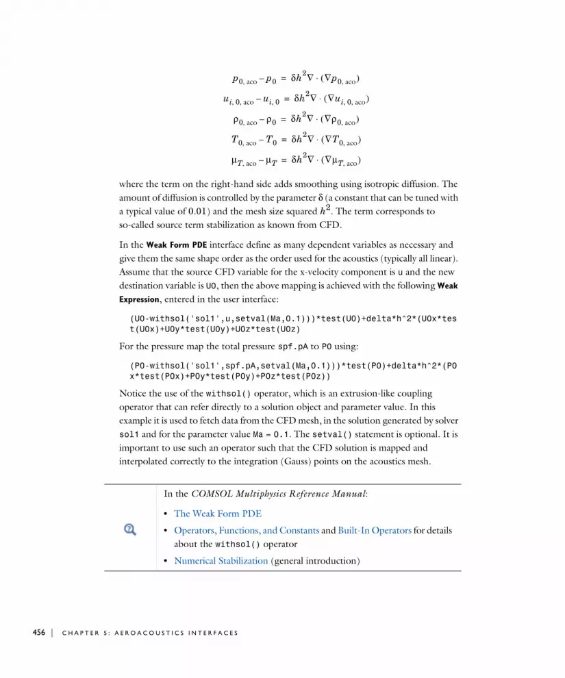
456 | C H A P T E R

where the term on the right-hand side adds smoothing using isotropic diffusion. The amount of diffusion is controlled by the parameter δ (a constant that can be tuned with a typical value of 0.01) and the mesh size squared h2. The term corresponds to so-called source term stabilization as known from CFD.

In the Weak Form PDE interface define as many dependent variables as necessary and give them the same shape order as the order used for the acoustics (typically all linear). Assume that the source CFD variable for the x-velocity component is u and the new destination variable is U0, then the above mapping is achieved with the following Weak

Expression, entered in the user interface:

(U0-withsol('sol1',u,setval(Ma,0.1)))*test(U0)+delta*h^2*(U0x*test(U0x)+U0y*test(U0y)+U0z*test(U0z)

For the pressure map the total pressure spf.pA to P0 using:

(P0-withsol('sol1',spf.pA,setval(Ma,0.1)))*test(P0)+delta*h^2*(P0x*test(P0x)+P0y*test(P0y)+P0z*test(P0z))

Notice the use of the withsol() operator, which is an extrusion-like coupling operator that can refer directly to a solution object and parameter value. In this example it is used to fetch data from the CFD mesh, in the solution generated by solver sol1 and for the parameter value Ma = 0.1. The setval() statement is optional. It is important to use such an operator such that the CFD solution is mapped and interpolated correctly to the integration (Gauss) points on the acoustics mesh.

p0 aco, p0– δh2∇ ∇p0 aco,( )⋅=

ui 0 aco, , ui 0,– δh2∇ ∇ui 0 aco, ,( )⋅=

ρ0 aco, ρ0– δh2∇ ∇ρ0 aco,( )⋅=

T0 aco, T0– δh2∇ ∇T0 aco,( )⋅=

μT aco, μT– δh2∇ ∇μT aco,( )⋅=


• The Weak Form PDE

• Operators, Functions, and Constants and Built-In Operators for details about the withsol() operator

• Numerical Stabilization (general introduction)


In some cases it can be necessary to extend the mapping equation with boundary conditions for the mapped variables. This should be done at symmetry planes for the mapped velocity field. This is also the cases when flow details near walls are important, for example, resolving the acoustic boundary layer. In this case add a no-slip condition on u0,aco. In general constraining the value of the mapped variables to the value in the CFD model values at boundaries can be necessary.

Coupling to Turbulent Flows (Eddy Viscosity)

When acoustic waves propagate through a turbulent flow they will experience attenuation due to the turbulence. It can be shown theoretically (see Ref. 18 and Ref. 19) that the experienced attenuation corresponds to extending the value of the dynamic viscosity μ to include the eddy viscosity μτ, such that the total effective viscosity is:

This effect can be included in the linearized Navier–Stokes model by using the effective dynamic viscosity as taken from a CFD model spf.mu_eff. This option is available in the Background Fluid Flow Coupling. This variable includes the dynamic viscosity and the turbulent viscosity (spf.muT). Notice, however, that the value of the turbulent viscosity can be much larger than the true eddy viscosity and that it depends on the turbulence model selected. This means that the experienced attenuation can be too large. Typically, more advanced turbulence models like the SST model give less numerical diffusion and thus a better estimate of the eddy viscosity.

Eigenfrequency Studies

Both the linearized Euler and the linearized Navier–Stokes interfaces have the Eigenfrequency study as a predefined study type. It should be noted that this analysis type is challenging when a nonzero background mean flow is present. Mathematically it can be very difficult to identify the pure acoustic eigenvalues.

In order to identify acoustic modes in the eigenvalue spectrum it can be a good idea to use the Region option in the Eigenfrequency search method when setting up an eigenfrequency study step. In this way the nonacoustic modes that consist of entropy and vorticity waves (eigenfrequencies with large imaginary components) can be filtered out. The pure acoustic modes typically have eigenfrequencies with a small complex component can then more easily be identified. The finals identification needs to be done with a visual inspection of the mode shape in postprocessing. Set the search

μt μ μτ+=


458 | C H A P T E R

region for the real part as desired and then set a small interval for the imaginary part, for example, from −0.02 to 0.02.

Suppressing Constraints on Lower Dimensions

Sometimes, boundary conditions on two adjacent objects can come into conflict on a shared object (point or edge). For the all the boundary conditions in the thermoviscous physics that are based on constraints, you have the possibility to select that certain objects of lower dimensions should be excluded from the main selection. To do this, you must first click the Show More Options button ( ) and select Advanced

Physics Options in the Show More Options dialog box. In the settings a new sections named Excluded Edges and/or Excluded Points will then appear (when applicable). In these sections, you can select geometrical objects which should be excluded from the main selection when the constraint is applied.

Kutta Like Conditions for Linearized EulerA Kutta condition can be set up to handle edge singularities that appear, for example, at the trailing edge of an airfoil or at the transition from a liner (modeled with an Ingard-Myers type impedance) to a hard wall. By using Exclude Edges and Exclude

Points the appropriate Kutta condition can be set up. The problematic edges or points are excluded from the adjacent conditions and extra conditions can be set up here using the user defined Pointwise Constraint.

Velocity Condition for Linearized Navier–StokesWhen prescribing a velocity condition to you may get conflicts if it is located next to a no-slip condition (a wall). To remedy this, you can exclude the common edge or point.

Periodic ConditionWhen using the periodic condition, you may get conflicts or duplicates which makes the model either overconstrained, or problematic for the automatic constraint elimination algorithm. If you are aware of such situations, it is good practice to remove one of the potentially conflicting constraints. This could be in multiphysics models where you combine solid mechanics with thermoviscous acoustics and have edges where you both apply a periodic condition (solid and thermoviscous acoustics) and the Thermoviscous Acoustic- Structure Boundary multiphysics coupling.

For more details see the Eigenfrequency section in the COMSOL Multiphysics Reference Manual


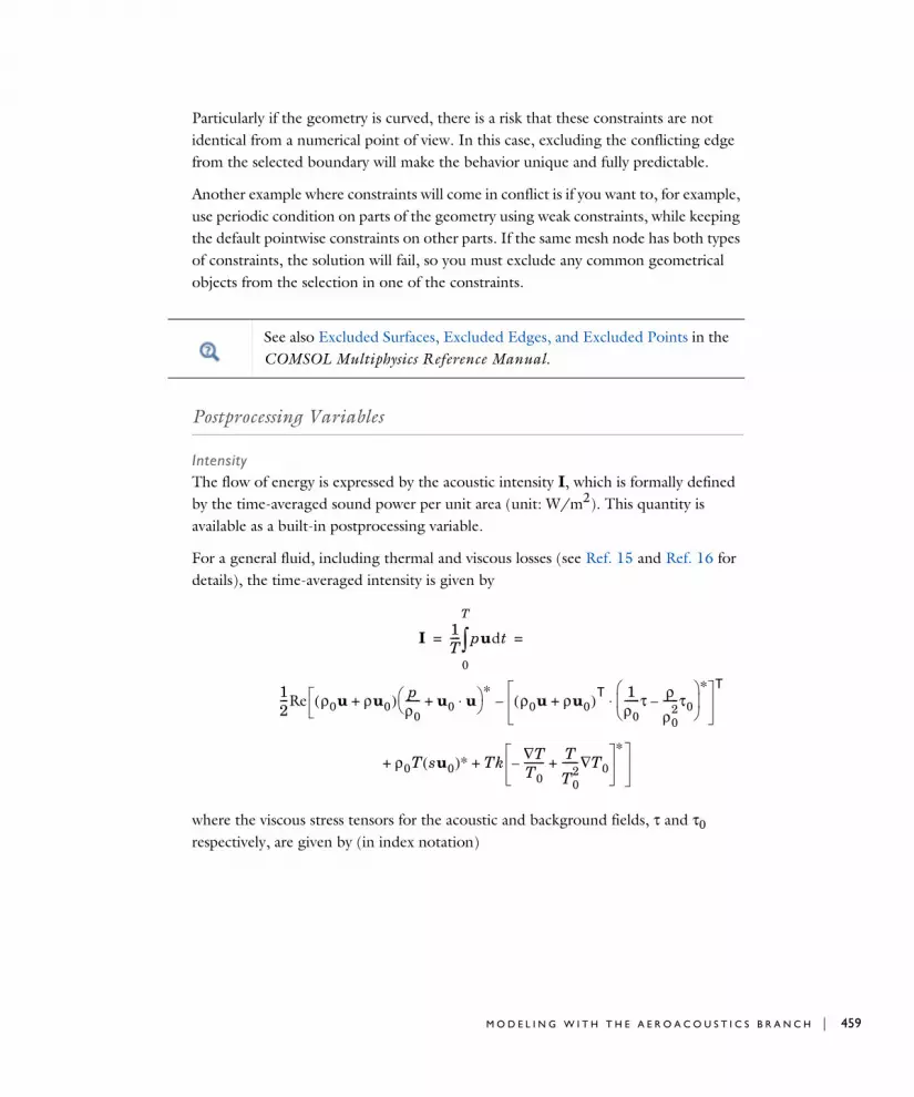
Particularly if the geometry is curved, there is a risk that these constraints are not identical from a numerical point of view. In this case, excluding the conflicting edge from the selected boundary will make the behavior unique and fully predictable.

Another example where constraints will come in conflict is if you want to, for example, use periodic condition on parts of the geometry using weak constraints, while keeping the default pointwise constraints on other parts. If the same mesh node has both types of constraints, the solution will fail, so you must exclude any common geometrical objects from the selection in one of the constraints.


IntensityThe flow of energy is expressed by the acoustic intensity I, which is formally defined by the time-averaged sound power per unit area (unit: W/m2). This quantity is available as a built-in postprocessing variable.

For a general fluid, including thermal and viscous losses (see Ref. 15 and Ref. 16 for details), the time-averaged intensity is given by

where the viscous stress tensors for the acoustic and background fields, τ and τ0 respectively, are given by (in index notation)

See also Excluded Surfaces, Excluded Edges, and Excluded Points in the COMSOL Multiphysics Reference Manual.

I 1T---- pudt

0

T

= =

12---Re ρ0u ρu0+( ) p

ρ0------ u0 u⋅+ ∗

ρ0u ρu0+( )T 1ρ0------τ ρ

ρ02

------τ0– ∗

⋅T

–

ρ+ 0T su0( )∗ Tk T∇T0--------–

T

T02

------ T0∇+∗

+


460 | C H A P T E R

It is understood that all dependent variables in these equations are the complex amplitudes.

In the time domain, the equivalent quantity is the instantaneous intensity i given by

where the dependent variables now include the explicit time dependence. The instantaneous expression is not defined in the frequency domain since it would represent effects happening at the double frequency.

The intensity variables are defined for most Aeroacoustics physics where it makes sense. That is, the instantaneous quantities are defined in the time domain and the (time averaged) intensity variables are defined in the frequency domain. It is understood that the intensity vector is in general the time averaged quantity. For the Linearized Potential Flow interface, the variables are not defined in the time domain since it would require solving for an extra variable.

τij μxi∂

∂ujxj∂

∂ui+

μB23---μ–

xk∂

∂uk

δij–=

τ0ij μxi∂

∂u0jxj∂

∂u0i+ 2

3---μ

xk∂∂u0k

δij–=

i pv ρ0u ρu0+( ) pρ0------ u0 u⋅+ ρ0u ρu0+( )T 1

ρ0------τ ρ

ρ02

------τ0–

⋅T

–= =

ρ+ 0Tsu0 Tk T∇T0--------–

T

T02

------ T0∇++

See also the theory section The Energy Corollary for the Linearized Euler interface.








phys_id.Ii_mag Magnitude of the instantaneous intensity vector (time domain only)

phys_id.Iix x-component of the instantaneous intensity vector (time domain only)

phys_id.Iiy y-component of the instantaneous intensity vector (time domain only)

phys_id.Iiz z-component of the instantaneous intensity vector (time domain only)

TABLE 5-2: INTENSITY VARIABLES IN 2D AXISYMMETRIC



phys_id.Ir r-component of the intensity vector (frequency domain only)



phys_id.Iir r-component of the instantaneous intensity vector (time domain only)

phys_id.Iiz z-component of the instantaneous intensity vector (time domain only)







phys_id.Iix x-component of the instantaneous intensity vector (time domain only)

phys_id.Iiy y-component of the instantaneous intensity vector (time domain only)




462 | C H A P T E R

Th eo r y Ba c k g r ound f o r t h e A e r o a c ou s t i c s B r an c h

The scientific field of aeroacoustics deals with the interaction between a background mean flow and an acoustic field propagating in this flow. In general, this concerns both the very complex description of the creation of sound by turbulence in the background flow, that is, flow induced noise and the influence the background mean flow has on the propagation of an externally created sound field, that is, flow borne noise or convected acoustics. The computational aeroacoustics (CAA) capabilities of the aeroacoustics interfaces in COMSOL Multiphysics only cover the convected acoustics situation.

Aeroacoustic simulations would ideally involve solving the fully compressible continuity, momentum (Navier–Stokes equations), and energy equations in the time domain. The acoustic pressure waves would then form a subset of the fluid solution. This approach is often impractical for real-world CAA applications due to the required computational time and memory resources. Instead, for solving many practical engineering problems, a decoupled two-step approach is used: first solve for the fluid flow, then the acoustic perturbations of the flow.

For solving the acoustic problem, the governing equations are linearized around the background mean flow and only solved for the acoustic perturbation. Acoustic variables are assumed to be small and perturbation theory can be used, for example, the total pressure

is the sum of the background mean pressure p0 and the acoustic pressure variations p (sometimes labeled p’ or p1).

This section presents the basic mathematical framework for the aeroacoustic equations solved in the aeroacoustic interfaces, starting with the general governing equations for fluid flow, that is, conservation equations, constitutive equations, and equations of state. Then the linearized Navier–Stokes equations, the linearized Euler equations, the linearized potential flow equations, and finally the equations for the compressional potential flow are presented.

ptot p0 p+=


In this section the theory background for:

• General Governing Equations

• Linearized Navier–Stokes

• Linearized Euler

• Scattered Field Formulation for LE and LNS

• Linearized Potential Flow

• Compressible Potential Flow

General Governing Equations

The equations governing the physics in any fluid are the foundation for deriving the linearized aeroacoustic equations and in general any acoustics equations. The governing equations for the motion of a compressible fluid are the continuity equation (mass conservation), the Navier–Stokes equation (momentum conservation), and the general heat transfer equation (energy conservation). In order to close the system of equations, constitutive equations are needed, along with the equation of state, and thermodynamic relations. See, for example, Ref. 3, Ref. 4, Ref. 5, Ref. 6, or Ref. 7 for details and further reading.

C O N S E R V A T I O N E Q U A T I O N S

The conservation equations are for mass, momentum, and energy:

(5-5)

where u is the velocity field, ρ is the density, T is the temperature, s is the specific entropy, σ is the stress tensor, q is the local heat flux, Φ is the viscous dissipation function, and M, F, and Q are source terms. The operator D/Dt is the material derivative (or advection operator) defined as

∂ρ∂t------ ∇ ρu( )⋅+ M=

ρDuDt-------- ρ ∂u

∂t------ u ∇⋅( )u+ ∇ σ F+⋅= =

ρTDsDt------- ρT ∂s

∂t----- u ∇⋅( )s+ ∇ q Φ Q+ +⋅–= =

DDt------- ∂

∂t----- u ∇⋅( )+=

T H E O R Y B A C K G R O U N D F O R T H E A E R O A C O U S T I C S B R A N C H | 463

464 | C H A P T E R

T H E R M O D Y N A M I C R E L A T I O N S

Some thermodynamic relations are necessary when reformulating the energy equations in terms of other sets of thermodynamic variables, like (p, T) or (ρ, p). They are the density differential, the specific energy relation, a relation due to Helmholtz, and the fundamental entropy relation:

where u is the specific internal energy, αp is the coefficient of thermal expansion (isobaric), and βT is the isothermal compressibility. See, for example, Ref. 5 and Ref. 6 for details. They are defined together with the specific heat at constant pressure Cp and specific heat at constant volume Cv as

Using the above thermodynamic relations, the entropy differential can be expressed as (used for the linearized Navier–Stokes equations)

while for an ideal gas it can be given as (used for the linearized Euler equations)

C O N S T I T U T I V E E Q U A T I O N S

The constitutive equations are the equations of state (density expressed in terms of any set of thermodynamic variables), the Stokes expression for the stress tensor, and the Fourier heat conduction law

dρρ

------- αpdT– βTdp+=

du ∂u∂T-------

ρ

∂u∂ρ------

T+=

∂u∂ρ------

T

1

ρ2------ p

αpβT------T–

=

ds 1T----du p

T----d ρ 1–( )+=

αp1ρ--- ∂ρ

∂T-------

p–= βT

1ρ--- ∂ρ

∂p------

T=

Cv∂u∂T-------

ρ= Cp

∂u∂T-------

p=

ρTds ρCpdT αpTdp–=

ds Cvdpρ

------- Cpdρp

-------–=


where k is the thermal conduction, μ is the dynamic viscosity, and μB is the bulk viscosity. This then also defines the viscous dissipation function

P E R T U R B A T I O N T H E O R Y

In the following, the governing equations are linearized and expanded to first order in the small parameters around the average stationary background solution. For details about perturbation theory see Ref. 3, Ref. 4, and Ref. 8. The small parameter variables (1’st order) represent the acoustic variations on top of the stationary background mean (or average) flow (0’th order solution). Note that, when solving the equations, the value of the acoustic field variables can also represent nonacoustic waves like thermal waves (entropy waves) and vorticity waves. In the time domain, these can be linear instabilities and can actually represent the onset of turbulence.

The dependent variables and sources are expanded according to

where A is any of the dependent variables or sources. In the frequency domain, the first order variables are assumed to be harmonic and expanded into Fourier components, such that

The first order variation to material parameters, that are not treated as dependent variables like the density ρ in the Linearized Navier–Stokes interface, is expressed using the density differential and related to perturbations in the temperature and the pressure.

The above perturbation schemes are inserted into the governing equations and the linearized acoustic equations are derived retaining only first order linear terms.

σ pI– τ+ pI– μ ∇u ∇u( )T+( ) μB

23---μ–

∇ u⋅( )I+ += =

q k∇T–=

Φ ∇u:τ=

A A0 x( ) A1 x t,( )+=

A A0 x( ) A1 x( )eiωt+=


466 | C H A P T E R

Linearized Navier–Stokes

The linearized Navier–Stokes equations are derived by linearizing the full set of fluid flow equations given in General Governing Equations. After some manipulation, the continuity, momentum, and energy equations and are:

(5-6)

where p, u, and T are the acoustic perturbations to the pressure, velocity, and temperature, respectively. In the frequency domain, the time derivatives of the dependent variables are replaced by multiplication with iω. The stress tensor is σ and Φ is the viscous dissipation function. The variables with a zero subscript are the background mean flow values and the subscript “1” is dropped on the acoustic variables.

The constitutive equations are the stress tensor and the linearized equation of state, while the Fourier heat conduction law is readily included in the above energy equation,

The linearized viscous dissipation function is defined as

The terms in the governing equations presented in Equation 5-6 can be divided into four categories. The time derivative (or frequency dependent) term, convective terms like u0 ⋅ ∇p, reactive terms like u ⋅ ∇p0, diffusive terms, and source terms. In many aeroacoustic formulations the reactive terms are removed (or simplified) from the

∂ρ∂t------ ∇ ρ0u ρu0+( )⋅+ M=

ρ0∂u∂t------ u ∇⋅( )u0 u0 ∇⋅( )u+ + ρ u0 ∇⋅( )u0+ ∇ σ F u0M–+⋅=

ρ0Cp∂T∂t------- u ∇⋅ T0 u0 ∇⋅ T+ + ρCp u0 ∇⋅ T0( )+

α– pT0∂p∂t------ u ∇⋅ p0 u0 ∇⋅ p+ + αpT u0 ∇⋅ p0( )– ∇ k∇T( ) Φ Q+ +⋅=

σ pI– μ ∇u ∇u( )T+( ) μB

23---μ–

∇ u⋅( )I+ +=

ρ ρ0 βTp αpT–( )=

Φ ∇u:τ u0( ) ∇u0:τ u( )+=

τ u( ) μ ∇u ∇u( )T+( ) μB

23---μ–

∇ u⋅( )I+=

τ u0( ) μ ∇u0 ∇u0( )T+( ) μB

23---μ–

∇ u0⋅( )I+=


governing equations in order to avoid the Kelvin-Helmholtz instabilities. This is sometimes referred to as gradient term stabilization (GTS).

Linearized Euler

The linearized Euler equations are derived from Euler’s equations, that is Equation 5-5 with no thermal conduction and no viscous losses. The fluid in the linearized Euler physics interface is assumed to be an ideal gas. The energy equation is also often written in terms of the pressure. This manipulation is possible using the thermodynamic differential for the entropy valid for an ideal gas. This is the common approach in literature. A review of the linearized Euler equations is found in, for example, Ref. 12 and Ref. 13.

G O V E R N I N G E Q U A T I O N S

A linearization of the governing equations yields after some manipulation

(5-7)

Here, the subscript “1” has been dropped on the acoustic perturbation variables. The time derivatives are replaced with multiplication by iω in the frequency domain. And source terms include a mass source M, a volume force F, and a heat source Q.

Some ideal gas relations of interest are the equation of state, specific heat capacity and specific gas constant relations, and the isothermal compressibility and isobaric coefficients of thermal expansion:

∂ρt∂t-------- ∇ ρtu0 ρ0ut+( )⋅+ M=

∂ut∂t

--------- utρtρ0------u0+ ∇⋅

u0 u0 ∇⋅( )ut1ρ0------∇pt+ + +

1ρ0------ F u0M–( )=

∂pt∂t-------- ut ∇p0 ptγ ∇ u0⋅( ) u0 ∇pt γp0 ∇ ut⋅( )+⋅+ +⋅+ γ 1–( )Q

γp0ρ0---------M+=

c02 γp0

ρ0--------- RsγT0= =

γCpCv-------= Cp Cv Rs+=

αp1

T0------= βT

1p0------=


468 | C H A P T E R

It also follows from the governing equations and the thermodynamic relations that the acoustic variations in the specific entropy s and in the temperature T are given by

I N S T A B I L I T I E S

When the linearized Euler (LE) equations are solved in the time domain (or in the frequency domain with an iterative solver), linear physical instability waves can develop, the so-called Kelvin-Helmholtz instabilities. They are instabilities that grow exponentially because no losses exist in the LE equations (no viscous dissipation and no heat conduction). Furthermore, they are limited by nonlinearities in the full Navier–Stokes flow equations. It has been shown that in certain cases the growth of these instabilities can be limited, while the acoustic solution is retained, by canceling terms involving gradients of the mean flow quantities. This is known as gradient terms suppression (GTS) stabilization. See more details in Ref. 9, Ref. 10, and Ref. 11.

Gradient terms suppression (GTS) stabilization is available for the linearized Euler equations. The reactive terms involving gradients of the background flow can be disabled individually. These terms are responsible for the generation of the instabilities. It is also possible to disable all convective terms if desired.

T H E E N E R G Y C O R O L L A R Y

Expressions for the energy flux, that is, the acoustic intensity vector, are often referred to as Myers’ energy corollary, see Ref. 15 and Ref. 16. The instantaneous intensity vector Ii is defined for both transient and frequency domain models as

The (time averaged) intensity vector I is given in the frequency domain by

sCvp0------p

Cpρ0-------ρ–=

T T0pp0------ ρ

ρ0------–

=

The specific heat capacity at constant volume and constant pressure are often labeled with a lowercase c, here we use uppercase C’s but they are the specific quantities.

Ii ρ0u ρu0+( ) pρ0------ u0 u⋅+ ρ0u0Ts+=


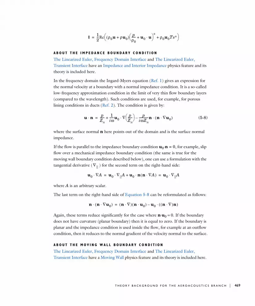
A B O U T T H E I M P E D A N C E B O U N D A R Y C O N D I T I O N

The Linearized Euler, Frequency Domain Interface and The Linearized Euler, Transient Interface have an Impedance and Interior Impedance physics feature and its theory is included here.

In the frequency domain the Ingard-Myers equation (Ref. 1) gives an expression for the normal velocity at a boundary with a normal impedance condition. It is a so-called low-frequency approximation condition in the limit of very thin flow boundary layers (compared to the wavelength). Such conditions are used, for example, for porous lining conditions in ducts (Ref. 2). The condition is given by:

(5-8)

where the surface normal n here points out of the domain and is the surface normal impedance.

If the flow is parallel to the impedance boundary condition u0·n = 0, for example, slip flow over a mechanical impedance boundary condition (the same is true for the moving wall boundary condition described below), one can use a formulation with the tangential derivative ( ) for the second term on the right-hand side:

where A is an arbitrary scalar.

The last term on the right-hand side of Equation 5-8 can be reformulated as follows:

Again, these terms reduce significantly for the case where n⋅u0 = 0. If the boundary does not have curvature (planar boundary) then it is equal to zero. If the boundary is planar and the impedance condition is used inside the flow, for example at an outflow condition, then it reduces to the normal gradient of the velocity normal to the surface.

A B O U T T H E M O V I N G W A L L B O U N D A R Y C O N D I T I O N

The Linearized Euler, Frequency Domain Interface and The Linearized Euler, Transient Interface have a Moving Wall physics feature and its theory is included here.

I 12---Re ρ0u ρu0+( ) p

ρ0------ u0 u⋅+ ∗

ρ0u0Ts∗+ =

u n⋅ pZn------ 1

iω------u0 ∇ p

Zn------ p

iωZn-------------n n ∇u0⋅( )⋅–⋅+=

∇||

u0 ∇A⋅ u0 ∇||A u0 n n ∇A⋅( )⋅+⋅ u0 ∇||A⋅= =

n n ∇u0⋅( )⋅ n ∇⋅( ) n u0⋅( ) u0 n ∇⋅( )n( )⋅–=


470 | C H A P T E R

Myers’ equation (Ref. 1) gives the expressions used for a boundary condition at a moving wall. In the frequency domain it is given by

The inward normal displacement is given by

where un is the inward normal velocity is.

In the time domain, the condition on the normal velocity is given by

where the inward normal displacement is given by vn = −n⋅v (SI unit: m).

Scattered Field Formulation for LE and LNS

The governing equations, given above in Equation 5-7 and Equation 5-6, are defined in the general scattered field formulation. Assuming that all the acoustic fields are the sum of a background (prescribed) field and the resulting scattered field, the total fields can be written as

where subscript “t” stands for total, subscript “s” for scattered, and subscript “b” for background. The scattered field is the field solved for, that is the dependent variables p, u, T, and ρ (depending on the interface). If no background acoustic field is defined (the default) the scattered field is equal to the total field. The governing equations and all boundary conditions are expressed in terms of the total fields. The background acoustic fields are defined by adding the Background Acoustic Fields feature in the LE interface or the Background Acoustic Fields feature in the LNS interface. The features have a user defined option where all fields can be entered, either as analytical expressions or defined in terms of a solution to another study or model.

u n⋅ iωvn– u0 ∇ vn( ) vnn n ∇u0⋅( )⋅+⋅–=

vn n vn⋅– iω( ) 1– un= = un n ub⋅–=

u n⋅∂vn∂t

---------– u0 ∇ vn( ) vnn n ∇u0⋅( )⋅+⋅–=

pt ps pb+= ut us ub+= Tt Ts Tb+= ρt ρs ρb+=

p ps≡ u us≡ T Ts≡ ρ ρs≡


Linearized Potential Flow

The equations presented here are the linearized potential flow equations. This restricts the applications of the physics interface to systems where the background flow is well described by a compressible potential flow, that is, a flow that is inviscid, barotropic, and irrotational. The sound sources also need to be external to the flow or at least they need to be represented by simple well defined sources. Application areas typically include modeling of how jet engine noise is influenced by the mean flow.

The basic dependent variable is the velocity potential conventionally defined by the relationship

where u = u(r, t) is the particle velocity associated with the acoustic wave motion. The total particle velocity is given by

(5-9)

where V denotes the local mean velocity for the fluid motion (the mean flow is labeled u0 in the linearized Euler and Navier–Stokes interfaces). The dynamic equations for this mean-flow field are described in the next subsection. For now, just assume V to be a given irrotational background velocity field; hence, also the mean-flow velocity can be defined in terms of a potential field Φ, by V = ∇Φ.

The linearized equation for the velocity potential , governing acoustic waves in a background flow with mean background velocity V, mean background density ρ0, and mean background speed of sound c0, is

(5-10)

In deriving this equation, all variables appearing in the full nonlinear fluid-dynamics equations were first split in time-independent and acoustic parts, in the manner of Equation 5-9. Then, linearizing the resulting equations in the acoustic perturbation and eliminating all acoustic variables except the velocity potential gives Equation 5-10. Thus, the density ρ in this equation is the time-independent part. The corresponding acoustic part is ρ(r, t) = p(r, t)/c0

2 where p is the acoustic pressure, given by

φ

u φ∇=

utot r t,( ) V x( ) u r t,( )+=

φ

ρ0

c02

------–t∂

∂t∂

∂φ V φ∇⋅+ ∇ ρ0 φ∇

ρ0

c02

------t∂

∂φ V φ∇⋅+ V–⋅+ 0=

p r t,( ) ρ0 t∂∂φ V φ∇⋅+ –=


472 | C H A P T E R

Hence, once Equation 5-10 has been solved for the velocity potential, the acoustic pressure can easily be calculated.

When transformed to the frequency domain, the wave Equation 5-10 reads

while the acoustic pressure is

Typical boundary conditions include:

• Sound-hard boundaries or walls

• Sound-soft boundaries

• Impedance boundary conditions

• Radiation boundary conditions

F R E Q U E N C Y D O M A I N E Q U A T I O N S

In the frequency domain the velocity potential is assumed to be a harmonic wave of the form

The governing frequency domain — or time-harmonic — equation is

In 2D, where

the out-of-plane wave number kz enters the equations when the ∇ operators are expanded:

ρ0

c02

------– iω iωφ V φ∇⋅+( ) ∇ ρ0 φ∇ρ0

c02

------ iωφ V φ∇⋅+( )V–⋅+ 0=

p r( ) ρ0 iωφ V φ∇⋅+( )–=

φ

φ r t,( ) φ r( )eiωt=

ρ0

c02

------– iω iωφ V φ∇⋅+( ) ∇ ρ0 φ∇ρ0

c02

------ iωφ V φ∇⋅+( )V–⋅+ 0=

φ r t,( ) φ x y,( )ei ωt kz z–( )=


The default value of the out-of-plane wave number is 0, that is, no wave propagation perpendicular to the 2D plane. In a mode analysis the equations are solved for kz.

For 2D axisymmetric components

the azimuthal wave number m similarly appears in the equation as a parameter:

T I M E - D E P E N D E N T E Q U A T I O N

In the time domain, the physics interface solves for the velocity potential with an arbitrary transient dependency. The following equation governs the acoustic waves in a mean potential flow:

(5-11)

Here ρ0 (SI unit: kg/m3) is the background mean flow density, V (SI unit: m/s) denotes the background mean velocity, and c0 (SI unit: m/s) refers to the speed of sound. The software solves the equation for the velocity potential , with SI unit m2/s. The validity of this equation relies on the assumption that ρ0, V, and c0 are approximately constant in time, while they can be functions of the spatial coordinates.

i– ωρ0

c02

------ iωφ V φ∇⋅ ikzVzφ–+( ) ∇ ρ0 φ∇ Vρ0

c02

------ iωφ V φ∇⋅ ikzVzφ–+( )–

⋅+

ρ0+ kz2φ ikzVz

ρ0

c02

------ iωφ V φ∇⋅ ikzVzφ–+( )+ 0=

φ r t,( ) φ r z,( ) ei ωt mϕ–( )=

i– ωρ0

c02

------ iωφ V φ∇⋅+( ) ∇ ρ0 φ∇ Vρ0

c02

------ iωφ V φ∇⋅+( )–

ρ 0mr2-----

2φ+⋅+ 0=

The background velocity field V cannot have an azimuthal component because the flow is irrotational.

φ

ρ0

c02

------–t∂

∂t∂

∂φ V φ∇⋅+ ∇ ρ0 φ∇

ρ0

c02

------t∂

∂φ V φ∇⋅+ V–⋅+ 0=

φ

The background velocity field V cannot have an azimuthal component because the flow is irrotational.


474 | C H A P T E R

B O U N D A R Y M O D E A N A L Y S I S

The boundary mode analysis type in 3D uses the eigenvalue solver to solve the equation

(5-12)

for the eigenmodes, , and eigenvalues, λ = −ikz, on a bounded two-dimensional domain, Ω, given well-posed edge conditions on ∂Ω. In this equation, is the velocity potential, ρ0 is the background mean flow density, c0 is the speed of sound, ω is the angular frequency, and kz is the out-of-plane wave number or propagation constant. Furthermore, Vt denotes the background mean velocity in the tangential plane while Vn is the background mean velocity component in the normal direction.

Compressible Potential Flow

Consider a compressible and inviscid fluid in some domain Ω. The motion and state of the fluid is described by its velocity V, density ρ, pressure p, and total energy per unit volume e. Its dynamics is governed by the Euler equations, expressing the conservation of mass, momentum, and energy (see General Governing Equations):

(5-13)

Here a volume force F has been included on the right-hand side of the momentum equation, whereas a possible heat-source term on the right-hand side of the energy equation (the last one) has been set to zero.

i– ωρ0

c02

------ iωφ Vt φ∇⋅( ) ikzVnφ–+( ) ∇ ρ0 φ∇ Vtρ0

c02

------ iωφ Vt φ∇⋅( ) ikzVnφ–+( )–

⋅+

ρ 0+ kz2φ ikzVn

ρ0

c02

------ iωφ V φ∇⋅( ) ikzVnφ–+( )+ 0=

φφ

Although the out-of-plane wave number is called kz, the two-dimensional surface on which Equation 5-12 is defined does not necessarily have to be normal to the z-axis for 3D geometries.

t∂∂ρ ∇ ρV( )⋅+ 0=

ρt∂

∂V V ∇⋅( )V+ p∇+ F=

∂e∂t----- ∇ e p+( )V( )⋅+ 0=


To close this system of five equations with six unknowns, an equation of state is required. Here, this is taken to be the equation for an ideal barotropic fluid,

where γ = Cp /CV is the ratio of specific heats, Cp is the specific heat at constant pressure and CV at constant volume, while pref and ρref are reference quantities for the pressure and the density, respectively. An alternative form of the ideal-fluid state equation is

The assumption that the fluid is barotropic means that p = p(ρ). Taking the total time derivative and using the chain rule, leads to the relation

where, using the equation of state,

defines the speed of sound in the ideal fluid.

Assuming the flow to be irrotational, there exists a velocity potential field Φ, such that V = ∇Φ. If, in addition, the volume force is assumed to be given by F = −ρ∇Ψ, where Ψ is referred to as the force potential, the second of Equation 5-13 can be integrated to yield the Bernoulli equation

In this equation, two additional reference quantities have entered: the velocity vref, and the force potential Ψref, both valid at the same reference point as pref and ρref. Note, in particular, that neither the pressure p, nor the energy per unit volume e, appears in this equation.

T I M E D E P E N D E N T S T U D Y

Collecting the results, the equations governing the compressible, inviscid, irrotational flow of an ideal fluid are

p prefρ

ρref-------- γ

=

p ρ γ 1–( )e=

tddp

ρddp

tddρ c2

tddρ≡=

c γ pρ---=

∂Φ∂t------- 1

2--- Φ∇ 2 γ

γ 1–-----------

prefρ

-------- ρρref-------- γ

Ψ+ + +

12---vref

2 γγ 1–( )

----------------prefρref-------- Ψref+ +=


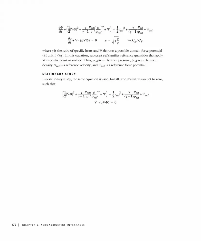
476 | C H A P T E R

where γ is the ratio of specific heats and Ψ denotes a possible domain force potential (SI unit: J/kg). In this equation, subscript ref signifies reference quantities that apply at a specific point or surface. Thus, pref is a reference pressure, ρref is a reference density, vref is a reference velocity, and Ψref is a reference force potential.

S T A T I O N A R Y S T U D Y

In a stationary study, the same equation is used, but all time derivatives are set to zero, such that

∂Φ∂t------- 1

2--- Φ∇ 2 γ

γ 1–-----------

prefρ

-------- ρρref-------- γ

Ψ+ + +

12---vref

2 γγ 1–( )

----------------prefρref-------- Ψref+ +=

t∂∂ρ ∇ ρ Φ∇( )⋅+ 0= c γ p

ρ---= γ Cp CV⁄≡

12--- Φ∇ 2 γ

γ 1–-----------

prefρ

-------- ρρref-------- γ

Ψ+ + 1

2---vref

2 γγ 1–( )

----------------prefρref-------- Ψref+ +=

∇ ρ∇Φ( )⋅ 0=


Re f e r e n c e s f o r t h e A e r o a c ou s t i c s B r an c h I n t e r f a c e s

1. M. K. Myers, “On the basic boundary condition in the presence of flow”, J. of Sound and Vibration, vol. 71, p. 429, 1980.

2. W. Eversman, “The boundary condition at an impedance wall in a non-uniform duct with potential mean flow”, J. of Sound and Vibration, vol. 246, p. 63, 2001.


4. H. Bruus, Theoretical Microfluidics, Oxford University Press, 2010.

5. G.K. Bachelor, An Introduction to Fluid Dynamics, Cambridge University Press, 2000.

6. L. D. Landau and E. M. Lifshitz, Fluid Mechanics, Course on Theoretical Physics volume 6, Butterworth-Heinemann, 2003.

7. B. Lautrup, Physics of Continuous Matter, Exotic and Every Day Phenomena in the Macroscopic World, 2nd ed., CRC Press, 2011.

8. C. M. Bender and S. A. Orszag, Advanced Mathematical Methods for Scientists and Engineers: Asymptotic Methods and Perturbation Theory, Springer, 1999.

9. C. Bogey, C. Bailly, and D. Juvé, “Computation of Flow Using Source Terms in Linearized Euler’s Equations”, AIAA Journal, vol. 40, p. 235, 2002.

10. P. P. Rao and P. J. Morris, “Use of Finite Element Methods in Frequency Domain Aeroacoustics”, AIAA Journal, vol. 44, p. 1643, 2006.

11. A. Agarwal, P. J. Morris, and R. Mani, “Calculation of Sound Propagation in Nonuniform Flows: Suppression of Instability Waves”, AIAA Journal, vol. 42, p.80, 2004.

12. C. Bailly and D. Juvé, “Numerical Solution of Acoustic Propagation Problems Using Linearized Euler Equations”, AIAA Journal, vol. 38, p. 22, 2000.

13. C. W. Tam, “Computational Aeroacoustics: Issues and Methods”, AIAA Journal, vol. 33, 1995.

R E F E R E N C E S F O R T H E A E R O A C O U S T I C S B R A N C H I N T E R F A C E S | 477

478 | C H A P T E R

14. G. Hauke and T. J. R. Hughers, “A comparative study of different sets of variables for solving compressible and incompressible flows”, Comput. Methods Appl. Mech. Engrg., vol. 153, pp. 1–44, 1998.

15. M. K. Myers, “An Exact Energy Corollary for Homentropic Flows”, J. Sound. Vib., vol. 109, pp. 277–284, 1986.

16. M. K. Myers, “Transport of energy disturbances in arbitrary steady flows”, J. Fluid Mech., vol. 226, pp. 383–400, 1991.

17. C. K. W. Tam and Z. Dong, “Radiation and Outflow Boundary Conditions for Direct Computation of Acoustic and Flow Disturbances in Nonuniform Mean Flow”, J. of Comp. Acoustics 4, pp. 175–201, 1996.

18. L. Du, A. Holmberg, M. Karlsson, and M Åbom, “Sound amplification at a rectangular T-junction with merging mean flows”, J. Sound Vib., vol. 367, pp. 69–83 2016.

19. J. Gikadi, S. Föller, T. Sattelmayer, “Impact of turbulence on the prediction of linear aerodynamic interactions: Acoustic response of a turbulent shear layer”, J. Sound Vib., vol. 333, pp. 6548–6559, 2014.

20. S. Redonnet and G. Cunha, “An advanced hybrid method for the acoustic prediction”, Adv. Eng. Softw., vol. 88, pp. 30–52, 2015.

21. J. Gikadi, “Prediction of Acoustic Modes in Cumbustors using Linearized Navier–Stokes Equations in the Frequency Domain”, Ph.D. thesis, TUM, 2013.

22. O. C. Zienkiewicz, R. L. Taylor, and P. Nithiarasu, “The Finite Element Method for Fluid Dynamics”, Butterworth-Heinemann, 7th edition, 2014.

23. G, Hauke, “Simple stabilizing matrices for the computation of compressible flows in primitive variables,” Comp. Methods. Appl. Mech. Engrg., vol. 190, pp. 6881–6893, 2001.


6

T h e r m o v i s c o u s A c o u s t i c s I n t e r f a c e s

This chapter describes the physics interfaces found under the Thermoviscous

Acoustics branch ( ).

• The Thermoviscous Acoustics, Frequency Domain Interface

• The Thermoviscous Acoustics, Transient Interface

• The Thermoviscous Acoustics, Boundary Mode Interface

• The Acoustic-Thermoviscous Acoustic Interaction, Frequency Domain Interface

• The Thermoviscous Acoustic-Solid Interaction, Frequency Domain Interface

• The Thermoviscous Acoustic-Shell Interaction, Frequency Domain Interface

• Modeling with the Thermoviscous Acoustics Branch

• Theory Background for the Thermoviscous Acoustics Branch

479

480 | C H A P T E R

Th e Th e rmov i s c o u s A c ou s t i c s , F r e qu en c y Doma i n I n t e r f a c e

The Thermoviscous Acoustics, Frequency Domain (ta) interface ( ), found under the Thermoviscous Acoustics branch ( ) when adding a physics interface, is used to compute the acoustic variations of pressure, velocity, and temperature. This physics interface is required to accurately model acoustics in geometries of small dimensions. Near walls, viscous losses and thermal conduction become important because a boundary layers exists. The thicknesses of these boundary layers are also known as the viscous and thermal penetration depth. For this reason, it is necessary to include thermal conduction effects and viscous losses explicitly in the governing equations. It is, for example, used when modeling the response of transducers like microphones, miniature loudspeakers and receivers. Other applications include analyzing feedback in hearing aids and in mobile devices, or studying the damped vibrations of MEMS structures.

The physics interface solves the equations in the frequency domain assuming all fields and sources to be harmonic. The harmonic variation of all fields and sources is given by using the +iω convention. Linear acoustics is assumed. Nonlinear effects can be included when modeling in the time domain using The Thermoviscous Acoustics, Transient Interface and the Nonlinear Thermoviscous Acoustics Contributions feature.

The equations defined by the Thermoviscous Acoustics, Frequency Domain interface are the linearized Navier-Stokes equations in quiescent background conditions solving the continuity, momentum, and energy equations (first order perturbation equations). Thermoviscous acoustics is also known as viscothermal acoustics or sometimes thermoacoustics (not to be confused with the field discussing heating and cooling using acoustics). Due to the detailed description necessary when modeling thermoviscous acoustics, the model simultaneously solves for the acoustic pressure p, the acoustic velocity variation u (particle velocity), and the acoustic temperature variations T. It is available for 3D, 2D, and 1D Cartesian geometries as well as for 2D and 1D axisymmetric geometries.

The Thermoviscous Acoustics, Frequency Domain interface is formulated in the so-called scattered field formulation where the total field (subscript t) is the sum of the

eiωt

6 : T H E R M O V I S C O U S A C O U S T I C S I N T E R F A C E S

scattered field (the field solved for, p, u, and T) and a possible background acoustic field (subscript b), such that

When no Background Acoustic Fields feature is present (the background field values are zero per default) the total field is simply the field solved for, pt = p, ut = u, and Tt = T. All governing equations and boundary conditions are formulated in the total field variables.


Builder — Thermoviscous Acoustics Model, Wall, and Initial Values. Then, from the Physics toolbar, add other nodes that implement, for example, boundary conditions and sources. You can also right-click Thermoviscous Acoustics to select physics features from the context menu.

On the Thermoviscous Acoustics Physics InterfaceThe Thermoviscous Acoustics, Frequency Domain interface solves, as mentioned, the full linearized Navier-Stokes (momentum), continuity, and energy equations. It solves for the propagation of compressible linear waves in a general viscous and thermally conductive fluid. The length scale at which the thermoviscous acoustic description is necessary is given by the thickness of the viscous boundary layer (the viscous penetration depth), which is

and the thickness of the thermal boundary layer (the thermal penetration depth)

where the definition of the symbols f, μ, ρ0, k, and Cp may be found in Table 6-1. The thickness of both boundary layers depends on the frequency f and decreases with increasing frequency. The ratio of the two length scales is related to the nondimensional Prandtl number Pr, by


For good modeling strategies, solver suggestions, postprocessing information, as well as tips and tricks, see the Modeling with the Thermoviscous Acoustics Branch section.

δvμ

πfρ0------------=

δtk

πfρ0Cp-------------------=

T H E T H E R M O V I S C O U S A C O U S T I C S , F R E Q U E N C Y D O M A I N I N T E R F A C E | 481

482 | C H A P T E R

which define the relative importance of the thermal and viscous effects for a given material. In air at 20 oC and 1 atm, the viscous boundary layer thickness is 0.22 mm at 100 Hz while it is only 55 μm in water under the same conditions. The Prandtl number is 0.7 in air and 7 in water.

The physical quantities commonly used in the thermoviscous acoustics interfaces are defined in Table 6-1 below.

δvδt-----

μCpk

----------- Pr= =

Evaluate the value of the viscous and thermal boundary layer thickness as well as the Prandtl number in postprocessing. They are defined by the variables ta.d_visc, ta.d_therm, and ta.Pr, respectively.

TABLE 6-1: THERMOVISCOUS ACOUSTICS, FREQUENCY DOMAIN PHYSICAL QUANTITIES.


Pressure (acoustic) p pascal Pa

Total acoustic pressure pt pascal Pa

Scattered acoustic pressure ps pascal Pa

Temperature variation (acoustic)

T kelvin K

Total temperature variation Tt kelvin K

Scattered temperature variation

Ts kelvin K

Acoustic velocity field u = (u, v, w) meter/second m/s

Total acoustic velocity field ut meter/second m/s

Scattered acoustic velocity field

us meter/second m/s

Dynamic viscosity μ pascal-second Pa·s

Bulk viscosity μB pascal-second Pa·s

Thermal conductivity k watt/meter-kelvin W/(m·K)

Heat capacity at constant pressure

Cp joule/meter3-kelvin J/(m3·K)

Isothermal compressibility βT 1/pascal 1/Pa

Coefficient of thermal expansion (isobaric)

αp 1/kelvin 1/K


S E T T I N G S



The default Name (for the first physics interface in the model) is ta.

E Q U A T I O N

Expand the Equation section to see the equations solved for with the Equation form specified. The default selection for Equation form is set to Study controlled. The available studies are selected under Show equations assuming.


Ratio of specific heats γ (dimensionless) 1

Frequency f hertz Hz

Wave number k 1/meter 1/m

Equilibrium pressure p0 pascal Pa

Equilibrium density ρ0 kilogram/meter3 kg/m3

Equilibrium temperature T0 kelvin K

Speed of sound c meter/second m/s

Acoustic impedance Z pascal-second/meter Pa·s/m

TABLE 6-1: THERMOVISCOUS ACOUSTICS, FREQUENCY DOMAIN PHYSICAL QUANTITIES.


As the thermoviscous acoustics physics interface solves for both pressure, velocity, and temperature, models can easily become large and contain many DOFs. See Solver Suggestions for Large Thermoviscous Acoustics Models for suggestions on how to solve large thermoviscous acoustic models.


484 | C H A P T E R

• For Frequency domain you can manually enter the scaling parameter Δ under the Thermoviscous Acoustics Equation Settings section.

• For Mode analysis you can manually enter the Mode analysis frequency (applicable in 2D and 2D axisymmetry).

T H E R M O V I S C O U S A C O U S T I C S E Q U A T I O N S E T T I N G S

Click to select Adiabatic formulation to use an adiabatic equation of state and disable the temperature degree of freedom for the thermoviscous acoustic equations. This formulation is applicable when the thermal losses can be disregarded, this is often the case in liquids, like water. In gases, like air, on the other hand the full formulation is necessary. When Adiabatic formulation is selected all temperature conditions and options are disabled in the user interface.

For all component dimensions, and if required, click to expand the Equation section, then select Frequency domain as the Equation form and enter the settings as described below.

The default Scaling factor Δ is 1/(iω). This value corresponds to the equations for a Frequency Domain study when the equations are study controlled. To get the equations corresponding to an Eigenfrequency study, change the Scaling factor Δ to 1. Changing the scaling factor influences the coupling to other physics.



T Y P I C A L W A V E S P E E D F O R P E R F E C T L Y M A T C H E D L A Y E R S

Enter a value or expression for the typical wave speed for perfectly matched layers cref (SI unit: m/s). The default is 343 m/s.


To display this section, click the Show More Options button ( ) and select Stabilization. Select No stabilization applied (the default), Galerkin least-squares (GLS)

stabilization, or Streamline upwind Petrov-Galerkin (SUPG) stabilization. When linear thermoviscous acoustic problems are solved (like in the frequency domain) the numerical problem is stable with the default P1-P2-P2 discretization. Enabling stabilization will ensure stability also for other combinations of discretization orders.


G L O B A L P O R T S E T T I N G S

Select to enable the Activate port sweep option (not selected per default). This option is used to compute the full scattering matrix when Port conditions are used. For more details see The Port Sweep Functionality subsection. The section only exists for 3D, 2D, and 2D axisymmetry.

Select the Mode shape normalization as Amplitude normalized (the default) or Power

normalized. This setting controls if the mode shapes are normalized to have a unit maximum pressure amplitude or carry unit power. The selection determines how the scattering matrix is to be interpreted.


From the list select the element order and type (Lagrange or serendipity) for the Pressure, the Velocity field, and the Temperature variation, respectively. The default is Linear for the pressure and Quadratic Lagrange for the velocity and the temperature.


This physics interface defines these dependent variables (fields): the Pressure p, the Velocity field u and its components, and the Temperature variation T. The names can

• For numerical stability reasons, the element order for the pressure should be one less than the element order for the velocity. Unless Stabilization is enabled, in which case, for example, a P1-P1-P1 discretization can be used.

• In fluids where the thermal and viscous boundary layer thickness are of the same order of magnitude (where the Prandtl number Pr is of the order 1, like in air), it is recommended to use the same element order for the temperature and the velocity. Both fields vary equally over the same length scale in the acoustic boundary layers near walls.

Choosing between Lagrange and Serendipity Shape Functions has influence on the number of DOFs solved for and on stability for distorted meshes.


486 | C H A P T E R

be changed but the names of fields and dependent variables must be unique within a model.

Domain, Boundary, and Pair Nodes for the Thermoviscous Acoustics, Frequency Domain Interface

The Thermoviscous Acoustics, Frequency Domain Interface has these domain, boundary, and pair nodes available from the Physics ribbon toolbar (Windows users), Physics context menu (Mac or Linux users), or right-click to access the context menu (all users).

• Domain, Boundary, and Pair Nodes for the Thermoviscous Acoustics, Frequency Domain Interface



• Uniform Layer Waveguide: Application Library path Acoustics_Module/Verification_Examples/uniform_layer_waveguide

• Transfer Impedance of a Perforate: Application Library path Acoustics_Module/Tutorials,_Thermoviscous_Acoustics/

transfer_impedance_perforate

• Generic 711 Coupler — An Occluded Ear-Canal Simulator: Application Library path Acoustics_Module/




Some of the following nodes are available from the Mechanical and Thermal submenus (listed in alphabetical order):

Thermoviscous Acoustics Model

Use the Thermoviscous Acoustics Model node to define the model inputs (the background equilibrium temperature and pressure) and the material properties of the fluid (dynamic viscosity, bulk viscosity, thermal conductivity, heat capacity at constant pressure, and equilibrium density) necessary to model the propagation of acoustic compressible waves in a thermoviscous acoustic context. Extended inputs are available


The Continuity node with this physics interface is available as a pair boundary condition. This gives continuity in pressure, temperature variation, velocity, and in the flux on a pair boundary between thermoviscous acoustic domains.

• Adiabatic

• Axial Symmetry


• Boundary Stress

• Heat Flux

• Heat Source

• Initial Values

• Interior Normal Impedance

• Interior Temperature Variation

• Interior Velocity

• Interior Wall

• Isothermal

• Normal Impedance

• No Slip

• No Stress


• Port

• Pressure (Adiabatic)

• Slip

• Symmetry

• Temperature Variation

• Thermoviscous Acoustics Model

• Velocity

• Wall


488 | C H A P T E R

for the coefficient of thermal expansion and the compressibility, which enables modeling of any constitutive relation for the fluid.


This section contains field variables that appear as model inputs. The fields for the Equilibrium pressure p0 and the Equilibrium temperature T0 are always active as they enter the governing equations explicitly. If material properties depend on other model inputs they will automatically appear in this section.

Select User defined (the default), Common model input, or an existing variable from another physics interface.

The Equilibrium pressure p0 (SI unit: Pa) has the default value set to 1 atm. The Equilibrium temperature T0 (SI unit: K) has the default value set to 293.15 K (that is, 20oC).


Define the material properties of the fluid by selecting an Equilibrium density — Ideal

gas, From material, or User defined.

• If From material is selected (the default), the equilibrium density, and its dependence on the equilibrium pressure p0 and temperature T0, is taken from the defined material. Make sure that the Thermal Expansion and Compressibility settings are correct.

• For Ideal gas also select the Gas constant type — select Specific gas constant Rs (SI unit: J/(kg·K) or Mean molar mass Mn (SI unit: kg/mol)

• For User defined enter a value or expression for the Equilibrium density ρ0(p0, T0) (SI unit: kg/m3). The default is ta.p0/(287[J/kg/K]*ta.T0), which is the ideal gas law.

The other thermoviscous acoustic model parameters defaults use values From material.

For User defined enter another value or expression for:




• Bulk viscosity μB (SI unit: Pa·s). The bulk viscosity parameter describes the difference between the mechanical and thermodynamic pressures. It is associated with losses due to expansion and compression.


• Heat capacity at constant pressure Cp (SI unit: J/(kg·K)). This is the specific heat capacity or heat capacity per unit mass.

T H E R M A L E X P A N S I O N A N D C O M P R E S S I B I L I T Y

One of the main characteristics of an acoustic wave is that it is a compressional wave. In the detailed thermoviscous acoustic description, this property is closely related to the constitutive relation between the density, the pressure, and the temperature. This results in the important (linear) relation for the acoustic density variation

where ρt is the total density variation, pt is the total acoustic pressure, Tt is the total acoustic temperature variations, βT is the (isothermal) compressibility of the fluid, and αp the (isobaric) coefficient of thermal expansion (sometimes named α0). If this constitutive relation is not correct, then no waves propagate or possibly they propagate at an erroneous speed of sound. The default behavior is to define both quantities from the speed of sound and the ratio of specific heats (using the From speed of sound option) which are material properties often more readily available.

Note that, when the Adiabatic formulation is selected option under the Thermoviscous Acoustics Equation Settings section the equation of stated reduces to

.

When the From equilibrium density option is selected for the coefficient of thermal expansion and the compressibility, both values are derived from the equilibrium density ρ0(p0,T0) using their defining relations

For a discussion about the air and water materials as commonly used in acoustics and other material properties, such as the bulk viscosity, see the Acoustic Properties of Fluids chapter of this manual.


ρt ρ0βspt ρ0βTγ

------pt= =

βT1ρ0------

∂ρ0∂p0---------

T0

= αp1ρ0------–

∂ρ0∂T0----------

p0

=


490 | C H A P T E R

If the equilibrium density ρ0 is a user-defined constant value, is picked up from another physics interface, or the material model does not define both a pressure and temperature dependence for ρ0, the coefficient of thermal expansion and/or the compressibility will evaluate to 0. Then the default From speed of sound option or the User defined options should be used.

The Thermal Expansion and Compressibility section is displayed if From material or User

defined is selected as the Equilibrium density under Thermoviscous Acoustics Model. For the Ideal gas option, the parameters are readily defined.

Select an option from the Coefficient of thermal expansion αp list — From material, From

equilibrium density, From speed of sound (the default), or User defined. For User defined enter a value for αp (SI unit: 1/K = K-1).

Select an option from the Isothermal compressibility βT list — From equilibrium density,

From isentropic compressibility, From speed of sound (the default), or User defined. For User defined, enter a value for βT (SI unit: 1/Pa = Pa-1).

The different options for defining the coefficient of thermal expansion and the compressibility stem from their thermodynamic definitions:

For each of the following, and based on the above selection, the default is taken From

material. For User defined enter another value or expression in the text field.


If the material is air, the From equilibrium density option works well as the equilibrium density ρ0 = ρ0(p0,T0) is defined as a function of both pressure and temperature.

For the water material the coefficient of thermal expansion is well defined as ρ0 = ρ0(T0), while the compressibility should be defined using the default From speed of sound option.

βT1ρ0------

∂ρ0∂p0---------

T

1ρ0------ γ

c2----- γβs= = =

αp1ρ0------–

∂ρ0∂T0----------

p

1c---

Cp γ 1–( )T0

------------------------= =


• Ratio of specific heats γ (dimensionless). The default is 1.

• Isentropic compressibility βs (SI unit: 1/Pa = Pa-1) .


When the Background Acoustic Fields feature is added to a domain, it is possible to define the value of the background acoustic field variables pb, ub, and Tb. Use this feature to set up scattering problems. To define fields at the inlet of a waveguide, it is recommended to use the Port condition.


This section contains field variables that appear as model inputs. The fields are always active as the equilibrium (background) temperature T0 enters the governing energy equation explicitly. It is used for the Plane wave option.

See the Theory Background for the Thermoviscous Acoustics Branch section for a detailed description of the governing equations and the constitutive relations.

To visualize the dissipated energy due to viscosity and thermal conduction in postprocessing. Three postprocessing variables exist:

• The viscous power dissipation density ta.diss_visc.

• The thermal power dissipation density ta.diss_therm.

• The total thermo-viscous power dissipation density ta.diss_tot.

In certain cases, it can be interesting not to include thermal conduction in the model and treat all processes as adiabatic (isentropic). This is, for example, relevant for most liquids where the thermal boundary layer is much thinner than the viscous. Not solving for the temperature field T also saves some degrees of freedom (DOFs). This is achieved by selecting the Adiabatic formulation option under the Thermoviscous Acoustics Equation Settings section.

See also Solver Suggestions for Large Thermoviscous Acoustics Models for suggestions on how to select an iterative solver for large problems.


492 | C H A P T E R


Select the Acoustic field type — User defined (the default) or Plane wave.

When User defined is selected, enter expressions for the Background acoustic pressure pb, the Background acoustic velocity ub, and the Background temperature variation Tb. These can be analytical expressions or values of dependent variables solved in a previous study that defines the background field.

When Plane wave is selected, enter the Pressure Amplitude |pb| (given at x = 0) and the wave direction vector ek (this vector is automatically normalized). Finally, select where the Material data should be taken from; the default is From material model (the same as the domain model material) or select a material from the list. This will set up the background pressure, velocity, and temperature variations for a plane wave with the correct thermoviscous attenuation compatible with the governing equations.

Heat Source

Use the Heat Source node to define the heat source for the thermoviscous acoustics model. This adds a domain heat source Q to the right-hand side of the energy equation.

H E A T S O U R C E

Enter a value for the Heat source Q (SI unit: W/m3).

Initial Values

The Initial Values node adds initial values for the sound pressure, velocity field, and temperature variation. If necessary, add more Initial Values nodes from the Physics toolbar to give initial values in, for example, other domains.


Enter values or expressions for the Pressure p (SI unit: Pa), Velocity field u (SI unit: m/s), and Temperature variation T (SI unit: K).

A model showcasing the plane wave background field option: Transfer Impedance of a Perforate. Application Library path Acoustics_Module/

Tutorials/transfer_impedance_perforate


Axial Symmetry


Wall

Use the Wall node to model the most common conditions at solid surfaces. This is the default boundary condition. This condition contains both a mechanical and a thermal selection. The default is a no-slip and isothermal condition applicable in most cases. More advanced conditions at boundaries can be set up by combining any of the Mechanical and Thermal conditions available.

The Wall condition is also the default condition added when the physics interface is set up. Note that the selections in this default condition can be changed (they are not locked to all boundaries). When used together with a perfectly matched layer (PML) it is recommended to use the no-slip option at the outer boundary of the layer. Specifically, using the slip condition in combination with a rational scaling in the PML will lead to a singularity and an error.

The no-slip condition is the origin of the viscous boundary layer and the isothermal condition is the origin of the thermal boundary layer. It is within these acoustic boundary layers that the main dissipation happens. See the Theory Background for the Thermoviscous Acoustics Branch section for more details.

M E C H A N I C A L


T H E R M A L




Physics Options in the Show More Options dialog box. If Slip is selected for the Mechanical

condition and Use weak constraints is enabled, then the default discontinuous Galerkin



494 | C H A P T E R

(penalty like) formulation is switched to a Lagrange multiplier formulation instead. See the Slip condition for details. For the No-slip and Isothermal selections a weak formulation is used instead of a pointwise constraint.




Pressure (Adiabatic)

Use the Pressure (Adiabatic) node to specify a prescribed pressure pbnd, that acts as a pressure source at the boundary, typically an inlet or outlet. In the frequency domain pbnd is the amplitude of a harmonic pressure source. The adiabatic condition states that no heat flows into or out of the boundary:

This condition is in general not physically correct on a solid wall because solids are generally better thermal conductors than air.

P R E S S U R E

Enter the value of the Pressure pbnd (SI unit: Pa) at the boundary. The default is 0 Pa.







pt pbnd=

ptI– μ ut∇ ut∇( )T+( ) 2μ3

------- μB– ∇ ut⋅( )I–+ n pbndn–=

n– k Tt∇–( )⋅ 0=


Symmetry

The Symmetry node for The Thermoviscous Acoustics, Frequency Domain Interface adds a boundary condition that represents symmetry. It corresponds to the Slip condition for the mechanical degrees of freedom and the Adiabatic condition for the temperature variation.







Port

The Port boundary condition is used to excite and absorb acoustic waves that enter or leave waveguide structures, like small ducts or channels, in an acoustic model. The thermoviscous port formulation ensures that the nontrivial mode shapes of the acoustic velocity and thermal fields are captured correctly.

A given port condition supports one specific propagating mode. To provide the full acoustic description, combine several port conditions on the same boundary. Typically, only the plane wave mode is propagating in small structures where the thermoviscous representation is necessary. The port condition provides a superior nonreflecting or radiation condition for waveguides compared to a simple impedance condition or a perfectly matched layer (PML) configuration. The same port boundary condition feature should not be applied to several waveguide inlets/outlets. The port condition supports S-parameter (scattering parameter) calculation but it can also be used as a source to just excite a system.

The Port boundary condition exists for 3D, 2D, and 2D axisymmetric models.


496 | C H A P T E R

On a given boundary, a combination of ports will define the total acoustic fields (sum of incident and outgoing pressure, temperature, and velocity waves) as

where the summation “i” is over all ports on the given boundary “bnd”, Sij is the scattering parameter, Ain is the amplitude of the incident field and φ the phase (at port “j”), and pi, ui, and Ti are the mode shape of the i-th port. The mode shape is normalized to have either a unit maximum amplitude (for the pressure pi) or carry unit power (see the normalization option in the Global Port Settings section). For both definitions the scattering parameter Sij defines the amplitude of mode i when a system is exited at port j (with mode j). For the power scaling, |Sij|

2 directly gives the power of the given mode. This corresponds to a multi-mode expansion of the solution on the given boundary. The scattering parameters are automatically calculated when an acoustic model is set up with just one port exciting the system. To get the full scattering matrix The Port Sweep Functionality can be used.

P O R T P R O P E R T I E S

Enter a unique Port name. Only nonnegative integer numbers can be used as Port name as it is used to define the elements of the S-parameter matrix. The numeric port names

Only one port should be excited at a time if the purpose is to compute S-parameters. The S-parameters are defined as ta.S11, ta.S21, etc. and can be used in postprocessing.

In other cases, having more than one port exciting the system might be wanted, but the S-parameter variables cannot be correctly computed. So, when several ports are excited, the S-parameter output is turned off.

If only two ports are added to the system and a port sweep is performed, the system transfer matrix and system impedance matrices are also computed.

pt Aineiφ Sij δij+( )pii bnd∈=

ut Aineiφ Sijui δij ui 2n n ui⋅( )–( )+( )i bnd∈=

Tt Aineiφ Sij δij+( )Tii b d=


are also required for the port sweep functionality. The port name is automatically incremented by one every time a port condition is added.

Select a Type of port: User defined (the default), Numeric (plane wave mode), Circular

(plane wave mode), or Slit (plane wave mode). Depending on the selection, different options appear in the Port Mode Settings section (see below). Use the Circular (plane

wave mode) for a port with a circular cross section in 3D or 2D axisymmetry and the Slit (plane wave mode) option in 2D. If the port has a different cross section then either of these, use the User defined option or the Numeric (plane wave mode) port.

P O R T M O D E S E T T I N G S

Depending on the option selected in the Type of port (see above):

• For User defined, enter user defined expressions for the Mode shape pn, un, Tn, and the Mode wave number kn (SI unit: rad/m). The mode shape will automatically be scaled before it is used in the port condition. Use the user defined option to enter a known analytical expression or to use the solution from The Thermoviscous Acoustics, Boundary Mode Interface. The solutions from the boundary mode analysis can be referenced using the withsol() operator.

• The Numeric (plane wave mode) port options is used for waveguides of arbitrary cross sections. In this case, the shape of the propagating plane wave mode (0,0) is solved on the port face. The boundary conditions for the mode are taken from the adjacent waveguide boundaries. This automatic detection works for slip, no-slip, adiabatic, isothermal, and symmetry conditions (including the same options when selected in the wall condition).

For this option, a special solver sequence is automatically generated since the port mode shape (the port variables psi, Psi_th, Psi_v, and vip) should be solved before the domain problem (the main degrees of freedom p, u, T, and Sparam1). If an iterative solver suggestion is to be used, keep the linear solver for the first segregated step and then select the iterative suggestion for the second segregated step.

• The Circular (plane wave mode) port option is used for waveguides of circular cross section. The analytical mode is a plane wave mode (0,0) given by a constant cross section pressure, no-slip condition for the velocity, and isothermal condition for the


498 | C H A P T E R

temperature. An example of the propagating mode shape in a cylindrical waveguide is seen below.

Figure 6-1: Plane wave mode for a circular duct of 1 mm diameter at f = 250 Hz.

Select how the Circle radius of the cross section is defined, either Automatic (the default) or User defined. The latter option can for some geometry configurations increase the numerical precision of the computed mode.

• The Slit (plane wave mode) port option only exists in 2D on a boundary. In 2D, the geometry is assumed infinite in the out-of-plane direction and represents a slit. The analytical mode is a plane wave mode (0,0) given by a constant cross section pressure, no-slip condition for the velocity, and isothermal condition for the temperature.


Activate if the given port is excited by an incident wave of the given mode shape. For the first Port condition added in a model, the Incident wave excitation at this port is set to On. For subsequent conditions added the excitation is set to Off per default. If more than one port in a model is excited, the S-parameter calculation is not performed.

pn |un| Tn

The solution for the numeric port is obtained using the generalized low reduced frequency (LRF) approximation commonly used in thermoviscous acoustics. The theory is based on an order of magnitude analysis of the full thermoviscous equations and on the assumption of a plane propagating mode (constant pressure in cross section). The circular and slit options use an analytical solution for the given cross section.

The mode shapes based on LRF approximation are valid as long as the wavelength is much larger than the waveguide cross section (λ >> a) and the wavelength is much larger than the boundary layer thickness (λ >> δvisc and λ >> δtherm).


When the Incident wave excitation at this port is set to On, then select how to define the incident wave. Select the Define incident wave: Amplitude (the default) or Power (Power per unit length in 2D models)

• For Amplitude enter the amplitude Ain (SI unit: Pa) of the incident wave. This is in general defined as the maximum pressure amplitude for a given mode shape.

• For Power enter the power Pin (SI unit: W) of the incident mode. In 2D models this will be a Power per unit length (SI unit: W/m).

• Enter the phase φ (SI unit: rad) of the incident wave. This phase contribution is multiplied with the amplitude defined through the above two options. The Amplitude input can be a complex number.

Note, that when the Activate port sweep option is selected at the physics level, the options in the Incident Mode Settings section are deactivated. This is because this option automatically sends in a mode of unit amplitude, sweeping through one port at the time.




All ports with incident wave excitation turned off have an arrow symbol, added in the Graphics window, that points outward. When incident wave excitation is turned on, the arrow symbol points inward.

If a waveguide is cut with one or several symmetry planes, care should be taken when setting up the port modes and when postprocessing.

For the Circular and Slit options, make sure to only select modes that are actually symmetric according to the symmetry planes.

When postprocessing, remember that absolute values like, for example, the outgoing power at port 1, ta.port1.P_out, needs to be multiplied with an appropriate factor. Multiplication with two if one symmetry plane is used etc.


500 | C H A P T E R



Physics Options in the Show More Options dialog box. See Suppressing Constraints on Lower Dimensions for details

T H E P O R T S W E E P F U N C T I O N A L I T Y

The port sweep functionality is used to reconstruct the full scattering matrix Sij by automatically sweeping the port excitation through all the ports included in the model. When the port sweep is activated, the options in the Incident Mode Settings in the port conditions are deactivated and COMSOL controls which port is excited with an incident mode.

The port sweep functionality is activated at the main physics interface level by selecting Activate port sweep in the Global Port Settings section. Enter the Sweep parameter

name, the default is PortName. Create a parameter with the same name under Global

Definitions>Parameters 1. This is the name of the parameter to be used in a parametric sweep; it should represent the Port name integer values (defined when adding the port conditions). Add a parametric sweep study step and run the sweep over the PortName parameter with an integer number of values representing all the ports in the model. Once the model is solved, the full scattering matrix can be evaluated using the defined global variables ta.S11, ta.S21, ta.S12 etc. The transmission loss (TL) between two given ports is also computed, for example, the variable for the TL loss from port 1 to 2 is given by ta.TL_12.

If only two ports are added to the thermoviscous model, COMSOL also automatically computes the transfer matrix of the system (variables ta.T11, ta.T12, ta.T21, ta.T22) and the impedance matrix of the system (ta.Z11, ta.Z12, ta.Z21, ta.Z22). These expressions are only true if plane wave modes are used. This is nearly the case in all configurations when working with microacoustic systems. For ports in thermoviscous acoustics, the Circular, Slit, and Numeric options are for plane waves only.

Use the Global Matrix Evaluation under Derived Values to evaluate the full scattering matrix ta.S.


Higher order modes can only be introduced with the User defined option. The transfer matrix representation is often used in electroacoustic modeling.

Periodic Condition

The Periodic Condition node adds a periodic boundary condition that can be used to reduce the model size by using symmetries and periodicities in the geometry and physics interfaces being modeled. This feature works well for cases like opposing parallel boundaries. In other cases, use a Destination Selection subnode to control the destination. By default, it contains the source and destination selection that COMSOL Multiphysics identifies. The periodic condition automatically defines a mapping between the source xs and the destination xd points on the boundaries.


Select a Type of periodicity: Continuity (the default), Antiperiodicity, Floquet periodicity (Bloch periodicity), Cyclic symmetry, or User Defined.

• For Continuity the values of the field variables at destination are set equal to the source: p(xd) = p(xs), u(xd) = u(xs), and T(xd) = T(xs). If the source and destination boundaries are rotated with respect to each other, a transformation is automatically performed, so that corresponding velocity components are connected.

• For Antiperiodicity the values of the field variables on the destination are set equal to the values on the source with the sign reversed: p(xd) = -p(xs), u(xd) = -u(xs), and T(xd) = -T(xs). If the source and destination boundaries are rotated with respect to each other, a transformation is automatically performed, so that corresponding velocity components are connected.

• For Floquet periodicity, also known as Bloch periodicity, enter a k-vector for Floquet

periodicity kF (SI unit: rad/m) for the x, y, and z coordinates (3D components), the r and z coordinates (2D axisymmetric components), or x and y coordinates (2D components). This is the wave number of the excitation.

This condition is used to model infinite periodic structures with nonnormal incident pressure fields or excitations. Use it to model, for example, a large perforated plate

Wax Guard Acoustics: Transfer Matrix Computation: Application Library path Acoustics_Module/Tutorials,_Thermoviscous_Acoustics/

wax_guard_acoustics


502 | C H A P T E R

with an oblique incident wave with wave vector k (and set kF = k) by only analyzing one hole or one subset of holes that is periodic.

• For Cyclic symmetry select a Sector angle: Automatic (the default) or User defined. For User defined enter a value for θS (SI unit: rad). Enter an Azimuthal mode number m (dimensionless).

This condition is used to model any geometry that has a cyclic periodic structure such as a microphone or a loudspeaker driver. Setting the azimuthal mode number determines what mode is analyzed. The response of the full system to an external excitation is in general a linear combination of many different modes.

• For User defined select the check box for any of the field variables as needed. Then for each selection, choose the Type of periodicity — Continuity or Antiperiodicity. If the source and destination boundaries are rotated with respect to each other, a transformation is automatically performed, so that corresponding velocity components are connected.

In the time domain, both the Cyclic symmetry and the Floquet periodicity boundary conditions reduce to the continuity condition.







To optimize the performance of the Floquet periodicity and the Cyclic

symmetry conditions, it is recommended that the source and destination meshes are identical. This can be achieved by first meshing the source boundary or edge and then copying the mesh to the destination boundary or edge. When the Periodic Condition stretches across regions with a mix of default material models, PMLs, background pressure fields, or background acoustic fields, it is recommended to add one Periodic

Condition for each set of such boundaries.





Interior Wall

The Interior Wall boundary condition is used to model a wall condition on an interior boundary. It is similar to the Wall boundary condition available on exterior boundaries except that it applies on both sides (up and down) of an internal boundary. It allows discontinuities (in pressure, velocity, and temperature) across the boundary. Use the Interior Wall boundary condition to avoid meshing thin structures by applying this slip-like condition on interior curves and surfaces instead.

M E C H A N I C A L


T H E R M A L





If Slip is selected for the Mechanical condition and Use weak constraints is enabled, the default discontinuous Galerkin (penalty like) formulation is switched to a Lagrange multiplier formulation instead. For the No-slip and Isothermal selections a weak formulation is used instead of a pointwise constraint.




See Orientation of Source and Destination in the COMSOL Multiphysics Reference Manual.


504 | C H A P T E R

Interior Normal Impedance

Use the Interior Normal Impedance node to apply a transfer impedance condition on an interior boundary. The condition relates the normal stress at the two sides of the boundary (up and down) to the normal velocity via the normal transfer impedance Zn. The condition allows discontinuities (a slit) in pressure and temperature depending on the condition chosen for the temperature.

M E C H A N I C A L

Enter a value or expression for the Normal impedance Zn (SI unit: Pa⋅s/m). This is the transfer impedance of the interior boundary.

Select a condition for the Tangential velocity — Slip (the default) or No slip. The No Slip option will apply an additional constraint for the velocity in the tangential direction on the two sides of the interior boundary.

T H E R M A L








Interior Velocity

Use the Interior Velocity node to specify a velocity on an interior boundary in thermoviscous acoustics. The condition can be used to specify sources, for example,

σup σdown–( )n Zn ut n⋅( )n=

σ ptI– μ ut∇ ut∇( )T+( ) 2μ3

------- μB– ∇ ut⋅( )I–+=

Znpt,down pt,up–

ut n⋅-----------------------------------=


the velocity of a diaphragm in a miniature transducer that is modeled using a lumped circuit model. The velocity components can be prescribed independently, and there is an option to force continuity in pressure across the boundary, as well as options for the thermal conditions.

M E C H A N I C A L

Select the Continuous pressure check box if the velocity condition is to be used as a source where the pressure should not be slit.

T H E R M A L




Physics Options in the Show More Options dialog box. For the Interior Velocity condition the Constraint method is set to Nodal.




Interior Temperature Variation

Use the Interior Temperature Variation condition to model a thermal type of source on an interior boundaries, Tt = Tbnd. This can, for example, be a thin sheet that has a

To define a prescribed velocity for each space direction (x and y, plus z for 3D), select one or more of the Prescribed in x direction, Prescribed in y

direction, and Prescribed in z direction check boxes. Then enter a value or expression for the prescribed velocities u0x, u0y, or u0z (SI unit: m/s).

To define a prescribed velocity for each space direction (r and z), select one or both of the Prescribed in r direction and Prescribed in z direction check boxes. Then enter a value or expression for the prescribed velocities u0r or u0z (SI unit: m/s).


506 | C H A P T E R

harmonically varying temperature, given by Tbnd, for example, due to ohmic heating. This temperature fluctuation will give rise to acoustic waves that can be modeled using the Thermoviscous Acoustics interface and this boundary condition.

M E C H A N I C A L


T H E R M A L

Enter a value or expression for the Temperature variation Tbnd (SI unit: K) that has to be applied at the interior boundary.







No Slip

The No Slip node sets up a no-slip condition for the acoustic velocity fluctuations on a hard wall. Add this node from the Mechanical submenu. The condition reads ut = 0.








Slip

Use the Slip node to prescribe zero normal velocity, and therefore also zero tangential stress, condition on the boundary. Add this node from the Mechanical submenu. The condition reads

This results in a so-called no-penetration condition where no viscous boundary layer is created. Use the condition in places where the viscous losses in the boundary layer are nonimportant. Here it is not necessary to mesh the boundary layer resulting in fewer mesh elements.

When running a model with a perfectly matched layer (PML), it is recommended not to combine a Slip condition with a rational scaling in the PML, as this will lead to a singularity and an error.

Per default, the Slip condition uses a so-called discontinuous Galerkin or penalty formulation to prevent locking problems on curved surfaces.




Select Use weak constraints if you want to switch from the default discontinuous Galerkin (penalty like) formulation to a Lagrange multiplier formulation for the slip

Mechanical and thermal boundary conditions contribute such that a condition can be set on the velocity and temperature simultaneously (they do not override). Thermal type condition override each other and the same is true for mechanical type conditions.

n ut⋅ 0=

σn σn n⋅( )n– 0=

σn ptI– μ ut∇ ut∇( )T+( ) 2μ3

------- μB– ∇ ut⋅( )I–+ n=


508 | C H A P T E R

condition (this formulation is not suited for an iterative solver). The Lagrange multiplier formulation also prevents locking problems.




Velocity

Use the Velocity node to define the prescribed velocities u0 on the boundary. Add this node from the Mechanical submenu. The condition reads ut = u0. This condition is useful, for example, when modeling a vibrating wall.

V E L O C I T Y



Physics Options in the Show More Options dialog box. For the Velocity condition the Constraint method is set to Nodal.




To define a prescribed velocity for each space direction (x and y, plus z for 3D), select one or more of the Prescribed in x direction, Prescribed in y

direction, and Prescribed in z direction check boxes. Then enter a value or expression for the prescribed velocities u0x, u0y, or u0z (SI unit: m/s).

To define a prescribed velocity for each space direction (r and z), select one or both of the Prescribed in r direction and Prescribed in z direction check boxes. Then enter a value or expression for the prescribed velocities u0r or u0z (SI unit: m/s).


No Stress

Use the No Stress node to set the total surface stress equal to zero. Add this node from the Mechanical submenu. The condition reads

Boundary Stress

Use the Boundary Stress node to define the total surface (boundary) stress through a stress tensor, a traction force, or a pressure. Add this node from the Mechanical

submenu. The stress condition reads

where is a symmetric stress tensor, the product defines a traction force. The traction condition reads

where Ftr is the surface traction force. The pressure condition reads

where pbnd is the pressure applied to the boundary (acting in the normal direction).

S T R E S S

Select a Stress type — Stress tensor, Traction (the default), or Pressure. For Stress tensor enter the (symmetric) Stress tensor (SI unit: N/m2) components, for Traction enter the traction force Ftr (SI unit: N/m2) components, and for Pressure enter the boundary pressure pbnd (SI unit: Pa).

Normal Impedance

Use the Normal Impedance node to specify a normal specific impedance Z0 on a boundary. Add this node from the Mechanical submenu. This feature is useful outside the viscous boundary layer, as this condition mimics the behavior of a corresponding

ptI– μ ut∇ ut∇( )T+( ) 2μ3

------- μB– ∇ ut⋅( )I–+ n 0=

ptI– μ ut∇ ut∇( )T+( ) 2μ3

------- μB– ∇ ut⋅( )I–+ n σpn=

σp σpn

ptI– μ ut∇ ut∇( )T+( ) 2μ3

------- μB– ∇ ut⋅( )I–+ n Ftr=

ptI– μ ut∇ ut∇( )T+( ) 2μ3

------- μB– ∇ ut⋅( )I–+ n pbndn–=

σp


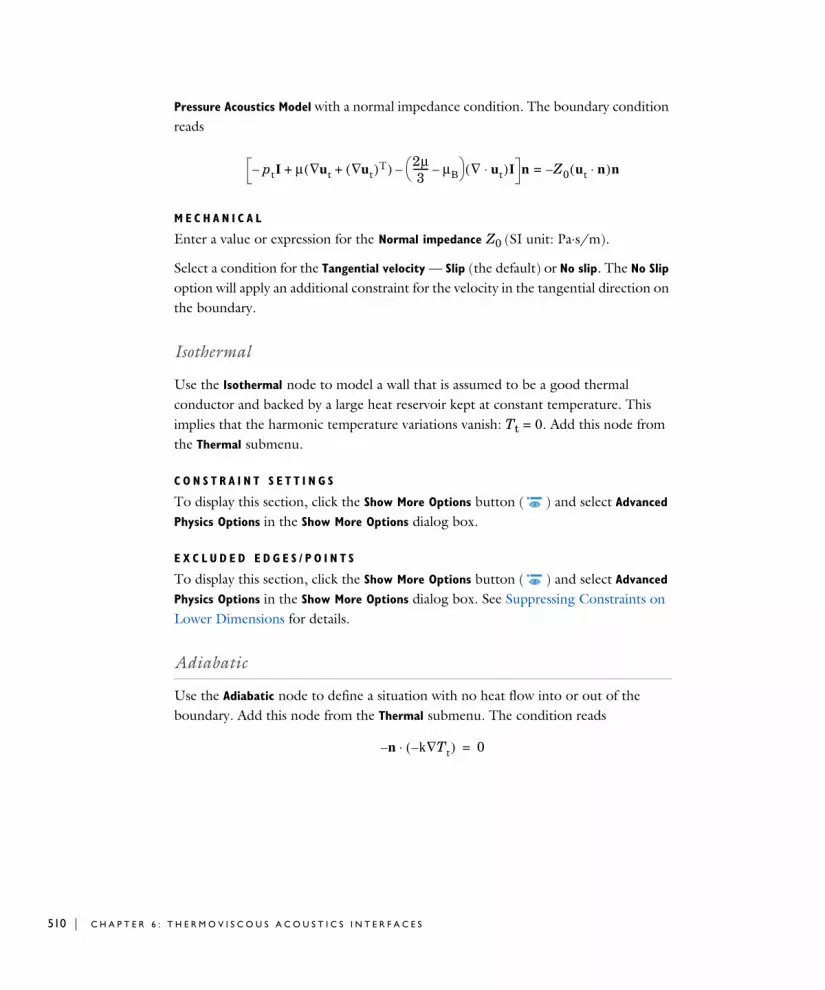
510 | C H A P T E R

Pressure Acoustics Model with a normal impedance condition. The boundary condition reads

M E C H A N I C A L

Enter a value or expression for the Normal impedance Z0 (SI unit: Pa⋅s/m).

Select a condition for the Tangential velocity — Slip (the default) or No slip. The No Slip option will apply an additional constraint for the velocity in the tangential direction on the boundary.

Isothermal

Use the Isothermal node to model a wall that is assumed to be a good thermal conductor and backed by a large heat reservoir kept at constant temperature. This implies that the harmonic temperature variations vanish: Tt = 0. Add this node from the Thermal submenu.







Adiabatic

Use the Adiabatic node to define a situation with no heat flow into or out of the boundary. Add this node from the Thermal submenu. The condition reads

ptI– μ ut∇ ut∇( )T+( ) 2μ3

------- μB– ∇ ut⋅( )I–+ n Z0 ut n⋅( )n–=

n– k Tt∇–( )⋅ 0=


Temperature Variation

Use the Temperature Variation node to define the temperature variation on the boundary Tbnd. Add this node from the Thermal submenu. In the frequency domain, this is the amplitude of a harmonic temperature variation, Tt = Tbnd.

T E M P E R A T U R E V A R I A T I O N

Enter a value or expression for the Temperature variation Tbnd (SI unit: K).







Heat Flux

Use the Heat Flux node to define a thermal source given by an inward normal heat flux qn = -n·q through the boundary. Add this node from the Thermal submenu. The condition reads

H E A T F L U X

Enter a value for the Inward normal heat flux qn (SI unit: W/m2).

n– k Tt∇–( )⋅ qn=


512 | C H A P T E R

Th e Th e rmov i s c o u s A c ou s t i c s , T r a n s i e n t I n t e r f a c e

The Thermoviscous Acoustics, Transient (tatd) interface ( ), found under the Thermoviscous Acoustics branch ( ) when adding a physics interface, is used to compute the transient evolution of the acoustic variations in pressure, velocity, and temperature. The interface is the time domain equivalent of The Thermoviscous Acoustics, Frequency Domain Interface. This physics interface is required to accurately model acoustics in geometries of small dimensions. Near walls, viscous losses and dissipation due to thermal conduction become important because boundary layers exists. The thicknesses of these boundary layers are known as the viscous and thermal penetration depth. For this reason, it is necessary to include thermal conduction effects and viscous losses explicitly in the governing equations. It is, for example, used when modeling the response of transducers like microphones, miniature loudspeakers and receivers. Other applications include analyzing feedback in hearing aids, smart phones and in mobile devices, or studying the damped vibrations of MEMS structures.

The physics interface solves the equations in the time domain. The model can be extended to model nonlinear effects by adding the Nonlinear Thermoviscous Acoustics Contributions feature. In the time domain it is also possible to model nonlinear effects due to topology changes, like nonlinear squeeze film damping. This is achieved when combining the interface with the Moving Mesh functionality.

The equations defined by the Thermoviscous Acoustics, Transient interface are the first and second order perturbation formulation of the Navier-Stokes equations in quiescent background conditions solving the continuity, momentum, and energy equations. Due to the detailed description necessary when modeling thermoviscous acoustics, the model simultaneously solves for the acoustic pressure p, the acoustic velocity variation u (particle velocity), and the acoustic temperature variations T. It is available for 3D, 2D, and 1D Cartesian geometries as well as for 2D and 1D axisymmetric geometries.

The Thermoviscous Acoustics, Transient interface is, as the frequency domain variant, formulated in the so-called scattered field formulation where the total field (subscript t) is the sum of the scattered field (the field solved for, p, u, and T) and a possible background acoustic field (subscript b), such that


The scattered field formulation is not applicable in domains where the Nonlinear Thermoviscous Acoustics Contributions are included. When no Background Acoustic Fields feature is present (the background field values are zero per default) the total field is simply the field solved for, pt = p, ut = u, and Tt = T. All governing equations and boundary conditions are formulated in the total field variables.


Builder — Thermoviscous Acoustics Model, Wall, and Initial Values. Then, from the Physics toolbar, add other nodes that implement, for example, boundary conditions and sources. You can also right-click Thermoviscous Acoustics to select physics features from the context menu.

S E T T I N G S



The default Name (for the first physics interface in the model) is tatd.


For good modeling strategies, solver suggestions, postprocessing information, as well as tips and tricks, see the Modeling with the Thermoviscous Acoustics Branch section.

For more details about the physics interface see On the Thermoviscous Acoustics Physics Interface subsection, under The Thermoviscous Acoustics, Frequency Domain Interface section. Details about the governing equations are found in the Theory Background for the Thermoviscous Acoustics Branch section.

T H E T H E R M O V I S C O U S A C O U S T I C S , T R A N S I E N T I N T E R F A C E | 513

514 | C H A P T E R

E Q U A T I O N

Expand the Equation section to see the equations solved for with the Equation form specified. The default selection for Equation form is set to Study controlled. The available studies are selected under Show equations assuming.


• For Frequency domain you can manually enter the scaling factor Δ under the Thermoviscous Acoustics Equation Settings section.

T H E R M O V I S C O U S A C O U S T I C S E Q U A T I O N S S E T T I N G S

See Thermoviscous Acoustics Equation Settings.


To display this section, click the Show More Options button ( ) and select Stabilization. Select No stabilization applied (the default), Galerkin least-squares (GLS)

stabilization, or Streamline upwind Petrov-Galerkin (SUPG) stabilization. When linear thermoviscous acoustic problems are solved, the problem is stable (with the default P1-P2-P2 discretization), but as soon as the Nonlinear Thermoviscous Acoustics Contributions feature is used, stabilization may be required. For weakly nonlinear problems no, stabilization is necessary, but for moderate and highly nonlinear problems using stabilization is essential. In most of those cases, use the Galerkin

least-squares (GLS) stabilization option.



Details about Transient Solver Settings are found in the section Modeling with the Thermoviscous Acoustics Branch.



From the list select the element order and type (Lagrange or serendipity) for the Pressure, the Velocity field, and the Temperature variation, respectively. The default is Linear for the pressure and Quadratic Lagrange for the velocity and the temperature.


This physics interface defines these dependent variables (fields), the Pressure p, the Velocity field u and its components, and the Temperature variation T. The names can be changed but the names of fields and dependent variables must be unique within a model.

Domain, Boundary, and Pair Nodes for the Thermoviscous Acoustics, Transient Interface

The Thermoviscous Acoustics, Transient Interface has these domain, boundary, and pair nodes available from the Physics ribbon toolbar (Windows users), Physics context menu (Mac or Linux users), or right-click to access the context menu (all users).

• For numerical stability reasons, the element order for the pressure should one less than the element order for the velocity. Unless Stabilization is enabled, in which case, for example, a P1-P1-P1 discretization can be used.

• In fluids where the thermal and viscous boundary layer thickness are of the same order of magnitude (where the Prandtl number Pr is of the order 1, like in air), it is recommended to use the same shape order for the temperature and the velocity. Both fields vary equally over the same length scale in the acoustic boundary layers near walls.




516 | C H A P T E R

All of the boundary conditions available with the Thermoviscous Acoustics, Transient interface are the same as for the Frequency Domain version, and are described there (see the following list). Some of the following nodes are available from the Mechanical and Thermal submenus (listed in alphabetical order):


The Continuity node with this physics interface is available as a pair boundary condition. This gives continuity in pressure, temperature variation, velocity, and in the flux on a pair boundary between thermoviscous acoustic domains.

• Adiabatic1

• Axial Symmetry1


• Boundary Stress1

• Heat Flux1

• Heat Source1

• Initial Values1

• Interior Normal Impedance1

• Interior Temperature Variation1

• Interior Velocity1

• Interior Wall1

• Isothermal1

• Nonlinear Thermoviscous Acoustics Contributions

• Normal Impedance1

• No Slip1

• No Stress1


• Pressure (Adiabatic)1

• Slip1

• Symmetry1

• Temperature Variation1


• Velocity1

• Wall1




Use the Thermoviscous Acoustics Model node to define the model inputs (the background equilibrium temperature and pressure) and the material properties of the fluid (equilibrium density, dynamic viscosity, bulk viscosity, thermal conductivity, and heat capacity at constant pressure) necessary to model the transient propagation of acoustic compressible waves in a thermoviscous acoustic context. Extended inputs are available for the coefficient of thermal expansion and the compressibility, which enables modeling of any constitutive relation for the fluid.

The equations solved are the linear (first order) perturbation equations for the conservation of mass, momentum, and energy. The model also assumes a linear equation of state relating acoustic density, pressure, and temperature fluctuations. The governing equations are given by:

(6-1)

The Model Inputs, the Thermoviscous Acoustics Model, and the Thermal Expansion and

Compressibility sections are the same as for the frequency domain interface. They are described under the Thermoviscous Acoustics Model section in The Thermoviscous Acoustics, Frequency Domain Interface.

Note that for the transient interface, it is equally important as for the frequency domain interface, to set the material parameters correctly. The values of the coefficient of thermal expansion and the isothermal compressibility are prone to errors, so make sure to take a thorough look at the Thermal Expansion and Compressibility section.

Nonlinear Thermoviscous Acoustics Contributions

The Nonlinear Thermoviscous Acoustics Contributions feature adds the necessary contributions to the governing Equation 6-1 in order to model nonlinear effects in a transient thermoviscous simulation. The contributions allow modeling of vortex shedding that may happen at sudden expansions, like in a perforate, a grill, or at a miniature sound port. Vortex shedding will in general introduce distortion in the

∂ρt∂t-------- ∇ ρ0ut( )⋅+ 0=

ρ0∂ut∂t

--------- ∇ σ⋅ F+= σ ptI– μ ut∇ ut∇( )T+( ) 2μ3

------- μB– ∇ ut⋅( )I–+=

ρ0Cp∂Tt∂t

--------- ut ∇T0⋅+ T0αp

∂pt∂t-------- ut ∇p0⋅+ – ∇ k– Tt∇( )⋅– Q+=



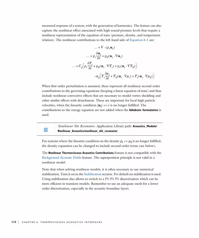
518 | C H A P T E R

measured response of a system, with the generation of harmonics. The feature can also capture the nonlinear effect associated with high sound pressure levels that require a nonlinear representation of the equation of state (pressure, density, and temperature relation). The nonlinear contributions to the left-hand side of Equation 6-1 are:

When first order perturbation is assumed, these represent all nonlinear second order contributions to the governing equations (keeping a linear equation of state) and thus include nonlinear convective effects that are necessary to model vortex shedding and other similar effects with detachment. These are important for local high particle velocities, when the linearity condition |ut| << c is no longer fulfilled. The contributions to the energy equation are not added when the Adiabatic formulation is used.

For systems where the linearity condition on the density ρt << ρ0 is no longer fulfilled, the density expansion can be changed to include second order terms (see below).

The Nonlinear Thermoviscous Acoustics Contributions feature is not compatible with the Background Acoustic Fields feature. The superposition principle is not valid in a nonlinear model.

Note that when solving nonlinear models, it is often necessary to use numerical stabilization. Turn it on in the Stabilization section. Per default no stabilization is used. Using stabilization also allows to switch to a P1-P1-P1 discretization which can be more efficient in transient models. Remember to use an adequate mesh for a lower order discretization, especially in the acoustic boundary layers.

… ∇ ρtut( )⋅+

… ρt∂ut∂t

--------- ρ0 ut ∇ut⋅( )+ +

… Cp ρt∂Tt∂t

--------- ρ0 ut ∇Tt⋅( ) ρt ut ∇T0⋅( )+ + +

αp Tt∂pt∂t-------- T0 ut ∇pt⋅( ) Tt ut ∇p0⋅( )+ +

–

Nonlinear Slit Resonator. Application Library path: Acoustics_Module/

Nonlinear_Acoustics/nonlinear_slit_resonator



The model inputs for the Equilibrium pressure p0 and the Equilibrium temperature T0 are always visible as they contribute to the governing equations.

D E N S I T Y R E P R E S E N T A T I O N

In models with high local sound pressure levels, the linear equation of state may no longer be valid. This happens when the linearity condition on the density ρt << ρ0 is no longer fulfilled. If necessary, change the default Density expansion from First order to Second order.

When Second order is selected, additional inputs to the model are necessary. For the general case, the second order derivatives of the equilibrium density ρ0 = ρ0(p0,T0) with respect to pressure p0 an temperature are necessary T0 are needed. They contribute to the second-order Taylor expansion of the density. Per default, they are taken From equilibrium density; this implies that the dependency of the density on pressure and temperature should be correct.

If the Adiabatic formulation is used (see Thermoviscous Acoustics Equation Settings), the user interface inputs correspond to the Nonlinear Acoustics (Westervelt) Contributions equation in Pressure Acoustics, Transient. Select to specify the Parameter of nonlinearity (default), the Ratio of specific heats (for gases), or the Coefficient of nonlinearity.

V I S C O U S H E A T I N G

Click to select Include viscous dissipation (disabled per default). This will add a right-hand heat source to the energy equation. The viscous dissipation is a nonlinear (second order) effect and can only be included in the nonlinear model.


When the Background Acoustic Fields feature is added to a domain, it is possible to define the value of the background acoustic field variables pb, ub, and Tb. Using this feature, it is possible to set up scattering problems as well as defining acoustic fields at an inlet of a waveguide (using a small domain at the inlet). The feature cannot be used together with the Nonlinear Thermoviscous Acoustics Contributions, as splitting into background and scattered field is not possible for nonlinear equations.


Enter expressions for the Background acoustic pressure pb, the Background acoustic

velocity ub, and the Background temperature variation Tb. These can be analytical


520 | C H A P T E R

expressions or values of dependent variables solved in a previous study that defines the background field. The time-domain version of the background acoustics field feature does not include the plane wave option available for the frequency domain interface.


Th e Th e rmov i s c o u s A c ou s t i c s , Bounda r y Mode I n t e r f a c e

The Thermoviscous Acoustics, Boundary Mode (tabm) interface ( ), found under the Thermoviscous Acoustics branch ( ) when adding a physics interface, is used to compute and identify propagating and nonpropagating modes in waveguides and ducts. The interface performs a boundary mode analysis on a given boundary, including the thermal and viscous loss effects that are important in the acoustic boundary layer near walls.

The interface is applied at boundaries which represent the cross section or the inlet of a waveguide or duct of small dimensions. It solves for the acoustic variations of pressure p, velocity u, and temperature T, as well as the out-of-plane wave number kn of the modes. Near walls, viscous losses and thermal conduction become important because boundary layers exists. The thickness of these layers is known as the viscous and thermal penetration depth. For this reason, it is necessary to include thermal conduction effects and viscous losses explicitly in the governing equations. The Thermoviscous Acoustics, Boundary Mode interface is, for example, used when setting up sources in systems with small ducts like hearing aids or mobile devices. It can also be used to identify the propagating wave number and characteristic impedance of a duct cross section and use that information in the homogenized Narrow Region Acoustics model in The Pressure Acoustics, Frequency Domain Interface.

The Thermoviscous Acoustics, Boundary Mode interface solves the equations defined by the linearized Navier-Stokes equations (linearized continuity, momentum, and energy equations), in quiescent background conditions, on boundaries, searching for the out-of-plane wave numbers at a given frequency. All gradients in the governing equations are expressed in terms of the in-plane gradient and the out-of-plane wave number that is being solved for. Due to the detailed description necessary when modeling thermoviscous acoustics, the model simultaneously solves for the acoustic pressure p, the velocity variation u (particle velocity), and the acoustic temperature

The propagation wave number is defined by the postprocessing variable tabm.kn and the (lumped) characteristic impedance by the variable tabm.Zc. Both are global variables.

T H E T H E R M O V I S C O U S A C O U S T I C S , B O U N D A R Y M O D E I N T E R F A C E | 521

522 | C H A P T E R

variations T. The interface is available on boundaries for 3D and on edges for 2D axisymmetric geometries.


Builder — Thermoviscous Acoustics Model, Wall, and Initial Values. Then, from the Physics toolbar, add other nodes that implement, for example, boundary conditions and sources. You can also right-click Thermoviscous Acoustics, Boundary Mode to select physics features from the context menu.

S E T T I N G S



The default Name (for the first physics interface in the model) is tabm.

E Q U A T I O N

Expand the Equation section to see the equations solved for with the Equation form specified. The default selection is Equation form is set to Study controlled. The available studies are selected under Show equations assuming.

• For Study controlled, the frequency used for the mode analysis study is given in the study.

• For Mode analysis you can set the frequency manually. The default Mode analysis

frequency f is 100 Hz.



For details about the governing equations, see the Theory Background for the Thermoviscous Acoustics Branch.



From the list, select the element order for the Pressure, the Velocity field, and the Temperature variation. The default uses Linear elements for the pressure and Quadratic for the velocity field and the temperature variations.

In order for the system to be numerically stable, it is important that the order for the pressure degree of freedom (DOF) is one lower than the velocity field. Per default, the velocity components and the temperature share the same element order as they vary similarly over the same length scale in the acoustic boundary layer. Therefore, both typically require the same spatial accuracy.


This physics interface defines these dependent variables (fields), the Pressure p, the Velocity field u and its components, and the Temperature variation T. The names can be changed but the names of fields and dependent variables must be unique within a model.

Increase the element order to, for example, quadratic for the pressure and cubic for the velocity and temperature dofs. This can add additional accuracy but it also adds additional degrees of freedom compared to the default setting and will be computationally more expensive.

• Domain, Boundary, and Pair Nodes for the Thermoviscous Acoustics, Frequency Domain Interface




524 | C H A P T E R

Domain, Boundary, and Pair Nodes for the Thermoviscous Acoustics, Boundary Mode Interface

The Thermoviscous Acoustics, Boundary Mode Interface has these boundary and pair nodes available from the Physics ribbon toolbar (Windows users), Physics context menu (Mac or Linux users), or right-click to access the context menu (all users).

All of the boundary conditions available with the Thermoviscous Acoustics, Boundary Mode interface are the same as for the Frequency Domain and Transient version, and are described there (see the following list). The Thermoviscous Acoustics Model



The Continuity node with this physics interface is available as a pair boundary condition. This gives continuity in pressure, temperature variation, velocity and in the flux on a pair boundary between thermoviscous acoustic domains.


feature is described here. Some of the following nodes are available from the Mechanical and Thermal submenus (listed in alphabetical order):


Use the Thermoviscous Acoustics Model node to define the model inputs (the background equilibrium temperature and pressure) and the material properties of the fluid (dynamic viscosity, bulk viscosity, thermal conductivity, heat capacity at constant pressure, and equilibrium density) necessary to model the propagation of acoustic compressible waves in a thermoviscous acoustic context. Extended inputs are available for the coefficient of thermal expansion and the compressibility, which enables modeling of any constitutive relation for the fluid.

The Model Inputs, the Thermoviscous Acoustics Model, and the Thermal Expansion and

Compressibility sections are the same as for the frequency domain and transient interfaces. They are described under the Thermoviscous Acoustics Model section in The Thermoviscous Acoustics, Frequency Domain Interface.

Note that for the boundary mode interface it is equally important as for the frequency domain and transient interfaces to set the material parameters correctly. The values of the coefficient of thermal expansion and the isothermal compressibility are prone to

• Adiabatic1

• Boundary Stress1

• Heat Flux1

• Heat Source1

• Initial Values1

• Isothermal1

• Normal Impedance1

• No Slip1

• No Stress1

• Pressure (Adiabatic)1

• Slip1

• Symmetry1

• Temperature Variation1


• Velocity1

• Wall1




526 | C H A P T E R

errors, so make sure to take a thorough look at the Thermal Expansion and Compressibility section.

B O U N D A R Y M O D E S E T T I N G S

This section contains an input for the Propagation direction n of the modes analyzed with the interface. Typically, this direction is equal to the surface or boundary normal. The default value is (tabm.nx, tabm,ny, tabm,nz) in 3D and (tabm.nr, tabm.nz) in 2D axisymmetric. When setting up models, this vector defines the positive propagation direction for the waves and thus the sign of the wave number.


Th e A c ou s t i c - T h e rmov i s c o u s A c ou s t i c I n t e r a c t i o n , F r e qu en c y Doma i n I n t e r f a c e

The Acoustic-Thermoviscous Acoustic Interaction, Frequency Domain multiphysics interface ( ), found under the Thermoviscous Acoustics branch ( ) when adding a physics interface, combines the Thermoviscous Acoustics, Frequency Domain and Pressure Acoustics, Frequency Domain interfaces together with the Acoustic-Thermoviscous Acoustic Boundary multiphysics coupling. To couple the two physics and use Thermoviscous Acoustics only where necessary can reduce the computational cost of a model.

The physics interface solves the equations in the frequency domain assuming all fields and sources to be harmonic. Linear acoustics is assumed.

When a predefined Acoustic-Thermoviscous Acoustic Interaction, Frequency Domain

interface is added from the Acoustics>Thermoviscous Acoustics branch of the Model

Wizard or the Add Physics windows, the Thermoviscous Acoustics, Frequency Domain and Pressure Acoustics, Frequency Domain interfaces are added to the Model Builder.

In addition, the Multiphysics node is added, which automatically includes the multiphysics coupling Acoustic-Thermoviscous Acoustic Boundary.


When a predefined multiphysics interface is used, for example Acoustic-Thermoviscous

Acoustic Interaction, Frequency Domain, the Selection on the multiphysics couplings is automatically set to All boundaries. In this way, the multiphysics coupling is

For details about all the multiphysics couplings in the Acoustics Module, see Multiphysics Couplings.

The use of multiphysics couplings helps improve the flexibility and design options for your modeling. For for details, see The Multiphysics Branch and Multiphysics Modeling Workflow in the COMSOL Multiphysics Reference Manual.

T H E A C O U S T I C - T H E R M O V I S C O U S A C O U S T I C I N T E R A C T I O N , F R E Q U E N C Y D O M A I N I N T E R F A C E | 527

528 | C H A P T E R

automatically active on all boundaries with Thermoviscous Acoustics, Frequency Domain

on one side and Pressure Acoustics, Frequency Domain on the other.


For example, if the single interfaces are added, COMSOL adds an empty Multiphysics node. You can choose the available multiphysics couplings, but you need to manually select on which boundaries they need to be applied, or select All boundaries to recover the predefined behavior.


Multiphysics CouplingSee Acoustic-Thermoviscous Acoustic Boundary in the Multiphysics Couplings chapter.


Multiphysics couplings are available from the context menu (right-click the Multiphysics node) or from the Physics toolbar, Multiphysics menu.




• The available physics features for The Thermoviscous Acoustics, Frequency Domain Interface are listed in the section Domain, Boundary, and Pair Nodes for the Thermoviscous Acoustics, Frequency Domain Interface.

• The available physics features for The Pressure Acoustics, Frequency Domain Interface are listed in the section Domain, Boundary, Edge, Point, and Pair Nodes for the Pressure Acoustics, Frequency Domain Interface



T H E A C O U S T I C - T H E R M O V I S C O U S A C O U S T I C I N T E R A C T I O N , F R E Q U E N C Y D O M A I N I N T E R F A C E | 529

530 | C H A P T E R

Th e Th e rmov i s c o u s A c ou s t i c - S o l i d I n t e r a c t i o n , F r e qu en c y Doma i n I n t e r f a c e

The Thermoviscous Acoustic-Solid Interaction, Frequency Domain multiphysics interface ( ), found under the Thermoviscous Acoustics branch ( ) when adding a physics interface, combines the Thermoviscous Acoustics, Frequency Domain and Solid Mechanics interfaces. The physics interface solves for, and has predefined couplings between, the displacement field in the solid and the acoustic variations in the fluid domains.


When a predefined Thermoviscous Acoustic-Solid Interaction, Frequency Domain interface is added from the Acoustics>Thermoviscous Acoustics branch of the Model Wizard or the Add Physics windows, the Thermoviscous Acoustics, Frequency Domain and Solid

Mechanics interfaces are added to the Model Builder.

In addition, the Multiphysics node is added, which automatically includes the multiphysics coupling Thermoviscous Acoustic-Structure Boundary.


When a predefined multiphysics interface is used, for example Thermoviscous

Acoustic-Solid Interaction, Frequency Domain, the Selection on the multiphysics coupling is automatically set to All boundaries. In this way, the multiphysics coupling is automatically active on all boundaries with Thermoviscous Acoustics, Frequency Domain

on one side and Solid Mechanics on the other.




For example, if the single interfaces are added, COMSOL Multiphysics adds an empty Multiphysics node. You can choose the available multiphysics couplings, but you need to manually select on which boundaries they need to be applied, or select All boundaries to recover the predefined behavior.


Multiphysics CouplingSee Thermoviscous Acoustic-Structure Boundary in the Multiphysics Couplings chapter.



• Regarding the available structural-mechanics features and their theory background, see The Solid Mechanics Interface.





T H E T H E R M O V I S C O U S A C O U S T I C - S O L I D I N T E R A C T I O N , F R E Q U E N C Y D O M A I N I N T E R F A C E | 531

532 | C H A P T E R

Th e Th e rmov i s c o u s A c ou s t i c - S h e l l I n t e r a c t i o n , F r e qu en c y Doma i n I n t e r f a c e

The Thermoviscous Acoustic-Shell Interaction, Frequency Domain multiphysics interface ( ), found under the Acoustics>Thermoviscous Acoustics branch ( ) when adding a physics interface, combines the Thermoviscous Acoustics, Frequency Domain and Shell interfaces. The physics interface solves for and has a predefined coupling between the displacement field of the shell and the acoustic variations in the fluid domains. It can be used, for example, for modeling the vibrating response of micromirrors in MEMS applications. The physics interface is available for 3D and 2D axisymmetric geometries, and it is capable of modeling the coupled thermoviscous acoustics and shell vibrations in the frequency domain.


When a predefined Thermoviscous Acoustic-Shell Interaction, Frequency Domain interface is added from the Acoustics>Thermoviscous Acoustics branch of the Model Wizard or the Add Physics windows, the Thermoviscous Acoustics, Frequency Domain and Shell interfaces are added to the Model Builder.

In addition, the Multiphysics node is added, which automatically includes the multiphysics coupling Thermoviscous Acoustic-Structure Boundary. This multiphysics coupling automatically couples the thermoviscous acoustic domain to exterior shells (on exterior boundaries) and to interior shells (on interior boundaries).

This physics interface requires a Structural Mechanics Module license. For theory and physics interface feature descriptions relating to the Shell interface, see the Structural Mechanics Module User’s Guide.




When a predefined multiphysics interface is used, for example Thermoviscous

Acoustic-Shell Interaction, Frequency Domain, the Selection on the multiphysics coupling is automatically set to All boundaries. In this way, the multiphysics coupling is automatically active on all boundaries with Thermoviscous Acoustics, Frequency Domain

on one side (exterior shells) or on both sides (interior shells) of Shell boundaries.


For example, if the single interfaces are added, COMSOL adds an empty Multiphysics node. You can choose the available multiphysics couplings, but you need to manually select on which boundaries they need to be applied, or select All boundaries to recover the predefined behavior.


Multiphysics CouplingSee Thermoviscous Acoustic-Structure Boundary in the Multiphysics Couplings chapter.





T H E T H E R M O V I S C O U S A C O U S T I C - S H E L L I N T E R A C T I O N , F R E Q U E N C Y D O M A I N I N T E R F A C E | 533

534 | C H A P T E R


• The available physics features for Results Evaluation are listed in the section Domain, Boundary, Edge, Point, and Pair Nodes for the Shell and Plate Interfaces in the Structural Mechanics Module User’s Guide




Mode l i n g w i t h t h e Th e rmov i s c o u s A c ou s t i c s B r an c h

This section contains modeling tips and tricks, information about solvers, postprocessing variables, and meshing.

In this section:

• Meshing the Boundary Layer

• Solver Suggestions for Large Thermoviscous Acoustics Models


• Transient Solver Settings


• Suppressing Constraints on Lower Dimensions

Meshing the Boundary Layer

When modeling using the Thermoviscous Acoustics interfaces, several length scales become important when setting up the mesh.

• First, there is the wavelength which should still be resolved as in pressure acoustics, see Meshing (Resolving the Waves) in the Pressure Acoustics Interfaces chapter.

• Secondly, there is the thickness of the viscous and thermal boundary layers. In order for the model to include the correct amount of damping, the boundary layers need to be resolved. Ideally this is done using a Boundary Layers mesh. The Thickness of

first boundary layer and the Number of boundary layers should be set such that they

M O D E L I N G W I T H T H E T H E R M O V I S C O U S A C O U S T I C S B R A N C H | 535

536 | C H A P T E R

resolve the boundary layer at the specific modeling frequency. Remember that the boundary layer thickness scales as one over the square root of the frequency.

Finally, it is important to consider the thickness of the boundary layer compared to the physical dimensions of the model, for example, the viscous boundary layer thickness δv compared to the tube radius a. This is sometimes known as the Womersley number

.

where δv is the viscous boundary layer thickness and Pr is the Prandtl number. If the Womersley number is very small, say Wo < 0.1, the effect associated with the losses in the viscous boundary layer can normally be disregarded. In this case, the boundary layer do not need to be meshed and a Slip condition can be used instead of a No-slip condition. The same is true for the thermal boundary layer thickness compared to the tube radius. Here, an Isothermal condition can be replaced by an Adiabatic condition.

If the No-slip or Isothermal conditions are kept (when Wo < 0.1), then remember to add at least one boundary layer mesh that is of roughly the size of the acoustic boundary layer. If this is not done, erroneous losses can be introduced in the model.

Solver Suggestions for Large Thermoviscous Acoustics Models

Solving thermoviscous acoustic problems can easily involve solving for many degrees of freedom (DOFs) as the model solves for the acoustic variations in both pressure, velocity field (2 or 3 components), and temperature. First of all, it is important to

A great deal of information about meshing and modeling with the Thermoviscous acoustics interface can be found in two COMSOL Blog posts. They are:

• www.comsol.com/blogs/theory-thermoacoustics-acoustics-thermal-viscous-losses/

• www.comsol.com/blogs/modeling-thermoacoustic-interface-comsol/

See the Boundary Layers section in the COMSOL Multiphysics Reference Manual for more details.

Wo ωρa2

μ-------------- a 2

δv----------- a

δt---- 2

Pr-------= = =


https://www.comsol.com/blogs/theory-thermoacoustics-acoustics-thermal-viscous-losses/

https://www.comsol.com/blogs/theory-thermoacoustics-acoustics-thermal-viscous-losses/

https://www.comsol.com/blogs/modeling-thermoacoustic-interface-comsol/

https://www.comsol.com/blogs/modeling-thermoacoustic-interface-comsol/

restrict the use of the thermoviscous acoustics model to domains and regions of the model where it is necessary. Couple to Pressure Acoustics using the multiphysics coupling. In the frequency domain use the Narrow Region Acoustics feature or the Thermoviscous Boundary Layer Impedance feature of Pressure Acoustics to reduce the number of DOFs. Secondly, care should be taken when meshing the computational domain. If these two things have been carefully considered, the solver can be changed from its default Direct setting to use an Iterative solver suggestion. Depending on the model size and involved physics two options are described below.

In both cases, a good starting point for setting up a new solver configuration is to right-click the study node and select Show Default Solver, then expand the Solver

Configuration tree under Stationary Solver or Time-Dependent Solver. Predefined iterative solver suggestions are automatically generated. Per default, a direct solver is used and two iterative solvers are suggested and disabled. To turn on one of these approaches, right-click the solver and select Enable (or press F4).

• The first suggestion (GMRES with Direct Precon.) uses an iterative solver with a direct preconditioner. This method is typically faster than the direct solver and uses 20% less memory.

• The second suggestion (GMRES with DD) uses an iterative solver with the domain decomposition method. This method is very robust (also for multiphysics applications) and very memory efficient, but it can be slow.

Both suggestions are described below as well as how to set them up manually (in most cases the default suggestions should be used). In liquids where thermal effects can be neglected, the model can be solved in the Adiabatic formulation and DOFs saved. Choosing different shape functions can also reduce the memory consumption, for example, switching to serendipity elements. Finally, the default P1-P2-P2 discretization can be changed to an all linear discretization if Stabilization is enabled.

• Iterative Solver with Direct Preconditioner using Hybridization

• Iterative Solver with Domain Decomposition

• Solving in the Adiabatic Case

• Choosing Shape Functions

I T E R A T I V E S O L V E R W I T H D I R E C T P R E C O N D I T I O N E R U S I N G

H Y B R I D I Z A T I O N

For large 2D problems and 3D problems, that only involve thermoviscous acoustics, using the following approach will save around 20% memory and can speed up the solution procedure by a factor 2 or 3. Under the Stationary Solver node take the


538 | C H A P T E R

following steps: Add an Iterative solver with the GMRES solver. As preconditioner add the Direct Preconditioner and switch the solver to PARDISO. Expand the Hybridization section and select Multi preconditioner in the Preconditioner variables list add the Pressure and Velocity field. Add a second direct preconditioner with the same settings but now select only the Temperature as preconditioner variables. Set the Pivoting

Perturbation to 1e-13 for the pressure-velocity group. The reason for splitting the equations up in this manner is that the energy equation is only loosely coupled to the momentum and continuity equations.

I T E R A T I V E S O L V E R W I T H D O M A I N D E C O M P O S I T I O N

A more advanced approach, to handle very large 3D models, is again to use the GMRES iterative solver but now with the domain decomposition preconditioner. This approach can also be used for multiphysics problems involving several physics.

Start by adding an Iterative solver and select GMRES as the solver. Then right-click the iterative node and select Domain Decomposition (Schwartz). A good starting point for this solver, is to use the default settings with only a few changes:

• If you set Recompute and clear subdomain data to On you will get a very memory lean solver (but the solution may take longer). Recompute and clear subdomain data is a list with the options Automatic, Off, and On. If the option Automatic is chosen, the recompute and clear mechanism is activated if there is an out-of-memory-error during the domain decomposition setup phase. The setup is then repeated with recompute and clear activated (which can be costly in terms of time, but is better than failure). A warning is given in this case.

• In the Coarse Level section change the Use coarse level to Aggregation.

• In the direct solver under the Coarse Solver and Domain Solvers subnodes use the PARDISO solver and set the Pivoting perturbation to 1e-13.

This type of approach should allow you to solve large thermoviscous acoustics models, also including multiphysics interactions, using a minimum of RAM. Possibly increase

See the Direct Preconditioner section in the COMSOL Multiphysics Reference Manual for more details.

The direct preconditioner approach is used in the model: Transfer Impedance of a Perforate. Application Library path Acoustics_Module/

Tutorials/transfer_impedance_perforate


the value of the Maximum number of DOFs per subdomain option to use a larger amount of the RAM at your disposition.

S O L V I N G I N T H E A D I A B A T I C C A S E

In certain cases, it is a good assumption to not include thermal conduction in the model and treat all processes as adiabatic (isentropic). This is, for example, relevant for fluids where the thermal boundary layer is much thinner than the viscous, like in water. Not solving for the temperature field T also saves some degrees of freedom (DOFs).

This is achieved by selecting the Adiabatic formulation option under the Thermoviscous Acoustics Equation Settings section. When Adiabatic formulation is selected, all temperature options and conditions are disabled in the user interface.

C H O O S I N G S H A P E F U N C T I O N S

In models with a structured mesh, it can be advantageous to switch to the serendipity shape functions instead of the default Lagrange, see Lagrange and Serendipity Shape Functions below. In general, if a boundary layer mesh is used (to resolve the thermal and viscous boundary layers) or if a PML is used in the model, the mesh contains structured mesh regions.


In most of the physics interfaces in the Acoustics Module and specifically in the Thermoviscous Acoustic interfaces, you can choose between two families of shape functions in the Discretization section: Lagrange and serendipity. The current default is to use Lagrange shape functions.

When using a structured mesh, it may be advantageous to switch to the serendipity elements as they generate significantly fewer degrees of freedom (DOFs). The accuracy is in most cases almost as good as for the Lagrange elements. The Lagrange elements are, however, less sensitive to strong mesh distortions.

See the Domain Decomposition (Schwarz) section in the COMSOL Multiphysics Reference Manual for more details


540 | C H A P T E R

The serendipity shape functions differ from the Lagrange shape functions only for the following element shapes:




Transient Solver Settings

When solving transient wave problems, it is recommended to use fixed time stepping in the solver (the manual option in the solver configuration). In general, there is no point in using an automatic time-step control, which can be provided by the time-dependent solver. The tolerances in the automatic error control are difficult to tune in wave problems when there is weak but important high-frequency content. It is recommended to use the suggestion generated when the Fixed (preferred) method is chosen (the default) in the Transient Solver Settings section. The internal time step of the solver that is generated, when the Maximal frequency to resolve is set, will in most cases produce a solver that is adequate. It is assuming that the user has generated a mesh that properly resolves the same maximal frequency (minimal wavelength).


This section contains information about variables for:

• Viscous and Thermal Boundary Layer Variables

• Material Properties




For further details see the Time Stepping in Transient Models section in Modeling with the Thermoviscous Acoustics Branch.


• Stress Tensor Components

• Power Dissipation and Intensity Variables

• In and Out-of-Plane Variables for the Boundary Mode Interface

V I S C O U S A N D T H E R M A L B O U N D A R Y L A Y E R V A R I A B L E S

The viscous and thermal boundary layer thickness (thermal and viscous penetration depth) as defined in Theory Background for the Thermoviscous Acoustics Branch can be evaluated in postprocessing for the frequency domain models. The same is the case for the Prandtl number relating the two length scales (available in both frequency and time domain).

M A T E R I A L P R O P E R T I E S

Material properties are readily available for postprocessing in plots. In plots, click the Replace Expression icon and browse to the Material properties list under the thermoviscous acoustics interface. Important parameters to plot are the coefficient of thermal expansion phys_id.alpha0 and the isothermal compressibility phys_id.betaT. These should not evaluate to zero.

S T R E S S T E N S O R C O M P O N E N T S

The stress tensor components are defined as variables and can be evaluated in postprocessing or used to create exotic couplings between physics. In the table below only the xx component of the stress tensor and the x component of the stress are shown. Change the spatial reference accordingly,

In the variable names, in the tables below, phys_id represents the interface name. For example, ta for the frequency domain interface, tatd for the transient interface, and tabm for the boundary mode interface.

TABLE 6-2: BOUNDARY LAYER VARIABLES


phys_id.d_visc Viscous boundary layer thickness

phys_id.d_therm Thermal boundary layer thickness

phys_id.Pr Prandtl number

TABLE 6-3: STRESS VARIABLES ONE COMPONENT IN 3D


phys_id.K_stress_tensorxx Viscous stress tensor, xx-component

phys_id.T_stress_tensorxx Total stress tensor, xx-component


542 | C H A P T E R

P O W E R D I S S I P A T I O N A N D I N T E N S I T Y V A R I A B L E S

The thermoviscous acoustics interface models the energy dissipation process which stem from viscous and thermal dissipation processes. The amount of dissipated energy can be of interest as a results analysis variable or as a source term for a multiphysics problem.

The energy conservation-dissipation corollary describes the transport and dissipation of energy in a system (see Ref. 1 p. 516 or Ref. 6). In linear acoustics, this equation is derived by taking the dot product (scalar product) of the momentum and the velocity v, adding it to the continuity equation, and then adding the entropy. After some manipulation and integration, the use of the divergence theorem yields Equation 6-2

(6-2)

where w is the disturbance energy of the control volume, u = |u| is the velocity, T is the temperature variation, p is the acoustic pressure variations, p0 is the background equilibrium pressure, T0 the background equilibrium temperature, ρ0 the background density, c0 the (isentropic) speed of sound, Cp the heat capacity at constant pressure (per unit mass), k the coefficient of thermal conduction, i is the instantaneous intensity (flux of energy out of a control volume), Δ is the dissipated energy per unit volume and time (SI unit: Pa/s = J/(m3s) = W/m3), s is the entropy, τ is the viscous stress tensor, is the viscous dissipation function, and T indicates transpose of vector. Δv and Δt are the viscous and thermal contributions to the dissipation function. In Equation 6-2 we have made use of Ref. 6 for the expression for the intensity I.

In the Thermoviscous Acoustics, Frequency Domain interface, the dissipation term Δ is directly given by the RMS value of the tensor expression

phys_id.K_stressx Viscous stress, x-component (on boundaries)

phys_id.T_stressx Total stress, x-component (on boundaries)

TABLE 6-3: STRESS VARIABLES ONE COMPONENT IN 3D


t∂∂ w Vd

Ω i n⋅( ) Ad

∂Ω+ Δ Vd

Ω–= or ∂w

∂t------- ∇ i⋅+ Δ–=

w 12---ρ0u2 1

2--- p2

ρ0c02

----------- 12---

ρ0T0Cp

-------------s2+ +=

i pu uT τ⋅[ ]T

–k

T0------T T∇–=

Δ τ:∇u kT0------ T∇( )2

+ Δv Δt+= =

τ:∇u


(6-3)

where “:” in Equation 6-3 is the double dot operator (or total inner product) and * is the complex conjugate. In the above expressions, the time averaged expressions for a product in the frequency domain is defined as:

The power dissipation variables are defined in Table 6-4.

In the Thermoviscous Acoustics, Frequency Domain interface the (time averaged) intensity I is given by averaging the instantaneous intensity vector i in Equation 6-2 using the same time averaged products defined above. The intensity and intensity magnitude are defined in Table 6-5.

In the Thermoviscous Acoustics, Transient interface the instantaneous intensity i variables is available for postprocessing. The instantaneous intensity and instantaneous intensity magnitude are defined in Table 6-6.

TABLE 6-4: POWER DISSIPATION VARIABLES


phys_id.diss_therm Thermal power dissipation density

phys_id.diss_visc Viscous power dissipation density

phys_id.diss_tot Total thermal and viscous power dissipation density

TABLE 6-5: INTENSITY VARIABLES


phys_id.Ix Intensity x-component (in 1D, 2D, and 3D)

phys_id.Iy Intensity y-component (in 2D, and 3D)

phys_id.Iz Intensity z-component (2D axisymmetric and 3D)

phys_id.Ir Intensity r-component (2D axisymmetric)

phys_id.I_mag Intensity magnitude

TABLE 6-6: INSTANTANEOUS INTENSITY VARIABLES


phys_id.Iix Instantaneous intensity x-component (in 1D, 2D, and 3D)

phys_id.Iiy Instantaneous intensity y-component (in 2D, and 3D)

phys_id.Iiz Instantaneous intensity z-component (2D axisymmetric and 3D)

Δv τ:∇u 14--- τ∗:∇u τ: ∇u( )∗+( )= =

AB Re Aeiωt( )Re Beiωt( ) 14--- A∗B AB∗+( )= =


544 | C H A P T E R

I N A N D O U T - O F - P L A N E V A R I A B L E S F O R T H E B O U N D A R Y M O D E

I N T E R F A C E

Several dedicated variables exist for The Thermoviscous Acoustics, Boundary Mode Interface where quantities are defined in terms of their in-plane and out-of-plane values. For example, the intensity variable I has the following derived values

where ip stands for in-plane and op for out-of-plane. These two variables are named tabm.Iip and tabm.Iop (with spatial components x, y, and z). The magnitude of these two variables is given by tabm.Iip_mag and tabm.Iop_mag. In the same manner variables exist for the acceleration and the velocity.

Suppressing Constraints on Lower Dimensions

Sometimes, boundary conditions on two adjacent objects can come into conflict on a shared object (point or edge). For the boundary conditions in the thermoviscous physics that are based on constraints, you have the possibility to select that certain objects of lower dimensions should be excluded from the main selection. To do this, you must first click the Show More Options button ( ) and select Advanced Physics

Options in the Show More Options dialog box. In the settings, a new section named Excluded Edges and/or Excluded Points will then appear (when applicable). In these sections, you can select geometrical objects which should be excluded from the main selection when the constraint is applied.

Velocity ConditionWhen using the mechanical Velocity condition to you may get conflicts if it is located next to a no-slip condition (a wall). To remedy this, you can exclude the common edge or point.

Periodic ConditionWhen using the Periodic Condition, you may get conflicts or duplicates which makes the model either overconstrained, or problematic for the automatic constraint elimination algorithm. If you are aware of such situations, it is good practice to remove

phys_id.Iir Instantaneous intensity r-component (2D axisymmetric)

phys_id.Ii_mag Instantaneous intensity magnitude

TABLE 6-6: INSTANTANEOUS INTENSITY VARIABLES


Iip I I n⋅( )n–=

Iop I n⋅( )n=


one of the potentially conflicting constraints. This could be in multiphysics models where you combine solid mechanics with thermoviscous acoustics and have edges where you both apply a periodic condition (solid and thermoviscous acoustics) and the Thermoviscous Acoustic- Structure Boundary multiphysics coupling.

Particularly if the geometry is curved, there is a risk that these constraints are not identical from a numerical point of view. In this case, excluding the conflicting edge from the selected boundary will make the behavior unique and fully predictable.

Another example where constraints will come in conflict is if you want to, for example, use periodic condition on parts of the geometry using weak constraints, while keeping the default pointwise constraints on other parts. If the same mesh node has both types of constraints, the solution will fail, so you must exclude any common geometrical objects from the selection in one of the constraints.

See also Excluded Surfaces, Excluded Edges, and Excluded Points in the COMSOL Multiphysics Reference Manual.


546 | C H A P T E R

Th eo r y Ba c k g r ound f o r t h e Th e rmov i s c o u s A c ou s t i c s B r an c h

The Thermoviscous Acoustics, Frequency Domain Interface, The Thermoviscous Acoustics, Transient Interface, and The Thermoviscous Acoustics, Boundary Mode Interface are designed for the analysis of acoustics in viscous and thermally conducting, compressible Newtonian fluids. The physics interface solves the linearized Navier-Stokes equation, the continuity equation, and the energy equation. This corresponds to a small parameter expansion of the dependent variables. The physics interface solves for the acoustic pressure variations p, the fluid velocity variations u, and the acoustic temperature variations T. The interface uses a scattered field formulation where it is possible to define background acoustic fields. All equations and boundary conditions are formulated in the total fields and solve for the scattered fields.

The Thermoviscous Acoustics, Frequency Domain Interface is available for 3D, 2D, and 1D Cartesian geometries as well as for 2D and 1D axisymmetric geometries. The physics interface solves problems in the frequency domain, that is, Frequency Domain, Frequency-Domain Modal, and Eigenfrequency type analysis. In 2D and 1D axisymmetric systems, a Mode Analysis study is also available for the out-of-plane component.

The Thermoviscous Acoustics, Transient Interface is available for 3D, 2D, and 1D Cartesian geometries as well as for 2D and 1D axisymmetric geometries. The physics interface solves problems in the time domain using the Time Dependent analysis type.

The Thermoviscous Acoustics, Boundary Mode Interface is available on boundaries in 3D and 2D axisymmetric geometries. The physics interface helps identify and solve for propagating and nonpropagating modes using the Mode Analysis study.

In this section:

• The Viscous and Thermal Boundary Layers

• General Linearized Compressible Flow Equations

• Acoustic Perturbation and Linearization

• Scattered Field Formulation and Background Acoustic Fields

• Formulation for Eigenfrequency Studies

• Formulation for Mode Analysis in 2D and 1D Axisymmetry


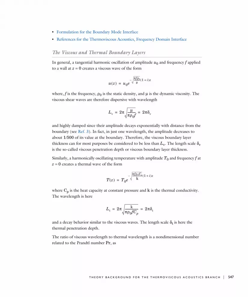
• Formulation for the Boundary Mode Interface

• References for the Thermoviscous Acoustics, Frequency Domain Interface

The Viscous and Thermal Boundary Layers

In general, a tangential harmonic oscillation of amplitude u0 and frequency f applied to a wall at z = 0 creates a viscous wave of the form

where, f is the frequency, ρ0 is the static density, and μ is the dynamic viscosity. The viscous shear waves are therefore dispersive with wavelength

and highly damped since their amplitude decays exponentially with distance from the boundary (see Ref. 3). In fact, in just one wavelength, the amplitude decreases to about 1/500 of its value at the boundary. Therefore, the viscous boundary layer thickness can for most purposes be considered to be less than Lv. The length scale δv is the so-called viscous penetration depth or viscous boundary layer thickness.

Similarly, a harmonically oscillating temperature with amplitude T0 and frequency f at z = 0 creates a thermal wave of the form

where Cp is the heat capacity at constant pressure and k is the thermal conductivity. The wavelength is here

and a decay behavior similar to the viscous waves. The length scale δt is here the thermal penetration depth.

The ratio of viscous wavelength to thermal wavelength is a nondimensional number related to the Prandtl number Pr, as

u z( ) u0eπfρ0

μ----------- 1 i+( )z–

=

Lv 2π μπρ0f------------ 2πδv= =

T z( ) T0e

πfρ0Cp

k------------------ 1 i+( )z–

=

Lt 2π kπρ0fCp------------------- 2πδt= =

T H E O R Y B A C K G R O U N D F O R T H E T H E R M O V I S C O U S A C O U S T I C S B R A N C H | 547

548 | C H A P T E R

In air, this ratio is roughly 0.8, while in water, it is closer to 2.7. Thus, at least in these important cases, the viscous and thermal boundary layers are of the same order of magnitude. Therefore, if one effect is important for a particular geometry, so is probably the other.

General Linearized Compressible Flow Equations

In general, the motion of a viscous compressible Newtonian fluid, including the energy equation, is governed by the set of equations listed in Equation 6-4 below.

(6-4)

where the dependent variables are pressure p, velocity u, temperature T, and density ρ. The first three equations are the continuity equation, the momentum equation (the Navier-Stokes equation), and the energy equation, respectively. The last three equation are the constitutive equations. They define the total stress tensor σ and the viscous stress tensor τ through Stokes expression, the Fourier heat conduction law, and an equation of state. See, for example, Ref. 1 to 7 for further details.

The material time derivatives (or total derivatives) d/dt are in the following expanded according to

where A is a dummy variable. The equation of state relates local values of pressure, density and temperature and is therefore an algebraic equation or an ODE, rather than

LvLt------

μCpk

----------- Pr= =

tddρ ρ ∇ u⋅( )+ 0=

ρtd

du ∇ σ⋅ F+=

ρCp tddT αpT

tddp

– ∇ q⋅– φ Q+ +=

σ pI– τ+ pI– μ u∇ u∇( )T+( ) 2μ3

------- μB– ∇ u⋅( )I–+= =

q k– T∇=

ρ ρ p T,( )=

dA x t,( )dt

--------------------- ∂A∂t------- u A∇⋅+=


a PDE. A common form of state equations is to know the density as function of pressure and temperature, ρ = ρ(p, T). In the following, it is assumed that the state equation has this form.

The basic properties of the fluid are the dynamic viscosity μ and thermal conductivity k. The coefficient μB is the bulk (or second) viscosity and describes losses due to compressibility (expansion and contraction of the fluid), where μ describes losses due to shear friction. The bulk viscosity can in some cases be used to model an empirically observed deviation from Stokes’ assumption but is usually negligible compared to μ unless the motion is irrotational; see Ref. 3 and Ref. 4. These three properties are taken to be constant or at most weakly temperature-dependent. The specific heat at constant pressure Cp (per unit mass) and the (isobaric) coefficient of volumetric thermal expansion αp (sometimes denoted α0),

are both possibly functions of pressure and temperature.

In the energy equation

is the viscous dissipation function — that is, the scalar contraction of the viscous stress tensor τ with the rate of strain tensor S. Both tensors are seen as functions of a velocity vector. If the mean velocity is zero, this term vanishes in the following linearization because it is homogeneous of second order in the velocity gradients. Otherwise, it acts as an oscillating source or sink (the term is included in the full Linearized Navier-Stokes interfaces). In the right sides of Equation 6-4, F and Q are a volume force and a heat source, respectively.

Acoustic Perturbation and Linearization

For small perturbations around steady-state solution, the dependent variables and sources can be assumed to take on the following form:

αp1ρ---

T∂∂ρ

–p

=

φ τ u( ):S u( ) τ u( ): u∇= =


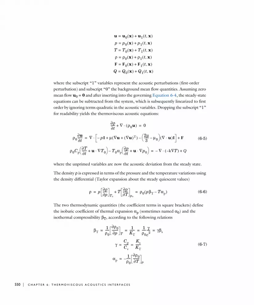
550 | C H A P T E R

where the subscript “1” variables represent the acoustic perturbations (first-order perturbation) and subscript “0” the background mean flow quantities. Assuming zero mean flow u0 = 0 and after inserting into the governing Equation 6-4, the steady-state equations can be subtracted from the system, which is subsequently linearized to first order by ignoring terms quadratic in the acoustic variables. Dropping the subscript “1” for readability yields the thermoviscous acoustic equations:

(6-5)

where the unprimed variables are now the acoustic deviation from the steady state.

The density ρ is expressed in terms of the pressure and the temperature variations using the density differential (Taylor expansion about the steady quiescent values)

(6-6)

The two thermodynamic quantities (the coefficient terms in square brackets) define the isobaric coefficient of thermal expansion αp (sometimes named α0) and the isothermal compressibility βT, according to the following relations

(6-7)

u u0 x( ) u1 t x,( )+=

p p0 x( ) p1 t x,( )+=

T T0 x( ) T1 t x,( )+=

ρ ρ0 x( ) ρ1 t x,( )+=

F F0 x( ) F1 t x,( )+=

Q Q0 x( ) Q1 t x,( )+=

∂ρ∂t------ ∇ ρ0u( )⋅+ 0=

ρ0∂u∂t------- ∇ pI– μ u∇ u∇( )T+( ) 2μ

3------- μB– ∇ u⋅( )I–+⋅ F+=

ρ0Cp∂T∂t------- u ∇T0⋅+ T0αp

∂p∂t------ u ∇p0⋅+ – ∇ k– T∇( )⋅– Q+=

ρ p ∂ρ∂p------

T0

T ∂ρ∂T-------

p0

+ ρ0 pβT Tαp–( )= =

βT1ρ0------

∂ρ0∂p---------

T

1KT------- 1

ρ0------ γ

c2----- γβs= = = =

γCpCv-------

KsKT-------= =

αp1ρ0------–

∂ρ0∂T---------

p=


where Ks is the isentropic bulk modulus (sometimes named K0), KT the isothermal bulk modulus, Cv is the heat capacity at constant volume (per unit mass), c is the (isentropic) speed of sound, and γ is the ratio of specific heats (the adiabatic index). The isothermal compressibility βT is related to the isentropic (or adiabatic) compressibility βs (sometimes named β0) and the coefficient of thermal expansion αp via the thermodynamic relations

(6-8)

It is derived using the Maxwell relations; see, for example, Ref. 5 and Ref. 7.

From Equation 6-7 and Equation 6-8 the isothermal compressibility and the isobaric coefficient of thermal expansion can be expressed in terms of the speed of sound as

(6-9)

The equations presented in Equation 6-5 and Equation 6-6 are the ones solved in the time domain in The Thermoviscous Acoustics, Transient Interface. Assuming small harmonic oscillations about a steady-state solution, the dependent variables and sources can be assumed to take on the following form

Inserting this into the governing equations and performing the linearization yield the equations solved in the frequency domain in The Thermoviscous Acoustics, Frequency Domain Interface:

(6-10)

The system of equations implemented in the thermoviscous acoustics interfaces is further given in a scattered field formulation, as described below in Scattered Field Formulation and Background Acoustic Fields.

βs βTαp

2T0ρ0Cp-------------–= βT γβs=

βT1ρ0------ γ

c2-----= αp

1c---

Cp γ 1–( )T0

------------------------=

u u0 u1eiωt+= p p0 p1eiωt+=

T T0 T1eiωt+= ρ ρ0 ρ1eiωt+=

F F0 F1eiωt+= Q Q0 Q1eiωt+=

iωρ ∇ ρ0u( )⋅+ 0=

iωρ0u ∇ pI– μ u∇ u∇( )T+( ) 2μ3

------- μB– ∇ u⋅( )I–+⋅ F+=

ρ0Cp iωT u ∇T0⋅+( ) T0αp iωp u ∇p0⋅+( )– ∇ k– T∇( )⋅– Q+=

ρ ρ0 pβT Tαp–( )=


552 | C H A P T E R

When the Adiabatic formulation option under the Thermoviscous Acoustics Equation Settings section the solved equations reduce to:

(6-11)

where the temperature T depends directly on the acoustic pressure p.

I D E A L G A S

For an ideal gas, the equation of state p = ρRT, where R is the specific gas constant, leads to

and the density

Inserting these expressions and dividing the continuity equation by the reference density, Equation 6-10 in the frequency domain take on the following simplified form

This is, for example, the system of equations implemented in the Thermoviscous Acoustics, Frequency Domain interface when the ideal gas law is selected.

I S E N T R O P I C ( A D I A B A T I C ) I D E A L G A S C A S E

If the process is assumed to be adiabatic and reversible — that is, isentropic — the thermal conductivity is effectively zero. Then also the temperature can be eliminated, giving for the ideal gas case:

iωρ ∇ ρ0u( )⋅+ 0=

iωρ0u ∇ pI– μ u∇ u∇( )T+( ) 2μ3

------- μB– ∇ u⋅( )I–+⋅ F+=

ρ ρ0βsp= TαpT0ρ0Cp-------------p=

βT1p0------= α0

1T0------=

ρ ρ0pp0------ T

T0------–

=

iω pp0------ T

T0------–

∇ u⋅+ 0=

iωρ0u ∇ pI– μ u∇ u∇( )T+( ) 2μ3

------- μB– ∇ u⋅( )I–+⋅=

iω ρ0CpT p–( ) u ∇p0 ρ0Cp u ∇T0⋅( )+⋅+ ∇ k– T∇( )⋅– Q+=


(6-12)

where we have assumed constant background properties. Defining the speed of sound c in analogy with the standard assumptions for linear acoustics (term in front of the pressure in the continuity equation), it is found that

or

In the case with a general fluid, the corresponding relation is using Equation 6-7 and Equation 6-8:

where K0 is the adiabatic bulk modulus, KT the isothermal bulk modulus, and α0 the coefficient of thermal expansion.

I S O T H E R M A L C A S E

If, on the other hand, the thermal conductivity is high, or the thermoviscous acoustic waves propagate in a narrow space between highly conductive walls, the temperature can be assumed to be constant (isothermal assumption) and the system of equations for an ideal gas becomes:

which, again comparing to standard assumptions, gives

iω 1p0------ 1

ρ0CpT0--------------------–

p ∇ u⋅+ 0=

iωρ0u ∇ pI– μ u∇ u∇( )T+( ) 2μ3

------- μB– ∇ u⋅( )I–+⋅=

1ρ0c2------------ 1

p0------ 1

ρ0CpT0--------------------–

1p0------ 1 R

Cp-------–

1γp0---------= = =

cγp0ρ0---------=

1ρ0c2------------ 1

K0------- 1

ρ0------

∂ρ0∂p---------

T

T0ρ0Cp------------- 1

ρ0------

∂ρ0∂T---------

p

2–

1KT-------

T0αp2

ρ0Cp-------------–= = =

iωρ0u ∇ pI– μ u∇ u∇( )T+( ) 2μ3

------- μB– ∇ u⋅( )I–+⋅=

iω 1p0------ p ∇ u⋅+ 0=


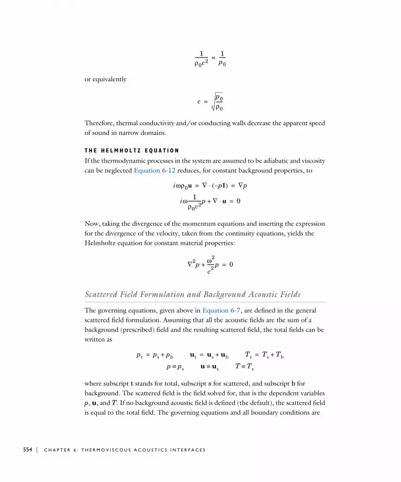
554 | C H A P T E R

or equivalently

Therefore, thermal conductivity and/or conducting walls decrease the apparent speed of sound in narrow domains.

T H E H E L M H O L T Z E Q U A T I O N

If the thermodynamic processes in the system are assumed to be adiabatic and viscosity can be neglected Equation 6-12 reduces, for constant background properties, to

Now, taking the divergence of the momentum equations and inserting the expression for the divergence of the velocity, taken from the continuity equations, yields the Helmholtz equation for constant material properties:

Scattered Field Formulation and Background Acoustic Fields

The governing equations, given above in Equation 6-7, are defined in the general scattered field formulation. Assuming that all the acoustic fields are the sum of a background (prescribed) field and the resulting scattered field, the total fields can be written as

where subscript t stands for total, subscript s for scattered, and subscript b for background. The scattered field is the field solved for, that is the dependent variables p, u, and T. If no background acoustic field is defined (the default), the scattered field is equal to the total field. The governing equations and all boundary conditions are

1ρ0c2------------ 1

p0------=

cp0ρ0------=

iωρ0u ∇ pI–( )⋅ ∇p= =

iω 1ρ0c2------------p ∇ u⋅+ 0=

∇2p ω2

c2------p+ 0=

pt ps pb+= ut us ub+= Tt Ts Tb+=

p ps≡ u us≡ T Ts≡


expressed in terms of the total fields. The equations solved for are thus, in general, for the frequency domain case given by

(6-13)

The background acoustic fields are defined by adding the Background Acoustic Fields feature. The feature has a user defined option where all fields can be entered, either as analytical expressions or defined in terms of a solution to another study or model. The background acoustic fields feature also has a plane-wave option (in the frequency domain interface) that defines a plane propagating attenuated wave.

P L A N E W A V E S O L U T I O N

The plane wave option in the Background Acoustic Fields feature (in the frequency domain only) defines the following fields

(6-14)

where kb is the is the wave number of a plane propagating wave (in the direction nk) with viscous and thermal attenuation, see Ref. 3. The expressions given in Equation 6-14 are an exact solution to the governing equations Equation 6-13.

Formulation for Eigenfrequency Studies

When performing an eigenfrequency study, the governing equations (Equation 6-7) are on the form:

iωρt ∇ ρ0ut( )⋅+ 0=

iωρ0ut ∇ ptI– μ ut∇ ut∇( )T+( ) 2μ3

------- μB– ∇ ut⋅( )I–+⋅=

ρ0Cp iωTt ut ∇T0⋅+( ) T0αp iωpt ut ∇p0⋅+( )– ∇ k– Tt∇( )⋅– Q+=


pb pb ekb nk x⋅( )–

=

ubω βTpb αpTb–( )

kb------------------------------------------nk=

TbiωαpT0pb

iωρ0Cp kkb2

+------------------------------------=

kbωc---- 1

iωbtv

ρ0c2--------------+

12---

= btv43---μ μB

γ 1–( )kCp

--------------------+ +=


556 | C H A P T E R

where the eigenvalue is λ = −iω. It is important to note that there is a difference between regular pressure acoustics and thermoviscous acoustics in terms of what modes can exist and which modes are found during an eigenfrequency study. In pressure acoustics only the pure acoustic modes exist; the equations and assumptions made ensure this. In thermoviscous acoustics, on the other hand, the equations are formulated for all small signal components that can exist. This means that other nonacoustic modes also exist, that is, thermal and vorticity modes.

V O R T I C I T Y A N D T H E R M A L M O D E S

When solving an eigenfrequency problem in thermoviscous acoustics, it is important to take a close look at the obtained eigenfrequencies and assess if they are acoustic or not. The nature of the solution is of the form

where λ is the eigenvalue. Typically, eigenvalues exist near the positive real axis, where β ≈ 0. These are exponentially decaying nonacoustic (nonoscillating) modes that stem from the thermal equation or the deviatoric part of the momentum equation (the nonpressure and nonvolume part of the stress tensor) also called the vorticity modes. The acoustic eigenvalues on the other hand lie close to the imaginary axis and are oscillating and slightly damped.

O T H E R S P U R I O U S M O D E S

Note that other spurious and nonacoustic modes can also exist when, for example, a PML layer is used to model an open boundary. These modes stem from nonphysical phenomena and the scaling inside the PML layer. In all cases, it is a good idea to have an a priori knowledge of the location/type of the eigenvalues, maybe from solving an lossless pressure acoustics model, and also to look at the modes in terms of, for example, the pressure field.

λρ– ∇ ρ0u( )⋅+ 0=

λρ0– u ∇ pI– μ u∇ u∇( )T+( ) 2μ3

------- μB– ∇ u⋅( )I–+⋅=

ρ– 0Cp λTt ut ∇T0⋅+( ) T0αp λpt ut ∇p0⋅+( )+ ∇ k– T∇( )⋅– Q+=

ρ ρ0 βTp αpT–( )=

p x t,( ) p x( )e λt–∼ p x( )eiωt= λ α iβ+= ω β– iα+=


Formulation for Mode Analysis in 2D and 1D Axisymmetry

The Mode Analysis study type is available for The Thermoviscous Acoustics, Frequency Domain Interface in 2D and 1D axisymmetric models. This type of study is used to determine the form of the propagating acoustic modes in waveguide structures. The analyzed 2D and 1D axisymmetric geometries can be thought of as the cross sections of a waveguide. This study is really restricted to the cross section of the waveguides. To calculate the modes in 3D structures at the inlet of the waveguide use The Thermoviscous Acoustics, Boundary Mode Interface, described below.

The spatial dependency in the (out-of-plane) axial z direction along the waveguide is assumed to be of the form of a traveling wave with wave number kz. The dependent variables in 2D are rewritten as

and in 1D axisymmetric as

Using this form of the dependent variables, differentiation with respect to z reduces to a multiplication with −ikz. The propagating modes are determined by solving an eigenvalue problem in the variable λ = −ikz.

The expression for the pressure can now be written retaining the harmonic time dependency, as

where x is the in plane coordinate(s). The axial wave number is split into a real and an imaginary part. The imaginary part α of the wave number describes how fast the propagating modes decay along the waveguide, it is often referred to as the attenuation coefficient. The real part β is related to the phase speed cph of the propagating mode by cph = β/ω. In thermoviscous acoustics, the obtained wave numbers always have an

p p x y,( )e ikzz–=

u u x y,( )e ikzz–=

T T x y,( )e ikzz–=

p p r( )e ikzz–=

u u r( )e ikzz–=

T T r( )e ikzz–=

kz β iα+=

p p x( )e ikzz–eiωt p x( )eαzei ωt βz–( )

= =


558 | C H A P T E R

imaginary part as the modeled system always includes losses. The relation between the angular frequency ω and the axial wave number kz is called the dispersion relation.

Formulation for the Boundary Mode Interface

The Thermoviscous Acoustics, Boundary Mode Interface interface adds extended functionality to the abovementioned mode analysis available in 2D and 1D axisymmetric geometries. The interface can be applied on boundaries in 3D (and 2D axisymmetric) geometries and can be used to compute the propagating modes and out-of-plane wave number kn on a (flat) surface of any orientation in 3D. This makes it possible to more easily set up boundary conditions at inlets of waveguides using the mode information.

The equations solved are the same as for The Thermoviscous Acoustics, Frequency Domain Interface but using modified expressions for the gradients. The implementation assumes propagation in the out-of-plane direction (that is, in the normal direction n), and the fields can then be written as

where xip is the in-plane coordinate, xop is the out-of-plane coordinate, and kn is the wave number that this formulation computes. Because of the above assumption about the acoustic fields, the gradient operator can be split into a tangential in-plane component (||) and an normal out-of-plane component (⊥), such that

The in-plane gradient is defined in COMSOL Multiphysics by the tangential derivative operator dtang(). The divergence of the velocity field is defined as the trace of the Jacobian, that is

• Mode Analysis in the COMSOL Multiphysics Reference Manual

p p xip( )e iknxop–=

u u xip( )e iknxop–=

T T xip( )e iknxop–=

∇p ∇||p iknpn–=

∇u ∇||u ikn u nT⋅( )–=

∇T ∇||T iknTn–=


With the above modifications and redefinition of the gradient operators, solving for the propagating modes reduces to an eigenvalue problem solving for the acoustic field and the out-of-plane wave number for a given frequency.

References for the Thermoviscous Acoustics, Frequency Domain Interface

1. W.M. Beltman, P.J.M. van der Hoogt, R.M.E.J. Spiering, and H. Tijdeman, “Implementation and Experimental Validation of a New Viscothermal Acoustic Finite Element for Acousto-Elastic Problems”, J. Sound and Vibration, vol. 216, pp. 159–185, 1998.

2. M. Malinen, M. Lyly, and others, “A Finite Element Method for the Modeling of Thermo-Viscous Effects in Acoustics”, Proc. ECCOMAS 2004, Jyväskylä, 2004.


4. H. Bruus, Theoretical Microfluidics, Oxford University Press, 2010.

5. G.K. Bachelor, An Introduction to Fluid Dynamics, Cambridge University Press, 2000.

6. M.K. Myers, “Transport of energy by disturbances in arbitrary steady flows,” J. Fluid Mech., vol. 226, pp. 383–400, 1991.

7. B. Lautrup, Physics of Continuous Matter, Exotic and Every Day Phenomena in the Macroscopic World, 2nd ed., CRC Press, 2011.

8. A.S. Dukhin and P.J. Goetz, “Bulk viscosity and compressibility measurements using acoustic spectroscopy,” J. Chem. Phys., vol. 130, p. 124519-1, 2009.

9. M. S. Cramer, “Numerical estimate for the bulk viscosity of ideal gases,” Phys. Fluids, vol. 30, pp. 066102, 2012.

∇ u⋅ trace ∇u( )=


560 | C H A P T E R

7

U l t r a s o u n d I n t e r f a c e s

This chapter describes the physics interfaces found under the Acoustics>Ultrasound

branch ( )

• The Convected Wave Equation, Time Explicit Interface

• The Nonlinear Pressure Acoustics, Time Explicit Interface

• Modeling with the Convected Wave Equation Interface

• Modeling with the Nonlinear Pressure Acoustics, Time Explicit Interface

• Theory for the Convected Wave Equation Interface

• Theory for the Nonlinear Pressure Acoustics, Time Explicit Interface

• References for the Ultrasound Interface

561

562 | C H A P T E R

Th e Con v e c t e d Wav e Equa t i o n , T ime Exp l i c i t I n t e r f a c e

The Convected Wave Equation, Time Explicit (cwe) interface ( ), found under the Acoustics>Ultrasound subbranch ( ) when adding a physics interface, is used to solve large transient linear acoustic problems containing many wavelengths in a stationary background flow. It is suited for time-dependent simulations with arbitrary time-dependent sources and fields. In general, the interface is suited for modeling the propagation of acoustic signals over large distances relative to the wavelength, for example, linear ultrasound problems. Application areas include ultrasound flowmeters and other ultrasound sensors where time of flight is an important parameter. The applications are not restricted to ultrasound. The interface includes absorbing layers that are used to set up effective nonreflecting like boundary conditions. The interface exists in 2D, 2D axisymmetric, and 3D.


In the no-flow case it can be advantageous to use The Pressure Acoustics, Time Explicit Interface instead. The equations are the same but the latter interface has more options to, for example, model scattering phenomena using a scattered field formulation and a background acoustic field.

The interface solves the linearized Euler equations assuming an adiabatic equation of state. The dependent variables are the acoustic pressure p and the acoustic velocity perturbation u. The background mean flow can be any stationary flow with small to moderate velocity gradients. General bulk dissipation (volumetric damping) can be added to model real fluids.


Builder — Convected Wave Equation Model, Sound Hard Wall, Initial Values, and Axial

When solving models that are based on the dG method, optimizing the mesh is important. For further details see Optimizing the Mesh for DG in the Meshing, Discretization, and Solvers section.

7 : U L T R A S O U N D I N T E R F A C E S

Symmetry (in case of 2D axisymmetric). Then, from the Physics toolbar, add other nodes that implement, for example, boundary conditions. You can also right-click Convected Wave Equation, Time Explicit to select physics features from the context menu.

S E T T I N G S



The default Name (for the first physics interface in the model) is cwe.




Absorbing Layers section you can change and control the values set for the filter used in the Absorbing Layers. The values of the filter parameters defined here are used in all absorbing layers added to the model and they override the value of filter parameters enabled in the material model (Convected Wave Equation Model). The default values of the filter parameters α, ηc, and s are set to 0.1, 0.01, and 2, respectively. Inside the absorbing layer it is important to use a filter that is not too aggressive since this will result in spurious reflections.

E Q U A T I O N S E T T I N G S ( 2 D A X I S Y M M E T R I C O N L Y )

This section is only available in 2D Axisymmetric. Per default the acoustic velocity perturbation u is assumed to have only two components: the radial component ur and the axial component uz. You can select the Include out-of-plane components check box to enable the third — circumferential component , which physically can only be nonzero if the background mean flow has the corresponding component.


uϕ

T H E C O N V E C T E D W A V E E Q U A T I O N , T I M E E X P L I C I T I N T E R F A C E | 563

564 | C H A P T E R



velocity. Per default both are set to Quartic (4th order). Using quartic elements together with a mesh size equal to approximately half the wavelength to be resolved, leads to the best performance when using the dG method. For further details see the Meshing, Discretization, and Solvers section.


The dependent variables (field variables) are the Acoustic pressure, Acoustic velocity, and Acoustic velocity, components. The names can be changed, but the names of fields and dependent variables must be unique within a model.

Domain, Boundary, Edge, Point, and Pair Nodes for the Convected Wave Equation Interface

The Convected Wave Equation, Time Explicit Interface has these domain, boundary, edge, point, and pair nodes, listed in alphabetical order, available from the Physics ribbon toolbar (Windows users), Physics context menu (Mac or Linux users), or

• For information about modeling strategies, meshing, the absorbing layer and more, see Modeling with the Convected Wave Equation Interface.

• For the theoretical background of the model solved, see Theory for the Convected Wave Equation Interface.

• Gaussian Pulse in 2D Uniform Flow: Convected Wave Equation and Absorbing Layers. The Application Library path: Acoustics_Module/Tutorials,_Pressure_Acoustics/ gaussian_pulse_absorbing_layers

• Ultrasound Flowmeter with Generic Time-of-Flight Configuration.

The Application Library path: Acoustics_Module/Ultrasound/ultrasound_flow_meter_generic

• Ultrasonic Flowmeter with Piezoelectric Transducers: Coupling Between FEM and DG. The Application Library path: Acoustics_Module/Ultrasound/flow_meter_piezoelectric_transducers


right-click to access the context menu (all users). Continuity in pressure and velocity is the default condition on interior boundaries.

Convected Wave Equation Model

The Convected Wave Equations node adds the equations for modeling the propagation of acoustic waves in a stationary background flow. Adiabatic behavior is assumed, meaning that this in some sense represents pressure acoustics in the presence of flow. The convected wave equation model solves the linearized Euler equations also referred to as linear acoustic equations for moving media. The equations are valid for any stationary background mean flow as long as there are not too large gradients in the background properties.

The linear continuity equation, momentum equation, and equation of state solved are given by:


• Acoustic Impedance

• Convected Wave Equation Model

• Domain Sources


• Initial Values


• Interior Wall

• Normal Velocity

• Pressure

• Sound Hard Wall

• Symmetry



566 | C H A P T E R

where u0 is the background mean flow velocity, p0 is the background mean flow pressure, ρ0 is the background mean flow density, and c0 is the speed of sound. All background properties can vary in space. The right-hand side sources fp and fv can be defined by the Domain Sources. More information about the governing equations is given in the Theory for the Convected Wave Equation Interface section.

In the Settings window, define the properties for the acoustics model and model inputs including the background mean flow, pressure, and velocity.


In order to model the influence the background mean flow has on the propagation of the acoustic waves in the fluid, the Background mean flow pressure p0 and Background

mean flow velocity u0 need to be defined. If a material that is temperature dependent is used the Background mean flow temperature T0 field is also present.

All the background mean flow parameters can be functions of space. They can be either analytical expressions (user defined) or they can be picked up from a fluid flow simulation performed using the CFD Module. In this case use the Background Fluid Flow Coupling multiphysics feature to ensure correct mapping of the flow data. By default they are set to the quiescent constant background conditions of air.


Select a Fluid model either as Linear elastic (the default) or General dissipation. For both options define the background mean flow density ρ0 (SI unit: kg/m3) and the background mean flow speed of sound c0 (SI unit: m/s). The default is to use the property values from the material (From material). Select User defined from the list to enter a user-defined value in the text field that appears. For the General dissipation option also define the Sound diffusivity δ (SI unit: m2/s). For numerical stability reasons it is recommended to use physical values of attenuation properties.

∂ρ∂t------ u0 ∇⋅( )ρ u ∇⋅( )ρ0 ρ ∇ u0⋅( ) ρ0 ∇ u⋅( )+ + + + fp=

∂u∂t------- u0 ∇⋅( )u u ∇⋅( )u0

1ρ0------∇p ρ

ρ02

------∇p0–+ + + fv=

ρ p

c02

-----=


The density can also be picked up from a fluid flow simulation when the Background Fluid Flow Coupling multiphysics feature is used.

L A X – F R I E D R I C H S F L U X P A R A M E T E R

To display this section, click the Show More Options button ( ) and select Stabilization in the Show More Options dialog box. In this section, you specify the value of the Lax–Friedrichs flux parameter τLF (default value: 0.2). This value controls the numerical flux between the elements (nodal discontinuous Lagrange elements) used with the discontinuous Galerkin (dG) method. The numerical flux defines how adjacent elements are connected and how continuous p and u are. Different definitions of the numerical flux lead to different variants of the dG method. The flux implemented here is the so-called global Lax–Friedrichs numerical flux. The value of the parameter τLF should be between 0 and 0.5. For τLF = 0 a so-called central flux is obtained. Setting τLF = 0.5 gives a maximally dissipative global Lax–Friedrichs flux.



Physics Options in the Show More Options dialog box. By default, the filter parameters α, ηc, and s are not active. Select the Activate check box to activate the filter. The filter provides higher-order smoothing for the dG formulation and can be used to stabilize the solution, for example, when a large background flow is present or large gradients are present. Inside absorbing layers the settings given here are overridden by the Filter Parameters for Absorbing Layers.

Enter values for the filter parameters in the corresponding text fields (default values: 36, 0.6, and 3). α must be positive and lie between 0 and 36. α = 0 means no dissipation and α = 36 means maximal dissipation. ηc should be between 0 and 1, where 0 means maximal filtering and 1 means no filtering (even if filtering is active). The s parameter should be larger than 0 and controls the order of the filtering (a

The relation between the sound diffusivity δ and the equivalent (plane wave) attenuation coefficient α, at a given frequency f, is given by the expression , where ω = 2πf and c is the speed of sound.α δω2 2c3( )⁄=



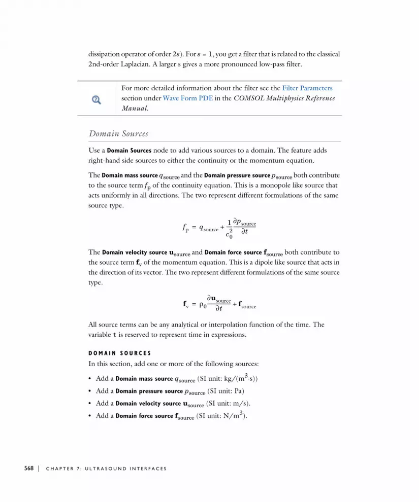
568 | C H A P T E R

dissipation operator of order 2s). For s = 1, you get a filter that is related to the classical 2nd-order Laplacian. A larger s gives a more pronounced low-pass filter.

Domain Sources

Use a Domain Sources node to add various sources to a domain. The feature adds right-hand side sources to either the continuity or the momentum equation.

The Domain mass source qsource and the Domain pressure source psource both contribute to the source term fp of the continuity equation. This is a monopole like source that acts uniformly in all directions. The two represent different formulations of the same source type.

The Domain velocity source usource and Domain force source fsource both contribute to the source term fv of the momentum equation. This is a dipole like source that acts in the direction of its vector. The two represent different formulations of the same source type.

All source terms can be any analytical or interpolation function of the time. The variable t is reserved to represent time in expressions.


In this section, add one or more of the following sources:

• Add a Domain mass source qsource (SI unit: kg/(m3·s))

• Add a Domain pressure source psource (SI unit: Pa)

• Add a Domain velocity source usource (SI unit: m/s).

• Add a Domain force source fsource (SI unit: N/m3).


fp qsource1

c02

-----∂psource

∂t-------------------+=

fv ρ0∂usource

∂t-------------------- fsource+=


Sound Hard Wall

The Sound Hard Wall adds a boundary condition for a sound hard boundary or wall, which is a boundary at which the normal component of the velocity is zero (a slip condition). This is assumed true for both the acoustic velocity and the background velocity

Note that this condition is not identical to the Symmetry condition where only the normal component of the acoustic velocity is assumed to be zero.

Initial Values




Normal Velocity

The Normal Velocity adds an inward normal velocity either given as a scalar vn or as a velocity vector vb, the condition given is

where n is the surface normal. Both expressions should be functions of time. This feature represents an external source term. It can also be used to model a vibrating transducer surface or other vibrating surfaces.


Select a Type — Inward Velocity (the default) or Velocity.

• For Inward Velocity enter an expression for the Inward velocity vn(t) (SI unit: m/s). Use a positive value for inward velocity or a negative value for outward velocity.

• For Velocity enter expressions for the components of the Velocity vb(t) (SI unit: m/s).

n– u⋅ 0= n– u0⋅ 0=

n– u⋅ vn t( ) n vb t( )⋅–= =


570 | C H A P T E R

Pressure

The Pressure node creates a boundary condition that acts as a pressure source at the boundary. The acoustic pressure is given at the boundary p = pb(t).

P R E S S U R E

Enter an expression for the Boundary pressure pb (SI unit: Pa).

Symmetry


Acoustic Impedance

The Acoustic Impedance node adds a boundary condition defining a relation between the local acoustic pressure p and the normal acoustic velocity n·u, that is, the acoustic impedance Z. The condition specifies the inward normal velocity

This condition can be used to model the properties of artificial boundaries. When the impedance is set equal to the characteristic specific impedance of a propagating plane wave ρ0c0, the condition represent the simplest nonreflecting boundary condition. This is also the default value of the impedance when the impedance condition is added.

Note that this condition is not equivalent to the general impedance condition, as given by Myers (see Ref. 4), when a flow is present. This means that, for example, it cannot be used at a reacting surface which has a tangential flow. For this kind of detailed conditions a frequency domain representation is needed.

The acoustic impedance condition (with the default value ρ0c0) should be used at the outer boundary when Absorbing Layers are used in a model.

n– u⋅ 0=

n– u⋅ pZ----–=


A C O U S T I C I M P E D A N C E

Enter a value or expression for the Acoustic Impedance Z (SI unit: Pa·s/m). The default expression is cwe.c0*cwe.rho0 which is the characteristic specific impedance ρ0c0 of a propagating plane wave.

Interior Wall

The Interior Wall node adds the boundary condition for a sound hard boundary or wall on interior boundaries. The condition reads

The condition ensures that the normal velocity is zero on both the up and down side of the boundary, while applying a slit on the pressure (the pressure is discontinuous across the boundary). The condition also assumes that the background flow has a similar condition applied at the boundary.


The Interior Normal Velocity node adds the boundary condition for a moving interior boundary. This can, for example, represent a thin vibrating structure or s speaker membrane. The condition reads

The condition ensures that the normal velocity is defined on both the up and down side of the boundary, while applying a slit on the pressure (the pressure is discontinuous across the boundary).


Select the Type: Velocity (default) or Inward velocity and specify either the Velocity (vector) vb(t) or the normal component through the Inward normal velocity vn(t).

General Flux/Source

The General Flux/Source node, found under the More submenu, adds the most general boundary condition for the convected wave equation, as it is formulated (in the

uup n⋅ udown n⋅ 0= =

u0 up, n⋅ u0 down, n⋅ 0= =

ut,up n⋅ vb t( ) n⋅ vn t( )–= =

ut,down n⋅ vb t( ) n⋅ vn t( )–= =


572 | C H A P T E R

conservative form) for the discontinuous Galerkin method (dG). The condition defines the normal flux g at an exterior boundary, given by

where u = (u, v, w), u0 = (u0, v0, w0), and n = (nx, ny, nz) (n = (nr, , nz) in 2D axisymmetric) is the surface normal. Care should be taken when using this advanced condition as the method is sensitive to proper formulation of boundary conditions. Only one characteristic can enter the domain at any boundary at the time, meaning that it is easy to over-specify the problem. Use the mesh normals (nxmesh, nymesh, and nzmeshor, respectively, nrmesh, nphimesh, and nzmesh) in the expression you define.




The General Interior Flux node, found under the More submenu, adds a the most general interior boundary condition for the convected wave equation, as it is formulated (in the conservative form) for the discontinuous Galerkin method (dG). The condition defines the normal flux g on an interior boundary by

here Γ* represents the total numerical flux. This means that if this condition is added on an interior boundary it overrides the existing Lax–Friedrichs numerical flux. So care should be taken when specifying this condition as it needs to include the necessary numerical flux contribution to ensure stability of the method.

On an interior boundary you can use the up() and down() operators to access values from both sides of the boundary. If a dependent variable is used in this expression

n Γ⋅–

ρ0 n u⋅( ) p

c02

----- n u0⋅( )+

p

c02

-----u0 n u0⋅( ) ρ0 u n u0⋅( ) u0 n u⋅( )+( ) n1p+ +

p

c02

-----v0 n u0⋅( ) ρ0 v n u0⋅( ) v0 n u⋅( )+( ) n2p+ +

p

c02

-----w0 n u0⋅( ) ρ0 w n u0⋅( ) w0 n u⋅( )+( ) n3p+ +

g= =

nϕ

n Γ∗⋅– g=


(without up() or down() operators) an implicit mean() operation is invoked taking the average of the up and down side values. Use the mesh normals (nxmesh, nymesh, and nzmesh or, respectively, nrmesh, nphimesh, and nzmesh) in the expression you define.




574 | C H A P T E R

Th e Non l i n e a r P r e s s u r e A c ou s t i c s , T ime Exp l i c i t I n t e r f a c e

The Nonlinear Pressure Acoustics, Time Explicit (nate) interface ( ), found under the Acoustics>Ultrasound subbranch ( ) when adding a physics interface, is used to model the propagation of nonlinear finite amplitude acoustic waves in computational domains that contain many wavelengths. It is suited for time-dependent simulations with arbitrary time-dependent sources and fields. Absorbing layers are used to set up effective nonreflecting-like boundary conditions. Application areas include biomedical applications, for instance, ultrasonic imaging and high-intensity focused ultrasound (HIFU). The applications are not restricted to ultrasound. The interface exists in 2D, 2D axisymmetric, and 3D.


In the linear case it can be advantageous to use The Pressure Acoustics, Time Explicit Interface instead, for example, when modeling scattering phenomena using a scattered field formulation and a background acoustic field. This split is not possible for nonlinear problems. In the presence of a stationary background flow and linear propagation the The Convected Wave Equation, Time Explicit Interface should be used, for example, when modeling ultrasonic flow meters.

For modeling acoustic-structure interaction (ASI) or vibroacoustic problems the interface is fully multiphysics enabled and can be coupled to the The Elastic Waves, Time Explicit Interface, using either the Acoustic-Structure Boundary, Time Explicit or the Pair Acoustic-Structure Boundary, Time Explicit multiphysics couplings.

The interface solves the second-order nonlinear governing equations for the acoustic pressure p and the acoustic velocity perturbations u. The interface is suited for modeling progressive wave propagation phenomena when the cumulative nonlinear effects surpass the local nonlinear effects. Thus the model is consistent with the second-order Westervelt equation for the acoustic pressure (see also the Nonlinear Acoustics (Westervelt) Contributions feature available with The Pressure Acoustics, Transient Interface). General bulk dissipation (volumetric damping) can be added to model real fluids.


Several features are available to help solve the nonlinear and highly nonlinear problems including the use of a numerical Limiter (to capture shocks) but also the use of Adaptive Mesh Refinement.

S E T T I N G S



The default Name (for the first physics interface in the model) is nate.




Absorbing Layers section you can change and control the values set for the filter used in the Absorbing Layers. The values of the filter parameters defined here are used in all absorbing layers added to the model and they override the value of filter parameters enabled in the material model (Nonlinear Pressure Acoustics, Time Explicit Model). The default values of the filter parameters α, ηc, and s are set to 0.1, 0.01, and 2, respectively. Inside the absorbing layer it is important to use a filter that is not too aggressive since this will result in spurious reflections.

N U M E R I C A L F L U X

To display this section, click the Show More Options button ( ) and select Stabilization

in the Show More Options dialog box. Only one option exists for the Numerical flux formulation used in the numerical scheme when solving the dG problem. For Lax–Friedrichs (the only option) enter the Lax–Friedrichs flux parameter τLF (default is 0.2). The value of the parameter τLF should be between 0 and 0.5. A parameter value of 0 represents a central flux, which is the least dissipative but also the least stable numerical flux. A parameter value of 0.5 gives a maximally dissipative global Lax–Friedrichs flux (see The Lax–Friedrichs Flux).


T H E N O N L I N E A R P R E S S U R E A C O U S T I C S , T I M E E X P L I C I T I N T E R F A C E | 575

576 | C H A P T E R

L I M I T E R

To display this section, click the Show More Options button ( ) and select Stabilization

in the Show More Options dialog box. The limiter is used to control and stabilize highly nonlinear problems with shock formation. The limiter can only be used with linear discretization. For details see the Solving Highly Nonlinear Problems section in Modeling with the Nonlinear Pressure Acoustics, Time Explicit Interface.



velocity (the same is used for both). Per default both are set to Quartic (4th order). Using quartic elements together with a mesh size equal to approximately one and a half of the wavelength to be resolved, leads to the best performance when using the dG method.


The dependent variables are the Acoustic pressure, and the Acoustic velocity. The names can be changed, but the names of fields and dependent variables must be unique within a model. The name for the Acoustic velocity, components can also be selected individually.

• For an example of a highly nonlinear problem that uses the WENO limiter see the Nonlinear Propagation of a Cylindrical Wave — Verification Model tutorial model. The Application Library path Acoustics_Module/Nonlinear_Acoustics/ nonlinear_cylindrical_wave

• For an example of a nonlinear problem with pulse propagation that uses mesh adaptation see the High-Intensity Focused Ultrasound (HIFU) Propagation Through a Tissue Phantom tutorial model. The Application Library path Acoustics_Module/

Nonlinear_Acoustics/hifu_tissue_sample

• For information specific to modeling nonlinear problems using the time explicit interface, see Modeling with the Nonlinear Pressure Acoustics, Time Explicit Interface.

• For information about modeling strategies, meshing, the absorbing layer and more, see the relevant information in the Modeling with the Convected Wave Equation Interface.


Domain, Boundary, Edge, and Point Nodes for the Nonlinear Pressure Acoustics, Time Explicit Interface

The Nonlinear Pressure Acoustics, Time Explicit Interface has the following domain and boundary conditions listed in alphabetic order, available from the Physics ribbon toolbar (Windows users), Physics context menu (Mac or Linux users), or right-click to access the context menu (all users). Continuity in velocity and pressure is the default condition on interior boundaries. If a boundary separates two different materials the Material Discontinuity or Continuity condition (the pair version of material discontinuity condition) has to be applied to ensure the continuity in velocity and pressure.

Nonlinear Pressure Acoustics, Time Explicit Model

The Nonlinear Pressure Acoustics, Time Explicit Model node adds the equations for modeling the propagation of nonlinear acoustic waves. The nonlinear continuity equation and momentum equation solved are given by:

(7-1)

• Continuity



• Heat Source

• Impedance

• Initial Values



• Mass Source


• Nonlinear Pressure Acoustics, Time Explicit Model

• Normal Velocity

• Pressure



• Symmetry

• Volume Force Source

1

ρc2---------

∂pt∂t-------- ∇ 1

βpt

ρc2---------+

ut⋅+ Qm=

ρ∂ut∂t

--------- ∇ ptI( )⋅+ qd=

pt p= ut u=


578 | C H A P T E R

where pt is the total acoustic pressure and ut is the total acoustic velocity fluctuations. Because the problem solved is nonlinear the superposition principle does not apply which means that the “total” fields are always equal to the dependent variables.

In the Settings window, define the properties for the acoustics model, model inputs, and material properties.


Depending on the material selected enter values for the Model Inputs, typically the Temperature T, the Pressure pA, and possibly the Relative Humidity .


Select the Fluid model — Linear elastic, Viscous, Thermally conducting, Thermally

conducting and viscous, General dissipation, or Ideal gas. The settings are the same as for the Pressure Acoustics, Time Explicit Model.

C O E F F I C I E N T O F N O N L I N E A R I T Y

Select how to define the Coefficient of nonlinearity β — From parameter of nonlinearity (default) or User defined. The Parameter of nonlinearity B/A can be taken From material or entered as a User defined expression. For the Ideal gas fluid model, it is also possible to compute the Coefficient of nonlinearity β From ratio of specific heats.



Physics Options in the Show More Options dialog box. By default, the filter parameters α, ηc, and s are not active. Select the Activate check box to activate the filter. The filter provides higher-order smoothing for the DG formulation. Inside absorbing layers the settings given here are overridden by the Filter Parameters for Absorbing Layers.

Initial Values


φ





Mass Source

The Mass Source sets up the right-hand side of the continuity equation, in Equation 7-1, in terms of a mass rate of change. This is a monopole-like source that acts uniformly in all directions.

M A S S S O U R C E

Enter the Mass source M (SI unit: kg/(m3·s)).

Heat Source

The Heat Source sets up the right-hand side of the continuity equation, in Equation 7-1, in terms of a heat density source. This is a monopole-like source that acts uniformly in all directions.

where αp is the (isobaric) coefficient of thermal expansion, ρ is the density, Cp is the heat capacity at constant pressure, and Qheat is the heat source.

M O D E L I N P U T

Enter the ambient Temperature T, the default is 293.15[K].

H E A T S O U R C E

Enter the Heat Source Qheat (SI unit: W/m3).


Enter the Heat capacity at constant pressure Cp and the Ratio of specific heats γ either selected From material or User defined. The ratio of specific heats is used to calculate the coefficient of thermal expansion through the thermodynamic relation

Qm1ρ---M=

Qmαp

ρCp----------Qheat=


580 | C H A P T E R

Volume Force Source

The Volume Force Source sets up the right-hand side of the momentum equation, in Equation 7-1, in terms of a volumetric force. This is a dipole-like source that acts differently in two directions.

V O L U M E F O R C E S O U R C E

Enter the Volume force source F (SI unit: N/m3).


The Sound Hard Boundary (Wall) adds a boundary condition for a sound hard boundary or wall, which is a boundary at which the normal component of the velocity is zero (a slip condition)

The condition is also available from the Pairs submenu, as an option at interfaces between parts in an assembly. This effectively introduces a condition similar to the Interior Sound Hard Boundary (Wall) but used on an assembly.

Sound Soft Boundary

The Sound Soft Boundary conditions adds a boundary condition for a sound soft boundary, where the acoustic pressure vanishes pt = 0. It is an appropriate approximation, for example, for a liquid-gas interface or in some cases for external waveguide ports.

Pressure

The Pressure node creates a boundary condition that acts as a pressure source at the boundary. The total acoustic pressure is given at the boundary pt = p0(t).

αp1c---

Cp γ 1–( )T

------------------------=

qd F=

n ut⋅ 0=


P R E S S U R E

Enter an expression for the Pressure p0(t) (SI unit: Pa). The input can be any analytical function or interpolation data that can be function of both time and space.

Symmetry


Normal Velocity

The Normal Velocity condition adds a source specified in terms of an inward normal velocity vn(t) or velocity v0(t) of the boundary. The component in the normal direction is used to define the boundary condition. This feature represents an external source term like a vibrating surface. The condition is also available from the Pairs submenu, as an option at interfaces between parts in an assembly. This effectively introduces a condition similar to the Interior Normal Velocity but used on an assembly.



• For Inward Velocity enter the value of the Inward velocity vn (SI unit: m/s).


Impedance

The Impedance condition adds a boundary condition defining the relation between the local acoustic pressure p and the normal acoustic velocity n·ut, that is, the specific acoustic impedance Zi. The model includes the option to define the nonlinear or second order pressure-velocity relation to extend the validity of the impedance condition to higher pressure amplitudes.

The second order impedance expression specifies how the normal velocity relates to the pressure through the impedance, including a correction factor, according to

n ut⋅ 0=


582 | C H A P T E R

This condition can be used to model the properties of artificial boundaries by adding resistive losses (no reactive components can be added). When the impedance is set equal to the characteristic specific impedance of a propagating plane wave ρc, the condition represent the simplest nonreflecting boundary condition. This is also the default value of the impedance when the condition is added.

The acoustic impedance condition (with the default value ρc) should be used at the outer boundary when Absorbing Layers are used in a model.

I M P E D A N C E

Select the Pressure-particle velocity relation used for the impedance formulation First order (default) or Second order. Enter a value or expression for the Impedance Zi (SI unit: Pa·s/m). The default expression is nate.c*nate.rho which is the characteristic specific impedance ρc of a propagating plane wave (linear theory).


The Interior Sound Hard Boundary (Wall) node, found under the Interior Conditions

submenu, adds the boundary condition for a sound hard boundary or wall on interior boundaries. The condition reads

The condition ensures that the total normal velocity is zero on both the up and down side of the boundary, while applying a slit on the pressure (the pressure is discontinuous across the boundary).


The Interior Normal Velocity node, found under the Interior Conditions submenu, adds the boundary condition for a moving interior boundary. This can, for example, represent a thin vibrating structure or s speaker membrane. The condition reads

n ut⋅ptZi----- 1

βpt

2ρc2------------–

=

ut, up n⋅ 0=

ut, down n⋅ 0=

ut, up n⋅ v0 t( ) n⋅ vn t( )–= =

ut, down n⋅ v0 t( ) n⋅ vn t( )–= =


The condition ensures that the total normal velocity is defined on both the up and down side of the boundary, while applying a slit on the pressure (the pressure is discontinuous across the boundary).


Select the Type: Velocity (default) or Normal velocity and specify either the Velocity (vector) v0 or the normal component through the Normal velocity vn.


The Material Discontinuity node, found under the Interior Conditions submenu, adds an interior boundary condition to handle jumps in material properties. As the interface is based on the discontinuous Galerkin method special handling is necessary when a jump exists in the specific characteristic impedance Z0 = ρc of the medium.

The condition implements continuity in total pressure and in the normal velocity over the interior boundary:


Continuity

The Continuity node, exists as an option at interfaces between parts in an assembly, from the Pairs submenu. The condition is similar to the Material Discontinuity condition that applies to interior boundaries. The difference is that the Continuity condition should also be applied when the same material exists on both sides of a pair. The advantage of using a pair feature is that the mesh does not need to be conforming on the two sides of the interface (the two parts pf the assembly). This is especially advantageous for the time explicit discontinuous Galerkin method as the time step depends on mesh size and local speed of sound.

The condition implements continuity in total pressure and in the normal velocity over the pair:

pup pdown=

n uup⋅ n udown⋅=

pt, src pt, dst=

nsrc ut, src⋅ ndst ut, dst⋅–=


584 | C H A P T E R

Subscripts “src” and “dst” in the equation refer to the source and destination in the pair; that is, the two sides in the pair.

General Flux/Source

The General Flux/Source node, found under the More submenu, adds the most general boundary condition for the Nonlinear Pressure Acoustics, Time Explicit model, as it is formulated (in the conservative form) for the discontinuous Galerkin method (dG). The condition defines the normal pressure and velocity fluxes gp and gu at an exterior boundary, given by

where u = (u, v, w) and n = (nx, ny, nz) in 3D and 2D, or n = (nr, nϕ, nz) in 2D axisymmetric. Note that this condition is expressed in terms of the dependent variables and not the total fields. Care should be taken when using this advanced condition as the method is sensitive to proper formulation of boundary conditions. Only one characteristic can enter the domain at any boundary at the time, meaning that it is easy to overspecify the problem. Use the mesh normals (nxmesh, nymesh, and nzmesh; or nrmesh, nphimesh, and nzmesh) in the expression you define.




The General Interior Flux node, found under the More submenu, adds the most general interior boundary condition for the Nonlinear Pressure Acoustics, Time Explicit model, as it is formulated (in the conservative form) for the discontinuous Galerkin method (dG). The condition defines the normal flux g = [gp gu] at an interior boundary. It should include any necessary numerical flux (as it overrides the Numerical Flux). Care should be taken when using this advanced condition as the method is sensitive to proper formulation of boundary conditions.



n Γp⋅– 1 βp

ρc2---------+

n u⋅– gp= =

n Γu⋅– np– gu= =


Mode l i n g w i t h t h e Con v e c t e d Wav e Equa t i o n I n t e r f a c e

This section contains information about:

• Meshing, Discretization, and Solvers

• Postprocessing: Variables and Quality

• Absorbing Layers

• Stabilizing Physical Instabilities (Filtering)

• Storing Solution on Selections for Large Models

• Assemblies and Pair Conditions

Meshing, Discretization, and Solvers

The Convected Wave Equation, Time Explicit Interface (CWE) is based on the discontinuous Galerkin method also known as dG-FEM or simply dG. The method is very memory efficient and is based on a time explicit formulation. This means that it is not necessary to invert a full system matrix when stepping forward in time. Inversion of this matrix is necessary in time implicit methods and is very memory consuming for large problems. Because the CWE interface is not based on the classical FEM formulation, used in most of the other acoustics interfaces, other strategies apply for meshing and discretization.

The internal time stepping size of a time explicit method is strictly controlled by the CFL condition and thus the mesh size. Meaning that the smallest mesh elements will restrict the time steps (see Optimizing the Mesh for DG below). It turns out that the dG formulation has a sweet spot for speed and efficiency for wave problems. This is achieved by using fourth order (quartic) shape functions (the default in the interface) and a mesh with the element size of about half the wavelength of the highest frequency component that needs to be resolved. In practice a mesh with size set to λmin/2 to λmin/1.5 can usually be used.

The interface is supported on all mesh types and for all combinations of mesh. The internal time step, used by the solver, is automatically calculated based on mesh size (inscribed circle metric), the wave speed and background mean flow speed, and the specifics of the solver selected. By default the time explicit solver uses the Runge-Kutta

M O D E L I N G W I T H T H E C O N V E C T E D W A V E E Q U A T I O N I N T E R F A C E | 585

586 | C H A P T E R

4th order the method (RK4). This method is good as long as the mesh has a uniform mesh element size. If a mesh includes a large distribution of mesh element sizes (in particular in cases with only a few small elements) it can be advantageous to switch to the Adam-Bashforth 3 (local) method (AB3loc). This method uses intermediate local time steps in the region where there are small mesh elements. It is not expected that AB3loc will outperform RK4 for problems with a relatively uniform distribution of elements. For these cases RK4 is be the best choice.

O P T I M I Z I N G T H E M E S H F O R D G

As mentioned above, the internal time step, used by the solver, is controlled by the smallest mesh element in the model. So when meshing care should be taken to avoid small elements.

To visualize a metric for the time step used in elements, plot the variable cwe.wtc. When plotting this variable set the Resolution to No refinement and the Smoothing to None, both settings in the Quality section of the plot. This can help identify problematic mesh element in th model.

Some important meshing and geometry strategies apply:

1 In 3D mesh, always use the Avoid too small elements option in the Element Quality

Optimization settings on the Free Tetrahedral nodes in the mesh. The Optimization

Level can be set to different degrees Basic, Medium, or High. Using this option can greatly improve the mesh for dG applications and thus speed up the computation significantly. It is recommended to avoid mesh elements with short edges, since these are bad for the dG method

2 In 2D mesh, a possible strategy is to create a mapped mesh. This will give a uniform mesh distribution. This however only works if a mapped mesh can be constructed. In general the mesh can be optimized by adding an Adapt node after meshing (one for each region with a given mesh size). In the Adaption section set Solution to None, Type of expression to Absolute size, and then in the Size expression enter the mesh size for the domain. Then set the Maximum number of refinements to 0. This operation will move mesh nodes around to try to maximize the mesh size and try to remove small mesh elements.

3 Avoid small edges and surfaces in the geometry as these control the mesh. Several tools exist to remedy this by using the Virtual Operations in the geometry.

For general information about the two methods see The Time-Explicit Solver Algorithms in the COMSOL Multiphysics Reference Manual.


4 Curved surfaces and boundaries need to be resolved adequately to ensure numerical stability. Typically using a Curvature factor of 0.3 to 0.4 will work well. If a curved boundary is not adequately resolved it may result in too large internal time-steps. At the same time too small elements should of course be avoided.

Postprocessing: Variables and Quality

P O S T P R O C E S S I N G V A R I A B L E S

Several variables are defined to be used when postprocessing. They include the pressure, velocity components, and the norm of the velocity, as well as material parameters. The instantaneous intensity also exists as a variable (cwe.Ii). It is defined as

Notice that the instantaneous intensity differs from the usual intensity which is an averaged value.

Q U A L I T Y

When analyzing the results from a simulation with the CWE interface, be aware of the fact that fourth order elements are used to discretize the dependent variables (as discussed in the section above). This, in some sense, means that within a mesh element, the shape function has a lot of freedom and can contain a lot of details. These details are revealed by setting a high Resolution in the Quality section in the plots. The default plots generated already have that option set. If you add more user defined plots, remember to set the resolution.

Absorbing Layers

The Convected Wave Equation, Time Explicit Interface includes so-called absorbing layers, also often referred to as sponge layers. The layers work by combining three

For general information about optimizing quality see Element Quality Optimization in the COMSOL Multiphysics Reference Manual.

For information about virtual operations see Virtual Geometry and Mesh Control Operations in the COMSOL Multiphysics Reference Manual.

i ρ0u ρu0+( ) pρ0------ u u0⋅+ =


588 | C H A P T E R

techniques: a scaling system, filtering, and simple nonreflecting conditions. For a review of the method see, for example, Ref. 5.

The layers are set up by adding the Absorbing Layer under the Definitions node. This adds a special scaled system. The scaling effectively slows down the propagating waves and ensures that they “align up” (normal) toward the outer boundary. This means that the waves will hit the outer boundary in a closer to normal direction. Filtering attenuates and filters out high frequency components of the wave. The filter parameters are controlled under the Filter Parameters for Absorbing Layers section at the main physics level. Finally, at the outer boundary of the layer add a simple Acoustic Impedance condition, which will work well to remove all remaining waves, as normal incidence has been ensured.

The physical thickness of the layer should be such that it contains 2 to 3 mesh elements. This in practice means that it should roughly have a thickness equal to the largest wavelength resolved in the model. This is due to the meshing requirements described in the Meshing, Discretization, and Solvers section. You want to avoid to create small mesh elements in the absorbing layers. These can potentially slow down the solution procedure since the internal time stepping is controlled by the mesh size.

For the Absorbing Layers select the Type (Cartesian, cylindrical, spherical, or user defined) under the Geometry section. Enter values for the Physical Width and Pole

Distance under the Scaling section.

For the layers to work optimally the filter should not be too aggressive. Moreover, the scaled coordinates in the layer domain should also vary smoothly. To inspect the scaled system you can, for example, plot the coordinate variables x_absorb_ab1, y_absorb_ab1, and z_absorb_ab1. In 2D axisymmetric they are r_absorb_ab1 and z_absorb_ab1. Note that the variables are not in the plot menu under the Replace

Expression.




Using the absorbing layers with the three combined techniques will enable the reduction of spurious reflections by a factor between 100 and 1000 compared to the incident amplitude.

Stabilizing Physical Instabilities (Filtering)

In the Convected Wave Equation Model (at the domain level), it is possible to activate a filter similar to the one used in the absorbing layer. This filter can be used to stabilize and suppress physical instabilities that can occur in the solution. These are well known in linearize-Euler-like equations, see Ref. 6. In the presence of a background flow, vorticity waves can occur; these are propagated with the background flow and are not acoustic waves.

Storing Solution on Selections for Large Models

Since the CWE interface is suited for solving large acoustic problems (measured in the number of wavelengths per geometry unit it can handle), the model solved can easily contain many million degrees of freedom (DOFs). Storing the solution with a desired time resolution can thus results in huge data files. To circumvent this, a good practice is to use the Store fields in output option found under the Values of Dependent Variables section in the main Time Dependent solver (for example, in the Study 1>Step 1:

Time Dependent node). Using the For selections option, it is possible to only store data on predefined selections. This can, for example, be on a symmetry plane, along an edge, or at the location of a receiver in a model. When postprocessing the data, best results are obtained by adding the same selections to the dataset used.

Assemblies and Pair Conditions

When setting up model based on the discontinuous Galerkin time explicit interfaces it can be advantageous to use assemblies in the geometry and pair conditions in the physics interface. This allows to use non-conforming meshes at the interface between, for example, two materials. Different materials are used in the different parts of the

See the Gaussian Pulse in 2D Uniform Flow: Convected Wave Equation and Absorbing Layers tutorial model for an example. The Application Library path Acoustics_Module/Tutorials/gaussian_pulse_absorbing_layers


590 | C H A P T E R

assembly. To couple the parts, at the physics level, the pair boundary conditions should be used. They are in general available from the Pairs submenu.

For more detailed information about assemblies see the The Form Union/Assembly Node — Uniting the Geometry section in the COMSOL Multiphysics Reference Manual.

For more detailed information about the pair features see the Continuity on Interior Boundaries and Identity and Contact Pairs sections in the COMSOL Multiphysics Reference Manual.


Mode l i n g w i t h t h e Non l i n e a r P r e s s u r e A c ou s t i c s , T ime Exp l i c i t I n t e r f a c e

This section contains information about:

• Solving Highly Nonlinear Problems

• Adaptive Mesh Refinement

Solving Highly Nonlinear Problems

When solving nonlinear problems the degree of nonlinearity, the number of harmonics generated and resolved, as well as the possibility of shock formation needs to be taken into account.

• For nonlinear problems where only a few harmonics are generated the default physics and solver settings will work well.

• For highly nonlinear problems (with no shock formation), where more than a few harmonics are generated, it is recommended to make some changes to the Time-Explicit Solver. Change the Update time step to Manual, this will ensure that the local speed of sound is reevaluated and the internal time step is updated to ensure numerical stability.

• For models that are highly nonlinear and exhibit shock formation, the use of the WENO limiter is necessary. This functionality is only available for linear discretization. Change the Element order to Linear in the Discretization section on the physics interface level. Then, in the Limiter section select WENO. When limiters are used and the problem is highly nonlinear changes in the Time-Explicit Solver are also necessary. The computation of discontinuous solutions requires that a Strong Stability Preserving (SSP) Runge–Kutta method be used. The third order SSP Runge–Kutta method is achievable by changing the Order of the Runge–Kutta method from the default 4 to 3. Moreover change the Update time step to Manual,

M O D E L I N G W I T H T H E N O N L I N E A R P R E S S U R E A C O U S T I C S , T I M E E X P L I C I T I N T E R F A C E | 591

592 | C H A P T E R

this will ensure that the local speed of sound is reevaluated and the internal time step is update to ensure numerical stability.

Adaptive Mesh Refinement

One challenge when solving nonlinear problems is that the mesh should potentially resolve many harmonics to get accurate solutions. To remedy this, adaptive mesh refinement technology can be used. The method will automatically refine the mesh to resolve large gradients, that is, sharp signal details that include several harmonics. The approach is useful for modeling the propagation of spatially localized signals like tone bursts or Gaussian pulses.

To use the adaptive mesh refinement in a model follow these steps:

• Mesh to resolve only the fundamental frequency in the model.

• In the Time Dependent study step, under the Adaption section, select Adaptive mesh

refinement. Then generate the default solver sequence.

• Expand the solver tree and go to the Adaptive Mesh Refinement node. Some changes need to be done here. For the Adaption method select General modifications. Do not enable Allow coarsening as the mesh needs to resolve the fundamental frequency. Finally, update the Error indicator expression to use the pressure gradient norm. In a 2D axisymmetric model the expression is sqrt(comp1.pr^2+comp1.pz^2) and in a 3D model the expression is sqrt(comp1.px^2+comp1.py^2+comp1.pz^2).

• For highly localized signals, where the mesh adaption generates a localized region with small elements, it can also be advantageous to switch from the default Runge-Kutta (RK4) solver method to the Adams-Bashforth 3 (local) method.

For an example of a highly nonlinear problem with shocks see the Nonlinear Propagation of a Cylindrical Wave — Verification Model tutorial model. The Application Library path: Acoustics_Module/Nonlinear_Acoustics/nonlinear_cylindrical_wave

For an example of a nonlinear problem with pulse propagation that uses mesh adaptation see the High-Intensity Focused Ultrasound (HIFU) Propagation Through a Tissue Phantom tutorial model. The Application Library path: Acoustics_Module/Nonlinear_Acoustics/hifu_tissue_sample


Th eo r y f o r t h e Con v e c t e d Wav e Equa t i o n I n t e r f a c e

The Convected Wave Equation, Time Explicit Interface theory is described in this section:

• Governing Equations of the Convected Wave Equation

• Boundary Conditions

• The Lax–Friedrichs Flux

Governing Equations of the Convected Wave Equation

The governing equations solved in the Convected Wave Equation (CWE) interface describe the propagation of linear acoustic waves (assuming an adiabatic equation of state) in the presence of a background flow. These equation are derived by Pierce in Ref. 1 (section 8.6) and Ref. 2 and are the equations solved by this interface,

(7-2)

Pierce argues for the use of the adiabatic assumption for the acoustic processes (perturbations in the entropy, s = 0) but also for not retaining the 0th order entropy variable s0 (background mean flow entropy). The argument is that the entropy s only varies because of variations in the background fields (it is zero in a homogeneous medium). This leads to a term in the momentum equation that is second order in gradients of the background field, for example, and so forth. These terms are disregarded. This also means that the equations are not valid when these terms are large, meaning when gradients in the background fields are large.

In order to fit into the discontinuous Galerkin (dG) formulation, the governing equations need to be put on a general conservative form of the type

∂ρ∂t------ u0 ∇⋅( )ρ u ∇⋅( )ρ0 ρ ∇ u0⋅( ) ρ0 ∇ u⋅( )+ + + + fp=

∂u∂t------- u0 ∇⋅( )u u ∇⋅( )u0

1ρ0------∇p ρ

ρ02

------∇p0–+ + + fv=

ρ p

c02

-----=

∂u0 ∂x⁄( )2

T H E O R Y F O R T H E C O N V E C T E D W A V E E Q U A T I O N I N T E R F A C E | 593

594 | C H A P T E R

(7-3)

where U is the vector containing the dependent variables (p, u), da is the mass matrix of the system, Γ is the flux matrix, and S is the right-hand-side (RHS) source vector. The conservative form of Equation 7-2 is derived as follows. Start with Euler’s equations on a conservative form (omitting the RHS). For now, the dependent variables represent the full fields (not the acoustic perturbations). The continuity, momentum, and equation of state can be written

(7-4)

The equations describe the conservation of mass ρ and momentum flux ρu. Linearize these equations according to the usual scheme, using

Now, insert these into Equation 7-4 and retain only 1st order terms (the acoustic perturbations)

(7-5)

This is the conservative form of the equations implemented in the CWE interface. In the remaining of this section, the subscript 1 will be omitted from the acoustic fields. The subscript 0 is kept on the variables that represent the background mean properties.

Equation 7-5 can now be put on the form given in Equation 7-3 yielding the following components

da∂∂t-----U ∇ Γ U( )⋅+ S=

∂ρ∂t------ ∇ ρu( )⋅+ 0=

∂ρu∂t

----------- ∇ pI ρuuT+( )⋅+ 0=

ρ ρ p( )=

p p0 x( ) p1 x t,( )+= u u0 x( ) u1 x t,( )+= ρ ρ0 x( ) ρ1 x t,( )+=

∂ρ1∂t

--------- ∇ ρ1u0 ρ0u1+( )⋅+ 0=

ρ0∂u1∂t

---------- u0∂ρ1∂t

--------- ∇ p1I ρ1u0u0T ρ0u1u0

T ρ0u0u1T

+ + +( )⋅+ + 0=

ρ1p1

c02

------=


(7-6)

with u = [u, v, w]T and u0 = [u0, v0, w0]T, and the flux components are

(7-7)

Boundary Conditions

Within the dG formulation all boundary conditions are given in terms of the normal flux -n·Γ at a given (exterior) boundary. Thus prescribing a boundary condition means specifying the vector g in the expression

(7-8)

U

puvw

= da

1 c02⁄ 0 0 0

u0 c02⁄ ρ0 0 0

v0 c02⁄ 0 ρ0 0

w0 c02⁄ 0 0 ρ0

= Γ U( )

Γ U( )p

Γ U( )u

Γ U( )v

Γ U( )w

=

Γ U( )p ρ0u p

c02

-----u0+=

Γ U( )up

c02

-----u0u0 ρ0 uu0 u0u+( )p00

+ +=

Γ U( )vp

c02

-----v0u0 ρ0 vu0 v0u+( )0p0

+ +=

Γ U( )wp

c02

-----w0u0 ρ0 wu0 w0u+( )00p

+ +=

n Γ⋅–

ρ0 n u⋅( ) p

c02

----- n u0⋅( )+

p

c02

-----u0 n u0⋅( ) ρ0 u n u0⋅( ) u0 n u⋅( )+( ) n1p+ +

p

c02

-----v0 n u0⋅( ) ρ0 v n u0⋅( ) v0 n u⋅( )+( ) n2p+ +

p

c02

-----w0 n u0⋅( ) ρ0 w n u0⋅( ) w0 n u⋅( )+( ) n3p+ +

g= =

T H E O R Y F O R T H E C O N V E C T E D W A V E E Q U A T I O N I N T E R F A C E | 595

596 | C H A P T E R

This very general condition is the one available in the General Flux/Source condition. Details about the proper formulation of the flux terms entering the vector g can be found in Ref. 3.

The Lax–Friedrichs Flux

The Lax–Friedrichs (LF) flux parameter used in the definition of the Lax–Friedrichs numerical flux is given, element wise for each dependent variable, by the expression

(7-9)

where is the norm of the background mean flow velocity. In the CWE interface we use the local value of the velocity. See Ref. 3 for further details on the numerical fluxes in general.

The value of the parameter τLF (the parameter that can be edited in the user interface) controls the numerical flux between the elements (nodal discontinuous Lagrange elements) used with the dG method. The numerical flux defines how adjacent elements are connected and how continuous p and u are. Different definitions of the numerical flux lead to different variants of the dG method. The flux implemented here is the so-called global Lax–Friedrichs numerical flux. The value of the parameter τLF should be between 0 and 0.5. For τLF = 0 a so-called central flux is obtained. Setting τLF = 0.5 gives a maximally dissipative global Lax–Friedrichs flux.

τ∗ τLF=

c0 u0+

c02

------------------

c0 u0+( )ρ0

c0 u0+( )ρ0

c0 u0+( )ρ0

u0 u0=



Th eo r y f o r t h e Non l i n e a r P r e s s u r e A c ou s t i c s , T ime Exp l i c i t I n t e r f a c e

The The Nonlinear Pressure Acoustics, Time Explicit Interface theory is described in this section.

• Governing Equations for Nonlinear Pressure Acoustics, Time Explicit

Governing Equations for Nonlinear Pressure Acoustics, Time Explicit

The Nonlinear Pressure Acoustics, Time Explicit interface solves the nonlinear continuity equation and momentum equation that represent the physics described by the Westervelt equation (see Ref. 7). It is derived assuming that the cumulative nonlinear effects surpass the local nonlinear effects. That is, the contribution of the Lagrangian energy density is negligible:

The governing equations are given by:

(7-10)

where pt is the total acoustic pressure, ut is the total acoustic velocity fluctuations, and β is the coefficient of nonlinearity. Because the problem solved is nonlinear the superposition principle does not apply which means that the “total” fields are always equal to the dependent variables.

Equation 7-10 is a nonlinear hyperbolic system written in the conservative form. The system allows solution discontinuities, and the conservative formulation is the only one that gives correct discontinuous (shock) solutions, see Ref. 8.

L 12---ρ ut

2 pt2

2ρc2------------– 0= =

1

ρc2---------

∂pt∂t-------- ∇ 1

βpt

ρc2---------+

ut⋅+ Qm=

ρ∂ut∂t

--------- ∇ ptI( )⋅+ qd=

pt p= ut u=

T H E O R Y F O R T H E N O N L I N E A R P R E S S U R E A C O U S T I C S , T I M E E X P L I C I T I N T E R F A C E | 597

598 | C H A P T E R

Re f e r e n c e s f o r t h e U l t r a s o und I n t e r f a c e

1. A.D. Pierce, Acoustics and Introduction to its Physical Principles and Applications, Acoustical society of America, 1991.

2. A.D. Pierce, “Wave equation for sound in fluids with unsteady inhomogeneous flow,” J. Acoust. Soc. Am., vol. 87, p. 2293, 1990.

3. J.S. Hesthaven and T. Warburton, Nodal Discontinuous Galerkin Methods: Algorithms, Analysis, and Applications, Springer, 2008.

4. M.K. Myers, “On the Acoustic Boundary Condition in the Presence of Flow,” J. Sound Vibration, vol. 73, pp. 429–434, 1980.

5. P.G. Petropoulos, L. Zhao, and A.C. Cangellaris, “A Reflectionless Sponge Layer Absorbing Boundary Condition for the Solution of Maxwell’s Equations with High-Order Staggered Finite Difference Schemes,” J. Comp. Phys., vol. 139, pp. 184–208, 1998.

6. C.W. Tam, “Computational Aeroacoustics: Issues and Methods,” AIAA Journal, vol. 33, 1995.

7. M.D. Diaz, M.A. Solovchuk, and T.W.H. Sheu, “A conservative numerical scheme for modeling nonlinear acoustic propagation in thermoviscous homogeneous media,” J. Comp. Phys., vol. 363, pp. 200–230, 2018.

8. E.F. Toro, Riemann Solvers and Numerical Methods for Fluid Dynamics. A Practical Introduction, 3rd Ed., Springer, 2009.


8

G e o m e t r i c a l A c o u s t i c s I n t e r f a c e s

This chapter describes the physics interfaces found under the Acoustics > Geometrical Acoustics branch ( ).

• The Ray Acoustics Interface

• Modeling with the Ray Acoustics Interface

• Theory for the Ray Acoustics Interface

• The Acoustic Diffusion Equation Interface

• Modeling with the Acoustic Diffusion Equation Interface

• Theory for the Acoustic Diffusion Equation Interface

599

600 | C H A P T E R

T h e Ra y A c ou s t i c s I n t e r f a c e

The Ray Acoustics (rac) interface ( ), found under the Acoustics>Geometrical

Acoustics subbranch ( ) when adding a physics interface, is used to compute the trajectories, phase, and intensity of acoustic rays. Ray acoustics is valid in the high-frequency limit where the acoustic wavelength is much smaller than the characteristic geometric features. The interface can be used to model room acoustics in concert halls, theaters, class rooms, or car cabins, but also for underwater acoustics, atmospheric acoustics, and other outdoor environments.

The properties of the media in which the rays propagate can be constant within domains, change continuously within domains (graded media) or discontinuously at boundaries. At exterior boundaries it is possible to assign a variety of wall conditions, including combinations of specular and diffuse reflection. Impedance and absorption can depend on the frequency, intensity, and direction of incident rays. Transmission and reflection are also modeled at material discontinuities. A background velocity may also be assigned to any medium to, for example, model the effects of wind in atmospheric acoustics.

For room acoustics applications the impulse response can be determined in postprocessing by combining the information of the simulated rays collected by a Receiver dataset and postprocess using the dedicated Impulse Response plot. The energy and level decay curves as well as room acoustic metrics can be computed with the Energy Decay subfeature. For details see the Impulse Response Plot and Receiver Dataset section in Modeling with the Ray Acoustics Interface.


Builder: Medium Properties, Wall, Material Discontinuity, and Ray Properties. Then, from

• For a tutorial model on room acoustics and impulse response computation, see the Small Concert Hall Acoustics. The Application Library path: Acoustics_Module/Building_and_Room_Acoustics/ small_concert_hall

• For an underwater acoustics tutorial, see the Underwater Ray Tracing Tutorial in a 2D Axisymmetric Geometry tutorial in the COMSOL Application Gallery: https://www.comsol.com/model/44711

8 : G E O M E T R I C A L A C O U S T I C S I N T E R F A C E S

https://www.comsol.com/model/underwater-ray-tracing-tutorial-in-a-2d-axisymmetric-geometry-44711

the Physics toolbar, add other nodes that implement, for example, boundary conditions. You can also right-click Ray Acoustics to select physics features from the context menu.

S E T T I N G S



The default Name (for the first physics interface in the model) is rac.

R A Y R E L E A S E A N D P R O P A G A T I O N

By default, the Allow frequency distributions at release features check box is cleared. Select this check box to model propagation of rays of different frequencies simultaneously. The ray frequency can be specified at release features by entering a value or expression, sampling the frequency from a distribution, or entering a list of values. If this check box is cleared, the frequency is the same for all rays and is specified in the settings for the Ray Properties node.

Regardless of whether the Allow frequency distributions at release features check box is selected, properties at walls can depend on the frequency (variable rac.f) of each ray released. Domain material properties, like the speed of sound, can also depend on the frequency. Entering a frequency distribution of the released rays also enables emitting more complex source signals (decomposed in their Fourier components).

The Maximum number of secondary rays prevents an inordinate number of rays from being generated by capping them at the number supplied in the text field. The default is 500. Rather than being produced directly by release features such as the Release from Grid node, secondary rays are released when an existing ray is subjected to certain

To define the speed of sound or another medium property as a function of ray properties such as the ray frequency or intensity, the ray variable must be enclosed in the noenv() operator. For example, to use the ray frequency rac.f in an expression for the speed of sound, it must be included as part of the expression noenv(rac.f). See also Medium Properties.

T H E R A Y A C O U S T I C S I N T E R F A C E | 601

602 | C H A P T E R

boundary conditions. For example, when a ray undergoes refraction at a Material Discontinuity between different media, the incident ray is refracted and a reflected ray is created; the degrees of freedom for this reflected ray are taken from one of the available secondary rays, which are preallocated when the study begins.

If an insufficient number of secondary rays are preallocated, a reflected ray may not be released when an existing ray undergoes refraction. Thus, the Maximum number of

secondary rays should be large enough that all reflected rays which significantly affect the solution can be released.

M A T E R I A L P R O P E R T I E S O F E X T E R I O R A N D U N M E S H E D D O M A I N S

Enter a value or expression for the Speed of sound cext (SI unit: m/s). The default value is 343[m/s]. Then enter a value or expression for the Density ρext (SI unit: kg/m3). The default value is 1.2[kg/m^3]. When one of the Intensity Computation options is selected (see below), enter a value for the Attenuation coefficient αext (SI unit: No/m). These material properties are used when tracing rays outside the geometry or when tracing rays through domains that are not included in the selection of the Ray Acoustics physics interface. That is, meshless ray tracing. The medium properties in the deselected and exterior void domains must be constant and cannot be functions of any field variables, such as temperature. The properties like the attenuation can depend on a parameter like the band center frequency when modeling room acoustics applications, see the Impulse Response Plot and Receiver Dataset section.

I N T E N S I T Y C O M P U T A T I O N

Select an option from the Intensity computation list: None (the default), Compute

intensity, Compute power, Compute intensity and power, Compute intensity in graded

The definition of the attenuation coefficient implemented in the Ray Acoustics interface results in a power that scales as Q(x) = Q0exp(−2αextx), where x is the distance traveled (this is not including terms based on curvature) and Q0 is the initial power. The factor 2αext is sometimes referred to as the intensity absorption coefficient. In most room acoustics references, this value is called the attenuation constant m. When setting up models, it is important to know which definition is used and possibly divide the input data with 2, as αext = m/2.


media, or Compute intensity and power in graded media. For None the ray intensity and power is not computed.

• For Compute intensity, auxiliary dependent variables are used to compute the intensity of each ray. For a complete list of the auxiliary dependent variables that are defined, see Intensity and Wavefront Curvature in Theory for the Ray Acoustics Interface. This option is more accurate and is usually less computationally demanding than Compute intensity in graded media, but is only valid for computing intensity in homogeneous (constant speed of sound) media.

• For Compute power, the total power transmitted by each ray is defined as an auxiliary dependent variable, in addition to the auxiliary dependent variables that are declared when Compute intensity is selected. Like intensity, the power is affected by absorbing media and by reflection or refraction at boundaries. Unlike intensity, ray power does not change due to the convergence or divergence of a bundle of rays. The Sound Pressure Level Calculation subnode is available for the Wall feature. The Compute

power option is necessary for the impulse response postprocessing, see Impulse Response Plot and Receiver Dataset.

• The option Compute intensity and power combines the dependent variables created by the Compute intensity and Compute power options.

• For Compute intensity in graded media, auxiliary dependent variables are used to compute the intensity of each ray. The intensity is affected by gradients in the speed of sound. Graded media may be present, for example, when modeling the effect of the saline climb in underwater acoustics. For a complete list of the auxiliary dependent variables that are defined, see Intensity and Wavefront Curvature in Theory for the Ray Acoustics Interface. This intensity computation method is valid for both homogeneous and graded media. If all media are homogeneous, meaning that the gradient of the speed of sound is zero everywhere except at material discontinuities, then it is recommended to select Compute intensity instead, since it is the more accurate intensity computation method for such cases.

• For Compute intensity and power in graded media, the total power transmitted by each ray is defined as an auxiliary dependent variable, in addition to the auxiliary dependent variables that are declared when Compute intensity in graded media is selected. The Sound Pressure Level Calculation subnode is available for the Wall feature. If all media are homogeneous then it is recommended to select Compute

intensity and power instead.

When the ray intensity or power is solved for (one of the options Compute intensity, Compute power, Compute intensity and power, Compute intensity in graded media, or


604 | C H A P T E R

Compute intensity and power in graded media is selected), a list for the Reference pressure

for the sound pressure level appears. Select Use reference pressure for air (the default) to set the reference pressure to 20 μPa, Use reference pressure for water to set the reference pressure to 1 μPa, or User-defined reference pressure to enter a value or expression in the text field. The reference pressure is used to calculate the sound pressure level (variable rac.Lp) and sound intensity level (variable rac.LI) along rays.

If the ray intensity is solved for (one of the options Compute intensity, Compute intensity

and power, Compute intensity in graded media, or Compute intensity and power in graded

media is selected), the Compute phase check box is available. By default, the Compute

phase check box is cleared. Select this check box to compute the phase along each ray. An auxiliary dependent variable for the phase rac.Psi is created. The phase changes along the ray trajectory based on its frequency and is also subjected to phase shifts that happen at walls with specular reflection and absorption.

When Compute intensity in graded media or Compute intensity and power in graded

media is selected from the Intensity computation list, enter a Tolerance for curvature

tensor computation (dimensionless). This tolerance is used internally when computing the principal radii of curvature in a graded medium, and is used to define a criterion by which both principal radii of curvature are declared approximately equal. A larger tolerance makes the solution less accurate but more stable.

A D D I T I O N A L V A R I A B L E S

Select the Count reflections check box to allocate an auxiliary dependent variable for the number of reflections undergone by each ray, including reflections by the Wall and Material Discontinuity features. The auxiliary variable begins at 0 when rays are released and is incremented by 1 every time a ray is reflected at a boundary. The Count

reflections option is necessary for the impulse response postprocessing, see Impulse Response Plot and Receiver Dataset.

By default, the Store ray status data check box is cleared. Select this check box to add new variables for quantities that cannot necessarily be recovered from the ray trajectory data alone. This is especially true if automatic remeshing has been used in a model. The following variables are created:

• The release time of a given ray (variable name rac.rti).


• The time at which a ray stopped at a boundary (variable name rac.st).

• The final status of the ray (variable name rac.fs). This indicates the status of a ray at the final time step. The value is an integer which has one of the following values:

- 0 for unreleased rays

- 1 for rays that are still in the modeling domain

- 2 for frozen rays

- 3 for stuck rays

- 4 for rays that have disappeared.

To summarize the total number of rays having each final status, the following global variables are also defined.

The global variable names in Table 8-1 all take the unreleased secondary rays into account. For example, suppose an instance of the Ray Acoustics interface includes 100 primary rays and 100 allocated secondary rays. At the last time step, suppose that 80 of the primary rays have disappeared at boundaries and that 40 secondary rays have been emitted, all of which are still active. Then the variable rac.fac, the fraction of active rays at the final time step, would have the value (20 + 40)/(100 + 100) or 0.3.


This section is only shown when Advanced Physics Options are enabled (click the Show

More Options button in the Model Builder toolbar).

The Wall accuracy order sets the accuracy order of the time stepping used for time steps during which a ray-wall interaction happens. Select an order of 1 to use a forward Euler step and compute the motion both before and after the wall collision. Select an order

TABLE 8-1: GLOBAL VARIABLES BASED ON RAY STATUS

NAME DESCRIPTION

fac Fraction of active rays at final time step

fds Fraction of disappeared rays at final time step

ffr Fraction of frozen rays at final time step

fse Fraction of secondary rays released

fst Fraction of stuck rays at final time step

nsr Number of released secondary rays

nsrf Number of released secondary rays at final time step

nsu Number of unreleased secondary rays

nsuf Number of unreleased secondary rays at final time step


606 | C H A P T E R

of 2 (the default) to use a second-order Taylor method and compute the motion before the wall collision. After the collision a second-order Runge-Kutta method is used.

Select an option from the Arguments for random number generation list: Generate unique

arguments, Generate random arguments, or User defined. This setting determines how the additional argument to random functions is defined in features such as the Wall boundary condition with the Diffuse scattering wall condition. Typically, the random numbers are functions of the ray index, position, time, and another argument i, which is defined as follows:

• For Generate unique arguments, the additional argument is based on the position of each node in the Model Builder. As a result, random numbers generated in different nodes are created independently of each other, but the same result can be reproduced by running the same study several times.

• For Generate random arguments, the additional argument is randomly created, causing the random functions to return different results each time the study is run.

• For User defined, the additional argument is defined by a user input in the Settings window each feature. Independent solutions can be obtained by running a parametric sweep for different values of i.

The Allow multiple release times check box, which is cleared by default, allows an array of release times for the rays to be specified in any of the ray release features. If the check box is cleared, all rays are released at time t = 0.

By default the Exclude Jacobian contributions from ray equations check box is cleared. If this check box is selected, then expressions for the time derivatives of the degrees of freedom on rays are not included in the Jacobian matrix. Excluding contributions to the Jacobian can significantly improve solution time. The drawback is that the Jacobian is not exact, so smaller time steps or path length intervals may be needed to obtain an accurate solution. This drawback is most noticeable when computing the ray intensity or power in attenuating media.

By default, the Treat unmeshed releasing entities as errors check box is selected. Certain ray release features, such as the Release and Release from Boundary features, compute the ray release positions based on a geometric entity, which must be meshed. While this check box is selected, failure to mesh the selections of such features will result in an error message when running any study in the model. If this check box is cleared, failure to mesh the selections of such features will result in them releasing zero rays, but will otherwise not interrupt the computation. Other physics features will still be able to release rays normally.


Enter a value for the Maximum number of wall interactions per time step. The default value is 1000. If a ray undergoes more than the specified number of boundary interactions in a single time step taken by the solver, the ray will disappear. This is included as a safeguard to prevent rays from getting stuck in infinite loops if the time between successive ray-wall interactions becomes infinitesimally small.


The dependent variables (field variables) are the Ray position components and Wave

number components. The name can be changed but the names of fields and dependent variables must be unique within a model.

Domain, Boundary, and Global Nodes for the Ray Acoustics Interface

The Ray Acoustics Interface has these domain, boundary, and global nodes available (listed in alphabetical order).

Theory for the Ray Acoustics Interface




608 | C H A P T E R

Medium Properties

Use the Medium Properties node to specify the speed of sound and density of the medium. This node is created by default and includes all of the selected domains for the physics interface.


This section is available if the ray intensity or power is computed in the model. Select an option from the Fluid model list: Linear elastic (the default), Linear elastic with

attenuation, or Thermally conducting and viscous. This section determines which additional fluid properties can be specified in the Medium Properties section below.

M E D I U M P R O P E R T I E S

The default Speed of sound c (Si unit: m/s) uses values From material. For User defined enter a value or expression. The default is 343 m/s.

• Accumulator (Boundary)

• Accumulator (Domain)

• Auxiliary Dependent Variable

• Axial Symmetry

• Background Velocity

• Release from Boundary

• Release from Symmetry Axis


• Medium Properties

• Nonlocal Accumulator

• Ray Continuity

• Ray Detector

• Ray Properties

• Ray Termination

• Release

• Release from Data File

• Release from Edge

• Release from Grid

• Release from Grid on Axis

• Release from Point

• Release from Point on Axis

• Sound Pressure Level Calculation

• Wall



If the ray intensity or power is solved for, the following text fields are available, depending on the option selected from the Fluid model list in the Pressure Acoustics

Model section:

• If Linear elastic is selected, specify the Density ρ (SI unit: kg/m3). The default density uses values From material. For User defined enter a value or expression. The default is 1.2 kg/m3.

• If User-defined attenuation is selected, specify the Density ρ (SI unit: kg/m3). The default density uses values From material. For User defined, enter a value or expression. The default is 1.2 kg/m3. Enter a value or expression for the Attenuation coefficient α (SI unit: 1/m). Do not confuse this coefficient with the attenuation constant m most often defined in room acoustics (also known as the intensity attenuation coefficient). The two are related through 2α = m.

• For Ocean attenuation enter the following:

- Temperature T (SI unit: K) in the Model Inputs section. This can be User defined or taken from the Common model input. For User defined the default is 293.15 K.

- Practical salinity Sp (dimensionless) in the Model Inputs section. This can be User

defined or taken from the Common model input. For User defined the default is 35.

- Depth D (SI unit: m) in the Model Inputs section. This can be User defined or taken from the Common model input. For User defined the default is 0.

- pH value pH (dimensionless). The default is 8.

The definition of the attenuation coefficient implemented in the Ray Acoustics interface results in an intensity that scales as I(x) = I0exp(−2αx), where x is the distance traveled (this is not including terms based on curvature) and I0 is the initial intensity. The factor 2α is sometimes referred to as the intensity absorption coefficient. In most room acoustics references this value is called the attenuation constant m. When setting up models it is important to know which definition is used and possibly divide the input data with 2, as α = m/2.

The Practical salinity is defined on the Practical Salinity Scale. It represents a specif way of measuring salinity through electric conductivity. Practical salinity is a unit-less quantity, although it can be thought off a given in units of g/kg. The default value for the Practical salinity Sp is 35. For details see Ref. 22.


610 | C H A P T E R

• For Atmosphere attenuation enter the following:

- Temperature T (SI unit: K) in the Model Inputs section. This can be User defined or taken from the Common model input. For User defined the default is 293.15 K.

- Absolute pressure pA (SI unit: Pa) in the Model Inputs section. This can be User

defined or taken from the Common model input. For User defined the default is 1 atm.

- Relative humidity (dimensionless) in the Model Inputs section. This can be User

defined or taken from the Common model input. For User defined the default is 0.

• If Thermally conducting and viscous is selected, specify the following material properties. By default, all fluid properties take default values From material. Choose User defined to enter a value or expression for the:

- Density ρ (SI unit: kg/m3). The default is 1.2 kg/m3.

- Heat capacity at constant pressure Cp (SI unit: J/(kg·K)). The default value is 1005.4 J/(kg·K).

- Ratio of specific heats γ (dimensionless). The default value is 1.4.

- Thermal conductivity k (SI unit: W/(m·K)). The default value is 0.0257 W/(m·K). For ray acoustics, the thermal conductivity is assumed to be isotropic.

- Dynamic viscosity μ (SI unit: Pa·s). The default value is 0.0181 mPa·s.

- Bulk viscosity μB (SI unit: Pa·s). The default is 0.

To define the attenuation coefficient or another medium property as a function of ray properties such as the ray frequency or intensity, the ray variable must be enclosed in the noenv() operator. For example, to use the ray frequency rac.f in an expression for the speed of sound, it must be included as part of the expression noenv(rac.f).

Wall

Use the Wall node to determine what happens to the rays when contact with a boundary is made. The Wall node is the default boundary condition on all exterior boundaries.

φ

Attenuation Within Domains


The Accumulator (Boundary) subnode is available from the context menu (right-click the parent node) or from the Physics toolbar, Attributes menu.

W A L L C O N D I T I O N

Select a Wall condition: Freeze (the default), Specular Reflection, Stick, Disappear, Pass

through, Diffuse scattering, Isotropic scattering, Mixed diffuse and specular reflection, or General reflection.

TABLE 8-2: WALL CONDITION OPTIONS

OPTIONS DESCRIPTION

Freeze Select to fix the ray position and wave vector at the instant a wall is struck. So, the ray position no longer changes after contact with the wall and the wave vector of the ray remains at the same value as when the ray struck the wall. This boundary condition is typically used to recover the ray intensity or phase at the instant contact was made with the wall.

Specular Reflection

Select to specularly reflect from the wall, so that the angle of incidence and the angle of reflection are equal.

Stick Select to fix the ray position at the instant the wall is struck. The wave vector components are set to zero.

Disappear This option means that the ray is not displayed once it has made contact with the wall. Use it if the ray location after contact with the wall is not of interest.

Pass through This option allows rays to cross the boundary unimpeded. It does not cause rays to be refracted at the boundary between different materials, though; to model refraction, instead use the Material Discontinuity feature.

Diffuse scattering

Select to reflect rays at a wall according to Lambert’s cosine law. That is, the probability of a reflected ray propagating in a given direction within a solid angle dω is given by cos(θ)dω where θ is the angle between the direction of the ray and the wall normal.

Isotropic scattering

Select to reflect rays at a wall isotropically in random directions.

Mixed diffuse and specular reflection

Select to reflect rays at a wall either specularly or according to Lambert’s cosine law, based on a user-defined probability.

General reflection

Select to allow an arbitrary direction vector to be specified after a ray makes contact with the wall. The ray direction vector components can be functions of the incident ray direction, phase, or any other quantity.


612 | C H A P T E R

G E N E R A L R E F L E C T I O N S E T T I N G S

This section is available when General reflection (see Table 8-2) is selected as the Wall

condition.

Enter values for the Reflected ray direction vector Lp (dimensionless) either in Cartesian coordinates (x, y, z) (the default) or select the Specify tangential and normal direction

vector components check box to enter coordinates in the tangent-normal coordinate system (t1, t2, n). In this case, the normal direction is selected so that an incident ray is reflected back into the domain it previously occupied if the specified normal direction vector component is positive. The tangential directions are oriented so that they form a right-handed coordinate system, together with the normal direction.

P R I M A R Y R A Y C O N D I T I O N

Use this section to apply two different wall conditions on the same set of boundaries based on a probability or logical expression.

Select a Primary ray condition: None (the default), Probability, or Expression. When the default, None, is kept, it means that the Wall condition is always respected by the incident rays.

ProbabilityIf Probability is selected, the Wall condition is applied with a certain probability. Enter a value for the Probability, γ (dimensionless). If the Wall condition is not used, the ray instead behaves according to the Otherwise setting.

For example, if the Wall condition is set to:

• Freeze and γ is set to 0.1, then for every 10 rays that strike the wall, on average one freezes and the remaining 9 rays behave according to the Otherwise setting.

• Stick and γ is set to 0.5 then on average half of the rays stick to the wall and the other half behave according to the Otherwise setting.

ExpressionIf Expression is selected, the Evaluation expression e (dimensionless) is evaluated whenever a ray strikes the wall. The default expression is 1. If the Evaluation expression is nonzero, the ray behaves according to the Wall condition, otherwise the ray behaves according to the Otherwise setting.

The value of γ should always be between 0 and 1.


OtherwiseThe options available for the Otherwise setting are the same as for the Wall Condition, except that General reflection and Mixed diffuse and specular reflection are not available. The Otherwise setting can be used to make rays interact with a wall differently with a certain probability or when a certain condition is satisfied. For example, to model reflection at a partially specular surface in which 50% of the ray intensity is absorbed and 30% is reflected specularly:

• Select Mixed diffuse and specular reflection as the Wall condition.

• Set the Probability of specular reflection to 0.3/(1-0.5).

• Set the Primary ray condition to Probability.

• Set the Probability to 1-0.5.

• Select Freeze as the Otherwise option.

P H A S E S H I F T

This section is available when:

• The ray intensity is solved for in the model.

• The Compute phase check box is selected under the physics interface Advanced

settings section.

• The Wall condition is set to Specular Reflection, Diffuse scattering, Isotropic scattering, General reflection, or Mixed diffuse and specular reflection.

Select the Apply manual phase shift check box to specify the phase shift applied to reflected rays. By default this check box is cleared, causing the phase shift be derived from the reflection coefficient.

If the Apply manual phase shift check box is selected, enter a Phase shift ΔΨ (SI unit: rad). The default is 0.

If the Wall condition is set to Mixed diffuse and specular reflection, this section is instead called Phase shifts and the phase shifts for the diffusely and specularly reflected rays are specified separately. All of the text fields are given subscripts s or d for specularly and diffusely reflected rays, respectively.

A B S O R P T I O N C O E F F I C I E N T

This section is available when the ray intensity or power is solved for in the model, and the Wall condition is set to any option that can reflect rays, including the following:

• Specular Reflection,


614 | C H A P T E R

• Diffuse scattering,

• Isotropic scattering,

• General reflection, or

• Mixed diffuse and specular reflection.

Select one of the following from the Compute reflected intensity using list: Absorption

coefficients, Absorber, specified impedance, Reflection coefficients, Fluid-fluid interface, Fluid-solid interface, or Layered fluid half space.

• For Absorption coefficients enter the Absorption coefficient α (dimensionless). The default is 0. The intensity or power of the reflected ray will be proportional to 1 − α.

• For Absorber, specified impedance enter the Characteristic impedance of absorber Z1 (SI unit: Pa·s/m). The default value is 1 GPa·s/m, corresponding to a hard wall.

• For Reflection coefficients enter the Reflection coefficient R (dimensionless). The default value is 1. The intensity or power of the reflected ray will be proportional to R2.

• For Fluid-fluid interface enter the following:

- Speed of sound, adjacent fluid c1 (SI unit: m/s). The default is 1500 m/s.

- Density, adjacent fluid ρ1 (SI unit: kg/m3). The default is 1000 kg/m3.

- Attenuation coefficient, adjacent fluid α1 (SI unit: 1/m). The default is 0.

• For Fluid-solid interface enter the following:

- Compressional speed of sound, adjacent solid cp,1 (SI unit: m/s). The default is 1500 m/s.

- Shear speed of sound, adjacent solid cs,1 (SI unit: m/s). The default is 1500 m/s.

- Density, adjacent solid ρ1 (SI unit: kg/m3). The default is 1000 kg/m3.

- Compressional attenuation coefficient, adjacent solid αp,1 (SI unit: 1/m). The default is 0.

- Shear attenuation coefficient, adjacent solid αs,1 (SI unit: 1/m). The default is 0.


• For Layered fluid half-space enter the following:

- Thickness, adjacent fluid layer h (SI unit: m). The default is 1 μm.

- Speed of sound, adjacent fluid layer c1 (SI unit: m/s). The default is 1500 m/s.

- Density, adjacent fluid layer ρ1 (SI unit: kg/m3). The default is 1000 kg/m3.

- Attenuation coefficient, adjacent fluid layer α1 (SI unit: 1/m). The default is 0.

- Speed of sound, adjacent fluid domain c2 (SI unit: m/s). The default is 1500 m/s.

- Density, adjacent fluid domain ρ2 (SI unit: kg/m3). The default is 1000 kg/m3.

- Attenuation coefficient, adjacent fluid domain α2 (SI unit: 1/m). The default is 0.

If the Wall condition is set to Mixed diffuse and specular reflection, this section is instead called Absorption Coefficients and the absorption coefficients for the diffusely and specularly reflected rays are specified separately. All of the text fields are given subscripts s and d for specularly and diffusely reflected rays, respectively.

S U R F A C E R O U G H N E S S

This section is available when

• the ray intensity or power is solved for in the model, and

• the Wall condition is set to Specular Reflection, General reflection, or Mixed diffuse and

specular reflection. For Mixed diffuse and specular reflection the roughness only applies to the specularly reflected rays.

Select an option from the Surface roughness model list: None (the default) or Rayleigh

roughness. If Rayleigh roughness is selected, enter the RMS roughness σ (SI unit: m). The default is 0. Use this setting to reduce the intensity of rays that are reflected by a rough wall.

To create detailed models the wall properties, for example, the surface normal impedance or the absorption coefficient, must depend on the properties of the incident ray. Doing this is possible as all wall properties may depend on:

• The frequency of the ray rac.f

• The direction of the ray, the acute angle of incidence rac.phii

• Even the intensity of the ray rac.I


616 | C H A P T E R

N E W V A L U E O F A U X I L I A R Y D E P E N D E N T V A R I A B L E S

This section is available if an Auxiliary Dependent Variable has been added to the model.

When a ray crosses or touches a boundary, the values of the user-defined auxiliary dependent variables can be changed. The value can be a function of any combinations of ray variables and variables defined on the boundary.

Select the Assign new value to auxiliary variable check box or boxes based on the number of auxiliary variables in the model. Then enter the new value or expression in the field. For example, if there is an auxiliary variable, psi, then enter a value for psinew in the field. So, to increment the value of psi by 1 when a ray touches or crosses a boundary, enter psi+1 in the text field for psinew.


If the Primary ray condition is set to Probability, or if the Diffuse scattering, Isotropic

scattering, or Mixed diffuse and specular reflection wall condition is used, then the Wall feature generates random numbers.

If, in addition, the Arguments for random number generation setting is set to User defined in the physics interface Advanced Settings section, the Advanced Settings section is available.

Enter the Additional input argument to random number generator i (dimensionless). The default value is 1.

Axial Symmetry

The Axial Symmetry node is automatically added to 2D axisymmetric models. The options available for the feature are the same as for Wall, except as follows. The Boundary Selection is locked and is only applicable to edges on the symmetry axis. The only wall conditions available are Specular reflection (the default), Freeze, Stick, and Disappear. In addition, the Primary Ray Condition section is not included.


Accumulator (Boundary)

The Accumulator subnode is available from the context menu (right-click the Wall or Material Discontinuity parent node) or from the Physics toolbar, Attributes menu. Each Accumulator subnode defines a variable, called the accumulated variable, on each boundary element in the selection of the parent node. The accumulated variables are incremented when rays interact with the boundaries where they are defined.

A C C U M U L A T O R S E T T I N G S

Select an option from the Accumulator type list: Density (default) or Count.

• For Density the accumulated variable is divided by the surface area of the boundary element where it is defined.

• For Count the accumulated variable is the sum of the source terms of all rays that hit the boundary element, and is unaffected by the boundary element size.

Select an option from the Accumulate over list: Ray-wall interactions (the default) or Rays in boundary elements.

• For Ray-wall interactions the accumulated variable is affected by all rays that hit the boundary element.

• For Rays in boundary elements the accumulated variable is only affected by rays that freeze or stick to the boundary element.

Enter the Accumulated variable name. The default is rpb. The accumulated variable is defined as <scope>.<name>, where <scope> includes the name of the physics

The Axial Symmetry condition only applies to straight boundaries that are both on the axis of symmetry and adjacent to a domain in the selection of the physics interface. If rays are propagating in the void region outside of the selected domains, it is possible for the rays to enter the region where r < 0, even though no geometry is defined there.

To ensure that rays cannot propagate into the region where r < 0, draw line segments on the parts of the symmetry axis where no geometric entities exist, then add the Wall node to these edges. Keep in mind that rays can only be subjected to boundary conditions if the corresponding boundaries are meshed.


618 | C H A P T E R

interface node, parent boundary condition, and the Accumulator node, and <name> is the accumulated variable name.

For example, if the Accumulator subnode is added to a Wall node in an instance of the Ray Acoustics interface using the default variable name rpb, the accumulated variable name might be rac.wall1.bacc1.rpb.

Enter a Source R. The unit of the source term depends on the settings in the Units section. Whenever a ray collides with a boundary element in the selection of the parent node, the accumulated variable in that element is incremented by the source term. If the Accumulator type is set to Density, the source term is divided by the area of the boundary element (in 3D) or the length of the boundary element (in 2D).

For example, if the source is 1 and Count is selected from the Accumulator type list, a variable is created to store the number of times each boundary element is hit by a ray.

U N I T S

Select a Dependent variable quantity from the list; the default is Dimensionless [1]. To enter a unit, select None from the list and in the Unit field enter a value, for example, K, m/s, or mol/m^3.

S M O O T H I N G

The accumulated variables are computed using discontinuous shape functions. Select the Compute smoothed accumulated variable check box to compute a smoothed accumulated variable by computing the average value of the variable within a sphere of a user-defined radius. Then enter a Smoothing radius r (SI unit: m). The default is 1 m.


The Material Discontinuity node is the default feature on interior boundaries.

The Ray Acoustics interface always applies reflection and refraction at boundaries between different media using a deterministic ray splitting approach. The direction of the refracted ray is computed using Snell’s law, based on the speed of sound on either side. If extra degrees of freedom have been allocated for secondary rays, a reflected ray is also released. If the incident ray undergoes total internal reflection, no refracted ray is produced and no secondary rays are needed to release the reflected ray.

Accumulator Theory: Boundaries


If the ray intensity or power is solved for in the model, the Material Discontinuity feature computes the new values of these variables for the reflected and refracted rays.

The Accumulator (Boundary) subnode is available from the context menu (right-click the parent node) or from the Physics toolbar, Attributes menu.

R A Y S T O R E L E A S E

Use the inputs in this section to control whether the incident ray is split into a reflected and refracted ray at the material discontinuity. Select an option from the Release

reflected rays list: Always (the default), Never, or Based on logical expression.

• If Always is selected, whenever a ray hits the material discontinuity, the incident ray is refracted across the boundary, and a reflected ray is produces using some of the preallocated degrees of freedom for secondary rays.

• If Never is selected, the incident ray is refracted, but no reflected ray is produced. This does not prevent a ray from undergoing total internal reflection at the boundary.

• If Based on logical expression is selected, enter a value or expression for the Evaluation

expression e (dimensionless). The default is 1. A reflected ray is produced only if the value of this expression is nonzero for the incident ray.

If the ray intensity is solved for in the model, enter a Threshold intensity Ith (SI unit: W/m2). The default is 1 mW/m2. If the interaction of a ray with a material discontinuity would create a reflected ray of intensity less than the threshold intensity, the release of this reflected ray is suppressed.

If the ray power is solved for in the model, enter a Threshold power Qth (SI unit: W). The default is 10-3 mW. If the interaction of a ray with a material discontinuity would create a reflected ray of power less than the threshold power, the release of this reflected ray is suppressed.

If both the Evaluation expression and the Threshold intensity are specified, a reflected ray is only released if the value of the expression is nonzero and the intensity of the reflected ray exceeds the threshold. In other words, a ray must satisfy all of the criteria in the Rays to Release section in order to be released, not just one of them.

The maximum number of reflected rays can be controlled via the Maximum number of secondary rays text field, which is found under the Ray

Release and Propagation section for the physics interface.


620 | C H A P T E R

The release of reflected rays at a material discontinuity can be suppressed to prevent an arbitrarily large number of degrees of freedom from being used to model rays of extremely low intensity. Keep in mind that this can lead to a reduction in the total energy of the system.

A U X I L I A R Y D E P E N D E N T V A R I A B L E S , R E F R A C T E D R A Y

If an Auxiliary Dependent Variable has been added to the model then there is an option to reinitialize the values of auxiliary dependent variables for the refracted ray. These settings are the same as in the New Value of Auxiliary Dependent Variables section for the Wall feature.

A U X I L I A R Y D E P E N D E N T V A R I A B L E S , R E F L E C T E D R A Y

If an Auxiliary Dependent Variable has been added to the model then there is an option to reinitialize the values of auxiliary dependent variables for the reflected ray. These settings are the same as in the New Value of Auxiliary Dependent Variables section for the Wall feature.


Select the Show boundary normal check box to view the boundary normal in the Graphics window.

Ray Properties

The Ray Properties node is added by default. Only one instance of this node can exist for each physics interface. The Ray Properties node defines the equations for ray propagation and may also include inputs for some ray properties.

R A Y P R O P E R T I E S

This section is shown when the Allow frequency distributions at release features check box is cleared in the physics interface Ray Release and Propagation section. Otherwise the ray frequency is controlled separately by each ray release feature.

Enter a Ray frequency f (SI unit: Hz) here. The default is 1000 Hz.

Material Discontinuity Theory


Release

Use the Release node to release rays within domains based on arbitrary expressions or based on the positions of the mesh elements.

R E L E A S E T I M E S

This section is only available when the Allow multiple release times check box has been selected in the physics interface Advanced Settings section. Enter Release times (SI unit: s) or click the Range button ( ) to select and define a range of specific times. At each release time, rays are released with initial position and ray direction vector as defined next.

I N I T I A L P O S I T I O N

Select an Initial position: Density (the default) or Mesh based.

DensityFor Density enter a value for the Number of rays per release N (dimensionless). The default is 100. Then enter a value or expression for the Density proportional to ρ (dimensionless). The default is 1.

The Density proportional to ρ can be an expression rather than a number; the resulting ray distribution approximately has a number density that is proportional to this expression. The resulting distribution looks a bit random, and it depends on the order in which the mesh elements are numbered. The distribution is probably not exactly the same in different COMSOL Multiphysics versions, but the total number of rays released is always N.

Advanced Options for Density-Based ReleaseThe following options can be adjusted to make the number density of rays more closely conform to the Density proportional to expression.

Select a Release distribution accuracy order between 1 and 5 (the default is 5), which determines the integration order that is used when computing the number of rays to release within each mesh element. The higher the accuracy order, the more accurately rays will be distributed among the mesh elements.

The Density proportional to expression must be strictly positive.


622 | C H A P T E R

The Position refinement factor (default 0) must be a nonnegative integer. When the refinement factor is 0, each ray is always assigned a unique position, but the density is taken as a uniform value over each mesh element. If the refinement factor is a positive integer, the distribution of rays within each mesh element is weighted according to the density, but it is possible for some rays to occupy the same initial position. Further increasing the Position refinement factor increases the number of evaluation points within each mesh element to reduce the probability of multiple rays occupying the same initial position.

Mesh BasedFor Mesh based the rays are released from a set of positions determined by a selection of geometric entities (of arbitrary dimension) in the mesh. Given a Refinement factor between 1 and 5, the centers of the refined mesh elements are used. Thus, the number of positions per mesh element is refine^dim, except for pyramids, where it is (4*refine2-1)*refine/3.

R A Y D I R E C T I O N V E C T O R

Select an option from the Ray direction vector list: Expression (the default), Spherical, Hemispherical, Conical, or Lambertian (3D only).

• For Expression a single ray is released in the specified direction. Enter coordinates for the Ray direction vector L0 (dimensionless) based on space dimension.

• For Spherical a number of rays are released at each point, sampled from a spherical distribution in wave vector space. Enter the Number of rays in wave vector space Nw (dimensionless). The default is 50.

• For Hemispherical a number of rays are released at each point, sampled from a hemispherical distribution in wave vector space. Enter the Number of rays in wave

vector space Nw (dimensionless). The default is 50. Then enter coordinates for the Hemisphere axis r based on space dimension.

• For Conical a number of rays are released at each point, sampled from a conical distribution in wave vector space. Enter the Number of rays in wave vector space Nw (dimensionless). The default is 50. Then enter coordinates for the Cone axis r based on space dimension. Then enter the Cone angle α (SI unit: rad; default π/3).

• The Lambertian option is only available in 3D. A number of rays are released at each point, sampled from a hemisphere in wave vector space with probability density based on the cosine law. Enter the Number of rays in wave vector space Nw (dimensionless). The default is 50. Then enter coordinates for the Hemisphere axis r based on space dimension.


If Conical is selected in a 3D model, select an option from the Conical distribution list:

• Uniform density (the default): rays are released with polar angles from 0 to the specified cone angle. The rays are distributed in wave vector space so that each ray subtends approximately the same solid angle.

• Specify polar and azimuthal distributions: specify the Number of polar angles Nθ (dimensionless) and the Number of azimuthal angles Nϕ (dimensionless). Rays are released at uniformly distributed polar angles from 0 to the specified cone angle. A single axial ray (θ = 0) is also released. For each value of the polar angle, rays are released at uniformly distributed azimuthal angles from 0 to 2π. Unlike other options for specifying the conical distribution, it is not necessary to directly specify the Number of rays in wave vector space Nw (dimensionless), which is instead derived from the relation Nw = Nθ × Nϕ + 1.

• Hexapolar: specify the Number of polar angles Nθ (dimensionless). In this distribution, for each release point, one ray will be released along the cone axis. Six rays are released at an angle α/Nθ from the cone axis, then 12 rays at an angle of 2α/Nθ, and so on. The total number of directions is Nw = 3Nθ(Nθ + 1) + 1.

• Flat: rays are released in a flat fan shape within the specified angle.

• Marginal rays only: the rays are all released at an angle α with respect to the cone axis. The rays are released at uniformly distributed azimuthal angles from 0 to 2π.

• Marginal and axial rays only: the rays are all released at an angle α with respect to the cone axis, except for one ray which is released along the cone axis. The marginal rays are released at uniformly distributed azimuthal angles from 0 to 2π.

Figure 8-1: Comparison of the available cone-based release distributions.

Hexapolar Uniform density Polar and azimuthal

Marginal and axial Marginal only Flat


624 | C H A P T E R

In 3D for the Conical distribution you can also let the Transverse direction be Automatic (the default) or User defined. For User defined enter the components of et. This controls, for example, the orientation of the ray fan when Flat is selected.

For Spherical, Hemispherical, Conical, and Lambertian, select an option from the Sampling from Distribution list: Deterministic (the default) or Random. If Deterministic is selected, the initial ray direction vectors are computed using an algorithm that seeks to distribute the rays as evenly as possible in wave vector space. This algorithm will give the same initial ray directions whenever the study is run. If Random is selected, the initial direction of each ray is sampled from a probability distribution in wave vector space using pseudorandom numbers. The result may be the same when rerunning the study multiple times on the same computer, but the solution is likely to be different on different architectures.

For Expression it is also possible to initialize the ray direction vector either in the global coordinate system or in a coordinate system that moves with the same velocity as the background medium. Select an option from the Initial wave vector specification list: With respect to fluid (the default) or With respect to coordinate system.

• For With respect to fluid the initial wave vector is computed with respect to a coordinate system that moves at the background velocity, so the initial ray direction might not be parallel to the vector entered in the Ray direction vector text field if the medium is moving.

• For With respect to coordinate system the initial ray direction is parallel to the vector entered in the Ray direction vector text field as long as a ray could reasonably propagate in that direction. For example, rays cannot be released in certain directions if the background fluid is moving with a supersonic velocity.

I N I T I A L R A Y F R E Q U E N C Y

This section is available when the Allow frequency distributions at release features check box is selected under the physics interface Ray Release and Propagation section.

Select a Distribution function: None (the default), Normal, Lognormal, Uniform, or List of

values.

When None is selected, enter an initial value f0 (SI unit: Hz). The default value is 1000 Hz.

Select Normal to create a normal distribution function, Lognormal to create a log-normal distribution function, or Uniform to create a uniform distribution function. For any of these distributions, select an option from the Sampling from distribution


check box: Deterministic (the default) or Random. For Random sampling the mean and standard deviation may not be exactly equal to the specified values but will statistically converge as the number of rays is increased. The Number of values sets the number of values that are sampled from the distribution function at each release point.

For the Normal or Lognormal distribution enter a user-defined Mean (default 1000 Hz) and Standard deviation (default 100 Hz). For the Uniform distribution enter the Minimum ray frequency fmin (default 1000 Hz) and Maximum ray frequency fmax (default 2000 Hz).Select List of values to enter a list of distinct frequency values.

I N I T I A L P H A S E

This section is available when the Compute phase check box is selected under the physics interface Intensity Computation section. Enter an Initial phase Ψ0 (SI unit: rad). The default value is 0.

I N I T I A L I N T E N S I T Y

This section is available when the ray intensity is solved for in the model and Expression is selected as the Ray direction vector. Enter a value for the Initial intensity I0 (SI unit: W/m2). The default is 1000 W/m2.

I N I T I A L R A D I I O F C U R V A T U R E

This section is available when the ray intensity is solved for in the model and Expression is selected as the Ray direction vector. Select a Wavefront shape. In 3D the available options are Plane wave (the default), Spherical wave, and Ellipsoid. In 2D the available options are Plane wave (the default) and Cylindrical wave.

• For an idealized plane wave the radii of curvature would be infinite. However, because the algorithm used to compute intensity requires finite values, when Plane

wave is selected the initial radii of curvature are instead given an initial value that is 108 times greater than the characteristic size of the geometry.


626 | C H A P T E R

• For a Spherical wave or Cylindrical wave, enter the Initial radius of curvature r0 (SI unit: m).

• For an Ellipsoid, enter the Initial radius of curvature, 1 r1,0 (SI unit: m) and the Initial

radius of curvature, 2 r2,0 (SI unit: m). Also enter the Initial principal curvature

direction, 1 e1,0 (dimensionless).

T O T A L S O U R C E P O W E R

This section is available:

• when the ray intensity is solved for, and

• when Spherical, Hemispherical, or Conical is selected as the Ray direction vector.

• It is also available when the ray power is solved for, and then any choice of Ray

direction vector displays this section.

Enter a Total source power Psrc (SI unit: W). The default is 1 W. In 2D, instead enter the Total source power per unit thickness Psrc (SI unit: W/m). The default is 1 W/m.

I N I T I A L V A L U E O F A U X I L I A R Y D E P E N D E N T V A R I A B L E S


For each of the Auxiliary Dependent Variable nodes added to the model, select a Distribution function for the initial value of the auxiliary dependent variables and whether the initial value of the auxiliary dependent variables should be a scalar value or sampled from a distribution function.

The number of rays simulated can increase substantially and the following options are available for each Auxiliary Dependent Variable added to the model.

For spherical and cylindrical waves the Initial radius of curvature must be nonzero. To release a ray such that the initial wavefront radius of curvature is zero, instead select a different option such as Conical from the Ray direction vector list.

Principal Radii of Curvature


When None is selected, enter an initial value. The symbol for the initial value is the auxiliary variable name followed by a subscript 0, so for the default name rp the initial value has symbol rp0.

For the initial value of the auxiliary dependent variables, select Normal to create a normal distribution function, Lognormal to create a log-normal distribution function, or Uniform to create a uniform distribution function. For any of these distributions, select an option from the Sampling from distribution check box: Deterministic (the default) or Random. For Random sampling the mean and standard deviation may not be exactly equal to the specified values but will statistically converge as the number of rays is increased. The Number of values sets the number of values that are sampled from the distribution function at each release point.

For the Normal or Lognormal distribution enter the Mean (default 0) and Standard

deviation (default 1). For the Uniform distribution enter the Minimum (default 0) and Maximum (default 1). Select List of values to enter a set of numerical values directly.

By default auxiliary dependent variables are initialized after all other degrees of freedom. Select the Initialize before wave vector check box to compute the initial value of the auxiliary dependent variable immediately after computing the initial wave vectors of the rays. By selecting this check box it is possible to define the initial ray direction as a function of the auxiliary dependent variables.

Sound Pressure Level Calculation

When the ray power is solved for, the Sound Pressure Level Calculation subnode is available from the context menu (right-click the Wall, parent node) or from the Physics toolbar, Attributes menu. The Sound Pressure Level Calculation subnode computes the sound pressure level resulting from the interaction of the incident and reflected acoustic waves at the wall.


628 | C H A P T E R

S M O O T H I N G

Select the Compute smoothed accumulated variable check box to enter a Smoothing

radius r (SI unit: m) The smoothing radius functions like the corresponding setting for the Accumulator (Boundary) node.

Accumulator (Domain)

Use the Accumulator node to define additional degrees of freedom on a domain. Each Accumulator defines a variable, called the accumulated variable, on each domain element in the selection list. The values of the accumulated variables are determined by the properties of rays in each domain element.


Select an Accumulator type: Density (default) or Count.

• For Density, the accumulated variable is divided by the volume of the mesh element where it is defined.

• For Count, the accumulated variable is unaffected by the element size.

Select an option from the Accumulate over list: Elements (the default) or Elements and

time.

• For Elements, the value of the accumulated variable in an element is the sum of the source terms of all rays in that element. If the Accumulator type is set to Density, this sum is divided by the mesh element volume.

• For Elements and time, the time derivative of the accumulated variable in an element is the sum of the source terms of all rays in that element. If the Accumulator type is set to Density, this sum is divided by the mesh element volume. As each ray propagates through a series of mesh elements, it leaves behind a contribution to the accumulated variable that remains even after the ray has moved on.

When the Compute smoothed accumulated variable is selected, smoothed variables are defined for the intensity and sound pressure level. They can be plotted in postprocessing and are, for example, named rac.wall1.spl1.Iw_sm and rac.wall1.spl1.Lp_sm.

Sound Pressure Level Calculation Theory


Enter the Accumulated variable name. The default is rpd. The accumulated variable is defined as <name>.<varname>, where <name> is the physics interface name and <varname> is the accumulated variable name. For example, in an instance of the Ray Acoustics interface with default name rac and default accumulated variable name rpd, the variable would be named rac.rpd.

Enter a Source R. The unit of the source depends on the settings in the Units section. The source term is used to calculate the accumulated variable in a manner specified by the Accumulate over and Accumulator type settings.

If Elements and time is selected from the Accumulate over list, select an option from the Source interpolation list: Constant, Linear (the default), Quadratic, or Exponential. The Source interpolation determines what functional form the Source is assumed to follow during each time step taken by the solver. This information is used to compute the accumulated variable in mesh elements that the rays pass through during each time step.

U N I T S


Nonlocal Accumulator

Use the Nonlocal Accumulator subnode to communicate information from a ray’s current position to the position from which it was released.

The subnode is available from the context menu (right-click the Release from Boundary parent node) or from the Physics toolbar, Attributes menu.

Each Nonlocal accumulator subnode defines a variable, called the accumulated variable, that is computed using variables defined on rays released by the parent Release from

Boundary node or on domains and boundaries encountered by such rays.


Select an Accumulator type: Density (default) or Count.

• For Density, the accumulated variable is divided by the volume of the mesh element where it is defined.

• For Count, the accumulated variable is unaffected by the element size.


630 | C H A P T E R

Select an option from the Accumulate over list: Elements (default) or Elements and

time.

• For Elements, the accumulated variable is proportional to the instantaneous value of the Source term R for all applicable rays.

• For Elements and time, the time derivative of the accumulated variable is proportional to the instantaneous value of the Source term R for all applicable rays, and thus the accumulated variable considers the time history of rays in the modeling domain instead of just their current values.

Enter the Accumulated variable name. The default is rpi.

Enter a Source R. The unit of the source depends on the settings in the Units section. The source term is used to calculate the accumulated variable in a manner specified by the Accumulate over and Accumulator type settings.

Select a Source geometric entity level: Domains, Boundaries, or Domains and boundaries.

• If Domains is selected, rays only contribute to the accumulated variable on their releasing surface if they are still active; that is, they are still propagating through a domain.

• If Boundaries is selected, the rays only contribute to the accumulated variable if they have become stuck or frozen to a boundary somewhere in the model.

• If Domains and boundaries is selected, all of the active, stuck, and frozen rays released by a feature can contribute to the accumulated variable.

U N I T S


S M O O T H I N G

Select the Compute smoothed accumulated variable check box to enter a Smoothing

radius r (SI unit: m). The default is 0.1 m.

Release from Boundary

Use the Release from Boundary node to determine how to release rays on an interior or exterior boundary in a specific direction.


The Nonlocal Accumulator subnode is available from the context menu (right-click the parent node) or from the Physics toolbar, Attributes menu.

See Release for information on the following sections: Release Times, Initial Ray

Frequency, Initial Phase, Initial Intensity, Total Source Power, and Initial Value of Auxiliary

Dependent Variables.


It is possible to specify the initial ray direction in terms of the global coordinates or in another coordinate system defined for the model Component. Select an option from the Coordinate system list. By default Global coordinate system is selected. If other coordinate systems are defined, they can also be selected from the list. When specifying the initial ray direction (see the Ray Direction Vector section), direction components can be specified using the basis vectors of whichever coordinate system has been selected from the list.

When a coordinate system other than Global coordinate system is selected from the Coordinate system list, arrows will appear in the Graphics window to indicate the orientation of the basis vectors of the coordinate system on the selected boundaries.


Select an Initial position: Uniform distribution (the default for 2D components) Projected plane grid (the default for 3D components), Mesh based, or Density. Mesh based and Density have the same settings as described for the Release node.

For 2D components, if Uniform distribution is selected, enter the Number

of rays per release N (dimensionless). The union of the selected boundaries is divided into N segments of approximately equal length, and a ray is placed in the middle of each segment.

For 3D components, if Projected plane grid is selected, enter the Number

of rays per release N (dimensionless). The rays are distributed on a plane grid in planes that are approximately tangential to the selected boundaries (for a plane boundary, you get a uniform distribution).


632 | C H A P T E R


Select an option from the Ray direction vector list: Expression (the default), Hemispherical, Conical, or Lambertian (3D only).

• For Expression, a single ray is released in the specified direction. Enter coordinates for the Ray direction vector L0 (dimensionless) based on space dimension. Select the Specify tangential and normal vector components check box to specify the initial direction using a coordinate system based on the directions tangential and normal to the surface (t1, t2, n).

• For Hemispherical, a number of rays are released at each point, sampled from a hemispherical distribution in wave vector space. Enter the Number of rays in wave

vector space Nw (dimensionless). The default is 50. Then enter coordinates for the Hemisphere axis r based on space dimension. Select the Specify tangential and normal

vector components check box to specify the hemisphere axis using a coordinate system based on the directions tangential and normal to the surface (t1, t2, n).

• For Conical, a number of rays are released at each point, sampled from a conical distribution in wave vector space. Enter the Number of rays in wave vector space Nw (dimensionless). The default is 50. Then enter coordinates for the Cone axis r based on space dimension. Then enter the Cone angle α (SI unit: rad). The default is π/3 radians. Select the Specify tangential and normal vector components check box to specify the cone axis using a coordinate system based on the directions tangential and normal to the surface (t1, t2, n).

• The Lambertian option is only available in 3D. A number of rays are released at each point, sampled from a hemisphere in wave vector space with probability density based on the cosine law. Enter the Number of rays in wave vector space Nw (dimensionless). The default is 50. Then enter coordinates for the Hemisphere axis r based on space dimension. Select the Specify tangential and normal vector


components check box to specify the hemisphere axis using a coordinate system based on the directions tangential and normal to the surface (t1, t2, n)

If Conical is selected in a 3D model, select an option from the Conical distribution list:

• Uniform density (the default): rays are released with polar angles from 0 to the specified cone angle. The rays are distributed in wave vector space so that each ray subtends approximately the same solid angle.

• Specify polar and azimuthal distributions: specify the Number of polar angles Nθ (dimensionless) and the Number of azimuthal angles Nϕ (dimensionless). Rays are released at uniformly distributed polar angles from 0 to the specified cone angle. A single axial ray (θ = 0) is also released. For each value of the polar angle, rays are released at uniformly distributed azimuthal angles from 0 to 2π. Unlike other options for specifying the conical distribution, it is not necessary to directly specify the Number of rays in wave vector space Nw (dimensionless), which is instead derived from the relation Nw = Nθ × Nϕ + 1.

• Hexapolar: specify the Number of polar angles Nθ (dimensionless). In this distribution, for each release point, one ray will be released along the cone axis. Six rays are released at an angle α/Nθ from the cone axis, then 12 rays at an angle of 2α/Nθ, and so on. The total number of ray directions in the distribution is Nw = 3Nθ(Nθ + 1) + 1.

• Flat: rays are released in a flat fan shape within the specified angle.

When the Specify tangential and normal vector components check box is selected, arrows indicating the normal direction on the selected boundaries will appear in the Graphics window.

Note that the normal direction may be opposite the built-in variable for the boundary normal (for example, nx, ny, and nz) to ensure that a positive value causes rays to be released into the simulation domain. This often occurs when the release is applied to exterior boundaries.

When the normal direction used by the Release from Boundary feature is opposite the normal vector defined by the geometry, the tangential directions are similarly inverted to ensure that the boundary coordinate system is right-handed.


634 | C H A P T E R

• Marginal rays only: the rays are all released at an angle α with respect to the cone axis. The rays are released at uniformly distributed azimuthal angles from 0 to 2π.

• Marginal and axial rays only: the rays are all released at an angle α with respect to the cone axis, except for one ray which is released along the cone axis. The marginal rays are released at uniformly distributed azimuthal angles from 0 to 2π.

The available Conical distribution options are illustrated in Figure 8-1.

In 3D for the Conical distribution you can also let the Transverse direction be Automatic (the default) or User defined. For User defined enter the components of et. This controls, for example, the orientation of the ray fan when Flat is selected.

For Hemispherical, Conical, and Lambertian, select an option from the Sampling from

Distribution list: Deterministic (the default) or Random. If Deterministic is selected, the initial ray direction vectors are computed using the same algorithm, which seeks to distribute the rays as evenly as possible in wave vector space, whenever the study is run. If Random is selected, the initial direction of each ray is sampled from a probability distribution in wave vector space using pseudorandom numbers.

I N I T I A L R A D I I O F C U R V A T U R E

This section is available when the ray intensity is solved for in the model and Expression is selected as the Ray direction vector. Select a Wavefront shape. In 3D the available options are From surface curvature (the default), Plane wave, Spherical wave, and Ellipsoid. In 2D the available options are Plane wave (the default) and Cylindrical wave.

• For a Spherical wave or Cylindrical wave, enter the Initial radius of curvature r0 (SI unit: m).

• For an Ellipsoid (3D only), enter the Initial radius of curvature, 1 r1,0 (SI unit: m) and the Initial radius of curvature, 2 r2,0 (SI unit: m). Also enter the Initial principal

curvature direction, 1 e1,0 (dimensionless).

For spherical and cylindrical waves the Initial radius of curvature must be nonzero. To release a ray such that the initial wavefront radius of curvature is zero, instead select a different option such as Conical from the Ray direction vector list.

Principal Radii of Curvature


Release from Symmetry Axis

Use the Release from Symmetry Axis node to release rays from specified edges along the axis of symmetry in a 2D axisymmetric geometry. It functions like the Release from Boundary node, except that it can only be applied to the axis of symmetry and that the options in the Ray Direction Vector section are slightly different.

See Release for information on the following sections: Release Times, Initial Ray

Frequency, Initial Phase, Initial Intensity, Initial Radii of Curvature, Total Source Power, and Initial Value of Auxiliary Dependent Variables.


Select an Initial position: Uniform distribution (the default), Mesh based, or Density. Mesh

based and Density have the same settings as described for the Release node.

If Uniform distribution is selected, enter the Number of rays per release N (dimensionless). The default is 100. The union of the selected boundaries is divided into N segments of approximately equal length, and a ray is placed in the middle of each segment.


Select an option from the Ray direction vector list: Expression (the default), Spherical, or Conical.

• For Expression, a single ray is released in the specified direction. Enter the radial and axial components of the Ray direction vector L0 (dimensionless).

• For Spherical, a number of rays are released at each point, from the negative z direction to the positive z direction in the half plane with r > 0. These rays are sampled from an anisotropic hemispherical distribution in wave vector space, so that rays are more heavily weighted toward the r direction rather than the ±z directions. In 3D this would correspond to a spherical distribution of rays such that each ray subtends approximately the same solid angle in wave vector space.

Enter the Number of rays in wave vector space Nw (dimensionless). The default is 50. Then enter coordinates for the Hemisphere axis r based on space dimension. Select the Specify tangential and normal vector components check box to specify the hemisphere axis using a coordinate system based on the directions tangential and normal to the surface (t1, t2, n).

• For Conical, a number of rays are released at each point, sampled from a conical distribution in wave vector space. Enter the Number of rays in wave vector space Nw (dimensionless). The default is 50. Then enter coordinates for the Cone axis r based


636 | C H A P T E R

on space dimension. Then enter the Cone angle α (SI unit: rad). The default is π/3 radians. Unlike the Spherical distribution, the rays in the Conical distribution each subtend the same angle in 2D, not the same solid angle in 3D.

For Hemispherical and Conical, select an option from the Sampling from Distribution list: Deterministic (the default) or Random. If Deterministic is selected, the initial ray direction vectors are computed using the same algorithm, which seeks to distribute the rays as evenly as possible in wave vector space, whenever the study is run. If Random is selected, the initial direction of each ray is sampled from a probability distribution in wave vector space using pseudorandom numbers.

Background Velocity

The Background Velocity node is used to assign a velocity to the medium in which the rays propagate. When no Background velocity node is present, the medium is assumed to be stationary.

B A C K G R O U N D V E L O C I T Y

The default Velocity field u (SI unit: m/s) is User defined. Enter values or expressions for the vector components.

Auxiliary Dependent Variable

Use the Auxiliary Dependent Variable node to solve additional first-order ordinary differential equations for each ray released.

A U X I L I A R Y D E P E N D E N T V A R I A B L E

Enter a Field variable name. The default is rp and can be changed to anything provided it does not conflict with the name of the variables for the position or momentum degrees of freedom. The name should not conflict with other auxiliary dependent variables.

Enter a Source R. The unit of the source depends on the unit of the auxiliary dependent variable and the option selected from the Integrate list described below.

Select a way to Integrate the equation you have defined: With respect to time or Along

ray trajectory. If you are interested in the residence time of a group of rays in a given system then you can set the Source to 1 and set Integrate to With respect to time. To compute the length of the ray trajectory you can set the Source to 1 and set Integrate to Along ray trajectories.


U N I T S

These settings are the same as for Accumulator (Domain).

Release from Edge

Use the Release from Edge node to release rays from positions along a set of edges in a 3D geometry.

See Release for information on the following sections: Release Times, Ray Direction

Vector, Initial Ray Frequency, Initial Phase, Initial Intensity, Initial Radii of Curvature, Total

Source Power, and Initial Value of Auxiliary Dependent Variables.


Select an Initial position: Mesh based (the default), Uniform distribution, or Density. Mesh based and Density have the same settings as described for the Release node. If Uniform

distribution is selected, enter the Number of rays per release N (dimensionless). The union of the selected edges is divided into N segments of approximately equal length, and a ray is released from the middle of each segment.

Release from Point

Use the Release from Point node to release rays from a set of points in a geometry. By default, one ray is released at every selected point, although it is possible to release multiple rays at each point if the initial direction or an auxiliary dependent variable is sampled from a distribution.




Release from Point on Axis

The Release from Point on Axis feature is similar to the Release from Point feature, except that it can only release rays from points along the axis of symmetry in a 2D axisymmetric geometry.

See Release from Boundary for information on the Ray Direction Vector section.

For all other sections, see Release from Grid.


638 | C H A P T E R

Release from Grid

Use the Release from Grid node to release rays from a user-defined grid of points.




I N I T I A L C O O R D I N A T E S

Select an option from the Grid type list: All combinations (the default), Specified

combinations, Cylindrical (3D only), or Hexapolar (3D only).

Linear, Rectangular, and Arbitrary GridsFor All combinations and Specified combinations enter Initial coordinates based on space dimension (qx,0, qy,0, and qz,0 for 3D components) for the ray positions or click the Range button ( ) to select and define a range of specific coordinates.

If Specified combinations is selected, the number of initial coordinates entered for each space dimension must be equal, and the total number of rays released is equal to the length of one of the lists of initial coordinates. If All combinations is selected, the total number of rays released is equal to the product of the lengths of each list of initial coordinates.

For example, suppose a 2D component includes a Release from Grid node with the following initial coordinates:

• qx,0 = range(0,1,3)

• qy,0 = range(2,2,8)

If All combinations is selected, a total of 16 rays will be released, including every possible combination of the initial x- and y-coordinates. If Specified combinations is selected, 4 rays will be released with initial positions (0,2), (1,4), (2,6), and (3,8).

Cylindrical GridsFor Cylindrical, enter coordinates for the Center location qc (SI unit: m). By default, the distribution is centered at the origin. Then enter the components of the Cylinder axis

direction rc (dimensionless). The rays will be released at specified radial distances and angles in the plane containing the point qc and orthogonal to the direction rc.

Select an option from the Radial distribution list: Uniform radius intervals (the default), Uniform number density, or User defined.


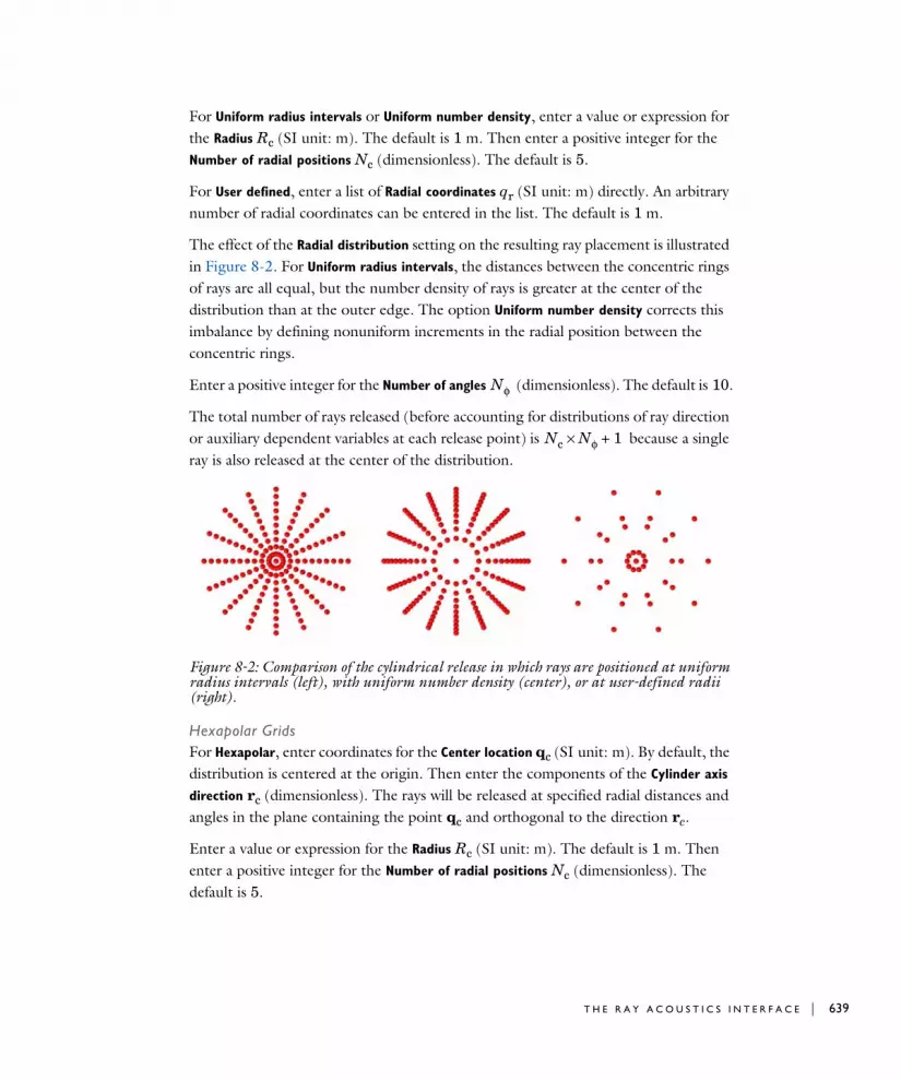
For Uniform radius intervals or Uniform number density, enter a value or expression for the Radius Rc (SI unit: m). The default is 1 m. Then enter a positive integer for the Number of radial positions Nc (dimensionless). The default is 5.

For User defined, enter a list of Radial coordinates qr (SI unit: m) directly. An arbitrary number of radial coordinates can be entered in the list. The default is 1 m.

The effect of the Radial distribution setting on the resulting ray placement is illustrated in Figure 8-2. For Uniform radius intervals, the distances between the concentric rings of rays are all equal, but the number density of rays is greater at the center of the distribution than at the outer edge. The option Uniform number density corrects this imbalance by defining nonuniform increments in the radial position between the concentric rings.

Enter a positive integer for the Number of angles (dimensionless). The default is 10.

The total number of rays released (before accounting for distributions of ray direction or auxiliary dependent variables at each release point) is because a single ray is also released at the center of the distribution.

Figure 8-2: Comparison of the cylindrical release in which rays are positioned at uniform radius intervals (left), with uniform number density (center), or at user-defined radii (right).

Hexapolar GridsFor Hexapolar, enter coordinates for the Center location qc (SI unit: m). By default, the distribution is centered at the origin. Then enter the components of the Cylinder axis

direction rc (dimensionless). The rays will be released at specified radial distances and angles in the plane containing the point qc and orthogonal to the direction rc.

Enter a value or expression for the Radius Rc (SI unit: m). The default is 1 m. Then enter a positive integer for the Number of radial positions Nc (dimensionless). The default is 5.

Nφ

Nc Nφ× 1+


640 | C H A P T E R

Unlike the Cylindrical grid types described in the previous section, each concentric ring of the Hexapolar grid releases a different number of rays, as shown in Figure 8-3. One ray is always released at the center. The first ring of rays surrounding the center has 6 rays arranged in a regular hexagon. Each ring of rays beyond the first has 6 more rays than the ring preceding it, with the grid points arranged in a regular polygon. The radius increments between consecutive rings are uniform.

The total number of grid points generated is

Thus the relationship between the number of radius intervals and the total number of grid points is quadratic.

Figure 8-3: Comparison of hexapolar grids with 2 rings (left), 5 rings (middle), and 10 rings (right).

Previewing Grid PointsIn the Initial Coordinates section, you can click the Preview Initial Coordinates and Preview Initial Extents buttons to visualize the ray release positions. Clicking Preview Initial Coordinates will cause a point to appear in the Graphics window for every release position. Clicking Preview Initial Extents will cause a bounding box to appear, indicating the spatial extents of the released rays. Examples are shown in Figure 8-4 and Figure 8-5.

Ngrid 1 3Nc Nc 1+( )+=


Figure 8-4: Graphics window after clicking the Preview Initial Coordinates button.

Figure 8-5: Graphics window after clicking the Preview Initial Extents button.

Release from Grid on Axis

The Release from Grid on Axis feature is similar to the Release from Grid feature, except that it can only release rays from a grid of points along the axis of symmetry in a 2D axisymmetric geometry; that is, qr,0 = 0 for all released rays.

See Release from Boundary for information on the Ray Direction Vector section.

For all other sections, see Release from Grid.


642 | C H A P T E R

Release from Data File

Use a Release from Data File node to specify the initial ray position, direction, and values of auxiliary dependent variables using data from a text file.

See Release for information on the following sections: Release Times, Initial Phase, Initial Intensity, Initial Radii of Curvature, and Total Source Power.

Formatting Guidelines for Files Containing Ray DataThe imported data file should be a text file (*.txt) arranged in a spreadsheet format; that is, each row corresponds to a distinct ray and should have the same number of columns as all other rows. Columns can be separated by spaces, tabs, or a combination of the two. Begin a line with the percent (“%”) character to include comments or empty lines in the data file.

For example, a data file containing the following text would release rays at the positions (0.1, 0.2, 0.6) and (0.2, 0.4, 0.8) in a three-dimensional geometry:

% Ray release positions% qx0 qy0 qz00.1 0.2 0.60.2 0.4 0.8


Browse your computer to select a text file, then click Import to import the data. To remove the imported data, click Discard. Enter the Index of first column containing

position data i to indicate which column represents the first coordinate of the ray position vectors. The default value, 0, indicates the first column.


Select an option from the Ray direction vector list: Expression (the default), From file, Spherical, Hemispherical, Conical, or Lambertian (3D only).

• For From file, enter the Index of first column containing velocity data i. The default is 3. The columns are zero-indexed; that is, an index of 0 corresponds to the first column.

• For all other settings, the settings are the same as for the Release node.

I N I T I A L R A Y F R E Q U E N C Y

This section is available when the Allow frequency distributions at release features check box is selected under the physics interface Ray Release and Propagation section.


Select a Distribution function: None (the default), Normal, Lognormal, Uniform, List of

values, or From file.

• When From file is selected, enter the Index of column containing frequency data. The default value is 3. The columns are zero-indexed; that is, an index of 0 corresponds to the first column.

• For all other options, the settings are the same as for the Release node.

I N I T I A L V A L U E O F A U X I L I A R Y D E P E N D E N T V A R I A B L E S


For each of the active Auxiliary Dependent Variable nodes in the model, choose an option from the Distribution function list: From file, None (the default), Normal, Lognormal, Uniform, or List of Values.

• When From file is selected, enter the Index of column containing data. The default value is 3. The columns are zero-indexed; that is, an index of 0 corresponds to the first column.

For all other options, the settings are the same as for the Release node.

Ray Continuity

Use the Ray Continuity node to specify that rays should cross a pair boundary as if it were invisible. Pair boundaries appear when the geometry sequence ends in Form

Assembly instead of Form Union. Such boundaries require special handling because the mesh elements on either side of the pair boundary aren’t required to match up exactly.


Select one or more identity pairs to allow rays to cross between the source and destination boundaries of these pairs. Such identity pairs are typically created


644 | C H A P T E R

automatically on interior boundaries when the geometry sequence ends in a Form

Assembly node instead of a Form Union node.

Ray Termination

Use the Ray Termination feature to remove rays from the model as they exit the geometry, or to annihilate rays of sufficiently low intensity or power. Only one Ray

Termination node can be added to the model, but it is possible to combine position-based and intensity-based criteria for removing rays if the ray intensity or power is computed by the model.

T E R M I N A T I O N C R I T E R I A

Select an option from the Spatial extents of ray propagation list: Bounding box, from

geometry (the default), Bounding box, user defined, or None. This list controls whether rays are terminated based on their positions.

• For Bounding box, from geometry, a ray is immediately terminated if it reaches the surface of the bounding box of the geometry, defined as the smallest rectangle or rectangular prism with edges parallel to the axes of the global coordinate system that encloses all of the geometric entities. This bounding box is extended by 5% in each direction so that rays can still interact with boundaries that coincide with the perimeter of the bounding box. Therefore, rays can propagate a short distance away from the geometry before disappearing.

• For Bounding box, user defined, a ray is immediately terminated if it reaches the surface of a box of user-specified dimensions. To define the box, enter maximum and minimum values of each spatial coordinate.

• For None, the rays that propagate outward from the geometry will continue to propagate until the study is complete. If the maximum path length for the Ray Tracing study step is too large, this may result in trajectories that are extremely long relative to the characteristic geometry size.

The Ray Continuity node does not cause the ray position components to change discontinuously; the source and destination boundaries for the identity pairs must be overlapping.

If the geometry sequence ends in a Form Union node, the Ray Continuity node usually isn’t necessary because rays can freely cross interior boundaries where no boundary condition has been applied.


If rays are released from outside the bounding box, they won’t immediately disappear; instead, they will only disappear if they enter the bounding box and then exit it again.

Intensity- and Power-Based Termination CriteriaIf the ray intensity or power is being computed in the model, you can then terminate rays based on either or both of these quantities.

Select an option from the Additional termination criteria list. None (the default) is always available. If ray intensity is solved for, then Intensity is available. If ray power is solved for, then Power is available. If both ray intensity and power are solved for, the Intensity

and Power option is also shown.

• For Intensity or Intensity and power, enter the Threshold intensity Ith (SI unit: W/m2). The default is 1e-12[W/m^2]. Rays will be removed from the model if their intensity decreases below the specified value.

• For Power or Intensity and power, enter the Threshold power Qth (SI unit: W). The default is 1e-3[mW].

Ray Detector

Use the Ray Detector feature to compute information about rays that are located in a set of selected domains or on a set of selected boundaries. The detector may detect all rays or only the rays released by a specified release feature. Computed variables are the

The Ray Termination feature can terminate rays at the exact time at which their intensity or power reaches the specified threshold (to within numerical precision), if there exists a closed-form analytic expression for this time. Such a closed-form analytic solution exists if:

• The rays represent planar wavefronts in an absorbing medium, or

• The rays represent spherical or ellipsoidal wavefronts in a nonabsorbing medium.

Otherwise, the rays are stopped at the first discrete time step taken by the solver for which the intensity or power is less than the threshold value.

Ray Termination Theory


646 | C H A P T E R

number of rays transmitted, the transmission probability, and a logical expression which can be used to filter the rendered rays during results processing.

The Ray Detector feature is also capable of computing the total transmitted ray power. If the ray power is solved for, then a global variable for the total power transmitted to the detector is available.

R A Y D E T E C T O R

Select an option from the Release feature list: All (the default), or any of the features which are capable of releasing rays. When All is selected, the variables computed are summed over all release features in the model.


Mode l i n g w i t h t h e Ra y A c ou s t i c s I n t e r f a c e

In this section:

• Mixed Diffuse and Specular Wall Conditions

• Assigning Directivity to a Source

• Impulse Response Plot and Receiver Dataset

• Stopping Rays for a Given Condition

• Mesh Guidelines

• Nonlocal Couplings

• Using Ray Detectors

• Other Results Plots, Datasets, and Derived Values

Mixed Diffuse and Specular Wall Conditions

At a wall where both specular reflections and diffuse reflections occur it is common to define the scattering coefficient s. This coefficient relates the amount of energy that is specularly Es and diffusely Ed reflected to the (total) absorption coefficient α. The normalized total reflected energy is Et. The relations between these are

where αs is the specular absorption coefficient and αd is the diffuse absorption coefficient.

In the Ray Acoustics interface the mixed reflection condition is treated using a Monte Carlo like approach. When a ray hits a mixed wall condition the ray is either diffusely or specularly reflected according to the Probability of specular reflection γs. This means that the probability plays the role of the scattering coefficient, by setting γs = 1 − s. The Specular absorption coefficient and the Diffuse absorption coefficient should both be set equal to the total absorption α.

Et 1 α– Es Ed+= =

Es 1 α–( ) 1 s–( ) 1 αs–= =

Ed 1 α–( )s 1 αd–= =

M O D E L I N G W I T H T H E R A Y A C O U S T I C S I N T E R F A C E | 647

648 | C H A P T E R

Assigning Directivity to a Source

Acoustic sources often have a certain directivity, for example, the directivity of a loudspeaker or even the directivity of a human speaker. When setting up sources in a ray acoustics model this directivity can be specified. In order to do that, you need to modify the source power expression in, for example, a Release from Boundary feature (with tag rac.relb1) where the Ray direction vector has been set to Hemispherical.

If you have a directivity and sensitivity function f(alpha, beta, freq) with alpha the angle in xy-plane, beta the angle in xz-plane, and freq the ray frequency, then the function to modify the ray power/intensity is as follows:

Q*f(alpha,beta,freq)*rac.relb1.Ntf/rac.racop1(f(alpha,beta,freq))

where Q is the base intensity, rac.relb1.Ntf is the total number of rays released, and rac.racop1(f) weighs the function f, for the normalization of the task.

Impulse Response Plot and Receiver Dataset

The impulse response (IR) in a room acoustics simulation can be analyzed by collecting the ray information using the Receiver dataset and then postprocess using the Impulse Response plot. Room acoustic metrics like reverberation times, early energy metrics, and speech intelligibility can also be postprocessed using the Energy Decay subfeature. The IR can be determined for sources and boundary data (absorption coefficients, scattering parameters, source directivity, volume attenuation etc.) given in octave, 1/3 octave, or 1/6 octave bands.

P R E P A R I N G A R O O M A C O U S T I C S S I M U L A T I O N

When setting up a Ray Acoustics simulation and preparing it for a room acoustics simulation where the impulse response (IR) is an important output, certain considerations and steps need to be taken. They are as follows:

• Decide on the interpretation of the frequency in the ray acoustics simulation. To be able to reconstruct the IR with the dedicated plot, the frequency should represent the center frequency of octaves, 1/3 octave, or 1/6 octave bands. The center frequency is also used as input for boundary conditions (absorption coefficients and scattering parameter), for sources (source strength and directivity), and for the volume absorption in the medium, typically air.

• Create a parameter under Global Definitions > Parameters for the band center frequency, for example, f0.


• Set up interpolation functions for the properties that depend on the frequency. The data can easily be stored in a Spreadsheet formatted file and interpolation can be set to Nearest neighbor. An example, of the format for a (.txt) file, that specifies absorption coefficients for some boundaries in a simulation could be (data is invented):

%f0, wall, entrance, window, floor, diffusers, seats125 0.1 0.4 0.01 0.02 0.1 0.05250 0.07 0.2 0.01 0.03 0.1 0.06500 0.05 0.12 0.02 0.05 0.1 0.071000 0.04 0.07 0.02 0.1 0.1 0.152000 0.04 0.05 0.02 0.3 0.1 0.354000 0.05 0.05 0.03 0.5 0.1 0.48000 0.08 0.05 0.04 0.5 0.1 0.616000 0.1 0.05 0.05 0.5 0.1 0.6

• Make sure that either the Compute intensity and power or the Compute power option is selected in the Intensity Computation section. The Compute power option requires fewer degrees of freedom and is more robust. If it is selected the ray intensity (rac.I and rac.logI) cannot be visualized in ray trajectories plots, but both the Sound Pressure Level Calculation on boundaries and the impulse response can be computed.

• Make sure that Count reflections is selected in the Additional Variables section.

• Also make sure that the parameter that you created for the band center frequency (say f0) is used as the Ray frequency under the Ray Properties node.

• Set up the ray acoustics model with appropriate boundary conditions and sources.

• To be able to postprocess the IR, a Parametric Sweep needs to be used in the study around the Ray Tracing study step. The sweep parameter should be the frequency defined in the parameters. To easily create a Parameter value list representing the center frequencies of the bands use the ISO preferred frequencies entry method.

• For the Times, specified under the Ray Tracing study step, only enter 0 and the final simulation time (the final time should be around the estimated reverberation time). COMSOL uses small internal steps that accurately account for all reflections. The so-called Extra Time Steps are used when reconstructing the IR and other data (see below).

• Run the simulation.

R E C E I V E R D A T A S E T

Use a Receiver 2D ( ) or Receiver 3D dataset ( ), selected from the More 2D Datasets submenu and the More 3D Datasets submenu, respectively, to collect the data necessary


650 | C H A P T E R

to visualize the impulse response using an Impulse Response Plot. The Impulse

Response plot uses the data from a Receiver dataset as input

DataSelect the appropriate ray dataset in the Dataset list. Then select the frequency parameters that should be used by the receiver; select one frequency for a single band analysis or all for the broad band analysis. This is the typical behavior if a parametric sweep has been set up, as described in Preparing a Room Acoustics Simulation.

ReceiverThe receiver behaves as a (transparent) sphere with a given radius and located at a center position (the microphone needs to have a certain finite size such that there is a reasonable probability of rays interacting with it). By changing the center position the receiver can be moved around without the need to run the simulation again.

• Under Center, specify the x, y, and (3D only) z coordinates for the center of the receiver.

• Under Radius, specify the radius of the receiver. From the Radius input list, choose Expression to determine the radius using an expression (see below) or choose User

defined to enter a value for the radius in the Radius field (SI unit: m). Different theories exist for the appropriate size of the receiver.

The following built-in expression determines the radius R of the receiver:

where you enter the values for the Number of rays, N; Room volume, V (SI unit: m2); and Source-receiver distance, dSR (SI unit: m), to determine the radius. See Ref. 19 for details on the expression.

DirectivityFrom the Directivity type list, choose Omnidirectional (the default), User defined (dB), or User defined (linear) and enter a directivity expression in the Expression field.

• The User defined (dB) option applies the given gain to the received signal (positive or negative gain).

• The User defined (linear) option applies a linear gain. If a negative value is used the phase of the arriving ray is inverted.

The expression can depend on the ray direction vector components (rac.nix, rac.niy, rac.niz) in order to set up a complex directivity pattern.

R log10 V( )dSR4N----=


Extra Time StepsUse the default All option. The impulse response plot has been tuned to use this option in order to get accurate and fast evaluation of arrival time and ray power.

AdvancedFor the Interpolation between time steps list always use the default Linear interpolation option. The Cubic interpolation is not applicable for the impulse response computation and can lead to erroneous results.

Under Normal variables and Other variables, if desired, you can change the default names of the created variables:

• The normal direction of the receiver surface (nx, ny, and, in 3D, nz).

• The Distance traveled, that is the distance traveled by a ray inside the receiver.

• The receiver Volume.

• The Directivity, that can be used to visualize the expression for the directivity.

• The First ray arrival time.

Evaluation and ExportThe main purpose for the Receiver dataset is to be used as input for the Impulse Response Plot. However, the data generated by the dataset can also be exported and used in an external analysis tool or software (ray power and arrival times).

Right-click the dataset and select Add Data to Export, then enter the desired data. For example, export the arrival time of the rays t, the frequency of the rays rac.f, the power of the rays rac.Q, the distance traveled by the rays in receiver re1dist, and so forth. The exported data can be stored and sorted in several formats.

When working with phase alignment of loudspeakers, it can be useful to evaluate the arrival time if the first ray. This is easily done in a Derived Values > Global Evaluation feature that points to the receiver dataset. Simply evaluate the special variable re1first.

I M P U L S E R E S P O N S E P L O T

In room acoustics applications, the impulse response (IR) of a source-receiver configuration represents one of the most important postprocessing results. To create the plot based on the data collected by the Receiver dataset, add an Impulse Response

See also the Receiver 2D and Receiver 3D section in the COMSOL Multiphysics Reference Manual.


652 | C H A P T E R

subnode ( ) to a 1D Plot Group to create the impulse response plot. After defining the characteristics of the impulse response, click Plot ( ) to create the plot. The Energy Decay ( ) subnode can be added to perform an analysis of the impulse response to get room acoustic metrics and the energy/level decay curves. The first rendering of the IR plot can take some time. As the data is cached any subsequent changes to the plot will be fast.

In the ray tracing methodology it is, as discussed above, typical to characterize sources and boundaries in frequency bands. This also means that some of the frequency content is lost. This frequency content is reconstructed when determining or reconstructing the IR. For each ray that interacts with the receiver, a small piece of signal with appropriate amplitude, arrival time, phase, and frequency content is added to the IR (the filter bank kernel). The sum of all the contributions reconstruct the full IR.

DataFrom the Dataset list, choose the appropriate Receiver Dataset. Then from the Frequency interpretation list choose an interpretation of the frequency: Octave (the default), 1/3 octave, or 1/6 octave. This selections should coincide with the frequency interpretation used in boundary conditions and sources in the underlying ray acoustics simulation, as described in Preparing a Room Acoustics Simulation. The frequency content and resolution of the impulse response is based on this selection.

ExpressionsSet up the variables that are necessary for reconstructing the impulse response (typically use the defaults). These variables are used to define and add the contribution of each ray, that intersects the receiver dataset, to the impulse response.

• Define the frequency variable for the rays (SI unit: Hz) in the Frequency field. The default is rac.f.

• Define the power variable for the rays (SI unit: kg·m2/s2) in the Power field. The default is rac.Q.

• Define the density (SI unit: kg/m3) in the Density field. The default is rac.rho.

The Small Concert Hall Acoustics model is a tutorial on how to compute the impulse response using the Ray Acoustics interface. Application Library path: Acoustics_Module/Building_and_Room_Acoustics/

small_concert_hall


• Define the speed of sound (SI unit: m/s) in the Speed of Sound field. The default is rac.c.

• Define the number of reflections undergone by the rays (SI unit: 1) in the Number

of reflections field. The default is rac.Nrefl.

x-Axis DataFrom the Transformation list, choose a transformation of the data on the x-axis: None (the default), for no transformation, to show the time domain signal, or Frequency

spectrum. The latter will perform an FFT of the IR and depict the power spectra as function of frequency.

AdvancedThe following advanced settings are available to control some aspects of the IR reconstruction as well as the underlying filter kernel used.

• Define a sampling frequency fs (SI unit: Hz). The default is 44100.

• Define the Zero passing length. The default is 11025.

The next two options are legacy options (to achieve behavior for COMSOL Multiphysics releases older than version 5.6).

• Select Remove noncausal signal to remove the signal (force it to zero) prior to the arrival of the first ray. Using this option will alter the energy content of the early energy component of the IR.

• Select Use fully randomized phase to use the legacy method for reconstructing the IR. The fully randomized phase method (see Ref. 20) can lead to unwanted cancellations of the direct sound and early energy contributions.

The following options control the filter kernel used to reconstruct the impulse response. Advanced options allow to modify the kernel, enter a user-defined analytical kernel, or a user-defined kernel based on an interpolation function. The default is to use a Brick-wall with Kaiser window filter kernel (see Ref. 21).

• Select Show the filters to show and inspect the filter bank in the Graphics window, click Plot ( ) to create the plot. To switch between time domain and frequency domain representation change the Transformation option in the x-Axis Data section.

• Select the Filter kernel to use Brick-wall with Kaiser window (the default) or User

defined. When User defined is selected enter the expression for the filter kernel hfc[m]. Use and set up parameters in the Parameters table (as you would use variables). The parameter fc is reserved for the band center frequency; fs is reserved for the sampling frequency; and m is the zero centered index. Note that per


654 | C H A P T E R

default the User defined option sets up the rick-wall with Kaiser window filter kernel for octaves.

• If the default Brick-wall with Kaiser window is selected. You can control the ripple factor δ (the default is 0.05) and the passband slope factor E (the default is 1.03).

Coloring and Style, and LegendsYou can also make change in the Coloring and Style section or add and format a legend in the Legends section.

E N E R G Y D E C A Y A N D O B J E C T I V E R O O M A C O U S T I C M E T R I C S

For further analysis of the impulse response, add the Energy Decay ( ) subnode to the Impulse Response plot. Once selections have been made, click Plot ( ) to create the plot.

DisplaySelect the Band type as Broadband (the default) or Individual bands. For the Individual

bands option select the Band frequency, either an individual band or All. For All, all the level or energy decay curves are plotted.

Select the Plot as Energy decay (the default), Level decay, or Modulation transfer function, to define the type of graphical analysis of the impulse response to be plotted in the Graphics window.

TableSelect the room acoustic metrics to be included in the results table, per default all objective quality metrics are selected. The default name of the table is Objective Quality

Metrics. The table displays the results in columns with the band center frequency fc in the first column. The results table can also be located under the Results > Tables node. A plot of the results located in the table can be created using the Table Graph plot.

See also the Impulse Response section tn the COMSOL Multiphysics Reference Manual.

The speech transmission index (STI) metric is defined as a single value that combines information from 14 modulation transfer function bands and 7 octave bands. To get the value specified by the standard solve the model for octaves from 125 Hz to 8 kHz. When evaluating use the Band

type set to the default Broadband option.


C U S T O M P L O T S

The energy response depicted as a reflectogram or echogram can be plotted using a Ray (Plot) and depict the expression re1dist*rac.Q/re1vol. This will give the intensity received by the “microphone” for each ray.

Stopping Rays for a Given Condition

For some ray acoustics applications it can be advantageous to stop rays once their intensity falls below a certain threshold. This can be simply achieved at walls using the Primary ray condition with an Expression. Here you can enter a logical expression that must be satisfied for a ray to undergo a certain type of ray-wall interaction. For the intensity specify a condition of the type rac.I<threashold. Then the ray is either reflected according the selected condition or it can Freeze or Disappear, depending on your selection.

The number of reflections can be used in such an Expression. This variable is readily set up under the Additional Variables section.

The Ray Termination feature can also be used in a similar manner to remove rays for certain conditions, without the need for a wall interaction.

Mesh Guidelines

When setting up a mesh for a Ray Acoustics simulation the following guidelines should be followed:

• For modeling ray propagation within domains and interaction with flat surfaces, the mesh can be very coarse.

• When rays may interact with curved boundaries (either reflection or refraction), the accuracy of the reinitialized ray trajectory (that is, the reinitialized wave vector k) depends on the mesh. To create a very fine mesh on curved surfaces without making the mesh unnecessarily fine elsewhere, use the Curvature factor in the Size settings window. The closer this number is to zero, the finer the mesh will be on a curved surface. A value of 0.1 seems adequate for most applications. If there are small, tightly curved surfaces in the model, it might also be necessary to reduce the Minimum element size to allow the small curvature factor to do its job.

• When computing ray intensity, the accuracy of the reinitialized intensity at a curved wall or material discontinuity usually doesn't depend on the level of mesh refinement because it uses surface curvature variables that are based directly on the


656 | C H A P T E R

geometry, not on the mesh. However, if ALE is included in the model, the accuracy of the surface curvature does depend on the mesh.

• Domains that are not included in the selection for the Ray Acoustics interface do not need to be meshed. However, a boundary mesh must always be defined wherever any boundary condition is applied. In addition, it is assumed that the speed of sound and density in all deselected domains are the Speed of sound in

exterior domains and Density of exterior domains, which are specified in the physics interface Ray Release and Propagation section. Thus, media with graded or temperature-dependent material properties must always be included in the selection of the Ray Acoustics interface, and they must always be meshed.

• Accumulator features (both on surfaces and on domains) work by defining additional dependent variables using constant shape functions. When using an Accumulator on a Wall, for example, the contribution from each ray is distributed uniformly over whatever boundary element it hits. If the mesh on the boundary is very fine, this will make the value of the accumulated variable look noisy unless the number of rays hitting the boundary is much larger than the number of boundary elements.

R E P R E S E N T A T I O N O F C U R V E D S U R F A C E S

When rays reach the boundaries of geometric entities in a model, they do not interact with an exact parameterized representation of the geometry. Rather, they propagate through the mesh elements that discretize the modeling domain and interact with the boundary elements that cover the surfaces of the geometric entities.

When the surfaces of the geometry are flat, the shape of the surface mesh is indistinguishable from the shape of the geometric entities themselves. Therefore, the fact that rays interact with the mesh instead of the geometry does not introduce any discretization error, and it is possible to accurately compute ray trajectories even when the mesh is extremely coarse.

Curved surfaces in the geometry, however, usually incur a significant amount of discretization error when predicting how rays will interact with them. The time and location at which the ray interacts with the boundary mesh element might be slightly different from the time at which it would have interacted with an exact representation of the surface. In addition, the tangential and normal directions on the boundary mesh element may differ from the tangential and normal directions on the surface, affecting the accuracy of boundary conditions that involve the tangential and normal directions, such as the Specular reflection condition.

The order of the curved mesh elements used to determine the geometry shape is controlled by the Geometry shape order list in the Model Settings section of the Settings


window for the main Component node. If Automatic, the default, is selected, the curved mesh elements are usually represented by quadratic curves; in some cases, linear functions are used to prevent inverted mesh elements from being created.

The effect of the geometry shape order is most notable on a coarse mesh, as shown in Figure 8-6. The mesh elements are shown as pale gray lines in the background and the ray trajectories are represented as thick red arrows. The rays initially propagate downward and are specularly reflected by a parabolic surface. If Linear is selected from the Geometry shape order list, all rays that hit the same boundary element are specularly reflected in the same direction, as shown on the left. Even though the bottom surface is parabolic, the rays don’t all intersect at a single focus due to the discretization error. If Quadratic or Automatic is selected, rays that hit the same boundary element can still be reflected in different directions because the tangential and normal directions can vary along the surface of the curved element. As a result, the rays reflected by the parabolic surface all intersect at a well-defined focal point as expected.

Figure 8-6: Comparison of rays being specularly reflected at a curved boundary represented using linear elements (left) and quadratic elements (right).

R A Y T R A C I N G I N A N I M P O R T E D M E S H

It is also possible to compute ray trajectories in an imported mesh. The mesh can be imported from a COMSOL Multiphysics file (.mphbin for a binary file format or .mphtxt for a text file format) or from a NASTRAN file (.nas, .bdf, .nastran, or .dat).

If the mesh is imported from a COMSOL Multiphysics file, the imported mesh always uses linear geometry shape order for the purpose of modeling ray-boundary


658 | C H A P T E R

interactions, even if the model used to generate the mesh had a higher geometry shape order.

If the mesh is imported from a NASTRAN file, the ray-boundary interactions may be modeled using either linear or higher geometry shape order. If Export as linear elements is selected when generating the NASTRAN file, or if Import as linear elements is selected when importing the file, then linear geometry shape order will be used.

Nonlocal Couplings

The purpose of a model is often to compute the sum, average, maximum value, or minimum value of a quantity over a group of rays, such as the average intensity or the maximum path length. An instance of the Ray Acoustics interface with Name <name> creates the following four nonlocal couplings:

• <name>.<name>op1(expr) evaluates the sum of the expression expr over the rays. The sum includes all rays that are active, frozen, or stuck to boundaries. It excludes rays that have not yet been released and those that have disappeared.

• <name>.<name>op_all1(expr) evaluates the sum of the expression expr over all rays, including rays those that are not yet released or have disappeared. Since the coordinates of unreleased and disappeared rays are not-a-number (NaN), the sum may return NaN if the model includes unreleased or disappeared rays. An expression such as rac.racop1(isnan(qx)) can be used to compute the total number of unreleased and disappeared rays.

• <name>.<name>aveop1(expr) evaluates the average of the expression expr over the active, frozen, and stuck rays. Unreleased and disappeared rays contribute to neither the numerator nor the denominator of the arithmetic mean.

• <name>.<name>aveop_all1(expr) evaluates the average of the expression expr over all rays. It is likely to return NaN if the model includes unreleased or disappeared rays.

• <name>.<name>maxop1(expr) evaluates the maximum value of the expression expr over all active, frozen, and stuck rays.

• <name>.<name>maxop_all1(expr) evaluates the maximum value of the expression expr over all rays.

• <name>.<name>maxop1(expr, evalExpr) evaluates the expression evalExpr for the ray that has the maximum value of the expression expr out of all active, frozen, and stuck rays. For example, the expression rac.racmaxop1(rac.I, qx) would evaluate the x-coordinate qx of the ray with the greatest intensity rac.I.


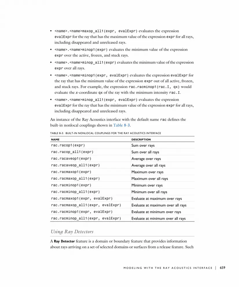
• <name>.<name>maxop_all1(expr, evalExpr) evaluates the expression evalExpr for the ray that has the maximum value of the expression expr for all rays, including disappeared and unreleased rays.

• <name>.<name>minop1(expr) evaluates the minimum value of the expression expr over the active, frozen, and stuck rays.

• <name>.<name>minop_all1(expr) evaluates the minimum value of the expression expr over all rays.

• <name>.<name>minop1(expr, evalExpr) evaluates the expression evalExpr for the ray that has the minimum value of the expression expr out of all active, frozen, and stuck rays. For example, the expression rac.racminop1(rac.I, qx) would evaluate the x-coordinate qx of the ray with the minimum intensity rac.I.

• <name>.<name>minop_all1(expr, evalExpr) evaluates the expression evalExpr for the ray that has the minimum value of the expression expr for all rays, including disappeared and unreleased rays.

An instance of the Ray Acoustics interface with the default name rac defines the built-in nonlocal couplings shown in Table 8-3.

Using Ray Detectors

A Ray Detector feature is a domain or boundary feature that provides information about rays arriving on a set of selected domains or surfaces from a release feature. Such

TABLE 8-3: BUILT-IN NONLOCAL COUPLINGS FOR THE RAY ACOUSTICS INTERFACE

NAME DESCRIPTION

rac.racop1(expr) Sum over rays

rac.racop_all1(expr) Sum over all rays

rac.racaveop1(expr) Average over rays

rac.racaveop_all1(expr) Average over all rays

rac.racmaxop1(expr) Maximum over rays

rac.racmaxop_all1(expr) Maximum over all rays

rac.racminop1(expr) Minimum over rays

rac.racminop_all1(expr) Minimum over all rays

rac.racmaxop1(expr, evalExpr) Evaluate at maximum over rays

rac.racmaxop_all1(expr, evalExpr) Evaluate at maximum over all rays

rac.racminop1(expr, evalExpr) Evaluate at minimum over rays

rac.racminop_all1(expr, evalExpr) Evaluate at minimum over all rays


660 | C H A P T E R

quantities include the number of rays transmitted, the transmission probability, and a logical expression for ray inclusion. The feature provides convenient expressions that can be used in the Filter node of the Ray Trajectories plot, which allows only the rays which reach the ray detector selection to be visualized. The following variables are provided by the Ray Detector feature, with the feature tag <tag>:

• <tag>.Ntf is number of transmitted rays from the release feature to the ray detector at the end of the simulation.

• <tag>.alpha is the transmission probability from the release feature to the ray detector.

• <tag>.rL is a logical expression for ray inclusion. This can be set in the Filter node of the Ray Trajectories plot in order to visualize the rays which connect the release feature to the detector.

Other Results Plots, Datasets, and Derived Values

A variety of dedicated postprocessing tools are available with this physics interface. They are listed below and referred to in the COMSOL Multiphysics Reference Manual.

S O U N D P R E S S U R E L E V E L O N S U R F A C E S A N D I N C R O S S S E C T I O N S

The sound pressure level on surfaces is plotted using the Sound Pressure Level

Calculation subfeature to a Wall node.

The SPL can also be visualized on an interior cut-like plane by adding a plane in the geometry, meshing it, and then apply a wall with the Wall condition set to Pass through. In this way the boundary will only be used to map the SPL and will have no influence on the ray propagation.

The Ray Detector feature only creates variables, which do not affect the solution. Therefore, they can be added to a model without the need to re-compute the solution, it just needs to be updated. To do this, right click on the Study node and select Update Solution. The new variables described above will be immediately available for results processing.


P L O T S

R A Y D A T A S E T

R A Y E V A L U A T I O N D E R I V E D V A L U E S


• Ray (Plot)

• Ray Trajectories

• Filter for Ray and Ray Trajectories

• Particle (Plot)

• Impulse Response

• Plot Groups and Plots


• Ray (Dataset)

• Receiver 2D and Receiver 3D

• Datasets


• Ray Evaluation

• Derived Values, Evaluation Groups, and Tables


662 | C H A P T E R

Th eo r y f o r t h e Ra y A c ou s t i c s I n t e r f a c e

The Ray Acoustics Interface theory is described in this section:

• Introduction to Ray Acoustics

• Initial Conditions: Direction

• Material Discontinuity Theory

• Intensity and Wavefront Curvature

• Intensity and Phase Reinitialization

• Wavefront Curvature Calculation in Graded Media

• Attenuation Within Domains

• Ray Termination Theory

• Accumulator Theory: Domains

• Accumulator Theory: Boundaries

• Sound Pressure Level Calculation Theory

• References for the Ray Acoustics Interface

Introduction to Ray Acoustics

It is often convenient to express an acoustic wave in a stationary fluid as a plane wave of the form

where (SI unit: m2/s) is the velocity potential of the fluid, a is its amplitude of the velocity potential, and Ψ (SI unit: rad) is the phase. When the distance from any source is many orders of magnitude larger than the wavelength of the acoustic wave, the wave may be assumed to be locally plane; that is,

where k (SI unit: rad/m) is the wave vector, q (SI unit: m) is the position vector, c (SI unit: m/s) is the speed of sound in the medium, and t (SI unit: s) is the time.

φ aeiΨ=

φ

Ψ k q kct–⋅=


While the velocity potential is defined with a stationary fluid in mind, it is possible to apply the same treatment to a homogeneous fluid moving at velocity u (SI unit: m/s) by first formulating the equation of the acoustic wave in a coordinate system in which the fluid is stationary. This results in a more general form of the acoustic wave equation,

By defining the angular frequency of the wave as

it follows that the equation of the acoustic wave may be expressed in the Hamiltonian form

This is a mixed time-frequency formulation that has many advantages. See, for example, Ref. 1 and Ref. 5 for further details. It allows a ray acoustic problem to be broken down into its Fourier components, solving for the propagation of one frequency component per ray. Another benefit is the simple use of frequency dependent boundary conditions.

Initial Conditions: Direction

There are several options available for specifying the initial direction of rays. These options work by assigning values to the degrees of freedom corresponding to the wave vector k (SI unit: rad/m) of each ray.

E X P R E S S I O N

The default is to enter an expression for the Ray direction vector L0 (dimensionless). This vector need not have a magnitude of unity because it is always normalized automatically. The initial wave vector is

where ω (SI unit: rad/s) is the angular frequency and c (SI unit: m/s) is the speed of sound in the medium.

Ψ k q kc k u⋅+( )t–⋅=

ω ck u k⋅+=

dkdt------- ∂ω

∂q-------

dqdt-------

–

∂ω∂k-------

=

=

kωL0c L0-------------=

T H E O R Y F O R T H E R A Y A C O U S T I C S I N T E R F A C E | 663

664 | C H A P T E R

S P H E R I C A L

When Spherical is selected the initial wave vectors are sampled from a distribution in wave vector space at each release point. The number of rays released from each point is usually equal to the specified value Nw (dimensionless), although it may be larger if the initial values of any auxiliary dependent variables are also sampled from a distribution.

In 2D the initial wave vector components are

where θ goes from 0 to 2π in Nw steps. In 3D the initial wave vector components are sampled according to the expressions

The azimuthal angle is uniformly distributed from 0 to 2π. The polar angle θ is sampled from the interval [0, π] with probability density proportional to sin θ. The polar angle is arbitrarily chosen as the angle that the initial wave vector makes with the positive z-axis, but any direction could be chosen because the sphere is isotropic. Therefore, each ray subtends approximately the same solid angle in wave vector space.

H E M I S P H E R I C A L

The Hemispherical option is the same as the Spherical option, except that in 2D θ goes from 0 to π and in 3D θ goes from 0 to π/2. The angle is measured from the direction given by the Hemisphere axis setting.

C O N I C A L

The Conical option is the same as the Spherical option, except that θ goes from 0 to α. The angle is measured from the direction given by the Cone axis setting.

kxωc---- θcos=

kyωc---- θsin=

kxωc---- θ ϕcossin=

kyωc---- θsin ϕsin=

kzωc---- θcos=

ϕ


L A M B E R T I A N

The Lambertian option releases rays within a hemisphere in 3D, but the probability distribution function is different from that of the Hemispherical option. Recall that for an isotropic hemispherical distribution the polar angle θ has a probability density proportional to sin θ; for the Lambertian distribution the probability density is instead proportional to sin θ cos θ. Because of this extra cosine term, distributions following this probability density are said to follow Lambert’s cosine law.

Material Discontinuity Theory

At a Material Discontinuity between two different media, the wave vector is reinitialized using Snell’s law. First, the angle of incidence θi is computed:

where ni is a unit vector in the direction of the incident ray and ns is a unit vector normal to the material discontinuity.

At a boundary between two isotropic, nonabsorbing media, the refracted ray propagates in the direction nt given by the following relations:

where the ray propagates from the medium with speed of sound c1 into the medium with speed of sound c2.

If the maximum number of secondary rays has not yet been released, a reflected ray is also released at the material discontinuity with the initial direction

If the ray intensity is computed, the release of secondary rays may be suppressed when the intensity of the reflected ray is less than the user-defined Threshold intensity Ith

θini ns⋅ni ns------------------ acos=

nt ηni γns+=

γ η θi θtcos+cos–=

ηc2c1-----=

θt η θisin( )asin=

nr ni 2ns θicos–=


666 | C H A P T E R

(SI unit: W/m2). Similarly, when ray power is computed, a Threshold power Qth (SI unit: W) can be specified.

Intensity and Wavefront Curvature

The following describes the algorithm used to compute the ray intensity when Intensity

computation is set to Compute intensity or Compute intensity and power in the physics interface Intensity Computation section. In this algorithm, each ray is treated as a propagating wavefront subtending a small solid angle. The algorithm is only valid when the rays propagate in homogeneous media. The following auxiliary dependent variables are defined for each ray:

In 3D:

• The initial ray intensity I0, which is reinitialized at material discontinuities and walls.

• The integral A of the attenuation coefficient along the ray path.

• Two initial principal radii of curvature, r1,i and r2,i.

• Two principal radii of curvature, r1 and r2, which represent the maximum and minimum radii of curvature of the intersection of the wavefront with an arbitrary plane.

• Three components of a unit vector e1 in the direction corresponding to the first principal radius of curvature. This information is used to reinitialize the principal radii of curvature at curved boundaries.

In 2D:

• The initial ray intensity I0.


• One initial principal radius of curvature, r1,i.

• One radius of curvature r1 of the wavefront. All wavefronts are assumed to be converging or diverging cylindrical waves, so it is not necessary to define a second radius of curvature.

A different algorithm is used to compute the intensity of each ray if the Intensity

computation is instead set to Compute intensity in graded media or Compute intensity and

power in graded media. This algorithm accounts for the effect of graded media on the ray intensity, but it is also slower and less accurate for homogeneous media. The following auxiliary dependent variables are defined for each ray:

In 3D:


• The intensity help variable Γ.


• Two principal curvature calculation help variables α1 and α2 and the rotation angle , which indicates the orientation of the principal curvature directions. An

additional help variable is used internally to detect poles in the local coordinate system definition and to redefine the local coordinate system accordingly.

In 2D:

• The intensity help variable Γ.


• One principal curvature calculation help variable α1.

For the options Compute Power, Compute intensity and power, and Compute intensity

and power in graded media an additional auxiliary dependent variable is defined to indicate the total power transmitted by each ray. Like intensity, power is affected by absorbing media and by reflection or refraction at boundaries. Unlike intensity, power doesn’t change due to the focusing or divergence of a ray bundle.

P R I N C I P A L R A D I I O F C U R V A T U R E

In 3D models, each ray is treated as a wavefront for which two principal radii of curvature, r1 and r2, are defined. In addition, the values of the two principal radii of curvature are stored as r1,i and r2,i whenever the ray reaches a boundary.

Within domains, the equations

are solved. Negative radii of curvature indicate that the wavefront is expanding as the ray propagates, while positive radii of curvature indicate that the wavefront is converging. A continuous locus of points at which either of the principal radii of curvature equals zero is called a caustic surface. The unit vector e1 is defined so that r1 is the radius of curvature of the intersection of the wavefront with the plane tangent to e1 and the wave vector k. Similarly, if a vector e2 is defined so that

φ

dr1ds--------- 1

dr2ds--------- 1–=–=

e2k e× 1k e× 1------------------=


668 | C H A P T E R

Then r2 is the radius of curvature of the intersection of the wavefront with a plane tangent to e2 and k. The components of e1 are stored as auxiliary dependent variables for each ray. The components of e2 can then be derived from e1 and k at any time.

The principal radii of curvature are reinitialized at material discontinuities, and the orientation of the unit vectors e1 and e2 may change. If the unit vector in the direction of the incident ray ni is not parallel to the surface normal ns, then it is possible to define a unique tangent plane, called the plane of incidence, that contains the incident, reflected, and refracted rays. The unit vector normal to this plane, u0, is defined as

If the ray is normal to the surface, then the incident ray is parallel to the refracted ray and antiparallel to the reflected ray, and u0 can be any arbitrary unit vector orthogonal to ni. In addition to the unit vector normal to the plane of incidence, the following unit vectors tangent to the incident wavefront, refracted wavefront, reflected wavefront, and surface normal are defined:

where the subscripts i, t, and r denote the incident, refracted, and reflected wavefronts, respectively. For a wavefront propagating in a direction n, with principal curvatures k1 = 1/r1 and k2 = 1/r2 defined for directions e1 and e2, respectively, the principal curvatures in two other orthogonal directions e1' and e2' (both orthogonal to n) are

(8-1)

where θ is the angle of rotation about n which transforms the vectors e1 and e2 to e1' and e2', respectively. Because k1' and k2' are not principal curvatures, it is necessary to include off-diagonal elements of the wavefront curvature tensor equal to k12'.

The following algorithm is used to reinitialize the principal radii of curvature of the wavefront and their orientations. The reinitialization of the curvature variables follows the method of Stavroudis in Ref. 2.

u0ni ns×ni ns×---------------------=

ui ni u0×ut nt u0×ur nr u0×us ns u0×=

===

k1' k1 θcos2 k2 θsin2

k2'+

k1 θsin2 k2 θcos2

k12'+

k1 k2–( ) θ θsincos

=

=

=


1 Given ni and ns, compute unit vectors in the directions of the reflected and refracted rays, nr and nt.

2 Compute the vectors u0, ui, ut, ur, and us.

3 Compute the angle of rotation θ(i) needed to transform the local coordinate system with axes parallel to e1, e2, and ni to a local coordinate system with axes parallel to u0, ui, and ni. (Note: the superscript (i) is used to distinguish this coordinate system rotation angle from the angle of incidence of the ray, often denoted θi.)

4 Transform the principal curvatures to the local coordinate system defined by u0, ui, and ni by using Equation 8-1, substituting θ(i) for θ.

5 Given the two principal curvatures of the surface, k1,s and k2,s with directions e1,s and e2,s, transform the curvature variables to a local coordinate system with axes parallel to u0, us, and ns. Let the new curvature variables be denoted by k1,s', k2,s', and k12,s'.

6 The curvatures of the wavefront and the surface have now been defined in coordinate systems that share the axis u0 and only differ by a rotation by the angle of incidence θi about u0. Defining the variables η and γ as in Material Discontinuity Theory, compute the curvature variables of the refracted ray in a coordinate system defined by u0, ut, and nt using the equations

7 Obtain the principal curvatures of the refracted ray by rotating the coordinate system defined by u0, ut, and nt by an angle θ(t) about nt. The angle θ(t) is defined as

8 Reinitialize the principal curvatures of the refracted ray:

k1 t, ' ηk1' γk1 s, '

k12 t, 'η θicos

θtcos------------------k12' γ

θtcos--------------k12 s, '

k2 t, 'η θicos2

θtcos2--------------------k2' γ

θtcos2-----------------k2 s, '+=

+=

+=

θ t( ) 12---

2k12 t, 'k1 t, ' k2 t, '–---------------------------- atan=

k1 t, k1 t, ' θ t( )cos2 2k12 t, ' θ t( ) θ t( )sincos k2 t, ' θ t( )sin2

k2 t, k1 t, ' θ t( )sin2 2k12 t, ' θ t( ) θ t( )sincos– k2 t, ' θ t( )cos2+=

+ +=


670 | C H A P T E R

9 Invert the principal curvatures to obtain the principal radii of curvature of the refracted ray. Rotate u0 about nt by the angle θ(t) to obtain the reinitialized principal curvature direction e1,t.

10 If a reflected ray is released, compute the curvature variables of the reflected ray in a coordinate system defined by u0, ur, and nr using the equations

11 Obtain the principal curvatures of the reflected ray by rotating the coordinate system defined by u0, ur, and nr by an angle θ(r) about nr. The angle θ(r) is defined as

12 Initialize the principal curvatures of the reflected ray:

13 Invert the principal curvatures to obtain the principal radii of curvature of the reflected ray. Rotate u0 about nr by the angle θ(r) to obtain the initialized principal curvature direction e1,r.

In 2D components, only one principal radius of curvature is computed; each ray is treated as a cylindrical wave. In addition, no auxiliary degrees of freedom for the principal curvature direction are required because the out-of-plane direction can always be treated as one of the axes of the local coordinate system that defines the orientation of the wavefront.

In 2D axisymmetric model components, radii of curvature are computed for the in-plane direction (that is, the rz-plane) as well as the out-of-plane or azimuthal directions. During ray-boundary interactions, these radii of curvature are reinitialized as if the ray interacted with a 3D surface of revolution, which may have finite radii of curvature in both the in-plane and out-of-plane directions.

k1 r, ' k1' 2k1 s, ' θi

k12 r, ' k– 12' 2k12 s, '

k2 r, ' k2' 2θicos

--------------k2 s, '–=

+=

cos–=

θ r( ) 12---

2k12 r, 'k2 r, ' k1 r, '–----------------------------- atan=

k1 r, k1 r, ' θ r( )cos2 2k12 r, ' θ r( ) θ r( )sincos k2 r, ' θ r( )sin2

k2 r, k1 r, ' θ r( )sin2 2k12 r, ' θ r( ) θ r( )sincos– k2 r, ' θ r( )cos2+=

+ +=


I N T E N S I T Y C A L C U L A T I O N

The value of the ray intensity is stored as the auxiliary dependent variable I0 when a ray is released. At any point along the ray’s trajectory, the intensity is equal to

In 2D, the second principal radius of curvature r2 is treated as an arbitrarily large distance that remains constant for each ray.

Intensity and Phase Reinitialization

At a material discontinuity, the intensity of the reflected and refracted rays can be computed using the material properties of the media in the adjacent domains:

(8-2)

where ρ is the density of the medium and cc is the complex speed of sound,

where

• c (SI unit: m/s) is the real speed of sound in the medium,

• ω (SI unit: rad/s) is the angular frequency of the acoustic ray, and

• α (SI unit: 1/m) is the attenuation coefficient.

The subscripts 1 and 2 denote the sides of the boundary into which the reflected and refracted ray propagate, respectively; see Ref. 4.

At a Wall, the reflection coefficient R can be defined explicitly or in terms of the absorption coefficient α or characteristic impedance of absorber Z1. In terms of the absorption coefficient,

I I0r1 i, r2 i,

r1r2------------------=

Ir I R 2=

It I 1 R 2–( )=

RZ2 θi Z1 θtcos–cosZ2 θi Z1 θtcos+cos-------------------------------------------------=

Z ρcc=

ccc

1 i cω----α–

--------------------=


672 | C H A P T E R

Where the principal square root is used for purposes of phase reinitialization. In terms of the characteristic impedance of absorber,

The Wall feature also includes built-in options to compute the reflection coefficient for fluid-fluid interfaces, fluid-solid interfaces, and a fluid layer adjacent to a semi-infinite fluid domain. When treating the Wall boundary as a Fluid-fluid interface, the reflection coefficient is computed using Equation 8-2 as if the wall were a material discontinuity where the fluid properties of the adjacent medium are specified, except that no refracted ray is produced.

If the Wall boundary is modeled as a Fluid-solid interface, the reflection coefficient is instead defined as

where

where the subscripts p and s refer to the propagation of compressional and shear waves in the adjacent solid domain, respectively. For example, θp,t is the refraction angle computed using the compressional complex speed of sound in the adjacent solid domain.

If the Wall boundary is modeled as a Layered fluid half-space, the boundary is treated as a thin layer of one fluid backed by a semi-infinite domain of a second fluid. The reflection coefficient is

R 1 α–=

RZ1 θcos Z0⁄ 1–

Z1 θcos Z0⁄ 1+----------------------------------------=

Z0 ρcc=

RZtot

Z0θicos

--------------–

ZtotZ0

θicos--------------+

-------------------------------=

ZtotZp 1,

θp t,cos-------------------cos2 2θs t,( )

Zs 1,θs t,cos

-------------------sin2 2θs t,( )+=

Rζ1 ζ2 ζ0–( ) i ζ1

2 ζ0ζ2–( ) φtan–

ζ1 ζ2 ζ0+( ) i ζ12 ζ0ζ2–( ) φtan–

--------------------------------------------------------------------------------=


where the subscripts 1 and 2 refer to the properties of the thin layer and the semi-infinite fluid domain, respectively. For example, θt,1 is the angle of refraction in the thin layer. The angle is the phase delay in the thin layer,

where h1 (SI unit: m) is the layer thickness.

If the Rayleigh roughness model is used, the reflected intensity is multiplied by an additional factor to account for surface roughness:

where k (SI unit: rad/m) is the wave vector magnitude of the ray and σ (SI unit: m) is the RMS roughness of the surface.

If the phase of the ray is also computed, the phase shift of the reflected ray at a boundary is

At material discontinuities, the phase of the refracted ray is unchanged.

Wavefront Curvature Calculation in Graded Media

It is possible to compute the ray intensity by changing Intensity computation to Compute intensity or Compute intensity in graded media in the Settings window for the Ray Acoustics interface. The options Compute intensity and power and Compute

intensity and power in graded media can also be used to compute intensity, with the only difference being that these options define an additional auxiliary dependent variable for the total power transferred by the ray. The setting Compute intensity is more robust and accurate than Compute intensity in graded media, but is only applicable to

ζ0Z0

θicos--------------

ζ1Z1

θt 1,cos-------------------

ζ2Z2

θt 2,cos-------------------

=

=

=

φ

φ ωc1-----h1 θt 1,cos=

Ir I R 0.5Γ2–( )exp2

=

Γ 2kσ θicos=

ΔΨr R( )arg=


674 | C H A P T E R

homogeneous media. The setting Compute intensity in graded media can be used for both homogeneous and graded media, but it introduces more numerical error than Compute intensity.

A S S U M P T I O N S F O R C O M P U T I N G I N T E N S I T Y I N H O M O G E N E O U S M E D I A

When Compute intensity is selected, the ray intensity is computed along each ray path using the following assumptions:

1 The wavefront represented by each ray subtends a constant plane angle (2D) or solid angle (3D), which can change only when rays are reflected or refracted at boundaries.

2 Given the radii of curvature at two positions within the same domain and the intensity at one of these two positions, the intensity at the other position can be computed using the relationship

3 Except when rays are reflected or refracted at boundaries, the principal radii of curvature change at a constant rate:

4 The principal curvature directions do not change, except when rays are reflected or refracted at boundaries.

These assumptions are not valid in graded media, in which the speed of sound changes continuously as a function of position. It is possible for the angle between two different rays to change as they propagate through the medium, so the solid angle subtended by the wavefront is no longer constant. As a result, the ray intensity cannot be expressed using the ratio of initial and final principal radii of curvature.

C U R V A T U R E T E N S O R D E F I N I T I O N I N G R A D E D M E D I A

The calculation of ray intensity in graded media is based on the concept of a curvature tensor K, defined in terms of the principal curvatures κ1 and κ2 and the corresponding principal curvature directions e1 and e2:

I I0r1 0, r2 0,

r1r2---------------------=

dr1ds---------

dr2ds--------- 1–= =

K κ1e1e1T κ2e2e2

T+=


Because e1 and e2 are orthogonal, it follows that κ1 and κ2 are eigenvalues of K. It also follows that K is singular because there is no contribution that is orthogonal to both e1 and e2.

The signs of the principal curvatures are chosen so that positive curvature indicates that the wavefront is converging, whereas negative curvature indicates that the wavefront is diverging.

The selection of the coordinate system in which the curvature tensor is defined is crucial. It is convenient to describe the coordinate system so that two of the coordinate axes lie in the plane containing e1 and e2, since this reduces the number of nonzero terms in K. Further reduction in the number of nonzero terms can be achieved if K can be defined in a coordinate system in which e1 and e2 are basis vectors. This is possible in 2D because one of the principal curvature directions is always parallel to the out-of-plane direction, but in 3D it is not feasible because the principal curvature directions can change as rays propagate through a graded medium.

In the most general 3D case, the curvature tensor is described using the following symbols, each of which corresponds to a different orthonormal basis:

• KX: curvature tensor defined in the Cartesian coordinate system with basis vectors x, y, and z.

• KW: curvature tensor defined in the coordinate system consisting of the two principal curvature directions e1 and e2 and the direction of propagation t.

• KS: curvature tensor defined in a coordinate system in which one basis vector is the direction of propagation t. The other two basis vectors s1 and s2 can be determined arbitrarily, as long as they are orthogonal to each other and to t, such that

. It is more convenient to operate in this coordinate system if the basis vectors can be expressed strictly in terms of x, y, z, and t.

The basis vectors s1 and s2 are defined as follows:

To avoid poles in the definition of the basis vectors, the following alternative definitions are used when the rays propagate nearly parallel to the z-axis:

s1 s2× t=

s1t z×t z×---------------=

s2 t s1×=

s1t x×t x×---------------=


676 | C H A P T E R

The relationship between s1, s2, e1, and e2 is given by

where the rotation angle is an auxiliary dependent variable that is stored for each ray.

The relationship between KS and KW is given by

where Q0 is the rotation matrix:

The relationship between KX and KS is given by

where Q is the rotation matrix:

In 2D, one of the principal curvature directions is always known, so it is possible to define s1 and s2 so that they coincide with e1 and e2. The rotation matrix Q0 is the identity, and the auxiliary dependent variable for the angle can be omitted.

D E R I V A T I V E S O F T H E C U R V A T U R E T E N S O R

Following Ref. 3, the derivative of the curvature tensor along the ray trajectory in a graded medium is given by the expression

s2 t s1×=

e1 s1 φ s2 φsin–cos=

e2 s1 φ s2 φcos+sin=

φ

KS Q0KWQ0T

=

Q0

s1 e1⋅ s1 e2⋅ s1 t⋅

s2 e1⋅ s2 e2⋅ s2 t⋅

t e1⋅ t e2⋅ t t⋅

φcos φsin 0φsin– φcos 0

0 0 0

= =

KX QKSQT=

Q

x s1⋅ x s2⋅ x t⋅

y s1⋅ y s2⋅ y t⋅

z s1⋅ z s2⋅ z t⋅

=

φ

dKSds

------------ Mi

i 1=

5

=


where the terms Mi correspond to the different ways in which the curvature can depend on the medium properties. They are defined using the following expressions:

where Π is the projection matrix:

The gradient operator ∇S consists of derivatives that are taken with respect to the local coordinates with basis vectors s1, s2, and t.

D E R I V A T I V E S O F T H E P R I N C I P A L C U R V A T U R E S

By application of the chain rule, the derivatives of the nonzero elements of KS can be expressed in terms of the principal curvatures that occupy the diagonal elements of KW and the rotation angle :

N U M E R I C A L S T A B I L I Z A T I O N

The principal curvatures κ1 and κ2 are not ideal choices for the auxiliary dependent variables stored by each ray because their values can become arbitrarily large as rays approach caustics. Similarly, the principal radii of curvature r1 and r2 are not ideal choices because their values can become arbitrarily large when a diverging wavefront begins to converge while propagating through a graded medium.

M1 KS KS

M2

⋅

c t ∇S1c--- ⋅

KS

M3

–

cΠ ∇S ∇S1c--- ⊗

M4

–

2c2Π ∇S1c--- ∇S

1c--- ⊗

Π

M5 c K∇S1c---

t t ∇S

1c--- K⊗+⊗–

=

=

=

=

=

Π I t t⊗( )–=

φ

∂κ1∂s

---------∂KS 11,

∂s------------------cos2φ 2

∂KS 12,∂s

------------------ φ φ∂KS 22,

∂s------------------sin2φ+cossin–=

∂κ2∂s

---------∂KS 11,

∂s------------------sin2φ 2

∂KS 12,∂s

------------------ φ φ∂KS 22,

∂s------------------cos2φ+cossin+=

∂φ∂s------ 1

κ2 κ1–------------------

∂KS 12,∂s

------------------ 2φ( ) 12---

∂KS 11,∂s

------------------∂KS 22,

∂s------------------–

2φ( )sin+cos=


678 | C H A P T E R

Instead, the auxiliary dependent variables stored by each ray are the help variables α1 and α2. In 2D, only one help variable is allocated because the out-of-plane principal radius of curvature is assumed to be infinite. The principal curvatures are expressed in terms of the help variables using the expression

where κ0 = 1 1/m and i ∈ [1, 2]. The derivatives are then related by the expression

Similarly, the intensity may become infinitely large at caustics, and its reciprocal becomes infinitely large as rays undergo attenuation, so a help variable Γ is used to represent the intensity of the ray:

where I0 = 1 W/m2. The relationship between the ray intensity help variable and the principal curvatures is

where α is the attenuation coefficient of the medium.

Attenuation Within Domains

Rays can gradually lose energy as they propagate through absorbing media. For a plane wave propagating through an absorbing medium with attenuation coefficient α (SI unit: 1/m), the intensity decreases exponentially:

(8-3)

The Ray Acoustics interface defines an additional dependent variable A (dimensionless) for the path integral of the attenuation coefficient,

κi κ0 αtan=

dαi

ds--------- 1

κ0------

dκids---------cos2αi=

I I0 Γtan=

dΓds------- 1

2--- 2Γ( ) κ1 κ2 2α–+[ ]sin=

dIds------ 2αI–=


(8-4)

Despite requiring an extra degree of freedom per ray, the advantage of Equation 8-4 over Equation 8-3 is that the dependent variables in Equation 8-4 all vary linearly within a homogeneous medium. This makes Equation 8-4 much less prone to numerical stiffness; that is, it remains more accurate when the solver takes long time steps, compared to Equation 8-3, potentially reducing solution time and improving accuracy.

The attenuation coefficient is controlled by the option selected from the Fluid model list in the Pressure Acoustics Model section of the Medium Properties.

If Linear elastic is selected, no attenuation occurs.

If Linear elastic with attenuation is selected, the attenuation factor is user-defined.

If Thermally conducting and viscous is selected, the attenuation factor is defined in terms of the medium properties:

where

• c (SI unit: m/s) is the speed of sound in the medium,

• ρ (SI unit: kg/m3) is the density.

• Cp (SI unit: J/(kg·K)) is the heat capacity at constant pressure.

• γ (dimensionless) is the ratio of specific heats.

• k (SI unit: W/(m·K)) is the thermal conductivity.

dI0ds--------- 0

I I0 A( )

dAds--------

exp

2α–

=

=

=

α ω2b

2ρc3------------=

b 43---μ μB

γ 1–( )kCp

--------------------+ +≡


680 | C H A P T E R

• μ (SI unit: Pa·s) is the dynamic viscosity.

• μB (SI unit: Pa·s) is the bulk viscosity.

Ray Termination Theory

The Ray Termination feature can annihilate rays when their intensity or power decreases below a specified threshold.

If the ray intensity is computed, then the threshold ray intensity Ith (SI unit: W/m2) can be specified. Then the termination criterion is

If the ray power is computed, then the threshold ray power Qth (SI unit: W) can be specified. Then the termination criterion is

It is also possible to specify termination criteria based on both intensity and power; in this case, the rays terminate if either criterion is satisfied.

Whenever possible, the Ray Termination feature attempts to stop rays at the exact instant when the ray intensity or power reaches a specified threshold value. A closed-form analytic solution for the exact stop time is available under the following circumstances:

• The rays represent planar wavefronts in an absorbing medium, or

• The rays represent spherical or ellipsoidal wavefronts in a nonabsorbing medium.

If neither of these special conditions is met, the ray can only terminate if the termination criterion is met at the beginning of a time step taken by the solver; the ray intensity or power at the instant the ray is stopped may be less than the threshold.

P L A N A R W A V E F R O N T S I N A N A B S O R B I N G M E D I U M

In this special case, the principal wavefront radii of curvature are so large that the ray intensity can only change significantly in an attenuating medium. The exact time ts (SI unit: s) at which the ray intensity reaches the threshold value is

Built-in models for attenuation in the ocean and atmosphere are also available. The theory for these features can be found in the Attenuation and Loss Models section in the Acoustic Properties of Fluids chapter.

I Ith<

Q Qth<


where

• t0 (SI unit: s) is the previous time step, reflection time, or refraction time,

• I (SI unit: W/m2) is the intensity at t0, and

• Ith (SI unit: W/m2) is the threshold intensity.

If the termination criterion is based on the ray power Q (SI unit: W) instead of ray intensity, the analogous expression for the stop time is

The characteristic time for ray attenuation τ (SI unit: s) is

where

• α (SI unit: 1/m) is the attenuation coefficient of the medium and

• Vg (SI unit: m/s) is the group velocity magnitude.

D I V E R G I N G W A V E F R O N T S I N A N O N A B S O R B I N G M E D I U M

In a nonabsorbing medium in which the wavefront is nonplanar, the ray can only terminate due to the intensity decreasing below the threshold, since the power does not change. The time ts (SI unit: s) at which the ray intensity reaches the threshold in a nonattenuating, homogeneous medium is

where

• t0 (SI unit: s) is the previous time step, reflection time, or refraction time,

• Vg (SI unit: m/s) is the group velocity magnitude,

• r1 (SI unit: m) is the first principal radius of curvature of the wavefront at t0,

• r2 (SI unit: m) is the second principal radius of curvature of the wavefront at t0,

ts t0 τ IIth------- log+=

ts t0 τ QQth--------- log+=

τ 12αVg--------------=

ts t01

2Vg---------- r1 r2 r1 r2–( )2 4 I

Ith------- r1r2++ +

+=


682 | C H A P T E R

• I (SI unit: W/m2) is the intensity at t0, and

• Ith (SI unit: W/m2) is the threshold intensity.

In 2D models, or in 3D models where the wavefronts are cylindrical (one extremely large radius of curvature and one finite radius of curvature), the stop time is instead

where r1 (SI unit: m) is the finite principal radius of curvature of the cylindrical wavefront.

Accumulator Theory: Domains

The Accumulator (Domain) node is used to transfer information from rays to the domains they occupy or pass through. Each Accumulator defines a variable, called the accumulated variable, in the selected domains. The accumulated variable is discretized using constant shape functions, so its value is uniform over every mesh element and may be discontinuous between adjacent mesh elements.

The name of the accumulated variable is specified in the Accumulated variable name field in the Accumulator Settings section of the Settings window. The default variable name, rpd, will be used in the remainder of this section when referring to the accumulated variable.

A C C U M U L A T O R T Y P E

The options in the Accumulator type list are Density and Count. If Density is selected, the source term is divided by the area or volume of the mesh element when calculating each ray’s contribution to the accumulated variable. If Count is selected, no division by the area or volume of the mesh element occurs.

The equations in the following section are valid for the Density type. The corresponding value of the accumulated variable for the Count type is

where V is the mesh element volume (in 3D) or area (in 2D).

ts t01

Vg------ r1

IIth------- r1+

+=

rpdcount rpddensity V×=


A C C U M U L A T I O N O V E R E L E M E N T S

When Elements is selected from the Accumulate over list, the value of the accumulated variable in a mesh element is the sum of the source terms Ri evaluated for all rays in that mesh element:

where N is the total number of rays in the element and V is the area or volume of the mesh element. In other words, the contribution of each ray to the accumulated variable is distributed uniformly over the mesh element the ray is in, regardless of the ray’s exact position within the element.

If Elements and time is selected from the Accumulate over list, then the sum of the source terms for rays in the mesh element is used to define the time derivative of the accumulated variable, rather than its instantaneous value:

Thus the value of the accumulated variable depends on the time history of rays in the mesh element, instead of the instantaneous positions of the rays. As each ray propagates, it will leave behind a trail based on its contributions to the accumulated variables in mesh elements it has traversed. The algorithm for accumulating over time takes into account the fraction of a time step taken by the solver that the ray spends in each mesh element, even if it crosses between elements during the time step.

Accumulator Theory: Boundaries

The Accumulator (Boundary) feature transfers information from rays to the boundaries they hit or pass through. Each Accumulator defines a variable, called the accumulated variable, on the selected boundaries. The accumulated variable is discretized using constant shape functions, so its value if uniform over every mesh element and may be discontinuous between adjacent mesh elements.

The name of the accumulated variable is specified in the Accumulated variable name field in the Accumulator Settings section of the settings window. The default variable name, rpb, will be used in the remainder of this section when referring to the accumulated variable.

rpd 1V---- Ri

i 1=

N

=

d rpd( )dt

------------------ 1V---- Ri

i 1=

N

=


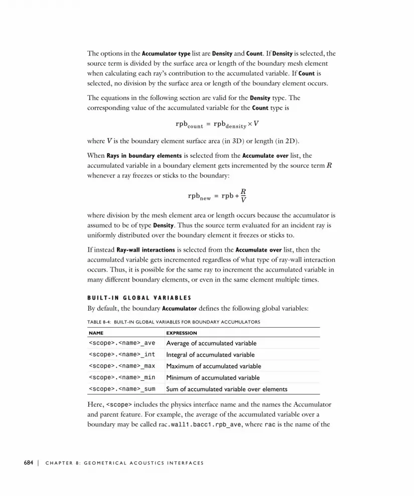
684 | C H A P T E R

The options in the Accumulator type list are Density and Count. If Density is selected, the source term is divided by the surface area or length of the boundary mesh element when calculating each ray’s contribution to the accumulated variable. If Count is selected, no division by the surface area or length of the boundary element occurs.

The equations in the following section are valid for the Density type. The corresponding value of the accumulated variable for the Count type is

where V is the boundary element surface area (in 3D) or length (in 2D).

When Rays in boundary elements is selected from the Accumulate over list, the accumulated variable in a boundary element gets incremented by the source term R whenever a ray freezes or sticks to the boundary:

where division by the mesh element area or length occurs because the accumulator is assumed to be of type Density. Thus the source term evaluated for an incident ray is uniformly distributed over the boundary element it freezes or sticks to.

If instead Ray-wall interactions is selected from the Accumulate over list, then the accumulated variable gets incremented regardless of what type of ray-wall interaction occurs. Thus, it is possible for the same ray to increment the accumulated variable in many different boundary elements, or even in the same element multiple times.

B U I L T - I N G L O B A L V A R I A B L E S

By default, the boundary Accumulator defines the following global variables:

Here, <scope> includes the physics interface name and the names the Accumulator and parent feature. For example, the average of the accumulated variable over a boundary may be called rac.wall1.bacc1.rpb_ave, where rac is the name of the

TABLE 8-4: BUILT-IN GLOBAL VARIABLES FOR BOUNDARY ACCUMULATORS

NAME EXPRESSION

<scope>.<name>_ave Average of accumulated variable

<scope>.<name>_int Integral of accumulated variable

<scope>.<name>_max Maximum of accumulated variable

<scope>.<name>_min Minimum of accumulated variable

<scope>.<name>_sum Sum of accumulated variable over elements

rpbcount rpbdensity V×=

rpbnew rpb RV----+=


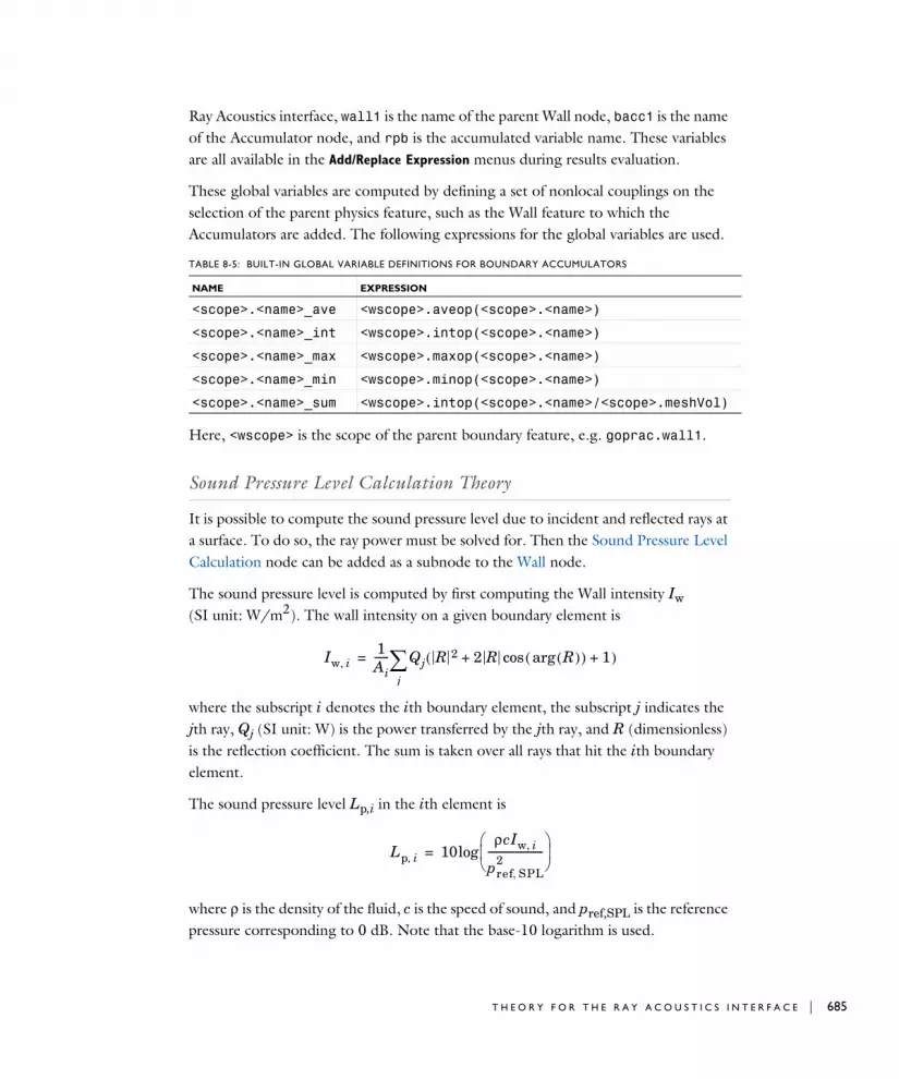
Ray Acoustics interface, wall1 is the name of the parent Wall node, bacc1 is the name of the Accumulator node, and rpb is the accumulated variable name. These variables are all available in the Add/Replace Expression menus during results evaluation.

These global variables are computed by defining a set of nonlocal couplings on the selection of the parent physics feature, such as the Wall feature to which the Accumulators are added. The following expressions for the global variables are used.

Here, <wscope> is the scope of the parent boundary feature, e.g. goprac.wall1.

Sound Pressure Level Calculation Theory

It is possible to compute the sound pressure level due to incident and reflected rays at a surface. To do so, the ray power must be solved for. Then the Sound Pressure Level Calculation node can be added as a subnode to the Wall node.

The sound pressure level is computed by first computing the Wall intensity Iw (SI unit: W/m2). The wall intensity on a given boundary element is

where the subscript i denotes the ith boundary element, the subscript j indicates the jth ray, Qj (SI unit: W) is the power transferred by the jth ray, and R (dimensionless) is the reflection coefficient. The sum is taken over all rays that hit the ith boundary element.

The sound pressure level Lp,i in the ith element is

where ρ is the density of the fluid, c is the speed of sound, and pref,SPL is the reference pressure corresponding to 0 dB. Note that the base-10 logarithm is used.

TABLE 8-5: BUILT-IN GLOBAL VARIABLE DEFINITIONS FOR BOUNDARY ACCUMULATORS

NAME EXPRESSION

<scope>.<name>_ave <wscope>.aveop(<scope>.<name>)

<scope>.<name>_int <wscope>.intop(<scope>.<name>)

<scope>.<name>_max <wscope>.maxop(<scope>.<name>)

<scope>.<name>_min <wscope>.minop(<scope>.<name>)

<scope>.<name>_sum <wscope>.intop(<scope>.<name>/<scope>.meshVol)

Iw i,1Ai------ Qj R 2 2 R R( )arg( ) 1+cos+( )

j=

Lp i, 10ρcIw i,

pref SPL,2

----------------------

log=


686 | C H A P T E R

References for the Ray Acoustics Interface

1. L.D. Landau and E.M. Lifshitz, Fluid Mechanics, Course of Theoretical Physics, Volume 6, Butterworth-Heinemann, 2003.

2. O.N. Stavroudis, The Optics of Rays, Wavefronts, and Caustics, Academic, 1972.

3. R.M. More and K. Kosaka, “Wave-front curvature in geometrical optics”, Phys. Rev. E, vol. 57, no. 5, pp. 6127–6134, 1998.

4. A. D. Pierce, Acoustics: An Introduction to Its Physical Principles and Applications, Acoustical Society of America, 1991.

5. F. B. Jensen, W. A. Kuperman, M. B. Porter, and H. Schmidt, Computational Ocean Acoustics, Second Edition, Springer, 2011.


Th e A c ou s t i c D i f f u s i o n Equa t i o n I n t e r f a c e

The Acoustic Diffusion Equation (ade) interface ( ), found under the Acoustics>Geometrical Acoustics subbranch ( ), solves a diffusion equation for the acoustic energy density. This type of analysis also known as energy finite elements or EFEM. It is applicable for high-frequency acoustics inside coupled rooms when the acoustic fields are diffuse. The interface only exists in 3D. The diffusion of the acoustic energy density depends on the mean free acoustic path and thus on the individual room geometry. Absorption may be applied at walls and a transmission loss may be applied when coupling rooms together. Increased diffusion due to room fitting can be added. Material properties and sources may be specified in frequency bands.

The interface is well suited for quick assessment of sound pressure level distribution inside buildings and other large structures. Compared to a ray acoustics simulation this interface does not include any phase information, direct sound, and early reflections. The interface supports stationary studies for modeling a steady state sound energy or sound pressure level distribution. A time dependent study can be used to determine energy decay curves and reverberation times. The reverberation time of coupled and uncoupled rooms can also be determined using the eigenvalue study. The eigenvalue is directly related to the exponential decay time.


Builder — Acoustic Diffusion Model, Room, and Initial Values. Then, from the Physics toolbar, add other nodes that implement, for example, boundary conditions. You can also right-click Acoustic Diffusion Equation to select physics features from the context menu.

For tutorial models that use the Acoustic Diffusion Equation, see the Application Gallery models:

• One-Family House Acoustics: www.comsol.com/model/20169

• Acoustics of Coupled Rooms Using the Acoustic Diffusion Equation: www.comsol.com/model/20171

• Acoustic Mean Free Path in a Room: www.comsol.com/model/72491

T H E A C O U S T I C D I F F U S I O N E Q U A T I O N I N T E R F A C E | 687

https://www.comsol.com/model/one-family-house-acoustics-20169

https://www.comsol.com/model/acoustics-of-coupled-rooms-using-the-acoustic-diffusion-equation-20171

https://www.comsol.com/model/acoustic-mean-free-path-in-a-room-72491

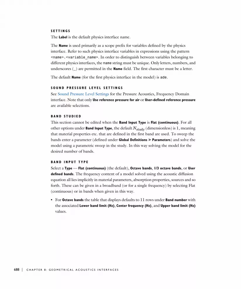
688 | C H A P T E R

S E T T I N G S



The default Name (for the first physics interface in the model) is ade.


See Sound Pressure Level Settings for the Pressure Acoustics, Frequency Domain interface. Note that only Use reference pressure for air or User-defined reference pressure are available selections.

B A N D S T U D I E D

This section cannot be edited when the Band Input Type is Flat (continuous). For all other options under Band Input Type, the default Nstudy (dimensionless) is 1, meaning that material properties etc. that are defined in the first band are used. To sweep the bands enter a parameter (defined under Global Definitions > Parameters) and solve the model using a parametric sweep in the study. In this way solving the model for the desired number of bands.

B A N D I N P U T T Y P E

Select a Type — Flat (continuous) (the default), Octave bands, 1/3 octave bands, or User

defined bands. The frequency content of a model solved using the acoustic diffusion equation all lies implicitly in material parameters, absorption properties, sources and so forth. These can be given in a broadband (or for a single frequency) by selecting Flat (continuous) or in bands when given in this way.

• For Octave bands the table that displays defaults to 11 rows under Band number with the associated Lower band limit (Hz), Center frequency (Hz), and Upper band limit (Hz) values.


• For 1/3 octave bands the table that displays defaults to 32 rows under Band number with the associated Lower band limit (Hz), Center frequency (Hz), and Upper band limit

(Hz) values.

• For User defined bands the table that displays defaults to 1 row under Band number with default associated values in the Lower band limit (Hz), Center frequency (Hz), and Upper band limit (Hz) columns.

- Under the table click the Add ( ) or Delete ( ) buttons to edit the table contents. Or right-click a table cell and select Add or Delete.

- To save the contents of a table, click the Save to File button ( ) and enter a File name in the Save to File dialog box, including the extension .txt. Click to Save the text file. The information is saved in space-separated columns in the same order as displayed on screen.

- Use the Load from File button ( ) and Load from File dialog box to import data in text files, generated by, for example, a spreadsheet program. Data must be separated by spaces or tabs (or be in a Microsoft Excel Workbook spreadsheet if the license includes LiveLink™ for Excel®).


This physics interface defines one dependent variable (field), the Sound energy

density w. If required, edit the name, which changes both the field name and the dependent variable name. If the new field name coincides with the name of another pressure field in the model, the interfaces share degrees of freedom and dependent variable name. The new field name must not coincide with the name of a field of another type, or with a component name belonging to some other field.

The lower band limit, center frequency, and upper band limit in the studied band are defined as the global variables ade.fL, ade.fC, and ade.fU, respectively. These can, for example, be used when plotting data in postprocessing.

Note that the tables that are imported, using the Load from File button ( ), will replace the existing data. You can only import a table that has the expected size. The band number column is disregarded when importing. To create a data file to load, it is recommended to save the existing table (octaves or 1/ octaves) and then edit and change the values in that file.


690 | C H A P T E R


From the list select the element order for the Sound energy density, the default is Quadratic.

Domain, Boundary, and Global Nodes for the Acoustic Diffusion Equation Interface

The Acoustic Diffusion Equation Interface has these domain, boundary, and point nodes available (listed in alphabetical order).


• Domain, Boundary, and Global Nodes for the Acoustic Diffusion Equation Interface

• Theory for the Acoustic Diffusion Equation Interface




Acoustic Diffusion Model

The Acoustic Diffusion Model is added by default and is used to define the material properties and the governing diffusion equations.

M A T E R I A L P R O P E R T I E S

For each of the following properties the default takes values From material, or select User defined to enter a different value or expression in the text field.

• Density ρ (SI unit: kg/m3). The default is 1.2 kg/m3.

• Speed of sound c (SI unit: m/s). The default is 343 m/s.

• Volume absorption coefficient ma (SI unit: 1/m). The default is 0 1/m. This parameter determines the amount of absorption due to losses in the air. The effects are usually of interest in very large rooms/volumes or at very high frequencies. The built-in option Classical viscous and thermal absorption defines the frequency absorption coefficient due to viscous and thermal losses. For the Flat (continuous) band option it is evaluated at the studied frequency feval (the default is 1000 Hz) while it is averaged over the studied band for the other Band Input Type.

Room

The Room node is added by default and is used to define the mean free path model of each room on a model. A Wall subnode is also added by default. Additional Wall subnodes and the Inward Energy Flux subnode are available from the context menu (right-click the parent node) or from the Physics toolbar.

Each room in a model needs a Room node with associated definitions of all wall properties. The volume and surface area of the room is calculated and used to determine the mean free path (depending on the model selected).

• Acoustic Diffusion Model

• Continuity1

• Destination Selection

• Domain Source

• Fitted Domain

• Initial Values

• Inward Energy Flux

• Mapped Room Coupling

• Point Source

• Room

• Room Coupling

• Wall

1Described for the Pressure Acoustics, Frequency Domain interface


692 | C H A P T E R

M E A N F R E E P A T H M O D E L

Select a Mean free path model — Regular cubic room (the default), Long room, or User

defined. For User defined enter a Mean free path λ (SI unit: m). In most cases the regular cubic room is applicable and valid for an ideal diffuse field. For the user defined case the mean free path can be computed using a ray acoustics model.

Wall

The Wall subnode is available from the context menu (right-click the Room parent node) or from the Physics toolbar, Attributes menu. It is used to define the wall absorption properties.

W A L L A B S O R P T I O N P R O P E R T I E S

The absorption coefficient properties to define depend on the choice of Band Input Type for The Acoustic Diffusion Equation Interface. The absorption is defined

For a tutorial model that computes the mean free path, see the Application Gallery model: Acoustic Mean Free Path in a Room www.comsol.com/model/acoustic-mean-free-path-in-a-room-724915

Classical statistical room acoustic variables that are based on the room geometry and absorption properties of the walls are defined and can be used for postprocessing. See Statistical Model of Reverberation Time for details. They are:

• The total room absorption ade.A

• The Sabine reverberation time ade.T60_Sabine

• The Eyring-Norris reverberation time ade.T60_EN

• The Schroeder frequency of the room ade.f_Schroeder

Each room feature (say ade.room1, ade.room2, etc.) also has several room variables associated that may be plotted in postprocessing. They are:

• The room volume ade.room1.V

• The room surface area ade.room1.S

• The mean free path of the room ade.room1.lambda


https://www.comsol.com/model/acoustic-mean-free-path-in-a-room-72491

through the random incidence absorption coefficient α (the value is different from the normal incidence absorption typically used in, for example, pressure acoustics).

• If the Band Input Type is Flat (continuous) enter an Absorption coefficient α (dimensionless).

• For Octave bands, 1/3 octave bands, or User defined bands, enter an Absorption

coefficient α (dimensionless) in each row corresponding to the Band Number.

Select an Exchange coefficient model — Sabine type (the default), Eyring type, Modified

Eyring type, or User defined. For User defined enter an Exchange coefficient h (SI unit: m/s). The choice gives different statistical models which are applicable for different ranges of absorption coefficients. The Sabine type is applicable for α < 0.2 while the two others are valid up to an absorption of 1.

Inward Energy Flux

The Inward Energy Flux subnode is available from the context menu (right-click the Room parent node) or from the Physics toolbar, Attributes menu. It is used to define the energy flux that stems from wall sources. This could be a vibrating wall of a structure or the energy flux as measured from external sources to a building.

E N E R G Y F L U X

The inward energy flux properties to define depend on the choice of Band Input Type for The Acoustic Diffusion Equation Interface.

• If the Band Input Type is Flat (continuous) enter an Inward energy flux Jin (SI unit: W/m2).

• For Octave bands, 1/3 octave bands, or User defined bands, enter an Inward energy flux

Jin (SI unit: W/m2) in each row corresponding to the Band Number.

Note that the tables that are imported, using the Load from File button ( ), will replace the existing data. You can only import a table that has the expected size. The band number column is disregarded when importing. To create a data file to load, it is recommended to save the existing table and then edit and change the values in that file.


694 | C H A P T E R

Initial Values

The Initial Values node adds initial values for the sound energy density. Add more Initial

Values nodes from the Physics toolbar. When calculating the energy impulse response of a system using a time dependent study set the initial value inside a small volume (small domain) or define it in terms of a Gaussian shape.


Enter a value or expression for the Sound energy density w (SI unit: J/m3) initial value. The default is 0 J/m3.

Fitted Domain

Use the Fitted Domain node to define the fitting parameters. These are parameters that define a region with, for example, furniture inside a room. The domain is characterized in terms if its average statistical properties.

F I T T E D D O M A I N P A R A M E T E R S

Enter values or expressions for the following:

• Number density of fitting nf (SI unit: 1/m3).

• Average cross-section of fitting Qf (SI unit: m2).

How you define the Absorption coefficient of fitting is based on the choice of Band Input Type for The Acoustic Diffusion Equation Interface.

• If the Band Input Type is Flat (continuous) enter a value in the text field for the Absorption coefficient of fitting α f (dimensionless). For Octave bands, 1/3 octave

bands, or User defined bands, enter an Absorption coefficient of fitting α f (dimensionless) in each row corresponding to the Band Number.

Domain Source

Use the Domain Source node to define a source, the right-hand side of the governing diffusion equation. The source can be a constant value defined inside a small volume, it can be a function of time, or it can a function of space. The value corresponds to the total emitted power Q of the source it is automatically transformed into a power density q by dividing with the source domain volume (calculated automatically).


D O M A I N S O U R C E

How you define the domain source depends on the choice of Band Input Type for The Acoustic Diffusion Equation Interface.

• If the Band Input Type is Flat (continuous) enter a Domain source Q(SI unit: W).

• For Octave bands, 1/3 octave bands, or User defined bands, enter a Domain source Q(SI unit: W) in each row corresponding to the Band Number.

Room Coupling

Use the Room Coupling node to couple rooms together allowing an acoustic energy flux back and forth. This can be used to model transmission through walls or openings defined in terms of their transmission loss. The feature is also used to couple rooms that are connected through a large open surface. It is also available as the Pair Room

Coupling.

T R A N S M I S S I O N L O S S

How you define the transmission loss depends on the choice of Band Input Type for The Acoustic Diffusion Equation Interface.

• If the Band Input Type is Flat (continuous) enter a Transmission loss TL (SI unit: dB).

• For Octave bands, 1/3 octave bands, or User defined bands, enter a Transmission loss

TL (SI unit: dB) in each row corresponding to the Band Number.

C O N T I N U I T Y

Select the Force continuity check box to constrain the dependent variable resulting in a zero transmission loss. Use this option when rooms are coupled through large open surfaces. Note that the absorption properties of these surfaces need to be set correctly independent of this option.




Mapped Room Coupling

Use the Mapped Room Coupling node to couple two rooms when they do not share a common inner boundary. This is, for example, necessary if mid-planes have not been added in the CAD drawing. The condition has the same functionality as the Room


696 | C H A P T E R

Coupling feature except that a mapping is used between the source and destination walls. The Destination Selection subnode is available from the context menu (right-click the parent node) or from the Physics toolbar, Attributes menu.

T R A N S M I S S I O N L O S S

How you define the transmission loss depends on the choice of Band Input Type for The Acoustic Diffusion Equation Interface.

• If the Band Input Type is Flat (continuous) enter a Transmission loss TL (SI unit: dB).

• For Octave bands, 1/3 octave bands, or User defined bands, enter a Transmission loss

TL (SI unit: dB) in each row corresponding to the Band Number.

C O N T I N U I T Y

Select the Force continuity check box to ensure continuity resulting in a zero transmission loss.




Destination Selection

The Destination Selection subnode is available from the context menu (right-click the Mapped Room Coupling parent node) or from the Physics toolbar, Attributes menu.

Point Source

Use the Point Source node to add a point source to model a source of small dimensions. For a time dependent model it is possible to enter an expression that depend on time.

P O I N T S O U R C E

Enter a Point source power qp (SI unit: W). The default is 0 W.


Mode l i n g w i t h t h e A c ou s t i c D i f f u s i o n Equa t i o n I n t e r f a c e

In this section:

• The Eigenvalue Study Type

• Combined Stationary and Time Dependent Study

The Eigenvalue Study Type

The Acoustic Diffusion Equation interface and eigenvalue study will produce the modes that decay exponentially for each room including the effect of couplings to adjacent rooms and wall absorption. The modes are of the form

where each mode wi has an associated eigenvalue λi (this is the exponential time scale). The eigenvalue directly gives the reverberation time T60 of that subsystem

Typically, there will be as many modes as there are rooms in the building.

A list relating the eigenvalues to the reverberation times is automatically shown under Derived Values in the Results node. Identify the mode associated with a given reverberation time by looking at the default plot Sound Energy Density Mode.

Combined Stationary and Time Dependent Study

By combining a Stationary and a Time Dependent study you can readily model the so-called steady state decay behavior of the system. Use the stationary solution as an initial condition for the transient model. Remember to disable all sources in the transient study step by enabling the Modify physics tree and variables for study step option. Evaluating the sound pressure level, ade.Lp, in different points will result in the energy decay curves.

w x t,( ) wi x( )e λit–=

T6060

10log10 e( )λi--------------------------------- 55.3

4λi-----------≈=

M O D E L I N G W I T H T H E A C O U S T I C D I F F U S I O N E Q U A T I O N I N T E R F A C E | 697

698 | C H A P T E R

Th eo r y f o r t h e A c ou s t i c D i f f u s i o n Equa t i o n I n t e r f a c e

This section contains a small review of the classical models for the prediction of reverberation time in room acoustics followed by the theory background of the acoustic diffusion equation.

In this section:

• Statistical Model of Reverberation Time

• The Acoustic Diffusion Equation

• References for the Acoustic Diffusion Equation Interface

Statistical Model of Reverberation Time

In classical statistical acoustics (see Ref. 9 and Ref. 16) the reverberation time T60 (RT) is the time taken for the sound pressure level (created by an impulse source) to decay 60 dB. The reverberation time can be calculated using the Sabine formula

where V is the room volume, c is the speed of sound, and A is the total absorption of all surfaces. The factor 55.3 is a roundoff of 24·ln(10). The total absorption is calculated by

where Si and αi denote the area and absorption of the i’th area. S is the total surface area and is the average absorption of the room. For large rooms this equation is corrected by the absorption of air

where ma is the air absorption constant (see Table 3.1 in Ref. 9). Other versions of the T60 reverberation time exist one is the Eyring–Norris given by

T6055.3V

cA---------------=

A Siαi Sα= =

α

T6055.3V

cA 4maV+-----------------------------=


The models for the reverberation time given above are statistical models for diffuse sound field (large number of reflections). At low frequencies the modal behavior of the room becomes important. The lower bound for the application of these statistical models is the Schroeder frequency (see Ref. 10 and Ref. 16) given by

The classical expressions given above are available for postprocessing in the Acoustic Diffusion Equation interface.

The Acoustic Diffusion Equation

The acoustic diffusion model is based on the assumption that the volumes (rooms) studied contain scatterers that uniformly scatter the sound field and that the sound field is diffuse (large number of reflections). Using the diffusion of light in a scattering environment as an analogy one can express a diffusion equation for the sound-energy density w = w(x,t) (SI unit: J/m3). The diffusion equation describes the energy flow from high to low energy regions. Further details about the model equations and boundary conditions are found in papers by Xiang and others (see Ref. 3, Ref. 7, and Ref. 8) and in papers by Billon, Valeau, and more (see Ref. 5, Ref. 6, Ref. 11, and Ref. 15).

D O M A I N E Q U A T I O N S

The domain diffusion equation for the sound-energy density w = w(x,t) is given by

where the local energy flux vector J (SI unit: J/m2/s = W/m2) is defined in the usual way, as

The total diffusion coefficient is Dt = D = λc/3 (SI unit: m2/s), λ is the mean free path (SI unit: m), c is the speed of sound (SI unit: m/s), and ma is the volumetric absorption coefficient of air (SI unit: 1/m). The volumetric absorption coefficient (or attenuation coefficient) should not be confused with the energy absorption coefficient α used in boundary conditions which is dimensionless. The source term q represents

T6055.3V

cS 1 α–( )ln–-----------------------------------=

f 2000 m/s( )3 2⁄ T60 V⁄>

∂w∂t------- ∇ J cmaw+⋅+ q x t,( )=

J Dt∇w–=

T H E O R Y F O R T H E A C O U S T I C D I F F U S I O N E Q U A T I O N I N T E R F A C E | 699

700 | C H A P T E R

the spatial sound source (SI unit: J/m3/s = W/m3). The term cmaw accounts for volume absorption in air (dissipation). Note that in certain models the cmaw term accounts for the total absorption at boundaries in a “mean” sense (only using no flux boundary conditions), this approach is not used here.

In the interface, ma can be given as a user input or it can be defined as the “classical viscous and thermal (volumetric) absorption” coefficient (as in pressure acoustics) given by

The absorption coefficient is either integrated over the band or it is given at a certain frequency. The volumetric absorption is only important for very large domains/rooms. It is furthermore assumed that ma λ << 1 such that the diffusion coefficient remains unchanged.

The mean free path λ is the distance a sound particle on average travels between reflections. It is related to the average reflections frequency by λ = c/ . The mean free path is a property of each room and for a regular cubic like room it can be calculated by (the usual convention)

where V is the room volume and S the total room surface area (see Ref. 18). The mean free path is defined for every room as it depends on the room geometry and shape. For long rooms like corridors Visentin (see Ref. 13 and Ref. 14) proposes to use another definition of the mean free path given by

In general, the mean free path varies for different room shapes. Entering a user defined mean free path based on for example measurements is also possible (see Ref. 1, Ref. 2, and Ref. 17).

Fitted rooms/zones with obstacles (chairs, machines etc.):In zones with fittings, like furniture or other absorbers, the scatterers are modeled statistically by their number density nf (SI unit: 1/m3), their average cross-section Qf (SI unit: m2), and their absorption coefficient αf (dimensionless). For the domain with scatterers the mean free path becomes

ma classical,ω2μ

2ρc3------------ 4

3--- γ 1–

Pr-----------+

=

n n

λ 4VS

-------=

λ S4π------=


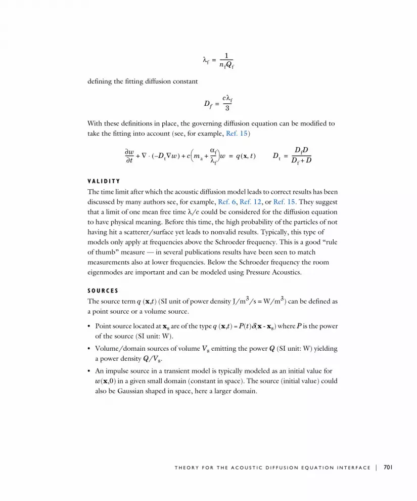
defining the fitting diffusion constant

With these definitions in place, the governing diffusion equation can be modified to take the fitting into account (see, for example, Ref. 15)

V A L I D I T Y

The time limit after which the acoustic diffusion model leads to correct results has been discussed by many authors see, for example, Ref. 6, Ref. 12, or Ref. 15. They suggest that a limit of one mean free time λ/c could be considered for the diffusion equation to have physical meaning. Before this time, the high probability of the particles of not having hit a scatterer/surface yet leads to nonvalid results. Typically, this type of models only apply at frequencies above the Schroeder frequency. This is a good “rule of thumb” measure — in several publications results have been seen to match measurements also at lower frequencies. Below the Schroeder frequency the room eigenmodes are important and can be modeled using Pressure Acoustics.

S O U R C E S

The source term q (x,t) (SI unit of power density J/m3/s = W/m3) can be defined as a point source or a volume source.

• Point source located at xs are of the type q (x,t) = P(t)δ(x - xs) where P is the power of the source (SI unit: W).

• Volume/domain sources of volume Vs emitting the power Q (SI unit: W) yielding a power density Q/Vs.

• An impulse source in a transient model is typically modeled as an initial value for w(x,0) in a given small domain (constant in space). The source (initial value) could also be Gaussian shaped in space, here a larger domain.

λf1

nfQf-----------=

Dfcλf3

-------=

∂w∂t------- ∇ Dt∇w–( ) c ma

αfλf-----+

w+⋅+ q x t,( )= DtDfD

Df D+-----------------=


702 | C H A P T E R

B O U N D A R Y C O N D I T I O N S

Wall (with different absorption properties):At walls, a mixed boundary condition accounting for absorption losses is used (the surface normal n being outward to the volume Ω)

where h is the exchange coefficient. Different models exist for this coefficient as given by Xiang and others (see Ref. 3 and Ref. 4). The Sabine type exchange coefficient is

This expression is valid for surfaces where the absorption coefficient is smaller than 0.2. The Eyring type model is defined by

This model is not suited for absorption coefficients close to 1. Finally, there is the (modified) model by Jing and Xiang (see Ref. 4)

In this model, the boundary condition is theoretically grounded and can model high absorption for a small portion of surfaces. In addition, the diffusion-equation model inherently assumes that overall absorption in rooms under test must not be “high”.

Interior BCs (coupling between rooms/volumes):On interior boundaries between rooms (thin walls, doors, grills, thin panels etc.) there can be a transmission loss (TL) associated. The transmission loss is related to the transmission coefficient τ of the boundary as

This results in a condition where the field w is discontinuous across the boundary (a slit). Using the usual up/down conventions the condition, including possible absorption. The TL for an opening is typically given for the boundary in which the opening is located. That is the combined transmission and absorption is smeared on a boundary.

J n⋅ Dt∂w∂n-------– Jout hw= = =

h cAS cα4---= = for α 0.2<

h cAE c 1 α–( )ln–4

---------------------------+= = for α 1<

h cAM c α2 2 α–( )---------------------= = for α 1≤

TL 10 1τ--- log=


With the surface normal pointing out of the domains, the flux on the down side of the surface/wall (including absorption) is

on the up side of the surface/wall (including absorption) the total flux is

The transmission coefficient is due to reciprocity the same from both sides. This results in the combined condition

The “room coupling” condition adds the fluxes related to the TL. Note also that the terms of the type τcw/4 should probably be modified for small TL because τ then becomes larger than 0.2 (at around 7 dB). An option exists to force continuity by constraining

which basically corresponds to a null transmission loss.

Inflow and Outflow Boundary Conditions:Some general boundary conditions defining a total inflow or outflow of energy are added as

P O S T P R O C E S S I N G V A R I A B L E S / E X P R E S S I O N S

The square pressure (valid for spatially averaged quantities and volumes that are large compared to the wavelength but small compared to the mean free path):

Solution of the energy equation yields (with an impulse source) the energy room impulse response (excluding the direct sound, as the sound field is assumed diffuse).

J ndown⋅ down hw τc4-----w+

up τc4-----w –=

J nup⋅ up hw τc4-----w+

down τc4-----w –=

J nup J ndown⋅–⋅ hw[ ]up hw[ ]down–τc4----- wup wdown–( )–=

wup wdown=

J n⋅ Dt∂w∂n-------– Jout= =

J n⋅ Dt∂w∂n-------– Jin–= =

p2 x t,( ) ρc2w x t,( )=


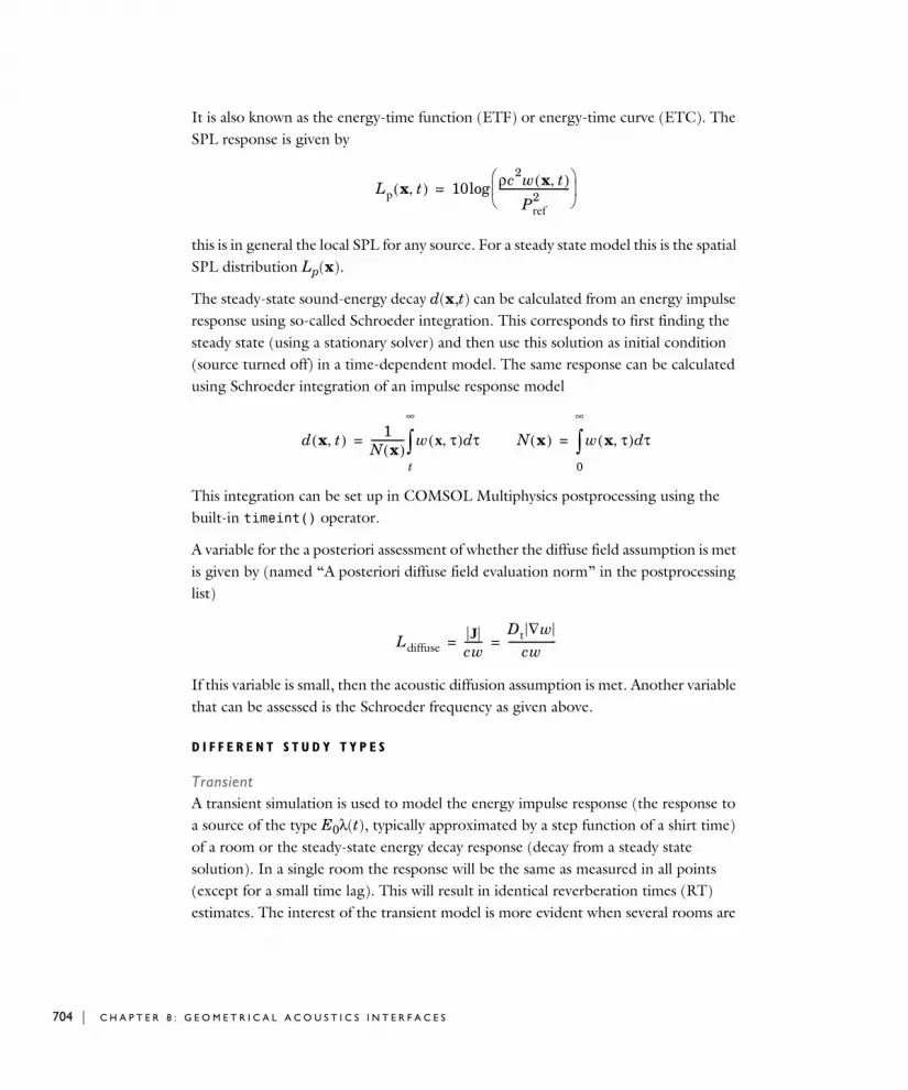
704 | C H A P T E R

It is also known as the energy-time function (ETF) or energy-time curve (ETC). The SPL response is given by

this is in general the local SPL for any source. For a steady state model this is the spatial SPL distribution Lp(x).

The steady-state sound-energy decay d(x,t) can be calculated from an energy impulse response using so-called Schroeder integration. This corresponds to first finding the steady state (using a stationary solver) and then use this solution as initial condition (source turned off) in a time-dependent model. The same response can be calculated using Schroeder integration of an impulse response model

This integration can be set up in COMSOL Multiphysics postprocessing using the built-in timeint() operator.

A variable for the a posteriori assessment of whether the diffuse field assumption is met is given by (named “A posteriori diffuse field evaluation norm” in the postprocessing list)

If this variable is small, then the acoustic diffusion assumption is met. Another variable that can be assessed is the Schroeder frequency as given above.

D I F F E R E N T S T U D Y T Y P E S

TransientA transient simulation is used to model the energy impulse response (the response to a source of the type E0λ(t), typically approximated by a step function of a shirt time) of a room or the steady-state energy decay response (decay from a steady state solution). In a single room the response will be the same as measured in all points (except for a small time lag). This will result in identical reverberation times (RT) estimates. The interest of the transient model is more evident when several rooms are

Lp x t,( ) 10 ρc2w x t,( )Pref

2----------------------------

log=

d x t,( ) 1N x( )------------- w x τ,( ) τd

t

∞

= N x( ) w x τ,( ) τd

0

∞

=

LdiffuseJ

cw-------

Dt ∇wcw

-------------------= =


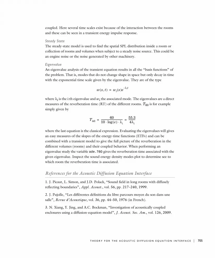
coupled. Here several time scales exist because of the interaction between the rooms and these can be seen in a transient energy impulse response.

Steady StateThe steady-state model is used to find the spatial SPL distribution inside a room or collection of rooms and volumes when subject to a steady noise source. This could be an engine noise or the noise generated by other machinery.

EigenvalueAn eigenvalue analysis of the transient equation results in all the “basis functions” of the problem. That is, modes that do not change shape in space but only decay in time with the exponential time scale given by the eigenvalue. They are of the type

where λi is the i:th eigenvalue and wi the associated mode. The eigenvalues are a direct measures of the reverberation time (RT) of the different rooms. T60 is for example simply given by

where the last equation is the classical expression. Evaluating the eigenvalues will gives an easy measures of the slopes of the energy-time functions (ETFs) and can be combined with a transient model to give the full picture of the reverberation in the different volumes (rooms) and their coupled behavior. When performing an eigenvalue study the variable ade.T60 gives the reverberation time associated with the given eigenvalue. Inspect the sound energy density modes plot to determine see to which room the reverberation time is associated.

References for the Acoustic Diffusion Equation Interface

1. J. Picaut, L. Simon, and J.D. Polack, “Sound field in long rooms with diffusely reflecting boundaries”, Appl. Acoust., vol. 56, pp. 217–240, 1999.

2. J. Pujolle, “Les différentes définitions du libre parcours moyen du son dans une salle”, Revue d’Acoustique, vol. 36, pp. 44–50, 1976 (in French).

3. N. Xiang, Y. Jing, and A.C. Bockman, “Investigation of acoustically coupled enclosures using a diffusion-equation model”, J. Acoust. Soc. Am., vol. 126, 2009.

w x t,( ) wi x( )e λ it–=

T6060

10 e( ) λi⋅log⋅------------------------------------ 55.3

4λi-----------= =


706 | C H A P T E R

4. Y. Jing and N. Xiang, “On boundary conditions for the diffusion equation in room-acoustic prediction”, J. Acoust. Soc. Am. vol. 123, pp. 145–153, 2008.

5. A. Billon and others, “Modeling the sound transmission between rooms coupled through partition walls by using a diffusion model”, J. Acoust. Soc. Am., vol. 123, 2008.

6. V. Valeau and others, “On the use of a diffusion equation for room acoustic prediction”, J. Acoust. Soc. Am., vol. 119, 2006.

7. Y. Jing and N. Xiang, “On The Use of a Diffusion Equation Model for Sound Energy Flow Prediction in Acoustically Coupled Spaces”, COMSOL Conference Boston 2008. www.comsol.com/paper/on-the-use-of-a-diffusion-equation-model-for-sound-energy-flow-prediction-in-aco-5124

8. Y. Jing and N. Xiang, “Boundary Conditions for the Diffusion Equation Model in Room-acoustic Prediction”, COMSOL Conference Boston 2007.

9. T. J. Cox and P. D’Antonio, Acoustic, Absorbers and Diffusers, Taylor and Francis, 2009.

10. R. Schroeder, “New method of measuring reverberation time”, J. Acoust. Soc. Am., vol. 37, pp. 409–412, 1965.

11. C. Foy, V. Valeau, A. Billon, J. Picaut, and M. Hodgson, “An Empirical Diffusion Model for Acoustic Prediction in Rooms with Mixed Diffuse and Specular Reflections”, Acta Acustica united with Acustica, vol. 95, pp. 97–105, 2009.

12. J. Escolano, J.M. Navarro, and J.L. Lopes, “On the limitation of a diffusion equation model for acoustic predictions of rooms with homogeneous dimensions (L)”, J. Acoust. Soc. Am., vol. 128, p. 1586, 2010.

13. C. Visentin, N. Prodi, V. Valeau, and J. Picaut, “A numerical investigation of the Fick’s law of diffusion in room acoustics”, J. Acoust. Soc. Am., vol. 132, p. 3180, 2012.

14. C. Visentin, A numerical and experimental validation of the diffusion equation applied to room acoustics, Ph.D. thesis, 2012.

15. V. Valeau, M. Hodgson, and J. Picaut, “A Diffusion-Based Analogy for the Prediction of Sound Fields in Fitted Rooms”, Acta Acustica united with Acustica, vol. 93, pp. 94–105, 2007.


http://www.comsol.com/paper/on-the-use-of-a-diffusion-equation-model-for-sound-energy-flow-prediction-in-aco-5124/

16. A. D. Pierce, Acoustics, An Introduction to Its Physical Principles and Applications, Chapter SIX, Acoustical Society of America, 1991.

17. L. Beranek and N. Nishihara, “Mean-free-paths in concert and chamber music halls and the correct method for calibrating dodecahedral sound sources”, J. Acoust. Soc. Am., vol. 135, p. 223, 2014.

18. H. Kuttruff, Room Acoustics, Fifth Edition, Spon Press, 2009.

19. Z. Xiangyang, C. Ke’an, and S. Jincai, “On the accuracy of the ray-tracing algorithms based on various sound receiver models”, Appl. Acoust. vol. 64, pp. 433–441 (2003).

20. F. Pind, “Broadband Hybrid Room Acoustic Simulations”, Master Thesis, Technical University of Denmark, DTU, 2013.

21. J. Soares Augusto, “The Io-sinh function, calculation of Kaiser windows and design of FIR filters”, (2015). 10.13140/RG.2.1.3247.0489.

22. IOC, SCOR and IAPSO, 2010: The international thermodynamics equation of seawater - 2010: Calculation and use of thermodynamic properties. Intergovernmental Oceanographic Commission, Manuals and Guides No. 56, UNESCO (English), 196 pp.


708 | C H A P T E R

9

P i p e A c o u s t i c s I n t e r f a c e s

This chapter describes the physics interfaces found under the Pipe Acoustics branch ( ) and background theory.

• The Pipe Acoustics Frequency Domain and Transient Interfaces

• Theory for the Pipe Acoustics Interfaces

709

710 | C H A P T E R

Th e P i p e A c ou s t i c s F r e qu en c y Doma i n and T r a n s i e n t I n t e r f a c e s

In this section:

• The Pipe Acoustics, Frequency Domain Interface

• The Pipe Acoustics, Transient Interface

• Edge, Boundary, Point, and Pair Nodes for the Pipe Acoustics Interfaces

The Pipe Acoustics, Frequency Domain Interface

The Pipe Acoustics, Frequency Domain (pafd) interface ( ), found under the Acoustics>Pipe Acoustics branch ( ) when adding a physics interface, is used to compute the acoustic pressure and velocity variations when modeling the propagation of sound waves in flexible pipe systems. The governing equations are formulated in a general way to include the possibility of a stationary background flow. The physics interface can for example be used to compute the propagation of sound waves in HVAC systems, other large piping systems, or simply in an organ pipe.

In the frequency domain all sources and variations are assumed to be harmonic. The solved equations assume that the propagating waves are plane. The propagation of higher-order modes that exist above their cutoff frequency, dictated by the pipe cross section, is not modeled.

The equations governing the propagation of sound in pipes stem from considering momentum, mass, and energy balances for a control volume of a piece of pipe. The resulting equations are expressed in the cross-sectional averaged variables and reduce the equations to a 1D component with scalar dependent variables. The physics interface is available in 3D on edges and points, and in 2D on boundaries and points.

In the no-background flow case, the 1D pipe domain can be coupled to a 3D pressure acoustics model using the Acoustic-Pipe Acoustic Connection multiphysics coupling.


Builder: Fluid Properties, Pipe Properties, Closed, and Initial Values. Then, from the Physics toolbar, add other nodes that implement, for example, boundary conditions and point conditions. You can also right-click Pipe Acoustics, Frequency Domain to select physics features from the context menu.

9 : P I P E A C O U S T I C S I N T E R F A C E S

S E T T I N G S



The default Name (for the first physics interface in the model) is pafd.









Select the discretization of the element types used in the finite element formulation. Select the Pressure and Tangential velocity discretization orders. The default is to use a Quadratic/Linear formulation which also ensures numerical stability of the problem.


12--- p p∗=

For postprocessing, plot the sound pressure level pafd.Lp, which depends on the selected reference pressure. You can also plot the intensity magnitude pafd.I_mag (this is an RMS value) in the frequency domain or the instantaneous intensity magnitude patd.Ii_mag.in the time domain.

T H E P I P E A C O U S T I C S F R E Q U E N C Y D O M A I N A N D T R A N S I E N T I N T E R F A C E S | 711

712 | C H A P T E R


This section is used to define the dependent variables (fields) for Pressure p (SI unit: Pa) and Tangential velocity u (SI unit: m/s). If required, edit the name, but dependent variables must be unique within a model.

The Pipe Acoustics, Transient Interface

The Pipe Acoustics, Transient (patd) interface ( ), found under the Acoustics>Pipe

Acoustics branch ( ) when adding a physics interface, is used to compute the acoustic pressure and velocity variations when modeling the propagation of sound waves in flexible pipe systems. The governing equations are formulated in a general way to include the possibility of a stationary background flow. The physics interface can for example be used to compute the propagation of sound waves in HVAC systems, other large piping systems, or simply in an organ pipe.

The solved equations assume that the propagating waves are plane. The propagation of higher-order modes that exist above their cutoff frequency, dictated by the pipe cross section, is not modeled.

The equations governing the propagation of sound in pipes stem from considering momentum, mass, and energy balances for a control volume of a piece of pipe. The resulting equations are expressed in the cross-sectional averaged variables and reduce the equations to a 1D component with scalar dependent variables. The physics interface is available in 3D on edges and points, and in 2D on boundaries and points.

In the no-background flow case, the 1D pipe domain can be coupled to a 3D pressure acoustics model using the Acoustic-Pipe Acoustic Connection multiphysics coupling.


Builder: Fluid Properties, Pipe Properties, Closed, and Initial Values. Then, from the Physics toolbar, add other nodes that implement, for example, boundary conditions and point conditions. You can also right-click Pipe Acoustics, Transient to select physics features from the context menu.

S E T T I N G S






The default Name (for the first physics interface in the model) is patd.


Select the Time stepping (method) as Manual (default and recommended) or Automatic/

free and then enter the Maximum frequency to resolve in the model. The default frequency is set to 1000[Hz] but should be changed to reflect the frequency content of the sources used in the model. The generated solver will be adequate in most situations if the computational mesh also resolves the frequency content in the model. Note that any changes made to these settings (after the model is solved the first time) will only be reflected in the solver if Show Default Solver or Reset Solver to Defaults is selected in the study.

The rest of the settings are the same as for The Pipe Acoustics, Frequency Domain Interface.

Edge, Boundary, Point, and Pair Nodes for the Pipe Acoustics Interfaces

The Pipe Acoustics, Frequency Domain Interface and The Pipe Acoustics, Transient Interface have these edge, boundary, point, and pair nodes, listed in alphabetical order, available from the Physics ribbon toolbar (Windows users), Physics context menu (Mac or Linux users), or right-click to access the context menu (all users).





714 | C H A P T E R

Initial Values

The Initial Values node adds initial values for the pressure and tangential velocity that can serve as an initial condition for a transient simulation or as an initial guess for a nonlinear solver.


Enter values or expressions for the initial value of the Pressure p (SI unit: Pa) and the Tangential Velocity u (SI unit: m/s).

Fluid Properties

The Fluid Properties node adds the momentum and continuity equations solved by the physics interface, except for volume forces which are added by the Volume Force node. The node also provides an interface for defining the material properties of the fluid.


Enter a value for the and Background mean flow pressure p0 (SI unit: Pa) and the Background mean flow temperature T0 (SI unit: K). These will also serve as input the material parameters that depend on the pressure and temperature.

B A C K G R O U N D V E L O C I T Y

Enter a value or expression for the Background mean flow velocity u0 (SI unit: m/s). Values for the background variables for the pressure p0 and velocity u0 can be obtained by solving a Pipe Flow model on the same geometry. The Pipe Flow interface requires the Pipe Flow Module.

• Closed

• End Impedance

• Fluid Properties

• Initial Values

• Pipe Properties

• Pressure

• Velocity

• Volume Force



P H Y S I C A L P R O P E R T I E S

Select a Fluid model as Linear elastic (the default). Then select the Fluid Material as Edge

Material (the default) or select another material if added to the Materials node.

The default Density ρ (SI unit: kg/m3) and Speed of sound cs (SI unit: m/s) use the values From material. For User defined enter different values or expressions.

Pipe Properties

The Pipe Properties node is used to define the pipe shape, pipe model, wall drag force, and flow profile correction factor.

P I P E S H A P E

Select a pipe shape from the list — Not set (the default), Circular, Square, Rectangular, or User defined.

• For Circular enter a value or expression for the Inner diameter di (SI unit: m). The default is 10 cm (0.1 m).

• For Square enter a value or expression for the Inner width wi (SI unit: m). The default is 5 cm (0.05 m).

• For Rectangular enter a value or expression for the Inner width wi (SI unit: m; the default is 5 cm) and Inner height hi (SI unit: m; the default is 10 cm).

• For User defined enter a value or expression for the Cross-sectional area A (SI unit: m2; the default is 0.01 m2) and Wetted perimeter Z (SI unit: m; the default is 0.4 m).

P I P E M O D E L

Select a Pipe model — Incompressible cross section (the default), Zero axial stress, Anchored at one end, or Anchored at both ends.

When Zero axial stress, Anchored at one end, or Anchored at both ends is chosen, select an option from the Young’s modulus E (SI unit: Pa) and Wall thickness Δw lists — Not

set (the default) or User defined. For User defined in either case, enter different values or expressions.

For Anchored at one end or Anchored at both ends also select an option from the Poisson’s ratio v (dimensionless) list — Not set (the default) or User defined. For User

defined enter a value or expression for Poisson’s ratio.


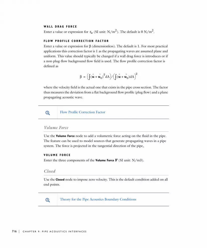
716 | C H A P T E R

W A L L D R A G F O R C E

Enter a value or expression for τw (SI unit: N/m2). The default is 0 N/m2.

F L O W P R O F I L E C O R R E C T I O N F A C T O R

Enter a value or expression for β (dimensionless). The default is 1. For most practical applications this correction factor is 1 as the propagating waves are assumed plane and uniform. This value should typically be changed if a wall drag force is introduces or if a non-plug-flow background flow field is used. The flow profile correction factor is defined as

where the velocity field is the actual one that exists in the pipe cross section. The factor thus measures the deviation from a flat background flow profile (plug flow) and a plane propagating acoustic wave.

Volume Force

Use the Volume Force node to add a volumetric force acting on the fluid in the pipe. The feature can be used to model sources that generate propagating waves in a pipe system. The force is projected in the tangential direction of the pipe,

V O L U M E F O R C E

Enter the three components of the Volume Force F (SI unit: N/m3).

Closed

Use the Closed node to impose zero velocity. This is the default condition added on all end points.

β u u0˜+( )

2dA

u u0˜+( )dA

2⁄=

Flow Profile Correction Factor

Theory for the Pipe Acoustics Boundary Conditions


Pressure

Use the Pressure node to define the boundary pressure at the pipe ends.

P R E S S U R E

Enter a value or expression for the Pressure p (SI unit: Pa). The default is 0 Pa.

In the frequency domain p represents the amplitude and phase (if it is complex-valued) of a harmonic pressure source.

In the time domain enter an expression for the pressure p, for example, a forward moving sinusoidal wave of amplitude 1 Pa can be written as 1[Pa]*sin(omega*t-k*x), where omega and k are parameters defining the angular frequency and wave number, respectively.




Velocity

Use the Velocity node to prescribe a velocity at the pipe ends.

V E L O C I T Y

Enter a value or expression for the velocity uin (SI unit: m/s) at the inlet and/or outlet of a pipe. The default is 0 m/s. The velocity uin is defined relative to background flow u0 and thus in the tangential coordinate system. Enable the Show physics symbols from the Graphics and Plot Windows menu on the Preference dialog box in order to visualize the boundary or edge tangent direction. Click the Fluid Properties node to see the tangents as a red arrows.


• Theory for the Pipe Acoustics Boundary Conditions

• The Preferences Dialog Box in the COMSOL Multiphysics Reference Manual


718 | C H A P T E R

End Impedance

Use the End Impedance node to model conditions at the end of a pipe. The condition can either model an infinite pipe and thus represent the characteristic impedance of the pipe system at that point. This results in a zero reflection condition. Alternatively, the condition can represent the radiation impedance of an open pipe in either a flanged (in an infinite baffle) or unflanged (a pipe ending in free open space). The end impedance can also be user defined and could then represent modeled or experimental values for a specific pipe configuration.

E N D I M P E D A N C E

Select an Impedance model.

For The Pipe Acoustics, Transient Interface select Infinite pipe (low Mach number limit) (the default) or User defined. The Infinite pipe (low Mach number limit) models and infinite pipe by specifying the characteristic impedance at that point. This condition creates a non-reflecting boundary. The expression is valid for small values of the Mach number Ma = u0/c. For User defined enter an End impedance Zend (SI unit: Pa·s/m). The default is patd.rho*(sqrt(1/patd.invc2)), which is ρ·c.

For The Pipe Acoustics, Frequency Domain Interface select from the following — Infinite pipe (low Mach number limit) (the default), Infinite pipe, Flanged pipe, circular, Flanged pipe, rectangular, Unflanged pipe, circular (low ka limit), Unflanged pipe, circular, or User defined.

• For Infinite pipe enter a Wave number k (SI unit: rad/m). The default expression is pafd.omega*(sqrt(pafd.invc2)). This end impedance models the infinite pipe using the full (nonlinear) dispersion relation. It is valid for all Mach numbers but requires the additional input of the wave number k.

• For Flanged pipe, circular enter an Inner radius a (SI unit: m). The default expression is pafd.dh/2. This end impedance models the radiation impedance of a circular pipe terminated in an infinite baffle. It is an exact analytical result valid for all

The wave speed c in the pipe can be different from the speed of sound cs in an open space. It then depends on the elastic properties of the pipe structure. It is defined in Equation 9-6 in the Governing Equations section.

The wave speed can be evaluated as sqrt(1/patd.invc2) or sqrt(1/pafd.invc2) during the analysis and results stage.


frequencies and pipe radii. In the low frequency limit it reduces to the classical results:

• For Flanged pipe, rectangular enter an Inner width wi (SI unit: m). The default is 5 cm (0.05 m). Also enter an Inner height hi (SI unit: m). The default is 10 cm (0.1 m). This end impedance models the radiation impedance of a pipe of rectangular cross section terminated in an infinite baffle. The model is only valid in the low frequency range where and .

• For Unflanged pipe, circular (low ka limit) or Unflanged pipe, circular enter an Inner

radius a (SI unit: m). The default expression is pafd.dh/2. These two end impedance models prescribe the radiation impedance of an unflanged circular pipe (a pipe ending in free open space). The first model is the classical low-frequency approximation valid for . While the second model extends the frequency range to ka < 3.83.

For User defined enter an End impedance Zend (SI unit: Pa⋅s/m). The default expression is pafd.rho*(sqrt(1/pafd.invc2)), which is ρ·c.

Zend ρc 12--- ka( )2 i 0.8216 ka⋅( )+ =

kwi 1« khi 1«

ka 1«

For a detailed review of the end impedance models see: Theory for the Pipe Acoustics Boundary Conditions.


720 | C H A P T E R

Th eo r y f o r t h e P i p e A c ou s t i c s I n t e r f a c e s

The equations governing the propagation of sound in pipes stem from considering momentum, mass, and energy balances for a control volume of a piece of pipe. The resulting equations are expressed in the cross-sectional averaged variables and reduces the equations to a 1D component with scalar dependent variables. The present theory assumes no thermal conduction and thus no losses due to thermal conduction (isentropic sound propagation).

In this section:

• Governing Equations

• Theory for the Pipe Acoustics Boundary Conditions

• Solving Transient Problems

• Cutoff Frequency

• Flow Profile Correction Factor

• References for the Pipe Acoustics Interfaces

Governing Equations

The continuity equation derived for a control volume is given by

(9-1)

and the corresponding momentum balance equation is

(9-2)

where Z is the inner perimeter of the pipe and A = A(x, p,...) is the inner wetted cross-sectional area, u is the area-averaged mean velocity, which is also defined in the tangential direction u = uet, p is the mean pressure along the pipe, τw is the wall drag force, and F is a volume force. The gradient is taken in the tangential direction et. The term β is a flow profile correction factor relating the mean of the squared total velocity to the square of the mean velocity. Such that

∂ Aρ( )∂t

---------------- ∇ Aρu( )⋅+ 0=

∂ ρAu( )∂t

-------------------- ∇ ρAβu2( )+ A∇p– τw– Z AF+=


(9-3)

where

and

are the local non-averaged parameters. Again p and u are the area-averaged dependent variables.

L I N E A R I Z A T I O N

The governing equations are now linearized; that is, all variables are expanded to first order assuming stationary zero-order values (steady-state background properties). The acoustic variations of the dependent variables are assumed small and on top of the background values. This is done according to the following scheme:

where A0 is often only function of x; however, A0 can be changed by external factors such as heating or structural deformation, thus the time dependency. The first-order terms represent small perturbations on top of the background values (zero order). They are valid for

Moreover, the perturbations for the fluid density and cross-sectional area are expanded to first order in p0 in a Taylor series such that

where the subscript s refers to constant entropy; that is, the processes are isentropic. The relations for the fluid compressibility and the cross-sectional area compressibility are

u 1A---- u Ad⋅= p 1

A---- p Ad= β 1

A---- u

2Ad

u2⁄=

p p x( )= u u x( )=

u x t,( ) u0 x( ) u1 x t,( )+=

p x t,( ) p0 x( ) p1 x t,( )+=

ρ x t,( ) ρ0 x( ) ρ1 x t,( )+=

A x t,( ) A0 x( ) A1 x t,( )+=

ρ1 ρ0« p1 ρ0c02

« u1 c0« A1 A0«

ρ1 ρ ρ0– p p0–( ) ∂ρ∂p------

s 0

= =

A1 A A0– p p0–( ) ∂A∂p-------

s 0

= =

T H E O R Y F O R T H E P I P E A C O U S T I C S I N T E R F A C E S | 721

722 | C H A P T E R

Here, β0 is the fluid compressibility at the given reference pressure p0, the isentropic bulk speed of sound is denoted cs, and ρ0 is the fluid density at the given reference temperature and reference pressure. βA is the effective compressibility of the pipe’s cross-sectional A0 due to changes in the inner fluid pressure. The bulk modulus K is equal to one over the compressibility.

Inserting the above expansions into the governing equations (Equation 9-1 and Equation 9-2) and retaining only first-order terms yield the pipe acoustics equations including background flow. These are:

(9-4)

where c is the effective speed of sound in the pipe (it includes the effect due to the elastic properties of the pipe defined through KA). The bulk modulus for the cross-sectional area KA is given by the pipe material properties according to the so-called Korteweg formula (see Ref. 2). For a system with rigid pipe walls cs = c as KA tends to infinity.

Using the fact that the velocity is taken along the tangential direction et, the governing equations are rewritten in terms of the scalar values u and p and projected onto the tangent. The 0 subscript is dropped on the density and area and the 1 subscript is also dropped on the dependent variables.

β01

K0------- 1

Ks------ 1

ρ0------ ∂ρ

∂p------

s 0

1ρ0------ 1

cs2

-----= = = =

βA1

A0-------=

∂A∂p-------

s 0

1KA-------=

A01

c2-----

∂p1∂t

--------- ∇ A0ρ0 u1u0

ρ0c2-----------p1+

⋅+ 0=

ρ0A0∂u1∂t

----------u0

ρ0c2-----------

∂p1∂t

---------+

∇ A0βu0

2

c2------p1 2ρ0A0βu0u1+

+

A0 ∇p1 p1+ βA∇p0( ) τ+ wZ A– F+ 0=

1

c2----- ρ0 β0 βA+( ) ρ0

1K0------- 1

KA-------+

1

cs2

-----ρ0KA-------+= = =


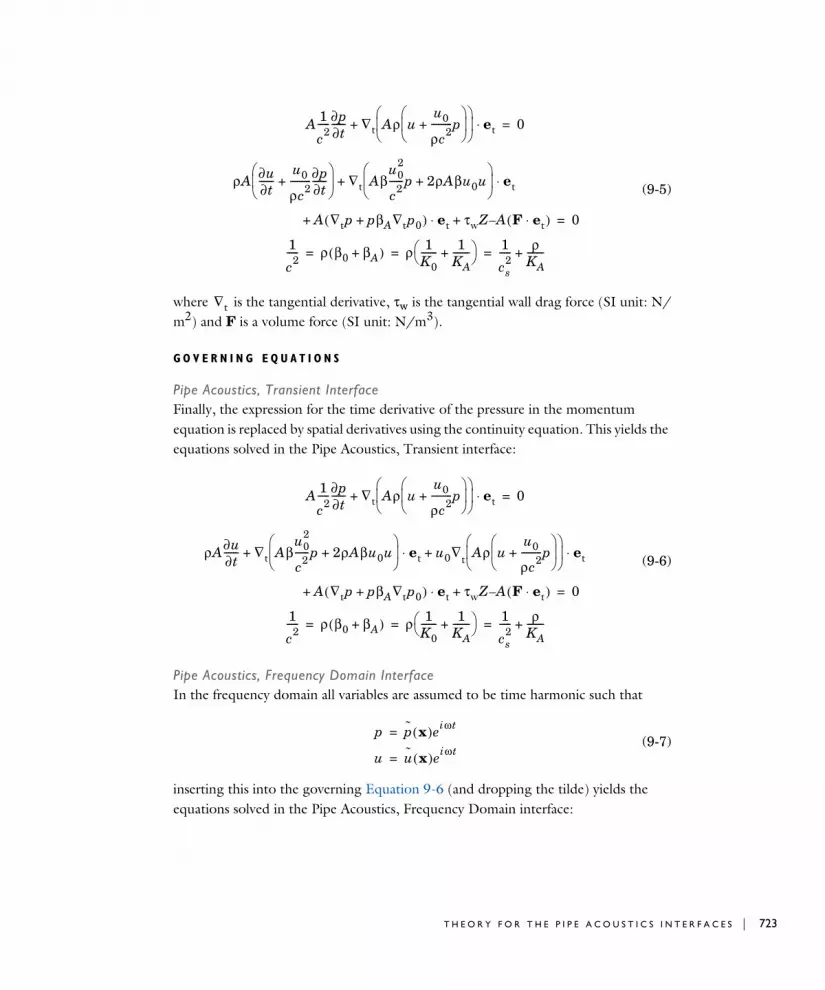
(9-5)

where is the tangential derivative, τw is the tangential wall drag force (SI unit: N/m2) and F is a volume force (SI unit: N/m3).

G O V E R N I N G E Q U A T I O N S

Pipe Acoustics, Transient InterfaceFinally, the expression for the time derivative of the pressure in the momentum equation is replaced by spatial derivatives using the continuity equation. This yields the equations solved in the Pipe Acoustics, Transient interface:

(9-6)

Pipe Acoustics, Frequency Domain InterfaceIn the frequency domain all variables are assumed to be time harmonic such that

(9-7)

inserting this into the governing Equation 9-6 (and dropping the tilde) yields the equations solved in the Pipe Acoustics, Frequency Domain interface:

A 1

c2-----∂p

∂t------ ∇t Aρ u

u0

ρc2---------p+

et⋅+ 0=

ρA ∂u∂t------

u0

ρc2---------∂p

∂t------+

∇t Aβu0

2

c2------p 2ρAβu0u+

et⋅+

A ∇tp p+ βA∇tp0( ) et⋅ τwZ A– F et⋅( )+ + 0=

1

c2----- ρ β0 βA+( ) ρ 1

K0------- 1

KA-------+

1

cs2

----- ρKA-------+= = =

∇t

A 1

c2-----∂p

∂t------ ∇t Aρ u

u0

ρc2---------p+

et⋅+ 0=

ρA∂u∂t------ ∇t Aβ

u02

c2------p 2ρAβu0u+

et u0∇t Aρ uu0

ρc2---------p+

et⋅+⋅+


1

c2----- ρ β0 βA+( ) ρ 1

K0------- 1

KA-------+

1

cs2

----- ρKA-------+= = =

p p x( )eiωt=

u u x( )eiωt=


724 | C H A P T E R

(9-8)

where ω = 2π f is the angular frequency and f is the frequency.


P R E S S U R E , O P E N , A N D C L O S E D C O N D I T I O N S

The simplest boundary conditions to specify are to prescribe the pressure or the velocity at the pipe ends. These result in the Pressure condition

and the Velocity condition

and can be set independently of each other leaving the other dependent variable free. A special subclass of the velocity condition is the Closed condition, where

corresponds to the sound-hard wall condition in pressure acoustics. It is also assumed here that u0 = 0 at a closed boundary.

E N D I M P E D A N C E C O N D I T I O N

At the end of pipes the relation between the pressure and the velocity can be defined in terms of an end impedance Zend. The End Impedance condition is in the Pipe Acoustics interface given by

(9-9)

iω A

c2-----p ∇t Aρ u

u0

ρc2---------p+

et⋅+ 0=

iωρAu ∇t Aβu0

2

c2------p 2ρAβu0u+

et u0∇t Aρ uu0

ρc2---------p+

et⋅+⋅+


1

c2----- ρ β0 βA+( ) ρ 1

K0------- 1

KA-------+

1

cs2

----- ρKA-------+= = =

p pin=

u uin=

u 0=

A ρuu0

c2------p+

A ρ 1Zend-----------

u0

c2------+

p=


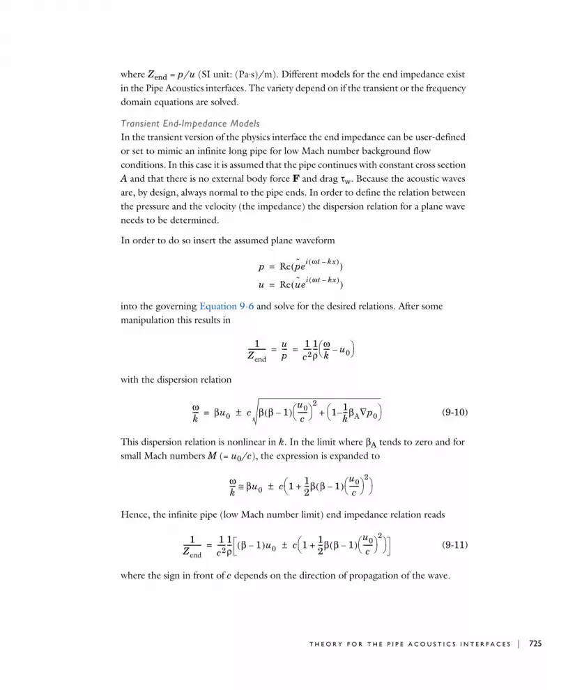
where Zend = p/u (SI unit: (Pa⋅s)/m). Different models for the end impedance exist in the Pipe Acoustics interfaces. The variety depend on if the transient or the frequency domain equations are solved.

Transient End-Impedance ModelsIn the transient version of the physics interface the end impedance can be user-defined or set to mimic an infinite long pipe for low Mach number background flow conditions. In this case it is assumed that the pipe continues with constant cross section A and that there is no external body force F and drag τw. Because the acoustic waves are, by design, always normal to the pipe ends. In order to define the relation between the pressure and the velocity (the impedance) the dispersion relation for a plane wave needs to be determined.

In order to do so insert the assumed plane waveform

into the governing Equation 9-6 and solve for the desired relations. After some manipulation this results in

with the dispersion relation

(9-10)

This dispersion relation is nonlinear in k. In the limit where βA tends to zero and for small Mach numbers M (= u0/c), the expression is expanded to

Hence, the infinite pipe (low Mach number limit) end impedance relation reads

(9-11)

where the sign in front of c depends on the direction of propagation of the wave.

p Re pei ωt kx–( )( )=

u Re uei ωt kx–( )( )=

1Zend----------- u

p--- 1

c2-----1

ρ--- ω

k---- u0– = =

ωk---- βu0 c± β β 1–( )

u0c

------

21 1

k---βA– ∇p0

+=

ωk---- βu0 c± 1 1

2---β β 1–( )

u0c

------

2+

≅

1Zend----------- 1

c2-----1

ρ--- β 1–( )u0 c± 1 1

2---β β 1–( )

u0c

------

2+

=


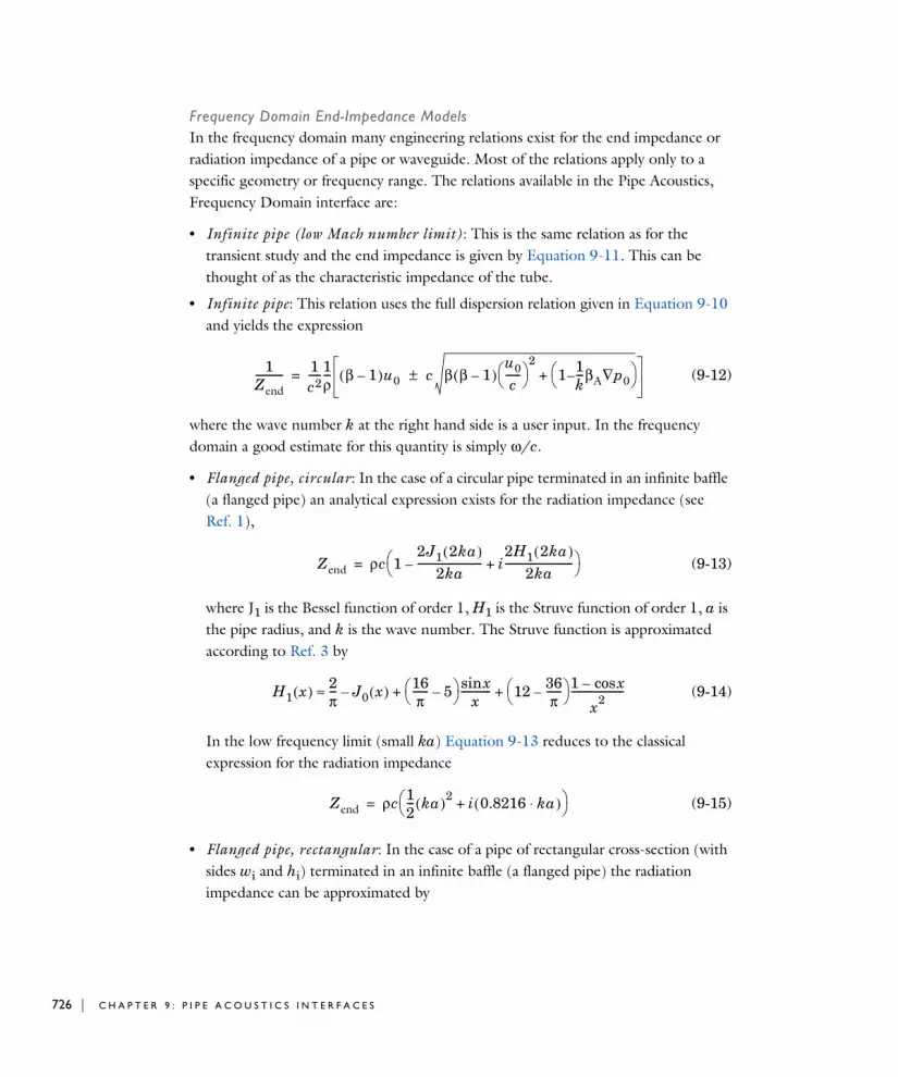
726 | C H A P T E R

Frequency Domain End-Impedance ModelsIn the frequency domain many engineering relations exist for the end impedance or radiation impedance of a pipe or waveguide. Most of the relations apply only to a specific geometry or frequency range. The relations available in the Pipe Acoustics, Frequency Domain interface are:

• Infinite pipe (low Mach number limit): This is the same relation as for the transient study and the end impedance is given by Equation 9-11. This can be thought of as the characteristic impedance of the tube.

• Infinite pipe: This relation uses the full dispersion relation given in Equation 9-10 and yields the expression

(9-12)

where the wave number k at the right hand side is a user input. In the frequency domain a good estimate for this quantity is simply ω/c.

• Flanged pipe, circular: In the case of a circular pipe terminated in an infinite baffle (a flanged pipe) an analytical expression exists for the radiation impedance (see Ref. 1),

(9-13)

where J1 is the Bessel function of order 1, H1 is the Struve function of order 1, a is the pipe radius, and k is the wave number. The Struve function is approximated according to Ref. 3 by

(9-14)

In the low frequency limit (small ka) Equation 9-13 reduces to the classical expression for the radiation impedance

(9-15)

• Flanged pipe, rectangular: In the case of a pipe of rectangular cross-section (with sides wi and hi) terminated in an infinite baffle (a flanged pipe) the radiation impedance can be approximated by

1Zend----------- 1

c2-----1

ρ--- β 1–( )u0 c± β β 1–( )

u0c

------

21 1

k---βA– ∇p0

+=

Zend ρc 12J1 2ka( )

2ka--------------------------– i

2H1 2ka( )2ka

---------------------------+ =

H1 x( ) 2π--- J0 x( )–

16π

------ 5– xsin

x------------ 12 36

π------–

1 xcos–

x2---------------------+ +≈

Zend ρc 12--- ka( )2 i 0.8216 ka⋅( )+ =


(9-16)

see Ref. 4 and Ref. 5.

• Unflanged pipe, circular (low ka limit): In the case of a circular pipe of radius a ending in free air the classical low ka limit for the radiation impedance is given by

(9-17)

see Ref. 1 and Ref. 5.

• Unflanged pipe, circular: A solution for the unflanged pipe exists for the case when , it is presented in Ref. and is based on solving the

Wiener-Hopf integral, it reads

(9-18)

where δ is an interpolation function found by numerical integration for ka = 0, δ = 0.6133.

Common for the last four radiation impedance relations is that they do only apply when there is no background flow present u0 = 0 (or at least when it is very small).

Solving Transient Problems

When solving transient acoustic problems where the wave shape is not necessarily harmonic it might be necessary to resolve its spatial variations with a fine mesh, say with a minimal scale dx. Now, in order for the numerical solution of the temporal development of the acoustic field to be good it is necessary to restrict the maximal time steps dt taken by the solver. The condition is known as the CFL condition (Courant–Friedrichs–Lewy condition). For transient acoustic problems it is defined as

Zendρc2π------ k2 wihi( )2 ik wihi( )3 2⁄ f

wihi------ +

= kwi 1 khi 1«,«

f x( ) 2x1 2⁄ sinh 1– x 1– 2x 1– 2⁄ sinh 1– x 23---x3 2⁄ 2

3---x 3– 2⁄ 2

3--- x x 1–

+( )3 2⁄

–+ + +=

Zend ρc 14--- ka( )2 i 0.6133 ka⋅( )+ = ka 1«

ka 3.83« 1.22π=

Zend ρc1 R+1 R–--------------= R R e2ikaδ

=

R e ka( )2 2⁄– 1 16--- ka( )4 1

γka--------- 19

12------+

ln+ γ e0.5772 ka 1<==

R πkae ka– 1 332------ 1

ka( )2--------------+

1 ka 3.83<<=

C cxd

dt⋅=


728 | C H A P T E R

where C is the Courant number, and c is the velocity.

For applications where all the shape functions are quadratic the Courant number should be around 0.2. This condition restricts any acoustic disturbances to propagate more than 20% of the mesh size dx during one time step dt. In the Pipe Acoustics interface where a mixed formulation exists, with linear elements for the pressure and quadratic elements for the velocity, the condition might have to be tightened such that C < 0.2.

Cutoff Frequency

The Pipe Acoustics interface assumes plane wave propagation. This means that it cannot model the propagation of the higher order modes that can propagate above their cutoff frequency fc. In a rectangular pipe of cross-section width wi and height hi, the cutoff frequency is

In a pipe of circular cross section (with radius a), the cutoff frequency is

where α'mn is the n’th zero of the differential of the Bessel function J’m(x) or order m. The first few values are α'01 = 0, α'02 = 3.83, α'11 = 1.84, and α'21 = 3.05 (see Ref. 1 and Ref. 5 for further details).

Flow Profile Correction Factor

The flow profile correction factor, β, accounts for the ratio of the integrated local square velocity field to the square of the integrated local velocity field (see Equation 9-3). It is defined in terms of the total velocity field (background plus acoustic variations).

For an example where the CFL condition is used see Water Hammer: Application Library path Pipe_Flow_Module/Verification_Examples/

water_hammer_verification.

fmnc 1

2---c m

wi------ 2 n

hi----- 2

+=

fmnc α'mnc

2πa---------------=


In the case of no-background flow (u0 = 0) β is 1 in the absence of a wall drag coefficient, as only plane wave modes propagate. If a wall drag force is introduced, to model some loss mechanism, β starts to differ slightly from 1. This can for example be losses introduced to model viscous and thermal effects in narrow pipes.

In the presence of a background u0 the factor β can be set different 1 in order to model a non-flat velocity profile inside the tube. The value of b (and the actual shape of the background field) influences the convective momentum transfer balances. The places where β enter the governing equations are multiplied with either the Mach number or the Mach number squared, indicating that the effects become important for an increasing background flow.

References for the Pipe Acoustics Interfaces


2. M.S. Ghidaoui, M. Zhao, D.A. McInnis, and D.H. Axworthy, “A Review of Water Hammer Theory and Practice”, Applied Mechanics Reviews, ASME, 2005.

3. R.M. Aarts and A.J.E.M. Janssen, “Approximation of the Struve Function H1 Occurring in Impedance Calculations”, J. Acoust. Soc. Am., vol. 113, pp. 2635–2637, 2003.

4. O.A. Lindemann, “Radiation Impedance of a Rectangular Piston at Very Low Frequencies”, J. Acoust. Soc. Am., vol 44, pp. 1738–1739, 1968.

5. A.D. Pierce, Acoustics: An Introduction to its Physical Principles and Applications, Acoustics Society of America, 1994.

H. Levine and J. Schwinger, “On the Radiation of Sound from an Unflanged Circular Pipe”, Phys. Rev., vol. 73, pp. 383–406, 1948.


730 | C H A P T E R

10

M u l t i p h y s i c s C o u p l i n g s

This chapter contains a description of all the Multiphysics coupling features of the Acoustics Module. Several of the coupling features are used in predefined multiphysics interfaces but can as well be added manually when modeling multiphysics systems.

• Coupling Features

• Predefined Multiphysics Interfaces

• Modeling with Multiphysics Couplings

731

732 | C H A P T E R

Coup l i n g F e a t u r e s

The Acoustics Module contains a number of Multiphysics Coupling features that can couple acoustic domains to structures and porous materials, thermoviscous acoustics to pressure acoustics, or simply a flow to an aeroacoustic interface. The couplings features are described below.

The couplings features that exist are:

• Acoustic-Structure Boundary

• Thermoviscous Acoustic-Structure Boundary

• Aeroacoustic-Structure Boundary

• Acoustic-Thermoviscous Acoustic Boundary

• Acoustic-Porous Boundary

• Porous-Structure Boundary

• Background Potential Flow Coupling

• Background Fluid Flow Coupling

• Acoustic FEM-BEM Boundary

• Acoustic-Pipe Acoustic Connection

• Acoustic-Structure Boundary, Time Explicit

• Pair Acoustic-Structure Boundary, Time Explicit

• Lorentz Coupling

Acoustic-Structure Boundary

The Acoustic-Structure Boundary coupling ( ) is used to couple a Pressure Acoustics model to any structural component. This includes both the FEM based acoustics interfaces and the BEM based acoustics interface. The feature couples to Solid Mechanics, Poroelastic Waves, Shell, Layered Shell, Membrane, and Multibody Dynamics interfaces.

The coupling includes the fluid load on the structure and the structural acceleration as experienced by the fluid. For thin interior structures like shells or membranes with fluid on both sides, a slit is added to the pressure variable and care is taken to couple the up and down sides.

1 0 : M U L T I P H Y S I C S C O U P L I N G S

Mathematically the condition on exterior boundaries reads

where utt is the structural acceleration, n is the surface normal, pt is the total acoustic pressure and FA is the load (force per unit area) experienced by the structure. On interior boundaries the condition reads

such that the acoustic load is given by the pressure drop across the thin structure. The up and down subscripts refer to the two sides of the interior boundary.

S E T T I N G S

The Label is the default multiphysics coupling feature name.

The Name is used primarily as a scope prefix for variables defined by the coupling node. Refer to such variables in expressions using the pattern <name>.<variable_name>. In order to distinguish between variables belonging to different coupling nodes or physics interfaces, the name string must be unique. Only letters, numbers, and underscores (_) are permitted in the Name field. The first character must be a letter.

The default Name (for the first multiphysics coupling feature in the model) is asb1.

n 1ρc----- ∇pt qd–( )–

⋅– n utt⋅–=

FA ptn=

n 1ρc----- ∇pt qd–( )–

up

⋅– n– utt⋅=

n 1ρc----- ∇pt qd–( )–

down

⋅– n utt⋅–=

FA pt,down pt,up–( )n=

In 2D components it is possible to define the out-of-plane thickness for the structural interfaces while in acoustics this thickness effectively is unity (set to 1 m). A rescaling is automatically performed for the pressure load to account for this difference in interpretation in 2D.

In models with large deformations of the structure, for example, if a membrane is prestressed and deforms, the resulting area change is automatically included when using the multiphysics coupling between the structure and the acoustic domain.

C O U P L I N G F E A T U R E S | 733

734 | C H A P T E R

C O U P L E D I N T E R F A C E S

This section defines the physics involved in the multiphysics coupling. The Acoustics

and Structure lists include all applicable physics interfaces.

The default values depend on how this node is created.

• If it is added from the Physics ribbon (Windows users), Physics contextual toolbar (Mac and Linux users), or context menu (all users), then the first physics interface of each type in the component is selected as the default.

• If it is added automatically when a multiphysics interface is selected in the Model

Wizard or Add Physics window, then the two participating interfaces are selected.

You can also select None from either list to uncouple this node from a physics interface. If the physics interface is removed from the Model Builder, for example Pressure

Acoustics, Frequency Domain is deleted, then the Acoustics list defaults to None as there is nothing to couple to.

Thermoviscous Acoustic-Structure Boundary

The Thermoviscous Acoustic-Structure Boundary coupling ( ) is used to couple a Thermoviscous Acoustics model to any structural component. The feature couples to Solid Mechanics, Shell, Layered Shell, Membrane, and Multibody Dynamics interfaces.

The coupling prescribes continuity in the displacement field

where ut,fluid is the total fluid velocity (including a background component if applicable) and usolid is the solid displacement. The first equation is in the frequency domain and the second in the time domain, respectively. This coupling results in the stress also being continuous across the boundary. The condition for the total temperature Tt can be set to either isothermal or adiabatic. In the case where a shell or

If a physics interface is deleted and then added to the model again, then in order to re-establish the coupling, you need to choose the physics interface again from the Acoustics or Structure lists. See Multiphysics Modeling Workflow in the COMSOL Multiphysics Reference Manual.

ut,fluid iωusolid= or ut,fluid∂usolid

∂t----------------=


membrane is interior to the thermoviscous acoustics domain, a slit is automatically applied to the pressure p and temperature T degrees of freedom (DOFs).

The coupling has a special formulation for eigenfrequency studies, which allows the program to find the eigenvalue for coupled systems.

S E T T I N G S

See Settings for further details about Label and Name.

The default Name (for the first multiphysics coupling feature in the model) is tsb1.


This section defines the physics involved in the multiphysics coupling. The Thermoviscous Acoustics and Structure lists include all applicable physics interfaces. See the Coupled Interfaces in Acoustic-Structure Boundary for details.

T H E R M A L

Select the Thermal condition that applies on the solid surface to be either Isothermal (the default selected) or Adiabatic.


These settings are shown when the Advanced Physics Options is selected. It controls how the constraints (continuity in displacement and the thermal condition) are handled. For the Mechanical constraints type, select either Study controlled (the default selected), Weak constraints, or Pointwise constraints. For the Thermal constraint type, select either Pointwise constraint (the default) or Weak constraints. Finally, select the Constraint

method to apply to the pointwise constraints, either Elemental (the default) or Nodal.

When the Mechanical constraints type is set to Study controlled, the weak constraints are automatically selected when an eigenfrequencies study is performed. This type of coupling is necessary as the eigenvalue (the angular frequency ω) enters the coupling expression. This will create extra variables at the boundary (so-called Lagrange multipliers), ensuring the correct behavior and solution. For a normal frequency domain study, the pointwise constraint is automatically selected. In the time domain there are no options, and the weak formulation is always used.

For an example using this multiphysics coupling see the Vibrating Micromirror with Viscous and Thermal Damping model: Application Library path Acoustics_Module/Vibrations_and_FSI/vibrating_micromirror


736 | C H A P T E R

Aeroacoustic-Structure Boundary

The Aeroacoustic-Structure Boundary coupling ( ) is used to couple an Aeroacoustic model (it only applies to the Linearized Navier-Stokes interfaces) to any structural component. The feature couples to Solid Mechanics, Shell, Layered Shell, Membrane, and Multibody Dynamics interfaces. The coupling can be used to, for example, model fluid-structure interaction (FSI) in the frequency domain.

The coupling prescribes continuity in the displacement field

where ut,fluid is the total fluid velocity (including a background component if applicable) and usolid is the solid displacement. The first equation is in the frequency domain and the second is in the time domain. This coupling results in the stress also being continuous across the boundary. The condition for the total temperature Tt can be set to either isothermal or adiabatic. In the case where a shell or membrane is interior to the thermoviscous acoustics domain, a slit is automatically applied to the pressure p and temperature T degrees of freedom (DOFs).

The coupling has a special formulation for eigenfrequency studies, which allows the user to find the eigenvalue for coupled systems.

S E T T I N G S


The default Name (for the first multiphysics coupling feature in the model) is aesb1.

T H E R M A L

Select the Thermal condition that applies on the solid surface to be either Isothermal (the default selected) or Adiabatic.


See Constraint Settings under the Thermoviscous Acoustic-Structure Boundary.


This section defines the physics involved in the multiphysics coupling. The Aeroacoustics and Structure lists include all applicable physics interfaces. See the Coupled Interfaces in Acoustic-Structure Boundary for details.

ut,fluid iωusolid= or ut,fluid∂usolid

∂t----------------=


Acoustic-Thermoviscous Acoustic Boundary

The Acoustic-Thermoviscous Acoustic Boundary coupling ( ) is used to couple a thermoviscous acoustics domain to a pressure acoustics domain (in both frequency and time domain). This includes both the FEM-based acoustics interfaces and the BEM-based acoustics interface. As it is only necessary to solve the full detailed thermally conducting and viscous model near walls in the boundary layer region, it makes sense to switch to classical pressure acoustics outside this region. This approach saves a lot of memory and solution time due to the reduced number of degrees of freedom.

Note that, when using the coupling at places where pressure acoustics and thermoviscous acoustics interact at a common wall, the coupling becomes unphysical if no-slip and isothermal conditions are used in the thermoviscous domain. The reason is that the conditions at the wall must match between the physics. The coupling assumes adiabatic behavior and normal-stress coupling only, which is not valid in the thermal and viscous boundary layers. The introduced error depends on the model size and the thickness of the acoustic boundary layer. If it makes physical sense then, use the slip and adiabatic options on that specific wall (add an extra wall boundary condition). In general using the coupling in a cross section of a waveguide will not be physically correct if the boundary layer effects are of importance.

The coupling prescribes continuity in the total normal stress (dynamic condition) and the total normal acceleration for the mechanical part (kinematic condition). An adiabatic condition is prescribed for the total temperature to match the physical assumptions of the pressure acoustics formulation. The coupling reads

The thermoviscous acoustic pressure variable is pt and the pressure acoustic pressure is here denoted for clarity.

S E T T I N G S


n 1ρc----- pt

pa qd–∇( )– ⋅– n iωut⋅–= (frequncy domain)

n 1ρc----- pt

pa qd–∇( )– ⋅– n

∂ut∂t--------⋅–= (time domain)

ptI– μ ut∇ ut∇( )T+( ) 2μ3

------- μB– ∇ ut⋅( )I–+ n pt

pan–=

n k∇Tt–( )⋅– 0=

ptpa


738 | C H A P T E R

The default Name (for the first multiphysics coupling feature in the model) is atb1.



and Thermoviscous Acoustics lists include all applicable physics interfaces. See the Coupled Interfaces in Acoustic-Structure Boundary for details.

Acoustic-Porous Boundary

The Acoustic-Porous Boundary coupling ( ) is used to couple a Pressure Acoustics, Frequency Domain interface to a porous material (Biot’s model) domain from the Poroelastic Waves interface. This includes both the FEM based acoustics interfaces and the BEM based acoustics interface. The boundary coupling feature includes the following interaction between the fluid and the porous domains:

• Continuity of the fluid pressure on the boundaries where the fluid interacts with the porous domain. The pore pressure in the porous domain is set equal to the total pressure in the fluid domain

• A pressure load from the fluid pressure is experienced by the elastic waves in the porous material

where pt is the total acoustic pressure in the fluid domain and the left hand side represents the total stress for the saturated porous domain.

• The pressure acoustic domain also experiences a normal acceleration that depends both on the acceleration of the porous matrix skeleton but also on the pore pressure. Because of the pressure boundary condition, which is a bidirectional constraint, this condition reduces to the fluid experiencing a normal acceleration

S E T T I N G S


The default Name (for the first multiphysics coupling feature in the model) is apb1.

ppore pt=

n σd αBpI–( )⋅ npt–=

an iω( )2u=




and Porous media lists include all applicable physics interfaces. See the Coupled Interfaces in Acoustic-Structure Boundary for details.

Porous-Structure Boundary

The Porous-Structure Boundary coupling ( ) is used to couple a porous domain (Biot’s model) domain from the Poroelastic Waves interface to a Solid Mechanics, Shell, Layered Shell, Membrane, or Multibody Dynamics interface. At the solid-porous boundaries continuity of the displacement field is applied.

S E T T I N G S


The default Name (for the first multiphysics coupling feature in the model) is psb1.


This section defines the physics involved in the multiphysics coupling. The Porous

media and Structure lists include all applicable physics interfaces. See the Coupled Interfaces in Acoustic-Structure Boundary for details.

Background Potential Flow Coupling

The Background Potential Flow Coupling ( ) is a one-way multiphysics coupling that couples the background flow calculated by a Compressible Potential flow to the

Headphone on an Artificial Ear: Application Library path Acoustics_Module/Electroacoustic_Transducers/headphone_artificial_ear

In 2D components it is possible to define the out-of-plane thickness for the structural interfaces while in acoustics this thickness effectively is unity (set to 1 m). A rescaling is automatically performed for the pressure load to account for this difference in interpretation in 2D.

Acoustics of a Particulate-Filter-Like System: Application Library path Acoustics_Module/Automotive/acoustics_particulate_filter


740 | C H A P T E R

Linearized Potential Flow interfaces. The coupling provides the inputs for the Linearized Potential Flow Model.

S E T T I N G S


The default Name (for the first multiphysics coupling feature in the model) is pfc1.


This section defines the physics involved in the multiphysics coupling. The Source and Destinations lists include all applicable physics interfaces. See the Coupled Interfaces in Acoustic-Structure Boundary for details.

Background Fluid Flow Coupling

The Background Fluid Flow Coupling ( ) is a one-way multiphysics coupling between a Fluid Flow interface and either the Linearized Navier-Stokes, Linearized Euler, or Convected Wave Equation interfaces. The coupling should be solved for in a separate study using the dedicated Mapping ( ) study.

The multiphysics coupling feature and mapping study, ensures that the fluid flow variables are mapped correctly from the fluid flow mesh to the acoustics mesh. The two mesh are typically different because of different resolution requirements, or in the case of the Convected Wave Equation interface because different shape function orders are used. The mapping also per default adds a small amount of smoothing of the mapped flow solution, this ensures that no unphysical numerical noise is introduced to the acoustics model through the reactive terms in the governing equations.


Select the Source fluid flow interface and the Destination acoustics interface.

V A R I A B L E S T O M A P

Select the variables that need to be mapped, this depends on the physics selected. For most cases the background mean flow velocity and pressure need to be mapped. If the flow is compressible, also map the density and if the flow is nonisothermal also map the

Helmholtz Resonator with Flow: Interaction of Flow and Acoustics. The Application Library path: Acoustics_Module/Aeroacoustics_and_Noise/

helmholtz_resnoator_with_flow


temperature. For Linearized Navier Stokes model the turbulent viscosity can also be mapped, this ensures that acoustic waves are correctly attenuated as they propagate through regions of high turbulence.

• Select Map the pressure (selected per default), Map the velocity (selected per default), Map the density, Map the temperature, or Map the turbulent viscosity as necessary.

• For the velocity select Use no slip boundary on no slip walls if the mapped variables should have a true/forced no-slip condition applied. This may modify the flow solution slightly near walls and should be used with care. When combined with the linearized Navier-Stokes physics this may be necessary to get consistent no-slip conditions at walls.

• The Use symmetry on symmetry walls option, selected per default, ensures that the mapped flow field is symmetric for symmetry conditions.

• For the pressure, velocity, density, temperature, and turbulent viscosity variables the option Constrain the (variable) on exterior boundaries option sets up a constrain on all exterior boundaries, where the mapped variable is set equal to the source fluid flow variable.

S M O O T H I N G

Select the Smoothing method as Isotropic diffusion (the default) or None. For the isotropic diffusion option set the (numerical) Diffusion constant (the default: 1e-2). It is recommended to always use a small amount of smoothing to ensure smooth gradients of the background mean flow variables. To verify that the amount added is adequate, for example, compare the mapped variables and the fluid flow variables in a plot.

Special care should be taken if perfectly matched layers (PMLs) are present in the acoustic model. In this case make sure to disable the PMLs (either in the model builder tree or in the study) when setting up and solving the fluid flow problem. Remember to enable the PMLs again (if disabled in the model tree) when solving the acoustics problem.

The coupling feature does not, in this version of COMSOL Multiphysics, support mapping from the High Mach Number Flow physics interfaces. Coupling can be achieved using Manual Mapping as described in the Modeling with the Aeroacoustics Branch section.


742 | C H A P T E R

Acoustic FEM-BEM Boundary

The Acoustic FEM-BEM Boundary coupling ( ) is used to couple the FEM based Pressure Acoustics, Frequency Domain interface to the BEM based Pressure Acoustics, Boundary Elements interface. The coupling works as a two way coupling as most other multiphysics couplings in the Acoustics Module. The coupling prescribes continuity in the total pressure

where pt.bem is the total pressure in the BEM based pressure acoustics interface and pt,fem is the total pressure in the FEM based pressure acoustics interface.

Using this coupling the strengths of the FEM and BEM methods can be used where they apply best. For example, the FEM based interface should be used in interior domains or to model porous domains with the Poroacoustics feature. When coupled to an open space where radiation occurs it can be advantageous to use BEM here. This is, for example, the case when modeling loudspeaker cabinets and enclosures that have a vent.

Another powerful application of the BEM-FEM coupling is to use the BEM based interface, when coupled to Pressure Acoustics, Frequency Domain, as a combined radiation condition and far-field calculating feature. The radiation condition will be perfect as the BEM problem is solved exactly and the BEM variables can be used in postprocessing instead of the usual far-field variables. The BEM variables like, for example, the sound pressure level pabe.Lp can be used in the existing far-field plots.

S E T T I N G S


The default Name (for the first multiphysics coupling feature in the model) is apb1.


This section defines the physics involved in the multiphysics coupling. The Boundary

elements acoustics and Finite elements acoustics lists include all applicable physics interfaces. See the Coupled Interfaces in Acoustic-Structure Boundary for details.

Acoustic-Pipe Acoustic Connection

The Acoustic-Pipe Acoustic Connection multiphysics coupling ( ) is use used to couple the pipe acoustics interfaces to the pressure acoustics interface. It applies in quiescent

pt,bem pt,fem=


conditions, that is, for zero background mean flow in the pipe acoustic interface. The coupling is between a point (the end of a 1D pipe) in the pipe acoustics interface and a boundary in the pressure acoustics interface.

S E T T I N G S


The default Name (for the first multiphysics coupling feature in the model) is apc1.

B O U N D A R Y S E L E C T I O N , A C O U S T I C S

Select the boundary in the pressure acoustics model that corresponds to the inlet/outlet of the 3D model coupled to pipe acoustics.

P O I N T S E L E C T I O N , P I P E A C O U S T I C S

Select the point in the pipe acoustics model that corresponds to the inlet/outlet of the pipe model coupled to the 3D pressure acoustics domain.

Acoustic-Structure Boundary, Time Explicit

The Acoustic-Structure Boundary, Time Explicit multiphysics coupling ( ) is used to couple the Pressure Acoustics, Time Explicit or the Nonlinear Pressure Acoustics, Time Explicit interface with the Elastic Waves, Time Explicit interface. The condition is added on the boundary between the fluid domain and the solid domain for modeling acoustic structure interaction (ASI) or vibroacoustic problems. If possible the Pair Acoustic-Structure Boundary, Time Explicit condition should be used as it will improve the performance of the time explicit method.

S E T T I N G S


The default Name (for the first multiphysics coupling feature in the model) is asbte1.

Acoustics of a Pipe System with 3D Bend and Junction. Application Library path: Acoustics_Module/Tutorials,_Pipe_Acoustics/

acoustics_pipe_system

Probe Tube Microphone. Application Library path: Acoustics_Module/

Tutorials,_Pipe_Acoustics/probe_tube_microphone


744 | C H A P T E R



and Structure lists include all applicable physics interfaces. That is The Pressure Acoustics, Transient Interface and The Nonlinear Pressure Acoustics, Time Explicit Interface, and The Elastic Waves, Time Explicit Interface can be selected here.

Pair Acoustic-Structure Boundary, Time Explicit

The Pair Acoustic-Structure Boundary, Time Explicit multiphysics coupling ( ) is used to couple the Pressure Acoustics, Time Explicit or the Nonlinear Pressure Acoustics, Time Explicit interface with the Elastic Waves, Time Explicit interface, in an assembly geometry where identity pairs have been created.

This pair version of the coupling makes it possible to take full advantage of the time explicit formulation, where the global time step is controlled by the minimum all local mesh based time steps (complying with the local CFL condition). That is using a mesh size based on the local minimum wave speed cmin, as the mesh sizes do not need to be conforming where the fluid and the solid domains meet. The local mesh size hmax should always comply with

where N depends on the element approximation order (1.5-2 for the default settings) and fmax is the maximum frequency to resolve. There will often be a clear advantage in the computation time using the Pair Acoustic-Structure Boundary, Time Explicit over the Acoustic-Structure Boundary, Time Explicit feature due to a larger internal time step and in general fewer degrees of freedom solved for.

S E T T I N G S


The default Name (for the first multiphysics coupling feature in the model) is aspte1.

Propagation of Seismic Waves Through Earth. The Application Library path: Acoustics_Module/Elastic_Waves/seismic_waves_earth

hmaxcmin

Nfmax---------------=




and Structure lists include all applicable physics interfaces. That is The Pressure Acoustics, Transient Interface and The Nonlinear Pressure Acoustics, Time Explicit Interface, and The Elastic Waves, Time Explicit Interface can be selected here.


Add and select the identity pairs where the pair multiphysics coupling feature is applied.

Lorentz Coupling

The Lorentz Coupling ( ) is a two-way multiphysics coupling feature between the Magnetic Fields interface and the Solid Mechanics interface. It passes the Lorentz force F = J × B from the Magnetic Fields interface to the Solid Mechanics interface and, passes the induced electric field E = v × B from the Solid Mechanics interface to the Magnetic

Fields interface. When modeling electroacoustic transducers, like loudspeakers, the coupling is typically added in the voice coil domain.

The Lorentz Coupling feature is available in 2D, 2D axisymmetric, and 3D geometries and is allowed for both time-dependent and frequency-domain studies. For time-dependent studies, it only accounts for the Lorentz force contribution when the Include geometric nonlinearity check box is selected. The coupling feature handles frames as well as the correct formulation for transient and frequency domain problems.

S E T T I N G S


The default Name (for the first multiphysics coupling feature in the model) is ltzc1.

Create separate Identity boundary Pairs for components of the boundary (where the coupling feature is used) if they meet at a corner or sharp edge. One identity pair for each boundary. By default, identity pairs are created automatically when forming an assembly. Use the automatically created identity boundary pair, duplicate it and then edit them removing boundaries, where necessary.


746 | C H A P T E R


This section defines the physics involved in the multiphysics coupling. The Magnetic

fields and Solid mechanics lists include all applicable physics interfaces.

Loudspeaker Driver — Frequency-Domain Analysis: Application Library path Acoustics_Module/Electroacoustic_Transducers/

loudspeaker_driver

Loudspeaker Driver — Transient Analysis: Application Library path Acoustics_Module/Electroacoustic_Transducers/loudspeaker_driver_transient


P r ed e f i n e d Mu l t i p h y s i c s I n t e r f a c e s

The Acoustics Module includes several predefined multiphysics interfaces. When these interfaces are selected from the Model Wizard or the Add Physics window both contributing physics and the multiphysics couplings are added to the Model Builder. It is always possible to build a model sequentially adding one physics at the time and then coupling them. Note that far from all possible couplings are represented in the predefined physics interfaces. All the couplings are listed in the Coupling Features section.

When physics interfaces are added using the predefined multiphysics interfaces, for example Thermoviscous Acoustic-Structure Interaction, the Selection of the coupling feature, in this case the Thermoviscous Acoustic-Structure Boundary, is automatically set to All boundaries. In this way the multiphysics coupling is automatically active on all boundaries with Thermoviscous Acoustics on one side and Solid Mechanics on the other.

If physics interfaces are added one at a time, followed by the coupling features, the selections are not automatically set. For example, if the single interfaces are added, COMSOL Multiphysics adds an empty Multiphysics Couplings node. You can choose the available coupling features, but you need manually to select on which boundaries they need to be applied, or select All boundaries to recover the predefined behavior.

The Acoustics Module includes the following predefined multiphysics interfaces:

• The Acoustic-Solid Interaction, Frequency Domain Interface

• The Acoustic-Solid Interaction, Transient Interface

• The Acoustic-Piezoelectric Interaction, Frequency Domain Interface

• The Acoustic-Piezoelectric Interaction, Transient Interface

• The Acoustic-Solid-Poroelastic Waves Interaction Interface

• The Acoustic-Poroelastic Waves Interaction Interface

• The Acoustic-Solid Interaction, Time Explicit Interface

• The Acoustic-Shell Interaction, Frequency Domain Interface

• The Acoustic-Shell Interaction, Transient Interface

• The Acoustic-Thermoviscous Acoustic Interaction, Frequency Domain Interface

• The Thermoviscous Acoustic-Solid Interaction, Frequency Domain Interface

• The Thermoviscous Acoustic-Shell Interaction, Frequency Domain Interface

P R E D E F I N E D M U L T I P H Y S I C S I N T E R F A C E S | 747

748 | C H A P T E R

Another option is to create the coupled predefined multiphysics interface by adding it from the Add Multiphysics window after adding the separate physics interfaces.


Mode l i n g w i t h Mu l t i p h y s i c s C oup l i n g s

Using the predefined multiphysics couplings has many advantages. It improves the flexibility and enables sequential modeling, increasing the complexity of a model step by step. Care is also taken to make the correct couplings both on the physics level but also from a numerics point of view. It is of course possible to couple physics manually and this is maybe also necessary in some cases when more advanced and exotic couplings are necessary.

In this section a few tips and tricks for modeling acoustics and vibration problems using the multiphysics couplings are presented.

• Use Selections

• The Override Behavior

• The Solvers

• Perfectly Matched Layers (PMLs)

Use Selections

When modeling it is always recommended to use selections to predefine and give names to several domains or boundaries. Define the selections under the Definitions node. Setting up these selections will for multiphysics modeling avoid adding two incompatible physics to the same domain. If acoustics and structures are coupled this happens at boundaries, where two distinct physics should meet. For, for example, piezoelectric devices the coupling between the electric and mechanical effect happen on the domain level. Operations can also be performed on the selections if the geometry is complex to find intersections, complement sets and so forth.

The predefined multiphysics coupling approach used improves the flexibility and design options for your modeling. For for details, see The Multiphysics Branch and Multiphysics Modeling Workflow in the COMSOL Multiphysics Reference Manual.

See Creating Named Selections in the COMSOL Multiphysics Reference Manual.

M O D E L I N G W I T H M U L T I P H Y S I C S C O U P L I N G S | 749

750 | C H A P T E R

The Override Behavior

When coupling acoustics, both Pressure Acoustics, Thermoviscous Acoustics, and Aeroacoustics, to a structure the behavior of the multiphysics coupling is such that it will override all boundary condition given on the acoustic side. Loads and constraints defined on the common boundaries in the structural physics interface will contribute with the coupling. In this way external forces that drive the system can be added here. It is also possible to constrain the structure on these boundaries while it will still experience the acoustic loads.

The Solvers

When solving a Multiphysics problem it is necessary to ensure that the solvers behave correctly. It is especially important to check if a model is solved Fully Coupled or in a Segregated way. COMSOL has built in logic to handle most multiphysics problems when the predefined multiphysics couplings are used ensuring that the model solves correctly. If many physics or couplings are added at the same time this logic can fail and manual settings should be performed. For large models COMSOL generates Iterative Solver Suggestions (see below).

It is also possible to enable and disable both physics and couplings from within a Study Step. This can be done in the Physics and Variables Selection section in Settings. This functionality can be used to solve a model both coupled and uncoupled by adding two Studies : one where the Multiphysics coupling is active and one where it has been deactivated.

I T E R A T I V E S O L V E R S U G G E S T I O N S

Multiphysics models can in 3D easily grow rapidly in size and become difficult to solve with a direct solver, simply because you run out of RAM. In this case it can be necessary to switch to an iterative solver approach. For most multiphysics couplings iterative solver suggestions are automatically generated. Set up a new solver configuration (first time the model is solved) or right click the study node and select Show Default Solver, then expand the Solver Configuration tree under Stationary Solver or Time-Dependent

Solver. The predefined iterative solver suggestions that are automatically generated can be seen here. In the predefined cases a direct solver is used as default and iterative

See Introduction to Solvers and Studies and Solution Operation Nodes and Solvers in the COMSOL Multiphysics Reference Manual.


solvers are suggested and disabled. To turn on one of these approaches right-click the solver and select Enable (or press F4). Predefined suggestions exist for:

• Acoustic-Structure Boundary, gives one iterative solver suggestion. The suggestion depends on which physics are coupled with the multiphysics coupling. Different suggestions are given when coupling acoustics to shell/membrane and solid. The suggestion will also be different depending on if the acoustics interface is based on the FEM or BEM formulation.

• Thermoviscous Acoustic-Structure Boundary, generates two suggestions. The first is fast and can save 20% of memory while the second that uses domain decomposition (DD) is very robust and memory lean, but it can be slow.

• Combining Acoustic-Structure Boundary and Piezoelectric Effect yields a suggestion that can be used for modeling large piezoelectric transducer assemblies.

• The Acoustic BEM-FEM Boundary generates a special hybrid iterative solver to solve the combined FEM and BEM problems.

All solver suggestions have a tag that makes it possible to see which physics feature that has generated them, for example, (asb1) means that the suggestion comes from the Acoustic-Structure Boundary 1 feature.

T I M E S T E P P I N G I N T R A N S I E N T M O D E L S

When a multiphysics model is solves in the time domain it is important to update the Transient Solver Settings section of the acoustics interface used in the model. The time stepping settings generated by these settings will also be applied to the coupled problem when a Multiphysics couplings is used.

Perfectly Matched Layers (PMLs)

Care should be taken when setting up perfectly matched layers (PMLs) in multiphysics models where different waves propagate. A discussion about the Acoustic-Structure interaction situation is given in Configuration of Perfectly Matched Layers (PMLs) for

Some tutorial models from the library that use a solver suggestions:

• Electroacoustic_Transducers/vented_loudspeaker_enclosure

• Automotive/test_bench_car_inerior

• Tutorials,_Thermoviscous_Acoustics/transfer_impedance_perforate

• Vibrations_and_FSI/vibrating_micromirror

M O D E L I N G W I T H M U L T I P H Y S I C S C O U P L I N G S | 751

752 | C H A P T E R

Acoustic-Structure Interaction Models in Modeling with the Acoustic-Structure Interaction Branch. The approach described is valid in general for models where several sound speeds are present.


11

S t r u c t u r a l M e c h a n i c s w i t h t h e A c o u s t i c s M o d u l e

Elastic waves and vibrations are an important part of acoustics. The Acoustics Module is therefore equipped with an extended version of the base package Solid Mechanics interface shipped with COMSOL Multiphysics. The interface contain less features when compared to the full Solid Mechanics interface available with the Structural Mechanics Module. This chapter describes the features and applications of the Solid Mechanics and Piezoelectricity interfaces available with the Acoustics Module. The physics interfaces is found under the Structural Mechanics branch ( ).

For a detailed overview of the functionality available in each product, visit https://www.comsol.com/products/specifications/

The full documentation of all features in the full Solid Mechanics interface and the Piezoelectricity interface is found in the Structural Mechanics Module User’s Guide, specifically in these sections:

• Solid Mechanics

• Structural Mechanics Modeling

753

https://www.comsol.com/products/specifications/

https://www.comsol.com/products/specifications/

754 | C H A P T E R

• Structural Mechanics Theory

• Multiphysics Interfaces and Couplings and specifically The Piezoelectricity Interface

In this chapter:

• Vibroacoustic Applications

• The Solid Mechanics Interface

• The Piezoelectricity Interface

• Acoustic-Structure Multiphysics Interaction

Vibroacoustic Applications

The Solid Mechanics and Piezoelectricity interfaces are available with the Acoustics Module such that vibroacoustic problems involving solids, piezoelectric materials, and acoustic domains can be modeled. These multiphysics applications include piezo transducers, loudspeaker drivers, loudspeaker cabinets, automotive applications, and sound transmission/isolation problems. Pure elastic wave problems can also be modeled as the Solid Mechanics equations are formulated include the full dynamic behavior.

Additional multiphysics capabilities of the Acoustics Module are enabled when it is combined with the Structural Mechanics Module. The Shell interface, which is part of the Structural Mechanics Module, enables predefined acoustic-shell couplings. The Acoustic-Shell and Thermoacoustic-Shell interaction multiphysics interfaces are enabled. The option to couple to shells, membranes and multibody dynamics using the Acoustic-Structure Boundary is also enabled, see the Multiphysics Couplings chapter for further details.

The Solid Mechanics Interface

Included in the Acoustics Module is an extended version of the Solid Mechanics interface shipped with COMSOL Multiphysics. The interface contain less features when compared to the full Solid Mechanics interface available with the Structural Mechanics Module.

The Piezoelectricity Interface

The Piezoelectricity interface is also included in the Acoustics Module. This is a Multiphysics interface that couples the Electrostatics interface with the Solid

1 1 : S T R U C T U R A L M E C H A N I C S W I T H T H E A C O U S T I C S M O D U L E

Mechanics interface. See Modeling Piezoelectric Problems section in the Structural Mechanics Module User’s Guide or further details.

Acoustic-Structure Multiphysics Interaction

As soon as an acoustics interface and a structural mechanics interface are present in the same model the Multiphysics node appear, if there exist a predefined coupling between the two interfaces. Under the Multiphysics node you can add the predefined multiphysics couplings that couple the fluid domain and to the solid domain. The couplings are described in detail in the Multiphysics Couplings chapter.

You can also find a set of predefined multiphysics interface that will automatically sets up the involved single physics and the multiphysics coupling. These are described in the Acoustic-Structure Interaction Interfaces chapter. Here you will also find modeling tips for acoustic-structure interaction problems in the Modeling with the Acoustic-Structure Interaction Branch section.

| 755

756 | C H A P T E R
1 1 : S T R U C T U R A L M E C H A N I C S W I T H T H E A C O U S T I C S M O D U L E

12

S t u d y T y p e s

The Acoustics Module contains a number of study types suited for acoustics simulations.

This chapter provides information about those study types — including stationary, frequency-domain, and time-dependent study types — and how you can use them for different types of acoustics simulations.

In this chapter:

• Acoustics Module Study Types

757

758 | C H A P T E R

A c ou s t i c s Modu l e S t u d y T yp e s

The Acoustics Module is designed for both frequency-domain simulations and transient analysis. The frequency domain simulations include the related eigenvalue and mode analysis problems. The Pressure Acoustics interfaces support most study types with certain exceptions; the Pressure Acoustics, Boundary Element interface only supports frequency domain and the Pressure Acoustics, Time Explicit only the time domain analysis. The Thermoviscous Acoustics and the linearized Aeroacoustic (or convected acoustics) interfaces all support both transient and frequency-domain analysis. The Compressible Potential Flow interface is tailored to model a stationary background flow to be used in a subsequent time-harmonic aeroacoustics simulation. In the Solid Mechanics interface, the static analysis type is also included and can be used to model the stationary state of prestressed systems subject to time-harmonic vibrations.

The analysis types require different solvers and equations. The following study types, briefly discussed in this section, can help you find good candidates for the application:

• Stationary Study


• Eigenfrequency Study

• Mode Analysis Study

• Boundary Mode Analysis

• Time Dependent Study

• Frequency Domain, Modal and Time-Dependent, Modal Studies

• Ray Tracing

• Modal Reduced Order Model

• Additional Analysis Capabilities

• Mapping

Studies and Solvers and Harmonic Perturbation, Prestressed Analysis, and Small-Signal Analysis in the COMSOL Multiphysics Reference Manual.

Prestressed Acoustic-Structure Interaction type of problems are also sported using a combination of a stationary solver and a frequency domain perturbation solver.

1 2 : S T U D Y T Y P E S

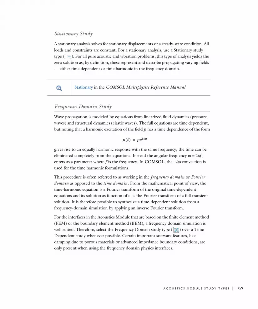
Stationary Study

A stationary analysis solves for stationary displacements or a steady-state condition. All loads and constraints are constant. For a stationary analysis, use a Stationary study type ( ). For all pure acoustic and vibration problems, this type of analysis yields the zero solution as, by definition, these represent and describe propagating varying fields — either time dependent or time harmonic in the frequency domain.

Frequency Domain Study

Wave propagation is modeled by equations from linearized fluid dynamics (pressure waves) and structural dynamics (elastic waves). The full equations are time dependent, but noting that a harmonic excitation of the field p has a time dependence of the form

gives rise to an equally harmonic response with the same frequency; the time can be eliminated completely from the equations. Instead the angular frequency ω = 2πf, enters as a parameter where f is the frequency. In COMSOL, the +iω convection is used for the time harmonic formulations.

This procedure is often referred to as working in the frequency domain or Fourier domain as opposed to the time domain. From the mathematical point of view, the time-harmonic equation is a Fourier transform of the original time-dependent equations and its solution as function of ω is the Fourier transform of a full transient solution. It is therefore possible to synthesize a time-dependent solution from a frequency-domain simulation by applying an inverse Fourier transform.

For the interfaces in the Acoustics Module that are based on the finite element method (FEM) or the boundary element method (BEM), a frequency domain simulation is well suited. Therefore, select the Frequency Domain study type ( ) over a Time Dependent study whenever possible. Certain important software features, like damping due to porous materials or advanced impedance boundary conditions, are only present when using the frequency domain physics interfaces.

Stationary in the COMSOL Multiphysics Reference Manual

p t( ) peiωt=

A C O U S T I C S M O D U L E S T U D Y T Y P E S | 759

760 | C H A P T E R

The result of a frequency domain analysis is a complex time-dependent field p, which can be interpreted as an amplitude pamp = abs(p) and a phase angle pphase = arg(p). The actual pressure at any point in time is the real part of the solution

Visualize the amplitudes and phases as well as the solution at a specific angle (time). When using the Solution datasets, the solution at angle (phase) parameter makes this task easy. When plotting the solution, COMSOL Multiphysics multiplies it by eiϕ, where is the angle in radians that corresponds to the angle (specified in degrees) in the Solution at angle field. The plot shows the real part of the evaluated expression:

The angle is available as the variable phase (in radians) and is allowed in plot expressions. Both the frequency freq and angular frequency omega are available variables.

Eigenfrequency Study

If all sources are removed from a frequency-domain equation, its solution becomes zero for all but a discrete set of angular frequencies ω, where the solution has a well-defined shape but undefined magnitude. These solutions are known as eigenmodes and their corresponding frequencies as eigenfrequencies.

The eigenmodes and eigenfrequencies have many interesting mathematical properties, but also direct physical significance because they identify the resonance frequency (or frequencies) of the structure. When approaching a resonance frequency in a harmonically-driven problem, a weaker and weaker source is needed to maintain a

p t( ) pamp 2πf t pphase+⋅( )cos=

ϕ

p pamp ϕ pphase+( )cos=

ϕ

In a frequency domain study, almost everything is treated as harmonic — prescribed pressures, displacements, velocities, and accelerations — not only the forces and dependent fields. Notable exceptions are certain quantities, such as the sound pressure level or intensity, which by definition are time averages.

Frequency Domain and Solution (datasets) in the COMSOL Multiphysics Reference Manual


given response level. At the actual eigenfrequency, the time-harmonic problem loses the uniqueness of the solution for a nonzero excitation.

Select the Eigenfrequency study type ( ) when you are interested in the resonance frequencies of the acoustic domain or the structure, whether you want to exploit them, as in a musical instrument, or avoid them, as in a reactive muffler or inside a hi-fi speaker system. To an engineer, the distribution of eigenfrequencies and the shape of eigenmodes can also give a good first impression about the behavior of a system.

An eigenfrequency analysis solves for the eigenfrequencies and the shape of the eigenmodes. When performing an eigenfrequency analysis, specify whether to look at the mathematically more fundamental eigenvalue λ (available as the variable lambda) or the eigenfrequency f, which is more commonly used in an acoustics context:

N O N L I N E A R E I G E N F R E Q U E N C Y A N A L Y S I S

In certain circumstances the material properties or boundary conditions can be frequency dependent. This is, for example, the case if a model set up with The Pressure Acoustics, Frequency Domain Interface contains a Narrow Region Acoustics or a Poroacoustics equivalent fluid model. The same is true if the Impedance boundary condition is added: most of the options listed in Theory for the Boundary Impedance Models define the acoustic impedance as a function of frequency. If the frequency dependence in these models is nonlinear, this will lead to a so-called nonlinear eigenvalue problem, which is more complex and therefore often must be treated carefully.

While solving a nonlinear eigenvalue problem, the linearization around some linearization point takes place behind the scenes. Expand the Study node, right-click the Solver Configurations node, and select Show Default Solver. In the generated solver sequence, navigate to the Eigenvalue Solver node and find the Transform point field. The value specified there will be used as the linearization point in the eigenvalue study, and therefore it is very important to set up for nonlinear eigenvalue problems.

The default Transform point value used in the acoustics interfaces is 100 Hz. If the eigenfrequencies of interest lie in kHz or MHz range, the default value of the linearization point may not ensure an accurate solution of a nonlinear eigenvalue problem — depending on its nonlinear properties. In this case, it is good practice to move the linearization point closer to the range of desired eigenfrequencies. For example, it can be the mean of the range. The other option is to define the Transform

f λ–2πi---------=


762 | C H A P T E R

point as a parameter, for example TP, add a Parametric Sweep over this parameter to the study, and search for one eigenfrequency around TP. This approach will be more accurate if the model exhibits strong nonlinear behavior within the range of desired eigenfrequencies, where a constant linearization point in not enough.

Mode Analysis Study

The Mode Analysis study ( ) is available with The Pressure Acoustics, Frequency Domain Interface, The Linearized Potential Flow, Frequency Domain Interface, and The Thermoviscous Acoustics, Frequency Domain Interface in plane 2D and axially symmetric 1D acoustics interfaces.

The Pressure Acoustics, Boundary Mode Interface, The Thermoviscous Acoustics, Boundary Mode Interface, and The Linearized Potential Flow, Boundary Mode Interface are special interfaces for more advanced Mode Analysis studies on boundaries in 3D and 2D axisymmetry. Acoustic waves can propagate over large distances in ducts and pipes, with a generic name referred to as waveguides. After some distance of propagation in a waveguide of uniform cross section, such guided waves can be described as a sum of just a few discrete propagating modes, each with its own shape and phase speed. The equation governing these modes can be obtained as a spatial Fourier transform of the time-harmonic equation in the waveguide axial direction (here assuming propagation in the z direction) or by inserting the assumption that the mode is harmonic in space,

and eliminating all out-of-plane z dependence. Here p(x,y) is the in-plane mode shape.

Similar to the full time-harmonic equation, the transformed equation can be solved at a given frequency with a nonzero excitation for most axial wave numbers kz. But at certain discrete values the equation breaks down. These values are the propagation constants or wave numbers of the propagating or evanescent waveguide modes. The

Eigenfrequency in the COMSOL Multiphysics Reference Manual

The axial wave number kz is a parameter in the 2D acoustics interfaces.

p x( ) p x y,( )e ikz z–=


eigenvalue solver can solve for these propagation constants together with the corresponding mode shapes.

The most common use for the Mode Analysis is to define sources for a subsequent time-harmonic simulation. If there is a component with one or more waveguide connections, its behavior can be described by simulating its response to the discrete set of propagating modes on the waveguide port cross sections. The Port boundary condition in Pressure Acoustics uses this concept to define sources and absorb outgoing modes. In thermoviscous acoustics, a Mode Analysis study also provides information about the absorption coefficient for the propagating modes. The complex wave number (solved for) and characteristic impedance (defined in postprocessing) define the homogenized propagation variables that can be used in Narrow Region Acoustics.

Boundary Mode Analysis

The Boundary Mode Analysis study ( ) is used when solving for the propagating modes used in a Port boundary condition in The Pressure Acoustics, Frequency Domain Interface. The study has special settings that can match the shape and wave number of the mode to a given port condition.

Time Dependent Study

The complete equations behind the theory of acoustic wave propagation are time dependent, as discussed in the Frequency Domain Study section. Solving time-domain equations is more complicated from a numerical point of view. They are necessary when studying systems where the time of flight is of importance, like in a flowmeter

The propagating wave number is a function of the frequency. The relation between the two is commonly referred to as a dispersion curve.

Mode Analysis in the COMSOL Multiphysics Reference Manual

Jet Pipe: Application Library path Acoustics_Module/

Aeroacoustics_and_Noise/jet_pipe


764 | C H A P T E R

application. Short-term transient processes like step and impulse responses can benefit from modeling in the time domain, if not for efficiency so for convenience.

A dedicated Transient Solver Settings settings section exist at the physics level for all the transient acoustics interfaces where the Maximum frequency to resolve should be entered.

Frequency Domain, Modal and Time-Dependent, Modal Studies

The Frequency Domain, Modal study type ( ) is used to do modal analysis in the frequency domain and the Time-Dependent, Modal study ( ) is used to do time-dependent modal analysis.

Ray Tracing

The Ray Tracing study type ( ) is used when solving acoustic problems using The Ray Acoustics Interface. It is a special case of the Time Dependent study and is used to compute the trajectories of rays. Special built-in stop conditions can be used to stop

Some central modeling techniques, such as the use of PMLs, are not available for all physics with the Time Dependent study type. PMLs only exist in the time domain for the Pressure Acoustics, Time Domain interface. Be careful when defining your sources to avoid, as far as possible, exciting waves at frequencies that the mesh cannot resolve.

Time Dependent in the COMSOL Multiphysics Reference Manual.

Further details on Time Stepping in Transient Models in the Modeling with the Pressure Acoustics Branch (FEM-Based Interfaces) section.

Frequency Domain, Modal and Time Dependent, Modal in the COMSOL Multiphysics Reference Manual

Helmholtz Resonator Analyzed with Different Frequency Domain Solvers: Application Library path Acoustics_Module/

Tutorials,_Pressure_Acoustics/helmholtz_resonator_solvers


the solver when no active rays remain or the intensity of the rays is below a certain criterion.

Modal Reduced Order Model

The Model Reduction and Modal Reduced Order Model study steps have the property that they can assemble the modal matrices and make them available for output. In the Model

Reduction node, the Store reduced matrices check box must be selected.

After solving the model, right-click the Derived Values node (under Results) and select System Matrix. In the output section, select the Matrix to display and the Format. Using the Matrix settings it is possible to access the stiffness, damping, and mass matrices of the system, for example.

Additional Analysis Capabilities

In a multiphysics interface you might want to use different analysis types for the different dependent variables. This can be done by adding an Empty Study ( ), and then adding different study steps to this study. Also perform parametric analyses by using the Parametric Sweep study node ( ). Typical parameters to vary include geometric properties, the frequency band in ray tracing, and the out-of-plane or axial wave number.

Mapping

The Mapping ( ) study is a dedicated study to use when the Background Fluid Flow Coupling couples a Fluid Flow interface and an Aeroacoustics interface. The study should only solve for the multiphysics coupling. The study uses a Stationary solver. Together with the multiphysics coupling, the study handles the mapping of dependent


• Modal Reduced-Order Model and Introduction to Solvers and Studies

• System Matrix and Results Analysis and Plots

Parametric Sweep in the COMSOL Multiphysics Reference Manual


766 | C H A P T E R

variables between the fluid flow mesh and the acoustics mesh for consistent simulation results.

P H Y S I C S A N D V A R I A B L E S S E L E C T I O N

Only select the Background Fluid Flow Coupling as being Solved for. No other physics will be solved by the mapping study.

S O L U T I O N T O M A P

From the Study list select the study containing the coupled fluid flow interface to map. Depending on the type of study, used for the fluid flow simulation, you will get a different type of list to choose from: time steps or parameter values. From the list, select the appropriate solution or solutions to map. The option All will automatically add a parameter sweep and map all parameter values from the selected solution. The Mapping study step will automatically ensure that those parameter values are used.

Note that the mapping does not benefit from running continuation for any parameter. When the solution is mapped for all parameter values, for a multiple parameter sweep where continuation was used in the fluid flow study, the resulting dataset structure of the two studies will therefore be slightly different.

D E S T I N A T I O N M E S H S E L E C T I O N

Select the destination/target mesh of the mapping, that is, the acoustics mesh used for the aeroacoustics simulation.


13

A c o u s t i c P r o p e r t i e s o f F l u i d s

The Acoustics Module contains a number of models describing attenuation processes and loss mechanisms, and they have various inputs for the acoustic relevant material properties of fluids. This chapter provides information about those properties and puts them all in context.

In this chapter:

• Material Properties

• The Bulk Viscosity

• Attenuation and Loss Models

• References for The Acoustic Properties of Fluids

767

768 | C H A P T E R

Ma t e r i a l P r op e r t i e s

The Acoustics Module includes two material databases: Liquids and Gases, with temperature-dependent fluid dynamic and thermal properties, and a Piezoelectric Materials database with common piezoelectric materials.

Probably, the two most common materials used in acoustics are air and water. In this section we shortly discuss the definition and properties of the built-in Air and Water, liquid materials from the Material Library.

The built-in air and water materials are general and to some extent simplified models. For example, the air represents dry air and the material properties do not depend on moisture. This means that for high-precision absolute-value simulations, detailed material data need to be entered. Two options exist:

1 Using the Predefined System for Moist air, Dry air, or Water-steam defined in the Thermodynamics feature available with the Liquid & Gas Properties Module. Once set up, a material can be automatically generated.

2 Create your own material, for example, following the IEC standard for moist air (see Ref. 13). Set up a material and let it depend on the necessary model inputs (pressure, temperature, or relative humidity). Then, set up the necessary interpolation functions or analytical expressions and store the material under the User-Defined Library for future use.

Moist air is generated from Thermodynamics in the Pressure Reciprocity Calibration Coupler with Detailed Moist Air Material Properties tutorial. Application Library path Acoustics_Module/Tutorials,_Thermoviscous_Acoustics/

pressure_reciprocity_calibration_coupler

The Air and Water, liquid materials were updated for the COMSOL version 5.4 release. Some material data has been added to simplify modeling, and inconsistencies due to rounding have been removed.

To take advantage of the new and updated material data, when opening an existing model (older than version 5.4), delete the material and add it again from the Materials window.

1 3 : A C O U S T I C P R O P E R T I E S O F F L U I D S

T H E ( D R Y ) A I R M A T E R I A L

The built-in Air material, located both in the Built-In and the Liquids and Gases library, is commonly used in applications and models. The material properties represent those of dry air without the inclusion of moisture.

The air material defines common material parameters and their dependency on the ambient pressure pA and temperature T. The relations are simplified and not all thermodynamic dependencies are taken into account. The speed of sound c and the density ρ are defined through the ideal gas law (assuming adiabatic behavior) following

with the ratio of specific heats γ = 1.4, the gas constant R (COMSOL has a built-in constant called R_const), and the molar mass Mn = 0.02897 kg/mol. This is an idealization of air valid in many cases; see Ref. 2. This means that the speed of sound is not a function of the ambient pressure for this built-in Air material.

Some material properties are only temperature dependent and are given by polynomial fit curves like:

• The dynamic viscosity μ = μ(T)

• The (specific) heat capacity at constant pressure Cp = Cp(T)

• The thermal conductivity k = k(T)

Some properties are defined as constant:

• The ratio of specific heats γ = 1.4

• The molar mass Mn = 0.02897 kg/mol

Furthermore, there are material parameters and properties that are derived from their definitions and the above material data:

For detailed information about Materials, the Liquids and Gases Materials Library, and the Piezoelectric Materials Library see the COMSOL Multiphysics Reference Manual.

For detailed information about the Predefined system see the Thermodynamics chapter in the Liquid & Gas Properties User’s Guide.

c2 γ RMn--------T= ρ

MnpART

---------------=

M A T E R I A L P R O P E R T I E S | 769

770 | C H A P T E R

• The bulk viscosity μB is defined as μB = 0.6·μ(T) in order to comply with the absorption behavior (see discussion in The Bulk Viscosity section).

• The (isobaric) coefficient of thermal expansion is defined as αp = 1/T, following the ideal gas law.

• The parameter of nonlinearity B/A is also defined for gases following the ideal gas law as B/A = (γ+1)/2 (see Ref. 12).

T H E ( C L E A N ) W A T E R M A T E R I A L

The built-in Water, liquid material, located both in the Built-In and the Liquids and Gases library, is also commonly used in applications and models. These material properties represent those of clean water without the dependency on, for example, salinity or pH value necessary to describe salt water in the ocean.

Specifically for acoustics applications, the water material properties include properties that are temperature dependent like:

• The speed of sound c = c(T)

• The density ρ = ρ(T)

• The dynamic viscosity μ = μ(T)

• Thermal conductivity k = k(T)

• The heat capacity at constant pressure Cp = Cp(T)

Furthermore, there are detailed material parameters that are derived from the above definitions:

• The bulk viscosity is defined as μB = 2.79·μ(T). In order to comply with the absorption behavior, (see the discussion in The Bulk Viscosity section).

• The (isobaric) coefficient of thermal expansion is defined through the thermodynamic definition as

• The ratio of specific heats γ = γ(Τ) is based on the thermodynamic relation

αp1ρ---–

∂ρ∂T-------

pA

=


.

This definition is necessary in detailed models solving the thermoviscous acoustics or the linearized Navier-Stokes equations in water. The definition ensures that it is not just set to γ = 1.

γ 1Tαp

2c2

Cp----------------+=

M A T E R I A L P R O P E R T I E S | 771

772 | C H A P T E R

Th e Bu l k V i s c o s i t y

The bulk viscosity μB of a fluid is also known as the volume viscosity or the second viscosity. It is often not used in classical CFD applications but it plays a role in acoustics as well as in high-velocity compressible flows. The bulk viscosity is associated with losses due to expansion and compression, that is, the compressional resistance. The parameter describes the difference between the mechanical and thermodynamic pressures. It is often described as representing all the effects that describe the time it takes to establish thermodynamic equilibrium for vibrational and rotational motion of the fluid molecules (see Ref. 18). In some sense, it can be said to describe low frequency relaxation processes.

In acoustics, the losses associated with the bulk viscosity only really play a role in high-frequency ultrasound propagation. The bulk viscosity term in the thermoviscous acoustics or the linearized Navier-Stokes equations is sometimes used to model the frequency dependent losses due to relaxation processes. Various models exist to include these effects; details can be found in Ref. 17.

The Value of the Bulk Viscosity

The value of the bulk viscosity is difficult to measure and typically requires absorption experiments to be determined. For most fluids, its numerical value is of the same order as the dynamic viscosity. For some further details see, for example, Ref. 14 for fluids, Ref. 16 for water values, and Ref. 15 for gases.

The bulk viscosity enters the classical (pure) thermoviscous attenuation coefficient defined as

This is the attenuation experienced by plane propagating waves away from boundaries. The expression is derived directly from the full thermoviscous acoustics equations. In the Air and Water, liquid materials in the Material Library, the bulk viscosity is defined to match the high-frequency absorption properties of the fluids.

In Figure 13-1 standardized atmosphere attenuation curves (see the Atmosphere Attenuation Fluid Model in pressure acoustics) are depicted for various relative humidities together with the classical thermoviscous attention. The graph also shows

αtvω2

2ρc3------------ 4

3---μ μB

k γ 1–( )Cp

--------------------+ + =


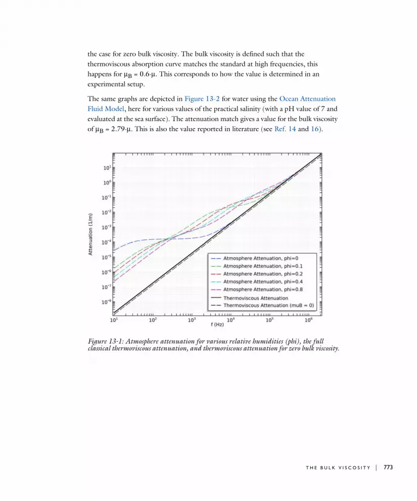
the case for zero bulk viscosity. The bulk viscosity is defined such that the thermoviscous absorption curve matches the standard at high frequencies, this happens for μB = 0.6·μ. This corresponds to how the value is determined in an experimental setup.

The same graphs are depicted in Figure 13-2 for water using the Ocean Attenuation Fluid Model, here for various values of the practical salinity (with a pH value of 7 and evaluated at the sea surface). The attenuation match gives a value for the bulk viscosity of μB = 2.79·μ. This is also the value reported in literature (see Ref. 14 and 16).

Figure 13-1: Atmosphere attenuation for various relative humidities (phi), the full classical thermoviscous attenuation, and thermoviscous attenuation for zero bulk viscosity.

T H E B U L K V I S C O S I T Y | 773

774 | C H A P T E R

Figure 13-2: Ocean attenuation for various practical salinities (S·1000), the full classical thermoviscous attenuation, and thermoviscous attenuation for zero bulk viscosity.


A t t e nua t i o n and Lo s s Mode l s

The Acoustics Module includes several different physics interfaces and various features that introduce acoustic losses. These describe everything from thermoviscous boundary layer losses to the attenuation experienced when acoustic waves propagate over long distances in the ocean. The models have different applicability depending on the frequency regime and the system modeled.

This section first gives a short description of the different loss mechanism, then the applicability and the regime where boundary layer and bulk losses apply is discussed, and finally some remarks are given on the bulk viscosity and how it is related to attenuation.

In this section:

• Loss Mechanisms

• The Atmosphere and Ocean Attenuation Models

• Boundary Layer vs. Bulk Losses

Loss Mechanisms

Loss mechanisms in acoustics due to viscosity, thermal conduction, relaxation processes, and other processes cause absorption and dissipation of the acoustic energy. These result in a reduction in the pressure wave amplitude. This is not due to geometrical spreading where no energy is lost, but because heating actually takes place. When an acoustic wave undergoes absorption, this process is in general also accompanied by dispersion, that is, the dependence of the speed of sound on frequency.

Loss mechanism in acoustics can roughly be divided into four categories, but can of course also happen simultaneously. The division is mostly conceptual:

1 Bulk or volume losses are associated with the propagation of waves over long distances or at very high frequencies (also known as internal damping). The (plane wave) attenuation coefficient α (SI unit: 1/m) is often associated with this mechanism. Several loss models are included in the Pressure Acoustics model (see also Theory for the Equivalent Fluid Models) including: User-Defined Attenuation Fluid Model, Atmosphere Attenuation Fluid Model, Ocean Attenuation Fluid Model, or Thermally Conducting and/or Viscous Fluid Model. Note that the

A T T E N U A T I O N A N D L O S S M O D E L S | 775

776 | C H A P T E R

Thermally Conducting and/or Viscous Fluid Model should not be confused with boundary layer losses (see next point). Bulk losses are due to several different mechanisms including viscous and thermal dissipation, relaxation processes, and other loss mechanism.

2 Viscous and thermal boundary-layer losses occur at hard walls because of the effective no-slip and isothermal conditions. These are most important in geometries of small dimensions comparable to the boundary layer thickness. The losses can be included in a very general manner using one of the Thermoviscous Acoustics Interfaces. The Narrow Region Acoustics feature can be used in narrow waveguides of constant cross section, while the Thermoviscous Boundary Layer Impedance condition can be used an any boundary as long as no boundary layers are overlapping. The latter two features are great engineering approximations (often yielding exact results) to include the losses at a lower computational cost using the The Pressure Acoustics, Frequency Domain Interface.

3 In porous materials, losses are again due to viscous and thermal boundary layer losses, here inside the channels of the porous matrix. The losses are also caused by damping because of the coupling to the porous matrix structure. Detailed modeling is done using The Poroelastic Waves Interface that solves the full Biot model for the coupled pressure and structural waves. A simplified so-called equivalent fluid description can be done using the Poroacoustics feature (see also Theory for the Equivalent Fluid Models).

• Losses can also occur due to interaction with the surroundings like solids and membranes. This is best modeled using multiphysics, see Acoustic-Structure Boundary in the Multiphysics Couplings chapter. Here, simplified models exist using the many options available with the Impedance boundary conditions (see Theory for the Boundary Impedance Models).

The Atmosphere and Ocean Attenuation Models

The Pressure Acoustics, Frequency Domain Interface and The Ray Acoustics Interface include two semi analytical fluid models that are calibrated with extensive measurement data. This is the Atmospheric attenuation and the Ocean attenuation models. Both include effects due to viscosity and thermal conduction and relaxation processes of molecules.

The Atmospheric attenuation model defines attenuation in atmospheric air that follows the ANSI standard S1.26-2014, see Ref. 3 (Appendix B), 4, 5, and 6 for details. The model describes attenuation due to thermal and viscous effects (primarily pure air), the


relaxation processes for nitrogen and oxygen, and the dependency on atmospheric pressure (absolute pressure), temperature, and relative humidity. The attenuation in air is important for propagation over large distances and for high frequency processes. This also means that the attenuation effect is more important in ray tracing simulations where propagation can be simulated over much larger distances and especially at higher frequencies. In the next section, we will see when the full details of this model are necessary when compared to boundary layer losses.

The Ocean attenuation model defines attenuation in seawater of the ocean. The model is based on a semianalytical model with parameters that are based on extensive measurement data. No standard exists for the attenuation in sea water. It includes effects due to viscosity in pure water, the relaxation processes of boric acid and magnesium sulfate, as well as depth, temperature, practical salinity, and pH value. For further details see Ref. 7, 8, 9, 10, and 11. Like the atmosphere model, the ocean attenuation model is important in ray tracing simulations where propagation can be simulated over much larger distances.

Boundary Layer vs. Bulk Losses

As discussed in the above sections, the Acoustics Module includes models for both bulk losses and boundary layer losses. In pressure acoustics, you can include either form of losses. For example, the Atmosphere attenuation fluid model in pressure acoustics is a detailed bulk loss model that includes all dissipation effects and it complies with the ANSI standard. On the other hand, the Narrow Region Acoustics feature includes the boundary layer losses for narrow waveguide structures.

The importance of the two loss mechanisms (bulk and boundary layer) depend on the geometry scale and the frequency range studied. As an example, the losses experienced by a plane wave propagating in an air filled narrow circular duct is depicted in Figure 13-3. The graph includes:

• The bulk atmosphere attenuation for different relative humidities ( , 20 % and 80 %).

• The classical (bulk) thermoviscous attenuation.

• The thermoviscous boundary layer attenuation for different duct radii (a = 0.5 mm, 2.0 mm, and 10.0 mm) modeled using the Narrow Region Acoustic feature.

• The solution using the full thermoviscous acoustics equations in the cylindrical duct of radius a = 2.0 mm. This can be seen as a reference solution since it models both boundary layer and thermoviscous bulk losses.

φ 0 %=

A T T E N U A T I O N A N D L O S S M O D E L S | 777

778 | C H A P T E R

From the graph, it is evident that in relatively narrow waveguide structures the boundary layer losses far surpass the bulk losses in a large frequency range. The transition happens in the ultrasound regime. The graph also shows that (for air) the real life relaxation effects captured by the atmosphere attenuation model can be disregarded in most waveguides and really only are important away from boundaries and for propagation over large distances.

The transition between the two loss regimes is captured by the full thermoviscous acoustics models. For the vast majority of practical applications, when using the Thermoviscous Acoustics physics interfaces, it is not necessary to include the “true” bulk behavior captured by the atmosphere model. This is simply because it is not computationally possible to model large scale acoustics with the Thermoviscous Acoustics interfaces - their true application is in complex narrow geometries.

Figure 13-3: The importance of various attenuation mechanisms for the propagation of plane waves in a cylindrical duct of radius a. The plot shows the (bulk) atmosphere attenuation contribution for different relative humidities φ, the classical (bulk) thermoviscous attenuation, the thermoviscous boundary layer attenuation for different duct radii a, and reference solution using the full thermoviscous acoustics model (in the duct with a radius of 2.0 mm).


Re f e r e n c e s f o r T h e A c ou s t i c P r op e r t i e s o f F l u i d s

1. S. Temkin, Elements of Acoustics, Acoustical Society of America, 2001.

2. A.D. Pierce, Acoustics: An Introduction to its Physical Principles and Applications, Acoustical Society of America (second print), 1991.


4. . E. Bass, L. C. Sutherland, A. J. Zuckerwar, D. T. Blackstock, and D. M. Hester, “Atmospheric absorption of sound: Further developments,” J. Acoust. Soc. Am., vol. 97, pp. 680-683, 1995; “Erratum” J. Acoust. Soc. Am., vol. 99, p. 1259. 1996.

5. ANSI S1.26-2014 (supersedes ANSI S1.26-1995) “American National Standard method for calculation of the absorption of sound by the atmosphere” (Acoustical Society of America, New York, 2014).

6. National Physics Lab (NPL), “NPL Acoustics: Calculation of absorption of sound by the atmosphere,” http://resource.npl.co.uk/acoustics/techguides/absorption/

7. R. E. Francois and G. R. Garrison, “Sound absorption based on ocean measurements: Part I: Pure water and magnesium sulfate contributions,” J. Acoust. Soc. Am., vol. 72, pp. 896-907, 1982.

8. R. E. Francois and G. R. Garrison, “Sound absorption based on ocean measurements: Part II: Boric acid contribution and equation for total absorption,” J. Acoust. Soc. Am., vol. 72, pp. 1879-1890, 1982.

9. M. A Ainslie and J. G. McColm, “A simplified formula for viscous and chemical absorption in sea water,” J. Acoust. Soc. Am., vol. 103, pp. 1671-1672, 1998.

10. Fisher F. H., Simmons V. P., “Sound absorption in seawater,” J. Acoust. Soc. Am., vol. 62, pp. 558-564, 1977.

11. National Physics Lab (NPL), “Calculation of absorption of sound in seawater,” http://resource.npl.co.uk/acoustics/techguides/seaabsorption/

12. M. F. Hamilton and D. T. Blackstock, “On the coefficient of nonlinearity in nonlinear acoustics”, J. Acoust. Soc. Am., vol. 83, pp. 74-77, 1988.

R E F E R E N C E S F O R T H E A C O U S T I C P R O P E R T I E S O F F L U I D S | 779

780 | C H A P T E R

13. IEC 61094-2:2009, “Electroacoustics - Measurement microphones - Part 2: Primary method for pressure calibration of laboratory standard microphones by the reciprocity technique,” International Standard.

14. A. S. Dukhin and P. J. Goetz, “Bulk viscosity and compressibility measurements using acoustic spectroscopy”, J. Chem. Phys., vol. 130, p. 124519-1, 2009.

15. M. S. Cramer, “Numerical estimate for the bulk viscosity of ideal gases”, Phys. Fluids, vol. 30, p. 066102, 2012.

16. P. B. Muller and H. Bruus, “Numerical study of thermoviscous effects in ultrasound-induced acoustic streaming in microchannels,” Phys. Rev. E, vol. 90, pp. 043016, 2014.

17. E. M. Viggen, “The lattice Boltzmann method: Fundamentals and acoustics,” Ph.D. Thesis, NTNU-Trondheim, 2014.

18. P. M Morse and K. U. Ingard, Theoretical Acoustics, Princeton University Press, 1986.


14

G l o s s a r y

This Glossary of Terms contains finite element modeling terms in an acoustics context. For mathematical terms as well as geometry and CAD terms specific to the COMSOL Multiphysics® software and documentation, see the glossary in the COMSOL Multiphysics Reference Manual. For references to more information about a term, see the index.

781

782 | C H A P T E R

G l o s s a r y o f T e rm sacoustic impedance At a specified surface, the complex quotient of acoustic pressure by normal fluid velocity. SI unit: Pa/(m/s) .

acoustic reactance The imaginary part of the acoustic impedance.

acoustic resistance The real part of the acoustic impedance.

acoustic-structure interaction A multiphysics phenomenon where the fluid’s pressure causes a fluid load on the solid domain, and the structural acceleration affects the fluid domain as a normal acceleration across the fluid-solid boundary.

adiabatic bulk modulus One over the compressibility βs measured at constant entropy. The adiabatic bulk modulus is denoted Ks and gives a measure of the compressibility of the fluid and is directly related to the speed of sound cs in the fluid. SI unit: Pa.

admittance The reciprocal of impedance.

aeroacoustics The scientific field of study used to couple acoustics and fluid dynamics.

anisotropy Variation of material properties with direction.

arbitrary Lagrangian-Eulerian (ALE) method A technique to formulate equations in a mixed kinematical description. An ALE referential coordinate system is typically a mix between the material (Lagrangian) and spatial (Eulerian) coordinate systems.

Bernoulli equation An integrated form of Euler’s momentum equation along a line of flow. The equation gives an expression for an invariant quantity in an inviscid fluid. A decrease in the speed of the fluid translates to an increase in the fluid pressure and/or potential energy.

bulk modulus One over the compressibility. It gives a measure of the compressibility of the fluid and is related to the speed of sound in the fluid. SI unit: Pa. See also adiabatic bulk modulus.

Ks1βs----- ρ0cs

2= =

1 4 : G L O S S A R Y

characteristic impedance The product of the equilibrium density and the speed of sound in a medium. SI unit: Pa/(m/s).

compliance Reciprocal of stiffness.

compliance matrix The inverse of the elasticity matrix. See elasticity matrix.

Cauchy stress The most fundamental stress measure defined as force/deformed area in fixed directions not following the body.

constitutive equations Equations that relate two physical quantities. In thermoviscous acoustics both the stress tensor (relating velocity to stress) and Fourier’s law of heat conduction (relating heat conduction to temperature) are constitutive relations. In structural mechanics this is the equation formulating the stress-strain relationship of a material. Constitutive equations are supplemented by equilibrium equations (mass, momentum, and energy) and an equation of state to provide a full physical description.

creep Time-dependent material nonlinearity that usually occurs in metals at high temperatures in which the effect of the variation of stress and strain with time is of interest.

damping Dissipation of energy in the fluid or a vibrating structure. The damping is typically due to viscous losses or thermal conduction. In acoustics this happens in structures with small geometrical dimensions, for example, small pipes or porous materials. In structures a common assumption is viscous damping where the damping is proportional to the velocity. See also Rayleigh damping.

decibel (dB) Logarithmic unit that indicates the ratio of a physical quantity relative to a reference value.

dipole source An acoustic source that behaves as a translational oscillating sphere.

Doppler effect Change in the observed frequency of a wave caused by a time rate of change in the effective length of the path of travel between the source and the observation point.

effective sound pressure RMS instantaneous sound pressure at a point during a time interval, T, long enough that the measured value is effectively independent of small changes in T. SI unit: Pa = N/m2.

G L O S S A R Y O F T E R M S | 783

784 | C H A P T E R

equation of state The thermodynamic relation between three independent thermodynamic variables. Typically in acoustics it is the density ρ = ρ(p,s) given as function of the entropy s and the pressure p.

eigenmode A possible propagating mode of an acoustic wave.

elasticity matrix The matrix D relating strain to stresses:

Eulerian Model described and solved in a coordinate system that is fixed (spatial). See also Lagrangian and arbitrary Lagrangian-Eulerian method.

Green-Lagrange strain Nonlinear strain measure used in large-deformation analysis. In a small strain, large rotation analysis, the Green-Lagrange strain corresponds to the engineering strain, with the strain values interpreted in the original directions. The Green-Lagrange strain is a natural choice when formulating a problem in the undeformed state. The conjugate stress is the second Piola-Kirchhoff stress.

impedance At a specified frequency, the quotient of a dynamic field quantity (such as force, sound, or pressure) by a kinematic field quantity (such as vibration velocity or particle velocity).

instantaneous sound pressure Total instantaneous pressure at a point in a medium minus the static pressure at the same point. SI unit: Pa = N/m2.

irrotational background velocity field A velocity field u that has the property of having rotation everywhere, where the first term is the vorticity of the fluid. In such a fluid the viscous stress does not contribute to the acceleration of the fluid. The mean pressure in this fluid is described by Bernoulli’s equation.

Lagrangian Model described and solved in a coordinate system that moves with the material. See also Eulerian and arbitrary Lagrangian-Eulerian method.

monopole source An acoustic source that behaves as a radially oscillating sphere.

particle velocity In a sound field, the velocity caused by a sound wave of a given infinitesimal part of the medium relative to the medium as a whole.

σ Dε=

∇ u× 0=

1 4 : G L O S S A R Y

PML (perfectly matched layer) Domain adjoined at a system boundary designed to emulate a nonreflecting boundary condition independently of the shape and frequency of the incident wavefront.

principle of virtual work States that the variation in internal strain energy is equal to the work done by external forces.

propagating acoustic modes The acoustic modes or wave shapes that propagate with no significant damping for a given frequency in a duct of a given cross-section.

Rayleigh damping A viscous damping model where the damping is proportional to the mass and stiffness through the mass and stiffness damping parameters.

reference sound pressure See definition in the entry for sound pressure level.

resonance frequency A frequency at which the system has the tendency to oscillate at a greater amplitude than at nonresonance frequencies. At the resonance frequencies the system can easily transfer energy from the actuation to the vibrating structure or acoustic wave.

RMS value Root-mean-square value; for the (complex) sound pressure, p(t), over the time interval T1 < t < T2 defined as

For a harmonic pressure wave, , the time interval is taken to be a complete period, resulting in pRMS = p0 /√2.

second Piola-Kirchhoff stress Conjugate stress to Green-Lagrange strain used in large deformation analysis.

sound energy Total energy in a given part of a medium minus the energy that would exist at the same part in the absence of sound waves. SI unit: J.

sound-energy flux density See sound intensity.

sound intensity Average rate of sound energy transmitted in a specified direction at a point through a unit area normal to this direction. SI unit: W/m2.

sound pressure See effective sound pressure.

pRMS1

T2 T1–------------------- Re p t( )[ ] 2 td

T1

T2=

p t( ) p0eiωt=


786 | C H A P T E R

sound pressure amplitude Absolute instantaneous sound pressure in any given cycle of a sound wave at some specified time. SI unit: W/m2.

sound power density See sound intensity.

sound pressure level Ten times the logarithm (to the base ten) of the ratio of the time-mean-square pressure of a sound, in a stated frequency band, to the square of a reference sound pressure, pref. For gases, pref = 20 μ Pa, for other media (unless otherwise specified) pref = 1 μ Pa. Unit: dB (decibel).

sound source strength Maximum instantaneous rate of volume displacement produced by a source when emitting a harmonic sound wave. SI unit: m3/s.

specific acoustic impedance At a point in a sound field, the quotient of sound pressure by particle velocity. SI unit: Pa/(m/s).

speed of sound The rate of change of particle displacement with distance for a sound wave. SI unit: m/s.

spin tensor The skew-symmetric part of the velocity gradient tensor.

static pressure Pressure that would exist at a point in the absence of a sound wave.

stiffness Ratio of change of force (or torque) to the corresponding change in translational (or rotational) displacement of an elastic element.

thermoviscous acoustics The interaction between thermodynamic and acoustic phenomena, which takes into account the temperature oscillations that accompany the acoustic pressure oscillations. The combination of these oscillations produces thermoviscous acoustic effects. Thermoviscous acoustic phenomena are modeled by solving the full linearized Navier-Stokes equation (momentum equation), the continuity equation, and the energy equation. Thermoviscous acoustics is also known as viscothermal acoustics or thermoacoustics.

velocity potential When a flow is irrotational the vector field (velocity field) can always be derived from a scalar potential φ(x) as , where φ is the velocity potential. See also irrotational background velocity field.

waveguide structures Structures that have the property of guiding sound waves. See also propagating acoustic modes.

∇ u× 0=

u ∇φ=

1 4 : G L O S S A R Y


788 | C H A P T E R
1 4 : G L O S S A R Y

I n d e x

A accumulator (node), boundaries 617

accumulator (node), domains 628

accuracy order, of time stepping 605

acoustic diffusion equation interface 687

acoustic diffusion model (node) 691

acoustic intensity vector 204

acoustic-elastic waves interaction inter-

face 360

acoustic-piezoelectric interaction, fre-

quency domain (acpz) interface 352

acoustic-piezoelectric interaction, tran-

sient (acpztd) interface 355

acoustic-poroelastic waves interaction

interface 358

acoustic-porous boundary (multiphysics

coupling) 738

acoustic-shell interaction, frequency do-

main interface 365

acoustic-shell interaction, transient in-

terface 368

acoustic-solid interaction, frequency do-

main interface 346

acoustic-solid interaction, transient in-

terface 349

acoustic-structure boundary (multiphys-

ics coupling) 732

acoustic-thermoacoustic boundary (mul-

tiphysics coupling) 737

acoustic-thermoacoustic interaction,

frequency domain 527

adiabatic (node) 419, 510

adiabatic bulk modulus 226

adiabatic, reversible processes 552

aeroacoustic-structure boundary (multi-

physics coupling) 736

analysis. see study types.

Application Libraries window 46

application library examples

acpr interface 61, 739, 743, 746, 768

actd interface 138, 142, 233

ae interface 426

aebm interface 440

background pressure field 85

Biot equivalent fluid model 277

cpf interface 443

cylindrical wave radiation 114

eigenfrequency study 231

Eigenmodes in a Muffler 153

far field calculation 101, 108

far field plots 213–214

flow point source 127

fluid model 73

Gaussian pulse point source 146

Generic 711 Coupler — An Occluded

Ear-Canal Simulator 93

interior normal acceleration 118

Lumped Receiver Connected to Test

Setup with an 0.4-cc Coupler 81

mass flow point source 434

mode analysis study 763

pipe acoustics, transient 728

point source 94, 127

poroelastic waves 297

pressure acoustics, frequency domain

61, 739, 743, 746, 768

spherical wave radiation 156

ta interface 486, 735

artificial boundary conditions 36

asymptotic far-field radiation (node) 391

attenuation coefficient 66, 557

auxiliary dependent variable 616

auxiliary dependent variable (node) 636

I N D E X | 789

790 | I N D E X

axial symmetry (node) 87, 435

B background potential flow (multiphysics

coupling) 739

background pressure field (node) 82, 143

background pressure wave 56

background velocity (node) 636

barotropic fluids 475

Bernoulli equation 475

Biot theory 332

Biot’s high frequency range 333

Bloch periodicity 501

boundary mode acoustics (acbm) inter-

face 151

theory 233

boundary nodes

acbm interface 153

acpr interface 61

actd interface 138

ae interface 426

aebm interface 440

aetd interface 437

cpf interface 443

cwe interface 564

lef and let interfaces 380

lnsf and lnst interfaces 403

pelw interfaces 298


tabm interface 524

boundary-layer absorption 280

bulk modulus 722

elastic moduli 316

pressure acoustics 33

C caustic surface 667

CFL condition 727

circular duct 283

circular source (node) 134

circumferential wave number 229, 234

common settings 44

complex conjugate operator 206

complex impedance 34

complex wave numbers 34

compressible potential flow (cpf) inter-

face 442

compressible potential flow model

(node) 444

compute intensity 603

compute intensity and power 603

compute intensity and power in graded

media 603

compute intensity in graded media 603

continuity (node)

acpr interface 122

ae interface 392, 433

lns interface 420

convected wave equation interface 562

count reflections 604

Coupling Operators 658

Courant number 728

cwe nodes

acpr interface 564

cylindrical wave radiation (node) 113

D damping

boundaries 36

degrees of freedom 186

Density of exterior domains 602, 656

diffuse scattering, wall condition 611

dipole point source (node) 128

dipole source (node) 86

dipole sources 226

disappear, wall condition 611

dispersion curves 763

dispersion relation 558

documentation 45

domain nodes

acbm interface 153

acpr interface 61

actd interface 138

ae interface 426

aetd interface 437

cpf interface 443

cwe interface 564



pelw interfaces 298


domain source (node) 694

domain sources (node) 385, 409

double dot operator 543

E edge nodes

acbm interface 153

acpr interface 61

actd interface 138

ae interface 426

aebm interface 440

aetd interface 437

eigenfrequency study 760

pressure acoustics 230

elastic waves (elw) interface

theory 331

elkernel element 240

emailing COMSOL 47

empty study 765

end impedance (node) 718

pipe acoustics 718

equilateral triangular duct 283

equivalent fluid model 65, 162, 267

equivalent fluid models 262

Euler equations 474

evanescent modes 762

evanescent wave components 209

F far field variables 211

far-field calculation (node) 98

far-field limits 210, 239

far-field regions 208

far-field variables 210

first order material parameters (node)

409

fitted domain (node) 694

fixed (node) 306

Floquet periodicity 501

fluid models 262

fluid models, pressure acoustics 64, 162

Fraunhofer diffraction 209

freeze, wall condition 611

frequency domain modal study 764

frequency domain study 759

ae interface 472

Fresnel numbers 209

G general reflection, wall condition 611

Green’s function 238

H Hankel function 238

harmonic time dependence 204

heat flux (node) 419

heat source (node) 492

Helmholtz-Kirchhoff integral 209, 237

Higdon conditions 235

high frequency range 333

I ideal barotropic fluids 475

ideal gas fluid model 69

impedance (node) 389

acpr interface 90

ae interface 432

impedance, complex 34

incident acoustic fields (node) 386

incident pressure field (node) 114, 144

incident velocity potential (node) 430

initial values (node)

abe interface 694

acbm interface 152

acpr interface 85, 569

ae interface 427

I N D E X | 791

792 | I N D E X

cpf interface 445

elw interface 306

lem interface 385

let interface 397


pafd interface 714

patd interface 714

ta interface 492

inlet on axis (node) 635

insertion loss curves 204

intensity 602

intensity attenuation coefficient 66

intensity computation 666

intensity variables 203

interior impedance (node) 119, 389

interior normal acceleration (node) 117

interior normal displacement (node) 118,

149

interior normal impedance (node) 414,

504

interior normal velocity (node) 118, 149

interior perforated plate (node) 120

interior sound hard boundary (wall)

(node)

acpr interface 117

ae interface 433

interior velocity (node) 504

interior wall (node) 391, 413, 503

internet resources 44

inward energy flux (node) 693

irrotational velocity fields 471

isentropic processes 552

isentropic speed of sound 542

isothermal (node) 418, 510

isotropic meshes 186

isotropic scattering, wall condition 611

J JCA model 75

JCAL model 76

JCAPL model 76

K knowledge base, COMSOL 48

Korteweg formula 722

L Lagrange elements 187

Lamé parameters 316

large acoustics problems 192

Lax-Friedrichs flux parameter 175, 318,

567

limp frame 71

limp porous matrix model 267

line source (node) 122

line source on axis (node) 125

linear elastic fluid model 262

linearized Euler model (node) 381

linearized Euler, frequency domain inter-

face 377

linearized Euler, transient interface 394

linearized Navier-Stokes model (node)

404

linearized Navier-Stokes, frequency do-

main interface 399

linearized Navier-Stokes, transient inter-

face 421

linearized potential flow model (node)

427

linearized potential flow, boundary mode

interface 439

linearized potential flow, frequency do-

main interface 424

linearized potential flow, transient inter-

face 436

liquids and gases materials 216, 768

low reduced frequency (LRF) 283

M mapped room coupling (node) 695

mass flow (node) 446

mass flow circular source (node) 434

mass flow edge source (node) 434

mass flow line source on axis (node) 435

mass flow point source (node) 434

mass flows 429

matched boundary (node) 97

matched boundary conditions 36

material discontinuity (node) 618

materials

porous absorbing 34

medium properties (node) 608

mixed diffuse and specular reflection,

wall condition 611

mode analysis study 762

boundary mode acoustics 233

theory 557

monopole point source (node) 126

monopole source (node) 85

monopole sources 226

motionless skeleton model 267

moving wall (node) 390, 397

MPH-files 46

multigrid solvers 192

multiphysics 346, 349, 365, 368, 527, 530

multiphysics coupling

acoustic-porous boundary (node) 738

acoustic-structure boundary (node)

732

acoustic-thermoacoustic boundary

(node) 737

aeroacoustic-structure boundary

(node) 736

background potential flow (node) 739

porous-structure boundary (node) 739

thermoviscous acoustic-structure

boundary (node) 734

N narrow region acoustics (node) 78

near-field regions 209

no slip (node) 415, 506

no stress (node) 417, 509

nodes, common settings 44

no-flow conditions 428, 433

nonlinear pressure acoustics time explic-

it interface 574

nonlocal accumulator (node) 629

nonreflecting boundary conditions 36

normal acceleration (node) 87–88, 146–

147, 180, 569

normal flow (node) 445

normal impedance (node) 418, 509

normal mass flow (node) 429

normal velocity (node) 431

NRBC. see nonreflecting boundary con-

dition. 97

Nyquist criterion 197

O outflow boundary (node) 392

out-of-plane wave number 229, 472

P pair impedance (node)

acpr interface 119

ae interface 432

pair nodes

acpr interface 61

ae interface 426

aebm interface 440

aetd interface 437

cpf interface 443

cwe interface 564



pelw interfaces 298


tabm interface 524

pair perforated plate (node) 120

pair room coupling (node) 695

parameter of nonlinearity 232

particle velocity 204

pass through, wall condition 611

perfectly matched layers (node) 198

I N D E X | 793

794 | I N D E X

periodic condition (node) 95

phase factors, pressure acoustics 229

phase variables 760

physics interfaces, common settings 44

pipe acoustics, frequency domain (pafd)

interface 710

pipe acoustics, transient (patd) interface

712

theory 720

plane of incidence 668

plane wave radiation (node)

acpr interface 112

ae interface 429

point nodes

acbm interface 153

acpr interface 61

actd interface 138

ae interface 426

aebm interface 440

aetd interface 437

cwe interface 564

point source (node)

ade interface 696

Poisson’s ratio 316

poroacoustics (node) 70

poroelastic material (node) 298

poroelastic waves (elw) interface 296

poroelastic waves (pelw) interface

theory 331

porous absorbing materials 34

porous, free (node) 305

porous, pressure (node) 307

porous-structure boundary (multiphys-

ics coupling) 739

power dissipation variables 206

ppr() operator 100

Prandtl number 481

prescribed acceleration (node) 309

prescribed acoustic fields (node) 387

prescribed displacement (node) 307

prescribed pressure (node) 417

prescribed temperature (node) 419

prescribed velocity (node) 308, 416

pressure (adiabatic) (node) 412

pressure (isentropic) (node) 387

pressure (node) 89, 570

pressure acoustics (node) 63, 565

pressure acoustics interfaces 224

pressure acoustics model, fluid models

263

pressure acoustics models, theory 262

pressure acoustics theory 224

pressure acoustics, frequency domain

(acpr) interface 56, 154

pressure acoustics, time explicit (pate)

interface 170

pressure acoustics, time explicit model

(node) 173

pressure acoustics, transient (actd) in-

terface 136

pressure, adiabatic (node) 494

pressure-wave speeds 316

principal radii of curvature 667

propagating acoustic modes 557

propagating modes 762

Q quadrupole point source (node) 129

R radiation boundary conditions 36

random number generation 616

ray acoustics interface 600

ray continuity (node) 643

ray properties (node) 620

ray termination (node) 644

ray termination, theory 680

Rayl unit 91

rectangular duct 283

release (node) 621

release from boundary (node)

ray acoustics 630

release from data file (node) 642

release from edge (node) 637

release from grid (node) 638

release from grid on axis (node) 641

release from point (node) 637

release from point on axis (node) 637

resonance frequency 760

results analysis and variables 203

rigid frame 71

rigid porous matrix model 267

rigid wall (node) 384

roller (node) 310

room (node) 691

room coupling (node) 695

S septum boundary load (node) 310

shear modulus expression 316

shear-wave speeds 316

slip (node) 415, 507

slip velocity (node) 445

slit 283

solving large problems 192

sound hard boundary (wall) (node)

acpr interface 87, 569

ae interface 428

sound pressure level calculation (node),

boundaries 627

sound soft boundary (node)

acpr interface 89

ae interface 430

source term 206, 542

specular reflection, wall condition 611

Speed of sound in exterior domains 602,

656

spherical wave radiation (node) 113

standard settings 44

stationary study 476, 759

stick, wall condition 611

study types

acbm interface 233

actd interface 231

ae interface 472

swirl-correction factor 720

symmetry (node) 95, 389, 570

ta interface 495

symmetry planes, far-field analysis 99

T Taylor series 721

technical support, COMSOL 47

temperature variation (node) 511

theory 224

acbm interface 233

elw and pelw interfaces 331

patd interface 720

pressure acoustics models 262

ta interface 546

tas interface 546

thermal dissipation 206, 542

thermally conducting and viscous fluid

model 265

thermally conducting fluid model 265

thermoacoustics 480

thermoviscous acoustics model (node)

487, 525

thermoviscous acoustics, frequency do-

main (ta) interface 480, 521

theory 546

thermoviscous acoustic-shell interac-

tion, frequency domain (tash) inter-

face 532

thermoviscous acoustic-solid interac-

tion, frequency domain 530

thermoviscous acoustic-solid interac-

tion, frequency domain (tas) inter-

face

theory 546

I N D E X | 795

796 | I N D E X

thermoviscous acoustic-structure

boundary (multiphysics coupling)

734

time dependent study 763

pressure acoustics, transient 231

time-dependent, modal study 764

time-harmonic study

aeroacoustics 472

transient pressure acoustics model

(node) 139

transmission loss 204

U U-P formulation 334

user-defined attenuation fluid model 264

V variables

for far fields 211

intensity 203

phase 760

power dissipation 206

results analysis 203

velocity (node) 508, 717

velocity potential (node) 428

velocity potential, compressible poten-

tial flow, and 475

very narrow circular ducts (isothermal)

282

viscothermal acoustics 480

viscous dissipation 206, 542

viscous fluid model 68, 265

vortex sheet (node) 432

W wall (node) 411, 493, 692

ray optics 610

wall condition 611

wave numbers 34, 229, 472

wave radiation equations 235

wave speeds 317

waveguide 762

waveguide structures 557

websites, COMSOL 48

wide ducts 281

Womersley number 536

Y Young’s modulus expression 316

Documents

The Acoustics Module User's Guide - COMSOL Documentation