Testing for Endogenous Sunk Costs in the Retail Industry

Munich Personal RePEc Archive

Testing for Endogenous Sunk Costs in

the Retail Industry

Roman, Hernan

Universidad Andrés Bello

2010

Online at https://mpra.ub.uni-muenchen.de/67250/

MPRA Paper No. 67250, posted 17 Oct 2015 05:51 UTC

Testing for Endogenous Sunk Costs

in the Retail Industry

Hernán Román G.

Abstract

This paper uses data from retail industries in Chile to testShaked and Sutton’s (1987) hypothesis of endogenous sunk costs.I find that industries which are less likely to have endogenous sunkcosts display a significant negative relationship between marketsize and concentration. In contrast, in the supermarket industry,where investment in advertising is presumed to be more intense,the tests show that concentration does not vary with market sizeand is bounded away from zero.

1 Testing for Endogenous Sunk Costs in the Retail

Industry: The Chilean Case

1.1 Introduction

The goal of this paper is to test the hypothesis of endogenous sunk costsproposed by Shaked and Sutton (1987) and Sutton (1991). The mainimplication of Sutton’s model is that one observes large markets withonly a few large firms instead of a large number of firms. Many theories ofoligopolistic competition predict, on the contrary, that when the marketincreases in size more firms enter and thus concentration decreases. Thenovelty of Sutton’s result relies on the presence of endogenous sunk costs.There are some papers that have empirically tested Sutton’s theory.

Sutton himself did it for twenty narrowly defined food and drink indus-tries across six developed countries (Sutton, 1991). Also, Robinson andChiang (1996) analyze a cross-section of consumer and industrial goodsmanufacturing businesses in some of the largest markets in the US find-ing that most results are robust to Sutton’s theory. More recently, Berryand Waldfogel (2003) test the theory for restaurants and newspapers,and Bronnenberg, Dhar and Dubé (2005) for consumer package goods’

1

industries using a database of 31 industries located in the 50 largest USmetropolitan markets. Both papers find support for Sutton’s theory.Finally, Dick (2007) runs the tests for the banking industry and Ellick-son (2007) studies the theory for supermarkets and beauty salons for 51distinct geographic markets in the US, being the first work of this kindto be focused on the retail industry.This paper is a contribution to the empirical work that focuses on

retail markets, being the first one to use panel data. Furthermore, it isone of the very few that tests the theory for industries in a developingcountry. The only other study I have knowledge of is Rosende (2008)who tested the theory for the Brazilian manufacturing industry in 2005,finding no evidence of endogenous sunk costs.Sutton’s idea is simple, and based on a 2-stage game. At stage 1 of

the game, a firm decides how much to spend in advertising (or R&D),assuming that it is possible to enhance consumers’ willingness-to-payfor a given product to some minimal degree by way of a proportionateincrease in fixed cost (with either no increase or only a small increase inunit variable cost). At stage 2, firms compete on prices. The differencewith respect to the case of exogenous sunk costs is that in this case,the decision of a firm about incurring a greater advertising (or R&D)expenditure at stage 1 enhances the demand for its product at stage2. Then, the game played at stage 1 might involve some escalation ofthe advertising outlays that leaves only a few firms able to compete inthe second stage. Therefore, at the end of the game, an equilibriumis achieved where few firms compete in the second stage, all of whichincurred fairly high (endogenous) sunk costs, and where this structureremains no matter how large the market becomes.In order to test the theory I use annual data for local markets (comu-

nas)1 for the retail industry in Chile, from 1994 to 2000. To maximizethe probability of defining a local market through a comuna, I focus onindustries that are present in at least 60% of the comunas and for whichcustomers primarily belong to the same comuna where the firm oper-ates. This is most likely to happen within the retail industry especiallyif I focus on markets that are non-metropolitan. Also, I chose retailindustries in non-metropolitan areas to minimize the problem of dealingwith firms that have more than one establishment in that area.I estimate lower bounds for concentration and also run a linear panel

data (random effect) regression with a concentration index as the de-pendent variable. The key independent variable is a measure of marketsize. I also include a set of control variables that takes into account the

1A comuna is comparable to a county. It is the definition of local market we usethroughout the paper.

2

socioeconomic differences among comunas. For most industries, theresults show a significant negative relationship between market size andconcentration. I also find that this effect is stronger in industries that Ipresume make little investment in the first stage of the game, replicatingthe results found in the literature for most oligopoly markets. Neverthe-less, there is one industry, supermarkets, where I find that the elasticityof concentration with respect to the market size is not statistically dif-ferent from zero for some of the specifications, replicating the resultspredicted by Sutton’s model.

2 Related Papers

Although most of this paper is based in Sutton (1991) there are threeother studies that are closely related. The first one is Campbell andHopenhayn (2005), where two approaches are empirically contrasted tomodeling competition among a large number of producers. One approachis monopolistic competition, in which the distribution of producer’s ac-tions, profits and sizes are invariant to the number of consumers. Thesecond approach is oligopolistic competition in which producer’s size in-creases as the number of consumers increases. In particular, the latterimplies that larger markets present tougher competition as implied bylower markups. Using data for 13 retail trade industries with an impor-tant presence in 225 Metropolitan Statistical Areas in the United States,the authors compare producer’s size across large and small markets andfind evidence that supports the oligopolistic approach. The results arerobust to different measures of producer’s size, market size and to differ-ent estimation techniques, as well as being robust to the use of differentcontrol variables and sample sizes. Most of the data was obtained fromthe 1992 Census of Retail Trade and the 1992 County Business Patterns.The second related paper is that of Bresnahan and Reiss (1991),

where they propose to measure how fast price-cost margins fall in com-petition, especially in concentrated markets. They use data of geograph-ically isolated monopolies and oligopolies and study the relationship be-tween the number of firms in a market, the size of the market, and com-petition. The results suggest that competitive conduct changes quicklyas the number of incumbents increases. Surprisingly, when there are 1or 2 firms in the market the addition of an extra one makes the pricego down. Nevertheless, once the market has between 3 and 5 firms, thenext entrant has little effect on competitive conduct. They use a modelof entry for situations in which one does not observe incumbents’ orentrants’ price-cost margins. They observe 202 markets that differ pri-marily in the number of local residents, and they estimate probit modelsof the equilibrium number of markets. Structural shifts in these models

3

allow for the estimation of the effect of entry on firm profits. This paperis related to mine in that it intends to explain the features of oligopolis-tic markets and that the sample is composed by small geographicallyisolated markets. However it departs from mine in the use of a morestructural model and in that it is focused particularly on concentratedmarkets.The last related paper is Ellickson (2007). He tests the hypothesis

of endogenous sunk costs for supermarkets in the US adapting Sutton’s(1991) model of advertising to include some specific features of the su-permarket competition. In particular, he assumes that supermarketscompete for customers by offering a greater variety of products. To beable to offer a large variety of products a firm needs to have invested ina large portion of land and in an advanced distribution systems. Firmsthat fail to match these variety increases cannot survive, so as marketsgrow, firms need to incur higher costs to stay in business, and this es-calation of costs will prevent other firms from entering the market. Heuses data from the Trade Dimension’s Tenant Database for 1998, con-taining supermarkets with at least $2 million in yearly revenues in 51US markets, defining the distribution areas as those using the observednetworks of stores and warehouses. Ellickson estimates lower bounds ofconcentration showing that the supermarket industry does not fragmentas market size increases. He also contrasts these results with an esti-mation of lower bounds for barber shops and beauty salons (clearly anexogenous cost industry). In this case the lower bound of concentrationdecreases monotonically to zero.

3 Data

The dataset used in this paper consists of the universe of firms competingin different economic sectors in the Chilean economy. By universe offirms I mean that for each year I observe practically all the firms inthe formal sector that were economically active. The period covered is1994-2000, that is, I have information for 7 years. The data was gatheredby the Chilean Internal Revenue Service (SII from its name in Spanish)directly from the firms by means of their tax forms. For each observation(each firm) I have the following information:

1. ID: Unique identification number that allows one to track each firmthroughout the years.

2. Economic Sector: International Uniform Industrial Classification(CIIU) with 5 digits. Hence one can differentiate more than 580different sectors.2

2For this particular project we work with 17 different retail or services industries

4

3. Geographic location (comuna): Each firm is located in one of 341municipalities, or local governments.

4. Sales: Each firm is classified into one of 13 tiers. This is enoughto approximate the size of the firm.

The period 1994-2000, is characterized in general terms by the reestab-lishment of democracy and the consolidation of the internationalizationof the Chilean economy. The average growth rate of real GDP was closeto 5%, the highest being 10.49% in 1994, and the lowest being -0.73%in 1999, the latter explained by the effects of the Asian crisis.For the analysis, I chose 13 industries that are present in 342 comunas

along the country. Not all industries are present in each comuna. Tohave a better idea, Table 1 shows the chosen industries and their presencein local markets. For the purpose of this paper, only industries withpresence in more than 60% of the comunas are selected.In order to define a local market I consider each comuna as an isolated

local market. For that reason, I chose those that were non-metropolitanareas because in metropolitan areas the relevant market of firms operat-ing in a comuna is probably determined by many of the comunas around.In addition, I eliminate all comunas with more than 50,000 people be-cause it is likely that for some industry there is more than one market inthose comunas. In the end, I keep 198 non-metropolitan comunas withpopulations smaller than 50,000 people.In order to show how heterogeneous the sample is, Table 2 presents

the number of firms by industry and year for the chosen non-metropolitanlocal markets.Given that I observe the universe of firms present in each market,

I construct a Herfindahl concentration index (H) by year, industry andcomuna using the sales variable. In order to do this, I assume that, onaverage, each firms’ total sales correspond to the midpoint of each tier.For instance, tier 1 is composed of firms that sell between $1 and $14,999per year, and I assume that average sales on tier 1 are $7,500. For thelast tier, where firms sell more than $225 million per year, I assume thatthe $225 million point is the midpoint between the average sales for tier11 and the average sales for tier 12. I tried with other rules, but themain results remained unchanged. In Table 3, it is interesting to checkhow heterogeneous industries are in terms of concentration with grocerystores having a Herfindahl index (averaged by comuna) of 0.168 and gasstations with one of 0.789. We also report the 4-firm concentration ratio,C4.

which are presented in Table 1.

5

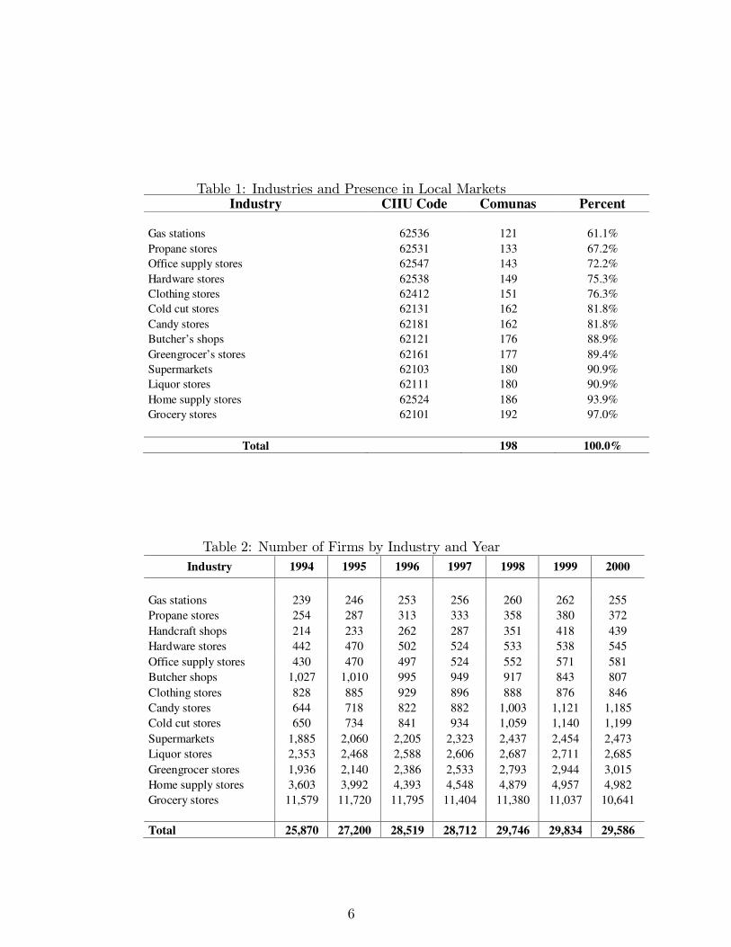
Table 1: Industries and Presence in Local MarketsIndustry CIIU Code Comunas Percent

Gas stations 62536 121 61.1%Propane stores 62531 133 67.2%Office supply stores 62547 143 72.2%Hardware stores 62538 149 75.3%Clothing stores 62412 151 76.3%Cold cut stores 62131 162 81.8%Candy stores 62181 162 81.8%Butcher’s shops 62121 176 88.9%Greengrocer’s stores 62161 177 89.4%Supermarkets 62103 180 90.9%Liquor stores 62111 180 90.9%Home supply stores 62524 186 93.9%Grocery stores 62101 192 97.0%

Total 198 100.0%

Table 2: Number of Firms by Industry and Year

Industry 1994 1995 1996 1997 1998 1999 2000

Gas stations 239 246 253 256 260 262 255Propane stores 254 287 313 333 358 380 372Handcraft shops 214 233 262 287 351 418 439Hardware stores 442 470 502 524 533 538 545Office supply stores 430 470 497 524 552 571 581Butcher shops 1,027 1,010 995 949 917 843 807Clothing stores 828 885 929 896 888 876 846Candy stores 644 718 822 882 1,003 1,121 1,185Cold cut stores 650 734 841 934 1,059 1,140 1,199Supermarkets 1,885 2,060 2,205 2,323 2,437 2,454 2,473Liquor stores 2,353 2,468 2,588 2,606 2,687 2,711 2,685Greengrocer stores 1,936 2,140 2,386 2,533 2,793 2,944 3,015Home supply stores 3,603 3,992 4,393 4,548 4,879 4,957 4,982Grocery stores 11,579 11,720 11,795 11,404 11,380 11,037 10,641

Total 25,870 27,200 28,519 28,712 29,746 29,834 29,586

6

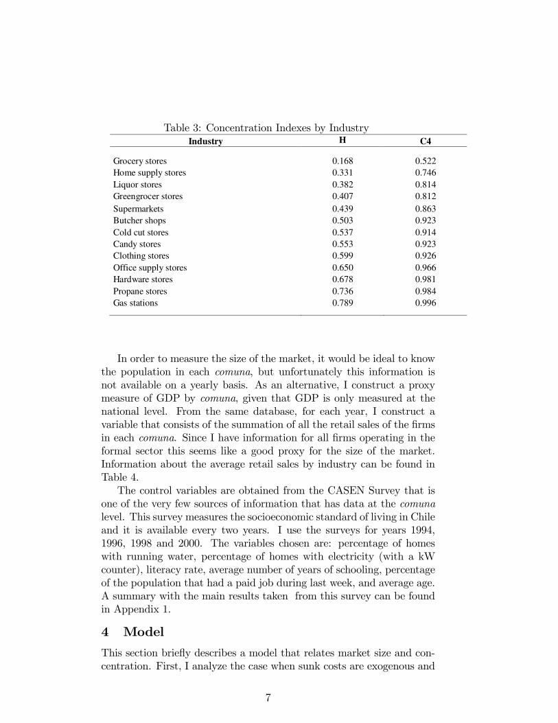
Table 3: Concentration Indexes by IndustryIndustry H C4

Grocery stores 0.168 0.522Home supply stores 0.331 0.746Liquor stores 0.382 0.814Greengrocer stores 0.407 0.812

Supermarkets 0.439 0.863Butcher shops 0.503 0.923Cold cut stores 0.537 0.914Candy stores 0.553 0.923Clothing stores 0.599 0.926Office supply stores 0.650 0.966Hardware stores 0.678 0.981Propane stores 0.736 0.984Gas stations 0.789 0.996

In order to measure the size of the market, it would be ideal to knowthe population in each comuna, but unfortunately this information isnot available on a yearly basis. As an alternative, I construct a proxymeasure of GDP by comuna, given that GDP is only measured at thenational level. From the same database, for each year, I construct avariable that consists of the summation of all the retail sales of the firmsin each comuna. Since I have information for all firms operating in theformal sector this seems like a good proxy for the size of the market.Information about the average retail sales by industry can be found inTable 4.The control variables are obtained from the CASEN Survey that is

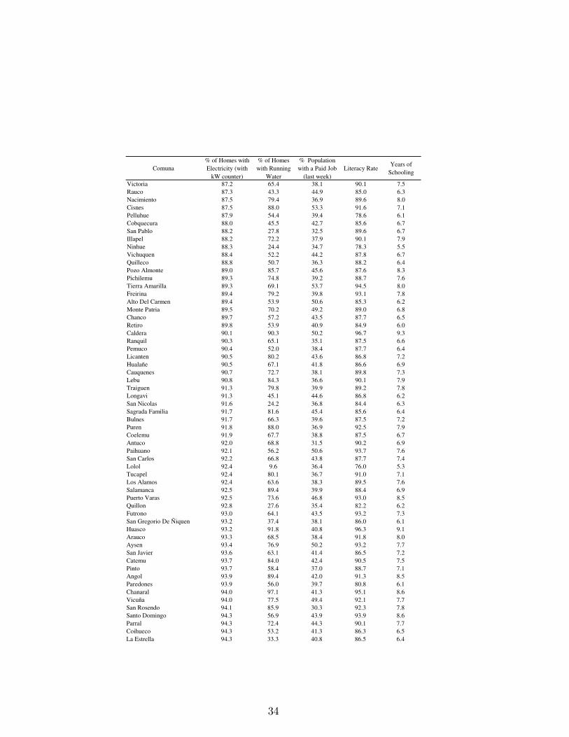
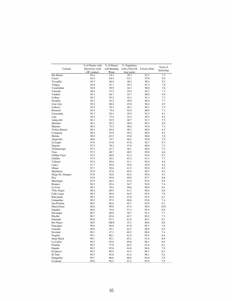
one of the very few sources of information that has data at the comunalevel. This survey measures the socioeconomic standard of living in Chileand it is available every two years. I use the surveys for years 1994,1996, 1998 and 2000. The variables chosen are: percentage of homeswith running water, percentage of homes with electricity (with a kWcounter), literacy rate, average number of years of schooling, percentageof the population that had a paid job during last week, and average age.A summary with the main results taken from this survey can be foundin Appendix 1.

4 Model

This section briefly describes a model that relates market size and con-centration. First, I analyze the case when sunk costs are exogenous and

7

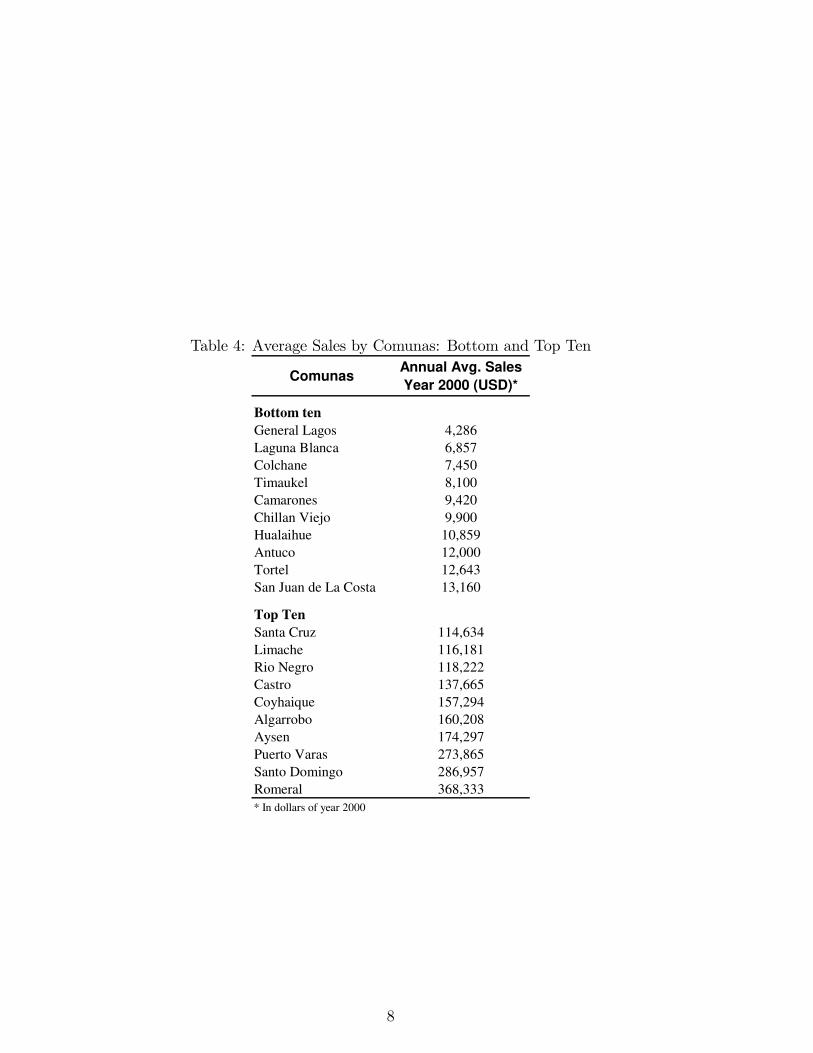
Table 4: Average Sales by Comunas: Bottom and Top Ten

ComunasAnnual Avg. Sales

Year 2000 (USD)*

Bottom ten

General Lagos 4,286Laguna Blanca 6,857Colchane 7,450Timaukel 8,100Camarones 9,420Chillan Viejo 9,900Hualaihue 10,859Antuco 12,000Tortel 12,643San Juan de La Costa 13,160

Top Ten

Santa Cruz 114,634Limache 116,181Rio Negro 118,222Castro 137,665Coyhaique 157,294Algarrobo 160,208Aysen 174,297Puerto Varas 273,865Santo Domingo 286,957Romeral 368,333* In dollars of year 2000

8

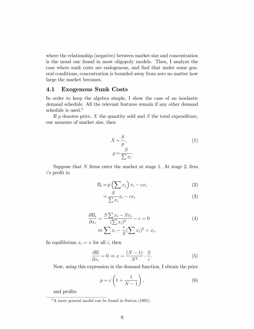
where the relationship (negative) between market size and concentrationis the usual one found in most oligopoly models. Then, I analyze thecase where sunk costs are endogenous, and find that under some gen-eral conditions, concentration is bounded away from zero no matter howlarge the market becomes.

4.1 Exogenous Sunk Costs

In order to keep the algebra simple, I show the case of an isoelasticdemand schedule. All the relevant features remain if any other demandschedule is used.3

If p denotes price, X the quantity sold and S the total expenditure,our measure of market size, then

X =S

p, (1)

p=S∑xi.

Suppose that N firms enter the market at stage 1. At stage 2, firmi’s profit is:

Πi= p(∑

xj

)xi − cxi (2)

=S∑xixi − cxi (3)

∂Πi∂xi

=S∑xi − Sxi

(∑xi)2

− c = 0 (4)

⇔∑

xi −c

S(∑

xi)2 = xi.

In equilibrium xi = x for all i, then

∂Π

∂xi= 0⇒ x =

(N − 1)

N2·S

c. (5)

Now, using this expression in the demand function, I obtain the price

p = c

(1 +

1

N − 1

), (6)

and profits

3A more general model can be found in Sutton (1991).

9

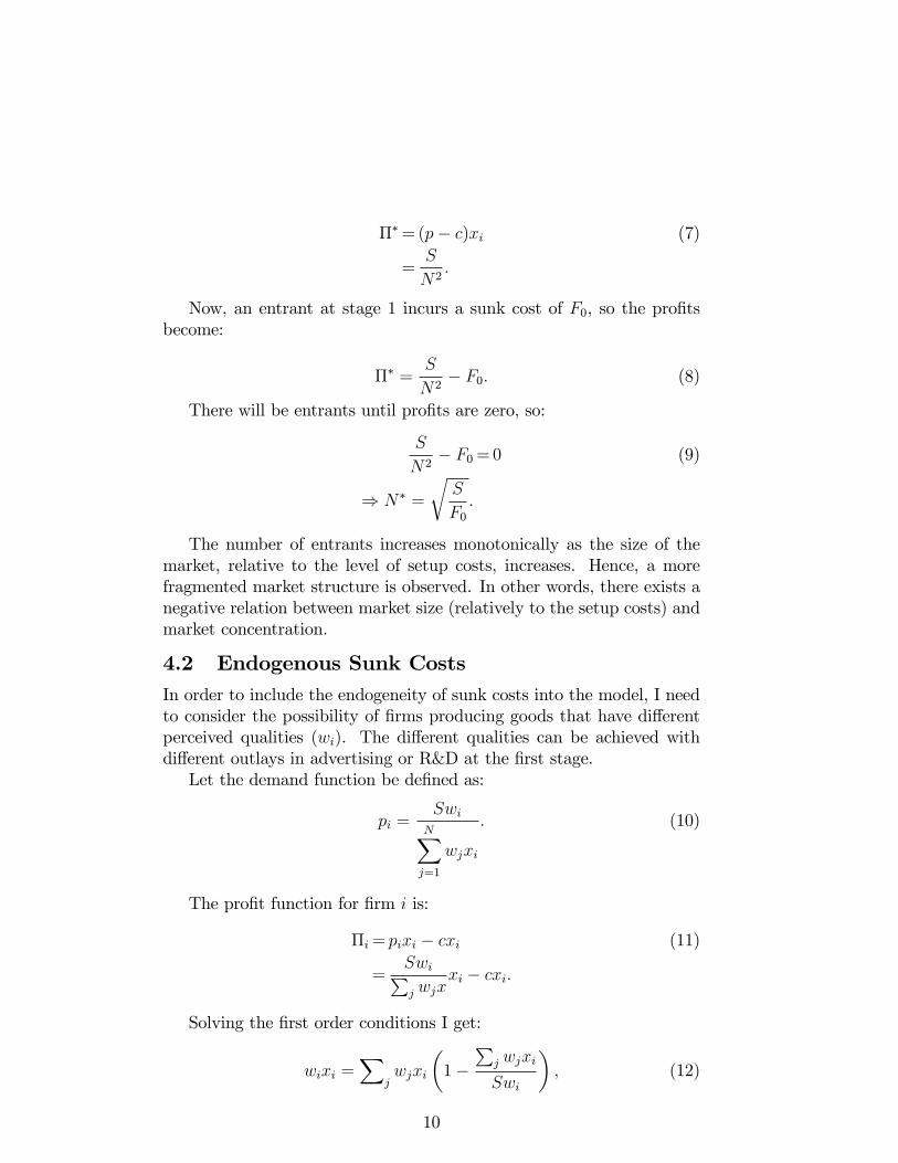
Π∗=(p− c)xi (7)

=S

N2.

Now, an entrant at stage 1 incurs a sunk cost of F0, so the profitsbecome:

Π∗ =S

N2− F0. (8)

There will be entrants until profits are zero, so:

S

N2− F0=0 (9)

⇒ N∗ =

√S

F0.

The number of entrants increases monotonically as the size of themarket, relative to the level of setup costs, increases. Hence, a morefragmented market structure is observed. In other words, there exists anegative relation between market size (relatively to the setup costs) andmarket concentration.

4.2 Endogenous Sunk Costs

In order to include the endogeneity of sunk costs into the model, I needto consider the possibility of firms producing goods that have differentperceived qualities (wi). The different qualities can be achieved withdifferent outlays in advertising or R&D at the first stage.Let the demand function be defined as:

pi =Swi

N∑

j=1

wjxi

. (10)

The profit function for firm i is:

Πi= pixi − cxi (11)

=Swi∑j wjx

xi − cxi.

Solving the first order conditions I get:

wixi =∑

jwjxi

(1−

∑j wjxi

Swi

), (12)

10

and then summing over all products and rearranging, the equilibriumquantity is:

xi =S

c·N − 1

wi∑

j(1wj)

[

1−N − 1

wi∑

j(1wj)

]

. (13)

Solving now for prices:

pi =

[cwiN − 1

∑j

1

wj

]. (14)

Plugging xi and pi into the profit function and simplifying, the profitfunction becomes:

Πi = S

[

1−N − 1

wi·

1∑

j(1wj)

]2. (15)

With this function I can calculate a threshold level for w (w0) thatmakes profits equal to zero and so any firm that chooses to produce withquality w < w0 will not survive,

S

[

1−N − 1

w0·

1∑

j(1wj)

]2= 0, (16)

⇒ the threshold is w0 =N − 1∑

j(1wj). (17)

Therefore, the summation in the profit expression considers the Nfirms that produce with quality w ≥ w0.Let us now consider a 3-stage game where in the first stage firms

decide whether to enter or not. If they decide to enter they need to paya fixed cost F0 > 0. At stage 2 they choose the quality level w ∈ [1,∞)for an additional fixed cost A(w), which makes it the total fixed costequal to F (w) = F0 + A(w). At the final stage, firms compete à laCournot, taking quality as fixed, as solved above. The relevant firmpayoff equals: Π− F (w).A complete treatment of this model is developed in Sutton (1991), so

here I use some simplifications and parameterizations just to show thetheoretical relationship between market size and concentration.

Stage 2 At the second stage of the game, the number of firms aretaken as a parameter (from stage 1) and so at this point all entrants havealready incurred a fixed cost F0 and alsoA(w), that is the portion of fixedcosts associated with quality. The symmetric Nash equilibrium outcometakes one of these two forms ∂Πi

∂wi|wi=w=1 ≤

∂F (w)∂w

|w=1 or∂Πi∂wi|wi=w=1 >

∂F (w)∂w

|w=1.

11

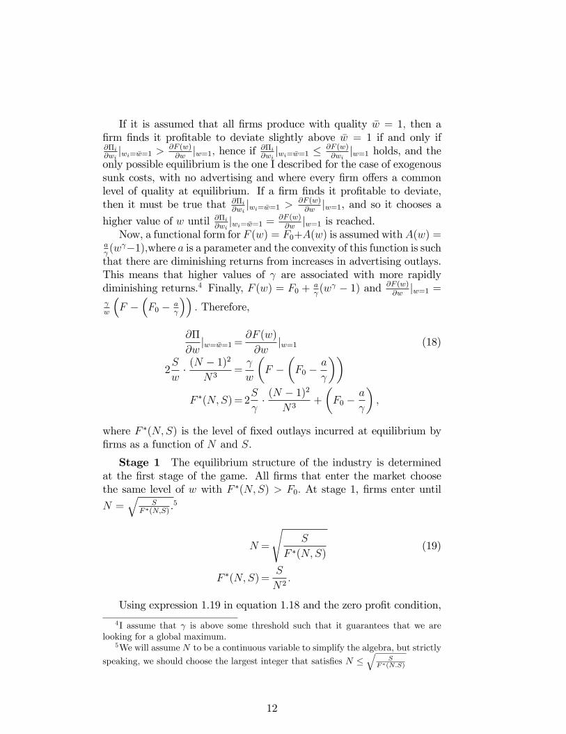
If it is assumed that all firms produce with quality w = 1, then afirm finds it profitable to deviate slightly above w = 1 if and only if∂Πi∂wi|wi=w=1 >

∂F (w)∂w

|w=1, hence if∂Πi∂wi|wi=w=1 ≤

∂F (w)∂wi

|w=1 holds, and theonly possible equilibrium is the one I described for the case of exogenoussunk costs, with no advertising and where every firm offers a commonlevel of quality at equilibrium. If a firm finds it profitable to deviate,then it must be true that ∂Πi

∂wi|wi=w=1 >

∂F (w)∂w

|w=1, and so it chooses a

higher value of w until ∂Πi∂wi|wi=w=1 =

∂F (w)∂w

|w=1 is reached.Now, a functional form for F (w) = F0+A(w) is assumed withA(w) =

aγ(wγ−1),where a is a parameter and the convexity of this function is suchthat there are diminishing returns from increases in advertising outlays.This means that higher values of γ are associated with more rapidlydiminishing returns.4 Finally, F (w) = F0 +

aγ(wγ − 1) and ∂F (w)

∂w|w=1 =

γw

(F −

(F0 −

aγ

)). Therefore,

∂Π

∂w|w=w=1=

∂F (w)

∂w|w=1 (18)

2S

w·(N − 1)2

N3=γ

w

(F −

(F0 −

a

γ

))

F ∗(N,S)= 2S

γ·(N − 1)2

N3+

(F0 −

a

γ

),

where F ∗(N,S) is the level of fixed outlays incurred at equilibrium byfirms as a function of N and S.

Stage 1 The equilibrium structure of the industry is determinedat the first stage of the game. All firms that enter the market choosethe same level of w with F ∗(N,S) > F0. At stage 1, firms enter until

N =√

SF ∗(N,S)

.5

N =

√S

F ∗(N,S)(19)

F ∗(N,S)=S

N2.

Using expression 1.19 in equation 1.18 and the zero profit condition,

4I assume that γ is above some threshold such that it guarantees that we arelooking for a global maximum.

5We will assume N to be a continuous variable to simplify the algebra, but strictly

speaking, we should choose the largest integer that satisfies N ≤√

S

F∗(N.S)

12

an equilibrium is found:

S

N2=2

S

γ·(N − 1)2

N3+

(F0 −

a

γ

)(20)

1=2

γ·(N − 1)2

N+N2

S

(F0 −

a

γ

)

(N − 1)2

N=γ

2

[1−

N2

S

(F0 −

a

γ

)]=γ

2

1−

(F0 −

aγ

)

F

.

This equilibrium in the advertising zone is described by the intersec-tion of this combination of N and F and the zero profit condition. AsS →∞, the above expression is transformed into

(N − 1)2

N=γ

2. (21)

The N that solves this implicit function is N(γ/2) and it only de-pends on γ.Next, I analyze the shape of this relation between F and N in order

to find the possible equilibria:

(N − 1)2

N=γ

2

1−

(F0 −

aγ

)

F

(22)

F =

(F0 −

aγ

)

1− 2(N−1)2

γN

.

The slope of this F function is given by:

∂F

∂N=

(F0 −

aγ

)

(1− 2(N−1)2

γN

)22(N2 − 1)

γN2(23)

=

(F0 −

aγ

)

(+)

(+)

(+).

The sign of the slope determines three different cases:

If F0 =a

γ→∂F

∂N= 0, (24)

13

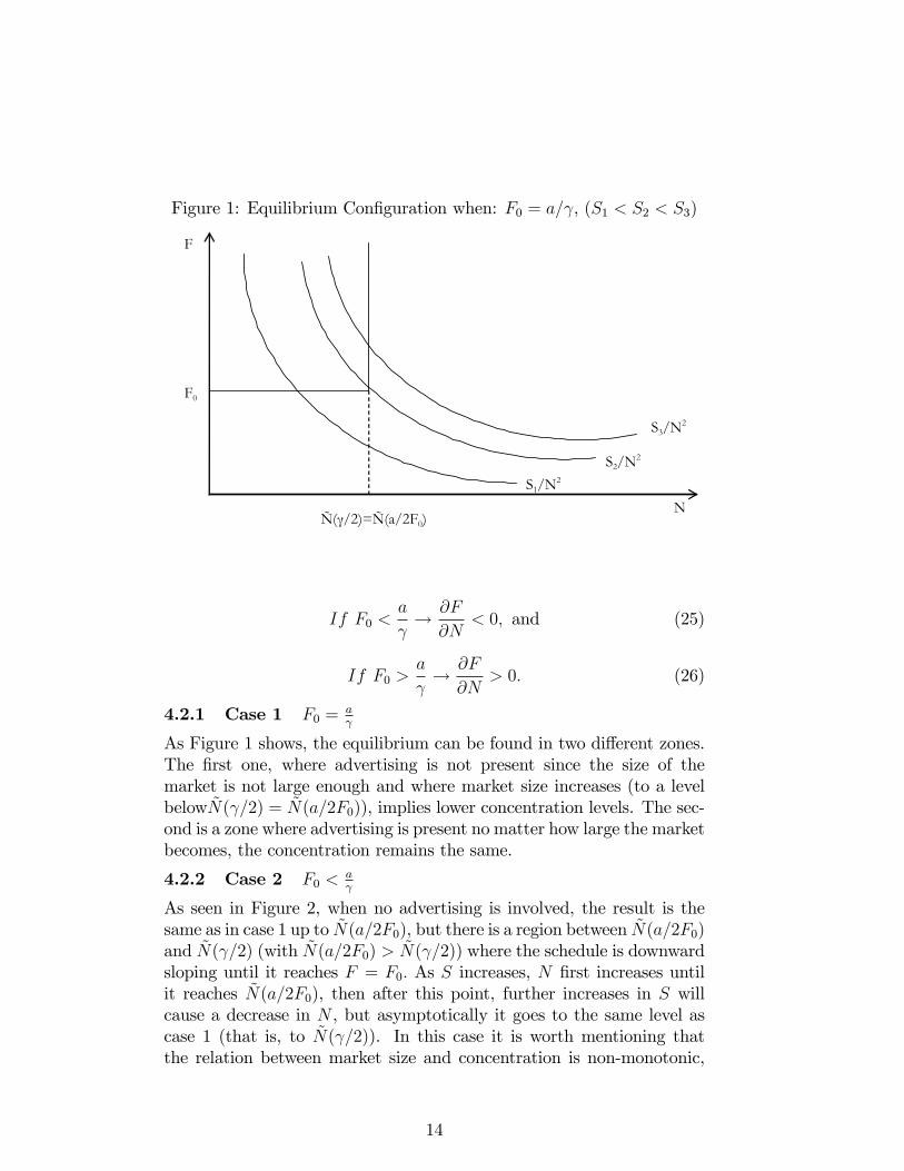
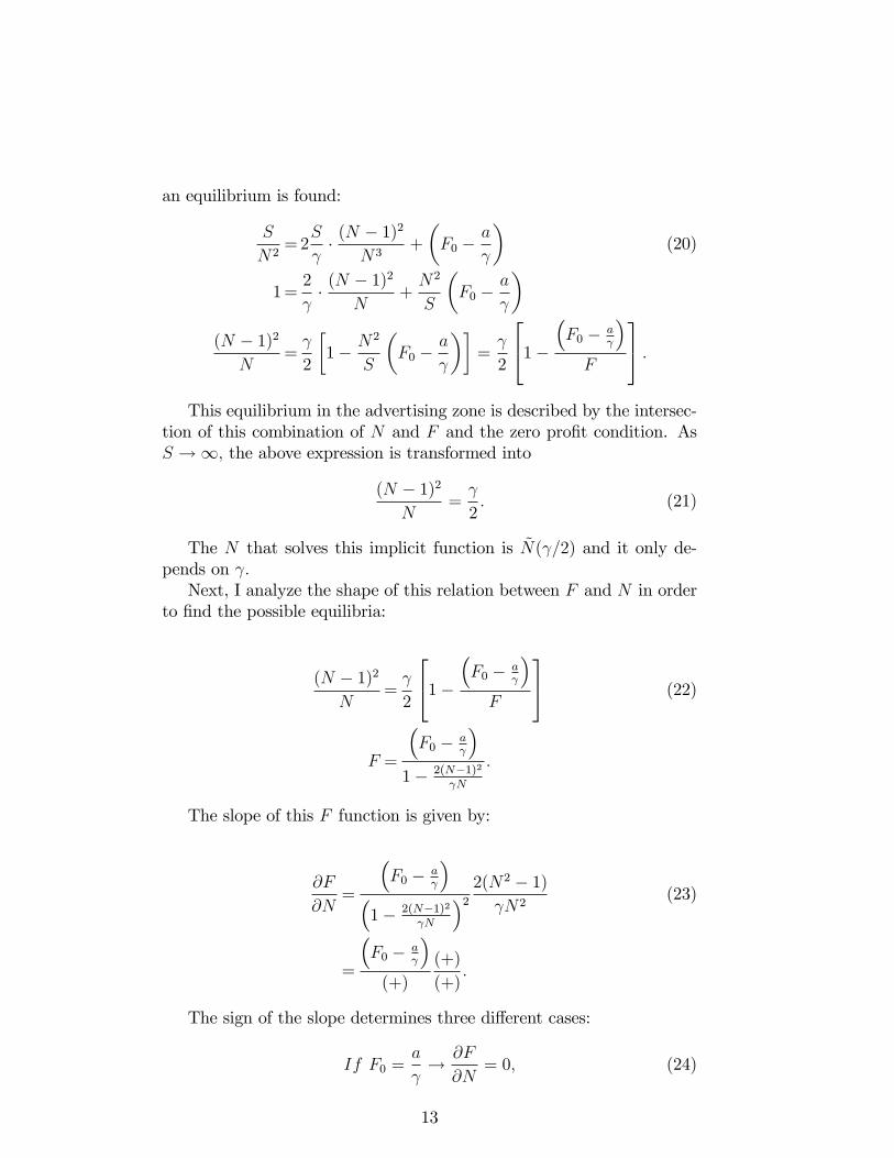
Figure 1: Equilibrium Configuration when: F0 = a/γ, (S1 < S2 < S3)

S3/N2

S1/N2

S2/N2

F

F0

Ñ(γ/2)=Ñ(a/2F0)N

If F0 <a

γ→∂F

∂N< 0, and (25)

If F0 >a

γ→∂F

∂N> 0. (26)

4.2.1 Case 1 F0 =aγ

As Figure 1 shows, the equilibrium can be found in two different zones.The first one, where advertising is not present since the size of themarket is not large enough and where market size increases (to a levelbelowN(γ/2) = N(a/2F0)), implies lower concentration levels. The sec-ond is a zone where advertising is present no matter how large the marketbecomes, the concentration remains the same.

4.2.2 Case 2 F0 <aγ

As seen in Figure 2, when no advertising is involved, the result is thesame as in case 1 up to N(a/2F0), but there is a region between N(a/2F0)and N(γ/2) (with N(a/2F0) > N(γ/2)) where the schedule is downwardsloping until it reaches F = F0. As S increases, N first increases untilit reaches N(a/2F0), then after this point, further increases in S willcause a decrease in N , but asymptotically it goes to the same level ascase 1 (that is, to N(γ/2)). In this case it is worth mentioning thatthe relation between market size and concentration is non-monotonic,

14

Figure 2: Equilibrium Configuration when: F0 < a/γ, (S1 < S2 < S3)

S1/N2

S2/N2

S3/N2

N

F

F0

Ñ(γ/2) Ñ(a/2F0)

although concentration remains bounded away from zero as market sizeincreases.

4.2.3 Case 3 F0 >aγ

In this case, as shown in Figure 3, when no advertising is present, theresults are the same as case 1 and 2 only until N(a/2F0). After thispoint, the schedule that relates F and N is upward sloping until N(γ/2)(for this case N(a/2F0) < N(γ/2)). Hence, as S increases the concen-tration drops, but it is asymptotically bounded by 1

N(γ/2), converging to

the same point as the other two cases.

5 Estimation

In this section, I test the central implications of the theory. I begin test-ing whether the level of concentration is bounded away from zero whenmarket size increases in the advertising intensive industries. This is theapproach taken by most empirical work in this area (Ellickson 2007,Bronnenberg et al. 2005, etc.), since the presence of market heterogene-ity makes it hard to uncover a clear relationship between concentrationand market size. Nevertheless, since I am using a panel dataset forthe estimation that permits to control for unobserved heterogeneity, Ialso estimate the elasticity of concentration on market size. I expect anegative estimated coefficient for industries where I presume exogenoussunk costs are involved and one close to zero for advertising-intensive

15

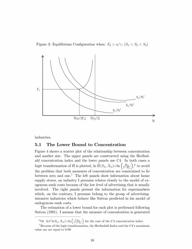
Figure 3: Equilibrium Configuration when: F0 > a/γ, (S1 < S2 < S3)

N

S1/N2

S2/N2

S3/N2

F0

Ñ(a/2F0) Ñ(γ/2)

industries.

5.1 The Lower Bound to Concentration

Figure 4 shows a scatter plot of the relationship between concentrationand market size. The upper panels are constructed using the Herfind-ahl concentration index and the lower panels use C4. In both cases a

logit transformation of H is plotted, ln H(Sit, Xit)=ln(

Hit1−Hit

),6 to avoid

the problem that both measures of concentration are constrained to liebetween zero and one.7 The left panels show information about homesupply stores, an industry I presume relates closely to the model of ex-ogenous sunk costs because of the low level of advertising that is usuallyinvolved. The right panels present the information for supermarketswhich, on the contrary, I presume belong to the group of advertising-intensive industries which behave like Sutton predicted in his model ofendogenous sunk costs.The estimation of a lower bound for each plot is performed following

Sutton (1991). I assume that the measure of concentration is generated

6Or ln˜

C4(Sit, Xit)=ln(

C4it1−C4it

)for the case of the C4 concentration index.

7Because of the logit transformation, the Herfindahl Index and the C4’s maximumvalue are set equal to 0.99.

16

Figure 4: Concentration and Market Size

by an extreme value Weibull distribution that can be estimated by a two-step approach proposed by Smith (1985, 1994), given that the maximumlikelihood estimation does not work for some ranges of parameters ofthe Weibull.8 In order to parameterize the lower bound, Sutton suggestsestimating:

Cn = a+b

ln(S)+ εi (εi > 0), (27)

where Cn is a measure of concentration and the residuals εi are distrib-uted as a two parameter Weibull (ε ∼Weibull(α, s)). Then,

F (ε) = 1− e(−εs)

α

. (28)

On a first step, the parameters a and b are estimated by the simplexmethod, solving:

mina,b

n∑

i=1

[log

(Hi

1−Hi

)−

(a+

b

ln(Si)

)](29)

8As Sutton (1991) estates "For 1 < α ≤ 2, a local maximum of the likelihoodfunction extist, but it does not have the usual asymptotic properties; for 0 ≤ α ≤ 1,no local maximum of likelihood function exist."

17

Figure 5: Lower Bound Estimations in Supermarket and Home SupplyIndustry

s.t.

log

(Hi

1−Hi

)≥

(a+

b

ln(Si)

).

Then, assuming ε ∼Weibull(α, s), on a second step I estimate the twoother parameters, α and s, by maximizing the pseudo-likelihood that wasconstructed by substituting the value of the estimated residuals obtainedin the first step,

maxα,s

n∑

i=1

log

[α

sε(α−1)i exp

(−εαis

)]. (30)

The results obtained using the described procedure can be seen inFigure 5. At first sight the results are not that promising since bothindustries show that concentration will go to zero as market size in-creases. Nevertheless, the lack of difference is due to the presence ofoutliers. As Robinson and Chiang (1996), Giorgetti (2003) and Rosende(2008) state, a lower bound function can be strongly influenced by evena single outlier. In a sample of 1,224 observations it is not surprisingthat a few outliers distort the analysis. Following Robinson and Chiang(1996) I delete 1% of the sample that has the smallest market size and1% of the sample that has the lowest level of concentration. This simpleguideline was enough to remove a few obvious outliers but was harmless

18

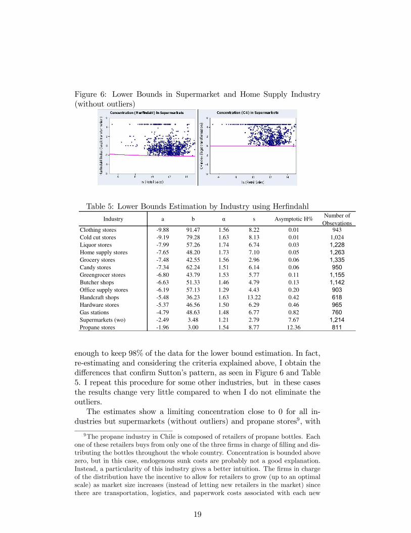
Figure 6: Lower Bounds in Supermarket and Home Supply Industry(without outliers)

Table 5: Lower Bounds Estimation by Industry using Herfindahl

Industry a b α s Asymptotic H%Number of

ObsevationsClothing stores -9.88 91.47 1.56 8.22 0.01 943Cold cut stores -9.19 79.28 1.63 8.13 0.01 1,024Liquor stores -7.99 57.26 1.74 6.74 0.03 1,228

Home supply stores -7.65 48.20 1.73 7.10 0.05 1,263

Grocery stores -7.48 42.55 1.56 2.96 0.06 1,335

Candy stores -7.34 62.24 1.51 6.14 0.06 950

Greengrocer stores -6.80 43.79 1.53 5.77 0.11 1,155

Butcher shops -6.63 51.33 1.46 4.79 0.13 1,142

Office supply stores -6.19 57.13 1.29 4.43 0.20 903

Handcraft shops -5.48 36.23 1.63 13.22 0.42 618

Hardware stores -5.37 46.56 1.50 6.29 0.46 965

Gas stations -4.79 48.63 1.48 6.77 0.82 760

Supermarkets (wo) -2.49 3.48 1.21 2.79 7.67 1,214

Propane stores -1.96 3.00 1.54 8.77 12.36 811

enough to keep 98% of the data for the lower bound estimation. In fact,re-estimating and considering the criteria explained above, I obtain thedifferences that confirm Sutton’s pattern, as seen in Figure 6 and Table5. I repeat this procedure for some other industries, but in these casesthe results change very little compared to when I do not eliminate theoutliers.The estimates show a limiting concentration close to 0 for all in-

dustries but supermarkets (without outliers) and propane stores9, with

9The propane industry in Chile is composed of retailers of propane bottles. Eachone of these retailers buys from only one of the three firms in charge of filling and dis-tributing the bottles throughout the whole country. Concentration is bounded abovezero, but in this case, endogenous sunk costs are probably not a good explanation.Instead, a particularity of this industry gives a better intuition. The firms in chargeof the distribution have the incentive to allow for retailers to grow (up to an optimalscale) as market size increases (instead of letting new retailers in the market) sincethere are transportation, logistics, and paperwork costs associated with each new

19

limiting concentrations of around 8% and 12%, respectively. The es-timated values for the parameter α range between 1 and 2, justifyingthe use of the method proposed by Smith (1994). Results for C4 arepresented in the Appendix.

5.2 The Elasticity of Concentration on Market Size

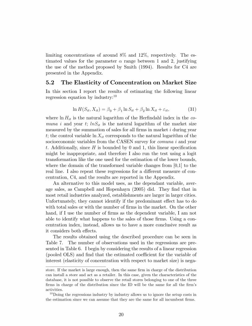
In this section I report the results of estimating the following linearregression equation by industry:10

lnH(Sit, Xit) = β0 + β1 lnSit + β2 lnXit + εit, (31)

where lnHit is the natural logarithm of the Herfindahl index in the co-muna i and year t; lnSit is the natural logarithm of the market sizemeasured by the summation of sales for all firms in market i during yeart; the control variable lnXit corresponds to the natural logarithm of thesocioeconomic variables from the CASEN survey for comuna i and yeart. Additionally, since H is bounded by 0 and 1, this linear specificationmight be inappropriate, and therefore I also run the test using a logittransformation like the one used for the estimation of the lower bounds,where the domain of the transformed variable changes from [0,1] to thereal line. I also repeat these regressions for a different measure of con-centration, C4, and the results are reported in the Appendix.An alternative to this model uses, as the dependant variable, aver-

age sales, as Campbell and Hopenhayn (2005) did. They find that inmost retail industries analyzed, establishments are larger in larger cities.Unfortunately, they cannot identify if the predominant effect has to dowith total sales or with the number of firms in the market. On the otherhand, if I use the number of firms as the dependent variable, I am notable to identify what happens to the sales of those firms. Using a con-centration index, instead, allows us to have a more conclusive result asit considers both effects.The results obtained using the described procedure can be seen in

Table 7. The number of observations used in the regressions are pre-sented in Table 6. I begin by considering the results of a linear regression(pooled OLS) and find that the estimated coefficient for the variable ofinterest (elasticity of concentration with respect to market size) is nega-

store. If the market is large enough, then the same firm in charge of the distributioncan install a store and act as a retailer. In this case, given the characteristics of thedatabase, it is not possible to observe the retail stores belonging to one of the threefirms in charge of the distribution since the ID will be the same for all the firm’sactivities.10Doing the regressions industry by industry allows us to ignore the setup costs in

the estimation since we can assume that they are the same for all incumbent firms.

20

tive and significantly different from zero (at a 99% confidence level) for12 out of 13 industries. These industries are presumed to have a smallcomponent of sunk costs since advertising (or R&D) is not usually seen.For these industries, for instance in home supply stores, greengrocerstores and office supply stores among others, I find that the estimatedelasticity is the most negative, a result that is in line with the one pre-dicted by the model with exogenous sunk costs (as market size increasesthe concentration decreases steadily).Nevertheless there is one industry, supermarkets, where the elasticity

coefficient is pretty close to zero, or not statistically different from zeroat the 5% level. For this industry, the results behave in a fashion likethe one predicted by Sutton (1991), indicating that, no matter how bigthe market becomes, the concentration index changes very little and it isbounded away from zero. One explanation for this result would be thatfirms in the supermarket industry tend to invest more in advertising, andthis investment will improve their position in order to compete on pricesas market size increases. Nevertheless, in this case, the supermarketindustry is composed of small single-unit firms in markets belonging tonon-metropolitan areas where probably advertising expenditures are notvery common especially those incurred as a sunk fixed cost. In this case,probably Ellickson’s (2007) explanation might be better suited, whereinvestment in land allows firms to offer, in the future, a larger variety ofproducts as market size increases, making entry less attractive to otherfirms and keeping concentration bounded above zero.Next, I estimate the regressions again, industry by industry, but us-

ing a Panel data model (random effect) that controls for unobservedheterogeneity, since ignoring this might bias the results presented ear-lier. The coefficient of the elasticity for this case is again negative andsignificantly different from zero (at a 99% confidence level) for 12 outof 13 industries. Although the coefficients change, supermarkets stillbehave according to the model of endogenous sunk costs and results areeven stronger, confirming the results commented upon earlier.I also estimate the OLS and Panel R.E. models without the con-

trol variables and most of the results still hold, as the estimates andtheir statistical significance change very little. For supermarkets, thecoefficient continues to be the lowest of all industries but it is differentfrom zero at 99% confidence. The inclusion of these variables results inadded explanatory power but only slightly changes the estimated effectof market size on concentration.Finally, I repeat all regressions for the logit transformation of the

Herfindahl and this time the coefficient on the market size variable is nolonger statistically zero. Nevertheless, the coefficient for the supermar-

21

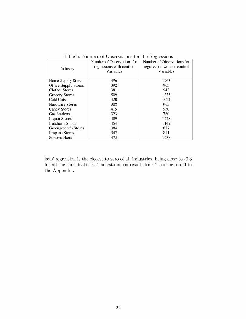
Table 6: Number of Observations for the Regressions

Industry

Number of Observations forregressions with control

Variables

Number of Observations forregressions without control

Variables

Home Supply Stores 496 1263Office Supply Stores 392 903Clothes Stores 381 943Grocery Stores 509 1335Cold Cuts 420 1024Hardware Stores 388 965Candy Stores 415 950Gas Stations 323 760Liquor Stores 489 1228Butcher’s Shops 454 1142Greengrocer’s Stores 384 877Propane Stores 342 811Supermarkets 475 1238

kets’ regression is the closest to zero of all industries, being close to -0.3for all the specifications. The estimation results for C4 can be found inthe Appendix.

22

Table 7: Regressions of Concentration Ratios (H) on Market Size

See Table 1.6 for the number of observations.All Coefficients significant at 1% level.* Significant at the 10% level.+ Not statistically significant.

Panel R.E(over Comunas)

Pooled OLS Panel R.E.no control Var.

Pooled OLSno control Var.

Home supply stores-0.494(0.032)

-0.507(0.026)

-0.355(0.022)

-0.428(0.013)

Office supply stores-0.342(0.027)

-0.338(0.022)

-0.289(0.021)

-0.290(0.012)

Clothing stores-0.293(0.034)

-0.315(0.026)

-0.247(0.025)

-0.293(0.015)

Grocery stores -0.281(0.031)

-0.306(0.027)

-0.199(0.022)

-0.327(0.013)

Cold cut stores -0.265(0.034)

-0.269(0.027)

-0.229(0.024)

-0.253(0.015)

Hardware stores -0.245(0.026)

-0.265(0.020)

-0.196(0.019)

-0.242(0.011)

Candy stores -0.234(0.027)

-0.247(0.023)

-0.272(0.021)

-0.296(0.014)

Gas stations -0.229(0.025)

-0.250(0.020)

-0.168(0.019)

-0.199(0.011)

Liquor stores -0.222(0.033)

-0.316(0.026)

-0.162(0.024)

-0.281(0.014)

Butcher shops -0.207(0.031)

-0.243(0.025)

-0.128(0.020)

-0.198(0.012)

Greengrocer stores-0.194(0.039)

-0.226(0.031)

-0.188(0.029)

-0.238(0.017)

Propane stores -0.112(0.029)

-0.137(0.025)

-0.112(0.022)

-0.130(0.013)

Supermarkets-0.040+(0.035)

-0.051*(0.027)

-0.070(0.023)

-0.099(0.014)

23

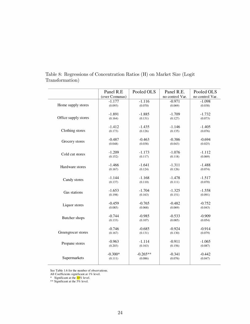
Table 8: Regressions of Concentration Ratios (H) on Market Size (LogitTransformation)





-1.116(0.070)

-0.971(0.069)

-1.098(0.038)


-1.885(0.131)

-1.709(0.127)

-1.732(0.073)


-1.435(0.126)

-1.146(0.135)

-1.405(0.076)


-0.463(0.038)

-0.386(0.043)

-0.694(0.025)


-1.173(0.117)

-1.076(0.118)

-1.112(0.069)


-1.641(0.124)

-1.311(0.126)

-1.488(0.074)


-1.168(0.110)

-1.478(0.111)

-1.517(0.070)


-1.704(0.163)

-1.325(0.151)

-1.558(0.091)


-0.765(0.068)

-0.482(0.069)

-0.752(0.043)


-0.985(0.107)

-0.533(0.085)

-0.909(0.054)


-0.685(0.131)

-0.924(0.130)

-0.914(0.079)


-1.114(0.163)

-0.911(0.156)

-1.065(0.087)

Supermarkets-0.300*(0.111)

-0.265**(0.086)

-0.341(0.076)

-0.442(0.047)

See Table 1.6 for the number of observations.All Coefficients significant at 1% level.* Significant at the 10% level.** Significant at the 5% level.

24

6 Conclusions

The purpose of this paper is to present empirical evidence of Sutton’shypothesis of endogenous sunk costs. I present the estimations of lowerbounds to show that concentration is bounded away from zero for su-permarkets, an industry that I presume has an important component ofendogenous sunk costs. I complement these results with the estima-tion of the elasticity of concentration with respect to market size, beingable to control for unobserved heterogeneity captured by R.E. estima-tions, providing more evidence to Sutton’s hypothesis. The nature ofthese results can be explained by investment in advertising in the initialstages or an alternative explanation proposed by Ellickson (2007), whichis investment in land and/or distribution centers. This investment al-lows firms to offer, in the future, a larger variety of products as marketsize increases, making entry less attractive to other firms and keepingconcentration bounded above zero. The idea of distribution centersprobably does not apply since the supermarket industry I analyze hereis an industry of small single-plant supermarkets in local markets so thescale is not enough to make the investment in sophisticated distributioncenters profitable.

25

References

[1] Berry, S.and Waldfogel, J. (2010). “Product Quality andMarket Size”. The Journal of Industrial Economics, LVIII,1.

[2] Bresnahan, T.F. and Reiss, P. C. (1991). “Entry and Compe-tition in Concentrated Markets”. Journal of Political Econ-omy, 99, 977-1,099.

[3] Bornnenberg, B., Dhar, S. and Dubé, J. (2005). “EndogenousSunk Costs and the Geographic Distribution of Brand Sharesin Consumer Package Goods Industries”. Mimeo.

[4] Campbell, J.R. and Hopenhayn, H.A. (2005). “Market SizeMatters”. The Journal of Industrial Economics, LIII, 1.

[5] Dick, A. (2007). “Market Size Service Quality, and Compe-tition in Banking”. Journal of Money, Credit and Banking,39, 1, February, 49-81.

[6] Ellickson, S. (2007). “Does Sutton Apply to Supermarkets”.RAND Journal of Economics, 38, 1, Spring, 43-59.

[7] Giorgetti, M. (2003). “Lower Bound Estimation - QuantileRegression and Simplex Method: An Application to Ital-ian Manufacturing Sectors”. The Journal of Industrial Eco-nomics, 51, 113-120.

[8] Robinson, WT. and Chiang J.(1996). “Are Sutton’s Predic-tion Robust: Empirical Insights into Advertising, R&D andConcentration”. The Journal of Industrial Economics, 94,389-408.

[9] Rosende, M. (2008). “Concentration and Market Size: LowerBound Estimates for the Brazilian Industry". CESifo, Work-ing Paper No.2441.

[10] Schumpeter, J. (1942). Capitalism, Socialism and Democ-

racy. New York: Harper and Row.[11] Shaked, A. and Sutton, J. (1987). “Product Differentiation

and Industrial Structures”. Journal of Industrial Economics,36, 131-146.

[12] Smith, R. (1985). “Maximum Likelihood Estimation in aClass of Nonregular Cases”. Biometrica, 72, 67-90.

[13] Smith, R. (1994). “Nonregular Regression”. Biometrica, 81,1, 173-183.

[14] Sutton, J. (1991). Sunk Costs and Market Structure. MITPress, Cambridge, MA.

[15] Sutton, J. (1997). “Gibrat’s Legacy”. Journal of EconomicLiterature, XXXV, 40-59.

26

7 Appendix: Tables and Figures

27

Table 9: Socieconomic Information by Comuna from the CASEN survey

Comuna% of Homes withElectricity (with

kW counter)

% of Homeswith Running

Water

% Populationwith a Paid Job

(last week)Literacy Rate

Years ofSchooling

Camarones 10.5 21.5 67.0 84.2 6.4Camina. 14.4 76.8 62.4 89.3 6.3General Lagos 15.0 30.0 60.6 71.8 4.8Colchane 15.8 61.1 39.1 76.9 5.5Quinchao 36.2 26.6 48.6 94.1 7.4Canela 37.1 29.9 34.3 83.9 6.0Huara 37.1 47.3 55.8 90.8 7.2Quemchi 43.8 22.4 50.0 91.2 6.6Contulmo 46.8 25.7 40.2 83.6 5.5Los Sauces 50.9 23.7 41.0 82.7 5.6San Pedro De Atacama 51.0 80.1 49.8 88.3 7.0Mariquina 51.1 43.0 38.3 88.3 6.8Chonchi 51.6 18.7 43.7 90.1 6.2Lonquimay 52.1 32.4 39.7 86.8 6.3Tirua 56.7 36.8 36.8 84.6 6.1Chile Chico 58.8 58.0 55.1 83.7 5.3Hualaihue 61.4 27.6 42.2 91.5 6.9Lumaco 62.0 32.2 37.3 83.4 6.1Curaco De Velez 63.4 26.6 44.0 89.8 6.8Collipulli 66.0 55.9 37.5 86.5 6.7Putre 66.3 72.5 64.1 81.9 6.5Santa Barbara 69.0 22.9 39.3 87.1 6.5San Juan De La Costa 69.1 8.0 44.4 89.1 6.3Punitaqui 69.2 30.6 36.7 88.4 6.6La Higuera 69.3 49.2 46.6 84.3 5.9Quilaco 69.8 35.9 30.2 86.7 6.2Los Muermos 71.5 19.5 46.9 89.2 6.2Calbuco 72.6 39.8 44.3 93.8 7.0Fresia 74.0 22.6 47.5 91.3 6.9Porvenir 74.0 71.9 53.0 97.7 8.5Dalcahue 75.1 27.8 50.9 90.9 6.8Los Lagos 76.3 10.4 36.7 88.6 6.5Rio Ibañez 77.1 74.4 51.0 86.5 6.4Rio Hurtado 77.4 70.0 42.6 86.9 6.2Panguipulli 77.8 46.5 33.6 94.0 7.6San Fabian 77.8 45.0 39.2 81.3 6.2Combarbala 78.4 68.1 39.1 88.6 7.1Cochamo 80.4 60.8 46.6 92.5 7.2Santa Cruz 82.1 61.0 43.5 88.4 7.5El Carmen 82.1 13.9 37.5 86.7 6.4Puerto Octay 82.3 18.9 47.1 91.6 6.7Ancud 82.4 63.9 46.9 93.6 7.8Taltal 82.7 74.6 43.7 95.8 8.5Maullin 83.1 59.8 48.3 92.8 7.3Puerto Natales 83.5 72.6 51.5 94.8 7.7Portezuelo 83.5 38.0 30.3 79.8 6.0Lago Ranco 84.0 36.9 32.7 90.9 7.0Ercilla 84.2 53.5 39.4 85.0 6.2Paillaco 84.7 39.0 34.9 83.7 6.2San Ignacio 84.9 47.3 33.8 86.6 6.4Mulchen 85.3 69.6 37.2 90.0 7.0Chepica 85.6 72.4 40.8 85.7 6.9Coyhaique 85.8 83.8 50.4 92.7 8.2Trehuaco 86.0 34.6 34.9 81.6 5.7La Union 86.1 68.2 38.5 92.8 7.8Sierra Gorda 86.2 99.0 49.5 96.3 8.7Los Vilos 86.3 84.3 43.4 93.3 8.0Cañete 86.6 67.3 36.0 87.0 7.1Petorca 86.7 84.7 35.9 89.9 7.4


kW counter)


Water



Years ofSchooling

Victoria 87.2 65.4 38.1 90.1 7.5Rauco 87.3 43.3 44.9 85.0 6.3Nacimiento 87.5 79.4 36.9 89.6 8.0Cisnes 87.5 88.0 53.3 91.6 7.1Pelluhue 87.9 54.4 39.4 78.6 6.1Cobquecura 88.0 45.5 42.7 85.6 6.7San Pablo 88.2 27.8 32.5 89.6 6.7Illapel 88.2 72.2 37.9 90.1 7.9Ninhue 88.3 24.4 34.7 78.3 5.5Vichuquen 88.4 52.2 44.2 87.8 6.7Quilleco 88.8 50.7 36.3 88.2 6.4Pozo Almonte 89.0 85.7 45.6 87.6 8.3Pichilemu 89.3 74.8 39.2 88.7 7.6Tierra Amarilla 89.3 69.1 53.7 94.5 8.0Freirina 89.4 79.2 39.8 93.1 7.8Alto Del Carmen 89.4 53.9 50.6 85.3 6.2Monte Patria 89.5 70.2 49.2 89.0 6.8Chanco 89.7 57.2 43.5 87.7 6.5Retiro 89.8 53.9 40.9 84.9 6.0Caldera 90.1 90.3 50.2 96.7 9.3Ranquil 90.3 65.1 35.1 87.5 6.6Pemuco 90.4 52.0 38.4 87.7 6.4Licanten 90.5 80.2 43.6 86.8 7.2Hualañe 90.5 67.1 41.8 86.6 6.9Cauquenes 90.7 72.7 38.1 89.8 7.3Lebu 90.8 84.3 36.6 90.1 7.9Traiguen 91.3 79.8 39.9 89.2 7.8Longavi 91.3 45.1 44.6 86.8 6.2San Nicolas 91.6 24.2 36.8 84.4 6.3Sagrada Familia 91.7 81.6 45.4 85.6 6.4Bulnes 91.7 66.3 39.6 87.5 7.2Puren 91.8 88.0 36.9 92.5 7.9Coelemu 91.9 67.7 38.8 87.5 6.7Antuco 92.0 68.8 31.5 90.2 6.9Paihuano 92.1 56.2 50.6 93.7 7.6San Carlos 92.2 66.8 43.8 87.7 7.4Lolol 92.4 9.6 36.4 76.0 5.3Tucapel 92.4 80.1 36.7 91.0 7.1Los Alamos 92.4 63.6 38.3 89.5 7.6Salamanca 92.5 89.4 39.9 88.4 6.9Puerto Varas 92.5 73.6 46.8 93.0 8.5Quillon 92.8 27.6 35.4 82.2 6.2Futrono 93.0 64.1 43.5 93.2 7.3San Gregorio De Ñiquen 93.2 37.4 38.1 86.0 6.1Huasco 93.2 91.8 40.8 96.3 9.1Arauco 93.3 68.5 38.4 91.8 8.0Aysen 93.4 76.9 50.2 93.2 7.7San Javier 93.6 63.1 41.4 86.5 7.2Catemu 93.7 84.0 42.4 90.5 7.5Pinto 93.7 58.4 37.0 88.7 7.1Angol 93.9 89.4 42.0 91.3 8.5Paredones 93.9 56.0 39.7 80.8 6.1Chanaral 94.0 97.1 41.3 95.1 8.6Vicuña 94.0 77.5 49.4 92.1 7.7San Rosendo 94.1 85.9 30.3 92.3 7.8Santo Domingo 94.3 56.9 43.9 93.9 8.6Parral 94.3 72.4 44.3 90.1 7.7Coihueco 94.3 53.2 41.3 86.3 6.5La Estrella 94.3 33.3 40.8 86.5 6.4

34


kW counter)


Water



Years ofSchooling

Rio Bueno 94.4 54.1 38.3 92.1 7.3Castro 94.5 84.4 53.1 97.0 9.0Tocopilla 94.7 94.9 40.2 98.4 9.3Yungay 94.8 81.7 38.5 91.5 7.8Curanilahue 94.8 89.9 34.2 90.0 7.6Litueche 94.9 47.5 39.4 84.7 7.3Yumbel 95.1 64.7 32.7 88.0 6.9Colbun 95.2 83.2 42.3 91.3 7.3Peralillo 95.2 93.5 39.8 89.4 7.7Llay-Llay 95.4 88.4 45.8 94.4 8.5Cabrero 95.5 76.7 38.3 90.1 7.3Romeral 95.5 73.4 52.9 88.9 7.1Curacautin 95.7 92.3 39.5 92.3 8.1Laja 95.9 73.6 35.4 90.5 8.4Andacollo 96.1 92.9 38.7 91.7 7.5Quirihue 96.1 85.2 40.9 89.7 8.0Hijuelas 96.2 72.3 48.6 91.0 7.3Yerbas Buenas 96.3 69.4 48.2 88.0 6.7Cartagena 96.4 93.8 40.4 96.0 8.5Molina 96.8 83.5 45.0 90.8 7.8Algarrobo 96.8 74.7 46.2 93.0 7.9La Ligua 97.0 91.0 47.8 92.7 8.3Negrete 97.3 78.3 37.6 88.9 7.2Chimbarongo 97.4 81.7 46.1 90.6 7.2Teno 97.5 68.7 48.5 85.8 6.6Chillan Viejo 97.5 88.0 41.4 93.6 8.7Cabildo 97.5 95.2 43.2 91.3 7.7Vallenar 97.6 89.0 41.1 95.2 9.0Lanco 97.7 69.8 35.6 92.9 8.2Olmue 97.7 58.6 41.5 95.6 8.5Mejillones 97.8 97.0 45.8 98.7 9.5Diego De Almagro 97.8 92.6 44.2 95.4 9.1Pica 97.8 95.6 49.0 97.7 8.8Marchigue 97.9 64.5 43.9 87.6 6.9Renaico 98.3 85.4 34.7 92.0 7.4La Cruz 98.3 78.4 50.0 96.0 8.4Villa Alegre 98.4 80.5 41.2 90.4 8.0Calle Larga 98.4 89.6 44.5 93.4 7.9Rinconada 98.5 94.6 47.8 92.5 8.1Llanquihue 98.5 97.5 46.6 93.6 7.4San Esteban 98.5 86.6 45.1 92.0 8.1Maria Elena 98.6 99.8 47.4 98.9 10.0Zapallar 98.6 74.6 47.4 92.9 8.0Purranque 98.7 88.8 38.7 91.3 7.7Placilla 98.7 82.6 42.7 89.2 7.3Putaendo 98.8 91.3 41.8 90.3 8.1Rio Negro 98.9 100.0 35.3 89.6 8.0Nancagua 99.0 90.6 47.8 90.7 7.6Limache 99.0 92.1 44.2 96.0 9.4Navidad 99.1 47.3 40.2 88.6 7.4Nogales 99.1 86.1 41.6 94.5 8.4Santa Maria 99.1 92.1 45.4 91.6 8.0La Calera 99.2 95.0 45.0 96.1 8.9Frutillar 99.2 77.8 44.5 93.4 8.1Papudo 99.3 92.0 44.8 94.6 7.9El Quisco 99.5 89.5 44.3 96.7 8.5El Tabo 99.5 85.0 41.4 98.1 9.2Panquehue 99.7 86.6 46.8 92.0 7.8Cochrane 99.8 99.5 43.2 87.6 7.5

35

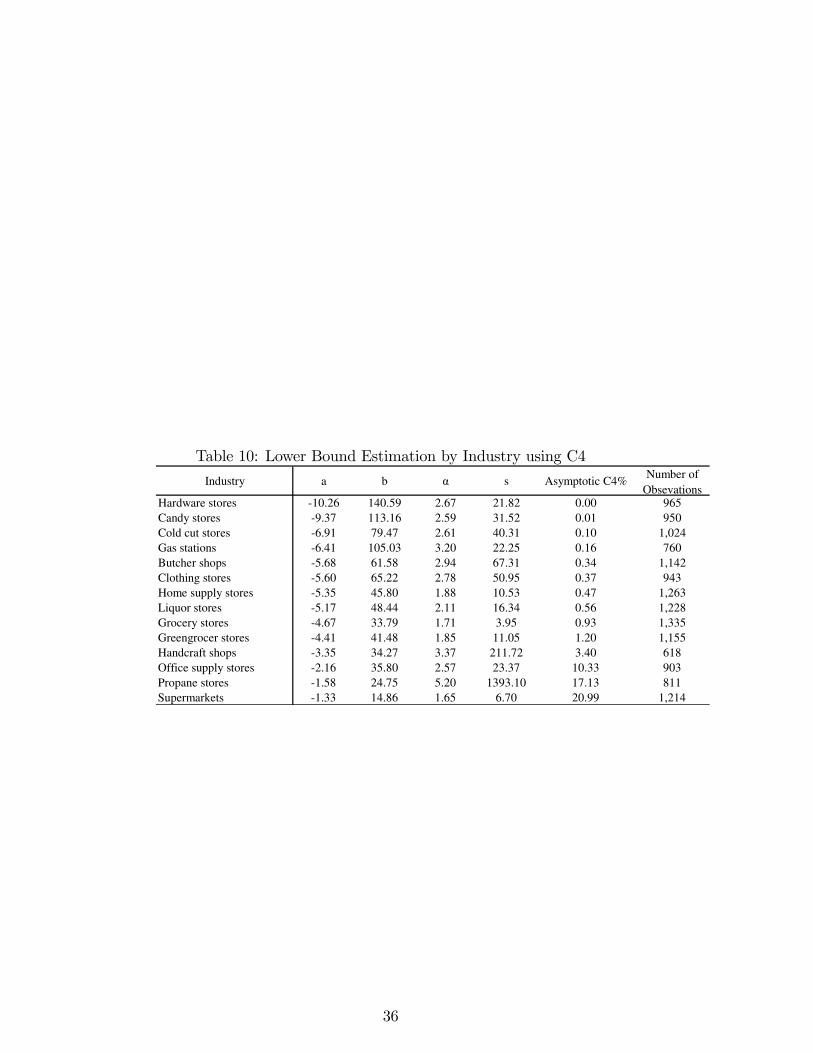
Table 10: Lower Bound Estimation by Industry using C4

Industry a b α s Asymptotic C4%Number of

ObsevationsHardware stores -10.26 140.59 2.67 21.82 0.00 965Candy stores -9.37 113.16 2.59 31.52 0.01 950Cold cut stores -6.91 79.47 2.61 40.31 0.10 1,024Gas stations -6.41 105.03 3.20 22.25 0.16 760Butcher shops -5.68 61.58 2.94 67.31 0.34 1,142Clothing stores -5.60 65.22 2.78 50.95 0.37 943Home supply stores -5.35 45.80 1.88 10.53 0.47 1,263Liquor stores -5.17 48.44 2.11 16.34 0.56 1,228Grocery stores -4.67 33.79 1.71 3.95 0.93 1,335Greengrocer stores -4.41 41.48 1.85 11.05 1.20 1,155Handcraft shops -3.35 34.27 3.37 211.72 3.40 618Office supply stores -2.16 35.80 2.57 23.37 10.33 903Propane stores -1.58 24.75 5.20 1393.10 17.13 811Supermarkets -1.33 14.86 1.65 6.70 20.99 1,214

36

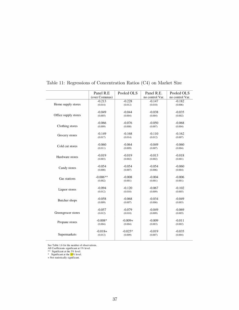
Table 11: Regressions of Concentration Ratios (C4) on Market Size





-0.228(0.012)

-0.147(0.010)

-0.182(0.006)


-0.044(0.004)

-0.038(0.004)

-0.035(0.002)


-0.076(0.008)

-0.050(0.007)

-0.068(0.004)


-0.168(0.014)

-0.110(0.012)

-0.162(0.007)


-0.064(0.009)

-0.049(0.007)

-0.060(0.004)


-0.019(0.002)

-0.013(0.002)

-0.018(0.001)


-0.054(0.007)

-0.054(0.006)

-0.060(0.004)

Gas stations -0.006**(0.002)

-0.008(0.001)

-0.004(0.001)

-0.006(0.001)


-0.120(0.010)

-0.067(0.009)

-0.102(0.005)


-0.068(0.007)

-0.034(0.006)

-0.049(0.003)


-0.079(0.010)

-0.049(0.009)

-0.069(0.005)

Propane stores -0.008*(0.004)

-0.009+(0.004)

-0.009(0.003)

-0.011(0.002)

Supermarkets-0.018+

(0.012)-0.025*(0.009)

-0.019(0.007)

-0.035(0.004)

See Table 1.6 for the number of observations.All Coefficients significant at 1% level.** Significant at the 5% level.* Significant at the 10% level.+ Not statistically significant.

37

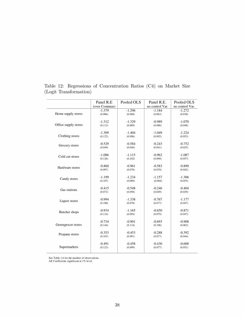
Table 12: Regressions of Concentration Ratios (C4) on Market Size(Logit Transformation)





-1.296(0.068)

-1.184(0.063)

-1.272(0.038)


-1.329(0.089)

-0.989(0.086)

-1.070(0.048)


-1.404(0.096)

-1.049(0.092)

-1.224(0.053)


-0.584(0.040)

-0.243(0.041)

-0.752(0.025)


-1.115(0.102)

-0.962(0.090)

-1.087(0.057)


-0.961(0.078)

-0.583(0.070)

-0.890(0.042)


-1.234(0.089)

-1.157(0.084)

-1.306(0.055)


-0.548(0.058)

-0.246(0.049)

-0.404(0.029)


-1.338(0.078)

-0.767(0.077)

-1.177(0.047)


-1.165(0.094)

-0.650(0.079)

-0.871(0.047)


-0.901(0.114)

-0.693(0.106)

-0.908(0.062)


-0.453(0.091)

-0.288(0.077)

-0.392(0.044)

Supermarkets-0.491(0.123)

-0.458(0.099)

-0.430(0.077)

-0.600(0.051)

See Table 1.6 for the number of observations.All Coefficients significant at 1% level.

38

Documents

Testing for Endogenous Sunk Costs in the Retail Industry