Embed Size (px)
Citation preview

https://helda.helsinki.fi
Teachers' and fourth graders' questions during a
problem-solving lesson
Laine, Anu
Eötvös University Press
2014
Laine , A , Näveri , L , Kankaanpää , A , Ahtee , M & Pehkonen , E 2014 , Teachers' and
fourth graders' questions during a problem-solving lesson . in A Ambrus & E Vasarhelyi
(eds) , Problem Solving in Mathematics Education: Proceedings of the 15th ProMath
conference : Proceedings of the 15th ProMath conference . Eötvös University Press , pp.
þÿ�1�2�4�-�1�3�5� �,� �P�r�o�b�l�e�m� �S�o�l�v�i�n�g� �i�n� �M�a�t�h�e�m�a�t�i�c�s� �E�d�u�c�a�t�i�o�n� �� �t�h�e� �1�5�t�h� �P�r�o�M�a�t�h� �C�o�n�f�e�r�e�n�c�e� �i�n
Eger , Eger , Hungary , 30/08/2013 . <
http://webdoc.urz.uni-halle.de/dl/287/pub/ProMath2013.pdf >
http://hdl.handle.net/10138/230168
publishedVersion
Downloaded from Helda, University of Helsinki institutional repository.
This is an electronic reprint of the original article.
This reprint may differ from the original in pagination and typographic detail.
Please cite the original version.

András Ambrus
Éva Vásárhelyi (Eds.)
Problem Solving in
Mathematics Education
Proceedings of the 15th ProMath conference
30 August – 1 September, 2013 in Eger
EÖTVÖS LORÁND UNIVERSITY, FACULTY OF SCIENCE, INSTITUTE OF MATHEMATICS,
MATHEMATICS TEACHING AND EDUCATION CENTER
ESZTERHÁZI KÁROLY COLLEGE
INSTITUTE OF MATHEMATICS AND INFORMATICS

Problem Solving in Mathematics Education
Proceedings of the 15th
ProMath conference
30 August – 1 September, 2013 in Eger
ISBN
Editors: András Ambrus and Éva Vásárhelyi
Layout: Éva Vásárhelyi
Printing: Haxel nyomda
Hungary
http://www.haxel.hu
Publisher:
Eötvös Loránd University, Faculty of Science, Institute of Mathematics
Mathematics Teaching and Education Center
and
Eszterházi Károly College, Institute of Mathematics and Informatics
All Rights Reserved © 2014 Mathematics Teaching and Education Center
Copies available by Mathematics Teaching and Education Center;
Contact: Éva Vásárhelyi [email protected]

Content
Éva Vásárhelyi:
Preface ……………………………………………………………………………... 5
Gabriella Ambrus:
Problem solving and Modelling – Traditions and Possibilities in Hungarian Math-
ematics Education ………………………………………………………………….
7
Krisztina Barczi:
How do they solve problems? Mathematical problem solving of the average and
the talented …………………………………………………………………………
18
Lars Burman:
About problem sequences designed for heterogeneous classes in grade seven …… 35
Katalin Földesi:
Kangaroo problems for student teachers in Sweden ………………………………. 43
Torsten Fritzlar:
Prospective Teachers’ Conceptions of problem oriented Mathematics teaching –
explored and challenged …………………………………………………………… 53
Günter Graumann:
Problems with the Imagination of Astronomical Measurements ………………….. 67
Tünde Kántor:
Historical aspects in teaching mathematics ……………………………………….. 80
Eszter Herendiné-Kónya:
How can high school students solve problems based on the concept of area
measurement? ……………………………………………………………………… 95
Ana Kuzle:
Talent or Something Else? Preservice Teachers on Mathematical (Problem
Solving) Abilities: Implications for Professional Development …………………... 108
Anu Laine, Liisa Näveri, Anu Kankaanpää, Maija Ahtee & Erkki Pehkonen:
Teachers’ and Fourth graders’ questions during a problem-solving lesson ………. 124
Józsefné Libor:
When do we have to use recursive or asymptotic formulas or Monte Carlo
simulation? ………………………………………………………………………… 136
Erkki Pehkonen:
Open problems as means for promoting mathematical thinking and understanding 152
Richárd Rakamazi:
Solving Diophantine equations with elementary methods and with the help of
Gaussian integers in high school mathematics study group sessions .......................
163
Benjamin Rott:
Rethinking Heuristics – Characterizations and Examples ………………………… 176
Takácsné Bubnó Katalin and Viktor László Takács:
Solving word problems by computer programming ………………………………. 193
Ferenc Várady:
Solving differential calculus problems with graphic calculators in a secondary
grammar school ……………………………………………………………………. 209
Bernd Zimmerman:
The Role of affective Components in mathematical Problem Solving ……………. 232


5
Preface
ProMath (Problem Solving in Mathematics Education) is a group of didactics of mathematics
from all over Europe, who have the common aim of furthering and scientifically exploring
problem-solving activity in mathematics among students, exploring the possibilities and pre-
conditions of problem-solving orientation in mathematics teaching, and promoting it.
ProMath was founded by Günter Graumann (University of Bielefeld, Germany), Erkki
Pehkonen (University of Helsinki, Finland) and Bernd Zimmermann (Friedrich-Schiller-
University of Jena, Germany). One of the activities of this group is to organize the annual
conferences since 1999.
It is a great pleasure and honour for us to organize and support the 15th
ProMath Meeting in
Pólya’s home country, which took place from August 30 to September 1, 2013 at the Institute
of Mathematics and Informatics of Eszterházy Károly College, Eger, Hungary.
"Mathematical Problem Solving Not Only For Talented"
has been chosen as a central theme of the 15th ProMath conference
This choice was justified on the website of ProMath (http://promath.org/meeting2013.html)
by the following:
"The fostering of talented students in mathematics education has a long tradition in
the whole world.
No doubt that the high ability students differ in a great manner form average in their
ability, interest, motivation, learning habits, memory, noticing the solution patterns,
problem solving strategies without extra teaching them. On the ProMath2013 Eger
meeting we are interested for studies and experiences dealing with students not only
highly talented concerning mathematical problem solving. “Not only” means that
studies about talented or high-achieving pupils are also welcome."
It is very interesting to see year in year out the evolution of the ProMath conference.
On one hand there is a dynamic change with respect to the participants. The partici-
pants were novice teachers, doctoral students, and retired professors as well, which
enables a thought-provoking dialogue between the founders and the young
researchers.
On the other hand one can see dynamic changes in the content of the conference. In
addition to presenting interesting problems − with historical aspects and their multi-
6
colored and varied solutions −, there are more and more examinations regarding to the
role of modern teaching tools and methods. (Modelling, graphic calculators, computer
simulation, programming, cooperative teaching and learning, ...)
Thirdly there is a striking expansion of the research aspects, for example the psycho-
logical aspects of learning are increasingly prevailing in the system of criteria. You
can find this various aspects in school-reality, in didactical researches, and within the
topics of this book and of the conference.
This volume contains the papers of the talks given during the meeting. The papers of this vol-
ume are peer-reviewed according to the contents, organized by András Ambrus. Each author
is responsible for the proper English of his or her paper.
I want to thank all participants for their valuable contributions. Let me mention those talks of
the conference, which are not represented by any article in this volume:
A. Ambrus: The role of working memory in mathematical problem solving teaching,
E. Árokszállási: Using different representations in algebraic identities teaching,
J. Boda: Problems in symbolic calculation created by adult high school students,
T. Hodnik Cadez: Preschool teachers’ and children’s competences in problem solving,
L. Naeveri: Connection between teachers’ actions and fifth-graders’ performances
when solving a non-standard problem.
Special thanks to Ilona Oláhné Téglási and to the Institute of Mathematics and Informatics of
the Eszterházi Károly College for the organization and for their hospitality. The charming lit-
tle town of Eger also contributed to the success of the conference.
We have to thank the Mathematics Teaching and Education Center of the Eötvös Loránd Uni-
versity as well Eszterházi Károly College for supporting this volume.
The figure on the front page is an illustration of the following problem: Show that the area of
the dotted and the shaded parts are equal.
Budapest, 2014.
Éva Vásárhelyi

7
Problem solving and Modelling – Traditions and Possibilities in Hungarian
Mathematics Education
Gabriella Ambrus
Eötvös Lóránd University Budapest, Hungary
Abstract
Problem solving and solving modelling tasks are obviously in connection with
each other. However, a traditional mathematics problem and a modelling task are
different from several points of view so we may assume for example that a tradi-
tionally clever problem solver in mathematics is not necessarily good at solving
modelling tasks. I am going to discuss some questions in this subject considering
the results of modelling tasks solved by secondary school students.
Key words: Problem solving and modelling, modelling tasks, research in mathematics education
ZDM classification: D50, M13, M14, F93, F94, F99
Introduction
The Hungarian education is changing rapidly and these changes with their new contents in
several fields are hard to follow. The limit of human flexibility and a pithy reform require
(need) a thoughtful consideration of the possibilities which are provided by good teaching
traditions.
The application of knowledge for everyday situations has been emphasized for a long time in
Hungarian mathematics teaching but for the realisation of this idea only closed word-
problems have been used which are based in a lot of cases on a not really real situation. The
Hungarian traditions of problem solving may provide a good basis for teaching new or „new
like” content, so for teaching modelling as well, which has become one of the main points in
the National Curriculum 2013 (NAT 2013).
Theoretical background
There are several definitions for modelling; generally it means the process which describes
the solution of modelling tasks. The necessary definitions for the subject can be characterised
in the following way:

8
Modelling means abstraction of reality by mathematical methods (Greefrath, 2007, 15).
Modelling tasks are solved by modelling process (in an ideal case it’s a Modelling Cycle,
Blum, Leiss 2006), they are problem centred authentic open word problems.
Modelling competency means the competencies, which are necessary for solving modelling
tasks (without the competencies while working only mathematically) and these competencies
can be given by the Modelling Cycle. To solve modelling tasks based on problem solving,
first we should look at the similarity of the four-step model of problem solving to the four-
step model of modelling.
1. Understanding the problem 2.-3. Organizing the information according to mathematical
concepts and identifying the relevant mathematics 4. Solving the mathematical problem 5. Interpreting, validating
Figure 1: Chart according to Pólya’s steps of
problem-solving (Greefrath, 2007)
Figure 2: Modelling cycle (PISA 2003)
Based on Pólya’s steps we can create another chart, which is more relevant to the modelling
cycle (Blum/Leiss, 2006).
Figure 3: Possible extension of Pólya’s steps for a
modelling cycle (Ambrus/Vancsó/ Koren, 2012)
Figure 4: Modelling cycle (Blum/Leiss, 2006)

9
Analysing the modelling routes of pupils, Borromeo Ferri completed the ideal cycle of
Blum/Leiss (2006) with phases referring to individuals' characteristics and she obtained dif-
ferent pictures about the connections among the elements in the cycle in case of pupils with
different thinking types (Borromeo Ferri 2010, p. 113).
Greefrath (2010) points out that the Blum/Leiß 2006 cycle theoretically allows the problem
solving and the modelling process to be considered as parallel. Each step of the modelling can
be interpreted as a separate problem solving process as well. Observing pupils while model-
ling he concluded, that modelling can be observed through the glasses of problem-solving,
however this is not appropriate because of the different character of modelling tasks.
There is a rich tradition of problem solving in Hungarian mathematics teaching, so the ques-
tion is given: to what extent is it possible to lean on these traditions while solving modelling
tasks in schools. Modelling tasks are not used in the everyday practice in Hungarian mathe-
matics lessons nowadays, this way the former question can be formulated as:
How can Hungarian pupils solve modelling tasks without any experience with modelling tasks?
There are several studies about how Hungarian pupils solve word problems (Csíkos et al.
2011). One of them deals with a survey of 4000 students (grades 5-6) using 5 simple model-
ling tasks. They were asked to choose from three possible answers (solutions) of the three fol-
lowing types: a) routine-based, non-realistic, b) a numerical response that takes realistic ele-
ments and considerations into account, c) a realistic response that also refers to the situational
complication of the problem but says that therefore the problem cannot be solved for each of
the tasks. This last answer can be considered as a modelling solution.
Authors emphasize that in spite of the realistic character of the tasks the majority of students
chose a non - realistic answer. However, it is important to mention that in case of some tasks
nearly the same number of students chose type b) as type a).
Finally 26,5 % of the students gave for at least 4 tasks a type b answer. The average mark of
the pupils in mathematics who gave the answer b is 4,43 (in Hungarian schools students are
assessed on a five–level scale, 5 indicating the best and 1 indicating the worst achievement.)
Research questions
Even if a student has a good mark in mathematics it does not necessarily mean that he or she
is a good problem solver. However, it seems that pupils with good marks are better at solving
modelling tasks.

10
Considering the connection between problem solving and modelling, in this piece of work the
central research questions are:
To what extent are Hungarian students able to work with modelling tasks?
Which strategies are used by solving modelling tasks and to what extent are strategies
known and important for Hungarian students who are good at school mathematics?
Theoretical framework
The first question focuses practically on the modelling competency of students. There are
several ways (all having their barriers) to measure this competency (Riebel, 2010). Riebel
mentions a method where students receive a point for every correct modelling step. The prob-
lem with this method is that a student who has constructed an incorrect model automatically
loses points on the following steps. It seems more appropriate to modify the method and “give
points” for every step that is acceptable.
In this paper we follow this latter method, every step is worth a point if it is correct, because
the focus is on the process and not on the result.
For the process analysis the following modelling steps are considered:
1. From the real problem into a mathematical problem
2. Solution of the mathematical problem
3. From the mathematical result to a real-result
4. Interpretation of the real result
For investigating the second question the method of „using self-commented strategies”
(selbstberichtete Strategienutzung”) is used (Schukajlow/Leiss, 2011).
In this research, after solving some modelling tasks, the students received a questionnaire
with statements concerning their strategy. They had to rate each strategy from 1 to 5 deciding
to what extent they found the strategy useful while working on the given modelling task.
In the research the following theoretically founded statements were used in a modified ver-
sion (Fig. 5). We used these statements with the modelling task presented in this paper with
four students after recording their solutions.
The students' knowledge about strategies was compared to the strategies used while solving
the task.

11
To what extent do you think are the following strategies important for a successful solution? Rate the statements from 1-5.
While solving this task I would
1. reread some sentences
2. highlight (i.e. underline) some important data in the text
3. make a plan
4. make sketches and figures
5. check several times whether my way of solution correct is
6. look for similar tasks and I would revise their solution before
7. divide the problem into subtasks before solving it
8. simplify the task and I would solve this version first
9. interpret my result whether it is approximately correct
Figure 5: The statements (strategies) of the students
Methodology and design of the study
For the study I utilised some results of my student B. Tóth (2013), furthermore we recorded
and videotaped the students' solutions of a modelling task.
In the first case three versions (for three different age groups) (situation: Olympic Stadium)
were created and solved by about 120 pupils (grades 7-11) of a Hungarian secondary school
in the autumn of 2012. In every year group two groups (students taking part in normal or in
high level course in mathematics) solved it. The versions were different regarding their com-
plexity. The students did not have any former modelling experience. They had about half an
hour to solve the problem.
In case of the 120 students we had only their written tests. To get some insight into the
thoughts of students while working with a modelling task (without any previous experience)
four solutions of the version for grades 9-10 students of the Olympic Stadium were recorded
or videotaped in secondary schools in Budapest. This version was chosen for collecting data
from different grade students and the complexity of this task fitted this purpose the best. Finally,
these four solutions were collected only from students who are interested in mathematics.
The students who were asked to share their thoughts while solving the task were selected by
their teachers and they could decide whether to take part in the survey. They are all good at
mathematics. The teachers were asked to give a short description of the pupils as well. Among
the 4 students 3 were classmates (grade 11) in a secondary school, the last one was a grade 11 stu-
dent in a bilingual secondary school (grade 11 means here only a grade 10 in terms of mathemati-
cal studies because of a preparatory year). The names of the students were changed in the paper.

12
Tasks
Figure 6: Tasks

13
Some results of the study
About the students’ work that were created in the classes
Among the 120 pupils there were 60 who prepared a model as the first step. In the solutions
the occurrence of the 4th
step was the rarest. Most of the students who were uncertain in their
result wrote an interpretation for their solutions.
Pupils who had some idea for solving the task made 3 steps and got a sort of result as well.
The average number of steps shows an interesting picture. In every age group the number of
steps is higher in the high level classes, and older age means generally higher average number
of steps, however the tendency isn’t linear.
Figure 7: Average number of modelling steps
Although several models were constructed in every age group, these were mostly unaccept-
able, especially among the works of the pupils in grade 7. Their work was often based on an
incorrect assumption regarding the length and width of the runway.
Figure 8: The student assumed that the runway is 1 m wide and so every runway is 1 m longer than the
previous one.
Although the starting ideas were right, many students could not use the picture on the sheet
but they tried to work only from the text. They prepared a very simple model; they worked
out mostly unfounded estimations.
Results of the recorded solutions
The students worked on the version of the “Olympic Stadium” task which was created for
grade 9-10. Three students are classmates in a year 11 class; while the fourth is a grade 10

14
student in a secondary school.
Géza: A boy with an inconsistent behaviour, sometimes he cannot be trusted, but otherwise he
is a nice fellow. He always has some ideas. Mathematics is important for him, he wants to be
better, but does not always have a 5 mark. He spent the previous year abroad; he has been in
the current class since last September.
He started to solve the task coolly and it seemed that he knew how to begin. He prepared a
first cast after he threw away his first idea: to work with the number of rows in the picture. He
went through the modelling steps neglecting the last interpretation step. In his “final” solution
he assumed that the shape of the stadium is a circle and r = 180/2 = 90 m. He obtained an
acceptable result, about 700 people in the first row.
He needed about 11 minutes for the solution.
After solving the task he rated the following strategies as the most important ones (4 or 5
marks): Rereading some sentences, making a plan; checking several times, dividing in sub-
tasks, and interpreting the result. He used these strategies except for the interpretation of the
final result.
Zsuzsi: She has a scrupulous character and she usually writes the mathematics tests without
mistakes. She is meticulous, and usually does not add anything new to things. She is dutiful,
accomplishes what she is asked. She has a steady 5 in mathematics.
She was surprised by the task. She used only the picture for the solution, and made several as-
sumptions for the circumference of the first row. Finally, she took it for 500 m and found that
the number of people in the first row is about 880 (60 cm for a person). She didn’t interpret
the final result, so she used 3 modelling steps.
She needed about 12 minutes for the solution.
After solving the task she rated the following strategies as the most important (with 4 or 5
marks): Rereading of the text, making sketches and figures, checking several times, dividing
into subtasks, simplifying the task, and interpreting the result. She used some from these
strategies while solving the task: rereading of the text, making sketches and figures, checking
several times, simplifying the task (she worked only on the picture).
Árpád: He is good at and interested in mathematics. Furthermore, he is creative but often has
a problem with accepting novelty. He is a good problem solver and is quick in the uptake. He
can’t give up things; he often struggles with problems.
It was immediately obvious that he found the task very strange. He said that he had expected a
really difficult mathematics problem (not this one). He didn’t understand what the expected
15
solution was he tried to find it out (by direct questions) several times while solving the task.
He made a sketch, he gave the length of the semicircles and parts by assumption. Afterwards,
he gave an average number for the radius of the stadium and he worked with circles (concern-
ing the shape of the runway). For the number of people in the first row his result was 836. He
found that it is too many and took (without any explanation referring to the picture) 700 as the
answer. He went through the modelling steps neglecting the last interpretation.
He needed about 24 minutes for the solution.
After solving the task he rated the following strategies as the most important (4 or 5 marks):
Making sketches, figures, simplifying, and interpretation of the result. While solving the task
he used: making sketches, simplifying (temptation several times).
It is to mention that from the statements he considered the least important (rated 1-2) he used
several strategies: making a plan, looking for a similar task, checking several times (mostly by
asking whether his way of solution is correct).
Zoli: He is quick in uptake and good at mathematics. He likes to finish the tasks quickly; he
always focuses on the result.
After receiving the task he was thinking for a long time. He tried to work in the picture. He
found 72 sectors on the figure so he assumed that about 80 000 : 72 = 1111 people were in
one sector. He got stuck here. After a while he went on with another method. He assumed that
the runway was a 100 x 100 rectangle (a square) and so calculated 250 people (40 cm for one
person) on one side, so 1000 people would sit in the first row. After the question of the
teacher who made the videotaping whether this result was realistic, he corrected the place
needed for one person to 50 cm obtaining the final result of 800 people. He didn’t interpret
the final result.
He needed 11 minutes for the solution. He went through the modelling steps neglecting the
last interpretation.
After the solution of the task he rated the following strategies as the most important (4 or 5
marks): Making sketches, checking several times, interpretation of the final result. He used
these while solving the task except for the interpretation - he did it only after the teacher’s
remark.
Discussion
The samples we used to obtain the results had different size (120 students and 4 students).
The number of modelling steps used by the students in their work shows – although they had

16
not solved modelling tasks before – that many students seem to be able to do an „intuitional
modelling”. However, doing several modelling steps does not necessary mean finding an ac-
ceptable solution.
Students who are good at problem solving are generally able to execute more modelling steps;
it means that they can make a better start with modelling tasks. They consider the task as a
problem that they have to solve. Presumably this better result is supported by their positive
belief about mathematics as well.
The four observed students rated “making a plan” generally as „unimportant”. It coincides
with the result of Schukajlow/Leiss 2011 in which this problem is discussed in detail. Al-
though an interpretation of the final result was missing in almost everyone's work, they
checked their solution several times while working on the task. The four good problem
solvers mentioned different number of strategies as important when solving this task, so it
seems that they know about strategies which can help the problem-solving. The character of
the problem solver, i.e. mathematical thinking style (visual thinking style, analytical thinking
style, integrated thinking style, Borromeo Ferri, 2010) may have an effect on the person's
modelling process and on the quality of the solution as well.
Conclusion and further perspective
Although the questions were investigated only with a few students so the results are not
enough for general statements, it is promising that several modelling steps are present in the
work of the investigated students without having any previous experience with modelling.
This refers to a basically good modelling competency in these cases mostly among good prob-
lem solvers. The knowledge of strategies is pretty good among the investigated good problem
solvers but there is a discrepancy between this knowledge and the application of strategies in
a given situation. An important experience is that during the investigation students must be
helped and encouraged while solving unusual tasks. They need (would have needed) more
feedback while solving the task. While working on this type of task alone, students may have
negative, uncertain feelings which may influence their modelling work and the acceptance of
this type of task in a contra productive way as it happened in the case of Árpád. A previous
discussion of the modelling process and the character of modelling tasks seem to be necessary
especially for low achieving students.
For a more thorough analysis of the research question further investigations are needed. For
example:

17
Further collection of data among good and normal problem solvers with different types of
modelling tasks.
Investigation among students with different ability in mathematics (with a control group)
whether a reassuring feedback from the teacher or the possibility of a discussion with other
pupils (i.e. working in groups) has a positive influence on working with modelling tasks.
In this paper we considered the use of strategies only among good Hungarian problem
solvers. A wider investigation could clarify whether a correlation between strategy
knowledge and achievement in mathematics exists. In their investigation Schukajlow/Less
2011 couldn’t find such a correlation.
Acknowledgments: Thanks to Hegyi Györgyné, Koren Balázs for their help with the realisa-
tion of videotaping and recording student’s solutions.
References
Ambrus, G., Vancsó Ö., Koren B. (2012). The Application of Modelling Tasks in the Class-
room – Why and How? 10/2 231-244 TMCS, Debrecen
Blum, W., Leiss, D. (2006). „Filling up” – The Problem of Independence-Preserving Teacher
Interventions in Lessons with Demanding Modelling Tasks. I.: Bosch, M. (Ed.)
CERME-4 – Proceedings of the Fourth Conference of the European Society for
Research in Mathematics Education, Guixol
Borromeo Ferri, R. (2010). On the Influence of Mathematical Thinking Styles on Learners’
Modelling Behaviour 31: 99-118, JMD
Borromeo Ferri, R.: Mathematical thinking styles- an empirical study
http://www.dm.unipi.it/~didattica/CERME3/proceedings/Groups/TG3/TG3_BorromeoF
erri_cerme3.pdf (15.06.2013)
Csíkos, Cs., Kelemen, R., Verschaffel, L. (2011), Fifth-grade students’ approaches to and be-
liefs of mathematics problem solving: a large sample Hungarian study, 43: 561-571
ZDM, Springer Verlag
Greefrath, G. (2007). Modellieren lernen mit offenen realitätsnahen Aufgaben, Aulis Verlag, Köln
Greefrath, G. (2010). Problemlösen und Modellieren- zwei Seiten der gleichen Medaille
2010/3: 44-56 Mathematikunterricht, Friedrich Verlag
Riebel, J. (2010). Modellierungskompetenzen beim mathematischen Problemlösen. Inventari-
sierung von Modellierungsprozessen beim Lösen mathematischer Textaufgaben und
Entwicklung eines diagnostischen Instrumentariums. Dissertation, Universität Koblenz-
Landau, Fachbereich Psychologie, Landau.
Schukaljov, S., Leiss, D. (2011) . Selbstberichtete Strategienutzung und mathematische Mo-
dellierungskompetenz, 32: 53-77 JMD, Springer Verlag
Schukaljov, S. (2010). Schüler-Schwierigkeiten und Schüler-Strategien beim Bearbeiten von
Modellierungsaufgaben als Bausteine einer lernprozessorientierten Didaktik, Disserta-
tion http://kobra.bibliothek.uni-kassel.de/bitstream/urn:nbn:de:hebis:34-
2010081133992/7/DissertationSchukajlowWasjutinski.pdf (18.06.2013)

18
How do they solve problems?
Mathematical problem solving of the average and the talented
Krisztina Barczi
University of Debrecen, Neumann János Secondary School, Hungary
Abstract
When it comes to mathematical problem solving probably everybody has a prefer-
ence in terms of how to handle the task in hand. The choice of solution method
depends - among many other things - on the students’ level of Maths knowledge.
Those who are talented prefer one way while those who have a rather average
ability in Maths prefer another one. This article compares and contrasts the prob-
lem solving style of a talented and that of an average ability student in different
types of lessons. In one lesson frontal teaching was used and in the other one co-
operative teaching techniques were applied.
Key words: cooperative learning, talented, average ability, mathematics
ZDM classification: C20, C30, C40, C60, D40
1. Introduction
In Hungarian secondary schools mathematics is mainly taught in heterogeneous classes,
which means that talented students work together with the average ability ones and the low-
achievers. This scenario requires differentiation from the teacher which is not always easy to
accomplish. Furthermore, in this environment the teacher needs to ensure some kind of suc-
cess for all students regardless of their mathematical ability.
Although more and more alternative teaching methods are appearing in schools the most
widely used teaching method is still frontal teaching where differentiation is not impossible
but sometimes is really challenging. Even students with similar ability level can have different
working paces, or some are slower in grasping concepts and ideas even if they are good at ac-
tually solving problems.
This article describes an experiment that was carried out in a secondary school class and
whose main aim was to find out how different ability students reacted in different problem
solving situations. For this, two students – based on the students’ previous mathematical

19
achievement and occasional competition results one of them can be considered as talented in
Maths and the other one as an average ability student – were observed in two types of lessons.
In one type of the lessons frontal teaching was used while in the other one cooperative teach-
ing techniques were applied. Here, we summarize our experience.
2. Theoretical background
The aims of teaching Mathematics
One of the main aims of teaching mathematics is to make students understand mathematical
concepts and their relations and to help them acquire thinking skills that can be used in prob-
lem solving regardless of the content, both in the field of mathematics and in other areas as
well. (Ambrus, 2004)
As understanding has a primary importance, let us examine first how concepts are formed in
our mind. Most everyday concepts are formed with the help of objects or experiences from
our everyday life. That is why most of them are easy to remember since we can connect them
to something we know very well. The difficulty of understanding and learning mathematical
concepts lies in their abstractness. Students cannot learn mathematical concepts from their
own experiences only with the help of someone else. In schools teachers try to choose good
examples that demonstrate the nature of a concept. Furthermore, according to Skemp (2005)
when teaching mathematical concepts the level of the students’ knowledge and that of the
concept should be in line.
Understanding and learning a mathematical concept is only the beginning of a process. In or-
der to become successful problem solvers students need to be able to apply what they learnt.
A concept can be applied if it is fully understood. Two types of transfers can prove that a stu-
dent had understood a concept. Near transfer means using the concept in a situation that is
similar to the ones used in the teaching situation while far or knowledge transfer means that
the student can apply the concept in a context that is completely different from the above
mentioned one. (Dobi, 2002) For the low-achiever or average ability students achieving near
transfer already means success.
Besides helping students understand mathematics and helping them be able to use what they
learnt in different problem solving situations, it is important that they experience the joy of
thinking. (Szendrei, 2005) For average ability students it is slightly more difficult to show that
mathematical thinking can be similar to playing with different thoughts but if the teacher

20
manages to make these students feel that doing maths can be creative and enjoyable than they
can become more successful.
Furthermore, for helping all students experience success effective differentiation is needed in
the classroom, for which recognizing talented students in mathematics is necessary. As Miller
(1990) says students who are talented in mathematics have an ability to understand even com-
plex mathematical ideas and can use mathematical reasoning very well, but they are not nec-
essary the students who are good at arithmetic calculations or have top grades in Maths. Fur-
thermore, maths talents often have emotions related to numbers and they have an interest in
the subject in their early years already. They like solving puzzles and they are successful in
completing tests that measure memory or visual skills. Moreover, these students often use
specific procedures for solving problems. (Gyarmathy, 2006)
Different students have different problem solving preferences which depend on their person-
ality, their mathematical ability, their motivation … etc, so there is no rule which tells us that
for talented students we should use a specific approach. For high ability students fast track or
acceleration programs might be beneficial especially if talent is matched with motivation. On
the other hand, slower or less motivated students might do better if the learning pace is slower
and the learning focuses deliberately on the mathematical concepts being taught. (Miller,
1990) In an average classroom using cooperative learning structures might be beneficial for
both types of students.
Talent or average ability, all students gain from learning in a mathematically enriched envi-
ronment. For this social interactions between students should be encouraged, the appearance
of emotional connections should be facilitated, the students’ individual style should be taken
into consideration and the development of students’ self-confidence should be emphasized
(Caine et al, 2004). Again, when using cooperative learning structures the above mentioned
factors appear more easily than in a frontal class.
Cooperative teaching and learning
In cooperative learning students are arranged in groups so that they have to work together in
order to achieve a common goal, to solve a problem. For successfully overcoming the possi-
ble difficulties the members of the teams must rely on each other, respect and support each
other since their success depends on their ability to work together. (Kagan, 2004) In Hungary
it was József Benda whose work had an effect on the appearance of cooperative teaching in
education as he believed that this teaching method can contribute to the integration, achieve-
ment and development of students. (Józsa & Székely, 2004)

21
Many people think that using cooperative techniques is the same as simply making students
work in groups. I want to clarify a difference. In group work students are put together and
given a task to solve and it is their job to find out who does which part of the task and share
out the responsibilities. This working format often results in the best student doing all the
work while the others copy everything while some students might not even listen. To avoid
this, cooperative structures were created in a way that the following four principles are always
present: Positive interdependence; Individual accountability; Equal participation; Simultane-
ous interactions. These four principles ensure that every member of the group is an active par-
ticipant and the team’s success is everyone’s responsibility. (Johnson & Johnson, 1994) To
help teachers explain and students to remember these structures they were given catchy
names. (Kagan, 2003) Here are some examples for cooperative structures: 1) Think-Pair-
Share: Students work in groups of four. A problem is presented to the students. They are
given time to think on their own about possible answers for a specific amount of time. Stu-
dents discuss their answers in twos. 2) Round Robin: This structure gives an opportunity for
each member of the group to speak. Starting with one student, everyone gets 1- 3 minutes to
present their point of view. (Kagan, 2004) 3) Jigsaw: Each team needs to become an expert of
a topic/solution of a problem. New groups are formed with one member from each of the
original groups. They share their knowledge. Finally, everyone goes back to the original
groups (Slavin, 1995).
When using cooperative teaching techniques the issue of composing the groups is important.
How the teacher forms groups might depend on the teacher, on the students, on the type of the
lesson … etc. However, no matter what the arranging principle is an ideal group consists of
four members. The reason for this is that in a group of four two pairs can be formed, further-
more if every member needs to communicate with every member than the number of interac-
tions is 6 and nobody is left out, while if the number of group members is three or five one
student might feel neglected (Burns, 1990).
In cooperative teaching and learning not only the classroom setting but the teacher’s role is
different. First of all, instead of being the person who takes control over the whole teaching
and learning process and leads the students through the lesson, the teachers becomes an ob-
server or a coach who consults the groups or with individual students and helps the ones who
are left behind. The teacher is still needed in the classroom only the function has changed.
Since the teacher can walk around the classroom, he can give an instant feedback for the
groups or he can help the groups overcome the obstacles to learning or problem solving.
(Crabill, 1990) However, it is still the teacher’s responsibility to ensure the right environment

22
for learning. Just because students are working in groups and there are parallel discussions the
classroom should not turn into a permissive and chaotic place. (Dees, 1990)
3. Questions
During the experiment and the two particular lessons we focused on the following questions:
1) How do talented/average ability students solve problems in frontal classwork?
2) How do talented/average ability students solve problems in cooperative work?
3) How do they feel about the different scenarios?
4. The experiment
The two lessons where these two specific students were observed were part of a longer ex-
periment. This experiment was an action research, which is usually carried out by practicing
teachers who would like to achieve professional development. According to Koshy (2005) ac-
tion research is a kind of enquiry during which the teacher constantly changes and refines his
practice and this process leads to his professional development. Since action research is about
the researcher’s own practice, it is participatory and situation – based. Furthermore, action re-
search is a tool that brings the goal of mathematics teachers and researchers of maths educa-
tion closer. (Zimmermann, 2009)
The present experiment was carried out in a mixed comprehensive secondary school whose
students are 12-20 years old. The school is considered “a good school” since the students at-
tending here are the ones who did best on the entrance exam.
Sixteen 16 - 17 years old students took part in the experiment. In the academic year when the
experiment happened they attended a class that specializes in maths and foreign languages. In
their preparatory year the number of maths lessons per week was three, in the following two
years they had four maths lessons every week. That year the class followed the year 10
scheme of work for Hungarian secondary schools. The teacher of the class was the researcher,
as well.
In the first part of the experiment 12 lessons were held where 5 mathematical problems were
discussed – there were 2-3 lessons planned for each problem. Although these problems were
curriculum-based Maths tasks, they were different from the ones that are used in an average
Maths class. These problems were open-ended problems or investigations. These 12 lessons
were planned with cooperative method only.
In the second part of the experiment, in the rest of the school year the students continued

23
working with the official scheme of work and they had lessons with cooperative method once
every 2-3 weeks, depending on the material.
During the experiment for collecting data the following methods were used: 1) students had
so called “reflection booklets” which were exercise books where students solved the problems
and recorded their feelings and ideas about the methods used; 2) half of the lessons were
video recorded; 3) the work of every group was voice recorded; 4) students completed pre-,
post and delayed mathematical tests; 5) students completed pre- and post- psychological ques-
tionnaires.
5. Focus on these two students
During the above described experiment all 16 students were observed, but in this article the
focus will be on two particular students. To obtain a picture on their problem solving style
and problem solving preferences their notes from their “reflection booklets” were checked, in
addition they filled out a questionnaire1 on cooperative learning at the end of the experiment.
The results of these students on the three mathematical tests were analysed as well. Further-
more, these two students were observed in two specific lessons which were planned in the
same topic with different teaching methods, one of them with frontal teaching using closed
problems, the other with using cooperative techniques and an investigation task. The teacher’s
notes from these two lessons will be discussed, too.
The students
Let us call the two students Richard who is the talented and Alex who is the average ability
student. In the following section their attitude towards mathematics, their behaviour in maths
lessons and their maths results are summarized.
Richard’s mathematics grades contained mostly 5s2 with some 4s in the past three years. He
often participated in mathematics competitions where he achieved good results, besides he
regularly attended maths group study sessions. His attitude towards mathematics was defi-
nitely positive and he showed great confidence when it came to sharing ideas with the class.
In lessons he took part actively in discussions but worked well individually if necessary.
When solving a new task he often contributed with useful ideas or comments.
Alex’s mathematics grades contained 2s, 3s, 4s and 5s. His half year mark in 2012/2013 was
3 while his end of year mark was 5. His achievement was rather fluctuating, it often depended
1 Appendix
2 In the Hungarian system 5 is the best grade and 1 is the worst.

24
on the topic how well he completed a test. His work was mainly focused on classwork and
completing the homework but Alex never attended group study sessions or never applied for
competitions in maths in the past 3 years. Especially at the beginning of his first year in this
school he had low self-confidence in terms of mathematical knowledge and in a problem solv-
ing situation he often relied on the other students’ ideas or help. During classwork he often
sought assistance, mainly from the teacher, or simply just wanted reassurance. In class discus-
sions he participated only when he was asked.
6. The lessons
Frontal teaching
The topic of the lesson that was taught using frontal teaching was generalizing trigonometric
ratios; the type of the lesson was practice. The students had previously learned how to inter-
pret trigonometric ratios for angles bigger than 90º and how to find angles if the trigonometric
ratio was given. In this lesson they had to work from the following worksheet:
Complete the following tasks.
1. Without using a protractor mark the following angles in the Cartesian coordinate grid:
a) 120° c) – 130° e) – 90°
b) – 45° d) 270° f) 750°
2. Find the acute angles whose trigonometric ratio is equal to:
a) sin (240°) c) sin (210°) e) sin (810°)
b) cos (315°) d) cos (– 45°)
3. Find all angles for which the following equations are fulfilled:
a) sin α = 0,47 c) cos α = 1 e) sin α = – 0,6
b) cos α = – 0,17 d) sin α = 0
In this lesson the students were given the above worksheet and they were asked to solve the
tasks. The answers were checked as they proceeded and when we found a question that eve-
rybody had difficulty with we had a class discussion. When individual students got stuck on a
problem they either helped each other or they asked for the teachers’ help.
Cooperative lesson
The topic of this lesson was generalizing trigonometric ratios too, and its type was also prac-
tice through an investigation. With cooperative techniques there is a better opportunity to use
so called open problems or investigations which can be considered as open problems.
(Pehkonen, 1999)

25
In the lesson students were working in groups of four and they had to solve the following
task: Given two segments and the trigonometric ratio of an angle. Are there any triangles
whose sides are the segments and whose angle is the given angle? Try to find and draw all
possible triangles.3
The lesson plan was the following:
1. Forming groups
2. Trying to solve the task using the structures “Think-Pair-Share” and “Round Robin”
3. Group discussion in groups of four to make sure that every member understands the
ideas and the group’s solution
4. Sharing the different solutions of the groups using the structure “Jigsaw”
5. Collecting all the solutions and checking ideas through class discussion
7. Observations and experience
The teacher’s perspective
As mentioned before observations were made during the two particular lessons with special
attention on the two students, Richard and Alex. Their classwork and participation can be de-
scribed as the following.
Frontal lesson
Richard worked really well on his own. He used his previous knowledge confidently and
when he was ahead of the others in answering the questions he was happy to help them. Rich-
ard copied a task first then he solved it and proceeded through the whole worksheet without
changing the order of the exercises. During the task solving phase he never asked for help or
for reassurance from the teacher. However, he was an active participant in class discussions,
when we were checking the solution methods and the answers.
On the other hand, Alex did try to work on his own, but with less success. He often looked
puzzled and he was trying to check what his neighbour was doing. When he had no idea how
to start he looked back in his exercises book trying to find examples that he could use. In spite
of the fact that he did not always know how to answer the questions Alex did not speak to
anyone and he hardly asked for help. Even when he decided to ask for clarification of the task
or just for some guidelines he chose to ask the teacher. From the worksheet first he copied all
3 The four groups received four different data to work with. The trigonometric ratio was always the sin ratio

26
the questions and only thereafter did he try to solve them.4 During class discussions Alex only
listened to the discussion instead of taking actively part in the conversation. He checked his
answers and copied the missing ones or corrected the incorrect ones but never asked why his
solution was incorrect or how to obtain the right answer.
Cooperative lesson
First of all it is important to mention that this lesson was only one of the many where the stu-
dents used cooperative techniques for mathematical problem solving. By the time this lesson
was taught the students had had experience with working in groups.
As mentioned before, Richard preferred working alone and this was obvious from his attitude
to cooperative work as well. For him his own success and progress was always more impor-
tant than that of his group. He was not willing to share his ideas and thoughts if he did not
have to. However, when he was talking to his group mates he behaved as if he was superior to
the others and played more of a leading role rather than cooperating with the others.
As for Alex the grouping of this lesson was not the most fortunate for him.5 After receiving
the task first he looked puzzled then waited. Following that, all of a sudden he started writing
down some ideas then stopped. When he had to share his ideas he was very brief and not
really confident. In earlier classes with cooperative learning he was a more active participant.
When using the structure “Jigsaw” new groups were formed which had a positive effect on
the work of both students being observed.
Richard was more willing to share his work and he was proudly sharing his group’s ideas and
solutions with the others. However, he still found it hard to listen to the other students and he
preferred being the one who tells the others what to do.
This grouping suited Alex better than the previous one which was reflected in his attitude and
class work. He became a more active listener and when it was his turn to speak and share
ideas he was much more confident, moreover he did not mind making mistakes and was
braver in taking the risk of saying something that was not necessary correct.
8. The students’ comments on cooperative learning
The following ideas were written in the students’ “reflection booklets” after the 12 cooperative
lessons at the beginning of the school year.
4 I believe that the reason for this behaviour is that the student wanted the others to think that he was busy work-
ing on the problems. I think, in this way he was trying to hide the fact that his knowledge was not stable
enough. 5 Alex and Richard ended up in the same group.

27
Richard wrote: “At first I didn’t prefer working in groups but often it was useful since we
were able to discuss results with each other. We managed to find many solutions that I had
never thought of before. Basically now I like cooperative work, although it depends on the
members of my group. If my group mates were inactive or just messed about it made progress
more difficult.”
Alex wrote: “I didn't always like my group mates. There was always someone to help. For me
cooperative work was sometimes too much. The tasks were interesting and varied. Since I
prefer working alone cooperative work was a negative experience for me. However, in this
way we solved special problems. We could come up with good ideas. In the future I would like
to avoid working in groups, although it is a good idea.”
9. Questionnaire about cooperative work
The questionnaire contained 20 statements6. For analysing students’ answers the statements
were organized into three groups on the basis of the following aspects: (1) statements related
to cooperative work; (2) statements related to attitude towards Mathematics; (3) statements
about relationship to the others (students or the teacher).
Cooperative work
Statement 1
(+)
2
(+)
3
(+)
5
(+)
11
(+)
12
(+)
13
(+)
14
(+)
16
(-)
17
(-)
18
(-)
19
(-)
Richard 3 4 3 1 3 5 5 5 2 5 3 4
Alex 3 2 2 2 3 3 2 2 3 4 5 5
The above table shows how the two students reacted to statements that are related to coopera-
tive work. The statements whose number is marked with (+) are the ones that are in favour of
cooperative work while the ones marked with (-) describe some disadvantages of working in
groups. The mean average score for Richard on the statements marked with a (+) is 3.625 and
the standard deviation is 1.4 while the mean average of Alex’s answers is 2.375 and the stan-
dard deviation is 0.5. This means that in general Richard had a more positive attitude to group
work but his answers have a wider range. Moreover, there are aspects of cooperative work
(statement 12, 13, 14) that Richard definitely liked.
On the other hand, Alex’s answers clearly show that he did not feel the positive statements
true for him. His average score is lower, so is the standard deviation which means that his
opinion on group work was quite consistent.
6 Appendix
28
Statements 16, 17, 18 and 19 are negative statements about cooperative work and the scores
of both students are in line with their opinion on group work.
Maths related feelings
Statement 4 6 7 9 10 20
Richard 2 1 4 3 1 1
Alex 3 3 5 3 2 2
The second table summarizes the answers for statements that refer to the students’ attitude to
mathematics or a change in their feelings towards the subject. The mean average of Richard’s
scores is 1.71, the standard deviation is 1.38. The mean average of Alex’s scores is 2.57, the
standard deviation is 1.51. The data shows that there was no significant change in Richard’s atti-
tude towards mathematics – from experience it can be said that it had already been positive.
Alex’s answers show that there was less change in his attitude in the positive direction; how-
ever, the scores in the last two statements refer to a positive change in his confidence in doing
(?) mathematics.
Relationship
Statement 8 15
Richard 1 6
Alex 4 2
Only two statements were related to the relationship with others. The 8th
statement asks about
the attitude to the teacher. Although the table shows that for Richard being brave enough to
ask questions from the teacher is not true, experience proves the opposite. He never had issues
with asking for help or further explanation, so he must have misunderstood the statement. On
the other hand, Alex said that he became more confident when it comes to asking questions.
Statement 20 is about attitude to fellow students. It can be clearly seen that Richard definitely
became more patient with others, so cooperative work improved his interpersonal skills which
is supported by the teacher’s observation, too. On the other hand, group work did not have
much effect on Alex’s attitude to his classmates
10. The students’ achievement on the mathematical tests
As mentioned before during this action research students had to complete three mathematical
tests, one before the 12 lessons, one after the 12 lessons and one test about 8 months after the

29
post-test. All three tests contained 9 mathematical problems which were designed so that they
measure the students’ knowledge in mathematical areas that will be needed for the discussion
of the 5 problems at the beginning of the experiment. Furthermore, they tested how well the
students use different problem solving methods (eg.: thinking backwards, trial and improve-
ment … etc. (Ambrus, 2004)
Some of the pre-test tasks were repeated in the post-test, however, the latest contained
questions trying to elicit knowledge gained during the 12 lessons of the experiment, too. The
delayed test was completely identical to the post-test. When marking the test the individual
tasks were equally weighed. All 9 tasks were worth 5 marks. The following diagrams show
Richard’s and Alex’s achievement on the three different tests and the last graph compares the
total of their marks on the mathematical tests.
In the pre-test Richard completed 6 tasks fully (see: Figure 1), this number remained the same
throughout the three tests. It can clearly be seen that his achievement was already good on the
pre-test and he managed to perform similarly on the following two tests as well.
Figure 1
On the pre-test he had difficulties with solving the following problems: 5. permutations; 6.
word problem that can be solved with simple equation; 7. calculating area. On the post-test
the following types were problematic for him: 2. the justification of a divisibility problem; 4.
permutations; 6. justification of a problem including number theory. Finally, on the delayed
test the solution of the following problems was incomplete or left out: 4. permutations; 6.
justification of a problem including number theory; 8. geometry.
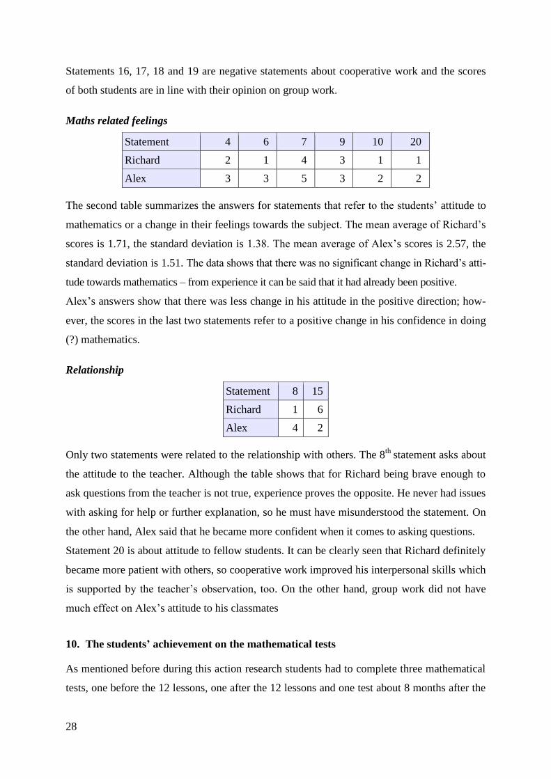
Figure 2 clearly shows that Alex’s achievement was not steady. In the pre-test he managed to
solve three tasks fully and this number decreased to two in the post-test and increased back to
three in the delayed test. On the pre-test he had difficulties with solving the following
problems: 3. thinking backwards; 4. and 5. permutations – systematic thinking; 6. word
30
problem that can be solved with simple equation; 7. calculating area; 9. pattern recognition.
On the post-test the following types were problematic for Alex: 2. the justification of a
divisibility problem; 4. and 5. permutations; 6. justification of a problem including number
theory; 7. calculating area; 8. geometric calculation; 9. pattern recognition. Finally, on the
delayed test the solution of the following problems was either missing or incomplete:
1. greatest common divisor (gcd) – systematic thinking; 2. justifying a divisibility problem;
4. permutations; 6. justification of a problem including number theory; 7. area calculation;
8. geometry.
Figure 2
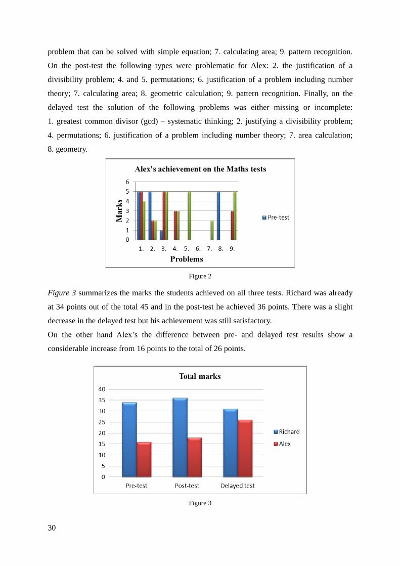
Figure 3 summarizes the marks the students achieved on all three tests. Richard was already
at 34 points out of the total 45 and in the post-test he achieved 36 points. There was a slight
decrease in the delayed test but his achievement was still satisfactory.
On the other hand Alex’s the difference between pre- and delayed test results show a
considerable increase from 16 points to the total of 26 points.
Figure 3

31
11. Discussion
Taking both the particular lessons and the whole school year into consideration the following
observations and thoughts can be phrased.
For Richard, the talented student there was no significant difference between his results in the
pre-, post- or delayed Mathematics test. Of course, since his achievement was quite good on
the first test already there was not too much area for improvement. However, there were tasks
where he showed some improvement, for example in problems that involved permutations his
marks were higher in the post- and delayed - tests.
On the other hand there was definitely a positive change in his attitude towards the others. He
became more patient with the other students when he had to explain something or when he
presented his ideas. From the teacher’s observations it is clear that Richard was more and
more willing to be a “team player”. Moreover, there was a positive change in terms of his
classroom activity, too.
Alex’s mathematical achievement had never been steady which can be clearly seen from his
test result throughout the three years when we worked together. During this experiment he
achieved better result in some post-test tasks and his delayed test marks were much better.
Comparing the post- and the delayed tests Alex definitely showed an improvement in prob-
lems that required pattern recognition (9.), moreover he received more marks for problems
where permutations had to be applied (4. and 5.). Besides these tests there was an improve-
ment in his school grades as well which might be a result of his personality becoming more
mature, too. His half year mark was 3, while by the end of the school year he managed to
achieve 5.
As for Alex’s attitude to cooperative work from his comments it is not obvious whether he
liked them or not as his opinion is rather inconsistent7. However, from the observations it is
clear that his self-confidence changed in the positive direction. He became a more confident
presenter and he needed less reassurance by the end of the school year.
Since using cooperative techniques definitely had a positive impact on both students, in my
future classes I will use this method to encourage the average ability students to share their
mathematical ideas and to help talented students to be more willing to share their knowledge
with their classmates.
7 See his comment

32
12. Future work
The broader action research resulted in a massive amount of data that needs to be organized
and analysed. The psychological questionnaires of the other participating students need to be
analysed and the results compared to that of the above discussed students. The comments and
solutions in the “reflection booklets” should be interpreted as well, and the video and voice
recordings contain valuable pieces of information, too. After analysing all the tests and
questionnaires a new experiment could be designed with another group of students from a
different age group with using different problems.
Acknowledgement
This research was supported by the European Union and the State of Hungary, co-financed
by the European Social Fund in the framework of TÁMOP 4.2.4. A/2-11-1-2012-0001
‘National Excellence Program’.
References
1. Ambrus, A. (2004). Bevezetés a matematika didaktikába. (Introduction to Mathematical
Didactics) Budapest: ELTE Eötvös kiadó.
2. Burns, M. (1990). Using Groups of Four. In N. Davidson (Ed.), Cooperative-learning in
Mathematics (pp. 21 - 46). Boston: Addison-Wesley Publishing Company.
3. Caine, R. N., Caine, G., McClintic, C. L., & Klimek, K. J. (2004). 12 Brain/Mind Learning
Principles in Action: Fieldbook for Making Connections, Teaching, and the Human Brain.
Corwin Press.
4. Crabill, C. D. (1990). Small-group Learning in the Secondary Mathematics Classroom. In
N. Davidson (Ed.), Cooperative-learning in Mathematics (pp. 201 - 227). Boston:
Addison-Wesley Publishing Company.
5. Dees, R. L. (1990) Cooperation in the Mathematics Classroom: A User’s Manual. In N.
Davidson (Ed.), Cooperative-learning in Mathematics (pp. 160 - 200). Boston: Addison-
Wesley Publishing Company.
6. Dobi, J. (2002). Megtanult és megértett matematikatudás (Learnt and understood
mathematical knowledge). In Csapó B. (Ed), Az iskolai tudás (Knowledge acquired in
school). (pp. 177 - 200). Budapest: Osiris Kiadó.
7. Gyarmathy, É. A. (2006). A tehetség (Talent). Budapest: ELTE Eötvös kiasó.
8. Johnson, R. T. and Johnson, D. W. (1994). An Overview of Cooperative Learning. In J.
Thousand., A. Villa and A. Nevin (Eds.), Creativity and Collaborative Learning.
Baltimore: Brookes Press.
9. Johnson, D. W and Johnson, R. T. (2009). An Educational Psychology Success Story:
Social Interdependence Theory and Cooperative Learning. Educational Research, Vol. 38,
No. 5, 365 – 379.

33
10. Józsa, K., Székely, Gy. (2004). Kísérlet a kooperatív tanulás alkalmazására a matematika
tanítása során. (Experiment for Using Cooperative Learning in Teaching Mathematics)
Magyar pedagógia, 104. (3), 339 - 362.
11. Kagan, S. (2003). A Brief History of Kagan Structures. Kagan Online Magazine. San
Clemente, CA: Kagan Publishing.
12. Kagan, S. (2004). Kooperatív tanulás. (Coopartive Learning) Budapest: Önkonet.
13. Koshy, V. (2005). Action Research for Improving Practice. London: Paul Chapman
Publishing.
14. Mécs, A. (2009). Miben segíti a kooperatív módszer a matematika tananyag megértését?
(How do cooperative teachniques help understand Mathematics?). (MSc dissertation).
ELTE, Budapest.
15. Miller, R. C. (1990). Discovering Mathematical Talent. Retrieved November, 02, 2013,
from (http://files.eric.ed.gov/fulltext/ED321487.pdf).
16. Pehkonen, E. (1999). Open-ended Problems: A Method for an Educational Change. In
International Symposium on Elementary Maths Teaching (SEMT 99). Prague: Charles
University
17. Pólya, Gy. (1973). How to Solve it. New Jersey: Princeton University Press.
18. Schoenfeld, A. H. (1992). Learning to Think Mathematically: Problem Solving,
Metacognition, and Sense-making in Mathematics. In D. Grouws (Ed.), Handbook for
Research on Mathematics Teaching and Learning (pp. 334-370). New York: MacMillan.
19. Skemp, R. R. (2005). A matematikatanulás pszichológiája. (The Psychology of Learning
Mathematics). Budapest: Edge 2000.
20. Slavin, R. E. (1995). Cooperative Learning. Allyn & Bacon.
21. Szendrei, J. (2005). Gondolod, hogy egyre megy? (Dialogues about teaching
Mathematics). Budapest: Typotex.
22. Zimmermann, B. (2009). “Open ended Problem Solving in Mathematics Instruction and
some Perspectives on Research Questions” revisited – New Bricks from the Wall?. In A.
Ambrus, & É. Vásárhelyi. Problem Solving in Mathematics Education, proceedings from
the 11th
ProMath conference, September 2009 (pp. 143-157). Budapest, ELTE.

34
Appendix
Questionnaire on cooperative learning (Mécs, 2009)
1 - not true for me 6 - totally true for me
Statements
1 2 3 4 5 6
1. The other students’ explanations helped.
2. I liked working together.
3. I enjoy lessons with group work more.
4. I understood maths better than in the previous year.
5. I liked talking to people to whom I have never spoken before.
6. I’m not afraid of maths.
7. I could explain the solutions to others.
8. I dare to ask questions from my teacher.
9. I paid more attention and solved more tasks in maths.
10. Doing homework is easier now.
11. I understand my classmates’ explanations better.
12. I prefer sharing my ideas in small groups.
13. I would like group work in Maths next year.
14. I am more active when working in groups.
15. I became more patient with others.
16. The noise was disruptive.
17. I would have been faster alone.
18. I prefer doing maths tasks alone.
19. I prefer my teacher’s explanations.
20. I don’t mind sharing my ideas with the whole class.

35
About problem sequences designed for heterogeneous classes in grade seven
Lars Burman
Abo Akademi University Vaasa, Finland
Abstract
In this article teaching of problem solving in grade seven is addressed. Based on a
proposal of teacher-guided practice with problem sequences by Burman and
Wallin (2014), the author deals with the challenge that problem solving in mathe-
matics should be designed for all pupils and not only for the talented. Problem se-
quences may be seen as a supplement to ordinary teaching in mathematics and the
article describes pilot-tests in a lower-secondary school in Finland. The tests are
situated in a Finnish reality but the design of the teaching process is based on ear-
lier research with a connection to ProMath-conferences and combined with Nor-
dic research. In a problem sequence the pupils work partly in groups and partly
individually, they discuss the results with the teacher, they receive new informa-
tion and guide-lines and then they proceed. The pilot-tests in a heterogeneous
class seem promising as two main bases to build a development on have been
found.
Key words: Grade seven, heterogeneous classes, problem sequences, problem solving,
teacher-guided practice.
ZDM classification: D50, D73
Introduction
In the Finnish Matriculation Examination there is an extremely long tradition to test the stu-
dents’ competencies in mathematics by giving them ten tasks to solve in six hours.1 Conse-
quently, there is a very strong focus on tasks which can be solved within half an hour whereas
tasks of other types, e.g. problems and modeling projects, are not given so much focus. Fur-
thermore, the Matriculation Examination has a great influence, not only on the instruction in
upper-secondary school, but also on instruction in grades seven to nine. Accordingly,
Pehkonen and Rossi (2007) conclude that the conventional teaching method is still the domi-
nant one although alternative teaching methods (including problem solving and project work,
the author’s remark) have been delivered to Finnish teachers since more than twenty years.
1 Nowadays the students have to choose their 10 tasks among 15 tasks.

36
In comparison to other Nordic countries, Denmark is well-known for the competence perspec-
tive on mathematics education, as presented in Danish research by Niss and Jensen (2002).
For instance, Blomhøj and Jensen (2007) define the concept competence as someone’s in-
sightful readiness to act in response to the challenge of a given situation. In their visual repre-
sentation of the eight competences in mathematics, four are particularly interesting. These
competencies are mathematical thinking competence, reasoning competence, problem tack-
ling competence and modeling competence.
The aim of the research and the aim of this article
The aim of the research behind this article is to design tasks larger than short problem-solving
tasks (and the tasks in the Finnish Matriculation Examination) but not as extended as projects.
The purpose of the tasks is to develop the instruction in grade seven (and furthermore, in
grades eight and nine) and more precisely to strengthen the pupils’ skills in mathematical
thinking and reasoning, problem solving and readiness to work with applications and model-
ing. It should be stressed that my purpose is to design some kind of supplement to the courses
in mathematics, a supplement that teachers would consider an opportunity and not an obstacle
to cover the normal content in the courses of the curriculum. The special focus of this article
is to address that fact that problem solving in mathematics should be designed for all pupils
and not only for the talented.
Starting point and framework
Almost thirty years ago, Mason, Burton and Stacey (1985) argued that the rapid ques-
tion/answer format of many mathematics classrooms is the antithesis of the time and space
upon which developing mathematical thinking depends. Instead they stated that practice de-
mands ample time for tackling each question independently and the quality of the reflection
depends upon the time to review thoughtfully, to consider alternatives and to follow exten-
sions. Furthermore, they urged teachers to choose questions which can provoke thinking and
to recognize how essential confidence is and to create a supportive environment where some
success comes to each pupil. According to them, working in groups was helpful, choosing of
suitable questions was essential and mathematical thinking could be improved by practice
with reflection.
In the introduction to 14th
ICMI Study Volume, Niss, Blum and Galbraith (2007) outlined a
framework that is very useful when the aim is to develop tasks for problem solving. They de-

37
scribed the starting point as a space where problem solving meets application and modeling.
Accordingly, a problem is a task that cannot be solved using only previously known standard
methods. Moreover, a method may be standard for one individual at the same time that it is
not for another individual. The concept problem is used in a broad sense, including not only
practical problems, but also problems of a more intellectual nature that aims at describing, ex-
plaining, understanding or even designing parts of the world. Problems taken from the real
world have to do with nature, society or culture, including everyday life. In the term modeling
they included the entire process of structuring, generating real world facts and data, mathema-
tizing, working mathematically and interpreting and validating, perhaps several times round
(parts of) the loop. Then, an application (of mathematics) is a real world problem that has
been addressed by means of mathematics. A competency is the ability of an individual to per-
form certain appropriate actions in problem situations where these actions are required and
desirable. Consequently, we can speak about problem-solving competency as the ability to
find the solution to a task not corresponding to the previously known standard methods, and
(mathematical) modeling competency as the ability to identify relevant questions, variables,
relations or assumptions in a given real world situation, to translate these into mathematics
and to interpret and validate the solution of the resulting mathematical problem in relation to
the given situation. As the problem-solving competency and the modeling competency are not
sufficient to solve real-world tasks, we also need other competencies such as representing
mathematical objects involved in an appropriate way and arguing and justifying what is being
done when applying mathematical algorithms and procedures. As problem solving and model-
ing often are used as a group activity, social competency, more or less specific for mathemat-
ics, is needed for an effective cooperative teamwork and must not be forgotten. Finally, deal-
ing with applications and modeling in mathematics, there are a challenge, a dilemma or a
problem, and questions, which together form an issue.
I have found it appropriate to use a framework, very similar to that outlined by Niss, Blum
and Galbraith in my research and also to use it in order to reach the aim of this article. But in
addition to the definition of problem above, Pehkonen (1997) provides two definitions for my
work. He deals with methods for educational change and suggests the use of problem fields as
such a method. In this context, he defines a problem field as a set of connected problems and
the connected problems form a sequence of problems. He also notes that in a problem field,
the difficulty of the problems may range from very simple ones that can be solved by the
whole class, to more difficult problems which only the more advanced students might be able
to solve. I agree with Pehkonen and accept his definition of problem fields but prefer to use

38
the concept problem sequence from now on, when I focus on problems formed by the se-
quence of subproblems more than on problems as separate problems linked to each other or
problems as more or less separate extensions from a certain problem.
In an article in the proceedings of the 11th
ProMath conference 2009, in Budapest, Henze and
Fritzlar (2010) examine model-building processes by the example of Fermi questions and
show in a figure that there are several similarities between problem solving and modeling.
They also conclude that modeling processes can be understood as one specific type of prob-
lem solving. Furthermore, in his doctoral thesis, Ärlebäck (2009) also refers to Fermi prob-
lems, as he addresses the issue of how to introduce mathematical modeling to upper-
secondary students. He has found that groups of students engaged in solving realistic Fermi
problems display problem-solving behavior resembling sub-activities of the modelling pro-
cess. Consequently, I find that if there is a problem-solving behavior resembling sub-activities
of the modeling process, it might be possible to find certain problems or tasks which could be
used as good problem-solving tasks but also as an introduction to and exercise for future
mathematical modeling tasks. On the other hand, good exercise in problem solving may also
include elements resembling modelling processes.
Theoretical conclusions and the design product
Based on the theoretical background above, I conclude that there is a need to improve mathe-
matical thinking and the quality of reflection and thought. This can be done by offering the
pupils good questions and challenges, as well as possibilities to work with a somewhat more
extended problem. I find an advantage in dividing the work with problems into steps and giv-
ing the pupils possibilities to discuss within the whole class and with the teacher between the-
se steps. Apparently, in this case the pupils receive exercise in handling with different kinds
of problems and they are not only tested if they are able to solve a certain problem by them-
selves. If possible, it is preferable that the problems should have a real world connection, but
equally important is the need to create a supportive environment, where working in groups
and good teamwork are successful.
Consequently, the way of working in a math class should combine the pupils’ own problem
solving in groups with discussions about the results so far and new information and new di-
rections for the on-going work given by the teacher. I prefer to divide the process in steps, as
the teacher then can give new information between the steps and sometimes give the work a
more or less new orientation. Depending on the time available, the teacher could also give the

39
pupils one of the steps as an individual homework. As a whole, the way of working, including
the kind of problems used, can be described as using
teacher-guided problem sequences.
In this article I have a special focus on obstacles occurring as the instruction is designed to in-
clude all pupils and not only talented pupils. When considering this focus, two aspects seem
to be very important:
* Doing some of the steps in groups may inspire all pupils to do their very best in order to
give their contribution to the group. Furthermore, the positive feeling of having been part of a
successful problem solving is more likely to emerge after working in a group than after an in-
dividual work.
* The problem sequences or at least some steps in a sequence can be constructed to include
problems at different levels of demands. In addition, connected problems may have an in-
creased level of difficulty from (very) easy to (much) more demanding.
Two examples of problem sequences
In the following, I present two examples of problem sequences in order to highlight some of
the benefits of the method used.
Example 1 Find the prime factors of the numbers 1 - 50.
Step 1 The teacher gives an introduction to the problem and demonstrates the solution for
the numbers 1 - 16. The teacher shows for instance 11 = 11, 12 = 3 ∙ 2 ∙ 2, 13 = 13 and
14 = 7 ∙ 2 and the pupils make a list. The teacher has told them to reserve space for all the
whole numbers up to 50.
Step 2 Pupils are divided into groups and every group receives one paper where the task is
to find and write down the prime factors of the numbers 17 - 32. The pupils are also asked to
try to find and write down some smart ways of reasoning as they are solving the task.
After step 2 the groups hand in their papers. Then, the teacher notes the prime factors of the
numbers 17 - 32 to ensure that every pupil has got a correct list up to the number 32.
Step 3 Pupils are asked to follow the previous examples and the smart ideas from the dis-
cussion and are given the numbers 33 - 50 as homework. As a special challenge they receive
an optional task to answer the question how it is possible to decide that a number is a prime
number or more precisely to know when it is no longer necessary to check any more possibili-
ties to factorize the actual number.

40
Next lesson, there is a kind of follow-up where the main concern is threefold: to ensure that
everybody has got the right prime factors for the numbers up to 50, to repeat the “smart ideas”
and to give an answer to the special challenge.
Step 4 For this step, which is the last one in the sequence, there are two options, of which
also only one can be used. If there is time, at least for some pupils, it is possible to enlarge the
list of numbers with prime factors. Another possibility is to check the pupils’ ability to find
prime factors to some number both below and above 50 in some kind of summative assess-
ment.
The task is not new but I have chosen to implement it in steps as a teacher-guided problem
sequence. The task can be considered central and important as both the way of working with
it and the result of it are important in tasks to come in the future. In the pilot-test, step 1 was
done as a teacher-led information and demonstration, but of course, the pupils were constantly
asked to participate in the work. Step 2 was carried out as a group work. In the discussion in
the pilot group after step 2, most of the pupils found multiplication tables very useful. Some
other suggestions were also made, for instance the idea to use the prime factors of 15 when
the actual number was 30 and it was possible to write 30 = 15 ∙ 2. Step 3 was an individual
work, but any kind of help and co-work at home was not excluded in step 3. Finally, in step 4,
the abilities of the pupils were checked individually.
Concerning the focus on teaching in a heterogeneous group, the step 2 was a work made in
groups, and in all the steps 1 - 3, there were numbers which were easy to factorize. In some
cases there were also very similar factorizations to imitate. A special notation must be given
to the fact that after this problem sequence, all pupils have got a list of their own, where they
can find the prime factors of all the numbers from 1 to 50.
Example 2 Find the angle between minute and hour hands of the clock (at different times).
Step 1 The teacher gives an introduction to the problem sequence. After a short discussion
with questions and answers, the main information should be clear to everybody: at the same
time when the minute hand covers a full angle, 360°, the hour hand covers an angle of 30°.
Step 2 The pupils are divided into groups with approximately three pupils in each group.
They are asked to find the angle between minute and hour hands of the clock at the following
times: 13.00, 13.30, 13.15 and 13.45. Every group receives a paper on which the pupils are
supposed to draw figures and write down their answers.

41
The groups hand in their papers and the results are discussed with the teacher, who may give
explanations to some of the answers.
Step 3 The pupils are asked to solve similar problems individually. Every pupil receives a
paper and the given times are: 11.00 , 17.00 , 14.30 , 15.15 , 12.45 , 14.25 and 17.48.
When a certain time has passed (or when everybody is ready), the papers are handed in and
the results are discussed. If necessary, the teacher explains some of the results.
In the third step the pupils’ papers can be used for a summative assessment. It is also possible
to use four steps. In that case the third step may be done as a homework and the fourth step as
a summative assessment in class. If three steps are used, it may be possible to do the whole
sequence within a lesson. If four steps are used, including a homework-step, it means that the
sequence might require more time but there is also the advantage that the problems have been
present at three different occasions. As in the example 1, another possibility is to see what the
pupils can achieve in some kind of summative assessment later on.
The second problem is also a classic one, but implemented in steps as a teacher-guided prob-
lem sequence. The task can be used to train logical work with proportionalities. In this se-
quence there were steps of teacher-led information and demonstration, group work and indi-
vidual work. In a heterogeneous group it was important that the work in step 2 was made in
groups, and that there was a gradually increasing difficulty level in the steps 2 - 3. Of course,
the last time was supposed to be a challenge to most of the pupils in the seventh grade.
Concluding remarks
I have found the use of problem sequences in a heterogeneous class in the seventh grade very
useful. It is possible and also desirable to construct and use problem sequences which include
group work and problems with an increasing level of difficulty. Then, every pupil is invited to
contribute to the solution of the problems in the group and it is more likely that everybody
gets to experience the feeling of success in at least some sense. Group activities possess the
potential to provide everybody with the feeling of having solved the problems together. Last
but not least, with using the problem sequences it was possible to reach a development in the
direction towards higher-order thinking, when the pupils had no previously solved tasks to
imitate. The results strongly suggest research and development of teacher-guided problem se-
quences in a larger scale in Finland, as well as in other countries.

42
References
Blomhøj, M., & Jensen, T. H., (2007). What’s all the fuss about competencies? In Blum, W.,
Galbraith, P. L., Henn, H.-W., & Niss, M. (Eds.). Modelling and Applications in Math-
ematics Education (pp. 45-56). New York. Springer Science Business Media.
Burman, L., & Wallin, S., (2014). Teacher guided practice with problem sequences. In Pro-
ceedings of the 30th
symposium of the Finnish Mathematics and Science Education Re-
search Association in Vaasa, November 6-8, 2013. (in press)
Henze, J., & Fritzlar, T. (2010). Primary school children’s model building processes by the
example of Fermi questions. In A. Ambrus, & È. Vásárhelyi (Eds.). Problem Solving in
Mathematics Education (pp. 60-75). Budapest. Eötvös Loránd University.
Mason, J. with Burton, L., & Stacey, K. (1985). Thinking mathematically. Wokingham. Addi-
son-Wesley Publishing Company.
Niss, M., Blum, W., & Galbraith. P., (2007). Introduction. In Blum, W., Galbraith, P. L.,
Henn, H.-W., & Niss, M. (Eds.). Modelling and Applications in Mathematics Education
(pp. 3-32). New York. Springer Science Business Media.
Niss, M., Jensen, T. H., (2002). Kompetencer og matematiklæring . Utdannelsesstyrelsens
temahæfteserie nr 18. København. Undervisningsministeriet.
Pehkonen, E., (1997). Use of problem fields as a method for educational change. In
Pehkonen, E. (Ed.). Use of open-ended problems in mathematics classroom, (pp. 73-
84). Helsinki. University of Helsinki.
Pehkonen, E., & Rossi, M, (2007). Some alternative teaching methods in mathematics. In
Pehkonen, E., Ahtee, M., & Lavonen, J. (Eds.). How Finns Learn Mathematics and Sci-
ence, (pp. 143-154). Rotterdam. SensePublishers.
Ärlebäck, J. B., (2009). Mathematical modelling in upper secondary mathematics education
in Sweden. Linköping. Linköping University.

43
Kangaroo problems for student teachers in Sweden
Katalin Földesi
Mälardalen University, Eskilstuna-Västerås, Sweden
Abstract
One of the important goals of student teacher education is for the students to de-
velop their problem solving skills.This is the basis of the student learning basic
didactic skills within this area. We know from many years of teaching experience
that at our university, student teachers have a troubled relationship with mathe-
matics.Thus, we are looking for teaching material that does three things simulta-
neously: develops the students' problem solving abilities, helps the students im-
prove their knowledge of didactics within the field of problem solving by working
through problems with didactics specifically in mind, and helps the students
achieve a positive relationship with mathematics. Since the main goal of the inter-
national Kangaroo competition is the popularization of mathematics for students,
and it allows students of ages 6 to 19 to participate, we chose its problem collec-
tion to conduct our research with. The experiences of the last few years have
shown us that carefully selected competition problems, and their conscious appli-
cation helps the achievement of all three goals. Our experiences also show that the
problem solving skills of our university's student teachers are weaker than the
problem solving skills of the best of the students they, in turn, teach.
Key words: Mathematics education, Kangoroo competition, problemsolving, student teacher
education
ZDM Classification: D53, D59, D63, D69
Introduction
The importance of mathematical problem solving is evident from the fact that the concept ap-
pears predominantly in the Swedish math syllabus even prior to 2011. In 2011, however, a
new syllabus and a new system of evaluation came into effect across the entire Swedish gen-
eral education, and at the same time, the renewal of Swedish student teaching was kicked off
as well.
The prominence of problem solving in the 2011 Swedish math syllabus is emphasized by it
being an element of content, an element on the list of skills that needs to be developed, and an
element of the evaluation process as well.

44
Between 2013 and 2016, all Swedish math teachers are required to take a compulsory course
called Matematiklyft. Part of this course deals with mathematical problem solving.
The Kangaroo competition (http://www.math-ksf.org) presents an opportunity to grapple with
mathematical problems for a wide range of students: from the first year of secondary school
all the way to fourth year of high school.
With regard to students teachers, two observations beckon to be made here: the problems re-
quire a way of mathematical reasoning that is very unusual for the students, and especially in
the beginning feel very difficult. Solving the problems is especially difficult for students who,
up to this point, had practiced math in a way that emphasized procedural calculations and the
solution of a narrow class of problems that can be easily expressed using algorithms, usually
presented by their teacher in the first few minutes of class, after which they practiced solving
similar problems using the same methodology.
First I will write about the situation with mathematical problem solving in Sweden, and then
about a few of the general and Sweden-specific characteristics of the Kangaroo competition.
The situation of problem solving in Sweden
György Pólya's book "How to solve it?", first published in 1943, is of particular significance
when it comes to the didactics of mathematical problem solving. A few years ago it was still
mentioned in a couple of high school course books, along with the photo and brief biography
of Pólya, as well as five point problem solving method that he had developed - however, none
of it got used in Swedish math teaching.
For the last couple of years, the theoretical foundation of mathematical problem solving in
Sweden has been a single concept, and later, an American study handling the concept in a
special way. This concept is "rich mathematical problem". It appeared in mathematical di-
dactic literature a few years ago. Below is an example of such a problem, from a Swedish
mathematical didactics book:
“Linda bought books at the book store. She bought three books for a total of 450 SEK, Kier-
kegaard, Magorian and Ende. Kierkegaard cost 100 SEK more than Ende. Kierkegaard and
Ende together cost 190 SEK more than Magorian.
A) How much did each book cost?
B) Formulate a similar problem and solve it.” (Hagland-Taflin-Hedrén, 2005)
The problem contains the following mathematical concepts: natural numbers, sum, difference,
table, equation, matrix and logic. One of the purposes of question B) is to allow the teacher to

45
evaluate the extent to which the student understands the math behind the problem. This par-
ticular problem was aimed at secondary school students, years 7-9.
The rich mathematical problem's strong dependence on the math taught in the secondary
schools of a country is immediately obvious, since the same problem is used as a simple but
very important practice question in several other countries.
Today in Sweden an American study is used as a model for treating rich mathematical prob-
lems in the classroom. (Stein at al., 2008)
The study presents in detail a method for treating problem solving. It comes with the warmest
of recommendations for any student teacher. Reading the study, and then trying out the meth-
od is warmly recommended to all Swedish math teachers that enroll in the continuation
course.
The main points of the method are as follows:
• The teacher presents the problem and makes sure the students understand it linguistically
and mathematically
• Each student spends a few minutes trying to solve it individually or in pair
• The students continue to work on the problem in small groups, agree to a solution, the
teacher walks between the groups
• Some of the solutions are presented at the blackboard and are discussed by the group or
the entire class
According to the method it is extremely important that the teacher selects which solutions to
be presented in front of the class based on a mathematically and didactically well thought-
through structure and during the discussion labors on the deepening of the mathematical con-
tent of the solutions presented by the students.
About the Kangaroo Competition in Sweden
To start with, I would like to summarize some general characteristics of the competition then,
I will mention some things that are specific to Sweden.
The competition is individual. It is arranged to take place annually in March. Its goal is the
popularization of mathematics, which also means that it does not require extensive technical
preparation, making it readily available to a huge number of students. It consists of 12-24
problems, mostly multiple choice questions with five possible choices. Each question has only
one correct answer. The time allotted for the competition is 60 minutes. After the competition,
the teacher can quickly correct the answers using the provided solution key, and can then send

46
in the results. A few weeks after the competition, the problems, the correct answers including
brief solutions as well as materials that will help the mathematical and didactical write-up of
the solutions are presented on the competition web page.
The top results, along with the students' names and schools, are presented on the competition's
web page. However, only the top 15 placements are shown on these lists. Thus, students with
lower scores lose not only the little bit of publicity in connection with this, but also the oppor-
tunity to show development over the past year. Both of these can be incredibly important mo-
tivational factors. This way of presenting the top placements obviously reflects some aspects
of Swedish culture.
Since 2000, competition materials can be freely downloaded, copied and edited as well, which
for practicing student teachers provides an easy way to construct interesting series of prob-
lems.
For the practicing student teacher, enrolling in the competition, running the actual competi-
tion, marking the answers and sending in the results can be done with a minimum of extra
work.
I would like to mention a few characteristics of the problems. I feel that these characteristics
make them especially suitable for use in the training of teachers.
Many problems contain visual information, pictures, illustrations, geometrical figures, nota-
tions, graphs et cetera. Since most Swedish primary, secondary and high school math is about
practical usability and preparation for further studies, when it comes to the selection and dis-
cussion of the materials used, analytical students that are good at numbers have an immeasur-
able advantage, while students who think visually, and mainly think in pictures and have a
rich mathematical intuition are disadvantaged.
The problems contain modern mathematical subjects in much greater measure than the nor-
mally used course books: graphs, topology, combinatorics, number theory, logic, set theory
and so on. This is important, should either the teacher or the student decide to complement the
occurring mathematics from other sources.
The problem texts are short, barely a few lines, and are formulated simply, often containing
explanatory elements.
Routine problems do not occur at all, which can be somewhat refreshing for students weary of
them.
For several years now there have been signs that some students, who traditionally perform
poorly at school mathematics, achieve excellent results at the Kangaroo competition.

47
My own anecdote adding to this is that I have had a student who answered 23 out of 24 ques-
tions correctly during the competition, but a week later was able to provide complete, mathe-
matically correct solutions to just a third of the problems.
Currently there is research underway to explore the correlation between students who achieve
good results at the Kangaroo competition, and their performance at school mathematics.
Could it be that the Kangaroo competition can be used to discover students whose perfor-
mance is weak, but who have a talent for mathematics?
Now I would like to present the names of the levels of the competition, as well as the corre-
sponding school classes, and high school course names, in Sweden:
• Milou – primary school and secondary school years 1-2
• Ecolier – secondary school years 3-4
• Benjamin – secondary school years 5-7
• Cadet – secondary school years 8-9 as well as Math A (first math course) in high school
• Junior - Math B (second math course and so on) and C in high school
• Student- Math D and E in high school
It can be seen almost immediately that there are two disadvantageous categories for many of
the participants: Benjamin and Cadet, which both spam three years and that will not help their
mathematical development. Splitting those two categories into several would, from a mathe-
matical didactical point of view, be much more advantageous, even though it would no doubt
lead to a considerably increased work load.
Research questions
1. How can we use the Kangaroo competition and its problems in the education of math
student teachers?
2. What experience can we gain?
Methodology
I carried out four way of applying Kangaroo competition in the education of students.
Method 1: Student teacher participation in the Kangaroo competition
Most of our student teachers have no experience of mathematical competitions. This is one of
the reasons I began to encourage our students to participate in the Kangaroo Competition on
the same terms as the other (non-teacher) students. The competition committee found this idea

48
to be good and accepted it. For several of the student teachers, even just one such experience
was enough to make them organize competition participation in their own classes in turn.
Method 2: Competition participation, and analyzing the problems
Within my own mathematical and didactical courses, I tried a second method. First, the stu-
dents participated in the live competition. Immediately afterwards, the complete solution of
the competition problems was given to them as homework. Next time the class met, the stu-
dents worked in threes on the problems. The solution of each problem was then presented at
the blackboard by one or more students. Afterwards, both the problems and the solutions were
analyzed mathematically and didactically.
Method 3: Problem analysis without competition participation, with group discussion
This method was tried several times, too: the competition problems were given to the students
as homework, with a full week to complete it, without knowing the correct answers. After the
week had passed, one or more students presented the solutions in front of the class. Naturally,
the presented solutions were discussed and analyzed from both a mathematical and a didacti-
cal point of view.
Method 4: Competition problem analysis as homework, with complete, written solutions
required
I would like to present a fourth method as well, which I tried with several students who were
specializing in mathematics. In this case, the competition problems were given to the students
without the solutions. Complete, written solutions were requested.
Results and discussion
I had to work hard at convincing the students to participate in the competition. For many stu-
dents, the experience of the competition was just one more in a row of negative memories.
Due to organizational reasons, I did not always have an opportunity to discuss of the competi-
tion problems within a sufficiently short time frame after the competition. To me it is obvious
that continuous practice of mathematical problem solving using with help from the teacher
would be the optimal solution, but making this happen may not be possible in the current or-
ganizational frameworks, and the country's cultural traditions present an additional difficulty.
Although we regularly have about a hundred new students on our mathematics and mathemat-
ical didactics courses, each year only about 15 participate in the Kangaroo competition.
My experience with the third method has been the following: the students I tried this method
on were not specializing in math, were extremely unsure of math in general, and it was for

49
them an added difficulty to stand in front of the class and present their solution. Many of the
students heavily opposed this method, and I was not always good at handling the opposition
pedagogically. On the other hand, several students distinguished themselves by giving very
clear presentations, showing a high degree of mathematical clarity. While this ability should
be a very important characteristic of a teacher, it was only present in a small subset of the stu-
dents.
Students, solved Kangaroo problems by Method 4, ended up having a much more difficult
time, than the students using the 2nd method. Often they could not make use of help, or the
knowledge of math was lacking, or their knowledge of mathematical problem solving was
lacking. My conclusion regarding this method is that oral discussion is indispensable when it
comes to the development of the students. One reason for this may be the students' insuffi-
cient skill at communicating math in writing.
Next I have collected some important experiences.
• On the importance of knowledge of basic set theory and mathematical logic
I would like to mention some particular difficulties I ran into. Knowledge of the basic ele-
ments of mathematical logic and set theory are indispensable for our students. In accordance
with the previous (pre-2011) math syllabus, these became present only at the end of the stu-
dents' high school years, and even then only in the classes that studied most maths. Mathemat-
ical didactical research supports that these basic elements of mathematics must be present
during the whole stretch of secondary and high school studies. I would like to give an exam-
ple of such a problem.
“The two cats Bill and Bull sometimes run into the two dogs Karo and Lufs. Bill is afraid of
both dogs, but Bull is only afraid of Karo and is a good friend with Lufs. Which statement is
incorrect?
A: Each cat is afraid of some dog.
B: Some cat is friend with one dog.
C: There is a dog that scares both cats.
D: Each dog scares some cat.
E: There is a dog which is good friend with both cats.” (Problem 18, Ecolier level, 2005.)
The most difficult thing for the students was to understand that of the possible choices, each
choice is either true or false, with nothing in between. "All", "each" and "there exist" were all
constructs that had to be explained. Because of these mathematical difficulties, many students
did not notice the subtle humor of the problem, even though cats and dogs are both favorite

50
pets in Sweden, to such an exists that they are usually included in the answer to the question
"Who are in your family?".
• A piece of good advice: “Do just as the problem text says!”
Swedish math teaching is still all too focused on numbers, calculations and algorithms, with-
out much formal explanation of the algorithm itself. As a result, most problems that deviate
even just a little bit from the usual end up being incredibly difficult for the students.
Even just understanding the problem text often turned out to be very difficult for many stu-
dents. In these cases, the following simple instruction turned out to be of great help: “Do just
as the problem text says, follow it exactly!” The following problem was of this kind.
“There is room for four people around a square table, with one person on each side. For the
school prom, the students line up seven such tables next to each other, forming a single long
table. How many people is there room for around with long table?” (Problem 6, Ecolier level,
2006)
In this case, following the text of the problem on paper, e.g. using a simple drawing, may not
only give the student a key to the solution, but in the process of drawing also show how the
problem could be generalized.
• The mathematical and didactical analysis of the Kangaroo-problems
It was often very difficult to work through the problem mathematically: How did you solve
the problem? What mathematical tools did you use? When? How? Can you expand the prob-
lem? Can you rewrite it and make it easier or more difficult?
Then came the didactical analysis of the problem: What mathematical concepts are present in
the problem? In what class would you present this problem to your students? Why?
I would like to give an example of such a problem.
“Four house sparrows sit on a fence. They’re Leo, Olle, Moa and Ida. Leo is sitting between
Olle and Moa. The distance between Olle and Leo is the same as the distance between Moa
and Ida. Leo is sitting 4 meters from Ida. What is the distance between Ida and Olle?” (Prob-
lem 15, Ecolier level, 2006)
It required lots of assistance from the teacher to make the students realize that the four spar-
rows represent four points on a line segment. This may be a result of the minimal content of
Swedish geometry teaching.
• Fruitful visual problems
Some problems have almost no mathematical prerequisites, but the ability to be able to inter-
pret an image, a graph or other visual information and work with it. Here is an example:

51
“A toy store sells a construction set consisting of black and while blocks arranged in four lay-
ers. Each layer consists of blocks of the same color. The image on the right shows the set
from above. How many white blocks are there in the construction set? (Figure 1)
Figure 1
(Problem 4, Benjamin level, 2008)
• Problems with possible solutions at different levels
“A class of 28 children stands in line. Ali has twice as many children behind him as in front.
Where in the line is Ali?” (Problem 17, Ecolier level, 2002)
It is possible to solve this problem immediately using a drawing, but you can also arrive at an
answer by introducing an unknown and setting up a simple equation.
Finally, I would like to compare the different categories of students with regard to how they
handled the increasing difficulty levels of the Kangaroo Competition (Table 1).
competition
categories Student teachers
Primary school to secondary school,
Grade 5-6, no math
Secondary school, Grade 7-9 and high
school, math
Milou yes, but needs to think more than usual yes
Ecolier yes, but the difficulties begin here yes
Benjamin yes, but even more difficulties yes
Cadet no, definitely yes, but the difficulties begin
Junior no, some exceptions yes, but more difficulties
Student no, some exceptions yes, but even more difficulties
Table 1
The table clearly shows and reflects my several years of experiences, that in both categories,
the problem solving levels of future math teachers is below the problem solving levels of their
brightest students.

52
Summary
Experiences so far show that at our university, the Kangaroo competition and its problems
work very well at developing and deepening the problem solving skills of future mathematics
teachers. Additional efforts need to be made to increase the number of participations in the
competition.
References
Polya, G. (1957). How to solve it? – A new aspect of mathematical method. Princeton, NJ:
Princeton University Press.
Kangurun. http://ncm.gu.se/kangaru, (2014-02-26)
“Kangourou sans frontieres” Association. http://www.math-ksf.org, (2014-02-26)
Hagland, K. Taflin, E. Hedrén, R. (2005). Rika matematiska problem (Rich mathematical
problems), Liber.
Stein, M. K. Engle, R. A. Smith M. S. Hughes E. K. (2008). Orchestrating Productive Math-
ematical Discussions: Five Practices forHelping Teachers Move Beyond Show and Tell,
Mathematical Thinking and Learning, 10:4, 313-340.

53
Prospective Teachers’ Conceptions of problem oriented Mathematics
teaching – explored and challenged
Torsten Fritzlar
University of Halle-Wittenberg, Germany
Abstract
Supporting prospective teachers in developing appropriate conceptions of mathe-
matics, and of teaching and learning mathematics, is an important task of teacher
education. In this article, I report on a university seminar in which I tried to ex-
plore and challenge the conceptions of (the complexity of) problem solving
mathematics teaching of eight teacher students.
Key words: beliefs, problem oriented mathematics teaching, teacher education
ZDM Classification: B50, D50
Introduction
Beliefs, attitudes and conceptions of teachers are a scientific research field that has been fre-
quently addressed by scholars in school research, education sciences, and, in recent years,
also in didactics (Forgasz & Leder, 2008; Leder, Pehkonen, & Törner, 2002). However, there
is no general agreement on the definition of this research objects (e. g. Forgasz & Leder,
2008; Mason, 2004; Pajares, 1992); it depends largely on the respective specialist discipline
or on the research interest in question.
Pehkonen (1994) describes beliefs as relatively stable, experience-based, subjective and often
implicit knowledge of a certain object or concern, combined with an affective, meaning-
constitutive component. Furthermore, they are of course not free of norms and values
(Zimmermann, 1991). The cognitive components are often also referred to as conceptions
(Pehkonen & Törner, 1996).
It seems certain that teachers’ conceptions have a significant influence on the dynamics in
class, on the interaction and communication processes in class and, finally, also on what pu-
pils learn (Forgasz & Leder, 2008; Mayers, 1994; Staub & Stern, 2002; Thompson, 1992).
Yet, it cannot be assumed that there is a simple unidirectional or monocausal correlation be-
tween teachers’ conceptions and their actions (Clarke & Hollingsworth, 2002; Devlin, 2006).

54
An important task in both teacher education and advanced vocational training thus seems to
lie in supporting students and teachers in developing appropriate conceptions (e. g. Mayers,
1994; Rolka, Rösken, & Liljedahl, 2006; Tillema, 2000). If, for instance, one wants to achieve
a stronger problem orientation in mathematics classes – as called for by mathematics educa-
tionalists all over the world for very good reasons –, it does not suffice to develop a new cur-
riculum and provide teaching materials. Rather, one should (sustainably) influence and
change the (prospective) teachers’ conceptions of problem solving teaching. E. g., regarding
the failure of the problem-solving based reforms of the mathematics curriculum in the USA in
the late 1980s (Schoenfeld, 2007), Rösken, Pepin & Törner (2011, p. 451) summarize: “Nu-
merous studies have detected that the reasons for that ‘failure’ were to some extent the ‘inap-
propriate’ beliefs of teachers concerning mathematics in general, and the process of problem
solving and characteristics of doing mathematics in particular, in addition to strong teacher
convictions concerning students’ apparent lack of ability.”
However, changing conceptions is not a simple exercise because e. g. already first year stu-
dents, from their time at school, possess distinctive conceptions of teaching methods, of what
defines a good teacher and how they see themselves as teachers (e. g. Kagan, 1992). On the
other hand, conceptions that have once been acquired are considered to be stable and difficult
to change, also due to their self-stabilising effects that can be explained by both their filter ef-
fect (Ambrose, 2004; Pajares, 1992) and by cross-linkages and clustering (Pehkonen, 1994).
Nevertheless, a number of studies indicate that conceptions of (future) teachers can be
changed or at least challenged (Fennema et al., 1996; Mayers, 1994). First steps in this direc-
tion could be to problematise current conceptions and practices, and to sensitise for new pos-
sibilities in mathematics teaching (Kaasila, Hannula, Laine, & Pehkonen, 2006; Ponte &
Mercê, 2011; Thompson, 1991).
What could be beneficial conceptions of mathematics teaching?
But which conceptions should teachers actually have of mathematics as a school subject? In
search of possible answers, teachers’ conceptions of mathematics and mathematics teaching
are often divided into different groups (e. g. Thompson, 1992) which are not independent of
each other (Felbrich & Müller, 2007).
With regard to conceptions of mathematics, it is useful to understand mathematics as an open,
dynamically developing system, as a creative, generally insecure construct of research com-
munities that is culturally embedded and historically grown (cf. Ernest, 1991).

55
With regard to conceptions of teaching and learning mathematics, we can, in a first approxi-
mation, differentiate between a transmission paradigm which is oriented towards association-
istic theories, and a constructivist paradigm which emphasizes the independent learning ac-
tivities of pupils. In the Scholastik study, Staub and Stern (2002) were able to show that pri-
mary school teachers with a cognitive-constructivist view are far more likely to see greater
learning progress among their pupils, both with regard to demanding word problems and basic
numerical abilities.
Moreover, conceptions of mathematics classes seem particularly important to me. In this con-
text, Kießwetter (1994) has called attention to a fundamental consideration in mathematics
education. To him, teaching is “problem solving in complex constellations”. Classroom con-
stellations are highly complex – i. e they are characterised by a particularly high comprehen-
siveness, they are dynamic, somewhat non-transparent and full of insecurities (Fritzlar, 2004).
For these reasons, they are generally not designed to result in optimum outcomes, but in ac-
ceptable compromises. From my point of view, the complexity of problem oriented mathe-
matics classes even goes beyond this level. This is due to the mathematical comprehensive-
ness and to the manifold different, simultaneous and highly dynamic working processes of the
pupils which should be supervised and supported if necessary. However, these working proc-
esses are often surprising, hardly predictable and difficult to understand, also because they are
influenced by various classroom conditions and elements of lesson design (Fritzlar, 2004).
If a stronger problem orientation is to be achieved in mathematics classes, teacher students
and teachers should also be made aware of this complexity and the associated challenges and
limitations. This could be important to enable a reflexive mode of handling and reducing
complexities (Helsper, 2003), to initiate a less dogmatic and corrigible manner of dealing with
knowledge and apparent certainties, a thinking in possibilities and a curious eye for the uncer-
tain (cf. Blanck, 2007). The availability of routines that reduce complexity, which have
played a significant role in research on teachers’ expertise for many years (e. g. Bromme,
1992), is important due to the limited capacity of humans to process information. What mat-
ters, however, is that these routines and the resulting reduction of complexity can be ques-
tioned and given up, and that a willingness, an openness to actually do this is developed. An
according sensitization in this context can help to reduce the fear of uncertainties and make
unavoidable deficiencies of human action in highly complex situations more bearable
(Kießwetter, 1994).
In the following, concept and course of a practical seminar at university are reported, whereby
I pursued the aim to problematise students’ current conceptions on problem oriented mathe-

56
matics teaching and to make them aware of its complexity and its effects.
The seminar participants were asked, amongst other things, to collect and reflect on the results
of their work in a journal, and occasionally they were explicitly required to submit written
thoughts and evaluations relevant to the topic. At the end of the seminar, I conducted a con-
cluding discussion with each of the students, giving the chance to reflect once more on the
outcomes and processes of one’s work as well as possible learning experiences.
The written and oral comments were examined for expressions indicating conceptions on
problem oriented mathematics teaching, especially regarding its complexity, and expressions
which imply a questioning or changing of these conceptions. In the following sections of this
article, selected search results are presented waiving detailed qualitative and quantitative
analysis. First of all, they are gathered to demonstrate that it indeed seems possible to
question conceptions on problem oriented mathematics teaching at university within a short
period of time.
A practical seminar on the doily-problem
Students at the Martin-Luther-University in Halle-Wittenberg were given the opportunity to
exemplarily gather (partly first) experiences on problem oriented mathematics teaching in the
context of a practical seminar in 2010. Participants of the seminar were eight first- and second
year female teacher students for primary school (which were not selected by the author). Their
task was to each have one Year 4 class work on the following problem, which is mathemati-
cally rather comprehensive but at the same time approachable even by primary school pupils
in a number of different ways (cf. Fritzlar, 2004).
The doily-problem (formulation not for pupils)
A rectangular A4 sheet of paper is halved by folding it parallel to the shorter edge. The result-
ing double sheet can be halved again by folding parallel to the shorter edge and so on. After n
folding procedures the corners of the resulting stack of paper sheets are cut off. By un-folding
the paper, we will find that (for n > 1) a doily with holes has resulted.
Find and explain a connection between the number n of folding procedures and the number
A(n) of holes in the reopened paper.
The uncertainty and complexity of problem oriented mathematics classes were to be made
tangible and graspable in a number of different ways in the course of this seminar:
Students work on a mathematically comprehensive problem and are introduced to a
number of different approaches within the group.

57
In pairs, students plan a lesson on the doily-problem, exchanging ideas and view-
points, negotiating different options of designing the lesson, balancing the pros and
cons of decisions.
As a group, the eight students get to know four different lesson designs on the same
topic, possibly with very different conceptions, intentions and approaches.
Each tandem carries out a lesson plan in two fourth grade classes. They can observe
which respective steps of the plan are carried out by the teacher, how pupils react,
which questions, ideas, approaches they develop, how the teacher in turn reacts to
these etc. In the following video-supported reflection of the class run by students in
pairs, observations, intentions, considerations, questions, doubts… are addressed.
Finally, the tandems present, analyse and compare their experiences to and with the
rest of the group, especially with regard to similarities and differences in their
plans, implementations and results.
The following table gives a summarised overview of the seminar course plan and explicit as-
signments regarding reflections in the journal.
1st group meeting
Students are introduced to the doily-problem, they can work on it as long
as they wish, but are also allowed to “take it home”.
Work in pairs Further work on the doily-problem if necessary, while students may also
use and refer to a text on its mathematical background.
Reflection
assignment
Students are asked to think about the suitability of the doily-problem for
a problem oriented mathematics class, which arguments speak for or
against its use in a Year 4 class.
2nd
group meet-
ing
Students present their results and their approaches.
Work in pairs
Student tandems each attend lessons in two primary school classes with
which they can work on the doily-problem later on. Afterwards, the tan-
dem plans such a lesson.
3rd
group meeting Students present their thoughts regarding the appropriate design of a les-
son on the doily-problem to the group and discuss the options.1
Work in pairs Using the discussions during group meetings as a starting point, the
teams’ lesson designs are further elaborated and/or modified.
Reflection
assignment
The participants are asked to
assess once more the suitability of the doily-problem for a problem
oriented mathematics class in Year 4 and mention eventual changes in
this regard;
think about what is of particular importance to them for their lesson;
designate the specific challenges they may possibly see for themselves
with regard to the upcoming lesson they have planned.
Work in pairs The doily-problem is used in eight fourth grade classes, observed by the
respective tandem partner and video-recorded (by the lecturer).
1 The session is audio-recorded.

58
Shortly after both tandem partners have given their planned lesson (often
even on the same day), a meeting is held between the tandem and the
lecturer during which they watch the video recordings of the lessons.
The students are asked to talk about everything that is going through
their heads. Occasionally, the lecturer encourages them to reflect on
certain issues. In a final discussion, attention is directed at specific chal-
lenges during class, deviations from the original plan, particularly im-
portant decisions to be made by the teacher as well as observed similari-
ties and differences between the lessons taught by the tandem partners.1
Work in pairs
The tandem partners prepare a short presentation for the following
group meeting in which they summarise some important impressions and
experiences, sections of their lessons, pupils’ results etc.
4th
group meet-
ing.
In the final group meeting, the tandems first of all present their teaching
experiences, discuss similarities and differences as well as possible rea-
sons for them. Afterwards, the lecturer presents further variations of the
lesson design. The group discuss their eventual implications on the fur-
ther progress of the lesson and possible outcomes.1
Concluding
discussion
At the end of the course, the lecturer meets with every student individu-
ally for about 30 minutes to address and evaluate the newly gained ex-
periences.1
Some Impressions of the practical seminar
Due to the limited scope of this paper, I can only summarise some impressions that derive
from my observations and analyses of the classes taught by the participating students, their
plans and reflections as well as their journals and interviews. In order to illustrate my argu-
ment, I include selected quotations (partly tidied up for easier reading) of comments made by
the students in their journals or from the audio-recordings. Some of the students’ considera-
tions may be critically questioned; I would however like to refrain from commenting them in
detail or even assessing them at this point.
What needs to be said first of all is that all participants were highly motivated and committed
to the work at hand. For instance, they worked on the doily-problem for at least 60 minutes
during the first meeting, even though it was planned as an open-ended session. All tandems
made tables which often also showed the number of folding lines – differentiated by their ver-
tical/horizontal orientation – and the number of resulting sections in the sheet of paper. On
this basis, they tried to determine the according arithmetic patterns. That duplications and
powers of 2 played a role was frequently identified: three tandems looked for a multiplicative
pattern, the other team tried to formulate a general relationship between the number of sec-
tions – that had been identified as powers of 2 – and the respective number of holes in the
sheet of paper.

59
U2 made the following comment on the doily-problem in her journal: “After all this endless
calculating, I started to resign and asked myself: How are Year 4 kids supposed to find a so-
lution to such a complex problem if even I can’t do it? … But later on I realized that it isn’t
all that difficult to make a complicated mathematical problem suitable for children. You just
have to simplify the problem and the solution you expect from them accordingly.” The second
part of her statement already touches the question of whether the doily-problem is appropriate
for mathematics classes in grade 4. Other participants also commented on this issue:
R: “I think this problem is very suitable for use in classroom lessons, especially be-
cause it allows for many solutions on different levels and can be approached in a
very practical way. … However, I don’t believe that a 45-minute period is enough
to deal with the problem intensively – particularly considering that even we as stu-
dents already spent more than an hour on it.“ (Journal)
L: “When I thought about this question [of suitability], my first thought was that this is
too hard for primary school pupils because it was quite tricky even for us to solve,
and especially this whole thinking in formulae is only really something for kids that
are highly interested and mathematically gifted.“ (Journal)
S: “… but if, for instance, you provide certain solution approaches or a table or give
them a specific introduction into the process, almost every child can really – with
appropriate assistance – understand and partly even solve this problem. That’s why
I find it suitable, because it also demands quite a few own intellectual approaches.
As far as I can remember, we never did something like this when I was at primary
school.“ (Concluding discussion)
K: “From my own experience I can say that you tend to underestimate the children’s
capabilities far too often. You think that they are capable of much less than they ac-
tually are. But I think that this will teach us better.” (Journal)
In the second group meeting, the tandems presented their approaches to the problem and some
suggestions for solutions. The small size of the group contributed to an open and relaxed at-
mosphere in which also partial solutions and wrong ideas could be presented. As my students
found the doily-problem to be very demanding, I had decided to show some selected results
that had been developed by pupils in previous classroom experiments: The aim was to
demonstrate that the problem can, in fact, also be solved by fourth graders, and in many dif-
ferent ways.
On the basis of these experiences, each team prepared a draft for a teaching unit. The four
teaching plans displayed numerous similarities: The first introductory part consisted of a prac-
tical exercise in which both pupils and teachers – comparable to their own introduction to the
problem – went through several folding-and-cutting-procedures together. Every time before
each sheet of paper was unfolded, the pupils were asked to make assumptions on what could
2 The names of the participating students are abbreviated to their initials: tandem 1: L and R, tandem 2: K and U,
tandem 3: G and S, tandem 4: H and N.

60
have happened. For the subsequent main part of the lesson, pupils were asked to work on the
doily-problem in pairs or in teams, and the lesson was concluded by a presentation of the pu-
pils’ and partly also the students’ results. This points to one of many differences in the design
of the teaching plans, which, of course, existed alongside the similarities:
When formulating the goals and objectives of their lesson plan, for instance, the first tan-
dem also emphasized the geometrical aspects of the doily-problem: “All pupils realize
that new holes appear where two folding lines intersect, that the number of vertical fold-
ing lines multiplied by the number of horizontal folding lines equals to the number of
holes, that both horizontally and vertically there is always one folding line less than there
are sections. Furthermore, pupils can see that the number of sections doubles with each
new folding procedure and that this duplication alternates between the horizontal and
vertical orientations.” (L & R, Journal)
Also other details of the lesson plan placed special attention on geometrical elements, e.g.
in already discussing folding edges, corners and sections during the introductory part of
the lesson. Potential assistance for the group work phase was directed at determining the
number of folding lines, the location of (new) holes in the sheet of paper or the appear-
ance of the unfolded sheet.
For the first collective exercise of folding and cutting the sheet of paper, it was important
to K and U to not only ask their pupils about their assumptions regarding the number of
holes, but also for the reasons behind these assumptions. How important a „graspable“
result was to the second tandem can also be seen in their first draft for the lesson, in
which about one third of the time available was dedicated to the presentation of the re-
sults, including a comprehensive presentation of their own solution that they prepared.
The most important goal of the lesson for tandem partners H and N was for their pupils to
be able to calculate the number of holes by the end of the lesson. Already their introduc-
tion to the problem thus included giving their pupils a prepared table and filling out the
first few rows together. They also told the children about a character called Mathematicus
who already knows from the very beginning that if you fold the sheet of paper seven
times and cut the edges accordingly, a total number of 105 holes will appear. The chil-
dren’s task is to get on to his track (H & N, Journal).
G and S set great value upon motivating their pupils. For this reason, they want to work
with a stuffed toy called Billy the Beaver, who loves to do handicrafts but needs the chil-
dren’s help to solve the doily-problem. They can help him find out “whether or how the
number of foldings is related to the number of holes” (G & S, Journal).

61
Other students also found that designing a motivating introduction was an important challenge
in the preparation of their lesson, apart from time management and considerations regarding
the appropriate assistance of pupils they hardly knew. S’s concluding remarks on planning the
teaching unit are: “Well, because that was really complex somehow. You kept remembering
one or the other thing that you may have forgotten or that you could also… Then you thought,
now we’re done, but then we realized that we still needed some little cards, or hadn’t decided
on what kind of sheets of paper we wanted to use, and how we’d introduce the problem to the
kids …” (Concluding discussion)
Reflections of teacher students
All students perceived the lessons to be particularly demanding; it was, above all, not easy to
interpret the frequently different working processes of pupils, react quickly but appropriately
to all classroom situations and, in doing so, parting from one’s own plans.
R: “It is extremely difficult in the beginning, you still try really hard to follow it [your
teaching plan] exactly the way you wrote it down, … it’s my goal to put my plan
into action in the best possible way. But sometimes it’s actually much better to di-
vert from it and go down a different track, and realize that at this and this point it’s
necessary to divert from my plan and do something else. But in the beginning, I
think, that’s still really hard to do.“ (Concluding discussion)
U: “The lesson I was able to draw from this class overall was that I still have to learn
to concentrate on so many kids at the same time. For example, I let a couple of
really good ideas presented by the pupils slip through my fingers that I could and
should have encouraged and developed further.” (Journal)
“I think my greatest challenge was to react to situations that I didn’t anticipate, that
I didn’t prepare myself for, that I didn’t imagine possible beforehand.” (Concluding
discussion)
S: “I guess such a lesson is especially difficult because you have to understand what
these kids mean so quickly and if what they say is correct.” (Note by the author)
“And then to really respond to each of them… and then also to react so quickly…“
(Concluding discussion)
Reviewing the video-recordings of the lessons in tandems and presenting and discussing the
students’ experiences in the group (4th
group meeting) make it possible to compare their plans
and implementations as well as pupils’ work processes and results. Here, students address a
large part of the possible variations; mathematical and cognitive aspects, however, play a mi-
nor role.
N: “And that there are many different ways of making a topic appealing and interest-
ing in various manners, with different goals, different approaches.” (4th
group meet-
ing)

62
K: “I wouldn’t have thought that the differences are really that striking, that other
classes find out more, progress further… But maybe it also depends on the plans we
made and of course also on the classes themselves, they were totally different from
each other… That was really fascinating to see.” (Concluding discussion)
The concluding one-on-one conversations clearly showed that the participating students had
acquired new and (in my opinion) important experiences in problem oriented mathematics
teaching:
R: “What I learned for myself, what I still have to learn, is to hold myself back… You
really have to learn to hold your horses a little as well and let the kids go ahead with
their ideas.” (Concluding discussion)
“And this practical experience in particular, that it can actually really work in prac-
tice …“ (Concluding discussion)
G: “…that you can just do it, that you can trust the children to do it, that you can have
the confidence that they are capable of finding their own ways, that you shouldn’t
underestimate them.“ (Concluding discussion)
S: “First of all: you should have confidence in these kids… I have learned that this al-
so works, that you can also achieve it that way. Then, the complexity of such a les-
son, especially problem oriented, if you have to prepare it and… that sometimes
things don’t quite go according to plan or that you don’t always immediately have
an answer up your sleeve.” (Concluding discussion)
Finally, the students were asked to comment on the statement “Teaching is to act and decide
in complex and uncertain situations“:
R: “Well, this is something I really noticed about my lesson: It’s first of all really
complex, it’s really difficult to assess, especially because we didn’t know the class
beforehand. But I think that even if you do know the class it can be really tricky at
times to decide somehow what would be the right move at the right time. And also
the dynamics as well… And you constantly have to readjust to the changing situa-
tions. So our preparations, in the beginning, they really helped, but at the end of the
day, in the concrete situation, you actually do have to deviate from the original plan
sometimes and make other decisions.” (Concluding discussion)
K: “… you can make plans and prepare yourself, but at the same time you have to be
flexible as well. That is probably the most difficult competency to develop for a
teacher, that you’re ultimately flexible concerning your plan and that you bring the
plan in line with your pupils. I think this requires the most practice of all.” (Con-
cluding discussion)
U: “Classroom teaching is simply an interaction that you can never be 100 per cent
prepared for. You would have to prepare for every kind of possible situation,
which, of course, you can’t. There can always be things you aren’t prepared for.”
(Concluding discussion)
G: “… sometimes it really comes down to one decision that you make, and the ripple
effect from this decision affects the lesson in a way that you perhaps aren’t able to
predict beforehand.” (Concluding discussion)
S: “I think that’s one thing you also saw on the video, that when you’re teaching in
class it’s like you’re – not under pressure to act, but you have to react at once, …

63
you really have to do something immediately and decide on the spot. And that is
complex, of course, because there are so many different possibilities. And that’s
why, I think, it’s important that you don’t always stick to the same pattern and base
your decisions on that, but that you always have several alternatives up your sleeve.
It is hard, I believe, once you’ve developed a routine over the years to still think of
alternatives, what would have been another way of doing it and not always system-
atically follow your one fixed plan. And uncertainty is always part of the deal. It
also depends on the kids, on the class, on the problems, sometimes maybe even on
how you personally feel on the day – or … But I guess that’s part of being a teacher
… you always deal with situations that are uncertain and indeterminable.” (Con-
cluding discussion)
Discussion
The reported seminar seems to be an effective possibility for prompting teacher students to
challenge their conceptions on problem oriented mathematics teaching. Nevertheless, several
critical questions arise. One could ask, for instance, whether students with very little teaching
experience are actually a suitable target group. Teaching primary school children in class def-
initely placed the students in a special and also psychologically challenging situation. On the
other hand, it might just be particularly beneficial to deal with and question one’s previously
developed conceptions of (problem oriented) mathematics teaching at a very early stage of
university education.
Given the students’ limited previous experience, integrating a more theory-focused unit into
the seminar (on e.g. different movements in the didactics of mathematics) might seem appro-
priate before commencing work on classroom experiments and teaching plans. This would,
however, probably have obscured the students’ own conceptions of problem oriented mathe-
matics teaching. In this context, R remarked that “the lecturer’s decision to run the seminar
without an introduction to problem oriented mathematics teaching made it more demanding
for the students, but also opened up more opportunities to learn.” (Journal)
So what were the learning effects for the students – given that they received no theoretical in-
put and prepared only one single lesson? In my opinion, the students’ impressions and reflec-
tions that have been compiled in the previous section of this paper clearly illustrate, amongst
other things, that they have become aware of a number of different issues: They have been in-
troduced to a new, challenging mathematical problem and have seen that it is (nonetheless)
suitable for a regular primary school class, they have realized how many different possibilities
there are to design a lesson unit on the same topic without determining an ideal outcome, that
a similar approach in different classes can lead to very different results, that problem oriented
mathematics teaching requires good preparation but can take very unexpected and surprising

64
turns in class all the same, and that it places specific demands on the teacher. Conceptions on
problem oriented mathematics teaching were also challenged, in my opinion. G writes, for in-
stance: “This seminar has essentially contributed to the fact that I look at the issue of ‘prob-
lem oriented teaching’ with much less skepticism than before. Before, I always asked myself
whether you should allow pupils to work so independently, but the class I ran on my own, and
also the other teams’ classes, clearly proved that it works. Pupils are often underestimated in
their ability to work with difficult concepts, and this is why you often use a well-established
and well-known pattern that you want them to apply instead of letting them experience for
themselves and explore the problem on their own.“ (Journal)
The variety of different plans for the teaching unit, and the corresponding approaches taken
by the pupils to solve the problem, would probably have been larger if there had been no col-
lective introduction for the students into the doily-problem (i.e. group session of folding, cut-
ting, assuming, unfolding), or if possible variations of the lesson (e.g. regarding the formula-
tion of problem statements and work assignments) are brought up in group discussions early
on in the process. Yet, this would probably also have made it more difficult to comprehend
the problem and its stimulative nature would have been less apparent; on the whole, “access-
ing” the subject would have been much more tedious for the students. Giving them a ready-to-
use “toolkit” of various „modules“ they can use for planning their lesson would likely have
distracted them from their own ideas, their own conceptions and perhaps even taken too much
work out of their hands. Asked about this issue, K replied: “More input? I don’t really think
so. Essentially, it’s not only problem oriented for the kids but also for us, i.e. that we have to
figure it out. Actually, I believe that giving us less advice and clues made us think about it
more thoroughly. … This way, we had to think about it ourselves. I think that was actually
quite OK.“ (Concluding discussion)
K’s comment suggests a certain self-reference: the seminar on problem oriented mathematics
teaching was deliberately designed to be problem oriented for the teacher students. It was also
self-referential for the lecturer, though. The deliberations of this section show that already the
attempt of making (at least aspects of) the complex reality of problem oriented mathematics
teaching tangible to students, encouraging and animating them to reflect their experiences
and, in doing so, sensitizing them a little bit for this complexity, is complex in itself.
References

65
Ambrose, R. (2004). Initiating change in prospective elementary school teachers' orientations
to mathematics teaching by building on beliefs. Journal of Mathematics Teacher Edu-
cation, 7, 91–119.
Blanck, B. (2007). Unterrichtsqualität entwickeln durch professionellen Umgang mit Unge-
wissheiten beim Lernen und Lehren. In K. Möller et al. (Eds.), Qualität von Grund-
schulunterricht. Entwickeln, erfassen und bewerten (pp. 111–114). Wiesbaden: VS Ver-
lag für Sozialwissenschaften.
Bromme, R. (1992). Der Lehrer als Experte. Bern: Huber.
Clarke, D., & Hollingsworth, H. (2002). Elaborating a model of teacher professional growth.
Teaching and Teacher Education, 18, 947–967.
Devlin, M. (2006). Challenging accepted wisdom about the place of conceptions of teaching
in university teaching improvement. International Journal of Teaching and Learning in
Higher Education, 18(2), 112–119.
Ernest, P. (1991). The philosophy of mathematics. Basingstoke, UK: Falmer Press
Felbrich, A., & Müller, C. (2007). Erste Ergebnisse aus P-TEDS: Mathematische Weltbilder
und Vorstellungen zum Lehren und Lernen von Mathematik. In Beiträge zum Mathema-
tikunterricht 2007 (pp. 573–576). Hildesheim: Franzbecker.
Fennema, E., Carpenter, T. P., Franke, M. L., Levi, L., Jacobs, V. R., & Empson, S. B.
(1996). A longitudinal study of learning to use children's thinking in mathematics in-
struction. Journal for Research in Mathematics Education, 27(4), 403–434.
Forgasz, H. J., & Leder, G. C. (2008). Beliefs about mathematics and mathematics teaching.
In P. Sullivan & T. Wood (Eds.), The international handbook of mathematics teacher
education. Knowledge and beliefs in mathematics teaching and teaching development
(Vol. 1, pp. 173–192). Rotterdam: Sense Publishers.
Fritzlar, T. (2004). Zur Sensibilität von Studierenden für die Komplexität problemorientierten
Mathematikunterrichts. Hamburg: Kovač.
Helsper, W. (2003). Ungewissheit im Lehrerhandeln als Aufgabe der Lehrerbildung. In W.
Helsper, R. Hörster, & J. Kade (Eds.), Ungewissheit. Pädagogische Felder im Moderni-
sierungsprozess (pp. 142–161). Weilerswist: Velbrück Wissenschaft.
Kaasila, R., Hannula, M. S., Laine, A., & Pehkonen, E. (2006). Facilitators for change of ele-
mentary teacher student's view of mathematics. In J. Novotná, H. Moraová, M. Krátká,
& N. Stehliková (Eds.), Proceedings of the 30th Conference of the International Group
for the Psychology of Mathematics Education (Vol. 3, pp. 385–392). Prague: PME.
Kagan, D. M. (1992). Professional growth among preservice and beginning teachers. Review
of Educational Research, 62 (2), 129–169.
Kießwetter, K. (1994). Unterrichtsgestaltung als Problemlösen in komplexen Konstellationen.
In F. Padberg (Ed.), Beiträge zum Lernen und Lehren von Mathematik (pp. 106–116).
Seelze: Kallmeyer.
Leder, G. C., Pehkonen, E., & Törner, G. (Eds.) (2002). Beliefs: A hidden variable in mathe-
matics education? Dordrecht: Kluwer Academic Publishers.
Mason, J. (2004). Are beliefs believable? Mathematical Thinking and Learning, 6 (3), 343–
352.

66
Mayers, C. (1994). Mathematics and mathematics teaching: Changes in pre-service student-
teachers’ beliefs and attitudes. In G. Bell, B. Wright, N. Leeson, & J. Geeke (Eds.),
Proceedings of the Seventeenth Annual Conference of the Mathematics Education Re-
search Group of Australasia (MERGA-17) (pp. 419–428). Lismore.
Pajares, M. F. (1992). Teachers’ beliefs and educational research: Cleaning up a messy con-
struct. Review of Educational Research, 62 (3), 307–332.
Pehkonen, E. (1994). On teachers’ beliefs and changing mathematics teaching. Journal für
Mathematikdidaktik, 15 (3/4), 177–209.
Pehkonen, E., & Törner, G. (1996). Mathematical beliefs and different aspects of their mean-
ing. Zentralblatt für Didaktik der Mathematik, 28 (4), 101–108.
Ponte, J. P. da, & Mercê, C. (2011). A teacher education experiment to challenge conceptions
and practices. ZDM-The International Journal on Mathematics Education, 43 (6-7),
847–859.
Rolka, K., Rösken, B., & Liljedahl, P. (2006). Challenging the mathematical beliefs of
preservice elementary school teachers. In J. Novotná, H. Moraová, M. Krátká, & N.
Stehliková (Eds.), Proceedings of the 30th Conference of the International Group for
the Psychology of Mathematics Education (Vol. 4, pp. 441–448). Prague: PME.
Rösken, B., Pepin, B., & Törner, G. (2011). Beliefs and beyond: affect and the teaching and
learning of mathematics. ZDM-The International Journal on Mathematics Education,
43(4), 451–455.
Schoenfeld, A. H. (2007). Problem solving in the United States, 1970–2008: research and
theory, practice and politics. ZDM-The International Journal on Mathematics Educa-
tion, 39(5-6), 537–551.
Staub, F. C., & Stern, E. (2002). The nature of teachers’ pedagogical content beliefs matters
for students’ achievement gains: quasi-experimental evidence from elementary mathe-
matics. Journal of Educational Psychology, 94 (2), 344–355.
Tillema, H. H. (2000). Belief change towards self-directed learning in student teachers: im-
mersion in practice or reflection on action. Teaching and Teacher Education, 16, 575–
591.
Thompson, A. G. (1991). The development of teachers’ conceptions of mathematics teaching.
In R. G. Underhill (Ed.), Proceedings of the Thirteenth Annual Meeting. North Ameri-
can Chapter of the International Group for the Psychology of Mathematics Education
(pp. 2-8–2-14). Blacksburg (VA).
Thompson, A. G. (1992). Teachers’ beliefs and conceptions: A synthesis of the research. In
D. A. Grouws (Ed.), Handbook Of Research On Mathematics Teaching And Learning
(pp. 127–146). New York: MacMillan.
Zimmermann, B. (1991). Heuristik als ein Element mathematischer Denk- und Lernprozesse.
Habilitationsschrift, Hamburg.

67
Problems with the Imagination of Astronomical Measurements
Günter Graumann
University of Bielefeld, Germany
Abstract
During the whole time of school students are confronted with measurements like
monetary value, linear measure, measure of weight, measure of time etc. Usually
the size of these measurements are within normal ranges. But since grade five the
pupils also come up against with very small as well as very big sizes. One field of
huge measurements is that within astronomy. To get an outlook and imagination
of such measurements and for better memorization of facts one has to find rela-
tions between different sizes, correlations with other types of measurement and
special representations. In this presentation besides some facts we will look out
for getting relations and representations about linear measures in the near of the
earth, within our planetary system and within the whole universe.
Key words: problem field, astronomical measurements, representations of distances
ZDM classification: D53, D59, D83, M53, M59.
Introduction
Since first grade children of primary school are confronted with different measurements like
monetary value, linear measure, measure of weight, measure of time, etc. But the size of the
measurements range within body measures or measures of normal environment. For example
children learn to get an imagination of distances of “1 mm” (e.g. with the thickness of a 1 cent
coin as main representative), “1 cm” (thickness of a thumb), “1 dm” (spread of open hand), “1
m” (one big footstep), “1 km” (perhaps the walking distance from home to school) and may
be also of “10 km” (spread of a small town) and “100 km” (distance to the next big city).
Since grade five the pupils also come up against with smaller and bigger sizes like “1 m”
and “1000 km” or “10 000 km” and computing with translations of scales. But with bigger
distances e.g. we all have problems of imagination.
“Man is the measurement of all” Protagoras did say about 2500 years ago. This is true still to-
day for normal life. But we also today have to do with things outside of the all-day experienc-
es. States have to compute with huge amounts of money, rackets have huge velocities and we
hear of huge distances in the space.

68
To get an outlook and imagination of such measurements and for better memorization of facts
one has to find relations between different sizes, to detect correlations between different rang-
es and types of measurement and discover special representations of huge measurements.
How this can be done I will discuss on the field of huge measurements – especially linear
measures - within astronomy. This is a problem field with a lot of different aspects and in the
given frame I can only present some information on main points.
Pupils can find many possibilities for creative work and own decisions in this problem field
and can make investigations (within astronomy as well mathematics). They also in the begin-
ning have to structure the whole problem field. Most information the pupils as well as the
teachers can find in books and in the internet. But didactical literature in respect to this theme
except some special aspects for higher grades you can find hardly.
For this presentation I structured the problem field of linear measures within the astronomy in
three domains: The astronomical neighborhood of our earth (the atmosphere and the satellites
as well as the moon), our planetary system (sun and the planets from Mercury to Neptune as
well as the outer sphere of our sun system with comets etc.) and the whole universe (with
some stars nearer to the sun, our galaxy, other galaxies, clusters of galaxies and the end of the
visible universe).
The astronomical neighbourhood of our earth
We start with our earth and its satellites. I first present some facts pupils for example can find
in the internet or in special books:
- Radius of the earth is 6 370 km so that the mean diameter of the earth is 12 740 km
[polar-diameter 12756 km and equatorial diameter 12714 km]
- Height of atmosphere (from ocean level) is
for the troposphere 7 km to 17 km,
for the stratosphere until about 50 km and
for the mesosphere until about 85 km.
The thermosphere and exosphere (were nearly no air exists) is estimated until 10.000 km.
- Low Earth Orbit (LEO) satellites circle in a height (measured from ocean level) of 200
km to 1 500 km. They need 1.5 – 2 hour for one cycle. The ISS for example circles in
about 400 km height and needs 90 minutes for one cycle.

69
- Medium Earth Orbit (MEO) satellites circle in a height of 6 000 km – 36 000 km. GPS-
satellites or Navigation-satellites like Galileo circle in a height of about 20 000 km
respectively 32 000 km.
- Geostationary Orbit (GEO) satellites circle in a height of 35 790 km. Their cycle time is
exact 24 hours so that they have the same movement like the earth and keep staying above
a fixed point of the earth. The telecommunication satellites like Astra, Eutelsat, Immarsat
and the metrological satellite Meteosat stand in this height.
- The average radius of the orbit of the moon is 384 400 km (363 300 km – 405 500 km)
To get an imagination of these distances we look out for different scales to put the distances
on. The pupils first may try to let the earth look like a coin (e.g. a 1 Euro-coin with diameter
of 2.3 cm). This leads to a scale of about 1 : 554 000 000 or better rounded down 1 : 500
Mill. Then we have the
diameter of the earth about 2.55 cm
mean thickness of the troposphere about 0.0024 cm (≈ 1/40 mm)
thickness of the atmosphere up to the mesosphere a bit more than 0.017 cm (≈ 1/6
mm like the skin of an apple)
ISS (with orbit radius 400 km above earth’s surface) 0.08 cm (≈ 1 mm)
geostationary satellites (with 35 790 km above earth’s surface) 7.16 cm
moon orbit with range from 73 cm to 81 cm.
The pupils will find out that this scale is not a good one for the atmosphere and the LEO-
satellites but it shows already some relations between the radius of the earth, the thickness of
the atmosphere and the height of satellite orbits as well as the moon orbit.
A better scale might be then the earth big like a ball or a terrestrial globe so that we set 25 cm
12 500 km with the scale 1 : 50 Million. Then we have the
diameter of the earth 25,5 cm
thickness of troposphere and stratosphere 0.1 cm (1 mm)
height of the ISS is 0.8 cm (8 mm)
height of GPS-satellites is 40 cm
height of geostationary satellites is 71.6 cm
radius of the moon orbit between 727 cm and 811 cm (≈ 77 m).

70
With these representations we already can visualize the relations between the named linear
measures. To deepen this we can compute some quotients and e.g. get the following
representation:
mean thickness of the troposphere ∙ 4
> thickness of troposphere plus stratosphere ∙ 200
> distance from earth’s surface to end of the exosphere
mean thickness of the troposphere ∙ 1 000
> diameter of earth ∙ 30
> radius of moon orbit
∙ 30 000
height of ISS ∙ 50
> height of GPS-satellites ∙ 1.8
> height of geostationary satellites
∙ 90 If we want to put the earth until the geostationary satellites (with only half earth circle) on a
DIN A4 paper in oblong format then we can use a scale 1 : 150 Mill. whereat the radius of the
earth becomes about 4 cm, the thickness of the atmosphere until the stratosphere ⅓ mm and
the distance from the midpoint of the earth to a geostationary satellite 28.1 cm.
To get all above distances (devoid of the radius of the moon orbit) in an upright format we can
use the scale with 1 : 330 Mill. so that (as in the following figure) the
diameter of the earth is 3.86 cm
thickness of troposphere and stratosphere is 0.015 cm (≈ 1/7 mm)
height of the ISS is 0.121 cm (≈ 1/9 mm)
height of GPS-satellites is 6.1 cm
height of geostationary satellites is 10.85 cm.
On the sports field of the school we can represent this with a scale like 1 : 500 000, i.e.
the earth is represented as circle with diameter 2548 cm (25 m 48 cm)
The mean thickness of the troposphere is 2.4 cm
the thickness of troposphere plus stratosphere is 10 cm
the distance (from the earth ground level) to the ISS is 80 cm
the distance (from the earth ground level) to GPS-satellites is 4000 cm (40 m)

71
the distance (from the earth ground level) to geostationary sat. is 7158 cm (71.58 m)
The distance from midpoint of the earth to a geostationary sat. is 8432 cm (≈ 84.3 m)
Another way of getting an impression of these distances the pupils can find by driving with an
“imaginary” car with a constant speed of 100 km/h. This is a speed we know from driving on
a motor way. From earth ground we then would need
to the end of the troposphere not more than 10 minutes
to the end of the stratosphere 30 minutes
to the ISS 4 hours
to GPS-satellites 8 days and 8 hours
to a geostationary satellites 14 days and 22 hours
to the moon on a straight way about 160 days.
If you take a supersonic transport (like the Concorde) with 2000 km/h then the above times
have to be divided by twenty. For example to get to the stationary satellites you need already a
little bit less than a half day.
A rocket with constant speed of 20 000 km/h would need
to the end of the troposphere not more than 3 seconds
to the end of the stratosphere 9 seconds
to the ISS 1 minute and 12 seconds
to GPS-satellites 1 hour
to a geostationary satellites about 1¾ hours
to the moon on a straight way about 19 hours.
By finding out and putting down all these named representations and by building quotients
between the named distances the pupils will get a better imagination of these different dis-
tances.
Our planetary system
After the first experience with astronomical distances we turn towards our solar system with
its planets. This is a theme that appears very often in school, for instance in grade five at ge-
ography. Then (but also at other times) it is good to pick up this theme in mathematics to
deepen the imagination of the distances in our planetary system.
Let us start again with data the pupils can find in books or in the internet:

72
Sun: Radius 696 000 km, weight about 2∙1030
kg, density 1.41 g/cm³
Earth: Radius 6370 km, weight about 6∙1024
kg, density 5.51 g/cm³
Moon: Radius 1738 km, weight about 7⅓∙1022
kg, density 3,34 g/cm³
For the planets we e.g. can find the following information:
Planet Radius distance to the sun time of circulation
Mercury 2 439 km 58 Mill. km 87.9 days
Venus 6 052 km 108 Mill. km 224.5 days
Earth 6 370 km 149.6 Mill. km about 365¼ days
Mars 3 397 km 228 Mill. km 1.88 years
Jupiter 71 398 km 778 Mill. km 11.84 years
Saturn 60 000 km 1 432 Mill. km 29.43 years
Uranus 25 400 km 2 884 Mill. km 84.18 years
Neptune 24 300 km 4 509 Mill. km 164.56 years
We now may start with looking out for scaling the named radii and start with such a scale that
the circle of the sun is going on a normal sheet of paper with width of 21 cm. If we take 1cm
for 100 000 km the diameter of the sun is 13,92 cm. Multiplying this with 1.5 we get 20.88
cm, i.e. nearly 21 cm. Thus we have the scale 1,5 cm 100 000 km = 10 000 000 000 cm,
i.e. 1 : 6 666 666 667 (= ⅔ ∙ 10 Bill.). With this we can get the circles of the sun and the plan-
ets on a DIN 4 paper (without correct distances) by following scaled diameters:
Sun Mercury Venus Earth
208.8 mm 0.7 mm 1.8 mm 1.9 mm
Mars Jupiter Saturn Uranus Neptune
1.0 mm 21.4 mm 18.0 mm 7.6 mm 7.3 mm
This shows that with this scale Mercury and Mars have a diameter of nearly 1 mm, Venus and
Earth of nearly 2 mm, Uranus and Neptune of nearly 7 mm and Jupiter and Saturn lay in the
near of 2 cm. All these measures we just can put on our paper.
If we use this scale for the distances to the sun then the planet farthest away from the sun, the
Neptune, will lay about 676 m away. This is not a good scale for sheets of paper and even not
on the school yard. The sports field of a school often has a length of about 100 m. To get the
distance of Neptune – Sun on it we should minimize the length of 676 m by 7. A better scale

73
we will get if we multiply the scale with 7.5 instead of 7. Thus in the next step we will use the
scale 1 : 50 Bill. [Remark: 1 Bill. = 1 000 000 000 and is called in some countries 1 Millard.]
Then we have:
diameter distance to the sun
Sun 27.8 mm -
Mercury 0.1 mm (very small point) 1.16 m
Venus 0.2 mm (small point) 2.16 m
Earth 0.3 mm (normal point) 2.99 m
Mars 0.1 mm (very small point) 4.56 m
Jupiter 2.9 mm (very thick point) 15.56 m
Saturn 2.4 mm (very thick point) 28.64 m
Uranus 1.0 mm (thick point) 57.77 m
Neptune 1.0 mm (thick point) 90.18 m
To get these distance on our paper we have to use the scale 1 : 25 Trill. ( = 25 ∙ 1012
).
Another possibility to get an impression of these distances is to look out for a planet path and
to walk on such path. In Bielefeld in 2003 for example students of a middle school planed
and built such a planet path starting at their school.

74
You can find several such planet paths in Germany and presumably also in other countries.
The scales are mostly 1 : 1 Bill. or 1 : 1.5 Bill. or 1 : 2 Bill. That one in Bielefeld has the
scale named in the middle.
For the scale 1 : 1.5 Bill. (1 : 1 500 000 000) we have:
diameter distance to the sun
Sun 92.67 cm -
Mercury 3.3 mm 38.7 m
Venus 8.1 mm 72.0 m
Earth 8.5 mm 99.8 m
Mars 4.5 mm 152.0 m
Jupiter 95.2 mm 518.7 m
Saturn 80.0 mm 954.7 m
Uranus 33.9 mm 1 922.7 m
Neptune 32.4 mm 3 006.0 m
In addition: Some larger distances of our solar system (“trans-neptune-objects”)
First in the so-called Kupier-Belt we find dwarf planets like Pluto (in elderly books it is
named a planet but since 2006 it is a dwarf planet which has characteristics of a planet as well
as a comet). Pluto’s distance to the sun is about 5 900 Mill. km (in our scale about 3 933 m).
In the next sphere of our solar system, the so-called Helio sphere - where the magnetic field of
the sun begins to interact with interstellar media - we can find comets like Hale-Bopp with a
distance of about 55.6 Bill. km (in our scale about 37 km) or the dwarf planet Sedna with a
distance of about 75 Bill. km (in our scale 50 km) to the sun.
Some people say that the solar system does end here. But latterly some scientist say that the
solar system ends much more farer with the so-called Oort cloud whose radius in respect to

75
the sun is about 15 Trill. km (in our scale 1 000 km).
The distances of Hale-Bopp and Sedna and all the more the distance to the end of the Oort
cloud can not be represented in a planet path. But by looking up these in the internet and
translating them to our scale we get an imagination about the range of our solar system and
the gravitation force of the sun.
Interesting in this connection might be also the time the Voyager 1 satellite (the today fur-
thest away satellite which just now is outgoing of the sun system) took to go into these dis-
tances:
- Start from Earth Sept. 1977
- Passage of Jupiter 1 ½ year later (March 1979)
- Passage of Saturn again about 3 years after start (Nov. 1980)
- Begin of interstellar mission about 13 year after start (1990)
- Going into Heliosphere 28 years after start (2005)
- Distance today (after 36 years) about 20 Bill. km.
The present speed of Voyager 1 is 61 380 km/h, so that its distance from sun increases about
540 Mill. km per year.
Up from the distances of the end of the solar system astronomers use another unit of length,
the so-called light year (lj). It is the length a light ray (or any electro-magnetic wave) goes in
a Julian year of 365.25 days. It is equal to 9 460 730 472 580 800 m ≈ 9.46 ∙ 1012
km = 9.46 ∙
1015
m ≈ 1016
m). This says that the light from the sun needs about 1 year to get to the end of
the solar system.
Sometimes one uses also the units of a light hour, a light minute or a light second at which
1 light hour ≈ 1012
m, 1 light minute ≈ 1.8∙1010
m and 1 light second ≈ 3∙108 m. A good
small problem field for the pupils in this connection is that of getting exact computations
about theses distances. But we also can compute with our given distances how long light or
radio signals do need for the considered distance.
This leads us to another way of comparing the distances within the solar system: We look out
for the time light or radio signals do need for several distances. So e.g.
the light from sun to earth needs 8⅓ minutes
the light from sun to Neptune needs a little bit more than 4 hours.
a laser beam from earth to the moon takes a little bit more than 1 second

76
the radio signal from the satellite on Mars to earth (with distance to the earth between 56
and 400 Mill. km – at present about 250 Mill. km) takes currently about 14 minutes.
And a radio signal from Voyager 1 to earth requires about 12 hours.
With all these given or computed data and descriptions one can get an imagination of the
distances within our solar system. Of course there are other possibilities to deepen this
(especially by looking out for other scales) or to fill up with new details (for example about
asteroids and comets). For instance from the assumedly oldest big asteroid Fester which has a
500 km diameter we just got wonderful pictures from a satellite that circled this asteroid (see:
http://de.wikipedia.org/wiki/Dawn_%28Raumsonde%29). More information from many
asteroids and comets one can get from the internet.
The whole universe
But now we will leave our solar system and look out for stars and galaxies in the universe. A
good introduction to distances in the universe is looking at a movie called “Powers to ten”
made by Charles and Ray Eames in 1977 (see: www.youtube.com/watch?v=0fKBhvDjuy0 or
google “Powers of ten”). It gives an imaginary journey from the earth to the furthest away
quasars with a logarithmic scale using the powers of ten from 1 m to 1026
m (≈ 10 Bill. light
years).
One has to watch this film several times to get out most of the information and fix them on a
paper. Also it is good to complete this information with others in the internet (e.g.
http://www. powersof10.com/ or https://en.wikipedia.org/ wiki/Quasar) and in books (like
“Powers of Ten: A Book About the Relative Size of Things in the Universe and the Effect of
Adding another Zero” (1982,1994), by Philip and Phylis Morrison or “An Introduction to
Modern Astrophysics”, by Carroll and Ostlie, 2007).
But after sampling the information we should work with the information. And at first we can
rediscover our measures of our solar system whereat we have to transpose all measures in
powers of ten with m as base item, so that we get e.g.
Distance Earth – Moon 3.8 ∙ 108 m (± 6.6 %)
Distance Earth – Sun 1.5 ∙ 1011
m (± 1.6 %)
(The exact mean length of 149 597 870 700 m is called 1 au, i.e. 1 astronomic unit)
Distance Jupiter – Sun 7.8 ∙ 1011
m (≈ 5¼ au)

77
Distance Saturn – Sun 1.4 ∙ 1012
m (≈ 9⅓ au)
Distance Neptune – Sun 4.5 ∙ 1012
m (≈ 30 au)
Distance of Voyager 1 - Sun 1.9 ∙ 1013
m (≈ 125 au)
Distance End of solar system – Sun about 1.5 ∙ 1016
m (≈ 100 000 au)
A little bit outside of our solar system we find the nearest stars (seen in an approximate dis-
tance from the earth).
Proxima Centauri: 4 ∙ 1016
m (≈ 4.2 light years)
Alpha Centauri: 4 ∙ 1016
m (≈ 4.3 light years)
Sirius: 8 ∙ 1016
m (≈ 8.6 light years)
Ross 248: 9.8 ∙ 1016
m (≈ 10.3 light years)
(Ross 248 is a red dwarf star. Voyager 2 is going in its direction and might arrive there
in
40 000 years – see: http://www.marspages.eu/index.php?page=592)
Within the next three powers of ten there are several stars but mostly isolated and in the
named movie it was told that the picture always is the same: several sparkling point. The
amount of lucent point rises up in the next power of ten when we reach the disk of our galaxy.
One also can discuss how long a “prospective rocket” with speed similar to speed of light
would need to reach such stars. Some distances within our galaxy we will fix.
Pollux (in Gemini): 3 ∙ 1017
m (≈ 34 light years)
Schedir (in Cassiopeia): 2 ∙ 1018
m (≈ 230 light years)
Polar star: 4 ∙ 1018
m (≈ 430 light years)
Antares (in Skorpius): 5.7 ∙ 1018
m (≈ 600 light years)
Beteugeuze (in Orion): 6 ∙ 1018
m (≈ 680 light years)
Canis Majoris (very big): 4.6 ∙ 1019
m (≈ 4 900 light years)
Super novo from 1604: 1.9 ∙ 1020
m (≈ 20 000 light years)
Center of our galaxy: 2.5 ∙ 1020
m (≈ 26 000 light years)
And outside of our milky way galaxy we find other galaxies and clusters of galaxies as well
as super clusters of galaxies. Here are only a few examples with their distance to the earth:
Conis major (nearest galaxy): ≈ 4 ∙ 1020
m (≈ 42 000 light years)

78
Andomeda galaxy: ≈ 2.4 ∙ 1022
m (≈ 2.5 Mill. light years)
Centaurus A (nearest radio galaxy): ≈ 1 ∙ 1023
m (≈ 10 Mill. light years)
Virgo galaxy cluster (in the mean): ≈ 6.5 ∙ 1023
m (≈ 65 Mill. light years)
Quasar (quasi stellar object) Mark 509: ≈ 4.1 ∙ 1024
m (≈ 440 Mill. light years)
Quasar High Red Shift: ≈ 1.1 ∙ 1026
m (≈ 12 Bill. light years)
Furthest away galaxy (known today): ≈ 1.2 ∙ 1026
m (≈ 13 Bill. light years)
[see e.g. http://www.welt.de/wissenschaft/weltraum/article10428102/
Astronomen-erreichen-das-Ende-des-Universums.html ]
In addition to these data of astronomic distances metered from the earth or the sun we can
take data about diameters from several astronomic objects:
Diameter of the moon: ≈ 3.5 ∙ 106 m
Diameter of the earth: ≈ 1.3 ∙ 107 m
Diameter of Jupiter: ≈ 1.4 ∙ 108 m
Diameter of the sun: ≈ 1.4 ∙ 109 m
Diameter of Pollux: ≈ 1.3 ∙ 1010
m
Diameter of Antares: ≈ 2.5 ∙ 1011
m
Diameter of Beteigeuze: ≈ 1.4 ∙ 1012
m
Diameter of Canis Majoris: ≈ 2.0 ∙ 1012
m
Major Diameter of comet halley: ≈ 5.3 ∙ 1012
m
Diameter of the heliosphere: ≈ 2.3 ∙ 1013
m
Diameter of the whole solar system: ≈ 3.0 ∙ 1016
m (3.2 light years)
Diameter of our galaxy: ≈ 1 ∙ 1021
m (100 000 light years)
Diameter of a cluster of galaxies: ≈ 1 ∙ 1023
m (10 Mill. light years)
Diameter of a galaxy-supercluster: ≈ 2 ∙ 1024
m (200 Mill. light years)
Diameter of the whole universe: ≈ 1.3 ∙ 1026
m (14 Bill. light years).
(observable farthest object)
Besides looking at the powers of ten the pupils also should calculate quotients between some
distances so that they e.g. can find out that the distances to the nearest stars Proxima Centauri
and Alpha Centauri is about 100 000 times of the distance from Earth to the sun and that the
distance to the center of our galaxy is 10 000 times bigger than the distance to the Centauris
and so on.
So we can find e.g. (including also the named diameters):

79
Sun-Earth ∙ 100 000
> Sun-Centauri ∙ 10 000
> Sun-Milkyway center ∙ 1 Mill.
> end of the universe
Diameter of moon ∙ 3.6
> diameter of earth ∙ 11
> diameter of Jupiter ∙ 9.7
> diameter of sun ∙ 109
∙ 400
Diameter of sun ∙ 11
> diameter of Pollux ∙ 19
> diameter of Antares ∙ 8
> diameter of Canis
∙ 1500 [The star Canis Majoris with its big diameter in the position of our sun would reach beyond Saturn.]
Diameter of the heliosphere ∙ 43 Mill.
> diameter of our galaxy ∙ 70 000
> diameter of universe ∙ 3 Trillion
I think it is very difficult not only for pupils to get an imagination of all these distances. Also
a journey with a very fast rocket does it not make better because even with the fastest speed,
the speed of light, we have a range from one light year in our solar system to millions of light
years. There is no proportional scale we can put on these distances. We only can produce a
logarithmic scale in the style of the movie “Powers of Ten”.
In such a scale (as to be seen in the following – but better one uses a scale with a length of
about 55 cm) the pupils can put in all the data we got before. This might deepen the
recognition of the data.
Final comment
Above all named and possible investigations about astronomic distances one also can look out
for numbers of stars one can see in the night without clouds, the estimated number of stars or
galaxies in the universe, the amount of visible and dark material in the universe or the mass of
different astronomic objects. But here I will end with the given ideas about investigating
astronomic measures.

80
Historical aspects in teaching mathematics
Tünde Kántor
University of Debrecen, Hungary
Abstract
In our school practice it is very important to work out mathematical problem
fields for secondary school pupils. We have to arouse the pupils’ interest in the
classroom too. There is growing debate concerning the role of the history of
mathematics in mathematics education. Nowadays the new Hungarian mathemat-
ics curriculum (NAT) emphasizes the role of history, so we have chosen the topic
of the problem field from the history of mathematics, from the geometry of trian-
gles: Viviani’s theorem and its generalizations.
We wanted to acquaint our pupils with famous mathematicians (V. Viviani, L. J.
Mordell, P. Erdős) and with their mathematical works and results.
On the one hand our main point was to enrich the teaching of mathematics with
historical aspects; on the other hand we focused our teaching on the pupils’ own
heuristic work. We formulated the posed problems as open problems. So pupils
can create their own mathematical ideas, similarly to the historical way. They did
their problem solving as a research work. We carried out our experiments using
the traditional way and by using modern techniques (GeoGebra).
We developed this teaching material for pupils of normal secondary schools (Part
I -II.), for students with high ability (Part III- VIII.) and for teachers as guideline.
We tested it in five secondary schools (normal and special courses). We applied it
on the teacher training track at the university on semester courses (Chapters of
Teaching Mathematics), and in-service training of mathematics teachers. Mathe-
matics teachers can benefit from it.
Key words: history of mathematics, teaching of mathematics, material for teaching, Viviani’s
theorem, problemfield
ZDM classification: A30, C30, G10
Aims by using historical aspects
Viviani’s theorem is suitable to illustrate the derivation of a problem field, to build new con-
cepts, to generalize theorems and to investigate the converse problem too. In our teaching
material there are easier questions for investigation in classroom not only for the talented pu-
pils, and there are also harder problems aimed at advanced pupils. I intended to improve prob-
lem solving and problem posing abilities that are essential for teaching mathematics. It is
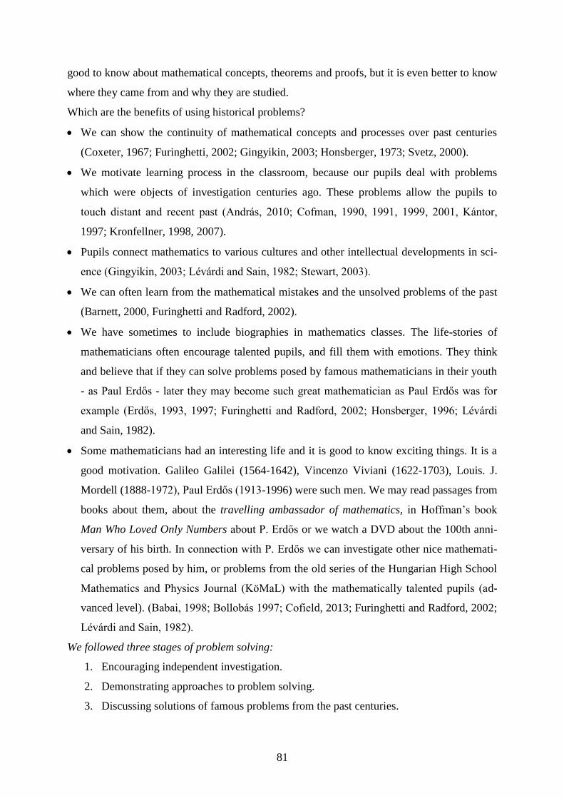
81
good to know about mathematical concepts, theorems and proofs, but it is even better to know
where they came from and why they are studied.
Which are the benefits of using historical problems?
We can show the continuity of mathematical concepts and processes over past centuries
(Coxeter, 1967; Furinghetti, 2002; Gingyikin, 2003; Honsberger, 1973; Svetz, 2000).
We motivate learning process in the classroom, because our pupils deal with problems
which were objects of investigation centuries ago. These problems allow the pupils to
touch distant and recent past (András, 2010; Cofman, 1990, 1991, 1999, 2001, Kántor,
1997; Kronfellner, 1998, 2007).
Pupils connect mathematics to various cultures and other intellectual developments in sci-
ence (Gingyikin, 2003; Lévárdi and Sain, 1982; Stewart, 2003).
We can often learn from the mathematical mistakes and the unsolved problems of the past
(Barnett, 2000, Furinghetti and Radford, 2002).
We have sometimes to include biographies in mathematics classes. The life-stories of
mathematicians often encourage talented pupils, and fill them with emotions. They think
and believe that if they can solve problems posed by famous mathematicians in their youth
- as Paul Erdős - later they may become such great mathematician as Paul Erdős was for
example (Erdős, 1993, 1997; Furinghetti and Radford, 2002; Honsberger, 1996; Lévárdi
and Sain, 1982).
Some mathematicians had an interesting life and it is good to know exciting things. It is a
good motivation. Galileo Galilei (1564-1642), Vincenzo Viviani (1622-1703), Louis. J.
Mordell (1888-1972), Paul Erdős (1913-1996) were such men. We may read passages from
books about them, about the travelling ambassador of mathematics, in Hoffman’s book
Man Who Loved Only Numbers about P. Erdős or we watch a DVD about the 100th anni-
versary of his birth. In connection with P. Erdős we can investigate other nice mathemati-
cal problems posed by him, or problems from the old series of the Hungarian High School
Mathematics and Physics Journal (KöMaL) with the mathematically talented pupils (ad-
vanced level). (Babai, 1998; Bollobás 1997; Cofield, 2013; Furinghetti and Radford, 2002;
Lévárdi and Sain, 1982).
We followed three stages of problem solving:
1. Encouraging independent investigation.
2. Demonstrating approaches to problem solving.
3. Discussing solutions of famous problems from the past centuries.

82
We formulated the posed problems as follows: “What happens if…?” “What is your conjec-
ture?” “How can you change the conditions or the way of the proof?” So pupils can create
their own mathematical ideas.
The problem field of Viviani’s theorem
Part I. We have chosen the topic of the problem field from the history of mathematics, from
the geometry of triangles: Viviani’s theorem and its generalizations.
Viviani’s theorem
For any point P inside an equilateral triangle ABC the sum s of the length of the per-
pendiculars d1, d2, d3 from the point P to the sides is equal to the altitude h.
We started with this well known property of the equilateral triangle (Problem 1) and discussed
five ways for its proof.
Part II. We changed the position of the point P, and we supposed that it lies on a vertex or on
a side of the equilateral triangle ABC, or outside the triangle, or on the extension of a
side. (Problem 2, Problem 3, Problem 4).
Part III. We changed the perpendiculars to other segments (Problem 5, Problem 6 as a com-
plementary problem).
Part IV. We changed the equilateral triangle to an isosceles triangle (Problem 7).
Part V. We generalized the regular triangle to regular n-gon (Problem 8, advanced level).
Part VI. We changed the dimension of the equilateral and scalene triangle. We left the plane
and went over to space: regular tetrahedron (Problem 9) and its converse theorem.
Part VII. Here we collected some theorems only for mathematically gifted students on high
level: Generalized inequality of Erdős-Mordell (Problem 10), Barrow’s theorem
(Problem 11), generalized Erdős-Mordell inequality for the tetrahedron (Problem 12)
and K. Kazarinoff’s inequalities (Problem 13).
Part VIII. Contest Problems or advanced level Problems (Contest Problems 1- 4). The
range of the problems is very wide, from simple exercises (aged 13-14) through con-
test problems (aged 14-18) to scientific theorems; such as theorem of Erdős-Mordell,
Barrow’s theorem, inequality of Kazaniroff (aged 16-19), or on university level
Viviani’s four window problem, trisection of an angle by using an equilateral hyper-
bola, Viviani’s curve, tangent to a cyclois (aged 18-20).

83
Part I.
Problem 1: Consider an equilateral triangle ABC and an arbitrary point P inside the triangle
ABC. Let PD, PE, PF, be the segments from P perpendicular to the sides BC, AC, AB, respec-
tively. Consider the sum s = PD + PE + PF. What is your conjecture?
Conjecture: The sum of PD + PE + PF is equal to the length of an altitude of the equilateral
triangle.
Discussion: First we allowed the pupils to draw, to measure, and to formulate their conjecture
and then to prove it theoretically.
We hoped that pupils would recognize that
1. The sum of PD + PE + PF = s is equal to the length of the altitude of the equilateral
triangle, i.e., s = h = 2
3a, where h denotes the length of the altitude of equilateral
triangle ABC and a is the length of its side.
2. The sum s is independent from the position of the interior point P.
Our pupils found several ways for proving of the conjecture.
Way 1
The idea of the proof was that we can write the area of
the equilateral triangle ABC as a sum of the areas of the
triangle ABP, triangle ACP and triangle BCP because
each of them has the same base length and the measure
of area is additive.
The proof shows that the sum s is independent of the
position of the interior point P.
Discussion: The pedagogical advantage of this method is the fact that the proof uses the con-
cept of area. We should use this proof if we want to enter into the topic of area or if we want
to recall or reintroduce the area of an equilateral triangle.

84
Way 2
We draw parallel lines to the sides AC, AB, CB through
the point P.
We get three parallelograms and three small triangles.
We can give the altitude of the triangle ABC with the help
of the altitudes of small triangles (PD + PF + PE = AS).
Discussion: Our second way uses two main concepts, similar triangles and their properties,
and the properties of parallelograms (LPK ∆ ≈ MNP ∆ ≈ PIJ ∆ ≈ ABC ∆). This might be a
nice way to review or to remind our pupils of the concepts that they have previously studied.
Way 3
Discussion: The third way utilizes rotation and translation. We rotate segments PF and PE
through 600 about point P and then we translate the latter vertically by the length of segment
PF. From this we obtained by aligning that PD + PF + PE = AS, which is equal to the length
of the altitude of the equilateral triangle ABC.
Way 4
We consider a shifted copy A’B’C’ of triangle
ABC, such that point P lies on B’A’. We
construct PT such that PT is parallel to C’B’. Let
Q be the foot of the perpendicular from A’ onto
PT, and L be the foot of the perpendicular from P
onto A’C’. Then AS = A’Q + PD = PL +PD =
FL+ PF + PD = PE + PF + PD.
(This can be done with GeoGebra too.)

85
Discussion: Way 3 and Way 4 use the concept of geometrical transformations. Pupils
manipulated with the perpendicular segments, tried forming a straight line, by placing one
next to, or on top of, each other, so that they can then be easily compared to the length of our
altitude. We think Way 4 would be the first on we would show a class when discussing the
problem, and then ask them to find other ways to prove the same thing. This proof belongs to
the category PWW (Proofs Without Words) (Nelsen, Roger B. 1994).
Way 5
Way 5 uses the method of coordinate-geometry and the distance formula to show that the sum
of the perpendiculars from P is equal to the length of altitude.
Discussion: Way 5 is interesting for lower classes if we use dynamic geometry (GeoGebra).
They got immediately the length of these line segments. For higher classes we use the method
of coordinate-geometry. In this case the proof requires the knowledge of the distance formula.
Part II.
It is very useful if the secondary school pupils can pose new problems, if they ask new ques-
tions after looking over the solved problem (Cofman, 2000; Schupp, 2002).
Viviani’s theorem can be generalized and modified in many directions. Our next questions for
the discussion were: What happens if in the equilateral triangle ABC the point P is not located
inside the triangle?
From the pupils we got different options for locating the point P and formulated new prob-
lems. The simplest problems were special extreme cases of Problem 1.
Point P coincides with one of the vertices of the triangle ABC.
Point P is placed on one of the sides of the triangle ABC.
We formulated then following questions as open problems:
Problem 2: What happens with the sum s of the distances if in the equilateral triangle ABC
the point P coincides with one of the vertices or it is on one of the sides of the triangle ABC?
Discussion: It is obvious that in the first case s = h, and in the second case s = d1 + d 2 = h.
Both the first and second ways (Way 1, Way 2) are suitable in this case.
The proofs are obvious from the figures (pupil’s work). (They used the notations x, y instead
of d1,,d2.)

86
C
Problem 3: What happens if in the equilateral triangle ABC point P lies on the extension of a
side of triangle ABC?
Pupil’s work: (They used the notations x, y instead of d1,,d2.)
Discussion: They found that s = d2 – d1 or s = d1 - d2. The result surprised them, because it
depended on the position of the point P.
We could unify the two values with the help of the absolute value s = h = |d1 – d2|.
We summarized by h = k1d1 + k2d2 where k1 = 1 and k2 = – 1 or k1 = – 1 and k2 = 1.
Problem 4: Consider an equilateral triangle ABC and a point P in the exterior of the triangle
ABC. How can we express the length of the altitude h with the help of the distances from
point P to the three side-lines?
Discussion: Solving Problem 4 seemed to be a bit complicated. The point P can be placed
outside of the triangle ABC. Pupils found different locations of the point P and got different
results for the linear combinations of the distances. In this case the altitude can be computed
by a combination of addition and subtraction of the three distances. Each line containing one
of the three sides of the triangle defines two half-planes of the whole plane. One of these half-
planes Π contains the interior of the given triangle, the other one does not. There must be the
sign plus before the front of the distance di if P belongs to Π, otherwise the sign must be mi-
nus. We presented the situations on the Figures. For each situation we can do the proof with
the help of Way 1 with computing the areas of the proper triangles.

87
The pupils recognized that coefficients k1, k2, k3 are equal to 1, depending on the location of
the point P, but at first they did not know which distances will be positive or negative. Their
conjecture was that the decisive factor is whether the foot of the perpendicular intersects a
side of the triangle or whether it intersects the extension of the side. But it was easy to show
that this conjecture was not true (if the foot points E and D are outside the side CB, and AB
respectively, and the foot point F is inside the side AC, then dPF + dPE + dPD = h.
By looking at the figures and rethinking the various cases they found that the sign of the dis-
tance in the linear combination depends on the relative position of the side to which its per-
pendicular is drawn and the vertex opposite that side (barycentre coordinates).
Part III.
If we follow the Way 2 in the proof of Viviani’s theorem we get other variations and new
theorems. First we formulated a new open problem.
Problem 5: Consider an equilateral triangle ABC and a point P inside of the triangle ABC.
We draw parallels through the point P to the sides. These parallels cut out three segments
from the triangle ABC. What can we say about the sum of these three segments?
Conjecture: The sum of the three segments is constant, d1 + d2 + d3 = 2a (a is the length of
the side of the equilateral triangle ABC.
Pupil’s solution: (They used the notations x, y, z instead of d1, d2, d3).
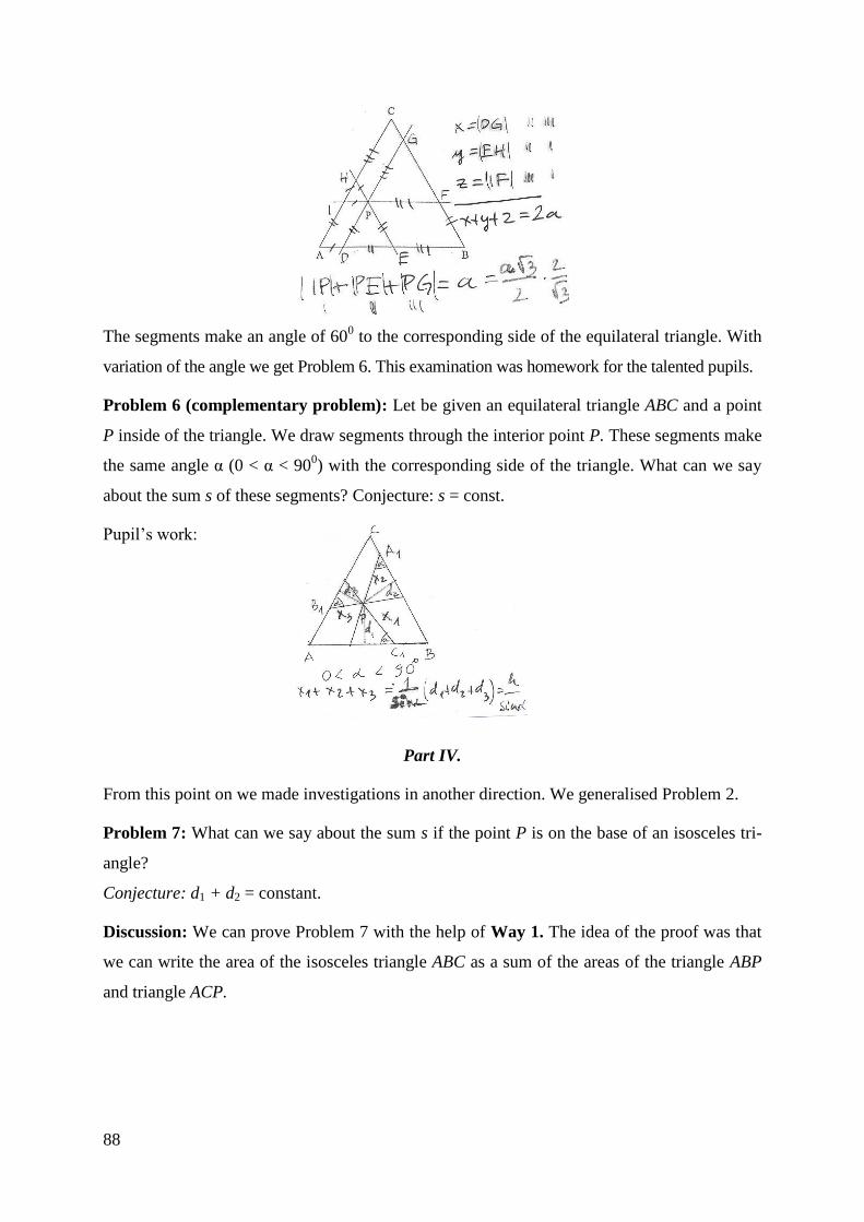
88
The segments make an angle of 600 to the corresponding side of the equilateral triangle. With
variation of the angle we get Problem 6. This examination was homework for the talented pupils.
Problem 6 (complementary problem): Let be given an equilateral triangle ABC and a point
P inside of the triangle. We draw segments through the interior point P. These segments make
the same angle α (0 < α < 900) with the corresponding side of the triangle. What can we say
about the sum s of these segments? Conjecture: s = const.
Pupil’s work:
Part IV.
From this point on we made investigations in another direction. We generalised Problem 2.
Problem 7: What can we say about the sum s if the point P is on the base of an isosceles tri-
angle?
Conjecture: d1 + d2 = constant.
Discussion: We can prove Problem 7 with the help of Way 1. The idea of the proof was that
we can write the area of the isosceles triangle ABC as a sum of the areas of the triangle ABP
and triangle ACP.

89
Pupil’s work:
Now the question of the converse theorems arises. Which of the discussed problems have a
true converse theorem? Can we invert Viviani’s theorem? We discussed these problems only
with talented pupils of advanced level.
Conjectures: Viviani’s theorem has a converse theorem and we can prove it in different ways.
Part V.
We continued our investigations in the direction of regular n-gons.
Problem 8: Consider a regular n-gon (n > 3) and a point P inside of it. What can we say
about the sum s of the distances from the point P to the sides of the regular n-gon?
Conjecture: s = d1 + d2 + … + dn = const.
Pupil’s work:
Discussion: The first step was to change the regular triangle to a square, to a regular 5-gon,
regular 6-gon (etc.) at finally to a regular n-gon. For solving these problems we need the re-
sults of Problems 1-4.
We asked the question of converse theorem, but it was easy to find a counter-example in the
case of convex n-gons a counter-example: if we take a rectangle ABCD (AB = BC), we can
immediately see that for an arbitrary interior point P of the rectangle ABCD the sum of the
distances from the point P to the sides of the rectangle is constant and it is equal to the sum of
the length of its two different sides.
At normal high school level we can extend Viviani’s theorem to space and we can formulate a
similar theorem for a regular tetrahedron.

90
Part VI.
Problem 9: Consider a regular tetrahedron ABCD and a point P inside it. Find the sum s of
the distances from the point P to the four faces. Is the sum s = d1 + d2 + d3 + d4 constant and
independent from the position of the interior point P?
Discussion: Proof of Problem 9 is similar to the first proof of Problem 1 in the plane. We use
the fact that the volume of the regular tetrahedron ABCD is equal to the sum of the volumes of
the tetrahedra PABC, PABD, PACD, PCDB and the value s is constant and equal to the length
of the tetrahedron’s altitude (s = h = 3
2a ).
We formulated the converse theorem too. The pupils were convinced that it will be true.
Their concept was false. The converse theorem of Problem 9 is not true.
From the sum d1 + d2 + d3 + d4 = h = 2A
V3 follows only equality of the areas of triangles
ABC, ABD, ACD and BCD, i.e. the tetrahedron ABCD is not necessarily regular, only its fac-
es have equal areas (equipages tetrahedron).
Part VII.
The other parts of the problemfield of Viviani’s theorem are difficult; they are only for talent-
ed pupils. It is only at the advanced secondary school level or at university in courses of ele-
mentary mathematics that we can deal with the theorem of Erdős-Mordell, Barrow’s theorem
for scalene triangle, with the generalization of Problem 9 to an outside point P, with the gen-
eralized inequality of Erdős-Mordell for a tetrahedron, Barrow’s theorem and Kazarinoff’s in-
equality for a tetrahedron.
Problem 10 (inequality of Erdős–Mordell) (for talented pupils): If P is arbitrary point inside
or on the boundary of a triangle ABC and if d1, d2, d3 are the distances from point P to the
sides of the triangle then dPA + dPB + dPC 2 (d1 + d2 + d3), with equality if and only if trian-
gle ABC is equilateral and the point P is its circumcenter.
Discussion: The first proof of Problem 10 was published in the Hungarian KöMal in1935 by
Professor Mordell. A trigonometric solution by Mordell and Barrow appeared in the Ameri-
can Monthly in 1937. An elementary proof was published in 1956. In 1957 Kazarinoff pub-
lished an even more elementary proof, based on a theorem of Pappus of Alexandria’s Mathe-
matical Collection. It based upon the idea of reflection. We can find Bankhoff’s elementary
proof in the American Monthly (1958, Vol. 65). Barrow proved a generalized form of the

91
Erdős-Mordell inequality, which follows from Barrow’s theorem as a special case. In 2007
Claudi Alsina and Roger B. Nelsen gave a visual proof of it. They presented a visual proof of
a lemma that reduced the proof to elementary algebra. In our mathematical camps the teachers
often discuss the inequality of Erdős-Mordell. (Kubatov, 2012).
Problem 11 (Barrow’s theorem) (for talented pupils): Let P be an arbitrary interior point of
the triangle ABC. Prove that dPA + dPB + dPC 2(dPA’ + dPB’ + dPC’), where A’, B’, C’ are the
intersection point of the bisectors of the angles BCP, CPA, ABC with the sides BC, CA, AB of
the triangle ABC.
Discussion: We find the proofs of these problems in several Hungarian mathematical books.
The proofs require only elementary knowledge, but the methods are different (principle of re-
flection, use of congruence transformations, computation of areas, trigonometrical relations).
The Erdős-Mordell inequality has a generalization for the tetrahedron.
Problem 12 (D. K. Kazarinoff's inequality for tetrahedra only for talented pupils): Let P be an
arbitrary interior point of the tetrahedron ABCD. Prove that
dPA + dPB + dPC + dPD ≥ 2 2 (dPA’ + dPB’ + dPC’ + dPD’),
where A’, B’, C’, D’ are the perpendicular projections of the point P to the planes BCD, CDA,
DAB, ABC.
Discussion: Problem 12 is a generalization of Problem 10. We found that the value of the co-
efficient in the plane was 2, so we expected that the value of the coefficient in the space will
be 3. But it is not true. D. K. Kazarinoff constructed an orthogonal tetrahedron with the coef-
ficient 2 2 .
Problem 13 (for talented pupils): The tetrahedron ABCD is equifaced and point P its interior
point. Prove that
dPA + dPB + dPC + dPD 3(d1 + d2 + d3 + d4)
where di (i = 1, 2, 3, 4) are distances of P to the faces of the tetrahedron. In the case of equali-
ty the tetrahedron ABCD is regular and the point P is the centre of its circumscribed sphere.
Part VIII. Contest Problems
For talented pupils of different age we can find a lot of contest problems. Viviani’s theorem
and its variants are popular at secondary school contests and in Geometrical Problem books. I
collected some of them (aged 13-18). If we prepare our pupils for the contests or for the final
examination on advanced level, we have to solve these problems with them.

92
Contest Problem 1 (aged 13) (Varga Tamás contest, 1994/95): The length of the sides of an
equilateral triangle is 5. Let us draw parallel through the interior point P to the sides. For
which point / points P will the sum of these parallel segments be maximal?
Contest Problem 2 (aged 14) (Varga Tamás contest, 1997/98): Consider an equilateral trian-
gle and a point P inside of the triangle ABC. We denote the feet of perpendiculars from the
point P to the sides AB, BC, CA by D, E, F. Prove that the value of the fraction
PD PE PF
BC AC AB
is independent of the position of the point P.
Contest Problem 3 (aged 14) (Hungarian Geometrical Problem Book): Consider an equilat-
eral triangle and a point P inside of the triangle. The feet of the perpendiculars to the sides di-
vide each side into two segments. Prove that the sum of the non-joint 3 segments is independ-
ent of the location of the point P.
Contest Problem 4 (aged 17-18) (final examination problem, 1993): The point P is an interi-
or point of a regular tetrahedron. From this point P we draw perpendiculars intersect the plane
of the face-sides at the points X, Y, Z. Prove that the sum dPX + dPY + dPZ is independent of the
location of the interior point.
Summary
We carried out experiments using history of mathematics in the classroom. We started with
the historical Problem of Viviani, we dealt with an important property of the regular triangle
and with variations of the conditions we solved a lot of problems, from the simple ones to the
serious scientific problems. So our pupils have been all over the stages of the history of math-
ematics, from the ancient time to our age.
We observed the same results which Furinghetti and Radford (2002), András (2010) and Law-
rence (2010) found. There is a parallel between history and pupils’ individual learning pro-
cess. The development of concepts and proofs followed the historical sequence. Their solu-
tions and mistakes were similar to the old ones.
For the average pupils we made mathematic classes more enjoyable by telling them the life-
stories of famous mathematicians (V. Viviani, P. Erdős, L. Mordell).
References
1. Alsina, C., Roger B. Nelsen.: A visual proof of the Erdős-Mordell inequality, Forum
Geometricum Vol.7 (2007) 99-102.

93
2. András, Sz.: Inquiry Based Teaching of Mathematics (Primas Project), (Hungarian),
Státus, Miercurea Ciuc 2010.
3. Babai L., Pomerance C., Vértesi P.: The Mathematics of Paul Erdős, Notices, MAS, Vol.
45, No 1 (1998) 19-31.
4. Barnett. J. H.: Anomalies and the Development of Mathematical Understanding, MAA
Notes 51, 2000, 77-88.
5. Bollobás B.: Paul Erdős –life and work in: The Mathematics of Paul Erdős, vol. 1(Eds.
R.L. Graham et al.) Algorithms and Combinatorics 13, Springer Verlag, Berlin-
Heidelberg-New York, 1997, 1- 41.
6. Bos, Henk J. M.: Lectures in the History of Mathematics, American Mathematical Socie-
ty, London Mathematical Society, 1993.
7. Boyer, B. C.: A History of Mathematics, Wiley, 1968.
8. Cantor, M.: Vorlesungen über Geschichte der Mathematik Vol. 3 (1894-1896).
9. Cofield C.: An Arbitrary Number of Years Since Mathematician Paul Erdős’s Birth, Sci-
entific American March, 26, 2013.
10. Cofman, J.: What to solve? Clarendon Press, Oxford University Press, 1990.
11. Cofman, J.: Numbers and shapes revisited. Clarendon Press, Oxford University Press,
1995.
12. Cofman, J.: How to motivate 10-18 years old pupils to work indepently on solving math-
ematical problems The Teaching of mathematics, Vol. III. 2, 2000, 83-94
13. Cofman, J.: Insight into the history of mathematics I-II. (German: Einblicke in die Ge-
schichte der Mathematik I-II.) Spektrum, Heidelberg, 1999, 2001.
14. Coxeter H.S.M., Greitzer, S.L.: Geometry Revisited Yale University, 1967 ( Hungarian)
15. Erdős P.: Some of my favourite problems (Hungarian) Polygon Vol. III. (1993) No 2. 65-
67.
16. Erdős P.: Some of my favourite problems and results, in: The Mathematics of Paul Erdős,
vol. 1(Eds. R.L. Graham et al.) Algorithms and Combinatorics 13, Springer Verlag, Ber-
lin-Heidelberg-New York, 1997, 47-67.
17. Eves, H.: An introduction to the History of Mathematics, Saunders College Publishing,
1983.
18. Furinghetti F., Radford L.: Historical Conceptual Developments and the Teaching of
Mathematics: from Phylogenesis and Onthogenesis, Theory to Classroom Practice, in:
Handbook of International Research in Mathematics Education (Ed.: Lyn D. English)
Lawrence Erlbaum Assosiates, Publishers, Mahwah, New Jersey, 2002, p. 631-654.
19. Gingyikin, S.G.: Stories about Physicians and Mathematicians (Hungarian), Typotex,
Budapest, 2003.
20. Grugnetti, L.: The History of Mathematics and its Influence on Pedagogical Problems,
MAA Notes 51, 2000, 29-35.
21. Horvay, K., Reiman I.: Geometrical Problem book I. (Hungarian) Budapest, 2004.
22. Honsberger, R.: Mathematical Gems, MAA, 1973, USA.
23. Honsberger, R.: From Erdős to Kiev, Problems of Olympiad Caliber, MAA 1996, USA.

94
24. Kántor T.: History of Mathematics in the Secondary School (Hungarian). Matematika
tanárképzés-matematika-tanártovábbképzés, Varga Tamás Napok előadásai, Calibra
Kiadó 1997, 51-68.
25. Katz, V. (ed.): Using History to Teach Mathematics: An International Perspective, MAA
Notes 51, 2000.
26. Kazarinoff, N.D.: Geometric inequalities, MAA 1961, USA.
27. Kronfellner, M.: Historische Aspekte im Mathematikunterricht, Eine didaktische Analyse
mit unterrichtspezifieschenh Beispielen. Verlag Hölder-Pichler-Tempsky, Wien, 1998.
28. Kronfellner, M.: Historical Aspects in Calculus Teaching. Matematika v škole dnes a
zajtra, Zborník 8. ročníka konferencie s medzinarodnou účast’ou (2007), Ped. Fakulta
Katolíckej University v Ružomberku Katedra Matematiky, p 39-48..
29. Kubatov A.: The Erdős-Mordell theorem (Hungarian) http:// matek.fazekas. hu / por-
tal/tanitasianyagok.
30. Lakatos, I.: Proofs and Refutations, Cambridge University Press, 1976 ( Hungarian trans-
lation, 1998, Typotex, Budapest)
31. Lawrence, S.: History of Mathematics in mathematics classroom. Practical mathematics
from long ago- original sources in mathematics classroom. Lecture on History of Mathe-
matics and Teaching of Mathematics Conference, Szeged, 2010.
32. Lévárdi, L., Sain, M.: Problems from History of Mathematics (Hungarian), Tankönyv-
kiadó, Budapest, 1982.
33. Nelsen, Roger B.: Proofs Without Words, MA, 1994.
34. O’ Connor J. J., Robertson E. F.: Louis Joel Mordell, http:// www-history.
mcs.st.andrews.ac.uk / Biographies/ Mordell.html
35. Schupp, H.: Thema mit Variationen, Verlag Franzbecker, Hildesheim, Berlin, 2002
36. Shklarsky, D.Q., Chentzow, N.N., Yaglom, I. M.: The USSR Olympiad Problem Book,
Freeman, San Francisco and London, 1962.
37. Stewart, J.: Preface in: Mankiewicz: History of Mathematics (Hungarian Translation,
HVG Publisher, Budapest, 2003)
38. Svetz, F.J: Problem Solving from the History of Mathematics, MAA Notes 51, 2000, 59-
65.
39. Temple G.: 100 Years of Mathematics, Duckworth, 1981.
40. Zimmermann, B.: Interim Report on a Project to identify and foster mathematically gifted
students. Problem solving- a World View, Proceeding of a Problem Solving Theme
Group, ICME 5, (Ed.: Burkhardt, H., Groves S., Schoenfeld A., Stacey K.) Adelaide,
1984.
41. Zimmermann, B.: History of mathematical thinking and problem solving: possible gain
for modern mathematics instruction, Problem Solving in Mathematics Education,
Proccedings of the 10th
ProMath Conference (Ed.: L. Burman). Publications from the
faculty of Education, Åbo University No27/2009, 37-49.

95
How can high school students solve problems based on the concept of area
measurement?
Eszter Herendiné-Kónya
University of Debrecen, Hungary
Abstract
Mathematical activity like problem solving involves work with concepts. Refer-
ring to the work of Usiskin, understanding of a concept in mathematics has differ-
ent aspects. These aspects are skill-algorithm understanding, property-proof un-
derstanding, use-application understanding, representation-metaphor under-
standing and history-cultural understanding.
The aim of this study is to investigate how these aspects appear in problems based
on the concept area measurement, and to look for the reasons of unsuccessful
problem solving connected to this topic. The research reports the typical solving
strategies and thinking mistakes concerning 5 tasks developed for high school
students of class 9.
Key words: area measurement, concept formation, dimensions of understanding, problem
solving strategy
ZDM classification: D53, D73, G33
Introduction
The term mathematical understanding includes understanding both of concepts and of prob-
lems.
Mathematics as an activity “consists of concepts and problems or questions: mathematicians
employ and invent concepts to answer questions and problems; mathematicians pose ques-
tions and problems to delineate concepts.” (Usiskin, 2012)
We investigate the interaction between concept-formation and problem-solving. Problem-
solving requires preliminary knowledge and understanding of concepts connected to the prob-
lem: „Do you understand all the words used in stating the problem?” (Polya, 1957) On the
other hand the level of understanding of a concept is recognizable through solving problems
connected to this concept. The analysis of the process of problem-solving contributes to the
exploration of the concept deficiencies.
The aim of this study is to answer the question how the different aspects of understanding the

96
same object namely the concept of area measurement appear in problems, and to look for the
reason of unsuccessful problem solving connected to this topic.
Theoretical background
Skemp (1976) distinguish two meanings of the world “understanding”. The relational under-
standing means knowing what to do and why, and the instrumental understanding means
knowing and using rules. Usiskin (2012) views this meanings as different aspects or dimen-
sion of understanding the same subject furthermore he speaks about more than two aspects.
The dimensions of understanding according to Usiskin:
1. Skill-algorithm dimension (instrumental or procedural understanding): Knowing how to
get an answer. Obtaining the correct answer in an efficient manner.
2. Property-proof dimension: Knowing why your way of obtaining the answer worked.
3. Use-application dimension (modeling): Knowing when to do something.
4. Representation-metaphor dimension: Knowing represent the concept in some way (with
concrete object, picture or metaphor)
5. History-culture dimension (genetic approach, ethno mathematics): Knowing the history of
the concept and its treatment in different cultures.
„The dimensions of understanding are relatively independent in the sense that they can be,
and are often, learned in isolation from each other, and no particular dimension need precede
any of the others … .Ordering ideas or concepts in terms of difficulty is only appropriate if
these items are in the same dimension.” (Usiskin, 2012)
In my paper I apply Usiskin’s multidimensional view of understanding, because it helps to
clarify the meaning of concepts and broadens options for developing these concepts.
After studying his examples for clarification the meaning of these dimensions, I delineate the
first four dimensions of understanding the concept of area measurement.
1. Skill-algorithm understanding is choosing an appropriate algorithm to calculate the area
depending on the plane figure and the given sizes.
2. Property-proof understanding includes derivations of the basic formulas for the areas of
triangles and other polygons, relations between area and perimeter of the same figure etc.
3. Use-application understanding includes area measurement in everyday life, applications in
complex problems etc.
4. Representation-metaphor understanding includes area measurement with congruent tiles,
cutting and rearranging polygons, area representation with an array of dots etc.

97
If we would like to know the level of learners understanding concerning to a concrete con-
cept, it is necessary to pose them problems connected to this concept. In many cases the sim-
ple routine tasks can’t highlight the gaps and misunderstandings well. So the process of prob-
lem solving serves for detection of typical mistakes of the concept-formation too.
In his famous work How to solve it? Polya write down the main four steps of problem solv-
ing: understanding the problem; devising a plan; carrying out the plan; looking back. If some-
body want to devise a plan, it is necessary – after understanding the problem – to activate his
or her preliminary knowledge. The main point of the plan is to find the connection between
the problem and the appropriate elements of the preliminary knowledge.
A well-stocked and well-organized store of knowledge is an important asset of the problem
solver … . In any subject matter there are some key-facts which should be stored somehow in
the forefront of your memory. When you are starting a problem, you should have some key
facts around you close at hand, just as an expert workman lays out his most frequently used
tools around him when he starts working.” (Polya, 1962)
Making and carrying out a good plan also means to find the connections between the un-
known and the givens. Polya use a graphical representation to demonstrate these connections,
where the unknown (what we are looking for); the data (what we have); the auxiliary un-
known (what we are looking for to solve an appropriate related problem) are symbolized as
points, and the relations connecting the objects are indicated by lines (Figure 1).
Figure 1
If we can’t make direct relation between the unknown and data (we can’t solve the proposed
problem), we introduce auxiliary unknowns and join these to the original one and so indicate
the relation between the quantities. The aim is to establish direct or indirect connection be-
Unknown
Auxilary
unknown
Data Data Data
Auxilary
unknown
Auxilary
unknown

98
tween the unknown and the data through some auxiliary unknowns. The graphical representa-
tion seems to be a suitable tool for investigating learners’ different solving strategies.
There are many studies on solving problems with focus on area measurement. The researchers
agree that measurement of area is more complex than measurement of length since length is
directly measured by ruler while area is indirectly measured through the lengths appearing in
the formula for calculating it (Zacharos 2006, Murphy 2009). According to Santi&Sbaragli
(2007) the early use of formulas has been criticized on the grounds that it generates miscon-
ceptions about area measurement and it could bring children to confuse area and perimeter.
Another possible cause of the conflict perimeter vs. area that the intuitive rule “more A, more
B” (Stavy&Tirosh 1996) means in case of geometrical shapes that as the perimeter increases
so the area increase. Kospentaris at al. (2011) investigates students’ strategies in area conser-
vation geometrical tasks and highlights the role of visual estimation.
Research questions
In this research I investigate the understanding of the concept of area measurement through
the solution of five associated problems.
1. Which dimensions of understanding the problems refer to? How perform students in class
9 regarding to these dimensions?
2. What kinds of methods use the students if they haven’t got the preliminary knowledge
necessary to solve the problem?
Methodology
The 27 students participating in this study are 9th
graders in a Hungarian high school, in the
same class. The class is a special „language-class”, they have mainly English lessons in the
whole school year and only two mathematics lessons per week. The goal of this year is to pre-
serve their previous mathematical knowledge. The students involved in this study had varied
backgrounds in mathematics. In the previous school year they learned in different upper second-
ary schools. Students don’t show up particular motivation, talent and interest in mathematics.
A 45-minute written test was designed in a way that the 5 tasks are built on each other, be-
cause we wanted to help students to find a right idea for the solution. For example Task 1 can
be understood as an auxiliary problem of Task 2. The solution of the Task 1 may become the
part of the solution of the Task 2 and it may suggest the direction in which students should
start working. It was considered to be also important to have a real-size picture to every task.

99
The test was written in March of 2013, earlier in the high school nothing has been taught from
the topic of area measurement.
Analysis of students answers
In connection with the first research question I present and identify the area-tasks with dimen-
sions of understanding, then discuss on the students’ responses.
Figure 2
The dimensions of understanding:
Task 1a requires only skill-algorithm understanding in a very simple way.
Task 1b requires three dimensions: representation-metaphor understanding, since the area
means covering with tiles; use-application understanding, namely using the formula for the
area of the rectangle and skill-algorithm understanding that is breaking down the irregular
polygon into pieces that are easier to manage, then add or subtract the areas of the pieces.
Table 1a and Table 1b show the distributions of the answers of students:
A = aa A = a2 A = ab A = 44 A = 4a A = ab2 T = 44a ----
8 7 5 3 1 1 1 1
correct: 23 wrong: 4
Table 1a
Remark:
26 students used some formula to calculate the area of the square, 23 of them were correct. 1
student couldn’t answer.
addition
of areas
of pieces
subtraction
of areas of 2
squares
A=12 A=ab2 A=ab multiplication of
sides perimeter
A=48
or
A=16
----
9 5 1 1 1 1 1 2 6
correct: 15 wrong: 12
Table 1b
Task 1
Determine the area of the following plane figures!
4
4
a) b)

100
Remarks:
From the 15 correct answers 9 students added and 5 subtracted the areas of known pieces i.e.
squares or rectangles and 1 student answered well without reasoning. Between the wrong cal-
culations appeared the multiplication or addition of all the sides (1-1 students).
Figure 3
Task 1b is an auxiliary problem of this task especially if somebody solves it applying subtraction.
The dimensions of understanding:
Representation-metaphor us.: the same as in Task 1b.
Use-application us.: using the formula for the area of the square and the circle
Skill-algorithm us.: the same as in Task 1b.
The expected steps of solution: 1. calculation of the area of the square (AS); 2. calculation of
the area of a quarter of a circle (AQC); 3. the area of the colored shape (A) is AS-AQC.
Table 2 shows the number of students related to the steps of solution:
subtraction
A=AS-AQC AS=a
2 AQC=AC/4 AC=a
2
AAS/4, AAS/3,
AAS/2 -----
3 13 1 0 7 12
Table 2
Remarks:
Nobody gave correct answer. 13 students determined
the area of the square, but only 3 students indicated
the subtraction of the areas. 1 student recognized that
the colored shape is a quarter of a circle (Figure 4);
however he didn’t remember the formula of the area
of a circle (AC). There were 7 students who used vis-
ual estimation to determine the area A. 12 student
didn’t deal with this task. Figure 4
Task 2
Determine the area of the colored shape, if the length of the square
side is 6 cm!

101
Figure 5
The dimensions of understanding:
Skill-algorithm us.: calculating the area of an irregular polygon (cutting into triangles, calcu-
lating the areas, then adding them).
Use-application us.: using the formula for the area of the triangle.
Representation-metaphor us.: recognizing the necessary data (side and the corresponding
height) to use the formula.
Table 3 shows the performance of the students.
correct answer see 3 triangles
on the picture
determine sides
of pentagon add all the data -----
5 students 3 students 3 students 1 student 15
Table 3
Remarks:
15 students (more then the half of them) couldn’t work on this task. There were only 5 correct
answer, and further 3 students saw the 3 triangles as useful parts of the irregular pentagon. 3
students determined or tryed to determine the sides of the pentagon, for example Levente, who
calculated the lenghts of the missing sides with a „formula” ac=b2 (Figure 6).
Figure 6
Task 3
Calculate the area of the attached polygon! (Numbers are in cm.)

102
Figure 7
The dimensions of understanding:
Property-proof us.: What is the formula for triangles and why? What are the conditions of ar-
ea conservation?
Representation-metaphor us.: pictorial understanding of the concepts of area, recognizing
base and corresponding height in the picture. In this case cutting and rearranging one triangle
into other is not easy.
The skill-algorithm understanding doesn’t work, because we know one side exactly, but the
height not.
Table 4 shows the performance of our students.
AABC=ADEF
(without reasoning)
AABC<ADEF
(without reasoning)
determined the
length of sides
compared
triangles to
parallelograms
---
4 students 8 students 10 students 1 student 13
Table 4
Remarks
4 students answered that the areas are equal (AABC=ADEF) but nobody gave correct reason-
ing. Only one solution (Figure 8) indicated the property-proof understanding: Evelin complet-
ed triangles into parallelograms however the statement that the areas are equal was missing.
Figure 8
8 students noticed that the area of the triangle DEF is larger than the area of the triangle ABC
(AABC<ADEF). 10 students tried to calculate the length of the 3 sides to determine the areas of
triangles.
Task 4
Determine the relation between the areas of triangles ABC and DEF if AB=DE=4 cm!
A
E A
D B
A
A
A
A
C A
F

103
This task is a typical area invariance problem concerning triangles with the same base and
equal heights between parallel lines (Kospentaris at all 2011). Kospentaris, Spyrou and
Lappas investigated the solutions of 12th
graders. 47.3% of the student gave correct answer,
but only 8% of them wrote a correct argument. Among the wrong answers 77% noticed that
triangle with obtuse vertex has larger area. The explanations, if there were any, corresponded
to visual estimations or false reasoning, like “smaller sides, smaller area”.
Figure 9
The dimensions of understanding:
Skill-algorithm us.: calculating area with the help of grid; completing the polygon into rectan-
gle then subtracting the calculated area of the right triangles and square.
Representation-metaphor us: the area means covering tiles (squares).
Use-application us.: Using the formula of the area of right triangle and rectangle.
Table 5 shows the performance of the students.
Table 5
Remarks:
Task 1b and 2 are related to this task, but here the additional rectangles aren’t drawn, only the
grid.
Nobody solved the task correctly. 4 students counted the number of units approximately, so
they gave a quite good estimation for the area of the polygons. 5 students drawn the smallest
rectangle which enclosed the triangle or quadrilateral, but they didn’t continue the work, and
didn’t determine the area of the complemented triangles. 12 students tried to determine the
lengthy of sides again, and gave “formula” to calculate the area from the sides. For example
Anna thought that the area of every polygon is calculated by multiplication of its sides
(Figure 10).
completed into
rectangle
determined the number of
units (squares)
determined the length of
sides ----
5 students 4 students 12 students 8 students
Task 5
Determine the area of the triangle and quadri-
lateral, if the distance of two adjacent grid-
points is 1 unit!
Determine the relation between the areas of
triangles ABC and DEF if AB=DE=4 cm!

104
Figure 10
Solving strategies if the preliminary knowledge is missing
“If you are familiar with the domain to which your problem belongs, you know its “key
facts”, the facts you had most opportunity to use.” (Polya, 1962) However the appropriate el-
ements of our formerly acquired knowledge are missing, we have to use alternative solving
methods. I adopt Polya’s diagram, a graphical tool to describe students solving strategies.
I give two examples to present two different solving strategies in both cases.
Figure 11
In Task 2 we have the problem to find the area of the colored figure. The area of an irregular
shape can be computed as the difference of areas of shapes we are more familiar with. In this
A
AS AQC
a

105
task we have to subtract the area of a quarter of a circle (AQC) from the area of the square (AS)
if the side of the square (a) is given. We can see in Dominika’s solution, that the relation be-
tween a and AQC is missing, so at first she gave up the work (Figure 11).
Dominika tried to solve the problem once again: Instead of the missing connection between a
and AQC she used visual estimation (Figure 12). She recognized that the area of the triangle
DBC is the quarter of the area of the square (ADBC=9 cm2). She assumed that the unknown ar-
ea is the double of the half of this area, so A=9 cm2. It’s an acceptable approximation for A.
Figure 12
In Task 4 we have to recognize the equality of the areas of the two triangles. The “key facts”
of the solution is to realize that the parallel lines make sure the equality of the heights:
d=h1=h2. Dominika couldn’t use this visual data, so there are missing lines on the diagram
describing her solving strategy. (Figure 14)
She tried to overlap the triangles and assumed special properties incorrectly instead: ABC is
equilateral triangle (1); DEF is isosceles triangle (2). She interpreted the concept of „base and
height” not a flexible way, because she wanted to calculate the height starting from the ob-
tuse-vertex (Figure 13).
Figure 13
A
ADC
B
AS
a

106
Following Dominika’s solution we can see that the diagram is much more complicated, be-
cause three new points (1, 2, DF) and seven new lines appear (Figure 15).
Figure 14 Figure 15
Conclusion
We can examine all the 4 dimensions of the understanding of the concept of area measure-
ment in simple and in complex problems too. We find the representation-metaphor under-
standing in many problems, which is related to the correct concept image of the area. Howev-
er the property-proof understanding appears only in a few cases.
Problem-solving is useful to examine the level of the concept formation especially in the cas-
es where the necessary preliminary knowledge is in the long term memory. There are missing
preliminary knowledge by most students. They often replace these concepts with false analo-
gy, false assumptions or visual estimation as one can see well from the diagrams based on
their solving strategies.
Studied the problem solving process of students we detected some frequent mistakes accord-
ing to the concept of area:
1) The area of a triangle is connected to the length of sides.
2) Triangles with larger perimeter have larger area.
3) The formula for the area and perimeter of a rectangle is well-known, however the students
expend it in an inadequate way, for example multiply all the sides of a polygon to deter-
mine its area.
4) In obtuse angled triangle the „base” has to be the side opposite to the vertex of obtuse an-
gle.
A1 A2
AB
DF
d (1) (2)
h1 h2
DE
<? >? =?
AB d DE
h1 h2
A1 A2
<? >? =?
107
The detected mistakes in points 1) and 2) are in keeping with findings of researchers men-
tioned in the theoretical background section, however they in points 3) and 4) are not. I’m
convinced that the analysis of further problems posing for students makes the process of con-
cept formation more clearly.
References
Kospentaris, G. Spyrou, P. Lappas, D. (2011). Exploring students’ strategies in area conversa-
tion geometrical tasks. Educational Studies 77, 105-127.
Murphy, C. (2010). The role of subject knowledge in primary student teachers’ approaches to
teaching the topic of area. Proceedings CERME 6, 1821-1830.
Polya, G. (1957). How to solve it? – A new aspect of mathematical method. Princeton, NJ:
Princeton University Press.
Polya, G. (1962). Mathematical discovery: On understanding, learning and teaching problem
solving. Vol. I and II. John Wiley & Sons, New York.
Skemp, R. (1976). Relational understanding and instrumental understanding. Mathematics
Teaching, 77, 20-26.
Stavy, R. Tirosh, D. (1996). Intuitive rules in science and mathematics: the case of ‘more of
A-more of B’. International Journal of Science Education, 18(6), 653-667.
Tall, D. Vinner, S. (1981). Concept Image and Concept Definition in Mathematics with par-
ticular reference to Limits and Continuity. Educational Studies in Mathematics, 12,
151–169.
Usiskin, Z. (2012). What does it mean to understand some mathematics? paper for the ICME-
12, Seoul.
Zacharos, K. (2006). Prevailing educational practices for area measurement and students’
failure in measuring areas. Journal of Mathematical Behavior, 25, 224-239.

108
Talent or Something Else? Preservice Teachers on Mathematical (Problem
Solving) Abilities: Implications for Professional Development
Ana Kuzle
University of Paderborn, Germany
Abstract
Problems have an individual component allowing learning opportunities for both
low- and high-achieving students. Developing problem solving abilities for all
students has become a goal of various professional organizations and reformed
curricula (Connected Mathematics Project, Core-Plus Mathematics Project,
NCTM, etc.). According to these documents, problem solving encompasses work-
ing on given problems individually, posing new problems and solving them using
different heuristic strategies, principles and tools, reflecting on the outcome as
means of building new mathematical knowledge, and developing reasoning flexi-
bility. However, what abilities one draws on when problem solving? Pólya,
though he had reflected throughout his long life on the question of how he and
others do mathematics, in his interview with Kilpatrick in 1978 showed, that he
had not given much thought as to what abilities are needed. This question was
given to a group of preservice teachers who were enrolled in a problem solving
content seminar. In this paper, I report on preservice teachers’ views on (problem
solving) abilities of a mathematically competent person. The data also revealed
that held views on problem solving abilities may influence if and how they im-
plement problem solving in their future classroom as well as what type of prob-
lems they will use to reach students of different mathematical aptitude.
As a result of research reported here, a concept for a professional development for
teachers in problem solving developed within the German Center for Mathematics
Teacher Education (DZLM, www.dzlm.de) is presented. Specifically, design of a
wide range of learning activities for mathematics teachers is considered in order to
achieve the vision of problem solving as culture and standard of mathematics
classroom for all.
Key words: problem solving ability, professional development, teacher education, beliefs
ZDM classification: C30, D50
Introduction
Mathematical problems have been central in the mathematics school curriculum since antiqui-
ty, but since the 1980s, mathematics educators have agreed upon the idea of developing prob-
lem-solving ability, and problem solving has become a focus of mathematics education as a
means of teaching curricular material and seeking the goals of education (Stanic & Kilpatrick,
1989). Following Pólya (1945/1973), for whom problem solving was a major theme of doing

109
mathematics in his book, How to Solve It, the National Council of Teachers of Mathematics
(NCTM, 1989, 2000) has strongly endorsed the inclusion of problem solving in school math-
ematics for several reasons: (1) to build new mathematical knowledge, (2) to solve problems
that arise in mathematics and in other contexts, (3) to apply and adapt a variety of problem-
solving strategies, and (4) to monitor and reflect on the mathematical problem-solving pro-
cesses. Problem solving is considered to be one of the most important aspects of today’s
mathematics curriculum, which is reflected by new curricula, books (e.g., Fey, Hollenbeck, &
Wray, 2010), professional organizations, etc. (NCTM, 1989, 2000). This is quite similar to the
objectives stated by the German Kulturministerkonferenz ([KMK], 2003, 2012), which repre-
sent all government departments of education. Nowadays, topics taught in mathematical clas-
ses require more than mere arithmetic or calculation skills, but rather extension and adaptabil-
ity of previous knowledge, and flexibility in thinking. Problem solving offers students oppor-
tunities to learn and do mathematics by the means of posing and solving problems.
Problem solving is an extremely complex human endeavor and for many students is not an
easy task. Based on the analysis of both North Rhine-Westphalia curriculum and German
standards (KMK, 2003, 2012; NRW, 2004, 2007, 2011), problem solving encompasses work-
ing on given and newly posed problems by using heuristics and tools, evaluating the reasona-
bility of the results and negating ideas for problem solving. Thus, it requires numerous cogni-
tive activities and many types of knowledge. However, the abilities one draws on when prob-
lem solving is not discussed. Pólya, though he had reflected throughout his long life on the
question of how he and others do mathematics, in his interview with Kilpatrick in 1978
showed, that he had not given much thought as to what abilities are needed. Through the con-
versation with Kilpatrick and his prompts, Pólya outlined and described the different dimen-
sions of ability of someone that is capable in mathematics: good spatial ability, good and or-
ganized memory, ask good questions, draw figures, etc. Moreover, both agreed that to some
extent mathematicians do not have certain special kinds of abilities, but have ordinary abilities
that they then apply to mathematics. With respect to problem solving ability he said, “I think
it is not so much ‘develop’ as it is ‘awaken’” (Kilpatrick, 2011, p. 5), but added that some
kind of “probability” has to exist. That is, you have to have a genetic predisposition, which
then through good teachers can be awakened.
On the other hand, teachers’ personal beliefs and theories about mathematics, learners and
learning, teaching, subjects or curriculum, learning to teach, and about the self are widely
considered to play a significant role in teaching practices (Pajares, 1992; Wilson & Cooney,
2002), task definition and selection (Schoenfeld, 1988), interpretation of content, and com-

110
prehension monitoring (Thompson, 1992), and implementation of curriculum reform
(Howson, Keitel, & Kilpatrick, 1981). In the rest of the paper a term “view” will be used ra-
ther than “beliefs” to allow reporting on non-cognitive dimensions which is then more holistic
(Rösken, Hannula, & Pehkonen, 2011).
Taken the above listed considerations in mind, I sought to study prospective teachers’ views
on (problem solving) abilities of a mathematically competent person and its change as they
progresses through a 15-week seminar on problem solving as well as how these held beliefs
might influence their teaching practices with respect to problem solving. The following ques-
tions were of interest:
What are prospective teachers’ views on the mathematical problem solving abilities?
How do their views about the mathematical problem solving abilities change at the
end of the semester?
Which elements of their views towards the mathematical problem solving abilities can
be identified as relevant factors influencing their future teaching practices?
In addition, based on the results of the study I will present a concept for professional devel-
opment that would allow the vision of problem solving for all as advocated by new curricula.
Theoretical background
“The preeminence of increased problem-solving ability as a goal of mathematics instruction
has long been admitted“ (Kilpatrick, 1969, p. 523), whereas this ability is characterized both
in terms of content (what mathematics students know) and process (how students go about do-
ing and understanding mathematics). Werdelin (1958) gave a definition for the term:
The mathematical ability is the ability to understand the nature of mathematical (or simi-
lar) problems, symbols, methods and proofs; to learn them, to retain them in memory,
and to reproduce them; to combine them with other problems, symbols, methods, and
proofs; and to use them when solving mathematical (and similar) tasks. (p. 13)
The notion of mathematical types or disposition has been a topic of interest by both research-
ers and laymen. It is not rare to hear a student say that his poor mathematical performance is
due to the lack of a “mathematical gene”. Some researchers, such as a Russian researcher
Krutetskii (1969), contended that a mathematical frame of mind distinguishes mathematically
competent individuals from mathematically not so competent ones.
By examining the relationship between the individual’s success in problem solving and his or
her cognitive and non-cognitive processes, research studies sought to explain the phenomenon
“ability to solve mathematical problems”. Studies of mathematical abilities of school and

111
university students revealed factors of mathematical ability:
Deductive reasoning (Blackwell, 1940; Kline, 1960; Werdelin, 1966)
Inductive reasoning (Werdelin, 1958)
Numerical ability (Kline, 1960; Martin, 1963; Werdelin, 1958, 1966)
Spatial-perceptual ability (Blackwelll, 1940; Werdelin, 1966)
Verbal comprehension (Blackwell, 1940; Kline, 1960; Martin, 1963; Werdelin, 1968,
1966) (as cited in Aiken, 1973, p. 407).
On the other hand, Krutetskii’s (1966, 1969) research focused on the components of mathe-
matical ability, that he had isolated from his observations of Russian school children when
solving problems. Based on the logical analysis, he identified the following structure of math-
ematical ability:
1. Obtaining mathematical information
the ability for formalized perception of mathematical material and for grasping the
formal structures of a given problem.
2. Processing mathematical information
the ability for logical thought structure of mathematics (mathematical symbols)
the ability for generalization of mathematical material (objects, relations, opera-
tions) = generalization
the ability for curtailment of thought = condensation
the ability to think flexibly during a mathematical activity = flexibility
striving for economy of mental forces = being economical
the ability for rapid reconstruction of mental processes in mathematical reasoning
= reversibility
an ability to visualize abstract mathematical relationship and dependencies = visu-
alization
an ability for spatial concepts and spatial imagination = spatial reasoning
3. Retaining mathematical information
mathematical memory for symbols, numbers and formulas, mathematical relation-
ships, schemes of arguments and proofs, methods of problem solving and princi-
ples of approach = structural memory
4. General synthetic component
the ability to find mathematical meaning in many aspects of realty that on surface
might not seem mathematical with a tendency to categorize the world in terms of

112
mathematics and logic = mathematical frame of mind
Krutetskii (1976) contended that these components are interrelated and influence one another
forming a single integral system of individual’s mathematical ability. Hence, mathematical
talent is multidimensional and unique; for some it is analytical using verbal-logical reasoning
(abstract cast of mind), for some geometrical using visual and spatial reasoning (mathemati-
cally pictorial cast of mind), and for some it is harmonic which is a combination of the former
too (abstract and image-bearing cast of mind). He said that the harmonic thinker is ingenious
in solving various mathematical problems, whereas the two other types are limited to certain
mathematical areas. Krutetskii’s (1966, 1969) structure of mathematical ability served as a
theoretical framework for this study and taxonomy for the measurement instrument to analyze
prospective teachers’ views about mathematical and problem solving abilities.
Methodology
Settings and Participants
The research was conducted within a problem solving seminar “Problem solving in mathe-
matics” at a large state university in Germany, that was offered both to elementary (grades 1-
4) and lower secondary preservice teachers (grades 5-10). The seminar took place once per
week for 90 minutes and was organized by both the author of this paper and the students. On
the one hand, the course concentrated on learning about problem solving (e.g., problem solv-
ing models, heuristics, self-regulated problem solving) done through student presentations,
whilst at the same time focusing on solving mathematics problems and how problem solving
activities can be implemented in mathematics instruction led mainly by the instructor. The
problems came from many sources and contexts in which mathematical ideas were examined
with the use of different resources, such as technology, references or colleagues, to engage in
genuine mathematics problem solving. The aim of the seminar was to provide the participants
a deeper understanding of the problem solving through self-study, inquiry, investigation and
exploration.
In total 21 students in their 3rd
till 6th
semester participated in the study. The cohort included
14 elementary and 7 lower secondary students. The participants had limited, if any, experi-
ence in problem solving and knowledge about it. Their school memories of mathematics
classroom portrayed a traditional classroom, where the teacher presented learning materials
and algorithms. This was then followed by practicing the algorithms on textbook tasks. Nei-
ther open-ended problems nor interdisciplinary problems were a part of the instruction. Very
few had experienced problem solving – those who did associated problem solving with solv-

113
ing puzzle, modeling and word problems. With respect to their later university experience,
some reported being introduced to the topic and engaged in problem solving. Hence, the par-
ticipants had limited practical experience with problem solving, whereas some got the theoret-
ical experience within methods courses.
Data Collection
Data collection methods included several different written materials: paper on problem solv-
ing abilities and its revision at the end of the semester, problem solving homework and reflec-
tion on the problem solving process, and final reflection paper. A large amount of data was
collected to allow confirming and disconfirming data and to refine the characterization of par-
ticipants’ views as suggested by Philipp (2007). At the beginning of the semester the partici-
pants had to write a 2-pages long paper on the problem solving abilities, where the two fol-
lowing aspects were described: (1) what abilities distinguish a mathematical competent per-
son from a less competent one and (2) what competencies are important for mathematical
problem solving. At the end of the semester, each participant had to read its paper and revise
it. In the paper revision they had to elaborate if and how their views about the listed mathe-
matical problem solving abilities changed. As noted above, the participants during the semes-
ter wrote several reflection papers and solved homework with different mathematical prob-
lems. These instruments were designed to elicit how their held views affect their future teach-
ing decisions with respect to implementing problem solving. The study design and data re-
sources are summarized in Figure 1.
Figure 1: Overview of the study design.
Data Analysis
Start
Throughout End
Beliefs survey
Reflection on problem
solving
Final reflection
Paper on problem solving com-
petencies

114
After data collection was completed, data analysis started including several phases through
the data sources (see Figure 1) as suggested by Patton (2002) and Merriam (1998). For each
participant, certain survey items relevant to the research questions, reflection papers and paper
on problem solving competencies were examined to ascertain initial and ending views about
problem solving abilities and their influence on their future professional activities. I conduct-
ed a content analysis to determine commonalities and trends in light of the framework intro-
duces earlier in the paper. Nevertheless, in addition I used inductive analytical method (Pat-
ton, 2002) to note additional categories not given a priori. Here identification of pertinent pas-
sages from the data sources (paper on problem solving competencies, final reflection paper,
reflection papers on the problem solving process) for establishing and confirming evidence
took place in order to characterize each participant’s views. To detect shifts in participant’s
views similar process was undertaken on reflection papers. This allowed also confirming or
disconfirming previously established views. To answer the third question, I examined the fi-
nal paper to derive factors that may be influential for their future teaching practices. From
there, I was able to draw conclusions that are presented in the next section.
Results
In this section, I present participants’ responses with respect to the research questions. I first
present the initial data on prospective teachers’ on mathematical problem abilities, followed
by reporting shifts in their views. In the end, I focus on reporting the data relevant for their fu-
ture teaching practices.
Prospective teachers’ views on the mathematical problem solving abilities
The findings from the paper on problem solving abilities were tabulated and compared. The
participants (74%) found it difficult to tackle the question of mathematical abilities. Almost
all participants (82%) shared the view that a set of particular abilities that differ a more math-
ematical capable from a less mathematical capable person does not exist. For instance, one
student said “People have different strengths and weaknesses in general und hence also in the
area of mathematics. Each possesses a diversity of abilities.” On the other hand, the rest
(18%) contended that such a set of abilities exists including: high IQ, mathematical
knowledge and relationships taught in school mathematics classes, and the ability for logical
and abstract thought. In Table 1 frequency of participants’ views on mathematical problem
solving abilities is outlined. The abilities belonging to processing information were highly
coded (47 times), followed by retaining information (23 times), obtaining information (3

115
times) and general component (1 time). All participants listed at least one subcategory of pro-
cessing mathematical information, whereas others (83%) listed one of the retaining mathemat-
ical information subcategories. Very few of them (13%) listed abilities to obtain mathematical
information. Only one participant indicated general component as a factor.
Table 1
Frequency of Participants’ View on (Mathematical) Problem Solving Abilities
Problem solving abilities Code frequency Participants (n=23) %
Obtaining mathematical information 3 3 13
Processing mathematical information 47 23 100
Retaining mathematical information 23 19 83
General component 1 1 4
The abilities for processing mathematical information were with the highest frequency coded
(Table 2). Here not all of the categories, as proposed by Krutetskii (1976), were identified,
namely, being economical. Very few participants (4%) listed reversibility, reflection and be-
ing able to quickly think as a factor, whereas some listed generalization (9%), and condensa-
tion and creativity (13%) as a factor. For the rest relevant factors were ability for logical
thought (30%), ability to visualize mathematical structures and dependencies and spatial rea-
soning (39%), and the ability to think flexibly when solving a mathematical problem (48%).
Table 2
Participants’ Views on (Mathematical) Problem Solving Abilities with Respect to Processing
Mathematical Information
Processing information Participants (n=23) %
Flexibility 11 48
Visualization 9 39
Spatial reasoning 9 39
Logical thinking 7 30
Condensation 3 13
Creativity 3 13
Generalization 2 9
Reflection 1 4
Reversibility 1 4
Being economical 0 0

116
Presented in Table 3 are participants’ views on (mathematical) problem solving abilities with
respect to retaining information. With respect to retaining information, 19 participants of par-
ticipants (83%) mentioned it as a factor, whereas 6 participants held memory for mathematics
relationships (26%), 5 participants methods of problem solving (22%), and 2 participants
principles of approach for important ones (9%). None explicitly mentioned schemes of argu-
ments and proofs.
Table 3
Participants’ Views on (Mathematical) Problem Solving Abilities with Respect to Retaining
Mathematical Information
Retaining information Participants (n=23) %
Mathematical knowledge 6 26
Problem solving methods 5 22
Mathematical approaches 2 9
Proofs 0 0
Given that the inductive methods took place, additional categories were elicited, that were not
outlined in the framework from Krutetskii (1966, 1967): ability to convey mathematics to
others, IQ and the ability to regulate non-cognitive factors (motivation, enthusiasm, persever-
ance, volition) as outlined in Table 4.
Table 4
Additional View on (Mathematical) Problem Solving Abilities
Problem solving abilities Code frequency Participants (n=23) %
Nature of phenomenon 17 17 74
Obtaining ability 15 15 65
Affect 22 10 43
IQ 2 2 9
Conveying mathematics 4 3 17
Interestingly, some participants (17%) approached the problem also from a practitioners’ per-
spective. The three participants added that the ability to convey mathematical knowledge, ide-
as, and thinking on others is a factor that distinguishes a competent person from a less compe-
tent one. Two participants (9%) on the other hand held the view that IQ is an important factor.
Interestingly, 9 participants (39%) reported the ability to regulate affective domain as an im-
portant ability. In addition, 17 participants (74%) argued as to how “mathematical ability” is

117
obtained. The majority (87%) held the view that mathematical ability is genetically predis-
posed, but that it can be awakened. That is, each child has a good opportunity for it can be
awakened through a good teacher. Only two participants also contended that mathematical
ability is genetically predisposed, but were not so optimistic as the majority. One participant
wrote, “What is there, can be trained, but what is not there, cannot be developed.”
Shift in prospective teachers’ views on the mathematical problem solving abilities
Although the participants entered the seminar with held views on problem solving abilities,
the majority by the end of the seminar recognized and came to value different set of mathe-
matical abilities and the need to awaken and support them in their students. Two participants
did not submit the assignment, whereas nine participants (39%) reported not having changed
their views, but again repeated what they wrote at the beginning of the semester (see Figure
2). These included: visualization, spatial reasoning, organized memory, flexibility, IQ and
logical thinking. From the participants (n=2) who changed (4%) or refined (n=10) their views
(48%) the following categories were identified: logical thinking, flexibility, reversibility,
creativity, reflection, speed, memory of mathematical relationships and problem solving
methods and approaches, general component and conveying mathematical knowledge and
abilities. The rest explicated in detail how their views either changed or were modified. Only
one participant reported having changed his views. Many of them said that participation in the
seminar allowed them to think about the topic of problem solving abilities from a different
perspective; not only as a learner but also as a future practitioner. Such shift allowed them to
broaden their spectrum. The participants mostly commented on the two abilities: the ability to
process the information and the ability to retain the information. With respect to the ability to
process mathematical information three subcategories were emphasized: flexibility, reversibil-
ity and reflection. Having solved many problems within the seminar, they emphasized that it
is important to “to be able to shift thinking, change the approach, consider another idea” and
“look at the problems from different perspectives”. In addition, being able to rapidly recon-
struct the direction of mental processes alternating from a direct to a reverse train of thought
was recognized as an important ability.

118
Figure 2: Overview of preservice teachers’ shifts in views on the mathematical abilities.
During the seminar the participants had to write a protocol of their problem solving process.
The data shed the light on how this activity was an eye-opener. All of the participants noted
that “structured observation of one’s own actions” was an important ability for processing
mathematical information. By looking back at the solution, students were able to consolidate
their knowledge and develop their ability to solve problems. With respect to the ability to re-
tain mathematical information, the participants emphasized the importance of mathematical
memory being organized. Hence, they articulated that the information (mathematical
knowledge, relationships between mathematical knowledge, heuristics) has to be “well-
structured”, so that the problem solver can productively use it. Moreover, the participants ex-
plicitly listed factors needed for productive problem solving: “substantial mathematical
knowledge”, “understand mathematical relationships”, “consciously use heuristic methods”
and “orchestrate the mathematical tools”. One participant summarized his view nicely,
However, it become clear to me that mere knowledge is not enough. The ele-
mentary aspects, such as, structure, organization, individuality, organized
memory, conscious use of heuristics, but also the productivity and creativity, in
retrospect through the entire semester have shown to be of importance.
At the beginning of the semester the theme of obtaining mathematical abilities was self-
initiated by the participants. With the end of the semester they broached this issue once again.
While at the beginning of the semester the participants focused on how problem solving abili-
ties are obtained from a learner’s perspective, at the end of the semester a shift was noticed.
They reported that students can learn different heuristics as well as when and how to apply
them, use different mathematical models and procedures when required by the situation and
develop reflective activity and willingness to work hard. For instance, one participant said,
… students can be ‘brought up’ into a mathematically competent person. In the
seminar I learned that plethora of mathematical abilities can be developed with

119
a continuous repetition and training, continuous engagement with mathematics.
Each kid possesses some potential, which in a right manner must be awakened.
Relevant factors influencing future teaching practices
Through self-engagement in problem solving the participants realized their capacity as practi-
tioners to foster and enhance different mathematical abilities in their students. In order words,
shifts in their views about what it means to be a mathematically competent problem solver
was a newly found awareness of the complexity of teaching mathematics and problem solving
so that their students would develop different problem solving competencies. One participant
said, “I need to activate previous knowledge, create new knowledge through mathematical
problems and foster it.” Hence, the view was held that mathematical abilities could be awak-
ened, broadened and fostered. This can be achieved through learning how to problem-solve,
using good tasks and implementing phases of practice followed by reflection.
The type of problems they would use was highly coded. The participants talked about routine,
open, middle-open, open-ended, puzzles, and Fermi problems, whereas types of problems
were tools with which certain goals can be achieved. Fermi problems were seen as good prob-
lems as they “require search for information”, “support child’s creativity”, “allow each
child to participate in problem solving”, “interdisciplinary”, “cognitive potential”, “use of
different strategies”, “motivate kids to do mathematics”, etc. Similarly, puzzle tasks were
favored for logico-mathematical support, and open-ended problems as allowing different
problem solving pathways. On the other hand, proofs and “hard problems” would not be
used, because they could be demotivating. Moreover, geometry tasks were excluded as well
because “geometry is hard” and “they can be depressing and lead to frustration”. Moreover,
the participants emphasized the role of reflective activity as a way to “to improve any solution
or the understanding of the solution.” Thus, reflection practices would be fostered so that stu-
dents can consolidate their knowledge, and develop their ability to solve problems. These few
thoughts show that the participants began to see value in teaching differently, than experi-
enced thus far, to meet the needs of their students.
Conclusions and implications for practice
Teacher beliefs and practices are known to be extremely resistant to change. Explicitly mak-
ing prospective mathematics teachers aware of their views, challenging them and fostering re-
flection seems to impact their views about teaching and teaching practices. Through reflec-
tion one starts to see differently things and hence, challenge their existing beliefs leading to
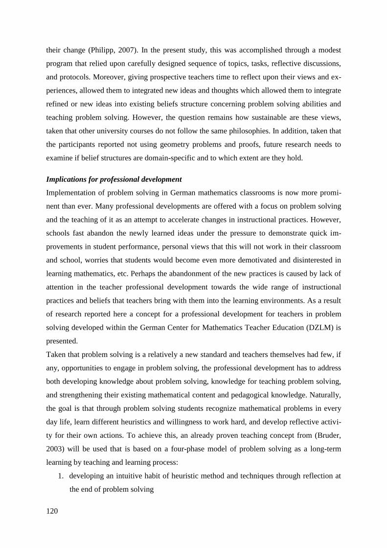
120
their change (Philipp, 2007). In the present study, this was accomplished through a modest
program that relied upon carefully designed sequence of topics, tasks, reflective discussions,
and protocols. Moreover, giving prospective teachers time to reflect upon their views and ex-
periences, allowed them to integrated new ideas and thoughts which allowed them to integrate
refined or new ideas into existing beliefs structure concerning problem solving abilities and
teaching problem solving. However, the question remains how sustainable are these views,
taken that other university courses do not follow the same philosophies. In addition, taken that
the participants reported not using geometry problems and proofs, future research needs to
examine if belief structures are domain-specific and to which extent are they hold.
Implications for professional development
Implementation of problem solving in German mathematics classrooms is now more promi-
nent than ever. Many professional developments are offered with a focus on problem solving
and the teaching of it as an attempt to accelerate changes in instructional practices. However,
schools fast abandon the newly learned ideas under the pressure to demonstrate quick im-
provements in student performance, personal views that this will not work in their classroom
and school, worries that students would become even more demotivated and disinterested in
learning mathematics, etc. Perhaps the abandonment of the new practices is caused by lack of
attention in the teacher professional development towards the wide range of instructional
practices and beliefs that teachers bring with them into the learning environments. As a result
of research reported here a concept for a professional development for teachers in problem
solving developed within the German Center for Mathematics Teacher Education (DZLM) is
presented.
Taken that problem solving is a relatively a new standard and teachers themselves had few, if
any, opportunities to engage in problem solving, the professional development has to address
both developing knowledge about problem solving, knowledge for teaching problem solving,
and strengthening their existing mathematical content and pedagogical knowledge. Naturally,
the goal is that through problem solving students recognize mathematical problems in every
day life, learn different heuristics and willingness to work hard, and develop reflective activi-
ty for their own actions. To achieve this, an already proven teaching concept from (Bruder,
2003) will be used that is based on a four-phase model of problem solving as a long-term
learning by teaching and learning process:
1. developing an intuitive habit of heuristic method and techniques through reflection at
the end of problem solving

121
2. becoming aware of special heuristics on a basis of an example
3. introducing deliberate practice phases on tasks of different difficulty
4. context extension of strategy application
Specifically, this research suggests that when conceptualizing professional development on
problem solving following learning opportunities need to be considered:
allow for teacher’s growth of mathematical knowledge for teaching problem solving
as well as to shape the forms of the knowledge produced
encourage teachers to use more challenging examples than they would normally use
provide teachers with activities that foster differentiation to reach every student’s po-
tential
provide opportunities that challenge teachers’ beliefs on student problem solving pre-
dispositions through “cognitive conflict” (e.g., through authentic videos).
Adoption of new curriculum standards is not an easy task for teachers. As a community, we
know what types of professional development support teachers so that their teaching practices
would reflect the ongoing reforms. “Teacher development must be rooted in the ability of the
individual teacher to doubt, reflect and reconstruct” (Wilson & Cooney, 2002, p. 132). That
said, the reform of mathematics classroom is a hard, but a worthy cause where different facets
have to be taken into consideration and addressed. Based on the growing body of knowledge,
we hope that our conception of professional development would allow for transformation of
teaching and learning as suggested by reformed curricula, organizations and research.
References
Aiken, L. R. Jr. (1973). Ability and creativity in mathematics. Review of Educational Re-
search, 43(4), 405–432.
Bruder, R. (2003): Methoden und Techniken des Problemlöselernens. Material im Rahmen
des BLK-Programms „Sinus“ zur „Steigerung der Effizienz des mathematisch-
naturwissenschaftlichen Unterrichts. Kiel: IPN.
Fey, J. T., Hollenbeck, R. M., & Wray, J. A. (2010). Technology and the mathematics
curriculum. In B. J. Reys, R. E. Reys, & R. Rubenstein (Eds.), Mathematics curriculum:
Issues, trends, and future directions (pp. 41–49). Reston, VA: National Council of
Teachers of Mathematics.
Howson, G., Keitel, C., & Kilpatrick, J. (1981). Curriculum development in mathematics.
Cambridge, UK: Cambridge University Press.
Kilpatrick, J. (1969). Problem solving and creative behavior in mathematics. In J. W. Wilson
& L. R. Carey (Eds.), Review of recent research in mathematics education studies in
mathematics series. Studies in Mathematics Series (Vol. 19, pp. 153–187). Stanford,
CA: School Mathematics Study Group.

122
Kilpatrick, J. (2011). Pólya on mathematical abilities. The Mathemetics Educator, 21(1), 3–8.
Krutetskii, V.A. (1966). Age peculiarities in the development of mathematical abilities in stu-
dents. Soviet Education, 8,15–27.
Krutetskii, V. A. (1969). Mathematical aptitudes. In J. Kilpatrick & I. Wirszup (Eds.), The
structure of mathematical abilities. Soviet studies in the psychology of learning and
teaching mathematis (Vol. 2, pp. 5–57 ). Standford: School Mathematics Study.
Krutetskii, V. A. (1976). The psychology of mathematical abilities in school children.
Chicago, IL: University of Chicago Press.
Kultusministerkonferenz (2003). Bildungsstandards im Fach Mathematik für den mittleren
Schulabschluss. Bonn: KMK.
Kultusministerkonferenz (2012). Bildungsstandards im Fach Mathematik für die allgemeine
Hochschulreife. Bonn: KMK.
Merriam, S. B. (1998). Qualitative research and case study applications in education (2nd
ed.). San Francisco: Jossey-Bass.
Ministerium für Schule, Jugend und Kinder des Landes Nordrhein-Westfalen [NRW] (2004).
Kernlehrplan für die Gesamtschule – Sekundarstufe I in Nordrhein-Westfalen.
Ministerium für Schule, Jugend und Kinder des Landes Nordrhein-Westfalen [NRW] (2007).
Kernlehrplan für das Gymnasium – Sekundarstufe I (G8) in Nordrhein-Westfalen.
Ministerium für Schule, Jugend und Kinder des Landes Nordrhein-Westfalen [NRW] (2011).
Kernlehrplan und Richtlinien für die Hauptschule in Nordrhein-Westfalen.
National Council of Teachers of Mathematics. (1989). Curriculum and evaluation standards
for school mathematics. Reston, VA: Author.
National Council of Teachers of Mathematics. (2000). Principles and standards for school
mathematics. Reston, VA: Author.
Pajares, F. (1992). Teachers’ beliefs and educational research: Cleaning up a messy construct.
Review of Educational Research, 62(3), 307-332.
Patton, M. Q. (2002). Qualitative research and evaluation methods. Thousand Oaks, CA:
Sage.
Philipp, R. A. (2007). Mathematics teachers’ beliefs and affect. In F. K. Lester (Ed.), Second
handbook of research on mathematics teaching and learning (Vol. 2, pp. 257–315).
Charlotte, NC: Information Age.
Pólya, G. (1973). How to solve it: A new aspect of mathematical method. Princeton, NJ:
Princeton University Press. (Original work published in 1945).
Rösken, B., Hannula, M. S., & Pehkonen, E. (2011). Dimensions of students’ views of them-
selves as learners of mathematics. ZDM - The International Journal on Mathematics
Education, 43 (4), 497–506.
Schoenfeld, A. H. (1988). When good teaching leads to bad results: The disasters of
“well‒taught” mathematics courses. Educational Psychologist, 23(2), 145–166.
Stanic, G., & Kilpatrick, J. (1989). Historical perspectives on problem solving in mathematics
curriculum. In R. I. Charles & E. A. Silver (Eds.), The teaching and assessing of
mathematical problem solving (pp. 1–31). Reston, VA: National Council of Teachers of
Mathematics.

123
Thompson, A. (1992). Teacher’s beliefs and conceptions: A synthesis of the research. In D. A.
Grouws (Ed.), Handbook of research on mathematics teaching and learning (pp. 127–
146). New York: MacMillan.
Werdelin, I. (1985). The mathematical ability: Experimental and factorial studies. Lund,
Sweden: C. W. K. Gleerup.
Wilson, M., & Cooney, T. J. (2002). Mathematics teacher change and development. In G. C.
Leder, E. Pehkonen, & G. Törner (Eds.), Beliefs: A hidden variable in mathematics ed-
ucation? (pp. 127–147). Dordrecht, The Netherlands: Kluwer.

124
Teachers’ and Fourth graders’ questions during a problem-solving lesson
Anu Laine, Liisa Näveri, Anu Kankaanpää, Maija Ahtee & Erkki Pehkonen
University of Helsinki, Finland
Abstract
We have studied the teachers’ and their pupils questioning during a problem-
solving lesson when a nonstandard problem was used. Based on the videotaped
lessons the teachers’ questions were classified into six categories (Task assign-
ment and marking the solution, Way of working, Progress of working, Asking for
justification, Deepening of understanding, and Questions not related to the prob-
lem solving) using inductive content analysis. The teachers asked mostly about
the task assignment, prompting the pupils to understand the problem and to start
solving it. The number of teachers’ questions aiming at understanding varied sub-
stantially (0% - 47%), but their number was small on average. Pupils’ questions
were classified into six categories. The average proportion of the pupils’questions
from all the questions was about 30%. The number of teachers’ and pupils’ ques-
tions seems to be interrelated.
Key words: open problem, teachers’ and pupils’ questions, Finnish primary school
ZDM classification: C50, D50
Introduction
At all levels of the Finnish school system, the aim of learning mathematics is, according to the
curriculum (NBE 2004), to understand mathematical structures and develop mathematical un-
derstanding, not merely the operations of mechanical calculation. Problem solving is consid-
ered to be a central tool in the development of mathematical thinking internationally (e.g. Ma-
son, Burton & Stacey 1982, Schoenfeld 1985, Stanic & Kilpatric 1988). Problem solving has
even been set as one of the formal objectives for all school subjects in the Finnish national
curriculum for comprehensive school (NBE 2004).
This paper considers the use of problem solving – especially open problems – in teaching, and
especially teachers’ questioning in guiding pupils during problem-solving lessons. We are al-
so interested in how pupils’ questions are related to the teacher’s questions. Based on the
questions it is possible to get a view of the conversation during a problem-solving lesson and
thus also about the learning possibilities that the teacher offers during the lesson. With her

125
questions the teacher has an influence on the process of how pupils concentrate and try to
solve the given problem. The teacher leads and focuses pupils’ thinking, including ways of
finding solutions and deepening their understanding with the questions. When posing a ques-
tion, pupils need to evaluate new information based on their own knowledge and beliefs. Thus
the teacher can derive from pupils’ questions knowledge about how pupils have understood
the topic.
Here we will use a rather widely used characterization for a problem (cf. Kantowski 1980): a
task is said to be a problem, if it demands that solvers must connect their earlier knowledge in
a new way. If the problem solvers can immediately recognize the procedure needed for solv-
ing the task, it is for them a routine task (or a standard problem or an exercise). The concept
of ‘problem’ is thus relative in terms of time and of the person concerned. In an open-ended
problem (cf. Pehkonen 2004), the starting point is given, but the end is open, and therefore,
there are usually many possible answers. An example of an open-ended task is as follows:
“Divide a rectangule into three triangles. Can you find another solution?”
Teacher’s questions
The problem-solving literature includes advice on how a teacher could guide students’ prob-
lem-solving activity. The teacher can scaffold students’ problem solving in different ways
(e.g., Anghileri 2006) or the teacher may use careful questioning to promote students’ reason-
ing (e.g., Sahin & Kulm 2008; Martino & Maher 1999).
Teacher’s questions can be divided into different categories, for example based on their form
(Myhill 2006). These types of questions are
1) closed, factual questions, e.g. “What is 5 plus 5?”
2) speculative questions that have no predetermined answer, e.g. questions about opinions
3) process questions which invite children to explain their thinking, e.g. “How do you
know that?”
4) procedural questions which are related to the organization of the lesson, e.g. “Can you
all see at the table?”
It is important to notice that despite the form of the question its function can vary. Myhill
(2006) divides teacher’s questions, based on their function, into 11 categories. For example
the meaning of the factual question can vary from remembering the fact to pondering the
meaning of the fact. Sahin and Kulm (2008) divide questions into three main types: 1) factual

126
questions which check, for example, that the pupil knows the central facts concerning the
problem, 2) probing questions which ask for justification or explanation, and 3) guiding ques-
tions which help pupils ahead in their problem-solving process. Myhill’s process questions
and Sahin and Kulm’s probing questions require pupils to explain their thinking.
In problem solving, questions that enhance pupils’ ability to argue and justify their solutions
are central. Martino and Maher (1999) have analysed these type of questions more closely.
They can be divided into six categories: questions that 1) estimate pupils’ understanding, 2)
direct pupils’ attention to an incomplete component in their argument, 3) sustain pupils’ inter-
est in the problem, 4) encourage mathematical justification, 5) direct pupils to consider justi-
fication produced by another pupil, and 6) promote generalization of a solution to similar
problem tasks.
Research problems
In this paper our aim is to discover what kind of questions teachers use during a problem-
solving lesson when pupils solve an open-ended problem. We are also interested in seeing
how the pupils’ questions are related to the teacher’s questions. Thus the research questions
can be formulated as follows:
(1) What kind of questions do the teachers use when guiding their pupils during the
problem- solving lesson?
(2) What kind of questions do the pupils pose to the teacher during the problem-solving
lesson?
(3) How do the teachers’ and the pupils’ questions related to problem solving vary in
different classrooms?
Method
This study is a part of the three-year follow-up Finland–Chile research project, financed by
the Academy of Finland (project number #1135556). In the project, we try to develop a model
for improving the level of pupils’ mathematical understanding by using open problems in
mathematics teaching. Once a month on average, during the mathematics lessons of the ex-
perimental group (10 teachers), one open problem will be dealt with and recorded using video
equipment. The same problems are also being used in Chile, but the comparison material is
not part of this study and comes only later.

127
Here we consider the results of the task, Gary the Snail, that was implemented in September
2011. Gary the snail is clearly a non-standard problem, and essentially needs creativity in or-
der to be solved:
Gary the snail climbs a wall very slowly. Some days the snail ascends 10 cm, some
days it ascends 20 cm, some days it sleeps and doesn’t move, and other days it is
sound asleep and falls 10 cm. The height of the wall is 100 cm. At the end of the tenth
day Gary the snail is at the middle of the height of the wall. What could have been
happening during the first 10 days? Show as many ways as possible.
Eight teachers from the experimental group (Anna, Barbara, Cloe, Daisy, Ella, Flora, Grace,
Hannah) and their fourth-grade pupils took part in this study. All the teachers work in schools
in the Helsinki capital area. All except Daisy have over 10 years of teaching experience. In
the mathematics test (max 32 points) carried out at the beginning of the project, the pupils’
results varied from 22.3 to 26.7 points. Barbara’s and Hannah’s pupils had the best results
and, respectively, Grace’s and Cloe’s pupils had the lowest results on the test.
During the lessons (45 minutes/lesson), one of the researchers (LN) recorded the teachers’
working. The videos were transcribed. Based on looking at the videos and reading the
transcriptions the teachers’ questions were categorized. After creating the categories the data
was re-read and the categorization was checked. This was done several times. After this some
categories which contained similar ideas were joined together and the final categories were
decided. When all the questions were categorized the frequencies were counted. One
researcher (AK) made the classification and another researcher (MA) made the parallel
coding. Uniformity of the teachers’ questions scored 97% and uniformity of the pupils’ ques-
tions scored 94%. The analysis is qualitative and it can be characterized as inductive content
analysis (cf. Patton 2002) because we tried to make sense of the situation without imposing
any pre-existing expectations. Pearson’s correlation and regression analysis were used to find
out the relation between the teachers’ and the pupils’ questions.
The teachers’ lesson plans were also used as research data. Noticeable is that Anna and
Barbara had already written in their lesson plan that they were not going to guide their pupils.
They wanted to see how the pupils would manage to solve the problem by themselves.
Results
In the results we first analyze the teachers’ questions, then the questions that the pupils pose
to the teachers and, finally, the relationship between these questions.

128
Teachers’ questions
The teachers asked plenty of questions already from the beginning of the lesson. They guided
the pupils mostly just by asking questions that were connected to the information in the task
assignment. Some of the questions were directed to the whole class, whereas some of them
were clearly focused on only one pupil at a time. At the end of the lesson some of the teachers
used questioning when they went through the task and its different solutions. The teachers’
questions were classified into the following six categories: A) Task assignment and marking
the solution, B) Way of working, C) Progress of working, D) Asking for justification, E)
Deepening of understanding, and F) The others, i.e. incoherent or unconnected to problem
solving. Often the teacher repeated the same question many times during the lesson. She
might have presented her question first to several pairs in turn and finally to the whole class in
the common discussion. However, here a question consists of a statement that may contain
more than one interrogative or the repetition of the same question many times and using dif-
ferent wording.
The questions in category A, Task assignment and marking the solution, formed a consid-
erable portion of the teachers’ questions. For example, most of Anna’s and Flora’s questions
belong to this category. Many of the teachers’ questions pertained to both task assignment and
the marking of the solution simultaneously. These questions were asked immediately in the
beginning of the lesson when the task was read or when the teacher was walking around
helping the pupils. With these questions the teachers encouraged the pupils to return to the
task assignment and rethink the conditions in it. With their questions the teachers also guided
the pupils to write down their solutions. In part of the questions the teachers helped the pupils
to solve the problem by looking at one day at a time.
“But, what is written in the instruction? How much could it ascend?” (Barbara)
“Here, it is the second day. What is happening during it?” (Grace)
“How did you mark them?” (Daisy)
The questions in category B, The way of working, are related to how the pupils started to
solve the problem. In their questions the teachers commented on the strategy that the pupils
had chosen to solve the problem, and proposed other alternative ways. In this category there
are also the questions with which the teacher urges the pupils to think and plan their solution
process.
“Is there some way how you could draw it?” (Grace)
“Yees, how do you think that division could have been used here?” (Barbara)

129
“What…, how could you solve this?” (Grace)
Also the questions in category C, Progress in working, were presented often, especially
when the teacher was walking around and helping the pupils. The teachers used these ques-
tions often as openings for discussion by asking the pupils to tell about their working methods
and their solutions. In this category there are also the questions with which the teacher dis-
covered whether the pupils had understood how to work with the problem.
“How many different alternatives have you already found?” (Anna)
“Did quite many of you now catch the plot?” (Daisy)
With the questions belonging to category D, Asking for justification, the teachers guided the
pupils to tell what they were thinking in solving the problem. These questions turned up espe-
cially when, near the end of the lesson, the pupils presented their solutions to the other pupils.
The teachers asked the pupils also to justify the way they had found their solution. In some
cases the teachers tried to help the pupils to find the error in their suggestion for a solution. In
the data there were also some questions that were related to the pupils’ feelings and to facing
the nonstandard problem.
“Yees, so how did you from this first solution ... get this second solution?” (Hannah)
“Explain to me why, if you make the mark here and not to this line, how does it in-
crease the number of your possibilities?” (Cloe)
The teacher used such comments to encourage the pupils to try to approach the problem in
some new way or to find more solutions, and these were classified into category E, Deepen-
ing of understanding. Also included in this category were those questions with which the
teacher guided the pupils to ponder in a larger and deeper way in finding a proper solution.
For example, Hannah encouraged the pupils to think how they could modify a new solution
from the solution that they had already found. The questions in this category have been
chosen by looking at the whole event: For example the teacher’s question on whether the snail
could move up along the wall more than 50 cm on one day and then descend, totally changed
one pupil’s way of thinking about the problem.
“You found thirteen, but do you mean that you found all the possible alternatives?”
(Barbara)
“What was among these different ways, don’t think only your own way … What was
the easiest way to find the solution?” (Grace)
The distribution of the question categories among the teachers is shown in Table 1. The
teachers were clearly quite different both as to the number of questions they used and also as
to what kind of questions they asked. During this problem-solving lesson the total number of

130
questions per teacher varies from 16 to 90. Half of the questions were classified as Task as-
signment and marking the solution (A). These questions were mostly factual (e.g. “What will
happen to the snail during deep sleep?”). Questions that were related to the working process
(B & C) were partly factual and partly guiding (e.g. “Is there a way how you could draw it?”)
(cf. Myhill 2006; Sahin & Kulm 2008).
The teachers differed very much also in the number of questions (D & E) that promote under-
standing. Some of the questions required justifications and the others aimed to deepen their
understanding by generalizing the problem (cf. Martino & Maher). Anna and Daisy did not
ask these types of questions at all whereas Hannah asked up to 72 such questions which is
almost half of her total amount of questions. Most of the questions that encouraged pupils to
justify their thinking were process questions but some of them were also speculative (e.g.
“But now I ask again the same question: what is a problem? Is it only in mathematics where
there are those problems?”).
Table 1. The distribution of the number of the teachers’ questions in the categories A) Task
assignment and marking the solution, B) Way of working, C) Progress of working, D) Asking
for justification, E) Deepening of understanding, and F) The others. The percentage in the
brackets is calculated from the teacher’s total questions.
Teacher A B C D E F Total
Anna 11 (69) 0 1 (6) 0 0 4(25) 16 (100)
Barbara 5 (26) 1 (5) 5 (26) 4 (21) 2 (11) 2(11) 19 (100)
Cloe 15 (63) 0 5 (21) 3 (13) 0 1 (4) 24 (100)
Daisy 12 (46) 1 (4) 5 (19) 0 0 8(31) 26 (100)
Ella 19 (54) 4 (11) 4 (11) 2 (6) 2 (6) 4(11) 35 (100)
Flora 43 (74) 3 (5) 4 (7) 3 (5) 0 5 (9) 58 (100)
Grace 47 (68) 3 (4) 2 (3) 9 (13) 5 (7) 4 (5) 69 (100)
Hannah 18 (20) 7 (8) 18 (20) 27 (30) 15 (17) 5 (6) 90 (100)
Total 170 (50) 19 (6) 44(13) 48 (14) 24 (7) 33 (10) 338 (100)
Pupils’ questions to the teacher
We were also interested in examining the pupils’ questions in order to get a better overwiew
of the whole process of questioning in the different classes. The pupils’ questions which they
posed to their teachers were classified in the following six categories: I) Understanding the

131
task and marking the solution, II) Aim of the task, III) Way of working, IV) Checking of
understanding, V) Request for help, and VI) The others, i.e. incoherent or unconnected to
open-ended problem solving. In Table 2 we present a summary of pupils’ questions in
different classrooms.
Table 2. The distribution of pupils’ questions in different categories: I) Understanding the task
and marking the solution, II) Aim of the task, III) Way of working, IV) Checking of under-
standing, V) Request for help, and VI) Other questions.
Classroom I II III IV V VI Total
Anna 1 2 1 0 0 2 6
Barbara 3 1 1 0 0 2 7
Cloe 13 2 7 1 3 2 28
Daisy 7 1 6 0 5 14 33
Ella 4 3 3 3 0 5 18
Flora 22 5 5 4 2 4 42
Grace 4 1 1 1 0 9 16
Hannah 6 2 2 0 1 2 13
Total 60 17 26 9 11 40 163
Most of the pupils’ questions were classified in category I) Understanding the task and
marking the solution.
“Is the starting point always there?” (Cecilia’s pupil)
“Can I put here that it climbs first for example one centimeter and then eight?”
(Hannah’s pupil)
Questions related to the target of the task (category II) pupils clarified and confirmed that they
had understood the idea of the problem. These kinds of questions were also posed later when
they were solving the problem.
“Am I supposed to do the same calculation again?” (Grace’s pupil)
”So is the purpose here now to invent new ways?” (Hannah’s pupil)
Students were figuring out how they should work during the lesson and what they should do
next by posing questions classified in the category Way of working (category III). These
questions were not related to finding the solution or marking the solution. Instead they were
connected to the ways of working, pair work or working equipment.
“Can I do this in a group?” (Grace’s pupil)

132
“So can we have another paper?” (Cloe’s pupil)
Pupils asked teachers during the lessons to comment if their solution was correct. These kinds
of questions were classified in category IV Checking of understanding.
“Is this wrong?” (Ella’s pupil)
“So is this good?” (Flora’s pupil)
With questions containing Request for help (category V) pupils were asking the teacher to
come and help them.
“Can you come here for a second?” (Cloe’s pupil)
In category VI The others, the pupils’ questions were incoherent, unconnected to the problem
or to solving it, or to anything related to the working at the problem.
“What? Is that a camera?” (Daisy’s pupil)
“How did you then translate that from Spanish?”(Grace’s pupil)
The relation between teachers’ and pupils’ questions
The total number of questions asked in the different classrooms varied quite a lot. During one
lesson in different classrooms, pupils posed from 6 to 42 questions, whereas the teachers
posed from 16 to 90 questions. We wanted to find out the connection between the number of
the teachers’ and pupils’ questions. Would it be possible that teachers’ questions also promote
pupils to ask more questions? Because we were especially interested in the questions that
were related to solving the problem, we eliminated the category ‘The others’ from both the
teachers’ and the pupils’ questions (see Table 3).
Table 3. Number of questions related to problem solving in different classrooms
Teacher Teachers’
questions
Pupils’
questions
The proportion of pupils’
questions of all questions
Anna 12 4 25%
Barbara 17 5 23%
Cloe 23 26 53%
Daisy 18 19 51%
Ella 31 13 30%
Flora 53 38 42%
Grace 65 7 10%
Hannah 85 11 11%
Total 304 134 31%

133
From Table 3 it can be concluded that in most of the classes, when the number of the
teacher’s questions increases it is also observed that the number of the pupils’ questions to the
teacher increases. Two classrooms (Grace’s and Hannah’s) are exceptions. In these class-
rooms the teacher asks many questions, but the pupils ask only a few. The proportion of the
pupils’ questions from all the questions is only about 10% when the average is about 30%.
Based on the video material, we found that in these classrooms the atmosphere was very
authoritarian and therefore the pupils were not so ready to ask questions. It could also be pos-
sible that the pupils did not have time to ask questions, because they were kept busy in
answering the teachers’ questions. However, this explanation was not true in these cases.
During the lesson, Hannah asked a lot of questions with which she guided her pupils in the
right direction to their solutions, and she was not expecting any answers from them. In the
next example Hannah guides one group of pupils: “Quite good, you have found one solution.
Can you find another?” She continues with another group: “Could you take advantage of
this? You have one good model here. Think how you could advance from it?” When Hannah
moves from one group to another the pupils ponder her questions rather than pose new ones.
Whereas Grace prompts her pupils to think by themselves and therefore her pupils do not
bother to ask any questions: “It is wrong then. It has moved a little too much. What do you
do? How do you correct it? This is zero…mm…you must take this away… You must probably
correct some number. How would you correct it? I don’t tell you because you have not
counted.”
Anna and Barbara asked very few questions. They had already written in their lesson plans
that this time they were going to try seeing how the pupils would manage solving the problem
without guidance. On the basis of this plan we may also therefore conclude that the pupils
asked very few questions.
In Cloe’s, Daisy’s and Flora’s classrooms the proportion between the teacher’s and the pupils’
questions seems to be quite the same. Based on the video material, the atmosphere in the
classrooms was confidential during all these lessons. It seemed to be easy for the pupils to
approach their teacher and ask questions, and the teacher’s response to the questions was
appropriate.
Ella seems to be an average teacher both as to the total number of questions and to the distri-
bution of the questions between the teacher and the pupils. However, she and her class seem
not to represent a typical situation in this research group.
The relation between teachers’ and pupils’ questions related to problem solving is presented
graphically in figure 1. When we leave two teachers (G and H) out of the examination

134
because of their exceptional behavior we get a linear correlation of 0.83 between the number
of teachers’ and pupils’ questions. On this area the model describing the relation between
questions is linear (R Square Change =.671a , sig. F Change = .046). Coefficient of determina-
tion is 67% which means that the number of teachers’ questions explain 67% of the number of
pupils’ questions (or the other way around). It appears that, when teachers’ questions increase
over some point, the pupils’ questions start to decline. If we take into account all teachers, we
receive a curved, i.e. parable model (y = -0.0102x2+0.9724x, R
2=0.304) and for the coeffi-
cient of determination 30%. Because the linear model explains more of the variation than the
curved one, we choose the first one. This decision is supported by the observation that
Grace’s and Hannah’s actions differ from the other teachers’ actions during the problem-
solving lesson.
Figure 1. The relation between the teachers’ and the pupils’ questions.
Discussion
The teachers asked most about the task assignment because the pupils had difficulties to get
started on the problem. The teachers asked plenty of good questions with which they
prompted the pupils to understand the problem and did not just say what they should do. The
teachers asked a very different number of questions during the lesson. The difference between
the pupils’ knowledge between different classrooms does not explain the number of questions
because, based on the mathematics test done at the beginning of the project, there were many
(and respectively a few) questions in the classrooms of both good and poor achieving pupils.
The number of questions depends therefore evidently on the teachers’ philosophy of teaching
and on the working culture of the class.
It is also important to pay attention to the quality of the questions and not only to their num-
ber. On average there were, however, only a few questions that aimed specifically at under-

135
standing. The proportion of these questions varied a lot (0% - 47%) according to the teacher.
From the viewpoint of promoting mathematical thinking, it would be important that there
were more questions aimed at judging and deepening the solutions. It would be interesting to
see whether the teachers’ questions will change during the research project, after the teachers
have had more guidance and experience in teaching problem solving.
It is also important to find out what kind of questions and answers to pupils’ questions en-
courages the pupils to ask questions that promote the problem-solving process and therefore
contribute to a fruitful discussion in a classroom. Later we shall concentrate more explicitly
on studying this process with the video material about the communication in the classrooms.
Furthermore, in the future we shall also look at the pupils’ achievements and compare them
with the discussions in the classrooms.
References
Anghileri, J. (2006). Scaffolding practices that enhance mathematics learning. Journal of
Mathematics Teacher Education, 9, 33–52
Kantowski, M.G. (1980). Some Thoughts on Teaching for Problem Solving. In: Problem
Solving in School Mathematics (eds. S. Krulik & R.E. Reys), 195–203. NCTM Year-
book 1980. Reston (VA): Council.
Martino, A. & Maher, C. (1999). Teacher questioning to promote justification and generaliza-
tion in mathematics: What research practice has taught us. Journal of Mathematical Be-
havior, 18(1), 53-78.
Mason, J., Burton, L. & Stacey, K. (1982). Thinking mathematically. London: Addison-Wesley.
Myhill, D. (2006). Talk, Talk, Talk: Teaching and learning in whole class discourse. Research
Papers in Education, 21 (1), 19–41.
NBE (2004). National Core Curriculum for Basic Education 2004.
http://www.oph.fi/english/publications/2009/national_core_curricula_for basic_education
Patton, M. (2002). Qualitative research & evaluation methods. Thousand Oaks: Sage.
Pehkonen, E. (2004). State-of-the-Art in Problem Solving: Focus on Open Problems. In:
ProMath Jena 2003. Problem Solving in Mathematics Education (eds. H. Rehlich & B.
Zimmermann), 93–111. Hildesheim: Verlag Franzbecker.
Sahin, A. & Kulm, G. (2006). Sixth grade mathematics teachers’ intentions and use of prob-
ing, quiding, and factual questions. Journal of mathematics teacher education, 11 (3),
221–241.
Schoenfeld A.H. (1985). Mathematical Problem Solving. Orlando (FL): Academic Press.
Stanic, G. & Kilpatrick , J. (1988). Historical perspectives on problem solving in the mathe-
matics curriculum. In: Teaching and learning mathematical problem solving: Multiple
research perspectives (eds. R. Charles and E. Silver). Reston VA, National Council of
Teachers of Mathematics: 1-22.

136
When do we have to use recursive or asymptotic formulas or Monte Carlo
simulation?
Józsefné Libor
Apor Vilmos Catholic University College, Hungary
Abstract
If you see or hear the word didactic, usually a primary or secondary school comes to
your mind as a place where it is used. But at least as important in higher education too
the choice of the most appropriate method to be more effective in educating. My choice
of topic partly originates from the continuing decline in the results of college students
that can be observed for several years by now, and is a general trend in higher education
but is especially true for mastering scientific disciplines. On the other hand because of
the continuously decreasing number of class hours and other reasons, there is hardly
enough time and opportunity available, especially in terms of teaching of probability, to
carry out or at least to demonstrate teaching experiments of acceptable quantity and
quality. Therefore those methods and techniques allowing the students to get familiar
with more concepts and see their practical application can have a positive effect on
mastering the theoretical concepts. For the analysis of this topic my work focuses on a
field of probability theory (the analysis of the longest runs), which can be easily
understood by the students and can be linked to their everyday experiences and thus
provide a way for easy comparison. There is no exact andclosed expression for the
distribution function describing the length of the longest runs. Thus for the discussion of
this particular topic the differences and the applicability between the various methods
becomes more obvious. Observing these differences provides a deeper understanding of
the different terms, the applications of the different techniques for the topic (the longest
runs) can be demonstrated appropriately.
Key words and phrases: longest run, recursive formula, asymptotic theorem, simulation
ZDM classification: K108, K508, U708
1. Introduction
In my study I present a method that helps to understand the concepts and techniques
mentioned in the title, which can be a useful didactic tool for colleagues teaching in academic
institutions. The recursive expressions give exact values but they are not closed expressions
and calculating the exact values after a greater number of elements can sometimes be
problematic even when calculating with a computer. The asymptotic values become more
accurate with the increase in the number of constituents (with an increasing n ) however they

137
only provide approximate values, whereas repeated studies of simulation experiments provide
average results. These terms and definitions can be applied in other fields of mathematics by
the students.
Although in various fields of mathematics the basic terminology, definitions, the introduction
of computations can be based upon everyday observations and experiences to a great extent,
however in the case of probably calculations our situation is a little more difficult. In the
introduction of the article by Tibor Nemetz [9] the author writes the following: "Most of the
time the students have vague understanding how to interpret an uncertain event, etc.; quite
frequently their judgment on random, large scale phenomena is wrong or rather they cannot
comprehend the existence or application of such laws." Furthermore, as Alfréd Rényi, [11] the
founder of the Hungarian school of probability writes in many cases even the teachers are
reluctant to present these experiments. "Statistical principles can be demonstrated by data take
from books and newspapers; however it has a greater effect on students if they obtain these
results presented to them or, even better if the results originate fromexperiments performed by
them. Some teachers do not agree with this as they fear that the experiments will not yield
results that they expect as it can happen from the nature of these experiments. I don’t think
that this fear is justified and if the teacher understands probability calculus well, then he or
she cannot end up in an uncomfortable situation. Naturally the teacher has to react quickly as
the evaluation of results, which even the teacher could not foresee is more difficult than the
analysis ofexamples which were evaluated in advance by the teacher." Of course these
experiments will provide further experiences not only to the students but to the instructor as
well, which can be a very important point of view especially for the discussion of random
events.
In higher education the general opinion of the teachers is that the knowledge of students
displays greater insufficiency and the general performance is dropping every year. Many
institutions provide preparation courses and additional coaching courses to treat the problem;
however I find that it is also just as important to understand the terms, definitions and get
proficient with their application during BA education. Everybody knows the obvious fact that
there is a direct relationship between theoreticalknowledge and problem solving skills it is
justified to expect that results will improve with the better understanding of definitions.
Recursive formulae, asymptotic theorems and simulations play an important role in several
fields of math-teaching in higher education. But the exact knowledge of these notions leaves a
lot to be desired. The study of some illustrative problems may help to understand them. While
solving these problems students have an opportunity to compare these definitions.

138
In this paper I shall use the well-known coin tossing experiment to compare the results of
recursive formulae, asymptotic theorems and computer simulations. In connection with coin
tossing we examine the length of the longest run. For a sequence of independent coin tosses
with p (0 1p ), the longest run of consecutive heads in the first n tosses is a natural
object of study. In my work the longest run means the longest sequence of the same objects,
for example the longest head-run means the longest sequence among the sequences of
homogeneous heads, which is not interrupted by tail. My research includes the examination of
the length of the longest head-run and the length of the longest whatever - head or tail - run,
studying fare coin. (I have studied the event of biased coin too, so if you are interested in it do
not hesitate to write to me to discuss about that.)
The following well-known example by T. Varga can be an interesting introduction to the
problem for students. We can read this for example in Révész [12]. A class of school children
is divided into two sections. In one of them each child is given a coin which he or she throws
two hundred times, recording the resulting head and tail sequence on a piece of paper. In the
other section the children do not receive coins but are told instead that they should try to write
down a ’random’ head and tail sequence of length in 200 . Collecting and mixing all the slips
of paper, the teacher then tries to subdivide them into their original groups. Most of the time
he succeeds quite well. His secret is that he has observed the following. In a randomly
produced sequence of length in two hundred, there are, say, head-runs of length seven
(knowing Rényi’s log 2200 result). On the other hand, he has also observed that most of those
children who had to write down an imaginary random sequence are usually afraid ofwriting
down runs of longer than four. Hence, in order to find the slips coming from the coin tossing
group, he simply selects the ones which contain runs longer than five. When I had the
privilege of meeting professor Révész, he talked about the continuation of Varga’s
experiment. He made his students acquainted with Varga’s experiment and the result of it.
Then they made the trial again. Professor Révész was successful in subdividing the slips of
paper with quite good accuracy again. His secret was very easy. The students focused on the
length of pure head run for example, but they did not pay attention to the length of pure tail
run or the length of the head-tail pairs run. These experiments led us to ask the following
questions. What is the length ofthe longest head run or the longest whatever run in coin
tossing?
For the investigation of the mentioned definitions (recursive formula, asymptotic theorem,
simulation) our chosen field - coin tossing - is perfect in many respects. We know that there is

139
no exact and closed formula to give the length of the longest run in case of any n . The
recursive formulae are exact, - they give correct results - but using them for large n , is very
time- and storage-consuming even if we use very good computer. For large n we can use the
asymptotic theorems, but these give only approaching results. And finally, the simulation
gives an average value from a lot of repetitions of the trial. Considering these, we can
examine the meaning of these definitions by studying the coin tossing trial. Our graphs will
show the differences between the values in case of small and large n too and the limits of the
scope of the notions.
Consider n independent tosses of a fair coin, and let nR represent the length of the longest
run of heads, and similarly let nR be the length of the longest whatever (head or tail) run. As
we have got a regular (fair) coin, the probability ofhead-tossing equals 0 5p , and of course
the probability of tail-tossing is equal to 1 0 5q p . The problem facing us is the
following. What is the length of the longest head or whatever run?
2. Recursive formulae
Sometimes it is difficult to define an object explicitly. However, it may be easy to define the
object in terms of itself. We define a function or a special series with a recursive formula with
defining the starting value (or values) and generally we provide a formula for calculating the
subsequent values using the previous value(s) with various operations. Thus the process has
two important components. First we need to define the starting value (values) which are the
first elements of our recursive series. Then we need to supply the correspondence which
demonstrates how the subsequent members are derived from the previous members of the
series. It is important to keep in mind that recursive formulas always yield accurate results
and they are not average or approximate values. The application of recursive formulas has one
disadvantage and barrier at the same time: the calculation of the thn element with an
increasing n becomes complicated even with the application of a computer. The recursive
functions, which form a class of computable functions, take their name from the process of
’recurrence’ or ’recursion’. In its most general numerical form the recursion process consists
in defining the value of a function by using other - the previous - valuesof the same function.
A recursive sequence is a sequence of numbers ( )f n indexed by an integer n and generated
by solving a recurrence equation.
And now back to our coin tossing problem.

140
2.1. Longest head run
Let nR represent the length of the longest run of heads and let ( )nA x be the number of
sequences of length n in which the longest head run does not exceed x . The distribution
function of nR is
( )
( ) ( )2n
n n n
A xF x P R x (1)
First we have to give the initial condition that tells where the sequence starts, then the
recursion formula that tells how any term of the sequence relates to the preceding term. Using
the results of Schilling [13], we have the following recursive formula for ( )nA x
1
0
( ) if( )
2 if 0
x
n jjn
n
A x n xA x
n x
(2)
To see how this works, consider the case in which the longest head run consists of at most four
heads. If 4n , then clearly (4) 2n
nA since any outcome is a favorable one. For 4n , each
favorable sequence begins with either T, HT, HHT, HHHT or HHHHT and is followed by a
string having not more than four consecutive heads. Thus,
1 2 3 4 5(4) (4) (4) (4) (4) (4)n n n n n nA A A A A A for 4n .
From this we can calculate the values of (4)nA :
n 0 1 2 3 4 5 6 7 8 …
(4)nA 1 2 4 8 16 31 61 120 236 …
Remark 1. For 1 2 3n the number (1)nA of sequences of length n where n does not
continue two consecutive heads is the ( 2)n nd Fibonacci number.
Remark 2. The values of ( )nA k can be given with the help of thk degree Fibonacci numbers.
Moreover, we can study the case of biased coins using the application of thk degree Fibonacci
polynomials. (See Philippou-Makri, [10].)
2.2 Longest whatever run
Consider n independent tosses of a fair coin, and let nR represent the length of the
longest run of heads or tails (whatever). If ( )nB x is the number of sequences of length n
in which the longest run does not exceed x , then the (cumulative) distribution function is
( )
2( ) ( ) n
n
B x
n nF x P R x . Schilling [13] has proved that 1( ) 2 ( 1)n nB x A x , for 1x .

141
To prove it consider a sequence of length n consisting of signs H and T (representing ’head’
and ’tail’, respectively). Write below of this sequence another sequence of signs S and D
(representing ’same’ and ’different’, respectively). We write S if twoconsecutive signs in the
first sequence are the same, and write D if they are different. Now a run of length 1x
consisting of signs S represents a run of length x in the first sequence. We also see that any
sequence containing signs S and D belongs to two sequences of signs H and T. Finally,
observe that 1( 1)nA x can be considered as the number of sequences of length 1n and
containing signs S and D but not having S-run of length x . (We need a factor 2, because the
longest run can occur from heads or from tails same times.)
The example below shows one of the strings that contributes to 13(4)B :
H H H T H T H T T T T H H
S S D D D D D S S S D S
So we can reduce this case to the case of the longest head run
1 111
( ) 2 ( 1) ( 1)( ) ( ) ( 1)
2 2 2n n n
n n nn n n
B x A x A xF x P R x F x
(3)
The implication of (3) is that for n tosses of a fair coin the longest run tends to be one longer
than the longest run of heads alone.
3. Asymptotic theorems
Asymptotic behavior is a property that certain mathematical expressions demonstrate if the
subsequent values of a series approach the values of a function closer and closer, but they
never actually reach it, even in an infinite number of steps. Therefore in case of large n the
asymptotic values are so close to the real values that we can apply them with confidence if the
real values cannot be defined accurately, or can only be defined in a difficult and complicated
manner.
For the longest head run we have strong limit theorems and results on the limiting behavior of
the distribution. A well-known theorem of Rényi says that the length of the longest run in n
tosses of a fair coin is about 2log n . This was generalized to excessive blocks by the Erdős-
Rényi [4] laws of large numbers.
For the limiting behavior of the distributions there are several known results. Let us see the
case of the longest head run. The asymptotic behavior of nR is described by the following
theorem.

142
Theorem 1. Földes (1979) [5]. For any integer k we have
21 log
2log exp 2 (1)k n
nP R n k o
(4)
where [ ]a denotes the integer part of a and [ ]{a} a a .
Similarly we can see the asymptotic behavior of nR . Using the above theorem of Földes and
(3) we have the following asymptotic result for nR .
Theorem 2. For any integer k we have
2log ( 1)
2log ( 1) exp 2 (1)k n
nP n k oR
(5)
where [ ]a denotes the integer part of a and [ ]{a} a a .
4. Simulation
The mathematical simulation is known as the Monte Carlo method, it is called after the city in
the Monaco Principality, because of roulette, a simple random number generator. The name
and the systematic development of this method dates from about 1944 (see [7] and [8]).
Simulation methods can play an important role in teaching several topics not only
mathematics. We can identify the average value of a random variable if we do not know, or if
cannot or are not willing to perform complex calculations to define the distribution function.
According to the law of large numbers if we supply a sufficient number of samples the
resulting average value is going to be close to the unknown real value. Using simulation the
quoted law can also be more comprehensible for the students. We can easily show that if we
do not perform a sufficient number of repeated measurements we cannot obtain good results.
However if we perform a sufficiently large (at least in the order of thousands) repeated
measurement (or we perform them using a computer) then the resulting average values will be
a really good approximation of the real values.
Here we deal with the simplest version of the stochastic simulation. We need the numerical
value of a quantity p . Moreover, p can be considered as the probability of an event A :
( )P A p . Repeat the experiment N times and calculate the relative frequency of A . Denote
it by Ak
N . Then, by the Bernoulli law of large numbers, Ak
Np almost surely as N .
However, usually we make our experiment on a computer. Using our computer programme,
we build the experiment, and we record if A occurs or not. Repeat the computer experiment
N times. It means that we run our programme N times with N consecutive random

143
numbers. However, as the coin tossing experiment is a random experiment itself, wedevelop
our computer model as follows. Using the first n random numbers, we can perform the coin
tossing experiment of length n . Then repeat it N times ( N is a large integer, 1000N ,
say). Therefore, for any fixed n , the distribution of nR can be obtained as N . (It is an
important issue, because in the previous section we considered the asymptotic distribution of
nR , as n.)
5. Comparison of numerical results, conclusions
Now let us see our problem. For numerical calculations we used MATLAB software and a
high-capacity PC (INTEL Core Quad Q9550 processor, 4Gb. DDR3 memory). We calculated
the distribution of nR and nR . We considered the precise values obtained by recursions, the
asymptotic values offered by asymptotic theorems, and used simulation with 20,000
repetitions. On the figures below denotes the result of the recursion, o belongs to the
asymptotic result, while the histogram shows the relative frequencies calculated by
simulation. On the left side you can see the case of the longest head run and on the right side
you can see the case of the longest whatever run.
Distribution of the longest head run Distribution of the longest run
0 5 50p n 0 5 50p n

144
Distribution of the longest head run Distribution of the longest run
0 5 250p n 0 5 250p n
Distribution of the longest head run Distribution of the longest run
0 5 1000p n 0 5 1000p n

145
Distribution of the longest head run Distribution of the longest run
0 5 3100p n 0 5 3100p n
Distribution of the longest head run Distribution of the longest run
0 5 50000p n 0 5 50000p n

146
First we emphasize that the precise values of the distributions are given by the recursive
formulae. The practical drawbacks of recursive formulae are the following. They are limited
by the capacity of the computer and they can be influenced by numerical errors. On the other
hand, asymptotic theorems always offer approximations but they are easy to compute. The
approximations are quite bad for a small n but they are almost precise for a large n . Finally,
simulation always gives random approximations but it is quite precise if the number of
repetitions is large. The above figures show the properties of the procedures mentioned. For a
fair coin we studied short trials ( 50n ), medium size trials ( 250n ), long trials, ( 1000n
and 3100n ) and very long trials ( 50 000n ).
If n is small or medium sized, we can see that the recursive results are closer to the simulated
values, than the results given by asymptotic theorems. Although we can say that if n is small,
the recursive algorithm is fast, but it slows down if n increases. The next table demonstrates
this statement showing some running times.
n repet. running time
100,000 20,000 773.575832 s.
10,000 20,000 31.795056 s.
5,000 20,000 14.398654 s.
3,100 20,000 9.009479 s.
1,000 20,000 3.984981 s.
500 20,000 3.240019 s.
250 20,000 2.412824 s.
50 20,000 2.092010 s.
30 20,000 1.935557 s.
For a large n the asymptotic values are closer to the simulated results, so we can use them
instead of the recursive values. The asymptotic value is a good approximation if 1000n ,
and it is practically precise if 10 000n .
The figures show that the distribution of nR can practically be obtained from the distribution
of nR by shifting it to the right by 1, as we have seen in (3).
6. The St. Petersburg Paradox
Almost the most common question of our students is the following. Where and how can I use,
apply this or that theorem? What is the economic application of this or that? To show some
financial and economic aspects of the studied field is very useful in teaching of Business
Mathematics. In connection with the previous part, we should examine a very interesting pa-

147
radox, the St. Petersburg paradox. What is this paradox? Peter and Paul play a game with a
fair coin. (The probability of head-tosses and the probability of tail-tosses are the same:
50 50% .) Paul tosses the coin and Peter pays 2 ducats (or euros, or dollars, or what you
want) if it shows head on the first toss, 4 ducats if the first head appears on the second toss, 8
ducats if the first head appears on the third toss, and so on. So Peter pays 2k ducats if the first
head appears only on the thk toss. How much should Peter charge Paul as an entrance fee to
this game so that the game will be fair? (Fair game means that neither of gamblers wins or
loses any money on average.) Surprisingly, the game cannot be made fair, no matter how
large the entrance fee is. Paul is always in a wining position, but as Nicolaus Bernoulli wrote
in the XVIII. century [3]: "there ought not be asane man who would not happily sell his
chance for forty ducats". How can we solve this paradox? Let us see our data in the following
table, where ix means the amount of ducats if the first head appears on the i th toss and ip
means the probability of this event. Even the not excellent students can calculate these values,
so this can rewarding ad for them.
Payoff values and probabilities
ix 2 4 8 16 32 … 2k …
ip 1/2 2(1 2) 3(1 2) 4(1 2) 5(1 2) … (1 2)k …
For example, let us see the first column. Paul gets 2 ducats if the first tossing is head. The
probability of this equals 0 5 . On the second column we can see that Paul gets 4 ducats if the
first toss is tail and only the second one is head. The probability of this equals 0 5 times 0 5
(because the tosses are independent). Following this, Paul gets 2k ducats if the first 1k
tosses are tails but the thk toss is head. The probability of this equals 1(1 2) (1 2) (1 2)k k .
And we can continue it to infinite. This is right, because the sum of the probabilities equals:
1(1 2) 1k
k
. Now we can calculate the expected value of the payoffs, which will be
infinite.
2 3
1 1
( ) 2 1 2 4 (1 2) 8 (1 2) 2 (1 2) 1k k
i ii i
E X x p … …
(6)
So this means that Paul needs to pay an infinite value to Peter as an entrance fee. However,
this is a requirement to which almost no rational person would agree to or be able to satisfy.
We can see this, because if 2x then the probability of winning at least x value equals the

148
following: 2 2
[log ] [log ]
2 1( ) (1 2) (1 2) 1 (1 2)k
x xk k
k x kP X x
where [ ]a means the
integer part of a : [ ]a max{b Z b a} . Using this, we can give the distribution function:
2[ ]
0 if 2( ) ( )
1 2 if 2log x
xF x P X x
x
(7)
So, 2[log ]( ) 2 xP X x as for example the probability of winning greater than 40 ducats
equals ( 40) 1 32 0 03125P X , or the probability of winning a "much bigger" value, for
example the probability of winning a value which is greater than 32 000 ducats equals about
0 00006 . So Paul does not want to risk a big value (not even 40 ducats!) to enter the game.
Although the calculation of Paul’s expectation is mathematically correct, the paradoxical
conclusion was regarded by many early researchers of probability as unacceptable. It is worth
to mention Keynes’s words [6]: "We are unwilling to be Paul, partly because we do not
believe Peter will pay us if we have good fortune in the tossing, partly because we do not
know what we should do with so much money … if we won it, partly because we do not
believe we should ever win it, and partly because we do not think would be a rational act to
risk an infinite sum or even a very large sum for an infinitely larger one, whose attainment is
infinitely unlikely." We can ask students about their opinion of the amount of the entrance
fee. For example: Who would like to pay (or to accept) for example 30 ducats for the game?
The answers can be very interesting, surprising and varied. If the teachers has got enough
time, to talk about the history and some previous solutions of the paradox can be very useful.
There are some students who are not good in maths but they are interested in history. We can
give some research works for them in this theme. (It has got a huge but very interesting
history, so students hopefully will enjoy this work.)
Let us make calculation and simulation for studying the St. Petersburg game. Suppose that we
play only finite times, for example 102 1024n . As the probability of head-tossing equals
0 5 , we expect that half of the games, 512 games complete afterthe first tossing. The amount
of payoff equals 2 . We can say the same for the remaining games, so the half of the
remaining games complete after the next (second) tossing. This means that the quarter of
games 216 games complete after the second tossing. The amount of payoff equals 4 in this
case. Continuing this line of thought, we can say that only the last game will continue after
the 10th tossing. This concrete case can easily be studied with even weaker students also and
the general case will be more understandable.

149
The first head occurs on the thk tossing (k) 1 2 3 4 5 6 7 8 9 10
Number of completed games 512 256 128 64 32 16 8 4 2 1
Payoff ( 2k ) 2 4 8 16 32 64 128 256 512 1024
Table 1. Playing St. Petersburg game 1024 times
Let us see the average of payoffs: 2 10
10
512 2 256 2 12 102410242
10( ) 10… payoff of the last game c c , where
1024
payoff of the last gamec . Now study the value of c . The game would end on the 11th tossing with
probability 0 5 and the payoff would be 112 , so 11
102
22c . But two additional tosses are
required to finish the game with 0 25 probability, and in this case c would be 12
102
24 and so
on. So the average of payoffs equals 10 2 12 with 0 5 probability, 10 4 14 with 0 25
probability and so on.
Generalize the problem, suppose that we play 2kn games. Our data are the followings:
The first head occurs on the thk tossing (k) 1 2 3 … k-1 k
Number of completed games 12k 22k 32k … 2 1
Payoff ( 2k ) 2 4 8 … 12k 2k
Table 2. St. Petersburg game in general
After the first tossing, the half of the games, 12k games complete. After the second tossing
22k games complete and so on, after the thk tossing only 1 game completes. The sum of the
completed games equals 1 22 2 2 1 2 1k k k… , so 1 game would continue after the thk
tossing. But this game would complete after the next ( 1)thk tossing with 0 5 probability,
after the ( 2)thk tossing with 0 25 probability and so on. The average of payoffs equals:
1 2 0
2
2
2 2 2 4 2 2
2
k
k
k k k
k
… payoff of the last gamek c k c
, where c equals 2 with
0 5 probability, 4 with 0 25 probability and so on. So we can demonstrate the averages of
payoffs with a set of lines, exactly 2k line with 0 5 probability, 4k line with 0 25
probability, 8k line with 0 125 probability and so on.
Now simulate the game with MATLAB for example, where 20k . Our values are on the
broken (red) line, and we can draw our lines in the first four events. Students can easily see
that the simulated values are consistent with the calculated results.

150
Figure 1. Simulated and calculated values of the game
Buffon and other mathematicians thought that Paul has to pay 2logn n ducats for n games, so
2log n ducats are spent per game. If Paul would like to play the game 1048575 times, he
would have to pay 20 ducats per game. But as these gameswould take almost 30 years, we
do not need to study this situation. Therefore, about 10 ducats per game can be an acceptable
amount.
Csörgö and Simons existed an extensive literature on asymptotic theory for St. Petersburg
games [2]. Csörgö explained why 2logn n will not satisfy the banker, and generally no
satisfactory solution can be based on laws of large numbers. (There is no asymptotic
distribution.) He remarked that in n games 2log n fee per game is too little, if Paul passes up
his biggest win, but it is too much if he passes up the biggest two wins. The research is still
ongoing, many Hungarian mathematicians work in this filed successfully.
Many examples of St. Petersburg games and their generalizations are studied in the statistics,
economics, and mathematics literature and in many fields of life. It is well-known in
economics that Daniel Bernoulli’s work in 1738 was the basis of the formation of the modern
utility concept that the economists and psychologists and other researchers use even today [1].
An interesting example of a modified St. Petersburg game is a popular television game show,
Who Wants to be a Millionaire? It offers players the chance to win up to one million dollars.
Moreover, we can mention the so-called "martingale strategy", that many gamblers like to
use. In this game we play against the bank with a 50% chance to win. If we lose in the first
game, we double the bet. If we lose in the second game again, we also double the previous
bet, and so on, until we win. If our first bet equals A dollar and we lose in the first n-1 game
but we win in the n th game, then our winning amount equals 2nA , but we had to pay out

151
1(1 2 4 2 ) (2 1)n nA A dollars. So our benefit is A . It seems to be a good strategy,
but thereare some problems. Usually we have not got infinite money (perhaps we win in
infinite), and if we have a lot of money then to win A dollars, does not matter. Last but not
least, of course the casinos know about this strategy so they limit the amount ofbets. Using the
modified paradox Székely and Richards gave an interesting study of economic crisis in [14].
These and many other interesting examples can engage the interest of weaker students either.
References
[1] Bernstein, P. L.: Against the Gods: The Remarkable Story of Risk New York: Wiley 1996.
[2] Csörgö, Simons: Pooling strategies for St. Petersburg gamblers Bernoulli 12, (6), 2006.
pp. 971-1002.
[3] Dutka, J.: On the St. petersburg Paradox Archive for History of Exact Sciences, Vol, 39.
Number 1. pp.13-39.
[4] Erdős, P., Révész P.: On a new law of large numbers. J. Analyse Math. 23 (1970), pp.
103-111.
[5] Földes, A. : The limit distribution of the length of the longest head-run. Period. Math.
Hungar. 10 (1979), no. 4, pp. 301-310.
[6] Keynes, J. M.: A treatise on probability London, Macmillan, 1921.
[7] Metropolis, N.: The Beginning of the Monte Carlo Method. Los Alamos Science, Special
Issue (1987)
[8] Metropolis, N., Ulam, S.: The Monte Carlo Method. Journal of the American Statistical
Association, Vol.44, No.247. (Sep. 1949) pp. 335-341.
[9] Nemetz, T.: Egy lehetőség valószínűségszámítási fogalmak bevezető szemléltetésére. A
matematika tanítása (1970) pp. 143-149.
[10] Philippou, A.N.; Makri, F.S.: Longest success runs and Fibonacci-type polinomials. The
Fibonacci Quarterly (1985), no. 23
[11] Rényi, A.: Ars Mathematica. Typotex, Budapest (2005)
[12] Révész, P.: Regularities and irregularities in a random 0,1 sequence. Statistical Papers
31, (1990) pp. 95-101.
[13] Schilling, Mark F.: The longest run of heads. College Math. J. 21 (1990) no. 3, pp. 196-
207.
[14] Székely, J. G., Richards, P.: The St. Petersburg Paradox and the Crash of High-Tech
Stocks in 2000 The American Statistician, August 2004. Vol 58, No.3. pp. 225-231.

152
Open problems as means for promoting mathematical thinking and under-
standing
Erkki Pehkonen
Teacher Education, University of Helsinki, Finland
Abstract
The paper focuses on one method to promote mathematical thinking and understanding:
the use of problem fields. They are open problems that are gaining more and more em-
phasis in all over the world. When using open problems in a proper way, a teacher can
improve his mathematics teaching in school. The terms ’open problem’ and ’problem
field’ will be discussed and enlightened with some examples. Furthermore, an example
of problems fields is presented and dealt with in detail.
Key words: problem solving, open problems, mathematical thinking
ZDM Classification: D50
Introduction
In Finland the objectives of mathematics teaching for all school forms contain understanding
of mathematical structures and development of mathematical thinking, not only the practicing
of calculation skills (NBE 2004). The same is valid also for other countries, for example
Germany (KMK 2005) and the States (NCTM 2000). The purpose of school teaching in all
countries is to develop such citizens that are independent and eigen-initiative as well as are
thinking critically. Furthermore, pupils should learn to be motivated and able to meet the situ-
ations encountered in their life.
This purpose is not so easy to implement in the conventional mathematics teaching, where the
teacher is very eager to take a mathematics book and practice with some calculation tasks.
Therefore, one should add new obligatory elements into the school instruction: such tasks
where the teacher will practice especially his1 pupils’ problem solving and thinking skills.
On mathematical understanding
Mathematical understanding can be characterized as a continuous process that is fixed to a
certain person, a mathematical content domain and a special environment (cf. Hiebert & Car-
1 If we don’t know the gender of the person in question, we will use the male form.

153
penter 1992). Mathematical understanding answers the question ”Why?” and, in addition, en-
tails, among other factors, the skills required to analyze mathematical statements. In the US-
Standards on Mathematics Teaching given by the NCTM about 15 years ago, understanding is
one of the important goals of mathematics teaching (cf. NCTM 2000).
In recent decades there have been numerous research projects on pupils’ mathematical under-
standing. Different concepts of understanding were developed that might be important e.g. to
curriculum development, evaluation of mathematics teaching or teacher education. In her
overview study, Mousley (2005) distinguishes between three types of models for understand-
ing mathematics: understanding as structured progress, understanding as forms of knowing,
and understanding as process.
In the first category are, for example, models that are based on ideas of Piaget, or Vygotsky’s
“zones of development”. A well-known model of the second category was developed by
Skemp who firstly differentiated between instrumental und relational understanding and later
added logical understanding as a third kind (Skemp, 1987). Whereas Pirie and Kieren (1994)
presented a model of the third type: understanding as process.
Another aspect of understanding is presented by Leinonen (2011) who discusses different
kinds of understanding and their meaning in the learning process of problem solving. Accord-
ing to him understanding has, in this context, four modes: conceptual knowledge, grasping
meaning, comprehension and accommodation. The function of those modes is to give the
background and conceptual instruments for thinking, to interpret the information, to synthe-
size the knowledge, to integrate the message into permanent memory, and to reorganize the
cognitive structure.
In the reported study we investigate development of pupils’ (and teacher’) mathematical un-
derstanding. Therefore, we will use here the terms of Leinonen when speaking on understand-
ing und trying to understand the term “understanding”.
Open approach
Problem solving has a long tradition in school mathematics. Since in the literature there exists
no generally accepted characterization for problem solving, we will introduce here the defini-
tion we are using, in order to have a common language, when speaking about tasks and prob-
lems:

154
Such a task situation will be named a problem, where an individual needs to combine the (for
him) known information in a (for him) new way, in order to be able to solve the problem (cf.
Kantowski 1980). If he knows the procedures needed, the task is for him a routine task (or a
practice task or a standard task). Often one uses the term non-standard task that means such a
task that one cannot, especially earlier, usually find in mathematics school books.
For example, Schröder & Lester (1989) have pointed out that problem solving should not be
considered only as a teaching content, but also as a teaching method. In their paper, they in-
troduced three different aspects of teaching problem solving (PS): teaching about PS, teach-
ing for PS, teaching via PS. In the following we concentrate on the last aspect, i.e. using prob-
lem solving as a teaching method.
Open problems
The most mathematics problems in the school textbook are closed, i.e. the starting and goal
position are exactly formulated. Whereas a problem is called open, if its starting and/or goal
position are not exactly given (cf. Pehkonen 1995a). In such problems, pupils have some free
space for solving the problem, since there are some parameters in the problem that the pupils
might decide themselves. This means that they can result different but also correct solutions,
since the result depends on their additional hypothesis during the solution process. Therefore,
open problems have usually many correct answers. When the teacher uses open problems in
his mathematics teaching, his pupils have an opportunity to work as creative mathematicians
(cf. Brown 1997). Thus, in using open problems in school mathematics pupils can experiences
what mathematics really is.
Using only conventional mathematics tasks will limit pupils’ understanding of mathematics
rather easily to a very narrow one, whereas with the help of open problems this view can be
enlarged. Open problems offer on one hand to pupils more discretion in the solving phase, but
on the other hand they are compelled to use their knowledge more diverse.
Example 1: Pupils are given a parallelogram that is cut from a DINA4 paper and a pair of
scissors. Their task is to find out, whether it is possible to cut the parallelogram into two
pieces in such a way that one may put from the pieces a rectangular together. The next ques-
tion might be, whether there is another solution to the problem. How many different solutions
are there altogether?
When using open problems we can response challenges of the developing mathematics teach-
ing. Such a teaching will lead almost automatically to problem-oriented teaching and will

155
clearly head to increasing of communication. This is a way to add also openness and pupil-
centeredness to teaching.
In the literature, there are some overviews on the situation of open problem solving. About
ten years ago Pehkonen (2004) wrote a overview of open problem solving world-wide. And
some years later Zimmermann (2010) described the development of open problem solving
within the last 20 years in Germany. Both papers deliver a broad picture on the use of open
problems.
Problem posing
In the Finnish curriculum (NBE 2004), one of the general goals for all subjects is the devel-
opment of pupils’ creativity. If a teacher aims in his mathematics teaching especially to the
development of creativity, the use of problem solving is not enough. It is true that in problem
solving there is a creative element always present but not so much freedom, and creativity
demands freedom. Thus, a natural solution is to give pupils more freedom, e.g. in such a way
that they can solve problems formulated themselves.
About 30 years ago, the open approach method was developed in Japan (cf. Nohda 1991) that
would maximize the freedom in problem solving: open-ended tasks. Here the teacher gives to
his pupils a problem, but the question is not to solve the problem but the pupils should just
find as many different solution ways as possible (cf. Shimada 1997). Investigations developed
in 1970’s in England form another type of open-ended problems (cf. Cockcroft 1982). In an
investigation, the teacher gives to his pupils some starting problems in a problem situation,
and then the pupils solve the problems and continue on their own.
Problem posing and problem generating have been studied more than 20 years in the mathe-
matics education (cf. Brown & Walter 1983). Problem posing means the formulation (or pos-
ing) of a problem from a situation, in such a way that it becomes into a solvable form. But be-
hind every such a problem there is a big variety of potential interesting problems, i.e. the vari-
ations of the original problem (cf. Schupp 2002). One strategy to grip such unknown prob-
lems is to put forward a couple of basic questions on the problem in question: What kind of
information do we get from the problem? What kind of information do we have on the un-
known (the wanted solution)? What kind of restrictions do we have for the solution? (cf. Mo-
ses & al. 1990). And when reformulating this information we will get a big variety of related
problems.

156
The following example (Ulam’s spirale) points out how problem posing is functioning. First
the situation (i.e. the framework) will be given within which pupils may work. Pupils should
generate themselves an interesting problem in the framework and formulate it, and at the end
the problem will be solved. If the teacher gives such a freedom for his pupils, the learning at-
mosphere of the class will be improved (cf. Pehkonen 1995b).
Example 2: The Ulam’s spirale
The positive integers will be written in a form of a spiral (Fig. 1). Formulate a problem that is
connected to this number schema, and try to solve it.
Fig. 1. The starting situation in the Ulam’s spirale (e.g. Brown & Walter 1990, 94).
At first, a solver should find a proper problem and formulate it (problem posing). Some ex-
amples of possible problems could be the following: “Is there some pattern in the diagonal
number sequence 1, 3, 13, …?” and “What would be the n. term in the diagonal sequence?”
It is good to notice that from the Ulam’s spirale one can develop very many problems that are
proper also for mathematics teaching of secondary schools. Then the pupil in question should
think different methods to solve the problem. Therefore, this represents such a situation where
professional mathematicians (research mathematicians) are when they try to generate new in-
formation (Brown 1997). Nobody will give them a ready-formulated problem, but they must
find it themselves and formulate it, and try to solve it.
Problem fields in teaching
A typical investigation is an open-ended problem where pupils have the starting situation, and
they should explore further. Investigations can be divided into structured and non-structured
ones. The latter ones have been used in England since the 1970’s (cf. Cockcroft 1982): A
problem situation is given to pupils as well as a couple of starting problems, and then the pu-
pils should work independently further. The structured investigations are called problem fields
(or problem domains or problem sequences). Here the teacher has a lot of further questions

157
(problems) on the starting situation, and he decides according to the solving activity of the
teaching group, which way he will take and how far he will continue with the problem field in
question.
An example: Calculation Pyramid
Here we will look at one concrete teaching unit of problem fields. These problem fields are
planned for lower secondary mathematics teaching (about 13–15 years old pupils) in Finland.
The problem field in question is published earlier in a German teacher journal (cf. Pehkonen
1991).
The objectives for the use of this problem field are two-fold: 1) Pupils practice the calculation
with integral numbers. 2) Pupils learn to reason by making different connections. For pupils
the important tool here is to make a guess on a general rule, and to check their guess with cal-
culations. Thus pupils begin to see the reasons why their guess is correct or not.
Example 3: Calculation Pyramid
The scheme in Fig. 2 will be called a four-step calculation pyramid that has -2, 3, -7 and 5 as
its start numbers.
Add always the numbers in the two boxes below and put the sum into the box above. Which
number will you get into the uppermost box?
-2 3 -7 5
-2
Fig. 2. A four-step calculation pyramid.
Question series 1:
If one changes any of the start numbers (-2, 3, -7, 5), what kind of change has it in the number
of the uppermost box?
Try to change only one start number and with only one unit (e.g. -1, 3, -7, 5), and make your
suggestion before calculation.

158
Can you find a pattern, in order you can tell beforehand what kind of change will happen?
Check your idea?
Question series 2:
In the example above (Fig. 2) the number -9 was found as the uppermost number.
Investigate, whether it is possible to construct another number pyramid (i.e. with different
start numbers than -2, 3, -7 and 5) where the uppermost number is -9.
Can you find still another different number pyramid that also has -9 as its uppermost number?
How many different number pyramids are there altogether that has -9 as its uppermost num-
ber? What would you guess? How could you reason your hypotheses?
Question series 3:
Try to construct a number pyramid that has 10 as its uppermost number.
What about a number pyramid that has -100 as its uppermost number? Investigate which
numbers are possible as the uppermost number in a number pyramid. Why?
My teaching experiences
This problem field has been probed in several classes in natural settings. It represents such a
mathematical problem that we have developed for the classroom use in heterogeneous classes
of the Finnish comprehensive school (e.g. Pehkonen 1997). Within every problem field the
level of problem difficulty varies from very easy ones that probably the whole class can solve,
to more complicated problems that, perhaps, only the most talented pupils can solve.
The problem field is very flexible in the following sense: If we change the negative numbers
in the starting situation to positive ones, the problem field is proper to use also in the elemen-
tary level. And if we take complex numbers (a + bi), the problem field is good for upper sec-
ondary level to practice addition of complex numbers.
On the use of problem fields
Since problem fields are planned to promote in the first place problem solving skills and crea-
tivity, they are not connected to a certain grade level (cf. Pehkonen 1989). The same problem
field is usually proper for mathematics teaching from elementary level to teacher education.
The role of easier problems in a problem field is to strengthen pupils’ problem solving persis-
tence, and offer the participating possibility also to low-achievers.

159
The most important aspect in these problem fields is the way they are presented in class: A
problem field should be given to pupils in small pieces, and the continuation with it depends
on pupils’ solutions. Instead of answers and results the most important in the process of solv-
ing a problem field is pupils’ independent solving process; therefore, the answers are not giv-
en here. The essential task of this method is to apply and develop pupils’ creativity. How far
the teacher will work in a class with one problem field depends essentially from pupils’ an-
swers. When pupils do not find more solutions, the teacher can leave the problem field and,
perhaps, come back later on.
During the solution process the teacher’s role is, as Schoenfeld (1985) puts it, only to act as a
discussion moderator and assistant. I.e. the teacher writes everything offered from the class on
the blackboard (also possible errant ways) without any comments, and at the end all offered
solution possibilities shall be discussed together. Then the class (pupils together) decide the
correctness of the solution paths (and errant ways), and will check their credibility. Of course,
the teacher may use pupils’ ideas for new problems, and thus develop the problem field fur-
ther.
The use of problem fields is not meant to substitute conventional mathematics teaching, but to
enrich it. Pupils will learn other part of mathematics than plain calculations. When one uses a
problem field in the normal school teaching, the probed method is to discuss them in small
pieces at the end of the teaching unit (e.g. about 10 min). And to give as much as possible of
the rest of the problems to pupils as a homework. Then all pupils have enough time to think
about the problems, and therefore, success experiences are more common. The rest of the les-
sons (beginning) can be used e.g. for conventional mathematics teaching.
What is the meaning of problem fields?
Conventional school teaching has been accused of that it considers as totally separate the ac-
tion and the context where learning happens. However, psychological investigations have
shown that (also mathematics) learning is strongly situation-bound (e.g. Brown & al. 1989,
Collins & al. 1989, Bereiter 1990). Learning psychological research has confirmed the earlier
hypotheses that learning of facts and processes happens via different mechanisms (Bereiter &
Scardamalia 1996). Therefore, we do need new elements into the school learning process, for
instance open problems.
Conventional teaching is proper for learning facts, but for processes new elements will be
needed, such elements that emphasis pupils’ spontaneous studying. The use of open problems

160
offers here an opportunity, since they enable the use of real problems and learning in natural
settings. Solving open problems sets pupils into real problem solving environment, and thus it
can combine phenomena of real world and classroom.
The use of problem fields brings openness into the teaching. Furthermore, the use of problem
fields promotes pupils’ thinking skills and creativity which both are important in pupils’ fu-
ture life. The usual understanding of mathematics as a rigid and abstract discipline can be re-
placed by a wider view of mathematics: mathematics can also be enjoyable. As a result, there
are more pupils who enjoy doing mathematical tasks and will have experiences of success.
When pupils are solving problems during mathematics lessons, especially open problems, ac-
cording to my experiences also the teacher will experience mathematics lessons more interest-
ing. He must think himself on the problems, and not only mechanically do some routine pro-
cedure. He should learn to accept the fact that he does not know everything, and not to be
afraid to show it. Thus his pupils will consider him more human. Today one should develop
richer problem fields and probe them in mathematics teaching. Additionally, it is important to
convoy the information to other teachers e.g. in teachers’ journals.
If one will develop the use of open problems in teaching of school mathematics, the teacher’s
own conceptions on good mathematics teaching are very strongly in a leading position: they
conduct the implementation of instruction. If the conception of open teaching is not coherent
with the teacher’s understanding of teaching, the new teaching will not be successful, alt-
hough the teacher has been trained to use open problems. Therefore, the teacher’s own beliefs
and conceptions on mathematics teaching are in a key position (cf. Shaw & al. 1991).
End notes
The Finnish curriculum demands that in teaching of mathematics one should develop, besides
calculation skills, also skills in problem solving and mathematical thinking, from the very be-
ginning (NBE 2004). This purpose does not seem to be implemented within the conventional
teaching where the teacher too eagerly takes the textbook and uses the teaching method of
working with calculation tasks. Therefore, one should bring new elements into the instruction:
such tasks with which the teacher can develop his pupils problem solving and thinking skills.
In order teachers can implement such teaching, they should have interests in developing their
teaching as well as they should be committed to implement new ideas in their classrooms (cf.
Shaw & al. 1991).

161
Literature
Bereiter, C. 1990. Aspects of an Educational Learning Theory. Review of Educational Re-
search, 60 (4), 603 - 624.
Bereiter, C. & Scardamalia, M. 1996. Rethinking learning. In: The handbook of education and
learning. New models of learning, teaching and schooling (eds. D.R. Olson & N. Torrance).
Cambridge (MA): Blackwell.
Brown, S. I. 1997. Thinking Like a Mathematician: A Problematic Perspective. For the
Learning of Mathematics 17 (2), 36–38.
Brown, J.S., Collins, A. & Duguid, P. 1989. Situated cognition and the culture of learning. Educa-
tional Researcher, 18 (1), 32 - 42.
Brown, S.I. & Walter, M.I. 1983. The art of problem posing. Philadelphia (PA): Franklin Institute
Press.
Cockcroft Report 1982. Mathematics counts. Report of the Committee of Inquiry into the
Teaching of Mathematics in Schools. H.M.S.O.
Hiebert, J. & Carpenter, T.P. 1992. Learning and teaching with understanding. In: Handbook
of research on mathematics learning and teaching (ed. D.A. Grouws), 65–97. New York:
Macmillan.
Kantowski, M.G. 1980. Some Thoughts on Teaching for Problem Solving. In: Problem
solving. NCTM Yearbook 1980, 195-203.
KMK 2005. Bildungsstandards im Fach Mathematik für den Primarbereich. München:
Luchterhand.
Leinonen, J. 2011. Understanding and Mathematical Problem Solving. In: K. Szücs & B.
Zimmermann (eds.), Proceedings of the ProMath meeting in Jena 2010. University of Je-
na.
Moses, B., Bjork, E. & Goldenberg, E.P. 1990. Beyond problem solving: Problem posing. In:
Teaching and learning mathematics in the 1990s (eds. T.J. Cooney & C.R. Hirsch), 82–91.
NCTM 1990 Yearbook. Reston (VA): NCTM.
Mousley, J. 2005. What Does Mathematics Understanding Look Like? In P. Clarkson, A.
Downton, D. Gronn, M. Horne, A. McDonough, R. Pierce (Eds.), Building connections:
Theory, research and practice. Proceedings of the 28th annual conference of the Mathe-
matics Education Research Group of Australasia, Melbourne. Sydney: MERGA.
NBE 2004. Perusopetuksen opetussuunnitelman perusteet 2004 [The basics of the curriculum
for the basic instruction 2004]. National Board of Education. Helsinki: Opetushallitus.
NCTM 2000. Principles and Standards for school mathematics. Reston, VA: National Coun-
cil of Teachers of Mathematics.
Nohda, N. 1991. Paradigm of the ”open-approach” method in mathematics teaching: Focus on
mathematical problem solving. Zentralblatt für Didaktik der Mathematik 23 (2), 32–37.
Nohda, N. 2000. Teaching by Open-Approach Method in Japanese Mathematics Classroom.
In: Proceedings of the PME-24 Conference (eds. T. Nakahara & M. Koyama), Vol.1, 39–
53. Hiroshima University (Japan).
Pehkonen, E. 1989. Der Umgang mit Problemfeldern im Mathematikunterricht der Sek. I. In:
Beiträge zum Mathematikunterricht 1989, 290-293. Verlag Franzbecker, Bad Salzdetfurth.

162
Pehkonen, E. 1991. Die Rechenpyramide: ein Problemfeld zur Entwicklung des Denkens und
zur Verbesserung der Rechenfertigkeit. Mathematische UnterrichtsPraxis 12 (1), 25–29.
Pehkonen, E. 1995a. Introduction: Use of Open-ended Problems. Zentralblatt für Didaktik der
Mathematik 27 (2), 55-57.
Pehkonen, E. 1995b. On pupils’ reactions to the use of open-ended problems in mathematics.
Nordic Studies in Mathematics Education 3 (4), 43–57.
Pehkonen, E. 2004. State-of-the-Art in Problem Solving: Focus on Open Problems. In:
ProMath Jena 2003. Problem Solving in Mathematics Education (eds. H. Rehlich & B.
Zimmermann), 93–111. Hildesheim: Verlag Franzbecker.
Schoenfeld, A.H. 1985. Mathematical problem solving. Orlando (FL): Academic Press.
Schroeder, T.L. & Lester, F.K. 1989. Developing Understanding in Mathematics via Problem
Solving. In: New Directions for Elementary School Mathematics (eds. P. R. Trafton & A.
P. Shulte), NCTM 1989 Yearbook, Reston (VA): NCTM.
Schupp, H. 2002. Thema mit Variationen. Aufgabenvariation im Mathematikunterricht. Ver-
lag Franzbecker: Hildesheim.
Shaw, K.L., Davis, N.T. & McCarty, J. 1991. A cognitive framework for teacher change. In:
Proceedings of PME-NA 13 (ed. R.G. Underhill). Volume 2, 161–167. Blacksburg (VA):
Virginia Tech.
Shimada, S. 1997. The Significance of an Open-Ended Approach. In: The open-ended ap-
proach (eds. J. Becker & L. Shimada), 1–9. Reston (VA): NCTM.
Skemp, R. R. 1987. The psychology of learning mathematics. Hillsdale, New Jersey: Law-
rence Erlbaum Associates.
Zimmermann, B. 2010. „Open ended problem solving in mathematics instruction and some
perspectives on research question“ revisited – new bricks from the wall? In: Problem
Solving in Mathematics Education. Proceedings of the 11th
ProMath conference in Buda-
pest (eds. A. Ambrus & E. Vasarhelyi), 143–157. Eötvös Lorand University.

163
Solving Diophantine equations with elementary methods and with the help
of Gaussian integers in high school mathematics study group sessions
Richárd Rakamazi
Baár-Madas Secondary School Budapest, Hungary
Abstract
Through solving Diophantine equations, this paper aims to illustrate how we can apply
successfully the Gaussian integers in high school study group sessions or even in a math
contest. The complex numbers z a bi , where a and b are integers, are called Gaus-
sian integers. Actually, the complex numbers do not occur in high school curriculum,
therefore the Gaussian integers are not mentioned either. However, if we disregard the
usual precise discussion of the theory, and refer to the most difficult theorems without
proof, then we can solve interesting and beautiful number theory problems without
requiring extensive background knowledge. We start the paper with some “usual”
elementary solutions of contest problems, showing different methods and also some
generalizations. These can help the deeper understanding, and motivate the most
talented students. We give also a solution with Gaussian integers to each problem. In
the second part of the paper we deal with Diophantine equations, where elementary
solution is often very difficult, and it is much more efficient to work with the Gaussian
integers. As an illustration, also the author‘s own elementary solution is presented for
the Mordell equation 2 31x y .
Key words and phrases: Diophantine equations; Gaussian integer; problem solving situation
ZDM classification: D50, F50, F60
The students learn about Diophantine equations in the 9th grade first. The theme usually
arises in classes with a stronger mathematical curriculum at the end of an algebraic section.
The time given for this topic comprises usually 3 4 lessons, which proves to be sufficient in
most cases for the students to get acquainted with the basic tools and methods. The students
can experience how they can use their factoring and other techniques in these new problem-
solving situations. The teacher can show some examples for Diophantine equations
– especially linear ones –, where we rely on the previously acquired knowledge in number
theory. Another typical situation is when we want to prove, that an equation has no integer
solutions. In these cases, generally, we have to consider the possible remainders for some
modulus of certain types of terms (square numbers, cubes, etc.). Study group sessions help to
develop the mathematical problem-solving ability of talented and motivated students. The

164
material is integrally connected to the curriculum of the 9th grade and deepens thoroughly
the skills and understanding of the students. Fortunately, teachers usually have sufficient
freedom to provide some time to deal in depth with Diophantine equations according to their
own discretion. There are many excellent problem collections, study group session booklets
([2], [3], [4]) featuring also Diophantine equations. The outward goal of the study group
sessions is to promote the successful preparation to math contests. Since in these contests we
usually meet Diophantine equations, it is useful to update and extend the relevant knowledge
later (in 11th and 12th grades). It is our personal observation, that the majority of the
students participating in the study group sessions like solving equations, in particular if it is a
challenge or it has several different approaches. In this paper the author presents a possible
extension of the topic which will be “tested” by his own students in a study group session in
the near future. The discussion requires the basic concepts of complex numbers leading us to
the Gaussian integers. From the theory of the Gaussian integers we shall use without proof the
unique prime factorization theorem, the units and the list of Gaussian primes (see e.g. [1]).
Armed with this new knowledge we will be able to solve interesting problems which are often
very difficult to be handled with elementary tools. We are confident that, using this
experience, the students will be more effective in the various national contests later, and also
better prepared for the mathematical studies in higher educational institutions.
In the first part of the paper we discuss several solutions of two contest problems. The
Diophantine equation 2 2 2( 7)xy x y will be solved by five different methods the first
four of which are elementary, and the last one uses Gaussian integers. For the second problem
we present three different solutions, one of which uses Gaussian integers. As an interesting
application we solve the Diophantine equation 2 34p a related to the problem. This leads
us to the second part of the paper where we examine the so-called Mordell equation
2 3x k y for some values of k . For 7k we present an elementary solution, whereas for
1k we give two different solutions, from which the first one is the author’s own argument,
illustrating that the elementary approach seems to be rather complicated, while the second one
is a simpler proof using Gaussian integers. As a byproduct of the elementary solution, we
determine also the integer solutions of the equation 4 2 2 46 3 1n m n m with infinite
descent. Finally we solve the generalized Mordell equation 2 1 nx y , 3n , using Gaussian
integers.

165
Problem 1. Solve the Diophantine equation 2 2 2( 7)xy x y among the nonnegative inte-
gers. (Indian National Mathematical Olympiad 1990)
Solution 1
Expanding the expression on the LHS, and adding 2xy to both sides, we get
2 2( 6) 13 ( )xy x y
We can rewrite this as
6 ( ) 6 13xy x y xy x y
Since the factors are integers and 6 6xy x y xy x y , therefore only the following
two cases are possible
6 1
6 13
xy x y
xy x y
6 13
6 1
xy x y
xy x y
From the first system of equations we get the solutions 3x , 4y , and 4x , 3y . From
the second system we obtain 0x , 7y , and 7x , 0y .
Solution 2
If 0x , then 7y , and if 0y , then 7x . If for example 1x , then 2 2( 7) 1y y has
no integer solutions in y . Hence we may assume 2x y . If 7xy x y , then
2 2 2 2 2 2( 7) ( )x y xy x y x y yields a contradiction. Therefore, only 7xy x y ,
i.e. ( 1)( 1) 8x y is possible, which can be satisfied only by finitely many integers
2x y . For symmetry reasons it is enough to check 2 8x , and we can get an integer for
y only for 3x and 4x . The relevant values for y are 4y and 3y .
Solution 3
We rewrite the equation as
2 2 2( 1) 14 49 0y x yx y
If we consider this as a quadratic equation in x , then we can get integer solutions only if the
discriminant is a perfect square, i.e.
(1) 4 2 24 4 196y y d

166
for some integer 0d , and we get 2
14
2 2
y d
yx
from the quadratic formula. We can transform
(1) into
2 2 2 2 2(2 1) 195 ( 2 1)( 2 1) 195y d d y d y
If 0y , then 7x from the original equation. If 0y , then the second factor of the LHS of
the last form of our equation is greater than the first one. Therefore, only the following cases
are possible:
2 2 2 2
2 2 2 2
2 1 1 2 1 3 2 1 5 2 1 13
2 1 195 2 1 65 2 1 39 2 1 15
d y d y d y d y
d y d y d y d y
We obtain 98 34 22d , and 14, resp., and these will yield the same nonnegative integer
solutions which we found by the previous methods.
Solution 4
If 0x , then 7y , and if 0y , then 7x . Further, suppose that 0x y . From
2 2 2( 7)xy x y we have gcd( 7) 1x y xy or gcd( 7) 7x y xy . In the first case the
well-known formulas for the Pythagorean triples give
2 2
2 2
2
7
x u v
y uv
xy u v
for some integers u v of opposite parity with gcd( ) 1u v and 0u v . From here
2 2 2 22 ( ) 7u v uv u v . Since 1v u , therefore
2 2( 1) 2 ( )( ) 7 2 ( 1) 7u u uv u v u v u u
from which we get 2 u . This is possible only for 2u , 1v , and we will get the solution
3x , 4y . For symmetry reasons, also interchanging the variables provides a solution.
If gcd( 7) 7x y xy , then 7x x , 7y y , 7 7(7 1)xy x y , and we have to solve the
equation 2 22 (7 1)x yyx , where 7 1x y x y are already relatively primes. Thus, there
are integers r s of different parity for which 0r s , gcd( ) 1r s , and
2 2
2 2
2
1
x r s
y rs
x y r s
This leads to the equation 2 2 2 22 ( ) 1rs r s r s . A modulo 4 check shows that this has no
integer solutions.

167
Solution 5
From Solution 4, we use that gcd( 7) 1x y xy , or gcd( 7) 7x y xy .
If gcd( 7) 1x y xy , the variables x and y have opposite parities, since otherwise we get a
contradiction modulo 4. Assume that x is odd and y is even. The RHS of the equation can
be factored among the Gaussian integers:
2( 7) ( )( )xy x yi x yi
We show that gcd( ) 1x yi x yi . If x yi and x yi , then 2x and 2yi , hence
gcd(2 2 ) 2x yi . Since 22 ( )(1 )i i and 1 i is a Gaussian prime, therefore is a unit
or is divisible by 1 i . However, this latter is not possible, since ( )
1 2
x yi x y y x i
i
is not a
Gaussian integer. By the unique prime factorization theorem (UFT) for the Gaussian integers
we have 2 2 2( ) ( 2 )x yi u vi u v uvi , where u and v are integers and is a unit.
For 1 , we have 2 2x u v and 2y uv , by comparing the real and imaginary parts. Let
us note, that if is another unit, the solutions are similar as above. The handling of the
problem can be completed with the formulas for x and y similarly as in Solution 4 . Finally,
the case gcd( 7) 7x y xy can be treated the same way as described above.
Remark 1. In Solution 1 we used a standard method for Diophantine equations. We formed a
product on the LHS side of the equation so it was enough to check the divisors of the integer
on the RHS, and solve the appropriate systems of equations. The students were familiar with
some similar examples, thus we can expect, that most of the solutions given by the students
will follow this line. In Solution 2 we considered the order of magnitude of the two sides: the
LHS was greater than the RHS, apart from finitely many integer values of the variables. Here
the students can make some nice observations, since this method might already have been in-
troduced in the study group sessions. A typical example is to show that an expression cannot
be a square by proving that it falls between two consecutive squares. In Solution 3 we con-
sidered one variable as a parameter and solved the quadratic equation for the other variable.
This type of application is less familiar to the students, even though they already met with
parametric equations in their earlier studies. For Solution 4 one has to know the characteriza-
tion of the Pythagorean triples, which is discussed only in classes with a higher number of
math lessons. And we cannot expect Solution 5 even from them, since it uses Gaussian inte-
gers, which is currently not part of any high school curriculum. However, students learning
math along a stronger curriculum often get familiar with complex numbers in the study group

168
sessions, and develop a routine for working with these numbers. If the group consists of moti-
vated, interested and outstandingly talented students, then we can talk to them about Gaussian
integers, and use certain theorems, usually without rigorous proof, of course. Finally, we note
that in the manner seen in Solution 5 we can get the formula for the Pythagorean triples di-
rectly.
Remark 2. If we are looking for all integer solutions, not only for the nonnegative ones, then
we can argue as follows. If ( )x y is a positive solution, then obviously ( )x y and ( )y x
are integer solutions, as well. The solutions where x and y have opposite signs can be
derived from the positive solutions of 2 2 2( 7)xy x y , and this equation can be treated
similarly as our original one. Another generalization is the Diophantine equation
2 2 2( )xy c x y , where c is a fixed integer. Our first method shows, that this equation can
have only finitely many solutions, since it is equivalent to 2 22 1 ( )( 1) c x yxy c .
Problem 2. Let 3 p q be primes where both 1p and 1q are divisible by 4 . Show,
that 2 2q p cannot be a square (Dániel Arany Mathematical Contest 1976)
Solution 1
Proof by contradiction. Assume that for some integer a we have 2 2 2q p a , i.e.
2( )( )q p q p a . If gcd( )q p q p d , then adding and subtracting relations d q p
and d q p , we obtain 2d p and 2d q . This implies gcd(2 2 ) 2d p q , and since q p
and q p are even, we have gcd( ) 2q p q p . Dividing the equation by 4, we obtain
2
2 2 2
q p q p a
The factors on the LHS are positive and relatively prime, hence each factor must be a square
itself, i.e. 2
2
q p x and 2
2
q p y for some integers x and y . Adding these we get 2 2q x y ,
which is a contradiction, since a number of form 4 1k cannot be the sum of two squares.
(Actually, we used only condition 4 1q , and this holds also for the next two solutions.)
Solution 2
Again, assume 2 2 2q p a , or
2 2 2a p q . Obviously gcd( ) 1a p q , therefore a p q

169
form a primitive Pythagorean triple. Thus for some integers u v , gcd( ) 1u v , 0u v and
2 u v
2 2
2 2
2
p u v
a uv
q u v
The last equation yields a contradiction, because a number of form 4 1k cannot be the sum
of two squares.
Remark 3. The argument in Solution 1 already shows the way, how we can prove the formu-
las for the Pythagorean triples. It may well prepare the proof and the better understanding of
the theorem about these triples.
Solution 3
This proof uses Gaussian integers. Assuming again 2 2 2q a p , the RHS can be factored
among the Gaussian integers: 2 ( )( )q a pi a pi . Since q is a prime number of form
4 1k , it is prime also among the Gaussian integers. Hence it can divide the RHS only if it
divides (at least) one of the factors. If e.g. q a pi , then pa
q qi is a Gaussian integer.
However, this contradicts q p .
In the following, we examine an interesting variant of the problem with the help of Gaussian
integers. Instead of the difference of two squares of different primes, let us consider their sum.
It is easy to see, that the sum cannot be a square, therefore let us investigate, when the sum
equals a cube.
Problem 3. If 0 p q are primes and a is a positive integer, then the only solution of 2 2 3p q a is 2p , 11q , 5a .
Solution
The usual modulo 4 check implies that p and q must have opposite parities, hence 2p
and q is odd. Factoring the LHS of 2 34q a among the Gaussian integers we obtain
(2) 3( 2 )( 2 )q i q i a
We show that gcd( 2 2 )q i q i , where is a unit. Here
4( 2 ) ( 2 ) 4 ( ) (1 )q i q i i i i , where 1 i is a Gaussian prime and 2 2 2
1 2 2( )q i q q
ii

170
shows, that 1 i is not a divisor of 2q i , hence is a unit, indeed.
Using the UFT and the fact that every unit is the third power of some unit, the factors on the
LHS of (2) must be cubes themselves. Therefore 32 ( )q i a bi for some integers a and b .
Comparing the real and the imaginary parts, we get
3 2
2 3
3
2 3
q a ab
a b b
The second equality implies 2b , and we will obtain a solution only for 2b , 1a ,
11q .
Remark 4. The equation 2 34q a just studied is a special case of the equation
2 3x k y ,
where k Z . These are commonly called Mordell equations, since Mordell proved in 1922,
that for 0k the equation can have only finitely many solutions in integers, in fact no solu-
tions at all in most cases. First we shall give an elementary solution for 7k
(Problem 4). Then we turn to 1k , where we present two proofs (Problem 5). The first one is
an elementary but rather complicated argument of the author, involving the elementary
solution of another interesting Diophantine equation (Problem 6). The second one, using
Gaussian integers, is much simpler. Finally, the generalization of the case 1k for higher
powers instead of cubes will be treated using Gaussian integers (Problem 7).
Problem 4. The Diophantine equation 2 37x y has no integer solution.
Solution
A modulo 4 check shows that y must be odd, moreover of form 4 1k , and also 1y .
Now 2 3 21 8 ( 2)( 2 4)x y y y y , and 2 3 mod4y imply that the RHS has a
prime divisor of form 4 3k . But using Fermat’s little theorem it can be proved, that 2 1x
cannot have such a prime divisor, a contradiction.
Problem 5. The only solution for the Diophantine equation 2 31x y is 0x , 1y .
Solution 1
We have to show that no solution exists where 0x y . Write the equation as
2 2( 1)( 1)x y y y
As 2 21 ( 1) 3( 1) 3y y y y indicates,
2gcd( 1 1) 1y y y or 3 .

171
If 2gcd( 1 1) 1y y y , then
2
2 2
1
1
y a
y y b
for some integers a and b , but 2 2 21 ( 1)y y y y shows that
2 1y y cannot be a
square. If 2gcd( 1 1) 3y y y , then
2 21 1
3 3 3
x y y y
The factors on the RHS are relatively prime, hence for some positive integers u v with
gcd( ) 1u v we have
2
22
1
3
1
3
yu
y yv
After substitution and rearrangement we get 4 2 23 3 1u u v . A modulo 4 check shows that
u must be even. Substituting 2u t , and forming complete squares, we arrive at
2 222 2 23 8 1 1 4 2 3 8 1 1t v v t
In the decomposition 2 23(8 1) (2 1)(2 1)t v v the factors on the RHS are relatively prime,
therefore two cases can occur.
Case 1. With suitable odd and relatively prime integers 0 , we obtain
2
2
2 1 3
2 1
v
v
Then 2 23 2 , which has no integer solutions, since the LHS is 0 or 1 modulo 3.
Case 2 . Now
2
2
2 1
2 1 3
v
v
imply 2 23 2 and
28 1t . Here and are both odd of form 4 1l , or both of
them are of form 4 1l , because their product is of form 4 1s . The last two equations imply
2( )( 3 ) 16t
An easy calculation shows, that the greatest common divisor of the factors on the LHS divides
4, hence according to our comment made for , the greatest common divisor will be

172
exactly 4. Thus 3 2
4 4t implies that for suitable relatively prime m n we have
2
2
4
3
4
m
n
and mn t . Solving this system of equations we get
2 2 2 23m n n m
Substituting this into equation 2 23 2 , we obtain 4 2 2 46 3 1n m n m . Hence we are
done, if we show that this equation has no solution in positive integers.
Problem 6. The only solution of 4 2 2 46 3 1n m n m in non-negative integers is 1n ,
0m .
Solution
We consider the equation as a quadratic equation in variable 2n . To obtain an integer
solution, the discriminant must be a perfect square: 4 4 2
136 4(3 1)m m z for some integer
1 0z . Dividing by 4, we obtain 4 212 1m z , where 1 2z z . This can be rewritten as
4 1 13
2 2
z zm
The factors on the RHS are relatively prime, therefore two cases are possible: either 412
3z A
and 412
z B , or 412
z A and 412
3z B , for some relatively prime integers A and B . These
imply 4 43 1B A and 4 43 1B A , resp. The second one is impossible modulo 3, hence we
have 4 43 1B A , where 1B , 0A is a trivial solution. We show by infinite descent that
no solution exists with 2B , 2A . Assume the converse, and start with a solution, where
A has a minimal value, then construct a solution with 0 t A , which yields a contradiction.
A modulo 8 check shows that B is odd and A is even. Substituting 2A C , we get
2 2
4 1 112
2 2
B BC
The second factor is odd, and is not divisible by 3 , thus
2 2
4 1 1
24 2
B BC
Then, for some integers r and s we have 2 41 24B r and 2 41 2B s , hence
4 412 1s r .
Similarly to the previous argument, we obtain

173
2 2
4 1 1
6 2
s sr
From equations 2 41 6s t and 2 41 2s w we get 4 43 1w t . Since 2B , 1s and
0t , also 2A C , C rs and r tw , thus 2A wst t . Hence we obtained a solution of
4 43 1x y where x w and y t A which contradicts the minimality of A .
Solution 2 of Problem 5.
Clearly gcd( ) 1x y , and by a modulo 4 check we see that x is even and y is odd. Factoring
the LHS among the Gaussian integers we obtain
3( )( )x i x i y
We will prove that gcd( )x i x i , where is a unit. If x i and x i , then 2i .
Since 22 (1 )i i and 1 i is a Gaussian prime, it is enough to show that 1 i x i :
( )(1 ) 1 1
1 2 2 2
x i x i i x xi
i
and since x is even, the quotient is not a Gaussian integer, i.e. gcd( )x i x i is a unit
indeed. Since every unit is the cube of a unit, and the UFT is valid, therefore 3( )x i u vi
for some integers u and v , i.e.
(3) 3 2 2 33 (3 )x i u uv u v v i
Comparing the imaginary parts, we get 2 33 1u v v . Since v divides the LHS, only 1v , or
1v are possible. We get a solution for u only with 1v , 0u . Substituting this into
(3), we obtain 0x , 1y .
Now, let us solve the following generalization of Problem 5 by using Gaussian integers.
Problem 7. For 2n the Diophantine equation 2 1 nx y has only trivial solutions,
i.e. 0x , 1y , and for n even also 0x , 1y .
Solution
If 2n k , then 2 21 ( )kx y means that two consecutive integers are both squares, hence
0x , 1ky , from which we get 0x and 1y , indeed.
For n odd, it is enough to prove the statement for the prime values of n , since a non-trivial
solution for n would mean also a non-trivial solution for p using 2 1
np
p
x y
for some

174
prime factor p of n . Thus consider 2 1 px y , where 3p is a prime. Clearly x is even
and y is odd. Assume that we have a solution where 2x and 3y . Let us factor the LHS
among the Gaussian integers. For the sake of simpler calculations we will use the
decomposition (1 )(1 )xi xi instead of the usual ( )( )x i x i factorization:
(1 )(1 ) pxi xi y
As in the solution of Problem 5, we obtain that gcd(1 1 )xi xi is a unit. Again, using the
UFT and the fact that every unit is the pth power of a unit ( 3p prime), therefore
1 ( )pxi a bi and 1 ( )pxi a bi for some integers a and b .
Expanding 1 ( )pxi a bi by the binomial theorem, and comparing the real parts we get
2 2 4 4 112 4 1
p p p pp p p
a a b a b … abp
Since the RHS is divisible by a , therefore 1a , i.e. 1a . At the same time b is even, since
otherwise each of the 12p terms 2 2p j ja b would be odd thus giving an even sum instead of 1.
Since b is even, a modulo 4 check gives 1 mod4pa , hence only 1a is possible.
Substituting 1a , and dividing by ( 2 0b ) we obtain
2 4 3
2 4 6 1
pp p p p
b b … bp
We will show that the LHS is divisible by a smaller power of 2 , than the RHS. Write
1 2lp s , where 1s is odd. Then 2
p
is divisible exactly by the 1l st power of 2.
A general term appearing on the RHS is
2 2( 1) ( 2 1)
(2 )
mp p p mb
m
where 1
22 pm . In the numerator every second factor is divisible by 2, hence the exponent
of 2 is at least ( 1)l m , the exponent of 2 is at least 2 2m in 2 2mb
. On the other hand, it is
known, that every prime factor of n can appear at most with exponent 1n , hence the
exponent of 2 in the denominator is at most 2 1m . Thus the exponent of 2 in the general
term is at least 1 2 2 (2 1) 2l m m m l m . Since 2m , thus 2 1l m l , and
we have completed the proof.

175
References
[1] T. Andreescu, D. Andrica, and I. Cucurezeanu An Introduction to Diophantine Equations,
Springer (2010) , 151 162
[2] L. Faragó Elements of Number Theory second ed., Tankönyvkiadó Budapest, (1967)
(in Hungarian)
[3] S. Róka, 2000 Problems In Elementary Mathematics, fifth ed., Typotex Budapest,
(2006) , 29 33 (in Hungarian)
[4] W. Sierpinski, 250 Problems In Elementary Number Theory, American Elsevier Publis-
hing Company, Inc. New York, Warszawa, (1970) , 11 17

176
Rethinking Heuristics – Characterizations and Examples
Benjamin Rott
Freiburg, Germany
Abstract
The concept of “heuristics” or “heuristic strategies” is central to (mathematical)
problem solving and related research; however, there is no generally accepted
definition of this term. Trying to clarify the concept might help avoiding misun-
derstands and difficulties in dealing with studies that use different terms meaning
the same concepts or that use the same terms meaning different concepts.
I’m going to discuss differing definitions of the term “heuristics” on a theoretical
basis as well as on the basis of judgments by specialists in mathematics education.
The goals of this research are a clarification of the term and suggestions for the
use of it in future research.
Key words: Heuristics, Problem Solving, Theoretical Foundation
ZDM classification: D 20, D50
Introduction
Heuristics or heuristic strategies are central to problem solving and related research. “Once
nearly forgotten [before Pólya revived it], heuristics have now become nearly synonymous
with mathematical problem solving.” (Schoenfeld 1985, p. 23) But what are heuristics? Asked
about heuristic techniques, examples like “means-ends-analysis” or “drawing a figure” come
to mind quickly. But what does the term mean in general? And how can it be differentiated
from routine techniques and algorithms on the one hand and from self- and process-regulatory
activities (as parts of metacognition) on the other hand?
Despite its importance for problem solving (research), there is not a generally accepted defini-
tion of the term “heuristic”. McClintock (1979, p. 174) calls heuristics “the ancient, ill-
defined discipline” and other authors approve that there is no agreed upon characterization
(e.g., Romanycia & Pelletier 1985).
In most studies the term “heuristic” is not properly defined but only examples of heuristic
strategies and techniques are given (like “working backwards” or “examining special cases”),
if at all. This is even worse if the term “heuristic” is used in differing meanings.
One could argue that so far research has done fine without a proper definition, so why bother?
We should bother, because of several good reasons for proper definitions: Firstly, it is of aca-

177
demic interest to clarify often used terms, especially if they are used as widely as “heuristics”.
Secondly, trying to specify this term might help avoiding misunderstandings and difficulties
when dealing with studies regarding it. There are studies that use different terms meaning the
same concepts and there are studies that use the same terms meaning different concepts. And
thirdly, using straight definitions might help judging studies and the extent to which their out-
come is due to heuristics or to other activities (cf. Romanycia & Pelletier 1985, p. 47).
Theoretical Background
The word “heuristic” origins in the ancient Greek heurisko (ǫυρισκo: “I find out”, “I discov-
er”; also note the famous exclamation “Eureka!” by Archimedes), but a direct translation does
not really help to define its meaning. A translation is especially insufficient when characteriz-
ing the usages of the term in the differing contexts of mathematics, mathematics education,
psychology, or artificial intelligence (AI). To illustrate the differences between usages of the
term “heuristics” in various scientific fields, I point out three different concepts:
(1) Heuristics as rules of thumb, as hints, and as recommendations to problem solvers (that
are stuck in their process). Examples are: to better understand the problem, draw a fig-
ure or add auxiliary elements or do you know a similar problem that may help you?
Representatives of this concept are: Pólya (1945); Schoenfeld (1985).
(2) Heuristics as (computer-based) devices (programs, rules, etc.) that operate in a formal
problem space; especially for situations in which no algorithm is known or applicable.
An example is: use the Ant Colony Optimization Algorithm (cf. Dorigo & Stützle 2004)
for your Traveling Salesman Problem, because the brute force approach would take
years to perform. Representatives for this concept are: Feigenbaum & Feldman (1963);
Romanycia & Pelletier (1985); Michalewicz & Fogel (2004).
(3) Heuristics as subconscious, automatic answers to difficult questions; shortcuts that can
produce efficient decisions (as opposed to conscious, slow, effortful strategic proce-
dures). An example is: instead of answering the question “How happy are you with your
life these days?” our subconsciousness comes up with an answer to “What is my mood
right now?” Representatives are: Kahneman (2012); Gigerenzer (1991).
Concept (3) originates in Cognitive Psychology and differs fundamentally from the concepts
(1) and (2). In mathematics education, concept (3) is not (widely) used; thus, in this article I
will focus on the other two concepts – but one should keep (3) in mind.
Heuristics are an important aspect of solving tasks and problems; therefore, they are closely
related to other aspects of task and problem solving like “algorithms” and “metacognition”.

178
Metacognition “refers to one’s knowledge concerning one’s own cognitive processes and
products or anything related to them […] [it] refers, among other things, to the active moni-
toring and consequent regulation and orchestration of these processes in relation to the cogni-
tive objects or data on which they bear […].“ (Flavell 1976, p. 232)
An algorithm “is a finite sequence of executable instructions which allows one to find a defi-
nite result for a given class of problems.” (Brousseau 1997, p. 129 f.)
There have been a few approaches at characterizing heuristics, most notably by McClintock
(1979) and Romanycia and Pelletier (1985) and to some parts by Koichu et al. (2007). These
researchers’ considerations influenced the “deductive approach” of my analysis (see the
methodology part for details)
My research intention is to help clarify the (ill-defined) term “heuristics” and to provide a
better understanding of it. My approach to do so consists of the following steps: (1.a) Looking
up definitions, descriptions, and characterizations of the terms “heuristics”, “heuristic strate-
gies”, and “problem solving strategies”. (1.b) Analyzing the selected characterizations, identi-
fying commonalities and differences. (2.a) Asking experts in the research on mathematical
problem solving for their opinion on selected characterizations. (2.b) Applying selected char-
acterizations to real and fictional situations.
In this article, due to space reasons, I can only show a part of all the characterizations I looked
up (1.a) and of the according analyses (1.b); more precisely, I chose nine characterizations for
further discussion (see Table 1; reasons for this selection are presented in the methodology
part of this paper). Furthermore, I focus on the opinions of experts (2.a), leaving out the anal-
yses of examples (2.b) for future research.
Methodology
Looking up characterizations. For my Ph.D. thesis (Rott 2013), I obtained a broad overview
of the problem solving literature from mathematics education and psychology in general and
of heuristics related literature in particular. For this article, I additionally looked up review ar-
ticles on the topic of heuristics and scanned their reference sections to identify other potential-
ly relevant articles.
I then carefully searched all the books and articles for definitions or characterizations of the
terms “heuristics”, “heuristic strategies”, or “problem solving strategies” – which most of
them did not provide. This search resulted in a list of more than 20 characterizations, nine of
which are presented in Table 1 (the reasons for this selection lie in the fact that certain aspects
of these characterizations should be represented in this sample; details are discussed below).

179
To some extent, the data accumulation took place during analyzing / coding (see the next par-
agraph for details of the coding process). Whenever I had found a new category I could look
for additional characterizations that contributed to it. Therefore, the process of data gathering
could be interpreted as a “theoretical sampling” up to “saturation” sensu Grounded Theory
(cf. Glaser 2004, paragraph 3.7).
Table 1: Characterizations (C1 – C9) chosen for the questionnaire and the discussion in this article
# Author(s) Characterization
C1 Kilpatrick
(1967, p. 19)
“A precise definition of heuristic in information-processing terms will probably include
some procedures that would be better classed as algorithms and will almost necessarily
exclude some procedures that aid in problem solving. Let us forego such precision,
therefore, and define a heuristic as any device, technique, rule of thumb, etc. that im-
proves problem-solving performance. We consider heuristics to be typically provisional,
without guarantee of effectiveness, but we do not attempt to contrast them with algo-
rithms. If algorithms are heuristics, they are the least interesting sort for our purposes.”
C2 Koichu,
Berman, &
Moore (2007,
p. 101)
“We refer to the concept of heuristics as a systematic approach to representation, analy-
sis and transformation of scholastic mathematical problems that actual (or potential)
solvers of those problems use (or can use) in planning and monitoring their solutions.
Some heuristics are narrow and domain-specific [...], whereas others are universal and
cut across many problem-solving domains [...]. [...] Heuristics at large can be seen as a
cognitive tool used to approach problems, effectiveness of which is never known in ad-
vance.”
C3 Bruder (2000,
p. 72 f.)
[translated by
BR]
“Disciplinary as well as interdisciplinary methods and techniques for solving problems
by mathematical means are called heuristic education. […]
Heuristic methods and techniques differ in multiple ways from the usual mathematical
terms, theorems and procedures. Most striking characteristic: By using them there is no
guarantee for a solution. […]
Heuristic education can be viewed as a way to partly compensate a lack of mental flexi-
bility via a higher awareness of goals and methods.”
C4 Tietze, Klika
& Wolpers
(2000, p. 98)
[translated by
BR]
“Heuristic rules, principles and aids – in short heuristics – shall support the student (a) to
understand the problem via analyzing it properly and transforming it into a more acces-
sible representation and (b) to plan the process of solution consciously, not to conduct a
goalless trial-and-error procedure. […]
It is useful to divide heuristics roughly into two groups: those which relate to the whole
process of problem solving, for example general planning (global heuristics), and those
which are local in their nature.”
C5 Heinze (2007,
p. 6) [translat-
ed by BR]
“The goal of a problem solver is […] to find a sequence of operators that transform a
given initial state into a desired final state. The operators that are activated within the
problem solver and the thereby accessible intermediate states are called search space.
This search space can be narrowed by heuristics.”
C6 Dörner (1979,
p. 38)
[translated by
BR]
“We call the very structure that organizes and controls such a [problem solving] process
a heuristic, a procedure to find a solution. The most primitive form of a heuristic is a
program for an unsystematic trial-and-error procedure. Therefore, heuristics are in a
sense programs for cognitive operations with which problems of a certain type may po-
tentially be solved. The application of a heuristic does not guarantee the solution, other-
wise it would be no problem.”
C7 Pólya (1945,
p. 112, p. 129
f.)
“The aim of heuristic is to study the methods and rules of discovery and invention. […]
Modern heuristic endeavors to understand the process of solving problems, especially
the mental operations typically useful in this process.”
C8 Schoenfeld
(1985, p. 23)
“Heuristic strategies are rules of thumb for successful problem solving, general sugges-
tions that help an individual to understand a problem better or to make progress toward
its solution.”
C9 Winter (1989,
p. 35) [trans-
lated by BR]
“[M]athematical heuristic is the information of gaining, finding, discovering, develop-
ing new knowledge and of solving problems methodically (Greek: heuriskein = finding,
discovering).”

180
Analysis of the characterizations. I analyzed the selected passages using the Qualitative
Content Analysis by Mayring (2000). Coding the characterizations, I started with categories
from the literature (deductive approach) and added categories out of the material (inductive
approach). The finalized system of categories will be described in the following paragraph.
I have to admit that so far I was the only one to rate these characterizations. Thus, I cannot
give a coefficient for the interrater agreement of the coding process.
Deductive approach. Romanycia & Pelletier (1985) identified some elements in the character-
izations of “heuristics” in the literature on artificial intelligence that most of these characteri-
zations had in common – though some of them missed one element or another. Heuristics…
do not necessarily lead to successful problem solving (lack of guarantee);
are not algorithmic procedures (arbitrary device);
can reduce the problem space that needs to be searched (effort reduction);
often do not lead to the best solution but to a sufficient one (satisfactory solution);
can sometimes be very special and domain specific, and sometimes be applied to a
broad class of problems (domain dependence).
For their own analysis of the concept “heuristics”, Romanycia and Pelletier (ibid., p. 51 ff.)
proposed four “dimensions of meaning”:
(uncertainty of outcome) – Heuristics exist in a “context of subjective uncertainty as to
the success of their application”; they are “perfectly compatible with algorithms” and
only opposed to those algorithms which “guarantee a practical solution to a problem”.
(basis in incomplete knowledge) – Heuristics are plausible without being certain; they
are neither optimal efficient algorithms nor inefficient algorithms or processes.
(improvement of performance) – In some characterizations, heuristics include perfor-
mance improvements whereas in others they need merely be useful.
(guidance of decision making) – Heuristics as a group do not consistently influence
memory, clarity of vision, creativity, thoroughness, or any other feature of problem
solving; they guide decision making.
Inductive approach. To analyze the selected characterizations, I tried to use the elements and
dimensions by Romanycia and Pelletier; some of which were included into my set of catego-
ries. Nevertheless, there were certain aspects in the characterizations that were not covered by
these elements and dimensions. This is the reason why I developed additional categories after
going through the characterizations thoroughly.
Table 2 contains the finalized set of category names and descriptions as well as coding

181
examples; Figure 1 shows a sample coding of characterization C2.
Table 2: Descriptions of the coding categories for analyzing the characterizations of “heuristics”
Category Definition Examples
Descrip-
tion
According to the author(s), what is the
nature of heuristics? Descriptions range
from “rules of thumb” to “kinds of in-
formation” and “cognitive tools”.
“rules of thumb, general suggestions” (C8)
“cognitive tools used to approach problems” (C2)
“methods and techniques for solving problems” (C3)
Effective-
ness
What does the characterization say about
the effectiveness of heuristics? Most say
they offer “no guarantee for a solution”,
but heuristics can also be defined as be-
ing “helpful for problem solving”.
“Let us [...] define a heuristic as any device,
technique, rule of thumb, etc. that improves problem-
solving performance.” (C1)
“Most striking characteristic: By using them there is no
guarantee for a solution.” (C3)
“Heuristics at large can be seen as […], effectiveness
of which is never known in advance.” (C2)
Analysis Does the characterization explicitly
mention understanding and analyzing
the problem?
“Heuristic strategies […] help an individual to under-
stand a problem better […].” (C8)
“approach to representation, analysis and […]” (C2)
Metacog-
nition
Does the characterization explicitly
mention metacognitive or self-regulatory
activities? Are they included into or ex-
cluded from “heuristics”?
“We call the very structure that organizes and controls
such a [problem solving] process a heuristic […].” (C6)
“solvers of those problems use (or can use) in planning
and monitoring their solutions” (C2)
Range Do the authors mention some kind of
range of heuristics? To what kind of
problems are they applicable? Are there
different types of heuristics (e.g., local
and global or domain-specific and gen-
eral ones) with different fields of appli-
cation?
“Some heuristics are narrow and domain-specific [...],
whereas others are universal and cut across many prob-
lem-solving domains […].” (C2)
“[…] divide heuristics roughly into two groups: those
which relate to the whole process of problem solving,
for example general planning (global heuristics), and
those which are local in their nature.” (C4)
Algorithm Does the characterization mention algo-
rithms or other “standard procedures”?
Are these included into or excluded from
the definition of heuristics?
“A precise definition of heuristic […] will probably
include some procedures that would be better classed
as algorithms […].” (C1)
“Heuristic methods and techniques differ in multiple
ways from the usual mathematical terms, theorems and
procedures.” (C3)
Awareness Does the characterization mention
whether problem solving techniques
have to be executed consciously to be
regarded as heuristics? Some characteri-
zations speak of “systematical” or “me-
thodical approaches” which seem to ex-
clude implicit / subconscious / intuitive
uses of such techniques.
“We refer to the concept of heuristics as a systematic
approach to representation, analysis and transformation
of scholastic mathematical problems […]” (C2)
“[M]athematical heuristic is the information of […]
solving problems methodically” (C9)
Problem
Space
Does it refer to the concept of problem
space (Newell & Simon 1972)?
“This search space can be narrowed by heuristics.”
(C5)
Others Are there any other features that haven’t
been covered by the other categories?
“can be viewed as a way to partly compensate a lack of
mental flexibility” (C3)
“The aim of heuristic is to study the methods and rules
of discovery and invention.” (C7)
“gaining, finding, discovering, developing new
knowledge and of solving problems” (C9)

182
Figure 1: Sample coding of characterization C2
Development of the questionnaire. For the second part of the study, I developed a question-
naire to ask problem solving experts from mathematics education for their opinion on selected
characterizations of “heuristics”. This idea goes back to a book chapter of Furinghetti and
Pehkonen (2002) who analyzed the term “belief” in the very same way. For this question-
naire, the number of characterizations had to be reduced to keep the effort for filling it out
within limits. I chose nine of the previously analyzed characterizations (see Table 1) making
sure that entries of all the categories from the content analysis were represented in this sam-
ple. Also, some “famous” characterizations were included (C7, C8). In the questionnaire, the
authors of the characterizations were not indicated. For each characterization, I asked the ex-
perts to answer the following two questions (like Furinghetti & Pehkonen 2002, p. 48):
Do you consider the characterization to be a proper one?
Please, give reasons for your decision!
The final item was:
Your characterization: Please write your own characterization for the concept of “heu-
ristic”.
Evaluation of the questionnaire. Like Furinghetti and Pehkonen, I sent my questionnaire via
e-mail to fellow researchers1 asking them to judge the given characterizations. In the period
before the ProMath 2013 conference (August 30th
until September 1st), I got 18 responses
from experts from seven different countries.2 There were six experts from Germany (which is
my home country so many of my contacts are German) as well as six experts from Hungary
1 In July 2013, I wrote e-mails to all 18 problem solving researchers that preregistered for the 2013 ProMath con-
ference in Eger (Hungary). I additionally addressed 20 colleagues I knew from previous conferences on problem
solving as well as experts from a list of researchers that Erkki Pehkonen kindly provided me with. 2 11 of the 18 preregistered conference participants (not counting myself) answered my call; 7 additional experts
filled out the questionnaire. All in all, 47% answered my call.

183
(the place of the conference). Additionally, there was one expert each from Australia, Finland,
Greece, Israel, and Sweden. To determine the experts’ nationalities, I used the nationality of
the universities they were affiliated with at the time of the ProMath 2013 conference, because
I did not gather personal information of the experts (one of them, for example, is originally
from Croatia but works in Germany for some years, so s/he was considered German).
Most of the experts judged all nine characterizations, some skipped particular characteriza-
tions and many of them wrote down their own characterizations. For a first overview, I coded
the responses of the experts on a five-step scale, based on the research by Furinghetti and
Pehkonen (2002): Y (= full agreement), P+ (= partial agreement with a positive orientation),
P (= partial agreement), P- (= partial agreement with a negative orientation), N (= full disa-
greement).3 Sample codings are provided in Table 3 (experts being indicated by a “#”).
The experts’ reasons for (dis)agreement have been considered carefully and all arguments that
have been given individually by at least two experts are stated in the results section.
Table 3: Excerpts of the experts’ responses in the questionnaire and examples of my codings
Expert Response To Code
#7 No, I don’t. It’s too general term for me. C1 N
#6 I accept partly the characterization #3, because the heuristic tools, principles, strategies
help to involve the solution and understand the problem.
C3 P+
#6 This is very important, because in “ad hoc” method could prevent the problem solving. C4 P+
#11 Yes, I can agree. Students can have a sense of security if they know a heuristic method
to solve a problem.
C4 Y
#3 This is the classical way, representatives of the information processing approach deal
with problem solving and heuristics. For modern educational/practical use (and after
ten years of teaching!) it seems to me too technical and too formal.
C5 P-
#7 No, I don’t. It’s oversimplification of the concept of heuristic. C5 N
#11 I can’t take a commitment, because I feel, it can be truth, if ever it’s proved, that our
mind and thinking and our whole world are computable. But if we assume the opposite
of this, than I must believe that we can never understand nor the process of problem
solving nor other complex mental operations in our mind by examinations of heuristic
methods. We can simulate/model something near to this process, but not exactly that.
That’s why heuristic methods are strange from many people’s thinking.
C7 P
#1 This definition has other character than the ones listed above. This is Pólya’s character-
ization of heuretic or heuristic. At that time the term heuristic, or heuretic, was used to
describe a field of study. The next sentence elaborates on the educational use of the
term heuristic that has developed historically to describe a process. So these are two
distinct things. However, this is a simplistic interpretation of Pólya’s writing and no
theory developed so far can explain the complexity of his words.
C7 ?
#1 Somewhat; Schoenfeld’s definition is okay, besides the first part of it (rules of thumb
for successful problem solving). I would not use the word rule and thumb because it
implies sort of mechanical decision-making. Besides, the usage of it, does not neces-
sarily imply success.
C8 P
#18 Rather not. If one reads “science” for “information” it remains the task to precisely
characterize how to gaining, find, discover, develope new knowledge and of solving
problems methodically.
C9 P-
3 Erkki Pehkonen (mail from April 19
th 2013) perfectly summarizes the benefits of written responses compared
to marks on a Likert-scale: “I would today do just the same, since getting the written responses, you may ponder
the answers. If you get only a number from 1…5, you cannot do anything else but calculate the mean value.”

184
Results
The theoretical analyses of the characterizations as well as the evaluation of the experts’ opin-
ions both show that there is a wide variety of different – sometimes even contradictory – as-
pects of the term “heuristics” given and preferred respectively. No characterization covers all
aspects of the categories from Table 2 and sometimes the aspects of one characterization con-
flict those of others. Additionally, there is no characterization favored by all experts.
This section begins with results of the questionnaire evaluation and continues with a theoreti-
cal discussion of the characterizations (including some of the experts’ comments).
Evaluation of the questionnaires – results. The individual coding of the experts’ responses
is reported in Table 6 in the appendix; in the last column, the sign “*” means that an own
characterization was provided.
In order to get a better overview, the experts’ judgments are grouped according to their grade
of approval / rejection in Table 4. There are four characterizations that seem to be generally
approved (C4, C7, C8, C9), four that are rejected by the majority of experts (C1, C3, C5, C6),
and one that is approved / rejected to almost even parts (C2). The reasons given by the experts
are presented in Table 5 and are discussed below.
Table 4: Degree of agreement / disagreement with the characterizations (C1 – C9) by the experts
Code C1 C2 C3 C4 C5 C6 C7 C8 C9
Y = Yes 0 3 0 4 0 2 6 4 4
P+ = Partly Yes 5 4 4 4 2 2 2 6 4
P = Partly 1 2 2 3 2 1 1 4 3
P- = Partly No 1 2 4 3 4 6 2 0 3
N = No 7 3 4 1 6 4 3 2 2
No answer / judgment 4 4 4 3 4 3 4 2 2
(Y&P+) vs. (P-&N) 5/8 7/5 4/8 8/4 2/10 4/10 8/5 10/2 8/5
Reasons for approval. The characterizations C7 and C8 by Pólya and Schoenfeld have been
recognized by (nearly) all experts. Reasons for these characterizations’ approval might be the
authority of their authors or because they are used widely (and everybody got used to them).
Or maybe, they just “fit” to what is needed by most researchers. The characterizations C4 and
C9 have been translated by me (BR) from German into English; therefore, I highly doubt that
being well-known could have been a reason for these two to be approved (like it might have
been for C7 and C8). The experts stated that they liked the reference to (Pólya’s) problem
solving phases and to the etymology of the word “heuristics”.

185
Reasons for rejection. Three of the four characterizations that were rejected by the majority of
experts, C3, C5, and C6 (but not C1), have been translated by me; thus, there might be trans-
lation errors that led to rejection, but this does not seem to be the case here. Also, being origi-
nally in German, these characterizations are not well-known to an international audience. Be-
ing unfamiliar with a characterization might lead to its rejection, but there are well-argued
reasons: The experts do not agree to heuristics compensating a lack of mental flexibility. They
also do not agree with heuristics controlling a process or focusing on only the reduction of the
problem space. To some extent, the inclusion of “unsystematic trial-and-error procedures”
caused a controversy.
Table 5: Reasons for approval / rejection by the experts (number of experts who say so in brackets)
C. Experts’ Commentaries to the Characterization
C1 Most experts (8) stated that heuristics should not include algorithms and would rather contrast these two.
C2 Some experts (3) mentioned that they would not limit heuristics to “scholastic” problems.
Also, they would not speak of a “systematic approach” (5).
C3 Some experts (2) were puzzled by the word “education” in this characterization; and they would not re-
strict heuristics to “mathematical means” (4), but to non-mathematical techniques as well.
A good part of the experts (6) does not agree to the claim that heuristics can be viewed as a way to “com-
pensate a lack of mental flexibility”.
C4 There were experts (2) that complained about this characterization not being a proper definition, but giv-
ing only reasons why to use them.
Many experts (6) agreed to highlighting phases in the problem solving process, but on the other hand,
some of them missed phases like reflecting the problem or being stuck apart from having a plan.
C5 Most experts (8) located this definition in the computer science / Newell & Simon tradition of problem
solving research; though it was published in a pure mathematics education journal.
Some experts (5) pointed out that no real definition of the term heuristic is given.
Also, some experts (4) did not agree with heuristics being limited to narrowing the search space. They
stated that the search space could also be expanded by heuristics etc.
C6 Some experts (4) did not agree with heuristics controlling a process, which belongs to metacognition.
Also, the expression “unsystematic trial-and-error procedure” caused some converse responses (4). Some
agreed to this procedure being included into heuristics whereas others did not like it that way or thought
this to be contradictory to “being a program” (from this very characterization).
C7 Most experts (11) agreed that this characterization differs from the other ones of the list presented. Instead
of defining heuristic techniques, it gives aims of the scientific discipline of heuristic research.
C8 Some experts (3) stated the term “rule of thumb” does not really fit to heuristics (if this is the only attrib-
ute to characterize them).
Most experts (7) did not agree to heuristics being for “successful problem solving” only, because there is
no guarantee of success.
C9 Some experts (2) liked the reference to the etymology of the word “heuristic”.
A few experts (2) pointed out that heuristics do not necessarily belong to mathematics (e.g., working
backwards) and that the term “methodically” does not fit the nature of most heuristic techniques (3).
Also, some experts (6) stated that the word “information” does not make sense; this could be a translation
error, the German original uses the word “Kunde” which could also mean lore, news, or knowledge; I
used “information” because Wilson et al. (1993) used this very expression in their characterization.
Analysis of the characterizations – results. In this paragraph, I discuss different aspects of
heuristics, structured by my categories for the analysis of the characterizations (Table 2).
► Effectiveness. Schoenfeld (C7) and Kilpatrick (C1) speak of “successful problem solving”
and “improv[ing] problem-solving performance” respectively, whereas others like Bruder

186
(C3) speak of “no guarantee for a solution”. Actually, I doubt there is a serious discussion
whether heuristics do or do not offer a guarantee of success; there is no good reason why they
should be able to do so. Even Kilpatrick admits that there is “no guarantee of effectiveness” in
the sentence following his initially cited statement. Some experts explicitly stated that lacking
such a guarantee is one of the defining aspects of heuristics. For example, expert #3 added to
Schoenfeld's characterization: “with a higher rate of probability (than without them)”.
► Analysis. Some characterizations explicitly mention that heuristics can help to understand a
problem (Koichu et al., C2); others do not mention this feature; no authors explicitly exclude
analyzing a problem from their characterization of the concept. Again, I doubt that there is –
or could be – a serious discussion about this feature. I see no reasons why this should not be
part of anyone's concept of heuristics. (Experts #7 and #8 actually vote for also including oth-
er Pólya-phases like “Looking Back” into proper characterizations of the term “heuristics”.)
► Awareness. We have seen that the term “heuristics” can be used for subconscious thoughts
and processes (cf. Kahneman 2012) and expert #3 stated that “normally a heuristic method is
applied unconsciously”. Though, several of the characterizations speak of a “systematic ap-
proach” (Koichu et al, C2), or “to plan […] consciously” (Tietze et al., C4). Kahneman (2012,
p. 98) himself states that his interpretation of heuristics differs significantly from that of
Pólya's (“procedures that are deliberately implemented”).
► Problem Space. With this category, I wanted to check whether there is a direct reference to
the concept of the “problem space” (cf. Newell & Simon 1972). There are characterizations
with such a reference (like Heinze, C 5) and there are characterizations without. I see no rea-
son for such a reference being important for the understanding of the term “heuristics”, maybe
apart from one aspect: References to the “problem space” most often imply an understanding
of the problem solving process (and heuristics) as it is used in the AI community. This would
come along with a conscious interpretation of the term “heuristics” as programs that affect the
problem space. Therefore, this category could be related to the category of “Awareness”.
► Range. Some characterizations speak of “disciplinary as well as interdisciplinary methods
and techniques” (Bruder, C3) and of “narrow and domain-specific [or] universal and cut
across many problem-solving domains” (Koichu et al., C2). No characterization opposes this
view that heuristics can be used widely, but the question arises whether general strategies like
means-ends analysis or situation analysis (often used in psychology) are applicable to prob-
lems that are relevant for mathematics education research. On the other hand, several experts
stated that heuristics should not be limited to “scholastic” problems or “mathematical means”.

187
► Algorithm. Kilpatrick (C1) points out that “[a] precise definition of heuristic […] will
probably include some procedures that would better be classified as algorithms”; whereas
others like Bruder (C3) oppose the concepts of “heuristics” and “algorithms”. This opposition
is often grounded in the “Effectiveness” and the “Range” of these two concepts (in a sense of
“algorithms can only be applied to a narrow set of tasks but guarantee success, whereas heu-
ristics can be applied to a vast set of tasks and problems but do not offer such a guarantee”).
At least five of the experts did not want to include algorithms into the concept of “heuristics”.
► Metacognition. Authors like Dörner (C6, “the very structure that organizes and controls a
process”) or Koichu et al. (C2, “in planning and monitoring”) explicitly include metacognitive
activities, whereas authors like Schoenfeld (1985) differentiate between “heuristics” and
“control” as different aspects of problem solving. Some experts (#1, #4, #8 amongst others)
do not agree to metacognitive activities being part of “heuristics”, whereas others (#2) do not
agree in differentiating these two concepts. No characterization explicitly excludes metacog-
nition from “heuristics” but the question remains whether or not this should be done.
► Description. What actually are heuristics? In the characterizations, it varies between a “de-
vice, technique, rule of thumb” (C1), a “cognitive tool” (C2), a “structure” (C6), or no real
description (e.g., C4 and C5). And also in the experts’ own characterizations, this varies be-
tween “conscious and non-conscious methods” (#8), “kind of things (e.g., information), avail-
able to a person in making decisions during a problem solving act” (#1), “strategies that po-
tentially can be applied to any mathematical structure” (#10), or “rules of thumb” (#3). An
answer to this question should be related to the question whether heuristics are conscious or
subconscious (“Awareness”). It should be obvious, that there has to be a description and not
everything that “improves problem solving performance” should be regarded as a heuristic.
Expert #13 states that “[t]here are also good habits and general advice for effective problem
solving that are NOT heuristics, such as keeping good records or mulling on a problem after a
period of intense work, talking to a friend about it, writing up the solution so far etc.”
► Others. There are additional aspects in some characterizations that need to be discussed
further. For examples, for some authors, heuristics might also help in “finding, discovering,
developing new knowledge” (Winter, C9) or they might help in the compensation of missing
subconscious skills (mental flexibility) (Bruder, C3). For Pólya (C7) and expert #13, “heuris-
tics” also stands for the “study of methods and rules of discovery and invention”.
In addition to the experts’ comments presented in the theoretical analyses (see above), I pre-
sent three (of 13) notable characterizations by the experts (with footnotes by me).

188
Expert #2: this expert prefers a definition according to Daniel Kahneman (“world fa-
mous psychologist and Nobel Price winner in economy”): “Heuristics is a procedure,
which helps to find a suitable – many times not a perfect – answer for difficult ques-
tions.”4
Expert #13: “The subject ‘heuristic’ is the study of methods of discovery, invention
and problem solving.5 The outcome is a set of ‘heuristics’. Heuristics are general ap-
proaches to problem solving, discovery and invention that are known to frequently
move the solver towards a solution from a state of being ‘stuck’. Examples are […].”
Expert #15: “I like this Wikipedia quote: “Computer Science: a procedure for solving
problems that is uncertain, inexact or not working for all input values; often used as a
substitute for an algorithm that theoretically produces a more precise solution or even
the best one, but needs too much time or too much effort.”6
Discussion and Conclusions
Expert #17 questioned my whole approach of asking experts by saying: “any definition is ac-
ceptable or not depending, in particular, on how you want to use it.” Of course, this statement
is correct and it is hard to argue against, but nonetheless, there are good reasons for compar-
ing characterizations: The evaluation of the questionnaires and the analyses of the selected
characterizations show that there is no generally (and implicitly) accepted characterization of
the term “heuristics” everyone can refer to. This is the reason why due to significantly differ-
ent meanings (e.g., subconscious vs. conscious use), a clarification is needed for every study
that uses the concept (which is most often not given). With this research, I want to demon-
strate the importance of a (good) definition of the term “heuristics”; however, I am not the
one to tell anybody which understanding of the term should be the “right one” (actually, I
doubt there is a right one). This research also might point out some aspects of the term “heu-
ristics” which are worth a discussion or which are especially arguable.
Suggestions for a unification of concepts. For some of the differences stated above, I pro-
pose ideas that might help clarifying the concept of “heuristics” for mathematics education.
► Algorithm. I would tie this aspect to the “Effectiveness” in the way Romanycia and Pelle-
4 Kahneman (2012, p. 98) distinguishes his definition of heuristics from that of Pólya’s. Pólya’s heuristics are
deliberately and consciously implemented, whereas Kahneman’s heuristics are a product of the subconscious
processes. 5 This fits Pólya’s view of “heuristic” (C7).
6 Actually, this quote is from the German Wiktionary and was translated into English by me (BR) for this article.
This description reminds me of the “ant colony optimization algorithm” (cf. Dorigo & Stützle 2004).

189
tier (1985, p. 57) did: “any device […] which one is not entirely confident will be useful in
providing a practical solution, but which one has reason to believe will be useful […].” Ac-
cording to this characterization, something like the application of the p-q-formula for quadrat-
ic expressions7 would – dependent on the situation – sometimes be classified as a heuristic
and sometimes as algorithmic. But this assignment would be done comprehensibly.
► Awareness. Whether heuristics are conscious or subconscious (or both?) should be stated
by everyone who uses the term. I would plead for “conscious”, because, for example, this de-
cision has direct implications for studies regarding the training of heuristic strategies.
► Metacognition. The intermixture of the concepts of heuristics and metacognition might be
unproblematic from the practitioners’ perspective (e.g., teachers). But for researchers, it is
very important to differentiate between these two concepts (as hard as it might be). There are
studies that would be impossible without such a differentiation like the one by Collet (2009)
who compared a training of heuristics with a training of self-regulation as well as a combined
training.
As far as I know, there are two main reasons for the two concepts not often being differentiat-
ed in the literature: (1) In problem solving processes, it is very hard to distinguish between
recognizing the need for heuristics and choosing an appropriate strategy, remembering and
applying such a strategy, and evaluating its use afterward. (2) When Pólya (1945) wrote about
problem solving in the 1940ies, about controlling the process as well as posing heuristic ques-
tions, the term “metacognition” had not been defined properly. When Flavell (1976) did so in
the 1970ies, he mentioned several techniques that have also been described by Pólya.
My own definition of the term “heuristics”. I hesitate to give a “final definition”, especially
not before having conducted all the planned research (analyzing more definitions, applying
them to examples, etc.). So far, I can present the following characterization which might be
somewhat “clunky”, trying to cover many of the categories discussed above:
“Heuristics is a collective term for devices, methods, or (cognitive) tools, often based
on experience. They are used under the assumption of being helpful when solving a
problem (but do not guarantee a solution). There are general (e.g., “working back-
wards”) as well as domain-specific (e.g., “reduce fractions first”) heuristics. Heuristics
being helpful regards all stages of working on a problem, the analysis of its initial
state, its transformation as well as its evaluation. Heuristics foster problem solving by
7 The p-q-formula is an example used by expert #18 as a criterion for judging the characterizations – any charac-
terizations of the term “heuristics” that also included the use of this algorithm was a bad one for this expert.

190
reducing effort (e.g., by narrowing the search space), by generating new ideas (e.g., by
changing the problem’s way of representation or by widening the search space), or by
structuring (e.g., by ordering the search space or by providing strategies for working
on or evaluating a problem). Though their nature is cognitive, the application and
evaluation of heuristics is operated by metacognition.
Future prospects. As stated before, I’m planning on analyzing more characterizations and
applying them to examples. Expert #17 had the same idea: “For instance, "trial and error" is a
heuristic strategy by some of the definitions in the questionnaire, and by some others it is not.
Is it good or bad? How can we decide whether or not "trial and error" should be tagged heu-
ristics? What are the consequences of either decision for research or practice?”
I would like to come up with a better characterization of the term “heuristics” and to clarify
related concepts like “mental flexibility”. Also, the way heuristics work, why they are some-
times helpful in problem solving, needs to be discussed further. The characterizations give
some ideas, it might be due to reducing effort (narrowing search space), or due to generating
ideas (widening search space, compensating a lack of mental flexibility), or a combination of
these and other effects.
References
Brousseau, G. (1997). Theory of didactical situations in mathematics: didactique des mathé-
matiques, 1970 – 1990. Translated from French by Cooper, M. et al. Springer.
Bruder, R. (2000). Akzentuierte Aufgaben und heuristische Erfahrungen. In Herget, W. &
Flade, L. (Eds.). Lehren und Lernen nach TIMSS. Berlin: Volk & Wissen, pp. 69 – 78.
Collet, C. (2009). Förderung von Problemlösekompetenzen in Verbindung mit Selbstregulati-
on – Wirkungsanalysen von Lehrerfortbildungen. Münster: Waxmann.
Dorigo, M. & Stützle, T. (2004). Ant Colony Optimization. MIT Press.
Dörner, D. (1979). Problemlösen als Informationsverarbeitung. Stuttgart: Kohlhammer, 2nd
ed.
Feigenbaum, E. A. & Feldman, J. (1963). Computers and Thought. McGraw-Hill Book.
Flavell, J. H. (1976). Metacognitive Aspects of Problem Solving. In Resnick, L. B. (Ed.). The
Nature of Intelligence. Hillsdale, NJ: Lawrence Erlbaum, pp. 231 – 235.
Furinghetti, F. & Pehkonen, E. (2002). Rethinking Characterizations of Beliefs. In Leder, G.;
Pehkonen, E., & Törner, G. (Eds.). Beliefs: A hidden variable in mathematics educa-
tion? Dordrecht: Kluwer Academic Publishers, pp. 39 – 57.
Gigerenzer, G. (1991). How to Make Cognitive Illusions Disappear: Beyond “Heuristics and
Biases”. In Stroebe, W. & Hewstone, M. (Eds.). European Review of Social Psychology
(Vol. 2). Chichester: Wiley, pp. 83 – 115.
Glaser, B. G. with the assistance of Holton, J. (2004). Remodeling Grounded Theory [80 par-
agraphs]. Forum Qualitative Sozialforschung / Forum: Qualitative Social Research,

191
5(2), Art. 4. URL (20.08.2013): http://www.qualitative-
research.net/index.php/fqs/article/view/607/1316
Heinze, A. (2007). Problemlösen im mathematischen und außermathematischen Kontext. In
Journal für Mathematik-Didaktik, Jg. 28(1), pp. 3 – 30.
Kahneman, D. (2012). Thinking, Fast and Slow. London: Penguin Books.
Kilpatrick, J. (1967). Analyzing the solutions of word problems in mathematics: An explorato-
ry study. Unpublished doctoral dissertation, Stanford University. Dissertation Abstracts
International, 1968, 28, 4380-A. (University Microfilms, 68-5, 442).
Koichu, B.; Berman, A.; & Moore, M. (2007). Heuristic literacy development and its relation
to mathematical achievements of middle school students. In Instructional Science, 35,
pp. 99 – 139.
Mayring, P. (2000). Qualitative Content Analysis [28 paragraphs]. Forum Qualitative
Sozialforschung / Forum: Qualitative Social Research, 1(2), Art. 20. URL (26.07.2013):
http://www.qualitative-research.net/index.php/fqs/article/view/1089
Michalewicz, Z. & Fogel, D. B. (2004). How to Solve It: Modern Heuristics. Berlin: Springer.
2nd
ed.
McClintock, C. E. (1979). Heuristic Processes as Task Variables. In Goldin, G. A. &
McClintock, C. E. (Eds.). Task Variables in Mathematical Problem Solving. Philadelph-
ia, PA: Franklin Institute Press, pp. 171 – 234.
Newell, A. & Simon, H. (1972). Human Problem Solving. E. Cliffs, NJ: Prentice Hall.
Pólya, G. (1945). How to Solve It. Princeton, University Press.
Romanycia, M. H. J. & Pelletier, F. J. (1985). What is a heuristic? In Computational Intelli-
gence, Volume 1, Issue 1, January 1985, pp. 47–58.
Rott, B. (2013). Mathematisches Problemlösen – Ergebnisse einer empirischen Studie.
Münster:WTM
Schoenfeld, A. H. (1985). Mathematical Problem Solving. Orlando: Academic Press.
Tietze, U.-P.; Klika, M.; & Wolpers, H. (2000). Mathematikunterricht in der Sekundarstufe II
– Band 1. Braunschweig: Vieweg. 2nd
ed.
Wilson, J. W.; Fernandez, M. L.; & Hadaway, N. (1993). Mathematical problem solving. In
Wilson, P. S. (Ed.). Research ideas for the classroom: High school mathematics. ch. 4,
pp. 57 – 77.
Winter, H. (1989). Entdeckendes Lernen im Mathematikunterricht – Einblicke in die Ideenge-
schichte und ihre Bedeutung für die Pädagogik. Braunschweig: Vieweg.

192
Appendix
Table 6: The codings of the experts’ responses in the questionnaires
Expert C1 C2 C3 C4 C5 C6 C7 C8 C9 Def
#1 N N N P+ N N ? P N *
#2 - - - - - - P+ P+ P+ -
#3 P+ P P- P P- P- Y P+ P- *
#4 N N P- P- N P- N N P -
#5 N P+ P- N N P+ N P+ P+ *
#6 P+ Y P+ P+ P P Y P Y *
#7 N N N P N N Y P P+ -
#8 N P- N P- P- N P- P+ N *
#9 P+ P+ P Y P+ Y P+ Y P *
#10 P P P P P- P- Y Y P *
#11 P- Y P+ Y ? P- P Y Y *
#12 - - - - - - - - - *
#13 N P+ P+ P+ P P- Y Y P+ *
#14 P+ P- P+ P+ P- P- ? P+ Y *
#15 P+ Y P- Y P+ Y Y P+ Y *
#16 - - - P- N N P- P P- -
#17 - - - - - - - - - -
#18 N P+ N Y N P+ N N P- *

193
Solving word problems by computer programming
Takácsné Bubnó Katalin and Viktor László Takács
University of Debrecen, Hungary
[email protected], [email protected]
Abstract
In every age and in every school word problems pose difficulties. Furthermore,
we can state the same about learning computer programming in computer science.
We draw parallels between the two domains, searching for similarities as well as
differences. We introduce a graphical programming environment called Blockly
[10], which can help us overcome obstacles and develope the abilities in solving
word problems and programming.
Blockly is the first block programming language available by a simple Internet
browser. It is a user friendly, web-based (cloud-based), graphical programming
editor developed by Google Inc. (based on the theoretical foundations of MIT’s
block language projects ([17], [18], [20]). There is no need to type programming
codes or to learn the language’s syntactical or semantical rules, so it is suitable for
children’s first programming language and for those teachers who are not quali-
fied in information technology. Last but not least, it is free, available via web-
browsers, we do not need to install anything to our computer device or to our in-
teractive whiteboard in the classroom, or even our own tabletPC or smartphone. It
is available from everywhere via Internet, therefore we can use it in the school or
at home.
In this paper we present an introduction to Blockly and some of its uses in
mathematics: we solve word problems with Blockly showing several exercises
from different classes and ages of pupils to illustrate the analogy of the two fields.
We had experiments both in primary and secondary school. With the conclusions
of the primary school testing we started further experiment in secondary school.
Our other testing group was in the Grammar Secondary School of University of
Debrecen. We plan to teach computer programming and algorithmization topics in
Computer Science lessons in the secondary school from the October, 2013 to
January 2014. So, we could not show the final results from all of pupils’ works in
this paper. We plan it in another paper. Now, we can report the first conclusions
and a short comparison between the primary and the secondary students’ works,
attitudes and difficulties with this type of problem solving method.
Blockly is a new, cloud-based programming language, and we have not found
publications about previous experiments where it was used for solving various
kind of mathematical word problems. We was wandered if Blockly was suitable
programming tool as first programming language and mathematical word prob-
lems were suitable as first programming tasks that a child met in computer pro-
gramming lessons.
Key words: word problems, problem solving, computer programming, Blockly
ZDM classification: D53, Q63, R23

194
1. About word problems
Our modern world is strongly based upon the applied sciences including information
technology. The first application of mathematics a child meets is word problem. Children do
not like this type of exercises. Many publications investigate why are word problems so
difficult for them and what kind of strategies can help in this topic of mathematical education
[1], [5], [7], [9], [11], [14], [16], [19], [23].
The list below is a collection what didactic literature enumerate as the most common
difficulties when we teach word problems [11]:
– comprehension;
– recognizing relevant data;
– modelling the problem;
– formalizing open sentences (translating into mathematical notations);
– counting difficulties;
– monitoring and answering the question (translating back to the situation).
2. About computer programming
By computer programming we solve some kind of ’word problems’ even they seem much
more difficult that we have met before in mathematical lessons in the school. Our goal is to
teach computer-aided mathematical problem solving. However, the ’tool’ we use is not a
prefabricated mathematical software, but computer programming language, which we think
the essence of computer science teaching. By the Hungarian National Curricula the basic
elements of algorithmization are compulsorily acquired for everyone, but it is not specified
any concrete programming language. So if we are computer science teachers we have quite a
free choice. We can choose, for example, that we teach only as the tools of algorithmization
like blockdiagrams, or describing algorithmization languages, so called pseudo-codes. We
think, it could be better to teach algoritmization in practice with a children-friendly
programming language, and it could be more successful if we teach this topics through well-
known problems, like mathematical word problems.
3. Analogies and differencies
We explored some analogies between mathematical problem solving and computer
programming. The first we have to state that mathematics is never about just counting, as
programming is never about only coding.

195
The next analogies are based upon George Polya’s famous problem solving model [19].
Word problems in mathematics Computer programming
1. Comprehension, understanding the problem
2. Devising a plan
Determinantion of unknown variable Declaration of variables
Mathematical model (plan) Algorithms and their implementation (plan)
3. Carrying the plan
Solving equations Compiling and running
Answering to the questions of the starting problem
4. Discussion (Looking back)
changing initial conditions testing
generalizing the problem debugging
looking for other methods for solution optimizing code
We have to mention also in the second phase of computer programming the algorithm part of
the ‘plan’ (we can also call a pseudocode) is could be the mathematical model (equations, di-
agrams, graphs, etc.).
Obviously we could find also many differences between the two area. The most interesting
for us is the problem of different notations in mathematics and in computer languages.
Most of the standard notations and methods in mathematics are well-known all around the
world. This fact provides us more generality and public understanding. But in computer
science lessons we can choose several kind of algorithmization tool or dozens of
programming language to teach. These languages have various kind of syntactical and
semantical rules. Furthermore, this question will be more complicated because of the
orientation of language which are suitable for implementation. Different syntaxes of different
languages use various kind of mathematical notations, rare the ones we have learnt before in
mathematical lessons. Children can hardly to accomodate to the many kind of notations and
rules.
So in the algorithmic and implementation phase we translate our model to mathematical nota-
tions first, and after that we translate again into the chosen programming language.
The second we have to mention about ‘translating’ is the method of nominating our variables
and other parameters. In mathematics we try to create short one-letter names for variables and
we can give general names like x or y as unknown. In computer programming we must not do
that, because later, if we have a long (many hundreds of rows) program code, even the most
experienced programmer can not read a code with too general names. So the variables have to
refer the thing what we want to use for.

196
We suggest for the nomination should be used similar as Hungarian notation, what Charles
Simonyi introduced for computer programming in C language [22].
4. Blockly. A visual programming editor
Now we introduce Blockly, a free, open, graphical, web-based, interactive developing tool for
young people and laymen to learn computer programming. The Blockly is one of the Google
Inc’s projects; it started August, 2012 under the guidance of Neil Fraser’s engineering team
[10]. Let us see its main characteristics.
– It is free: there is no costs overloading families’ and our school’s budget if we
wish to use it in our mathematical lessons.
– Open: It can be used by anyone, without registration.
– Graphical: We don’t need to type programming code, we just ’puzzle’ the code.
– Web-based and interactive: Most of interactive, web-based called tool are only an
interactive Flash-animation, nothing else. Blockly is not Flash-based tool. Blockly
is really web-based, it is run in computing cloud. So it is device-free, and we don’t
have to install anything special to our computing device (smartphone, computer,
tabletPC, interactive whiteboard, etc.), we just need a web-browser. To tell the
truth it is optimized for Chrome browser, but it have become one of the most
popular browsers in the last two year. When we finish our program we get a link
of our project what is stored in Google cloud, and we can refer and look back our
work everytime when we open this link.
Our meeting with Blockly was, when – as usual – Google the ’outsource’ translating,
naturalizing and testing of their beta version software product. One of the authors undertake
this testing and translated into Hungarian as a hobby activity. He made own applications as
well. Later we decided to teach this simple programming tool for children in Hungarian
primary and secondary schools.
5. About block languages
Blockly is one of the newest representative of the big family of block languages. There are
other projects too (e.g., Scratch [20], MIT App Inventor [17], Code.org [6]), what are very
interesting and motivative for learning computer programming, and, of course, there is a long
history of this kind of languages and the idea of ’democratization’ of computer programming.

197
In the 1970’ies when personal computers have become more popular there was a thought that
children from their early years should have to introducing computers and computer
programming [18]. And not only children but everybody needs some knowledge about com-
puter programming, because in our everyday life we can realize that computers can help in
our work if we are able to control them, but they can embitter if we are not. Some of compu-
ter scientists told it from the very beginning, and they worked for solving this question [21].
The timeline below shows the milestones of this process:
Figure 1: Milestones in the History of Block Languages
The latest remarkable event in the history of block languages was in December, 2013.
Google, Apple, MIT, Microsoft and many other information technology companies
campaigned for teaching computer programming in schools. The name of the event was the
’Hour of Code’[6]. All over the world several educational institutions, pupils, teachers joint
the event, and finally more than 27 million students have done the Hour of Code and written
more than 993 million lines of code. The most popular languages were block languages, and
well-known personalities from great information technology firms advocate the event and
specially the teaching of computer programming prefered block languages.
6. What kind of problems can we use and what teaching for?
The varieties of usage are wide. It is a general programming language, but it has several ready
applications beside the programming environment. In these applications we get a problem, for
example a maze, where we have to walk out a man from. We can solve this problem, if we
’write’ a program with given programming elements from the set of Blockly’s elements.
These applications provide us some kind of introduction into the using of the language before
we start to create an own program. Some of the applications are mathematical applications,
for example there is a function plotter application. There is ’turtle graphics’ what is similar to

198
LOGO programming language. In this we can navigate a turtle, we can draw with it and we
can transform our drawings. Plane application is a 3 level application for creating
mathematical formulas for a given problem. With Block editor we can create own blocks, if
we miss something from the set of elements, or we need some special, or we want to make
own application (for example our Pursuit application in Figure 3).
What we used was the ’Code’ page, where we can make own computer programs like in any
other developing environments. The word problems we solved with the children were from
Hungarian textbooks ([3], [4], [8], [12], [13], [15]), and the solutions were pupils’ solutions,
obviously in Hungarian. The translating of the problems[2] attached before the screenshots.
Let us see some examples.
– To practice declaration of variables – problems of type ’I think of a number’.
’I think of a number. If I add 5 to it, then I divide the getting number by ten, then I subtract
two I get zero. Which number I have thought?’
Figure 2: Pupils’ solution
With this type of problems – perhaps it is not a classical word problem – we want to show,
how we could prepare the students to solve equations by Blockly. This could be the first step,
when we show children how to solve the problem in details and how to use opposite (inverse)
operations.
– To use variables and simple mathematical operations – several types of word
problems, algebraic or early diophantine word problems, joint work problems,
problems from physics or chemistry which lead to linear equations or inequalities.
Pursuit application is our own application. We made it with Blockly’s block editor. It is based
on a classical Diophantine problem for young children.

199
’I have 35Fts in my pursuit. How many 2Ft and how many 5Ft coins I have, if I have maxi-
mum 21 from each type of coins. Write the plan with the program blocks how could you
count!’
Figure 3: Our own application
The other classical problem to illustrate these simple problems is Santa Claus’s pocket-
problem.
‘There are some peanuts in Santa Claus’s pocket. He says, he has 44 peanuts in his two pock-
ets. If he put 12 peanuts from his left pocket into his right pocket, he has equal number of
peanuts in his two pockets. How many peanuts are there in Santa’s left and right pocket?’
Figure 4: Pupils’ solution

200
– To use loops – sequences (arithmetic, geometric)
– To use conditional statements – early heuristic problems
’David’s mother is older than 24 but younger than 51. If we summarize the digits of the year
she was born we get 22. How old is she now?’
Figure 5: Pupils’ solution
In these examples we can see a heuristic problem solving by computer programming. Most
children think about heuristic problem solving is just aimless trial and error experience what
we do, and they hardly see the systematic way of thinking in it. But with computer
programming we can show children this ’systematic trial’ (we can use program control
structures for it, like loops, and ’if…then’ structures, and we think this is why children
realized that this type of problem solving as serious and concious mathematically as solving
of equations.
– Introducing list, as a data structure – special algebraic problems
In the following example we can see the using of program structures in a simple arithmetic
inequalitiy problem.
(As we can see the editor of Blockly has an opportunity to comments on our blocks.)

201
’Write a program what counts which numbers from the list make the inequalities true.’
Figure 6: Program structures
7. About our experiment
First we tested our idea in small groups of primary school children. We had two small study
groups – 6 and 8 pupils from different classes and ages from 8–14. First group is a regular
AppInventor and mobile device study group (we taught it in an elementary school in Debre-
cen; mainly boys were interested in the topics. The other group is a random group, in a
summer day care camp organized by a cultural centre in Bátonyterenye, Nógrád County).
We let children ’play’ with Blockly, to develop it, and we waited for the result. First, we
introduced ready applications (airplane, pursuit, Turtle Graphics, etc.), later we gave them
word problems and asked them to solve it by Blockly. What we must mention first, that no
one of children missed paper! They started to solve the problem by their computer device at
once, and they did not have difficulties with the use of the tool at all. But to tell the truth there
were very simple problems what lead to simple equations.
In this ages we stated the following:
– children have difficulties with formalizing something into mathematical notation;

202
– the opposite operation is not obvious at all for them;
– they had difficulties to state a model;
– they also had difficulties when they should talk about a modelled or formalized
problem, and say by their own words what is it about.
So we suggest to practice it more often both on mathematics and computer science lessons, to
develop the meaning of formalization. In our experiences it is a common weakness of
mathematics and computer science teaching.
In Blockly’s syntax we don’t have parantheses, but we must embedding one expression into
another when we want to demonstrate the brackets or when we want to make operations with
more than two variables. It posed some difficulties to children to think about the right
sequence of the expressions and variables, but we think it is another benefit of the Blockly
method, because the usage of parantheses could be more conscious.
By Blockly we can inspire children to make problems by their own, what is important to get a
familiarity in discussing of problems.
No one of children like when realize, that his/her solution is false. But we saw children accept
the criticism of a machine easier than that of a person, and we saw that programming was the
best tool to teach children to accept their own mistakes and at this point not to leave the
problem but to encourage correcting errors.
’The area of a city is from 5 coincident squares. The layout of the city is L-shaped. The stone
wall, bordering the city is the same km long, as the area of the city in km2. How long is the
stone wall?’
Figure 7: Pupils’ wrong solution

203
After testing, when we broke their programs with wrong testing data children realized what
did they wrong, and corrected their thinking about the problem.
Figure 8: Pupils’ good solution
Most of children monitore their result in paper, but they did not want to do that in computer!
They said, that computer counted well, so they did not have to control. (So we can see
children think, monitoring is about developing miscounts only!). So we suggested to build the
answer and the monitoring into the program (as we can saw it at the examples).
The typical problems we found were:
– Declaration of variables. One of children’s typical mistake was that they wanted
to declare too much variables, or they often made rotary declaration, what compu-
ter could not understand. So we had to draw their attention to express one variable
from another instead of declaring always a new one, but we should do it carefully
because of the rotary declaration what did not lead anywhere nor in mathematical
problem solving nor in computer programming, as computer indicated for us with
an error message.
– Mathematical modelling problems. We met similar problems as in the former test
group.
– Distinguish between the knowledge of the user and the computer. It was a really
interesting and instructive thing that children believe that computer is more
intelligent than it is, and computer posseses the knowledge what they have. But,
obviously, computer doesn not have that knowledge so they realized that
programmer has to build into the programcode any small thing what we want to

204
be as the ’knowledge of the computer’. We think, this is a very important
experience for children which make them more responsible about using
technology.
– Finding connection between the elements of mathematical model and the elements
of algorithmization. It was not a serious problem; we found difficulties only in the
beginning of the studying of programming. Pupils in secondary school correspond
the elements of mathematical model and the appropiate algoritmization tool, as
primary school children. It seemed children had to be some maturity to this
process.
– Using controling structures. Secondary school children in our test group were
different orientation groups. We can state that every groups like the Blockly as
programming tool, but there were more difficulties about the computer
programming those groups whose orientation was not mathematical or
engineering. At the same time we can state that the enthusiasm for Blockly was
much more definite in the language orientation group as in the others including
engineering team. Language orientation team like very much that they can control
the computer. Engineering team has already met computer programming topic
before, so it was not new to them.
We have not detected problems with the following:
– Comprehension - understanding problem. We can state that children in this
secondary school have no difficulties in comprehension or the meaning of the
problem.
– Mathematical formalizing and notations. Children can use mathematical
formalizing elements well.
– Using Blockly’s graphical interface and syntax. Using of drag-and-drop based
graphical interface was natural for pupils. The syntactical elements were also clear
for them. Difficulties of using the tool did not divert their attention from the
problem and did not take to discourage from solving the basic problem.
– Speed of solving problems. The time they solved the problem with Blockly was
not slower than with paper and pencil.
– Understanding the importance of built-in monitoring and answering and
discussing the problems. It was the first moment that monitoring, answering and
discussing becomes children’s natural offer. This processes started so naturally in

205
the first time that later pupils initiated the analysis of the problems by their own
and made tests with interesting data. So they wanted their solution to be reliable
and they checked it.
If someone could not finish his work in the lesson, he could continue it at home, if he saved
into the cloud storage and sended the link himself about his program for example via e-mail
or other way. For each five study group we created a closed group on Facebook. (All of our
children were more than 13 years old, and they had Facebook-accounts.) They liked this
method because they could share their solutions with each other or with us. We could
discussed if someone need a help in homework as well by this way.
The pupils in our test group were different orientation, class, grade and gender. They studied
in five groups. We introduce them in Figure 9 infographics which is made with the data
visualization tool of Microsoft Excel 2013 with Power Pivot 2013 business intelligence and
data visualization software. The final analysis of the results for another paper will be
processed with this program as well.
An important benefit of the work was in the secondary school that students started to inquire
computer programming. In December of 2013, the school and students joint the national event
called the ’Hour of Code’, where we can show Blockly and AppInventor for Android block
languages for other pupils in the school, and we made own moble device applications with
them.
Figure 9: Composition of test group
8. Conclusions
Using Blockly we obtain a promising new method to make mathematical lessons more
interesting and more interactive for children. Furthermore, children in early scool year can see

206
that computer is not just a toy but a valuable tool to work, and they can see the relationship
between mathematics and computer science in practice.
We think, most of mathematics teacher feel the problem that they have to renew their
methods. But they do not know, how could be modern, and, at the same time, how could they
preserve the natural worths of mathematics. We think Bockly is a suitable tool for this
purpose. Using Blockly requires creativity and autonomy from teachers and also from
children. With the usage of Blockly in mathematical lessons an innovative mathematics
teacher will not depend neither on ready exercise books nor on ready computer programs.
Teachers can create own problems to their lessons, and they can also improvise with
discussing problems, changing initial conditions etc.
Blockly’s benefits for mathematical and computer literacy could be its:
– simplicity,
– quickness,
– minimal syntactical errors,
– similarity to mathematical knowledge,
– accessibility,
– easier using to any mathematical editor,
– no accomodation of rules of programming languages,
– built-in automated translator,
– speed of solving problems.
It is worth to explain the last two statement in details.
Blockly has a built-in automated translator into other programming languages. So it can be
suitable for talented children who are interested in computer programming seriously to start
introducing other programming languages, like Java or Python.
We examed the speed of solving problems by paper and by Blockly. We can say, when
children are well read up on themselves in Blockly there was no difference between the
duration of the two solving methods. The speed of Blockly method in problem solving is not
slower at all as paper and pecil method, so teachers should not have to calculate with time loss
when they plan their lessons with Blockly. At the same time, with Blockly we can solve those
type of problems, specially heuristic problems, what we would not make in mathematical
lessons because of their time-consuming counting periods. We write a program, so we make
the model (the plan) of the solution, but we do not have to waste the time for long counting.
The application of Blockly did not posed difficulties for children at all. They used it naturally.
But as difficulties or problems we have to mention the rapid developing of the programming

207
environment. It is independent from us and we are providing the changes of the device, what
we have to respond quickly. It is not favoured in mathematics teaching, but, in cloud
computing technology it is natural, so, from the point of computer science teaching it has
some benefit that we can demonstrate it to our pupils.
It could be weakness from mathematical didactical point of view, that there is only
mathematical operations with two variables in Blockly language. So, if we want for example
add three or more variables, we have to embed more blocks into each other, and too much
embeddings can result complicated formulas. We had to state, that it was difficult for primary
school children.
We think that mathematical and computer science program solving are similar intellectual
processes, so they require analog didactical, pedagogical approach and methodological
strategies. Mathematical didactics have a very large literature to make the problem solving
process easier and help teacher how to teach it. We suggest for computer science teacher to
’hire’ these methods and implement it into their own subject and lessons. First meeting with
computer programming could be by solving mathematical word problems.
Finally we can state that the main advantage of this method that children consider much more
seriously the solving methods when they solved problems by programming. First they model-
led the problem mathematically, and then code to Blockly what is fitting to mathematical
thinking and problem solving methods and it is a trendy latest technology (cloud computing)
tool what is an important motivation aspect for the digital generation. So we can say that
Blockly is an excellent tool of supporting subjects contact, in our case mathematical exercises
what help computer science teaching, and computer programming that helps teaching
mathematical problem solving.
Bibliography
[1] Ambrus, A. (1995). Introduction to mathematical didactics. Budapest: ELTE Eötvös
Kiadó, (Hungarian)
[2] Aufman, R. (1985). Introductory algebra. Houghton Mifflin Co.
[3] Balassa, L. (2007). 4th
textbook in mathematics. Apáczai Kiadó, (Hungarian)
[4] Balassa, L. (2009). 3rd
textbook in mathematics. Apáczai Kiadó, (Hungarian)
[5] C. Neményi, E. (1999). Teaching of counting; Word problems. Budapesti Tanítóképző
Főiskola, (Hungarian)
[6] Code.org. (2013). Source: http://learn.code.org/
[7] Csíkos, C. (2010). The role of visual representations in mathematical problem solving.
Magyar Pedagógia, 110(2), 149-166. (Hungarian)

208
[8] Esztergályos, J. (2007). My mathematics, 2nd
grade. Apáczai Kiadó, (Hungarian)
[9] Faragó, L. (1963). Solving word problems with equation. Tankönyvkiadó, (Hungarian)
[10] Fraser, N. (2012). Blockly. A visual programming editor. Source:
https://code.google.com/p/blockly
[11] Gooding, S. (2009). Children's difficulties with mathematical word problems.
Proceedings of the British Society for Research into Learning Mathematics.
[12] Hajdu, S. (2012). Mahematics 7. B version. Műszaki Kiadó, (Hungarian)
[13] Hajdu, S. (2012). Mahematics 8. B version. Műszaki Kiadó, (Hungarian)
[14] Lants-Andersson, A. (2009). Framing in Education Practices. Learning activity, digital
technology and the logic of situated action. Göteborgs Universität.
[15] Kuruczné Borbély, M. (2007). My mathematics. Apáczai Kiadó, (Hungarian)
[16] Michalewicz, Z. (2008). Puzzle-based learning. Hybrid Publishers.
[17] MIT App Inventor. (2012). Source: http://appinventor.mit.edu/
[18] Papert, S. (1993). Mindstorms. Children, computers and powerful ideas. Basic Books.
[19] Polya, G. (1957). How to solve it. Doubleday.
[20] Scratch. (s.a.). Source: http://scratched.mit.edu/
[21] Sebesta, R. (2010). Concepts of programming languages. Pearson.
[22] Simonyi, C. (1999). Hungarian notation. Microsoft Corp.
[23] Török, T. (2009). Word problems, and solutions, teachers' manual. Nemzeti
Tankönyvkiadó, (Hungarian)

209
Solving differential calculus problems with graphic calculators in a second-
ary grammar school
Ferenc Várady
Budapest Business School, CCCT, Hungary
Abstract
Use of graphic calculators is officially not allowed in Hungarian middle and sec-
ondary schools. But in the last years more and more mathematics teachers may
use the smart boards. Numerous functions of graphic calculators can be realized
with help of smart boards. This makes necessary to think more consciously about
the use of graphic calculators. I am teaching in a German school in Budapest,
where the use of graphic calculators based on German curriculums is allowed. In
two groups of students Grade 10 I made an experiment about the introducing the
differential calculus with help of graphic calculators. We concentrated for two as-
pects, how much should we teach without graphic calculators at the concept for-
mation and problem solving, and at what point is desirable to allow their use in
the teaching process. At the use of graphic calculators the visual representations of
mathematical concepts comes in the foreground. Many students have problems
with different representations of the function. They do not see the connection be-
tween them and cannot transform one representation into another. In our experi-
ment we emphasized these activities. In the brain-based mathematics teaching use
of different representations is a base idea. In our experiment we tried to take into
consideration of some new results of brain research.
Key words: difference quotient; differential quotient; graphing calculator; representations;
secondary grammar school
ZDM Subject Classification: D43; D53; I43; R23
Introduction
Recently the usage of graphing calculators has been introduced in a lot of countries, including
Germany, but unfortunately not in Hungary. Many studies showed (Ambrus, 1995; Dunham,
2000; Lichtemberg, 1997) how graphing calculators can help pupils develop their knowledge
and skills e.g. in the following areas: concept development, problem solving and computation
skills. “Using graphing calculators in mathematics education bring also new methods of work
- especially the possibility of exploration and modelling of mathematical problems, multiple
representation of mathematical problems (numerical, algebraic, graphic, algorithmic repre-

210
sentation) and graphic support of the results obtained by algebraic procedures” (Robova,
2002).
In my paper there are two mathematical concepts in the centre: the concept of the difference
and differential quotient and the increase and decrease of a function in a given interval. Con-
cerning of these concepts representation has a very important role. The appropriate concept
image of the difference quotient can be developed with this dual representation (Tall, Vinner,
1981). Pupils have to learn to change between the enactive, iconic and after that the symbolic
meaning of representation and applying them at problem solving. In this process the GC can
provide much help, according to Kamarulhaili and Sim (2005): “The cognitive gain in number
sense, conceptual development, and visualisation can empower and motivate students to en-
gage the true mathematical problem solving at a level preciously denied to all but the most
talented. The calculator is an essential tool to all students in mathematics.”
In Germany in the last decade teaching has had the following two significant characteristics:
1. They have started to support the content of the curriculum with real life problems, and to-
day on them based mathematics is still present in great volume. 2. In secondary education it is
compulsory to use a graphing calculator. Naturally, questions arise regarding both points: Are
not the often dominant exercises used at the expense of theoretical knowledge? Are pupils
able to apply mathematical relations in different contexts if theory is not appropriately estab-
lished? While using the opportunities provided by the graphing calculator do not they forget
basic mathematical operations? How can they be trained in teaching to do basic exercises se-
curely also without a calculator?
My answers to the first two questions point to the same direction. In my experience, if pupils
do not get sufficient theoretical background, most of them do not see beyond relations drilled
in practical exercises, they cannot generalise. In the case of questions asked in altered con-
texts they do not recognise relations, often they are not able to use the rules learned if the
question is asked in other words. This is why I consider the five phases of learning defined by
Meir Ben-Hur essential: Practice, De-contextualisation, Encapsulating a generalization in
words, Re-contextualisation, Realisation (Meir Ben-Hur, 2006). I would like to point out the
third phase, the encapsulating process, where generalisation has to be done and deepened in
words and mathematically at the same time. I am going to answer the other two questions in
this work.
In the school where I teach and I made the experiment it is required to use a GC from class 9
(14-15 years old pupils). The experimental classes were both 10th classes. In these classes are
the main concepts of the difference calculus introduced. During this work great emphasis was

211
placed on methodology, I tried to use the advantages of teaching with and without a GC in
parallel.
Theoretical background
Memory structures
In the cognitive psychology we differentiate three forms of memories: sensory (perceptual),
working memory, long term memory. The role of working memory is decisive at learning,
problem solving.
THE WORKING MEMORY:
CENTRAL EXECUTIVE
Phonological loop Episodic buffer Visuo-spatial sketchpad
(inner voice) (inner eye)
Executive functions: goal setting, planning, organizing, prioritizing, initiating, holding infor-
mation, inhibiting irrelevant information, self-monitoring, memorizing, self-regulating, repre-
senting, problem solving
Limits of WM: very limited capacity holding 7 2 info units,
time limit: 18 – 20 sec, goal maintenance, inhibit irrelevant information
Overcoming the limits of Working Memory
Chunking. It means the compression of information into lager units. For example to remember
the number 238465197 is easier by building groups: 238 – 465 – 197.
Another possibility is connecting the information to previous knowledge. We can build a con-
crete metaphor to the abstract situation.
Automatism: if a student can handle a mathematical concept or apply an algorithm automati-
cally, there is no need extra capacity for them in working memory, more free space remains
for other mental activities.
To write down the relevant data, using graphs, tables.
Brain-compatible guidelines for mathematics instruction (Bender, 2009)
We analyse in detail only the role of representations as a relevant question in our topic.
Bender writes about the use of representations. “New concepts in math should be presented at
three levels: concrete (e. g. manipulative), pictorial or visual and abstract. Visualizing of math
problems through the use of concrete examples and /or representational examples assists
many students in mastery at almost every grade level. Manipulatives should be used across
the grade levels for students with learning problems. Teachers should have students visualize

212
problems using manipulatives and then explain the result to each other. Have other students to
develop a representation of a problem, while still others consider it abstractly. Have students
consider the question: „How can we make mathematics representational?” This will assist
learners who have strength in spatial intelligence.”
The graphic calculators are god tools to realize the change of representations. As for the
memory it is better to have 3 different memory traces for the same concept. In this case the
chance for retrieval will be much higher.
Basic instructional strategies to enhance learning.
1. Gaining students’ attention. No attention, no engagement, no learning!
2. Activating students’ prior knowledge and experiences. Having prior knowledge and experi-
ence that relate to current learning enhances memory and visa versa. In our case this was a
difficult phase.
3. Actively involving students in the learning process. Students will be able to retain 10% of
what they read, 20% of what they hear, 30% of what they see, 50% of what they see and hear,
70% of what they say, 90% of what they say and do
4. Facilitate the ability of students to construct meaning. Mind tends to remember content that
is meaningful and well structured.
5. Students demonstrate their learning. It needs a careful preparation: organizing, separating
essential vs. nonessential, connecting to previous knowledge, constructing meaning, chunking
(compressing information into blocks), summarizing, teach to take tests. The aim should be
the development of self evaluation of students, ability to reflect on himself (herself) as a
learner: How do I plan to learn? How do I monitor my learning? How well did I do? Do I
need to make changes? (Banikowksi, A. 1999)
In our experiment we concentrated to realize these five ideas, at the constructing the meaning
first of all the visual representations played dominant role. The visual representations of func-
tions gave a holistic picture about the whole concept.
About the use of graphic calculators
Horton (2004) thinks that GCs can help make connections among representations in the
mathematics education and so they can help “permit realism through the use of authentic
data”. In 2000 the National Council of Teachers of Mathematics summarised the results of
many resources (e.g Ruthven, 1990; Smith & Shotsberger, 1997; Tolias, 1993) about the posi-
tive effects of using a GC:

213
Speed: After students have mastered a skill, teachers allow the usage of graphing cal-
culators to compute, graph, or create a table of values quickly.
Leaping Hurdles: Without technology, it was nearly impossible for students who had
few skills and little understanding of fractions and integers to study algebra in a mean-
ingful way. Consequently, lower level high school courses often became arithmetic
remediation courses. With technology, all students now have the opportunity to study
rich mathematics. They can use their calculators to perform the skills that they are un-
able to do themselves.
Connections: A sophisticated use of graphing calculators is to help students make con-
nections among different representations of mathematical models. Users can quickly
manoeuvre among tabular, graphical, and algebraic forms.
Realism: No longer are teachers restricted to using contrived data that lead to only
whole number or other simplistic solutions. Graphing calculators permit the creation
of several types of best-fitting regression models. This capability allows data analysis
to become integrated within the traditional curriculum; the tedium and difficulty of
calculating a best-fit model are no longer factors in introducing data analysis into the
curriculum. (pp. 24-32)
Tiwari (2007) proved in his study too that the connection between the algebraic and the geo-
metric representations by GC can be deeper in calculus; the GC can support the understanding
“when it is used as a supplementary instructional tool in achieving conceptual understanding
and enhancing problem solving abilities of students in learning differential calculus”. Van
Streun, Harskamp and Suhre (2000) showed in a study that the use of GCs can lead to
changes in students’ approaches in problem solving. These positive changes have affected
student achievement. Jones (2005) got similar results. He thinks that using graphing calcula-
tors, pupils can approach problems graphically, numerically and algebraically. Ng Wee Leng
(2009) found that the use of various problem-solving approaches can support students’ visu-
alization in finding the solution and allow them to explore problem situations which they
might otherwise not be able to handle.
The technological advancement makes the usage of the tools of information technology and
the media possible. Today the range of these tools is rather diverse. We may talk about differ-
ent computer applications, software, educational videos, and interactive boards. In recent
times easily portable tools have come to the foreground. These might be „simple” or graphing

214
calculators, voting-machines, and we can download several useful mathematical and scientific
applications even on smart phones. Timo Leuders also points this out in his work. In his opi-
nion, applying these new technologies may be especially important in mathematics: „Neue
Technologien und neue Medien (gemeint ist meist: Computer) bieten für den Mathematikun-
terricht – mehr noch als die meisten anderen Schulfächer – die Chance zu einer grundlegen-
den inhaltlichen und methodischen Reform. Sie ermöglichen eine Entlastung von Routinear-
beiten und bahnen daher exploratives und kreatives Arbeiten, ebenso die Behandlung realisti-
scher Anwendungssituationen und das Vernetzen von Inhalten.”1 (Leuders, 2010)
The question is, to what extent it is necessary and possible to use these new opportunities in
teaching. According to Tulodziecky, the different tools of information technology have to be
used as support and encouragement in school education, if the teaching process is problem,
decision and organisation oriented (Tulodziecky, 2007). Tulodziecky considers the applica-
tion of the media especially important in five cases: 1. Difficult exercises with adequate de-
gree of complexity as initial conditions; 2. If we want to exemplify the goal or the route to the
solution; 3. If the individual or cooperative work form comes to the foreground while solving
a difficult task; 4. When comparing different modes of solution; 5. During the application of
the theory learned and reflections to them. In my experience, pupils use the graphing calcula-
tor with pleasure, and they even use such applications that they do not need.2 Finally, I would
like to mention the viewpoints of Erwin Abfalterer, which have to be considered by all means
when planning a lesson with the computer (graphing calculator), so that the lesson flows with
the greatest efficiency in the time available: 1. The software has to be prepared and tested; 2.
The flow of the lesson is planned and the goals are set; 3. The exercises are given, the role of
the teacher is clear; 4. A short feedback always needs to be possible.
Research question
How much supportive can be a graphing calculator in problem solving related to tangent line
and the increase and decrease of functions?
Research methodology
In my school, in the Deutsche Schule Budapest the curriculum of the German Baden-
1 „New technologies and new media (is usually meant: computer) provide for teaching mathematics - more so
than most other school subjects - the opportunity for a fundamental substantive and methodological reform.
They provide relief from routine tasks and thus pave explorative and creative work, as well as the treatment of
realistic situations and use the cross-linking of content.” 2 Namely, in the 11th class it occurred in the case of a simple linear equation that a pupil could not solve it with-
out a calculator, because the calculator had been doing it for him using the appropriate command for years.

215
Württenberg province is used. Pupils first meet the notion of functions shortly at the end of
the sixth grade. However, this time they do not use the abstract signs yet that they are going to
use later, but they examine the simultaneous changing of related phenomena (direct, inverse
proportionality). The real concept of functions appears in the following year, also in connec-
tion with direct and inverse proportionality and the linear function. Here the mathematical
meaning of the function concept already appears together with basic functional definitions
(domain, range, zero of a function), representing functions (plotting), and the textbook and its
publisher (Klett Verlag) provides the opportunity for the application of the graphing calcula-
tor. The quadratic function is introduced in the seventh grade, when exercises requiring deep
mathematical knowledge and understanding are also integrated. Plenty of practical applica-
tions help pupils understand the forth and back relations between the real activity (enactive
mode), the visual representation (iconic mode) and the abstract mathematical language (sym-
bolic mode). The concept of the function is then extended, the parametric functions are intro-
duced. We have the opportunity to plan lessons with the application of graphing calculators,
but pupils only get these in the ninth grade. In my opinion, as long as they do not work se-
curely with functions, it is not either advisable to give them such directions. During class
work we use the software GeoGebra that they also download at home, and they have to do
homework with the help of the software as well. However, at this grade the spine line of the
learning process is provided by the traditional method. The theme of functions does not ap-
pear in the ninth grade, it is present indirectly in the exponential, logarithmic part.
Fortunately, all of the classes are provided with smart boards. They can help a lot during the
teaching-learning process. The lessons are saved by me and they are uploaded on the internet
so they can be downloaded by the pupils. During the lesson I can scroll to the earlier board
pictures every time when I want to, so I can refer to the material learned earlier. Pictures made
with GeoGebra can be saved as well. During the lessons I always have the opportunity to
communicate with pupils and to help them. Furthermore, if some of them have problems, they
can help each other as well.
We had altogether 28 lessons for the examined topic – 7 weeks, four lessons a week. During
this period the following chapters were covered:
Lessons 1-4.: Reviewing functional elements. Domain, range, zero point, function value.
Practice.
Lesson 5-8.: Introducing the difference quotient. Practice.
Lessons 9-12.: The differential quotient. Practice.
Lessons 13-16.: Calculation of the differential quotient. Practice.

216
Lessons 17-20.: Derivative function. Practice.
Lessons 21-24.: Derivative rules. Practice.
Lessons 25-26.: Summary, practice.
Lessons 27-28.: Test
Discussion of Experiment
I am teaching the two examined tenth classes. The 10a class consisted of 18, the 10b consisted
of 19 pupils in the observation period. The mathematical knowledge of the pupils is consid-
ered to be general, the averages not considering this test were 2.73(standard deviation: 1.46)
and 2.89 (1.24) in the whole of the classes (according to the German system, where 1 is the
best and 6 is the worst.) The test was written by 12 and 13 pupils in the classes -due to illness.
The averages of these pupils in the year apart from this test were 2.50 (standard deviation:
1.26) and 2.57 (1.17).
The pupils bought the TI-nspire CAS type graphing calculator (GC) that is used constantly in
class and at home as well. The tenth grade mathematics curriculum starts with the functions.
As a first step, we reviewed the most important definitions, and then five other lessons fol-
lowed. On these lessons we introduced the notions of the difference quotient, the derivate,
derivate function, and the derivate rules, together with some simple related definitions. In this
chapter I tried to use the graphing calculator and handmade calculation in parallel.
We had altogether 28 lessons for the examined topic – 7 weeks, four lessons a week. During
this period the following chapters were covered:
Reviewing basic notions of function
Domain, range, zero point, function value.
In this chapter we discussed general functions, like e.g. quadratic function, square-root func-
tion, rational function. Pupils had to recognise them and determine their domain, and they had
to test points- if they could be found on the graph of the function or not.
Word problems also appeared in this chapter: the volume of a roller had to be expressed
through a radius.
A tin has a volume of 0,5 l. Its radius is r, its height is h.
a) How is the function equation ?
b) Graph the function with GC and calculate the volume by !
c) A tin has a radius r and a height h. Its surface is 1000 cm2.
Give the function equation !
Give the maximum domain of the function g!

217
This task was not easy for most pupils, nobody could have solved the part a) alone and they
actively needed teacher’s support. Two children from the group could have solved the prob-
lem helping them, with others we gave together the equation. We graphed the function with a
GC and – by reading it – we determined the approximate radius. After that they calculated ap-
proximately the same value. The pupils had no problem with this part, they could have helped
each other. In the question c) they had a same problem like in part one but three of them could
have given the equation. With the others we solved the part together. Only few pupils could
not give the maximum domain after the equation.
Introducing the difference quotient
The German textbook uses the phrase „Mittlere Änderungsrate – Main rate of change” besides
the previously mentioned phenomena. After some practical introduction, e.g.: a ball is rolling
down a slope and pupils had to determine its average speed, there were some elementary cal-
culation tasks and word problems among the exercises. Among the word problems there was
the growth of a plant in a given interval described in a table, where the task asked about sev-
eral intervals.
The height of a plant was measured during nine days.
Day (d) 1 2 3 4 5 6 7 8 9
Height (mm) 0 0 0 0 1 2 4 6 7
How is the main rate of change of the function :
a) In the whole 9 days; b) In the first 3 days;
c) In the last 3 days; d) In the 3 days in the middle?
In this task the pupils worked in pairs. All of the pairs could have solved the problem cor-
rectly, they found out the right answers without my support. In the next exercises the pupils
solved all day problems. Here pupils had to see the degree of growth ( ) and the
length of the interval punctually ( ). There were tasks for the approximately determined
average flying speed that could be read from a graph and naturally, the exact average speed of
a process given by the function term. Thus pupils met the most various problems. They had to
examine the tasks accurately, they needed to filter out the important information and solve the
exercise. The chapter could not be lack of the geometric discussion of the difference quotient,
which was the slope of secant line. When solving exercises I always put great emphasis on us-
ing opportunities of doing a task with and without a GC parallel, so as to be able to improve
the skills supported by both parts the best possible way. Later in the test I checked both op-
portunities through appropriate tasks.

218
Lessons 9-12.: The differential quotient
The introduction of the differential quotient in this chapter began with the same ball exercise
as in the previous topic, but the speed measurement interval was shorter
etc. Pupils faced the same various group of problems in the tasks as in the previous chapter.
The calculator played a more important role here than before, as it could count the value of
differential quotient a specific point. In this chapter the phenomena of the limit of difference
quotient appeared ( , however, we counted with an appropriately low h value. This way
we could only determine an approximate value, but the punctual GC solution was very similar
to this. When using a GC it caused some difficulty that the formula for counting the differen-
tial quotient had to be given a little bit differently in the algebraic form than in the geometric
form. This still caused problems for a few pupils later, after several weeks of practice.
Differences between algebraic and geometric usage of GC
Algebraic process Geometric process
A: Calculate Calculus Derivative at a Point
B: Graph 2: Derivative at a Point
Classes began with concrete counting exercises, and then we determined the approximate
value of the differential quotient through a graph in given tasks. These exercises were fol-
lowed by word problems, like the actual speed of a consistently slowing car at specific mo-
ments, or counting the amount of water flowing in a reservoir at a specific moment with the
help of the derivative of the given function. In this chapter we determined the term of tangent
line at a given point with a GC. The difficulty in this process for many pupils was that with
and without a GC algebraic and geometric processes were different.
Calculation of the differential quotient
The limit of difference quotient appeared here, which meant that the value of differential quo-
tient was already calculated with the help of the limit , but still not at specific points.

219
After the calculation of functions term we solved two word problems again, where the topic
was consistently accelerating movement. The problems were finally solved correctly with a
lot of teacher’s help explanation. Fortunately, pupils were discussing the same topic in Phys-
ics at the same time, so it was easy to draw a connection between the two subjects. At the end
of the chapter we deducted the equation of the tangent line and solved exercises. Later, in task
6 of the test I asked pupils to: ”Determine the tangent term of the function using GC:
at ! Describe briefly how you proceeded! Sketch the
function and the tangent line using the GC on the sheet.” I wanted to know if there were pu-
pils who were going to deduce the term besides the GC solution and compare the two solu-
tions. One pupil did it.
Derivative function
In this chapter we derived a few derivative functions of polynomial functions (in their largest
real domain), like:
.
Pupils had to memorize these; they knew in advance that I was going to check one of them in
the test. The graph of a function and the graph of a derivative function also had important
roles here. Pupils faced such problems where the two graphs had to be paired and such where
the derivative function had to be drawn in the given graph of function and vice versa. They
had to explain the connection between the graphs in each case.
Derivative rules
Three simple derivative rules were introduced in this chapter –without proof. These were the
following: 1. Constant multiple rule; 2. Sum rule; 3. The polynomial or elementary power
rule. With these rules we solved a lot of exercises, we derived functions.
During the lessons and in the homework I encouraged pupils to do the exercises with and also
without the graphing calculator. There were some situations where they were not allowed to
use it, and there were some, where the function describing the process was such that they
were not able to do the task without a calculator. Naturally, at the end of the chapter pupils
wrote a test, where they were not allowed to use the GC for some exercises, one task could be
done with and also without the calculator, and the last two exercises could only be done with
the help of the calculator. I tried to combine a variety of tasks and it was very important for
me that the pupils could also explain what they had done. In the first part there was an exer-
cise for a theorem and its proof, one exercise for the application of the definition of the differ-
ence quotient and derivate, one exercise for the visual representation of the the increase and

220
decrease of the function graph and its tangent lines at special points, and at the end an exer-
cise where the pupils had to find the pairs of functions and their derivate functions – they had
to explain why they had made the pairs. In the second part the pupils used their GC. In the
first task of this part they had to give the derivate function and the slope of the tangent line at
a special point. The pupils could choose between solving this with derivate rules or with a
GC. In the second task they had to give the term of the tangent line with a GC and to plot the
function with their tangent line. In the third phase of this part the pupils had to plot a polyno-
mial function in a given interval and its derivate function and they had to explain the relations
between them. There were two groups in which the tasks were similar to each other. One of
the task sheets looked like the following:
The function test
Group
Part A
It is NOT ALLOWED to use a GC!
1. Given the function . Give the derivate function and prove it.
(1+3)
2. Given the function .
a) Give the difference quotient in interval [0; 2]. (3)
b) Give the geometric meaning of the result. (1)
c) Give the differential of f at with . (3)
d) Give the derivate of function. (2)
e) Give the geometric meaning of the result in c). (1)
3. See the function graph in interval
and answer the questions.
a) Give the intervals when the slope of
the function (of the tangent line) is
positive. (3)
b) Arrange the slopes of the tangents at the
points marked in a growing order. (4)
c) Draw the approximate tangent lines at
the points B, C and D, and evaluate
their slopes. (1,5+1,5)
4. Couple the graphs of the functions (red) with the derivative functions (blue) and
explain shortly why just the specified pairs were chosen. (4+4)
A
B
C
D

221
1.
2.
3.
4.
Group
Part B
It is ALLOWED to use a GC!
5. Give the derivative functions of the following functions, and calculate the slope at the
point ! Suggestion: calculate the derivative function and the value function without
a GC, and then you can check them with a GC.
a) (3+2)
b) (4+2)
6. Determine the tangent term of the function using GC:
at ! Describe briefly how you proceeded! Sketch
the function and the tangent line using the GC on the sheet. (3+2+3)
7. Given the function .
a) Plot the function AND its derivative function with a GC, and sketch them appropri-
ately on the sheet. (3+3)
b) Explain briefly why the derivative function is just seen at the zero points, or why the
derivative function is only positive / negative where you see it. (3)
The test was written by 25 pupils on time, and 12 pupils wrote a similar one two weeks later
because of illness. There were no such big differences between the two groups (group and
group ) and between the two classes, therefore I assessed the results of the two classes to-
gether. These were the following (regarding the 25 tests):
Part A
1st task:
Given the function . Give the derivate function and prove it.
The theorem was perfectly written by 22 pupils, and 10 pupils gave the proof correctly. 3
children began to write the proof but they could not end it. Unfortunately, 12 of them did not
start to write the proof, however they should have learnt it and it was not necessary to find out
new ideas. The results of this part were 84% and 46.7%.
2nd task:
Given the function .
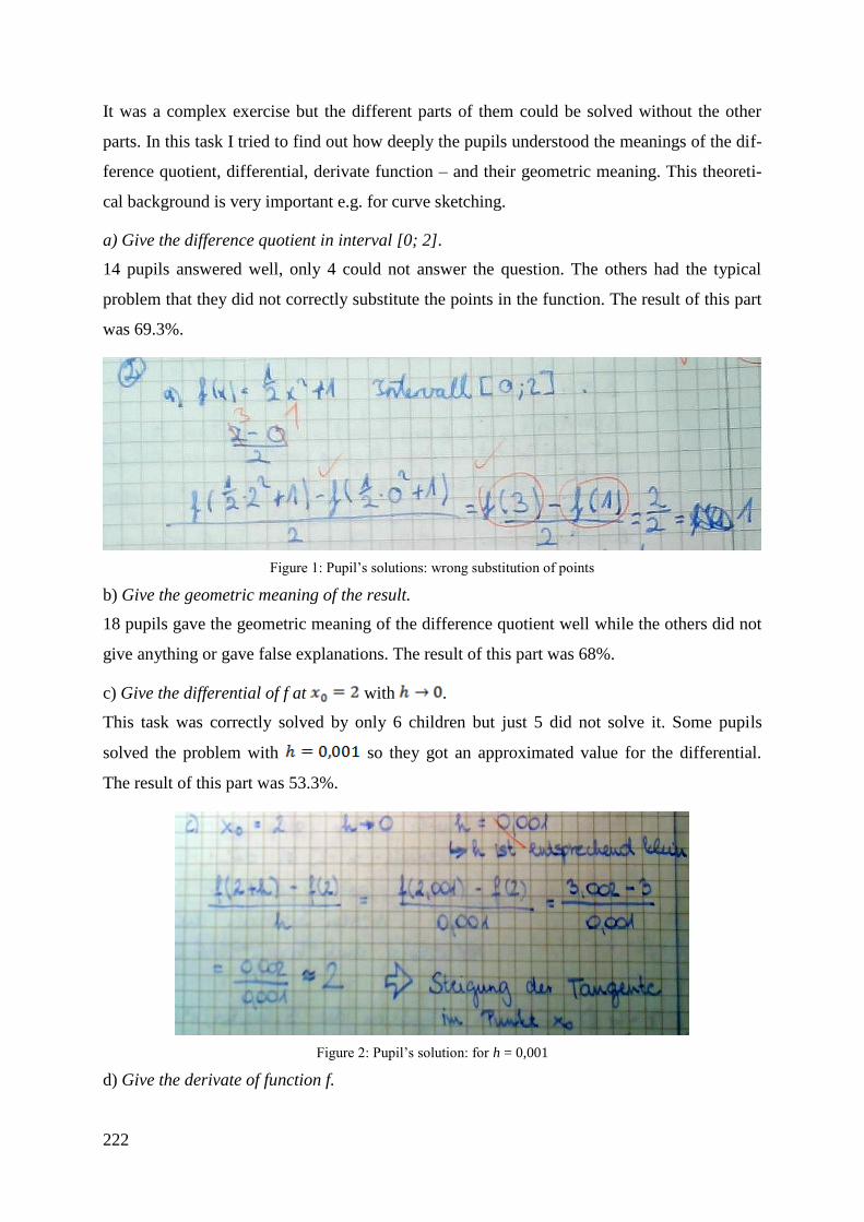
222
It was a complex exercise but the different parts of them could be solved without the other
parts. In this task I tried to find out how deeply the pupils understood the meanings of the dif-
ference quotient, differential, derivate function – and their geometric meaning. This theoreti-
cal background is very important e.g. for curve sketching.
a) Give the difference quotient in interval [0; 2].
14 pupils answered well, only 4 could not answer the question. The others had the typical
problem that they did not correctly substitute the points in the function. The result of this part
was 69.3%.
Figure 1: Pupil’s solutions: wrong substitution of points
b) Give the geometric meaning of the result.
18 pupils gave the geometric meaning of the difference quotient well while the others did not
give anything or gave false explanations. The result of this part was 68%.
c) Give the differential of f at with .
This task was correctly solved by only 6 children but just 5 did not solve it. Some pupils
solved the problem with so they got an approximated value for the differential.
The result of this part was 53.3%.
Figure 2: Pupil’s solution: for h = 0,001
d) Give the derivate of function f.

223
In this part it was interesting for me which method was chosen by pupils for giving the deri-
vate function. Two opportunities were given: 1. with definition of derivate function 2. with
derivate rules. Altogether 15 right solutions were given, and all of the pupils solved the prob-
lem with derivate rules. 3 children were not able to do it and the others made some mistakes.
The result of this part was 72%.
e) Give the geometric meaning of the result in c) .
17 pupils gave the geometric meaning of the difference quotient well; the others did not give
anything or gave false explanations. The result of this part was 68%.
3rd task:
See the function graph in interval and answer the questions.
It was important for me in this task that the pupils did not only know the theoretical geometric
meaning of the difference quotient, but they were able to apply it as well. If they could draw
the tangent line, they could give its slope approximately.
a) Give the intervals when the slope of the function (of the tangent line) is positive.
13 of them found all of the three intervals and only 3 could not find any. The others gave one
or two right intervals. The result of this part was 73.3%.
b) Arrange the slopes of the tangents at the points marked in a growing order.
14 pupils gave the right growing order for all points so they knew when the slope was positive
or negative, too. Only three pupils could not understand the exercise, the others solved the
problem partly right. The result of this part was 69%.
c) Draw the approximate tangent lines at the points B, C and D, and evaluate their slopes.
Seven pupils could draw the tangent lines correctly and could give their slopes too. Two chil-
dren drew only the tangent lines – without the slopes, and one of them could not begin this
part. The others made some mistakes. The result of this part was 71.3%.
4th task:
Couple the graphs of the functions (red) with the derivative functions (blue) and explain
shortly why just the specified pairs were chosen.
The first part of this task was the most successful of all parts in this test. All pupils began this
task and only two children made a little mistake. The result of this part was 95%. In the ex-
amination part there were some false pieces of information but except for two of them, pupils
could give partly correct interpretations. The result of this part was 78%.

224
In this first part of the test it was not allowed to use a graphing calculator. The result of this
part (A) was 71.1%. Here the pupils had to use the theoretical background of differential cal-
culus and they had to see the geometric meaning, too. In my opinion, they understood it well,
thus the result of this part was quite good.
In the second part it was necessary to use the GC.
Part B
5th task:
Give the derivative functions of the following functions, and calculate the slope at the
point . Suggestion: calculate the derivative function and the value function without a
GC, and then you can control it with a GC.
a)
In this part the derivate function was given by 21 pupils correctly. 4 children could not give it
nor with rules neither with a GC. The same happened with the substitution of , but one
of the 21 pupils calculated wrong. The results of this part were 82.7% and 80%.
Figure 3: Pupil’s solution with wrong substitutions
b)
In this exercise the parts of the function are more difficult than in a), consequently, the num-
ber of correct answers was lower. 15 pupils gave the correct derivate function and all of them
could calculate the substitution of 3. Unfortunately, 6 pupils could not begin this task.
The results of this part were 68% and 60%. In this task I could not recognise if the GC was
used for checking the derivate functions or for substitutions or not.
However, the GC was necessary for the solution of the next two tasks.
6th task:
Determine the tangent term of the function using GC:

225
at . Describe briefly how you proceeded. Sketch the function and the tangent line us-
ing the GC on the sheet.
Six pupils could not solve the first part, one child solved it with both methods: with a GC and
without a GC too, but he did not get the same term. The others solved it correctly, and the
other two questions they could answer correctly. It is interesting that one pupil who could not
solve the first part answered the other two questions correctly. The results of this part were
74.7% 76% and 85.3%.
Figure 4: Pupil’s and GC solution for tangent line
In plotting the function and its tangent line at the following result was proceeded .e.g.:
Figure 5: Pupil’s and GC plotting of tangent line
7th task:
Given the function .
a) Plot the function AND its derivative function with a GC, and sketch them appropriately on
the sheet.

226
In this exercise the pupils had to plot the functions graph and its derivate function with a GC.
The difficulty with their TI-nspire GC is that there is another way to calculate the derivate
function than to plot it. In the homework and in the lessons a few pupils always had problems
because of the different ways of calculation. Finally, only two children could not plot the
function correctly (92%), and two others could not either plot the derivate function (84%).
Figure 6: Pupil’s and GC plotting of function and derivate function
b) Explain briefly why the derivative function is just seen at the zero points, or why the de-
rivative function is only positive / negative where you see it.
In this part the pupils had to explain why the derivate function is such in the picture. These
descriptions were mostly correct by those who could plot both of them. There were just little
mistakes or inaccuracies. The result of part b) was 74.7%.
While I was writing the article we also discussed the topic of function analysis with the pu-
pils. During this chapter I strived to the above described methodological duality, which means
that we solved exercises partly with a GC and partly without it. The test for assessing this part
also showed this duality, and the results of the two parts were quite similar. In the last exer-
cise a word problem appeared here, where pupils not only had to solve the task with a GC, but
they also had to choose the calibration of the function window of the GC well, and they had to
answer and interpret the results based on the words of the exercise. Although this caused
smaller or bigger difficulties for a few pupils, I still think that compared to the opportunities
and the difficulty of the problem results were good:
The next function gives the profile of a landscape in interval [1; 7]. The value x is km, the
value of h(x) is 10 meters.
a) Sketch the function with GC and draw the curve on the sheet.
b) Calculate the maxima and minima of the landscape and their values with GC.
c) Give the intervals of increase and decrease.
The difficulties for some pupils were caused by the fact that the GC did not sketch the func-
tion in such an interval that would have been appropriate for them. First the division of the

227
axes should have been changed and then they would have been able to sketch it well (Figure
5). Those who did not do this got partly wrong solutions. Still, 18 pupils did the sketching
well, which I consider a very good result. The maxima, minima were well determined by all
the 18 pupils within the interval with the help of the calculator, but only eight of them paid at-
tention to examining the end points of the closed interval. Because of the above reasons, these
eight pupils determined the intervals of increase and decrease perfectly.
Figure 7: Sketching of functioning exercise 4 with intervals
Conclusions
The application of GCs in teaching is ambiguous. On the one hand, they provide help with
exercises that need a lot of calculation but have easy algorithms. Pupils use them with pleas-
ure, though the appropriate use of each application requires a lot of attention. On the other
hand, such exercises can be solved with the help of GCs the mathematical background of
which pupils know and are able to use, but with their familiar mathematical tools these tasks
are not, or only difficultly solvable.
However, we have to make sure that pupils are aware of the mathematical background as well
and that they are able to do the learned processes without a GC where possible, so as to avoid
the situation that I described in the introduction. I placed especially high emphasis on this idea
when planning the lessons, in homework and in assessment. In this test I tried to find balance
between theory and praxis and I wanted that pupils not only perfectly knew how to use a GC
but they were able to understand the theoretical background, too.
My research question was: “How much supportive can be a graphing calculator in problem
solving related to tangent line and the increase and decrease of functions?”
Pupils have to use GC in lot of problems in the curriculum of Germany. It is necessary to un-
derstand the meaning of tangent line and decrease of functions but without a lot of representa-
tions it is impossible. While the understanding of these mathematical concepts without GC is
possible but in my opinion the GC is very usefully during this work. The pupils could have
plotted the function of a mathematical problem; with the iconic representation of GC they
could have started it with the solution. They were able to reflect immediately when the solu-

228
tions are different with and without GC. During the lessons I was talking a lot with pupils
about the exercises and of course about using GC. According to the children’s opinion they
could have understood the problems of tangent line and slope of function better because they
immediately saw the representations of this with GC. Firstly they had problems with program-
ing the calculators but they had possibility to help each other and of course, I supported them,
too if nobody was able to solve the problem.
According to my opinion, these were the reasons why pupils could have written the test with
better results, what I had not hoped before: the average was in the theoretical part (Part A)
71.1%. In this part there were lots of questions about the meaning of tangent line and about
the slope of functions without GC. In the GC part (Part B) the result was 78% where the pu-
pils got questions, among others about the meaning of tangent line and the slope of functions.
Both of them are good rates in an average class and they are also balanced.
The tasks in the first part, where the pupils had to use the concept of the difference and differ-
ential quotient and the increase and decrease of a function, were:
2.
3.
6.
Average
a) b) c) d) e) a) b) c) a) b) c)
69,3 68 53,3 72 68 73,3 69 71,3 74,7 76 85,3 70,9%
However, the average of these tasks is a little bit lower than the average of the whole test but
the difference is not significant. This can represent that the pupils were able to understand the
theoretical background of the difference and differential quotient and the increase and de-
crease of a function as well.
Unfortunately in Hungarian public and tertiary education it is still forbidden to use graphing
calculators, which is regulated in the maturity examination system in the following way: „In
solving the problems, you are allowed to use a calculator that cannot store and display verbal
information. You are also allowed to use any book of four-digit data tables. The use of any
other electronic devices or printed or written material is forbidden.” Based on my research
experiences it would be desirable to introduce the use of GC-s in Hungarian secondary
schools too.
References
Abfalterer E.: Foren Wikis Weblogs und Chats im Unterricht, Fachverlag für Medientechnik
und –wirtschaft, p. 108 (2007)
Ambrus A.: Some Experiences with Graphing calculator in a Secondary School in Hungary.
In.: Proceedings of the seminar „Graphing calculators in High School Mathematics
Teaching and in Education of Mathematics Teachers“, MFF UK Prague. (1995)

229
Banikowks A.: Strategies to enhance memory based on brain-research. Focus on exceptional
children. 32(2). 1999.
Ben-Hur M.: Concept-Rich Mathematics Instruction Building a Strong Foundation for Rea-
soning and Problem Solving, Association for Supervision and Curriculum Development
(USA) (2006)
Dunham P. H.: Hand-held Calculators in Mathematics Education: A Research Perspective.
Hand-Held Technology in Mathematics and Science Education: A Collection of Papers.
The Ohio State University. (2000)
Haju S., Czeglédi I., Hajdu S., Kovács Z.: Matematika 11. évfolyam – Gondolkodnijó, p 76-
80. (2012)
Horton R. M., Storm J., Leonard W.H.: The graphing calculator as an aid to teaching algebra.
Contemporary Issues in Technology and Teacher Education [Online serial], 4(2). Avail-
able: http://www.citejournal.org/vol4/iss2/mathematics/article1.cfm(2004)
Jones, K.: Graphing calculators in the teaching and learning of mathematics: A research bibli-
ography, Micromath, 21(2), 31-33.(2005)
Kamarulhaili H, Sim, L, B: Graphing Calculator as a teaching and learning aid for secondary
school students and teachers. The 2nd
International Conference on Research and Educa-
tion in Mthematics (ICREM 2). (2005)
Leuders T.: Mathematikdidaktik - Praxishandbuchfür die Sekundarstufe I und II., Berlin:
Cornelsen. p.199 (2010)
Lichtenberg W.: EinsatzgraphikfähigerTaschenrechnerimgymnasialenMathematikunterricht
(1991-1996). LISA, Halle. (1997)
National Council of Teachers of Mathematics: Principles and standards for school mathemat-
ics. Reston, VA: Author.(2000)
Leng, N., Chuen, T., & Ng Meow Leng, N.: Teaching and Learning Calculus with the TI-
Nspire: A Design Experiment. Paper presented at the Asian Technology Conference in
Mathematics, Beijing, China. (2009).
Robova, J: Graphing calculator as a tool for enhancing the efficacy of mathematics teach-
ing.2nd International Conference on the Teaching of Mathematics. 2002
Ruthven, K.: The influence of graphing calculator use on translation from graphic to symbolic
forms. Educational Studies in Mathematics, 21, 431-450.(1990)
Smith, K. B., Shotsberger, P. G.: Assessing the use of graphing calculators in college algebra:
reflecting on dimensions of teaching and learning. School Science and Mathematics,
97(7), 368-373.(1997)
Tall, D. - Vinner, S.: Concept image and concept definition in mathematics with particular
reference to limits and continuity. Journal Educational Studies in Mathematics, 12 no. 2,
(1981)
Tiwari, T. K.: Computer graphics as an instructional aid in an introductory differential calcu-
lus course, International Electronic Journal of Mathematics Education, 2(1), 35-
48.(2007)
Tolias, G.: The effects of using graphing technology in college pre calculus. Dissertation Ab-
stracts International, 50(04), 1274A-1275A.(1993)

230
Tulodziecky G.: Handlungs- und entwicklungsorientierte Medienpädagogiktheoretische
Grundlagen, Umsetzung und Forschung. In W. Sesnik, M. Kerres, & H. Moser, Jahr-
buch Medienpädagogik 6. Wiesbaden: Verlag für Sozialwissenschaften. p. 110 – 111.
(2007)
VanStreun, A., Harskamp, E. &Suhre, C.: The effect of the graphing calculator on students’
solution approaches: A secondary analysis, Hiroshima Journal of Mathematics Educa-
tion, 8, 27-39. (2000)
Annex
The detailed results of the test (1)
A♥ A♣ A♣ B♥ B♣ B ♥ ♣ AB
1. thesis 1 100,0 85,7 91,7 85,7 66,7 76,9 91,7 85,7 84,0
proof 3 66,7 42,9 52,8 38,1 44,4 41,0 50,0 43,6 46,7
2. a) 3 100,0 76,2 86,1 47,6 61,1 53,8 69,4 69,2 69,3
b) 1 80,0 57,1 66,7 71,4 66,7 69,2 75,0 61,5 68,0
c) 3 60,0 47,6 52,8 57,1 50,0 53,8 58,3 48,7 53,3
d) 2 90,0 71,4 79,2 64,3 66,7 65,4 75,0 69,2 72,0
e) 1 60,0 57,1 58,3 71,4 83,3 76,9 66,7 69,2 68,0
3. a) 3 73,3 76,2 75,0 71,4 72,2 71,8 72,2 74,4 73,3
b) 4 70,0 57,1 62,5 75,0 75,0 75,0 72,9 65,4 69,0
c) 3 76,7 66,7 70,8 66,7 77,8 71,8 70,8 71,8 71,3
4. a) 4 100,0 82,1 89,6 100,0 100,0 100,0 100,0 90,4 95,0
b) 4 100,0 71,4 83,3 71,4 75,0 73,1 83,3 73,1 78,0
5. a1) 3 100,0 85,7 91,7 71,4 77,8 74,4 83,3 82,1 82,7
a2) 2 100,0 71,4 83,3 71,4 83,3 76,9 83,3 76,9 80,0
b1) 4 100,0 57,1 75,0 57,1 66,7 61,5 75,0 61,5 68,0
b2) 2 100,0 57,1 75,0 42,9 50,0 46,2 66,7 53,8 60,0
6. a) 3 80,0 85,7 83,3 81,0 50,0 66,7 80,6 69,2 74,7
b) 2 100,0 85,7 91,7 71,4 50,0 61,5 83,3 69,2 76,0
c) 3 93,3 85,7 88,9 76,2 88,9 82,1 83,3 87,2 85,3
7. a1) 3 100,0 85,7 91,7 100,0 83,3 92,3 100,0 84,6 92,0
a2) 3 100,0 57,1 75,0 100,0 83,3 92,3 100,0 69,2 84,0
b) 3 100,0 66,7 80,6 61,9 77,8 69,2 77,8 71,8 74,7
Sum: 60 53,5 41,7 46,6 42,6 42,8 42,7 47,1 42,2 44,6
Average of
part 1
32 82,2 66,1 72,8 68,3 70,8 69,5 74,1 68,3 71,1
Average of
part 2
28 97,1 73,5 83,3 74,0 72,0 73,1 83,6 72,8 78,0
Average 89,2 69,5 77,7 71,0 71,4 71,2 78,5 70,4 74,3

231
The detailed results of the test (2)

232
The Role of affective Components in mathematical Problem Solving
Bernd Zimmerman
Friedrich-Schiller-University of Jena, Germany
Abstract
This paper is based on the dissertation „Analyzing problem solving processes in-
volved in problems from incidence-geometry“. First we give a summary of the
goals, design and results of this work. We focus on the part of affective behavior
which was analyzed too, but has not been published until now. The main affects
which were detected in videotaped think-aloud sessions were reactions of the sub-
jects which were interpreted as feelings close to the goal, reactions which were in-
terpreted as feelings distant from the goal and reactions which could not inter-
preted clearly (hesitations).
Keywords: problem solving, problem solving processes, affect, incidence geometry, category
systems, sequence-analysis
ZDM-classification: C 34, C 24, D 54, E 45
Introduction
While empirical studies on the cognitive aspect of mathematical problem solving have already
a long tradition (cf. e.g. Duncker 19, Wertheimer 1945), the affective aspect of problem solv-
ing seemed to be neglected for sometime (Silver 1985, 254). This component gained increas-
ing attendance during the last years (cf., e.g., Goldin/Hannula 2013). For that reason we de-
cided to present some results, which had been gained in connection with a PhD study (Zim-
mermann 1977), but had not been published until now. It might contribute to the present dis-
cussion of this issue.
First a summary of the foregoing study will be presented to highlight the background (includ-
ing the theoretical one) of that specific part we publish here for the first time.
Background
An exploratory study of mathematical problem solving processes was carried out with student
teachers and some pupils from the upper grade of a gymnasium (n = 22; cf. Zimmermann
1977). Starting points were - except the well-known books of Pólya - the habilitations of the
cognitive psychologists Lüer 1973 and Dörner 1974, who analyzed think aloud protocols

from students, who solved problems from the “Principia Mathematics” (Whithead/Russel
1964). One outcome was a “fundamental rhythm of thinking”. Our original question was:
What could be the specific role of different representations (esp. of perception; cf. Bruner
1966) during problem-solving processes? As we started this study in 1973, it was still the time
of “New Maths” and “Boubakism”. So logic, formalism and abstract structures were still
dominating the discussion in mathematics education of that days (as it is still up to date in
mathematics university teaching, especially in eastern European states). The logical problems
fit into this environment. We decided therefore to take problems from the domain of inci-
dence geometry. Besides logical inferences being also involved, there was the advantage, that
different representations of “lines”1 and “points” might have some impact on problem solving
processes. Two questions evolved: 1. Could we observe a similar fundamental rhythm of
thinking as Lüer/Dörner? 2. What would be the role of perception in this case?
The theoretical background was set up by the “information processing approach” mainly (cf.
e. g. Newell/Simon 1972 and Klix 1971).
Main results were as follows:
A classification system of mathematical problems referring to
o formal (what is the problem?),
o personal (for whom it is a problem?) and
o normative (who is posing the problem?) aspects.
A method to construct categories for describing problem solving processes in a very flexi-
ble way.
A method for analyzing sequences of action which occurred more often than it could be
expected by random.
Following hypotheses were generated:
o There is a fundamental rhythm “weaker” than that found by Lüer.
o Higher achievers solve problems in a more systematic way.
o There is no difference between males and females in this context.
o Reflective thinking (metacognition) has a positive effect on problem solving suc-
cess.
1 Experience in a pilot study proved that students’ intuitive perception of “lines” hampered their concentration on
the logical content of the axioms. E. g. it was very hard for the students to prove by referring to the axioms only,
that if a line intersects one of two parallel lines, then it will intersect also the second one. As to their intuitive ex-
perience, this is a complete obvious fact, where nothing is to be proved. This “functional fixedness” to percep-
tion was loosened to some extent, when we replaced “lines” by “curves”. In this way changes between different
representations (writing, drawing, and “laying” by wool-threads) were facilitated.

234
o Possible reasons for changes of representations are systematical one, critical situa-
tions, notations of ideas for possible solutions, writing down the result of a thought
process.
o There are two types of problem solving types: an iconic and an enactive one. The
former represents objects by drawings, is more reflective, systematic, refers less to
own writings and is a little bit more successful while the latter represents curves
only by threads and points by rings, is impulsive, less systematic, refers more to
own writings and is a little bit less successful.
We sketch now the problem domain of incidence geometry, to give some ideas about the
mathematical content:
The subjects had to do their proofs by referring to the following Axioms exclusively:
(1) Exactly one curve passes through two points
(2) Parallel-axiom
(3) Existence of at least 3 points not all on the same curve.
They had to prove three theorems as follows:
Theorem: There exist at least 4 different points, from which no 3 points are located on the
same curve.
More details can be also found in Zimmermann 1980, 1982.
Goal of the study
What is the role of affective behavior when solving problems from incidence geometry?
Method
We used the following three categories concerning affect:
Affective expressions of feeling closer to a solution of the problem were detected by reactions
of the subject like:
being motivated (“now I am on the right track!”)
praising her/himself
being positive surprised (aha-experience)
expressing (subjective) idea of solution
Affective expressions of feeling more distant from a solution of the problem were detected by
reactions like being insecure, helpless, depressed, aggressive or embarrassed
Finally, there we observed hesitations which could not be attributed clearly to such feelings.

The problem solving sessions were videotaped and - using this and the comprehensive and
very flexible category-system - written protocols were created.
The protocols had the following structure (X denots different arbitrary actions):
Table 1. Parallel sequences of actions referring to different foci. After setting priorities, these were “compressed”
into one (shaded) sequence to be analyzed
When transcribing the videotapes, we looked for twelve different aspects where we noted ac-
tions (from left to right) which could also happen simultaneously. We came from one “mo-
ment” (micro-episode) to the next, if at least one activity in the very column changed (average
time for one such “moment”: about 20 seconds). After transcribing all videotapes of all ses-
sions, we made a validity check by two additional researchers (Prof. Hefendehl and Prof.
Bedürftig). The rate of correspondence was between 70% and 80%.
Because we were interested in specific actions (e.g., solution ideas, mistakes, but especially
now: affective behavior) and possible reasons and consequences of their occurrence, we made

236
a sequence analysis of their “pre-“ and “post-history”, i. e. we formed single sequences of ac-
tions were we looked for sequences of two up to 5 consecutive actions (including the specific
one), which occurred more often than it could be expected by random.
To form one out of twelve sequences, we implemented all protocols into a computer and put
all protocols of all subjects together to a “super-protocol”. Then, we started with the line “ver-
bal”, because this proved to be the most objective and reliable information, set priorities and
substituted all actions in “verbal” by actions of the other lines, if they had a higher priority.
In case of occurrence in the same line, content of a cell in the first line (“verbal”) was to be
replaced in the given order by (cf. Table 1)
(1) Affective behavior
(2) (objective) solution idea (if there is no (1) in the same column)
(3) Change of representation (if there is neither (1) nor (2) in the same column; writing (w),
drawing (d), manipulating (m))
(4) Reference to writing, drawing, manipulating (no (1, 2, 3) in the same column).
After this process was finished, we analyzed new single sequences, created in this way, like
(real sequences were much longer):
… verbal ut-
terances: close obj. idea drawing ref. draw. X …
Table 2. Super-sequences of actions to be analyzed, including expressions of affective behavior and other actions
of high priorities
Of course, other substitutions by other priorities are possible.
First we detected the absolute and relative number of all such actions with respect to the total
number of all “micro-episodes” of all subjects. The computer detected 4477 actions, corre-
sponding to a little bit more than on average one hour of problem solving time of every subject.
Action Frequency abs. (total 4477) Frequency rel. %
affective
behavior
Close 273 6.1
Distant 252 5.6
Hesitating 381 8.5
(objective) idea 115 1.5
writing 192 4.2
drawing 112 2.5
manipulating 46 1.0
reference to writing 147 3.2
reference to drawing 243 5.4
reference to manipulating 25 0.6
Table 3. Absolute and relative frequencies of affective actions and others of high priority

For carrying out the sequence-analysis, we estimated the probability of each action by its
relative frequency. Assuming random distribution and independence of the variables, the
probability of the occurrence of the sequence of the three consecutive actions
closeideadrawing (cid) can be estimated by P(cid) = 0.061*0.015*0.025=0.000024.
We checked now by binomial-test, which of all such 3-sequences (n=4357) occurred more of-
ten than it could be expected by random. Taking into account the accumulation of the error
probability when applying such test repeatedly, we set the error-probability for a single test
p=0.00001, to get an error probability for all tests of =1-(1-0.00001)4357
0.04.
Results
The results for all significant sequences with three actions, containing “feeling close” to the
goal, are as follows:
Frequency ab-
solute Action 1 Action 2 Action 3
20 reading/interpreting text close reading/interpreting
text
7 writing close ref. to written
6 referring to written writing close
3 idea close intention to write
2 intention to write ref. to written close
2 I feel close close I go for goal
2 referring to written close new start
2 intention to write ref. to written close
2 short break idea close
46 total 1%
Table 4. All significant sequences of three consecutive actions which include “feeling close to the goal”
(abs. fr. 2; 0.04)
We can see that the feeling of being “close to the goal” seems to be mainly related with read-
ing, writing or referring to text.
The results for all significant sequences with three actions, containing “feeling distant” from
the goal, are the following:

238
Frequency ab-
solute Action 1 Action 2 Action 3
9 reading/interpreting
text distant
intervention
7 distant intervention distant
7 intervention distant intervention
6 referring to drawing intervention distant
4 short break reading/interpreting text distant
2 distant intervention checking goal-
distance
2 distant intends to search an “oper-
ator”
operator not appro-
priate
Total 37 0.8%
Table 5. All significant sequences of three consecutive actions which include “feeling distant from the goal”
(abs. fr. 2; 0.04)
There is the impression that “feeling distant from the goal” is mainly related to interventions
of the observer of the problem solving session, whose only task was to keep the subjects
thinking aloud. So it seems plausible that in situations where the subject feels stuck, the leader
of the session has to motivate to continue to talk. Furthermore; referring to (given) text draw-
ings seem to be also somewhat tied to this feeling of distant.
The “local context” of “hesitation” was as follows:
Frequency
absolute Action 1 Action 2 Action 3
19 reading/interpreting
text hesitating reading/interpreting
text
15 reading/interpreting ac-
tual problem hesitating reading/interpreting ac-
tual problem
4 hesitating reading/interpreting the
actual problem checking goal-distance
2 memorizing text hesitating constructing connec-
tions
2 intends to draw hesitating drawing
2 checking goal-distance hesitating makes additional as-
sumption
Total 44 1%
Table 6. All significant sequences of three consecutive actions which include “hesitating”
(abs. fr. 2; 0.04)

“Hesitating” seems to occur mainly in situations where the subjects is reading or interpreting
text, especially that of the actual problem. This might be interpreted as attempt to understand
better important “givens”. Also the other significant sequences might express somewhat inse-
curity or attempts to compare the very status with requirements still to be fulfilled.
We carried out additional tests with sequences of 4 consecutive actions, including at least one
of these three feelings. But we gained not new insight, as can be see form Table 7:
Frequency
absolute Action 1 Action 2 Action 3 Action 4
11 reading/interpreting
text (prob.) hesitating reading/interpreting
text hesitating
6 reading/interpreting
text (prob.)
break reading/interpreting
text distant
3 referring to drawing reading/interpreting
text hesitating
distant
3 operator not appro-
priate
reading/interpreting
text
referring to drawing close
3 referring to written writing close referring
to written
Abs. frequ. 3; total 26 0.6%
Table 7. All significant sequences of four consecutive actions which include “close”, “distant” and “hesitating”
(abs. fr. 3; 0.04)
Summary
All registered affects were mainly connected with reading and interpreting text.
Positive affects were additionally related to own productions.
Hesitation and negative affects were sometimes additionally related to reference to draw-
ings.
Discussion
Appropriate reading- and writing competences (cf. PISA-outcomes) seem to be important
also in this “classical” domain.
The type of problems was quite normal at that time - it was the time of “New Maths” also
at school. Incidence geometry is still a usual esp. at university-curriculum, esp. in Eastern
Europe.
The normal habit of trusting your perception and the formal, axiomatic approach, required
here, were often conflicting.
The methodology presented here can be applied also in settings of today.

240
References:
Bruner, J. S. 1966. Toward a Theory of Instruction, Cambridge, Mass.: Belkapp Press.
Dörner, D. 1974. Die kognitive Organisation beim Problemlösen (Cognitive organization in
problem solving). Versuche zu einer kybernetischen Theorie der elementaren Informa-
tionsverarbeitungsprozesse beim Denken. Bern-Stuttgart-Wien: Huber.
Duncker, K. 1974³. Zur Psychologie des produktiven Denkens. (Psychology of Productive
Thinking). Dritter Neudruck von 1935. New York, Berlin, Heidelberg: Springer.
Goldin, G. A.; Hannula, M. S. 2013. Emotions in the psychology of mathematics teaching and
learning. In: Lindmeier, A. M. & Heinze, A. (Eds.). Proceedings of the 37th Conference
of the International Group for the Psychology of Mathematics Education, Vol. 1, p.
216. Kiel, Germany: PME.
Klix, F. 1971. Information und Verhalten. Bern-Stuttgart-Wien: Huber.
Lüer, Gerd 1973. Gesetzmäßige Denkabläufe beim Problemlösen. (Regular patterns of
thought processes in problem solving). Habilitation. Beltz: Weinheim und Basel.
Newell, A.; Simon, H. A. 1972. Human Problem Solving. Englewood Cliffs: Prentice Hall.
Silver, E. A. 1985. Research on Teaching Mathematical Problem Solving: Some underrepre-
sented Themes and Directions. In: Silver, E. A. (ed. 1985): Teaching and Learning
Mathematical Problem Solving: Multiple Research Perspectives. Hillsdale: Lawrence
Erlbaum Associates.
Wertheimer, M. 1945. Productive Thinking. New York: Harper.
Whitehead, A. N.; Russel, B. 1964. Principia Mathematica. London, Ibadan, New York:
Cambridge University Press.
Zimmermann, B. 1977. Analyse von Problemlöseprozessen bei Aufgaben aus der Inzidenzge-
ometrie. Paderborn: Dissertation.
Zimmermann, B. 1980. Analyzing Problem Solving Processes involved with Problems from
Incidence Geometry - An Exploratory Study. ERIC No. ED 191 685, Columbus, Ohio.
Zimmermann, B. 1982. Denkprozesse beim Lösen mathematischer Deduktionsaufgaben - Be-
richt über eine exploratorische Untersuchung. In: Journal für Mathematikdidaktik 3/4,
175 - 206.