Target Tracking for Multistatic Radar with TransmitterUncertainty∗

Sora Choi, Christian R. Berger, David Crouse, Peter Willett, and Shengli ZhouECE Department, U-2157, University of Connecticut, Storrs CT 06269†

ABSTRACT

We present a target tracking system for a specific sort of passive radar, that using a Digital Audio/VideoBroadcast (DAB/DVB) network for illuminators of opportunity. The system can measure bi-static range andrange-rate. Angular information is assumed here unavailable. The DAB/DVB network operates in a singlefrequency mode; this means the same data stream is broadcast from multiple senders in the same frequencyband. This supplies multiple measurements of each target using just one receiver, but introduces an additionalambiguity, as the signals from each sender are indistinguishable. This leads to a significant data associationproblem: as well as the usual target/measurement uncertainty there is additional “list” of illuminators that mustbe contended with.

Our intention is to provide tracks directly in the geographic space, as opposed to a two-step procedure offormation of tracks in (bi-static) range and range-rate space to fuse these onto a map. We offer two solutions:one employing joint probabilistic data association (JPDA) based on an Extended Kalman Filter (EKF), and theother a particle filter. For the former, we explain a “super-target” approach to bring what might otherwise bea three-dimensional assignment list down to the two dimensions the JPDAF needs. The latter approach wouldseem prohibitive in computation even with these; as such, we discuss the use of a PMHT-like measurement modelthat greatly reduces the numerical load.

1. INTRODUCTION

Passive radar is a bi-static system [5] that uses illuminators of opportunity to detect and track airborne targets.In a bi-static radar, sender and receiver are not co-located; in passive radar radio or television stations take theplace of the sender and only the receiver is under control. Our interest is on a target tracking system usingpassive radar with digital broadcast signals: Digital Audio/Video Broadcast (DAB/DVB) [6,15].

It is important to recognize the difference between passive radar using DAB/DVB versus more traditionalsystems using, for example, commercial FM stations [12] or television [13]. In the traditional case the receiverobserves a “direct blast” of signal followed by replicas representing reflections of the signal off whatever targets(and clutter) may be in the scene. Detection of these replicas is difficult because:

• The observations process is continuous in time: there is no “pulse” or “scan” concept as one might find ina traditional surveillance system.

• It is tempting to use the “direct” signal as a matched filter, to correlate for potential replicas. However,the signal contains both noise and reflections from the same targets at earlier times: the “known” signalin the matched filter is actually not known.

• The reflections are themselves corrupted by the in-band direct-blast signal which is, essentially, noise. Thatis, the signal to noise ratio (SNR) is necessarily strongly negative.

On the other hand, the DAB/DVB signals that we are interested in are orthogonal frequency-division multiplexed(OFDM). OFDM signals are relatively long packets of digital signals (actually, each amongst a large set of severalhundred sinusoids modulates its own digital signature) and the target-reflection replicas are generally of a delaythat falls well within the packet’s duration. That is, in contrast to the traditional case:

∗This work was supported by the US Office of Naval Research under contract N00014-09-10613.†Contact: willett@engr.uconn.edu.

• Each packet (or group of packets if information integration becomes necessary) gives rise to a “scan” ofpassive radar “hits.”

• Since digital waveforms can be exactly demodulated essentially without error (television and radio wouldnot work, otherwise) there is no concern about a dirty matched-filter template.

• The reflections from targets can be thought of as forming the digital channel’s “impulse response” ratherin the same way as multipath propagation would. From the perspective of OFDM these are a nuisance,but one that is easy to observe in the frequency domain as a predictable phase shift per carrier. That is,target reflections come for free as part of the OFDM demodulation process.

Actually, a receiver in the OFDM-based DAB/DVB system would be able to “hear” several transmitters: thenearest, but also some others more distant. In some modulation schemes (as cellular telephony) this would beundesirable interference, and is avoided (in the cell case) by a re-use pattern of frequencies that avoids adjacentcells utilizing on the same bands. However, in OFDM as part of what one might think of as the equalizationprocess the multiple transmissions become essentially overlaid, and, remarkably, actually enhance the SNR [18].The European system is an almost perfect match to surveillance needs, and might ultimately be considered asdeployable, in force-projection situations. The domestic (US) system uses 8VSB [19], and although there areadvantages versus analog transmission, the benefits to surveillance are less clear.

A passive radar can be covert, but the primary advantages in a non-hostile situation (where television andradio stations are available and working) are of cost and ubiquity: receivers are comparatively cheap, andwith enough of them an air picture of considerable accuracy can be made available. But there are challenges,and here we shall focus on two of them. One is the measurements: The current receiver can give bi-staticrange and range-rate, but no angular measurements or only measurements of poor accuracy. Bi-static range byone illuminator indicates an ellipse on which target lies. Range-rate is dependent on location and velocity oftarget based on geometry of illuminator and receiver. Without angular information, to decide the location oftarget we need at least three illuminators. Coupled to this, another challenge is the unknown data associationbetween measurements and illuminators. DAB/DVB operates in a so-called single frequency network (SFN) thatintroduces ambiguity: uncertainty of association between illuminator and signal.

To address this challenge in passive radar, recent work has tried to extract additional features [11]. Theyproposed the use of the radar cross section (RCS). On the other hand, estimation of the trajectory in onlyrange and range-rate has been suggested. One approach is target tracking based on the probability hypothesisdensity (PHD) [16]. Another approach uses a multi-stage Multi Hypothesis Tracking (MHT) as the solution forremoving ghosts [8], and track initiation is incorporated in [3]. Estimation of the geo-trajectory is considerablymore involved: one approach is to track in range and range-rate, and to fuse the resultant tracks. Our desire,however, is a direct geo-coordinate estimation algorithm, and we present two of these in this manuscript.

The first is a JPDA/EKF. Considering the uncertainty of association between sender and signal, it becomesa 3-D association problem between measurements, targets, and illuminators. Three dimensional associationimplies high complexity and does not match the JPDAF model. To avoid it we will introduce the concept of a“super-target,” whereby 3-D association can be recast as 2-D association.

The second is a particle filter. However, multi-target tracking in with particle filters is difficult due to dataassociation: we need to calculate particles’ likelihoods, and in order to do this under the usual target trackingmodel we must consider all possible 3-D assignment tables from the target/measurement/illuminator lists. Thatis, of course, possible, but the numerical load is unattractive. Consequently here data association is simplifiedby choosing the measurement model used in probabilistic multiple hypothesis tracking (PMHT). To the PMHT,each measurement’s assignment is independent of all other measurements. In our problem, then, each delay cancome from any illuminator/target (or false-alarm) pair; and the event that all measurements from the same pairis not impossible. In a sense, there is no concept of a “scan” and it is a perfectly valid PMHT implementation toupdate separately using each measurement, one at a time; but for us, the feature is that the particles’ likelihoodsmultiply across measurements.

Our manuscript is structured as follow. Section 2 establishes the model. The JPDA/EKF is describedwith simulation results in Section 3. In Section 4 we apply the PMHT-like particle filter to our problem withsimulation results. We compare the two filters in Section 5, and summarize in Section 6.

2. SCENARIO

There are several senders at x(i)s = (xs, ys) for i = 1, · · · , Ns and only one receiver located at xr = (xr, yr). The

receiver can measure range γ(t) and range rate γ(t). If the target is located at p(t) = (x(t), y(t)) with velocityv(t) = (x(t), y(t)), the state x(k) of the target is (x(t), x(t), y(t), y(t)). Then,

γ(x(t),x(i)s ) = ||p(t)− xr||+ ||p(t)− x(i)

s || (1)

γ(x(t),x(i)s ) =

(p(t)− xr)T · v(t)||p(t)− xr|| +

(p(t)− x(i)s )T · v(t)

||p(t)− x(i)s ||

. (2)

We use the typical discrete dynamic system [2], described by

x(k) = F(k)x(k − 1) + ν(k). (3)

in which ν(k) is the sequence of zero-mean white Gaussian process noise with covariance Q(k). Although a linearplant is considered in this paper, it can be easily extended to nonlinear.

The measurements at the receiver are delay and Doppler, so the observations model function h(x(k),xs) is

h(x(k),xs) = [γ(x(k),xs), γ(x(k),xs)]T . (4)

Hence, the measurement equation is described by

z(k) = h(x(k),x(i)s ) + ω(k) (5)

with ω(k) being a sequence of zero-mean white Gaussian measurement noises with covariance R(k).

As a reference for evaluation, the Cramer-Rao Lower bound (CRLB) of measurements based on range andrange-rate for single time is considered, and is useful to identify illuminator/receiver/target geometries thatare difficult. While the estimate at each time is using the previous estimated results, the measurement CRLB(MCRLB) does not reflect previous measurements, association, missed detections nor clutter and may not matchclosely the tracking performance. The likelihood function is

Λ(x) =Ns∏

i=1

12πR

exp(−1

2(z− h(x,x(i)

s ))T R−1(z− h(x,x(i)s ))

)(6)

The Fisher Information matrix, the inverse of the CRLB, is the following:

F = E[∇x lnΛ · ∇x ln Λ′] (7)

=Ns∑

i=1

∇xh(x,x(i)s )R−1∇xh(x,x(i)

s )′ (8)

in which

∇xh =

[∂γ(x,x(i)

s )∂x

∂γ(x,x(i)s )

∂x

](9)

and

∂γ

∂p=

p− x(i)s

||p− x(i)s ||

+p− xr

||p− xr|| (10)

∂γ

∂v= 0 (11)

∂γ

∂p=

(p− x(i)s ) · (v · (p− x(i)

s ))

||p− x(i)s ||3

+(p− xr) · (v · (p− xr))

||p− xr||3 (12)

∂γ

∂v=

p− x(i)s

||p− x(i)s ||

+p− xr

||p− xr|| (13)

where v = (−y(t), x(t)) and p = (y(t),−x(t)).

3. JOINT PROBABILISTIC DATA ASSOCIATION VIA SUPER-TARGETS

3.1 The Algorithm

The usual JPDA is based on measurement-to-target association probabilities (the “β’s) but does not considerilluminators as the association is assumed to be known. After introducing the general JPDA, we will extend theJPDA to incorporate an illuminator association list.

The basic assumptions of the JPDA [1] are the following:

1. The number of target is known.

2. One measurement is associated with at most one target

3. Every measurement is independent on each other.

Let us consider just measurement-to-target association. Association events show how all measurements arerelated to targets (and clutter, usually the 0th target). These events are winnowed via validation gates: If theevent are feasible by gating, the event is chosen. Those events θ = [θjt] can be expressed by event matrix: If ameasurement j and a target t including clutter is associated, the entry θjt is 1, else 0. Based on feasible events,joint association event probabilities are calculated, and from these the marginal association probability for eachmeasurement and each target can be derived.

In our scenario, one more association list – illuminators – is required, and thus 3-dimensional associationevents need to be generated. However, if the probability of clutter does not vary with illuminator, 3-dimensionalassociation is unnecessary. Let us consider a pair, of a target plus an illuminator, as a “super-target”. If wehave three illuminators, then for each target there are three super-targets. By increasing the number of targets,3-D association can be recast as 2-D. Note that the first of the two JPDA assumptions are satisfied under thisformulation. The third is not: If three measurements come from one target via three different illuminators, thosemeasurements cannot be independent.

In a feasible joint association events θ, θjt expresses association between a super-target t and measurementj. The marginal association probability of each measurement and target is

βjt , P{θjt|Zk} =∑

θ:θjt=1

P (θ|Zk) (14)

Let M(k) be the number of measurements in the validation region at time k and Zk the set of measurements upto and including time k. By Bayes’ rule the joint association event probabilities P{θ(k)|Zk} are

P{θ(k)|Zk} =1cP{Z(k)|θ(k),M(k), Zk−1}P{θ(k)|M(k)} (15)

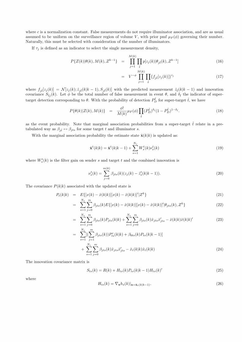
where c is a normalization constant. False measurements do not require illuminator association, and are as usualassumed to be uniform on the surveillance region of volume V , with prior pmf µF (φ) governing their number.Naturally, this must be selected with consideration of the number of illuminators.

If τj is defined as an indicator to select the single measurement density,

P{Z(k)|θ(k), M(k), Zk−1} =M(k)∏

j=1

∏

t

p[zj(k)|θjt(k), Zk−1] (16)

= V −φ

M(k)∏

j=1

∏

t

{fjt[zj(k)]}τj (17)

where fjt[zj(k)] = N [zj(k); zjt(k|k − 1), Sjt(k)] with the predicted measurement zt(k|k − 1) and innovationcovariance Stj(k). Let φ be the total number of false measurement in event θ, and δt the indicator of super-target detection corresponding to θ. With the probability of detection P t

D for super-target t, we have

P{θ(k)|Z(k),M(k)} =φ!

M(k)µF (φ)

∏

t

(P tD)δt(1− P t

D)1−δt . (18)

as the event probability. Note that marginal association probabilities from a super-target t relate in a pre-tabulated way as βjt ↔ βjts for some target t and illuminator s.

With the marginal association probability the estimate state x(k|k) is updated as:

xt(k|k) = xt(k|k − 1) +Ns∑s=1

W ts(k)νt

s(k) (19)

where W ts(k) is the filter gain on sender s and target t and the combined innovation is

νts(k) =

m(k)∑

j=0

βjts(k)(zj(k)− zts(k|k − 1)). (20)

The covariance P (k|k) associated with the updated state is

Pt(k|k) = E{[x(k)− x(k|k)][x(k)− x(k|k)]′|Zk} (21)

=Ns∑s=1

m∑

j=0

βjts(k)E{[x(k)− x(k|k)][x(k)− x(k|k)]′|θjts(k), Zk} (22)

=Ns∑s=1

m∑

j=0

βjts(k)Pjts(k|k) +Ns∑s=1

m∑

j=0

βjts(k)xjtsx′jts − x(k|k)x(k|k)′ (23)

=Ns∑s=1

[(m∑

j=1

βjts(k))P cts(k|k) + β0ts(k)Pts(k|k − 1)]

+Ns∑s=1

m∑

j=0

βjts(k)xjtsx′jts − xt(k|k)xt(k|k) (24)

The innovation covariance matrix is

Sts(k) = R(k) + Hts(k)Pts(k|k − 1)Hts(k)′ (25)

whereHts(k) = ∇xhs(k)|x=xt(k|k−1). (26)

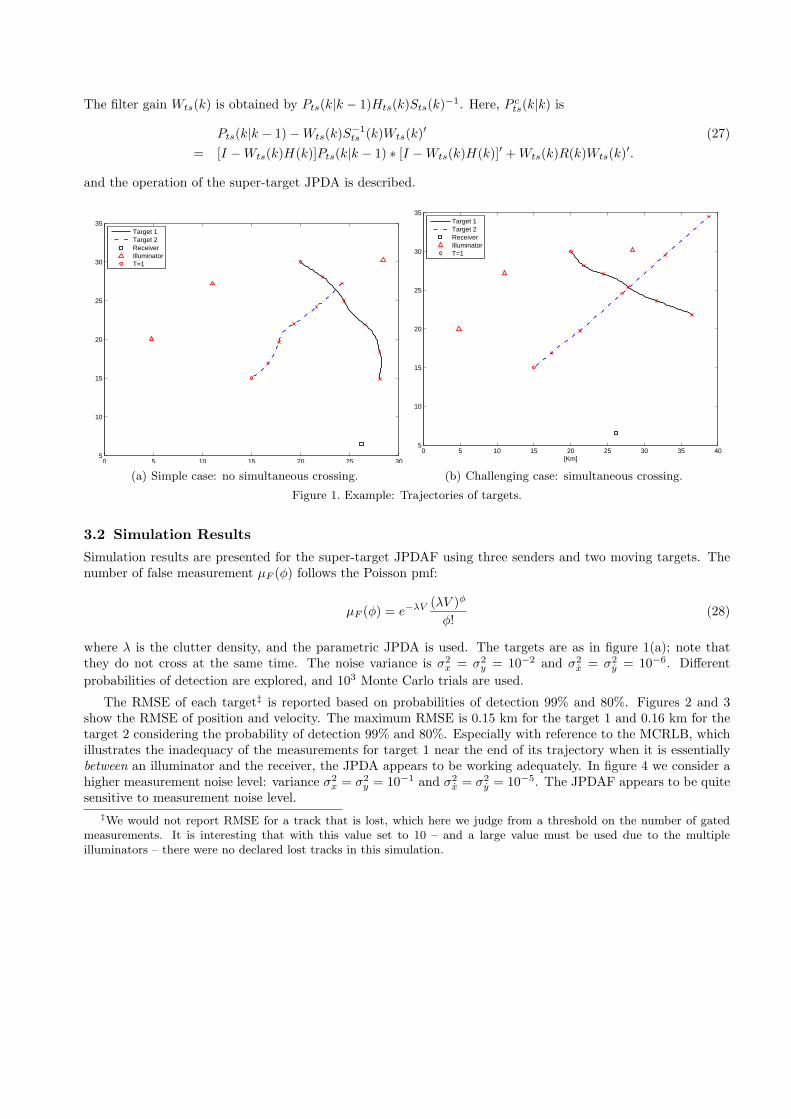
The filter gain Wts(k) is obtained by Pts(k|k − 1)Hts(k)Sts(k)−1. Here, P cts(k|k) is

Pts(k|k − 1)−Wts(k)S−1ts (k)Wts(k)′ (27)

= [I −Wts(k)H(k)]Pts(k|k − 1) ∗ [I −Wts(k)H(k)]′ + Wts(k)R(k)Wts(k)′.

and the operation of the super-target JPDA is described.

0 5 10 15 20 25 305

10

15

20

25

30

35

Target 1Target 2ReceiverIlluminatorT=1

(a) Simple case: no simultaneous crossing.

0 5 10 15 20 25 30 35 405

10

15

20

25

30

35

[Km]

Target 1Target 2ReceiverIlluminatorT=1

(b) Challenging case: simultaneous crossing.

Figure 1. Example: Trajectories of targets.

3.2 Simulation Results

Simulation results are presented for the super-target JPDAF using three senders and two moving targets. Thenumber of false measurement µF (φ) follows the Poisson pmf:

µF (φ) = e−λV (λV )φ

φ!(28)

where λ is the clutter density, and the parametric JPDA is used. The targets are as in figure 1(a); note thatthey do not cross at the same time. The noise variance is σ2

x = σ2y = 10−2 and σ2

x = σ2y = 10−6. Different

probabilities of detection are explored, and 103 Monte Carlo trials are used.

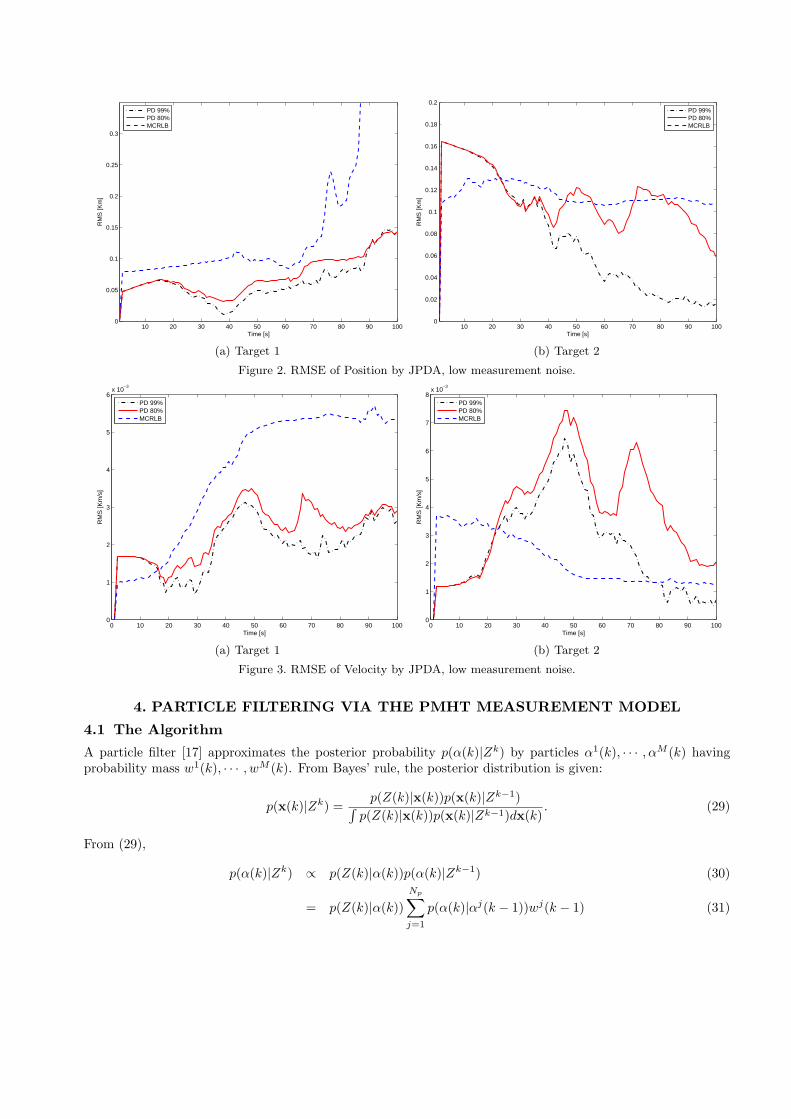
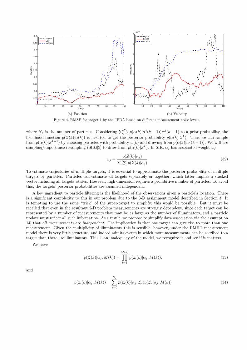
The RMSE of each target‡ is reported based on probabilities of detection 99% and 80%. Figures 2 and 3show the RMSE of position and velocity. The maximum RMSE is 0.15 km for the target 1 and 0.16 km for thetarget 2 considering the probability of detection 99% and 80%. Especially with reference to the MCRLB, whichillustrates the inadequacy of the measurements for target 1 near the end of its trajectory when it is essentiallybetween an illuminator and the receiver, the JPDA appears to be working adequately. In figure 4 we consider ahigher measurement noise level: variance σ2

x = σ2y = 10−1 and σ2

x = σ2y = 10−5. The JPDAF appears to be quite

sensitive to measurement noise level.‡We would not report RMSE for a track that is lost, which here we judge from a threshold on the number of gated

measurements. It is interesting that with this value set to 10 – and a large value must be used due to the multipleilluminators – there were no declared lost tracks in this simulation.

10 20 30 40 50 60 70 80 90 1000

0.05

0.1

0.15

0.2

0.25

0.3

Time [s]

RM

S [K

m]

PD 99%PD 80%MCRLB

(a) Target 1

10 20 30 40 50 60 70 80 90 1000

0.02

0.04

0.06

0.08

0.1

0.12

0.14

0.16

0.18

0.2

Time [s]

RM

S [K

m]

PD 99%PD 80%MCRLB

(b) Target 2

Figure 2. RMSE of Position by JPDA, low measurement noise.

0 10 20 30 40 50 60 70 80 90 1000

1

2

3

4

5

6x 10

−3

Time [s]

RM

S [K

m/s

]

PD 99%PD 80%MCRLB

(a) Target 1

0 10 20 30 40 50 60 70 80 90 1000

1

2

3

4

5

6

7

8x 10

−3

Time [s]

RM

S [K

m/s

]

PD 99%PD 80%MCRLB

(b) Target 2

Figure 3. RMSE of Velocity by JPDA, low measurement noise.

4. PARTICLE FILTERING VIA THE PMHT MEASUREMENT MODEL

4.1 The Algorithm

A particle filter [17] approximates the posterior probability p(α(k)|Zk) by particles α1(k), · · · , αM (k) havingprobability mass w1(k), · · · , wM (k). From Bayes’ rule, the posterior distribution is given:

p(x(k)|Zk) =p(Z(k)|x(k))p(x(k)|Zk−1)∫

p(Z(k)|x(k))p(x(k)|Zk−1)dx(k). (29)

From (29),

p(α(k)|Zk) ∝ p(Z(k)|α(k))p(α(k)|Zk−1) (30)

= p(Z(k)|α(k))Np∑

j=1

p(α(k)|αj(k − 1))wj(k − 1) (31)

10 20 30 40 50 60 70 80 90 1000

0.05

0.1

0.15

0.2

0.25

0.3

0.35

0.4

0.45

0.5

Time [s]

RM

S [K

m]

High RLow RMCRLB

(a) Position

10 20 30 40 50 60 70 80 90 1000

1

2

3

4

5

6

7x 10

−3

Time [s]

RM

S [K

m/s

]

High RLow RMCRLB

(b) Velocity

Figure 4. RMSE for target 1 by the JPDA based on different measurement noise levels.

where Np is the number of particles. Considering∑Np

j=1 p(α(k)|αj(k − 1))wj(k − 1) as a prior probability, thelikelihood function p(Z(k)|α(k)) is inserted to get the posterior probability p(α(k)|Zk). Thus we can samplefrom p(α(k)|Zk−1) by choosing particles with probability w(k) and drawing from p(α(k)|αj(k− 1)). We will usesampling/importance resampling (SIR)[9] to draw from p(α(k)|Zk). In SIR, αj has associated weight wj

wj =p(Z(k)|αj)∑Np

i=1 p(Z(k)|αj)(32)

To estimate trajectories of multiple targets, it is essential to approximate the posterior probability of multipletargets by particles. Particles can estimate all targets separately or together, which latter implies a stackedvector including all targets’ states. However, high dimension requires a prohibitive number of particles. To avoidthis, the targets’ posterior probabilities are assumed independent.

A key ingredient to particle filtering is the likelihood of the observations given a particle’s location. Thereis a significant complexity to this in our problem due to the 3-D assignment model described in Section 3. Itis tempting to use the same “trick” of the super-target to simplify; this would be possible. But it must berecalled that even in the resultant 2-D problem measurements are strongly dependent, since each target can berepresented by a number of measurements that may be as large as the number of illuminators, and a particleupdate must reflect all such information. As a result, we propose to simplify data association via the assumption14] that all measurements are independent. The implication is that one target can give rise to more than onemeasurement. Given the multiplicity of illuminators this is sensible; however, under the PMHT measurementmodel there is very little structure, and indeed admits events in which more measurements can be ascribed to atarget than there are illuminators. This is an inadequacy of the model, we recognize it and see if it matters.

We have

p(Z(k)|αj ,M(k)) =M(k)∏

i=1

p(zi(k)|αj ,M(k)), (33)

and

p(zi(k)|αj ,M(k)) =Ns∑s=0

p(zi(k)|αj ,Ls)p(Ls|αj ,M(k)) (34)

where Ls means that the measurement is associated with illuminator s. If s = 0, zi(k) is from clutter andp(zi(k)|L0) = 1

V +NsPd(Nt−1) approximately. For s = 1, · · · , Ns,

p(zi(k)|αj ,Ls) = N (hs(αj), R). (35)

By the fact∑Ns

s=0 p(Ls|αj ,M(k)) = 1, p(L0|αj ,M(k)) = 1 − ∑Ns

s=1 p(Ls|αj ,M(k)). From here, s > 0 is as-sumed and we use the concept of the super-target again. Since we consider the targets individually, eachtarget/illuminator pair can be regarded as a different target. In [7], p(zi(k)|αj , M(k)) is calculated under sameassumption. Then,

p(Ls|αj ,M(k)) =

1−Nsp(L1|αj ,M(k)) s = 0∑min(M(k),Ns)

k=1 kξ(M(k)−k)(Nsk )P k

d (1−Pd)Ns−k

NsM(k)∑min(M(k),Ns)

i=1 ξ(M(k)−i)(Nsi )P i

d(1−Pd)Ns−is 6= 0

(36)

where ξ(k) = (λV )k

k! exp(−λV ).

Based on the weights above, the SIR filter is implemented in the following steps:

1. Prediction: Draw new particles as

αj(k|k − 1) = F(k)αj(k − 1) + v(k) (37)

2. Weighting: Calculate the weights wj .

3. Sampling: Following wj , α1(k), · · · , αNp(k) are resampled from α1(k|k − 1), · · · , αNp(k|k − 1).

4.2 Simulation

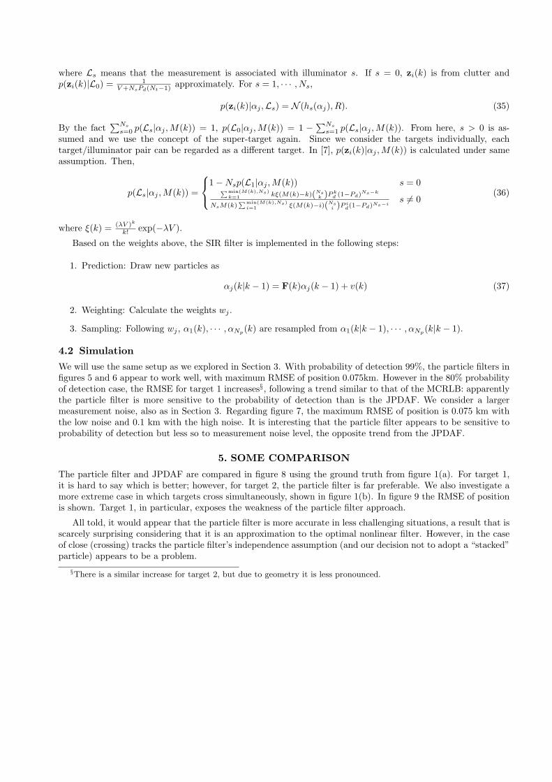
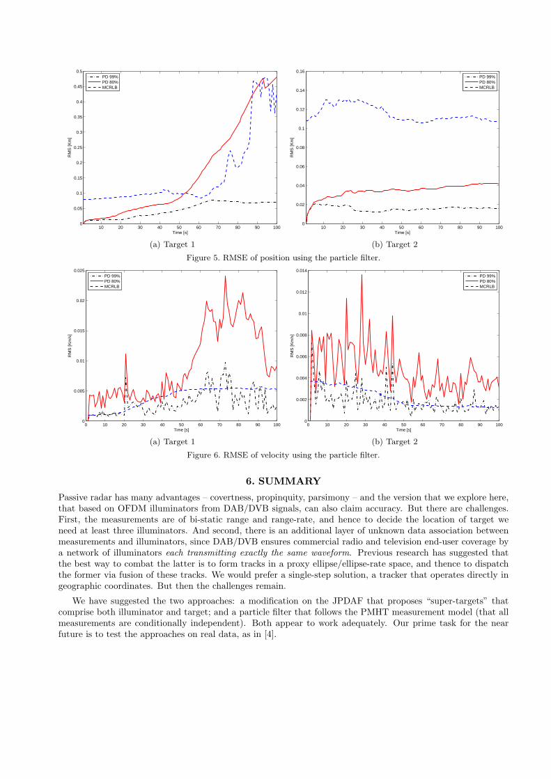
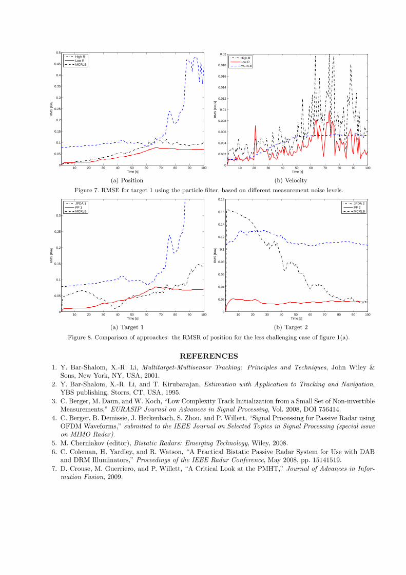
We will use the same setup as we explored in Section 3. With probability of detection 99%, the particle filters infigures 5 and 6 appear to work well, with maximum RMSE of position 0.075km. However in the 80% probabilityof detection case, the RMSE for target 1 increases§, following a trend similar to that of the MCRLB: apparentlythe particle filter is more sensitive to the probability of detection than is the JPDAF. We consider a largermeasurement noise, also as in Section 3. Regarding figure 7, the maximum RMSE of position is 0.075 km withthe low noise and 0.1 km with the high noise. It is interesting that the particle filter appears to be sensitive toprobability of detection but less so to measurement noise level, the opposite trend from the JPDAF.

5. SOME COMPARISON

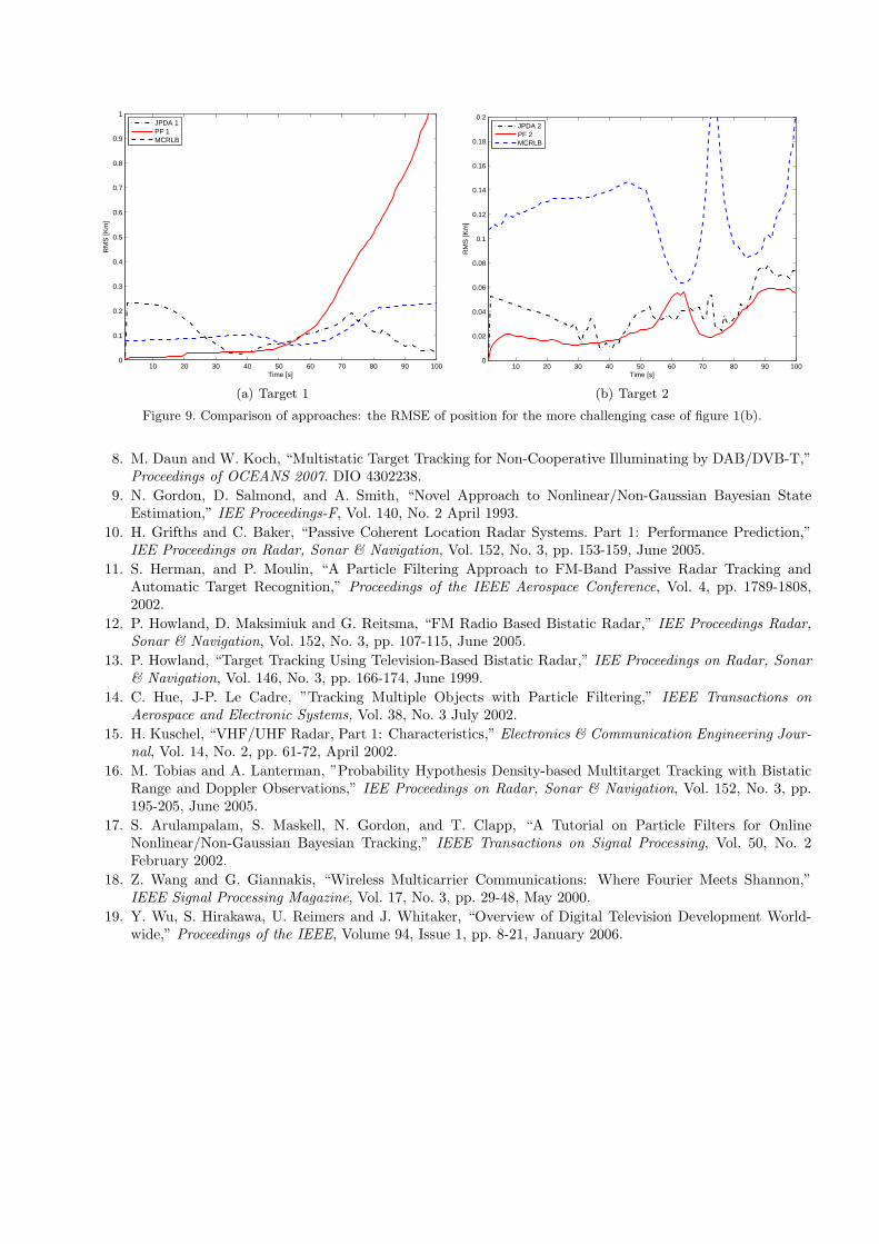
The particle filter and JPDAF are compared in figure 8 using the ground truth from figure 1(a). For target 1,it is hard to say which is better; however, for target 2, the particle filter is far preferable. We also investigate amore extreme case in which targets cross simultaneously, shown in figure 1(b). In figure 9 the RMSE of positionis shown. Target 1, in particular, exposes the weakness of the particle filter approach.

All told, it would appear that the particle filter is more accurate in less challenging situations, a result that isscarcely surprising considering that it is an approximation to the optimal nonlinear filter. However, in the caseof close (crossing) tracks the particle filter’s independence assumption (and our decision not to adopt a “stacked”particle) appears to be a problem.

§There is a similar increase for target 2, but due to geometry it is less pronounced.

10 20 30 40 50 60 70 80 90 1000

0.05

0.1

0.15

0.2

0.25

0.3

0.35

0.4

0.45

0.5

Time [s]

RM

S [K

m]

PD 99%PD 80%MCRLB

(a) Target 1

10 20 30 40 50 60 70 80 90 1000

0.02

0.04

0.06

0.08

0.1

0.12

0.14

0.16

Time [s]

RM

S [K

m]

PD 99%PD 80%MCRLB

(b) Target 2

Figure 5. RMSE of position using the particle filter.

0 10 20 30 40 50 60 70 80 90 1000

0.005

0.01

0.015

0.02

0.025

Time [s]

RM

S [K

m/s

]

PD 99%PD 80%MCRLB

(a) Target 1

0 10 20 30 40 50 60 70 80 90 1000

0.002

0.004

0.006

0.008

0.01

0.012

0.014

Time [s]

RM

S [K

m/s

]

PD 99%PD 80%MCRLB

(b) Target 2

Figure 6. RMSE of velocity using the particle filter.

6. SUMMARY

Passive radar has many advantages – covertness, propinquity, parsimony – and the version that we explore here,that based on OFDM illuminators from DAB/DVB signals, can also claim accuracy. But there are challenges.First, the measurements are of bi-static range and range-rate, and hence to decide the location of target weneed at least three illuminators. And second, there is an additional layer of unknown data association betweenmeasurements and illuminators, since DAB/DVB ensures commercial radio and television end-user coverage bya network of illuminators each transmitting exactly the same waveform. Previous research has suggested thatthe best way to combat the latter is to form tracks in a proxy ellipse/ellipse-rate space, and thence to dispatchthe former via fusion of these tracks. We would prefer a single-step solution, a tracker that operates directly ingeographic coordinates. But then the challenges remain.

We have suggested the two approaches: a modification on the JPDAF that proposes “super-targets” thatcomprise both illuminator and target; and a particle filter that follows the PMHT measurement model (that allmeasurements are conditionally independent). Both appear to work adequately. Our prime task for the nearfuture is to test the approaches on real data, as in [4].

10 20 30 40 50 60 70 80 90 1000

0.05

0.1

0.15

0.2

0.25

0.3

0.35

0.4

0.45

0.5

Time [s]

RM

S [K

m]

High RLow RMCRLB

(a) Position

10 20 30 40 50 60 70 80 90 1000

0.002

0.004

0.006

0.008

0.01

0.012

0.014

0.016

0.018

0.02

Time [s]

RM

S [K

m/s

]

High RLow RMCRLB

(b) Velocity

Figure 7. RMSE for target 1 using the particle filter, based on different measurement noise levels.

10 20 30 40 50 60 70 80 90 1000

0.05

0.1

0.15

0.2

0.25

0.3

Time [s]

RM

S [K

m]

JPDA 1PF 1MCRLB

(a) Target 1

10 20 30 40 50 60 70 80 90 1000

0.02

0.04

0.06

0.08

0.1

0.12

0.14

0.16

0.18

Time [s]

RM

S [K

m]

JPDA 2PF 2MCRLB

(b) Target 2

Figure 8. Comparison of approaches: the RMSR of position for the less challenging case of figure 1(a).

REFERENCES1. Y. Bar-Shalom, X.-R. Li, Multitarget-Multisensor Tracking: Principles and Techniques, John Wiley &

Sons, New York, NY, USA, 2001.2. Y. Bar-Shalom, X.-R. Li, and T. Kirubarajan, Estimation with Application to Tracking and Navigation,

YBS publishing, Storrs, CT, USA, 1995.3. C. Berger, M. Daun, and W. Koch, “Low Complexity Track Initialization from a Small Set of Non-invertible

Measurements,” EURASIP Journal on Advances in Signal Processing, Vol. 2008, DOI 756414.4. C. Berger, B. Demissie, J. Heckenbach, S. Zhou, and P. Willett, “Signal Processing for Passive Radar using

OFDM Waveforms,” submitted to the IEEE Journal on Selected Topics in Signal Processing (special issueon MIMO Radar).

5. M. Cherniakov (editor), Bistatic Radars: Emerging Technology, Wiley, 2008.6. C. Coleman, H. Yardley, and R. Watson, “A Practical Bistatic Passive Radar System for Use with DAB

and DRM Illuminators,” Proceedings of the IEEE Radar Conference, May 2008, pp. 15141519.7. D. Crouse, M. Guerriero, and P. Willett, “A Critical Look at the PMHT,” Journal of Advances in Infor-

mation Fusion, 2009.

10 20 30 40 50 60 70 80 90 1000

0.1

0.2

0.3

0.4

0.5

0.6

0.7

0.8

0.9

1

Time [s]

RM

S [K

m]

JPDA 1PF 1MCRLB

(a) Target 1

10 20 30 40 50 60 70 80 90 1000

0.02

0.04

0.06

0.08

0.1

0.12

0.14

0.16

0.18

0.2

Time [s]

RM

S [K

m]

JPDA 2PF 2MCRLB

(b) Target 2

Figure 9. Comparison of approaches: the RMSE of position for the more challenging case of figure 1(b).

8. M. Daun and W. Koch, “Multistatic Target Tracking for Non-Cooperative Illuminating by DAB/DVB-T,”Proceedings of OCEANS 2007. DIO 4302238.

9. N. Gordon, D. Salmond, and A. Smith, “Novel Approach to Nonlinear/Non-Gaussian Bayesian StateEstimation,” IEE Proceedings-F, Vol. 140, No. 2 April 1993.

10. H. Grifths and C. Baker, “Passive Coherent Location Radar Systems. Part 1: Performance Prediction,”IEE Proceedings on Radar, Sonar & Navigation, Vol. 152, No. 3, pp. 153-159, June 2005.

11. S. Herman, and P. Moulin, “A Particle Filtering Approach to FM-Band Passive Radar Tracking andAutomatic Target Recognition,” Proceedings of the IEEE Aerospace Conference, Vol. 4, pp. 1789-1808,2002.

12. P. Howland, D. Maksimiuk and G. Reitsma, “FM Radio Based Bistatic Radar,” IEE Proceedings Radar,Sonar & Navigation, Vol. 152, No. 3, pp. 107-115, June 2005.

13. P. Howland, “Target Tracking Using Television-Based Bistatic Radar,” IEE Proceedings on Radar, Sonar& Navigation, Vol. 146, No. 3, pp. 166-174, June 1999.

14. C. Hue, J-P. Le Cadre, ”Tracking Multiple Objects with Particle Filtering,” IEEE Transactions onAerospace and Electronic Systems, Vol. 38, No. 3 July 2002.

15. H. Kuschel, “VHF/UHF Radar, Part 1: Characteristics,” Electronics & Communication Engineering Jour-nal, Vol. 14, No. 2, pp. 61-72, April 2002.

16. M. Tobias and A. Lanterman, ”Probability Hypothesis Density-based Multitarget Tracking with BistaticRange and Doppler Observations,” IEE Proceedings on Radar, Sonar & Navigation, Vol. 152, No. 3, pp.195-205, June 2005.

17. S. Arulampalam, S. Maskell, N. Gordon, and T. Clapp, “A Tutorial on Particle Filters for OnlineNonlinear/Non-Gaussian Bayesian Tracking,” IEEE Transactions on Signal Processing, Vol. 50, No. 2February 2002.

18. Z. Wang and G. Giannakis, “Wireless Multicarrier Communications: Where Fourier Meets Shannon,”IEEE Signal Processing Magazine, Vol. 17, No. 3, pp. 29-48, May 2000.

19. Y. Wu, S. Hirakawa, U. Reimers and J. Whitaker, “Overview of Digital Television Development World-wide,” Proceedings of the IEEE, Volume 94, Issue 1, pp. 8-21, January 2006.