Embed Size (px)
Citation preview

Revista Colombiana de EstadísticaJanuary 2015, Volume 38, Issue 1, pp. 239 to 266DOI: http://dx.doi.org/10.15446/rce.v38n1.48813
TAR Modeling with Missing Data when the WhiteNoise Process Follows a Student’s t-Distribution
Modelamiento TAR con datos faltantes cuando el proceso del ruidoblanco tiene una distribución t de Student
Hanwen Zhang1,a, Fabio H. Nieto2,b
1Facultad de Estadística, Universidad Santo Tomás, Bogotá, Colombia2Departamento de Estadística, Facultad de Ciencias, Universidad Nacional de
Colombia, Bogotá, Colombia
Abstract
This paper considers the modeling of the threshold autoregressive (TAR)process, which is driven by a noise process that follows a Student’s t-dis-tribution. The analysis is done in the presence of missing data in boththe threshold process {Zt} and the interest process {Xt}. We develop athree-stage procedure based on the Gibbs sampler in order to identify andestimate the model. Additionally, the estimation of the missing data and theforecasting procedure are provided. The proposed methodology is illustratedwith simulated and real-life data.
Key words: Bayesian Statistics, Gibbs Sampler, Missing Data, Forecasting,Time Series, Threshold Autoregressive Model.
Resumen
En este trabajo consideramos el modelamiento de los modelos autoregre-sivos de umbrales (TAR) con datos faltantes tanto en la serie de umbralescomo la serie de interés cuando el proceso del ruido blanco sigue una distribu-ción t de student. Desarrollamos un procedimiento de tres etapas basado enel muestreador de Gibbs para identificar y estimar el modelo, además de laestimación de los datos faltantes y el procedimiento para el pronóstico. Lametodología propuesta fue aplicada a datos simulados y datos reales.
Palabras clave: datos faltantes, estadística Bayesiana, modelo autoregre-sivo de umbrales, muestreador de Gibbs, pronóstico, series de tiempo.
aProfessor. E-mail: [email protected]. E-mail: [email protected]
239

240 Hanwen Zhang & Fabio H. Nieto
1. Introduction
TAR models proposed by Tong (1978) assume that the values of a process{Zt} (the threshold process) determine not only the values of the process of inter-est {Xt}, but also its dynamics. When the threshold process is the same processof interest but is lagged, the model is known as SETAR (Self-exciting TAR, Briñez& Nieto, 2005). Nieto (2005) developed a Bayesian methodology for the identifi-cation and estimation of TAR models allowing missing data in the both thresholdprocess and the process of interest. On the other side, Nieto (2008, 2011) char-acterized in univariate TAR models in terms of their mean, conditional mean,variance, conditional variance and also found the expressions for the best predic-tor. Vargas (2012) improved the prediction with TAR models, taking into accountthe variability in the parameters and Nieto & Moreno (2013) explored three kindsof conditional variance in order to try to compare this type of nonlinear modelswith GARCH models. Also the TAR models can be easily extended to thresh-old autoregressive moving average (TARMA) models, and its Bayesian modelingwith two regimes has been investigated in Sáfadi & Morettin (2000) and Xia, Liu,Pan & Liang (2012). Another extension of the TAR model is when there are twothreshold variables instead of one and this is done by Chen, Chong & Bai (2012)within the particular case of two regimes.
Despite TAR models usefulness, they are not easily identified due to the largenumber of parameters and the nesting structure between the parameters. For SE-TAR models, Tsay (1989) provided a simple and widely applicable model-buildingprocedure. However, generally speaking, most of the parameters, as the thresh-olds and the number of regimes, are assumed to be known; otherwise they can beidentified using Tong (1990)’s NAIC criterion together with some graphical tech-niques. Assuming that the noise process is Gaussian, Nieto (2005) developed aBayesian procedure in order to identify the number of regimes and estimate theother parameters, once the thresholds are identified, using NAIC criterion for eachpossible number of regimes. This work is accomplished in the presence of missingdata in both the process of interest and the threshold process.
In many cases, the data cannot be appropriately described by the Gaussiandistribution; for example, it is well-known that financial time series often haveheavy tails, and the t-distribution could be more appropriate for the noise processthan the Gaussian distribution. Zhang (2012) estimated the parameters of theTAR model with t distributed error process when the model is completely identi-fied. However, in practice, the identification problem may be difficult to be carryout, because this requires some additional knowledge about the phenomenon andthis fact is particularly unrealistic due to the complex model structure. The focusof this work is to propose a Bayesian methodology which includes model identi-fication in the TAR modelling. Specifically, a three-stage methodology based onthe Gibbs sampler is proposed: in the first stage, the number of regimes togetherwith the thresholds are estimated; in the second, the autoregressive orders in theregimes are estimated, and finally, in the last stage, the autoregressive orders, thevariance weights and other parameters of the noise process are estimated. In thisway, the identification of the model takes place in the first two stages, and the
Revista Colombiana de Estadística 38 (2015) 239–266

TAR Modeling with Missing Data 241
estimation of the model in the last stage. Additionally, a Bayesian methodologyfor the estimation of missing data and the forecasting issue is developed. Themethodologies developed are illustrated with simulated and real-life data in thefinance field.
The work is organized as follows: in Section 2, we introduce the TAR modelwith t distributed noise process; in Section 3, we present the estimation procedurefor the non structural parameters when the structural parameters are known; inSection 4, we present the identification for the structural parameters; in Sections5 and 6, we present forecasting and missing-data estimation procedures. Finally,in Section 7, we illustrate the developed methodology in simulated and real-lifedata.
2. TAR Model with T -Distributed Noise
In order to introduce the TAR model, first suppose that the set of real numbersis divided in l disjoint intervals as R =
⋃lj=1Rj where Rj = (rj−1, rj ], where
r1 < · · · < rl−1 and r0 = −∞, rl = ∞. The R1, . . . , Rl are denomited theregimes and the values r1, . . . , rl−1 are denominated the thresholds. Let {Zt}be a stochastic process with stochastic behaviour described by a Markov chain oforder p called the threshold process and let {Xt} be the process of interest.
The dynamic of the process {Xt} is determined by the process {Zt} in the waythat when Zt ∈ Rj = (rj−1, rj ] for some j = 1, . . . , l the model for {Xt} is
Xt = a(j)0 +
kj∑i=1
a(j)i Xt−i + h(j)et. (1)
The values k1, . . . , kl are nonnegative integer numbers representing the autore-gressive orders in the l regimes, that is, different autoregressive orders are allowedin different regimes. h(j) > 0 for j = 1, . . . , l, Nieto & Moreno (2013) found thatthe parameters (h(j))2 correspond to the variance of Xt conditional on the regimeand the past values of X, the so-called type II conditional variance. With respectto the noise process {et}, Nieto (2005) uses a Gaussian distribution, in this paper aStudent’s t-distribution is used. However, in order to mantain the interpretation of(h(j))2 mentioned before, we use a t-distribution with degrees of freedom n dividedby its standard deviation
√n/(n− 2), that is, et ∼iid tn√
n/(n−2)with n > 2, which
is mutually independent from the process {Zt}; in this way, V ar(et) = 1 for all tand hence, following Nieto & Moreno (2013), (h(j))2 = V ar(Xt|Rj , xt−1, . . . , x1).Additionally, we assume that {Zt} is exogenous in the sense that there is no feed-back of {Xt} towards it.
Nieto & Moreno (2013) found conditions on the coefficients a(j)i to achieve
stationarity when the distribution for the noise process is Gaussian; however, aspointed out by Nieto (2005), the stationarity is not required for the correct imple-mentation of the proposed Bayesian methodology; we have the same situation in
Revista Colombiana de Estadística 38 (2015) 239–266

242 Hanwen Zhang & Fabio H. Nieto
this paper and the corresponding conditions for stationarity deserve future inves-tigations.
The parameters of the model can be divided into two groups:
• Structural parameters: the number of regimes l, the l − 1 thresholds r1, . . .,rl−1 and the autoregressive orders of the l regimes k1, . . ., kl.
• Non-structural parameters: the autoregressive coefficients a(j)i with i =
0, . . . , kj and j = 1, . . . , l, the variance weights h(1), . . ., h(l) and the de-grees of freedom of the noise process, n.
In this research, we use the following notation: θ′j = (a(j)0 , a
(j)1 , . . . , a
(j)kj
)′ forj = 1, . . . , l, θ′ = (θ′1, . . . ,θ
′l)′. and h′ = (h(1), . . . , h(l))′.
2.1. Conditional Likelihood Function of the Model
According to Nieto (2005) and conditioned upon the values of the structural pa-rameters, the initial values xk = (x1, . . . , xk)′, where k = max{k1, . . . , kl} and theobserved data of the threshold process z = (z1, . . . , zT )′, the conditional likelihoodfunction is given by:
f(x|z,θx,θz) = f(xk+1|xk, z,θx,θz) · · · f(xT |xT−1, . . . , x1, z,θx,θz),
where θz denotes the vector of parameters of the threshold process {Zt} andθx denotes the vector of all the non structural parameters, that is θ′x = (θ′,h′, n).As et ∼ tn√
n/(n−2), for t = k+1, . . . , T , the variable xt|xt−1, . . . , x1, z is distributed
as a tn variable multiplied by h(jt)√n/(n−2)
and adding a(jt)0 +
∑kjti=1 a
(jt)i xt−i, where
jt = j if Zt ∈ Rj = (rj−1, rj ] for some j = 1, . . . , l. That is, the distribution ofxt, conditioned upon the past values of x and z, is the non-standardized Student’st-distribution with n degrees of freedom, location parameter a(jt)
0 +∑kjti=1 a
(jt)i xt−i
and scale parameter h(jt)√n/(n−2)
. Thus,
f(xt|xt−1, . . . , x1, z,θx,θz) =
Γ(n+12 )√
π(n− 2)Γ(n2 )
1
h(jt)
1 +
[xt − a(jt)
0 −∑kjti=1 a
(jt)i xt−i
]2(h(jt))2(n− 2)
−n+1
2
.
Consequently, the conditional likelihood function is given by
f(x|z,θx,θz) =[Γ(n+1
2 )√π(n− 2)Γ(n2 )
]T−k T∏t=k+1
[h(jt)
]−1 T∏t=k+1
(1 +
e2t
n− 2
)−n+12
, (2)
with et = 1h(jt)
(xt − a(jt)
0 −∑kjti=1 a
(jt)i xt−i
)and jt = j when Zt ∈ Rj .
Revista Colombiana de Estadística 38 (2015) 239–266
TAR Modeling with Missing Data 243
3. Estimation of Non Structural Parameters
In this part of the research, the structural parameters are assumed to be known,and we focus on finding the posterior conditional distributions of the autoregres-sive coefficients θj , the variance weights h(j) with j = 1, . . . , l and the degreesof freedom of the noise process n. Additionally we assume prior independencebetween the parameters θ, h and n, as well as prior independence among the nonstructural parameters in each one of the l regimes.
The prior distribution for the vector θj is a multivariate normal distributionwith mean vector θ0,j and covariance matrix V−1
0,j , denoted as θj ∼ N(θ0,j ,V−10,j ),
and the posterior conditional distribution of θj is given by the following result:
Proposition 1. For each j = 1, . . . , l, the conditional distribution of θj given thestructural parameters θi, with i 6= j, h, and n is given by
p(θj |θi, i 6= j,h,x, z, n) ∝∏
{t:jt=j}
1 +
[xt − a(j)
0 −∑kji=1 a
(j)i xt−i
]2(h(j))2(n− 2)
−n+1
2
× exp
{−1
2(θj − θ0,j)
′V0,j(θj − θ0,j)
}.
(3)
Note that the posterior conditional distribution of θj is affected only by h(j),but not the other components of h in regimes different from j, so we have someclass of posterior independence between regimes.
Now, with respect to the variance weights h(j), we follow the standard Bayesianmethodology assigning an inverse Gamma distribution with shape parameter α andscale parameter β, (IG(α, β)), as the prior distribution of (h(j))2, that is,
p((h(j))2) ∝ (h(j))−2α−2 exp{−β/(h(j))2}I(0,∞)((hj)2).
Combining this prior distribution of (h(j))2 and the conditional likelihood func-tion, we have the following posterior conditional distribution (h(j))2:
Proposition 2. For each j = 1, . . . , l, the posterior distribution of (h(j))2 giventhe structural parameters, θj, j = 1, . . . , l, h(i), with i 6= j and n, is given by
p((h(j))2|θ1, . . . ,θl, h(i), i 6= j,x, z, n)
∝∏
{t:jt=j}
1 +
[xt − a(j)
0 −∑kji=1 a
(j)i xt−i
]2(h(j))2(n− 2)
−n+1
2
× (h(j))−2α−2−nj exp{−β/(h(j))2}.
(4)
Note that, the posterior conditional distribution of (h(j))2 is affected only byθj , but not by θi with i 6= j, so again we have the posterior independence betweenθj , h(j) in different regimes.
Revista Colombiana de Estadística 38 (2015) 239–266
244 Hanwen Zhang & Fabio H. Nieto
Finally, we found the posterior conditional distribution of the degrees of free-dom of the noise process n. The prior distribution of n is a Gamma distri-bution following the suggestion of Watanabe (2001), since in the distributionGamma(α′, β′), the expectation and the variance are given by α′β′ and α′β′2,respectively. Actually, α′ and β′ can be chosen according to prior knowledgeabout n, and in case that there is no prior information about n, we can choose aquite large prior variance to represent the high degree of uncertainty in the priorinformation of n. The prior distribution of n is given by
p(n) ∝ nα′−1 exp{−n/β′}.
Using this prior distribution, we find the posterior conditional distributionof n.
Proposition 3. The posterior conditional distribution of the degrees of freedomof the noise process {et} is given by
p(n|θ1, . . . ,θl,h,x, z)
∝
[Γ(n+1
2 )√n− 2 Γ(n2 )
]T−k T∏t=k+1
1 +
[xt − a(jt)
0 −∑kjti=1 a
(jt)i xt−i
]2(h(jt))2(n− 2)
−n+1
2
× nα′−1 exp{−n/β′}.
(5)
In conclusion, the estimation of non structural parameters can be carried outby means of a Gibbs sampler, using the conditional densities (3), (4) and (5).We use the grid method to simulate values from these distributions; in order todefine the parameter space, we fit an autoregressive AR(p) model (where p =max{k1, . . . , kl}) and use the estimation plus and minus two times the standarderror as the parameter space. For example, suppose that l = 2, k1 = 1 and k2 = 2,and the estimated coefficients of the AR(2) model are 0.8 and -0.4 with standarderror 0.1 and 0.2, then the parameter space for a(1)
1 and a(2)1 would be (0.6,1) and
the parameter space for a(2)2 would be (-0.8,0). Also for the coefficients h(j) we
take into account the estimation of the error variance in the AR(2) fitting. Finally,for the degree of freedom n, we choose the parameter space to be (2,30), since thet distribution has no finite variance when n ≤ 2 and would be too similar to anormal distribution for n > 30.
4. Estimation of Structural Parameters
In this section, we develop the results concerning the estimation of the struc-tural parameters, i.e. the identification of a TAR model. Firstly, we assume thatthe number of regimes l and the l − 1 thresholds are known, and we estimatethe autoregressive orders in these regimes; then we consider the case where thethresholds are known, and finally, we have the general case, where all the structuralparameters are unknown.
Revista Colombiana de Estadística 38 (2015) 239–266

TAR Modeling with Missing Data 245
4.1. Estimation of the Autoregressive Orders k1, . . . , kl
As we assume that the number of the regimes and the thresholds are known,remaining parameters to be estimated are the autoregressive orders and the non-structural parameters.
We assume that the autoregressive orders k1, . . . , kl are realizations of discreterandom variables K1, . . . ,Kl, and each of theses variables takes value in the set{0, 1, . . . , kmax}. It is important to note that when the values of some autoregres-sive orders change, the specification of the TAR model changes and the dimensionof the vector of the autoregressive coefficients Θ also changes. Carlin & Chib(1995) developed a Bayesian methodology for the selection of models, and Nieto(2005) adapted this methodology in order to identify the TAR model with Gaus-sian noise. In this research, we adapt the same methodology to identify the TARmodel with t distributed noise. Suppose that M is a discrete random variable in-dexing the model which takes values 1, . . . , (kmax + 1)l. For each possible modelM = m, we define the vector of parameters Θm as Θ′m = (θ′1, . . . ,θ
′l,h′) for the
model m with m = 1, . . . , (kmax+1)l. The degrees of freedom n can be consideredas a nuisance parameter, since its dimension is the same for all models as well asits interpretation.
Carlin & Chib (1995) found the following conditional densities
p(M = m|Θ,y) =p(y|Θm, M = m)P (M = m)∑m′ p(y|Θ
′m, M = m′)P (M = m′)
. (6)
where Θ = {Θ1, . . . ,Θ(kmax+1)l}, y = (x, z) is the vector of full data. And
p(Θm|Θm′ 6=m,M,y) ∝
{p(y|Θm, M = m)p(Θm|M = m) if M = m,
p(Θm|M = m) if M 6= m.(7)
The densities p(Θm|M = m) are denominated as the link functions which canbe taken as the prior distribution of Θm.
In the context of the problem of identification of the autoregressive orders, themodel indicator M is determined jointly by the values of variables K1, . . . ,Kl.In this way, computing the density (6) is equivalent to computing the densitiesp(kj |Θ, ki,i 6=j ,y) with j = 1, . . . , l, because when we know the conditional dis-tribution of each kj , we can sample values of kj by using a Gibbs sampler and,thus, we can sample values of the model indicator M . In order to compute thesedensities, Nieto (2005) found that
p(kj |Θ, ki,i 6=j , l,x, z) =p(x|z,Θ,h,k, l)p(kj)∑k̄j
k′j=0 p(x|z,θ,h,k′, l)p(k′j), (8)
where k = (k1, . . . , kl), and k′ is obtained by replacing the component kj ofthe vector k by k′j for all j = 1, . . . , l.
Revista Colombiana de Estadística 38 (2015) 239–266
246 Hanwen Zhang & Fabio H. Nieto
In summary, using the densities (3), (4), (5) and (8), a Gibbs sampler can beimplemented in order to obtain the estimations of the probabilities of all the possi-ble values for each Kj with j = 1, . . . , l. Denoting these estimated probabilities asp̂0j , p̂1j , . . . , p̂kmaxj , we can choose the value of Kj for which the highest probabilityis associated.
4.2. Estimation of the Number of Regimes l
In order to estimate the number of regimes, we use again the approach devel-oped in Nieto (2005) adapting the methodology of Carlin & Chib (1995). Supposethat the number of regimes l is the realization of a discrete random variable Lwhich takes values in the set {2, . . . , lmax}, and the prior distribution of L is de-noted by p(l).
Clearly, when the value of l changes, the model specification also changes; wehave lmax − 1 possible models. Suppose that M is the discrete random variableindexing the model, then M takes values 2, . . ., lmax, and for each possible model,M = j, Θj denotes the vector of the parameters in this model, that is:
Θ′j = (θ′1, . . . ,θ′j ,h′j ,k′j , n),
with k′j = (k1j , . . . , kjj)′, where kij denotes the autoregressive order in the i-
th regime in the model M = j, h′j = (h(1), . . . , h(j))′. Finally, we define Θ′ =
(Θ′2, . . . ,Θ′lmax
), the vector containing all the parameters for all the possible mod-els.
Nieto (2005) found the following conditional densities
p(M = j|Θ,y) = p(l|Θ,y) ∝ p(x|z,Θl, l)p(l) for l = 2, . . . , lmax, (9)
p(kij |Θ−kij , l,y) =
p(x|z,Θl, l)p(kij)∑kmax
k′il=0 p(x|z,Θl, l)p(k′il)if j = l,
p(kij) if j 6= l,
(10)
where Θ−kij denotes the vector Θ without the element kij , and
p(θj , h(j)|Θ−θj ,h(j) , l,y) ∝
{p(y|Θl, l)p(Θl) if j = l,
p(Θj) if j 6= l,(11)
where Θ−θj ,h(j) denotes the vector Θ without the components θj and h(j).
Jointly using the conditional densities (9), (10), (11) and (5), we can implementa Gibbs sampler and obtain the posterior probabilities for all possible values of L.The estimation of the number of regimes l could be the value with major posteriorprobability or the mode of the value of L in the iterations of the Gibbs sampler.
Revista Colombiana de Estadística 38 (2015) 239–266

TAR Modeling with Missing Data 247
4.3. Estimation of the Number of Regimes l and theThresholds
Finally, we assume that the l − 1 thresholds are also unknown, and they needto be estimated jointly with the number of regimes l. Following the approach ofCarlin & Chib (1995), the model is indexed by a discrete variable M , which takesvalues 2, . . . , lmax according to the value of the variable L. For each possible modelM = j, the thresholds are denoted as rj = (r1, . . . , rj−1)′ with j = 2, . . . , lmax.
It is straightforward to obtain the posterior conditional density of rj given thevalues of other structural and non-structural parameters, given by
p(rj |l,Θ−rj ,y)
∝
T∏
t=k+1
[h(jt)]−1T∏t=1
1 +
[xt−a(jt)0 −
∑kjti=1 a
(jt)i xt−i
]2(h(jt))2(n−2)
−n+12
if j = l,
p(rj) if j 6= l,
(12)
where jt = j if Zt ∈ Rj = (rj−1, rj ] for some j = 1, . . . , l. The posterior conditionaldensity of l is given by (9). Note that the expression in (12) depends on thethresholds rj since jt = j if Zt ∈ Rj = (rj−1, rj ], so Rj and jt depend on thethresholds, and so does the expression (12). In this way, using the posteriorconditional density of rj , l, and Θj , we can implement a Gibbs sampler and obtainthe estimation of the number of regimes and thresholds. In order to extract samplesfrom this density, we use the grid method where the parameter space consists ofall possible ordered values of Zt.
With respect to the prior density of rj , we recall that the values of the thresh-olds are based on the values of the process {Zt}, so we can assume that thethresholds take values in a interval (a, b), appropriately specified; furthermore, weassume a uniform distribution for the thresholds r1, . . ., rj−1, that is
p(rj) = p(r1, . . . , rj−1) ∝ k if a < r1 < · · · < rj−1 < b,
for j = 2, . . . , lmax.
4.4. Proposed Algorithm
In conclusion, a three-stage process is proposed for the identification and es-timation of TAR models with t-distributed noise with no missing data. Thisalgorithm consists of the following steps:
1. The number of regimes and thresholds are estimated using a Gibbs samplerbased on the densities (9), (10), (11), (12) and (5).
2. The number of regimes and thresholds are fixed and the autoregressive ordersare estimated using a Gibbs sampler based on the densities (7), (8) and (5).
Revista Colombiana de Estadística 38 (2015) 239–266
248 Hanwen Zhang & Fabio H. Nieto
3. Finally, conditioned upon the estimated structural parameters, we estimatethe non-structural parameters using a Gibbs sampler with densities (3), (4)and (5).
5. Forecasting
In order to develop the predictive inference, we focus on finding the posteriorpredictive distribution of the variable XT+h conditional on the observed xT =(x1, . . . , xT ) and zT = (z1, . . . , zT ) with h > 0. Vargas (2012) worked on theformal Bayesian approach to find the predictive density of XT+h involving thevariability in the parameters of the model; this predictive density is given by:
p(xT+h|xT , zT ) =
l∑j=1
p(xT+h|Rj ,xT , zT )pj(h),
where pj(h) = P (ZT+h ∈ Rj |xT , zT ), for h = 1, 2, . . ., and j = 1, . . . , l, and
p(xT+h|Rj ,xT , zT ) =
∫Θj
p(xT+h,θ(j)|Rj ,xT , zT )dθ(j)
=
∫Θj
p(xT+h|θ(j), Rj ,xT , zT )p(θ(j)|Rj ,xT , zT )dθ(j),
(13)
where θ(j) denotes the vector of the non-structural parameters in the regime j,and
p(xT+h|θ(j), Rj ,xT , zT ) =
∫· · ·∫p(xT+h|θ(j), Rj ,xT+h−1)
× p(xT+h−1|θ(j), Rj ,xT+h−2)
× · · · × p(xT+1|θ(j), Rj ,xT )dxT+1 · · · dxT+h−1.
(14)
On the other hand, in order to forecast the threshold variable ZT+h, Nieto(2008) found that:
p(zT+h|zT ) =
∫· · ·∫p(zT+h|zT+h−1, zT+1, zT )
× p(zT+h−1|zT+h−2, zT+1, zT ) · · · p(zT+1|zT )dzT+1 · · · dzT+h−1. (15)
Based on the equations (13), (14) and (15), we can compute forecasts forboth processes {Xt} and {Zt}. In order to draw values from p(zT+h|zT ) withh = 1, 2, . . ., Congdon (2001) suggests to draw a value for zT+1 from p(zT+1|zT ),then draw value for zT+2 from p(zT+2|zT+1, zT ) and so on.
On the other hand, in order to forecast the process {Xt}, notice that p(xT+h|xT , zT ) is a mixture density, so we just draw a value from p(xT+h|Rj ,xT , zT ) withprobability pj(h). Secondly, we note that each term p(xT+m|θ(j), Rj ,xT+m−1, ) for
Revista Colombiana de Estadística 38 (2015) 239–266
TAR Modeling with Missing Data 249
m = 1, . . . , h corresponds to the density of a non-standarized Student’s t-distribu-
tion with n degrees of freedom, location parameter a(j)0 +
kj∑i=1
a(j)i xT+m−i and scale
parameter h(j)√n/(n−2)
. This concludes the forecasting process.
6. Estimation of Missing Data
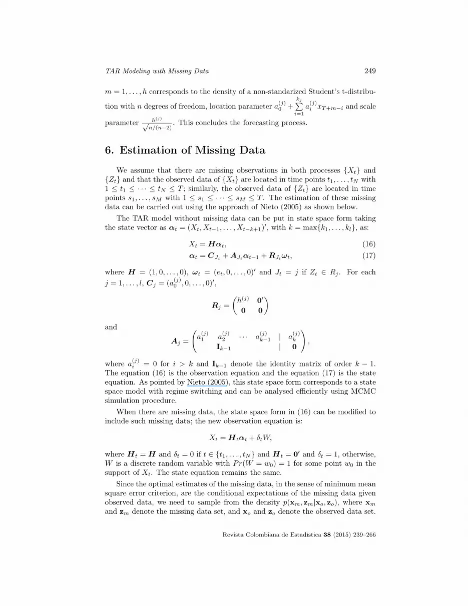
We assume that there are missing observations in both processes {Xt} and{Zt} and that the observed data of {Xt} are located in time points t1, . . . , tN with1 ≤ t1 ≤ · · · ≤ tN ≤ T ; similarly, the observed data of {Zt} are located in timepoints s1, . . . , sM with 1 ≤ s1 ≤ · · · ≤ sM ≤ T . The estimation of these missingdata can be carried out using the approach of Nieto (2005) as shown below.
The TAR model without missing data can be put in state space form takingthe state vector as αt = (Xt, Xt−1, . . . , Xt−k+1)′, with k = max{k1, . . . , kl}, as:
Xt = Hαt, (16)αt = CJt +AJtαt−1 +RJtωt, (17)
where H = (1, 0, . . . , 0), ωt = (et, 0, . . . , 0)′ and Jt = j if Zt ∈ Rj . For eachj = 1, . . . , l, Cj = (a
(j)0 , 0, . . . , 0)′,
Rj =
(h(j) 0′
0 0
)and
Aj =
(a
(j)1 a
(j)2 · · · a
(j)k−1 | a
(j)k
Ik−1 | 0
),
where a(j)i = 0 for i > k and Ik−1 denote the identity matrix of order k − 1.
The equation (16) is the observation equation and the equation (17) is the stateequation. As pointed by Nieto (2005), this state space form corresponds to a statespace model with regime switching and can be analysed efficiently using MCMCsimulation procedure.
When there are missing data, the state space form in (16) can be modified toinclude such missing data; the new observation equation is:
Xt = Htαt + δtW,
where Ht = H and δt = 0 if t ∈ {t1, . . . , tN} and Ht = 0′ and δt = 1, otherwise,W is a discrete random variable with Pr(W = w0) = 1 for some point w0 in thesupport of Xt. The state equation remains the same.
Since the optimal estimates of the missing data, in the sense of minimum meansquare error criterion, are the conditional expectations of the missing data givenobserved data, we need to sample from the density p(xm, zm|xo, zo), where xmand zm denote the missing data set, and xo and zo denote the observed data set.
Revista Colombiana de Estadística 38 (2015) 239–266

250 Hanwen Zhang & Fabio H. Nieto
Nieto (2005) states that this goal can be achieved by sampling from p(α, z|x),where x and z are constituted by full data x1, . . . , xN and z1, . . . , zN , and themissing data are replaced by artificial data, for example, the median of {xt} and{zt} and α = (α1, . . . ,αT )′.
Nieto (2005) propose the use of a Gibbs sampler in order to draw samples fromp(z|α,x) and p(α|z,x). The density p(z|α,x) it is found to be:
p(z|α,x) = p(zT |α,x)
T−p∏t=1
p(zt|zt+p,xt,αt),
where zt = (zt−p+1, . . . , zt), αt and xt are similarly defined, and
p(zT |α,x) ∝T∏
j=T−p+1
p(αj |zT , αj−1)fp(zT )
and for t = T − p, . . . , 1
p(zt|zt+p,αt,xt) ∝ p(αt|zt+p−1,αt−1)fp(zt+p|zt+p−1)fp(zt+p−1).
Finally, in order to sample values from the joint distribution of p(α|z,x), notethat
p(α|z,x) = p(αT |αT−1, . . . ,α1, z,x)p(αT−1|αT−2, . . . ,α1, z,x) · · · p(α2|α1, z,x),
where sampling each term p(αt|αt−1, . . . ,α1, z,x) is equivalent to sample valuesfrom αt|αt−1, Zt since αt = (Xt, Xt−1, . . . , Xt−k+1)′; and this is equivalent tosample values from the density p(Xt|Xt−1, . . . , Xt−k, Zt), so we just need to sam-ple values from the density of a non-standardized Student’s t-distribution with n
degrees of freedom, location parameter a(j)0 +
kj∑i=1
a(j)i xT+m−i and scale parameter
h(j)√n/(n−2)
.
In summary, the estimation of missing data in TAR models can be carried outas follows:
1. Completion of the time series replacing the missing data {xt} and {zt}, withtheir respective median.
2. Identification and estimation of the TAR model using the completed timeseries following the algorithm presented in subsection 2.4.
3. Estimation of the missing data by means of a Gibbs sampler using the abovemethodology.
4. Re-estimation of the TAR model with the missing data replaced by theirestimates.
Revista Colombiana de Estadística 38 (2015) 239–266

TAR Modeling with Missing Data 251
7. Illustrations
7.1. Simulated Examples
In this section we present two simulation examples in order to illustrate theperformance of the proposed methodology.
7.1.1. Example 1
We simulated a series {xt} of 100 observations from the model:
Xt =
{1 + 0.5Xt−1 − 0.3Xt−2 + et if Zt ≤ 0
−0.5− 0.7Xt−1 + 1.5et if Zt > 0,(18)
with et ∼ t5√5/3
, Zt = 0.5Zt−1 + εt and εt is a Gaussian white noise process of
mean 0 and variance 1 (GWN(0,1)). The simulated series are shown in Figure 1.
Time
Z
0 20 40 60 80 100
−20
2
Time
X
0 20 40 60 80 100
−40
4
Figure 1: Simulated data in example1.
In the first stage, we identified the number of regimes and the thresholds.Following Nieto, Zhang & Li (2013), the prior distribution for l is the Poissondistribution truncated1 in the set {2, 3, 4} with parameter 3, and the prior distri-bution of the thresholds is as described above. We run a Gibbs sampler of 1,000iterations with a burn-in period of 200. In order to ensure that for each parame-ter, the draws have converged to the posterior distribution, we use the Geweke’sZ-score plot (Geweke 1992) from the package coda in R (Plummer, Best, Cowles &Vines 2006). Geweke’s Z-score computes the difference between the means of thefirst and last part of the draws of a Markov chain, and the plot shows the valuesof the Z-score where successively larger numbers (at most half of the chain) ofiterations are removed from the beginning of the chain. For the number of regimesand autoregressive orders, we monitor the corresponding posterior probabilities.Since there are a lot of parameters in the model, we cannot show all the plots, only
1Note that we have excluded the value 1 which corresponds to a linear AR model, in realapplications, non-linear should be carried out.
Revista Colombiana de Estadística 38 (2015) 239–266

252 Hanwen Zhang & Fabio H. Nieto
a few where we consider that the burn-in period of 200 iterations is appropriate(Figure 2).
0 100 200 300 400 500
-2-1
01
2
First iteration in segment
Z-score
var1
0 100 200 300 400 500
-2-1
01
2
First iteration in segment
Z-score
var1
0 100 200 300 400 500
-3-2
-10
12
3
First iteration in segment
Z-score
var1
0 100 200 300 400 500
-3-2
-10
12
3
First iteration in segment
Z-score
var1
Figure 2: Geweke’s Z-score for some of the parameters in the Gibbs sampler.
The posterior probability of the number of regimes is given in Table 1, where wecan see that the number of regimes associated with the largest posterior probabilityis 2.
Table 1: Posterior probability for the number of regimes L in example 1.
l 2 3 4Posterior probability 0.60 0.40 0
The estimation of the threshold is 0.08462. The 95% credible interval for thethreshold is given by (-0.2892, 0.6737) containing the real threshold 0.
2For a certain model l = j, the possible values of the thresholds rj are the quantiles of theprocess {Zt}, after removing the thresholds that induce regimes with too little data; in this case,we eliminate the thresholds that induce any regime with less than 20 data.
Revista Colombiana de Estadística 38 (2015) 239–266

TAR Modeling with Missing Data 253
In the second stage, we estimated the autoregressive order in each of the tworegimes where the number of regimes is fixed to be 2 and the value of the thresholdto be 0.0846. The prior distribution for kj is the truncated Poisson distributionwith parameter 2 in the set {0, 1, 2, 3}3 for each j = 1, 2. We run a Gibbs samplerof 1,000 iterations, and obtained the posterior probabilities for k1 and k2 displayedin Table 2. We can see that the identified autoregressive orders are k̂1 = 2 andk̂2 = 1, corresponding to the real autoregressive orders.
Table 2: Posterior probabilities of the variables K1 and K2 in example 1.
Autoregressive order Regime1 2
0 0.00 0.001 0.00 0.722 0.51 0.173 0.49 0.11
Finally, we estimated the non-structural parameters: autoregressive coeffi-cients, the variance weights and the degrees of freedom of the process of error.The prior distribution for these parameters is: N(0, 10) for the autoregressive co-efficients aji with i = 1, · · · , kj and j = 1, 2; distribution IG(2, 3) for the varianceweights (h(1))2 and (h(2))2; and distribution Gamma(1, 0.1) for the degrees of free-dom n. In this way, the prior mean of n is 10 and the prior variance is 100, whichcan be considered as a non-informative prior distribution.
We run another Gibbs sampler of 1,000 iterations; the estimation and the 95%credible intervals of the autoregressive coefficients and the variance weights aregiven in Table 3. These estimations are close to the true parameters and all the95% credible intervals contain the true parameters.
Table 3: Estimation and 95% credible intervals for the non-structural parameters forthe simulated data in example 1.
Regime a(j)i h(j)
1 0.89 0.55 -0.41 0.95(0.58, 1.20) (0.41, 0.68) (-0.52, -0.28) (0.74, 1.25)
2 -0.38 -0.67 1.49(-0.74, 0.00) (-0.84, -0.52) (1.21, 1.89)
With respect to the degrees of freedom n, the results obtained from the Gibbssampler are displayed in Figure 4, where we noted that the values of n with largeposterior probability is around the true parameter 5. The posterior mean of n isgiven by 7.25, and a 95% credible interval of n is given by (3.3, 21.56). In orderto check the appropriateness of the model, we use the CUSUM and CUSUMSQplot of the standardized residuals since to our knowledge, there is no investigationabout the distribution of the usual statistical tests in TAR models. These plotsare shown in the Figure (3) where we can see that the overall performance is good.
3The maximum autoregressive order is chosen to be the autoregressive order p of the linearmodel AR(p) that best fitted the data, which is 3
Revista Colombiana de Estadística 38 (2015) 239–266

254 Hanwen Zhang & Fabio H. Nieto
0 20 40 60 80 100
−30
020
CUSUM
t
0 20 40 60 80 100
0.0
0.4
0.8
CUSUMSQ
t
Figure 3: CUSUM and CUSUMSQ plot of the standardized residuals of the estimatedmodel in example 1.
Histogram of n
n
Freq
uenc
y
5 10 15 20 25 30
050
100
150
200
Figure 4: Histogram of the simulated values of the degrees of freedom n in example 1.
In conclusion, identification and estimation results were satisfactory, and weproceeded with the illustration of the estimation of the missing data. We set thenumber of missing data in the processes {Zt} and {Xt} to be 4 and 6, respectively,and placed the missing data randomly. The resulting missing data for {Zt} and{Xt} were situated at time points 8, 55, 63, 83 and 2, 13, 37, 41, 77, 80, respectively.The estimation and the credible intervals for the missing data after 5000 iterationsare shown in Table 4. We can see that the overall performance of the procedure issatisfactory except at time 63 for {Zt}, where the observed value lays beyond the95% credible interval.
Revista Colombiana de Estadística 38 (2015) 239–266

TAR Modeling with Missing Data 255
Table 4: Estimation and 95% credible intervals for the missing data in example 1.
Process {Zt}Time Observed Estimated Credible interval8 -0.86 -0.37 (-2.0, 1.14)55 -0.63 -0.33 (-1.8, 1.24)63 -2.13 -0.14 (-1.67, 1.43)83 -0.05 -0.42 (-2.21, 1.03)
Process {Xt}Time Observed Estimated Credible interval2 1.17 -0.19 (-3.10, 2.69)13 -0.03 -0.95 (-3.81, 1.80)37 -0.17 -0.35 (-3.15, 2.75)41 -1.30 -1.22 (-4.05, 1.75)77 -0.51 -1.73 (-4.72, 1.24)80 0.65 0.16 (-2.697, 3.092)
Finally, we illustrate the forecast procedure where the sample period consid-ered is 1-92, and the forecast horizon is set to be 8. We assume that non-structuralparameters are known and for each horizon we simulate 100 series from the model(18). For each we estimate the structural parameters and compute the forecastingvalue and the respective credible interval. In order to illustrate the results we com-pute the percentage of these 100 credible intervals containing the true observation.In Table 5 we show these percentages.
Table 5: Coverage of the credible intervals of forecasting results for the simulated {Xt}in example 1.
Forecasting horizonCoverage 1 2 3 4 5 6 7 8
Xt 1 1 1 1 1 1 1 1
Also we illustrate the predictive density using kernel density for one of the 100iterations described before (see Figure 5).
7.1.2. Example 2
We simulated a series {xt} of 300 observations from the model
Xt =
1 + 0.5Xt−1 + et if Zt ≤ −0.6
0.5 + 0.2Xt−1 + 0.5Xt−2 + 1.5et if −0.6 < Zt ≤ 0.6
−0.5− 0.7Xt−1 + 2et if Zt > 0.6
,
with et ∼ t5√5/3
, Zt = 0.5Zt−1 + εt and εt ∼ GWN(0, 1). The simulated series are
shown in Figure 6.
Revista Colombiana de Estadística 38 (2015) 239–266
256 Hanwen Zhang & Fabio H. Nieto
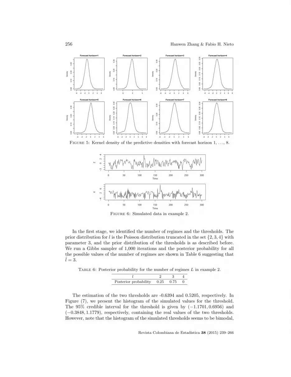
Figure 5: Kernel density of the predictive densities with forecast horizon 1, . . ., 8.
Time
Z
0 50 100 150 200 250 300
−30
24
Time
X
0 50 100 150 200 250 300
−42
6
Figure 6: Simulated data in example 2.
In the first stage, we identified the number of regimes and the thresholds. Theprior distribution for l is the Poisson distribution truncated in the set {2, 3, 4} withparameter 3, and the prior distribution of the thresholds is as described before.We run a Gibbs sampler of 1,000 iterations and the posterior probability for allthe possible values of the number of regimes are shown in Table 6 suggesting thatl̂ = 3.
Table 6: Posterior probability for the number of regimes L in example 2.
l 2 3 4Posterior probability 0.25 0.75 0
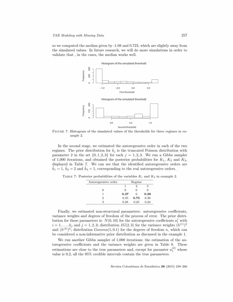
The estimation of the two thresholds are -0.6394 and 0.5205, respectively. InFigure (7), we present the histogram of the simulated values for the threshold.The 95% credible interval for the threshold is given by (−1.1701, 0.6956) and(−0.3848, 1.1779), respectively, containing the real values of the two thresholds.However, note that the histogram of the simulated thresholds seems to be bimodal,
Revista Colombiana de Estadística 38 (2015) 239–266
TAR Modeling with Missing Data 257
so we computed the median given by -1.08 and 0.723, which are slightly away fromthe simulated values. In future research, we will do more simulations in order tovalidate that , in the cases, the median works well.
Histogram of the simulated threshold
First threshold
Freq
uenc
y
−1.0 −0.5 0.0 0.50
200
400
Histogram of the simulated threshold
Second threshold
Freq
uenc
y
0.0 0.5 1.0
015
030
0
Figure 7: Histogram of the simulated values of the thresholds for three regimes in ex-ample 2.
In the second stage, we estimated the autoregressive order in each of the tworegimes. The prior distribution for kj is the truncated Poisson distribution withparameter 2 in the set {0, 1, 2, 3} for each j = 1, 2, 3. We run a Gibbs samplerof 1,000 iterations, and obtained the posterior probabilities for K1, K2 and K3,displayed in Table 7. We can see that the identified autoregressive orders arek̂1 = 1, k̂2 = 2 and k̂3 = 1, corresponding to the real autoregressive orders.
Table 7: Posterior probabilities of the variables K1 and K2 in example 2.
Autoregressive order Regime1 2 3
0 0 0 01 0.37 0 0.382 0.35 0.75 0.383 0.28 0.25 0.24
Finally, we estimated non-structural parameters: autoregressive coefficients,variance weights and degrees of freedom of the process of error. The prior distri-bution for these parameters is: N(0, 10) for the autoregressive coefficients aji withi = 1, . . . , kj and j = 1, 2, 3; distribution IG(2, 3) for the variance weights (h(1))2
and (h(2))2; distribution Gamma(1, 0.1) for the degrees of freedom n, which canbe considered a non-informative prior distribution as discussed in the example 1.
We run another Gibbs sampler of 1,000 iterations; the estimation of the au-toregressive coefficients and the variance weights are given in Table 8. Theseestimations are close to the true parameters and, except for paramter a(2)
1 whosevalue is 0.2, all the 95% credible intervals contain the true parameters.
Revista Colombiana de Estadística 38 (2015) 239–266

258 Hanwen Zhang & Fabio H. Nieto
Table 8: Estimation and 95% credible intervals for the non-structural parameters inexample 2.
Regime a(j)i h(j)
1 0.94 0.53 1.21(0.66, 1.22) (0.43, 0.63) (0.99, 1.47)
2 0.40 0.32 0.52 1.43(0.19, 0.66) (0.21, 0.44) (0.39, 0.64) (1.19, 1.76)
3 -0.68 -0.61 1.82(-0.97, -0.38) (-0.71, -0.49) (1.49, 2.24)
With respect to the degrees of freedom n, the results obtained from the Gibbssampler are displayed in Figure 8, where we noted that the values of n with largeposterior probability are around the true parameter 5. The posterior mean of n isgiven by 5.11 and a 95% credible interval of n is given by (3.17, 8.92).
Histogram of n
n
Freq
uenc
y
2 4 6 8 10 12
010
2030
4050
60
Figure 8: Histogram of the simulated values of the degrees of freedom n in example 2.
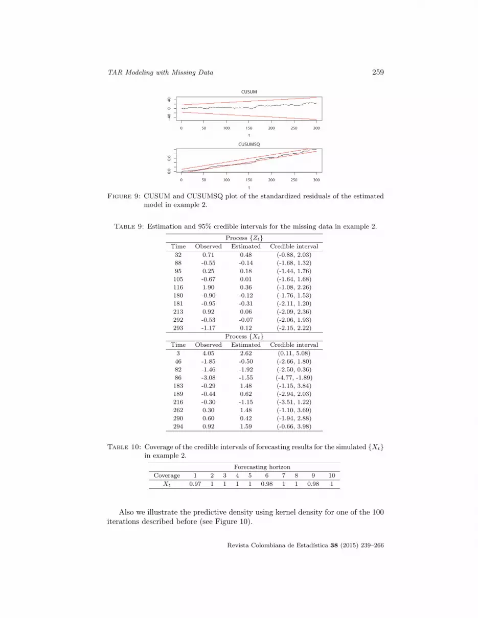
The CUSUM and CUSUMSQ plot of standardized residuals of the estimatedmodel are shown in the Figure (9).
Since identification and estimation results are, generally speaking, satisfactory,we proceeded with the estimation of the missing data. We set the number ofmissing data in the processes {Zt} and {Xt} to be 10 in both series, and placedthe missing data randomly. The estimation and the credible intervals after 5000iterations are shown in Table 9. We can see that the overall performance of theprocedure is satisfactory in the sense that all the observed data are within the 95%credible interval.
Finally, we illustrate the forecast procedure where the sample period consideredis 1-290, and the forecast horizon is set to be 10. We assume that the non-structuralparameters are known and for each horizon we simulate 100 series from the model(18). Like the previous example, we compute the percentage of these 100 credibleintervals containing the true observation. In Table 10 we show these percentages.
Revista Colombiana de Estadística 38 (2015) 239–266
TAR Modeling with Missing Data 259
0 50 100 150 200 250 300
−40
040
CUSUM
t
0 50 100 150 200 250 300
0.0
0.6
CUSUMSQ
t
Figure 9: CUSUM and CUSUMSQ plot of the standardized residuals of the estimatedmodel in example 2.
Table 9: Estimation and 95% credible intervals for the missing data in example 2.
Process {Zt}Time Observed Estimated Credible interval32 0.71 0.48 (-0.88, 2.03)88 -0.55 -0.14 (-1.68, 1.32)95 0.25 0.18 (-1.44, 1.76)105 -0.67 0.01 (-1.64, 1.68)116 1.90 0.36 (-1.08, 2.26)180 -0.90 -0.12 (-1.76, 1.53)181 -0.95 -0.31 (-2.11, 1.20)213 0.92 0.06 (-2.09, 2.36)292 -0.53 -0.07 (-2.06, 1.93)293 -1.17 0.12 (-2.15, 2.22)
Process {Xt}Time Observed Estimated Credible interval3 4.05 2.62 (0.11, 5.08)46 -1.85 -0.50 (-2.66, 1.80)82 -1.46 -1.92 (-2.50, 0.36)86 -3.08 -1.55 (-4.77, -1.89)183 -0.29 1.48 (-1.15, 3.84)189 -0.44 0.62 (-2.94, 2.03)216 -0.30 -1.15 (-3.51, 1.22)262 0.30 1.48 (-1.10, 3.69)290 0.60 0.42 (-1.94, 2.88)294 0.92 1.59 (-0.66, 3.98)
Table 10: Coverage of the credible intervals of forecasting results for the simulated {Xt}in example 2.
Forecasting horizonCoverage 1 2 3 4 5 6 7 8 9 10
Xt 0.97 1 1 1 1 0.98 1 1 0.98 1
Also we illustrate the predictive density using kernel density for one of the 100iterations described before (see Figure 10).
Revista Colombiana de Estadística 38 (2015) 239–266

260 Hanwen Zhang & Fabio H. Nieto
Figure 10: Kernel density of the predictive densities with forecast horizon 1, . . ., 10.
7.2. An Application in Finance
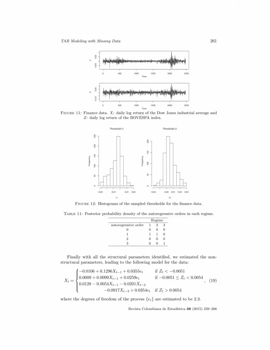
In this section, we applied the proposed algorithm to financial time seriesto illustrate the methodology. Specifically, we used the daily log return of theDow Jones industrial average as the threshold series, and the daily log return ofthe BOVESPA index (Brasil Sao Paulo Stock Exchange Index) as the series ofinterest, from December 12th, 2000 to June 2nd, 2010. Moreno (2010) testedthe non-linearity of the data using the test of Tsay (1998) with lag up to 4for the log return of the Dow Jones index, and found that the appropriate lagis 0. In this way, we defined Xt = ln(BOV ESPAt) − ln(BOV ESPAt−1) andZt = ln(DOWJONESt) − ln(DOWJONESt−1). The log return of these seriesis displayed in Figure 11.
In the first stage of the algorithm, the identified number of regimes is 3 withprobability 1, that is, in all of the 1,000 iterations of the Gibbs sampler, thesampled value of L is 3. The estimated thresholds are -0.0051 and 0.0054, with re-spective credible intervals (-0.0242, 0.0099) and (-0.0081, 0.0226). The histogramsof the sampled thresholds are shown in Figure 12. Observing the values of thetwo thresholds, we could name the three regimes as large negative return in DowJones, small return in Dow Jones and large positive return in Dow Jones.
Once the number of regimes and thresholds were identified, we proceeded withthe identification of the autoregressive orders using another Gibbs sampler. InTable 11, we show the posterior probabilities for all possible values of the autore-gressive orders, suggesting that k̂1 = k̂2 = 1 and k̂3 = 3.
Revista Colombiana de Estadística 38 (2015) 239–266
TAR Modeling with Missing Data 261
Time
Z
0 500 1000 1500 2000 2500
−0.05
0.05
Time
X
0 500 1000 1500 2000 2500
−0.10
0.05
Figure 11: Finance data. X: daily log return of the Dow Jones industrial average andZ: daily log return of the BOVESPA index.
Threshold r1
r1
Freq
uenc
y
−0.03 −0.01 0.01 0.02
050
100
150
200
250
Threshold r2
r2
Freq
uenc
y
−0.02 0.00 0.01 0.02 0.03
050
100
150
200
Figure 12: Histograms of the sampled thresholds for the finance data.
Table 11: Posterior probability density of the autoregressive orders in each regime.
Regimeautoregressive order 1 2 3
0 0 0 01 1 1 02 0 0 03 0 0 1
Finally with all the structural parameters identified, we estimated the non-structural parameters, leading to the following model for the data:
Xt =
−0.0106 + 0.1296Xt−1 + 0.0355et if Zt < −0.0051
0.0009 + 0.0099Xt−1 + 0.0259et if −0.0051 ≤ Zt < 0.0054
0.0128− 0.0054Xt−1 − 0.0201Xt−2
−0.0917Xt−3 + 0.0354et if Zt > 0.0054
, (19)
where the degrees of freedom of the process {et} are estimated to be 2.3.
Revista Colombiana de Estadística 38 (2015) 239–266

262 Hanwen Zhang & Fabio H. Nieto
The credible intervals of the parameters in (19) are given in
Table 12: 95% credible intervals for the parameters in the model (19).
Regime a(j)i h(j)
1 (-0.012, -0.009) (0.062,0.189) (0.033,0.037)2 (0.000, 0.001) (-0.030,0.052) (0.025,0.027)3 (0.012, 0.014) (-0.068,0.062) (-0.085,0.040) (-0.152,-0.023) (0.033,0.037)
Moreno (2010) found a similar TARmodel for the same data using the approachof Nieto (2005), that is, assuming the Gaussian distribution for the noise process.The TAR model found in Moreno (2010) is:
Xt =
−0.0127 + 0.111Xt−1 − 0.068Xt−2 + 0.0198et if Zt < −0.00540.00068 + 0.0137et if −0.0054 ≤ Zt < 0.0057
0.0135− 0.0837Xt−1 − 0.0684Xt−2 − 0.1687Xt−3
−0.0633Xt−4 + 0.0191et if Zt > 0.0057
(20)
We can observe that the number of regimes is the same and that the twothresholds are quite similar. Also, the type II conditional variance in the first andthird regimes are similar and larger than the conditional variance in the secondregime, that is, the series of log return of BOVESPA is more stable when theDow Jones index is relatively stable. On the other hand, in spite of the factthat the autoregressive orders are different in the two models, the autoregressivecoefficients in common are also similar. However, we note a better fit with t noisesince the DIC (deviance information criterion) is 5,485.377 for the TAR modelwith Gaussian error and 4338.799 for TAR with t error (up to a constant).
In order to check the appropriateness of the model, we use the CUSUM andCUSUMSQ plot of standardized residuals, shown in Figure 13, which suggests thatthe fitted model (19) is appropriate.
0 500 1000 1500 2000 2500
−150
010
0
CUSUM
t
0 500 1000 1500 2000 2500
0.0
0.4
0.8
CUSUMSQ
t
Figure 13: CUSUM and CUSUMSQ plot of the standardized residuals of the model(19).
As shown in the work of Moreno (2010), the TAR model with Gaussian noise(20), in spite of showing good performance in the CUSUM and CUSUMSQ plots
Revista Colombiana de Estadística 38 (2015) 239–266

TAR Modeling with Missing Data 263
of the residuals, the squared residuals show large autocorrelations, which is adisadvantage compared to the family of GARCH models where the residuals showstrong evidence of independence (see the ACF of residuals and squared residuals ofa GARCH(1,1) model in Figure 14). In Figure 15, we can observe the ACF of theresiduals and squared residuals, and obviously the squared residuals of the TARmodel with t distributed noise still exhibit the same problem as the TAR modelwith Gaussian noise. Although the TAR model seems to fail in capturing all thestructure of dependence in the data, Nieto & Moreno (2013) found the expressionfor the conditional variance V ar(Xt|xt−1, . . . , x1) in a TAR model, making thisclass of model comparable with the GARCH models. In Figure 16, we show theconditional variance V ar(Xt|xt−1, . . . , x1) in the TAR model 19, as well as theGARCH(1,1) model; we can see that the general behaviour is similar for the twomodels, although the bottom line in the TAR model is around 0.0076, while in theGARCH model it around 0.0003.
0 5 10 15 20 25 30
0.0
0.6
Lag
ACF
Residuals
0 5 10 15 20 25 30
0.0
0.6
Lag
ACF
Squared residuals
Figure 14: ACF of residuals and squared residuals of the model GARCH(1,1).
0 5 10 15 20 25 30
0.0
0.6
Lag
ACF
Residuals
0 5 10 15 20 25 30
0.0
0.6
Lag
ACF
Squared residuals
Figure 15: ACF of residuals and squared residuals of the model (19).
Revista Colombiana de Estadística 38 (2015) 239–266

264 Hanwen Zhang & Fabio H. Nieto
TAR model
Time0 500 1000 1500 2000 2500
0.00
750
0.00
770
GARCH model
Time
0 500 1000 1500 2000 2500
0.00
00.00
2
Figure 16: Conditional variance of the TAR model and the GARCH model.
8. Conclusion
In this work, we proposed a new family of TAR models: the TAR models witht-distributed noise process with a three-stage procedure consisting of: (1) iden-tifying the number of regimes and the corresponding thresholds, (2) identifyingthe autoregressive order in each regime, and (3) estimating non-structural pa-rameters, i.e., the autoregressive coefficients and the type II conditional variancein each regime, and other parameters that each particular model may contain.The performance of the developed methodology is satisfactory in simulated data,however, the GARCH models seems to better capture the heterocedastic aspectcontained in financial data. In future investigation the GARCH models may beused together with the TAR model.[
Received: October 2013 — Accepted: November 2014]
References
Briñez, A. & Nieto, F. (2005), ‘Fitting a nonlinear model to the precipitationvariable in a Colombian Hydrological/Meteorological station’, Revista Colom-biana de Estadística 28, 113–124,.
Carlin, B. P. & Chib, S. (1995), ‘Bayesian model choice via Markov Chain MonteCarlo Methods’, Journal of the Royal Statistical Society. Serie B 37(3), 473–484.
Chen, H., Chong, T. T. & Bai, J. (2012), ‘Theory and applications of TAR modelwith two threshold variables’, Econometric Reviews 31, 142–170.
Congdon, P. (2001), Bayesian Statistical Modeling, John Wiley & Sons, New York.
Revista Colombiana de Estadística 38 (2015) 239–266

TAR Modeling with Missing Data 265
Geweke, J. (1992), Evaluating the accuracy of sampling-based approaches to thecalculation of posterior moments, in ‘Bayesian Statistics’, University Press,pp. 169–193.
Moreno, E. (2010), Modelos TAR en series de tiempo financieras, Master’s thesis,Universidad Nacional de Colombia.
Nieto, F. H. (2005), ‘Modeling bivariate threshold autoregressive processes in thepresence of missing data’, Communications in Statistics, Theory and Methods.34, 905–930.
Nieto, F. H. (2008), ‘Forecasting with univariate TAR models’, Statistical Method-ology. 5, 263–276.
Nieto, F. H. & Moreno, E. (2013), A note on the specification of conditionalheteroscedasticity using a TAR model, Technical Report RI21, UniversidadNacional de Colombia.
Nieto, F. H., Zhang, H. & Li, W. (2013), ‘Using the Reversible Jump MCMCProcedure for Identifying and Estimating Univariate TAR Models’, Commu-nications In Statistics. Simulation And Computation 42(4), 814–840.
Nieto, F. & Hoyos, M. (2011), ‘Testing linearity against a univariate TAR speci-fication in time series with missing data’, Revista Colombiana de Estadística34, 73–94.
Plummer, M., Best, N., Cowles, K. & Vines, K. (2006), ‘Coda: Convergencediagnosis and output analysis for mcmc’, R News 6(1), 7–11.*http://CRAN.R-project.org/doc/Rnews/
Sáfadi, T. & Morettin, P. (2000), ‘Bayesian analysis of thresholds autoregressivemoving average models’, The Indian Journal of Statistics 62, 353–371.
Tong, H. (1978), On a Threshold Model, in C. H. Chen, ed., ‘Pattern Recognitionand Signal Processing’, Sijthoff & Noordhoff, Netherlands, pp. 575–586.
Tsay, R. S. (1989), ‘Testing and modeling threshold autoregressive processes’, Jour-nal of American Statistical Association 84, 231–240.
Tsay, R. S. (1998), ‘Testing and modeling multivariate threshold models’, Journalof American Statistical Association 93, 1188–1202.
Vargas, L. (2012), Cálculo de la distribución predictiva en un modelo TAR, Mas-ter’s thesis, Universidad Nacional de Colombia.
Watanabe, T. (2001), ‘On sampling the degree-of-freedom of Student’s-t distur-bances’, Statistics & Probability Letters 52, 177–181.
Xia, Q., Liu, L., Pan, J. & Liang, R. (2012), ‘Bayesian analysis of two-regimethreshold autoregressive moving average model with exogenous inputs’, Com-munications in Statistics - Theory and Methods 41, 1089–1104.
Revista Colombiana de Estadística 38 (2015) 239–266

266 Hanwen Zhang & Fabio H. Nieto
Zhang, H. (2012), ‘Estimación de los modelos TAR cuando el proceso del ruidosigue una distribución t’, Comunicaciones en Estadística 4(2), 109–119.
Revista Colombiana de Estadística 38 (2015) 239–266