Embed Size (px)
Citation preview

Tabled Higher-Order Logic Programming
Brigitte Pientka
December 2003
CMU-CS-03-185
School of Computer Science
Carnegie Mellon University
Pittsburgh, PA 15213
Submitted in partial fulfillment of the requirements
for the degree of Doctor of Philosophy
Thesis Committee:
Frank Pfenning, Carnegie Mellon University, Chair
Robert Harper, Carnegie Mellon University
Dana Scott, Carnegie Mellon University
David Warren, University of New York at Stony Brook
Copyright 2003 Brigitte Pientka
This research was sponsored by the US Air Force (USAF) under grant F1962895C0050, the NationalScience Foundation (NSF) under grant CCR-9619584 and grant CCR-9988281, and by a generousdonation from the Siebel Scholars Program. The views and conclusions contained in this documentare those of the author and should not be interpreted as representing the official policies, eitherexpressed or implied, of the USAF, NSF, the U.S. government or any other entity.

Keywords: Logic programming, Type theory, Automated theorem proving, Logi-
cal frameworks

Abstract
A logical framework is a general meta-language for specifying and implementing de-
ductive systems, given by axioms and inference rules. Based on a higher-order logic
programming interpretation, it supports executing logical systems and reasoning with
and about them, thereby reducing the effort required for each particular logical system.
In this thesis, we describe different techniques to improve the overall performance
and the expressive power of higher-order logic programming. First, we introduce tabled
higher-order logic programming, a novel execution model where some redundant infor-
mation is eliminated using selective memoization. This extends tabled computation
to the higher-order setting and forms the basis of the tabled higher-order logic pro-
gramming interpreter. Second, we present efficient data-structures and algorithms for
higher-order proof search. In particular, we describe a higher-order assignment algo-
rithm which eliminates many unnecessary occurs checks and develop higher-order term
indexing. These optimizations are crucial to make tabled higher-order logic program-
ming successful in practice. Finally, we use tabled proof search in the meta-theorem
prover to reason efficiently with and about deductive systems. It takes full advantage
of higher-order assignment and higher-order term indexing.
As experimental results demonstrate, these optimizations taken together constitute
a significant step toward exploring the full potential of logical frameworks in practice.


Contents
1 Introduction 11
2 Dependently typed lambda calculus based on modal type theory 19
2.1 Motivation . . . . . . . . . . . . . . . . . . . . . . . . . . . . . . . . . . 20
2.2 Syntax . . . . . . . . . . . . . . . . . . . . . . . . . . . . . . . . . . . . 21
2.3 Substitutions . . . . . . . . . . . . . . . . . . . . . . . . . . . . . . . . 21
2.4 Judgments . . . . . . . . . . . . . . . . . . . . . . . . . . . . . . . . . . 24
2.5 Typing rules . . . . . . . . . . . . . . . . . . . . . . . . . . . . . . . . . 25
2.6 Definitional equality . . . . . . . . . . . . . . . . . . . . . . . . . . . . 26
2.7 Elementary properties . . . . . . . . . . . . . . . . . . . . . . . . . . . 29
2.8 Type-directed algorithmic equivalence . . . . . . . . . . . . . . . . . . . 38
2.9 Completeness of algorithmic equality . . . . . . . . . . . . . . . . . . . 44
2.10 Soundness of algorithmic equality . . . . . . . . . . . . . . . . . . . . . 50
2.11 Decidability of type-checking . . . . . . . . . . . . . . . . . . . . . . . . 56
2.12 Canonical forms . . . . . . . . . . . . . . . . . . . . . . . . . . . . . . . 59
2.13 Implementation of existential variables . . . . . . . . . . . . . . . . . . 62
2.14 Conclusion and related work . . . . . . . . . . . . . . . . . . . . . . . . 63
3 Toward efficient higher-order pattern unification 65
3.1 Higher-order pattern unification . . . . . . . . . . . . . . . . . . . . . . 66
3.1.1 Unifying an existential variable with another term . . . . . . . . 71
3.1.2 Unifying two identical existential variables . . . . . . . . . . . . 84
3.2 Rules for higher-order pattern unification . . . . . . . . . . . . . . . . . 95
3.3 Linearization . . . . . . . . . . . . . . . . . . . . . . . . . . . . . . . . 95
5

3.4 Assignment for higher-order patterns . . . . . . . . . . . . . . . . . . . 101
3.5 Experiments . . . . . . . . . . . . . . . . . . . . . . . . . . . . . . . . . 104
3.5.1 Higher-order logic programming . . . . . . . . . . . . . . . . . . 105
3.5.2 Higher-order theorem proving . . . . . . . . . . . . . . . . . . . 107
3.5.3 Constraint solvers . . . . . . . . . . . . . . . . . . . . . . . . . . 108
3.6 Related work and conclusion . . . . . . . . . . . . . . . . . . . . . . . . 109
4 Tabled higher-order logic programming 111
4.1 A motivating example: subtyping . . . . . . . . . . . . . . . . . . . . . 112
4.2 Tabled logic programming: a quick review . . . . . . . . . . . . . . . . 115
4.3 Tabled higher-order logic programming . . . . . . . . . . . . . . . . . . 117
4.4 Subordination . . . . . . . . . . . . . . . . . . . . . . . . . . . . . . . . 119
4.5 A foundation for tabled higher-order logic programming . . . . . . . . . 120
4.5.1 Uniform proofs . . . . . . . . . . . . . . . . . . . . . . . . . . . 120
4.5.2 Uniform proofs with answer substitutions . . . . . . . . . . . . . 123
4.5.3 Tabled uniform proofs . . . . . . . . . . . . . . . . . . . . . . . 129
4.5.4 Related work and conclusion . . . . . . . . . . . . . . . . . . . . 134
4.6 Case studies . . . . . . . . . . . . . . . . . . . . . . . . . . . . . . . . . 135
4.6.1 Bidirectional typing (depth-first vs memoization) . . . . . . . . 136
4.6.2 Parsing (iterative deepening vs memoization) . . . . . . . . . . 140
4.7 Related work and conclusion . . . . . . . . . . . . . . . . . . . . . . . . 142
5 Higher-order term indexing 145
5.1 Higher-order substitution trees . . . . . . . . . . . . . . . . . . . . . . . 147
5.1.1 Standardization: linear higher-order patterns . . . . . . . . . . . 148
5.1.2 Example . . . . . . . . . . . . . . . . . . . . . . . . . . . . . . . 149
5.2 Insertion . . . . . . . . . . . . . . . . . . . . . . . . . . . . . . . . . . . 153
5.3 Retrieval . . . . . . . . . . . . . . . . . . . . . . . . . . . . . . . . . . . 170
5.4 Experimental results . . . . . . . . . . . . . . . . . . . . . . . . . . . . 178
5.4.1 Parsing of first-order formulae . . . . . . . . . . . . . . . . . . . 179
5.4.2 Refinement type-checker . . . . . . . . . . . . . . . . . . . . . . 180
5.4.3 Evaluating Mini-ML expression via reduction . . . . . . . . . . 181
5.5 Related work and conclusion . . . . . . . . . . . . . . . . . . . . . . . . 182

6 An implementation of tabling 185
6.1 Background . . . . . . . . . . . . . . . . . . . . . . . . . . . . . . . . . 186
6.2 Support for tabling . . . . . . . . . . . . . . . . . . . . . . . . . . . . . 188
6.2.1 Table . . . . . . . . . . . . . . . . . . . . . . . . . . . . . . . . . 191
6.2.2 Indexing for table entries . . . . . . . . . . . . . . . . . . . . . . 193
6.2.3 Answers . . . . . . . . . . . . . . . . . . . . . . . . . . . . . . . 194
6.2.4 Suspended goals . . . . . . . . . . . . . . . . . . . . . . . . . . . 195
6.2.5 Resuming computation . . . . . . . . . . . . . . . . . . . . . . . 197
6.2.6 Multi-staged tabled search . . . . . . . . . . . . . . . . . . . . . 198
6.3 Variant and subsumption checking . . . . . . . . . . . . . . . . . . . . . 198
7 Higher-order theorem proving with tabling 203
7.1 Example: type system with subtyping . . . . . . . . . . . . . . . . . . . 204
7.2 Twelf: meta-theorem prover . . . . . . . . . . . . . . . . . . . . . . . . 209
7.3 Generic proof search based on memoization . . . . . . . . . . . . . . . . 212
7.4 Experiments . . . . . . . . . . . . . . . . . . . . . . . . . . . . . . . . . 213
7.4.1 Type preservation for type system with subtyping . . . . . . . . 213
7.4.2 Derived rules of inference in classical natural deduction . . . . . 215
7.4.3 Refinement types . . . . . . . . . . . . . . . . . . . . . . . . . . 216
7.4.4 Rewriting semantics . . . . . . . . . . . . . . . . . . . . . . . . 216
7.5 Conclusion . . . . . . . . . . . . . . . . . . . . . . . . . . . . . . . . . . 218
8 Conclusion 221


Acknowledgments
First of all I would like to thank my advisor Frank Pfenning for all his support and
patience even before I started as a graduate student at CMU. His ideas shaped this
thesis in many ways. His persistent questions and insistence on clarity and precision
have been instrumental in understanding and writing about some of the issues pre-
sented in this thesis. In particular I appreciate his openness to always discuss technical
problems, trying to make sense of half-baked ideas, and patiently explaining problems.
Second, I would like to thank the members of my thesis committee, Bob Harper,
Dana Scott and David Warren for serving on my committee, giving valuable criticism
and support. In particular, I would like to thank David Warren for his insights into
XSB and his eagerness to understand some of the higher-order logic programming
issues.
Third, my thanks go to Christoph Kreitz who has been a mentor during my year at
Cornell and has been instrumental in my decision to come the US and join a graduate
program. I also want to thank Alan Bundy and Bob Constable who gave me valuable
research opportunities before I started graduate school.
Special thanks go to Carsten Schurmann for his support during my time at CMU,
his friendship and all the technical discussions about Twelf. For many discussions and
valuable feedback I would like to thank the members of the POP-group, in particular
Andrew Bernard, Karl Crary, Aleksander Nanevski, Susmit Sarkar, and Kevin Watkins.
Many thanks also go to Chad Brown for endless discussions about type-theory.
I could not have completed this journey without some friends in Pittsburgh and
elsewhere. Women@scs has been a welcoming and supporting community and I have
met many extraordinary women in computer science through them. It certainly has
made my time at CMU more fun and rewarding. In particular, I would like to thank
9
Laurie Hiyakumoto, Jorjeta Jetcheva, Orna Raz, and Bianca Schroder for all their
support, understanding, time and care of each other. They were always willing to
spare some time, share the ups and downs in graduate school, and provide much needed
distractions and breaks from work.
For providing me with an escape from Wean Hall and a different view to life and
work, my thanks go to Uljana Feest who seemed to always enjoy life to the fullest while
earning a philosophy PhD incidentally. For their support from abroad and for always
welcoming me in Berlin and Jena, I would like to thank Vicky Temperton and Katrin
Teske. I am also indebted to my parents who allowed me to go my way, although it
was sometimes hard for them to understand and agree.
Last but not least, I want to thank Dirk Schlimm – without him I would not have
made it to Pittsburgh. He always believed in me, patiently endured all my stubbornness
and shared all the frustration and joy.
And, I almost forgot..., thanks also to Bruno, the cat, who has been teaching me
that life isn’t so hard after all ...

Chapter 1
Introduction
A logical framework is a general meta-language for specifying and implementing de-
ductive systems, given by axioms and inference rules. Examples of deductive systems
are plentiful in computer science. In computer security, we find authentication and
security logics to describe access and security criteria. In programming languages, we
use deductive systems to specify the operational semantics, type-systems or other as-
pects of the run-time behavior of programs. Recently, one major application of logical
frameworks has been in the area of “certified code”. To provide guarantees about the
behavior of mobile code, safety properties are expressed as deductive systems. The
code producer then verifies the program according to some predetermined safety pol-
icy, and supplies a binary executable together with its safety proof (certificate). Before
executing the program, the host machine then quickly checks the code’s safety proof
against the binary. The safety policy and the safety proofs can be expressed in the
logical framework thereby providing a general safety infrastructure.
There are two main variants of logical frameworks which are specifically designed
to support the implementation of deductive systems. λProlog and Isabelle are based
on hereditary Harrop formulas, while the Twelf system [53] is an implementation of
the logical framework LF, a dependently typed lambda calculus. In this thesis, we
will mainly focus on the latter. By assigning a logic programming interpretation to
types [47], we obtain a higher-order logic programming language. Higher-order logic
programming in Twelf extends traditional first-order logic programming in three ways:
First, we have a rich type system based on dependent types, which allows the user to
11

CHAPTER 1. INTRODUCTION
define her own higher-order data-types and supports higher-order abstract syntax [52].
Variables in the object language can be directly represented as variables in the meta-
language thereby directly inheriting capture-avoiding substitution and bound variable
renaming. Second, we not only have a static set of program clauses, but clauses may
be introduced dynamically and used within a certain scope during proof search. Third,
we have an explicit notion of proof, i.e., the logic programming interpreter does not
only return an answer substitution for the free variables in the query, but also the
actual proof of the query as a term in the dependently typed lambda-calculus. This
stands in sharp contrast to higher-order features supported in many traditional logic
programming languages (see for example [13]) where we can encapsulate predicate
expressions within terms to later retrieve and invoke such stored predicates. Twelf’s
higher-order logic programming interpreter is complemented by a meta-theorem prover,
which combines generic proof search based on higher-order logic programming with
inductive reasoning [53, 63].
The Twelf system has been successfully used to implement, execute and reason
about a wide variety of deductive systems. However, experience with real-world appli-
cations in different projects on certified code [4, 15, 3] have increasingly demonstrated
the limitations of Twelf’s higher-order logic programming proof search. To illustrate,
let us briefly consider the foundational proof-carrying code project at Princeton. As
part of this project, the researchers at Princeton have implemented between 70,000
and 100,000 lines of Twelf code, which includes data-type definitions and proofs. The
higher-order logic program, which is used to execute safety policies, consists of over
5,000 lines of code, and over 600 – 700 clauses. Such large specifications have put to
test implementations of logical frameworks and exposed several problems. First, per-
formance of the higher-order logic programming interpreter may be severely hampered
by redundant computation, leading to long response times and slow development of
formal specifications. Second, many straightforward specifications of formal systems,
for example recognizers and parsers for grammars, rewriting systems, type systems
with subtyping or polymorphism, are not executable, thus requiring more complex
and sometimes less efficient implementations. Thirdly, redundancy severely hampers
the reasoning with and about deductive systems in general, limiting the use of the
meta-theorem prover.
In applications to certified code, efficient proof search techniques not only play an
12

important role to execute safety polices and generate a certificate that a given program
fulfills a specified safety policy, but it also can be used to check the correctness of a
certificate [42]. Necula and Rahul [42] propose as a certificate a bit-string of the
non-deterministic choices in the proof. Hence, a proof can be checked by guiding the
higher-order logic programming interpreter with the bit-string and reconstructing the
actual proof. As pointed out by Necula and Lee, typical safety proof in the context
of certified code commonly have repeated sub-proofs that should be hoisted out and
proved only once. The replication of common sub-proofs leads to redundancy in the
bit-strings representing the safety proof and it may take longer to reconstruct the safety
proof using a guided higher-order logic programming interpreter.
In this thesis, we develop different techniques which improve the overall performance
and the expressive power of the higher-order logic programming interpreter. We also
apply these ideas in the meta-theorem prover to overcome existing limitations when
reasoning about deductive systems. These optimizations taken together constitute a
significant step toward exploring the full potential of logical frameworks in real-world
applications. Some of the work in this thesis has been previously published in different
forms [54, 55, 56, 57, 41]
Contributions
The contributions in this thesis are in three main areas: First, we introduce tabled
higher-order logic programming, a novel execution model where some redundant in-
formation is eliminated using selective memoization. This forms the basis of the
tabled higher-order logic programming interpreter. Second, we develop efficient data-
structures and algorithms for higher-order proof search. These optimizations are cru-
cial to make tabled higher-order logic programming successful in practice. Although
we develop these techniques in the context of tabled logic programming, they are
also independently useful and important to other areas such as higher-order rewrit-
ing, higher-order theorem proving and higher-order proof checking. Third, we use
memoization-based proof search in the meta-theorem prover, to reason efficiently with
and about deductive systems. This demonstrates the importance of memoization in
general. Next, we will discuss briefly each of these contributions.
13

CHAPTER 1. INTRODUCTION
Tabled higher-order logic programming
Tabled first-order logic programming has been successfully applied to solve complex
problems such as implementing recognizers and parsers for grammars [68], representing
transition systems CCS and writing model checkers [16]. The idea behind it is to elim-
inate redundant computation by memoizing sub-computation and re-using its results
later. The resulting search procedure is complete and terminates for programs with
the bounded-term size property. The XSB system [62], a tabled logic programming
system, demonstrates impressively that tabled together with non-tabled programs can
be executed efficiently in the first-order setting.
The success of memoization in first-order logic programming strongly suggests that
memoization may also be valuable in higher-order logic programming. In fact, Necula
and Lee point out in [44] that typical safety proofs in the context of certified code
commonly have repeated sub-proofs that should be hoisted out and proved only once.
Memoization has potentially three advantages. First, proof search is faster thereby
substantially reducing the response time to the programmer. Second, the proofs them-
selves are more compact and smaller. This is especially important in applications to
secure mobile code where a proof is attached to a program, as smaller proofs take up less
time to check and transmit to another host. Third, substantially more specifications,
for example recognizers and parser for grammars, evaluators based on rewriting or type
systems with subtyping, are executable under the new paradigm thereby extending the
power of the existing system.
Using memoization in higher-order logic programming poses several challenges,
since we have to handle type dependencies and may have dynamic assumptions which
are introduced during proof search. This is unlike tabling in XSB, where we have no
types and it suffices to memoize atomic goals. Moreover, most descriptions of tabling
in the first-order setting are closely oriented on the WAM (Warren Abstract Machine)
making it hard to transfer tabling techniques and design extensions to other logic
programming interpreters.
In this thesis, we introduce a novel execution model for logical frameworks based
on selective memoization.
Proof-theoretic characterization of uniform proofs and memoization We give
a proof-theoretic characterization of tabling based on uniform proofs, and show
14

soundness of the resulting interpreter. This provides a high-level description of a
tabled logic programming interpreter and separates logical issues from procedural
ones leaving maximum freedom to choose particular control mechanisms.
Implementation of a tabled higher-order logic programming interpreter We
give a high-level description of a semi-functional implementation for adding tabling
to a higher-order logic programming interpreter. We give an operational interpre-
tation of the uniform proof system and discuss some of the implementation issues
such as suspending and resuming computation, retrieving answers, and trailing.
Unlike other description, it does not require an understanding or modifications,
and extensions to the WAM (Warren abstract machine). It is intended as a high-
level explanation and guide for adding tabling to an existing logic programming
interpreter. This is essential for rapidly prototyping tabled logic programming
interpreters, even for linear logic programming and other higher-order logic pro-
gramming systems.
Case studies We discuss two case studies to illustrate the use of memoization in the
higher-order setting. We consider a parser and recognizer for first-order formulas
into higher-order abstract syntax. To model left and right associativity of the
different connectives, we mix left and right recursion in the specification of the
parser. Although this closely models the grammar, it leads to an implementation
which is not executable with traditional logic programming interpreters which
are based on depth-first search.
The second case study is an implementation of a bi-directional type-checker by
Davies and Pfenning [17]. The type-checker is executable with the original logic
programming interpreter, which performs a depth-first search. However, redun-
dant computation may severely hamper its performance as there are several
derivations for proving that a program has a specified type.
Efficient data-structures and algorithms
Efficient data-structures and implementation techniques play a crucial role in utilizing
the full potential of a reasoning environment in large scale applications. Although
15

CHAPTER 1. INTRODUCTION
this need has been widely recognized for first-order languages, efficient algorithms for
higher-order languages are still a central open problem.
Proof-theoretic foundation for existential variables based on modal logic
We give a dependent modal lambda calculus, which extends the theory of the
logical framework LF [29] conservatively with modal variables. Modal variables
can be interpreted as existential variables, thereby clearly distinguishing them
from ordinary bound variables. This is critical to achieve a simplified account of
higher-order unification and allows us to justify different optimizations such as
as lowering, raising, and linearization [57, 41]. It also serves as a foundation for
designing higher-order term indexing strategies.
Optimizing unification Unification lies at the heart of logic programming, theorem
proving, and rewriting systems. Thus, its performance affects in a crucial way
the global efficiency of each of these applications. Higher-order unification is
in general undecidable, but decidable fragments, such as higher-order patterns
unification, exist. Unfortunately, the complexity of this algorithm is still at best
linear, which is impractical for any useful programming language or practical
framework. In this thesis, we present an assignment algorithm for linear higher-
order patterns which factors out unnecessary occurs checks. Experiments show
that we get a speed-up by up to a factor 2 – 5 making the execution of some
examples feasible. This is a significant step toward efficient implementation of
higher-order reasoning systems in general [57].
Higher-order term indexing Proof search strategies, such as memoization, can only
be practical if we can access the memo-table efficiently. Otherwise, the rate of
drawing new conclusions may degrade sharply both with time and with an in-
crease of the size of the memo-table. Term indexing aims at overcoming pro-
gram degradation by sharing common structure and factoring common opera-
tions. Higher-order term indexing has been a central open problem, limiting
the application and the potential impact of higher-order reasoning systems. In
this thesis, we develop and implemented higher-order term indexing techniques.
They improve performance by up to a factor of 9, illustrating the importance of
indexing [56].
16

Meta-theorem proving based on memoization
The traditional approach for supporting theorem proving in logical frameworks is to
guide proof search using tactics and tacticals. Tactics transform a proof structure
with some unproven leaves into another. Tacticals combine tactics to perform more
complex steps in the proof. Tactics and tacticals are written in ML or some other
strategy language. To reason efficiently about some specification, the user implements
specific tactics to guide the search. This means that tactics have to be rewritten for
different specifications. Moreover, the user has to understand how to guide the prover
to find the proof, which often requires expert knowledge about the systems. Proving
the correctness of the tactic is itself a complex theorem proving problem.
The approach taken in the Twelf system is to endow the framework with the oper-
ational semantics of logic programming and design general proof search strategies for
it. Twelf’s meta-theorem prover combines general proof search based on higher-order
logic programming with inductive reasoning. Using the proof-theoretic characteriza-
tion of tabling, we develop a general memoization-based proof search strategy which
is incorporated in Twelf’s meta-theorem prover. As experiments demonstrate, elimi-
nating redundancy in meta-theorem proving is critical to prove properties about larger
and more complex specifications. We discuss several examples including type preserva-
tion proofs for type-system with subtyping, several inversion lemmas about refinement
types, and reasoning in classical natural deduction. These examples include several
lemmas and theorems which were not previously provable. Moreover, we show that in
many cases no bound is needed on memoization-based search. As a consequence, if
a sub-case is not provable, the user knows, that in fact no proof exists. This in turn
helps the user to revise the formulation of the theorem or the specification. Overall
the benefits of memoization are an important step towards a more robust and more
efficient meta-theorem prover.
17

CHAPTER 1. INTRODUCTION
18

Chapter 2
Dependently typed lambda calculus
based on modal type theory
In this chapter, we introduce a dependently typed lambda calculus based on modal
type theory. The underlying motivation for this work is to provide a logical founda-
tion for the implementation of logical frameworks and the design choices one has to
make in practice. One such choice is for example the treatment of existential variables.
Existential variables are usually implemented via mutation. However, previous formu-
lations of logical frameworks [28, 29] do not capture or explain this technique. The
framework presented in this chapter serves as a foundation for the subsequent chapters
on higher-order unification, higher-order proof search, and higher-order term indexing.
We present here an abstract view of existential variables based on modal type
theory. Existential variables u (or v) are treated as modal variables. This allows us
to reason about existential variables as first-class objects and directly explain many
optimizations done in implementations. In this chapter, we will conservatively extend
the theory of the logical framework LF given by Harper and Pfenning in [29] with
modal variables. Following Harper and Pfenning, we will introduce this language and
show that definitional equality remains decidable. In addition, normalization and type-
checking are decidable.
19

CHAPTER 2. DEPENDENTLY TYPED LAMBDA CALCULUS BASED ON MODAL TYPE THEORY
2.1 Motivation
Before presenting the foundation for dependently typed existential variables, we briefly
motivate our approach based on modal logic. Following the methodology of Pfenning
and Davies [51], we can assign constructive explanations to modal operators. A key
characteristic of this view is to distinguish between propositions that are true and
propositions that are valid. A proposition is valid if its truth does not depend on the
truth of any other propositions. This leads to the basic hypothetical judgment
A1 valid , . . . An valid ;B1 true, . . . , Bm true ` C true.
Under the multiple-world interpretation of modal logic, C valid corresponds to
C true in all reachable worlds. This means C true without any assumptions, except
those that are assumed to be true in all worlds. We can generalize this idea to also
capture truth relative to a set of specified assumptions by writing C valid Ψ, where Ψ
is the abbreviation for C1 true, . . . , Cn true. In terms of the multiple world semantics,
this means that C is true in any world where C1 through Cn are all true and we say C
is valid relative to the assumptions in Ψ. Hypotheses about relative validity are more
complex now, so our general judgment form is
A1 valid Ψ1, . . . , An valid Ψn;B1 true, . . . , Bm true ` C true
While it is interesting to investigate this modal logic above in its own right, it does
not come alive until we introduce proof terms. In this chapter, we investigate the
use of a modal proof term calculus as a foundation for existential variables. We will
view existential variables u as modal variables of type A in a context Ψ while bound
variables are treated as ordinary variables. This allows us to distinguish between
existential variables u::(Ψ`A) for relative validity assumptions A valid Ψ declared in a
modal context, and x:A for ordinary truth assumptions A true declared in an (ordinary)
context. If we have an assumption A valid Ψ we can only conclude A true if we can
verify all assumptions in Ψ.
∆, A valid Ψ,∆′; Γ ` Ψ
∆, A valid Ψ,∆′; Γ ` A true(∗)
In other words, if we know A true in Ψ, and all elements in Ψ can be verified from
the assumptions in Γ, then we can conclude A true in Γ. As we will see in the next
20

2.2. SYNTAX
section, this transition from one context Ψ to another context Γ, can be achieved via
a substitutions from Ψ to Γ.
2.2 Syntax
We conservatively extend LF [28] with modal variables. Existential variables u (or v)
are treated as modal variables and x denotes ordinary variables. Existential variables
are declared in a modal context ∆, while bound variables x:A are declared in a context
Γ or Ψ. Note that the modal variables u declared in ∆ carry their own context of
bound variables Ψ and type A. The substitution σ is part of the syntax of existential
variables. c and a are constants, which are declared in a signature.
Substitutions σ, τ ::= · | σ,M/x
Objects M,N ::= c | x | u[σ] | λx:A. M |M1 M2
Families A,B,C ::= a | AM | Πx:A1. A2
Kinds K ::= type | Πx:A. K
Signatures Σ ::= · | Σ, a:K | Σ, c:AContexts Γ,Ψ ::= · | Γ, x:A
Modal Contexts ∆ ::= · | ∆, u::(Ψ`A)
We use K for kinds, and A, B, C for type families, M , N for object. Signatures,
contexts and modal contexts may declare each constant and variable at most once.
For example, when we write Γ, x:A we assume that x is not already declared in Γ. If
necessary, we tacitly rename x before adding it to the context Γ. Similarly, when we
write ∆, u::(Ψ ` A), we assume that u is not already declared in ∆. Terms that differ
only in the names of their bound and modal variables are considered identical.
2.3 Substitutions
We write the substitution operation as a defined operations in prefix notation [σ]P ,
for an object, family, or kind P . These operations are capture-avoiding as usual.
Moreover, we always assume that all free variables in P are declared in σ. Substitutions
that are part of the syntax are written in postfix notation, u[σ]. Note that such
21

CHAPTER 2. DEPENDENTLY TYPED LAMBDA CALCULUS BASED ON MODAL TYPE THEORY
explicit substitutions occur only for variables u labeling relative validity assumptions.
Substitutions are defined in a standard manner.
Substitutions
[σ](·) = (·)[σ](τ,N/y) = ([σ]τ, [σ]N/y) provided y not declared or free in σ
Objects
[σ]c = c
[σ1,M/x, σ2]x = M
[σ](u[τ ]) = u[[σ]τ ]
[σ](N1 N2) = ([σ]N1) ([σ]N2)
[σ](λy:A. N) = λy:[σ]A. [σ, y/y]N provided y not declared or free in σ
Families
[σ]a = a
[σ](AM) = ([σ]A) ([σ]M)
[σ](Πy:A1. A2) = Πy:[σ]A1. [σ, y/y]A2 provided y not declared or free in σ
Kinds
[σ]type = type
[σ](Πy:A. K) = Πy:[σ]A. [σ, y/y]K provided y not declared or free in σ
The side conditions can always be verified by (tacitly) renaming bound variables.
We do not need an operation of applying a substitution σ to a context. The last
principle makes it clear that [σ]τ corresponds to composition of substitutions, which is
sometimes written as τ σ.
Lemma 1 (Composition of substitution)
1. [σ]([τ ]τ ′) = [[σ]τ ]τ ′
2. [σ]([τ ]M) = [[σ]τ ]M
3. [σ]([τ ]A) = [[σ]τ ]A
22

2.3. SUBSTITUTIONS
4. [σ]([τ ]K) = [[σ]τ ]K
Proof: By simultaneous induction on the definition of substitutions. 2
Note substitutions σ are defined only on ordinary variables x and not modal vari-
ables u. We write idΓ for the identity substitution (x1/x1, . . . , xn/xn) for a context
Γ = (·, x1:A1, . . . , xn:An). We will use π for a substitution which may permute the
variables, i.e π = (xΦ(1)/x1, . . . , xΦ(n)/xn) where Φ is a total permutation and π is
defined on the elements from a context Γ = (·, x1:A1, . . . , xn:An). We only consider
well-typed substitutions, so π must respect possible dependencies in its domain. We
also streamline the calculus slightly by always substituting simultaneously for all ordi-
nary variables. This is not essential, but saves some tedium in relating simultaneous
and iterated substitution. Moreover, it is also closer to the actual implementation
where we use de Bruijn indices and postpone explicit substitutions.
A new and interesting operation arises from the substitution principles for modal
variables. Modal substitutions are defined as follows.
Modal Substitutions θ ::= · | θ,M/u
We write θ for a simultanous substitution [[M1/u1, . . . ,Mn/un]] where u1, . . . , un are
distinct modal variables. The new operation of substitution is compositional, but two
interesting situations arise: when a variable u is encountered, and when we substitute
into a λ-abstraction (or a dependent type Π respectively).
Substitutions
[[θ]](·) = ·[[θ]](σ,N/y) = ([[θ]]σ, [[θ]]N/y)
Objects
[[θ]]c = c
[[θ]]x = x
[[θ1,M/u, θ2]](u[σ]) = [[[θ1,M/u, θ2]]σ]M
[[θ]](N1 N2) = ([[θ]]N1) ([[θ]]N2)
[[θ]](λy:A. N) = λy:[[θ]]A. [[θ]]N
23

CHAPTER 2. DEPENDENTLY TYPED LAMBDA CALCULUS BASED ON MODAL TYPE THEORY
Families
[[θ]]a = a
[[θ]]x = x
[[θ]](AM) = ([[θ]]A) ([[θ]]M)
[[θ]](Πy:A1. A2) = Πy:[[θ]]A1. [[θ]]A2
Kind
[[θ]]type = type
[[θ]](Πy:A. K) = Πy:[[θ]]A. [[θ]]K
Contexts
[[θ]](·) = ·[[θ]](Γ, y:A) = ([[θ]]Γ, y:[[θ]]A)
We remark that the rule for substitution into a λ-abstraction and similarly the rule
for Π-abstraction does not require a side condition. This is because the object M is
defined in a different context, which is accounted for by the explicit substitution stored
at occurrences of u. This ultimately justifies implementing substitution for existential
variables by mutation.
Finally, consider the case of substituting into a closure, which is the critical case of
this definition.
[[θ1,M/u, θ2]](u[σ]) = [[[θ1,M/u, θ2]]σ]M
This is clearly well-founded, because σ is a subexpression (so [[M/u]]σ will terminate)
and application of an ordinary substitution has been defined previously without ref-
erence to the new form of substitution. We will continue the discussion of modal
variables in chapter 3 and focus here on type-checking and definitional equality of the
conservative extension of LF.
2.4 Judgments
We now give the principal judgments for typing and definitional equality. We presup-
pose a valid signature Σ, which will be omitted for sake of brevity. If J is a typing
or equality judgment, then we write [σ]J for the obvious substitution of J by σ. For
example. if J is M : A, then [σ]J stands for the judgment [σ]M : [σ]A.
24

2.5. TYPING RULES
` ∆ mctx ∆ is a valid modal context
∆ ` Ψ ctx Ψ is a valid context
∆; Γ ` σ : Ψ Substitution σ matches context Ψ
∆; Γ ` M : A Object M has type A
∆; Γ ` A : K Family A has kind K
∆; Γ ` K : kind K is a valid kind
∆; Γ ` M ≡ N : A M is definitional equal to N
∆; Γ ` A ≡ B : K A is definitional equal to B
∆; Γ ` K ≡ L : kind K is definitional equal to L
We start by defining valid modal context and valid context.
Modal Context
` (·) mctx
` ∆ mctx ∆ ` Ψ ctx ∆; Ψ ` A : type
` (∆, u::(Ψ`A)) mctx
Context
∆ ` (·) ctx
∆ ` Ψ ctx ∆; Ψ ` A : type
∆ ` (Ψ, x:A) ctx
Note that there may be dependencies among the modal variables defined in ∆.
2.5 Typing rules
In the following, we will concentrate on the typing rules and definitional equality rules
for substitutions, objects, types families, and kinds. We will follow the formulation of
the typing rules given in [29]. We presuppose that all modal contexts ∆ and bound
variable context Γ in judgments are valid.
25

CHAPTER 2. DEPENDENTLY TYPED LAMBDA CALCULUS BASED ON MODAL TYPE THEORY
Substitutions
∆; Γ ` (·) : (·)∆; Γ ` σ : Ψ ∆; Γ `M : [σ]A
∆; Γ ` (σ,M/x) : (Ψ, x:A)
Object
∆; Γ, x:A,Γ′ ` x : Avar
∆, u::(Ψ`A),∆′; Γ ` σ : Ψ
∆;u::(Ψ`A),∆′; Γ ` u[σ] : [σ]Amvar
∆; Γ, x:A1 `M : A2 ∆; Γ ` A1 : type∆; Γ ` λx:A1. M : Πx:A1. A2
∆; Γ `M1 : Πx:A2. A1 ∆; Γ `M2 : A2
∆; Γ `M1 M2 : [idΓ,M2/x]A1
∆; Γ `M : B ∆; Γ ` A ≡ B : type∆; Γ `M : A
conv
Families
a:K in Σ∆; Γ ` a : K
∆; Γ ` A : Πx:B.K ∆; Γ `M : B
∆; Γ ` A M : [idΓ,M/x]K
∆; Γ ` A1 : type ∆; Γ, x:A1 ` A2 : type∆; Γ ` Πx:A1.A2 : type
∆; Γ ` A : K ∆; Γ ` K ≡ L : kind∆; Γ ` A : L
Kind
∆; Γ ` type : kind∆; Γ ` A : type ∆; Γ, x:A ` K : kind
∆; Γ ` Πx:A.K : kind
Note that the rule for modal variables is the rule (*) presented earlier, annotated
with proof terms and slightly generalized, because of the dependent type theory we
are working in. This rule also justifies our implementation choice of using existential
variables only in the form u[σ].
2.6 Definitional equality
Next, we give some rules for definitional equality for objects, families and kinds in ∆.
Some of the typing premises marked as . . . are redundant, but we cannot prove this
until validity has been established. We do not include reflexivity, since it is admissi-
26

2.6. DEFINITIONAL EQUALITY
ble. The interesting case is the one for modal variables. Two modal (or existential)
variables are considered definitional equal, if they actually are the same variable and
the associated substitutions are definitionally equal. This means that if we implement
existential variables via references, then two uninstantiated existential variables are
only definitional equal if they point to the same reference under the same substitution.
Substitutions
∆; Γ ` · ≡ · : ·∆; Γ `M ≡ N : [σ]A ∆; Γ ` σ ≡ σ′ : Ψ
∆; Γ ` (σ, M/x) ≡ (σ′, N/x) : (Ψ, x:A)
Simultaneous Congruence
∆; Γ ` A ≡ A′ : type ∆; Γ ` A′′ ≡ A′ : type ∆; Γ, x:A `M ≡ N : B
∆; Γ ` λx:A′.M ≡ λx:A′′.N : Πx:A.B
∆; Γ `M1 ≡ N1 : Πx:A2. A1 ∆; Γ `M2 ≡ N2 : A2
∆Γ `M1 M2 ≡ N1 N2 : [idΓ,M2/x]A1
∆, u::(Ψ`A),∆′; Γ ` σ ≡ σ′ : Ψ
∆, u::(Ψ`A),∆′; Γ ` u[σ] ≡ u[σ′] : [σ]A
∆; Γ, x:A,Γ′ ` x ≡ x : A
c:A in signature Σ
∆; Γ ` c ≡ c : A
Parallel conversion
∆; Γ ` A : type ∆; Γ, x : A `M2 ≡ N2 : B ∆; Γ `M1 ≡ N1 : A
∆; Γ ` (λx:A.M2)M1 ≡ [idΓ, N1/x]N2 : [idΓ,M1/x]B
Extensionality
∆; Γ ` N : Πx:A1.A2∆; Γ `M : Πx:A1.A2 ∆; Γ ` A1 : type ∆; Γ, x:A1 `M x ≡ N x : A2
∆; Γ `M ≡ N : Πx:A1.A2
27

CHAPTER 2. DEPENDENTLY TYPED LAMBDA CALCULUS BASED ON MODAL TYPE THEORY
Equivalence
∆; Γ ` N ≡M : A
∆; Γ `M ≡ N : A
∆; Γ `M ≡ N : A ∆; Γ ` N ≡ O : A
∆; Γ `M ≡ O : A
Type conversion
∆; Γ `M ≡ N : A ∆; Γ ` A ≡ B : type∆; Γ `M ≡ N : B
Family congruence
a:K in Σ∆; Γ ` a ≡ a : K
∆; Γ ` A ≡ B : Πx:C.K ∆; Γ `M ≡ N : C
∆; Γ ` AM ≡ BN : [idΓ,M/x]K
∆; Γ ` A1 ≡ B1 : type ∆; Γ ` A1 : type ∆; Γ, x:A1 ` A2 ≡ B2 : type
∆; Γ ` Πx:A1.A2 ≡ Πx:B1.B2 : type
Family equivalence
∆; Γ ` A ≡ B : K
∆; Γ ` B ≡ A : K
∆; Γ ` A ≡ B : K ∆; Γ ` B ≡ C : K
∆; Γ ` A ≡ C : K
Kind conversion
∆; Γ ` A ≡ B : K ∆; Γ ` K ≡ L : kind∆; Γ ` A ≡ B : L
Kind congruence
∆; Γ ` type ≡ type : kind
∆; Γ ` A ≡ B : type ∆; Γ ` A : type ∆; Γ, x:A ` K ≡ L : kind
∆; Γ ` Πx:A.K ≡ Πx:B.L : kind
Kind equivalence
∆; Γ ` K ≡ L : kind∆; Γ ` L ≡ K : kind
∆; Γ ` K ≡ L′ : kind ∆; Γ ` L′ ≡ L : kind∆; Γ ` K ≡ L : kind
28

2.7. ELEMENTARY PROPERTIES
2.7 Elementary properties
We will start by showing some elementary properties.
Lemma 2 (Weakening)
1. If ∆; Γ,Γ′ ` J then ∆; Γ, x:A,Γ′ ` J
2. If ∆, ∆′; Γ ` J then ∆, u::(Ψ`A),∆′; Γ ` J
Proof: Proof by induction over the structure of the given derivation. 2
Next, we show that reflexivity is admissible.
Lemma 3 (Reflexivity)
1. If ∆; Γ ` σ : Ψ then ∆; Γ ` σ ≡ σ : Ψ
2. If ∆; Γ `M : A then ∆; Γ `M ≡M : A
3. If ∆; Γ ` A : K then ∆; Γ ` A ≡ A : K
4. If ∆; Γ ` K : kind then ∆; Γ ` K ≡ K : kind
Proof: Proof by induction over the structure of the given derivation. 2
First, we show some simple properties about substitutions, which will simplify some
of the following proofs. We always assume that the contexts for bound variables Γ and
Ψ are valid. Similarly, the modal context ∆ is valid.
Lemma 4 Let ∆; Γ ` σ1 : Ψ1 and ∆; Γ ` (σ1, σ2) : (Ψ1,Ψ2).
1. If ∆; Ψ1 ` τ : Ψ′ then [σ1, σ2](τ) = [σ1](τ).
2. If ∆; Ψ1 `M : A then [σ1, σ2]M = [σ1](M) and [σ1, σ2]A = [σ1](A).
3. If ∆; Ψ1 ` A : K then [σ1, σ2]A = [σ1](A) and [σ1, σ2]K = [σ1](K).
4. If ∆; Ψ1 ` K : kind then [σ1, σ2]K = [σ1](K).
29
CHAPTER 2. DEPENDENTLY TYPED LAMBDA CALCULUS BASED ON MODAL TYPE THEORY
5. If ∆; Γ ` idΓ : Γ and ∆; Γ ` σ : Ψ then [idΓ](σ) = σ
6. If ∆; Γ ` σ : Ψ and ∆; Ψ ` idΨ : Ψ then [σ](idΨ) = σ
Proof: The statement (1) to (4) are proven by induction on the first derivation. The
statement (5) by induction on the derivation ∆; Γ ` σ : Ψ and the last one by induction
on the size of idΨ using statement (1). 2
Lemma 5 (Inversion on substitutions)
If ∆; Γ ` (σ1, N/x, σ2) : (Ψ1, x : A,Ψ2) then ∆; Γ ` N : [σ1]A and ∆; Γ ` σ1 : Ψ1
Proof: Structural induction on σ2. 2
Lemma 6 (General substitution properties)
1. If ∆; Γ ` σ : Ψ and ∆; Ψ ` τ : Ψ′ then ∆; Γ ` [σ]τ : Ψ′.
2. If ∆; Γ ` σ : Ψ and ∆; Ψ ` τ1 ≡ τ2 : Ψ′ then ∆; Γ ` [σ]τ1 ≡ [σ]τ2 : Ψ′.
3. If ∆; Γ ` σ : Ψ and ∆; Ψ ` N : C then ∆; Γ ` [σ]N : [σ]C.
4. If ∆; Γ ` σ : Ψ and ∆; Ψ ` N ≡M : A then ∆; Γ ` [σ]N ≡ [σ]M : [σ]A.
5. If ∆; Γ ` σ : Ψ and ∆; Ψ ` A : K then ∆; Γ ` [σ]A : [σ]K.
6. If ∆; Γ ` σ : Ψ and ∆; Ψ ` A ≡ B : K then ∆; Γ ` [σ]A ≡ [σ]B : [σ]K.
7. If ∆; Γ ` σ : Ψ and ∆; Ψ ` K : kind then ∆; Γ ` [σ]K : kind.
8. If ∆; Γ ` σ : Ψ and ∆; Ψ ` K ≡ L : kind then ∆; Γ ` [σ]K ≡ [σ]L : kind.
Proof: By simultaneous induction over the structure of the second derivation. We
give some cases for (3).
Case D =∆; (Ψ1, x:A,Ψ2) ` x : A
∆; Ψ1 ` A : type by validity of ctx Ψ
∆; Γ ` (σ1, N/x, σ2) : Ψ1, x:A,Ψ2 by assumption
∆; Γ ` N : [σ1]A and ∆; Γ ` σ1 : Ψ1 by lemma 5
∆; Γ ` N : [σ1, N/x, σ2]A by lemma 4
30

2.7. ELEMENTARY PROPERTIES
Case D = ∆; Ψ, x:A1 `M : A2 ∆; Ψ ` A1 : type
∆; Ψ ` λx:A1.M : Πx:A1.A2
∆; Γ ` σ : Ψ by assumption
∆; Γ ` [σ]A1 : type by i.h.
∆ ` Γ ctx by asumption
∆ ` Γ, x:[σ]A1 ctx by rule
∆; Γ, x:[σ]A1 ` σ : Ψ by weakening
∆; Γ, x:[σ]A1 ` x : [σ]A1 by rule
∆; Γ, x:[σ]A1 ` (σ, x/x) : (Ψ, x:A1) by rule
∆; Γ, x:[σ]A1 ` [σ, x/x]M : [σ, x/x]A2 by i.h.
∆; Γ ` λx:[σ]A1.[σ, x/x]M : Πx:[σ]A1.[σ, x/x]A2 by rule
∆; Γ ` [σ](λx:A1.M) : [σ](Πx:A1.A2) by subst. definition
Case D = ∆; Ψ `M1 : Πx:A2.A1 ∆; Ψ `M2 : A2
∆; Ψ ` (M1 M2) : [idΨ,M2/x]A1
∆; Γ ` [σ]M1 : [σ]Πx:A2.A1 by i.h.
∆; Γ ` [σ]M1 : Πx:[σ]A2.[σ, x/x]A1 by subst. definition
∆; Γ ` [σ]M2 : [σ]A2 by i.h.
∆; Γ ` ([σ]M1) ([σ]M2) : [idΓ, [σ]M2/x]([σ, x/x]A1) by rule
[idΓ, [σ]M2/x](σ, x/x) = ([idΓ, [σ]M2/x]σ, [σ]M2/x) by subst. definition
= ([σ], [σ]M2/x) by lemma 4
= ([σ](idΨ), [σ]M2/x) by lemma 4
= [σ](idΨ,M2/x) by subst. definition
∆; Γ ` [σ](M1 M2) : [σ]([idΨ,M2/x]A1) by subst. definition
Case D =∆, u::Ψ1`A1,∆
′; Ψ ` τ : Ψ1
∆, u::Ψ1`A1,∆′; Ψ ` u[τ ] : [τ ]A1
∆, u::Ψ1`A1,∆′; Γ ` ([σ]τ) : Ψ1 by i.h.
∆, u::Ψ1`A1,∆′; Γ ` u[[σ]τ ] : [[σ]τ ]A1 by rule
31

CHAPTER 2. DEPENDENTLY TYPED LAMBDA CALCULUS BASED ON MODAL TYPE THEORY
∆, u::Ψ1`A1,∆′; Γ ` [σ](u[τ ]) : [σ]([τ ]A1) by lemma 1 and subst. definition
Case D = ∆; Ψ `M : B ∆; Ψ ` B ≡ A : type
∆; Ψ `M : A
∆; Γ ` [σ]M : [σ]B by i.h.
∆; Γ ` [σ]B ≡ [σ]A : type by i.h.
∆; Γ ` [σ]M : [σ]A by rule
2
Lemma 7 (Renaming substitution) ∆; Γ, y:A ` (idΓ, y/x) : (Γ, x:A).
Proof:
∆; Γ ` idΓ : Γ by definition
∆; Γ, y:A ` idΓ : Γ by weakening
∆; Γ, y:A ` y : A by rule
∆; Γ, y:A ` y : [idΓ]A by definition
∆; Γ, y:A ` (idΓ, y/x) : (Γ, x:A) by rule
2
Lemma 8 (Context Conversion)
Assume Γ, x:A is a valid context and Γ ` B : type.
If ∆; Γ, x:A ` J and ∆; Γ ` A ≡ B : type then ∆; Γx:B ` J .
Proof: direct using weakening and substitution property (lemma 6).
∆; Γ, x:B ` x : B by rule
∆; Γ ` B ≡ A : type by symmetry
∆; Γ, y:A ` (idΓ, y/x) : (Γ, x:A) renaming substitution
∆; Γ, y:A ` [idΓ, y/x]J renaming of assumption
∆; Γ, x:B, y:A ` [idΓ, y/x]J weakening
∆; Γ, x:B ` (idΓ, x/x) : (Γ, x:B) by definition
∆; Γ, x:B ` B ≡ A : type by weakening
32

2.7. ELEMENTARY PROPERTIES
∆; Γ, x:B ` x : A by rule (conv)
∆; Γ, x:B ` x : [idΓ, x/x]A by subst. definition
∆; Γ, x:B ` (idΓ, x/x, x/y) : (Γ, x:B, y:A) by rule
∆; Γ, x:B ` [idΓ, x/x, x/y]([idΓ, y/x]J) by substitution property
∆; Γ, x:B ` [idΓ, x/x]J by subst. definition and lemma 4
∆; Γ, x:B ` J by subst. definition
2
Next, we prove a general functionality lemma which is suggested by the modal
interpretation.
Lemma 9 (Functionality of typing under substitution) Assume ∆; Γ ` σ : Ψ,
∆; Γ ` σ′ : Ψ and ∆; Γ ` σ ≡ σ′ : Ψ.
1. If ∆; Ψ ` τ : Ψ′ then ∆; Γ ` ([σ]τ) ≡ ([σ′]τ) : Ψ′
2. If ∆; Ψ `M : A then ∆; Γ ` [σ]M ≡ [σ′]M : [σ]A.
3. If ∆; Ψ ` A : K then ∆; Γ ` [σ]A ≡ [σ′]A : [σ]K.
4. If ∆; Ψ ` K : kind then ∆; Γ ` [σ]K ≡ [σ′]K : kind.
Proof: Simultaneous induction on the given derivation. First, the proof for (1).
Case D =∆; Γ ` · : ·
∆; Γ ` · ≡ · : · by rule
∆; Γ ` [σ](·) ≡ [σ′](·) : · by subst. definition
Case D =
D1
∆; Ψ ` N : [τ ]AD2
∆; Ψ ` τ : Ψ′
∆; Ψ ` (τ, N/x) : (Ψ′, x:A)
∆; Γ ` ([σ]τ) ≡ ([σ′]τ) : Ψ′ by i.h. on D2
33

CHAPTER 2. DEPENDENTLY TYPED LAMBDA CALCULUS BASED ON MODAL TYPE THEORY
∆; Γ ` [σ]N ≡ [σ′]N : [σ]([τ ]A) by i.h. on D1
∆; Γ ` [σ]N ≡ [σ′]N : [[σ]τ ]A by lemma 1
∆; Γ ` ([σ]τ, [σ]N/x) ≡ ([σ′]τ, [σ′]N/x) : (Ψ′, x:A) by rule
∆; Γ ` [σ](τ,N/x) ≡ [σ′](τ,N/x) : (Ψ′, x:A) by subst. definition
Next, the proof for (2). We only show the case for modal variable u.
Case D =∆1, u::Ψ′`A, ∆2; Ψ ` τ : Ψ′
∆1, u::Ψ′`A, ∆2; Ψ ` u[τ ] : [τ ]A
∆1, u::Ψ′`A, ∆2; Γ ` ([σ]τ) ≡ ([σ′]τ) : Ψ′ by i.h.
∆1, u::Ψ′`A, ∆2; Γ ` u[[σ]τ ] ≡ u[[σ′]τ ] : [[σ]τ ]A by rule
∆1, u::Ψ′`A, ∆2; Γ ` [σ](u[τ ]) ≡ [σ′](u[τ ]) : [σ]([τ ]A) by lemma 1
and subst. definition
2
Lemma 10 (Inversion on products)
1. If ∆; Γ ` Πx:A1.A2 : K then ∆; Γ ` A1 : type and ∆; Γ, x:A1 ` A2 : type
2. If ∆; Γ ` Πx:A.K : kind then ∆; Γ ` A : type and ∆; Γ, x:A1 ` K : kind
Proof: Part (1) follows by induction on the derivation. Part (2) is immediate by
inversion. 2
Lemma 11 (Validity)
1. If ∆; Γ `M : A then ∆; Γ ` A : type.
2. If ∆; Γ ` A : K then ∆; Γ ` K : kind.
3. If ∆; Γ ` σ ≡ σ′ : Ψ then ∆; Γ ` σ : Ψ and ∆; Γ ` σ′ : Ψ
4. If ∆; Γ `M ≡ N : A, then ∆; Γ `M : A, ∆; Γ ` N : A and ∆; Γ ` A : type.
5. If ∆; Γ ` A ≡ B : K, then∆; Γ ` A : K, ∆; Γ ` B : K and ∆; Γ ` K : kind.
34

2.7. ELEMENTARY PROPERTIES
6. If ∆; Γ ` K ≡ L : kind, then ∆; Γ ` K : kind, ∆; Γ ` L : kind.
Proof: Simultaneous induction on derivations. The functionality lemma is needed for
application and modal variables. In addition, the cases for modal variables use the
validity of the modal context ∆. The typing premises on the rule of extensionality
ensure that strengthening is not required. First, we show the case for modal variables
in the proof for (1).
Case D =
D1
∆, u::Ψ`A,∆′; Γ ` σ : Ψ
∆, u::Ψ`A,∆′; Γ ` u[σ] : [σ]A
∆; Ψ ` A : type by validity of mctx
∆, u::Ψ`A,∆′; Ψ ` A : type by weakening
∆, u::Ψ`A,∆′; Γ ` [σ]A : type by lemma 6
Consider the proof for (4).
Case D =
D1
∆, u::Ψ`A,∆′; Γ ` σ ≡ σ′ : Ψ
∆, u::Ψ`A,∆′; Γ ` u[σ] ≡ u[σ′] : [σ]A
∆, u::Ψ`A,∆′; Γ ` σ : Ψ by i.h.
∆, u::Ψ`A,∆′; Γ ` u[σ] : [σ]A by rule
∆, u::Ψ`A,∆′; Γ ` σ′ : Ψ by i.h.
∆, u::Ψ`A,∆′; Γ ` u[σ′] : [σ′]A by rule
∆; Ψ ` A : type by validity of mctx
∆, u::Ψ`A,∆′; Ψ ` A : type by weakening
∆, u::Ψ`A,∆′; Ψ ` A ≡ A : type by reflexivity (lemma 3)
∆, u::Ψ`A,∆′; Γ ` σ′ ≡ σ : Ψ by symmetry
∆, u::Ψ`A,∆′; Γ ` [σ′]A ≡ [σ]A : type by functionality (lemma 9)
∆, u::Ψ`A,∆′; Γ ` u[σ′] : [σ]A by type conversion
Case D =
D1
∆; Γ ` A1 : typeD2
∆; Γ, x:A1 `M2 ≡ N2 : A2
D3
∆; Γ `M1 ≡ N1 : A1
∆; Γ ` (λx:A1.M2) M1 ≡ [idΓ, N1/x]N2 : [idΓ,M1/x]A2
35

CHAPTER 2. DEPENDENTLY TYPED LAMBDA CALCULUS BASED ON MODAL TYPE THEORY
∆; Γ, x:A1 ` A2 : type by i.h.
∆; Γ, x:A1 `M2 : A2 by i.h.
∆; Γ ` λx:A1.M2 : Πx:A1.A2
by rule
∆; Γ `M1 : A1 by i.h.
∆; Γ ` (λx:A1.M2) M1 : [idΓ,M1/x]A2 by rule
∆; Γ, x:A1 ` N2 : A2 by i.h.
∆; Γ ` N1 : A1 by i.h.
∆; Γ ` idΓ : Γ by definition
∆; Γ ` N1 : [idΓ]A1 by definition
∆; Γ ` (idΓ, N1/x) : (Γ, x:A1) by rule
∆; Γ ` [idΓ, N1/x]N2 : [idΓ, N1/x]A2 by substitution (lemma 6)
∆; Γ, x:A1 ` A2 ≡ A2 : type by reflexivity (lemma 3)
∆; Γ ` idΓ ≡ idΓ : Γ by defintion
∆; Γ `M1 ≡ N1 : A1 by assumption D3
∆; Γ `M1 ≡ N1 : [idΓ]A1 by definition
∆; Γ ` (idΓ,M1/x) ≡ (idΓ, N1/x) :)Γ, x:A1 by defintion
∆; Γ ` [idΓ,M1/x]A2 ≡ [idΓ, N1/x]A2 : type by functionality lemma 9
∆; Γ ` [idΓ, N1/x]A2 ≡ [idΓ,M1/x]A2 : type by symmetry
∆; Γ ` [idΓ, N1/x]N2 : [idΓ,M1/x]A2 by type conversion
∆,Γ ` idΓ : Γ by definition
∆; Γ `M1 : A1 by i.h.
∆; Γ `M1 : [idΓ]A1 by definition
∆; Γ ` (idΓ,M1/x) : Γ, x:A1 by rule
∆; Γ ` [idΓ,M1/x]A2 : type by substitution lemma 6
2
Lemma 12 (Typing Inversion)
1. If ∆; Γ ` x : A then x:B in Γ and ∆; Γ ` A ≡ B : type for some B.
2. If ∆; Γ ` c : A then c:B in Σ and ∆; Γ ` A ≡ B : type for some B.
36

2.7. ELEMENTARY PROPERTIES
3. If ∆; Γ `M1 M2 : A then ∆; Γ `M1 : Πx:A2.A1, ∆; Γ `M2 : A2 and
∆; Γ ` [idΓ,M2/x]A1 ≡ A : type for some A1 and A2.
4. If ∆; Γ ` λx:A.M : B then ∆; Γ ` B ≡ Πx:A.A′ : type and ∆; Γ, x:A ` M : A′
and ∆; Γ ` A : type for some A and A′.
5. If ∆; Γ ` u[σ] : B then (∆1, u::Ψ`A,∆2) = ∆ and ∆1, u::Ψ`A,∆2; Γ ` σ : Ψ and
∆1, u::Ψ`A,∆2; Γ ` B ≡ [σ]A : type for some Ψ, A, ∆1 and ∆2.
6. If ∆; Γ ` Πx:A1.A2 : K then ∆; Γ ` K ≡ type : kind, ∆; Γ ` A1 : type and
∆; Γ, x:A1 ` A2 : type.
7. If ∆; Γ ` a : K then a:L in Σ and ∆; Γ ` K ≡ L : kind for some L.
8. If ∆; Γ ` AM : K, then ∆; Γ ` A : Πx:A1.K2, ∆; Γ `M : A1 and
∆; Γ ` K ≡ [idΓ,M/x]K2 : kind for some A1 and K2.
Proof: By straightforward induction on typing derivations. Validity is needed in most
cases in order to apply reflexivity. 2
Lemma 13 (Redundancy of typing premises) The indicated typing premises in
the rules of parallel conversion and instantiation of modal variables are redundant.
Proof: By inspecting the rules and validity. 2
Lemma 14 (Equality inversion)
1. If ∆; Γ ` K ≡ type : kind or ∆; Γ ` type ≡ K : kind then K = type.
2. If ∆; Γ ` K ≡ Πx:B1.L2 : kind or ∆; Γ ` Πx:B1.L2 ≡ K : kind then
K = Πx:A1.K2 such that ∆; Γ ` A1 ≡ B1 : kind and ∆; Γ, x:A1 ` K2 ≡ L2 : kind.
3. If ∆; Γ ` A ≡ Πx:B1.B2 : type or ∆; Γ ` Πx:B1.B2 ≡ A : type then
A = Πx:A1.A2 for some A1 and A2 such that ∆; Γ ` A1 ≡ B1 : type and
∆; Γ, x:A1 ` A2 ≡ B : type.
Proof: By induction on the given equality derivations. 2
37

CHAPTER 2. DEPENDENTLY TYPED LAMBDA CALCULUS BASED ON MODAL TYPE THEORY
Lemma 15 (Injectivity of Products)
1. If ∆; Γ ` Πx:A1.A2 ≡ Πx:B1.B2 : type then ∆; Γ ` A1 ≡ B1 : type and
∆; Γ, x:A1 ` A2 ≡ B2 : type.
2. If ∆; Γ ` Πx:A1.K2 ≡ Πx:B1.L2 : kind then ∆; Γ ` A1 ≡ B1 : type and
∆; Γ, x:A1 ` K2 ≡ L2 : kind.
Proof: Immediate by equality inversion (lemma 14). 2
2.8 Type-directed algorithmic equivalence
One important question in practice is whether it is still possible to effectively decide
whether two terms are definitionally equal. In [29], Harper and Pfenning present a
type-directed equivalence algorithm. We will extend this algorithm to allow modal
variables. Crucial in the correctness proof for the algorithmic equality in [29] is the
observation that we can erase all dependencies among types to obtain a simply typed
calculus and then show that algorithm for equality is correct in this simply typed
calculus. This idea carries over to the modal extension straightforwardly. Following
[29], we write α for simple base types and have a special type constants, type−.
Simple Kinds κ ::= type− | τ → κ
Simple Types τ ::= α | τ1 → τ2
Simple contexts Ω,Φ ::= · | Ω, x:τ
Simple modal contexts Λ ::= · | Λ, x:(Φ ` τ)
We write A− for the simple type that results from erasing dependencies in A, and
similarly K−.
38

2.8. TYPE-DIRECTED ALGORITHMIC EQUIVALENCE
(a)− = a−
(A M)− = A−
(Πx:A1.A2)− = A−1 → A−2
type− = type−
(Πx:A.K)− = A− → K−
(·)− = ·(Γ, x:A)− = Γ−, x:A−
(·)− = ·(∆, x:(Ψ ` A)− = ∆−, x:(Ψ− ` A−)
(kind)− = kind−
Lemma 16 (Erasure preservation)
1. If ∆; Γ ` A ≡ B : K then A− = B−.
2. If ∆; Γ ` K ≡ L : kind then K− = L−.
3. If ∆; Γ ` B : K and ∆; Ψ ` σ : Γ then B− = [σ]B−.
4. If ∆; Γ ` K : kind and ∆; Ψ ` σ : Γ then K− = [σ]K−.
5. If ∆; Γ ` idΓ : Γ then idΓ = idΓ−.
Proof: By induction over the structure of the given derivation. 2
The following four judgments describe algorithmic equality:
Λ; Ω `M whr−→M ′ M weak head reduces to M ′
Λ; Ω `M ⇐⇒ N : τ M is equal to N
Λ; Ω `M ←→ N : τ M is structurally equal to N
Λ; Ω ` σ ←→ σ′ : Φ σ is structurally equal to σ′
For the weak head reduction, it is not strictly necessary to carry around Λ and Ω
explicitely, but it will make the weak head reduction rules more precise. Next, we give
the type-directed equality rules.
39

CHAPTER 2. DEPENDENTLY TYPED LAMBDA CALCULUS BASED ON MODAL TYPE THEORY
Substitution equality
Λ; Ω ` · ←→ · : ·Λ; Ω ` σ ←→ σ′ : Φ Λ; Ω `M ⇐⇒ N : τ
Λ; Ω ` (σ,M/x)←→ (σ′, N/x) : (Φ, x:τ)
Weak head reduction
Λ; Ω ` (λx:A1.M2)M1whr−→ [idΩ,M1/x]M2
Λ; Ω `M1whr−→M ′
1
Λ; Ω `M1 M2whr−→M ′
1 M2
Type-directed object equality
Λ; Ω `M whr−→M ′ Λ; Ω `M ′ ⇐⇒ N : α
Λ; Ω `M ⇐⇒ N : α
Λ; Ω ` N whr−→ N ′ Λ; Ω `M ⇐⇒ N ′ : α
Λ; Ω `M ⇐⇒ N : α
Λ; Ω `M ←→ N : α
Λ; Ω `M ⇐⇒ N : α
Λ; Ω, x:τ1 `M x⇐⇒ N x : τ2
Λ; Ω `M ⇐⇒ N : τ1 → τ2
Structural object equality
x:τ in ΩΛ; Ω ` x←→ x : τ
c:A in ΣΛ; Ω ` c←→ c : A−
u::(Φ ` τ) in Λ Λ; Ω ` σ ←→ σ′ : Φ
Λ; Ω ` u[σ]←→ u[σ′] : τ∗
Λ; Ω `M1 ←→ N1 : τ2 → τ1 Λ; Ω `M2 ⇐⇒ N2 : τ2
Λ; Ω `M1 M2 ←→ N1 N2 : τ1
Note that in the rule *, we do not apply σ to the type τ . Since all dependencies
have been erased, τ cannot depend on any variables in Ω. The algorithm is essentially
deterministic in the sense that when comparing terms at base type, we first weakly
head normalize both sides and then compare the results structurally. Two modal
variables are only structurally equal if they actually are the same modal variable. This
means that if we implement existential variables via references, then two uninstantiated
existential variables are only structurally equal if they point to the same reference. This
algorithm closely describes the actual implementation and the treatment of existential
variables in it. We mirror these equality judgements on the family and kind level.
40

2.8. TYPE-DIRECTED ALGORITHMIC EQUIVALENCE
Kind-directed object equality
Λ; Ω ` A←→ B : type−
Λ; Ω ` A⇐⇒ B : type−Λ; Ω, x:τ ` Ax⇐⇒ B x : κ
Λ; Ω ` A⇐⇒ B : τ → κ
Structural family equality
a:K in ΣΛ; Ω ` a←→ a : K−
Λ; Ω ` A←→ B : τ → κ Λ; Ω `M ⇐⇒ N : τ
Λ; Ω ` AM ←→ BN : κ
Algorithmic kind equality
Λ; Ω ` type⇐⇒ type : kind−Λ; Ω ` A⇐⇒ B : type− Λ; Ω ` K ⇐⇒ L : kind−
Λ; Ω ` Πx:A.K ⇐⇒ Πx:B.L : kind−
The algorithmic equality satisfies some straightforward structural properties, such
as exchange, contraction, strengthening, and weakening. Only weakening is required
in the proof of its correctness.
Lemma 17 (Weakening)
1. If Λ; Ω,Ω′ ` σ ←→ σ′ : Ω′′ then Λ; Ω, x:τ,Ω′ ` σ ←→ σ′ : Ω′′.
2. If Λ; Ω,Ω′ `M ⇐⇒ N : κ then Λ; Ω, x:τ,Ω′ `M ⇐⇒ N : κ.
3. If Λ; Ω,Ω′ `M ←→ N : κ then Λ; Ω, x:τ,Ω′ `M ←→ N : κ.
4. If Λ; Ω,Ω′ ` A⇐⇒ B : κ then Λ; Ω, x:τ,Ω′ ` A⇐⇒ B : κ
5. If Λ; Ω,Ω′ ` A←→ B : κ then Λ; Ω, x:τ,Ω′ ` A←→ B : κ
6. If Λ; Ω,Ω′ ` K ⇐⇒ L : kind− then Λ; Ω, x:τ,Ω′ ` K ⇐⇒ L : kind−
To show the above extension to the equality algorithm is correct, we can follow the
development in [29]. We first consider determinacy of algorithmic equality.
Theorem 18 (Determinacy of algorithmic equality)
41

CHAPTER 2. DEPENDENTLY TYPED LAMBDA CALCULUS BASED ON MODAL TYPE THEORY
1. If Λ; Ω `M whr−→M1 and Λ; Ω `M whr−→M2 then M1 = M2.
2. If Λ; Ω `M ←→ N : τ then there is no M ′ such that Λ; Ω `M whr−→M ′.
3. If Λ; Ω `M ←→ N : τ then there is no N ′ such that Λ; Ω ` N whr−→ N ′.
4. If Λ; Ω `M ←→ N : τ and Λ; Ω `M ←→ N : τ ′ then τ = τ ′.
5. If Λ; Ω ` A←→ B : κ and Λ; Ω ` A←→ B : κ′ then κ = κ′.
Proof: The proofs follow [29]. Proof of (1) is a straightforward induction on the
derivation. For (2), we assume
SΛ; Ω `M ←→ N : τ and
W
Λ; Ω `M whr−→M ′
for some M ′. We show by induction over S and W that these assumptions are con-
tradictory. Whenever, we have constructed a judgment such that there is no rule that
could conclude this judgment we say we obtain a contradiction by inversion.
Case S = x:τ in Ω
Λ; Ω ` x←→ x : τ
Λ; Ω ` x whr−→M ′ by assumption
Contradiction by inversion
Case S =Λ, u::Φ`τ,Λ′; Ω ` u[σ]←→ u[σ] : τ
Λ, u::Φ`τ,Λ′; Ω ` u[σ]whr−→M ′ by assumption
Contradiction by inversion
Case S =
S1
Λ; Ω `M1 ←→ N1 : τ2 → τ1 Λ; Ω `M2 ⇐⇒ N2 : τ2
Λ; Ω `M1 M2 ←→ N1 N2 : τ1
Λ; Ω `M1 M2whr−→M ′ by assumption
42

2.8. TYPE-DIRECTED ALGORITHMIC EQUIVALENCE
Sub-case W =Λ; Ω ` (λx:A1.M
′1)M2
whr−→ [idΩ,M2/x]M ′1
M1 = λx:A1.M′1
Λ; Ω ` (λx:A1.M′1)←→ N2 : τ2 → τ1 by S1
contradiction by inversion
Sub-case W =
W1
Λ; Ω `M1whr−→M ′
1
Λ; Ω `M1 M2whr−→M ′
1 M2
contradiction by i.h. on S1 and W1
2
Using determinacy, we can then prove symmetry and transitivity of algorithmic
equality.
Theorem 19 (Symmetry of algorithmic equality)
1. If Λ; Ω ` σ ←→ σ′ : Φ then Λ; Ω ` σ′ ←→ σ : Φ.
2. If Λ; Ω `M ←→ N : τ then Λ; Ω ` N ←→M : τ .
3. If Λ; Ω `M ⇐⇒ N : τ then Λ; Ω ` N ⇐⇒M : τ .
4. If Λ; Ω ` A←→ B : κ then Λ; Ω ` B ←→ A : κ.
5. If Λ; Ω ` A⇐⇒ B : κ then Λ; Ω ` B ⇐⇒ A : κ.
6. If Λ; Ω ` K ←→ L : kind− then Λ; Ω ` L←→ K : kind−.
Proof: By simultaneous induction on the given derivation. 2
Theorem 20 (Transitivity of algorithmic equality)
1. If Λ; Ω ` σ1 ←→ σ2 : Φ and Λ; Ω ` σ2 ←→ σ3 : Φ then Λ; Ω ` σ1 ←→ σ3 : Φ.
43

CHAPTER 2. DEPENDENTLY TYPED LAMBDA CALCULUS BASED ON MODAL TYPE THEORY
2. If Λ; Ω `M ⇐⇒ N : τ and Λ; Ω ` N ⇐⇒ O : τ then Λ; Ω `M ⇐⇒ O : τ .
3. If Λ; Ω `M ←→ N : τ and Λ; Ω ` N ←→ O : τ then Λ; Ω `M ←→ O : τ .
4. If Λ; Ω ` A⇐⇒ B : κ and Λ; Ω ` B ⇐⇒ C : κ then Λ; Ω ` A⇐⇒ C : κ.
5. If Λ; Ω ` A←→ B : κ and Λ; Ω ` B ←→ C : κ then Λ; Ω ` A←→ C : κ.
6. If Λ; Ω ` K ⇐⇒ L : kind− and Λ; Ω ` L⇐⇒ L′ : kind−
then Λ; Ω ` K ⇐⇒ L′ : kind−.
Proof: By simultaneous inductions on the structure of the given derivations. In each
case, one of the two derivations is strictly smaller, while the other derivation is either
smaller or the same. The proof requires determinacy and follows the proof in [29]. 2
2.9 Completeness of algorithmic equality
We now develop the completeness theorem for the type-directed equality algorithm by
an argument via logical relations. The logical relations are defined inductively on the
approximate type of an object.
The completeness theorem can be stated as follows for type-directed equality:
If ∆; Γ `M ≡ N : A then ∆−; Γ− `M ⇐⇒ N : A−.
Here we define a logical relation Λ; Ω ` M = N ∈ [[τ ]] that provides a stronger
induction hypothesis s.t.
1. if ∆; Γ `M ≡ N : A then ∆−; Γ− `M = N ∈ [[A−]]
2. if ∆; Γ `M = N ∈ [[A−]] then ∆−; Γ− `M ⇐⇒ N : A−
Following Harper and Pfenning, we define a Kripke logical relation inductively on
simple types. At base type we require the property we eventually want to prove. At
higher types we reduce the property to those for simpler types. We extend here the
logical relation given in [29] to allow modal contexts. Since we do not introduce any
new modal variables in the algorithm for type-directed equivalence, the modal context
44

2.9. COMPLETENESS OF ALGORITHMIC EQUALITY
does not change and is essentially just carried along. In contrast, the context Ω for
bound variables may be extended. This is accounted for in the case for the function
type. We say Ω′ extends Ω (written Ω′ ≥ Ω) if Ω′ contains all declarations in Ω and
possibly more.
1. Λ; Ω ` σ = θ ∈ [[ · ]] iff σ = · and θ = ·.
2. Λ; Ω ` σ = θ ∈ [[Φ, x:τ ]] iff σ = (σ′,M/x) and θ = (θ′, N/x) where
Λ; Ω ` σ′ = θ′ ∈ [[Φ]] and Λ; Ω `M = N ∈ [[τ ]].
3. Λ; Ω `M = N ∈ [[α]] iff Λ; Ω `M ⇐⇒ N : α
4. Λ; Ω `M = N ∈ [[τ1 → τ2]] iff for every Ω′ extending Ω and for all M1 and N1
s. t. Λ; Ω′ `M1 = N1 ∈ [[τ1]] we have Λ; Ω′ `M M1 = N N1 ∈ [[τ2]].
5. Λ; Ω ` A = B ∈ [[type−]] iff Λ; Ω ` A⇐⇒ B : type−
6. Λ; Ω ` A = B ∈ [[τ → κ]] iff for every Ω′ extending Ω and for all M and N
s. t. Λ; Ω′ `M = N ∈ [[τ ]] we have Λ; Ω′ ` A M = B N ∈ [[κ]].
The general structural properties of logical relations that we can show directly by
induction are exchange, weakening, contraction and strengthening. We only prove and
use weakening.
Lemma 21 (Weakening)
For all logical relations R, if Λ; (Ω,Ω′) ` R then Λ; (Ω, x:τ,Ω′) ` R.
Proof: By induction on the structure of the definition of R. 2
It is straightforward to show that logically related terms are considered identical
by the algorithm.
Theorem 22 (Logically related terms are algorithmically equal)
1. If Λ; Ω ` σ = σ′ ∈ [[Φ]] then Λ; Ω ` σ ←→ σ′ : Φ.
2. If Λ; Ω `M = N ∈ [[τ ]] then Λ; Ω `M ⇐⇒ N : τ .
45

CHAPTER 2. DEPENDENTLY TYPED LAMBDA CALCULUS BASED ON MODAL TYPE THEORY
3. If Λ; Ω `M ←→ N : τ then Λ; Ω `M = N ∈ [[τ ]].
4. If Λ; Ω ` A = B ∈ [[κ]] then Λ; Ω ` A⇐⇒ B : κ.
5. If Λ; Ω ` A←→ B : κ then Λ; Ω ` A = B ∈ [[κ]].
Proof: The statements are proven by simultaneous induction on the structure of τ or
Φ respectively.
Proof of (1): Induction on Φ.
Case Φ = ·Λ; Ω ` · = · ∈ [[ · ]] by assumption
Λ; Ω ` · = · : · by rule
Case Φ = Φ′, x:τ
Λ; Ω ` σ1 = σ2 ∈ [[Φ′, x:τ ]] by assumption
σ1 = (σ,M/x) and σ2 = (σ′, N/x) by definition
Λ; Ω ` σ = σ′ ∈ [[Φ′]]
Λ; Ω `M = N ∈ [[τ ]]
Λ; Ω `M ⇐⇒ N : τ by i.h. (2)
Λ; Ω ` σ ←→ σ′ : Φ′ by i.h. (1)
Λ; Ω ` (σ,M/x)←→ (σ′, N/x) : (Φ′, x:τ) by rule
Proof of (2) by induction on the structure of τ :
Case τ = α
Λ; Ω `M = N ∈ [[α]] by assumption
Λ; Ω `M ⇐⇒ N : α by definition
Case τ = τ1 → τ2
Λ; Ω `M = N ∈ [[τ1 → τ2]] by assumption
Λ; Ω, x:τ1 ` x←→ x : τ1 by rule
Λ; Ω, x:τ1 ` x = x ∈ [[τ1]] by i.h. (3)
Λ; Ω, x:τ1 `M x = N x ∈ [[τ2]] by definition
Λ; Ω, x:τ1 `M x⇐⇒ N x : τ2 by i.h. (2)
Λ; Ω `M ⇐⇒ N : τ1 → τ2 by rule
46

2.9. COMPLETENESS OF ALGORITHMIC EQUALITY
Proof of (3):
Case τ = α
Λ; Ω `M ←→ N : α by assumption
Λ; Ω `M ⇐⇒ N : α by rule
Λ; Ω `M = N ∈ [[α]] by def.
Case τ = τ1 → τ2
Λ; Ω `M ←→ N : τ1 → τ2 by assumption
Λ; Ω+ `M1 = N1 ∈ [[τ1]] for any arbitrary Ω+ ≥ Ω by new assumption
Λ; Ω+ `M1 ⇐⇒ N1 : τ1 by i.h. (2)
Λ; Ω+ `M ←→ N : τ1 → τ2 by weakening
Λ; Ω+ `MM1 ←→ N N1 : τ2 by rule
Λ; Ω+ `MM1 = N N1 ∈ [[τ2]] by i.h. (3)
Λ; Ω `M = N ∈ [[τ1 → τ2]] by definition
2
Lemma 23 (Closure under head expansion)
1. If Λ; Ω `M whr−→M ′ and Λ; Ω `M ′ = N ∈ [[τ ]] then M = N ∈ [[τ ]].
2. If Λ; Ω ` N whr−→ N ′ and Λ; Ω `M = N ′ ∈ [[τ ]] then M = N ∈ [[τ ]].
Proof: By induction on the structure of τ .
Case τ = α
Λ; Ω `M whr−→M ′ by assumption
Λ; Ω `M ′ ⇐⇒ N : α by definition of [[α]]
Λ; Ω `M ⇐⇒ N : α by rule
Λ; Ω `M = N ∈ [[α]] by definition
Case τ = τ1 → τ2
Λ; Ω `M whr−→M ′ by assumption
Λ; Ω `M ′ = N ∈ [[τ1 → τ2]] by assumption
Λ; Ω+ `M1 = N1 ∈ [[τ1]] for Ω+ ≥ Ω by new assumption
Λ; Ω+ `M ′M1 = N N1 ∈ [[τ2]] definition
47

CHAPTER 2. DEPENDENTLY TYPED LAMBDA CALCULUS BASED ON MODAL TYPE THEORY
Λ; Ω `MM1whr−→M ′M1 by whr rule
Λ; Ω+ `MM1 = N N1 ∈ [[τ2]] by i.h.
Λ; Ω `M = N ∈ [[τ1 → τ2]] by definition [[τ1 → τ2]]
2
Note that the proof of this lemma only depends on the structure of τ and not on
the derivations of weak head reduction. This lemma is critical in order to prove that
definitional equal terms are logically related under substitutions.
Lemma 24 (Symmetry of logical relations)
1. If Λ; Ω ` σ = θ ∈ [[Φ]] then Λ; Ω ` θ = σ ∈ [[Φ]]
2. If Λ; Ω `M = N ∈ [[τ ]] then Λ; Ω ` N = M ∈ [[τ ]]
3. If Λ; Ω ` A = B ∈ [[κ]] then Λ; Ω ` B = A ∈ [[κ]]
Proof: By induction on the structure of τ and Φ, using lemma on symmetry of algo-
rithmic equality. 2
Lemma 25 (Transitivity of logical relations)
1. If Λ; Ω ` σ = θ ∈ [[Φ]] and Λ; Ω ` θ = ρ ∈ [[Φ]] then Λ; Ω ` σ = ρ ∈ [[Φ]]
2. If Λ; Ω `M = N ∈ [[τ ]] and Λ; Ω ` N = O ∈ [[τ ]] then Λ; Ω `M = O ∈ [[τ ]]
3. If Λ; Ω ` A = B ∈ [[κ]] and Λ; Ω ` B = C ∈ [[κ]] then Λ; Ω ` A = C ∈ [[κ]]
Proof: By induction on the structure of τ and Φ using lemma on transitivity of algo-
rithmic equality. 2
Lemma 26 (Definitionally equal terms are logically related under substitutions)
1. If ∆; Γ ` ρ ≡ ρ′ : Ψ and ∆−; Ω ` σ = θ ∈ [[Γ−]]
then ∆−; Ω ` ([σ]ρ) = ([θ]ρ′) ∈ [[Ψ−]].
2. If ∆; Γ `M ≡ N : A and ∆−; Ω ` σ = θ ∈ [[Γ−]]
then ∆−; Ω ` [σ]M = [θ]N ∈ [[A−]].
48

2.9. COMPLETENESS OF ALGORITHMIC EQUALITY
3. If ∆; Γ ` A ≡ B : K and ∆−; Ω ` σ = θ ∈ [[Γ−]]
then ∆−; Ω ` [σ]A = [θ]B ∈ [[K−]].
Proof: By induction on the derivation of definitional equality. The proof follows the
development in [29]. We only give the case for modal variables.
Case D =
D1
∆1, u::Ψ`A,∆2; Γ ` ρ ≡ ρ′ : Ψ
∆1, u::Ψ`A,∆2; Γ ` u[ρ] ≡ u[ρ′] : [ρ]A
∆−1 , u::Ψ−`A−,∆−2 ; Ω ` σ = θ ∈ [[Γ−]] by assumption
∆−1 , u::Ψ−`A−,∆−2 ; Ω ` ([σ]ρ) = ([θ]ρ′) ∈ [[Ψ−]] by i.h.
∆−1 , u::Ψ−`A−,∆−2 ; Ω ` ([σ]ρ)←→ ([θ]ρ′) : Ψ− by lemma 22
∆−1 , u::Ψ−`A−,∆−2 ; Ω ` u[[σ]ρ]←→ u[[θ]ρ′] : A− by rule
∆−1 , u::Ψ−`A−,∆−2 ; Ω ` u[[σ]ρ] = u[[θ]ρ′] ∈ [[A−]] by lemma 22
∆−1 , u::Ψ−`A−,∆−2 ; Ω ` [σ](u[ρ]) = [θ](u[ρ′]) ∈ [[A−]] by subst. definition
∆−1 , u::Ψ−`A−,∆−2 ; Ω ` [σ](u[ρ]) = [θ](u[ρ′]) ∈ [[[ρ]A−]] by erasure lemma 16
2
Lemma 27 (Identity substitutions are logically related)
∆−; Γ− ` idΓ = idΓ ∈ [[Γ−]]
Proof: By structural induction on [[Γ−]] and theorem 22(3). 2
Theorem 28 (Definitionally equal terms are logically related)
1. If ∆; Γ `M ≡ N : A then ∆−; Γ− `M = N ∈ [[A−]].
2. If ∆; Γ ` A ≡ B : K then ∆−; Γ− ` A = B ∈ [[K−]].
Proof: Direct by lemma 27 and lemma 26. 2
Theorem 29 (Completeness of algorithmic equality)
1. If ∆; Γ `M ≡ N : A then ∆−; Γ− `M ⇐⇒ N : A−.
2. If ∆; Γ ` A ≡ B : K then ∆−; Γ− ` A⇐⇒ B : K−.
Proof: Direct by theorem 28 and theorem 22 2
49

CHAPTER 2. DEPENDENTLY TYPED LAMBDA CALCULUS BASED ON MODAL TYPE THEORY
2.10 Soundness of algorithmic equality
We prove soundness of algorithmic equality via subject reduction. The algorithm for
type-directed equality is not sound in general. However, when applied to valid objects
of the same type, in a valid modal context ∆ it is sound and relates only equal terms.
Lemma 30 (Subject reduction)
If ∆−; Γ− `M whr−→M ′ and ∆; Γ `M : A then ∆; Γ `M ′ : A and ∆; Γ `M ≡M ′ : A.
Proof: By induction on the definition of weak head reduction. The two cases follow
the proof in [29].
Case W =∆−; Γ− ` (λx:A1.M2) M1
whr−→ [idΓ− ,M1/x]M2
∆; Γ ` (λx:A1.M2) M1 : A by assumption
∆; Γ ` λx:A1.M2 : Πx:B1.B2 by inversion lemma 12
∆; Γ `M1 : B1 and ∆; Γ ` [idΓ,M1/x]B2 ≡ A : type
∆; Γ ` A1 : type and ∆; Γ, x:A1 `M2 : A2 by inversion lemma 12
∆; Γ ` Πx:A1.A2 ≡ Πx:B1.B2 : type
∆; Γ ` A1 ≡ B1 : type by injectivity of products (lemma 15)
∆; Γ, x:A1 ` A2 ≡ B2 : type
∆; Γ `M1 : A1 by type conversion
∆; Γ ` idΓ : Γ by definition
∆; Γ ` (idΓ,M1/x) : (Γ, x:A1) by substitution rule
∆; Γ ` [idΓ,M1/x]A2 ≡ [idΓ,M1/x]B2 : type by substitution lemma 6
∆; Γ ` [idΓ,M1/x]A2 ≡ A : type transitivity
∆; Γ, x:A1 `M2 ≡M2 : A2 by reflexivity
∆; Γ `M1 ≡M1 : A1 by reflexivity
∆; Γ ` (λx:A1.M2) M1 ≡ [idΓ,M1/x]M2 : [idΓ,M1/x]A2 by rule
∆; Γ ` (λx:A1.M2) M1 ≡ [idΓ,M1/x]M2 : A by type conversion
∆; Γ ` (λx:A1.M2) M1 ≡ [idΓ− ,M1/x]M2 : A by erase lemma 16
∆; Γ ` [idΓ,M1/x]M2 : [idΓ,M1/x]A2 by subst. property lemma 6
∆; Γ ` [idΓ,M1/x]M2 : A by type conversion
∆; Γ ` [idΓ− ,M1/x]M2 : A by erase lemma 16
50

2.10. SOUNDNESS OF ALGORITHMIC EQUALITY
Case W =∆−; Γ− `M whr−→ N
∆−; Γ− `M M2whr−→ N M2
∆; Γ `M M2 : A by assumption
∆; Γ ` [idΓ,M2/x]A1 ≡ A : type by inversion lemma 12
∆; Γ `M : Πx:A2.A1 and ∆; Γ `M2 : A2
∆; Γ ` N : Πx:A2.A1 by i.h.
∆; Γ `M ≡ N : Πx:A2.A1 by i.h.
∆; Γ `M2 ≡M2 : A2 by reflexivity
∆; Γ `M M2 ≡ N M2 : [idΓ,M2/x]A1 by rule
∆; Γ `M M2 ≡ N M2 : A by type conversion
∆; Γ ` N M2 : [idΓ,M2/x]A1 by rule
∆; Γ ` N M2 : A by type conversion
2
Theorem 31 (Soundness of algorithmic equality)
1. If ∆; Γ ` σ : Ψ and ∆; Γ ` σ′ : Ψ and ∆−; Γ− ` σ ←→ σ′ : Ψ− then
∆; Γ ` σ ≡ σ′ : Ψ
2. If ∆; Γ `M : A and ∆; Γ ` N : A and ∆−; Γ− `M ⇐⇒ N : A− then
∆; Γ `M ≡ N : A.
3. If ∆; Γ `M : A and ∆; Γ ` N : B and ∆−; Γ− `M ←→ N : τ then
∆; Γ `M ≡ N : A and ∆; Γ ` A ≡ B : type and A− = B− = τ .
4. If ∆; Γ ` A : K and ∆; Γ ` B : K and ∆−; Γ− ` A⇐⇒ B : K− then
∆; Γ ` A ≡ B : K.
5. If ∆; Γ ` A : K and ∆; Γ ` B : L and ∆−; Γ− ` A←→ B : κ then
∆; Γ ` A ≡ B : K and ∆; Γ ` K ≡ L : kind and K− = L− = κ.
6. If ∆; Γ ` K : kind and ∆; Γ ` L : kind and ∆−; Γ− ` K ⇐⇒ L : kind− then
∆; Γ ` K ≡ L : kind.
51

CHAPTER 2. DEPENDENTLY TYPED LAMBDA CALCULUS BASED ON MODAL TYPE THEORY
Proof: By induction on the structure of the given derivations for algorithmic equality.
Proof for (1).
Case T =∆−; Γ− ` · ←→ · : ·
∆; Γ ` · ≡ · : · by rule
Case T =∆−; Γ− `M ⇐⇒ N : A− ∆−; Γ− ` σ ←→ σ′ : Ψ−
∆−; Γ− ` (σ,M/x)←→ (σ′, N/x) : (Ψ−, x:A−)
∆; Γ ` (σ,M/x) : (Ψ, x:A) by assumption
∆; Γ ` σ : Ψ and ∆; Γ `M : [σ]A by inversion
∆; Γ ` (σ′, N/x) : (Ψ, x:A) by assumption
∆; Γ ` σ : Ψ and ∆; Γ ` N : [σ′]A by inversion
∆; Γ ` σ ≡ σ′ : Ψ by i.h.
∆; Γ ` A : type by validity of ctx Ψ
∆; Γ ` [σ]A ≡ [σ′]A : type by functionality lemma 9
∆; Γ ` [σ′]A ≡ [σ]A : type by symmetry
∆; Γ ` N : [σ]A by type conversion
∆−; Γ− `M ⇐⇒ N : ([σ]A)− by erase lemma 16
∆; Γ `M ≡ N : [σ]A by i.h.
∆; Γ ` (σ,M/x) ≡ (σ′, N/x) : (Ψ, x:A) by rule
Proof for (2)
Case T =
W1
∆−; Γ− ` N whr−→M ′T2
∆−; Γ− `M ′ ⇐⇒M : A−
∆−; Γ− ` N ⇐⇒M : A−
∆; Γ ` N : A by assumption
∆; Γ `M : A by assumption
∆; Γ ` N ≡M ′ : A by subject reduction on W1
∆; Γ `M ′ : A by validity
52

2.10. SOUNDNESS OF ALGORITHMIC EQUALITY
∆; Γ `M ′ ≡M : A by i.h. on T2
∆; Γ ` N ≡M : A by transitivity
Case T =
W1
∆−; Γ− `M whr−→M ′T2
∆−; Γ− ` N ⇐⇒M ′ : A−
∆−; Γ− ` N ⇐⇒M : A−
similar to the one above (symmetric).
Case T =∆−; Γ− `M ←→ N : A−
∆−; Γ− `M ⇐⇒ N : A−
∆; Γ `M : A by assumption
∆; Γ ` N : A by assumption
∆; Γ `M ≡ N : A by i.h.
Case T =
T1∆−; Γ−, x:τ1 `M x⇐⇒ N x : τ2
∆−; Γ− `M ⇐⇒ N : τ1 → τ2
∆; Γ `M : Πx:A1.A2 by assumption
∆; Γ ` N : Πx:A1.A2 by assumption
(A1)− = τ1 and (A2)− = τ2 by erasure def.
∆; Γ ` Πx:A1.A2 : type by validity
∆; Γ ` A1 : type and ∆; Γ, x:A1 ` A2 : type by inversion lemma 12
∆; Γ, x:A1 ` x : A1 by var rule
∆; Γ, x:A1 `M : Πx:A1.A2 by weakening
∆; Γ, x:A1 `M x : A2 by rule (app)
∆; Γ, x:A1 ` N x : A2 by rule (app) and weakening
∆; Γ, x:A1 `M x ≡ N x : A2 by i.h. on T1
∆; Γ `M ≡ N : Πx:A1.A2 by rule (extensionality)
Proof (3), we only give the case for modal variable.
Case S =u::(Ψ)− ` (A1)− ∈ ∆−
S1
(∆)−; Γ− ` σ ←→ σ′ : Ψ−
(∆)−; Γ− ` u[σ]←→ u[σ′] : τ
53

CHAPTER 2. DEPENDENTLY TYPED LAMBDA CALCULUS BASED ON MODAL TYPE THEORY
∆; Γ ` u[σ] : A by assumption
∆; Γ ` u[σ′] : B by assumption
∆; Γ ` A ≡ [σ]A1 : type and ∆ = ∆1, u::Ψ`A1,∆2 by inversion lemma 12
∆; Γ ` σ : Ψ
∆1, u::Ψ`A1,∆2; Γ ` B ≡ [σ′]A1 : type by inversion lemma 12
∆; Γ ` σ′ : Ψ
∆1, u::Ψ`A1,∆2; Γ ` [σ′]A1 ≡ B : type by symmetry
∆1, u::Ψ`A1,∆2; Γ ` σ ≡ σ′ : Ψ by i.h. on S1
∆1, u::Ψ`A1,∆2; Ψ ` A1 : type by validity and weakening
∆1, u::Ψ`A1,∆2; Ψ ` A1 ≡ A1 : type by reflexivity
∆1, u::Ψ`A1,∆2; Γ ` [σ]A1 ≡ [σ′]A1 : type by functionality lemma 9
∆1, u::Ψ`A1,∆2; Γ ` A ≡ [σ′]A1 : type by transitivity
∆1, u::Ψ`A1,∆2; Γ ` A ≡ B : type by transitivity
∆1, u::Ψ`A1,∆2; Γ ` u[σ] ≡ u[σ′] : [σ]A1 by rule
∆1, u::Ψ`A1,∆2; Γ ` u[σ] ≡ u[σ′] : A by type conversion
(A)− = ([σ]A1)− = (A1)− = τ by erasure property
(B)− = ([σ′]A1)− = (A1)− = τ by erasure property
2
Corollary 32 (Logically related terms are definitionally equal)
1. If ∆; Γ `M : A, ∆; Γ ` N : A, and ∆−; Γ− `M = N ∈ [[A−]]
then ∆; Γ `M ≡ N : A.
2. If ∆; Γ ` A : K, ∆; Γ ` B : K, and ∆−; Γ− ` A = B ∈ [[K−]]
then ∆; Γ ` A ≡ B : K.
Proof: Direct from assumptions and prior theorems.
∆−; Γ− `M = N ∈ [[A−]] by assumption
∆−; Γ− `M ⇐⇒ N : A− by completeness theorem 22
∆; Γ `M ≡ N : A by soundness theorem 31
2
54

2.10. SOUNDNESS OF ALGORITHMIC EQUALITY
We can now show that the inference rules for algorithmic equality constitute a
decision procedure. We say an object is normalizing iff it is related to some term by
the type-directed equivalence algorithm. More precisely, M is normalizing at simple
type τ iff Λ; Ω `M ⇐⇒M ′ : τ for some term M ′. By transitivity and symmetry, this
implies that Λ; Ω `M ⇐⇒M : τ . A term M is structurally normalizing iff it is related
to some term by the structural equivalence algorithm, i.e. Λ; Ω ` M ←→ M ′ : τ for
some M ′. Equality is decidable on normalizing terms.
Lemma 33 (Decidability for normalizing terms)
1. If Λ; Ω ` σ ←→ σ′ : Φ and Λ; Ω ` τ ←→ τ ′ : Φ
then it is decidable whether Λ; Ω ` σ ←→ τ : Φ.
2. If Λ; Ω `M ⇐⇒M ′ : τ and Λ; Ω ` N ⇐⇒ N ′ : τ
then it is decidable whether Λ; Ω `M ⇐⇒ N : τ .
3. If Λ; Ω `M ←→M ′ : τ1 and Λ; Ω ` N ←→ N ′ : τ2
then it is decidable whether Λ; Ω `M ←→ N : τ3 for some τ3.
4. If Λ; Ω ` A⇐⇒ A′ : κ and Λ; Ω ` B ⇐⇒ B′ : κ
then it is decidable whether Λ; Ω ` A⇐⇒ B : κ.
5. If Λ; Ω ` A←→ A′ : κ1 and Λ; Ω ` B ←→ B′ : κ2
then it is decidable whether Λ; Ω ` A←→ B : κ3 for some κ3.
6. If Λ; Ω ` K ⇐⇒ K ′ : kind− and Λ; Ω ` L⇐⇒ L′ : kind−
then it is decidable whether Λ; Ω ` K ⇐⇒ L : kind−.
Proof: By structural induction on the derivations 2
Theorem 34 (Decidability of algorithmic equality)
1. If ∆; Γ `M : A and ∆; Γ ` N : A
then it is decidable whether ∆−; Γ− `M ⇐⇒ N : A−.
2. If ∆; Γ ` A : K and ∆; Γ ` B : K
then it is decidable whether ∆−; Γ− ` A⇐⇒ B : K−.
55

CHAPTER 2. DEPENDENTLY TYPED LAMBDA CALCULUS BASED ON MODAL TYPE THEORY
3. If ∆; Γ ` K : kind and ∆; Γ ` L : kind
then it is decidable whether ∆−; Γ− ` K ⇐⇒ L : kind−.
Proof: By reflexivity of definitional equality and completeness of algorithmic equality,
both M and N are normalizing. Therefore, by the previous lemma, the algorithmic
equivalence is decidable. 2
Theorem 35 (Decidability of definitional equality)
1. If ∆; Γ `M : A and ∆; Γ ` N : A then it is decidable whether ∆; Γ `M ≡ N : A.
2. If ∆; Γ ` A : K and ∆; Γ ` B : K then it is decidable whether ∆; Γ ` A ≡ B : K.
3. If ∆; Γ ` K : kind and ∆; Γ ` L : kind then it is decidable whether
∆; Γ ` K ≡ L : kind.
Proof: By soundness and completeness it suffices to check algorithmic equality which
is decidable by the previous lemma. 2
2.11 Decidability of type-checking
Next, we give a type-checking algorithm which uses algorithmic equality. It is bi-
directional and uses the following two judgments:
∆; Γ ` σ ⇐ Ψ Check σ against Ψ
∆; Γ `M ⇒ A Synthesize a type A for M
While we can synthesize a type A for an object M , we need to check the substitution
σ against a context Ψ. We assume that the modal context ∆ and the context Γ and
Ψ are valid.
Substitutions
∆; Γ ` · ⇐ ·∆; Γ ` σ ⇐ Ψ ∆; Γ `M ⇒ A′ ∆; Γ ` A′ ⇐⇒ [σ]A
∆; Γ ` (σ,M/x)⇐ (Ψ, x:A)
Note that we synthesize a type A′ for M , and then check separately that A′ is
definitional equal to [σ]A.
56

2.11. DECIDABILITY OF TYPE-CHECKING
Objects
x:A in Γ∆; Γ ` x⇒ A
c:A in Σ∆; Γ ` c⇒ A
∆, u::(Ψ`A),∆′; Γ ` σ ⇐ Ψ
∆;u::(Ψ`A),∆′; Γ ` u[σ]⇒ [σ]A
∆; Γ ` A1 ⇒ type ∆; Γ, x:A1 `M ⇒ A2
∆; Γ ` λx:A1. M ⇒ Πx:A1. A2
∆; Γ `M1 ⇒ Πx:A2. A1 ∆; Γ `M2 ⇒ A′2 ∆; Γ ` A′2 ⇐⇒ A2 : type
∆; Γ `M1 M2 ⇒ [idΓ,M2/x]A1
Families
a⇒ K in signature
∆; Γ ` a⇒ K
∆; Γ ` A1 ⇒ type ∆; Γ, x:A1 ` A2 ⇒ type∆; Γ ` Πx:A1. A2 ⇒ type
∆; Γ ` A⇒ Πx:B′. K ∆; Γ `M ⇒ B ∆; Γ ` B ⇐⇒ B′ : type
∆; Γ ` AM ⇒ [idΓ,M/x]K
Kinds
∆; Γ ` type⇒ kind∆; Γ, x:A ` K ⇒ kind ∆; Γ ` A⇒ type
∆; Γ ` Πx:A. K ⇒ kind
Similar rules exist for checking validity of context and signatures.
Theorem 36 (Correctness of algorithmic type-checking)
1. If ∆; Γ ` σ ⇐ Ψ then ∆; Γ ` σ : Ψ.
2. If ∆; Γ `M ⇒ A then ∆; Γ `M : A.
3. If ∆; Γ ` σ : Ψ then ∆; Γ ` σ ⇐ Ψ.
4. If ∆; Γ `M : A then ∆; Γ `M ⇒ A′ for some A′ such that ∆; Γ ` A ≡ A′ : type.
Proof: Part (1) and (2) follows by simultanous induction on the first derivation using
validity, soundness of algorithmic equality and the rule of type conversion. Part (3) and
(4) follows by induction on the first derivation using transitivity of equality, inversion
on type equality and completeness of algorithmic equality. 2
57

CHAPTER 2. DEPENDENTLY TYPED LAMBDA CALCULUS BASED ON MODAL TYPE THEORY
Since the algorithmic typing rules are syntax-directed and algorithmic equality is
decidable, there either exists a unique A′ s.t. ∆; Γ `M ⇒ A′ or there is no such A′. By
correctness of algorithmic type-checking, we have ∆; Γ `M : A iff ∆; Γ ` A′ ≡ A : type
which can be decided by checking ∆−; Γ− ` A′ ⇐⇒ A : type.
Theorem 37 (Decidability of type-checking)
1. It is decidable if ∆ is valid.
2. Given a valid ∆, it is decidable if Γ is valid.
3. Given a valid ∆, Γ, M and A, it is decidable whether ∆; Γ `M : A.
4. Given a valid ∆, Γ, A and K, it is decidable whether ∆; Γ ` A : K.
5. Given a valid ∆, Γ, and K, it is decidable whether ∆; Γ ` K : kind.
Proof: We note that the algorithmic typing rules are syntax-directed and algorithmic
equality is decidable (see theorem 34). Hence, there either exists a unique A′ s.t.
∆; Γ ` M ⇒ A′ or there is no such A′. By correctness of algorithmic type-checking,
we then have ∆; Γ ` M : A iff ∆; ΓA′ ≡ A : type, which can be decided by checking
∆−; Γ− ` A′ ⇐⇒ A : type. 2
The correctness of algorithmic type-checking allows us to show strengthening.
Lemma 38 (Strengthening)
1. If ∆; Γ, x:A,Γ′ ` J and x does not occur in the free ordinary variables of J and
does not occur in the free ordinary variables of Γ′, then ∆; Γ,Γ′ ` J .
2. If ∆, u::(Ψ`A),∆′; Γ ` J and u does not occur in the free modal variables of J
and u does not occur in the free modal variables of ∆′,
then ∆,∆′; Γ ` J .
Proof: Strengthening for the algorithmic version of type-checking follows by structural
induction over the structure of the given derivation, taking advantage of the obvious
strengthening for algorithmic equality. Strengthening for the original typing rules then
follows by soundness and completeness of algorithmic typing. Strengtheing for equal-
ity judgments follows from completeness (theorem 29, soundness (theorem 31), and
strengthening for the typing judgments. 2
58

2.12. CANONICAL FORMS
2.12 Canonical forms
In this section, we discuss canonical forms where canonical forms are η-long and β-
normal forms. We will start by instrumenting the algorithmic equality judgements to
produce the mediating object for two equal objects. These mediating objects will be
unique. Since algorithmic equality uses simplified types, no typing information is avail-
able on the bound variables in lambda-abstractions. Fortunately, we can reconstruct
the typing information and the type labels are uniquely determined.
We formalize this idea using quasi-canonical and quasi-atomic forms, in which type
labels have been deleted.
Quasi-canonical Objects U ::= λx. U | RQuasi-atomic Objects R ::= c | x | u[η] | RU
Quasi-canonical Substitutions η ::= · | η, U/x
Now, we instrument the algorithmic equality relations to extract a common quasi-
canonical or quasi-atomic form for the terms being compared.
Instrumented type-directed object equality
Λ; Ω `M whr−→M ′ Λ; Ω `M ′ ⇐⇒ N : α ⇑ RΛ; Ω `M ⇐⇒ N : α ⇑ R
Λ; Ω ` N whr−→ N ′ Λ; Ω `M ⇐⇒ N ′ : α ⇑ RΛ; Ω `M ⇐⇒ N : α ⇑ R
Λ; Ω `M ←→ N : α ↓ RΛ; Ω `M ⇐⇒ N : α ⇑ R
Λ; Ω, x:τ1 `M x⇐⇒ N x : τ2 ⇑ UΛ; Ω `M ⇐⇒ N : τ1 → τ2 ⇑ λx.U
Instrumented structural object equality
x:τ in ΩΛ; Ω ` x←→ x : τ ↓ x
c:τ in signatureΣ
Λ; Ω ` c←→ c : τ ↓ c
u::(Φ ` τ) in Λ Λ; Ω ` σ ←→ σ′ : Φ ⇑ ηΛ; Ω ` u[σ]←→ u[σ′] : τ ↓ u[η]
59

CHAPTER 2. DEPENDENTLY TYPED LAMBDA CALCULUS BASED ON MODAL TYPE THEORY
Λ; Ω `M1 ←→ N1 : τ2 → τ1 ↓ R Λ; Ω `M2 ⇐⇒ N2 : τ2 ⇑ UΛ; Ω `M1 M2 ←→ N1 N2 : τ1 ↓ RU
Instrumented substitution equality
Λ; Ω ` · ←→ · : · ⇑ ·Λ; Ω ` σ ←→ σ′ : Φ ⇑ η Λ; Ω `M ⇐⇒ N : τ ⇑ UΛ; Ω ` (σ,M/x)←→ (σ′, N/x) : (Φ, x:τ) ⇑ (η, U/x)
We say that a term M has a quasi-canonical form U if Λ; Ω ` M ⇐⇒ M : τ ⇑ Ufor appropriate Λ, Ω and τ , and similarly for quasi-canonical forms. From the previous
development, it follows that every well-formed term has a unique quasi-canonical form.
Theorem 39 (Quasi-canonical and quasi-atomic forms)
1. If ∆; Γ ` M1 : A and ∆; Γ ` M2 : A and ∆−; Γ− ` M1 ⇐⇒ M2 : A− ⇑ U
then there is an N such that |N | = U , ∆; Γ ` N : A, ∆; Γ ` M1 ≡ N : A and
∆; Γ `M2 ≡ N : A.
2. If ∆; Γ ` M1 : A and ∆; Γ ` M2 : A and ∆−; Γ− ` M1 ←→ M2 : A− ↓ R then
∆; Γ ` A1 ≡ A2 : type, A− = B− = τ and there exists a N such that |N | = R,
∆; Γ ` N : A, ∆; Γ `M1 ≡ N : A and ∆; Γ `M2 ≡ N : A
3. If ∆; Γ ` σ1 : Ψ and ∆; Γ ` σ2 : Ψ and ∆−; Γ− ` σ1 ←→ σ2 : Ψ− ⇑ η then
there exists a τ such that |τ | = η, ∆; Γ ` τ : Ψ, ∆; Γ ` σ1 ≡ τ : Ψ and
∆; Γ ` σ2 ≡ τ : Ψ
Proof: By simultaneous induction on the instrumented equality derivations, using
validity of Γ, functionality lemma 9, type conversion and symmetry for the substitution
case (part 3). 2
In the implementation, we use a stronger normal form where existential variables
(represented here by modal variables) must also be of atomic type. This is accomplished
by a technique called lowering. Lowering replaces a variable u::(Ψ`Πx:A1.A2) by a new
variable u′:(Ψ, x:A1`A2). This process is repeated until all existential variables have
a type of the form Ψ ` bN1 . . . Nk. This operation has been proved correct for the
simply-typed case by Dowek et al. [22], but remains somewhat mysterious. Here, it is
justified by the modal substitution principle.
60

2.12. CANONICAL FORMS
Lemma 40
1. (Lowering) If ∆, u::(Ψ`Πx:A1. A2),∆′; Γ `M : A
then ∆, u′::(Ψ, x:A1`A2),∆′#; Γ# `M# : A#
where (P )# = [[(λx:A1.u′[idΨ, x/x])/u]]P .
2. (Raising) If ∆, u′::(Ψ, x:A1`A2),∆′; Γ `M : A
then ∆, u::(Ψ`Πx:A1. A2),∆′+; Γ+ `M+ : A+
where (P )+ = [[(u[idΨ]x)/u′]]P .
3. ()+ and ()# are inverse substitutions (modulo definitional equality).
Proof: Direct, by weakening and the modal substitution principle. For part (1) we
observe that ∆, u′::(Ψ, x:A1`A2); Ψ ` λx:A1.u′[idΨ, x/x] : Πx:A1. A2.
For part (2) we use instead that ∆, u::(Ψ`Πx:A1. A2); Ψ, x:A1 ` u[idΨ]x : A2. Part (3)
is direct by calculation. 2
Since we can lower all modal variables, we can change the syntax of canonical forms
so that terms u[η] are also canonical objects of base type, rather than atomic objects.
This is, in fact, what we chose in the implementation.
For deciding definitional equality between canonical objects, we can use syntactic
equality modulo renaming of bound variables, as usual. For syntactic equality between
two canonical objects U1 and U2, we write U1 = U2. The algorithm is similar to the
structural equality for objects given earlier, except we are now allowed to descend
into the body of λ-abstractions and compare the bodies directly. Since we know, the
objects are in canonical form, we eliminate the weak head reduction rules and the eta-
rule. In other words, type-directed equality can be replaced by syntactic equality for
λ-abstractions.
Finally, we would like to point out that for canonical forms we can refine the bi-
directional type checking rules given earlier on page 56 in such a way that we check
quasi-canonical (normal) terms agains a type A while we infer a type A for quasi-atomic
(neutral) terms.
61

CHAPTER 2. DEPENDENTLY TYPED LAMBDA CALCULUS BASED ON MODAL TYPE THEORY
2.13 Implementation of existential variables
In the implementation the modal variables in ∆ are used to represent existential vari-
ables (also known as meta-variables), while the variables in Γ are universal variables
(also known as parameters).
Existential variables are created in an ambient context Ψ and then lowered. We do
not explicitly maintain a context ∆ of these existential variables, but it is important
that a proper order for them exists. Existential variables are created with a mutable
reference, which is updated with an assignment when we need to carry out a substitu-
tion [[M/u]].
In certain operations, and particularly after type reconstruction, we need to abstract
over the existential variables in a term. Since the LF type theory provides no means
to quantify over u::(Ψ`A) we raise such variables until they have the form u′::(·`A′).It turns out that in the context of type reconstruction we can now quantify over them
as ordinary variables x′:A′. However, this is not satisfactory as it requires first raising
the type of existential variables for abstraction, and later again lowering the type of
existential variables during unification to undo the effect of raising. To efficiently treat
existential variables, we would like to directly quantify over modal variables u.
The judgmental reconstruction in terms of modal logic suggests two ways to incor-
porate modal variables. One way is via a new quantifier Π2u::(Ψ`A1). A2, the other is
via a general modal operator 2Ψ. Proof-theoretically, the former is slightly simpler, so
we will pursue this here. The new operator then has the form Π2u::(Ψ`A1). A2 and is
defined by the following rules.
∆; Ψ ` A : type ∆, u::(Ψ`A); Γ ` B : type
∆; Γ ` Π2u::(Ψ`A). B : type
∆, u::(Ψ`A); Γ `M : B
∆; Γ ` λ2u. M : Π2u::(Ψ`A). B
∆; Γ ` N : Π2u::(Ψ`A). B ∆; Ψ `M : A
∆; Γ ` N 2 M : [[M/u]]B
The main complication of this extension is that variables u can now be bound and
substitution must be capture avoiding. In the present implementation, this is handled
by de Bruijn indices. In this thesis, we do not develop a theory where lambda-box and
pi-box are first class abstractions.
62

2.14. CONCLUSION AND RELATED WORK
2.14 Conclusion and related work
In this chapter, we presented an abstract view of existential variables based on modal
type theory and showed that type-checking remains decidable and canonical forms
exist. Central to the development is the clear distinction between existential variables
declared in the modal context ∆ and bound variables declared in the context Γ. Unlike
calculi of explicit substitutions [1, 22], our system does not require de Bruijn indices nor
does it require closure M [σ] as first-class terms. Although the use of de Bruijn indices in
calculi of explicit substitutions leads to a simple formal system, the readability may be
obstructed and critical principles are obfuscated by the technical notation. In addition,
some techniques like pre-cooking of terms [22] and optimizations such as lowering and
grafting remain ad hoc. This makes it more difficult to transfer these optimizations to
other calculi.
Viewing existential variables as modal variables leads to a simple clean framework
which allows us to explain techniques such as lowering and raising logically by substitu-
tion principles. Surprisingly, the presented framework justifies with hindsight logically
many techniques and decisions in the Twelf implementation [53].
63

CHAPTER 2. DEPENDENTLY TYPED LAMBDA CALCULUS BASED ON MODAL TYPE THEORY
64

Chapter 3
Toward efficient higher-order
pattern unification
Unification lies at the heart of automated reasoning systems, logic programming and
rewrite systems. Thus its performance affects in a crucial way the global efficiency
of each of these applications. This need for efficient unification algorithms has led to
many investigations in the first-order setting. However, the efficient implementation of
higher-order unification, especially for dependently typed λ-calculus, is still a central
open problem limiting the potential impact of higher-order reasoning systems such as
Twelf [53], Isabelle [45], or λProlog [39].
The most comprehensive study on efficient and robust implementation techniques
for higher-order unification so far has been carried out by Nadathur and colleagues
for the simply-typed λ-calculus in the programming language λProlog [37, 38]. The
Teyjus compiler [40] embodies many of the insights found, in particular an adequate
representation of lambda terms and mechanisms to delay and compose substitutions.
Higher-order unification is implemented via Huet’s algorithm [31] and special mecha-
nisms are incorporated into the WAM instruction set to support branching and post-
poning unification problems. To only perform an occurs-check when necessary, the
compiler distinguishes between the first occurrence and subsequent occurrences of a
variable and compiles them into different WAM instructions. While for the first oc-
currence of a variable the occurs-check may be omitted, full unification is used for all
subsequent variables. This approach seems to work well in the simply-typed setting,
65

CHAPTER 3. TOWARD EFFICIENT HIGHER-ORDER PATTERN UNIFICATION
however it is not clear how to generalize it to dependent types.
In this chapter, we discuss the efficient implementation of higher-order pattern
unification for the dependently typed lambda-calculus. Unlike Huet’s general higher-
order unification algorithm which involves branching and backtracking, higher-order
pattern unification [34, 48] is deterministic and decidable. An important step toward
the efficient implementation of higher-order pattern unification was the development
based on explicit substitutions and de Bruijn indices [22] for the simply-typed lambda-
calculus. This allows a clear distinction between bound and existential variables and
reduces the problem to essentially first-order unification. Although the use of de Bruijn
indices leads to a simple formal system, the readability may be obstructed and critical
principles are obfuscated by the technical notation. In addition, as we have argued
in Chapter 2, some techniques like pre-cooking of terms and optimizations such as
lowering and grafting remain ad hoc.
In this chapter, we will particularly focus on one optimization called linearization,
which eliminates many unnecessary occurs-checks and delays any computationally ex-
pensive higher-order parts. Based on the modal dependently typed lambda calculus,
we present a higher-order unification algorithm for linear patterns. We will assume
that all terms are in canonical form and all existential variables must be of atomic
type. As pointed out previously, this can be achieved by lowering and raising (see
Chapter 2). We have implemented this optimization of higher-order unification as part
of the Twelf system. Experimental results which we discuss at the end of this chap-
ter demonstrate significant performance improvement, including those in the area of
proof-carrying code.
3.1 Higher-order pattern unification
In the following, we will consider the pattern fragment of the modal lambda-calculus.
Higher-order patterns are terms where existential variables must be applied to distinct
bound variables. This fragment was first identified by Miller [34] for the simply-typed
lambda-calculus, and later extended by Pfenning [48] to the dependently typed and
polymorphic case. We enforce that all terms are in canonical form, and the type of
existential variables has been lowered and is atomic. We call a normal term U an
66

3.1. HIGHER-ORDER PATTERN UNIFICATION
atomic pattern, if all the subterms of the form u[σ] are such that σ = y1/x1, . . . yk/xk
where y1, . . . , yk are distinct bound variables. This is already implicitly assumed for
x1, . . . , xk because all variables defined by a substitution must be distinct. Such a
substitution is called a pattern substitution. Moreover the type of any occurrence of
u[σ] is atomic, i.e., of the form a M1 . . .Mn. We will write Q for atomic types. As
a consequence, any instantiation of u must be a neutral object R, but can never be
a lambda-abstraction. We write θ for simultaneous substitutions [[R1/u1, . . . Rn/un]]
for existential variables. As a consequence, canonical forms are preserved even when
applying the modal substitution to instantiate modal variables.
We emphasize that throughout this chapter we only deal with canonical terms de-
noted by U for normal and R for neutral objects. Moreover, we only consider existential
variables of atomic type and consider them as neutral objects. If the distinction is not
important we may still use M and N to denote objects. Similarly, we will continue
to denote the declarations of modal variables in a modal context ∆ as u::Ψ`Q, where
Q = a M1 . . .Mn. Where the distinction is not important, we may still use A to
denote arbitrary types.
Before we describe higher-order pattern unification, we give some details on modal
substitutions. Recall the definition of modal substitutions from Chapter 2.
∆ ` θ : ∆′ Modal substitution θ matches context ∆′
Substitutions
[[θ]](·) = ·[[θ]](σ, U/y) = ([[θ]]σ, [[θ]]U/y)
Objects
[[θ]]c = c
[[θ]]x = x
[[θ1, U/u, θ2]](u[σ]) = [[[θ1, U/u, θ2]]σ]U
[[θ]](RU) = ([[θ]]R) ([[θ]]U)
[[θ]](λy:A. U) = λy:[[θ]]A. [[θ]]U
Context
[[θ]]· = ·[[θ]](Γ, x:A) = [[θ]]Γ, x:[[θ]]A
67

CHAPTER 3. TOWARD EFFICIENT HIGHER-ORDER PATTERN UNIFICATION
Typing rules for modal substitutions are given next:
Modal substitutions
∆ ` (·) : (·)∆ ` θ : ∆′ ∆; [[θ]]Ψ ` U : [[θ]]A
∆ ` (θ, U/u) : (∆′, u::Ψ`A)
We write id∆ for the identity modal substitution [[u1[idΨ1 ]/u1, . . . , un[idΨn ]/un]] for
a modal context ∆ = (·, u1::(Ψ1`A1), . . . , un::(Ψn`An)). By definition, we then have
∆ ` id∆ : ∆. In an implementation, where existential variables are realized via pointers,
this essentially means the store of pointers for existential variables does not change.
Next, we show some properties of modal substitutions.
Lemma 41 (Modal substitution properties)
If ∆′ ` θ : ∆ and ∆; Γ ` J then ∆′; [[θ]]Γ ` [[θ]]J .
Proof: By simultaneous structural induction on the second derivation. 2
Similar to composition of ordinary substitution, we prove some composition for
modal substitutions.
Lemma 42 (Composition of modal substitutions)
1. [[θ2]]([[θ1]][σ]) = [[[[θ2]]θ1]][σ]
2. [[θ2]]([[θ1]]U) = [[[[θ2]]θ1]]U
3. [[θ2]]([[θ1]]R) = [[[[θ2]]θ1]]R
4. [[θ2]]([[θ1]]A) = [[[[θ2]]θ1]]A
5. [[θ2]]([[θ1]]K) = [[[[θ2]]θ1]]K
6. [[θ2]]([[θ1]]Γ) = [[[[θ2]]θ1]]Γ
Proof: By simultaneous induction on the definition of modal substitutions. 2
In addition, we show the following property relating modal and ordinary substitu-
tions.
68
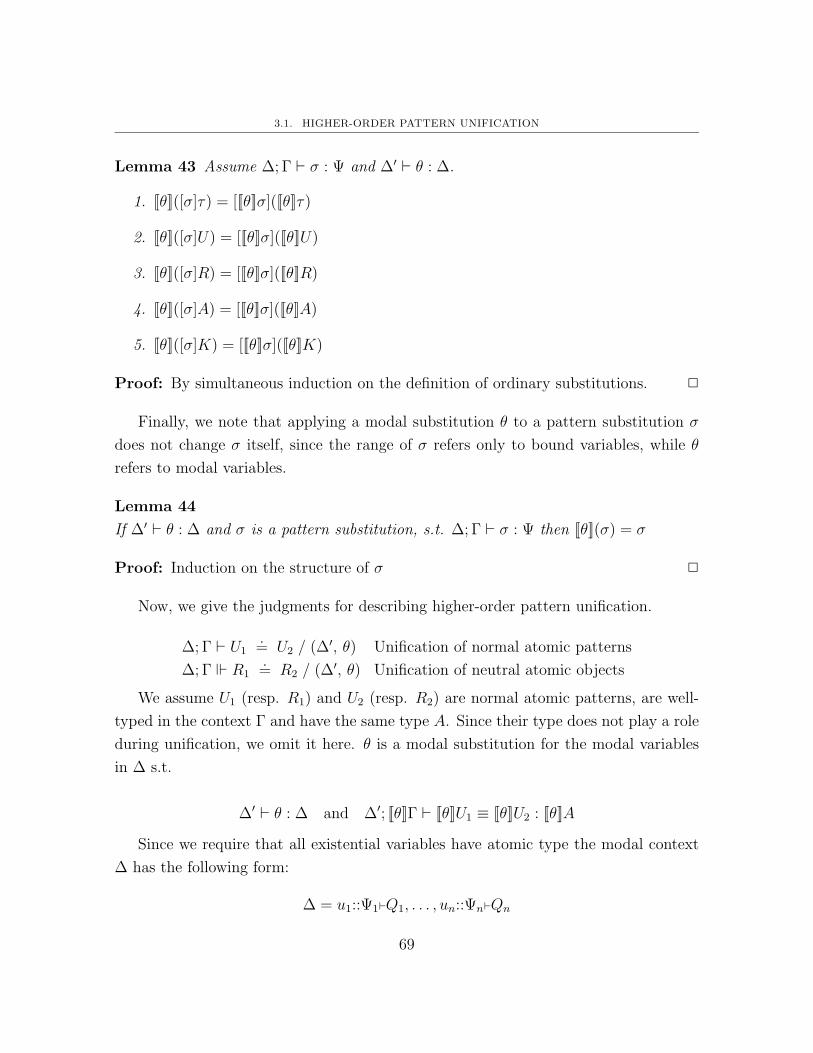
3.1. HIGHER-ORDER PATTERN UNIFICATION
Lemma 43 Assume ∆; Γ ` σ : Ψ and ∆′ ` θ : ∆.
1. [[θ]]([σ]τ) = [[[θ]]σ]([[θ]]τ)
2. [[θ]]([σ]U) = [[[θ]]σ]([[θ]]U)
3. [[θ]]([σ]R) = [[[θ]]σ]([[θ]]R)
4. [[θ]]([σ]A) = [[[θ]]σ]([[θ]]A)
5. [[θ]]([σ]K) = [[[θ]]σ]([[θ]]K)
Proof: By simultaneous induction on the definition of ordinary substitutions. 2
Finally, we note that applying a modal substitution θ to a pattern substitution σ
does not change σ itself, since the range of σ refers only to bound variables, while θ
refers to modal variables.
Lemma 44
If ∆′ ` θ : ∆ and σ is a pattern substitution, s.t. ∆; Γ ` σ : Ψ then [[θ]](σ) = σ
Proof: Induction on the structure of σ 2
Now, we give the judgments for describing higher-order pattern unification.
∆; Γ ` U1.= U2 / (∆′, θ) Unification of normal atomic patterns
∆; Γ R1.= R2 / (∆′, θ) Unification of neutral atomic objects
We assume U1 (resp. R1) and U2 (resp. R2) are normal atomic patterns, are well-
typed in the context Γ and have the same type A. Since their type does not play a role
during unification, we omit it here. θ is a modal substitution for the modal variables
in ∆ s.t.
∆′ ` θ : ∆ and ∆′; [[θ]]Γ ` [[θ]]U1 ≡ [[θ]]U2 : [[θ]]A
Since we require that all existential variables have atomic type the modal context
∆ has the following form:
∆ = u1::Ψ1`Q1, . . . , un::Ψn`Qn
69

CHAPTER 3. TOWARD EFFICIENT HIGHER-ORDER PATTERN UNIFICATION
Moreover, we will never instantiate an existential variable with a lambda-abstraction.
Hence, the modal substitution θ has the following form:
θ = (R1/u1, . . . , Rn/un)
where R denotes a neutral atomic object which can be a bound variable, a constant,
an application, or another existential variable which has atomic type. Moreover, since
we require that U1 (resp. R1) and U2 (resp. R2) are in canonical form, and all existential
variables are of atomic type, canonical forms are preserved when applying the modal
substitution θ and in fact we can check if [[θ]]U1 is definitionally equal to [[θ]]U2 by
checking syntactic equality between these two objects. Similar statments hold for
types, kinds, and the bound variable context Γ.
Theorem 45
1. If U is a normal term and all modal variables are of atomic type and ∆′ ` θ : ∆
and ∆; Γ ` U : A then [[θ]]U is a normal term.
2. If R is a neutral term and all modal variables are of atomic type and ∆′ ` θ : ∆
and ∆; Γ ` R : A then [[θ]]R is neutral.
Proof: Simultaneous structural induction on the structure of normal and neutral
terms. The key observation is that θ only substitutes neutral objects R for modal
variables. 2
Theorem 46 Let U and U ′ be normal terms and R and R′ be neutral terms and all
modal variables are of atomic type and ∆ ` θ : ∆′.
1. [[θ]]U = [[θ′]]U ′ iff ∆; [[θ]]Γ ` [[θ]]U ≡ [[θ]]U ′ : [[θ]]A.
2. [[θ]]R = [[θ′]]R′ iff ∆; [[θ]]Γ ` [[θ]]R ≡ [[θ]]R′ : [[θ]]A.
Proof: By the previous theorem, we know [[θ]]U and [[θ]]U ′ are canonical. As dis-
cussed in Chapter 2 on page 61, definitionally equality reduces to syntactic equality
for canonical forms. 2
70

3.1. HIGHER-ORDER PATTERN UNIFICATION
Higher-order pattern unification can be done in two phases (see [48, 22] for another
account). During the first phase, we decompose the terms until one of the two terms
we unify is an existential variable u[σ]. This decomposition phase is straightforward
and resembles first-order unification closely.
∆; Γ, x:A ` U1.= U2 / (∆′, θ)
∆; Γ ` λx:A.U1.= λx:A.U2 / (∆′, θ)
lam∆; Γ R1
.= R2 / (∆′, θ)
∆; Γ ` R1.= R2 / (∆′, θ)
coerce
∆; Γ x.= x / (∆, id∆)
var∆; Γ c
.= c / (∆, id∆)
const
∆; Γ R1.= R2 / (∆1, θ1) ∆1; [[θ1]]Γ ` [[θ1]]U1
.= [[θ1]]U2 / (∆2, θ2)
∆; Γ R1 U1.= R2 U2 / (∆2, [[θ1]](θ2))
app
Note that we do not need to worry about capture in the rule lam, since existential
variables and bound variables are defined in different contexts. During the second
phase, we need to find an actual instantiation for the existential variable u. There are
two main cases to distinguish: (1) when we unify two existential variables, u[σ].= v[σ′],
and (2) when we unify an existential variable with another kind of term, u[σ].= U .
In the following, we consider each of these two cases separately.
3.1.1 Unifying an existential variable with another term
The case for unifying an existential variable u[σ] with another term U can be trans-
formed into u.= [σ]−1 U assuming u does not occur in U and all variables v[τ ] are
pruned so that the free variables in τ all occur in the image of σ (see below or [34, 22]
for details). Before considering the pruning operation, we define the inverse substitu-
tion. Note that we view [σ]−1 U as a new meta-level operation such as substitution,
because it may be defined even if σ is not invertible in full generality. This meta-level
operation is defined as follows1.
1We do not omit the type label on the lambda-abstraction here, since it is sometimes convenientto have access to the type of the bound variable x. This is not strictly necessary, since we require allterms are canonical and type labels can be omitted.
71

CHAPTER 3. TOWARD EFFICIENT HIGHER-ORDER PATTERN UNIFICATION
[σ]−1 c = c
[σ]−1 x = y if x/y ∈ σ, undefined otherwise
[σ]−1 (v[τ ]) = v[[σ]−1 τ ]
[σ]−1 (RU) = ([σ]−1 R) ([σ]−1 U)
[σ]−1 (λx:A. U) = λx:([σ]−1 A). [σ, x/x]−1 U if x not declared or free in σ
[σ]−1 (·) = (·)[σ]−1 (τ, U/x) = ([σ]−1 τ, [σ]−1 U/x)
Note that the defined meta-level operation of inverting substitutions is only defined
for a variable x if x/y is in σ and undefined otherwise, thus enforcing that the resulting
term [σ]−1 U is total and exists. It is important to note that the meta-level operation of
inverting substitutions and applying the modal substitution commute. This property
only holds if the inverse substitution in fact exists.
Lemma 47 (Property of inverting substitutions) Let τ and σ be pattern substi-
tutions.
1. If [σ]−1 τ and [σ]−1 ([[θ]]τ) exist then [σ]−1 ([[θ]](τ)) = [[θ]]([σ]−1 τ).
2. If [σ]−1 U and [σ]−1 ([[θ]]U) exist then [σ]−1 ([[θ]]U) = [[θ]]([σ]−1 U).
3. If [σ]−1 R and [σ]−1 ([[θ]]R) exist then [σ]−1 ([[θ]]R) = [[θ]]([σ]−1 R).
Proof: By simultaneous induction on the structure of τ , U , and R. 2
Lemma 48
1. If [σ]−1 τ exists then [σ]([σ]−1 τ) = τ .
2. If [σ]−1 U exists then [σ]([σ]−1 U) = U .
3. If [σ]−1 R exists then [σ]([σ]−1 R) = R.
Proof: The lemmas are proven by simultaneous structural induction on τ , U , and R.
2
72

3.1. HIGHER-ORDER PATTERN UNIFICATION
Lemma 49
1. If σ is a pattern substitution and [σ]U = U ′ then U = [σ]−1 U ′
2. If σ is a pattern substitution and [σ]R = R′ then R = [σ]−1 R′
Proof: The statement is proven by a simultaneous induction on the structure of U
and R. 2
Lemma 50 Let τ and σ be pattern substitutions.
1. If [σ]−1 τ exists and ∆; Γ ` τ : Ψ1 and ∆; Γ ` σ : Ψ2, then ∆; Ψ2 ` [σ]−1 τ : Ψ1.
2. If [σ]−1 U exists and ∆; Γ ` U : [σ]Q and ∆; Γ ` σ : Ψ2, then ∆; Ψ2 ` [σ]−1 U : Q.
3. If [σ]−1 R exists and ∆; Γ ` R : [σ]Q and ∆; Γ ` σ : Ψ2, then ∆; Ψ2 ` [σ]−1 U : Q.
Proof: By simultaneous structural induction on the definition of inverse substitutions
for τ , U , R. 2
Next, we discuss pruning for normal and neutral objects.
∆; Γ ` U | [σ]−1 ⇒ (∆′, ρ) Prune U with respect to σ
∆; Γ R | [σ]−1 ⇒ (∆′, ρ) Prune R with respect to σ
Let ∆ be the modal variables in U (and R resp). Then pruning with respect to
the substitution σ, will return a modal substitution ρ s.t. ∆′ ` ρ : ∆ and [σ]−1 ([[ρ]]U)
exists. The modal substitution ρ replaces modal variables ui in ∆, where ui[τ ] occurs
as a subterm in U (or R resp.) and [σ]−1 (ui[τ ]) is not defined, with new modal
variables v[τ ′], s.t. τ ′ prunes the substitution τ and [σ]−1 (v[[τ ]τ ′]) exists. In other
words, pruning ensures that all bound variables occurring in [[ρ]]U occur in the range
of σ which is achieved by applying the modal pruning substitution ρ to U .
∆; Γ, x:A ` U | [σ, x/x]−1 ⇒ (∆1, ρ1)
∆; Γ ` λx:A.U | [σ]−1 ⇒ (∆1, ρ1)
∆; Γ R | [σ]−1 ⇒ (∆′, ρ)
∆; Γ ` R | [σ]−1 ⇒ (∆′, ρ)
(∆1, v::Ψ1`Q,∆2); Γ ` τ : Ψ1 | [σ]−1 ⇒ Ψ2 ∆′2 = [[id∆1 , v′[idΨ2 ]/v]]∆2
(∆1, v::Ψ1`Q,∆2); Γ v[τ ] | [σ]−1 ⇒ ((∆1, v′::Ψ2`Q,∆
′2), (id∆1 , v
′[idΨ2 ]/v, id∆2))
73

CHAPTER 3. TOWARD EFFICIENT HIGHER-ORDER PATTERN UNIFICATION
∆; Γ R | [σ]−1 ⇒ (∆1, ρ1) ∆1; [[ρ1]]Γ ` [[ρ1]]U1 | [σ]−1 ⇒ (∆2, ρ2)
∆; Γ R U | [σ]−1 ⇒ (∆2, [[ρ2]](ρ1))
[σ]−1 x exists
∆; Γ1, x:A,Γ2 x | [σ]−1 ⇒ (∆, id∆) ∆; Γ c | [σ]−1 ⇒ (∆, id∆)
Applying a modal substitution θ to a modal context ∆ is defined as follows:
[[θ]](·) = ·[[θ]](u::Ψ`A,∆) = (u::[[θ]]Ψ`[[θ]]A, [[θ, u[idΨ]/u]]∆)
if u does not occur in [[θ]]Ψ and [[θ]]A
The application of θ to some modal context ∆ is only defined if we do not create
any circularities in the resulting context [[θ]]∆. This ensures that the resulting modal
context [[θ]]∆ is well-formed. In the previous rule for pruning a modal variable v[τ ] with
respect to [σ]−1 , we create a new context ∆′2 = [[id∆1 , v′[idΨ2 ]/v]]∆2. Since the range
of [[id∆1 , v′[idΨ2 ]/v]] is different from the modal variables declared in ∆2, we always will
obtain a well-formed ∆′2.
Note that pruning of an object U (resp. R) does not always succeed. In particular,
if U contains a bound variable x which does not occur in the image of the substitution σ
pruning will fail. When we prune an object U (resp. R), we assume that ∆; Γ ` U : A
and if pruning succeeds it will return a new context ∆′ and a modal substitution ρ
such that ∆′ ` ρ : ∆.
Note that τ is a pattern substitution and therefore we do not need to recursively
prune the substitutions. However, we may need to prune some bound variables because
[σ]−1 τ may not necessarily exist. Next, we describe the pruning of a substitution τ
with respect to a substitution [σ]−1 .
Given a substitution τ such that ∆; Γ ` τ : Ψ1, pruning τ with respect to [σ]−1 ,
where ∆; Γ ` σ : Ψ returns a context Ψ2 such that [σ]−1 ([τ ]idΨ2) exists. The following
judgment describes the pruning of a substitution τ .
∆; Γ ` τ : Ψ1 | [σ]−1 ⇒ Ψ2
74

3.1. HIGHER-ORDER PATTERN UNIFICATION
Ψ2 is well-formed context such that Ψ2 ≤ Ψ1 and ∆; Ψ1 ` idΨ2 : Ψ2. Pruning
the substitution τ with respect to [σ]−1 will always succeed and return a well-formed
context Ψ2.
∆; Γ ` · : · | [σ]−1 ⇒ ·∆; Γ ` τ : Ψ1 | [σ]−1 ⇒ Ψ2 [σ]−1 (y) exists
∆; Γ ` (τ, y/x) : (Ψ1, x:A) | [σ]−1 ⇒ (Ψ2, x:A)
∆; Γ ` τ : Ψ1 | [σ]−1 ⇒ Ψ2 [σ]−1 (y) does not exists
∆; Γ ` (τ, y/x) : (Ψ1, x:A) | [σ]−1 ⇒ Ψ2
Before we show some properties about pruning, we summarize some of the consid-
erations in defining pruning judgments. Recall that we call pruning when unifying an
object u[σ] with another object U . Since we only unify terms of the same type, we
know that ∆; Γ ` u[σ] : Q′ and ∆; Γ ` U : Q′. We also know by typing invariant
that u::Ψ`Q in ∆ and in fact ∆; Γ ` u[σ] : [σ]Q and ∆; Γ ` σ : Ψ. By the previous
two assumptions, we know that in fact Q′ = [σ]Q. Moreover, ∆ = ∆1, u::Ψ`Q,∆2 and
∆1; Ψ ` Q : type. Since σ is a pattern substitution, we must have ∆1; Γ ` [σ]Q : type.
We first argue why we do not need to prune the types when pruning an existential
variable v[τ ] with respect to [σ]−1 and when pruning a substitution τ with respect
to [σ]−1 . Moreover, we show when pruning τ with respect to [σ]−1 the resulting
context Ψ2 must be well-formed. We say a variable y is shared between two pattern
substitutions τ and σ if y is in the image of both τ and σ. It is easy to see that if
∆; Γ ` τ : Ψ1 | [σ]−1 ⇒ Ψ2, then Ψ2 contains exactly those variables x in Ψ1 such that
[τ ]x is shared between τ and σ.
Lemma 51 (Well-formedness of pruned context)
If ∆; Γ ` τ : Ψ1 | [σ]−1 ⇒ Ψ2, ∆; Γ ` τ : Ψ1 and ∆; Γ ` σ : Ψ then ∆ ` Ψ2 ctx and
Ψ2 ≤ Ψ1.
Proof: Proof by structural induction on the first derivation.
Case D =∆; Γ ` · : · | [σ]−1 ⇒ ·
∆ ` · ctx by rule
· ≤ ·
75

CHAPTER 3. TOWARD EFFICIENT HIGHER-ORDER PATTERN UNIFICATION
Case D =∆; Γ ` τ : Ψ1 | [σ]−1 ⇒ Ψ2 [σ]−1 (y) exists
∆; Γ ` (τ, y/x) : (Ψ1, x:A) | [σ]−1 ⇒ (Ψ2, x:A)
∆; Γ ` (τ, y/x) : (Ψ1, x:A) by assumption
∆; Γ ` τ : Ψ1 and ∆; Γ ` x:[τ ]A (*) by inversion
∆; Γ ` σ : Ψ by assumption
∆ ` Ψ2 ctx and Ψ2 ≤ Ψ1 by i.h.
Γ(y) = B = [τ ]A by inversion on (*)
σ = (σ1, y/z, σ2) and Ψ = (Ψ′, z:A′,Ψ′′) since [σ]−1 (y) exists
Γ(y) = B[σ1]A′ since ∆; Γ ` σ : Ψ
[τ ]A = [σ1]A′ transitivity of equality
[τ ]A can only depend on variables shared between τ and σ1
τ and σ1 are pattern substitutions
A can only depend on variables from Ψ2 see remark before this proof
∆; Ψ1 ` A : type from above
∆ ` Ψ2, x:A ctx by rule
(Ψ2, x:A) ≤ (Ψ1, x:A) by i.h.
Case D =∆; Γ ` τ : Ψ1 | [σ]−1 ⇒ Ψ2 [σ]−1 (y) does not exist
∆; Γ ` (τ, y/x) : (Ψ1, x:A) | [σ]−1 ⇒ Ψ2
∆; Γ ` (τ, y/x) : (Ψ1, x:A) by assumption
∆; Γ ` τ : Ψ1 and ∆; Γ ` y:[τ ]A by inversion
∆; Γ ` σ : Ψ by assumption
∆ ` Ψ2 ctx and Ψ2 ≤ (Ψ1, x:A) by i.h.
2
Lemma 52 (Well-formed pruning substitution)
1. If ∆; Γ ` U | [σ]−1 ⇒ (∆′, ρ) and ∆; Γ ` U : [σ]A and ∆; Γ ` σ : Ψ
then ∆′ ` ρ : ∆.
2. If ∆; Γ R | [σ]−1 ⇒ (∆′, ρ) and ∆; Γ ` R : [σ]A and ∆; Γ ` σ : Ψ
then ∆′ ` ρ : ∆.
76

3.1. HIGHER-ORDER PATTERN UNIFICATION
Proof: Simultaneous structural induction on the first derivation. We show a few cases
of the proof.
Case D =∆; Γ, x:A ` U | [σ, x/x]−1 ⇒ (∆′, ρ)
∆; Γ ` λx:A.U | [σ]−1 ⇒ (∆′, ρ)
∆; Γ ` λx:A.U : [σ]B by assumption
B = Ψx:B1.B2 for some B1 and B2
∆; Γ ` [σ]B ≡ Πx:[σ]B1.[σ, x/x]B2 : type and
∆; Γ, x:A ` U : [σ, x/x]B2 by typing inversion lemma 12
∆; Γ ` [σ]B ≡ Πx:[σ]B1.[σ, x/x]B2 : type and by equality inversion 14
∆; Γ ` [σ]B1 ≡ A : type and ∆; Γ ` [σ, x/x]B2 ≡ [σ, x/x]B2 : type
∆; Γ ` σ : Ψ by assumption
∆; Γ, x:A ` σ : Ψ by weakening
∆; Γ, x:A ` x : A by rule
∆; Γ, x:A ` x : [σ]B1 by rule
∆; Γ, x:A ` (σ, x/x) : (Ψ, x:B1) by rule
∆′ ` ρ : ∆ by i.h.
Case D =(∆1, v::Ψ1`Q,∆2); Γ ` τ : Ψ1 | [σ]−1 ⇒ Ψ2
(∆1, v::Ψ1`Q,∆2); Γ v[τ ] | [σ]−1 ⇒ (∆′, ρ)
∆′ = (∆1, v′::Ψ2`Q,∆
′2) and ∆′2 = [[id∆1 , v
′[idΨ2 ]/v]]∆2 and ρ = (id∆1 , v′[idΨ2 ]/v, id∆2)
(∆1, v::Ψ1`Q,∆2); Γ ` v[τ ] : A by assumption
(∆1, v::Ψ1`Q,∆2); Γ ` τ : Ψ1 and
(∆1, v::Ψ1`Q,∆2); Γ ` [σ]A ≡ [τ ]Q : type by typing inversion 12
(∆1, v::Ψ1`Q,∆2); Γ ` σ : Ψ by assumption
∆ ` Ψ2 ctx and Ψ2 ≤ Ψ1 by lemma 51
∆1 ` Ψ1 ctx by well-typedness of (∆1, v::Ψ1`Q,∆2)
∆1 ` Ψ2 ctx since Ψ2 ≤ Ψ1
A = [σ]−1 ([τ ]Q) and [σ]−1 ([τ ]Q) exists by lemma 49
so pruning τ with respect to [σ]−1 should not affect any variables in Q. Therefore,
∆1; Ψ2 ` Q : type. Moreover,(∆1, v
′::Ψ2`Q,∆′2) ` (id∆1 , v
′[idΨ2 ]/v, id∆2) : (∆1, v::Ψ1`Q,∆2)
77

CHAPTER 3. TOWARD EFFICIENT HIGHER-ORDER PATTERN UNIFICATION
Case D =∆; Γ R | [σ]−1 ⇒ (∆1, ρ1) ∆1; [[ρ1]]Γ ` [[ρ1]]U1 | [σ]−1 ⇒ (∆2, ρ2)
∆; Γ R U | [σ]−1 ⇒ (∆2, [[ρ2]](ρ1))
∆; Γ ` R U : [σ]A by assumption
∆; Γ ` R : [σ](Πx:A1.A2) and ∆; Γ ` U : [σ]A1 and
∆; Γ ` [σ, U/x]A2 ≡ [σ]A : type by typing inversion 12
∆1 ` ρ1 : ∆ by i.h.
∆1; [[ρ1]]Γ ` [[ρ1]]U : [[ρ1]]([σ]A1) by substitution property
∆1; [[ρ1]]Γ ` [[ρ1]]U : [σ]([[ρ1]]A1) since ρ1 is a pattern substitution
∆2 ` ρ2 : ∆1 by i.h.
∆2 ` [[ρ2]]ρ1 : ∆ by composition of modal substitutions
2
Moreover, we show that if the modal variable u does not occur in R, then pruning
R with respect to some σ, results in the modal context ∆′ and the pruning substitution
ρ, where u will be mapped to itself.
Lemma 53
1. If the modal variable u does not occur in U and ∆; Γ ` U | [σ]−1 ⇒ (∆∗, ρ) and
∆ = (∆1, u::Ψ`Q,∆2), then ∆∗ = (∆∗1, u::[[ρ]]Ψ`[[ρ]]Q,∆∗2) and ρ = (ρ1, u[id[[ρ]]Ψ]/u, ρ1).
2. If the modal variable u does not occur in R and ∆; Γ R | [σ]−1 ⇒ (∆∗, ρ) and
∆ = ∆1, u::Ψ`Q,∆2, then ∆∗ = (∆∗1, u::[[ρ]]Ψ`[[ρ]]Q,∆∗2) and ρ = (ρ1, u[id[[ρ]]Ψ]/u, ρ1).
Proof: Simultaneous structural induction on the pruning derivation. 2
Next, we show correctness of pruning.
Lemma 54 (Pruning – Soundness)
1. If ∆; Γ ` τ : Ψ1 | [σ]−1 ⇒ Ψ2 and ∆; Γ ` τ : Ψ1 and ∆; Γ ` σ : Ψ then
[σ]−1 ([τ ](idΨ2)) exists.
2. If ∆; Γ ` U | [σ]−1 ⇒ (∆′, ρ) and ∆; Γ ` U :A and ∆; Γ ` σ : Ψ then [σ]−1 ([[ρ]]U)
exists.
78

3.1. HIGHER-ORDER PATTERN UNIFICATION
3. If ∆; Γ R | [σ]−1 ⇒ (∆′, ρ) and ∆; Γ ` R:A and ∆; Γ ` σ : Ψ then [σ]−1 ([[ρ]]R)
exists.
Proof: The lemmas are proven by simultaneous structural induction on the first
derivation.
Case ∆; Γ R U | σ−1 ⇒ (∆2, [[ρ2]]ρ1)
∆; Γ R | σ−1 ⇒ (∆1, ρ1) by premise
∆1; [[ρ1]]Γ ` [[ρ1]]U | σ−1 ⇒ (∆2, ρ2) by premise
∆; Γ ` R U : A by assumption
∆; Γ ` R : Πx:A1.A2
∆; Γ ` U : A1 and
∆; Γ ` [idΓ, U/x]A2 ≡ A : type by typing inversion lemma 12
∆1 ` ρ1 : ∆ by lemma 52
∆1; [[ρ1]]Γ ` [[ρ1]]U : [[ρ1]]A1 by substitution property
∆2 ` ρ2 : ∆1 by lemma 52
[σ]−1 ([[ρ1]]R) exists by i.h.
[σ]−1 ([[ρ2]]([[ρ1]]U)) exists by i.h.
[σ]−1 ([[[[ρ2]]ρ1]]U) exists by substitution property
[[ρ2]][σ]−1 ([[ρ1]]R) exists by substitution property
[σ]−1 ([[ρ2]][[ρ1]]R) exists by previous lines
[σ]−1 ([[[[ρ2]]ρ1]]R) exists by substitution definition
Case ∆; Γ ` v[τ ] | σ−1 ⇒ (∆′, ρ)
∆ = ∆1, v::Ψ`Q,∆2
∆′ = (∆1, v′::Ψ2`Q,∆
′2) where and ∆′2 = [[id∆1 , v
′[idΨ2 ]/v]]∆2
ρ = (id∆1 , v′[idΨ2 ]/v, id∆2) by premise
∆; Γ ` τ | [σ]−1 ⇒ Ψ2 by premise
∆; Γ ` v[τ ] : A by assumption
∆; Γ ` τ : Ψ and
∆; Γ ` A ≡ [τ ]Q : type by typing inversion lemma 12
[σ]−1 ([τ ](idΨ2) exists by (1)
79

CHAPTER 3. TOWARD EFFICIENT HIGHER-ORDER PATTERN UNIFICATION
v′[[σ]−1 ([τ ](idΨ2))] exists
[σ]−1 v′[[τ ](idΨ2)] exists by inverse substitution definition
[σ]−1 ([[ρ]]v[τ ]) exists by substitution definition
2
Lemma 55 (Pruning – Completeness)
1. If ∆; Γ ` τ : Ψ and ∆; Γ ` σ : Ψ′ then ∆; Γ ` τ : Ψ | [σ]−1 ⇒ Ψ2 for some Ψ2.
2. If ∆; Γ ` U : [σ]A and ∆; Γ ` σ : Ψ and ∆′ ` θ : ∆ and [σ]−1 ([[θ]]U) exists, then
∆; Γ ` U | [σ]−1 ⇒ (∆′′, ρ) for some ∆′′ and ρ and there exists a substitution ρ′
such that θ = [[ρ′]]ρ and ∆′ ` ρ′ : ∆′′.
3. If ∆; Γ ` R : [σ]A and ∆; Γ ` σ : Ψ and ∆′ ` θ : ∆ and [σ]−1 ([[θ]]R) exists, then
∆; Γ ` R | [σ]−1 ⇒ (∆′′, ρ) for some ∆′′ and ρ and there exists a substitution ρ′
such that θ = [[ρ′]]ρ and ∆′ ` ρ′ : ∆′′.
Proof: The statement is proven by simultaneous structural induction on the typing
derivation. We show a few cases.
Case ∆; Γ ` v[τ ] : [σ]A
∆; Γ ` τ : Ψ1 by typing inversion lemma 12
∆ = (∆1, v::Ψ1`Q1,∆2) and ∆; Γ ` [σ]A ≡ [τ ]Q1 : type
∆; Γ ` σ : Ψ by assumption
∆; Γ ` τ : Ψ1 | [σ]−1 ⇒ Ψ2 by (1)
∆; Γ ` v[τ ] | [σ]−1 ⇒ ((∆1, v′::Ψ2`Q1,∆
′2), (id∆1 , v
′[idΨ2 ]/v, id∆′2)) by rule
∆1; Ψ2 ` Q1 : type since [σ]A = [τ ]Q1 and
Ψ2 contains exactly those variables shared between σ and τ
∆′ ` (θ1, U/v, θ2) : (∆1, v::Ψ1`Q1,∆2) by assumption
let ρ′ = (θ1, U/v′, θ2) then we have θ = [[ρ′]]((id∆1 , v
′[idΨ2 ]/v, id∆′2).
Case ∆; Γ ` λx:A.U : [σ]B
∆; Γ, x:A ` U : [σ, x/x]B2 and
∆; Γ ` [σ]B ≡ Πx:A.[σ, x/x]B2 : type by typing inversion 12
80

3.1. HIGHER-ORDER PATTERN UNIFICATION
∆; Γ ` [σ]B ≡ Πx:[σ]B1.[σ, x/x]B2 : type and
∆; Γ ` A ≡ [σ]B1 : type by equality inversion 14
∆; Γ ` σ : Ψ by assumption
∆; Γ, x:A ` x : A by rule
∆; Γ, x:A ` x : [σ]B1 by rule
∆; Γ, x:A ` (σ, x/x) : (Ψ, x:B1) by rule
[σ]−1 ([[θ]](λx:A.U)) exists by assumption
λx:[σ]−1 ([[θ]]A).([σ, x/x]−1 [[θ]]U) exists by definition of inverse substitution
([σ, x/x]−1 [[θ]]U) exists
∃ρ′.θ = [[ρ′]]ρ and ∆; Γ, x:A ` U | [σ, x/x]−1 ⇒ (∆′, ρ) by i.h.
∆; Γ ` λx:A.U | [σ]−1 ⇒ (∆′, ρ) by rule
2
Now, we can give the cases for unifying an existential variable with another kind of
term. Since we are requiring that all existential variables are of atomic type, this term
R can only be a modal variable v[τ ′], where v is different from u, an application, an
ordinary variable or a constant.
∆; Γ ` R | [σ]−1 ⇒ (∆∗, ρ) ∆∗ = (∆∗1, u::[[ρ]]Ψ`[[ρ]]Q,∆∗2)
u does not occur in R ∆′2 = [[id∆∗1, [σ]−1 ([[ρ]]R)/u]]∆∗2
(∆1, u::Ψ`Q,∆2); Γ u[σ].= R / ((∆∗1,∆
′2), [[id∆∗1
, [σ]−1 ([[ρ]]R)/u, id∆∗2]]ρ)
ex1
∆; Γ ` R | [σ]−1 ⇒ (∆∗, ρ) ∆∗ = (∆∗1, u::[[ρ]]Ψ`[[ρ]]Q,∆∗2)
u does not occur in R ∆′2 = [[id∆∗1, [σ]−1 ([[ρ]]R)/u]]∆∗2
(∆1, u::Ψ`Q,∆2); Γ R.= u[σ] / ((∆∗1,∆
′2), [[id∆∗1
, [σ]−1 ([[ρ]]R)/u, id∆∗2]]ρ)
ex2
The side condition “u does not occur in R” ensures that we obey the occurs-
check. Note, that we do not need to ensure that u does not occur in the type of
R. Recall that by invariant, we know that ∆; Γ ` u[σ] : Q′ and ∆; Γ ` R : Q′.
We also know by typing invariant that u::Ψ`Q in ∆ and ∆; Γ ` u[σ] : [σ]Q and
∆; Γ ` σ : Ψ. By the previous two assumptions, we know that Q′ = [σ]Q. Moreover,
∆ = ∆1, u::Ψ`Q,∆2 and ∆1; Ψ ` Q : type. Since σ is a pattern substitution, we must
81

CHAPTER 3. TOWARD EFFICIENT HIGHER-ORDER PATTERN UNIFICATION
have ∆1; Γ ` [σ]Q : type. Since [σ]Q = Q′, we know that u cannot occur in the type
Q′. Therefore we do not need to perform the occurs check on the type of R.
However, since there may be dependencies among the types and declarations in ∆2
may depend on u, it is not necessarily obvious why traversing R and checking whether u
occurs in R suffices in the higher-order dependently typed setting. Potentially we could
be in the following situation: a modal variable v[τ ′] occurs in R, but v::Ψ′`Q′ occurs in
∆2 and depends on u. When we construct the new ∆′2 = [id∆1 , [σ]−1 ([[ρ]]R)/u]∆2, we
will replace occurrences of u in Ψ′ and Q′ with [σ]−1 ([[ρ]]R). But since R itself refers to
v, we may be creating a circular new declaration for v and the resulting modal context
∆′2 may not be well-formed.
Lemma 56
1. If ∆; Γ ` U ⇐ A and ∆ = (∆1, u::Ψ`Q,∆2) and u does not occur in Γ, U , and
A, then for any modal variable v where v is different from u that occurs in U and
v::Ψ′`Q′ is declared in ∆, u does not occur in Ψ′ and Q′.
2. If ∆; Γ ` R ⇒ A and ∆ = (∆1, u::Ψ`Q,∆2) and u does not occur in Γ, R, then
u does not occur in A and for any modal variable v where v is different from u
that occurs in R and v::Ψ′`Q′ is declared in ∆, u does not occur in Ψ′ and Q′.
Proof: By simultaneous induction on the algorithmic typing derivation.
Case ∆; Γ ` R U ⇒ [idΓ, U/x]A2
∆; Γ ` R⇒ Πx:A′1.A2
∆; Γ ` U ⇐ A1 and ∆; Γ ` A1 ⇐⇒ A′1 : type by inversion
A1 = A′1 since A1, A′1 are canonical
u does not occur in R U by assumption
u does not occur in R
u does not occur in U
u does not occur in G by assumption
u does not occur in Πx:A′1.A2 and for any modal variable v::Ψ′`Q′ occurring in R,
u does not occur in Ψ′ and Q′ by i.h.
u does not occur in A′1
82

3.1. HIGHER-ORDER PATTERN UNIFICATION
u does not occur in A1 since A1 ⇐⇒ A′1for any modal variable v::Ψ′`Q′ occurring in U ,
u does not occur in Ψ′ and Q′ by i.h.
for any modal variable v::Ψ′`Q′ occurring in R U ,
u does not occur in Ψ′ and Q′
Case (∆′, v::Ψ′`Q′,∆′′); Γ ` v[τ ]⇒ [τ ]Q′
∆ = (∆′, v::Ψ′`Q′,∆′′) and ∆; Γ ` τ ⇐ Ψ′ by inversion
u does not occur in Γ by assumption
u does not occur in Ψ′ since τ is a pattern substitution
u does not occur in [τ ]Q′ by assumption
u does not occur in Q′ since τ is a pattern substitution
Case ∆; Γ ` c⇒ A
c is defined in the signature Σ. Σ(c) = A. Moreover, A must be closed and cannot
refer to any modal variables. Therefore, u cannot occur in A.
Case ∆; Γ ` x⇒ A
Γ(x) = A by inversion
u does not occur in A since u does not occur in Γ
Case ∆; Γ ` λx:A1.U ⇐ Πx:A1.A2
∆; Γ, x:A1 ` U ⇐ A2 by inversion
u does not occur in Γ by assumption
u does not occur in Πx:A1.A2 by assumption
u does not occur in A1 and A2
u does not occur in Γ, x:A1
for any v::Ψ′`Q′ occuring in U
u does not occur in Ψ′ and Q′ by i.h.
for any v::Ψ′`Q′ occuring in λx:A1.U
u does not occur in Ψ′ and Q′
83

CHAPTER 3. TOWARD EFFICIENT HIGHER-ORDER PATTERN UNIFICATION
2
The last lemma justifies why a simple occurs check also suffices in the higher-order
dependently typed setting. In an implementation, we may combine computing the
pruning substitution with the occurs check. Since we already traverse the term R to
check whether [σ]−1 R exists, we may simultaneously check whether u occurs in R.
However, the previous lemma shows that for higher-order patterns, we do not need to
prune types and the bound variable context. Moreover, we do not need to perform an
occurs check on the types of modal variables which may occur in R2 .
3.1.2 Unifying two identical existential variables
For unifying the two existential variables which are the same, we need an additional
auxiliary judgment, which computes the intersection of two substitutions.
∆; Γ ` σ ∩ τ : Ψ⇒ Ψ′
Given the substitution ∆; Γ ` σ : Ψ and ∆; Γ ` τ : Ψ, we construct a context Ψ′
which is well-formed and for the substitution idΨ′ such that ∆; Ψ ` idΨ′ : Ψ′ we have
[σ](idΨ′) = [τ ](idΨ′).
∆; Γ ` · ∩ · : · ⇒ ·
∆; Γ ` τ ∩ σ : Ψ⇒ Ψ′
∆; Γ ` (τ, y/x) ∩ (σ, y/x) : (Ψ, x:A)⇒ (Ψ′, x:A)
∆; Γ ` τ ∩ σ : Ψ⇒ Ψ′ z 6= y
∆; Γ ` (τ, z/x) ∩ (σ, y/x) : (Ψ, x:A)⇒ Ψ′
We say a variable y is strictly shared between two pattern substitutions τ and σ if
there is an x such that y = [τ ]x = [σ]x. It is easy to see that if ∆; Γ ` τ ∩ σ : Ψ⇒ Ψ′
then Ψ′ contains exactly those variables x in Ψ such that y = [τ ]x = [σ]x (in other
words, y is strictly shared between τ and σ). The resulting context Ψ′ will always be
well-formed. To illustrate the difference between the notion of ”shared” and ”strictly
2It seems possible that an extended occurs check would lead to incompleteness, no?
84

3.1. HIGHER-ORDER PATTERN UNIFICATION
shared” consider the substitution [y/x1, z/x2] and [z/x1, y/x2]. Here, y and z are
shared, but not strictly shared. y and z will be retained under inverse substitution,
but they are pruned under intersection.
Lemma 57 If ∆; Γ ` τ ∩ σ : Ψ⇒ Ψ′, ∆; Γ ` τ : Ψ and ∆; Γ ` σ : Ψ then ∆ ` Ψ′ ctx.
Proof: Structural induction on the first derivation. We consider the interesting case,
where
∆; Γ ` τ ∩ σ : Ψ⇒ Ψ′
∆; Γ ` (τ, y/x) ∩ (σ, y/x) : (Ψ, x:B)⇒ Ψ′, x:B
∆; Γ ` (τ, y/x) : (Ψ, x:B) by assumption
∆; Γ ` τ : Ψ by inversion
∆; Γ ` y : [τ ]B by inversion
Γ(y) = B′ = [τ ]B by inversion
∆; Γ ` (σ, y/x) : (Ψ, x:B) by assumption
∆; Γ ` σ : Ψ by inversion
∆; Γ ` y : [σ]B by inversion
Γ(y) = B′ = [σ]B by inversion
B′ = [τ ]B = [σ]B by previous lines
B can only depend on variables strictly shared between τ and σ
∆ ` Ψ′ ctx by i.h.
∆; Ψ′ ` B : type since Ψ′ contains exactly those variables strictly shared by τ and σ
∆ ` (Ψ′, x:B) ctx 2
Next, we show correctness of computing the intersection between two substitutions.
Lemma 58
1. If ∆; Γ ` τ : Ψ and ∆; Γ ` σ : Ψ and ∆ = ∆1, u::Ψ`Q,∆2 then
∆; Γ ` τ ∩ σ : Ψ⇒ Ψ′
2. If ∆; Γ ` τ ∩ σ : Ψ⇒ Ψ′ then
[σ](idΨ′) = [τ ](idΨ′) and ∆; Ψ ` idΨ′ : Ψ′.
85

CHAPTER 3. TOWARD EFFICIENT HIGHER-ORDER PATTERN UNIFICATION
Proof: The first statement is proven by structural induction on the first derivation.
The second statement is proven by induction on the first derivation using lemma 4. 2
Now we can give the rule for unifying two modal variables which are the same.
(∆1, u::Ψ`Q,∆2); Γ ` τ ∩ σ : Ψ⇒ Ψ2 ∆′2 = [[id∆1 , v′[idΨ2 ]/v]]∆2
(∆1, u::Ψ`Q,∆2); Γ u[σ].= u[τ ] / ((∆1, v::Ψ2`Q,∆
′2), (id∆1 , v[idΨ2 ]/u, id∆2))
ex3
We have shown that the resulting Ψ2 of computing the intersection of τ and σ, is
indeed well-formed (lemma 57). We can also justify why in the unification rule itself
the type Q of two existential variables must be well-typed in the pruned context Ψ2.
Recall that by typing invariant, we know that ∆; Γ ` τ : Ψ and ∆; Γ ` σ : Ψ and
[σ]Q = [τ ]Q = Q′. But this mean that Q can only depend on the variables strictly
shared by τ and σ. Since Ψ2 is exactly the context, which captures the shared variables,
Q must also be well-typed in Ψ2.
During unification, we ensure that the resulting modal substitution θ maps all the
modal variables in ∆ to a new modal context ∆′.
Lemma 59
1. If ∆; Γ ` U1.= U2 / (∆′, θ) and ∆; Γ ` U1 : A and ∆; Γ ` U2 : A
then ∆′ ` θ : ∆.
2. If ∆; Γ R1.= R2 / (∆′, θ) and ∆; Γ ` U1 : A and ∆; Γ ` U2 : A
then ∆′ ` θ : ∆.
Proof: Structural induction on the first derivation. We show the cases for unifying an
existential variable with another term and unifying two identical existential variables.
Case D = ∆; Γ ` u[σ].= R / ((∆∗1,∆
′2), [[id∆∗1
, [σ]−1 ([[ρ]]R)/u, id∆∗2]]ρ)
∆ = (∆1, u::Ψ`Q,∆2)
∆; Γ ` R | [σ]−1 ⇒ (∆∗, ρ) and u does not occur in R by premises
∆; Γ ` u[σ] : A by assumption
∆; Γ ` σ : Ψ and ∆; Γ ` A ≡ [σ]Q : type by typing inversion lemma 12
u does not occur in Ψ and Q by well-formedness of ∆
∆; Γ ` R : [σ]Q by assumption
86

3.1. HIGHER-ORDER PATTERN UNIFICATION
∆∗ ` ρ : ∆ by lemma 52
[σ]−1 [[ρ]]R exists by lemma 54
∆∗ = (∆∗1, u::[[ρ]]Ψ`[[ρ]]Q,∆∗2) and ρ = (ρ∗1, u[id[[ρ]]Ψ]/u, ρ∗2) by lemma 53
∆∗; [[ρ]]Γ ` [[ρ]]R : [[ρ]]([σ]Q) by substitution property (lemma 41)
∆∗; [[ρ]]Γ ` [[ρ]]R : [σ]([[ρ]]Q) since σ is a pattern substitution
∆∗; [[ρ]]Γ ` σ : [[ρ]]Ψ by substitution property
∆∗; [[ρ]]Ψ ` [σ]−1 ([[ρ]]R) : [[ρ]]Q by lemma 50
u does not occur in [[ρ]]Ψ and [[ρ]]Q and [σ]−1 ([[ρ]]R because ρ only replaces modal
variables with new variables
for any modal variable v occuring in [σ]−1 ([[ρ]]R) where v::Ψ′`Q′,
u cannot occur in Ψ′ and Q′ by lemma 56
∆′2 = [[id∆∗1, [σ]−1 ([[ρ]]R)/u]]∆∗2 and ` ∆′2 mctx by previous lines
i.e. no circularities are created in ∆′2θ = [[id∆∗1
, [σ]−1 ([[ρ]]R)/u, id∆∗2]]ρ = (ρ∗1, [σ]−1 ([[ρ]]R)/u, ρ∗2) by substitution definition
(∆∗1,∆′2); [[ρ]]Ψ ` [σ]−1 ([[ρ]]R) : [[ρ]]Q since u does not occur in Ψ, R or Q
(∆∗1,∆′2); [[ρ∗1]]Ψ ` [σ]−1 ([[ρ]]R) : [[ρ∗1]]Q since ∆1; Ψ ` Q : type
(∆∗1,∆′2) ` ρ∗1 : ∆1 since the pruning substitution ρ∗ only instantiates
modal variables from ∆ with new modal variables
(∆∗1,∆′2) ` (ρ∗1, [σ]−1 ([[ρ]]R)/u) : (∆1, u::Ψ`Q) by previous lines
(∆∗1,∆′2) ` (ρ∗1, [σ]−1 ([[ρ]]R)/u, ρ∗2) : ∆ by typing rules
Case D = ∆; Γ ` u[σ].= u[τ ] / ((∆1, v::Ψ2`Q,∆
′2), [[id∆1 , v[idΨ2 ]/u, id∆2 ]])
∆ = (∆1, u::Ψ`Q,∆2)
∆; Γ ` τ ∩ σ : Ψ⇒ Ψ2 by premise
∆; Γ ` u[τ ] : A by assumption
∆; Γ ` τ : Ψ and ∆; Γ ` A ≡ [τ ]Q : type by typing inversion 12
∆; Γ ` u[σ] : A by assumption
∆; Γ ` σ : Ψ and ∆; Γ ` A ≡ [σ]Q : type by typing inversion lemma 12
∆; Γ ` [σ]Q ≡ [τ ]Q : type by transitivity
Q can only depend on those bound variables which are strictly shared by τ and σ
Ψ2 exactly contains those shared variables
∆1; Ψ ` Q : type by well-typedness of ∆
87

CHAPTER 3. TOWARD EFFICIENT HIGHER-ORDER PATTERN UNIFICATION
∆1; Ψ2 ` Q : type by previous lines
(∆1, v::Ψ2`Q,∆′2) ` (id∆1 , v[idΨ2 ]/u, id∆2) : ∆ by previous lines and typing rules
2
Recall, we assume that the two objects we unify are in canonical form, in particular
we may omit the type label on λ-abstractions.
For soundness, we show that if two objects U1 and U2 unify under the modal sub-
stitution θ, then [[θ]]U1 is definitional equal to [[θ]]U2. Since we concentrate on canonical
forms, definitional equality can be established by checking whether two objects are
syntactically equal. Now we show that if the object U1 and U2 unify under the modal
substitution θ, then [[θ]]U1 is syntactically equal to [[θ]]U2, thereby showing indirectly
that [[θ]]U1 and [[θ]]U2 must also be definitional equal.
Theorem 60 (Soundness of higher-order pattern unification)
1. If ∆; Γ ` U1.= U2 / (∆′, θ) and ∆; Γ ` U1 : A, and ∆; Γ ` U2 : A
then [[θ]]U1 = [[θ]]U2.
2. If ∆; Γ R1.= R2 / (∆′, θ) and ∆; Γ ` R1 : A, and ∆; Γ ` R2 : A
then [[θ]]R1 = [[θ]]R2.
Proof: By simultaneous structural induction on the first derivation. Below, we give a
few cases.
Case D =∆; Γ, x:A ` U1
.= U2/(∆
′, θ)
∆; Γ ` λx:A.U1.= λx:A.U2/(∆
′, θ)
∆; Γ ` λx:A.U1 : A′ by assumption
∆; Γ, x:A ` U1 : B by inversion lemma 12
∆; Γ ` A : type and ∆; Γ ` A′ ≡ Πx:A.B : type
∆; Γ ` λx:A.U2 : A′ by assumption
∆; Γ, x:A ` U2 : B by inversion lemma 12
[[θ1]]U1 = [[θ]]U2 by i.h.
88

3.1. HIGHER-ORDER PATTERN UNIFICATION
∆′ ` θ : ∆ by lemma 52
[[θ]]A = [[θ]]A by reflexivity
λx:[[θ]]A.[[θ]]U1 = λx:[[θ]]A.[[θ]]U2 by syntactic equality
[[θ]](λx:A.U1) = [[θ]](λx:A.U2) by modal substitution definition
Case D =
D1
∆; Γ R1.= R2/(∆1, θ1)
D2
∆1; [[θ1]]Γ ` [[θ1]]U1.= [[θ1]]U2/(∆2, θ2)
∆; Γ R1 U1.= R2 U2/(∆2, [[θ2]](θ1))
∆; Γ ` R1 U1 : A by assumption
∆; Γ ` R2 U2 : A by assumption
∆; Γ ` R1 : Πx:A2.A1 by inversion lemma 12
∆; Γ ` U1 : A2 and ∆; Γ ` [idΓ, U1/x]A1 ≡ A : type
∆; Γ ` R2 : Πx:A2.A1 by inversion lemma 12
∆; Γ ` U2 : A2 and ∆; Γ ` [idΓ, U2/x]A1 ≡ A : type
[[θ1]]R1 = [[θ1]]R2 by i.h.
∆2 ` θ2 : ∆1 by lemma 52
[[θ2]]([[θ1]]R1) = [[θ2]]([[θ1]]R2) by modal substitution lemma 41
[[[[θ2]]θ1]](R1) = [[[[θ2]]θ1]](R2) by modal comp. lemma 42
∆1 ` θ1 : ∆ by lemma 52
∆1; [[θ1]]Γ ` [[θ1]]U1 : [[θ1]]A2 by modal substitution lemma 41
∆1; [[θ1]]Γ ` [[θ1]]U2 : [[θ1]]A2 by modal substitution lemma 41
[[θ2]]([[θ1]]U1) = [[θ2]]([[θ1]]U2) by i.h.
[[[[θ2]]θ1]]U1 = [[[[θ2]]θ1]]U2 by modal comp. lemma 42
[[[[θ2]]θ1]](R1 U1) = [[[[θ2]]θ1]](R2 U2) by rule and modal sub. def.
Case D = (∆1, u::Ψ`Q,∆2); Γ u[σ].= R / (∆′, θ)
∆′ = (∆∗1,∆′2) and θ = [[id∆∗1
, [σ]−1 ([[ρ]]R)/u, id∆∗2]]ρ by premise
∆; Γ ` R | [σ]−1 ⇒ (∆∗, ρ) and by premise
∆∗ = (∆∗1, u::[[ρ]]Ψ`[[ρ]]Q,∆∗2) and u does not occur in R by inversion
∆∗ ` ρ : ∆ by lemma 51
ρ = (ρ1, u[id[[ρ]]Ψ]/u, ρ2) by lemma 53
89
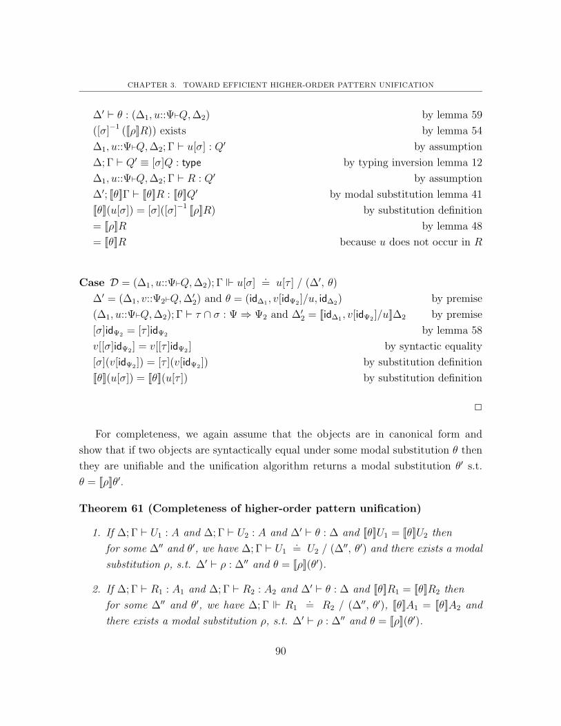
CHAPTER 3. TOWARD EFFICIENT HIGHER-ORDER PATTERN UNIFICATION
∆′ ` θ : (∆1, u::Ψ`Q,∆2) by lemma 59
([σ]−1 ([[ρ]]R)) exists by lemma 54
∆1, u::Ψ`Q,∆2; Γ ` u[σ] : Q′ by assumption
∆; Γ ` Q′ ≡ [σ]Q : type by typing inversion lemma 12
∆1, u::Ψ`Q,∆2; Γ ` R : Q′ by assumption
∆′; [[θ]]Γ ` [[θ]]R : [[θ]]Q′ by modal substitution lemma 41
[[θ]](u[σ]) = [σ]([σ]−1 [[ρ]]R) by substitution definition
= [[ρ]]R by lemma 48
= [[θ]]R because u does not occur in R
Case D = (∆1, u::Ψ`Q,∆2); Γ u[σ].= u[τ ] / (∆′, θ)
∆′ = (∆1, v::Ψ2`Q,∆′2) and θ = (id∆1 , v[idΨ2 ]/u, id∆2) by premise
(∆1, u::Ψ`Q,∆2); Γ ` τ ∩ σ : Ψ⇒ Ψ2 and ∆′2 = [[id∆1 , v[idΨ2 ]/u]]∆2 by premise
[σ]idΨ2 = [τ ]idΨ2 by lemma 58
v[[σ]idΨ2 ] = v[[τ ]idΨ2 ] by syntactic equality
[σ](v[idΨ2 ]) = [τ ](v[idΨ2 ]) by substitution definition
[[θ]](u[σ]) = [[θ]](u[τ ]) by substitution definition
2
For completeness, we again assume that the objects are in canonical form and
show that if two objects are syntactically equal under some modal substitution θ then
they are unifiable and the unification algorithm returns a modal substitution θ′ s.t.
θ = [[ρ]]θ′.
Theorem 61 (Completeness of higher-order pattern unification)
1. If ∆; Γ ` U1 : A and ∆; Γ ` U2 : A and ∆′ ` θ : ∆ and [[θ]]U1 = [[θ]]U2 then
for some ∆′′ and θ′, we have ∆; Γ ` U1.= U2 / (∆′′, θ′) and there exists a modal
substitution ρ, s.t. ∆′ ` ρ : ∆′′ and θ = [[ρ]](θ′).
2. If ∆; Γ ` R1 : A1 and ∆; Γ ` R2 : A2 and ∆′ ` θ : ∆ and [[θ]]R1 = [[θ]]R2 then
for some ∆′′ and θ′, we have ∆; Γ R1.= R2 / (∆′′, θ′), [[θ]]A1 = [[θ]]A2 and
there exists a modal substitution ρ, s.t. ∆′ ` ρ : ∆′′ and θ = [[ρ]](θ′).
90

3.1. HIGHER-ORDER PATTERN UNIFICATION
Proof: Proof by simultaneous induction on the structure of U1 and U2 (and R1, R2
respectively). Most cases are straightforward and we give a few cases to illustrate.
Case U1 = λx.U ′ and U2 = λx.U ′′
[[θ]](λx.U ′) = [[θ]](λx.U ′′) by assumption
λx.[[θ]](U ′) = λx.[[θ]]U ′′ by substitution definition
[[θ]](U ′) = [[θ]](U ′′) by definition of syntactic equality
∆; Γ ` λx.U ′ : A by assumption
∆; Γ, x:A1 ` U ′ : A2 by inversion lemma 12
∆; Γ ` A1 : type and ∆; Γ ` A ≡ Πx:A1.A2 : type
∆; Γ ` λx.U ′′ : A by assumption
∆; Γ, x:A′1 ` U ′′ : A′2 by inversion lemma 12
∆; Γ ` A′1 : type and ∆; Γ ` A ≡ Πx:A′1.A′2 : type
∆; Γ ` Πx:A1.A2 ≡ Πx:A′1.A′2 : type by transitivity
∆; Γ ` A1 ≡ A′1 : type and ∆; Γ, x:A1 ` A2 ≡ A′2 : type by injectivity of products
(lemma 15)
∆; Γ, x:A1 ` U ′.= U ′′ / (∆′′, θ′) by i.h.
θ = [[ρ]](θ′) and ∆′′ ` θ′ : ∆ and θ = [[ρ]](θ′)
∆; Γ ` λx.U ′ .= λx.U ′′ / (∆′′, θ′) by rule
Case U1 = R1 U′1 and U2 = R2 U
′2
∆; Γ ` R1 U′1 : A by assumption
∆; Γ ` R1 : Πx:A1.A2 by typing inversion lemma 12
∆; Γ ` U ′1 : A1 and ∆; Γ ` A ≡ [idΓ, U1/x]A2 : type
∆; Γ ` R2 U′2 : A by assumption
∆; Γ ` R2 : Πx:A′1.A′2 by typing inversion lemma 12
∆; Γ ` U ′2 : A′1 and ∆; Γ ` A ≡ [idΓ, U2/x]A′2 : type
∆′ ` θ : ∆ by assumption
[[θ]](R1 U′1) = [[θ]](R2 U
′2) by assumption
([[θ]]R1) ([[θ]]U ′1) = ([[θ]]R2) ([[θ]]U ′2) by substitution definition
([[θ]]R1) = ([[θ]]R2) and ([[θ]]U ′1) = ([[θ]]U ′2) by definition of syntactic equality
91

CHAPTER 3. TOWARD EFFICIENT HIGHER-ORDER PATTERN UNIFICATION
∆; Γ R1.= R2/(∆1, θ1) and [[θ]](Πx:A1.A2) = [[θ]](Πx:A′1.A
′2) by i.h.
∃ρ.∆′ ` ρ : ∆1 and θ = [[ρ]]θ1
∆1 ` θ1 : ∆ by lemma 59
∆1; [[θ1]]Γ ` [[θ1]]U ′1 : [[θ1]]A1 by substitution property (lemma 41)
∆1; [[θ1]]Γ ` [[θ1]]U ′2 : [[θ1]]A′1 by substitution property (lemma 41)
Πx:[[θ]]A1.[[θ]]A2 = Πx:[[θ]]A′1.[[θ]]A′2 by substitution property
[[θ]]A1 = [[θ]]A′1 by syntactic equality
[[[[ρ]]θ1]]A1 = [[[[ρ]]θ1]]A′1 and [[θ1]]A1 = [[θ1]]A′1 by previous lines
[[[[ρ]]θ1]]U ′1 = [[[[ρ]]θ1]]U ′2 by previous lines
[[ρ]]([[θ1]]U ′1) = [[ρ]]([[θ1]]U ′2) by substitution definition
∆1; [[θ1]]Γ ` [[θ1]]U ′1.= [[θ1]]U ′2/(∆2, θ2) by i.h.
∃ρ′.ρ = [[ρ′]]θ2 and ∆′ ` ρ′ : ∆2
∆; Γ (R1 U′1)
.= (R2 U
′2)/(∆2, [[θ2]]θ1) by rule
θ = [[[[ρ′]]θ2]]θ1 = [[ρ′]]([[θ2]]θ1) by substitution definition
Case U1 = u[σ] and u does not occur in U2 By assumption, the type of U2 must be
atomic, that is, U2 = R2.
[[θ]](u[σ]) = [[θ]]R2 by assumption
θ = (θ1, R/u, θ2) by assumption
∆ = ∆1, u::Ψ`Q,∆2 by assumption
[σ]R = [[θ]]R2 by substitution definition
R = [σ]−1 [[θ]]R2 by lemma 49
θ = (θ1, R/u, θ2) = (θ1, [σ]−1 [[θ]]R2/u, θ2) by previous assumptions
∆; Γ ` u[σ] : [σ]Q by assumption
∆; Γ ` σ : Ψ by typing inversion
∆′ ` (θ1, [σ]−1 [[θ]]R2/u, θ2) : ∆ by assumption
∆′; [[θ1]]Ψ ` [σ]−1 [[θ]]R2 : [[θ1]]Q by typing rules
∆′; [[θ]]Ψ ` [σ]−1 [[θ]]R2 : [[θ]]Q by weakening
∆′; [[θ]]Γ ` σ : [[θ]]Ψ by modal substitution property
∆′; [[θ]]Γ ` [σ][σ]−1 [[θ]]R2 : [σ][[θ]]Q by substitution property
∆′; [[θ]]Γ ` [[θ]]R2 : [[θ]][σ]Q by lemma 44 and 48
92

3.1. HIGHER-ORDER PATTERN UNIFICATION
∆; Γ ` R2 : [σ]Q by modal substitution property
∆; Γ ` R2 | [σ]−1 ⇒ (∆∗, ρ) and
∃ρ′. θ = [[ρ′]]ρ and ∆′ ` ρ′ : ∆∗ by lemma 55
∆∗ ` ρ : ∆ by lemma 52
ρ = (ρ1, u[id[[ρ]]Ψ]/u, ρ2) and ∆∗ = (∆∗1, u::[[ρ]]Ψ`[[ρ]]Q,∆∗2) by lemma 53
∆; Γ u[σ].= R2 / ((∆∗1,∆
′2), [[id∆∗1
, [σ]−1 ([[ρ]]R2)/u, id∆∗2]]ρ)
with ∆′2 = [[id∆∗1, [σ]−1 ([[ρ]]R2)/u, id∆∗2
]]∆∗2 by rule
θ = (θ1, R/u, θ2) = (θ1, [σ]−1 ([[θ]]R2)/u, θ2) by previous lines
= (θ1, [σ]−1 ([[[[ρ′]]ρ]]R2)/u, θ2) by previous lines
= (θ1, [σ]−1 ([[ρ′]][[ρ]]R2)/u, θ2) by substitution definition
= (θ1, [[ρ′]][σ]−1 ([[ρ]]R2)/u, θ2) since by lemma 54 [σ]−1 ([[ρ]]R2) exists
and by lemma 47, [σ]−1 ([[ρ′]][[ρ]]R2) = [[ρ′]][σ]−1 ([[ρ]]R2)
= [[ρ′]]ρ
= [[ρ′]](ρ1, u[id[[ρ]]Ψ]/u, ρ2)
= ([[ρ′]]ρ1, [[ρ′]](u[id[[ρ]]Ψ])/u, [[ρ′]]ρ2) by substitution definition
Since (θ1, [[ρ′]][σ]−1 ([[ρ]]R2)/u, θ2) = ([[ρ′]]ρ1, [[ρ
′]](u[id[[ρ]]Ψ])/u, [[ρ′]]ρ2),
we must have the following:
[[ρ′]](u[idΨ]) = [[ρ′]]([σ]−1 ([[ρ]]R2)) and by previous lines
ρ′ = (ρ′1, [[ρ′]]([σ]−1 ([[ρ]]R2))/u, ρ′2) by previous lines
= [[ρ′1, ρ′2]](id∆∗1
, ([σ]−1 ([[ρ]]R2))/u, id∆∗2) by substitution definition
and the fact that u does not occur in R itself
θ = [[[[ρ′1, ρ′2]](id∆∗1
, ([σ]−1 ([[ρ]]R2))/u, id∆∗2)]]ρ by previous lines
= [[ρ′1, ρ′2]]([[id∆∗1
, ([σ]−1 ([[ρ]]R2))/u, id∆∗2]]ρ) by substitution definition
Case U1 = u[σ] and U2 = u[τ ]
∆; Γ ` u[σ] : Q′ by assumption
∆; Γ ` σ : Ψ and ∆; Γ ` Q′ ≡ [σ]Q : type by typing inversion lemma 12
∆ = ∆1, u::Ψ`Q,∆2
∆; Γ ` u[τ ] : Q′ by assumption
∆; Γ ` τ : Ψ and
∆; Γ ` Q′ ≡ [τ ]Q : type by typing inversion lemma 12
93

CHAPTER 3. TOWARD EFFICIENT HIGHER-ORDER PATTERN UNIFICATION
∆; Γ ` [σ]Q ≡ [τ ]Q : type by transitivity
∆; Γ ` τ ∩ σ : Ψ⇒ Ψ2 by lemma 58
(∆1, u::Ψ`Q,∆2); Γ u[σ].= u[τ ] / ((∆1, v::Ψ2`Q,∆
′2), (id∆1 , v[idΨ2 ]/u, id∆2))
with ∆′2 = [[id∆1 , v′[idΨ2 ]/v]]∆2 by rule
θ = (θ1, U/u, θ2) and ∆; Ψ ` U : Q by assumption
[[θ]](u[σ]) = [[θ]](u[τ ]) by assumption
[σ]U = [τ ]U by substitution definition
([idΨ2 ]U) = U by definition
let be ρ′ = (θ1, U/v, θ2)
θ = [[ρ′]](id∆1 , v[idΨ2 ]/u, id∆2)
2
The main efficiency problem in pattern unification lies in treating the case for
existential variables. In particular, we must traverse the term U . First of all, we must
perform the occurs-check to prevent cyclic terms. Second, we may need to prune the
substitutions associated with existential variables occurring in U . Third, we need to
ensure that all bound variables occurring in U do occur in the range of σ, otherwise
[σ]−1 U does not exist.
In the next section, we will show how linearization can be used to enforce the two
criteria which eliminates the need to traverse U . First, we will enforce that all ex-
istential variables occur only once, thereby eliminating the occurs-check. Second, we
will require that the substitution σ associated with existential variables is always a
permutation π, thereby restricting higher-order patterns further. This ensures that
the substitutions are always invertible and eliminates the need for pruning. Restrict-
ing higher-order patterns even further to patterns where existential variables must be
applied to all bound variables has also been used by Hanus and Prehofer [26] in the
context of simply-typed higher-order functional logic programming. While Hanus and
Prehofer syntactically disallow terms which are not fully applied, we translate any
term into a linear higher-order pattern thereby factoring out and delaying subterms
which are not applied to all bound variables. The resulting assignment algorithm is a
specialization of the presented higher-order pattern unification algorithm.
94

3.2. RULES FOR HIGHER-ORDER PATTERN UNIFICATION
3.2 Rules for higher-order pattern unification
∆; Γ, x:A ` U1.= U2 / (∆′, θ)
∆; Γ ` λx:A.U1.= λx:A.U2 / (∆′, θ)
lam∆; Γ R1
.= R2 / (∆′, θ)
∆; Γ ` R1.= R2 / (∆′, θ)
coerce
∆; Γ ` R | [σ]−1 ⇒ (∆∗, ρ) ∆∗ = (∆∗1, u::[[ρ]]Ψ`[[ρ]]Q,∆∗2)
u does not occur in R ∆′2 = [[id∆∗1, [σ]−1 ([[ρ]]R)/u, id∆∗2
]]∆∗2
(∆1, u::Ψ`Q,∆2); Γ u[σ].= R / ((∆∗1,∆
′2), [[id∆∗1
, [σ]−1 ([[ρ]]R)/u, id∆∗2]]ρ)
ex1
∆; Γ ` R | [σ]−1 ⇒ (∆∗, ρ) ∆∗ = (∆∗1, u::[[ρ]]Ψ`[[ρ]]Q,∆∗2)
u does not occur in R ∆′2 = [[id∆∗1, [σ]−1 ([[ρ]]R)/u, id∆∗2
]]∆∗2
(∆1, u::Ψ`Q,∆2); Γ R.= u[σ] / ((∆∗1,∆
′2), [[id∆∗1
, [σ]−1 ([[ρ]]R)/u, id∆∗2]]ρ)
ex2
(∆1, u::Ψ`Q,∆2); Γ ` τ ∩ σ : Ψ⇒ Ψ2 ∆′2 = [[id∆1 , v′[idΨ2 ]/v]]∆2
(∆1, u::Ψ`Q,∆2); Γ u[σ].= u[τ ] / ((∆1, v::Ψ2`Q,∆
′2), (id∆1 , v[idΨ2 ]/u, id∆2))
ex3
∆; Γ R1.= R2 / (∆1, θ1) ∆1; [[θ1]]Γ ` [[θ1]]U1
.= [[θ1]]U2 / (∆2, θ2)
∆; Γ R1 U1.= R2 U2 / (∆2, [[θ1]](θ2))
app
∆; Γ x.= x / (∆, id∆)
var∆; Γ c
.= c / (∆, id∆)
const
3.3 Linearization
One critical optimization in unification is to perform the occurs-check only when nec-
essary. While unification with the occurs-check is at best linear in the sum of the sizes
of the terms being unified, unification without the occurs-check is linear in the smallest
term being unified. In fact the occurs-check can be omitted if the terms are linear, i.e.,
every existential variable occurs only once.
Let us consider a program which evaluates expressions from a small functional
language Mini-ML. First, we give the grammar for expressions.
expressions e ::= z | s e | lam x.e | (app e1 e2) | . . .
95

CHAPTER 3. TOWARD EFFICIENT HIGHER-ORDER PATTERN UNIFICATION
To describe that expression e evaluates to some value v, we use the following judg-
ment: e → v.
z → z
e → v
(s e) → (s v) lam x.e → lam x.e
e1 → lam x.e′ e2 → v2 [v2/x]e′ → v
app e1 e2 → v
The grammar of expressions and the evaluation judgment are represented in pure
LF the following way. For a more detailed general introduction, we refer the reader to
[49].
exp : type.
z : exp.
s : exp→ exp.
app : exp→ exp→ exp.
lam : (exp→ exp)→ exp.
eval : exp→ exp→ type.
Next, we represent the evaluation inference rules in pure LF. We concentrate here
on the rule for functions.
ev lam : Πe:(exp→ exp).eval (lam (λx:exp.e x)) (lam (λx:exp.e x)).
The variable e is quantified outside with a Π. When executing this signature as
a logic program, we view the variable e as a logic (existential) variable, which will
be instantiated using unification during the execution of the logic program. A more
detailed description of the operational semantics and interpreting LF types as logic
programs is given later in Chapter 4. Here we just note that existential variables arise
during logic programming execution and need to be instantiated via unification. Note
that e has function type exp→ exp. The instantiation for e will be some λ-abstraction
where x needs to be applied to. β-reduction needs to be applied to reduce the resulting
expression.
96

3.3. LINEARIZATION
The modal term language introduced earlier in Chapter 2, allows a more compact
description.
ev lam : Π2e::(y:exp`exp).eval (lam (λx:exp.e[x/y])) (lam (λx:exp.e[x/y])).
The existential variable e in the clause ev lam is quantified by Π2e::(y:exp`exp).
Note that here the variable e is already lowered and has atomic type. We can now use
just first-order replacement (or grafting) to instantiate the variable e. To enforce that
every existential variable occurs only once, the clause head of ev lam can be translated
into the linear type
Π2e::(y:exp`exp).Π2e′::(z:exp`exp).eval (lam (λx:exp.e[x/y])) (lam (λx:exp.e′[x/z]))
together with the variable definition
∀x:exp.e′[x/z]D= e[x/y])
where e′ is a new existential variable. Variable definitions are defined as follows:
Residuals defining variables D ::= true | u[idΨ]D= U | D1 ∧ D2 | ∀x:A.D
Then we can use a constant time assignment algorithm for assigning a linear clause
head to a goal, and the residuating variable definitions are solved later by conventional
unification. As a result, the occurs-check is only performed if necessary. Note that the
Π2-quantifier will only appear at the outside, and we can view the clause in Π2-form
as the compiled form of the original pure LF clause.
In the dependently typed lambda-calculus, there are several difficulties in perform-
ing this optimization. First of all, all existential variables carry their context Ψ and
type A. If we introduce a new existential variable, then the question arises what type
should be assigned to it. As type inference is undecidable in the dependently typed
case, this may be expensive. In general, we may even obtain a term which is not
necessarily well-typed.
To illustrate, let us modify the previous example, and annotate the expressions
with their type thus enforcing that any evaluation of a Mini-ML expression will be
97

CHAPTER 3. TOWARD EFFICIENT HIGHER-ORDER PATTERN UNIFICATION
well-typed. First, we give the grammar for Mini-ML types which includes the natural
numbers nat and the function type t1 → t2.
Mini-ML types t ::= nat | t1 → t2
Next, we give typing rules for Mini-ML expressions. The main typing judgment is
the following:
Γ ` e : t
which means the Mini-ML expression e has Mini-ML type t in the typing context
Γ. The typing rules are straightforward:
Γ ` z : nat
Γ ` e : nat
Γ ` (s e) : nat
Γ, x:t1 ` e : t2
Γ ` lam x.e : t1 → t2
Γ ` e1 : t2 → t Γ ` e2 : t2
Γ ` (app e1 e2) : t
To allow for Mini-ML types also in our LF specification, we declare a type family
tp for Mini-ML types, which has as elements the Mini-ML type nat and →.
tp : type.
nat : tp.
arr : tp→ tp→ tp.
Instead of implementing the typing rules for Mini-ML separately to the evaluation
rules, we annotate the expressions with their corresponding Mini-ML types by using the
dependent types available in LF. The dependent types then ensures that any evaluation
of Mini-ML expressions is well-typed. This has the advantage that a type-preservation
theorem does not need to be established separately. We proceed as follows. The type
family exp for Mini-ML expressions is indexed by Mini-ML types tp.
exp : tp→ type.
z : exp nat.
s : exp nat→ exp nat.
app : Πt1:tp.Πt2:tp.exp (arr t1 t2)→ exp t1 → exp t2.
lam : Πt1:tp.Πt2:tp.((exp t1)→ (exp t2))→ (exp (arr t1 t2)).
98

3.3. LINEARIZATION
The LF-types of the constants z, s , app , and lam directly encode the previous
Mini-ML typing rules and ensure that only expressions which are well-typed according
to the Mini-ML typing rules can be stated. In the modal LF calculus, the LF-types
for app and lam are written as follows.
app : Π2t1::(·`tp).Π2t2::(· ` tp).exp (arr t2 t)→ exp t2 → exp t.
lam : Π2t1::(·`tp).Π2t2::(·`tp).((exp t2)→ (exp t))→ (exp (arr t2 t)).
In the following discussion, we will directly write the LF signatures using the Π2-
notation. The evaluation judgment, now takes an expression of Mini-ML type t and
returns an expression of the same type. This can be enforced using dependent types
of LF as follows:
eval : Π2t::(·`tp).exp t → exp t → type.
Next, we reformulate the evaluation rule for lambda-expressions give it in fully
explicit form.
ev lam : Π2t1::(·`tp).Π2t2::(·`tp).Π2e::(y:exp t1`exp t2).
eval (arr t1 t2) (lam t1 t2 (λx:exp t1.e[x/y])) (lam t1 t2 (λx:exp t1.e[x/y])).
Note that the constructor lam is indexed by the Mini-ML types t1 and t2. Similarly
eval is indexed by the Mini-ML type (arr t1 t2). Due to these dependencies, we now
have multiple occurrences of t1 and t2, in addition to the duplicate occurrence of e.
During linearization, the clause head of ev lam will now be translated into
Π2t1::(·`tp).Π2t2::(·`tp).Π2e::(y:exp t1`exp t2).
Π2t3::(·`tp).Π2t4::(·`tp).Π2t5::(·`tp).Π2t6::(·`tp).Π2e′::(z:exp t1`exp t2).
eval (arr t1 t2)(lam t3 t4 (λx:exp t1.e[x/y])) (lam t5 t6 (λx:exp t1.e′[x/z])).
and the following residuals for defining variables
t1D= t3 ∧ t1
D= t5 ∧ t2
D= t4 ∧ t2
D= t6 ∧ ∀x:exp t1.e
′[x/z]D= e[x/y]
Note, that due to the linearization, the linear clause head is clearly not well-typed.
However, the clause head is well-typed after carrying out the substitution
[[t1/t3, t1/t5, t2/t4, t2/t6, e[z/y]/e′]]
99

CHAPTER 3. TOWARD EFFICIENT HIGHER-ORDER PATTERN UNIFICATION
This relies on the fact, that we can find an appropriate ordering of the existen-
tial variables in ∆ such that dependencies among existential variables and variable
definitions are obeyed. It is worth pointing out that these complications are due to
dependent types in our framework and do not arise in the simply typed case. Note that
some of these variable definitions are in fact redundant, which is another orthogonal
optimization (see [43] for an analysis on a fragment of LF).
Another approach would be to interpret the new existential variables modulo vari-
able definitions, by introducing a new quantifier Π2u = U ::Ψ`A which corresponds to
the variable definition u[idΨ]D= U . This would allow us to type-check clauses which may
contain variable definitions directly, without applying the variable definitions. Using
this new notation the linear clause head becomes
Π2t1::(·`tp).Π2t2::(·`tp).Π2e::(y:exp t1`exp t2).
Π2t3 = t1::(·`tp).Π2t4 = t2::(·`tp).Π2t5 = t1::(·`tp).Π2t6 = t2::(·`tp).
Π2e′ = e[z/y]::(z:exp t1`exp t2).
eval (arr t1 t2)(lam t3 t4 (λx:exp t1.e[x/y])) (lam t5 t6 (λx:exp t1.e′[x/z])).
Here, we do not pursue this idea further, since the variable definitions are treated
in a very special manner in the implementation.
The idea of factoring out duplicate existential variables can be generalized to replac-
ing arbitrary subterms by new existential variables and creating variable definitions. In
particular, the process of linearization also replaces any existential variables v[σ] where
σ is not a permutation by a new variable u[idΨ] and a variable definition u[idΨ]D= v[σ].
Thus, our linear term language can be characterized as follows:
Normal Linear Objects L ::= λx:A. L | u[πΓ]|PNeutral Linear Objects P ::= c | x | P L
We assume that all normal linear objects are in canonical form and all existential
variables are of atomic type. As shown in Chapter 2, this can be achieved by lowering
and raising operations which are justified by lemma 40. The linearization itself is quite
straightforward and we will omit the details here. In the actual implementation, we
do not generate types A and contexts Ψ for the new, linearly occurring existential
variables, but ensure that all such variables are instantiated and disappear by the time
the variable definitions have been solved.
100

3.4. ASSIGNMENT FOR HIGHER-ORDER PATTERNS
3.4 Assignment for higher-order patterns
In this section, we give a refinement of the general higher-order pattern unification
which exploits the presented ideas. The algorithm proceeds in three phases. First we
will unify a linear atomic higher-order pattern L with a normal object U . Note that
U may not be linear and does not refer to any variable definitions. During the first
phase, we decompose the objects L and U and assign terms to the existential variables
occurring in L. The following judgments capture the assignment between a linear
atomic higher-order pattern L and a normal object U . We write θ for simultaneous
substitutions [[U1/u1, . . . Un/un]] for existential variables.
∆; Γ ` L .= U/(θ,∆′, E) assignment for normal objects
∆; Γ P.= R/(θ,∆′, E) assignment for atomic objects
where P is a linear neutral object and L is a normal linear object. In contrast,
U is a normal object and R is a neutral object, both of which are not necessarily
linear. Similar to higher-order pattern unification, the assignment algorithm returns
a substitution θ and a modal context ∆′. In addition, we may generate some residual
equations E. As discussed earlier, linearization of a term may in general lead to
linear term which is not necessarily dependently typed. However, the term is still
approximately well-typed when all the dependencies among types are erased (for more
on erasing types see 2). Here, we assume that both L (resp. P) and U (resp. R) are
approximately well-typed in context ∆ and Γ, i.e. when we erase the type-dependencies
then L− (resp. P−)is approximately well-typed in the erased modal context ∆− and
erased context Γ−. Moreover, approximate typing invariants are preserved during linear
higher-order pattern unification.
There are two possible kinds of residual equations we need to solve after assignment
succeeds, residuals due to variable definitions and residuals due to the fact that one of
the terms in the unification is non-linear. So in addition to the residuals for defining
variables, we define the residuals E as follows:
Residual Equation E := true | U1.= U2 | E1 ∧ E2 | ∀x:A.E
The assignment algorithm itself is given below is a specialization of the previous
higher-order pattern unification algorithm.
101
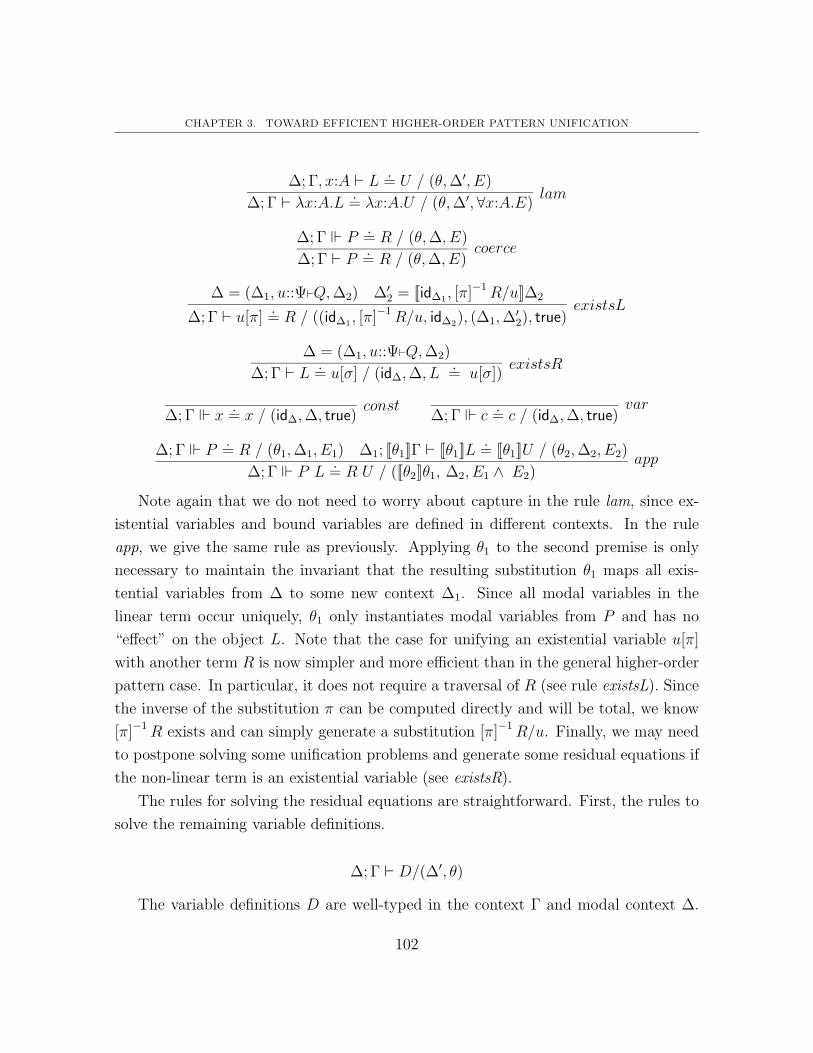
CHAPTER 3. TOWARD EFFICIENT HIGHER-ORDER PATTERN UNIFICATION
∆; Γ, x:A ` L .= U / (θ,∆′, E)
∆; Γ ` λx:A.L.= λx:A.U / (θ,∆′,∀x:A.E)
lam
∆; Γ P.= R / (θ,∆, E)
∆; Γ ` P .= R / (θ,∆, E)
coerce
∆ = (∆1, u::Ψ`Q,∆2) ∆′2 = [[id∆1 , [π]−1 R/u]]∆2
∆; Γ ` u[π].= R / ((id∆1 , [π]−1 R/u, id∆2), (∆1,∆
′2), true)
existsL
∆ = (∆1, u::Ψ`Q,∆2)
∆; Γ ` L .= u[σ] / (id∆,∆, L
.= u[σ])
existsR
∆; Γ x.= x / (id∆,∆, true)
const∆; Γ c
.= c / (id∆,∆, true)
var
∆; Γ P.= R / (θ1,∆1, E1) ∆1; [[θ1]]Γ ` [[θ1]]L
.= [[θ1]]U / (θ2,∆2, E2)
∆; Γ P L.= R U / ([[θ2]]θ1, ∆2, E1 ∧ E2)
app
Note again that we do not need to worry about capture in the rule lam, since ex-
istential variables and bound variables are defined in different contexts. In the rule
app, we give the same rule as previously. Applying θ1 to the second premise is only
necessary to maintain the invariant that the resulting substitution θ1 maps all exis-
tential variables from ∆ to some new context ∆1. Since all modal variables in the
linear term occur uniquely, θ1 only instantiates modal variables from P and has no
“effect” on the object L. Note that the case for unifying an existential variable u[π]
with another term R is now simpler and more efficient than in the general higher-order
pattern case. In particular, it does not require a traversal of R (see rule existsL). Since
the inverse of the substitution π can be computed directly and will be total, we know
[π]−1 R exists and can simply generate a substitution [π]−1 R/u. Finally, we may need
to postpone solving some unification problems and generate some residual equations if
the non-linear term is an existential variable (see existsR).
The rules for solving the residual equations are straightforward. First, the rules to
solve the remaining variable definitions.
∆; Γ ` D/(∆′, θ)
The variable definitions D are well-typed in the context Γ and modal context ∆.
102

3.4. ASSIGNMENT FOR HIGHER-ORDER PATTERNS
If the variable definitions can be solved, then a modal substitution θ is returned, s.t.
∆′ ` θ : ∆. Note, that we assume that the modal substitution θ1, which is the result of
the previous assignment algorithm, has been already applied, when we use the following
rules to solve the residual variable definitions.
∆; Γ, x:A D/(∆′, θ)∆; Γ ∀x:A.D/(∆′, θ)
∆; Γ D1/(∆1, θ1) ∆1; [[θ1]]Γ [[θ1]]D2/(∆2, θ2)
∆; Γ D1 ∧ D2/(∆2, [[θ2]](θ1)
∆′2 = [[id∆1 , U/u]]∆2
∆1, u::(Γ`A),∆2; Γ u[idΓ]D= U/(∆1,∆
′2), (id∆1 , U/u, id∆2))
(∗)
∆; Γ ` U ′ .= U/(∆′, θ)
∆; Γ U ′D= U/(∆′, θ)
∆; Γ true/(∆, id∆)
Solving variable definitions is then straightforward. The only case we need to pay
attention is the rule (*). This case may arise if u[idΓ] is a modal variable which has not
been instantiated yet during assignment. In this case, we simply assign u the object U .
This ensures that after the variable definitions are solved, no modal variables which are
used in variable definitions are left uninstantiated. In other words, all the intermediate
modal variables which have been introduced during linearization are now instantiated.
Next, we show the rules for solving the residual equations, which have been gener-
ated during assignment. The algorithm is straightforward and very similar to solving
variable definitions, except that no special provisions have to be made.
∆; Γ `e E / (∆′, θ)
The residual equations E are well-typed in the context Γ and modal context ∆.
If the residual equations can be solved, then a modal substitution θ is returned, s.t.
103

CHAPTER 3. TOWARD EFFICIENT HIGHER-ORDER PATTERN UNIFICATION
∆′ ` θ : ∆.
∆; Γ, x:A `e E/(∆′, θ)∆; Γ `e ∀x:A.E/(∆′, θ)
∆; Γ `e E1/(∆1, θ1) ∆1; [[θ1]]Γ `e [[θ1]]E2/(∆2, θ2)
∆; Γ `e E1 ∧ E2/(∆2, [[θ2]](θ1))
∆; Γ ` L .= U/(∆′, θ)
∆; Γ `e L .= U/(∆′, θ) ∆; Γ `e true/(∆, id∆)
The overall algorithm can be summarized as follows:
1. Higher-order assignment: ∆; Γ ` L .= U/(θ1,∆1, E)
2. Solving variable definitions: ∆1; · ` [[θ1]]D/(θ2,∆2)
3. Solving residual equations: ∆2; · ` [[[[θ2]]θ1]]E/(∆3, θ3)
The final result of the overall algorithm is the modal substitution [[θ3]]([[[[θ2]]θ1]]).
For the higher-order pattern fragment, we can now show that assignment algorithm
is sound and complete for linear higher-order patterns. In principle, it is possible to
generalize these statements further to include variable definitions and residual equations
E and show that linearization together with linear higher-order pattern unification is
sound and complete. This would requires a more precise description of the linearization
process and how variable definitions can be eliminated. In particular the completeness
theorem would be more complicated
3.5 Experiments
We have implemented the presented algorithm as part of the Twelf system. The instan-
tiation is applied eagerly by using destructive updates. As mentioned before, lowering
and grafting are also done eagerly using destructive updates. In this section, we discuss
some experimental results with different programs written in Twelf. All experiments
are done on a machine with the following specifications: 1.60GHz Intel Pentium Pro-
cessor, 256 MB cache. We are using SML of New Jersey 110.0.3 under Linux Red Hat
7.1. Times are measured in seconds. In the tables below, the column “opt” refers
to the optimized version with linearization and assignment, while the column “stand”
refers to the standard implementation using general higher-order pattern unification.
104

3.5. EXPERIMENTS
The column “trivial” indicates the percentage of problems which are already linear and
have no residuating variable definitions. The column “fail” indicates how many vari-
able definitions were not solvable, if there were any. The last column gives the overall
success rate with respect to the total number of calls to assignment made. The col-
umn “time reduction” refers to how much time is saved. This is calculated as follows:
(timeold− timenew)/timeold. In addition, we give the factor of improvement, which can
be calculated timeold/timenew3.
3.5.1 Higher-order logic programming
In this section, we present two experiments with higher-order logic programming. The
first one uses an implementation of a meta-interpreter for ordered linear logic by Po-
lakow and Pfenning [58]. In the second experiment we evaluate our unification al-
gorithm using an implementation of foundational proof-carrying code developed at
Princeton University [2].
Meta-interpreter for ordered linear logic
example opt stand reduction improve variable def assignin time trivial fail succeed
sqnt (bf) 0.84 2.09 60% 2.49 44% 46% 23%sqnt (dfs) 0.93 2.35 60% 2.52 44% 47% 22%sqnt (perm) 4.44 7.11 38% 1.60 44% 52% 20%sqnt (rev) 1.21 1.70 29% 1.40 45% 48% 21%sqnt (mergesort) 2.26 3.39 33% 1.50 46% 53% 20%
As the results for the meta-interpreter demonstrate, performance is improved by
to a factor of 2.5. Roughly, 45% of the time there were no variable definitions at all.
From the non-trivial equations roughly 45% were not unifiable. This means overall, in
approx. 20% - 30% of the cases the assignment algorithm succeeded and the failure of
unification was delayed. It is worth noting that 77% to 80% of the calls to assignment
presented in Section 3.4 fail immediately.
3Note that from the factor of improvement one can compute the time-reduction automatically.If the factor of improvement is k then this results in 1 − (1/k) reduction in time, since (timeold −timenew)/timeold = 1− (timenew/timeold) = 1− (1/k).
105

CHAPTER 3. TOWARD EFFICIENT HIGHER-ORDER PATTERN UNIFICATION
Recently, Twelf has been applied to mobile code security in the foundational proof-
carrying code project at Princeton [3]. To provide guarantees about the behavior of
mobile code, programs are equipped with a certificate (proof) that asserts certain safety
properties. These safety properties are represented as higher-order logic programs.
Twelf’s logic programming interpreter then executes the specification and generates a
certificate (proof) that a given program fulfills a specified safety policy. We have had
the opportunity to evaluate the presented assignment algorithm using programs from
the proof-carrying code benchmark provided by Andrew Appel’s group at Princeton
University.
Foundational proof-carrying code
example opt stand reduction improve variable def assignin time trivial fail succeed
inc 5.8 9.19 36.7% 1.58 64% 46% 18%switch 36.00 49.69 27.54% 1.38 64% 48% 19%mul2 5.51 9.520 42.86% 1.72 64% 46% 18%div2 121.96 153.610 20.63% 1.26 63% 48% 20%divx 333.69 1133.150 70.50% 3.39 63% 50% 21%listsum 1073.33 ∞ ∞ ∞ 65% 45% 18%polyc 2417.85 ∞ ∞ ∞ 65% 41% 17%pack 197.07 1075.610 81.65% 5.45 66% 45% 19%
In the table above we show the performance on programs from the proof-carrying
code benchmark. Performance is improved by up to a factor of 5.45 and some ex-
amples are not executable without linearization and assignment. The results clearly
demonstrate that an efficient unification algorithm is critical in large-scale examples.
There are several reasons for this substantial performance improvement. 1) We
reduced the need for trailing instantiations of meta-variables in the implementation.
As all meta-variables in the clause head have been created since the last choice point,
no trailing should be necessary. As a consequence, less space is needed for storing
instantiation of variables. However, to enforce this trailing policy in a high-level imple-
mentation this may require additional bookkeeping mechanism. The presented simple
assignment algorithm opened another possibility to reduce the need for trailing with-
out modifying the actual trailing mechanism. 2) We not only factor out duplicate
106

3.5. EXPERIMENTS
meta-variables, but also expressions which call external constraint solvers. Calling the
external constraint solvers may be expensive, especially if unification fails at a later
point anyway. Factoring out constraint expressions and delaying their solution, allows
us to fail quickly and disregard a clause as not applicable. As over 80% of the clauses
tried fail, this is particularly important.
Remark: There are several other standard optimizations possible such as for ex-
ample first-argument indexing. Maybe surprisingly, first-argument indexing did not
improve performance. Although the number of calls to assignment were reduced by
roughly 10%, this did not seem to influence the overall performance. One reason we
found was that unification and weak head normal form dominate the run-time dramat-
ically.
3.5.2 Higher-order theorem proving
Besides a logic programming engine, the Twelf system also provides a theorem prover
which is based on iterative deepening search. In this section, we consider two exam-
ples, theorem proving in an intuitionistic sequent calculus and theorem proving in the
classical natural deduction calculus.
As the results demonstrate, the performance of the theorem prover is not greatly
influenced by the optimized unification algorithm. The main reason is that we have
many dynamic assumptions, which need to be unified with the current goal. However,
we use the standard higher-order pattern unification algorithm for this operation and
use the optimized algorithm only for selecting a clause. For dynamic assumptions we
cannot maintain the linearity requirement and linearizing the dynamic assumptions at
run-time seems too expensive.
Proof search in the intuitionistic sequent calculus
example opt stand reduction improve variable def assignin time trivial fail success
dist-1 53.00 57.11 7% 1.08 100% 0% 52%distImp 0.40 0.44 9% 1.10 100% 0% 53%pierce 1520.77 1563.35 3% 1.03 100% 0% 52%trans 0.13 0.13 0% 1.00 100% 0% 53%
107

CHAPTER 3. TOWARD EFFICIENT HIGHER-ORDER PATTERN UNIFICATION
Proof search in NK (and, impl, neg)
example opt stand reduction improve variable def assign
in time trivial fail success
andEff1-nk 7.67 13.14 42% 1.71 100% 0% 80%
andEff2-nk 3.86 6.58 41% 1.70 100% 0% 81%
assocAnd-nk 2.24 3.74 40% 1.67 100% 0% 81%
combS-nk 3.85 6.64 42% 1.72 100% 0% 81%
The second example is theorem proving in the natural deduction calculus. In con-
trast to the previous experiments with the sequent calculus, there is a substantial
performance improvement by factor 1.7. It is worth pointing out that in both ex-
amples, all clause heads can be solved by the optimized unification algorithm and no
non-trivial variable definitions arise. Moreover, most of the time unification succeeds.
This is not surprising when considering the formulation of the natural deduction sys-
tem as any elimination rule will be applicable at any given time. Although linear head
compilation substantially improves performance, more optimizations, such as tabling
and indexing, are needed to solve more complex theorems.
3.5.3 Constraint solvers
Finally, we consider problems using constraint solvers.
Examples using constraint solvers
example opt stand reduction improve variable def assign
in time trivial fail success
solve 1.73 1.11 -56% 0.36 7.8% 42% 82%
represent 0.16 0.16 0% 1.00 85% 33% 93%
cont fraction 0.61 0.64 33% 1.50 79% 12% 82%
mortgage 4.88 6.84 29% 1.40 66% 0% 100%
sieve 500 2.61 4.88 46% 1.86 50% 47% 79%
In our implementation, we delay solving any sub-terms which call constraint solvers.
As the results below demonstrate this may be beneficial as in the sieve 500 problem,
108

3.6. RELATED WORK AND CONCLUSION
but it may also degrade performance in rare case as the first problem demonstrates. We
left out the reduction of time, since there is none – in fact time increases. This has been
the only time we found that performance deteriorated. The reason for performance
degradation in this example is that most unification problems were outside the fragment
of linear higher-order patterns.
3.6 Related work and conclusion
The language most closely related to our work is λProlog. Two main different imple-
mentations of λProlog exist, Prolog/Mali and Teyjus. In Prolog/Mali implementation,
the occurs-check is left out entirely [6]. While Teyjus [38, 37] also eliminates some
unnecessary occurs-checks statically during compilation. However, in addition to the
presence of dependencies in Twelf, there are several other differences between our
implementation and Teyjus. 1) Teyjus compiles first and subsequent occurrences of
existential variables into different instructions. Therefore, assignment and unification
are freely mixed during the execution. This may lead to expensive failure in some cases,
since unification is still called. In our approach, we perform a simple fast assignment
check and delay unification entirely. As the experimental results demonstrate, only
a small percentage of the cases fails after it already passed the assignment test and
most cases benefit from a fast simple assignment check. 2) We always assume that
the types of existential variables are lowered. This can be done at compile time and
incurs no run-time overhead. In Huet’s unification algorithm, projection and imitation
rules are applied at run-time to construct the correct prefixes of λ-abstractions. 3) Our
approach can easily incorporate definitions and constraint domains. This is important
since unifying definitions and constraint expressions may potentially be expensive. In
fact, we generalize and extend the idea of linearization in the implementation and fac-
tor out not only duplicate existential variables but also any difficult sub-expressions
such as definitions and constraint expressions. Therefore, our approach seems more
general than the one adopted in Teyjus.
As experiments show, performance is improved substantially. This is especially
important in large-scale applications such as proof-carrying code and allows us explore
the full potential of logical frameworks in real-world applications. This may however
109

CHAPTER 3. TOWARD EFFICIENT HIGHER-ORDER PATTERN UNIFICATION
only be considered as a first step towards reducing the performance gap between higher-
order and first-order system. Another optimization which is particularly important to
sustain performance in large-scale examples is term indexing. We will present a higher-
order term indexing technique based on the ideas of linearization and assignment later
in chapter 5,
110

Chapter 4
Tabled higher-order logic
programming
Tabled first-order logic programming has been successfully applied to solve complex
problems such as implementing recognizers and parsers for grammars [68], representing
transition systems CCS and writing model checkers [16]. The idea behind it is to
eliminate redundant computation by memoizing sub-computations and re-using their
results later. The resulting search procedure is complete and terminates for programs
with the bounded-term size property. The XSB system [62], a tabled logic programming
system, demonstrates impressively that tabled together with non-tabled programs can
be executed efficiently.
Higher-order logic programming languages such as Elf [47] extend first-order logic
programming in three ways: first, they allow the programmer to define his or her
own higher-order data-types together with constructors. In particular, constructors
may take functions as arguments to denote the scope of bound variables. Dependent
types allows us to model dependencies among the constructor arguments. Second,
we may generate and use dynamic assumptions during proof search. Third, Elf’s logic
programming engine not only succeeds or fails, but also returns a proof giving evidence
why it succeeded.
In this chapter, we give a motivating example and explained the basic idea behind
tabled higher-order logic programming where some redundant computation is eliminated
by memoizing sub-computations and re-using their result later. In particular, we will
111
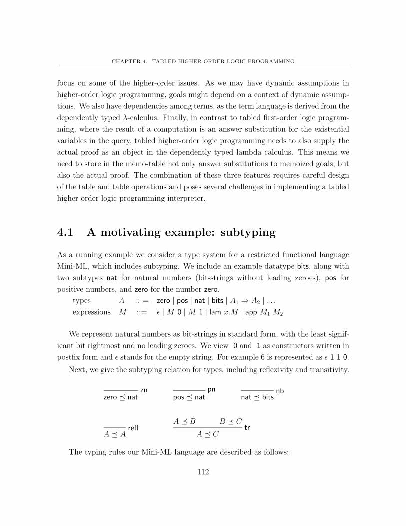
CHAPTER 4. TABLED HIGHER-ORDER LOGIC PROGRAMMING
focus on some of the higher-order issues. As we may have dynamic assumptions in
higher-order logic programming, goals might depend on a context of dynamic assump-
tions. We also have dependencies among terms, as the term language is derived from the
dependently typed λ-calculus. Finally, in contrast to tabled first-order logic program-
ming, where the result of a computation is an answer substitution for the existential
variables in the query, tabled higher-order logic programming needs to also supply the
actual proof as an object in the dependently typed lambda calculus. This means we
need to store in the memo-table not only answer substitutions to memoized goals, but
also the actual proof. The combination of these three features requires careful design
of the table and table operations and poses several challenges in implementing a tabled
higher-order logic programming interpreter.
4.1 A motivating example: subtyping
As a running example we consider a type system for a restricted functional language
Mini-ML, which includes subtyping. We include an example datatype bits, along with
two subtypes nat for natural numbers (bit-strings without leading zeroes), pos for
positive numbers, and zero for the number zero.
types A :: = zero | pos | nat | bits | A1 ⇒ A2 | . . .expressions M ::= ε |M 0 |M 1 | lam x.M | app M1 M2
We represent natural numbers as bit-strings in standard form, with the least signif-
icant bit rightmost and no leading zeroes. We view 0 and 1 as constructors written in
postfix form and ε stands for the empty string. For example 6 is represented as ε 1 1 0.
Next, we give the subtyping relation for types, including reflexivity and transitivity.
znzero nat
pnpos nat
nbnat bits
reflA A
A B B Ctr
A C
The typing rules our Mini-ML language are described as follows:
112

4.1. A MOTIVATING EXAMPLE: SUBTYPING
Γ ` ε : bits
Γ `M : postp z1
Γ `M 0 : pos
Γ `M : bitstp z2
Γ `M 0 : bits
Γ `M : nattp o1
Γ `M 1 : pos
Γ `M : bitstp o2
Γ `M 1 : bits
Γ `M : A′ A′ Atp sub
Γ `M : A
Γ, x:A1 `M : A2tp lam
Γ ` lam x.M : A1 ⇒ A2
The subtyping relation is directly translated into Elf using logic programming no-
tation. We first declare a type family tp for Mini-ML types with constants bit, zero,
pos, and nat represent the basic types and the function type is denoted by T1 => T2.
Similarly, we declare a type family exp for Mini-ML expressions.
tp : type. exp : type.
zero : tp. e : exp.
pos : tp. 0 : exp -> exp.
bits : tp. 1 : exp -> exp.
=> : tp -> tp -> tp. lam : (exp -> exp) -> exp.
app : exp -> exp -> exp.
To ease readability, we assume the function type => is declared as an infix operator,
and the constructors 0 and 1 are declared as postfix operators.
Next, we give an implementation of the subtyping relation and the typing rules as
higher-order logic programs. Throughout this example, we reverse the arrow A1 → A2
writing instead A2 ← A1. From a logic programming point of view, it might be more
intuitive to think of the clause H ← A1 ← . . .← An as H ← A1 , . . . , An.
sub : tp -> tp -> type.
refl : sub A A. zn : sub zero nat.
nb : sub nat bits. pn : sub pos nat.
tr : sub A C arr : sub (A1 => A2) (B1 => B2)
<- sub A B <- sub B1 A1
<- sub B C. <- sub A2 B2.
113

CHAPTER 4. TABLED HIGHER-ORDER LOGIC PROGRAMMING
of : exp -> tp -> type.
tp sub : of M A tp lam : of (lam ([x] M x)) (A1 => A2)
<- of M A’ <- (x:exp of x A1 -> of (M x) A2).
<- sub A’ A.
tp app : of (app M1 M2) T
<- of M1 (T2 => T)
<- of M2 T2.
Note that the capital variables A, B, C etc. are implicitly quantified at the outside.
Twelf internally reconstructs the types of the logic variables A, B, etc. In LF, the
transitivity clause is written as follows:
tr : Πa:tp.Πb:tp.Πc:tp.sub b c→ sub a b→ sub a c.
Under the type-theoretic view, Πa:tp.Πb:tp.Πc:tp.sub b c → sub a b → sub a c is the
type of the constant tr. Under the logic programming interpretation, we interpret types
as formulas and we refer to Πa:tp.Πb:tp.Πc:tp.sub b c → sub a b → sub a c as a clause
and tr as the name of the clause. and In the following presentation, we often use types
and formulas interchangeably.
The proof for zero bits which is given by the following derivation
zero natzn
nat bitsnb
zero bitstr
is represented as a proof term (tr zero nat bits nb zn) in LF. The constant tr is a
function where the existential variables a, b, c are instantiated to zero, nat, bits. In
addition we pass in as arguments the proof term nb for nat bits and the proof term zn
for zero nat. Note that we usually omit the implicit arguments zero and nat, which
denote the instantiation of transitivity rule and just write (tr nb zn) for the proof of
zero bits. In Twelf notation, this corresponds to the proof term (tr bn zn) for the
proof of the query (sub zero bit).
Although the specification and implementation of the typing rules including sub-
typing is straightforward, the implementation is not directly executable. Computation
may be trapped in infinite paths and performance may be hampered by redundant
computation. For example, the execution of the query sub zero T will end in an
infinite branch trying to apply the transitivity rule. Similarly, the execution of the
114

4.2. TABLED LOGIC PROGRAMMING: A QUICK REVIEW
query of (lam [x] x) T will not terminate and fail to enumerate all possible types.
In addition, we repeatedly type-check sub-expressions, which occur more than once.
To eliminate redundancy, some sophisticated type checkers for example for refinement
types memoize the result of sub-computations to obtain more efficient implementa-
tions. In this chapter, we extend higher-order logic programming languages such as
Elf with generic memoization techniques, called tabled higher-order logic programming.
This has several advantages. Although it is possible to derive an algorithmic subtyping
relation for the given example, this might not be trivial in general. One could argue
that the user can refine the implementation further and add an extra argument to the
type family of, which can be used to store intermediate results, thereby developing a
customized type-checker with explicit support for memoization. However, this com-
plicates the type checker substantially and proving the correctness of the type-checker
with special memoization support will be hard, because we need to reason explicitly
about the structure of memoization. Moreover, the certificates, which are produced as
a result of the execution, are larger and contain references to the explicit memoization
data-structure. This is especially undesirable in the context of certified code where
certificates are transmitted to and checked by a consumer, as sending larger certifi-
cates takes up more bandwidth and checking them takes more time. Finally, tabled
logic programming provides a complete proof search strategy. For programs with the
bounded-term size property, tabled logic programming terminates and we are able to
disprove certain statements1. This in turn helps the user to debug the specification
and implementations.
4.2 Tabled logic programming: a quick review
Tabling methods evaluate programs by maintaining tables of subgoals and their an-
swers and by resolving repeated occurrences of subgoals against answers from the table.
1The size of a term is defined recursively where the size of a bound or modal variable or constant is1 and the size of R U is the size of R plus the size of U . In the higher-order setting, we can in additiondefine the size of λx:A.U , as 1 plus the size of U and assume that all terms must be eta-expanded. Afinite program P has the bounded-term size property if an atomic query Q has no arguments whosesize exceeds n and there is a function f(n), then there is no atomic subgoal in the derivation whosean argument size exceeds f(n). (see [12], section 5.4).
115

CHAPTER 4. TABLED HIGHER-ORDER LOGIC PROGRAMMING
We review briefly Tamaki and Sato’s multi-stage strategy [65], which differs only in-
significantly from SLG resolution [12] for programs without negation. To demonstrate
tabled computation, we consider the evaluation of the query sub zero T in more detail.
The search proceeds in multiple stages. The table serves two purposes: 1) We
record all sub-goals encountered during search. If the current goal is not in the table or
more precisely there is no entry A s.t. A is an alpha-variant of the current goal, then
we add it to the table and proceed with the computation. We consider a goal A an
alpha-variant of another goal A′ if there exists a bijection between the modal variables
and ordinary variables.
Computation at a node is suspended, if the current goal is a variant of a table entry.
2) In addition to the sub-goals we are trying to solve, we also store the result of the
computation in the table as a list of answers to the sub-goals. An answer is a pair of
a substitution θ for the existential variables in the current goal A together with the
actual proof P .
In each stage we apply program clauses and answers from the table. Figure 4.1
illustrates the search process.
The root of the search tree is labeled with the goal sub zero A. Each node is labeled
with a goal statement and each child node is the result of applying a program clause
or an answer from the table to the leftmost atom of the parent node. Applying a
clause H ← A1 ← A2 . . . ← An results in the subgoals A1, A2, . . . , An where all of
these subgoals need to be satisfied. We will then expand the first subgoal A1 carrying
the rest of the subgoals A2, . . . , An along. If a branch is successfully solved, we show
the obtained answer. To distinguish between program clause resolution and re-using
of answers, we have two different kinds of edges in the tree. The edges obtained by
program clause resolution are solid annotated with the clause name used to derive
the child node. Edges obtained by reusing answers from the table are dashed and
annotated with the answer used to derived the child node. Using the labels at the
edges, we can reconstruct the proof term for a given query. In general, we will omit
the actual substitution under that the parent node unifies with the program clause to
avoid cluttering the example. To ensure we generate all possible answers for the query,
we restrict the re-use of answers from the table. In each stage, we are only allowed to
re-use answers that were generated in previous stages. Answers from previous stages
(available for answer resolution) are marked gray, while current answers (not available
116

4.3. TABLED HIGHER-ORDER LOGIC PROGRAMMING
sub zero A
A = zero
A = nat
sub zero R ,
sub R A.
sub nat A
sub zero A
A = zero
A = nat
A = nat
A = bits
A = bits
A = bits
sub bits R ,
sub R A.
refl
tr
sub nat A
sub bits A
sub bits A
sub bits A
A = nat
A = bits
A = bits
A = bits
A = bitssub bits A
: refl: zn: (tr bn zn): refl: nb
: refl
(1)(2)(3)(4)(5)
sub nat A
A = zeronatbitsnatbits
: refl: zn: (tr bn zn): refl: nb
(1)(2)A = nat
sub zero A A = zero
refl
tr
zn
Stage 1
refl
tr
nb
sub R A.
sub nat R ,
(1)(2)
(3)
(4)
(5)
(1)
(2)
Stage 2
(4)
(5)
(3)
Stage 3
(6)
(6) (6)
Stage 4
Entry Answers
A A = zeroA = nat
sub zero
A = bitssub nat A A = nat
A = bits
Entry Answers
A A = zeroA = nat
sub zero
A = bitssub nat A A = nat
A = bits
bitssub bits A A =
: refl: zn: (tr bn zn): refl: nb
: refl
Entry Answers
AA =
sub zero
A = A = A =
(1)(2)(3)(4)(5)
(1)(2)(3)(4)(5)
(6) (6)
: refl
AnswersEntry
: zn
Figure 4.1: Staged computation
yet) are black. In the first stage no answers are available yet. In the second stage, we
are only allowed to use answers (1) and (2). In the third stage, we may use all answers
from (1) up to (5). In the final stage, we are allowed to use all answers.
4.3 Tabled higher-order logic programming
In tabled higher-order logic programming, we extend tabling to handle sub-goals that
may contain implications and universal quantification and our term language is the
dependently typed λ-calculus. The table entries are no longer atomic goals, but atomic
goals A together with a context Γ of assumptions. In addition, terms might depend
on assumptions on Γ. To highlight some of the challenges we present the evaluation of
117

CHAPTER 4. TABLED HIGHER-ORDER LOGIC PROGRAMMING
tp_sub
tp_lam u:of x A1 of x A2
u:of x T sub T A2
sub B1 T.sub T B2
A = T => A
sub B Asub (T => T) B,
. . .
refl
tr
arr
u:of x A1 of x A2 u:of x A1 of x A2
of (lam [x] x) A
of (lam [x] x) B,
sub B A
Stage 1 Stage 2
(1)
(2)
sub (T => T) A
Entry Answers
A = T => T
A = T => T
B1 = S, T = S
Entry Answers
u
tp_sub
sub B A2
A1 = T, A2 = T, A = T => T
(1)
(2)
(3)
B1 = nat, T = bitsB1 = pos, T = natB1 = zero, T = nat
A = T => T
A1 = T, A2= T
: (tp_lam [u] u) (1)
: u (2)
u:of x A1 of x B,
A1 = T, A2= T
of (lam [x] x) A
sub (T => T) A
sub B1 T.
of (lam [x] x) A : (tp_lam [u] u)
: u
: refl
(4): refl: zn: pn: nb (7)
(6)(5)
Figure 4.2: Staged computation for identity function
the query of (lam [x] x) T in Figure 4.2.
The possibility of nested implications and universal quantifiers adds a new degree
of complexity to memoization-based computation. Retrieval operations on the table
need to be redesigned. One central question is how to look up whether a goal Γ ` P is
already in the table. There are two options: In the first option we only retrieve answers
for a goal P given a context Γ, if the goal together with the context matches an entry
Γ′ ` P ′ in the table. In the second option we match the subgoal P against the goal
P ′ of the table entry Γ′ ` P ′, and treat the assumptions in Γ′ as additional subgoals,
thereby delaying satisfying these assumptions. We choose the first option of retrieving
goals together with their dynamic context Γ′. One reason is that it restricts the number
of possible retrievals early on in the search. For example, to solve subgoal u:of x A1 `
118

4.4. SUBORDINATION
of x B, sub B A2, we concentrate on solving the left-most goal u:of x A1 ` of x B
keeping in mind that we still need to solve u:of x A1 ` sub B A22. As there exists
a table entry u:of x A1 ` of x A2, which is a variant of the current goal u:of x A1 `of x B, computation is suspended. Note, we adopted a common convention in logic,
where we omitted the explicit declaration of the parameter x in the context. To be
more precise, we write in the following development x:exp, u:of x A1 for the context of
ordinary variables instead of just u:of x A1.
4.4 Subordination
Due to the higher-order setting, the predicates and terms might depend on assumptions
in the context Γ. Virga [67] developed in his PhD thesis techniques, called subordi-
nation, to analyze dependencies in Elf programs statically before execution. In the
Mini-ML example, the terms of type exp and tp are independent of each other. On
the level of predicates, the type checker of depends on the subtyping relation sub, but
not vice versa. When checking whether a subgoal Γ ` P is already in the table, we ex-
ploit the subordination information in two ways. First, we use it to analyze the context
Γ and determine which assumptions might contribute to the proof of P . For example
the proof for x:exp, u:of x A1 ` of x A2 depends on the assumption u. However, the
predicate sub does not refer to the predicate of. Similarly, the predicate sub does not
refer to expressions exp. Therefore the proof for x:exp, u:of x T ` sub A A2 cannot de-
pend on the assumption u or x. When checking whether u:of x T ` sub T A2 is already
in the table, it suffices to look for a variant of sub T A2. In the given example, compu-
tation at subgoal x:exp, u:of x T ` sub T A2 is suspended during stage 2 as the table
already contains sub B1 T . If we for example first discover x:exp, u:of x T ` sub T A2,
then we store the strengthened goal sub T A2 in the table with an empty context.
Second, subordination provides information about terms. As we are working in a
higher-order setting, solutions to new existential variables, which are introduced during
execution, might depend on assumptions from Γ. For example, applying the subtyping
2Note that u in the declaration u:of x A1 denotes an ordinary bound variable, not a modal variable.Recall that to denote the declaration of the modal variable u we write u::Ψ`A
119

CHAPTER 4. TABLED HIGHER-ORDER LOGIC PROGRAMMING
rule to x:exp, u:of x A1 ` of x A2 yields the following new goal
x:exp, u:of x A1 ` of x (B x u) , sub (B x u) A2
where the solution for the new variable B might depend on the new variable x:exp
and the assumptions u:of x A1. However, we know that the solution must be an object
of type tp and that objects of type tp are independent of Mini-ML expressions exp and
the Mini-ML typing rules of. Hence, we can omit x and u and write x:exp, u:of x A1 `of x B, sub B A2. Before comparing goals with table entries and adding new table
entries, we eliminate unnecessary dependencies from the subgoal Γ ` P . This allows
us to detect more loops in the search tree and eliminate more redundant computation.
We come back to this issue of subordination and other optimizations to detect more
loops in the higher-order setting later in the chapter on implementation of a tabled
higher-order logic programming interpreter.
4.5 A foundation for tabled higher-order logic pro-
gramming
In this section, we give a proof-theoretic characterization of tabled higher-order logic
programming based on uniform proofs [36] and show soundness of the resulting in-
terpreter. This work forms the basis of the implemented tabled interpreter for the
language Elf. Although we concentrate on the logical framework LF, which is the basis
of Elf, it seems possible to apply the presented approach to λProlog [39] or Isabelle [45],
which are based on hereditary Harrop formulas and simply typed terms.
4.5.1 Uniform proofs
Computation in logic programming is achieved through proof search. Given a goal
(or query) A and a program Γ, we derive A by successive application of clauses of
the program Γ. Miller et al [36] propose to interpret the connectives in a goal A
120

4.5. A FOUNDATION FOR TABLED HIGHER-ORDER LOGIC PROGRAMMING
as search instructions and the clauses in Γ as specifications of how to continue the
search when the goal is atomic. A proof is goal-oriented if every compound goal is
immediately decomposed and the program is accessed only after the goal has been
reduced to an atomic formula. A proof is focused if every time a program formula is
considered, it is processed up to the atoms it defines without need to access any other
program formula. A proof having both these properties is uniform and a formalism such
that every provable goal has a uniform proof is called an abstract logic programming
language.
Elf is one example of an abstract logic programming language, which is based on
the LF type theory. Πx:A1.A2 denotes the dependent function type where the type
A2 may depend on an object x of type A1. Whenever x does not occur free in A2 we
may abbreviate Πx:A1.A2 as A1 → A2. Using the types as formulas interpretation,
we refer to Πx:A1.A2 as the universal quantifier and treat A1 → A2 as an implication.
Moreover, the typing context Γ is viewed as a context of formulas which represents
the program. We will use types and formulas interchangeably in the presentation. We
give the fragment used for logic programming in LF below. Types and programs are
defined as follows:
Types A ::= P | A1 → A2 | Πx : A1.A2
Programs Γ ::= · | Γ, x:A
P ranges over atomic formulas i.e. a M1 . . . Mn. The clause
tr:sub A C <- sub A B <- sub B C.
is interpreted as
tr:Πt:tp.Πs:tp.Πr:tp.sub r s→ (sub t r → sub t s)
Every type (or formula) has a corresponding proof term U . We assume that all
proof terms are in canonical form. Recall that applications which are in canonical form
are of the following form: (((H U1) U2) . . . Un) where head H is either a constant c or a
variable x. To allow direct head access, we flatten the representation of applications and
decompose the previous application into its head c and the arguments U1, U2, . . . Un.
The spine-notation as introduced in [11] essentially achieves this idea.
121

CHAPTER 4. TABLED HIGHER-ORDER LOGIC PROGRAMMING
Terms U ::= H · S | λx:A.U
Spines S ::= nil | U ;S
Heads H ::= c | x
In the example from Sec. 4.1, the proof term corresponding to sub zero bits is
given as tr zn refl. Note that we actually omitted the implicit arguments zero and nat,
which denote the instantiation of transitivity rule. In the following discussion, we will
include implicit arguments in the proof term representation. To give an intuition for
this notation we give a few examples.
(((((tr zero) nat) bits) nb) zn)
is denoted using spine notation by
tr · (zero ; nat ; bits ; nb ; zn ; nil).
The proof term
((((tp lam T ) (λx:exp.x)) T ) (λx:exp.λu:of x T. u))
is denoted by
tp lam · (T ; (λx:exp.x · nil) ; T ; (λx:exp.λu:of x T. u · nil) ; nil).
where T denotes a term of type tp for example the term (nat · nil). We can charac-
terize uniform proofs by two main judgments:
Γu−→ U : A U is a uniform proof for A from Γ
Γ Af−→ S : P S is a focused proof for the atom P by focusing on clause A
Taking a type-theoretic view, we can interpret the first judgment as U has type A
in the context Γ and the later as S has type P in context Γ. Note that we assume
all operations are capture-avoiding and we can rename bound variables if necessary.
Inference rules describing uniform and focused proofs are given in Figure 4.3.
In the rule f∀, we instantiate the bound variable x with a term U . As x has type A1,
we check that U has type A1 in Γ. The proof term represents the witness of the proof.
When searching for a uniform proof, the proof term is constructed simultaneously. In
the following discussion, we will often ignore proof terms, but keep in mind that they
are silently generated as a result of the proof.
122

4.5. A FOUNDATION FOR TABLED HIGHER-ORDER LOGIC PROGRAMMING
Γ, x : A,Γ′ Af−→ S : P
u atomΓ, x : A,Γ′
u−→ x · S : Pf atom
Γ Pf−→ nil : P
Γ, x : A1u−→ U : A2
u∀Γ
u−→ λx : A1.U : Πx : A1.A2
Γ [idΓ, U/x]A2f−→ S : P Γ ` U : A1
f∀Γ Πx : A1.A2
f−→ U ;S : P
Γ, c : A1u−→ U : A2
u→c
Γu−→ λc : A1.U : A1 → A2
Γ A1f−→ S : P Γ
u−→ U : A2f→
Γ A2 → A1f−→ U ;S : P
Figure 4.3: Uniform deduction system for L
4.5.2 Uniform proofs with answer substitutions
The result of a computation in logic programming is generally an answer substitution
θ for the existentially quantified variables in a goal A. To obtain an algorithm that
computes answer substitutions, we substitute existential variables u for the bound
variable x in the f∀ rule. We will interpret the existential variables as modal variables
again and generalize the previous judgment to include a context ∆ of modal variables.
Existential variables are later instantiated later during unification yielding a sub-
stitution θ. We will concentrate here on the case of higher-order pattern unification.
There are different alternative approaches to treat existential variables. One we
have explored in [55] relies on the following fact: If U is a solution for x in the con-
text Γ then there exists a solution U ′ of type ΠΓ.A1 such that U ′ · Γ is also a solu-
tion for x and U ′ is well-typed in the empty context. We write ΠΓ.A1 for the type
Πx1:B1. . . .Πxn:Bn.A1 where Γ is a context x1:B1, . . . , xn:Bn and U ′ · Γ as an abbre-
viation for U ′ · x1; . . . ;xn; nil. Moreover, there is a one-to-one correspondence between
these two solutions, as U ′ · Γ reduces to U . This has been shown by Miller [35] for the
simply-typed case and by Pfenning in the dependently typed and polymorphic case
[48]. Following Miller’s terminology, we say U ′ is the result of raising U . Intuitively, U
depends globally on the assumptions in Γ. Raising allows us to localize dependencies
by replacing U with U ′ · Γ. Then we can translate the f∀ rule to
123

CHAPTER 4. TABLED HIGHER-ORDER LOGIC PROGRAMMING
Γ [idΓ, U′ · Γ/x]A2
f−→ S : P · u−→ U ′ : ΠΓ.A1f∀
Γ Πx : A1.A2f−→ (U ′ · Γ);S : P
To obtain a calculus with existential variables, we then replace U ′ with a new
existential variable which is annotated with its type. Another alternative would be
to use mixed-prefixes [35] to model dependencies. However this would complicate
the presentation further. Here, we use the modal context and modal substitution as
previously introduced in chapter 2. This eliminates the need of first translating the
f∀-rule. The two main judgments for computing answer substitutions are
∆; Γu−→ A/(∆′, θ) Uniform proof with answer substitution ∆′ ` θ : ∆
∆; Γ Af−→ P/(∆′, θ) Focused proof with answer substitution ∆′ ` θ : ∆
We assume that A is well-typed in the modal context ∆ and bound variable context
Γ. The inference rules are given in Figure 4.4.
To obtain an algorithm, we impose left-to-right order on the solution of the fs →rule. This matches our intuitive understanding of computation in logic programming.
In the fs→ rule for example we first decompose the focused clause until we reach the
head of the clause. After we unified the head of the clause with our goal A on the right-
hand side of the sequent and completed this branch, we proceed proving the subgoals.
This left-to-right evaluation strategy only fixes a don’t care non-deterministic choice in
the inference system. In the fs∀ rule we delay the instantiation of x by introducing a
new modal variable u[idΓ]. Note that this variable is created with type A and context Γ.
There is no condition needed to ensure that θ does not leave its scope in the conclusion
of the rule fs∀ since θ only depends on modal variables in ∆ and is independent of the
bound variables in Γ. In the fs atom rule the instantiation for existentially quantified
variables is obtained by unifying P with P ′ in the context Γ. θ is a solution to the
unification problem ∆; Γ ` P .= P ′ where P and P ′ are higher-order patterns.
There is still some non-determinism left in Lθ, which needs to be resolved in an
actual implementation. In the us atom rule, we do not specify which clause from Γ we
pick and focus on. Moreover, usually the order of clauses in Γ is determined by the order
of the clauses in the program. Logic programming interpreters then usually try the
clauses in Γ in order and do not backtrack over different choices since this is considered
124

4.5. A FOUNDATION FOR TABLED HIGHER-ORDER LOGIC PROGRAMMING
Uniform Proof:
∆; Γ, x:A,Γ′ Af−→ P/(∆′, θ)
us atom∆; Γ, x:A,Γ′ u−→ P/(∆′, θ)
∆; Γ, x:A1u−→ A2/(∆, θ)
us∀∆; Γ u−→ Πx : A1.A2/(∆, θ)
∆; Γ, x : A1u−→ A2/(∆, θ)
us→x
∆; Γ u−→ A1 → A2/(∆, θ)
Focused Proof
∆; Γ ` P ′ .= P/(∆′, θ)fs atom
∆; Γ P ′f−→ P/(∆′, θ)
∆, u::(Γ`A1); Γ [idΓ, u[idΓ]/x]A2f−→ P/(∆′, (θ, U/u)) u is a new modal variable
fs∀∆; Γ Πx : A1.A2
f−→ P/(∆′, θ)
∆; Γ A1f−→ P/(∆1, θ1) ∆1; [[θ1]]Γ u−→ [[θ1]]A2/(∆2, θ2)
fs→∆; Γ A2 → A1
f−→ P/(∆2, [[θ2]]θ1)
Figure 4.4: Uniform deduction system for Lθ with substitutions
too expensive. This choice renders the search strategy incomplete in practice. However,
the presented deductive system Lθ, which generates answer substitutions, is sound and
complete, as expressed by the following two theorems.
Theorem 62 (Soundness)
1. If ∆; Γu−→ A/(∆′, θ) then for any modal substitution · ` ρ : ∆′ we have
·; [[[[ρ]]θ]]Γu−→ [[[[ρ]]θ]]A.
2. If ∆; Γ Af−→ P/(∆′, θ) then for any modal substitution · ` ρ : ∆′ we have
·; [[[[ρ]]θ]]Γ [[[[ρ]]θ]]Af−→ [[[[ρ]]θ]]P .
Proof: Structural simultaneous induction on the derivation D.
125

CHAPTER 4. TABLED HIGHER-ORDER LOGIC PROGRAMMING
Case D =∆; Γ, x:A1
u−→ A2/(∆, θ)us∀
∆; Γu−→ Πx : A1.A2/(∆, θ)
[[[[ρ]]θ]](Γ, x:A1)u−→ [[[[ρ]]θ]]A2 by i.h.
[[[[ρ]]θ]](Γ), x:[[[[ρ]]θ]](A1)u−→ [[[[ρ]]θ]]A2 by substitution definition
[[[[ρ]]θ]](Γ)u−→ Πx:[[[[ρ]]θ]](A1).[[[[ρ]]θ]]A2 by rule
[[[[ρ]]θ]](Γ)u−→ [[[[ρ]]θ]]Πx:A1.A2 by substitution definition
Case D =∆; Γ, c : A1
u−→ A2/(∆, θ)us→c
∆; Γu−→ A1 → A2/(∆, θ)
[[[[ρ]]θ]](Γ, c : A1)u−→ [[[[ρ]]θ]]A2 by i.h.
[[[[ρ]]θ]](Γ), c : [[[[ρ]]θ]](A1)u−→ [[[[ρ]]θ]]A2 by substitution definition
[[[[ρ]]θ]](Γ)u−→ [[[[ρ]]θ]](A1)→ [[[[ρ]]θ]]A2 by rule
[[[[ρ]]θ]](Γ)u−→ [[[[ρ]]θ]](A1 → A2) by substitution definition
Case D =∆; Γ A1
f−→ P/(∆1, θ1) ∆1; [[θ1]]Γu−→ [[θ1]]A2/(∆2, θ2)
fs→∆; Γ A2 → A1
f−→ P/(∆2, [[θ2]]θ1)
[[[[ρ]]θ1]]Γ [[[[ρ]]θ1]]A1f−→ [[[[ρ]]θ1]]P by i.h.
let ρ = [[ρ′]]θ2
[[[[ρ′]]θ2]][[θ1]]Γu−→ [[[[ρ′]]θ2]][[θ1]]A2 by i.h.
[[[[ρ′]]θ2]][[θ1]]Γ [[[[ρ′]]θ2]][[θ1]]A1 → [[[[ρ′]]θ2]][[θ1]]A2f−→ [[[[ρ′]]θ2]][[θ1]]P by rule
[[[[ρ′]]θ2]][[θ1]]Γ [[[[ρ′]]θ2]][[θ1]](A1 → A2)f−→ P by substitution definition
Case D =∆, u::(Γ`A1); Γ [idΓ, u[idΓ]/x]A2
f−→ P/(∆′, (θ, U/u))fs∀
∆; Γ Πx : A1.A2f−→ P/(∆′, θ)
u is a new modal variable by assumption
[[[[ρ]](θ, U/u)]]Γ [[[[ρ]](θ, U/u)]]([idΓ, u[idΓ]/x]A2)f−→ [[[[ρ]](θ, U/u)]]P by i.h.
· ` ρ : ∆′
126

4.5. A FOUNDATION FOR TABLED HIGHER-ORDER LOGIC PROGRAMMING
[[[[ρ]](θ, U/u)]]Γ = [[[[ρ]]θ]]Γ by strengthening
[[[[ρ]](θ, U/u)]]P = [[[[ρ]]θ]]P by strengthening
[[[[ρ]](θ, U/u)]] = [[[[ρ]]θ, [[ρ]]U/u]]
[[[[ρ]](θ)]]Γ ([id[[[[ρ]]θ]]Γ, [[ρ]]U/x]A2)f−→ [[[[ρ]](θ)]]P by substitution definition
∆′ ` (θ, U/u) : (∆, u::Γ`A1) by invariant
∆′ ` θ : ∆ by inversion
∆′; [[θ]]Γ ` U : [[θ]]A1 by inversion
·; [[ρ]][[θ]]Γ ` [[ρ]]U : [[ρ]][[θ]]A1 by substitution property (lemma 41)
·; [[[[ρ]]θ]]Γ ` [[ρ]]U : [[[[ρ]]θ]]A1 by composition lemma 42
·; [[[[ρ]]θ]]Γ Πx:[[[[ρ]]θ]]A1.[[[[ρ]]θ]]A2f−→ [[[[ρ]]θ]]P by rule
·; [[[[ρ]]θ]]Γ [[[[ρ]]θ]](Πx:A1.A2)f−→ [[[[ρ]]θ]]P by substitution definition
Case D =∆; Γ ` P ′ .
= P/(∆′, θ)fs atom
∆; Γ P ′f−→ P/(∆′, θ)
[[θ]]P ′ = [[θ]]P by soundness of pattern unification 60
∆′ ` θ : ∆ by lemma 59
for any modal substitution ρ such that · ` ρ : ∆′
[[ρ]][[θ]]P ′ = [[ρ]][[θ]]P by substitution property (lemma 41)
[[[[ρ]]θ]]P ′ = [[[[ρ]]θ]]P by substitution property (lemma 41)
Γ [[[[ρ]]θ]]P ′f−→ [[[[rho]]θ]]P by rule
2
Theorem 63 (Completeness)
1. If ·; [[ρ]]Γu−→ [[ρ]]A for a modal substitution ρ, s.t. · ` ρ : ∆
then ∆; Γu−→ A/(∆′, θ) for some θ and ρ = [[ρ′]]θ for some ρ′ s.t. · ` ρ′ : ∆′.
2. If ·; [[ρ]]Γ [[ρ]]Af−→ [[ρ]]P for a modal substitution ρ s.t. · ` ρ : ∆
then ∆; Γ Af−→ P/(∆′, θ) for some θ and ρ = [[ρ′]]θ for some ρ′, s.t. · ` ρ′ : ∆′.
Proof: Simultaneous structural induction on the first derivation.
127

CHAPTER 4. TABLED HIGHER-ORDER LOGIC PROGRAMMING
Case D = Γu−→ Πx : A1.A2
[[ρ]]Γu−→ [[ρ]](Πx : A1.A2) by assumption
[[ρ]]Γu−→ Πx : [[ρ]]A1.[[ρ]]A2 by substitution definition
[[ρ]]Γ, x : [[ρ]]A1u−→ [[ρ]]A2 by inversion
[[ρ]](Γ, x : A1)u−→ [[ρ]]A2 by substitution definition
∆; Γ, x : A1u−→ A2/(∆
′, θ) and ρ = [[ρ′]]θ by i.h.
∆; Γu−→ Πx : A1.A2/(∆
′, θ) by rule
Case D = Γu−→ A1 → A2
[[ρ]]Γu−→ [[ρ]](A1 → A2) by assumption
[[ρ]]Γu−→ [[ρ]](A1)→ [[ρ]](A2) by substitution definition
[[ρ]]Γ, c:[[ρ]]A1u−→ [[ρ]]A2 by inversion
[[ρ]](Γ, c:A1)u−→ [[ρ]]A2 by substitution definition
∆; Γ, c:A1u−→ A2/(∆
′, θ′) and ρ = [[ρ′]]θ by i.h.
∆; Γu−→ A1 → A2/(∆
′, θ′) by rule
Case D = Γ A2 → A1f−→ P
[[ρ]]Γ [[ρ]](A2 → A1)f−→ [[ρ]]P by assumption
[[ρ]]Γ [[ρ]](A2)→ [[ρ]](A1)f−→ [[ρ]]P by substitution definition
[[ρ]]Γ [[ρ]]A1f−→ [[ρ]]P by inversion
[[ρ]]Γu−→ [[ρ]]A2 by inversion
∆; Γ A1f−→ P/(∆1, θ1) and ρ = [[ρ′]]θ1 by i.h.
[[[[ρ′]]θ1]]Γu−→ [[[[ρ′]]θ1]]A2
[[ρ′]]([[θ1]]Γ)u−→ [[ρ′]]([[θ1]]A2) by composition lemma 42
∆1; [[θ1]]Γu−→ [[θ1]]A2/(∆1, θ2) and ρ′ = [[ρ′′]](θ2) by i.h.
∆; Γ (A2 → A1)f−→ P/(∆2, [[θ2]]θ1) by rule
ρ = [[ρ′′]][[θ2]]θ1
Case D = Γ Πx:A1.A2f−→ P
·; [[ρ]]Γ [[ρ]](Πx:A1.A2)f−→ [[ρ]]P by assumption
·; [[ρ]]Γ Πx:[[ρ]]A1.[[ρ]]A2f−→ [[ρ]]P by substitution definition
128

4.5. A FOUNDATION FOR TABLED HIGHER-ORDER LOGIC PROGRAMMING
·; [[ρ]]Γ [id[[ρ]]Γ, U/x]([[ρ]]A2)f−→ [[ρ]]P for some U by inversion
·; [[ρ]]Γ ` U : [[ρ]]A1 by inversion
· ` ρ : ∆ by assumption
· ` (ρ, U/u) : (∆, u::Γ`A1 by rule
[id[[ρ]]Γ, U/x][[ρ]]A2 = [[ρ]]([idΓ, U/x]A2) = [[ρ, U/u]]([idΓ, u[idΓ]/x]A2) where u is new
by substitution property
·; [[ρ, U/u]]Γ [[ρ, U/u]]([idΓ, u[idΓ]/x]A2)f−→ [[ρ, U/u]]P by substitution definition
∆, u::Γ`A1; Γ [idΓ, u[idΓ]/x]A2f−→ P/(∆′, θ′) and
(ρ, U/u) = [[ρ′]]θ′ for some θ′ and ρ′ by i.h.
let θ′ = (θ, U ′/u).
(ρ, U/u) = [[ρ′]](θ, U ′/u) = ([[ρ′]]θ, [[ρ]]U ′/u) by substitution definition
ρ = [[ρ′]]θ and U = [[ρ]]U ′ by syntactic equaltiy
∆; Γ Πx:A1.A2f−→ P/(∆′, θ) by rule
Case D = Γ Pf−→ P
·; [[ρ]]Γ [[ρ]]Pf−→ [[ρ]]P by assumption
[[ρ]]P = [[ρ]]P and · ` ρ : ∆
∆; Γ ` P .= P / (∆′, θ) and there exists a ρ′ s.t. · ` ρ′ : ∆′ and ρ = [[ρ′]]θ
by completeness of higher-order pattern unification (lemma 61)
∆; Γ Pf−→ P / (∆′, θ) by rule
2
In the next section, we extend this system Lθ to include memoization.
4.5.3 Tabled uniform proofs
The idea behind tabled uniform proofs is to extend our two basic judgments with a
table T in which we record atomic sub-goals and the corresponding answer substitutions
and proof terms. A subgoal is a sequent ∆; Γu−→ P where ∆ describes the existential
variables, Γ is a program context and P is an atomic goal, which we need to derive
from Γ. When we discover the sub-goal ∆; Γu−→ P for the first time, we memoize
this goal in the table. Note that the sequent ∆; Γu−→ P might potentially contain
existential variables. Once we have proven the sub-goal ∆; Γu−→ P , we add the answer
129

CHAPTER 4. TABLED HIGHER-ORDER LOGIC PROGRAMMING
substitution ∆′ ` θ : ∆ to the table. We keep in mind that we are silently generating
proof terms together with answer substitutions. We assume that some predicates are
designated as tabled predicates where we record subgoals and corresponding answers.
For predicates not designated as tabled the us atom rule still applies.
Definition 64 (Table) A table entry consists of two parts: a goal ∆; Γu−→ P and
a list A of pairs, answer substitutions ∆′ ` θ : ∆ and proof terms U , such that
∆′; [[θ]]Γu−→ [[θ]]U : [[θ]]P is a solution. A table T is a collection of table entries.
The table is a store of proven and still open conjectures. The open conjectures are
the table entries that have an empty list of answers. The proven conjectures (lemmas)
are the table entries that have a list of answer substitutions associated with them. As
proof terms are generated and stored together with answer substitutions, we also have
the actual proof for the given conjecture. We will design the inference rules in such a
way that for any solution in the table ∆′; [[θ]]Γu−→ [[θ]]U : [[θ]]P there exists a derivation
∆; Γu−→ U : P/(∆′, θ). We will keep all the previous inference rules, but keep in mind
that we are silently passing around a table T . Any substitution we apply to Γ and
P (see for example the fs→ rule) will not effect the table. This is important because
we do want to have explicit control over the table. The application of inference rules
should not have any undesired effects on the table. The main judgments are
T ; ∆; Γu−→ U : A/(∆′, θ, T ′)
T ; ∆; Γ Af−→ S : P/(∆′, θ, T ′)
In addition to the us atom inference rule, we will have the rules extend and retrieve.
The extend rule adds a subgoal and its answer to the table. When we encounter a new
subgoal, we add a new entry with an empty answer list to the table. Once we have
proven this subgoal, we add the answer substitution and proof term to its answer list,
and we can later use it as a lemma. retrieve allows us to close a branch by applying
a lemma from the table. If we are proving ∆; Γu−→ P , where Γ and P may contain
existential variables and we have a proof for ∆′; [[θ]]Γu−→ [[θ]]U : [[θ]]P in the table then
we can just re-use it by applying the answer substitution θ and substituting the proof
term [[θ]]U for it. Applying the retrieve rule corresponds to introducing an analytic cut
in the proof using a lemma from the table.
130

4.5. A FOUNDATION FOR TABLED HIGHER-ORDER LOGIC PROGRAMMING
Before we present these two rules, we define when a goal is α-variant to a table
entries. We consider ∆; Γu−→ P a variant of ∆′; Γ′
u−→ P ′ if there exists a renaming
of the ordinary variables in Γ and the modal variables in ∆ such that ∆; Γu−→ P is
equal to ∆′; Γ′u−→ P ′.
Definition 65 (Variant) The goal ∆; Γu−→ P is a variant of ∆′; Γ′
u−→ P ′ if
• there exists a bijection ρ between the modal variables in ∆ and ∆′ such that
∆′ ` ρ : ∆.
• there exists a bijection σ between the ordinary variables in [[ρ]]Γ and Γ′ such that
∆′; Γ′ ` σ : [[ρ]]Γ
• and [σ][[ρ]]P = P ′.
This definition of variant can be extended to terms. We say a term ∆; Γ ` U is a
variant of term ∆′; Γ′ ` U ′ if there exists a bijection between the modal variables in
∆ and ∆′ and a bijection between the ordinary variables in Γ and Γ′. Next, we define
when two modal substitutions are variants of each other.
Definition 66 The modal substitution ∆′1 ` θ1 : ∆1 is a variant of ∆′2 ` θ2 : ∆2
• ∆1 ` · : · is a variant of ∆2 ` · : ·.
• ∆′1 ` (θ1, U/u) : (∆1, u::(Ψ`A)) is a variant of ∆′2 ` (θ2, N/u) : (∆2, u::(Ψ′`A′)
iff
1. ∆′1 ` θ1 : ∆1 is a variant of ∆′2 ` θ2 : ∆2
2. ∆′1; Ψ ` U is a variant of ∆′2; Ψ′ ` N
Now we can define the three main operations on the table, extending the table,
inserting an answer in the table and retrieving an answer from the table.
Definition 67 (extend) extend(T ,∆; Γu−→ P ) = T ′
Let T be a table, ∆; Γu−→ P be a goal.
• If there exists a table entry (∆′; Γ′u−→ P ′,A) in T and A is non-empty such that
∆′; Γ′u−→ P ′ is a variant of ∆; Γ
u−→ P then return T .
131

CHAPTER 4. TABLED HIGHER-ORDER LOGIC PROGRAMMING
• If there exists no table entry (∆′; Γ′u−→ P ′,A) in T such that ∆′; Γ′
u−→ P ′ is a
variant of ∆; Γu−→ P , then we obtain the extended table T ′ by adding ∆; Γ
u−→ P
to the table T with an empty solution list.
Definition 68 (insert) insert(T ,∆; Γu−→ P,U, θ) = T ′
Let T be a table, ∆; Γu−→ P be a goal and ∆′ ` θ : ∆ be a corresponding answer
substitution and U a proof term such that ∆; Γ ` U : P . Let (∆i; Γiu−→ Pi,A) be in
the table T and Γiu−→ Pi is a variant of ∆; Γ
u−→ P . If there exists no ∆′i ` θi : ∆i
in the answer substitution list A, such θi is a variant of θ, then we add ∆′ ` θ : ∆
together with the proof term U to the the answer list A.
If we generate and try to insert an answer substitution θ which already exists in
the answer list, then we fail.
Definition 69 (retrieve) retrieve(T ,∆; Γu−→ P ) = (∆′, θ, U)
Let T be a table and ∆; Γu−→ P be a goal. If there exists a table entry (∆i; Γi
u−→Pi,Ai) such that ∆i; Γi
u−→ Pi is variant of ∆; Γu−→ P and there exists an answer
substitution ∆′i ` θi : ∆ together with a proof term U in Ai then return (∆′i, θi, U).
Now we can give the additional rules extend and retrieve.
extend(T , ∆; (Γ, x:A,Γ′)u−→ P ) = T1
T1; ∆; (Γ, x:A,Γ′) Af−→ S : P/(∆′, θ, T2)
insert(T2,∆; (Γ, x:A,Γ′)u−→ P,U,∆′, θ) = T3
T ; ∆; (Γ, x:A,Γ′)u−→ x · S : P/(∆′, θ, T3)
extend
retrieve(T ; ∆; Γu−→ P ) = (∆′, θ, U)
retrieveT ; ∆; Γ
u−→ U : P/(∆′, θ, T )
The rule extend is applicable, even if a table entry already exists. In this case, the
goal ∆; Γu−→ P will not be added to the table, but we will still try to find a solution
for the modal variables in ∆. This is correct, since we may need to generate more than
one answer substitution θ which needs to be added to the the table.
If we discover a sub-goal P in a context Γ, which is already in the table T but with
an empty answer substitution list, then we have discovered a loop in the computation.
132

4.5. A FOUNDATION FOR TABLED HIGHER-ORDER LOGIC PROGRAMMING
No inference rule is applicable, and therefore computation fails. The extend rule is not
applicable, since we extend will only succeed if the subgoal P in the context Γ is not
already in the table or it is in the table, but it must have a non-empty answerlist. The
retrieve rule is also not applicable, since we have an empty answer list. The definitions
of insert prevents us from inferring the same solution twice. If a sub-goal P is already
in the table, but has some answers in the answer list A, then we retrieve the answers.
As we might need additional answers for P which are not already in the table yet, we
need to still be able to apply extend rule.
The presented inference rules leave several choices undetermined. For example, we
do not specify the order in which we use program clauses. This choice was already
present in the non-tabled system. Similarly, the rules to allow memoization leave
open in what order we retrieve answers, when to retrieve answers and when to apply
the extend rule. In an implementation, we need to resolve these choices. We have
chosen a high-level declarative description of the memoization based proof search. An
advantage is that is is abstract and clearly illustrates the use of memoization as analytic
cut. On the other hand, failure in such a proof system is implicit, i.e. if no inference
rule is applicable, then we fail, “backtrack”, and try another rule. Upon failure, we
backtrack and reset the state of the table. In an implementation, the table T is
usually implemented via a global variable, and persists, even if proof search fails.
Unfortunately, there is no way to express the persistence of the table in the proof
system without making failure explicit in the deductive system.This is beyond the
scope of this thesis. We are still able to prove soundness of memoization-based search,
however completeness and termination are harder to establish.
Theorem 70 (Soundness)
1. If D : T ; ∆; Γu−→ A/(∆′, θ, T ′) then we have E : ∆; Γ
u−→ A/(∆′, θ).
2. If D : T ; ∆; Γ Af−→ P/(∆′, θ, T ′) then we have E : ∆; Γ A
f−→ P/(∆′, θ).
Proof: Structural simultaneous induction on the derivation D. The proof is straight-
forward using the fact that for every answer in the table we have a proof term. this
proof term can be expanded into a proof. 2
133

CHAPTER 4. TABLED HIGHER-ORDER LOGIC PROGRAMMING
As we mentioned earlier, there are several choices left undetermined in the given
proof system which we need to resolve in an actual implementation. The multi-stage
strategy discussed earlier is one possible solution. In this strategy we proceed in lock-
steps. First, we apply the extend rule until all clauses from Γ have been tried, and then
allow the application of the retrieve rule. The strategy also restricts the retrieve rule,
i.e. only answers from previous stages can be retrieved. Alternatively, we could use
SCC scheduling (strongly connected components), which allows us to consume answers
as soon as they are available [62]. As mentioned earlier, the proof system does not
give us an explicit notion of failure and the table is not persistent across branches.
In a real implementation, we make the table globally available. Moreover, we do not
want to retract all our steps, when we discover a loop. Instead, we want to freeze
the current proof state, suspend solving the goal and later resume computation. After
some answers have been generated for the sequent Γu−→ P , we awaken the suspended
goal and resume computation of the pending sub-goals. Finally, we want to point out
that although we used variant checking in the definitions, it is possible to extend and
modify them to allow subsumption checking.
4.5.4 Related work and conclusion
This proof-theoretic view on computation based on memoization provides a high-level
description of a tabled logic programming interpreter and separates logical issues from
procedural ones leaving maximum freedom to choose particular control mechanisms.
In fact, it is very close to our prototype implementation for Elf. So far all descriptions
of tabling are highly procedural, either designed as an extension of SLD resolution [65]
or to the WAM abstract machine[62]. Certificates, which provide evidence for the ex-
istence of a proof, have been added to tabled logic programming by Roychoudhury [61]
and are called justifiers. The relationship between the certificate and SLD resolution
is extrinsic rather then intrinsic and needs to be established separately. The proof-
theoretical characterization offers a uniform framework for describing and reasoning
about program clauses, goals and certificates (proof terms). It seems possible to ap-
ply the techniques described to other logic programming languages such as λProlog.
Linear logic programming [30, 8] has been proposed as an extension of higher-order
logic programming to model imperative state changes in a declarative (logical) way.
134

4.6. CASE STUDIES
We believe our techniques can be extended to cover this case, but it requires some new
considerations. In particular, we plan to investigate the interaction between resource
management strategies [10] or constraints [27] with tabling.
With tabled uniform proof search we will find fewer proofs than with uniform proofs.
For example in the subtyping example given in Sec. 4.1 the query sub zero zero has
infinitely many proofs under the traditional logic programming interpretation while we
find only one proof under the tabled logic programming interpretation. However, we
often do not want and need to distinguish between different proofs for a formula A,
but only care about the existence of a proof for A together with a proof term. In [50]
Pfenning develops a dependent type theory for proof irrelevance and discusses potential
applications in the logical framework. This allows us to treat all proofs for A as equal
if they produce the same answer substitution. In this setting, it seems possible to show
that search based on tabled uniform proofs is also non-deterministically complete, i.e.
if computation fails, then there exists no proof.
4.6 Case studies
In this section, we discuss experiments with tabled higher-order logic programming.
We compare the performance of proof search based memoization, depth-first search,
iterative deepening using two applications: 1) bi-directional type checking using sub-
typing and intersection types and 2) parsing into higher-order abstract syntax. As the
experiments demonstrate proof search based on memoization can lead to substantial
performance improvements, making the execution of some queries feasible.
While computation using memoization yields better performance for programs with
transitive closure or left-recursion, Prolog-style evaluation is more efficient for right
recursion. For example, Prolog has linear complexity for a simple right recursive gram-
mar, but with memoization the evaluation could be quadratic as calls need to be
recorded in the tables using explicit copying. Therefore it is important to allow tabled
and non-tabled predicates to be freely intermixed and be able to choose the strategy
that is most efficient for the situation at hand. Hence in the current prototype, the
user declares predicates to be tabled, if he/she wishes to use memoization for it. Mix-
ing tabled and non-tabled predicates is essential, in order to obtain an efficient proof
135

CHAPTER 4. TABLED HIGHER-ORDER LOGIC PROGRAMMING
search engine.
4.6.1 Bidirectional typing (depth-first vs memoization)
In this section, we discuss experiments with a bi-directional type-checking algorithm
for a small functional language with intersection types which has been developed by
Davies and Pfenning [17]. Type inference in a functional language with subtyping and
intersection types is usually considered impractical, as no principal types exist. The
idea behind bi-directional type-checking is to distinguish expressions for which a type
can be synthesized from expressions which can be checked against a given type. The
programmer specifies some types to guide inferring a type for certain expressions.
Inferable I ::= x | ε | I 0 | I 1 | app IC | C : A
Checkable C :: = I | lam x.C | let u = I in C |case I of ε ⇒ C1|x 0⇒ C2|x1⇒ C3
The intention is that given a context Γ and an expression I, we use type-inference
to show expression I has type A and type-checking for verifying that expression C has
type A. In an implementation of the bi-directional type checking algorithm, there may
be many ways to derive that I has a type A and similarly there are more than one way
to check that C has a given type A. To discuss the full bi-directional type-checking
algorithm is beyond the scope of this paper and the interested reader is referred to the
original paper by Davies and Pfenning [17].
We use an implementation of the bi-directional type-checker in Elf by Pfenning.
The type-checker is executable with the original logic programming interpreter, which
performs a depth-first search. However, redundant computation may severely hamper
its performance as there are several derivations for proving that a program has a
specified type. For example, there are approximately 20,000 ways to show that the
program plus has the intersection type (nat → nat → nat) ∧ (nat → pos → pos) ∧(pos → nat → pos) ∧ (pos → pos → pos). It might be argued that we are only
interested in one proof for showing that plus has the specified type and not in all of them.
However, it indicates that already fairly small programs involve a lot of redundant
computation. More importantly than succeeding quickly may be to fail quickly, if
plus has not the specified type. Failing quickly is essential in debugging programs
136

4.6. CASE STUDIES
and response times of several minutes are unacceptable. In the experiments, we are
measuring the time it takes to explore the whole proof tree. This gives us an indication
how much redundancy is in the search space. When checking a term C against a type A,
we use memoization. The proof search based on memoization uses strengthening and
variant checking. Using the refinement type-checker, we check programs for addition,
subtraction, and multiplication. Note that in order to for type-check, for example, the
multiplication program, we need to also type-check any auxiliary programs used such
as addition and shift. Table 4.1 summarizes the results for finding all solutions to a
type-checking problem. The number associated with each program name denotes the
depth of the intersection type associated with it. For example, plus4 means we assigned
4 types by using intersections to plus. mult1a indicates we associated one possible type
to the multiplication program. If a program label is marked with (np), it means this
query does not have a solution and the type-checker should reject the query.
Program Depth-First Memoization #Entries #SuspGoals
plus’4 483.070 sec 2.330 sec 151 48
plus4 696.730 sec 3.150 sec 171 74
plus4(np) 22.770 sec 1.95 sec 143 56
sub’1a 0.070 sec 0.240 sec 58 11
sub’3a 0.130 sec 0.490 sec 92 20
sub1a 3.52 sec 7.430 sec 251 135
sub1b 3.88 sec 7.560 sec 252 138
sub3a 10.950 sec 9.970 sec 277 167
sub3b 10.440 sec 11.200 sec 278 170
mult1(np) 1133.490 sec 4.690 sec 217 83
mult1a 807.730 sec 4.730 sec 211 78
mult1b 2315.690 sec 6.050 sec 226 101
mult1c 2963.370 sec 5.310 sec 226 107
mult4 ∞ 17.900 sec 298 270
mult4(np) ∞ 13.140 sec 275 194
Table 4.1: Finding all solutions: depth-first vs memoization-based search
137

CHAPTER 4. TABLED HIGHER-ORDER LOGIC PROGRAMMING
For type-checking programs plus and multiplication proofs search based on memo-
ization outperforms depth-first search. This is surprising, as no sophisticated indexing
is used for accessing the table. It indicates that already simple memoization mechanism
can substantially improve performance. In the case of multiplication, it makes type-
checking possible. We stopped the depth-first search procedure after 10h. Of course
proof search based on memoization has some overhead in storing and accessing goals
in the table. As indicated with subtraction programs, this overhead might degrade
the performance of memoization based proof search. When type-checking subtraction
program depth-first search performs better than memoization-based search for the first
5 sample programs. In the last example sub3b however memoization-based search wins
over depth-first search.
Program Depth-First Memoization #Entries #SuspGoals
plus’4 0.08 sec 0.180 sec 54 0
plus4 0.1 sec 0.430 sec 72 0
plus4(np) 22.770 sec 1.95 sec 143 56
sub’1a 0.050 sec 0.240 sec 64 11
sub’3a 0.110 sec 0.410 sec 92 20
sub1a 0.250 sec 6.210 sec 251 135
sub1b 0.250 sec 5.020 sec 242 121
sub3a 0.280 sec 7.80 sec 277 161
sub3b 0.350 sec 8.160 sec 278 164
mult1(np) 1133.490 sec 4.690 sec 217 83
mult1a 0.160 sec 2.900 sec 201 60
mult1b 0.180 sec 4.090 sec 222 90
mult1c 0.170 sec 2.930 sec 211 60
mult4 0.250 sec 7.150 sec 272 181
mult4(np) ∞ 13.020 sec 275 194
Table 4.2: Finding the first solution: depth-first vs memoization-based search
We include also a comparison between the two search strategies, when we stop
after the first answer has been found (see table 4.2). It is apparent that currently
138

4.6. CASE STUDIES
finding the first solution to a solvable type-checking problem (i.e., it is provable that
the program has the specified type) always takes longer with proof search based on
memoization – in some cases considerably longer (see subtraction and multiplication).
This is an indication that accessing the table is still quite expensive in the current
implementation. This comes as no real surprise, because no sophisticated techniques
such as term indexing are used. This problem will be addressed in Chapter 5. The other
reason for the poor performance of memoization-based search is due the multi-stage
search strategy. Although this strategy is relatively easy to implement and understand,
it restricts retrieval of answers present in the table to answers generated in previous
stages. This causes subgoals to be suspended, although answers might be available,
and solving those subgoals is delayed. For this reason, XSB uses the SCC (strongly
connected component) scheduling strategy, which allows to re-use answers from the
table as soon as they are available. But the benefits of memoization-based search are
apparent when comparing the time it takes to reject a program by the type-checker
as the examples plus4(np) and mult1(np) indicate. Overall, the performance of the
memoization based search is much more consistent, i.e., it takes approximately the
same time to accept or reject a program.
To make bi-directional type-checking reasonably efficient in practice, Davies and
Pfenning currently investigate an algorithm which synthesizes all types of an inferable
term and tracks applicable ones through the use of boolean constraints. This is however
far from trivial and refining the Elf implementation by adding an extra argument
to the type-checker to memoize solutions, complicates the type checker substantially.
As a consequence, the certificates, which are produced as a result of the execution,
are larger and contain references to the explicit memoization data-structure. This is
especially undesirable in the context of certified code where certificates are transmitted
to and checked by a consumer, as sending larger certificates takes up more bandwidth
and checking them takes more time. Moreover, proving the correctness of the type-
checker with special memoization support will be hard, because we need to reason
explicitly about the structure of memoization. The experiments demonstrate that
proof search based on memoization has the potential to turn the bi-directional type-
checking algorithm into a quite efficient type-checker without any extra effort on behalf
of the user.
139

CHAPTER 4. TABLED HIGHER-ORDER LOGIC PROGRAMMING
4.6.2 Parsing (iterative deepening vs memoization)
Recognition algorithms and parsers for grammars are an excellent way to illustrate the
benefits of tabled evaluation. Warren [68] notes that implementations of context-free
grammars in Prolog result in a recursive descent recognizer, while tabled logic pro-
gramming turns the same grammar into a variant of Early’s algorithm (also known as
active chart recognition algorithm) whose complexity is polynomial. Moreover, tabled
logic programming allows us to execute left and right recursive grammars that would
otherwise loop under Prolog-style execution (e.g. left recursive ones). We illustrate
tabled computation with parsing of first-order formulas into higher-order abstract syn-
tax. First-order formulas are defined as usual.Propositions A ::= atom P | ¬A | A & A | A v A | A⇒ A | true | false |
forall x.A | exists x.A | (A)Terms are either constants or variables or functions with arguments. Atomic propo-
sitions are either propositional constant or a predicate with terms as arguments. In
addition to the given grammar, we impose the following precedence ordering: ¬ >
& > v > ⇒. Conjunction and disjunction are left associative, while implication is
right associative.
fall: fq C (’forall’ ; I ; F) F’ (forall P)
<- (x:id fq ((bvar I x) # C) F F’ (P x)).
fex: fq C (’exist’ ; I ; F) F’ (exist P)
<- (x:id fq ((bvar I x) # C) F F’ (P x)).
cq : fq C F F’ P
<- fi C F F’ P.
% implication -- right associative
fimp: fi C F F’ (P1 => P2)
<- fo C F (’imp’ ; F1) P1
<- fi C F1 F’ P2.
ci: fi C F F’ P
<- fo C F F’ P.
% disjunction -- left associative
for: fo C F F’ (P1 v P2)
<- fo C F (’or’ ; F1) P1
<- fa C F1 F’ P2.
140

4.6. CASE STUDIES
The parser takes a context for the bound variables, a lists of tokens and returns a
list of tokens and a valid formula represented in higher-order abstract syntax [52]. For
example, in the predicate fi C F F’ P, C represents the context for bound variables,
F denotes the input stream, F’ is a sub-list of the input stream s.t. (F1 ; F’) = F and
F1 is translated into the formula P. The other predicates work similarly. The complete
implementation of the parser is given in the appendix. Initially the context of bound
variables is empty, the first list of tokens represents the input stream, the second
list is empty and P will eventually contain the result. Using higher-order abstract
syntax, variables bound in constructors such as forall and exists will be bound with
λ in Elf. The simplest way to implement left and right associativity properties of
implications, conjunction and disjunction is to mix right and left recursive program
clauses. Clauses for conjunction and disjunction are left recursive, while the program
clause for implication is right recursive.
Such an implementation of the grammar is straightforward mirroring the defined
properties such as left and right associativity and precedence ordering. However, the
execution of the grammar will loop infinitely when executed with a traditional logic
programming interpreter. Hence we compare execution of some sample programs using
proof search based on memoization and with proof search based on iterative deepening,
as performed by the current theorem prover Twelf [64]. Iterative deepening search
requires the user to provide a depth-bound. It is worth pointing out that iterative
deepening search will stop after it found its first solution or it hits a depth-bound,
while search based on memoization will stop after it found a solution (and showed that
no other solution exists) or proved no other solution exists. This means, we cannot
use iterative deepening search to decide whether a given stream of tokens should be
accepted or not, while the memoization-based search yields a decision procedure.
The experiments indicate that proof search based on memoization provides a more
efficient way to decide whether a given stream of tokens belongs to the language of
formulas. In fact for input streams whose length is greater than 50 tokens, we stopped
the iterative deepening procedure after several hours.
Remark 1: It is worth noting that in general the straightforward approach of adding
an extra argument to the non-terminals of the input grammar – representing the por-
tion of the parse tree that each rule generates – and naturally to also add the necessary
code that constructs the parse tree can be extremely unsatisfactory from a complex-
141

CHAPTER 4. TABLED HIGHER-ORDER LOGIC PROGRAMMING
Length of input Iter. deepening Memoization #Entries #SuspGoals
5 0.020 sec 0.010 sec 15 11
20 1.610 sec 0.260 sec 60 54
32 208.010 sec 2.020 sec 176 197
56 ∞ 7.980 sec 371 439
107 ∞ 86.320 sec 929 1185
Table 4.3: Comparison between iterative deepening and memoization based search
ity standpoint. Polynomial recognition algorithms might be turned into exponential
algorithm since there may be exponentially many parse trees for a given input string.
However in this example, there is exactly one parse trace associated to each formula,
therefore adding an extra argument to the recognizer only adds a constant factor.
Remark 2: Instead of representing the input string as a list, we can store it in
the database as a set of facts. We can think of each token in the input stream being
numbered starting from 1. Then we will store the string as a set of facts of the form
word 1 ’forall’. word 2 ’x’. etc. where word i tok i represents the ith token
of the input stream.
4.7 Related work and conclusion
A number of different frameworks similar to Elf have been proposed such as λProlog [39,
24] or Isabelle [45, 46]. While Elf is based on the LF type theory, λProlog and Isabelle
are based on hereditary Harrop formulas. The traditional approach for supporting
theorem proving in these frameworks is to guide proof search using tactics and tacticals.
Tactics transform a proof structure with some unproven leaves into another. Tacticals
combine tactics to perform more complex steps in the proof. Tactics and tacticals
are written in ML or some other strategy language. To reason efficiently about some
specification, the user implements specific tactics to guide the search. This means
that tactics have to be rewritten for different specifications. Moreover, the user has
to understand how to guide the prover to find the proof, which often requires expert
knowledge about the systems. Proving the correctness of the tactic is itself a complex
142

4.7. RELATED WORK AND CONCLUSION
theorem proving problem. The approach taken in Elf is to endow the framework
with the operational semantics of logic programming and design general proof search
strategies for it. The user can concentrate on developing the high-level specification
rather than getting the proof search to work. The correctness of the implementation is
enforced by type-checking alone. The preliminary experiments demonstrate that proof
search based on memoization offers a powerful search engine.
143

CHAPTER 4. TABLED HIGHER-ORDER LOGIC PROGRAMMING
144

Chapter 5
Higher-order term indexing
Efficient term indexing techniques have resulted in dramatic speed improvements in
all major first-order logic programming and theorem proving systems and have been
crucial to their success. Broadly speaking, term indexing techniques facilitate the rapid
retrieval of a set of candidate terms satisfying some property (e.g. unifiability, instance,
variant etc.) from a large collection of terms. In logic programming, for example, we
need to select all clauses from the program which unify with the current goal. In tabled
logic programming we memoize intermediate goals in a table and reuse their results
later in order to eliminate redundant and infinite computation. Here we need to find
all entries in the table such that the current goal is a variant or an instance of a table
entry and re-use the associated answers. If there is no such table entry, we need to
add the current goal to the table. Since rapid retrieval and efficient storage of large
collection of terms plays a central role in logic programming and in proof search in
general, a variety of indexing techniques have been proposed for first-order terms (see
[60] for a survey). However, indexing techniques for higher-order terms are missing
thereby severely hampering the performance of higher-order systems such as Twelf
[53], λProlog [39] or Isabelle [45].
In this chapter, we present a higher-order term indexing technique based on sub-
stitution trees. Substitution tree indexing [25] is a highly successful first-order term
indexing strategy which allows the sharing of common sub-expressions via substitu-
tions. Given the following two terms:
pred (h (g a)) (g b) a and pred (h (g b)) (g b) a
145

CHAPTER 5. HIGHER-ORDER TERM INDEXING
we can compute the most specific linear generalization (mslg) of both terms, which
is
pred (h (g *)) (g b) a
where ∗ is a placeholder. Then we obtain the first term by substituting a for the
placeholder and the second term by substituting b for it.
In this chapter we present an indexing technique for terms of the dependently typed
lambda-calculus. on computing the most specific linear generalization of two terms.
However in the higher-order setting, the most specific linear generalization of two terms
does not exist in general. Second, retrieving all terms, which unify or match, needs to be
efficient – but higher-order unification is undecidable in general. As discovered by Miller
[34], there exists a decidable fragment, called higher-order patterns. For this fragment,
unification and computing the most specific linear generalization is decidable even in
rich type theories with dependent types and polymorphism as shown by Pfenning [48].
However, these algorithms may not be efficient in practice [57] and hence it is not
obvious that they are suitable for higher-order term indexing techniques.
In this chapter, we present substitution tree indexing for higher-order terms based
on linear higher-order patterns (see Chapter 3). Linear higher-order patterns refine the
notion of higher-order patterns further and factor out any computationally expensive
parts. As we have shown in Chapter 3, many terms encountered fall into this fragment
and linear higher-order pattern unification performs well in practice. In this chapter,
we give algorithms for computing the most specific linear generalization of two linear
higher-order patterns, for inserting terms in the index and for retrieving a set of terms
from the index such that the query is an instance of the term in the index. This
indexing structure is implemented as part of the Twelf system [53] to speed-up the
execution of the tabled logic programming interpreter [55]. Experimental results show
substantial performance improvements, between 100% and over 800%.
The chapter is organized as follows: In Section 5.1, we present the general idea of
higher-order substitution trees. In Section 5.2, we give algorithms for computing the
most specific linear generalization of two terms and inserting terms into the index. Re-
trieval is discussed in Section 5.3. In Section 5.4, we present some experimental results
comparing the tabled higher-order logic programming interpreter with and without
indexing.
146

5.1. HIGHER-ORDER SUBSTITUTION TREES
5.1 Higher-order substitution trees
The general indexing problem can be described as follows: Given a large set S of
indexed terms and a single term U called the query term, we have to retrieve quickly
each term V ∈ S such that a retrieval condition R holds between U and V . In
general the retrieval condition can be unifiability, instance or variant checking, or
finding generalizations. The term indexing problem consists of finding a data-structure,
called the index, which allows one to perform efficiently the following operations: 1)
index maintenance, i.e. changing the index when terms are inserted (or deleted) from
the set of indexed terms. 2) term retrieval i.e. finding some (or all) terms V ∈ S s.t.
V and the query term U are in relation to each other.
To illustrate the notation, we give a sample signature together with a set of terms
we want to index. We define a type family exp for expressions. In addition, we give
constants a, b, c and constructors f, g, h for building expressions of this small language.
exp: type.
a: exp. h: exp -> exp.
b: exp. g: exp -> exp.
c: exp. f: (exp -> exp) -> exp.
Finally, we define a predicate pred which takes in three arguments, where each
argument is an expression
pred: exp -> exp -> exp -> type.
Next, we give four examples of the predicate pred:
pred (h (g b)) (g b) a (1)
pred (h (g b)) (g b) b (2)
Π2v:: · `exp. pred (h (h b)) (g b) (f λx.v[·]) (3)
Π2u::x:exp`exp. pred (h (h c)) (g b) (f λx.u[id]) (4)
The first two predicates are closed, while predicate (3) and (4) contain existential
variables v and u respectively which are bound by Π2. Using these examples, we
will briefly highlight some of the subtle issues concerning the interplay of bound and
existential variables. The third predicate (3) refers to the existential variable v. Note
147

CHAPTER 5. HIGHER-ORDER TERM INDEXING
that v is associated with the empty substitution, although it occurs in the context of
a bound variable x. This means that any instantiation we find for v is not allowed
to depend on the bound variable x. In contrast, predicate (4) refers to an existential
variable u, which is associated with the identity substitution. This means that any
instantiation we find for u may depend on the bound variable x. We come back to
this point in Section 5.1.1. All these terms share some structural information. For
example, the third argument is same in all the terms. When storing these terms, we
would like to store the subterm (g b) only once. Similarly, when looking up if a query
U is already in the index, we only want to check once if the third argument of U is
(g b). In other words, an indexing data-structure should allow us to share common
structure and common operation.
In this chapter, we will focus on substitution tree indexing. We start by giving
the general idea higher-order substitution tree. To build a higher-order substitution
tree, we proceed in two steps: First, we standardize the terms and convert terms into
linear higher-order patterns. Second, we represent terms as a sequence of substitutions,
which are stored in a tree.
5.1.1 Standardization: linear higher-order patterns
To get the maximum structure sharing across different indexed terms it is important to
use variables in a consistent manner. In first-order term indexing we therefore standard-
ize the term before inserting a term into an index. In addition, first-order term indexing
strategies often employ linearization. When converting the term into standard form
every occurrence of an existential variable is represented as a distinct standardized ex-
istential variable. Together with the linear term, we then also store variable definitions,
which establish the equality between these two variables. One of the reasons for using
linearization is efficiency. Nonlinear terms may have multiple occurrences of the same
existential variable and therefore requiring to check whether different substitutions for
the same variable are consistent. Since such consistency checks can be potentially ex-
pensive and may lead to performance degradation, most first-order indexing techniques
rely on a post-processing step to carry out the consistency checks.
To design a higher-order indexing technique, we will extend this notion of lineariza-
tion and standardization. We will require that terms are linear higher-order patterns.
148

5.1. HIGHER-ORDER SUBSTITUTION TREES
Higher-order patterns [34, 48] are terms where every existential variable must be applied
to some distinct bound variables. Linear higher-order patterns (see Chapter 3) impose
some further restrictions on the structure of terms: First, all existential variables must
occur only once. This allows us to delay any expensive consistency checks. Second, all
existential variables must be applied to all distinct bound variables. This eliminates
any computationally expensive checks involving bound variables. This observation to
restrict higher-order patterns even further to patterns where existential variables must
be applied to all bound variables has also been made by Hanus and Prehofer [26] in
the context of higher-order functional logic programming. While Hanus and Prehofer
syntactically disallow terms which are not fully applied, we translate any term into a
linear higher-order pattern together with some variable definitions. As we have shown
in Chapter 3, performance of unification is improved substantially by this technique.
To illustrate, let us consider the previous term pred (h (g b)) (g b) (f λx.v[·]).The existential variable v[·] occurs only once, but is not applied to all distinct bound
variables, since v is not allowed to depend on the bound variable x. Therefore v[·] is a
higher-order pattern, but it is not linear. We can enforce that every existential variable
occurs only once and is applied to all bound variables, by translating it into a linear
higher-order pattern:
pred (h (g b)) (g b) (f λx.u[x/x])
together with a variable definition,
∀x:exp.u[x/x]D= v[·]
where u is a new existential variable which is applied to the bound variable x. Similarly
to first-order standardization and linearization, linearization in the higher-order case
remains quite straightforward and can be done by traversing the term once. The main
difference is that the postponed variable definitions may be more complex, as we have
discussed earlier in Chapter 3.
5.1.2 Example
In this section, we show the substitution tree for the set of terms given earlier. In
each node, we store a set of substitutions, which we write here as U = i where i is
149

CHAPTER 5. HIGHER-ORDER TERM INDEXING
an internal modal variable and i will always be applied to all bound variables it may
depend on. Therefore it will always be associated with the identity substitution id.
i1i2 = (f lax x. E x)
i1(g b) =
i2 i2
true true
a = b =
(1) (2)
i2i2id
= i0pred (h ) (g b)
i3 i3
i1id
(h ) = i3id =
i2id
(3)
b =
E1unif true(4)
c =
Note that variable definitions are stored at the leafs. By composing the substitutions
in the right-most branch for example we get
[[c/i3]][[f λx. u[id]/i2, (h i3[id])/i1]][[pred (h i1[id]) (g b) i2[id]/i0]]i0[id]
which represents the term (4) pred (h (h c)) (g b) (f λx. u[id]). Note that in
the implementation we can omit the identity substitution i2[id]/i2 and maintain as an
invariant that the substitutions in each node can be extended appropriately.
Higher-order substitution trees are designed for linear higher-order patterns. As
discussed in Chapter 3, linearization of a term may lead to a linear term which is not
necessarily dependently typed. However, the term is approximately well-typed when
all the dependencies among types are erased. In Chapter 2, we have used erasure of
150

5.1. HIGHER-ORDER SUBSTITUTION TREES
type dependencies to describe a definitional equality algorithm. Here, we apply this
idea of approximate types to define higher-order substitution trees. The algorithms
for insertion and retrieval in substitution trees are based on mslg and unifiability, but
types itself do not play a role when computing the mslg and unifiers. We know the term
is well-typed before it is inserted into the substitution tree, and it will be well-typed,
once all the linear substitutions on one path are composed to obtain the original term.
We may think of linear terms as a representation which is only used internally within
substitution trees, but not externally during proof search. It suffices to show that
approximate types are preserved in substitution trees, and all intermediate variables
introduced are only used within this data-structure, but do not leak outside. We will
write Λ for the modal context ∆ where all the type dependencies have been erased.
Similarly, we write Ω for the ordinary context Γ where all the dependencies have been
erased.
In the definition of higher-order substitution trees we will distinguish between a
modal context Λ which denotes the original modal variables and a modal context Σ
for the internal modal variables. Similarly to Λ, Σ denotes a modal context where
all the dependencies have been erased. Note that the modal variables in Σ have no
dependencies among each other and can be arbitrarily re-ordered. Moreover, every
internal modal variable i will be created in such a way that it is applied to all bound
variables, i.e. it will be associated with the identity substitution id. A higher-order
substitution tree is a node with substitution ρ such that (Λ,Σ) ` ρ : (Λ,Σ′) and every
child node has a substitution ρi such that (Λ,Σi) ` (idΛ, ρi) : (Λ,Σ). At the leaf, we
have a substitution ρ such that Λ ` (idΛ, ρ) : (Λ,Σ).
Moreover, for every path from the top node ρ0 where (Λ,Σ1) ` ρ0 : (Λ,Σ0) to
the leaf node ρn, we have Λ ` [[ρn]]([[ρn−1]] . . . ρ0) : (Λ,Σ0). In other words, there are
no internal modal variables left after we compose all the substitutions ρn up to ρ0.
Moreover, let δ be the modal substitution corresponding to the variable definitions,
then the term, which we obtain after composing the modal substitution δ with all the
substitutions ρn up to ρ0, will be well-typed.
Inserting a new term U into the substitution tree corresponds to inserting the sub-
stitution U = i0. Before presenting the algorithms for building substitution trees, we
discuss our reasons for adapting substitution tree indexing to the higher-order setting.
First, we note that the order of term traversal is not fixed in advance. For example, in
151

CHAPTER 5. HIGHER-ORDER TERM INDEXING
the substitution tree given earlier we compare the substitution for the third argument
before the substitutions for the first argument when looking up the term (3) and term
(4). While we traverse the term (1) and (2) from left to right. This feature leads to very
compact substitution trees and better memory usage and retrieval times. However, in
general there may be multiple ways to insert a term and no optimal substitution trees
exist. In contrast to other indexing techniques such as discrimination tries, substitution
trees allows the sharing of common sub-expressions rather than common prefixes.
This is especially important for indexing dependently typed terms. To illustrate
this point, we define a data-structure for lists consisting of characters and we keep
track of the size of the list by using dependent types.
char : type. list : char→ type.
a : char. nil : list 0.
b : char. cons : Π2n::int .char→ list n→ list (n+ 1).
test : Π2n::int .list n→ type.
The size of lists is an explicit argument to the predicate test. Hence test takes in
two arguments, the first one is the size of the list and the second one is the actual list.
The list constructor cons takes in three arguments. The first one denotes the size of
the list, the second argument denotes the head and the third one denotes the tail. To
illustrate, we give a few examples. We use gray color for the explicit arguments.
test 4 (cons 4 a (cons 3 a (cons 2 a (cons 1 b nil))))
test 5 (cons 5 a (cons 4 a (cons 3 a (cons 2 a (cons 1 b nil)))))
test 6 (cons 6 a (cons 5 a (cons 4 a (cons 3 b (cons 2 a (cons 1 b nil))))))
If we use non-adaptive indexing techniques such as discrimination tries, we process
the term from left to right and we will be able to share common prefixes. In the given
example, such a technique discriminates on the first argument, which denotes the size
of the list and leads to no sharing between the second argument. The substitution tree
on the other hand allows us to share the structure of the second argument. The most
specific linear generalization in this example is
test i1[id] (cons i2[id] a (cons i3[id] a (cons i4[id] a (cons i5[id] i6[id] nil)))).
152

5.2. INSERTION
This allows us to skip over the implicit first argument denoting the size and indexing
on the second argument, the actual list. It has been sometimes argued that it is
possible to retain the flexibility in non-adaptive indexing techniques by reordering
the arguments to test. However, this only works easily in an untyped setting and it
is not clear how to maintain typing invariants in a dependently typed setting if we
allow arbitrary reordering of arguments. Hence higher-order substitution trees offer a
adaptive compact indexing data-structure while maintaining typing invariants.
5.2 Insertion
Insertion of a term U into the index is viewed as insertion of the substitution U/i0.
Assuming that U has type α in a modal context Λ and a bound variable context Ω,
U/i0 is a modal substitution such that Λ ` U/i0 : i0::(Ω`α). We will call the modal
substitution which is going to be inserted into the index ρ. It is often convenient to
consider the extended modal substitution Λ ` idΛ, U/i0 : (Λ, i0::(Ω`α)). This will sim-
plify the following theoretical development. Again we note that in an implementation,
we do not need to carry around explicitely the modal substitution idΛ, but can always
assume that any substitution can be extended appropriately.
The insertion process works by following down a path in the tree that is compatible
with the modal substitution ρ. To formally define insertion, we show how to compute
the most specific linear generalization (mslg) of two modal substitutions and describe
the most specific linear generalization of two terms. We start by giving the judgments
for computing the most specific linear generalization of two modal substitutions.
(Λ,Σ1) ` ρ1 t ρ2 : Σ2 =⇒ ρ/(Σ, θ1, θ2) ρ is the mslg of ρ1 and ρ2
If (Λ,Σ1) ` (idΛ, ρ1) : (Λ,Σ2) and (Λ,Σ1) ` (idΛ, ρ2) : (Λ,Σ2) then ρ is the mslg of
ρ1 and ρ2. Moreover, ρ is a modal substitution such that [[idΛ, θ1]]ρ is structurally equal
to ρ1 and [[idΛ, θ2]]ρ is structurally equal to ρ2 and (Λ,Σ) ` ρ : Σ2. We think of ρ1 as
the modal substitution which is already in the index, while the modal substitution ρ2
is to be inserted. As a consequence, only ρ1 will refer to the internal modal variables
in Σ1, while ρ2 only depends on the modal variables in Λ. The result of the mslg are
the modal substitution θ1 and θ2, where Λ,Σ1 ` θ1 : Σ and Λ,Σ1 ` θ2 : Σ. In other
words, θ1 (resp. θ2) only replaces internal modal variables in Σ. Note that any modal
153

CHAPTER 5. HIGHER-ORDER TERM INDEXING
substitution ρ or θ with domain Σ, can be extended to a modal substitution (idΛ, ρ)
(or (idΛ, θ) resp.) with domain (Λ,Σ).
First, we give the rules for computing the most specific linear generalization of two
modal substitutions.
(Λ,Σ) ` · t · : · =⇒ ·/(·, ·, ·)
(Λ,Σ1) ` ρ1 t ρ2 : Σ2 =⇒ ρ/(Σ, θ1, θ2) (Λ,Σ1); Ω ` L1 t L2 : τ =⇒ L/(Σ′, θ′1, θ′2)
(Λ,Σ1) ` (ρ1, L1/i) t (ρ2, L2/i) : (Σ2, i::(Ω`τ)) =⇒ (ρ, L/i)/((Σ,Σ′), (θ1, θ′1), (θ2, θ
′2))
Note, that we are allowed to just combine the modal substitutions θ1 (θ2 resp.)
and θ′1 (θ′2 resp.) since we require that they refer to distinct modal variables and all
the modal variables occur uniquely. Computing the most specific linear generalization
of two modal substitutions relies on finding the most specific linear generalization of
two objects. Note that we require that all objects are linear higher-order patterns
and are in quasi-canonical form (see Chapter 2). Quasi-canonical forms are βη-normal
forms where the type information on the bound variables in lambda-abstraction may
be omitted. Moreover, we assume that all modal variables are lowered and have atomic
type. We will use the spine notation introduced earlier in Chapter 4.
(Λ,Σ); Ω ` L1 t L2 : τ =⇒ L/(Σ′, θ1, θ2) L is the mslg of L1 and L2
(Λ,Σ); Ω ` S1 t S2 : τ > α =⇒ S/(Σ′, θ1, θ2) S is the mslg of S1 and S2
If the terms L1 and L2 have type τ in modal context (Λ,Σ) and bound variable
context Ω, then L is the most specific linear generalization of L1 and L2 such that
[[idΛ, θ1]]L is structurally equal to L1 and [[idΛ, θ2]]L is structurally equal to L2. Moreover,
θ1 and θ2 are modal substitutions which map modal variables from Σ′ to the modal
context (Λ,Σ). Finally, (Λ,Σ′); Ω ` L : τ . For spines a similiar invariant holds. If S1
and S2 are spines from heads of type τ to terms of type α, then S is the mslg of S1 and
S2 such that [[idΛ, θ1]]S is structurally equal to S1 and [[idΛ, θ2]]S is structurally equal
to S2. θ1 and θ2 are modal substitutions which map modal variables from Σ′ to the
modal context (Λ,Σ).
We think of L1 (or S1) as an object which is already in the index and L2 (or S2) is
the object to be inserted. As a consequence, only L1 (and S1) may refer to the internal
154

5.2. INSERTION
variables in Σ, while L2 (and S2) only depends on Λ. The inference rules for computing
the mslg are given next.
Normal linear objects
(Λ,Σ); Ω, x:τ1 ` L1 t L2 : τ2 =⇒ L/(Σ′, θ1, θ2)
(Λ,Σ); Ω ` λx.L1 t λx.L2 : τ1 → τ2 =⇒ λx.L/(Σ′, θ1, θ2)
u::(Φ`α) ∈ Λ
(Λ,Σ); Ω ` u[π] t u[π] : α =⇒ u[π]/(·, ·, ·) (∗)
u::Φ`α ∈ Λ i must be new L 6= u[π]
(Λ,Σ); Ω ` u[π] t L : α =⇒ i[idΩ]/(i::Ω`α, u[π]/i, L/i)(1a)
i::Ω`α ∈ Σ(Λ,Σ); Ω ` i[idΩ] t L : α =⇒ i[idΩ]/(i::Ω`α, i[idΩ]/i, L/i)
(1b)
u::(Φ`α) ∈ Λ L 6= i[id] L 6= u[π]
(Λ,Σ); Ω ` L t u[π] : α =⇒ i[idΩ]/(i::Ω`α, L/i, u[π]/i)(2)
(Λ,Σ); Ω ` S1 t S2 : τ > α =⇒ S/(Σ′, θ1, θ2)
(Λ,Σ); Ω ` H · S1 tH · S2 : α =⇒ H · S/(Σ′, θ1, θ2)(3a)
H1 6= H2 i must be new
(Λ,Σ); Ω ` H1 · S1 tH2 · S2 : α =⇒ i[idΩ]/((i::Ω`α), (H1 · S1/i), (H2 · S2/i))(3b)
Normal linear spines
(Λ,Σ); Ω ` nil t nil : α > α =⇒ nil/(·, ·, ·)
(Λ,Σ); Ω ` L1 t L2 : τ1 =⇒ L/(Σ1, θ1, θ′1)
(Λ,Σ); Ω ` S1 t S2 : τ2 > α =⇒ S/(Σ2, θ2, θ′2)
(Λ,Σ); Ω ` (L1;S1) t (L2;S2) : τ1 → τ2 > α =⇒ (L;S)/((Σ1,Σ2), (θ1, θ2), (θ′1, θ′2))
(4)
Note in the rule for lambda, we do not need to worry about capture, since modal
variables and bound variables are defined in different context. Rule (*) treats the case
where both terms are existential variables. Note that we require that both existential
variables must be the same and their associated substitutions must also be equal. In
rule (1) and (2), we just create the substitution u[π]/i. In general, we would need
to create [idΩ]−1 (u[π]), but since we know that π is a permutation substitution, we
155

CHAPTER 5. HIGHER-ORDER TERM INDEXING
know that [idΩ]−1 (π) exists. In addition, the inverse substitution of the identity is
the identity. Note that we distinguish between the internal modal variables i and the
“global” modal variables u in the rules (1a) and (1b). The key distinction is that we
pick a new internal modal variable i in rule (1a) while we re-use the internal modal
variable i in rule (1b). This is important for maintaining the invariant that any child
of (Λ,Σ2) ` (idΛ, ρ) : (Λ,Σ1) has the form (Λ,Σ3) ` (idΛ, ρ′) : (Λ,Σ2) during insertion
(see the insertion algorithm later on).
In rule (3a) and (3b) we distinguish on the head symbol H and compute the most
specific linear generalization of two objects H1 · S1 and H1 · S1. If H1 and H2 are
not equal, then we generate a new internal modal variable i[idΩ] together with the
substitutions H1 · S1/i and H2 · S2/i. Otherwise, we traverse the spines S1 and S2 and
compute the most specific linear generalization of them. In rule (4), we can just combine
the substitution θ1 and θ2, as we require that all modal variables occur uniquely, and
hence there are no dependencies among Σ1 and Σ2.
Definition 71 (Compatibility of normal objects) Two normal objects L1 and L2
are incompatible, if (Λ,Σ); Ω ` L1 t L2 : τ =⇒ i[idΩ]/(i::Ω`τ, L1/i, L2/i). Otherwise,
we call L1 and L2 compatible.
In other words, we call two terms compatible, if they share at least the head symbol
or a λ-prefix. Moreover, if two terms are incompatible then they must be syntactially
different. Similarly, we can define the compatibility of two substitutions.
Definition 72 (Compatibility of modal substitutions)
Two modal substitutions (Λ,Σ1) ` ρ1 : Σ2 and (Λ,Σ1) ` ρ2 : Σ2 are incompatible, if
(Λ,Σ1) ` ρ1 t ρ2 : Σ2 =⇒ idΣ/(Σ, ρ1, ρ2). Otherwise, we call ρ1 and ρ2 compatible.
As a consequence, if ρ1 and ρ2 are incompatible, then for any L1/i ∈ ρ1 and
L2/i ∈ ρ2, we know that L1 and L2 are incompatible. Next, we prove that we can
always extend modal substitutions.
Lemma 73
1. Let Σ ` σ : Σ′. If Λ ` θ : Σ, and Λ ` (θ1, θ) : (Σ1,Σ) and Λ ` (θ, θ2) : (Σ,Σ2)
then [[θ]]σ = [[θ1, θ]]σ = [[θ, θ2]]σ.
156

5.2. INSERTION
2. If Λ ` θ : Σ, and Λ ` (θ1, θ) : (Σ1,Σ) and Λ ` (θ, θ2) : (Σ,Σ2)
then [[θ]]L = [[θ1, θ]]L = [[θ, θ2]]L.
3. If Λ ` θ : Σ and Λ ` (θ1, θ) : (Σ1,Σ) and Λ ` (θ, θ2) : (Σ,Σ2)
then [[θ]]S = [[θ1, θ]]S = [[θ, θ2]]S.
Proof: Induction on the structure of σ, L and S. 2
Theorem 74 (Soundness of mslg for objects)
1. If (Λ,Σ); Ω ` L1 t L2 : τ =⇒ L/(Σ′, θ1, θ2) and
(Λ,Σ); Ω ` L1 : τ and (Λ,Σ); Ω ` L2 : τ
then (Λ,Σ) ` θ1 : Σ′ and (Λ,Σ) ` θ2 : Σ′ and
L1 = [[idΛ, θ1]]L and L2 = [[idΛ, θ2]]L and (Λ,Σ′); Ω ` L : τ .
2. If (Λ,Σ); Ω ` S1 t S2 : τ > α =⇒ S/(Σ′, θ1, θ2) and
(Λ,Σ); Ω ` S1 : τ > α and (Λ,Σ); Ω ` S2 : τ > α
then (Λ,Σ) ` θ1 : Σ′ and (Λ,Σ) ` θ2 : Σ′ and
S1 = [[idΛ, θ1]]S and S2 = [[idΛ, θ2]]S and and (Λ,Σ′); Ω ` S : τ > α .
Proof: Simultanous induction on the structure of the first derivation. We give here a
few cases.
Case D = (Λ,Σ); Ω ` λx.L1 t λx.L2 : τ1 → τ2 =⇒ λx.L/(Σ′, θ1, θ2)
(Λ,Σ); Ω, x:τ1 ` L1 t L2 : τ2 =⇒ L/(Σ′, θ1, θ2) by premise
(Λ,Σ); Ω ` λx.L1 : τ1 → τ2 by assumption
(Λ,Σ); Ω, x:τ1 ` L1 : τ2 by inversion
(Λ,Σ); Ω ` λx.L2 : τ1 → τ2 by assumption
(Λ,Σ); Ω, x:τ1 ` L2 : τ2 by inversion
(Λ,Σ) ` θ1 : Σ′ by i.h.
(Λ,Σ) ` θ2 : Σ′ by i.h.
L1 = [[idΛ, θ1]]L by i.h.
λx.L1 = λx.[[idΛ, θ1]]L by rule
λx.L1 = [[idΛ, θ1]](λx.L) by modal substitution definition
L2 = [[idΛ, θ2]]L by i.h.
157

CHAPTER 5. HIGHER-ORDER TERM INDEXING
λx.L2 = λx.[[idΛ, θ2]]L by rule
λx.L2 = [[idΛ, θ2]](λx.L) by modal substitution definition
(Λ; Σ′); Ω, x:τ1 ` L : τ2 by i.h.
(Λ; Σ′); Ω ` λx.L : τ1 → τ2 by rule
Case D = (Λ,Σ); Ω ` u[π] t u[π] : α =⇒ u[π]/(·, ·, ·)
u::(Φ`α) ∈ Λ by premise
(Λ,Σ); Ω ` u[π] : α by assumption
u[π] = u[π] by reflexivity
(Λ,Σ) ` · : · by rule
Λ; Ω ` u[π] : α by strengthening
Case D = (Λ,Σ); Ω ` u[π] t L : α =⇒ i[idΩ]/(i::Ω`α, u[π]/i, L/i)
u::(Φ`α) ∈ Λ by premise
(Λ,Σ); Ω ` u[π] : α by assumption
(Λ,Σ); Ω ` L : α by assumption
u[π] = [[idΛ, u[π]/i]]i[idΩ]
u[π] = u[π] by reflexivity
L = [[idΛ, L/i]]i[idΩ]
L = L by reflexivity
(Λ,Σ) ` L/i : i::Ω`α by rule using assumption
(Λ,Σ) ` u[π]/i : i::Ω`α by rule using assumption
(Λ, i::Ω`α); Ω ` idΩ : Ω by definition
(Λ, i::Ω`α); Ω ` i[idΩ] : α by rule
Case D = (Λ,Σ); Ω ` H · S1 tH · S2 : α =⇒ H · S/(Σ′, θ1, θ2)
(Λ,Σ); Ω ` S1 t S2 : τ > α =⇒ S/(Σ′, θ1, θ2) by premise
(Λ,Σ); Ω ` H · S1 : α by assumption
(Λ,Σ); Ω ` S1 : τ > α by inversion
(Λ,Σ); Ω ` H · S2 : α by assumption
(Λ,Σ); Ω ` S2 : τ > α by inversion
S1 = [[idΛ, θ1]]S by i.h.
158

5.2. INSERTION
S2 = [[idΛ, θ2]]S by i.h.
(Λ,Σ) ` θ1 : Σ1 by i.h.
(Λ,Σ) ` θ2 : Σ1 by i.h.
H · S1 = H · [[idΛ, θ1]]S by rule
H · S1 = [[idΛ, θ1]](H · S) by modal substitution definition
H · S2 = H · [[idΛ, θ2]]S by rule
H · S2 = [[idΛ, θ2]](H · S) by modal substitution definition
(Λ,Σ′); Ω ` S : τ > α by i.h.
(Λ,Σ′); Ω ` H · S : α by rule
Case D = (Λ,Σ); Ω ` H1 · S1 tH2 · S2 : α =⇒ i[idΩ]/(i::Ω ` α, H1 · S1/i, H2 · S2/i)
(Λ,Σ); Ω ` H1 · S1 : α by assumption
(Λ,Σ); Ω ` H2 · S2 : α by assumption
H1 · S1 = [[(H1 · S1)/i]](i[idΩ]) by modal substitution definition
H1 · S1 = H1 · S1 by reflexivity
H2 · S2 = [[H2 · S2/i]](i[idΩ]) by modal substitution definition
H2 · S2 = H2 · S2 by reflexivity
(Λ, i::(Ω`α)); Ω ` idΩ : Ω by definition
(Λ, i::(Ω`α)); Ω ` i[idΩ] : α by rule
Case D = (Λ,Σ); Ω ` (L1;S1) t (L2;S2) : (τ1 → τ2) > α
=⇒ (L;S)/((Σ1,Σ2), (θ1, θ′1), (θ2, θ
′2))
(Λ,Σ); Ω ` L1 t L2 : τ1 =⇒ L/(Σ1, θ1, θ2) by premise
(Λ,Σ); Ω ` S1 t S2 : τ2 > α =⇒ S/(Σ2, θ′1, θ
′2)
(Λ,Σ); Ω ` (L1;S1) : τ1 → τ2 > α by assumption
(Λ,Σ); Ω ` L1 : τ1 by inversion
(Λ,Σ); Ω ` S1 : τ2 > α
(Λ,Σ); Ω ` (L2;S2) : τ1 → τ2 > α by assumption
(Λ,Σ); Ω ` L2 : τ1 by inversion
(Λ,Σ); Ω ` S2 : τ2 > α
L1 = [[idΛ, θ1]]L by i.h.
159

CHAPTER 5. HIGHER-ORDER TERM INDEXING
L2 = [[idΛ, θ2]]L by i.h.
S1 = [[idΛ, θ′1]]S by i.h.
S2 = [[idΛ, θ′2]]S by i.h.
L1 = [[idΛ, θ1, θ′1]]L by lemma 73
L2 = [[idΛ, θ2, θ′2]]L by lemma 73
S1 = [[idΛ, θ1, θ′1]]S by lemma 73
S2 = [[idΛ, θ2, θ′2]]S by lemma 73
(L1;S1) = ([[idΛ, θ1, θ′1]]L; [[idΛ, θ1, θ
′1]]S) by rule
(L1;S1) = [[idΛ, θ1, θ′1]](L;S) by modal substitution definition
(L2;S2) = ([[idΛ, θ2, θ′2]]L; [[idΛ, θ2, θ
′2]]S) by rule
(L2;S2) = [[idΛ, θ2, θ′2]](L;S) by modal substitution definition
(Λ,Σ) ` (θ1, θ′1) : (Σ1,Σ2) θ1 and θ′1 refer to distinct modal variables (lemma 73)
(Λ,Σ) ` (θ2, θ′2) : (Σ1,Σ2) θ2 and θ′2 refer to distinct modal variables (lemma 73)
(Λ,Σ1); Ω ` L : τ1 by i.h.
(Λ,Σ2); Ω ` S : τ2 > α by i.h.
(Λ,Σ1,Σ2); Ω ` L : τ1 by weakening
(Λ,Σ1,Σ2); Ω ` S : τ2 > α by weakening
(Λ,Σ1,Σ2); Ω ` (L ; S) : α by rule
2
Theorem 75 (Completeness of mslg of terms)
1. If Λ,Σ ` θ1 : Σ′ and Λ,Σ ` θ2 : Σ′ and θ1 and θ2 are incompatible and
L1 = [[idΛ, θ1]]L and L2 = [[idΛ, θ2]]L then there exists a modal substitution θ∗1, θ∗2,
and a modal context Σ∗, such that (Λ,Σ); Ω ` L1 t L2 : A =⇒ L/(Σ∗, θ∗1, θ∗2) and
θ∗1 ⊆ θ1, θ∗2 ⊆ θ2 and Σ∗ ⊆ Σ′
2. If Λ,Σ ` θ1 : Σ′ and Λ,Σ ` θ2 : Σ′ and θ1 and θ2 are incompatible and
S1 = [[idΛ, θ1]]S and S2 = [[idΛ, θ2]]S then there exists a modal substitution θ∗1, θ∗2,
and a modal context Σ∗, such that (Λ,Σ); Ω ` S1 t S2 : A =⇒ S/(Σ∗, θ∗1, θ∗2) and
θ∗1 ⊆ θ1, θ∗2 ⊆ θ2 and Σ∗ ⊆ Σ′.
Proof: Simultanous induction on the structure of L and S.
160

5.2. INSERTION
Case L = u[π] and u::Φ`α ∈ Λ
L1 = [[idΛ, θ1]](u[π]) by assumption
L1 = u[π] by modal substitution definition
u[π] = u[π] by inversion
and L1 = u[π]
(Λ,Σ); Ω ` u[π] t u[π] : α =⇒ u[π]/(·, ·, ·) by rule
· ⊆ Σ′, · ⊆ θ1, · ⊆ θ2
Case L = λx.L′.
L1 = [[idΛ, θ1]](λx.L′) by assumption
L1 = λx.[[idΛ, θ1]]L′ by modal substitution definition
L′1 = [[idΛ, θ1]]L′ by inversion
and L1 = λx.L′1L2 = [[idΛ, θ2]](λx.L′) by assumption
L2 = λx.[[idΛ, θ2]]L′ by modal substitution definition
L′2 = [[idΛ, θ2]]L′ by inversion
and L2 = λx.L′2(Λ,Σ); Ω, x:τ1 ` L′1 t L′2 : τ2 =⇒ L′/(Σ∗, θ∗1, θ
∗2) by i.h.
Σ∗ ⊆ Σ′, θ∗1 ⊆ θ1, θ∗2 ⊆ θ2
(Λ,Σ); Ω ` λx.L′1 t λx.L′2 : τ1 → τ2 =⇒ λx.L′/(Σ∗, θ∗1, θ∗2) by rule
Case L = i[idΩ]
L1 = [[idΛ, θ1]](i[idΩ]) by assumption
L2 = [[idΛ, θ2]](i[idΩ]) by assumption
L′/i ∈ θ1 and L′′/i ∈ θ2 by assumption
L′ and L′′ are incompatible by assumption
L1 = L′ by modal substitution definition
L2 = L′′ by modal substitution definition
Case: L1 = u[π] and L2 = L′′
(Λ,Σ); Ω ` u[π] t L′′ : α =⇒ i[idΩ]/(i::Ω ` α, u[π]/i, L′′/i) by rule
i::(Ω ` α) ⊆ Σ′, (u[π]/i) ⊆ θ1, (L′′/i) ⊆ θ2
Case: L1 = L′ and L2 = u[π]
(Λ,Σ); Ω ` L′ t u[π] : α =⇒ i[idΩ]/(i::Ω ` α, L′/i, u[π]/i) by rule
161

CHAPTER 5. HIGHER-ORDER TERM INDEXING
(i::(Ω ` α)) ⊆ Σ′, (u[π]/i) ⊆ θ2, (L′/i) ⊆ θ1
Case: L1 = H · S1 and L2 = H2 · S2
H1 · S1 is incompatible with H2 · S2 and H1 6= H2 by assumption
(Λ,Σ); Ω ` H1 · S1 tH2 · S2 : α =⇒ i[idΩ]/(i::Ω ` α,H1 · S1/i,H2 · S2/i) by rule
(i::(Ω ` α)) ⊆ Σ′, (H1 · S1/i) ⊆ θ1, (H2 · S2/i) ⊆ θ2
2
Theorem 76 (Soundness for mslg of substitutions)
If (Λ,Σ1) ` ρ1 t ρ2 : Σ2 =⇒ ρ/(Σ, θ1, θ2) and
(Λ,Σ1) ` ρ1 : Σ2 and (Λ,Σ1) ` ρ2 : Σ2 then [[θ1]]ρ = ρ1 and [[θ2]]ρ = ρ2
Proof: Induction on the first derivation.
Case D =(Λ,Σ1) ` · : · =⇒ ·/(·, ·, ·)
· = · by syntactic equality
· = [[ · ]](·) modal substitution definition
Case D = (Λ,Σ1) ` (ρ1, L1/i) t (ρ2, L2/i) : (Σ2, i::(Φ ` α))
=⇒ (ρ, L/i)/((Σ,Σ′), (θ1, θ′1), (θ2, θ
′2))
(Λ,Σ1) ` ρ1 t ρ2 : Σ2 =⇒ ρ/(Σ, θ1, θ2) by premise
(Λ,Σ1); Φ ` L1 t L2 : α =⇒ L/(Σ′, θ′1, θ′2) by premise
(Λ,Σ1) ` (ρ1, L1/i) : (Σ2, i::(Φ ` α)) by assumption
(Λ,Σ1) ` ρ1 : Σ2 by inversion
(Λ,Σ1); Φ ` L1 : α
(Λ,Σ1) ` (ρ2, L2/i) : (Σ2, i::(Φ ` α)) by assumption
(Λ,Σ1) ` ρ2 : Σ2 by inversion
(Λ,Σ1); Φ ` L2 : α
L1 = [[idΛ, θ′1]]L by lemma 74
L2 = [[idΛ, θ′2]]L by lemma 74
L1 = [[idΛ, θ1, θ′1]]L by lemma 73
L2 = [[idΛ, θ2, θ′2]]L by lemma 73
ρ1 = [[idΛ, θ1]]ρ by i.h.
ρ2 = [[idΛ, θ2]]ρ by i.h.
162

5.2. INSERTION
ρ1 = [[idΛ, θ1, θ′1]]ρ by lemma 73
ρ2 = [[idΛ, θ2, θ′2]]ρ by lemma 73
(ρ1, L1/i) = ([[idΛ, θ1, θ′1]]ρ, [[idΛ, θ1, θ
′1]]L/i) by rule
(ρ2, L2/i) = ([[idΛ, θ2, θ′2]]ρ, [[idΛ, θ2, θ
′2]]L/i) by rule
(ρ1, L1/i) = [[idΛ, θ1, θ′1]](ρ, L/i) by modal substitution definition
(ρ2, L2/i) = [[idΛ, θ2, θ′2]](ρ, L/i) by modal substitution definition
(Λ,Σ′) ` ρ : Σ2 by i.h.
(Λ,Σ′′); Ω ` L : α by i.h.
(Λ,Σ′,Σ′′) ` ρ : Σ2 by weakening
(Λ,Σ′,Σ′′); Ω ` L : α by weakening
(Λ,Σ′,Σ′′) ` (ρ, L/i) : (Σ2, i::Ω`α) by rule
2
Theorem 77 (Completeness for mslg of modal substitutions)
If (Λ,Σ) ` θ1 : Σ′ and (Λ,Σ) ` θ2 : Σ′ and θ1 and θ2 are incompatible and
ρ1 = [[idΛ, θ1]]ρ and ρ2 = [[idΛ, θ2]]ρ then (Λ,Σ) ` ρ1 t ρ2 : Σ1 =⇒ ρ/(Σ∗, θ∗1, θ∗2) such
that Σ∗ ⊆ Σ′, θ∗1 ⊆ θ1, θ∗2 ⊆ θ2.
Proof: Induction on the structure of ρ.
Case ρ = ·
ρ1 = [[idΛ, θ1]](·) by assumption
ρ1 = · and Σ1 = · by inversion
ρ2 = [[idΛ, θ2]](·) by assumption
ρ2 = · and Σ1 = · by inversion
(Λ,Σ) ` · t · : · =⇒ ·/(·, ·, ·) by rule
· ⊆ Σ1, · ⊆ θ1, · ⊆ θ2
Case ρ = (ρ′, L/i)
ρ′1 = [[idΛ, θ1]](ρ′, L/i)
ρ′1 = ([[idΛ, θ1]](ρ′), [[idΛ, θ1]]L/i) by modal substitution definition
ρ′1 = (ρ1, L1/i)
ρ1 = [[idΛ, θ1]]ρ′
163

CHAPTER 5. HIGHER-ORDER TERM INDEXING
L1 = [[idΛ, θ1]]L
ρ′2 = [[idΛ, θ2]](ρ′, L/i)
ρ′2 = ([[idΛ, θ2]](ρ′), [[idΛ, θ2]]L/i) by modal substitution definition
ρ′2 = (ρ2, L2/i)
ρ2 = [[idΛ, θ2]]ρ′
L2 = [[idΛ, θ2]]L
(Λ,Σ); Φ ` L1 t L2 : α =⇒ L/(Σ∗, θ∗1, θ∗2) by completeness lemma 75
Σ∗ ⊆ Σ′, θ∗1 ⊆ θ1, θ∗2 ⊆ θ2
(Λ,Σ) ` ρ1 t ρ2 : Σ1 =⇒ ρ′/(Σ∗∗, θ∗∗1 , θ∗∗2 ) by i.h.
Σ∗∗ ⊆ Σ′, θ∗∗1 ⊆ θ1, θ∗∗2 ⊆ θ2(Λ,Σ) ` (ρ1, L1/i) t (ρ2, L2/i) : (Σ1, i::Φ`α)
=⇒ (ρ′, L/i)/((Σ∗∗,Σ∗), (θ∗∗1 , θ∗1), (θ∗∗2 , θ
∗2)) by rule
(Σ∗∗,Σ∗) ⊆ Σ′, (θ∗∗1 , θ∗1) ⊆ θ1, (θ∗∗2 , θ
∗2) ⊆ θ2
2
When inserting a substitution ρ2 into a substitution tree, we need to traverse the
index tree and compute at each node N with substitution ρ the mslg between ρ and
ρ2. Before we describe the traversal more formally, we give a more formal definition of
substitution trees.
Node N ::= (Σ`ρ C)
Children C ::= [N,C] | nil
A tree is a node N with a modal substitution ρ and a list of children C. In general,
we will write Λ ` N : Σ′ where N = (Σ`ρ C) which means that (Λ,Σ) ` ρ : Σ′ and
all the children Ni in C, Λ ` Ni : Σ.
To insert a new substitution ρ2 in to the substitution tree N where Λ ` N : Σ, we
proceed in two steps. First, we inspect all the children Ni of a parent node N , where
Ni = Σi`ρi Ci and check if ρ1 is compatible with ρ2. This compatibility check has
three possible results:
1. (Λ,Σi) ` ρi t ρ2 : Σ =⇒ idΣ/(Σ, ρi, ρ2) :
This means ρi and ρ2 are not compatible
2. (Λ,Σi) ` ρi t ρ2 : Σ =⇒ ρ1/(Σi, idΣi , θ2)
This means ρ2 is an instance of ρi and we will continue to insert θ2 into the
164

5.2. INSERTION
children Ci. In this case [[idΛ, θ2]]ρ2 is structurally equivalent to ρi and we will
call ρ2 fully compatible with ρi.
3. (Λ,Σi) ` ρi t ρ2 : Σ =⇒ ρ′/(Σ′′, θ1, θ2)
ρi and ρ2 are compatible, but we need to replace node Ni with a new node
Σ′′`ρ′ C ′ where C ′ contains two children, the child node Σi`θ1 Ci and the
child node Σi`θ2 nil. In this case we will call ρ2 partially compatible with ρi.
This idea can be formalized by using the following judgment to filter out all children
from C which are compatible with ρ2. Moreover, we will distinguish between the fully
compatible children, which we collect in V , and the partially compatible children, which
we collect in S.
Λ ` C t ρ2 : Σ =⇒ (V, S)
Fully compatible children V ::= · | V, (N, θ)Partially compatible children S ::= · | S, (N,Σ`ρ, θ1, θ2)
δ is a modal substitution such that Λ ` δ : Σ, and for all the children Ci = (Σi`ρi
C ′) in C, we have Λ,Σi ` ρi : Σ. Then V and S describe all the children from C which
are compatible with δ. We distinguish three cases.
Λ ` nil t δ : Σ =⇒ (nil, nil)
Λ ` C t δ : Σ =⇒ (V, S) Λ,Σ1 ` ρ1 t δ : Σ =⇒ idΣ/(Σ, ρ1, δ)
Λ ` [(Σ1`ρ1 C1), C] t δ : Σ =⇒ (V, S)NC
Λ ` C t δ : Σ =⇒ (V, S) Λ,Σ1 ` ρ1 t δ : Σ =⇒ ρ1/(Σ1, idΣ1 , θ2) ρ1 6= idΣ1
Λ ` [(Σ1`ρ1 C1), C] t δ : Σ =⇒ ((V, ((Σ1`ρ1 C1), θ2)), S)FC
Λ ` C t δ : Σ =⇒ (V, S) Λ,Σ1 ` ρ1 t δ : Σ =⇒ ρ/(Σ2, θ1, θ2) ρ 6= ρ1 6= idΣ2
Λ ` [(Σ1`ρ1 C1), C] t δ : Σ =⇒ (V, (S , ((Σ1`ρ1 C1),Σ2`ρ, θ1, θ2))PC
The NC rule describes the case where the child Ci is not compatible with δ. Rule
FC describes the case where δ is fully compatible with the child Ci and the rule
PC describes the case where δ is partially compatible with Ci. Before we describe
the traversal of the substitution tree, we prove some straightforward properties about
these rules
165

CHAPTER 5. HIGHER-ORDER TERM INDEXING
Lemma 78
If Λ ` C t δ : Σ =⇒ (V, S) and Λ ` δ : Σ and for any (Σi`ρi C ′) ∈ C with
Λ,Σi ` ρi : Σ then
1. for any (Ni, θ2) ∈ V where Ni = (Σi ` ρi Ci), we have [[θ2]]ρi = δ.
2. for any (Ni,Σ′ ` ρ′, θ1, θ2) ∈ S where Ni = (Σi ` ρi Ci), we have [[θ2]]ρ′ = δ
and [[θ1]]ρ′ = ρi.
Proof: By structural induction on the first derivation and by using the previous sound-
ness lemma for mslg of substitutions (lemma 76).
Case D =Λ ` nil t δ : Σ =⇒ (nil, nil)
.
Trivially true.
Case D =Λ ` C t δ : Σ =⇒ (V, S) Λ,Σ1 ` ρ1 t δ : Σ =⇒ idΣ/(Σ, ρ1, δ)
NCΛ ` [(Σ1`ρ1 C1), C] t δ : Σ =⇒ (V, S)
By i.h., for any (Ni, θ2) ∈ V , Ni = (Σi ` ρi Ci), we have [[θ2]]ρi = δ and for
any (Ni,Σ′ ` ρ′, θ′1, θ′2) ∈ S where Ni = (Σi ` ρi Ci), we have [[θ′2]]ρ′ = δ and
[[θ′1]]ρ′ = ρi.
Case D =Λ ` C t δ : Σ =⇒ (V, S) Λ,Σ1 ` ρ1 t δ : Σ =⇒ ρ1/(Σ1, idΣ1 , θ2)
FCΛ ` [(Σ1`ρ1 C1), C] t δ : Σ =⇒ ((V , (Σ1`ρ1 C1)), S)
By i.h., for any (Ni, θ2) ∈ V , Ni = (Σi ` ρi Ci), we have [[θ2]]ρi = δ and for
any (Ni, (Σ′ ` ρ′, θ′1, θ′2)) ∈ S where Ni = (Σi ` ρi Ci), we have [[θ′2]]ρ′ = δ
and [[θ′1]]ρ′ = ρi. By soundness lemma 76, [[θ2]]ρ1 = δ, therefore for any (Ni, θ′) ∈
(V, ((Σ1`ρ1 C1), θ2)), where Ni = (Σi ` ρi Ci) we have [[θ′]]ρi = δ.
Case D =Λ ` C t δ : Σ =⇒ (V, S) Λ,Σ1 ` ρ1 t δ : Σ =⇒ ρ∗/(Σ2, θ1, θ2)
PCΛ ` [(Σ1`ρ1 C1), C] t δ : Σ =⇒ (V, (S , ((Σ1`ρ1 C1),Σ2`ρ
∗, θ1, θ2))
By i.h., for any (Ni, θ′2) ∈ V , Ni = (Σi ` ρi Ci), we have [[θ′2]]ρi = δ and for
any (Ni, (Σ′ ` ρ′, θ′1, θ′2)) ∈ S where Ni = (Σi ` ρi Ci), we have [[θ′2]]ρ′ = δ and
[[θ′1]]ρ′ = ρi. By soundness lemma 76, [[θ2]]ρ∗ = δ and [[θ1]]ρ∗ = ρ1, therefore for
any (Ni,Σ′ ` ρ′, θ′1, θ′2) ∈ (S , ((Σ1`ρ1 C1),Σ2`ρ
∗, θ1, θ2)), where Ni = (Σi `ρi Ci) we have [[θ′1]]ρ′ = ρi and [[θ′2]]ρ′ = δ.
166

5.2. INSERTION
2
Next, we show insertion of a substitution δ into a substitution tree N . The main
judgment is the following:
Λ ` N t δ : Σ =⇒ N ′ Insert δ into the substitution tree N
If N is a substitution tree and δ is not already in the tree, then N ′ will be the
new substitution tree after inserting δ into N . We write [N ′/Ni]C to indicate that
the i-th node Ni in the children C is replaced by the new node N ′. Recall that the
substitution δ which is inserted into the substitution tree N does only refer to modal
variables in Λ and does not contain any internal modal variables. Therefore, a new leaf
with substitution δ must have the following form: ·`δ nil. Similarly, if we split the
current node and create a new leaf ·`θ2 nil (see rule “Split current node”).
Create new leaf
Λ ` C t δ : Σ′ =⇒ (·, ·)Λ ` (Σ`ρ C) t δ : Σ′ =⇒ (Σ`ρ (C, (·`δ nil))
Recurse
Λ ` C t δ : Σ′ =⇒ (V, S) Ni ∈ C (Ni, θ2) ∈ V Λ ` N t θ2 =⇒ N ′
Λ ` (Σ′`ρ C) t δ : Σ =⇒ (Σ′`ρ [N ′/Ni]C
Split current node
Λ ` C t δ : Σ =⇒ (·, S) Ni ∈ C Ni = (Σi`ρi Ci) (Ni,Σ∗`ρ, θ1, θ2) ∈ S
Λ ` (Σ′`ρ C) t δ : Σ =⇒ (Σ′`ρ [(Σ∗`ρ ((Σi`θ1 Ci), (·`θ2 nil)))/Ni]C)
The above rules always insert a substitution δ into the children C of a node Σ`ρ
C. We start inserting a substitution L/i0 into the empty substitution tree which
contains the identity substitution i0[id]/i0 and has an empty list of children. After the
first insertion, we obtain the substitution tree which contains the identity substitution
i0[id]/i0 and the child of this node contains the substitution L/i0. In other words,
we require that the top node of a substitution tree contains a redundant identity
substitution which allows us to treat insertion of a substitution δ into a substiution tree
uniformly. This leads us to the following soundness statement where we show that if we
inserte a substiutition δ into the children C, then there exists a child Ci = Σi`ρi C ′iin C and a path from ρi to ρn, where ρn is at a leaf such that [[ρn]][[ρn−1]] . . . ρi = δ.
167

CHAPTER 5. HIGHER-ORDER TERM INDEXING
Theorem 79 (Soundness of insertion)
If Λ ` (Σ′`ρ′ C)tδ : Σ =⇒ (Σ′`ρ′ C ′) then there exists a child Ci = (Σi`ρi C ′)
and a path from ρi to ρn such that [[ρn]][[ρn−1]] . . . ρi = δ.
Proof: By induction on the first derivation using the previous lemma 78. 2
We illustrate this process by an example. Assume we have the following two modal
substitutions:
ρ1 = [[(g a)/i1, f (λx.u[id])/i2, (h c)/i3]]
δ = [[(g b)/i1, c/i2, (h a)/i3]]
Then, the most specific linear common generalization of the substitution is com-
puted as follows. We compute the most specific linear generalization for each ele-
ment. Hence the resulting most specific linear common substitution ρ of ρ1 and δ is
[[(g i4[id])/i1, i2[id]/i2, (h i5[id])/i3]]. In addition, ρ1 will be split into the most specific
linear common substitution ρ and the substitution θ1 = [[a/i4, f (λx.u[id])/i2, c/i5]],
s.t. [[θ1]]ρ = ρ1. Similarly δ will be split into ρ and the substitution θ2 = [[b/i4, c/i2, a/i5]],
s.t. [[θ2]]ρ = δ. Next, we illustrate the process of inserting the terms (1) to (4) from
page 147 into a higher-order substitution tree.
168

5.2. INSERTION
i2 =
i2i2
i1
= i0
i0 =
i1
i2 i2
true true
a = b =
(1) (2)
i2 = (g b) = i2id
i3
insertpred (h (h a)) (g b) (f lax x. E x)s
pred (h (g b)) (g b) b
insert
= i0
true(1)
i1i2 =
i0 = pred (h ) (g b)
i1
i2 i2
true true
a = b =
(1) (2)
i2 = (g b) = i2id
= i0
i3
and E1unifs
true
a = b =
(2)
i1id
i3id
pred (h (g b)) (g b)
(f lax x. E x)
i2id
(h ) =
pred (h ) (g b)
i2id
true(1)
b =
insert
pred (h (h b)) (g b) (f lax x. E x)s
pred (h (g b)) (g b) a
(h b) = (f lax x. E x)
i2idi1id
(3)E1unif
(3)E1unif
a =
(4)true
In the second step, we can see why it is important to re-use the name of internal
modal variables when computing the mslg of two terms. Here we need to compute the
mslg of pred (h (g b)) (g b) i2[id] and pred (h (h b)) (g b) (f λx.u[id]). The result is
the substitution θ1 = [[(g b)/i1, i2[id]/i2]] and θ2 = [[(h b)/i1, (f λx.u[id])/i2]]. Since we
chose to re-use the variable i2 and created a substitution i2[id]/i2, we can add a new
node with the substitution θ2 and children a = i2 and b = i2 into the tree without
violating the stated invariant or renaming the children.
Finally, we note that we may need to apply weakening before inserting a substitu-
tion δ into the substitution tree N . Consider the first two insertions into the empty
substitution tree in the previous example. Since the first two terms inserted, do not
refer to any modal variables Λ = ·. In other words, if the top node in the substitution
tree is well-defined in the empty modal context and Λ = ·. In the third step, we are
inserting the object pred (h (h b)) (g b) (f λx.u[id]) which refers to the modal variable
u. Hence before inserting the third term, we need to weaken the modal context Λ such
169

CHAPTER 5. HIGHER-ORDER TERM INDEXING
that such that Λ ` N : Σ and Λ ` δ : Σ.
5.3 Retrieval
In general, we can retrieve all terms from the index which satisfy some property. This
property may be finding all terms from the index which unify with a given term U or
finding all terms V from the index, s.t. a given term U is an instance or variant of
V . One advantage of substitution trees is that all these retrieval operations can be
implemented with only small changes. A key challenge in the higher-order setting is
to design efficient retrieval algorithms which will perform well in practice. In Chapter
3 we presented a unification algorithm for linear higher-order patterns. We specialize
this algorithm to check whether the term L2 is an instance of the term L1. We treat
again internal modal variables differently than global modal variables. In addition,
both terms must be linear unlike the algorithm in Chapter 3 where only one of them
has to be. The principal judgement are as follows:
(Λ,Σ); Ω ` L1.= L2 : τ/(θ, ρ) L2 is an instance of L1
(Λ,Σ); Ω ` S1.= S2 : τ > α/(θ, ρ) S2 is an instance of S2
Again we assume that L1 and L2 must be well-typed in the modal context Λ,Σ and the
bound variable context Ω. We assume that only L1 contains internal modal variables
and is stored in the index, while L2 is given, and that the modal variables occurring in
L1 are distinct from the modal variables occuring in L2. This implies that (Λ1,Σ); Ω `L1 : τ and Λ2; Ω ` L2 : τ and Λ = (Lambda1,Λ2). ρ is the substitution for some
internal modal variables in Σ while θ is the substitution for some modal variables in
Λ1. Both substitutions can always be extended with identity substitutions such that
the extension of θ (e.g. ρ) covers all the variables in Λ (e.g. Σ). Moreover, [[idΛ2 , θ, ρ]]L1
is syntactically equal to L2.
170

5.3. RETRIEVAL
i::Ω`α ∈ Σ(Λ,Σ); Ω ` i[idΩ]
.= L : α / (·, (L/i)) existsL− 1
u::Φ`α ∈ Λ
(Λ,Σ); Ω ` u[π].= L : α / (([π]−1 L/u), ·)
existsL− 2
(Λ,Σ); Ω, x:τ1 ` L1.= L2 : τ2 / (θ, ρ)
(Λ,Σ); Ω ` λx.L1.= λx.L2 : τ1 → τ2 / (θ, ρ)
lam
(Λ,Σ); Ω S1.= S2 : τ > α / (θ, ρ)
(Λ,Σ); Ω ` H · S1.= H · S2 : a / (θ, ρ)
(Λ,Σ); Ω nil.= nil : α > α / (·, ·)
(Λ,Σ); Ω ` L1.= L2 : τ1 / (θ1, ρ1) (Λ,Σ); Ω S1
.= S2 : τ2 > α / (θ2, ρ2)
(Λ,Σ); Ω (L1;S1).= (L2;S2) : τ1 → τ2 > α / ((θ1, θ2), (ρ1, ρ2))
Note that we need not worry about capture in the rule for lambda expressions
since existential variables and bound variables are defined in different contexts. In
the rule app, we are allowed to union the two substitutions θ1 and θ2, as the linearity
requirement ensures that the domains of both substitutions are disjoint. Note that the
case for matching an existential variable u[π] with another term L is simpler and more
efficient than in the general higher-order pattern case. In particular, it does not require
a traversal of L (see rules existsL-1 and existsL-2). Since the inverse of the substitution
π can be computed directly and will be total, we know [π]−1 L exists and can simply
generate a substitution [π]−1 L/u. The algorithm can be easily specialized to retrieve
variances by requiring in the existsL-2 rule that L must be u[π]. To check unifiability
we need to add the dual rule to existsL-2 where we unify L with an existential variable
u[π]. The only complication is that L may contain internal modal variables which are
defined later on the path in the substitution tree.
The instance algorithm for terms can be straightforwardly extended to instances of
substitutions. We define the following judgment for it:
Λ,Σ ` ρ1.= ρ2 : Σ′/(θ, ρ) ρ2 is an instance of ρ1
We assume that ρ1 and ρ2 are modal substitutions from a modal context Σ′ to a
modal context Λ,Σ. ρ is a modal substitution for the modal variables in Σ, while θ is
171

CHAPTER 5. HIGHER-ORDER TERM INDEXING
the modal substitution for the modal variables in Λ such that [[θ, σ]]ρ1 is syntactically
equal to ρ2.
(Λ,Σ) ` · .= · : ·/(·, ·)
(Λ,Σ1) ` ρ1.= ρ2 : Σ2/(θ, ρ) (Λ,Σ1); Ω ` L1
.= L2 : τ/(θ′, ρ′)
(Λ,Σ1) ` (ρ1, L1/i).= (ρ2, L2/i) : (Σ2, i::(Ω`τ))/((θ, θ′), (ρ, ρ′)
Now we show soundness and completeness of the retrieval algorithm. We first show
soundness and completeness of the instance algorithm for terms.
Theorem 80 (Soundness)
1. If (Λ,Σ); Ω ` L1.= L2 : τ/(θ, ρ) for some Λ1 and Λ2 where Λ = (Lambda1,Λ2)
and (Λ1,Σ); Ω ` L1 : τ and Λ2; Ω ` L2 : τ then [[idΛ2 , θ, ρ]]L1 = L2.
2. If (Λ,Σ); Ω ` S1.= S2 : τ > α/(θ, ρ) for some Λ1 and Λ2 where Λ =
(Lambda1,Λ2) and (Λ1,Σ); Ω ` S1 : τ > α and Λ2; Ω ` S2 : τ > α then
[[idΛ2 , θ, ρ]]S1 = S2.
Proof: Simultanous structural induction on the first derivation. The proof is straigh-
forward, and we give a few cases here.
Case D = i::Ω`αexistsL− 1
(Λ,Σ); Ω ` i[idΩ].= L : α / (·, (L/i))
i::Ω`α; Ω ` i[idΩ] : α by assumption
Λ2; Ω ` L : α and Λ = Λ2 by assumption
L = L by reflexivity
[[idΛ2 , L/i]](i[idΩ]) = L by substitution definition
Case D = u::Φ`α ∈ ΛexistsL− 2
(Λ,Σ); Ω ` u[π].= L : α / (([π]−1 L/u), ·)
u::Φ`α; Ω ` u[π] : α by assumption
Λ2; Ω ` L : α and Λ = Λ2, u::Φ`α by assumption
[π]([π]−1 L) = L by property of inversion
[[idΛ2 , [π]−1 L/u]](u[π]) = L by substitution definition
172

5.3. RETRIEVAL
Case D =(Λ,Σ); Ω, x:τ1 ` L1
.= L2 : τ2 / (θ, ρ)
lam(Λ,Σ); Ω ` λx.L1
.= λx.L2 : τ1 → τ2 / (θ, ρ)
(Λ1,Σ); Ω ` λx.L1 : τ1 → τ2 by assumption
(Λ1,Σ); Ω, x:τ1 ` L1 : τ2 by inversion
Λ2; Ω ` λx.L2 : τ1 → τ2 by assumption
Λ2, ; Ω, x:τ1 ` L2 : τ2 by inversion
[[idΛ2 , θ, ρ]]L1 = L2 by i.h.
Case D =(Λ,Σ); Ω ` L1
.= L2 : τ1 / (θ1, ρ1) (Λ,Σ); Ω S1
.= S2 : τ2 > α / (θ2, ρ2)
(Λ,Σ); Ω (L1;S1).= (L2;S2) : τ1 → τ2 > α / ((θ1, θ2), (ρ1, ρ2))
(Λ1; Σ); Ω ` (L1;S1) : τ > α by assumption
(Λ1; Σ); Ω ` L1 : τ1 by inversion
(Λ1; Σ); Ω ` S1 : τ1 → τ2 > α
Λ2; Ω ` L2 : τ1 by inversion
Λ2; Ω ` S2 : τ1 → τ2 > α
[[idΛ2 , θ1, ρ1]]L1 = L2 by i.h.
[[idΛ2 , θ2, ρ2]]S1 = S2 by i.h.
[[idΛ2 , θ1, θ2, ρ1, ρ2]]L1 = L2 by weakening
[[idΛ2 , θ1, θ2, ρ1, ρ2]]S1 = S2 by weakening
[[idΛ2 , θ1, θ2, ρ1, ρ2]](L1 S1) = [[idΛ2θ1, θ2, ρ1, ρ2]](L2 S2) by rule
and substitution definition
2
Next, we show soundness of retrieval for substitions.
Theorem 81 (Soundness of retrieval for substitutions)
If (Λ,Σ) ` ρ1.= ρ2 : Σ′/(θ, ρ) and (Λ1,Σ) ` ρ1 : Σ′ and Λ2 ` ρ2 : Σ′ and (Λ1,Λ2) = Λ
and all the variables in Σ, Λ1 and Λ2 are distinct then [[idΛ2 , θ, ρ]]ρ1 = ρ2.
Proof: Structural induction on the first derivation and using previous lemma 80. 2
For completeness we show that if the term L2 is an instance of a linear term L then
the given algorithm will succeed and return substitution θ∗ for the modal variables
173

CHAPTER 5. HIGHER-ORDER TERM INDEXING
and a substitution ρ∗ for the internal modal variables ocurring in L. This establishes a
form of local completeness of the given retrieval algorithm. We will show later a global
completeness theorem, which states that any time we compute the msgl of a term L1
and L2 to be L, then we can show that L2 is in fact an instance of L. More generally,
we show that any time we insert a substiution L2/i0 we can also retrieve it.
Theorem 82 (Completeness of instance algorithm for terms)
1. If (Λ1,Σ); Ω ` L : τ and Λ2; Ω ` L2 : τ and Λ = (Λ1,Λ2) and Λ ` θ : Λ1 and
Λ ` ρ : Σ and [[idΛ2 , θ, ρ]]L = L1 then (Λ,Σ); Ω ` L .= L2 : τ/(θ∗, ρ∗) where θ∗ ⊆ θ
and ρ∗ ⊆ ρ.
2. If (Λ1,Σ); Ω ` S : τ > α and Λ2; Ω ` S2 : τ > α and Λ = (Λ1,Λ2) and Λ ` θ : Λ1
and Λ ` ρ : Σ and [[idΛ2 , θ, ρ]]S = S2 then (Λ,Σ); Ω ` S .= S2 : τ > α/(θ∗, ρ∗)
where θ∗ ⊆ θ and ρ∗ ⊆ ρ.
Proof: Simultanous structural induction on the first typing derivation.
Case D =(Λ1,Σ); Ω, x:τ1 ` L : τ2
(Λ1,Σ); Ω ` λx.L : τ1 → τ2
Λ2; Ω ` λx.L2 : τ1 → τ2 by assumption
Λ2; Ω, x:τ1 ` L2 : τ2 by inversion
[[idΛ2 , θ, ρ]](λx.L) = λx.L2 by assumption
λx.[[idΛ2 , θ, ρ]](L) = λx.L2 by substitution definition
[[idΛ2 , θ, ρ]](L) = L2 by syntactic equality
(Λ,Σ); Ω, x:τ1 ` L.= L2 : τ2/(θ
∗, ρ∗) by i.h.
θ∗ ⊆ θ and ρ∗ ⊆ ρ
(Λ,Σ); Ω ` λx.L .= λx.L2 : τ1 → τ2/(θ
∗, ρ∗) by rule
Case D = i::Ω`α ∈ Σ
(Λ1,Σ); Ω ` i[idΩ] : α
i::Ω`α; Ω ` i[idΩ] : α by rule
Σ = Σ1, i::Ω`α,Σ2
Λ2; Ω ` L2 : α by assumption
174

5.3. RETRIEVAL
[[idΛ2 , θ, ρ]](i[idΩ]) = L2 by assumption
L′/i ∈ ρ by assumption
L′ = L2 and L2/i ∈ ρ by substitution definition
(Λ, i::Ω`α); Ω ` i[idΩ].= L2 : α/(·, L2/i) by rule
· ⊆ idΛ and (L2/i) ⊂ ρ
Case D = u::Φ`α ∈ Λ1
(Λ1,Σ); Ω ` u[π] : α
u::Φ`α; Ω ` u[π] : α by rule
Λ1 = Λ′1, u::Φ`α,Λ′′1Λ2; Ω ` L2 : α by assumption
θ = (θ1, L/u, θ2) by assumption
[[idΛ2 , θ, ρ]](u[π]) = L2 by assumption
[π]L = L2 by substitution definition
L = [π]−1 L2 and [π]([π]−1 L2) = L2 by inverse substitution property
Λ2, u::Φ`α; Ω ` u[π].= L2 : α/([π]−1 L2/u, ·) by rule
([π]−1 L2/u) ⊆ θ and · ⊆ ρ
Case D =(Λ1,Σ); Ω ` L1 : τ1 (Λ1,Σ); Ω S1 : τ1 → τ > α
(Λ1,Σ); Ω (L1;S1) : τ > α
[[idΛ2 , θ, ρ]](L1;S1) = S ′ by assumption
[[idΛ2 , θ, ρ]](L1) ; [[idΛ2 , θ, ρ]](S1) = S ′ by substitution definition
S ′ = (L2;S2) by inversion
[[idΛ2 , θ, ρ]](L1) = L2 by inversion
[[idΛ2 , θ, ρ]](S1) = S2 by inversion
Λ2; Ω ` (L2;S2) : τ > α by assumption
Λ2; Ω ` L2 : τ1 by inversion
Λ2; Ω ` S2 : τ1 → τ > α
(Λ,Σ); Ω ` L1.= L2 : τ1/(θ
∗1, ρ∗1) and θ∗1 ⊆ θ and ρ∗1 ⊆ ρ by i.h.
(Λ,Σ); Ω ` S1.= S2 : τ1 → τ > α/(θ∗2, ρ
∗2) and θ∗2 ⊆ θ and ρ∗2 ⊆ ρ by i.h.
175

CHAPTER 5. HIGHER-ORDER TERM INDEXING
(Λ,Σ); Ω ` L1.= L2 : τ1/(θ
∗1, ρ∗1) by weakening
(Λ,Σ); Ω ` S1.= S2 : τ1 → τ > α/(θ∗2, ρ
∗2) by weakening
(Λ,Σ); Ω ` (L1;S1).= (L2;S2) : τ > α/((θ∗1, θ
∗2), (ρ∗1, ρ
∗2)) by rule
(θ∗1, θ∗2) ⊆ θ and (ρ∗1, ρ
∗2) ⊆ ρ by subset property
2
Next, we show the global completeness of the mslg and instance algorithm. We
show that if the mslg of object L1 and L2 returns the modal substitutions θ1 and θ2
together with the mslg L, then in fact the retrieval algorithm shows that L1 is an
instance of L under θ1 and L2 is an instance of L under θ2. This guarantees that any
time we insert a term L2 we can in fact retrieve it.
Theorem 83 (Interaction between mslg and instance algorithm)
1. If for some Λ1 and Λ2 where (Λ1,Σ); Ω ` L1 : τ and Λ2; Ω ` L2 : τ and Λ =
(Λ1,Λ2) and (Λ,Σ); Ω ` L1 t L2 : τ =⇒ L/(Σ′, θ1, θ2) then
((Λ,Σ),Σ′); Ω ` L .= L1 : τ/(θ′, θ1) and
((Λ,Σ),Σ′); Ω ` L .= L2 : τ/(θ′′, θ2) and θ′ ⊆ id(Λ,Σ) and θ′′ ⊆ id(Λ,Σ).
2. If for some Λ1 and Λ2 where (Λ1,Σ); Ω ` S1 > α : τ and Λ2; Ω ` S2 : τ > α and
Λ = (Λ1,Λ2) and (Λ,Σ); Ω ` S1 t S2 : τ > α =⇒ S/(Σ′, θ1, θ2) then
((Λ,Σ),Σ′); Ω ` S .= S1 : τ > α/(θ′, θ1) and
((Λ,Σ),Σ′); Ω ` S .= S2 : τ > α/(θ′′, θ2) and θ′ ⊆ id(Λ,Σ) and θ′′ ⊆ id(Λ,Σ).
Proof: Simultanous structural induction on the first derivation.
Case D =(Λ,Σ); Ω, x:τ1 ` L1 t L2 : τ2 =⇒ L/(Σ′, θ1, θ2)
(Λ,Σ); Ω ` λx.L1 t λx.L2 : τ1 → τ2 =⇒ λx.L/(Σ′, θ1, θ2)
(Λ,Σ); Ω, x:τ1 ` L.= L1 : τ2/(θ
′, θ1) and θ′ ⊆ id(Λ,Σ) by i.h.
(Λ,Σ); Ω ` λx.L .= λx.L1 : τ1 → τ2/(θ
′, θ1) by rule
(Λ,Σ); Ω, x:τ1 ` L.= L2 : τ2/(θ
′′, θ2) and θ′′ ⊆ id(Λ,Σ) by i.h.
(Λ,Σ); Ω ` λx.L .= λx.L2 : τ1 → τ2/(θ
′′, θ2) by rule
176

5.3. RETRIEVAL
Case D =u::(Φ`α) ∈ Λ
(Λ,Σ); Ω ` u[π] t u[π] : α =⇒ u[π]/(·, ·, ·)
[π]−1 (u[π])/u) = (u[idΦ]/u) = idΛ1 where Λ1 = u::Φ`α
Λ,Σ; Ω ` u[π].= u[π] : α/(u[idΦ]/u, ·) and u[idΦ/u] ⊆ id(Λ,Σ) by rule existsL− 2
Case D =u::Φ`α ∈ (Λ,Σ) i must be new
1a(Λ,Σ); Ω ` u[π] t L : α =⇒ i[idΩ]/(i::Ω`α, u[π]/i, L/i)
Λ,Σ; Ω ` i[idΩ].= u[π] : α/(·, u[π]/i) and · ⊆ id(Λ,Σ) by rule
Λ,Σ; Ω ` i[idΩ].= L : α/(·, L/i) and · ⊆ id(Λ,Σ) by rule
Case Cases for rules (1b) and (2) follow the same pattern.
Case D = H1 6= H2 i must be new
(Λ,Σ); Ω ` H1 · S1 tH2 · S2 : α =⇒ i[idΩ]/((i::Ω`α), (H1 · S1/i), (H2 · S2/i))
Λ,Σ; Ω ` i[idΩ].= H1 · S1 : α/(·, H1 · S1/i) and · ⊆ id(Λ,Σ) by rule
Λ,Σ; Ω ` i[idΩ].= H2 · S2 : α/(·, H2 · S2/i) and · ⊆ id(Λ,Σ) by rule
Case D = (Λ,Σ); Ω ` (L1;S1) t (L2;S2) : τ1 → τ2 > α =⇒(L;S)/((Σ1,Σ2), (θ1, θ2), (θ′1, θ
′2))
(Λ,Σ); Ω ` L1 t L2 : τ1 =⇒ U/(Σ1, θ1, θ′1) by inversion
(Λ,Σ); Ω ` S1 t S2 : τ2 > α =⇒ S/(Σ2, θ2, θ′2)
(Λ,Σ); Ω ` L t L1 : τ1/(θ∗1, θ1) and θ∗1 ⊆ id(Λ,Σ) by i.h.
(Λ,Σ); Ω ` L t L2 : τ1/(θ∗2, θ2) and θ∗2 ⊆ id(Λ,Σ) by i.h.
(Λ,Σ); Ω ` S t S1 : τ2 > α/(θ∗∗1 , θ′1) and θ∗∗1 ⊆ id(Λ,Σ) by i.h.
(Λ,Σ); Ω ` S t S2 : τ2 > α/(θ∗∗2 , θ′2) and θ∗∗2 ⊆ id(Λ,Σ) by i.h.
(Λ,Σ); Ω ` (L;S) t (L1;S1) : τ1/((θ∗1, θ∗∗1 ), (θ1, θ
′1)) by rule
(Λ,Σ); Ω ` (L;S) t (L2;S2) : τ1/((θ∗2, θ∗∗2 ), (θ2, θ
′2)) by rule
(θ∗2, θ∗∗2 ) ⊆ id(Λ,Σ) and (θ∗1, θ
∗∗1 ) ⊆ id(Λ,Σ)
2
177

CHAPTER 5. HIGHER-ORDER TERM INDEXING
Theorem 84 (Interaction of insertion and retrieval for substitutions)
If (Λ,Σ) ` ρ1 t ρ2 : Σ′ =⇒ ρ/(Σ′′, θ1, θ2) then (Λ,Σ),Σ′′ ` ρ .= ρ1 : Σ′/(θ′, θ1) and
(Λ,Σ),Σ′′ ` ρ .= ρ2 : Σ′/(θ′′, θ2) and θ′ ⊆ id(Λ,Σ) and and θ′′ ⊆ id(Λ,Σ).
Proof: Structural induction on the first derivation and use of lemma 83. 2
Next, we show how to traverse the tree, find a path [[ρn]][[ρn−1]] . . . ρ1 such that ρ2 is
an instance of it and return a modal substitution θ such that [[θ]][[ρn]][[ρn−1]] . . . ρ1 = ρ2.
Traversal of the tree is straightforward.
Λ,Σ ` ρ .= ρ2 : Σ′/(θ′, ρ′) Λ ` C .
= ρ′ : Σ/θ
Λ ` [(Σ`ρ C), C ′].= ρ2 : Σ′/(θ′, θ)
there is no derivation such thatΛ,Σ ` ρ .= ρ2 : Σ′/(θ′, ρ′)
Λ ` C ′ .= ρ : Σ/θ
Λ ` [(Σ`ρ C), C ′].= ρ2 : Σ′/θ
Theorem 85 (Soundness of retrieval)
If Λ ` C .= ρ′ : Σ′/θ then there exists a child Ci with substitution ρi in C such that the
path [[θ]][[ρn]][[ρn−1]] . . . [[ρi]] = ρ′.
Proof: By structrural induction on the first derivation and use of lemma 81. 2
Finally, we show that if we insert ρ into a substitution tree and obtain a new tree,
then we are able to retrieve ρ from it.
Theorem 86 (Interaction between insertion and retrieval)
If Λ ` (Σ ` ρ C) t ρ2 : Σ =⇒ (Σ ` ρ C ′) then Λ ` C .= ρ2/id∆.
Proof: Structural induction on the derivation using lemma 84. 2
5.4 Experimental results
In this section, we discuss examples from three different applications which use the
tabled logic programming engine in Twelf. Here we focus on an evaluation of the
178

5.4. EXPERIMENTAL RESULTS
indexing technique. For a more in depth-discussion of tabling and these examples we
refer the reader to the previous chapter 4. All experiments are done on a machine with
the following specifications: 1.60GHz Intel Pentium Processor, 256 MB RAM. We are
using SML of New Jersey 110.0.3 under Linux Red Hat 7.1. Times are measured in
seconds. All the examples use variant checking as a retrieval mechanism. Although we
have implemented subsumption checking, we did not observe substantial performance
improvements using subsumption. A similar observation has been made for tabling in
the first-order logic programming engine XSB [59]. Potentially subsumption checking
becomes more important in theorem proving, as the experience in the first-order setting
shows.
5.4.1 Parsing of first-order formulae
Parsing and recognition algorithms for grammars are excellent examples for tabled
evaluation, since we often want to mix right and left recursion (see also [68]). In
this example, we adapted ideas from Warren [68] to implement a parser for first-order
formulas using higher-order abstract syntax (see also Chapter 4).
#tok noindex index reduction improvement
in time factor
20 0.13 0.07 46% 1.85
58 2.61 1.25 52% 2.08
117 10.44 5.12 51% 2.03
178 32.20 13.56 58% 2.37
235 75.57 26.08 66% 2.90
The first column denotes the number of tokens which are parsed. This example
illustrates that indexing can lead to improvements by over a factor of 2.90. In fact, the
more tokens need to be parsed and the longer the tabled logic programming engine runs,
the larger the benefits of indexing. The table grows up to over 4000 elements in this
example. This indicates that indexing prevents to some extent program degradation
due to large tables and longer run-times.
179

CHAPTER 5. HIGHER-ORDER TERM INDEXING
5.4.2 Refinement type-checker
In this section, we discuss experiments with a bi-directional type-checking algorithm
for a small functional language with intersection types which has been developed by
Davies and Pfenning [17]. We use an implementation of the bi-directional type-checker
in Elf by Pfenning. The type-checker is executable with the original logic programming
interpreter, which performs a depth-first search. However, redundant computation may
severely hamper its performance as there are several derivations for proving that a
program has a specified type (see also Chapter 4).
We give several examples which are grouped in three categories. In the first cat-
egory, we are interested in finding the first answer to a type checking problem and
once we have found the answer execution stops. The second category contains exam-
ple programs which are not well-typed and the implemented type-checker rejects these
programs as not well-typed. The third category are examples where we are interested
in finding all answer to the type-checking problem.
First answer
example noindex index reduction improvementtime factor
sub1 3.19 0.46 86% 6.93sub2 4.22 0.55 87% 7.63sub3 5.87 0.63 89% 9.32mult 7.78 0.89 89% 8.74square1 9.08 0.99 89% 9.17square2 9.02 0.98 89% 9.20
Not provable
example noindex index reduction improvementtime factor
multNP1 2.38 0.38 84% 6.26multNP2 2.66 0.51 81% 5.22plusNP1 1.02 0.24 76% 4.25plusNP2 6.48 0.85 87% 7.62squareNP1 9.29 1.09 88% 8.52squareNP2 9.26 1.18 87% 7.85
180

5.4. EXPERIMENTAL RESULTS
All answersexample noindex index reduction improvement
time factor
sub1 6.88 0.71 90% 9.69sub2 3.72 0.48 87% 7.75sub3 4.99 0.59 88% 8.46mult 9.06 0.98 89% 9.24square1 10.37 1.11 89% 9.34square2 10.30 1.08 90% 9.54
As the results demonstrate indexing leads to substantial improvements by over a
factor of 9. Table sizes are around 500 entries.
5.4.3 Evaluating Mini-ML expression via reduction
In the third experiment we use an implementation which evaluates expressions of a
small functional language via reduction. The reduction rules are highly non-deterministic
containing reflexivity and transitivity rules.
example noindex index reduction improvement
time factor
mult1 10.86 6.26 57% 1.73
mult2 39.13 18.31 47% 2.14
addminus1 54.31 14.42 73% 3.77
addminus2 57.34 15.66 73% 3.66
addminus3 55.23 25.45 54% 2.17
addminus4 144.73 56.63 61% 2.55
minusadd1 1339.16 462.83 65% 2.89
As the results demonstrate, performance is improved by up to 3.77. Table size was
around 500 entries in the table. The limiting factor in this example is not necessarily
the table size but the large number of suspended goals which is over 6000. This may be
the reason why the speed-up is not as large as in the refinement type-checking example.
181

CHAPTER 5. HIGHER-ORDER TERM INDEXING
5.5 Related work and conclusion
We have presented a higher-order term indexing technique, called higher-order substitu-
tion trees. We only know of two other attempts to design and implement a higher-order
term indexing technique. L. Klein [32] developed in his master’s thesis a higher-order
term indexing technique for simply typed terms where algorithms are based on a frag-
ment of Huet’s higher-order unification algorithm, the simplification rules. Since the
most specific linear generalization of two higher-order terms does not exist in general,
he suggests to maximally decompose a term into its atomic subterms. This approach
result in larger substitution trees and stores redundant substitutions. In addition, he
does not use explicit substitutions leading to further redundancy in the representa-
tion of terms. As no linearity criteria is exploited, the consistency checks need to be
performed eagerly, potentially degrading the performance.
Necula and Rahul briefly discuss the use of automata driven indexing for higher-
order terms in [42]. Their approach is to ignore all higher-order features when main-
taining the index, and return an imperfect set of candidates. Then full higher-order
unification on the original terms is used to filter out the ones which are in fact unifi-
able in a post-processing step. They also implemented Huet’s unification algorithm,
which is highly nondeterministic. Although they have achieved substantial speed-up
for their application in proof-carrying code, it is not as general as the technique we
have presented here. The presented indexing technique is designed as a perfect filter
for linear higher-order patterns. For objects which are not linear higher-order patterns,
we solve variable definitions via higher-order unification, but avoid calling higher-order
unification on the original term.
So far, we have implemented and successfully used higher-order substitution trees
in the context of higher-order tabled logic programming. The table is a dynamically
built index, i.e. when evaluating a query we store intermediate goals encountered dur-
ing proof search. One interesting use of indexing is in indexing the actual higher-order
logic program. For this we can build the index statically. Although the general idea
of substitution trees is also applicable in this setting there are several important opti-
mizations. For example, we can compute an optimal substitution tree via unification
factoring [18] for a static set of terms to get the best sharing among clause heads.
In the future, we plan to adopt and optimize substitution tree indexing for indexing
182

5.5. RELATED WORK AND CONCLUSION
higher-order logic programming clauses.
183

CHAPTER 5. HIGHER-ORDER TERM INDEXING
184

Chapter 6
An implementation of tabling
Tabled logic programming has been successfully applied in a wide variety of applica-
tions, such as parsing, deductive databases, program analysis and more recently in
verification through model checking. In previous chapters, we have shown that tabling
techniques are also very useful and effective in the higher-order setting. Although the
overall idea of tabling is easy to understand on an informal level, there is surprisingly
little work on how to implement a tabled logic programming interpreter efficiently and
describing its essential features.
The most successful implementation of tabling is found in XSB. It is also the only
general Prolog system that offers tabling implemented at the level of the underlying
abstract machine. XSB is based on the SLG-WAM, an extension of the WAM (Warren
Abstract Machine) with special tabling support [62]. Techniques like suspending and
resuming computation, require a fair amount of modifications to some of the WAM’s
instructions. Although this approach seems to work efficiently, it is difficult to under-
stand and to re-implement. The WAM itself already “resembles an intricate puzzle,
whose many pieces fit tightly together in a miraculous way” [5]. The SLG-Wam is
a carefully engineered extension where special support for tabling is woven into the
WAM instruction set. This results in a small run-time overhead (roughly 10%), even
if no tabled predicate is executed. To remedy this situation and provide a simpler
explanation to implementing tabling, Demoen and Sagonas [20, 21] propose a different
approach. Execution environments of the WAM are preserved by copying the state to
a separate memory area. In theory, this approach can be arbitrarily worse, but it is
185

CHAPTER 6. AN IMPLEMENTATION OF TABLING
competitive and often faster than SLG-WAM in practice. Although this approach does
not require modifications to the WAM instructions, it is still very closely tied into the
WAM.
In this chapter, we describe the implementation of a tabled higher-order logic pro-
gramming interpreter in a functional language like SML. The implementation follows
closely the previous semi-functional implementation of the higher-order logic program-
ming interpreter [23]. We describe a true tabled interpreter, rather than how to imple-
ment tabling within logic programming or within the WAM. We give an operational
interpretation of the uniform proof system presented in Chapter 4. In particular, we
will focus on some of the implementation issues such as suspending and resuming com-
putation, retrieving answers, and trailing. It is intended as a high-level explanation of
adding tabling to an existing logic programming interpreter. This hopefully enables
rapid prototype implementations of tabled logic programming interpreters, even for lin-
ear logic programming and other higher-order logic programming systems. In addition,
it facilitates the comparisons and experiments with different implementations.
6.1 Background
We first describe on a high-level how the higher-order logic programming interpreter
works operationally. We omit a discussion on compilation, but rather focus on the
uniform proof system given in Chapter 4. The interested reader can find a first step
on compiling uniform proofs into an intermediate language in [9]. Here we give an
operational view of the overall search and discuss some of the implementation issues.
Computation starts by decomposing the goal A, which we are trying to prove, until
it is atomic.
1. Given an atomic goal P , look through the program Γ to establish a proof for P .
2. Given goal A1 → A2, add the dynamic assumption A1 to the programs in Γ and
attempt to solve the goal A2 from the extended program Γ, c:A1.
3. Given a universally quantified goal Πx:A1.A2, we generate a new parameter c,
and attempt to solve [c/x]A2 in the extended program context Γ, c:A1.
186

6.1. BACKGROUND
Once the goal is atomic, we need to select a clause from the program context Γ to
establish a proof for P . In a logic program interpreter, we consider all the clauses in
Γ in order. First, we will consider the dynamic assumptions, and then we will try the
static program clauses one after the other. Let us assume, we picked a clause A from
the program context Γ and we now need to establish a proof for P .
1. Given the atomic clause P ′, we establish a proof for the atomic goal P by checking
if P ′ unifies with P . If yes then succeed. Otherwise fail and backtrack.
2. Given the clause A2 → A1, we attempt to establish a proof of the atomic goal P ,
by trying to use the clause A1 to establish a proof for P . If it succeeds attempt
to solve the goal A2. If it fails, backtrack.
3. Given the clause Πx:A1.A2, we establish a proof for the atomic goal P by gen-
erating a new logic (existential) variable u, and use the clause [[u[id]/x]]A2 to
establish a proof for the atomic goal P .
There are several issues which come up when implementing this operational view.
The first question is how to implement backtracking. The fundamental idea underlying
our implementation is the concept of continuations. When solving a goal A2 → A1, we
continue decomposing the clause A1 to establish a proof for a goal P and delay the task
of solving the sub-goal A2 into the success continuation. So we can think of the success
continuation as a stack of open proof obligations. Once we succeed in using the clause
A1 to establish a proof for the goal P , we call the success continuation. Backtracking
is achieved by using the internal failure continuation of the ML interpreter. The failure
continuation is triggered by simply returning from solving the goal A1 with an unin-
teresting value. This is a technique which goes back to Carlson [7] and is described in
more detail in [23].
The second implementation choice concerns the representation of variables. We use
de Bruijn indices and explicit substitutions to implement bound variables. De Bruijn
indices allow a standard representation without introducing names for bound variables.
As a consequence, we need not re-name bound variables. Explicit substitutions [1] allow
us to delay applying substitutions. In other words, substitutions are handled lazily in
the implementation and only applied when needed. A similar idea has been employed
187
CHAPTER 6. AN IMPLEMENTATION OF TABLING
in the Teyjus compiler [40] for λProlog seems crucial to efficient implementations of
higher-order systems. The third choice concerns the handling of existential (logic)
variables. We implement existential variables via references and destructive updates.
This has several consequences. First, the existential variables occur free in objects. This
is unlike the modal variables used in the theoretical development which are declared
in a modal context ∆. We can translate an object U with free existential variables
into a closed object U ′ where existential variables are interpreted as modal variables
and declared in a modal context ∆ by abstracting over the free existential variables in
U . The second consequence is that whenever we instantiate an existential variable to
a term, any occurrence of this existential variable is immediately updated. Since these
updates continue to exist until we undo them, we need to make provisions to roll back
the instantiation of existential variables upon backtracking. We use a global trail to
keep track of instantiations of existential variables. The trail is implemented as a stack
of references. At a choice point, we set a marker on the trail. Upon backtracking to
this choice point, we uninstantiate all variables, which have been pushed onto the trail
and simultaneously unwind the trail (that is pop the stack). Therefore, we proceed as
follows: when selecting a clause A from the program context Γ to solve an atomic goal
P , we set a choice-point on the trail. If we cannot establish a proof for the goal P
using clause A, we come back to this choice-point, unwind the trail, and try the next
clause from Γ.
Finally, we are not only interested in establishing that there exists a proof for a goal
P , but in addition to the answer substitution, we return the actual proof as a proof
term. During proof search, we simultaneously construct a proof term M . This is done
in the success continuation.
A more detailed description of a semi-functional implementation of a higher-order
logic programming interpreter together with ML-code can be found in [23].
6.2 Support for tabling
Next, we consider the implementation of a tabled higher-order logic interpreter. In
Chapter 4, we described the underlying idea and presented an abstract view of a tabled
higher-order logic programming interpreter. Here we discuss the implementation of the
188

6.2. SUPPORT FOR TABLING
tabled higher-order logic programming interpreter in a semi-functional language.
Tabling eliminates redundant and infinite computation by memoizing subcomputa-
tions and re-using their results later. When attempting to solve an atomic goal P in
the program context Γ, we first check if the type family that P belongs to is marked
tabled. If it is not, then we proceed as previously. If it is marked as tabled, then we
proceed as follows: We check if we have seen the atomic goal P in context Γ before.
If the current atomic goal P in context Γ is not in the table, we add it and proceed.
Once we have established a proof for it, we will add the answer to it in the table.
If the atomic goal P in context Γ is already in the table, then there are two choices:
If there are answers available, we would like to re-use them and continue. If no answers
are available, then we need to suspend the execution and resume computation later
on. In this case, we copy the trail together with the atomic goal P and the program
context Γ and execution just fails. The overall search backtracks to the last choice
point.
To illustrate the search process, recall the example given in Chapter 4. We first
repeat the two clauses of the implementation of the type system including subtyping.
tp sub : of E T’ tp lam : of (lam ([x] E x)) (T1 => T2)
<- of E R <- (x:exp of x T1 -> of (E x) T2).
<- sub R T’.
Next, recall the proof tree for computing the types of the identity function.
189

CHAPTER 6. AN IMPLEMENTATION OF TABLING
tp_sub
tp_lam u:of x T1 of x T2
u:of x T1 of x R,
u
tp_sub
sub R T2
T1 = T3, T2 = T3, T = T3 => T3
35
1
2
4
of (lam [x] x) T
of (lam [x] x) R,
sub R T
Stage 1
Suspend
Suspend
We start with the goal of (lam [x] x) T marked with number (1). Before we apply
the program clause tp sub, we put a choice-point marker on the trail. Once the head of
E T’ of the clause tp sub unifies with the current goal, we add to the trail T’ := T. Since
the goal of (lam [x] x) R is a variant of the original goal, computation is suspended, and
the overall search fails and backtracks to the last choice point. Then we try the next
clause tp lam. When we unify the head of (lam [x] E x) (T1 => T2) with the current
goal, we add two more entries to the trail. The evolution of the trail up to subgoal (4)
is depicted below. Each column is labelled with the subgoal it belongs to.
190

6.2. SUPPORT FOR TABLING
mark
(1)
T’ := T
mark
(2)
mark
(1)
T := T1 ⇒ T2
E := [x] x
mark
(3)
T2 := T3
T1 := T3
mark
T := T1 ⇒ T2
E := [x] x
mark
(4)
T := T1 ⇒ T2
E := [x] x
mark
(3)
Next, we will discuss the table, answers and suspended goals.
6.2.1 Table
The table plays a central role in the overall design of the tabled logic programming
interpreter. Recall the definition of a table given earlier in Chapter 4. A table T is
a collection of table entries. A table entry consists of two parts: a goal ∆; Γu−→ a
and a list A of pairs, answer substitutions ∆′ ` θ : ∆ and proof terms M , such that
∆′; [[θ]]Γu−→ [[θ]]M : [[θ]]a is a solution.
A central question is then how to implement the table, store the table entries and
answers, and define the right interface for accessing the table. We start with some
general remark about the table and its entries. First of all, we implement for each
tabled predicate a separate table and each table will be stored in a reference cell. So
we have an array where the element i of the array contains the pointer (or reference)
to the table of predicate i.
Second, we need to ensure quick table access. As we have shown in Chapter 3,
higher-order pattern unification may not be efficient in general, but we can obtain an
efficient algorithm for linear higher-order patterns. To ensure quick table access we
therefore linearize the atomic goal P and the context Γ. As a result, we obtain a linear
atomic goal al and a linear context Γl together with some variable definitions e.
Third, table entries must be closed in the sense that they are not allowed to con-
tain any references to existential variables. References to existential variables may be
instantiated during proof search which pollutes the table and would change the table
entries destructively. To avoid this problem, we de-reference and abstract over all the
existential variables in a term before inserting it into the table. We translate a term
where existential variables may occur free into a term which is closed and existential
191

CHAPTER 6. AN IMPLEMENTATION OF TABLING
variables are translated into modal variables which are bound in the modal context ∆.
Abstraction of the atomic goal P in program context Γ returns four parts:
• ∆: is the context for the modal variables
• Γ′: is the abstraction of the context Γ
• P ′: is the abstraction of the atomic goal P .
• e′: is the abstraction of the variable definitions e.
By invariant the abstracted atomic goal P ′ is well-typed in the ordinary context Γ′
and the modal context ∆ modulo the variable definitions e′. A table entry consists of
this abstraction together with a reference to the corresponding answer list.
modal context dynamic context atomic goal variable definitions Answer Ptr
∆ Γ′ P ′ e answRef
Table Entry
Now we can check if the abstracted linear atomic goal P ′ together with the context
Γ, the modal context ∆ and the variable definitions e is already in the table. To be
more precise, if there is a table entry which is a variant of the abstracted goal. Since
we use de Bruijn indices for representing bound variables, and all entries are in normal
form, this can be done by checking syntactic equality. If the result is yes, we will return
a pointer to the answer list. If the result is no, we add it to the table together with a
pointer to an empty answer list and also return a pointer answRef to the still empty
answer list. The intention is that once the goal P in context Γ has been solved, we add
the answer substitution to the answer list answRef is pointing to. This is done in the
success continuation.
This task will be just added to the success continuation. In other words the success
continuation is not only a stack of open proof obligations (subgoals), but also of other
obligations such as adding answers to the table. We illustrate this idea again by
considering the previous example. At node (5), the success continuation looks as
follows.
192

6.2. SUPPORT FOR TABLING
solve (sub R T2) using the program clauses and the dynamic assumption of x T
add answers for T1 and T2 to the answRef corresponding to of x T1 ` of x T2
add answer for T to answRef corresponding to of (lam [x] x) T
initial success continuation
It not only contains the open subgoal sub R T2, but also the tasks of adding answers.
It is important to note that adding answers to a table entry does not require another
table lookup, since we have direct access to the reference of the corresponding answer
list.
To facilitate adding answer substitutions, we extend the abstraction process slightly.
Given a linear atomic goal al in a context Γl and the variable definitions e let X1, . . . , Xn
be the free existential variables occurring in it. We not only compute the abstraction
∆; Γ′ ` a′ together with the variable definitions e′, but also return a substitution θ from
the context ∆ to the existential variables X1, . . . , Xn. In other words, the substitution
θ, maps every abstracted existential variable in ∆ to its reference such that [[θ]]Γ′ ` [[θ]]a′
modulo the variable definitions [[θ]]e′ is a variant of the original the original goal Γ ` a.
Creating such a substitution θ for the existential variables is important for mainly
two reasons: (1) As we will establish a proof for the goal Γ ` a, its existential variables
will be instantiated. As a side-effect, θ will exactly contain these instantiations. Once
we have found a proof for Γ ` a, θ will contain the answer substitution, and we can
directly add θ to the answer list, without another additional table lookup. (2) Any
retrieval operations will require no additional table lookup up. Since the substitution
θ captures the free variables in the goal, and we have direct access to the answer list,
subsequent retrieval operations do not again traverse the index together with the term,
but can work solely on the substitutions. Therefore, we do exactly one lookup in the
table for each tabled goal.
6.2.2 Indexing for table entries
The table itself is implemented via substitution tree indexing. We index on the ab-
stracted linear atomic goal. At the leafs of the substitution tree we not only store the
variable definitions e′, but also the context Γ and the modal context ∆. In addition,
we keep a pointer to the corresponding answer list at the leaf (see Figure 6.2.2).
193

CHAPTER 6. AN IMPLEMENTATION OF TABLING
There have been several reasons for this design, which we briefly discuss. First,
indexing on the goal, rather than on the context ∆ and Γ, allows for more structure
sharing, since often the goals are similar, but the context Γ and ∆ may differ. In
addition it allows direct access to the goal of the table entry and allows to implement
a table for each type family. Finally, the design is suitable for other optimization such
as strengthening or context subsumption.
6.2.3 Answers
Next, we will describe adding answers and the answer list itself in more detail. Once we
have solved a tabled goal, we need to add the answer substitution θ to the answer list.
Recall that checking whether the table entry (∆; Γ′; a′; e) is already in the table, returns
a reference answRef to an answer list. Once we have established a proof for this entry,
we need to add the corresponding answer substitutions θ to answRef . When adding
the answer substitution to the answer list, there are two important observations to take
into account. First, answer substitutions θ may contain free existential variables, as the
previous example illustrates. Again we need to ensure that any answer substitutions
in the table are ”closed” to avoid pollution of the table. Therefore we abstract over
the answer substitution. Let θ′ together with the modal context ∆ be the abstraction
of the answer substitution θ.
The second observation is that we not only generate answer substitutions, but also
proof terms. One way to handle this issue is to store not only the abstracted answer
substitution θ′ together with the modal context ∆, but also the proof term. In the
previous example, the corresponding proof term to node (3) is (tp lam [u:of x P ] u)1.
In practice however the corresponding proof terms may be large and may lead to severe
performance penalties. Since the size of the actual proof term may be large, it would
not be very space efficient to store them. Second, we also would need to compute
proof terms simultaneously during proof search. This also may be expensive. In the
implementation, we therefore choose to only carry around a skeleton of the proof term,
from which the actual proof can be reconstructed. The skeleton keeps track of clauses
have been applied to establish a proof, without keeping track of typing dependencies.
For static clauses we take the identifier of the clause name and for dynamic clauses we
1We omitted here the implicit argument x. The explicit form is (tp lam [x:exp] [u:of x P ] u).
194

6.2. SUPPORT FOR TABLING
take their position in the dynamic context Γ. So in the previous example, we store the
identifier of tp lam and a 1, denoting we used the first dynamic assumption. This is
a simplified version of Necula and Rahul’s proposal of oracles [42]. Necula and Rahul
are even more minimalistic since they only encode the non-deterministic choices in the
proof. In our setting, the answer list is set up as follows:
modal context answer substitution skeleton
∆′ θ′ sk
Answer List
Finally, we need to have some more control on what answer substitutions are allowed
to be re-used. As described previously, we enforce a multi-stage strategy, where we are
only allowed to use answers from previous stages. Hence we also add a lookup counter
n, which indicates any element greater then n is not allowed to be used.
The access cost for answers is proportional to the size of the answer substitution,
rather than to the size of the answer itself. This idea is also known as substitution
factoring [59]. As we see, this idea can be adopted to the higher-order setting in a
straightforward way and modal substitutions inherently support substitution factoring.
Every answer is essentially a reference to the actual answer record which allows direct
access to answer substitutions.
To achieve a more efficient representation of the solutions, it is possible to replace
the list of pairs, answer substitutions and proof skeletons with a trie. This would
allow sharing of prefixes of substitutions. However, since in most example we did not
encounter large lists of answer substitutions, we have not pursued this optimization.
6.2.4 Suspended goals
If we detect a a goal which is a variant of a table entry, we need to suspend the
computation. We only need to store enough information to recover and retrieve answers
once they become available. In fact, we only need to store a substitution θ, which
contains the free existential variables, such that · ` θ : ∆. In addition, we store
the success continuation sc and the pointer answRef to the answer list. The idea is
that once answers become available, we instantiate the substitution θ with the answer
195

CHAPTER 6. AN IMPLEMENTATION OF TABLING
substitution from answRef . As we have direct access to answRef and we need no
additional table lookup, we do not need to store the complete goal. We also do not
store the stack of failure continuations. When resuming the suspended goals, we will
not backtrack past them, since any earlier choice points have already been explored.
A similar observation has been made by Demoen and Sagonas [19]. This also justifies
our choice to re-use the ML internal continuation as a failure continuation, even if we
add tabling to the interpreter.
This is however still not quite sufficient. The problem stems again from the existen-
tial variables which are implemented via references. Once we come back and resume
the computation, the free existential variables in the substitution θ and in the success
continuation may not be in the same state anymore. Therefore, we need to be able to
capture the state of the existential variables and reconstruct it. We do this by copying
the trail and storing a copy of the trail together with the substitution θ, the success
continuation and the pointer to the answer list.
When copying the trail, we can remove all the marks from the trail, since we do not
need to keep the choice points. In other words, we only need to store pairs of references
and terms.
T’ := T1
mark
T := T1 ⇒ T2
mark
ref
Trail
⇒T’ T1
T T1 ⇒ T2
E [x] x
ref. inst.
Copied Trail
Copying the trail may be quite expensive and it may be possible to share common
prefixes of the trails in suspended goals or even with the current trail. However, we
have not investigated this idea further.
Finally, we need some more control on which answers from the answer list have been
already used. Therefore, we associate with every suspended goal a lookup pointer k to
which answers have already been used. So the suspended goals consist of the following
5 parts.
196

6.2. SUPPORT FOR TABLING
substitution success cont. copied trail lookup ptr reference to answer
θ sc ctrail k answRef
Suspended Goal
All the suspended goals are stored in a global queue, and resumed in the order they
were suspended.
6.2.5 Resuming computation
To resume suspended goals, we set a choice-point and reset the existential variables on
the copied trail to their previous state when we suspended the computation. Then we
resume the computation by retrieving answers from the answer list answRef.
Recall that we use a multi-stage strategy, which restricts the the re-use of answers
to the ones which have been derived in previous stages. Consider the following answer
list to illustrate.
(∆1, θ1), sk1 (∆2, θ2), sk2 (∆3, θ3), sk3 (∆4, θ4), sk4 . . .
k n
n marks the answers generated in previous stages and any answers smaller than n
are allowed to be re-used. The index k associated with every suspended goal, indicates
that all answers smaller than k have already been re-used. Hence, we only retrieve
answers between k and n.
Retrieval of an answer substitution is done in two steps: First, we create new
existential variables for each element in ∆i, s.t. ρ is a substitution with these fresh
existential variables from modal context ∆i to the empty context. The composition
[[ρ]]θi then re-introduces fresh existential variables to the closed answer substitution
θi. Second, we unify [[ρ]]θi with the substitution θ. If this succeeds, we return the
corresponding proof skeleton ski to the success continuation and proceed to solve the
success continuation.
If re-using the answer substitution θi failed, we backtrack the the last choice-point,
and reuse the next answer substitution θi+1. If all answer substitutions have been
re-used, we backtrack and try another suspended goal.
197

CHAPTER 6. AN IMPLEMENTATION OF TABLING
6.2.6 Multi-staged tabled search
Tabled search proceeds in stages. A stage terminates if all the nodes in the proof search
tree are either success nodes or failure nodes. Once a stage terminates, we check if the
table has changed, i.e. new answers have been added. If this is the case, then we revive
the suspended goals and resume computation with the newly derived answers. If no
new answers and no new table entries have been added, i.e. the table did not change,
we are done and the search space has been saturated.
At the end of each stage, we update the answer pointer n, which indicates which
answers were generated in previous stages and are therefore allowed to be reused.
6.3 Variant and subsumption checking
So far we have described tabled higher-order logic programming based on variant check-
ing. The implementation is carefully designed and makes use of some important invari-
ants to achieve efficient execution. For example, for each tabled goal we do exactly one
lookup in the table. By returning the pointer to the answer list, subsequent retrieval
operations only access the answer list, but do not again traverse the index together
with the term. Moreover, no overhead is imposed for non-tabled evaluation, except one
check whether the predicate is declared tabled or not. Any changes needed for tabling
do not affect the execution of non-tabled predicates.
Subsumption checking allows us to check whether there is a more general entry
already in the table such that the current goal is an instance of it. A clear advantage
of subsumption checking is that it can potentially detect more loops and leads to
smaller table sizes. Unfortunately, we cannot maintain all the invariants we exploit
for variant-based lookups. In particular, there may be more than one entry which is
more general than the current goal. Therefore a complete subsumption-based strategy
needs to return all answer lists of these entries. This means that for each tabled goal,
we may need more than one table lookup. When we encounter a tabled goal, we need
to check whether it is already in the table. Later, any time when we retrieve answers
for it, we need to perform another table-look up.
Experience in XSB has shown that although the table size may be smaller, the
additional overhead required for subsumption often does not lead to performance im-
198

6.3. VARIANT AND SUBSUMPTION CHECKING
provements in tabled logic programming.
In the current implementation of the tabled higher-order logic programming in-
terpreter, we have tried to minimize the changes and preserve the design for variant-
checking. In particular, when a goal is added to the table, we still return a pointer to
its answer list, and we will retrieve answers only from this list. This may possibly delay
the reuse of answers and lead to incompleteness, but it avoids the effort of maintaining
two different implementations.
The design previously discussed is then extended to allow subsumption checking
in the following way: Look-up in the table is subsumption based, i.e. we check if the
current abstracted linear atomic goal P ′ in context Γ′ and modal context ∆′ is an
instance of a table entry ∆; Γ ` P . Recall that all table entries are in canonical form.
Therefore, ∆′; Γ′ ` P ′ is an instance of ∆; Γ ` P , if there exists a substitution ρ such
that ∆′ ` ρ : ∆ and ∆; [[ρ]]Γ ` [[ρ]]Pc⇐⇒ P ′. In this case, we return the substitution
ρ together with a reference answRef to the associated answer list. If ∆′; Γ; ` P ′ is a
variant of the table entry ∆; Γ ` P then ρ will be a renaming substitution.
For retrieval, we then unify the composition of ρ and σ with the re-instantiated
answer substitution θi. This is a conservative approach, which ties each goal to a unique
table entry and avoids another table lookup, once we retrieve answers. Alternatively,
we could do another table lookup when retrieving answers. We retrieve all answer lists
of table entries such that the current goal is an instance of the entry. Note that in
general there may be more than one such table entry. This may allow us to retrieve
answers earlier, because we are not tied to one table entry. However, it requires an
additional lookup every time we retrieve answers.
Although subsumption-checking allows many more optimizations and may lead to
smaller tables, we have not found a substantial performance improvement. This is in
fact consistent with observations made in the XSB system with subsumption-based
tabling. On the other hand, theorem provers always rely on subsumption rather than
variant checking to eliminate redundancy. As we will discuss in the next Chapter,
subsumption-based checking may be more useful in higher-order theorem proving.
199

CHAPTER 6. AN IMPLEMENTATION OF TABLING
subof
Table Table
200

6.3. VARIANT AND SUBSUMPTION CHECKING
Referenceto answer list
De, Ga, e,
a’
201

CHAPTER 6. AN IMPLEMENTATION OF TABLING
202

Chapter 7
Higher-order theorem proving with
tabling
In this chapter, we concentrate on automating proof search in Twelf. Twelf not only
provides a higher-order logic programming interpreter, but also a meta-theorem prover
for reasoning with the inference rules of a deductive system and also about deduc-
tive systems using induction. The meta-theorem prover supports three key operations,
splitting a proof into different cases, generating instances of the induction hypothe-
sis and deriving a conjecture from a given set of assumptions and rules of inference.
Using these three key operations, Twelf can prove many theorems and lemmas about
specifications automatically.
Currently, the general proof search strategy used in Twelf is based on iterative
deepening proof search. Although this works in many examples, it also has clear
limitations. First, as the user has to specify a bound, failure of proof search becomes
meaningless. The user does not know whether the bound was too low or whether
there exists no proof for the conjecture. Moreover, often the performance of the search
procedure highly depends on choosing the minimal bound. Although in theory it
should not matter, if we give the minimal bound, in practice this may often be crucial
for finding the proof.
Second, redundant computation may severely hamper the performance of proof
search in Twelf in larger and more complex specifications. To prove properties about
deductive systems often requires several lemmas and their application may lead to an
203
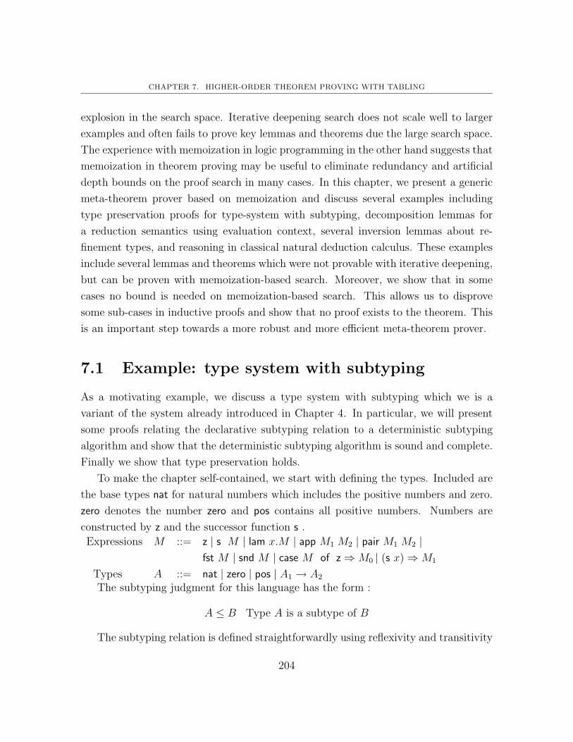
CHAPTER 7. HIGHER-ORDER THEOREM PROVING WITH TABLING
explosion in the search space. Iterative deepening search does not scale well to larger
examples and often fails to prove key lemmas and theorems due the large search space.
The experience with memoization in logic programming in the other hand suggests that
memoization in theorem proving may be useful to eliminate redundancy and artificial
depth bounds on the proof search in many cases. In this chapter, we present a generic
meta-theorem prover based on memoization and discuss several examples including
type preservation proofs for type-system with subtyping, decomposition lemmas for
a reduction semantics using evaluation context, several inversion lemmas about re-
finement types, and reasoning in classical natural deduction calculus. These examples
include several lemmas and theorems which were not provable with iterative deepening,
but can be proven with memoization-based search. Moreover, we show that in some
cases no bound is needed on memoization-based search. This allows us to disprove
some sub-cases in inductive proofs and show that no proof exists to the theorem. This
is an important step towards a more robust and more efficient meta-theorem prover.
7.1 Example: type system with subtyping
As a motivating example, we discuss a type system with subtyping which we is a
variant of the system already introduced in Chapter 4. In particular, we will present
some proofs relating the declarative subtyping relation to a deterministic subtyping
algorithm and show that the deterministic subtyping algorithm is sound and complete.
Finally we show that type preservation holds.
To make the chapter self-contained, we start with defining the types. Included are
the base types nat for natural numbers which includes the positive numbers and zero.
zero denotes the number zero and pos contains all positive numbers. Numbers are
constructed by z and the successor function s .
Expressions M ::= z | s M | lam x.M | app M1 M2 | pair M1 M2 |fst M | snd M | case M of z⇒M0 | (s x)⇒M1
Types A ::= nat | zero | pos | A1 → A2
The subtyping judgment for this language has the form :
A ≤ B Type A is a subtype of B
The subtyping relation is defined straightforwardly using reflexivity and transitivity
204

7.1. EXAMPLE: TYPE SYSTEM WITH SUBTYPING
by the following rules
A ≤ AA1 ≤ A2 A2 ≤ A3
A1 ≤ A3
pos ≤ nat zero ≤ nat
A1 ≤ B1 A2 ≤ B2
A1 ∗ A2 ≤ B1 ∗B2
B1 ≤ A1 A2 ≤ B2
A1 → A2 ≤ B1 → B2
Next, we give the typing judgment and the evaluation judgment:
Γ `M : A Term M has type A in context Γ
M → V Term M evaluates to value V
Typing rules
Γ `M : A′ A′ ≤ AΓ `M : A
Γ ` z : nat Γ ` z : zeroΓ `M : nat
Γ ` s M : natΓ `M : nat
Γ ` s M : pos
Γ `M : nat Γ `M1 : A Γ, x:nat `M2 : A
Γ ` case M of z⇒M1 | (s x)⇒M2 : A
Γ `M : zero Γ `M1 : A
Γ ` case M of z⇒M1 | (s x)⇒M2 : A
Γ `M : pos Γ, x:nat `M2 : A
Γ ` case M of z⇒M1 | (s x)⇒M2 : A
Γ `M1 : A1 Γ `M2 : A2
Γ ` pair M1 M2 : (A1 ∗ A2)
Γ `M : (A1 ∗ A2)
Γ ` fst M : A1
Γ `M : (A1 ∗ A2)
Γ ` snd M : A2
Γ, x:A1 `M : A2
Γ ` lam x.M : (A1 → A2)
Γ `M1 : (A2 → A) Γ `M2 : A2
Γ ` app M1 M2 : A
z → zM → V
s M → s V
Evaluation rules
M →M ′ N → N ′
pair M N → pair M ′ N ′M → pair V1V2
fst M → V1
M → pair V1V2
snd M → V2
205

CHAPTER 7. HIGHER-ORDER THEOREM PROVING WITH TABLING
M → z M1 → V1
case M of z⇒M1 | (s x)⇒M2 → V1
M → (s V2) [V2/x]M2 → V2
case M of z⇒M1 | (s x)⇒M2 → V2
lam x.M → lam x.M
M1 → lam x.M ′ M2 → V2 [V2/x]M ′
app M1 M2 → V
The following substitution principle holds:
Lemma 87 (Substitution principle)
If Γ, x:A `M : B and Γ ` N : A then Γ ` [N/x]M : B.
Proof: Induction on the first derivation. 2
The subtyping rules above do not immediately yield an algorithm for deciding
subtyping. Thus we will present an algorithmic subtyping judgment and show that it
is equivalent to the one above.
AB Type A is a subtype of B
nat nat pos pos zero zero
zero nat pos nat
A1 B1 A2 B2
(A1 ∗ A2) (B1 ∗B2)
B1 A1 A2 B2
(A1 → A2) (B1 → B2)
Theorem 88 (Admissibility of reflexivity)
For any type A, there exists a derivation A A.
Proof: Structural induction on A. 2
Theorem 89 (Admissibility of transitivity)
If D1 : AB and D2 : B C then E : A C.
206

7.1. EXAMPLE: TYPE SYSTEM WITH SUBTYPING
Proof: The size of a judgment A B is determined by the size of A plus the size of
B. Induction on the size of the judgment1. 2
Theorem 90 (Soundness and completeness of algorithmic subtyping)
1. If E : A1 A2 then D : A1 ≤ A2
2. If D : A1 ≤ A2 then E : A1 A2
Proof: Soundness: Proof by structural induction on E .
Completeness: Proof by structural induction on D referring to reflexivity and transi-
tivity lemma. 2
To prove type preservation, we need a couple of inversion lemmas.
Theorem 91 (Inversion)
1. If Γ ` z : A and A pos then this is a contradiction.
2. If Γ ` s M : A and A pos then Γ `M : nat.
3. If Γ ` s M : A and A nat then Γ `M : nat.
4. If Γ ` s M : A and A zero then this is a contradiction.
5. If Γ ` lam x.M : A and A (A1 → A2) then Γ, x:A1 `M : A2.
6. If Γ ` pair M1 M2 : A and A (A1 ∗ A2) then Γ `M1 : A2 and Γ `M2 : A2.
Proof: All the proofs follow by structural induction on the first derivation. 2
Theorem 92 (Type preservation)
If D : Γ `M : A and E : M → V then Γ ` V : A.
1Because of the contra-variance of types in the subtyping rule for function types, the inductionordering is a little tricky. In Twelf, we use a trick to handle this induction. We use simultaneousinduction on D1 and D2 and define a second copy of the transitivity relation to handle the contra-variance case, by a structural nested induction on D1 and D2.
207

CHAPTER 7. HIGHER-ORDER THEOREM PROVING WITH TABLING
Proof: Structural lexicographic induction on D and E using the previously proven
lemmas. We only show a few cases here to illustrate the overall structure of the proof.
Case D =
D1
Γ `M : BD2
Γ ` B ≤ A
Γ `M : A
M → V by assumption
Γ ` V : B by induction hypothesis
Γ ` V : A by tp sub
Case D =
D1
Γ `M1 : (A→ B)D2
Γ `M2 : A
Γ ` (app M1 M2) : B
app M1 M2 → V by assumption
M1 → (λx.M ′) and M2 → V2 and [V2/x]M ′ → V by inversion
Γ ` V2 : A by induction hypothesis
Γ ` λx.M ′ : (A→ B) by induction hypothesis
Γ, x:A `M ′ : B by inversion lemma
Γ ` [V2/x]M ′ : B by substitution lemma
Γ ` V : B by induction hypothesis
Case D =
D1
Γ `M : (A ∗B)
Γ ` (fst M) : A
fst M → V1 by assumption
M → (pair V1 V2) by inversion
Γ ` (pair V1 V2) : (A ∗B) by induction hypothesis
Γ ` V1 : A by inversion lemma
2
The proofs are straightforward by hand. We distinguish cases on the derivations (or
on the type), reason by induction hypothesis, and apply lemmas or rules of inference
to deduce the correct conclusion. On the other hand, these proofs, in particular the
final type preservation theorem, are quite challenging for an automated meta-theorem
prover.
208

7.2. TWELF: META-THEOREM PROVER
7.2 Twelf: meta-theorem prover
In previous chapters, we outlined how to implement the previous type-system in Twelf
as a higher-order logic program and discussed how to execute. In this chapter, we are
interested in automating the reasoning with and about deductive systems. Examples of
such meta-reasoning are the admissibility lemmas and the equivalence theorem about
the refinement type systems in the previous section. We also refer to these properties
as meta-theorems.
Schurmann showed in his Ph.D. thesis [63] that it is possible to reconcile higher-
order abstract syntax and inductive reasoning in theory and even automate the induc-
tive reasoning in practice. The theoretical development is complex, and we refer the
interested reader to [63, 64]. In this section, we review the design and implementation
of the inductive meta-theorem prover. Closely following the informal proof above, the
meta-theorem prover has three main operations it iterates over. Case analysis (reason-
ing by inversion), computing instances of the induction hypothesis, proof search where
we directly prove the current conclusion from the current proof assumptions and the
rules of inference. Proof assumptions are either instances of the induction hypothe-
sis or other assumptions generated applying case analysis, and assumptions from the
statement of the theorem. Note that generating instances of the induction hypothesis
is separated from proof search itself and added to the set of proof assumptions. During
proof search, induction hypotheses are treated as any other proof assumptions.
The design reflects the three key operations in the informal proof: analyzing cases,
generating instances of the induction hypothesis, and deriving a proof for using infer-
ence rules and proof assumptions. The overall meta-theorem prover simply iterates
over all the three operations, until a proof for all open cases has been found. It is
important to point out, that the meta-theorem prover can only make progress in the
proof, once proof search has failed to show that the conclusion is derivable from the cur-
rent proof assumptions. This is the pre-requisite to splitting a conjecture into different
cases. Hence quick failure is essential to the overall performance of the meta-theorem
prover.
Consider the proof for type preservation given earlier. First the meta-theorem
prover will try to show that F : Γ ` v : a is derivable from the rules of inference, the
lemmas and the assumptions D : Γ ` m : a and E : m → v. We write small letters v, m,
209

CHAPTER 7. HIGHER-ORDER THEOREM PROVING WITH TABLING
Induction hypothesis generation
program clauseslemmasproof assumptionsinduction hypotheses
induction hypothesis
proof assumptions
Case Splitting
Proof search based on logic programming
depth
Figure 7.1: Design of the induction meta-theorem prover
a to indicate these variables are universal and are treated like constants. If direct proof
search fails, then we split the conjecture into different cases. There are two possibilities:
case analysis on E : m → v and D : Γ ` m : a. Using heuristics, the meta-theorem
prover chooses to split on the typing derivation D : Γ ` m : a. Applying inversion on
the subtyping rule, this leads to the new proof assumptions Γ ` m : a′ and a′ ≤ a.
Next, we generate Γ ` v : a′ which is an instance of the induction hypothesis. Finally,
using all these assumptions, we search for a proof of Γ ` v : a. We can establish a
proof for it, but using the proof assumption a′ ≤ a, the induction hypothesis Γ ` v : a′
and the subtyping rule.
To complete the proof, we need to consider the remaining 12 cases for typing rules.
As the example illustrate, generic proof search plays an important role in establish-
ing a proof for type preservation automatically. It is first used to show that no proof
210

7.2. TWELF: META-THEOREM PROVER
exists for the original statement F : Γ ` v : a, which is a prerequisite for applying
case-analysis. Second, it is used to close the proof in each of the cases after induction
hypotheses are generated.
Schurmann adopted in his Ph.D. thesis the simplest solution possible for searching
for a proof given a set of assumptions. In principle, we can just use the proof search pro-
cedure of the logic programming interpreter to search for a proof. The main drawback
of the depth-first search strategy used in the logic programming is that it is incomplete
and may get stuck in a branch, and never consider other more fruitful branches in
the proof tree. Therefore, the approach taken in [63] is to replace the incomplete and
unfair depth-first proof search strategy of the logic programming interpreter with the
fair bounded iterative deepening proof search. This means proof search will still be
incomplete, but at least we can switch to other potentially more fruitful branches in
the proof tree, once we have reached the bound. Although this seems to work well
in many examples, it has several shortcomings: First, the user has to specify a depth
bound. This has two consequences. If a proof does not exist within the given bound,
then the user does not know whether the stated conjecture is unprovable or the bound
was set to low. As a result, failure is not meaningful in this setting making the task of
developing formal systems and proofs about them frustrating. Second, there may be
redundancy in the proof search hampering the overall performance. Note that quick
failure is essential in the overall design of the meta-theorem prover, to make progress
and split the conjecture in different cases. Let us briefly consider the previous example
for type preservation proof again. Before we can split the conjecture into different
cases, we need to show that F : Γ ` v : a is not derivable from the current proof
assumptions D : Γ ` m : a and E : m → v, inference rules and lemmas. One of the
inversion lemmas and the subtyping rule are applicable and can be used in the first
step. This can quickly lead to an explosion in the search space. In practice this means
iterative deepening gets bogged down in the very first step and cannot make progress,
thereby failing to establish an inductive proof for type preservation.
Third, iterative deepening search can be quite fragile. The order in which the
inference rules are implemented matters a lot and proving lemmas and adding them to
the database of known facts may have drastic effects on how well proof search performs.
While it is reasonable to ask the user to carefully implement the typing rules, the user
has little control over the use of lemmas and other proof assumptions.
211

CHAPTER 7. HIGHER-ORDER THEOREM PROVING WITH TABLING
In this chapter we propose memoization-based search as an alternative to iterative
deepening. Memoization-based search terminates for programs over a finite domain.
For those programs where memoization-based search may not terminate, the user still
has to give a bound, within which the memoization-based search procedure will try
to find a proof or establish that no proof exists. Experiments show that handling
redundancy is critical to prove meta-theorems like the ones above leading to a more
efficient and more powerful meta-theorem prover.
7.3 Generic proof search based on memoization
Memoization-based proof search is based on the tabled uniform proof system given
in Chapter 4. Although the underlying ideas and large parts of the implementation
are shared between tabled higher-order logic interpreter and the memoization-based
higher-order proof search, there are a few key difference: 1) In logic programming,
it is important to maintain an easy to understand and clearly defined operational
semantics. The programmer can then exploit this semantics when writing programs.
For this reason, the programmer may find an unfair but easy to understand strategy
preferable in logic programming. In theorem proving, we want to know if a proof exists
and an unfair search strategy is unacceptable, since it may prevent us from finding
a proof. Since memoization-based proof search does not terminate in all cases, we
cannot eliminate bounds completely. The search procedure will let the user know, if
the search was not completed within this bound. However, as we will show in many
cases the search is complete thereby providing valuable feedback for the user and quick
failure. 2) In logic programming we have a fixed set of program clauses, over which
the programmer has control. On the other hand in meta-theorem proving, we have
additional proof assumptions such as induction hypotheses and lemmas, which are
generated during proof search, and over which the programmer has no control. This
makes the problem of search for a proof harder.
Overall, we have taken a very conservative approach of adding memoization to the
meta-theorem prover. We only replace iterative deepening search procedure with the
new memoization-based search. However after the memoization-based search fails or
succeeds, we clear the memo-table. A more aggressive approach could be to have the
212

7.4. EXPERIMENTS
memo-table survive across iterations. We mainly focus on using variance checking in
the memoization-based search. The main reason has been to minimize the overhead of
maintaining two very different implementations, one for the interpreter and one for the
meta-theorem prover. However, we will show using proofs about refinement types that
unlike higher-order logic programming the use of subsumption can be very valuable in
meta-theorem proving.
We also discuss some of differences of iterative deepening search and memoization-
based search. (1) Iterative deepening means, we first try to find a proof for depth 1
with depth-first search, then we try to find a proof of depth 2 with depth-first search
etc. If the branch is deeper than k, then we fail and backtrack. This means if there
exists a proof with depth k, we may have explored the left-most branches in the search
tree up to depth k. Obviously, if proof search fails, then we have to explore the whole
search space. (2) Memoization-based search bounded by n: we traverse the search
space using depth-first search and memoization. if we explore a branch with depth
greater than n we fail and backtrack. This means although we only needed depth k,
where k is smaller than n, we explored fruitless branches up to depth n. As a result,
it potentially may take longer to find solutions to some problems.
7.4 Experiments
We have carried out several experiments so far, including a refinement type system
(soundness and completeness of algorithmic subtyping algorithm), type-system with
subtyping (soundness and completeness of algorithmic subtyping and type preserva-
tion) and theorem proving in classical natural deduction. The meta-theorems were not
previously provable with the iterative deepening proof search, thereby demonstrating
that memoization-based search leads to a more powerful meta-theorem prover. In ad-
dition, we give some examples which were provable with iterative deepening with a
bound, and can be proven without a bound using memoization-based search.
7.4.1 Type preservation for type system with subtyping
First, we consider the proofs about the type-system with subtyping given earlier. The
proofs themselves are not hard, but the number of applicable lemmas increases the
213

CHAPTER 7. HIGHER-ORDER THEOREM PROVING WITH TABLING
search space as we continue. Lemmas are turned into logic programming clauses which
can be used during proof search. For example, the lemma
If Γ ` s M : A and A pos then Γ `M : nat.
will be turned into the clauseinvNat : of M nat
<- of (s M) A
<- A <| pos
From a logic programming view, this clause may lead to an explosion in search space.
Therefore we see that iterative deepening proof search deteriorates if we continue and
prove more lemmas about the type-system. Figure 7.2 gives the run-time for proving
all the lemmas and theorems needed in the type preservation proof. We did not include
any speed-ups in this table since many numbers are very small and for those the speed-
up is not very meaningful.
theorem tabled iterative deep
refl 0.18 0.00
trans 0.29 0.02
sound 0.19 0.01
comp 0.21 0.02
imposAll 0.04 0.00
inv+z+pos 0.08 0.00
inv+suc+pos 0.08 0.00
inv+suc+nat 0.09 0.23
inv+suc+zero 0.10 0.93
inv+lam 0.21 7.27
inv+pair 0.18 ∞tps 2.89 –
Figure 7.2: Type preservation for system with subtyping
The memoization-based meta-theorem prover has some overhead in managing the
table which leads to slight deterioration in the first few examples. However, in the inver-
sion lemma for functions memoization starts paying off and the proof for the inversion
214

7.4. EXPERIMENTS
lemma for pairs cannot be found by iterative deepening search within a reasonable
amount of time. The main benefits of memoization are not in quickly finding a proof
for a sub-case in the proof, but rather in quickly failing, i.e. in showing no proof exists
from the current proof assumptions, and therefore triggering a case split. The proof of
the inversion lemma for functions for example has between 37 and 67 suspended goals.
The proof of type preservation has between 31 and over 70 suspended goals. All these
loops were detected when proving that it is not possible to derive the conclusion from
the current set of assumptions. Hence, the overall performance improvement is mainly
due to quick failure which allows the theorem prover to make progress. As a result, we
succeed in proving all the lemmas including the final type preservation theorem using
the memoization-based prover. The iterative deepening prover gets stuck during the
proof for the inversion lemma for pairs. Even if we add the inversion lemma for pairs
without a proof to the set of lemmas, the iterative deepening prover does not succeed
in proving type preservation.
7.4.2 Derived rules of inference in classical natural deduction
Next, we show some experiments using classical natural deduction. Proof search in
natural deduction calculi is considered hard. Memoization can lead to quicker proofs
in some examples, while imposing a some performance penalty in others. In Table 7.3,
we give the run-times for proving several derived rules. These examples do not require
induction.
theorem tabled search depth-first-bounded iterative deepening
split’ 9.20 0.19 0.29
join’ 9.18 1.68 1.69
assoc 20.14 450.53 451.49
uncurry 33.45 450.97 452.42
Figure 7.3: Derived rules of inference in NK (classical natural deduction with not, imp,
and, double negation rule)
215
CHAPTER 7. HIGHER-ORDER THEOREM PROVING WITH TABLING
7.4.3 Refinement types
In this sections we used the memoization-based prover to proof all the lemmas leading
up to the type preservation theorem. We use an implementation of the type system for
refinement types by Pfenning [17]. For proving these statements, we used subsumption-
based memoization. It is important to note, that this example clearly demonstrates the
use of subsumption, since with variant-based memoization we still cannot find some
proofs. Subsumption is critical to detect quickly that no proof exists and we need
to split the conjecture into different cases. It also is critical to complete some of the
sub-proofs2.
Iterative deepening works fine for the first few proofs. In fact, its performance is
better than memoization-based proof search. However, it cannot prove the inversion
lemmas. Attempting the proof for the inversion lemma for functions, iterative deep-
ening cannot find a proof within a reasonable amount of time. When skipping the
inversion lemma for functions, we are able to make some more progress by proving the
two impossibility lemma, but we get again stuck when proving the lemma imp+1+zero.
Some of the lemmas, we are able to prove individually. However, this is unsatisfactory
for developing the meta-proofs about the refinement types.
Using subsumption-based memoization, we detected over 100 loops when proving
inversion lemmas. Similar to the subtyping example, memoization was most valuable
for detecting that the current proof assumptions do not suffice to derive the conclusion.
7.4.4 Rewriting semantics
Next, we give two examples which were provable before but did require a bound. In
fact, the user has to choose the minimal bound in order to get the meta-theorem
prover to prove these theorems. With memoization, no bounds are required. This is
especially important if we want to disprove conjectures and debug implementations
and proofs about them. We first consider a rewriting semantic with weak congruence
closure and show that any big-step evaluation has a sequence of rewriting steps in
the reduction semantic (evalRed theorem). Next, we try to prove that any rewriting
sequence has a corresponding big-step evaluation (RedEval theorem). However, this
2run-times for variant-based memoization to be added
216

7.4. EXPERIMENTS
theorem tabled search (subsumption) iterative deepening
lemma1 3.72 0.08
refl 0.21 0.00
trans 1.63 0.02
comp¡— 1.81 0.01
sound¡— 0.41 0.01
inv+lam 0.36 –
impossAll 0.020 –
impRV 0.140 –
imp+e+pos 0.220 –
imp+1+zero 0.260 –
imp+0+zero 0.28 –
inv+e+bits 0.080 –
inv+e+nat 0.08 –
inv+1+bits 0.450 –
inv+0+bits 0.500 –
inv+0+nat 0.520 –
inv+1+nat 0.510 –
inv+0+pos 0.510 –
inv+1+pos 0.490 –
conjLemma 0.110 –
Figure 7.4: Refinement type checking [17]
217

CHAPTER 7. HIGHER-ORDER THEOREM PROVING WITH TABLING
is in fact not true the way the rewrite rules are stated, since we not always will get
back a value. Memoization-based search will return and say that no proof is possible.
This in turn is valuable to analyze the specification and potentially change it. Finally,
we include a type preservation theorem about the reduction semantics. Run-times for
the memoization-based prover are slightly worse than the iterative deepening prover.
However, we get a more expressive prover which doesn’t require bounds.
theorem tabled search iterative deepening
evalRed (sound) 0.37sec 0.01sec
RedEval (complete) 9.88sec –
typeRed 0.93sec 0.01sec
Figure 7.5: Proofs about the rewrite semantics vs big-step evaluation semantics
Similarly, for the proofs about Mini-ml we observe that the theorems fall into the
complete fragment, and the theorem prover does not require any bounds. Again we
include the proofs about the original specification and contrast it with slightly modified
specification where the proofs about type preservation and value soundness fail.
theorem tabled search iterative deepening
val-sound 0.33sec 0.32sec
tp-preseve 0.53sec 0.01sec
tp-preserve (mod) 1.18sec –
Figure 7.6: Proofs about big-step evaluation semantics, type preservation, value sound-
ness, mini-ml
7.5 Conclusion
Redundancy elimination is critical to reason with and about non-trivial deductive sys-
tems. We have shown that memoization-based search can be smoothly integrated into
the meta-theorem prover. This allows us to prove more complicated theorems which
218

7.5. CONCLUSION
rely on several lemmas. From our experience, the better failure behavior is particularly
useful in developing and debugging specifications and theorems. In addition, it leads
to a substantial improvement of the overall performance of the meta-theorem prover.
As we are able to fail quicker, we are able to make progress faster.
However, the conservative memoization-based search also has some limitations,
which we plan to address in the future. In particular the proofs about refinement
types illustrate that subsumption based memoization is useful in theorem proving. As
we mentioned earlier, we have only an incomplete subsumption-based memoization
strategy in the current implementation, to minimize the effort required to maintain
different implementations for variant- and subsumption-based memoization. In the
long run, it seems interesting to develop a complete subsumption-based memoization
proof search procedure for the meta-theorem prover.
219

CHAPTER 7. HIGHER-ORDER THEOREM PROVING WITH TABLING
220

Chapter 8
Conclusion
In this thesis, we develop different techniques to efficiently execute and reason with and
about deductive systems. We have shown that memoization as a form of redundancy
elimination is a useful extension to the higher-order logic programing interpreter. It
allows us to execute more examples and have better and more meaningful failure. It
also plays an important role in the meta-theorem prover. To achieve good performance
of memoization-based search, we have developed higher-order term indexing techniques
and an optimized higher-order pattern unification algorithm, which eliminates many
unnecessary occurs checks. Taken together the presented techniques constitute a sig-
nificant step toward exploring the full potential of logical frameworks in real-world
applications where deductive systems and proofs about them may be more complex.
Future Work
Applications: Typed Assembly Language
Recently, Twelf has been used in developing a foundational approach for typed as-
sembly language [14, 15]. This approach is similar to the foundational proof-carrying
code project [2] in the sense that we try to minimize the trusted computing base. In
particular, we do not need to trust the safety policy, but the safety policy is proven
sound. While in the foundational proof-carrying code approach higher-order logic to-
gether with some axioms about arithmetic is used as a foundation to define safety
221

CHAPTER 8. CONCLUSION
policies, the logical framework LF itself serves as the foundation for implementing dif-
ferent safety policies. In addition to the safety policy, described by a type system,
all the meta-proofs required to prove soundness are implemented in Twelf. However,
so far Twelf has been mainly used as a specification framework and not fully uti-
lized the expressiveness and power of execution and reasoning strategies. There are
many applications of the described work to the foundational typed assembly language
project. First, it seems interesting to experiment and generate safety certificates for
sample programs using Twelf’s logic programming interpreter. Second, it would be
interesting to investigate if some of the meta-theorems about the safety policy can be
proven automatically using the memoization-based meta-theorem prover. Third, we
can instrument Twelf’s higher-order logic programming interpreter to produce a bit-
string that encodes the non-deterministic choices in a proof and use memoization to
factor out common subproofs. This extends prior work by Necula and Rahul [42] to
full LF. Moreover, preliminary experiments demonstrate that memoization can lead to
bit-string which are up to 40% smaller in size than their counterparts produced without
memoization.
Eliminating further redundant typing information
There is still some redundancy in proof search which is due to dependent types. De-
pendent type information needs to be carried around during proof search imposing a
substantial overhead [33]. Necula and Lee [43] have investigated the problem of redun-
dant type information in the context of type-checking. They propose a more efficient
term representation for a fragment of LF which eliminates a lot of the redundant typing
information thereby minimizing the amount of information we need to keep for type-
checking. One direction is to extend Necula and Lee’s work to full LF type theory,
thereby eliminating further redundancy. Moreover, it may be used to not only improve
the performance of type-checking in Twelf, but also of proof search itself.
Completeness of memoization-based proof search
In this thesis, we have mainly focused on proving soundness of memoization-based proof
search. Completeness of memoization-based proof search is harder to establish. The
222

main reason is that we will find fewer proofs than with uniform proofs. For example
in the subtyping example given in Sec. 4.1 the query sub zero zero has infinitely many
proofs under the traditional logic programming interpretation while we find only one
proof under the tabled logic programming interpretation. However, we often do not
want or need to distinguish between different proofs for a formulaA, but only care about
the existence of a proof for A together with a proof term. In [50] Pfenning develops
a dependent type theory for proof irrelevance and discusses potential applications in
the logical framework. This could allow us to treat all proofs for A as equal if they
produce the same answer substitution. In this setting, it seems possible to show that
search based on tabled uniform proofs is complete, i.e. if there is a (canonical) proof
M : A then we can find A.
Optimizations for memoization-based search
Re-use of answers
Memoization-based search is critically influenced by when we retrieve answers and when
we suspend goals and when and in what order we awaken suspended goals. Currently,
we have implemented multi-stage depth-first strategy. As we have discussed in Chapter
4, this strategy might delay the re-use of answers, since we are not allowed to retrieve
answers from the current stage. The XSB system therefore uses a strategy based on
strongly connected components, which allows us to consume answers as soon as they are
available. We build a dependency graph of the predicates and identify different inde-
pendent sub-graphs, called strongly connected components. This dependency analysis
separates subgoals that can and cannot influence each other. If computation for all
the subgoals within a sub-graph is saturated, then we can dispose all the suspended
sub-goal belonging to this component. As we are able to delete suspended nodes that
cannot contribute to new solutions anymore, this leads to fewer suspended nodes and
has the potential to be more space and time efficient. This might be advantageous es-
pecially in theorem proving, where we only care about one answer to the query and are
not interested in mimicking Prolog execution. In LF, subordination analysis provides
information about dependencies of predicates and constructs a subordination graph.
Analyzing and exploiting the subordination information, it seems possible to design
223

CHAPTER 8. CONCLUSION
similar strategies as in XSB which allow the re-use of answers as soon as they are
available and detect when all answers have been generated.
Subsumption
As some of the experiments in Chapter 7 suggest, the use of subsumption-based mem-
oization in proof search is useful in meta-theorem proving. As we have also mentioned
in Chapter 7, so far the implementation of subsumption is a conservative extension of
the variant-based memoization proof search and may be incomplete. In the future, it
seems fruitful to develop a complete subsumption-based proof search procedure for the
meta-theorem prover.
High-level optimizations to proof search
Although memoization-based computation aims to make reasoning within logical speci-
fication efficient, it cannot rival the performance of a theorem prover that is specifically
built for a given logic. One reason is that specialized state-of-the-art theorem provers
exploit properties of the theory they are built for. For example, inverse method theorem
provers for first-order logic like Gandalf [66] exploit the subformula property. Other
theorem provers like Spass [69], which are very successful in equational reasoning, rely
on orderings to restrict the search. These meta-level optimizations can improve per-
formance of higher-order logic programming dramatically. Therefore, one interesting
path to explore is to verify such properties about logical specifications in advance and
exploit them during search.
Modal dependent type theory
In Chapter 2, we have conservatively extended the LF type theory with modal variables
and shown that canonical forms exist and type-checking remains decidable. As we
have briefly discussed in Chapter 2, there are two simple and clean ways to incorporate
such variables. One is via a general modal operator 2Ψ, and the other is via a new
quantifier Π2u::(Ψ`A1). A2. The main complication with the general modal operator
is that canonical forms do not exist. In this thesis, we suggested the use of Π2 to
quantify over modal variables explicitely, but we have not fully extended the LF type
224

theory. In the future, it seems interesting to develop the theory further towards a modal
dependent type theory. The Π2-abstraction and the 2-application is less powerful than
the general box-operator. We conjecture that canonical forms exist for this fragment
and type-checking remains decidable.
In Chapter 3, we have briefly mentioned an extension which allows us to quantify
directly over variable definitions using Π2u = M ::(Ψ`A). This would have two main
advantages: First, we would be able to type-check linearized objects L directly. This
avoids translating variable definitions into a modal substitution θ and the type-checking
[[θ]]L. Second, it would allow us to describe proof terms as directed-acyclic graph and
type-check them directly.
Linear logic programming
Linear logic programming [30, 8] has been proposed as an extension of higher-order
logic programming to model imperative state changes in a declarative (logical) way. We
believe that the some of the techniques presented in this thesis can be extended to linear
logic programming, but it requires some new considerations. In particular, we plan to
investigate the use of memoization in linear higher-order logic programming. This
requires new consdiderations concerning the interaction between resource management
strategies [10] or constraints [27] with tabling. However, the approach presented seems
general and amenable also to the linear case.
225

CHAPTER 8. CONCLUSION
226

Bibliography
[1] Martın Abadi, Luca Cardelli, Pierre-Louis Curien, and Jean-Jacques Levy. Ex-
plicit substitutions. In Conference Record of the Seventeenth Annual ACM Sympo-
sium on Principles of Programming Languages, San Francisco, California, pages
31–46. ACM, 1990.
[2] Andrew Appel. Foundational proof-carrying code. In J. Halpern, editor, Pro-
ceedings of the 16th Annual Symposium on Logic in Computer Science (LICS’01),
pages 247–256. IEEE Computer Society Press, June 2001. Invited Talk.
[3] W. Appel and Amy P. Felty. A semantic model of types and machine instruc-
tions for proof-carrying code. In 27th ACM SIGPLAN-SIGACT Symposium on
Principles of Programming Languages (POPL ’00), pages 243–253, Jan. 2000.
[4] Andrew Bernard and Peter Lee. Temporal logic for proof-carrying code. In Pro-
ceedings of the 18th International Conference on Automated Deduction (CADE-
18), volume 2392 of Lecture Notes in Artificial Intelligence, pages 31–46, Copen-
hagen, Denmark, July 2002.
[5] Egon Borger and Dean Rosenzweig. The WAM – definition and compiler correct-
ness. In C. Beierle and L. Plumer, editors, Logic Programming: Formal Methods
and Proactical Applications, pages 1–71. Elsevier Science Publishers B.V., 1994.
[6] Pascal Brisset and Olivier Ridoux. Naive reverse can be linear. In Koichi Furukawa,
editor, International Conference on Logic Programming, pages 857–870, Paris,
France, June 1991. MIT Press.
[7] M. Carlson. On implementing Prolog in functional programming. New Generation
Computin, 2(4):347–357, 1984.
227

BIBLIOGRAPHY
[8] Iliano Cervesato. A Linear Logical Framework. PhD thesis, Dipartimento di
Informatica, Universita di Torino, February 1996.
[9] Iliano Cervesato. Proof-theoretic foundation of compilation in logic programming
languages. In J. Jaffar, editor, Proceedings of the 1998 Joint International Con-
ference and Symposium on Logic Programming — JICSLP’98, pages 115–129,
Manchester, UK, 16–19 June 1998. MIT Press.
[10] Iliano Cervesato, Joshua S. Hodas, and Frank Pfenning. Efficient resource man-
agement for linear logic proof search. Theoretical Computer Science, 232(1–2):133–
163, February 2000.
[11] Iliano Cervesato and Frank Pfenning. A linear spine calculus. Technical Report
CMU-CS-97-125, Department of Computer Science, Carnegie Mellon University,
April 1997.
[12] W. Chen and D. S. Warren. Tabled evaluation with delaying for general logic
programs. Journal of the ACM, 43(1):20–74, January 1996.
[13] Weidong Chen, Michael Kifer, and David Scott Warren. HILOG: A foundation for
higher-order logic programming. Journal of Logic Programming, 15(3):187–230,
1993.
[14] Karl Crary. Toward a foundational typed assembly language. In 30th ACM Sym-
posiumn on Principles of Programming Languages (POPL), pages 198–212, New
Orleans, Louisisana, January 2003. ACM-Press.
[15] Karl Crary and Susmit Sarkar. Foundational certified code in a metalogical frame-
work. In 19th International Conference on Automated Deduction, Miami, Florida,
USA, 2003. Extended version published as CMU technical report CMU-CS-03-108.
[16] B. Cui, Y. Dong, X. Du, K. N. Kumar, C.R. Ramakrishnan, I.V. Ramakrish-
nan, A. Roychoudhury, S.A. Smolka, and D.S. Warren. Logic programming and
model checking. In Catuscia Palamidessi, Hugh Glaser, and Karl Meinke, editors,
International Symposium on Programming Language Implementation and Logic
Programming (PLILP’98), volume 1490 of Lecture Notes in Computer Science,
pages 1–20. Springer-Verlag, 1998.
228

BIBLIOGRAPHY
[17] Rowan Davies and Frank Pfenning. Intersection types and computational effects.
In Proceedings of the International Conference on Functional Programming (ICFP
2000), Montreal, Canada, pages 198–208. ACM Press, 2000.
[18] Steve Dawson, C. R. Ramakrishnan, Steve Skiena, and Terrance Swift. Princi-
ples and practice of unification factoring. ACM Transactions on Programming
Languages and Systems, 18(6):528–563, 1995.
[19] Bart Demoen and Konstantinos Sagonas. CAT: The copying approach to tabling.
In Catuscia Palamidessi, Hugh Glaser, and Karl Meinke, editors, International
Symposium on Programming Language Implementation and Logic Programming
(PLILP’98), Lecture Notes in Computer Science (LNCS), vol. 1490, pages 21–36,
1998.
[20] Bart Demoen and Konstantinos Sagonas. CAT: The copying approach to tabling.
Journal of Functional and Logic Programming, 2:1–38, 1999.
[21] Bart Demoen and Konstantinos Sagonas. CHAT: The copy-hybrid approach to
tabling. In The First International Workshop on Practical Aspects of Declarative
Languages, Lecture Notes in Computer Science (LNCS), vol. 1551, pages 106–121,
San Antonio, January 1999. Springer.
[22] Gilles Dowek, Therese Hardin, Claude Kirchner, and Frank Pfenning. Unification
via explicit substitutions: The case of higher-order patterns. In M. Maher, edi-
tor, Proceedings of the Joint International Conference and Symposium on Logic
Programming, pages 259–273, Bonn, Germany, September 1996. MIT Press.
[23] Conal Elliott and Frank Pfenning. A semi-functional implementation of a higher-
order logic programming language. In Peter Lee, editor, Topics in Advanced Lan-
guage Implementation, pages 289–325. MIT Press, 1991.
[24] Amy Felty. Implementing tactics and tacticals in a higher-order logic programming
language. Journal of Automated Reasoning, 11(1):43–81, August 1993.
[25] Peter Graf. Substitution tree indexing. In Proceedings of the 6th International
Conference on Rewriting Techniques and Applications, Kaiserslautern, Germany,
229
BIBLIOGRAPHY
Lecture Notes in Computer Science (LNCS) 914, pages 117–131. Springer-Verlag,
1995.
[26] Michael Hanus and Christian Prehofer. Higher-order narrowing with definitional
trees. Journal of Functional Programming, 9(1):33–75, 1999.
[27] James Harland and David Pym. Resource-distribution via boolean constraints.
In W. McCune, editor, Proceedings of the 14th International Conference on Au-
tomated Deduction (CADE-14), pages 222–236, Townsville, Australia, July 1997.
Springer-Verlag LNAI 1249.
[28] Robert Harper, Furio Honsell, and Gordon Plotkin. A framework for defining log-
ics. Journal of the Association for Computing Machinery, 40(1):143–184, January
1993.
[29] Robert Harper and Frank Pfenning. On equivalence and canonical forms in the LF
type theory. Transactions on Computational Logic, 2003. To appear. Preliminary
version available as Technical Report CMU-CS-00-148.
[30] Joshua Hodas and Dale Miller. Logic programming in a fragment of intuitionistic
linear logic. Information and Computation, 110(2):327–365, 1994. A preliminary
version appeared in the Proceedings of the Sixth Annual IEEE Symposium on
Logic in Computer Science, pages 32–42, Amsterdam, The Netherlands, July 1991.
[31] Gerard Huet. A unification algorithm for typed λ-calculus. Theoretical Computer
Science, 1:27–57, 1975.
[32] Lars Klein. Indexing fur Terme hoherer Stufe. Diplomarbeit, FB 14, Universitat
des Saarlandes, Saarbrucken, Germany, 1997.
[33] Spiro Michaylov and Frank Pfenning. An empirical study of the runtime behavior
of higher-order logic programs. In D. Miller, editor, Proceedings of the Work-
shop on the λProlog Programming Language, pages 257–271, Philadelphia, Penn-
sylvania, July 1992. University of Pennsylvania. Available as Technical Report
MS-CIS-92-86.
230

BIBLIOGRAPHY
[34] Dale Miller. Unification of simply typed lambda-terms as logic programming.
In Eighth International Logic Programming Conference, pages 255–269, Paris,
France, June 1991. MIT Press.
[35] Dale Miller. Unification under a mixed prefix. Journal of Symbolic Computation,
14:321–358, 1992.
[36] Dale Miller, Gopalan Nadathur, Frank Pfenning, and Andre Scedrov. Uniform
proofs as a foundation for logic programming. Annals of Pure and Applied Logic,
51:125–157, 1991.
[37] Gopalan Nadathur. A treatment of higher-order features in logic programming.
Technical Report draft, available upon request, Department of Computer Science
and Engineering, University of Minnesota, January 2003.
[38] Gopalan Nadathur, Bharat Jayaraman, and Debra Sue Wilson. Implementation
considerations for higher-order features in logic programming. Technical Report
CS-1993-16, Department of Computer Science, Duke University, June 1993.
[39] Gopalan Nadathur and Dale Miller. An overview of λProlog. In Kenneth A.
Bowen and Robert A. Kowalski, editors, Fifth International Logic Programming
Conference, pages 810–827, Seattle, Washington, August 1988. MIT Press.
[40] Gopalan Nadathur and Dustin J. Mitchell. System description: Teyjus – a compiler
and abstract machine based implementation of Lambda Prolog. In H. Ganzinger,
editor, Proceedings of the 16th International Conference on Automated Deduction
(CADE-16), pages 287–291, Trento, Italy, July 1999. Springer-Verlag LNCS.
[41] Aleksander Nanevski, Brigitte Pientka, and Frank Pfenning. A modal foundation
for meta-variables. In 2nd ACM SIGPLAN Workshop on Mechanized Reason-
ing about Languages with variable binding (Merlin), Uppsala, Sweden, Electronic
Notes in Theoretical Computer Science (ENTCS), 2003.
[42] G. Necula and S. Rahul. Oracle-based checking of untrusted software. In 28th ACM
Symposium on Principles of Programming Languages (POPL’01), pages 142–154,
2001.
231

BIBLIOGRAPHY
[43] George C. Necula and Peter Lee. Efficient representation and validation of logical
proofs. In Vaughan Pratt, editor, Proceedings of the 13th Annual Symposium on
Logic in Computer Science (LICS’98), pages 93–104, Indianapolis, Indiana, June
1998. IEEE Computer Society Press.
[44] George C. Necula and Peter Lee. Safe, untrusted agents using proof-carrying code.
In Giovanni Vigna, editor, Mobile Agents and Security, pages 61–91. Springer-
Verlag LNCS 1419, August 1998.
[45] Lawrence C. Paulson. Natural deduction as higher-order resolution. Journal of
Logic Programming, 3:237–258, 1986.
[46] Lawrence C. Paulson. Isabelle: The next seven hundred theorem provers. In
E. Lusk and R. Overbeek, editors, Proceedings of the 9th International Conference
on Automated Deduction, pages 772–773, Argonne, Illinois, 1988. Springer Verlag
Lecture Notes in Computer Science (LNCS) 310. System abstract.
[47] Frank Pfenning. Elf: A language for logic definition and verified meta-
programming. In Fourth Annual Symposium on Logic in Computer Science, pages
313–322, Pacific Grove, California, June 1989. IEEE Computer Society Press.
[48] Frank Pfenning. Unification and anti-unification in the Calculus of Constructions.
In Sixth Annual IEEE Symposium on Logic in Computer Science, pages 74–85,
Amsterdam, The Netherlands, July 1991.
[49] Frank Pfenning. Computation and deduction, 1997.
[50] Frank Pfenning. Intensionality, extensionality, and proof irrelevance in modal
type theory. In J. Halpern, editor, Proceedings of the 16th Annual Symposium
on Logic in Computer Science (LICS’01), pages 221–230, Boston, Massachusetts,
June 2001. IEEE Computer Society Press.
[51] Frank Pfenning and Rowan Davies. A judgmental reconstruction of modal logic.
Mathematical Structures in Computer Science, 11(4):511–540, 2001.
232

BIBLIOGRAPHY
[52] Frank Pfenning and Conal Elliott. Higher-order abstract syntax. In Proceedings
of the ACM SIGPLAN ’88 Symposium on Language Design and Implementation,
pages 199–208, Atlanta, Georgia, June 1988.
[53] Frank Pfenning and Carsten Schurmann. System description: Twelf — a meta-
logical framework for deductive systems. In H. Ganzinger, editor, Proceedings
of the 16th International Conference on Automated Deduction (CADE-16), pages
202–206, Trento, Italy, July 1999. Springer-Verlag Lecture Notes in Artificial In-
telligence (LNAI) 1632.
[54] Brigitte Pientka. Memoization-based proof search in LF: an experimental evalua-
tion of a prototype. In Third International Workshop on Logical Frameworks and
Meta-Languages (LFM’02), Copenhagen, Denmark, Electronic Notes in Theoret-
ical Computer Science (ENTCS), 2002.
[55] Brigitte Pientka. A proof-theoretic foundation for tabled higher-order logic pro-
gramming. In P. Stuckey, editor, 18th International Conference on Logic Program-
ming, Copenhagen, Denmark, Lecture Notes in Computer Science (LNCS), 2401,
pages 271 –286. Springer-Verlag, 2002.
[56] Brigitte Pientka. Higher-order substitution tree indexing. In C. Palamidessi, edi-
tor, 19th International Conference on Logic Programming, Mumbai, India, Lecture
Notes in Computer Science (LNCS), to appear. Springer-Verlag, 2003.
[57] Brigitte Pientka and Frank Pfennning. Optimizing higher-order pattern unifica-
tion. In F. Baader, editor, 19th International Conference on Automated Deduction,
Miami, USA, Lecture Notes in Artificial Intelligence (LNAI) 2741, pages 473–487.
Springer-Verlag, July 2003.
[58] Jeff Polakow and Frank Pfenning. Ordered linear logic programming. Techni-
cal Report CMU-CS-98-183, Department of Computer Science, Carnegie Mellon
University, December 1998.
[59] I. V. Ramakrishnan, P. Rao, K. Sagonas, T. Swift, and D. Warren. Efficient access
mechanisms for tabled logic programs. Journal of Logic Programming, 38(1):31–
54, Jan 1999.
233

BIBLIOGRAPHY
[60] I. V. Ramakrishnan, R. Sekar, and A. Voronkov. Term indexing. In Alan Robinson
and Andrei Voronkov, editors, Handbook of Automated Reasoning, volume 2, pages
1853–1962. Elsevier Science Publishers B.V., 2001.
[61] Abhik Roychoudhury, C. R. Ramakrishnan, and I. V. Ramakrishnan. Justifying
proofs using memo tables. In International Conference on Principles and Practice
of Declarative Programming(PPDP’00), pages 178–189, 2000.
[62] Konstantinos Sagonas and Terrance Swift. An abstract machine for tabled execu-
tion of fixed-order stratified logic programs. ACM Transactions on Programming
Languages and Systems, 20(3):586–634, 1998.
[63] Carsten Schurmann. Automating the meta theory of deductive systems. PhD
thesis, Department of Computer Sciences, Carnegie Mellon University, Available
as Technical Report CMU-CS-00-146, 2000.
[64] Carsten Schurmann and Frank Pfenning. Automated theorem proving in a simple
meta-logic for LF. In Claude Kirchner and Helene Kirchner, editors, Proceedings
of the 15th International Conference on Automated Deduction (CADE-15), pages
286–300, Lindau, Germany, July 1998. Springer-Verlag Lecture Notes in Computer
Science (LNCS) 1421.
[65] H. Tamaki and T. Sato. OLD resolution with tabulation. In E. .Shapiro, editor,
Proceedings of the 3rd International Conference on Logic Programming, volume
225 of Lecture Notes in Computer Science, pages 84–98. Springer, 1986.
[66] T. Tammet. A resolution theorem prover for intuitionistic logic. In Proceedings
of the 13th International Conference on Automated Deduction, New Brunswick,
NJ, July 1996, volume 1104 of Lecture Notes in Artificial Intelligence, pages 2–16,
1996.
[67] Roberto Virga. Higher-Order Rewriting with Dependent Types. PhD thesis, De-
partment of Mathematical Sciences, Carnegie Mellon University, Available as
Technical Report CMU-CS-99-167, Sep 1999.
[68] David S. Warren. Programming in tabled logic programming. draft available from
http://www.cs.sunysb.edu/warren/xsbbook/book.html, 1999.
234

BIBLIOGRAPHY
[69] C. Weidenbach. Combining superposition, sorts and splitting. In A. Robinson and
A. Voronkov, editors, Handbook of Automated Reasoning, volume II, chapter 27,
pages 1965–2013. Elsevier Science, 2001.
235


