Embed Size (px)
Citation preview

N° 34 – June 2015
Italian Journal of Pure andApplied Mathematics
ISSN 2239-0227
EDITOR-IN-CHIEFPiergiulio Corsini
Editorial BoardSaeid Abbasbandy
Reza AmeriLuisa Arlotti
Krassimir AtanassovMalvina Baica
Federico BartolozziRajabali Borzooei
Carlo CecchiniGui-Yun Chen
Domenico Nico ChillemiStephen Comer
Irina CristeaMohammad Reza Darafsheh
Bal Kishan DassBijan Davvaz
Mario De SalvoAlberto Felice De Toni
Franco EugeniGiovanni Falcone
Yuming FengAntonino Giambruno
Furio Honsell
Luca IseppiJames Jantosciak
Tomas KepkaDavid Kinderlehrer
Andrzej LasotaVioleta Leoreanu-Fotea
Maria Antonietta LepellereMario Marchi
Donatella MariniAngelo MarzolloAntonio Maturo
M. Reza MoghadamSyed Tauseef Mohyud-Din
Petr NemecVasile Oproiu
Livio C. PiccininiGoffredo PieroniFlavio Pressacco
Vito RobertoIvo RosenbergGaetano RussoPaolo Salmon
Maria Scafati TalliniKar Ping ShumAlessandro Silva
Florentin SmarandacheSergio Spagnolo
Stefanos SpartalisHari M. SrivastavaMarzio Strassoldo
Yves SureauCarlo TassoIoan TofanAldo Ventre
Thomas VougiouklisHans Weber
Xiao-Jun YangYunqiang Yin
Mohammad Mehdi ZahediFabio ZanolinPaolo Zellini
Jianming Zhan
F O R U M

EDITOR-IN-CHIEF
Piergiulio Corsini Department of Civil Engineering and Architecture Via delle Scienze 206 - 33100 Udine, Italy [email protected]
VICE-CHIEFS
Violeta LeoreanuMaria Antonietta Lepellere
MANAGING BOARD
Domenico Chillemi, CHIEFPiergiulio CorsiniIrina CristeaAlberto Felice De ToniFurio HonsellVioleta LeoreanuMaria Antonietta LepellereElena MocanuLivio PiccininiFlavio PressaccoNorma Zamparo
EDITORIAL BOARD
Saeid Abbasbandy Dept. of Mathematics, Imam Khomeini International University, Ghazvin, 34149-16818, Iran [email protected]
Reza Ameri Department of Mathematics University of Tehran, Tehran, Iran [email protected]
Luisa Arlotti Department of Civil Engineering and Architecture Via delle Scienze 206 - 33100 Udine, Italy [email protected]
Krassimir Atanassov Centre of Biomedical Engineering, Bulgarian Academy of Science BL 105 Acad. G. Bontchev Str. 1113 Sofia, Bulgaria [email protected]
Malvina Baica University of Wisconsin-Whitewater Dept. of Mathematical and Computer Sciences Whitewater, W.I. 53190, U.S.A. [email protected]
Federico Bartolozzi Dipartimento di Matematica e Applicazioni via Archirafi 34 - 90123 Palermo, Italy [email protected]
Rajabali Borzooei Department of Mathematics Shahid Beheshti University, Tehran, Iran [email protected]
Carlo Cecchini Dipartimento di Matematica e Informatica Via delle Scienze 206 - 33100 Udine, Italy [email protected]
Gui-Yun Chen School of Mathematics and Statistics, Southwest University, 400715, Chongqing, China [email protected]
Domenico (Nico) Chillemi Executive IT Specialist, IBM Software Group IBM Italy SpA Via Sciangai 53 – 00144 Roma, Italy [email protected]
Stephen Comer Department of Mathematics and Computer Science The Citadel, Charleston S. C. 29409, USA [email protected]
Irina Cristea CSIT, Centre for Systems and Information Technologies University of Nova Gorica Vipavska 13, Rožna Dolina, SI-5000 Nova Gorica, Slovenia [email protected]
Mohammad Reza Darafsheh School of Mathematics, College of Science University of Tehran, Tehran, Iran [email protected]
Bal Kishan Dass Department of Mathematics University of Delhi, Delhi - 110007, India [email protected]
Bijan Davvaz Department of Mathematics, Yazd University, Yazd, Iran [email protected]
Mario De Salvo Dipartimento di Matematica e Informatica Viale Ferdinando Stagno d'Alcontres 31, Contrada Papardo 98166 Messina [email protected]
Alberto Felice De Toni Udine University, Rector Via Palladio 8 - 33100 Udine, Italy [email protected]
Franco Eugeni Dipartimento di Metodi Quantitativi per l'Economia del Territorio Università di Teramo, Italy [email protected]
Giovanni Falcone Dipartimento di Metodi e Modelli Matematici viale delle Scienze Ed. 8 90128 Palermo, Italy [email protected]
Yuming Feng College of Math. and Comp. Science, Chongqing Three-Gorges University, Wanzhou, Chongqing, 404000, P.R.China [email protected]
Antonino Giambruno Dipartimento di Matematica e Applicazioni via Archirafi 34 - 90123 Palermo, Italy [email protected]
Furio Honsell Dipartimento di Matematica e Informatica Via delle Scienze 206 - 33100 Udine, Italy [email protected]
Luca Iseppi Department of Civil Engineering and Architecture, section of Economics and Landscape Via delle Scienze 206 - 33100 Udine, Italy [email protected]
James Jantosciak Department of Mathematics Brooklyn College (CUNY) Brooklyn, New York 11210, USA [email protected]
Tomas Kepka MFF-UK Sokolovská 83 18600 Praha 8,Czech Republic [email protected]
David Kinderlehrer Department of Mathematical Sciences Carnegie Mellon University Pittsburgh, PA15213-3890, USA [email protected]
Andrzej Lasota Silesian University Institute of Mathematics Bankova 14 40-007 Katowice, Poland [email protected]
Violeta Leoreanu-Fotea Faculty of Mathematics Al. I. Cuza University 6600 Iasi, Romania [email protected]
Maria Antonietta Lepellere Department of Civil Engineering and Architecture Via delle Scienze 206 - 33100 Udine, Italy [email protected]
Mario Marchi Università Cattolica del Sacro Cuore via Trieste 17, 25121 Brescia, Italy [email protected]
Donatella Marini Dipartimento di Matematica Via Ferrata 1- 27100 Pavia, Italy [email protected]
Angelo Marzollo Dipartimento di Matematica e Informatica Via delle Scienze 206 - 33100 Udine, Italy [email protected]
Antonio Maturo University of Chieti-Pescara, Department of Social Sciences, Via dei Vestini, 31 66013 Chieti, Italy [email protected]
M. Reza Moghadam Faculty of Mathematical Science Ferdowsi University of Mashhadh P.O.Box 1159 - 91775 Mashhad, Iran [email protected] Syed Tauseef Mohyud-Din Faculty of Sciences HITEC University Taxila Cantt Pakistan [email protected]
Petr Nemec Czech University of Life Sciences, Kamycka’ 129 16521 Praha 6, Czech Republic [email protected]
Vasile Oproiu Faculty of Mathematics Al. I. Cuza University 6600 Iasi, Romania [email protected]
Livio C. Piccinini Department of Civil Engineering and Architecture Via delle Scienze 206 - 33100 Udine, Italy [email protected]
Goffredo Pieroni Dipartimento di Matematica e Informatica Via delle Scienze 206 - 33100 Udine, Italy [email protected]
Flavio Pressacco Dept. of Economy and Statistics Via Tomadini 30 33100, Udine, Italy [email protected]
Vito Roberto Dipartimento di Matematica e Informatica Via delle Scienze 206 - 33100 Udine, Italy [email protected]
Ivo Rosenberg Departement de Mathematique et de Statistique Université de Montreal C.P. 6128 Succursale Centre-Ville Montreal, Quebec H3C 3J7 - Canada [email protected]
Gaetano Russo Department of Civil Engineering and Architecture Via delle Scienze 206 33100 Udine, Italy [email protected] Paolo Salmon Dipartimento di Matematica Università di Bologna Piazza di Porta S. Donato 5 40126 Bologna, Italy [email protected]
Maria Scafati Tallini Dipartimento di Matematica "Guido Castelnuovo" Università La Sapienza Piazzale Aldo Moro 2 - 00185 Roma, Italy [email protected]
Kar Ping Shum Faculty of Science The Chinese University of Hong Kong Hong Kong, China (SAR) [email protected]
Alessandro Silva Dipartimento di Matematica "Guido Castelnuovo" Università La Sapienza Piazzale Aldo Moro 2 - 00185 Roma, Italy [email protected]
Florentin Smarandache Department of Mathematics University of New Mexico Gallup, NM 87301, USA [email protected]
Sergio Spagnolo Scuola Normale Superiore Piazza dei Cavalieri 7 - 56100 Pisa, Italy [email protected]
Stefanos Spartalis Department of Production Engineering and Management, School of Engineering Democritus University of Thrace V.Sofias 12, Prokat, Bdg A1, Office 308 67100 Xanthi, Greece [email protected]
Hari M. Srivastava Department of Mathematics and Statistics University of Victoria Victoria, British Columbia V8W3P4, Canada [email protected]
Marzio Strassoldo Department of Statistical Sciences Via delle Scienze 206 - 33100 Udine, Italy [email protected]
Yves Sureau 27, rue d'Aubiere 63170 Perignat, Les Sarlieve - France [email protected]
Carlo Tasso Dipartimento di Matematica e Informatica Via delle Scienze 206 - 33100 Udine, Italy [email protected]
Ioan Tofan Faculty of Mathematics Al. I. Cuza University 6600 Iasi, Romania [email protected]
Aldo Ventre Seconda Università di Napoli, Fac. Architettura, Dip. Cultura del Progetto Via San Lorenzo s/n 81031 Aversa (NA), Italy [email protected]
Thomas Vougiouklis Democritus University of Thrace, School of Education, 681 00 Alexandroupolis. Greece [email protected]
Hans Weber Dipartimento di Matematica e Informatica Via delle Scienze 206 - 33100 Udine, Italy [email protected]
Xiao-Jun Yang Department of Mathematics and Mechanics, China University of Mining and Technology, Xuzhou, Jiangsu, 221008, China [email protected]
Yunqiang Yin School of Mathematics and Information Sciences, East China Institute of Technology, Fuzhou, Jiangxi 344000, P.R. China [email protected]
Mohammad Mehdi Zahedi Department of Mathematics, Faculty of Science Shahid Bahonar, University of Kerman Kerman, Iran [email protected]
Fabio Zanolin Dipartimento di Matematica e Informatica Via delle Scienze 206 - 33100 Udine, Italy [email protected]
Paolo Zellini Dipartimento di Matematica Università degli Studi Tor Vergata, via Orazio Raimondo (loc. La Romanina) - 00173 Roma, Italy [email protected]
Jianming Zhan Department of Mathematics, Hubei Institute for Nationalities Enshi, Hubei Province,445000, China [email protected]

ITALIAN JOURNAL OF PURE AND APPLIED MATHEMATICS – N. 34-2015 i

ITALIAN JOURNAL OF PURE AND APPLIED MATHEMATICS – N. 34-2015 ii

ITALIAN JOURNAL OF PURE AND APPLIED MATHEMATICS – N. 34-2015
Italian Journal of Pure and Applied MathematicsISSN 2239-0227
Web Sitehttp://ijpam.uniud.it/journal/home.html
Twitter@ijpamitaly
https://twitter.com/ijpamitaly
EDITOR-IN-CHIEFPiergiulio Corsini
Department of Civil Engineering and ArchitectureVia delle Scienze 206 - 33100 Udine, Italy
Vice-CHIEFS Violeta Leoreanu-Fotea
Maria Antonietta Lepellere
Managing Board Domenico Chillemi, CHIEF
Piergiulio CorsiniIrina Cristea
Alberto Felice De ToniFurio Honsell
Violeta Leoreanu-FoteaMaria Antonietta Lepellere
Elena MocanuLivio Piccinini
Flavio PressaccoNorma Zamparo
Editorial BoardSaeid Abbasbandy
Reza AmeriLuisa Arlotti
Krassimir AtanassovMalvina Baica
Federico BartolozziRajabali Borzooei
Carlo CecchiniGui-Yun Chen
Domenico Nico ChillemiStephen Comer
Irina CristeaMohammad Reza Darafsheh
Bal Kishan DassBijan Davvaz
Mario De SalvoAlberto Felice De Toni
Franco EugeniGiovanni Falcone
Yuming FengAntonino Giambruno
Furio Honsell
Luca IseppiJames Jantosciak
Tomas KepkaDavid Kinderlehrer
Andrzej LasotaVioleta Leoreanu-Fotea
Maria Antonietta LepellereMario Marchi
Donatella MariniAngelo MarzolloAntonio Maturo
M. Reza MoghadamSyed Tauseef Mohyud-Din
Petr NemecVasile Oproiu
Livio C. PiccininiGoffredo PieroniFlavio Pressacco
Vito RobertoIvo RosenbergGaetano RussoPaolo Salmon
Maria Scafati TalliniKar Ping Shum
Alessandro SilvaFlorentin Smarandache
Sergio SpagnoloStefanos SpartalisHari M. SrivastavaMarzio Strassoldo
Yves SureauCarlo TassoIoan Tofan
Aldo VentreThomas Vougiouklis
Hans WeberXiao-Jun YangYunqiang Yin
Mohammad Mehdi ZahediFabio ZanolinPaolo Zellini
Jianming Zhan
Forum Editrice Universitaria Udinese SrlVia Larga 38 - 33100 Udine
Tel: +39-0432-26001, Fax: [email protected]
1

ITALIAN JOURNAL OF PURE AND APPLIED MATHEMATICS – N. 34-2015
Italian Journal of Pure and Applied Mathematics – N. 34 (2015)
A recursive formula for power moments of 2-dimensional Kloosterman sums associated with general linear groupsDae San Kim, Seung-Hwan Yang pp. 7-16A note on the Cafiero criterion in effect algebrasGiuseppina Barbieri pp. 17-22On inclusion between ΛBV(p), Chanturyia and Hpw classesAlireza Ahmadi Ledari, Habib Naderi pp. 23-28Influence of variable fluid properties, thermal radiation and chemical reaction on MHD slip flow over a flat plateKalidas Das, Subrata Jana pp 29-44Normal induced fuzzy topological spacesApu Kumar Saha, Debasish Bhattacharya pp. 45-56Some results on Laguerre transform in two variablesI.A. Salehbhai, A.K. Shukla pp. 57-62Growth analysis of wronskians based on relative L* -order and relative L* -typeS.K. Datta, T. Biswas, C. Biswas pp. 63-70Soft fuzzy disconnectedness in dimension theoryD. Vidhya, E. Roja, M.K. Uma pp. 71-80Factor bisemiringsFawad Hussain pp. 81-88Fuzzy parameterized fuzzy soft rings and applications Xianping Liu, Jianming Zhan pp. 89-100A secure and efficient authentication with key agreement scheme based on elliptic curve cryptosystemJuan Qu, Yuming Feng, Yi Huang pp. 101-112Diameters of semi-ideal based zero-divisor graphs for finite direct product of posetsK. Porselvi, B. Elavarasan pp. 113-122On commuting traces of generalized biderivations of prime ringsAsma Ali, Faiza Shujat, Shahoor Khan pp. 123-132On connections between vector spaces and hypercompositional structuresChristos G. Massouros pp. 133-150On the conjugation invariant problem in the mod p dual Steenrod algebraNeşet Deniz Turgay pp. 151-158M-Fuzzy h-ideals in h-semisimple M-Γ-hemiringsDeng Pan, Jianming Zhan, Hee Sik Kim pp. 159-170On algebraic and analytic core IIAbdelaziz Tajmouati, Abdeslam El Bakkali, Mohamed Karmouni pp. 171-180Jacobi fields on the manifold of FreundMuhammad Shoaib Arif, Zhang Er-chuan, Sun Hua-fei pp. 181-188Local largest Lyapunov exponent is critical to threshold voltage and refractory periods for Hodgkin-Huxley modelHong Cheng, Lan Guo pp. 189-200An approach to the relative order based growth properties of differential monomialsSanjib Kumar Datta, Tanmay Biswas, Sarmila Bhattacharyya pp. 201-212Uniformly stability of impulsive delayed linear systems with impulse time windowsYuming Feng, Dan Tu, Chuandong Li, Tingwen Huang pp. 213-220T-systems in ternary semigroupsP. Bindu, Sarala Yella, Madhusudana Rao Dasari pp. 221-224Some new operations on interval-valued intuitionistic fuzzy soft setsJinyan Wang, Suqin Tang pp. 225-242Fuzzy hyper KS-semigroupsBijan Davvaz, Ann Leslie O. Vicedo, Jocelyn P. Vilela pp. 243-250On Engel fuzzy subgroupsR. Ameri, E. Mohammadzadeh pp. 251-262On 2-absorbing primary and weakly 2-absorbing elements in multiplicative latticesFethi Çallialp, Ece Yetkin, Unsal Tekir pp. 263-276Fuzzy ideals of implication groupoidsRavi Kumar Bandaru, K. P. Shum, N. Rafi pp. 277-290Some refinements of the Heinz inequalitiesJianming Xue pp. 291-298Computation of topological indices of non-commuting graphsM. Jahandideh pp. 299-310Characterization of bi Γ-ternary semigroups by their idealsMuhammad Akram, Jacob Kavikumar, Azme Khamis pp. 311-328(i; j)-!-b-open sets and (i; j)-!-b-continuity in bitopological spacesCarlos Carpintero, Sabir Hussain, Ennis Rosas pp. 329-338Intuitionistic fuzzy seis in UP-algebrasBodin Kesorn, Khanrudee Maimun, Watchara Ratbandan, Aiyared Iampan pp. 339-364Equitable colorings of Cartesian products of fans with bipartite graphsLiancui Zuo, Fanglan Wu, Shaoqiang Zhang pp. 365-374Subordination results for a certain subclass of non-Bazilevic analytic functions defined by linear operatorAdnan G. Alamoush, Maslina Darus pp. 375-388On fully stable actsMehdi Sadiq Abbas, Hiba Rabee Baanoon pp. 389-396An effective boundary integral approach for the solution of nonlinear transient thermal diffusion problemsOkey Oseloka Onyejekwe pp. 397-412
2

ITALIAN JOURNAL OF PURE AND APPLIED MATHEMATICS – N. 34-2015
On improved Young type inequalities for matricesXingkai Hu, Fengzao Yang, Jianming Xue pp. 413-420Soft isomorphism therems for soft hemiringsKuanyun Zhu, Jianming Zhan pp. 421-430Finite p-groups in which normal closures for every nonnormal subgroups are minimal nonabelianDapeng Yu, Guiyun Chen, Haibo Xue, Heng Lv pp 431-436Scott closed injectivity and retractness of directed complete poset actsMojgan Mahmoudi, Mahdieh Yavari pp. 437-448A Monge-Ampère type operator in 2-dimensional special Lagrangian geometryQianqian Kang pp. 449-462The fractional (DξαG/G)-expansion method and its applications for solving four nonlinear space-time fractional PDEs in Mathematical PhysicsElsayed M. E. Zayed, Yasser A. Amer, Reham M. A. Shohib pp. 463-482Rough fuzzy (fuzzy rough) strong h-ideals of hemiringsJianming Zhan, Qi Liu, Hee Sik Kim pp. 483-496On fuzzy soft graphsMuhammad Akram, Saira Nawaz pp. 497-514A note on The tripartite Ramsey numbers rt(C4; 2) and rt(C4; 3)'S. Buada, D. Samana, V. Longani pp. 515-517
ISSN 2239-0227
3

ITALIAN JOURNAL OF PURE AND APPLIED MATHEMATICS – N. 34-2015
Exchanges
Up to December 2013 this journal is exchanged with the following periodicals:
1. Acta Cybernetica - Szeged H2. Acta Mathematica et Informatica Universitatis Ostraviensis CZ3. Acta Mathematica Vietnamica – Hanoi VN4. Acta Mathematica Sinica, New Series – Beijing RC5. Acta Scientiarum Mathematicarum – Szeged H6. Acta Universitatis Lodziensis – Lodz PL7. Acta Universitatis Palackianae Olomucensis, Mathematica – Olomouc CZ8. Actas del tercer Congreso Dr. Antonio A.R. Monteiro - Universidad Nacional del Sur Bahía Blanca AR9. AKCE International Journal of Graphs and Combinatorics - Kalasalingam IND10. Algebra Colloquium - Chinese Academy of Sciences, Beijing PRC11. Alxebra - Santiago de Compostela E12. Analele Ştiinţifice ale Universităţii “Al. I Cuza” - Iaşi RO13. Analele Universităţii din Timişoara - Universitatea din Timişoara RO14. Annales Academiae Scientiarum Fennicae Mathematica - Helsinki SW15. Annales de la Fondation Louis de Broglie - Paris F16. Annales Mathematicae Silesianae – Katowice PL17. Annales Scientif. Université Blaise Pascal - Clermont II F18. Annales sect. A/Mathematica – Lublin PL19. Annali dell’Università di Ferrara, Sez. Matematica I20. Annals of Mathematics - Princeton - New Jersey USA21. Applied Mathematics and Computer Science -Technical University of Zielona Góra PL22. Archivium Mathematicum - Brnö CZ23. Atti del Seminario di Matematica e Fisica dell’Università di Modena I24. Atti dell’Accademia delle Scienze di Ferrara I25. Automatika i Telemekhanika - Moscow RU26. Boletim de la Sociedade Paranaense de Matematica - San Paulo BR27. Bolétin de la Sociedad Matemática Mexicana - Mexico City MEX28. Bollettino di Storia delle Scienze Matematiche - Firenze I29. Buletinul Academiei de Stiinte - Seria Matem. - Kishinev, Moldova CSI30. Buletinul Ştiinţific al Universităţii din Baia Mare - Baia Mare RO31. Buletinul Ştiinţific şi Tecnic-Univ. Math. et Phyis. Series Techn. Univ. - Timişoara RO32. Buletinul Universităţii din Braşov, Seria C - Braşov RO33. Bulletin de la Classe de Sciences - Acad. Royale de Belgique B34. Bulletin de la Societé des Mathematiciens et des Informaticiens de Macedoine MK35. Bulletin de la Société des Sciences et des Lettres de Lodz - Lodz PL36. Bulletin de la Societé Royale des Sciences - Liege B37. Bulletin for Applied Mathematics - Technical University Budapest H38. Bulletin Mathematics and Physics - Assiut ET39. Bulletin Mathématique - Skopje Macedonia MK40. Bulletin Mathématique de la S.S.M.R. - Bucharest RO41. Bulletin of the Australian Mathematical Society - St. Lucia - Queensland AUS42. Bulletin of the Faculty of Science - Assiut University ET43. Bulletin of the Faculty of Science - Mito, Ibaraki J44. Bulletin of the Greek Mathematical Society - Athens GR45. Bulletin of the Iranian Mathematical Society - Tehran IR46. Bulletin of the Korean Mathematical Society - Seoul ROK47. Bulletin of the Malaysian Mathematical Sciences Society - Pulau Pinang MAL48. Bulletin of Society of Mathematicians Banja Luka - Banja Luka BiH49. Bulletin of the Transilvania University of Braşov - Braşov RO50. Bulletin of the USSR Academy of Sciences - San Pietroburgo RU51. Busefal - Université P. Sabatier - Toulouse F52. Calculus CNR - Pisa I53. Chinese Annals of Mathematics - Fudan University – Shanghai PRC54. Chinese Quarterly Journal of Mathematics - Henan University PRC55. Classification of Commutative FPF Ring - Universidad de Murcia E56. Collectanea Mathematica - Barcelona E57. Collegium Logicum - Institut für Computersprachen Technische Universität Wien A58. Colloquium - Cape Town SA59. Colloquium Mathematicum - Instytut Matematyczny - Warszawa PL60. Commentationes Mathematicae Universitatis Carolinae - Praha CZ61. Computer Science Journal of Moldova CSI62. Contributi - Università di Pescara I63. Cuadernos - Universidad Nacional de Rosario AR64. Czechoslovak Mathematical Journal - Praha CZ65. Demonstratio Mathematica - Warsawa PL66. Discussiones Mathematicae - Zielona Gora PL67. Divulgaciones Matemáticas - Universidad del Zulia YV68. Doctoral Thesis - Department of Mathematics Umea University SW69. Extracta Mathematicae - Badajoz E70. Fasciculi Mathematici - Poznan PL71. Filomat - University of Nis SRB72. Forum Mathematicum - Mathematisches Institut der Universität Erlangen D73. Functiones et Approximatio Commentarii Mathematici - Adam Mickiewicz University L74. Funkcialaj Ekvaciaj - Kobe University J75. Fuzzy Systems & A.I. Reports and Letters - Iaşi University RO76. General Mathematics - Sibiu RO77. Geometria - Fasciculi Mathematici - Poznan PL78. Glasnik Matematicki - Zagreb CRO79. Grazer Mathematische Berichte – Graz A80. Hiroshima Mathematical Journal - Hiroshima J81. Hokkaido Mathematical Journal - Sapporo J
4

ITALIAN JOURNAL OF PURE AND APPLIED MATHEMATICS – N. 34-2015
82. Houston Journal of Mathematics - Houston - Texas USA83. IJMSI - Iranian Journal of Mathematical Sciences & Informatics, Tarbiat Modares University, Tehran IR84. Illinois Journal of Mathematics - University of Illinois Library - Urbana USA85. Informatica - The Slovene Society Informatika - Ljubljana SLO86. Internal Reports - University of Natal - Durban SA87. International Journal of Computational and Applied Mathematics – University of Qiongzhou, Hainan PRC88. International Journal of Science of Kashan University - University of Kashan IR89. Iranian Journal of Science and Technology - Shiraz University IR90. Irish Mathematical Society Bulletin - Department of Mathematics - Dublin IRL91. IRMAR - Inst. of Math. de Rennes - Rennes F92. Israel Mathematical Conference Proceedings - Bar-Ilan University - Ramat -Gan IL93. Izvestiya: Mathematics - Russian Academy of Sciences and London Mathematical Society RU94. Journal of Applied Mathematics and Computing – Dankook University, Cheonan – Chungnam ROK95. Journal of Basic Science - University of Mazandaran – Babolsar IR96. Journal of Beijing Normal University (Natural Science) - Beijing PRC97. Journal of Dynamical Systems and Geometric Theory - New Delhi IND98. Journal Egyptian Mathematical Society – Cairo ET99. Journal of Mathematical Analysis and Applications - San Diego California USA100. Journal of Mathematics of Kyoto University - Kyoto J101. Journal of Science - Ferdowsi University of Mashhad IR102. Journal of the Bihar Mathematical Society - Bhangalpur IND103. Journal of the Faculty of Science – Tokyo J104. Journal of the Korean Mathematical Society - Seoul ROK105. Journal of the Ramanujan Mathematical Society - Mysore University IND106. Journal of the RMS - Madras IND107. Kumamoto Journal of Mathematics - Kumamoto J108. Kyungpook Mathematical Journal - Taegu ROK109. L’Enseignement Mathématique - Genève CH110. La Gazette des Sciences Mathématiques du Québec - Université de Montréal CAN111. Le Matematiche - Università di Catania I112. Lecturas Matematicas, Soc. Colombiana de Matematica - Bogotà C113. Lectures and Proceedings International Centre for Theorical Phisics - Trieste I114. Lucrările Seminarului Matematic – Iaşi RO115. m-M Calculus - Matematicki Institut Beograd SRB116. Matematicna Knjiznica - Ljubljana SLO117. Mathematica Balcanica – Sofia BG118. Mathematica Bohemica - Academy of Sciences of the Czech Republic Praha CZ119. Mathematica Macedonica, St. Cyril and Methodius University, Faculty of Natural Sciences and Mathematics - Skopje MK120. Mathematica Montisnigri - University of Montenegro - Podgorica MNE121. Mathematica Moravica - Cacak SRB122. Mathematica Pannonica - Miskolc - Egyetemvaros H123. Mathematica Scandinavica - Aarhus - Copenhagen DK124. Mathematica Slovaca - Bratislava CS125. Mathematicae Notae - Universidad Nacional de Rosario AR126. Mathematical Chronicle - Auckland NZ127. Mathematical Journal - Academy of Sciences - Uzbekistan CSI128. Mathematical Journal of Okayama University - Okayama J129. Mathematical Preprint - Dep. of Math., Computer Science, Physics – University of Amsterdam NL130. Mathematical Reports - Kyushu University - Fukuoka J131. Mathematics Applied in Science and Technology – Sangyo University, Kyoto J132. Mathematics Reports Toyama University - Gofuku J133. Mathematics for Applications - Institute of Mathematics of Brnö University of Technology, Brnö CZ134. MAT - Prepublicacions - Universidad Austral AR135. Mediterranean Journal of Mathematics – Università di Bari I136. Memoirs of the Faculty of Science - Kochi University - Kochi J137. Memorias de Mathematica da UFRJ - Istituto de Matematica - Rio de Janeiro BR138. Memorie linceee - Matematica e applicazioni - Accademia Nazionale dei Lincei I139. Mitteilungen der Naturforschenden Gesellschaften beider Basel CH140. Monografii Matematice - Universitatea din Timişoara RO141. Monthly Bulletin of the Mathematical Sciences Library – Abuja WAN142. Nagoya Mathematical Journal - Nagoya University,Tokyo J143. Neujahrsblatt der Naturforschenden Gesellschaft - Zürich CH144. New Zealand Journal of Mathematics - University of Auckland NZ145. Niew Archief voor Wiskunde - Stichting Mathematicae Centrum – Amsterdam NL146. Nihonkai Mathematical Journal - Niigata J147. Notas de Algebra y Analisis - Bahia Blanca AR148. Notas de Logica Matematica - Bahia Blanca AR149. Notas de Matematica Discreta - Bahia Blanca AR150. Notas de Matematica - Universidad de los Andes, Merida YV151. Notas de Matematicas - Murcia E152. Note di Matematica - Lecce I153. Novi Sad Journal of Mathematics - University of Novi Sad SRB154. Obzonik za Matematiko in Fiziko - Ljubljana SLO155. Octogon Mathematical Magazine - Braşov RO156. Osaka Journal of Mathematics - Osaka J157. Periodica Matematica Hungarica - Budapest H158. Periodico di Matematiche - Roma I159. Pliska - Sofia BG160. Portugaliae Mathematica - Lisboa P161. Posebna Izdanja Matematickog Instituta Beograd SRB162. Pre-Publicaçoes de Matematica - Univ. de Lisboa P163. Preprint - Department of Mathematics - University of Auckland NZ164. Preprint - Institute of Mathematics, University of Lodz PL165. Proceeding of the Indian Academy of Sciences - Bangalore IND166. Proceeding of the School of Science of Tokai University - Tokai University J167. Proceedings - Institut Teknology Bandung - Bandung RI168. Proceedings of the Academy of Sciences Tasked – Uzbekistan CSI169. Proceedings of the Mathematical and Physical Society of Egypt – University of Cairo ET170. Publicaciones del Seminario Matematico Garcia de Galdeano - Zaragoza E171. Publicaciones - Departamento de Matemática Universidad de Los Andes Merida YV172. Publicaciones Matematicas del Uruguay - Montevideo U173. Publicaciones Mathematicae - Debrecen H
5

ITALIAN JOURNAL OF PURE AND APPLIED MATHEMATICS – N. 34-2015
174. Publicacions mathematiques - Universitat Autonoma, Barcelona E175. Publications de l’Institut Mathematique - Beograd SRB176. Publications des Séminaires de Mathématiques et Informatiques de Rennes F177. Publications du Departmenet de Mathematiques, Université Claude Bernard - Lyon F178. Publications Mathematiques - Besançon F179. Publications of Serbian Scientific Society - Beograd SRB180. Publikacije Elektrotehnickog Fakulteta - Beograd SRB181. Pure Mathematics and Applications - Budapest H182. Quaderni di matematica - Dip. to di Matematica – Caserta I183. Qualitative Theory of Dynamical Systems - Universitat de Lleida E184. Quasigroups and Related Systems - Academy of Science - Kishinev Moldova CSI185. Ratio Mathematica - Università di Pescara I186. Recherche de Mathematique - Institut de Mathématique Pure et Appliquée Louvain-la-Neuve B187. Rendiconti del Seminario Matematico dell’Università e del Politecnico – Torino I188. Rendiconti del Seminario Matematico - Università di Padova I189. Rendiconti dell’Istituto Matematico - Università di Trieste I190. Rendiconti di Matematica e delle sue Applicazioni - Roma I191. Rendiconti lincei - Matematica e applicazioni - Accademia Nazionale dei Lincei I192. Rendiconti Sem. - Università di Cagliari I193. Report series - Auckland NZ194. Reports Math. University of Stockholm - Stockholm SW195. Reports - University Amsterdam NL196. Reports of Science Academy of Tajikistan – Dushanbe TAJ197. Research Reports - Cape Town SA198. Research Reports - University of Umea - Umea SW199. Research Report Collection (RGMIA) Melbourne AUS200. Resenhas do Instituto de Matemática e Estatística da universidadae de São Paulo BR201. Review of Research, Faculty of Science, Mathematics Series - Institute of Mathematics University of Novi Sad SRB202. Review of Research Math. Series - Novi Sad YN203. Revista Ciencias Matem. - Universidad de la Habana C204. Revista Colombiana de Matematicas - Bogotà C205. Revista de Matematicas Aplicadas - Santiago CH206. Revue Roumaine de Mathematiques Pures et Appliquées - Bucureşti RO207. Ricerca Operativa AIRO - Genova I208. Ricerche di Matematica - Napoli I209. Rivista di Matematica - Università di Parma I210. Sains Malaysiana - Selangor MAL211. Saitama Mathematical Journal - Saitama University J212. Sankhya - Calcutta IND213. Sarajevo Journal of Mathematics BIH214. Sciences Bulletin, DPRK, Pyongyang KR215. Scientific Rewiev - Beograd SRB216. Scientific Studies and Research, Vasile Alecsandri University Bacau RO217. Semesterbericht Funktionalanalysis - Tübingen D218. Séminaire de Mathematique - Université Catholique, Louvain la Neuve B219. Seminario di Analisi Matematica - Università di Bologna I220. Serdica Bulgaricae Publicaciones Mathematicae - Sofia BG221. Serdica Mathematical Journal - Bulgarian Academy of Sciences, University of Sofia BG222. Set-Valued Mathematics and Applications – New Delhi IND223. Sitzungsberichte der Mathematisch Naturwissenschaflichen Klasse Abteilung II – Wien A224. Southeast Asian Bulletin of Mathematics - Southeast Asian Mathematical Society PRC225. Studia Scientiarum Mathematica Hungarica – Budapest H226. Studia Universitatis Babes Bolyai - Cluj Napoca RO227. Studii şi Cercetări Matematice - Bucureşti RO228. Studii şi Cercetări Ştiinţifice, ser. Matematică - Universitatea din Bacău RO229. Sui Hak - Pyongyang DPR of Korea KR230. Tamkang Journal of Mathematics - Tamsui - Taipei TW231. Thai Journal of Mathematics – Chiang Mai TH232. Task Quarterly PL233. The Journal of the Academy of Mathematics Indore IND234. The Journal of the Indian Academy of Mathematics - Indore IND235. The Journal of the Nigerian Mathematical Society (JNMS) - Abuja WAN236. Theoretical and Applied Mathematics – Kongju National University ROK237. Thesis Reprints - Cape Town SA238. Tohoku Mathematical Journal – Sendai J239. Trabalhos do Departamento de Matematica Univ. - San Paulo BR240. Travaux de Mathematiques – Bruxelles B241. Tsukuba Journal of Mathematics - University of Tsukuba J242. UCNW Math. Preprints Prifysgol Cymru - University of Wales – Bangor GB243. Ukranii Matematiskii Journal – Kiev RU244. Uniwersitatis Iagiellonicae Acta Mathematica – Krakow PL245. Verhandlungen der Naturforschenden Gesellschaft – Basel CH246. Vierteljahrsschrift der Naturforschenden Gesellschaft – Zürich CH247. Volumenes de Homenaje - Universidad Nacional del Sur Bahía Blanca AR248. Yokohama Mathematical Journal – Yokohama J249. Yugoslav Journal of Operations Research – Beograd SRB250. Zbornik Radova Filozofskog – Nis SRB251. Zbornik Radova – Kragujevac SRB252. Zeitschrift für Mathematick Logic und Grundlagen der Math. – Berlin D
6

italian journal of pure and applied mathematics – n. 34−2015 (7−16) 7
A RECURSIVE FORMULA FOR POWER MOMENTSOF 2-DIMENSIONAL KLOOSTERMAN SUMSASSOCIATED WITH GENERAL LINEAR GROUPS1
Dae San KimSeung-Hwan Yang
Department of MathematicsSogang UniversitySeoul 121-742South Koreae-mails: [email protected]
Abstract. In this paper, we construct a binary linear code connected with the Klooster-man sum for GL(2, q). Here q is a power of two. Then we obtain a recursive formulagenerating the power moments 2-dimensional Kloosterman sum, equivalently that ge-nerating the even power moments of Kloosterman sum in terms of the frequencies ofweights in the code. This is done via Pless power moment identity and by utilizing theexplicit expression of the Kloosterman sum for GL(2, q).
Keywords: recursive formula, power moment, Kloosterman sum, 2-dimensional Kloos-terman sum, general linear group, Pless power moment identity, weight distribution.
2010 Mathematics Subject Classification: 11T23, 20G40, 94B05.
1. Introduction
Let ψ be a nontrivial additive character of the finite field Fq with q = pr elements(p a prime), and let m be a positive integer. Then the m-dimensional Kloostermansum Km(ψ; a)([10]) is defined by
Km(ψ; a) =∑
α1,...,αm∈F∗qψ(α1 + · · ·+ αm + aα−1
1 · · ·α−1m ) (a ∈ F∗q).
In particular, if m = 1, then K1(ψ; a) is simply denoted by K(ψ; a), and is calledthe Kloosterman sum. For this, we have the Weil bound(cf. [10])
(1.1) |K(λ; a)| ≤ 2√
q.
The Kloosterman sum was introduced in 1926([8]) to give an estimate for theFourier coefficients of modular forms.
1The work was supported by National Foundation of Korea Grant funded by the KoreanGovernment (2009-0072514).

8 d.s. kim, s.-h. yang
For each nonnegative integer h, we denote by MKm(ψ)h the h-th moment ofthe m-dimensional Kloosterman sum Km(ψ; a), i.e.,
MKm(ψ)h =∑
a∈F∗qKm(ψ; a)h.
If ψ = λ is the canonical additive character of Fq, then MKm(λ)h will be simplydenoted by MKh
m. If further m = 1, for brevity, MKh1 will be indicated by MKh.
Explicit computations on power moments of Kloosterman sums were initiatedin the paper [13] of Salie in 1931, where it is shown that for any odd prime q,
MKh = q2Mh−1 − (q − 1)h−1 + 2(−1)h−1 (h ≥ 1).
Here M0 = 0, and for h ∈ Z>0,
Mh =∣∣∣
(α1, ..., αh) ∈ (F∗q)h|h∑
j=1
αj = 1 =h∑
j=1
α−1j
∣∣∣.
For q = p odd prime, Salie obtained MK1, MK2, MK3, MK4 in that same paperby determining M1, M2, M3.
From now on, let us assume that q = 2r. Carlitz [1] evaluated MKh for h ≤ 4.Moisio was able to find explicit expressions of MKh, for h ≤ 10 (cf. [12]). This wasdone, via Pless power moment identity, by connecting moments of Kloostermansums and the frequencies of weights in the binary Zetterberg code of length q +1,which were known by the work of Schoof and Vlugt in [14].
In [5], for both n, q powers of two, a binary linear code C(SL(n, q)) associatedwith the finite special linear group SL(n, q) was constructed in order to produce arecursive formula for the power moments of multi-dimensional Kloosterman sumsin terms of the frequencies of weights in that code. On the other hand, in [6], for q apower of three, two infinite families of ternary linear codes associated with doublecosets in the symplectic group Sp(2n, q) were constructed in order to generateinfinite families of recursive formulas for the power moments of Kloosterman sumswith square arguments and for the even power moments of those in terms of thefrequencies of weights in those codes.
In this paper, we will utilize one simple identity connecting the Klooster-man sum for GL(2, q) and the ordinary Kloosterman sum (cf. (2.3)). Then wewill be able to produce a recursive formula generating the power moments of2-dimensional Kloosterman sums, equivalently that generating the even powermoments of Kloosterman sums. To do that, we construct a binary linear codeconnected with the Kloosterman sum for GL(2, q).
Theorem 1.1 of the following (cf. (1.2)-(1.4)) is the main result of this paper.Henceforth, we agree that the binomial coefficient
(ba
)= 0, if a > b or a < 0.
Theorem 1.1 Let q = 2r. Then we have the following:

a recursive formula for power moments of 2-dimensional ... 9
(a) For r ≥ 2, and h = 1, 2, ...,
MKh2 =
h−1∑
l=0
(−1)h+l+1
(h
l
)(q3 − 2q2 − q + 1)h−lMK l
2
+ q1−h
minN,h∑j=0
(−1)h+jCj
h∑t=j
t!S(h, t)2h−t
(N − j
N − t
),
(1.2)
(b) For r ≥ 2, and h = 1, 2, ...,
MK2h =h−1∑
l=0
(−1)h+l+1
(h
l
)(q3 − 2q2 + 1)h−lMK2l
+ q1−h
minN,h∑j=0
(−1)h+jCj
h∑t=j
t!S(h, t)2h−t
(N − j
N − t
),
(1.3)
where N = |GL(2, q)| = q(q − 1)(q2 − 1), and CjNj=0 is the weight distribution
of C(GL(2, q)) given by
(1.4) Cj =∑ (
m0
ν0
) ∏
|t|<2√
q, t≡−1(4)
∏
K(λ;β−1)=t
(mt
νβ
)(j = 0, · · · , N),
with the sum running over all the sets of nonnegative integers νββ∈Fq satisfying
∑
β∈Fq
νβ = j and∑
β∈Fq
νββ = 0,
m0 = q(2q2 − 2q − 1) and mt = q(q2 − 2q − 1 + t),
for all integers t satisfying |t| < 2√
q and t ≡ −1(mod 4).In addition, S(h, t) is the Stirling number of the second kind given by
(1.5) S(h, t) =1
t!
t∑j=0
(−1)t−j
(t
j
)jh.
2. Preliminaries
Throughout this paper, the following notations will be used:
q = 2r (r ∈ Z>0),
Fq = the finite field with q elements,
tr(x) = x + x2 + · · ·+ x2r−1
the trace function Fq → F2,
λ(x) = (−1)tr(x) the canonical additive character of Fq.
Then any nontrivial additive character ψ of Fq is given by ψ(x) = λ(ax), for aunique a ∈ F∗q.

10 d.s. kim, s.-h. yang
For any nontrivial additive character ψ of Fq and a ∈ F∗q, the Kloostermansum KGL(t,q)(ψ; a) for GL(t, q) is defined as
KGL(t,q)(ψ; a) =∑
g∈GL(t,q)
ψ(Trg + aTrg−1).
Observe that, for t = 1,KGL(1,q)(ψ; a) denotes the Kloosterman sum K(ψ; a).In [4], it is shown that KGL(t,q)(ψ; a) satisfies the following recursive relation:
for integers t ≥ 2, a ∈ F∗q,
(2.1) KGL(t,q)(ψ; a)=qt−1KGL(t−1,q)(ψ; a)K(ψ; a)+q2t−2(qt−1−1)KGL(t−2,q)(ψ; a),
where we understand that KGL(0,q)(ψ; a) = 1.
Theorem 2.1 ([2]) For the canonical additive character λ of Fq, and a ∈ F∗q,
(2.2) K2(λ; a) = K(λ; a)2 − q.
Our paper will be based on the t = 2 case of the identity in (2.1).
Proposition 2.2 For the canonical additive character λ of Fq, we have:
(2.3) KGL(2,q)(λ; a) = qK(λ; a)2 + q2(q − 1) = qK2(λ; a) + q3.
Proposition 2.3 ([7]) For n = 2s (s ∈ Z≥0), λ the canonical additive characterof Fq, and a ∈ F∗q,(2.4) K(λ; an) = K(λ; a).
Remark 2.4 In fact, (2.4) holds more generally for multi-dimensional Klooster-man sums. For n = 2s (s ∈ Z≥0), λ the canonical additive character of Fq, a ∈ F∗q,and any positive integer m,
(2.5) Km(λ; an) = Km(λ; a).
The order of the general linear group GL(n, q) is given by
(2.6) gn =n−1∏j=0
(qn − qj) = q(n2)
n∏j=1
(qj − 1).
3. Construction of codes
Let
(3.1) N = |GL(2, q)| = q(q − 1)(q2 − 1).
Here we will construct a binary linear code C of length N connected with theKloosterman sum for GL(2, q).

a recursive formula for power moments of 2-dimensional ... 11
Let g1, ..., gN be a fixed ordering of the elements in GL(2, q), and let v =(Trg1+Trg1
−1, ..., T rgN +TrgN−1) ∈ FN
q . The binary linear code C = C(GL(2, q))is defined as
(3.2) C = u ∈ FN2 | u · v = 0.
The following Delsarte’s theorem is well-known.
Theorem 3.1 ([11]) Let B be a linear code over Fq. Then (B|F2)⊥ = tr(B⊥).
In view of this theorem, the dual C⊥ of C is given by
(3.3) C⊥ = c(a) = (tr(a(Trg1 + Trg1−1)), ..., tr(a(TrgN + TrgN
−1))) | a ∈ Fq.The following estimate is very coarse but will serve for our purpose.
Lemma 3.2 For any a ∈ F∗q, and ψ any nontrivial additive character of Fq,
(3.4)|KGL(n,q)(ψ; a)| < |GL(n, q)|, for n ≥ 2 and q ≥ 4, and
|KGL(1,q)(ψ; a)| < |GL(1, q)|, for q ≥ 8.
Proof. For n=1, this is trivial, since 2√
q < q−1, for q ≥ 8. For n=2, from (2.1)
(3.5) KGL(2,q)(ψ; a) = qK(ψ; a)2 + q2(q − 1),
and hence from (1.1) and (3.5), for q ≥ 4,
(3.6) |KGL(2,q)(ψ; a)| ≤ q3 + 3q2 < q(q − 1)(q2 − 1) = |GL(2, q)|.For n = 3, from (2.1),
(3.7) KGL(3,q)(ψ; a) = q2KGL(2,q)(ψ; a)K(ψ; a) + q4(q2 − 1)K(ψ; a),
and hence from (1.1), (3.6), and (4.6), for q ≥ 4,
|KGL(3,q)(ψ; a)| < 2q72 (q2 − 1)(2q − 1) < q3(q − 1)(q2 − 1)(q3 − 1) = |GL(3, q)|.
Assume now that n ≥ 4 and that (3.4) holds for all integers less than n and greaterthan and equal to 2, for q ≥ 4. Then, from (1.1), (2.1), and (2.6), and for q ≥ 4,
|KGL(n,q)(ψ; a)| < q(n2)(q + 2
√q)
n−1∏j=1
(qj − 1) < q(n2)
n∏j=1
(qj − 1) < |GL(n, q)|.
Remark 3.3 It was shown in [3, Theorem 2] that, for any nontrivial additivecharacter ψ of Fq and a ∈ F∗q,
KGL(n,q)(ψ; a2) =∑
g∈GL(n,q)
ψ(a(Trg + Trg−1)) = (−1)nq(n2)
n∑j=0
[nj
]
q
ωjωn−j,
where ω, ω are complex numbers, depending on ψ and a, with |ω|=|ω|=√q. Thus

12 d.s. kim, s.-h. yang
|KGL(n,q)(ψ; a2)| ≤ q12n2
n∑j=0
[nj
]
q
,
and, in particular, we get|KGL(2,q)(ψ; a2)| ≤ q2
2∑j=0
[2j
]
q
= q2(q + 3).
Proposition 3.4 The map Fq → C⊥ (a 7→ c(a)) is an F2-linear isomorphism forq ≥ 4.
Proof. The map is clearly F2-linear and surjective. Let a be in the kernel of themap. Then tr(a(Trg + Trg−1)) = 0, for all g ∈ GL(2, q). Suppose that a 6= 0.Then, on the one hand,
(3.8)
|GL(2, q)| =∑
g∈GL(2,q)
(−1)tr(a(Trg+Trg−1)) =∑
g∈GL(2,q)
λ(a(Trg + Trg−1))
=∑
g∈GL(2,q)
λ(Trg + a2Trg−1) (g → a−1g) = KGL(2,q)(λ; a2).
As q ≥ 4, (3.8) is on the other hand strictly less than |GL(2, q)| by Lemma 3.2.This is a contradiction. So we must have a = 0.
Remark 3.5 (a) If q = 2, one checks easily that the kernel of the map F2 → C⊥
is F2.(b) The fact that the map in Proposition 3.4 is injective follows also from
(1.1) and (3.11), since they imply that n(β) > 0, for all β, provided that q ≥ 4.
Proposition 3.6 ([7]) Let λ be the canonical additive character of Fq, m ∈ Z>0,β ∈ Fq. Then
(3.9)∑
a∈F∗qλ(−aβ)Km(λ; a) =
qKm−1(λ; β−1) + (−1)m+1, if β 6= 0,
(−1)m+1, if β = 0.
with the convention K0(λ; β−1) = λ(β−1).
Let
(3.10) n(β) = |g ∈ GL(2, q)|Trg + Trg−1 = β|.Then, with N as in (3.1),
qn(β) = N +∑
α∈F∗qλ(−αβ)
∑g∈GL(2,q) λ(α(Trg + Trg−1))
= N +∑
α∈F∗qλ(−αβ)KGL(2,q)(λ; α2)
= N +∑
α∈F∗qλ(−αβ)(qK2(λ; α2) + q3)(cf.(2.3))
= N + q∑
α∈F∗qλ(−αβ)K2(λ; α2) + q3
∑α∈F∗q
λ(−αβ)
= N + q∑
α∈F∗qλ(−αβ)K2(λ; α) + q3
∑α∈F∗q
λ(−αβ) (cf. (2.5)).
Now, from Proposition 3.6, we obtain the following.

a recursive formula for power moments of 2-dimensional ... 13
Proposition 3.7 Let n(β) be as in (3.10). Then we have
(3.11) n(β) =
q(q2 − 2q − 1 + K(λ; β−1)), if β 6= 0,
q(2q2 − 2q − 1), if β = 0.
4. Power moments of 2-dimensional Kloosterman sums
In this section, we will be able to find, via Pless power moment identity, a recursiveformula for the power moments of 2-dimensional Kloosterman sums or equivalentlyfor the even power moments of Kloosterman sums in terms of the frequencies ofweights in C = C(GL(2, q)).
Theorem 4.1 (Pless power moment identity): Let B be a q-ary [n, k] code, andlet Bi (resp. B⊥
i ) denote the number of codewords of weight i in B (resp. in B⊥).Then, for h = 0, 1, 2, ...,
(4.1)n∑
j=0
jhBj =
minn,h∑j=0
(−1)jB⊥j
h∑t=j
t!S(h, t)qk−t(q − 1)t−j
(n− j
n− t
),
where S(h, t) is the Stirling number of the second kind defined in (1.5).
From now on, we will assume that q ≥ 4 (i.e., r ≥ 2), so that every codewordin C(GL(2, q))⊥ can be written as c(a), for a unique a ∈ Fq (cf. Proposition 3.4).This also allows one to use Theorem 4.5.
Lemma 4.2 Let c(a)=(tr(a(Trg1+Trg1−1)), ..., tr(a(TrgN+TrgN
−1)))∈C(GL(2, q))⊥,for a ∈ F∗q. Then the Hamming weight w(c(a)) can be expressed as follows:
w(c(a)) =1
2q(q3 − 2q2 + 1−K(λ; a)2)(4.2)
=1
2q(q3 − 2q2 − q + 1−K2(λ; a)).(4.3)
Proof.
w(c(a)) =1
2
N∑i=1
(1− (−1)tr(a(Trgi+Trg−1i )))
=1
2(N −
∑
g∈GL(2,q)
λ(a(Trg + Trg−1)))
=1
2(N −
∑
g∈GL(2,q)
λ(Trg + a2Trg−1))
=1
2(N −KGL(2,q)(λ; a2))
=1
2(N − qK(λ; a)2 − q2(q − 1)) (cf.(2.3), (2.4))
=1
2q(q3 − 2q2 + 1−K(λ; a)2) (cf.(3.1))
=1
2q(q3 − 2q2 − q + 1−K2(λ; a)) (cf.(2.2)).

14 d.s. kim, s.-h. yang
Let u = (u1, ..., uN) ∈ FN2 , with νβ 1’s in the coordinate places where Trgj +
Trgj−1 = β, for each β ∈ Fq. Then we see from the definition of the code
C(GL(2, q)) (cf. (3.2)) that u is a codeword with weight j if and only if∑
β∈Fq
νβ = j
and∑
β∈Fq
νββ = 0 (an identity in Fq). As there are∏
β∈Fq
(n(β)νβ
)many such codewords
with weight j, we obtain the following result.
Proposition 4.3 Let CjNj=0 be the weight distribution of C(GL(2, q)), where
Cj denotes the frequency of the codewords with weight j in C. Then
(4.4) Cj =∑ ∏
β∈Fq
(n(β)
νβ
),
where the sum runs over all the sets of nonnegative integers νββ∈Fq (0 ≤ νβ ≤n(β)), satisfying
(4.5)∑
β∈Fq
νβ = j and∑
β∈Fq
νββ = 0.
Corollary 4.4 Let CjNj=0 be the weight distribution of C(GL(2, q)). Then we
have:Cj = CN−j,
for all j, with 0 ≤ j ≤ N .
Proof. Under the replacements νβ → n(β)−νβ, for each β ∈ Fq, the first equationin (4.5) is changed to N − j, while the second one in (4.5) and the summands in(4.4) are left unchanged. Here the second sum in (4.5) is left unchanged, since∑β∈Fq
n(β)β = 0, as one can see by using the explicit expression of n(β) in (3.11).
Theorem 4.5 ([9]) Let q = 2r, with r ≥ 2. Then the range R of K(λ; a), as avaries over F∗q, is given by
R = t ∈ Z | |t| < 2√
q, t ≡ −1(mod 4).In addition, each value t ∈ R is attained exactly H(t2− q) times, where H(d)
is the Kronecker class number of d.
Now, we get the following formula in (4.6), by applying the formula in (4.4)to C(GL(2, q)), using the explicit values of n(β) in (3.11) and taking Theorem 4.5into consideration.
Theorem 4.6 Let CjNj=0 be the weight distribution of C(GL(2, q)). Then
(4.6) Cj =∑(
m0
ν0
) ∏
|t|<2√
q, t≡−1(4)
∏
K(λ;β−1)=t
(mt
νβ
)(j = 0, ..., N),

a recursive formula for power moments of 2-dimensional ... 15
where the sum is over all the sets of nonnegative integers νββ∈Fq satisfying
∑β∈Fq
νβ = j and∑
β∈Fq
νββ = 0,
m0 = q(2q2 − 2q − 1), and mt = q(q2 − 2q − 1 + t),
for all integers t satisfying |t| < 2√
q and t ≡ −1(mod 4).
We now apply the Pless power moment identity in (4.1) to C(GL(2, q))⊥,in order to obtain the results in Theorem 1.1 (cf. (1.2)-(1.4)) about recursiveformulas.
Then the left hand side of that identity in (4.1) is equal to
(4.7)∑
a∈F∗qw(c(a))h,
with the w(c(a)) given either by (4.2) or by (4.3).
Using the expression of w(c(a)) in (4.3), (4.7) is
(4.8)
(q
2
)h ∑
a∈F∗q(q3 − 2q2 − q + 1−K2(λ; a))h
=(q
2
)h ∑
a∈F∗q
h∑
l=0
(−1)l
(h
l
)(q3 − 2q2 − q + 1)h−lK2(λ; a)l
=(q
2
)hh∑
l=0
(−1)l
(h
l
)(q3 − 2q2 − q + 1)h−lMK l
2.
Equivalently, using the expression of w(c(a)) in (4.2), (4.7) is
(4.9)(q
2
)hh∑
l=0
(−1)l
(h
l
)(q3 − 2q2 + 1)h−lMK2l.
On the other hand, the right hand side of the identity in (4.1) is
(4.10) q
minN,h∑j=0
(−1)jCj
h∑t=j
t!S(h, t)2−t
(N − j
N − t
).
Our main results in Theorem 1.1 (cf. (1.2)-(1.4)) now follow by equating (4.8)and (4.10), and (4.9) and (4.10). Also, one has to separate the term correspondingto l = h in (4.8) and (4.9), and note dimF2C(GL(2, q)) = r.
Note here that, in view of (2.2), obtaining power moments of 2-dimensionalKloosterman sums is equivalent to getting even power moments of Kloostermansums.

16 d.s. kim, s.-h. yang
References
[1] Carlitz, L., Gauss sums over finite fields of order 2n, Arta Arith., 15(1969), 247–265.
[2] Carlitz, L., A note on exponential sums, Pacific J. Math., 30 (1969), 35–37.
[3] Chae, Hi-joon, Kim, D.S., L functions of some exponential sums of finiteclassical groups, Math. Ann., 326 (3) (2003), 479–487.
[4] Kim, D.S., Gauss sums for symplectic groups over a finite field, Mh. Math.,126 (1998), 55–71.
[5] Kim, D.S., Codes associated with special linear groups and power momentsof multi-dimensional Kloosterman sums, Ann. Mat. Pura Appl., 190 (2011),61-76.
[6] Kim, D.S., Infinite families of recursive formulas generating power momentsof ternary Kloosterman sums with square arguments arising from symplecticgroups, Adv. Math. Commun., 3 (2009), 167–178.
[7] Kim, D.S., Codes associated with O+(2n, 2r) and power moments ofKloosterman sums, Integers, 11 (2011), A62, 19 pp.
[8] Kloosterman, H.D., On the representation of numbers in the form ax2 +by2 + cz2 + dt2, Acta Math., 49 (1926), 407–464.
[9] Lachaud, G., Wolfmann, J., The weights of the orthogonals of the ex-tended quadratic binary Goppa codes, IEEE Trans. Inform. Theory, 36 (1990),686–692.
[10] Lidl, R., Niederreiter, H., Finite Fields, Cambridge University Pless,Cambridge, 1997.
[11] MacWilliams, F.J., Sloane, N.J.A., The Theory of Error CorrectingCodes, North-Holland, Amsterdam, 1998.
[12] Moisio, M., The moments of a Kloosterman sum and the weight distribu-tion of a Zetterberg-type binary cyclic code, IEEE Trans. Inform. Theory, 53(2007), 843–847.
[13] Salie, H., Uber die Kloostermanschen Summen S(u, v; q), Math. Z., 34(1931), 91–109.
[14] Schoof, R., van der Vlugt, M., Hecke operators and the weight distri-butions of certain codes, J. Combin. Theory Ser. A, 57 (1991), 163–186.
Accepted: 28.11.2010

italian journal of pure and applied mathematics – n. 34−2015 (17−22) 17
A NOTE ON THE CAFIERO CRITERION IN EFFECT ALGEBRAS
Giuseppina Barbieri
Dipartimento di Matematica e InformaticaUniversita di UdineVia delle Scienze 20633100 UdineItalye-mail: [email protected]
Abstract. We give an alternative proof of a Cafiero type theorem for measures oneffect algebras.
1. Introduction
In this note, we want to give an alternative proof of the Cafiero theorem valid formeasures on effect algebras as contained in (cf. [1]). Avallone reduced the proofto the classical case using techniques elaborated in [11]; we here give a direct proofimitating de Lucia and Cavaliere’s paper (see [7]). Effect algebras (alias D-posets)have been independently introduced in 1994 by D.J. Foulis and M. K. Bennett in[3] and by F. Chovanek and F. Kopka in [5] for modelling unsharp measurementin a quantum mechanical system. They are a generalization of many structureswhich arise in Quantum Physics [8] and in Mathematical Economics [6], [4], inparticular they are a generalization of orthomodular posets and MV-algebras andtherefore of Boolean algebras.
2. Preliminaries
Definition 2.1 Let (L,≤) be a poset with a smallest element 0 and a greatestelement 1 and let ª be a partial operation on L such that bª a is defined if andonly if a ≤ b and for all a, b, c ∈ L:
If a ≤ b, then bª a ≤ b and bª (bª a) = a;If a ≤ b ≤ c, then cª b ≤ cª a and (cª a)ª (cª b) = bª a.
Then (L,≤,ª) is called a difference poset (D-poset for short), or a differencelattice (D-lattice for short) if L is a lattice.

18 g. barbieri
One defines in L a partial operation ⊕ as follows:
a⊕ b is defined and a⊕ b = c if and only if cª b is defined and cª b = a.
The operation ⊕ is well-defined by the cancellation law [8, page 13] (a ≤ b, c andbª a = cª a implies b = c), and (L,⊕, 0, 1) is an effect algebra (see [8, Theorem1.3.4]), that is the following conditions are satisfied for all a, b, c ∈ L:
If a⊕ b is defined, then b⊕ a is defined and a⊕ b = b⊕ a;
If b⊕ c is defined and a⊕ (b⊕ c) is defined, then a⊕ b and (a⊕ b)⊕ c aredefined, and a⊕ (b⊕ c) = (a⊕ b)⊕ c;
There exists a unique a′ ∈ E such that a⊕ a′ is defined and a⊕ a′ = 1;
If a⊕ 1 is defined, then a = 0.
We say that a and b are orthogonal if a ≤ b′ and we write a ⊥ b. Therefore a⊕ bis defined if and only if a ⊥ b, and in this case a ⊕ b = (a′ ª b)′ by [8, Lemma1.2.5].
From now on, let L be a D-lattice.
In the sequel we deal with functions defined on L with values in a topologicalspace (S, τ).
Definition 2.2 A map µ : L → S is called a measure if µ(a ⊕ b) = µ(a) + µ(b)whenever a, b ∈ L are orthogonal.
Classical measures on Boolean algebras are example of measures on effectalgebras. We employ the notation:
Notation 2.3 Let e be a point of S. We denote by M the collection of all func-tions µ : L → S such that µ(0) = e and by τ [e] a fundamental system of neigh-bourhoods of e. Moreover M ∈ I∞(N) means that M is an infinite subset of N.
Definition 2.4 A function of M is said exhaustive whenever limk µ(ak) = e forevery orthogonal sequence (ak) as well as a sequence (µn) of elements of M is saidto be uniformly exhaustive if limk µn(ak) = e, uniformly with respect to n ∈ N,for any orthogonal sequence (ak) in L. For any function µ ∈M we put
µ(a) := µ(b) : b ∈ L, b ≤ a for every a ∈ L.
Lemma 2.5 If µ ∈M is exhaustive and (ak) is an orthogonal sequence in L, thenfor every P ∈ I∞(N) and every U ∈ τ [0], there exists M ∈ I∞(P ) such that
⊕k∈M
ak
exists in L and µ
( ⊕k∈M
ak
)⊆ U.
Proof. The proof is straightforward.
In [1] Avallone introduced the following definition:

a note on the cafiero criterion in effect algebras 19
Definition 2.6 We say that L satisfies the D-subsequential completeness pro-perty (D-SCP, for short) if for every orthogonal sequence (an) in L there isM ∈ I∞(N) such that
⊕n∈M
an exists.
Lemma 2.7 Let L be with the D-SCP property. If (µn) is a sequence of exhaustiveelements of M, then, for every U ∈ τ [0], any orthogonal sequence (ak) in L admits
a subsequence akisuch that the sum
⊕i∈N
akiexists in L and µkj
(⊕i>j
aki
)⊆ U for
every j ∈ N.
Proof. Let U ∈ τ [0] and let (ak) be an orthogonal sequence in L.Since µ1 is exhaustive, by Lemma 2.5, there exists M0 ∈ I∞(N \ 1) such
that⊕
k∈M0
ak exists in L and µ1(⊕k∈M0ak) ⊆ U . Let k1 := min M0. By Lemma
2.5 again, there exists M1 ∈ I∞(M0 \ k1) such that⊕
k∈M1
ak exists in L and
µk1
( ⊕k∈M1
ak
)⊆ U . Going on by induction, one can determine an increasing
sequence (km) in N and a decreasing sequence (Mm) in I∞(N) such that for every
m ∈ N,⊕
k∈Mm
ak exists in L and µkm
( ⊕k∈Mm
ak
)⊆ U with km 6∈ Mm.
By the D-SCP property, the orthogonal sequence (akm) admits a subsequence(akmi
) such that there exists in L the supremum⊕
akmi.
Since for every j ∈ N it holds that⊕i>j
akmi≤ ⊕
k∈Mmj
ak one has
µkmj
(⊕i>j
akmi
)⊆ U ∀j ∈ N
which ends the proof.
Definition 2.8 The function µ inM is called quasi-triangular whenever for everyU in τ [0] there exists V (U) ∈ τ [0] such that it holds
a ⊥ b, µ(a) ∈ V, µ(b) ∈ V =⇒ µ(a⊕ b) ∈ U ;
a ⊥ b, µ(a) ∈ V, µ(a⊕ b) ∈ V =⇒ µ(b) ∈ U.
The functions (µn) in M are called uniformly quasi-triangular whenever for everyU in τ [0] there exists V (U) ∈ τ [0] such that, for all n ∈ N, it holds
a ⊥ b, µn(a) ∈ V, µn(b) ∈ V =⇒ µn(a⊕ b) ∈ U ;
a ⊥ b, µn(a) ∈ V, µn(a⊕ b) ∈ V =⇒ µn(b) ∈ U .
Quasi-triangular functions generalize functions µ : L → [0, +∞] satisfying
|µ(a⊕ b)− µ(a)| ≤ µ(b)
for orthogonal elements a, b ∈ L. Such functions were considered in the classicalcontext and are called triangular by some authors.

20 g. barbieri
Lemma 2.9 Let L be with the D-SCP property. Given a sequence (µn) of ex-haustive and uniformly quasi-triangular elements of M , if
for every U0 ∈ τ [0] and for every orthogonal sequence (bk) in L there existsk0 ∈ N such that n ∈ N : µn(bk0) 6∈ U0 is finite,
then for every U ∈ τ [0] and every orthogonal sequence (ak) in L such that µk(ak) 6∈ Ufor all k ∈ N, there exist an increasing sequence (km) in N and M ∈ I∞(N) such
that there exists⊕j∈M
akjand µkm
(⊕j∈M
akj
)6∈ V (U) for all m ∈ N.
Proof. Let U ∈ τ [0] be given. Since the µn’s are uniformly quasi-triangular,one can consider V0 := V (U) and Vn = Vn−1 ∩ V (Vn−1) like in Definition 2.8. ByLemma 2.7, taking subsequences if needed, one has
(1) µm(⊕k>mak) ⊆ V1 ∀m ∈ N.
Moreover, from assumptions there exist two natural numbers k1 and n1 suchthat
µn(ak1) ∈ V2 ∀n > n1
as well as there exist n2 and k2 such that
k2 > maxk1, n1, n2 > n1, µn(ak2) ∈ V3 ∀n > n2.
Thus, by induction, one can construct two strictly increasing sequence (kj) and(nj) such that
(2) kj > nj−1 and µkm(akj) ∈ Vj+1;∀m > j.
Since L has the D-SCP property, there exists M ∈ I∞(N) such that there exists⊕j∈Makj
.
Moreover, one infers from (1) that µkm
(⊕
j>m,∈M
akj
)⊆ V1 ∀m ∈ N, and
from (2) that
µkm
( ⊕j<m,∈M
akj
)∈ V1 ∀m ∈ N.
Hence, by the uniform quasi-triangularity of the µn, it follows that
µkm
( ⊕
j 6=m,∈M
akj
)∈ V0 ∀m ∈ N,
so by assumptions one can establish that µkm
(⊕j∈M
akj
)6∈ V0 for all m ∈ N, as
desired.
3. Cafiero criterion
Now, we are able to proof our main result.

a note on the cafiero criterion in effect algebras 21
Theorem 3.1 Let L be with the D-SCP property. Let (µn) be a sequence ofexhaustive and uniformly quasi-triangular functions. Then (µn) is uniformly ex-haustive if and only if the following condition holds for every U ∈ τ [0] and everyorthogonal sequence (ak) there exist k0, n0 ∈ N such that µn(ak0) ∈ U for alln ≥ n0.
Proof. The necessity of the condition is trivial.For the sufficiency, we argue by contradiction. Let us assume, by passing
to a subsequence if necessary, that there exists an orthogonal sequence (ak) suchthat µn(an) 6∈ U0 for all n ∈ N. Let (Pk) be a disjoint sequence in I∞(N) whoseelements cover N. By 2.9 for every k ∈ N there exists Mk ∈ I∞(Pk) such that
there exists ⊕j∈Mkaj and the set
n ∈ N : µn
(⊕
j∈Mk
aj
)6∈ V (U0)
is infinite.
The above construction guarantees that the sequence (⊕j∈Mkaj)k is orthogo-
nal and that for every k ∈ N the set
n ∈ N : µn
(⊕
j∈Mk
aj
)6∈ V (U0)
is infinite,
but this contradicts the hypothesis.
Theorem 3.2 Let L be with the D-SCP property. Let (µn) be a sequence of ex-haustive and uniformly quasi-triangular elements of M . If (µn) converges point-wise to a exhaustive element µ of M, then (µn) is uniformly exhaustive.
Proof. Let us consider an open element U of τ [0] and an orthogonal sequence(ak). Since µ is exhaustive, there exists k0 ∈ N such that µ(ak) ∈ U for everyk ≥ k0. Thus, the result comes applying 3.1.
Theorem 3.2 furnishes an alternative proof of [1, Theorem 4.3].
References
[1] Avallone, A., Cafiero and Nikodym boundedness theorems in effect algebras,Ital. J. Pure Appl. Math., 20 (2006), 203-214.
[2] Cafiero, F., Sulle famiglie di funzioni additive dinsieme, uniformementecontinue, Atti Accad. Naz. Lincei. Rend. Cl. Sci. Fis. Mat. Nat., (8) 12,(1952). 155-162.
[3] Bennett, M.K., Foulis, D.J., Effect algebras and unsharp quantum logics.Special issue dedicated to Constantin Piron on the occasion of his sixtiethbirthday, Found. Phys., 24 (10) (1994), 1331-1352.
[4] Butnariu, D., Klement, P., Triangular Norm-based Measures and Gameswith Fuzzy Coalitions, Kluwer Academic Publishers, Dordrecht, 1993.

22 g. barbieri
[5] Chovanek, F., Kopka, F., D-posets, Math. Slovaca, 44(1) (1994), 21-34
[6] Epstein, L.G., Zhang, J., Subjective probabilities on subjectively unam-biguous events, Econometrica, 69 (2) (2001), 265-306.
[7] de Lucia, P., Cavaliere, P., The Cafiero criterion on a Boolean ring,Rend. Accad. Sci. Fis. Mat. Napoli, (4) 75 (2008), 1-5.
[8] Dvurecenskij, A., Pulmannova, P., New trends in quantum structuresKluwer Academic Publishers, Bratislava, 2000.
[9] Ventriglia, F., Cafiero and Brooks-Jewett theorems for Vitali spaces, Ric.Mat., 56 2 (2007), 209-216.
[10] Ventriglia, F., Cafiero theorem for k-triangular functions on an ortho-modular lattice, Rend. Accad. Sci. Fis. Mat. Napoli, (4) 75 (2008), 45-52.
[11] Weber, H., Compactness in spaces of group-valued contents, the Vitali-Hahn-Saks theorem and Nikodim’s boundedness theorem, Rocky Mountain J.Math., 16 2 (1986), 253-275.
Accepted: 23.02.2011

italian journal of pure and applied mathematics – n. 34−2015 (23−28) 23
ON INCLUSION BETWEEN ΛBV (p), CHANTURYIA AND Hpw CLASSES
Dedicated to the memory of professor Parviz Azimi
Alireza Ahmadi Ledari
Habib Naderi
Department of mathematicsUniversity of Sistan and BaluchestanZahedanIrane-mails: [email protected]
Abstract. In this paper We prove inclusion relations between ΛBV (p) and V[v] andgive a necessary condition for the inclusion of ΛBV (p) in classes Hp
ω.
Keywords: ΛBV (p), Hpω classes.
2010 Mathematics Subject Classification: 26A16, 46B04; 46B20.
1. Introduction
In 1972, Waterman [7] introduced the class of functions of ΛBV . In 1980, Shiba[5] generalized this class and introduced the class ΛBV (p) (p ≥ 1). In 2006,Vyas [6] proved ΛBV (p) is a Banach space with suitable norm, the intersectionof ΛBV (p), over all sequences Λ, is the class of functions BV (p) and the unionof ΛBV (p), over all sequences Λ, is the class of functions having right- and left-hand limits at every point. In [1], Avdispahic gave inclusion relations betweenΛBV and V[v]. For p ≥ 1, we give inclusion relation between ΛBV (p) and V[v].Goginava in [3] gave a necessary condition for inclusion ΛBV in Hp
ω. Here, wegive a necessary condition for inclusion ΛBV (p) in Hp
ω. First, we define the classesΛBV (p), Chanturia and Hp
ω.
Definition 1.1 Given an interval I, and a sequence of positive real numbersΛ = λm, (m=1,2,...) such that
∑∞m=1(1/λm) diverges and 1 ≤ p < ∞, we say
that f ∈ ΛBV (p)(I) (that is f is a function of p−Λ−bounded variation over I) if
V (f) = VΛ(f, p, I) = supIm
VΛ(Im, f, p, I) < ∞,

24 a.a. ledari, h. naderi
where VΛ(Im, f, p, I) =(∑
m|f(am)−f(bm)|p
λm
)1/p
, and Im is a sequence of non-
overlapping subintervals Im = [am, bm] ⊂ I = [a, b]. For any x ∈ I = [a, b], wedefine
v(x) = vΛ(f ; x) = vΛ(f, p, [a, x]).
For f ∈ ΛBV (p)(I), we define ||f || = |f(a)|+ V (f) where I = [a, b].
Definition 1.2 The modulus of variation of a Λ function f is the function νf (n)with domain the positive integers, defined by
νf (n) = supΠn
n∑
k=1
|f(Ik)|
where Πn is an arbitrary system of n disjoint intervals Ik = [ak, bk] ⊂ (0, 1) andf(Ik) = f(bk)− f(ak).
The modulus of variation of any function is nondecreasing and upwards con-vex. If the modulus of variation ν(n) is given, then V [ν] denotes the class offunctions for which νf (n) = O(ν(n)) when n →∞.
Definition 1.3 If ω(δ) is a modulus of continuity , then Hωp , p ≥ 1 , denotes the
class of functions f ∈ Lp([0, 1]) for which ω(δ, f)p = O(ω(δ)) as δ → 0+, where
ω(δ, f)p = sup0<h≤δ
(∫ 1
0|f(x + h)− f(x)|pdx
)1/p
.
2. On the classes ΛBV (p) and V [ν]
In [1], Avdispahic gave inclusion relations between ΛBV and V [v]. Here, we giveinclusion relations between ΛBV (p) and V [v]. Theorem 1 of [4] shows that
Theorem 2.1 ΛBV (p) ⊂ V [
(n/
(n∑
i=1
)1/λi
)].
Theorem 2.2 ΛBV (p) contains every class V [ν] such that the condition
∞∑
k=1
∆(1/λk)νp(k) < ∞
is satisfied, where ∆ak = ak − ak+1.
Proof. Let Ik, k = 1, . . . , n, be an arbitrary collection of nonoverlappingintervals, Ik ⊂ [0, 1]. By partial summaion we obtain
n∑
k=1
|f(Ik)|p/λk =n−1∑
k=1
∆(1/λk)k∑
i=1
|f(Ii)|p + 1/λn
n∑i=1
|f(Ii)|p
≤n−1∑
k=1
∆(1/λk)νp(k) + νp(n)/λn
and νp(n)/λn ≤∑
k=n ∆(1/λk)νp(k).

on inclusion between ΛBV (p), chanturyia and Hpw classes 25
Theorem 2.3 If p > 1 and k∆( 1λk
) = O(1), then
V
[n
(∑n
i=1 1/λi)p
]⊂ ΛBV (p).
Proof. Let us denote uk = k∆(1/λk), Sn =∑n
k=1 uk. By [2, Theorem 2], Sn →∞as n →∞. Hence by [1, p. 905, Corollary to theorem 1] we have
∞∑
k=1
∆
(1
λk
) (k
1p
∑ki=1(1/λi)
)p
≤∞∑
k=1
uk
Spk
< ∞
The conclusion follows by Theorem 2.2.It can be observed that the sequence νn := n1/p∑n
i=11λi
is equivalent to a modulus
of variation. Thus, the class appearing in the statement of theorem 2.4 is aChanturia class, in fact.
Immediately, from Theorem 2.3 and Theorem 2.1 we see that
Theorem 2.4 V [n1p /ln n] ⊂ HBV (p) ⊂ V [n/ ln
1p n].
3. On the imbedding of ΛBV (p) class in the class Hpω
In [3], Goginava gave a necessary condition for inclusion ΛBV in Hpω. Here, we
give a necessary condition for inclusion ΛBV (p) in Hpω.
Theorem 3.1 Let ΛBV (p) ⊂ Hωp for some p ∈ [1,∞) then
(1) lim supn→∞
1
ω(1/n)n1/pmax
1≤m≤n
m1/p
∑mi=1 1/λi
< ∞.
Proof. Assume condition (1) is not satisfied. As an example, we construct afunction from ΛBV (p) that is not in Hω
p . Since condition (1) is not satisfied, thereexists a sequence of integers γk, k ≥ 1 such that
limk→∞
1
ω(1/γk)γ1/pk
max1≤m≤γk
m1/p
∑mi=1 1/λi
= ∞ .
Let γ′k, k ≥ 1 be a sequence of integers for which 2γ′k−1 ≤ γk < 2γ
′k . The fact
that ω(δ) is nondecreasing yields
21/p
ω(2−γ′k)2γ
′k/p
max1≤m≤2
γ′k
m1/p
∑mi=1 1/λi
≥ 1
ω(1/γk)γ1/pk
max1≤m≤γk
m1/p
∑mi=1 1/λi
,
where
lim supk→∞
1
ω(2−γ′k)2−γ
′k/p
max1≤m≤2
γ′k
m1/p
∑mi=1 1/λi
< ∞.

26 a.a. ledari, h. naderi
Then, a sequence of integers n′k : k ≥ 1 ⊂ γ′k : k ≥ 1 exist such that
(2) limk→∞
1
ω(2−n′k)
1∑m(n
′k)
i=1 1/λi
(m(n
′k)
2n′k
)1/p
< ∞ ,
where
max1≤m≤2
n′k
m1/p
∑mi=1 1/λi
=(m(n
′k))
1/p
∑m(n′k)
i=1 1/λi
.
The following three cases are possible:
(a) (a) there exists a sequence of integers s′k : k ≥ 1 ⊂ n′k : k ≥ 1 such that
m(s′k) < 22s
′k−1 ;
(b) there exists a sequence of integers q′k : k ≥ 1 ⊂ n′k : k ≥ 1 such that
22q′k−1 ≤ m(q
′k) < 2q
′k−q
′k−1 ;
(c) 2n′k−n
′k−1 ≤ m(n
′k) < 2n
′k for all k ≥ k0.
First, consider case (a). We choose a sequence of integers sk : k ≥ 1 ofs′k : k ≥ 1 such that
m(sk)∑i=1
1
λi
≥ 22sk−1/p.
Then, relation (2) yields
limk→∞
ω
(1
2sk
)2sk/p = 0.
Let rk : k ≥ 1 ⊂ sk : k ≥ 1 be such that
(3) ωp
(1
2rk
)2rk/p ≤ ω
(1
2rk
)2rk/p ≤ 4−k.
Consider the function f defined as follows:
f(x) =
2cj(2rjx− 1), x ∈ [2−rj , 3(2−rj−1)),
−2cj(2rjx− 2), x ∈ [3(2−rj−1), 2(2−rj)) for j = 1, 2, ...,
0, otherwise ,
andf(x + l) = f(x), l = ±1,±2, ...,
where cj =√
ω(
12rj
)2rj/p. From the construction of the function f and relation
(3) it follows that f ∈ ΛBV (p).

on inclusion between ΛBV (p), chanturyia and Hpw classes 27
Now, consider case (b). Let qk : k ≥ 1 ⊂ q′k : k ≥ 1 be such that
(4)1
ω(2−qk)
1∑m(qk)i=1 1/λi
(m(qk)
2qk
)1/p
≥ 4k.
Consider the function gk defined as follows:
gk(x) =
hk(2qkx− 2j + 1), x ∈ [(2j − 1)/2qk , 2j/2qk),
−hk(2qkx− 2j − 1), x ∈ [2j/2qk , (2j + 1)/2qk)
for j = m(qk−1), ..., m(qk)− 1,
0, otherwise ,
where hk = 1
2k∑m(qk)
j=1 1/λj
.
Let
g(x) =∞∑
k=2
gk(x), g(x + l) = g(x), l = ±1,±2, ....
First, we prove that g ∈ ΛBV (p). For each non overlapping intervals In : n ≥ 1,we have
∞∑j=1
|g(Ij)|pλj
≤ 2p
∞∑i=1
hpi
m(qi)∑j=1
1
λj
≤ 2p
∞∑i=1
hi
m(qi)∑j=1
1
λj
= 2p
∞∑i=1
1
2i< ∞.
Hence, g ∈ ΛBV (p).
Finally, consider case (c). Let nk : k ≥ 1 ⊂ n′k : k ≥ k0 be such that
(5) nk ≥ 2nk−1 + 1,
(6)1
ω (2−nk)
1∑m(nk)i=1 1/λi
(m(nk)
2nk
)1/p
≥ 22nk−1/p+k.
Consider the function φk defined as follows:
φk(x) =
dk(2nkx− 2j + 1), x ∈ [(2j − 1)/2nk , 2j/2nk),
−dk(2nkx− 2j − 1), x ∈ [2j/2nk , (2j + 1)/2nk)
for j = 2nk−1−nk−2 , ..., 2nk−nk−1−1 − 1,
0, otherwise ,
where dk = 1
2k∑m(nk)
j=1 1/λj
.
Let
φ(x) =∞∑
k=3
φk(x), φ(x + l) = φ(x), l = ±1,±2, ....

28 a.a. ledari, h. naderi
For every choice of nonoverlapping intervals In, n ≥ 1, we have
∞∑j=1
|φ(Ij)|pλj
≤ 2p
∞∑i=2
dpi
2ni−ni−1−1∑j=1
1
λj
≤ 2p
∞∑i=2
di
2ni−ni−1−1∑j=1
1
λj
≤ 2p
∞∑i=2
di
m(ni)∑j=1
1
λj
≤ 2p
∞∑i=2
1
2i< ∞.
Hence φ ∈ ΛBV (p), by [3, Theorem 1] we have f, g and φ do not belong to Hpω.
Therefore the proof is completed.
References
[1] Avdispahic, M., On the classes ΛBV and V [ν], Proc. Amer. Math. Soc.,95 (1985), 230235.
[2] Bari, N.K., Trigonometrickeskive ryady, Fiamatgiz, Moscow, 1961 (Englishtransl., A treaties on trigonometric series), vols. 1 and 2, MacMillan NewYork, 1964.
[3] Goginava, U., On the imbedding of ΛBV (p) class in the class Hpω, Ukrainian
Mathematical Journal, 57 (2005), 1818-1824.
[4] Hormozi, M., Ledari, A.A., Prus-Wisniowski, F., On p-Λ-boundedvariation, Bulletin of the Iranian Mathematical cociety, 37 (4) (2011), 35-49.
[5] Shiba, M., On the absolute convergence Fourier series of functions classΛBV (p), Sci. Rep. Fukushima Univ., 30 (1980), 7-10.
[6] Vyas, R.G., Properties of functions of generalized bounded variation,Matematiqki Vesnik, 58 (2006), 91-96.
[7] Waterman, D., On convergence of Fourier series of functions of boundedvariation, Studia Math., 44 (1972), 107-117.
[8] Waterman, D., On Λ-bounded variation, Studia Math., 57 (1976), 33-45.
Accepted: 10.06.2011

italian journal of pure and applied mathematics – n. 34−2015 (29−44) 29
INFLUENCE OF VARIABLE FLUID PROPERTIES,THERMAL RADIATION AND CHEMICAL REACTIONON MHD SLIP FLOW OVER A FLAT PLATE
Subrata Jana
Prafullanagar Vidyamandir (H.S)Habra-Prafullanagar, Habra, 24Pgs(N)West Bengal, Pin: 743268Indiae-mail: [email protected]
Kalidas Das
Department of MathematicsA.B.N.Seal College, CoochbeharWest Bengal, Pin: 736101Indiae-mail: kd [email protected]
Abstract. In the present study the magneto hydrodynamic (MHD) slip flow and heattransfer over a flat plate with convective surface heat flux at the boundary and tempe-rature dependent fluid properties has been presented in presence of chemical reactions,thermal radiation and non-uniform heat source/sink. The transverse magnetic field isassumed as a function of the distance from the origin. Also it is assumed that the fluidviscosity and the thermal conductivity vary as an inverse function and linear functionof temperature respectively. Using the similarity transformation, the governing systemof equations are transformed into similarity non-linear ordinary differential equationswhich are solved numerically using symbolic software MATHEMATICA. As a result,the dimensionless velocity, temperature, concentration, the skin friction coefficient, theNusselt number and the local Sherwood number are presented through graphs and ta-bles for several sets of values of the involved parameters of the problem and discussedin details from the physical point of view.
Keywords: slip flow, variable viscosity, variable thermal conductivity, chemical reac-tion.
2010 Mathematics Subject Classification: 76W05, 76V05.
1. Introduction
The boundary layer flow for an electrically conducting fluid have been discussedby many authors [1]-[9] and historically Rossow [1] was the first to study the hy-drodynamic behavior of the boundary layer on a semi-infinite plate in the presenceof a uniform transverse magnetic field. Varshney and Kumar [10] studied mag-netohydrodynamic boundary layer flow of non-Newtonian fluid past a flat plate.

30 s. jana, k. das
The similarity solution for the thermal boundary layer for the case of constantsurface temperature at the plate is well established [11]. Kays and Crawford [12]proposed that similarity solution does not exist for the boundary condition ofconstant heat flux at the plate. Bejan [13] disproved their claim by suggesting adifferent similarity temperature variable which reduced the energy equation to anordinary differential equation. Aziz [14] has studied thermal boundary layer flowover a flat plate considering convective surface heat flux at the lower surface ofthe plate and established a condition for similarity solution. Later on Ishak [15],Yao and Zhong [16] developed the problem under different conditions and in thepresence of various physical effects.
In all the aforementioned papers the thermo physical properties of the ambientfluid were assumed to be constant. However, it is well known [17]-[21] that thesephysical properties may change with temperature, especially fluid viscosity andthermal conductivity. For lubricating fluids, heat generated by internal frictionand the corresponding rise in the temperature affects the physical properties of thefluid and so the properties of the fluid are no longer assumed to be constant. Theincrease in temperature leads to increase in the transport phenomena by reducingthe physical properties across the thermal boundary layer and so the heat transferat the wall is also affected. Therefore to predict the flow and heat transfer rates,it is necessary to take into account the variable fluid properties.
Slip flow happens if the characteristic size of the flow system is small or theflow pressure is very low. In no-slip-flow, as a requirement of continuum physics,the fluid velocity is zero at a solid-fluid interface. When fluid flows in micro electromechanical system (MEMS), the no slip condition at the solid-fluid interface is nolonger applicable. Beavers and Joseph [22] were the first to investigate the fluidflow at the interface between a porous medium and fluid layer in an experimentalstudy and proposed a slip boundary conditions at the porous interface. The slipflows under different flow configurations have been studied in recent years [23]-[27]. Recently, Das [28] have considered the slip effects on heat and mass transferin MHD micropolar fluid flow over an inclined plate with thermal radiation andchemical reaction.
However, the effect of thermal radiation on the flow and heat transfer havenot been taken into account in the most of the investigations. The effect of ra-diation on MHD flow and heat transfer problem have become more importantindustrially. At high operating temperature, radiation effect can be quite signifi-cant. Cogley et al. [29] showed that in the optically thin limit, the fluid does notabsorb its own emitted radiation but the fluid does absorb radiation emitted bythe boundaries. Raptis [30] investigated the steady flow of a viscous fluid througha porous medium bounded by a porous plate subject to a constant suction ve-locity in presence of thermal radiation. Makinde [31] examined the transient freeconvection interaction with thermal radiation of an absorbing emitting fluid alongmoving vertical permeable plate. Ibrahim et al. [32] discussed the case of mixedconvection flow of a micropolar fluid past a semi infinite, steady moving porousplate with varying suction velocity normal to the plate in presence of thermalradiation and viscous dissipation. Recently, Das [33] investigated the impact of

influence of variable fluid properties, thermal radiation ... 31
thermal radiation on MHD slip flow over a flat plate with variable fluid properties.The present trend in the field of chemical reaction analysis is to give a math-
ematical model for the system to predict the reactor performance. In particular,the study of heat and mass transfer with chemical reaction is of considerableimportance in chemical and hydro metallurgical industries. Chamkha [34] inves-tigated the problem of heat and mass transfer by steady flow of an electricallyconducting fluid past a moving vertical surface in presence of first order chemicalreaction. The problems involving chemical reactions can be found in the studiesof Damseh et al. [35], Magyari and Chamkha [36] and Das [37]. Yazdi et al.[38] discussed slip MHD liquid flow and heat transfer over non-linear permeablestretching surface with chemical reaction.
In this paper, the work of Das [33] has been extended to investigate the ef-fect of chemical reaction on the hydro-magnetic flow and heat transfer over animpermeable flat plate with variable fluid properties in presence of thermal radia-tion. The resulting governing equations have been transformed into a system ofnon-linear ordinary differential equations by applying a suitable similarity trans-formation.
2. Mathematical formulation of the problem
Consider a steady two dimensional laminar flow of an electrically conducting in-compressible fluid moving over an impermeable flat plate under the influence ofa transverse magnetic field ~B in the presence of non-uniform heat source/sink,chemical reaction and thermal radiation. The magnetic Reynolds number of theflow is taken to be small enough so that induced magnetic field is assumed to benegligible in comparison with applied magnetic field so that ~B=[0, B(x)], whereB(x) is the applied magnetic field acting normal to the plate and varies in strengthas a function of x. The flow is assumed to be in the x-direction which is takenalong the plate and y-axis is normal to it. The viscosity and thermal conductivityof the fluid are assumed to be functions of temperature.
Under the foregoing assumptions, the governing boundary layer equations[20, 33] for the present problem can be written as
∂u
∂x+
∂v
∂y= 0,(2.1)
ρ
(u∂u
∂x+ v
∂u
∂y
)=
∂
∂y
(µ
∂u
∂y
)− σB2(x)(u− U∞),(2.2)
ρcp
(u∂T
∂x+ v
∂T
∂y
)=
∂
∂y
(κ∂T
∂y
)− ∂qr
∂y+ q′′′,(2.3)
u∂C
∂x+ v
∂C
∂y= Dm
∂2T
∂y2− krC
m,(2.4)
where u, v are velocity components along x, y-axis respectively, U∞ is the freestream velocity, σ is the electrical conductivity of the fluid, T is the temperatureof the fluid within the boundary layer, κ is the thermal conductivity of the fluid,cp is the specific heat at constant pressure p, µ is the dynamic viscosity, ρ is the

32 s. jana, k. das
constant fluid density, C is the concentration of the fluid within the boundarylayer, Dm is the chemical molecular diffusivity, kr is the chemical reaction rateconstant and m is order of chemical reaction.
The radiative heat flux term qr by using the Rosseland approximation isgiven by
(2.5) qr = −4σ∗
3k∗∂T 4
∂y
where σ∗ is the Stefan-Boltzmann constant and k∗ is the mean absorption coeffi-cient. Assuming that the differences in temperature within the flow are such thatT 4 can be expressed as a linear combination of the temperature, we expand T 4 inTaylor’s series about T∞ and neglecting higher order terms, we get
(2.6) T 4 = 4T 3∞T − 3T 4
∞
Thus we have
(2.7)∂qr
∂y= −16T 3
∞σ∗
3k∗∂2T
∂y2
Using equation (2.7) in equation (2.3), we obtain
(2.8) ρcp
(u∂T
∂x+ v
∂T
∂y
)=
∂
∂y
[(κ +
16T 3∞σ∗
3k∗
)∂T
∂y
]+ q′′′,
The appropriate boundary conditions for the present problem are
(2.9)
u = L∂u
∂y(partial slip), v=0 (impermeable surface),
C = Cw − κ∂T
∂y= hw(Tw − T ) (convective surface heat flux) for y = 0,
u = U∞, T = T∞, C = C∞ as y →∞
where L is the slip length and hw is the convective heat transfer coefficient.Now we transform the system of equations (2.2), (2.4), (2.8) and (2.9) into a
dimensionless form. To this end, let the us introduce the following dimensionlessvariables:
(2.10)
η = y
(U∞v∞x
)1/2
, f(η) =ψ
(U∞v∞x)1/2,
θ(η) =T − T∞Tw − T∞
, φ(η) =C − C∞Cw − C∞
where ψ(x, y) is the stream function, v∞ = µ∞/ρ is the kinematic viscosity of theambient fluid. Since u = ∂ψ
∂yand v = −∂ψ
∂x, we have from (2.10)
(2.11) u = U∞f ′ and v = −1
2
(v∞U∞
x
)1/2
(f − ηf ′)

influence of variable fluid properties, thermal radiation ... 33
where f is non-dimensional stream function and prime denotes differentiation withrespect to η.
In order to predict the flow and heat transfer rates accurately, Ling and Dybbs[42] suggested a temperature dependent viscosity of the form
(2.12)1
µ=
1
µ∞[1 + γ(T − T∞)]
where γ is the thermal property of fluid, T∞ is the temperature of the fluid outsidethe boundary layer and µ∞ is the dynamic viscosity at ambient temperature.
Equation (2.12) can be written as
(2.13)1
µ= A(T − Tr)
where A = γµ∞
and Tr = T∞ − 1γ. In general, A > 0 corresponds to liquids and
A < 0 to gases when the temperature at the plate is larger than that of thetemperature at far away from the plate.
The non-uniform heat source/sink q′′′ is given by [33]
(2.14) q′′′ =κ∞U0
2ν∞x[Q(T − T∞) + Q∗(Tw − T∞)e−α′y]
where κ∞ is the thermal conductivity at ambient temperature, Q and Q∗ are thecoefficients of space and temperature dependent heat source/sink terms respec-tively and α′ is the thermal property of fluid.
The dimensionless temperature θ can also be written as
(2.15) θ =T − Tr
Tw − T∞+ θr
where θr = Tr − T∞/(Tw − T∞) = −1/δ(Tw − T∞). Using (2.15), equation (2.13)becomes
(2.16) µ = µ∞
(θr
θr − θ
)
Following Chiam [17], we consider the specific model for variable thermal conduc-tivity as
(2.17) κ = κ∞
(1 + ε
T − T∞∆T
)
where ε is the thermal conductivity parameter and ∆T = Tw − T∞. This relationcan be written as
(2.18) κ = κ∞(1 + εθ)

34 s. jana, k. das
Now, introducing equations (2.16) and (2.18) into equations (2.2), (2.4) and (2.8),we obtain,
(θr
θr − θ
)f ′′′ +
1
2ff ′′ +
θr
(θr − θ)2f ′′θ′ −M(f ′ − 1) = 0,(2.19)
(1 + εθ + Nr)θ′′ + εθ′2 +1
2Pr∞fθ′ + Qθ + Q∗e−αη = 0,(2.20)
φ′′ + Scfφ′ −Krφm = 0(2.21)
where M = σ′B2(x)/ρU∞ is the magnetic field parameter, Pr∞ = µ∞cp/κ∞is the ambient Prandtl number, Nr = 16T 3
∞σ∗/3k∗κ∞ is the thermal radiationparameter, α = α′(ν∞x
U∞) is the thermal property of fluid, Sc = ν/Dm is the
Schmidt number and Kr = krν2/DmU2∞ is the chemical reaction rate parameter.
The corresponding boundary conditions (2.9) become
(2.22)f = 0, f ′ = δf ′′, θ′ = −a
(1− θ(0)
1 + εθ(0)
), φ = 1 for η = 0,
f ′ = 1, θ = 0, φ = 0 as η →∞
where a = hw
κ∞
(ν∞xU∞
)1/2
is the surface convection parameter and δ = L(
U∞ν∞x
)1/2
is the slip parameter.In the present study, both viscosity and thermal conductivity vary across the
boundary layer so it is reasonable to consider the Prandtl number as a variableand is defined as (see Rahman [20] and Rahman et al. [21])
(2.23) Pr =µcp
κ=
( θr
θr−θ)µ∞cp
κ∞(1 + εθ)=
1
(1− θθr
)(1 + εθ)Pr∞
Using equation (2.23), the non-dimensional energy equation (2.20) can bewritten as
(2.24) (1+εθ+Nr)θ′′+εθ′2+Pr
(1− θ
θr
)(1+εθ)(fθ′−f ′θ)+Qθ+Q∗e−αη = 0
It should be noted that for large θr and small ε i.e θr →∞ and ε → 0, the variablePrandtl number Pr becomes the ambient Prandtl number Pr∞ and in that caseequation (2.24) reduces to the equation (2.20).
The quantities of main physical interest are the skin friction coefficient (rateof shear stress), the Nusselt number (rate of heat transfer) and the Sherwoodnumber (rate of mass transfer). The equation defining the wall shear stress is
(2.25) τw = µ
(∂u
∂y
)
y=0
The local skin friction coefficient is defined as
(2.26) Cf = 2Re−1/2x
[(θr
θr − θ(0)
)]f ′′(0)

influence of variable fluid properties, thermal radiation ... 35
or,
(2.27) C∗f =
(θr
θr − θ(0)
)f ′′(0) where C∗
f =1
2Re1/2
x Cf
Knowing the temperature field, it is interesting to study the effect of the freeconvection and thermal radiation on the rate of heat transfer qw, is given by
(2.28) qw = −κ
(∂T
∂y
)
y=0
− 4σ∗
3k∗
(∂T 4
∂y
)
y=0
So the rate of heat transfer in terms of the dimensionless Nusselt number is definedas follows:
(2.29) Nu = −1
2Re1/2
x (1 + εθ(0) + Nr)θ′(0)
or,
(2.30) Nu∗ = −(1 + εθ(0) + Nr)θ′(0) where Nu∗ = 2Re−1/2x Nu
Similarly, the rate of mass transfer in terms of local Sherwood number is given by
(2.31) Sh∗ = −φ′(0)
3. Method of solution
The non-linear differential equations (2.19), (2.21) and (2.24) with boundary con-ditions (2.22) have been solved in the symbolic computation software MATHE-MATICA using finite difference code that implements the 3-stage Lobatto IIIaformula for partitioned Runge-Kutta method. For numerical computation infini-ty condition has been taken at a large but finite value of η where no considerablevariation in velocity, temperature etc. occur. To check the validity of the presentcode, the values of −θ′(0) have been calculated for different values of the surfaceconvection parameter a and Prandtl number Pr in Table 1. From Table 1, ithas been observed that the data produced by present code and those of Rahman[20] and Das [33] show excellent agreement and so justifies the use of the presentnumerical code.
4. Numerical results and discussions
In order to get a clear insight of the present problem, the numerical results forvelocity, temperature, concentration etc. have been presented graphically in Figs.1-10 and in Tables 1-3 for several sets of values of the pertinent parameters. Inthe simulation the default values of the parameters are considered as δ = 0.2,a = 0.2, θr = 2.5, ε = 0.5, M = 0.5, Nr = 0.2, Pr = 0.71, α = 1, Q = 0.2,Q∗ = 0.3, Kr = 0.3, Sc = 0.4 and m = 1 unless otherwise specified.

36 s. jana, k. das
4.1. Computational results for velocity profiles
In Figs. 1-4 we presented the behavior of the fluid velocity for various materialparameters. It can be easily seen from Fig. 1 that the fluid velocity withinthe boundary layer increases with the increase of δ and, as a result, thickness ofmomentum boundary layer increases. From Fig. 2 we see that f ′(η) is conside-rably increased with an increase in the surface convection parameter a but effectis not significant for higher values of a. The variations of the velocity profilesagainst transverse coordinate η are shown in Figs.3 for various values of viscosityparameter θr. The results indicate that with increase in the parameter θr, thevelocity profiles increases within the boundary region. Fig. 4 illustrates the effectof thermal radiation parameter Nr on velocity profiles. From figure we see thatthe velocity increases as η increases for a fixed value of Nr. For a non-zerofixed value of η, the velocity distribution across the boundary layer increases withthe increasing values of Nr. Table 2 shows that surface convection parameter aenhances the skin friction coefficient C∗
f . It is evident from the table 3 that theskin friction coefficient C∗
f decreases on increasing δ and θr.
4.2. Computational results for temperature profiles
The effect of various physical parameters on the fluid temperature are illustratedin Figs. 5-8. Fig. 5 shows that the fluid temperature is the maximum near theboundary layer region and it decreases on increasing boundary layer coordinateη to approach free stream value. Also fluid temperature decreases on increasingδ in the boundary layer region and, as a consequence, thickness of the thermalboundary layer decreases. Fig. 6 demonstrates the effects of a on fluid temperaturein the presence of non-uniform heat source/sink. It is observed from the figurethat temperature θ(η) decreases on increasing a in the boundary layer region andis maximum at the surface of the plate. The solution approaches to the solutionfor constant surface temperature for large values of a, i.e., a →∞. For a non-zerofixed value of η, temperature distribution across the boundary layer decreaseswith the increasing values of Nr and hence the thickness of thermal boundarylayer decreases as shown in Fig. 7. The influence of viscosity parameter θr ontemperature distribution are highlighted in Fig. 8. It is seen that as θr increases,the thickness of the thermal boundary layer decreases with a consequent reductionof the temperature in the boundary layer. From Table 2, we observed that Nu∗
increases with increasing a and Nr. The influence of variable viscosity parameterθr on Nu∗ is presented in Table 3. It is observed from this table that θr enhancesthe dimensionless Nusselt number.
4.3. Computational results for concentration profiles
Fig. 9 illustrates the variation of the concentration distribution across the boun-dary layer for various values of the chemical reaction parameter Kr. It is seenthat the effect of increasing values of the chemical reaction parameter results indecreasing concentration distribution across the boundary layer. Fig. 10 showsthe variation of concentration profiles for different values of reaction order pa-rameter m. It is observed from this figure that the concentration profiles increase

influence of variable fluid properties, thermal radiation ... 37
with increasing m but effect is not significant for higher order reaction. It is foundfrom Table 2 that an increase in Kr leads to increase in the values of the dimen-sionless Sherwood number Sh∗. It is observed from Table 3 that as reaction-orderparameter m increases, the dimensionless Sherwood number Sh∗ decreases.
5. Conclusions
The effects of chemical reaction and thermal radiation on steady two dimensionalboundary layer flow of an incompressible electrically conducting fluid over a flatplate with partial slip at the surface of the boundary with temperature dependentfluid viscosity as well as with variable thermal conductivity have been studiedin the present paper. Numerical results are presented to illustrate the details ofthe flow, heat and mass transfer characteristics and their dependence on materialparameters. Following conclusions can be drawn from the present investigation:
(i) The velocity distribution are increasing for increasing values of slip param-eter δ, surface convection parameter a and variable viscosity parameter θr.
(ii) The temperature profile decreases with a increasing of slip parameter δ,surface convection parameter a and thermal radiation parameter Nr whilethe opposite effect is observed for variable viscosity parameter θr.
(iii) The chemical species concentration decreases with increase of Kr but reverseeffect occurs for m.
(iv) The skin friction coefficient decreases with increase of thermal radiationparameter Nr, slip parameter δ and variable viscosity parameter θr buteffect is reverse for surface convection parameter a.
(v) Nusselt number Nu∗ increases for increasing of surface convection parametera, thermal radiation parameter Nr and variable viscosity parameter θr whileit decreases for increasing slip parameter δ.
(vi) Sherwood number Sh∗ decreases with increase of reaction-order parameterm but effect is opposite for chemical reaction parameter Kr.
Acknowledgement. The authors wish to express their cordial thanks to re-viewers for valuable suggestions and comments to improve the presentation ofthis article.

38 s. jana, k. das
Table 1. Comparison of the values of −θ′(0) for various values of ain the absence of mass transfer
Rahman [20] Das [33] Present results
a Pr = 0.1 Pr = 0.71 Pr = 0.1 Pr = 0.71 Pr = 0.1 Pr = 0.710.05 0.036900 0.042781 0.036866 0.042767 0.036863 0.0427620.2 0.082477 0.119358 0.082473 0.119295 0.082483 0.1192880.6 0.113688 0.198155 0.113741 0.198051 0.113722 0.1980511.0 0.122999 0.228303 0.123074 0.228178 0.123039 0.2281785.0 0.136400 0.279283 0.136515 0.279131 0.136519 0.279135
Table 2. Effects of a, Kr and Q,Q∗ on C∗f , Nu∗ and Sh∗.
a Kr Q = Q∗ C∗f Nu∗ Sh∗
0.0 0.3 0.5 0.583515 0.0000000.4 0.605034 0.1220741.0 0.612411 0.1586390.2 0.0 0.5 0.407903
0.6 0.826480.9 0.984198
0.2 0.3 0.0 0.576377 0.1831160.5 0.788644 -0.8900341.0 0.476148 0.876308
Table 3. Effects of θr, δ and m on C∗f , Nu∗ and Sh∗
θr δ m C∗f Nu∗ Sh∗
2.0 0.3 1.0 0.677068 0.08824785.0 0.598672 0.0934037∞ 0.559764 0.09646552.0 0.0 1.0 0.732151
0.6 0.583071.2 0.476659
2.0 0.3 1.0 0.6402092.0 0.5776293.0 0.543216

influence of variable fluid properties, thermal radiation ... 39
Figure 1: Velocity profiles for various values of δ
Figure 2: Velocity profiles for various values of a
Figure 3: Velocity profiles for various values of θr.

40 s. jana, k. das
Figure 4: Velocity profiles for various values of Nr.
Figure 5: Temperature profiles for various values of δ.
Figure 6: Temperature profiles for various values of a.

influence of variable fluid properties, thermal radiation ... 41
Figure 7: Temperature profiles for various values of Nr.
Figure 8: Temperature profiles for various values of θr.
Figure 9: Concentration profiles for various values of Kr.

42 s. jana, k. das
Figure 10: Concentration profiles for various values of m.
References
[1] Rossow, V.J., On flow of electrically conducting fluids over a flat plate inthe presence of a transverse magnetic field, NACA TN-3971, 1957.
[2] Kapur, J.N., Srivastava, R.C., Similar solution of the boundary equationfor power law fluid, ZAMP, 14 (1963), 383-389.
[3] Hodgkin, A.L., Huxley, A.F., Eccles, S.J., Ionic mechanics involvedin verse cell activity, The Nobel prize for physiology or medicine, 1963.
[4] Kumari, M., Nath, G., Conjugate MHD flow past a flat plate, Acta Mech.,106 (1994), 215-220.
[5] Soundalgekar, V.M., Takhar, H.S., Boundary layer flow of a microp-olar fluid on a continuous moving plate, Int. Jour. Engng. Sci., 21 (1983),961-965.
[6] Sherief, H., Ezzat, M.A., A problem of a viscoelastic magneto-hydrodyanimic fluctuating boundary layer flow past an infinite porous plate,Can. Jour. Phys., 71 (1994), 97-105.
[7] Ezzat, M.A., Zakaria, M., State space approach to visco-elastic fluidflow of hydromagnetic fluctuating boundary layer through a porous medium,Z. Angew. Math. Mech., 77 (1997), 197-207.
[8] Das, K., Hydromagnetic unsteady free convection flow past an impulsivelystarted vertical plate, Jour. Mech. Cont. Math. Sci., 1 (2006), 27-31.
[9] Sanyal, D.C., Das, K., Heat transfer in visco elastic conducting fluid overan infinite flat surface, Ind. Jour. Theo. Phys., 55 (2007), 279-288.
[10] Varshney, N.K., Kumar, S., Magneto-hydrodynamics boundary layerflows of non-Newtonianfluid past a flat plate through a porous medium, Bull.Cal. Math. Soci., 97 (2005), 21-30.
[11] Incropera, F.P. DeWitt, D.P., Bergman, T.L., Lavine, A.S., Fun-damentals of heat and mass transfer, 6th edn. Wiley, New York 2007.
[12] Kays, W.M., Crawford, M.E., Convective heat and mass transfer,McGraw Hill, New York, 1980, 51-54.

influence of variable fluid properties, thermal radiation ... 43
[13] A. Bejan, A., Convective heat transfer, 3rd ed. Wiley, New York, 2004, 84.
[14] Aziz, A., A similarity solution for laminar thermal boundary layer over aflat plate with a convective surface boundary condition, Commun. NonlinearSci. Numer. Simul., 14 (2009), 1064-1068.
[15] Ishak, A., Similarity solutions for flow and heat transfer over a perme-able surface with convective boundary condition, Appl. Math. Comput., 217(2010), 837-842.
[16] Yao, S., Fang, T., Zhong, Y., Heat transfer of a generalizedstretching/shrinking wall problem with convective boundary conditions, Com-mun. Nonlinear Sci. Numer. Simul., 16 (2011), 752-760.
[17] Chiam, T.C., Heat transfer in a fluid with variable thermal conductivity overa linearly stretching sheet, Acta Mech. 129 (1998), 63-72.
[18] Rahman, M.M., Uddin, M.J., Aziz, A., Effects of variable electric con-ductivity and non-uniform heat source (or sink) on convective micropolarfluid flow along an inclined flat plate with surface, Int. Jour. Thermal. Sci.,48 (2009), 2331-2340.
[19] Prasad, K.V., Vajravelu, K., Datti, P.S., The effects of variable fluidproperties on the hydro-magnetic flow and heat transfer over a non-linearstretching sheet, Int. Jour. Thermal Sci., 49 (2010), 603-610.
[20] Rahman, M.M., Locally similar solutions for hydromagnetic and thermalslip flow boundary layers over a flat plate with variable fluid propertiesand convective surface boundary condition, Meccanica. 2011, DOI 10.1007/s11012-010-9372-2.
[21] Rahman, M.M., Aziz, A., AI-Lawatia, M., Heat transfer in micropolarfluid along an inclined permeable plate with variable properties, Int. Jour.Thermal Sci., 49 (2010), 993-1002.
[22] Beavers, G.S., Joseph, D.D., Boundary condition at a naturally perme-able wall, Jour. Fluid Mechs., 30 (1967), 197-207.
[23] Fang, T., Lee, C.F., Exact solutions of incompressible Couette flow withporous walls for slightly rarefied gases, Heat Mass Transfer., 42 (2006), 255-262.
[24] Fang, T., Zhang, J., Yao, S., Slip MHD viscous flow over a stretchingsheet an exact solution, Commun. Nonlinear Sci. Numer. Simul., 14 (2009),3731-3737.
[25] Wang, C.Y., Analysis of viscous flow due to a stretching sheet with surfaceslip and suction, Nonlinear Anal. Real World Appl., 10 (2009), 375-380.
[26] Fang, T., Yao, S., Zhang, J., Aziz, A., Viscous flow over a shrinkingsheet with a second order slip flow model, Commun. Nonlinear Sci. Numer.Simul., 15 (2010), 1831-1842.
[27] Aziz, A., Hydrodynamic and thermal slip flow boundary layers over a flatplate with constant heat flux boundary condition, Commun. Nonlinear Sci.Numer. Simul., 15 (2010), 573-580.
[28] Das, K., Slip effects on heat and mass transfer in MHD micropolar fluidflow over an inclined plate with thermal radiation and chemcal reaction, Int.Jour. Num. Meth. Fluids. 2011, DOI. 10. 1002/fld 2683.

44 s. jana, k. das
[29] Cogley, A.C., Vincenty, W.E., Gilles, S.E., Differential approxima-tion for radiation in a non-gray gas near equilibrium, AIAA Jour. 6 (1968),551-553.
[30] Raptis, A., Radiation and free convection flow through a porous medium,Int. Commun. Heat Mass Transfer., 25 (1998), 289-295.
[31] Makinde, O.D., Free convection flow with thermal radiation and masstransfer past amoving vertical porous plate, Int. Comm. Heat Mass Trans-fer., 32 (2005), 1411-1419.
[32] Ibrahim, F.S., Elaiw, A.M., Bakr, A.A., Influence of viscous dissipa-tion and radiation on unsteady MHD mixed convection flow of micropolarfluids, Appl. Math. Inf. Sci., 2 (2008), 143-162.
[33] Das, K., Impact of thermal radiation on MHD slip flow over a flate plate withvariable fluid properties, Heat Mass and Transfer. 2011; DOI: 1. 1007/s00231-011-0924-3.
[34] Chamkha, A.J., MHD flow of a uniformly stretched vertical permeable sur-face in the presence of heat generation/absorption and a chemical reaction,Int Comm Heat Mass Transfer., 30 (2003), 413-422.
[35] Damseh, R.A., Al-Odat, M.Q., Chamkha, A.J., Shannak, B.A.,Combined effect of heat generation or absorption and first-order chemical re-action on micropolar fluid flows over a uniformly stretched permeable surface,Int. J. Therm Sci., 48 (2009), 1658-1663.
[36] Magyari, E., Chamkha, A.J., Combined effect of heat generation or ab-sorption and first-order chemical reaction on micropolar fluid flows over auniformly stretched permeable surface: The full analytical solution, Int. J.Therm Sci., 49 (2010), 1821-1828.
[37] Das, K., Effect of chemical reaction and thermal radiation on heat and masstransfer flow of MHD micropolar fluid in a rotating frame of reference, Int.J. Heat Mass Transfer., 54 (2011), 3505-3513.
[38] Yazdi, M.H., Abdullah, S., Hashim, I., Sopian, K., Slip MHD liq-uid flowvand heat transfer over non-linear permeable stretching surface withchemical reaction, Int. J. Heat Mass Transfer., 54 (2011), 3214-3225.
[39] Ling, J.X., Dybbs, A., Forced convection over a flat plate submersed in aporous medium: Variable viscosity case, ASME, Paper 87-WA/HT-23, ASMEwinter annual meeting, Boston, Massachusetts 1987; 13-18.
Accepted: 14.02.2012

italian journal of pure and applied mathematics – n. 34−2015 (45−56) 45
NORMAL INDUCED FUZZY TOPOLOGICAL SPACES
Apu Kumar Saha
Debasish Bhattacharya
Department of MathematicsNational Institute of TechnologyAgartala, Jirania-799055TripuraIndiae-mails: apusaha [email protected]
bhattacharyad [email protected]
Abstract. The motto of the present treatise is to introduce and characterize the conceptof n-infy induced fuzzy topological spaces generated by normal lower semi-continuousfunctions. Examples of n-infy induced fuzzy topological spaces are given and its proper-ties are studied. Interrelationship between the newly defined induced spaces and theircorresponding topological spaces are examined.
Keywords: Regular open and regular closed subsets, normal lower semi-continuousfunction, topology, induced fuzzy topological space, n-continuous mapping, r-continuousmapping.
AMS Classification: 54 A 40.
1. Introduction
In 1965, L.A. Zadeh introduced the fuzzy set in his classical paper [16]. Since thenmany researchers used this tool to generalize different concepts of Mathematics.One such successful generalization is fuzzy topology from general topology. Withthe help of fuzzy set, C.L. Chang [6] defined fuzzy topological space as a genera-lization of topological space as follows:
Let X be a non-empty set. A family F of fuzzy subsets of X is called fuzzytopology on X if
(i) 0(≡ µφ), 1(≡ µX) ∈ F
(ii) arbitrary supremum of members of F is in F (iii) finite infimum of membersof F is in F .
Later, R. Lowen [11] suggested an alternative and more natural definition of fuzzytopology for achieving more results which are compatible to the general case

46 apu kumar saha, debasish bhattacharya
in topology by incorporating all constant functions instead of only 0 and 1 in(i) of Chang’s definition. It has been seen that fuzzy topology has numerousapplications in science and technology including medical sciences.
After this, several researchers successfully generalized the concepts of fuzzytopology further. Fuzzy supra topology and fuzzy minimal structure are twoexamples of these kinds. Monsef and Ramadan [12] introduced the concept offuzzy supra topology and Alimohammady and Roohi [1] introduced fuzzy minimalstructure. Again it has been seen that these generalized fuzzy structures also haveapplications in various branches of science and technology.
Again Weiss [15] showed that there is a natural way to associate a fuzzytopology F on a set X with a given topology T on X by means of collectionsof lower semi continuous (LSC) functions from a topological space (X, T ) to unitclosed interval I and he called this fuzzy topology as induced fuzzy topology onX. In 1976, R. Lowen [11] noticed the natural association between a topologicalspace and a fuzzy topological space on a set X and introduced the notion oftopologically generated space which is same as the induced fuzzy topological spaceof Weiss and further studied category of the fuzzy topological space. The notionof induced fuzzy topological spaces was further studied in [4], [5], [13].
Defining all the concepts stated above, the LSC function and their strongerforms (viz. Completely LSC, δ-LSC) played the key role. But it is interesting tonotice that all the stronger forms of LSC functions fails to satisfy the conditionsto become a fuzzy topology. So, it would be interesting to study such structuresformed by other forms of LSC functions which either
(i) fail to preserve point wise arbitrary suprema but is closed under countablepoint wise suprema and finite infima, or
(ii) is closed under finite infima only but not closed even under finite suprema.
In this paper, we study the structure formed by the functions that are of category(ii) only. The structure formed by the functions of the category (i) has beendefined as countable fuzzy topology in [2] and with the help of regular lower semicontinuous (RLSC) functions [10] a countably induced fuzzy topological space viz.r-countably induced fuzzy topological space has been introduced and studied in[2], [3].
The motivation of the present paper is to search for a function which isnot closed even under finite suprema but is closed under finite infima and toform a generalized induced fuzzy topological structure viz. n-infy induced fuzzytopological space. This has further tempted us to define infy fuzzy topology inthis paper and the properties of this generalized fuzzy structure will be studiedelsewhere.
Let us first introduce the concept of fuzzy infy topological space in the fol-lowing way.
Definition 1.1: A family F of fuzzy sets in X is said to form a fuzzy infytopology in X if i) r1X ∈ F , for r ∈ I. ii) For any two fuzzy subset λ and µ of F ,λ ∧ µ ∈ F .

normal induced fuzzy topological spaces 47
The space (X, F ) is called fuzzy infy topological space. Every member of F iscalled fuzzy i-open set and complement of an i-open set is called i-closed set.In section 2, we recall the definition of NLSC function and then prove that thecollection of all NLSC functions from a topological space X to I is closed underfinite point wise infima but fails to be closed even under finite suprema. This ledus to define a new structure viz. infy induced fuzzy topological space.The infy induced fuzzy topological spaces generalize the usual notion of inducedfuzzy topological spaces; for, every induced fuzzy topological space is infy inducedfuzzy topological space but not conversely (Example 2.14). So, the properties pos-sessed by infy induced fuzzy topological spaces will also valid for induced fuzzytopological spaces, which makes the study of such spaces worthy and meaningful.
2. n-infy induced fuzzy space
In this section, we introduce the concept of n-infy induced fuzzy topological spacewith the help of NLSC functions. Before proceeding further, we define the con-cepts which are relevant for our proposed study and the results will be used inthe sequel without any specific reference.
Definition 2.1 [14] A subset A of X is said to be regular open if A = int(cl A).Alternatively, A is regular open if A is the interior of some closed set.
Clearly, every regular open set is open but the converse is not true, e.g. letX = [0, 1], the set A = (1/2, 1) is open in X. But cl A = [1/2, 1] and int (cl A) =(1/2, 1] 6= A. Thus A is open but not regular open in X.
Definition 2.2. [14] A subset A of X is said to be regular closed if A = cl(int A).Alternatively, A is regular closed if A is the closure of some open set.
Clearly, every regular closed set is closed but the converse is not true, e.g., letX = [0, 1], A = [0, 1/2] ∪ 1 which is closed in X. Again, int A = (0, 1/2) andcl (int A) = [0, 1/2] 6= A. Thus, A is closed but not regular closed in X.
It may be remarked here that the intersection of two regular open sets is re-gular open and union of two regular closed sets is regular closed. The complementof a regular open set is regular closed and conversely.
Definition 2.3. [9] A function f : X → R is called upper semi-continuous (res-pectively, lower semi-continuous) if for each r ∈ R, the set x : f(x) < r (res-pectively x : f(x) > r) is open in X, i.e. the set x : f(x) ≥ r (respectively,x : f(x) ≤ r) is closed in X.
Definition 2.4. [7] An upper semi-continuous (USC) function φ on X is normaliff for each x ∈ X, Φ(x) > λ and an open set U containing x, there exists anon-void open set V , V ⊂ U with φ(v) < λ for each v ∈ V , here V = cl(V ).

48 apu kumar saha, debasish bhattacharya
Definition 2.5. [7] An USC function Φ on X is normal iff for each λ ∈ R, theset x : Φ(x) > λ is a union of regular closed sets.
Dually, one can define and characterize normal lower semi-continuous functionas follows:
Definition 2.6. [7] A lower semi-continuous (LSC) function φ on X is normal ifffor each x ∈ X, φ(x) < λ and an open set U containing x, there exists a non-voidopen set V , V ⊂ U with φ(v) < λ for each v ∈ V .
Theorem 2.7. [7] An LSC function φ on X is normal iff for each λ ∈ R, the setx : φ(x) < λ is a union of regular closed sets.
Corollary 2.8. The characteristic function of a regular open (resp. regularclosed) set is NLSC (resp. NUSC) [8].
It can be easily seen that every continuous function is NLSC but the converseis not true, which is shown in the following example.
Example 2.9. Let X = [0, 1] and A = (1/2, 1]. Then cl(A) = [1/2, 1] and intcl(A) = (1/2, 1] = A. Thus, A is regular open. Let us now define a functionf : X → I such that
f(x) =
0, x /∈ A
1, x ∈ A.
Clearly, f is NLSC. Let us now consider an open set B of I, given by B = [0, 2/3).So f−1(B) = X − A, which is not open in X. Hence, f is not continuous.
Next, we study some properties of NLSC functions.
Theorem 2.10. If f is NLSC, then for a ¿ 0, af is also NLSC.
Proof. Let f is NLSC, so for each r ∈ R, the set x : f(x) < r is a union ofregular closed sets. Again, let us consider the set x : af(x) < t, t ∈ R. Now,x : af(x) < t = x : f(x) < t/a = x : f(x) < p, p = t/a, which is a union ofregular closed sets, since f is NLSC. Similarly, we can check that, since f is LSC,af (a > 0) is also LSC. Hence, af is NLSC.
That the finite suprema of NLSC functions may not be NLSC is shown in thefollowing example.
Example 2.11. Let X = [0, 1], then A1 = [0, 1/3) and A2 = (1/3, 1] be tworegular open subset of X. Now, we define
φ1(x) =
1/2, x ∈ A1
0, x /∈ X − A1

normal induced fuzzy topological spaces 49
and
φ2(x) =
1/3, x ∈ A2
0, x /∈ X − A2
Then, φ1, φ2 are two NLSC functions on X. Now, Φ = Sup φ1, φ2 is given by
Φ(x) =
1/2, x ∈ [0, 1/3)
0, x ∈ 1/3
1/3 x ∈ (1/3, 1]
.
Now, we see that Φ is not NLSC at x = 1/3. For this, we note that Φ(1/3) =0 < 1/6 (= λ, say) and U = (1/6, 1/2) is an open set containing 1/3. It can beseen that there does not exist any non-void open subset V of U with V ⊂ U suchthat Φ(v) < λ, for all v ∈ V . Thus suprema of two NLSC functions may not beNLSC.
Remark. The above example further shows that the sum of two NLSC functionsmay not be an NLSC function, because the sum of the two functions φ1(x) andφ2(x) is same as their supremum Φ(x), which is not NLSC.
That the finite pointwise infima of NLSC functions is NLSC is shown in thefollowing theorem.
Theorem 2.12. The finite infima of NLSC functions is NLSC.
Proof. Let ψ(x) = inf φi(x) , i = 1, 2, ..., n and x ∈ X, where each φi(x) isNLSC. We prove that ψ(x) is NLSC. Let for x ∈ X, ψ(x) < λ and U be an openset containing x. Now, ψ(x) < λ i.e. inf(φi(x)) < λ implies that, there exists atleast one i, say j, for which φj(x) < λ. Again, φj being NLSC, φj(x) < λ andU is an open set containing x, so there exists a non-void open set Vj such thatVj ⊂ U and φj(vα,j) < λ for all vα,j ∈ Vj. Now, φj(vα,j) < λ for all vα,j ∈ Vj
implies infφi(v) < λ for all v ∈ ∪jVj, i.e. ψ(v) < λ for all v ∈ ∪jVj = V (say),where V = ∪jVj ⊆ ∪jVj ⊂ U . Again, since the finite infimum of LSC functions isalso LSC, so ψ is also LSC. Hence, ψ = infφi, i = 1, 2, ..., n is NLSC.
Now, we cite examples of infy induced fuzzy topological space.
Example 2.13. Let A be a regular open set of a topological space X. We definea family F = fa : a ∈ I of functions as follows:
fa(x) =
a if x ∈ A
0 if x ∈ X − A
Clearly, all the members of F are NLSC. Now, we construct a family F ∗ offunctions as follows: F ∗ = rfa : fa ∈ F , 0 ≤ r ≤ 1
So, F ∗ is a collection of NLSC functions on X such that
(i) t1X ∈ F ∗, for all t ∈ I.
(ii) Let, r1fa1 , r2fa2 , ...., rnfan ∈ F ∗.

50 apu kumar saha, debasish bhattacharya
Then, ∧irifai = g (say) is given by
g(x) =
∧iai if x ∈ A
0 if x ∈ X − A where 0 ≤ ai ≤ 1,
which shows that g(x) belongs to F ∗.Thus, we see that (X, F ∗) forms an infy induced fuzzy topological space.
Example 2.14. Let us consider the family of functions Σ = 0, 1, φ1, φ2 definedon the topological space X = [0, 1] with usual topology, where φ1 and φ2 aredefined as in Example 2.11. Then Σ forms an infy induced fuzzy topologicalspace on X but (X, Σ) is not a induced fuzzy topological space.
Now, let us consider the family F = fα : α ∈ ∧ of all NLSC functions froma topological space X to the closed unit interval I. Thus, by Theorems 2.10 and2.12, we see that F satisfies the following properties:
(i) t1X ∈ F , for all t ∈ I.
(ii) fi ∈ F ⇒ infi fi ∈ F , i = 1, 2, ..., n.
Thus, by Definition 1.1, the family F of all NLSC functions from X to I (hence-forth denoted by nL(X)) forms a fuzzy infy topological space.
Definition 2.15. The family F = fα : α ∈ ∧ of all NLSC functions from atopological space X to the closed unit interval I forms a fuzzy infy topology onX, this induced fuzzy infy topology is called normal infy induced fuzzy topologyon X and the corresponding space denoted by (X, n(T )) is called normal infyinduced fuzzy topological space or in short n-infy induced fts. The members ofn(T ) are called n-open sets.
Definition 2.16. A subset H of X is said to be G∗ if it can be expressed asintersection of regular open sets, i.e. H is G∗ if H = ∩a intFa, where a ∈ ∧ andeach Fa is closed. Here, we note that every regular open subset is clearly openG∗. With the help of G∗ subset we have the following characterization of NLSCfunctions.
Definition 2.17. An LSC function f : X → R is NLSC iff the set x : f(x) ≥ ris a G∗ set.
Proof. Let f be NLSC. So the set A = x ∈ X : f(x) < r is a union of regularclosed sets. i.e., A = ∪aclGa, where each Ga is open.
Now, B = x ∈ X : f(x) ≥ r = X − x ∈ X : f(x) < r = X − ∪aclGa =∩a(X − clGa) = ∩aint(X − Ga) = ∩a int Fa, where each Fa = X − Ga is closed.Thus, B is G∗ set.
Conversely, let f be LSC and the set B = x ∈ X : f(x) ≥ r be a G∗
set. So B = ∩a intFa , where each Fa is closed. Let us consider the set A =x ∈ X : f(x) < r. Then, A = X − x ∈ X : f(x) ≥ r = X − ∩a intFa = ∪a(X − intFa) = ∪acl(X −Fa) = ∪aclGa , where each Ga = X −Fa is open.Thus A is a union of regular open subsets of X and hence NLSC.

normal induced fuzzy topological spaces 51
Theorem 2.18. Characteristic function of an open G∗ set is NLSC.
Proof. It is straightforward.
Again, since every regular open set is open G∗, as a corollary of this result itfollows that the characteristic function of a regular open set is NLSC.
For further discussion of the newly introduced n-infy induced fuzzy space, weassume the following property to hold in its underlying topological space (X,T ).
Definition 2.19. A topological space (X, T ) is said to have the property ∗ if foreach NLSC function f on X, x ∈ X : f(x) ≤ r = clXx ∈ X : f(x) < r.
Since f is LSC, so the set A = x ∈ X : f(x) > r is open and so no pointof A is the limit point of x ∈ X : f(x) < r. i.e., clXx ∈ X : f(x) < r ⊆x ∈ X : f(x) ≤ r.
Now, let x0 ∈ x ∈ X : f(x) ≤ r − clXx ∈ X : f(x) < r which impliesthat f(x0) = r and there exists a neighbourhood of x0, say N(x0) such thatN(x0) ∩ f(x) < rl = φ.
Thus, we infer that if there exists a point x0 ∈ X, f(x0) = r such that N(x0)is a subset of x : f(x) > r ∪ x0, then the reverse inclusion is not true. Thusthe property ∗ follows from the condition that the set of the form x : f(x) < r,which is a union of regular closed sets, is not closed in X, i.e. the setx : f(x) ≥ ris not open.
In the sequel all the topological spaces considered are assumed to have theproperty ∗.Theorem 2.20. A fuzzy subset λ ∈ IX in an n-infy induced fts (X, n(T )) isn-open iff for each r ∈ I, the strong r-cut σr(λ) is regular open in the topologicalspace (X, T ).
Proof. Let λ ∈ n(T ), i.e., λ be an NLSC function. Now, as λ is NLSC, so λ isLSC and for each r ∈ R, the set x ∈ X : λ(x) < r is a union of regular closedsets. i.e., x ∈ X : λ(x) < r = ∪α(clXGα), where each Gα is open. Again, theset x ∈ X : λ(x) > r is open, i.e., the set x ∈ X : λ(x) ≤ r is closed. But, byproperty ∗, we have
x ∈ X : λ(x) ≤ r = clXx ∈ X : λ(x) < r = clX(∪α(clXGα)),
which is regular closed [8]. Hence, σr(λ) = x ∈ X : λ(x) > r is regular open.Conversely, let us assume that the strong r-cut σr(λ) = x ∈ X : λ(x) > r
is regular open, i.e., the sets of the form x ∈ X : λ(x) ≤ r is regular closed.So λ is LSC (since the regular open sets are open). Now, let us consider the setB = x ∈ X : λ(x) < r. We see that
B = x ∈ X : λ(x) < r = ∪n∈Nx ∈ X : λ(x) ≤ r − 1/n.But x ∈ X : λ(x) ≤ r − 1/n is a regular closed set for each n. Thus B is aunion of regular closed sets and hence λ is NLSC and thus belongs to n(T ).

52 apu kumar saha, debasish bhattacharya
Lemma 2.21. A function f : (X,T ) → (R, σ1), where σ1 = (r,∞) : r ∈ R isNLSC function iff the inverse image of an open subset of (R, σ1) is regular openin (X,T ).
Proof. Let f : (X,T ) → (R, σ1) be NLSC. We consider the open subset (r, ∞)of (R, σ1), where r ∈ R. We are to show that f−1(r,∞) = x ∈ X : f(x) > r isregular open. Since f is NLSC, we have x ∈ X : f(x) < r = ∪α(clXGα), whereeach Gα is open in X. Now, let us consider the set A = x ∈ X : f(x) ≤ r.Then, A = x ∈ X : f(x) ≤ r = clXx ∈ X : f(x) < r = clX(∪α(clXGα)) [8],which is regular closed.
Again, f−1(r,∞) = x ∈ X : f(x) > r = X − x ∈ X : f(x) ≤ r, which isregular open.
Conversely, let f−1(r,∞) = x ∈ X : f(x) > r be regular open, i.e.,x ∈ X : f(x) ≤ r is regular closed.
But, x ∈ X : λ(x) < r = ∪n∈Nx ∈ X : λ(x) ≤ r − 1/n, which is a unionof regular closed sets. Also, since x ∈ X : f(x) > r is regular open and henceopen; so f is LSC. Therefore, f : (X, T ) → (R, σ1) is NLSC.
Definition 2.22. Let f : (X,n(T1)) → (Y, n(T2)) be a mapping between twon-infy induced fuzzy topological spaces. Then f is called fuzzy n-continuous ifthe inverse image of an n-open fuzzy subset of n(T2) is an n-open fuzzy subsetof n(T1).
Definition 2.23. A mapping f : X → Y is said to be an r-continuous if theinverse image under f of any regular open subset of Y is regular open in X.
Theorem 2.24. A mapping f : (X, n(T1)) → (Y, n(T2)) is fuzzy n-continuous iffthe mapping f : (X, T1) → (Y, T2) is r-continuous.
Proof. Let f : (X,n(T1)) → (Y, n(T2)) be a fuzzy n-continuous mapping and letB be a regular open subset of (Y, T2). Now,
f−1(B) = x ∈ X : f(x) ∈ B= x ∈ X : µBf(x) = 1,
where µB is the characteristic function of the crisp set B.
= x ∈ X : µBf(x) > r, 0 ≤ r < 1= x ∈ X : (f−1(µB))(x) > r, 0 ≤ r < 1= σr(f
−1(µB))
Now µB, being the characteristic function of a regular open set of Y , is anNLSC function. So, µB ∈ n(T2). Again, f : (X,n(T1)) → (Y, n(T2)) being a fuzzyn-continuous mapping, so f−1(µB) ∈ n(T1).
Hence, by Theorem 2.20, f−1(B) = σr(f−1(µB)) is a regular open subset ofX, i.e. f : (X,T1) → (Y, T2) is r-continuous.

normal induced fuzzy topological spaces 53
Conversely, let f : (X, T1) → (Y, T2) be an r-continuous mapping and β bean n-open fuzzy subset of (Y, n(T2)). We are to show that f−1(β) is a member ofn(T1). Now, for 0 < r < 1,
σr(f−1(β)) = x ∈ X : (f−1(β))(x) > r
= x ∈ X : β(f(x)) > r= (βf)−1(r, 1]
= f−1β−1(r, 1]
= f−1(β−1(r, 1])
= f−1(σr(β))
Now, since β ∈ n(T2) i.e. β is NLSC in Y . So σr(β) = y ∈ Y : β(y) > r isa regular open subset of Y . Finally, f : (X,T1) → (Y, T2), being an r-continuousmapping, σr(f
−1(β)) = f−1(β−1(r, 1]) is a regular open subset of X.Hence, f−1(β) ∈ n(T1) and thus f is fuzzy n-continuous.To conclude, we investigate the conditions under which a fuzzy topological
space (X, F ) on a given set X becomes an infy-induced fuzzy topological spaceof the topology formed by the crisp members of F . We first recall a theoremfrom [5].
Theorem 2.25. Let (X, F ) be a fuzzy topological space and T = F ∩ 2X be thecrisp members of F . Then, the following two statements are equivalent:
(a) For any fuzzy subset λ and r ∈ I,ωr(clF (λ)) = ∩clT (ωs(λ)) : s < r is regular closed in X.
(b) For any fuzzy subset µ and p ∈ I,σp(intF (µ)) = ∪intT (σt(µ)) : p < t is regular open in X.
Theorem 2.26. Let (X, F ) be a fuzzy topological space and let T = F ∩ 2X thecrisp part of F . Then, the following statements are equivalent:
(a) For any fuzzy subset λ of X,ωr(λ) = σr(clF (λ)) = ∪clT (ωs(λ)) : s > ris regular closed in (X, T ).
(b) For any fuzzy subset µ of X,σp(µ) = ωp(intF (µ)) = ∩(σt(µ)) : p > t is regular open in (X,T ).
Proof. Let λ be a closed subset of (X, F ) and r ∈ I. Then, by the givencondition,
ωr(λ) = ωr(clF (λ)) = ∩clT (ωt(λ)) : t < ris a regular closed subset of (X, T ). Taking complement, we get
X − ωr(λ) is a regular open subset of (X,T),
i.e., σ1−r(1X − λ) is a regular open subset of (X,T ), i.e., (1X − λ) is n-open in(X, n(T )), i.e., λ is closed in (X, n(T )).

54 apu kumar saha, debasish bhattacharya
Again, let µ be a closed fuzzy subset in (X,n(T )) and r ∈ I. Then, by givencondition,
ωr(clF (µ)) = ∩clT (ωt(µ)) : t < r is a regular closed subset of (X,T ).
Since µ is closed in n(T ), it can be seen that ωt(µ) is regular closed in (X,T ) andhence closed in (X,T ).
Thus, clT (ωt(µ)) = ωt(µ).Hence, ωr(clF (µ)) = ∩(ωt(µ)) : t < r = ωr(µ), i.e., µ = clF (µ).Hence, µ is closed in (X, F ), which implies that the above two spaces (X, F )
and (X, n(T )) are equivalent, i.e., F = n(T ).
Theorem 2.27. Let (X, F ) be a infy induced fuzzy topological space and T =F ∩ 2X , the crisp part of F . Then the following statements are equivalent:
(a) For any fuzzy subset λ of X,ωr(λ) = σr(clF (λ)) = ∪clT (ωs(λ)) : s > r is regular closed in (X, T ).
(b) For any fuzzy subset µ of X,σp(µ) = ωp(intF (µ)) = ∩intT (σt(µ)) : p > t is regular open in (X,T).
Proof. (a) ⇒ (b). ωr(λ) = σr(clF (λ)) = ∪clT (ωs(λ)) : s > r is regular closedin (X,T ). i.e., X−ωr(λ) = X−σr(clF (λ)) = X−∪clT (ωs(λ)) : s > r is regularopen in (X, T ).
Now, X−ωr(λ) = σ1−r(1X−λ). Thus, X−ωr(clF (λ)) = ω1−r(1X−clF (λ)) =ω1−r(intF (1X − λ)). Again,
X − ∪clT (ωs(λ)) : s > r = ∩(XclT (ωs(λ)) : s > r)= ∩intT (X(ωs(λ))) : s > r= ∩intT (σ1−s(1X − λ)) : s > r
i.e., σ1−r(1X − λ) = ω1−r(intF (1Xλ)) = ∩(ω1−s(1X − λ)) : s > r, is regularopen in (X, T ). Putting 1 − r = p, 1 − s = t and 1X − λ = µ, we get, σp(µ) =ωp(intF (µ)) = ∩int(σt(µ)) : p > t, p, t ∈ I is regular open in (X, T ).
(b) ⇒ (a). σp(µ) = ωp(intF (µ)) = intT (σt(µ)) : p > t, p, t ∈ I is regularopen in (X,T). i.e., X − σp(µ) = X − ωp(intFµ)) = X − ∩intT (σt(µ)) : p > t,p, t ∈ I is regular closed in (X,T). Now, X − σp(µ) = ω1−p(1X − µ) = ωr(λ).Again,
X − ωp(intF (µ)) = σ1−p(1X − intF (µ))
= σ1−p(clF (1X − µ))
= σr(clF (λ))
and
X − ∩intT (σt(µ)) : p > t = ∪X − intT (σt(µ)) : p > t= ∪clT (X − σt(µ)) : p > t= ∪clT (ω1−t(1X − µ)) : p > t= clT (ωs(λ)) : s > r

normal induced fuzzy topological spaces 55
i.e., ωr(λ) = σr(clF (λ)) = ∪clT (ωs(λ)) : s > r is regular closed in (X,T).This completes the proof.
Theorem 2.28. Let (X, F ) be a fuzzy topological space and let T = F ∩ 2X bethe crisp members of F . Then the n-infy induced fuzzy topology n(T ) on X isequivalent to the fuzzy topology F if for any fuzzy subset λ and r ∈ I
ωr(λ) = σr(clF (λ)) = ∪clT (ωs(λ)) : s > r is regular closed in (X,T ).
Proof. We are to show that, under the given condition, F = n(T ). Let the givencondition holds and let λ be closed in F . Then, σr(λ) = σr(clF (λ)) = ωr(λ) isregular closed in (X,T ) and hence σ1−r(1X − λ) is regular open in (X, T ), i.e.,1X − λ ∈ n(T ), i.e., λ is closed in n(T ).
Again, let α be closed in n(T ) and t ∈ I. Then,
σt(clF (α)) = ∪clT(ωp(α)) : p > t = ∪ωp(α) : p > t = σt(α).
Thus, σt(clF (α)) = σt(α) for all t ∈ I, i.e., clF (α) = α, i.e., α is closed in F .Hence, F = n(T ).
In this paper, a new fuzzy topological structure namely infy induced fuzzytopological space has been introduced with the help of NLSC functions and underthe influence of the space various properties of fuzzy subsets has been studied.Also, the conditions under which a fuzzy topological space becomes an infy in-duced fuzzy topological space has been investigated. The newly introduced spaceactually generalizes the concept of fuzzy topology and so there is ample scope toinvestigate various topological properties on this generalized space.
References
[1] Alimohammady, M., Roohi, M., Fuzzy minimal structure and fuzzy mi-nimal vector spaces, Chaos, Solitons and Fractals, 27 (2006), 599-605.
[2] Bhattacharya, D., Saha, A.K., Fuzzy topological spaces induced by re-gular lower semi-continuous functions, Proc. Nat. Sem. On Fuzzy Math andIts Appl., Nov 25-26, 2006, 47-56.
[3] Bhattacharya, D., Saha, A.K., A Note on R-Countably Induced FuzzyTopological Space, Proc. Nat. Sem. On Rec. Dev. In Math. and Its Appl.,Nov. 14-15, 2008, 1-5.
[4] Bhaumik, R.N., Mukherjee, A., Completely induced fuzzy topologicalspaces, Fuzzy Sets and Systems, 47 (1992), 387-390.
[5] Bhaumik, R.N., Mukherjee, A., Some more results on completely inducedfuzzy topological spaces, Fuzzy Sets and Systems, 50 (1992), 113-117.

56 apu kumar saha, debasish bhattacharya
[6] Chang, C.L., Fuzzy topological space, J. Math. Anal. Appl., 24 (1968), 182-190.
[7] Dilworth, R.P., The normal completion of lattice of continuous functions,Trans. Amer. Math. Soc., 68 (1950), 427-438.
[8] Hardy, K., Woods, R.G., On C-real compact spaces and locally boundednormal functions, Pacific J. of Mathematics, 43 (3) (1972), 647-656.
[9] Kelley, J.L., General Topology, D. Van Nostrand, Princeton, NJ, 1955.
[10] Lane, E.P., Weak C insertion of a continuous function, Notices, Amer.Math. Soc., 26 (1979), A-231.
[11] Lowen, R., Fuzzy topological spaces and fuzzy compactness, J. Math. Anal.Appl., 56 (1976), 621-633.
[12] Monsef, M.E. Abd. El., Ramadan, A.E., On fuzzy supra topological spaces,Indian J. Pure and Appl. Math., 18 (1987), 322-329.
[13] Mukherjee, A., Halder, S., δ-induced fuzzy topological spaces, Proc. Nat.Sem. On Recent Trends in Maths. & Its App., April 28-29, 2003, 177-182.
[14] Vellico, N.V., H-closed topological space, Trans. Amer. Math. Soc., 78(1968), 103-118.
[15] Weiss, M.D., Fixed Points, Separation and induced topologies for fuzzy sets,J. Math. Anal. Appl., 50 (1975), 142-150.
[16] Zadeh, L.A., Fuzzy sets, Inform. and Control, 8 (1965), 338-353.
Accepted: 13.09.2012

italian journal of pure and applied mathematics – n. 34−2015 (57−62) 57
SOME RESULTS ON LAGUERRE TRANSFORMIN TWO VARIABLES
I.A. Salehbhai
Department of MathematicsGovernment Engineering CollegeBharuch – 392002, GujaratIndiae-mail: [email protected]
A.K. Shukla
Department of Applied Mathematics & HumanitiesS.V. National Institute of TechnologySurat, GujaratIndiae-mail: [email protected]
Abstract. An attempt is made to investigate some results on Laguerre transform intwo variables [8]. In this paper, Laguerre transform of some particular functions andintegral formulas have been obtained.
Keywords: Laguerre transform, Laguerre polynomials, Laguerre transform in two va-riables.
AMS Classification: 44A15, 44A30, 33C45.
1. Introduction
Basic concepts and applications of the Laguerre transform and the generalizedLaguerre transform can be found in Debnath et al. [2]. Recently Shukla et al. [8]introduced the Laguerre transform of f (x, y) as
(1.1) L f (x, y) = Fn (α, β) =
∞∫
0
∞∫
0
e−(x+y)xαyβK(α,β)n (x, y) f (x, y) dxdy,
where f (x, y) be a Riemann integrable function (see [7]) defined on the set
S = R+ × R+ ,α > −1 , β > −1, n is non-negative integer and K(α,β)n (x, y) =
Lαn (x) Lβ
n (y).Shukla et al. [8] proved the following theorem:

58 i.a. salehbhai, a.k. shukla
Theorem 1.1. If K(α,β)n (x, y) = Lα
n (x) Lβn (y), then
(1.2)
∞∫
0
∞∫
0
e−(x+y)xαyβK(α,β)n (x, y)K(α,β)
m (x, y) dxdy = δnδm n,
where δm n (Kronecker delta symbol) is defined as
δm n =
0, m 6= n
1, m = n,
δn =Γ (n + α + 1) Γ (n + β + 1)
(n!)2 ,
α > −1 and β > −1.
Howell [4] proved the following results:∫ ∞
0
xα+a−1e−xLαn(x)dx =
Γ(a+α)Γ(n−a+1)
n!Γ(1−a)
∫ ∞
0
e−(1+a)xyβLβn(y)Lβ
m(y)dy =Γ(n+α+1)Γ(m+α+1)(a−1)n−m+α+1
n!m!Γ(1+α)an+m+2α+2
(1.3)
×2F1
(n + α + 1,
m + a + 1
a + 1,
1
a2
)(1.4)
∞∫
0
e−sttαLαn (t) dt =
Γ (n + α + 1) (s− 1)n
n!sn+α+1,(1.5)
where Re (α) > −1 ,Re (s) > 0, and
(1.6)
ex+y(xy)−αΓ (α, max (x, y)) γ (α, min (x, y))
=∞∑
m=0
m!
(m + 1) (α)m+1
Lαm (x) Lα
m (y),
where γ (α, x) is incomplete gamma functions and Γ (α, x) = Γ (α)− γ (α, x) .
ex+y(xy)−α Γ (α, max (x, y))− Γ (α, x) Γ (α, y) /Γ (α)
(1.7) =∞∑
m=0
m!
(m + 1) Γ (m + α + 1)Lα
m (x) Lαm (y)
e−12(x+y)(xy)−
12αe−απiγ
(α, eiπ min (x, y)
)
(1.8) =∞∑
m=0
m!
(m + α) Γ (m + α + 1)Lα
m (x) Lαm (y).

some results on laguerre transform in two variables 59
2. Laguerre Transforms of some particular functions
In this section, some properties of Laguerre transform in two variables [8] havebeen obtained, this work can be considered as an extension of [8] and [9].
By using the orthogonal property (1.2), we can prove:
(2.1) LK(α,β)
n (x, y)
=
0, m 6= n
Γ (n + α + 1) Γ (n + β + 1)
(n!)2 , m = n
From definition (1.1) and result (1.3) of Howell [4], we get the following result as:
If f (x, y) = xa−1yb−1, where a and b are positive numbers, then
(2.2) L f (x, y) =Γ (a + α) Γ (b + β) Γ (n− a + 1) Γ (n− b + 1)
(n!)2Γ (1− a) Γ (1− b)
From (1.5), we can prove the following result as:
If f (x, y) = e−(a x + b y), where a > −1 and b > −1 then,
(2.3) L f (x, y) =(ab)nΓ (n + α + 1) Γ (n + β + 1)
(n!)2(a + 1)n+α+1(b + 1)n+β+1
Applying (1.1) to equation (1.4) and further simplification gives the followingresult.
If f (x, y) = e−(a x + b y)K(α,β)m (x, y), where a > −1 and b > −1 then,
L f (x, y) =Γ (n + α + 1) Γ (n + β + 1)
(n!)2(m!)2Γ (1 + α) Γ (1 + β)
×Γ (m + α + 1) Γ (m + β + 1) (a− 1)n−m+α+1(b− 1)n−m+β+1
an+m+2α+2bn+m+2β+2
(2.4) ×2F1
(n + α + 1,
m + a + 1
a + 1,
1
a2
)2F1
(n + β + 1,
m + b + 1
b + 1,
1
b2
).
From (1.2) and (1.6), we arrive at following result:
If f (x, y) = ex+y(xy)−αΓ (α, max (x, y)) γ (α, min (x, y))and Fn (α, β) = L f (x, y) , α, β, n then,
(2.5) Fn (α, α) =Γ (α) Γ (n + α + 1)
(n + 1)!
Also from (1.7) and (1.2) further proceeding as above, this yields:

60 i.a. salehbhai, a.k. shukla
If f (x, y) = ex+y(xy)−α Γ (α, max (x, y))− Γ (α, x) Γ (α, y) /Γ (α)and Fn (α, β) = L f (x, y) , α, β, n then,
(2.6) Fn (α, α) =Γ (n + α + 1)
(n + 1)!.
By using (1.8) and (1.2), we can say:
If f (x, y) = e−12(x+y)(xy)−
12αe−απiγ (α, eiπ min (x, y)) then,
(2.7) L f (x, y) , α, α, n =Γ (n + α + 1)
(n + 1)!
3. Some integral formula
Laguerre polynomials occur in many fields of research in science, engineering andnumerical mathematics such as, in quantum mechanics [5], communication theory[1] and numerical inverse Laplace transform [6]. Explicit evaluation of integralsinvolving Laguerre polynomials is very often required in these and other appliedareas of research. In this section, we derive some integral formula.
This is interesting to write (2.5) in the following form as,
(3.1)
∫ ∞
0
∫ ∞
0
Lαn(x)Lα
n(y)Γ(α, max (x, y))γ(α, min(x, y))dxdy =Γ(α)Γ(n+α+1)
(n+1)!
Proof of (3.1). To prove (3.1), first replace β by α in the definition (1.1), andwe have
Fn (α, α) =
∫ ∞
0
∫ ∞
0
e−(x+y)(xy)αLαn (x) Lα
n (y) f (x, y) dxdy
By substituting the value of f (x, y), we get
Fn (α, α) =
∫ ∞
0
∫ ∞
0
e−(x+y)(xy)αLαn (x) Lα
n (y)∞∑
m=0
m!
(m + 1) (α)m+1
Lαm (x) Lα
m (y)dxdy
By applying the orthogonal property (1.2),
Fn (α, α) =∞∑
m=0
m!
(m + 1) (α)m+1
δnδm n
and using the definition of Kronecker delta δm n and δn , we have
Fn (α, α) =n!
(n + 1) (α)n+1
Γ (n + α + 1) Γ (n + α + 1)
(n!)2
Further simplification yields (3.1).

some results on laguerre transform in two variables 61
By using (1.2),(1.7) and (2.6),we get
(3.2)
∫ ∞
0
∫ ∞
0
Lαn(x)Lα
n(y)Γ(α, max(x, y))−Γ(α, x)Γ(α, y)/Γ(α)dxdy =Γ(n+α+1)
(n+1)!
(3.3)
∫ ∞
0
∫ ∞
0
e12(x+y)(xy)
12αe−απiγ(α, eiπ min(x, y))Lα
n(x)Lαn(y)dxdy =
Γ(n+α+1)
(n+1)!
Proof (3.3). By setting β = α in (1.1), this reduces to
Fn (α, α) =
∫ ∞
0
∫ ∞
0
e−(x+y)(xy)αLαn (x) Lα
n (y) f (x, y) dxdy
and substituting the value of f (x, y), we arrive at
Fn (α, α)
=
∫ ∞
0
∫ ∞
0
e−(x+y)(xy)αLαn (x) Lα
n (y) e−12(x+y)(xy)−
12αe−απiγ
(α, eiπ min (x, y)
)dxdy
Now, applying the same argument as in proof (3.1), gives
Fn (α, α) =n!
(n + 1) Γ (n + α + 1)
Γ (n + α + 1) Γ (n + α + 1)
(n!)2
Further simplification yields (3.3).
References
[1] Beckmann, P., Orthogonal Polynomials for Engineers and Physicists, TheGolem Press, Boulder, Colorado, 1973.
[2] Debnath, L., Bhatta, D., Integral Transforms and their Applications,Chapman & Hall/CRC Press, Boca Raton/London/New York, 2007.
[3] Erdlyi, A., Higher Transcendental Functions, Vols. 1, McGraw-Hill, NewYork, 1953.
[4] Howell, R., A definite integral for Legendre functions, Phil. Mag., 25(1938), 1113-1115.
[5] Mavromatis, H.A., An interesting new result involving associated Laguerrepolynomials, Int. J. Comput. Math., 36 (1990), 257-261.
[6] Piessens, R., Branders, M., Numerical inversion of the Laplace trans-form using generalized Laguerre polynomials, Proc. IEE, 118 (1971), 1517-1522.
[7] Pugh, C.C., Real Mathematical Analysis, Springer-Verlag, New York, 2002.

62 i.a. salehbhai, a.k. shukla
[8] Shukla, A.K., Salehbhai, I.A., Prajapati, J.C., On the Laguerretransform in two variables, Integral Transforms Spec. Funct., 20 (2009), 459-470.
[9] Shukla, A.K., Salehbhai, I.A., Note on Laguerre transform in two va-riables, Advances in Pure Mathematics, vol. 1, 2011, 201-203.
Accepted: 24.03.2013

italian journal of pure and applied mathematics – n. 34−2015 (63−70) 63
GROWTH ANALYSIS OF WRONSKIANS BASED ON RELATIVEL∗-ORDER AND RELATIVE L∗-TYPE
Sanjib Kumar Datta
Department of MathematicsUniversity of KalyaniKalyani, Dist-Nadia, PIN–741235West BengalIndiae-mail: sanjib kr [email protected]
Tanmay Biswas
Rajbari, Rabindrapalli, R.N. Tagore RoadP.O. Krishnagar, Dist-Nadia, PIN–741101West BengalIndiae-mail: tanmaybiswas [email protected]
Chinmay Biswas
Taraknagar Jamuna Sundari High SchoolVill+P.O. Taraknagar, P.S. Hanskhali, Dist.- NadiaPIN-741502West BengalIndiae-mail: [email protected]
Abstract. In this paper, we establish the relationship between the relative L-order(relative L∗-order), relative L-type (relative L∗-type) and relative L-weak type (relativeL∗-weak type) of a transcendental meromorphic function f with respect to an entirefunction g and that of Wronskian generated by the meromorphic f and entire g.
Keywords and phrases: transcendental entire function, transcendental meromorphicfunction, relative order (relative lower order), relative type (relative lower type), relativeweak type, wronskian, slowly changing function.
AMS Subject Classification (2010): 30D20,30D30,30D35.
1. Introduction, definitions and notations
Let C be the set of all finite complex numbers. For a meromorphic function fdefined on C, the Wronskian determinant W (f) = W (a1, a2, ....ak, f) is defined as

64 s.k. datta, t. biswas, c. biswas
W (f) =
∣∣∣∣∣∣∣∣∣∣∣∣∣∣∣
a1 a2 . . . ak f
a′1 a
′2 . . . a
′k f
′
. . . . . . .
. . . . . . .
. . . . . . .
a(k)1 a
(k)2 . . . a
(k)k f (k)
∣∣∣∣∣∣∣∣∣∣∣∣∣∣∣
where a1, a2, ....ak are linearly independent meromorphic functions and small with
respect to f (i.e., Tai(r) = S (r, f) or, in other words,
Tai (r)
S(r,f)→ 0 as r → ∞ for
i = 1, 2, 3...k, Tf (r) being the Nevanlinna Characteristic function of f).
We do not explain the standard notations and definitions in the theory ofentire and meromorphic functions as those are available in [3] and [6]. From theNevanlinna’s second fundamental theorem, it follows that the set of values ofa ∈ C ∪ ∞ for which δ (a; f) > 0 is countable and
∑a 6=∞
δ (a; f) + δ (∞; f) ≤ 2
(cf. [3], p. 43), where δ (a; f) = 1−lim supr→∞
N(r,a;f)Tf (r)
= lim infr→∞
m(r,a;f)Tf (r)
. If, in particular,∑
a6=∞δ (a; f) + δ (∞; f) = 2, we say that f has the maximum deficiency sum.
Somasundaram and Thamizharasi [5] introduced the notions of L-order andL-lower order for entire functions where L ≡ L (r) is a positive continuous functionincreasing slowly i.e.,L (ar) ∼ L (r) as r → ∞ for every positive constant “a”.Their definitions are as follows:
Definition 1 [5] The L-order ρLf and the L-lower order λL
f of a meromorphicfunction f are defined as follows:
ρLf = lim sup
r→∞
log T (r, f)
log [rL (r)]and λL
f = lim infr→∞
log T (r, f)
log [rL (r)].
For L (r) ≡ 1, the definitions of L-order and the L-lower order of a meromor-phic function f respectively reduce to the classical definitions of order and lowerorder of the same.
The more generalized concept of L-order and L-lower order of meromorphicfunctions are L∗-order and L∗-lower order respectively which are as follows:
Definition 2 The L∗-order ρL∗f and the L∗-lower order λL∗
f of a meromorphicfunction f are defined by
ρL∗f = lim sup
r→∞
log T (r, f)
log [reL(r)]and λL∗
f = lim infr→∞
log T (r, f)
log [reL(r)].

growth analysis of wronskians ... 65
It is well known that the Nevanlinna’s characteristic function Tg (r) of anentire function g is defined as
Tg (r) =1
2π
2π∫
0
log+∣∣g(reiθ)
∣∣ dθ,
where log+ x = max (0, log x) for x > 0. If g is non-constant then Tg (r) is strictlyincreasing and continuous and its inverse T−1
g : (Tg (0) ,∞) → (0,∞) exists andis such that lim
s→∞T−1
g (s) = ∞.
Lahiri and Banerjee [4] introduced the definition of relative order of a mero-morphic function with respect to an entire function in the following way:
Definition 3 [4]Let f be meromorphic and g be entire. The relative order of fwith respect to g denoted by ρg (f) is defined as
ρg (f) = inf
µ > 0 : Tf (r) < Tg (rµ)
for all sufficiently large r
= lim sup
r→∞
log T−1g Tf (r)
log r.
For g (z) = exp z, the above definition coincides with the classical one [4].
Analogously, the relative lower order λg (f) of a meromorphic function f withrespect to an entire function g is defined.
Datta and Biswas [1] gave the definition of relative type and relative weaktype of a meromorphic function with respect to an entire function g which are asfollows:
Definition 4 [1] The relative type σg (f) and lower relative type−σg (f) of a mero-
morphic function f with respect to an entire function g are defined as
σg (f) = lim supr→∞
T−1g Tf (r)
rρg(f)and
−σg (f) = lim inf
r→∞T−1
g Tf (r)
rρg(f),
where 0 < ρg (f) < ∞.
Definition 5 [1] The relative weak type τg (f) of a meromorphic function f withrespect to an entire function g with finite positive relative lower order λg (f) isdefined by
τg (f) = lim infr→∞
T−1g Tf (r)
rλg(f).
Similarly, one can define the growth indicator−τg (f) by replacing ”lim inf” with
”lim sup” in Definition 5.
In order to prove our results, we require the following definitions:

66 s.k. datta, t. biswas, c. biswas
Definition 6 The relative L-order ρLg (f) (the relative L-lower order λL
g (f)), re-
lative L-type σLg (f) (relative L-lower type
−σ
L
g (f)) and relative L-weak type τLg (f)
(growth indicator−τ
L
g (f)) of a meromorphic function f with respect to an entirefunction g are defined as follows:
ρLg (f) = lim sup
r→∞
log T−1g Tf (r)
log [rL (r)]
(λL
g (f) = lim infr→∞
log T−1g Tf (r)
log [rL (r)]
),
σLg (f) = lim sup
r→∞
T−1g Tf (r)
[rL (r)]ρLg (f)
(−σ
L
g (f) = lim infr→∞
T−1g Tf (r)
[rL (r)]ρLg (f)
),
where 0 < ρLg (f) < ∞, and
τLg (f) = lim inf
r→∞T−1
g Tf (r)
[rL (r)]λLg (f)
(−τ
L
g (f) = lim supr→∞
T−1g Tf (r)
[rL (r)]λLg (f)
),
where 0 < λLg (f) < ∞.
The more generalized concept of relative L-order (relative L-lower order),relative L-type (relative L-lower type) and relative L-weak type of a meromorphicfunction with respect to an entire function are relative L∗-order (relative L∗-lower order), relative L∗-type ( relative L∗-lower type) and relative L∗-weak typerespectively which may be defined as follows:
Definition 7 The relative L∗-order ρL∗f ( relative L∗-lower order λL∗
f ), relative
L∗-type σL∗g (f) (relative L∗-lower type
−σ
L∗
g (f)) and relative L∗-weak type τL∗g (f)
(the growth indicator−τ
L∗
g (f)) of a meromorphic function f with respect to entireg are respectively defined as follows:
ρL∗g (f) = lim sup
r→∞
log T−1g Tf (r)
log [reL(r)]
(λL∗
g (f) = lim infr→∞
log T−1g Tf (r)
log [reL(r)]
),
σL∗g (f) = lim sup
r→∞
T−1g Tf (r)
[reL(r)]ρL∗
g (f)
(−σ
L∗
g (f) = lim infr→∞
T−1g Tf (r)
[reL(r)]ρL∗
g (f)
)
where 0 < ρL∗g (f) < ∞, and
τL∗g (f) = lim inf
r→∞T−1
g Tf (r)
[reL(r)]λL∗
g (f)
(−τ
L∗
g (f) = lim supr→∞
T−1g Tf (r)
[reL(r)]λL∗
g (f)
),
where 0 < λL∗g (f) < ∞.

growth analysis of wronskians ... 67
Since the natural extension of a derivative is a differential polynomial, in thispaper we prove our results for a special type of linear differential polynomialsviz. the Wronskians. In the paper, we establish the relationship between therelative L-order (relative L∗-order), relative L-type (relative L∗-type) and relativeL-weak type (relative L∗-weak type) of a transcendental meromorphic functionf with respect to an entire function g and that of Wronskian generated by themeromorphic f and entire g.
2. Lemmas
In this section, we present a lemma which will be needed in the sequel.
Lemma 1 [2] Let f be a transcendental meromorphic function having the maxi-mum deficiency sum and g be a transcendental entire function with regular growthand non zero finite order. Also, let
∑a 6=∞
δ (a; g) + δ (∞; g) = 2. Then
limr→∞
log T−1W (g)TW (f) (r)
log T−1g Tf (r)
= 1.
Lemma 2 [2] Let f be a transcendental meromorphic function having the maxi-mum deficiency sum and g be a transcendental entire function of regular growthand non zero finite type. Also let
∑a 6=∞
δ (a; g) + δ (∞; g) = 2. Then
limr→∞
T−1W (g)TW (f) (r)
T−1g Tf (r)
=
(1 + k1 − k1δ (∞; f)
1 + k2 − k2δ (∞; g)
) 1ρg
,
where W (f) = W (a1, a2, ....ak1 , f) and W (g) = W (a1, a2, ....ak2 , g) .
3. Theorems
In this section, we present the main results of the paper.
Theorem 1 Let f be a transcendental meromorphic function with the maximumdeficiency sum and g be a transcendental entire function of regular growth havingnon zero finite order and
∑a6=∞
δ (a; g) + δ (∞; g) = 2. Then the relative L-order
and relative L-lower order of W (f) with respect to W (g) are same as those of fwith respect to g.
Proof. By Lemma 1 we obtain that

68 s.k. datta, t. biswas, c. biswas
ρLW (g) (W (f)) = lim sup
r→∞
log T−1W (g)TW (f) (r)
log [rL (r)]
= lim supr→∞
log T−1
g Tf (r)
log [rL (r)]·log T−1
W (g)TW (f) (r)
log T−1g Tf (r)
= lim supr→∞
log T−1g Tf (r)
log [rL (r)]· lim
r→∞
log T−1W (g)TW (f) (r)
log T−1g Tf (r)
= ρLg (f) · 1 = ρL
g (f) .
In a similar manner,λL
W (g) (W (f)) = λLg (f) .
This proves the theorem.
Theorem 2 Let f be a transcendental meromorphic function with the maximumdeficiency sum and g be a transcendental entire function of regular growth havingnon zero finite order and
∑a 6=∞
δ (a; g) + δ (∞; g) = 2. Then the relative L∗-order
and relative L∗-lower order of W (f) with respect to W (g) are same as those of fwith respect to g.
We omit the proof of Theorem 2 because it can be carried out in the line ofTheorem 1.
Theorem 3 Let f be a transcendental meromorphic function with the maximumdeficiency sum and g be a transcendental entire function of regular growth havingnon zero finite type and
∑a6=∞
δ (a; g) + δ (∞; g) = 2. Then the relative L-type and
relative L-lower type of W (f) with respect to W (g) are
(1 + k1 − k1δ (∞; f)
1 + k2 − k2δ (∞; g)
) 1ρg
times that of f with respect to g if ρLg (f) is positive finite.
Proof. From Lemma 2 and Theorem 1, we get that
σLW (g) (W (f)) = lim sup
r→∞
T−1W (g)TW (f) (r)
[rL (r)]ρw(g)(w(f))
= limr→∞
T−1W (g)TW (f) (r)
T−1g Tf (r)
· lim supr→∞
T−1g Tf (r)
[rL (r)]ρLg (f)
=
(1 + k1 − k1δ (∞; f)
1 + k2 − k2δ (∞; g)
) 1ρg
σLg (f) .
Similarly,
−σ
L
W (g) (W (f)) =
(1 + k1 − k1δ (∞; f)
1 + k2 − k2δ (∞; g)
) 1ρg · −σ
L
g (f) .
Thus, the theorem is established.

growth analysis of wronskians ... 69
Theorem 4 If f be a transcendental meromorphic function with the maximumdeficiency sum and g be a transcendental entire function of regular growth havingnon zero finite type and
∑a 6=∞
δ (a; g) + δ (∞; g) = 2 then the relative L∗-type and
relative L∗-lower type of W (f) with respect to W (g) are
(1 + k1 − k1δ (∞; f)
1 + k2 − k2δ (∞; g)
) 1ρg
times that of f with respect to g if ρL∗g (f) is positive finite.
We omit the proof of Theorem 4 because it can be carried out in the line ofTheorem 3.
Now, we state the following two theorems without their proofs because thosecan be carried out in the line of Theorem 3 and Theorem 4 respectively.
Theorem 5 Let f be a transcendental meromorphic function with the maximumdeficiency sum and g be a transcendental entire function of regular growth ha-ving non zero finite type and
∑a 6=∞
δ (a; g) + δ (∞; g) = 2. Then τLW (g) (W (f)) and
−τ
L
W (g) (W (f)) are
(1 + k1 − k1δ (∞; f)
1 + k2 − k2δ (∞; g)
) 1ρg
times that of f with respect to g i.e.,
τLW (g) (W (f)) =
(1 + k1 − k1δ (∞; f)
1 + k2 − k2δ (∞; g)
) 1ρg · τL
g (f)
and
−τ
L
W (g) (W (f)) =
(1 + k1 − k1δ (∞; f)
1 + k2 − k2δ (∞; g)
) 1ρg · −τ
L
g (f)
when λLg (f) is positive finite.
Theorem 6 If f be a transcendental meromorphic function with the maximumdeficiency sum and g be a transcendental entire function of regular growth ha-ving non zero finite type and
∑a6=∞
δ (a; g) + δ (∞; g) = 2, then τL∗W (g) (W (f)) and
−τ
L∗
W (g) (W (f)) are
(1 + k1 − k1δ (∞; f)
1 + k2 − k2δ (∞; g)
) 1ρg
times that of f with respect to g, i.e.,
τL∗W (g) (W (f)) =
(1 + k1 − k1δ (∞; f)
1 + k2 − k2δ (∞; g)
) 1ρg · τL∗
g (f)
and
−τ
L∗
W (g) (W (f)) =
(1 + k1 − k1δ (∞; f)
1 + k2 − k2δ (∞; g)
) 1ρg · −τ
L∗
g (f)
when λL∗g (f) is positive finite.
70 s.k. datta, t. biswas, c. biswas
4. Conclusion
The notions of order (type), L-order (L-type) and L∗-order (L∗-type) which arethe main tools to study the composite growth properties of entire and meromor-phic functions are very much classical in complex analysis. On the basis of theorder (type), L-order (L-type) and L∗-order (L∗-type) of entire or meromorphicfunctions, several researchers have already explored their works in the area ofcomparative growth rates of composite entire and meromorphic functions in dif-ferent directions. In fact, the main aim of this paper is actually to extend thesenotions to the relativeness of growth indicators in case of wronskians. Actually,the relative order, relative type etc. are the gradation of the growth indicatorsof entire and meromorphic functions. So keeping all these in mind, it is quiteexpected to explore and establish similar strong results using the existing litera-ture and theorems of this paper in the field of growth analysis of complex valued,bi-complex valued and fuzzy complex valued functions.
References
[1] Datta, S.K., Biswas, A., On relative type of entire and meromorphic func-tions, Advances in Applied Mathematical Analysis, 8 (2) (2013), 63-75.
[2] Datta, S.K., Biswas, T., Ali, S., Some growth properties of wronskiansusing their relative order, Journal of Classical Analysis, 3 (1) (2013), 91-99.
[3] Hayman, W.K., Meromorphic Functions, The Clarendon Press, Oxford,1964.
[4] Lahiri, B.K., Banerjee, D., Relative order of entire and meromorphicfunctions, Proc. Nat. Acad. Sci. India, 69 (A) III (1999), 339-354.
[5] Somasundaram, D., Thamizharasi, R., A note on the entire functions ofL-bounded index and L-type, Indian J. Pure Appl. Math., 19 (3) (March 1988),284-293.
[6] Valiron, G., Lectures on the general theory of integral functions, ChelseaPublishing Company, 1949.
Accepted: 10.07.2014

italian journal of pure and applied mathematics – n. 34−2015 (71−80) 71
SOFT FUZZY DISCONNECTEDNESS IN DIMENSION THEORY
D. Vidhya1
E. Roja
M.K. Uma
Department of MathematicsSri Sarada College for WomenSalem-16, Tamil NaduIndia
Abstract. In this paper the concept of soft fuzzy B disconnected space is introducedand studied. In particular, soft fuzzy B disconnectedness via dimension theory is es-tablished.
Keywords: soft fuzzy B boundary, soft fuzzy B extremally disconnected, soft fuzzy B
basically disconnected, soft fuzzy large inductive dimension function.
2000 Mathematics Subject Classification: 54A40, 03E72.
1. Introduction
The concept of fuzzy set was introduced by L.A. Zadeh [19]. Fuzzy sets haveapplications in many fields such as information [12] and control [13]. The theoryof fuzzy topological spaces was introduced and developed by C.L. Chang [8],and since then various notions in classical topology have been extended to fuzzytopological spaces. G. Balasubramanian [6], [7] introduced the concepts of fuzzyextremally disconnectedness and fuzzy basically disconnectedness. The concept ofsoft fuzzy topological space was introduced by Ismail U. Triyaki [15]. J. Tong [16]introduced the concept of B-set in topological space. The concept of fuzzy B-setwas introduced by M.K. Uma, E. Roja and G. Balasubramanian [17]. D. Vidhya,E. Roja and M.K. Uma [18] introduced the concept of soft fuzzy B-open set.
J.R. Munkers [10], A.R. Pears [11] and R. Engleking [9] discussed the con-cept of ”dimension” in topological space. A.R. Pears [11] and R. Engleking [9]discussed the concepts of small inductive dimension function, ind and large induc-tive dimension function, Ind. D. Adnadjevic [1], [2] introduced the concepts ofF -ind and F -Ind and discussed some of its basic properties in GF -spaces. D. Ad-nadjevic and A.P. Sostak [3] developed these concepts in Hutton fuzzy topological
1Corresponding Author. E-mail: [email protected]

72 d. vidhya, e. roja, m.k. uma
spaces. In 2007, S.S. Benchalli, B.M. Ittanagi and P.G. Patil [4] proved that, ifX is a fuzzy topological space such that IndfX = 0 then X is a normal fuzzytopological space.
Based on the above concepts, the present, study is on ”soft fuzzy discon-nectedness in dimension theory”. Some basic definitions are given in section 2.Section 3 is divided into two parts: soft fuzzy extremally disconnectedness andsoft fuzzy basically disconnectedness. In these two sections, we have introducedthe concepts of soft fuzzy extremally disconnectedness and soft fuzzy basicallydisconnectedness and their basic propositions are also discussed. The main pur-pose of section 4 is to introduce, a new concept called soft fuzzy large inductivedimension function, SFInd on soft fuzzy topological space. This concept is ap-plied, for proving the soft fuzzy large inductive zero dimension function of softfuzzy topological space is disconnectedness.
2. Preliminaries
Definition 2.1. [14] Let A and B be any two sets. The relative complement ofB in A (or of B with respect to A), written as A − B, is that the set consistingof all elements of A which are not elements of B, that is,
A−B = x|x ∈ A ∧ x 6∈ B = x|x ∈ A ∧ ¬(x ∈ B).
The relative complement of B in A is also called the difference of A and B.
Definition 2.2. [14] Let A and B be any two sets. The symmetric difference(or Boolean sum) of A and B is the set A+B is defined by A+B = (A−B)∪(B−A)or x ∈ A + B ⇐⇒ x ∈ x ∈ A∨x ∈ B where ∨ is the exclusive disjunction.
Definition 2.3. [6] Suppose (X, T (X)) be any fuzzy topological space. X is saidto be fuzzy extremally disconnected if λ ∈ T (X) implies λ ∈ T (X).
Definition 2.4. [7] Let (X, T ) be a fuzzy topological space. A fuzzy set λ : X →[0, 1] is said to a fuzzy Gδ-set if λ = ∧∞i=1λi where each λi ∈ T . The complementof a Gδ-set is Fσ-set.
Definition 2.5. [7] Let (X, T ) be any fuzzy topological space. (X, T ) is calledfuzzy basically disconnected if the closure of every fuzzy open Fσ set is fuzzy open.
Definition 2.6. [15] Let X be a non-empty set. A soft fuzzy set(in short, SFS)A have the form A = (λ,M) where the function λ : X → I denote the degreeof membership and M is the subset of X. The set of all soft fuzzy set will bedenoted by SF (X).
Proposition 2.1. [15] If (µj, Nj) ∈ SF (X), j ∈ J, then the family (µj, Nj)|j ∈ Jhas a meet, ie., g.l.b., in (SF (X),v) denoted by uj∈J(µj, Nj) and given byuj∈J(µj, Nj) = (µ,N) where µ(x) = ∧j∈Jµj(x)∀x ∈ X and M = ∩Mj for j ∈ J.

soft fuzzy disconnectedness in dimension theory 73
Proposition 2.2. [15] If (µj, Nj) ∈ SF (X), j ∈ J, then the family (µj, Nj)|j ∈ Jhas a join, ie., l.u.b., in (SF (X),v) denoted by tj∈J(µj, Nj) and given bytj∈J(µj, Nj) = (µ,N) where µ(x) = ∨j∈Jµj(x)∀x ∈ X and M = ∪Mj for j ∈ J.
Definition 2.7. [15] Let X be a non-empty set and the soft fuzzy sets A and Cbe in the form A = (λ,M) and C = (µ,N). Then
(i) A v C if and only if λ(x) ≤ µ(x) for all x ∈ X and M ⊆ N .
(ii) A = C if and only if λ(x) = µ(x) for all x ∈ X and M = N .
(iii) A u C = (λ,M) u (µ,N) if and only if λ(x) ∧ µ(x) for all x ∈ X, M ∩N .
(iv) A t C = (λ,M) t (µ,N) if and only if λ(x) ∨ µ(x) for all x ∈ X, M ∪N .
Definition 2.8. [15] For (µ,N) ∈ SF (X) the soft fuzzy set (µ,N)′ = (1−µ,X\N)is called the complement of (µ,N).
Remark 2.1. (1− µ,X/N) = (1, X)− (µ,N).
Proof. (1, X)−(µ,N) = (1, X)u(µ,N)′ = (1, X)u(1−µ,X/N) = (1−µ,X/N).
Definition 2.9. [15] Let X be a set. Let T be family of soft fuzzy subsets of X.Then T is called a soft fuzzy topology on X if T satisfies the following conditions:
(i) (0, ∅) and (1, X) ∈ T .
(ii) If (µj, Nj) ∈ T, j = 1, 2, ..., n then unj=1(µj, Nj) ∈ T .
(iii) If (µj, Nj) ∈ T, j ∈ J then tj∈J(µj, Nj) ∈ T .
The pair (X, T ) is called a soft fuzzy topological space(in short, SFTS ). The mem-bers of T are soft fuzzy open sets and its complement is soft fuzzy closed sets.
Definition 2.10. [18] Let (X,T ) be a soft fuzzy topological space. Let (λ,M)be any soft fuzzy set. Then (λ,M) is said to be a soft fuzzy t open set ifSFint(λ,M) = SFint(SFcl(λ,M))
Definition 2.11. [18] Let (X,T ) be a soft fuzzy topological space. Let (λ,M)be any soft fuzzy set. Then (λ, M) is said to be a soft fuzzy B open set(in short,SFBoS) if (λ,M) = (µ,N) u (γ, L)) where (µ,N) is a soft fuzzy open set and(γ, L) is a soft fuzzy t open set. The complement of soft fuzzy B open set is a softfuzzy B closed set (in short, SFBcS).
Definition 2.12. [18] Let (X,T ) be a soft fuzzy topological space. Let (λ,M)be any soft fuzzy set. Then the soft fuzzy B closure (in short, SFBcl) of (λ,M)is defined as follows:
SFBcl(λ,M)= u (µ,N)|(µ,N) is a soft fuzzy B closed set and (λ,M)v(µ, N).

74 d. vidhya, e. roja, m.k. uma
Definition 2.13. [18] Let (X,T ) be a soft fuzzy topological space. Let (λ,M)be any soft fuzzy set. Then the soft fuzzy B interior(in short, SFBint) of (λ,M)is defined as follows:
SFBint(λ,M)= t (µ,N)|(µ, N) is a soft fuzzy B open set and (µ, N)v(λ,M).
Property 2.1. [18] Let (X,T ) be a soft fuzzy topological space. For any two softfuzzy sets (λ,M) and (µ,N) the following statements are valid.
(i) (λ, M) v (µ,N) implies SFBcl(λ,M) v SFBcl(µ,N).
(ii) SFBcl((λ,M) u (µ,N)) v SFBcl(λ,M) u SFBcl(µ,N).
(iii) SFBcl((λ,M) t (µ,N)) = SFBcl(λ,M) t SFBcl(µ,N).
Property 2.2. [18] Let (X, T ) be a soft fuzzy topological space. For any soft fuzzyset (λ, M) in X, the following statements are valid.
(i) SFBint(λ,M) v (λ,M) v SFBcl(λ,M).
(ii) (SFBint(λ,M))′ = SFBcl(λ,M)′.
(iii) (SFBcl(λ,M))′ = SFBint(λ,M)′.
Definition 2.14. [19] Let (X,T ) be a soft fuzzy topological space. Let (λ,M)be a soft fuzzy set of X. Then (λ, M) is said to be a soft fuzzy Gδ set (in short,SFGδ) if (λ,M) = u∞i=1(µi, Ni), where each (µi, Ni) is a soft fuzzy open set. Thecomplement of soft fuzzy Gδ set is a soft fuzzy Fσ set (in short, SFFσ).
3. Soft fuzzy B extremally disconnected and soft fuzzy B basicallydisconnected spaces via soft fuzzy large inductive dimension function
3.1. Soft fuzzy B extremally disconnectedness
Definition 3.15. Let (λ,M) and (µ,N) be any two soft fuzzy sets. Then (λ,M)+(µ,N) is defined by (λ, M) + (µ,N) = ((λ,M) u (µ,N)′) t ((λ,M)′ u (µ,N)).
Definition 3.16. Let (X,T ) be a soft fuzzy topological space. Then (X, T ) issaid to be soft fuzzy B extremally disconnected space if the soft fuzzy B closureof every soft fuzzy B open set is a soft fuzzy B open set.
Property 3.3. Let (X,T ) be a soft fuzzy topological space. Then the followingconditions are equivalent:
(i) (X, T ) is a soft fuzzy B extremally disconnected space.
(ii) For each soft fuzzy B closed set (λ,M), SFBint(λ,M) is soft fuzzy B closed.

soft fuzzy disconnectedness in dimension theory 75
(iii) For each soft fuzzy B open set (λ,M),
SFBcl(λ,M) + SFBcl(SFBcl(λ,M))′ = (1, X).
(iv) For every pair of soft fuzzy B open sets (λ,M) and (µ,N) with SFBcl(λ,M)+(µ, N) = (1, X), we have SFBcl(λ, M) + SFBcl(µ,N) = (1, X).
Proof. (i)⇒(ii). Let (λ,M) be any soft fuzzy B closed Gδ set in X. Then (λ,M)′
is a soft fuzzy B open set. Now,
SFBcl(λ,M)′= (SFBint(λ,M))
′.
By (i), SFBcl(λ,M)′is a soft fuzzy B open set. Then SFBint(λ,M) is a soft
fuzzy B closed set.
(ii)⇒(iii). Let (λ,M) be any soft fuzzy B open set. Then
(3.1)SFBcl(λ,M) + SFBcl(SFBcl(λ,M))
′
= SFBcl(λ,M) + SFBcl(SFBint(λ,M)′)
Since (λ,M) is a soft fuzzy B open set, (λ,M)′is a soft fuzzy B closed set. Hence
by (ii), SFBint(λ,M)′is soft L-fuzzy B closed. Therefore, by (3.1)
SFBcl(λ,M) + SFBcl(SFBcl(λ,M))′
= SFBcl(λ,M) + SFBcl(SFBint(λ,M)′)
= SFBcl(λ,M) + SFBint(λ,M)′
= SFBcl(λ,M) + (SFBcl(λ,M))′
= (1, X).
Therefore, SFBcl(λ,M) + SFBcl(SFBcl(λ,M))′= (1, X).
(iii)⇒(iv). Let (λ,M) and (µ,N) be any two soft fuzzy B open sets such that
(3.2) SFBcl(λ, M) + (µ,N) = (1, X).
Then by (iii),
(1, X) = SFBcl(λ,M) + SFBcl(SFBcl(λ,M))′
= SFBcl(λ,M) + SFBcl(µ,N), by (3.2).
Therefore, SFBcl(λ,M) + SFBcl(µ,N) = (1, X).
(iv)⇒(i). Let (λ,M) be any soft fuzzy B open Fσ set. Put (µ,N) = (SFBcl(λ,M))
′= (1, X) − SFBcl(λ,M). Then SFBcl(λ,M) + (µ,N) = (1, X).
Therefore by (iv), SFBcl(λ,M) + SFBcl(µ,N) = (1, X). This implies thatSFBcl(λ,M) is a soft fuzzy B open set and so (X,T ) is a soft fuzzy B extremallydisconnected space.

76 d. vidhya, e. roja, m.k. uma
Property 3.4. Let (X, T ) be a soft fuzzy topological space. Then (X, T ) issoft fuzzy B extremally disconnected if and only if for all soft fuzzy B openset (λ,M) and every soft fuzzy B closed set (µ,N) such that (λ,M) v (µ,N),SFBcl(λ,M) v SFBint(µ,N).
Proof. Let (λ,M) be any soft fuzzy B open set and (µ,N) be any soft fuzzyB closed set with (λ,M) v (µ,N). By (ii) of Property 3.1, SFBint(µ,N) isa soft fuzzy B closed set. Therefore, SFBcl(SFBint(µ,N)) = SFBint(µ, N).Also, since (λ, M) is a soft fuzzy B open set and (λ,M) v (µ,N), SFBcl(λ,M)v SFBint(µ, N). Therefore, SFBcl(λ,M) v SFBint(µ,N).
Conversely, let (µ,N) be any soft fuzzy B closed set then SFBint(µ,N)is soft fuzzy B open and SFBint(µ,N) v (µ,N). Therefore by assumption,SFBcl(SFBint(µ,N)) v SFBint(µ,N). This implies that, SFBint(µ,N) is asoft fuzzy B closed set. Hence by (ii) of Property 3.1, it follows that (X, T ) is asoft fuzzy B extremally disconnected space.
Property 3.5. Let (X,T ) be a soft fuzzy B extremally disconnected space. Let(λi,Mi), (µi, Ni)
′/i ∈ N be collection such that every (λi,Mi)′s be a soft fuzzy
B open sets and every (µi, Ni)′s be a soft fuzzy B closed sets and let (λ,M) and
(µ,N) be soft fuzzy B clopen sets. If
(λi,Mi) v (λ, M) v (µj, Nj) and (λi,Mi) v (µ,N) v (µj, Nj)
for all i, j ∈ N, then there exists a soft fuzzy B clopen set (γ, L) such that SFBcl(λi, Mi) v (γ, L) v SFBint(µj, Nj) for all i, j ∈ N.
Proof. By Property 3.2, SFBcl(λi, Mi) v SFBcl(λ,M) u SFBint(µ,N) vSFBint (µj, Nj) for all i, j ∈ N. Letting, (γ, L) = SFBcl(λ,M)uSFBint(µ, N)is a soft fuzzy B clopen set satisfying the required conditions.
3.2. Soft fuzzy B basically disconnectedness
Definition 3.17. Let (X,T ) be a soft fuzzy topological space. Let (λ,M) be anysoft fuzzy set. Then (λ,M) is said to be a soft fuzzy Gδ set (in short, SFGδ) if(λ,M) = u∞i=1(µi, Ni), where each (µi, Ni) is a soft fuzzy open set. The comple-ment of soft fuzzy Gδ set is a soft fuzzy Fσ set (in short, SFFσ).
Definition 3.18. Let (X,T ) be a soft fuzzy topological space. Let (λ,M) be anysoft fuzzy set. Then (λ,M) is said to be a
(i) soft fuzzy B open Fσ set if (λ, M) is both soft fuzzy B open and soft fuzzyFσ set.
(ii) soft fuzzy B closed Gδ set if (λ,M) is both soft fuzzy B closed and soft fuzzyGδ set.
(iii) soft fuzzy B clopen GδFσ set if (λ,M) is both soft fuzzy B open Fσ set andsoft fuzzy B closed Gδ set.

soft fuzzy disconnectedness in dimension theory 77
Definition 3.19. Let (X,T ) be a soft fuzzy topological space. Then (X, T ) issaid to be a soft fuzzy B basically disconnected space if the soft fuzzy B closureof every soft fuzzy B open Fσ set is a soft fuzzy B open set.
Property 3.6. Let (X, T ) be a soft fuzzy topological space, the following state-ments are equivalent:
(i) (X, T ) is a soft fuzzy B basically disconnected space.
(ii) For each soft fuzzy B closed Gδ set (λ, M), SFBint(λ,M) is soft fuzzy Bclosed Gδ set.
(iii) For each soft fuzzy B open Fσ set (λ,M),
SFBcl(λ,M) + SFBcl(SFBcl(λ,M))′ = (1, X).
(iv) For every pair of soft fuzzy B open Fσ sets (λ,M) and (µ,N) with SFBcl(λ,M)+ (µ,N) = (1, X), we have SFBcl(λ,M)+SFBcl(µ,N) = (1, X).
Proof. The proof is similar to that of Property 3.1.
Property 3.7. Let (X, T ) be soft fuzzy topological space. Then (X, T ) is asoft fuzzy B basically disconnected space if and only if for all soft fuzzy Bclopen GδFσ sets (λ,M) and (µ,N) such that (λ,M) v (µ,N), SFBcl(λ,M) vSFBint(µ,N).
Proof. Let (λ,M) and (µ, N) be any two soft fuzzy B clopen GδFσ sets with(λ,M) v (µ,N). By (ii) of Property 3.4, SFBint(µ,N) is a soft fuzzy Bclosed Gδ set. Therefore, SFBcl(SFBint(µ,N)) = SFBint(µ,N). Also, since(λ,M) is soft fuzzy B clopen GδFσ set and (λ,M) v (µ,N), SFBcl(λ,M)v SFBint(µ, N). Therefore, SFBcl(λ,M) v SFBint(µ,N).
Conversely, let (µ,N) be any soft fuzzy B clopen GδFσ set then SFBint(µ,N)is a soft fuzzy B open Fσ set and SFBint(µ,N) v (µ,N). Therefore by assump-tion, SFBcl(SFBint(µ,N)) v SFBint(µ,N). This implies that SFBint(µ,N)is a soft fuzzy B closed Gδ set. Hence by (ii) of Property 3.4, it follows that (X,T )is a soft fuzzy B basically disconnected space.
Property 3.8. Let (X, T ) be a soft fuzzy B basically disconnected space. Let(λi,Mi), (µi, Ni)
′/i ∈ N be a collection such that (λi,Mi)′s and (µi, Ni)
′s aresoft fuzzy B clopen GδFσ sets and let (λ,M) and (µ,N) be soft fuzzy B clopenGδFσ sets. If
(λi,Mi) v (λ, M) v (µj, Nj) and (λi,Mi) v (µ,N) v (µj, Nj)
for all i, j ∈ N, then there exists a soft fuzzy B clopen GδFσ set (γ, L) such thatSFBcl (λi,Mi) v (γ, L) v SFBint(µj, Nj) for all i, j ∈ N.

78 d. vidhya, e. roja, m.k. uma
Proof. By Property 3.5, SFBcl(λi, Mi) v SFBcl(λ,M) u SFBint(µ,N) vSFBint (µj, Nj) for all i, j ∈ N. Therefore, (γ, L)=SFBcl(λ,M)uSFBint(µ, N)is a soft fuzzy B clopen GδFσ set satisfying the required conditions.
3.3. Soft fuzzy dimension theory
Definition 3.20. Let (X,T ) be a soft fuzzy topological space. Let (λ,M) be anysoft fuzzy set. Then the soft fuzzy boundary of (λ,M), is denoted and defined as
SFbd(λ,M) = SFcl(λ,M)− SFint(λ,M).
Definition 3.21. Let (X,T ) be a soft fuzzy topological space. Let (λ,M) beany soft fuzzy set. Then the soft fuzzy B boundary of (λ,M), is denoted anddefined as
SFBbd(λ,M) = SFBcl(λ,M)− SFBint(λ, M).
Property 3.9. Let (X,T ) be a soft fuzzy topological space. Let (λ,M) be any softfuzzy set. Then SFBbd(λ,M) = (0, ∅) iff (λ,M) is both soft fuzzy B open andsoft fuzzy B closed.
Proof. The proof follows from Definition 4.2.
Definition 3.22. Let (X,T ) be a soft fuzzy topological space. Then the soft fuzzylarge inductive dimension of (X, T ), denoted by SFIndX, is defined as follows.
(i) SFIndX = −1 iff X = ∅.(ii) For any positive integer n, SFIndX v n if for each soft fuzzy B closed set
(λ, M) and each soft fuzzy B open set (µ,N) in (X, T ) such that (λ,M) v(µ, N) there exists a soft fuzzy B open set (γ, L) in (X, T ) such that (λ,M) v(γ, L) v (µ,N) and SFIndSFBbd(γ, L) v n− 1.
(iii) SFIndX = n if SFIndX v n is true and SFIndX v n− 1 is not true.
(iv) SFIndX = ∞ if SFIndX v n is not true for every n.
Property 3.10. Let (X,T ) be a soft fuzzy topological space. If SFIndX = 0then (X, T ) is a soft fuzzy B extremally disconnected space.
Proof. Let (λ,M) be any soft fuzzy B open set and (µ,N) be any soft fuzzyB closed set such that (λ,M) v (µ,N). By Property 3.2, SFBcl(λ,M) vSFBint(µ,N). Since SFIndX v 0 and by Definition 4.3, there exist a soft fuzzyB open set (γ, L) in (X, T ) such that SFBcl(λ,M) v (γ, L) v SFBint(µ,N)and SFIndSFBbd(γ, L) v 0 − 1. Therefore, SFBbd(γ, L) = (0, ∅). SinceSFBbd(γ, L) = (0, ∅) from Property 4.1, (γ, L) is both soft fuzzy B open andsoft fuzzy B closed. By Property 3.3, SFBcl(λ,M) v (γ, L) v SFBint(µ, N).Hence (X, T ) is a soft fuzzy B extremally disconnected space.
Property 3.11. Let (X,T ) be a soft fuzzy topological space. If SFIndX = 0then (X, T ) is a soft fuzzy B basically disconnected space.

soft fuzzy disconnectedness in dimension theory 79
Proof. The proof is similar to that of Property 4.2.
Acknowledgements. The first author would like to thank the UGC for their fi-nancial support. The authors are grateful to the referees for their valuable supportto publish this paper.
References
[1] Adnadjevic, D., Dimension in Fuzzy Spaces, Fuzzy sets and Systems, 26(1988), 85-92.
[2] Adnadjevic, D., Some Properties of The Dimension F-Ind of GF-spaces,Fuzzy sets and Systems, 54 (1993), 221-224.
[3] Adnadjevic, D., Sostsak, A.P., On Inductive Dimensions for FuzzyTopological Spaces, Fuzzy sets and Systems, 73 (1995), 5-12.
[4] Benchalli, S.S., Ittanagi, B.M., Patil, P.G., Dimension Theory inFuzzy Topoloigcal Spaces, Inter. J. Mathematics and Mathematical Sciences,1-8 (2006).
[5] Azad, K.K., On Fuzzy Semicontinuity, Fuzzy Almost Continuity and FuzzyWeakly Continuity, J. Math. Anal. Appl., 82 (1981), pp, 14-32.
[6] Balasubramanian, G., Fuzzy Disconnectedness and Its Stonger Forms,Indian J. Pure Appl. Math., 24 (1) (1993), 27-30.
[7] Balasubramanian, G., Maximal Fuzzy Topologies, Kybernetika, 31(1995), 459-465.
[8] Chang, C.L., Fuzzy Topological Spaces, J. Math. Anal. Appl., 24 (1968),182-190.
[9] Engelking, R., General Topology, Sigma Series in Pure Mathematics,Heldermann Verlag, (6) 1989.
[10] Munkers, J.R., Topology, Prentice Hall of India, New Delhi, 1975.
[11] Pears, A.R., Dimension Theory of General Spaces, Cambridge UniversityPress, Cambridge, 1975.
[12] Smets, P., The Degree of Belief in a Fuzzy Event, Information Sciences, 25(1981), 1-19.
[13] Sugeno, M., An Introductory Survey of Fuzzy Control, Information Scien-ces, 36 (1985), 59-83.

80 d. vidhya, e. roja, m.k. uma
[14] Tremblay, J.P., Manohar,R., Discrete Mathematical Structures withApplications to Computer Science, McGraw-Hill, 1975.
[15] Triyaki, I.U., Fuzzy Sets Over The Poset I, Hacettepe J. of Math. andStat., 37 (2008), 143-166.
[16] Tong, J., On Decompositon of Continuity in Topological Spaces, Acta Math.Hungarica, 54 (1989), 51-55.
[17] Uma, M.K., Roja, E., Balasubramanian, G., A New Characterizationof Fuzzy Extremally Disconnected Spaces, Korektury, Atti. Sem. Mat. Fis.Univ, Modenae Reggio Emilia, L III, (2005), 289-297.
[18] Vidhya, D., Roja, E., Uma, M.K., On Soft Fuzzy B Open Sets, TheJournal of Fuzzy Mathematics, 21(2)(2013), 333-348.
[19] Zadeh, L.A., Fuzzy Sets, Information and Control, 8 (1965), 338-353.
Accepted: 23.07.2014

italian journal of pure and applied mathematics – n. 34−2015 (81−88) 81
FACTOR BISEMIRINGS
Fawad Hussain
Department of MathematicsHazara UniversityMansehra, KPKPakistane-mail: [email protected]
Abstract. In this paper we define congruence relations on bisemirings and bisemiringhomomorphisms. We show that each bisemiring homomorphism defines a congruencerelation on a bisemiring and then we introduce factor bisemirings. In the last section,we prove analogue of the isomorphism theorems.
Keywords: congruences, homomorphisms, analogue of the isomorphism theorems.
1. Introduction
In 1934, Vandever introduced the notion of a semiring which was a commongeneralization of rings and distributive lattices. The following definition has beentaken from [4].
A semiring (R, +, ·) is a non-empty set in which (R, +) and (R, ·) are semi-groups such that “·” is distributive over “ + ”.
Corresponding to semiring in 2001, M.K. Sen, Shamik Ghosh and SumaGhosh introduced the concept of a bisemiring in [3]. A bisemiring (R, +, ·,×)is a non-empty set in which (R, +, ·) and (R, +,×) are semirings. In other words(R, +), (R, ·) and (R,×) are semigroups such that for all a, b, c ∈ R,
a · (b + c) = a · b + a · c(b + c) · a = b · a + c · a
anda× (b · c) = (a× b) · (a× c)
(b · c)× a = (b× a) · (c× a)
where “ + ” is called addition “ · ” is called multiplication and “ × ” is calledproduct. To understand the above concept we give some examples. The followingexamples have been taken from [3].

82 f. hussain
Example 1.1.
(i) Let P (X) be the power set on a non-empty set X. Then (P (X),4,∩,∪)is a bisemiring.
(ii) Let N be the set of natural numbers. Then (N, min, max, +), (N, min, max, ·)are bisemirings.
(iii) Consider again the set N of natural numbers. Define a + b = gcd(a, b) anda · b = lcm(a, b) and a× b = ab. Then (N, +, ·,×) is a bisemiring.
2. Congruences on Bisemirings
In this section we define left compatible (left congruence), right compatible (rightcongruence) and compatible (congruence) relations on bisemirings. The ideacomes from the book [2] in which the author has defined these terms for semi-groups. At the end of this section we prove a result which gives equivalent condi-tions for congruence relations on bisemirings by using the same idea of [2].
Definition 2.1. Let (R, +, ·) be a bisemiring. A relation ρ on R is said to be leftcompatible if for all s, t and a ∈ R such that (s, t) ∈ ρ implies that (a + s, a + t),(a · s, a · t) and (a× s, a× t) ∈ ρ.
The relation ρ is said to be right compatible if for all s, t and b ∈ R such that(s, t) ∈ ρ implies (s + b, t + b), (s · b, s · b) and (s× b, t× b) ∈ ρ.
It is called compatible if for all s, t, u and v ∈ R, (s, t) and (u, v) ∈ ρ impliesthat (s + u, t + v), (s · u, t · v) and (s× u, t× v) ∈ ρ.
A left (right) compatible equivalence relation is called a left (right) congruencerelation. A compatible equivalence relation is called a congruence relation.
To understand the above notion we give an example.
Example 2.2. Let P (X) be the power set on a non-empty set X. Then(P (X),4,∩,∪) is a bisemiring as discussed in Section 1. Let ρ=(A, B) : A=Bbe a relation on P (X). Then one can easily verify that ρ is a congruence relationon P (X).
We are now going to state and prove a result which gives equivalent conditionsbetween left (right) congruence relations and congruence relations.
Proposition 2.3. A relation ρ on a bisemiring R is a congruence relation if andonly if it is both a left and a right congruence relation.
Proof. Suppose that ρ is a congruence relation on R. Let s, t and a ∈ R suchthat (s, t) ∈ ρ, then (a+ s, a+ t), (a · s, a · t) and (a× s, a× t) ∈ ρ, since (a, a) ∈ ρ.This shows that ρ is a left congruence relation. In the same way we can show thatρ is a right congruence relation. Conversely, assume that ρ is both right and leftcongruence relation. Let s, t, u and v ∈ R such that (s, t) and (u, v) ∈ ρ. Thisimplies that (s+u, t+u), (s·u, t·u) and (s×u, t×u) ∈ ρ, as ρ is a right compatible

factor bisemirings 83
relation and (t+u, t+v), (t ·u, t ·v) and (t×u, t×v) ∈ ρ, as ρ is a left compatiblerealtion. This implies that (s + u, t + v), (s · u, t · v) and (s× u, t× v) ∈ ρ, as ρ istransitive. Thus ρ is a congruence relation.
Like homomorphisms of other algebraic structures such as groups and rings,homomorphisms of bisemirings are maps which preserve binary operations. In thefollowing section we give a proper definition of a bisemiring homomorphism.
3. Homomorphisms of bisemirings
Definition 3.1. Let (R, +, ·,×) and (S,⊕, ,⊗) be two bisemirings. A functionf : R → S is said to be a bisemiring homomorphism or simply a homomorphismif it satisfies the following conditions:
(i) f(r + s) = f(r)⊕ f(s) for all r, s ∈ R;
(ii) f(r · s) = f(r) f(s) for all r, s ∈ R;
(iii) f(r × s) = f(r)⊗ f(s) for all r, s ∈ R.
The terms monomorphism, epimorphism, isomorphism, endomorphism andautomorphism can be defined in the same way. If there is an isomorphism from abisemiring R to a bisemiring S, then we say that R is isomorphic to S and writeR ∼= S.
To understand the above concept we give an example.
Example 3.2. Let N be the set of natural numbers. Then (N, min, max, +) and(2N, min, max, +) are bisemirings as discussed in Section 1. Now define a mapθ : N → 2N by θ(n) = 2n. Then it can be easily verified that θ is a bisemiringhomomorphism.
We are now going to state a result in which we prove that correspondingto every homomorphism there is a congruence relation. The result is importantbecause once we get this congruence relation we can get factor bisemiring.
Theorem 3.3. If f is a homomorphism from a bisemiring R to a bisemiring S,then f defines a congruence relation ρ on R given by rρs if and only if f(r) = f(s).
Proof. First, we show that this is an equivalence relation. Since f(r) = f(r) forall r ∈ R, therefore rρr and the relation is reflexive. If rρs, then f(r) = f(s) andthis implies that f(s) = f(r). Thus sρr and so the relation is symmetric. Now,if rρs and sρt, then f(r) = f(s) and f(s) = f(t) and this gives us f(r) = f(t).This shows that rρt and so the relation is transitive. Now, let rρs and tρu, thenf(r) = f(s) and f(t) = f(u). As f(r + t) = f(r) + f(t) = f(s) + f(u) = f(s + u).So we get r + t ρ s + u. Similarly r · t ρ s · u and r× t ρ s× u. Thus the relationis compatible. This completes the proof.

84 f. hussain
Let ρ be an equivalence relation on a set A. Then the equivalence classcorresponding to an element a of A is denoted by the symbol aρ and is defined as:
aρ = x ∈ A = (a, x) ∈ ρ.If ρ is a congruence relation on a bisemiring R, then we say that aρ is a congruenceclass corresponding to the element a of R. Let R/ρ denote the set of all congruenceclasses, i.e., R/ρ = aρ : a ∈ R. We are now going to state a result which hasbeen taken from [1] and will be used later. The result is true for classes but sincewe know that every class is a set, so in particular it is true for sets as well.
Lemma 3.4. Let ρ be an equivalence relation on a set A, then aρ = bρ if andonly if (a, b) ∈ ρ.
Let a, b ∈ R and aρ, bρ represent the congruence classes corresponding to aand b, then we can define binary operations on the quotient set R/ρ as follows:
aρ + bρ = (a + b)ρ,
aρ · bρ = (a · b)ρand
aρ× bρ = (a× b)ρ.
These operations are well defined, since for all a, b, c and d ∈ R if aρ = cρand bρ = dρ, then by the above lemma, (a, c) ∈ ρ and (b, d) ∈ ρ. Thus(a + b, c + d), (a · b, c · d), (a × b, c × d) ∈ ρ, as ρ is a congruence relation. Thusagain by the above lemma this implies that (a + b)ρ = (c + d)ρ, (a · b)ρ = (c · d)ρand (a× b)ρ = (c× d)ρ. Further,
Associative laws:
(i) With respect to addition:
Let a, b and c ∈ R such that aρ, bρ and cρ ∈ R/ρ, then
(aρ + bρ) + cρ = (a + b)ρ + cρ
= ((a + b) + c))ρ
= ((a + (b + c))ρ
= aρ + (b + c)ρ
= aρ + (bρ + cρ).
(ii) With respect to multiplication:
(aρ · bρ) · cρ = (a · b)ρ · cρ= ((a · b) · c))ρ= ((a · (b · c))ρ= aρ · (b · c)ρ= aρ · (bρ · cρ).

factor bisemirings 85
(iii) With respect to product:
(aρ× bρ)cρ = (a× b)ρ× cρ
= ((a× b)× c))ρ
= ((a× (b× c))ρ
= aρ× (b× c)ρ
= aρ× (bρ× cρ).
Thus (R/ρ, +), (R/ρ, ·) and (R/ρ,×) are semigroups.
Distributive laws:
(i) Multiplication is distributive over addition:
aρ · (bρ + cρ) = aρ · (b + c)ρ
= (a · (b + c))ρ
= (a · b + a · c)ρ= (a · b)ρ + (a · c)ρ= aρ · bρ + aρ · cρ
Similarly,(aρ + bρ) · cρ = aρ · cρ + bρ · cρ
(ii) Product is distributive over multiplication:
aρ× (bρ · cρ) = aρ× (b · c)ρ= (a× (b · c))ρ= (a× b · a× c)ρ
= (a× b)ρ · (a× c)ρ
= aρ× bρ · aρ× cρ.
Similarly,(aρ · bρ)× cρ = aρ× cρ · bρ× cρ.
Thus (R/ρ, +, ·,×) is a bisemiring which is called a factor bisemiring.We are now going to state and prove the bisemiring analogues of the first,
second and third isomorphism theorems. The semigroup equivalents can be foundin [2].
Theorem 3.5. (First Isomorphism Theorem) If ρ is a congruence on a bisemi-ring R. Then R/ρ is a bisemiring with respect to the operations
aρ + bρ = (a + b)ρ,
aρ · bρ = (a · b)ρaρ× bρ = (a× b)ρ.

86 f. hussain
The mapping ρ : R → R/ρ defined by ρ#(a) = aρ for all a ∈ R is anepimorphism. If
φ : R → S
is a homomorphism where R and S are bisemirings, then the relation
kerφ = (a, b) ∈ R×R : φ(a) = φ(b)is a congruence relation on R and there is a monomorphism α : R/ker → S suchthat ranα = ranφ and the diagram
R
(ker φ)#
²²
φ //S
R/ ker φ
α
::vvvvvvvvv
commutes.
Proof. We have already proved that R/ρ is a bisemiring. Now, let a and b ∈ R,then
ρ#(a + b) = (a + b)ρ = aρ + bρ = ρ#(a) + ρ#(b),
ρ#(a · b) = (a · b)ρ = aρ · bρ = ρ#(a) · ρ#(b)
ρ#(a× b) = (a× b)ρ = aρ× bρ = ρ#(a)× ρ#(b)
Thus ρ is a homomorphism. kerφ is a congruence relation on R by Theorem 3.3.Next we define α : R/kerφ → S by α(akerφ) = φ(a). Then α is both well definedand one-one, since for all a, b ∈ R
akerφ = bkerφ ⇔ (a, b) ∈ kerφ ⇔ φ(a) = φ(b) ⇔ α(akerφ) = α(bkerφ).
It is a homomorphism, since for all a, b ∈ R
α[(akerφ) + (bkerφ)] = α[(a + b)kerφ]
= φ(a + b)
= φ(a) + φ(b)
= α(akerφ) + α(bkerφ),
α[(akerφ) · (bkerφ)] = α[(a · b)kerφ]
= φ(a · b)= φ(a) · φ(b)
= α(akerφ) · α(bkerφ)
andα[(akerφ)× (bkerφ)] = α[(a× b)kerφ]
= φ(a× b)
= φ(a)× φ(b)
= α(akerφ)× α(bkerφ).
Clearly, ranα = ranφ and from the definition it is obvious that for all a ∈ R,α[(kerφ)#(a)] = α(akerφ) = φ(a). That is, the diagram commutes.

factor bisemirings 87
Theorem 3.6. (Second Isomorphism Theorem) Let ρ be congruence relation on abisemiring R. If φ : R −→ S is a homomorphism where R and S are bisemiringssuch that ρ ⊆ kerφ, then there is a unique homomorphism β : R/ρ −→ S suchthat ranβ = ranφ and the diagram
R
ρ#
²²
φ //S
R/ρβ
==||||||||
commutes.
Proof. Define β : R/ρ −→ S by β(aρ) = φ(a) where aρ ∈ R/ρ. Then β is welldefined, since for all a, b ∈ R,
aρ = bρ ⇒ (a, b) ∈ ρ ⊆ kerφ ⇒ φ(a) = φ(b) ⇒ β(aρ) = β(bρ)β.
β is a homomorphism, because if aρ, bρ ∈ R/ρ, then
β(aρ + bρ) = β[(a + b)ρ] = φ(a + b) = φ(a) + φ(b) = β(aρ) + β(aρ),
β(aρ · bρ) = β[(a · b)ρ] = φ(a · b) = φ(a) · φ(b) = β(aρ) · β(aρ)
β(aρ× bρ) = β[(a× b)ρ] = φ(a× b) = φ(a)× φ(b) = β(aρ)× β(aρ).
Now, β[ρ#(a)] = β(aρ) = φ(a). That is the diagram commutes and it is obviousthat ranβ = ranφ. Finally, let β1 : R/ρ −→ S be another homomorphism suchthat β1ρ
# = φ. Let a ∈ R, then
β1[ρ#(a)] = φ(a) = β[ρ#(a)].
Soβ1(aρ) = β(aρ),
i.e.β1 = β.
Theorem 3.7. (Third Isomorphism Theorem) Let ρ and σ be congruence relationson a bisemiring R such that ρ ⊆ σ. Then
σ/ρ = (xρ, yσ) ∈ R/ρ×R/ρ : (x, y) ∈ σ
is a congruence relation on R/ρ and
R/ρ|σ/ρ ∼= R/σ.
Proof. First, we show that σ/ρ is a congruence relation. Let x ∈ R, then(x, x) ∈ σ, as σ is reflexive. Then (xρ, xρ) ∈ σ/ρ, so σ/ρ is reflexive. Now, letx, y ∈ R such that (xρ, yρ) ∈ σ/ρ, then (x, y) ∈ σ and this implies (y, x) ∈ σ,as σ is symmetric. Then (yρ, xρ) ∈ σ/ρ, so σ/ρ is symmetric. Now, let x, y andz ∈ R such that (xρ, yρ) and (yρ, zρ) ∈ σ/ρ, then (x, y) and (y, z) ∈ σ and this

88 f. hussain
implies (x, z) ∈ σ, as σ is transitive. Then (xρ, zρ) ∈ σ/ρ, so σ/ρ is transitive.This shows that σ/ρ is an equivalence relation.
Now, let w, x, y and z ∈ R such that (wρ, xρ) and (yρ, zρ) ∈ σ/ρ, then (w, x)and (y, z) ∈ σ.This implies that (w + y, x + z), (w · y, x · z) and (w× y, x× z) ∈ σ,as σ is compatible, and this implies
((w + y)ρ, (x + z)ρ), ((w · y)ρ, (x · z)ρ) and ((w × y)ρ, (x× z)ρ) ∈ σ/ρ.
This shows that σ/ρ is compatible.Now, define β : R/ρ −→ R/σ by β(aρ) = aσ. Let aρ and bρ ∈ R/ρ, then
β(aρ + bρ) = β((a + b)ρ) = (a + b)σ = aσ + bσ = β(aρ) + β(bρ)
β(aρ · bρ) = β((a · b)ρ) = (a · b)σ = aσ · bσ = β(aρ) · β(bρ).
Similarly,
β(aρ× bρ) = β((a× b)ρ) = (a× b)σ = aσ × bσ = β(aρ)× β(bρ)
Thus, β is homomorphism. So, by Theorem 3.5, there is a monomorphism
α : R/ρ|keβ −→ R/σ
defined by α((aρ) ker β) = aσ. Clearly, it is onto. Thus, R/ρ| ker β ∼= R/σ. Now,
ker β = (xρ, yρ) ∈ R/ρ×R/ρ : β(xρ) = β(yρ)= (xρ, yρ) ∈ R/ρ×R/ρ : xσ = yσ= (xρ, yρ) ∈ R/ρ×R/ρ : (x, y) ∈ σ= σ/ρ.
Thus, R/ρ|σ/ρ ∼= R/σ, as required.
References
[1] Pinter, C., Set theory, Addison-Wesley Publishing Co, London, 1971.
[2] Howie, J.M., An introduction to semigroup theory, Acad. Press, London,1976.
[3] Sen, M.K., Ghosh, S. and Ghosh, S., An introduction to bisemirings,Southeast Asian Bulletin of Mathematics, 28 (3) (2001), 547-559.
[4] Ghosh, S., A characterization of ring congruences on semirings, SoochowJournal of Mathematics, 19 (3) (1993), 305-312.
Accepted: 01.08.2014

italian journal of pure and applied mathematics – n. 34−2015 (89−100) 89
FUZZY PARAMETERIZED FUZZY SOFT RINGSAND APPLICATIONS
Xianping Liu
Jianming Zhan1
Department of MathematicsHubei Minzu UniversityEnshi, Hubei Province 445000Chinae-mails: [email protected]
Abstract. The concepts of FP -fuzzy soft rings, FP -equivalent fuzzy soft rings andFP -increasing(decreasing) fuzzy soft rings are introduced. Then some properties ofthem are given. Finally, aggregate fuzzy subrings are proposed by aggregate fuzzy setsof FP -fuzzy soft rings.
Keywords: FP -fuzzy soft rings; FP -equivalent fuzzy soft rings; FP -increasing(decreasing) fuzzy soft rings; FP -fuzzy soft homomorphism; aggregate fuzzy subrings.
2010 Mathematics Subject Classification: 16Y60; 13E05; 03G25.
1. Introduction
In dealing with the complicated problems in economics, engineering and environ-mental sciences, we are usually unable to apply the classical methods becausethere are various uncertainties in these problems. Some kinds of theories weredeveloped like theory of fuzzy sets, soft sets, i.e., which can be used as the funda-mental tools for dealing with uncertainties.
The concept of fuzzy sets and fuzzy set operations, introduced by L.A. Zadeh[18], have been extensively applied to many scientific fields. In 1971, A. Rosenfeld[17] applied the concept to the theory of groupoids and groups. In 1982, W. Liu [8]defined and studied fuzzy subrings as well as fuzzy ideals. Since then many papersconcerning various fuzzy algebraic structures have appeared in the literature.
The concept of soft sets was introduced by D. Molodtsov in 1999 [15], whichwas another mathematical tool for dealing with uncertainties. At present, thealgebraic structure of set theories dealing with uncertainties has been studied by
1Corresponding author.

90 x. liu, j. zhan
many authors. H. Aktas et al. [1] applied the notion of soft sets to the theory ofgroups. Y.B. Jun [6] introduced the notions of soft BCK/BCI-algebras, and theninvestigated their basic properties [7]. We also noticed that F. Feng et al. [5] havealready investigated the structure of soft semirings. In [9], we have proposed thedefinition of soft rings and established three isomorphism theorems. Furthermore,we gave three fuzzy isomorphism theorems of soft rings in [10].
In 2001, P.K. Maji et al. [13] presented the definition of fuzzy soft set, andRoy et al. presented some applications of this notion to decision-making problemsin [14]. We notice that E. Inan et al. [4] have already introduced the definition offuzzy soft rings and studied some of their basic properties.
Furthermore, N. Cagman introduced fuzzy parameterized soft sets [2] andfuzzy parameterized fuzzy soft sets [3], in short written FP -soft sets and FP -fuzzysoft sets, respectively, whose parameters sets are fuzzy sets and have improvedseveral results. In [3], the authors also defined their operation and soft aggregationoperator to form FP -fuzzy soft decision making method that allows constructingmore efficient decision processes. FP -soft sets and FP -fuzzy soft sets have alreadybeen studied by some authors. We have studied FP -soft rings on FP -soft settheory in [11].
In this paper, we study FP -fuzzy soft rings on FP -fuzzy soft set theory.We first introduce FP -fuzzy soft rings generated by FP -fuzzy soft sets and someproperties of FP -fuzzy soft rings will be given. Then FP -equivalent soft ringsand FP -accelerating(decelerating) fuzzy soft rings will be studied. Moreover, thenotions of FP -fuzzy homomorphisms of FP -fuzzy soft rings are proposed andsome examples are given. Finally, aggregate fuzzy subrings will be proposed byaggregate operator and an example will be given to show that the methods canbe successfully applied to many problems that contain uncertainties.
2. Preliminaries
Definition 2.1 [16](i) A fuzzy set µ in a ring R is said to be a fuzzy subring of R if the following
conditions hold for all x, y ∈ R:
(1) µ(x− y) ≥ minµ(x), µ(y), and
(2) µ(xy) ≥ minµ(x), µ(y).(ii) A fuzzy set µ in a ring R is said to be a fuzzy left (right) ideal of R if the
following conditions hold for all x, y ∈ R : (1) µ(x− y) ≥ minµ(x), µ(y),and (3) µ(xy) ≥ µ(y) (µ(xy) ≥ µ(x)).
(iii) A fuzzy set µ is said to be a fuzzy ideal of R if it is both a fuzzy left idealof R and a fuzzy right ideal of R.
Definition 2.2 [12] Let f : X → Y be a mapping of sets, µ a fuzzy set of Xand ν a fuzzy set of Y . Then the image f(µ) of µ and preimage f (−1)(ν) of ν areboth fuzzy sets defined respectively as follows:

fuzzy parameterized fuzzy soft rings and applications 91
f(µ)(y) =
supx∈f (−1)(y)
µ(x) if f (−1)(y) 6= ∅,
0 otherwise.
f (−1)(ν)(x) = ν(f(x)), x ∈ X.
Definition 2.3 [3] Let U be an initial universe, E be the set of all parametersand X be a fuzzy set over E with the membership function µX : E −→ [0, 1] andγX(x) be a fuzzy set over U for all x ∈ E, F (U) be the set of all fuzzy set ofU . Then an fuzzy parameterized fuzzy soft set ΓX on U is defined by a functionγX(x) representing a mapping
γX : E −→ F (U)
such that γX(x) = ∅ if µX(x) = 0. Here, γX is called the fuzzy approximatefunction of the fuzzy parameterized fuzzy soft set ΓX , and the value γX(x) is afuzzy set called x−element of the fuzzy parameterized fuzzy soft set for all x ∈ E.Thus a fuzzy parameterized fuzzy soft set ΓX over U can be represented by theset of ordered pairs
ΓX = (µX(x)/x, γX(x)) : x ∈ E, γX(x) ∈ F (U), µX(x) ∈ [0, 1].
A fuzzy parameterized fuzzy soft set is briefly said to be an FP -fuzzy softset. The set of all FP -fuzzy soft sets is denoted by FPFS(U).
Definition 2.4 [3] Let ΓX ∈ FPFS(U).
(i) If γX(x) = ∅ for all x ∈ E, then ΓX is called an X-empty FP -fuzzy soft set,denoted by Γ∅X
.
(ii) If X = ∅, then the ΓX is called an empty FP -fuzzy soft set, denoted by Γ∅.
(iii) If µX(x) = 1 and γX(x) = U for all x ∈ E, then ΓX is called an X-universalFP -fuzzy soft set, denoted by (ΓU)X .
(iv) If X = E, then the X-universal FP -fuzzy soft set is called an universalFP -fuzzy set, denoted by ΓE.
Definition 2.5 [3] Let ΓX , ΓY ∈ FPFS(U). Then
(i) ΓX is an FP -fuzzy soft subset of ΓY , denoted by ΓX⊆ΓY , if µX(x) ≤ µY (x)and γX(x) ⊆ γY (x) for all x ∈ E.
(ii) ΓX and ΓY are FP -equal, denoted by ΓX = ΓY , if µX(x) = µY (x) andγX(x) = γY (x) for all x ∈ E.

92 x. liu, j. zhan
Definition 2.6 [3] Let ΓX ∈ FPFS(U). Then the complement of ΓX , denotedby Γc
X , is an FP -fuzzy soft set defined by
µcX(x) = 1− µ(x) and γ c
X(x) = U \ γX(x).
Definition 2.7 [3] Let ΓX , ΓY ∈ FPFS(U).
(i) The union of ΓX and ΓY , denoted by ΓX∪ΓY , is defined byµX∪Y (x) = maxµX(x), µY (x) and γX∪Y (x) = γX(x)∪ γY (x) for all x ∈ E.
(ii) The intersection of ΓX and ΓY , denoted by ΓX∩ΓY , is defined byµX∩Y (x) = minµX(x), µY (x) and γX∩Y (x) = γX(x) ∩ γY (x) for all x ∈ E.
3. Fuzzy parameterized fuzzy soft rings
Definition 3.1 Let R be a ring, E be a set of parameters and X be a fuzzy setover E, ΓX = (µX(x)/x, γX(x)) : x∈E, γX(x)∈F (R), µX(x)∈[0, 1]∈FPFS(R).Then ΓX is said to be an FP -fuzzy soft ring over R if, for any x ∈ E, γX(x)is a fuzzy subring of R.
Example 3.2 Let R = Z4 = 0, 1, 2, 3 be a ring and E = a, b be a set ofparameters. If X = 0.2/a, 0.4/b, γX(a) = 0/0.5, 1/0.3, 2/0.4, 3/0.3, γX(b) =0/0.4, 1/0.2, 2/0.3, 3/0.2, then ΓX is an FP -fuzzy soft ring over R.
Theorem 3.3 Let R be a ring, E be a set of parameters. Then
(1) Γ∅Xand Γ∅ are FP -fuzzy soft rings.
(2) (ΓR)X and (ΓR)cX are FP -fuzzy soft rings.
(3) Γc∅ and Γc
E are FP -fuzzy soft rings.
Proof. By Definitions 2.4 and 3.1, the proofs of (1) and (2) are straightforward.Since Γc
∅ = (ΓR)E and ΓcE = Γ∅, then (3) is hold.
Theorem 3.4 Let R be a ring, E be a set of parameters and ΓX and ΓY be FP -fuzzy soft rings over R. Then their intersection ΓX∩ΓY is still an FP -fuzzy softring over R.
Proof. We can write ΓX∩ΓY = ΓX∩Y . For all x ∈ E, µX∩Y (x) = minµX(x),µY (x), γX(x) and γY (x) are fuzzy subrings of R, then γX∩Y (x) = γX(x)∩ γY (x)
is a fuzzy subring of R. Therefore, ΓX
⋂ΓY is an FP -fuzzy soft ring over R.
Theorem 3.5 Let R be a ring, E be a set of parameters and ΓX and ΓY be FP -fuzzy soft rings over R with X ∩ Y = ∅. Then their union ΓX∪ΓY is still anFP -fuzzy soft ring over R.

fuzzy parameterized fuzzy soft rings and applications 93
Proof. We can write ΓX∪ΓY = ΓX∪Y . For all x ∈ E, µX∪Y (x) = maxµX(x),µY (x), then µX∪Y (x) = µX(x) or µX∪Y (x) = µY (x) since X ∩ Y = ∅. Therefore,γX∪Y (x) = γX(x) or γX∪Y (x) = γY (x), so γX∪Y (x) is a fuzzy subring of R, then
ΓX
⋃ΓY is an FP -fuzzy soft ring over R.
Definition 3.6 Let ΓX , ΓY be FP -fuzzy soft rings over R. Then ΓX is said tobe an FP -fuzzy soft subring of ΓY , if µX(x) ≤ µY (x) and γX(x) is a fuzzy subsetof γY (x) for all x ∈ E.
Example 3.7 Let R = Z4 = 0, 1, 2, 3 be a ring and E = a, b be a set ofparameters. If X = 0.2/a, 0/b, γX(a) = 0/0.5, 1/0.3, 2/0.4, 3/0.3, γX(b) = ∅,and Y =0.4/a, 0.3/b, γY (a)=0/0.6, 1/0.4, 2/0.5, 3/0.4, γY (b) = 0/0.4, 1/0.2,2/0.3, 3/0.2, then ΓX and ΓY are FP -fuzzy soft rings over R, and ΓX is anFP -fuzzy soft subring of ΓY .
Theorem 3.8 Let R be a ring, E be a set of parameters, ΓX and ΓY are FP -fuzzysoft subrings of ΓZ.
(1) ΓX
⋂ΓY is an FP -fuzzy soft subring of ΓZ.
(2) If X ∩ Y = ∅, then ΓX
⋃ΓY is an FP -fuzzy soft subring of ΓZ.
Proof. The proofs are similar to the proofs of Theorems 3.4 and 3.5.
Definition 3.9 Let ΓX=(µX(x)/x, γX(x)) : x∈A, γX(x)∈F (R), µX(x)∈[0, 1]and ΓY = (µY (y)/y, γY (y) : y ∈ B, fY (y) ∈ F (K), µY (y) ∈ [0, 1] be FP -fuzzy soft rings over rings R and K, respectively. If f : R → K and g : A → Bare two functions, then (f, g) is called an FP -fuzzy soft homomorphism such that(f, g) is an FP -fuzzy soft homomorphism from ΓX to ΓY . The latter is writtenby ΓX ∼ ΓY if the following conditions are satisfied:
(1) f is an epimorphism from R to K,
(2) g is a surjective mapping, and
(3) f(γX(x)) = γY (g(x)) and µX(x) = µY (g(x)) for all x ∈ A.
In the above definition, if f is an isomorphism from R to K and g is a bijectivemapping, then (f, g) is called an FP -fuzzy soft isomorphism so that (f, g) is anFP -fuzzy soft isomorphism from ΓX to ΓY , denoted by ΓX ' ΓY .
Example 3.10 Let R=(Z, +,×) and K=(4Z, +,×), A=1, 3 and B=2, 6.Define a homomorphism f from R onto K by f(r) = 4r for r ∈ R, and a mappingg from A onto B by g(x) = 2x, for x ∈ A.
Let X be a fuzzy set over A defined by µX = 1/0.5, 3/0.8,Let Y be a fuzzy set over B defined by µY = 2/0.5, 6/0.8.

94 x. liu, j. zhan
Let γX : A → F (R) defined by
(γX(1))(r) =
0.1, r = 2k + 1, k ∈ Z,
0.3, r = 2k, k ∈ Z.
(γX(3))(r) =
0.2, r = 2k + 1, k ∈ Z,
0.4, r = 2k, k ∈ Z.
Let γY : B → F (K) defined by
(γY (2))(r) =
0.1, r = 8k + 4, k ∈ Z,
0.3, r = 8k, k ∈ Z.
(γY (6))(r) =
0.2, r = 8k + 4, k ∈ Z,
0.4, r = 8k, k ∈ Z.
It is clear that ΓX and ΓY are FP -fuzzy soft rings over R and K, respectively. Wecan immediately see that f is an isomorphism from R to K and g is a bijectivemapping, µX(x) = µY (g(x)) and we can deduce that f(γX(x)) = γY (g(x)) for allx ∈ A. Hence (f, g) is an FP -fuzzy soft isomorphism from ΓX to ΓY .
The following lemma is similar to fuzzy subgroups in [12], and we omit the proof.
Lemma 3.11 If f : R → K is an epimorphism of rings and µ a fuzzy subring(ideal)of R, then f(µ) is a fuzzy subring(ideal) of K.
Theorem 3.12 Let ΓX = (µX(x)/x, γX(x)) : x∈A, γX(x)∈F (R), µX(x)∈[0, 1]be an FP -fuzzy soft ring over R and ΓY =(µY (y)/y, γY (y)) : y∈B, γY (y) ∈ F (K),µY (y) ∈ [0, 1] be an FP -fuzzy soft set over ring K. If ΓX is FP -fuzzy soft homo-morphic to ΓY , then ΓY is an FP -fuzzy soft ring over K.
Proof. Let (f, g) be an FP -fuzzy soft homomorphism from ΓX to ΓY . Since ΓX
is an FP -fuzzy soft ring over R, f(R) = K and γX(x) is a fuzzy subring of R forall x ∈ A. Now, for all y ∈ B, there exists x ∈ A such that g(x) = y. Hence,γY (y) = γY (g(x)) = f(γX(x)) is a fuzzy subring of the ring K and µY (y) =µY (g(x)) = µX(x), so ΓY must be an FP -fuzzy soft ring over K as well.
4. FP -equivalent fuzzy soft rings
Definition 4.1 Let ΓX=(µX(x)/x, γX(x)) : x∈E, γX(x)∈F (R), µX(x) ∈ [0, 1]be an FP -fuzzy soft ring over R. Then ΓX is said to be FP -equivalent fuzzysoft ring over R if, for any x, y ∈ E, µX(x) = µX(y), we have γX(x) = γX(y).
Example 4.2 Let R = Z4, E = x1, x2, x3, x4 be and X be a fuzzy set over E de-fined by X = 0.1/x1, 0.5/x2, 0.5/x3, 0.3/x4, γX(x1) = 0/1, 1/0.4, 2/0.5, 3/0.4,γX(x2) = 0/0.8, 1/0.5, 2/0.6, 3/0.5, γX(x3) = 0/0.8, 1/0.5, 2/0.6, 3/0.5,γX(x4) = 0/0.7, 1/0.3, 2/0.5, 3/0.3, It is clearly that ΓX is an FP -equivalentfuzzy soft ring over R.

fuzzy parameterized fuzzy soft rings and applications 95
Theorem 4.3 Let R be a ring, E be a set of parameters. Then
(1) Γ∅Xand Γ∅ are FP -equivalent fuzzy soft rings.
(2) (ΓR)X and (ΓR)cX are FP -equivalent fuzzy soft rings.
(3) Γc∅ and Γc
E are FP -equivalent fuzzy soft rings.
Proof. By Definitions 2.4 and 4.1, the proofs of (1) and (2) are straightforward.Since Γc
∅ = (ΓR)E and ΓcE = Γ∅, then (3) is hold.
Notation 4.4 If ΓX = µX(x)/x, γX(x)) : x ∈ E, γX(x) ∈ F (R), µX(x) ∈ [0, 1]and ΓY = (µY (x)/x, γY (x)) : x ∈ E, γY (x) ∈ F (R), µY (x) ∈ [0, 1] are FP -equivalent fuzzy soft rings over ring R, ΓX∩ΓY is not always an FP -equivalentfuzzy soft ring over R.
Example 4.5 Let R = Z4, E = x1, x2, x3, x4. Let ΓX be an FP -fuzzy soft setover R defined by
X = 0.1/x1, 0.5/x2, 0.5/x3, 0.3/x4,γX(x1) = 0/1, 1/0.4, 2/0.5, 3/0.4, γX(x2) = 0/0.8, 1/0.5, 2/0.6, 3/0.5,γX(x3) = 0/0.8, 1/0.5, 2/0.6, 3/0.5, γX(x4) = 0/0.7, 1/0.3, 2/0.5, 3/0.3.
And let ΓY be an FP -fuzzy soft set over R defined byY = 0.3/x1, 0.3/x2, 0.6/x3, 0.1/x4,γY (x1) = 0/0.5, 1/0.3, 2/0.4, 3/0.3, γY (x2) = 0/0.5, 1/0.3, 2/0.4, 3/0.3,γY (x3) = 0/0.6, 1/0.4, 2/0.5, 3/0.4, γY (x4) = 0/0.8, 1/0.2, 2/0.7, 3/0.2,
It is clearly that ΓX and ΓY are FP -equivalent fuzzy soft rings over R.We can see thatX ∩ Y = 0.1/x1, 0.3/x2, 0.5/x3, 0.1/x4, µ(X∩Y )(x1) = µ(X∩Y )(x4), butγ(X∩Y )(x1) = 0/0.5, 1/0.3, 2/0.4, 3/0.3,γ(X∩Y )(x4) = 0/0.7, 1/0.2, 2/0.5, 3/0.2.
Then ΓX∩ΓY is not an FP -equivalent fuzzy soft ring over R.
Notation 4.6 If ΓX = µX(x)/x, γX(x)) : x ∈ E, γX(x) ∈ F (R), µX(x) ∈ [0, 1]and ΓY = (µY (x)/x, γY (x)) : x ∈ E, γY (x) ∈ F (R), µY (x) ∈ [0, 1] are FP -equivalent fuzzy soft rings over ring R with X ∩ Y = ∅, ΓX∪ΓY is not always anFP -equivalent fuzzy soft ring over R.
Example 4.7 Let R = Z4, E = x1, x2, x3, x4. Let ΓX be an FP -fuzzy soft setover R defined by
X = 0/x1, 0.5/x2, 0.5/x3, 0/x4,γX(x1) = ∅, γX(x2) = 0/0.6, 1/0.4, 2/0.5, 3/0.4γY (x3) = 0/0.6, 1/0.4, 2/0.5, 3/0.4, γY (x4) = ∅.
Let ΓY be an FP -fuzzy soft set over R defined byY = 0.5/x1, 0/x2, 0/x3, 0.5/x4,γY (x1) = 0/0.4, 1/0.2, 2/0.3, 3/0.2, γY (x2) = ∅,γY (x3) = ∅, γY (x4) = 0/0.4, 1/0.2, 2/0.3, 3/0.2.
It is clear that ΓX and ΓY are FP -equivalent fuzzy soft rings over R and X∩Y = ∅.

96 x. liu, j. zhan
We can see thatµ(X∪Y )(x1) = µ(X∪Y )(x2), butγ(X∪Y )(x1) = 0/0.4, 1/0.2, 2/0.3, 3/0.2 6= γ(X∪Y )(x2)
= 0/0.6, 1/0.4, 2/0.5, 3/0.4.Then ΓX∪ΓY is not an FP -equivalent fuzzy soft ring over R.
Theorem 4.8 Let ΓX=(µX(x)/x, γX(x)) : x∈A, γX(x)∈F (R), µX(x)∈[0, 1] bean FP -equivalent fuzzy soft ring over R and ΓY = (µY (x)/x, γY (x)) : x ∈ B,γY (x) ∈ F (K), µY (x) ∈ [0, 1] be an FP -fuzzy soft set over ring K. If ΓX isFP -fuzzy soft homomorphic to ΓY , then ΓY is an FP -equivalent fuzzy soft ringover K.
Proof. Let (f, g) be an FP -fuzzy soft homomorphism from ΓX to ΓY . Since ΓX
is an FP -equivalent fuzzy soft ring over R, γX(x1) = γX(x2) for all x1, x2 ∈ A,µX(x1) = µX(x2). Now, for all y1, y2 ∈ B and µY (y1) = µY (y2), then there existx1, x2 ∈ A such that g(x1) = y1, g(x2) = y2. Since µY (y1) = µY (g(x1)) = µX(x1)and µY (y2) = µY (g(x2)) = µX(x2), then µX(x1) = µX(x2). Hence, γY (y1) =γY (g(x1)) = f(γX(x1)) = f(γX(x2)) = γY (g(x2)) = γY (y2) and ΓY must be anFP -soft fuzzy ring over K as well.
5. FP -increasing(decreasing) fuzzy soft rings
Definition 5.1 Let ΓX=(µX(x)/x, γX(x)) : x∈E, γX(x)∈F (R), µX(x)∈[0, 1] bean FP -fuzzy soft ring over R. Then ΓX is said to be FP -increasing fuzzy soft ringover R if, for any x, y ∈ E, µX(x) ≤ µX(y), we have γX(x) ⊆ γX(y), and ΓX is saidto be FP -decreasing fuzzy soft ring over R if, for any x, y ∈ E, µX(x) ≤ µX(y),we have γX(x) ⊇ γX(y).
Example 5.2 Let R = Z4, E = x1, x2, x3, x4 and X be a fuzzy set over Edefined by
X = 0.6/x1, 0.5/x2, 0.3/x3, 0.2/x4,γX(x1) = 0/1, 1/0.6, 2/0.7, 3/0.6, γX(x2) = 0/0.8, 1/0.5, 2/0.6, 3/0.5,γX(x3) = 0/0.8, 1/0.5, 2/0.6, 3/0.5, γX(x4) = 0/0.7, 1/0.3, 2/0.5, 3/0.3,
It is clearly that FX is an FP -increasing fuzzy soft ring over R.
Notation 5.3 If ΓX = µX(x)/x, γX(x)) : x ∈ E, γX(x) ∈ F (R), µX(x) ∈ [0, 1]and ΓY = (µY (x)/x, γY (x)) : x ∈ E, γY (x) ∈ F (R), µY (x) ∈ [0, 1] are FP -increasing fuzzy soft rings over ring R, ΓX∩ΓY is not always an FP -increasingfuzzy soft ring over R.
Example 5.4 Let R = Z4, E = x1, x2. Let X be a fuzzy set over E defined byX = 0.5/x1, 0.4/x2,γX(x1) = 0/1, 1/0.6, 2/0.7, 3/0.6, γX(x2) = 0/0.7, 1/0.2, 2/0.3, 3/0.2.
Let Y be a fuzzy set over E defined byY = 0.1/x1, 0.9/x2,

fuzzy parameterized fuzzy soft rings and applications 97
γY (x1) = 0/0.6, 1/0.4, 2/0.5, 3/0.4, γY (x2) = 0/0.8, 1/0.5, 2/0.6, 3/0.5.It is clear that ΓX and ΓY are FP -increasing fuzzy soft rings over R. We can seethat
X ∩ Y = 0.1/x1, 0.4/x2, butγ(X∩Y )(x1) = 0/0.6, 1/0.4, 2/0.5, 3/0.4,γ(X∩Y )(x2) = 0/0.7, 1/0.2, 2/0.3, 3/0.2.
Then ΓX∩ΓY is not an FP -increasing fuzzy soft ring over R.
Notation 5.5 If ΓX = µX(x)/x, γX(x)) : x ∈ E, γX(x) ∈ F (R), µX(x) ∈ [0, 1]and ΓY = (µY (x)/x, γY (x)) : x ∈ E, γY (x) ∈ F (R), µY (x) ∈ [0, 1] are FP -increasing fuzzy soft rings over ring R with X ∩ Y = ∅, ΓX∪ΓY is not always anFP -increasing fuzzy soft ring over R.
Example 5.6 Let R = Z4, E = x1, x2. Let X be a fuzzy set over E defined byX = 0/x1, 0.5/x2,γX(x1) = ∅, γX(x2) = 0/0.6, 1/0.4, 2/0.5, 3/0.4.
Let Y be a fuzzy set over E defined byY = 0.9/x1, 0/x2,γY (x1) = 0/0.5, 1/0.2, 2/0.3, 3/0.2, γY (x2) = ∅.
It is clear that FX and FY are FP -increasing fuzzy soft rings over R and X∩Y = ∅.We can see that
(X ∪ Y ) = 0.9/x1, 0.5/x2, butγ(X∪Y )(x1) = 0/0.5, 1/0.2, 2/0.3, 3/0.2,γ(X∪Y )(x2) = 0/0.6, 1/0.4, 2/0.5, 3/0.4.
Then ΓX∪ΓY is not an FP -increasing fuzzy soft ring over R.
Theorem 5.7 Let ΓX=(µX(x)/x, γX(x)) : x∈A, γX(x)∈F (R), µX(x)∈[0, 1] bean FP -increasing fuzzy soft ring over R and ΓY = (µY (x)/x, γY (x)) : x ∈ B,γY (x) ∈ F (K), µY (x) ∈ [0, 1] be an FP -fuzzy soft set over ring K. If ΓX isFP -fuzzy soft homomorphic to ΓY , then ΓY is an FP -increasing fuzzy soft ringover K.
Proof. Let (f, g) be an FP -fuzzy soft homomorphism from ΓX to ΓY . Since ΓX
is an FP -increasing fuzzy soft ring over R, for all x1, x2 ∈ A, µX(x1) ≤ µX(x2),γX(x1) ⊆ γX(x2). Now, for all y1, y2 ∈ B and µY (y1) ≤ µY (y2), then there existx1, x2 ∈ A such that g(x1) = y1, g(x2) = y2. Since µY (y1) = µY (g(x1)) = µX(x1)and µY (y2) = µY (g(x2)) = µX(x2), then µX(x1) ≤ µX(x2). Hence, γY (y1) =γY (g(x1)) = f(γX(x1)) ⊆ f(γX(x2)) = γY (g(x2)) = γY (y2) and ΓY must be anFP -increasing fuzzy soft ring over K as well.
Corollary 5.8 If ΓX=(µX(x)/x, γX(x)) : x∈E, γX(x)∈F (R), µX(x)∈[0, 1] isboth a FP -equivalent fuzzy soft ring and FP -increasing fuzzy soft ring over ringR, then ΓX = (µX(x)/x, γX(x)) : x ∈ E, γX(x) ∈ F (R), µX(x) ∈ [0, 1] is anFP -increasing fuzzy soft ring over ring R.

98 x. liu, j. zhan
6. Aggregate fuzzy subrings
In [3], N. Cagman et al. defined an aggregate fuzzy set of an FP -fuzzy soft set.They also defined FPFS-aggregation operator that produced an aggregate fuzzyset from an FP -fuzzy soft set and its fuzzy parameter set.
Definition 6.1 [3] Let ΓX ∈ FPFS(U). Then FPFS-aggregation operator,denoted by FPFSagg is defined by
FPFSagg : F (E)× FPFS(U) −→ F (U),
FPFSagg(X, ΓX) = Γ∗X
where
Γ∗X = µΓ∗X (u)/u : u ∈ Uwhich is a fuzzy set over U . The value Γ∗X is called aggregate fuzzy set of the ΓX .Here the membership degree µΓ∗X (u) of u is defined as follows
µΓ∗X (u) =1
| E |∑x∈E
µX(x)µγX(x)(u)
where | E | is the cardinality of E.
Theorem 6.2 Let ΓX=(µX(x)/x, γX(x)) : x∈E, γX(x)∈F (R), µX(x)∈[0, 1] bean FP -fuzzy soft ring over R. Then the aggregate fuzzy set Γ∗X of ΓX is a fuzzysubring of R.
Proof. For any x ∈ E, γX(x) is a fuzzy subring of R. Then for all r, s ∈ R,µγX(x)(r−s)≥minµγX(x)(r), µγX(x)(s) and µγX(x)(rs)≥minµγX(x)(r), µγX(x)(s).Then
µΓ∗X (r − s) =1
| E |∑x∈E
µX(x)µγX(x)(r − s)
≥ min
1
| E |∑x∈E
µX(x)µγX(x)(r),1
| E |∑x∈E
µX(x)µγX(x)(s)
= minµΓ∗X (r), µΓ∗X (s).
In the same way, we can obtain µΓ∗X (rs) ≥ minµΓ∗X (r), µΓ∗X (s). Which is to saythat Γ∗X is a fuzzy subring of R.
Notation 6.3 Above Γ∗X is called an aggregate fuzzy subring of FP -fuzzy softring ΓX .

fuzzy parameterized fuzzy soft rings and applications 99
Example 6.4 Let R be a full matrix ring, written by Mn, let A be an uppertriangular matrix ring and B a symmetrical matrix ring. And let E = a, b,the parameters a, b stand for “upper triangular” and “symmetrical”, respectively.And X be a fuzzy set over E defined by
µX(x) =
1, x = a,
0.8, x = b.
Let γX be defined by
µγX(a)(r) =
0, r is not an upper triangular matrix,
1, r is an upper triangular matrix.
µγX(b)(r) =
0, r is not symmetrical,
1, r is symmetrical.
It is clear that ΓX is an FP -fuzzy soft ring over Mn. The aggregate fuzzy setcan be found as
Γ∗X(m) =
0.9, if m ∈ A ∩B ,
0.5, if m ∈ A−B,
0.4, if m ∈ B − A,
0, otherwise.
We can verify that Γ∗X is a fuzzy ring of Mn.
Notation 6.5 Let R be a subring of Mn, if ΓX is defined as in Example 6.4, thenR is a diagonal matrix ring if and only if the aggregate fuzzy subring of ΓX isΓ∗X = 0.9.
Notation 6.6 Let R be a subring of Mn, if ΓX is defined as in Example 6.4,then the Γ∗X is called a fuzzy diagonal subring of R related to the FP -fuzzy softring ΓX .
Remark 6.7 We can define another fuzzy diagonal subring of R related toanother FP -fuzzy soft ring.
Acknowledgement. This research is partially supported by a grant of NationalNatural Science Foundation of China (11461025) and Innovation Term of HubeiUniversity for Nationalities (MY2014T002).
References
[1] Aktas, H., Cagman, N., Soft sets and soft groups, Inform. Sci., 177 (2007),2726-2735.
[2] Cagman, N., Cıtak, F., Enginoglu, S., FP -soft sets and its applica-tions, Ann. Fuzzy Math. Inform., 2 (2011), 219-226.

100 x. liu, j. zhan
[3] Cagman, N., Cıtak, F., Enginoglu, S., Fuzzy parameterized fuzzy softset theory and its applications, Turkish J. Fuzzy Syst,. 1 (2010), 21-35.
[4] Inan, E., Ozturk, M.A., Fuzzy soft rings and fuzzy soft ideals, NeuralComput. Appl., 21 (2012), 1-8.
[5] Feng, F., Jun, Y.B., Zhao, X., Soft semirings, Comput. Math. Appl., 56(2008), 2621-2628
[6] Jun, Y.B., Soft BCK/BCI-algebras, Comput. Math. Appl., 56 (2008), 1408-1413.
[7] Jun, Y.B., Park, C.H., Applications of soft sets in ideal theory ofBCK/BCI-algebras, Inform. Sci., 178 (2008), 2466-2475.
[8] Liu, W., Fuzzy invariant subgroups and fuzzy ideals, Fuzzy Sets Syst., 8(1982), 133-139.
[9] Liu, X., Xiang, D., Zhan, J., Shum, K.P., Isomorphism theorems forsoft rings, Algebra Colloq., 19 (2012), 391-397.
[10] Liu, X., Xiang, D., Zhan, J., Fuzzy isomorphism theorems of soft rings,Neural Comput. Appl., 21 (2012), 391-397.
[11] Liu, X., FP-soft rings, Int. J. of Algebra and Statistics, 1 (2012), 8-15.
[12] Liu, Y., Liu, S., Fuzzy isomorphism theorems of groups, Far East J. Appl.Math., 16 (2004), 77-89.
[13] Maji, P.K., Biswas, R., Roy, A.R., Fuzzy soft sets, J. Fuzzy Math., 9(2001), 589-602.
[14] Roy, A.R., Maji, P.K., A fuzzy soft set theoretic approach to decisionmaking problems, J. Comput. Appl. Math., 203 (2007), 412-418.
[15] Molodtsov, D., Soft set theory-first results, Comput. Math. Appl., 37(1999), 19-31.
[16] Mukherjee, T.K., Sen, M.K., On fuzzy ideals on a ring I, Fuzzy SetsSyst., 21 (1987), 99-104.
[17] Rosenfeld, A., Fuzzy groups, J. Math. Anal. Appl., 35 (1971), 512-517.
[18] Zadeh, L.A., Fuzzy sets, Inform. Control, 8 (1965), 338-353.
Accepted: 20.09.2014
italian journal of pure and applied mathematics – n. 34−2015 (101−112) 101
A SECURE AND EFFICIENT AUTHENTICATIONWITH KEY AGREEMENT SCHEME BASED ON ELLIPTIC CURVECRYPTOSYSTEM
Juan Qu
Yuming Feng
Yi Huang
School of Mathematics and StatisticsChongqing Three Gorges UniversityChongqing, 404100Chinae-mails: [email protected] (Juan Qu)
[email protected] (Yuming Feng)
Abstract. Recently, Li et al. [20] proposed an improved authentication with keyagreement scheme on elliptic curve cryptosystem for global mobility networks to remedythe weaknesses of Rhee et al.’s scheme. Li et al.’s scheme not only achieves mutualauthentication, but also provides the procedure for key agreement and updates of secretsfor users and servers. However, we find that Li et al.’s scheme is still insecure andvulnerable to insider attack, impersonation attack and unverifiable password change.In order to eliminate these pitfalls, we propose a new authenticated with key agreementscheme based on elliptic curve cryptosystem. The analysis shows that the proposedscheme is more secure and more suitable for global mobility networks.
Keywords: authentication, elliptic curve cryptosystem, key agreement, impersonationattack
2000 Mathematics Subject Classification: 20C15.
1. Introduction
Mutual authentication between a remote user and a server is the most commonapproach to ensure that the legal user can access the resources provided by remotesystems over unreliable networks. In 1981, Lamport [1] first proposed a password-based authentication scheme to solve the secure communication problem. Sincethen, some password authentication schemes have been extensively investigatedin [2], [3], [4], [5]. However, these schemes have security problems such as pass-word attack, the system overhead of keeping the password tables. To avoid the

102 j. qu, y. feng, y. huang
above problems, smart-card-based password authentication schemes [6], [9], [10],[11], [12], [13], [14], [15] have been proposed. In a smart-card-based passwordauthentication scheme, users insert their smart card into a card reader and inputa password for the card. Then, the smart card generates the user’s login request,and sends the request to the server. After the user and the server mutual authen-ticate the identity with each other, they share the common session key for futurecommunication. Although the smart-card-based password authentication schemeimproves the system security and solves many security attacks. However, mostof user authentication schemes are subject to stolen smart card attack, off-linepassword guessing attack, impersonation attack and so on. Moreover, the smart-card-based password authentication schemes need the cards and readers which areincreasing the cost of deployment.
In order to reduce the deployment cost, the memory device-aided (e.g., USBsticks, mobile phones, PDAs) password authentication protocol has been pro-posed. In 2009, Rhee et al. [16] first analyzed the security of the existing schemesusing smart cards when the tamper-resistant property is eliminated from smartcard. Then, Rhee et al. [16] proposed an enhanced scheme based on Khan-Zhang’s scheme [17]. In 2012, Chen et al. [18] proposed a password-based remoteuser authentication and key agreement scheme without using smart cards. Theypointed out that their scheme not only could resist off-line dictionary attack,replay, forgery and impersonation attacks but also guaranteed mutual authenti-cation. But, in 2013, Jiang et al. [19] found that Chen et al.’s [18] scheme wasinsecure against off-line dictionary attacks. To remedy the security flaw, they pro-posed an improved password authentication protocol without using smart cards.Recently, Li et al. [20] pointed out Rhee et al.’s [16] authentication scheme is notsecure against user impersonation attack caused by mathematical homomorphismcomputed in the finite field based upon the discrete logarithm. And Li et al.[20] proposed a new password-based authentication with key agreement schemefor portable devices on an elliptic curve cryptosystem. However, we find that Liet al.’s scheme is also existing some flaws, such as insider attack, impersonationattack, unverifiable password change. In this paper, to overcome these securityflaws, we propose a secure and efficient authentication with key agreement schemebased on elliptic curve cryptosystem.
The rest of this paper is organized as follows. Some preliminaries are givenin Section 2. In Section 3, we give a brief review of Li et al.’s scheme. Section4 describes the cryptanalysis of Li et al.’s scheme. Our scheme is proposed inSection 5, its security is proved in Section 6. Finally, we draw our conclusion inSection 7.
2. Preliminaries
In this section, we will introduce the basic concepts of ECC. In all elliptic curvecryptosystem, the elliptic curve equation is defined as the form of Ep(a, b): y2 =x3 + ax + b(mod p). Given an integer s ∈ F ∗
p and a point P ∈ Ep(a, b), thepoint-multiplication sP over Ep(a, b) can be defined as s ·P = P +P +P + · · ·+P

a secure and efficient authentication with key agreement ... 103
(s times). Generally, the security of ECC relies on the difficulties of the followingproblems.
Definition 1. Given two points P and Q over Ep(a, b), the elliptic curve discretelogarithm problem (ECDLP) is to find an integer s ∈ F ∗
p such that Q = s · P .
Definition 2. Given three points P , s · P , and t · P over Ep(a, b) for s, t∈ F ∗p ,
the computational Diffie-Hellman problem(CDLP) is to find the point (st)P overEp(a, b).
Definition 3. Given two points P and Q = s · P + t · P over F ∗p for s, t∈ F ∗
p ,the elliptic curve factorization problem(ECFP) is to find two points s ·P and t ·Pover Ep(a, b).
3. Review of Li et al.’s scheme
In this section, we briefly review Li et al.’s scheme [20]. The notations used in Liet al.’s scheme are defined in Table 1.
Table 1: Some important notations used in Li et al.’s scheme
p a large prime numberEp(a, b) an elliptic curve in the prime finite field Fp
P the generator of order nH(·) a key derivation functionIDi the identity of the client Ui
pwi the password of the client Ui
xS server S’s secret keyni a large unique number generated by Sm session identifier‖ concatenation operation
3.1. Registration phase
1. A client Ui chooses his/her valid identifier IDi with password pwi, thensends IDi and pwi to S over a secure channel.
2. Upon receiving the registration request message IDi and pwi
from Ui, S computes Ui’s authentication information Yi = (Yi,1, Yi,2) =(IDi · ri · ni · xS · P + pwi · P, ri · P ) where ri is a random number onlyused once in this phase and ni is a large unique number generated randomlyby S for every user.

104 j. qu, y. feng, y. huang
3. S sends H(·), p, Ep(a, b), P, Yi to Ui over a secure(or public) channel andstores the list IDi − ni in its database privately.
4. Upon receiving the authentication information, Ui stores it in his/her storagedevice and remembers his/her IDi with pwi.
3.2. Login phase
Ui can perform the following operations to login in to the authentication server:
1. Ui inputs his/her IDi with pwi into his/her device.
2. The device chooses temporary secret random numbers a, b, c, d, k1 ∈ F ∗p .
The random numbers mentioned in the scheme are only used once and willnot be dropped until the scheme is terminated.
3. Computes Y ′i,1 = Yi,1 − pwi · P = IDi · ri · ni · xS · P , C1 = a · Y ′
i,1 =a · IDi · ri · ni · xS · P , C2 = a · Yi,2 = a · ri · P , C3 = b · Yi,2 = b · ri · P ,C4 = c · Yi,2 = c · ri ·P , C5 = c · Y ′
i,1 + k1 ·P = c · IDi · ri · ni · xS ·P + k1 ·P ,C6 = d · Yi,2 = d · ri · P .
4. Ui sends to S the login request message M1=IDi, Yi,2, C1, C2, C3, C4, C5, C6.
3.3. Authentication with key agreement phase
1. Upon receiving the login request message, S checks whether the IDi is validin the registration table at first and extracts ni corresponding to IDi in itsdatabase, then verifies if the equation IDi ·ni ·xS ·C2 = C1 holds. If it holds,S accepts U ,
i s login request; otherwise it rejects.
2. S computes k1 · P = C5 − IDi · ni · xS · C4. Then S can get the session keysk = H(Kx), where Kx is the x-coordinate of the point K = k1 · k2 · P onEp(a, b), k2 ∈ F ∗
p is a random number generated by S.
3. S computes C7 = IDi · ni · xS · C3 = IDi · ni · xS · b · ri · P , C8 = IDi · ni ·xS · C6 + k2 · P , C9 = Esk(IDi ‖ m ‖ S), where m is a session identifier.
4. Finally, S sends to Ui the message M2 = C7, C8, C9 for mutual authenti-cation and key confirmation.
3.4. Mutual authentication and key confirmation
Upon receiving the message M2 from S, Ui performs the following steps:
1. Ui verifies whether the equation b · Y ′i,1 = C7 holds. If so, Ui believes the
response of the message is correct from the responding server; otherwise itrejects.

a secure and efficient authentication with key agreement ... 105
2. After the mutual authentication process, Ui computes k2 · P = C8 − d · Y ′i,1
and contains the session key sk = H(Kx). Then, Ui can decrypt the messageC9 with sk and confirm the session key if S and IDi are correct in C9.
3. Ui computes C10 = Esk(IDi ‖ m ‖ S) and sends M3 = C10 to S.
4. At the end of the scheme S should execute the final key confirmation bydecrypting C10 with sk. If the information is correct in C10, the scheme isfinished successfully; otherwise it terminates in failure.
3.5. Secret update phase
1. Password update phase: the client Ui could change his/her password offlineanytime and anywhere by computing Y ∗
i = (Y ∗i,1, Yi,2) = (Yi,1 − pwi · P +
pw∗i · P, Yi,2) and replacing Yi by Y ∗
i with a new password pw∗i .
2. Secret number update phase: the server S could change its secret numberxS online by interacting with its client. This phase is executed after theauthentication with key agreement procedures and a secure channel basedon the session key sk. Thus S and the user Ui can communicate witheach other securely using symmetric cryptography algorithm, i.e. all ofthe following information is encrypted by sk using the symmetric crypto-graphy algorithm. Ui sends the update request. Then S computes the newY′∗i,1 = IDi·r∗i ·ni·x∗S ·P , Y
′∗i,2 = r∗i ·P and sends these new values to Ui. Finally,
Ui computes Y ∗i,1 = Y
′∗i,1 + pwi · P and replaces the original authentication
information Yi = (Yi,1, Yi,2) by Y ∗i = (Y ∗
i,1, Y∗i,2).
4. Comments on Security Pitfalls of Li et al.’s scheme
In this section, the security of Li et al.’s scheme has been analyzed carefully andwe have found some security pitfalls such as insider attack, impersonation attackand unverifiable password change. Now we are going to explore these securityflaws.
4.1. Insider attack
The insider attack is defined that any manager of system purposely leaks the secretinformation, and then leads to serious security flaws of authentication scheme. Inthe registration phase of Li et al.’s scheme, Ui sends his/her password pwi to theserver S in plain text. Thus, the password of the user Ui will be revealed to theremote system. If the user offers the same password to access the other remoteservers for the convenience, it is possible that the privileged insider of the remoteserver S can successfully impersonate Ui to login to the other remote servers byusing pwi.

106 j. qu, y. feng, y. huang
4.2. Impersonation attack
In the secure analysis section of Li et al.’s scheme, he said that impersonationattack could not be effective in their scheme. However, we find that a malicioususer UA can be authenticated to remote system even if he or she does not havethe valid password pwi. Assume that the malicious user UA has intercepted of thelegal user U ,
is previous login message IDi, Yi,2, C1, C2, C3, C4, C5, C6 from thepublic channel. An impersonation attack can be performed as given below:
1. The malicious user UA computes C ′1 = a′ · C1 = a′ · a · IDi · ri · ni · xS · P ,
C ′2 = a′ · C2 = a′ · a · ri · P .
2. The malicious user sends the fabricated login message M ′1 = IDi, Yi,2, C
′1, C
′2,
C3, C4, C5, C6 to the S.
3. When the S receives the login request message M ′1 = IDi, Yi,2, C
′1, C
′2,
C3, C4, C5, C6, S checks whether the IDi is valid in the registration tableat first and extracts ni corresponding to IDi in its database, then verifiesif the equation IDi · ni · xS · C ′
2 = IDi · ni · xS · a · a′ · ri · P is equal to C ′1.
It is obvious that the equation holds. So, the server S accepts U ,i s login
request. From the description above, we know that Li et al.’s scheme suffersfrom impersonation attack.
4.3. Unverifiable password change
In the secret update phase of Li et al.’s scheme, when Ui wants to change his/herpassword, he/she chooses a new password pw∗
i by himself/herself, and computesY ∗
i = (Y ∗i,1, Yi,2) = (Yi,1 − pwi · P + pw∗
i · P, Yi,2), and there is no authenticationprocedure in password change phase. If the malicious user UA obtains U ,
i s storagedevice, UA may arbitrarily key in new and obsolete passwords. Then the storagedevice will replace Yi by Y ∗
i . Thereupon, even if the original legal user Ui useshis/her own the storage device, he or she cannot access the remote server Sanymore.
5. Our proposed scheme
According to our cryptanalysis, some of the cryptanalysis attacks cannot be pre-vented in Li et al.’s scheme. Therefore, we propose a more secure remote authenti-cation scheme using elliptic curve cryptosystem to remove the security weaknessesexisting in Li et al.’s scheme. The proposed scheme has five phases: system ini-tialization phase, the registration phase, the login phase, the authentication withkey agreement phase and secret update phase. The details of these phases are asfollows.
5.1. System initialization phase
The system initialization phase consists of two steps in our proposed scheme:

a secure and efficient authentication with key agreement ... 107
1. Let p > 3 be a large prime number, and Ep(a, b) be an elliptic curve in theprime finite field Fp. P is a generator of order n and n must be large enoughso that the ECDLP is difficult in the cyclic subgroup < P >.
2. The server S chooses three one-way secure hash functions H1 : 0, 1∗ → Gp,H2 : 0, 1∗×Gp → 0, 1k, H3 : Gp×Gp → 0, 1k, H4 : 0, 1∗×0, 1∗×Gp ×Gp → 0, 1k and the server S selects a random number xS (which isthe master secret of the server S) from [1, n− 1].
3. The server S publishes p, Ep(a, b), P, H1(·), H2(·), H3(·), H4(·) as systemparameters and keep the master key xS secret.
4. All the operation are in Fp, and it omits mod p for the sake of simplicity.
5.2. Registration phase
1. A client Ui chooses his/her IDi, pwi and a random number b, then Ui submitsIDi, H1(pwi ‖ b) · P to S over a secure channel.
2. Upon receiving the registration request message IDi, H1(pwi ‖ b) · Pfrom Ui, S computes Xi = H2(IDi ‖ H1(pwi ‖ b) · P ), Yi = (Yi,1, Yi,2) =(IDi · ri · ni · xS · P + H1(pwi ‖ b) · P, ri · P ), where ri is a random numberonly used once in this phase.
3. S sends (Xi, Yi) to Ui over a secure(public) channel and stores the list IDi−ni in its database privately.
4. Upon receiving the authentication information, Ui stores it in his/her storagedevice and enters b into his/her storage device.
5.3. Login phase
When the client Ui wants to login the authentication server, the user Ui performthe following steps to generate a valid login request message.
1. Ui inputs his/her IDi, pwi into his/her device.
2. The device computes X ′i = H2(IDi ‖ H1(pwi ‖ b) · P ) and checks whether
X ′i = Xi. If it is not equal, the session is terminated. Otherwise, the user’s
identity IDi and password pwi are verified, and the device performs the nextsteps.
3. The device chooses temporary secret random numbers a, b, c, d, k1 ∈ F ∗p and
computes Y ′i,1 = Yi,1−H1(pwi‖b)·P , C1 = H3(a·Y ′
i,1), C2 = a·Yi,2, C3 = b·Yi,2,C4 = c · Yi,2, C5 = c · Y ′
i,1 + k1 · P , C6 = d · Yi,2.
4. Ui sends to S the login request message M1=IDi, Yi,2, C1, C2, C3, C4, C5, C6.

108 j. qu, y. feng, y. huang
5.4. Authentication with key agreement phase
1. Upon receiving the login request message, S checks whether the IDi is validin the registration table at first and extracts ni corresponding to IDi in itsdatabase, then verifies if the equation H3(IDi · ni · xS ·C2) = C1 holds. If itholds, S accepts U ,
i s login request; otherwise it rejects.
2. S computes k1 ·P = C5− IDi · ni · xS ·C4, C7 = IDi · ni · xS ·C3 = IDi · ni ·xS ·b ·ri ·P , C8 = IDi ·ni ·xS ·C6 +k2 ·P , C9 = H4(IDi ‖ m ‖ k1 ·P ‖ k2 ·P ),where m is a session identifier, k2 ∈ F ∗
p is a random number generated by S.
3. Finally, S sends to Ui the message M2 = C7, C8, C9 for mutual authenti-cation and key confirmation.
4. Upon receiving the message M2 from S, Ui performs the following steps:Ui verifies whether the equation b · Y ′
i,1 = C7 holds. If so, Ui computesk2 · P = C8 − d · Y ′
i,1, H4(IDi ‖ m ‖ k1 · P ‖ k2 · P ) and verifies whetherH4(IDi ‖ m ‖ k1·P ‖ k2·P ) = C9. If it is equal, the server S is authenticatedby the user Ui. At the end of the scheme, the user Ui and server S can sharea session key sk = k1 · k2 · P for future confidentiality communication.
5.5. Secret update phase
1. Password update phase: the client Ui inputs his/her IDi, pwi into his/herstorage device, and request to change his/her password. The device com-putes X ′
i = H2(IDi ‖ H1(pwi ‖ b) · P ) and checks whether X ′i = Xi. If
it is not equal, the password change request is rejected. Otherwise, theuser’s identity IDi and password pwi are verified, and the user inputs anew password pw∗
i . The device computes X∗i = H2(IDi ‖ H1(pw
∗i ‖ b) · P ),
Y ∗i = (Y ∗
i,1, Yi,2) = (Yi,1−H1(pwi ‖ b) ·P +H1(pw∗i ‖ b) ·P, Yi,2) and replaces
Xi, Yi by X∗i , Y ∗
i .
2. Secret number update phase: the server S could change its secret numberxS online by interacting with its client. This phase is executed after theauthentication with key agreement procedures and a secure channel basedon the session key sk. Thus S and the user Ui can communicate witheach other securely using symmetric cryptography algorithm, i.e. all of thefollowing information is encrypted by sk using the symmetric cryptographyalgorithm. Ui sends the update request. Then S computes the new Y
′∗i,1 =
IDi · r∗i ·ni ·x∗S ·P , Y′∗i,2 = r∗i ·P and sends these new values to Ui. Finally, Ui
computes Y ∗i,1 = Y
′∗i,1+H1(pw
∗i ‖ b)·P and replaces the original authentication
information Yi = (Yi,1, Yi,2) by Y ∗i = (Y ∗
i,1, Y∗i,2).
6. Security analysis and discussion
In this section, we discuss the security properties of our proposed scheme, andmake comparisons with some related schemes in functionality and computationcost.

a secure and efficient authentication with key agreement ... 109
6.1. Insider attack
In the proposed scheme, the server S cannot obtain the user Ui’s password pwi.Since in the registration phase, the user Ui chooses his/her IDi, pwi and a randomnumber b, then Ui submits IDi, H1(pwi ‖ b) ·P to the server S. It is computation-ally impossible that to derive the password pwi from H1(pwi ‖ b) · P , because ofthe difficulties of elliptic curve discrete logarithm problem(ECDLP) and the hard-ness of inverting hash function H1(·). Therefore, the proposed scheme is secureagainst insider attack.
6.2. Quickly detect the authorized login
In the login phase of our proposed scheme, when the user inputs identity IDi
and password pwi, the validity of identity IDi and password pwi can be verifiedby checks whether X ′
i = Xi. If it is not equal, it means that the user inputs awrong identity and password, then the storage device terminates the session. Onthe contrary, if it holds, the device performs the next steps. Thus, our proposedscheme can be quickly detect the wrong password by the device at the beginningof the login phase.
6.3. Impersonation attack
In our proposed scheme, if an adversary UA wants to impersonation as the legaluser Ui to pass the authentication of the server S, he/she must get Y ′
i,1 = IDi · ri ·ni · xS · P to compute the valid authentication message C1 and C2. However, anadversary UA cannot derive Y ′
i,1 without knowing the valid password pwi of the userUi. On the other hand, an adversary UA cannot get Y ′
i,1 from C1 = H3(a · Y ′i,1),
since it is protected by ECDLP and hash functions. Therefore, the proposedscheme is secure against impersonation attack.
6.4. Off-line password guessing attack
In the proposed scheme, there is no way for an adversary UA to guess the userUi’s password based on Xi = H2(IDi ‖ H1(pwi ‖ b) · P ) and Yi = (Yi,1, Yi,2) =(IDi · ri ·ni ·xs ·P +H1(pwi ‖ b) ·P, ri ·P ) which are from the storage device. Dueto hardness of ECDLP, the adversary UA cannot obtain Ui’s password pwi fromthe value Xi . Besides, the adversary UA cannot launch off-line dictionary attackwithout the secret random number, the server S’s secret key.
6.5. Replay attack
In the proposed scheme, the random numbers a, b, c, d, k1, k2 are different in eachnew session, which make all messages dynamic and valid for that session only.Thus, our proposed scheme is secure against replay attack.

110 j. qu, y. feng, y. huang
6.6. Server spoofing attack
If an adversary UA wants to masquerade as the server S to cheat the user Ui.He/She needs to generate the valid response message M2 = C7, C8, C9. However,he/she cannot correctly compute C7,C8,and C9 without the server’s secret key xS.Therefore, our scheme is secure against server spoofing attack.
6.7. Performance analysis
We analyze the functionary of the proposed scheme and make comparisons withother related schemes. Table 2 shows that our scheme is more secure and robustthan other related schemes and achieves more functionality features. Table 3summarizes the computation cost between our scheme and some related schemes.The following notations are used in Table 3. Besides, Table 3 demonstrates thatour scheme does not need symmetric encryption/decryption operations, only nee-ding point multiplication, point addition on ECC and hashing function operations.Hence, our proposed scheme is more secure and efficient than other authenticationschemes.
Table 2: Functionality comparisons
our scheme Rhee’s Yang’s Li’sAchieves mutual authentication Yes No Yes YesResist insider attack Yes No Yes NoResist replay attack Yes No No YesResist impersonation attack Yes No No NoResist off-line dictionary attack Yes No N/A YesResist the device stolen attack Yes No N/A YesResist server spoofing attack Yes No Yes YesQuickly detect the unauthorized login Yes No N/A No
Table 3: Comparisons of computation cost
TExp TECMul TECAdd Th TSym TMul Total
our scheme 0 34 9 14 0 031TECMul
+9TECAdd+11Th
Rhee’s 7 0 0 6 0 27TExp+6Th
+2TMul
Yang’s 0 9 5 9 0 09TECMul
+5TECAdd+9Th
Li’s 0 34 9 2 4 034TECMul+9TECAdd
+2Th+4TSym

a secure and efficient authentication with key agreement ... 111
Th : the time complexity of hashing operations;TExp : the time complexity of modular exponentiation in the finite field;TECAdd : the time complexity of point multiplication on ECC;TECMul : the time complexity of point addition on ECC;TSym : the time complexity of symmetric encryption/decryption;TMul : the time complexity of inverting operation in finite field.
7. Conclusions
We have identified security flaws in the authentication with key agreement schemeon elliptic curve cryptosystem of Li et al.’s scheme. To compensate for theseshortcomings, we propose a novel authentication with key agreement scheme.According to our analysis and discussion, the proposed scheme can withstandvarious attacks and has a lower computation cost.
Acknowledgement. This work is supported by the Scientific and Technolo-gical Research Program of Chongqing Municipal Education Commission (Nos.KJ1401006, KJ1401019) and the Fundamental Research Funds for the CentralUniversities ( No. XDJK2015D004).
References
[1] Lamport, L., Password authentication with insecure communication, Com-munications of the ACM, 24 (11) (1981), 770-772.
[2] Peyravian, M., Zunic, N., Methods for protetcting password transmission,Computers and Security, 19 (5) (2000), 466-469.
[3] Lee, C.C, Li, L.H., Hwang, M.S., A remote user authentication schemeusing hash functions, ACM SIGOPS Operating System Review, 36 (4) (2002),23-29.
[4] Lin, C.L, Hwang, T., A password authentication scheme with secure pass-word updating, Computers and Security, 22 (1) (2003), 68-72.
[5] Yoon, E.J., Ruy, E.K., Roo, K.Y., A secure user authentication schemeusing hash functions, ACM Operating Systems Review, 38 (2) (2004), 62-68.
[6] Chang, C., Wu, T., Remote Password Authentication with Smart Cards,IEE Proceedings – E Computers & Digital Techniques, 138 (3) (1991), 165-168.
[7] Sun, H.M., An efficient remote user authentication scheme using smartcards, IEEE Transactions on Consumer Electronics , 46 (4) (2000), 958-961.
[8] Yeh, K., Su, C., Lo, N., Li, Y., Hung, Y., Two robust remote userauthentication protocols using smart cards, Journal of Systems and Software,83 (12) (2010), 2556-2565.

112 j. qu, y. feng, y. huang
[9] Yang, J.H., Chang, C., An ID-based remote mutual authentication withkey agreement scheme for mobile devices on elliptic curve cryptosystem, Com-puters & Security, 28 (3) (2009), 138-143.
[10] Wen, F.T., Li, X.L., An improved dynamic ID-based remote user authen-tication with key agreement scheme, Computers and Electrical Engineering,38 (2) (2012), 381-87.
[11] Fan, C.I., Lin, Y.H., Provably Secure Remote Truly Three-Factor Authen-tication Scheme With Privacy Protection on Biometrics, Transactions OnInformation Forensics and Security, 4 (4) (2009), 933-945.
[12] Awasthi, A. K., Srivastava, K., Mittal, R.C., An improvedtimestamp-based remote user authentication scheme, Computers and Elec-trical Engineering, 37 (6) (2011), 869-874.
[13] Liao, C.H., Chen, H.C., Wang, C.T., An exquisite mutual authenticationschemes with key agreement using smart card, Informatica, 33 (2009), 125-132.
[14] Shin, S., Kim, K., Kim, K.H., Yeh, H.J., A remote user authenticationscheme with anonymity for mobile devices, International journal of advancedrobotic systems, DOI: 10.5772/50912, 2012.
[15] Khan, M.K., Kim, S.K., Alghathbar, K., Cryptanalysis and securityenhancement of a more efficient and secure dynamic ID-based remote userauthentication scheme, Computer Communications, 34 (3) (2011), 305-09.
[16] Rhee, H.S., Kwon, J.Q., Lee, D.H., A remote user authenticationscheme without using smart cards, Computer standards & interfaces, 31 (1)(2009), 6-13.
[17] Khan, M.K., Zhang, J., Improving the security of a flexible biometricsremote user authentication scheme, Computer Standards & Interfaces, 29 (1)(2007), 82-85.
[18] Chen, B.L., Kuo, W.C., Wuu, L.C., A secure password-based remoteuser authentication scheme without smart cards, Information Technology andControl, 41 (1) (2012), 53-59.
[19] Jiang, Q., Ma, J.F., Li, G.S., Ma, Z., An improved pssword-based remoteuser authentication protocol without smart cards, Information technology andcontrol, 42 (2) (2013), 150-158.
[20] Li, X.L., Wen, Q.Y., Zhang, H., Jin, Z.P., An improved authenti-cation with key agreement scheme on elliptic curve cryptosystem for globalmobility networks, International journal of network management, DOI:10.1002/nem.1827, 2013.
Accepted: 29.09.2014

italian journal of pure and applied mathematics – n. 34−2015 (113−122) 113
DIAMETERS OF SEMI-IDEAL BASED ZERO-DIVISOR GRAPHSFOR FINITE DIRECT PRODUCT OF POSETS
K. Porselvi
B. Elavarasan1
Department of MathematicsSchool of Science and HumanitiesKarunya UniversityCoimbatore – 641 114TamilnaduIndiae-mails: [email protected]
Abstract. In this paper, we characterize the diameter of zero-divisor graph for directproduct P1 × P2 × ... × Pn with respect to direct product I1 × I2 × ... × In, whereI1, I2, ..., In are semi-ideals of posets P1, P2, ..., Pn, respectively.
Keywords: posets, direct product, semi-ideals, prime semi-ideals and diameter.
2000 Mathematics Subject Classification: 06D6.
1. Preliminaries
Throughout this paper, (P,≤) denotes a poset with zero element 0 and the graphGI(P ) denotes the semi-ideal based zero-divisor graph of a poset P with respectto a semi-ideal I of P. For M ⊆ P, let (M)l := x ∈ P : x ≤ m for all m ∈ Mdenotes the lower cone of M in P. For A,B ⊆ P, we write (A,B)l instead of(A∪B)l. If M = x1, ..., xn is finite, then we use the notation (x1, ..., xn)l insteadof (x1, ..., xn)l. By a semi-ideal we mean a non-empty subset I of P such thatif b ∈ I and a ≤ b, then a ∈ I. A proper semi-ideal I of P is called prime if forany a, b ∈ P, (a, b)l ⊆ I implies a ∈ I or b ∈ I.
In [2], I. Beck introduced the concept of a zero-divisor graph of a commutativering with identity, but this work was mostly concerned with coloring of rings.Later D.F. Anderson and P.S. Livingston in [1] studied the subgraph Γ(R) ofG(R) whose vertices are the nonzero zero-divisors of R and two distinct verticesx and y are joined by an edge if xy = 0. In [11], S.P. Redmond has generalized
1Corresponding author.

114 k. porselvi, b. elavarasan
the notion of the zero-divisor graph. For a given ideal I of a commutative ring R,he defined an undirected graph ΓI(R) with vertices x ∈ R\I : xy ∈ I for somey ∈ R\I, where distinct vertices x and y are adjacent if and only if xy ∈ I. Thezero-divisor graph of various algebraic structures have been studied by severalauthors ([4], [5], [6] and [7]).
In [9], Radomr Halas and Marek Jukl have introduced the concept of a graphstructure of a posets, let (P,≤) be a poset with 0. Then the zero-divisor graph of P,denoted by Γ(P ), is an undirected graph whose vertices are just the elements of Pwith two distinct vertices x and y are joined by an edge if and only if L(x, y) = 0,and proved some interesting results related with clique and chromatic number ofthis graph structure. In [8], we have studied the semi-ideal-based zero-divisorgraph of a poset P. Let P be a poset and I a semi-ideal of P. Then the graph ofP with respect to the semi-ideal I, denoted by GI(P ), is the graph whose verticesare the set x ∈ P\I : (x, y)l ⊆ I for some y ∈ P\I with distinct vertices x andy are adjacent if and only if (x, y)l ⊆ I. If I = 0, then GI(P ) = G(P ), and I isa prime semi-ideal of P if and only if GI(P ) = φ. And investigated the interplaybetween the poset properties of P and the graph-theoretic properties of GI(P ).
The direct product of posets P and Q is the poset P × Q = (x, y) : x ∈ P,y ∈ Q such that (x, y) ≤ (x′, y′) in P ×Q if x ≤ x′ in P and y ≤ y′ in Q.
Throughout this paper, let us denote I1, I2, ...., In be semi-ideals of posetsP1, P2, ..., Pn, respectively and P = P1×P2×...×Pn, and I = I1×I2×...×In. Forj = 1, 2, ..., m, if |Pj| = nj, then we can observe that |V (GI(P ))| ≤ n1n2...nm−|I|,if Pj for each j has a greatest element ej, then |V (GI(P ))| < n1n2...nm − |I|. Inthis paper, we investigate the relationship between the diameter of GI(P ) andproperties of Pi with respect to V (GIi
(Pi)) for i = 1, 2, ..., n. The notations ofgraph theory are from [3], the notations of posets from [10].
2. Main results
Lemma 2.1 Let I1, I2, ..., In be semi-ideals of posets P1, P2, ..., Pn, respectively,Then I is a semi-ideal of P.
Proof. It is trivial.
The following example shows that I is not necessarily to be a prime semi-idealof P even if I1, I2, ..., In are prime semi-ideals of posets P1, P2, ..., Pn, respectively.
Example 2.2 Let P1 = 1, 2, 4 and P2 = 1, 3, 9 be posets with respect todivision. Then I1 = 1 and I2 = 1 are prime semi-ideals of P1 and P2,respectively. Here I = I1 × I2 is a semi-ideal of P = P1 × P2, but not primesemi-ideal.
Theorem 2.3 Let I1, I2, ..., In be prime semi-ideals of posets P1, P2, ..., Pn, respec-
tively. Then V (GI(P ))∪ I =n⋃
j=1
(P1×P2× ...× Ij× ...×Pn) is a prime semi-ideal
of P.

diameters of semi-ideal based zero-divisor graphs ... 115
Proof. Let y = (y1, ..., yn), yi /∈ Ii for all i. Suppose that (y, x)l ⊆ I for somex ∈ V (GI(P )). Then (yi, xi)
l ⊆ Ii for all i. Since I ′is are prime semi-ideals ofposets P ′
is, we have xi ∈ Ii for all i. So x /∈ V (GI(P )), a contradiction. So,
V (GI(P )) ∪ I =n⋃
j=1
(P1 × P2 × ...× Ij × ...× Pn).
Now, we claim that V (GI(P )) ∪ I is a prime semi-ideal of P. Let a =(a1, a2, ..., an), b = (b1, b2, ..., bn) ∈ P. Suppose that (a, b)l ⊆ V (GI(P )) ∪ I anda, b /∈ V (GI(P )) ∪ I. Then ai /∈ Ii and bi /∈ Ii for all i, which implies (ai, bi)
l * Ii
for all i. So there exists ti ∈ (ai, bi)l such that ti /∈ Ii. Set t = (t1, t2, ..., tn). Then
t ∈ (a, b)l ⊆ V (GI(P )) ∪ I, a contradiction to ti /∈ Ii for all i.
Theorem 2.4 Let I1, I2, ..., In be prime semi-ideals of posets P1, P2, ..., Pn, res-pectively. Then GI(P ) is a n-partite graph. Moreover, if V1, V2, ..., Vn are parti-tions of V (GI(P )), then there exists an induced subgraph K|X1|,|X2|,...,|Xn|, whereφ 6= Xi ⊆ Vi. Also there exist |X1||X2|...|Xn| number of induced subgraphs K ′
ns inK|X1|,|X2|,...,|Xn|.
Proof. Let
V1 =⋃
2≤k≤n
((P1\I1)× P2 × ...× Ik...× Pn),
V2 =⋃
3≤k≤n
(I1 × (P2\I2)× ...× Ik...× Pn),
V3 =⋃
4≤k≤n
(I1 × I2 × (P3\I3)× ...× Ik...× Pn), ...,
Vn = I1 × I2 × ...× In−1 × (Pn\In).
Then V1, V2, ..., Vn are nonempty disjoint n-subsets of V (GI(P )).Let x = (x1, x2, ..., xn), y = (y1, y2, ..., yn) ∈ Vj for some j. Then we have
xj, yj /∈ Ij which implies (xj, yj) * Ij, so (x, y)l * I. Thus no two vertices of Vj
are adjacent and hence GI(P ) is an n-partite graph.For moreover case, take
X1 = (P1\I1)× I2 × ...× In,
X2 = I1 × (P2\I2)× ...× In,
X3 = I1 × I2 × (P3\I3)× ...× In, ...,
Xn = I1 × I2 × ...× (Pn\In).
Then X ′is are subset of V ′
i s and forms K|X1|,|X2|,...,|Xn| and x1, x2, ..., xn formsKn for xi ∈ Xi.
Corollary 2.5 Let I1, I2, ..., In be prime semi-ideals of posets P1, P2, ..., Pn, res-pectively. Then the clique of GI(P ) is n.
Theorem 2.6 Let I1 and I2 be prime semi-ideals of posets P1 and P2, respectively.Then GI(P ) is complete bipartite graph.

116 k. porselvi, b. elavarasan
Proof. By Theorem 2.3 and Theorem 2.4, GI(P ) is bipartite graph with vertexset V1 = (P1\I1)× I2 and V2 = I1 × (P2\I2) which forms K|V1|,|V2|.
The following example shows that GI(P ) need not be a complete n-partitegraph if n > 2.
Example 2.7 Let P1 = 1, 2, P2 = 1, 3 and P3 = 1, 5 be posets withrespect to division and I1 = 1, I2 = 1 and I3 = 1 be prime semi-ideals ofposets P1, P2 and P3, respectively. Then GI(P ) with respect to I = (1, 1, 1) is:
b b b
b b
b
(2,1,5) (2,1,1) (2,3,1)
(1,3,5)
(1,3,1)
(1,1,5)
Here GI(P ) is 3-partite graph, but not complete 3-partite graph.
Lemma 2.8 Let I1 be semi-ideal of poset P1 with diam(GI1(P1)) = 1. Then(x, y)l ⊆ I1 for all x, y ∈ V (GI1(P1)), also if P1 = V (GI1(P1)) ∪ I1, then(x, y)l ⊆ I1 for all x, y ∈ P1.
Proof. It is trivial.
Theorem 2.9 Let I1, I2, ..., In be semi-ideals of posets P1, P2, ..., Pn, respectively.Then GI(P ) is connected and diam(GI(P )) ≤ 3.
Proof. Let x = (x1, x2, ..., xn), y = (y1, y2, ..., yn) ∈ V (GI(P )). Then there exista = (a1, a2, ..., an), b = (b1, b2, ..., bn) ∈ V (GI(P )) such that (x, a)l ⊆ I and(y, b)l ⊆ I. If (x, y)l ⊆ I, then diam(GI(P )) = 1. Suppose that (x, y)l * I. If(a, b)l ⊆ I, then we have a path x−a− b−y of length 3. Suppose that (a, b)l * I.Then (aj, bj)
l * Ij for some j, so we can find tj ∈ (aj, bj)l with tj /∈ Ij for some
aj, bj ∈ Pj\Ij. Now for t = (i1, i2..., ij−1, tj, ij+1, ..., in) /∈ I, we have (x, t)l ⊆ I and(y, t)l ⊆ I, which imply x− t− y is a path of length 2. Hence GI(P ) is connectedand diam(GI(P )) ≤ 3.
Lemma 2.10 Let I1, I2, ..., In be semi-ideals of posets P1, P2, ..., Pn, respectively.If diam(GI1(P1)) = diam(GI2(P2)) = .... = diam(GIn(Pn)) = 1, then the followinghold:
(i) diam(GI(P )) 6= 1
(ii) diam(GI(P )) = 2 if and only if Pj = V (GIj(Pj))∪Ij for all j ∈ 1, 2, ..., n.
(iii) diam(GI(P )) = 3 if and only if Pj 6= V (GIj(Pj))∪Ij for some j ∈ 1, 2, ..., n.

diameters of semi-ideal based zero-divisor graphs ... 117
Proof. (i) Let a = (a1, a2, ...., an) and b = (a1, i2, ..., in) ∈ V (GI(P )) with a 6= b,where a1 ∈ V (GI1(P1)). Then (a, b)l * I and hence diam(GI(P )) 6= 1.
(ii) Assume that Pj = V (GIj(Pj)) ∪ Ij for all j ∈ 1, 2, ..., n. If there
exist distinct vertices c = (c1, c2, ..., cn), d = (d1, d2, ..., dn) in V (GI(P )) witha − c − d − b is a path of length 3, then (aj, dj)
l * Ij for some aj, dj ∈ Pj\Ij,a contradiction to diam(GIj
(Pj)) = 1. Thus we have a path a − t − b oflength 2 for all t ∈ V (GI(P )). So diam(GI(P )) = 2. Conversely, assume thatdiam(GI(P )) = 2. Suppose that Pj 6= V (GIj
(Pj)) ∪ Ij for some j ∈ 1, 2, ..., n.Then there exists xj ∈ Pj\(V (GIj
(Pj)) ∪ Ij) for some j ∈ 1, 2, ..., n. Since foreach zk ∈ V (GIk
(Pk)), there exists z′k ∈ V (GIk(Pk)) such that (zk, z
′k)
l ⊆ Ik for allk. So, if a = (z1, x2, ..., xn) and b = (x1, z2, x3, ..., xn), then (a, (z′1, i2, ..., in))l ⊆ Iand (b, (i1, z
′2, ..., in))l ⊆ I which imply a, b ∈ V (GI(P )). Since (a, b)l * I and by
assumption, there exists c = (c1, c2, ..., cn) ∈ V (GI(P )) such that (a, c)l ⊆ I and(b, c)l ⊆ I which imply cj ∈ Ij, a contradiction. Thus Pj = V (GIj
(Pj))∪ Ij for allj ∈ 1, 2, ..., n.
(iii) This follows from (i) and (ii).
Theorem 2.11 Let I1, I2, ..., In be semi-ideals of posets P1, P2, ..., Pn, respectively.If diam(GI1(P1)) = diam(GI2(P2)) = ... = diam(GIn(Pn)) = 2, then the followinghold:
(i) diam(GI(P )) 6= 1.
(ii) diam(GI(P )) = 2 if and only if Pj = V (GIj(Pj)) ∪ Ij,
for all j ∈ 1, 2, ..., n.(iii) diam(GI(P )) = 3 if and only if Pj 6= V (GIj
(Pj)) ∪ Ij,for some j ∈ 1, 2, ..., n.
Proof. (i) It is clear.
(ii) Let Pj = V (GIj(Pj))∪Ij for all j ∈ 1, 2, ..., n. By (i), there are elements
x = (x1, x2, ..., xn), y = (y1, y2, ..., yn) ∈ V (GI(P )) such that x 6= y and (x, y)l * Iwhich imply (xj, yj)
l * Ij for some j. Since xj, yj ∈ Pj and by assumption,we have (xj, zj)
l ⊆ Ij and (yj, zj)l ⊆ Ij for some zj ∈ V (GIj
(Pj)). Now letz = (i1, ...ij−1, zj, ij+1, ..., in). Then z /∈ I with (x, z)l ⊆ I and (y, z)l ⊆ I whichimply x− z − y is a path of length 2. So diam(GI(P )) = 2.
Conversely, assume that diam(GI(P )) = 2 and let Pj 6= V (GIj(Pj)) ∪ Ij
for some j ∈ 1, 2, ..., n. Then we can find some mj ∈ Pj\(V (GIj(Pj)) ∪ Ij).
Since for each i, ei ∈ V (GIi(Pi)), there is an element e′i of V (GIi
(Pi)) suchthat (ei, e
′i)
l ⊆ Ii. If a = (e1,m2, ...,mn) and b = (m1, e2,m3, ..., mn), then(a, (e′1, i2, ..., in))l ⊆ I and (b, (i1, e
′2, i3, ..., in))l ⊆ I. So a, b ∈ V (GI(P )) and
(a, b)l * I. Since diam(GI(P )) = 2, there exists c = (c1, ..., cn) ∈ V (GI(P ))such that (a, c)l ⊆ I and (b, c)l ⊆ I. Thus cj ∈ Ij, a contradiction. ThusPi = V (GIi
(Pi)) ∪ Ii for all i ∈ 1, 2..., n.(iii) It follows from (i) and (ii).

118 k. porselvi, b. elavarasan
Theorem 2.12 Let I1, I2, ..., In be semi-ideals of posets P1, P2, ..., Pn, respectively.If diam(GI1(P1)) = diam(GI2(P2)) = ... = diam(GIn(Pn)) = 3, then
diam(GI(P )) = 3.
Proof. Assume that for each j ∈ 1, 2, ..., n, diam(GIj(Pj)) = 3, there exist
xj, yj ∈ V (GIj(Pj)) with xj 6= yj, (xj, yj)
l * Ij such that there is no zj ∈V (GIj
(Pj)) with (xj, zj)l ⊆ Ij and (yj, zj)
l ⊆ Ij. Consider x = (x1, x2, ..., xn) andy = (y1, y2, ..., yn). For each j ∈ 1, 2, ..., n, there are elements x′j, y
′j ∈ V (GIj
(Pj))such that (xj, x
′j)
l ⊆ Ij and (yj, y′j)
l ⊆ Ij. So x, y ∈ V (GI(P )) and (x, y)l * I. Ifdiam(GI(P )) = 2, then there exists a = (a1, ..., an) ∈ V (GI(P )) with (x, a)l ⊆ Iand (y, a)l ⊆ I which imply (xj, aj)
l ⊆ Ij and (yj, aj)l ⊆ Ij, a contradiction. So
diam(GI(P )) = 3.
Theorem 2.13 Let I1, I2, ..., In be semi-ideals of posets P1, P2, ..., Pn, respectively.If diam(GIj
(Pj)) = 1, diam(GIk(Pk)) = 2 for some j, k ∈ 1, 2, ..., n and there
is no m ∈ 1, 2, ..., n with diam(GIm(Pm)) = 3, then the following hold:
(i) diam(GI(P )) 6= 1.
(ii) diam(GI(P )) = 2 if and only if Pj = V (GIj(Pj)) ∪ Ij,
for all j ∈ 1, 2, ..., n.(iii) diam(GI(P )) = 3 if and only if Pj 6= V (GIj
(Pj)) ∪ Ij,for some j ∈ 1, 2, ..., n.
Proof. (i) It is clear.
(ii) Let Pj = V (GIj(Pj)) ∪ Ij for all j ∈ 1, 2, ..., n. By Lemma 2.8,
(xj, yj)l ⊆ Ij for all xj, yj ∈ V (GIj
(Pj)) ∪ Ij. By (i), there are distinct verticesx = (x1, x2, ..., xn) and y = (y1, y2, ..., yn) in V (GI(P )) such that (x, y)l * I.
We divided the proof into two cases.
Case (a): diam(GIj(Pj)) = 1. If zj ∈ V (GIj
(Pj)), then
(x, (i1, ..., ij−1, zj, ij+1, ..., in))l ⊆ I and (y, (i1, ...ij−1, zj, ij+1, ..., in))l ⊆ I.
Thus we have a path x− z − y of length 2. So diam(GI(P )) = 2.
Case (b): diam(GIj(Pj)) = 2. Then, for some xj, yj ∈ V (GIj
(Pj)), thereexists zj ∈ V (GIj
(Pj)) such that (xj, zj)l ⊆ Ij and (yj, zj)
l ⊆ Ij. Set z =(i1, ...ij−1, zj, ij+1, ..., in). Then (x, z)l ⊆ I and (y, z)l ⊆ I. So we must have apath x− z − y of length 2 and hence diam(GI(P )) = 2.
Conversely, assume that diam(GI(P )) = 2. Suppose that Pj 6= V (GIj(Pj))∪Ij
for some j∈1, 2, ..., n. Then we can find some elements mj∈Pj\(V (GIj(Pj))∪Ij).
Since for each i, xi ∈ V (GIi(Pi)), there is an element x′i of V (GIi
(Pi)) such that(xi, x
′i)
l ⊆ Ii for all i. If a = (x1,m2, ..., mn) and b = (m1, x2,m3, ..., mn), then

diameters of semi-ideal based zero-divisor graphs ... 119
(a, (x′1, i2, ..., in))l ⊆ I and (b, (i1, x′2, i3, ..., in))l ⊆ I. So a, b ∈ V (GI(P )) and
(a, b)l * I. Since diam(GI(P )) = 2, there exists c = (c1, ..., cn) ∈ V (GI(P ))such that (a, c)l ⊆ I and (b, c)l ⊆ I which imply cj ∈ Ij, a contradiction. ThusPj = V (GIj
(Pj)) ∪ Ij for all j ∈ 1, 2..., n.
(iii) It follows from (i) and (ii).
Theorem 2.14 Let I1, I2, ..., In be semi-ideals of posets P1, P2, ..., Pn, respectively.If diam(GIj
(Pj)) = 1, diam(GIk(Pk)) = 3 for some j, k ∈ 1, 2, ..., n and there
is no m ∈ 1, 2, ..., n with diam(GIm(Pm)) = 2, then the following hold:
(i) diam(GI(P )) 6= 1.
(ii) diam(GI(P )) = 2 if and only if diam(GIj(Pj)) = 1
and Pj = V (GIj(Pj)) ∪ Ij for all j ∈ 1, 2, ..., n.
(iii) diam(GI(P )) = 3 if and only if there is no j ∈ 1, 2, ..., nwith diam(GIj
(Pj)) = 1 and Pj = V (GIj(Pj)) ∪ Ij.
Proof. (i) It is clear.
(ii) Assume that diam(GIj(Pj)) = 1 and Pj = V (GIj
(Pj)) ∪ Ij for allj ∈ 1, 2, ..., n. Then by Lemma 2.8, (xj, yj)
l ⊆ Ij for all xj, yj ∈ V (GIj(Pj))∪Ij.
By (i), there are distinct vertices x = (x1, x2, ..., xn) and y = (y1, y2, ..., yn)in V (GI(P )) such that (x, y)l * I. Let aj ∈ V (GIj
(Pj)) and seta = (i1, ...ij−1, aj, ij+1, ..., in). Then (x, a)l ⊆ I and (y, a)l ⊆ I which implya ∈ V (GI(P )) and x− a− y is a path of length 2. So diam(GI(P )) = 2.
Conversely, assume that diam(GI(P ))=2. We now show that diam(GIi(Pi))=1
and Pi = V (GIi(Pi)) ∪ Ii for all i ∈ 1, 2, ..., n. Suppose not. Let i1, i2, ..., ik
be such that diam(GIir(Pir)) = 1 (1 ≤ r ≤ k), and let j1, j2, ..., jt be such
that diam(GIjs(Pjs)) = 3 (1 ≤ s ≤ t). Then for each s, there exist distinct
vertices xjs , yjs ∈ V (GIjs(Pjs)) such that (xjs , yjs)
l * Ijs and there is no zjs ∈V (GIj
(Pjs)) with (xjs , zjs)l ⊆ Ijs and (zjs , yjs)
l ⊆ Ijs . Moreover, for each s(1 ≤ s ≤ t), there must exist x′js
, y′js∈ V (GIjs
(Pjs)) with (xjs , x′js
)l ⊆ Ijs and(yjs , y
′js
)l ⊆ Ijs . Now, for each r (1 ≤ r ≤ k), let mir ∈ Pir\(V (GIir(Pir)) ∪ Iir).
Set c = (mi1 , ..., xj1 , ..., xjt , ..) and d = (mi1 , ..., yj1 , ..., yjt , ..). Then(c, (i1, ..., x
′j1
, ij+1, ..., in)) ⊆ I and (d, (i, ..., y′j1 , i, ..., i)) ⊆ I, which implyc, d ∈ V (GI(P )) and (c, d)l * I. Since diam(GI(P )) = 2, there exists e =(e1, ..., en) ∈ V (GI(P )) such that (c, e)l ⊆ I and (d, e)l ⊆ I. Thus ei ∈ Ii, a contra-diction. Thus diam(GIi
(Pi)) = 1 and Pi = V (GIi(Pi)) ∪ Ii for all i ∈ 1, 2..., n.
(iii) If diam(GI(P )) = 2, then by (ii), we have diam(GIi(Pi)) = 1 and
Pi=V (GIi(Pi))∪Ii for all i ∈ 1, 2..., n, a contradiction. Thus diam(GI(P )) = 3.
Theorem 2.15 Let I1, I2, ..., In be semi-ideals of posets P1, P2, ..., Pn, respectively.If diam(GIj
(Pj)) = 2, diam(GIk(Pk)) = 3 for some j, k ∈ 1, 2, ..., n and there
is no m ∈ 1, 2, ..., n with diam(GIm(Pm)) = 1, then the following hold:

120 k. porselvi, b. elavarasan
(i) diam(GI(P )) 6= 1.
(ii) diam(GI(P )) = 2 if and only if diam(GIj(Pj)) = 2
and Pj = V (GIj(Pj)) ∪ Ij for all j ∈ 1, 2, ..., n.
(iii) diam(GI(P )) = 3 if and only if there is no j ∈ 1, 2, ..., nwith diam(GIj
(Pj)) = 2 and Pj = V (GIj(Pj)) ∪ Ij.
Proof. (i) It is clear.
(ii) Assume that diam(GIj(Pj)) = 2 and Pj = V (GIj
(Pj)) ∪ Ij for all j ∈1, 2, ..., n. By (i), there are elements x = (x1, x2, ..., xn), y = (y1, y2, ..., yn) ∈V (GI(P )) such that (x, y)l * I which implies (xj, yj)
l * Ij for some j. Thenthere exists aj ∈ V (GIj
(Pj)) such that (aj, xj)l ⊆ Ij and (aj, yj)
l ⊆ Ij. Seta = (i1, ...ij−1, aj, ij+1, ..., in). Then (x, a)l ⊆ I and (y, a)l ⊆ I which implya ∈ V (GI(P )) and x− a− y is a path of length 2, so diam(GI(P )) = 2.
Conversely, assume that diam(GI(P ))=2. We now show that diam(GIi(Pi))=2
and Pi = V (GIi(Pi)) ∪ Ii for all i ∈ 1, 2, ..., n. Suppose that for some i
(1 ≤ i ≤ n), if diam(GIi(Pi)) = 2, then Pi = V (GIi
(Pi)) ∪ Ii. Let i1, i2, ..., ikbe such that diam(GIir
(Pir)) = 2 (1 ≤ i ≤ k), and let j1, j2, ..., jt be suchthat diam(GIjs
(Pjs)) = 3 (1 ≤ s ≤ t). Now for each r(1 ≤ r ≤ k), Pir 6=V (GIir
(Pir))∪Iir . For each r (1 ≤ r ≤ k), let mir ∈ Pir\(V (GIir(Pir))∪Iir). Since
for each s (1 ≤ s ≤ t), diam(GIjs(Pjs)) = 3, there exist xjs , yjs ∈ V (GIjs
(Pjs))with xjs 6= yjs , (xjs , yjs)
l * Ijs such that there is no zjs ∈ V (GIjs(Pjs)) with
(xjs , zjs)l ⊆ Ijs and (zjs , yjs)
l ⊆ Ijs . Moreover, for each s(1 ≤ s ≤ t), there mustexist x′js
, y′js∈ V (GIjs
(Pjs)) with (xjs , x′js
)l ⊆ Ijs and (yjs , y′js
)l ⊆ Ijs . Set c =(mi1 , ..., xj1 , ..., xjt , ..) and d=(mi1 , ..., yj1 , ..., yjt , ..). Then (c, (i, ..., x′j1 , i, ..., i)) ⊆ Iand (d, (i, ..., y′j1 , i, ..., i)) ⊆ I, and so c, d ∈ V (GI(P )). Since (c, d)l * I anddiam(GI(P )) = 2, there must be some e = (e1, ..., en) such that (c, e)l ⊆ Iand (d, e)l ⊆ I. Thus ei ∈ Ii, a contradiction. Thus diam(GIi
(Pi)) = 2 andPi = V (GIi
(Pi)) ∪ Ii for all i ∈ 1, 2..., n.(iii) It follows from (i) and (ii).
Theorem 2.16 Let I1, I2, ..., In be semi-ideals of posets P1, P2, ..., Pn, respectively.If diam(GIj
(Pj)) = 1, diam(GIk(Pk)) = 2 and diam(GIm(Pm)) = 3 for some
j, k, m ∈ 1, 2, ..., n, then the following hold:
(i) diam(GI(P )) 6= 1.
(ii) diam(GI(P )) = 2 if and only if diam(GIj(Pj)) ≤ 2
and Pj = V (GIj(Pj)) ∪ Ij for some j ∈ 1, 2, ..., n.
(iii) diam(GI(P )) = 3 if and only if there is no j ∈ 1, 2, ..., nwith diam(GIj
(Pj)) ≤ 2 and Pj = V (GIj(Pj)) ∪ Ij.
Proof. (i) It is clear.

diameters of semi-ideal based zero-divisor graphs ... 121
(ii) Let diam(GIi(Pi)) ≤ 2 and Pi = V (GIi
(Pi)) ∪ Ii for all i ∈ 1, 2, ..., n.We divide the proof into two cases.
Case (a): diam(GIi(Pi)) = 1 and Pi = V (GIi
(Pi)) ∪ Ii for all i ∈ 1, 2, ..., n.By a similar argument as in Theorem 2.14 (ii), we get
diam(GI(P )) = 2.
Case (b): diam(GIi(Pi)) = 2 and Pi = V (GIi
(Pi)) ∪ Ii for all i ∈ 1, 2, ..., n.By a similar argument as in Theorem 2.15 (ii), we get
diam(GI(P )) = 2.
Conversely, suppose that diam(GI(P )) = 2. It is easy to see from Theorem 2.15(ii)that
diam(GIi(Pi)) ≤ 2 and Pi = V (GIi
(Pi)) ∪ Ii for all i.
(iii) It follows from (i) and (ii).
References
[1] Anderson, D.F., Livingston, P.S., The zero-divisor graph of a commu-tative ring, J. Algebra, 217 (1999), 434-447.
[2] Beck, I., Coloring of commutative rings, J. Algebra, 116 (1988), 208-226.
[3] Bondy, J.A., Murty, U.S.R., Graph theory with applications, North-Holland, Amsterdam, 1976.
[4] DeMeyer, F., DeMeyer, L., Zero divisor graphs of semigroups, J. Alge-bra, 283 (2005), 190-198.
[5] DeMeyer, F.R., McKenzie, T., Schneider, K., The zero-divisor graphof a commutative semigroups, Semigroup Forum, 65 (2002), 206-214.
[6] Dheena, P., Elavarasan, B., An ideal based-zero-divisor graph of 2-primal near-rings, Bull. Korean Math. Soc., 46 (6) (2009), 1051-1060.
[7] Ebrahimi Atani, S., Shajari, M., The diameter of a zero-divisor graph forfinite direct product of commutative rings, Sarajevo Journal of Mathematics,3 (16) (2007), 149-156.
[8] Elavarasan, B., Porselvi, K., An ideal-based zero-divisor graph of posets,Commun. Korean Math. Soc., 28 (1) (2013), 79-85.

122 k. porselvi, b. elavarasan
[9] Halas, R., Jukl, M., On Beck’s coloring of posets, Discrete Mathematics,309 (2009), 4584-4589.
[10] Halas, R., On extensions of ideals in posets, Discrete Mathematics, 308(2008), 4972-4977.
[11] Redmond, S.P., An ideal-based zero-divisor graph of a commutative ring,Comm. Algebra, 31 (9)(2003), 4425-4443.
Accepted: 08.10.2014

italian journal of pure and applied mathematics – n. 34−2015 (123−132) 123
ON COMMUTING TRACES OF GENERALIZED BIDERIVATIONSOF PRIME RINGS
Asma Ali
Department of MathematicsAligarh Muslim UniversityAligarhIndiae-mail: asma [email protected]
Faiza Shujat
Department of Applied Mathematics, Z.H.C.E.T.Aligarh Muslim UniversityAligarhIndiae-mail: [email protected]
Shahoor Khan
Department of MathematicsAligarh Muslim UniversityAligarhIndiae-mail: [email protected]
Abstract. In this paper, we prove some theorems on symmetric generalized bideriva-tions of a ring, which extend a result of Vukman [9, Theorem 1] and a result of Bresar[3, Theorem 4.1].Keywords: prime rings, Symmetric generalized biderivations, cocommuting mappings.2010 Mathematics Subject Classification: 16W25, 16R50, 16N60.
1. Introduction
Throughout the paper all ring will be associative. We shall denote by Z(R) thecentre of ring R and by C the extended centroid of R, which is the centre of thetwo sided Martindale quotients ring Q (we refer the reader [3] for more details).A ring R is said to be prime (resp. semiprime) if aRb = (0) implies that eithera = 0 or b = 0 ( resp. aRa = (0) implies that a = 0). We shall write forany pair of elements x, y ∈ R the commutator xy − yx and x y stands forthe skew commutator xy + yx. We make extensive use of the basic commutatoridentities (i) [x, yz] = [x, y]z + y[x, z] and (ii) [xy, z] = [x, z]y + x[y, z]. Anadditive mapping d : R −→ R is called a derivation if d(xy) = d(x)y + xd(y),for all x, y ∈ R. A derivation d is inner if there exists an element a ∈ R suchthat d(x) = [a, x] for all x ∈ R. A mapping D : R × R −→ R is said to besymmetric if D(x, y) = D(y, x), for all x, y ∈ R. A mapping f : R −→ R defined

124 a. ali, f. shujat, s. khan
by f(x) = D(x, x), where D : R × R −→ R is a symmetric mapping, is calledthe trace of D. It is obvious that in the case D : R × R −→ R is a symmetricmapping which is also biadditive (i.e. additive in both arguments). The trace fof D satisfies the relation f(x + y) = f(x) + f(y) + 2D(x, y), for all x, y ∈ R. Abiadditive symmetric mapping D : R×R −→ R is called a symmetric biderivationif D(xy, z) = D(x, z)y + xD(y, z) for all x, y, z ∈ R. Obviously, in this case therelation D(x, yz) = D(x, y)z + yD(x, z) is also satisfied for all x, y, z ∈ R.
Typical examples are mapping of the form (x, y) 7→ λ[x, y] where λ ∈ C. Weshall call such maps inner biderivations. In [6] it was shown that every biderivationD of a noncommutative prime ring R is of the form D(x, y) = λ[x, y] for someλ ∈ C. Further Bresar extended this result for semiprime rings. Some results onbiderivations can be found in[2], [6] and [8].
G. Maksa [8] introduced the concept of a symmetric biderivation (see also [9],where an example can be found). It was shown in [8] that symmetric biderivationsare related to general solution of some functional equations. Some results onsymmetric biderivation in prime and semiprime rings can be found in [5], [11] and[12]. The notion of additive commuting mappings is closely connected with thenotion of biderivations. Every commuting additive mapping f : R −→ R givesrise to a biderivation on R. Namely linearizing [x, f(x)] = 0 for all x, y ∈ R(x, y) 7→ [f(x), y] is a biderivation (moreover, all derivations appearing are inner).
The notion of generalized symmetric biderivations was introduced by Nurcan[1]. More precisely, a generalized symmetric biderivation is defined as follows: LetR be a ring and D : R × R −→ R be a biadditive map. A biadditive mapping∆ : R × R −→ R is said to be generalized biderivation if for every x ∈ R,the map y 7→ ∆(x, y) is a generalized derivation of R associated with functiony 7→ D(x, y) as well as if for every y ∈ R, the map x 7→ ∆(x, y) is a generalizedderivation of R associated with function x 7→ D(x, y) for all x, y ∈ R. It alsosatisfies ∆(x, yz) = ∆(x, y)z+yD(x, z) and ∆(xy, z) = ∆(x, z)y+xD(y, z) for allx, y, z ∈ R. For example consider a biderivation ∆ of R and biadditive a functionα : R × R −→ R such that α(x, yz) = α(x, y)z and α(xy, z) = α(x, z)y for allx, y, z ∈ R. Then ∆ + α is a generalized ∆-biderivation of R.
An additive mapping h : R −→ R is called left (resp. right) multiplierof R if h(xy) = h(x)y (resp. h(xy) = xh(y)) for all x, y ∈ R. A biadditivemapping D : R × R −→ R is said to be a left (resp. right) bi-multiplier of R ifD(x, yz) = D(x, y)z (resp. D(xz, y) = xD(z, y)) for all x, y, z ∈ R.
In this paper, we prove some theorems on symmetric generalized biderivationsof a ring which extend a result of Vukman [9, Theorem 1] and a result of Bresar[3, Theorem 4.1].
2. Generalized biderivations on prime rings
The result proved in this section generalizes Theorem 1 in [11]. More precisely, weconsider the case when the ring R is prime and replace symmetric biderivationswith symmetric generalized biderivations.

on commuting traces of generalized biderivations ... 125
In [11], Vukman proved the following result: Let R be a noncommutativeprime ring of characteristic different from two and D : R × R −→ R be a sym-metric biderivation with trace f . If f is commuting on R, then d = 0. Vukman[10, Theorem 2] further generalized the result by proving that let R be a non-commutative prime ring of characteristic different from two. Suppose there existsa symmetric biderivation D : R × R −→ R with trace f such that the mappingx 7→ [f(x), x] is centralizing on R. In this case D = 0.
Theorem 2.1. Let R be a prime ring of characteristic different from two andI be a nonzero left ideal of R. If ∆ is a symmetric generalized biderivation withassociated biderivation D such that [∆(x, x), x] = 0 for all x ∈ I, then either R iscommutative or ∆ acts as a left bimultiplier on I.
Proof. Suppose that
(2.1) [∆(x, x), x] = 0, for all x ∈ I.
Linearization of (2.1) yields that
(2.2)[∆(x, x), x] + [∆(x, x), y] + [∆(x, y), x] + [∆(x, y), y] + [∆(y, x), x]
+[∆(y, x), y] + [∆(y, y), x] + [∆(y, y), y] = 0, for all x, y ∈ I.
Since ∆ is symmetric and using (2.1), we obtain
(2.3)[∆(x, x), y] + 2[∆(x, y), x] + 2[∆(x, y), y] + [∆(y, y), x] = 0,
for all x, y ∈ I.
Substituting −y for y in (2.3), we have
(2.4)−[∆(x, x), y]− 2[∆(x, y), x] + 2[∆(x, y), y] + [∆(y, y), x] = 0,
for all x, y ∈ I.
Adding (2.3) and (2.4) and using char R 6= 2, we find
(2.5) 2[∆(x, y), y] + [∆(y, y), x] = 0, for all x, y ∈ I.
Replace x by xz in (2.5) to get
(2.6)2∆(x, y)[z, y] + 2[∆(x, y), y]z + 2x[D(z, y), y] + 2[x, y]D(z, y)
+[∆(y, y), x]z + x[∆(y, y), z] = 0, for all x, y, z ∈ I.
In view of (2.5), (2.6) gives that
(2.7)∆(x, y)[z, y] + 2x[D(z, y), y] + 2[x, y]D(z, y) + x[∆(y, y), z] = 0,
for all x, y, z ∈ I.
Substitute y for z to obtain
(2.8) 2x[D(y, y), y] + 2[x, y]D(y, y) = 0, for all x, y ∈ I.

126 a. ali, f. shujat, s. khan
Since char R not two, we have
(2.9) x[D(y, y), y] + [x, y]D(y, y) = 0, for all x, y ∈ I.
Substitute rx for x in (2.9) and using (2.9), we obtain
(2.10) [r, y]xD(y, y) = 0, for all x, y ∈ I, for all r ∈ R.
Replace r by rs in (2.10), we find
(2.11) [r, y]RxD(y, y) = 0, for all x, y ∈ I, for all r ∈ R.
Primeness of R yields that either [y, r] = 0 or xD(y, y) = 0 for all x, y ∈ I.If [y, r] = 0 for all y ∈ I and r ∈ R, then I is contained in Z(R). Since I is acentral ideal of R, we have R is commutative by [10]. On the other hand, we havexD(y, y) = 0 for all x, y ∈ I. Linearization in y yields that xD(y, z)+xD(z, y) = 0for all x, y, z ∈ I. Since D is symmetric and using char R 6= 2, we get xD(y, z) = 0for all x, y, z ∈ I, i.e. ∆ acts as a left bimultiplier on I.
Corollary 2.1. Let R be a prime ring of characteristic different from two andI be a nonzero left ideal of R. If ∆ is a symmetric generalized biderivation withassociated biderivation D such that ∆(x, y) ∓ [x, y] ∈ Z(R) for all x, y ∈ I, theneither R is commutative or ∆ acts as a left bimultiplier on I.
Corollary 2.2. Let R be a prime ring of characteristic different from two andI be a nonzero left ideal of R. If ∆ is a symmetric generalized biderivation withassociated biderivation D such that ∆(x, y) ∓ x y ∈ Z(R) for all x, y ∈ I, theneither R is commutative or ∆ acts as a left bimultiplier on I.
Theorem 2.2. Let R be a prime ring of characteristic different from two andI be a nonzero left ideal of R. If ∆ is a symmetric generalized biderivation withassociated biderivation D such that ∆(x, x) x = 0 for all x ∈ I, then either R iscommutative or ∆ acts as a left bimultiplier on I.
Proof. By assumption, we have
(2.12) ∆(x, x) x = 0 for all x ∈ I.
Linearization of (2.12) yields that
(2.13)
∆(x, x)x + ∆(y, y)x + 2∆(x, y)x + ∆(x, x)y + ∆(y, y)y
+2∆(x, y)y + x∆(x, x) + x∆(y, y) + 2x∆(x, y) + y∆(x, x)
+y∆(y, y) + 2y∆(x, y) = 0 for all x, y ∈ I.
In view of (2.12), (2.13), gives that
(2.14)∆(y, y)x + 2∆(x, y)x + ∆(x, x)y + 2∆(x, y)y + x∆(y, y)
+2x∆(x, y) + y∆(x, x) + 2y∆(x, y) = 0 for all x, y ∈ I.

on commuting traces of generalized biderivations ... 127
Substituting −y for y in (2.14), we have
(2.15)∆(y, y)x− 2∆(x, y)x−∆(x, x)y + 2∆(x, y)y + x∆(y, y)
−2x∆(x, y)− y∆(x, x) + 2y∆(x, y) = 0 for all x, y ∈ I.
Adding (2.14) and (2.15) and using the fact that charR 6= 2, we get
(2.16) ∆(y, y)x + 2∆(x, y)y + x∆(y, y) + 2y∆(x, y) = 0, for all x, y ∈ I.
Replacing x by xu in (2.16), we have
(2.17)∆(y, y)xu + 2∆(x, y)uy + 2xD(u, y)y + xu∆(y, y)
+2y∆(x, y)u + 2yxD(u, y) = 0 for all x, y ∈ I.
Right multiplying (2.16) by u and then subtracting from (2.17), we obtain
(2.18)2∆(u, y)[u, y] + 2x∆(u, y)y + x[u, ∆(y, y)] + 2yxD(u, y) = 0,
for all x, y, u ∈ I.
Substituting u by y in (2.18), we get
(2.19) 2x∆(y, y)y + x[y, ∆(y, y)] + 2yxD(y, y) = 0 for all x, y ∈ I.
Replacing rx for x in (2.19) and using it, we obtain
(2.20)2rx∆(y, y)y + rx[y, ∆(y, y)] + 2yrxD(y, y) = 0,
for all x, y ∈ I and for all r ∈ R.
Left multiplying (2.19) by r and then subtracting from (2.20), we get
(2.21) 2[y, r]xD(y, y) = 0, for all x, y ∈ I and for all r ∈ R.
This implies that 2[y, r]RxD(y, y) = 0 for all x, y ∈ I and for all r ∈ R. SincecharR 6= 2 we have [y, r]RxD(y, y) = 0 for all x, y ∈ I and for all r ∈ R.Primeness of R yields that either [y, r] = 0 or xD(y, y) = 0 for all x, y ∈ I and forall r ∈ R. Arguing in the similar manner as in the proof of Theorem 2.1, we getthe result.
Theorem 2.3. Let R be a 2, 3 and 5-torsion free semiprime ring, I an additivesubgroup of R such that x2 ∈ I for all x ∈ I and ∆ : R× R → R be a symmetricgeneralized biderivation associated with biderivation D with the trace f of ∆. Iff is centralizing on I, then f is commuting on I.
Proof. Let x ∈ I and take t = [f(x), x], where f(x) = ∆(x, x). Then t ∈ Z(R).By our hypothesis, we have
(2.22) [f(x), x] ∈ Z(R) for all x ∈ I.

128 a. ali, f. shujat, s. khan
Replacing x by x + y in (2.22), we have
(2.23)[f(x), x] + [f(x), y] + [f(y), x] + [f(y), y] + [∆(x, y), x] + [∆(y, x), x]
+[∆(y, x), y] + [∆(x, y), y] ∈ Z(R) for all x, y ∈ I.
Putting x = −x in (2.23) and using (2.22), we get
(2.24) [f(x), y] + 2[∆(x, y), x] ∈ Z(R) for all x, y ∈ I.
Substituting x2 for y in (2.24), we have
(2.25) [f(x), x2] + [∆(x, x)x + xD(x, x), x] ∈ Z(R) for all x ∈ I.
We have [f(x), x2] = [f(x), x]x + x[f(x), x] = 2tx.Since [∆(x, x2), x] = 2tx + 2x[D(x, x), x], the last expression reduces to
(2.26) 2(x[D(x, x), x] + 2tx) ∈ Z(R) for all x ∈ I.
Since R is 2-torsion free, we get x[D(x, x), x] + 2tx ∈ Z(R.Let z = x[D(x, x), x] + 2tx ∈ Z(R). This implies that
(z − 2tx) = x[D(x, x), x].
Replacing x by x2 in our hypothesis, we can write
[f(x2), x2] = [∆(x2, x2), x2] = [∆(x2, x)x + xD(x2, x), x2]
= [∆(x2, x), x2]x + x[D(x2, x), x2]x
= [∆(x, x)x + xD(x, x), x2]x + x[D(x, x)x + xD(x, x), x2]
= [∆(x, x), x2]x2 + x[D(x, x), x2]x + x[D(x, x), x2]x + x2[D(x, x), x2]
= [∆(x, x), x]x3 + x[∆(x, x), x]x2 + 2x2[D(x, x), x]x
+2x[D(x, x), x]x2 + x3[D(x, x), x] + x2[D(x, x), x]x
= 2tx3 + 2x(z − 2tx)x + 2(z − 2tx)x2 + x2(z − 2tx) + x(z − 2tx)x
= −10tx3 + 6zx2
This implies that −10tx3 + 6zx2 ∈ Z(R). Commuting both sides with f(x), weget [f(x),−10tx3 + 6zx2] = 0, i.e.,
−10t[f(x), x3] + 6z[f(x), x2]
= −10t[f(x), x]x2 − 10tx[f(x), x2] + 6z[f(x), x]x + 6zx[f(x), x]
= −10t2x2 − 10tx[f(x), x]x− 10tx2[f(x), x] + 12ztx
= −30t2x2 + 12ztx = 0.
Again commuting with f(x), we have
−30t2[f(x), x2] + 12zt[f(x), x] = −30t2[f(x), x]x− 30t2x[f(x), x] + 12zt2
= −60t3x + 12zt2 = 0.

on commuting traces of generalized biderivations ... 129
Repeating the same argument, we finally arrive at −60t4 = 0. Since R is 2, 3 and5 torsion free, we get t4 = 0. Since the center of a semiprime ring contains nononzero nilpotent elements, we conclude that t = 0. This completes the proof.
3. Cocommuting biderivations
In this section, we consider the case in which the mappings µ, φ : R −→ R satisfyµ(x)x + xφ(x) = 0 for all x ∈ R. Bresar [3, Theorem 4.1] proved that if R is aprime ring, I a nonzero left ideal of R and α and β are nozero derivations of Rsatisying α(x)x − xβ(x) ∈ Z(R) for all x ∈ I, then R is commutative. Argac [1,Theorem 3.5] proved a result for generalized derivation of R.
We extend the aforementioned results by proving the following theorem for abiderivation of R.
Theorem 3.1. Let R be a prime ring of characteristic not two, I a nonzeroleft ideal of R and D, G be symmetric biderivations of R with trace f and grespectively. If D(x, x)x+xG(x, x) = 0 for all x ∈ I, then either R is commutativeor G acts as a left bimultiplier on I. Moreover, in the last case either D = 0 orI[I, I] = 0.
Proof. By hypothesis, we have
(3.1) f(x)x + xg(x) = 0 for all x ∈ I,
where f(x) = D(x, x) and g(x) = G(x, x). Linearization of (3.1) yields that
(3.2)f(y)x + f(x)y + 2D(x, y)x + 2D(x, y)y + xg(y) + yg(x)
+2xG(x, y) + 2yG(x, y) = 0, for all x, y ∈ I.
Substituting −y for y in (3.2), we get
(3.3)f(y)x− f(x)y − 2D(x, y)x + 2D(x, y)y + xg(y)− yg(x)
−2xG(x, y) + 2yG(x, y) = 0, for all x, y ∈ I.
Adding (3.1) and (3.2), we obtain
(3.4) 2f(y)x + 4D(x, y)y + 2xg(y) + 4yG(x, y) = 0, for all x, y ∈ I.
Since char R is not two, we have
(3.5) f(y)x + 2D(x, y)y + xg(y) + 2yG(x, y) = 0, for all x, y ∈ I.
Replacing x by xz in (3.5), we obtain(3.6)
f(y)xz + 2D(x, y)zy + 2xD(z, y)y + xzg(y) + 2yG(x, y)z + 2yxG(z, y) = 0,
for all x, y, z ∈ I.

130 a. ali, f. shujat, s. khan
Comparing (3.5) and (3.6), we obtain
(3.7)−2D(x, y)yz − xg(y)z + 2D(x, y)zy + 2xD(z, y)y + xzg(y)
+2yxG(z, y) = 0, for all x, y, z ∈ I.
This implies that
(3.8)2D(x, y)[z, y] + x[z, g(y)] + 2xD(z, y)y + 2yxG(z, y) = 0,
for all x, y, z ∈ I.
Substituting rx for x in (3.8), we get
(3.9)
2rD(x, y)[z, y] + 2D(r, y)x[z, y] + rx[z, g(y)]
+2rxD(z, y)y + 2yrxG(z, y) = 0,
for all x, y, z ∈ I, for all r ∈ R.
Comparing (3.8) and (3.9), we get
(3.10)2D(r, y)x[z, y] + 2yrxG(z, y)− 2ryxG(z, y) = 0,
for all x, y, z ∈ I, for all r ∈ R.
Since R is of characteristic not two, we obtain
(3.11) D(r, y)x[z, y] + [y, r]xG(z, y) = 0, for all x, y, z ∈ I, for all r ∈ R.
Replacing y by z in (3.12), we obtain
(3.12) [z, r]xg(z) = 0, for all x, z ∈ I, for all r ∈ R
Substituting rx for x in (3.12), we get
(3.13) [z, r]Rxg(z) = 0, for all x, z ∈ I, for all r ∈ R
Primeness of R yields that either [z, r] = 0 or xg(z) = 0. If [z, r] = 0 for all z ∈ Iand r ∈ R, then R is commutative by [10]. Suppose xg(z) = 0 for all x, z ∈ I.Linearization in z yields that
0 = xG(z, y) + xG(y, z) = 2xG(y, z)
and using R is not of characteristic two, we get
xG(y, z) = 0 for all x, y, z ∈ I.
This implies thatG(x, yz) = G(x, y)z.
Hence G acts as left multiplier. Since xG(y, z) = 0 for all x, y, z ∈ I and using(3.11), we arrive at
(3.14) D(r, y)x[z, y] = 0, for all x, y, z ∈ I, r ∈ R.

on commuting traces of generalized biderivations ... 131
Replace r by rs in (3.14) to get
(3.15) D(r, y)Rx[z, y] = 0, for all x, y, z ∈ I, r ∈ R.
Primeness of R implies that either D(r, y) = 0 or x[z, y] = 0 for all x, y, z ∈ I.Later yields that I[I, I] = 0 as D 6= 0.
Proceeding on the same parallel lines, we can prove the following:
Theorem 3.2. Let R be a prime ring of characteristic not two, I a nonzeroright ideal of R and D, G are symmetric biderivations of R with trace f andg respectively. If D(x, x)x + xG(x, x) = 0 for all x ∈ I, then then either Ris commutative or D acts as a left bimultiplier on I. Moreover in the last caseeither G = 0 or I[I, I] = 0.
Acknowledgment. The authors would like to express their thanks to the refereesfor the careful reading of the paper and several helpful suggestions.
References
[1] Argac, N., On prime and semiprime rings with derivations, Algebra Col-loq., 13 (3) (2006), 371-380.
[2] Ali, A., Filippis, V.D., Shujat, F., Results concerning symmetric gene-ralized biderivations of prime and semiprime rings, Matematiqki Vesnik, 66(4) (2014), 410417.
[3] Beidar K.I., Martindale, W.S., Mikhalev, A.V., Rings with genera-lized identities, Pure and Appl. Math. Dekker, New York (1996).
[4] Bresar, M., Centralizing mappings and derivations in prime rings, J. Alge-bra 156 (1993), 385-394.
[5] Bresar, M., On gneralized biderivations and related maps, J. Algebra, 172(1995), 764-686.
[6] Bresar, M., Martindale, W.S., Miers, C.R., Centralizing maps inprime rings with involution, J. Alg., 161 (2) (1993), 342-257.
[7] Herstein, I.N., Rings with involution, Chicago Lectures in Mathematics,University of Chicago Press, Chicago III USA (1976).
[8] Maksa, Gy., A remark on symmetric biadditive functions having non-negative diagonalization, Glasnik. Mat., 15 (35) (1980), 279-282.
[9] Maksa, Gy., On the trace of symmetric biderivations, C.R. Math. Rep.Acad. Sci. Canada, 9 (1987), 303-307.

132 a. ali, f. shujat, s. khan
[10] Mayne, J.H., Ideals and centralizing mappings in prime rings, Proc. Amer.Math. Soc., 86 (2) (1982), 211-212.
[11] Vukman, J., Symmetric biderivations on prime and semiprime rings,Aequationes Math., 38 (1989), 245-254.
[12] Vukman, J., Two results concerning symmetric biderivations on primerings, Aequationes Math., 40 (1990), 181-189.
Accepted:08.10.2014

italian journal of pure and applied mathematics – n. 34−2015 (133−150) 133
ON CONNECTIONS BETWEEN VECTOR SPACESAND HYPERCOMPOSITIONAL STRUCTURES
Christos G. Massouros
Technological Institute of Sterea HellasEvia, GR344 00Greecee-mail: [email protected]:http://www.teihal.gr/gen/profesors/massouros/index.htm
Abstract. During his sort life, F. Marty, through three articles of his, introduced thenotion of hypergroup. W. Prenowitz utilized this structure in the study of Geometry.This paper contributes to the methodology of connecting vector spaces with hyper-groups. Convexity is presented in hypercompositional algebra terms and we get to thetheorems of Kakutani, Stone, Helly, Randon, Caratheodory and Steinitz, through moregeneral theorems which are valid in hypergroups.
Key words and phrases: Vector spaces, convex sets, hypergroups.
Mathematics Subject Classification: 15A03, 52A05, 52A35, 20N20.
1. Hypergroups and the theorems of Kakutani and Stone
In 1934, F. Marty, in order to study problems in non-commutative algebra, suchas cosets determined by non-invariant subgroups, generalized the notion of thegroup, thus defining the hypergroup [19], [20], [21], an algebraic structure in whichthe result of the composition of two elements is not an element, but a set ofelements. More specifically, an operation or composition in a non-void set H isa function from H × H to H, while a hyperoperation or hypercomposition is afunction from H × H to the powerset P (H) of H. An algebraic structure thatsatisfies the axioms
(i) a · (b · c) = (a · b) · c) for every a, b, c ∈ H (associative axiom), and
(ii) a ·H = H · a = H for every a ∈ H (reproductive axiom),
is called group if ”·” is a composition, and hypergroup if ”·” is a hypercomposition[36], [37].
Proposition 1.1. If a non-void set H is endowed with a composition whichsatisfies the associative and the reproductive axiom, then H has a bilateral neutralelement and any element in H has a bilateral symmetric.

134 christos g. massouros
Proof. Let x ∈ H. Because of reproductive axiom x ∈ xH. Therefore, thereexists e ∈ H such that xe = x. Next, let y be an arbitrary element in H.Per reproductive axiom there exists z ∈ H such that y = zx. Consequently,ye = (zx)e = z(xe) = zx = y. Hence e is a right neutral element. In an analogousway, there exists a left neutral element e′. Then, the equality e = e′e = e′ isvalid. Therefore, e is the bilateral neutral element of H. In addition, because ofreproductive axiom e ∈ xH. Thus, there exists x′ ∈ H, such that e = xx′. Hence,any element in H has a right symmetric. Similarly, any element in H has a leftsymmetric and it is easy to prove that these two symmetric elements coincide.
Remark. An analogous proposition to Proposition 1.1 is not valid when H isendowed with a hypercomposition. In hypergroups there exist different typesof neutral elements [34], [53] (e.g., scalar [4], [45], strong [17], [30], [41] etc.).There also exist special types of hypergroups which have a neutral element andeach one of their elements has one symmetric element (e.g., canonical hyper-groups [45], quasicanonical hypergroups [27], fortified join hypergroups [41], for-tified transposition hypergroups [17]) or more symmetric elements (e.g., transpo-sition polysymmetrical hypergroups [30], canonical polysymmetric hypergroups[48], M -polysymmetric hypergroups [33]).
Both equations a = xb and a = bx have a unique solution in groups. On thecontrary, in the case of hypergroups, the analogous relations a ∈ xb and a ∈ bxdo not have unique solutions. Thus, F. Marty in [19] defined the two inducedhypercompositions (right and left division) that derive from the hypercompositionof the hypergroup:
a
|b = x ∈ H | a ∈ xb anda
b| = x ∈ H | a ∈ bx.
If H is a group, thena
|b = ab−1 anda
b| = b−1a. It is obvious that if ”.” is com-
mutative, then the right and the left division coincide. For the sake of notationalsimplicity, a/b or a : b is used to denote the right division (or right hyperfraction)as well as the division in commutative hypergroups and b \ a or a..b is used todenote the left division (or left hyperfraction) [16], [22], [25].
Consequences of axioms (i) and (ii) are [22], [25]:
(i) ab 6= ∅, for all a, b in H,
(ii) a/b 6= ∅ and a \ b 6= ∅, for all a, b in H,
(iii) H = H/a = a/H and H = a \H = H \ a, for all a in H.
Proposition 1.2. [16], [22], [25] In any hypergroup
(i) (a/b)/c = a/(cb) and c \ (b \ a) = (bc) \ a (mixed associativity),
(ii) (b \ a)/c = b \ (a/c),
(iii) b ∈ (a/b) \ a and b ∈ a/(b \ a).

on connections between vector spaces ... 135
A hypercomposition in a non-void set H is called closed if the two participa-ting elements are always included in the result, i.e., if a, b ∈ ab for all a, b ∈ H.For example, if H is a non-void set and ab = a, b for all a, b ∈ H or, if (H, ·) is asemigroup and ab = a, b, a ·b for all a, b ∈ H, then these are closed hypercompo-sitions. A hypercomposition is called right closed if a ∈ ba for all a, b ∈ H and leftclosed if a ∈ ab for all a, b ∈ H. A hypercomposition is called right open if a /∈ bafor all a, b ∈ H with b 6= a. The definition of the left open hypercomposition issimilar. Obviously, a hypercomposition is open, if it is both right and left open.
Proposition 1.3. The hypercomposition in a hypergroup H is right closed if andonly if a/a = H for all a ∈ H, while it is left closed if and only if a \ a = H forall a ∈ H.
Proof. Suppose that the hypercomposition is right closed. Then a ∈ xa for allx ∈ H. Hence x ∈ a/a for all x ∈ H. Therefore, H = a/a. Conversely now. LetH = a/a for all a ∈ H. Then a ∈ ba for all a, b ∈ H. Thus the hypercompositionis right closed.
Proposition 1.4. The hypercomposition in a hypergroup H is right open if andonly if a/a = a for all a ∈ H, while it is left open if and only if a \ a = a for alla ∈ H.
Proof. Suppose that the hypercomposition is right open. Let a be an arbitraryelement of H. Then a /∈ ba for all b ∈ H with b 6= a. Hence b /∈ a/a for allb ∈ H with b 6= a. Moreover, because of the reproductive axiom, a ∈ Ha, thusa ∈ aa. Therefore, a = a/a. Conversely now. Let a/a = a for all a ∈ H. Thenb /∈ a/a for all b ∈ H with b 6= a. So a /∈ ba, for all b ∈ H with b 6= a, i.e., thehypercomposition is right open.
Proposition 1.5. If the hypercomposition in a hypergroup H is right or left open,then all its elements are idempotent.
Proof. Suppose that the hypercomposition is right open and that for some a ∈ Hthere exists b 6= a, such that b ∈ aa. Then, a/b ⊆ a/aa. Because of Propositions1.2(i) and 1.4, a/(aa) = (a/a)/a = a/a = a. Thus, a/b = a. Therefore, a ∈ ab,which contradicts the assumption. Hence, aa = a for all a ∈ H.
A non-empty subset K of H is called semi-subhypergroup when it is stableunder the hypercomposition, i.e., it has the property xy ⊆ K for all x, y ∈ K.
Proposition 1.6. If A,B are semi-subhypergroups of a commutative hypergroupH, then AB is a semi-subhypergroup of H as well.
K is a subhypergroup of H, if it satisfies the axiom of reproduction, i.e. ifthe equality xK = Kx = K is valid for all x ∈ K. This means that whenK is a subhypergroup, the relations a ∈ bx and a ∈ yb can always be solvedin K. The non-void intersection of two subhypergroups, although stable underthe hypercomposition, usually is not a subhypergroup, since the reproduction is

136 christos g. massouros
not always valid. In other words the solutions of the relation a ∈ yb and a ∈ bxdo not lie in the intersection when a and b are elements of the intersection. Thisled (from the very early steps of hypergroup theory) to the consideration of morespecial types of subhypergroups. One of them is the closed subhypergroup. A sub-hypergroup K of H is called left closed with respect to H, if for any two elementsa and b in K all possible solutions of the relation a ∈ yb lie in K. This meansthat K is left closed if and only if a/b ⊆ K, for all a, b ∈ K. Similarly, K is rightclosed when all possible solutions of the relation a ∈ bx lie in K or, equivalently,if b \ a ⊆ K for all a, b ∈ K [24], [25], [37]. Finally, K is closed when it is bothright and left closed. The non-void intersection of two closed subhypergroups isa closed subhypergroup.
It has been proven ([24], [25]) that the set of the semi-subhypergroups (resp.,the set of the closed subhypergroups) which contain a non-void subset E is acomplete lattice. Hence, given a non-empty subset E of a hypergroup H, theminimum semi-subhypergroup (in the sense of inclusion) which contains E canbe assigned. This semi-subhypergroup is denoted by [E] and it is called thegenerated by E semi-subhypergroup of H. Similarly, 〈E〉 is the generated byE closed subhypergroup of H. For notational simplicity, if E = a1, ..., an,[E] = [a1, ..., an] and 〈E〉 = 〈a1, ..., an〉 are used instead.
F. Marty’s life was short, as he died in a military mission during World WarII and [19], [20], [21] are the only works on hypergroups he left behind. However,several papers by other authors began to appear shortly thereafter and until nowhundreds of papers have been written on this issue (e.g. see [4], [9]). Moreoversince the hypergroup is a very general structure, it was progressively enrichedwith further axioms, more or less powerful, thus leading to a significant numberof special hypergroups – e.g., [4], [9], [11], [16], [17], [18], [28], [29], [30], [33], [41],[45], [47], [52]. Thus, W. Prenowitz enriched hypergroups with an axiom, in orderto use them in the study of geometry. More precisely, he introduced into thecommutative hypegroup, the transposition axiom:
a/b ∩ c/d 6= ∅ implies ad ∩ bc 6= ∅ for all a, b, c, d ∈ H
and named this new hypergroup join space [54], [55], [56], [57], [58], [59]. W. Preno-witz utilized this structure in the study of Geometry. Prenowitz was followed byothers, such as J. Jantosciak [15], [58],V.W. Bryant, R.J. Webster [2], D. Freni[12], [13] etc. Material from the above mentioned authors, as well as from pre-vious work of the author of this paper, is used in this study in order to make itself-contained.
At this point, it is worth mentioning that a big number of researchers dealtwith the further study of the certain hypergroup which W. Prenowitz introduced(see, e.g., [1], [3], [5], [6], [7], [8], [10], [14], [28], [29], [30], [35], [65]).
It is also worth mentioning that the generalization of the vector spaces, whichare associated directly with the algebraic study of geometry, attracted the inte-rest of many researchers. So, J. Mittas [46], [50] and M. Scafati-Tallini [60]-[64] presented their approach to the generalization of the vector spaces in thehypercompositional algebra.

on connections between vector spaces ... 137
Later on, J. Jantosciak generalized the transposition axiom in an arbitraryhypergroup as follows:
b \ a ∩ c/d 6= ∅ implies ad ∩ bc 6= ∅ for all a, b, c, d ∈ H.
He named this particular hypergroup transposition hypergroup [16]. For the sakeof terminology unification, join spaces are also called join hypergroups. It has beenproven that these hypergroups also comprise a useful tool in the study of languagesand automata [31], [38], [40], [43] and a constructive origin for the developmentof other, new hypercompositional structures [32], [39], [42], [44], [50], [51].
Proposition 1.7. [24], [29] The following are true in any join hypergroup:
(i) a(b/c) ∪ b(a/c) ∪ a/(c/b) ∪ b/(c/a) ⊆ ab/c,
(ii) (a/b)(c/d) ∪ (a/d)(c/b) ∪ (a/b)/(d/c) ∪ (a/d)/(b/c) ∪ (c/d)/(b/a)∪ (c/b)/(d/a) ⊆ ac/bd.
Corollary 1.1. If A,B are semi-subhypergroups of a join hypergroup H, thenA/B is a semi-subhypergroup of H.
Proposition 1.8. Let V be a vector space over an ordered field F . Then V , whenendowed with the hypercomposition
ab = κa + λb | κ, λ > 0, κ + λ = 1,
becomes a join hypergroup (join space).
This hypergroup, which was derived from the vector space and is connectedwith it, was named attached hypergroup of V [24], [25]. Observe that the hyper-composition of the attached hypergroup is an open hypercomposition. In [49], onecan find some other hypergroups annexed to vector spaces and in [23], [26] morehypecompositional structures connected to vector spaces. A direct consequenceof the above proposition is that the convex sets of V are the semi-subhypergroupsof the attached hypergroup HV , while the subspaces of V are the closed subhy-pergroups of this hypergroup [24], [25].
The following two theorems result in two known propositions of vector spaces,thus showing the importance of the connection of vector spaces with hyper-groups,which is achieved through the attached hypergroup.
Theorem 1.1. Let A,B be two disjoint semi-subhypergroups in a join hypergroupand let x be an idempotent element not in the union A∪B. Then [A∪x]∩B = ∅or [B ∪ x] ∩ A = ∅.
Proof. Suppose that [A ∪ x] ∩ B 6= ∅ and [B ∪ x] ∩ A 6= ∅. Since x isidempotent, the equalities [A ∪ x] = Ax and [B ∪ x] = Bx are valid. Thus,there exists a ∈ A and b ∈ B, such that ax ∩ B 6= ∅ and bx ∩ A 6= ∅. Hence,

138 christos g. massouros
x ∈ B/a and x ∈ A/b. Thus, B/a ∩ A/b 6= ∅. Next, by application of thetransposition axiom, we arrive at Bb ∩ Aa 6= ∅. However, Bb ⊆ B and Aa ⊆ A,since A,B are semi-subhypergroups. Therefore, A∩B 6= ∅, which contradicts thetheorem’s assumption.
Corollary 1.2. Let H be a join hypergroup endowed with an open hypercomposi-tion. If A,B are two disjoint semi-subhypergroups of H and x is an element notin the union A ∪B, then [A ∪ x] ∩B = ∅ or [B ∪ x] ∩ A = ∅.
Corollary 1.3. (Kakutani’s Lemma) If A,B are disjoint convex sets in a vectorspace and x is a point not in their union, then either the convex envelope of A∪xand B or the convex envelope of B ∪ x and A are disjoint.
Theorem 1.2. Let H be a join hypergroup consisting of idempotent elements andsuppose that A,B are two disjoint semi-subhypergroups in H. Then, there existdisjoint semi-subhypergroups M, N such that A ⊆ M , B ⊆ N and H = M ∪N .
Proof. Suppose that M and N are the maximum disjoint semi-subhypergroupssuch that A ⊆ M , B ⊆ N . If we assume that M ∪ N ⊂ H, then there existsan element w in H, which does not belong to the union M ∪ N . Therefore,per Theorem 1.1, either [M ∪ w] ∩ N = ∅ or [N ∪ w] ∩ M = ∅ is valid.This contradicts the hypothesis that M and N are the maximum disjoint semi-subhypergroups with the required property. Hence H = M ∪N .
Corollary 1.4. (Stone’s Theorem) If A,B are disjoint convex sets in a vectorspace V , there exist disjoint convex sets M and N , such that A ⊆ M , B ⊆ N andV = M ∪N .
2. Closed subhypergroups and Helly’s theorem
As mentioned above, every vector subspace of a vector space V , considered as asubset of the attached hypergroup of V , is a closed subhypergroup of this hyper-group. Therefore, properties of vector subspaces can derive as corollaries of moregeneral properties that are valid in closed subhypergroups. An interesting issueis the construction of closed subhypergroups from a finite set of elements.
Proposition 2.1. Let H be a commutative hypergroup and a1, ..., an ⊆ H. Then,
[a1, a2, ..., an] = ([a1]∪[a2]∪· · ·∪[an])∪([a1][a2]∪· · ·∪[an−1][an])∪· · ·∪([a1] · · · [an]).
Proof. It is obvious that the right part of the above equality is a subset ofthe left part. Inversely, suppose that x ∈ [ai1 ] · · · [aim ] and y ∈ [aj1 ] · · · [ajn ].Then, xy ⊆ [ai1 ] · · · [aim ][aj1 ] · · · [ajn ] and, through rearrangement of the indices,xy ⊆ [ak1 ] · · · [akr ].

on connections between vector spaces ... 139
Proposition 2.2. Let H be a hypergroup and a ∈ H. Then, [a] = a1 ∪ a2 ∪ · · · ∪ak ∪ · · · , where a1 = a, a2 = aa and ai = aai−1.
Proposition 2.3. If the hypercomposition in a hypergroup H is right (resp. left)open, then a/[a] = a (resp. [a] \ a = a).
Proof. Because of mixed associativity and per Proposition 1.4, the equalitya/aa = (a/a)/a = a/a = a is valid. The rest follow throw induction.
Proposition 2.4. [25] In every commutative hypergroup H, the setn∏
i=1
[ai] is a
semi-subhypergroup of H, which absorbs every element of [a1, ..., an].
An extensive presentation of properties of semi-subhypergroups of commuta-tive hypergroups can be found in [25].
Definition 2.1. In a hypergroup H the elements a1, ..., an are called correlated,if there exist distinct integers i1, ..., ik, j1, ..., jn that belong to 1, ..., n, such that[ai1 , ..., aik ] ∩ [aj1 , ..., ajm ] 6= ∅. Otherwise, a1, a2, ..., an are called non-correlated.
In a hypergroup endowed with an open hypercomposition, elements a1, ..., an
are correlated, if there exist distinct integers i1, ..., ik, j1, ..., jm ∈ 1, ..., n, suchthat ai1 · · · aik ∩ aj1 · · · ajm 6= ∅. As proven in [24], [25], in the case of the attachedhypergroup HV of a vector space V , a subset of HV consists of correlated elementsif and only if these elements are affinely dependent in V .
Proposition 2.5. Let A be a semi-subhypergroup of a join hypergroup H. Then,A/A is a closed subhypergroup of H containing A.
Proof. Let x, y be arbitrary elements in A/A. Then, there exist a, b, c, d ∈ Asuch that x ∈ a/b and y ∈ c/d. Per Proposition 1.7(ii):
xy ⊆ (a/b)(c/d) ⊆ ac/bd ⊆ A/A
and
x/y ⊆ (a/b)/(c/d) ⊆ ad/bc ⊆ A/A.
Hence, A/A is stable both under the hypercomposition and the induced hyper-composition. Next, xA ⊆ A is valid for all x ∈ A. Hence x ∈ A/A for all x ∈ A.Therefore, A ⊆ A/A.
Proposition 2.6. Let H be a join hypergroup and let a1, ..., an ⊆ H. Then,
〈a1, a2, ..., an〉 = [a1] · · · [an]/[a1] · · · [an].

140 christos g. massouros
Proof. Because of Proposition 2.4,n∏
i=1
[ai] = [a1] · · · [an] is a semi-subhypergroup
of H. Therefore, because of Proposition 2.5,n∏
i=1
[ai]/n∏
i=1
[ai] is a closed subhy-
pergroup of H. Since [ai] is a semi-subhypergroup, the inclusion ai[ai] ⊆ [ai] isvalid. Hence, ai[a1] · · · [an] ⊆ [a1] · · · [an]. Therefore, ai ∈ [a1] · · · [an]/[a1] · · · [an],1 ≤ i ≤ n.
Corollary 2.1. If H is a join hypergroup endowed with open hypercompositionand a1, ..., an ⊆ H, then 〈a1, a2, ..., an〉 = a1 · · · an/a1 · · · an.
Theorem 2.1. Suppose that elements a1, ..., an of a hypergroup H are correlated.Consider all the semi-subhypergroups of H generated from n − 1 elements of theabove. Then, the intersection of all these semi-subhypergroups is non-void.
Proof. Since the elements are correlated, there are distinct integers i1, ..., ir, j1, ...,js ∈ 1, ..., n such that [ai1 , ..., air ]∩[aj1 , ..., ajs ] 6= ∅. But [ai1 , ..., air ] or [aj1 , ..., ajs ]is contained in any semi-subhypergroup which is generated by n−1 elements froma1, ..., an. Thus, the intersection of all these semi-subhypergroups contains the el-ements of [ai1 , ..., air ] ∩ [aj1 , ..., ajs ] and, therefore, is non-void.
Theorem 2.2. Suppose that H is a hypergroup in which every set of cardinalitygreater than n consists of correlated elements. If (Ki)i∈I , card I > n, is a finitefamily of semi-subhypergroups of H, in which the intersection of every n membersis non-void, then all the semi-subhypergroups (Ki)i∈I have a non-void intersection.
Proof. The theorem will be proven by induction. First, it will be shown thatthe intersection of every n + 1 semi-subhypergroups is non-void. Without lossof generality, this will be proven for semi-subhypergroups Ki, 1 ≤ i ≤ n + 1.Thus, let xi ∈ ⋂
j 6=i
Kj. Then, x1, ..., xi−1, xi+1, ..., xn+1 ∈ Ki. Therefore,
[x1, ..., xi−1, xi+1, ..., xn+1] ⊆ Ki. Since every n + 1 elements of H are corre-lated, the elements x1, ..., xn+1 are correlated. Because of Theorem 2.1, the semi-subhypergroups [x1, ..., xi−1, xi+1, ..., xn+1], 1 ≤ i ≤ n+1, have a non-void intersec-tion. Consequently, the sets Ki, 1 ≤ i ≤ n + 1, also have a non-void intersection.Next, suppose that the intersection of the members of each set of (card I) − 1semi-subhypergroups is non-void. For each i ∈ I, we choose an element xi of theintersection
⋂j 6=1
Kj. Then, sets Xi = xj, j ∈ I − i ⊆ Ki are constructed.
These sets generate the semi-subhypergroups [Xi], i ∈ I. Since every n + 1 ele-ments of H are correlated, elements xi, i ∈ I are correlated and, because ofTheorem 2.1, semi-subhypergroups [Xi], i ∈ I, have a non-void intersection. Con-sequently, semi-subhypergroups Ki, i ∈ I, have a non-void intersection.
In the case of the attached hypergroup of a vector space V , a subset of HV
consists of correlated elements if and only if these elements are affinely dependent[24], [25]. Therefore, we have the corollary:

on connections between vector spaces ... 141
Corollary 2.2. (Helly’s Theorem) Let us consider a finite family (Ci)i∈I of convexsets in Rd, with d+1 < card I. Then, if any d+1 of the sets Ci have a non-emptyintersection, all the sets Ci have a non-empty intersection.
3. Dimension theory in hypergroups and Randon’s theorem
During his study on join spaces, Prenowitz introduced a new axiom, which henamed ”exchange postulate”:
if c ∈ 〈a, b〉 and c 6= a, then 〈a, b〉 = 〈a, c〉 .
Consequently, join spaces that satisfy this axiom were named ”exchange spaces”[55], [57], [59]. The above axiom enabled Prenowitz to develop a theory of linearindependence and dimension of a type familiar to classical geometry. On the otherhand, a generalization of this theory has been achieved by Freni, who developedthe notions of independence, dimension, etc. in a hypergroup H that satisfies onlythe axiom:
x ∈ 〈A ∪ y〉 , x /∈ 〈A〉 =⇒ y ∈ 〈A ∪ x〉 , for every x, y ∈ H and A ⊆ H.
Freni called these hypergroups cambiste [4], [12], [13].A subset B of a hypergroup H is called free or independent if either B = ∅,
or x /∈ 〈B − x〉 for all x ∈ B, otherwise it is called non-free or dependent. Bgenerates H, if 〈B〉 = H, in which case B is a set of generators of H. If Hhas a finite set of generators, it is called a finite type hypergroup. A free set ofgenerators is a basis of H. Among the results reached by Freni are:
Proposition 3.1. Let B be a non-empty subset of a cambiste hypergroup H. Bis a basis of H if and only if:
(i) B is a maximal free set, and
(ii) B is a minimal set of generators of H.
Proposition 3.2. Every cambiste hypergroup has at least one basis.
Proposition 3.3. All the bases of a cambiste hypergroup have the same cardi-nality.
The dimension of a cambiste hypergroup H (denoted by dim H) is the cardi-nality of any basis of H.
The dimension theory gives very interesting results in convexity hypergroups.A convexity hypergroup is a join hypergroup which satisfies the axioms:
(i) the hypercomposition is open,
(ii) ab ∩ ac 6= ∅ implies b = c or b ∈ ac or c ∈ ab.

142 christos g. massouros
Prenowitz, defined this hyperstructure with equivalent axioms to the above, namedit convexity space and used it, as did Bryant and Webster [2], for generalizing someof the theory of linear spaces. A direct consequence of Propositions 1.4 and 1.5 isthe following propositions:
Proposition 3.4. All the elements of a convexity hypergroup H are idempotentand, moreover, a/a = a for all a ∈ H.
Proposition 3.5. The following are true in any convexity hypergroup:
(i) ab/ac = (b/c) ∪ (ab/c) ∪ (b/ac),
(ii) ab/a = b ∪ ab ∪ (b/a),
(iii) a/ab = a/b.
Proof. (i) Let x ∈ ab/ac. Then, ab ∩ a(xc) 6= ∅. Hence, b ∈ xc or b ∈ a(xc) =x(ac) or xc ∩ ab 6= ∅. Therefore, x ∈ b/c or x ∈ b/ac or x ∈ ab/c. Thus,ab/ac ⊆ (b/c) ∪ (ab/c) ∪ (b/ac). Next, for the opposite inclusion, suppose that:
(a) x ∈ b/c, then b ∈ cx =⇒ ab ∈ acx =⇒ x ∈ ab/ac.
(b) x ∈ ab/c, then xc ∩ ab 6= ∅. Since the hypercomposition is open, aa = a isvalid. Therefore, xac ∩ ab 6= ∅. Hence, x ∈ ab/ac.
(c) x ∈ b/ac, then b ∈ acx =⇒ ab ∩ acx 6= ∅. Hence, x ∈ ab/ac.
From (a), (b) and (c), the desired result follows. Therefore, (i) is valid.
(ii) According to Proposition 1.7(i), we have
a(b/a) ∪ b(a/a) ∪ a/(a/b) ∪ b/(a/a) ⊆ ab/a.
Since the hypercomposition is open, a/a = a is valid. Also, according to Propo-sition 1.2(iii), b ∈ a/(a/b) is valid. From the above inclusion it follows thatba ∪ b ∪ b/a ⊆ ab/a. The opposite inclusion is easily proven and, therefore, (ii)follows.
(iii) is a direct consequence of mixed associativity.
Corollary 3.1. If a, b with a 6= b are two elements of a convexity hypergroup H,then ab/ab = ab ∪ a/b ∪ b/a ∪ a, b.
Remark. The above proposition supplies us with a simplification canon (rule)for hyperfractions in convexity hypergroups.
So, we are naturally led to the following definition:
Definition 3.1. A hyperfraction whose numerator and denominator consist ofhyperproducts in which a common factor does not exist, will hereafter be calledirreducible hyperfraction.

on connections between vector spaces ... 143
Proposition 3.6. If K is a closed subhypergroup of a convexity hypergroup H,then 〈x ∪K〉 = K ∪ xK/K ∪K/x.
Proof. Since x is idempotent, according to Proposition 1.6, xK is a semi-subhypergroup and, therefore, according to Proposition 2.5, xK/xK is a closedsubhypergroup. Next, suppose that t ∈ K. Equality xt = xt, combined withProposition 3.4, gives: xxt = xt =⇒ x ∈ xt/xt and xtt = xt =⇒ t ∈ xt/xt.Hence, x∪K ⊆ xK/xK. Proposition 3.5 is employed to conclude that xK/xK =K/K ∪ xK/K ∪K/xK. Since K is closed, K/K = K is valid and mixed associa-tivity gives K/xK = (K/K)/x = K/x. Therefore, the proposition is established.
Proposition 3.7. If a1, ..., an are elements of a convexity hypergroup, then theclosed subhypergroup generated by these elements is the union of hyperproducts ofthe form ai1 , ..., ais (where 1 ≤ ij ≤ n) and irreducible hyperfractions of the formai1 · · · aik/aik+1
· · · air , 1 ≤ k < r ≤ n.
Proof. According to Corollary 2.1, 〈a1, a2, ..., an〉 = a1a2 · · · an/a1a2 · · · an. Next,the previous proposition applies and yields the equality:
a1a2 · · · an/a1a2 · · · an
= a2 · · · an/a2 · · · an ∪ a1a2 · · · an/a2 · · · an ∪ a2 · · · an/a1a2 · · · an.
The previous proposition applies again repeatedly to rewrite the sets of the right-hand side of the above equality as union of hyperproducts and irreducible hyper-fractions and so the proposition is established.
Example. If a, b with a 6= b are two elements in a convexity hypergroup H,then [a, b] = ab. Therefore, 〈a, b〉 = ab/ab. Hence, according to Corollary 3.1,〈a, b〉 = ab ∪ a/b ∪ b/a ∪ a, b.Proposition 3.8. Every convexity hypergroup is a cambiste hypergroup.
Proof. Suppose that A is a subset of a convexity hypergroup H and that x, y areelements of H such that x ∈ 〈A ∪ y〉, x /∈ 〈A〉. Then, the previous propositionapplies, yielding 〈y ∪ A〉 = A∪yA/A∪A/y. Thus, either x ∈ yA/A or x ∈ A/y.Hence, y ∈ xA/A or y ∈ A/x. Therefore, y ∈ 〈A ∪ x〉.Theorem 3.1. Every n + 1 elements of an n-dimensional convexity hypergroupH are correlated.
Proof. Let A = a1, ..., an, an+1 be a subset of n + 1 elements of H. Withoutloss of generality, suppose that an+1 ∈ 〈a1, ..., an〉. Then, according to Proposition3.7, either an+1 ∈ ai1 · · · ais or an+1 ∈ ai1 · · · aik/aik+1
· · · air , where 1 ≤ ij ≤ n,1 ≤ k < r ≤ n and ij 6= i`, when j 6= `. In the first case, [an+1] ∩ [ai1 , ..., ais ] 6= ∅and in the second case, [an+1, aik+1
, ..., air ] ∩ [ai1 , ..., aik ] 6= ∅.One can easily see that the attached hypergroup of a vector space is a con-
vexity hypergroup and, moreover, if the dimension of the attached hypergroupHV of a vector space V is n, then the dimension of V is n− 1.
Corollary 3.2. (Radon’s Theorem). Any set of d + 2 points in Rd can be parti-tioned into two disjoint subsets, whose convex hulls intersect.

144 christos g. massouros
4. Caratheodory-type theorems
Proposition 4.1. Suppose that an element x of a convexity hypergroup belongsboth to a hyperproduct a1 · · · an and to an irreducible hyperfractionai1 · · · aik/aik+1
· · · air , where ai1 , ..., aik and aik+1, ..., air are non-empty sub-
sets of a1, ..., an. Then, x belongs to a hyperproduct with factors from a propersubset of a1, ..., an.
Proof. The proposition will be proven by induction on the denominator of the hy-perfraction. Without loss of generality, suppose that x ∈ ai1 · · · aik/a1. Then, a1 ∈ai1 · · · aik/x. Moreover, x ∈ a1 · · · an, hence, a1 ∈ x/a2 · · · an. The above, in com-bination with the transposition axiom, lead to x ∈ a2 · · · an. Thus, the propositionis true, if the denominator of the hyperfraction consists of one element. Next, as-sume that the proposition holds true if the hyperproduct of the denominator hasm factors. Without loss of generality, suppose that x ∈ ai1 · · · aik/a1 · · · amam+1.Then, a1 ∈ ai1 · · · aik/xa2 · · · amam+1. Moreover, a1 ∈ x/a2 · · · an. Therefore,the transposition axiom implies that xa2 · · · amam+1 ∩ a2 · · · an 6= ∅. Thus, x ∈a2 · · · an/a2 · · · amam+1. Proposition 3.7 applies, yielding either x ∈ ai1 · · · ais ,where ai1 , ..., ais ⊂ a1, ..., an, and so x is written in the desired form, orx ∈ ai1 · · · aik/aik+1
· · · air , where ai1 , ..., aik and aik+1, ..., air are non-empty
disjoint subsets of a1, ..., an. In this latter case the number of factors of thedenominator is less than m + 1 and the induction hypothesis implies the result.
Theorem 4.1. If an element x of an n-dimensional convexity hypergroup Hbelongs to a hyperproduct of n + 1 elements, then there exists a proper subset ofthese elements which contains x in their hyperproduct.
Proof. Suppose that a1, ..., an, an+1 are n + 1 elements of H, such that x ∈a1 · · · anan+1. Without loss of generality, suppose that an+1 ∈ 〈a1, ..., an〉. Then,according to Proposition 3.7, either an+1 ∈ ai1· · ·ais , or an+1 ∈ ai1· · ·aik/aik+1
· · ·air ,where 1 ≤ ij ≤ n, 1 ≤ k < r ≤ n and ij 6= i`, when j 6= `. In the first case,x ∈ a1 · · · an. In the second case, Proposition 1.7(i) applies, yielding
x ∈ a1 · · · anan+1 =⇒ x ∈ a1 · · · an(ai1 · · · aik/aik+1· · · air) ⊆ a1 · · · an/aik+1
· · · air .
Hence, according to Proposition 3.7, either x ∈ ai1· · ·iis or x ∈ ai1· · ·aik/aik+1· · ·air ,
where 1 ≤ ij ≤ n, 1 ≤ k < r ≤ n and ij 6= i`, if j 6= `. In the former case, the theo-rem is proven. In the latter case, the theorem results by using Proposition 4.1.
Corollary 4.1. (Caratheodory’s Theorem) Any convex combination of points inRd is a convex combination of at most d + 1 of them.
Corollary 4.2. Let S and T be two finite sets of elements in an n-dimensionalconvexity hypergroup H. If any semi-subhypergroup generated by k + 1, k ≤ nelements of S is disjoint to any semi-subhypergroup generated by ` + 1, ` ≤ nelements of T , then [S] ∩ [T ] = ∅.

on connections between vector spaces ... 145
Proof. Suppose that [S] ∩ [T ] 6= ∅ and let x ∈ [S] ∩ [T ]. Proposition 2.1 yieldsx ∈ s1 · · · si ∩ t1 · · · tj, where s1, ..., si ⊆ S and t1, ..., tj ⊆ T . Then, perTheorem 4.1, there exists proper subsets of s1, ..., si and t1, ..., tj not exceedingn elements, which contains x in their hyperproduct, i.e. x ∈ s1 · · · sp ∩ t1 · · · tq,p, q ≤ n. The contradiction obtained proves the validity of the corollary.
Proposition 4.2. Suppose that an element x of a convexity hypergroup belongsboth to a hyperproduct a1 · · · an and to an irreducible hyperfractionyai1 · · · aik/aik+1
· · · air , where ai1 , ..., aik and aik+1, ..., air are non-empty sub-
sets of a1, ..., an. Then, there is a hyperproduct containing x with factors fromboth y and a proper subset of a1, ..., an.
The proof of the above Proposition is similar to that of Proposition 4.1. Next,using techniques analogous to those used in proving Theorem 4.1, we are led tothe following theorem:
Theorem 4.2. In an n-dimensional convexity hypergroup H, if A=a1, ..., an, an+1,x ∈ a1 · · · anan+1 and y ∈ [a1, ..., an, an+1], then there exists a subset B of A con-taining at most n− 1 elements of A, such that x belongs to the hyperproduct of yby the elements of B.
This theorem essentially asserts that one of the n factors of the hyperproductof Theorem 4.1 may be chosen arbitrarily from the semi-subhypergroup which isgenerated by the n + 1 elements, i.e. it can be any element of [A]. When thistheorem is applied to the attached hypergroup of a vector space, it produces anobvious generalization of Caratheodory’s Theorem. Moreover, from the abovetheorem follows the next theorem which is an extension of Caratheodory’s Theo-rem.
Theorem 4.3. In an n-dimensional convexity hypergroup H, if A is a subsetof H, Y is a subset of [A] and card Y ≥ 2, then there exists a subset B of Acontaining at most (n− 1)card Y elements of A, such that Y ⊆ [B].
Proof. Let y be an arbitrary element of Y . For each x ∈ Y , let Bx be thesubset of A, containing at most n − 1 elements of A, such that x belongs to thehyperproduct of the fixed element y by the elements of Bx. Note that Bx existsbecause of Theorem 4.2. Consider the union C =
⋃x∈Y−y
Bx. Then, card C ≤(n− 1)(card Y − 1) and x ∈ [C ∪ y] for each x 6= y. Next, consider an arbitraryelement b ∈ C. According to the above theorem, there exists a subset By of Acontaining at most n−1 elements of A, such that y belongs to the hyperproduct ofb by the elements of By. We define B = C∪By. Then, card B ≤ card C+card By ≤(n− 1)card Y .
Definition 4.1. An element a of a semi-subhypergroup S is called interior ele-ment of S if, for each x ∈ S, x 6= a, it exists y ∈ S, y 6= a, such that a ∈ xy.

146 christos g. massouros
Consequently to the above Definition 4.1, in the case of an n-dimensionalcambiste hypergroup H, an element a of a semi-subhypergroup S of H, is interiorelement of S, if for every closed subhypergroup K, with dim K = n−1 and a ∈ K,the intersections of S with the two disjoint classes K/x and K/y are non-void,i.e. (K/x) ∩ S 6= ∅ and (K/y) ∩ S 6= ∅.
Proposition 4.3. Let H be a hypergroup endowed with an open hypercompositionand K a subhypergroup of H. Then any element of K is an interior element.
Proposition 4.4. Let H be a hypergroup endowed with an open hypercomposition,S a semi-subhypergroup of H and I the subset of the interior elements of S. ThenI absorbs S, i.e. IS ⊆ I.
Proof. Suppose that a ∈ I and b ∈ S. Let r be an element of ab. In order toprove that r is an interior element, we have to show that for any x ∈ S it existsy ∈ S such that r ∈ xy. Since a is an interior element, there exists z ∈ S, suchthat a ∈ xz. Hence, r ∈ ab ⊆ (xz)b = x(zb). But zb ⊆ S. So, there exists y ∈ Ssuch that r ∈ xy.
Proposition 4.5. Let H be a hypergroup endowed with an open hypercomposition,S a semi-subhypergroup of H and I the subset of the interior elements of S. ThenI is a subhypergroup of H.
Proof. Suppose that a ∈ I. Because of Proposition 4.4, aI ⊆ I. To prove thereverse inclusion, let b ∈ I. Since b is an interior element, there exists z ∈ S, suchthat b ∈ az. Per Proposition 1.5, aa = a, hence az = (aa)z = a(az). Because ofProposition 4.4, az ⊆ aS ⊆ I. Thus, there exists w ∈ I, such that b ∈ aw.
An almost direct consequence of Theorem 4.1 and Proposition 4.5 is thefollowing proposition:
Proposition 4.6. Let a be an interior element of a semi-subhypergroup S of ann-dimensional convexity hypergroup H. Then a is interior element of [A], whereA is a subset of S with card A ≤ (n + 1)2.
This proposition states that any interior element of a semi-subhypergroupS of an n-dimensional convexity hypergroup is interior to a finitely generatedsemi-subhypergroup of S.
A refinement of this proposition is the following theorem:
Theorem 4.4. Let a be an interior element of a semi-subhypergroup S of ann-dimensional convexity hypergroup H. Then a is interior element of a semi-subhypergroup of S, which is generated by at most 2n elements.
Corollary 4.3. (Steinitz’s Theorem) Any point interior to the convex hull of aset E in Rd is interior to the convex hull of a subset of E, containing 2d pointsat the most.

on connections between vector spaces ... 147
In [28], one can see that some of the above landmark theorems are also validin other types of hypergroups.
References
[1] Ameri, R., Zahedi, M.M., Hypergroup and join space induced by a fuzzysubset, Pure Mathematics and Applications, vol. 8, no 2-4 (1997), 155-168.
[2] Bryant, V.W., Webster, R.J., Generalizations of the Theorems ofRadon, Helly and Caratheodory, Monatshefte fur Mathematik, vol. 73 (1969),309-315.
[3] Corsini, P., Graphs and Join Spaces, J. of Combinatorics, Information andSystem Sciences, vol. 16, no 4 (1991), 313-318.
[4] Corsini, P., Prolegomena of hypergroup theory, Aviani Editore, 1993.
[5] Corsini, P., Join Spaces, Power Sets, Fuzzy Sets, Proceedings of the 5thInternational Congress on Algebraic Hyperstructures and Applications, Iasi,Romania, 1993, Hadronic Press 1994, 45-52.
[6] Corsini, P., Binary relations, interval structures and join spaces, Journalof Applied Mathematics and Computing, vol. 10, no 1-2 (2002), 209-216.
[7] Corsini, P., Cristea, I., Fuzzy sets and non complete 1-hypergroups, An.St. Univ. Ovidius Constanta, vol. 13 no 1 (2005), 27-54.
[8] Corsini, P., Leoreanu, V., Fuzzy sets and join spaces associated withrough sets, Rendiconti del Circolo Matematico di Palermo, vol. 51, no 3(2002), 527-536.
[9] Corsini, P., Leoreanu, V., Applications of Hyperstructures Theory,Kluwer Academic Publishers, 2003.
[10] Corsini, P., Leoreanu-Fotea, V., On the grade of a sequence of fuzzysets and join spaces determined by a hypergraph, Southeast Asian Bulletin ofMathematics, vol. 34, no 1 (2010), 231-242.
[11] De Salvo, M., Freni, D., Lo Faro, G., Fully simple semihypergroups,Journal of Algebra, 399 (2014), 358-377.
[12] Freni, D., Sur les hypergroupes cambistes, Rendiconti Istituto Lombardo,vol. 119 (1985), 175-186.
[13] Freni, D., Sur la theorie de la dimension dans les hypergroupes, Acta Univ.Carolinae, Math. et Physica, vol. 27, n. 2 (1986).
[14] Hoskova, S., Chvalina, J., Rackova, P., Transposition hypergroups ofFredholm integral operators and related hyperstructures (Part I), Journal ofBasic Science, vol. 4, no. 1 (2008), 43-54.
[15] Jantosciak, J., Classical geometries as hypergroups, Atti del Convegnosu Ipergruppi altre Structure Multivoche et loro Applicazioni, Udine 15-18Octobr, 1985, 93-104.

148 christos g. massouros
[16] Jantosciak, J., Transposition hypergroups, Noncommutative Join Spaces,Journal of Algebra, 187 (1997), 97-119.
[17] Jantosciak, J., Massouros, Ch.G., Strong Identities and fortificationin Transposition hypergroups, Journal of Discrete Mathematical Sciences &Cryptography, vol. 6, no 2-3 (2003), 169-193.
[18] Krasner, M., A class of hyperrings and hyperfields, Internat. J. Math. andMath. Sci. vol. 6, no. 2 (1983), 307-312.
[19] Marty, F., Sur un generalisation de la notion de groupe, Huitieme Congresdes Mathematiciens Scand., Stockholm 1934, 45-49.
[20] Marty, F., Role de la notion de hypergroupe dans l’etude de groupes nonabeliens, C.R. Acad. Sci. (Paris) 201 (1935), 636-638.
[21] Marty, F., Sur les groupes et hypergroupes attaches a une fraction ra-tionelle, Annales de l’ecole normale, 3 ser., vol. 53 (1936), 83-123.
[22] Massouros, Ch.G., Hypergroups and their applications, Doctoral Thesis,National Technical University of Athens, 1988.
[23] Massouros, Ch.G., Free and cyclic hypermodules, Annali di MathematicaPura ed Applicata, vol. CL (1988), 153-166.
[24] Massouros, Ch.G., Hypergroups and convexity, Riv. di Mat. Pura ed Ap-plicata, no 4 (1989), 7-26.
[25] Massouros, Ch.G., On the semi-subhypergroups of a hypergroup, Internat.J. Math. & Math. Sci., vol. 14, no 2 (1991), 293-304.
[26] Massouros, Ch.G., Constructions of hyperfields, Mathematica Balkanica,vol. 5, fasc. 3 (1991), 250-257.
[27] Massouros, Ch.G., Quasicanonical Hypergroups, Proceedings of the 4thInternational Congress on Algebraic Hyperstructures and Applications, Xan-thi, Greece, 1990, World Scientific 1991, 129-136.
[28] Massouros, Ch.G., Hypergroups and Geometry, Mem. Acad. Romana,Mathematics, special issue, ser. IV, tom. XIX (1996), 185-191.
[29] Massouros, Ch.G., Canonical and Join Hypergroups, An. St. Univ. AL.I.Cuza, tom. XLII, Matematica, fasc. 1 (1996), 175-186.
[30] Massouros, Ch.G., Massouros, G.G., Transposition polysymmetricalhypergroups with strong identity, Journal of Basic Science, vol. 4, no. 1 (2008),85-93.
[31] Massouros, Ch.G., Massouros, G.G., Hypergroups associated withGraphs and Automata, Proceedings of the International Conference on Nu-merical Analysis and Applied Mathematics, ICNAAM 2009 Crete, AmericanInstitute of Physics (AIP) Conference Proceedings, 164-167.
[32] Massouros, Ch.G., Massouros, G.G., On Join Hyperrings, Proceed-ings of the 10th International Congress on Algebraic Hyperstructures andApplications, Brno, Czech Republic 2009, 203-215.

on connections between vector spaces ... 149
[33] Massouros, Ch.G., Mittas, J., On the theory of generalized M-polysymmetric hypergroups, Proceedings of the 10th International Congresson Algebraic Hyperstructures and Applications, Brno, Czech Republic 2009,217-228.
[34] Massouros, Ch.G., Massouros, G.G., Identities in Multivalued Alge-braic Structures, Proceedings of the International Conference on NumericalAnalysis and Applied Mathematics, ICNAAM 2010 Rhodes, American Insti-tute of Physics (AIP) Conference Proceedings, 2065-2068.
[35] Massouros, Ch.G., Massouros, G.G., The Transposition Axiom in Hy-percompositional Structures, Ratio Mathematica, no. 21 (2011), 75-90.
[36] Massouros, Ch.G., Massouros, G.G., On certain fundamental proper-ties of hypergroups and fuzzy hypergroups. Mimic fuzzy hypergroups, Interna-tional Journal of Risk Theory, vol. 2, no. 2 (2012), 71-82.
[37] Massouros, Ch.G., Some properties of certain subhypergroups, RatioMathematica, no. 25 (2013), 67-76.
[38] Massouros, G.G., Automata, Languages and hypercompositional struc-tures, Doctoral thesis, National Technical University of Athens, 1993.
[39] Massouros, G.G., Automata and Hypermoduloids, Proceedings of the 5thInternat. Cong. on Algebraic Hyperstructures and Applications, Iasi 1993,Hadronic Press 1994, 251-266.
[40] Massouros, G.G., Hypercompositional Structures in the Theory of Lan-guages and Automata, An. St. Univ. Al.I. Cuza, Iasi, Sect. Inform., t. iii(1994), 65-73.
[41] Massouros, G.G., Massouros, Ch.G., Mittas, J., Fortified join hyper-groups, Annales Mathematiques Blaise Pascal, vol. 3, no. 2 (1996), 155-169.
[42] Massouros, G.G., The Hyperringoid, Multiple Valued Logic, 3 (1998), 217-234.
[43] Massouros, G.G., Hypercompositional Structures from the Computer The-ory, Ratio Matematica, 13 (1999), 37-42.
[44] Massouros, G.G., Massouros, Ch.G., Homomorphic relations on Hy-perringoids and Join Hyperrings, Ratio Matematica, 13 (1999), 61-70.
[45] Mittas, J., Hypergroupes canoniques, Mathematica Balkanica, 2 (1972),165-179.
[46] Mittas, J., Espaces vectoriels sur un hypercorps. Introduction des hyper-spaces affines et Euclidiens, Mathematica Balkanica, 5 (1975), 199-211.
[47] Mittas, J., Hypergroupes canoniques values et hypervalues, Hypergroupesfortement et superieurement canoniques, Bull. of the Greek Math. Soc., 23(1982), 55-88.
[48] Mittas, J., Hypergroupes polysymetriques canoniques, Atti del convegno suipergruppi, altre strutture multivoche e loro applicazioni, Udine 1985, 1-25.
[49] Mittas, J., Massouros, Ch.G., Hypergroups defined from a linear space,Bull. Greek Math. Soc., 30 (1989), 64-78.

150 christos g. massouros
[50] Mittas, J., Sur les structures hypercompositionnelles, Proceedings of the4th International Congress on Algebraic Hyperstructures and Applications,Xanthi, Greece, 1990, World Scientific, 1991, 9-31.
[51] Mittas, J., Sur certaines classes de structures hypercompositionnelles, Pro-ceedings of the 5th International Congress on Algebraic Hyperstructures andApplications, Iasi, Romania, 1993, Hadronic Press, 1994, 13-33.
[52] Novak, M., EL-hyperstructures: an overview, Ratio Mathematica, 23(2012), 65-80.
[53] Pelea, C., Purdea, I., Identities in multialgebra theory, Proceedings of the10th International Congress on Algebraic Hyperstructures and Applications,Brno, Czech Republic 2009, 251-266.
[54] Prenowitz, W., Projective Geometries as multigroups, Amer. J. Math., 65(1943), 235-256.
[55] Prenowitz, W., Descriptive Geometries as multigroups, Trans. Amer.Math. Soc., 59 (1946), 333-380.
[56] Prenowitz, W., Spherical Geometries and multigroups, Canad. J. Math.,2 (1950), 100-119.
[57] Prenowitz, W., A Contemporary Approach to Classical Geometry, Amer.Math. Month., vol. 68, no. 1, part II (1961), 1-67.
[58] Prenowitz, W., Jantosciak, J., Geometries and Join Spaces, J. ReineAngew. Math., 257 (1972), 100-128.
[59] Prenowitz, W., Jantosciak, J., Join Geometries. A Theory of convexSets and Linear Geometry, Springer Verlag, 1979.
[60] Scafati-Tallini, M., Hypervector spaces, Proceedings of the 4th Inter-national Congress on Algebraic Hyperstructures and Applications, Xanthi,Greece, 1990, World Scientific, 1991, 197-202.
[61] Scafati-Tallini, M., Matroidal Hypervector Space, Journal of Geometry,vol. 42, no. 1-2 (1991), 132-140.
[62] Scafati-Tallini, M., Weak Hypervector Spaces and Norms in such Spaces,Proceedings of the 5th International Congress on Algebraic Hyperstructuresand Applications, Iasi, Romania, 1993, Hadronic Press, 1994, 199-206.
[63] Scafati-Tallini, M., La categoria degli spazi ipervettoriali, Rivista di Mat.Pura e Appl., 15 (1994), 97-109.
[64] Scafati-Tallini, M., Characterization of remarkable Hypervector Spaces,Proceedings of the 8th International Congress on Algebraic Hyperstructuresand Applications, Samotraki 2002, Greece, Spanidis Press, 2003, 231-237.
[65] Stefanescu, M., Cristea, I., On the fuzzy grade of hypergroups, FuzzySets and Systems, 159 (2008), 1097-1106.
Accepted: 12.10.2014

italian journal of pure and applied mathematics – n. 34−2015 (151−158) 151
ON THE CONJUGATION INVARIANT PROBLEM IN THE MOD pDUAL STEENROD ALGEBRA
Neset Deniz Turgay
Bornova-Izmir 35050Turkeye-mail: Deniz [email protected]
Abstract. The Leibniz–Hopf algebra F is the free associative Z-algebra on one gene-rator in each positive degree, with coproduct given by the Cartan formula. Fix an oddprime p, and let A denote the Bockstein–free part of the mod p Steenrod algebra. Weinvestigate an alternative approach to the conjugation invariant problem in the dualSteenrod algebra A∗ using the conjugation invariants in F∗ ⊗ Z/p.
Keywords: antipode, Hopf algebra, Leibniz–Hopf algebra, Steenrod algebra, quasi-symmetric functions.
Mathematics Subject Classification: 55S10, 16T05, 57T05.
1. Introduction
Let p be a fixed odd prime and F (p) = FpS0, S1, . . . , Si, . . . , the free associativegraded algebra over a field of characteristic p, Fp on generators Si of degree i whereS0 is the unit. We may extend F (p) to more rich algebraic structures. Particulary,omitting the above grading and setting Si = P i, where P i, i ≥ 0, represent theSteenrod reduced powers [19] of degree 2i(p − 1), we see that the Bockstein–freepart of the mod p Steenrod algebra, which we denote by A is naturally defined asthe quotient of F (p) by the Adem relations [19] and P0 = 1, the identity element.Topologically, A is also known as the algebra of stable cohomology operations forordinary cohomology H∗ over Fp. Furthermore, Milnor [17] has showed that A isa graded connected Hopf algebra.
We now investigate a relationship between F (p) and the Leibniz–Hopf alge-bra. Precisely, F (p) can be turned into a graded connected Hopf algebra by defi-ning a coproduct to be that given by the Cartan formula ∆(Sn) =
∑ni=0 Si⊗Sn−i.
This Hopf algebra is cocommutative in the strict (i.e., non-graded) sense. Now letF denote the Leibniz–Hopf algebra [11, Section 1]. In particular, setting Fp = Z/p,we may see that F (p) is the mod p reduction of the Leibniz–Hopf algebra, F⊗Z/p.F is also known as the algebra of non-commutative symmetric functions [10] andhas been also studied in [12–16, 18] because of its various connections to otheralgebraic structures. The graded dual Hopf algebra F∗ is the Hopf algebra of qua-

152 n.d. turgay
sisymmetric functions and also known as the overlapping shuffle algebra [11, Sec-tion 1]. F∗ has been of interest to combinatorialists, topologists, algebraists, andstudied in [2–4,13].
We now investigate F and F∗ in connection with the Steenrod algebra. Re-calling the preceding paragraphs, we may see that A is the quotient algebra ofF ⊗ Z/p by the Adem relations. This quotient structure gives us the surjectiveHopf algebra morphism π : F ⊗ Z/p → A, where π(Si) = P i. Moreover, givinga new grading to F on generators Si of degree 2i(p − 1), i ≥ 0, π extends to agraded homomorphism (from now on, we use this grading). Following this, wearrive at the graded Hopf algebra inclusion π∗ : A∗ → F∗ ⊗ Z/p [4, Section 5](where A∗ denotes the graded dual of A) dual to the homomorphism π. This willbe the heart of this paper. Note that this homomorphism is also considered in [22].The Hopf algebra structure of A∗ admits a unique Hopf algebra conjugation (or“antipode”), χA∗ . Invariant problem under χA∗ has been studied in [8], since it isrelevant for the commutativity of ring spectra [1, Lecture 3].
In this paper we reconsider this problem. Let us explain briefly. The conju-gation invariants in A∗ form a subvector space, Ker(χA∗ − 1) (where 1 denotesthe identity homomorphism). Crossley and Whitehouse [8, Section 1] have givena description of Ker(χA∗ − 1) in some generality. Particularly, it has been showedthat how the Poincare series for Ker(χA∗ − 1) can be determined using Molien’stheorem. In Section 3, we give an alternative approach for this (Theorem 3.3).We refer reader to [1, Lecture 3] and [7] for more detailed motivation.
The arguments used to obtain the results in this present paper are similarto those of their mod 2 corresponding parts in [21, Section 5]. However, thereare two notable differences that appear in the odd primary case. Let us explainbriefly. Firstly, we have to deal with making the homomorphism, π graded, andalso modify some of the early results according to this (see Remark 3.2). Secondly,conjugation formula (1) is sign involved. This fact together with mod p binomialcoefficients necessitate more careful analysis in Section 3. These difficulties causethe results obtained in this work to be not quite straightforward.
2. Preliminaries
As a vector space, F ⊗Z/p has a basis of words Sj1Sj2 · · ·Sjr (of finite length) inthe letters Sj1 , Sj2 , . . . , which we denote by Sj1,j2,...,jr . The degree of an elementSj1,j2,...,js is defined to be 2(p− 1)
∑si=1 ji. We denote the dual basis for F∗⊗Z/p
by Sj1,j2,...,jr. A conjugation formula for this Hopf algebra is given by the modp reduction of formula [9, Proposition 3.4] as follows.
χ(Sj1,...,jr) = (−1)r∑
Sb1,...,bn(1)
summed over all coarsenings b1, . . . , bn of the reversed word jr, . . . , j1, i.e., allwords b1, . . . , bn that admit jr, . . . , j1 as a refinement [6]. For instance,
χ(S5,3,2) = −S2,3,5 − S5,5 − S2,8 − S10.

on the conjugation invariant problem ... 153
We now recall the overlapping shuffle product from [21, Section 2]: the over-lapping shuffle product of Sa1,...,at and Sb1,...,by is defined by
µ(Sa1,...,at ⊗ Sb1,...,by) =∑
h
h(Sa1,...,at,b1,...,by),
where h first inserts a certain number ` of 0s into a1, . . . , at, and inserts a numberof `
′of 0s into b1, . . . , by, where
0 ≤ ` ≤ y, 0 ≤ `′ ≤ t, t + ` = y + `
′,
then it adds the first indices together, then the second, and so on. The sum isover all such h for which the result contains no 0s. For instance,
µ(S4,3 ⊗ S2) = S4,3,2 + S4,2,3 + S2,4,3 + S6,3 + S4,5.
We refer to [11, Section 2] for an alternative definition of this product. We nowgive some background for A∗. Beside its Hopf algebra structure, Milnor [17] alsoshowed that A∗ is the polynomial part of the mod p dual Steenrod algebra ongenerators ξi (i ≥ 1) of degree 2(pi−1) (see Section 3 of [19, Chapter 6]). Turningto the Hopf algebra homomorphism π∗ in Section 1. We now recall the followingformulas from [4, Section 5] as follows:
π?(ξn) = Spn−1,pn−2,...,p,1,(2)
π?(ξpm
n ) = Spm+n−1,pm+n−2,...,pm+1,pm .(3)
It is worth pointing out that we obtain calculations in F∗, and π∗ is an algebramorphism on the target overlapping shuffle product [11, Section 6].
Now we recall some of the terminology from [6]. A word Sj1,j2,...,jn is a palin-drome if j1 = jn, j2 = jn−1, and so on. A palindrome is referred to as aneven-length palindrome, which we denote by ELP, if its length is even. For exam-ple, S8,3,3,8 is an ELP. A non-palindrome Sj1,...,jr is referred to as a higher non-palindrome, which we denote by HNP if j1, . . . , jr is lexicographically bigger thanits reverse jr, . . . , j1. For instance, S8,5,4,8 is an HNP.
3. A different approach on the conjugation invariant problem in A∗
We now introduce a different approach to determine a basis for Ker(χA∗ − 1).
Theorem 3.1 [5, Theorem 2.5] In the dual Leibniz–Hopf algebra, F∗, and inthe mod p dual F∗ ⊗ Z/p for any prime p > 2, the submodule Ker(χ − 1) isequal to Im(χ + 1) and is free on a basis consisting of: the (χ + 1)-images of allELPs and HNPs. Thus, in degree n, this module has rank 2n−2 if n is even, and2n−2 − 2(n−3)/2 if n is odd.

154 n.d. turgay
Remark 3.2 In [5, Theorem 2.5], graded algebra structure of F is obtained bygiving Sn, n ≥ 1, degree n. Thus, when p > 2, recalling the modified grading fromthe Section 1, we give the adapted version of the dimension formula of Ker(χ− 1)in Theorem 3.1 as: in 2(p − 1)n, degrees Ker(χ − 1) has dimension 2n−2 if n iseven, and 2n−2 − 2(n−3)/2 if n is odd.
For simplicity, from now on, we denote F∗ ⊗ Z/p by F∗. To have a connectionbetween conjugation invariants in F∗ and A∗, we reconsider the graded Hopfalgebra inclusion. In particular, π∗, being a Hopf algebra morphism, we see thatthe following diagram commutes
(4) A∗
χA∗²²
Â Ä π∗ // F∗
χ
²²A∗ Â Ä π∗ // F∗
.
Moreover, being an injective morphism, in each fixed degree, this gives the fol-lowing relationship between the conjugation invariants in A∗ and F∗.
Theorem 3.3 π∗(Ker(χA∗ − 1)) = Ker(χ− 1) ∩ Im(π∗).
Proposition 3.4 Let Spa,pb ∈ F∗. Then
π?(ξpa
1 ξpb
1 ) = (χ + 1)(Spa,pb).
Proof. Let Spa,pb ∈ F∗. Then, by formula (1), we obtain
(χ + 1)(Spa,pb) = Spa,pb + Spb,pa + Spb+pa .
On the other hand, as π∗ is an algebra morphism, formula (3) gives
π?(ξpa
1 ξpb
1 ) = (χ + 1)(Spa,pb).
Corollary 3.5 Let Spa,pb be an HNP or an ELP. Then in pa + pb degrees
(χ + 1)(Spa,pb) ∈ Ker(χ− 1) ∩ Im(π∗).
We demonstrate Theorem 3.3 in the following examples at the prime 3.
Example 3.6 In degree 8, F∗ has a basis: S2, S1,1. By Theorem 3.1, (χ + 1)-images of HNPs and ELPs form a basis for Ker(χ − 1), that is (χ + 1)(S1,1) =S2 + 2S1,1. On the other hand, in the same degree, ξ2
1 is a basis for A∗. Hence,Im(π∗) has π∗(ξ2
1) as a basis, since π∗ is a monomorphism. Following this, byformula (2), we have π∗(ξ2
1) = S2 + 2S1,1 from which we conclude that
Ker(χ− 1) = Im(π∗).
It follows that, by Theorem 3.3, we see that π∗(ξ21) is a basis for π∗(Ker(χA∗−1)),
and hence ξ21 is a basis for Ker(χA∗ − 1), since π∗ is a monomorphism.

on the conjugation invariant problem ... 155
Example 3.7 In degree 12, F∗ has a basis S3, S2,1, S1,2, S1,1,1. By Theorem 3.1and Table 2, we see that Ker(χ− 1) ∩ π∗(A∗
p) = ∅ , and hence Ker(χA∗ − 1) = ∅.Example 3.8 We now recall a more efficient method from [21, Section 5]. Indegree 16, we first give an order to the monomial basis of F∗ with respect tolexicographic order. We denote this ordered basis by U which is given as follows:
U = S4, S3,1, S2,2, S2,1,1, S1,3, S1,2,1, S1,1,2, S1,1,1,1.For example, the basis U tells us that S2,2 is lexicographically bigger than S1,2,1.We now recall linear algebra from [20, pp. 199-200]: if V is the column space of amatrix A, and W is the column space of a matrix B, then V + W is the columnspace of the matrix D = [A B] and dim(V + W ) = rank (D) and dim(V ∩W ) =nullity of D which leads the following formula:
dim(V + W ) + dim(V ∩W ) = dim(V ) + dim(W ).(5)
Table 1: Bases of Im(π∗) in degrees 12, 16, 20.
Degree 12 π∗(ξ31) = S3
Degree 16 n1 = π∗(ξ41) = S4 + S3,1 + S1,3
n2 = π∗(ξ2) = S3,1
Degree 20 n′1 = π∗(ξ5
1) = S5 + 2S4,1 + S3,2 + 2S3,1,1 + S2,3+2S1,4 + 2S1,3,1 + 2S1,1,3
n′2 = π∗(ξ2ξ1) = S4,1 + S3,2 + 2S3,1,1 + S1,3,1
Note that Table 1 is also partially used in another point of view in [22].
Table 2: Bases of Ker(χ− 1) in degrees 12, 16, 20.
Degree 12 (χ + 1)(S2,1) = S3 + S2,1 + S1,2
t1 = (χ + 1)(S3,1) = S4 + S3,1 + S1,3
t2 = (χ + 1)(S2,2) = S4 + 2S2,2
Degree 16 t3 = (χ + 1)(S2,1,1) = −S4 − S2,2 + S2,1,1 − S1,3 − S1,1,2
t4 = (χ + 1)(S1,1,1,1) = S4 + S3,1 + S2,2 + S2,1,1 + S1,3+S1,2,1 + S1,1,2 + 2S1,1,1,1
t′1 = (χ + 1)(S4,1) = S5 + S4,1 + S1,4
t′2 = (χ + 1)(S3,2) = S5 + S3,2 + S2,3
t′3 = (χ + 1)(S3,1,1) = −S5 + S3,1,1 − S2,3 − S1,4 − S1,1,3
Degree 20 t′4 = (χ + 1)(S2,2,1) = −S5 − S3,2 + S2,2,1 − S1,4 − S1,2,2
t′5 = (χ + 1)(S2,1,1,1) = S5 + S3,2 + S2,3 + S2,1,2 + S2,1,1,1+
S1,4 + S1,2,2 + S1,1,3 + S1,1,1,2
t′6 = (χ + 1)(S1,2,1,1) = S5 + S4,1 + S2,3 + S2,2,1 + S1,4+
S1,3,1 + S1,2,1,1 + S1,1,3 + S1,1,2,1

156 n.d. turgay
To use the above argument, using Tables 1 and 2, we first write out the basismatrix of Im(π∗), denoted by [N ]Y , and of Ker(χ− 1), denoted by [T ]U , relativeto the basis U in the following:
[N ]U =
1 01 10 00 01 00 00 00 0
, [T ]U =
1 1 −1 11 0 0 10 2 −1 10 0 1 11 0 −1 10 0 0 10 0 −1 10 0 0 2
.
Let us be precise. The first column of [N ]U represents the coordinate vectorof basis element n1 in Table 1, relative to the basis U . On the other hand, thefirst column of [T ]U represents the coordinate vector of basis element t1 in Table2, relative to the basis U , the second column of [T ]U represents the coordinatevector of basis element t2 in Table 2, relative to the basis Y , and so on.
It is now clear to see the rank of D = [[N ]U [T ]U ] is 5. Thus, by for-mula (5), we obtain: 5 + dim([N ]U ∩ [T ]U) = 6, from which we can deducedim([M ]Y ∩ [N ]Y ) = 1. By Tables 1 and 2, Im(π∗) and Ker(χ − 1) have π∗(ξ4
1)as a common basis element. Therefore, by dimension reason, π∗(ξ4
1) has to be abasis for Ker(χ−1)∩Im(π∗), and hence Ker(χA∗−1) has a basis ξ4
1 in degree 16.
Example 3.9 In degree 20 we briefly give details of the calculations. We againgive lexicographical order to the monomial basis of F∗, which we denote by U
′
and given in the following:
U′= S5, S4,1, S3,2, S3,1,1, S2,3, S2,2,1, S2,1,2, S2,1,1,1, S1,4, S1,3,1, S1,2,2,
S1,2,1,1, S1,1,3, S1,1,2,1, S1,1,1,2, S1,1,1,1,1.By Tables 1 and 2, writing the basis matrix of Im(π∗), denoted by
[N
′]U′ ,
and of Ker(χ−1), denoted by[T′]
U ′ , relative to the basis U′, we see that the rank
of D =
[ [N
′]U ′
[T′]
U ′
]is 8. Precisely, this is because, both n
′1 and n
′2 in Table 1
have a summand with a coefficient 2 and these do not allow n′1 and n
′2 to be written
as linear combinations of t′1, . . . , t′6. On the other hand, rank
( [N
′]U ′
)= 2
and rank
( [T′]
U ′
)= 6. Therefore, 8 + dim(N
′ ∩ T′) = 8 from which we can
deduceKer(χ− 1) ∩ Im(π∗) = ∅,
and hence Ker(χA∗ − 1) = ∅.We refer the reader to (http://www.skaji.org/code) for a computer-aided ap-
proach to obtain conjugation invariants in the dual Leibniz-Hopf algebra and thedual Steenrod algebra. None of the calculations in this present paper depends onthe above computer-aided approach.

on the conjugation invariant problem ... 157
Acknowledgements. The author thanks the anonymous referee for his/her use-ful comments and suggestions.
References
[1] Adams, J.F., Lectures on generalised cohomology, Springer Lecture Notesin Mathematics, 99 (1969), Springer-Verlag, Berlin-Heidelberg-New York, 1–138.
[2] Baker, A., Richter, B., Quasisymmetric functions from a topologicalpoint of view, Math. Scand., 103 (2008), 208–242.
[3] Crossley, M.D., The Steenrod algebra and other copolynomial Hopf alge-bras, B. Lond. Math. Soc., 32 (2000), 609–614.
[4] Crossley, M.D., Some Hopf algebras of words, Glasgow Math. J., 48(2006), 575–582.
[5] Crossley, M.D., Turgay, N.D., Conjugation invariants in the Leibniz–Hopf Algebra, J. Pure Appl. Algebra, 217 (2013), 2247–2254.
[6] Crossley, M.D., Turgay, N.D., Conjugation invariants in the mod 2dual Leibniz–Hopf algebra, Commun. Algebra, 41 (2013), 3261–3266.
[7] Crossley, M.D., Whitehouse, S., On conjugation invariants in the dualSteenrod algebra, P. Am. Math. Soc., 128 (2000), 2809-2818.
[8] Crossley, M.D., Whitehouse, S., Higher conjugation cohomology incommutative Hopf algebras, P. Edinburgh. Math. Soc., 44(2) (2001), 19–26.
[9] Ehrenborg, R., On posets and Hopf algebras, Adv. Math., 119 (1996),1–25.
[10] Gelfand, I.M., Krob, D., Lascoux, A., Leclerc, B., Retakh,V.S., Thibon, J.-Y., Noncommutative symmetric functions, Adv. Math.112 (1995), 218–348.
[11] Hazewinkel, M., Generalized overlapping shuffle algebras, J. Math. Sci.New. York, 106 (2001), 3168–3186.
[12] Hazewinkel, M., The algebra of quasi-symmetric functions is free over theintegers, Adv. Math., 164 (2001), 283–300.
[13] Hazewinkel, M., Symmetric functions, noncommutative symmetric func-tions, and quasisymmetric functions. Monodromy and differential equations,Acta Appl. Math., 75 (2003), 55–83.

158 n.d. turgay
[14] Hazewinkel, M., Symmetric functions, noncommutative symmetric func-tions, and quasisymmetric functions. Monodromy and differential equations.II, Acta Appl. Math., 85 (2005) 319–340.
[15] Hazewinkel, M., Explicit polynomial generators for the ring of quasi-symmetric functions over the integers, Acta. Appl. Math., 109 (2010), 39–44.
[16] Malvenuto, C., Reutenauer, C., Duality between quasi-symmetric func-tions and the Solomon descent algebra, J. Algebra, 177 (1995), 967–982.
[17] Milnor, J., The Steenrod algebra and its dual, Ann. Math., 67 (1958), 150–171.
[18] Solomon, L., A Mackey formula in the group ring of a Coxeter group,J. Algebra, 41 (1976), 255–268.
[19] Steenrod, N.E., Epstein, D.B.A., Cohomology operations, Ann. ofMath. Stud., 50 Princeton Univ. Press, 1962.
[20] Strang, G., Linear Algebra and its Application, 3rd ed. San Diego, CA,USA, Harcourt Brace Jonanovich, 1988.
[21] Turgay, N.D., An alternative approach to the Adem relations in the mod2 Steenrod algebra, Turk. J. Math. 38 (5) (2014), 924–934.
[22] Turgay, N.D., An alternative approach to the Adem relations in the modp Steenrod algebra, preprint.
Accepted: 16.10.2014

italian journal of pure and applied mathematics – n. 34−2015 (159−170) 159
M-FUZZY h-IDEALS IN h-SEMISIMPLE M-Γ-HEMIRINGS
Deng Pan
Jianming Zhan1
Department of MathematicsHubei Minzu UniversityEnshi, Hubei Province 445000Chinae-mail: [email protected] (J. Zhan)
Hee Sik Kim
Department of MathematicsHanyang UniversitySeoul 133-791Koreae-mail: [email protected]
Abstract. In this paper, the concepts of M -fuzzy h-interior ideals and prime M -fuzzyh- ideals in M -Γ-hemirings are introduced. Some new properties of these kinds ofM -fuzzy h-ideals are also given. Finally, some characterizations of the h-semisimpleM -Γ-hemirings are investigated by these kinds of M -fuzzy h-ideals.
Keywords: M -Γ-hemiring, M -fuzzy h-interior ideal, prime M -fuzzy h-ideal, h-semi-simple M -Γ-hemiring.
2010 Mathematics Subject Classification: 16Y60; 13E05; 16Y99.
1. Introduction
The concept of Γ-rings was first introduced in 1966 by Barnes [1] which is more ageneral concept than that of a ring. After the paper of Barnes, many researcherswere engaged in studying of some special Γ-rings. Jun and Lee [6] discussed fuzzyΓ-rings, and Jun [5] investigated fuzzy prime ideals of Γ-rings. In particular, Duttaand Chanda [3] studied the structure of fuzzy ideals of a Γ-ring. The concept ofΓ-semirings was then introduced by Rao [15], and some properties of such Γ-semirings have been studied by Sardar et al. [16]. Recently, Ma and Zhan [11]investigated fuzzy h-ideals in h-hemiregular and h-semisimple Γ-hemiring, andZhan and Shum [23] discussed fuzzy h-ideals in Γ-hemirings.
1Corresponding author. E-mail: [email protected] (J. Zhan)

160 d. pan, j. zhan, h.s. kim
The notion of semirings was first introduced by H. S. Vandiver in 1934. Inthe 1980’s the theory of semirings contributed to computer science, since therapid development of computer science need additional theoretical mathematicalbackground. We note that the ideals of semirings also play a crucial role in thestructure theory. Although ideals in semirings are useful in their own way, theydo not in general coincide with the role of ideals in a ring. For this reason, theusage of ideals in semirings was somewhat limited. By a hemiring, we mean aspecial semiring with a zero and with a commutative addition. The propertiesof h-ideals of hemirings were thoroughly investigated by Torre [17]. By using h-ideals in hemirings, Torre established the quotient hemirings which are an exactanalog to the ring theory. Recently, Han et al. [4] investigated some characteriza-tions of semiring orders in a semiring, In 2004, Jun [7] defined the fuzzy h-idealsin hemirings. Yin and Li [19] introduced the concepts of fuzzy h-bi-ideals andfuzzy h-quasi-ideals of hemirings. After that, Ma and Zhan [10] introduced theconcepts of (∈, ∈γ∨qδ)-fuzzy h-bi-ideals (resp., h-quasi-ideals) of a hemiring andinvestigated some of their properties. Recently, Ma et al. [8] introduced the con-cepts of (∈γ,∈γ∨qδ)-fuzzy h-bi-(h-quasi-)ideals of hemirings. In particular, somecharacterizations of the h-intra-hemiregular and h-quasi-hemiregular hemiringswere investigated by these kinds of fuzzy h-ideals. The general properties of fuzzyh-ideals have been considered by Dudek, Kim, Jun, Ma, Zhan, and others. Thereaders refer to [2], [6], [9], [12], [22] in detail.
In 2007, Zhan and Davvaz [21] gave the fuzzy h-ideals with operators inhemirings and some properties were investigated. Pan [14] gave the concept ofM -Γ-hemiring, and established a new fuzzy left h-ideal with operators. The pre-sent paper is organized as follows. In Section 2, we recall some basic definitions andproperties of M -Γ-hemirings and fuzzy sets. In Sections 3 and 4, we introducethe concepts of M -fuzzy h-interior ideals and prime M -fuzzy h-ideals of M -Γ-hemirings, and we give some related properties. In Section 5, we describe thecharacterizations of h-semisimple M -Γ-hemirings.
2. Preliminaries
First, we recall some basic notions and results concerning Γ-hemirings, M -Γ-hemirings and fuzzy sets (for more details, see [11, 23]).
2.1. Γ-hemirings
Let S and Γ be two commutative additive semigroups. Then S is said to be aΓ-semiring if there exists a mapping S × Γ× S → S (images are denoted by aαbfor a, b ∈ S and α ∈ Γ) satisfying the following conditions:
(i) aα(b + c) = aαb + aαc,
(ii) (a + b)αc = aαc + bαc,

M-fuzzy h-ideals in h-semisimple M-Γ-hemirings 161
(iii) a(α + β)c = aαc + aβc,
(iv) aα(bβc) = (aαb)βc.
By a zero of a Γ-semiring S, we mean an element 0 ∈ S such that 0αx =xα0 = 0 and 0 + x = x + 0 = x, for all x ∈ S and α ∈ Γ. A Γ-semiring with azero is said to be a Γ-hemiring.
Throughout this paper, S is a Γ-hemiring and we use the symbol 0S to denotethe zero element of S.
A left (resp., right) ideal of a Γ-hemiring S is a subset A of S which is closedunder addition such that SΓA ⊆ A (resp., AΓS ⊆ A), where SΓA = xαy | x ∈ S,y ∈ A,α ∈ Γ. Naturally, a subset A of S is called an ideal of S if it is both a leftand a right ideal of S. A subset A of S is called an interior ideal if A is closedunder addition such that AΓA ⊆ A and SΓAΓS ⊆ A.
A left ideal (right ideal, ideal) A of S is called a left h-ideal (right h-ideal,h-ideal, ) of S, respectively, if, for any x, z ∈ S and a, b ∈ A, x + a + z = b + zimplies that x ∈ A.
The h-closure A of A in S is defined by A = x ∈ S | x + a1 + z = a2 + z forsome a1, a2 ∈ A, z ∈ S.
Clearly, if A is a left ideal of S, then A is the smallest left h-ideal of S
containing A. We also have A = A, for each A ⊆ S. Moreover, A ⊆ B ⊆ Simplies A ⊆ B.
An interior ideal A of S is called an h-interior ideal of S if A is closed underaddition such that AΓA ⊆ A, SΓAΓS ⊆ A and x + a + z = b + z implies thatx ∈ A, for all x, z ∈ S, a, b ∈ A.
Definition 2.1 ( [11], [23])
(i) Let µ and ν be fuzzy subsets of S. Then the h-product of µ and ν isdefined by
(µΓhν)(x) =∨
x+a1γ1b1+z=a2γ2b2+z
minµ(a1), µ(a2), ν(b1), ν(b2)
(µΓhν)(x) = 0 if x cannot be expressed as x + a1γ1b1 + z = a2γ2b2 + z.
(ii) Let µ and ν be fuzzy subsets of M -Γ-hemiring S, for any x ∈ S, there exista1, a2, z ∈ S, γ1, γ2 ∈ Γ and m1,m2,∈ M . Then the M -h-product of µ andν is defined by
(µΓhν)(x) =∨
x+m1γ1a1+z=m2γ2a2+z
minµ(m1), µ(m2), ν(a1), ν(a2)
(µΓhν)(x) = 0 if x cannot be expressed as x + m1γ1a1 + z = m2γ2a2 + z.
A fuzzy set is a function µ: S → [0, 1]. For any A ⊆ S, we denote thecharacteristic function of A by χA
χA =
1 if x ∈ A,0 if x /∈ A.

162 d. pan, j. zhan, h.s. kim
Proposition 2.2 ( [11], [23]) Let A,B ⊆ S. Then, the following statements hold:
(1) A ⊆ B ⇔ χA ⊆ χB,
(2) χA ∩ χB = χA∩B,
(3) χAΓhχB = χAΓB.
2.2. M-Γ-hemirings
Definition 2.3 ( [14]) A Γ-hemiring S with operators is an algebraic system con-sisting of a Γ-hemiring S, a set M and a function defined in the product setM × Γ× S and having values in S (M × Γ× S → S) such that, if mαx denotesthe elements in S determined by the element m of M , x of S and the elementsα, β of Γ, then
mα(x + y) = mαx + mαy
andmα(xβy) = (mαx)β(mαy)
hold for any x, y ∈ S, m ∈ M and α, β ∈ Γ. We usually use the phrase “S is anM -Γ-hemiring” instead of a “Γ-hemiring with operators”.
Example 2.4 Let S = 0, a, b be a set with an addition operation (+) and amultiplication operation (·) as follows:
+ 0 a b0 0 a ba a a bb b b b
and
· 0 a b0 0 0 0a 0 a ab 0 a a
Then S is an M -Γ-hemiring where Γ = M = S.
Definition 2.5 ( [14]) A left h-ideal I of an M -Γ-hemiring S is called a leftM-h-ideal of S if mαx ∈ I for all m ∈ M,x ∈ I and α ∈ Γ.
Definition 2.6 ( [14]) Let S be an M -Γ-hemiring and µ a fuzzy h-ideal of S. Ifthe inequality µ(mαx) > µ(x) holds for any x ∈ S, m ∈ M and α ∈ Γ, then µ issaid to be a fuzzy left h-ideal with operators of S. We use the phrases “an M -fuzzyleft h-ideal of S” instead of “a fuzzy h-ideal with operators of S”.
Definition 2.7 ( [14]) A fuzzy set µ over M -Γ-hemiring S is called an M-fuzzyleft (resp., right) h-ideal over S if it satisfies:
(F1) µ(x + y) ≥ minµ(x), µ(y) for all x, y ∈ S,
(F2) µ(xαy) ≥ µ(y) for all x, y ∈ S and α ∈ Γ (resp., µ(xαy) ≥ µ(x)),
(F3) x + a + z = b + z implies µ(x) ≥ minµ(a), µ(b) for all a, b, x, z ∈ S,
(F4) µ(mαx) ≥ µ(x) for all x ∈ S, m ∈ M and α ∈ Γ.

M-fuzzy h-ideals in h-semisimple M-Γ-hemirings 163
3. M-fuzzy h-interior ideals
It is well known that ideal theory plays a fundamental role in the developmentof hemirings. In this section, we consider M -fuzzy h-interior ideals of M -Γ-hemirings.
Definition 3.1 An h-interior ideal I of an M -Γ-hemiring S is called a M -h-interior ideal of S if mαx ∈ I for all m ∈ M, x ∈ I and α ∈ Γ.
Definition 3.2 A fuzzy set µ over M -Γ-hemiring S is called an M -fuzzy h-interior ideal over S if it satisfies (F1), (F3), (F4) and
(F5) µ(xαy) ≥ minµ(x), µ(y) for all x, y ∈ S, α ∈ Γ,
(F6) µ(xαyβz) ≥ µ(y) for all x, y, z ∈ S and α, β ∈ Γ.
Example 3.3 Assume S = Z3 = 0, 1, 2, non-negative positive integers module3. Then S is an M -Γ-hemiring where Γ = M = 0, 1. Let α, β ∈ [0, 1) be suchthat α ≥ β. Define a fuzzy set µ over S by µ(0) = α, µ(1) = µ(2) = β. The onecan easily check that µ is an M -h-interior ideal of S.
Note that, if µ is an M -fuzzy h-interior ideal of S, then µ(0) ≥ µ(x).For any t ∈ [0, 1], the set
U(µ; t) = x ∈ S|µ(x) ≥ t
is called a level subset of µ.
Lemma 3.4 [23] A fuzzy set µ in a Γ-hemiring S is a fuzzy h-interior ideal ofS if and only if the each nonempty level subset U(µ; t), t ∈ (0, 1), of µ is anh-interior ideal of S.
Theorem 3.5 A fuzzy set µ in an M-Γ-hemiring S is an M-fuzzy h-interior idealof S if and only if the each nonempty level subset U(µ; t), t ∈ (0, 1), of µ is anM-h-interior ideal of S.
Proof. Let µ be an M -fuzzy h-interior ideal of S. Assume that U(µ; t) 6= ∅for t ∈ [0, 1]. Then by Lemma 3.4, U(µ; t) is an h-interior ideal of S. For everyx ∈ U(µ; t), α ∈ Γ, m ∈ M , we have
µ(mαx) > µ(x) > t,
and hence mαx ∈ U(µ; t). Thus U(µ; t) is an M -fuzzy h-interior ideal of S.Conversely, suppose that U(µ; t) 6= ∅ is an M -h-interior ideal of S. Then µ is
a fuzzy h-interior ideal of S by Lemma 3.3. Now assume that there exist y ∈ S,γ ∈ Γ and k ∈ M such that
µ(kγy) < µ(y).

164 d. pan, j. zhan, h.s. kim
Taking
t0 :=1
2(µ(kγy) + µ(y)),
we obtain t0 ∈ [0, 1] andµ(kγy) < t0 < µ(y).
This implies that kγy /∈ U(µ; t0) and y ∈ U(µ; t0), which leads a contradiction.Therefore
µ(kγy) ≥ µ(y),
for all y ∈ S, γ ∈ Γ and k ∈ M . This completes the proof.
Proposition 3.6 Every M-fuzzy h-ideal of M-Γ-hemiring S is an M-fuzzy h-interior ideal.
Proof. By the Definitions 2.7 and 3.2, we only prove (F6) holds. Assume µ isan M -fuzzy h-ideal of S. Let y, z ∈ S, α, β ∈ Γ. Then we have µ(xαyβz) ≥µ(yβz) ≥ µ(y) since µ is an M -fuzzy h-ideal of S. Hence, µ(xαyβz) ≥ µ(y).
4. Prime M-fuzzy h-ideals
In this section, we consider prime M -fuzzy h-ideals of M -Γ-hemirings. A left(right) M -h-ideal P of S is said to be prime if P 6= S and for any two left (right)h-ideals A and B of S from AΓB ⊆ P it follows either A ⊆ P or B ⊆ P .
Definition 4.1 An M -fuzzy left (resp., right) h-ideal ψ of S is said to be primeif ψ is a non-constant function and for any two M -fuzzy left(right) h-ideals µ andν of S, µΓν ⊆ ψ implies µ ⊆ ψ or ν ⊆ ψ.
Example 4.2 Let (S, +) and (Γ, +) be two semigroups, where S and Γ are thesets of all non-negative integers and the operations are the usual additive opera-tions. Define a mapping S × Γ × S → S by aγb = a · γ · b, for all a, b ∈ S andγ ∈ Γ, where “·” is the usual multiplication. Then it can be easily verified thatS, under the above multiplication and the structure Γ-mapping, is a Γ-hemiring.If we let M := 1, then it is clear that S is an M -Γ-hemiring. Let r, s ∈ [0, 1)be such that r ≤ s. Define a fuzzy set µ over S by
µ(x) =
s if x is even,
r otherwise.
Then µ is a prime M -fuzzy h-ideal over S.
Proposition 4.3 A fuzzy set χP in an M-Γ-hemiring S is a prime M-fuzzyleft(right) h-ideal of S if and only if P is a prime left(right) M-h-ideal of S,respectively.
Proof. Straightforward.

M-fuzzy h-ideals in h-semisimple M-Γ-hemirings 165
Theorem 4.4 A fuzzy subset ζ of M-Γ-hemiring S is a prime M-fuzzy left(right)h-ideal of S if and only if
(1) ζ0 = x ∈ S|ζ(x) = ζ(0) is a prime left(right) M-h-ideal of S,
(2) Imζ = ζ(x)|x ∈ S contains exactly two elements,
(3) ζ(0) = 1.
Proof. We prove only the case of M -fuzzy left h-ideals. The proof for the righth-ideals is similar, and we omit it.
(1) Let ζ be a prime M -fuzzy left h-ideal of S. Then it is easy to check thatζ0 is a prime left M -h-ideal of S.
(2) Suppose that Imζ has more than two values. Then there exist two ele-ments p, q ∈ S \ ζ0 such that ζ(p) 6= ζ(q). Without loss of generality, we canassume that ζ(p) < ζ(q). Since ζ is an M -fuzzy left h-ideal and q /∈ ζ0, it followsthat ζ(p) < ζ(q) < ζ(0). Hence there exist r, t ∈ [0, 1] such that
ζ(p) < r < ζ(q) < t < ζ(0). (∗)
Let ν and µ be M -fuzzy left h-ideals defined by
ν(x) =
r if x ∈ 〈p〉,0 otherwise,
and µ(x) =
t if x ∈ 〈q〉,0 otherwise
where 〈p〉 and 〈q〉 are ideals generated by p and q, respectively.
Then, for any x ∈ S, which can not be expressed in the form
x + m1γ1b1 + z = m2γ2b2 + z,
where z ∈ S, m1,m2 ∈ 〈p〉, b1, b2 ∈ 〈q〉 and γ1, γ2 ∈ Γ, we have
(νΓµ)(x) = 0.
Otherwise,
(νΓhµ)(x) =∨
x+m1γ1b1+z=m2γ2b2+z
(minν(m1), ν(m2), µ(b1), µ(b2))
= minr, t = r.
Since ζ is an M -fuzzy left h-ideal, from x + m1γ1b1 + z = m2γ2b2 + z it followsthat
ζ(x) ≥ ζ(m1γ1b1) ∧ ζ(m2γ2b2) ≥ ζ(b1) ∧ ζ(b2) ≥ r.
So, (νΓhµ)(x) ≤ ζ(x), whence νΓhµ ⊆ ζ, for ζ is a prime M -fuzzy left h-ideal, wecan get ν ⊆ ζ or µ ⊆ ζ. Therefore, ν(p) = r ≤ ζ(p) or µ(q) = t ≤ ζ(q) whichcontradicts to (∗). Consequently, Imζ contains exactly two elements.

166 d. pan, j. zhan, h.s. kim
(3) Suppose that ζ(0) 6= 1. Then, according to (2), Imζ = a, b, where0 ≤ a < b < 1. Since ζ(0) ≥ ζ(x) for all x ∈ S, we have ζ(0) = b. Thus,
ζ(x) =
b if x ∈ ζ0,
a otherwise,
Consider, for fixed p ∈ ζ0 and q ∈ S \ ζ0, two fuzzy subsets
µ(x) =
t if x ∈ 〈p〉,0 otherwise,
and ν(x) =
r if x ∈ 〈q〉,0 otherwise
where 0 ≤ a < r < b < t ≤ 1.It is clear that µ and ν are M -fuzzy left h-ideals of S.Then, for any x ∈ S, if x does not satisfy the equality
x + m1γ1b1 + z = m2γ2b2 + z,
where z ∈ S, m1,m2 ∈ 〈p〉, b1, b2 ∈ 〈q〉 and γ1, γ2 ∈ Γ, we have
(νΓµ)(x) = 0.
Otherwise,
(µΓhν)(x) =∨
x+m1γ1b1+z=m2γ2b2+z
(minµ(m1), µ(m2), ν(b1), ν(b2))
= mint, r = r.
By (1), ζ0 is a prime left M -h-ideal. If a1, a2 ∈ 〈p〉, then a1, a2 ∈ ζ0, becausep ∈ ζ0 and 〈p〉 ⊆ ζ0. This implies x ∈ ζ0. Thus ζ(x) = b > r = (µΓhν)(x).Therefore, µΓhν ⊆ ζ. But µ(p) = t > b = ζ(p) and ν(q) = r > a = ζ(q), whichgives µ * ζ and ν * ζ. This contradicts to the assumption that ζ is a primeM -fuzzy left h-ideal of S. Hence ζ(0) = 1.
5. h-semisimple M-Γ-hemirings
In this section, we describe the characterizations of h-semisimple M -Γ-hemirings.
Definition 5.1
(1) A subset A of S is said to be Γ-idempotent if A = AΓA.
(2) A fuzzy set µ over S is said to be M -fuzzy idempotent if µ = µΓhµ.
(3) An M -Γ-hemiring S is said to be h-semisimple if every M -h-idealis Γ-idempotent.

M-fuzzy h-ideals in h-semisimple M-Γ-hemirings 167
Now, we can give the following lemma.
Lemma 5.2 Let S be an M-Γ-hemiring. Then the following statements are equi-valent:
(1) S is h-semisimple,
(2) x ∈ MΓxΓSΓxΓS, for all x ∈ S,
(3) A ⊆ MΓAΓSΓAΓS, for all A ∈ S.
Proof. (1) ⇒ (2): Let S be an h-semisimple M -Γ-hemiring. Then, for any x ∈ S,we have
MΓS + SΓx + SΓxΓS + N0x,
where N0 = 0, 1, 2, · · · , is the principle M -h-ideal of S generated by x. Thus,
x ∈ (MΓS+SΓx+SΓxΓS+N0x)Γ(MΓS+SΓx+SΓxΓS+N0x) ⊆ MΓxΓSΓxΓS,
which implies x ∈ MΓxΓSΓxΓS, for all x ∈ MΓxΓSΓxΓS.
(2) ⇒ (3) It is obvious.
(3) ⇒ (1) Let A be any M -h-ideal of S. Then,
A ⊆ MΓAΓSΓAΓS ⊆ AΓSΓSA ⊆ AΓA.
Therefore, S is h-semisimple.
Next, we discuss the relationship between M -fuzzy h-ideals and M -fuzzy h-interior ideals in h-semisimple M -Γ-hemirings.
Theorem 5.3 Let S be an h-semisimple M-Γ-hemiring and let µ be any fuzzyset of S. Then µ is an M-fuzzy h-ideal if and only if it is an M-fuzzy h-interiorideal.
Proof. If µ is an M -fuzzy h-ideal of S. Then, by Proposition 3.4, we know thatµ is an M -fuzzy h-interior ideal.
Conversely, if µ is an M -fuzzy h-interior ideal of S. For any x, y ∈ S andα ∈ Γ. Since S is h-semisimple, by Lemma 5.2, there exist ai, a
′i, z ∈ S(i = 1, 2, 3),
βi, β′i,∈ Γ(i = 1, 2, 3, 4, 5) and m,m′ ∈ M such that
x + mβ1xβ2a1β3a2β4xβ5a3 + z = m′β′1xβ′2a′1β
′3a′2β
′4xβ′5a
′3 + z,
and so
xαy + mβ1xβ2a1β3a2β4xβ5a3αy + zαy = m′β′1xβ′2a′1β
′3a′2β
′4xβ′5a
′3αy + zαy.
Thus we have
µ(xαy) > µ(mβ1xβ2a1β3a2β4xβ5a3αy) ∧ µ(m′β′1xβ′2a′1β
′3a′2β
′4xβ′5a
′3αy)
> µ(x).

168 d. pan, j. zhan, h.s. kim
This proves that µ is an M -fuzzy right h-ideal of S. Similarly, we can prove thatµ is an M -fuzzy left h-ideal of S. Therefore µ is an M -fuzzy h-ideal of S.
Finally, we give a characterization of h-semisimple M -Γ-hemirings by M -fuzzyh-interior ideals.
Theorem 5.4 An M-Γ-hemiring S is h-semisimple if and only if µ ∩ ν = µΓhν,for any M-fuzzy h-interior ideals µ and ν.
Proof. Let S be an h-semisimple M -Γ-hemiring. If µ and ν are M -fuzzy h-interior ideals, then by Proposition 3.4, we know µ and ν are M -fuzzy h-ideals ofS. Thus, we have µΓhν ⊆ µΓhχS ⊆ µ and µΓhν ⊆ χSΓhν ⊆ ν. So µΓhν ⊆ µ ∩ ν.
For any x ∈ S, since S is h-semisimple, by Lemma 5.2, there exist ai, a′i, z ∈ S
(i = 1, 2, 3), βi, β′i,∈ Γ (i = 1, 2, 3, 4, 5) and m,m′ ∈ M such that
x + mβ1xβ2a1β3a2β4xβ5a3 + z = m′β′1xβ′2a′1β
′3a′2β
′4xβ′5a
′3 + z,
Thus we have
(µΓhν)(x) =∨
x+m1γ1b1+z=m2γ2b2+z
(minµ(m1), µ(m2), ν(b1), ν(b2))
≥ minµ(mβ1xβ2a1), µ(m′β′1xβ′2a′1), ν(a2β4xβ5a3), ν(a′2β
′4xβ′5a
′3)
≥ minµ(x), ν(x)= (µ ∩ ν)(x),
i.e., µ ∩ ν ⊆ µΓhν, whence µ ∩ ν = µΓhν.
Conversely, let A be any M -h-ideal of S, then it is an M -h-interior ideal.Thus, we have
χA = χA ∩ χA = χAΓhχA = χAΓA,
which implies, A = AΓA. Thus S is h-semisimple.
Acknowledgements. This research is partially supported by a grant of ScienceFoundation of Hubei Province (2014CFC1125).
References
[1] Barnes, W.E., On the Γ-rings of Nobusawa, Pacific J. Math., 18 (1966),411-422.
[2] Dudek, W.A., Shabir, M., Anjum, R., Characterizations of hemiringsby their h-ideals, Comput. Math. Appl., 59 (2010), 3167-3179.

M-fuzzy h-ideals in h-semisimple M-Γ-hemirings 169
[3] Dutta, T.K., Chanda, T., Structures of fuzzy ideals of Γ-rings, Bull.Malays. Math. Sci. Soc., 28 (1) (2005), 9-15.
[4] Han, J.S., Kim, H.S., Neggers, J., Semiring orders in a semiring, Appl.Math. Inf. Sci., 6 (2012), 99–102.
[5] Jun, Y.B., On fuzzy prime ideals of Γ-rings, Soochow J. Math., 21 (1)(1995), 41-48.
[6] Jun, Y.B., Lee, C.Y., Fuzzy Γ-rings, Pusan Kyongnan Math. J. (presently,East Asian Math. J.), 8 (2) (1992), 163-170.
[7] Jun, Y.B., Ozturk, M.A., Song, S.Z., On fuzzy h-ideals in hemirings,Inform. Sci 162 (2004), 211-226.
[8] Ma, X., Yin, Y., Zhan, J., Characterizations of h-intra- and h-quasi-hemiregular hemirings, Comput. Math. Appl., 63 (2012), 783-793.
[9] Ma, X., Zhan, J., On fuzzy h-ideals of hemirings, J. Syst. Sci. Complexity,20 (2007), 470-478.
[10] Ma, X., Zhan, J., Generalized fuzzy h-bi-ideals and h-quasi-ideals of hemi-rings, Inform. Sci., 179 (2009), 1249-1268.
[11] Ma, X., Zhan, J., Fuzzy h-ideals in h-hemiregular and h-semisimple Γ-hemirings, Neural Comput. Appl., 19 (2010), 477-485.
[12] Ma, X., Zhan, J., Shum, K.P., Generalized fuzzy h-ideals of hemirings,Bull. Malays. Math. Sci. Soc., (2), 34 (3) (2011), 561-574.
[13] Ozturk, M.A., Uckum, M., Jun, Y.B., Fuzzy ideals in Gamma-rings,Turk. J. Math., 27 (2003), 369-374.
[14] Pan, D., Zhan, J., Fuzzy h-ideals with operarors in Γ-hemirings, Ann.Fuzzy Math. Inform., 5 (2013), 183-192.
[15] Rao, M.K., Γ-semirings 1, Southeast Asian Bull. Math., 19 (1995), 49-54.
[16] Sardar, S.K., Mandal, D., Fuzzy h-ideal in Γ-hemiring, Int. J. PureAppl. Math., 56 (2009), 439–450.
[17] La Torre, D.R., On h-ideals and k-ideals in hemirings, Publ. Math.(Debrecen), 12 (1965), 219-226.
[18] Yin, Y., Huang, X., Xu, D., Li, H., The characterizations of h-semisimple hemirings, Int. J. Fuzzy Systems, 11 (2009), 116-122.
[19] Yin, Y., Li, H., The characterizations of h-hemiregular hemirings and h-intra-hemiregular hemirings, Inform Sci., 178 (2008), 3451-3464.
[20] Zadeh, L.A., Fuzzy sets, Inform. Control, 8 (1965), 338-353.

170 d. pan, j. zhan, h.s. kim
[21] Zhan, J., Davvaz, B., L-fuzzy h-ideals with operators in hemirings, North-east Math. J., 23 (1) (2007), 1-14.
[22] Zhan, J., Dudek, W., Fuzzy h-ideal of hemirings, Inform. Sci., 177 (2007),876-886.
[23] Zhan, J., Shum, K.P., On fuzzy h-ideals in Γ-hemirings, Neural Comput.Appl., 20 (2011), 495-505.
Accepted: 16.10.2014

italian journal of pure and applied mathematics – n. 34−2015 (171−180) 171
ON ALGEBRAIC AND ANALYTIC CORE II
Abdelaziz Tajmouati
Sidi Mohamed Ben Abdellah UniversityFaculty of Sciences Dhar El MarhazFezMoroccoe-mail: [email protected]
Abdeslam El Bakkali
Chouaib Dokkali UniversityFaculty of SciencesEl JadidaMoroccoe-mail: [email protected]
Mohamed Karmouni
Sidi Mohamed Ben Abdellah UniversityFaculty of Sciences Dhar El MarhazFezMoroccoe-mail: [email protected]
Abstract. In this paper, we continue the study of the algebraic core spectrum and theanalytic core spectrum of an operator T on the complex Banach space X: σalc(T ) =λ ∈ C : C(λI − T ) = 0 and σac(T ) = λ ∈ C : K(λI − T ) = 0 where C(T )and K(T ) are respectively the algebraic core and the analytic core for T . We shallbe concerned with the relations between σac(·) (σalc(·)) and different classical partsof spectrum: the point spectrum, the approximate point spectrum, the surjectivityspectrum and the Kato spectrum. Moreover, some applications are given.
Keywords: local spectral theory, algebraic core spectrum, analytic core spectrum,Kato resolvent set, quasi-similar operators.
1. Introduction
Throughout, X denotes a complex Banach space and B(X) denotes the Banachalgebra of all bounded linear operators on X, let I be the identity operator,
and for T ∈ B(X) we denote by T ∗, R(T ), R∞(T ) =⋂n≥0
R(T n), ρ(T ), σ(T ),

172 a. tajmouati, a. el bakkali, m. karmouni
σp(T ), σap(T ) and σsu(T ) respectively the adjoint, the range, the hyper-range, theresolvent set, the spectrum, the point spectrum, the approximate point spectrumand the surjectivity spectrum of T .
Recall that for T ∈ B(X) and x ∈ X the local resolvent of T at x definedas the union of all open subset U of C for which there is an analytic functionf : U → X such that the equation (T − µI)f(µ) = x holds for all µ ∈ U .The local spectrum σT (x) of T at x is defined as σT (x) = C \ ρT (x). Evidentlyρ(T ) ⊆ ρT (x), ρT (x) is open and σT (x) is closed.
Also, an important concept in local spectral theory is the local spectral sub-space for an operator T ∈ B(X). For subset Ω of C the local spectral subspaceof T associated with Ω is the set XT (Ω) = x ∈ X : σT (x) ⊆ Ω, evidentlyXT (Ω) is a hyperinvariant subspace of T not always closed, if Ω1 ⊆ Ω2 ⊆ C thenXT (Ω1) ⊆ XT (Ω2). We refer the reader to [1], [3], [4], [6] for the properties of thelocal spectrum and local spectral subspaces .
Next, let T ∈ B(X), T is said to have the single valued extension property atλ0 ∈ C (SVEP) if for every open neighbourhood U ⊆ C of λ0, the only analyticfunction f : U −→ X which satisfies the equation (T − zI)f(z) = 0 for all z ∈ Uis the function f ≡ 0. T is said to have the SVEP if T has the SVEP for everyλ ∈ C. Denote by A(T ) = λ ∈ C : T has the SVEP at λ, by [3, Proposition1.2.16] A(T ) = C if and only if XT (∅) = 0, if and only if XT (∅) is closed.
Recall that T ∈ B(X) is said to be Kato operator or semi-regular [3], [7] ifR(T ) is closed and N(T −λ) ⊆ R∞(T −λ). Denote by ρK(T ): ρK(T ) = λ ∈ C :T −λI is Kato the Kato resolvent and σK(T ) = C\ρK(T ) the Kato spectrum ofT . It is well known that ρK(T ) is on open subset of C and may be decomposed inconnected disjoint open nonempty components [1], σK(T ) play an important rolein local spectral theory; in particular, we have
∂σT (x) ⊆ σK(T ) ⊆ σsu(T ) ∩ σap(T ) ⊆ σ(T ) for all x ∈ X.
According to [1, Definition 1.40], we say that T ∈ B(X) admits a generalizedKato decomposition, abbreviated GKD if there exists a pair of T -invariant closedsubspaces (M, N) such that X = M ⊕N , the restriction TpM is semi-regular, andTpN is quasinilpotent. Obviously, every Kato operator admits a GKD becausein this case M = X and N = 0, again the quasi-nilpotent operator admits aGKD: Take M = 0 and N = X. If we suppose that TpN is nilpotent of orderd ∈ N, then T is said to be of Kato type of operator of order d. Finally, T issaid essentially semi-regular if it admits a GKD (M, N) such that N is finite-dimensional. Evidently, every essentially semi-regular operator is of Kato type.The Kato type spectrum of T is defined by
σKt(T ) = λ ∈ C : T − λI is not of Kato type,evidently σKt(T ) ⊆ σK(T ). We refer to [1] for more information about the Katotype spectrum.
Let T ∈ B(X). The ascent of T is defined by
a(T ) = minp : N(T p) = N(T p+1).

on algebraic and analytic core ii 173
If such p does not exist, we let a(T ) = ∞. Analogously, the descent of T isd(T ) = minq : R(T q) = R(T q+1); if such q does not exist, we let d(T ) = ∞ [4].It is well known that, if both a(T ) and d(T ) are finite, then a(T ) = d(T ) and wehave the decomposition X = R(T p)⊕N(T p), where p = a(T ) = d(T ).
Recall that, for T ∈ B(X), the algebraic core C(T ) for T is the greatestsubspace M of X for which T (M) = M . Equivalently,
C(T ) = x ∈ X : ∃(xn)n≥0 ⊂ X, such that x0 = x, Txn = xn−1 for all n ≥ 1Moreover, the analytical core for T is a linear subspace of X defined by:
K(T ) = x ∈ X : ∃(xn)n≥0 ⊂ X and δ > 0 such that x0 = x, Txn = xn−1,
∀n ≥ 1 and ‖xn‖ ≤ δn‖x‖There are some relations between the algebraic core and the analytical core,
see [1], [3], [5], [9], [11]:
• T (K(T )) = K(T ), T (C(T )) = C(T ) and K(T ) ⊆ C(T ).
• If C(T ) is closed, then C(T ) = K(T ).
• K(T ) = XT (C\0) = x ∈ X : 0 ∈ ρT (x).• XT (∅) ⊂ K(T ) ⊆ C(T ) ⊂ R∞(T ) ⊂ R(T ).
• N(T − λI) ⊆ K(T − µI) for all λ 6= µ.
• The function : λ → K(T − λI) is constant on component of ρK(T ).
• If λ ∈ ρK(T ), then:
K(T − λI) = C(T − λI) = XT (C\λ) = R∞(T − λI).
Now, denoteRac(X) = T ∈ B(X) : K(T ) 6= 0Ralc(X) = T ∈ B(X) : C(T ) 6= 0
In [8], we have investigated the study of sets Rac(X) and Ralc(X), we haveshowed that these parts of B(X) are regularities in Kordulla-Muller’s sense; con-sequently
σalc(T ) = λ ∈ C : λI − T 6∈ Ralc(X) = λ ∈ C : C(λI − T ) = 0 and
σac(T ) = λ ∈ C : λI − T 6∈ Rac(X) = λ ∈ C : K(λI − T ) = 0respectively the algebraic core spectrum and the analytic core spectrum satisfiethe mapping spectral theorem. We refer the reader to [2], [6], [7] for properties ofthe regularity theory.
Write ρalc(T ) = C\σalc(T ) and ρac(T ) = C\σac(T ) respectively the algebraiccore resolvent and the analytic core resolvent of T .

174 a. tajmouati, a. el bakkali, m. karmouni
In the following section we continue the study of relations between σalc(.),σac(·) or ρalc(·), ρac(·) and the classical parts of spectrum: σp(·), σap(·), σsu(·),σK(·) respectively the point spectrum, the approximate point spectrum, the sur-jectivity spectrum and the Kato spectrum. On other hand some results andapplications are given.
2. Main results
We begin by the following proposition.
Proposition 2.1 Let T ∈ B(X). Then
σalc(T ) ⊆ σac(T ) ⊆ σsu(T ).
Proof. Let λ ∈ C \ σsu(T ), no loss of generality we can assume that λ = 0, wehave T (X) = X = K(T ); hence K(T ) 6= 0 and consequently 0 ∈ C \ σca(T ) .
Remarks.
1. We showed already in [11] that σalc(T ) ⊆ σac(T ) ⊆ σT (x) for all x ∈ X\0;on the other hand, we know that σsu(T ) =
⋃x∈X
σT (x). Then, we obtain
Proposition 2.1.
2. If, for all λ ∈ ρK(T ), we have R∞(T − λI) 6= 0, then
σalc(T ) ⊆ σac(T ) ⊆ σK(T ) ⊆ σsu(T )
Proposition 2.2 Let T ∈ B(X). Then σac(T ) ⊆ A(T ).
Proof. Let λ ∈ σac(T ) then K(T − λI) = 0. Since XT−λI(∅) ⊆ K(T − λI),then XT−λI(∅) = 0; therefore, T satisfies the (SVEP) in λ.
Remarks.
1. If 0 ∈ σac(T ), then σp(T ) ⊆ 0. Indeed, we have N(T−λI) ⊆ K(T ) = 0,for all λ 6= 0, then σp(T ) ⊆ 0.
2. Let T ∈ B(X), then σalc(T ) ⊆ σac(T ) ⊆ σ(T|F ), for all closed subspaceF 6= 0 of X. Indeed, let λ ∈ σca(T ), then K(T −λI) = 0. If (T −λI)|Fis invertible, then (T − λI)(F ) = F , therefore F ⊆ K(T − λI) = 0,contradiction.
3. Let T ∈ B(X), assume then T is of Kato type, then K(T ) = R∞(T ). If wesuppose that, for all λ ∈ ρKt(T ), we have R∞(T − λI) 6= 0, then
σalc(T ) ⊆ σac(T ) ⊆ σKt(T )

on algebraic and analytic core ii 175
Example 1. Let T ∈ B(X) a quasi-nilpotent operator, then σ(T ) = 0, by [1,Corollary 2.28] we have K(T ) = 0, therefore σac(T ) = σ(T ) = 0.
Example 2. Let T ∈ B(X) an injective compact operator. It is well known thatσ(T ) contains at most countable set of point, and each nonzero point of σ(T ) is anisolated eigenvalue, i.e., σ(T ) = 0⋃
σp(T ). Moreover, for each λ ∈ σ(T )\0,we know that T − λI is Fredholm operator. By [1, Corollary 3.21], we haveK(T − λI) = R∞(T − λI) = (T − λI)p(X) where p = d(T − λI) = a(T − λI).Then, we obtain σac(T ) ⊆ 0, but if σac(T ) = 0 then, by the last remark (1),it follows that σp(T ) ⊆ 0, a contradiction. Consequently, σac(T ) = ∅.
Lemma 2.1 Let T ∈ B(X). Then
ρK(T ) ∩ σap(T ) ⊆ ρac(T ).
Proof. Let λ ∈ ρK(T ) ∩ σap(T ), then N(T − λI) 6= 0 and N(T − λI) ⊆R∞(T − λI), hence there exists x ∈ N(T − λI) ⊆ R∞(T − λI) = K(T − λI), thisimplies that K(T − λI) 6= 0 and consequently λ ∈ ρac(T ).
Lemma 2.2 Let T ∈ B(X). Then
ρK(T ) ∩ σsu(T ) ⊆ ρac(T∗).
Proof. We know that σsu(T ) = σap(T∗) and ρK(T ) = ρK(T ∗). Therefore,
ρK(T ) ∩ σsu(T ) = ρK(T ∗) ∩ σap(T∗) ⊆ ρac(T
∗).
Proposition 2.3 Let T ∈ B(X). Then
ρK(T ) ∩ σ(T ) ⊆ ρca(T∗) ∪ ρac(T ).
Proof. It is well known that σ(T ) = σap(T )∪σsu(T ) and σp(T ) ⊆ σap(T ). Applynow Lemmas 2.1 and 2.2.
Proposition 2.4 Let T ∈ B(X). Then
[σap(T ) ∩ σsu(T )]\[ρca(T ) ∩ ρca(T∗)] ⊆ σK(T ).
Proof. By Lemmas 2.1 and 2.2, we have
ρK(T ) ∩ σap(T ) ∩ σsu(T ) ⊆ ρac(T ) ∩ ρalc(T∗).
Consequently, [σap(T ) ∩ σsu(T )]\[ρac(T ) ∩ ρac(T∗)] ⊆ σK(T ).
Proposition 2.5 Let T ∈ B(X). Then
1. σ(T )\σap(T ) ⊆ ρK(T ) ∩ σsu(T ) ⊆ ρac(T∗)
2. σ(T )\σsu(T ) ⊆ ρK(T ) ∩ σap(T ) ⊆ ρac(T )

176 a. tajmouati, a. el bakkali, m. karmouni
Proof. 1. Let λ ∈ σ(T )\σap(T ) then T − λI is not invertible, since N(T − λI) =0 and R(T − λI) is closed, then λ ∈ σsu(T ) and λ ∈ ρK(T ). It follows thatσ(T )\σap(T ) ⊆ ρK(T ) ∩ σsu(T ), by Lemma 2.2 we conclude 1.
2. is immediate by duality σsu(T ) = σap(T∗) and σsu(T
∗) = σap(T ).
Proposition 2.6 Let T ∈ B(X). Then
1. σK(T ) ∪ ρca(T ) = σap(T ) ∪ ρac(T );
2. σK(T ) ∪ ρca(T∗) = σsu(T ) ∪ ρac(T
∗).
Proof. 1. Since σK(T ) ⊆ σap(T ), then σK(T )∪ρac(T ) ⊆ σap(T )∪ρac(T ). Supposethat λ /∈ σK(T )∪ρac(T ), then R(T−λI) is closed and N(T−λI) ⊆ R∞(T−λI) =K(T − λI) = 0, therefore λ /∈ σap(T ) and λ /∈ ρac(T ).
2. is clair by duality.
Theorem 2.1 Let T ∈ B(X). Then, for all subsets Ω ⊆ of C, we have
XT (Ω) 6= 0 ⇒ σac(T ) ⊆ Ω.
Proof. Let λ /∈ Ω then
0 6= XT (Ω) = XT (Ω\λ) ⊆ XT (C\λ) = K(T − λI).
Therefore, λ /∈ σac(T ).
Proposition 2.7 Let T ∈ B(X), then
λ ∈ σp(T ) =⇒ σac(T ) ⊆ λ.Proof. Let λ ∈ σp(T ). This implies 0 6= N(T − λI) ⊆ K(T − µ) for all λ 6= µ.Consequently, K(T − µI) 6= 0 for all µ 6= λ, hence σac(T ) ⊆ λ.Theorem 2.2 Let T ∈ B(X), if Ω is a connected component of ρK(T ) we have
Ω ⊆ ρac(T ) ⇐⇒⋂
λ∈Ω
R∞(T − λI) 6= 0.
Proof. Suppose that Ω ⊆ ρac(T ). Then we have K(T − λI) 6= 0 for all λ ∈ Ω.Since Ω ⊆ ρac(T ), then the application λ → K(T − λI) is constant in Ω, and
0 6= K(T − λI) =⋂
λ∈Ω
K(T − λI) =⋂
λ∈Ω
R∞(T − λI).
So, it follows that ⋂
λ∈Ω
R∞(T − λI) 6= 0.
Conversely, since 0 6=⋂
λ∈Ω
R∞(T−λI) = R∞(T−λI) = K(T−λI), therefore
K(T − λI) 6= 0 for all λ ∈ Ω.

on algebraic and analytic core ii 177
Corollary 2.1 Let T ∈ B(X), if Ω is a connected component of ρK(T ) we have
ρac(T ) ∩ Ω 6= ∅ =⇒ Ω ⊆ ρac(T )
Proof. Let λ0 ∈ Ω ∩ ρac(T ), then for all λ ∈ Ω we obtain
R∞(T − λI) = K(T − λI) = K(T − λ0I) 6= 0
because λ → K(T − λI) is constant, hence K(T − λI) 6= 0 for all λ ∈ Ω and,therefore, Ω ⊆ ρac(T ).
Remark. Know that σca(T ) is closed; then immediately, by Corollary 2.1,
σca(T ) ∩ Ω 6= ∅ =⇒ Ω ⊆ σca(T ).
Theorem 2.3 Let T ∈ B(X) and Ω be connected components of ρK(T ), such thatG ∩ σac(T ) 6= ∅. Then
1. σp(T ) is empty;
2. σ(T ) and σT (x) are connected ∀x ∈ X.
Proof.
1. Suppose that λ ∈ σp(T ), then σac(T ) ⊆ λ, this is a contradiction becauseσac(T ) ∩ Ω 6= ∅ =⇒ Ω ⊆ σac(T ).
2. Suppose that there exists x0 ∈ X such that σT (x0) is non-connected. Then,there is two non-empty closed subsets σ1 and σ2 of C such that σT (x0) =σ1 ∪ σ2 and σ1
⋂σ2 = ∅. By [1, Theorem 2.17] there exists x1, x2 ∈ X such
that σT (x1) ⊆ σ1 and σT (x2) ⊆ σ2. Therefore,
G ⊆ σac(T ) ⊆ σT (x1) ∩ σT (x2) ⊆ σ1 ∩ σ2 = ∅,
a contradiction. Now, since σp(T ) = ∅ by 1), then T has the SVEP, hence
σ(T ) = σsu(T ) =⋃x∈X
σT (x).
Consequently, σ(T ) is connected.
Example 3. Let H be a separable Hilbert space with an orthonormal basis(en)n≥0, and let ω := (ωn)n≥0 be a bounded sequence of strictly positive realnumbers. Consider the unilateral weighted right shift operator defined by [3], [10]:
Sen = ωnen+1
• The spectrum of S is given by
σ(S) = z ∈ C : |z| ≤ r(S)

178 a. tajmouati, a. el bakkali, m. karmouni
• The approximate point spectrum of S is the annulus
σap(S) = z ∈ C : r1(S) ≤ |z| ≤ r(S)
Suppose that r1(S) > 0 and let Ω := z ∈ C : |z| < r1(S), then
Ω ⊆ C\σap(S) ⊆ ρK(S)
and G is a connected component of ρK(T ). We have
⋂n≥0
R(Sn) = 0,
hence K(T ) = 0 and 0 ∈ σac(S).
Therefore, σac(S) ∩ Ω 6= ∅. By Theorem 2.3, it follows that:
1. σp(S) is empty;
2. σS(x) is connected for all x ∈ H;
3. σ(S) is connected.
Let T, S ∈ B(X), T and S are said quasi-similarly if there is R, L ∈ B(X)injective and has dense range such that RT = SR and TL = LS. We said that Tand S are similar if there exists R ∈ B(X) invertible such that TR = RS.
Recall that tow similar operators are some spectral properties (spectrum,approximate point spectrum, essential spectrum...)
In the following result, we show that the algebraic core spectrum and analyticcore spectrum are invariant by similarity.
Theorem 2.4 Let T, S ∈ B(X) such that Let T and S are quasi-similar, then
σalc(T ) = σalc(S) and σac(T ) = σac(S).
Proof. Since T and S are quasi-similar, then there exists R, L ∈ B(X) such thatRT = SR and TL = LS. Therefore T − λI and S − λI are quasi-similar for allλ ∈ C.
We show that R(K(T − λI)) ⊆ K(S − λI). Indeed, with no loss of thegenerality we can suppose that λ = 0. Let y ∈ R(K(T )), then y = Rx suchthat x ∈ K(T ) or equivalently there exists a sequence (xn)n≥0 ⊆ X and δ > 0satisfying Txn = xn−1, x = x0 and ||xn|| < δn||x||.
Consider the sequence (yn)n≥0, where yn = Rxn, we have y0 = Rx, Syn =SRxn = RTxn = Rxn−1 = yn−1 and ||yn|| < ||R||δn||x||, which implies thatR(K(T )) ⊆ K(S). And, by similarity, we prove that L(K(S−λI)) ⊆ K(T −λI).
Now, if K(S − λI) = 0 then by injectivity of R we have K(T − λI) = 0.Let λ ∈ σac(S), then K(S − λI) = 0 and it follows that K(T − λI) = 0 andλ ∈ σac(T ), consequently σac(S) ⊆ σac(T ).
Similarly, we have σac(T ) ⊆ σac(S).

on algebraic and analytic core ii 179
Theorem 2.5 For two injective operators T, S ∈ B(X), the following statementshold:
1. K(ST − λI) 6= 0 ⇔ K(TS − λI) 6= 0, for all λ ∈ C;
2. C(ST − λI) 6= 0 ⇔ C(TS − λI) 6= 0 , for all λ ∈ C;
3. σalc(TS) = σalc(ST ) and σac(TS) = σac(ST ).
Proof. 1. We begin by the implication K(ST −λI) 6= 0 =⇒ K(TS−λI) 6= 0∀λ ∈ C. Of course, if K(ST−λI) 6= 0, then there exists a sequence (xn)n≥0 ⊆ Xand δ > 0 such that x := x0 6= 0, (ST − λI)xn = xn−1 and ||xn|| < δn||x||.
Let zn := Txn. We have (TS − λI)zn = (TS − λI)Txn = T (ST − λ)xn =Txn−1 = zn−1. Since T is injective, then z := z0 = Tx 6= 0. On the other hand,||zn|| < δn||z||. Hence z ∈ K(TS − λI) and consequently K(TS − λI) 6= 0.
Conversely, K(TS − λI) 6= 0 implies that there is (xn)n≥0 ⊆ X and δ > 0which x := x0 6= 0, (TS − λI)xn = xn−1 and ||xn|| < δn||x||.
Let zn := Sxn, then (ST−λI)zn = (ST−λI)Sxn = S(TS−λI)xn = Sxn−1 =zn−1. But S is injective then z := z0 = Sx 6= 0, and ||zn|| < δn||z||. Therefore,z ∈ K(ST − λI) and K(ST − λI) 6= 0.
2. Similar to 1.
3. Apply 1, 2 and the definition of σalc(TS) and σac(TS).
Theorem 2.6 Let T, S, R ∈ B(X) such that T is injective and TST = TRT . Letλ ∈ C. Then
1. K(ST − λI) 6= 0 =⇒ K(TR− λI) 6= 0;2. C(ST − λI) 6= 0 =⇒ C(TR− λI) 6= 0.
Either, if ST 2 = T 2S, then
K(ST − λI) 6= 0 ⇐⇒ K(TR− λI) 6= 0;C(ST − λI) 6= 0 ⇐⇒ C(TR− λI) 6= 0.
Proof. 1. Suppose K(ST −λI) 6= 0, then there is a sequence (xn)n≥0 ⊆ X andδ > 0 such x := x0 6= 0, (ST − λI)xn = xn−1, ||xn|| < δn||x||.
Let zn := Txn, then (TR−λI)zn = (TR−λ)Txn = T (ST−λI)xn = Txn−1 =zn−1. Since T is injective, we have z := z0 = Tx 6= 0 and ||zn|| < δn||z||. Hencez ∈ K(TR− λI) and, therefore, K(TR− λI) 6= 0.
If ST 2 = T 2R we shall prove the converse. Indeed, suppose that K(TR −λI) 6= 0, then there is (xn)n≥0 ⊆ X and δ > 0 which x := x0 6= 0, (TR−λI)xn =xn−1 and ||xn|| < δn||x||.
Consider zn := Txn, then (ST − λI)zn = (ST − λI)Txn = T (TR − λI)xn =Txn−1 = zn−1. But T is injective then z := z0 = Tx 6= 0, we have ||zn|| < δn||z||.Consequently z ∈ K(ST − λI), this implies K(ST − λI) 6= 0.
2. This is a consequence of 1.
Under the conditions of Theorem 2.6, we have the following results.

180 a. tajmouati, a. el bakkali, m. karmouni
Corollary 2.2 Let T, S, R ∈ B(X) such that T is injective and TST = TRT.Then
σc(TR) ⊆ σc(ST ) and σca(TR) ⊆ σca(ST )
Either, if ST 2 = T 2R:
σalc(TR) = σalc(ST ) and σac(TR) = σca(ST ).
References
[1] Aiena, P., Fredholm and Local Spectral Theory with Applications to Multi-pliers, Kluwer Acad. Press, 2004.
[2] Kordula, V., Muller, V., On the axiomatic theory of spectrum , StudiaMathematica, 119 (1996), 109-128.
[3] Laursen, K.B., Neumann, M.M., An introduction to Local Spectral The-ory, in: London Mathematical Society Monograph, New series, vol. 20,Clarendon Press, Oxford, 2000.
[4] Lay, D., Taylor, A., Introduction to functional analysis, J. Wiley andSons, New York, 1980.
[5] Mbekhta, M., Local spectrum and generalized spectrum, Proc. Amer. Math.Soc., 112 (1991), 457-463.
[6] Muller, V., Mbekhta, M., On the axiomatic theory of spectrum II, StudiaMathemtica, 119 (1996), 129-147.
[7] Muller, V., Spectral Theory of Linear Operators and Spectral Systems inBanach Algebras, 2nd edition. Oper. Theory Advances and Applications, vol139 (2007).
[8] Tajmouati, A., El Bakkali, A., Karmouni, M., On algebraic andanalytic core, International journal of Mathematical Analysis, vol. 8, no. 47(2014), 2303-2309.
[9] Saphar, P., Contribution a l’etude des applications lineaires dans un espacede Banach, Bull. Soc. Math. France, 92 (1964), 363-384.
[10] Shields, A.L., Weighted shift operators and analytic function theory. InTopics in operator theory, Mathematical Surveys, no. 13 (ed. C. Pearcy).American Mathematical Society, 1974, 49-128.
[11] Vrbova, P., P. Vrbova, On local spectral properties of operators in Banachspaces, Czechoslovak Math. J., 23 (98) (1973), 483-92.
Accepted: 18.10.2014

italian journal of pure and applied mathematics – n. 34−2015 (181−188) 181
JACOBI FIELDS ON THE MANIFOLD OF FREUND
Muhammad Shoaib Arif
Zhang Er-chuan
Sun Hua-fei
School of MathematicsBeijing Institute of TechnologyBeijing 100081Chinae-mails: [email protected]
[email protected]@bit.edu.cn
Abstract. In this paper, the geometric structures of Freund manifold are considered Bydefining a Riemannian metric, the curvature tensor and the scalar curvature are given.Then, the Jacobi fields on the Freund manifold have been considered to investigatethe instability of the geodesics in view of differential geometry. Moreover, we takesubmanifold of Freund manifold as an example to illustrate our results.
Keywords: Freund manifold; Riemannian metric; α-connection; α-curvature tensor;Jacobi field.
2000 Mathematics Subject Classification: 53B20, 22E60, 47A64.
1. Introduction
Since people consider all the probability density functions as manifolds and treatthe Fisher information matrices as the Riemannian metric, the research concerningthe geometric structures of all the statistic manifolds achieves a lot of attention.Based on this fundamental idea, geometry is widely used in several fields says,information theory, computer science and radar imaging. By now the geomet-ric structures of some important statistic manifolds have already been investi-gated. Further more we use these geometric structures to study other propertiesof statistic manifolds. Especially the study concerning the stability of Jacobi fieldon statistic manifold is becoming a hot research field. Cafaro [4], L. Peng [8],[9], C. Li [10] and L. Casetti [5] studied the stability of Jacobi fields on some ofstatistical manifolds.
In this paper, authors consider the two dimensional Freund distribution as astatistical manifold. First, we define the Riemannian metric on it, also give the

182 m.s. arif, z. er-chuan, s. hua-fei
corresponding Riemannian connection and curvature tensor then calculate thecorresponding geometric variables. Finally, we illustrate the Jacobi field by thesubmanifold of the Freund manifold and analysis the stability of geodesic.
2. The geometric structure of the Freund manifold
Definition 2.1. We call the set
M =
p
∣∣∣∣∣∣∣p(x, y, ζ) =
α1β2e−β2y−(α1+α2−β2)x, 0 < x < y
α2β1e−β1x−(α1+α2−β1)y, 0 < y < x
,
ζ = (ζ1, ζ2, ζ3, ζ4) = (α1, β1, α2, β2) ∈ R4+
as a Freund manifold, where
p(x, y, ζ) =
α1β2e−β2y−(α1+α2−β2)x, 0 < x < y
α2β1e−β1x−(α1+α2−β1)y, 0 < y < x
,
ζ = (ζ1, ζ2, ζ3, ζ4) = (α1, β1, α2, β2) ∈ R4+
is the probability density function of 2-dimensional Freund distribution [6].
Definition 2.2. The fisher information matrix (gij) is defined as
(1) (gij) = E[∂il∂jl],
where l(x, ζ) = lnp(x, ζ), ∂il =∂l(x, ζ)
∂θi, and E denotes the expectation of
p(x, ζ) [1].
Proposition 2.3. The Fisher information matrix (gij) is
(2) (gij) =
1
ζ1(ζ1 + ζ3)0 0 0
0 ζ3
(ζ2)2(ζ1+ζ3)0 0
0 01
ζ3(ζ1 + ζ3)0
0 0 0ζ1
(ζ4)2(ζ1 + ζ3)
Definition 2.4. The Riemannian connection ∇ with respect to Riemannianmetric (1) is given by
(3) g(∇∂i∂j, ∂k) = Γijk =
1
2(∂igjk + ∂jgki − ∂kgij),

jacobi fields on the manifold of freund 183
α−connection is defined by
(4) Γ(α)ijk = Γijk − α
2Tijk,
where Tijk = E[∂il∂jl∂kl].
According to calculations, we get
Proposition 2.5. The nonzero α-connection coefficients on the Freund manifoldare obtained as follows:
Γ(α)111 =
2(α− 1)ζ1 − (1 + α)ζ3
2(ζ1)2(ζ1 + ζ3)2, Γ
(α)113 =
1 + α
2ζ1(ζ1 + ζ3)2,
Γ(α)221 =
(1 + α)ζ3
2(ζ2)2(ζ1 + ζ3)2, Γ
(α)223 =
(1 + α)ζ1
2(ζ2)2(ζ1 + ζ3)2,
Γ(α)331 =
1 + α
2ζ3(ζ1 + ζ3)2, Γ
(α)333 =
2(α− 1)ζ3 − (1 + α)ζ1
2(ζ3)2(ζ1 + ζ3)2,
Γ(α)441 =
(1 + α)ζ3
2(ζ4)2(ζ1 + ζ3)2, Γ
(α)443 =
(1 + α)ζ1
2(ζ4)2(ζ1 + ζ3)2,
Γ(α)222 =
(1− α)ζ3
(ζ2)3(ζ1 + ζ3), Γ
(α)444 =
(1− α)ζ1
(ζ4)3(ζ1 + ζ3),
Γ(α)131 = Γ
(α)311 =
1− α
2ζ1(ζ1 + ζ3)2, Γ
(α)133 = Γ
(α)313 =
1− α
2ζ3(ζ1 + ζ3)2,
Γ(α)122 = Γ
(α)212 =
(1− α)ζ3
2(ζ2)2(ζ1 + ζ3)2, Γ
(α)344 = Γ
(α)434 =
(1− α)ζ1
2(ζ4)2(ζ1 + ζ3)2,
Γ(α)232 = Γ
(α)322 =
(1− α)ζ1
2(ζ2)2(ζ1 + ζ3)2, Γ
(α)144 = Γ
(α)414 =
(1− α)ζ3
2(ζ4)2(ζ1 + ζ3)2.
Definition 2.6. α-connection tensor is defined by
(5) R(α)ijkm = (∂iΓ
(α)sjk − ∂jΓ
(α)sik )gsm + Γ
(α)itmΓ
(α)tjk − Γ
(α)jtmΓ
(α)tik .
where Γ(α)kij = Γ
(α)ijmgmk, α-Ricci curvature R
(α)ik and α-scalar curvature R(α) are
defined as
(6) R(α)ik = R
(α)ijklg
ji
and
(7) R(α) = R(α)ik gik
respectively.
By calculations, we obtain the following proposition

184 m.s. arif, z. er-chuan, s. hua-fei
Proposition2.7. The non-zero α-curvature tensors on the Freund manifold are
R(α)1212 = − (1− α2)(ζ3)2
4ζ1(ζ2)2(ζ1 + ζ3)3,
R(α)3434 = − (1− α2)(ζ1)2
4ζ3(ζ4)2(ζ1 + ζ3)3,
R(α)1414 = − (1− α2)ζ3
4(ζ4)2(ζ1 + ζ3)3,
R(α)2323 = − (1− α2)ζ1
4(ζ2)2(ζ1 + ζ3)3,
R(α)2424 = − (1− α2)ζ1ζ3
4(ζ2)2(ζ4)2(ζ1 + ζ3)2,
R(α)2123 =
(1− α2)ζ3
4(ζ2)2(ζ1 + ζ3)3,
R(α)4341 =
(1− α2)ζ1
4(ζ4)2(ζ1 + ζ3)3.
Freund manifold is ±1 flat which means that all these α−curvature vanish whenα = ±1. The non-zero α-Ricci curvature on the Freund manifold are
R(α)11 = − (1− α2)ζ3
2ζ1(ζ1 + ζ3)2,
R(α)22 = − (1− α2)ζ3
2(ζ2)2(ζ1 + ζ3),
R(α)33 = − (1− α2)ζ1
2ζ3(ζ1 + ζ3)2,
R(α)44 = − (1− α2)ζ1
2(ζ4)2(ζ1 + ζ3),
R(α)13 =
1− α2
2(ζ1 + ζ3)2.
α-scalar curvature satisfies
R(α) = −3
2(1− α2)
Definition 2.8. [1] The geodesic on the n-dimensional Riemannian manifold canbe denoted by
(8)d2ζk
dt2+ Γk
ij
dζ i
dt
dζj
dt= 0, k = 1, 2, ..., n.
Example 2.9. Consider the 2-dimensional submanifold of the Freund manifold
M1 =
p
∣∣∣∣∣∣∣p(x, y, ζ) =
α1β2e−β2y−(α1+α2−β2)x, 0 < x < y,
α2β1e−β1x−(α1+α2−β1)y, 0 < y < x,
,
ζ = (ζ2, ζ4) = (β1, β2) ∈ R2+.

jacobi fields on the manifold of freund 185
From (2) we get
(gij) =
ζ3
(ζ2)2(ζ1 + ζ3)0
0ζ1
(ζ4)2(ζ1 + ζ3)
and its inverse matrix is
(gij) =
(ζ2)2(ζ1 + ζ3)
ζ30
0(ζ4)2(ζ1 + ζ3)
ζ1
the corresponding non-zero α-connection coefficients are
(9) Γ(α)222 = −1− α
ζ2, Γ
(α)444 = −1− α
ζ4.
From (5) we get R(α)2424 = 0, so the Gaussian curvature is
(10) K = − R(α)2424
g22g44 − (g24)2= 0.
3. The Jacobi field on the Freund manifold
Now, we consider the Jacobi field on the Freund manifold (M1, g). Let ζ l : [a, b]→M1
be the geodesic on M1, ζ l(t, β) : [a, b]× (−ε, ε) → M1 is a variation of ζ. For eachfixed β, the curvature ζ l(t, β) is a geodesic, which is called a geodesic variation ofζ. The Jacobi equation along the geodesic satisfies
(11)D2J
Dt2+ R(J, v)v = 0,
where t is the time, R(J, v) is the Riemannian curvature tensor.D
Dtis the cova-
riant derivative along the geodesic, v =∂θk
∂tis the velocity of geodesic. J is called
the Jacobi field. The component of Jacobi equation can be denoted by
(12)D2(δζ i)
Dt2+ Ri
kml
∂ζk
∂t
∂ζ l
∂tδζm = 0,
where δζk = Jk is the component of the Jacobi field. From (12) we get
(13) gijD2(δζ i)
Dt2+ Rjkml
∂ζk
∂t
∂ζ l
∂tδζm = 0,

186 m.s. arif, z. er-chuan, s. hua-fei
the length of Jacobi field J is defined by
(14) J2 = J iJj = gijjiJ j
As an application, we calculate the Jacobi equation in the manifold M1 given inexample and study its stability. From (8) and (9) we get the geodesic equationon manifold M1 as follows
d2βk
dt2− 1− α
βk
(dβk
dt
)2
= 0, k = 1, 2.
when α = 0, we get the solution
(15) βk = ζ2k = C2k−1ec2kt, k = 1, 2,
where Ci (i = 1, ..., 4) are integration constants. Then we consider the stability ofJacobi field. From (13), we get the Jacobi equation on M1 as
D2(δζ i)
Dt2= 0.
then we get
(16)
d2δζ2k
dt2+ 2Γk
kk
dδζ2k
dt
dζ2k
dt
+
[Γk
kk
d2ζ2k
dt2+
∂Γkkk
∂ζ2k
(dζ2k
dt
)2
+
(Γk
kk
dζ2k
dt
)2]
δζ2k = 0
where k = 1, 2 put (9) and (15) in to (16) we get
(17)d2δζ2k
dt2− 2C2k
dδζ2k
dt+ (C2k)
2δζ2k = 0.
Integrate (17), we obtain
δζ2k = (C2k+3t + C2k+4)eC2kt, k = 1, 2,
where Ci (i = 1, ..., 8) are integration constants. Finally, from (14) we get theJacobi field on M as follows
J2M = g22(δζ
2)2 + g44(δζ4)2
=α2
(α1 + α2)(C1)2(C5t + C6)
2 +α1
(α1 + α2)(C3)2(C7t + C8)
2.
then
(18) J2M = O(t2).
Equation (18) shows that J2M is divergent when t →∞ which means Jacobi field
is unstable.

jacobi fields on the manifold of freund 187
Conclusion
We consider the probability density function of the two-dimensional Freund distri-bution as a statistical manifold, define the Riemannian metric give the α-connec-tion and the α−curvature. Moreover, we study the Jacobi field on it and obtainthe convergence of the geodesic, which is the foundation of information geometrytheory that play crucial role in practical applications.
Acknowledgement. This subject is supported by the National Natural ScienceFoundations of China (No. 61179031, No. 10932002)
References
[1] Amari, S., Differential geometrical methods in statistics, Springer-Verlag,Berlin, 1985.
[2] Amari, S., Nagaoka, H., Methods of information geometry, Oxford Uni-versity Press, Oxford, 2000.
[3] Barbaresco, F., Interactions between Symmetric Cones and InformationGeometrics: Bruhat-Tits and Siegel Spaces Models for High Resolution Auto-regressive Doppler Imagery, ETCV08 Conference, Ecole Polytechnique, Nov.2008, published by Springer in Lecture Notes in Computer.
[4] Cafaro, C., Ali, S.A., Jacobi fields on statistical manifolds of negativecurvature, Physica D, 234 (1) (2007), 70-80.
[5] Casetti, L., Pettini, M., Cohen, E.G.D., Geometric approach toHamiltonian dynamics and statistical mechanics, Physics Reports, 337 (3)(2000), 237-341.
[6] Cao, L., Sun, H., Wang, X., The geometric structure of the Weibulldistribution manifold and the generalized exponential distribution manifold,Tamkang Journal of Mathematics, 39 (1) (2008), 45-51.
[7] Khadiga, Arwini, Dodson, C.T.J., Neighborhoods of independence forrandom processes via information geometry, Mathematica Journal 9 (4)(2005), 863-877.
[8] Peng, L., Sun, H., Sun, D., Yi, J., The geometric structures and insta-bility of entropic dynamical models, Advances in Mathematics, 227 (2011),459-471.
[9] Peng, L., Sun, H., Xu, G., Information geometric characterization of thecomplexity of fractional Brownian motions, Journal of Mathematical Physics,53 (2012), 123-305.

188 m.s. arif, z. er-chuan, s. hua-fei
[10] Li, C., Sun, H., Zhang, S., Characterization of the complexity of anED model via information geometry, The European Physical Journal Plus,128(2013).
[11] Lenglet, C., Rousson, M., Deriche, R. et al., Statistics on the manifoldof multivariate normal distributions: Theory and application to diffusion ten-sor MRI processing, Journal of Mathematical Imaging and Vision, 25 (2006),423-444.
[12] Moakher, M., A differential geometric approach to the geometric mean ofsymmetric positivedefinite matrices, SIAM J. Matrix Anal. Appl., 26 (2005),735-747.
[13] Zhang, Z., Sun, H., Zhong, F., Geometric structure of stable outputfeedback system, Kybernetika, 45 (3) (2009), 387-404.
Accepted: 25.10.2014

italian journal of pure and applied mathematics – n. 34−2015 (189−200) 189
LOCAL LARGEST LYAPUNOV EXPONENT IS CRITICALTO THRESHOLD VOLTAGE AND REFRACTORY PERIODSFOR HODGKIN-HUXLEY MODEL
Hong Cheng
Department of Mathematics, MOE-LSCShanghai Jiaotong University UniversityShanghai 200240Chinaclx [email protected]
Lan Guo
JiangXi Modern Polytechnic CollegeNanChang [email protected]
Abstract. It is not known whether the spike threshold voltage and refractory periods inneocortical neurons reflects the reliability of spike timing underlying mechanisms. Thepaper scrutinizes their relationship with local largest Lyapunov exponent (lLLE) in anexcitatory Hodgkin-Huxley system under either sinusoidal drive or stochastic Poissondrive. The influence of the forcing on the response of the system is examined in therealm of suprathreshold amplitudes. Our results demonstrate that the average lLLEin spike and non-spike regions is different under the physiological threshold voltage andrefractory periods. These dynamics contains
(i) The average values of the lLLE in spike region are almost negative, and almostpositive in non-spike region under sinusoidal driving.
(ii) The values in spike region are nearly constant under sinusoidal drive with varyingfrequency; however, the values in non-spike region are different.
(iii) Under low Poisson spike rate and different Poisson inputs strength, the averagevalues of lLLE almost remain the same constant in spike and non-spike region.
Keywords: Hodgkin-Huxley, Lyapunov exponent, refractory periods, thresholdvoltage.
2010 Mathematics Subject Classification: 34H25, 92B99, 65L20, 65P20.

190 h. cheng, l. guo
1. Introduction
Single neuron is the fundamental elements of every nervous system. Understan-ding the mechanism of these exquisitely structured elements is an important stepto explore the mysteries of the brain. Besides, how do single-cell properties con-tribute to information processing and, ultimately, behavior? [8] is the core ofneuroscience. The reliability of spike timing in the cerebral cortex [4] is a classicalproblem. Meanwhile, a spike produce in the external drive seems that the neuronsare unable to adapt their response threshold to change. But it is well known thatmany sensory neurons do have adaptive capabilities [8], [5]. So, the threshold isvery important to the neurons signal processing and system dynamics.
In addition, Berry et al. [3] investigated the relationship between the re-fractory period of a neuron and its firing precision. The refractoriness of themembrane in the wake of the action potential is another important quantity. Thetransitory changes make it harder for the axon to produce subsequent action po-tentials during an interval [15]. Thus, the refractory periods ensure the excitabilityof neurons more reasonable.
On the other hand, quantifying structures of attractors of dynamical systemshas now become an important and common pursuit in scientific fields [20]. Thespectrum of Lyapunov exponents (LEs) contains abundant physical informationfor dynamical system, and it is usually taken as one of the most important andprecise dynamical diagnostics to provide characteristics of attractors [12]. Espe-cially, the existence of positive largest Lyapunov exponent (LLE) is an indicatorthat determines whether the system is chaotic or not. Therefore, the computa-tions of LLE is a very important part for analyze dynamical systems. For smoothdynamical systems [6], [11], the algorithms for computing the LEs have been wellestablished, which often involve the Gram-Schmidt Reorthonormalization (GSR)procedure [2], [19], [13]. In this paper, we will use an accurate and stable numericalalgorithm to compute Lyapunov exponents for the Hodgkin-Huxley system.
Scientists and other researchers focus their interests on the dynamics of sys-tems, and hardly ever kick around the relationship between local largest Lyapunovexponent (lLLE) and voltage threshold, refractory periods. And we rarely findthis point; thus, this is our motive for discuss these problems. Through somenumerical results, we find the results of the average of lLLE over samples arevery different in spike and non-spike region under different sinusoidal stimuli, andan important observation is that the average values of lLLE in spike region arenearly constant under different sinusoidal drive with varying frequency, even un-der low rate Poisson drive cases, at an appropriate choice of threshold voltageand refractory periods. Therefore, we can explain the wide application of thethreshold voltage and refractory periods are reasonable from another perspective.
The paper is organized as follows. In Section 2, we briefly introduce theHodgkin-Huxley model and different H-H structure in different stimuli. In Sec-tion 3, we discuss the numerical algorithm of calculating LEs for smooth dynamicalsystems. In Section 4, we apply the method to H-H model and investigate therelationship between the mean lLLE and threshold, refractory periods for thismodel under different stimuli. Section 5 contains discussion and conclusion.

local largest lyapunov exponent is critical... 191
2. The Hodgkin-Huxley model
Hodgkin-Huxley model [9] is the well-known model of neural excitability. Someresearchers show which combination of dynamical variables governs the thresholdoperation [18] and how adaptation [1] and spike-generation mechanisms [7] influ-ence spike trains. Therefore, we hope to illustrate what lLLE phenomena willemerge under appropriate threshold and refractory periods.
The dynamic equations for the Hodgkin-Huxley model to be considered inthis paper are identical to those used by Sun and Zhou [17]:
cd
dtV = −GNam
3h(V−VNa)−GKn4(V−VK)−GL(V − VL)+Iext(2.1)
dm
dt= αm(V )(1−m)− βm(V )m(2.2)
dh
dt= αh(V )(1− h)− βh(V )h(2.3)
dn
dt= αn(V )(1− n)− βn(V )n(2.4)
where C=1µF/cm2 is the cell membrane capacitance and V is its membranepotential, m and h are the activation and inactivation variables of the sodiumcurrent, respectively, and, n is the activation variable of the potassium current[5], [9]. The parameters GNa=120mS/cm2, GK=36mS/cm2, and GL=0.3mS/cm2
are the maximum conductances for the sodium, potassium and leak currents,respectively, Vna = 50mV , VK = −77mV , and VL = −54.387mV are the corres-ponding reversal potentials.
αm(V ) = 0.1(V + 40)/(1− exp(−V + 40)/10))(2.5)
βm(V ) = 4 exp(−(V + 65)/18)(2.6)
αh(V ) = 0.07 exp(−(V + 65)/20)(2.7)
βh(V ) = 1/(1 + exp(−(35 + V )/10))(2.8)
αn(V ) = 0.01(V + 55)/(1− exp(−V + 55)/10))(2.9)
βn(V ) = 0.125 exp(−(V + 65)/80)(2.10)
There is also a current parameter Iext which stands for an external periodic signalcurrent or poisson current where
Iext = Isine = Ishift + sin(2πf
3t)(2.11)
or
Iext = Ipoisson = −G(t)(V (t)− VG)(2.12)
Ishift = 10µA/cm2, being the amplitude of current shift, and f being the stimulusfrequency, G(t) are the conductances, and VG is the reversal potential (V E
G = 0mV ,

192 h. cheng, l. guo
V IG = −80mV ). The dynamics of synaptic interactions by using a continuous
function. Therefore, the dynamics of G(t) is governed by
d
dtG(t) = −G(t)
σr
+ G(t)(2.13)
d
dtG(t) = −G(t)
σd
+∑
k
Fδ(t− T F
k
)(2.14)
Each neuron is either excitatory or inhibitory, as indicated by its type E, I.In the whole work, we consider the coupled H-H systems with only excitatoryneurons: a fast rise and a slow decay timescale ,σr = 0.5ms and σd = 3ms,respectively.
The system is also driven by stochastic inputs: we use a spike train sampledfrom a Poisson process with rate r as the stimulus. We denote T F
k as the kthspike from the poisson input to the neuron and its force strength is F .
Additionally, in order to analyze the lLLE relationship with refractory pe-riods, we will discuss the refractory periods of H-H neuronal model at first. Ge-nerally, the period from the initiation of the action potential to immediately afterthe peak is referred to as the absolute refractory period(ARP). During the ARP,a second stimulus (no matter how strong) will not excite the neuron. After theARP, if strong enough stimuli are given to the neuron, it may respond again bygenerating action potentials. So, the period during which a stronger normal sti-mulus is needed in order to elicit an action potentials is referred to as the relativerefractory period (RRP) [14].
0 5 10 15 20
−80
−60
−40
−20
0
20
40
Time (ms)
Voltage (mV)
E
K
VThreshold
V
E
Na
rest
Relative refractory period
Ab
so
lute
re
fra
cto
ry P
eri
od
Figure 1: Absolute and relative refractory periods under sine driven at Ishift = 10,f = 0.
The ARP and RRP constitute the refractory periods in this paper. Differentneurons have different scales of refractory period. Fig. 1 shows the refractoryperiods of H-H neuron. The refractory period time is about 10ms.
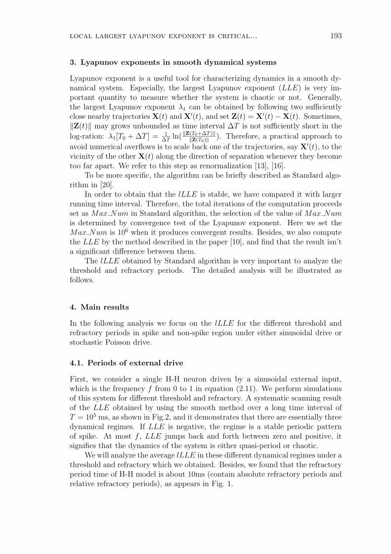
local largest lyapunov exponent is critical... 193
3. Lyapunov exponents in smooth dynamical systems
Lyapunov exponent is a useful tool for characterizing dynamics in a smooth dy-namical system. Especially, the largest Lyapunov exponent (LLE) is very im-portant quantity to measure whether the system is chaotic or not. Generally,the largest Lyapunov exponent λ1 can be obtained by following two sufficientlyclose nearby trajectories X(t) and X′(t), and set Z(t) = X′(t)−X(t). Sometimes,‖Z(t)‖ may grows unbounded as time interval ∆T is not sufficiently short in the
log-ration: λ1[T0 + ∆T ] = 1∆T
ln(‖Z(T0+∆T )‖‖Z(T0)‖ ). Therefore, a practical approach to
avoid numerical overflows is to scale back one of the trajectories, say X′(t), to thevicinity of the other X(t) along the direction of separation whenever they becometoo far apart. We refer to this step as renormalization [13], [16].
To be more specific, the algorithm can be briefly described as Standard algo-rithm in [20].
In order to obtain that the lLLE is stable, we have compared it with largerrunning time interval. Therefore, the total iterations of the computation proceedsset as Max Num in Standard algorithm, the selection of the value of Max Numis determined by convergence test of the Lyapunov exponent. Here we set theMax Num is 106 when it produces convergent results. Besides, we also computethe LLE by the method described in the paper [10], and find that the result isn’ta significant difference between them.
The lLLE obtained by Standard algorithm is very important to analyze thethreshold and refractory periods. The detailed analysis will be illustrated asfollows.
4. Main results
In the following analysis we focus on the lLLE for the different threshold andrefractory periods in spike and non-spike region under either sinusoidal drive orstochastic Poisson drive.
4.1. Periods of external drive
First, we consider a single H-H neuron driven by a sinusoidal external input,which is the frequency f from 0 to 1 in equation (2.11). We perform simulationsof this system for different threshold and refractory. A systematic scanning resultof the LLE obtained by using the smooth method over a long time interval ofT = 105 ms, as shown in Fig.2, and it demonstrates that there are essentially threedynamical regimes. If LLE is negative, the regime is a stable periodic patternof spike. At most f , LLE jumps back and forth between zero and positive, itsignifies that the dynamics of the system is either quasi-period or chaotic.
We will analyze the average lLLE in these different dynamical regimes under athreshold and refractory which we obtained. Besides, we found that the refractoryperiod time of H-H model is about 10ms (contain absolute refractory periods andrelative refractory periods), as appears in Fig. 1.
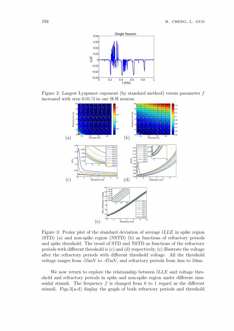
194 h. cheng, l. guo
0 0.2 0.4 0.6 0.8 1−0.03
−0.02
−0.01
0
0.01
0.02
0.03
0.04
f (Hz)
LLE
Single Neuron
Figure 2: Largest Lyapunov exponent (by standard method) versus parameter fincreased with step 0.01/3 in one H-H neuron.
(a)−54 −52 −50 −48
40
50
60
70
80
90
100
Threshold (mv)
Ref
ract
ory
(0.1
ms)
0.05
0.1
0.15
0.2
(b)−54 −52 −50 −48
40
50
60
70
80
90
100
Threshold (mv)
Ref
ract
ory
(0.1
ms)
0.05
0.06
0.07
0.08
0.09
0.1
0.11
0.12
0.13
(c)4 5 6 7 8 9 10
0
0.05
0.1
0.15
0.2
0.25
Refractory (ms)
ST
D
−55mv−54mv−53mv−52mv−51mv−50mv−49mv−48mv−47mv4 6 8 10
0.01
0.015
0.02
0.025
(d)4 5 6 7 8 9
0.05
0.06
0.07
0.08
0.09
0.1
0.11
0.12
0.13
0.14
Refractory (ms)
NS
TD
5 10
0.05
0.06
0.07
−55mv−54mv−53mv−52mv−51mv−50mv−49mv−48mv−47mv
(e)4 5 6 7 8 9 10
−76
−74
−72
−70
−68
−66
−64
−62
Refractory (ms)
Afte
r_R
efra
ctor
y_V
olta
ge
9.2 9.4 9.6
−65.6−65.4−65.2
−65−64.8−64.6
−55mv−54mv−53mv−52mv−51mv−50mv−49mv−48mv−47mv
Figure 3: Pcolor plot of the standard deviation of average lLLE in spike region(STD) (a) and non-spike region (NSTD) (b) as functions of refractory periodsand spike threshold. The trend of STD and NSTD as functions of the refractoryperiods with different threshold is (c) and (d) respectively, (e) illustrate the voltageafter the refractory periods with different threshold voltage. All the thresholdvoltage ranges from -55mV to -47mV, and refractory periods from 4ms to 10ms.
We now return to explore the relationship between lLLE and voltage thre-shold and refractory periods in spike and non-spike region under different sinu-soidal stimuli. The frequency f is changed from 0 to 1 regard as the differentstimuli. Figs.3(a-d) display the graph of both refractory periods and threshold

local largest lyapunov exponent is critical... 195
voltage with the standard deviation of the average lLLE for various values of f(We set STD and NSTD is the standard deviation of average lLLE in spike andnon-spike region respectively).
It is seen that the smallest STD in the area of threshold about −50mV,refractory periods from 7 ms to 10 ms, and the STD decreases along the axisfrom the bottom to the top as Fig.3(a) shows. The deeper the blue color is,the smaller the STD becomes. Fig.3(b) shows that the NSTD is opposite STDexcept the lower-left corner. For more accurate description, Fig.3(c) shows thatthe STD decreases with the increase of refractory periods (RPT) under differentspike threshold. From the vertical, when the threshold voltage is −50 mV, thesmallest STD curve as showed in the enlarged portion of the above screenshot,and the STD reaches a minimum at RPT being 9.5 ms and threshold voltageis −50 mV. Fig.3(d) shows that the NSTD increases with the increase of RPTwith different spike threshold, and in most cases, the NSTD is larger than STD,indicating that the average values of lLLE in spike region are more stable thannon-spike region. In order to verify whether or not the voltage is at resting stateafter RPT, we draw a picture as Fig.3(e) shows. In the enlarged portion of theFig.3(e), the voltage is at resting state. Therefore, the RPT and threshold voltagehave been chosen for analysis are reasonable that the RPT is 9.5 ms and thresholdvoltage is −50 mV respectively. Then, we compute the average values of the lLLEin spike and non-spike region respectively, whose results are shown in Fig.4.
−1
−0.8
−0.6
−0.4
−0.2
0
Ave
rag
e o
f L
oca
l L
LE
in
Sp
ike
Re
gio
n
Stimulus f (Hz)0 0.1 0.2 0.3 0.4 0.5 0.6 0.7 0.8 0.9 1
−0.1
0.2
0.4
0.6
0.8
Ave
rag
e o
f L
oca
l L
LE
in
No
nS
pik
e R
eg
ion
Figure 4: The average lLLE as functions of stimulus f (Hz), the threshold voltageis −50 mV, refractory period is 9.5 ms.
In Fig.4, it reveals that the average values of lLLE are stable about −0.19 inspike region (blue curve in Fig.4), with the STD is about 0.00704, indicating thatthe attractor of the system is contraction in spike region. However, the averagevalues of lLLE are unstable (dark green curve in Fig.4) and more vibrant in non-spike region, with the NSTD is about 0.10973, and we find the curve is verysimilar to largest Lyapunov exponent as Fig.2. The average values of lLLE aremostly greater than zero, indicating that attractor of the system is divergent innon-spike region. These phenomena can best demonstrate that the threshold andrefractory periods express an especial neuron dynamics that the spike region ismiraculous that the local Lyapunov exponent represents.

196 h. cheng, l. guo
We will analyze the average local LLE in these three dynamical regimes inspike and non-spike region.
(a)
−0.195 −0.19 −0.185 −0.18 −0.175 −0.17 −0.1650
2
4
6Spike Region_Chaotic
Average of Local LLEN
umbe
r
0.1 0.2 0.3 0.4 0.50
1
2 NonSpike Region_Chaotic
Average of Local LLE
Num
ber
Std=0.00568
Std=0.05892
(b)
−0.26 −0.24 −0.22 −0.2 −0.18 −0.16 −0.140
10
20
30Spike Region_Period
Average of Local LLE
Num
ber
−0.1 0 0.1 0.2 0.3 0.4 0.5 0.60
2
4
NonSpike Region_Period
Average of Local LLE
Num
ber
Std=0.01095
Std=0.12526
(c)
−0.2 −0.195 −0.19 −0.185 −0.18 −0.1750
100
200
300Spike Region_QuasiPeriod
Average of Local LLE
Num
ber
0.2 0.25 0.3 0.35 0.4 0.450
50
100NonSpike Region_QuasiPeriod
Average of Local LLE
Num
ber
Std=0.01599
Std=0.00192
(d)
−0.26 −0.24 −0.22 −0.2 −0.18 −0.16 −0.140
100
200
300Spike Region
Average of Local LLE
Num
ber
−0.1 0 0.1 0.2 0.3 0.4 0.5 0.60
50
100NonSpike Region
Average of Local LLE
Num
ber
Std=0.00704
Std=0.10972
Figure 5: Histogram 1 to 3 graph is the average local LLE in Spike and Non-Spike region in three dynamical regimes (Chaotic, Period, Quasi-Period). Thelast graph is the average local LLE in Spike and Non-spike region. The standarddeviation of spike are smaller than non-spike in chaotic, period and quasi-period.Threshold voltage is −50 mV and refractory period is 9.5 ms.
In Fig.5, we describe the average lLLE in three dynamical regimes(Chaotic,Period, Quasi-Period)with spike and non-spike region. We find the average valuesof lLLE are more directly concentrated in spike region than non-spike region.Besides, the mean lLLE is smaller than zero in spike region, it is indicating thatthe attractor is contraction in these three dynamical regimes. Meanwhile, thereason that some value of the mean lLLE in non-spike region is smaller than zerois that the attractor is divergent in period regime, as shown in Fig.5(b). What isthe difference between the three dynamical regimes in no spike region? The mostsignificant difference is the average value of lLLE became more concentrated inquasi-period than other regimes.
4.2. Poisson of feedforward input
It has shown that chaos can arise in the dynamics of single H-H neuron, forexample, under a periodic external drive as part 4.1. Therefore, there is a naturalquestion: what about a single H-H neuron under a stochastic external Poissoninput, and can it be chaotic?
So, the system is also considered as another drive by feedforward inputs.Here, we consider stochastic inputs: we use a spike train sampled from a Poissonprocess with rate r as the feedforward input. We also hope to find the different

local largest lyapunov exponent is critical... 197
dynamical regimes, but only one dynamical regime is period in one neuron model.The results are shown in Fig.6(a). This case is consistent with Sun [17] results.
(a)0 0.2 0.4 0.6 0.8 1
−0.7
−0.6
−0.5
−0.4
−0.3
−0.2
−0.1
0
Force Input (ms/cm^2)
Largest Lyapunov Exponent
Rate=6
Rate=10
Rate=15
Rate=0.4
Rate=0.5
Rate=0.6
Rate=0.3
0.06 0.08 0.1
−0.12
−0.1
−0.08
−0.06
−0.04
−0.02
(b)
0.05 0.06 0.07 0.08 0.09−0.8
−0.6
−0.4
−0.2
0.05 0.1−1
−0.8
−0.6
Rate=0.3 Std=0.01145Rate=0.4 Std=0.01287Rate=0.5 Std=0.01610Rate=0.6 Std=0.01848
0.05 0.06 0.07 0.08 0.09 0.1
−0.6
−0.4
−0.2
0
Force Input (ms/cm2)
Ave
rage
of L
ocal
LE
0.05 0.1−0.2
0
0.2
Rate=0.3 Std=0.03343Rate=0.4 Std=0.03243Rate=0.5 Std=0.03038Rate=0.6 Std=0.02809
Spike Region
Non−Spike Region
(c)
0.05 0.06 0.07 0.08 0.09
0
0.5
1
0.05 0.06 0.07 0.08 0.09 0.1−0.5
0
0.5
1
Force Input(mS/cm2)
Ave
rage
of L
ocal
LE
Rate=6 Std=0.03283Rate=10 Std=0.18587Rate=15 Std=0.06024
Rate=6 Std=0.06345Rate=10 Std=0.18731Rate=15 Std=0.15550
Spike Region
Non−Spike Region
Figure 6: (a) The Largest Lyapunov exponent of the HH neuron system withdifferent rate of poisson input versus the force input strength parameter F is[0, 1], the enlarged portion is the F ranging from 0.05 to 0.1, force strength F .(b) The average local LLE versus the different Poisson input strength in lowfrequency Poisson spike. (c) The average local LLE versus the different Pois-son input strength in high frequency Poisson spike. Threshold is −50 mV andrefractory periods is 9.5 ms.
Here, we vary the parameter of the strength of Poisson ranging from 0 to 1mS/cm2 to perform seven systematic scanning tests for seven different parametervalues of the Poisson rate r = 0.3, 0.4, 0.5, 0.6, 6, 10, 15, respectively. We findthe largest Lyapunov exponent is negative for any values of Poisson rate r andstrength F , which indicates that the dynamics of a single neuron in this system isnot chaotic. As shown in Fig.6(a), when the Poisson rate r = 0.3, 0.4, 0.5, 0.6, thevalue increases as the rate increases, but for the other case of large rate r = 6, 10and 15, the value of LLE decreases as the rate increases in the strength F rangingfrom 0.15 to 1, and we also find the LLE in high frequency is smaller than lowfrequency when the strength F ranges from 0.25 to 1. In very low force strengthof Poisson spike ranging from 0 to 0.05, the LLE increase with increasing Poissonrate in the high Poisson spike frequency region, however, in the low frequencyregion, the LLE decrease with increasing Poisson rate.
In Fig.6(b), we show that the average lLLE in Spike and Non-Spike region arenearly constant under different stimuli of Poisson force strength input in each smallrate of Poisson spike. We also show that the average values of lLLE are negativeabout −0.8 in spike region; however, the average values of lLLE are monotonicallyincreasing as F increases in non-spike region. The Poisson force strength rangingfrom 0.05 to 0.1 mS/cm2 followed as Sun and Zhou [17]. The standard deviationof the average lLLE increases as the rate r increases and expands at large strength

198 h. cheng, l. guo
in spike region, but the value decreases as the r increases and tightens at largestrength in non-spike region in the low frequency Poisson spike. Therefore, theseresults demonstrated that the average lLLE is stable in different Poisson inputstrengths in each Poisson spike rate.
In Fig.6(c), we find that the average values of local lyapunov exponent areunstable in spike and non-spike region in high frequency Poisson spike stimuli.And the values sign of the mean lLLE are different with the results of sinusoidaldriven; therefore, in high frequency case, the conclusion as other case can not bereached.
5. Discussion and conclusion
We have presented a numerical study of the value of the average llLLE of HHneuron under Sinusoidal drive and conductance drive with a stochastic nature,such as feedforward Poisson spikes, which are more realistic as an approximation tocortical spike trains. We found three typical dynamical regimes in Sinusoidal driveas the sine frequency varies from weak to strong, and only one dynamical regimein Poisson input as the input strength varies from 0 to 1. We have also discoveredthe relationship between the lLLE and spike threshold voltage and refractoryperiods. That is, the average lLLE is stable in spike region and unstable innon-spike region, under different sinusoidal drive, and it has some similar resultsunder Poisson force strength in each fix low Poisson spike rate in spike region.But the value is different with the case at sinusoidal external stimulus in non-spike region. Also, the analysis demonstrates that the reason of choosing thethreshold voltage and refractory periods value in physiologically have an intrinsicdynamical structure. This phenomenon estranges us from the unfamiliarity withthe threshold voltage and refractory periods from a new perspective, and carvesout a specific way to uncover the physical interpretation of the spike encoding andreliability of spike timing.
Acknowledgment. We would like to thank Douglas Zhou and David Cai fororiginally suggesting this problem and stimulating discussions.
References
[1] Benda, J., Herz, A.V., A universal model for spike-frequency adaptation,Neural Computation, 15 (11) (2003), 25232564.
[2] Benettin, G., Galgani, L., Giorgilli, A., Strelcyn, J.-M., Lya-punov characteristic exponents for smooth dynamical systems and for Hamil-tonian systems; a method for computing all of them. Part 1: Theory, Mecca-nica, 15 (1) (1980), 920.

local largest lyapunov exponent is critical... 199
[3] Berry, M.J., Meister, M., Refractoriness and neural precision, in: Neu-ral Information Processing Systems, 1997.
[4] Brette, R., Guigon, E., Reliability of spike timing is a general pro-perty of spiking model neurons, Neural Computation, 15 (2003), 279308.doi:10.1162/089976603762552924.
[5] Dayan, P., Abbott, L.F., Theoretical Neuroscience: Computational andMathematical Modeling of Neural Systems, MIT Press, 2001.
[6] Eckmann, J.-P., Ruelle, D., Ergodic theory of chaos and strange attrac-tors, Reviews of Modern Physics, 57 (3) (1985), 617.
[7] Fourcaud-Trocme, N., Hansel, D., Van Vreeswijk, C., Brunel,N., How spike generation mechanisms determine the neuronal response tofluctuating inputs, The Journal of Neuroscience, 23 (37) (2003), 1162811640.
[8] Herz, A.V., Gollisch, T., Machens, C.K., Jaeger, D., Modelingsingle-neuron dynamics and computations: a balance of detail and abstrac-tion, Science, 314 (5796) (2006), 8085.
[9] Hodgkin, A.L., Huxley, A.F., A quantitative description of membranecurrent and its application to conduction and excitation in nerve, Journal ofNeurophysiology, 117 (1952), 500544. doi:10.1007/bf02459568.
[10] Kim, B.J., Choe, G.H., High precision numerical estimation of the largestLyapunov exponent, Communications in Nonlinear Science and NumericalSimulation, 15 (5) (2010), 13781384.
[11] Lichtenberg, A.J., Lieberman, M.A., Regular and Chaotic Dynamics,Springer New York, 1992.
[12] Oseledec, V.I., A multiplicative ergodic theorem: Liapunov characteris-tic numbers for dynamical systems, Trans. Moscow Math. Soc., 19 (1968),197221.
[13] Parker, T.S., Chua, L.O., Parker, T.S., Practical numerical algo-rithms for chaotic systems, Springer New York, 1989.
[14] PhysiologyWeb, Neuronal action potential: Refractory periods, 2014. URLhttp://www.physiologyweb.com
[15] Purves, D., Augustine, G.J. et al. (eds.), Neuroscience, 2nd edition. TheRefractory Period. Sunderland, MA: Sinauer Associates, 2001.
[16] Ramasubramanian, K., Sriram, M., A comparative study of compu-tation of lyapunov spectra with different algorithms, Physica D: NonlinearPhenomena, 139 (1) (2000), 7286.

200 h. cheng, l. guo
[17] Sun, Y., Zhou, D., Rangan, A., Cai, D., Pseudo-Lyapunov exponentsand predictability of hodgkinhuxley neuronal network dynamics, Journal ofComputational Neuroscience, 28 (2) (2010), 247266.
[18] Uera y Arcas, B.A., Fairhall, A.L., Bialek, W., Computation in asingle neuron: Hodgkin and Huxley revisited, Neural Computation, 15 (2003),17151749.
[19] Wolf, A., Swift, J.B., Swinney, H.L., Vastano, J.A., Determininglyapunov exponents from a time series, Physica, (1985), 285317.
[20] Zhou, D., Sun, Y., Rangan, A.V., Cai, D., Spectrum of Lyapunov ex-ponents of non-smooth dynamical systems of integrate-and-fire type, Journalof Computational Neuroscience, 28 (2) (2010), 229245.
Accepted: 29.10.2014

italian journal of pure and applied mathematics – n. 34−2015 (201−212) 201
AN APPROACH TO THE RELATIVE ORDER BASED GROWTHPROPERTIES OF DIFFERENTIAL MONOMIALS
Sanjib Kumar Datta
Department of MathematicsUniversity of KalyaniP.O. Kalyani, Dist-NadiaPIN: 741235, West BengalIndiae-mail: sanjib kr [email protected]
Tanmay Biswas
Rajbari, Rabindrapalli, R.N. Tagore RoadP.O. Krishnagar, P.S. Kotwali, Dist-NadiaPIN: 741101, West BengalIndiae-mail: tanmaybiswas [email protected]
Sarmila Bhattacharyya
Jhorehat F.C. High School for GirlsP.O. Jhorehat, P.S. Sankrail, Dist-HowrahPIN: 711302, West BengalIndiae-mail: [email protected]
Abstract. In this paper an attempt is taken to study the comparative growth propertiesof composition of entire and meromorphic functions on the basis of relative order andrelative lower order of differential monomials generated by transcendental entire andtranscendental meromorphic functions.Keywords and Phrases: transcendental entire function, transcendental meromorphicfunction, relative order, relative lower order, differential monomial.AMS Subject Classification (2010): 30D30, 30D35, 30D20.
1. Introduction
Let f be an entire function defined in the open complex plane C. The functionMf (r) on |z| = r known as maximum modulus function corresponding to f isdefined as follows:
Mf (r) = max|z|=r
|f (z)| .
When f is meromorphic, Mf (r) cannot be defined as f is not analytic. In thissituation, one may define another function Tf (r) known as Nevanlinna’s Charac-teristic function of f, playing the same role as Mf (r) in the following manner:
Tf (r) = Nf (r) + mf (r) .
202 s.k. datta, t. biswas, s. bhattacharyya
Given two meromorphic functions f and g, the ratioTf (r)
Tg(r)as r →∞ is called
the growth of f with respect to g in terms of their Nevanlinna’s Characteristicfunctions.
When f is entire function, the Nevanlinna’s Characteristic function Tf (r) off is defined as
Tf (r) = mf (r) .
We call the function Nf (r, a)
( −Nf (r, a)
)as counting function of a-points
(distinct a-points) of f . In many occasions Nf (r,∞) and−
Nf (r,∞) are denoted
by Nf (r) and−
Nf (r) respectively. We put
Nf (r, a) =
r∫
0
nf (t, a)− nf (0, a)
tdt +
−nf (0, a) log r ,
where we denote by nf (r, a)( −nf (r, a)
)the number of a-points (distinct a-points)
of f in |z| ≤ r and an ∞ -point is a pole of f . Also we denote by nf |=1(r, a) ,thenumber of simple zeros of f − a in |z| ≤ r.
Accordingly, Nf |=1(r, a) is defined in terms of nf |=1(r, a) in the usual way andwe set
δ1(a; f) = 1− lim supr→∞
N(r, a; f |= 1)
Tf (r)(cf. [8]) ,
the deficiency of ‘a’ corresponding to the simple a- points of f i,e. simple zeros off − a. In this connection Yang [7] proved that there exists at most a denumerablenumber of complex numbers a ∈ C ∪ ∞ for which
δ1(a; f) > 0 and∑
a∈C∪∞δ1(a; f) ≤ 4.
On the other hand, m(r, 1
f−a
)is denoted by mf (r, a) and we mean mf (r,∞)
by mf (r) , which is called the proximity function of f . We also put
mf (r) =1
2π
2π∫
0
log+∣∣f (
reiθ)∣∣ dθ,
where log+ x = max (log x, 0) for all x > 0.Further, a meromorphic function b ≡ b (z) is called small with respect to f if
Tb (r) = Sf (r) where Sf (r) = o Tf (r) i.e.,Sf (r)
Tf (r)→ 0 as r → ∞. Moreover, for
any transcendental meromorphic function f , we call P [f ] = bfn0(f (1))n1 ...(f (k))nk ,
to be a differential monomial generated by it wherek∑
i=0
ni ≥ 1 ( all ni | i = 0, 1, ..., k
are non-negative integers) and the meromorphic function b is small with respect

an approach to the relative order based growth properties... 203
to f. In this connection the numbers γP [f ] =k∑
i=0
ni and ΓP [f ] =k∑
i=0
(i + 1)ni are
called the degree and weight of P [f ] respectively cf. [2].The order of a meromorphic function f which is generally used in computa-
tional purpose is defined in terms of the growth of f with respect to the exponentialfunction as
ρf = lim supr→∞
log Tf (r)
log Texp z (r)= lim sup
r→∞
log Tf (r)
log(
rπ
) = lim supr→∞
log Tf (r)
log r + O(1).
Lahiri and Banerjee [5] introduced the relative order (respectively relativelower order) of a meromorphic function with respect to an entire function to avoidcomparing growth just with exp z. Extending the notion of relative order as citedin the reference, Datta, Biswas and Bhattacharyya [3] gave the definition of relativeorder (respectively relative lower order) of differential monomials generated bytranscendental entire and transcendental meromorphic functions.
For entire and meromorphic functions, the notion of their growth indicatorssuch as order and lower order are classical in complex analysis and during thepast decades, several researchers have already been continuing their studies inthe area of comparative growth properties of composite entire and meromorphicfunctions in different directions using the same. But at that time, the concept ofrelative order and consequently relative lower order of entire and meromorphicfunctions with respect to another entire function was mostly unknown to complexanalysis and they are not aware of the technical advantages of using the relativegrowth indicators of the functions. Therefore the growth of composite entire andmeromorphic functions needs to be modified on the basis of their relative orderand relative lower type some of which has been explored in this paper. Actuallyin this paper we establish some newly developed results based on the growthproperties of relative order and relative lower order of monomials generated bytranscendental entire and transcendental meromorphic functions.
2. Notation and preliminary remarks
We use the standard notations and definitions of the theory of entire and mero-morphic functions which are available in [4] and [6]. Henceforth, we do not explainthose in details. Now, we just recall some definitions which will be needed in thesequel.
Definition 1 The order ρf and lower order λf of a meromorphic function f aredefined as
ρf = lim supr→∞
log Tf (r)
log rand λf = lim inf
r→∞log Tf (r)
log r.
The notion of order (lower order) to determine the relative growth of twomeromorphic functions having same non zero finite order is classical in complexanalysis and is given by

204 s.k. datta, t. biswas, s. bhattacharyya
Given a non-constant entire function f defined in the open complex planeC, its Nevanlinna’s Characteristic function is strictly increasing and continuous.Hence there exists its inverse function T−1
g : (Tg(0),∞) → (0,∞) withlims→∞
T−1g (s) = ∞.
Lahiri and Banerjee [5] introduced the definition of relative order of a mero-morphic function f with respect to an entire function g, denoted by ρg (f) asfollows:
ρg (f) = inf µ > 0 : Tf (r) < Tg (rµ) for all sufficiently large r
= lim supr→∞
log T−1g Tf (r)
log r.
The definition coincides with the classical one [5] if g (z) = exp z. Similarly,one can define the relative lower order of a meromorphic function f with respectto an entire g denoted by λg (f) in the following manner :
λg (f) = lim infr→∞
log T−1g Tf (r)
log r.
In this connection, the following two definitions are relevant:
Definition 2 [1] A non-constant entire function f is said to have the property(A) if for any δ > 1 and for all large r, [Mf (r)]2 ≤ Mf
(rδ
)holds. For examples
of functions with or without the property (A), one may see [1].
Definition 3 Two entire functions g and h are said to be asymptotically equiva-lent if there exists l (0 < l < ∞) such that
Mg (r)
Mh (r)→ l as r →∞
and in this case we write g ∼ h . Clearly if g ∼ h then h ∼ g.
3. Some examples
In this section, we present some examples in connection with definitions given inthe previous section.
Example 1 (Order (lower order)) Given any natural number n, let f(z) =exp zn. Then Mf (r) = exp rn. Therefore putting R = 2 in the inequality Tf (r) ≤log Mf (r) ≤ R+r
R−rTf (R) (cf. [4]) we get that Tf (r) ≤ rn and Tf (r) ≥ 1
3
(r2
)n.
Hence
ρf = lim supr→∞
log Tf (r)
log r= n and λf = lim inf
r→∞log Tf (r)
log r= n .
Further, if we take g = exp[2] z, then Tg (r) ∼ exp r
(2π3r)12
(r →∞) . Therefore
ρf = λf = ∞ .

an approach to the relative order based growth properties... 205
Example 2 (Relative order (relative lower order)) Suppose f = g = exp[2] zthen Tf (r) = Tg (r) ∼ exp r
(2π3r)12
(r →∞) . Now we obtain that
Tg (r) ≤ log Mg (r) ≤ 3Tg (2r) (cf. [4])
i.e., Tg (r) ≤ exp r ≤ 3Tg (2r) .
Therefore
T−1g Tf (r) ≥ log
(exp r
(2π3r)12
), i.e., lim inf
r→∞log T−1
g Tf (r)
log r≥ 1
and
T−1g Tf (r) ≤ 2 log
(3 exp r
(2π3r)12
), i.e., lim sup
r→∞
log T−1g Tf (r)
log r≤ 1 .
Henceρg (f) = λg (f) = 1 .
4. Lemmas
In this section, we present some lemmas which will be needed in the sequel.
Lemma 1 [1] Let g be an entire function and α > 1, 0 < β < α. Then
Mg (αr) > βMg (r) for all sufficiently large r.
Lemma 2 [1] Let f be an entire function which satisfies Property (A). Then forany positive integer n and for all sufficiently large r
[Mf (r)]n ≤ Mf
(rδ
)
holds where δ > 1.
Lemma 3 Let g be an entire. Then for all sufficiently large values of r,
Tg (r) ≤ log Mg (r) ≤ 3Tg (2r) .
Lemma 3 follows from Theorem 1.6 (cf. [4], p.18), on putting R = 2r.
Lemma 4 [4] Suppose f be a transcendental meromorphic function of finite or-der or of non-zero lower order and
∑a∈C∪∞
δ1(a; f) = 4. Also, let g be a tran-
scendental entire function of regular growth having non zero finite order and∑a∈C∪∞
δ1(a; g) = 4. Then the relative order and relative lower order of P [f ]
with respect to P [g] are same as those of f with respect to g.

206 s.k. datta, t. biswas, s. bhattacharyya
Lemma 5 Let g and h be any two transcendental entire functions of regulargrowth having non zero finite order with
∑a∈C∪∞
δ1(a; g) = 4 and∑
a∈C∪∞δ1(a; h) = 4
respectively. Then for any transcendental meromorphic function f of finite orderor of non-zero lower order and
∑a∈C∪∞
δ1(a; f) = 4,
ρP [g] (P [f ]) = ρP [h] (P [f ])
andλP [g] (P [f ]) = λP [h] (P [f ]) .
if g and h have Property (A) and g ∼ h.
Proof. Let ε > 0 is arbitrary. Now, we get from Definition 3 and Lemma 1 forall sufficiently large values of r that
(1) Mg (r) < (l + ε) Mh (r) ≤ Mh (αr) ,
where α > 1 is such that l + ε < α.Now, from Lemma 3 and in view of definition of relative order, we obtain for
all sufficiently large values of r that
Tf (r) ≤ Tg
[(r)(ρg(f)+ε)
], i.e., Tf (r) ≤ log Mg
[(r)(ρg(f)+ε)
].
Therefore, in view of (1), Lemma 2 and Lemma 3, it follows from above for anyδ > 1 that
Tf (r) ≤ 1
3log
[Mh
[(αr)(ρg(f)+ε)
]]3
i.e., Tf (r) ≤ 1
3log Mh
[(αr)δ(ρg(f)+ε)
]
i.e., Tf (r) ≤ Th
[(2αr)δ(ρg(f)+ε)
]
i.e.,log T−1
h Tf (r)
log r≤ δ (ρg (f) + ε)
log (2αr)
log r.
Letting δ → 1+, we get from above that
(2) ρh (f) ≤ ρg (f) .
Since h ∼ g, we also obtain that
(3) ρg (f) ≤ ρh (f) .
Now in view of Lemma 4, we obtain from (2) and (3) that
ρP [g] (P [f ]) = ρP [h] (P [f ]) .
Similarly, we haveλP [g] (P [f ]) = λP [h] (P [f ]) .
Thus the lemma follows.

an approach to the relative order based growth properties... 207
5. Theorems
In this section, we present the main results of the paper.
Theorem 1 Suppose f be a transcendental meromorphic function of finite orderor of non-zero lower order and
∑a∈C∪∞
δ1(a; f) = 4. Also, let h be a transcendental
entire function of regular growth having non zero finite order with∑
a∈C∪∞δ1(a; h) = 4
and g be any entire function such that
0 < λh (f g) ≤ ρh (f g) < ∞ and 0 < λh (f) ≤ ρh (f) < ∞.
Thenλh (f g)
ρh (f)≤ lim inf
r→∞log T−1
h Tfg (r)
log T−1P [h]TP [f ] (r)
≤ λh (f g)
λh (f)
≤ lim supr→∞
log T−1h Tfg (r)
log T−1P [h]TP [f ] (r)
≤ ρh (f g)
λh (f).
Proof. From the definition of ρh (f) and λh (f g) and Lemma 4 we have forarbitrary positive ε and for all sufficiently large values of r that
(4) log T−1h Tfg (r) > (λh (f g)− ε) log r
and
log T−1P [h]TP [f ] (r) ≤ (
ρP [h] (P [f ]) + ε)log r
i.e., log T−1P [h]TP [f ] (r) ≤ (ρh (f) + ε) log r .(5)
Now, from (4), (5) it follows for all sufficiently large values of r that
log T−1h Tfg (r)
log T−1P [h]TP [f ] (r)
> (λh (f g)− ε) log r
(ρh (f) + ε) log r.
As ε (> 0) is arbitrary , we obtain that
(6) lim infr→∞
log T−1h Tfg (r)
log T−1P [h]TP [f ] (r)
> λh (f g)
ρh (f).
Again for a sequence of values of r tending to infinity,
(7) log T−1h Tfg (r) ≤ (λh (f g) + ε) log r
and for all sufficiently large values of r,
log T−1P [h]TP [f ] (r) >
(λP [h] (P [f ])− ε
)log r
i.e., log T−1P [h]TP [f ] (r) > (λh (f)− ε) log r .(8)

208 s.k. datta, t. biswas, s. bhattacharyya
Combining (7) and (8) , we get for a sequence of values of r tending to infinitythat
log T−1h Tfg (r)
log T−1P [h]TP [f ] (r)
≤ (λh (f g) + ε) log r
(λh (f)− ε) log r.
Since ε (> 0) is arbitrary, it follows that
(9) lim infr→∞
log T−1h Tfg (r)
log T−1P [h]TP [f ] (r)
≤ λh (f g)
λh (f).
Also for a sequence of values of r tending to infinity that
log T−1P [h]TP [f ] (r) ≤ (
λP [h] (P [f ]) + ε)log r
i.e., log T−1P [h]TP [f ] (r) ≤ (λh (f) + ε) log r .(10)
Now, from (4) and (10) , we obtain for a sequence of values of r tending to infinitythat
log T−1h Tfg (r)
log T−1P [h]TP [f ] (r)
≥ (λh (f g)− ε) log r
(λh (f) + ε) log r.
As ε (> 0) is arbitrary, we get from above that
(11) lim supr→∞
log T−1h Tfg (r)
log T−1P [h]TP [f ] (r)
≥ λh (f g)
λh (f).
Also for all sufficiently large values of r,
(12) log T−1h Tfg (r) ≤ (ρh (f g) + ε) log r .
Now, it follows from (8) and (12) for all sufficiently large values of r that
log T−1h Tfg (r)
log T−1P [h]TP [f ] (r)
≤ (ρh (f g) + ε) log r
(λh (f)− ε) log r.
Since ε (> 0) is arbitrary, we obtain that
(13) lim supr→∞
log T−1h Tfg (r)
log T−1P [h]TP [f ] (r)
≤ ρh (f g)
λh (f).
Thus the theorem follows from (6) , (9) , (11) and (13) .The following theorem can be proved in the line of Theorem 1 and so the
proof is omitted.
Theorem 2 Suppose g be a transcendental entire function of finite order or ofnon-zero lower order and
∑a∈C∪∞
δ1(a; g) = 4. Also let h be a transcendental entire
function of regular growth having non zero finite order with∑
a∈C∪∞δ1(a; h) = 4

an approach to the relative order based growth properties... 209
and f be any meromorphic function such that 0 < λh (f g) ≤ ρh (f g) < ∞and 0 < λh (g) ≤ ρh (g) < ∞. Then
λh (f g)
ρh (g)≤ lim inf
r→∞log T−1
h Tfg (r)
log T−1P [h]TP [g] (r)
≤ λh (f g)
λh (g)
≤ lim supr→∞
log T−1h Tfg (r)
log T−1P [h]TP [g] (r)
≤ ρh (f g)
λh (g).
Theorem 3 Suppose f be a transcendental meromorphic function of finite orderor of non-zero lower order and
∑a∈C∪∞
δ1(a; f) = 4. Also, let h be a transcendental
entire function of regular growth having non zero finite order with∑
a∈C∪∞δ1(a; h) = 4
and g be any entire function with 0 < ρh (f g) < ∞ and 0 < ρh (f) < ∞. Then
lim infr→∞
log T−1h Tfg (r)
log T−1P [h]TP [f ] (r)
≤ ρh (f g)
ρh (f)≤ lim sup
r→∞
log T−1h Tfg (r)
log T−1P [h]TP [f ] (r)
.
Proof. From the definition of ρP [h] (P [f ]) and in view of Lemma 4, we get for asequence of values of r tending to infinity that
log T−1P [h]TP [f ] (r) >
(ρP [h] (P [f ])− ε
)log r
i.e., log T−1P [h]TP [f ] (r) > (ρh (f)− ε) log r .(14)
Now, from (12) and (14) , it follows for a sequence of values of r tending to infinitythat
log T−1h Tfg (r)
log T−1P [h]TP [f ] (r)
≤ (ρh (f g) + ε) log r
(ρh (f)− ε) log r.
As ε (> 0) is arbitrary, we obtain that
(15) lim infr→∞
log T−1h Tfg (r)
log T−1P [h]TP [f ] (r)
≤ ρh (f g)
ρh (f).
Again for a sequence of values of r tending to infinity,
(16) log T−1h Tfg (r) > (ρh (f g)− ε) log r .
So combining (5) and 16, we get for a sequence of values of r tending to infinitythat
log T−1h Tfg (r)
log T−1P [h]TP [f ] (r)
> (ρh (f g)− ε) log r
(ρh (f) + ε) log r.
Since ε (> 0) is arbitrary, it follows that
(17) lim supr→∞
log T−1h Tfg (r)
log T−1P [h]TP [f ] (r)
> ρh (f g)
ρh (f).
Thus the theorem follows from (15) and (17) .The following theorem can be carried out in the line of Theorem 3 and there-
fore we omit its proof.

210 s.k. datta, t. biswas, s. bhattacharyya
Theorem 4 Suppose g be a transcendental entire function of finite order or ofnon-zero lower order and
∑a∈C∪∞
δ1(a; g) = 4. Also let h be a transcendental entire
function of regular growth having non zero finite order with∑
a∈C∪∞δ1(a; h) = 4 and
f be any meromorphic function such that 0 < ρh (f g) < ∞ and 0 < ρh (g) < ∞.Then
lim infr→∞
log T−1h Tfg (r)
log T−1P [h]TP [g] (r)
≤ ρh (f g)
ρh (g)≤ lim sup
r→∞
log T−1h Tfg (r)
log T−1P [h]TP [g] (r)
.
The following theorem is a natural consequence of Theorem 1 and Theorem 3:
Theorem 5 Suppose f be a transcendental meromorphic function of finite orderor of non-zero lower order and
∑a∈C∪∞
δ1(a; f) = 4. Also let h be a transcendental
entire function of regular growth having non zero finite order with∑
a∈C∪∞δ1(a; h) = 4
and g be any entire function with 0 < λh (f g) ≤ ρh (f g) < ∞ and0 < λh (f) ≤ ρh (f) < ∞. Then
lim infr→∞
log T−1h Tfg (r)
log T−1P [h]TP [f ] (r)
≤ min
λh (f g)
λh (f),ρh (f g)
ρh (f)
≤ max
λh (f g)
λh (f),ρh (f g)
ρh (f)
≤ lim sup
r→∞
log T−1h Tfg (r)
log T−1P [h]TP [f ] (r)
.
The proof is omitted.Analogously, one may state the following theorem without its proof.
Theorem 6 Suppose g be a transcendental entire function of finite order or ofnon-zero lower order and
∑a∈C∪∞
δ1(a; g) = 4. Also let h be a transcendental entire
function of regular growth having non zero finite order with∑
a∈C∪∞δ1(a; h) = 4
and f be any meromorphic function such that 0 < λh (f g) ≤ ρh (f g) < ∞and 0 < λh (g) ≤ ρh (g) < ∞ .Then
lim infr→∞
log T−1h Tfg (r)
log T−1P [h]TP [g] (r)
≤ min
λh (f g)
λh (g),ρh (f g)
ρh (g)
≤ max
λh (f g)
λh (g),ρh (f g)
ρh (g)
≤ lim sup
r→∞
log T−1h Tfg (r)
log T−1P [h]TP [g] (r)
.
Theorem 7 Suppose f be a transcendental meromorphic function of finite or-der or of non-zero lower order and
∑a∈C∪∞
δ1(a; f) = 4. Also let h be a tran-
scendental entire function of regular growth having non zero finite order with

an approach to the relative order based growth properties... 211
∑a∈C∪∞
δ1(a; h) = 4 and g be any entire function with 0 < ρh (f g) < ∞ and
0 < ρh (f) < ∞ and g ∼ h. Then
lim infr→∞
log T−1g Tf (r)
log T−1P [h]TP [f ] (r)
≤ 1 ≤ lim supr→∞
log T−1g Tf (r)
log T−1P [h]TP [f ] (r)
.
Proof. From the definition of ρg (f) , we get for all sufficiently large values of rthat
(18) log T−1g Tf (r) ≤ (ρg (f) + ε) log r
and for a sequence of values of r tending to infinity that
(19) log T−1g Tf (r) ≥ (ρg (f)− ε) log r .
Now, from (14) and (18) , it follows for a sequence of values of r tending to infinitythat
log T−1g Tf (r)
log T−1P [h]TP [f ] (r)
≤ (ρg (f) + ε) log r
(ρh (f)− ε) log r.
As ε (> 0) is arbitrary, we obtain that
(20) lim infr→∞
log T−1g Tf (r)
log T−1P [h]TP [f ] (r)
≤ ρg (f)
ρh (f).
Now, as g ∼ h, in view of Lemma 4 and Lemma 5 we obtain from (20) that
(21) lim infr→∞
log T−1g Tf (r)
log T−1P [h]TP [f ] (r)
≤ 1 .
Again combining (5) and (19) , we get for a sequence of values of r tending toinfinity that
log T−1g Tf (r)
log T−1P [h]TP [f ] (r)
> (ρg (f)− ε) log r
(ρh (f) + ε) log r.
Since ε (> 0) is arbitrary, it follows that
(22) lim supr→∞
log T−1g Tf (r)
log T−1P [h]TP [f ] (r)
> ρg (f)
ρh (f).
Now as g ∼ h , in view of Lemma 4 and Lemma 5 we obtain from (22) that
(23) lim supr→∞
log T−1g Tf (r)
log T−1P [h]TP [f ] (r)
> 1 .
Thus the theorem follows from (21) and (23) .

212 s.k. datta, t. biswas, s. bhattacharyya
6. Conclusion
Actually this paper deals with the extension of the works on the growth prop-erties concerning differential monomials generated by transcendental entire andtranscendental meromorphic functions on the basis of their relative orders andrelative lower orders. These theories can also be modified by the treatment of thenotions of generalized relative orders (generalized relative lower orders) and (p, q)-th relative orders ((p, q)-th relative lower orders). In addition, some extensions ofthe same may be done in the light of slowly changing functions. Moreover, the no-tion of relative order and relative lower order of differential monomials generatedby transcendental entire and transcendental meromorphic functions may have awide range of applications in Complex Dynamics, Factorization Theory of entirefunctions of single complex variable, the solution of complex differential equationsetc. which must be an active area of research.
References
[1] Bernal, L., Orden relative de crecimiento de funciones enteras, Collect.Math., 39 (1988), 209-229.
[2] Doeringer, W., Exceptional values of differential polynomials, Pacific J.Math., 98 (1)(1982), 55-62.
[3] Datta, S.K., Biswas, T., Bhattacharyya, S., On relative order andrelative type based growth properties of differential monomials, J. of IndianMath. Soc. (to appear).
[4] Hayman, W.K., Meromorphic Functions, The Clarendon Press, Oxford,1964.
[5] Lahiri, B.K., Banerjee, D., Relative order of entire and meromorphicfunctions, Proc. Nat. Acad. Sci. India, 69(A) III (1999), 339-354.
[6] Valiron, G., Lectures on the General Theory of Integral Functions, ChelseaPublishing Company, 1949.
[7] Yang, L., Value distribution theory and new research on it, Science Press,Beijing (1982).
[8] Yi, H.X., On a result of Singh, Bull. Austral. Math. Soc., 41 (1990), 417-420.
Accepted: 28.10.2014

italian journal of pure and applied mathematics – n. 34−2015 (213−220) 213
UNIFORMLY STABILITY OF IMPULSIVE DELAYED LINEARSYSTEMS WITH IMPULSE TIME WINDOWS
Yuming Feng
School of Mathematics and StatisticsChongqing Three Gorges UniversityWanzhou, Chongqing, 404100andSchool of Electronic Information EngineeringSouthwest UniversityChongqing, 400715P.R. Chinae-mail: [email protected]
Dan Tu
School of Physical EducationSouthwest UniversityChongqing, 400715P.R. Chinae-mail: [email protected]
Chuandong Li
School of Electronic Information EngineeringSouthwest UniversityChongqing, 400715P.R. Chinae-mail: [email protected]
Tingwen Huang
Department of MathematicsTexas A & M University at QatarDoha, P.O. Box 23874Qatare-mail: [email protected]
Abstract. In this paper, we formulate a new kind of mathematical model of impulsivedelayed linear system, which is called impulsive delayed linear system with impulse timewindows. By constructing a Lyaponov function, we obtain some conditions for theuniformly stability of the system. An example is also given to illustrate the efficiencyof the results.
Keywords: uniformly stability, delayed system, impulsive control system, impulse timewindows.

214 y. feng, d. tu, c. li, t. huang
1. Introduction
Impulsive control is a control paradigm based on impulsive differential equations.In recent years, many researchers have studied impulsive systems and impulsivecontrol, for example, [1]–[5].
Time delay phenomenon is very common in electric circuit systems. Manyresearchers have done outstanding works in this area. For instance, Zhang andSun [3] have studied the stability of impulsive linear differential equations withtime delay, Zhou and Wu [4] have given some conditions to ensure the exponen-tial stability of impulsive delayed linear differential equations, Liu et al. [5] haveobtained the stability criteria for impulsive systems with time delay, Su et al. [6]have researched the delay-dependent robust H∞ control for uncertain time-delaysystems, Wu et al. [7] have studied the stability and dissipativity analysis of staticneural networks with time delay, Shin and Cui in [8] have shown the computingtime delay and its effects on real-time control systems, Knospe and Roozbehani [9]have studied the stability of linear systems with interval time delays excludingzero, Zhang et al. [10] have designed a fuzzy controller for nonlinear impulsivefuzzy systems with time delay, Michiels, Van Assche and Niculescu [11] have re-searched the stabilization of time-delay systems with a controlled time-varyingdelay and applications.
Impulsive control can provide an efficient method for some cases in whichthe systems cannot endure continuous disturbance. For the traditional impulsivecontrol system, the impulses are assumed to put at fixed time or the occurrenceof the impulses is determined by the state of the system. In the latter situation,the time of the occurrence can also be calculated. How can we input impulses ifwe don’t know or we cannot calculate the the exact occurrence time, but we knowthat the occurrence time is limited to a small time interval? Can we find someconditions to ensure the system’s stability? In this paper, we will answer thesequestions.
We introduce a delayed impulsive control system with its occurrence time ofimpulses is limited to a small time interval, which is named by impulsive delayedlinear system with impulse time windows.
Figure 1: In an impulsive control system with impulse time windows, the occurrencetime τk (k = 0, 1, 2, ...) of impulses are unknown, but the impulse time windows [τ l
k, τrk )
are known, i.e., τ lk, τ r
k (k = 0, 1, 2, ...) are known
From Figure 1, we know that every occurrence time of impulses can be chosenrandomly in a small impulse time window. So the system is more complicated than

uniformly stability of impulsive delayed linear systems ... 215
the traditional one. To our knowledge, there are seldom papers dealt with delayedimpulsive control systems with impulse time windows.
The rest of the paper is organized as follows. In Section 2, we formulate theproblem and introduce some notions and definitions. We then obtain, in Section 3,several conditions to ensure that the system is uniformly stable. In Section 4, wegive a numerical example. Finally, we conclude our results.
2. Problem statement and preliminaries
Consider the impulsive delayed linear system with impulse time windows
(2.1)
x(t) = Ax(t) + Bx(t− τ), t ≥ t0, t 6= τk ∈ [τ l
k, τrk ),
∆x(t) = x(t)− x(t−) = Cx(t−), t = τk, k ∈ Z+,
where x ∈ Rn, A,B, C ∈ Rn×n, B is nonsingular, x(t+) = lims→t+
x(s), x(t−) =
lims→t−
x(s), [τ lk, τ
rk ) (k = 0, 1, 2, · · · ) are impulse time windows and τk (k = 0, 1, 2, · · · )
are unknown time points where the impulses occur. We assume that
0 = t0 = τ l0 = τ0 = τ r
0 ≤ τ l1 ≤ τ1 < τ r
1 ≤ · · · ≤ τ lk ≤ τk < τ r
k ≤ · · · ,
andlimk→∞
τk = ∞.
Obviously, x(t) = 0 is a solution of (2.1), which is called the zero solution.Let PC([−τ, 0], Rn) is a class of piecewise continuous functions φ : [−τ, 0]→Rn
and there is at most a finite number of discontinuous points t, at which both φ(t+)and φ(t−) exist and φ(t+) = φ(t).
For ψ ∈ PC([−τ, 0], Rn), the norm of ψ is defined by
|ψ| = sup−τ≤s≤0
||ψ(s)||,
where || · || denotes the norm of vector in Rn.Define
PC(ρ) = φ ∈ PC([−τ, 0], Rn) : |φ| < ρ,for any ρ > 0.
For given σ ≥ t0 and ϕ ∈ PC([−τ, 0], Rn), the initial value problem of (2.1) is
(2.2)
x(t) = Ax(t) + Bx(t− τ), t ≥ σ, t 6= τk ∈ [τ lk, τ
rk ),
∆x(t) = x(t)− x(t−) = Cx(t−), t = τk, k ∈ Z+,x(σ + t) = ϕ(t) t ∈ [−τ, 0].
Definition 1. The zero solution of (2.1) is stable if for any σ ≥ t0 and ε > 0there is a δ = δ(σ, ε) > 0 such that for t ≥ σ and ϕ ∈ PC(δ) we have that
||x(t, σ, ϕ)|| < ε.
The zero solution of (2.1) is said to be uniformly stable if δ is independent of σ.

216 y. feng, d. tu, c. li, t. huang
Definition 2. [1] For (t, x) ∈ (τi−1, τi]×Rn, we define
D+V (t, x) = limh→0+
sup1
h[V (t + h, x + hx)− V (t, x)]
and
D−V (t, x) = limh→0−
inf1
h[V (t + h, x + hx)− V (t, x)].
Through the rest of the paper, I stands for the identity matrix.
3. Theoretical analysis
Theorem 1. If there exists a symmetric and positive definite matrix P ∈ Rn×n,such that, for k = 0, 1, 2, · · · , we have that
λ3(τrk+1 − τ l
k) < − ln λ7,
where λ7= maxλ5, λ6, λ5 ∈ (0, 1) is the largest eigenvalue of P−1(I+C)T P (I+C).λ6 ∈ (0, 1) is the largest eigenvalue of (BT B)−1(I + C)T BT B(I + C) and λ3 isthe largest eigenvalue of P−1(AT P + PA + BT B + P T P ), then the zero solutionof (1) is uniformly stable.
Proof. Let λ1 > 0 and λ2 > 0 be the minimum eigenvalue and maximumeigenvalue of P , respectively. Let λ4 > 0 is the maximum eigenvalue of BT B. For
any ε > 0, there exists δ = δ(ε) > 0, such that δ <
√λ1λ7
λ2 + τλ4
ε.
Choose the Lyapunov function as
V (t, x(t)) = xT (t)Px(t) +
∫ t
t−τ
xT (s)BT Bx(s)ds,
then λ1||x(t)||2 ≤ V (t, x(t)) ≤ λ2||x(t)||2 + τλ4 sup−τ≤s≤0
||x(t + s)||2.If t 6= τk, k = 1, 2, · · · , we have that
D+V (t, x(t)) = (xT (t))′Px(t) + xT (t)Px′(t)
+xT (t)BT Bx(t)− xT (t− τ)BT Bx(t− τ)
= xT (t)(AT P + PA + BT B)x(t) + 2xT (t− τ)BT Px(t)
−xT (t− τ)BT Bx(t− τ)
≤ xT (t)(AT P + PA + BT B)x(t) + xT (t− τ)BT Bx(t− τ)
+xT (t)P T Px(t)− xT (t− τ)BT Bx(t− τ)
= xT (t)(AT P + PA + BT B + P T P )x(t)
≤ λ3xT (t)Px(t)
≤ λ3(xT (t)Px(t) +
∫ t
t−τ
xT (s)BT Bx(s)ds)
= λ3V (t, x(t)).

uniformly stability of impulsive delayed linear systems ... 217
For any σ ≥ t0 and ϕ ∈ PC(δ), set x(t) = x(t, σ, φ) be the solution of (2.1)through (σ, ϕ).
Suppose that σ ∈ [τ lm−1, τ
lm) is valid for some m ∈ Z+.
Two cases are possible:
Case 1. If τm−1 < σ < τ lm, then we have the fact that
(3.1) V (t, x(t)) ≤ λ2 + τλ4
λ7
δ2, σ ≤ t < τm.
Subcase 1 If t = σ, then
V (t, x(t)) = V (σ, x(σ))
= V (σ, ϕ(0))
≤ λ2||ϕ(0)||2 + τλ4 sup−τ≤s≤0
||x(s)||2
≤ (λ2 + τλ4)|ϕ|2≤ (λ2 + τλ4)δ
2
<λ2 + τλ4
λ7
δ2.
Subcase 2 If σ < t < τm and suppose that (3.1) is not valid for t ∈ (σ, τm), thenthere exists s ∈ (σ, τm), such that
V (s, x(s)) >λ2 + τλ4
λ7
δ2 > (λ2 + τλ4)δ2 ≥ V (σ, x(σ)).
From the continuity of V (t, x(t)) in (σ, τm), we know that there is a s1 ∈ (σ, s)such that
V (s1, x(s1)) =λ2 + τλ4
λ7
δ2,
V (t, x(t)) ≤ λ2 + τλ4
λ7
δ2, σ < t ≤ s1,
D+V (s1, x(s1)) ≥ 0.
Form the fact that V (σ, x(σ)) ≤ (λ2 + τλ4)δ2 <
λ2 + τλ4
λ7
δ2, we know that
there exists an s2 ∈ [σ, s1) such that
V (s2, x(s2)) = (λ2 + τλ4)δ2,
V (t, x(t)) ≤ (λ2 + τλ4)δ2, s2 ≤ t ≤ s1,
D+V (s2, x(s2)) ≥ 0.
From D+V (t, x(t)) ≤ λ3V (t, x(t)) we know thatD+V (t, x(t))
V (t, x(t))≤ λ3. Thus
∫ s1
s2
D+V (t, x(t))
V (t, x(t))dt ≤
∫ s1
s2
λ3dt ≤∫ τr
m
τ lm−1
λ3dt = λ3(τrm − τ l
m−1) < − ln λ7.

218 y. feng, d. tu, c. li, t. huang
At the same time,
∫ s1
s2
D+V (t, x(t))
V (t, x(t))dt =
∫ V (s1,x(s1))
V (s2,x(s2))
u−1du =
∫ λ2+τλ4λ7
δ2
(λ2+τλ4)δ2
u−1du
= ln
(λ2 + τλ4
λ7
δ2
)− ln((λ2 + τλ4)δ
2) = − ln λ7.
So, it is a contradiction. Hence, (3.1) is valid for t ∈ (σ, τm).Next, we will prove that, for any k = 0, 1, 2, · · · , the following is valid
(3.2) V (t, x(t)) ≤ λ2 + τλ4
λ7
δ2, τ lm+k ≤ t < τ l
m+1.
Since
V (τm, x(τm)) = V (τm, (I + C)x(τ−m))
= xT (τ−m)(I + C)T P (I + C)x(τ−m)
+
∫ 0
−τ
xT (s + τ−m)(I + C)T BT B(I + C)x(s + τ−m)ds
≤ λ5xT (τ−m)Px(τ−m) + λ6
∫ 0
−τ
xT (s + τ−m)BT Bx(s + τ−m)ds
≤ λ7V (τ−m, x(τ−m))
≤ (λ2 + τλ4)δ2,
then similarly to the proof of Case 1, we can easily prove that (3.2) is valid.Thus we obtain that
(3.3) V (t, x(t)) ≤ λ2 + τλ4
λ7
δ2, t ≥ σ.
Case 2 If τ lm−1 ≤ σ ≤ τm−1, then similar to the Case 1, we can prove that
V (t, x(t)) ≤ λ2 + τλ4
λ7
δ2, σ ≤ t < τm−1.
And finally we can obtain that (3.3) is valid.Hence, from (3.3) we know that
λ1||x(t)||2 ≤ V (t, x(t)) ≤ λ2 + τλ4
λ7
δ2, t ≥ σ,
which implies that
||x(t)|| ≤√
λ2 + τλ4
λ7
δ < ε.

uniformly stability of impulsive delayed linear systems ... 219
Therefore, the zero solution of (2.1) is uniformly stable and we complete theproof.
4. Numerical example
Consider the impulsive delayed linear system with impulse time windows as fol-lowing.
(4.1)
(x1(t)
x2(t)
)=
(1 0
2 1
) (x1
x2
)+
(0 2
1 0
)(x1(t−τ)
x2(t−τ)
),
t≥t0, t 6=τk ∈ [τ lk, τ
rk ),
(x1(τk)
x2(τk)
)=
(1/2 0
0 1/2
)(x1(τ
−k )
x2(τ−k )
), k ∈ Z+.
In the previous system, A =
(1 02 1
), B =
(0 21 0
)and I+C =
(1/2 00 1/2
).
Set P = I, then
P−1(I + C)T P (I + C) =
(1/4 00 1/4
),
(BT B)−1(I + C)T BT B(I + C) =
(1/4 00 1/4
),
P−1(AT P + PA + BT B + P T P ) =
(4 22 7
).
Thus λ7 = maxλ5, λ6 = λ5 = λ6 = 1/4, λ3 = 8. Apply Theorem 1,
(τ rk+1 − τ l
k) < − ln λ7
λ3
=ln 2
4.
So, the zero solution of system (4.1) is uniformly stable, if
(τ rk+1 − τ l
k) <ln 2
4.
5. Conclusions
In this paper, we have studied the uniformly stability of impulsive delayed linearsystems with impulse time windows. We have obtained some conditions to ensurethat the systems are uniformly stable. An example is also given to illustrate theefficiency of the results.

220 y. feng, d. tu, c. li, t. huang
Acknowledgements. This research is supported by the Natural Science Foun-dation of China (grant no: 61374078), NPRP grant # NPRP 4-1162-1-181 fromthe Qatar National Research Fund (a member of Qatar Foundation), Scientific &Technological Research Foundation of Chongqing Municipal Education Commis-sion (grant Nos. KJ1401006, KJ1401019) and the Fundamental Research Fundsfor the Central Universities (Grant No. XDJK2015D004).
References
[1] Yang, T., Impulsive Control Theory, Springer, Berlin, 2001.
[2] Sun, J., Zhang, Y., Stability analysis of impulsive control systems, ControlTheory and Applications, IEE Proceedings, vol. 150, issue 4 (2003), 331-334.
[3] Zhang, Y., Sun J., Stability of impulsive linear differential equations withtime delay, IEEE Transactions on Circuits and Systems II: Express Briefs,vol. 52, no. 10 (2005), 701-705.
[4] Zhou, J., Wu, Q., Exponential stability of impulsive delayed linear differen-tial equations, IEEE Transactions on Circuits and Systems II: Express Briefs,vol. 56, issue 9 (2009), 744-748.
[5] Liu, X., Shen, X., Zhang,Y., Wang, Q., Stability criteria for impulsivesystems with time delay and unstable system matrices, Circuits and SystemsI: Regular Papers, IEEE Transactions on Circuits and Systems I: RegularPapers, vol. 54, issue 10 (2007), 2288-2298.
[6] Su, N.-J., Su, H.-Y., Chu, J., Delay-dependent robust H∞ control foruncertain time-delay systems, Control Theory and Applications, IEE Pro-ceedings, vol. 150, issue 5 (2003), 489-492.
[7] Wu, Z., Lam, J., Su H., Chu, J., Stability and dissipativity analysis ofstatic neural networks with time delay, IEEE Transactions on Neural Net-works and Learning Systems, vol. 23, issue 2 (2012), 199-210.
[8] Shin, K.G., Cui, X., Computing time delay and its effects on real-timecontrol systems, IEEE Transactions on Control Systems Technology, vol. 3,issue 2 (1995), 218-224.
[9] Knospe, C.R., Roozbehani, M., Stability of linear systems with intervaltime delays excluding zero, IEEE Transactions on Automatic Control, vol.51, issue 8 (2006), 1271-1288.
[10] Zhang, H., Yan, H., Liu, T., Chen, Q., Fuzzy controller design fornonlinear impulsive fuzzy systems with time delay, IEEE Transactions onFuzzy Systems, vol. 19 , issue 5 (2011), 844-856.
[11] Michiels, W., Van Assche, V., Niculescu, S.-I., Stabilization of time-delay systems with a controlled time-varying delay and applications, IEEETransactions on Automatic Control, vol. 50, issue 4 (2005), 493-504.
Accepted: 8.11.2014

italian journal of pure and applied mathematics – n. 34−2015 (221−224) 221
T-SYSTEMS IN TERNARY SEMIGROUPS
P. Bindu
Department of MathematicsK.L. UniversityGuntur Dt., A.P.Indiae-mails: [email protected]
Sarala Yella
Department of MathematicsK.L. University VaddeswaramGuntur Dt., A.P.Indiae-mail: [email protected]
Madhusudana Rao Dasari
Department of MathematicsVSR & NVR CollegeTenaliGuntur Dt., A.P.Indiae-mail: [email protected]
Abstract. In this paper, we introduce the notions of right T-system transitive,T-homomorphism, semispace in ternary semigroups. We characterize different classesof ternary semigroups by the properties of their right T-system and T-homomorphism.
Keywords: ternary semigroup, right T-system, fixed element, transitive, irreducible,T-homomorphism, semispace.
1. Introduction
The theory of ternary algebraic systems was introduced by Lehmer [4] in 1932, butearlier such structures was studied by Kasner [3] who give the idea of n-ary alge-bras. Lehmer [4] investigated certain algebraic systems called triplexes which turnout to be commutative ternary groups. Ternary semigroups are universal algebraswith one associative ternary operation. Anjaneyulu [1] introduce S-semispace andobtain an isomorphism theorem of semigroup of S-homomorphism on semispacesand deduce the well known Ljapin’s [5] theorem on the semigroup of transforma-tions over a set. In this paper we introduce right T-system and T-semispace andstudy some properties of these T-systems.

222 p. bindu, sarala yella, madhusudana rao dasari
To present the main theorems, we first recall the definition of a ternary semi-group which is important here.
Definition. A nonempty set T is called a ternary semigroup [3] if there exists aternary operation T × T × T → T written as (x1, x2, x3) → [x1x2x3], satisfyingthe following identity, for any x1, x2, x3, x4, x5 ∈ T ,
[(x1x2x3) x4x5] = [x1 (x2x3x4) x5] = [x1x2 (x3x4x5)] .
Example. Let T = −i, 0, i. Then T is a ternary semigroup under the multipli-cation over complex number while T is not a semigroup under complex numbermultiplication.
2. T-systems in Ternary semigroups
Definition 2.1. Let T be a ternary semigroup. A non empty set M is called aright T-system provided there exists a mapping (m, n, s)→mns of M×M×T→Msuch that mn(stu) = m(nst)u = (mns)tu for all m,n ∈ M and s, t, u ∈ T . Wedenote a right T-system M by MT .
Let MT be a right T-system. Then an element m ∈ M is called a fixed elementof MT provided mmt = m for all t ∈ T .
If MT is a right T-system, then we denote the set
FM = m ∈ M : mnt = m for all t ∈ Tand FM is read as the set of fixed (invariant) elements of an operand MT over aternary semigroup T .
A right T-system MT is said to be a transitive provided for any m,n, p ∈ M ,there exists a t ∈ T such that mnt = p.
Let MT be a right T-system. Then a non empty subset N of M is called aT-subsystem of MT provided NNT ⊆ N , that is, for all m,n ∈ N and t ∈ T ,mnt ∈ N .
A right T-system MT is said to be irreducible provided MMT 6⊆ FM andthe only subsystem of M of cardinality greater than one is M itself.
Theorem 2.2. Let MT be a right T-system with FM = φ, that is, MT hasno fixed elements. Then MT is a transitive T-system if and only if MT is anirreducible.
Proof. Let MT is a transitive T-system. Suppose that if possible MT is notirreducible. Then MMT ⊆ FM ⇒ for all m ∈ M, t ∈ T , mmt = m and henceMT is not transitive. We have the contradiction. Therefore MMT 6⊆ FM impliesthat MT is an irreducible.
Conversely, suppose that MT is an irreducible T-system, i.e., MMT ⊆ FM ⇒for m ∈ M , mmt 6= m, for all t ∈ T ⇒ m,n, p ∈ M , there exists a t ∈ T suchthat mnt = p. Therefore, MT is a transitive T-system.

t-systems in ternary semigroups 223
Definition 3.3. Let MT and NT be two right T-systems. A mapping f : M → Nis called a T-homomorphism from MT into NT provided f (mnt) = f (m) nt, forall m ∈ M and n, t ∈ T .
We denote the set of all T-homomorphism from MT into NT by HT (M, N)and the set of all T-homomorphism from MT into itself by HT (M) or simply H.
Definition 3.4. An unital T-system MT is said to be a T-semispace or, simply, asemispace provided T is a ternary group such that mns = mnt, for some m,n ∈ M ,and s, t ∈ T implies s = t. We call T , a centralizer of M .
It can be observed that a semispace is a vector set with FM = φ in the senseof Hoehnke [2].
Let MT be any semispace. Then the transitive relation on MT is an equiva-lence relation and the corresponding equivalence classes as T-equivalence classes.Also, each equivalence class is a transitive T-system and hence an irreducibleT-system.
Let Cαα∈∆ be the family of T-equivalence classes. By the choice axiom,there exist Wαα∈∆ such that Wα ∈ Cα.
In what follows, we fix the family of elements Wαα∈∆ and, for simplicity,we write α instead of Wα for each α ∈ ∆, i.e., we consider ∆ as a subset of M .
Let α ∈ ∆, we define a mapping Sα on M as follows. Let m ∈ M . Thenm = βst, for some β ∈ ∆ and s, t ∈ T . Write for r ∈ T , msα = (βst) sα = αst.Now, clearly, sα is a T-homoorphism.
Theorem 3.5. For every X ∈ H, range of X is a union of T-equivalence classes.
Proof. Let n ∈ range of X. Then there exist an element m ∈ M such thatmX = n. If n ∈ Cα, then n = αpt, for some p ∈ M and t ∈ T .
Let q ∈ Cα. Then q = αps, for some s ∈ T . Consider (mt−1s) X =(mX) t−1s = nt−1s = αptt−1s = αps = q. So q ∈ range of X. Thus rangeof X is a union of T-equivalence classes.
Definition 3.6. Let X ∈ H. The cardinality of the set of all T-equivalenceclasses in the range of X is called the rank of X.
It is clear that the rank of X is greater than or equal to 1 for all X ∈ H and,for each α ∈ ∆, Tα has rank 1. We denote the set of all S-homomorphisms of rank1 by
⋃. We note that
⋃does not depend on ∆.
WriteV =
S ∈
⋃: αSS = α for some α ∈ ∆
.
We, now, characterize the idempotents of rank 1 in H.
Theorem 3.7. V is the set of all idempotents of rank 1 in H.
Proof. Let S ∈ V . So αS = α, for some α ∈ ∆. Since S has rank 1, the rangeof S is Cα. Let m, s ∈ M . Then m = βst for some β ∈ ∆ and t ∈ T . Assume

224 p. bindu, sarala yella, madhusudana rao dasari
βS = αpq for some p, q ∈ T . Now, mS3 = (βst) S3 = (βS) (stS2) = (αpq) stS2 =(αS) pqstS = αpqstS = (αS) pqst = αpqst = (βS) st = (βst) S = mS. Since thisis true for all m ∈ M , S is an idempotent.
Conversely, suppose that S ∈ ⋃is an idempotent. Suppose range of S is Cα.
If αT = αst for some s, t ∈ T , then αst = αS = αS3 = (αst) SS = (αS) stS =(αst) stS = (αS) stst = αs3t3. So s = t = e where e is the identity of T . HenceαS = α for some α ∈ ∆. Therefore, S ∈ V .
In the following theorem, we exhibit a class of primitive idempotents of rank1 in H.
Theorem 3.8. For each α ∈ ∆, the T-homomorphism Tα is a primitive idempo-tent in H.
Proof. Let α ∈ ∆. Clearly Sα is an idempotent in H. Suppose S is an idempotentin H such that SSα = SαS = S. Let m, s ∈ M . Then m = βst for some β ∈ ∆ andt ∈ T . Now, since mS ∈ M and range of S = rang of Sα = Cα, we have mS = αpq,for some p, q ∈ T . Now, (αS) st = (αst) S = (βst) SαS = (βst) S = (βst) S3 =(mS) SS = (αpq) SS = (αSS) pq = (αS) pqS = (αpq) S = (αS) pq. Since MT
is semispace, it follows that s = p, t = q. Therefore,, mS = αpq = αSt = mSα.Since this is true for all m ∈ M . We have S = Sα. Therefore Sα is a primitiveidempotent.
References
[1] Anjaneyulu, A., Structure and ideal theory of semigroups, Thesis ANU,1980.
[2] Hoehnki, H.J., Structure of semigroups, Canadian Jour. Math., 18 (1966),449-491.
[3] Kasner, F., An extension of the group concept, Bull. Amer. Math. Society,10 (1904), 290-291.
[4] Lehmer, D.H., A ternary analogue of abelian groups, Amer J. Math., 39(1932), 329-338.
[5] Ljapin, E.S., Semigroups, American Math. Society, Providence, Rhode Is-land, 1974.
[6] Ramakotaiah, D., Isomorphisms of near rings of transformations , Jour.London. Math Society, 9 (2) (1974), 272-278.
[7] Sioson, F.M., Ideal theory in ternary semigroups, Math. Japan, 10 (1965),63-84.
[8] Sen, M.K., Ameri, R., Ghowdhury, G., Hyper action of semigroups andmonoids, IJPAM, 28 (2011), 285-294.
Accepted: 13.11.2014

italian journal of pure and applied mathematics – n. 34−2015 (225−242) 225
SOME NEW OPERATIONS ON INTERVAL-VALUEDINTUITIONISTIC FUZZY SOFT SETS
Jinyan Wang1
Suqin Tang
Guangxi Key Lab of Multi-source Information Mining & SecurityGuangxi Normal UniversityGuilin, 541004ChinaandCollege of Computer Science and Information TechnologyGuangxi Normal UniversityGuilin, 541004China
Abstract. Interval-valued intuitionistic fuzzy soft set theory is an intuitionistic fuzzyextension of the interval-valued fuzzy soft set theory or an interval-valued fuzzy ex-tension of the intuitionistic fuzzy soft set theory. In this paper, we further considerinterval-valued intuitionistic fuzzy soft sets. Some new operations on interval-valuedintuitionistic fuzzy soft sets, i.e., “·”, “+” and Cartesian product, are defined, and somerelated properties are investigated.
Keywords: Soft sets; interval-valued intuitionistic fuzzy soft sets.
1. Introduction
Probability theory, fuzzy sets [35], interval mathematics [11], and other mathema-tical tools are often useful approaches to dealing with uncertainties [24]. However,all of these theories have their own difficulties, and one of the major reasons is theinadequacy of their parametrization [23]. Soft set theory is a new mathematicaltool for modeling uncertainties, which is free from the difficulties existing in thosetheories. At present, soft set theory has proven useful in many fields, such asprediction [30], [31], rules ming [12], decision making [7], [16], [36], mobile cloudcomputing [25], data analysis [8], [37]. Recently, many researches focused ontheoretical aspect of soft sets. As a continuation of Molodtsov’s pioneer work [23],Maji et al. [20] gave a detailed theoretical study on soft sets. Furthermore, Ali etal. [5] proposed some new operations on soft sets, such as restricted intersection,restricted union and restricted difference. Cagman and Enginoglu [6] defined softmatrices, which are representatives of soft sets. In [10], Gong et al. presented the
1Corresponding author. E-mail: [email protected]

226 j. wang, s. tang
bijective soft sets, which are special soft sets. As an extended concept of bijectivesoft sets, the exclusive disjunctive soft sets [29] were introduced. Furthermore,Jiang et al. [14] analyzed the existing problems of soft set theory, and presentedan extended soft set theory by using the concepts of description logics to act asthe parameters of soft sets. Also, the algebraic structures and hyperalgebraicstructures of soft sets have been studied increasingly. Aktas and Cagman [2]introduced soft groups and considered the relationship between fuzzy groups andsoft groups. Feng et al. [9] presented soft semirings, Acar et al. [1] defined softrings, and Jun et al. [15] discussed the soft ordered semigroups. Yamak et al.[33] considered soft hypergroupoids, and we studied soft polygroups [26] and softhypermodules [28].
Due to the fuzzy characters of parameters, the situation may be more com-plex in the practical applications of soft sets [34]. By combining fuzzy sets withsoft sets, Maji et al. [18] defined fuzzy soft sets. Majumdar and Samanta [22] fur-ther generalised the concept of fuzzy soft sets, and introduced generalised fuzzysoft sets, in which a degree is attached with the parametrization of fuzzy setswhile defining a fuzzy soft set. Yang et al. [32] presented interval-valued fuzzysoft sets, which is based on a combination of interval-valued fuzzy sets and softsets. Maji et al. [17], [19], [21] defined intuitionistic fuzzy soft sets by combiningintuitionistic fuzzy sets with soft sets. Moreover, Jiang et al. [13] introducedthe notion of interval-valued intuitionistic fuzzy soft sets, which is a combina-tion of interval-valued intuitionistic fuzzy sets and soft sets. Also, interval-valuedintuitionistic fuzzy soft sets can be considered as intuitionistic fuzzy extensionof interval-valued fuzzy soft sets or interval-valued fuzzy extension of intuitio-nistic fuzzy soft sets. Furthermore, We [27] discussed the necessity and possi-bility operations on interval-valued intuitionistic fuzzy soft sets, and Zhang etal. [36] developed an adjustable approach to decision making problems based oninterval-valued intuitionistic fuzzy soft sets. In this paper, we further considerinterval-valued intuitionistic fuzzy soft sets. Some new operations on interval-valued intuitionistic fuzzy soft sets are defined, and some related properties areinvestigated.
2. Preliminaries
We review some notions about interval-valued intuitionistic fuzzy sets and interval-valued intuitionistic fuzzy soft sets. Let U be an initial universe set, E be theuniverse set of parameters with respect to U and A ⊆ E. IVIF(U) denotes theset of all interval-valued intuitionistic fuzzy sets of U .
Let D[0, 1] denote the set of all closed subintervals of [0, 1]. An interval-valuedfuzzy set [11] A on a universe X is defined by A = 〈x, µA(x)〉|x ∈ X, whereµA : X → D[0, 1]. For every x ∈ X, µA(x) = [µ
A(x), µA(x)] is called the degree of
membership of an element x to A. µA(x) and µA(x) are referred to as the lower
and upper degrees of membership of x to A, where 0 ≤ µA(x) ≤ µA(x) ≤ 1.
Definition 2.1. ([3]) An interval-valued intuitionistic fuzzy set A over a universe

some new operations on interval-valued intuitionistic ... 227
X is an object having the form A = 〈x, µA(x), γA(x)〉|x ∈ X, where µA : X →D[0, 1] and γA : X → D[0, 1] satisfying the condition µA(x) + γA(x) ≤ 1 for allx ∈ X. The intervals µA(x) and γA(x) denote the degree of membership and thedegree of nonmembership of an element x to A, respectively.
Definition 2.2. ([4]) Let A and B be two interval-valued intuitionistic fuzzy setsof a universe X, then
(1) A ⊆ B iff µA(x) ≤ µ
B(x), µA(x) ≤ µB(x), γ
A(x) ≥ γ
B(x) and
γA(x) ≥ γB(x), for all x ∈ X;
(2) A = B iff A ⊆ B and B ⊆ A;
(3) AC = 〈x, γA(x), µA(x)〉|x ∈ X;(4) A ∪ B = 〈x, [sup(µ
A(x), µ
B(x)), sup(µA(x), µB(x))], [inf(γ
A(x), γ
B(x)),
inf(γA(x), γB(x))]〉|x ∈ X;(5) A ∩ B = 〈x, [inf(µ
A(x), µ
B(x)), inf(µA(x), µB(x))], [sup(γ
A(x), γ
B(x)),
sup(γA(x), γB(x))]〉|x ∈ X;(6) A + B = 〈x, [µ
A(x) + µ
B(x) − µ
A(x) · µ
B(x), µA(x) + µB(x) − µA(x) ·
µB(x)], [γA(x) · γ
B(x), γA(x) · γB(x)]〉|x ∈ X;
(7) A · B = 〈x, [µA(x) · µ
B(x), µA(x) · µB(x)], [γ
A(x) + γ
B(x) − γ
A(x) · γ
B(x),
γA(x) + γB(x)− γA(x) · γB(x)]〉|x ∈ X;(8) ¤A = 〈x, µA(x), [γ
A(x), 1− µA(x)]〉|x ∈ X;
(9) ♦A = 〈x, [µA(x), 1− γA(x)], γA(x)〉|x ∈ X.
If A and B are two interval-valued intuitionistic fuzzy sets over universes X1
and X2, respectively, then A×B = 〈〈x, y〉, [µA(x) ·µ
B(y), µA(x) ·µB(y)], [γ
A(x) ·
γB(y), γA(x) · γB(y)]〉|x ∈ X1, y ∈ X2.
Definition 2.3. ([13]) A pair 〈F, A〉 is called an interval-valued intuitionisticfuzzy soft set over U , where F is a mapping given by F : A → IVIF(U).
An interval-valued intuitionistic fuzzy soft set is a parameterized family ofinterval-valued intuitionistic fuzzy subsets of U . For any parameter ε ∈ A, F (ε) isreferred as the interval intuitionistic fuzzy value set of parameter ε. It is actuallyan interval-valued intuitionistic fuzzy set of U , written as
F (ε) = 〈x, µF (ε)(x), γF (ε)(x)〉 | x ∈ U,
where µF (ε)(x) is the interval-valued fuzzy membership degree that object x holdson parameter ε, and γF (ε)(x) is the interval-valued fuzzy membership degree thatobject x does not hold on parameter ε.

228 j. wang, s. tang
Definition 2.4. ([13]) Let 〈F, A〉 and 〈G,B〉 be two interval-valued intuitionisticfuzzy soft sets over U . Then 〈F,A〉 is called an interval-valued intuitionistic fuzzysoft subset of 〈G,B〉 denoted by 〈F, A〉 b 〈G,B〉, if the following conditions aresatisfied: (1) A ⊆ B; (2) for all ε ∈ A, F (ε) is an interval-valued intuitionisticfuzzy subset of G(ε), that is, for all x ∈ U and ε ∈ A, µ
F (ε)(x) ≤ µ
G(ε)(x),
µF (ε)(x) ≤ µG(ε)(x), γF (ε)
(x) ≥ γG(ε)
(x) and γF (ε)(x) ≥ γG(ε)(x).
Two interval-valued intuitionistic fuzzy soft sets 〈F,A〉 and 〈G,B〉 over Uare said to be interval-valued intuitionistic fuzzy soft equal, denoted by 〈F,A〉 =〈G, B〉, if 〈F, A〉 b 〈G, B〉 and 〈G, B〉 b 〈F, A〉.
Let E = e1, ..., en be a set of parameters. The not set of E, denoted by eE,is defined by eE = ee1, ..., een, where eei = not ei for all i ∈ 1, ..., n, whichholds the opposite meaning of parameter ei.
Definition 2.5. ([13]) The complement of an interval-valued intuitionistic soft set〈F, A〉, denoted by 〈F,A〉C , is defined by 〈F, A〉C = 〈FC , eA〉, whereFC :eA → IVIF(U) is a mapping given by FC(ε) = 〈x, γF (eε)(x), µF (eε)(x)〉|x ∈ U for all ε ∈eA.
Definition 2.6. ([13]). The union of two interval-valued intuitionistic fuzzy softsets 〈F,A〉 and 〈G, B〉 over U is the interval-valued intuitionistic fuzzy soft set〈H,C〉 = 〈F, A〉 d 〈G,B〉, where C = A ∪B, and for all ε ∈ C,
H(ε) =
〈x, µF (ε)(x), γF (ε)(x)〉|x ∈ U if ε ∈ A−B,
〈x, µG(ε)(x), γG(ε)(x)〉|x ∈ U if ε ∈ B − A,
〈x, [sup(µF (ε)
(x), µG(ε)
(x)), sup(µF (ε)(x), µG(ε)(x))],
[inf(γF (ε)
(x), γG(ε)
(x)), inf(γF (ε)(x), γG(ε)(x))]〉|x ∈ U if ε ∈ A ∩B.
Definition 2.7. ([13]). The intersection of two interval-valued intuitionistic fuzzysoft sets 〈F, A〉 and 〈G,B〉 over U is the interval-valued intuitionistic fuzzy softset 〈H,C〉 = 〈F, A〉 e 〈G,B〉, where C = A ∪B, and for all ε ∈ C,
H(ε) =
〈x, µF (ε)(x), γF (ε)(x)〉|x ∈ U if ε ∈ A−B,
〈x, µG(ε)(x), γG(ε)(x)〉|x ∈ U if ε ∈ B − A,
〈x, [inf(µF (ε)
(x), µG(ε)
(x)), inf(µF (ε)(x), µG(ε)(x))],
[sup(γF (ε)
(x), γG(ε)
(x)), sup(γF (ε)(x), γG(ε)(x))]〉|x ∈ U if ε ∈ A ∩B.
Definition 2.8. ([13]). Let 〈F,A〉 and 〈G,B〉 be two interval-valued intuitionisticfuzzy soft sets over U , then “〈F,A〉 or 〈G, B〉” is an interval-valued intuitionis-tic fuzzy soft set 〈H,A×B〉=〈F, A〉∨〈G,B〉, where H(α, β)=F (α) ∪ F (β) for all(α, β)∈A×B, that is H(α, β)=〈x, [sup(µ
F (α)(x), µ
G(β)(x)), sup(µF (α)(x), µG(β)(x))],
[inf(γF (α)
(x), γG(β)
(x)), inf(γF (α)(x), γG(β)(x))]〉|x ∈ U for all (α, β) ∈ A×B.

some new operations on interval-valued intuitionistic ... 229
Definition 2.9. ([13]). Let 〈F,A〉 and 〈G,B〉 be two interval-valued intuitionisticfuzzy soft sets over U , then “〈F, A〉 and 〈G, B〉” is an interval-valued intuitionis-tic fuzzy soft set 〈H, A × B〉 = 〈F,A〉 ∧ 〈G,B〉, where H(α, β) = F (α) ∩ F (β)for all (α, β) ∈ A×B, that is, H(α, β) = 〈x, [inf(µ
F (α)(x), µ
G(β)(x)), inf(µF (α)(x),
µG(β)(x))], [sup(γF (α)
(x), γG(β)
(x)), sup(γF (α)(x), γG(β)(x))]〉|x ∈ U for all (α, β) ∈A×B.
Definition 2.10. ([27]) The necessity operation on an interval-valued intuitio-nistic fuzzy soft set 〈F, A〉 is denoted by ¤〈F, A〉 and is defined as ¤〈F, A〉 =〈x, µ¤F (ε)(x), γ¤F (ε)(x)〉|x ∈ U and ε ∈ A, where µ¤F (ε)(x) = [µ
F (ε)(x), µF (ε)(x)]
is the interval-valued fuzzy membership degree that object x holds on parameterε, and γ¤F (ε)(x) = [γ
F (ε)(x), 1−µF (ε)(x)] is the interval-valued fuzzy membership
degree that object x does not hold on parameter ε.
Definition 2.11. ([27]) The possibility operation on an interval-valued intuitio-nistic fuzzy soft set 〈F,A〉 is denoted by ♦〈F,A〉 and is defined as ♦〈F, A〉 =〈x, µ♦F (ε)(x), γ♦F (ε)(x)〉|x ∈ U and ε ∈ A, where γ♦F (ε)(x) = [γ
F (ε)(x), γF (ε)(x)]
is the interval-valued fuzzy membership degree that object x does not hold onparameter ε, and µ♦F (ε)(x) = [µ
F (ε)(x), 1 − γF (ε)(x)] is the interval-valued fuzzy
membership degree that object x holds on parameter ε.
3. Some new operations on interval-valued intuitionistic fuzzy soft sets
In this section, we give several new operations on interval-valued intuitionisticfuzzy soft sets, and investigate some related properties.
Definition 3.1. The operation “·” of two interval-valued intuitionistic fuzzysoft sets 〈F, A〉 and 〈G,B〉 over U is the intuitionistic fuzzy soft set 〈H,C〉 =〈F, A〉 · 〈G,B〉, where C = A ∪B and for all ε ∈ C,
H(ε) =
〈x, [µF (ε)
(x) · µF (ε)
(x), µF (ε)(x) · µF (ε)(x)],
[γF (ε)
(x) + γF (ε)
(x)− γF (ε)
(x) · γF (ε)
(x),
γF (ε)(x) + γF (ε)(x)− γF (ε)(x) · γF (ε)(x)]〉|x ∈ U if ε ∈ A−B,
〈x, [µG(ε)
(x) · µG(ε)
(x), µG(ε)(x) · µG(ε)(x)],
[γG(ε)
(x) + γG(ε)
(x)− γG(ε)
(x) · γG(ε)
(x),
γG(ε)(x) + γG(ε)(x)− γG(ε)(x) · γG(ε)(x)]〉|x ∈ U if ε ∈ B − A,
〈x, [µF (ε)
(x) · µG(ε)
(x), µF (ε)(x) · µG(ε)(x)],
[γF (ε)
(x) + γG(ε)
(x)− γF (ε)
(x) · γG(ε)
(x),
γF (ε)(x) + γG(ε)(x)− γF (ε)(x) · γG(ε)(x)]〉|x ∈ U if ε ∈ A ∩B.
We can write 〈F,A〉 · 〈F,A〉 = 〈F,A〉2. For any positive integer n, 〈F,A〉n =〈x, µF (ε)n(x), γF (ε)n(x)〉|x ∈ U and ε ∈ A, where µF (ε)n(x) = [(µ
F (ε)(x))n,
(µF (ε)(x))n] and γF (ε)n(x) = [1− (1− γF (ε)
(x))n, 1− (1− γF (ε)(x))n].

230 j. wang, s. tang
Example 3.2. Let 〈F,A〉 be the interval-valued intuitionistic fuzzy soft set,which describes the “attractiveness of the houses” to Mr. X (say), where U isa set of three houses under the consideration of Mr. X to purchase, denoted byU = h1, h2, h3, A = convenient traffic, wooden, in good repair is a parameterset, and
F (convenient traffic) = 〈h1, [0.5, 0.7], [0.25, 0.3]〉, 〈h2, [0.6, 0.75], [0.15, 0.25]〉,〈h3, [0.85, 0.9], [0.03, 0.1]〉;
F (wooden) = 〈h1, [0.6, 0.75], [0.2, 0.25]〉, 〈h2, [0.73, 0.82], [0.1, 0.15]〉,〈h3, [0.55, 0.65], [0.26, 0.35]〉;
F (in good repair) = 〈h1, [0.76, 0.85], [0.08, 0.15]〉, 〈h2, [0.55, 0.65], [0.2, 0.3]〉,〈h3, [0.7, 0.8], [0.15, 0.2]〉.
Consider the interval-valued intuitionistic fuzzy soft set 〈G,B〉 over U , whichdescribes the “attractiveness of the houses” to Mrs. X, where B = beautiful,wooden, in good repair, in the green surroundings, and
G(beautiful) = 〈h1, [0.8, 0.9], [0.05, 0.1]〉, 〈h2, [0.65, 0.8], [0.1, 0.2]〉,〈h3, [0.7, 0.75], [0.2, 0.25]〉;
G(wooden) = 〈h1, [0.72, 0.8], [0.15, 0.2]〉, 〈h2, [0.6, 0.7], [0.2, 0.3]〉,〈h3, [0.65, 0.8], [0.15, 0.2]〉;
G(in good repair) = 〈h1, [0.7, 0.8], [0.1, 0.2]〉, 〈h2, [0.6, 0.75], [0.2, 0.25]〉,〈h3, [0.65, 0.85], [0.1, 0.15]〉;
G(in the green surroundings) = 〈h1, [0.75, 0.85], [0.1, 0.15]〉,〈h2, [0.7, 0.8], [0.05, 0.2]〉, 〈h3, [0.5, 0.6], [0.25, 0.35]〉.
According to Definition 3.1, 〈H, C〉 = 〈F,A〉 · 〈G,B〉, where C = beautiful,convenient traffic, wooden, in good repair, and
H(convenient traffic) = 〈h1, [0.25, 0.49], [0.4375, 0.51]〉, 〈h2, [0.36, 0.5625],[0.2775, 0.4375]〉, 〈h3, [0.7225, 0.81], [0.0591, 0.19]〉;
H(beautiful) = 〈h1, [0.64, 0.81], [0.0975, 0.19]〉, 〈h2, [0.4225, 0.64], [0.19, 0.36]〉,〈h3, [0.49, 0.5625], [0.36, 0.4375]〉;
H(wooden) = 〈h1, [0.432, 0.6], [0.32, 0.4]〉, 〈h2, [0.438, 0.574],[0.28, 0.405]〉, 〈h3, [0.3575, 0.52], [0.371, 0.48]〉;
H(in good repair) = 〈h1, [0.532, 0.68], [0.172, 0.32]〉, 〈h2, [0.33, 0.4875],[0.36, 0.475]〉, 〈h3, [0.455, 0.68], [0.235, 0.32]〉;
H(in the green surroundings) = 〈h1, [0.5625, 0.7225], [0.19, 0.2775]〉,〈h2, [0.49, 0.64], [0.0975, 0.36]〉,〈h3, [0.25, 0.36], [0.4375, 0.5775]〉.
Theorem 3.3. Let 〈F,A〉 and 〈G,B〉 be two interval-valued intuitionistic fuzzysoft sets over U . For any positive integer m,n, we have the following properties:
(1) 〈F,A〉 · 〈G,B〉 = 〈G,B〉 · 〈F, A〉;

some new operations on interval-valued intuitionistic ... 231
(2) (〈F, A〉 · 〈G,B〉)n = 〈F, A〉n · 〈G,B〉n;(3) 〈F,A〉m · 〈F,A〉n = 〈F,A〉m+n.
Proof. (1) It is straightforward.
(2) By Definition 3.1, we have (〈F, A〉 · 〈G,B〉)n = (H,C)n, where C = A∪B,and for all ε ∈ C,
H(ε)n =
〈x, [(µF (ε)
(x) · µF (ε)
(x))n, (µF (ε)(x) · µF (ε)(x))n],
[1− (1− (γF (ε)
(x) + γF (ε)
(x)− γF (ε)
(x) · γF (ε)
(x)))n,
1− (1− (γF (ε)(x) + γF (ε)(x)− γF (ε)(x) · γF (ε)(x)))n]〉|x ∈ Uif ε ∈ A−B,
〈x, [(µG(ε)
(x) · µG(ε)
(x))n, (µG(ε)(x) · µG(ε)(x))n],
[1− (1− (γG(ε)
(x) + γG(ε)
(x)− γG(ε)
(x) · γG(ε)
(x)))n,
1− (1− (γG(ε)(x) + γG(ε)(x)− γG(ε)(x) · γG(ε)(x)))n]〉|x ∈ Uif ε ∈ B − A,
〈x, [(µF (ε)
(x) · µG(ε)
(x))n, (µF (ε)(x) · µG(ε)(x))n],
[1− (1− (γF (ε)
(x) + γG(ε)
(x)− γF (ε)
(x) · γG(ε)
(x)))n,
1− (1− (γF (ε)(x) + γG(ε)(x)− γF (ε)(x) · γG(ε)(x)))n]〉|x ∈ Uif ε ∈ A ∩B.
Since 〈F,A〉n=〈x, [(µF (ε)
(x))n, (µF (ε)(x))n], [1−(1−γF (ε)
(x))n, 1−(1−γF (ε)(x))n]〉|x ∈ U and ε ∈ A and 〈G,B〉n = 〈x, [(µ
G(ε)(x))n, (µG(ε)(x))n], [1−(1−γ
G(ε)(x))n,
1− (1− γG(ε)(x))n]〉|x ∈ U and ε ∈ B, according to Definition 3.1, we can write〈F, A〉n · 〈G,B〉n = (O, C), where C = A ∪B, and for all ε ∈ C,
O(ε)=
〈x, [µF (ε)
(x))n · µF (ε)
(x))n, (µF (ε)(x))n · (µF (ε)(x))n],
[1− (1− γF (ε)
(x))n + 1− (1− γF (ε)
(x))n
−(1−(1−γF (ε)
(x))n)·(1−(1−γF (ε)
(x))n), 1−(1−γF (ε)(x))n + 1
−(1− γF (ε)(x))n − (1−(1−γF (ε)(x))n)·(1−(1−γF (ε)(x))n)]〉|x ∈ Uif ε ∈ A−B,
〈x, [µG(ε)
(x))n·µG(ε)
(x))n, (µG(ε)(x))n·(µG(ε)(x))n], [1−(1−γG(ε)
(x))n+1
−(1− γG(ε)
(x))n − (1− (1− γG(ε)
(x))n) · (1− (1− γG(ε)
(x))n),
1− (1− γG(ε)(x))n + 1− (1− γG(ε)(x))n
−(1− (1− γG(ε)(x))n)·(1− (1− γG(ε)(x))n)]〉|x ∈ Uif ε ∈ B − A,
〈x, [µF (ε)
(x))n · µG(ε)
(x))n, (µF (ε)(x))n · (µG(ε)(x))n], [1− (1− γF (ε)
(x))n
+1− (1− γG(ε)
(x))n − (1− (1− γF (ε)
(x))n) · (1− (1− γG(ε)
(x))n),
1− (1− γF (ε)(x))n + 1− (1− γG(ε)(x))n
−(1− (1− γF (ε)(x))n) · (1− (1− γG(ε)(x))n)]〉|x ∈ Uif ε ∈ A ∩B.
We have that

232 j. wang, s. tang
1−(1−γF (ε)
(x))n+1−(1−γG(ε)
(x))n−(1−(1−γF (ε)
(x))n) · (1−(1−γG(ε)
(x))n)
= (1− (1− γF (ε)
(x))n) · (1− (1− (1− γG(ε)
(x))n)) + 1− (1− γG(ε)
(x))n
= (1− (1− γF (ε)
(x))n) · (1− γG(ε)
(x))n + 1− (1− γG(ε)
(x))n
= (1− γG(ε)
(x))n − (1− γF (ε)
(x))n · (1− γG(ε)
(x))n + 1− (1− γG(ε)
(x))n
= 1− (1− γF (ε)
(x))n · (1− γG(ε)
(x))n
= 1− (1− (γF (ε)
(x) + γG(ε)
(x)− γF (ε)
(x) · γG(ε)
(x)))n.
Consequently, 〈H, C〉n and 〈O, C〉 are the same interval-valued intuitionistic fuzzysoft set. Therefore, (〈F,A〉 · 〈G,B〉)n = 〈F, A〉n · 〈G,B〉n.
(3) From Definition 3.1, it follows that
〈F,A〉m · 〈F,A〉n = 〈x, [(µF (ε)
(x))m · (µF (ε)
(x))n, (µF (ε)(x))m · (µF (ε)(x))n],
[1− (1− γF (ε)
(x))m + 1− (1− γF (ε)
(x))n
−(1− (1− γF (ε)
(x))m) · (1− (1− γF (ε)
(x))n),
1− (1− γF (ε)(x))m + 1− (1− γF (ε)(x))n
−(1− (1− γF (ε)(x))m) · (1− (1− γF (ε)(x))n)]〉|x ∈ U and ε ∈ A= 〈x, [(µ
F (ε)(x))m+n, (µF (ε)(x))m+n], [1− (1− γ
F (ε)(x))m · (1− γ
F (ε)(x))n),
1− (1− γF (ε)(x))m · (1− γF (ε)(x))n]〉|x ∈ U and ε ∈ A= 〈x, [(µ
F (ε)(x))m+n, (µF (ε)(x))m+n], [1− (1− γ
F (ε)(x))m+n,
1− (1− γF (ε)(x))m+n]〉|x ∈ U and ε ∈ A= 〈F, A〉m+n.
Theorem 3.4. Let 〈F,A〉 and 〈G,B〉 be two interval-valued intuitionistic fuzzysoft sets over U . For any positive integer n, we have the following properties:
(1) ¤〈F, A〉n = (¤〈F, A〉)n;
(2) ♦〈F,A〉n = (♦〈F, A〉)n.
Proof. (1) Since 〈F,A〉n = 〈x, [(µF (ε)
(x))n, (µF (ε)(x))n], [1 − (1 − γF (ε)
(x))n,
1−(1−γF (ε)(x))n]〉|x ∈ U and ε ∈ A, we have
¤〈F,A〉n=〈x, [(µF (ε)
(x))n, (µF (ε)(x))n], [1− (1− γF (ε)
(x))n, 1− (µF (ε)(x))n]〉|x ∈ U and ε ∈ A.
Since ¤〈F, A〉 = 〈x, [µF (ε)
(x), µF (ε)(x)], [γF (ε)
(x), 1−µF (ε)(x)]〉|x ∈ U and ε ∈ A,we have

some new operations on interval-valued intuitionistic ... 233
(¤〈F, A〉)n = 〈x, [(µF (ε)
(x))n, (µF (ε)(x))n], [1− (1− γF (ε)
(x))n,
1− (1− (1− µF (ε)(x)))n]〉|x ∈ U and ε ∈ A= 〈x, [(µ
F (ε)(x))n, (µF (ε)(x))n], [1− (1− γ
F (ε)(x))n,
1− (µF (ε)(x))n]〉|x ∈ U and ε ∈ A= ¤〈F, A〉n.
(2) The proof is similar to that of (1).
Theorem 3.5. Let 〈F,A〉 and 〈G,B〉 be two interval-valued intuitionistic fuzzysoft sets over U . For any positive integer m,n, we have the following properties:
(1) if m ≥ n, then 〈F, A〉m ⊆ 〈F, A〉n;
(2) if 〈F, A〉 b 〈G,B〉, then 〈F,A〉n b 〈G,B〉n;
(3) (〈F, A〉 d 〈G, B〉)n = 〈F, A〉n d 〈G,B〉n;
(4) (〈F, A〉 e 〈G, B〉)n = 〈F, A〉n e 〈G,B〉n;
(5) (〈F, A〉 ∨ 〈G, B〉)n = 〈F, A〉n ∨ 〈G,B〉n;
(6) (〈F, A〉 ∧ 〈G, B〉)n = 〈F, A〉n ∧ 〈G,B〉n.
Proof. (1) Since 0 ≤ µF (ε)
(x) ≤ 1, 0 ≤ µF (ε)(x) ≤ 1, 0 ≤ 1 − γF (ε)
(x) ≤ 1 and
0 ≤ 1−γF (ε)(x) ≤ 1, we have (µF (ε)
(x))m ≤ (µF (ε)
(x))n, (µF (ε)(x))m ≤ (µF (ε)(x))n,
1−(1−γF (ε)
(x))m ≥ 1−(1−γF (ε)
(x))n and 1−(1−γF (ε)(x))m ≥ 1−(1−γF (ε)(x))n.
Thus, we deduce that 〈F, A〉m ⊆ 〈F,A〉n.
(2) Since 〈F,A〉 b 〈G,B〉, we have µF (ε)
(x) ≤ µG(ε)
(x), µF (ε)(x) ≤ µG(ε)(x),
γF (ε)
(x) ≥ γG(ε)
(x) and γF (ε)(x) ≥ µG(ε)(x) for all x ∈ U and ε ∈ A. It follows
that (µF (ε)
(x))n ≤ (µG(ε)
(x))n, (µF (ε)(x))n ≤ (µG(ε)(x))n, 1 − (1 − γF (ε)
(x))n ≥1− (1− γ
G(ε)(x))n and 1− (1− γF (ε)(x))n ≥ 1− (1− γG(ε)(x))n for all x ∈ U and
ε ∈ A. Therefore, we have 〈F, A〉n b 〈G, B〉n.
(3) From Definition 2.6, we can write 〈F, A〉 d 〈G,B〉 = 〈H, C〉, whereC = A ∪B, and for all ε ∈ C,
H(ε)=
〈x, µF (ε)(x), γF (ε)(x)〉|x ∈ U if ε ∈ A−B,
〈x, µG(ε)(x), γG(ε)(x)〉|x ∈ U if ε ∈ B − A,
〈x, [sup(µF (ε)
(x), µG(ε)
(x)), sup(µF (ε)(x), µG(ε)(x))],
[inf(γF (ε)
(x), γG(ε)
(x)), inf(γF (ε)(x), γG(ε)(x))]〉|x ∈ U if ε ∈ A ∩B.

234 j. wang, s. tang
Then (〈F, A〉 d 〈G, B〉)n = 〈H, C〉n, where C = A ∪B, and for all ε ∈ C,
H(ε)n=
〈x, [(µF (ε)
(x))n, (µF (ε)(x))n],
[1− (1− γF (ε)
(x))n, 1− (1− γF (ε)(x))n]〉|x ∈ U if ε ∈ A−B,
〈x, [(µG(ε)
(x))n, (µG(ε)(x))n],
[1− (1− γG(ε)
(x))n, 1− (1− γG(ε)(x))n]〉|x ∈ U if ε ∈ B − A,
〈x, [(sup(µF (ε)
(x), µG(ε)
(x)))n, (sup(µF (ε)(x), µG(ε)(x)))n],
[1− (1− inf(γF (ε)
(x), γG(ε)
(x)))n,
1− (1− inf(γF (ε)(x), γG(ε)(x)))n]〉|x ∈ U= 〈x, [sup((µ
F (ε)(x))n, (µ
G(ε)(x))n), sup((µF (ε)(x))n, (µG(ε)(x))n)],
[inf(1− (1− γF (ε)
(x))n, 1− (1− γG(ε)
(x))n),
inf(1− (1− γF (ε)(x))n, 1− (1− γG(ε)(x))n)]〉|x ∈ U if ε ∈ A ∩B.
Consequently, (〈F,A〉 d 〈G,B〉)n = 〈F,A〉n d 〈G,B〉n.
(4) The proof is similar to that of (3).
(5) From Definition 2.8, we can write 〈F,A〉 ∨ 〈G,B〉 = 〈O,A×B〉, where
O(α, β) = 〈x, [sup(µF (α)
(x), µG(β)
(x)), sup(µF (α)(x), µG(β)(x))],
[inf(γF (α)
(x), γG(β)
(x)), inf(γF (α)(x), γG(β)(x))]〉|x ∈ U
for all (α, β) ∈ A × B. Thus, (〈F, A〉 ∨ 〈G,B〉)n = 〈O,A × B〉n, where for all(α, β) ∈ A×B,
O(α, β)n = 〈x, [(sup(µF (α)
(x), µG(β)
(x)))n, (sup(µF (α)(x), µG(β)(x)))n],
[1− (1− inf(γF (α)
(x), γG(β)
(x)))n, 1− (1− inf(γF (α)(x), γG(β)(x)))n]〉|x ∈ U·= 〈x, [sup((µ
F (α)(x))n, (µ
G(β)(x))n), sup((µF (α)(x))n, (µG(β)(x))n)],
[inf(1− (1− γF (α)
(x))n, 1− (1− γG(β)
(x))n), inf(1− (1− γF (α)(x))n,
1− (1− γG(β)(x))n)]〉|x ∈ U
Hence, we have (〈F, A〉 ∨ 〈G,B〉)n = 〈F,A〉n ∨ 〈G,B〉n.
(6) The proof is similar to that of (5).
Definition 3.6. The operation “+” of two interval-valued intuitionistic fuzzysoft sets 〈F, A〉 and 〈G,B〉 over U is the intuitionistic fuzzy soft set 〈H,C〉 =〈F, A〉+ 〈G,B〉, where C = A ∪B and for all ε ∈ C,

some new operations on interval-valued intuitionistic ... 235
H(ε) =
〈x, [µF (ε)
(x) + µF (ε)
(x)− µF (ε)
(x) · µF (ε)
(x),
µF (ε)(x) + µF (ε)(x)− µF (ε)(x) · µF (ε)(x)],[γ
F (ε)(x) · γ
F (ε)(x), γF (ε)(x) · γF (ε)(x)], 〉|x ∈ U if ε ∈ A−B,
〈x, [µG(ε)
(x) + µG(ε)
(x)− µG(ε)
(x) · µG(ε)
(x),
µG(ε)(x) + µG(ε)(x)− µG(ε)(x) · µG(ε)(x)],[γ
G(ε)(x) · γ
G(ε)(x), γG(ε)(x) · γG(ε)(x)]〉|x ∈ U if ε ∈ B − A,
〈x, [µF (ε)
(x) + µG(ε)
(x)− µF (ε)
(x) · µG(ε)
(x),
µF (ε)(x) + µG(ε)(x)− µF (ε)(x) · µG(ε)(x)],[γ
F (ε)(x) · γ
G(ε)(x), γF (ε)(x) · γG(ε)(x)]〉|x ∈ U if ε ∈ A ∩B.
We can write 〈F,A〉+〈F, A〉 = 2〈F,A〉. For any positive integer n, n〈F, A〉 =〈x, µnF (ε)(x), γnF (ε)(x)〉|x ∈ U and ε ∈ A, where µnF (ε)(x) = [1−(1−µ
F (ε)(x))n,
1− (1− µF (ε)(x))n] and γnF (ε)(x) = [(γF (ε)
(x))n, (γF (ε)(x))n].
Example 3.7. Let 〈F,A〉, 〈G,B〉 be the interval-valued intuitionistic fuzzy softsets defined in Example 3.2. According to Definition 3.6, 〈H, C〉=〈F,A〉+〈G,B〉,where C = beautiful, convenient traffic, wooden, in good repair, and
H(convenient traffic) = 〈h1, [0.75, 0.91], [0.0625, 0.09]〉, 〈h2, [0.84, 0.9375],[0.0225, 0.0625]〉, 〈h3, [0.9775, 0.99], [0.0009, 0.01]〉;
H(beautiful) = 〈h1, [0.96, 0.99], [0.0025, 0.01]〉, 〈h2, [0.8775, 0.96], [0.01, 0.04]〉,〈h3, [0.91, 0.9375], [0.04, 0.0625]〉;
H(wooden) = 〈h1, [0.888, 0.95], [0.03, 0.05]〉, 〈h2, [0.892, 0.946], [0.02, 0.045]〉,〈h3, [0.8425, 0.93], [0.039, 0.07]〉;
H(in good repair) = 〈h1, [0.928, 0.97], [0.008, 0.03]〉, 〈h2, [0.82, 0.9125],[0.04, 0.075]〉, 〈h3, [0.895, 0.97], [0.015, 0.03]〉;
H(in the green surroundings) = 〈h1, [0.9375, 0.9775], [0.01, 0.0225]〉,〈h2, [0.91, 0.96], [0.0025, 0.04]〉,〈h3, [0.75, 0.84], [0.0625, 0.1225]〉.
Theorem 3.8. Let 〈F,A〉 and 〈G,B〉 be two interval-valued intuitionistic fuzzysoft sets over U . For any positive integer m,n, we have the following properties:
(1) 〈F,A〉+ 〈G,B〉 = 〈G,B〉+ 〈F,A〉;(2) n(〈F,A〉+ 〈G, B〉) = n〈F, A〉+ n〈G,B〉;(3) m〈F, A〉+ n〈F,A〉 = (m + n)〈F, A〉.
Proof. The proof is similar to that of Theorem 3.3.
Theorem 3.9. Let 〈F,A〉 and 〈G,B〉 be two interval-valued intuitionistic fuzzysoft sets over U . For any positive integer n, we have the following properties:

236 j. wang, s. tang
(1) ¤n〈F, A〉 = n¤〈F,A〉;(2) ♦n〈F, A〉 = n♦〈F, A〉.
Proof. The proof is similar to that of Theorem 3.4.
Theorem 3.10. Let 〈F,A〉 and 〈G,B〉 be two interval-valued intuitionistic fuzzysoft sets over U . For any positive integer m,n, we have the following properties:
(1) if m ≤ n, then m〈F, A〉 ⊆ n〈F,A〉;(2) if 〈F, A〉 b 〈G,B〉, then n〈F, A〉 b n〈G,B〉;(3) n(〈F,A〉 d 〈G,B〉) = n〈F, A〉 d n〈G,B〉;(4) n(〈F,A〉 e 〈G,B〉) = n〈F, A〉 e n〈G,B〉;(5) n(〈F,A〉 ∨ 〈G,B〉) = n〈F, A〉 ∨ n〈G,B〉;(6) n(〈F,A〉 ∧ 〈G,B〉) = n〈F, A〉 ∧ n〈G,B〉.
Proof. The proof is similar to that of Theorem 3.5.
Theorem 3.11. Let 〈F,A〉 and 〈G,B〉 be two interval-valued intuitionistic fuzzysoft sets over U , then we have the following properties:
(1) ¤(〈F,A〉 · 〈G,B〉) = ¤〈F, A〉 ·¤〈G, B〉;(2) ¤(〈F,A〉+ 〈G, B〉) = ¤〈F, A〉+ ¤〈G,B〉;(3) ♦(〈F,A〉 · 〈G, B〉) = ♦〈F,A〉 · ♦〈G,B〉;(4) ♦(〈F,A〉+ 〈G,B〉) = ♦〈F,A〉+ ♦〈G, B〉;(5) (〈F, A〉 · 〈G,B〉)C = 〈F, A〉C + 〈G,B〉C;
(6) (〈F, A〉+ 〈G,B〉)C = 〈F,A〉C · 〈G,B〉C.
Proof. (1) From Definition 3.1 and Definition 2.10, we have ¤(〈F, A〉 · 〈G,B〉) =¤〈H, C〉, where C = A ∪B and for all ε ∈ C,
¤H(ε) =
〈x, [µF (ε)
(x) · µF (ε)
(x), µF (ε)(x) · µF (ε)(x)],
[γF (ε)
(x) + γF (ε)
(x)− γF (ε)
(x) · γF (ε)
(x),
1− µF (ε)(x) · µF (ε)(x)]〉|x ∈ U if ε ∈ A−B,
〈x, [µG(ε)
(x) · µG(ε)
(x), µG(ε)(x) · µG(ε)(x)],
[γG(ε)
(x) + γG(ε)
(x)− γG(ε)
(x) · γG(ε)
(x),
1− µG(ε)(x) · µG(ε)(x)]〉|x ∈ U if ε ∈ B − A,
〈x, [µF (ε)
(x) · µG(ε)
(x), µF (ε)(x) · µG(ε)(x)],
[γF (ε)
(x) + γG(ε)
(x)− γF (ε)
(x) · γG(ε)
(x),
1− µF (ε)(x) · µG(ε)(x)]〉|x ∈ U if ε ∈ A ∩B,

some new operations on interval-valued intuitionistic ... 237
Since ¤〈F,A〉 = 〈x, [µF (ε)
(x), µF (ε)(x)], [γF (ε)
(x), 1−µF (ε)(x)]〉|x ∈ U and ε ∈ Aand ¤〈G,B〉 = 〈x, [µ
G(ε)(x), µG(ε)(x)], [γ
G(ε)(x), 1−µG(ε)(x)]〉|x ∈ U and ε ∈ B,
it follows that ¤〈F, A〉 ·¤〈G,B〉 = (O,C), where C = A ∪B, for all ε ∈ C,
O(ε) =
〈x, [µF (ε)
(x) · µF (ε)
(x), µF (ε)(x) · µF (ε)(x)],
[γF (ε)
(x) + γF (ε)
(x)− γF (ε)
(x) · γF (ε)
(x),
1− µF (ε)(x) + 1− µF (ε)(x)− (1− µF (ε)(x)) · (1− µF (ε)(x))]〉|x ∈ U= 〈x, [µ
F (ε)(x) · µ
F (ε)(x), µF (ε)(x) · µF (ε)(x)],
[γF (ε)
(x) + γF (ε)
(x)− γF (ε)
(x) · γF (ε)
(x),
1− µF (ε)(x) · µF (ε)(x)]〉|x ∈ U if ε ∈ A−B,
〈x, [µG(ε)
(x) · µG(ε)
(x), µG(ε)(x) · µG(ε)(x)],
[γG(ε)
(x) + γG(ε)
(x)− γG(ε)
(x) · γG(ε)
(x),
1− µG(ε)(x) + 1− µG(ε)(x)− (1− µG(ε)(x)) · (1− µG(ε)(x))]〉|x ∈ U= 〈x, [µ
G(ε)(x) · µ
G(ε)(x), µG(ε)(x) · µG(ε)(x)],
[γG(ε)
(x) + γG(ε)
(x)− γG(ε)
(x) · γG(ε)
(x),
1− µG(ε)(x) · µG(ε)(x)]〉|x ∈ U if ε ∈ B − A,
〈x, [µF (ε)
(x) · µG(ε)
(x), µF (ε)(x) · µG(ε)(x)],
[γF (ε)
(x) + γG(ε)
(x)− γF (ε)
(x) · γG(ε)
(x),
1− µF (ε)(x) + 1− µG(ε)(x)− (1− µF (ε)(x)) · (1− µG(ε)(x))]〉|x ∈ U= 〈x, [µ
G(ε)(x) · µ
G(ε)(x), µG(ε)(x) · µG(ε)(x)],
[γG(ε)
(x) + γG(ε)
(x)− γG(ε)
(x) · γG(ε)
(x),
1− µF (ε)(x) · µG(ε)(x)]〉|x ∈ U if ε ∈ A ∩B.
Therefore, we have ¤(〈F,A〉 · 〈G,B〉) = ¤〈F, A〉 ·¤〈G,B〉.The proofs of (2)-(4) are similar to that of (1).
(5) According to Definition 3.1 and Definition 2.5, we have (〈F, A〉·〈G,B〉)C =〈H,A ∪B〉C = (HC , e(A ∪B)) = (HC , eA∪eB), where for all eε ∈eA∪eB,
HC(eε) =
〈x, [γF (ε)
(x) + γF (ε)
(x)− γF (ε)
(x) · γF (ε)
(x),
γF (ε)(x) + γF (ε)(x)− γF (ε)(x) · γF (ε)(x)],[µ
F (ε)(x) · µ
F (ε)(x), µF (ε)(x) · µF (ε)(x)]〉|x ∈ U if eε ∈eA−eB,
〈x, [γG(ε)
(x) + γG(ε)
(x)− γG(ε)
(x) · γG(ε)
(x),
γG(ε)(x) + γG(ε)(x)− γG(ε)(x) · γG(ε)(x)],[µ
G(ε)(x) · µ
G(ε)(x), µG(ε)(x) · µG(ε)(x)]〉|x ∈ U if eε ∈eB−eA,
〈x, [γF (ε)
(x) + γG(ε)
(x)− γF (ε)
(x) · γG(ε)
(x),
γF (ε)(x) + γG(ε)(x)− γF (ε)(x) · γG(ε)(x)],[µ
F (ε)(x) · µ
G(ε)(x), µF (ε)(x) · µG(ε)(x)]〉|x ∈ U if eε ∈eA∩eB.
Since 〈F,A〉C=〈FC , eA〉, where FC(eε)=〈x, [γF (ε)
(x), γF (ε)(x)], [µF (ε)
(x), µF (ε)(x)]〉|x ∈ U for all eε ∈eA, and 〈G,B〉C=〈GC , eB〉, where GC(eε)=〈x, [γ
G(ε)(x), γG(ε)(x)],
[µG(ε)
(x), µG(ε)(x)]〉|x ∈ U for all eε ∈eB, we have

238 j. wang, s. tang
〈F,A〉C + 〈G,B〉C = 〈FC , eA〉+ 〈GC , eB〉.According to Definition 3.5, we can write 〈FC , eA〉 + 〈GC , eB〉 = (O, eA∪eB),where
O(eε) =
〈x, [γF (ε)
(x) + γF (ε)
(x)− γF (ε)
(x) · γF (ε)
(x),
γF (ε)(x) + γF (ε)(x)− γF (ε)(x) · γF (ε)(x)],[µ
F (ε)(x) · µ
F (ε)(x), µF (ε)(x) · µF (ε)(x)]〉|x ∈ U if eε ∈eA−eB,
〈x, [γG(ε)
(x) + γG(ε)
(x)− γG(ε)
(x) · γG(ε)
(x),
γG(ε)(x) + γG(ε)(x)− γG(ε)(x) · γG(ε)(x)],[µ
G(ε)(x) · µ
G(ε)(x), µG(ε)(x) · µG(ε)(x)]〉|x ∈ U if eε ∈eB−eA,
〈x, [γF (ε)
(x) + γG(ε)
(x)− γF (ε)
(x) · γG(ε)
(x),
γF (ε)(x) + γG(ε)(x)− γF (ε)(x) · γG(ε)(x)],[µ
F (ε)(x) · µ
G(ε)(x), µF (ε)(x) · µG(ε)(x)]〉|x ∈ U if eε ∈eA∩eB.
Hence, we have (〈F, A〉 · 〈G,B〉)C = 〈F,A〉C + 〈G,B〉C .
(6) The proof is similar to that of (5).
Definition 3.12. Let 〈F, A〉 and 〈G,B〉 be two interval-valued intuitionistic fuzzysoft sets over U1 and U2, respectively. The Cartesian product of 〈F, A〉 and 〈G, B〉is the intuitionistic fuzzy soft set 〈H, A×B〉 = 〈F,A〉 × 〈G,B〉, where H(α, β) =〈〈x, y〉, [µ
F (α)(x)·µ
G(β)(y), µF (α)(x)·µG(β)(y)], [γ
F (α)(x)·γ
G(β)(y), γF (α)(x)·γG(β)(y)]〉|
x ∈ U1, y ∈ U2, for all α ∈ A and β ∈ B.
Example 3.13. Consider the interval-valued intuitionistic fuzzy soft set 〈F, A〉over U , defined in Example 3.2, which describes the “attractiveness of the houses”,and the interval-valued intuitionistic fuzzy soft set 〈G,B〉 over V , which describesthe “capacity of the building companies”, where V is a set of three buildingcompanies, denoted by V = c1, c2, c3, B = high quality, good service is aparameter set, and
G(high quality) = 〈c1, [0.73, 0.8], [0.1, 0.18]〉, 〈c2, [0.55, 0.6], [0.2, 0.35]〉,〈c3, [0.65, 0.75], [0.16, 0.23]〉 ;
G(good service) = 〈c1, [0.5, 0.6], [0.28, 0.35]〉, 〈c2, [0.75, 0.85], [0.1, 0.15]〉,〈c3, [0.63, 0.78], [0.1, 0.2]〉 .
According to Definition 3.12, 〈H, A×B〉 = 〈F,A〉 × 〈G,B〉, where
H(convenient traffic, high quality) = 〈〈h1, c1〉, [0.365, 0.56], [0.025, 0.054]〉,〈〈h1, c2〉, [0.275, 0.42], [0.05, 0.105]〉, 〈〈h1, c3〉, [0.325, 0.525], [0.04, 0.069]〉,〈〈h2, c1〉, [0.438, 0.6], [0.015, 0.045]〉, 〈〈h2, c2〉, [0.33, 0.45], [0.03, 0.0875]〉,〈〈h2, c3〉, [0.39, 0.5625], [0.024, 0.0575]〉,〈〈h3, c1〉, [0.6205, 0.72], [0.003, 0.018]〉,〈〈h3, c2〉, [0.4675, 0.54], [0.006, 0.035]〉,〈〈h3, c3〉, [0.5525, 0.675], [0.0048, 0.023]〉;

some new operations on interval-valued intuitionistic ... 239
H(convenient traffic, good service) = 〈〈h1, c1〉, [0.25, 0.42], [0.07, 0.105]〉,〈〈h1, c2〉, [0.375, 0.595], [0.025, 0.045]〉, 〈〈h1, c3〉, [0.315, 0.546], [0.025, 0.06]〉,〈〈h2, c1〉, [0.3, 0.45], [0.042, 0.0875]〉, 〈〈h2, c2〉, [0.45, 0.6375], [0.015, 0.0375]〉,〈〈h2, c3〉, [0.378, 0.585], [0.015, 0.05]〉,〈〈h3, c1〉, [0.425, 0.54], [0.0084, 0.035]〉,〈〈h3, c2〉, [0.6375, 0.765], [0.003, 0.015]〉,〈〈h3, c3〉, [0.5355, 0.702], [0.003, 0.02]〉;
H(wooden, high quality) = 〈〈h1, c1〉, [0.438, 0.6], [0.02, 0.045]〉,〈〈h1, c2〉, [0.33, 0.45], [0.04, 0.0875]〉,〈〈h1, c3〉, [0.39, 0.5625], [0.032, 0.0575]〉,〈〈h2, c1〉, [0.5329, 0.656], [0.01, 0.027]〉,〈〈h2, c2〉, [0.4015, 0.492], [0.02, 0.0525]〉,〈〈h2, c3〉, [0.4745, 0.615], [0.016, 0.0345]〉,〈〈h3, c1〉, [0.4015, 0.52], [0.026, 0.063]〉,〈〈h3, c2〉, [0.3025, 0.39], [0.052, 0.1225]〉,〈〈h3, c3〉, [0.3575, 0.4875], [0.0416, 0.0805]〉;
H(wooden, good service) = 〈〈h1, c1〉, [0.3, 0.45], [0.056, 0.0875]〉,〈〈h1, c2〉, [0.45, 0.6375], [0.02, 0.0375]〉,〈〈h1, c3〉, [0.378, 0.585], [0.02, 0.05]〉,〈〈h2, c1〉, [0.365, 0.492], [0.028, 0.0525]〉,〈〈h2, c2〉, [0.5475, 0.697], [0.01, 0.0225]〉,〈〈h2, c3〉, [0.4599, 0.6396], [0.01, 0.03]〉,〈〈h3, c1〉, [0.275, 0.39], [0.0728, 0.1225]〉,〈〈h3, c2〉, [0.4125, 0.5525], [0.026, 0.0525]〉,〈〈h3, c3〉, [0.3465, 0.507], [0.026, 0.07]〉;
H(in good repair, high quality) = 〈〈h1, c1〉, [0.5548, 0.68], [0.008, 0.027]〉,〈〈h1, c2〉, [0.418, 0.51], [0.016, 0.0525]〉,〈〈h1, c3〉, [0.494, 0.6375], [0.0128, 0.0345]〉,〈〈h2, c1〉, [0.4015, 0.52], [0.02, 0.054]〉,〈〈h2, c2〉, [0.3025, 0.39], [0.04, 0.105]〉,〈〈h2, c3〉, [0.3575, 0.4875], [0.032, 0.069]〉,〈〈h3, c1〉, [0.511, 0.64], [0.015, 0.036]〉,〈〈h3, c2〉, [0.385, 0.48], [0.03, 0.07]〉,〈〈h3, c3〉, [0.455, 0.6], [0.024, 0.046]〉;
H(in good repair, good service) = 〈〈h1, c1〉, [0.38, 0.51], [0.0224, 0.0525]〉,〈〈h1, c2〉, [0.57, 0.7225], [0.008, 0.0225]〉,〈〈h1, c3〉, [0.4788, 0.663], [0.008, 0.03]〉,〈〈h2, c1〉, [0.275, 0.39], [0.056, 0.105]〉,〈〈h2, c2〉, [0.4125, 0.5525], [0.02, 0.045]〉,〈〈h2, c3〉, [0.3465, 0.507], [0.02, 0.06]〉,〈〈h3, c1〉, [0.35, 0.48], [0.042, 0.07]〉,〈〈h3, c2〉, [0.525, 0.68], [0.015, 0.03]〉,〈〈h3, c3〉, [0.441, 0.624], [0.015, 0.04]〉.

240 j. wang, s. tang
4. Conclusions
In this paper, some new operations on interval-valued intuitionistic fuzzy soft sets,i.e., “·”, “+”and Cartesian product, are introduced, and some basic propertiesare investigated. In the following work, we will consider the entropy measure,similarity measure and inclusion measure of interval-valued intuitionistic fuzzysoft sets and their relations.
Acknowledgments. This paper was supported by the National Key Basic Re-search Program of China (973 Program, No. 2012CB326403), National NaturalScience Foundation of China (No. 61272535), Guangxi “Bagui Scholar” Teamsfor Innovation and Research Project, Guangxi Natural Science Foundation (No.2013GXNSFBA019263), Science and Technology Research Projects of GuangxiHigher Education (No. 2013YB029), Scientific Research Foundation of GuangxiNormal University for Doctors, and Guangxi Collaborative Innovation Center ofMultisource Information Integration and Intelligent Processing.
References
[1] Acar, U., Koyuncu, F., Tanay,B., Soft sets and soft rings,, Computersand Mathematics with Applications, 59 (2010), 3458-3463.
[2] Aktas, H., Cagman, N., Soft sets and soft groups, Information Sciences,177 (13) (2007), 2726-2735.
[3] Atanassov, K.T., Interval valued intuitionistic fuzzy sets, Fuzzy Sets andSystems, 31 (3) (1989), 343-349.
[4] Atanassov, K.T., Operators over interval valued intuitionistic fuzzy sets,Fuzzy Sets and Systems, 64 (1994), 159-174.
[5] Ali, M.I., Feng, F., Liu, X., Min, W.K., Shabira, M., On some newoperations in soft set theory, Computers and Mathematics with Applications,57, (9) (2009), 1547-1553.
[6] Cagman, N., Enginoglu, S., Soft matrix theory and its decision making,Computers and Mathematics with Applications, 59 (2010), 3308-3314.
[7] Das, S., Kar, S., Group decision making in medical system: An intuitio-nistic fuzzy soft set approach, Applied Soft Computing, 24 (2014), 196-211.
[8] Deng, T., Wang, X., An object-parameter approach to predicting unknowndata in incomplete fuzzy soft sets, Applied Mathematical Modelling, 37 (6)(2013), 4139-4146.

some new operations on interval-valued intuitionistic ... 241
[9] Feng, F., Jun, Y.B., Zhao, X., Soft semirings, Computers and Mathe-matics with Applications, 56 (10) (2008), 2621-2628.
[10] Gong, K., Xiao, Z., Zhang, X., The bijective soft set with its operations,Computers and Mathematics with Applications, 60 (2010), 2270-2278.
[11] Gorzalzany, M.B., A method of inference in approximate reasoning basedon interval-valued fuzzy sets, Fuzzy Sets and Systems, 21 (1987), 1-17.
[12] Herawan, T., Deris, M.M., A soft set approach for association rulesmining, Knowledge-Based Systems, 24 (2011), 186-195.
[13] Jiang, Y., Tang, Y., Chen, Q., Liu, H., Tang, J., Interval-valuedintuitionistic fuzzy soft sets and their properties, Computers and Mathematicswith Applications, 60 (2010), 906-918.
[14] Jiang, Y., Tang, Y., Chen, Q., Wang, J., Tang, S., Extending softsets with description logics, Computers and Mathematics with Applications,59 (2010), 2087-2096.
[15] Jun, Y.B., Lee, K.J., Khan, A., Soft ordered semigroups, MathematicalLogic Quarterly, 56 (1) (2010), 42-50.
[16] Kong, Z., Zhang, G., Wang, L., Wu, Z., et al., An efficient decisionmaking approach in incomplete soft set, Applied Mathematical Modelling, 38(2014), 2141-2150.
[17] Maji, P.K., More on intuitionistic fuzzy soft sets, in Proceedings of the12th International Conference on Rough Sets, Fuzzy Sets, Data Mining andGranular Computing, Lecture Notes in Computer Science 5908, Springer,2009, 231-240.
[18] Maji, P.K., Biswas, R., Roy, A.R., Fuzzy soft sets, The Journal of FuzzyMathematics, 9 (3) (2001), 589-602, 2001.
[19] Maji, P.K., Biswas, R., Roy, A.R., Intuitionistic fuzzy soft sets, TheJournal of Fuzzy Mathematics, 9 (3) (2001), 677-692.
[20] Maji, P.K., Biswas, R., Roy, A.R., Soft set theory, Computers andMathematics with Applications, 45 (2003), 555-562.
[21] Maji, P.K., Roy, A.R., Biswas, R., On intuitionistic fuzzy soft sets, TheJournal of Fuzzy Mathematics, 12 (3) (2004), 669-683.
[22] Majumdar, P., Samanta, S.K., Generalised fuzzy soft sets, Computersand Mathematics with Applications, 59 (2010), 1425-1432.
[23] Molodtsov, D., Soft set theory-First results, Computers and Mathematicswith Applications, 37 (4-5) (1999), 19-31.

242 j. wang, s. tang
[24] Wang, C., Qu, A., Entropy, similarity measure and distance measure ofvague soft sets and their relations, Information Sciences, 244 (2013), 92-106.
[25] Wang, Y., Liu, Z., Du, Z., Huang, Y., Mobile cloud computing net-work attack and defense learning system based on fuzzy soft sets, ProcediaComputer Science, 17 (2013), 214-221.
[26] Wang, J., Yin, M., Gu, W., Soft polygroups, Computers and Mathematicswith Applications, 62, no. 9, 3529-3537, 2011.
[27] Wang, J., Yin, M., Gu, W., Notes on: ‘Interval-valued intuitionistic fuzzysoft sets and their properties’ [Comput. Math. Appl. 60 (2010) 906-918], Com-puters and Mathematics with Applications, 64 (2012), 2954-2960.
[28] Wang, J., Yin, M., Gu, W., Some new results on soft hypermodules, ArsCombinatoria, 104, 289-306, 2012.
[29] Xiao, Z., Gong, K., Xia, S.S., Zou, Y., Exclusive disjunctive soft sets,Computers and Mathematics with Applications, 59 (2010), 2128-2137.
[30] Xiao, Z., Gong, K., Zou, Y., A combined forecasting approach based onfuzzy soft sets, Journal of Computational and Applied Mathematics, 228 (1)(2009), 326-333.
[31] Xu, W., Xiao, Z., Dang, X. et al., Financial ratio selection for businessfailure prediction using soft set theory, Knowledge-Based Systems, 63 (2014),59-67.
[32] Yang, X., Lin, T.Y., Yang, J., Li, Y., Yu, D., Combination of interval-valued fuzzy set and soft set, Journal of Computational and Applied Mathe-matics, 58 (3) (2009), 521-527.
[33] Yamak, S., Kazancı, O., Davvaz, B., Soft hyperstructure, Computersand Mathematics with Applications, 62 (2011), 797-803.
[34] Yang, X., Yu, D., Yang, J., Wu, C., Generalization of soft set theory:from crisp to fuzzy case, in Proceedings of the Second International Confe-rence of Fuzzy Information and Engineering, 345-355, 2007.
[35] A. Zadeh, L.A., Fuzzy sets, Information and Control, 8 (1965), 338-353.
[36] Zhang, Z., Wang, C., Tian, D., Li, K., A novel approach to interval-valued intuitionistic fuzzy soft set based decision making, Applied Mathema-tical Modelling, 38 (4) (2014) 1255-1270.
[37] Zou, Y., Xiao, Z., Data analysis approaches of soft sets under incompleteinformation, Knowledge-Based Systems, 21 (8) (2008), 941-945.
Accepted: 22.11.2014

italian journal of pure and applied mathematics – n. 34−2015 (243−250) 243
FUZZY HYPER KS-SEMIGROUPS
Bijan Davvaz
Department of MathematicsYazd UniversityYazdIrane-mail: [email protected]
Ann Leslie O. Vicedo
Jocelyn P. Vilela
Department of Mathematics and StatisticsMSU-Iligan Institute of TechnologyPhilippinese-mails: [email protected]
Abstract. Hyperstructure theory is applied to KS-semigroups, an algebra related toBCK-algebra and semigroup and thus, the notion of hyper KS-semigroups is introduced.
In this paper, the concept of fuzzy sets is applied to hyper KS-semigroups. In thisfuzzification, the notions of fuzzy hyper subKS-semigroups and fuzzy hyper KS-idealsare introduced and relationships among them are investigated. Using the concept ofupper level subsets, relationships between hyper subKS-semigroups (resp. hyper KS-ideals) and fuzzy hyper subKS-semigroups (resp. fuzzy hyper KS-ideals) are established.Finally, under a homomorphism f : G → H of hyper KS-semigroups, it is shown thatthe pre-image of a fuzzy hyper KS-ideal of H is a fuzzy hyper KS-ideal of G.
1. Introduction
KS-semigroups was introduced by K. H. Kim [6] which is a combination of BCK-algebra and semigroup.
Hyperstructure theory (also called multivalued algebras) was introduced byF. Marty at the 8th congress of Scandinavian Mathematicians in 1934. Recallthat in a classical algebraic structure, the image of two elements of a set is anelement of the set, while in an algebraic hyperstructure, the image of two elementsis a set. Thus, it is considered as a generalization of classical algebraic structures.

244 b. davvaz, a.l.o. vicedo, j.p. vilela
In [8], hyperstructure theory was applied to KS-semigroups and so a new classof algebra, called hyper KS-semigroups, was introduced. In this paper, we applythe concept fuzzy sets to hyper KS-semigroups.
2. Preliminaries
Let H be a non-empty set endowed with a hyperoperation “ ∗ ” that is, “ ∗ ” is afunction from H ×H to P ∗(H) = P (H) \ ∅. For two subsets A and B of H,
A ∗ B =⋃
a∈A,b∈B
a ∗ b. We shall use x ∗ y instead of x ∗ y, x ∗ y, or x ∗ y.
When A ⊆ H and x ∈ H, we agree to write A ∗ x instead of A ∗ x. Similarly,
we write x ∗ A for x ∗ A. In effect, A ∗ x =⋃a∈A
a ∗ x and x ∗ A =⋃a∈A
x ∗ a.
The structure (H, ·) is called a semihypergroup if (x · y) · z = x · (y · z), for allx, y, z ∈ H.
Definition 2.1 [5] A hyper BCK-algebra is a nonempty set H endowed with ahyperoperation “ ∗ ” and a constant 0 satisfying the following axioms: for allx, y, z ∈ H,
(H1) (x ∗ z) ∗ (y ∗ z) < x ∗ y,
(H2) (x ∗ y) ∗ z = (x ∗ z) ∗ y,
(H3) x ∗H ¿ x,
(H4) x ¿ y and y ¿ x imply x = y,
where (a) x ¿ y is defined by 0 ∈ x ∗ y, and (b) for every A,B ⊆ H, A ¿ B isdefined as follows: for all a ∈ A, there exists b ∈ B such that a ¿ b. In such case,we call “ ¿ ” the hyper order in H.
A nonempty subset I of a hyper BCK-algebra (H, ∗,0) is called a hyper BCK-idealif 0 ∈ I and for any x, y ∈ H, x ∗ y ¿ I and y ∈ I imply that x ∈ I.
In any hyper BCK-algebra (H, ∗,0), the following hold (see [5]) for all x ∈ H.
(A1) x ∗H ¿ x if and only if x ∗ y ¿ x for all y ∈ H,
(A2) x ¿ x and
(A3) x ∗ 0 = x.
Definition 2.2 [8] A hyper KS-semigroup is a nonempty set H together with twohyperoperations “∗” and “ ·” and a constant 0 satisfying the following conditions:
(i) (H, ∗,0) is a hyper BCK-algebra.

fuzzy hyper ks-semigroups 245
(ii) (H, ·) is a semihypergroup having zero as a bilaterally absorbing element,that is, x · 0 = 0 · x = 0 for all x ∈ H; and
(iii) “ · ” is left and right distributive over “ ∗ ”, that is, for any x, y, z ∈ H,
x · (y ∗ z) = (x · y) ∗ (x · z) and (x ∗ y) · z = (x · z) ∗ (y · z).
From now on, a hyper KS-semigroup (H, ∗, ·,0) shall be denoted by H andfor all x, y ∈ H, we agree to write x · y as xy.
Example 2.3 [8] Let H = 0, 1, 2. Then (H, ∗, ·, 0) is a hyper KS-semigroupwith hyperoperations “ ∗ ” and “ · ” defined as follows.
∗ 0 1 20 0 0 01 1 0, 1 0, 12 2 1, 2 0, 1, 2
· 0 1 20 0 0 01 0 1 0, 12 0 0, 1 0, 1, 2
Let I be a nonempty subset of a hyper KS-semigroup (H, ∗, ·,0). Then I issaid to be a hyper subKS-semigroup of H if for all x, y ∈ I, x ∗ y ⊆ I and xy ⊆ I.I is said to be a hyper left (resp. hyper right) stable if xa ⊆ I (resp. ax ⊆ I) forall x ∈ H and for all a ∈ I. I is said to be a hyper stable if I is both hyper leftand right stable. I is said to be a hyper left (resp. hyper right) KS-ideal if (i) Iis a hyper left (resp. hyper right) stable and (ii) for any x, y ∈ H, x ∗ y ¿ I andy ∈ I imply that x ∈ I. I is a hyper KS-ideal if I is both a hyper left and a hyperright KS-ideal.
Remark 2.4 A hyper KS-ideal contains 0 and hence, it is a hyper BCK-ideal.
3. Fuzzy sets in hyper KS-semigroups
In this section, we introduce the notions of fuzzy hyper subKS-semigroups andfuzzy hyper KS-ideals and provide some characterizations with respect to theirupper level subsets.
Throughout this paper, a hyper KS-semigroup (H, ∗, ·,0) shall be denoted byH with hyper order denoted by ¿. Note that the symbols ≤,≥, < and > refer tothe usual inequalities in real numbers.
Definition 3.1 A fuzzy set µ in a hyper KS-semigroup H is called a fuzzy hypersubKS-semigroup of H if it satisfies the following conditions: for all x, y ∈ H,
(i) infa∈x∗y
µ(a) ≥ minµ(x), µ(y) and
(ii) infa∈xy
µ(a) ≥ minµ(x), µ(y).

246 b. davvaz, a.l.o. vicedo, j.p. vilela
Lemma 3.2 Let µ be a fuzzy hyper subKS-semigroup of a hyper KS-semigroupH. Then for all x ∈ H, µ(0) ≥ µ(x). Moreover, if µ is onto, µ(0) = 1.
Proof. Let µ be a fuzzy hyper subKS-semigroup of H and let x ∈ H. By (A2),x ¿ x and so 0 ∈ x ∗ x. Thus,
µ(0) ≥ inft∈x∗x
µ(t) ≥ minµ(x), µ(x) = µ(x).
If µ is onto, then µ(x) = 1 for some x ∈ H. Hence, 1 = µ(x) ≤ µ(0) ≤ 1.Therefore, µ(0) = 1.
Definition 3.3 A fuzzy set µ in a hyper KS-semigroup H is called a left (resp.right ) fuzzy hyper KS-ideal of H if it satisfies the following conditions: for allx, y ∈ H,
(F1) x ¿ y implies µ(x) ≥ µ(y),
(F2) µ(x) ≥ min infa∈x∗y
µ(a), µ(y), and
(F3) infa∈xy
µ(a) ≥ µ(y) (resp. infa∈xy
µ(a) ≥ µ(x)).
A fuzzy set µ is a fuzzy hyper KS-ideal if it is both a left and a right fuzzy hyperKS-ideal of H.
In a hyper BCK-algebra, a fuzzy hyper BCK-ideal satisfies (F1) and (F2).
Example 3.4 Let H be the hyper KS-semigroup in Example 2.3. Define a fuzzyset µ in H by µ(0) = t1, µ(1) = t2 and µ(2) = t3 where t1, t2, t3 ∈ [0, 1] andt1 > t2 > t3. Then it can be shown that µ is a fuzzy hyper KS-ideal of H.
Theorem 3.5 A fuzzy hyper KS-ideal of a hyper KS-semigroup is a fuzzy hypersubKS-semigroup.
Proof. Let µ be a fuzzy hyper KS-ideal in H and let x, y ∈ H. By (A1),x ∗ y ¿ x. Thus, for all a ∈ x ∗ y, a ¿ x. By Definition 3.3(F1), µ(x) ≤ µ(a)for all a ∈ x ∗ y and so µ(x) ≤ inf
a∈x∗yµ(a). This implies that
min infa∈x∗y
µ(a), µ(y) ≥ minµ(x), µ(y)
and so it follows that infa∈x∗y
µ(a) ≥ min infa∈x∗y
µ(a), µ(y) ≥ minµ(x), µ(y). Also,
infa∈xy
µ(a) ≥ µ(y) and infa∈xy
µ(a) ≥ µ(x). Thus, infa∈xy
µ(a) ≥ minµ(x), µ(y). Hence,
µ is a fuzzy hyper subKS-semigroup in H.
The converse of the preceding theorem may not be true in general. Considerthe following example.

fuzzy hyper ks-semigroups 247
Example 3.6 Consider the hyper KS-semigroup (H, ∗, ·, 0) with hyperoperations“ ∗ ” and “ · ” defined as follows.
∗ 0 1 20 0 0 01 1 0, 1 0, 12 2 1, 2 0, 1, 2
· 0 1 20 0 0 01 0 1 0, 1, 22 0 0, 1 0, 2
Define a fuzzy set µ in H by µ(0) = t1, µ(1) = t2 and µ(2) = t3, wheret1, t2, t3 ∈ [0, 1] and t1 > t2 > t3. Then by routine calculations, we can showthat µ is a fuzzy hyper subKS-semigroup but not a fuzzy hyper KS-ideal sincet3 = µ(2) = inf
a∈1·2=0,1,2µ(a) < µ(1) = t2.
For two fuzzy sets µ and ν in H, (µ∩ ν)(x) = minµ(x), ν(x) for all x ∈ H.
Theorem 3.7 If µ and ν are fuzzy hyper subKS-semigroups of a hyper KS-semigroup H, then µ ∩ ν is also a fuzzy hyper subKS-semigroup of H.
Proof. Since µ and ν are fuzzy hyper subKS-semigroups of H, it follows thatfor all x, y ∈ H and a ∈ x ∗ y, µ(a) ≥ inf
a∈x∗yµ(a) ≥ minµ(x), µ(y) and ν(a) ≥
infa∈x∗y
ν(a) ≥ minν(x), ν(y) Thus, for all a ∈ x ∗ y, we have
(µ ∩ ν)(a) = minµ(a), ν(a)≥ minminµ(x), µ(y), minν(x), ν(y)= minminµ(x), ν(x), minµ(y), ν(y)= min(µ ∩ ν)(x), (µ ∩ ν)(y)
and so infa∈x∗y
(µ ∩ ν)(a) ≥ min(µ ∩ ν)(x), (µ ∩ ν)(y). Also, for all b ∈ xy,
(µ ∩ ν)(b) = minµ(b), ν(b)≥ minminµ(x), µ(y), minν(x), ν(y)= minminµ(x), ν(x), minµ(y), ν(y)= min(µ ∩ ν)(x), (µ ∩ ν)(y)
and so infb∈xy
(µ ∩ ν)(b) ≥ min(µ ∩ ν)(x), (µ ∩ ν)(y). Therefore, µ ∩ ν is a fuzzy
hyper subKS-semigroup of H.
For a fuzzy set µ in H, Hµ = x ∈ H|µ(x) = µ(0).
Theorem 3.8 Let µ be a fuzzy set in a hyper KS-semigroup H.
(i) If µ is a fuzzy hyper subKS-semigroup of H, then Hµ is a hyper subKS-semigroup of H.
(ii) If µ is a fuzzy hyper KS-ideal of H, then Hµ is a hyper KS-ideal of H.

248 b. davvaz, a.l.o. vicedo, j.p. vilela
Proof. Let Hµ = x ∈ H|µ(x) = µ(0).(i) Since 0 ∈ Hµ, Hµ 6= ∅. Clearly Hµ ⊆ H. Suppose that µ is a fuzzy hyper
subKS-semigroup of H. Let x, y ∈ Hµ. Then µ(x) = µ(0) = µ(y) and so forall a ∈ x ∗ y, b ∈ xy,
µ(a) ≥ infa∈x∗y
µ(a) ≥ minµ(x), µ(y) = minµ(0), µ(0) = µ(0) and
µ(b) ≥ infb∈xy
µ(b) ≥ minµ(x), µ(y) = minµ(0), µ(0) = µ(0).
By Lemma 3.2, µ(a) ≤ µ(0) and µ(b) ≤ µ(0). Hence, µ(a) = µ(0) andµ(b) = µ(0). Thus, a, b ∈ Hµ. Therefore, x ∗ y, xy ⊆ Hµ and so Hµ is ahyper subKS-semigroup of H.
(ii) Suppose that µ is a fuzzy hyper KS-ideal of H. From [4], Hµ satisfiescondition (ii) of a hyper KS-ideal. We only need to show that Hµ is hyperstable. Let x ∈ H and a ∈ Hµ. Then µ(a) = µ(0). Let b ∈ ax and c ∈ xa.Then
µ(b) ≥ infb∈ax
µ(b) ≥ µ(a) = µ(0) and µ(c) ≥ infc∈xa
µ(c) ≥ µ(a) = µ(0).
By Lemma 3.2, µ(0) ≥ µ(b) and µ(0) ≥ µ(c). Thus, µ(0) = µ(b) andµ(0) = µ(c) and so, b, c ∈ Hµ. Hence, ax, xa ⊆ Hµ so that Hµ is hyperstable. Therefore, Hµ is a hyper KS-ideal of H.
For a fuzzy set µ in H and t ∈ [0, 1], the upper level subset of µ is given byµt = x ∈ H|µ(x) ≥ t.Remark 3.9 µt = H if t = 0.
Theorem 3.10 Let µ be a fuzzy set in a hyper KS-semigroup H. Then µ is afuzzy hyper subKS-semigroup of H if and only if the upper level subset µt is ahyper subKS-semigroup of H whenever µt 6= ∅ for t ∈ [0, 1].
Proof. Suppose that µ is a fuzzy hyper subKS-semigroup of H and assume thatµt 6= ∅ where t ∈ [0, 1]. Let x, y ∈ µt. Then µ(x) ≥ t and µ(y) ≥ t. Thus, for alla ∈ x ∗ y and for all b ∈ xy,
µ(a) ≥ infa∈x∗y
µ(a) ≥ minµ(x), µ(y) ≥ mint, t = t and
µ(b) ≥ infb∈xy
µ(b) ≥ minµ(x), µ(y) ≥ mint, t = t.
Hence, µt is a hyper subKS-semigroup of H.Conversely, assume that for each t ∈ [0, 1], µt 6= ∅ is a hyper subKS-
semigroup of H. Let x, y ∈ H and t = minµ(x), µ(y). Then µ(x) ≥ t andµ(y) ≥ t. Thus, x, y ∈ µt. Since µt is a hyper subKS-semigroup of H, x∗y, xy ⊆ µt
and so for all a ∈ x ∗ y and for all b ∈ xy, µ(a) ≥ t and µ(b) ≥ t. Hence,inf
a∈x∗yµ(a) ≥ t = minµ(x), µ(y) and inf
b∈xyµ(b) ≥ t = minµ(x), µ(y). Therefore,
µ is a fuzzy hyper subKS-semigroup of H.

fuzzy hyper ks-semigroups 249
Theorem 3.11 Let µ be a fuzzy set in a hyper KS-semigroup H. Then µ isa fuzzy hyper KS-ideal of H if and only if the upper level subset µt is a hyperKS-ideal of H whenever µt 6= ∅ for t ∈ [0, 1].
Proof. Suppose that µ is a fuzzy hyper KS-ideal of H and assume that µt 6= ∅where t ∈ [0, 1]. From [3], µt satisfies condition (ii) of a hyper KS-ideal. Thus,we only need to show that ax, xa ⊆ µt for all x ∈ H and for all a ∈ µt. Letx ∈ H and a ∈ µt. Then µ(a) ≥ t. Now, by Definition 3.3(F3), we haveµ(z) ≥ inf
z∈axµ(z) ≥ µ(a) ≥ t and µ(w) ≥ inf
w∈xaµ(w) ≥ µ(a) ≥ t. Hence, z, w ∈ µt
and so ax, xa ⊆ µt. Thus, µt is hyper stable. Therefore, µt is a hyper KS-idealof H.
Conversely, assume that for each t ∈ [0, 1], µt 6= ∅ is a hyper KS-ideal ofH. From Remark [?] and [3], µ satisfies (F1) and (F2). We only need to showDefinition 3.3(F3). Let x, y ∈ H and take t = µ(y). Then y ∈ µt and since µt
is hyper stable, it follows that xy ∈ µt. Thus, for all a ∈ xy, a ∈ µt. That is,µ(a) ≥ t = µ(y). Hence, inf
a∈xyµ(a) ≥ t = µ(y). Similarly, take t = µ(x) so that
xy ⊆ µt and thus, for all a ∈ xy, a ∈ µt, that is, µ(a) ≥ t = µ(x). Hence,infa∈xy
µ(a) ≥ t = µ(x). Therefore, µ is a fuzzy hyper KS-ideal of H.
For any nonempty subset I of a hyper KS-semigroup H, we define a fuzzy setµI in H by
µI(x) =
1, if x ∈ I,
0, otherwise
that is, µI is the characteristic function of I.
Corollary 3.12 Let I be a nonempty subset I of a hyper KS-semigroup H andµI be the characteristic function of I.
(i) I is a hyper subKS-semigroup of H if and only if µI is a fuzzy hyper subKS-semigroup of H.
(ii) I is a hyper KS-ideal of H if and only if µI is a fuzzy hyper KS-ideal of H.
Proof. Observe the level subset of µI
(µI)t =
I, if t ∈ (0, 1],
H, if t = 0.
The results follow directly from Theorems 3.10 and 3.11.
Let (H1, ∗1, ·1, 01) and (H2, ∗2, ·2, 02) be hyper KS-semigroups and f : H1 → H2
be a map. Then f is called a hyper KS-semigroup homomorphism if f(x ∗1 y) =f(x) ∗2 f(y) and f(x ·1 y) = f(x) ·2 f(y) for all x, y ∈ H1.
Theorem 3.13 Let f : G → H be an epimorphism of hyper KS-semigroups. If νis a fuzzy hyper KS-ideal of H, then the homomorphic pre-image µ of ν under fis a fuzzy hyper KS-ideal of G.

250 b. davvaz, a.l.o. vicedo, j.p. vilela
Proof. Let f : G → H be an epimorphism of hyper KS-semigroups. FromRemark 2.4 and [4], µ satisfies (F1) and (F2). So, we only need to show (F3). Letx, y ∈ G. Then
infa∈xy
µ(a) = inff(a)∈f(x)f(y)
ν(f(a)) ≥ ν(f(x)) = µ(x) and
infa∈xy
µ(a) = inff(a)∈f(x)f(y)
ν(f(a)) ≥ ν(f(y)) = µ(y).
Thus, µ is a fuzzy hyper KS-ideal of G.
References
[1] Corsini, P. and Leoreanu, V., Applications of Hyperstructure Theory,Advances in Mathematics, Kluwer Academic Publishers, Dordrecht, 2003.
[2] Imai, Y. and Iseki, K., On Axiom systems of Propositional Calculi XIV,Proc. Japan Academy, 42 (1966), 19-22.
[3] Jun, Y.B., Xin, X.L., Fuzzy Hyper BCK-ideals of Hyper BCK-algebras,Scientiae Mathematicae Japonicae Online, 4 (2000), 415-422.
[4] Jun, Y.B., Shim, W.H., Fuzzy Implicative Hyper BCK-ideals of Hy-per BCK-algebras, International Journal of Mathematics and MathematicalSciences, 29 (2), (2002), 63-70.
[5] Jun, Y.B., Zahedi, M.M., Xin, X.L., Borzooei, R.A., On hyper BCK-algebras, Italian Journal of Pure and Applied Mathematics, 8 (2000), 127-136.
[6] Kim, K.H., On structure of KS-semigroups, International Mathematical Fo-rum, 1 (2006), 67-76.
[7] Saeid, A.B., Resvani M.A., On Fuzzy BF-algebras, International Mathe-matical Forum, 4 (1) (2009), 13-25.
[8] B. Davvaz, Vicedo, A.O., Vilela, J.P., Some Structural Properties ofHyper KS-semigroups, Italian Journal of Pure and Applied Mathematics, 33(2014) (to appear).
[9] Zadeh, L.A., Fuzzy Sets, Information and Control, 8 (1965), 338-353.
Accepted: 24.11.2014

italian journal of pure and applied mathematics – n. 34−2015 (251−262) 251
ENGEL FUZZY SUBGROUPS
R. AmeriSchool of MathematicsStatistic and Computer SciencesUniversity of TehranTehranIrane-mail: [email protected]
R.A. BorzooeiDepartment of MathematicsShaid Beheshti UniversityTehranIrane-mail: [email protected]
E. MohammadzadehDepartment of MathematicsFaculty of SciencePayame Noor UniversityP.O. Box 19395-3697TehranIrane-mail: [email protected]
Abstract. In this paper we introduce and study Engel fuzzy subgroups. We willproceed by introduce and study soluble and nilpotent fuzzy subgroups. In particular,we show that if x ∈ L3(µ) and µ(xpn
) = µ(e) for some integer n ≥ 2, then µ is fuzzysoluble.
Keywords: fuzzy subgroups, nilpotent fuzzy subgroup, Engel fuzzy subgroup, solublefuzzy subgroup.
1. Introduction
Let G be an arbitrary group and x, y ∈ G. Define inductively the n-commutator
[x,0 y] = x, [x,1 y] = x−1y−1xy
and, for all n > 0,[x,n y] = [[x,n−1 y], y].
Definition 1.1. A group G is called an Engel group if for each ordered pair(x, y) of elements in G there exists positive integer n(x, y) such that [x,n, y] = e;[x, y] = x−1y−1xy.

252 r. ameri, r.a. borzooei, e. mohammadzadeh
Suppose n = n(x, y) can be chosen independently of x, y then we say that Gis an n-Engel group. In this definition we have used bracket from the left. Butsince
[y,n x] = [nx−1, y]x
n
,
it does not matter whether we use bracketing from the right or from the left.If n = 1 then the 1-Engel group is abelian. Levi [3] proved that a group G isa 2-Engel group if and only if the normal closure xG of arbitrary element x isabelian. Furthermore, we have 2-Engel groups are nilpotent of class at most 3.Also, he has shown that every group of exponent 3 is a 2-Engel group. Heinken[6] shown that every 3-Engel group G is nilpotent of class at most 4 if G has noelement of orders 2, or 5. L. Kappe and W. Kappe [7] gave a characterization for3−Engel groups which is analogous to Levi,s theorem on 2−Engel groups. Theyshown that the following are equivalent:
1) G is a 3-Engel group.
2) xG is a 2−Engel group for all x ∈ G.
3) for all x ∈ G, xG is nilpotent of class at most 2.
We do not have a corresponding characterization for 4- Engel groups. Traustason[8] studied 4-Engel groups. The origin of Engel groups lies in the theory of liealgebras. In fact, they are a group theoretic analog of Engel lie algebras. Accor-ding to Engel,s theorem every finite dimensional Engel lie algebra over a field isnilpotent. In 1936 Zorn [5] proved a corresponding theorem for Engel groups.
Zorn’s Theorem. A finite Engel group is nilpotent.
Definition 1.2. [9] Let µ be a fuzzy subset of a semigroup G. Let
Z(µ) = x ∈ G; µ(xy) = µ(yx) and µ(xyz) = µ(yxz) for all y, z ∈ G.
Then µ is called commutative in G if Z(µ) = G.
We recall the notion of the ascending central series of a fuzzy subgroup anda nilpotent fuzzy subgroup of a group [9]. Let µ be a fuzzy subgroup of a groupG. Let Z0(µ) = e and π0 be the natural homomorphism of G onto G/Z0(µ).Suppose that Zi(µ) has been defined and that Zi(µ) is a normal subgroup of Gfor i ∈ N ∪ 0. Let πi be the natural homomorphism of G onto G/Zi(µ). DefineZi+1(µ) = π−1
i (Z(πi(µ))). Then Zi+1(µ) ⊇ Ker(πi) = Zi(µ) for i = 0, 1, .... Thenormality of Zi+1(µ) in G is proved.
Definition 1.3. Let µ be a fuzzy subgroup of a group G. The ascending centralseries of µ is defined to be the ascending chain of normal subgroups of G,
Z0(µ) ⊆ Z1(µ) ⊆ ....

on engel fuzzy subgroups 253
Definition 1.4. A fuzzy subgroup µ of a group G is called nilpotent if there exista nonnegative integer such that Zm(µ) = G. The smallest such integer is calledthe class of µ.
In [9] we have the following main results, that will be used throughout thispaper.
Theorem 1.5. Let µ be a fuzzy subgroup of a group G. If G is nilpotent of classm, then µ is nilpotent of class n for some nonnegative integer n ≤ m.
Theorem 1.6. Let λ be a nilpotent fuzzy subgroup of G. If µ is a fuzzy subgroupof G such that µ ⊆ λ, then µ is nilpotent.
Theorem 1.7. Let µ be a fuzzy subgroup of a group G. Then for all x, y ∈ G,µ(x) 6= µ(y) implies µ(xy) = µ(x) ∧ µ(y).
Theorem 1.8. Let µ be a fuzzy subgroup of a group G. Let i ∈ N . If xyx−1y−1 ∈Zi−1(µ) for all y ∈ G, then x ∈ Zi(µ).
Theorem 1.9. Let µ be a fuzzy subgroup of a group G. Let T = x ∈ G;µ(xyx−1y−1) = µ(e) for all y ∈ G. Then T = Z(µ).
2. Engel fuzzy subgroups
In this section we introduce the concept of Engel fuzzy subgroups and investigatesome basic properties of Engel fuzzy subgroups.
Definition 2.1. Let G be a group and µ : G −→ [0, 1] be a fuzzy subgroup.Then µ : G −→ [0, 1] is called an n-Engel fuzzy subgroup if for all x, y ∈ G,µ[x,n y] = µ(e), where e is identity element of G.
Example 2.2. Let D3 = 〈a, b; a3 = b2 = e, ba = a2b〉 be the dihedral group withsix element. Define a fuzzy subgroup µ of D3 by the following:
µ(x) =
t0 if x ∈ 〈a〉t1 if x 6∈ 〈a〉,
where t0 > t1. It is easy to see that µ is an 1-Engel fuzzy subgroup while D3 isnot an Engel group, since [a,n b] = a 6= e.
Theorem 2.3. Let µ be a fuzzy subgroup of a group G. If the non-empty α-levelcut µt is Engel group, for all t ∈ [0, 1], then µ is an Engel fuzzy subgroup of G. Ifµ(x) = µ(e), implies that x = e, then the converse of the theorem is true.
Proof. Let x, y ∈ G, and t = minµ(x), µ(y). Then µ(x) ≥ t and µ(y) ≥ t,so x, y ∈ µt. Now, by hypotheses, [x,n y] = e. Therefore, µ[x,n y] = µ(e). Theconverse is clear.

254 r. ameri, r.a. borzooei, e. mohammadzadeh
Theorem 2.4. [9] Let µ be a fuzzy subgroup of a group G. Then µ(xyx−1y−1) =µ(e), for all x, y ∈ G, if and only if µ is commutative in G.
Now, as a consequence of this theorem, we have that:
Theorem 2.5. Let µ : G −→ [0, 1] be a fuzzy subgroup. Then µ is commutativeif and only if µ is 1-Engel fuzzy subgroup. Moreover every 1-Engel fuzzy subgroupis nilpotent of class at most 1.
Theorem 2.6. Let µ be a fuzzy subgroup of a group G. Then µ is nilpotent ofclass at most 3 if G is a 2-Engel group.
Proof. It is the immediate result of Theorem 1.5 and Levi’s theorem.
Theorem 2.7. Let G and H be two groups and f : G −→ H be a group homo-morphism. If µ is an n-Engel fuzzy subgroup of H, then f−1(µ) is an n-Engelfuzzy subgroup of G.
Proof. Clearly, f−1(µ) is a fuzzy subgroup of G. Let x, y ∈ G and e, e′ be theidentity elements of G,H, respectively. Then
f−1µ[x,n y] = µ(f [x,n y]) = µ[f(x),n f(y)] = µ(e′) = f−1µ(e).
Theorem 2.8. Let µ be a n-Engel fuzzy subgroup of G and H be a group. Supposethat f : G −→ H is an onto homomorphism. Then f(µ) is an n-Engel fuzzysubgroup of H.
Proof. Clearly, f(µ) is a fuzzy subgroup of H. Let u, v ∈ H and e, e′
be theidentity elements of G,H, respectively. Then u = f(x), v = f(y) for somex, y ∈ G. Then
f(µ)[u,n v] = supµ(z), z ∈ f−1[u,n v]≥ supµ[x,n y], u = f(x), v = f(y)= µ(e)
= (fµ)(e′)
This completes the proof.
Theorem 2.9. Let µ, η be two Engel fuzzy subgroups then µ ∩ η and µ × η areEngel fuzzy subgroups too.
Proof.
µ× η[(x1, y1),n (x2, y2)] = µ× η([x1,n x2], [y1,n y2])
= minµ([x1,n x2]), η([y1,n y2])= minµ(e1), η(e2)= µ× η(e1, e2).
Also
(µ ∩ η)[x,n y] = minµ[x,n y], η[x,n y] = minµ(e), η(e) = (µ ∩ η)(e)
This completes the proof.

on engel fuzzy subgroups 255
Theorem 2.10. Let µ be a normal (n− 1)-Engel fuzzy subgroup of G, then µ isan n-Engel fuzzy subgroup.
Proof. Let x, y ∈ G. Then µ[x,n y] = µ[[x,n−1 y], y] = µ([x,n−1 y]−1[x,n−1 y]y) ≥minµ([x,n−1 y]−1), µ([x,n−1 y]y). Since µ is a normal (n − 1)-Engel fuzzy sub-group so µ[x,n−1 y] = µ(e). Therefore µ is an n-Engel fuzzy subgroup.
Theorem 2.11. If G is an n-Engel group then G/µ is n-Engel, where G/µ =xµ, x ∈ G, (xµ)o(yµ) = (xy)µ, (xµ)−1 = x−1µ.
Proof. First let n = 1 so
[xµ, yµ] = (x−1µ)o(y−1µ)o(xµ)o(yµ) = [x, y]µ.
And, by hypotheses, [xµ, yµ] = eµ. Therefore, G/µ is an 1-Engel group.Now, by induction on n, we have
[xµ,n yµ] = [[xµ,n−1 yµ], yµ]
= ([xµ,n−1 yµ]−1)o(y−1µ)o([xµ,n−1 yµ])o(yµ)
= ([x,n−1 y]−1µ)o(y−1µ)o[(x,n−1 y]µ)o(yµ)
= [[x,n−1 y], y]µ
= [x,n y]µ
=⇒ [xµ,n yµ] = eµ
This completes the proof.
Theorem 2.12. Let µ be a normal fuzzy subgroup. Then µ is an n-Engel fuzzysubgroup if and only if G/µ is an n-Engel group.
Proof. By (1.3.11) [9], µ(x) = µ(e) if xµ = eµ for a normal fuzzy subgroup µ.Also, if µ(x) = µ(e), then, for all z ∈ G, we have
(xµ)z = µ(x−1z) ≥ minµ(x), µ(z) = µ(z) = (eµ)z.
Therefore, xµ = eµ. If G/µ is n-Engel, then using the method of the last theorem
[xµ,n yµ] = [x,n y]µ = eµ
if and only if µ([x,n y]) = µ(e).
Theorem 2.13. LetG
µbe a nilpotent group of class n. Then µ is nilpotent of
class n.
Proof. SinceG
µis nilpotent of class n, then
G
µ= xµ; [xµ, y1µ, ..., ynµ] = eµ for all y1, ..., yn ∈ G.

256 r. ameri, r.a. borzooei, e. mohammadzadeh
Let x be an arbitrary element of G. Then xµ ∈ G
µimplies that, for all yiµ,
[xµ, y1µ, ..., ynµ] = eµ. Consequently, [x, y1, ..., yn]µ = eµ. Thus [x, y1, ..., yn−1] ∈Z(µ). By Theorem 1.8 we have , [x, y1, ..., yn−2] ∈ Z2(µ). By a similar method,[x, y1] ∈ Zn−1(µ). Thus x ∈ Zn(µ). Consequently, Zn(µ) = G . This completesthe result.
Theorem 2.14. Let µ be a normal finite Engel fuzzy subgroup. Then µ is nilpo-tent.
Proof. By 2.12,G
µis an Engel group. Now, Zorn’s theorem implies that
G
µis
nilpotent of class, say n. The result follows by the previous theorem.
Theorem 2.15. Let µ be a normal fuzzy subgroup. Then η = µ |yG is commutativefor all y if and only if µ is a 2-Engel fuzzy subgroup.
Proof. By hypotheses, Z(µ |yG) = yG. So, by 1.9, µ |yG [t, s] = µ |yG (e) = µ(e)for all s, t ∈ yG. Therefore,
µ[[x, y], y] = µ[y−xy, y] = µ |yG ([y−xy, y]) = µ |yG (e) = µ(e).
Conversely, let µ be a 2-Engel fuzzy subgroup so
µ |xG ([x, xy]) = µ([x, xy]) = µ([x, x[x, y]])
= µ([x, [x, y])
= µ(e).
Also
µ |xG ([xyxz, xs]) = µ |xG ([xy, xs]xz
[xz, xs])
≥ µ |xG ([x, xsy−1
]yxz
) ∧ µ |xG ([x, xsz−1
]z)
= µ(e).
This completes the proof.
Theorem 2.16. Let µ be a normal 2-Engel fuzzy subgroup and x, y, z, t, be ele-ments of G. Then the followings are equivalent:
(1) µ is 2-Engel,
(2) µ | xG is commutative,
(3) µ[x, y, z] = µ[z, x, y].
Proof. By the last theorem, it is enough to show that parts (2) and (3) areequivalent. Let A = xG. If part (2) holds, then µ[a1, a2] = µ(e) for all a1, a2 ∈ A.Now, since µ[x, y] ≥ µ(x), then
µ[a, y, y−1] = µ[[a, y], y]−y−1 ≥ µ[[a, y], y] ∧ µ[[a, y], y] = µ(e),

on engel fuzzy subgroups 257
which implies that
µ(e) = µ([a, yz, z−1y−1])= µ([a, z, y−1][a, z, y−1, [a, y]z][[a, y][a, y, z], y−1]
[a, z, z−1][[a, y]z, z−1][[a, z, z−1][[a, y]z, z−1], y−1])= µ([a, z, y−1][a, z, y−1, [a, y]z][a, y, y−1][a,y,z][a, y, z, y−1]
[a, z, z−1][a, y, z−1][a,y,z][a, y, z, z−1]).
By part (2), we have µ[a, z, y−1, [a, y]z]=µ(e)=µ[a, y, z, y−1]. Also eµ=[a, y, y−1]µ,eµ = [a, y, y]µ. Consequently, µ[a, y, z] = µ[a, z, y−1], which implies that µ[a, y, z] =µ[a, z, y−1]. Thus µ[x, y, z] = µ[x, z, y−1] = µ[x, z, y]−y−1
= µ[x, z, y][x, z, y, y−1].Now, if µ[x, z, y] = µ[x, z, y, y−1] then µ[x, y, z] ≥ µ(e) which implies thatµ[x, y, z] = µ[x, z, y] = µ(e). Also, if µ[x, z, y] 6= µ[x, z, y, y−1], then, by Theo-rem 1.7 and µ[a, y, y−1] = µ(e), we have µ[x, y, z] = µ[x, z, y].
On the other hand, µ[[x, z]−1, y] = µ[[x, z, y]−[x,z]−1. Therefore, since µ is
normal, we have µ[[x, z]−1, y] = µ[x, z, y]. Hence µ[x, y, z] = µ[z, x, y].If (3) is satisfied, then µ[xb, x] = µ([x, x][x,b][x, b, x]) = µ[x, b, x] = µ[x, x, b] =
µ(e). Thus (2) holds.
Theorem 2.17. Let µ be a fuzzy subgroup of G. Then the following are equivalent:
(1) µ is a fuzzy 3-Engel subgroup,
(2) µ |xG is a 2-Engel fuzzy subgroup for all x ∈ G,
(3) for all s, t ∈ xG, [t, s] ∈ Z(µ |xG).
Proof. (2) → (1) µ[x, y, y, y]=µ[y−xy, y, y]=µ |yG ([y−xy, y, y])=µ |yG (e) = µ(e).
(3) → (2) Since for all t, s ∈ xG, [t, s] ∈ Z(µ |xG), so µ |xG [[t, s], r] = µ(e) for allr ∈ xG. Hence, the result follows.
(1) → (3) Since µ is 3-Engel then Gµ
is 3-Engel. Now, by Kappe’s theorem, (xµ)Gµ
is nilpotent of class 2. Thus, for all g1, g2, g3 in G, we have:
[(xµ)g1µ, (xµ)g2µ, (xµ)g3µ] = eµ =⇒ [xg1 , xg2 , xg3 ]µ = eµ
=⇒ µ[xg1 , xg2 , xg3 ] = µ(e)
=⇒ [xg1 , xg2 ] ∈ Z(µ |xG).
3. Right and left Engel fuzzy subgroups
In this section, we will define right and left fuzzy Engel elements. Also we getsome results which are similar to theorems of right and left Engel elements.
Definition 3.1. Let µ : G −→ [0, 1] be a fuzzy subgroup. Then we call x ∈ Ga right fuzzy n-Engel element if µ[x,n y] = µ(e) for all y ∈ G. The set of allright(left) fuzzy n-Engel elements is called a right(left) fuzzy n-Engel set. Wedenote the set of all right(left) fuzzy n-Engel elements by Rn(µ), (Ln(µ)).

258 r. ameri, r.a. borzooei, e. mohammadzadeh
Theorem 3.2. Let µ be a normal fuzzy subgroup. Then
L2(µ) = x ∈ G,µ |xG is commutative.Proof. Let a, b ∈ G. Then
x ∈ L2(µ) ⇐⇒ µ[ab−1, x, x] = µ(e)
⇐⇒ µ[x−ab−1
x, x] = µ(e)
⇐⇒ µ([x−ab−1
, x]x[x, x]) = µ(e)
⇐⇒ µ([x−ab−1
, x]x) = µ(e)
⇐⇒ µ([xab−1
, x]−ab−1
) = µ(e)
⇐⇒ µ([xab−1
, x]) = µ(e)
⇐⇒ µ([xa, xb]b−1
) = µ(e)
⇐⇒ µ([xa, xb]) = µ(e).
By Theorem 2.4 µ |xG is commutative. This completes the proof.
Corollary 3.3. Let µ be a normal fuzzy subgroup. Then
L2(µ) = x ∈ G,µ |xG is nilpotent.Proof. It is clear by Theorem 3.2 and the definition of commutative and nilpotentfuzzy subgroups.
Theorem 3.4. Let µ be a normal fuzzy subgroup of G, a, g ∈ G and a ∈ Rn(µ).Then ag ∈ Rn(µ).
Proof. µ[a,n x] = µ(e) for all x ∈ G. Thus
µ[ag,n x] = µ([[ag, x],n−1 x])
= µ([[a, xg−1
]g,n−1 x])
= µ([a, xg−1
,n−1 xg−1
]g)
= µ([a,n xg−1
]) = µ(e).
This completes the proof.
Theorem 3.5. Let µ be a normal fuzzy subgroup. Then (Rn(µ))−1 ⊆ Ln+1(µ).
Proof.
µ[x,n+1 g] = µ([[x, g],n g])
= µ([x−1g−1xg,n g])
= µ([(g−1)xg,n g])
= µ([[(g−1)xg, g],n−1 g])
= µ([[(g−1)x, g]g,n−1 g])
= µ([(g−1)x,n g]g)
= µ([(g−1)x,n g]).

on engel fuzzy subgroups 259
If g ∈ (Rn(µ))−1, then g−1 ∈ (Rn(µ)). Therefore, by Theorem 3.4, (g−1)x ∈(Rn(µ)). Hence µ[x,n+1 g] = µ[(g−1)x,n g] = µ(e). This completes the proof.
Theorem 3.6. Let µ be a fuzzy subgroup of G. Then G = R(µ) if and only ifG = L(µ), where R(µ) (L(µ)) is the set of all right (left) Engel fuzzy elements.
Proof. Let g ∈ G = R(µ). Then g−1 ∈ G = R(µ). By Theorem 3.6 g ∈ L(µ).Conversely, let G = L(µ). Then, for all x ∈ G = L(µ) is a left Engel fuzzysubgroup. Thus, ∀x, ∀g, µ[g,n x] = µ(e). Thus for all g, g is a right Engel fuzzyelement. Now by Theorem 3.5 for all g, g−1 is a left Engel fuzzy element. Thus,for all g ∈ G, we have µ[x,n+1 g−1] = µ(e), ∀x, which implies that x is a rightEngel fuzzy element. Therefore, G = L(µ) ⊆ R(µ). Consequently, G = R(µ).
Remark 3.7. If µ is an n-Engel fuzzy subgroup of G, then every element of G isboth left and right n-Engel fuzzy element.
Theorem 3.8. Suppose µ be a normal fuzzy subgroup. Then x ∈ L3(µ) if andonly if µ|<x,xy> is nilpotent of class at most 2, x, y ∈ G.
Proof. Since [yε,3 x] = [x−1, [x−1, [x−1, yε]]]x3, where ε ∈ −1, 1, we have
x ∈ L3(µ) ⇐⇒ µ([y,3 x]) = µ([y−1,3 x]) = µ(e)⇐⇒ µ([x−1, [x−1, [x−1, y]]]) = µ([x−1, [x−1, [x−1, y−1]]]) = µ(e).
Therefore,
µ([x−x−y
, x−1]) = µ([(x−1)x−y
, x−1])
= µ([x−1[x−1, x−y], x−1])
= µ([[x−1, x−1][x−1,x−y][[x−1, x−y], x−1]])
= µ([[x−1, x−1[x−1, y]], x−1])
= µ([[[x−1, [x−1, y]][x−1, x−1][x−1,y], x−1])
= µ([x−1, [x−1, x−1, y]]−1)
= µ([x−1, x−1, x−1, y])
= µ(e).
Thus
µ(e)=µ([x−x−y
, x−1])=µ([(xx−y
)−1, x−1]) = µ([(xx−y
), x−1]−x−x−y
)=µ([(xx−y
), x−1]).
On the other hand
µ([[x−y, x−1], x−1]) = µ([xyxx−yx−1, x−1])
= µ([(xx−y)x−1, x−1])
= µ([(xx−y), x−1]x
−1[x−1, x−1]).
Since µ is normal and µ([(xx−y), x−1]) = µ(e), therefore,
µ([[x−y, x−1], x−1]) = µ(e). (I)

260 r. ameri, r.a. borzooei, e. mohammadzadeh
Also
µ([x−1, [x−1, [x−1, y−1]]]) = µ(e) =⇒ µ([[x−1, [x−1, y−1]], x−1]−1) = µ(e)
=⇒ µ([[x−1, [x−1, y−1]], x−1]) = µ(e)
=⇒ µ([x−x−y−1
, x−1]) = µ(e)
=⇒ µ([x−1[x−1, x−y−1
], x−1]) = µ(e)
=⇒ µ([x−1, x−y−1
, x−1]) = µ(e)
=⇒ µ([[x−y−1
, x−1]−1, x−1]) = µ(e)
=⇒ µ([[x−y−1
, x−1], x−1]−[x−y−1,x−1]−1
) = µ(e)
=⇒ µ([[x−y−1
, x−1], x−1]) = µ(e). (II)
=⇒ µ([x−1, x−y, x−y]) = µ(e). (III)
Now, we can show that µ|<x,xy> is nilpotent of class at most 2, since, by Theorem1.8, if for all z ∈< x, xy >, [x−1, z] ∈ Z(µ|<x,xy>), then x−1 ∈ Z2(µ|<x,xy>).Similarly, xy ∈ Z2(µ|<x,xy>). Therefore, Z2(µ|<x,xy>) =< x, xy >. Hence µ|<x,xy>
is nilpotent of class at most 2.
Corollary 3.9. Let µ be a normal fuzzy subgroup of G. Then L3(µ) = x ∈ G,µ|<x,xy> is nilpotent of class at most 2 for all y ∈ G.Theorem 3.10. Let µ be a normal fuzzy subgroup. Then R2(µ) ⊆ L2(µ).
Proof. Let a ∈ R2(µ). Then, for all x ∈ G, we have
µ[a, ax, ax] = µ(e) =⇒ µ[[a, a]x[a, x], ax] = µ(e)
=⇒ µ[[a, x], ax] = µ(e)
=⇒ µ([a, x, a]x[a, x, x]) = µ(e).
i) If µ([a, x, a]x)=µ([a, x, x]), then µ([a, x, x])=µ(e) implies that µ([a, x, a]x)=µ(e).Then by hypotheses µ([a, x, a])=µ(e). But µ(e) = µ([a, x, a]) = µ([[x, a]−1, a])= µ([x, a, a]−[x,a]−1
). Since µ is normal, then µ(e)=µ([x, a, a]−[x,a]−1)=µ([x, a, a]−1)
= µ([x, a, a]). Therefore, a ∈ L2(µ).
ii) if µ([a, x, a]x)6=µ([a, x, x]), then by Theorem 1.7 µ([a, x, a]x)=µ([a, x, x])=µ(e).Now, by the similar method of part (i), the result follows.
Theorem 3.11. Let µ be a normal fuzzy subgroup, x ∈ L3(µ) and p be a primenumber. If µ(xpn
) = µ(e) for some integer n ≥ 2, then xpn−1 ∈ L2(µ).
Proof. Let y be an arbitrary element of G. By the proof of Theorem 3.8,µ([x1, x2, x3]) = µ(e) for all xi ∈ 〈x, xy〉. Thus
µ([(x−y)pn−1
, xpn−1
]) = µ([(x−y)pn−2
p, xpn−1
]) = µ([(x−y)pn−2
, xpn−1
]pa), (I)
in which µ(a) = µ(e).

on engel fuzzy subgroups 261
i) If µ([(x−y)pn−2, xpn−1
]p) = µ(a) = µ(e), then
µ([(x−y)pn−1
, xpn−1
]) ≥ µ([(x−y)pn−2
, xpn−1
]p) ∧ µ(a) = µ(e).
Therefore, since µ([y, xpn−1, xpn−1
]) = µ([(x−y)pn−1, xpn−1
]), then xpn−1 ∈ L2(µ).
ii) If µ([(x−y)pn−2, xpn−1
]p) 6= µ(a), then, by Theorem 1.7, we have
µ([(x−y)pn−1
, xpn−1
]) = µ([(x−y)pn−2
, xpn−1
]p).
Similarly, µ([(x−y)pn−2, (xpn−1
)p]) = µ([(x−y)pn−2, xpn−1
]pb), in which µ(b) = µ(e).If µ([(x−y)pn−2
, xpn−1]p) = µ(b) = µ(e) then µ([(x−y)pn−1
, xpn−1]) = µ(e). Also, if
µ([(x−y)pn−2, xpn−1
]p) 6= µ(b), then, by Theorem 1.7, we have
µ([(x−y)pn−2
, (xpn−1
)p]) = µ([(x−y)pn−2
, (xpn−1
)]p).
Thus µ([(x−y)pn−1, xpn−1
]) = µ([(x−y)pn−2, (xpn−1
)p]) = µ([(x−y)pn−2, xpn
])≥ µ(xpn
) = µ(e). Hence xpn−1 ∈ L2(µ).
Definition 3.12. Let µ be a fuzzy subgroup of G.
1 £ H0... £ Hn = H
has a fuzzy commutative factor, if µ| Hi+1
Hiis commutative, it means that µ[xHi, yHi]
= µ(Hi) for all x, y ∈ Hi+1, 0 ≤ i ≤ n.
Definition 3.13. Let µ be a fuzzy subgroup of G. µ is called fuzzy soluble ifthere exist H ⊆ G such that its normal series have fuzzy commutative factors.
Example 3.14. Each fuzzy subgroup of a soluble group is a fuzzy soluble.
Theorem 3.15. Let µ, ν be two normal fuzzy subgroups of G, µ ⊆ ν andµ(e) = ν(e). If µ is a fuzzy soluble, then ν is.
Proof. By hypotheses there is H ⊆ G such that its normal series have fuzzycommutative factors with respect to µ. Now it is easy to see that this normalseries have fuzzy commutative factors with respect to ν.
Theorem 3.16. Let µ be a normal fuzzy subgroup and p be a prime number. Ifx ∈ L3(µ) and µ(xpn
) = µ(e) for some integer n ≥ 2, then µ is fuzzy soluble.
Proof. By Theorem 3.11, xpn−1∈ L2(µ). Therefore, using Theorem 3.3, µ|(〈xpn−1 〉)G
is commutative. Also µ |<xp1
>G
<xp2>G
is commutative, since by the same manipulation
of Theorem 3.15, for a, b ∈ G, we have µ([(xa)p < xp2> G, (xb)p < xp2
> G]) =µ([(xa)<xp2
>G, (xb)p <xp2>G]p(a<xp2
>G)), in which
µ(a<xp2
>G) = µ(e<xp2
>G). (∗)Now
1) if µ(a < xp2> G) = µ(e < xp2
> G) = [(xa) < xp2> G, (xb)p < xp2
> G]p, then

262 r. ameri, r.a. borzooei, e. mohammadzadeh
µ[(xa)p <xp2>G, (xb)p <xp2
>G] = µ(e<xp2>G). Therefore, we get the result.
2) If µ([(xa)<xp2>G, (xb)p <xp2
>G]p) 6= (a<xp2>G), then we have
µ([(xa)p <xp2
>G, (xb)p <xp2
>G]) = µ([(xa)<xp2
>G, (xb)p <xp2
>G]p). (∗∗)Now, we have two cases:
(i) If µ([(xa)<xp2>G, (xb)p <xp2
>G]p) = µ(e<xp2>G), then by (∗∗) we have
µ([(xa)p <xp2>G, (xb)p <xp2
>G]) = µ(e<xp2>G).
(ii) If µ[(xa) < xp2> G, (xb)p < xp2
> G]p 6= µ(e < xp2> G), then by the same
manipulation of Theorem 3.11, and (I) in the proof of Theorem 3.11, wehave µ[(xa)<xp2
>G, (xb)p <xp2>G]p = µ[(xa)<xp2
>G, (xb)p <xp2>G]p(b<
xp2> G) = µ[(xa)<xp2
> G, (xb)p <xp2> G]p in which µ(b<xp2
> G) = µ(e<xp2
> G). Therefore, by (∗∗), we have µ[(xa)p < xp2> G, (xb)p < xp2
> G] =µ[(xa)<xp2
>G, (xb)p <xp2>G] = µ[(xa)<xp2
>G, e<xp2>G] = e<xp2
>G.
Similarly, µ |<xpn−i
>G
<xpn−(i−1)>G
is commutative, which implies that 1 £ (〈xpn−1〉)G £ ... £
〈xp〉G is a series of normal subgroups of G with fuzzy commutative factors. Thusµ is soluble.
Acknowledgement. The first author is partially supported by Center of Excel-lence of Algebraic Hyperstructures and its Applications of Tarbiat Modares Uni-versity (CEAHA) and Research Center in Algebraic Hyperstructures and FuzzyMathematics, University of Mazandaran, Babolsar, Iran.
References
[1] Ameri, R., Mohammadzadeh, E., Engel groups derived from hypergroups,European Journal of Combinatorics, vol. 44, Part B, (2015) 191-197.
[2] Abdollahi, A., Engel elements in groups, arxive: 1002.0309v1.math.GR(2010).
[3] Levi, F.W., Groups in which the commutator operation satiesfies certainalgebric conditions, J. Indian Math. Soc., 6 (1942), 87-97.
[4] Abdollahi, A., Left 3-Engel elements in groups, Journal of Pure and Ap-plied Algebra, 188 (2004), 1-6.
[5] Zorn, M., Nilpotency of finite groups, Bull. Amer. Math. Soc. 42 (1936),485-486.
[6] Heineken, H., Engelsche Elemente der Lange drei, Illionis J. Math., 5(1961), 681-707.
[7] Kappe, L.C., Kappe, W.P., On three-Engle groups, Bull. Austral. Math.Soc., 7 (1972), 391-405.
[8] Traustason, G., On 4-Engle Groups, Christ Church, Oxford OXI IDP,England, 178 (1995), 414-429.
[9] Mordeson, J.N., Bhutani, K.R., Rosenfeld, A., Fuzzy subgrouptheory, Springer, 2005.
[10] Robinson, D.J.S., A Course in the Theory of Groups, Springer, 1980.
Accepted: 05.12.2014

italian journal of pure and applied mathematics – n. 34−2015 (263−276) 263
ON 2-ABSORBING PRIMARY AND WEAKLY 2-ABSORBINGELEMENTS IN MULTIPLICATIVE LATTICES
Fethi Callialp
Beykent UniversityFaculty of Science and ArtAyazaga-Maslak, IstanbulTurkeye-mail: [email protected]
Ece Yetkin
Unsal Tekir
Marmara UniversityDepartment of MathematicsZiverbey, Goztepe, 34722, IstanbulTurkeye-mails: [email protected] and
Abstract. In this paper, we introduce the concept of 2-absorbing primary and weakly2-absorbing primary elements which are generalizations of primary and weakly primaryelements in multiplicative lattices. Let L be a multiplicative lattice. A proper elementq of L is said to be a (weakly) 2-absorbing primary element of L if whenever a, b, c ∈ L
with (0 6= abc ≤ q) abc ≤ q implies either ab ≤ q or ac ≤ √q or bc ≤ √
q. Some proper-ties of 2-absorbing primary and weakly 2-absorbing primary elements are presented andrelations among prime, primary, 2-absorbing, weakly 2-absorbing, 2-absorbing primaryand weakly 2-absorbing primary elements are investigated. Furthermore, we determine2-absorbing primary elements in some special lattices and give a new characterizationfor principal element domains in terms of 2-absorbing primary elements.
Keywords: prime element, primary element, 2-absorbing element, 2-absorbing primaryelement, multiplicative lattice.
1991 Mathematics Subject Classification: Primary 16F10; Secondary 16F05,13A15.
1. Introduction
The concept of 2-absorbing ideal in a commutative ring with identity, which isa generalization of prime ideal, was introduced by Badawi in [7] and studiedin [8], [12], and [1]. Various generalizations of prime ideals are also studied in

264 f. callialp, e. yetkin, u. tekir
[5], [11], [14] and [6]. As a generalization of primary ideals the concept of 2-absorbing primary ideals and weakly 2-absorbing primary ideals are introducedin [9] and [10]. Our aim is to extend the concept of 2-absorbing primary ideals ofcommutative rings to 2-absorbing primary elements of non modular multiplicativelattices and give a characterization for principal element domains in terms of 2-absorbing primary elements.
A multiplicative lattice is a complete lattice L with the least element 0 andcompact greatest element 1, on which there is defined a commutative, associative,completely join distributive product for which 1 is a multiplicative identity. An
element a of L is said to be compact if whenever a ≤∨α∈I
aα implies a ≤∨
α∈I0
aα
for some finite subset I0 of I. By a C-lattice we mean a (not necessarily modular)multiplicative lattice which is generated under joins by a multiplicatively closedsubset C of compact elements. C-lattices can be localized. For any prime elementp of L, Lp denotes the localization at F = x ∈ C | x p. For details onC-lattices and their localization theory, the reader is referred to [15] and [19]. Wenote that in a C-lattice, a finite product of compact elements is again compact.Throughout this paper, L denotes a C-lattice and the set of all compact elementsof L is shown by L∗. An element e ∈ L is said to be principal [13], if it satisfiesthe meet principal property (i) a ∧ be = ((a : e) ∧ b)e and join principal property(ii) (ae ∨ b) : e = (b : e) ∨ a. A finite product of meet (join) principal elements ofL is again meet (join) principal from [13, Lemma 3.3 and Lemma 3.4].
If every element of L is principal, then L is called a principal element lattice.For more information about principal element lattices, the reader is referred to[3], [16] and [17]. L is called a totally ordered lattice, if any two elements of L arecomparable. L is said to be a Prufer lattice if every compact element is principle.
An element a ∈ L is said to be proper if a < 1. A proper element p of L(weakly, [4]) prime if (0 6= ab ≤ p) ab ≤ p implies either a ≤ p or b ≤ p. If 0 isprime, then L is said to be a domain. An element m < 1 in L is said to be maximalif m < x ≤ 1 implies x = 1. It can be easily shown that maximal elements areprime. A maximal element m of L is said to be simple, if there is no elementa ∈ L such that m2 < a < m. L is said to be quasi-local if it contains a uniquemaximal element. If L = 0, 1, then L is called a field. An element a ∈ L is said
to be a strong compact element if both a and aω =∞∧
n=1an are compact elements
of L. Strong compact elements have been studied in [16]. For a ∈ L, we defineradical of a as
√a = ∧p ∈ L : p is prime and a ≤ p. Note that in a C-lattice L,√
a = ∧p ∈ L : p is prime and a ≤ p = ∨x ∈ L∗ | xn ≤ a for some n ∈ Z+.(See also Theorem 3.6 of [21]). A proper element q is said to be (weakly) primaryif for every a, b ∈ L, (0 6= ab ≤ q) ab ≤ q implies either a ≤ q or bn ≤ q for somen ∈ Z+, [6]. If q is primary and if
√q = p is a prime element, then q is called
a p-primary element. A principally generated C-lattice domain L is said to be aDedekind domain, if every element of L is a finite product of prime elements of L.
Recall from [18] that a proper element q of L is called a (weakly) 2-absorbingelement of L if whenever a, b, c ∈ L with (0 6= abc ≤ q) abc ≤ q, then ab ≤ q or

on 2-absorbing primary and weakly 2-absorbing elements ... 265
ac ≤ q or bc ≤ q. In this paper, we introduce the concepts of 2-absorbing primaryand weakly 2-absorbing primary element which are generalizations of primary andweakly primary elements. A proper element q of L is said to be a (weakly) 2-absorbing primary element of L if whenever a, b, c ∈ L with (0 6= abc ≤ q) abc ≤ q,then ab ≤ q or ac ≤ √
q or bc ≤ √q.
Among many results in this paper, it is shown (Theorem 2.4) that the radicalof a 2-absorbing primary element of L is a 2-absorbing element of L. It is shown(Theorem 2.6) that if q1 is a p1-primary element of L for some prime element p1
of L and q2 is a p2-primary element of L for some prime element p2 of L, then q1q2
and q1∧q2 are 2-absorbing primary elements of L. It is shown (Theorem 2.7) thatif radical of q is primary, then q is a 2-absorbing primary element. 2-absorbingprimary and weakly 2-absorbing primary elements of cartesian product of multi-plicative lattices are presented (Theorem 2.20-2.24). A new characterization forprincipal element domains in terms of 2-absorbing primary elements is established(Theorem 3.30).
2. 2-absorbing primary and Weakly 2-absorbing primary elements
Definition 2.1
(1) A proper element q of L is called a 2-absorbing primary element of L ifwhenever a, b, c ∈ L and abc ≤ q, then ab ≤ q or bc ≤ √
q or ac ≤ √q.
(2) A proper element q of L is called a weakly 2-absorbing primary element of Lif whenever a, b, c ∈ L and 0 6= abc ≤ q, then ab ≤ q or ac ≤ √
q or bc ≤ √q.
The following theorem is obvious from the definitions, so the proof is omitted.
Theorem 2.2 Let q be a proper element of L. Then
(1) If q is a (weakly) prime element, then q is a (weakly) 2-absorbing primaryelement.
(2) If q is a (weakly) primary element, then q is a (weakly) 2-absorbing primaryelement.
(3) If q is a (weakly) 2-absorbing element, then q is a (weakly) 2-absorbingprimary element.
(4) If q is a 2-absorbing primary element, then q is a weakly 2-absorbing primaryelement.
It is known from [Theorem 1, [15]] that if L is a Prufer lattice and p is aprime element of L, then pn is p-primary element. Thus pn is a 2-absorbingprimary element of L for all n > 0.

266 f. callialp, e. yetkin, u. tekir
Theorem 2.3
(1) An element q ∈ L is a 2-absorbing primary element if and only if for anya, b, c ∈ L∗, abc ≤ q implies either ab ≤ q or bc ≤ √
q or ac ≤ √q.
(2) An element q ∈ L is a weakly 2-absorbing primary element if and only if forany a, b, c ∈ L∗, 0 6= abc ≤ q implies either ab ≤ q or bc ≤ √
q or ac ≤ √q.
Proof. (1) Assume that for any a, b, c ∈ L∗, abc ≤ q implies either ab ≤ q orbc ≤ √
q or ac ≤ √q. Let a, b, c ∈ L, abc ≤ q, bc 6≤ √
q and ac 6≤ √q. Then
there exist compact elements a′ ≤ a, b′ ≤ b and c′ ≤ c such that a′b′c′ ≤ q. Sinceac 6≤ √
q and bc 6≤ √q, there exist compact elements a1 ≤ a, c1 ≤ c, c2 ≤ c and
b1 ≤ b such that a1c1 6≤ √q and b1c2 6≤ √
q. Put c3 = c1 ∨ c2 ∨ c′, a2 = a1 ∨ a′,b2 = b1 ∨ b′. We show that ab ≤ q. Choose compact elements aα ≤ a and bα ≤ b.Then (a2∨aα)c3(b2∨bα) ≤ q, (a2∨aα)c3 6≤ √
q, c3(b2∨bα) 6≤ √q and hence by the
hypothesis, (a2 ∨ aα)(b2 ∨ bα) ≤ q. So aαbα ≤ q. Consequently, ab ≤ q. Thereforeq is a 2-absorbing element of L. The converse part is obvious.
(2) It can be easily shown similar to (1).
Theorem 2.4 If q is a 2-absorbing primary element of L, then√
q is a 2-absorbingelement of L.
Proof. Let a, b, c ∈ L such that abc ≤ √q, ac 6≤ √
q and bc 6≤ √q. Since
abc ≤ √q, there exists a positive integer n such that (abc)n = anbncn ≤ q. We
obtain ancn 6≤ √q and bncn 6≤ √
q. Since q is 2-absorbing primary, we concludethat anbn = (ab)n ≤ q, and hence ab ≤ √
q. Thus√
q is a 2-absorbing elementof L.
Theorem 2.5 Let q be a proper element of L. Then√
q is a (weakly) 2-absorbingelement of L if and only if
√q is a (weakly) 2-absorbing primary element of L.
Proof. Since√√
q =√
q, the proof is clear.
Theorem 2.6 If q is a 2-absorbing primary element of L, then one of the fol-lowing statements must hold.
(1)√
q = p is a prime element,
(2)√
q = p1∧p2, where p1 and p2 are the only distinct prime elements of L thatare minimal over q.
Proof. Suppose that q is a 2-absorbing primary element of L. Then√
q is a2-absorbing element by Theorem 2.4. Since
√√q =
√q, the claim follows from
Theorem 3 in [18].
Let q be a proper element of L. It is known that if√
q is a maximal elementof L, then q is a primary element of L. The following theorem states that it issufficient that if
√q is a primary element of L, then q is a 2-absorbing primary
element of L. Note that√
q is a (weakly) prime element of L if and only if√
q isa (weakly) primary element of L as
√q =
√√q.

on 2-absorbing primary and weakly 2-absorbing elements ... 267
Theorem 2.7 Let q be a proper element of L.
(1) If√
q is a primary element of L, then q is a 2-absorbing primary elementof L.
(2) If√
q is a weakly primary element of L, then q is a weakly 2-absorbingprimary element of L.
Proof. (1) Suppose that abc ≤ q for some a, b, c ∈ L and ab 6≤ q. Since (ac)(bc) =abc2 ≤ q ≤ √
q and√
q is a primary element of L, we have bc ≤ √q or ac ≤ √
q.Hence q is a 2-absorbing primary element of L.
(2) Suppose that 0 6= abc ≤ q for some a, b, c ∈ L and ab q. Suppose thatab 6≤ √
q. Since√
q is a weakly primary element of L, we have c ≤ √q, and thus
ac ≤ √q. Suppose that ab ≤ √
q. Since 0 6= abc ≤ q and ab ≤ √q, we have
0 6= ab ∈ √q. Since
√q is a weakly primary element of L and 0 6= ab ≤ √
q,we have a ≤ √
q or b ≤ √q. Thus ac ≤ √
q or bc ≤ √q. Thus q is a weakly
2-absorbing primary element of L.
Definition 2.8 Let q be a 2-absorbing primary element of L. Then p =√
q is a2-absorbing element by Theorem 2.2. We say that q is a p-2-absorbing primaryelement of L.
Theorem 2.9 Let q1 is a p1-primary element of L and q2 is a p2-primary elementof L for some prime elements p1 and p2 of L. Then the following statements hold.
(1) q1q2 is a 2-absorbing primary element of L.
(2) q1 ∧ q2 is a 2-absorbing primary element of L.
Proof. (1). Suppose that abc ≤ q1q2 for some a, b, c ∈ L, ac 6≤ √q1q2, and
bc 6≤ √q1q2. Then a, b, c 6≤ √
q1q2. As√
q1q2 = p1 ∧ p2,√
q1q2 is a 2-absorbingelement of L by [18]. Since ac, bc 6≤ √
q1q2, we have ab ≤ √q1q2. We show
that ab ≤ q1q2. Since ab ≤ √q1q2 ≤ p1, we may assume that a ≤ p1. Since
a 6≤ √q1q2 = p1 ∧ p2 and ab ≤ √
q1q2 ≤ p2, we conclude that a 6≤ p2 and b ≤ p2.Since b ≤ p2 and b 6≤ √
q1q2, we have b 6≤ p1. If a ≤ q1 and b ≤ q2, then ab ≤ q1q2,so we are done. Thus assume that a 6≤ q1. Since q1 is a p1-primary element of Land a 6≤ q1, we have bc ≤ p1. Since b ≤ p2 and bc ≤ p1, we have bc ≤ √
q1q2, acontradiction. Thus a ≤ q1. Similarly, if b 6≤ q2, we conclude ac ≤ √
q1q2, whichis again a contradiction. So a ≤ q1 and b ≤ q2 and thus ab ≤ q1q2.
(2). Let q = q1∧q2. Then√
q = p1∧p2 is a 2-absorbing element of L. Supposethat abc ≤ q for some a, b, c ∈ L, ac 6≤ √
q, and bc 6≤ √q. Then a, b, c 6≤ √
q =p1 ∧ p2 and ab ≤ √
q ≤ p1. We show that ab ≤ q. Since ab ≤ √q ≤ p1, we may
assume that a ≤ p1. Since a 6≤ √q and ab ≤ √
q ≤ p2, we conclude that a 6≤ p2
and b ≤ p2. Since b ≤ p2 and b 6≤ √q, we get b 6≤ p1. If a ≤ q1 and b ≤ q2, then
ab ≤ q and we are done. So suppose that a 6≤ q1. Since q1 is a p1-primary elementof L and a 6≤ q1, we have bc ≤ p1. Since b ≤ p2 and bc ≤ p1, we have bc ≤ √
q,

268 f. callialp, e. yetkin, u. tekir
a contradiction. Hence we have a ≤ q1. By the similar argument, we concludea ≤ q1 and b ≤ q2. Thus ab ≤ q.
As a consequence of Theorem 2.9, we have the following corollary.
Corollary 2.10 Let p1, p2 be prime elements of L. If pn1 is a p1-primary element
of L and pm2 is a p2-primary element of L for some positive integers n,m, then
pn1p
m2 and pn
1 ∧ pm2 are 2-absorbing primary elements of L.
Theorem 2.11 Let q1, q2, ..., qn be p-2-absorbing primary elements of L for some
2-absorbing element p of L. Then q =n∧
i=1
qi is a p-2-absorbing primary element
of L.
Proof. Let a, b, c ∈ L with abc ≤ q. Suppose that ab 6≤ q. Then ab 6≤ qi forsome i ∈ 1, 2, ..., n. It implies either bc ≤ √
qi = p or ac ≤ √qi = p. Since
√q =
n∧i=1
√qi = p, we are done.
Definition 2.12 Let q be a weakly 2-absorbing primary element of L. We say(a, b, c) is a triple-zero of q if abc = 0, ab q, bc √q, and ac √q.
Note that if q is a weakly 2-absorbing primary element of L that is not 2-absorbing primary element, then there exists a triple-zero (a, b, c) of q for somea, b, c ∈ L.
Theorem 2.13 Let q be a weakly 2-absorbing primary element of L and supposethat (a, b, c) is a triple-zero of q for some a, b, c ∈ L. Then
(1) abq = bcq = acq = 0,
(2) aq2 = bq2 = cq2 = 0.
Proof. (1) Suppose that abq 6= 0. Then there exists a compact element x ≤ q suchthat abx 6= 0. Hence 0 6= ab(c ∨ x) ≤ q. Since ab q and q is weakly 2-absorbingprimary, we have a(c ∨ x) ≤ √
q or b(c ∨ x) ≤ √q. So ac ≤ √
q or bc ≤ √q, a
contradiction. Thus abx = 0, and so abq = 0. Similarly, it can be easily verifiedthat bcq = acq = 0.
(2) Suppose that aq1q2 6= 0 for some compact elements q1, q2 ≤ q. Hence from(1) we have 0 6= a(b ∨ q1)(c ∨ q2) = aq1q2 ≤ q. It implies either a(b ∨ q1) ≤ qor a(c ∨ q2) ≤ √
q or (b ∨ q1)(c ∨ q2) ≤ √q. Thus ab ≤ q or ac ≤ √
q orbc ≤ √
q, a contradiction. Therefore aq2 = 0. Similarly, one can easily showthat bq2 = cq2 = 0.
Theorem 2.14 If q is a weakly 2-absorbing primary element of L that is not2-absorbing primary, then q3 = 0.

on 2-absorbing primary and weakly 2-absorbing elements ... 269
Proof. Suppose that q is a weakly 2-absorbing primary element that is not a2-absorbing primary element of L. Then there exists (a, b, c) a triple-zero of qfor some a, b, c ∈ L. Assume that q3 6= 0. Hence q1q2q3 6= 0, for some compactelements q1, q2, q3 ≤ q. By Theorem 2.13, we obtain (a ∨ q1)(b ∨ q2)(c ∨ q3) =q1q2q3 6= 0. This implies that (a ∨ q1)(b ∨ q2) ≤ q or (a ∨ q1)(c ∨ q3) ≤ √
q or(b∨q2)(c∨q3) ≤ √
q. Thus we have ab ≤ q or ac ≤ √q or bc ≤ √
q, a contradiction.Thus q3 = 0.
Corollary 2.15 If q is a weakly 2-absorbing primary element of L that is not2-absorbing primary, then
√q =
√0.
Theorem 2.16 Let q1, q2, ..., qn be weakly 2-absorbing primary elements of L that
are not 2-absorbing primary. Then q =n∧
i=1
qi is a weakly 2-absorbing primary
element of L.
Proof. Since qi’s are weakly 2-absorbing primary that are not 2-absorbing pri-mary, we get
√qi =
√0 for each 1 ≤ i ≤ n by Corollary 2.15. So the result is
obtained easily similar to the argument in the proof of Theorem 2.11.
Theorem 2.17 Suppose that 0 has a triple-zero (a, b, c) for some a, b, c ∈ L suchthat ab 6≤ √
0. Let q be a weakly 2-absorbing primary element of L. Then q is nota 2-absorbing primary element of L if and only if q ≤ √
0.
Proof. Suppose that q is not a 2-absorbing primary element of L. Then q ≤ √0
by Corollary 2.15. Conversely, suppose that q ≤ √0. By hypothesis, we conclude
that ab q, ac 6≤ √0, and bc 6≤ √
0. Thus (a, b, c) is a triple-zero of q. Hence q isnot a 2-absorbing primary element of L.
Recall that L is said to be reduced if√
0 = 0.
Corollary 2.18 Let L be a reduced lattice and q 6= 0 be a proper element of L.Then q is a weakly 2-absorbing primary element if and only if q is a 2-absorbingprimary element of L.
Theorem 2.19 Let m be a maximal element of L and q be a proper element ofL. If q is a 2-absorbing primary element of L, then qm is a 2-absorbing primaryelement of Lm.
Proof. Let a, b, c ∈ L∗ such that ambmcm ≤ qm. Then abc ≤ qm, so uabc ≤ qfor some u 6≤ m. Hence we get either uab ≤ q or bc ≤ √
q or uac ≤ √q. Since
(√
q)m =√
qm by [15], and um = 1m, it follows either ambm ≤ qm or bmcm ≤ √qm
or amcm ≤ √qm.It completes the proof.
Recall that for any a ∈ L, L/a = b ∈ L : a ≤ b is a multiplicative latticewith multiplication c d = cd ∨ a. For more details, the reader is referred to [2].

270 f. callialp, e. yetkin, u. tekir
Lemma 1 Let a and q be proper elements of L with a ≤ q. If q is a 2-absorbingprimary element of L, then q is a weakly 2-absorbing primary element of L/a.
Proof. The proof is clear.
Theorem 2.20 Let L = L1×L2, where L1 and L2 are C- lattices. Then a properelement q is a 2-absorbing primary element of L if and only if it has one of thefollowing three forms.
(1) q = (q1, 1L2) for some 2-absorbing primary element q1 of L1,
(2) q = (1L1 , q2) for some 2-absorbing primary element q2 of L2,
(3) q = (q1, q2) for some primary element q1 of L1 and some primary elementq2 of L2.
Proof. If q = (q1, 1L2) for some 2-absorbing primary element q1 of L1 or q =(1L1 , q2) for some 2-absorbing primary element q2 of L2, then it is clear that qis a 2-absorbing primary element of L. Hence assume that q = (q1, q2) for someprimary element q1 of L1 and some primary element q2 of L2. Then q′1 = (q1, 1L2)and q′2 = (1L1 , q2) are primary elements of L. Hence q′1 ∧ q′2 = (q1, q2) = q is a2-absorbing primary element of L by Theorem 2.9.
Conversely, suppose that q is a 2-absorbing primary element of L. Thenq = (q1, q2) for some element q1 of L1 and some element q2 of L2. Suppose thatq2 = 1L2 . Since q is a proper element of L, q1 6= 1L1 . Let L′ = L/0 × L2.Then q = (q1, 1L2) is a 2-absorbing primary element of L′ by Lemma 1. Now,we show that q1 is a 2-absorbing primary element of L1. Let abc ≤ q1 for somea, b, c ∈ L1. Hence (a, 1L2)(b, 1L2)(c, 1L2) = (abc, 1L2) ≤ q , which implies that(a, 1L2)(b, 1L2) ≤ q or (b, 1L2)(c, 1L2) ≤
√q or (a, 1L2)(c, 1L2) ≤
√q. It means that
either ab ≤ q1 or bc ≤ √q1 or ac ≤ √
q1. Thus q1 is a 2-absorbing primary elementof L1.
If q1 = 1L1 , then q2 can be obtained as a 2-absorbing primary element of L2 bythe similar way. Hence assume that q1 6= 1L1 and q2 6= 1L2 . Then
√q = (
√q1,√
q2).On the contrary, suppose that q1 is not a primary element of L1. Then there are a,b ∈ L1 such that ab ≤ q1 but neither a ≤ q1 nor b ≤ √
q1. Let x = (a, 1), y = (1, 0),and z = (b, 1). Then xyz = (ab, 0) ≤ q implies that either xy = (a, 0) ≤ q andxz = (ab, 1) ≤ √
q and yz = (b, 0) ≤ √q, a contradiction. Therefore q1 is a primary
element of L1. Similarly it can be easily seen that q2 is a primary element of L2,as needed.
Theorem 2.21 Let L1 and L2 be C-lattices, q be a proper element of L1, andL = L1 × L2. Then the following statements are equivalent.
(1) (q, 1L2) is a weakly 2-absorbing primary element of L.
(2) (q, 1L2) is a 2-absorbing primary element of L.
(3) q is a 2-absorbing primary element of L1.

on 2-absorbing primary and weakly 2-absorbing elements ... 271
Proof. (1)⇒(2) Since (q, 1L2) 6≤√
0, we conclude that (q, 1L2) is a 2-absorbingprimary element of L by Corollary 2.15.
(2)⇒(3) Suppose that q is not a 2-absorbing primary element of L1. Then thereexist a, b, c ∈ L1 such that abc ≤ q, but ab 6≤ q, bc 6≤ √
q, and ac 6≤ √q. Since
(a, 1L2)(b, 1L2)(c, 1L2) ≤ (q, 1L2), we have (a, 1L2)(b, 1L2) = (ab, 1L2) ≤ (q, 1L2) or(a, 1L2)(c, 1L2) = (ac, 1L2) ≤
√(q, 1L2) = (
√q, 1L2) or (b, 1L2)(c, 1L2) = (bc, 1L2) ≤√
(q, 1L2) = (√
q, 1L2). It follows that ab ≤ q or bc ≤ √q or ac ≤ √
q, a contradic-tion. Thus q is a 2-absorbing primary element of L1.
(3)⇒(1) Let q be a 2-absorbing primary element of L1. Then it can be easilyshown that (q, 1L2) is a 2-absorbing primary element of L, therefore (1) holds.
Theorem 2.22 Let L1 and L2 be C-lattices, q1, q2 be nonzero elements of L1 andL2, respectively, and let L = L1×L2. If (q1, q2) is a proper element of L, then thefollowing statements are equivalent.
(1) (q1, q2) is a weakly 2-absorbing primary element of L.
(2) q1 = 1L1 and q2 is a 2-absorbing primary element of L1 or q2 = 1L2 and q1
is a 2-absorbing primary element of L1 or q1, q2 are primary elements of L1
and L2, respectively.
(3) (q1, q2) is a 2-absorbing primary element of L.
Proof. (1)⇒(2) Assume that (q1, q2) is a weakly 2-absorbing primary element ofL. If q1 = 1L1 (q2 = 1L2), then q2 is a 2-absorbing primary element of L2 (q1
is a 2-absorbing primary element of L1) by Theorem 2.21. So we may assumethat q1 6= 1L1 and q2 6= 1L2 . Let a, b ∈ L2 such that ab ≤ q2 and let x ∈ L∗ with0 6= x ≤ q1. Then 0 6= (x, 1)(1, a)(1, b) = (x, ab) ≤ (q1, q2). Since q1 is proper,(1, a)(1, b) = (1, ab) 6≤
√(q1, q2). Hence we have (x, 1)(1, a) = (x, a) ≤ (q1, q2) or
(x, 1)(1, b) = (x, b) ≤√
(q1, q2), and so a ≤ q2 or b ≤ √q2. Thus q2 is a primary
element of L2. Similarly, it can be easily shown that q1 is a primary element of L1.
(2)⇒(3) The proof is clear by Theorem 2.20.
(3)⇒(1) It is clear.
Theorem 2.23 Let L1 and L2 be C-lattices and L = L1 × L2. Then a nonzeroproper element q of L is a weakly 2-absorbing primary element of L that is not2-absorbing primary if and only if one of the following conditions holds.
(1) q = (q1, q2), where q1 is a nonzero weakly primary element of L1 that is notprimary and q2 = 0 is a primary element of L2.
(2) q = (q1, q2), where q2 is a nonzero weakly primary element of L2 that is notprimary and q1 = 0 is a primary element of L1.

272 f. callialp, e. yetkin, u. tekir
Proof. Suppose that q is a nonzero weakly 2-absorbing primary element of L thatis not 2-absorbing primary element. Then q = (q1, q2) for some elements q1, q2 ofL1 and L2 respectively. Assume that q1 6= 0 and q2 6= 0. Then q is a 2-absorbingprimary element of L by Theorem 2.22, a contradiction. Therefore q1 = 0 orq2 = 0. Without loss of generality we may assume that q2 = 0. We show thatq2 = 0 is a primary element of L2. Let a, b ∈ L2 such that ab ≤ q2, and let x ∈ L∗such that 0 6= x ≤ q1. Since 0 6= (x, 1)(1, a)(1, b) = (x, ab) ≤ q and (1, a)(1, b) =(1, ab) √
q, we obtain (x, a) = (x, 1)(1, a) ≤ q or (x, b) = (x, 1)(1, b) ≤ √q,
and so a ≤ q2 or b ≤ √q2. Thus q2 = 0 is a primary element of L2. Next,
we show that q1 is a weakly primary element of L1. Let 0 6= ab ≤ q1, for somea, b ∈ L1. Since 0 6= (a, 1)(b, 1)(1, 0) ≤ (q1, 0) and (ab, 1) (q1, 0), we conclude
(a, 0) = (a, 1)(1, 0) ≤√
(q1, 0) =√
q or (b, 0) = (b, 1)(1, 0) ≤√
(q1, 0) =√
q.Thus a ≤ q1 or b ≤ √
q1, and therefore q1 is a weakly primary element of L1.Now, we show that q1 is not primary. Suppose that q1 is a primary element ofL1. Since q2 = 0 is a primary element of L2, we conclude that q = (q1, q2) is a2-absorbing primary element of L by Theorem 2.20, a contradiction. Thus q1 is aweakly primary element of L1 that is not primary.
Conversely, suppose that (1) holds. Assume that (0, 0) 6= (a, a′)(b, b′)(c, c′) ≤q = (q1, 0). Since a′b′c′ = 0 and (0, 0) 6= (a, a′)(b, b′)(c, c′) ≤ (q1, 0), we concludethat abc 6= 0. Assume (a, a′)(b, b′) q. We consider three cases.
Case one: Suppose that ab q1, but a′b′ = 0. Since q1 is a weakly primaryelement of L1, we have c ≤ √
q1. Since q2 = 0 is a primary element of L2, we havea′ = 0 or b′ ≤ √
q2. Thus (a, a′)(c, c′) ≤ √q or (b, b′)(c, c′) ≤ √
q.
Case two: Suppose that ab q1 and a′b′ 6= 0. Then (c, c′) ≤ (√
q1,√
0) =√
q.Thus (a, a′)(c, c′) ≤ √
q or (b, b′)(c, c′) ≤ √q.
Case three: Suppose that ab ≤ q1, but a′b′ 6= 0. Since 0 6= ab ≤ q1 and q1 is aweakly primary element of L1, we have a ≤ q1 or b ≤ √
q1. Since a′b′ 6= 0 andq2 = 0 is a primary element of L2, we have c′ ≤ √
q2. Thus (a, a′)(c, c′) ≤ √q or
(b, b′)(c, c′) ≤ √q. Hence q is a weakly 2-absorbing primary element of L. Since
q1 is not a primary element of L1, q is not a 2-absorbing primary element of L byTheorem 2.22.
Theorem 2.24 Let L = L1 × L2×...×Ln, where 2 < n < ∞, and L1, L2, ..., Ln
are C-lattices and let q be a nonzero proper element of L. Then the followingstatements are equivalent.
(1) q is a weakly 2-absorbing primary element of L.
(2) q is a 2-absorbing primary element of L.
(3) Either q = (qt)nt=1 such that for some k ∈ 1, 2, ..., n, qk is a 2-absorbing
primary element of Lk, and qt = 1Lt for every t ∈ 1, 2, ..., n \ k orq = (qt)
nt=1 such that for some k, m ∈ 1, 2, ..., n, qk is a primary element
of Lk, qm is a primary element of Lm, and qt = 1Lt for every t ∈ 1, 2, ..., n\k, m.

on 2-absorbing primary and weakly 2-absorbing elements ... 273
Proof. (1)⇔ (2) Since q is a proper element of L, we have q = (q1, · · · , qn),where every qi’s are element of Li, and qj 6= 1Lj
for some j ∈ 1, ..., n. Supposethat q = (q1, q2, ..., qn) 6= 0 is a weakly 2-absorbing primary element of L. Thenthere is a compact element 0 6= (a1, a2, ..., an) ≤ q. Hence 0 6= (a1, a2, ..., an) =(a1, 1, 1, ..., 1)(1, a2, 1, ..., 1)...(1, 1, ..., an) ≤ q implies there is a j ∈ 1, ..., n suchthat bj = 1Lj
and (b1, ..., bn) ≤ √q = (
√q1, ...,
√qn), where b1, ..., bn ∈ a1, ..., an.
Hence√
qj = 1Lj, and so qj = 1Lj
. Thus√
q 6= √0, and hence by Corollary 2.15,
q is a 2-absorbing primary element. The converse is obvious.
(2)⇔ (3) We use induction on n. If n = 2, then we are done by Theorem 2.22.Hence let 3 ≤ n < ∞ and assume that the result is satisfied when S = L1× · · · ×Ln−1. Thus L = S × Ln. Theorem 2.22 implies that q is a 2-absorbing primaryelement of L if and only if either q = (s, 1Ln) for some 2-absorbing primary elements of S or q = (1s, t) for some 2-absorbing primary element t of Ln or q = (s, t) forsome primary element s of S and some primary element t of Ln. Since a properelement s of S is a primary element of S if and only if s = (qk)
n−1k=1 such that for
some k ∈ 1, 2, ..., n − 1, we conclude that qk is a primary element of Lk, andqt = 1Lt for every t ∈ 1, 2, ..., n − 1 \ k. So this completes the proof of thetheorem.
3. 2-absorbing primary elements in some special lattices
Theorem 3.25 Suppose that√
0 is a prime (primary) element of L. Let q be aproper element of L. Then q is a weakly 2-absorbing primary element of L if andonly if q is a 2-absorbing primary element of L.
Proof. Suppose that q is a weakly 2-absorbing primary element of L. Assumethat abc ≤ q for some a, b, c ∈ L. If 0 6= abc ≤ q, then ab ≤ q or ac ≤ √
q or
bc ≤ √q. Hence assume that abc = 0 and ab q. Since abc = 0 ≤ √
0 and√0 is a prime element of L, we conclude that a ≤ √
0 or b ≤ √0 or c ≤ √
0.Since
√0 ≤ √
q, we conclude that ac ≤ √0 ≤ √
q or bc ∈ √0 ≤ √q. Thus q is a
2-absorbing primary element of L. The converse is clear.
Recall that L is called quasilocal if it has exactly one maximal element.
Theorem 3.26 Let L be a quasilocal lattice with maximal element√
0. The fol-lowing statements hold.
(1) Every element of L is a weakly 2-absorbing primary element of L.
(2) A proper element q of L is a weakly 2-absorbing primary element if and onlyif q is a 2-absorbing primary element.
Proof. It is obvious by Theorem 3.25.
Theorem 3.27 Let L1, L2 and L3 be C-lattices and let L = L1 × L2 × L3. Thenevery proper element of L is a weakly 2-absorbing primary element of L if andonly if L1, L2 and L3 are fields.

274 f. callialp, e. yetkin, u. tekir
Proof. Suppose that every proper element of L is a weakly 2-absorbing primaryelement of L. Without loss of generality, we may assume that L1 is not a field.Then there exists a nonzero proper element q of L1. Thus a = (q, 0, 0) is a weakly2-absorbing primary element of L, which contradicts with Theorem 2.24.
Conversely, suppose that L1, L2, L3 are fields. Then every nonzero properelement of L is a 2-absorbing element by Theorem 2.24. Since 0 is always weakly2-absorbing primary, the proof is completed.
Theorem 3.28 Suppose that every proper element of L is a weakly 2-absorbingprimary element. Then L has at most three incomparable prime elements.
Proof. Assume that there are p1, p2, p3 and p4 incomparable prime elements of L.Let q = p1 ∧ p2 ∧ p3. Hence
√q =
√p1 ∧√p2 ∧√p3. Thus
√q is not a 2-absorbing
element of L by Theorem 2.6. So q is not a 2-absorbing primary element of L byTheorem 2.2. Hence q3 = 0 by Theorem 2.14. Thus q3 = p3
1p32p
33 = 0 < p4 implies
that p1 < p4 or p2 < p4 or p3 < p4, a contradiction. Thus L has at most threeincomparable prime elements.
In view of Theorem 3.28, we have the following result.
Corollary 3.29 Suppose that every proper element of L is a weakly 2-absorbingprimary element. Then L has at most three maximal elements.
Theorem 3.30 Let L is a principally generated domain that is not a field. Thenthe following statements are equivalent.
(1) L is a principal element domain.
(2) Every maximal element is strong compact and a nonzero proper element qof L is a 2-absorbing primary element of L if and only if either q = mn forsome maximal element m of L and some positive integer n or q = mn
1mk2
for some maximal elements m1,m2 of L and some positive integers n, k.
(3) Every maximal element is strong compact and a nonzero proper element qof L is a 2-absorbing primary element of L if and only if either q = pn forsome prime element p of L and some positive integer n or q = pn
1pk2 for some
prime elements p1, p2 of L and some positive integers n, k.
Proof. (1) ⇒ (2). Let L be a principal element domain. Then every maximalelement is strong compact by [16, Theorem 2]. Suppose q is a nonzero 2-absorbingprimary element of L that is not maximal. Then q = mn1
1 mn22 . · · · .mnk
k for somedistinct maximal elements m1, ..., mk of L and some integers n1, ..., nk ≥ 1. Sinceevery nonzero prime element of L is maximal and
√q is either a maximal element
of L or q1∧ q2 for some maximal elements q1, q2 of L by Theorem 2.6, we concludethat either q = mn for some maximal element m of L and some n ≥ 1 or q = mn
1mk2
for some maximal elements m1,m2 of L and some n,m ≥ 1. Conversely, supposethat q = mn for some maximal element m of L and some positive integer n ≥ 1

on 2-absorbing primary and weakly 2-absorbing elements ... 275
or q = mn1m
k2 for some maximal elements m1,m2 of L and some integers n, k ≥ 1.
Then q is a 2-absorbing primary element of L by Theorem 2.9 and Corollary 2.10.
(2)⇒(3) It is clear.
(3)⇒(1) Suppose that m is a maximal element of L and q ∈ L with m2 ≤ q ≤ m.Then q is an m-primary element. Hence q is a 2-absorbing primary element. Fromthe hypothesis (3), either q = m or q = m2, so there is no element a ∈ L suchthat m2 < a < m which shows that m is simple. Therefore, by [16, Theorem 2],L is a principal element domain.
Suppose that L is principally generated. Then L is a Dedekind domain ifand only if L is a principal element lattice by Theorem 2.7 in [3]. So we have thefollowing result as a consequence of Theorem 3.30.
Corollary 3.31 Let L be a principally generated domain. If L is a Dedekinddomain, then 1L 6= q ∈ L is 2-absorbing primary if and only if q = pn for someprime element p of L, a positive integer n or q = pn
1pm2 for some prime elements
p1, p2 of L, some positive integers n,m.
Acknowledgements. This work is supported by the Scientific Research ProjectProgram of Marmara (BAPKO).
References
[1] Anderson, D.D., Badawi, A., On n-absorbing ideals of commutativerings, Comm. Algebra., 39 (2011), 1646-1672.
[2] Anderson, D.D., Abstract commutative ideal theory without chain condi-tion, Algebra Universalis, 6 (1976), 131-145.
[3] Anderson, D.D., Jayaram, C., Principal element lattices, CzechoslovakMathematical Journal, 46 (1996), 99-109.
[4] Anderson, D.D., Smith, E., Weakly prime ideals, Houston Journal ofMathematics, 29 (2003), 831-840.
[5] Anderson, D.D., Bataineh, N., Generalizations of prime ideals, Comm.Algebra, 36 (2008), 686-696.
[6] Atani, S.E., Farzalipour, F., On weakly primary ideals, Georgian Mathe-matical Journal, 12 (2005), 423-429.
[7] Badawi, A., On 2-absorbing ideals of commutative rings, Bull. Austral.Math. Soc., 75 (2007), 417-429.

276 f. callialp, e. yetkin, u. tekir
[8] Badawi, A., Yousefian Darani, A., On weakly 2-absorbing ideals ofcommutative rings, Houston J. Math., 39 (2013), 441–452.
[9] Badawi, A., Tekir, U., Yetkin, E., On 2-absorbing primary ideals incommutative rings, Bull. Korean Math. Soc., 51 (4) (2014), 1163–1173.
[10] Badawi, A., Tekir, U., Yetkin, E., On weakly 2-absorbing primary idealsin commutative rings, Journal of the Korean Mathematical Society (in press).
[11] Callıalp, F., Jayaram, C., Tekir, U., Weakly prime elements in mul-tiplicative lattices, Communications in Algebra, 40 (2012), 2825-2840.
[12] Darani, A.Y., Puczylowski, E.R., On 2-absorbing commutative semi-groups and their applications to rings, Semigroup Forum, 86 (2013), 83-91.
[13] Dilworth, R.P., Abstract commutative ideal theory, Pacific Journal ofMathematics, 12 (1962), 481-498.
[14] Ebrahimpour, M., Nekooei, R., On generalizations of prime ideals,Comm. Algebra, 40 (2012), 1268-279.
[15] Jayaram, C., Johnson, E.W., s-prime elements in multiplicative lattices,Periodica Mathematica Hungarica, 31 (1995), 201-208.
[16] Jayaram, C., Johnson, E.W., Strong compact elements in multiplicativelattices, Czechoslovak Mathematical Journal, 47 (122) (1997), 105-112.
[17] Jayaram, C., Primary elements in Pr··ufer lattices, Czechoslovak Mathema-
tical Journal, 52 (127) (2002), 585-593.
[18] Jayaram, C., Tekir, U., Yetkin, E., 2-absorbing and weakly 2-absorbingelements in multiplicative lattices, Communications in Algebra, 42 (2014),1-16.
[19] Johnson, J.A., Sherette, G.R., Structural properties of a new class ofCM-lattices, Canadian Journal of Mathematics, 38 (1986), 552-562.
[20] Payrovi, S., Babaei, S., On the 2-absorbing ideals, Int. Math. Forum, 7(2012), 265-271.
[21] Thakare, N.K., Manjarekar, C.S., Maeda, S., Abstract spectraltheory II, Minimal characters and minimal spectrums of multiplicative lat-tices, Acta. Sci. Math. (Szeged), 52 (1988), 53-67.
Accepted: 06.12.2014

italian journal of pure and applied mathematics – n. 34−2015 (277−290) 277
FUZZY IDEALS OF IMPLICATION GROUPOIDS
Ravi Kumar Bandaru
Department of Engineering MathematicsGITAM UniversityHyderabad Campus, Hyderabad, 502329Indiae-mail: [email protected]
K.P. Shum
Institute of MathematicsYunnan UniversityKunming-650091Chinae-mail: [email protected]
N. Rafi
Department of MathematicsBapatla Engg. CollegeBapatla, Andhra Pradesh, 522 101Indiae-mail: [email protected]
Abstract. In this paper, we introduce the concept of fuzzy ideals in implicationgroupoids and investigate its properties.
Keywords: implication groupoids, distributive implication groupoids, fuzzy ideals.AMS Subject Classification (2002): 06F35, 03G25.
1. Introduction
In 50-ties, L. Henkin and T. Skolem introduced the notion of Hilbert algebra as analgebraic counterpart of intuitionistic logic. The structure of Hilbert algebras hasbeen later studied by by D. Busneag [2] and Y.B. Jun [13]. It is well known thatthe filters of a Hilbert algebra forms a deductive system. Since there exist variousmodifications of the Hilbert algebra, we now cite the one given in [2]. Recall thata Hilbert algebra is an algebra H = (H, ∗, 1) of type (2, 0) satisfying the followingaxioms.
(H1) x ∗ (y ∗ x) = 1.(H2) (x ∗ (y ∗ z)) ∗ ((x ∗ y) ∗ (x ∗ z)) = 1.(H3) x ∗ y = 1 and y ∗ x = 1 imply x = y.
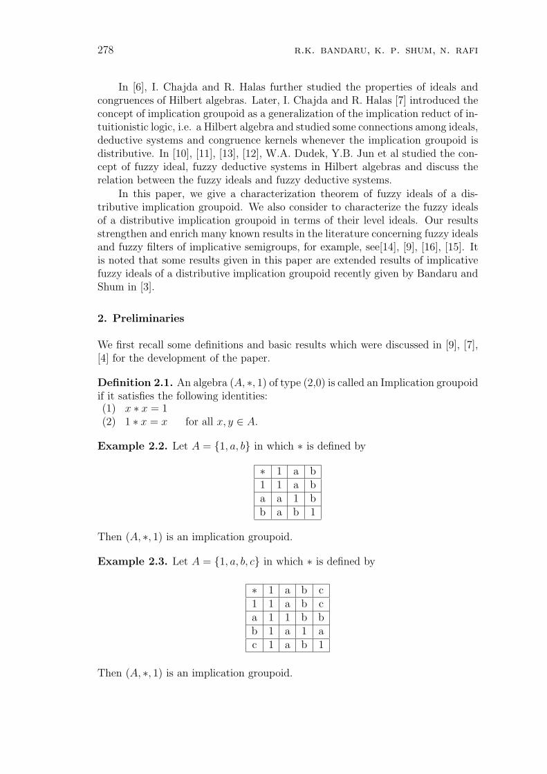
278 r.k. bandaru, k. p. shum, n. rafi
In [6], I. Chajda and R. Halas further studied the properties of ideals andcongruences of Hilbert algebras. Later, I. Chajda and R. Halas [7] introduced theconcept of implication groupoid as a generalization of the implication reduct of in-tuitionistic logic, i.e. a Hilbert algebra and studied some connections among ideals,deductive systems and congruence kernels whenever the implication groupoid isdistributive. In [10], [11], [13], [12], W.A. Dudek, Y.B. Jun et al studied the con-cept of fuzzy ideal, fuzzy deductive systems in Hilbert algebras and discuss therelation between the fuzzy ideals and fuzzy deductive systems.
In this paper, we give a characterization theorem of fuzzy ideals of a dis-tributive implication groupoid. We also consider to characterize the fuzzy idealsof a distributive implication groupoid in terms of their level ideals. Our resultsstrengthen and enrich many known results in the literature concerning fuzzy idealsand fuzzy filters of implicative semigroups, for example, see[14], [9], [16], [15]. Itis noted that some results given in this paper are extended results of implicativefuzzy ideals of a distributive implication groupoid recently given by Bandaru andShum in [3].
2. Preliminaries
We first recall some definitions and basic results which were discussed in [9], [7],[4] for the development of the paper.
Definition 2.1. An algebra (A, ∗, 1) of type (2,0) is called an Implication groupoidif it satisfies the following identities:(1) x ∗ x = 1(2) 1 ∗ x = x for all x, y ∈ A.
Example 2.2. Let A = 1, a, b in which ∗ is defined by
∗ 1 a b1 1 a ba a 1 bb a b 1
Then (A, ∗, 1) is an implication groupoid.
Example 2.3. Let A = 1, a, b, c in which ∗ is defined by
∗ 1 a b c1 1 a b ca 1 1 b bb 1 a 1 ac 1 a b 1
Then (A, ∗, 1) is an implication groupoid.

fuzzy ideals of implication groupoids 279
Definition 2.4. An Implication groupoid (A, ∗, 1) of type (2,0) is called a dis-tributive implication groupoid if it satisfies the following identity:
(LD) x ∗ (y ∗ z) = (x ∗ y) ∗ (x ∗ z) (left distributivity)
for all x, y, z ∈ A.
Example 2.5. Let A = 1, a, b, c, d in which ∗ is defined by
∗ 1 a b c d1 1 a b c da 1 1 b b 1b 1 a 1 1 dc 1 a 1 1 dd 1 1 c c 1
Then (A, ∗, 1) is a distributive implication groupoid.
In every implication groupoid, one can introduce the so called induced relation≤ by the setting
x ≤ y if and only if x ∗ y = 1.
Lemma 2.6. Let (A, ∗, 1) be a distributive implication groupoid. Then A satisfiesthe identities
x ∗ 1 = 1 and x ∗ (y ∗ x) = 1
Moreover, the induced relation ≤ is a quasiorder on A and the following relation-ships are satisfied:(i) x ≤ 1(ii) x ≤ y ∗ x(iii) x ∗ ((x ∗ y) ∗ y) = 1(iv) 1 ≤ x implies x = 1(v) y ∗ z ≤ (x ∗ y) ∗ (x ∗ z)(vi) x ≤ y implies y ∗ z ≤ x ∗ z(vii) x ∗ (y ∗ z) ≤ y ∗ (x ∗ z)(viii) x ∗ y ≤ (y ∗ z) ∗ (x ∗ z)
Definition 2.7. Let A = (A, ∗, 1) be an implication groupoid. A subset I ⊆ A iscalled an ideal of A if(I1) 1 ∈ I(I2) x ∈ A, y ∈ I imply x ∗ y ∈ I.(I3) x ∈ A, y1, y2 ∈ I imply (y2 ∗ (y1 ∗ x)) ∗ x ∈ I
Remark 2.8. If I is an ideal of an implication groupoid A = (A, ∗, 1) and a ∈ I,x ∈ A, then (a ∗ x) ∗ x ∈ I.
Definition 2.9. Let A = (A, ∗, 1) be an implication groupoid. A subset D ⊆ Ais called a deductive system of A if(D1) 1 ∈ D(D2) x ∈ D and x ∗ y ∈ D imply y ∈ D.

280 r.k. bandaru, k. p. shum, n. rafi
Lemma 2.10. Let A be an implication groupoid. Then every ideal of A is adeductive system of A.
It is noted that the converse of the above lemma does not hold in general.
Example 2.11. From Example 2.2, we can easily see that 1, a is its deductivesystem which is not an ideal since b ∗ a = b /∈ 1, a.Theorem 2.12. A nonempty subset I of a distributive implication groupoid A isan ideal if and only if it is a deductive system of A.
Definition 2.13. Let X be a set. A fuzzy set in X is a function µ : X −→ [0, 1].
Definition 2.14. Let µ be a fuzzy set in a set X. For α ∈ [0, 1], the set µα =x ∈ X | µ(x) ≥ α is called a level subset of µ.
Definition 2.15. If µ is a fuzzy relation on a set X and ν is a fuzzy set in X,then µ is called a fuzzy relation on ν if
µ(x, y) ≤ minν(x), ν(y) for all x, y ∈ X.
Definition 2.16. The Cartesian product of two fuzzy sets µ and ν in X is de-fined by
(µ× ν)(x, y) = minν(x), ν(y) for all x, y ∈ X.
Lemma 2.17. Let µ and ν be fuzzy sets in a set X. Then(i) µ× ν is a fuzzy relation on X.(ii) (µ× ν)α = µα × να for all α ∈ [0, 1].
Definition 2.18. Let ν be a fuzzy set in a set X. The strongest fuzzy relation onX is a fuzzy relation µν defined by µν defined by
µν(x, y) = minν(x), ν(y) for all x, y ∈ X.
Lemma 2.19. For a given fuzzy set ν in a set X, let µν be the strongest fuzzyrelation on X. Then for α ∈ [0, 1], we have (µν)α = να × να.
3. Fuzzy ideals
In this section we introduce the concept of fuzzy ideal in a distributive implicationgroupoid and study their properties.
In what follows, X is a distributive implication groupoid unless otherwisespecified.
Definition 3.1. A fuzzy set µ in X is called a fuzzy ideal of X if it satisfies thefollowing conditions:(i) µ(1) ≥ µ(x)(ii) µ(y) ≥ minµ(x), µ(x ∗ y), for all x, y ∈ X.

fuzzy ideals of implication groupoids 281
Example 3.2. Let A = 1, a, b, c, d in which ∗ is defined by
∗ 1 a b c d1 1 a b c da 1 1 1 1 db 1 1 1 1 dc 1 1 1 1 dd 1 a b c 1
Then (A, ∗, 1) is a distributive implication groupoid. Let t1, t2 ∈ [0, 1] be suchthat t1 > t2. Define a mapping µ : X −→ [0, 1] by µ(1) = µ(d) = t1 and µ(a) =µ(b) = µ(c) = t2. Then µ is a fuzzy ideal of X.
We now give a characterization theorem of fuzzy ideals of a distributive im-plication groupoid.
Theorem 3.3. Let µ be a fuzzy set in a distributive implication groupoid X. Thenµ is a fuzzy ideal of X if and only if for every α ∈ [0, 1], the level subset µα is anideal of X, when µα 6= ∅.
Proof. Let µ be a fuzzy ideal of X. Then µ(1) ≥ µ(x) for all x ∈ X.In particular, µ(1) ≥ µ(x) ≥ α for every x ∈ µα. Hence 1 ∈ µα.Let x, x ∗ y ∈ µα. Then µ(x) ≥ α and µ(x ∗ y) ≥ α and hence µ(y) ≥
minµ(x), µ(x ∗ y) ≥ α. Therefore y ∈ µα. Hence µα is an ideal of X.Conversely, assume that µα is an ideal of X for every α ∈ [0, 1] with µα 6= ∅.
Let x, y ∈ X and µ(x ∗ y) = α1 and µ(x) = α2. Then x ∗ y ∈ µα1 and x ∈ µα2 .Without loss of generality, we may assume that α1 ≤ α2. Then µα2 ⊆ µα1 andso x ∈ µα1 . Since µα1 is a ideal of X, we have y ∈ µα1 . Hence, µ(y) ≥ α1 =minµ(x ∗ y), µ(x).
Suppose µ(1) < µ(x0) for some x0 ∈ X. Let α0 = 12(µ(1) + µ(x0)). Then
µ(1) < α0 and 0 ≤ α0 < µ(x0) ≤ 1. Hence x0 ∈ µα0 and µα0 6= ∅. Since µα0 is aideal of X, we have 1 ∈ µα0 and so µ(1) ≥ α0. This is a contradiction and henceµ(1) ≥ µ(x) for all x ∈ X. Therefore, µ is a fuzzy ideal of X.
Definition 3.4. Let µ be a fuzzy ideal of X. Then for each α ∈ [0, 1],the ideal µα
of X, α ∈ [0, 1], is called a level ideals of µ, when µα 6= ∅.
Now, we give a crucial lemma concerning the level ideals of a distributiveimplication groupoid.
Lemma 3.5. Any ideal of a distributive implication groupoid X can be realizedas a level ideal of some fuzzy ideal of X.
Proof. Let A be an ideal of X and µ : X −→ [0, 1] be a fuzzy set defined by
µ(x) =
α if x ∈ A
0 if x /∈ A.

282 r.k. bandaru, k. p. shum, n. rafi
where α is a fixed number in (0, 1). Note that 1 ∈ A, so that µ(1) = α ≥ µ(x) forall x ∈ A. Let x, y ∈ X. Now, we verify condition (ii) of Definition 3.1.
If x ∈ A and x ∗ y ∈ A then y ∈ A and whence µ(y) = µ(x) = µ(x ∗ y) = α.Hence, we have
µ(y) ≥ minµ(x), µ(x ∗ y).If x /∈ A and x ∗ y /∈ A then µ(x) = µ(x ∗ y) = 0. This shows that
µ(y) ≥ minµ(x), µ(x ∗ y).
If exactly one of x and x ∗ y ∈ A then exactly one of µ(x) and µ(x ∗ y) isequal to 0. Hence,
µ(y) ≥ minµ(x), µ(x ∗ y)Therefore,
µ(y) ≥ minµ(x), µ(x ∗ y) for all x, y ∈ X.
This proves that µ is fuzzy ideal of X and µα = A.
In the following theorems, we consider the level ideals of a distributive impli-cation groupoid X.
Theorem 3.6. Let µ be a fuzzy ideal of a distributive implication groupoid X.Then two level ideals µα1 , µα2 (with α1 < α2) of µ are equal if and only if there isno x ∈ X such that α1 ≤ µ(x) < α2.
Proof. Assume that µα1 = µα2 for α1 < α2. If there exists x ∈ X such thatα1 ≤ µ(x) < α2 then µα2 is a proper subset of µα1 . This is impossible.
Conversely, suppose that there is no x ∈ X such that α1 ≤ µ(x) < α2. Notethat α1 < α2 implies µα2 ⊆ µα1 . If x ∈ µα1 , then µ(x) ≥ α1 and so µ(x) ≥ α2
because µ(x) ≮ α2. Hence x ∈ µα2 which says that µα1 ⊆ µα2 . Thus µα1 = µα2 .This completes the proof.
Let µ be a fuzzy set in X and denote the image of µ by Im(µ).
Theorem 3.7. Let µ be a fuzzy ideal of a distributive implication groupoid X. IfIm(µ) = α1, α2, ..., αn, where α1 < α2 < · · · < αn, then the family of idealsµαi
(i = 1, 2, ..., n) constitutes all the level ideals of µ.
Proof. Let α ∈ [0, 1] and α /∈ Im(µ). If α < α1, then µα1 ⊆ µα. Since µα1 = X, wehave µα = X and µα = µα1 . If αi < α < αi+1(1 ≤ i ≤ n−1), then there is no x ∈ Xsuch that α ≤ µ(x) < αi+1. Using Theorem 3.7, we obtain µα = µαi+1. This showsthat for any α ∈ [0, 1] with α ≤ µ(1), the level ideals µα is in µαi
| 1 ≤ i ≤ n.
The following lemma is obvious and we omit the proof.
Lemma 3.8. Let X be a distributive implication groupoid and µ a fuzzy ideal ofX. If α and β belong to Im(µ) such that µα = µβ then α = β.

fuzzy ideals of implication groupoids 283
Theorem 3.9. Let µ and ν be two fuzzy ideals of a distributive implicationgroupoid X such that µ and ν have the finite images and have the identical familyof level ideals. If Im(µ) = α1, α2, ..., αm and Im(ν) = β1, β2, ..., βn whereα1 > α2 > · · · > αm and β1 > β2 > · · · > βn then
(i) m = n,(ii) µαi
= νβifor i = 1, 2, ..., m,
(iii) if x ∈ X such that µ(x) = αi then ν(x) = βi for i = 1, 2, ..., m.
Proof. (i) By Theorem 3.7, we can say that the only level ideals of µ and ν areµαi
and νβirespectively. Since µ and ν have the identical family of level ideals, it
follows that m = n and so (i) holds.
(ii) Again, by Theorem 3.7, we get that
µα1 , µα2 , ..., µαm = νβ1 , νβ2 , ..., νbetam,
and, by Theorem 3.6, we have
µα1 ⊂ µα2 ⊂ · · · ⊂ µαm = A and νβ1 ⊂ νβ2 ⊂ · · · ⊂ νβm = A.
Hence µαi= βi for i = 1, 2, ..., m and (ii) holds.
(iii) Let x ∈ A be such that µ(x) = αi and let ν(x) = βj. Then x ∈ µαi= νβi
and so ν(x) ≥ βi. Hence βj ≥ βi which implies νβj⊆ νβi
. Since x ∈ νβj= µαj
,therefore αi = µ(x) ≥ αj. It follows that µαi
⊆ µαj. By (ii), νβi
= µαi, µαj
= νβj.
Consequently νβi= νβj
and by Lemma 3.8 we have βi = βj. Thus ν(x) = βi.
The following theorem can be proved easily.
Theorem 3.10. Let µ and ν be as in Theorem 3.9. Then µ = ν if and only ifIm(µ) = Im(ν).
Theorem 3.11. Let X be a distributive implication groupoid and let µ be a fuzzyset in X with Im(µ) = α0, α1, ..., αk where α0 > α1 > · · · > αk. Suppose thatthere exists a chain of ideals of X : A0 ⊂ A1 ⊂ · · · ⊂ Ak = A such that µ(An) = αn
where An = An − An−1, A−1 = ∅ for n = 0, 1, ..., k. Then µ is a fuzzy ideal of X.
Proof. Since 1 ∈ A0, we have µ(1) = α0 ≥ µ(x) for all x ∈ A. In order to provethat µ satisfies the condition (ii) of Definition 3.1, we divide into the followingcases:
If x and y belong to the same An, then µ(x) = µ(y) = αn and so
µ(y) ≥ minµ(x), µ(x ∗ y)
Assume that x ∈ Ai and y ∈ Aj for every i 6= j. Without loss of generality, wemay assume that i < j. Then µ(x) = αi > αj = µ(y) and so
minµ(y), µ(y ∗ x) ≤ µ(y) < µ(x).

284 r.k. bandaru, k. p. shum, n. rafi
Since x ∈ Ai, we have x ∈ Ai. It follows that x ∈ Aj−1 as i ≤ j − 1. Now, weassert that x ∗ y /∈ Dj−1. In fact, if not, then x ∗ y ∈ Aj−1 and x ∈ Aj−1 implyy ∈ Aj−1, which contradicts to y ∈ Aj = Aj − Aj−1. Hence µ(x ∗ y) ≤ αj and so
µ(y) ≥ minµ(x), µ(x ∗ y).
Summarizing the above results, we obtain that µ(y) ≥ minµ(x), µ(x ∗ y) for allx, y ∈ X. Therefore, µ is a fuzzy ideal of X.
Theorem 3.12. Let µ be a fuzzy ideal of a distributive implication groupoid X.If Im(µ) = α0, α1, ..., αk with α0 > α1 > · · · > αk, then An = µαn , n = 0, 1, ..., kare ideals of X and µ(An) = αn, n = 0, 1, 2, ..., k where An = An − An−1 andA−1 = ∅.
Proof. By Theorem 3.7, An = µαn(n = 0, 1, ..., k) is an ideal of X. Clearly,µ(A0) = α0. Since µ(A1) = α0, α1 for x ∈ A1 we have µ(x) = α1, namelyµ(A1) = α1. Repeating the above argument, we have µ(An) = αn(0 ≤ n ≤ k).
Theorem 3.13. If µ is a fuzzy ideal of a distributive implication groupoid X, thenthe set Xµ = x ∈ X | µ(x) = µ(1) is an ideal of X.
Proof. Clearly, 1 ∈ Xµ. Assume that x ∈ Xµ and x ∗ y ∈ Xµ. Then
µ(x) = µ(1) = µ(x ∗ y).
Since µ is a fuzzy ideal of X, we have
µ(y) ≥ minµ(x), µ(x ∗ y) = µ(1).
Therefore, µ(y) = µ(1). Hence y ∈ Xµ.
Using a given fuzzy ideal, we construct a new fuzzy ideal.Let α ≥ 0 be a real number. If m ∈ [0, 1], mα shall mean the positive root in
case α < 1. We define µα : X → [0, 1] by µα(x) = (µ(x))α.Finally, we conclude this section with the following theorem.
Theorem 3.14. If µ is a fuzzy ideal of a distributive implication groupoid X, thenµα is also a fuzzy ideal of X and Xµα = Xµ.
Proof. We have that µα(1) = (µ(1))α ≥ (µ(x))α = µα(x) for all x ∈ X. Letx, y ∈ X. We assert that µα(y) ≥ minµα(x), µα(x ∗ y). In fact, suppose thatµ(x) ≤ µ(x ∗ y). It follows from Definition 3.1(ii) that
µ(y) ≥ µ(x).
Hence µα(x) ≤ µα(x ∗ y) and µα ≤ µα(y) which imply that
µα(y) ≥ minµα(x), µα(x ∗ y).

fuzzy ideals of implication groupoids 285
The argument is similar if µ(x) ≥ µ(x ∗ y). Finally,
Xµα = x ∈ X | µα(x) = µα(1)= x ∈ X | (µ(x))α = (µ(1))α= x ∈ X | µ(x) = µ(1)= Xµ
4. Cartesian product of fuzzy ideals
Let (X, ∗, 1) and (Y, ∗, 1) be distributive implication groupoids. Define an opera-tion → on X × Y by
(x, y) → (s, t) = (x ∗ s, y ∗ t) for all (x, y), (s, t) ∈ X × Y.
Then we can easily verify that (X × Y,→, (1, 1)) is a distributive implicationgroupoid.
The following proposition can be proved easily.
Proposition 4.1. Let A1 and A2 be ideals of distributive implication groupoidsX and Y respectively. Then A1 × A2 is a ideal of X × Y.
Proposition 4.2. For a given fuzzy set ν in a distributive implication groupoidX, let µν be the strongest fuzzy relation on X. If µν is a fuzzy ideal of X×X thenν(x) ≤ ν(1) for all x ∈ X.
Proof. Since µν is a fuzzy ideal of X ×X, we have
µν(x, y) ≤ µν(1, 1) for all (x, y) ∈ X ×X.
Hence minν(x), ν(y) ≤ minν(1), ν(1) which implies that ν(x) ≤ ν(1) for allx ∈ X.
The following proposition follows from Lemma 2.19 and we omit the proof.
Proposition 4.3. If ν is a fuzzy ideal of a distributive implication groupoid Xthen the level ideals of µν are given by (µν)α = να × να for all α ∈ [0, 1].
Theorem 4.4. Let µ and ν be fuzzy ideals of a distributive implication groupoidX. Then µ× ν is a fuzzy ideal of X ×X.
Proof. For any (x, y) ∈ X ×X, we have
(µ× ν)(1, 1) = minµ(1), ν(1) ≥ minµ(x), ν(y) = (µ× ν)(x, y).
Now, let (x, y), (r, s) ∈ X ×X. Then

286 r.k. bandaru, k. p. shum, n. rafi
min(µ× ν)(x, y), (µ, ν)((x, y) → (r, s))= min(µ× ν)(x, y), (µ, ν)((x ∗ r, y ∗ s))= minminµ(x), ν(y),minµ(x ∗ r), ν(y ∗ s)= minminµ(x), µ(x ∗ r),minν(y), ν(y ∗ s)≤ minµ(r), ν(s)= (µ× ν)(r, s).
Theorem 4.5. Let µ and ν be fuzzy sets in a distributive implication groupoid Xsuch that µ× ν is a fuzzy ideal of X ×X. Then
(i) either µ(1) ≥ µ(x) or ν(1) ≥ ν(x) for all x ∈ X.(ii) if µ(1) ≥ µ(x) for all x ∈ X then ν(1) ≥ µ(x) or ν(1) ≥ ν(x) for all x ∈ X.(iii) if ν(1) ≥ ν(x) for all x ∈ X then µ(1) ≥ ν(x) or µ(1) ≥ µ(x) for all x ∈ X.(iv) either µ or ν is a fuzzy ideal of X.
Proof. (i) If both µ and ν do not satisfy µ(1) ≥ µ(x) and ν(1) ≥ ν(x) for allx ∈ X then there exist x, y ∈ X such that µ(x) > µ(1) and ν(y) > ν(1). Then
(µ× ν)(x, y) = minµ(x), ν(y) > minµ(1), ν(1) = (µ× ν)(1, 1)
which is contradiction. Hence (i) proved.
(ii) Again, we use reduction to absurdity. Let x, y ∈ X be such that µ(x) > ν(1)and ν(y) > ν(1). Then
(µ× ν)(1, 1) = minµ(1), ν(1) = ν(1)
and
(µ× ν)(x, y) = minµ(x), ν(y) > ν(1) = (µ× ν)(1, 1)
which is a contradiction. Hence (ii) is proved.
(iii) The proof is similar to (ii).
(iv) Since, by (i), either µ or ν satisfies Definition 3.1(i), without loss ofgenerality we may assume that µ satisfies Definition 3.1(i). Using (ii), we havethat either µ(x) ≤ ν(1) or ν(x) ≤ ν(1) for all x ∈ X.
If µ(x) ≤ ν(1) for all x ∈ X then
(µ× ν)(x, 1) = minµ(x), ν(1) = µ(x) for all x ∈ X.
Let (x, y), (r, s) ∈ X × X. Since µ × ν is a fuzzy ideal of X × X by Definition3.1(ii) we have
(µ× ν)(r, s) ≥ min(µ× ν)(x, y), (µ× ν)((x, y) → (r, s))= min(µ× ν)(x, y), (µ× ν)(x ∗ r, y ∗ s). (I)

fuzzy ideals of implication groupoids 287
If we take y = s = 1, then
µ(r) = (µ× ν)(r, 1)
≥ min(µ× ν)(x, 1), (µ× ν)(x ∗ r, 1 ∗ 1)= min(µ× ν)(x, 1), (µ× ν)(x ∗ r, 1)= minminµ(x), ν(1), minµ(x ∗ r), ν(1)= minµ(x), µ(x ∗ r)
showing that µ satisfies Definition 3.1(ii). Hence µ is a fuzzy ideal of X.
Now, we consider the case ν(x) ≤ ν(1) for all x ∈ X. Suppose that µ(y) > ν(1)for some y ∈ X. Then µ(1) ≥ µ(y) > ν(1). Since ν(x) ≤ ν(1) for all x ∈ X, itfollows that µ(1) > ν(x) for all x ∈ X. Hence (µ × ν)(1, x) = minµ(1), ν(x) =ν(x) for all x ∈ X.
Taking x = r = 1 in (I), then
ν(s) = (µ× ν)(1, s)
≥ min(µ× ν)(1, y), (µ× ν)(1 ∗ 1, y ∗ s)= min(µ× ν)(1, y), (µ× ν)(1, y ∗ s)= minminµ(1), ν(y), minµ(1), ν(y ∗ s)= minν(y), ν(y ∗ s),
which proves that ν satisfies Definition 3.1(ii). Hence ν is a fuzzy ideal of X.
Now, we give an example to show that if µ× ν is a fuzzy ideal of X×X thenµ and ν both need not be fuzzy ideals of X.
Example 4.6. Let X be a distributive implication groupoid with |A| ≥ 2 and letα, β ∈ [0, 1] be such that 0 ≤ α ≤ β < 1. Define the fuzzy sets µ and ν : X → [0, 1]by µ(x) = α and
ν(x) =
β, if x = 1;
1, if x 6= 1.
for all x ∈ X, respectively. Then (µ × ν)(x, y) = minµ(x), ν(y) = α for all(x, y) ∈ X ×X that is µ× ν : X ×X → [0, 1] is a constant function. Hence µ× νis a fuzzy ideal of X ×X. Now µ is a fuzzy ideal of X but ν is not a fuzzy idealof X because ν does not satisfy Definition 3.1(i).
In the following theorem, we characterize the fuzzy ideal of a distributiveimplication groupoid X.
Theorem 4.7. Let ν be a fuzzy set in a distributive implication groupoid X andlet µν be the strongest fuzzy relation on X. Then ν is a fuzzy ideal of X if andonly if µν is a fuzzy ideal of X ×X.

288 r.k. bandaru, k. p. shum, n. rafi
Proof. Assume that ν is a fuzzy ideal of X. We note from Definition 3.1(i) thatfor all (x, y) ∈ X ×X,
µν(x, y) = minν(x), ν(y) ≤ minν(1), ν(1) = µν(1, 1)
showing that µν satisfies Definition 3.1(i). Let (x, y), (r, s) ∈ X ×X. Then
minµν(x, y), µν((x, y) → (r, s))= minµν(x, y), µν((x ∗ r, y ∗ s))= minminν(x), ν(y), minν(x ∗ r), ν(y ∗ s)= minminν(x), ν(x ∗ r), minν(y), ν(y ∗ s)≤ minν(r), ν(s)= µν(r, s)
This proves that µν satisfies Definition 3.1(ii). Hence µν is a fuzzy ideal of X×X.Conversely, suppose that µν is a fuzzy ideal of X ×X. Then
minν(x), ν(y) = µν(x, y) ≤ µν(1, 1) = minν(1), ν(1) = ν(1),
for all x, y ∈ X. It follows that ν(x) ≤ ν(1) for all x ∈ X.For any (x, y), (r, s) ∈ X ×X, we have
minν(r), ν(s) = µν(r, s)
≥ minµν(x, y), µν((x, y) → (r, s))= minµν(x, y), µν((x ∗ r, y ∗ s))= minminν(x), ν(y), minν(x ∗ r), ν(y ∗ s)= minminν(x), ν(x ∗ r), minν(y), ν(y ∗ s).
In particular, if we take y = s = 1 (resp. x = r = 1), then
ν(r) ≥ minν(x), ν(x ∗ r)( resp. ν(s) ≥ minν(y), ν(y ∗ s)).
Definition 4.8. Let (X, ∗, 1) and (Y, ∆, 1′) be two distributive implication grou-poids. Then a mapping f : X → Y is called a homomorphism if f(x ∗ y) =f(x)∆f(y) for all x, y ∈ X.
Note that if f : X → Y is homomorphism of distributive implication groupoids,then f(1) = 1′.
Definition 4.9. Let f : X → Y be a mapping of distributive implicationgroupoids and µ be a fuzzy set of Y. The map µf is the pre-image of µ underf, if µf (x) = µ(f(x)) for all x ∈ X.
Theorem 4.10. Let f : X → Y be a homomorphism of distributive implicationgroupoids. If µ is a fuzzy ideal of Y then µf is a fuzzy ideal of X.

fuzzy ideals of implication groupoids 289
Proof. For any x ∈ X, we have
µf (x) = µ(f(x)) ≤ µ(1′) = µ(f(1)) = µf (1).
Let x, y ∈ X. Then
minµf (x ∗ y), µf (x) = minµ(f(x ∗ y)), µ(f(x))= minµ(f(x) ∗ f(y)), µ(f(x))≤ µ(f(y)) = µf (y).
Hence µf is a fuzzy ideal of X.
We conclude this paper with the following theorem.
Theorem 4.11. Let f : X → Y be an onto homomorphism of distributive impli-cation groupoids. If µf is fuzzy ideal of X, then µ is a fuzzy ideal of Y.
Proof. Let y ∈ Y . Then there exists x ∈ X such that f(x) = y. Then
µ(y) = µ(f(x)) = µf (x) ≤ µf (1) = µ(f(1)) = µ(1′).
Let x, y ∈ Y. Then there exist a, b ∈ X such that f(a) = x and f(b) = y. Itfollows that
µ(y) = µ(f(b))
= µf (b)
≥ minµf (a ∗ b), µf (a)= minµ(f(a ∗ b)), µ(f(a))= minµ(f(a) ∗ f(b)), µ(f(a))= minµ(x ∗ y), µ(x).
Hence µ is a fuzzy ideal of Y.
References
[1] Abbott, J.C., Semi-Boolean algebras, Mathematicki Vensik, 4 (19) (1976),177-198.
[2] Busneag, D., A note on deductive systems of a Hilberta algebra, Kobe J.Math., 2 (1985), 29-35.
[3] Bandaru, R.K., Shum, K.P., Implicative ideals and Fuzzy implicative idealof a distributive implication groupoid, Journal of Mathematical Research withApplications, 34 (6) (2014), 631-639.
[4] Bhattacharya, P., Mukherjee, N.P., Fuzzy relations and fuzzy groups,Inform. Sci., 36 (1985), 267-282.

290 r.k. bandaru, k. p. shum, n. rafi
[5] Chajda, I., The lattice of deductive systems in Hilbert algebras, SoutheastAsian Bull. Math., 26 (1) (2002), 21-26.
[6] Chajda, I., Halas, R., Congruences and ideals in Hilbert algebras, Kyung-pook Math. J., 39 (1999), 429-43.
[7] Chajda, I., Halas, R., Distributive and implication groupoids, CentralEuropean Journal of Mathematics, 5 (3) (2007), 484-49.
[8] Chajda, I., Halas, R., Zednik, J., Filters and annihilators in implicationalgebras, Acta Univ. Palack. Olomuc. Fac. Rerum Natur. Math., 37 (1998),41-45.
[9] Chan, M.W., Shum, K.P., Homomorphisms of implicative semigroups,Semigrpoup Forum 1993, 46 (1), 7-15.
[10] Dudek, W.A., On fuzzification in Hilbert algebras, Contributions to GeneralAlgebra, 11 (1999), 77-83
[11] Dudek, W.A., Jun, Y.B., On fuzzy ideals in Hilbert algebras, Novi Sad J.Math., 29 (2) (1999), 193-207.
[12] Jun, Y.B., Hong, S.M., On fuzzy deductive systems of Hilbert algebras,Indian Journal of Pure and Applied Mathematics, 27 (2) (1996), 141-151.
[13] Jun, Y.B., Deductive systems of Hilbert algebras, Math. Japon., 43(1996),51-54.
[14] Lee, S.Y., Shum, K.P., Wu, C.X., Filters in fuzzy implicative semigroups,Comm. Algebra, 32 (12) (2004), 4633-4651.
[15] Lee, S.Y., Shum, K.P., Wu, C.X., Broad fuzzy extention of certain fuzzyideals of semigroups on strong semilattices, J. Fuzzy Math., 13 (2005), no. 4,785-797.
[16] Sambassivarao, M., Shum, K.P., On filters of implicativen.p.o.semigroups, Asian-Eur.J.Math., 5 (3) (2012), 1-10.
[17] Wei, S., Meng, J., On implicative semigroups, Southeast Asian Bull.Math., 19 (1995), no. 3, 113-116.
Accepted: 20.12.2014

italian journal of pure and applied mathematics – n. 34−2015 (291−298) 291
SOME REFINEMENTS OF THE HEINZ INEQUALITIES
Jianming Xue
Oxbridge CollegeKunming University of Science and TechnologyKunming, Yunnan 650106P.R. Chinae-mail: [email protected]
Abstract. This paper aims to discuss Heinz inequalities for unitarily invariant norms.We present some refinements of the Heinz inequalities for matrices due to Kittaneh[Integr. Equ. Oper. Theory, 68:519-527, 2010]. Our results generalize the results shownby Feng [J. Inequal. Appl., 2012:18, 2012], Wang [J. Inequal. Appl., 2013:424, 2013]and Yan et al. [J. Inequal. Appl. 2014:50, 2014].
Keywords: Heinz inequality; convex function; unitarily invariant norm.
MSC (2010) Subject Classification: 47A30, 15A60.
1. Introduction
Let Mm,n be the space of m × n complex matrices and Mn = Mn,n. Let ||| · |||denote any unitarily invariant norm on Mn. So, |||UAV ||| = |||A||| for all A ∈ Mn
and for all unitary matrices U, V ∈ Mn. The Ky Fan k-norm ||| · |||(k) is defined as
|||A|||(k) =k∑
j=1
sj (A), k = 1, · · · , n,
where s1 (A) ≥ s2 (A) ≥ · · · ≥ sn−1 (A) ≥ sn (A) are the singular values of A, that
is, the eigenvalues of the positive semidefinite matrix |A| = (AA∗)12 , arranged
in decreasing order and repeated according to multiplicity. The Schattenp-norm||| · |||p is defined as
|||A|||p =
(n∑
j=1
spj (A)
)1/p
= (tr |A|p)1/p, 1 ≤ p < ∞.
It is known that these norms are unitarily invariant [1].

292 j. xue
Let A,B,X ∈ Mn such that A and B are positive semidefinite. Then, forevery unitarily invariant norm, the function
ϕ (v) = |||AvXB1−v + A1−vXBv|||
is convex on [0, 1], attains its minimum at v =1
2and attains its maximum at
v = 0 and v = 1. Moreover, ϕ (v) = ϕ (1− v) for 0 ≤ v ≤ 1 .
Bhatia and Davis proved Heinz inequalities in [2] that if A,B, X ∈ Mn suchthat A and B are positive semidefinite, for 0 ≤ v ≤ 1 and for every unitarilyinvariant norm, then
(1)2|||A 1
2 XB12 ||| ≤ |||AvXB1−v + A1−vXBv|||
≤ |||AX + AB|||.
For more information on Heinz inequality for matrices, the reader is referredto [2]-[7].
By the convexity of function ϕ (v) = |||AvXB1−v +A1−vXBv|||, Kittaneh [3],Feng [4], Wang [5] and Yan et al [6] got some refinements of (1). In this paper, wealso present several refinements of (1). Our results are generalization of resultsshown in [3]-[6].
2. Main results
In this section, we present several improvement refinements of the Heinz inequal-ities, to do this, we need the following lemmas.
Lemma 1. (Hermite-Hadamard Integral Inequality) [3] Let f be a real valuedconvex function on the interval [a, b]. Then
f
(a + b
2
)≤ 1
b− a
∫ b
a
f (t) dt ≤ f (a) + f (b)
2.
Lemma 2. Let f be a real valued convex function on the interval [a, b]. Then
f
(a + b
2
)≤ 1
b− a
∫ b
a
f (t) dt
≤ 1
2n
[(n− 1) f (a) + 2f
(a + b
2
)+ (n− 1) f(b)
]
≤ f (a) + f (b)
2,
where n ≥ 2 is an integer.

some refinements of the heinz inequalities 293
Proof. By Lemma 1, we can easily verify the inequality
1
2n
[(n− 1) f (a) + 2f
(a + b
2
)+ (n− 1) f(b)
]≤ f (a) + f (b)
2.
Then, we will prove the following inequality:
1
b− a
∫ b
a
f (t) dt ≤ 1
2n
[(n− 1) f (a) + 2f
(a + b
2
)+ (n− 1) f(b)
].
Using Lemma 1, we have
1
b− a
∫ b
a
f (t)dt =1
b− a
∫ a+b2
a
f (t)dt +1
b− a
∫ b
a+b2
f (t)dt
≤ 1
b− a
[f (a) + f
(a+b2
)
2· b− a
2+
f(
a+b2
)+ f (b)
2· b− a
2
]
=1
4
[f (a) + 2f
(a + b
2
)+ f (b)
]
=1
2n
[n
2f (a) + nf
(a + b
2
)+
n
2f (b)
]
≤ 1
2n
[n
2f (a) + 2f
(a + b
2
)+
n− 2
2(f (a) + f (b)) +
n
2f (b)
]
=1
2n
[(n− 1) f (a) + 2f
(a + b
2
)+ (n− 1) f(b)
].
This completes the proof.
Applying Lemma 2 to the function ϕ (v) = |||AvXB1−v + A1−vXBv||| on the
interval [u, 1− u] when 0 ≤ u <1
2, and on the interval [1− u, u] when
1
2< u ≤ 1,
we achieve a refinement of the first inequality in (1).
Theorem 1. Let A,B, X ∈ Mn such that A and B are positive definite, for0 ≤ u ≤ 1 and for every unitarily invariant norm. Then
(2)
2|||A 12 XB
12 ||| ≤ 1
|1− 2u|
∣∣∣∣∫ 1−u
u
|||AvXB1−v + A1−vXBv|||dv
∣∣∣∣
≤ 1
n
[(n− 1)|||AuXB1−u + A1−uXBu|||+ 2|||A 1
2 XB12 |||
]
≤ |||AuXB1−u + A1−uXBu|||,
where n ≥ 2 is an integer.

294 j. xue
Proof. If 0 ≤ u <1
2, then, by Lemma 2, we have
ϕ
(1− u + u
2
)≤ 1
1− 2u
∫ 1−u
u
ϕ (v) dv
≤ 1
2n
[(n− 1) ϕ (u) + 2ϕ
(1− u + u
2
)+ (n− 1) ϕ(1− u)
]
≤ ϕ (u) + ϕ (1− u)
2.
That is,
ϕ
(1
2
)≤ 1
1− 2u
∫ 1−u
u
ϕ (v) dv
≤ 1
n
[(n− 1)ϕ (u) + ϕ
(1
2
)]
≤ ϕ (u) ,
where ϕ (v) = |||AvXB1−v + A1−vXBv|||. Thus
(3)
2|||A 12 XB
12 ||| ≤ 1
1− 2u
∫ 1−u
u
|||AvXB1−v + A1−vXBv|||dv
≤ 1
n
[(n− 1)|||AuXB1−u + A1−uXBu|||+ 2|||A 1
2 XB12 |||
]
≤ |||AuXB1−u + A1−uXBu|||.
If1
2< u ≤ 1, then the proof is similar to the case 0 ≤ u <
1
2, so we obtain
(4)
2|||A 12 XB
12 ||| ≤ 1
2u−1
∫ u
1−u|||AvXB1−v + A1−vXBv|||dv
≤ 1
n
[(n− 1)|||AuXB1−u + A1−uXBu|||+ 2|||A 1
2 XB12 |||
]
≤ |||AuXB1−u + A1−uXBu|||.Hence,
limu→ 1
2
1
|1− 2u|
∣∣∣∣∫ 1−u
u
|||AvXB1−v + A1−vXBv|||dv
∣∣∣∣
= limu→ 1
2
1
n
[(n− 1)|||AuXB1−u + A1−uXBu|||+ 2|||A 1
2 XB12 |||
]
= 2|||A 12 XB
12 |||.
The inequalities in (2) follow by combining the inequalities (3) and (4). Thiscompletes the proof.

some refinements of the heinz inequalities 295
Applying Lemma 2 to the function ϕ (v) = |||AvXB1−v + A1−vXBv||| on theinterval
[u, 1
2
]when 0 ≤ u < 1
2, and on the interval
[12, u
]when 1
2< u ≤ 1, we
obtain the following result.
Theorem 2. Let A,B, X ∈ Mn such that A and B are positive definite. For0 ≤ u ≤ 1 and for every unitarily invariant norm. Then
(5)
|||A 1+2u4 XB
3−2u4 + A
3−2u4 XB
1+2u4 |||
≤ 2
|1− 2u|
∣∣∣∣∣∫ 1
2
u
|||AvXB1−v + A1−vXBv|||dv
∣∣∣∣∣
≤ 1
2n
[(n− 1)|||AuXB1−u + A1−uXBu|||
+2|||A 1+2u4 XB
3−2u4 + A
3−2u4 XB
1+2u4 |||+ 2(n− 1)|||A 1
2 XB12 |||]
≤ 1
2
(|||AuXB1−u + A1−uXBu|||+ 2|||A 1
2 XB12 |||
),
where n ≥ 2 is an integer.
Proof. The proof is similar to Theorem 1, so we omit it.
Inequalities (5) and the first inequality in (1) yield the following refinementof the first inequality in (1).
Corollary 1. Let A,B,X ∈ Mn such that A and B are positive definite. For0 ≤ u ≤ 1 and for every unitarily invariant norm. Then
(6)
2|||A 12 XB
12 ||| ≤ |||A 1+2u
4 XB3−2u
4 + A3−2u
4 XB1+2u
4 |||
≤ 2
|1− 2u|
∣∣∣∣∣∫ 1
2
u
|||AvXB1−v + A1−vXBv|||dv
∣∣∣∣∣
≤ 1
2n[(n− 1)|||AuXB1−u + A1−uXBu|||
+2|||A 1+2u4 XB
3−2u4 + A
3−2u4 XB
1+2u4 |||+ 2(n− 1)|||A 1
2 XB12 |||]
≤ 1
2
(|||AuXB1−u + A1−uXBu|||+ 2|||A 1
2 XB12 |||
)
≤ |||AuXB1−u + A1−uXBu|||,where n ≥ 2 is an integer.
It should be noticed here that in the inequalities (5) and (6)
limu→ 1
2
1
|1− 2u|
∣∣∣∣∣∫ 1
2
u
|||AvXB1−v + A1−vXBv|||dv
∣∣∣∣∣ = |||A 12 XB
12 |||.

296 j. xue
In the sequel, we get another refinement of the second inequality in (1).Applying Lemma 2 to the function ϕ (v) = |||AvXB1−v + A1−vXBv||| on the
interval [0, u] when 0 < u ≤ 1
2, and on the interval [u, 1] when
1
2≤ u < 1, we
obtain the following theorem.
Theorem 3. Let A,B, X ∈ Mn such that A and B are positive definite. Then
1. for 0 ≤ u ≤ 12
and for every unitarily invariant norm,
(7)
|||Au2 XB1−u
2 + A1−u2 XB
u2 |||
≤ 1
u
∫ u
0
|||AvXB1−v + A1−vXBv|||dv
≤ 1
2n[(n− 1)|||AX + XB|||+ 2|||Au
2 XB1−u2 + A1−u
2 XBu2 |||
+(n− 1)|||AuXB1−u + A1−uXBu|||]
≤ 1
2
(|||AX + XB|||+ |||AuXB1−u + A1−uXBu|||) ,
where n ≥ 2 is an integer,
2. for1
2≤ u ≤ 1 and for every unitarily invariant norm,
(8)
|||A 1+u2 XB
1−u2 + A
1−u2 XB
1+u2 |||
≤ 1
1− u
∫ 1
u
|||AvXB1−v + A1−vXBv|||dv
≤ 1
2n[(n− 1)|||AX + XB|||+ 2|||A 1+u
2 XB1−u
2 + A1−u
2 XB1+u
2 |||
+(n− 1)|||AuXB1−u + A1−uXBu|||]
≤ 1
2
(|||AX + XB|||+ |||AuXB1−u + A1−uXBu|||) ,
where n ≥ 2 is an integer.
Proof. The proof is similar to Theorem 1, so we omit it.
In view of the fact that the function ϕ (v) = |||AvXB1−v + A1−vXBv|||is decreasing on the interval
[0,
1
2
]and increasing on the interval
[1
2, 1
], by Theo-
rem 3, we have the following result, which is a refinement of the second inequalityin (1).

some refinements of the heinz inequalities 297
Corollary 2. Let A,B,X ∈ Mn such that A and B are positive definite. Then
1. for 0 ≤ u ≤ 1
2and for every unitarily invariant norm
(9)
|||AuXB1−u + A1−uXBu|||≤ |||Au
2 XB1−u2 + A1−u
2 XBu2 |||
≤ 1
u
∫ u
0
|||AvXB1−v + A1−vXBv|||dv
≤ 1
2n[(n− 1)|||AX + XB|||+ 2|||Au
2 XB1−u2 + A1−u
2 XBu2 |||
+(n− 1)|||AuXB1−u + A1−uXBu|||]
≤ 1
2
(|||AX + XB|||+ |||AuXB1−u + A1−uXBu|||)
≤ |||AX + XB|||,where n ≥ 2 is an integer.
2. for1
2≤ u ≤ 1 and for every unitarily invariant norm
(10)
|||AuXB1−u + A1−uXBu|||≤ |||A 1+u
2 XB1−u
2 + A1−u
2 XB1+u
2 |||
≤ 1
1− u
∫ 1
u
|||AvXB1−v + A1−vXBv|||dv
≤ 1
2n[(n− 1)|||AX + XB|||+ 2|||A 1+u
2 XB1−u
2 + A1−u
2 XB1+u
2 |||
+(n− 1)|||AuXB1−u + A1−uXBu|||]
≤ 1
2
(|||AX + XB|||+ |||AuXB1−u + A1−uXBu|||)
≤ |||AX + XB|||,where n ≥ 2 is an integer.
It should be noticed that in the inequalities (7) to (10), we have
limu→0
1
u
∫ u
0
|||AvXB1−v + A1−vXBv|||dv
= limu→1
1
1− u
∫ 1
u
|||AvXB1−v + A1−vXBv|||dv
= |||AX + XB|||.

298 j. xue
Remark 1. The three special values n = 2, n = 16 and n = 4 give the refinementsof Heinz inequalities obtained in [4], [5] and [6], respectively.
Acknowledgments. This research was supported by Scientific Research Fundof Yunnan Provincial Education Department (No. 2013C157).
References
[1] Bhatia, R., Matrix Analysis, Springer-Verlag, New York, 1997.
[2] Bhatia, R., Davis, C., More matrix forms of the arithmetic-geometricmean inequality, SIAM J. Matrix Anal. Appl., 14 (1993), 132–136.
[3] Kittaneh, F., On the convexity of the Heinz means, Integr. Equ. Oper.Theory, 68 (2010), 519-527.
[4] Feng, Y., Refinements of the Heinz inequalities, J. Inequal. Appl., 18 (2012).
[5] Wang, S., Some new refinements of Heinz inequalities of matrices,J. Inequal. Appl., 424 (2013).
[6] Yan, Y., Feng,Y., Chen, G., Refinements of the Heinz inequalities formatrices, J. Inequal. Appl., 50 (2014).
[7] Zou, L., He, C., On some inequalities for unitarily invariant norms andsingular values, Linear Algebra Appl., 436 (2012), 3354-3361.
Accepted: 22.12.2014

italian journal of pure and applied mathematics – n. 34−2015 (299−310) 299
COMPUTATION OF TOPOLOGICAL INDICESOF NON-COMMUTING GRAPHS
M. Jahandideh
Department of MathematicsShahid Chamran University of AhvazAhvazIranDepartment of MathematicsCollege of polymerIslamic Azad UniversityMahshahr BranchMahshahrIrane-mail: [email protected]
Abstract. Let G be a non-abelian finite group. The non-commuting graph ΓG of G
is defined as a graph with vertex set G − Z(G) in which two distinct vertices x andy are joined if and only if xy 6= yx. Various topological indices have been defined forsimple and connected graphs. Since non-commuting graph is a simple and connectedgraph, topological indices could be defined for it. The main object of this article isto calculate various indices like Wiener index, Hyper-Wiener index, Schultz index andGutman index for the non-commuting graph of the group G.
Keywords: non-commuting graph, Wiener index, hyper-Wiener index, Schultz index,Gutman index.
Mathematics Subject Classification: 05c12.
1. Introduction
Let G be a non-abelian finite group. Various graphs could be attributed to G,one of which is the non-commuting graph denoted by ΓG. The set of vertices andedges of ΓG are V (ΓG) and E(ΓG) respectively so that V (ΓG) = G − Z(G) inwhich Z(G) is the center of G and for every x, y ∈ V (ΓG) we have:
x, y ∈ E(ΓG) ⇐⇒ xy 6= yx
It is apparent that if G is an abelian group, ΓG would turn to a null graph. Forthis, G is assumed to be a non-abelian group. The centralizer of x within G whichis denoted by CG(x) is a subset of G which is defined as g ∈ G| gx = xg.

300 m. jahandideh
According to [8] the non-commuting graph of a finite group G was first intro-duced by Paul Erdos in connection with the following problem: let G be a groupwhose non-commuting graph ΓG has no infinite complete subgraphs. Is it truethat there is a finite bound on the cardinalities of complete subgraphs of ΓG? By[8] the answer to this question is positive and this was the origin of many similarquestions and research.
Assume that Γ = (V, E) is a graph in which V is the set of vertices and Eis the set of edges. This graph is assumed to be a finite graph whenever |V |, |E|are finite. We assume this graph is connected, the distance between two x and ythe vertex is shown as d(x, y). It is the shortest path between the two vertices xand y. The degree of the vertex x which is shown by ρ(x) equals to the numberof edges through x. The largest distance between all pairs of the vertices of G iscalled the diameter of G.
The Wiener index of the graph G which is shown as W (G) is defined asfollows:
W (G) =1
2
∑x,y∈V
d(x, y) =1
2
∑x∈V
d(x).
Where d(x) =∑v∈V
d(x, v).
The Wiener index is one of the oldest descriptors concerned with the molecu-lar graph. This index first was proposed by H. Wiener [9] and it is concerned withthe determination of the boiling points of Paraffins. In mathematical research,the Wiener index has been first studied in [4]. It is an invariant of the graph, itis invariant under the automorphism group of the graph.
The Hyper-Wiener index of the graph G which is shown as WW (G) is definedas follows:
WW (G) =1
2
∑
x,y⊂V
(d(x, y) + d2(x, y)).
The Hyper-Wiener index is one of the recently introduced distance-based mo-lecular structure-descriptors. It was put forward in 1993 and since then it hasattracted much attention of theoretical chemists. In parallel with the symbol Wfor the Wiener index the hyper-Wiener index is traditionally denoted by WW[3], [6].
Schultz in 1989 introduced a graph-theoretical descriptor for characterizingalkanes by an integer, namely the Schultz index, defined as
S(G) =∑
x,y⊂V
(ρ(x) + ρ(y))d(x, y).
The Gutman index (also known as Schultz index of the second kind [2], [3], [5],[7]) of a graph G is defined as
Gut(G) =∑
x,y⊂V
ρ(x)ρ(y)d(x, y).

computation of topological indices of non-commuting graphs 301
Our main goal is to calculate the above mentioned indices for the non-commutinggraph of G in terms of the order of G,Z(G) and the number of conjugacy classesof G. The following lemmas will be used repeatedly in calculating process:
Lemma 1.1. Let G be a non-abelian finite group, then diam(ΓG) = 2.
Proof. This is Proposition 2.1 in [1].
Lemma 1.2. Let G be a non-abelian finite group and k be the number of conjugacyclasses of G, then
|E(ΓG)| = 1
2|G|(|G| − k(G)).
Proof. See [1] Lemma 3.27.
Lemma 1.3. Let G be a non-abelian finite group. If x is one of the vertices ofΓG, then
ρ(x) = |G| − |CG(x)|.Proof. See Lemma 3.1 in [1].
2. The Wiener index of the non-commuting graph of a group
Before we calculate the Wiener index, we prove the following lemma.
Lemma 2.1. Let G be a finite group and k be the number of conjugacy classes ofG, then ∑
x6∈Z(G)
|CG(x)| = |G|(k − |Z(G)|).
Proof. We know that G is the union of its conjugacy classes and assume thatxik
i=1 is the set of the representatives of the conjugacy classes of G. Then wehave:
G =k⋃
i=1
class(xi)
Now, let xiti=1 be the set of non-central of G class representatives and then we
have k = t + |Z(G)|. Every x which is not placed within would be placed withinone of Z(G) in which class(xi)s in which 1 ≤ i ≤ t. Therefore we have:
∑
x 6∈Z(G)
|CG(x)| =t∑
i=1
| class(xi)| |CG(xi)| = |G|t = |G|(k − |Z(G)|).
Now, we calculate the Wiener index of the non-commuting graph of a group G.Assume that x, y ∈ G−Z(G) are two arbitrary distinct vertices of the graph
ΓG. According to the Lemma 1.1 we have d(x, y) = 1 or 2.If d(x, y) = 1, then xy 6= yx and y ∈ G− CG(x).If d(x, y) = 2, then xy = yx and x 6= y ∈ CG(x)− Z(G).

302 m. jahandideh
So, we have
W (ΓG) =1
2
∑
x∈G−Z(G)
d(x)
for all x ∈ G− Z(G). Therefore:
d(x) = 2 (The number of vertices whose distance from x is 2)
+ 1(The number of vertices whose distance from x is 1).
Then
d(x) = 2(|CG(x)| − |Z(G)| − 1) + (|G| − |CG(x)|) = |G|+ |CG(x)| − 2|Z(G)| − 2
Now, we can calculate the Wiener index:
W (ΓG) =1
2
∑
x∈G−Z(G)
d(x)
=1
2
∑
x∈G−Z(G)
(|G| − 2|Z(G)| − 2) + |CG(x)|
=1
2
(|G| − 2|Z(G)| − 2)(|G| − |Z(G)|) +
∑
x∈G−Z(G)
|CG(x)|
By Lemma 2.1, we have
W (ΓG) =1
2[(|G| − 2|Z(G)| − 2)(|G| − |Z(G)|) + |G|(k − |Z(G)|)]
So
W (ΓG) =1
2[(|G| − 2|Z(G)|)2− |G|(|G| − k) + |G|(|G| − 2)− 2|Z(G)|(|Z(G)| − 1)]
or
W (ΓG) =1
2[(|G| − 2|Z(G)|)2 − 2|E(ΓG)|+ |G|(|G| − 2)− 2|Z(G)|(|Z(G)| − 1)].
Therefore, we have proved the following:
Theorem 2.2. Let G be a non-abelian finite group and ΓG be its non-commutinggraph. Then
W (ΓG) =1
2[(|G| − 2|Z(G)|)2 − 2|E(ΓG)|+ |G|(|G| − 2)− 2|Z(G)|(|Z(G)| − 1)].

computation of topological indices of non-commuting graphs 303
3. The Hyper-Wiener index of non-commuting graph of a group
Assume that x, y are two arbitrary vertices of the non-commuting graph of thegroup G. The Hyper-Wiener index of this graph is defined as follows:
WW (G) =1
4
∑
x,y∈G−Z(G)
(d(x, y) + d2(x, y)).
In order to calculate the Hyper-Wiener index; first we calculate d2(x, y) for everyx, y ∈ G− Z(G).
Let us set G− Z(G) = ximi=1 where m = |G| − |Z(G)|. So we have:
∑
x,y∈G−Z(G)
d2(x, y) =∑
xi∈G−Z(G)
d2(x1, xi) + . . . +∑
xi∈G−z(G)
d2(xm, xi)
Without loss of generality, we calculate∑
xi∈G−Z(G)
d2(xj, xi) for a constant xj.
1) If d2(xj, xi) = 1, then xjxi 6= xixj and xi ∈ G− CG(xj).
2) If d2(xj, xi) = 4, then xjxi = xixj and xj 6= xi ∈ CG(xj)− Z(G).
Therefore:∑
xi∈G−Z(G)
d2(xj, xi) = 4 (The number of vertices whose distances from x is 2)
+ (The number of vertices whose distances from x is 1)
= 4(|CG(x1)| − |Z(G)| − 1) + (|G| − |CG(xj)|)= |G|+ 3|CG(xj)| − 4|Z(G)| − 4
But, xj is an arbitrary vertex. So we can write this formula for all xi in which1 ≤ i ≤ m. Now we calculate
∑x,y∈G−Z(G)
d2(x, y).
∑
x,y∈G−Z(G)
d2(x, y) =m∑
i=1
(|G|+ 3|CG(xi)| − 4|Z(G)| − 4)
= (|G| − 4|Z(G)| − 4)(|G| − |Z(G)|) + 3m∑
i=1
|CG(xi)|
= (|G| − 4|Z(G)| − 4)(|G| − |Z(G)|) + 3|G|(k − |Z(G)|)= (|G| − 4|Z(G)|)2 + |G|(3|G| − 4)
− 6|E(ΓG)| − 4|Z(G)|(3|Z(G)| − 1).
So, the Hyper-Wiener index is as follows:
WW (ΓG) =1
2W (ΓG) +
1
4[(|G| − 4|Z(G)|)2 + |G|(3|G| − 4)
−6|E(ΓG)| − 4|Z(G)|(3|Z(G)| − 1)].

304 m. jahandideh
By Lemma 2.1, we have:
WW (ΓG) =1
4[(|G| − 4|Z(G)|)2 + (|G| − 2|Z(G)|)2 − 8|E(ΓG)|
+ 2|G|(2|G| − 3)− 2|Z(G)|(7|Z(G)| − 3)].
Therefore, we have proved the following:
Theorem 3.1. Let G be a non-abelian finite group and ΓG be its non-commutinggraph. Then
WW (ΓG) =1
4[(|G| − 4|Z(G)|)2 + (|G| − 2|Z(G)|)2 − 8|E(ΓG)|
+ 2|G|(2|G| − 3)− 2|Z(G)|(7|Z(G)| − 3)].
4. The Schultz index of the non-commuting graph of a group
The Schultz index of a general graph Γ = (V,E) is as follows:
S(ΓG) =∑
x,y⊂V
(ρ(x) + ρ(y))d(x, y).
Without loss of generality we calculate∑
xi∈G−Z(G)
(ρ(xj) + ρ(xi))d(xj, xi) for a
fixed xj.
∑
xi∈G−Z(G)
(ρ(xj) + ρ(xi))d(xj, xi) =∑
xi∈G−CG(xj)
ρ(xj) + ρ(xi) + 2
=∑
xj 6=xi∈CG(xj)−Z(G)
ρ(xj) + ρ(xi)
Therefore, we have:
∑
xi∈G−Z(G)
(ρ(xj) + ρ(xi))d(xj, xi) =∑
xi∈G−CG(xj)
(2|G| − |CG(xj)| − |CG(xi)|)
+ 2∑
xj 6=xi∈CG(xj)−Z(G)
(2|G| − |CG(xj)| − |CG(xi)|)
= (2|G| − |CG(xj)|)(|G|+ |CG(xj)| − 2|Z(G)| − 2)
− ∑
xi∈G−CG(xj)
|CG(xj)|+∑
xj 6=xi∈CG(xj)−Z(G)
|CG(xi)|−
∑
xj 6=xi∈CG(xj)−Z(G)
|CG(xi)|
Such that G− Z(G) = ximi=1 by Lemma 2.1, we have:

computation of topological indices of non-commuting graphs 305
∑
xi∈G−Z(G)
(ρ(xj) + ρ(xi))d(xj, xi) = (|G|+ ρ(xj))(2|G| − 2|Z(G)| − 2)
+ |G|(|Z(G)|+ 1− |G|)− ρ(xj)(|G|+ 1 + ρ(xj))
+ 2|E(ΓG)| −∑
xj 6=xi∈CG(xj)−Z(G)
|CG(xi)|
xj is arbitrary. So we can write this formula for all xi in which 1 ≤ i ≤ m.Now, we continue to calculate the Schultz index of the non-commuting graph:
S(ΓG) =1
2
∑
xi∈G−Z(G)
(ρ(x1) + ρ(xi))d(x1, xi) + . . .
+∑
xi∈G−Z(G)
(ρ(xm) + ρ(xi))d(xm, xi)
=1
2[(2|G| − 2|Z(G)| − 2)(|G|(|G| − |Z(G)|) + 2|E(ΓG)|)
+ |G|(|G| − |Z(G)|)(|Z(G)|+ 1− |G|) + 2|E(ΓG)|(|G| − |Z(G)|)
− (|G|+ 1)(2|E(ΓG)|)−m∑
i=1
(ρ(xi))2
− ∑
x1 6=xi∈CG(x1)−Z(G)
|CG(xi)|+ . . . +∑
xm 6=xi∈CG(xm)−Z(G)
|CG(xi)|]
We can calculatem∑
i=1
(ρ(xi))2 as follows:
m∑i=1
(ρ(xi))2 =
m∑i=1
(|G| − |CG(xi)|)2
= 4|G| |E(ΓG)| − |G|2(|G| − |Z(G)|) +m∑
i=1
|CG(xi)|2
So, we have:
S(ΓG) =1
2[(2|G| − 2|Z(G)| − 2)(|G|(|G| − |Z(G)|) + 2|E(ΓG)|)
+ |G|(|G| − |Z(G)|)(|Z(G)|+ 1)− 2|E(ΓG)|(2|G|
+ |Z(G)|+ 1)−m∑
i=1
|CG(xi)|2
− ∑
x1 6=xi∈CG(x1)−Z(G)
|CG(xi)|+ . . . +∑
xm 6=xi∈CG(xm)−Z(G)
|CG(xi)|].

306 m. jahandideh
Therefore, we have the following theorem:
Theorem 4.1. Let G be a non-abelian finite group and ΓG be its non-commutinggraph. Then
S(ΓG) =1
2[(2|G| − 2|Z(G)| − 2)(|G|(|G| − |Z(G)|) + 2|E(ΓG)|)
+ |G|(|G| − |Z(G)|)(|Z(G)|+ 1)− 2|E(ΓG)|(2|G|
+ |Z(G)|+ 1)−m∑
i=1
|CG(xi)|2
−
m∑i=1
∑
xi 6=xj∈CG(xi)−Z(G)
|CG(xj)|].
Definition 4.2. Let G be a non-abelian group. G is called an AC-group if CG(x)is abelian for all x ∈ G− Z(G).
The following characterization of AC-group may be useful in some points.
Theorem 4.3. Let G be an AC-group, then
S(ΓG) =1
2[(2|G| − 2|Z(G)| − 2)|G|(|G| − |Z(G)|)
+ 2|G|(|G| − |Z(G)|)(|Z(G)|+ 1)
− 4|E(ΓG)|(|G|+ |Z(G)|+ 1)− 2∑
x∈G−Z(G)
(|G| − ρ(x))2].
Proof. We have:
S(ΓG) =1
2[(2|G| − 2|Z(G)| − 2)(|G|(|G| − |Z(G)|) + 2|E(ΓG)|)
+ |G|(|G| − |Z(G)|)(|Z(G)|+ 1)− 2|E(ΓG)|(2|G|
+ |Z(G)|+ 1)−m∑
i=1
|CG(xi)|2
−
m∑i=1
∑
xi 6=xj∈CG(xi)−Z(G)
|CG(xj)|].
G is an AC-group. So we can calculate∑
xj 6=xi∈CG(xj)−Z(G)
|CG(xi)| for all xi. It is
easy to prove that for all xj 6= xi ∈ CG(xj)− Z(G) that |CG(xi)| = |CG(xj)|.

computation of topological indices of non-commuting graphs 307
So, we have:
∑
x1 6=xi∈CG(x1)−Z(G)
|CG(xi)|+ . . . +∑
xm 6=xi∈CG(xm)−Z(G)
|CG(xi)|
= |CG(x1)|(|CG(x1)| − |Z(G)| − 1) + . . .
+ |CG(x1)|(|CG(x1)| − |Z(G)| − 1)
=m∑
i=1
|CG(xi)|2 − (|Z(G)|+ 1)m∑
i=1
|CG(xi)|
=m∑
i=1
|CG(xi)|2 − (|Z(G)|+ 1)|G|(k − |Z(G)|)
=m∑
i=1
|CG(xi)|2 − (|Z(G)|+ 1)− 2|E(ΓG)|+ |G|(|G| − |Z(G)|).
By using this formulation, we calculate the Schultz index of the non-commutinggraph of G.
S(ΓG) =1
2[(2|G| − 2|Z(G)| − 2)(|G|(|G| − |Z(G)|) + 2|E(ΓG)|)
+ |G|(|G| − |Z(G)|)(|Z(G)|+ 1)− 2|E(ΓG)|(2|G|
+ |Z(G)|+ 1)− 2m∑
i=1
|CG(xi)|2
+ (|Z(G)|+ 1)− 2|E(ΓG)|+ |G|(|G| − |Z(G)|)].
By easy calculation, we have:
S(ΓG) =1
2[(2|G| − 2|Z(G)| − 2)|G|(|G| − |Z(G)|)
+2|G|(|G| − |Z(G)|)(|Z(G)|+ 1)
−4|E(ΓG)|(|G|+ |Z(G)|+ 1)− 2∑
x∈G−Z(G)
(|G| − ρ(x))2].
5. The Gutman index of non-commuting graph of a group
The Gutman index of non-commuting graph is as follows:
Gut(ΓG) =∑
x,y⊂V (ΓG)
ρ(x)ρ(y)d(x, y).
We haveG− Z(G) = xim
i=1.

308 m. jahandideh
We can write:
Gut(ΓG) =1
2
[m∑
i=1
ρ(x1)ρ(xi)d(x1, xi) + . . . +m∑
i=1
ρ(xm)ρ(xi)d(xm, xi)
]
Without loss of generality, we calculatem∑
i=1
ρ(xj)ρ(xi)d(xj, xi) for a fixed xj.
m∑i=1
ρ(xj)ρ(xi)d(xj, xi) =∑
xi∈G−CG(xj)
ρ(xj)ρ(xi) + 2∑
xj 6=xi∈CG(xj)−Z(G)
ρ(xj)ρ(xi)
= ρ(xj)
∑
xi∈G−CG(xj)
ρ(xi) + 2∑
xj 6=xi∈CG(xj)−Z(G)
ρ(xi)
= ρ(xj)
∑
xi∈G−CG(xj)
(|G| − |CG(xi)|)
+2∑
xj 6=xi∈CG(xj)−Z(G)
(|G| − |CG(xi)|)
= ρ(xj)[|G|(|G| − |Z(G)| − 1)− ρ(xj)(|G|+ 1) + 2|E(ΓG)|
−∑
xj 6=xi∈CG(xj)−Z(G)
|CG(xi)|]
We can write this formula for all xi in which 1 ≤ i ≤ m. Now, we calculate theGutman index:
Gut(ΓG) =1
2
[m∑
i=1
ρ(x1)ρ(xi)d(x1, xi) + . . . +m∑
i=1
ρ(xm)ρ(xi)d(xm, xi)
]
=1
2
[2|E(ΓG)| |G|(|G| − |Z(G)| − 1) + (2|E(ΓG)|)2 − (|G|+ 1)
m∑i=1
(ρ(xi))2
−ρ(x1)
∑
x1 6=xi∈CG(x1)−Z(G)
|CG(xi)|+ . . . +ρ(xm)∑
xm 6=xi∈CG(xm)−Z(G)
|CG(xi)|
By using the quality ofm∑
i=1
(ρ(xi))2 and ρ(xj), we have:

computation of topological indices of non-commuting graphs 309
Gut(ΓG) =1
2[(2|E(ΓG)|)2 + |G|2(|G|+ 1)(|G| − |Z(G)|)
− 2|E(ΓG)| |G|(|G|+ |Z(G)|+ 3)− (|G|+ 1)m∑
i=1
|CG(xi)|2
− |G| ∑
x1 6=xi∈CG(x1)−Z(G)
|CG(xi)|+ . . . +∑
xm 6=xi∈CG(xm)−Z(G)
|CG(xi)|
+ |CG(x1)|∑
x1 6=xi∈CG(x1)−Z(G)
|CG(xi)|+ . . .
+ |CG(xm)|∑
xm 6=xi∈CG(xm)−Z(G)
|CG(xi)|].
Theorem 5.1. Let G ba a non-abelian finite group and ΓG be its non-commutinggraph. Then
Gut(ΓG) =1
2[(2|E(ΓG)|)2 + |G|2(|G|+ 1)(|G| − |Z(G)|)
− 2|E(ΓG)| |G|(|G|+ |Z(G)|+ 3)− (|G|+ 1)m∑
i=1
|CG(xi)|2
− |G| ∑
x1 6=xi∈CG(x1)−Z(G)
|CG(xi)|+ . . . +∑
xm 6=xi∈CG(xm)−Z(G)
|CG(xi)|
+m∑
i=1
|CG(xi)|∑
xi 6=xj∈CG(xi)−Z(G)
|CG(xj)|].
Theorem 5.2. Let G be an AC-group, then
Gut(ΓG) =1
2[(2|E(ΓG)|)2 + |G|2(|G|+ 1)(|G| − |Z(G)|)
− 2|E(ΓG)| |G|(|G|+ |Z(G)|+ 3)
+ |G|(|Z(G)|+ 1)(|G|(|G| − |Z(G)|)− 2|E(ΓG)|) +m∑
i=1
|CG(xi)|3
− (2|G|+ |Z(G)|+ 2)m∑
i=1
|CG(xi)|2].
Proof. Using Theorem 5.1 and Definition 4.2 the result follows easily.
References
[1] Abdollahi, A., Akbari, S., Maimani, H.R., Non-commuting graph of agroup, Journal of Algebra, 298 (2006), 468–492.

310 m. jahandideh
[2] Bonchev, D., The Wiener number-some applications and new developments,in: D.H. Rouvray, R.B. King (Eds.), Topology in Chemistry-Discrete Mathe-matics of Molecules, Horwood, Chichester, 2002, 58–88.
[3] Dobrynin, A.A., Entringer, R., Gutman, I., Wiener index of trees:theory and applications, Acta Appl. Math., 66 (2001), 211–249.
[4] Entringer, R.C., Jackson, D.E., Synder, D.A., Distance in graphs,Czechoslav, Math. J., 26 (1976), 283–296.
[5] Gutman, I., Polansky, O.E., Mathematical Concepts in Organic Che-mistry, Springer-Verlag, Berlin, 1986.
[6] Gutman, I., Potgieter, J.H., Wiener index and intermolecular forces, J.Serb. Chem. Soc., 62 (1997), 185.
[7] Gutman, I., Yeh, Y., Lee, S., Luo, Y., Some recent results in the theoryof the Wiener number, Indian J. Chem., 32A (1993), 651–661.
[8] Neuman, B.H., A problem of Paul Erdos on groups, J. Austral. Math. Soc.,Ser. A 21 (1976), 467–472.
[9] Wiener, H., Structural determination of paraffin boiling points, J. Am. Chem.Soc, 69 (1947), 17–20.
Accepted: 22.12.2014

italian journal of pure and applied mathematics – n. 34−2015 (311−328) 311
CHARACTERIZATION OF BI Γ-TERNARY SEMIGROUPSBY THEIR IDEALS
Muhammad Akram
Jacob Kavikumar
Azme Khamis
Department of Mathematics and StatisticsFaculty of Science, Technology and Human DevelopmentUniversiti Tun Hussein Onn MalaysiaBatu PahatMalaysiaemails: makram [email protected]
[email protected]@uthm.edu.my
Abstract. In this paper, the concept of biΓ-ternary semigroup has been introduced.The notion of biΓ-ternary subsemigroup, biΓ left (right, lateral) ideals, biΓ-quasi andbiΓ-bi-ideals of this newly defined structure has been introduced. Also the regular biΓ-ternary semigroups have been studied in terms of biΓ-ideals.
Keywords: ternary semigroup, Γ-semigroup, biΓ-ternary smigroup, biΓ-ideal, regularbiΓ-ternary smigroup.
2010 Mathematical Subject Classification: 20N10, 20N99, 20M12.
1. Introduction
The concept of a semigroup is very simple but it plays a key role in the devel-opment of Mathematics. The formal study of semigroups began in the early 20th
century. The semigroups are significantly important in many areas of mathematicsbecause they are the abstract algebraic underpinning of ”memoryless” systems:time-dependent systems that start from scratch at each iteration. In applied ma-thematics, semigroups are fundamental models for linear time-invariant systems.In partial differential equations, a semigroup is associated to any equation whosespatial evolution is independent of time. The theory of finite semigroups has beenof particular importance in theoretical computer science since 1950s because ofthe natural link between finite semigroups and finite automata. In probabilitytheory, semigroups are associated with Markov process.

312 m. akram, j. kavikumar, a. khamis
The algebraic theory of semigroups was widely studied by Clifford and Preston[1], [2], Petrich [15], [16], [17] and Ljapin [14]. They all discussed the notion of anideal in semigroups. Good and Hughes [6] and Lajos [11] presented the idea of bi-ideals in the semigroup. Lajos [12] and Szasz [26], [27] gave the notion of interiorideals in the semigroup. Steinfeld [25] introduced the notion of quasi-ideals in thesemigroups.
Lehmer [13], gave the formal definition of a ternary semigroup in 1932 butKasner and Prufer [10], [18] studied such structures earlier. Sioson [24] developedthe ideal theory of ternary semigroups. Dixit and Dewan [5] enhanced the theoryof quasi-ideal and bi-ideal of the ternary semigroups. Santiago [21], worked onthe theory of ternary semigroups and semiheaps. Dutta et al. [4] studied regularternary semigroups.
As a generalization of semigroup and ternary semigroup, Sen [22] introducedthe notion of Γ-semigroup in 1981 and developed a theory on Γ-semigroups [23].Many classical notions of semigroups have been extended to Γ-semigroups bySaha and Sen in [19, 20, 23]. The notion of bi-ideal in Γ-semigroup was introducedby Chinram and Jirojkul [3, 9]. Iampan [7] and Islam [8] extended the work onbi-ideals in Γ-semigroups.
In this paper we inspired from the concept of ternary semigroup and Γ-semigroup and obtain a new algebraic structure called biΓ-ternary semigroup.The word biΓ is used due to the double appearance of the nonempty set Γ in thestructure. Here the notions of biΓ-ternary subsemigroup, biΓ-left (right, lateral)ideal, biΓ-quasi ideal and biΓ-bi-ideal have been presented with the characteriza-tion of regular biΓ-ternary semigroup by these ideals.
2. Preliminaries
2.1. Semigroup
A semigroup is a set S along with a binary operation ” ∗ ” (that is, a function∗ : S × S → S) that satisfies the associative property. For all a, b, c ∈ S, theequation (a ∗ b) ∗ c = a ∗ (b ∗ c) holds. Generally, we write this as (ab)c = a(bc).The semigroup operation induces an operation on the collection of its subsets:given subsets A and B of a semigroup S, their product A ∗B, written commonlyas AB, is the set ab |a ∈ A and b ∈ B. In terms of this operations, a subsetA of S is called a subsemigroup of S if AA ⊆ A, a right ideal if AS ⊆ A, and aleft ideal if SA ⊆ A. If A is both a left ideal and a right ideal then it is calledan ideal (or a two-sided ideal). A subsemigroup A of S is called a bi-ideal of S ifASA ⊆ A. A nonempty subset A of S is called an interior ideal of S if SAS ⊆ A.
2.2. Ternary semigroup
A ternary semigroup T is a nonempty set whose elements are closed under theternary operation of multiplication and satisfies the associative law defined as
[[abc] de] = [a [bcd] e] = [ab [cde]] , for all a, b, c, d, e ∈ T.

characterization of bi Γ-ternary semigroups by their ideals 313
For simplicity we shall write [abc] as abc. A nonempty subset A of a ternarysemigroup T is called a ternary subsemigroup of T if AAA ⊆ A and is called anidempotent if AAA = A3 = A. A left (right, lateral) ideal of a ternary semigroupT is a nonempty subset A of T such that TTA ⊆ A (ATT ⊆ A, TAT ⊆ A).A nonempty subset of T is called an ideal if it is a left, a right and a lateralideal of T. A subsemigroup B of a ternary semigroup T is called a bi-ideal of Tif BTBTB ⊆ B. A nonempty subset A of T is called an interior ideal of T ifTTATT ⊆ A.
2.3. Γ-Semigroup
Let S = x, y, z, ... and Γ = α, β, γ, ... be two nonempty sets. Then S is calleda Γ-semigroup if it satisfies,
(i) xγy ∈ S
(ii) (xβy)γz = xβ(yγz), for all x, y, z ∈ S and β, γ ∈ Γ.
A nonempty subset ‘A’ of a Γ-semigroup S is called Γ-subsemigroup of S ifAΓA ⊆ A. By a left (right) Γ-ideal of a Γ-semigroup S we mean a nonemptysubset A of S such that SΓA ⊆ A (AΓS ⊆ A) and a two sided Γ-ideal or simplya Γ-ideal is that which is both a left and a right Γ-ideal of S. A Γ-subsemigroupB of a Γ-semigroup S is called a Γ-bi-ideal of S if BΓSΓB ⊆ B. A nonemptysubset A of T is called an interior ideal of T if TTATT ⊆ A.
3. BiΓ-ternary semigroup
3.1. Basic concepts
Here, we define the basic concepts of BiΓ-ternary semigroup.
Definition 3.1.1 Let T = x, y, z, ... and Γ = α, β, γ, ... be two nonemptysets. Then we call T as a BiΓ-ternary semigroup if it satisfies,
(i) (xαy)βz ∈ T
(ii) ((vαwβx)γy)δz = (vα(wβxγy))δz = vα(wβ(xγyδz),
for all x, y, z, v, w ∈ S and α, β, γ, δ ∈ Γ.
Example 3.1.2 Let T = 4n + 3, n ∈ N and Γ = 4n + 1, n ∈ N. Define themapping T × Γ× T × Γ× T → T as (xγy)δz = x + γ + y + δ + z. Let x, y, z ∈ Tand γ, δ ∈ Γ, then
(xαy)βz = x + α + y + β + z
= 4n1 + 3 + 4n′ + 1 + 4n2 + 3 + 4n′′ + 1 + 4n3 + 3
= 4(n1 + n′ + n2 + n′′ + n3 + 2) + 3
= 4n + 3,
(where, n = n1 + n′ + n2 + n′′ + n3 + 2 ∈ N, for n1, n′, n2, n
′′, n3 ∈ N )

314 m. akram, j. kavikumar, a. khamis
Also it is clear that ((vαwβx)γy)δz = (vα(wβxγy))δz = vα(wβ(xγyδz), for allx, y, z, v, w ∈ S and α, β, γ, δ ∈ Γ. Hence T is a biΓ-ternary semigroup.
Example 3.1.3 Let T = 2n, n ∈ N, Γ = α, β, γ.... Define (xγy)δz = x + y + z,for all, x, y, z ∈ T and γ, δ ∈ Γ. Then T is a biΓ-ternary semigroup.
Example 3.1.4 Let S = 0, a, b, c and Γ = α, β, consider the operation de-fined bellow
α 0 a b c0 0 0 0 0a 0 b 0 ab 0 b 0 cc 0 0 0 b
and
β 0 a b c0 0 0 0 0a a a a ab 0 0 0 0c a a a c
Then S is a neither a Γ-semigroup nor a biΓ-ternary semigroup, as we can see,
(aαc)αc = a 6= 0 = aα(cαc) and
((aαc)βb)αa = (aβb)αa = aαa = b
(aα(cβb))αa = b
aα((cβb)αa) = 0 6= b
aα(cβ(bαa) = b
0 6= b.
which implies that S is not a biΓ-ternary semigroup.
Remark 3.1.5 Every Γ-semigroup is a biΓ-ternary semigroup but the converseis not true.
Example 3.1.6 Let T = Z− and Γ ⊆ Z+. Define (xγy)δz, for x, y, z ∈ Tand γ, δ ∈ Γ as the usual multiplication of integers. Then for x, y, z ∈ T andγ, δ ∈ Γ, (xγy)δz ∈ T and ((vαwβx)γy)δz = (vα(wβxγy))δz = vα(wβ(xγyδz),for all x, y, z, v, w ∈ S and α, β, γ, δ ∈ Γ. Hence T is a biΓ-ternary semigroup.
Now for x, y ∈ T = Z− and α ∈ Γ = Z+, xαy /∈ T = Z−. Which shows thatT = Z− is not a Γ-semigroup.
Example 3.1.7 Let T = iR,where, i =√−1 and R is the set of real numbers.
If Γ ⊆ R and (xαy)βz is defined as the usual multiplication of complex numbers.Then, for x, y, z ∈ T there exist a, b, c ∈ R so that x = ai, y = bi and z = ci. For,α, β ∈ Γ,
(xαy)βz = (aiαbi)βci = abcαβi3 = −abcαβi = ri, where r = −abcαβ ∈ R.
Also,((vαwβx)γy)δz = (vα(wβxγy))δz = vα(wβ(xγyδz),
for all x, y, z, v, w ∈ S and α, β, γ, δ ∈ Γ. Hence T is a biΓ-ternary semigroup.But, for x = ai, y = bi ∈ T = iR and α ∈ Γ,
xαy = aiαbi = abαi2 = −abα /∈ T = iR,

characterization of bi Γ-ternary semigroups by their ideals 315
which shows that T is not a Γ-semigroup.
Definition 3.1.8 Let T be a biΓ-ternary semigroup and A be a nonempty subsetof T. Then A is called a biΓ-ternary subsemigroup of T if,
AΓAΓA ⊆ A.
Example 3.1.9 let T = N = 1, 2, 3, ... and Γ = 4n + 2, n ∈ N. Define(xαy)βz = x + α + y + β + z. Under this operation T is a biΓ-ternary semigroup.
Let A = 4n, n ∈ N be a nonempty subset of T. For x, y, z ∈ A and α, β ∈ Γ,
(xαy)βz = (x + α + y) + β + z
= (4n1 + 4n′ + 2 + 4n2) + 4n′′ + 2 + 4n3
= 4(n1 + n′ + n2 + n′′ + n3 + 1)
= 4n ∈ A
Where, n = n1 + n′ + n2 + n′′ + n3 + 1 ∈ N, for n1, n′, n2, n
′′, n3 ∈ N.
which implies that AΓAΓA ⊆ A. Hence A is a biΓ-ternary subsemigroup.
Definition 3.1.10 Let T be a biΓ-ternary semigroup and A a nonempty subsetof T. Then A is called a biΓ-left (right, lateral ) ideal of T if
TΓTΓA ⊆ A (AΓTΓT ⊆ A, TΓAΓT ⊆ A)
A is called a biΓ-ideal of T if it is a biΓ-left, a biΓ-right and a biΓ-lateral idealof T.
Example 3.1.11 Let T = 2n, n ∈ N, Γ = α, β, γ, ... and A = 4n, n ∈ N.Define, (xγy)δz = (2x + 2y) + z, for x, y, z ∈ T and γ, δ ∈ Γ. Then T is abiΓ-ternary semigroup. For x, y ∈ T, a ∈ A and α, β ∈ Γ, we have
(xγy)δa = (2x + 2y) + a
= 2(2n1 + 2n2) + 4n′, x = 2n1, y = 2n2 and a = 4n′
= 4(n1 + n2 + n′)
= 4n ∈ A (where, n = n1 + n2 + n′ ∈ N, for n1, n2, n′ ∈ N.
which implies that TΓTΓA ⊆ A. Hence A is a biΓ-left ideal of T.Now, consider
(aγx)δy = (2a + 2x) + y
= (8n′ + 4n1) + 2n2, x = 2n1, y = 2n2 and a = 4n′
= 4(2n′ + n1) + 2n2.
Taking n′ = n1 = n2 = 1,⇒ (aγx)δy = 4(2.1 + 1) + 2.1 = 14 /∈ A.
which implies that AΓTΓT /∈ A. Similarly we can show that TΓAΓT /∈ A. HenceA is neither a biΓ-right nor a biΓ-lateral ideal of T.

316 m. akram, j. kavikumar, a. khamis
Remark 3.1.12 If we define, (xγy)δz = (x+2y)+2z and (xγy)δz = (2x+y)+2zrespectively, then A is a biΓ-right and a biΓ-lateral ideal of T.
Example 3.1.13 In the above example if we define, (xγy)δz = (2x + 2y) + 2z,then A is a biΓ-left, a biΓ-right and a biΓ-lateral ideal of T. Hence A is a bi Γ-idealof T.
3.2. Main results
In what follows, let T denotes a biΓ-ternary semigroup, unless otherwise it isstated. In short, we shall use BΓTS(s) for biΓ-ternary semigroup(s), BΓTSS(s)for biΓ-ternary subsemigroup(s), BΓLI(s), BΓRI(s), BΓMI(s) and BΓI(s) forbiΓ-left ideal(s), biΓ-right ideal(s), biΓ-lateral ideal(s) and biΓ-ideal(s) of a biΓ-ternary semigroup.
Proposition 3.2.1 Let T be a BΓTS and φ 6= X ⊆ T , then
(i) TΓTΓX be a BΓLI of T.
(ii) XΓTΓT be a BΓRI of T.
(iii) TΓXΓT ∪ TΓTΓXΓT ΓT be a BΓMI of T.
Proof. It follows directly from the definitions of BΓLI, BΓRI and BΓMI.
Lemma 3.2.2 Let T be a BΓTS, for any t ∈ T, define,
(i) (t)l = t ∪ TΓTΓt
(ii) (t)r = t ∪ tΓTΓT
(iii) (t)m = t ∪ TΓtΓT ∪ TΓTΓtΓTΓT
(iv) (t) = t ∪ TΓTΓt ∪ tΓTΓT ∪ TΓtΓT ∪ TΓTΓtΓTΓT.
Then (t)l, (t)r, (t)m and (t) are BΓLI, BΓRI, BΓMI and BΓI of T respectively.
Proof. (i) Since (t)l = t ∪ TΓTΓt, then
TΓTΓ(t)l = TΓTΓ(t ∪ TΓTΓt)
= TΓTΓt ∪ TΓTΓTΓTΓt
⊆ TΓTΓt ∪ TΓTΓt, since TΓTΓT ⊆ T.
= TΓTΓt ⊆ t ∪ TΓTΓt = (t)l
TΓTΓ(t)l ⊆ (t)l, implies that (t)l is biΓ-left ideal of T.
(ii) and (iii). Proof is similar as (i).

characterization of bi Γ-ternary semigroups by their ideals 317
(iv) (t) = t ∪ TΓTΓt ∪ tΓTΓT ∪ TΓtΓT ∪ TΓTΓtΓTΓT. As,
TΓTΓ(t) = TΓTΓ(t ∪ TΓTΓt ∪ tΓTΓT ∪ TΓtΓT ∪ TΓTΓtΓTΓT )
= TΓTΓt ∪ TΓTΓTΓTΓt ∪ TΓTΓtΓTΓT ∪ TΓTΓTΓtΓT
∪TΓTΓTΓTΓtΓTΓT
⊆ TΓTΓt ∪ TΓTΓt ∪ TΓTΓtΓTΓT ∪ TΓtΓT ∪ TΓTΓtΓTΓT
= TΓTΓt ∪ TΓtΓT ∪ TΓTΓtΓTΓT
⊆ t ∪ TΓTΓt ∪ tΓTΓT ∪ TΓtΓT ∪ TΓTΓtΓTΓT = (t)
TΓTΓ(t) ⊆ (t),
implies that (t) is biΓ-left ideal. Similarly, we can show that it is biΓ-right ideal.Now consider,
TΓ(t)ΓT = TΓ(t ∪ TΓTΓt ∪ tΓTΓT ∪ TΓtΓT ∪ TΓTΓtΓTΓT )ΓT
= TΓtΓT ∪ TΓTΓTΓtΓT ∪ TΓtΓTΓTΓT ∪ TΓTΓtΓTΓT
∪TΓTΓTΓtΓTΓTΓT
⊆ TΓtΓT ∪ TΓtΓT ∪ TΓtΓT ∪ TΓTΓtΓTΓT ∪ TΓtΓT
= TΓtΓT ∪ TΓTΓtΓTΓT
⊆ t ∪ TΓTΓt ∪ tΓTΓT ∪ TΓtΓT ∪ TΓTΓtΓTΓT = (t)
TΓ(t)ΓT ⊆ (t), implies that (t) is biΓ-lateral ideal.
Hence (t) is biΓ-ideal of T.
Remark 3.2.3 The ideals (t)l, (t)m, (t)r, (t) are called principal biΓ-left, biΓ-right, biΓ-lateral and biΓ-ideal of T generated by t. Note that for any a ∈ A ⊆ T,∪
a∈A(a)l = (A)l, ∪
a∈A(a)m = (A)m, ∪
a∈A(a)r = (A)r and ∪
a∈A(a) = (A) are biΓ-left
ideal, biΓ-right ideal, biΓ-lateral ideal and biΓ-ideal of T generated by A.
Lemma 3.2.4 Let T be a BΓTS. Then
(i) The orbitrary intersection of BΓTSS(s) of T is again a BΓTSS of T.
(ii) The orbitrary intersection of BΓLI(s) (BΓRI(s), BΓMI(s), BΓI(s)) of Tis a BΓLI (BΓRI, BΓMI, BΓI) of T.
Proof. (i) Let Ai, i ∈ I be a collection of biΓ-ternary subsemigroups of T , thenAiΓAiΓAi ⊆ Ai, for all i ∈ I. Also ∩
i∈IAi ⊆ Ai for all i ∈ I then,
(∩i∈I
Ai)Γ(∩i∈I
Ai)Γ(∩i∈I
Ai) ⊆ AiΓAiΓAi ⊆ Ai, for all i ∈ I.
implies that
(∩i∈I
Ai)Γ(∩i∈I
Ai)Γ(∩i∈I
Ai) ⊆ ∩i∈I
Ai.

318 m. akram, j. kavikumar, a. khamis
Hence ∩i∈I
Ai is a biΓ-ternary subsemigroup of T .
(ii) Let Li, i ∈ I be a collection of biΓ-left ideals of T then TΓTΓLi ⊆ Li,for all i ∈ I. Also ∩
i∈ILi ⊆ Li for all i ∈ I then,
TΓTΓ(∩i∈I
Li) ⊆ TΓTΓLi ⊆ Li, for all i ∈ I.
TΓTΓ(∩i∈I
Li) ⊆ Li, for all i ∈ I. Implies that
TΓTΓ(∩i∈I
Li) ⊆ ∩i∈I
Li.
Hence ∩i∈I
Li is a biΓ-left ideal of T . Similarly, we can prove for biΓ-right and
biΓ-lateral ideal of T.
Definition 3.2.5 A nonempty subset Q of a biΓ-ternary semigroup T is called abiΓ-quasi-ideal of T if
QΓTΓT ∩ TΓQΓT ∩ TΓTΓQ ⊆ Q
andQΓTΓT ∩ TΓTΓQΓTΓT ∩ TΓTΓQ ⊆ Q.
Definition 3.2.6 A biΓ-bi-ideal B of a biΓ-ternary semigroup T is a biΓ-ternarysubsemigroup of T satisfying,
BΓTΓBΓTΓB ⊆ B.
We will write BΓQI(s) and BΓBI(s) for biΓ-quasi-ideal(s) and biΓ-bi-ideal(s),respectively.
Proposition 3.2.7 Let T be a BΓTS. Then every BΓQI of T is a BΓTSS of T.
Proof. We suppose that Q is a biΓ-quasi-ideal of T . Since
QΓQΓQ ⊆ QΓTΓT, QΓQΓQ ⊆ TΓQΓT and QΓQΓQ ⊆ TΓTΓQ.
⇒ QΓQΓQ ⊆ QΓTΓT ∩ TΓQΓT ∩ TΓTΓQ ⊆ Q.
⇒ QΓQΓQ ⊆ Q, since Q is biΓ-quasi-ideal.
Implies that Q is biΓ-ternary subsemigroup of T.
Proposition 3.2.8 The arbitrary intersection of BΓQI(s) of T is a BΓQI of T.
Proof. Straightforward.
Remark 3.2.9 Note that a BΓLI (BΓRI, BΓMI)of T is also BΓQI of T butany BΓQI of T may not be a BΓLI (BΓRI, BΓMI)of T, so we have followinglemma.

characterization of bi Γ-ternary semigroups by their ideals 319
Lemma 3.2.10 Let T be a BΓTS. Then every BΓLI (BΓRI, BΓMI) of T is aBΓQI of T.
Proof. Let L be a biΓ-left ideal of T, then
TΓTΓL ⊆ L,
which implies thatLΓTΓT ∩ TΓLΓT ∩ TΓTΓL ⊆ L,
alsoLΓTΓT ∩ TΓTΓLΓTΓT ∩ TΓTΓL ⊆ L.
Hence L is biΓ-quasi-ideal of T. Other cases are similar.
Lemma 3.2.11 A nonempty subset Q of T is a BΓQI of T if and only if it isan intersection of a BΓLI, a BΓMI and a BΓRI of T.
Proof. Let L,M and R be the biΓ-left, biΓ-lateral and biΓ-right ideals of T . LetQ = R ∩M ∩ L, then
QΓTΓT ∩ TΓQΓT ∩ TΓTΓQ
= (R ∩M ∩ L)ΓTΓT ∩ TΓ(R ∩M ∩ L)ΓT ∩ TΓTΓ(R ∩M ∩ L)
⊆ RΓTΓT ∩ TΓMΓT ∩ TΓTΓL
⊆ R ∩M ∩ L, since, L,M and R, are biΓ-left, biΓ-lateral, biΓ− right ideals.
= Q.
Similarly, QΓTΓT ∩ TΓTΓQΓTΓT ∩ TΓTΓQ ⊆ Q. Hence Q is a biΓ-quasi-idealof T.
Conversely, let Q be a biΓ-quasi-ideal of T. For any q ∈ Q, (q)l, (q)m, (q)r, bethe biΓ-left, biΓ-lateral and biΓ-right ideals of T generated by q, then
q ∈ (q)r ∩ (q)m ∩ (q)l
∪q∈Qq ⊆ ∪
a∈Q(q)r ∩ ∪
q∈Q(q)m ∩ ∪
q∈Q(q)l
Q ⊆ (Q)r ∩ (Q)m ∩ (Q)l.
Since, (Q)l = Q ∪ QΓTΓT, (Q)m = Q ∪ TΓQΓT ∪ TΓTΓQΓTΓT and (Q)r =Q ∪ TΓT ΓQ, then
(Q)r ∩ (Q)m ∩ (Q)l
= (Q ∪QΓTΓT ) ∩ (Q ∪ TΓQΓT ∪ TΓTΓQΓTΓT ) ∩Q ∪ TΓTΓQ
= Q ∪ (QΓTΓT ∩ TΓQΓT ∩ TΓTΓQ) ∪ (QΓTΓT ∩ TΓTΓQΓTΓT ∩ TΓTΓQ)
⊆ Q, Since Q is biΓ-quasi-ideal of T,
which implies that Q = (Q)r ∩ (Q)m ∩ (Q)l. Where, (Q)r, (Q)m, and (Q)l arebiΓ-left ideal, biΓ-lateral ideal and a biΓ-right ideal of T. Hence the proof.

320 m. akram, j. kavikumar, a. khamis
Lemma 3.2.12 Let T be a BΓTS and Ls,Ms,Rs be the smallest BΓLI, BΓMI,BΓRI of T. The Rs ∩Ms ∩ Ls is the smallest BΓQI of T.
Proof. Straightforward.
Lemma 3.2.13 Let T be a BΓTS. If Q be a BΓQI of T and S be a BΓTSS ofT, then Q ∩ S is a BΓQI of S.
Proof. Let Q be the biΓ-quasi-ideal and S be a biΓ-ternary subsemigroup of T.If Q ∩ S 6= φ, then as
(Q ∩ S)ΓSΓS ∩ SΓ(Q ∩ S)ΓS ∩ SΓSΓ(Q ∩ S)
⊆ SΓSΓS ∩ SΓSΓS ∩ SΓSΓS, since Q ∩ S ⊆ S.
= SΓSΓS ⊆ S.
Also,
(Q ∩ S)ΓSΓS ∩ SΓ(Q ∩ S)ΓS ∩ SΓSΓ(Q ∩ S)
⊆ QΓSΓS ∩ SΓQΓS ∩ SΓSΓQ, since Q ∩ S ⊆ Q.
⊆ QΓTΓT ∩ TΓQΓT ∩ TΓTΓQ, since S ⊆ T.
⊆ Q, since Q is biΓ-quasi-ideal of T,
which implies that
(Q ∩ S)ΓSΓS ∩ SΓ(Q ∩ S)ΓS ∩ SΓSΓ(Q ∩ S) ⊆ Q ∩ S.
Similarly,
(Q ∩ S)ΓSΓS ∩ SΓSΓ(Q ∩ S)ΓSΓS ∩ SΓSΓ(Q ∩ S) ⊆ Q ∩ S.
Hence, Q ∩ S is a biΓ-quasi-ideal of S.
Proposition 3.2.14 Let T be a BΓTS and X,Y ( 6= φ) ⊆ T, then XΓTΓY is aBΓBI of T.
Proof. Let B = XΓTΓY, as
BΓBΓB = (XΓTΓY )Γ(XΓTΓY )Γ(XΓTΓY )
= XΓTΓY ΓXΓTΓY ΓXΓTΓY
⊆ XΓTΓTΓTΓTΓTΓTΓTΓY
⊆ XΓTΓY = B
which implies that B = XΓTΓY is biΓ-ternary subsemigroup of T. Also
BΓTΓBΓTΓB = (XΓTΓY )ΓTΓ(XΓTΓY )ΓTΓ(XΓTΓY )
= XΓTΓY ΓTΓXΓTΓY ΓTΓXΓTΓY
⊆ XΓTΓTΓTΓTΓTΓTΓTΓTΓTΓY
⊆ XΓTΓY = B
Hence B is a biΓ-bi-ideal of T.

characterization of bi Γ-ternary semigroups by their ideals 321
Theorem 3.2.15 Let X, Y, Z(6= φ) ⊆ T, then XΓY ΓZ is a biΓ-bi-ideal of T ifany one of X, Y or Z is either a biΓ-left ideal or a biΓ-right ideal or a biΓ-lateralideal of T.
Proof. We suppose that Z is biΓ-left ideal of T then TΓTΓZ ⊆ Z. Let B =XΓY ΓZ then as,
BΓBΓB = (XΓY ΓZ)Γ(XΓY ΓZ)Γ(XΓY ΓZ)
⊆ XΓY ΓTΓTΓTΓTΓTΓTΓZ
⊆ XΓY ΓTΓTΓZ,
⊆ XΓY ΓZ = B, since TΓTΓZ ⊆ Z.
Implies that, B = XΓY ΓZ is a biΓ-ternary subsemigroup of T.Also
BΓTΓBΓTΓB = (XΓY ΓZ)ΓTΓ(XΓY ΓZ)ΓTΓ(XΓY ΓZ)
⊆ XΓY ΓTΓTΓTΓTΓTΓTΓTΓTΓZ
⊆ XΓY ΓTΓTΓZ
⊆ XΓY ΓZ = B, since TΓTΓZ ⊆ Z.
Hence B = XΓY ΓZ is a biΓ-bi-ideal of T.
Lemma 3.2.16 Let T be a BΓTS then every BΓQI of T is a BΓBI of T.
Proof. Let Q be a biΓ-quasi-ideal of a biΓ-ternary semigroup T then
QΓTΓT ∩ TΓQΓT ∩ TΓTΓQ ⊆ Q and
QΓTΓT ∩ TΓTΓQΓTΓT ∩ TΓTΓQ ⊆ Q.
Now, as
QΓTΓQΓTΓQ ⊆ QΓTΓTΓTΓT ⊆ QΓTΓT, and
QΓTΓQΓTΓQ ⊆ TΓTΓTΓTΓQ ⊆ TΓTΓQ, also
QΓTΓQΓTΓQ ⊆ TΓTΓQΓTΓT,
which implies that
QΓTΓQΓTΓQ ⊆ QΓTΓT ∩ TΓTΓQΓTΓT ∩ TΓTΓQ,
⇒ QΓTΓQΓTΓQ ⊆ Q.
Hence Q is a biΓ-bi-ideal of T.
Note that the converse of above lemma is not true (see Example 3.3.10).
Corollary 3.2.17 Let T be a BΓTS then every BΓLI (BΓRI, BΓMI)of a T isa BΓBI of T .

322 m. akram, j. kavikumar, a. khamis
Proof. Follows from Lemma 3.2.10 and Lemma 3.2.16.
Theorem 3.2.18 Let T be a BΓTS and A be a BΓI and Q be a BΓQI of T thenA ∩Q is a BΓBI of T .
Proof. Since A∩Q ⊆ A and A∩Q ⊆ Q, where A is a biΓ-ternary subsemigroupof T and Q is a biΓ-quasi-ideal of T then as,
(A ∩Q)Γ(A ∩Q)Γ(A ∩Q) ⊆ AΓAΓA ⊆ A, and
(A ∩Q)Γ(A ∩Q)Γ(A ∩Q) ⊆ QΓQΓQ ⊆ Q,
⇒ (A ∩Q)Γ(A ∩Q)Γ(A ∩Q) ⊆ A ∩Q,
implies that A ∩Q is a biΓ-ternary subsemigroup of T.Since Q is biΓ-quasi-ideal and hence a biΓ-bi-ideal then,
(A ∩Q)ΓTΓ(A ∩Q)ΓTΓ(A ∩Q) ⊆ QΓTΓQΓTΓQ ⊆ Q.
Also, since A is a biΓ-ideal and hence a biΓ-lateral ideal of T then
(A ∩Q)ΓTΓ(A ∩Q)ΓTΓ(A ∩Q) ⊆ AΓ(TΓAΓT )ΓA ⊆ AΓAΓA ⊆ A.
This implies that (A ∩ Q)ΓTΓ(A ∩ Q)ΓTΓ(A ∩ Q) ⊆ A ∩ Q. Hence A ∩ Q isbiΓ-bi-ideal of T.
Lemma 3.2.19 Let T be a BΓTS, then the arbitrary intersection of BΓBI(s) ofT is a BΓBI of T.
Proof. Straightforward.
3.3. Regular biΓ-ternary semigroup
Definition 3.3.1 Let T be a BΓTS. An element a ∈ T is called a biΓ-regularelement of T if a ∈ aΓTΓaΓTΓa, i.e. there exists x, y ∈ T and α, β, γ, δ ∈ Γ suchthat a = aαxβaγyδa. A BΓTS, T is called a regular biΓ-ternary semigroup if itsevery element is a biΓ-regular element.
Lemma 3.3.2 Every BΓMI ideal of a regular BΓTS is a regular BΓTS.
Proof. Let T be a regular BΓTS and M be a BΓMI of T then TΓMΓT ⊆ M.Let a ∈ M then a ∈ T and T is regular, so there exist x, y ∈ T, α, β, γ, δ ∈ T,such that
a = aαxβaγyδa
= aαxβaγyδaαxβaγyδa = aα(xβaγy)δaα(xβaγy)δa
= aαmδaαmδa, where m = xβaγy ∈ TΓMΓT ⊆ M.
∈ aΓMΓaΓMΓa,
which implies that a is regular in M. Hence M is regular biΓ-ternary semigroup.
Note that a BΓLI and a BΓRI of a regular BΓTS may not be a regularBΓTS.

characterization of bi Γ-ternary semigroups by their ideals 323
Corollary 3.3.3 Every BΓI of a regular BΓTS is a regular BΓTS.
Proof. Straightforward.
Definition 3.3.4 Let T be a BΓTS and I be a BΓI of T. Then I is called anidempotent BΓI of T if IΓIΓI = I.
Lemma 3.3.5 Let T be a regular BΓTS.Then every BΓMI of T is an idempotentBΓI of T.
Proof. let M be a biΓ-lateral ideal of a regular biΓ-ternary semigroup T thenMΓMΓM ⊆ TΓMΓT ⊆ M. For any m ∈ M , m ∈ T, (Since M ⊆ T ) and T isregular, m ∈ mΓTΓmΓTΓm implies that
m = mαxβmγyδm, for, x, y ∈ T and α, β, γ, δ ∈ Γ.
= mα(xβmγy)δm
∈ MΓMΓM, implies that
M ⊆ MΓMΓM.
Hence MΓMΓM = M, implies that M is idempotent.
Theorem 3.3.6 Let T be a BΓTS, then the following statements are equivalent,
(i) T is regular.
(ii) RΓMΓL = R ∩M ∩ L, where, L,R and M are BΓLI, BΓRI and BΓMIof T.
(iii) (a)rΓ(b)mΓ(c)l = (a)r ∩ (b)m ∩ (c)l, for every a, b, c ∈ T.
(iv) (t)rΓ(t)mΓ(t)l = (t)r ∩ (t)m ∩ (t)l, for each t ∈ T.
Proof. (i) ⇒ (ii) Let T be a regular BΓTS and R,M, L be the biΓ-right, biΓ-lateral and biΓ-left ideals of T then as
RΓMΓL ⊆ RΓTΓT ⊆ R
RΓMΓL ⊆ TΓMΓT ⊆ M and
RΓMΓL ⊆ TΓTΓL ⊆ L, implies that
RΓMΓL ⊆ R ∩M ∩ L.
Now let a ∈ R∩M∩L ⊆ T and T is regular then there exist x, y ∈ T, α, β, γ, δ ∈ Γsuch that a = aαxβaγyδa. Also
a = aαxβaγyδa = aα(xβaγy)δa ∈ RΓMΓL
⇒ R ∩M ∩ L ⊆ RΓMΓL.
Hence R ∩M ∩ L = RΓMΓL.

324 m. akram, j. kavikumar, a. khamis
(ii) ⇒ (iii) Let R ∩M ∩ L = RΓMΓL, for every biΓ-right R, biΓ-lateral Mand biΓ-left ideal L of T. For a, b, c ∈ T, taking R = (a)r,M = (b)m and L = (c)l,by (ii), we have (a)rΓ(b)mΓ(c)l = RΓMΓL = R ∩M ∩ L = (a)r ∩ (b)m ∩ (c)l.
(iii) ⇒ (iv) Taking a = b = c = t, then (iii) becomes (t)rΓ(t)mΓ(t)l =(t)r ∩ (t)m ∩ (t)l.
(iv) ⇒ (i) For any t ∈ T, the biΓ-right ideal, biΓ-lateral ideal and biΓ-leftideal of T generated by t are given as,
(t)r = t ∪ tΓTΓT,
(t)m = t ∪ TΓtΓT ∪ TΓTΓtΓTΓT
(t)l = t ∪ TΓTΓt.
By given condition
(t)r ∩ (t)m ∩ (t)l = (t)rΓ(t)mΓ(t)l
= (t ∪ tΓTΓT )Γ(t ∪ TΓtΓT ∪ TΓTΓtΓTΓT )Γt ∪ TΓTΓt
= (tΓtΓt) ∪ (tΓTΓtΓTΓt) ∪ (tΓTΓTΓtΓt) ∪ (tΓtΓTΓTΓt)
∪(tΓTΓTΓtΓTΓTΓt).
Since, t ∈ (t)r ∩ (t)m ∩ (t)l.If t ∈ tΓtΓt, then
t = tαtβt, for α, β ∈ Γ.
= tαtβtαtβt ∈ tΓTΓtΓTΓt, t is regular.
If t ∈ tΓTΓtΓTΓt, then t is regular.If t ∈ tΓTΓTΓtΓt, then
t = tαxβyγtδt, for x, y ∈ T, α, β, γ, δ ∈ Γ.
= tα(xβyγt)δtα(xβyγt)δt
∈ tΓTΓtΓTΓt, since, xβyγt ∈ T, ⇒ t is regular.
If t ∈ tΓtΓTΓTΓt, then
t = tαtβxγyδt, for x, y ∈ T, α, β, γ, δ ∈ Γ.
= tα(tβxγy)δtα(tβxγy)δt
∈ tΓTΓtΓTΓt, since, tβxγy ∈ T, ⇒ t is regular.
If t ∈ tΓTΓTΓtΓTΓTΓt, then as
tΓTΓTΓtΓTΓTΓt ⊆ tΓTΓTΓTΓTΓTΓt, since, t ∈ T.
⊆ tΓTΓt, since TΓTΓT ⊆ T.
t ∈ tΓTΓt, then
t = tαxβt, x ∈ T, α, β ∈ Γ.
= tαxβtαxβt ∈ tΓTΓtΓTΓt, ⇒ t is regular.
Since t ∈ T is arbitrary. Hence T is regular biΓ-ternary semigroup.

characterization of bi Γ-ternary semigroups by their ideals 325
Theorem 3.3.7 Let T be a BΓTS, then the following statements are equivalent,
(i) T is regular
(ii) RΓTΓL = R ∩ L, for every BΓRI, R and BΓLI, L of T.
(iii) (s)rΓTΓ(t)l = (s)r ∩ (t)l, for every s, t ∈ T.
(iv) (t)rΓTΓ(t)l = (t)r ∩ (t)l, for each t ∈ T.
Proof. Straightforward.
Theorem 3.3.8 Let T be a BΓTS then the following statements are equivalent,
(i) T is regular.
(ii) BΓTΓBΓTΓB = B, for every BΓBI, B of T.
(iii) QΓTΓQΓTΓQ = Q, for every BΓQI, Q of T.
Proof. (i) ⇒ (ii) Let T be a BΓTS and B be a BΓBI of T then BΓTΓBΓTΓB ⊆B. Now, for b ∈ B ⊆ T, where T is regular, b ∈ bΓTΓbΓTΓb ⊆ BΓTΓBΓTΓB,implies that, B ⊆ BΓTΓBΓTΓB. Hence BΓTΓBΓTΓB = B.
(ii) ⇒ (iii) We suppose that (ii) holds and Q be a biΓ-quasi-ideal of T thenby Lemma 3.2.16, Q is a biΓ-bi-ideal of T and by (ii), QΓTΓQΓTΓQ = Q, holds.
(iii) ⇒ (i) We suppose that for any biΓ-quasi-ideal Q of T, QΓTΓQΓTΓQ =Q holds. Let R,M and L be the the biΓ-right, biΓ-lateral and biΓ-left idealsof T respectively. Then R ∩ M ∩ L = Q1 be a biΓ-quasi-ideal of T and by thesupposition
Q1ΓTΓQ1ΓTΓQ1 = Q1 = R ∩M ∩ L, and
Q1ΓTΓQ1ΓTΓQ1 ⊆ RΓTΓMΓTΓL ⊆ RΓMΓL, since M is lateral ideal.
This implies that, R ∩M ∩ L ⊆ RΓMΓL.
Also,
RΓMΓL ⊆ RΓTΓT ⊆ R, RΓMΓL ⊆ M and RΓMΓL ⊆ L,
implies that, RΓMΓL ⊆ R ∩M ∩ L.
Hence RΓMΓL = R∩M ∩L, which implies that by Theorem 3.3.6, T is regular.
Lemma 3.3.9 Let T be a BΓTS. Then T is regular if and only if every BΓI ofT is an idempotent BΓI.

326 m. akram, j. kavikumar, a. khamis
Proof. Let T be a regular BΓTS and A be a biΓ-ideal of T. Then AΓAΓA ⊆ A.Now, let a ∈ A ⊆ T and T is regular then there exist x, y ∈ T and α, β, γ, δ ∈ Γsuch that
a = aα(xβaγy)δa,
∈ AΓAΓA, since, xβaγy ∈ TΓAΓT ⊆ A.
A ⊆ AΓAΓA.
Hence AΓAΓA = A i.e. A is idempotent.Conversely, we suppose that every biΓ-ideal of T is idempotent. Let A,B, C
be three biΓ-ideals of T then A ∩ B ∩ C is also a biΓ-ideal of T and hence bysupposition
(A ∩B ∩ C)Γ(A ∩B ∩ C)Γ(A ∩B ∩ C) = (A ∩B ∩ C).
Since, A,B,C are biΓ-ideals of T then AΓBΓC ⊆ AΓTΓT ⊆ A, AΓBΓC⊆ TΓBΓT ⊆ B and AΓBΓC ⊆ TΓTΓC ⊆ C, implies that AΓBΓC ⊆ A∩B ∩C.
Also, A ∩B ∩ C ⊆ A,A ∩B ∩ C ⊆ B and A ∩B ∩ C ⊆ C, implies that
(A ∩B ∩ C)Γ(A ∩B ∩ C)Γ(A ∩B ∩ C) ⊆ AΓBΓC,
implies that, A ∩B ∩ C ⊆ AΓBΓC.
Hence AΓBΓC = A ∩B ∩ C and by Theorem 3.3.6, T is regular.
Example 3.3.10 Let T be a BΓTS. Then a BΓBI of T may not be a BΓQIof T.
Proof. Let T be a BΓTS, which is not regular. Let Ls,Ms and Rs be thesmallest biΓ-left ideal, biΓ-lateral ideal and biΓ-right ideal of T then by Lemma3.2.12 and 3.2.16, RsΓMsΓLs is a biΓ-bi-ideal of T. We claim that RsΓMsΓLs isnot a biΓ-quasi ideal of T, otherwise, consider as
RsΓMsΓLs ⊆ RsΓTΓT ⊆ Rs, since Rs is biΓ-right ideal.
RsΓMsΓLs ⊆ TΓMsΓT ⊆ Ms, since Ms is biΓ-lateral ideal.
RsΓMsΓLs ⊆ TΓTΓLs ⊆ Ls, since Ls is biΓ-left ideal,
implies that, RsΓMsΓLs ⊆ Rs ∩Ms ∩ Ls.Now, if RsΓMsΓLs is a biΓ-quasi ideal of T then by Lemma 3.2.12, Rs ∩
Ms ∩ Ls is the smallest biΓ-quasi ideal of T. Which implies that Rs ∩Ms ∩ Ls ⊆RsΓMsΓLs. Hence Rs ∩Ms ∩ Ls = RsΓMsΓLs, where Ls,Ms and Rs be the biΓ-left ideal , biΓ-lateral ideal and biΓ-right ideal of T. But this hold only if T is aregular biΓ-ternary semigroup, which is a contradiction. Hence RsΓMsΓLs is abiΓ-bi-ideal of T but not a biΓ-quasi ideal of T .
From the above example, we can write the following lemma.
Lemma 3.3.11 Let T be a regular BΓTS. Then every BΓBI of T is a BΓQIof T.

characterization of bi Γ-ternary semigroups by their ideals 327
Proof. Straightforward.
By combining Lemmas 3.2.16 and 3.3.11, we can write the following theorem.
Theorem 3.3.12 Let T be a regular BΓTS. Then a nonempty subset A of T isa BΓBI of T if and only if it is a BΓQI of T.
Also, in view of Lemmas 3.2.11 and 3.3.11, we can write the following theorem.
Theorem 3.3.13 Let T be a regular BΓTS. Then a BΓTSS of T is a BΓBI ofT if and only if it is an intersection of a BΓLI, a BΓMI and a BΓRI of T.
References
[1] Clifford, A.H., Preston, G.B., The Algebraic Theory of Semigroups,vol. I. Mathematical Surveys, No. 7, American Mathematical Society, Provi-dence, R.I., 1961.
[2] Clifford, A.H., Preston, G.B., The Algebraic Theory of Semigroups,vol. II, Mathematical Surveys, No. 7, American Mathematical Society, Prov-idence, R.I., 1967.
[3] Chinram, R., Jirojkul, C., On bi-Γ-ideals in Γ-semigroups, Songklana-karin J. Sci. Technol., 29 (2007), 231-234.
[4] Dutta, T.K., Kar, S., Maity, B.K., On ideals in regular ternary semi-groups, Math. Gen. Algebra Appl., 28 (2008), 147-159.
[5] Dixit, V.N., Dewan, S., A note on quasi and bi-ideals in ternary semi-groups, Int. J. Math. Math. Sci., 18 (1995), 501-508.
[6] Good, R.A., Hughes, D.R., Associated groups for a semigroup, Bull.Amer. Math. Soc., 58 (1952), 624-625.
[7] Iampan, A., 2009. Note on bi-ideals in Γ-semigroups, Int. J. Algebra Com-put., 3 (4) (2009), 181-188.
[8] Islam, B., Relation Q and Bi-Ideals in Γ-Semigroups, International Mathe-matical Forum, 4 (1) (2009), 33-38.
[9] Jirojkul, C., Sripakorn, R., Chinram, R., Minimal quasi-ideals in Γ-semigroups, Int. Math. Forum., 4 (1) (2009), 7-11.
[10] Kasner, E. , An extension of the group concept, Bull. Amer. Math. Soc.,10 (1904), 290-291.
[11] Lajos, S., On the Bi-ideals in Semigroups, Proc. Japan Acad. 45 (1969),710-712.

328 m. akram, j. kavikumar, a. khamis
[12] Lajos, S., (m; k; n)-ideals in semigroups. Notes on Semigroups II, Karl MarxUniv. Econ.,Dept. Math. Budapest, No. 1 (1976), 12-19.
[13] Lehmer, D.H., A ternary analogue of abelian groups, Amer. J. Math.,(1932), 329-338.
[14] Ljapin, E.S., Semigroups, Translations of Math. Monographs, vol. 3, Amer.Math. Soc., 1974.
[15] Petrich, M., Introduction to semigroups, Merrill, Columbus, Ohio, 1973.
[16] Petrich, M., Lectures in semigroups, Wiley, 1977.
[17] Petrich, M., Inverse semigroups, Wiley, 1984.
[18] Prufer, H., Theorie der AbelschenGruppen, Mathematische Zeitschrift, 20(1) (1924), 166-187.
[19] Saha, N.K., On Γ-semigroup II. Bull. Cal. Math. Soc., 79 (1987), 331-335.
[20] Saha, N.K., On Γ-semigroup. III, Bull. Cal. Math. Soc., 80 (1988), 1-12.
[21] Santiago, M.L., Some contribution to the study of ternary semigroups andsemi-heaps, Ph.D. Thesis, University of Madras, India, 1983.
[22] Sen. M.K., On Γ-semigroups, Proc. Int. Conf. Algebra Appl. Decker Publi-cation. New York 301, 1982.
[23] Sen, M.K., Saha, N.K., On Γ-semigroup. I. Bull. Cal. Math. Soc., 78(1986), 180-186.
[24] Sioson, F.M., Ideal theory in ternary semigroups, Math. Japonica., 10(1965), 63-84.
[25] Steinfeld, O., Uber die quasi-ideals von Halbgruppen, Publ. Math. (Debre-cen), 4 (1956), 262-275.
[26] Szasz, G., Interior ideals in semigroups, Notes on semigroups IV, Karl MarxUniv. Econ., Dept. Math. Budapest, no. 5 (1977), 1-7.
[27] Szasz, G., Remark on interior ideals of semigroups, Studia Scient. Math.Hung., 16 (1981), 61-63.
Accepted: 01.01.2015

italian journal of pure and applied mathematics – n. 34−2015 (329−338) 329
(i, j)-ω-b-OPEN SETS AND (i, j)-ω-b-CONTINUITYIN BITOPOLOGICAL SPACES
Carlos Carpintero
Department of MathematicsUniversidad de OrienteNucleo de Sucre, CumanaVenezuelae-mail: [email protected]
Sabir Hussain
Department of MathematicsIslamia University BahawalpurPakistanandDepartment of MathematicsCollege of ScienceQassim UniversityP.O.BOX 6644, Buraydah 51482Saudi Arabiae-mail: [email protected]
Ennis Rosas
Department of MathematicsUniversidad de OrienteNucleo de Sucre, CumanaVenezuelae-mail: [email protected]
Abstract. As a generalization of (i, j)-b-open sets in bitopological spaces, we introduceand explore the notions of (i, j)-ω-b-open sets. We also develop its relationship withalready defined generalizations of b-open sets. Moreover we define and discuss theproperties of (i, j)-ω-b-continuous functions.
Keywords: bitopological spaces, (i, j)-ω-semiopen sets, (i, j)-ω-semiclosed sets.
AMS(MOS) Subject Classification Codes [2010]: 54A05,54C05,54C08.
1. Introduction
In [5], Kelly initiated the study of bitopological spaces. Thereafter a lot of workhave been done to generalize the topological concepts to bitopological setting.

330 c. carpintero, s. hussain, e. rosas
Andrejevic [2] introduced the concept of b- open sets and extended this notionsto a bitopological spaces. Recently in [4], Hdeib introduced the notions ω-closedset as generalization of closed sets. A point x ∈ X is called a condensation pointof A, if for each U ∈ τ with x ∈ U , the set U ∩ A is uncountable. A is said tobe ω-closed [4], if it contains all its condensation points. The complement of aω-closed set is said to be ω-open. It is well known that a subset W of a space(X, τ) is ω-open if and only if for each x ∈ W , there exists U ∈ τ such that x ∈ Uand U −W is countable. The set of all ω-open sets in (X, τ) is denoted by τω, τω
is a topology on X finer than τ . In this paper, as a generalization of (i, j)-b-opensets in bitopological spaces, we introduce and explore the notions of (i, j)-ω-b opensets. We also develop its relationship with already defined generalizations of b-open sets. Moreover we define and discuss the properties of (i, j)-ω-b-continuousfunctions. For a subset A of X, the closure of A and the interior of A are denotedby Cl(A) and Int(A), respectively. A subset A of a bitopological space (X, τ1, τ2)is said to be (i, j)-b- open, if A ⊆ τi-cl(τj-Int(A))∪ τi-Int(τj-Cl(A)), where i 6= j,i, j = 1, 2. The complement of a (i, j)-b-open set is said to be a (i, j)-b-closed.The (i, j)-b-closure of A, denoted by (i, j)-b-cl(A) is defined to be the intersectionof all (i, j)-b-closed sets containing A. The (i, j)-b-interior of A, denoted by(i, j)-b-Int(A) is defined to be the union of all (i, j)-b-open sets contained inA. The family of all (i, j)-b-open (respectively (i, j)-b-closed) subsets of a space(X, τ1, τ2) is denoted by (i, j)-BO(X), (respectively (i, j)-BC(X)). A functionf : (X, τ1, τ2) 7→ (Y, σ1, σ2) is said to be (i, j)-b- continuous, if the inverse image ofevery σi-open set in (Y, σ1, σ2) is (i, j)-b-open in (X, τ1, τ2), where i 6= j, i, j = 1, 2.Observe that a σi-open set U in (Y, σ1, σ2) means U ∈ σi.
2. (i, j)-ω-b-open sets
A set X equipped with two topologies is called a bitopological space. Throughoutthis paper, spaces (X, τ1, τ2) (or simply X) always means a bitopological spaceson which no separation axioms are assumed unless explicitly stated.
Definition 1 A subset A of a bitopological space X is (i, j)-ω-b-open, if for eachx ∈ A there exists a (i, j)-b- open subset Ux containing x such that Ux−A is acountable set. The complement of a (i, j)-ω-b-open is said to be (i, j)-ω-b-closedset.
The family of all (i, j)-ω-b-open (respectively (i, j)-ω-b-closed) subsets ofa space (X, τ1, τ2) is denoted by (i, j)-ω-BO(X), (respectively (i, j)-ω-BC(X)).Also the family of all (i, j)-ω-b-open sets of (X, τ1, τ2) containing x is denoted by(i, j)-ω-BO(X, x).
Example 2.1 Let X = a, b, c, τ1 = ∅, a, b, X, τ2 = ∅, b, c, X. Thena is a (i, j)-ω-b-open but not (i, j)-b-open.
Example 2.2 Let X be the real line, τ1 = τ2= the usual topology. Q is (1,2)-ω-b-open set but not either 12-bω-open neither 12-ωb-open, see [6], for the definitionof ij-bω-open and ij-ωb-open.

(i, j)-ω-b-open sets and (i, j)-ω-b-continuity ... 331
Example 2.3 Let X = A∪B∪C∪D, where A,B, C, D are disjoint uncountablesets, τ1 = τ2 = ∅, A,B,A ∪ B, A ∪ B ∪ C,X. Then A ∪ C is a (i, j)-ω-b-openbut not (i, j)-ωb-open set.
It is well known that every semiopen (respectively preopen) set is a b-openset, in consequence, every (i, j)-ω-semiopen (respectively (i, j)-ω-propen) set is an(i, j)-ω-b-open set and therefore the results obtained in this article generalize theresults obtained in [3] (respectively [8]).
Remark 2.4 It is easy to see in Example 2.3, the set A∪C is (i, j)-ω-b-open butis not (i, j)-ω-preopen set.
Theorem 2.5 Let A be a subset of a bitopological space X. A is an (i, j)-ω-b-open if and only if for every x ∈ A, there exists a (i, j)-b-open set Ux containingx and a countable subset C such that Ux − C ⊆ A.
Proof. Let A be an (i, j)-ω-b-open set and x ∈ A, then by Definition 1, thereexists an (i, j)-b-open subset Ux containing x such that Ux −A is countable. LetC = Ux − A = Ux ∩ (X − A). Then Ux − C ⊆ A. Conversely, let x ∈ A. Thenby hypothesis, there exists a (i, j)-b-open subset Ux containing x and a countablesubset C such that Ux − C ⊆ A. Thus Ux − A ⊆ C and Ux − A is countable andthe result follows.
Theorem 2.6 Let C be a subset of a bitopological space X. If C is an (i, j)-ω-b-closed set, then C ⊆ K ∪ B, for some (i, j)-b-closed subset K and a countablesubset B.
Proof. If C is a (i, j)-ω-b-closed set, then its complement X − C is a (i, j)-ω-b-open set and therefore by Theorem 2.5, for every x ∈ X − C, there exists a(i, j)-b-open set U containing x and a countable set B such that U −B ⊆ X −C.Thus C ⊆ X − (U − B) = X − (U ∩ (X − B)) = (X − U) ∪ B, let K = X − U .Follows that C ⊆ K ∪B and K is an (i, j)-b-closed set.
Theorem 2.7 The union of any family of (i, j)-ω-b-open sets is an (i, j)-ω-b-openset.
Proof. Let Aα : α ∈ I be a collection of (i, j)-ω-b-open subsets of X, thenfor every x ∈ ⋃
α∈I Aα, x ∈ Aα, for some α ∈ I. Hence, using Definition 1,there exists a (i, j)-b-open subset U containing x, such that U −Aα is countable.Now as U − (
⋃α∈I Aα) ⊆ U − Aα, it follows that U − (
⋃α∈I Aα) is countable. In
consequence,⋃
α∈I Aα is an (i, j)-ω-b-open set.
Definition 2 Let A be a subset of a bitopological space X, the union of all (i, j)-ω-b-open sets contained in A is called the (i, j)-ω-b-interior of A and is denotedby (i, j)−ω-b-Int(A). The intersection of all (i, j)-ω-b-closed sets of X containingA is called the (i, j)-ω-b-closure of A and is denoted by (i, j)-ω−b−Cl(A).
Remark 2.8 By Theorem 2.7, The (i, j)-ω-b-Cl(A) is a (i, j)-ω-b-closed set andthe (i, j)-ω-b− Int(A) is a (i, j)-ω-b-open set.

332 c. carpintero, s. hussain, e. rosas
Theorem 2.9 Let X be a bitopological space and A,B ⊆ X. Then the followingproperties hold:
(1) (i, j)-ω-b-Int((i, j)-ω-b-Int(A)) = (i, j)-ω-b-Int(A).
(2) If A ⊆ B, then (i, j)-ω-b-Int(A) ⊆ (i, j)-ω-b-Int(B).
(3) (i, j)-ω-b-Int(A ∩B) ⊆ (i, j)-ω-b-Int(A) ∩ (i, j)-ω-b-Int(B).
(4) (i, j)-ω-b-Int(A) ∪ (i, j)-ω-b-Int(B) ⊆ (i, j)-ω-b-Int(A ∪B).
(5) (i, j)-ω-b-Int(A) is the largest (i, j)-ω-b-open subset of X contained in A.
(6) A is (i, j)-ω-b-open if and only if A = (i, j)-ω-b-Int(A).
(7) (i, j)-ω-b-Cl((i, j)-ω-b-Cl(A)) = (i, j)-ω-b-Cl(A).
(8) If A ⊆ B, then (i, j)-ω-b-Cl(A) ⊆ (i, j)-ω-b-Cl(B).
(9) (i, j)-ω-b-Cl(A) ∪ (i, j)-ω-b-Cl(B) ⊆ (i, j)-ω-b-Cl(A ∪B).
(10) (i, j)-ω-b-Cl(A ∩B) ⊆ (i, j)-ω-b-Cl(A) ∩ (i, j)-ω-b-Cl(B).
Proof. (1), (2), (6), (7) and (8) follow directly from the definition 1 of (i, j)-ω-b-open and (i, j)-ω-b-closed sets. (3), (4) and (5) follow from (2). (9) and (10)follow by applying (8).
Example 2.10 Let X be the real line, τ1 = ∅,<, Qc and τ2 = ∅,<, Q,Qc.Take A = (0, 1), B = (1, 2), then (i, j)-ω-b-Cl(A ∩ B) ⊂ (i, j)-ω-b-Cl(A) ∩ (i, j)-ω-b-Cl(B).
Example 2.11 Let X be the real line, τ1 = ∅,<, Q and τ2 = ∅,<, Q. Thecollection of (i, j)-BO(X) is ∅,<, Q. take A = Q, B = π. Then (i, j)-ω-b-Cl(A) = Q, (i, j)-ω-b-Cl(B) = π and (i, j)-ω-b-Cl(A)∪(i, j)-ω-b-Cl(B) ⊂ (i, j)-ω-b-Cl(A ∪B).
Remark 2.12 Observe that the collection (i, j)-ω-BO(X) forms a minimalstructure.
The following theorem give a characterization of the (i, j)-ω-b-closure of a set.
Theorem 2.13 Let A be a subset of a bitopological space X and x ∈ X. Thenx ∈ (i, j)-ω-b-Cl(A) if and only if U ∩ A 6= ∅ for every U ∈ (i, j)-ω-BO(X, x).
Proof. Suppose that x ∈ (i, j)-ω-b-Cl(A) and we show that U ∩ A 6= ∅, for allU ∈ (i, j)-ω-BO(X, x). Suppose on the contrary that there exists U ∈ (i, j)-ω-BO(X, x) such that U ∩A = ∅, then A ⊆ X −U and X −U is a (i, j)-ω-b-closedset. This follows that (i, j)-ω-b-Cl(A) ⊆ (i, j)-ω-b-Cl(X − U) = X − U . Sincex ∈ (i, j)-ω-b-Cl(A), we have x ∈ X−U and hence x /∈ U . Which contradicts thefact that x ∈ U . Therefore, U ∩ A 6= ∅.

(i, j)-ω-b-open sets and (i, j)-ω-b-continuity ... 333
Conversely, suppose on the contrary that U ∩ A 6= ∅ for every U ∈ (i, j)-ω-BO(X, x). We shall prove that x ∈ (i, j)-ω-b-Cl(A). Suppose that x /∈ (i, j)-ω-b-Cl(A), let U = X − (i, j)-ω-b-Cl(A), then U ∈ (i, j)-ω-BO(X, x) and U ∩ A =(X − ((i, j)-ω-b-Cl(A))) ∩ A ⊆ (X − A) ∩ A = ∅. This is a contradiction to thefact that U ∩ A 6= ∅. Hence x ∈ (i, j)-ω-b-Cl(A).
The following theorem give the duality between the (i, j)-ω-b-closure and the(i, j)-ω-b-interior of a set.
Theorem 2.14 Let A be a subset of a bitopological space X. The following pro-perty holds:
(1) (i, j)-ω-b-Cl(X\A) = X\(i, j)-ω-b-Int(A).
Proof. (1). Let x ∈ X\(i, j)-ω-b-Cl(A). Then by Teorem 2.13, there existsV ∈ (i, j)-ω-BO(X, x) such that V ∩ A = ∅ and hence we obtain x ∈ (i, j)-ω-b-Int(X\A). This shows that X\(i, j)-ω-b-Cl(A) ⊂ (i, j)-ω-b-Int(X\A). Nowconsider x ∈ (i, j)-ω-b-Int(X\A). Since (i, j)-ω-b-Int(X\A) ∩ A = ∅, we obtainx /∈ (i, j)-ω-b-Cl(A). Therefore, we have, (i, j)-ω-b-Cl(X\A) = X\(i, j)-ω-b-Int(A).
Definition 3 Let A be a subset of a bitopological space X. A is said an (i, j)-ω-b-neighborhood of a point x ∈ X if there exists an (i, j)-ω-b-open set W suchthat x ∈ W ⊂ A.
Theorem 2.15 Let A be a subset of a bitopological space X. A is an (i, j)-ω-b-open set if and only if it is a (i, j)-ω-b-neighborhood of each of its points.
Proof. Let A be an (i, j)-ω-b-open set of X. Then by definition 3, A is an(i, j)-ω-b-neighborhood of each of its points. Conversely, suppose that A is an(i, j)-ω-b-neighborhood of each of its points. Then for each x ∈ A, there existsSx ∈ (i, j)-ω-BO(X, x) such that Sx ⊂ A. Then A =
⋃Sx : x ∈ A. Since eachSx is an (i, j)-ω-b-open, using Theorem 2.7, A is an (i, j)-ω-b-open in X.
Theorem 2.16 Let X be a bitopological space. If each nonempty (i, j)-ω-b-openset of X is uncountable, then (i, j)-b-Cl(A) = (i, j)-ω-b-Cl(A), for each subsetA ∈ τ1 ∩ τ2.
Proof. Always, (i, j)-ω-b−Cl(A) ⊆ (i, j)-b−Cl(A). Conversely, let x ∈ (i, j)-b−Cl(A) and B an (i, j)-ω-b-open set containing x. Using Theorem 2.5, there existsan (i, j)-b-open set V containing x and a countable set C such that V − C ⊆ B.Follows that (V − C) ∩ A ⊆ B ∩ A and so (V ∩ A) − C ⊆ B ∩ A. Now x ∈ V ,x ∈ (i, j)-b−Cl(A) such that V ∩A 6= ∅ where V ∩A is a (i, j)-ω-b-open set, sinceV is a (i, j)-b-open set and A ∈ τ1 ∩ τ2. Using the hypothesis, each nonempty(i, j)-ω-b-open set of X is uncountable and so is (V ∩ A)\C. Thus B ∩ A isuncountable. Therefore, B ∩ A 6= ∅ implies that x ∈ (i, j)-ω-b− Cl(A).
The following theorem give under some conditions, the collection (i, j)-ω-BO(X)) is a topology.

334 c. carpintero, s. hussain, e. rosas
Theorem 2.17 Let X be a bitopological space. If every (i, j)-b-open subset of Xis τi-open in X. Then (X, (i, j)-ω-BO(X)) is a topological space.
Proof. 1. ∅, X belong to (i, j)-ω-BO(X).
2. Let U, V be element of (i, j)-ω-BO(X) and suppose that x ∈ U ∩V . Thenby Definition 1, there exist (i, j)-b-open sets G,H in X containing x such that G\Uand H\V are countable. Since (G∩H)\(U ∩V ) = (G∩H)∩ ((X\U)∪ (X\V )) ⊆(G ∩ (X\U)) ∪ (H ∩ (X\V )) implies that (G ∩ H)\(U ∩ V ) is a countable setand by hypothesis, the intersection of two (i, j)-b-open set is (i, j)-b-open. HenceU ∩ V ∈ (i, j)-ω-BO(X)).
3. The union follows directly from Theorem 2.7.
The following example shows that the converse of the Theorem 2.17 not ne-cessarily is true.
Example 2.18 In the Example 2.1, the collection of (1, 2)-ω-BO(X) = P (X), inconsequence, is a topology on X, but the set a is (1, 2)-b-open and a /∈ τ1
3. (i, j)-ω-b-continuous functions
Definition 4 Let (X, τ1, τ2) and (Y, σ1, σ2) be bitopological spaces. A functionf : (X, τ1, τ2) → (Y, σ1, σ2) is:
(1) (i, j)-ω-b-continuous, if the inverse image of every σi-open set of Y is (i, j)-ω-b-open in (X, τ1, τ2), where i 6= j, i, j=1, 2.
(2) (i, j)-b-continuous, if the inverse image of every σi-open set of Y is (i, j)-b-open in (X, τ1, τ2), where i 6= j, i, j=1, 2.
Theorem 3.1 Every (i, j)-b-continuous function is (i, j)-ω-b-continuous.
Proof. The proof follows from the fact that every (i, j)-b-open set is (i, j)-ω-b-open.
However, the converse may be not true.
Example 3.2 Let X = a, b, c, τ1 = ∅, a, b, a, b, X, τ2 = ∅, a, X,σ1 = ∅, a, b, X, σ2 = ∅, a, c, X. Then the identity function f : (X, τ1, τ2)→ (X, σ1, σ2) is (i, j)-ω-b-continuous but not (i, j)-b-continuous.
Remark 3.3 Since every (i, j)-ω-preopen set is (i, j)-ω-b-open, then every (i, j)-ω-precontinuous function [8] is (i, j)-ω-b-continuous but not conversely.
Theorem 3.4 Let (X, τ1, τ2) and (Y, σ1, σ2) be a bitopological spaces and f :(X, τ1, τ2) → (Y, σ1, σ2) a function, the following statements are equivalent:
(1) f is (i, j)-ω-b-continuous;

(i, j)-ω-b-open sets and (i, j)-ω-b-continuity ... 335
(2) For each point x ∈ X and each σi-open set F in Y such that f(x) ∈ F ,there is a (i, j)-ω-b-open set A in X such that x ∈ A, and f(A) ⊂ F ;
(3) The inverse image of each σi-closed set in Y is a (i, j)-ω-b-closed in X;
(4) f((i, j)-ω-b− Cl(A)) ⊆ σi-cl(f(A)), for every A ⊆ X;
(5) (i, j)-ω-b-Cl(f−1(B)) ⊆ f−1(σi-cl(B)), for every B ⊆ Y ;
(6) f−1(σi-Int(C)) ⊆ (i, j)-ω-b-Int(f−1(C)), for every C ⊆ Y .
Proof. (1)⇒(2): Let x ∈ X and F be a σi-open set of Y containing f(x). By(1), f−1(F ) is (i, j)-ω-b-open in X. Let A = f−1(F ). Then x ∈ A and f(A) ⊂ F .
(2)⇒(1): Let F be σi-open in Y and let x ∈ f−1(F ). Then f(x) ∈ F . By (2),there is a (i, j)-ω-b-open set Ux in X such that x ∈ Ux and f(Ux) ⊆ F impliesx ∈ Ux ⊆ f−1(F ). Hence f−1(F ) is a (i, j)-ω-b-open in X.
(1)⇔(3): This follows from the fact that for any subset B of Y , f−1(Y \B)= X\f−1(B).
(3)⇒(4): Let A be a subset of X. Since A ⊆ f−1(f(A)), we have A ⊆f−1(σi-Cl(f(A))). By hypothesis f−1(σi-Cl(f(A))) is a (i, j)-ω-b-closed set in Xand hence (i, j)-ω-b-Cl(A)) ⊆ f−1(σi-Cl(f(A))). Follows f((i, j)-ω-b-Cl(A))) ⊆f(f−1(σi-Cl(f(A))) ⊆ σi-Cl(f(A)).
(4)⇒(3): Let F be any σi-closed subset of Y . Then f((i, j)-ω-b-Cl(f−1(F )) ⊆σi-cl(f(f−1(F ))) ⊆ σi-cl(F ) = F . Therefore, the (i, j)-ω-b-Cl(f−1(F )) ⊆ f−1(F ).Consequently, f−1(F ) is a (i, j)-ω-b-closed set in X.
(4)⇒(5): Let B ⊆ Y . Now, f((i, j)-ω-b-Cl(f−1(B))) ⊆ σi-Cl(f(f−1(B))) ⊆σi-Cl(B). Consequently, (i, j)-ω-b− Cl(f−1(B)) ⊆ f−1(σi-Cl(B)).
(5)⇒(4): Let B = f(A) where A ⊆ X. Then, (i, j)-ω-b-Cl(A) ⊆ (i, j)-ω-b − Cl(f−1(B)) ⊆ f−1(σi-Cl(B)) = f−1(σi-Cl(f(A))), and hence f((i, j)-ω-b-Cl(A)) ⊆ σi-Cl(f(A)).
(1)⇒(6): Let B ⊆ Y . Clearly, f−1(σi-Int(B)) is a (i, j)-ω-b-open and wehave f−1(σi-Int(B)) ⊆ (i, j)-ω-b-Int(f−1σi-Int(B)) ⊆ (i, j)-ω-b-Int(f−1B).
(6)⇒(1): Let B be a σi-open set in Y . Then σi-Int(B) = B and f−1(B) ⊆f−1(σi-Int(B)) ⊆ (i, j)-ω-b-Int(f−1(B)). Hence, we have f−1(B) = (i, j)-ω-b-Int(f−1(B)). This implies that f−1(B) is a (i, j)-ω-b-open in X.
Definition 5 Let (X, τ1, τ2) and (Y, σ1, σ2) be bitopological spaces and f :(X, τ1, τ2) → (Y, σ1, σ2) a function. The graph G(f) of f : (X, τ1, τ2) → (Y, σ1, σ2)is said to be (i, j)-ω-b-closed in X × Y , if for each (x, y) ∈ (X×Y ) \ G(f), thereexists U ∈ (i, j)-ω-BO(X, x), i, j = 1, 2 with i 6= j and a σi-open set V of Ycontaining y such that (U × V ) ∩ G(f) = ∅.Lemma 3.5 The graph G(f) of f : (X, τ1, τ2) → (Y, σ1, σ2) is (i, j)-ω-b-closed inX × Y if and only if for each (x, y) ∈ (X × Y ) \ G(f), there exists U ∈ (i, j)-ω-BO(X, x), i, j = 1, 2 and i 6= j and a σi-open set V of Y containing y such thatf(U) ∩ V = ∅.

336 c. carpintero, s. hussain, e. rosas
Proof. The proof is an immediate consequence of Definition 5.
Theorem 3.6 If f : (X, τ1, τ2) → (Y, σ1, σ2) is an (i, j)-ω-b-continuous functionand (Y, σi) is a T2-space, i = 1, 2, then G(f) is (i, j)-ω-b-closed.
Proof. Let (x, y) ∈ (X×Y ) \ G(f). Then y 6= f(x). Since (Y, σi) is T1, there exista σi-open set V and W of Y such that f(x) ∈ V and y /∈ W and V ∩W = ∅. Sincef is (i, j)-ω-b-continuous, there exists U ∈ (i, j)-ω-BO(X, x) such that f(U) ⊂ V .Therefore, f(U) ∩W = ∅. Therefore, by Lemma 3.5, G(f) is (i, j)-ω-b-closed.
Definition 6 A bitopological space X is said to be a (i, j)-ω-b-T2 space, if foreach pair of distinct points x, y ∈ X, there exist U, V ∈ (i, j)-ω-BO(X) containingx and y, respectively, such that U ∩ V = ∅.
Theorem 3.7 If f : (X, τ1, τ2) → (Y, σ1, σ2) is a (i, j)-ω-b-continuous injectivefunction and (Y, σi) is a T2 space, then (X, τ1, τ2) is a ω-b-T2 space.
Proof. The proof follows from the Definition 4 and 6.
Theorem 3.8 If f : (X, τ1, τ2) → (Y, σ1, σ2) is an injective (i, j)-ω-b-continuousfunction with (i, j)-ω-b-closed graph, then X is an (i, j)-ω-b-T2 space.
Proof. Let x1 and x2 be any pair of distinct points of X. Then f(x1) 6= f(x2),so (x1, f(x2)) ∈ (X × Y )\G(f). Since the graph G(f) is (i, j)-ω-b-closed, thenby Lemma 3.5, there exist an (i, j)-ω-b-open set U containing x1 and V ∈ σi
containing f(x2) such that f(U)∩V = ∅. Since f is (i, j)-ω-b-continuous, f−1(V )is an (i, j)-ω-b-open set containing x2 such that U ∩ f−1(V ) = ∅. Hence X is(i, j)-ω-b-T2.
Definition 7 Let A be a subset of a bitopological space X. A collectionUα : α ∈ I of (i, j)-b-open subsets of X is called an (i, j)-b-open cover of A, ifA ⊆ ⋃
α∈I Uα.
Definition 8 A bitopological space X is said to be (i, j)-b-Lindeloff, if every (i, j)-b-open cover of X has a countable subcover. A subset A of bitopological spaceX is said to be (i, j)-b-Lindeloff relative to X, if every cover of A by (i, j)-b-opensets of X has a countable subcover.
Theorem 3.9 Let X be a bitopological space. If every (i, j)-b-open subset is (i, j)-b-Lindeloff relative to X. Then every subset is (i, j)-b-Lindeloff relative to X
Theorem 3.10 For a bitopological space X. The following properties are equiva-lent:
(1) X is (i, j)-b-Lindeloff.
(2) Every countable cover of X by (i, j)-b-open sets has a countable subcover.

(i, j)-ω-b-open sets and (i, j)-ω-b-continuity ... 337
Proof. (2)⇒(1): Since every (i, j)-b-open set is (i, j)-ω-b-open, the proof follows.(1)⇒(2): Let Uα : α ∈ I be any cover of X by (i, j)-ω-b-open sets of X.For each x ∈ X, there exists an αx ∈ I such that x ∈ Uαx . Since Uαx is an(i, j)-ω-b-open, then using Definition 1, there exists a (i, j)-b-open set Vαx suchthat x ∈ Vαx and Vαx − Uαx is countable. The family Vα : α ∈ I is a (i, j)-b-open cover of X and X is (i, j)-b-Lindeloff. By Definition 8, the collectionVα : α ∈ I has a countable subcover Uαxi
i∈N such that X =⋃
i∈N Vαxi. Since
X =⋃
i∈N [(Vαxi−Uαxi
)∪Uαxi] =
⋃i∈N [(Vαxi
−Uαxi)⋃
i∈N Uαxi] and Vαxi
−Uαxiis
a countable set, for each αxi, there exists a countable subset Iα(xi) of I such that
Vαxi− Uαxi
⊆ ⋃Iα(xi)
Uα and therefore X =⋃
i∈N(⋃
α∈Iα(xi)Uα) ∪ (
⋃i∈N Uα(xi)).
Definition 9 A bitopological space X is called pairwise Lindeloff if each pairwiseopen cover of X has a countable subcover.
Theorem 3.11 Let f : (X, τ1, τ2) → (Y, σ1, σ2) be a surjective an (i, j)-ω-b-continuous function. If X is (i, j)-b-Lindeloff, then Y is pairwise Lindeloff.
Proof. Let Uα : α ∈ I be any pairwise open cover of Y by σi-open sets. Thenf−1(Uα) : α ∈ I is a (i, j)-ω-b-open cover of X. Since X is (i, j)-b-Lindeloff,there exists a countable subset I0 of I such that X =
⋃α∈I0
Uα. Therefore, Y is apairwise Lindeloff.
Definition 10 Let (X, τ1, τ2) and (Y, σ1, σ2) be a bitopological spaces. A functionf : (X, τ1, τ2) → (Y, σ1, σ2) is called:
1 (i, j)-ω-b-open if f(U) is an (i, j)-ω-b-open set in Y for every τi-open set Uof X.
2 (i, j)-ω-b-closed if f(U) is an (i, j)-ω-b-closed set in Y for every τi-closed setU of X.
The following theorem give a characterization of (i, j)-ω-b-open functions.
Theorem 3.12 Let (X, τ1, τ2) and (Y, σ1, σ2) be a bitopological spaces andf : (X, τ1, τ2) → (Y, σ1, σ2) a function, the following properties are equivalent:
(1) f is an (i, j)-ω-b-open.
(2) f(τi − Int(U)) ⊆ (i, j)-ω-b− Int(f(U)), for each subset U of X.
(3) τi − Int(f−1(V )) ⊆ f−1((i, j)-ω-b− Int(V )), for each subset V of Y .
Proof. (1)⇒(2): Let U be any subset of X. Then τi − Int(U) is a τi-open set ofX. Then f(τi−Int(U)) is a (i, j)-ω-b-open set of Y . Since f(τi−Int(U)) ⊆ f(U),f(τi − Int(U)) = (i, j)-ω-b− Int(f(τi − Int(U))) ⊆ (i, j)-ω-b− Int(f(U)).
(2)⇒(3): Let V be any subset of Y . Then f(τi − Int(f−1(V ))) ⊆ (i, j)-ω-b-Int(f(f−1(V ))). Hence τi-Int(f−1(V )) ⊆ f−1((i, j)-ω-b− Int(V )).
(3)⇒(1): Let U be any τi-open set of X. Then τi − Int(U) = U . Now,V = τi − Int(V ) ⊆ τi − Int(f−1(f(V )) ⊆ f−1((i, j)-ω-b − Int(f(V ))). Whichimplies that f(V ) ⊆ f(f−1((i, j)-ω-b − Int(f(V )))) ⊆ (i, j)-ω-b − Int(f(V )).Hence f(V ) is a (i, j)-ω-b-open set of Y . Thus f is (i, j)-ω-b-open.

338 c. carpintero, s. hussain, e. rosas
Theorem 3.13 Let f : (X, τ1, τ2) → (Y, σ1, σ2) be a function, then f is a (i, j)-ω-b-closed function if and only if the (i, j)-ω-b − Cl(f(V )) ⊆ f(τi − Cl(V ))) foreach subset V of X.
Proof. Let f be an (i, j)-ω-b-closed function and V be any subset of X. Thenf(V ) ⊆ f(τi−Cl(V )) and f(τi−Cl(V )) is an (i, j)-ω-b-closed set of Y . Hence(i, j)-ω-b-Cl(f(V )) ⊆ (i, j)-ω-b-Cl(f(τi − Cl(V ))) = f(τi − Cl(V ))).
Conversely, let V be a τi-closed set of X. Then f(V ) ⊆ (i, j)-ω-b−Cl(f(V )) ⊆f(τi − Cl(V ))) = f(V ). Hence f(V ) is an (i, j)-ω-b-closed set of Y . Therefore, fis an (i, j)-ω-b-closed function.
Definition 11 A bitopological space X is said to be (i, j)-ω-b-connected, if Xcannot be expressed as the union of two nonempty disjoint (i, j)-ω-b-open sets.
Example 3.14 The bitopological space defined in Example 2.2 is not (i, j)-ω-b-connected but the bitopological space defined in Example 2.3 is (i, j)-ω-b-connected
Definition 12 A bitopological space X is said to be pairwise connected [7], if itcannot be expressed as the union of two nonempty disjoint sets U and V suchthat U is τi-open and V is τj-open, where i, j = 1, 2 and i 6= j.
Example 3.15 The bitopological space defined in Example 2.3 is pairwise con-nected
Theorem 3.16 Let f : (X, τ1, τ2) → (Y, σ1, σ2) be a (i, j)-ω-b-continuous func-tion. If X is an (i, j)-ω-b-connected space then f(X) is pairwise connected.
Proof. The proof is clear.
References
[1] Abd EL-Monsef, M., EL-Atik, A. and EL-Sharkasy, M., SomeTopologies induced by b-open sets, Kyungpook Math., 45 (2005), 539-547.
[2] D. Andrijevic, D., On b-open sets, Mat. Vesnik, 48 (1996), 59-64.
[3] Carpintero, C., Hussain, S., Rosas, E., (i, j)-ω-semi open sets and(i, j)-ω-semicontinuity in Bitopological spaces, submitted (2014).
[4] Hdeib, H.Z., ω-closed mappings, Revista Colombiana Mat., 16 (1982),65-78.
[5] Kelly, J.C., Bitopological spaces, Proc. London Math. Soc 13(1963), 71-89.
[6] Alswidi, Luay A., Alhosani, Assad M.A., Weak forms of ω-open setsin bitopological spaces and Connectedness, European Journal of ScientificResearch, 52 (2) (2011), 204-212.
[7] Pervin, W.J., Connectedness in Bitopological spaces, Ind. Math., 29 (1967),369-372.
[8] Rajesh, N., Mustafa, J.M., On (i, j)-ω-preopen sets, Proyecciones Jour-nal of Mathematics, 31 (3) (2012), 235-246.
Accepted: 04.01.2015

italian journal of pure and applied mathematics – n. 34−2015 (339−364) 339
INTUITIONISTIC FUZZY SETS IN UP-ALGEBRAS1
Bodin Kesorn
Khanrudee Maimun
Watchara Ratbandan
Aiyared Iampan2
Department of MathematicsSchool of ScienceUniversity of PhayaoPhayao 56000Thailand
Abstract. The concept of intuitionistic fuzzy sets was first introduced by Atanassov,which is a generalization of the concept of fuzzy sets. In this paper, we apply the conceptof intuitionistic fuzzy sets to UP-algebras. The notions of intuitionistic fuzzy UP-idealsand intuitionistic fuzzy UP-subalgebras of UP-algebras are introduced and their basicproperties are investigated. Upper t-(strong) level subsets and lower t-(strong) levelsubsets are derived from some intuitionistic fuzzy sets.
Keywords: UP-algebra, intuitionistic fuzzy set, intuitionistic fuzzy UP-ideal, intuitio-nistic fuzzy UP-subalgebra, upper t-(strong) level subset, lower t-(strong) level subset.
Mathematics Subject Classification: 03G25.
1. Introduction and preliminaries
Among many algebraic structures, algebras of logic form important class of al-gebras. Examples of these are BCK-algebras [6], BCI-algebras [7], BCH-algebras[4], KU-algebras [18], SU-algebras [9] and others. They are strongly connectedwith logic. For example, BCI-algebras introduced by Iseki [7] in 1966 have con-nections with BCI-logic being the BCI-system in combinatory logic which hasapplication in the language of functional programming. BCK and BCI-algebrasare two classes of logical algebras. They were introduced by Imai and Iseki [6], [7]in 1966 and have been extensively investigated by many researchers. It is knownthat the class of BCK-algebras is a proper subclass of the class of BCI-algebras.
1This research is supported by the Group for Young Algebraists in University of Phayao(GYA), Thailand.
2Corresponding author. Email: [email protected]

340 b. kesorn, k. maimun, w. ratbandan, a. iampan
The fundamental concept of fuzzy sets in a set was first introduced by Zadeh[27] in 1965. The fuzzy set theories developed by Zadeh and others have foundmany applications in the domain of mathematics and elsewhere. The conceptof intuitionistic fuzzy sets was first published by Atanassov in his pioneer pa-pers [2], [3], as generalization of the notion of fuzzy sets. Several researches wereconducted on the generalizations of the notion of intuitionistic fuzzy sets and ap-plication to many logical algebras such as: In 2000, Jun and Kim [8] introducedthe notion of equivalence relations on the family of all intuitionistic fuzzy idealsof BCK-algebras. In 2004, Zhan and Z. Tan [30] introduced the notion of intui-tionistic fuzzy α-ideals of BCI-algebras. In 2005, Kim and Jeong [12] introducedthe notion of intuitionistic fuzzy o-subalgebra of BCK-algebras with condition (S).Xueling and Jianming [26] introduced the notion of intuitionistic Ω-fuzzy ideals ofBCK-algebras. Zahedi and Torkzadeh [28] introduced the notions of intuitionisticfuzzy dual positive implicative hyper K-ideals of types 1,2,3,4 and intuitionisticfuzzy dual hyper K-ideals. In 2006, Kim and Jeong [10] introduced the notionof intuitionistic fuzzy subalgebras of B-algebras which is related to several classesof algebras such as BCI/BCK-algebras. In 2007, Kim [11] introduced the notionof intuitionistic (T, S)-normed fuzzy subalgebras in BCK/BCI-algebras. Zarandiand A. B. Saeid [29] studied the intuitionistic fuzzification of the concept of sub-algebras and ideals of BG-algebras. In 2008, Akram, Dar, Meng and Shum [1]introduced the notion of interval-valued intuitionistic fuzzy ideals of K-algebras.In 2011, Mostafa, Naby and Elgendy [14] introduced the intuitionistic fuzzifi-cation of the concept of KU-ideals and the image (preimage) of KU-ideals inKU-algebras. Satyanarayana and Prasad [21] studied the intuitionistic fuzzy im-plicative ideals, intuitionistic fuzzy positive implicative ideals and intuitionisticfuzzy commutative ideals in BCK-algebras. In 2012, Malik and Touqeer [13] in-troduced the intuitionistic fuzzification of the concept of BCI-commutative idealsof BCI-algebras. Palaniappan, Veerappan and Devi [17] introduced the notion ofinterval valued intuitionistic fuzzy H-ideals of BCI-algebras. Senapati, Bhowmikand Pal [22] introduced the notion of interval-valued intuitionistic fuzzy closed ide-als of BG-algebras. In 2013, Nezhad, Rayeni and Rezaei [15] introduced the notionof intuitionistic fuzzy soft subalgebras (filters) of BE-algebras. Palaniappan, Deviand Veerappan [16] introduced the notion of intuitionistic fuzzy n-fold positiveimplicative ideals of BCI-algebras. In 2014, Ragavan, Solairaju and Balamuru-gan [19] introduced the notion of interval valued Intuitionistic Fuzzy R-ideals ofBCI-algebras. Satyanarayana, Krishna and Prasad [20] introduced the notions ofintuitionistic fuzzy (weak) implicative hyper BCK-ideals of hyper BCK-algebras.Senapati, Bhowmik and Pal [23] introduced the notions of fuzzy dot subalgebras,fuzzy normal dot subalgebras and fuzzy dot ideals of B-algebras. Sun and Li [25]introduced the notions of intuitionistic fuzzy subalgebras with thresholds (λ, µ)and intuitionistic fuzzy ideals with thresholds (λ, µ) of BCI-algebras.
Iampan [5] now introduced a new algebraic structure, called a UP-algebraand a concept of UP-ideals and UP-subalgebras of UP-algebras. The notions ofintuitionistic fuzzy UP-ideals and intuitionistic fuzzy UP-subalgebras play an im-portant role in studying the many logical algebras. In this paper, we introduce the

intuitionistic fuzzy sets in up-algebras 341
notions of intuitionistic fuzzy UP-ideals and intuitionistic fuzzy UP-subalgebrasof UP-algebras, and their properties are investigated.
Before we begin our study, we will introduce to the definition of a UP-algebra.
Definition 1.1. [5] An algebra A = (A; ·, 0) of type (2, 0) is called a UP-algebraif it satisfies the following axioms: for any x, y, z ∈ A,
(UP-1) (y · z) · ((x · y) · (x · z)) = 0,
(UP-2) 0 · x = x,
(UP-3) x · 0 = 0, and
(UP-4) x · y = y · x = 0 implies x = y.
Example 1.2. [5] Let X be a set. Define a binary operation · on the power setof X by putting A · B = B ∩ A′ for all A,B ∈ P(X). Then (P(X); ·, ∅) is aUP-algebra.
We can easily show the following example.
Example 1.3. [5] Let A = 0, a, b, c be a set with a binary operation · definedby the following Cayley table:
(1.1)
· 0 a b c0 0 a b ca 0 0 0 0b 0 a 0 cc 0 a b 0
Then (A; ·, 0) is a UP-algebra.
In what follows, let A denote a UP-algebra unless otherwise specified. Thefollowing proposition is very important for the study of UP-algebras.
Proposition 1.4. [5] In a UP-algebra A, the following properties hold: for anyx, y ∈ A,
(1) x · x = 0,
(2) x · y = 0 and y · z = 0 imply x · z = 0,
(3) x · y = 0 implies (z · x) · (z · y) = 0,
(4) x · y = 0 implies (y · z) · (x · z) = 0,
(5) x · (y · x) = 0,
(6) (y · x) · x = 0 if and only if x = y · x, and
(7) x · (y · y) = 0.

342 b. kesorn, k. maimun, w. ratbandan, a. iampan
On a UP-algebra A = (A; ·, 0), we define a binary relation ≤ on A as follows:for all x, y ∈ A,
(1.2) x ≤ y if and only if x · y = 0.
Proposition 1.5 obviously follows from Proposition 1.4.
Proposition 1.5. [5] In a UP-algebra A, the following properties hold: for anyx, y ∈ A,
(1) x ≤ x,
(2) x ≤ y and y ≤ x imply x = y,
(3) x ≤ y and y ≤ z imply x ≤ z,
(4) x ≤ y implies z · x ≤ z · y,(5) x ≤ y implies y · z ≤ x · z,(6) x ≤ y · x, and
(7) x ≤ y · y.From Proposition 1.5 and UP-3, we have Proposition 1.6.
Proposition 1.6. [5] Let A be a UP-algebra with a binary relation ≤ defined by(1.2). Then (A,≤) is a partially ordered set with 0 as the greatest element.
We often call the partial ordering ≤ defined by (1.2) the UP-ordering on A.From now on, the symbol ≤ will be used to denote the UP-ordering, unless spe-cified otherwise.
Definition 1.7. [5] A nonempty subset B of A is called a UP-ideal of A if itsatisfies the following properties:
(1) the constant 0 of A is in B, and
(2) for any x, y, z ∈ A, x · (y · z) ∈ B and y ∈ B imply x · z ∈ B.
Clearly, A and 0 are UP-ideals of A.
Theorem 1.8. [5] Let A be a UP-algebra and Bii∈I a family of UP-ideals of A.Then
⋂i∈I Bi is a UP-ideal of A.
Definition 1.9. [5] A subset S of A is called a UP-subalgebra of A if it constant0 of A is in S, and (S; ·, 0) itself forms a UP-algebra. Clearly, A and 0 areUP-subalgebras of A.
Applying Proposition 1.4 1.4, we can then easily prove the following propo-sition.

intuitionistic fuzzy sets in up-algebras 343
Proposition 1.10. [5] A nonempty subset S of a UP-algebra A = (A; ·, 0) is aUP-subalgebra of A if and only if S is closed under the · multiplication on A.
Theorem 1.11. [5] Let A be a UP-algebra and Bii∈I a family of UP-subalgebrasof A. Then
⋂i∈I
Bi is a UP-subalgebra of A.
Theorem 1.12. [5] Let A be a UP-algebra and B a UP-ideal of A. Then A·B ⊆ B.In particular, B is a UP-subalgebra of A.
We can easily show the following example.
Example 1.13. [5] Let A = 0, a, b, c, d be a set with a binary operation · definedby the following Cayley table:
(1.3)
· 0 a b c d0 0 a b c da 0 0 b c db 0 0 0 c dc 0 0 b 0 dd 0 0 0 0 0
Using the following program in the software “MATLAB”, we know that (A; ·, 0)is a UP-algebra, where we use numbers 1, 2, 3, 4 and 5 instead of 0, a, b, c and d,respectively.
Program for test UP-1
display([’Input n = 4 or n = 5’]);
n = input(’n = ’);
b = zeros(n,n);
if n == 4
b = [ 1 2 3 4;
1 1 1 1;
1 2 1 4;
1 2 3 1 ];
else
b = [ 1 2 3 4 5;
1 1 3 4 5;
1 1 1 4 5;
1 1 3 1 5;
1 1 1 1 1 ];
end
tc = 0;
cp = 0;
np = 0;
for i = 1:n
for j = 1:n

344 b. kesorn, k. maimun, w. ratbandan, a. iampan
for k = 1:n
tc = tc + 1;
rc = b(b(j,k),b(b(i,j),b(i,k)));
if rc == 1
cp = cp + 1;
else
np = np + 1;
end
end
end
end
We can check condition 1.7 in Definition 1.7 that the set 0, a, c is a UP-idealof A by using the following program.
Program for test Definition 1.7 1.7
clc,clear
display([’Input n = 4 or n = 5’]);
n = input(’n = ’);
b = zeros(n,n);
if n == 4
b = [ 1 2 3 4;
1 1 1 1;
1 2 1 4;
1 2 3 1 ];
else
b = [ 1 2 3 4 5;
1 1 3 4 5;
1 1 1 4 5;
1 1 3 1 5;
1 1 1 1 1 ];
end
tc = 0;
cp = 0;
scp = 0;
ncp = 0;
np = 0;
for i = 1:n
for j = 1:4
for k = 1:n
rc = b(i,b(j,k));
if (rc <= 2) | (rc == 4)
tc = tc + 1;
if j ~= 3
cp = cp + 1;

intuitionistic fuzzy sets in up-algebras 345
src = b(i,k);
if (src <= 2) | (src == 4)
scp = scp + 1;
else
ncp = ncp + 1;
end
end
end
if ((rc == 3) | (rc ==5)) & (j == 3)
np = np + 1;
end
end
end
end
We can check that the set 0, a, b is a UP-ideal of A.By Proposition 1.10, we can check that the set 0, a, b, c is a UP-subalgebra
of A.
2. Main results
In this section, firstly, we recall the definition of a fuzzy set in a nonempty set andthe definitions of a fuzzy UP-ideal and a fuzzy UP-subalgebra of a UP-algebra.Secondly, we introduce the notions of a intuitionistic fuzzy UP-ideal and a in-tuitionistic fuzzy UP-subalgebra of a UP-algebra and study some of their basicproperties.
Definition 2.1. [27] A fuzzy set in a nonempty set X (or a fuzzy subset of X)is an arbitrary function f : X → [0, 1] where [0, 1] is the unit segment of the realline. If A ⊆ X, the characteristic function fA of X is a function of X into 0, 1defined as follows:
fA(x) =
1 if x ∈ A,0 if x 6∈ A.
By the definition of the characteristic function, fA is a function of X into0, 1 ⊂ [0, 1]. Hence, fA is a fuzzy set in X.
Definition 2.2. Let f be a fuzzy set in A. The fuzzy set f defined by f(x) =1− f(x) for all x ∈ A is called the complement of f in A.
Definition 2.3. [24] A fuzzy set f in A is called a fuzzy UP-ideal of A if it satisfiesthe following properties: for any x, y, z ∈ A,
(1) f(0) ≥ f(x), and
(2) f(x · z) ≥ minf(x · (y · z)), f(y).

346 b. kesorn, k. maimun, w. ratbandan, a. iampan
Example 2.4. By Example 1.13, we get 0, a, b is a UP-ideal of A. Then
f(x) =
1 if x ∈ 0, a, b,0 if x ∈ c, d
is a fuzzy UP-ideal of A by using the following program.
clc,clear
display([’Input n = 4 or n = 5’]);
n = input(’n = ’);
b = zeros(n,n);
f = zeros(n,n);
if n == 4
b = [ 1 2 3 4;
1 1 1 1;
1 2 1 4;
1 2 3 1 ];
f = [ 1 1 0.3 0.4;
1 1 1 1;
1 1 1 0.4;
1 1 0.3 1 ];
else
b = [ 1 2 3 4 5;
1 1 3 4 5;
1 1 1 4 5;
1 1 3 1 5;
1 1 1 1 1 ];
f = [ 1 1 1 0 0;
1 1 1 0 0;
1 1 1 0 0;
1 1 1 1 0;
1 1 1 1 1 ];
end
tc = 0;
cp = 0;
ncp = 0;
az = 1;
bz = 1;
cz = 1;
dz = 0;
ez = 0;
for i = 1:n
for j = 1:n
for k = 1:n
re = b(j,k);
rc = f(i,re);

intuitionistic fuzzy sets in up-algebras 347
rm = b(i,k);
rd = f(i,k);
if(j==1)
tc = tc + 1;
if(rd >= min(rc,az))
cp=cp+1;
else
ncp=ncp+1;
end
end
if(j==2)
tc = tc + 1;
if(rd >= min(rc,bz))
cp=cp+1;
else
ncp=ncp+1;
end
end
if(j==3)
tc = tc + 1;
if(rd >= min(rc,cz))
cp=cp+1;
else
ncp=ncp+1;
end
end
if(j==4)
tc = tc + 1;
if(rd >= min(rc,dz))
cp=cp+1;
else
ncp=ncp+1;
end
end
if(j==5)
tc = tc + 1;
if(rd >= min(rc,ez))
cp=cp+1;
else
ncp=ncp+1;
end
end
end
end
end

348 b. kesorn, k. maimun, w. ratbandan, a. iampan
Definition 2.5. [24] A fuzzy set f in A is called a fuzzy UP-subalgebra in A if forany x, y ∈ A,
(2.1) f(x · y) ≥ minf(x), f(y).
Example 2.6. By Example 1.13, we get 0, a, b, c is a UP-subalgebra of A. Then
f(x) =
1 if x ∈ 0, a, b, c,0 if x ∈ d
is a fuzzy UP-subalgebra of A by using the following program.
clc,clear
display([’Input n = 4 or n = 5’]);
n = input(’n = ’);
g = zeros(n,n);
b = zeros(n,n);
f = zeros(n,n);
if n == 4
b = [ 0.7 0.7 0.7 0.3;
0.7 0.7 0.7 0.7;
0.7 0.7 0.7 0.3;
0.7 0.7 0.7 0.7 ];
f = [ 0.7 0.7 0.7 0.3;
0.7 0.7 0.7 0.3;
0.7 0.7 0.7 0.3;
0.7 0.7 0.7 0.3 ];
else
g = [ 1 2 3 4 5;
1 1 3 4 5;
1 1 1 4 5;
1 1 3 1 5;
1 1 1 1 1 ];
b = [ 1 1 1 1 0;
1 1 1 1 0;
1 1 1 1 0;
1 1 1 1 0;
1 1 1 1 1 ];
f = [ 1 1 1 1 0;
1 1 1 1 0;
1 1 1 1 0;
1 1 1 1 0;
1 1 1 1 0 ];
end
tc = 0;
cp = 0;

intuitionistic fuzzy sets in up-algebras 349
ncp = 0;
az = 0.7;
bz = 0.7;
cz = 0.7;
dz = 0.3;
ez = 0.2;
for i = 1:n
for j = 1:n
rc = b(i,j);
rd = f(i,j);
if(i==1)
tc = tc + 1;
if(rc >= min(az,rd))
cp = cp + 1;
else
ncp = ncp + 1;
end
end
if(i==2)
tc = tc + 1;
if(rc >= min(bz,rd))
cp = cp + 1;
else
ncp = ncp + 1;
end
end
if(i==3)
tc = tc + 1;
if(rc >= min(cz,rd))
cp = cp + 1;
else
ncp = ncp + 1;
end
end
if(i==4)
tc = tc + 1;
if(rc >= min(dz,rd))
cp = cp + 1;
else
ncp = ncp + 1;
end
end
if(i==5)
tc = tc + 1;
if(rc >= min(ez,rd))

350 b. kesorn, k. maimun, w. ratbandan, a. iampan
cp = cp + 1;
else
ncp = ncp + 1;
end
end
end
end
Definition 2.7. [2], [3] An intuitionistic fuzzy set (briefly, IFS) in a nonemptyset X is an object F having the form
(2.2) F = (x, µF (x), γF (x)) | x ∈ Xwhere the fuzzy sets µF : X → [0, 1] and γF : X → [0, 1] denote the degree ofmembership and the degree of nonmembership, respectively, and for all x ∈ X,
(2.3) 0 ≤ µF (x) + γF (x) ≤ 1.
An intuitionistic fuzzy set F = (x, µF (x), γF (x)) | x ∈ X in X can be identifiedto an ordered pair (µF , γF ) in [0, 1]X × [0, 1]X . For the sake of simplicity, we shalluse the symbol F = (µF , γF ) for the IFS F = (x, µF (x), γF (x)) | x ∈ X.Definition 2.8. An IFS F = (µF , γF ) in A is called an intuitionistic fuzzy UP-ideal of A if it satisfies the following properties: for any x, y, z ∈ A,
(1) µF (0) ≥ µF (x),
(2) γF (0) ≤ γF (x),
(3) µF (x · z) ≥ minµF (x · (y · z)), µF (y), and
(4) γF (x · z) ≤ maxγF (x · (y · z)), γF (y).Definition 2.9. An IFS F = (µF , γF ) in A is called an intuitionistic fuzzy UP-subalgebra of A if it satisfies the following properties: for any x, y ∈ A,
(1) µF (x · y) ≥ minµF (x), µF (y), and
(2) γF (x · y) ≤ maxγF (x), γF (y).Example 2.10. Consider a UP-algebra A = 0, a, b, c with the following Cayleytable:
· 0 a b c0 0 a b ca 0 0 0 0b 0 a 0 cc 0 a b 0
Let F = (µF , γF ) be an IFS in A defined by
µF (x) =
0.3 if x = c,0.7 if x 6= c

intuitionistic fuzzy sets in up-algebras 351
and
γF (x) =
0.5 if x = c,0.2 if x 6= c.
Then F = (µF , γF ) is an intuitionistic fuzzy UP-subalgebra of A by using thefollowing programs.
Program for test µF
clc,clear
display([’Input n = 4 or n = 5’]);
n = input(’n = ’);
b = zeros(n,n);
f = zeros(n,n);
if n == 4
b = [ 0.7 0.7 0.7 0.3;
0.7 0.7 0.7 0.7;
0.7 0.7 0.7 0.3;
0.7 0.7 0.7 0.7 ];
f = [ 0.7 0.7 0.7 0.3;
0.7 0.7 0.7 0.3;
0.7 0.7 0.7 0.3;
0.7 0.7 0.7 0.3 ];
else
b = [ 1 2 3 4 5;
1 1 3 4 5;
1 1 1 4 5;
1 1 3 1 5;
1 1 1 1 1 ];
end
tc = 0;
cp = 0;
ncp = 0;
az = 0.7;
bz = 0.7;
cz = 0.7;
dz = 0.3;
for i = 1:n
for j = 1:n
rc = b(i,j);
rd = f(i,j);
if(i==1)
tc = tc + 1;
if(rc >= min(az,rd))
cp = cp + 1;
else

352 b. kesorn, k. maimun, w. ratbandan, a. iampan
ncp = ncp + 1;
end
end
if(i==2)
tc = tc + 1;
if(rc >= min(bz,rd))
cp = cp + 1;
else
ncp = ncp + 1;
end
end
if(i==3)
tc = tc + 1;
if(rc >= min(cz,rd))
cp = cp + 1;
else
ncp = ncp + 1;
end
end
if(i==4)
tc = tc + 1;
if(rc >= min(dz,rd))
cp = cp + 1;
else
ncp = ncp + 1;
end
end
end
end
Program for test γF
clc,clear
display([’Input n = 4 or n = 5’]);
n = input(’n = ’);
b = zeros(n,n);
f = zeros(n,n);
if n == 4
b = [ 0.2 0.2 0.2 0.5;
0.2 0.2 0.2 0.2;
0.2 0.2 0.2 0.5;
0.2 0.2 0.2 0.2 ];
f = [ 0.2 0.2 0.2 0.5;
0.2 0.2 0.2 0.5;
0.2 0.2 0.2 0.5;
0.2 0.2 0.2 0.5 ];
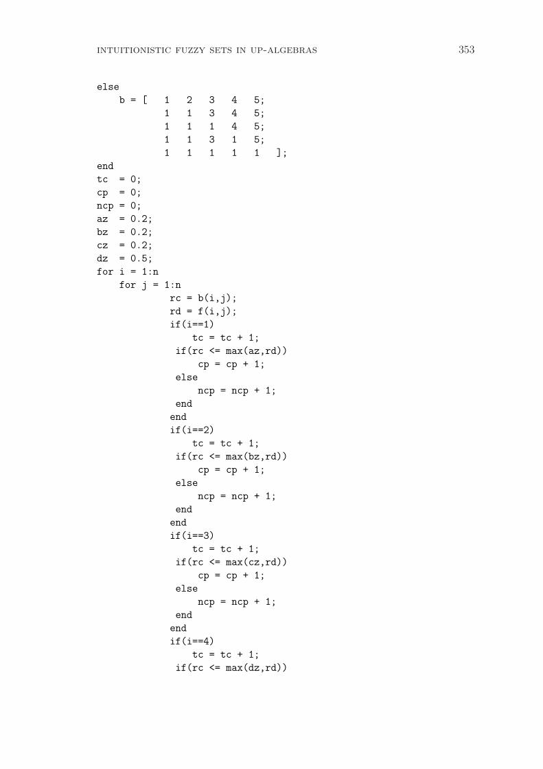
intuitionistic fuzzy sets in up-algebras 353
else
b = [ 1 2 3 4 5;
1 1 3 4 5;
1 1 1 4 5;
1 1 3 1 5;
1 1 1 1 1 ];
end
tc = 0;
cp = 0;
ncp = 0;
az = 0.2;
bz = 0.2;
cz = 0.2;
dz = 0.5;
for i = 1:n
for j = 1:n
rc = b(i,j);
rd = f(i,j);
if(i==1)
tc = tc + 1;
if(rc <= max(az,rd))
cp = cp + 1;
else
ncp = ncp + 1;
end
end
if(i==2)
tc = tc + 1;
if(rc <= max(bz,rd))
cp = cp + 1;
else
ncp = ncp + 1;
end
end
if(i==3)
tc = tc + 1;
if(rc <= max(cz,rd))
cp = cp + 1;
else
ncp = ncp + 1;
end
end
if(i==4)
tc = tc + 1;
if(rc <= max(dz,rd))

354 b. kesorn, k. maimun, w. ratbandan, a. iampan
cp = cp + 1;
else
ncp = ncp + 1;
end
end
end
end
Lemma 2.11. Every intuitionistic fuzzy UP-subalgebra F = (µF , γF ) of A satis-fies the inequalities: for all x ∈ A,
(1) µF (0) ≥ µF (x), and
(2) γF (0) ≤ γF (x).
Proof. Let x ∈ A. Then
µF (0) = µF (x · x)(By Proposition 1.4 1.4)
≥ minµF (x), µF (x)= minµF (x)= µF (x)
and
γF (0) = γF (x · x)(By Proposition 1.4 1.4)
≤ maxγF (x), γF (x)= maxγF (x)= γF (x).
Lemma 2.12. Let an IFS F = (µF , γF ) in A be an intuitionistic fuzzy UP-idealof A. If x, y ∈ A is such that y ≤ x in A, then
(1) µF (y) ≤ µF (x), and
(2) γF (y) ≥ γF (x).
Proof. Let x, y ∈ A be such that y ≤ x in A. Then y · x = 0. Thus
µF (x) = µF (0 · x)(By UP-2)
≥ minµF (0 · (y · x)), µF (y)= minµF (y · x), µF (y)(By UP-2)
= minµF (0), µF (y)= µF (y)

intuitionistic fuzzy sets in up-algebras 355
and
γF (x) = γF (0 · x)(By UP-2)
≤ maxγF (0 · (y · x)), γF (y)= maxγF (y · x), γF (y)(By UP-2)
= maxγF (0), γF (y)= γF (y).
Hence, µF is an order preserving fuzzy set and γF is an anti order preserving fuzzyset in A.
Lemma 2.13. Let an IFS F = (µF , γF ) in A be an intuitionistic fuzzy UP-idealof A. If w, x, y, z ∈ A is such that x ≤ w · (y · z) in A, then
(1) µF (x · z) ≥ minµF (w), µF (y), and
(2) γF (x · z) ≤ maxγF (w), γF (y).Proof. Let w, x, y, z ∈ A be such that x ≤ w · (y · z) in A. Then x · (w · (y · z)) =0. Hence,
µF (x · z) ≥ minµF (x · (y · z)), µF (y)(By Definition 2.8 2.8)
≥ minminµF (x · (w · (y · z))), µF (w), µF (y)(By Definition 2.8 2.8)
= minminµF (0), µF (w), µF (y)= minµF (w), µF (y)(By Definition 2.8 2.8)
and
γF (x · z) ≤ maxγF (x · (y · z)), γF (y)(By Definition 2.8 2.8)
≤ maxmaxγF (x · (w · (y · z))), γF (w), γF (y)(By Definition 2.8 2.8)
= maxmaxγF (0), γF (w), γF (y)= maxγF (w), γF (y)..(By Definition 2.8 2.8)
Corollary 2.14. Let an IFS F = (µF , γF ) in A be an intuitionistic fuzzy UP-idealof A. If x, y, z ∈ A is such that x ≤ y · z in A, then
(1) µF (x · z) ≥ µF (y), and
(2) γF (x · z) ≤ γF (y).
Proof. Let x, y, z ∈ A be such that x ≤ y · z in A. By Lemma 2.13, put w = 0.By UP-2, we have that x ≤ 0 · (y · z). Hence,
µF (x · z) ≥ minµF (0), µF (y) = µF (y)
andγF (x · z) ≤ maxγF (0), γF (y) = γF (y).

356 b. kesorn, k. maimun, w. ratbandan, a. iampan
Theorem 2.15. Every intuitionistic fuzzy UP-ideal of A is an intuitionistic fuzzyUP-subalgebra of A.
Proof. Let F = (µF , γF ) be an intuitionistic fuzzy UP-ideal of A and let x, y ∈ A.By Proposition 1.5 1.5, we have x ≤ y · x. It follows from Lemma 2.12 that
µF (y · x) ≥ µF (x) ≥ minµF (y), µF (x)
andγF (y · x) ≤ γF (x) ≤ maxγF (y), γF (x).
Hence, F = (µF , γF ) is an intuitionistic fuzzy UP-subalgebra of A.
The converse of Theorem 2.15 may not be true. For example, the intuitionisticfuzzy UP-subalgebra F = (µF , γF ) in Example 2.10 is not an intuitionistic fuzzyUP-ideal of A since
(2.4) γF (b · c) = 0.5 > 0.2 = maxγF (b · (a · c)), γF (a).
Lemma 2.16. Let f be a fuzzy set in A. Then the following statements hold: forany x, y ∈ A,
(1) 1−maxf(x), f(y) = min1− f(x), 1− f(y), and
(2) 1−minf(x), f(y) = max1− f(x), 1− f(y).Proof. 2.16 If maxf(x), f(y) = f(x), then f(y) ≤ f(x). Thus 1 − f(y) ≥1− f(x), so min1− f(x), 1− f(y) = 1− f(x) = 1−maxf(x), f(y). Similarly,if maxf(x), f(y) = f(y), then
min1− f(x), 1− f(y) = 1− f(y) = 1−maxf(x), f(y).
2.16 If minf(x), f(y) = f(x), then f(x) ≤ f(y). Thus 1 − f(x) ≥ 1 − f(y),so max1 − f(x), 1 − f(y) = 1 − f(x) = 1 − minf(x), f(y). Similarly, ifminf(x), f(y) = f(y), then
max1− f(x), 1− f(y) = 1− f(y) = 1−minf(x), f(y).
Theorem 2.17. An IFS F = (µF , γF ) is an intuitionistic fuzzy UP-ideal of A ifand only if the fuzzy sets µF and γF are fuzzy UP-ideals of A.
Proof. Assume that an IFS F = (µF , γF ) is an intuitionistic fuzzy UP-ideal ofA. Then for any x, y, z ∈ A, we have
µF (0) ≥ µF (x) and µF (x · z) ≥ minµF (x · (y · z)), µF (y).
Hence, µF is a fuzzy UP-ideal of A. Now, for any x, y, z ∈ A, we have
γF (0) ≤ γF (x) and γF (x · z) ≤ maxγF (x · (y · z)), γF (y).

intuitionistic fuzzy sets in up-algebras 357
Thus γF (0) = 1− γF (0) ≥ 1− γF (x) = γF (x) and
γF (x · z) = 1− γF (x · z)
≥ 1−maxγF (x · (y · z)), γF (y)= min1− γF (x · (y · z)), 1− γF (y)(By Lemma 2.16 2.16)
= minγF (x · (y · z)), γF (y).Hence, γF is a fuzzy UP-ideal of A.
Conversely, assume that µF and γF are fuzzy UP-ideals of A. Then for anyx, y, z ∈ A, we have
µF (0) ≥ µF (x) and µF (x · z) ≥ minµF (x · (y · z)), µF (y).Now, for any x, y, z ∈ A, we have
γF (0) ≥ γF (x) and γF (x · z) ≥ minγF (x · (y · z)), γF (y).Thus 1− γF (0) ≥ 1− γF (x), so γF (0) ≤ γF (x). Now,
1− γF (x · z) ≥ min1− γF (x · (y · z)), 1− γF (y)= 1−maxγF (x · (y · z)), γF (y),(By Lemma 2.16 2.16)
so γF (x · z) ≤ maxγF (x · (y · z)), γF (y). Hence, F = (µF , γF ) is an intuitionisticfuzzy UP-ideal of A.
Theorem 2.18. An IFS F = (µF , γF ) is an intuitionistic fuzzy UP-subalgebra ofA if and only if the fuzzy sets µF and γF are fuzzy UP-subalgebras of A.
Proof. Assume that an IFS F = (µF , γF ) is an intuitionistic fuzzy UP-subalgebraof A. Then for any x, y ∈ A, we have
µF (x · y) ≥ minµF (x), µF (y).Hence, µF is a fuzzy UP-subalgebra of A. Now, for any x, y ∈ A, we have
γF (x · y) ≤ maxγF (x), γF (y).Thus
γF (x · y) = 1− γF (x · y)
≥ 1−maxγF (x), γF (y)= min1− γF (x), 1− γF (y)(By Lemma 2.16 2.16)
= minγF (x), γF (y).Hence, γF is a fuzzy UP-subalgebra of A.
Conversely, assume that µF and γF are fuzzy UP-subalgebras of A. Then forany x, y ∈ A, we have
µF (x · y) ≥ minµF (x), µF (y).

358 b. kesorn, k. maimun, w. ratbandan, a. iampan
Now, for any x, y ∈ A, we have
γF (x · y) ≥ minγF (x), γF (y).Thus
1− γF (x · y) ≥ min1− γF (x), 1− γF (y)= 1−maxγF (x), γF (y),(By Lemma 2.16 2.16)
so γF (x · y) ≤ maxγF (x), γF (y). Hence, F = (µF , γF ) is an intuitionistic fuzzyUP-subalgebra of A.
Theorem 2.19. An IFS F = (µF , γF ) is an intuitionistic fuzzy UP-ideal of A ifand only if the IFSs ¤F = (µF , µF ) and ♦F = (γF , γF ) are intuitionistic fuzzyUP-ideals of A.
Proof. Assume that F = (µF , γF ) is an intuitionistic fuzzy UP-ideal of A. Thenfor any x, y, z ∈ A, we have
µF (0) ≥ µF (x) and µF (x · z) ≥ minµF (x · (y · z)), µF (y).Thus for any x, y, z ∈ A, we have µF (0) = 1− µF (0) ≤ 1− µF (x) = µF (x) and
µF (x · z) = 1− µF (x · z)
≤ 1−minµF (x · (y · z)), µF (y)= max1− µF (x · (y · z)), 1− µF (y)(By Lemma 2.16 2.16)
= maxµF (x · (y · z)), µF (y).Hence, ¤F = (µF , µF ) is an intuitionistic fuzzy UP-ideal of A. Now, for anyx, y, z ∈ A, we have
γF (0) ≤ γF (x) and γF (x · z) ≤ maxγF (x · (y · z)), γF (y).Thus for any x, y, z ∈ A, we have γF (0) = 1− γF (0) ≥ 1− γF (x) = γF (x) and
γF (x · z) = 1− γF (x · z)
≥ 1−maxγF (x · (y · z)), γF (y)= min1− γF (x · (y · z)), 1− γF (y)(By Lemma 2.16 2.16)
= minγF (x · (y · z)), γF (y).Hence, ♦F = (γF , γF ) is an intuitionistic fuzzy UP-ideal of A.
Conversely, assume that ¤F = (µF , µF ) and ♦F = (γF , γF ) are intuitionisticfuzzy UP-ideals of A. Then for any x, y, z ∈ A, we have
µF (0) ≥ µF (x) and µF (x · z) ≥ minµF (x · (y · z)), µF (y),and
γF (0) ≤ γF (x) and γF (x · z) ≤ maxγF (x · (y · z)), γF (y).Hence, F = (µF , γF ) is an intuitionistic fuzzy UP-ideal of A.

intuitionistic fuzzy sets in up-algebras 359
Theorem 2.20. An IFS F = (µF , γF ) is an intuitionistic fuzzy UP-subalgebra ofA if and only if the IFSs ¤F = (µF , µF ) and ♦F = (γF , γF ) are intuitionisticfuzzy UP-subalgebras of A.
Proof. Assume that F = (µF , γF ) is an intuitionistic fuzzy UP-subalgebra of A.Then for any x, y ∈ A, we have
µF (x · y) ≥ minµF (x), µF (y).Thus for any x, y ∈ A, we have
µF (x · y) = 1− µF (x · y)
≤ 1−minµF (x), µF (y)= max1− µF (x), 1− µF (y)(By Lemma 2.16 2.16)
= maxµF (x), µF (y).Hence, ¤F = (µF , µF ) is an intuitionistic fuzzy UP-subalgebra of A. Now, forany x, y ∈ A, we have
γF (x · y) ≤ maxγF (x), γF (y).Thus for any x, y ∈ A, we have
γF (x · y) = 1− γF (x · y)
≥ 1−maxγF (x), γF (y)= min1− γF (x), 1− γF (y)(By Lemma 2.16 2.16)
= minγF (x), γF (y).Hence, ♦F = (γF , γF ) in an intuitionistic fuzzy UP-subalgebra of A.
Conversely, assume that ¤F = (µF , µF ) and ♦F = (γF , γF ) are intuitionisticfuzzy UP-subalgebra of A. Then for any x, y ∈ A, we have
µF (x · y) ≥ minµF (x), µF (y) and γF (x · y) ≤ maxγF (x), γF (y).Hence, F = (µF , γF ) is an intuitionistic fuzzy UP-subalgebra of A.
Definition 2.21. Let f be a fuzzy set in A. For any t ∈ [0, 1], the set
U(f ; t) = x ∈ A | f(x) ≥ t and U+(f ; t) = x ∈ A | f(x) > tare called an upper t-level subset and an upper t-strong level subset of f , respec-tively. The set
L(f ; t) = x ∈ A | f(x) ≤ t and L−(f ; t) = x ∈ A | f(x) < tare called a lower t-level subset and a lower t-strong level subset of f , respectively.
Theorem 2.22. An IFS F = (µF , γF ) is an intuitionistic fuzzy UP-ideal of A ifand only if for all s, t ∈ [0, 1], the sets U(µF ; t) and L(γF ; s) are either empty orUP-ideals of A.
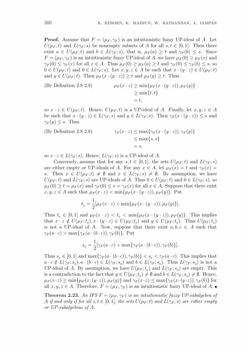
360 b. kesorn, k. maimun, w. ratbandan, a. iampan
Proof. Assume that F = (µF , γF ) is an intuitionistic fuzzy UP-ideal of A. LetU(µF ; t) and L(γF ; s) be nonempty subsets of A for all s, t ∈ [0, 1]. Then thereexist a ∈ U(µF ; t) and b ∈ L(γF ; s), that is, µF (a) ≥ t and γF (b) ≤ s. SinceF = (µF , γF ) is an intuitionistic fuzzy UP-ideal of A, we have µF (0) ≥ µF (x) andγF (0) ≤ γF (x) for all x ∈ A. Thus µF (0) ≥ µF (a) ≥ t and γF (0) ≤ γF (b) ≤ s, so0 ∈ U(µF ; t) and 0 ∈ L(γF ; s). Let x, y, z ∈ A be such that x · (y · z) ∈ U(µF ; t)and y ∈ U(µF ; t). Then µF (x · (y · z)) ≥ t and µF (y) ≥ t. Thus
µF (x · z) ≥ minµF (x · (y · z)), µF (y)(By Definition 2.8 2.8)
≥ mint, t= t,
so x · z ∈ U(µF ; t). Hence, U(µF ; t) is a UP-ideal of A. Finally, let x, y, z ∈ Abe such that x · (y · z) ∈ L(γF ; s) and y ∈ L(γF ; s). Then γF (x · (y · z)) ≤ s andγF (y) ≤ s. Thus
γF (x · z) ≤ maxγF (x · (y · z)), γF (y)(By Definition 2.8 2.8)
≤ maxs, s= s,
so x · z ∈ L(γF ; s). Hence, L(γF ; s) is a UP-ideal of A.Conversely, assume that for any s, t ∈ [0, 1], the sets U(µF ; t) and L(γF ; s)
are either empty or UP-ideals of A. For any x ∈ A, let µF (x) = t and γF (x) =s. Then x ∈ U(µF ; t) 6= ∅ and x ∈ L(γF ; s) 6= ∅. By assumption, we haveU(µF ; t) and L(γF ; s) are UP-ideals of A. Thus 0 ∈ U(µF ; t) and 0 ∈ L(γF ; s), soµF (0) ≥ t = µF (x) and γF (0) ≤ s = γF (x) for all x ∈ A. Suppose that there existx, y, z ∈ A such that µF (x · z) < minµF (x · (y · z)), µF (y). Put
t0 =1
2[µF (x · z) + minµF (x · (y · z)), µF (y)].
Thus t0 ∈ [0, 1] and µF (x · z) < t0 < minµF (x · (y · z)), µF (y). This impliesthat x · z /∈ U(µF ; t0), x · (y · z) ∈ U(µF ; t0) and y ∈ U(µF ; t0). Thus U(µF ; t0)is not a UP-ideal of A. Now, suppose that there exist a, b, c ∈ A such thatγF (a · c) > maxγF (a · (b · c)), γF (b). Put
s0 =1
2[γF (a · c) + maxγF (a · (b · c)), γF (b)].
Thus s0 ∈ [0, 1] and maxγF (a · (b · c)), γF (b) < s0 < γF (a · c). This implies thata · c /∈ L(γF ; s0), a · (b · c) ∈ L(γF ; s0) and b ∈ L(γF ; s0). Thus L(γF ; s0) is not aUP-ideal of A. By assumption, we have U(µF ; t0) and L(γF ; s0) are empty. Thisis a contradiction to the fact that y ∈ U(µF ; t0) 6= ∅ and b ∈ L(γF ; s0) 6= ∅. Hence,µF (x ·z) ≥ minµF (x ·(y ·z)), µF (y) and γF (x ·z) ≤ maxγF (x ·(y ·z)), γF (b) forall x, y, z ∈ A. Therefore, F = (µF , γF ) is an intuitionistic fuzzy UP-ideal of A.
Theorem 2.23. An IFS F = (µF , γF ) is an intuitionistic fuzzy UP-subalgebra ofA if and only if for all s, t ∈ [0, 1], the sets U(µF ; t) and L(γF ; s) are either emptyor UP-subalgebras of A.

intuitionistic fuzzy sets in up-algebras 361
Proof. Assume that F = (µF , γF ) is an intuitionistic fuzzy UP-subalgebra ofA. Let U(µF ; t) and L(γF ; s) be nonempty subsets of A for all s, t ∈ [0, 1]. Letx, y ∈ U(µF ; t). Then µF (x) ≥ t. Thus
µF (x · y) ≥ minµF (x), µF (y)(By Definition 2.9 2.9)
≥ mint, t= t,
so x · y ∈ U(µF ; t). It follows from Proposition 1.10 that U(µF ; t) is a UP-subalgebra of A. Finally, let x, y ∈ L(µF ; t). Then µF (y) ≥ t and
γF (x · y) ≤ maxγF (x), γF (y)(By Definition 2.9 2.9)
≤ maxs, s= s,
so x · y ∈ L(γF ; s). It follows from Proposition 1.10 that L(γF ; s) is a UP-subalgebra of A. Conversely, assume that for any s, t ∈ [0, 1], the set U(µF ; t)and L(γF ; s) are either empty or UP-subalgebras of A. For any x, y ∈ A, letminµF (x), µF (y) = t and maxγF (x), γF (y) = s. Then x, y ∈ U(µF ; t) 6= ∅and x, y ∈ L(γF ; s) 6= ∅. By assumption, we have U(µF ; t) and L(γF ; s) are UP-subalgebras of A and so x · y ∈ U(µF ; t) and x · y ∈ L(γF ; s). It follows thatµF (x · y) ≥ t = minµF (x), µF (y) and γF (x · y) ≤ s = maxγF (x), γF (y).Hence, F = (µF , γF ) is an intuitionistic fuzzy UP-subalgebra of A.
Theorem 2.24. If an IFS F = (µF , γF ) is an intuitionistic fuzzy UP-ideal ofA, then for all s, t ∈ [0, 1], the sets U
+(µF ; t) and L
−(γF ; s) are either empty or
UP-ideals of A.
Proof. Assume that F = (µF , γF ) is an intuitionistic fuzzy UP-ideal of A. Lets, t ∈ [0, 1] be such that U
+(µF ; t) and L
−(γF ; s) are nonempty subsets of A. Then
there exist a ∈ U+(µF ; t) and b ∈ L
−(γF ; s), that is, µF (a) > t and γF (b) < s.
Since F = (µF , γF ) is an intuitionistic fuzzy UP-ideal of A, we have µF (0) ≥ µF (x)and γF (0) ≤ γF (x) for all x ∈ A. Thus µF (0) ≥ µF (a) > t and γF (0) ≤ γF (b) < s,so 0 ∈ U
+(µF ; t) and 0 ∈ L
−(γF ; s). Let x, y, z ∈ A be such that x · (y · z) ∈
U+(µF ; t) and y ∈ U
+(µF ; t). Then µF (x · (y · z)) > t and µF (y) > t. Thus
µF (x · z) ≥ minµF (x · (y · z)), µF (y)(By Definition 2.8 2.8)
> mint, t= t,
so x · z ∈ U+(µF ; t). Hence, U
+(µF ; t) is a UP-ideal of A. Finally, let x, y, z ∈ A
be such that x · (y · z) ∈ L−(γF ; s) and y ∈ L
−(γF ; s). Then γF (x · (y · z)) < s and
γF (y) < s. Thus
γF (x · z) ≤ maxγF (x · (y · z)), γF (y)(By Definition 2.8 2.8)
< maxs, s= s,
so x · z ∈ L−(γF ; s). Hence, L
−(γF ; s) is a UP-ideal of A.

362 b. kesorn, k. maimun, w. ratbandan, a. iampan
Theorem 2.25. If for all s, t ∈ [0, 1], the sets U+(µF ; t) and L
−(γF ; s) are UP-
ideals of A, then an IFS F = (µF , γF ) is an intuitionistic fuzzy UP-ideal of A.
Proof. Assume that for all s, t ∈ [0, 1], the sets U+(µF ; t) and L
−(γF ; s) are
UP-ideals of A. For any x ∈ A, we have µF (x) ∈ [0, 1] and γF (x) ∈ [0, 1].By assumption, we have U
+(µF ; µF (x)) and L
−(γF ; γF (x)) are UP-ideals of A.
Thus 0 ∈ U+(µF ; µF (x)) and 0 ∈ L
−(γF ; γF (x)), that is, µF (0) > µF (x) and
γF (0) < γF (x). Suppose that there exist x, y, z ∈ A such that µF (x · z) <minµF (x · (y · z)), µF (y). Put t0 = 1
2[µF (x · z) + minµF (x · (y · z)), µF (y)].
Thus t0 ∈ [0, 1] and µF (x · z) < t0 < minµF (x · (y · z)), µF (y). This implies thatx · z /∈ U
+(µF ; t0), x · (y · z) ∈ U
+(µF ; t0) and y ∈ U
+(µF ; t0). Thus U
+(µF ; t0)
is not a UP-ideal of A. Now, suppose that there exist a, b, c ∈ A such thatγF (a · c) > maxγF (a · (b · c)), γF (b). Put s0 = 1
2[γF (a · c) + maxγF (a · (b ·
c)), γF (b)]. Thus s0 ∈ [0, 1] and maxγF (a · (b · c)), γF (b) < s0 < γF (a · c).This implies that a · c /∈ L
−(γF ; s0), a · (b · c) ∈ L
−(γF ; s0) and b ∈ L
−(γF ; s0).
Thus L−(γF ; s0) is not a UP-ideal of A. This is a contradiction to the fact that
for all s, t ∈ [0, 1], the sets U+(µF ; t) and L
−(γF ; s) are UP-ideals of A. Hence,
µF (x ·z) ≥ minµF (x ·(y ·z)), µF (y) and γF (x ·z) ≤ maxγF (x ·(y ·z)), γF (b) forall x, y, z ∈ A. Therefore, F = (µF , γF ) is an intuitionistic fuzzy UP-ideal of A.
Theorem 2.26. If an IFS F = (µF , γF ) is an intuitionistic fuzzy UP-subalgebraof A, then for all s, t ∈ [0, 1], the sets U
+(µF ; t) and L
−(γF ; s) are either empty
or UP-subalgebras of A.
Proof. Assume that F = (µF , γF ) is an intuitionistic fuzzy UP-subalgebra of A.Let s, t ∈ [0, 1] be such that U
+(µF ; t) and L
−(γF ; s) are nonempty subsets of A.
Let x, y ∈ U+(µF ; t). Then µF (x) > t and µF (y) > t. Thus
µF (x · y) ≥ minµF (x), µF (y)(By Definition 2.9 2.9)
> mint, t= t,
so x · y ∈ U+(µF ; t). It follows from Proposition 1.10 that U
+(µF ; t) is a UP-
subalgebra of A. Finally, let x, y ∈ L−(γF ; s). Then γF (x) < s and γF (y) < s.
Thus
γF (x · y) ≤ maxγF (x), γF (y)(By Definition 2.9 2.9)
< maxs, s= s,
so x · y ∈ L−(γF ; s). It follows from Proposition 1.10 that L
−(γF ; s) is a UP-
subalgebra of A.
Theorem 2.27. If for all s, t ∈ [0, 1], the sets U+(µF ; t) and L
−(γF ; s) are
UP-subalgebras of A, then an IFS F = (µF , γF ) is an intuitionistic fuzzy UP-subalgebra of A.

intuitionistic fuzzy sets in up-algebras 363
Proof. Assume that for all s, t ∈ [0, 1], the sets U+(µF ; t) and L
−(γF ; s) are
UP-subalgebras of A. Suppose that there exist x, y ∈ A such that µF (x · y) <minµF (x), µF (y). Put t0 = 1
2[µF (x · y) + minµF (x), µF (y)]. Thus t0 ∈ [0, 1]
and µF (x · y) < t0 < minµF (x), µF (y). This implies that x · y /∈ U+(µF ; t0),
x ∈ U+(µF ; t0) and y ∈ U
+(µF ; t0). Thus U
+(µF ; t0) is not a UP-subalgebra of
A. Now, suppose that there exist a, b ∈ A such that γF (a·b) > maxγF (a), γF (b).Put s0 = 1
2[γF (a·b)+maxγF (a), γF (b)]. Thus s0 ∈ [0, 1] and maxγF (a), γF (b) <
s0 < γF (a · b). This implies that a · b /∈ L−(γF ; s0), a ∈ L
−(γF ; s0) and b ∈
L−(γF ; s0). Thus L
−(γF ; s0) is not a UP-subalgebra of A. This is a contradic-
tion to the fact that for all s, t ∈ [0, 1], the sets U+(µF ; t) and L
−(γF ; s) are
UP-subalgebras of A. Hence, µF (x · y) ≥ minµF (x), µF (y) and γF (x · y) ≤maxγF (x), γF (y) for all x, y ∈ A. Therefore, F = (µF , γF ) is an intuitionisticfuzzy UP-subalgebra of A.
Acknowledgment. The authors wish to express their sincere thanks to thereferees for the valuable suggestions which lead to an improvement of this paper.
References
[1] Akram, M., Dar, K.H., Meng, B.L., Shum, K.P., Interval-valued in-tuitionistic fuzzy ideals of K-algebras, WSEAS Trans. Math., 7 (9) (2008),559–568.
[2] Atanassov, K.T., Intuitionistic fuzzy sets, Fuzzy Sets Syst., 20 (1986),87–96.
[3] Atanassov, K.T., New operations defined over the intuitionistic fuzzy sets,Fuzzy Sets Syst., 61 (1994), 137–142.
[4] Hu, Q.P., Li, X., On BCH-algebras, Math. Semin. Notes, Kobe Univ., 11(1983), 313–320.
[5] Iampan, A., A new branch of the logical algebra: UP-algebras, Manuscriptsubmitted for publication, April 2014.
[6] Imai, Y., Iseki, K., On axiom system of propositional calculi, XIV, Proc.Japan Acad., 42 (1) (1966), 19–22.
[7] Iseki, K., An algebra related with a propositional calculus, Proc. JapanAcad., 42 (1) (1966), 26–29.
[8] Jun, Y.B., Kim, K.H., Intuitionistic fuzzy ideal of BCK-algebras, Internat.J. Math. & Math. Sci., 24 (12) (2000), 839–849.
[9] Keawrahun, S., Leerawat, U., On isomorphisms of SU-algebras, Sci.Magna, 7 (2) (2011), 39–44.
[10] Kim, K.H., On structure of KS-semigroup, Int. Math. Forum, 1 (2) (2006),67–76.
[11] Kim, H.K., Intuitionistic (T, S)-normed fuzzy subalgebras of BCK-algebras,J. Chungcheong Math. Soc., 20 (3) (2007), 279–286.
[12] Kim, K.H., Lee, J.G., On intuitionistic fuzzy bi-ideals of semigroups, Turk.J. Math., 29 (2005), 201–210.
[13] Malik, M.A., Touqeer, M., Intuitionistic fuzzy BCI-commutative idealsin BCI-algebras, Pakistan J. Sci., 64 (4) (2012), 353–358.

364 b. kesorn, k. maimun, w. ratbandan, a. iampan
[14] Mostafa, S.M., Abdel Naby, M.A., Elgendy, O.R., Intuitionisticfuzzy KU-ideals in KU-algebras, Int. J. Math. Sci. Appl., 1 (3) (2011), 1379–1384.
[15] Nezhad, Rayeni, S.B., Rezaei, A., Intuitionistic fuzzy soft subalgebras(filters) on BE-algebras, Switzerland Research Park Journal, 102 (11) (2013),1447–1454.
[16] Palaniappan, N., Devi, R., Veerappan, P.S., Intuitionistic fuzzy nfoldBCI-positive implicative ideals in BCI-algebras, Int. J. Fuzzy Math. Syst., 3(1) (2013), 1–11.
[17] Palaniappan, N., Veerappan, P.S., Devi, R., Intuitionistic fuzzy h-ideals of BCI-algebras with interval valued membership & non membershipfunctions, Int. J. Contemp. Math. Sciences, 7 (43) (2012), 2125–2135.
[18] Prabpayak, C., Leerawat, U., On ideas and congruences in KU-algebras,Sci. Magna, 5 (1) (2009), 54–57.
[19] Ragavan, C., Solairaju, A., Balamurugan, M., Intuitionistic fuzzyR-ideal of BCI-algebras with interval valued membership & non membershipfunctions, IOSR Journal of Mathematics, 10 (2) (2014), 8–13.
[20] Satyanarayana, B., Krishna, L., Prasad, R.D., On intuitionisticfuzzy implicative hyper BCK-ideals of hyper BCK-algebras, InternationalJournal of Mathematics and Statistics Invention, 2 (2) (2014), 77–85.
[21] Satyanarayana, B., Prasad, R.D., Some results on intuitionistic fuzzyideals in BCK-algebras, Gen. Math. Notes, 4 (1) (2011), 1–15.
[22] Senapati, T., Bhowmik, M., Pal, M., Interval-valued intuitionistic fuzzyclosed ideals of BG-algebra and their products, Int. J. Fuzzy Log. Syst., 2 (2)(2012), 27–44.
[23] Senapati, T., Bhowmik, M., Pal, M., Fuzzy dot subalgebras and fuzzydot ideals of B-algebras, J. Uncertain Syst. 8 (2014), no. 1, 22-30.
[24] Somjanta, J., Thuekaew, N., Kumpeangkeaw, P., Iampan, A., Fuzzysets in UP-algebras, Ann. Fuzzy Math. Inform., Accepted manuscript.
[25] Sun, S., Li, Q., Intuitionistic fuzzy subalgebras (ideals) with thresholds (λ, µ)of BCI-algebras, Int. J. Math., Comput., Phys. Quantum Eng., 8 (2) (2014),1–11.
[26] Xueling, M., Jianming, Z., Intuitionistic Ω-fuzzy ideals of BCK-algebras,Sci. Math. Jpn. Online (2005), 299–303.
[27] Zadeh, L.A., Fuzzy sets, Inf. Cont. 8 (1965), 338–353.[28] Zahedi, M.M., Torkzadeh, L., Intuitionistic fuzzy dual positive implica-
tive hyper K-ideals, World Academy of Science, Engineering and Technology,5 (2005), 57–60.
[29] Zarandi, A., Saeid, A.B., Intuitionistic fuzzy ideal of BG-algebras, Inter-national Journal of Mathematical, Computational, Physical and QuantumEngineering, 1 (5) (2007), 244–246.
[30] Zhan, J., Tan, Z., Intuitionistic fuzzy α-ideals in BCI-algebras, SoochowJ. Math., 30 (2) (2004), 207–216.
Accepted: 08.01.2015

italian journal of pure and applied mathematics – n. 34−2015 (365−374) 365
EQUITABLE COLORINGS OF CARTESIAN PRODUCTS OF FANSWITH BIPARTITE GRAPHS1
Liancui Zuo2
Fanglan Wu
College of Mathematical ScienceTianjin Normal UniversityTianjin, 300387China
Shaoqiang Zhang
College of Computer and Information EngineeringTianjin Normal UniversityTianjin, 300387China
Abstract. In this paper, by the sorting method of vertices, it is obtained that theequitable chromatic number and the equitable chromatic threshold of the Cartesianproducts of fans with bipartite graphs.
Keywords: Cartesian product, equitable coloring, equitable chromatic number, equi-table chromatic threshold.
MR (2000) Subject Classification: 05C70, 05C15.
1 Introduction
All graphs considered in this paper are finite, undirected, loopless and withoutmultiple edges. For a positive integer k and a real number x, let [k] = 1, 2, ..., k,dxe and bxc denote the smallest integer not less than x and the largest integernot greater than x, respectively.
A graph G is said to be k-colorable if there is a map c : V (G) → [k] such thatadjacent vertices are mapped to distinct numbers. The map c is called a properk-coloring of G, and all pre-images of a fixed number form a so-called color class.No two vertices are adjacent in each color class. The chromatic number of G,denoted by χ(G), is the smallest number k such that G is k-colorable.
1Supported by NSFC for youth with code 61103073.2Corresponding author. E-mail: [email protected]; [email protected]

366 l. zuo, f. wu, s. zhang
A graph G = (V, E) is said to be equitably k-colorable if V (G) can be dividedinto k independent sets V1, V2, ..., Vk such that ||Vi| − |Vj|| ≤ 1 for all i, j ∈ [k].The smallest integer k for which G is equitably k-colorable is called equitablechromatic number of a graph G, and denoted by χ=(G). The equitable chromaticthreshold of a graph G, denoted by χ∗=(G), is the minimum t such that G isequitably k-colorable for all k ≥ t. It is evident from the definition that
χ(G) ≤ χ=(G) ≤ χ∗=(G)
for any graph G.Equitable coloring as a special vertex coloring on graphs was first introduced
by Meyer[1]. His motivation came from the problem of assigning one of the sixdays of the work week to each garbage collection route. Here, the vertices repre-sent garbage collection routes and two such vertices are joined by an edge whenthe corresponding routes should not be run on the same day. The problem ofassigning one of the six days of the work week to each route becomes the problemof 6-coloring of G. On practical grounds it might also be desirable to have anapproximately equal number of routes run on each of the six days, so we have tocolor the graph in the equitable way.
Another application of equitable coloring is in scheduling and timetabling.Consider, for example, a problem of constructing university timetables. It isknown that this problem can be modeled as coloring the vertices of a graph Gwhose nodes correspond to classes, edges correspond to time conflicts betweenclasses, and colors to hours. If the set of available rooms is restricted, then wemay be forced to partition the vertex set into independent subsets of as nearequal size as possible, since then the room usage is the highest. For applicationsof equitable coloring such as scheduling and constructing timetables, please see[1], [5], [11], [12], [13].
In [3], by Lin and Chang, it is obtained that the exact values or upper boundsof the equitable chromatic number on Kronecker products of G and H, when Gand H are complete graphs, bipartite graphs, paths or cycles, and in [4], it isstudied that the equitable colorings of Cartesian product of paths and cycles,respectively, with bipartite graphs. In [16], Lih and Wu studied the equitablecolorings of bipartite graphs, and in [17], Lih gave a good survey for this coloring.In [23], Zhu gave a survey for Hedetniemi’s conjecture about the tensor productof graphs. The general problem of deciding if χ=(G) ≤ 3 is NP-complete [10]. If,however, G has a regular or simplified structure we are sometimes able to providea polynomial algorithm coloring it in the equitable way. For more details aboutthis coloring, please see [1], [2], [6], [7], [8], [14], [20], [21], [22].
The Cartesian product of graphs G = (V1, E1) and H = (V2, E2) is the graphG2H with vertex set (u, x) | u ∈ V1, x ∈ V2 and edge set
(u, x) (v, y) |u = v with xy ∈ E2 or x = y with uv ∈ E1.
Graph products are interesting and useful in many situations. For example,Sabidussi [19] showed that any graph has the unique decomposition into prime

equitable colorings of cartesian products ... 367
factors under the Cartesian product. The complexity of many problems, alsoequitable coloring, that deal with very large and complicated graphs is reducedgreatly if one is able to fully characterize the properties of less complicated primefactors.
In the present paper, we study the equitable colorings of Cartesian productsof fans with complete bipartite graphs.
2. Main results
In the following, let s, l, m, n, n′ be all nonnegative integers, Fn′+1 represent theFan with vertex set V (Fn′+1) = x, x1, x2, ..., xn′ , and H represent a completebipartite graph with two parts Y = y1, y2, ..., ym and Z = z1, z2, ..., zn wherem ≥ n. We will study the equitable chromatic number and the equitable chro-matic threshold of the Cartesian product Fn′+12H according to the parity of n′
and m.On the other hand, if n = 1, then H is a star and denoted by Km,1. If
n′ + 1 = 2 or n′ + 1 = 3, then Fn′+1 is a path or a cycle. In this paper, we alwayssuppose that n′ + 1 > 3. Clearly, χ=(Fn′+12H) ≥ χ(Fn′+1) = 3.
r
rrrrr
rrrrr
`
`
``
DDDDDDDDD
CCCCCCC
BBBBBB
AAAA
@@
¥¥¥¥¥¥¥¥¥
¤¤¤¤¤¤¤
££££££
¢¢¢¢
¡¡`p p pp p p
x
xn′
xn′−1
xn′−2
xn′−3
xn′−4
x5
x4
x3
x2
x1
Fn′+1:
x
xn′−1
xn′−2
xn′−3
xn′−4
xn′
x5
x4
x3
x2
x1
``
rrrr
r
``
rrrrr
rz1
r
rrrr
r
rrrrr
rzn` ` ` ` ` `
` ` ` ` ` `` ` ` ` ` `` ` ` ` ` `` ` ` ` ` `` ` ` ` ` `` ` ` ` ` `
` ` ` ` ` `` ` ` ` ` `` ` ` ` ` `` ` ` ` ` `` ` ` ` ` `
` ` `®
©ª
®
©ªrr
rrrrr
rrrrr
rrrrr
rrrrr
rr r
rrrrr
rrrrr
rr
rrrrr
rrrrr
rr
` ` ` ` ` ` `y1 ys ys+1 ym
` ` ` ` ` `
` ` ` ` ` `
` ` ` ` ` ` `` ` ` ` ` ` `` ` ` ` ` ` `` ` ` ` ` ` `` ` ` ` ` ` `` ` ` ` ` ` `
```
```
` ` ` ` ` ` `` ` ` ` ` ` `` ` ` ` ` ` `` ` ` ` ` ` `` ` ` ` ` ` `
` ` ` ` ` ` `` ` ` ` ` ` `
` ` ` ` ` ` `` ` ` ` ` ` `` ` ` ` ` ` `` ` ` ` ` ` `
` ` ` ` ` ` `` ` ` ` ` ` `` ` ` ` ` ` `` ` ` ` ` ` `` ` ` ` ` ` `pp
pppppppppppppppppppppppppppppppppppp
Figure 1. The Cartesian product Fn′+1¤H
Theorem 2.1. Suppose that m ≥ n ≥ 1, l ≥ 2 and k ≥ 4. If n′ = 2l, thenFn′+12H is equitably k-colorable.
Proof. The structure of the Cartesian product graph Fn′+12H is represented inFigure 1.

368 l. zuo, f. wu, s. zhang
For m = 2p + 1, p ≥ 0 and s = p + 1 ( or for m = 2p, p ≥ 1 and s = p), wewill sort the vertices of Fn′+12H as following.
(x, y1) , (x, y2) , . . . , (x, ys) , (x1, z1) , (x3, z1) , . . . , (x2h−1, z1) , . . . , (xn′−1, z1) ,(x1, z2) , (x3, z2) , . . . , (x2h−1, z2) , . . . , (xn′−1, z2) , . . . , (x1, zn) , (x3, zn) , . . . ,(x2h−1, zn) , . . . , (xn′−1, zn) , (x2, ys+1) , (x4, ys+1) , . . . , (x2h, ys+1) , . . . , (xn′ , ys+1) ,(x2, ys+2) , (x4, ys+2) , . . . , (x2h, ys+2) , . . . , (x′n, ys+2) , . . . , (x2, ym) , (x4, ym) , . . . ,(x2h, ym) , . . . , (xn′ , ym) , (x2, y1) , (x2, y2) . . . , (x2, ys) , (x4, y1) , (x4, y2) . . . , (x4, ys) ,. . . , (x2h, y1) , (x2h, y2) . . . , (x2h, ys) , . . . , (xn′ , y1) , (xn′ , y2) , . . . , (xn′ , ys) ,(x, z1) , (x, z2) , . . . , (x, zn) , (x1, ys+1) , (x3, ys+1) , . . . ,(x2h−1, ys+1) , . . . , (xn′−1, ys+1) , (x1, ys+2) , (x3, ys+2) , . . . ,(x2h−1, ys+2) , . . . , (xn′−1, ys+2) , . . . , (x1, ym) , (x3, ym) , . . . ,(x2h−1, ym) , . . . , (xn′−1, ym) , (x1, y1) , (x1, y2) . . . , (x1, ys) ,(x3, y1) , (x3, y2) . . . , (x3, ys) , . . . , (x2h−1, y1) , (x2h−1, y2) . . . , (x2h−1, ys) ,. . . , (xn′−1, y1) , (xn′−1, y2) , . . . , (xn′−1, ys) , (x2, z1) , (x2, z2) , . . . , (x2, zn) ,(x4, z1) , (x4, z2) , . . . , (x4, zn) , . . . , (x2h, z1) , (x2h, z2) , . . . , (x2h, zn) , . . . ,(xn′ , z1) , (xn′ , z2) , . . . , (xn′ , zn) , (x, ys+1) , (x, ys+2) , . . . , (x, ym) ,
where h is a positive integer and 1 ≤ h ≤ l. It is not difficult to verify that thesmallest cardinality of independent set consisting of consecutive vertices is at leastminlp + nl + p + 1, 2pl + l + n for m = 2p + 1 and min2lp + n, nl + pl + p form = 2p.
Let
σt =
⌊(2l + 1)(m + n) + t− 1
k
⌋,
where t ∈ [k]. By l ≥ 2 and k ≥ 4, we have
σ1 =
⌊(2l + 1)(m + n)
k
⌋
≤ σk =
⌊(2l + 1)(m + n) + k − 1
k
⌋=
⌈(2l + 1)(m + n)
k
⌉≤
⌈(2l + 1)(m + n)
4
⌉.
If m = 2p + 1, then
σt ≤⌈
(2l + 1)(m + n)
4
⌉≤ minlp + nl + p + 1, 2pl + l + n.
If m = 2p, then
σt ≤⌈
(2l + 1)(m + n)
4
⌉< min2lp + n, nl + pl + p.
Hence, according to the vertex sorting above, the vertex set of Fn′+12H can bepartitioned into k independent sets with cardinality σ1, σ2, . . . , σk, respectively.Therefore Fn′+12H is equitably k-colorable.

equitable colorings of cartesian products ... 369
Theorem 2.2. Suppose that m ≥ n ≥ 1.
(1) For n′ = 4 and 2n−m ∈ 0,±1,±2, or
(2) For n′ = 2l, l ≥ 3 and m = 2n,we have that Fn′+12H is equitably 3-colorable, and then χ∗=(Fn′+12H) = 3.
Proof. (1) Assume that s is a nonnegative integer, then we can partition thevertex set V (Fn′+12H) into the following three parts:
V1 =
(x, y1), (x, y2), ..., (x, ys), (x1, z1), (x3, z1), (x1, z2), (x3, z2), ..., (x1, zn),(x3, zn), (x2, ys+1), (x4, ys+1), (x2, ys+2), (x4, ys+2), ..., (x2, ym), (x4, ym)
,
V2 =
(x1, y1), (x1, y2), ..., (x1, ys), (x3, y1), (x3, y2), ..., (x3, ys), (x2, z1), (x2, z2),..., (x2, zn), (x4, z1), (x4, z2), ..., (x4, zn), (x, ys+1), (x, ys+2), ..., (x, ym)
,
and
V3 =
(x2, y1), (x2, y2), ..., (x2, ys), (x4, y1), (x4, y2), ..., (x4, ys), (x, z1), (x, z2), ...,(x, zn), (x1, ys+1), (x3, ys+1), (x1, ys+2), (x3, ys+2), ..., (x1, ym), (x3, ym)
,
where |V1| = 2n + 2m− s, |V2| = 2n + m + s, and |V3| = n + 2m.
If m = 2n + 1 and s = n + 1, then |V1| = 2n + 2m − s = 5n + 1, |V2| =2n + m + s = 5n + 2, and |V3| = n + 2m = 5n + 2.If m = 2n− 1 and s = n, then|V1| = 5n− 2, |V2| = 5n− 1, and |V3| = 5n− 2.
If m = 2n and s = n, then |V1| = 2n + 2m− s = 5n, |V2| = 2n + m + s = 5n,and |V3| = n + 2m = 5n.
If m = 2n + 2 and s = n + 1, then |V1| = 2n + 2m − s = 5n + 3, |V2| =2n + m + s = 5n + 3, and |V3| = n + 2m = 5n + 4.
If m = 2n − 2 and s = n − 1, then |V1| = 2n + 2m − s = 5n − 3, |V2| =2n + m + s = 5n− 3, and |V3| = n + 2m = 5n− 4.
Therefore, Fn′+12H is equitably 3-colorable. By Theorem 2.1, we haveχ∗=(Fn′+12H) = 3.
(2) Assume that s = n and 1 ≤ h ≤ l, then we will partition the vertex setV (Fn′+12H) into the following three parts:
V1 =
(x, y1) , (x, y2) , . . . , (x, ys) , (x1, z1) , (x3, z1) , . . . , (x2h−1, z1) , . . . ,(xn′−1, z1) , (x1, z2) , (x3, z2) , . . . , (x2h−1, z2) , . . . , (xn′−1, z2) , . . . ,(x1, zn) , (x3, zn) , . . . , (x2h−1, zn) , . . . , (xn′−1, zn) , (x2, ys+1) , (x4, ys+1) ,. . . , (x2h, ys+1) , . . . , (xn′ , ys+1) , (x2, ys+2) , (x4, ys+2) , . . . , (x2h, ys+2) ,. . . , (xn′ , ys+2) , . . . , (x2, ym) , (x4, ym) , . . . , (x2h, ym) , . . . , (xn′ , ym)
,
V2 =
(x1, y1) , (x1, y2) . . . , (x1, ys) , (x3, y1) , (x3, y2) . . . , (x3, ys) ,. . . , (x2h−1, y1) , (x2h−1, y2) , . . . , (x2h−1, ys) , . . . , (xn′−1, y1) ,(xn′−1, y2) . . . , (xn′−1, ys) , (x2, z1) , (x2, z2) , . . . , (x2, zn) ,(x4, z1) , (x4, z2) , . . . , (x4, zn) , . . . , (x2h, z1) , (x2h, z2) , . . . , (x2h, zn) ,. . . , (xn′ , z1) , (xn′ , z2) , . . . , (xn′ , zn) , (x, ys+1) , (x, ys+2) , . . . , (x, ym)
,

370 l. zuo, f. wu, s. zhang
and
V3 =
(x2, y1) , (x2, y2) . . . , (x2, ys) , (x4, y1) , (x4, y2) . . . , (x4, ys) , . . . , (x2h, y1) ,(x2h, y2) , . . . , (x2h, ys) , . . . , (xn′ , y1) , (xn′ , y2) , . . . , (xn′ , ys) , (x, z1) ,(x, z2) , . . . , (x, zn) , (x1, ys+1) , (x3, ys+1) , . . . , (x2h−1, ys+1) ,. . . , (xn′−1, ys+1) , (x1, ys+2) , (x3, ys+2) , . . . , (x2h−1, ys+2) , . . . ,(xn′−1, ys+2) , . . . , (x1, ym) , (x3, ym) , . . . , (x2h−1, ym) , . . . , (xn′−1, ym)
.
It is easy to see that |V1| = (2l+1)n, |V2| = (2l+1)n, and |V3| = (2l+1)n. HenceFn′+12H is equitably 3-colorable. By Theorem 2.1, we have χ∗=(Fn′+12H) = 3.
Theorem 2.3. Suppose that m ≥ n ≥ 1, l ≥ 1 and k ≥ 4. If n′ = 2l + 1, thenFn′+12H is equitably k-colorable.
Proof. For m = 2p + 1, p ≥ 0 and s = p + 1 (or m = 2p, p ≥ 1 and s = p), wesort the vertex set of Fn′+12H as following:
(x, y1) , (x, y2) , . . . , (x, ys) , (x2, z1) , (x4, z1) , . . . , (x2h+2, z1) , . . . , (xn′−1, z1) ,(x2, z2) , (x4, z2) , . . . , (x2h+2, z2) , . . . , (xn′−1, z2) , . . . , (x2, zn) , (x4, zn) ,. . . , (x2h+2, zn) , . . . , (xn′−1, zn) , (x1, ys+1) , (x3, ys+1) , . . . , (x2h′+1, ys+1) ,. . . , (xn′ , ys+1) , (x1, ys+2) , (x3, ys+2) , . . . , (x2h′+1, ys+2) , . . . ,(xn′ , ys+2) , . . . , (x1, ym) , (x3, ym) , . . . , (x2h′+1, ym) , . . . , (xn′ , ym) ,(x1, y1) , (x1, y2) . . . , (x1, ys) , (x3, y1) , (x3, y2) . . . , (x3, ys) , . . . ,(x2h′+1, y1) , (x2h′+1, y2) . . . , (x2h′+1, ys) , . . . , (xn′ , y1) , (xn′ , y2) ,. . . , (xn′ , ys) , (x, z1) , (x, z2) , . . . , (x, zn) , (x2, ys+1) , (x4, ys+1) , . . . ,(x2h+2, ys+1) , . . . , (xn′−1, ys+1) , (x2, ys+2) , (x4, ys+2) , . . . , (x2h+2, ys+2) ,. . . , (xn′−1, ys+2) , . . . , (x2, ym) , (x4, ym) , . . . , (x2h+2, ym) , . . . , (xn′−1, ym) ,(x2, y1) , (x2, y2) . . . , (x2, ys) , (x4, y1) , (x4, y2) . . . , (x4, ys) , . . . , (x2h+2, y1) ,(x2h+2, y2) . . . , (x2h+2, ys) , . . . , (xn′−1, y1) , (xn′−1, y2) . . . , (xn′−1, ys) ,(x1, z1) , (x1, z2) , . . . , (x1, zn) , (x3, z1) , (x3, z2) , . . . , (x3, zn) , . . . ,(x2h′+1, z1) , (x2h′+1, z2) , . . . , (x2h′+1, zn) , . . . , (xn′ , z1) , (xn′ , z2) , . . . ,(xn′ , zn) , (x, ys+1) , (x, ys+2) , . . . , (x, ym) ,
where h, h′ are all nonnegative integers, 0 ≤ h ≤ l − 1, and 0 ≤ h′ ≤ l. It isobvious that the smallest cardinality of independent set consisting of consecutivevertices in the order above is at least
minlp + nl + 2p + 1, 2lp + l + n, pl + nl + p + l + n
when m = 2p + 1 and
min2lp + n, nl + p(l + 2), (l + 1)p + nl + n
when m = 2p.Let
σt =
⌊(2l + 2)(m + n) + t− 1
k
⌋,

equitable colorings of cartesian products ... 371
where t ∈ [k]. By l ≥ 1 and k ≥ 4, we can obtain that
σ1 =
⌊(2l + 2)(m + n)
k
⌋≤ σk =
⌊(2l + 2)(m + n) + k − 1
k
⌋=
⌈(2l + 2)(m + n)
k
⌉
≤⌈
(2l + 2)(m + n)
4
⌉.
If m = 2p + 1, then
σt ≤⌈
(2l + 2)(m + n)
4
⌉≤ minlp + nl + 2p + 1, 2lp + l + n, pl + nl + p + l + n.
If m = 2p, then
σt ≤⌈
(2l + 2)(m + n)
4
⌉≤ min2lp + n, nl + p(l + 2), (l + 1)p + nl + n.
Therefore, according to the vertex ordering above, the vertex set of Fn′+12H canbe partitioned into k independent sets with cardinality σ1, σ2, . . . , σk, respectively.Hence Fn′+12H is equitably k-colorable for k ≥ 4.
Theorem 2.4. Suppose that m ≥ n ≥ 1.(1) If n′ = 3, and 2n−m ∈ 0,±1,±2, or(2) if l ≥ 2, n′ = 2l + 1 and m = 2n,
then Fn′+12H is equitably 3-colorable, and χ∗=(Fn′+12H) = 3.
Proof. (1) Assume that s is a nonnegative integer, then we can partition thevertex set V (Fn′+12H) into the following three parts:
V1 =
(x, y1) , (x, y2) , . . . , (x, ys) , (x2, z1) , (x2, z2) , . . . , (x2, zn) ,(x1, ys+1) , (x3, ys+1) , (x1, ys+2) , (x3, ys+2) , . . . , (x1, ym) , (x3, ym)
,
V2 =
(x2, y1) , (x2, y2) . . . , (x2, ys) , (x1, z1) , (x1, z2) , . . . , (x1, zn) ,(x3, z1) , (x3, z2) , . . . , (x3, zn) , (x, ys+1) , (x, ys+2) , . . . , (x, ym)
,
and
V3 =
(x1, y1) , (x1, y2) . . . , (x1, ys) , (x3, y1) , (x3, y2) . . . , (x3, ys) ,(x, z1) , (x, z2) , . . . , (x, zn) , (x2, ys+1) , (x2, ys+2) , . . . , (x2, ym)
,
where |V1| = n + 2m− s, |V2| = 2n + m, and |V3| = n + m + s.If m = 2n + 1 and s = n + 1, then |V1| = n + 2m − s = 4n + 1, |V2| =
2n + m = 4n + 1, and |V3| = n + m + s = 4n + 2. If m = 2n− 1 and s = n, then|V1| = 4n− 2, |V2| = 4n− 1, and |V3| = 4n− 1.
If m = 2n and s = n, then |V1| = n + 2m − s = 4n, |V2| = 2n + m = 4n,and |V3| = n + m + s = 4n. If m = 2n − 2 and s = n − 1, then |V1| = 4n − 3,|V2| = 4n− 2, and |V3| = 4n− 3. If m = 2n + 2 and s = n + 1, then |V1| = 4n + 3,|V2| = 4n + 2, and |V3| = 4n + 3.

372 l. zuo, f. wu, s. zhang
Hence Fn′+12H is equitably 3-colorable. Applying Theorem 2.3, we haveχ∗=(Fn′+12H) = 3.
(2) Assume that s = n, 0 ≤ h ≤ l− 1, and 0 ≤ h′ ≤ l. Then we can partitionthe vertex set V (Fn′+12H) into the following three parts:
V1 =
(x, y1) , (x, y2) , . . . , (x, ys) , (x2, z1) , (x4, z1) , . . . , (x2h+2, z1) , . . . ,(xn′−1, z1) , (x2, z2) , (x4, z2) , . . . , (x2h+2, z2) , . . . , (xn′−1, z2) , . . . ,(x2, zn) , (x4, zn) , . . . , (x2h+2, zn) , . . . , (xn′−1, zn) , (x1, ys+1) ,(x3, ys+1) , . . . , (x2h′+1, ys+1) , . . . , (xn′ , ys+1) , (x1, ys+2) , (x3, ys+2) ,. . . , (x2h′+1, ys+2) , . . . , (xn′ , ys+2) , . . . , (x1, ym) , (x3, ym) ,. . . , (x2h′+1, ym) , . . . , (xn′ , ym)
,
V2 =
(x2, y1) , (x2, y2) . . . , (x2, ys) , (x4, y1) , (x4, y2) . . . , (x4, ys) , . . . ,(x2h+2, y1) , (x2h+2, y2) . . . , (x2h+2, ys) , . . . , (xn′−1, y1) , (xn′−1, y2) ,. . . , (xn′−1, ys) , (x1, z1) , (x1, z2) , . . . , (x1, zn) , (x3, z1) , (x3, z2) ,. . . , (x3, zn) , . . . , (x2h′+1, z1) , (x2h′+1, z2) , . . . , (x2h′+1, zn) , . . . ,(xn′ , z1) , (xn′ , z2) , . . . , (xn′ , zn) , (x, ys+1) , (x, ys+2) , . . . , (x, ym)
,
and
V3 =
(x1, y1) , (x1, y2) , . . . , (x1, ys) , (x3, y1) , (x3, y2) . . . , (x3, ys) ,. . . , (x2h′+1, y1) , (x2h′+1, y2) , . . . , (x2h′+1, ys) , . . . ,(xn′ , y1) , (xn′ , y2) , . . . , (xn′ , ys) , (x, z1) , (x, z2) , . . . , (x, zn) ,(x2, ys+1) , (x4, ys+1) , . . . , (x2h+2, ys+1) , . . . , (xn′−1, ys+1) ,(x2, ys+2) , (x4, ys+2) , . . . , (x2h+2, ys+2) , . . . , (xn′−1, ys+2) ,. . . , (x2, ym) , (x4, ym) , . . . , (x2h+2, ym) , . . . , (xn′−1, ym)
.
It is obvious that|V1| = |V2| = |V3| = (2l + 2)n.
Hence Fn′+12H is equitably 3-colorable.
By Theorem 2.3, we have χ∗=(Fn′+12H) = 3.
References
[1] Bollobas, B., Guy, R.K., Equitable and proportional coloring of trees,J. Combin. Theory, B, 34 (1983), 177-186.
[2] Chang, G.J., A note on equitable colorings of forests, European J. Combin.,30 (2009), 809-812.
[3] Lin, W.-H., Chang, G.J., Equitable colorings of Kronecker products ofgraphs, Discrete Applied Mathematics, 158 (2010), 1816-1826.
[4] Lin, W.-H., Chang, G.J., A Equitable colorings of Cartesian products ofgraphs, Discrete Appl. Math., 160 (2012), 239-247.

equitable colorings of cartesian products ... 373
[5] Baker, B., Coffman, E., Mutual exclusion scheduling, Theoret. Comput.Sci., 162 (2) (1996), 225-243.
[6] Blum, D., Torrey, D., Hammack, R., Equitable chromatic number ofcomplete multipartite graphs, Missouri J. Math. Sci., 15 (2) (2003), 75-81.
[7] Chen, B.-L., Lih, K.-W., Equitable coloring of trees, J. Combin. TheorySer., B, 61 (1) (1994), 83-87.
[8] Chen, B.-L., Lih, K.-W., Wu, P.-L., Equitable coloring and the maximumdegree, European J. Combin., 15 (5) (1994), 443-447.
[9] Duffus, D., Sands, B., Woodrow, R.E., On the chromatic number ofthe product of graphs, J. Graph Theory, 9 (4) (1985), 487-495.
[10] Furmanczyk, H., Equitable coloring of graphs, in: M. Kubale (ed.), Opty-malizacja dyskretna. Modele i metody kolorowania grafow, WNT Warszawa2002, 72 C92 (in Polish).
[11] Kierstead, H.A., Kostochka, A.V., A short proof of the Hajnal-Szemeredi theorem on equitable coloring, Combin. Probab. Comput., 17 (2)(2008), 265-270.
[12] Kierstead, H.A., Kostochka, A.V., An Ore-type theorem on equitablecoloring, J. Combin. Theory Ser., B, 98 (2008), 226-234.
[13] Kitagawa, F., Ikeda, H., An existential problem of a weight-controlledsubset and its application to schedule timetable construction, Discrete Math.,72 (1-3) (1988), 195-211.
[14] Kostochka, A.V., Equitable colorings of outerplanar graphs, DiscreteMath., 258 (1-3) (2002), 373-377.
[15] Lam, P.C.B., Shiu, W.C., Tong, C.S., Zhang, C.F., On the equitablechromatic number of complete n-partite graphs, Discrete Appl. Math., 113(2-3) (2001), 307-310.
[16] Lih, K.-W., Wu, P.-L., On equitable coloring of bipartite graphs, DiscreteMath., 151 (1-3) (1996), 155-160.
[17] Lih, K.-W., The equitable coloring of graphs, in: D.-Z. Du, P. Pardalos(Eds.), Handbook of Combinatorial Optimization, vol. 3, Kluwer, Dordrecht,1998, 543-566.
[18] Meyer, W., Equitable coloring, Amer. Math. Monthly, 80 (1973), 920-922.
[19] Sabidussi, G., Graphs with given group and given graph-theoretical proper-ties, Canad. J. Math., 9 (1957), 515-525.
[20] Wang, W., Zhang, K., Equitable colorings of line graphs and completer-partite graphs, Systems Sci. Math. Sci., 13 (2000), 190-194.

374 l. zuo, f. wu, s. zhang
[21] Yap, H.-P., Zhang, Y., The ∆-equitable coloring conjecture holds for outer-planar graphs, Bull. Inst. Math. Acad. Sin., 25 (2) (1997), 143-149.
[22] Yap, H.-P., Zhang, Y., Equitable colorings of planar graphs, J. Combin.Math. Combin. Comput., 27 (1998), 97-105.
[23] Zhu, X., A survey on Hedetniemi’s conjecture, Taiwanese J. Math., 2 (1)(1998), 1-24.
Accepted: 12.01.2015

italian journal of pure and applied mathematics – n. 34−2015 (375−388) 375
SUBORDINATION RESULTS FOR A CERTAIN SUBCLASSOF NON-BAZILEVIC ANALYTIC FUNCTIONS DEFINEDBY LINEAR OPERATOR
Adnan G. Alamoush
Maslina Darus1
School of Mathematical SciencesFaculty of Science and TechnologyUniversiti Kebangsaan Malaysia43600 UKM Bangi SelangorMalaysiaE-mails: adnan [email protected]
Abstract. In this work, by making use of the principle of subordination, we intro-duce a certain subclass of non-Bazilevic analytic functions defined by linear operator.Such results as subordination and superordination, sandwich theorem and inequalityproperties are given.
1. Introduction
Let As denote the class of the functions f of the form
(1) f(z) = z +∞∑
n=s+1
anzn, (s ∈ N = 1, 2, 3, ...),
which are analytic in the open unit disk U = z ∈ C : |z| < 1.If f(z) and F (z) are analytic in U. Then we say that the function f(z) is
subordinate to F (z) in U if there exists an analytic function w(z) in U such that|w(z)| ≤ 1 and f(z) = F (w(z)), denoted by f ≺ F or f(z) ≺ F (z). Furthermore,if the function F (z) is univalent in U, then we have the following equivalence(see [10]):
f(z) ≺ F (z) ⇔ f(0) = F (0) and f(U) ⊂ F (U).
Let ψ : C2 × U→ C and h(z) be univalent in U. If p(z) is analytic in U andsatisfies the first order differential subordination:
(2) ϕ (p(z), zp′(z); z) ≺ h(z),
1Corresponding author.

376 a.g. alamoush, m. darus
then p(z) is a solution of the differential subordination (2). The univalent functionq(z) is called a dominant of the solutions of the differential subordination (2) ifp(z) ≺ q(z) for all p(z) satisfying (2). A univalent dominant q that satisfies q ≺ qfor all dominants of (2) is called the best dominant. If p(z) and ϕ(p(z), zp′(z))are univalent in U and if p(z) satisfies first order differential superordination:
(3) h(z) ≺ ϕ (p(z), zp′(z); z) ,
then p(z) is a solution of the differential superordination (3). An analytic functionq(z) is called a subordinant of the solutions of the differential superordination (3)if q(z) ≺ p(z) for all p(z) satisfying (3). A univalent subordinant q that satisfiesq ≺ q for all subordinants of (3) is called the best subordinant. For furtherproperties of subordination and superordination, see [10] and [11].
For functions f, g ∈ As, where f is given by (1) and g is defined by g(z) =
z +∞∑
n=s+1
bnzn, then the Hadamard product (or convolution) f ∗ g of the functions
f and g is defined by
(f ∗ g)(z) = f(z) ∗ g(z) = z +∞∑
n=s+1
anbnzn.
For the functions f, g ∈ As, we define the linear operator Dkα,β,λ : Ak → Ak
(for k = 0, 1, 2, ... ), 0 < α ≤ 1, 0 < β ≤ 1, λ ≥ 0, and z ∈ U by:
D0α,β,λ(f ∗ g)(z) = (f ∗ g)(z),
D1α,β,λ(f ∗ g)(z) = Dα,β,λ(f ∗ g)(z)
= [1− λ(α + β − 1)](f ∗ g)(z) + zλ(α + β − 1)[(f ∗ g)(z)]′
= z +∞∑
n=s+1
[λ(α + β − 1)(n− 1) + 1] anbnzn,
and (in general)
(4)
Dkα,β,λ(f ∗ g)(z) = Dα,β,λ
(Dk−1
α,β,λ(f ∗ g)(z))
= z +∞∑
n=s+1
[λ(α + β − 1)(n− 1) + 1]k anbnzn, (λ ≥ 0).
Using (4), it is easy to verify that
(5)λ(α + β − 1)z[Dk
α,β,λ(f ∗ g)(z)]′
= Dk+1α,β,λ(f ∗ g)(z) + [1− λ(α + β − 1)]Dk
α,β,λ(f ∗ g)(z).
Remark 1. For bn = C(δ, n), the operator Dkα,β,λ(f ∗g)(z) extends to Dk
α,β,δ,λf(z),
where the operator Dkα,β,δ,λf(z) was introduced and studied by Alamoush and
Darus, which generalizes many other operators (see [1]), where
C(δ, n) =
(n + δ − 1
δ
).

subordination results for a certain subclass of non-bazilevic ...377
Definition 1. A function f ∈ As is said to be in the class Nkα,β,λ(g, ρ, µ; A,B) if
it satisfies the following subordination condition:
(6)(1 + ρ)
(z
Dkα,β,λ(f ∗ g)(z)
)µ
−ρDk+1
α,β,λ(f ∗ g)(z)
Dkα,β,λ(f ∗ g)(z)
(z
Dkα,β,λ(f ∗ g)(z)
)µ
≺ 1 + Az
1 + Bz,
where (g ∈ As, ρ ∈ C, 0 < µ < 1, −1 ≤ B < A ≤ 1, A 6= B, A ∈ R, andDk
α,β,λf(z) as defined on (4)). Here all the powers are the principal values.
Furthermore, the function f ∈ Nkα,β,λ(g, ρ, µ; $) if and only if f, g ∈ As and
Re
(1 + ρ)
(z
Dkα,β,λ(f ∗ g)(z)
)µ
− ρDk+1
α,β,λ(f ∗ g)(z)
Dkα,β,λ(f ∗ g)(z)
(z
Dkα,β,λ(f ∗ g)(z)
)µ> $,
where (0 ≤ $ < 1; z ∈ U).We note that:If k = 0, and bn = 1, then the class Nk
α,β,λ(g, ρ, µ; A,B) reduces to the classN(ρ, µ; A,B) which is defined by Wang el. at [5]. If k = 0, ρ = −1, n = 1, A = 1,B = −1 and bn = 1, then the class Nk
α,β,λ(g, ρ, µ; A,B) reduces to the class ofnon-Bazilevic functions which introduced by Obradovic [13]. If k = 0, ρ = −1,n = 1, A = 1−2$, B = −1 and bn = 1, then the class Nk
α,β,λ(g, ρ, µ; A,B) reducesto the class of non-Bazilevic functions of order $(0 ≤ $ < 1) which was givenby Tuneski and Darus [12]. Other works related to non-Bazilevic can be found in([2]-[7]).
In the present paper, we discuss and prove the subordination and super-ordination properties, sandwich theorem and inequality properties for the classNk
α,β,λ(g, ρ, µ; A,B).
2. Preliminary results
In order to establish our main results, we need the following definition and lemmas.
Definition 2. [9]. Denote by Q the set of all functions f that are analytic andinjective on U \ E(f), where
E(f) =
ζ ∈ ∂U : lim
z→ζf(z) = ∞
,
and such that f ′(ζ) 6= 0 for ζ ∈ U \ E(f)
Lemma 1. [10] Let the function h(z) be analytic and convex (univalent) in Uwith h(0) = 1. Suppose also that the function g(z) given by
(7) g(z) = 1 + ckzk + ck+1z
k+1 + ...

378 a.g. alamoush, m. darus
is analytic in U. If
(8) g(z) +zg′(z)
γ≺ h(z), (Re(γ) > 0; γ 6= 0; z ∈ U),
then
g(z) ≺ q(z) =γ
kz−
γk
∫h(t)t
γk−1dt ≺ h(z),
and q(z) is the best dominant of (8).
Lemma 2. [8] Let q(z) be a convex univalent function in U and let σ ∈ C,η ∈ C∗ = C\ 0 with
Re
(1 +
zq′′(z)
q(z)
)> max
0,−Re
(σ
η
).
If the function g(z) is analytic in U and
σg(z) + ηzg′(z) ≺ σq(z) + ηzq′(z),
then g(z) ≺ q(z) and q(z) is the best dominant.
Lemma 3. [9] Let q(z) be a convex univalent function in U and let k ∈ C. Furtherassume that Re(k) > 0. If
g(z) ∈ H[q(0), 1] ∩Q,
andg(z) + kzg′(z)
is univalent in U, then
q(z) + kzq′(z) ≺ g(z) + kzg′(z),
implies q(z) ≺ g(z) and q(z) and q is the best subordinant.
Lemma 4. [14] Let F be analytic and convex in U. If
f, g ∈ A and f, g ≺ F
thenλf + (1− λ)g ≺ F, (0 ≤ λ ≤ 1).
Lemma 5. [15] Let
f(z) = 1 +∞∑
n=1
anzn
be analytic in U and
g(z) = 1 +∞∑
n=1
bnzn
be analytic and convex in U . If f(z) ≺ g(z), then
|an| < |b1| (n ∈ N).

subordination results for a certain subclass of non-bazilevic ...379
3. Main results
We begin by presenting our first subordination property given by Theorem 1.
Theorem 1. For g ∈ As, ρ ∈ C, 0 < µ < 1, −1 ≤ B < A ≤ 1, A 6= B, A ∈ R,and Dk
α,β,λ(f ∗g) as defined by (4). Let f(z) ∈ Nkα,β,λ(g, ρ, µ; A,B) with Re(ρ) > 0.
Then
(9)
(z
Dkα,β,λ(f ∗ g)(z)
)µ
≺ q(z)
=µ
λ(α + β − 1)sρ
∫ 1
0
uµ
λ(α+β−1)sρ−1 1 + Azu
1 + Bzudu ≺ 1 + Az
1 + Bz
and q(z) is the best dominant.
Proof. Define the function g(z) by
(10) g(z) =
(z
Dkα,β,λ(f ∗ g)(z)
)µ
(z ∈ U).
Then g(z) is of the form (7) and analytic in U with g(0) = 1. Taking logarithmicdifferentiation of (10) with respect to z and using (5), we deduce that
(11)
(1 + ρ)
(z
Dkα,β,λ(f ∗ g)(z)
)µ
−ρDk+1
α,β,λ(f ∗ g)(z)
Dkα,β,λ(f ∗ g)(z)
(z
Dkα,β,λ(f ∗ g)(z)
)µ
= g(z) +λ(α + β − 1)ρ
µzg′(z).
Since f(z) ∈ Nkα,β,λ(g, ρ, µ; A,B), we have
g(z) +λ(α + β − 1)ρ
µzg′(z) ≺ 1 + Az
1 + Bz.
Applying Lemma 1 to (11) with γ =µ
λ(α + β − 1)ρ, we get
(z
Dkα,β,λ(f ∗ g)(z)
)µ
≺ q(z) =µ
λ(α + β − 1)sρz−
µλ(α+β−1)sρ
∫ 1
z
tµ
λ(α+β−1)sρ−1 1 + At
1 + Btdt
(12) =µ
λ(α + β − 1)sρ
∫ 1
0
uµ
λ(α+β−1)sρ−1 1 + Azu
1 + Bzudu ≺ 1 + Az
1 + Bz,
and q(z) is the best dominant. The proof of Theorem 1 is thus complete.

380 a.g. alamoush, m. darus
Theorem 2. Let q(z) be univalent in U, ρ ∈ C∗. Suppose also that q(z) satisfiesthe following inequality:
(13) Re
(1 +
zq′′(z)
q(z)
)> max
0,−Re
(µ
λ(α + β − 1)ρ
).
If f ∈ As satisfies the following subordination condition:
(14)
(1 + ρ)
(z
Dkα,β,λ(f ∗ g)(z)
)µ
−ρDk+1
α,β,λ(f ∗ g)(z)
Dkα,β,λ(f ∗ g)(z)
(z
Dkα,β,λ(f ∗ g)(z)
)µ
≺ q(z) +λ(α + β − 1)ρ
µzq′(z),
then (z
Dkα,β,λ(f ∗ g)(z)
)µ
≺ q(z)
and q(z) is the best dominant.
Proof. Let the function g(z) be defined by (10). We know that (11) holds true.Combining (11) and (14), we find that
(15) g(z) +λ(α + β − 1)ρ
µzg′(z) ≺ q(z) +
λ(α + β − 1)ρ
µzq′(z).
By using Lemma 2 and (15), we easily get the assertion of Theorem 2.
Taking q(z) =1 + Az
1 + Bzin Theorem 2, we get the following result.
Corollary 1. Let ρ ∈ C and −1 ≤ B < A ≤ 1. Suppose also that
Re
(1−Bz
1 + Bz
)> max
0,−Re
(µ
λ(α + β − 1)ρ
).
If f ∈ As satisfies the following subordination:
(1 + ρ)
(z
Dkα,β,λ(f ∗ g)(z)
)µ
− ρDk+1
α,β,λ(f ∗ g)(z)
Dkα,β,λ(f ∗ g)(z)
(z
Dkα,β,λ(f ∗ g)(z)
)µ
≺ 1 + Az
1 + Bz+
λ(α + β − 1)ρ
µ
(A−B)z
(1 + Bz)2,
then (z
Dkα,β,λ(f ∗ g)(z)
)µ
≺ 1 + Az
1 + Bz,
and the function1 + Az
1 + Bzis the best dominant.

subordination results for a certain subclass of non-bazilevic ...381
Now, by making use of Lemma 3, we now derive the following superordinationresult.
Theorem 3. Let q(z) be convex univalent in U, ρ ∈ C with Re(ρ) > 0. Also let
(z
Dkα,β,λ(f ∗ g)(z)
)µ
∈ H[q(0), 1] ∩Q
and
(1 + ρ)
(z
Dkα,β,λ(f ∗ g)(z)
)µ
− ρDk+1
α,β,λ(f ∗ g)(z)
Dkα,β,λ(f ∗ g)(z)
(z
Dkα,β,λ(f ∗ g)(z)
)µ
be univalent in U. If f ∈ As satisfies the following superordination:
q(z) +λ(α + β − 1)ρ
µzq′(z)
≺ (1 + ρ)
(z
Dkα,β,λ(f ∗ g)(z)
)µ
− ρDk+1
α,β,λ(f ∗ g)(z)
Dkα,β,δ,λ(f ∗ g)(z)
(z
Dkα,β,λ(f ∗ g)(z)
)µ
,
then
q(z) ≺(
z
Dkα,β,λ(f ∗ g)(z)
)µ
and the function q(z) is the best subordinant.
Proof. Let the function g(z) be defined by (10). Then
q(z) +λ(α + β − 1)ρ
µzq′(z) ≺ (1 + ρ)
(z
Dkα,β,λ(f ∗ g)(z)
)µ
− ρDk+1
α,β,λ(f ∗ g)(z)
Dkα,β,λ(f ∗ g)(z)
(z
Dkα,β,λ(f ∗ g)(z)
)µ
= g(z) +λ(α + β − 1)ρ
µzg′(z).
An application of Lemma 3 yields the assertion of Theorem 3.
Taking q(z) =1 + Az
1 + Bzin Theorem 3, we get the following result.
Corollary 2. Let ρ ∈ C and −1 ≤ B < A ≤ 1 with Re(ρ) > 0. Suppose also that
(z
Dkα,β,λ(f ∗ g)(z)
)µ
∈ H[q(0), 1] ∩Q,
and
(1 + ρ)
(z
Dkα,β,λ(f ∗ g)(z)
)µ
− ρDk+1
α,β,λ(f ∗ g)(z)
Dkα,β,λ(f ∗ g)(z)
(z
Dkα,β,λ(f ∗ g)(z)
)µ

382 a.g. alamoush, m. darus
be univalent in U. If f ∈ As satisfies the following superordination:
1 + Az
1 + Bz+
λ(α + β − 1)ρ
µ
(A−B)z
(1 + Bz)2
≺ (1 + ρ)
(z
Dkα,β,λ(f ∗ g)(z)
)µ
− ρDk+1
α,β,λ(f ∗ g)(z)
Dkα,β,λ(f ∗ g)(z)
(z
Dkα,β,λ(f ∗ g)(z)
)µ
,
then1 + Az
1 + Bz≺
(z
Dkα,β,λ(f ∗ g)(z)
)µ
and the function1 + Az
1 + Bzis the best subordinant.
Combining Theorems 2 and 3, we easily get the following “Sandwich-typeresult”.
Theorem 4. Let q1 be convex univalent and let q2 be univalent in U, ρ ∈ C withRe(ρ) > 0. Let q2 satisfies (13). If
(z
Dkα,β,λ(f ∗ g)(z)
)µ
∈ H[q1(0), 1] ∩Q
and
(1 + ρ)
(z
Dkα,β,λ(f ∗ g)(z)
)µ
− ρDk+1
α,β,λ(f ∗ g)(z)
Dkα,β,λ(f ∗ g)(z)
(z
Dkα,β,λ(f ∗ g)(z)
)µ
be univalent in U, also
q1(z) +λ(α + β − 1)ρ
µzq′1(z) ≺ (1 + ρ)
(z
Dkα,β,λ(f ∗ g)(z)
)µ
− ρDk+1
α,β,λ(f ∗ g)(z)
Dkα,β,λ(f ∗ g)(z)
(z
Dkα,β,λ(f ∗ g)(z)
)µ
= q2(z) +λ(α + β − 1)ρ
µzq′2(z),
then
q1(z) ≺(
z
Dkα,β,λ(f ∗ g)(z)
)µ
≺ q2(z).
and q1(z) and q2(z) are, respectively, the best subordinant and dominant.
Next, we consider the following:
Theorem 5. If ρ > 0 and f ∈ Nkα,β,λ(g, µ,$) (0 ≤ $ < 1), then f ∈ Nk
α,β,λ(g, ρ, µ; $)for |z| < R, where
(16) R =
√(λ(α + β − 1)sρ
µ
)2
+ 1− λ(α + β − 1)sρ
µ
1s
.
The bound R is the best possible.

subordination results for a certain subclass of non-bazilevic ...383
Proof. We begin by writing
(17)
(z
Dkα,β,λ(f ∗ g)(z)
)µ
= $ + (1−$)g(z) (z ∈ U, 0 ≤ $ < 1).
Then, clearly, the function g(z) is of the form (7), is analytic and has a positivereal part in U. By taking the derivatives of both sides of (17), we get
1
1−$
(1 + ρ)
(z
Dkα,β,λ(f ∗ g)(z)
)µ
− ρDk+1
α,β,λ(f ∗ g)(z)
Dkα,β,λ(f ∗ g)(z)
(z
Dkα,β,λ(f ∗ g)(z)
)µ
−$
(18) = g(z) +λ(α + β − 1)ρ
µzg′(z).
By making use of the following well-known estimate (see [16], Theorem 1):
|zg′(z)|Re g(z) ≤
2srs
1− 2r2s(|z| = r < 1)
in (18), we obtain
Re
(1
1−$
(1 + ρ)
(z
Dkα,β,λ(f ∗ g)(z)
)µ
− ρDk+1
α,β,λ(f ∗ g)(z)
Dkα,β,λ(f ∗ g)(z)
(z
Dkα,β,λ(f ∗ g)(z)
)µ
−$
)
(19) ≥ Re g(z)(
1− 2λ(α + β − 1)ρsrs
µ(1− r2s)
).
It is seen that the right-hand side of (19) is positive, provided that r < R, whereR is given by (16). In order to show that the bound R is the best possible, weconsider the function f(z) ∈ As defined by
(z
Dkα,β,λ(f ∗ g)(z)
)µ
= $ + (1−$)1 + zs
1− zs(z ∈ U, 0 ≤ $ < 1).
Noting that
1
1−$
(1 + ρ)
(z
Dkα,β,λ(f ∗ g)(z)
)µ
− ρDk+1
α,β,λ(f ∗ g)(z)
Dkα,β,λ(f ∗ g)(z)
(z
Dkα,β,λ(f ∗ g)(z)
)µ
−$
=1 + zs
1− zs+
2λ(α + β − 1)ρszs
µ(1− zs)2= 0
for |z| = R, we conclude that the bound is the best possible. Theorem 5 is thusproved.
Now, we give the inclusion properties:

384 a.g. alamoush, m. darus
Theorem 6. Let ρ2 ≥ ρ1 ≥ 0 and −1 ≤ B1 ≤ B2 < A2 ≤ A1 ≤ 1. Then
(20) Nkα,β,λ(g, ρ2, µ; A2, B2) ⊂ Nk
α,β,λ(g, ρ1, µ; A1, B1).
Proof. Let f ∈ Nkα,β,λ(g, ρ2, µ; A2, B2). Then we have
(1+ρ2)
(z
Dkα,β,λ(f ∗ g)(z)
)µ
−ρ2
Dk+1α,β,λ(f ∗ g)(z)
Dkα,β,λ(f ∗ g)(z)
(z
Dkα,β,λ(f ∗ g)(z)
)µ
≺ 1 + A2z
1 + B2z.
Since −1 ≤ B1 ≤ B2 < A2 ≤ A1 ≤ 1, we easily find that
(21)
(1 + ρ2)
(z
Dkα,β,λ(f ∗ g)(z)
)µ
− ρ2
Dk+1α,β,λ(f ∗ g)(z)
Dkα,β,λ(f ∗ g)(z)
(z
Dkα,β,λ(f ∗ g)(z)
)µ
≺ 1 + A2z
1 + B2z≺ 1 + A1z
1 + B1z,
that is f ∈ Nkα,β,λ(g, ρ2, µ; A1, B1). Thus the assertion of Theorem 6 holds for
ρ2 = ρ1 ≥ 0. If ρ2 > ρ1 ≥ 0, by Theorem 1 and (21), we know that f ∈Nk
α,β,λ(g, 0, µ; A1, B1), that is,
(22)
(z
Dkα,β,λ(f ∗ g)(z)
)µ
≺ 1 + A1z
1 + B1z.
At the same time, we have
(1 + ρ1)
(z
Dkα,β,λ(f ∗ g)(z)
)µ
− ρ1
Dk+1α,β,λ(f ∗ g)(z)
Dkα,β,λ(f ∗ g)(z)
(z
Dkα,β,λ(f ∗ g)(z)
)µ
(23) =
(1− ρ1
ρ2
) (z
Dkα,β,λ(f ∗ g)(z)
)µ
+ρ1
ρ2
[(1 + ρ2)
(z
Dkα,β,λ(f ∗ g)(z)
)µ
− ρ2
Dk+1α,β,λ(f ∗ g)(z)
Dkα,β,δ,λ(f ∗ g)(z)
(z
Dkα,β,λ(f ∗ g)(z)
)µ].
Moreover, since 0 ≤ ρ1
ρ2
< 1 and the function1 + A1z
1 + B1z(−1 ≤ B1 < A1 ≤ 1)
is analytic and convex in U. Combining (21)-(23) and Lemma 4, we find that
(1+ρ1)
(z
Dkα,β,λ(f ∗ g)(z)
)µ
−ρ1
Dk+1α,β,λ(f ∗ g)(z)
Dkα,β,λ(f ∗ g)(z)
(z
Dkα,β,λ(f ∗ g)(z)
)µ
≺ 1 + A1z
1 + B1z,
that is f ∈ Nkα,β,λ(g, ρ1, µ; A1, B1), which implies that the assertion (20) of Theo-
rem 6 holds.

subordination results for a certain subclass of non-bazilevic ...385
Theorem 7. Let f ∈ Nkα,β,λ(g, ρ, µ; A,B) with ρ > 0 and −1 ≤ B < A ≤ 1. Then
(24)
µ
λ(α + β − 1)sρ
∫ 1
0
uµ
λ(α+β−1)sρ−1 1− Au
1−Budu
< <(
z
Dkα,β,λ(f ∗ g)(z)
)µ<
µ
λ(α + β − 1)sρ
∫ 1
0
uµ
λ(α+β−1)sρ−1 1 + Au
1 + Budu.
The extremal function of (24) is defined by
(25)
F (z) = Dkα,β,λ(f ∗ g)(z)
= z
(µ
λ(α + β − 1)sρ
∫ 1
0
uµ
λ(α+β−1)sρ−1 1 + Auzs
1 + Buzsdu
)−1µ
.
Proof. Let f ∈ Nkα,β,λ(g, ρ, µ; A,B) with ρ > 0. From Theorem 1, we know that
(9) holds, which implies that
(26)
<(
z
Dkα,β,λ(f ∗ g)(z)
)µ
< supz∈U
<
µ
λ(α + β − 1)sρ
∫ 1
0
uµ
λ(α+β−1)sρ−1 1 + Auz
1 + Buzdu
≤ µ
λ(α + β − 1)sρ
∫ 1
0
uµ
λ(α+β−1)sρ−1 sup
z∈U
(1 + Auz
1 + Buz
)du
<µ
λ(α + β − 1)sρ
∫ 1
0
uµ
λ(α+β−1)sρ−1 1 + Au
1 + Budu
and
(27)
<(
z
Dkα,β,λ(f ∗ g)(z)
)µ
> infz∈U
<
µ
λ(α + β − 1)sρ
∫ 1
0
uµ
λ(α+β−1)sρ−1 1 + Auz
1 + Buzdu
≥ µ
λ(α + β − 1)sρ
∫ 1
0
uµ
λ(α+β−1)sρ−1 inf
z∈U
(1 + Auz
1 + Buz
)du
>µ
λ(α + β − 1)sρ
∫ 1
0
uµ
λ(α+β−1)sρ−1 1− Au
1−Budu.
Combining (26) and (27), we get (24). By noting that the function F (z) definedby (25) belongs to the class Nk
α,β,λ(g, ρ, µ; A, B), we obtain that equality (24) issharp. The proof of Theorem 7 is evidently complete.
Similarly, by applying the method of proof of Theorem 7, we easily get thefollowing result.

386 a.g. alamoush, m. darus
Corollary 3. Let f ∈ Nkα,β,λ(g, ρ, µ; A,B) with ρ > 0 and −1 ≤ B < A ≤ 1.
Then
(28)
µ
λ(α + β − 1)sρ
∫ 1
0
uµ
λ(α+β−1)sρ−1 1 + Au
1 + Budu
< <(
z
Dkα,β,λ(f ∗ g)(z)
)µ
<µ
λ(α + β − 1)sρ
∫ 1
0
uµ
λ(α+β−1)sρ−1 1− Au
1−Budu.
The extremal function of (28) is defined by (25).
Theorem 8. Let
(29) f(z) = z +∞∑
n=s+1
anzn ∈ Nkα,β,λ(g, ρ, µ; A,B), (s ∈ N = 1, 2, 3, ...).
Then
(30) |as+1| ≤ [λ(α + β − 1) + 1]−k (A−B)
|µ + λ(α + β − 1)ρ||bs+1| .
The inequality (30) is sharp, with the extremal function defined by (25).
Proof. Combining (6) and (29), we obtain
(31)(1 + ρ)
(z
Dkα,β,λ(f ∗ g)(z)
)µ
− ρDk+1
α,β,λ(f ∗ g)(z)
Dkα,β,λ(f ∗ g)(z)
(z
Dkα,β,λ(f ∗ g)(z)
)µ
= 1 + (µ + λ(α + β − 1)ρ) [λ(α + β − 1) + 1]k as+1bs+1z + ... ≺ 1 + Az
1 + Bz.
An application of Lemma 5 to (31) yields
(32)∣∣∣(µ + λ(α + β − 1)ρ) [λ(α + β − 1) + 1]k as+1bs+1
∣∣∣ < A−B.
Thus, from (32), we easily arrive at (30) asserted by Theorem 8.
Acknowledgements. The authors would like to acknowledge and appreciate thefinancial support received from Universiti Kebangsaan Malaysia under the grant:AP-2013-009.

subordination results for a certain subclass of non-bazilevic ...387
References
[1] Alamoush, A., Darus, M., New criteria for certain classes containing ge-neralised differential operator, Journal of Quality Measurement and Analysis,9 (2) (2013), 59-71.
[2] Alamoush, A., Darus, M., On certain class of non-Bazilevic functions oforder α + iβ defined by a differential subordination, International Journal ofDifferential Equations, Volume 2014, Article ID 458090, 6 pages.
[3] Ibrahim, R.W., Darus, M., Tuneski, N., (2010), On subordination forclasses of non-Bazilevic type, Annales Universitatis Mariae Curie-SklodowskaLublin-Polonia A, 64 (2) (2010), 49-60.
[4] Auof, M.K., Mostafa, A.O., Subordination results for a class of multiva-lent non-Bazilevic analytic functions defined by linear operator, Acta Univer-sitatis Apulensis, (2012), 307-320.
[5] Wang, Z., Gao, C., Liao, M., On certain generalized class of non-Bazilevicfunctions, Acta Math. Acad. Paed. Nyireyhaziensis, 21 (2005), 147-154.
[6] Goyal, S.P., Rakesh, K., Subordination and superordination results ofnon-Bazilevic functions involving Dziok-Srivastava operator, Int. J. OpenProblems Complex Analysis, 2 (1) (2010), 39-52.
[7] Shanmugam, T.N., Sivasubramanian, S., Darus, M., Kavitha, S.,On sandwich theorems for certain subclasses of non-Bazilevic functions in-volving Cho-Kim transformation, Complex Variables and Elliptic Equations,52 (10-11) (2007), 1017-1028.
[8] Shanmugam, T. N., Ravichandran, V., Sivasubramanian, S., Diffe-rential sandwich theorems for subclasses of analytic functions, Austr. J. Math.Anal. Appl., 3 (2006), 1-11.
[9] Miller, S.S., Mocanu, P.T., Subordinants of differential superordinations,Complex Var., 48 (2003), 815-826.
[10] Miller, S.S., Mocanu, P.T., Differential subordinations theory and itsapplications, Marcel Dekker Inc. New York, Basel, 2000.
[11] Bulboaca, T., Differential Subordinations and Superordinations, RecentResults, House of Scientific Book Publ., Cluj-Napoca, 2005.
[12] Tuneski, N., Darus, M., (2002), Fekete-Szego functional for non-Bazilevicfunctions, Acta Math. Acad. Paed. Nyıregyhaaziensis, 18 (2002), 63-65.
[13] Obradovic, M., (1998), A class of univalent functions, Hokkaido Math. J.,27 (2) (1998), 329-335.

388 a.g. alamoush, m. darus
[14] Liu, M.S., On certain subclass of analytic functions, J. South China NormalUniv., 4 (2002), 15-20 (in Chinese).
[15] Rogosinski, W., On the coefficients of subordinate functions, Proc. LondonMath. Soc., (Ser. 2), 48 (1943), 48-82.
[16] Bernardi, S.D., New distortion theorems for functions of positive real partand applications to the partial sums of univalent convex functions, Proc. Amer.Math. Soc., 45 (1) (1974), 113-118.
Accepted: 23.01.2015

italian journal of pure and applied mathematics – n. 34−2015 (389−396) 389
ON FULLY STABLE ACTS
Mehdi Sadiq Abbas
Hiba Rabee Baanoon
Department of MathematicsUniversity of MustansiriyaBaghdadIraqe-mails: [email protected]
Abstract. The purpose of this paper is to introduce and investigate the fully stableacts as a concept generalizing fully stable modules but is stronger than that of duo acts.In this study, we consider some properties and characterizations of the class of fullystable acts, and the relations between this class and other well studied classes of acts,like quasi-injective acts and acts satisfying Baer’s criterion.
Keywords: fully stable, Baer’s criterion, quasi-injective, right S-act.
Mathematics Subject Classification: 20M30.
1. Preliminaries
Let S be a monoid. A right S-act MS is a nonempty set M together witha map (written multiplicatively) from M × S into M satisfying m1 = m andm(st) = (ms)t, for all m ∈ M and s, t ∈ S.
A nonempty subset N of an S-act MS is S-subact if ns ∈ N for all s ∈ S andn ∈ N . We say that MS is a cyclic S-act if MS = uS for some u ∈ MS.
An element z ∈ MS is called a fixed element of MS if zs = z for all s ∈ S.The set of all fixed elements of MS will be denoted by F(M).
If MS has a unique fixed element z, then z is called zero element of MS. Wewill denote the zero element of MS by O. Every S-act MS can be extended to anS-act with fixed element z by taking the disjoint union: MS ∪ zS.
A nonempty subset K ⊆ S is called left ideal of a monoid S if SK ⊆ K;a right ideal of S if KS ⊆ K; an ideal of S if KS ⊆ K and SK ⊆ K.
Recall that, for two S-acts AS, BS a mapping θ : AS → BS is called ahomomorphism of S-acts or just an S-homomorphism if θ(as) = θ(a)s for alla ∈ AS, s ∈ S. The set of all S-homomorphisms from AS into BS will be denotedby Hom(AS, BS) or sometimes by HomS(A,B).

390 m.s. abbas, h.r. baanoon
Note that if θ : AS → BS is an S-homomorphism then Im θ = θ(AS) is asubact of BS, and the S-homomorphism f : MS → MS is called an endomorphismof MS.
The set HomS(M, M) which forms a monoid under composition of mappingsis denoted by EndS(M) and is called the endomorphism monoid of MS.
An equivalence relation ρ on an S-act MS is called an S-act congruence or acongruence on MS, if (m,n) ∈ ρ implies (ms, ns) ∈ ρ for m,n ∈ MS, s ∈ S. If Sis a monoid then any right (semigroup) congruence ρ on S is an act congruenceon SS. Also, for an S-act MS, H ⊂ S, K ⊂ M ×M , T ⊂ M , J ⊂ S × S.
LM(H) = (m,n) ∈ M ×M | mx = nx for all x ∈ H;RS(K) = s ∈ S | as = bs for all (a, b) ∈ K;RS(T ) = (a, b) ∈ S × S | ma = mb for all m ∈ T;LM(J) = m ∈ M | ma = mb for all (a, b) ∈ J.
The above is a kind of annihilator in S-act. Where LM(H) (resp. LM(J))are called the left annihilator of H (resp. J) and RS(K) (resp. RS(T )) are calledthe right annihilator of K (resp. T ).
Clearly,
RS(M) = (a, b) ∈ S × S | ma = mb, for all m ∈ M
is a right semigroup congruence on S and RS(K) is a right ideal of S. If S iscommutative then the set
LM(S) = (m,n) ∈ M ×M | mx = nx for all x ∈ S
is a congruence on MS and, if LM(J) 6= ∅, then it is a subact of MS.Recall that for a family Ai, i ∈ I, of right S-acts their Cartesian product∏
i∈I
Ai with the S-action (multiplication) defined by (ai)s = (ais) is the product of
a family of Ai, i ∈ I of a right S-act.The coproduct of a family of Ai, i ∈ I of a right S-act is their disjoint union
∐i∈I
Ai =
(⋃i∈I
Ai × i)
with the action of S defined by (a, i)s = (as, i) for a ∈ Ai and s ∈ S.For the family Ai : i ∈ I of S-acts with a unique fixed element (zero element
O), the direct sum⊕i∈I
Ai is defined as the subact of the product∏i∈I
Ai consisting
of all (ai)i∈I such that ai = O for all i ∈ I except a finite number. We use⊕i∈I
Ai
only when the S-acts Ai have unique fixed elements.An S-act MS is called injective if for each S-monomorphism g : AS → BS
(where AS, BS are any two S-acts) and each S-homomorphism f : AS → MS,there exists an S-homomorphism h : BS → MS such that hg = f .

on fully stable acts 391
A subact BS is essential in an S-act MS if for any S-act AS and any S-homomorphism f : MS → AS whose restriction to B is one-to-one, the map f isitself one-to-one. In such a case, we say that MS is an essential extension of BS.The minimal injective extension of MS is called the injective hull of MS and isdenoted by E(M). Note that E(M) is the injective hull of MS if and only if MS
is essential in E(M) and E(M) is injective [3].The Jacobson radical of an S-act MS (denoted J (MS)) is defined by:
J (MS) = m ∈ MS | λm is one-to-one only on one element right ideals of S,where the mappings λm : SS → MS are given by s 7→ ms for each s ∈ S.
For an S-act MS with zero elementO, the Jacobson radical J (MS) is a subactof MS [4].
2. Fully stable acts
In 1990, M.S. Abbas introduced a class of modules is called a fully stable asfollows, a submodule N of an R-module MR is called stable if f(N) ⊆ N foreach R-homomorphism f : N → M , M is called fully stable module in case eachsubmodule of M is stable [1].
In this section, we introduced the fully stable concept as a class of acts, andgive several characterizations of fully stable acts. Also we consider the relationsbetween this class and acts satisfying Baer’s criterion.
Definition 2.1. Let MS be an S-act. A subact NS of MS is called stable, iff(N) ⊆ N for each S-homomorphism f : N → M . The act M is called fullystable in case each subact of M is stable. A monoid S is fully stable if it is a fullystable S-act.
We have directly from the definition that every fully stable act is duo act,where by a duo S-act MS we mean an S-act in which every subact NS is fullyinvariant (i.e. f(N) ⊆ N for any S-homomorphism f : M → M [2]).
However, the converse need not to be true in general; for example, it is easyto see that the act Z(Z,.) of all integers is duo but not fully stable. For, if wedefine α : 2Z → Z by 2n 7→ 3n, then, clearly, α is a Z-homomorphism for whichα(2Z) * 2Z since α(2.1) = 3.1 = 3 /∈ 2Z.
Remarks 2.2.
1. Every subact of a fully stable act is fully stable.
2. The direct sum (hence, product) of fully stable acts need not be fully stable.For instance, let MS be a fully stable S-act with a unique fixed element (zeroelementO). The map f : M⊕O → M⊕M defined by f((m,O)) = (O,m)is an S-homomorphism. Hence from the definition of direct sum, thereis an element O 6= a ∈ M with f((a,O)) = (O, a) /∈ M ⊕ O. Thusf(M ⊕ O) *M ⊕ O.

392 m.s. abbas, h.r. baanoon
3. The coproduct of any family of fully stable acts need not be fully stable. Forexample, let MS be a fully stable S-act, N × 1 be a subact of M qM =M × 1 ∪M × 2. Define θ : N × 1 → M qM by θ((n, 1)) = (n, 2).Clearly, θ is an S-homomorphism but θ(N × 1) * N × 1, since for anyn ∈ N (n, 2) /∈ N × 1.
In the following corollary, it is seen that to determine whether an act is fullystable it suffices to consider stability of a very restricted class of subacts.
Corollary 2.3. An S-act MS is fully stable if and only if every cyclic subact isstable.
In the following proposition we give another characterization of fully stableacts which will be used later, when a monoid S is commutative.
Proposition 2.4. An S-act MS is fully stable if and only if for each x, y in M ,y /∈ xS implies RS(x) * RS(y).
Proof. Suppose that M is fully stable and that there exist two elements x,y ∈ Mwith y /∈ xS and RS(x) ⊆ RS(y), define f : xS → M by f(xr) = yr for r ∈ S.If xr1 = xr2 where r1, r2 ∈ S, then (r1, r2) ∈ RS(x) ⊆ RS(y). This implies thatyr1 = yr2, hence f(xr1) = f(xr2), and f is well-defined. Clearly, f is an S-homomorphism. Since M is fully stable, we have f(xS) ⊆ xS and y = f(x) ∈ xSwhich is a contradiction.
Conversely, assume that there exists a cyclic subact xS of M and an S-homomorphism θ : xS → M such that θ(xS) * xS. Then, there exists anelement y ∈ xS such that θ(y) /∈ xS. Let (s, t) ∈ RS(x), hence xs = xt. So
θ(y)s = θ(ys) = θ(xrs) = θ(xsr) = θ(xtr) = θ(xrt) = θ(yt) = θ(y)t.
Therefore, (s, t) ∈ RS(y) and RS(x) ⊆ RS(y), which is a contradiction.
It is well-known that the Jacobson radical J (M) of an S-act is a fully inva-riant subact [3].
The following proposition gives a kind of subact which is always stable inany act.
Proposition 2.5. The Jacobson radical of any act is a stable subact.
Proof. Let MS be an S-act and f : J (M) → M an S-homomorphism. If Ais a right ideal of S with more than one element i.e. |A| ≥ 2, then there exista1 6= a2 ∈ A such that ma1 = ma2. Hence
f(m)a1 = f(ma1) = f(ma2) = f(m)a2, for m ∈ J (M).
So λf(m) is not one-to-one on A. Thus f(m) ∈ J (M).
Definition 2.6. Let NS be a subact of some act MS. We say that NS satisfiesBaer criterion, if for every S-homomorphism f : NS → MS, there exists an elements ∈ S such that f(n) = ns for each n ∈ NS. An S-act MS is said to satisfy Baercriterion if every subact of MS satisfies Baer criterion.

on fully stable acts 393
Proposition 2.7. If MS is a fully stable S-act, then MS satisfies Baer criterionfor cyclic subacts (where S is a commutative monoid).
Proof. Let xS be a cyclic subact of MS and f : xS → M an S-homomorphism.Since xS is stable, we have f(xS) ⊆ xS and hence f(x) ∈ xS i.e. there is t ∈ Ssuch that f(x) = xt. Let w ∈ xS, hence w = xr for some r ∈ S and hencef(w) ∈ xS. So
f(w) = f(xr) = f(x)r = (xt)r = x(tr) = x(rt) = (xr)t = wt.
Hence there is t ∈ S such that f(w) = wt for every w ∈ xS. Thus Baer criterionholds for cyclic subacts.
In the following proposition and its corollary, we obtain another characteri-zation of fully stable acts. We assume the monoid S is commutative.
Proposition 2.8. For an S-act MS, Baer criterion holds for cyclic subacts if andonly if LM(RS(x)) = xS for all x ∈ M .
Proof. Assume that the Baer criterion holds for cyclic subacts of MS. Lety ∈ LM(RS(x)) and define θ : xS → M by θ(xr) = yr for each r ∈ S. Ifxr1 = xr2 where r1, r2 ∈ S, then (r1, r2) ∈ RS(x), hence yr1 = yr2 (sincey ∈ LMRS(x)). Thus θ is well-defined. It is clear that θ is an S-homomorphism.By the assumption, there exists an element t ∈ S such that θ(w) = wt for eachw ∈ xS.
In particular,y = θ(x) = xt ∈ xS.
This implies that LM(RS(x)) ⊆ xS; since the inclusion xS ⊆ LM(RS(x)) isalways true. Hence
LM(RS(x)) = xS.
Conversely, assume that LM(RS(x)) = xS for each x ∈ M . Then, for eachS-homomorphism f : xS → M and (s, t) ∈ RS(x), we have
xs = xt and f(x)s = f(xs) = f(xt) = f(x)t.
Thus f(x) ∈ LM(RS(x)) = xS. Therefore, f(x) = xt for some t ∈ S. Now, foreach w ∈ xS there exists r ∈ S such that w = xr, hence
f(w) = f(xr) = f(x)r = (xt)r = x(tr) = x(rt) = (xr)t = wt.
So there exists t ∈ S such that f(w) = wt for each w ∈ xS.
As we have mentioned earlier, any fully stable S-act satisfies Baer criterionfor cyclic subacts, thus we have the following corollary.
Corollary 2.9. An S-act MS is fully stable if and only if LM(RS(x)) = xS foreach x ∈ M .

394 m.s. abbas, h.r. baanoon
The results of this section can be summarized together with those of sectionone, in the following theorem.
Theorem 2.10. The following statements are equivalent for an S-act MS.
1. MS is a fully stable act.
2. Every cyclic subact of MS is stable.
3. For each x, y in MS, y /∈ xS implies RS(x) * RS(y).
4. MS satisfies Baer criterion for cyclic subacts.
5. For each x in MS, LM(RS(x)) = xS.
Another characterization of fully stable acts is given here.
Remark 2.11. An S-act MS is fully stable if and only if for each S-act AS andfor any two homomorphisms f, g : A → M , with g injective (one-to-one mapping),we have Im f ⊆ Im g.
Proof. (⇒) Let AS be an S-act and f, g : A → M S-homomorphisms. By injec-tivity of g, there exists an S-homomorphism h : g(A) → A such that h g = idA.Since g(A) is a subact of M , we have g(A) is stable. Hence f h(g(A)) ⊆ g(A).So f(h g(A)) ⊆ g(A) and f(A) ⊆ g(A). (⇐) Let NS be a subact of MS andf : N → M an S-homomorphism. Since the inclusion i : N → M is an injectivehomomorphism, we get f(N) ⊆ i(N) = N . Thus, MS is fully stable.
3. Fully stable and quasi-injective acts
Recall that an S-act AS is called quasi-injective [3] if for each subact BS ofAS and any S-homomorphism f : BS → AS there exists an S-homomorphismg : AS → AS extending f . We will discuss the relation between quasi-injectiveand fully stable acts under the assumption that the monoid S is commutative.First, we recall some concepts needed. Given some concrete category C, an ob-ject K ∈ C is called a cofree object in C if there exists I ∈ Set and a mappingψ : bKc → I such that the following universal property is valid: for every X ∈ Cand every mapping ξ : bXc → I there exists exactly one ξ∗ ∈ MorC(X,K) suchthat the following diagram in Set is commutative:
I bXcξoo
bξ∗c
bKc
ψ
OO

on fully stable acts 395
We write Cof(I) for K and say that K is I-cofree. The set I is called acobasis for K.
For the cofree concept in S-Act, we have the following proposition. But, first,recall that IS = Hom(SS1, 1I1) is a right S-act and fs for f ∈ IS, s ∈ S isdefined by (fs)(t) = f(st) for every t ∈ S, I 6= ∅, see [3, Remark 1.7.20].
Proposition 3.1. [2, p.151] Let I 6= ∅. The S-act IS with ψ(f) = f(1) for allf ∈ IS is an |I|-cofree object in Act-S.
The next proposition shows that cofree of a fully stable act is itself a fullystable act.
Proposition 3.2. If the S-act MS is a fully stable act, then (MS)S is fully stable(where S is a commutative monoid, i.e., the left S-act S is right).
Proof. Let f, g ∈ MS such that RS(g) ⊆ RS(f), where
RS(g) = (s, t) ∈ S × S | gs = gt and RS(f) = (s, t) ∈ S × S | fs = ft.Since M is a cobasis of MS, there exists an S-homomorphism ψ : MS → M suchthat ψ(f) = f(1), for each f ∈ MS. Hence f(1), g(1) ∈ M and
RS(g(1)) ⊆ RS(f(1)).
Since, if (s1, s2) ∈ RS(g(1)), then g(1)s1 = g(1)s2, hence g(s1) = g(s2) and henceg(s1)(1) = g(s2)(1). Now, for each t ∈ S, we have that
g(s1)(t) = g(s1)(1)t = g(s2)(1)t = g(s2)(t)
by commutativity of S, hence (s1, s2) ∈ RS(g) ⊆ RS(f), so that (s1, s2) ∈RS(f(1)). Thus,
RS(g(1)) ⊆ RS(f(1)).
By full stability of M , we have
f(1)S ⊆ g(1)S.
Therefore, f ∈ gS and, by Proposition 2.4, we have that MS is fully stable S-act.
Now, we ask the following question. Is there a relation between fully stableacts and quasi-injective acts? The following theorem answers this question.
Theorem 3.3. Every fully stable act is quasi-injective.
Proof. Let MS be a fully stable act. Hence, for any subact NS of MS andS-homomorphism α : N → M , we have that α(N) ⊆ N , that is α : N → N .
By the injectivity of E(M), the map α extends to an S-homomorphismβ : E(M) → E(M). But (MS)S is a cofree fully stable S-act, hence (MS)S
is injective fully stable act see Theorem 3.1.5 in [3], but E(M) is a minimal injec-tive extension of MS, hence E(M) is a subact of (MS)S and since every subactof fully stable is fully stable [Remark 2.2.1], hence E(M) is a fully stable actand then β : M → M is an extension of α where β = β|M . Therefore, M aquasi-injective.

396 m.s. abbas, h.r. baanoon
Corollary 3.4. The injective hull of fully stable act is fully stable.
The converse of Theorem 3.3 is not true in general as in the following example.
Example 3.5. Let S = 0, 1. Consider the S-act A = O, a, b, c with multipli-cation 0 = b0 = c0 = O. The act AS is injective, so it is must be quasi-injective.But it is not fully stable, because aS = O, a 6= LA(RS(a)) = A.
References
[1] Abbas, M.S., On fully stable modules, PhD thesis, Univ. of Baghdad, 1990.
[2] Anjaneyulu, A., Structure and ideal theory of duo semigroups, SemigroupForum, 22 (1981), 257–276.
[3] Kilp, M., Knauer, U., Mikhalev, A., Monoids, Acts and Categories,Walter de Gruyter, Berlin, New York, 2000.
[4] Lopez, Jr., A.M., Luedeman, J.K., Quasi-injective S-systems and theirS-endomorphism semigroup, Czechoslovak J. Math., 29 (1979), 97–104.
Accepted: 23.01.2015

italian journal of pure and applied mathematics – n. 34−2015 (397−412) 397
AN EFFECTIVE BOUNDARY INTEGRAL APPROACHFOR THE SOLUTION OF NONLINEAR TRANSIENTTHERMAL DIFFUSION PROBLEMS
Okey Oseloka Onyejekwe
Computational Science ProgramAddis Ababa UniversityArat Kilo CampusAddis AbabaEthiopia
Abstract. Numerical calculations of nonlinear transient thermal diffusion problems
have been carried out with a modified ‘simple’ boundary integral formulation known as
the Green element method (GEM). The theory of the formulation is based on the sin-
gular integral equation of the boundary element method (BEM) but its implementation
is element-by-element like the finite element method (FEM). Domain integrals resulting
from nonlinearity of the problems as well as those arising from the approximation of
the time derivative are encountered but unlike the classical approach, they are resolved
within the element domain. Comparisons of GEM results with those obtained analyti-
cally or from the finite difference Newton-Richtmeyer’s and the finite element method
(FEM) serve to confirm the usefulness of the proposed formulation in handling nonli-
nearity in an unambiguous, straightforward and elegant manner without transforming
or complicating the governing equations.
Keywords: nonlinearity, boundary element method, finite element method, finite diffe-
rence method, Green element method, Newton-Richtmeyer, transient, thermal, diffu-
sion.
1. Introduction
The overall conception that the boundary element method (BEM) is capable ofsolving many complex numerical problems in engineering and science is foundedon the volumes of published work in this field that have found their way into scien-tific literature for the past few decades. In addition the ease with which BEMhandles the aspect ratio degradation, its pointwise application of the discretizedgoverning equation which not only facilitates its handling of high gradient scalarfields but also enhances the use of coarser grids around the vicinity of point loadsand singularities, its ability to compute both the dependent variable and its fluxsimultaneously with the same level of accuracy, its relative ease of formulationand its boundary-only discretization which leads to a reduction in problem di-mensionality are among one of those attractive features which lend the methodits unique qualities. BEM superiority over other traditional numerical methods

398 okey oseloka onyejekwe
has been demonstrated in the way it handles the Laplace equation and in thesolution of those nonlinear problems that are amenable to transformations of thetype that enhance domain-avoidance. In all these demonstrations the full BEMcoefficient matrix equation has always been put to task[1]-[9]. In as much as therelative advantages of BEM attract more and more users there are still some issuesconcerning its application that have not been fully addressed. For example someof the relatively simple however extremely challenging problems that are yet tobe resolved include time-dependent heat diffusion problems, problems involvingnonlinearity, heterogeneity, non-smooth problems. Although some of these pro-blems have been used to validate BEM codes, the ponderous mathematical rigorinvolved in inventing techniques and artifices designed to contain body-force termsand deal with the problem domain have led to various types of BEM techniques[10]-[19]. Extensions to some nonlinear problems like the Navier-Stokes equationsare not straightforward and are still in their elementary stages of implementation.It still remains a concern how singularity in heat flux as well as issues related tononlinearity and heterogeneity have not been satisfactorily and straightforwardlydealt with by BEM approach. Neither is it clear why there is a noticeable scarcityof 1-D BEM codes specifically written to address 1-D type problems like in fi-nite difference and finite element methods. As a consequence, optimism aboutthe accuracy and advantages of BEM remain tenuous as we deal with a varietyof the problems mentioned above. This is indicative BEM’s restricted ability toonly handle steady state problems or any problem for that matter that does notinvolve any numerical calculations involving the problem domain. It is worthyof note that the reason for this dramatic loss of accuracy remains unclear andhas not been fully addressed in boundary element literature. Our primary aimin this paper is to further explore numerically the adaptation of the boundaryintegral formulation to handle nonlinearity and domain discretization [20]-[29].The singular integral equation which results from applying the Green’s secondidentity to the stationary part of the Laplace operator (the linear diffusion opera-tor) is applied to the problem domain in a way that is akin to the finite elementimplementation. This approach though boundary integral based adopts domaindiscretization unreservedly and gains immensely from the finite element handlingof the problem domain especially for those problems whose physics dictate an en-counter with domain discretization. Past experience [1]-[5] clearly indicates thatavoiding the problem domain at all costs or devising rigorous techniques to trans-fer all domain integrals to the boundary has not only met with mixed fortunes butin actual fact considerably slowed down the development of BEM into a highlyefficient and competitive numerical tool.
2. Theoretical background
Let us consider a heat conductor with a nonlinear constitutive equation for theheat flux. The heat conduction equation to be satisfied by the temperature fieldfor this specification is give by:
(1)∂
∂x
(D(θ) ∂θ
∂x
)= ρc
∂θ
∂t+ F (x, t, θ)

an effective boundary integral approach ... 399
where θ is the temperature, D, ρ and c are are the temperature dependent thermalconductivity, density and specific heat respectively and F is the heat source func-tion. Nonlinearity of the transient-state heat conduction is contributed generallyby: nonlinear boundary conditions as well as the thermal conductivity dependenceon the scalar variable. Such problems have found great relevance in various areasof engineering, mathematical physics, and applied science, especially in areas suchas thermo-structural design of nuclear reactors and microwave heating. The dif-ficulties arising from the nonlinearities associated with equation (1) informed thechoice of numerical technique for the solution. In boundary element applicationsmost of the approaches adopted relies heavily on the transformation of the gov-erning equations into corresponding analogs that help to eliminate or obfuscateall impacts of domain integrations on the solution profile. Though some of theearlier attempts in this field were beset by errors encountered in transformingfrom one plane of computation to the other recent improvements have resultedin encouraging results. One of the earliest attempts to deal with nonlinearity byadopting a boundary integral procedure can be found in [30-34]. Attempts toimprove on this body of work can only add to the competitiveness of BEM byinvestigating and clarifying in a realistic way specific problems that are peculiarto BEM formulation.
2.1. The Green element formulation by linear interpolation basisfunctions
A unique solution to the mathematical statement expressed by equation (1) canbe obtained when appropriate conditions for the dependent variable θ as well asits flux q = −D∇θ.n are specified on the boundary of the problem domain. Therecan be three of this namely: the Dirichlet-type condition specifies the temperatureon the boundary:
(2a) θ(x, t) = θ1(t)
The heat flux can be specified across another part of the problem domain to givethe Neumann-type boundary condition.
(2b) −D∇θ.n = q2(t)
The Robbin or Cauchy-type boundary condition can be specified on a boundaryto give:
(2c) ϑ1θ + ϑ2D∇θ.n = Ψ3(t)
GEM formulation starts by putting equation (1) into its Poisson form:
(3a)∂2θ
∂x2=
1
D(θ)
[−∂D∂θ
∂θ
∂x+ ρc
∂θ
∂x+ f(x, t, θ)
]or
(3b)∂2θ
∂x2= −∂LnD
∂xϑ+
1
D(θ)
[∂((β)θ)
∂t+ f
]where β(θ) = ρ(θ)c(θ) is the heat capacity of the medium and ϑ = ∂θ/∂x.

400 okey oseloka onyejekwe
The auxiliary differential equationd2G
dx2= δ(x − x1) as well as the Green’s
second identity are adopted to convert equation(1) into its integral analog:
(4)
λθ(xi, t) +G∗(x2, t)θx2, t−G∗(x1, t)θ(x1, t)
− G(x2, t)ϑ(x2, t) +G(x1, t)ϑ(x1, t)
+
∫ x2
x1
G(x, x1)
[−∂LnD
∂xϑ(x, t) +
1
D(θ)
(β(θ)
∂θ
∂t+ f
)]dx = 0
where the subscript I denotes the source point, λ is the Cauchy integration of theDirac delta function and is given a value of 0.5 when situated at the boundary of
the problem domain otherwise it is 0.5, G(x, x1) =(|x− x1|+ p)
2is the Green’s
function and G∗(x, x1) =dG(x, xi)
dxis the derivative of the Green’s function. It is
worthwhile to comment that equation (4) is a boundary integral formulation andapplies to both the problem domain as well as its boundary. The finite elementimplementation of equation(4) is the core of GEM and in line with this Lagrangetype interpolation function are prescribed for the dependent variable θ and its
functions: LnD(θ),1
D(θ), ϑ(θ). This is put in the general form:
(5) ξ ≈ ωjξj
where ωj is the interpolating function with respect to node j and the Einsteinsummation for the repeating index indicates summation for all the nodes in aparticular element of the problem domain. Substituting the interpolation functionas well as the expressions for G(v, xi) and G∗(x, xi) yields a system of discreteelement equations:
(6) Rijθj + (Lij − UinjΘn)ϑj + Tinj
(ψndθjdt
)= 0, i, j, n = 1, 2
where the discrete element matrices Rij,Lij,Uij, Tinj have all been defined [27].In GEM computation we propose that the problem domain be divided into afinite number of arbitrary sub-regions or elements where a continuous functionis approximated by a piecewise function in such a way that at the nodes, thevalues of the approximating function coincide with those of the approximatedfunction. Furthermore, the approximating functions are chosen in such a way asto satisfy the continuity requirement along the surfaces separating the adjacentelements. Given this procedure, we may look at the approximations of the scalarfield within a particular element independent of what happens in adjacent orneighboring elements. It is this unique aspect of the finite element technique thatenhances GEM’s handling of nonlinearity and heterogeneity.
Equation (6) represents a system of nonlinear equations that describes heatconduction in an element in terms of the values of the temperature at the nodesof that element. On assembling the whole system of element equations for the

an effective boundary integral approach ... 401
entire problem domain, the node points of each element, become the interior nodesexcept those on the boundaries which are referred to as the boundary nodes. Afinite difference approximation of the temporal derivative yields:
dθidt
∣∣∣∣t=tm+α∆t
=θmi − θm+1
i
∆t
where ∆t = t(m+1)−tm and α is a time weighting factor over a range 0 ≤ α ≤ 1.As a result, equation (6) becomes:
(7)
[αRij +
Tinj(αψ(m+1)n + (1− α)ψmn )
∆t
]θm+1j + α [Lij − UinjΘn]ϑ(m+1)j
+
[(1−α)Rij +
Tinj(αψ(m+1)n +(1−α)ψmn )
∆t
]θm+1j + (1−α)[Lij−UinjΘn]ϑ(m)j
+ Tinj[αkm+1n + (1−α)kmn ][αf (m+1)
n + (1−α)fmn ] ≡ gi = 0, i, j, n = 1, 2.
Equation (7) is a system of nonlinear element discrete equations. The Newton-Raphson technique is adopted for the linearization process to yield:
(8) Jm+1ij =
∂gi∂θj
∣∣∣∣θj= θ
m+1j
= αRij +Tinj[αψ
m+1n + (1− α)ψmn ]
∆t
+αTinj[αθ
m+1n + (1− α)θ
(m)n ]
∆t
dψ
dθj
−αUinjϕm+1,kn
Θl
dθj∂gi∂ϕj
∣∣∣∣ϕj=ϕ
m+1j
= α[Lij − UinjΘm+1,kn ]
The computation is initiated by an estimate of the unknown dependent variablesθm+1,k
j , ϕm+1,kj T and is updated according to θm+1,k
j +∆θm+1,kj +ϕm+1,k
j +∆ϕm+1,kj ,
where the incremental values ∆θm+1j ,∆m+1
j are obtained by solving the matrixequation
(9) [Jmij ]
∆θ
(m+1)j
∆ϕ(m+1)j
= −g(m+1)
i
where the superscript k represents the iteration counter. Equation (8) is solvediteratively until the difference between subsequent values falls within a predeter-mined value of error tolerance. We refer to this model as mod-1.
2.2. Green element formulation by cubic Hermitian basis function
In mod-1, line segments (elements) have been used to discretize the problem do-main and linear interpolation polynomials are applied to approximate the depen-dent variables and their functions within those line segments. These interpolating

402 okey oseloka onyejekwe
procedure guarantees what is known FEM speak as zero-order continuity in thesense that only the dependent variables and their functions are inter-element con-tinuous but not their first derivatives. For the second model we employ first-ordercubic Hermitian polynomials which ensures that both the dependent variables aswell as their first derivatives are continuous across an element. We expect animprovement in accuracy but at a price of more tedious computation. The lineintegral in equation (4) is evaluated by applying the cubic Hermitian interpolationfunction to approximate the dependent variable and its spatial derivative
(10) θ(x, t) ≈ Ωj(ξ)θ(t) + Ωj(ξ)∂θj(t)
∂x= Ω(ξ)θ(t) + Ωj(ξ)ϕj(t)
where Ωj and Ωj are defined in terms of a local coordinate ξ= (x−x1)(x2−x1)
= (x−x1)l
as
(11a) Ω1(ξ) = 1.0− 3ξ2 + 2ξ3
(11b) Ω2(ξ) = 3ξ2 − 2ξ3
(11c) Ω1(ξ) = lξ(ξ − 1)
(11d) Ω2(ξ) = lξ(ξ − 1)
Applying the cubic Hermitian interpolation, equation (4) becomes
(12)
Rijθj−VinjΘnθj−Vinj(dΘ
dθϕ
)n
θj+Sinjψn
(dθ
dt
)j
+Sinjψn
(dψ
dθ
)j
(dθ
dt
)n
+Lijθj−VinjΘnθj−Vinj(dΘ
dθϕ
)n
θj+Sinjψn
(dθ
dt
)j
+Sinjψn
(dψ
dθ
)j
(dϕ
dt
)n
+Sinjψnfj+Sinjψn
(dF
dθϕ
)j
+Sinj
(dψ
dθ
)j
fn+Sinj
(dψ
dθϕ
)n
(dF
dθϕ
)j
= 0
Equation(12) is a nonlinear system of discrete first-order differential equations inwhich the element matrices have the following expressions.
(13a) Rij =
[−1 11 −1
] [lmax −(l + lmax)
(l + lmax) −lmax
](13b) Vinj = 1
l
∫ 1
0G(ξ, ξi)
dΩndξ
dΩjdξdξ
(13c) Vinj = 1l
∫ 1
0G(ξ, ξi)
dΩndξ
dΩjdξdξ
(13d) Vinj = 1l
∫ 1
0G(ξ, ξi)
dΩndξ
dΩjdξdξ
(13e) Uinj = 1l
∫ 1
0G(ξ, ξi)Ωn
dΩjdξdξ
(13f) Uinj = 1l
∫ 1
0G(ξ, ξi)Ωn
dΩjdξdξ
(13g) Winj = 1l
∫ 1
0G(ξ, ξi)Ωn
dΩjdξdξ
(13h) Winj = 1l
∫ 1
0G(ξ, ξi)Ωn
dΩjdξdξ
(13i) Sinj = 1l
∫ 1
0G(ξ, ξi)ΩnΩjdξ

an effective boundary integral approach ... 403
(13j) Sinj = 1l
∫ 1
0G(ξ, ξi)ΩnΩjdξ
(13k) Sinj = 1l
∫ 1
0G(ξ, ξi)ΩnΩjdξ
A two-level discretization is applied to approximate the temporal derivativesand the Picard scheme is applied to linearize the nonlinear terms to yieldα
[Lijϕj−VinjαΘ
(m+i,k)n +ωΘ
(m)n −V inj
α
(dΘ
dθϕ
)(m+1,k)
n
+ ω
(dΘ
dθϕ
)(m)
n
]
+Sinj∆t
(αψ(m+1,k)n + ωψ(m)
n ) +Sinj∆t
(α
(dψ
dθ
)(m+1,k)
n
+ ω
(dψ
dθ
)(m)
n
)ϕ
(m+1,k+1)j
(14)
=−
ω[Rijθj−VinjαΘ
(m+1,k)n +ωΘ
(m)n −Vinj
α(dΘdθ ϕ
)(m+1,k)
n+ω
(dΘdθ ϕ
)(m)
n
]−Sinj
∆t (αΨ(m+1,k)n +ωψ
(m)n )− Sinj
∆t
(α(dΨdθ
)(m+1,k)
n+ω
(dΨdθ
)(m)
n
) θ
(m)j
+
ω[Lijϕj−VinjαΘ
(m+1,k)n +ωΘ
(m)n −Vinj
α(dΘdθ ϕ
)(m+1,k)
n+ω
(dΘdθ ϕ
)(m)
n
]− Sinj
∆t (αΨ(m+1,k)n +ωψ
(m)n )− Sinj
∆t
(α(dΨdθ
)(m+1,k)
n+ω
(dΨdθ
)(m)
n
)ϕ
(m)j
+Sinj [αΨ(m+1,k)n +ωΨ
(m)n ][αF
(m+1,k)n +ωF
(m)n ]
+Sinj [αΨ(m+1,k)n + ωΨ(m)n ]
[α(dFdθ ϕ
)(m+1,k)
n+ω
(dFdθ ϕ
)(m)
n
]+Sinj
[α(dΨdθ ϕ
)(m+1,k)
n+ω
(dΨdθ ϕ
)(m)
n
][αF
(m+1,k)n +ωF
(m)n ]
+Sinj
[α(dΨdθ ϕ
)(m+1,k)
n+ω
(dΨdθ ϕ
)(m)
n
] [α(dFdθ
)(m+1,k)
n+ω
(dFdθ
)(m)
n
]
where α is a temporal derivative approximation parameter which determines thelevel of the difference scheme. It takes a value between zero and unity. ω = 1−α.The superscript k shows the iteration number while m + 1 and m denote thecurrent(tm+1) and the previous (tm) levels. Equation (13) is solved iteratively toyield the current values of the dependent variables: θm+1,k
j and ϕm+1,kj . We refer
to this formulation as Mod-2.
2.3. The finite difference Newton-Richtmeyer Scheme
We adopt a model based on the finite difference Newton-Richtmeyer lineariza-tion scheme in order to compare the relative performance of the Green elementformulation against one of the traditional methods. A key issue of this methodwhich is worth mentioning is the ease with which it deals with nonlinearity andits eventual resolution of the coefficients into a tridiagonal form which enhancesnumerical implementation. The solution algorithm can be formally stated as:
(15)
∆θ∆t
=[D(θ)]ji+1/2(θji+1 − θ
ji )− [D(θ)]ji−1/2(θji − θ
ji−1)
∆x2
+[D(θ)]j
i+1/2(∆θji+1−∆θji )−[D(θ)]j
i−1/2(∆θji−∆θji−1)
∆x2
+
[∂D(θ)∂θ
]ji+1/2
(∆θj+1i+1−∆θj+1
i )(θji+1−θji )−
[∂D(θ)∂θ
]j1+1/2
(∆θj+1i −∆θj+1
i−1 )(θji−θji−1)
2∆x2

404 okey oseloka onyejekwe
And any nonlinearity resulting from source, sink or reaction terms is linearizedaccording to:
(16) [F ]j+1i = [F ]ji +
∂
∂t[F ]∆t
where i and j refer to the space and time coordinates and is the immediate depen-dent variable . The process is executed iteratively until the difference between theold and new values falls within a prescribed error tolerance. This is third modelmod-3 .
3. Numerical calculations
Examples of transient heat conduction in nonlinear materials are used to validateand compare the current models. The first example is a nonlinear heat conduc-tion problem with a constant heat capacity but without any exact solution. Thesecond example involves temperature dependence on both the conductivity andheat capacity in addition, it possesses a closed form solution. In the third setof calculations we shall verify the ability of the models to handle cases involvingnonlinear conductivity and reaction terms.
Example 3.1 [35] involves a semi-infinite bar 20.0cm long at an initial tempera-ture of and subjected to a temperature jump expressed by the following boundaryconditions at x = 0
θ = 200.0 0 < t ≤ 10.0θ = 100.0 t > 100
and at x = L : θ = 1000C t > 0.
The thermophysical properties are for both the heat capacity and the temperaturedependent thermal diffusion are given as: D(θ) = 2.0 + 0.01θ, ρc = 8.0. Thenumerical calculations for the three models are executed using 21 grid points in a1-D domain and a uniform time step of ∆t = 0.1 in line with the parameters usedin [35] in their FEM calculations. In order to enhance comparison and validation,mod-1, mod-2 and mod-3 calculations are plotted alongside the FEM solutions attime 10 and 13. Figure 1 illustrates the temperature histories predicted by thethree models in comparison with that of FEM. While those of mod-1 and mod-2are in close agreement with FEM solutions, mod-3 shows a minor deviation withthe rest especially in those areas which exhibit maximum slope in the solutionprofile. We carried the numerical experimentation a step further by decreasingthe time step (∆t = 0.01) for the three models and comparing the numericalresults with those of FEM at ∆t = 0.1.

an effective boundary integral approach ... 405
Figure 1: Temperature history predicted by the 3 models(∆t = 0.1)
Figure 2: Temperature history predicted by the 3 models(∆t = 0.01)

406 okey oseloka onyejekwe
Figure 2 shows that while there is hardly any change in the profiles for mod-1and mod-2, results obtained from mod-3 appear to be in closer agreement withthe other profiles. These results not only validate the formulations and accuracyof the models but also confirms the higher convergence rate of the GEM models.
Example 3.2 In this example, we consider a nonlinear transient heat conductionfor a 2.0 length semi-infinite bar with a constant heat input. The bar initially ata temperature of 00C throughout its entire length is subjected to a constant heatinput −D(∂θ∂n) = 1.0 at its left end boundary and a zero flux at the rightend(x = L). Both the heat capacity and thermal conductivity are expressed asD(θ) = ρ(θ) = 1.0 + 0.5θ. The analytical solution of this problem can be foundin [35] and is given as:
θ(x, t) = 2
√[1.0 + 2.0
√t√πexp(−x2
4t
)− xerfc
(x
2√t
)]− 1.0
Using a 0.1 length spatial elements for the problem domain and a time step of0.5 the scalar history for mod-1, mod2 and mod-3 together with the analyticalsolutions are presented in Figure 3.
Figure 3: Comparison of analytical and numerical results at t = 0.1 and t = 1.0
The results appear to be close. However, a more detailed analysis of theerror norms generated by the solutions as presented in Table 1 shows the overallsuperiority of mod-2 over the other two models.

an effective boundary integral approach ... 407
Error calculation For Example 2 (t = 0.1)
Models RMs L2norm Linf norm
Mod-1 0.566361e-02 0.2595393e-03 0.145253e-01
Mod-2 0.54185e-02 0.248309e-01 0.12457e-01
Mod-3 0.50504e-02 0.229876e-01 0.175463e-01
Error calculation For Example 2 (t = 0.5)
Models RMs L2norm Linf norm
Mod-1 0.964653e-02 0.513488e-01 0.233718e-01
Mod-2 0.696495e-02 0.319174e-01 0.180562e-01
Mod-3 0.816381e-02 0.665743e-01 0.300975e-01
Error calculation For Example 2 (t = 1)
Models RMs L2norm Linf norm
Mod-1 0.370983e-01 0.170000e+00 0.934392e-01
Mod-2 0.358708e-01 0.164381e+00 0.911992e-01
Mod-3 0.401325e-01 0.199785e+00 1.00875e-01
Table 1: Comparison of errors for the three models
Table 2 shows the temperature as a function of time at the left end boundarybrought about by a constant heat supply. Mod-2 displays a marginal superiorityover the other models followed by mod-1. This is an indication of the ability ofthe GEM technique to handle nonlinear boundary conditions in a straightforwardmanner.
Example 3.3 Our aim here is to check how the models can correctly representthe effects of nonlinear source terms on the scalar profile of a heat conductionprocess involving a thermally dependent conductivity term or variable properties[36]. Let us consider the following problem for the governing differential equationas represented by equation (1):
D(θ) = θ F (x, t, θ) = θ2
θ(0, t) = 1 θ(1, t) = 0.0
θ(x, 0) = 0.0
The steady state solution of the above problem is given as:
θ(x, t) =cosh[x
√2]− coth[
√2]sinh[x
√2]1/2
Table 3 shows that the numerical results for all the models are almost the samefor this problem at steady state. Whatever gains made by Mod-2 because of itsHermite interpolation procedure are hardly noticeable at steady state.

408 okey oseloka onyejekwe
Temperature at the left end boundary (x = 0)Time Analytical mod-1 mod-2 mod-30.05 0.2381e+00 0.2523e+00 0.2275e+00 0.2514e+000.10 0.3297e+00 0.3145e+00 0.3217e+00 0.3154e+000.15 0.3975e+00 0.3902e+00 0.3920e+00 0.3892e+000.20 0.4533e+00 0.4458e+00 0.4449e+00 0.4417e+000.25 0.5014e+00 0.4934e+00 0.4946e+00 0.4891e+000.30 0.5440e+00 0.5355e+00 0.53272e+00 0.5318e+000.35 0.5827e+00 0.5734e+00 0.5763e+00 0.5694e+000.40 0.6181e+00 0.6181e+00 0.6181e+00 0.6111e+000.45 0.6510e+00 0.6402e+00 0.6452e+00 0.6382e+000.50 0.6817e+00 0.6701e+00 0.6761e+00 0.6681e+000.55 0.7106e+00 0.6983e+00 0.7052e+00 0.6914e+000.60 0.7379e+00 0.7249e+00 0.7328e+00 0.7209e+000.65 0.7369e+00 0.7504e+00 0.7590e+00 0.7484e+000.70 0.7886e+00 0.7746e+00 0.7840e+00 0.7703e+000.75 0.8123e+00 0.7979e+00 0.8080e+00 0.7935e+000.80 0.8350e+00 0.8202e+00 0.8322e+00 0.7982e+000.85 0.8568e+00 0.8418e+00 0.8551e+00 0.8412e+000.90 0.8778e+00 0.8627e+00 0.8771e+00 0.8673e+000.95 0.8981e+00 0.8830e+00 0.8983e+00 0.8801e+001.00 0.9178e+00 0.9027e+00 0.8983e+00 0.8927e+00
Table 2: Temperature as a function of time at the left boundary
Numerical and analytic results at steady state
Coordinate Analytical mod-1 mod-2 mod-3
0.1 0.9219e+00 0.9220e+00 0.9219e+00 0.9221e+00
0.2 0.8467e+00 0.8465e+00 0.8465e+00 0.8471e+00
0.3 0.7735e+00 0.7735e+00 0.7735e+00 0.7742e+00
0.4 0.7013e+00 0.6994e+00 0.7016e+00 0.7022e+00
0.5 0.6287e+00 0.6282e+00 0.6285e+00 0.6298e+00
0.6 0.5539e+00 0.5528e+00 0.5538e+00 0.5551e+00
0.7 0.4739e+00 0.4732e+00 0.4736e+00 0.4735e+00
0.8 0.3835e+00 0.3832e+00 0.3835e+00 0.3849e+00
0.9 0.2697e+00 0.2695e+00 0.2695e+00 0.2708e+00
Table 3: Comparison of numerical and analytic solutions at steady state
Since all the models converge to the right results at steady state, we took acloser look at the scalar evolution of all the models at different times figure 4 byallowing the source term to vary from linear, quadratic and cubic.It is noticeable here that despite the power law variation of the source terms,the overall temperature approaches steady state at a relatively fast rate. This is

an effective boundary integral approach ... 409
Figure 4: Solution Profiles at different times
attributed to the nonlinearity of this problem caused by its temperature-dependentthermophysical properties. As a result, heat is prevented from being conducted asrapidly as would have been the case if it were a for a constant property problem.
4. Conclusion
In this paper, the usefulness of using a one-dimensional hybrid boundary elementmethod has been presented. Three models have been created and one of themuses a cubic hermitian formulation to interpolate the dependent variables. Therelative gains made by this more complicated formulation have been shown to bemarginal. This may have a bearing to the class of problems addressed in thiswork. It may prove to be the case, that when the steepness of the scalar variableis not so profound, that BEM hermitian interpolation may not be the directionto go. At the same time this work raises the issues involved in formulating robustone-dimensional boundary element algorithms that can straightforwardly handleproblems that have continuously raised concerns to the BEM community espe-cially those that are transient, heterogeneous, and nonlinear. The usual practiceof using two-dimensional formulation to solve problems that are typically one-dimensional by imposing no-flux conditions at the boundaries are issues that needbe addressed as relevant details concerning both the physics of the problem andits application stand the risk of being obfuscated. My current work points in thisdirection.

410 okey oseloka onyejekwe
Acknowledgement. I will like to thank my colleagues at the African Instituteof Mathematical Sciences (AIMS) at Muizenburg South Africa for giving accessto their facilities.
References
[1] Cho Lik Chan, A local iteration scheme for nonlinear two-dimensionalsteady-state heat conduction, a BEM approach Applied Math Mod., 17 (1993),650-657.
[2] Bialecki, R., Nowak, A.J., Boundary value problems in heat conductionwith nonlinear material and nonlinear boundary conditions, Applied MathMod., 5 (1981), 417.
[3] Bialecki, R., Nahlik, R., Solving nonlinear steady-state potential pro-blems in inhomogeneous bodies using boundary-element method, NumericalHeat Transfer, B 6 (1989), 79.
[4] Mukherjee, S., Morjaria, M., On the efficiency and accuracy of theboundary element method and finite element method, Int. Journal of Nume-rical Engineering, 50 (1982), 515.
[5] Mohammadi, M., Hematiyan, M.R., Marin, L., Boundary elementanalysis of nonlinear transient heat conduction problems involving non-homogeneous and nonlinear heat sources using time dependent fundamentalsolutions, Engineering Analysis with Boundary Elements, 34 (2010), 655-665.
[6] Branco, J.B., Ferreira, J.A., Boundary element analysis of nonlineartransient heat conduction problems involving non-homo generous and non-linear heat sources using time-dependent fundamental solutions, Applied Nu-merical Mathematics, 57 (2007), 89-102.
[7] Sladek, J., Sladek, V., Zang, Ch., A local BIEM for analysis of tran-sient heat conduction with nonlinear source terms in FGMs; Engnr, Anal.Boundary Elements, 28 (2004), 1-11.
[8] Tanaka, M., Matsumoto, T., Suda, Y., A dual reciprocity boundaryelement method applied to the steady state heat conduction problem of func-tionally graded materials, Electron J. Boundary Elem., 1 (2002), 128-135.
[9] Werner-Juszczuk, A.J., Sorko, S.A., Application of boundary elementmethod to the solution of transient heat conduction, Acta Mechanica et Au-tomatica, 6 (2012), 67-74.
[10] Bialecki, R.A., Jurga, P., Kuhn, G., Dual reciprocity BEM withoutmatrix inversion for transient heat conduction, Engineering Analysis withBoundary Elements, 26 (2002), 227-236.
[11] Erhat, K., Divo, E., Kassab, A.J., A parallel domain decompositionboundary element approach for the solution of large-scale transient heat con-duction problems, Engineering Analysis with Boundary Elements, 30 (2006),553-563.

an effective boundary integral approach ... 411
[12] Johanson, B.T., Lesnic, D., A method of fundamental solutions for tran-sient heat conduction, Engineering Analysis with Boundary Elements, 32(2008), 697-703.
[13] Johanson, T., Lesnic, D., A method of fundamental solutions for transientheat conduction in layered materials, Engineering Analysis with BoundaryElements, 33 (2008), 697-703.
[14] Tanaka, M., Takakuwa, S., Matsumoto, T., A time stepping DRBEMfor transient heat conduction in anisotropic solids, Engineering Analysis withBoundary Elements, 32 (2008), 1046-1053.
[15] Kikuta, M., Togoh, H., Tanaka, M., Boundary element analysis ofnonlinear transient heat conduction problems, Computer Methods in AppliedMechanics and Engineering, 62 (1987), 321-329.
[16] Pasqueti, R., Caruso, A., Boundary element approach for transient andnonlinear thermal diffusion, Numerical Heat Transfer, Part B 17 (1990), 83-89.
[17] Ochiai, Y., Kitayama, Y., Three-dimensional unsteady heat conductionanalysis by triple-reciprocity boundary element method, Engineering Analysiswith Boundary Elements, 33 (6) (2009), 789-795.
[18] Ochiai, Y., Sladek, V., Sladek, J., Transient heat conduction analy-sis by triple reciprocity boundary element method, Engineering Analysis withBoundary Element, 30 (3) (2006), 194-204.
[19] Yang, K., Gao, X.-W., Radial integration BEM for transient heat con-duction problems, Engineering Analysis with Boundary Elements, 34 (2010),557-563.
[20] Taigbenu, A.E., The Green element method, International Journal for Nu-merical methods in Engineering, 38 (1995), 2241-2263.
[21] Taigbenu, A.E., The Green element method, Kluwer Academic Publishers,Boston, Dordrecht, London, 1999.
[22] Taigbenu, A.E., Sada, E., A Green element model for variably saturatedgroundwater flow, Proc. International Conference on Computational Methodsin Water Resources, Denver CO; June 1992, 1219-227.
[23] Onyejekwe, O.O., A Green element application to the diffusion equationProceedings 35th heat transfer and fluid mechanics, Institute, California StateUniversity, Sacramento California, 1990, 75-90.
[24] Taigbenu, A.E., Onyejekwe, O.O., Green function-based integral ap-proached to nonlinear transient boundary-value problems (II), Applied Math.Modelling, 22 (1998), 241-253.
[25] Onyejekwe, O.O., Green element description of mass transfer in reactingsystems, Numerical Heat Transfer., B 30 (1996), 483-498.
[26] Taigbenu, A.E., The flux-correct Green element formulation for linear,nonlinear heat transport in heterogeneous media, Engineering Analysis forBoundary Element Method, 32 (2008), 52-63.

412 okey oseloka onyejekwe
[27] Onyejekwe, O.O., Green element procedures accompanied by nonlinear re-action, International Journal of Thermal Sciences, 42 (2003), 813-820.
[28] Onyejekwe, O.O., Subsurface drainage of sloping lands, Engineering Ana-lysis with Boundary Elements, 23 (1999), 619-624.
[29] Archer, R., Continuous solutions from Green element method using Over-hausser elements, App. Num. Maths., 56 (2006), 222-229.
[30] Taigbenu, A.E., Onyejekwe, O.O., Green element simulations of tran-sient nonlinear unsaturated flow equation, Applied Math. Medelling, 19(1995), 675-684.
[31] Onyejekwe, O.O., Boundary integral procedures for unsaturated flow pro-blems, Transport in Porous Media, 31 (1998), 313-330.
[32] Onyejekwe, O.O., Solution of nonlinear transient conduction equation bya modified boundary integral procedure, Int. Communications Heat and massTransfer, 25 (1998), 1189-2002.
[33] Taigbenu, A.E., Onyejekwe, O.O., A mixed Green element formulationfor transient Burgers’ equation, International Journal for Numerical methodsin Fluids, 24 (1997), 563-578.
[34] Onyejekwe, O.O., A Green element treatment of isothermal flow with se-cond order reaction, Int. Communication Heat and Mass Transfer, 97 (1997),251-264.
[35] Segal, A., Praagman, N., A fast implementation of explicit time-steppingalgorithms with the finite element method for a class of nonlinear evolutionproblems, Int. Jnl. Num. Mthd. Engnr., 14 (1979), 1461-1476.
[36] Moisheki, R.J., Makinde, O.D., Computational Modelling and simila-rity reduction of equations for transient fluid flow and heat transfer with va-riable properties, Advances in Mechanical Engineering, 2013 (2013), ArticleID 983962, 8 pages http://dx.doi.org/10.1155/2013/983962.
Accepted: 30.01.2015

italian journal of pure and applied mathematics – n. 34−2015 (413−420) 413
ON IMPROVED YOUNG TYPE INEQUALITIES FOR MATRICES
Xingkai Hu1
Fengzao Yang
Faculty of ScienceKunming University of Science and TechnologyKunming, Yunnan 650500P.R. China
Jianming Xue
Oxbridge CollegeKunming University of Science and TechnologyKunming, Yunnan 650106P.R. China
Abstract. This paper aims to give improved Young type inequalities which are due toHu [2]. Then we use these inequalities to establish corresponding Young type inequalitiesfor matrices.
Keywords: unitarily invariant norms; Young type inequality; positive semidefinitematrices; singular values.
2010 Mathematical Subject Classification: 47A30; 15A42; 15A60.
1. Introduction
Let Mn be the space of n × n complex matrices. Let ‖·‖ denote any unitarilyinvariant norm on Mn. So, ‖UAV ‖ = ‖A‖ for all A ∈ Mn and for all unitarymatrices U, V ∈ Mn. For A = (aij) ∈ Mn, the Hilbert-Schmidt norm and thetrace norm of A are defined by
‖A‖2 =
√√√√n∑
j=1
s2j (A), ‖A‖1 =
n∑j=1
sj (A), respectively,
where si (A) (i = 1, ..., n) are the singular values of A with s1 (A) ≥ · · · ≥ sn (A),
which are the eigenvalues of the positive semidefinite matrix |A| = (AA∗)12 , ar-
ranged in decreasing order and repeated according to multiplicity.The classical Young inequality says that if a, b ≥ 0 and 0 ≤ v ≤ 1, then
avb1−v ≤ va + (1− v) b(1.1)
1Corresponding author. E-mail address: [email protected] (X. Hu).

414 x. hu, f. yang, j. xue
with equality if and only if a = b.The Kontorovich constant is defined as
K (t, 2) =(t + 1)2
4t, t > 0.
Zuo, Shi and Fujii [1] obtained an improvement of inequality (1.1) which canbe stated as follows:
K (h, 2)r avb1−v ≤ va + (1− v) b,(1.2)
where h =a
band r = min v, 1− v.
In a recent work, Hu [2] gave the following Young type inequalities:
[(va)v b1−v]2+ v2 (a− b)2 ≤ v2a2 + (1− v)2 b2, 0 ≤ v ≤ 1
2,(1.3)
and
av[(1− v)b]1−v2 + (1− v)2(a− b)2 ≤ v2a2 + (1− v)2b2,1
2≤ v ≤ 1.(1.4)
Based on the scalar Young type inequalities (1.3) and (1.4), Hu proved in [2]that if A,B,X ∈ Mn such that A and B are positive semidefinite, then
‖vAX + (1− v) XB‖22 ≥ v2 ‖AX −XB‖2
2 + v2v ‖AvXB1−v‖22
+2v (1− v)∥∥A1/2XB1/2
∥∥2
2, 0 ≤ v ≤ 1
2
(1.5)
and
‖vAX + (1− v) XB‖22 ≥ (1− v)2 ‖AX −XB‖2
2
+ (1− v)2−2v ‖AvXB1−v‖22
+2v (1− v)∥∥A1/2XB1/2
∥∥2
2,
1
2≤ v ≤ 1.
(1.6)
These are the Hilbert-Schmidt norm versions of Young type inequalities.At the same time, Hu [2] obtained that if A,B ∈ Mn are positive definite, then
det (vA + (1− v) B)2 ≥ v2nv det (AvB1−v)2+ v2n det (A−B)2
+ (2v (1− v))n det B1/2AB1/2, 0 ≤ v ≤ 12
(1.7)
and
det (vA + (1− v) B)2 ≥ (1− v)2n(1−v) det (AvB1−v)2
+ (1− v)2n det (A−B)2
+ (2v (1− v))n det B1/2AB1/2,1
2≤ v ≤ 1.
(1.8)

on improved young type inequalities for matrices 415
These are the determinant versions of Young type inequalities.For more information on matrix versions of the Young inequality the reader
is referred to [3]-[7]. In this paper, we present improvements of inequalities (1.5),(1.6), (1.7) and (1.8).
2. Young type inequalities for scalars
We begin this section with the Young type inequalities for scalars.
Theorem 1. Let a, b ≥ 0. If 0 ≤ v ≤ 12, then
K (h, 2)r [(va)v b1−v
]2+ v2 (a− b)2 ≤ v2a2 + (1− v)2 b2,(2.1)
where h =va
b, r = min 2v, 1− 2v.
If1
2≤ v ≤ 1, then
K (h, 2)r av [(1− v) b]1−v2
+ (1− v)2 (a− b)2 ≤ v2a2 + (1− v)2 b2,(2.2)
where h =a
(1− v) b, r = min 2v − 1, 2− 2v.
Proof. If 0 ≤ v ≤ 1
2. Then, by inequality (1.2), we have
v2a2 + (1− v)2 b2 − v2 (a− b)2 = b [2v (va) + (1− 2v) b]
≥ bK (h, 2)r (va)2v b1−2v
= K (h, 2)r [(va)v b1−v]2,
and sov2a2 + (1− v)2 b2 ≥ K (h, 2)r [
(va)v b1−v]2
+ v2 (a− b)2 .
If1
2≤ v ≤ 1, then
v2a2 + (1− v)2 b2 − (1− v)2 (a− b)2 = a[(2v − 1) a + 2 (1− v)2 b
]
≥ aK (h, 2)r a2v−1 [(1− v) b]2−2v
= K (h, 2)r av [(1− v) b]1−v2
,
and so
v2a2 + (1− v)2 b2 ≥ K (h, 2)r av [(1− v) b]1−v2
+ (1− v)2 (a− b)2 .
This completes the proof.
Remark 1. Obviously, (2.1) and (2.2) are improvement of the scalar Young typeinequalities (1.3) and (1.4).

416 x. hu, f. yang, j. xue
3. Young type inequalities for matrices
Based on the scalar Young type inequalities (2.1) and (2.2), we obtain the Hilbert-Schmidt norm, the trace norm and the determinant versions of Young type inequa-lities.
Theorem 2. Let A,B,X ∈ Mn such that A and B are positive semidefinite. If
0 ≤ v ≤ 1
2, then
‖vAX + (1− v) XB‖22 ≥ v2 ‖AX −XB‖2
2 + Krv2v ‖AvXB1−v‖22
+2v (1− v)∥∥A1/2XB1/2
∥∥2
2,
(3.1)
where K = min
K
(vλi
µj
, 2
), i, j = 1, ..., n
, r = min 2v, 1− 2v.
If1
2≤ v ≤ 1, then
‖vAX + (1− v) XB‖22 ≥ (1− v)2 ‖AX −XB‖2
2
+Kr (1− v)2−2v ‖AvXB1−v‖22 + 2v (1− v)
∥∥A1/2XB1/2∥∥2
2,
(3.2)
where K = min
K
(λi
(1− v) µj
, 2
), i, j = 1, ..., n
, r = min 2v − 1, 2− 2v.
Proof. Since every positive semidefinite matrix is unitarily diagonalizable, itfollows that there are unitary matrices U, V ∈ Mn such that A = UDU∗ andB = V EV ∗, where
D = diag (λ1, ..., λn) , E = diag (µ1, ..., µn) , and λi, µi ≥ 0, i = 1, ..., n.
Let Y = U∗XV = (yij). Then
vAX + (1− v) XB = U (vDY + (1− v) Y E) V ∗ = U ((vλi + (1− v) µj) yij) V ∗,
AX −XB = U ((λi − µj) yij) V ∗, A1/2XB1/2 = U(λ1/2i µ
1/2j yij)V
∗
andAvXB1−v = U
(λv
i µ1−vj yij
)V ∗.
If 0 ≤ v ≤ 1
2, by inequality (2.1), we have
‖vAX + (1− v) XB‖22 =
n∑i,j=1
(vλi + (1− v) µj)2 |yij|2
=n∑
i,j=1
(v2λ2
i + (1− v)2 µ2j + 2v (1− v) λiµj
) |yij|2
≥ v2n∑
i,j=1
(λi − µj)2 |yij|2 + Krv2v
n∑i,j=1
(λv
i µ1−vj
)2 |yij|2 +n∑
i,j=1
2v (1− v) λiµj |yij|2
≥ v2 ‖AX −XB‖22 + Krv2v ‖AvXB1−v‖2
2 + 2v (1− v)∥∥A1/2XB1/2
∥∥2
2.
If1
2≤ v ≤ 1, then by the inequality (2.2) and the same method above, we have
the inequality (3.2). This completes the proof.

on improved young type inequalities for matrices 417
Remark 2. Obviously, (3.1) and (3.2) are improvement matrix Young typeinequalities (1.5) and (1.6).
To obtain refinements of the trace norm versions of Young type inequalities,we need the following lemmas.
Lemma 1. (Cauchy-Schwarz Inequality) [8] Let ai ≥ 0, bi ≥ 0 for i = 1, 2, ..., n,then
n∑i=1
aibi ≤(
n∑i=1
a2i
) 12(
n∑i=1
b2i
) 12
.
Lemma 2. [8] Let A,B ∈ Mn, then
n∑j=1
sj (AB) ≤n∑
j=1
sj (A)sj (B) .
Theorem 3. Let A,B ∈ Mn be positive semidefinite. If 0 ≤ v ≤ 1
2, then
Krv2v‖AvB1−v‖1 ≤ v2‖A‖1 + (1− v)2‖B‖1 − v2(√
‖A‖1 −√‖B‖1
)2
,(3.3)
where K = min
K(v
√sj(A)√sj(B)
, 2), j = 1, ..., n
, r = min2v, 1− 2v.
If1
2≤ v ≤ 1, then
Kr(1− v)2(1−v)‖AvB1−v‖1 ≤ v2‖A‖1 + (1− v)2‖B‖1
−(1− v)2(√‖A‖1 −
√‖B‖1)
2,(3.4)
where K = min
K( √
sj(A)
(1− v)√
sj(B), 2
), j = 1, ..., n
, r = min2v − 1, 2− 2v.
Proof. If 0 ≤ v ≤ 1
2, then using Lemma 1, Lemma 2 and the inequality (2.1), we
havetr
(v2A + (1− v)2 B
)= v2trA + (1− v)2 trB
=n∑
j=1
(v2sj (A) + (1− v)2 sj (B)
)
≥n∑
j=1
K
(v√
sj(A)√sj(B)
, 2
)r [(v√
sj (A)
)v √sj (B)
1−v]2
+v2
(n∑
j=1
sj (A) +n∑
j=1
sj (B)− 2n∑
j=1
√sj (A) sj (B)
)

418 x. hu, f. yang, j. xue
≥ Krn∑
j=1
[v2vsj (Av) sj (B1−v)]
+v2
‖A‖1 + ‖B‖1 − 2
(n∑
j=1
sj (A)
) 12(
n∑j=1
sj (B)
) 12
= Krv2vn∑
j=1
[sj (Av) sj (B1−v)] + v2(√‖A‖1 −
√‖B‖1
)2.
Thus
v2 ‖A‖1+(1− v)2 ‖B‖1−v2
(√‖A‖1 −
√‖B‖1
)2
≥ Krv2v
n∑j=1
[sj (Av) sj
(B1−v
)].
Then
Krv2v∥∥AvB1−v
∥∥1≤ v2 ‖A‖1 + (1− v)2 ‖B‖1 − v2
(√‖A‖1 −
√‖B‖1
)2
.
If1
2≤ v ≤ 1, then by the inequality (2.2) and the same method above, we have
the inequality (3.4). This completes the proof.
Theorem 4. Let A,B ∈ Mn be positive definite. If 0 ≤ v ≤ 1
2, then
det (vA + (1− v) B)2 ≥ Knrv2nv det (AvB1−v)2+ v2n det (A−B)2
+ (2v (1− v))n det B1/2AB1/2,(3.5)
where K = minK
(vsj
(B−1/2AB−1/2
), 2
), j = 1, ..., n
, r = min 2v, 1− 2v.
If1
2≤ v ≤ 1, then
det (vA + (1− v) B)2 ≥ Knr (1− v)2n(1−v) det (AvB1−v)2
+ (1− v)2n det (A−B)2
+ (2v (1− v))n det B1/2AB1/2,
(3.6)
where
K= min
K
(sj
(B−1/2AB−1/2
)
1− v, 2
), j = 1, ..., n
, r = min 2v − 1, 2− 2v .

on improved young type inequalities for matrices 419
Proof. If 0 ≤ v ≤ 1
2, then
det(vB−1/2AB−1/2 + (1− v) I
)2=
n∏j=1
(vsj
(B−1/2AB−1/2
)+ 1− v
)2
=n∏
j=1
(v2s2
j
(B−1/2AB−1/2
)+ (1− v)2 + 2v (1− v) sj
(B−1/2AB−1/2
))
≥n∏
j=1
(Krv2vs2vj
(B−1/2AB−1/2
)+ v2
(sj
(B−1/2AB−1/2
)− 1)2
+2v (1− v) sj
(B−1/2AB−1/2
))
≥ Knrv2nv
n∏j=1
s2vj
(B−1/2AB−1/2
)+ v2n
n∏j=1
(sj
(B−1/2AB−1/2
)− 1)2
+ (2v (1− v))nn∏
j=1
sj
(B−1/2AB−1/2
)
= Knrv2nv det(B−1/2AB−1/2
)2v+ v2n det
(B−1/2AB−1/2 − I
)2
+ (2v (1− v))n det B−1/2AB−1/2.
Thus, we have
det (vA + (1− v) B)2 ≥ Knrv2nv det (AvB1−v)2+ v2n det (A−B)2
+ (2v (1− v))n det B1/2AB1/2.
If1
2≤ v ≤ 1, then by the inequality (2.2) and the same method above, we have
the inequality(3.6). This completes the proof.
Remark 3. Obviously, (3.5) and (3.6) are improvement determinant versions ofYoung type inequalities (1.7) and (1.8).
Acknowledgments. This research was supported by Scientific Research Fundof Yunnan Provincial Education Department (No. 2013C157).
References
[1] Zuo, H., Shi, G., Fujii, M., Refined Young inequality with Kantorovichconstant, J. Math. Inequal., 5 (2011), 551-556.
[2] Hu, X., Young type inequalities for matrices, Journal of East China NormalUniversity, 4 (2012), 12-17.
[3] Ando,T., Matrix Young inequality, Oper. Theory Adv. Appl., 75 (1995),33-38.

420 x. hu, f. yang, j. xue
[4] Peng, Y., Young type inequalities for matrices, Italian Journal of Pure andApplied Mathematics, 32 (2014), 515-518.
[5] Zhan, X., Inequalities for unitarily invariant norms, SIAM J. Matrix Anal.Appl., 20 (1998), 466-470.
[6] He, C., Zou, L., Some inequalities involving unitarily invariant norms,Math. Inequal. Appl., 15 (2012), 767-776.
[7] Kittaneh, F., Manasrah, Y., Improved Young and Heinz inequalities formatrices, J. Math. Anal. Appl., 361 (2010), 262-269.
[8] Bhatia, R., Matrix Analysis, Springer-Verlag, New York, 1997.
Accepted: 03.02.2015

italian journal of pure and applied mathematics – n. 34−2015 (421−430) 421
SOFT ISOMORPHISM THEOREMS FOR SOFT HEMIRINGS
Kuanyun Zhu
Jianming Zhan1
Department of MathematicsHubei University for NationalitiesEnshi, Hubei Province 445000China
Abstract. In this paper, the concepts of soft strong h-ideals and strong h-idealisticsoft hemirings are introduced. Some properties of soft hemirings and strong h-idealisticsoft hemirings are given. In particular, we construct a novel soft quotient structure ofan idempotent hemiring. By means of a kind of new way, soft isomorphism theoremsof soft hemirings are established, which are different from soft isomorphism theorems ofsoft rings.
Keyword: soft strong h-ideal; strong h-idealistic soft hemiring; soft isomorphism theo-rems.
2000 Mathematics Subject Classification: 16Y60; 03G25.
1. Introduction
In 1999, Molodtsov [15] put forward the concept of soft sets as a new mathematicaltool for dealing with uncertainties. And then, the research on the soft set theoryhas been extensively studied by many authors. Recently, some basic operationson soft sets were defined by Maji [13] and Ali [2]. What’s more, Cagman [3],[4], [14] applied soft set theory to decision making. We also know that soft setscan also be applied in computer science and information science, which refereedto [13].
It is noted that some soft algebras were also discussed, such as [1], [8], [9].In 2005, a new definition of soft sets called the parametrization reduction wasintroduced by Chen[5]. By comparing their definition with the related conceptof attributed reduction on rough set theory, the theory of soft sets has beendeveloped.
1Corresponding author. E-mail address: [email protected] (J. Zhan)

422 k. zhu, j. zhan
The applications of soft set in the ideal theory of BCK/BCI-algebras wasinvestigated by Jun and Park [9], and then Feng [6] started to investigate thestructure of soft semirings. It is pointed out that some characterizations of hemi-rings by soft set theory were investigated by Ma, Zhan and others, which refereedto [10], [11], [12], [17], [18].
In this paper, we construct a novel soft quotient structure of an idempotenthemiring and then soft isomorphism theorems of soft hemirings are established.The remaining part of this paper is organized as follows. In section 2, we firstrecall some concepts and results on soft sets. In section 3, some properties of softhemirings will be given. Further, soft isomorphism theorems of soft hemirings areestablished. In the final section, we give a brief conclusion.
2. Preliminaries
By a hemiring, we mean an additively commutative semiring with zero. By zeroof a semiring (S, +, ·) we mean an element 0 ∈ S such that 0 · x = x · 0 = 0 and0 + x = x + 0 = x for all x ∈ S. Throughout this paper, S is a hemiring.
A non-empty subset A in S is called a subhemiring of S if A is closed underaddition and multiplication. A non-empty subset A in S is called a left (resp.right) ideal of S if A is closed under addition and SA ⊆ A (resp. AS ⊆ A).Further, A is called an ideal of S if it is both a left ideal and a right ideal of S.
An ideal I of S is called an h-ideal if x, z ∈ S, a, b ∈ I and x + a + z = b + zimplies x ∈ I. An ideal I of S is called a strong h-ideal if x, y, z ∈ S, a, b ∈ I andx + a + z = y + b + z implies x ∈ y + I [9], [16].
The strong h-closure A in S is defined by
y + A = x ∈ S
satisfying x + a1 + z = y + a2 + z for some a1, a2 ∈ A, y, z ∈ S.
Let ρ be a congruence relation on S, that is, ρ is an equivalence relation onS such that (a, b) ∈ ρ and (c, d) ∈ ρ in R implies (a+ c, b+d) ∈ ρ and (ac, bd) ∈ ρfor all a, b, c, d ∈ S.
Let I be a strong h-ideal of S, x, y ∈ S. We call x is congruent to y mod I,if and only if there exist a, b ∈ I and z ∈ S be such that x + a + z = y + b + z. Itis checked that the relation x ≡ y(mod I) is a congruence relation on S.
Definition 2.1 [15] A pair S = (F,A) is called a soft set over U , where A ⊆ Eand F : A → P(U) is a set-valued mapping.
For a soft set (F, A), the set Supp(F, A) = x ∈ A|F (x) 6= ∅ is called a softsupport of the soft set (F, A). Thus a null soft set is indeed a soft set with anempty support, and we say that a soft set (F, A) is non-null if Supp(F,A) 6= ∅.

soft isomorphism therems for soft hemirings 423
Definition 2.2 [6] Let (F, A) be a non-null soft set over S. Then
(1) (F, A) is called a soft hemiring over S if F (x) is a subhemiring of S for allx ∈ Supp(F,A);
(2) (F, A) is called an idealistic soft hemiring over S if F (x) is an ideal of S forall x ∈ Supp(F,A). The bi-idealistic (k-idealistic, h-idealistic) soft hemiringare defined similarly.
Definition 2.3 [7] Let (F,A) and (G,B) be two soft sets over a common universeU . The inclusion symbol “⊆” of (F,A) and (G,B), denoted by (F,A) ⊆ (G,B),is defined as
(1) A ⊆ B;
(2) F (x) ⊆ G(x) for all x ∈ A.
Definition 2.4 [2] Let (F, A) and (G,B) be two soft sets over a common uni-verse U .
(1) The bi-intersection of (F, A) and (G,B), is defined to the soft set (H,C),where C = A ∩ B, and H : C → P(U) is a mapping given by H(c) =F (c) ∩G(c) for all c ∈ C. This is denoted by (F,A)u(G, B) = (H, C).
(2) “(F, A) AND (G,B)”, denoted by (F, A)∧(G,B), is defined by (F, A)∧(G,B)= (H, A×B), where H(x, y) = F (x) ∩G(y) for all (x, y) ∈ A×B.
(3) The union of (F,A) and (G,B), denoted by (F, A)∪(G,B), is defined as thesoft set (H, C), where C = A ∪B, and ∀e ∈ C,
H(e) =
F (e), if e ∈ A−B,
G(e), if e ∈ B − A,
F (e) ∪G(e), if e ∈ A ∩B.
Definition 2.5 [6] Let (η,A) be a soft hemiring over S. A soft set (γ, I) over Sis called a soft ideal of (η,A), denote by (γ, I)/(η, A), if it satisfies:
(1) I ⊆ A;
(2) γ(x) is an ideal of η(x) for all x ∈ Supp(γ, I).
Definition 2.6 Let (F,A) be a soft hemiring over S. A soft set (G,B) over S iscalled a soft strong h-ideal of (F,A), denote by (G,B)/(F, A), if it satisfies:
(1) B ⊆ A;
(2) G(x) is a strong h-ideal of F (x) for all x ∈ B.

424 k. zhu, j. zhan
Theorem 2.7 Let (F, A) and (G,B) be strong h-ideals of a soft hemiring (H, C)over S. Then the soft set (F, A)u(G,B) is a soft strong h-ideal of (H, C).
Proof. Assume that (F, A)/(H,C) and (G,B)/(H, C). By Definition 2.4 (1), wecan write (F, A)u(G,B) = (γ, I), where I = A ∩ B and γ(x) = F (x) ∩ G(x) forall x ∈ I. Obviously, we have I ⊆ C. Suppose that the soft set (γ, I) is non-null.If x ∈ I, then γ(x) = F (x) ∩ G(x) 6= ∅. Since (F, A)/(H,C) and (G,B)/(H,C),we deduce that the nonempty sets F (x) and G(x) are both strong h-ideals ofH(x). It follows that γ(x) is a strong h-ideal of H(x) for all x ∈ I. Therefore(F, A)u(G,B) = (γ, I) is a soft strong h-ideal of (H,C) as required.
Theorem 2.8 Let (F, A) and (G,B) be strong h-ideals of a soft hemiring (H, C)over S. If A and B are disjoint, then the soft set (F,A)∪(G,B) is a soft strongh-ideal of (H, C).
Proof. Assume that (F,A)/(H, C) and (G,B)/(H,C). According 2.4 (3), we canwrite (F, A)∪(G,B) = (γ, I), where I = A ∪B and for every x ∈ I ,
γ(x) =
F (x), if e ∈ A−B,
G(x), if e ∈ B − A,
F (x) ∪G(x), if e ∈ A ∩B.
Clearly, we have I ⊆ C. Suppose that A and B are disjoint, i.e., A ∩ B = ∅.Then, for every x ∈ I, we know that either x ∈ A − B or x ∈ B − A. Ifx ∈ A−B, then γ(x) = F (x) 6= ∅ is a strong h-ideal of H(x) since (F, A)/(H,C).Similarly, if x ∈ B − A, then γ(x) = G(x) 6= ∅ is a strong h-ideal of H(x) since(G,B)/(H, C). Thus we conclude γ(x) is a strong h-ideal of H(x) for all x ∈ I,and so (F,A)∪(G,B) is a soft strong h-ideal of (H, C).
3. Strong h-idealistic soft hemirings and soft isomorphism theorems
In this section, we define the notion of strong h-idealistic soft hemirings, andthen construct a soft quotient structure of an idempotent hemiring. Further, softisomorphism theorems of soft hemirings are established.
Definition 3.1 Let (F,A) be a soft set over S. Then (F, A) is said to be a strongleft(right) h-idealistic soft hemiring over S if and only if F (x) is a strong left(right)h-ideal of S for all x ∈ A. (F, A) is said to be a strong h-idealistic soft hemiringover S if and only if (F, A) is both a strong right h-idealistic soft hemiring over Sand a strong left h-idealistic soft hemiring over S.
Example 3.2 Let S and A be the hemirings of all non-negative integers withrespect to the usual addition and multiplication of integers. ∀x ∈ A, let F (x) =y | yρx ⇐⇒ y = 2xa, a ∈ A. If y1, y2 ∈ F (x), then there exist a1, a2 ∈ A suchthat y1 = 2xa1, y2 = 2xa2, y1+y2 = 2xaa+2xa2 = 2x(a1+a2), then y1+y2 ∈ F (x).

soft isomorphism therems for soft hemirings 425
Let z1 ∈ S, y1z1 = 2xa1z1 = 2x(a1z1) ∈ F (x). Similarly, z1y1 ∈ F (x). So F (x) isan ideal of S. It is easy to check that x + a + z = y + b + z implies x ∈ y + F (x)for any x, y, z ∈ S and a, b ∈ F (x), then F (x) is a strong h-ideal of S and (F, A)is a strong h-idealistic soft hemiring.
Proposition 3.3 Let (F, A) be a soft set over S and let B ⊆ A. If (F, A) is astrong h-idealistic soft hemiring over S, then so is (F, B) whenever it is non-null.
Proof. Straightforward.
Theorem 3.4 Let (F, A) and (G,B) be two strong h-idealistic soft hemiringsover S. Then (F,A)u(G,B) is a strong h-idealistic soft hemiring over S if it isnon-null.
Proof. By Definition 2.4 (1), we can write (F, A)u(G,B) = (γ, I), where I =A∩B and γ(x) = F (x)∩G(x) for all x ∈ I. Suppose that (γ, I) is a non-null softset over S. If x ∈ I, then γ(x) = F (x)∩G(x) 6= ∅. Thus the nonempty sets F (x)and G(x) are strong h-ideals of S. It follows that γ(x) is a strong h-ideal of Sfor all x ∈ I. Hence, (γ, I) = (F,A)u(G, B) is a strong h-idealistic soft hemiringover S.
Theorem 3.5 Let (F,A) and (G,B) be two strong h-idealistic soft hemirings overS. If A and B are disjoint, then the union (F,A)∪(G, B) is a strong h-idealisticsoft hemiring over S.
Proof. According 2.4 (3), we can write (F, A)∪(G,B) = (γ, I), where I = A∪Band for every x ∈ I,
γ(x) =
F (x), if e ∈ A−B,
G(x), if e ∈ B − A,
F (x) ∪G(x), if e ∈ A ∩B.
Suppose that A ∩ B = ∅. Then, for every x ∈ I, we know that either x ∈ A− Bor x ∈ B − A. If x ∈ A − B, then γ(x) = F (x) is a strong h-ideal of S since(F, A) is a strong h-idealistic soft hemirings over S. Similarly, if x ∈ B − A,then γ(x) = G(x) is a strong h-ideal of S since (G, B) is a strong h-idealistic softhemirings over S. Thus we conclude that γ(x) is a strong h-ideal of S for all x ∈ I,and so (γ, I) = (F,A)∪(G,B) is a strong h-idealistic soft hemirings over S.
Theorem 3.6 Let (F, A) and (G,B) be two strong h-idealistic soft hemiringsover S. Then (F,A)∧(G,B) is a strong h-idealistic soft hemiring over S if it isnon-null.
Proof. According 2.4 (2), we can write (F, A)∧(G,B) = (γ, C), where C = A×Band γ(x, y) = F (x)∩G(y) for all (x, y) ∈ C. Suppose that (γ, C) is a non-null softset over S. If (x, y) ∈ C, then γ(x, y) = F (x)∩G(y) 6= ∅. Since (F, A) and (G,B)are strong h-idealistic soft hemirings over S, we deduce that the nonempty setsF (x) and G(y) are both strong h-ideals of S. Hence, γ(x, y) is a strong h-ideal ofS for all (x, y) ∈ C, and so we conclude that (γ, C) = (F,A)∧(G, B) is a strongh-idealistic soft hemirings over S.

426 k. zhu, j. zhan
Definition 3.7 Let (F,A) and (G,B) be soft hemirings over two hemirings Rand S, respectively. Let f : R → S and g : A → B be two mappings. Thenthe pair (f, g) is called a soft hemiring homomorphism if it satisfies the followingconditions:
(1) f is an epimorphism of hemirings.
(2) g is a surjective mapping.
(3) f(F (x)) = G(g(x)) for all x ∈ A.
If there exists a soft hemiring homomorphism between (F,A) and (G,B),we say that (F,A) is soft homomorphic to (G,B), which is denoted by (F, A) ∼(G,B). Moreover, if f is an isomorphism of hemirings and g is a bijective mapping,then (f, g) is called a soft hemiring isomorphism. In this case, we say that (F, A)is soft isomorphic to (G,B), which is denoted by (F,A) ' (G,B).
Example 3.8 Denote by Z and Zn the hemiring of integers and the hemiringof integers module(a positive integer) n, respectively. Let f : Z → Zn be thenatural mapping defined by f(x) = [x] for all x ∈ Z. Evidently, f is an epimor-phism of hemirings. Let Z+ be the set of positive integers and define a mappingg : Z+ → Zn by g(x) = [x] for all x ∈ Z+, then it is easy to see that the map-ping g is surjective. Let (α,Z+) be a soft set over Z, where α : Z → P(Z) is aset-valued function defined by α(x) = 3xk|k ∈ Z for all x ∈ Z+. One easilyverifies that α(x) = 3xZ is a subhemiring of Z for all x ∈ Z+. Thus (α, Z+) is asoft hemiring over Z. Let (β, Zn) be a soft set over Zn, where β : Zn → P(Zn) isa set-valued function given by β([x]) = [3xk]|k ∈ Z for all [x] ∈ Zn. Thenone can also prove that (β, Zn) is a soft hemiring over Zn. Moreover, sincef(α(x)) = f(3xZ) = [3xk]|k ∈ Z and β(g(x)) = β([x]) = [3xk]|k ∈ Zfor all x ∈ Z+, we deduce that f(α(x)) = β(g(x)) for all x ∈ Z+. Hence (f, g) isa soft hemiring homomorphism and (α,Z+) ∼ (β, Zn).
Lemma 3.9 [16] Let I be a strong h-ideal of S. If x, y ∈ S, then
[(1) x ∈ [y]I if and only if x ∈ y + I,
(2) [x]I + [y]I = [x + y]I ,
(3) ab|a ∈ [x]I , b ∈ [y]I ⊆ [xy]I .
Next, S is always an idempotent hemiring, we introduce the concepts of softquotient structure over an idempotent hemiring.
Lemma 3.10 Let (F, A) be a strong h-idealistic soft hemiring over S, andS/F (α) = [x]F (α) : x ∈ S, where α ∈ A. Then, for any α ∈ A, S/F (α) isa hemiring under the binary operation induced by S, which is given by
[x]F (α) + [y]F (α) = [x + y]F (α),
[x]F (α)[y]F (α) = [xy]F (α)
for all x, y ∈ S.

soft isomorphism therems for soft hemirings 427
Proof. Firstly, we show that the above binary operations are well defined. In fact,if [a]F (α) = [a′]F (α) and [b]F (α) = [b′]F (α) for all a, a′, b, b′ ∈ S, α ∈ A. Since (F, A)is a strong h-idealistic soft hemiring over S, then, by Definition 3.1, we know thatF (α) is a strong h-ideal of S for all α ∈ A.
By Lemma 3.8,
[a]F (α) = a + F (α), [a′]F (α) = a′ + F (α),
[b]F (α) = b + F (α), [b′]F (α) = b′ + F (α),
then we have
[a + b]F (α) = a + b + F (α) = a + F (α) + b + F (α)
= a′ + F (α) + b′ + F (α) = a′ + b′ + F (α)
= [a′ + b′]F (α),
[ab]F (α) = ab + F (α) = ab + aF (α) + F (α)b + F (α)2
= (a′ + F (α))(b′ + F (α)) = [a′b′]F (α).
Now, it is easy to check that S/F (α) is a hemiring.
Lemma 3.11 If A is an ideal of S, then A is a strong h-ideal of S containing A.
Proof. Let a, b ∈ A, then there exist y1, y2 ∈ S such that
y1 + a ∈ y1 + A
and
y2 + b ∈ y2 + A
satisfying
y1 + a + a1 + z1 = y1 + a2 + z1
and
y2 + b + b1 + z2 = y2 + b2 + z2
for some a1, a2, b1, b2 ∈ A, z ∈ S. Then we have
y1 + y2 + a + b + a1 + b1 + z1 + z2 = y1 + y2 + a2 + b2 + z1 + z2,
that is
a + b + a1 + b1 + z′ = a2 + b2 + z′,
where z′ = y1 + y2 + z1 + z2.Since a1, a2, b1, b2 ∈ A and A is an ideal, then we have a1+b1 ∈ A, a2+b2 ∈ A,
so a+b ∈ 0+ A. In a similar way, we have ra, ar ∈ A for r ∈ S. Thus A is a ideal.By the definition of strong h-closure, we know that A has the strong h-property,so A is a strong h-ideal.

428 k. zhu, j. zhan
Theorem 3.12 Let (F, A) be a strong h-idealistic soft hemiring over S. If (H,B)and (I, C) are soft strong h-ideals of (F, A), then (P, B) ' (Q,B) and(S, C) ' (T, C), where P (x) = H(x)/(M ∩ N), Q(x) = (H(x) + N)/N, S(x) =I(x)/(M ∩N), T (x) = (I(x) + M)/M, M =
⋂x∈B
H(x) and N =⋂
x∈C
I(x).
Proof. We first write
K = ˜<⋃
x∈B
H(x) > and L = ˜<⋃
x∈C
I(x) >.
By Lemma 3.11, we know that K and L are strong h-ideals of S. ThenM =
⋂x∈B
H(x) is a strong h-ideal of S. It is clear that M is also a strong h-
ideal of K so that M ∩ N is a strong h-ideal of K, and hence, (P, B) is a softhemiring over K/(M ∩N). Similarly, (Q,B) is a soft hemiring over (K + N)/N .
Now, we define f : K/(M ∩N) → (K +N)/N by f([k]M∩N) = [k]N for k ∈ Kand define g : B → B by g(x) = x. By Lemma 3.9, we can check that f is anisomorphism from K/(M ∩N) to (K +N)/N . Obviously, g is a bijective mappingand f(P (x)) = f(H(x)/(M ∩ N)) = (H(x) + N)/N = Q(x) = Q(g(x)). Thisshows that (P, B) ' (Q,B). Similarly, we can prove that (S, C) ' (T,C).
Theorem 3.13 Let (F, A) be a strong h-idealistic soft hemiring over S. If (H,B)and (I, C) are soft strong h-ideals of (F,A) with B ∩C 6= ∅ and I(x) ⊂ H(x) forall x ∈ B ∩ C, then (P,B ∩ C) ' (Q,B ∩ C), where P (x) = (F (x)/N)/(M/N)and Q(x) = F (x)/M with M =
⋂x∈B∩C
H(x) and N =⋂
x∈B∩C
I(x).
Proof. It can be easily verified that M =⋂
x∈B∩C
H(x) and N =⋂
x∈B∩C
I(x) are
strong h-ideals of S, and N is a strong h-ideal of M . Now it is easy to see that(P, B ∩C) is a soft hemiring over the hemiring (S/N)/(M/N) and so (Q,B ∩C)is a soft hemiring over S/M .
Define the mapping f : (S/N)/(M/N) → S/M by f([r]NM/N) = [r]M forr ∈ S and define g : B ∩ C → B ∩ C by g(x) = x. Then by Lemma 3.9, wecan check that f is an isomorphism from (S/N)/(M/N) to S/M . Obviously, g isa bijective mapping and f(P (x)) = f((F (x)/N)/(M/N)) = F (x)/M = Q(g(x)).Hence, (P, B ∩ C) ' (Q,B ∩ C).
Acknowledgements. This research is partially supported by a grant of NationalNatural Science Foundation of China (11461025), Natural Science Foundation ofHubei Province (2014CFC1125) and Key Subject of Hubei Province (Mathema-tics).

soft isomorphism therems for soft hemirings 429
References
[1] Aktas, H., Cagman, N., Soft sets and soft groups, Inform. Sci., 177 (2007),2726-2735.
[2] Ali, M.I., Feng, F., Liu, X., Min, W.K., Shabir, M., On some newoperations in soft set theory, Comput. Math. Appl., 57 (2009), 1547-1553.
[3] Cagman, N., Enginoglu, S., Soft matrix theory and its decision making,Comput. Math. Appl., 59 (2010), 3308-3314.
[4] Cagman, N., Enginoglu, S., Soft set theory and uni-int decision making,Eur. J. Oper. Res., 207 (2010), 848-855.
[5] Chen, D., Wang, C., Hu, Q., A new approach to attribute reductionof consistent and inconsistent covering decision systems with covering roughsets, Inform. Sci., 177 (2007), 3500-3518.
[6] Feng, F., Jun, Y.B., Zhao, X., Soft semiring, Comput. Math. Appl., 56(2008), 2621-2628.
[7] Feng, F., Liu, X.Y., Leoreanu-Fotea, V., Jun, Y.B., Soft sets andsoft rough sets, Inform. Sci., 181 (2011), 1125-1137.
[8] Jun, Y.B., Soft BCK/BCI-algebras, Comput. Math. Appl., 56 (2008),1408-1413.
[9] Jun, Y.B., Park, C.H., Applications of soft set in ideal theory ofBCK/BCI-algebras, Inform. Sci., 178 (2008), 2466-2475.
[10] Ma, X., Zhan, J., Applications of a new soft set to h-hemiregular hemiringsvia (M, N)-SI-h-ideals, J. Intell. Fuzzy Systems, 26 (2014), 2515-2525.
[11] Ma, X., Zhan, J., Soft intersection h-ideals of hemirings and its applica-tions, Ital. J. Pure Appl. Math., 32 (2014), 301-308.
[12] Ma, X., Zhan, J., Characterization of three kinds of hemirings by fuzzy softh-ideals, J. Intell. Fuzzy Systems, 24 (2013), 535-548.
[13] Maji, P.K., Bismas, R., Roy, A.R., Soft set theory, Comput. Math.Appl., 45 (2003), 555-562.
[14] Maji, P.K., Roy, A.R., Bismas, R., An application of soft sets in adecision making, Comput. Math. Appl., 44 (2002), 1077-1083.
[15] Molodtsov, D., Soft set theory-first results, Comput. Math. Appl., 37(1999), 19-31.

430 k. zhu, j. zhan
[16] Yin, Y., Wang, J., Fuzzy Hemirings, Science Press, 2010.
[17] Zhan, J., Cristea, I., Characterizations of fuzzy soft -hemirings, J. Intell.Fuzzy Systems, 26 (2014), 901-911.
[18] Zhan, J., Cagman, N., Singin, A., Applications of soft union sets tohemirings via SU-h-ideals, J. Intell. Fuzzy Systems, 26 (2014), 1363-1370.
Accepted: 04.02.2015

italian journal of pure and applied mathematics – n. 34−2015 (431−436) 431
FINITE p-GROUPS IN WHICH NORMAL CLOSURES FOR EVERYNONNORMAL SUBGROUPS ARE MINIMAL NONABELIAN
Dapeng Yu
School of Mathematics and StatisticsSouthwest UniversityChongqing 400715P.R. ChinaandDepartment of MathematicsChongqing University of Arts and SciencesChongqing 402160P.R. Chinae-mail: [email protected]
Guiyun Chen1
School of Mathematics and StatisticsSouthwest UniversityChongqing 400715P.R. Chinae-mail: [email protected]
Haibo Xue
School of Mechanical and Information EngineeringChongqing College of HumanitiesScience and TechnologyChongqing 401524P.R. Chinae-mail: [email protected]
Heng LvSchool of Mathematics and StatisticsSouthwest UniversityChongqing 400715P.R. Chinae-mail: [email protected]
Abstract. The authors study finite p-groups G such that AG is minimal non-abelianfor all non-normal subgroup A < G. This topic is Problem 805 posed by Berkovich andJanko in [4]. The authors give the complete classification of such kind of p-groups.
Keywords: finite p-group, normal closure, Minimal non-abelian, maximal class 2-group, regular p-group, 2-Engle group.
2010 Mathematics Subject Classification: 20D15.
1Corresponding author.

432 d. yu, g. chen, h. xue, h. lv
1. Introduction
Let G be a finite group, H a subgroup of G. It is well-known fact that the normalclosure HG of H in G plays a very important role in determining the structureof the group G, especially for a p-group. For example, let G be a p-group, forevery a ∈ G if 〈a〉G is abelian, then the nilpotence class of G is less or equal to3. Moreover the nilpotence class of 〈a〉G for every a ∈ G is equal or less than 2if and only if G is 3-Engel group. In [1] and [2], the authors studied p-groups Gsuch that 〈a〉G having a cyclic subgroup maximal subgroup for any a ∈ G.
Berkovich and Janko in [4] posed an open Problem 805: Study the p-groupsG such that AG is minimal nonabelian for all nonnormalabelian A < G.
In this paper, we study the above problem, i.e., finite p-groups G such thatAG is a minimal non-abelian group for all non-normal subgroup A < G and cometo the classification of such kinds of p-groups. For convenience, we say such ap-group satisfies AG-MNA-property.
All notations are the same as in [3] and [6].
2. Preliminaries
Lemma 2.1 Let G be a p-group satisfying AG-MNA-property. Then the fol-lowing holds:
(1) If an abelian subgroup A C G, then the subgroup of A is normal in G;
(2) If G is not a Dedekind group, then Cl(G) ≥ 3;
(3) For every a ∈ G, 〈ap〉 is normal in G;
(4) If p ≥ 3, then every element of order p is contained Z(G), i.e.,Ω1(G) ≤ Z(G).
Proof. (1) If there exists a subgroup B < A such that B is non-normal G, thenBG ≤ A is a minimal non-abelian subgroup, a contradiction.
(2) If Cl(G) ≤ 2, then G′ ≤ Z(G). Since G is not a Dedekind group, then
there exists a cyclic subgroup A of G such that A 5 G. It is easy to see thatAG ≤ AG
′, hence AG is abelian, a contradiction.
(3) Suppose that 〈ap〉 is not a normal subgroup in G. Then 〈a〉 5 G. Thus
〈a〉G is a minimal non-abelian subgroup. We have that 〈ap〉 ≤ Φ(〈a〉G) E G,where Φ(〈a〉G) is the Frattini subgroup of 〈a〉G. Clearly Φ(〈a〉G) is abelian. Hence〈ap〉E G, a contradiction.
(4) It is enough to show < a > CG for every element a of order p. Otherwise,there exists 〈a〉 not normal in G. Hence 〈a〉G is a minimal non-abelian subgroupand |〈a〉G| = p3. Since p ≥ 3, it follows that 〈a〉G has an abelian G-invariantsubgroup N of type (p, p) by Lemma 1.4 in [3]. Now, by (1), we get N ≤ Z(G)and 〈a〉G is abelian, a contradiction.

finite p-groups in which normal closures for every nonnormal ...433
Lemma 2.2 Suppose that G is not a Dedekind p-group and satisfies AG-MNA-property. Then Cl(G) ≤ 3 if p 6= 3, but Cl(G) ≤ 4 if p = 3.
Proof. Consider G = G/Z(G). Let 〈x〉 5 G, where x ∈ G. Obviously, 〈x〉is not normal in G. Then 〈x〉G is a minimal non-abelian group. If [x, xg] 6= 1for g ∈ G, then 〈x〉G = 〈x, xg〉 = H. Since H
′= [x, xg] is of order p, it follows
that [x, xg] ∈ Z(G). Hence 〈x〉G is abelian, thus G is a 2-Engel group. Therefore,Cl(G) ≤ 2 if p 6= 3, but Cl(G) ≤ 3 if p = 3, which concludes the lemma.
Proposition 2.3 Suppose that S is not a Dedekind p-group G and satisfies AG-MNA-property. Then p = 2 and Cl(G) = 3.
Proof. At first we show that p = 2. Otherwise, let 〈y〉 5 G. Then 〈y〉G is aminimal non-abelian group. By Lemma 2.1(4), we have |y| ≥ p2. But by Lemma2.1(3) it follows that 〈yp〉EG, hence 〈yp〉g = 〈yp〉 = 〈(yg)p〉. Therefore (yg)p = ydp,where (d, p) = 1. By regularity of 〈y〉G, we have (y−dyg)p = 1. Let y1 = y−dyg,then there exists an element y1 of order p such that 〈y〉G = 〈y, yg〉 = 〈y, y1〉.By Lemma 2.1(4), we have y1 ∈ Z(G), consequently 〈y〉G = 〈y, y1〉 is abelian, acontradiction.
Now, by Lemma 2.1(2) and Lemma 2.2, we have Cl(G) = 3 and p = 2.
3. Classification of p-groups satisfying AG-MNA-property
Theorem 3.1 Assume that a p-group G is not a Dedekind group and satisfiesAG-MNA-property. Then one of the following holds:
(1) G ∼= D24;
(2) G ∼= Q24;
(3) G ∼= SD24;
(4) G ∼= 〈x, y〉 and |G| = 25, where |x| = 8 and |y| = 4, 〈x〉∩〈y〉 = 1, Cl(G) = 3.
Proof. (a) We assume Ω1(G) Z(G) and prove (1) or (3) holds.At first we have p = 2 by Lemma 2.1 (4). Since G is not a Dedekind group,
there exists 〈x〉 5 G. Hence H = 〈x〉G is a minimal non-abelian subgroup by Gsatisfying AG-MNA-property, which implies H ∼= D8. Because Aut(D8) ∼= D8
and H/Z(H) ∼= Inn(H) ∼= C2 × C2, we have |G/HCG(H)| ≤ 2.If |G/HCG(H)| = 2. We assert that CG(H) ≤ H. Otherwise, there exists
y ∈ CG(H) − H. Let A = 〈x, y〉, then it must hold that A 5 G. In fact, ifAEG then 〈x〉EG for A is abelian and by Lemma 2.1(1), a contradiction. HenceAG ≤ HCG(H) is a minimal non-abelian subgroup. Since H ≤ AG, we haveH = AG, and then y ∈ H, which contradicts the fact y ∈ CG(H) \H. ThereforeG = HCG(H), consequently G ∼= D24 or G ∼= SD24 , i.e., (1) or (3) holds.
(b) Now, we assume Ω1(G) ≤ Z(G) and shall prove (2) or (4) holds.

434 d. yu, g. chen, h. xue, h. lv
(I) At first, we assume |Ω1(G)| = 2. Since G has no abelian G-invariant sub-groups of type (p, p), G is a 2-group maximal class by Lemma 1.4 in [3].Then, G ∼= Q24 , that is, G is as in (2).
(II) Now assume |Ω1(G)| ≥ 4. We have divided the proof into two subcases.
(i) If exp(G) ≤ 4. By Ω1(G) ≤ Z(G) and G is not a Dedekind group, thereexists some 〈a〉 5 G and |a| = 4. Let 〈a〉G = 〈a, ab〉. Since 〈a2〉E G by
Lemma 2.1 (3), we get that (a2)b = a2 = (ab)2. Hence |〈a〉G| = 8. But〈a〉G is a minimal non-abelian subgroup by hypothesis, it follows that〈a〉G ∼= D8. Also 〈a〉G can be generated by two elements of order 2 andΩ1(G) ≤ Z(G), so that 〈a〉G is abelian, a contradiction. Therefore Gis a Dedekind group, a last contradiction.
(ii) Suppose exp(G) ≥ 8. At first we claim that if x ∈ G of order ≥ 8 then〈x〉E G.
If there exists some x ∈ G such that |x| ≥ 8 and 〈x〉 5 G, then we may set
〈x〉G = 〈x, xg〉 = H for some g ∈ G. It follows that 〈x2〉 E G by Lemma 2.1 (3),hence (〈x2〉)g = 〈x2〉 = 〈x1
2〉. Therefore there exists k such that x2 = x12k where
(k, 2) = 1. By Hall-Petrescu formula and H is a minimal non-abelian subgroup,we have (xx1
−k)4 = x4(x1−k)4[x, x1
−k]6 = 1. If |xx1−k| = 2. Then it follows by
H = 〈xx1−k, x1〉 and Ω1(G) ≤ Z(G) that H is abelian, a contradiction. Thus
|xx1−k| = 4. Let x2 = xx−k
1 , then H = 〈x, x2〉. Since x22 = (xx−k
1 )2 ∈ 〈x〉and |x2| = 4, we come to x2
2 = [x, x1] and 〈x2〉 E H. Because Cl(H) = 2 andexp(H) = |x|, one has that x2
2 ∈ 〈x〉 ∩ 〈x2〉 6= 1. Hence 〈x〉 is a cyclic subgroup ofH having index 2 in G, so there exists x3 of order 2 such that H = 〈x, x3〉. Butx3 ∈ Z(G), we get that H is abelian, a contradiction. The claim follows.
Let x be an element of order 8, and y ∈ G an element of order 4 such that 〈y〉is not normal in G. Then 〈x〉 E G by above argument, thus K = 〈x, y〉 = 〈x〉〈y〉is a subgroup of order at most 32. In the following, we discuss the structure of Kcase by case.
Case 1. Assume that 〈x〉 ∩ 〈y〉 6= 1. By Ω1(G) ≤ Z(G), we have 〈y2〉 E G. IfCl(K) ≤ 2, since [x, y]2 = [x, y2] = [x2, y] = 1, then K is minimal non-abelian.By 〈x〉∩ 〈y〉 6= 1, then there exists l such that x4l = y2 where (l, 2) = 1. It followsthat (x−2ly)2 = x−4ly2 = 1. Hence |x−2ly| = 2. Obviously, since K = 〈x, x−2ly〉is minimal non-abelian, we get 〈x−2ly〉 5 G, which contradicts Ω1(G) ≤ Z(G).Therefore, Cl(K) = 3. Notice that K has a maximal and cyclic subgroup 〈x〉and Ω1(G) ≤ Z(G), we get that K ∼= Q24 . It follows that 〈y〉G = 〈y〉K ∼=Q8 E G. Let T = 〈y, Ω1(G)〉, since 〈y〉G ≤ 〈T 〉G, we have that 〈T 〉G is a non-abelian subgroup and T 5 G. Now because T is abelian, it follows that 〈T 〉G is a
minimal non-abelian subgroup. Hence 〈y〉G = 〈T 〉G. Otherwise, 〈y〉G is abelian,a contradiction. By Ω1(G) ≤ 〈T 〉G and |Ω1(〈T 〉G)| = |Ω1(〈y〉G)| = |Ω1(Q8)|=2, itfollows that |Ω1(G)| = 2, which contradicts |Ω1(G)| ≥ 4.
Case 2. Now, assume that 〈x〉 ∩ 〈y〉 = 1. If Cl(K) = 3. Take a ∈ G \ K, setT = 〈y, a〉. Because |K| = 25 and K
′ ≤ 〈x〉, if |K : K′| = 4, then K is of maximal

finite p-groups in which normal closures for every nonnormal ...435
nilpotent class, which contradicts Cl(K) = 3. Thus K′= 〈x2〉. If |〈y〉K | = 23,
then 〈y〉K is abelian by 〈y〉K ≤ 〈y〉K ′, so K is a 2-Engle group. Thus Cl(K) ≤ 2,
a contradiction. It follows that 〈y〉K = 〈x2, y〉 is a minimal non-abelian subgroup.If 〈y〉K < 〈y〉G, since 〈y〉G is a minimal non-abelian subgroup, then 〈y〉K is abelian,a contradiction too. Hence 〈y〉K = 〈y〉G = 〈x2, y〉. In order to prove that G = K,we divide the following proof into two subcases.
Subcase 1. While |a| = 2. By Ω1(G) ≤ Z(G), it follows that T is abelian.If T E G, then 〈y〉 is normal in G by Lemma 2.1(1), a contradiction. HenceT 5 G. Consequently TG is a minimal non-abelian subgroup, it follows that
〈y〉G = TG = 〈a〉〈y〉G = 〈y〉K , so that a ∈ K, a contradiction.
Subcase 2. While |a| = 4. Since TG = 〈a〉G〈y〉G = 〈a〉T 〈y〉T = T , then T E G.Thus T = 〈a〉〈y〉G. By a2 ∈ Ω1(〈y〉G), it follows |T | = 25. If exp(G) = 4, thenCl(G) ≤ 2 by the same argument in the proof of (i). Since T
′= 〈[a, y]〉 and
[a, y]2 = [a2, y] = 1, we have |T ′| = 2. It follows that T is a minimal non-abeliansubgroup. It follows by 〈y〉G < T that 〈y〉G is abelian, a contradiction. Hencethere exists a1 ∈ T \ 〈y〉G with |a1| = 8. If a1 ∈ K, then |〈a1, 〈y〉G〉| = 25. Itfollows that 〈a1, 〈y〉G〉 = T ≤ K, which contradicts a ∈ G \K. Thus a1 /∈ K. LetH = 〈a1, x〉. Because of 〈a1〉E G and 〈x〉E G, we get Cl(H) ≤ 2 by Theorem 21in [3]. By |T : 〈y〉G| = 2, it follows that a1
2 ∈ 〈y〉G. Hence |〈a1, x, y〉| = 26.If 〈a1〉 ∩ 〈x〉 = 1, then |〈a1, x〉| = 26. We get 〈a1, x〉 = 〈a1, x, y〉, which
contradicts Cl(〈x, y〉) = 3. Therefore, 〈a1〉 ∩ 〈x〉 6= 1.Now, assume that 〈a1〉 ∩ 〈x〉 = 〈a1
2〉. Since Cl(〈a1, x〉) ≤ 2, one has 〈a1, x〉 =〈a2, x〉, where |a2| = 2. By a2 ∈ Ω1(〈a1, x, y〉) = Ω1(〈x, y〉), it follows that a1 ∈〈a1, x〉 ≤ 〈x, y〉 = K, a contradiction. Hence 〈a1〉 ∩ 〈x〉 = 〈a1
4〉 = 〈x4〉. ByCl(〈a1, x〉) ≤ 2, there exists a3 of order 4 such that 〈a1, x〉 = 〈a3, x〉 = 〈x〉o 〈a3〉.Noticing 〈a3〉G ≤ Ω2(〈x, a1〉) and Ω2(〈x, a1〉) = 〈x2〉 × 〈a3〉 is abelian, we assert〈a3〉 E G. Otherwise, 〈a3〉G is abelian, a contradiction. Hence 〈a1, x〉 is abelian.If a3 ∈ K, then a1 ∈ 〈a1, x〉 = 〈a3, x〉 ≤ K, a contradiction. Thus a3 6∈ K. LetT2 = 〈y, a3〉. Since T2
G = 〈a3〉G〈y〉G = 〈a3〉〈y〉T2 = T2, T2 E G. Let t ∈ T2, thent = m1m2, where m1 ∈ 〈a3〉 and m2 ∈ 〈y〉G. By Hall-Petrescu formula, we gett4 = (m1m2)
4 = m14m2
4c26c3
4 = 1, where ci ∈ Ki(〈m1, m2〉), i = 2, 3. Henceexp(T2) = 4, it is impossible by the same argument in the proof of (i). Therefore|a| 6= 4.
Subcase 3. Assume that |a| ≥ 8. By T = 〈y, a〉, where a ∈ G \K and |y| = 4.Similarly, we have TG = 〈a〉〈y〉G = T E G. By the same reasoning as above, wehave 〈a〉∩〈y〉 = 1 and Cl(〈y, a〉) = 3. Since [a, y2] = 1, y induces an automorphismof order 2 of 〈a〉. We have ay = a1+2n−1
or ay = a−1+k2n−1. Since Cl(〈y, a〉) = 3,
then ay = a−1+k2n−1and |a| = 8. This case is subcase 2. Hence it is impossible if
|a| ≥ 8. Therefore, G = K.If Cl(K) = 2, it follows that [x, y2] = [x2, y] = [x, y]2 = 1 by y2 ∈ Z(G).
Since K′= 〈[x, y], γ3(K)〉 = 〈[x, y]〉, we have |K ′ | = 2, hence K is a minimal non-
abelian subgroup. Therefore x ∈ K = 〈y〉G. But 〈y〉G is a minimal non-abeliansubgroup, we get exp(〈y〉G) = 4, which contradicts |x| = 8.

436 d. yu, g. chen, h. xue, h. lv
Acknowledgement. This work was supported by National Natural ScienceFoundation of China (11271301, 11471266, 11171364 and 11426053), ScientificResearch Foundation of Chongqing Municipal Science and Technology Commis-sion (cstc2013jcyjA00034 and cstc2014jcyjA00010), Program for Innovation TeamBuilding at Institutions of Higher Education in Chongqing (KJTD201321), Fun-damental Research Funds for the Central Universities (XDJK2009C189) and Fun-damental Research Funds for the Central Universities (XDJK2009C068).
References
[1] Herzog, M., Longobardi, P., Maj, M., Mann, A., On generalizedDedekind groups and Tarski super Monsters, Journal of Algebra, 226 (2000),690-713.
[2] Lv, H., Zhou, W., Yu, D., Some finite p-groups with bounded index ofevery cyclic subgroup in its normal closure, Journal of Algebra, 338 (2011),169-179.
[3] Berkovich, Y., Janko, Z., Groups of Prime Order, vol. 1, Walter deGruyter, Berlin, 2008.
[4] Berkovich, Y., Janko, Z., Groups of Prime Order, vol. 2, Walter deGruyter, Berlin, 2011.
[5] Berkovich, Y., Janko, Z., Groups of Prime Order, vol. 3, Walter deGruyter, Berlin, 2008.
[6] Xu, Mingyao, Finite p-groups (Chinese), Peking University Press, Beijing,2010.
[7] Heineken, H., Engelsche elemente der lange drei (German), Illinois Journalof Mathematics, 5 (1961), 681-707.
Accepted: 04.02.2015

italian journal of pure and applied mathematics – n. 34−2015 (437−448) 437
SCOTT CLOSED INJECTIVITY AND RETRACTNESSOF DIRECTED COMPLETE POSET ACTS
Mojgan Mahmoudi
Mahdieh Yavari
Department of MathematicsShahid Beheshti UniversityG.C., Tehran 19839Irane-mails: [email protected]
Abstract. Domain theory, which studies directed complete partially ordered sets,was introduced by Scott in the 1970s as a foundation for programming semantics andprovides an abstract model of computation, and has grown into a respected field on theborderline between mathematics and computer science.
In this paper, we consider actions of a semigroup (monoid or group) on directedcomplete posets and study the algebraic notions of injectivity and retractness withrespect to Scott closed embeddings in the categories so obtained.
Keywords: Dcpo, S-Dcpo, Scott closed embedding, injective object, retract.
2010 Mathematical Subject Classification: 06F05, 08B30, 68Q70, 20M30, 20M50.
1. Introduction and preliminaries
Injectivity and retractness are crucial notions in many branches of mathematics.Many mathematicians studied these notions in different categories with respectto different classes of monomorphisms and investigated their relations, see forexample [5], [8], [6], [11], [9]. In this paper we study these notions with respectto the class of Scott closed embeddings in the category of actions of a monoid ondirected complete posets.
First we recall some preliminaries needed in the sequel. The reader can findmore details in [2], [4], [10], [13]. Let Pos denote the category of all partiallyordered sets (posets) with order-preserving (monotone) maps between them. Anon-empty subset D of a partially ordered set is called directed , denoted by D ⊆d
P , if for every a, b ∈ D there exists c ∈ D such that a, b ≤ c; and P is called

438 m. mahmoudi, m. yavari
directed complete, or briefly a dcpo, if for every D ⊆d P , the directed join∨d D
exists in P .A dcpo map or a continuous map f : P → Q between dcpo’s is a map with
the property that for every D ⊆d P , f(D) is a directed subset of Q and f(∨d D) =∨d f(D). Thus we have the category Dcpo of all dcpo’s with continuous maps
between them.A po-monoid (po-semigroup, po-group) S is a monoid (semigroup, group)
with a partial order ≤ which is compatible with its binary operation (that is, fors, t, s′, t′ ∈ S, s ≤ t and s′ ≤ t′ imply ss′ ≤ tt′). Similarly, a dcpo-monoid (group)is a monoid (group) which is also a dcpo whose binary operation is a continuousmap.
Recall that a (right) S-act or S-set for a monoid S is a set A equipped withan action A × S → A, (a, s) Ã as, such that ae = a (e is the identity elementof S) and a(st) = (as)t, for all a ∈ A and s, t ∈ S. Let Act-S denote the categoryof all S-acts with action preserving maps (f : A → B with f(as) = f(a)s, for alla ∈ A, s ∈ S). Let A be an S-act. An element a ∈ A is called a zero, fixed, or atrap element if as = a, for all s ∈ S.
For a po-monoid S, a (right) S-poset is a poset A which is also an S-act whoseaction λ : A × S → A is order-preserving, where A × S is considered as a posetwith componentwise order. The category of all S-posets with action preservingmonotone maps between them is denoted by Pos-S.
Also, for a dcpo-monoid S, a (right) S-dcpo is a dcpo A which is also an S-actwhose action λ : A× S → A is a continuous map.
A non-empty subset B of an S-dcpo A is called a sub S-dcpo of A if B is asub dcpo (a subset which is closed under directed joins) and subact of A. In thiscase, A is said to be an extension of B.
By an S-dcpo map between S-dcpo’s, we mean a map f : A → B which isboth continuous and action preserving. We denote the category of all S-dcpo’sand S-dcpo maps between them by Dcpo-S.
A morphism f : A → B in the category of all S-dcpo’s is called order -embedding, or briefly embedding, if for all x, y ∈ A, f(x) ≤ f(y) if and only ifx ≤ y.
Because of the fact that sub S-dcpo’s are exactly subsets for which the in-clusion map is order-embedding, we consider an arbitrary order-embedding as aninclusion from a sub S-dcpo.
Notice that order-embeddings are monomorphisms in the category of allS-dcpo’s. But the converse is not necessarily true. For example, take S to bethe one element dcpo-monoid, A = ⊥, a, a′ with the order ⊥ ≤ a, a′, a ‖ a′,and B the three element chain 3 = 0, 1, 2. Let g : A → B be defined asg(⊥) = 0, g(a) = 1, g(a′) = 2. Then, g is one-one and hence a monomorphismin Dcpo-S, but it is not an embedding.
Finally, recall that for a classM of monomorphisms in a category C, an objectA ∈ C is called M-injective if for each M-morphism f : B → C and morphismg : B → A there exists a morphism h : C → A such that hf = g.
Also, an object A of a category C is called M-absolute retract if it is a retract

scott closed injectivity and retractness... 439
of each of its M-extensions; that is, for each M-morphism f : A → C there existsa morphism h : C → A such that hf = idA, in which case h is said to be aretraction.
We say that C has enough M-injective objects if for each A ∈ C there existsan M-injective M-extension of A.
In this paper, we consider M to be the class sc of all Scott closed embeddings(will be introduced in the following) in the above mentioned category of dcpo-monoid actions. Then, we investigate injectivity and retractness with respect toScott closed embeddings in the category Dcpo-S and some of its subcategories.
2. Scott closed injectivity in Dcpo-S
In this section, we investigate injectivity with respect to Scott closed embeddingsin the category Dcpo-S and give a non-trivial sc-injective object. Then, weconsider the behaviour of sc-injective objects with products and coproducts.
Definition 2.1. A possibly empty subset B of a dcpo C is said to be Scott closedin C if B is a downward closed subset of C and for every D ⊆d B,
∨d D ∈ B.An embedding f : B → C is said to be Scott closed or sc-embedding if B is Scottclosed in C.
Definition 2.2. An S-dcpo A is said to be Scott closed injective or sc-injectiveif it is injective with respect to sc-embeddings.
Lemma 2.3. If A is an sc-injective object in Dcpo-S, then it has a zero topelement.
Proof. Let A be an sc-injective in Dcpo-S. Consider the S-dcpo C = A ⊕ θwhere θ is taken to be a zero element. Since A is sc-injective, there exists aretraction h : C → A. Then, the zero element h(θ) is the top element of A.
Recall from [13] that, for a dcpo A and dcpo-monoid S, the cofree S-dcpoon A is the set A(S), of all dcpo maps from S to A, with pointwise order and theaction given by (fs)(t) = f(st), for s, t ∈ S and f ∈ A(S).
Theorem 2.4. Let A be a dcpo which has a top element. Then A(S) is an sc-injective S-dcpo.
Proof. Let A be a dcpo with the top element TA, i : B → C be an sc-embeddingin Dcpo-S and g : B → A(S) be an S-dcpo map. We must find an S-dcpo maph : C → A(S) which extends g. Define h : C → A(S) where
h(x)(s) =
g(xs)(e) if xs ∈ B,
>A otherwise.
Now, we show that h is an S-dcpo map. First, we prove that h is well-defined andh(x) is a dcpo-map. We know h(x) preserves the order. To see this, let s, s′ ∈ S

440 m. mahmoudi, m. yavari
where s ≤ s′. So xs ≤ xs′. If xs′ ∈ B then, since B is Scott closed in C, we getxs ∈ B. Therefore, since g preserves the order, we have g(xs) ≤ g(xs′) and so
h(x)(s) = g(xs)(e) ≤ g(xs′)(e) = h(x)(s′).
Otherwise, if xs′ 6∈ B then, h(x)(s′) = >A and it is clear that h(x)(s) ≤ h(x)(s′) =>A. Now, we show that h(x) is continuous. To see this, let T ⊆d S. Since h(x)preserves the order, we get h(x)(T ) ⊆d A. Now, if x
∨d T ∈ B then, since B isScott closed in C and xt ≤ x
∨d T ∈ B for every t ∈ T , we get xt ∈ B, for everyt ∈ T . Since g is continuous and B is an S-dcpo, we get
h(x)
(d∨
T
)= g
(x
d∨T
)(e) = g
(d∨
t∈T
xt
)(e) =
d∨t∈T
g(xt)(e) =d∨
t∈T
h(x)(t).
Now, if x∨d T 6∈ B, then there exists t0 ∈ T such that xt0 6∈ B. The latter is
because if, on the contrary, for every t ∈ T , xt ∈ B then, since B is Scott closedin C, we get x
∨d T ∈ B, which is a contradiction. So
>A = h(x)(t0) ≤d∨
t∈T
h(x)(t) and h(x)
(d∨
T
)= >A =
d∨t∈T
h(x)(t).
Hence h(x) ∈ A(S) and h is well-defined. Now, we prove that h is an S-dcpo map.First, we show that h preserves the order. To see this, let x, x′ ∈ C where x ≤ x′.So for every s ∈ S, we get xs ≤ x′s. If x′s ∈ B, then, xs ∈ B. Since g preservesthe order, g(xs) ≤ g(x′s) and so h(x)(s) = g(xs)(e) ≤ g(x′s)(e) = h(x′)(s).Otherwise, if x′s 6∈ B then, two cases may occur.
Case (i): If xs ∈ B, then h(x)(s) = g(xs)(e) ≤ >A = h(x′)(s).
Case (ii): If xs 6∈ B, then h(x)(s) = >A = h(x′)(s).
Therefore, h(x) ≤ h(x′) and h preserves the order. Now, to show that h iscontinuous, let D ⊆d C. Then, since h preserves the order, we have h(D) ⊆d A(S).Now, two cases may occur.
Case (i): D ⊆ B. In this case,∨d D ∈ B. This is because B is Scott closed
in C. So, for every s ∈ S, (∨d D)s ∈ B. On the other hand,
ds ≤d∨
d∈D
ds =
(d∨
D
)s ∈ B,
for every d ∈ D. Since B is Scott closed in C, we get ds ∈ B, for every d ∈ D.Thus, for every s ∈ S, we have:
h
(d∨
D
)(s) = g
((d∨
D
)s
)(e) = g
(d∨
d∈D
ds
)(e) =
d∨
d∈D
g(ds)(e) =d∨
d∈D
h(d)(s).

scott closed injectivity and retractness... 441
So
h
(d∨
D
)=
d∨
d∈D
h(d).
Case (ii): D 6⊆ B. In this case,∨d D 6∈ B. This is because, on the contrary, if∨d D ∈ B, then, since B is Scott closed in C and for every d ∈ D, d ≤ ∨d D ∈ B
we get d ∈ B, for every d ∈ D. It contradicts D 6⊆ B. Now, two cases may occur.If (
∨d D)s ∈ B then, for every d ∈ D we get ds ∈ B. This is because, for everyd ∈ D, ds ≤ (
∨d D)s ∈ B and B is Scott closed in C. So
h
(d∨
D
)(s) = g
((d∨
D
)s
)(e) = g
(d∨
d∈D
ds
)(e) =
d∨
d∈D
g(ds)(e) =d∨
d∈D
h(d)(s).
Otherwise, if (∨d D)s 6∈ B then, there exists d0 ∈ D such that d0s 6∈ B. The
latter is because if, on the contrary, for every d ∈ D, ds ∈ B then, since B isScott closed in C, we have
d∨
d∈D
ds =
(d∨
D
)s ∈ B,
which is a contradiction. So
>A = h(d0)(s) ≤d∨
d∈D
h(d)(s) and h
(d∨
D
)(s) = >A =
d∨
d∈D
h(d)(s).
Now, we show that h preserves the action. To see this, let x ∈ C andt ∈ S. We prove that for every s ∈ S, h(xt)(s) = (h(x)t)(s). Let s ∈ S.Then, two cases may occur. If (xt)s = x(ts) ∈ B then, since g preserves theaction, we get h(xt)(s) = g((xt)s)(e) = g(x(ts))(e) = h(x)(ts) = (h(x)t)(s).Otherwise, if (xt)s = x(ts) 6∈ B, then h(xt)(s) = >A. On the other hand,(h(x)t)(s) = h(x)(ts) = >A. Hence h(xt)(s) = (h(x)t)(s), for every s ∈ S and hpreserves the action.
Finally, h|B = g. To prove this, let x ∈ B. Then, for every s ∈ S we haveh(x)(s) = g(xs)(e) = (g(x)s)(e) = g(x)(s), as required.
In the following, we consider the behaviour of sc-injective S-dcpo’s with pro-ducts and coproducts. First, we recall the following remark from [12].
Remark 2.5. Let Aii∈I be a family of S-dcpo’s. Then:
(i) The product of Ai’s in the category Dcpo-S, is their cartesian product∏i∈I
Ai
with componentwise action and order.
(ii) The coproduct of Ai’s in the category Dcpo-S, is their disjoint union⋃i∈I
Ai
with the order given by x ≤ y in⋃i∈I
Ai if and only if x, y ∈ Ai and x ≤ y in
Ai, for some i ∈ I; and with the action as Ai, for a ∈ Ai and s ∈ S.

442 m. mahmoudi, m. yavari
Theorem 2.6. Let Ai : i ∈ I be a family of S-dcpo’s. Then, the product∏i∈I
Ai
is sc-injective if and only if each Ai is sc-injective.
Proof. If each Ai is sc-injective then, by the universal property of products, itis clear that
∏i∈I
Ai is sc-injective. For the converse, let∏i∈I
Ai be sc-injective, and
j ∈ I. Then Aj is sc-injective. To see this, consider the diagram where f is ansc-embedding and g is an S-dcpo map. Define g : B → ∏
i∈I
Ai where
g(b)(i) =
g(b) if i = j,
θi if i 6= j,
where for i ∈ I, θi is a zero element of Ai which exists since∏i∈I
Ai has a zero top
element by Remark 2.3, and the i-th component of that zero element is a zeroelement of Ai, i ∈ I. We show that g is an S-dcpo map. Since g preserves theorder, it is clear that g preserves the order. Now, we prove that g is continuous.To see this, let D ⊆d B. Then we have g(D) ⊆d
∏i∈I
Ai, since g preserves the order.
Thus we get:
g
(d∨
D
)(i) =
g
(d∨
D
)=
d∨
d∈D
g(d) if i = j,
θi if i 6= j,
and
g(d)(i) =
g(d) if i = j,
θi if i 6= j,
for every d ∈ D. So, for all i ∈ I,
g
(d∨
D
)(i) =
d∨
d∈D
(g(d)(i)) =
(d∨
d∈D
g(d)
)(i).
Therefore,
g
(d∨
D
)=
d∨
d∈D
g(d).
Finally, g preserves the action. This is because, for every s ∈ S we have:
g(bs)(i) =
g(bs) = g(b)s if i = j,
θi if i 6= j.
Also
(g(b)(i))s =
g(b)s if i = j,
θis = θi if i 6= j,

scott closed injectivity and retractness... 443
and hence, for all i ∈ I,
g(bs)(i) = (g(b)(i))s = (g(b)s)(i) and g(bs) = g(b)s.
Now, since∏i∈I
Ai is sc-injective, there exists an S-dcpo map h : C → ∏i∈I
Ai, where
hf = g. It is clear that πjh : C → Aj extends g, where πj :∏i∈I
Ai → Aj is the j-th
projection map. So Aj is sc-injective.
Theorem 2.7. Let Ai : i ∈ I, |I| > 1 be an arbitrary family of S-dcpo’s. Then,∐i∈I
Ai is not sc-injective.
Proof. By Remark 2.5,∐i∈I
Ai is not bounded and so by Lemma 2.3, it is not
sc-injective.
3. Scott closed injectivity versus absolute retract in Dcpo-S
In this section, we investigate the relation between sc-injectivity and sc-absoluteretractness in the category Dcpo-S and its full subcategories R-Dcpo-S andSR-Dcpo-S of reversible and strongly reversible S-dcpo’s, respectively.
First, we mention that, similar to Lemma 2.3, we have:
Lemma 3.1. If A is an sc-absolute retract in Dcpo-S, then it has a zero topelement.
Theorem 3.2. Let S be a dcpo-monoid with any one of the following properties:
(1) ∀s ∈ S, ∃t ∈ S, e ≤ st.
(2) ∀s ∈ S, e ≤ s2.
(3) S is a dcpo-group.
(4) ⊥S= e.
(5) S is a right zero semigroup with an adjoined identity and has a top element.
Then, for object A in Dcpo-S, the following statements are equivalent:
(i) A has a zero top element.
(ii) A is sc-injective.
(iii) A is sc-absolute retract.

444 m. mahmoudi, m. yavari
Proof. (i)⇒(ii) (1) Let S be a dcpo-monoid with the property that for everys ∈ S, there exists t ∈ S such that e ≤ st and A be an S-dcpo with zero topelement >. Then, we prove that A is an sc-injective S-dcpo. To see this, letf : B → C be an sc-embedding in Dcpo-S and g : B → A be an S-dcpo map.Then, define h : C → A as:
h(x) =
g(x) if x ∈ B,
> otherwise.
We prove that h is an S-dcpo map. First, we show that h preserves the order.To see this, take x, x′ ∈ C where x ≤ x′. Two cases may occur. If x′ ∈ B then,since B is Scott closed in C, we get x ∈ B and so h(x) = g(x) ≤ g(x′) = h(x′).Otherwise, if x′ 6∈ B, then we have h(x) ≤ h(x′) = >. Now, we show that h iscontinuous. Let D ⊆d B. Then, since h preserves the order, we get h(D) ⊆d A.Two cases may occur:
Case (i): D ⊆ B.
In this case, since B is Scott closed in C, we have∨d D ∈ B. So,
h
(d∨
D
)= g
(d∨
D
)=
d∨
d∈D
g(d) =d∨
d∈D
h(d).
Case (ii): D 6⊆ B.
In this case∨d D 6∈ B. This is because on the contrary, if
∨d D ∈ B then, sinceB is Scott closed in C we get d ∈ B, for all d ∈ D. It contradicts D 6⊆ B. By theassumption, there exists d0 ∈ D where d0 6∈ B. So,
> = h(d0) ≤d∨
d∈D
h(d) and h
(d∨
D
)= > =
d∨
d∈D
h(d).
Finally, h preserves the action. To prove this, let x ∈ C and s ∈ S. Then,two cases may occur. If xs ∈ B then, since for s ∈ S, there exists t ∈ S suchthat x ≤ xst ∈ B and B is Scott closed in C, we get x ∈ B. So, h(xs) = g(xs) =g(x)s = h(x)s. Otherwise, if xs 6∈ B then, x 6∈ B. The latter is because, onthe contrary, if x ∈ B then, since B is an S-dcpo, we have xs ∈ B which is acontradiction. Therefore, h(xs) = > = >s = h(x)s.
Notice that if S is a dcpo-monoid with one of the properties (2)-(3) or (4),then, S is a dcpo-monoid with the property (1). So we get the result.
(5) Let S be a right zero semigroup with an adjoined identity and has a topelement. Also, let A be an S-dcpo with zero top element >, f : B → C be ansc-embedding in Dcpo-S and g : B → A be an S-dcpo map. Then, h is definedsimilar to the proof of case (1). The only part which needs to be changed, isshowing that h preserves the action. Let x ∈ C and s ∈ S. Then, if xs ∈ Bwe get x>S = (xs)>S ∈ B. On the other hand, x = xe ≤ x>S. Therefore,

scott closed injectivity and retractness... 445
x ∈ B, since B is Scott closed in C. Hence, h(xs) = g(xs) = g(x)s = h(x)s.Otherwise, if xs 6∈ B then, x 6∈ B. The latter is because, on the contrary, if x ∈ Bthen, since B is an S-dcpo, we have xs ∈ B, which is a contradiction. Therefore,h(xs) = > = >s = h(x)s.
(ii)⇒(iii) It is clear.
(iii)⇒(i) By Lemma 3.1, we get the result.
Corollary 3.3. If S is a dcpo-monoid with any one of the properties mentioned inTheorem 3.2, then Dcpo-S has enough injective objects with respect tosc-embeddings.
Proof. Let S be a dcpo-monoid with any one of the properties mentioned inTheorem 3.2 and A be an S-dcpo. Then, consider the sc-embedding i : A → A⊕>in Dcpo-S, where > is a zero element. Now by Theorem 3.2, we get the result.
Definition 3.4. An S-dcpo A is called reversible if for every a ∈ A and s ∈ S,there exists t ∈ S such that ast = a.
So, we have the category R-Dcpo-S of all reversible S-dcpo’s and S-dcpomaps between them.
Theorem 3.5. For object A in R-Dcpo-S, the following conditions are equiva-lent:
(i) A has a zero top element.
(ii) A is sc-injective.
(iii) A is sc-absolute retract.
Proof. (i)⇒ (ii) Suppose that B and C are reversible S-dcpo’s, A is a reversibleS-dcpo with zero top element >, f : B → C is an sc-embedding in R-Dcpo-Sand g : B → A is an S-dcpo map. Define h : C → A where:
h(x) =
g(x) if x ∈ B,
> otherwise.
We show that h is an S-dcpo map. The proof of the fact that h is continuous, issimilar to the proof of Theorem 3.2. The only part which needs to be changed,is that h preserves the action. To show this, let x ∈ C and s ∈ S. Then, twocases may occur. If xs ∈ B then, since B is a reversible S-dcpo, there existst ∈ S such that x = xst ∈ B. Therefore, h(xs) = g(xs) = g(x)s = h(x)s.Otherwise, if xs 6∈ B then, x 6∈ B. The latter is because, on the contrary, if x ∈ Bthen, since B is an S-dcpo, we have xs ∈ B which is a contradiction. Therefore,h(xs) = > = >s = h(x)s.
(ii)⇒(iii) is clear, and the proof of (iii)⇒(i) is similar to the proof of Lemma 3.1.
Now, similar to Corollary 3.3, we have:

446 m. mahmoudi, m. yavari
Corollary 3.6. R-Dcpo-S has enough injective objects with respect tosc-embeddings.
Definition 3.7. An S-dcpo A is called strongly reversible if for every a ∈ A ands ∈ S, we have as2 = a.
So, we have the category SR-Dcpo-S of all strongly reversible S-dcpo’s andS-dcpo maps between them.
Theorem 3.8. For object A in SR-Dcpo-S, the following conditions are equiva-lent:
(i) A has a zero top element.
(ii) A is sc-injective.
(iii) A is sc-absolute retract.
Proof. (i)⇒(ii) Suppose that B and C are strongly reversible S-dcpo’s, A is astrongly reversible S-dcpo with zero top element >, f : B → C is an sc-embeddingin SR-Dcpo-S and g : B → A is an S-dcpo map. Define h : C → A as:
h(x) =
g(x) if x ∈ B,
> otherwise.
We show that h is an S-dcpo map. The proof of the fact that h is continuous, issimilar to the proof of Theorem 3.2. The only part which needs to be changed, is toshow that h preserves the action. To see this, let x ∈ C and s ∈ S. Then, two casesmay occur. If xs ∈ B then, since B is a strongly reversible S-dcpo, x = xs2 ∈ B.Therefore, h(xs) = g(xs) = g(x)s = h(x)s. Otherwise, if xs 6∈ B then, x 6∈ B.The latter is because, on the contrary, if x ∈ B then, since B is an S-dcpo, wehave xs ∈ B, which is a contradiction. Therefore, h(xs) = > = >s = h(x)s.
(ii)⇒(iii) is clear, and the proof of (iii)⇒(i) is similar to the proof of Lemma 3.1.
Corollary 3.9. SR-Dcpo-S has enough injective objects with respect to sc-embeddings.
Let C ′ be the full subcategory of Dcpo-S whose objects are S-dcpo’s A withthe property that for every a ∈ A and s ∈ S, a ≤ as. In the following we see asimilar result to the categories of reversible and strongly reversible S-dcpo’s for C ′.
Theorem 3.10. For any object A in C ′, the following conditions are equivalent:
(i) A has a zero top element.
(ii) A is sc-injective.
(iii) A is sc-absolute retract.

scott closed injectivity and retractness... 447
Proof. (i)⇒(ii) Suppose that B and C are objects of C ′, A is an object of C ′ withthe zero top element >, f : B → C is an sc-embedding in C ′ and g : B → A is anS-dcpo map. Define h : C → A as:
h(x) =
g(x) if x ∈ B,
> otherwise.
We show that h is an S-dcpo map. The proof of the fact that h is continuous, issimilar to the proof of Theorem 3.2. The only part which needs to be changed,is showing that h preserves the action. To see this, let x ∈ C and s ∈ S. Then,two cases may occur. If xs ∈ B then, since for every s ∈ S, x ≤ xs and B isScott closed in C, we get x ∈ B and h(xs) = g(xs) = g(x)s = h(x)s. Otherwise,if xs 6∈ B then, x 6∈ B. The latter is because, on the contrary, if x ∈ B then,since B is an S-dcpo, we have xs ∈ B, which is a contradiction. Therefore,h(xs) = > = >s = h(x)s.
(ii)⇒(iii) is clear, and the proof of (iii)⇒(i) is similar to the proof of Lemma 3.1.
Acknowledgment. The authors gratefully acknowledge Professor M. MehdiEbrahimi’s comments and conversations during this work.
References
[1] Abramsky, S., Domain theory in logical form, Ann. Pure Appl. Logic, 51(1991), 1-77.
[2] Abramsky, S., Jung, A., Domain Theory, in: Abramsky, S., Gabbay,D.M., Maibaum, T.S.E. (eds.), Handbook of Logic in Computer Science 3,Clarendon Press, Oxford, 1995.
[3] Cagliari, F., Mantovani, S., Injectivity and sections, J. Pure Appl. Al-gebra, 204 (2006), 79-89.
[4] Davey, B.A., Priestly, H.H., Introduction to Lattices and Order, Cam-bridge University Press, Cambridge, 1990.
[5] Ebrahimi, M.M., Algebra in a topos of sheaves: Injectivity in quasi-equational classes, J. Pure Appl. Alg., 26 (1982), 269-280.
[6] Ebrahimi, M.M., Internal completeness and injectivity of Boolean algebrasin the topos of M-set, Bull. Austral. Math., 41(2) (1990), 323-332.
[7] Ebrahimi, M.M., M. Mahmoudi, M., The category of M-sets, Italian J.Pure Appl. Math., 9 (2001), 123-132.
[8] Ebrahimi, M.M., Mahmoudi, M., On injectivity of projection and sepa-rated projection algebras, Italian J. Pure Appl. Math., 29 (2012), 43-54.

448 m. mahmoudi, m. yavari
[9] Ebrahimi, M.M., Mahmoudi, M., Rasouli, H., Banaschewski’s Theo-rem for S-posets: Regular injectivity and Completeness, Semigroup Forum,80 (2) (2010), 313-324.
[10] Kilp, M., Knauer, U., Mikhalev, A., Monoids, Acts and Categories,Walter de Gruyter, Berlin, New York, 2000.
[11] Mahmoudi, M., Internal injectivity of Boolean algebras in MSet, AlgebraUniversalis, 41 (3) (1999), 155-175.
[12] Mahmoudi, M., Moghbeli, H., The category of monoid actions in Cpo,Bull. Iranian Math. Soc., 41 (1) (2015), 149-165.
[13] Mahmoudi, M., Moghbeli, H., Free and cofree acts of dcpo-monoidson directed complete posets, to appear in the Bull. Malays. Math.Sci. Soc. http://www.emis.de/journals/BMMSS/pdf/acceptedpapers/2013-03-007-R1.pdf
Accepted: 08.02.2015

italian journal of pure and applied mathematics – n. 34−2015 (449−462) 449
A MONGE-AMPERE TYPE OPERATOR IN 2-DIMENSIONALSPECIAL LAGRANGIAN GEOMETRY
Qianqian Kang1
Science and Technology InstituteZhejiang International Studies UniversityHangzhou 310012Chinae-mail: [email protected]
Abstract. In this paper, we construct a Monge-Ampere type operator in 2-dimensionalspecial Lagrangian geometry based on the calibrated geometry developed by Harvey andLawson. We give a special Lagrangian version of the Chern-Levine-Nirenberg estimatefor complex Monge-Ampere operator, which enables us to define the Monge-Amperetype operator on continuous φ-plurisubharmonic functions on a domain in C2.
Keywords: Monge-Ampere type operator, special Lagrangian n-plane, φ-plurisub-harmonic, Radon transform.
MR Subject Classification: 53C38, 32U05, 44A12.
1. Introduction
In [8]-[11], Harvey and Lawson introduce several concrete calibrations, and studyoperators, which define the notion of plurisubharmonic functions in calibratedgeometry. These functions generalize the classical plurisubharmonic functionsfrom complex geometry and enjoy their important properties. Based on that fact,we present a operator in 2-dimensional special Lagrangian geometry which hassimilar properties as complex Monge-Ampere operator.
Recall the definitions in [8], [10]. A calibration φ of degree p is a closed p-formon a Riemannian manifold X with the property that φ(ξ) ≤ 1 for all unit simpletangent p-vectors ξ on X. A unit simple tangent p-vectors ξ on X satisfying
(1) φ(ξ) = 1
is called φ-plane. We denote by G(φ) the set of all φ-planes on X. If the covariantderivative of a calibration is zero, then it is called parallel. In [9], Harvey andLawson give the definition of φ-plurisubharmonic function for general calibrations.
1Supported by the National Natural Science Foundation of China (No. 11326079) and theZhejiang Natural Science Foundation of China (No. LQ14A010003).

450 q. kang
Here we only need the definition for parallel calibrations. Let’s recall it. For anysmooth function f on X, the dφ-operator is defined as
dφf := ∇fcφ,
where c is the interior product of a differential form and ∇f is the gradientof f on X. For a parallel calibration φ, a function f ∈ C∞(X) is called φ-plurisubharmonic if
ddφf(ξ) ≥ 0, for each ξ ∈ G(φ).
Let D′(X) be the dual of the space of smooth functions on X. A distributionf ∈ D′(X) is called φ-plurisubharmonic if
ddφf(ξ)(λ) ≥ 0
for every smooth section ξ ∈ G(φ) and every smooth compactly supported non-negative multiple λ of the volume form on X. It is easy to see this definition iscompatible with the definition of f ∈ C∞(X) ⊂ D′(X). Denote PSH(X, φ) boththe smooth functions and the distributions which are φ-plurisubharmonic on X.In n-dimensional complex Euclidean space Cn with coordinates z = (z1, z2, ..., zn),the closed n-form φ = RedZ = Re(dz1 ∧ dz2 ∧ ... ∧ dzn) is a parallel calibration,called special Lagrangian calibration. Consider the grassmannian G(n, 2n) of ori-ented real n-planes in Cn. ξ ∈ G(n, 2n) is called Lagrangian if Ju⊥ξ for all u ∈ ξ,where J is the complex structure on R2n. Let SUn be the special unitary group.If Lagrangian n-plane ξ satisfies
ξ = Aξ0,
where A ∈ SUn and ξ0 ≡ spanRe1, e3, ..., e2n−1 ∼= Rn, then ξ is called specialLagrangian. Here e1, ..., e2n are orthonormal basis for R2n, e2j−1 is a vector withthe jth position 1 and others 0, e2j is a vector with the (n + j)th position 1and others 0. We know that a unit simple tangent vector ξ is a φ-plane withφ = RedZ if and only if ξ is special Lagrangian, see Proposition 2.2, or Theorem1.10 in Section 3 of [8].
For the calibration φ = Redz1 ∧ dz2 on special Lagrangian geometry C2, letf1, f2 be two smooth φ-plurisubharmonic functions on C2. We define the Monge-Ampere type operator on f1 and f2 as
ddφf1 ∧ ddφf2.
That operator has similar properties as complex Monge-Ampere operator. Espe-cially, it has an estimate, which is similar to the Chern-Levine-Nirenberg estimatefor complex Monge-Ampere operator established in [3]-[5], [14] etc. Now we givethat estimate for ddφf1 ∧ ddφf2 on special Lagrangian geometry C2.

a monge-ampere type operator in 2-dimensional special ... 451
Theorem 1.1. Let Ω be an open neighborhood of a compact set K ⊆ C2 andU be a compact neighborhood of K ⊂ Ω. For any ψ ∈ C∞
0 (Ω), there exist aconstant C > 0, which depends on U , Ω and ‖ψ‖C2, such that for smooth functionsf1, f2 ∈ PSH(Ω, φ) with φ = Re(dz1 ∧ dz2), the following estimate holds,
(2)
∣∣∣∣∫
K
ψddφf1 ∧ ddφf2
∣∣∣∣ ≤ C‖f1‖K‖f2‖U .
Based on that estimate, we can define the Monge-Ampere type operator oncontinuous φ-plurisubharmonic functions.
Theorem 1.2. Let f1, f2 be continuous φ-plurisubharmonic functions on a domainΩ ⊆ C2. Let f1,N , f2,N be two sequences of twice continuously differentiable φ-plurisubharmonic functions converging to f1 and f2 uniformly on compact subsetsof Ω respectively. Then ddφf1,N ∧ddφf2,N weakly converges to a distribution on Ω.This distribution depends only on f1 and f2, not on the choice of approximatingsequences f1,N and f2,N .
We denote by ddφf1∧ ddφf2 the limit in Theorem 1.2. So the Monge-Amperetype operator is well defined on continuous φ-plurisubharmonic functions f1 andf2, though the currents ddφf1 and ddφf2 can’t do exterior product on the form.
The complex Monge-Ampere operator is a positive distribution, so it is ameasure. But we only know that the special Lagrangian version Monge-Ampereoperator is a distribution. Hence, perhaps it doesn’t enjoy some deeper resultson complex Monge-Ampere operator. For example, Alesker [1], [2] deals withboundary value problem for Monge-Ampere equation. In [1], he first proves thatMonge-Ampere operator is well-defined as a measure, and then he proves theuniqueness for the boundary value problem. In addition, in [2], he also provesthe existence of the solution. So, next step, we need to investigate the specialLagrangian version Monge-Ampere operator from some other points of view.
The proof of Theorem 1.2 roughly follows the lines of the classical proof.In the process of proving, we need a fact that the linear combinations of delta-functions of special Lagrangian n-planes in Cn are dense in the space of all ge-neralized functions, which can be induced by the fact that Radon transform overspecial Lagrangian n-planes is injective, see Proposition 3.1. Hence, we show theRadon transform over the special Lagrangian n-planes in section ??.
2. Monge-Ampere type operator on C2
In this section, we give the representation of ddφf for special Lagrangian calibra-tion φ and a symmetrical property on the operator ddφf1 ∧ ddφf2 in C2, whichenables us to get the estimate in Theorem 1.1.
Consider the special Lagrangian calibration φ = RedZ on Cn. Let Zij bethe form obtained from dz1 ∧ dz2 ∧ ... ∧ dzn by replacing dzi with dzj (in the ithposition). For a smooth function f , we have the following proposition.

452 q. kang
Proposition 2.1.
(3) ddφf = 2Re
n∑
k,j=1
∂2f
∂zk∂zj
Zkj
+
1
2(∆f)Re(dZ).
Proof. Given a smooth φ-plurisubharmonic function f . Since
dφf=∇fcφ=n∑
k=1
(−1)k−1
(∂f
∂zk
dz1∧...∧dzk∧...∧dzn+∂f
∂zk
dz1∧...∧dzk∧...∧dzn
),
where dz1 ∧ ...∧ dzk ∧ ...∧ dzn denotes the form obtained from dz1 ∧ dz2 ∧ ...∧ dzn
by removing dzk. We have,
ddφf = d(∇fcφ) =n∑
k=1
∂2f
∂zk∂zk
dz1 ∧ ...dzn +n∑
k,j=1
∂2f
∂zk∂zj
Zkj
+∂2f
∂zk∂zj
Zkj +∂2f
∂zk∂zk
dz1 ∧ ...dzn
= 2Re
n∑
k,j=1
∂2f
∂zk∂zj
Zkj
+
1
2(∆f)Re(dZ).
Particularly, for n = 2, we have
(4)
ddφf =1
2
(∂2f
∂x21
− ∂2f
∂y21
)(dx1 ∧ dx2+dy1 ∧ dy2)
− ∂2f
∂x1∂y1
(dx1 ∧ dy2−dy1 ∧ dx2)
+1
2
(∂2f
∂x22
− ∂2f
∂y22
)(dx1 ∧ dx2 + dy1 ∧ dy2)
+∂2f
∂x2∂y2
(dx1 ∧ dy2 − dy1 ∧ dx2)
−(
∂2f
∂x1∂y2
+∂2f
∂x2∂y1
)dx2 ∧ dy2 +
(∂2f
∂x2∂y1
+∂2f
∂y2∂x1
)dx1 ∧ dy1
+1
2
2∑
k=1
(∂2f
∂x2k
+∂2f
∂y2k
)(dx1 ∧ dx2 − dy1 ∧ dy2)
=
(∂2f
∂x21
+∂2f2
∂x22
)dx1 ∧ dx2 −
(∂2f
∂y21
+∂2f
∂y22
)dy1 ∧ dy2
+
(∂2f
∂x2∂y2
− ∂2f
∂x1∂y1
)(dx1 ∧ dy2 − dy1 ∧ dx2)
+
(∂2f
∂x1∂y2
+∂2f
∂x2∂y1
)(dx1 ∧ dy1 − dx2 ∧ dy2).

a monge-ampere type operator in 2-dimensional special ... 453
Proposition 2.2. For the calibration φ = RedZ in Cn, with dZ = dz1∧dz2∧ ...∧dzn, the unit simple n-plane ξ is a φ-plane if and only if ξ is special Lagrangian.
Before proving the proposition, we need two lemmas. The proofs of thoselemmas have appeared in [8], so we cite them without proofs.
Lemma 2.1. (Theorem 1.7 in [8]) For any ξ ∈ G(n, 2n),
| dZ(ξ) |2= (RedZ(ξ)
)2+
(ImdZ(ξ)
)2=| ξ ∧ Jξ |.
Lemma 2.2. (Lemma 1.9 in [8]) |ξ ∧ Jξ| ≤ |ξ|2, for any ξ ∈ G(n, 2n), withequality if and only if ξ is Lagrangian.
Proof of Proposition 2.2. Let ξ be a φ-plane. Then |ξ| = 1 and
(5) φ(ξ) = RedZ(ξ) = 1.
Denote ε1, ..., εn an oriented orthonormal basis of ξ. Then by Lemma 2.1 and
Lemma 2.2,(RedZ(ξ)
)2+
(ImdZ(ξ)
)2= |ξ ∧ Jξ| ≤ |ξ|2 = 1. So ImdZ(ξ) = 0 and
|ξ ∧ Jξ| = |ξ|2 by (5). Hence, ξ is special Lagrangian.For the inverse, let ξ be a unit simple vector, i.e., |ξ| = 1. Suppose ξ is
special Lagrangian and ε1, ..., εn is an oriented basis for ξ ∈ G(n, 2n). Denotee1, ..., en, Je1, ..., Jen the standard basis for Rn ⊕ Rn = Cn, and A the linear mapsending ej to εj and Jej to Jεj. Then detCA = 1 and so ImdZ(ξ) = Im(detCA) = 0.Then, by Lemma 2.1 and Lemma 2.2 again,
(RedZ(ξ)
)2=
(RedZ(ξ)
)2+
(ImdZ(ξ)
)2= |ξ ∧ Jξ| = 1.
So ξ is a φ-plane.
Let z = (z1, z2) be the coordinates of C2, where z = x + iy with x = (x1, x2)and y = (y1, y2). Now we give a proposition of ddφf1∧ ddφf2 in C2. We follow theapproach to quaternionic Monge-Ampere operator of S. Alesker in [1].
Proposition 2.3. Let f0, f1, f2 be real valued compactly supported smooth func-tions on C2. Then the 3-linear functional
(6) L(f0, f1, f2) =
∫
C2
f0 ddφf1 ∧ ddφf2,
is symmetric with respect to f0, f1, f2.
Proof. Since ddφf1 is a 2-form, we have ddφf1 ∧ ddφf2 = ddφf2 ∧ ddφf1, i.e., L issymmetric with respect to f1 and f2. Thus it is sufficient to check that
(7) L(f0, f1, f2) = L(f1, f0, f2),
for any smooth compactly supported functions f0, f1, f2. Both sides of (7) makesense if f0 is a generalized function. Since linear combinations of delta-functions

454 q. kang
of points δz are dense in the space of all the generalized functions, it is sufficientto prove (7) for f0 = δ0, namely
(8) ddφf1 ∧ ddφf2|z=0 =
∫
C2
f1ddφδ0 ∧ ddφf2.
Clearly the right hand side of (8) depends only on derivatives at 0 of f1, f2, upto order 2. Consider the terms of the Taylor series of f1 at 0:
f1(z) = f1(0) +2∑
i=1
f ′1xi(0)xi + f ′1yi
(0)yi
+1
2!
2∑i,j=1
(f ′′1xixj
(0)xixj + f ′′1yiyj(0)yiyj + 2f ′′1xiyj
(0)xiyj
)+ O(|z|3)
= g(z) + h(z) + O(|z|3),where g is a polynomial of degree one and h is a quadratic term. So it is sufficientto prove the following two statements:
Case 1. f0 = δ0, f1 = h is a smooth compactly supported function which is ahomogeneous polynomial of degree 2 in a neighborhood of 0.
Case 2. f0 = δ0, f1 = g is a smooth compactly supported function which is apolynomial of degree 1 in a neighborhood of 0.
For Case 1. Write down L(h, δ0, f2) =∫C2 h(z)ddφδ0 ∧ ddφf2 as a polynomial
in ∂2f2
∂xi∂xj, ∂2f2
∂xi∂yjetc. and in ∂2δ0
∂xi∂xj, ∂2δ0
∂xi∂yjetc. Then we see that the derivatives of
δ0 enter at each monomial only once because of linearity of L with respect to eacharguments. For example, consider a monomial containing ∂2δ0
∂xi∂xj,
∫
C2
h(z)∂2δ0
∂xi∂xj
· ∂2f2 =∂2
∂xi∂xj
(h(z) · ∂2f2)|z=0 =∂2h(z)
∂xi∂xj
(0) · ∂2f2(0)
=∂2h(z)
∂xi∂xj
· ∂2f2|z=0.
The second identity holds since h and the first derivatives of h at 0 vanish. Thus in
each monomial the term h · ∂2δ0∂xi∂xj
∂2f2 is just replaced by ∂2h(z)∂xi∂xj
(0)∂2f2(0). Hence
the final expression is∫
C2
h(z)ddφδ0 ∧ ddφf2 = ddφh(z) ∧ ddφf2|z=0.
This proves Case 1.
Before proving Case 2, we claim that for any smooth compactly supportedfunction g which is equal to a polynomial of degree 1 inside a fixed neighborhoodU of origin and a generalized function f3 with support contained in U , we have
(9)
∫
Cn
g(z)ddφf3 ∧ ddφf2 = 0,

a monge-ampere type operator in 2-dimensional special ... 455
where f2 is a smooth function. Since g is a polynomial of degree 1, we have ddφg=0.Let f3 be δ0 in equation (9). By using that claim, we have
∫C2 gddφδ0∧ddφf2 = 0.
Hence,
0 = ddφg ∧ ddφf2|z=0 =
∫
C2
gddφδ0 ∧ ddφf2.
This proves Case 2.
Let’s prove the claim. By the following Proposition 3.1, we know that thelinear combinations of delta-functions of special Lagrangian 2-planes are densein the space of all generalized functions in C2. Hence it is sufficient to provethe claim for f3 = δξ0 , where ξ0 is a certain special Lagrangian 2-plane through0 satisfying y1 = 0, y2 = 0. Since δξ0 is invariant with respect to translations in
directions x1 = 0, x2 = 0, we have∂δξ0
∂xi= 0,
∂2δξ0
∂xi∂xj= 0,
∂2δξ0
∂xi∂yj= 0 for i, j = 1, 2.
By (4) in Proposition 2.1, we have ddφδξ0 = −(
∂2δξ0
∂y21
+∂2δξ0
∂y22
)dy1∧dy2. Hence, by
Proposition 2.1, we have
(10)
∫
C2
g(z)ddφδξ0 ∧ ddφf2 =
∫
C2
g(z)(∂2δξ0
∂y21
+∂2δξ0
∂y22
)(∂2f2
∂x21
+∂2f2
∂x22
)dV,
where dV = dx1 ∧ dy1 ∧ dx2 ∧ dy2 is the volume element of C2. Without loss ofgenerality, we can assume g(z) is a polynomial of degree one on z1.
Denote
Ai =
∫
C2
g(z1)∂2δξ0
∂y21
· ∂2f2
∂x2i
, Bi =
∫
C2
g(z1)∂2δξ0
∂y22
· ∂2f2
∂x2i
, i = 1, 2.
Let us consider monomials in the right side of (10). For i = 1, 2,
Ai =
∫
C2
δξ0
∂2
∂y21
(g(z1)
∂2f2
∂x2i
)
=
∫
C2
δξ0
(g(z1)
∂4f2
∂x2i ∂y2
1
+ 2∂g(z1)
∂y1
· ∂3f2
∂x2i ∂y1
)
=
∫
C2
∂δξ0
∂xi
(g(z1) · ∂3f2
∂xi∂y21
)−
∫
C2
δξ0
∂g(z1)
∂xi
· ∂3f2
∂xi∂y21
+ 2C1
∫
C2
δξ0 ·∂3f2
∂x2i ∂y1
= 0−∫
C2
∂δξ0
∂xi
(∂g(z1)
∂xi
· ∂2f2
∂y21
)+
∫
C2
δξ0
(∂2g(z1)
∂x2i
· ∂2f2
∂y21
)+ 2C1
∫
C2
δξ0
∂3f2
∂x2i ∂y1
= 2C1
∫
C2
∂δξ0
∂xi
∂2f2
∂xi∂y1
= 0.
Here C1 = ∂g(z1)∂y1
|ξ0 . The first identity is by the definition of generalized function
δξ0 . The second one holds since ∂2g(z1)∂2y1
= 0.

456 q. kang
Similarly,
Bi =
∫
C2
δξ0
∂2
∂y22
(g(z1)
∂2f2
∂x2i
)=
∫
C2
δξ0g(z1)∂4f2
∂y22∂x2
i
=
∫
C2
∂δξ0
∂xi
(g(z1) · ∂3f2
∂y22∂xi
)−
∫
C2
δξ0
∂g(z1)
∂xi
· ∂3f2
∂y22∂xi
= 0−∫
C2
∂δξ0
∂xi
(∂g(z1)
∂xi
· ∂2f2
∂y22
)+
∫
C2
δξ0
(∂2g(z1)
∂x2i
· ∂2f2
∂y22
)= 0.
Hence∫C2 g(z)ddφδξ0 ∧ ddφf2 = A1 + A2 + B1 + B2 = 0.
Before proving Theorem 1.1 and Theorem1.2, we need to show that a functionf is φ-plurisubharmonic if and only if ddφf is a φ-positive current for specialLagrangian calibration φ.
Let ΛpTxX be the vector space of p-vectors at x in a Riemannian manifoldX. The corresponding bundle is denoted by ΛpTX. Denote ΛpT ∗X the dual ofΛpTX. Recall [6] that a current T is representable by integration if T has measurecoefficients when expressed as a generalized differential form. Equivalently, themass norm MK(T ) of T on each compact set K is finite. Associated with such a
current T is a Radon measure ‖T‖ and a generalized tangent space−→T x ∈ ∧pTxX
defined for ‖T‖ almost every point x. Recall that each−→T x has mass norm one.
For any p-form α with compact support, we have T (α) =∫
α(−→T )d‖T‖. Let ∧(φ)
be the span of G(φ) ⊂ ΛpTX and ∧+(φ) ⊂ ∧(φ) be the convex cone on G(φ)with vertex the origin. Note that ∧+(φ) is just the cone on chG(φ). The followinglemma is needed for a robust understanding of the definition of φ-positive current.
Lemma 2.3. (Lemma 5.4 in [9]) The following conditions are equivalent:
(1)−→T ∈ ∧+(φ), ‖T‖ − a.e.,
(2)−→T ∈ chG(φ), ‖T‖ − a.e.,
(3) φ(−→T ) = 1, ‖T‖ − a.e.
A φ-positive current is a p-dimensional current T which is representable byintegration and for which the equivalent conditions of Lemma 2.3 are satisfied.
Let ∧+(φ) ⊂ ΛpT ∗X be the polar cone of ∧+(φ) ⊂ ΛpTX. By definition, thisis the set of α ∈ ΛpT ∗X such that α(ξ) ≥ 0 for all ξ ∈ ∧+(φ), or equivalently,
∧+(φ) := α ∈ ΛpT ∗X : α(ξ) ≥ 0 for all ξ ∈ ∧+(φ).
A ∧+(φ)-positive current is a p-dimension current T satisfying T (α) ≥ 0, forall p-forms α ∈ ∧+(φ) with compact support.
Theorem 2.1. (Theorem 5.13 in [9]) A current T is ∧+(φ)-positive if and onlyif it is φ-positive.

a monge-ampere type operator in 2-dimensional special ... 457
Proposition 5.19 in [9], the appendix: the reduced φ-Hessian, is on the relationof φ-plurisubharmonic function and φ-positive current. Here we only need theversion for parallel calibration φ. We can rewrite it as follows.
Proposition 2.4. For a parallel calibration φ in Riemannian manifold X, a func-tion f ∈ D′(X) is φ-plurisubharmonic if and only if ddφf is a φ-positive current.
Now, based on Propositions 2.3 and 2.4, we can give the proof of Theorem 1.1.
Proof of Theorem 1.1. Given smooth 2-forms ω, η ∈ Λ2T ∗C2. Let 〈ω, η 〉Λ2
be the inner product of ω and η. Let ∗ be the Hodge ∗-operator, (cf. P155 in[15]). Define ‖ ∗ ω‖Ω := sup
z∈Ω,ξ∈∧+φ| ∗ ω(z)(ξ)|. Note that there exists a constant C
satisfying C ≥ ‖ ∗ ω‖Ω, such that Cφ(ξ)− ∗ω(ξ) ≥ 0 for any ξ in the convex hullof G(φ), i.e., Cφ− ∗ω ∈ ∧+(φ). Since ∗φ = φ, we have
Cφ− ∗ω = ∗(C(∗φ)− ω) ∈ ∧+(φ).
ddφf2 is a φ-positive current since f2 is φ-plurisubharmonic by Proposition 2.4.Then we have
∫
Ω
ddφf2 ∧ (C(∗φ)− ω) =
∫
Ω
ddφf2 ∧ ∗(∗(C(∗φ)− ω))
= 〈 ddφf2, ∗ (C(∗φ)− ω) 〉Λ2
= ddφf2
(∗ (C(∗φ)− ω)
)≥ 0.
The first identity holds since ω is a 2-form, ∗(∗ω) = ω, and the fact ∗φ = φ, φ = φ.The second identity is by the fact 〈α, β〉Λ2 = α ∧ ∗β vol, for α, β ∈ Λ2T ∗C2, cf.P156 in [15]. The third one is by the definition of φ-positive current. Hence, forω ∈ Λ2T ∗C2, there exists a constant C > 0 depending on ω, such that
∫
Ω
ddφf2 ∧ ω ≤ C
∫
Ω
ddφf2 ∧ (∗φ).
Similarly, there exists a constant C > 0 depending on ω, such that− ∫Ω
ddφf2∧ω ≤C
∫Ω
ddφf2 ∧ (∗φ). Then
(11) |∫
Ω
ddφf2 ∧ ω |≤ C
∫
Ω
ddφf2 ∧ (∗φ).
Since φ ∈ ∧+(φ) and ddφf2 is φ-positive current, we have
ddφf2(φ) =
∫
Ω
ddφf2 ∧ (∗φ) > 0.
A direct calculation shows that
∗φ =1
4ddφ‖z‖2.

458 q. kang
Choose a non-negative function ψ0 ∈ C∞0 (Ω), satisfying ψ0 |K≡ 1 and vani-
shing on Ω \ U .For any ψ ∈ C∞
0 (Ω), we have
∣∣∣∣∫
K
ψddφf1 ∧ ddφf2
∣∣∣∣ =
∣∣∣∣∫
K
f1ddφψ ∧ ddφf2
∣∣∣∣ ≤ ‖f1‖K
∫
K
C1(∗φ) ∧ ddφf2
=1
4C1‖f1‖K
∫
K
ddφ‖z‖2 ∧ ddφf2 ≤ 1
4C1‖f1‖K
∫
Ω
ψ0ddφ‖z‖2 ∧ ddφf2
=1
4C1‖f1‖K
∫
Ω
f2ddφ‖z‖2 ∧ ddφψ0 ≤ 1
4C1C2‖f1‖K‖f2‖U
∫
Ω
ddφ‖z‖2 ∧ ∗φ
= C1C2‖f1‖K‖f2‖U
∫
Ω
∗φ ∧ ∗φ = C1C2‖f1‖K‖f2‖U
∫
Ω
2dV
= C‖f1‖K‖f2‖U ,
where C1 and C2 are chosen to satisfy C1 ≥ ‖ddφψ‖K and C2 ≥ ‖ddφψ0‖K ,C = C1C2
∫Ω
2dV. The first and third equations are due to Proposition 2.3. Thefirst and third inequalities are by equation (11).
Proof of Theorem 1.2. By Theorem 1.1, we see that for any compact subsetK ⊆ Ω, the sequence of ddφf1,N ∧ ddφf2,N |K is bounded. Thus it is sufficientto show that for any continuous compactly supported function ϕ the sequence∫Ω
ϕddφf1,N ∧ddφf2,N is a Cauchy sequence. Fix ε > 0, and a function ψ ∈ C∞0 (Ω)
such that ‖ϕ− ψ‖Ω < ε. Fix an arbitrary compact subset K ⊆ Ω and a compactneighborhood U of K in Ω. We have
∣∣∣∣∫
K
(ψ − ϕ)(ddφf1,M ∧ ddφf2,M − ddφf1,N ∧ ddφf2,N)
∣∣∣∣
=
∣∣∣∣∫
K
1
2(ψ−ϕ)(ddφ(f1,M−f1,N)∧ddφ(f2,M+f2,N)+ddφ(f1,M+f1,N)∧ddφ(f2,M−f2,N))
∣∣∣∣≤ C‖ψ − ϕ‖Ω(‖f1,M − f1,N‖K‖f2,M + f2,N‖U + ‖f1,M + f1,N‖K‖f2,M − f2,N‖U)
≤ Cε(‖f1,M − f1,N‖K‖f2,M + f2,N‖U + ‖f1,M + f1,N‖K‖f2,M − f2,N‖U).
For sufficient large M and N , the last expression can be estimated by 4Cε‖f1‖K‖f2‖U .Hence it is sufficient to prove that for any function ψ ∈ C∞
0 (Ω), the sequence∫Ω
ψddφf1,N ∧ ddφf2,N is a Cauchy sequence. By using Theorem 1.1 again, we get
∣∣∣∣∫
Ω
ψ(ddφf1,M ∧ ddφf2,M − ddφf1,N ∧ ddφf2,N)
∣∣∣∣
=
∣∣∣∣∫
K′
1
2ψ(ddφ(f1,M−f1,N)∧ddφ(f2,M+f2,N) + ddφ(f1,M+f1,N)∧ddφ(f2,M−f2,N))
∣∣∣∣≤ C(‖f1,M − f1,N‖K′‖f2,M + f2,N‖U ′ + ‖f1,M + f1,N‖K′‖f2,M − f2,N‖U ′),
where K ′ = suppψ ⊆ Ω and U ′ is a compact neighborhood of K ′ in Ω. Hence,ddφf1,N ∧ ddφf2,N has weak limit. Choose another two sequences g1,M and g2,M

a monge-ampere type operator in 2-dimensional special ... 459
which are also two twice continuous differentiable φ-plurisubharmonic functionsconverging to f1 and f2 uniformly on compact subsets of Ω respectively. We have
∣∣∣∣∫
Ω
ψ(ddφf1,M ∧ ddφf2,M − ddφg1,M ∧ ddφg2,M)
∣∣∣∣
=
∣∣∣∣∫
K′
1
2ψ(ddφ(f1,M−g1,M)∧ddφ(f2,M+g2,M)+ddφ(f1,M+g1,M)∧ddφ(f2,M−g2,M))
∣∣∣∣≤ C ′(‖f1,M − g1,M‖K′‖f2,M + g2,M‖U ′ + ‖f1,M + g1,M‖K′‖f2,M − g2,M‖U ′).
When M tends to +∞, the right of the inequality tends to 0. Hence they havethe same limit. We denote this limit by ddφf1 ∧ ddφf2. The theorem is proved.
3. Radon Transform over special Lagrangian n-planes in Cn
In this section, we give the definition of Radon transform over the special La-grangian n-planes in Cn. We prove that Radon transform is injective, whichenables us to prove the Theorem 1.2.
The theory of Radon transforms associated to a double fibration
(12)
G/(HX ∩HΞ)
X =G/HX Ξ = G/HΞ,
is introduced in Helgason [12,13], where X and Ξ are two left coset spaces of G,HX and HΞ are closed subgroups of G. Two elements x ∈ X, ξ ∈ Ξ are said tobe incident if as cosets in G they intersect. Let
(13)x = ξ ∈ Ξ : x and ξ incident,ξ = x ∈ X : x and ξ incident.
The Radon transform f → f associated to the double fibration (12) is defined as
(14) f(ξ) =
∫
ξ
f(x)dµξ(x), for any ξ ∈ Ξ,
where f is a rapidly decreasing function on Ξ, dµξ is the normalized HΞ-invariant
measure on ξ. The dual transform ψ→ψ for rapidly decreasing function ψ on Ξ is
(15) ψ(x) =
∫
x
ψ(ξ)dµx(ξ),
where dµx is the normalized HX-invariant measure on x. The integrals (14) and(15) are well-defined since f and ψ are rapidly decreasing.
Let SLAG0 ⊆ G(n, 2n) be the set of all special Lagrangian n-planes through 0.By definition, SUn acts transitively on SLAG0, and the isotropic subgroup of SUn

460 q. kang
at the point ξ0 = spanRe1, e3, ..., e2n−1 is SOn acting diagonally on Rn ⊕ Rn.Thus SLAG0
∼= SUn/SOn.Let SLAG ≡ (ξ, v) | ξ ∈ SLAG0, v ∈ R2n/SOn o Rn, it is the set of
all planes of the form ξ + v, ξ ∈ SLAG0, v ∈ R2n. Namely, SLAG ∼= SUn oR2n/SOnoRn. Here Rn = spanRe1, e3, ..., e2n−1 and the production on Lie groupSUn o R2n is defined as, for (A1, v1), (A2, v2) ∈ SUn o R2n, (A1, v1)(A2, v2) =(A1A2, A1v2 + v1). Thus we have the following double fibration,
(16)
SUn oR2n/SOn
R2n ∼= SUn oR2n/SUn SLAG ∼= SUn oR2n/SOn oRn.
Now we can define the Radon transform and its dual associated to the doublefibration (16). The Radon transform f of a rapidly decreasing function f on R2n is
(17) f(ξ) =
∫
ξ
f(x)dµξ(x), for any ξ ∈ SLAG,
where dµξ is the normalized SOnoRn-invariant measure on ξ. The dual transform
ψ → ψ for rapidly decreasing function ψ on SLAG is
(18) ψ(x) =
∫
x
ψ(ξ)dµx(ξ),
where dµx is the normalized SUn-invariant measure on x. The integrals (17) and(18) are well-defined since f and ψ are rapidly decreasing.
In our case, we know ξ are the points in R2n that lie in ξ by the secondequation of (13), i.e.
ξ = ξ.
The SOn o Rn-invariant measure dµξ on ξ is the Lebesgue measure on ξ up to aconstant factor. So the definition of Radon transform (14) can be written as
(19) f(ξ) =
∫
ξ
f(x)dm(x), for any ξ ∈ SLAG,
where dm is the Lebesgue measure on ξ.The following inversion formula (20) has appeared in Grinberg [7], section 8,
we cite this theorem without proof.
Theorem 3.1. Let G be a subgroup of the group of isometries of M = Rn. Assumethat G acts transitively on M and that M is still a two-point homogeneous spaceof G. Let X be a fixed k-plane in M and let R be the k-plane transform restrictedto the set of planes GX. Then R is invertible with inversion formula:
(20) ck,n∆k2 RtR = I.
Here ∆12 is the pseudodifferential operator on Rn, Rt is the dual of this Radon
transform R, and ck,n is a constant.

a monge-ampere type operator in 2-dimensional special ... 461
Let G in Theorem 3.1 be the group SUn, M in Theorem 3.1 be S2n−1 and Xin Theorem 3.1 be Rn, a fixed n-plane in S2n−1. By using the fact that SUn actstransitively on the unit sphere S2n−1, and Theorem 3.1, we can get the Radontransform over special Lagrangian n-planes is injective.
Similar to [1], we have the following proposition.
Proposition 3.1. The linear combinations of delta-functions of special Lagrangiann-planes in Cn are dense in the space of distributions.
Proof. Let S(Cn) be the rapidly decreasing functions on Cn and S ′(Cn) becontinuous dual of S(Cn) with the weak topology. Denote Z the closure of alllinear combinations of delta-functions of special Lagrangian n-planes in Cn inthe weak topology. Thus Z ⊂ S ′(Cn). Assume Z 6= S ′(Cn), then there existsu ∈ S ′(Cn) \ Z. By the Hahn-Banach theorem, there exists a continuous linearfunctional l on S ′(Cn) such that
l(u) 6= 0,(21)
l(Z) = 0.(22)
But any continuous linear functional a on S ′(Cn) is given by an element of S(Cn),namely there exists an element f ∈ S(Cn) such that
a(ψ) = ψ(f), for any ψ ∈ S ′(Cn).
Let us apply this fact for our functional l. That means there exists g ∈ S(Cn)such that l(ψ) = ψ(g) for any ψ ∈ S ′(Cn). (21) implies that
l(ψ) = ψ(g) 6= 0,
so g is not identically 0. (22) means that for any δξ ∈ Z, ξ is a special Lagrangiann-planes, we have
l(δξ) = δξ(g) = 0.
This means that the Radon transform over special Lagrangian n-planes of g va-nishes. By the injectivity of this Radon transform, we know g = 0. This is acontradiction.
Acknowledgements I would like to thank my tutor Prof. Wang Wei for hissupport and very instructive discussions and Prof. S. Alesker for his helpful sug-gestions.
References
[1] Alesker, S., Non-commutative linear algebra and Plurisubharmonic func-tions of quaternionic variables, Bull. Sci. Math., 127 (1) (2003), 1-35.

462 q. kang
[2] Alesk, S., Quaternionic monge-ampere equations, J. Geom. Anal., 13 (2)(2003), 205-238.
[3] Bedford, E., Taylor, B.A., The Dirichlet problem for a complex Monge-Ampere equation, Inventions Mathematics, 37 (1976), 37.
[4] Cegrell, U., An estimate of the complex Monge-Ampere operator. In:Lecture Notes in Mathematics, Analytic functions, Proceedings, Blazejewsko1982, vol. 1039, Springer, Berlin, 1983, 84-87.
[5] Chern, S.S., Levine, H., Nirenberg, L., Intrinsic norms on a complexmanifold, Global analysis, papers in honour of K. Kodaira, University ofTokyo Press, 1969, 119-139.
[6] Federer H., Geometric Measure Theory, Springer Verlag, New York, 1969.
[7] Grinberg, E., On images of Radon transforms, Duke Math. J., 52 (1985),52.
[8] Harvey, HLawson, H., Calibrated Geomtries, Acta Mathematica, 148(1982), 47-157.
[9] Harvey, R., Lawson, H., Plurisubharmonic functions in calibrated geo-metries, arXiv:math/0601484.
[10] Harvey, R., Lawson, H., An introduction to potential theory in calibratedgeometry, Amer. J. Math., 131 (4) (2009), 893-944. ArXiv:math.0710.3920.
[11] Harvey, R., Lawson, H., Duality of positive currents and Plurisubhar-monic functions in calibrated geometry, Amer. J. Math., 131 (5) (2009),1211-1240. ArXiv:math.0710.3921.
[12] Helgason, S., Group and Geometric Analysis, Academic Press, Orlando,1984.
[13] Helgason, S., The Radon Transform, Second edition, Birkhauser, Boston,1999.
[14] Klimek, M., Pluripotential Theory, Oxford, New York, Tokyo, ClarendonPress, 1991.
[15] Wells, R.O., Differential Analysis on Complex Manifolds, Graduate Textsin Mathematics, vol. 65, Springer-Verlag, New York Inc, 1980.
Accepted: 13.02.2015

italian journal of pure and applied mathematics – n. 34−2015 (463−482) 463
THE FRACTIONAL (Dαξ G/G)-EXPANSION METHOD
AND ITS APPLICATIONS FOR SOLVING FOUR NONLINEARSPACE-TIME FRACTIONAL PDES IN MATHEMATICAL PHYSICS
Elsayed M.E. Zayed
Yasser A. Amer
Reham M.A. Shohib
Department of MathematicsFaculty of ScienceZagazig UniversityP.O.Box44519, ZagazigEgypte-mails: [email protected]
[email protected]@yahoo.com
Abstract. The fractional (Dαξ G/G)-expansion method is applied in this article to
find the exact traveling wave solutions with parameters for four nonlinear space-timefractional partial differential equations (PDEs), namely the space-time fractional Po-tential Kadomtsev-Petviashvili (PKP) equation, the space-time fractional symmetricregularized long wave (SRLW) equation, the space-time fractional Sharma-Tasso Olver(STO) equation and the space-time fractional Kolmogorov-Petrovskii-Piskunov (KPP)equation. When these parameters are taken special values, we obtain three types ofsolutions via the solitary, trigonometric and rational solutions. Comparison betweenour recent results and the well-known results is given. The solutions of these equationswith numerical simulations are presented.
Keywords: fractional (Dαξ G/G)-expansion method; nonlinear space-time fractional
PDEs; exact traveling wave solutions; modified Riemann-Liouville derivative.
PACS: 02.30.Jr, 04.20.JB, 05.45.Yv.
1. Introduction
Exact traveling wave solutions for nonlinear fractional partial differential equa-tions (NFPDEs) are of fundamental and important in applied science becausethey are widely employed to explain some of the nonlinear fractional phenomenaand dynamical processes existed in nature world. Fractional partial differentialequations have been studied due to their special appearance in different fields,

464 e.m.e. zayed, y.a. amer, r.m.a. shohib
such as physics, biology, engineering, signal processing control theory, the financeand fractal dynamics, see for example the articles [11], [15], [20], [22], [25], [28],[29]. For better realizing the mechanisms of the complicated nonlinear physicalphenomena as well as further applications in practical life, the exact solutionsof such equations obtained in the articles [2], [16], [19], [27], [36], [37]. In thepast several decades, new exact solutions may help to find new phenomena. Avariety of powerful methods, such as the finite difference method [17], the finiteelement method [7], the differential transform method [3], [21], the Adomian de-composition method [4], [5], [12], [23], the variational iteration method [13], [24],[35], the homotopy perturbation method [8], the (G′/G)-expansion method [6],[9], [ 26], [31], [ 34], [38], the fractional (Dα
ξ G/G)-expansion method [34], [39]-[42],the Jacobi elliptic equation method [39], the fractional sub-equation method [1],[10], [34], [37]-[41], the modified simple equation method [32], the homogeneousbalance method [33], the variation of parameters method [30] and so on.
The objective of this paper is to apply the fractional (Dαξ G/G)-expansion
method [34], [39]-[42] for solving the nonlinear fractional NFPDEs, namely thespace-time fractional Potential Kadomtsev-Petviashvili (PKP) equation, the space-time fractional symmetric regularized long wave (SRLW) equation, the space-time fractional Sharma-Tasso Olver (STO) equation and the space-time fractionalKolmogorov-Petrovskii-Piskunov (KPP) equation in the sense of the modifiedRiemann-Liouville derivative obtained in [14], [18]. All these equations have beendiscussed in [31] using a different technique, namely the fractional complex trans-formation technique combined with the improved (G′/G)-expansion method.
The modified Riemann-Liouville derivative of order α [14], [18] is defined bythe following expression:
(1.1) Dαt f(t) =
1
Γ(1− α)
d
dt
∫ t
0
(t− η)−α [f(η)− f(0)] dη, 0 < α ≤ 1,
[f (n)(t)
](α−n), n ≤ α < n + 1, n ≥ 1.
We list some important properties for the modified Riemann-Liouville derivativeas follows:
Dαt tr =
Γ(1 + r)
Γ(1 + r − α)tr−α, r > 0(1.2)
Dαt [f(t)g(t)] = f(t)Dα
t g(t) + g(t)Dαt f(t)(1.3)
Dαt [f (g(t))] = f ′g (g(t)) Dα
t g(t) = Dαg f(g(t)) [g′(t)]α(1.4)
This paper is organized as follows: In Section 2, we give the description ofthe fractional (Dα
ξ G/G)-expansion method. In Section 3, we apply this method tofind many exact solutions for the space-time nonlinear fractional PKP equation,the space-time nonlinear fractional SRLW equation, the space-time nonlinear frac-tional STO equation and the space-time nonlinear fractional KPP equation. InSection 4, conclusions and discussions are obtained.

The fractional (Dαξ G/G)-expansion method ... 465
2. Description the fractional (Dαξ G/G)-expansion method
Suppose that we have the following nonlinear fractional PDE in the form:
(2.1) F (u,Dαt u,Dα
xu,D2αt u,D2α
x u, ...) = 0, 0 < α ≤ 1,
where Dαt u,Dα
xu,D2αt u,D2α
x u, ... are the modified Riemann Liouville derivativesand F is a polynomial in u(x, t) and its partial fractional derivatives, in which thehighest order fractional derivatives and the nonlinear terms are involved. In thefollowing, we give the main steps of this method:
Step 1: using the wave transformation
(2.2) u(x, t) = u(ξ), ξ = kx + ct,
where k, c are nonzero constants, to reduce equation (2.1) to the following non-linear fractional ODE:
(2.3) P (u, cαDαξ u, kαDα
ξ u, c2αD2αξ u, k2αD2α
ξ u, ...) = 0,
where P is a polynomial in u(ξ) and its total fractional derivatives.
Step 2: Assume that equation (2.3) has the formal solution:
(2.4) u(ξ) =N∑
i=−N
ai
[Dα
ξ G(ξ)
G(ξ)
]i
,
where ai (i = 0,±1,±2, ...,±N) are constants to be determined later, such thataN 6= 0 or a−N 6= 0, while the function G(ξ) satisfies the following fractionalordinary differential equation (ODE):
(2.5) D2αξ G(ξ) + λDα
ξ G(ξ) + µG(ξ) = 0,
where λ, µ are arbitrary constants.
Step 3: Determining the positive integer N in (2.4) by using the homogeneousbalance between the highest order fractional derivatives and the nonlinear termsin equation (2.3).
Step 4: Substituting (2.4) along with equation (2.5) into equation (2.3), we have
a polynomial in(
Dαξ G(ξ)
G(ξ)
). Equating each coefficient of this polynomial to be zero
yields a system of algebraic equations which can be solved by using the Maple orMathematica to find the values ai (i = 0,±1,±2, ...) and k, c.

466 e.m.e. zayed, y.a. amer, r.m.a. shohib
Step5: It is well-known [34], [39]-[42] that(
Dαξ G(ξ)
G(ξ)
)has the following forms:
√λ2 − 4µ
2
c1 cosh
(√λ2−4µ
2η
)+ c2 sinh
(√λ2−4µ
2η
)
c1 sinh
(√λ2−4µ
2η
)+ c2 cosh
(√λ2−4µ
2η
)
−
λ
2, λ2 − 4µ > 0,(2.6)
√4µ− λ2
2
−c1 sin
(√4µ−λ2
2η
)+ c2 cos
(√4µ−λ2
2η
)
c1 cos
(√4µ−λ2
2η
)+ c2 sin
(√4µ−λ2
2η
)
−
λ
2, λ2 − 4µ < 0,(2.7)
c2
c1 + c2η− λ
2, λ2 − 4µ = 0,(2.8)
where η =ξα
Γ(1 + α), while c1, c2 are arbitrary constants.
Step 6: Substituting the values ai, k, c as well as the values (2.6)-(2.8) into (2.4),we have the exact traveling wave solutions of equation (2.1).
3. Applications
In this section, we apply the above method described in Section 2 to find the exacttraveling wave solutions of the following four nonlinear fractional PDEs:
Example 1. The space-time nonlinear fractional PKP equation. Thisequation is well-known [1], [31] and has the form:
(3.1)1
4D4α
x u +3
2Dα
xuD2αx u +
3
4D2α
y u + Dαt (Dα
xu) = 0.
This equation has been discussed in [31] using a different technique, namely thefractional complex transformation technique combined with the improved (G′/G)-expansion method. Let us now solve equation (3.1) using the method of Section2. To this end, we use the following wave transformation:
(3.2) u(x, y, t) = u(ξ), ξ = k1x + k2y + ct,
where k1, k2 and c are constants, to reduce equation (3.1) to the following frac-tional ODE
(3.3) k4α1 D3α
ξ u + 3k3α1
(Dα
ξ u)2
+ (3k2α2 + 4kα
1 cα)Dαξ u = 0,
By balancing D3αξ u with
(Dα
ξ u)2
, we have N = 1. Consequently, equation (3.3)has the formal solution:
(3.4) u(ξ) = a1
(Dα
ξ G
G
)+ a0 + a−1
(Dα
ξ G
G
)−1
,

The fractional (Dαξ G/G)-expansion method ... 467
where a1, a0, a−1 are constants to be determined later, such that a1 6= 0 or a−1 6= 0.Substituting (3.4) along with equation (2.5) into equation (3.3), collecting all the
terms of the same orders(
Dαξ G
G
)i
, (i = 0,±1,±2, ...) and setting each coefficient
to zero, we have the following set of algebraic equations:(
Dαξ G
G
)4
: −3a1k3α1 (2kα
1 − a1) = 0,
(Dα
ξ G
G
)3
: −6a1λk3α1 (2kα
1 − a1) = 0,
(Dα
ξ G
G
)2
: −k4α1 (8a1µ + 7a1λ
2) + 3k3α1 (a2
1λ2 − 2a1a−1 + 2a2
1µ)
−a1(3k2α2 + 4kα
1 cα) = 0,(
Dαξ G
G
): −k4α
1 (8a1µλ + a1λ3) + 3k3α
1 (2a21µλ− 4a1a−1λ)
−a1λ(3k2α2 + 4kα
1 cα) = 0,(
Dαξ G
G
)0
: k4α1 (−2a1µ
2 − a1µλ2 + a−1λ2 + 2a−1µ) + 3k3α
1 (a2−1
−4a1a−1µ + a21µ
2 − 2a1a−1λ2) + (a−1 − a1µ)(3k2α
2 + 4kα1 cα) = 0,
(Dα
ξ G
G
)−1
: a−1λ [k4α1 (8µ + λ2) + 3k3α
1 (2a−1 − 4a1µ) + (3k2α2 + 4kα
1 cα)] = 0,
(Dα
ξ G
G
)−2
: k4α1 (8a−1µ
2 + 7a−1µλ2) + 3k3α1 (a2
−1λ2 + 2a2
−1µ− 2a1a−1µ2)
+a−1µ(3k2α2 + 4kα
1 cα) = 0,(
Dαξ G
G
)−3
: 6a−1µλk3α1 (2µkα
1 + a−1) = 0,
(Dα
ξ G
G
)−4
: 3a−1µ2k3α
1 (2µkα1 + a−1) = 0.
On solving the above algebraic equations with the aid of Maple or Mathematica,we have the following cases:
Case1.
(3.5)λ = 0, µ = µ, kα
1 = kα1 , kα
2 = kα2 , cα =
1
4kα1
(16k4α1 µ− 3k2α
2 ),
a−1 = −2kα1 µ, a1 = 2kα
1 .
Case2.
(3.6)λ = 0, µ = µ, kα
1 = kα1 , kα
2 = kα2 , cα =
1
4kα1
(4k4α1 µ− 3k2α
2 ),
a−1 = 0, a1 = 2kα1 .
Case3.
(3.7)µ = µ, kα
1 = kα1 , kα
2 = kα2 , cα =
−1
4kα1
(k4α1 (λ2 − 4µ) + 3k2α
2 ),
a−1 = −2kα1 µ, a1 = 0.

468 e.m.e. zayed, y.a. amer, r.m.a. shohib
Let us now write down the following exact solutions of the space-time fractionalPKP equation (3.1) for case 1 (similarly for cases 2 and 3 which are omitted herefor simplicity):
(i) If µ < 0 (Hyperbolic function solutions)
In this case, we have the exact wave solution:
u(x, y, t) = 2kα1
√−µ
[c1 cosh (
√−µη) + c2 sinh (√−µη)
c1 sinh (√−µη) + c2 cosh (
√−µη)
]+ a0
+2kα1
√−µ
[c1 cosh (
√−µη) + c2 sinh (√−µη)
c1 sinh (√−µη) + c2 cosh (
√−µη)
]−1
.(3.8)
If we set c1 = 0 and c2 6= 0 in (3.8) we have the solitary wave solution:
(3.9) u1(x, y, t) = 2kα1
√−µ[coth
(√−µη)
+ tanh(√−µη
)]+ a0,
while if we set c2 = 0 and c1 6= 0 in (3.8) we have the same solitary wave solution(3.9).
(ii) If µ > 0 (Trigonometric function solutions)
In this case, we have the exact wave solution:
u(x, y, t) = 2kα1
õ
[−c1 sin
(√µη
)+ c2 cos
(√µη
)
c1 cos(√
µη)
+ c2 sin(√
µη)
]+ a0
−2kα1
õ
[−c1 sin
(√µη
)+ c2 cos
(√µη
)
c1 cos(√
µη)
+ c2 sin(√
µη)
]−1
.(3.10)
If we set in c1 = 0 and c2 6= 0 (3.10) we have the periodic wave solution:
(3.11) u3(x, y, t) = 2kα1
õ [cot (
√µη)− tan (
√µη)] + a0,
while if we set c2 = 0 and c1 6= 0 in (3.10) we have the same periodic wave solution(3.11)
(iii) If µ = 0 (Rational function solutions)
In this case we have the rational solution
(3.12) u(x, y, t) = 2kα1
[c2
c1 + c2η
]+ a0,
where η =ξα
Γ(1 + α).

The fractional (Dαξ G/G)-expansion method ... 469
Example 2. The space-time nonlinear fractional SRLW equation. Thisequation is well-known [1], [31] and has the form:
(3.13) D2αt u + D2α
x u + uDαt (Dα
xu) + Dαt uDα
xu + D2αt
(D2α
x u)
= 0,
This equation has been discussed in [31] using a different technique, namely thefractional complex transformation technique combined with the improved (G′/G)-expansion method. Let us now solve equation (3.13) using the method of Section2. To this end, we use the following wave transformation:
(3.14) u(x, t) = u(ξ), ξ = kx + ct,
where k and c are constants, to reduce equation (3.13) to the following fractionalODE
(3.15) (k2α + c2α)u +kαcα
2u2 + k2αc2αD2α
ξ u = 0.
By balancing D2αξ u with u2, we have N = 2. Consequently, equation (3.15) has
the formal solutions
(3.16) u(ξ) = a2
(Dα
ξ G
G
)2
+a1
(Dα
ξ G
G
)+a0+a−1
(Dα
ξ G
G
)−1
+a−2
(Dα
ξ G
G
)−2
,
where a2, a1, a0, a−1, a−2 are constants to be determined later , such that a2 6= 0or a−2 6= 0. Substituting (3.16) along with equation (2.5) into equation (3.15),
collecting all the terms of the same orders(
Dαξ G
G
)i
, (i = 0,±1,±2, ...) and setting
each coefficient to be zero, we have the following set of algebraic equations:
(Dα
ξ G
G
)4
:kαcα
2a2
2 + 6a2k2αc2α = 0,
(Dα
ξ G
G
)3
: kαcαa1a2 + k2αc2α(2a1 + 10a2λ) = 0,
(Dα
ξ G
G
)2
: a2(k2α + c2α) +
kαcα
2(a2
1 + 2a0a2) + k2αc2α(8a2µ + 4a2λ2 + 3a1λ) = 0,
(Dα
ξ G
G
): a1(k
2α + c2α) + kαcα(a2a−1 + a0a1) + k2αc2α(6a2µλ + 2a1µ + a1λ2) = 0,
(Dα
ξ G
G
)0
: a0(k2α + c2α) +
kαcα
2(a2
0 + 2a2a−2 + 2a1a−1) + k2αc2α(2a2µ2 + a1µλ
+ a−1λ + 2a−2) = 0,
(Dα
ξ G
G
)−1
: a−1(k2α+c2α)+kαcα(a1a−2+a0a−1)+k2αc2α(6a−2λ+2a−1µ+a−1λ
2) = 0,
(Dα
ξ G
G
)−2
: a−2(k2α+c2α)+
kαcα
2(a2−1+2a0a−2)+k2αc2α(8a−2µ+4a−2λ
2+3a−1µλ) = 0,
(Dα
ξ G
G
)−3
: kαcαa−1a−2 + k2αc2α(2a−1µ2 + 10a−2µλ) = 0,

470 e.m.e. zayed, y.a. amer, r.m.a. shohib
(Dα
ξ G
G
)−4
:kαcα
2a2−2 + 6a−2µ
2k2αc2α = 0.
On solving the above algebraic equations with the aid of Maple or Mathematica,we have the following cases:
Case1.
(3.17)
λ = λ, cα = cα, kα = kα, µ =1
4k2αc2α(λ2k2αc2α − (
k2α + c2α)),
a−1 =−3λ
kαcα(λ2k2αc2α − (
k2α + c2α)), a1 = a2 = 0,
a−2 =−3
4k3αc3α(λ2k2αc2α − (
k2α + c2α))2,
a0 =−1
kαcα(3λ2k2αc2α − (
k2α + c2α)).
Case2.
(3.18)
cα = cα, kα = kα, µ =− (144 (k2α + c2α)− a2
1)
576k2αc2α, λ =
−a1
12kαcα
a0 =1
48kαcα
(48
(k2α + c2α
)− a21
), a−1 = a−2 = 0,
a1 = a1, a2 = −12kαcα.
Let us now write down the following exact solutions of the space-time fractionalSRLW equation (3.13) for case 1 (similarly for case 2 which is omitted here forsimplicity):
(i) If λ2 − 4µ > 0 (Hyperbolic function solutions)
In this case, we have the exact wave solution:
(3.19)
u(x, t) =− [3λ2k2αc2α − (k2α + c2α)]
kαcα− 3λ [λ2k2αc2α − (k2α + c2α)]
kαcα
×
−
λ
2+
1
2
√k2α + c2α
k2αc2α
c1 cosh
(12
√k2α+c2α
k2αc2α η
)+ c2 sinh
(12
√k2α+c2α
k2αc2α η
)
c1 sinh
(12
√k2α+c2α
k2αc2α η
)+ c2 cosh
(12
√k2α+c2α
k2αc2α η
)
−1
−3 [λ2k2αc2α − (k2α + c2α)]2
4k3αc3α
×
−
λ
2+
1
2
√k2α + c2α
k2αc2α
c1 cosh
(12
√k2α+c2α
k2αc2α η
)+ c2 sinh
(12
√k2α+c2α
k2αc2α η
)
c1 sinh
(12
√k2α+c2α
k2αc2α η
)+ c2 cosh
(12
√k2α+c2α
k2αc2α η
)
−2

The fractional (Dαξ G/G)-expansion method ... 471
If we set c1 = 0 and c2 6= 0 in (3.19) we have the solitary wave solution:
(3.20)
u1(x, t) =− [3λ2k2αc2α − (k2α + c2α)]
kαcα− 3λ [λ2k2αc2α − (k2α + c2α)]
kαcα
×[−λ
2+
1
2
√k2α + c2α
k2αc2αtanh
(1
2
√k2α + c2α
k2αc2αη
)]−1
−3 [λ2k2αc2α − (k2α + c2α)]2
4k3αc3α
[−λ
2+
1
2
√k2α + c2α
k2αc2αtanh
(1
2
√k2α + c2α
k2αc2αη
)]−2
while if we set c2 = 0 and c1 6= 0 in (3.19) we have the solitary wave solution:
(3.21)
u2(x, t) =− [3λ2k2αc2α − (k2α + c2α)]
kαcα− 3λ [λ2k2αc2α − (k2α + c2α)]
kαcα
×[−λ
2+
1
2
√k2α + c2α
k2αc2αcoth
(1
2
√k2α + c2α
k2αc2αη
)]−1
−3 [λ2k2αc2α − (k2α + c2α)]2
4k3αc3α
[−λ
2+
1
2
√k2α + c2α
k2αc2αcoth
(1
2
√k2α + c2α
k2αc2αη
)]−2
If c2 6= 0 and c21 < c2
2, then we have the solitary wave solution:
u3(x, t) =− [3λ2k2αc2α − (k2α + c2α)]
kαcα− 3λ [λ2k2αc2α − (k2α + c2α)]
kαcα
×[−λ
2+
1
2
√k2α + c2α
k2αc2αcoth
(ξ1 +
1
2
√k2α + c2α
k2αc2αη
)]−1
−3 [λ2k2αc2α − (k2α + c2α)]2
4k3αc3α(3.22)
×[−λ
2+
1
2
√k2α + c2α
k2αc2αcoth
(ξ1 +
1
2
√k2α + c2α
k2αc2αη
)]−2
where ξ1 = tanh−1(
c2c1
), while if c1 6= 0 and c2
2 < c21 , then we have the solitary
wave solution:
u4(x, t) =− [3λ2k2αc2α − (k2α + c2α)]
kαcα− 3λ [λ2k2αc2α − (k2α + c2α)]
kαcα
×[−λ
2+
1
2
√k2α + c2α
k2αc2αtanh
(ξ1 +
1
2
√k2α + c2α
k2αc2αη
)]−1
−3 [λ2k2αc2α − (k2α + c2α)]2
4k3αc3α(3.23)
[−λ
2+
1
2
√k2α + c2α
k2αc2αtanh
(ξ1 +
1
2
√k2α + c2α
k2αc2αη
)]−2
where ξ1 = coth−1(
c2c1
)and η =
ξα
Γ(1 + α).

472 e.m.e. zayed, y.a. amer, r.m.a. shohib
Example 3. The space-time nonlinear fractional STO equation. Thisequation is well-known [31], [40] and has the form:
(3.24) Dαt u + 3β (Dα
xu)2 + 3βu2Dαxu + 3βuD2α
x u + βD3αx u = 0,
where 0 < α ≤ 1. equation (3.24) has been investigated in [40] using the frac-tional sub-equation method. It is also discussed in [31] using a different technique,namely the fractional complex transformation technique combined with the im-proved (G′/G)-expansion method. Let us now solve equation (3.24) using themethod of Section 2. To this end, we use the wave transformation (3.14) toreduce equation (3.24) to the following fractional ODE:
(3.25) cαu + 3βk2αuDαξ u + βkαu3 + βk3αD2α
ξ u = 0.
By balancing D2αξ u with u3, we have N = 1. Consequently, equation (3.25 ) has
the formal solution:
(3.26) u(ξ) = a1
(Dα
ξ G
G
)+ a0 + a−1
(Dα
ξ G
G
)−1
,
where are a1, a0, a−1 constants to be determined later, such that a1 6= 0 or a−1 6= 0.Substituting (3.26) along with equation (2.5) into equation (3.25), collecting all
the terms of the same orders(
Dαξ G
G
)i
, (i = 0,±1,±2, ...) and setting each coeffi-
cient to zero, we have the following set of algebraic equations:
(Dα
ξ G
G
)3
: a1βkα(−3a1kα + a2
1 + 2k2α) = 0,
(Dα
ξ G
G
)2
: −3βk2α(a21λ + a0a1) + 3a0a
21βkα + 3a1λβk3α = 0,
(Dα
ξ G
G
): a1c
α−3βk2α(a21µ+a0a1λ)+βkα (3a2
0a1+3a21a−1) +βk3α (a1λ
2+2a1µ) = 0,
(Dα
ξ G
G
)0
: a0cα+3βk2α(a0a−1−a0a1µ)+βkα (a3
0+6a0a1a−1) +βk3α (a1µλ+a−1λ) = 0,
(Dα
ξ G
G
)−1
: a−1cα + 3βk2α(a2
−1 + a0a−1λ) + βkα(3a2
0a−1 + 3a2−1a1
)
+ βk3α (a−1λ2 + 2a−1µ) = 0,
(Dα
ξ G
G
)−2
: 3βk2α(a2−1λ + a0a−1µ) + 3a0a
2−1βkα + 3a−1µλβk3α = 0,
(Dα
ξ G
G
)−3
: a−1βkα(−3a−1µkα + a2−1 + 2µ2k2α) = 0.
On solving the above algebraic equations with the aid of Maple or Mathematica,we have the following cases:
Case1.
(3.27)λ = λ, µ = µ, β = β, kα = kα, cα = −βk3α(λ2 − 4µ),
a1 = 2kα, a0 = λkα, a−1 = 0.

The fractional (Dαξ G/G)-expansion method ... 473
Case2.
(3.28)λ = λ, µ = µ, β = β, kα = kα, cα = −βk3α(λ2 − 4µ),
a1 = 0, a0 = −λkα, a−1 = −2µkα.
Let us now write down the following exact wave solutions of the space-time frac-tional STO equation (3.24) for case 1 (similarly for case 2 which is omitted herefor simplicity):
(i) If λ2 − 4µ > 0 (Hyperbolic function solutions)
In this case, we have the exact wave solution:
(3.29) u(x, t) = kα√
λ2 − 4µ
c1 cosh
(√λ2−4µ
2η
)+ c2 sinh
(√λ2−4µ
2η
)
c1 sinh
(√λ2−4µ
2η
)+ c2 cosh
(√λ2−4µ
2η
)
.
If we set c1 = 0 and c2 6= 0 in (3.29) we have the solitary wave solution:
(3.30) u1(x, t) = kα√
λ2 − 4µ tanh
(√λ2 − 4µ
2η
).
while if we set c2 = 0 and c1 6= 0 in (3.29) we have the solitary wave solution:
(3.31) u2(x, t) = kα√
λ2 − 4µ coth
(√λ2 − 4µ
2η
).
If c2 6= 0 and c21 < c2
2, then we have the solitary wave solution:
(3.32) u3(x, t) = kα√
λ2 − 4µ coth
(ξ1 +
√λ2 − 4µ
2η
),
where ξ1 = tanh−1
(c2
c1
), while if c1 6= 0 and c2
2 < c21, then we have the solitary
wave solution:
(3.33) u4(x, t) = kα√
λ2 − 4µ tanh
(ξ1 +
√λ2 − 4µ
2η
),
where ξ1 = coth−1
(c2
c1
).
(ii) If λ2 − 4µ < 0 (Trigonometric function solutions)
In this case, we have the exact wave solution:
(3.34) u(x, t) = kα√
4µ− λ2
−c1 sin
(√4µ−λ2
2η
)+ c2 cos
(√4µ−λ2
2η
)
c1 cos
(√4µ−λ2
2η
)+ c2 sin
(√4µ−λ2
2η
)
,

474 e.m.e. zayed, y.a. amer, r.m.a. shohib
If we set c1 = 0 and c2 6= 0 in (3.34) we have the periodic wave solution:
(3.35) u1(x, t) = kα√
4µ− λ2 cot
(√4µ− λ2
2η
),
while if we set c2 = 0 and c1 6= 0 in (3.34) we have the periodic wave solution:
(3.36) u2(x, t) = −kα√
4µ− λ2 tan
(√4µ− λ2
2η
).
If c2 6= 0 and c21 < c2
2, then we have the periodic wave solution:
(3.37) u3(x, t) = kα√
4µ− λ2 cot
(ξ1 +
√4µ− λ2
2η
),
where ξ1 = tan−1
(c1
c2
), while if c1 6= 0 and c2
2 < c21, then we have the periodic
wave solution:
(3.38) u4(x, t) = kα√
4µ− λ2 tan
(ξ1 +
√4µ− λ2
2η
),
where ξ1 = cot−1
(c1
c2
)and η =
ξα
Γ(1 + α).
Example 4. The space-time nonlinear fractional KPP equation. Thisequation is well-known [6], [8], [31], [32] and has the form:
(3.39) Dαt u−D2α
x u + µ1u + γu2 + δu3 = 0,
where 0 < α ≤ 1 and µ1, γ, δ are nonzero constants. This equation is importantin the physical fields and it includes the fisher equation. Huxlay equation, Burgersequation, Chaffee-Infanfe eqution and Fitzhugh-Nagumo equation. When α = 1equation (3.39) has been discussed in [6] by using the -expansion method andin [32] using the modified simple equation method. Equation (3.39) has beenstudied in [8] by using the homotopy perturbation method. This equation hasbeen discussed in [31] by using a different technique, namely the fractional complextransformation technique combined with the improved (G′/G)-expansion method.Let us now solve equation (3.39) by using the method of Section 2. To this end,we use the wave transformation (3.14) to reduce equation (3.39) to the followingfractional ODE:
(3.40) cαDαξ u− k2αD2α
ξ u + µ1u + γu2 + δu3 = 0.
By balancing u3 with D2αξ u, we have N = 1. Consequently, equation (3.40) has
the formal solutions:
(3.41) u(ξ) = a1
(Dα
ξ G
G
)+ a0 + a−1
(Dα
ξ G
G
)−1
,

The fractional (Dαξ G/G)-expansion method ... 475
where are a1, a0, a−1 constants to be determined later, such that a1 6= 0 or a−1 6= 0.Substituting (3.41) along with equation (2.5) into equation (3.40), collecting all
the terms of the same orders(
Dαξ G
G
)i
, (i = 0,±1,±2, ...) and setting each coeffi-
cient to zero, we have the following set of algebraic equations:(Dα
ξ G
G
)3
: −2a1k2α + δa3
1 = 0,
(Dα
ξ G
G
)2
: −a1cα − 3a1λk2α + a2
1γ + 3a0a21δ = 0,
(Dα
ξ G
G
): −a1λcα − k2α(a1λ
2 + 2a1µ) + a1µ1 + 2a0a1γ + δ (3a20a1 + 3a2
1a−1) = 0,
(Dα
ξ G
G
)0
: cα(a−1−a1µ)−k2α(a1µλ+a−1λ)+a0µ1+γ (a20+2a1a−1) +δ (a3
0+6a0a1a−1) =
0,
(Dα
ξ G
G
)−1
: a−1λcα−k2α(a−1λ2+2a−1µ)+a−1µ1+2a0a−1γ+δ
(3a1a
2−1+3a2
0a−1
)= 0,
(Dα
ξ G
G
)−2
: a−1µcα − 3a−1µλk2α + a2−1γ + 3a0a
2−1δ = 0,
(Dα
ξ G
G
)−3
: −2a−1µ2k2α + δa3
−1 = 0.
On solving the above algebraic equations with the aid of Maple or Mathematica,we have the following cases:
Case1.
(3.42)
λ = 0, γ = γ, kα = kα, δ = δ, µ =−1
32δk2α(γ2 − 4δµ1),
a−1 =−(γ2 − 4δµ1)
32δkα
√2
δ, a1 = −kα
√2
δ, cα =
kαγ√2δ
, a0 =−γ
2δ.
Case2.
(3.43)λ = λ, µ = µ, kα = kα, δ = δ, µ1 =
1
4δ
[−2δk2α(λ2 − 4µ) + γ2],
a−1 = 0, a0 =[λkα
√12δ− γ
2δ
], a1 = 2kα
√12δ
, cα = −kαγ√
12δ
.
Let us now write down the following exact solutions of the space-time fractionalKPP equation (3.39) for case 1 (similarly for case 2 which is omitted here forsimplicity):
(i) If µ < 0 (Hyperbolic function solutions)
In this case, we have the exact wave solution:
u(x, t) = −kα
√−2µ
δ
[c1 cosh (
√−µη) + c2 sinh (√−µη)
c1 sinh (√−µη) + c2 cosh (
√−µη)
]− γ
2δ
−(γ2 − 4δµ1)
16δkα
√ −1
2µδ
[c1 cosh (
√−µη) + c2 sinh (√−µη)
c1 sinh (√−µη) + c2 cosh (
√−µη)
]−1
.(3.44)

476 e.m.e. zayed, y.a. amer, r.m.a. shohib
If we set c1 = 0 and c2 6= 0 in (3.44) we have the solitary wave solution:
(3.45)u1(x, t) = − kα
√−2µ
δtanh
(√−µη)− γ
2δ
− (γ2 − 4δµ1)
16δkα
√ −1
2µδcoth
(√−µη),
while if we set c2 = 0 and c1 6= 0 in (3.44) we have the solitary wave solution:
(3.46)u2(x, t) = − kα
√−2µ
δcoth
(√−µη)− γ
2δ
− (γ2 − 4δµ1)
16δkα
√ −1
2µδtanh
(√−µη),
If c2 6= 0 and c21 < c2
2, then we have the solitary wave solution:
(3.47)u3(x, t) = − kα
√−2µ
δtanh
(ξ1 +
√−µη)− γ
2δ
− (γ2 − 4δµ1)
16δkα
√ −1
2µδcoth
(ξ1 +
√−µη),
where ξ1 = tanh−1(
c1c2
).
(ii) If µ > 0 (Trigonometric function solutions)
In this case, we have the exact wave solutions:
u(x, t) = −kα
√2µ
δ
[−c1 sin
(√µη
)+ c2 cos
(√µη
)
c1 cos(√
µη)
+ c2 sin(√
µη)
]− γ
2δ
−(γ2 − 4δµ1)
16δkα
√1
2µδ
[−c1 sin
(√µη
)+ c2 cos
(√µη
)
c1 cos(√
µη)
+ c2 sin(√
µη)
]−1
.(3.48)
If we set c1 = 0 and c2 6= 0 in (3.48) we have the periodic wave solution:
(3.49) u1(x, t) = −kα
√2µ
δcot (
√µη)− γ
2δ− (γ2 − 4δµ1)
16δkα
√1
2µδtan (
√µη) ,
while if we set c2 = 0 and c1 6= 0 in (3.48) we have the periodic wave solution:
(3.50) u2(x, t) = kα
√2µ
δtan (
√µη)− γ
2δ+
(γ2 − 4δµ1)
16δkα
√1
2µδcot (
√µη) .
If c2 6= 0 and c21 < c2
2, then we have the periodic wave solution:
(3.51)u3(x, t) = − kα
√2µ
δcot (ξ1 +
√µη)− γ
2δ
− (γ2 − 4δµ1)
16δkα
√1
2µδtan (ξ1 +
√µη) ,

The fractional (Dαξ G/G)-expansion method ... 477
where ξ1 = tan−1(
c1c2
), while if c1 6= 0 and c2
2 < c21, then we have the periodic
wave solution:
(3.52)u4(x, t) = − kα
√2µ
δtan (ξ1 +
√µη)− γ
2δ
− (γ2 − 4δµ1)
16δkα
√1
2µδcot (ξ1 +
√µη) .
where ξ1 = cot−1(
c1c2
)and η =
ξα
Γ(1 + α).
(iii) If µ = 0 (Rational function solution)
In this case we have the rational solution
(3.53) u(x, t) = −kα
√2
δ
[c2
c1 + c2η
]− γ
2δ− 1
32δkα
√2
δ
[c2
c1 + c2η
]−1
.
where η =ξα
Γ(1 + α).
4. Physical explanations of our obtained solutions
Solitary, periodic and rational wave solutions can be obtained from the exact so-lutions by setting particular values in its unknown parameters. In this section, wehave presented some graphs for solitary and periodic wave solutions constructedby taking suitable values of involved unknown parameters to visualize the un-derlying mechanism of the original equations (3.1), (3.13), (3.24) and (3.39). Byusing the mathematical software Maple, the plots of some solutions have beenshown in Figs.1-5 as follows:
Fig.1. The plot of u1(x, 0, t) of (3.9)with k1 = 1, µ = −1, a0 = 0,c = 1, α = 1
2
Fig.2. The plot of u3(x, 0, t) of (3.11)with k1 = 1, µ = 1, a0 = 0,c = −1, α = 1
2

478 e.m.e. zayed, y.a. amer, r.m.a. shohib
Fig.3. The plot of (3.20) with k = 1,c = 1, λ = 2, α0 = 2
3
Fig.4. The plot of (3.45) with k = 1,c = −1, µ = −1, µ1 = 3, δ = 1,γ = 2, α = 3
8
Fig.5. The plot of (3.50) with k = 1, c = −1,µ = 1, µ1 = −1, δ = 1, γ = 2, α = 1
2
5. Conclusions and discussions
The fractional (Dαξ G/G)-expansion method was applied in this paper to construct
new exact traveling wave solutions for four nonlinear space- time fractional partialdifferential equations (PDEs) namely, the space-time fractional Potential Kadom-tsev Petviashvili (PKP) equation, the space-time fractional symmetric regularizedlong wave (SRLW) equation, the space-time fractional Sharma-Tasso Olver (STO)equation and the space-time fractional Kolmogorov-Petrovskii-Piskunov (KPP)equation. The graphical representations of some solutions of these equations havebeen presented. In [31] these equations have been discussed by using the fractionalcomplex transformation technique combined with the improved (G′/G)-expansionmethod for finding the exact solutions of these equations. On comparing our re-sults in this paper with those obtained in [31] we deduce that our results are newand different. This method can be applied to many other nonlinear fractional

The fractional (Dαξ G/G)-expansion method ... 479
partial differential equations (NFPDEs) in the mathematical physics. Finally,with help of Maple or Mathematica, we have made sure that our new solutionsobtained in this article satisfy the original four space- time fractional PDEs.
Acknowledgment. The authors wish to thank the referee for his commentson this paper.
References
[1] Alzaidy, J.F., The fractional sub-equation method and exact analytical so-lutions for some fractional PDEs, Amer. J. Math. Anal., 1 (2013), 14-19.
[2] Baleanu, D., Diethelm, K., Scalas, E., Trujillo, J.J., FractionalCalculus: Models and Numerical Methods, vol.3 of Series on Complexity,Nonlinearity and Chaos, World Scientific Publishing Boston, Mass, USA,2012.
[3] Deng, W., Finite element method for the space and time fractional Fokker-Planck equation, SIAM J. Numer. Anal., 47 (2008), 204-226.
[4] El-sayed, A.M.A., Gaber, M., The Adomian decomposition method forsolving partial differential equations of fractal order in finite domains, Phys.Lett., A, 359 (2006), 175-182.
[5] El-sayed, A.M.A., Behiry, S.H., Raslan, W.E., Adomian decomposi-tion method for solving an intermediate fractional advection-dispersion equa-tion, Comput. Math. Appl., 59 (2010), 1759-1765.
[6] Feng, J., Li, W., Wan, Q., Using (G′/G)-expansion method to seek tra-veling wave solution of Kadomtsev-Petviashvili-Piskkunov equation, Appl.Math. Comput., 217 (2011), 5860-5865.
[7] Gao, G.H., Sun, Z.Z., Zhang, Y.N., A finite difference scheme for frac-tional sub-diffusion equations on an unbounded domain using artificial boun-dary conditions, J. Comput. Phys., 231 (2012), 2865-2879.
[8] Gepreel, K.A., The homotopy perturbation method applied to nonlinearfractional Kadomtsev-Petviashvili-Piskkunov equations, Appl. Math. Lett.,24 (2011), 1428-1434.
[9] Gepreel, K.A., Omran, S., Exact solutions for nonlinear partial fractionaldifferential equation, Chin. Phys., B 21 (2012), 110204-110207.
[10] Guo, S., Mei, L., Li, Y., Sun, Y., The improved fractional sub-equationmethod and its applications to the space-time fractional differential equationsin fluid mechanics, Phys. Lett. A, 376 (2012), 407-411.

480 e.m.e. zayed, y.a. amer, r.m.a. shohib
[11] Hilfer, R., Applications of fractional Calculus in Physics, World ScientificPublishing, River Edge, NJ, USA, 2000.
[12] Hu, Y., Luo, Y., Lu, Z., Analytical solution of the linear fractional diffe-rential equation by Adomian decomposition method, J. Comput. Appl. Math.,215 (2008), 220-229.
[13] Inc, M., The approximate and exact solutions of the space-time fractionalBurgers equations with initial conditions by variational iteration method, J.Math, Anal. Appl., 345 (2008), 476-484.
[14] Jumarie, G., Modified Riemann-Liouville derivative and fractional Taylorseries of non-differentiable functions: Further results, Comput. Math. Appl.,51 (2006), 1367-1376.
[15] Kilabs, A.A., Srivastava, H.M., Trujillo, J.J., Theory and Applica-tions of Fractional Differential Equations, vol. 204, North-Holland Mathe-matics Studies, Elsevier Science, Amsterdam, The Netherlands, 2006.
[16] Kiryakova, V., Generalized Fractional Calculus and Application, vol. 301,Pitman Research Notes in Mathematics Series, Longman Scientific & Tech-nical, Harlow, UK, 1994.
[17] Li, C., Chen, A., Ye, J., Numerical approaches to frational calculus andfractional ordinary differential equation, J. Comput. Phys., 230 (2011), 3352-3368.
[18] Li, Z.B., He, J.H., Fractional complex transform for fractional differentialequations, Math. Comput. Appl., 15 (2010), 970-973.
[19] Mainardi, F., Fractional Calculus and Waves in Linear Viscoelasticity: AnIntroduction to Mathematical Models, Imperial College Press, London, UK,2010.
[20] Miller, K.S., Ross, B., An Introduction to the Fractional Calculus andFractional Differential Equations, Wiley & Sons, New York, NY, USA, 1993.
[21] Momani, S., Odibat, Z., Erturk, V.S., Generalized differential trans-form method for solving a space-time-fractional diffusion-wave equation,Phys. Lett. A, 370 (2007), 379-387.
[22] Oldham, K.B., Spanier, J., The Fractional Calculus, Academic Press,NewYork, NY, USA, 1974.
[23] Odibat, Z., Momani, S., A generalized differential transform method forlinear partial differential equations of fractional order, Appl. Math. Lett., 21(2008), 194-199.

The fractional (Dαξ G/G)-expansion method ... 481
[24] Odibat, Z., Momani, S., The variational iteration: an efficient scheme forhandling fractional partial differential equations in fluid mechanics, Comput.Math. Appl., 58 (2009), 2199-2208.
[25] Podlubny, I., Fractional Differential Equations, vol.198, Mathematics inScience and Engineering, Academic Press, San Diego, California, USA, 1999.
[26] Roshid, H.O., Hoque, M.F., Ali Akbar , M., New extended (G′/G)-expansion method for travelling wave solutions of nonlinear partial differentialequations (NPDEs) in mathematical physics, Italian J. Pure Appl. Math., 33(2014), 175-190.
[27] Sabatier, J., Agrawal, O.P., Machado, J.A.T., Advances in frac-tional calculus: Theoretical Developments and Applications in Physics andEngineering, Springer, NewYork, NY, USA, 2007.
[28] Samko, S.G., Kilbas, A.A., Marichev, O.I., Fractional Integrals andDerivative Gordon and Breach Science, Yverdon, Switherland, 1993.
[29] West, B.J., Bologna, M., Grigolini, P., Physics of Fractal Operators,Springer, NewYork, NY, USA, 2003.
[30] Zaidi, Z.A., Jan, S.U., Khan, N.A/U/. Mohyud-Din, S.T., Variationof parameters method for thin film flow of a third grade fluid down an inclinedplane, Italian J. Pure Appl. Math., 31 (2013), 161-168.
[31] Zayed, E.M.E., Amer, Y.A., Shohib, R.M.A., Exact Traveling wavesolutions for nonlinear fractional partial differential equations using the im-proved (G′/G)-expansion method, Int. J. Engng. Appl. Sci., 4 (2014), 18-31.
[32] Zayed, E.M.E., Hoda Ibrahim, S.A., Exact Solutions of Kolmogorov-Petrovskii-Piskunov equation using the modified simple equation method, ActaMath. Appl. Sinica, English Series, 30 (2014), 749-754.
[33] Zayed, E.M.E., Alurrfi, K.A.E., The homogeneous balance method andits applications for finding the exact solutions for nonlinear evolution equa-tions, Italian J. Pure Appli.Math., 33 (2014), 307-318.
[34] Wen, C., Zheng, B., A new fractional sub-equation method for fractionalpartial differential equations, WSEAS Trans. Math., 12 (2013), 564-571.
[35] Wu, G.C., Lee, E.W.M., Fractional variational iteration method and itsapplication, Phys. Lett. A, 374 (2010), 2506-2509.
[36] Yang, X.J., Local Fractional Functional Analysis and Its Applications,Asian Academic Publisher, Hong Kong,2011.
[37] Yang, X.J., Advanced Local Fractional Calculus and Its Applications, WorldScience Publisher, NewYork, NY, USA, 2012.

482 e.m.e. zayed, y.a. amer, r.m.a. shohib
[38] Zheng, B., (G′/G)-Expansion Method for Solving fractional partial differen-tial equations in the theory of mathematical physics, Commu. Theore. Phys.,58 (2012), 623-630.
[39] Zheng, B., A new fractional Jacobi elliptic equation method for solving frac-tional partial differential equations, Adv. Difference Equation, 228 (2014),1-11.
[40] Zheng, B., Wen, C., Exact solutions for fractional partial differential equa-tions by a new fractional sub-equation method, Adv. Difference Equations, 199(2013). doi: 10.1186/1687-1847-2013-199
[41] Zhang, S., Zhang, H.Q., Fractional sub-equation method and its applica-tions to nonlinear fractional PDEs, Phys. Lett. A, 375 (2011), 1069-1073.
[42] Zhang, Y., Feng, Q., Fractional Riccati equation rational expansionmethod for fractional differential equations, Appl. Math. Inf. Sci., 7 (2013),1575-1584.
Accepted: 20.02.2015

italian journal of pure and applied mathematics – n. 34−2015 (483−496) 483
ROUGH FUZZY (FUZZY ROUGH) STRONG h-IDEALSOF HEMIRINGS
Jianming Zhan
Qi Liu
Department of MathematicsHubei University for nationalitiesEnshi, Hubei Province 445000Chinae-mails: [email protected]
Hee Sik Kim
Department of MathematicsResearch Institute for Natural SciencesHanyang UniversitySeoul, 133-791Koreae-mail: [email protected]
Abstract. By means of Dubois and Prade’s idea, we apply rough fuzzy sets andfuzzy rough sets to algebraic structures. The concepts of rough fuzzy strong h-ideals(rough fuzzy prime ideals) and fuzzy rough strong h-ideals (fuzzy rough prime ideals) ofhemirings are introduced, respectively. The relationships between them are investigated.Some characterizations of these two kinds of rough set theory of hemirings are explored.
Keyword: rough set; strong h-ideal; rough fuzzy strong h-ideal; fuzzy rough strongh-ideal; rough fuzzy prime ideal; fuzzy rough prime ideal; hemiring.
2000 Mathematics Subject Classification: MSC 2010; 16Y60; 16Y99.
1. Introduction
Rough set theory, a new mathematical approach to deal with inexact and un-certain knowledge, was originally proposed by Pawlak [11]. There are at leasttwo methods for the development of this theory, the constructive and axiomaticapproaches. In constructive methods, lower and upper approximations are con-structed by basic concepts, such as equivalence relations on a universal set andneighborhood systems [12]. The Pawlak approximation operators are defined byan equivalence relation. However, an equivalence relation in Pawlak rough set

484 j. zhan, q. liu, h.s. kim
models seem to be a very restrictive condition. Hence, some more general mo-dels have been put forward, such as [10], [15], [20], [22]. In 1990, Dubois andPrade [4] introduced the concepts of fuzzy rough sets and rough fuzzy sets. Afterthat, some researchers put forward some generalized fuzzy rough sets, such as[21]. Nowadays, this theory has been applied successfully to many areas, suchas knowledge discovery, machine learning, information sciences, and intelligentsystems, and so on.
It naturally leads to a question of what happen if we substitute an algebraicsystem instead of a universe set. In 1997, Kuroki [7] studied the rough sets insemigroups and put forward two new algebraic structures, called rough semigroupsand rough ideals. Further, Davvaz [2], [3] introduced the concept of rough idealswith respect to an ideal of rings. After that, many researches investigated roughset theory in different algebraic structures, for example, see [1], [6].
We know that the ideals of semirings play a crucial role in the structure theory,but ideals in semirings do not in general coincide with the usage of ideals in semir-ings is somewhat limited. To overcome this difficulty, Torre [13] studied h-idealsand k-ideals of hemirings. In 2004, Jun [5] applied fuzzy set theory to hemirings.Zhan and Dudek [18] introduced the concept of h-hemiregular hemirings and in-vestigated this kind of hemirings by fuzzy h-ideals. Further, some characterizationof h-hemiregular and h-intra-henmiregular henmirings were investigated by Yin[16], [17]. In particular, some generalized fuzzy h-ideals of hemirings were studiedby Ma [8], [9].
The paper is organized as follows. In Section 2, we recall some concepts andresults on rough sets and hemirings. In Section 3, we introduce the concept ofrough fuzzy strong h-ideals and rough fuzzy prime ideals of hemirings and investi-gate some related properties. Finally, some characterizations of fuzzy rough strongh-ideals and fuzzy rough prime ideals of hemiring are investigated in Section 4.
2. Preliminaries
In this section, we divide into three parts. Some basic concepts and results onhemirings, strong h-ideals, congruence relations and rough sets are pointed out inthese three subsections.
2.1. (Prime) strong h-ideals
By zero of a semiring (S, +, ·) we mean an element 0 ∈ S such that 0 · x =x · 0 = 0 and 0 + x = x + 0 = x for all x ∈ S. A semiring with a zero anda commutative semiring (S, +) is called a hemiring[13]. In this paper, S alwaysdenotes a hemiring.
A non-empty subset A of S is called a subhemiring of S if A is closed underaddition and multiplication. A non-empty subset A of S is a left(right) ideal ofS if A closed under addition and SA ⊆ A(AS ⊆ A). An ideal A of S is primeideal such that xy ∈ A for some x, y ∈ S implies x ∈ A or y ∈ A. A subhemiring

rough fuzzy (fuzzy rough) strong h-ideals of hemirings ... 485
A of S is called an h-subhemiring if x, z ∈ S, a, b ∈ A and x + a + z = b + z,implies x ∈ A. Left(right) h-ideals are defined similarly. A subhemiring A of Sis called a strong h-subhemring if x, y, z ∈ S, a, b ∈ A and x + a + z = y + b + zimplies x ∈ y + A. Strong h-ideals are defined similarly. Clearly, every strongh-subhemiring (h-ideal) is an h-subhemiring (h-ideal).
2.2. Congruence relations
Recall that an equivalence relation θ on S is a reflexive, symmetric and transitivebinary relation on S. If θ is an equivalence relation on S, then the equivalenceclass of x ∈ S is the set y ∈ S|(x, y) ∈ θ, denoted by [x]θ. An equivalencerelation θ on S is called a congruence relation if (a, b) ∈ θ implies (a+x, b+x) ∈ θand (ax, bx) ∈ θ and (xa, xb) ∈ θ for all x ∈ S.
A congruence relation θ on S is called complete if [ab]θ = xy|x ∈ [a]θ,y ∈ [b]θ for all a, b ∈ S.
Let I be a strong h-ideal of S, x, y ∈ S. We say x is congruent to y moduloI, denoted by x ≡ y(mod I), if and only if there exist a, b ∈ I and z ∈ S suchthat x + a + z = y + b + z. Clearly, x ≡ y(mod I) is a congruence relation on S.
Lemma 2.1 [17] Let I be a strong h-ideal of S. If x, y ∈ S, then
(1) x ∈ [y]I if and only if x ∈ y + I,
(2) [x]I + [y]I = [x + y]I ,
(3) ab|a ∈ [x]I , b ∈ [y]I ⊆ [xy]I .
Remark 2.2 If I is an h-ideal of S, then the assertions (1) and (2) in abovelemma may not be true as shown in the following.
Example 2.3 The set N0 of all non-negative integers with usual addition andmultiplication operations is a hemiring, let I =< 3 >, then I is an h-ideal, but itis not a strong h-ideal of S, since 1+6+1 = 4+3+1, but 1 /∈ 4+I. By calculations,[4]I = 1, 4, 7, 10, ..., [5]I = 2, 5, 8, 11, ... and [9]I = 0, 3, 6, 9, 12, .... Thus,we have
(1) 1 ∈ [4]I , but 1 /∈ 4 + I.
(2) [4]I + [5] 6= [9]I .
Proposition 2.4 Let I be an idempotent (II = I) strong h-ideal of S. If x, y ∈ S,then
ab|a ∈ [x]I , b ∈ [y]I = [xy]I .
Proof. Let c ∈ [xy]I , by Lemma 2.1 (1), we have c ∈ xy + I = xy + II ⊆xy + xI + Iy + II = (x + I)(y + I) = [x]I [y]I , that is, [xy]I ⊆ [x]I [y]I . CombingLemma 2.1(3), we have ab|a ∈ [x]I , b ∈ [y]I = [xy]I .

486 j. zhan, q. liu, h.s. kim
2.3. Rough strong h-ideals
Definition 2.5 [11] For an approximation space(U, θ), by a rough approximationin (U, θ), we mean a mapping Apr : P (U) → P (U) × P (U) defined by for anyX ∈ P (U), Apr(X) = (Apr(X), Apr(X)), where Apr(X) = x ∈ U |[x]θ ⊆ Xand Apr(X) = x ∈ U |[x]θ uX 6= φ. Apr(X)(Apr(X)) is called a lower (upper)-
rough approximation of X in (U, θ). Apr(X) = (Apr(X), Apr(X)) is called a
rough set if Apr(X) 6= Apr(X).
Let I be a strong h-ideal of S and A ⊆ S. Then the sets
AprI(A) = x ∈ S|[x]I ⊆ A = x ∈ S|x + I ⊆ A and
AprI(A) = x ∈ S|[x]I ∩ A 6= ∅ = x ∈ S|x + I ∩ A 6= ∅are called, resp., lower and upper approximations of A with respect to (briefly,w.r.t.) I.
Clearly, AprI(A) and AprI(A) are subsets of S and Apr
I(A) ⊆ A ⊆ AprI(A).
We call AprI(A) = (AprI(A), AprI(A)) is a rough set on S if Apr
I(A) 6= AprI(A).
Definition 2.6 Let I be a strong h-ideal of S and A ⊆ S. Then A is calleda lower(upper) rough strong h-ideal w.r.t I of S if Apr
I(A)(AprI(A)) is strong
h-ideal of S. Moreover, AprI(A) is called a rough strong h-ideal w.r.t. I of S ifboth Apr
I(A) and AprI(A) are strong h-ideals of S.
Example 2.7 Let S = Z8, I = 0, 2, 4, 6 and A = 0, 1, 2, 4, 6. By calculations,AprI(A) = S and Apr
I(A) = 0, 1, 2, 4, 6. Hence AprI(A) is a rough strong h-
ideal w.r.t. I of S.
Lemma 2.8 [17] Let I be a strong h-ideal of S and A any non-empty subset inS. Then AprI(A) = I + A.
Lemma 2.9 [17] Let I and A be any two strong h-ideals of S. Then AprI(A) isa strong h-ideal of S.
Lemma 2.10 [17] Let I and A be any two strong h-ideals of S. If AprI(A) 6= ∅,
then AprI(A) = A and Apr
I(A) is a strong h-ideal of S.
Lemma 2.11 Let I be any idempotent strong h-ideal of S and A be any primeideal of S. Then AprI(A) is a prime ideal of S.
Proof. Assume that I is a strong h-ideal of S and A is a prime ideal of S. Thenwe have
(1) AprI(A) + AprI(A) = I + A + I + A = I + A = AprI(A).
(2) S AprI(A) = S(I + A) = SI + SA ⊆ I + A = AprI(A) and AprI(A) S =(I + A)S = IS + AS ⊆ I + A = AprI(A).
(3) Let xy ∈ AprI(A) for some x, y ∈ S, then [xy]I ∩ A = [x]I [x]I ∩ A 6= ∅.So there exist x′ ∈ [x]I and y′ ∈ [y]I such that x′y′ ∈ A. Thus [x]I ∩ A 6= ∅ or[y]I ∩ A 6= ∅, and so x ∈ AprI(A) or y ∈ AprI(A). Therefore AprI(A) is a primeideal of S.

rough fuzzy (fuzzy rough) strong h-ideals of hemirings ... 487
Lemma 2.12 Let I be an idempotent strong h-ideal of S and A a prime strongh-ideal of S. Then AprI(A) is a prime strong h-ideal of S.
Proof. Combining Lemmas 2.9 and 2.11, we obtain easily.
Lemma 2.13 Let I be any idempotent strong h-ideal of S and A be any primeideal of S. If Apr
I(A) 6= ∅, then Apr
I(A) is a prime ideal of S.
Proof. (1) Let A be any prime ideal of S and x, y ∈ AprI(A). Then [x]I ⊆ A
and [y]I ⊆ A. Since I is an h-ideal of S, so [x + y]I = [x]I + [y]I ⊆ A + A ⊆ A.That is x + y ∈ Apr
I(A).
(2) Let s ∈ S and x ∈ AprI(A), then [x]I ⊆ A. Since I is an idempotent h-ideal of S, then [sx]I = [s]I [x]I ⊆ [s]IA ⊆ A, this implies sx ∈ Apr
I(A). Similarly,
we can get xs ∈ AprI(A).
(3) Suppose that AprI(A) is not a prime ideal, then there exist x, y ∈ S such
that xy ∈ AprI(A), but x /∈ Apr
I(A) and y /∈ Apr
I(A), that is, [x]I [y]I = [xy]I ⊆ A
but [x]I 6⊆ A and [y]I 6⊆ A, then there exist x′ ∈ [x]I and y′[y]I such that x′ /∈ A,y′ /∈ A and x′y′ ∈ [x]I [y]I ⊆ A. Since A is a prime ideal, we have x′ ∈ A or y′ ∈ A,this contradiction the assumption. Hence Apr
I(A) is a prime ideal of S.
The following lemma follows from Lemma 2.10.
Lemma 2.14 Let I be a strong h-ideals of S and A a prime strong h-ideal of S.If Apr
I(A) 6= ∅, then Apr
I(A) is a prime strong h-ideal of S.
3. Rough fuzzy strong h-ideals
In this section, we introduce the concept of rough fuzzy strong h-ideals of hemir-ings and investigate some related properties.
A fuzzy set µ in S of the form
µ(y) =
r if y = x,
0 if y 6= x.
is called a fuzzy point with support x and r, and is denoted by xr. In particular,if r = 1, we denote x1.
Definition 3.1 [17] Let µ and ν be any fuzzy sets of S, we define the sum,denoted by µ + ν, of µ and ν by
(µ + ν)(x) =∨
x=a+b
µ(a) ∧ ν(b)
for all x ∈ S.In particular, for any x ∈ S, define x + µ by
(x + µ)(y) =
∨y=x+a
µ(a) if ∃a ∈ S. s.t. y = x + a,
0 otherwise.
For all x ∈ S, we have x + µ = x1 + µ.

488 j. zhan, q. liu, h.s. kim
Definition 3.2 A fuzzy set µ of S is called a fuzzy ideal of S if for all x, y ∈ S,if it satisfies:
(1) µ(x + y) ≥ µ(x) ∧ µ(y),(2) µ(xy) ≥ µ(x) ∨ µ(y).
Definition 3.3 A fuzzy ideal µ of S is called a fuzzy prime ideal of S if µ(xy) = µ(x)or µ(xy) = µ(y) for all x, y ∈ S.
Definition 3.4 [17] A fuzzy ideal µ of S is called a fuzzy strong h-ideal of S ifx + a + z = y + b + z → (y1 + µ)(x) ≥ µ(a) ∧ µ(b) for all x, y, z, a, b ∈ S.
A fuzzy strong h-ideal µ of S is called normal if µ(0) = 1.
Example 3.5 Let R[x] be a polynomial ring in a real number field R. DefineA = x2f(x)|f(x) ∈ R[x] and B = g(x) = a1 +a2x+ ... ∈ R[x] | a1 > 0, ai ∈ R,i = 1, 2.... Let S = A ∪ B. Then it is a hemiring. One can check that A is astrong h-ideal of S. Define a fuzzy set µ by
µ(x) =
0.8 if x ∈ A,
0.4 if x ∈ B.
One can check that µ is a fuzzy strong h-ideal of S.
Let µ be a fuzzy set of S and r ∈ [0, 1]. Then the sets µr = x ∈ S | µ(x) ≥ rand µs
r = x ∈ S | µ(x) > r are called r-level subset and r-strong level of µ,respectively.
Definition 3.6 A fuzzy ideal µ of S is called a fuzzy prime strong h-ideal of Sif µ is both a fuzzy prime ideal and a fuzzy strong h-ideal of S.
Theorem 3.7 [17] A fuzzy set µ of S is a fuzzy strong h-ideal of S if and only ifnon-empty subset µr (µs
r) is a strong h-ideal of S for all r ∈ [0, 1].
Theorem 3.8 A fuzzy set µ of S is a fuzzy prime ideal of S if and only if non-empty subset µr (µs
r) is a prime ideal of S for all r ∈ [0, 1].
Proof. We only prove the case for µr. The proof of µsr is similar.
Let µ be a fuzzy prime ideal of S, x, y ∈ µr and a ∈ S. Then µ(x + y) ≥µ(x)∧ µ(y) ≥ r, µ(ax) ≥ µ(a)∨ µ(x) ≥ r, and so x + y, ax ∈ µr. Similarly, we getxa ∈ µr, hence µr is an ideal of S.
Now, let x, y ∈ µr for some x, y ∈ S, then µ(xy) ≥ r. Since µ is a fuzzyprime ideal of S, we have µ(xy) = µ(x) ≥ r or µ(xy) = µ(y) ≥ r. Thus x ∈ µr ory ∈ µr. Therefore, µr is a prime ideal of S.
Conversely, assume that the given conditions hold. Let x′, y′ ∈ S. If possible,let µ(x′ + y′) < µ(x′) ∧ µ(y′). Choose r such that µ(x′ + y′) < r < µ(x′) ∧ µ(y′).Then x′, y′ ∈ µr, but x′ + y′ /∈ µr, a contradiction. Hence µ(x + y) ≥ µ(x) ∧ µ(y)for all x, y ∈ S. Similarly, we have µ(xy) ≥ µ(x) ∨ µ(y) for all x, y ∈ S.

rough fuzzy (fuzzy rough) strong h-ideals of hemirings ... 489
We can make clear from the above discussion that µ(xy) ≥ µ(x) and µ(xy) ≥ µ(y).Now assume there exist x′, y′ ∈ S such that µ(x′y′) 6= µ(x′) and µ(x′y′) 6= µ(y′),then we have µ(x′y′) > µ(x′) and µ(x′y′) > µ(y′), choose r such that µ(x′y′) >r > µ(x′) and µ(x′y′) > r > µ(y′). Then x′y′ ∈ µr but x′ /∈ µr and y′ /∈ µr, acontradiction. Hence µ(xy) = µ(x) or µ(xy) = µ(y) for all x, y ∈ S. This impliesthat µ is a fuzzy prime ideal of S.
Now, we introduce the concepts of rough fuzzy strong h-ideals (rough fuzzyprime ideals and rough fuzzy prime strong h-ideals) of hemirings.
Definition 3.9 Let I be a strong h-ideal of S and µ a fuzzy set of S. Then wedefine the two fuzzy sets Apr
I(µ) and AprI(µ) as follows:
AprI(µ)(x) =
∧
y∈[x]I
µ(y)
andAprI(µ)(x) =
∨
y∈[x]I
µ(y),
for all x ∈ S.
The fuzzy sets AprI(µ) and AprI(µ) are called, resp., the lower and upper
approximations of µ w.r.t. I of S. Moreover, AprI(µ) = (AprI(µ), AprI(µ)) is
called a rough fuzzy set w.r.t. I of S if AprI(µ) 6= AprI(µ).
Definition 3.10 Let I be a strong h-ideal of S and µ a fuzzy set of S. Thenµ is called a lower(upper) rough fuzzy strong h-ideal (rough fuzzy prime ideal,rough fuzzy prime strong h-ideal) w.r.t. I of S if Apr
I(µ) (AprI(µ)) is a fuzzy
strong h-ideal (fuzzy prime ideal, fuzzy prime strong h-ideal) of S. Moreover,AprI(µ) = (Apr
I(µ), AprI(µ)) is called a rough fuzzy strong h-ideal (rough fuzzy
prime ideal, rough fuzzy prime strong h-ideal) w.r.t. I of S if both AprI(µ) and
AprI(µ) are fuzzy strong h-ideals (fuzzy prime ideals, fuzzy prime strong h-ideals)of S.
Example 3.11 Consider a hemiring S = 0, a, b, c is the Klein’s four groupwith the multiplication xy = c if x, y ∈ b, c and xy = 0 otherwise.
Let I = 0, a, it is a strong h-ideal of S. Moreover, [0]I = 0, a and[b]I = b, c.
Define a fuzzy set µ of S by µ(0) = 0.8 and µ(a) = µ(b) = µ(b) = 0.6.By calculations, we have
AprI(µ) =
0.6
0+
0.6
a+
0.6
b+
0.6
cand
AprI(µ) =0.8
0+
0.8
a+
0.6
b+
0.6
c.
This implies that AprI(µ) is a rough fuzzy prime strong h-ideal w.r.t. I of S.

490 j. zhan, q. liu, h.s. kim
Now, we give the (strong) level subset of lower and upper rough approxima-tions of a fuzzy set µ w.r.t. I of hemirings.
Theorem 3.12 Let I be a strong h-ideal of S. If µ is a fuzzy set of S andr ∈ [0, 1]. Then
(1) (AprI(µ))r = Apr
I(µr),
(2) (AprI(µ))sr = AprI(µ
sr).
Proof. For any x ∈ S, we have
(i) x ∈ (AprI(µ))r ⇔ Apr
I(µ)(x) ≥ r
⇔ ∧y∈[x]I
µ(y) ≥ r
⇔ ∀y ∈ [x]I , µ(y) ≥ r
⇔ [x]I ⊆ µr
⇔ x ∈ AprI(µr).
(ii) x ∈ (AprI(µ))sr ⇔ AprI(µ)(x) > r
⇔ ∨y∈[x]I
µ(y) > r
⇔ ∃y ∈ [x]I , µ(y) > r
⇔ [x]I ∩ µsr 6= ∅
⇔ x ∈ AprI(µsr).
This completes the proof.
Theorem 3.13 Let I be a strong h-ideal of S. If µ is a fuzzy strong h-ideal ofS, then AprI(µ) is a fuzzy strong h-ideal of S.
Proof. Let µ be a fuzzy strong h-ideal of S. For any r ∈ [0, 1], by Theorem3.12(2), (AprI(µ))s
r = AprI(µsr). By Theorem 3.7, we know that µs
r is a strongh-ideal of S. Hence, by Lemma 2.9, AprI(µ
sr) is a strong h-ideal of S, and so
(AprI(µ))sr is also a strong h-ideal of S. Then, by Theorem 3.7, AprI(µ) is a fuzzy
strong h-ideal of S.
Theorem 3.14 Let I be a strong h-ideal of S. If µ is a fuzzy strong h-ideal of Sand Apr
I(µ) 6= ∅, then Apr
I(µ) is a fuzzy strong h-ideal of S.
Proof. Let µ be a fuzzy strong h-ideal of S. Since AprI(µ) 6= ∅, there exists
r ∈ [0, 1] such that (AprI(µ))r = Apr
I(µr) 6= ∅ by Theorem 3.12(1). Let r be
any value that fulfills the above property. Then it is clear that µr 6= ∅, and weknow from Theorem 3.7 that µr is a strong h-ideal of S. Hence, by Lemma 2.10,Apr
I(µr) is a strong h-ideal of S, and so (Apr
I(µ))r is also a strong h-ideal of S.
Then, by Theorem 3.7, AprI(µ) is a fuzzy strong h-ideal of S.

rough fuzzy (fuzzy rough) strong h-ideals of hemirings ... 491
Corollary 3.15 Let I be a strong h-ideal of S. If µ is a fuzzy strong h-ideal ofS and Apr
I(µ) 6= ∅, then AprI(µ) is a rough fuzzy strong h-ideal w.r.t. I of S.
Remark 3.16 The converse of Corollary 3.15 may not be true as shown in thefollowing :
Example 3.17 Let S = Z8 and I = 0, 2, 4, 6. Then I is a strong h-ideal of S.Clearly, [0]I = 0, 2, 4, 6 and [1]I = 1, 3, 5, 7.
Define a fuzzy set µ of S by µ(0) = 1, µ(1) = µ(2) = µ(4) = µ(6) = 0.8 andµ(3) = µ(5) = µ(7) = 0.6. Then we can check that µ is not a fuzzy strong h-idealof S.
By calculations, we have
AprI(µ) =1
0+
0.8
1+
1
2+
0.8
3+
1
4+
0.8
5+
1
6+
0.8
7
and
AprI(µ) =
0.8
0+
0.6
1+
0.8
2+
0.6
3+
0.8
4+
0.6
5+
0.8
6+
0.6
7.
This means that AprI(µ) and AprI(µ) are both fuzzy strong h-ideals of S, and so
AprI(µ) = (AprI(µ), AprI(µ)) is a rough fuzzy strong h-ideal w.r.t. I of S, but µ
is not a fuzzy strong h-ideal of S.
Theorem 3.18 Let I be an idempotent strong h-ideal of S. If µ is a fuzzy primeideal of S, then AprI(µ) is a fuzzy prime ideal of S.
Proof. Let µ be a fuzzy prime ideal of S. For any r ∈ [0, 1], by Theorem 3.12(2),(AprI(µ))s
r = AprI(µsr). By Theorem 3.8, we know that µs
r is a prime ideal of S.Then by Lemma 2.11, AprI(µ
sr) is a prime ideal of S, and so (AprI(µ))s
r is also aprime ideal of S. Then, by Theorem 3.8, AprI(µ) is a fuzzy prime ideal of S.
Theorem 3.19 Let I be an idempotent strong h-ideal of S. If µ is a fuzzy primeideal of S and Apr
I(µ) 6= ∅, then Apr
I(µ) is a fuzzy prime ideal of S.
Proof. Let µ be a fuzzy prime ideal of S. Since AprI(µ) 6= ∅, there exists r ∈ [0, 1]
such that (AprI(µ))r = Apr
I(µr) 6= ∅ by Theorem 3.12(1). Let r be any value
that fulfills the above property. Then it is clear that µr 6= ∅, and we know fromTheorem 3.8 that µr is a prime ideal of S. And then by Lemma 2.13, Apr
I(µr) is
a prime ideal of S, and so (AprI(µ))r is also a prime ideal of S. Then, by Theorem
3.8, AprI(µ) is a fuzzy prime ideal of S.
Combining Theorems 3.18 and 3.19, we can obtain the following result:
Corollary 3.20 Let I be a strong h-ideal of S. If µ is a fuzzy prime ideal of Sand Apr
I(µ) 6= ∅, then AprI(µ) is a rough fuzzy prime ideal w.r.t. I of S.

492 j. zhan, q. liu, h.s. kim
4. Fuzzy rough strong h-ideals
In this section, we investigate fuzzy rough strong h-ideals (fuzzy rough primeideals) of hemirings and show that every rough fuzzy strong h-ideal (rough fuzzyprime ideal) is a fuzzy rough strong h-ideal (fuzzy rough prime ideal) of hemirings.
Definition 4.1 Let µ be a normal fuzzy strong h-ideal of S and ν a fuzzy set ofS. Define two fuzzy sets Apr
µ(ν) and Aprµ(ν) in S by
Aprµ(ν)(x) =
∧y∈S
(1−∨
x+a+z=y+b+z
µ(a) ∧ µ(b)) ∨ ν(y)
andAprµ(ν)(x) =
∨y∈S
(∨
x+a+z=y+b+z
µ(a) ∧ µ(b)) ∧ ν(y)
for all x ∈ S.For any fuzzy set ν of S, Aprµ(ν) = (Apr
µ(ν), Aprµ(ν)) is called a fuzzy
rough set w.r.t. µ of S if Aprµ(ν) 6= Aprµ(ν).
Remark 4.2
(1) If µ is a crisp strong h-ideal of S and ν is a fuzzy set of S, then
Aprµ(ν)(x) =
∧y∈[x]µ
ν(y) and Aprµ(ν)(x) =∨
y∈[x]µ
ν(y), for all x ∈ S.
This means that every rough fuzzy set is a fuzzy rough set.
(2) If µ is a crisp strong h-ideal of S and ν is a non-empty subset of S, then
Aprµ(ν) = x ∈ S|x + µ ⊆ ν and Aprµ(ν) = x ∈ S|(x + µ) ∩ ν 6= ∅.
This means that (Aprµ(ν), Aprµ(ν)) is a Pawlak rough set.
Definition 4.3 Let µ be a normal fuzzy strong h-ideal of S and ν a fuzzy setof S. Then ν is called a lower (upper) fuzzy rough strong h-ideal (fuzzy roughprime ideal, fuzzy rough prime strong h-ideal) w.r.t µ of S if Apr
µ(ν)(Aprµ(ν))
is a fuzzy strong h-ideal (fuzzy prime ideal, fuzzy prime strong h-ideal) of S.Moreover, Aprµ(ν) = (Apr
µ(ν), Aprµ(ν)) is called a fuzzy rough strong h-ideal
(fuzzy rough prime ideal, fuzzy rough prime strong h-ideal) w.r.t µ of S if bothApr
µ(ν) and Aprµ(ν) are fuzzy strong h-ideals (fuzzy prime ideals, fuzzy prime
strong h-ideals) of S.
Example 4.4 Let S = Z8. Define two fuzzy sets µ and ν of S by
µ(0) = 1, µ(2) = µ(4) = µ(6) = 0.8 and µ(1) = µ(3) = µ(5) = µ(7) = 0.4.
ν(0) = 1, ν(1) = ν(2) = ν(4) = ν(6) = 0.7 and ν(3) = ν(5) = ν(7) = 0.3.
By calculations, Aprµ(ν) and Aprµ(ν) are fuzzy strong h-ideals of S, and so
Aprµ(ν) = (Aprµ(ν), Aprµ(ν)) is a fuzzy rough strong h-ideal w.r.t. µ of S.

rough fuzzy (fuzzy rough) strong h-ideals of hemirings ... 493
Now, we give strong level subsets of lower and upper rough approximationsof a fuzzy set w.r.t. µ of hemirings.
Theorem 4.5 Let µ be a normal fuzzy strong h-ideal and ν a fuzzy set of S andr ∈ [0, 1]. Then
(1) (Aprµ(ν))sr = Aprµs
r(νs
r),
(2) (Aprµ(ν))s
r = Aprµ1−r
(νsr).
Proof. For any x ∈ S, we have
(1) x ∈ Aprµ(ν)sr
⇔ ∨y∈S
( ∨x+a+z=y+b+z
µ(a) ∧ µ(b)
)∧ ν(y) > r
⇔ ∃y, z, a, b ∈ S with x + a + z = y + b + z s.t µ(a) ∧ µ(b) ∧ µ(y) > r
⇔ ∃y, z, a, b ∈ S with x + a + z = y + b + z s.t a, b ∈ µsr and y ∈ νs
r
⇔ x ∈ µsr + y and y ∈ νs
r
⇔ x ∈ µsr + νs
r
⇔ x ∈ Aprµsr(ν)s
r.
(2) x ∈ (Aprµ(ν))s
r
⇔ ∧y∈S
(1− ∨
x+a+z=y+b+z
µ(a) ∧ µ(b)
)∨ ν(y) > r
⇔ ∀y ∈ S,
(1− ∨
x+a+z=y+b+z
µ(a) ∧ µ(b)
)∨ ν(y) > r
⇔ ∀y ∈ S,
(1− ∨
x+a+z=y+b+z
µ(a) ∧ µ(b)
)≤ r ⇒ ν(y) > r
⇔ ∀y ∈ S,∨
x+a+z=y+b+z
µ(a) ∧ µ(b) ≥ 1− r ⇒ ν(y) > r
⇔ ∀y ∈ S, if there exist a, b, z ∈ S such that x + a + z = y + b + z
and µ(a) ∧ µ(b) ≥ 1− r, then ν(y) > r,
⇔ ∀y ∈ S, y ∈ [x]µ1−r ⇒ y ∈ νsr
⇔ [x]µ1−r ⊆ νsr ⇔ x ∈ Apr
µ1−r(νs
r).
Now, we investigate the properties of fuzzy rough strong h-ideals of hemirings.
Theorem 4.6 Let µ be a normal fuzzy strong h-ideals of S and ν a fuzzy strongh-ideal of S, then ν is an upper fuzzy rough strong h-ideal w.r.t. µ of S.
Proof. Let ν be a fuzzy strong h-ideal of S. For any r ∈ [0, 1], by Lemma 4.5,(Aprµ(ν))s
r=Aprµsr(νs
r). By Theorem 3.7, we know that µsr and νs
r are both strong
h-ideals of S. Then by Lemma 2.9, Aprµsr(νs
r) is a strong h-ideal of S, and so

494 j. zhan, q. liu, h.s. kim
(Aprµ(ν))sr is also a strong h-ideal of S. Then, by Theorem 3.7, Aprµ(ν) is a fuzzy
strong h-ideal of S. Thus, ν is an upper fuzzy rough strong h-ideal w.r.t. µ of S.
Similarly, we can obtain the following:
Theorem 4.7 Let µ be a normal fuzzy strong h-ideal of S and ν a fuzzy strongh-ideal of S and Apr
µ(ν) 6= ∅, then ν is a lower fuzzy rough strong h-ideal w.r.t.
µ of S.
Combining Theorems 4.6 and 4.7, we can obtain the following result:
Corollary 4.8 Let µ be a normal fuzzy strong h-ideal of S, if ν is a fuzzy strongh-ideal of S and Apr
µ(ν) 6= ∅, then Aprµ(ν) = (Apr
µ(ν), Aprµ(ν)) is a fuzzy
rough strong h-ideal w.r.t µ of S.
Remark 4.9 The converse of the above theorem may not be true as shown inthe following example.
Example 4.10 Consider Example 4.4. We know that Aprµ(ν) is a fuzzy roughstrong h-ideal w.r.t. µ of S, but ν is not a fuzzy strong h-ideal of S.
Theorem 4.11 Let µ be a normal fuzzy strong h-ideals of S and µrµr=µr for allr ∈ (0, 1], ν a fuzzy prime ideal (fuzzy prime strong h-ideal) of S, then ν is an up-per fuzzy rough prime ideal (upper fuzzy rough prime strong h-ideal) w.r.t. µ of S.
Proof. Let µ be a fuzzy strong h-ideal of S. For any r ∈ [0, 1], by Theorem4.5(1), (Aprµ(ν))s
r = Aprµsr(νs
r). By Theorems 3.7 and 3.8, we know that µsr is a
strong h-ideal of S and νsr is a prime ideal of S. Since µrµr = µr, then by Lemma
2.11, Aprµsr(νs
r) is a prime ideal of S, and so (Aprµ(ν))sr is also a prime ideal of S.
And then, by Theorem 3.8, Aprµ(ν) is a fuzzy prime ideal of S. Thus, ν is anupper fuzzy rough strong h-ideal w.r.t. µ of S. Similarly, we can prove the upperfuzzy rough prime strong h-ideal.
Theorem 4.12 Let µ be a normal fuzzy strong h-ideal of S and µrµr = µr for allr ∈ (0, 1], ν a fuzzy prime ideal (fuzzy prime strong h-ideal) of S and Apr
µ(ν) 6= ∅,
then ν is a lower fuzzy rough prime ideal (fuzzy rough prime strong h-ideal) w.r.t.µ of S.
Proof. Let µ be a normal fuzzy strong h-ideal of S. For any r ∈ [0, 1], byTheorem 4.5 (2), (Apr
µ(ν))s
r = Aprµ1−r
(νsr). Let r be any value that fulfills the
above property, then it is clear that µr 6= ∅. By Theorems 3.7 and 3.8, we knowthat µ1−r is a strong h-ideal of S and νs
r is a prime ideal of S. Since µrµr = µr,then by Lemma 2.13, Apr
µ1−r(νs
r) is a prime ideal of S, and so (Aprµ(ν))s
r is also
a prime ideal of S. Then, by Theorem 3.8, Aprµ(ν) is a fuzzy prime ideal of S.
Thus, ν is an lower fuzzy rough prime ideal w.r.t. µ of S. Similarly, we can provethe lower fuzzy rough prime strong h-ideal.
From the above discussion, we get the following result:

rough fuzzy (fuzzy rough) strong h-ideals of hemirings ... 495
Corollary 4.13 Let µ be a normal fuzzy strong h-ideal of S, if ν is a fuzzyprime ideal (fuzzy prime strong h-ideal) of S and Apr
µ(ν) 6= ∅, then Aprµ(ν) =
(Aprµ(ν), Aprµ(ν)) is a fuzzy rough prime ideal (fuzzy rough prime strong h-ideal)
w.r.t µ of S.
Acknowledgements. This research is partially supported by a grant of Na-tional Natural Science Foundation of China (11461025) and Key Subject of HubeiProvince (Mathematics).
References
[1] Ali, M.I., Shabir, M., Tanveer, S., Roughness in hemirings, NeuralComput. Appl., 21 (2012), 171-180.
[2] Davvaz, B., Roughness in rings, Inform. Sci., 164 (2004), 147-163.
[3] Davvaz, B., Roughness based on fuzzy ideals, Inform. Sci., 176 (2006), 2417-2437.
[4] Dubois, D., Prade, H., Rough fuzzy sets and fuzzy rough sets, Int. J.General Syset., 17 (1990), 191-209.
[5] Jun, Y.B., Ozturk, M.A., Sung, S.Z., On fuzzy h-ideals in hemirings,Inform. Sci., 162 (2004), 211-216.
[6] Kazanci, O., Davvaz, B., On the structure of rough prime(primary) idealsand rough fuzzy prime (primary) ideals in commutative rings, Inform. Sci.,178 (2008), 1343-1354.
[7] Kuroki, N., Rough ideals in semigroups, Inform. Sci., 100 (1997), 139-163.
[8] Ma, X., Yin, Y., Zhan, J., Characterizations of h-intra- and h-quasi-hemiregular hemirings, Comput. Math. Appl., 63 (2012), 783-793.
[9] Ma, X., Zhan, J., Generalized fuzzy h-bi-ideals of h-bi-ideals and h-quasi-ideals of hemirings, Inform. Sci., 179 (2009), 1249-1268.
[10] Liu, G., Zhu, W., The algebraic structures of generalized rough set theory,Inform. Sci., 178 (2008), 4105-4113.
[11] Pawlak, Z., Rough sets, Int. J. Comput Inform. Sci., 11 (1982), 341-365.
[12] Wu, W.Z., Zhang, W.X., Neighborood operator systems and approxima-tions, Inform. Sci., 144 (2012), 201-217.
[13] La Torre, D.R., On h-ideals and k-ideals in hemirings, Publ. Math. De-brecen., 12 (1965), 219-226.

496 j. zhan, q. liu, h.s. kim
[14] Wu, W.Z., Zhang, W.X., Constructive and axiomatic approaches of fuzzyapproximation operators, Inform. Sci., 159 (2004), 233-254.
[15] Yao, Y.Y., Three-way decisions with probabilistic rough sets, Inform. Sci.,180( 2010), 341-353.
[16] Yin, Y., Li, H., The characterization of h-hemiregular hemirings and h-intra-hemiregular hemirings, Inform. Sci., 178 (2008), 3451-3464.
[17] Yin, Y., Wang, J., Fuzzy Hemirings, Science Press, 2010.
[18] Zhan, J., Dudek, W.A., Fuzzy h-ideals of hemirings, Inform. Sci., 177(2007), 876-886.
[19] Zhan, J., Liu, Q., Davvaz, B., A new rough set theory: rough soft hemi-rings, J. Intell. Fuzzy Systems, 28 (2015), 1687-1697.
[20] Zhang, X.H., Dai, J.H., Yu, Y.C., On the union and intersection opera-tions of rough sets based on various approximation spaces, Inform. Sci., 292(2015), 214-229.
[21] Zhang, X.H., Zhou, B., Li, P., A general frame for intuitionistic fuzzyrough sets, Inform. Sci., 216 (2012), 34-49.
[22] Zhu, W., Relationships among basic concepts in covering-based rough sets,Inform. Sci., 179 (2009), 2479-2486.
Accepted: 12.03.2015

italian journal of pure and applied mathematics – n. 34−2015 (497−514) 497
ON FUZZY SOFT GRAPHS
Muhammad Akram
Department of Mathematics,University of the PunjabNew Campus, Lahore- Pakistane-mail: [email protected]
Saira Nawaz
Department of Mathematics,University of the PunjabNew Campus, Lahore- Pakistane-mail: [email protected]
Abstract. Fuzzy sets and soft sets are two different soft computing models for represen-ting vagueness and uncertainty. We apply these soft computing models in combinationto study vagueness and uncertainty in graphs. We introduce the notions of fuzzy softgraphs, strong fuzzy soft graphs, complete fuzzy soft graphs, regular fuzzy soft graphs,and investigate some of their properties.
Keywords and phrases: fuzzy soft graphs, strong fuzzy soft graphs, complete fuzzysoft graphs, regular fuzzy soft graphs.2000 Mathematics Subject Classification: 05C72, 05C99.
1. Introduction
Molodtsov [25] initiated the concept of soft set theory as a new mathematicaltool for dealing with uncertainties. It has been demonstrated that soft sets havepotential applications in various fields such as the smoothness of functions, gametheory, operations research, Riemann integration, Perron integration, probabilitytheory, and measurement theory [25], [27]. Since then research on soft sets hasbeen very active and received much attention from researchers worldwide. Fenget al. [16], [18] combined soft sets with rough sets and fuzzy sets, obtaining threetypes of hybrid models: rough soft sets, soft rough sets, and soft-rough fuzzy sets.Ali et al. [8] discussed the fuzzy sets and fuzzy soft sets induced by soft sets. Toextend the expressive power of soft sets, Jiang et al. [20] presented ontology-basedsoft sets, which extended soft sets with description logics. Ali et al. [9] proposedseveral new operations in soft set theory. Gong et al. [19] initiated the concept

498 m. akram, s. nawaz
of bijective soft sets. Babitha and Sunil [10] extend the concepts of relations andfunctions in the context of soft set theory. Moreover, Maji et al. [24] presentedthe definition of fuzzy soft sets and Roy et al. [30] presented some applications ofthis notion to decision making problems.
Fuzzy graph theory is finding an increasing number of applications in mode-ling real time systems where the level of information inherent in the system varieswith different levels of precision. Fuzzy models are becoming useful because oftheir aim in reducing the differences between the traditional numerical modelsused in engineering and sciences and the symbolic models used in expert systems.Kaufmann’s initial definition of a fuzzy graph [21] was based on Zadeh’s fuzzyrelations [32]. Bhattacharya [11] gave some remarks on fuzzy graphs. Mordesonand Peng [26] defined the concept of complement of fuzzy graph and studied someoperations on fuzzy graphs. Akram et al. [1]-[6] introduced many new concepts,including bipolar fuzzy graphs, strong intuitionistic fuzzy graphs, intuitionisticfuzzy hypergraphs, and intuitionistic fuzzy trees. Thumbakara and George [31]discussed the concept of soft graphs in the specific way. On the other hand, Akramand Nawaz [7] have introduced the concepts of soft graphs and vertex-induced softgraphs in broad spectrum. In this paper, we introduce the notions of fuzzy softgraphs, strong fuzzy soft graphs, complete fuzzy soft graphs, regular fuzzy softgraphs, and investigate some of their properties.
2. Preliminaries
First we review some definitions which can be found in [32, 24, 28, 31]. By agraph, we mean a pair G∗ = (V, E), where V is the set and E is a relation on V .The elements of V are vertices of G∗ and the elements of E are edges of G∗. Wecall V (G∗) the vertex set and E(G∗) the edge set of G∗. A fuzzy set A on a setV is characterized by its membership function µA : V → [0, 1], where µA(u) isdegree of membership of element u in fuzzy set A for each u ∈ V. A fuzzy relationon V is a fuzzy subset of V × V. A fuzzy relation ν on V is a fuzzy relation onµ if ν(u, v) ≤ µ(u) ∧ µ(v) for all u, v in V. A fuzzy graph G′ = (µ, ν) is a pairof functions µ : V → [0, 1] and ν : V × V → [0, 1], where for all u, v ∈ V ,we have ν(u, v) ≤ µ(u) ∧ µ(v). The underlying crisp graph of a fuzzy graphG′ = (µ, ν) is denoted by G′∗ = (µ∗, ν∗), where µ∗ = u ∈ V : µ(u) > 0 andν∗ = (u, v) ∈ V × V : ν(u, v) > 0. The strength of connectedness between twonodes u, v is defined as the maximum of strengths of all paths between u and v andis denoted by CONNG(u, v). A fuzzy graph G′ is connected if CONNG(u, v) > 0for all u, v ∈ V. The fuzzy graph H = (τ, ρ) is called a fuzzy subgraph of G′ = (µ, ν)if τ(u) ≤ µ(u) for all u ∈ V and ρ(u, v) ≤ ν(u, v) for all u, v ∈ V. A fuzzy graphG′ = (µ, ν) is a strong if ν(u, v) = µ(u) ∧ µ(v) for all (u, v) ∈ E and is a completefuzzy graph if ν(u, v) = µ(u) ∧ µ(v) for all u, v ∈ V. The order of fuzzy graphG is O(G′) =
∑u∈V
µ(u). The size of fuzzy graph G is S(G′) =∑
(u,v)∈E
ν(u, v). The
complement of a fuzzy graph G′ = (µ, ν) is a fuzzy graph G′ = (µ, ν) where µ = µand ν(u, v) = µ(u) ∧ µ(v) − ν(u, v) for all u, v ∈ V . The degree of a vertex u in

on fuzzy soft graphs 499
fuzzy graph G′ = (µ, ν) is degG′(u) = deg(u) =∑u 6=v
µ(u, v) =∑
uv∈E
µ(u, v). A fuzzy
graph G′ = (µ, ν) is said to be a regular if every vertex which is adjacent to verticeshaving same degrees.
Definition 2.1 [25] A pair S = (F,A) is called a soft set over U , where A ⊆ Pis a parameter set and F : A → P(U) is a set-valued mapping, called the ap-proximate function of the soft set S. In other words, a soft set over U is aparameterized family of subsets of U . For any ε ∈ A, F (ε) may be considered asset of ε-approximate elements of soft set (F,A).
Maji et al. [24] defined the fuzzy soft set in the following way.
Definition 2.2 Let U be an initial universe, P the set of all parameters, A ⊂ Pand P(U) the collection of all fuzzy subsets of U . Then (F , A) is called fuzzy soft
set, where F : A → P(U) is a mapping, called fuzzy approximate function of the
fuzzy soft set (F , A).
Definition 2.3 [14] Let (F1, A) and (F2, B) be two fuzzy soft sets over a common
universal set U. Then a relation R of (F1, A) to (F2, B) can be defined as a fuzzyapproximate function R : A × B → P (U2) such that ei ∈ A, ej ∈ B and forall up ∈ F1(ei), uq ∈ F2(ej), the relation R is characterized by the followingmembership function,
νR(u1, uk) = µF1(ei)(u1)× µF2(ej)(uk),
where u1 ∈ F1(ei), uk ∈ F2(ej).
3. Fuzzy soft graphs
Definition 2.1 A fuzzy soft graph G = (G∗, F , K, A) is a 4-tuple such that
(a) G∗ = (V,E) is a simple graph,
(b) A is a nonempty set of parameters,
(c) (F , A) is a fuzzy soft set over V ,
(d) (K, A) is a fuzzy soft set over E,
(e) (F (a), K(a)) is a fuzzy (sub)graph of G∗ for all a ∈ A. That is,
K(a)(xy) ≤ minF (a)(x), F (a)(y)
for all a ∈ A and x, y ∈ V . The fuzzy graph (F (a), K(a)) is denoted by
H(a) for convenience.

500 m. akram, s. nawaz
On the other hand, a fuzzy soft graph is a parameterized family of fuzzygraphs.
The class of all fuzzy soft graphs of G∗ is denoted by F(G∗).
Example 2.2 Consider a simple graph G∗ = (V,E) such that
V = a1, a2, a3 and E = a1a2, a2a3, a3a1.Let A = e1, e2, e3 be a parameter set and (F , A) be a fuzzy soft set over V
with its fuzzy approximate function F : A → P(V ) defined by
F (e1) = a1|0.2, a2|0.6, a3|0.8,F (e2) = a1|0.1, a2|0.3, a3|0.7,F (e3) = a1|0.4, a2|0.5, a3|0.9.
Let (K, A) be a fuzzy soft set over E with its fuzzy approximate function
K : A → P(E) defined by
K(e1) = a1a2|0.1, a2a3|0.2, a3a1|0.1,K(e2) = a1a2|0.1, a2a3|0.2, a3a1|0.1,K(e3) = a1a2|0.4, a2a3|0.4, a3a1|0.3.
Thus, H(e1) = (F (e1), K(e1)), H(e2) = (F (e2), K(e2)) and H(e3) = (F (e3), K(e3))are fuzzy graphs of G∗ as shown in Figure 1.
0.1
0.2
0.1
1a (0.1)
a (0.3)a (0.7)23
0.1
0.2
0.1
1
a (0.6)a (0.8)23
a (0.2)
0.4
0.4
0.3
1
a (0.5)a (0.9)23
a (0.4)
Figure 1: Fuzzy subgraphs

on fuzzy soft graphs 501
It is easy to verify that G = (G∗, F , K, A) is a fuzzy soft graph.
Example 2.3 Consider a crisp graph G∗ = (V,E) such that
V = a1, a2, a3, a4, a5 and E = a1a2, a2a3, a3a4, a4a5, a5a1, a2a5.
Let A = e1, e3, e5 be a parameter set and (F , A) be a fuzzy soft set over V
with its approximate function F : A → P(V ) defined by
F (e1) = a1|0.5, a2|0.7, a3|0.0, a4|0.0, a5|0.4,F (e3) = a1|0.0, a2|0.9, a3|0.8, a4|0.6, a4|0.0,F (e5) = a1|0.1, a2|0.5, a3|0.0, a4|0.7, a5|0.8.
Let (K, A) be a fuzzy soft set over E with its fuzzy approximate function
K : A → P(E) defined by
K(e1) = a1a2|0.4, a2a3|0.0, a3a4|0.0, a4a5|0.0, a1a5|0.2, a2a5|0.3,K(e3) = a1a2|0.0, a2a3|0.5, a3a4|0.6, a4a5|0.0, a5a1|0.0, a2a5|0.0,K(e5) = a1a2|0.1, a2a3|0.0, a3a4|0.0, a4a5|0.6, a1a5|0.1, a2a5|0.4.
Thus, the fuzzy subgraphs are,
H(e1) = (F (e1), K(e1)),
H(e3) = (F (e3), K(e3)),
H(e5) = (F (e5), K(e5)).
It is clear that H(e1), H(e3) and H(e5) are connected fuzzy graphs corre-sponding to the parameters e1, e3, e5, respectively, as shown in Figure 2.
a
a
aa
a
1
2
34
5
a2
a5
a1a2
a
(0.5)
(0.7)(0.4)
(0.6) (0.8)
(0.9)
0.4
0.3
0.2
0.6
0.5
(0.1)
(0.5)(0.8)
(0.7)
0.1
0.4
0.1
0.6
H(e )~
1 H(e )~
3H(e )~
5
4
Figure 2: Fuzzy subgraphs H(e1),H(e3),H(e5)
Hence, G = H(e1), H(e3), H(e5) is a fuzzy soft graph of G∗.

502 m. akram, s. nawaz
Definition 2.4 The order of a fuzzy soft graph is Ord(G) =∑
ei∈A
(∑a∈V
F (ei)(a)).
Definition 2.5 The size of a fuzzy soft graph is Siz(G) =∑
ei∈A
(∑
ab∈E
K(ei)(ab)).
In Example 2.3, the order of fuzzy soft graph is =∑
ei∈A
(∑a∈V
F (ei)(a))
=∑
ei∈A
(F (ei)(a1) + F (ei)(a2) + F (ei)(a3) + F (ei)(a4) + F (ei)(a5) = (0.5 + 0.7
+ 0.4) + (0.6 + 0.9 + 0.8) + (0.1 + 0.5 + 0.7 + 0.8) = 1.6 + 2.3 + 2.1 = 6.0
The size of fuzzy soft graph is =∑
ei∈A
(∑
ab∈E
K(ei)(ab)) =∑
ei∈A
(K(ei)(a1a2)
+ K(ei)(a2a3) + K(ei)(a3a4) + K(ei)(a4a5) + K(ei)(a5a1) + K(ei)(a2a5))
= (0.4 + 0.3 + 0.2) + (0.5 + 0.6) + (0.1 + 0.4 + 0.1 + 0.6) = 0.9 + 1.1 + 1.2 = 3.2.
Definition 2.6 A fuzzy soft graph G is a strong fuzzy soft graph if H(e) is astrong fuzzy graph for all e ∈ A, i.e.,
K(e)(ab) = minF (e)(a), F (e)(b)
for all ab ∈ E.A fuzzy soft graph G is a complete fuzzy soft graph if H(e) is a complete fuzzy
graph for all e ∈ A. That is,
K(e)(ab) = minF (e)(a), F (e)(b)
for all a, b ∈ V.
Example 2.7 Consider the crisp graph G∗ = (V,E) where
V = a1, a2, a3, a4 and E = a1a2, a2a3, a3a4, a4a1.
Let A = e1, e2 be a parameter set. Let (F , A) be a fuzzy soft set over Vwith its approximate function F : A → P(V ) given by
F (e1) = a1|0.5, a2|0.3, a3|0.2, a4|0.9,F (e2) = a1|0.7, a2|0.5, a3|0.1, a4|0.8.
Let (K, A) be a fuzzy soft set over E with its approximate functionK : A → P(E) given by
K(e1) = a1a2|0.3, a2a3|0.2, a3a4|0.2, a4a1|0.5,K(e2) = a1a2|0.5, a2a3|0.1, a3a4|0.1, a4a1|0.7.
It is easy to see that H(e1) = (F (e1), K(e1)) and H(e2) = (F (e2), K(e2)) are
strong fuzzy graphs. Hence G is a strong fuzzy soft graph of G∗ as shown inFigure 3.

on fuzzy soft graphs 503
4 3
21a (0.7)
a (0.8)
a (0.5)
a (0.1)
0.7
0.5
0.1
4 3
21a (0.5)
a (0.9)
a (0.3)
a (0.2)
0.5 0.2
H(e )1~
H(e )2~
0.3
0.2 0.1
Figure 3: Strong fuzzy soft graph
Example 2.8 Consider the simple graph G∗ = (V, E) where
V = a1, a2, a3, a4 and E = a1a2, a2a3, a3a4, a4a1, a1a3, a2a4.Let A = e1, e2. Let (F , A) be a fuzzy soft set over V with its approximate
function F : A → P(V ) defined by
F (e1) = a1|0.5, a2|0.3, a3|0.2, a4|0.9,F (e2) = a1|0.4, a2|0.3, a3|0.2, a4|0.7.
Let (K, A) be a fuzzy soft set over E with its approximate function
K : A → P(E) defined by
K(e1) = a1a2|0.3, a2a3|0.2, a3a4|0.2, a4a1|0.5, a1a3|0.2, a2a4|0.3,K(e2) = a1a2|0.3, a2a3|0.2, a3a4|0.2, a4a1|0.4, a1a3|0.2, a2a4|0.3.
It is clear that H(e1) = (F (e1), K(e1)) and H(e2) = (F (e2), K(e2)) are complete
fuzzy graphs. Hence G is a complete fuzzy soft graph as shown in Figure 4.
4 3
21a (0.4)
a (0.7)
a (0.3)
a (0.2)
0.4
0.3
0.2
4 3
21a (0.5)
a (0.9)
a (0.3)
a (0.2)
0.50.2
0.2
H(e )1~
H(e )2~
0.3
0.2
0.3
0.2
0.2 0.3
Figure 4: Complete fuzzy soft graph
Definition 2.9 Let G∗ = (V, E) be a crisp graph and G be a fuzzy soft graph of
G∗. Then G is said to be a regular fuzzy soft graph if H(e) is a regular fuzzy graph
for all e ∈ A. If H(e) is a regular fuzzy graph of degree r for all e ∈ A, then G isa r-regular fuzzy soft graph.

504 m. akram, s. nawaz
Example 2.10 Consider a crisp graph such that
V = a1, a2, a3, a4 and E = a1a2, a2a3, a3a4, a4a1.
Let A = e1, e2, e3, e4 be a parameter set and let (F , A) be a fuzzy soft set
over V with its approximate function F : A → P(V ) given by
F (e1) = a1|0.3, a2|0.4, a3|0.5, a4|0.2,F (e2) = a1|0.5, a2|0.4, a3|0.6, a4|0.7,F (e3) = a1|0.3, a2|0.5, a3|0.3, a4|0.7,F (e4) = a1|0.5, a2|0.6, a3|0.7, a4|0.8.
Let (K, A) be a fuzzy soft set over E with its approximate function
K : A → P(E) given by
K(e1) = a1a2|0.1, a2a3|0.2, a3a4|0.1, a4a1|0.2,K(e2) = a1a2|0.2, a2a3|0.4, a3a4|0.2, a4a1|0.4,K(e3) = a1a2|0.2, a2a3|0.3, a3a4|0.2, a4a1|0.3,K(e4) = a1a2|0.5, a2a3|0.4, a3a4|0.5, a4a1|0.4.
By routine computations, it is easy to see that fuzzy graphs
H(e1) = (F (e1), K(e1)),
H(e2) = (F (e2), K(e2)),
H(e3) = (F (e3), K(e3)),
H(e4) = (F (e4), K(e4)),
are regular are shown in Figure 5. Hence G is a regular fuzzy soft graph of G∗.
a a
aa
0.1
0.1
(0.3) (0.4)
(0.5)(0.2)
1 2
34
a a
aa
0.2
0.2
0.1
(0.5) (0.4)
(0.6)(0.7)
1 2
34
4
H(e )1
~H(e )2~
a a
aa
0.2
0.2
(0.3) (0.5)
(0.3)(0.7)
1 2
34
a a
aa
0.5
0.5
0.1
(0.5) (0.6)
(0.7)(0.8)
1 2
34
H(e )3~
H(e )4~
0.3 0.3
0.2 0.2 0.40.4
0.40.4
Figure 5: Regular fuzzy soft graph

on fuzzy soft graphs 505
Definition 2.11 Let G∗ = (V,E) be a simple graph and G be a fuzzy soft graph
of G∗. Then G is said to be a totally regular fuzzy soft graph if H(e) is a totally
regular fuzzy graph for all e ∈ A. If H(e) is a totally regular fuzzy graph of total
degree r for all e ∈ A, then G is called r-totally regular fuzzy soft graph.
Example 2.12 Consider a simple graph G∗ = (V, E) where
V = a1, a2, a3, a4 and E = a1a2, a2a3, a3a4.Let A = e1, e2 be a parameter set. Let (F , A) be a fuzzy soft set over V
with its approximate function F : A → P(V ) given by
F (e1) = a1|0.3, a2|0.2, a3|0.2, a4|0.3,F (e2) = a1|0.5, a2|0.4, a3|0.5, a4|0.6.
Let (K, A) be a fuzzy soft set over E with its approximate function
K : A → P(E) given by
K(e1) = a1a2|0.1, a2a3|0.1, a3a4|0.1,K(e2) = a1a2|0.2, a2a3|0.1, a3a4|0.1.
Fuzzy graphs are H(e1) = (F (e1), K(e1)) and H(e2) = (F (e2), K(e2)) as shownin Figure 6. By routine computations, we have
tdeg(a1) = 0.4, tdeg(a2) = 0.4,tdeg(a3) = 0.4, tdeg(a4) = 0.4,
in fuzzy graph H(e1), so H(e1) is a totally regular fuzzy graph.Also,
tdeg(a1) = 0.7, tdeg(a2) = 0.7,tdeg(a3) = 0.7, tdeg(a4) = 0.7,
in fuzzy graph H(e2), so H(e2) is a totally regular fuzzy graph. Hence G is totallyregular fuzzy soft graph. But deg(a1) = 0.1, deg(a2) = 0.2 in fuzzy subgraph
H(e1). Since deg(a1) 6= deg(a2), so H(e1) is not regular fuzzy graph. Hence G isnot regular fuzzy soft graph.
4
3
2
1a (0.5)
a (0.4)
a (0.5)
a (0.6)
0.20.1
0.1
4
3
2
1a (0.3)
a (0.2)
a (0.2)
a (0.3)
0.10.1
0.1
H(e )1~
H(e )2~
Figure 6: Fuzzy subgraphs

506 m. akram, s. nawaz
Example 2.13 Consider a simple graph G∗ = (V, E) as taken in Example 2.2.
Let A = e1, e2, e3. Let (F , A) be a fuzzy soft set over V with its fuzzy
approximate function F : A → P(V ) given by
F (e1) = a1|0.5, a2|0.6, a3|0.2,F (e2) = a1|0.2, a2|0.1, a3|0.4,F (e3) = a1|0.5, a2|0.6, a3|0.7.
Let (K, A) be a fuzzy soft set over E with its approximate function
K : A → P(E) given by
K(e1) = a1a2|0.2, a2a3|0.2, a3a1|0.2,K(e2) = a1a2|0.1, a2a3|0.1, a3a1|0.1,K(e3) = a1a2|0.5, a2a3|0.5, a3a1|0.5.
By routine calculations, it is easy to see that H(e1), H(e2) and H(e3) are regular
fuzzy graphs of G∗. Hence G is a regular fuzzy soft graph. But H(e) is not a
totally regular fuzzy graph for all e ∈ A. Hence G is not a totally regular fuzzysoft graph.
Example 2.14 Consider a simple graph G∗ = (V, E) where
V = a1, a2, a3, a4, a5 and E = a1a2, a2a3, a3a4, a4a5, a5a1.Let A = e1, e2 and (F , A) be a fuzzy soft set over V with its fuzzy approx-
imate function F : A → P(V ) given by
F (e1) = a1|0.5, a2|0.5, a3|0.5, a4|0.5, a5|0.5,F (e2) = a1|0.3, a2|0.3, a3|0.3, a4|0.3, a5|0.3.
Let (K, A) be a fuzzy soft set over E with its fuzzy approximate function
K : A → P(E) given by
K(e1) = a1a2|0.4, a2a3|0.4, a3a4|0.4, a4a5|0.4, a5a1|0.4,K(e2) = a1a2|0.2, a2a3|0.2, a3a4|0.2, a4a5|0.2, a5a1|0.2.
Clearly, deg(ai) = 0.8 in fuzzy graph H(e1) and deg(ai) = 0.4 in fuzzy graph
H(e2) for i = 1, 2, 3, 4, 5. So G is a regular fuzzy soft graph. Also tdeg(ai) = 1.3
in H(e1) and tdeg(ai) = 0.7 in H(e2) for i = 1, 2, 3, 4, 5. Hence G is totally regularfuzzy soft graph.
We have seen, in the above examples, there is no relationship between regularand totally regular fuzzy soft graph. So we proof the following theorems.
Theorem 2.15 Let G∗ = (V, E) be a simple graph and G be a fuzzy soft graph of
G∗. If G is a regular fuzzy soft graph and F is a constant function in fuzzy graphH(ei) of G∗ for all ei ∈ A for i = 1, 2, 3, ..., n. Then G is a totally regular fuzzysoft graph.

on fuzzy soft graphs 507
Proof. Suppose that G is a regular fuzzy soft graph and F is a constant function.Then F (ei)(a) = ci, ci is a constant, ci ∈ [0, 1], ∀ a ∈ V, ∀ ei ∈ A for i = 1, 2, 3, ..., n
and deg(a) = ri in fuzzy graphs H(ei), ∀ ei ∈ A for i = 1, 2, 3, ..., n and ∀ a ∈ V.
Since tdeg(a) = deg(a) + F (ei)(a). This implies tdeg(a) = ri + ci in fuzzy graphs
H(ei), ∀ ei ∈ A for i = 1, 2, 3, ..., n and for all a ∈ V. Hence G is a totally regularfuzzy soft graph.
Theorem 2.16 Let G∗ = (V,E) be a simple graph and G be a fuzzy soft graph
of G∗. If G is a totally regular fuzzy soft graph and F is a constant function infuzzy graph H(ei) for all ei ∈ A for i = 1, 2, 3..., n. Then G is a regular fuzzy softgraph.
Proof. Suppose that G is a totally regular fuzzy soft graph and F is a constantfunction. Then F (ei)(a) = ci, ci is a constant, ci ∈ [0, 1], ∀ a ∈ V, ∀ ei ∈ A for
i = 1, 2, 3, ..., n and tdeg(a) = ri in H(ei), ∀ ei ∈ A for i = 1, 2, 3, ..., n and for
all a ∈ V. As tdeg(a) = deg(a) + F (ei)(a) in H(ei), ∀ ei ∈ A for i = 1, 2, 3, ..., n
and for all a ∈ V. This implies deg(a) = tdeg(a)− F (ei)(a) in H(ei), ∀ ei ∈ A for
i = 1, 2, 3, ..., n and for all a ∈ V. This implies deg(a) = ri − ci in H(ei), ∀ ei ∈ A
for i = 1, 2, 3, ..., n and for all a ∈ V. Hence G is a regular fuzzy soft graph.
Theorem 2.17 If G is both regular and totally regular fuzzy soft graph. Then Fis a constant function in H(ei) of G∗ for all ei ∈ A for i = 1, 2, 3, ..., n.
Proof. Let G be both regular and totally regular fuzzy soft graph. Then deg(a) =
ri and tdeg(a) = si in fuzzy subgraphs H(ei) for all ei ∈ A for i = 1, 2, 3, ..., n
and for all a ∈ V. This implies deg(a) + F (ei)(a) = si in H(ei) for all ei ∈ A for
i = 1, 2, 3, ..., n and for all a ∈ V. This implies ri + F (ei)(a) = si in H(ei) for all
ei ∈ A for i = 1, 2, 3, ..., n and for all a ∈ V. This implies F (ei)(a) = si − ri in
H(ei) for all ei ∈ A for i = 1, 2, 3, ..., n and for all a ∈ V. Hence F is a constant
function in H(ei) of G∗ for all ei ∈ A for i = 1, 2, 3, ..., n.
The converse of the above theorem is not true in general, that is, if F (e) is a
constant function then G need not be both regular and totally regular fuzzy softgraph.
Example 2.18 Consider a simple graph G∗ = (V, E) as taken in Example 2.7.
Let A = e1, e2. Let (F , A) be a fuzzy soft set over V with its approximate
function F : A → P(V ) given by
F (e1) = a1|0.6, a2|0.6, a3|0.6, a4|0.6,F (e2) = a1|0.4, a2|0.4, a3|0.4, a4|0.4.
Let (K, A) be a fuzzy soft set over E with its approximate function
K : A → P(E) given by
K(e1) = a1a2|0.1, a2a3|0.2, a3a4|0.5, a4a1|0.3,K(e2) = a1a2|0.2, a2a3|0.4, a3a4|0.3, a4a1|0.1.

508 m. akram, s. nawaz
Clearly, F (ei) is constant in fuzzy graphs H(ei) for i = 1, 2. But G is neitherregular nor totally regular fuzzy soft graph.
Theorem 2.19 Let G be a fuzzy soft graph over an odd cycle G∗ = (V, E). Then
G is regular fuzzy soft graph if and only if K is a constant function in fuzzysubgraph H(ei) over H∗(ei), where H∗(ei) is an odd cycle for all ei ∈ A fori = 1, 2, 3, ..., n.
Proof. Suppose that K is a constant function. Then K(ei)(ab) = ci, a constant,
ci ∈ [0, 1], for all ei ∈ A for i = 1, 2, 3, ..., n in fuzzy graph H(ei) and for all
ab ∈ E. So deg(a) = 2ci, in fuzzy graph H(ei) for all ei ∈ A for i = 1, 2, 3, ..., n
and for all a ∈ V. Hence G is regular fuzzy soft graph.Conversely, assume that G is a regular fuzzy soft graph of G∗. Let d1, d2, d3, ...,
d2n+1 be the edges of G∗ in that order. Let K(ei)(d1) = ri in H(ei) for all ei ∈ A
for i = 1, 2, 3, ..., n. Since H(ei) is si- regular fuzzy graphs for all ei ∈ A for
i = 1, 2, 3, ..., n. Then K(ei)(d2) = si − ri for all ei ∈ A for i = 1, 2, 3, ..., n.
K(ei)(d3) = si − (si − ri) = ri and so on. Therefore,
K(ei)(dj) =
ri, if j is oddsi − ri, if j is even
So K(ei)(d1) = K(ei)(d2n+1) = ri for all ei ∈ A for i = 1, 2, 3, ..., n. Thus, if d1 and
d2n+1 incident at vertex v, then deg(v) = si H(ei) for all ei ∈ A for i = 1, 2, 3, ..., n.
Then K(ei)(d1) + K(ei)(d2n+1) = si for all ei ∈ A for i = 1, 2, ..., n.
ri + ri = si, 2ri = si, ri =si
2
Sosi − ri = si − si
2=
si
2.
Therefore, K(ei)(dj) = si
2in fuzzy graphs H(ei) for all j and for i = 1, 2, ..., n.
Hence K is a constant function.
Theorem 2.20 Let G be a fuzzy soft graph over an even cycle G∗ = (V, E). Then
G is regular fuzzy soft graph if and only if K is a constant function or alternateedges have same membership degrees in fuzzy subgraph H(ei) over H∗(ei), whereH∗(ei) is an even cycle for all ei ∈ A for i = 1, 2, ..., n.
Proof. If either K is a constant function or alternate edges have same membershipdegrees. Then G is regular fuzzy soft graph.
Conversely, assume that G is a regular fuzzy soft graph of G∗. Let d1, d2, d3, ...,d2n be the edges of G∗ in that order. Let K(ei)(d1) = ri in H(ei) for all ei ∈ A for
i = 1, 2, 3, ..., n. Since H(ei) is si- regular fuzzy graphs, for i = 1, 2, 3, ..., n. Then
K(ei)(d2) = si − ri, for i = 1, 2, 3, ..., n. K(ei)(d3) = si − (si − ri) = ri and so on.Therefore,
K(ei)(dj) =
ri, if j is oddsi − ri, if j is even

on fuzzy soft graphs 509
Proceeding as theorem 2.19, if ri = si − ri, then K is a constant function. Ifri 6= si − ri, then alternate edges have same membership degrees.
Note that the above theorems do not hold for totally regular fuzzy soft graphs.To illustrate we consider the following examples.
For example, consider an odd cycle G∗ = (V,E), where V = a1, a2, a3, a4, a5and E = a1a2, a2a3, a3a4, a4a5, a5a1. Let A = e1, e2 and (F , A) be a fuzzy soft
set over V with its approximate function F : A → P(V ) defined by
F (e1) = a1|0.5, a2|0.4, a3|0.3, a4|0.3, a5|0.5,F (e2) = a1|0.5, a2|0.4, a3|0.4, a4|0.5, a5|0.4.
Let (K, A) be a fuzzy soft set over E with its approximate function K : A → P(E)by
K(e1) = a1a2|0.2, a2a3|0.2, a3a4|0.3, a4a5|0.2, a5a1|0.1,K(e2) = a1a2|0.1, a2a3|0.3, a3a4|0.1, a4a5|0.2, a5a1|0.2.
By routine calculations, it is easy to see that H(e1) = (F (e1), K(e1)) and H(e2) =
(F (e2), K(e2)) are totally regular fuzzy graphs of G∗. Hence G is totally regular
fuzzy soft graph. But K is not a constant function.
Now, we take an even cycle G∗ = (V, E) as taken in Example 2.7.
Let A = e1, e2. Let (F , A) be a fuzzy soft set over V with its approximate
function F : A → P(V ) given by
F (e1) = a1|0.7, a2|0.8, a3|0.6, a4|0.5,F (e2) = a1|0.8, a2|0.6, a3|0.4, a4|0.6.
Let (K, A) be a fuzzy soft set over E with its fuzzy approximate function
K : A → P(E) given by
K(e1) = a1a2|0.2, a2a3|0.2, a3a4|0.4, a4a1|0.3,K(e2) = a1a2|0.1, a2a3|0.4, a3a4|0.3, a4a1|0.2.
H(e1) and H(e2) are totally regular fuzzy graphs of G∗. Hence G is totally regular
fuzzy soft graph. But in H(e), neither K is a constant function nor alternate edgeshave same membership degrees for all e ∈ A.
Theorem 2.21 If G is a regular fuzzy soft graph and F is a constant function,then Gc is a regular fuzzy soft graph.
Theorem 2.22 If G is a totally regular fuzzy soft graph and F is a constantfunction, then Gc is a totally regular fuzzy soft graph.
Theorem 2.23 A regular fuzzy soft graph G on G∗ with |V | ≥ 3 and H(ei) isregular fuzzy graph of degree si > 0, i = 1, 2, · · · , n have no end node.

510 m. akram, s. nawaz
Proof. Since H(ei) is regular fuzzy graph of degree si, so degH(ei)(a) = si for
all a ∈ V , for all ei ∈ A for i = 1, 2, ..., n. As si > 0, degH(ei)(a) > 0 for all
a ∈ V. That is, every node is adjacent to at least one other node. On contrary,suppose that b is an end node, then degH(ei)
(b) = si = KH(ei)(ab). Since H(ei)
is regular fuzzy graph with |V | ≥ 3 for i = 1, 2, ..., n then a must be adjacent to
an other node c 6= b. Then degH(ei)(a) = KH(ei)
(ab) + KH(ei)(ac) > KH(ei)
(ab) for
i = 1, 2, ..., n. ⇒ degH(ei)(a) > si, which is a contradiction to the fact that H(ei)
is regular fuzzy graph of degree si for i = 1, 2, ..., n. Hence G have no end node.
Definition 2.24 Let G be a fuzzy soft graph on G∗. Then G is called a partiallyregular fuzzy soft graph if H(e) is partially regular fuzzy graph for all e ∈ A.
If G is both regular and partially regular fuzzy soft graph, then G is called afull regular fuzzy soft graph.
Example 2.25 Consider a simple graph G∗ = (V, E) as taken in Example 2.7.
Let A = e1, e2 and let (F , A) be a fuzzy soft set over V with its approximate
function F : A → P(V ) given by
F (e1) = a1|0.4, a2|0.5, a3|0.7, a4|0.3,F (e2) = a1|0.9, a2|0.6, a3|0.8, a4|0.4.
Let (K, A) be a fuzzy soft set over E with its approximate function
K : A → P(E) by
K(e1) = a1a2|0.3, a2a3|0.4, a3a4|0.1, a4a1|0.2,K(e2) = a1a2|0.5, a2a3|0.4, a3a4|0.2, a4a1|0.3.
Fuzzy subgraphs are H(e1) = (F (e1), K(e1)) and H(e2) = (F (e2), K(e2)). Since
the underlying graphs of H(e1) and H(e2) are regular so H(e1) and H(e2) arepartially regular fuzzy graphs as shown in Figure 7.
3
2
4
1a (0.9)
a (0.4)
a (0.6)
a (0.8)
0.3
0.5
0.4
3
2
4
1a (0.4)
a (0.3)
a (0.5)
a (0.7)
0.2
0.3
0.4
H(e )1~
H(e )2~
0.20.1
Figure 7: Fuzzy subgraphs
Hence G is a partially regular fuzzy soft graph of G∗.

on fuzzy soft graphs 511
Remark 1 Every regular fuzzy soft graph may not be a partially regular fuzzysoft graph.
Remark 2 Every partially regular fuzzy soft graph may not be a regular fuzzysoft graph.
Theorem 2.26 Let G be a fuzzy soft graph such that K is constant in H(ei) for
all ei ∈ A for i = 1, 2, ..., n. Then G is a regular fuzzy soft graph if and only if Gis a partially regular fuzzy soft graph.
Proof. Suppose that K(ei)(ab) = ci, a constant for all ab ∈ E and for all ei ∈ A
for i = 1, 2, .., n. Now, degH(ei)(a) =
∑ab∈E
K(ei)(ab) =∑
ab∈E
ci = cidegH∗(ei)(a) for
all a ∈ V, ei ∈ A for i = 1, 2, ..., n. Let G be a regular fuzzy soft graph. ThendegH(ei)
(a) = cidegH∗(ei)(a) = ti for all a ∈ V and for all ei ∈ A for i = 1, 2, ..., n.
⇒ degH∗(ei)(a) = ti
cifor all a ∈ V, ei ∈ A for i = 1, 2, ..., n. ⇒ H∗(ei) is regular
graph for all ei ∈ A for i = 1, 2, ..., n. So H(ei) is a partially regular fuzzy graph
and hence G is a partially regular fuzzy soft graph.Conversely, suppose that G is a partially regular fuzzy soft graph. As-
sume that H∗(ei) is regular of degree ′s′i for all ei ∈ A for i = 1, 2, ..., n. ThendegH(ei)
(a) = cidegH∗(ei)(a) = cisi for all a ∈ V and for all ei ∈ A for i = 1, 2, ..., n.
Hence G is a regular fuzzy soft graph.
Remark 3 A regular or partially regular fuzzy soft graph need not be a fullregular fuzzy soft graph.
Theorem 2.27 Let G be a strong fuzzy soft graph such that F is a constantfunction. Then G is a regular fuzzy soft graph if and only if G is a partiallyregular fuzzy soft graph.
Proof. Suppose that F (ei)(a) = ci, where ci is a constant for all ei ∈ A and
for all a ∈ V for i = 1, 2, ..., n. Since G is a strong fuzzy soft graph, thenH(ei) is a strong fuzzy graph for all ei ∈ A for i = 1, 2, ..., n. This implies
K(ei)(ab) = min(F (ei)(a), F (ei)(b)) = ci for all ab ∈ E. Thus K is a constantfunction. Proceeding in the same way as in Theorem 2.26 we proof the theorem.
4. Conclusions
Fuzzy graph has numerous applications in modern sciences and technology, es-pecially in research areas of computer science including database theory, datamining, neural networks, expert systems, cluster analysis, control theory, andimage capturing. Fuzzy sets and soft sets are two different soft computing modelsfor representing vagueness and uncertainty. We have applied these soft computingmodels in combination to study vagueness and uncertainty in graphs. We haveinvestigated some properties of regular fuzzy soft graphs. We plan to extend ourresearch of fuzzification to (1) Interval-valued fuzzy soft graphs; (2) Bipolar fuzzysoft regular graphs.

512 m. akram, s. nawaz
References
[1] Akram. M, Bipolar fuzzy graphs, Information Sciences, 181 (2011), 5548-5564.
[2] Akram, M., Davvaz, B., Strong intuitionistic fuzzy graphs, Filomat, 26(2012), 177-196.
[3] Akram, M., Dudek, W.A., Interval-valued fuzzy graphs, Computers Ma-thematics. Appl., 61 (2011), 289-299.
[4] Akram, M., Dudek, W.A., Intuitionistic fuzzy hypergraphs with applica-tions, Information Sciences, 218 (2013), 182-193.
[5] Akram, M., Karunambigai, M.G., Kalaivani, O.K., Some metricaspects of intuitionistic fuzzy graphs, World Applied Sciences Journal, 17(2012), 1789-1801.
[6] Akram, M., Al-Shehrie, N.O., Intuitionistic fuzzy cycles and intuitio-nistic fuzzy trees, The Scientific World Journal, (2014), Article ID 305836,11 pages.
[7] Akram, M., Nawaz, S., Operations on soft graphs, Fuzzy Information andEngineering, (under process).
[8] Ali, M.I., A note on soft sets, rough soft sets and fuzzy soft sets, AppliedSoft Computing, 11 (2011), 3329-3332.
[9] Ali, M.I., Feng, F., Liu, X.Y., Min, W.K., Shabir, M., On some newoperations in soft set theory, Computers and Mathematics with Applications,57 (2009), 1547-1553.
[10] Babitha, K.V., Sunil, J.J., Soft set relations and functions, Computersand Mathematics with Applications, 60 (2010), 1840-1849.
[11] Bhattacharya, P., Some remarks on fuzzy graphs, Pattern RecognitionLetter, 6 (1987), 297-302.
[12] Bhutani, K.R., Battou, A., On M-strong fuzzy graphs, InformationSciences, 155 (12) (2003), 103-109.
[13] Feng, F., Akram, M., Davvaz, B., Fotea, V.L., A new approach to attributeanalysis of information systems based on soft implications, Knowledge-BasedSystems, 70 (2014), 281-292.
[14] Dusmanta Kumar Sut, An application of fuzzy soft relation in decisionmaking problems, International Journal of Mathematics Trends and Techno-logy, 3 (2) (2012), 50-53.

on fuzzy soft graphs 513
[15] Feng, F., Li, Y.M., Soft subsets and soft product operations, InformationSciences, 232 (2013), 44–57.
[16] Feng, F., Liu, X.Y., Leoreanu-Fotea, V., Jun, Y.B., Soft sets andsoft rough sets, Information Sciences, 181 (2011), 1125–1137.
[17] Feng, F., Jun, Y.B., Liu, X.Y., Li, L.F., An adjustable approach tofuzzy soft set based decision making, Journal of Computational and AppliedMathematics, 234 (2010), 10–20.
[18] Feng, F., Li, C.X., Davvaz, B., Irfan Ali, M., Soft sets combined withfuzzy sets and rough sets: a tentative approach, Soft Computing, 14 (2010),899–911.
[19] Gong, K., Xiao, Z., Zhang, X., Exclusive disjunctive soft sets, Compu-ters and Mathematics with Applications, 60 (2010), 2270–2278.
[20] Jiang, Y., Tang, Y., Chen, Q., Wang, J., Tang, S., Extending softsets with description logics, Computers and Mathematics with Applications,59 (2010), 2087-2096.
[21] Kauffman, A., Introduction a la theorie des sous-emsembles flous, Massonet Cie, vol.1, 1973.
[22] Mathew, S., Sunitha, M.S., Types of arcs in a fuzzy graph, InformationSciences, 179 (11) (2009), 1760-1768.
[23] Maji, P.K., Roy, A.R., Biswas, R., An application of soft sets in adecision making problem, Computers and Mathematics with Applications, 44(2002), 1077-1083.
[24] Maji, P.K., Roy, A.R., Biswas, R., Fuzzy soft sets, Journal of fuzzyMathematics, 9 (3)(2001), 589-602.
[25] Molodtsov, D.A., Soft set theory-first results, Computers and Mathema-tics with Applications, 37 (1999), 19-31.
[26] Mordeson, J.N., Nair, P.S., Fuzzy graphs and fuzzy hypergraphs, PhysicaVerlag, Heidelberg, 1998; Second Edition, 2001.
[27] Molodtsov, D.A., The Theory of Soft Sets (in Russian), URSS Publishers,Moscow, 2004.
[28] Nagoor Gani, A., Radha, K., On regular fuzzy graphs, Journal of Phy-sical Sciences, 12 (2010), 33-40.
[29] Rosenfeld, A., Fuzzy graphs, in: L.A. Zadeh, K.S. Fu and M. Shimura(Eds.), Fuzzy Sets and Their Applications, Academic Press, New York, 1975,77-95.

514 m. akram, s. nawaz
[30] Roy, A.R., Maji, P.K., A fuzzy soft set theoretic approach to decisionmaking problems, Journal of Computational and Applied Mathematics, 203(2007), 412-418.
[31] Thumbakara, R.K., George, B., Soft graphs, General MathematicsNotes, 21 (2) (2014), 75-86.
[32] Zadeh, L.A., Fuzzy sets, Information and Control, 8 (1965), 338-353.
Accepted: 22.05.2015

italian journal of pure and applied mathematics – n. 34−2015 (515−517) 515
A NOTE ON THE TRIPARTITE RAMSEY NUMBERSrt(C4; 2) AND rt(C4; 3)
S. Buada
Department of Science, Faculty of Science and TechnologyNakhon Sawan Rajabhat UniversityNakhon Sawan 60000andCentre of Excellence in Mathematics, CHESri Ayutthaya Road, Bangkok 10400Thailande-mail: [email protected]
D. Samana
Department of Mathematics, Faculty of ScienceKing Mongkut’s Institute of Technology LadkrabangBangkok 10520andCentre of Excellence in Mathematics, CHESri Ayutthaya Road, Bangkok [email protected]
V. Longani
Department of Mathematics, Faculty of ScienceCollege of Arts, Media and TechnologyChiang Mai UniversityChiang Mai 50200andCentre of Excellence in Mathematics, CHESri Ayutthaya Road, Bangkok [email protected]
Abstract. The k-colored tripartite Ramsey numbers rt(G; k) is the smallest positive
integer n such that any k-coloring of lines of a complete tripartite graph Kn,n,n there
always exists a monochromatic subgraph isomorphic to G. The values of rt(C4; 2) = 3,
and rt(C4; 3) = 7 are discussed in the article The tripartite Ramsey numbers rt(C4; 2)
and rt(C4; 3) of the Italian Journal of Pure and Applied Mathematics, n. 33-2014.
However, there are our technical mistakes on three figures of the article. In this note
we correct these mistakes.
Keywords and phrases: tripartite Ramsey numbers, bipartite Ramsey numbers,
Ramsey numbers, tripartite graphs.
AMS Subject Classification: 05C55; 05D10.

516 s. buada, d. samana, v. longani
Mistakes and Corrections
The details of the discussions on rt(C4; 2) = 3 and rt(C4; 3) = 7 are shown onpages 383-400 of [1]. There are mistakes, due to our technical problems, on Fi-gure 2.1, Figure 2.2, and Figure 2.3, i.e. lines of the graphs are not shown asintended. The corrections are given below.
(1) Figure 2.1 on page 385 of [1] should be replaced by
c1 c2 c3 c4 c5
(b)
r1r2r3r4
1 0 1 0 10 1 1 1 01 0 0 0 10 1 1 0 0
Figure 2.1
(2) Figure 2.2 on page 386 of [1] should be replaced by
Figure 2.2.

a note on the tripartite ramsey numbers rt(C4;2) and rt(C4;3) 517
(3) Figure 2.3 on page 388 of [1] should be replaced by
Figure 2.3.
Acknowledgments. The authors would like to thank Professor P. Corsini forhis helpful suggestion in correcting the mistakes of the paper. This research issupported by the Centre of Excellence in Mathematics, the Commission on HigherEducation, Thailand.
References
[1] Buada, S., Samana, D., Longani, V., The Tripartite Ramsey Numbersrt(C4; 2) and rt(C4; 3), Italian Journal of Pure and Applied Mathematics, 33(2014), 383-400.

ITALIAN JOURNAL OF PURE AND APPLIED MATHEMATICSINFORMATION FOR AUTHORS
• Before an article can be published in the Italian Journal of Pure and Applied Mathematics, the author is required to contribute with a small fee, which has to be calculated with the following formula:
fee = EUR (20 + 4n)
where n is the number of pages of the article to be published.
• The above amount has to be payed through an international credit transfer in the following bank account:
Bank name: CASSA DI RISPARMIO DEL FRIULI VENEZIA GIULIAIBAN code: IT 98 V 06340 12300 07404361962TBIC code: IBSPIT2Account owner: FORUM EDITRICE UNIVERSITARIA UDINESE SRL
VIA LARGA 3833100 UDINE (ITALY)
• All bank commissions must be payed by the author, adding them to the previous calculated net amount
• Include the following mandatory causal in the credit transfer transaction:
CONTRIBUTO PUBBLICAZIONE ARTICOLO SULL’ITALIAN JOURNAL OF PURE AND APPLIED MATHEMATICS
• Please, include also First Name, Last Name and Paper Title in the credit transfer transaction.
• After the transaction ends successfully, the author is requested to send an e-mail to the following addresses:
[email protected]@gmail.com
This e-mail should contain the author's personal information (Last name, First Name, Postemail Address, City and State, PDF copy of the bank transfer), in order to allow Forum Editrice to create an invoice for the author himself.
• Payments, orders or generic fees will not be accepted if they refer to Research Institutes, Universities or any other public and private organizations).
• Finally, when the payment has been done and the e-mail has been received, Forum Editrice will issue an invoice receipt in PDF format and will send it by e-mail to the author.

IJPAM – Italian Journal of Pure and Applied MathematicsIssue n° 34-2015
PublisherForum Editrice Universitaria Udinese Srl
Via Larga 38 - 33100 UdineTel: +39-0432-26001, Fax: +39-0432-296756
This journal is published with the financial support of: 1 - Hatef University, Zahedan, Iran
2 - Authors of the papers of the single number
Rivista semestrale: Autorizzazione Tribunale di Udine n. 8/98 del 19.3.98 - Direttore responsabile: Piergiulio Corsini
ISSN 2239-0227


