Synthesis and Characterisation of Barium Strontium Cobalt

Synthesis and Characterisation of

Barium Strontium Cobalt Iron Oxide Mixed Ionic and Electronic

Conductors

A thesis submitted to the University of Manchester for the degree of Doctor of Philosophy in the Faculty of Engineering

and Physical Sciences

2013

Colin John Norman

School of Materials

2

Table of Contents

Table of Contents .............................................................................................. 2

Abstract ............................................................................................................. 7

Declaration ........................................................................................................ 8

Copyright Statement .......................................................................................... 9

Acknowledgements .......................................................................................... 10

Sample Nomenclature ..................................................................................... 11

Abbreviations ................................................................................................... 12

1 Introduction ............................................................................................... 15

2 Literature Review ...................................................................................... 17

2.1 Applications ....................................................................................... 19

2.1.1 Oxygen production ..................................................................... 19

2.1.2 Catalytic Oxidation ...................................................................... 21

2.1.3 Hydrogen Production .................................................................. 21

2.1.4 Fuel Cells ................................................................................... 22

2.2 Materials ............................................................................................ 22

2.3 Synthesis ........................................................................................... 28

2.3.1 Solid State Reaction ................................................................... 28

2.3.2 Sol-Gel ....................................................................................... 29

2.3.3 Organic Gel ................................................................................ 29

2.3.4 Co-precipitation .......................................................................... 30

2.3.5 Finishing Processes ................................................................... 31

2.4 Properties .......................................................................................... 33

2.4.1 Oxygen Permeability .................................................................. 33

2.4.1.1 Mechanism of Permeation....................................................... 34

2.4.2 Electrical Properties .................................................................... 38

2.4.3 Stoichiometry .............................................................................. 43

3

2.4.4 Mechanical Properties ................................................................ 46

3 Experimental Methods ............................................................................... 50

3.1 Density .............................................................................................. 50

3.1.1 Methods ..................................................................................... 51

3.2 Iodometric Titration ............................................................................ 51

3.2.1 Titration of BSCF powder method ............................................... 52

3.2.2 Standardisation of the sodium thiosulphate solution ................... 53

3.2.3 Calculation of δ in Ba0.5Sr0.5Co0.8Fe0.2O3-∂ ................................... 53

3.3 Surface Area and Pore Volume ......................................................... 55

3.4 X-Ray Diffraction ............................................................................... 57

3.4.1 Phase identification .................................................................... 57

3.4.2 Line Broadening ......................................................................... 59

3.4.3 Glancing angle diffraction ........................................................... 60

3.5 Scanning Electron Microscopy ........................................................... 61

3.5.1 Imaging ...................................................................................... 61

3.5.2 Elemental Analysis ..................................................................... 62

3.6 X-Ray Fluorescence Analysis ............................................................ 62

3.6.1 Determination of method accuracy ............................................. 63

3.7 Electrical measurements ................................................................... 66

3.8 Oxygen Permeability.......................................................................... 75

3.8.1 Experimental Design .................................................................. 75

3.9 X-ray Photoelectron Spectroscopy ..................................................... 76

3.9.1 Introduction ................................................................................. 76

3.9.2 Analysis of spectra ..................................................................... 80

3.9.2.1 Subtraction of background ...................................................... 80

3.9.2.2 Selection of peak shape .......................................................... 81

3.9.2.3 Addition of constraints ............................................................. 81

3.10 Computerised X-Ray Tomography ..................................................... 81

4 Development of Synthesis Route .............................................................. 84

4

4.1 Introduction ........................................................................................ 84

4.2 Exploratory Series ............................................................................. 85

4.3 Equilibrium Evaluation ....................................................................... 88

4.4 Experimental Plan ............................................................................. 96

4.5 Results .............................................................................................. 98

4.5.1 Dried powders ............................................................................ 98

4.5.1.1 X-ray Analysis ......................................................................... 98

4.5.1.2 Thermogravimetric Analysis .................................................... 99

4.5.2 Calcined powders ..................................................................... 108

4.5.2.1 X-ray Diffraction Results ....................................................... 110

4.5.2.2 Thermogravimetric analysis .................................................. 114

4.5.2.3 Scanning Electron Microscopy .............................................. 118

4.5.2.4 Discussion of Powder Formation ........................................... 119

4.5.3 Sintered Ceramics .................................................................... 121

4.5.3.1 Determination of sintering conditions .................................... 121

4.5.3.2 General ceramic properties ................................................... 126

4.5.3.3 Microstructure ....................................................................... 126

4.5.3.4 X-Ray Diffraction ................................................................... 128

4.5.3.5 X-Ray Fluorescence Analysis ............................................... 129

4.5.3.6 Oxygen Permeability ............................................................. 130

4.5.3.7 Electrical Tests ...................................................................... 132

4.6 Discussion and Conclusions ............................................................ 144

5 Variation of Cation Ratios in BSCF .......................................................... 148

5.1 Introduction ...................................................................................... 148

5.2 Synthesis ......................................................................................... 148

5.3 Results ............................................................................................ 148

5.3.1 Dried Powders .......................................................................... 148

5.3.1.1 X-Ray Analysis ...................................................................... 149

5.3.1.2 Thermogravimetric Analysis .................................................. 150

5

5.3.2 Calcined Powders ..................................................................... 154

5.3.2.1 X-Ray Analysis ...................................................................... 154




5.3.3.1 Microstructure ....................................................................... 162

5.3.3.2 X-Ray Fluorescence .............................................................. 163

5.3.3.3 X-Ray Analysis ...................................................................... 163




6 Addition of Copper to BSCF .................................................................... 171

6.1 Introduction ...................................................................................... 171

6.2 Synthesis ......................................................................................... 172

6.3 Results ............................................................................................ 172

6.3.1 Dried Powders .......................................................................... 172

6.3.1.1 X-Ray Analysis ...................................................................... 172


6.3.2 Calcined Powders ..................................................................... 177

6.3.2.1 X-Ray Analysis ...................................................................... 177




6.3.3.1 Microstructure ....................................................................... 181

6.3.3.2 X-Ray Fluorescence .............................................................. 183

6.3.3.3 X-Ray Analysis ...................................................................... 184




6

7 In situ High Temperature Studies ............................................................ 193

7.1 Introduction ...................................................................................... 193

7.2 High temperature X-Ray Diffraction ................................................. 193

7.2.1 Equipment ................................................................................ 193

7.2.2 Material .................................................................................... 194

7.2.3 Experimental Settings ............................................................... 194

7.2.4 X-Ray Results .......................................................................... 194

7.3 In situ High temperature X-Ray Photoelectron Spectroscopy ........... 202

7.3.1 Equipment ................................................................................ 202

7.3.2 Material .................................................................................... 202

7.3.3 Experimental Settings ............................................................... 203

7.3.4 Sample Characterisation .......................................................... 204

7.3.5 Results ..................................................................................... 204

7.3.5.1 General ................................................................................. 204

7.3.5.2 Low Resolution XPS Scans ................................................... 205

7.3.5.3 High Resolution XPS Scans .................................................. 207

7.3.5.4 Ba 3d and Co 2p High Resolution Scans .............................. 208

7.3.5.5 Fe 2p High resolution Scans ................................................. 213

7.3.5.6 Sr 3p and Sr 3d high resolution XPS scans ........................... 214

7.3.5.7 O 1s High Resolution XPS Scans ......................................... 216

7.3.5.8 C 1s High Resolution XPS scans .......................................... 217

7.3.5.9 Quantification of Composition ............................................... 219


8 Conclusions ............................................................................................. 226

9 Further Work ........................................................................................... 229

10 References........................................................................................... 230

Word count 47289

7

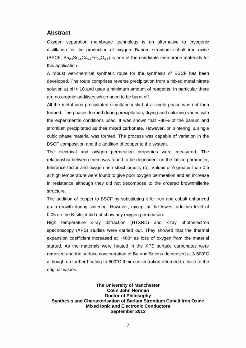
Abstract

Oxygen separation membrane technology is an alternative to cryogenic

distillation for the production of oxygen. Barium strontium cobalt iron oxide

(BSCF, Ba0.5Sr0.5Co0.8Fe0.2O3-δ) is one of the candidate membrane materials for

this application.

A robust wet-chemical synthetic route for the synthesis of BSCF has been

developed. The route comprises reverse precipitation from a mixed metal nitrate

solution at pH> 10 and uses a minimum amount of reagents. In particular there

are no organic additives which need to be burnt off.

All the metal ions precipitated simultaneously but a single phase was not then

formed. The phases formed during precipitation, drying and calcining varied with

the experimental conditions used. It was shown that ~80% of the barium and

strontium precipitated as their mixed carbonate. However, on sintering, a single

cubic phase material was formed. The process was capable of variation in the

BSCF composition and the addition of copper to the system.

The electrical and oxygen permeation properties were measured. The

relationship between them was found to be dependent on the lattice parameter,

tolerance factor and oxygen non-stoichiometry (δ). Values of δ greater than 0.5

at high temperature were found to give poor oxygen permeation and an increase

in resistance although they did not decompose to the ordered brownmillerite

structure.

The addition of copper to BSCF by substituting it for iron and cobalt enhanced

grain growth during sintering. However, except at the lowest addition level of

0.05 on the B-site, it did not show any oxygen permeation.

High temperature x-ray diffraction (HTXRD) and x-ray photoelectron

spectroscopy (XPS) studies were carried out. They showed that the thermal

expansion coefficient increased at ~400° as loss of oxygen from the material

started. As the materials were heated in the XPS surface carbonates were

removed and the surface concentration of Ba and Sr ions decreased at 3-500°C

although on further heating to 800°C their concentration returned to close to the

original values.

The University of Manchester Colin John Norman

Doctor of Philosophy Synthesis and Characterisation of Barium Strontium Cobalt Iron Oxide

Mixed Ionic and Electronic Conductors September 2013

8

Declaration

No portion of the work referred to in the thesis has been submitted in support of

an application for another degree or qualification of this or any other university

or other institute of learning.

9

Copyright Statement

i. The author of this thesis (including any appendices and/or schedules to this

thesis) owns certain copyright or related rights in it (the “Copyright”) and he

has given The University of Manchester certain rights to use such Copyright,

including for administrative purposes.

ii. Copies of this thesis, either in full or in extracts and whether in hard or

electronic copy, may be made only in accordance with the Copyright, Designs

and Patents Act 1988 (as amended) and regulations issued under it or,

where appropriate, in accordance with licensing agreements which the

University has from time to time. This page must form part of any such

copies made.

iii. The ownership of certain Copyright, patents, designs, trademarks and

other intellectual property (the “Intellectual Property”) and any reproductions

of copyright works in the thesis, for example graphs and tables

(“Reproductions”), which may be described in this thesis, may not be owned

by the author and may be owned by third parties. Such Intellectual Property

and Reproductions cannot and must not be made available for use without

the prior written permission of the owner(s) of the relevant Intellectual

Property and/or Reproductions.

iv. Further information on the conditions under which disclosure, publication

and commercialisation of this thesis, the Copyright and any Intellectual

Property and/or Reproductions described in it may take place is available in

the University IP Policy

(see http://documents.manchester.ac.uk/DocuInfo.aspx?DocID=487), in any

relevant Thesis restriction declarations deposited in the University Library,

The University Library’s regulations

(see http://www.manchester.ac.uk/library/aboutus/regulations) and in The

University’s policy on Presentation of Theses

10

Acknowledgements

I would like to thank my supervisor Dr Colin Leach for his help, advice and

encouragement as I embarked on an exploration of a new field.

I would like to thank the many members of the department who so gladly gave

of their time and expertise in setting me on the right route for using the

department’s facilities. In particular I would like to acknowledge:- Dr Rob

Bradley, Ivan Easdon, Mike Faulkner, Andy Forrest, Polly Greensmith, Gary

Harrison, Ken Gyves, Dr Fabien Leonard, Dr Tristan Lowe, Judith Shackleton,

Dave Strong, Andy Wallwork and Dr Chris Wilkins.

Dr Chris Muryn, Department of Chemistry, is thanked for his help in using the

high temperature x-ray diffractometer.

I am grateful for access to the Daresbury NCESS Facility under EPRSC grant

EP/E025722/1. Dr Daniel Law is thanked for his assistance in using the NCESS

facilities.

Mr William Wiseman, MEL Chemicals, a division of Magnesium Elektron

Limited, is thanked for carrying out the nitrogen adsorption experiments.

I am indebted to the members of the functional ceramics team and other

residents of E30a who made me very welcome as a mature student in particular;

Robert Lowndes, Margaret Wegrzyn, Steph Ryding, Nicola Middleton-Stewart,

James Griffiths, Ellyawan Arbintarso, Poonsuk Poosimma, Huanghai Lu, Zijing

Wang, Guannan Chen and Sam Jackson. This is not to forget the ever present

Dr Feridoon Azough.

I would like to thank Mark Sellers, Gareth Daniel and Alan Barbour for regularly

reminding me of the real world and who, despite my researching into ceramics,

won’t be getting their kitchens and bathrooms retiled!

Finally I would like to thank my wife, Helen, for her encouragement, support and

love as I embarked on a late career change.

11

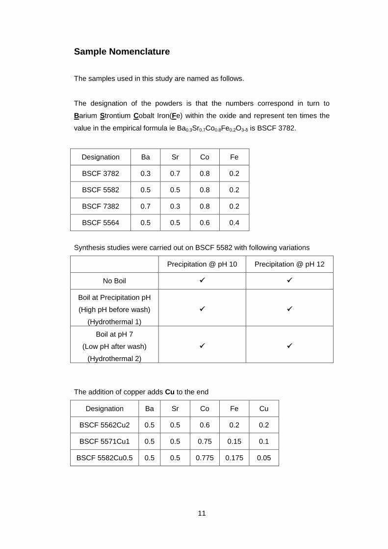
Sample Nomenclature

The samples used in this study are named as follows.

The designation of the powders is that the numbers correspond in turn to

Barium Strontium Cobalt Iron(Fe) within the oxide and represent ten times the

value in the empirical formula ie Ba0.3Sr0.7Co0.8Fe0.2O3-δ is BSCF 3782.

Designation Ba Sr Co Fe

BSCF 3782 0.3 0.7 0.8 0.2

BSCF 5582 0.5 0.5 0.8 0.2

BSCF 7382 0.7 0.3 0.8 0.2

BSCF 5564 0.5 0.5 0.6 0.4

Synthesis studies were carried out on BSCF 5582 with following variations

Precipitation @ pH 10 Precipitation @ pH 12

No Boil

Boil at Precipitation pH

(High pH before wash)

(Hydrothermal 1)

Boil at pH 7

(Low pH after wash)

(Hydrothermal 2)

The addition of copper adds Cu to the end

Designation Ba Sr Co Fe Cu

BSCF 5562Cu2 0.5 0.5 0.6 0.2 0.2

BSCF 5571Cu1 0.5 0.5 0.75 0.15 0.1

BSCF 5582Cu0.5 0.5 0.5 0.775 0.175 0.05

12

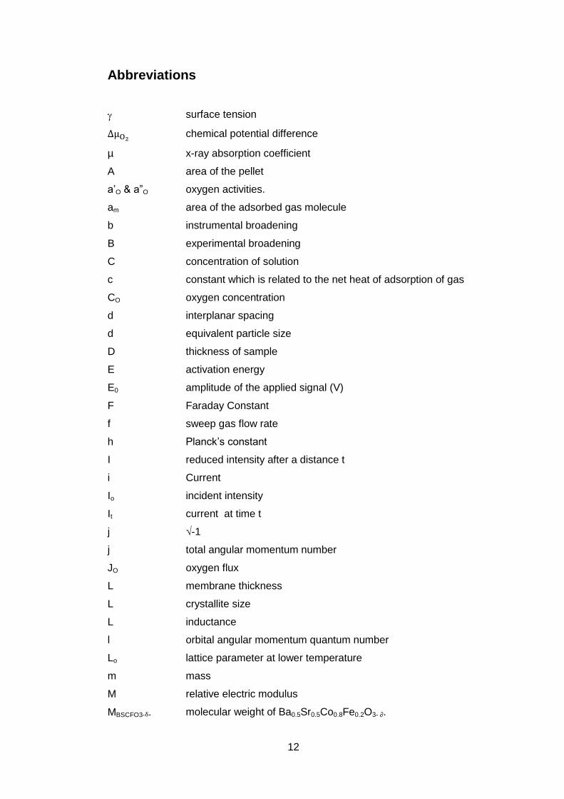
Abbreviations

surface tension

chemical potential difference

µ x-ray absorption coefficient

A area of the pellet

a’O & a”O oxygen activities.

am area of the adsorbed gas molecule

b instrumental broadening

B experimental broadening

C concentration of solution

c constant which is related to the net heat of adsorption of gas

CO oxygen concentration

d interplanar spacing

d equivalent particle size

D thickness of sample

E activation energy

E0 amplitude of the applied signal (V)

F Faraday Constant

f sweep gas flow rate

h Planck’s constant

I reduced intensity after a distance t

i Current

Io incident intensity

It current at time t

j √-1

j total angular momentum number

JO oxygen flux

L membrane thickness

L crystallite size

L inductance

l orbital angular momentum quantum number

Lo lattice parameter at lower temperature

m mass

M relative electric modulus

MBSCFO3-δ. molecular weight of Ba0.5Sr0.5Co0.8Fe0.2O3- ∂.

13

NA Avogadro’s constant

n number of moles of gas in the system

n amount of gas adsorbed

n order of diffraction = 1 for x-ray diffraction

n principal quantum number

nm monolayer capacity

P pressure

p partial pressure

p1 O2 and p2

O2

oxygen partial pressures

po saturation vapour pressure

R gas constant

R Resistance

rm radius of the meniscus

rX ionic radius of the ion in the ABO3 structure.

s spin angular momentum quantum number

SA surface area

T temperature

t path length

t tolerance factor

V volume of titre

V volume

V Voltage

VL molar volume of the liquid

Vm molar volume of an ideal gas

w weight of sample used

Y admittance

Z(ω) impedance

α exponent and equals 1 for a pure capacitor

α thermal expansion coefficient

Βs sample broadening

Δ MW change in molecular weight

ΔEa resolution of analyser.

ΔEn electronic transition line width

ΔEp energy width of exciting x-rays

ΔL lattice parameter change

14

ΔT temperature difference

ε relative permittivity

ε0 electrical permittivity of vacuum

εr dielectric constant

κ Boltzmann’s constant

diffraction angle

λ wavelength of x-rays

ρ theoretical density

ρb bulk density

ρL density of water

ρs apparent solid density

σ conductivity

Τ lifetime

φ phase shift.

Φ work function from the sample to free space

ω radial frequency (radian s-1) and equals 2πf where f is the

frequency (Hz)

15

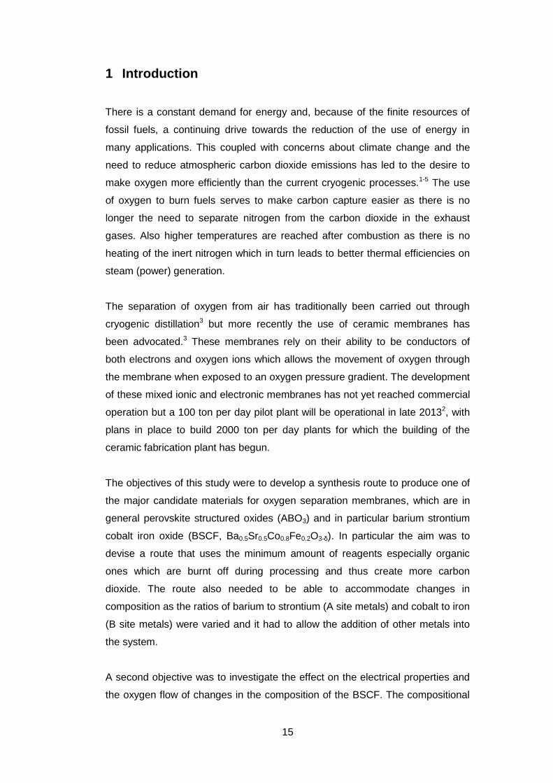
1 Introduction

There is a constant demand for energy and, because of the finite resources of

fossil fuels, a continuing drive towards the reduction of the use of energy in

many applications. This coupled with concerns about climate change and the

need to reduce atmospheric carbon dioxide emissions has led to the desire to

make oxygen more efficiently than the current cryogenic processes.1-5 The use

of oxygen to burn fuels serves to make carbon capture easier as there is no

longer the need to separate nitrogen from the carbon dioxide in the exhaust

gases. Also higher temperatures are reached after combustion as there is no

heating of the inert nitrogen which in turn leads to better thermal efficiencies on

steam (power) generation.

The separation of oxygen from air has traditionally been carried out through

cryogenic distillation3 but more recently the use of ceramic membranes has

been advocated.3 These membranes rely on their ability to be conductors of

both electrons and oxygen ions which allows the movement of oxygen through

the membrane when exposed to an oxygen pressure gradient. The development

of these mixed ionic and electronic membranes has not yet reached commercial

operation but a 100 ton per day pilot plant will be operational in late 20132, with

plans in place to build 2000 ton per day plants for which the building of the

ceramic fabrication plant has begun.

The objectives of this study were to develop a synthesis route to produce one of

the major candidate materials for oxygen separation membranes, which are in

general perovskite structured oxides (ABO3) and in particular barium strontium

cobalt iron oxide (BSCF, Ba0.5Sr0.5Co0.8Fe0.2O3-δ). In particular the aim was to

devise a route that uses the minimum amount of reagents especially organic

ones which are burnt off during processing and thus create more carbon

dioxide. The route also needed to be able to accommodate changes in

composition as the ratios of barium to strontium (A site metals) and cobalt to iron

(B site metals) were varied and it had to allow the addition of other metals into

the system.

A second objective was to investigate the effect on the electrical properties and

the oxygen flow of changes in the composition of the BSCF. The compositional

16

changes were varying the ratios of the A and B metals and further to examine

the effect of copper additions to the composition. A subsidiary objective was to

relate the oxygen flow properties and the measured electrical properties to each

other and the other properties of the ceramics.

Finally changes in the structure and surface chemistry would be studied using a

combination of high temperature x-ray diffraction and high temperature x-ray

photoelectron spectroscopy.

17

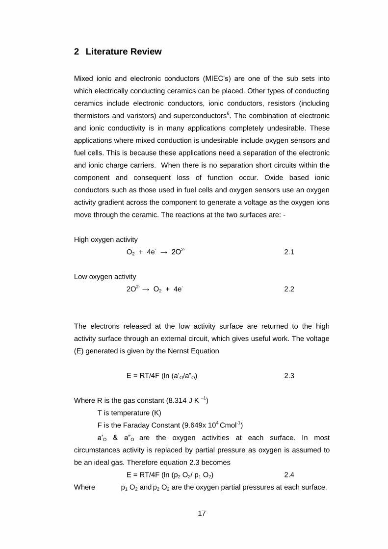
2 Literature Review

Mixed ionic and electronic conductors (MIEC’s) are one of the sub sets into

which electrically conducting ceramics can be placed. Other types of conducting

ceramics include electronic conductors, ionic conductors, resistors (including

thermistors and varistors) and superconductors6. The combination of electronic

and ionic conductivity is in many applications completely undesirable. These

applications where mixed conduction is undesirable include oxygen sensors and

fuel cells. This is because these applications need a separation of the electronic

and ionic charge carriers. When there is no separation short circuits within the

component and consequent loss of function occur. Oxide based ionic

conductors such as those used in fuel cells and oxygen sensors use an oxygen

activity gradient across the component to generate a voltage as the oxygen ions

move through the ceramic. The reactions at the two surfaces are: -

High oxygen activity

O2 + 4e- → 2O2- 2.1

Low oxygen activity

2O2- → O2 + 4e- 2.2

The electrons released at the low activity surface are returned to the high

activity surface through an external circuit, which gives useful work. The voltage

(E) generated is given by the Nernst Equation

E = RT/4F (ln (a’O/a”O) 2.3

Where R is the gas constant (8.314 J K –1)

T is temperature (K)

F is the Faraday Constant (9.649x 104 Cmol-1)

a’O & a”O are the oxygen activities at each surface. In most

circumstances activity is replaced by partial pressure as oxygen is assumed to

be an ideal gas. Therefore equation 2.3 becomes

E = RT/4F (ln (p2 O2/ p1 O2) 2.4

Where p1 O2 and p2 O2 are the oxygen partial pressures at each surface.

18

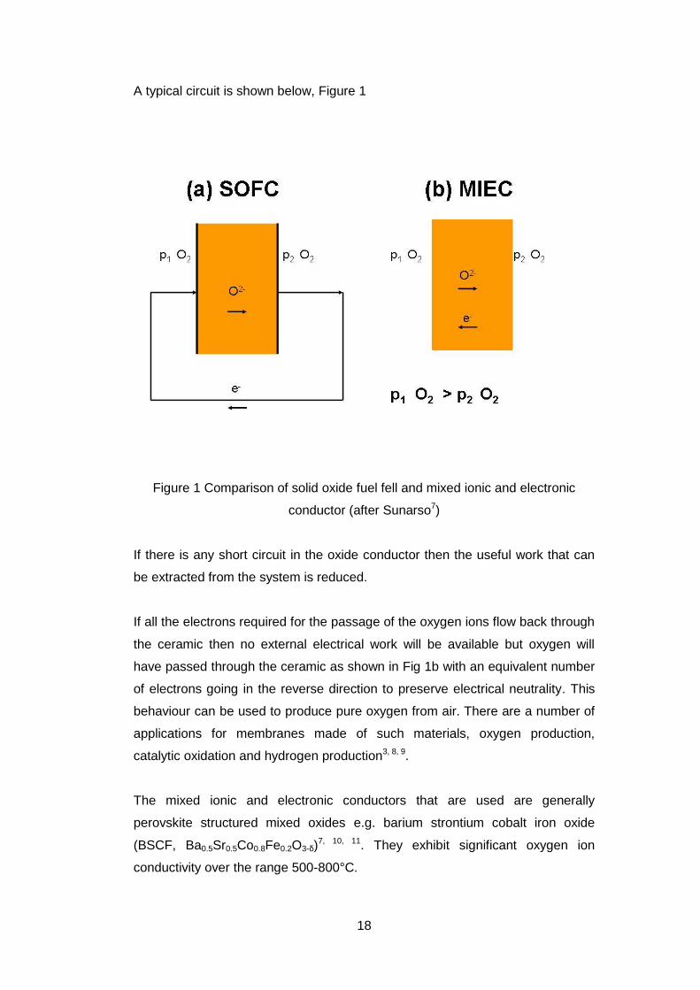
A typical circuit is shown below, Figure 1

Figure 1 Comparison of solid oxide fuel fell and mixed ionic and electronic

conductor (after Sunarso7)

If there is any short circuit in the oxide conductor then the useful work that can

be extracted from the system is reduced.

If all the electrons required for the passage of the oxygen ions flow back through

the ceramic then no external electrical work will be available but oxygen will

have passed through the ceramic as shown in Fig 1b with an equivalent number

of electrons going in the reverse direction to preserve electrical neutrality. This

behaviour can be used to produce pure oxygen from air. There are a number of

applications for membranes made of such materials, oxygen production,

catalytic oxidation and hydrogen production3, 8, 9.

The mixed ionic and electronic conductors that are used are generally

perovskite structured mixed oxides e.g. barium strontium cobalt iron oxide

(BSCF, Ba0.5Sr0.5Co0.8Fe0.2O3-δ)7, 10, 11. They exhibit significant oxygen ion

conductivity over the range 500-800°C.

19

2.1 Applications

2.1.1 Oxygen production

Pure oxygen is a major industrial raw material; world production is about

100x106 tons/annum12. The major applications are steel manufacturing,

chemical synthesis and energy production (power stations)13-15. The current

main processes for oxygen production are cryogenic distillation of liquid air and

pressure swing adsorption although the latter is only used for relatively small

volumes.16, 17

Cryogenic production is done on a large scale with plants typically producing

3000 tonnes/day. The technology is well established however it does have the

drawback of requiring large amounts of energy for the compression and cooling

required.

The requirement for better processes to produce oxygen is driven by the need to

reduce energy consumption and its inherent CO2 emissions. This is not just a

problem at the oxygen production stage.

One of the solutions to the reduction of CO2 emissions in energy production is

carbon capture. This involves collecting the CO2 generated in the combustion

process and then injecting it into suitable rock strata for long-term

storage/disposal. In a conventional power station the fuel is burnt in air and the

CO2 in the flue gas is separated from the water, nitrogen and particulate matter.

The gas separation of CO2 and nitrogen is not easy.

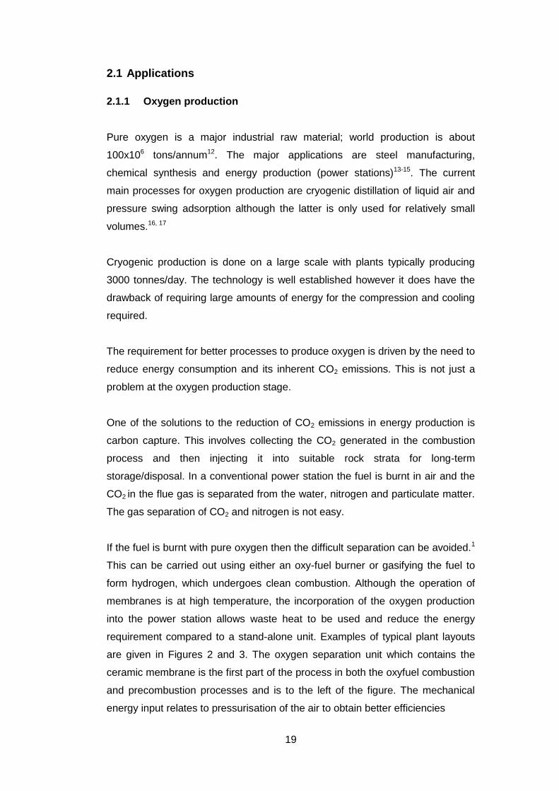
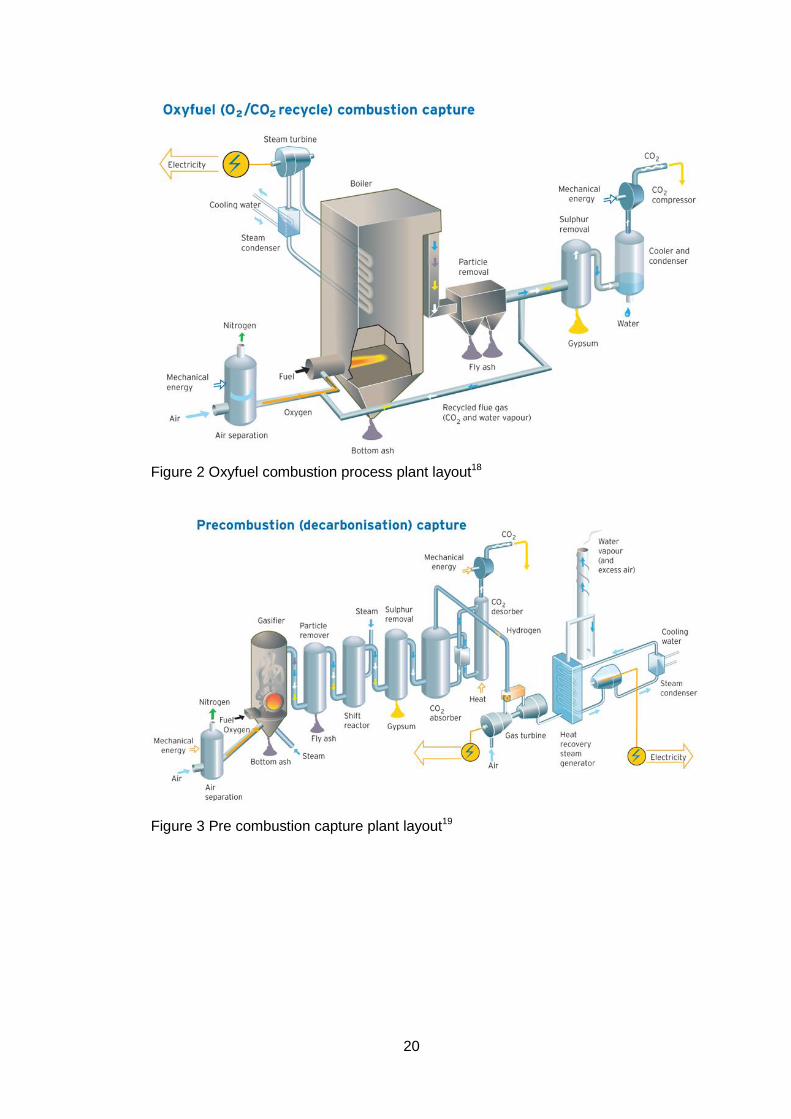
If the fuel is burnt with pure oxygen then the difficult separation can be avoided.1

This can be carried out using either an oxy-fuel burner or gasifying the fuel to

form hydrogen, which undergoes clean combustion. Although the operation of

membranes is at high temperature, the incorporation of the oxygen production

into the power station allows waste heat to be used and reduce the energy

requirement compared to a stand-alone unit. Examples of typical plant layouts

are given in Figures 2 and 3. The oxygen separation unit which contains the

ceramic membrane is the first part of the process in both the oxyfuel combustion

and precombustion processes and is to the left of the figure. The mechanical

energy input relates to pressurisation of the air to obtain better efficiencies

20

Figure 2 Oxyfuel combustion process plant layout18

Figure 3 Pre combustion capture plant layout19

21

2.1.2 Catalytic Oxidation

In many chemical processes there is a requirement for an intermediate product

to be oxidised20. This needs to be controlled to prevent complete oxidation to

CO2 and water. A large number of reagents can be used to effect oxidation but

their reduction products need to be separated from the reaction mix. The use of

oxygen removes many of these problems though it tends to be less selective

towards the partial oxidation reactions20.

The use of an oxygen membrane to supply the oxygen for the reaction can

enable better control of the partial oxidation reactions especially if a suitable

catalyst is applied on the reaction side. This approach has been studied for the

partial oxidation of methane to produce so called synthesis gas15.

2CH4 + O2 → 2CO + 4H2 2.5

This can be further reacted with steam to produce CO2 and more hydrogen.

These are also examples of the reactions occurring during fuel gasification.

Synthesis gas can be used to make many compounds including higher

hydrocarbons that make up petrol.

Partial oxidation of methane can also be used to produce methanol, an

important chemical intermediate.

2CH4 + O2 → 2CH3OH 2.6

Through the use of appropriate catalysts and the oxygen partial pressures

selectivity to desired reaction can be accomplished.

2.1.3 Hydrogen Production

As part of the need to reduce CO2 emissions non-carbon containing fuels are

being evaluated. The most promising of these is hydrogen as it burns cleanly

forming only water. The production of hydrogen is not so easy and despite large

amounts being made it is mainly formed through partial oxidation reactions as

22

described above. Electrolysis can also be used but that too relies on electricity

from carbon-derived sources.

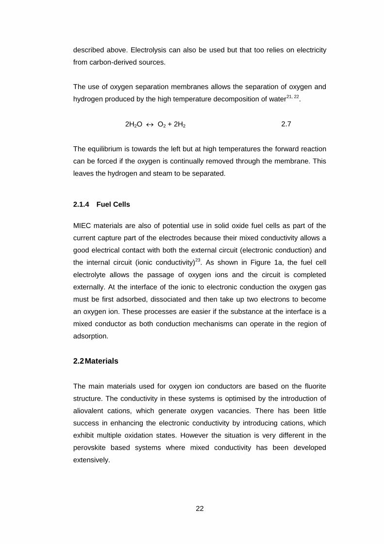
The use of oxygen separation membranes allows the separation of oxygen and

hydrogen produced by the high temperature decomposition of water21, 22.

2H2O O2 + 2H2 2.7

The equilibrium is towards the left but at high temperatures the forward reaction

can be forced if the oxygen is continually removed through the membrane. This

leaves the hydrogen and steam to be separated.

2.1.4 Fuel Cells

MIEC materials are also of potential use in solid oxide fuel cells as part of the

current capture part of the electrodes because their mixed conductivity allows a

good electrical contact with both the external circuit (electronic conduction) and

the internal circuit (ionic conductivity)23. As shown in Figure 1a, the fuel cell

electrolyte allows the passage of oxygen ions and the circuit is completed

externally. At the interface of the ionic to electronic conduction the oxygen gas

must be first adsorbed, dissociated and then take up two electrons to become

an oxygen ion. These processes are easier if the substance at the interface is a

mixed conductor as both conduction mechanisms can operate in the region of

adsorption.

2.2 Materials

The main materials used for oxygen ion conductors are based on the fluorite

structure. The conductivity in these systems is optimised by the introduction of

aliovalent cations, which generate oxygen vacancies. There has been little

success in enhancing the electronic conductivity by introducing cations, which

exhibit multiple oxidation states. However the situation is very different in the

perovskite based systems where mixed conductivity has been developed

extensively.

23

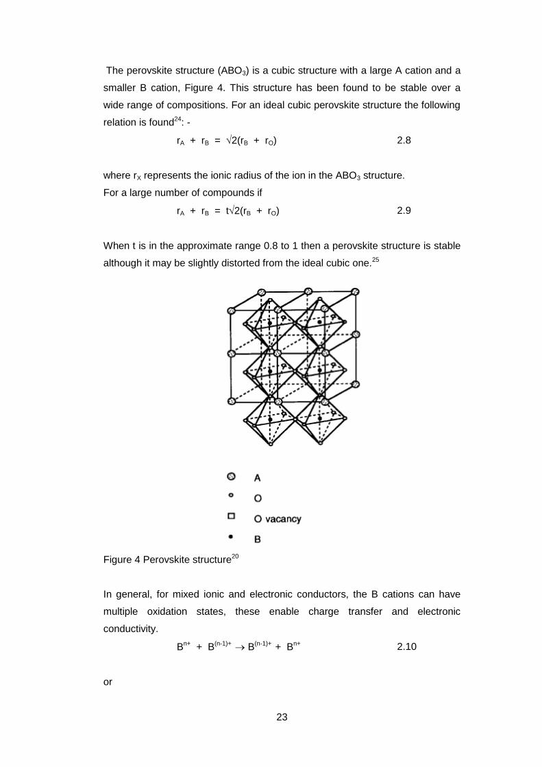
The perovskite structure (ABO3) is a cubic structure with a large A cation and a

smaller B cation, Figure 4. This structure has been found to be stable over a

wide range of compositions. For an ideal cubic perovskite structure the following

relation is found24: -

rA + rB = 2(rB + rO) 2.8

where rX represents the ionic radius of the ion in the ABO3 structure.

For a large number of compounds if

rA + rB = t2(rB + rO) 2.9

When t is in the approximate range 0.8 to 1 then a perovskite structure is stable

although it may be slightly distorted from the ideal cubic one.25

Figure 4 Perovskite structure20

In general, for mixed ionic and electronic conductors, the B cations can have

multiple oxidation states, these enable charge transfer and electronic

conductivity.

Bn+ + B(n-1)+ B(n-1)+ + Bn+ 2.10

or

24

2.11

B(n-1)+ Bn+ + e- 2.12

The larger A cations generally have a single oxidation state and are not involved

directly in electronic conductivity.

The oxygen ion conductivity occurs by oxygen ion hopping from a lattice site to

a neighbouring vacancy. In an ideal perovskite the charges on the A and B

cations add up to 6, this can be any combination of 1-5, 2-4 and 3-3 as long as

the tolerance factor is within the normal limits. Vacancies can form if the

multivalent cation is present in more than one oxidation state. The formula for

the perovskite is then ABO3-, where represents non-stoichiometry. The

determination of and the oxidation state of the cations will be discussed later

(Section 3.2.3).

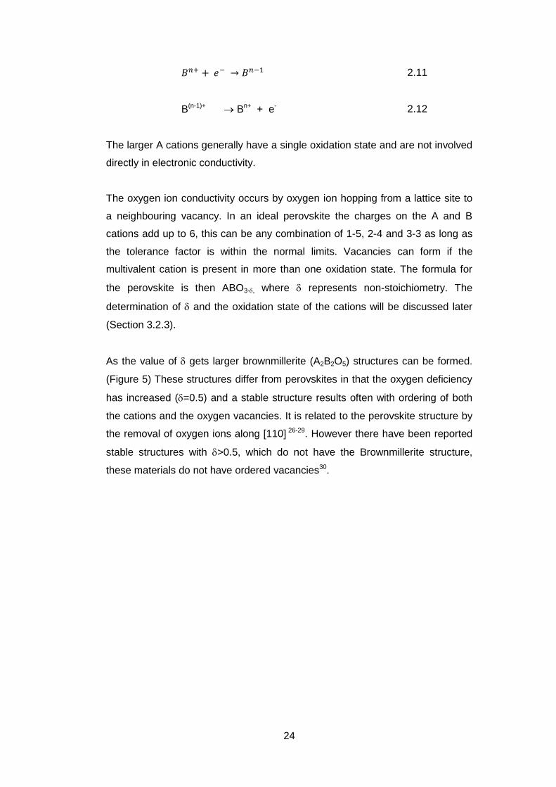
As the value of gets larger brownmillerite (A2B2O5) structures can be formed.

(Figure 5) These structures differ from perovskites in that the oxygen deficiency

has increased (=0.5) and a stable structure results often with ordering of both

the cations and the oxygen vacancies. It is related to the perovskite structure by

the removal of oxygen ions along [110] 26-29. However there have been reported

stable structures with >0.5, which do not have the Brownmillerite structure,

these materials do not have ordered vacancies30.

25

Figure 5 Brownmillerite structure20

The most common MIEC compositions were based on SrCoO323. It was found

that a number of different phases based on the perovskite structure could be

formed but the cubic phase exhibited the best oxygen permeability.27, 31 However

it did not have a good thermal stability and transformed to the other phases with

poorer properties. This meant that variants on the composition were sought

which gave the required stability. The composition changes were to use

lanthanides on the A site and other transition metals on the B site.32, 33 Some

workers were modifying LaCoO3 which was used as a catalyst composition. The

result of this work was that La0.6Sr0.4Co0.8Fe.2O3-δ was found to give the best

oxygen permeability.

This structure has 3+ and 2+ ions on the A site, this will reduce the oxygen

vacancies as extra oxygen ions will be needed to maintain overall electrical

neutrality. This reduction in the oxygen vacancies causes a reduction in the

oxygen permeability11. Therefore the substitution of La3+ with Ba2+ would enable

the vacancy concentration to be restored without affecting the thermal stability.

The composition Ba0.5Sr0.5Co0.8Fe0.2O3-δ was shown to have both good stability

and oxygen permeability.10 The effect of changing the barium strontium ratio

was further studied.11

26

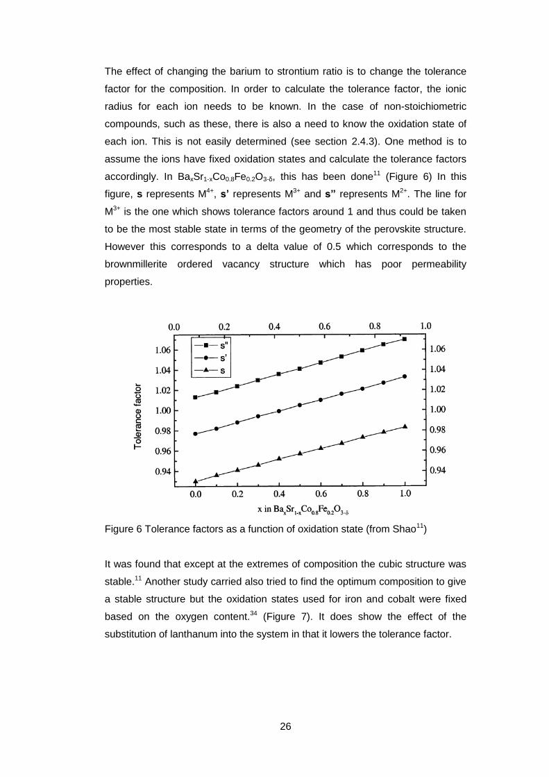
The effect of changing the barium to strontium ratio is to change the tolerance

factor for the composition. In order to calculate the tolerance factor, the ionic

radius for each ion needs to be known. In the case of non-stoichiometric

compounds, such as these, there is also a need to know the oxidation state of

each ion. This is not easily determined (see section 2.4.3). One method is to

assume the ions have fixed oxidation states and calculate the tolerance factors

accordingly. In BaxSr1-xCo0.8Fe0.2O3-δ, this has been done11 (Figure 6) In this

figure, s represents M4+, s’ represents M3+ and s” represents M2+. The line for

M3+ is the one which shows tolerance factors around 1 and thus could be taken

to be the most stable state in terms of the geometry of the perovskite structure.

However this corresponds to a delta value of 0.5 which corresponds to the

brownmillerite ordered vacancy structure which has poor permeability

properties.

Figure 6 Tolerance factors as a function of oxidation state (from Shao11)

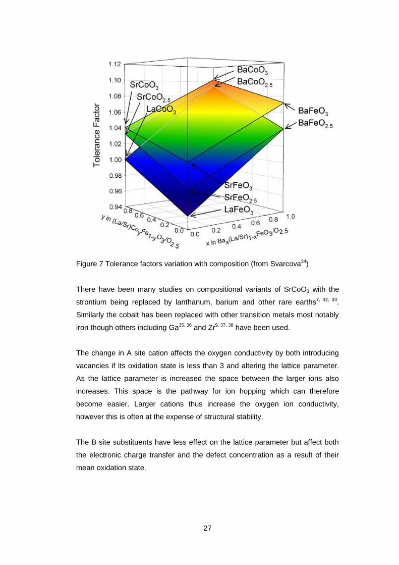
It was found that except at the extremes of composition the cubic structure was

stable.11 Another study carried also tried to find the optimum composition to give

a stable structure but the oxidation states used for iron and cobalt were fixed

based on the oxygen content.34 (Figure 7). It does show the effect of the

substitution of lanthanum into the system in that it lowers the tolerance factor.

27

Figure 7 Tolerance factors variation with composition (from Svarcova34)

There have been many studies on compositional variants of SrCoO3 with the

strontium being replaced by lanthanum, barium and other rare earths7, 32, 33.

Similarly the cobalt has been replaced with other transition metals most notably

iron though others including Ga35, 36 and Zr9, 37, 38 have been used.

The change in A site cation affects the oxygen conductivity by both introducing

vacancies if its oxidation state is less than 3 and altering the lattice parameter.

As the lattice parameter is increased the space between the larger ions also

increases. This space is the pathway for ion hopping which can therefore

become easier. Larger cations thus increase the oxygen ion conductivity,

however this is often at the expense of structural stability.

The B site substituents have less effect on the lattice parameter but affect both

the electronic charge transfer and the defect concentration as a result of their

mean oxidation state.

28

Although the compositions were originally based on SrCoO3,

Ba0.5Sr0.5Co0.8Fe0.2O3-δ is the leading candidate as it has one of the highest

oxygen permeabilities10.

2.3 Synthesis

The synthesis of MIEC compounds has been carried out using the standard

methods7, 39 used for mixed metal oxides, mixed powder, sol-gel, organic gel

(Pechini40 and variants) and co-precipitation41. The object of all the synthesis

routes is to produce a chemically homogenous powder, which will sinter at low

temperatures to form a fully dense single-phase ceramic. Each of the routes has

a number of advantages and disadvantages as will be discussed below with

respect to BSCF.

2.3.1 Solid State Reaction

In many ways this is the simplest procedure, the constituent oxides are mixed

together and heated until they react and form the desired compound. The oxides

can be replaced by hydroxides and carbonates for this process. Also a solution

of salts of the metals can be dried and then calcined. The simplicity of the

process though its chief advantage does bring some disadvantages. The

reactions between the components may take place at different temperature

which coupled with grain growth of the initially formed phase may not allow

complete homogenisation of the final product. The product is often

agglomerated and needs intensive milling prior to forming and sintering. The use

of salts may not give a very homogeneous dried product because of their

different solubilities. The salt with the lowest solubility crystallises first and then

the other salts crystallise in turn. This can lead to crystals with composition

gradients from the centre to the outside or a mixture of the various salts. This

can be overcome by drying rapidly using processes such as spray or freeze-

drying. Overall the mixed powder process has few variables and is therefore not

amenable to much optimisation.

29

2.3.2 Sol-Gel

There are a number of processes that can be called sol-gel they all involve the

hydrolysis of a solution to give a sol which then forms a gel which is dried and

calcined to give the desired compound. The conditions of the hydrolysis are

carefully controlled in order to give a homogeneous sol prior to gelation. The

major problem of this process is the difference in reactivity of the components so

that a series of sols form which yield an inhomogeneous system. There are

however many variables in terms of starting materials, the conditions of

hydrolysis and subsequent stages that can be varied which allow good control of

the powder properties.

2.3.3 Organic Gel

This is one of the most commonly used methods as it is in some ways a

variation on the drying and calcination of salt solutions. In order to prevent the

separation of the metal compounds the solution is gelled as a whole prior to

drying. Pechini did this by adding ethane-1,2-diol and citric acid to the solution

and heating it until gelation. More recent variations are to use EDTA and citric

acid42 with the gelation being controlled at a specific pH by the addition of

ammonia. It is a relatively easy route to carry out but does have a number of

disadvantages. The gel is quite voluminous relative to the final oxide content

and usually contains organic material, nitrate and ammonia. These could

combine during the drying and calcination phase to form explosive mixtures.39

This behaviour has been described in a number of ways e.g. Baumann et al43,

“Inside a fume hood, this mixture was then heated up until a spontaneous

combustion occurred.”, Bi et al44 “the solution was heated under stirring to

evaporate water until it changed into a viscous gel and finally ignited to flame,

resulting in a black ash.” and Moharil et al45 “When the heating was continued

further, the gel catched a burning flame itself and charred completely resulting

into a light and fragile ash”. In any case the nitrate will decompose giving off

noxious fumes.

After gel formation the system is either dried or heated to combustion, this is

prior to calcination. The formation of different phases at this stage has given

mixtures of BaCO3, BaFe2O4, CoO, SrO and Fe2O342. In another study46 a

30

different set of phases was found, namely, Ba0.5Sr0.5Co0.2Fe0.8O3-δ, BaCO3 and

CoFe2O4. In a similar preparation of Ba0.5Sr0.5Co0.8Zn0.2O3-δ no crystalline phases

were found until a calcination temperature in excess of 700°C was used47. At

that temperature the powder comprised barium-strontium carbonate, a zinc-iron

spinel and zinc oxide, which at higher temperatures formed a single phase

material. A simplification of the method was reported48 which just used ethylene

diamine N,N,N’,N’ tetra N-acetyl diamine as the complexing agent to replace

EDTA, citric acid, nitric acid and ammonia as the earlier system needed careful

pH control to prevent precipitation prior to gelation.

The decomposition of the metal compounds occurs at different temperatures,

which may give some inhomogeneity as found in the solid state method.

However the crystallite size may be much smaller and allow better homogeneity.

Oxides may form at low temperatures but then adsorb CO2 from the combustion

of the organics to form less reactive carbonates.

2.3.4 Co-precipitation

The addition of a precipitant to a mixed metal solution is seemingly a simple

process. However the different components have to be both soluble at the

starting point and ideally all insoluble at the same point during the precipitation

process. If the latter cannot be achieved because the precipitation of the solute

species occurs in stages as the solubility is reached as either the pH rises or the

precipitant concentration increases, then techniques such as continuous and

reverse precipitation can be employed. (Forward precipitation is the process

whereby the precipitant is added to the mixed metal salt solution.) In these latter

methods precipitation occurs under conditions where there is always an excess

of precipitant, which ensures simultaneous precipitation of all species. With

forward precipitation the least soluble component precipitates first followed

sequentially by the others. There are many variables in this process,

temperature, anions, concentration, precipitant and pH, which allow variations to

be made or control difficult. Drying often leads to leads to the formation of hard

agglomerates, which are difficult to break down either before or after calcination.

Pelosato et al49,50 used ammonium hydroxide solution and ammonium carbonate

to prepare La0.8Sr0.2Ga0.8Mg0.2O3-δ and LaMnO3, La0.7Sr0.3MnO3-δ, La0.8Sr0.2FeO3-δ

31

and La0.75Sr0.25Cr0.5Mn0.5O3-δ. Their aim was to achieve complete precipitation

and only have impurities (nitrates, carbonates and the ammonium ions) which

would be readily lost on calcination. In the case of La0.8Sr0.2Ga0.8Mg0.2O3-δ, when

ammonium hydroxide solution was used as the precipitant, strontium and

magnesium were detected in the filtrate. This was also the case when the mixed

nitrates were added directly to an excess of ammonium carbonate. Minor

magnesium losses only occurred when the mixed nitrates were added to a

stoichiometric amount of carbonate after the starting solution was reduced in pH

to 1 by the addition of nitric acid. In the second group of oxides an excess of

ammonium carbonate was found to be necessary in order to obtain complete

precipitation. It is clear that a generic method e.g. addition of excess ammonium

carbonate as the precipitant to an acidified mixed salt solution will not always

work. The method chosen must reflect the actual composition being

synthesised.

Toprak et al51 had problems using sol-gel methods used for the synthesis of

Ba0.5Sr0.5Co0.2Fe0.8O3-δ, as their active powders reacted with their crucibles and

substrates during calcination and sintering, respectively. Their solution was to

use a co-precipitation technique using oxalate as the precipitant. Using Medusa

software52 they found that in the pH range of 2-3 all the ions precipitated

completely (apart from Fe2+). The addition of oxalic acid to the mixed salt

solution only precipitated 80% of the iron present in solution so they added an

extra 20% iron nitrate to compensate which enabled the correct stoichiometry to

be obtained at the end of the synthetic route. The precipitates were dried at

110°C before carrying out thermogravimetric analysis. This showed 4

decomposition steps starting at ~100°C, 375°C, 420°C and 790°C. Powder was

calcined after each of these stages and examined by XRD. At all temperatures a

number of different phases were present before the single phase perovskite was

formed at 1000°C.

2.3.5 Finishing Processes

There are a number of additional stages that can be included in the 3 wet

processes41. Hydrothermal or solvothermal treatments can affect the powder

properties especially homogeneity and crystallinity prior to drying and

calcination.53

32

The drying stage can be varied and includes freeze and spray drying. The

temperature used affects the agglomeration and decompositions occurring at

this stage. Calcination can be carried out under different atmospheres, which

may affect the final product.

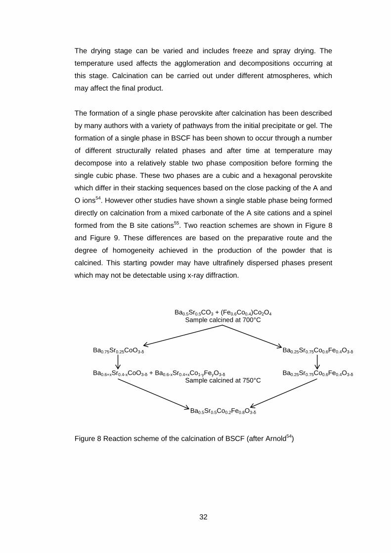
The formation of a single phase perovskite after calcination has been described

by many authors with a variety of pathways from the initial precipitate or gel. The

formation of a single phase in BSCF has been shown to occur through a number

of different structurally related phases and after time at temperature may

decompose into a relatively stable two phase composition before forming the

single cubic phase. These two phases are a cubic and a hexagonal perovskite

which differ in their stacking sequences based on the close packing of the A and

O ions54. However other studies have shown a single stable phase being formed

directly on calcination from a mixed carbonate of the A site cations and a spinel

formed from the B site cations55. Two reaction schemes are shown in Figure 8

and Figure 9. These differences are based on the preparative route and the

degree of homogeneity achieved in the production of the powder that is

calcined. This starting powder may have ultrafinely dispersed phases present

which may not be detectable using x-ray diffraction.

Ba0.5Sr0.5CO3 + (Fe0.6Co0.4)Co2O4 Sample calcined at 700°C

Ba0.75Sr0.25CoO3-δ Ba0.25Sr0.75Co0.6Fe0.4O3-δ

Ba0.6+xSr0.4-xCoO3-δ + Ba0.6-xSr0.4+xCo1-yFeyO3-δ Ba0.25Sr0.75Co0.6Fe0.4O3-δ Sample calcined at 750°C

Ba0.5Sr0.5Co0.2Fe0.8O3-δ

Figure 8 Reaction scheme of the calcination of BSCF (after Arnold54)

33

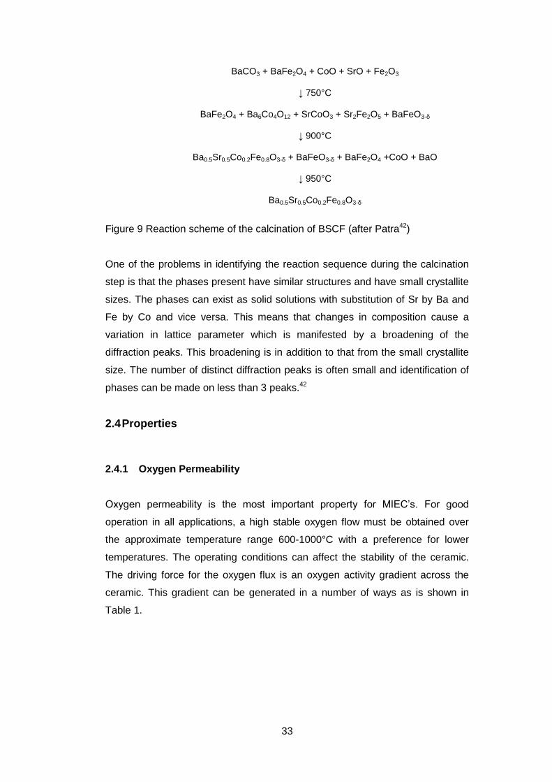
BaCO3 + BaFe2O4 + CoO + SrO + Fe2O3

↓ 750°C

BaFe2O4 + Ba6Co4O12 + SrCoO3 + Sr2Fe2O5 + BaFeO3-δ

↓ 900°C

Ba0.5Sr0.5Co0.2Fe0.8O3-δ + BaFeO3-δ + BaFe2O4 +CoO + BaO

↓ 950°C


Figure 9 Reaction scheme of the calcination of BSCF (after Patra42)

One of the problems in identifying the reaction sequence during the calcination

step is that the phases present have similar structures and have small crystallite

sizes. The phases can exist as solid solutions with substitution of Sr by Ba and

Fe by Co and vice versa. This means that changes in composition cause a

variation in lattice parameter which is manifested by a broadening of the

diffraction peaks. This broadening is in addition to that from the small crystallite

size. The number of distinct diffraction peaks is often small and identification of

phases can be made on less than 3 peaks.42

2.4 Properties

2.4.1 Oxygen Permeability

Oxygen permeability is the most important property for MIEC’s. For good

operation in all applications, a high stable oxygen flow must be obtained over

the approximate temperature range 600-1000°C with a preference for lower

temperatures. The operating conditions can affect the stability of the ceramic.

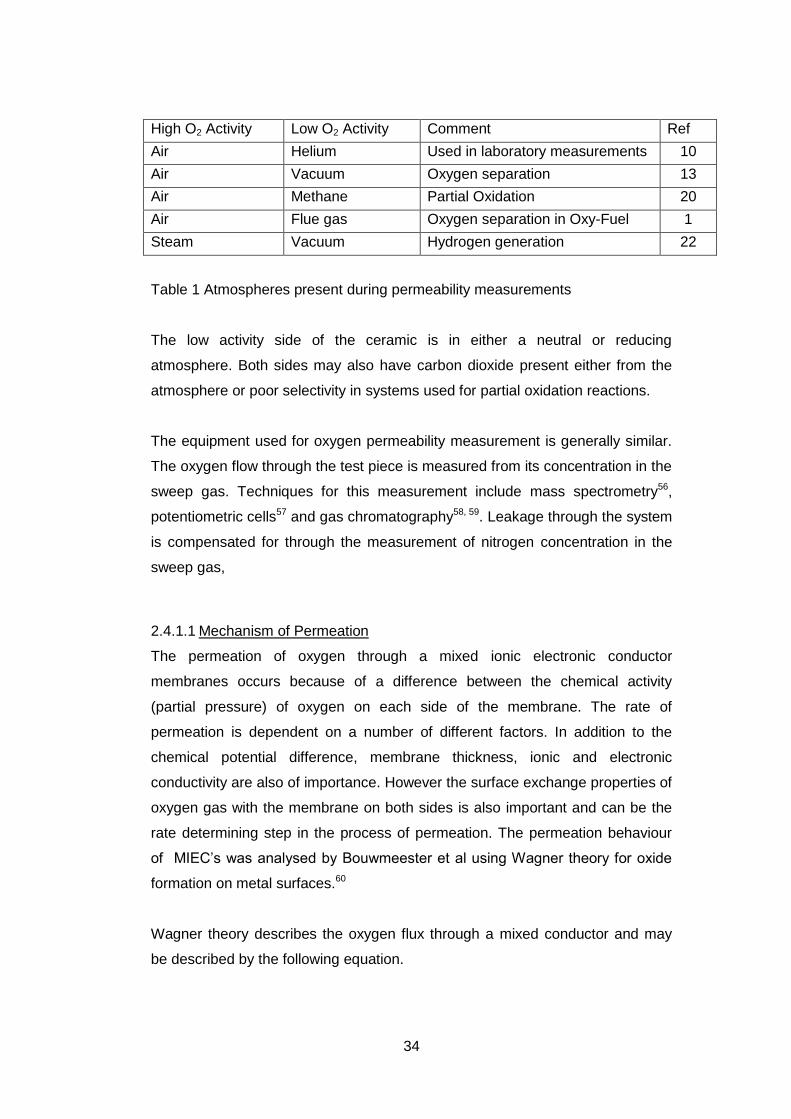
The driving force for the oxygen flux is an oxygen activity gradient across the

ceramic. This gradient can be generated in a number of ways as is shown in

Table 1.

34

High O2 Activity Low O2 Activity Comment Ref

Air Helium Used in laboratory measurements 10

Air Vacuum Oxygen separation 13

Air Methane Partial Oxidation 20

Air Flue gas Oxygen separation in Oxy-Fuel 1

Steam Vacuum Hydrogen generation 22

Table 1 Atmospheres present during permeability measurements

The low activity side of the ceramic is in either a neutral or reducing

atmosphere. Both sides may also have carbon dioxide present either from the

atmosphere or poor selectivity in systems used for partial oxidation reactions.

The equipment used for oxygen permeability measurement is generally similar.

The oxygen flow through the test piece is measured from its concentration in the

sweep gas. Techniques for this measurement include mass spectrometry56,

potentiometric cells57 and gas chromatography58, 59. Leakage through the system

is compensated for through the measurement of nitrogen concentration in the

sweep gas,

2.4.1.1 Mechanism of Permeation

The permeation of oxygen through a mixed ionic electronic conductor

membranes occurs because of a difference between the chemical activity

(partial pressure) of oxygen on each side of the membrane. The rate of

permeation is dependent on a number of different factors. In addition to the

chemical potential difference, membrane thickness, ionic and electronic

conductivity are also of importance. However the surface exchange properties of

oxygen gas with the membrane on both sides is also important and can be the

rate determining step in the process of permeation. The permeation behaviour

of MIEC’s was analysed by Bouwmeester et al using Wagner theory for oxide

formation on metal surfaces.60

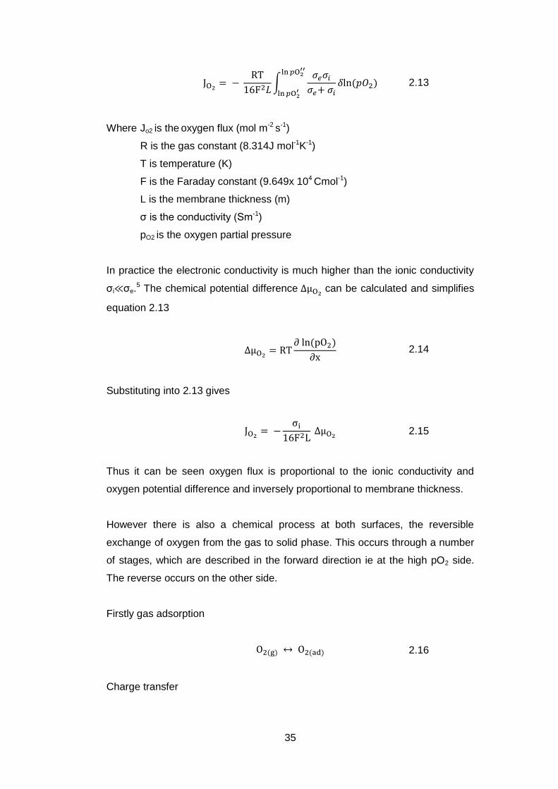
Wagner theory describes the oxygen flux through a mixed conductor and may

be described by the following equation.

35

∫

2.13

Where Jo2 is the oxygen flux (mol m-2 s-1)

R is the gas constant (8.314J mol-1K-1)


F is the Faraday constant (9.649x 104 Cmol-1)

L is the membrane thickness (m)

σ is the conductivity (Sm-1)

pO2 is the oxygen partial pressure

In practice the electronic conductivity is much higher than the ionic conductivity

σi σe.5 The chemical potential difference

can be calculated and simplifies

equation 2.13

2.14

Substituting into 2.13 gives

2.15

Thus it can be seen oxygen flux is proportional to the ionic conductivity and

oxygen potential difference and inversely proportional to membrane thickness.

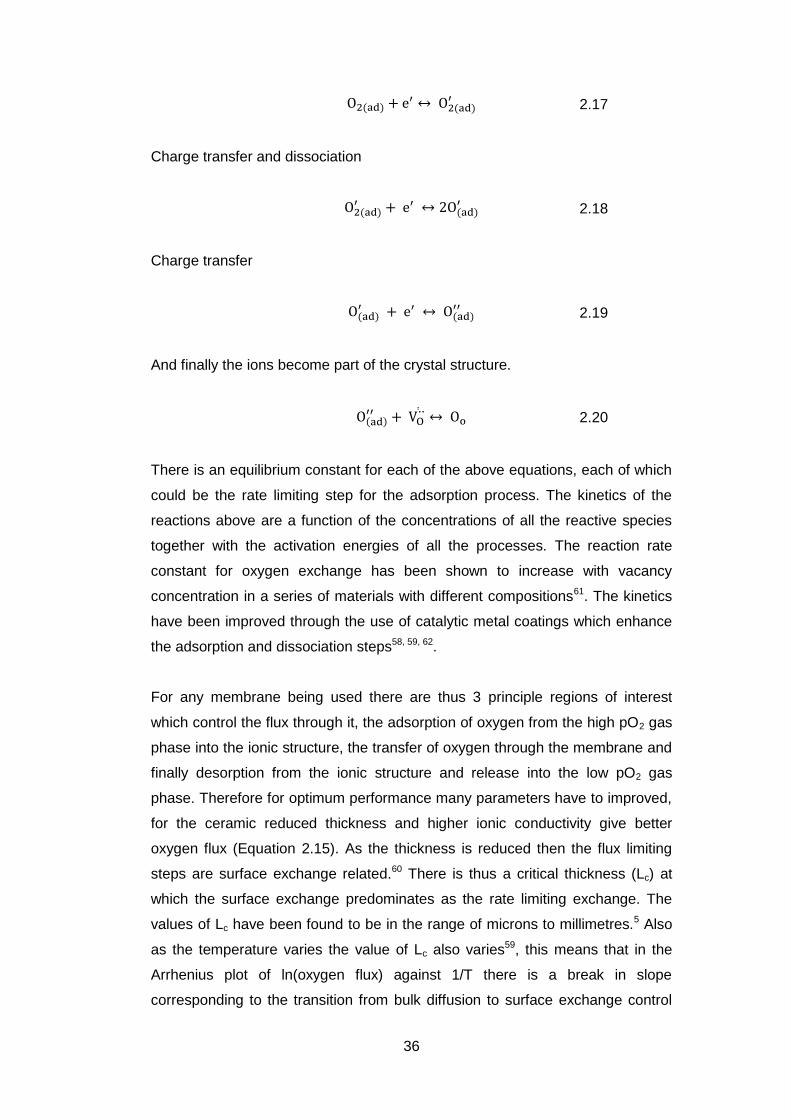
However there is also a chemical process at both surfaces, the reversible

exchange of oxygen from the gas to solid phase. This occurs through a number

of stages, which are described in the forward direction ie at the high pO2 side.

The reverse occurs on the other side.

Firstly gas adsorption

2.16

Charge transfer

36

2.17

Charge transfer and dissociation

2.18

Charge transfer

2.19

And finally the ions become part of the crystal structure.

2.20

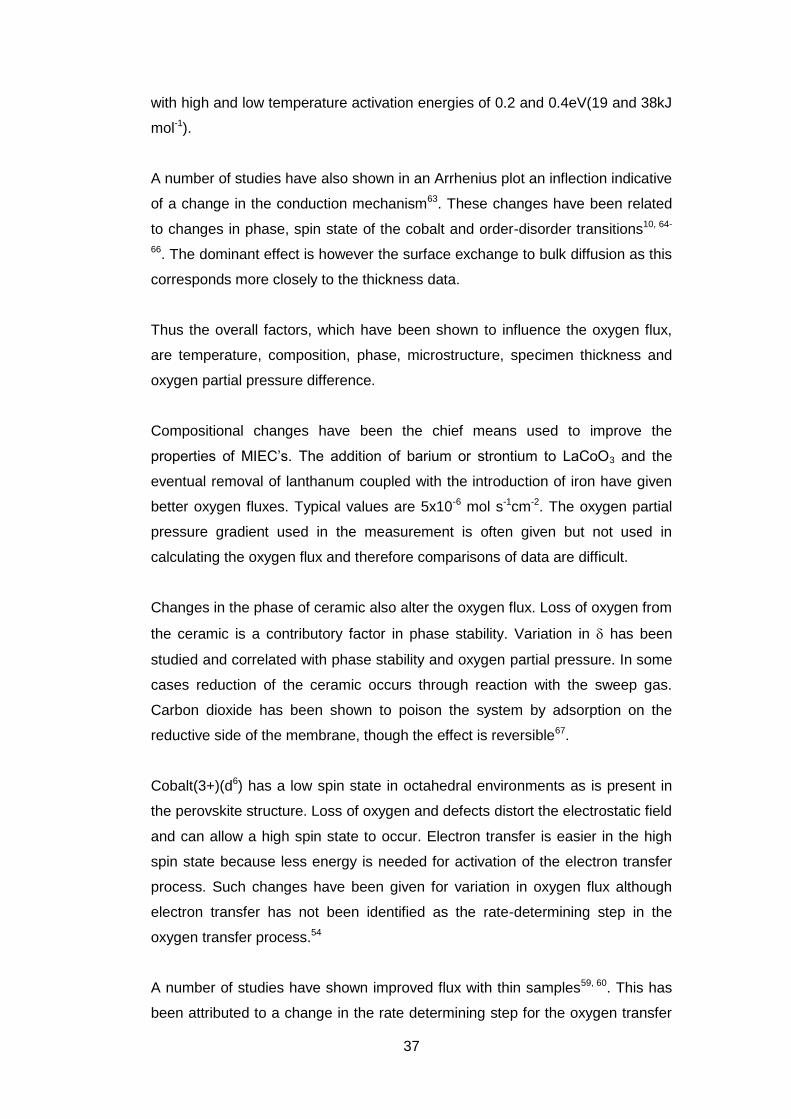
There is an equilibrium constant for each of the above equations, each of which

could be the rate limiting step for the adsorption process. The kinetics of the

reactions above are a function of the concentrations of all the reactive species

together with the activation energies of all the processes. The reaction rate

constant for oxygen exchange has been shown to increase with vacancy

concentration in a series of materials with different compositions61. The kinetics

have been improved through the use of catalytic metal coatings which enhance

the adsorption and dissociation steps58, 59, 62.

For any membrane being used there are thus 3 principle regions of interest

which control the flux through it, the adsorption of oxygen from the high pO2 gas

phase into the ionic structure, the transfer of oxygen through the membrane and

finally desorption from the ionic structure and release into the low pO2 gas

phase. Therefore for optimum performance many parameters have to improved,

for the ceramic reduced thickness and higher ionic conductivity give better

oxygen flux (Equation 2.15). As the thickness is reduced then the flux limiting

steps are surface exchange related.60 There is thus a critical thickness (Lc) at

which the surface exchange predominates as the rate limiting exchange. The

values of Lc have been found to be in the range of microns to millimetres.5 Also

as the temperature varies the value of Lc also varies59, this means that in the

Arrhenius plot of ln(oxygen flux) against 1/T there is a break in slope

corresponding to the transition from bulk diffusion to surface exchange control

37

with high and low temperature activation energies of 0.2 and 0.4eV(19 and 38kJ

mol-1).

A number of studies have also shown in an Arrhenius plot an inflection indicative

of a change in the conduction mechanism63. These changes have been related

to changes in phase, spin state of the cobalt and order-disorder transitions10, 64-

66. The dominant effect is however the surface exchange to bulk diffusion as this

corresponds more closely to the thickness data.

Thus the overall factors, which have been shown to influence the oxygen flux,

are temperature, composition, phase, microstructure, specimen thickness and

oxygen partial pressure difference.

Compositional changes have been the chief means used to improve the

properties of MIEC’s. The addition of barium or strontium to LaCoO3 and the

eventual removal of lanthanum coupled with the introduction of iron have given

better oxygen fluxes. Typical values are 5x10-6 mol s-1cm-2. The oxygen partial

pressure gradient used in the measurement is often given but not used in

calculating the oxygen flux and therefore comparisons of data are difficult.

Changes in the phase of ceramic also alter the oxygen flux. Loss of oxygen from

the ceramic is a contributory factor in phase stability. Variation in has been

studied and correlated with phase stability and oxygen partial pressure. In some

cases reduction of the ceramic occurs through reaction with the sweep gas.

Carbon dioxide has been shown to poison the system by adsorption on the

reductive side of the membrane, though the effect is reversible67.

Cobalt(3+)(d6) has a low spin state in octahedral environments as is present in

the perovskite structure. Loss of oxygen and defects distort the electrostatic field

and can allow a high spin state to occur. Electron transfer is easier in the high

spin state because less energy is needed for activation of the electron transfer

process. Such changes have been given for variation in oxygen flux although

electron transfer has not been identified as the rate-determining step in the

oxygen transfer process.54

A number of studies have shown improved flux with thin samples59, 60. This has

been attributed to a change in the rate determining step for the oxygen transfer

38

process from oxygen hopping to the surface reaction of oxygen gas adsorbing,

splitting and forming oxide ions59, 60. The surface vacancy concentration on each

surface is also important as this affects the kinetics of oxygen exchange prior to

ion diffusion through the bulk68. The two rate determining states and the oxygen

vacancy concentration which is itself dependent on the local oxygen partial

pressure and temperature combine to complicate the interpretation of

permeability data.

The influence of microstructure has not been extensively studied partially due to

the difficulty in making materials of high density and uniform phase. Increase in

grain size has shown increased oxygen flux and no separate phase was found

at the grain boundaries69. The densification rate has been shown to be slow and

long sintering times and slow heating rates are used70, 71. One problem, which

some workers but not all have reported, is the melting of the material56. The role

of grain size has also been shown to be insignificant56.. Consequently the roles

of grain boundary and bulk grain processes have not been studied.

Changes in the microstructure have been observed on both sides of the

membrane after oxygen permeation experiments. The perovskite phase

disappears on the reductive side whereas no phase change occurs on the

oxidative side. Changes in composition have been seen using EDS72.

2.4.2 Electrical Properties

The electrical properties of MIEC’s have been studied although in most cases

they are part of a complete fuel cell64, 73, 74. Changes in conductivity both positive

and negative have been observed in fuel cell structures as the measurement

atmosphere has been changed between oxygen, air and argon. Measurement of

pure nano-crystalline BSCF showed an improvement over conventional BSCF,

the conductivity reaching a plateau at ~700K 75, 76.

One study measured the conductivity of Ba0.5Sr 0.5CoxFe1-xO3- over a range of

temperatures and for x=0.8 oxygen partial pressure77. The behaviour seen with

temperature varied with a maximum in conductivity at ~500°C being seen in all

samples except x=1 which showed a continuous increase.(Figure 10) The

maximum conductivity was associated with the onset of mobile oxygen

39

vacancies. Further temperature increase gave loss of oxygen which resulted in

a higher oxygen vacancy concentration and a reduction in the iron and cobalt

oxidation state. Thus the number of electronic carriers is reduced.

In addition to direct current measurements of conductivity alternating current

methods have been used to measure the electrical properties of mixed

conductors. The details of the technique will be discussed later (Section 3.7).

These techniques can allow more information about the material to be obtained.

Figure 10 Variation of conductivity with temperature for different composition of

BSCF (from Jung77)

In contrast to purely ionic conductors e.g. tetragonal yttria-zirconia, which only

have oxygen ions as mobile charge carriers, mixed ionic-electronic conductors

have both electrons and oxygen ions as charge carriers. The combination of the

40

two carriers gives rise to two parallel sets of conduction pathways. The electrons

have one set of parameters for their conduction properties and the oxygen ions

another. This means that the electrical models used for the results from ionic

conductors may not be suitable for mixed conductors. A number of different

models have been developed for the behaviour of mixed conductors.43, 78-

83(Figure 11).The measurement of electrical properties and the subsequent

analysis frequently rely on the use of blocking electrodes which only allow the

passage of one of the charge carriers usually the oxygen ions43, 61, 81. These

charge blocking electrodes are therefore frequently ionic conductors such as

tetragonal yttria-zirconia. When these electrodes are placed either side of the

mixed conductor only oxygen ions can pass across the interface from the mixed

conductor into the blocking electrode. Therefore only the oxygen ion conduction

is measured.

The model shown in Figure 11 consists in part a of two parallel series of

electrical components one series represents the ionic pathway and the other is

the electronic pathway. The two are connected via a number of capacitors. At

the end, which is marked interface, is a blocking electrode which does not allow

the passage of electrons and therefore has a capacitor present.

41

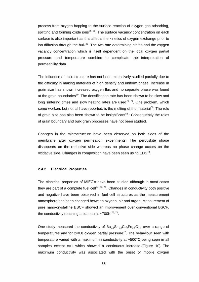
Figure 11 Circuit diagram for mixed conductor with blocking electrodes (from

Baumann81)

The two lines are simplified and the components further grouped to yield the

model in b. This is further simplified to give the model c which comprises of

three resistors and two constant phase elements (Q).(see section 3.7 for details

of constant phase elements) The high frequency (HF) medium frequency (MF)

and low frequency (LF) portions of the model are shown also. The component

Qchem is a chemical based constant phase element and is related to the surface

exchange of the oxygen.81

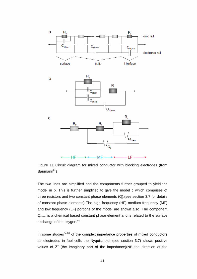
In some studies84-86 of the complex impedance properties of mixed conductors

as electrodes in fuel cells the Nyquist plot (see section 3.7) shows positive

values of Z” (the imaginary part of the impedance)(NB the direction of the

42

ordinate is reversed).(Figure 12) These parts of the plots are generally not

commented although they can be attributed to inductances in the measuring

system at high frequency.86, 87

Figure 12 Impedance plot of MIEC cathode containing fuel cell (from Li84)

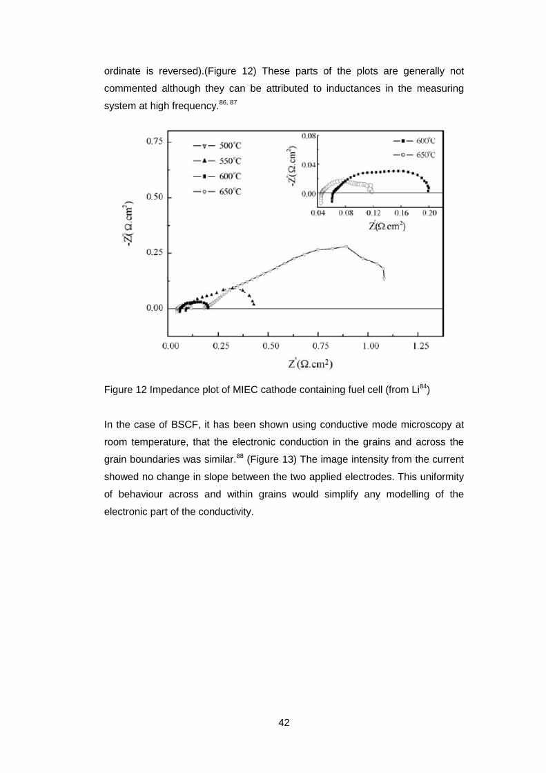
In the case of BSCF, it has been shown using conductive mode microscopy at

room temperature, that the electronic conduction in the grains and across the

grain boundaries was similar.88 (Figure 13) The image intensity from the current

showed no change in slope between the two applied electrodes. This uniformity

of behaviour across and within grains would simplify any modelling of the

electronic part of the conductivity.

43

Figure 13 Conductive mode microscopy of BSCF (a) Secondary electron image

(b) conductive mode image (c) line profile between two electrodes(from Salehi88)

2.4.3 Stoichiometry

As has been discussed above the role of the oxygen vacancy concentration has

a profound effect on the oxygen permeability and stability of the MIEC.

A number of different methods have been adopted for measuring the value of

in Ba0.5Sr0.5Co0.8Fe0.2O3-δ especially at elevated temperature. The most common

method is thermal gravimetric analysis and the weight loss as the material is

heated is measured89. This needs a value of for the starting point or finishing

point. If heated in a hydrogen atmosphere the following reaction occurs: -

Ba0.5Sr0.5Co0.8Fe0.2O3-δ + H2 0.5BaO + 0.5SrO + 0.2Fe + 0.8Co + H2O 2.21

44

If the relative proportion of metal ions at the start (or the finish) are known and

the weight at the end of the reduction a starting value of can be calculated

assuming the products are as shown in equation 2.21. It is important also to

ensure any adsorbed surface species, for example, water and carbon dioxide,

are either removed prior to measurement or otherwise allowed for in the

calculations90.

Iodometric titration has also been used to determine the vacancy concentration.

The sample is dissolved in acid and reacted with excess iodide prior to titration

with thiosulphate90. Similar titrations have been carried out using Cu+ and Fe2+

as the oxidant91. Care has to be taken in all the titrations to ensure complete

dissolution and to prevent oxidation by air.

The stoichiometry has been shown to vary with temperature and time, and

shows hysteresis on cooling. This change in vacancy concentration affects the

long-term stability of the oxygen flux. Coupled with the change in is an

associated compensatory change in the oxidation states of the iron and cobalt.

For a value of δ = 0, the oxidation state of the B site ions, if the A sites are

occupied by strontium and barium, is 4+. However as δ moves to 0.5 then the

oxidation state will reduce to 3+. These formal oxidation states are however the

overall state and individual ions can be higher or lower. With values in the range

of 0 < δ < 0.5, then there must be a mixture of oxidation states as otherwise

fractional charges would be present.

For BSCF compositions, the determination of δ and thus the oxidation state of

the B site cations has also looked at how the fractional charge has been

distributed between the iron and cobalt. One study looked at the stoichiometry

as a function of the cobalt-iron ratio.92 They used two techniques iodometric

titrations and thermogravimetry including hydrogen reduction. They assumed

that the iron oxidation state behaviour on heating was constant over all

compositions and that the cobalt changed independently. The sample with no

cobalt was taken as the baseline for calculating the cobalt oxidation state. Their

results showed that over the temperature range from room temperature to

900°C cobalt had a net oxidation state 0.3 to 0.1 lower than iron. Their ranges

were, for 3-δ, 2.65 at room temperature to 2.35 at 900°C and the corresponding

45

oxidation states were 3.3 to 2.6. This indicates the presence of 4+, 3+ and 2+

oxidation states.

Another study showed lower values for the non-stoichiometry93. They were using

different techniques, in addition to thermogravimetry including hydrogen

reduction, they used high temperature neutron diffraction. Their results gave

lower values of 3-δ but they only gave data from 600-900°C. At the highest

temperature a value of 2.25 was shown for 3-δ. In addition to conducting

experiments in pure oxygen they also carried them at lower partial pressures

(0.1, 0.01 and 0.001pO2/p).This resulted in lower values of the non-

stoichiometry. The neutron diffraction data was analysed without any reference

to the chemical analysis so could be regarded as an absolute value. However,

their pretreatments of the powders were quite extensive and only after changes

in the lattice parameter stopped during the isothermal hold at each temperature

was the data taken for full pattern fitting. These results, therefore, give results

lower than the ones based on dynamic methods where isothermal conditions do

not exist. They did not report on any differences between the cobalt and iron

oxidation states.

Mössbauer and x-ray absorption near edge spectroscopy (XANES) have also

been employed to investigate the oxidation state changes during heating63. The

Mössbauer data indicated that at room temperature the iron was present in

three oxidation states 4+, “3+” and “2+” and the proportions varied with

composition. The latter two oxidation states represent rapid hopping between

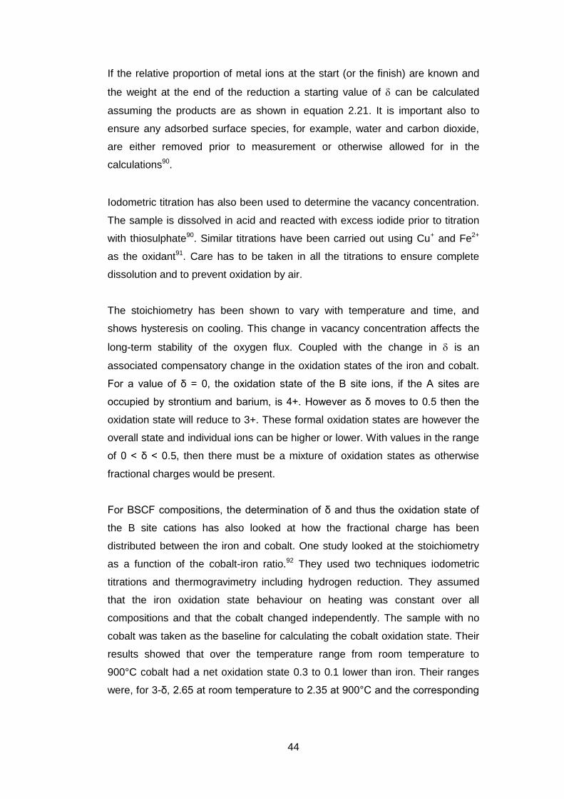
the lower state indicated and a higher state (Table 2).

x y Fe4+(%) Fe”3+”(%) Fe”2+”(%)

0.8 0.2 44 26 30

0.5 0.8 42 29 29

0.5 1.0 51 26 23

Table 2 Iron oxidation state in Ba1-xSrxCo1-yFeyO3-δ (after Harvey63)

The XANES data showed that the iron was mainly 3+ up to 960°C whereas the

cobalt reduces to 2+ above 800°C. The conclusion was that the iron was in a

46

higher oxidation state than the cobalt which was in agreement with the work of

Jung described above.92

The oxidation states have also been measured using X-ray photoelectron

spectroscopy (XPS).94, 95 In the former paper94, a ratio of Co3+ to Co4+ of 40:60 is

reported. However no account is taken of the overlap of the barium and cobalt

peaks which occurs with binding energies in the range 770 to 810eV. The same

part of the spectrum was analysed separately for barium and cobalt and

therefore no cognisance will be made of this paper. The second paper95 shows

that the iron is a mixture of Fe4+ and Fe3+ while the cobalt is present as Co3+.

These assignments were made on the basis that the two iron states have similar

binding energies whereas the cobalt 4+ has a binding energy at a significant

difference to the 3+ state. This latter paper confirms the previous discussion in

that the cobalt is at a lower oxidation state than iron.

Electron energy loss spectroscopy (EELS) has shown that in BSCF the loss of

oxygen is accompanied by a reduction in oxidation state of Co from 2.6-2.2 and

of Fe from 3.0-2.8 over the temperature range 25-950°C96. Again the cobalt is in

a lower oxidation state than the iron.

The oxygen non-stoichiometry can be measured by a variety of methods which

when compared under the same conditions correlate well with each other. For a

good comparison composition, pre-treatment conditions, atmosphere and time

for equilibration need to be the same. However the contribution of the two B site

cations to the overall resulting oxidation state is not as clear, the assignment of

charge between the two cations and the 3+ and 4+ oxidation states is not

unequivocal and involves a variety of assumptions which may not be verifiable.

There is general agreement that cobalt has a lower oxidation state than iron.

This may be due to the cobalt 3+ ion being a d6 species which has a low energy

low spin state as all the d electrons are paired.

2.4.4 Mechanical Properties

Good mechanical properties (strength, creep, thermal shock) of the ceramic

membranes are important for long lifetimes in the applications97-100. The

47

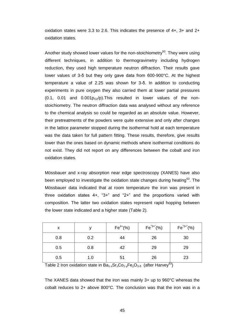
measurement against temperature of stiffness, toughness and fracture stress

has shown discontinuities around 200°C101-103. (Figure 14),

Figure 14 Mechanical properties of BSCF against temperature (from Huang103)

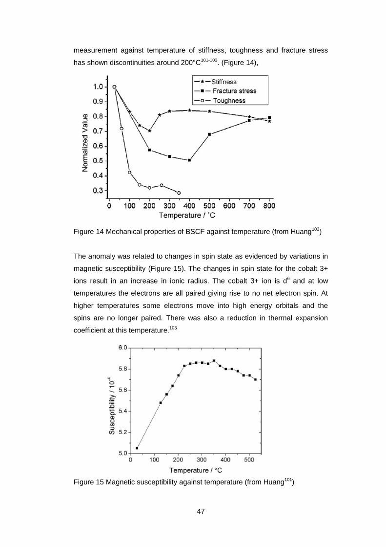
The anomaly was related to changes in spin state as evidenced by variations in

magnetic susceptibility (Figure 15). The changes in spin state for the cobalt 3+

ions result in an increase in ionic radius. The cobalt 3+ ion is d6 and at low

temperatures the electrons are all paired giving rise to no net electron spin. At

higher temperatures some electrons move into high energy orbitals and the

spins are no longer paired. There was also a reduction in thermal expansion

coefficient at this temperature.103

Figure 15 Magnetic susceptibility against temperature (from Huang101)

48

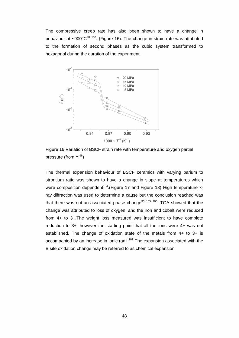
The compressive creep rate has also been shown to have a change in

behaviour at ~900°C98, 100. (Figure 16). The change in strain rate was attributed

to the formation of second phases as the cubic system transformed to

hexagonal during the duration of the experiment.

Figure 16 Variation of BSCF strain rate with temperature and oxygen partial

pressure (from Yi98)

The thermal expansion behaviour of BSCF ceramics with varying barium to

strontium ratio was shown to have a change in slope at temperatures which

were composition dependent104.(Figure 17 and Figure 18) High temperature x-

ray diffraction was used to determine a cause but the conclusion reached was

that there was not an associated phase change30, 105, 106. TGA showed that the

change was attributed to loss of oxygen, and the iron and cobalt were reduced

from 4+ to 3+.The weight loss measured was insufficient to have complete

reduction to 3+, however the starting point that all the ions were 4+ was not

established. The change of oxidation state of the metals from 4+ to 3+ is

accompanied by an increase in ionic radii.107 The expansion associated with the

B site oxidation change may be referred to as chemical expansion

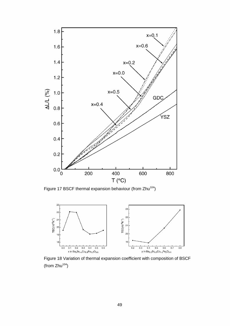
49

Figure 17 BSCF thermal expansion behaviour (from Zhu104)

Figure 18 Variation of thermal expansion coefficient with composition of BSCF

(from Zhu104)

50

3 Experimental Methods

3.1 Density

The density of the sintered samples was measured using an Archimedes

technique108. This technique measures the mass of the sample in air and whilst

suspended in a liquid, in this case water. The difference in mass is equal to the

mass of water displaced. By knowing the density of the liquid the volume

displaced can be calculated and this is equal to the volume of the solid sample.

The volume and mass of the solid are thus now known and the density can be

calculated.

However the ceramic pellets measured contained pores. These pores could be

either open in that they connected to the outside of the ceramic body or closed

whereby they were totally enclosed in the ceramic with no access to the exterior

of the body. When immersed in the liquid the air in the open pores may be

displaced by the liquid whereas the liquid cannot enter the closed pores. There

are thus 3 volumes that may exist for each object.

1) Bulk volume which corresponds to the sum of the solid volume, the open

pore volume and the closed pore volume. This approximates to the volume

as determined by measuring the volume of a regularly shaped solid.

2) True volume which corresponds to the volume of the solid with no pores.

This cannot be measured using an Archimedes technique unless another

independent method has verified the absence of closed pores.

3) Apparent solid volume which corresponds to the solid volume and the

volume of closed pores.

The bulk volume and apparent solid volume can both be used in density

calculations and give rise to the bulk and apparent solid density respectively.

Two methods were used to measure the density which differed in the way that

the samples were degassed before the mass was measured in the liquid,

51

3.1.1 Methods

1) The sample was weighed in air (m1)

2) The immersion process had two variants

a) The sample was placed in a beaker of deionised water and boiled gently

for 30minutes. After boiling the sample was left to cool back to ambient

temperature. The boiling in some cases caused some chipping of the

sample and therefore method b) was introduced.

b) The sample was placed in a shallow petri dish containing deionised

water, (which had been degassed by boiling) and ensuring the pellet was

totally immersed. The petri dish was placed in a vacuum desiccator and

evacuated until no more bubbles appeared from the sample. It was left

under vacuum for 30 minutes before opening the valve and restoring the

sample to atmospheric pressure.

3) The samples were then weighed under water using the suspension

attachment on the balance.(m2)

4) The sample was removed then dried quickly using a paper towel and then

reweighed.(m3)

Using the three weights and the density (ρL) of water (Table 2 in Reference 108),

the bulk (ρb) and apparent solid (ρs) densities were calculated according to the

two equations below.

3.1

3.2

3.2 Iodometric Titration

The determination of δ, the amount of the oxygen deficiency in the ABO3-δ

formula can be achieved through iodometric titration.91, 92, 109 In this method

iodide ions are oxidised by the multi-valent metal cations, formed by dissolution

of the solid in acid, to form iodine which is then titrated with standardised sodium

thiosulphate solution. The oxidation of iodide by cobalt 4+ is shown in Equation

3.3 below

3.3

52

The titration of the liberated iodine with sodium thiosulphate is shown in

equation 3.4 below

3.4

The above equations have been simplified because, in the presence of excess

iodide ions, iodine readily reacts reversibly with them to form the tri-iodide ion .

3.5

The sodium thiosulphate was standardised by titrating the iodine formed by

reacting potassium iodide with a known amount of potassium iodate in a dilute

acid solution. The reaction is shown below.

3.6

All the titrations were conducted whilst nitrogen was bubbled through the

solution to prevent oxidation of the iodide ions by oxygen

3.7

The presence of the excess iodide ions which forms the tri-iodide also helps

prevent the loss of liberated iodine through volatilisation.

The method used assumes that the dissolution of the BSCF powder in acid

occurs without any change in the oxidation state of the contained cations. If the

excess iodide is not present before the powder is added to the hydrochloric acid

chlorine is formed which indicates oxidation of the chloride by the cations prior

to the addition of iodide.

3.2.1 Titration of BSCF powder method

1) The powders were calcined in air at 1000°C for 2 hours to remove all

adsorbed water carbon dioxide and other volatiles. On cooling they were

stored in a desiccator containing both silica gel and soda lime. The latter

was to remove any carbon dioxide from the atmosphere.

53

2) Immediately prior to use the powders were ground in an agate mortar and

pestle so that dissolution would be easier. This prevented long dissolution

times which could lead to iodine loss by volatilisation.

3) 100cm3 of 1M HCl were added to a stirred conical flask and 2g of potassium

iodide added. Nitrogen was bubbled through the solution.

4) When the potassium iodide had completely dissolved, approximately 50mg

accurately weighed of the BSCF powder were added to the flask.

5) When all the powder had dissolved (normally less than 5 minutes), the

solution was titrated with approximately 0.02M sodium thiosulphate solution

until it was a pale yellow colour.

6) 1cm3 of 0.1% by weight starch solution was added and the titration was

continued until the solution changed from intense blue to colourless.

3.2.2 Standardisation of the sodium thiosulphate solution

1) Approximately 2.14g of dried potassium iodate were accurately weighed into

a 500cm3 volumetric flask and the solution made up to the mark109.

2) To a conical flask containing 25cm3 of deionised water were added 10cm3 of

1M HCl. Nitrogen was bubbled through the solution.

3) 5cm3 of the potassium iodate solution were pipetted into the flask. 1g of

potassium iodide was added and allowed to dissolve.

4) The solution was titrated with approximately 0.02M sodium thiosulphate

solution until it was a pale yellow colour.

5) 1cm3 of 0.1% by weight starch solution was added and the titration was

continued until the solution changed from intense blue to colourless.

3.2.3 Calculation of δ in Ba0.5Sr0.5Co0.8Fe0.2O3-∂

The titration was set up so that iodide reacted with M2+p+ to form I2 and M2+.

M2+p+ + p I- = M2+ + p/2 I2 3.8

The iodine is then reacted with thiosulphate.

p/2 I2 + p S2O32- = pI- + p/2 S4O6

2- 3.9

54

Therefore p mole of S2O32- is equivalent to p electrons/mole of reduction which

in turn is equivalent to p/2 moles Oxygen in excess of that required for M2+.

In 1g of sample there are CV/2w moles of oxygen in excess of that required for

Ba0.5Sr0.5Co0.8Fe0.2O2.

In one mole of sample there are 1-∂ moles of excess oxygen which equals

(CV/2w) x MBSCFO3-δ.

Where C = concentration of thiosulphate solution (M)

V = volume of titre of thiosulphate solution (l)

w = weight of sample used (g)

MBSCFO3-δ. = molecular weight of Ba0.5Sr0.5Co0.8Fe0.2O3- ∂.

3.10

The molecular weight in equation 3.10 is split into 2 parts.

3.11

The bracket is expanded.

3.12

The equation is rearranged.

3.13

The equation is factorised.

(

)

3.14

The equation is rearranged to give ∂.

55

(

) 3.15

3.3 Surface Area and Pore Volume

Specific surface area and pore volume were measured by nitrogen adsorption

on powders at the boiling point of nitrogen (77K)110. The technique involves the

measurement of the amount of gas adsorbed as the nitrogen partial pressure

above the powder is increased. This is accomplished by the introduction of a

known amount of gas (nitrogen) into the sample holder which is initially under

vacuum and waiting for the pressure to come to equilibrium. The amount of gas

adsorbed is calculated by examining the difference between the expected and

actual pressure difference on gas addition using the ideal gas law.

3.16

Where P is the pressure in the system (Pa)

V is the volume of the system (m3)

n is the number of moles of gas in the system



The adsorption of gas on a non-porous solid is generally explained by the BET

(Brunauer, Emmett and Teller)111 equation below.

( )

(

)

3.17

Where p is the partial pressure above the sample (Pa)

po is the saturation vapour pressure (Pa)

n is the amount of gas adsorbed (molg-1)

nm is the monolayer capacity of the powder (molg-1)

c is a constant which is related to the net heat of adsorption of the

gas.

56

The theory assumes a constant heat of adsorption of the gas onto the solid in

the formation of a monolayer and that subsequent adsorption onto this layer has

another constant heat of adsorption. During adsorption each layer need not be

complete before a further layer is formed.

A plot of

(

) against

will give a straight line with

(

) 3.18

3.19

from which nm and c can be calculated. From the value of nm the specific surface

area (A) can be calculated.

3.20

Where NA is Avogadro’s constant (6.022 x 1023 mol-1)

nm is the monolayer capacity of the powder (molg-1)

am is the area of the adsorbed gas molecule (m2)

In the case of a porous solid, the adsorbed gas layer builds up and in a pore will

form a meniscus corresponding to the pore diameter. The vapour pressure

above a curved surface is given by the Kelvin equation

3.21

where is the surface tension of the liquid adsorbate (Nm-1)

VL is molar volume of the liquid adsorbate (m3mol-1)



rm is radius of the meniscus (m).

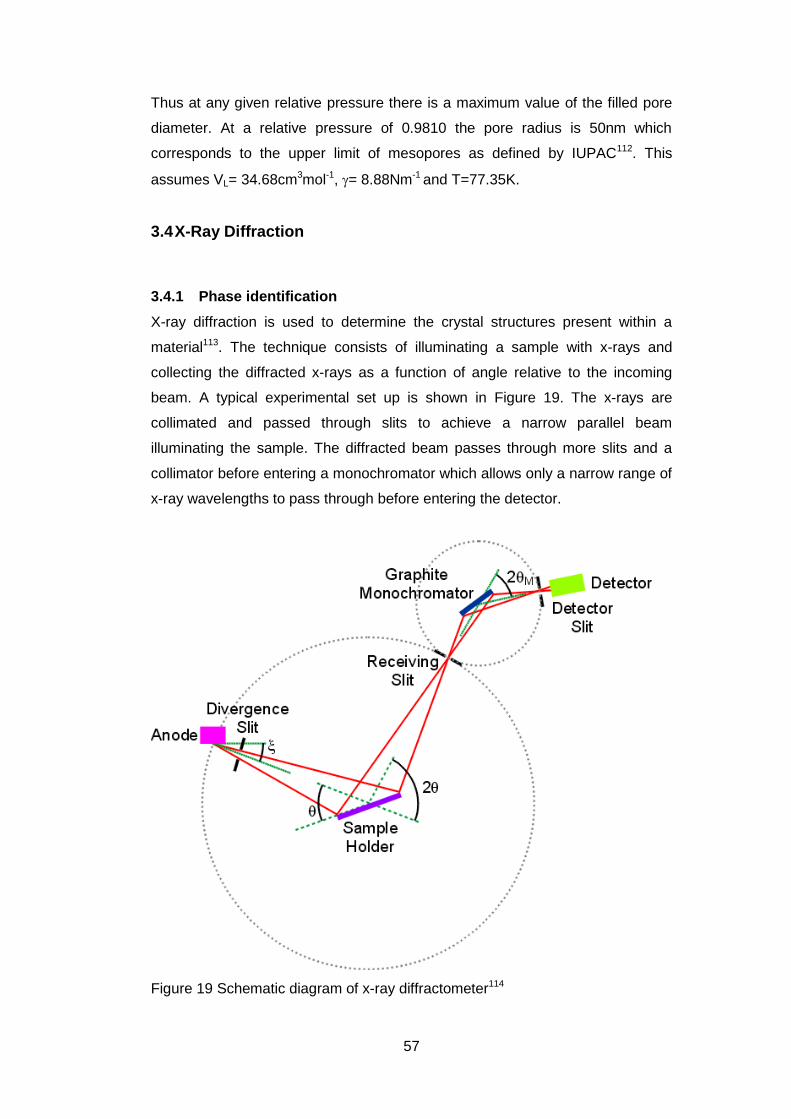
57

Thus at any given relative pressure there is a maximum value of the filled pore

diameter. At a relative pressure of 0.9810 the pore radius is 50nm which

corresponds to the upper limit of mesopores as defined by IUPAC112. This

assumes VL= 34.68cm3mol-1, = 8.88Nm-1 and T=77.35K.

3.4 X-Ray Diffraction

3.4.1 Phase identification

X-ray diffraction is used to determine the crystal structures present within a

material113. The technique consists of illuminating a sample with x-rays and

collecting the diffracted x-rays as a function of angle relative to the incoming

beam. A typical experimental set up is shown in Figure 19. The x-rays are

collimated and passed through slits to achieve a narrow parallel beam

illuminating the sample. The diffracted beam passes through more slits and a

collimator before entering a monochromator which allows only a narrow range of

x-ray wavelengths to pass through before entering the detector.

Figure 19 Schematic diagram of x-ray diffractometer114

58

A crystalline material consists of ions/atoms arranged in regular three

dimensional arrays. The incident x-rays interact with the electrons around each

atomic nucleus and are scattered. These scattered x-rays also interact with

each other and if they are in phase will constructively interfere and can therefore

be detected unlike the destructively interfering x-rays. The constructive

interference occurs at definitive angles from the planes of atoms in the 3D

structure. If the planes are at a distance (d) apart, and the wavelength (λ) of the

x-rays is known, then their relationship is given by Braggs law (equation 2.13)

3.22

Where n = order of diffraction = 1 for x-ray diffraction

= diffraction angle

The intensity of x-rays against angle shows a series of peaks each representing

a distinct interplanar distance (d). From the interplanar distances and the

associated peak intensity crystal structures can be identified and the atomic

positions within the structure determined. Structure identification was carried out

using HighScore plus (Phillips). Further fitting and quantification was carried out

using Topas software (Bruker)

The phase identification utilised the ICSD database and the High Score plus

search and match routine. The ICSD database includes for the substance its

name, formula, crystallographic parameters, peak list, atomic positions and an

ideal diagram of its x-ray diffractogram. The initial stage was to identify the

peaks present and then, after the selection of those elements present in the

material, run the routine. The matching phases were recorded and their

corresponding data file accessed to obtain the structural details for each phase.

In many cases, typically those with a single phase, this was sufficient to obtain a

good phase identification.

However in the multiphase materials this approach could not give an

unequivocal match. The reasons for this include broad peaks, overlapping

peaks and the very large number of Ba-Sr-Co-Fe-O systems that are present

within the database. In these cases which included the dried and calcined

powders, a good fit was taken and then used as a basis for refinement using

Topas.

59

Topas is a whole pattern fitting program. In order to fit the experimental it

requires an input of possible crystal structures. These inputs may be just the

space group and lattice parameters for a Pawley fit or the space group, lattice

parameters and atomic coordinates of all atoms within the unit cell for Rietveld

fitting. The latter is the ideal route as it can reveal differences in site occupancy

in a given structure. Differences in occupancy can be a result of initial

inhomogeneity subsequent disproportionation or reactions occurring with the

atmosphere. As good fits using Rietveld fitting could not be obtained as site

occupancies greater than 1 were obtained, the simpler Pawley method was also

used.

In addition to the crystal structures, the refinement requires information on the

peak shape. X-ray diffraction peaks have a shape which is a convolution of

Gaussian and Lorentzian peaks known as a pseudo-Voigt function. This can be

chosen at the start of refinement. In addition to these preselected items the

refinement also uses line breadth and background shape in optimising the

fitting.

3.4.2 Line Broadening

In an ideal case the x-ray diffraction peaks are broadened by both instrumental

and sample effects115, 116. The former include

the x-rays not being monochromatic

the x-rays not being parallel

the finite size of the x-ray beam.

The sample can cause broadening through two principal properties sample

crystallite size and inhomogeneous strain but could also include stacking faults

and concentration gradients within a crystal. The presence of small crystallites

means that there is not an infinite size to the diffracting planes and that the

interference between the scattered x-rays does not give a sharp cut off between

constructive and destructive interference. Non-uniform strain within the crystals

means that there will be a variation in peak position around a central point.

(Uniform strain produces a peak shift.)

If the instrumental broadening (b) can be measured using a large crystallite size

strain free sample then the crystallite size (L) can be determined if the

experimental broadening (B) is measured (equation 3.23), this assumes that

there is a Gaussian relationship between the two broadenings113. First

60

broadening from the sample (Βs) is calculated and the crystallite size is

measured using the Scherrer equation (3.24).

3.23

3.24

Where λ is the wavelength of the x-rays (nm)

Θ is the diffraction angle.

3.4.3 Glancing angle diffraction

Glancing angle x-ray diffraction is used to examine the crystallography of

surface layers. As well as being diffracted the x-rays incident on a sample can

be adsorbed, as can the diffracted beam, through a number of processes in

which electrons adsorb the x-rays and change their state often being ejected

from the substance as a photo electron (see section 3.9) or being excited to an

outer orbital. These excited electrons can subsequently decay to the lower state

and emitting x-rays of a specific wavelength. (This is the basis of x-ray

fluorescence). The absorption of x-rays is dependent on the path length (t) and

the absorption coefficient (µ) of the substance and is given by equation 2.16.

3.25

Where I = reduced intensity after a distance t

Io= Incident intensity

The absorption coefficient is derived for a material from the absorption

coefficients from the constituent elements. In conventional diffraction the

incident angle and diffracted angle are symmetrical with respect to the sample

surface and the path length is the constant for all values of θ. In glancing angle

mode the incident angle is kept constant and small this gives a longer path

length for material at a greater depth and enhances the contribution of surface

layers to the diffraction pattern.

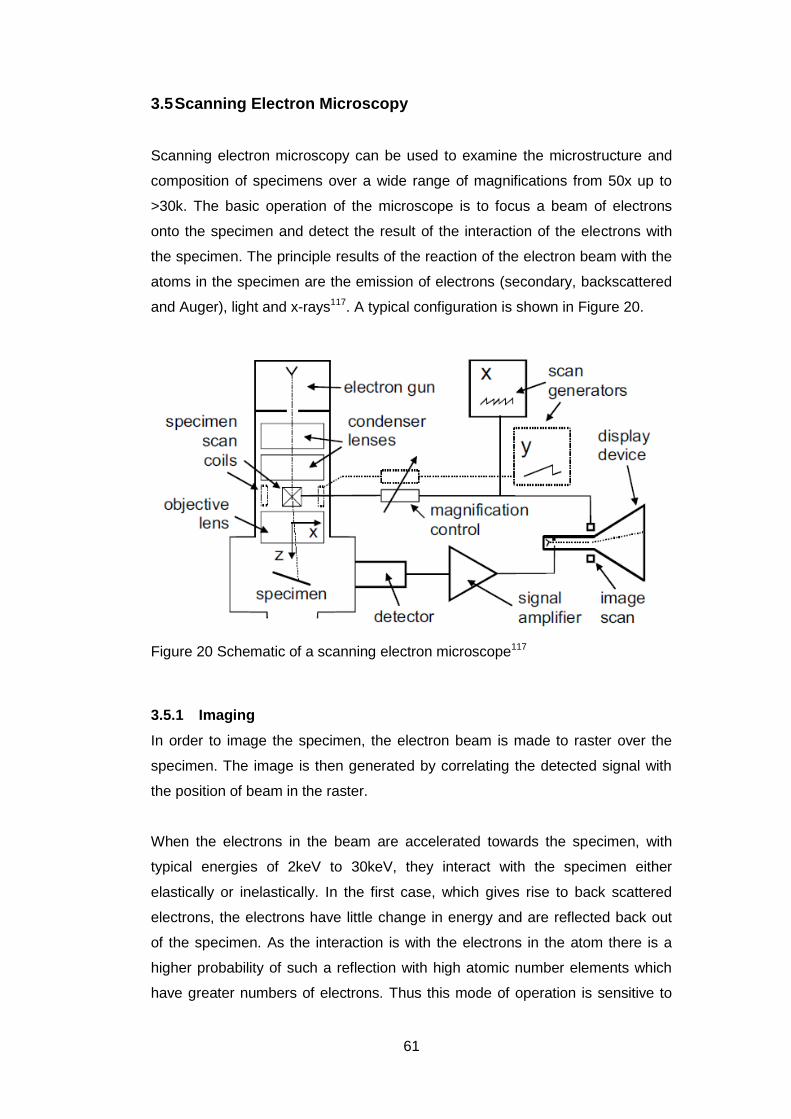
61

3.5 Scanning Electron Microscopy

Scanning electron microscopy can be used to examine the microstructure and

composition of specimens over a wide range of magnifications from 50x up to

>30k. The basic operation of the microscope is to focus a beam of electrons

onto the specimen and detect the result of the interaction of the electrons with

the specimen. The principle results of the reaction of the electron beam with the

atoms in the specimen are the emission of electrons (secondary, backscattered

and Auger), light and x-rays117. A typical configuration is shown in Figure 20.

Figure 20 Schematic of a scanning electron microscope117

3.5.1 Imaging

In order to image the specimen, the electron beam is made to raster over the

specimen. The image is then generated by correlating the detected signal with

the position of beam in the raster.

When the electrons in the beam are accelerated towards the specimen, with

typical energies of 2keV to 30keV, they interact with the specimen either

elastically or inelastically. In the first case, which gives rise to back scattered

electrons, the electrons have little change in energy and are reflected back out

of the specimen. As the interaction is with the electrons in the atom there is a

higher probability of such a reflection with high atomic number elements which

have greater numbers of electrons. Thus this mode of operation is sensitive to

62

variation in the average atomic number of specimen. The high energy of these

electrons means that they can escape from within the specimen without being

absorbed.

If the electrons in the beam interact inelastically they can cause inner core

electrons to be lost from the atoms in the specimen these have low energy and

may further interact with the specimen. These secondary electrons may leave

the surface and then can then be detected. The electrons leaving the surface

typically have energies of ~50eV117, much less than the back scattered

electrons. Their low energy means that only if they are very near the surface

(~1nm for 3keV beam energy) will they be detected. This gives a better

topological image of the specimen.

3.5.2 Elemental Analysis

When an inner core electron is removed from an atom, an outer core electron

may drop into the unfilled inner core, as this core has a lower energy then

energy will be released in the form of an x-ray with energy equal to the

difference of the two core shells which are element specific118. The x-rays can

be detected either by energy dispersive or wavelength dispersive detectors. In

the former the signal from the detector is discriminated on the basis of its energy

whereas in the latter the x-rays of different energies (wavelengths) are diffracted

by a crystal to separate them before their detection.

The conversion of the x-ray energies and intensities into composition is by

techniques similar to those used in x-ray fluorescence, (see section 3.6) in

which the x-rays are produced by exciting the inner core electrons with x-rays

and not electrons.

3.6 X-Ray Fluorescence Analysis

The elemental compositions of sintered pellets were measured by x-ray

fluorescence using a MiniPal 4 energy dispersive x-ray fluorescence

spectrometer. The standardless Ominian software was used for quantification.

X-ray fluorescence is a technique similar to energy dispersive x-ray analysis in

electron microscopy.119 In this case x-rays and not electrons are the excitation

63

source. A beam of x-rays irradiate the sample and either excite inner core

electrons to higher energy levels or excite them to leave the surface as

photoelectrons.(see section 3.9 below) Electrons in the excited atom can drop

into the vacant low energy level and simultaneously emit an x-ray whose energy

is dependent on the two energy levels involved. The emitted x-rays are detected

by an energy sensitive detector. The energy intensities are converted to

elemental concentrations through the use of databases containing details of x-

ray fluorescence yields and x-ray adsorption from all elements in the sample.120

3.6.1 Determination of method accuracy

Three pellets from 2 different samples were analysed to determine the errors in

the measurement. The nominal compositions for the two samples were

Ba0.7Sr0.3Co0.8Fe0.2O3-δ and Ba0.5Sr0.5Co0.8Fe0.2O3-δ. The results are given in

Table 3 and Table 4. Oxygen could not be measured in the instrument used.

The raw data for the cations was normalised to 100% on a weight basis (wt%)

and then converted to atomic ratios which were further normalised to a cation

atomic composition of 100 (Mole %). In order to allow comparison with the

empirical formula for each composition, the mole% was normalised to a total of

2 moles ie an assumption that the final composition was ABO3. The only

impurity found was calcium at approximately 0.3wt% which corresponded to

0.01 on the A site.

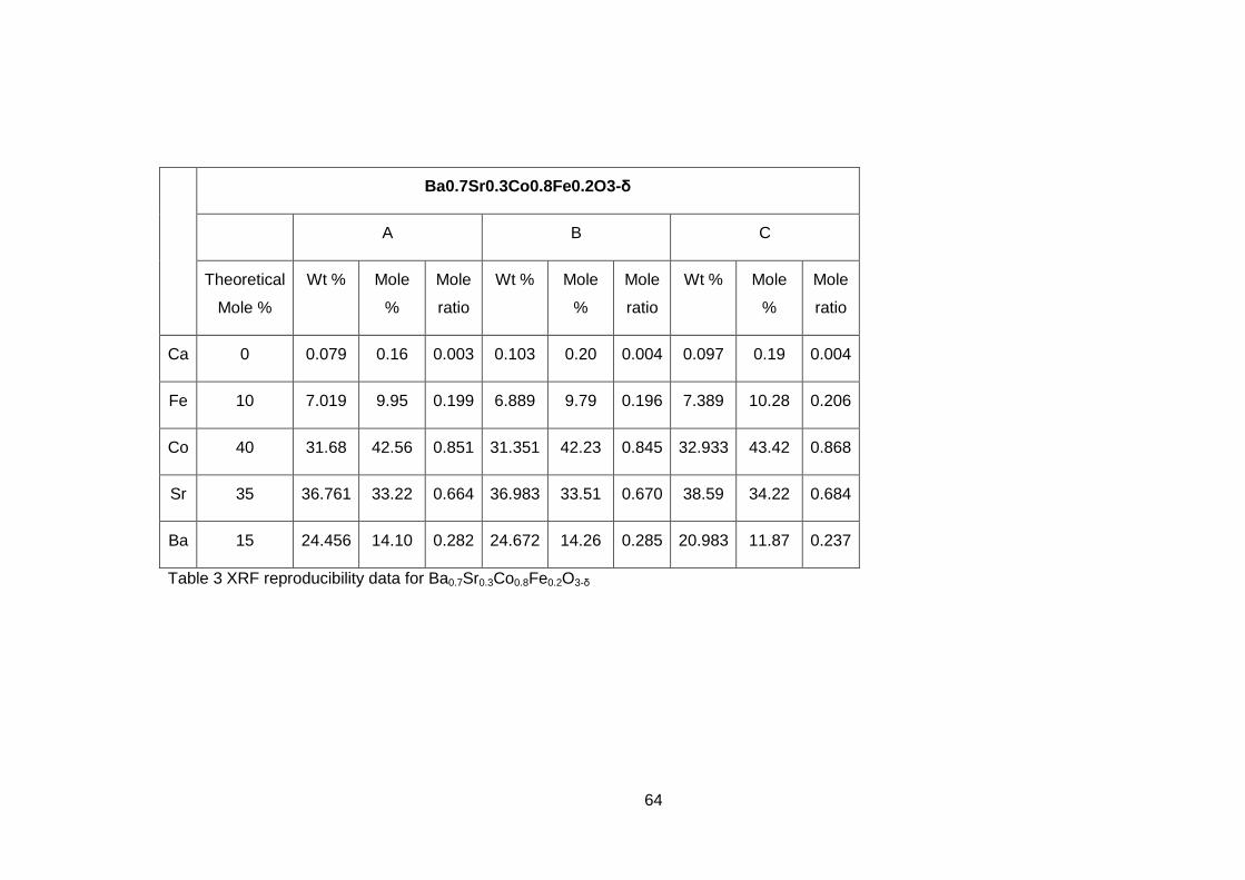
64


A B C

Theoretical

Mole %

Wt % Mole

%

Mole

ratio

Wt % Mole

%

Mole

ratio

Wt % Mole

%

Mole

ratio

Ca 0 0.079 0.16 0.003 0.103 0.20 0.004 0.097 0.19 0.004

Fe 10 7.019 9.95 0.199 6.889 9.79 0.196 7.389 10.28 0.206

Co 40 31.68 42.56 0.851 31.351 42.23 0.845 32.933 43.42 0.868

Sr 35 36.761 33.22 0.664 36.983 33.51 0.670 38.59 34.22 0.684

Ba 15 24.456 14.10 0.282 24.672 14.26 0.285 20.983 11.87 0.237

Table 3 XRF reproducibility data for Ba0.7Sr0.3Co0.8Fe0.2O3-δ

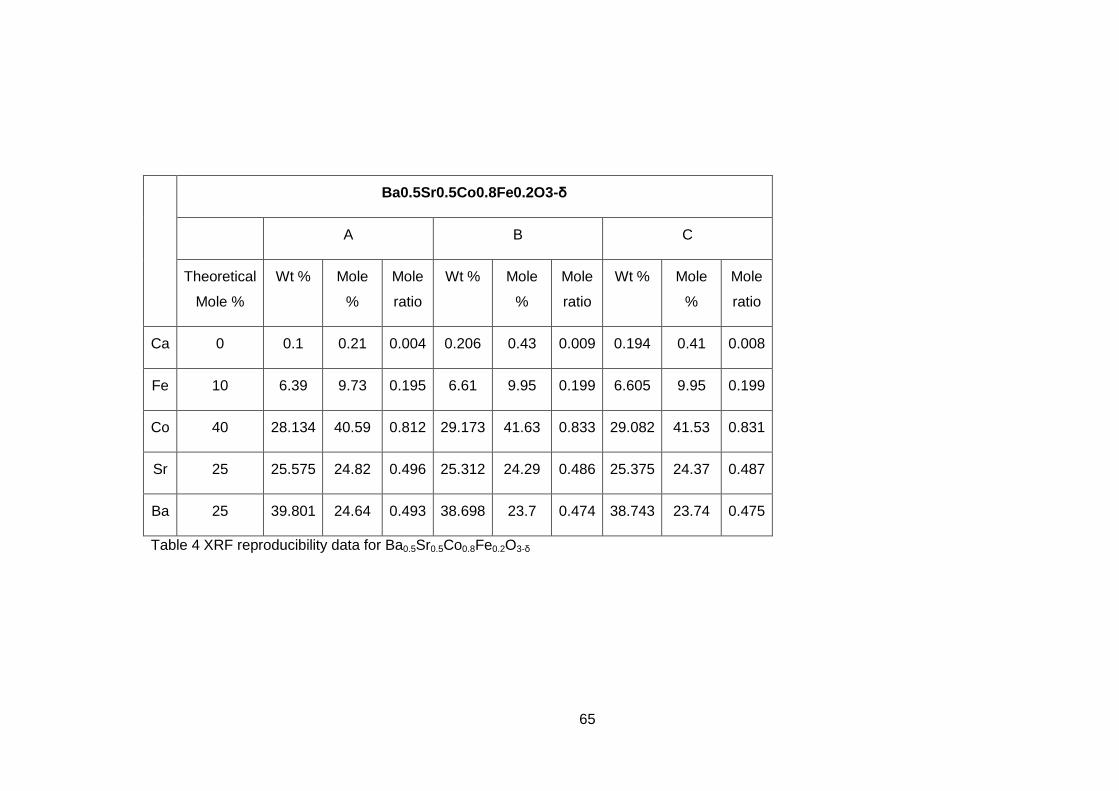
65


A B C

Theoretical

Mole %

Wt % Mole

%

Mole

ratio

Wt % Mole

%

Mole

ratio

Wt % Mole

%

Mole

ratio

Ca 0 0.1 0.21 0.004 0.206 0.43 0.009 0.194 0.41 0.008

Fe 10 6.39 9.73 0.195 6.61 9.95 0.199 6.605 9.95 0.199

Co 40 28.134 40.59 0.812 29.173 41.63 0.833 29.082 41.53 0.831

Sr 25 25.575 24.82 0.496 25.312 24.29 0.486 25.375 24.37 0.487

Ba 25 39.801 24.64 0.493 38.698 23.7 0.474 38.743 23.74 0.475

Table 4 XRF reproducibility data for Ba0.5Sr0.5Co0.8Fe0.2O3-δ

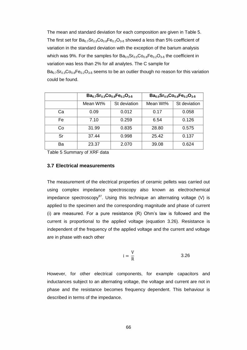
66

The mean and standard deviation for each composition are given in Table 5.

The first set for Ba0.7Sr0.3Co0.8Fe0.2O3-δ showed a less than 5% coefficient of

variation in the standard deviation with the exception of the barium analysis

which was 9%. For the samples for Ba0.5Sr0.5Co0.8Fe0.2O3-δ the coefficient in

variation was less than 2% for all analytes. The C sample for

Ba0.7Sr0.3Co0.8Fe0.2O3-δ seems to be an outlier though no reason for this variation

could be found.

Ba0.7Sr0.3Co0.8Fe0.2O3-δ Ba0.5Sr0.5Co0.8Fe0.2O3-δ

Mean Wt% St deviation Mean Wt% St deviation

Ca 0.09 0.012 0.17 0.058

Fe 7.10 0.259 6.54 0.126

Co 31.99 0.835 28.80 0.575

Sr 37.44 0.998 25.42 0.137

Ba 23.37 2.070 39.08 0.624

Table 5 Summary of XRF data

3.7 Electrical measurements

The measurement of the electrical properties of ceramic pellets was carried out

using complex impedance spectroscopy also known as electrochemical

impedance spectroscopy87. Using this technique an alternating voltage (V) is

applied to the specimen and the corresponding magnitude and phase of current

(i) are measured. For a pure resistance (R) Ohm’s law is followed and the

current is proportional to the applied voltage (equation 3.26). Resistance is

independent of the frequency of the applied voltage and the current and voltage

are in phase with each other

3.26

However, for other electrical components, for example capacitors and

inductances subject to an alternating voltage, the voltage and current are not in

phase and the resistance becomes frequency dependent. This behaviour is

described in terms of the impedance.

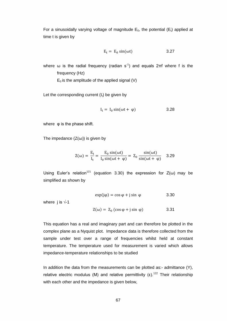
67

For a sinusoidally varying voltage of magnitude E0, the potential (Et) applied at

time t is given by

3.27

where ω is the radial frequency (radian s-1) and equals 2πf where f is the

frequency (Hz)

E0 is the amplitude of the applied signal (V)

Let the corresponding current (It) be given by

3.28

where φ is the phase shift.

The impedance (Z(ω)) is given by

3.29

Using Euler’s relation121 (equation 3.30) the expression for Z(ω) may be

simplified as shown by

3.30

where j is √-1

3.31

This equation has a real and imaginary part and can therefore be plotted in the

complex plane as a Nyquist plot. Impedance data is therefore collected from the

sample under test over a range of frequencies whilst held at constant

temperature. The temperature used for measurement is varied which allows

impedance-temperature relationships to be studied

In addition the data from the measurements can be plotted as:- admittance (Y),

relative electric modulus (M) and relative permittivity (ε).122 Their relationship

with each other and the impedance is given below,

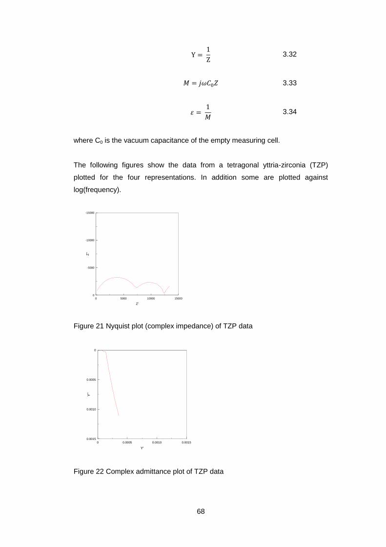
68

3.32

3.33

3.34

where C0 is the vacuum capacitance of the empty measuring cell.

The following figures show the data from a tetragonal yttria-zirconia (TZP)

plotted for the four representations. In addition some are plotted against

log(frequency).

Figure 21 Nyquist plot (complex impedance) of TZP data

Figure 22 Complex admittance plot of TZP data

0 5000 10000 15000

-15000

-10000

-5000

0

Z'

Z''

0 0.0005 0.0010 0.0015

0

0.0005

0.0010

0.0015

Y'

Y''

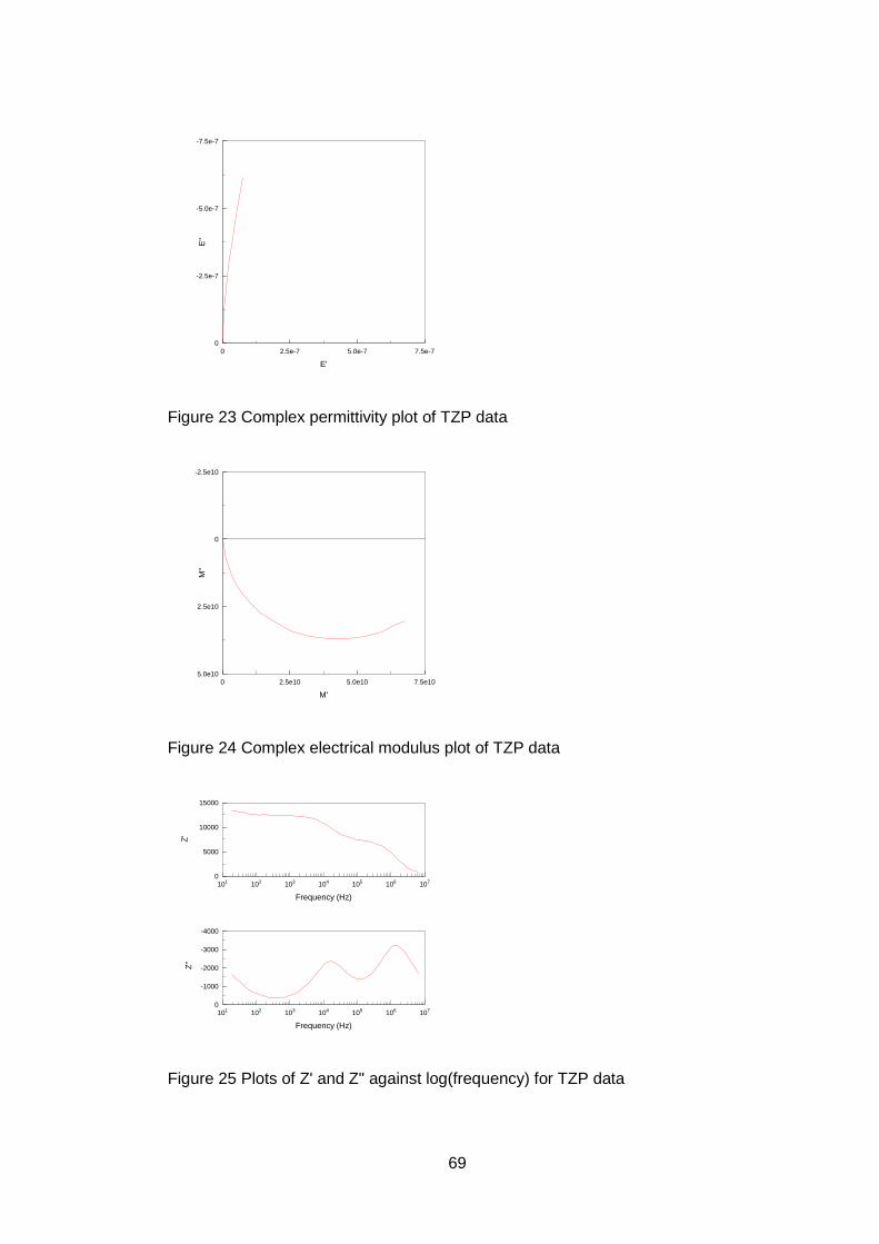
69

Figure 23 Complex permittivity plot of TZP data

Figure 24 Complex electrical modulus plot of TZP data

Figure 25 Plots of Z' and Z" against log(frequency) for TZP data

0 2.5e-7 5.0e-7 7.5e-7

-7.5e-7

-5.0e-7

-2.5e-7

0

E'

E''

0 2.5e10 5.0e10 7.5e10

-2.5e10

0

2.5e10

5.0e10

M'

M''

101 102 103 104 105 106 1070

5000

10000

15000

Frequency (Hz)

Z'

101 102 103 104 105 106 107

-4000

-3000

-2000

-1000

0

Frequency (Hz)

Z''

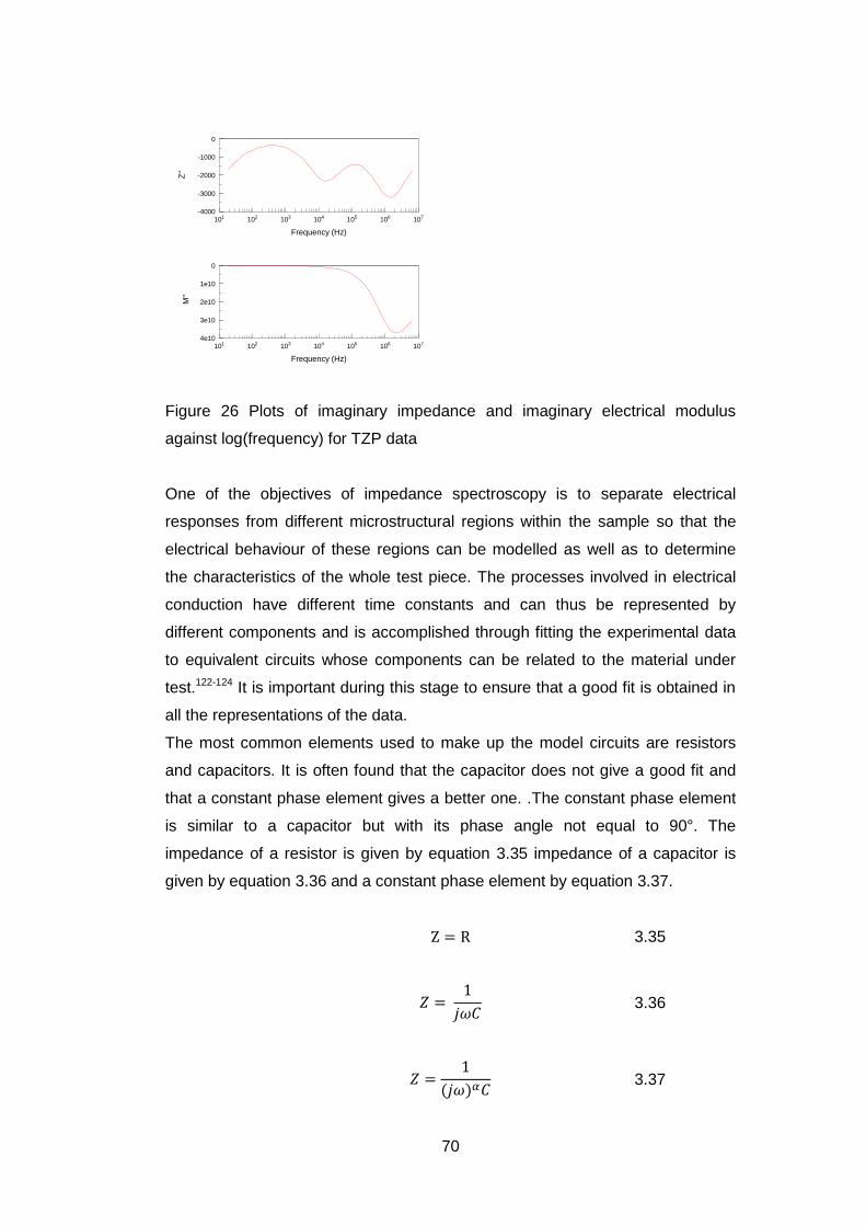
70

Figure 26 Plots of imaginary impedance and imaginary electrical modulus

against log(frequency) for TZP data

One of the objectives of impedance spectroscopy is to separate electrical

responses from different microstructural regions within the sample so that the

electrical behaviour of these regions can be modelled as well as to determine

the characteristics of the whole test piece. The processes involved in electrical

conduction have different time constants and can thus be represented by

different components and is accomplished through fitting the experimental data

to equivalent circuits whose components can be related to the material under

test.122-124 It is important during this stage to ensure that a good fit is obtained in

all the representations of the data.

The most common elements used to make up the model circuits are resistors

and capacitors. It is often found that the capacitor does not give a good fit and

that a constant phase element gives a better one. .The constant phase element

is similar to a capacitor but with its phase angle not equal to 90°. The

impedance of a resistor is given by equation 3.35 impedance of a capacitor is

given by equation 3.36 and a constant phase element by equation 3.37.

3.35

3.36

3.37

101 102 103 104 105 106 107-4000

-3000

-2000

-1000

0

Frequency (Hz)

Z''

101 102 103 104 105 106 107

0

1e10

2e10

3e10

4e10

Frequency (Hz)

M''

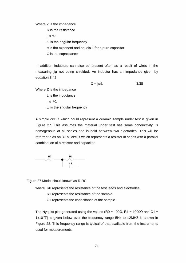
71

Where Z is the impedance

R is the resistance

j is √-1

ω is the angular frequency

α is the exponent and equals 1 for a pure capacitor

C is the capacitance

In addition inductors can also be present often as a result of wires in the

measuring jig not being shielded. An inductor has an impedance given by

equation 3.42

3.38

Where Z is the impedance

L is the inductance

j is √-1

ω is the angular frequency

A simple circuit which could represent a ceramic sample under test is given in

Figure 27. This assumes the material under test has some conductivity, is

homogenous at all scales and is held between two electrodes. This will be

referred to as an R-RC circuit which represents a resistor in series with a parallel

combination of a resistor and capacitor.

where R0 represents the resistance of the test leads and electrodes

R1 represents the resistance of the sample

C1 represents the capacitance of the sample

The Nyquist plot generated using the values (R0 = 100Ω, R1 = 1000Ω and C1 =

1x10-9F) is given below over the frequency range 5Hz to 12MHZ is shown in

Figure 28. This frequency range is typical of that available from the instruments

used for measurements.

R0 R1

C1

Figure 27 Model circuit known as R-RC

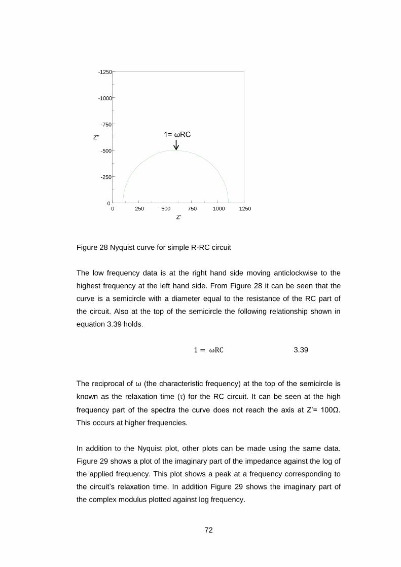
72

Figure 28 Nyquist curve for simple R-RC circuit

The low frequency data is at the right hand side moving anticlockwise to the

highest frequency at the left hand side. From Figure 28 it can be seen that the

curve is a semicircle with a diameter equal to the resistance of the RC part of

the circuit. Also at the top of the semicircle the following relationship shown in

equation 3.39 holds.

3.39

The reciprocal of ω (the characteristic frequency) at the top of the semicircle is

known as the relaxation time (τ) for the RC circuit. It can be seen at the high

frequency part of the spectra the curve does not reach the axis at Z’= 100Ω.

This occurs at higher frequencies.

In addition to the Nyquist plot, other plots can be made using the same data.

Figure 29 shows a plot of the imaginary part of the impedance against the log of

the applied frequency. This plot shows a peak at a frequency corresponding to

the circuit’s relaxation time. In addition Figure 29 shows the imaginary part of

the complex modulus plotted against log frequency.

0 250 500 750 1000 1250

-1250

-1000

-750

-500

-250

0

Z'

Z'' 1= ωRC

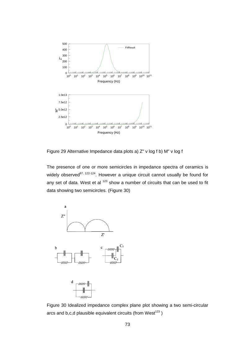
73

Figure 29 Alternative Impedance data plots a) Z" v log f b) M" v log f

The presence of one or more semicircles in impedance spectra of ceramics is

widely observed87, 122-124. However a unique circuit cannot usually be found for

any set of data. West et al 123 show a number of circuits that can be used to fit

data showing two semicircles. (Figure 30)

Figure 30 Idealized impedance complex plane plot showing a two semi-circular

arcs and b,c,d plausible equivalent circuits (from West123 )

100 101 102 103 104 105 106 107 108 109 1010 10110

100

200

300

400

500

Frequency (Hz)

Z''

FitResult

100 101 102 103 104 105 106 107 108 109 1010 10110

2.5e12

5.0e12

7.5e12

1.0e13

Frequency (Hz)

M''

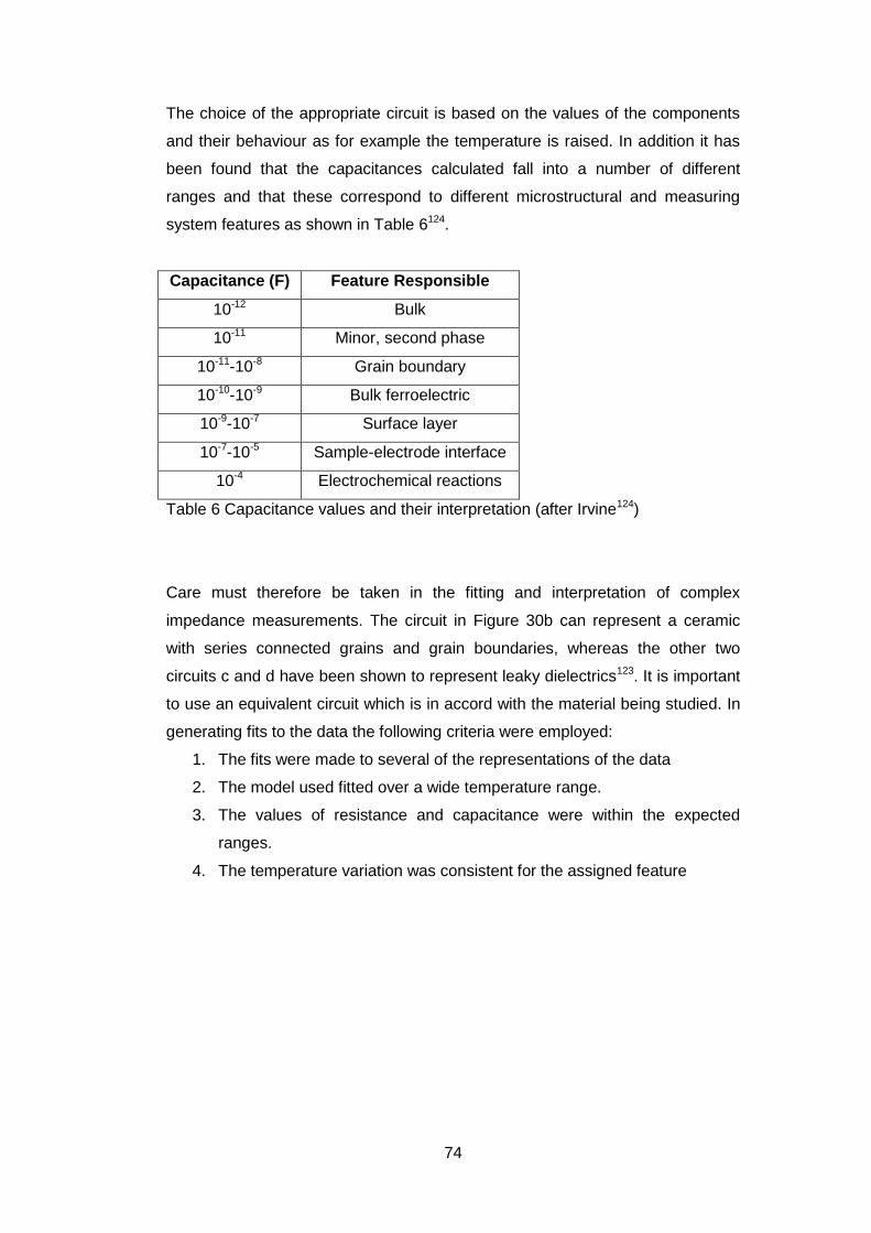
74

The choice of the appropriate circuit is based on the values of the components

and their behaviour as for example the temperature is raised. In addition it has

been found that the capacitances calculated fall into a number of different

ranges and that these correspond to different microstructural and measuring

system features as shown in Table 6124.

Capacitance (F) Feature Responsible

10-12 Bulk

10-11 Minor, second phase

10-11-10-8 Grain boundary

10-10-10-9 Bulk ferroelectric

10-9-10-7 Surface layer

10-7-10-5 Sample-electrode interface

10-4 Electrochemical reactions

Table 6 Capacitance values and their interpretation (after Irvine124)

Care must therefore be taken in the fitting and interpretation of complex

impedance measurements. The circuit in Figure 30b can represent a ceramic

with series connected grains and grain boundaries, whereas the other two

circuits c and d have been shown to represent leaky dielectrics123. It is important

to use an equivalent circuit which is in accord with the material being studied. In

generating fits to the data the following criteria were employed:

1. The fits were made to several of the representations of the data

2. The model used fitted over a wide temperature range.

3. The values of resistance and capacitance were within the expected

ranges.

4. The temperature variation was consistent for the assigned feature

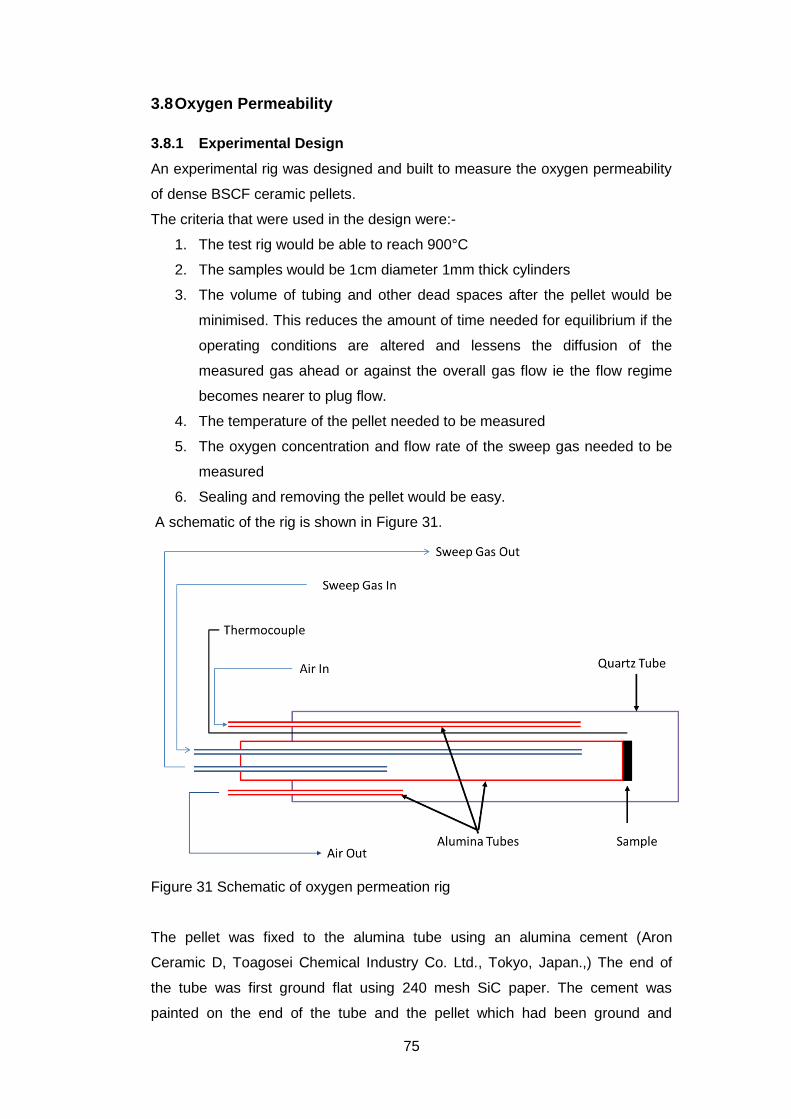
75

3.8 Oxygen Permeability

3.8.1 Experimental Design

An experimental rig was designed and built to measure the oxygen permeability

of dense BSCF ceramic pellets.

The criteria that were used in the design were:-

1. The test rig would be able to reach 900°C

2. The samples would be 1cm diameter 1mm thick cylinders

3. The volume of tubing and other dead spaces after the pellet would be

minimised. This reduces the amount of time needed for equilibrium if the

operating conditions are altered and lessens the diffusion of the

measured gas ahead or against the overall gas flow ie the flow regime

becomes nearer to plug flow.

4. The temperature of the pellet needed to be measured

5. The oxygen concentration and flow rate of the sweep gas needed to be

measured

6. Sealing and removing the pellet would be easy.

A schematic of the rig is shown in Figure 31.

Figure 31 Schematic of oxygen permeation rig

The pellet was fixed to the alumina tube using an alumina cement (Aron

Ceramic D, Toagosei Chemical Industry Co. Ltd., Tokyo, Japan.,) The end of

the tube was first ground flat using 240 mesh SiC paper. The cement was

painted on the end of the tube and the pellet which had been ground and

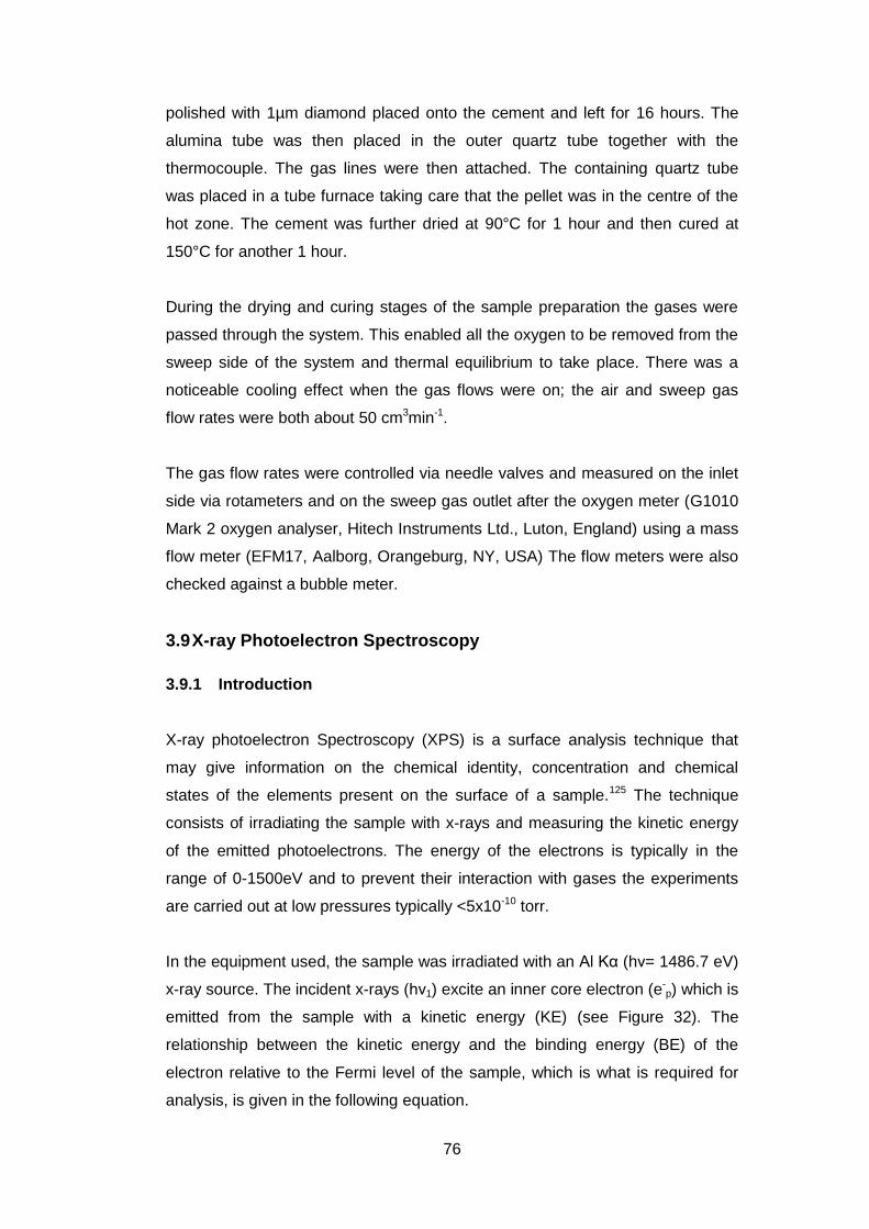
76

polished with 1µm diamond placed onto the cement and left for 16 hours. The

alumina tube was then placed in the outer quartz tube together with the

thermocouple. The gas lines were then attached. The containing quartz tube

was placed in a tube furnace taking care that the pellet was in the centre of the

hot zone. The cement was further dried at 90°C for 1 hour and then cured at

150°C for another 1 hour.

During the drying and curing stages of the sample preparation the gases were

passed through the system. This enabled all the oxygen to be removed from the

sweep side of the system and thermal equilibrium to take place. There was a

noticeable cooling effect when the gas flows were on; the air and sweep gas

flow rates were both about 50 cm3min-1.

The gas flow rates were controlled via needle valves and measured on the inlet

side via rotameters and on the sweep gas outlet after the oxygen meter (G1010

Mark 2 oxygen analyser, Hitech Instruments Ltd., Luton, England) using a mass

flow meter (EFM17, Aalborg, Orangeburg, NY, USA) The flow meters were also

checked against a bubble meter.

3.9 X-ray Photoelectron Spectroscopy

3.9.1 Introduction

X-ray photoelectron Spectroscopy (XPS) is a surface analysis technique that

may give information on the chemical identity, concentration and chemical

states of the elements present on the surface of a sample.125 The technique

consists of irradiating the sample with x-rays and measuring the kinetic energy

of the emitted photoelectrons. The energy of the electrons is typically in the

range of 0-1500eV and to prevent their interaction with gases the experiments

are carried out at low pressures typically <5x10-10 torr.

In the equipment used, the sample was irradiated with an Al Kα (hν= 1486.7 eV)

x-ray source. The incident x-rays (hν1) excite an inner core electron (e-p) which is

emitted from the sample with a kinetic energy (KE) (see Figure 32). The

relationship between the kinetic energy and the binding energy (BE) of the

electron relative to the Fermi level of the sample, which is what is required for

analysis, is given in the following equation.

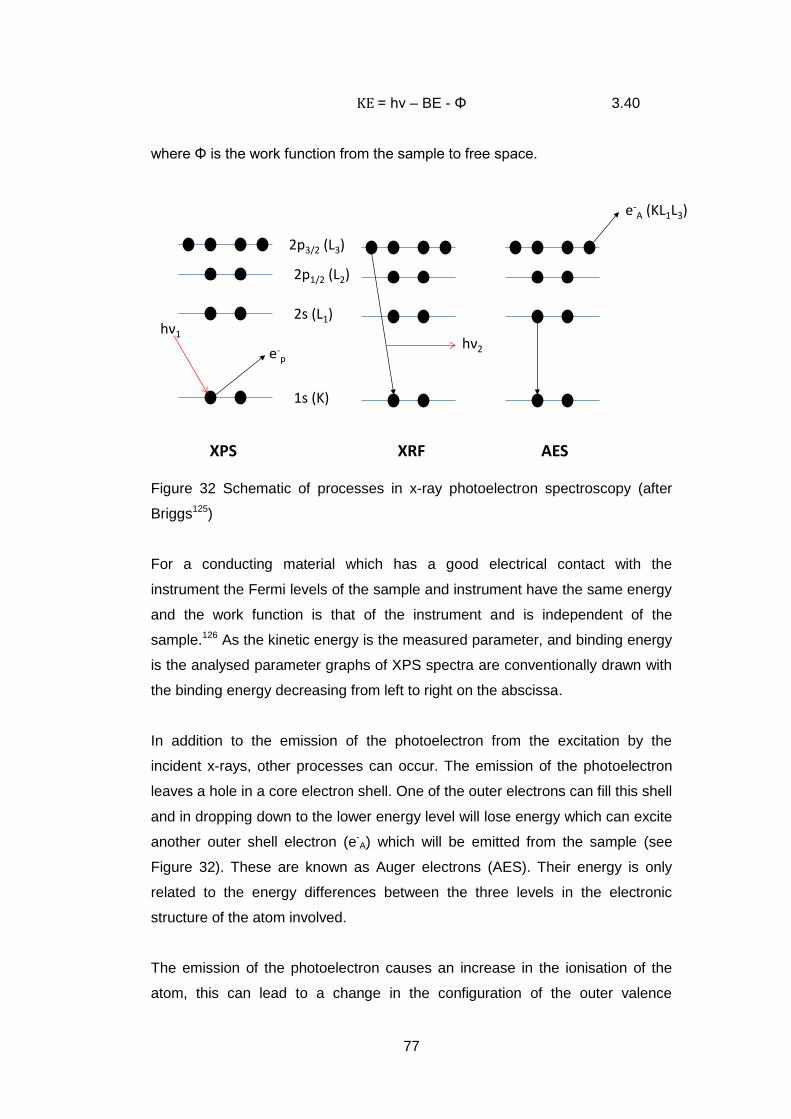
77

= hν – BE - Φ 3.40

where Φ is the work function from the sample to free space.

Figure 32 Schematic of processes in x-ray photoelectron spectroscopy (after

Briggs125)

For a conducting material which has a good electrical contact with the

instrument the Fermi levels of the sample and instrument have the same energy

and the work function is that of the instrument and is independent of the

sample.126 As the kinetic energy is the measured parameter, and binding energy

is the analysed parameter graphs of XPS spectra are conventionally drawn with

the binding energy decreasing from left to right on the abscissa.

In addition to the emission of the photoelectron from the excitation by the

incident x-rays, other processes can occur. The emission of the photoelectron

leaves a hole in a core electron shell. One of the outer electrons can fill this shell

and in dropping down to the lower energy level will lose energy which can excite

another outer shell electron (e-A) which will be emitted from the sample (see

Figure 32). These are known as Auger electrons (AES). Their energy is only

related to the energy differences between the three levels in the electronic

structure of the atom involved.

The emission of the photoelectron causes an increase in the ionisation of the

atom, this can lead to a change in the configuration of the outer valence

2p3/2 (L3)

2p1/2 (L2)

2s (L1)

1s (K)

hν1

e-p

hν2

e-A (KL1L3)

XPS XRF AES

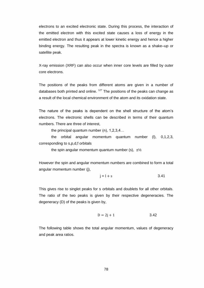
78

electrons to an excited electronic state. During this process, the interaction of

the emitted electron with this excited state causes a loss of energy in the

emitted electron and thus it appears at lower kinetic energy and hence a higher

binding energy. The resulting peak in the spectra is known as a shake–up or

satellite peak.

X-ray emission (XRF) can also occur when inner core levels are filled by outer

core electrons.

The positions of the peaks from different atoms are given in a number of

databases both printed and online. 127 The positions of the peaks can change as

a result of the local chemical environment of the atom and its oxidation state.

The nature of the peaks is dependent on the shell structure of the atom’s

electrons. The electronic shells can be described in terms of their quantum

numbers. There are three of interest,

the principal quantum number (n), 1,2,3,4…

the orbital angular momentum quantum number (l), 0,1,2,3,

corresponding to s,p,d,f orbitals

the spin angular momentum quantum number (s), ±½

However the spin and angular momentum numbers are combined to form a total

angular momentum number (j),

j = 3.41

This gives rise to singlet peaks for s orbitals and doublets for all other orbitals.

The ratio of the two peaks is given by their respective degeneracies. The

degeneracy (D) of the peaks is given by,

3.42

The following table shows the total angular momentum, values of degeneracy

and peak area ratios.

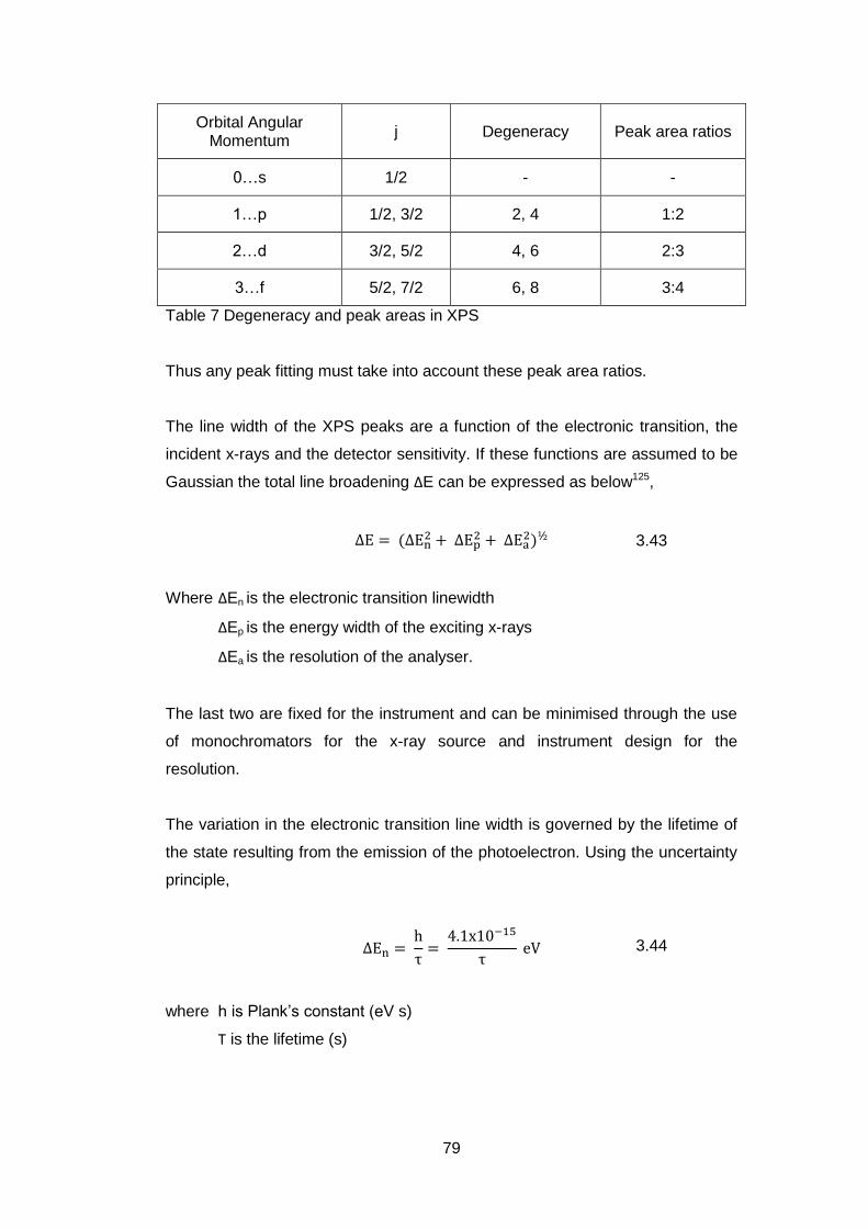
79

Orbital Angular Momentum

j Degeneracy Peak area ratios

0…s 1/2 - -

1…p 1/2, 3/2 2, 4 1:2

2…d 3/2, 5/2 4, 6 2:3

3…f 5/2, 7/2 6, 8 3:4

Table 7 Degeneracy and peak areas in XPS

Thus any peak fitting must take into account these peak area ratios.

The line width of the XPS peaks are a function of the electronic transition, the

incident x-rays and the detector sensitivity. If these functions are assumed to be

Gaussian the total line broadening ΔE can be expressed as below125,

3.43

Where ΔEn is the electronic transition linewidth

ΔEp is the energy width of the exciting x-rays

ΔEa is the resolution of the analyser.

The last two are fixed for the instrument and can be minimised through the use

of monochromators for the x-ray source and instrument design for the

resolution.

The variation in the electronic transition line width is governed by the lifetime of

the state resulting from the emission of the photoelectron. Using the uncertainty

principle,

3.44

where h is Plank’s constant (eV s)

Τ is the lifetime (s)

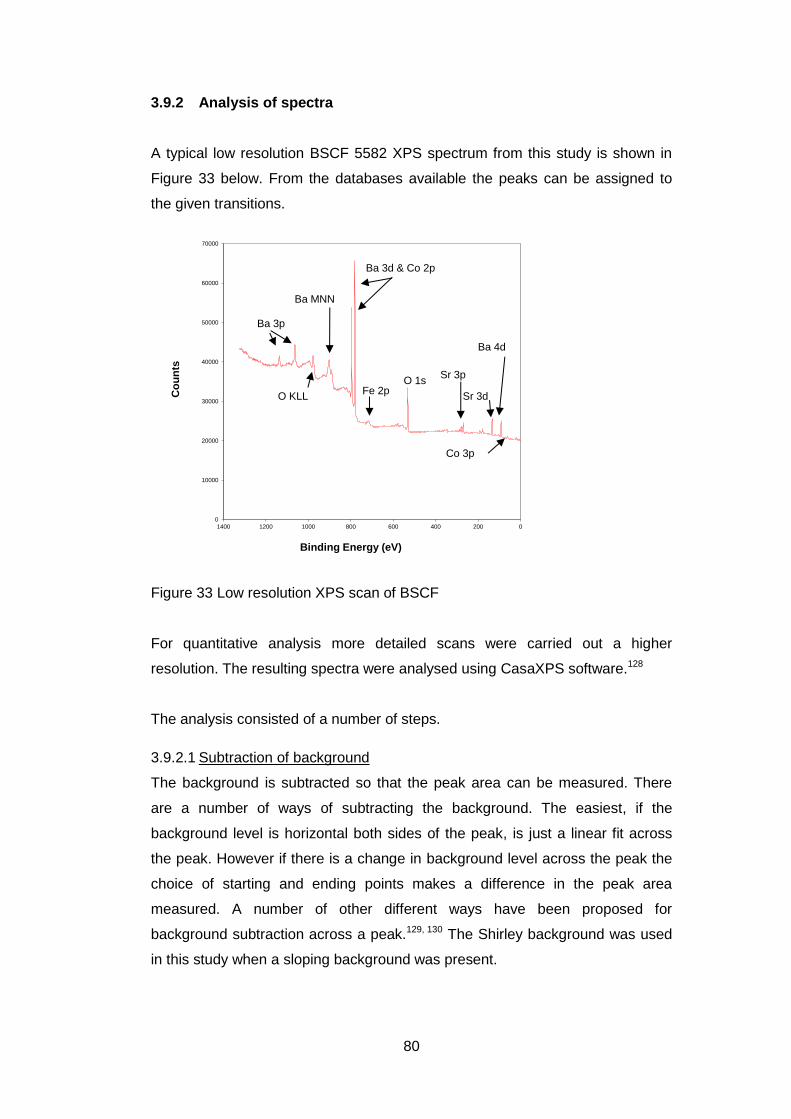
80

3.9.2 Analysis of spectra

A typical low resolution BSCF 5582 XPS spectrum from this study is shown in

Figure 33 below. From the databases available the peaks can be assigned to

the given transitions.

Figure 33 Low resolution XPS scan of BSCF

For quantitative analysis more detailed scans were carried out a higher

resolution. The resulting spectra were analysed using CasaXPS software.128

The analysis consisted of a number of steps.

3.9.2.1 Subtraction of background

The background is subtracted so that the peak area can be measured. There

are a number of ways of subtracting the background. The easiest, if the

background level is horizontal both sides of the peak, is just a linear fit across

the peak. However if there is a change in background level across the peak the

choice of starting and ending points makes a difference in the peak area

measured. A number of other different ways have been proposed for

background subtraction across a peak.129, 130 The Shirley background was used

in this study when a sloping background was present.

0

10000

20000

30000

40000

50000

60000

70000

0200400600800100012001400

Co

un

ts

Binding Energy (eV)

O 1s

Ba 3d & Co 2p

Sr 3p

Sr 3d

Ba 4d

Co 3p

Fe 2p

Ba 3p

Ba MNN

O KLL

81

3.9.2.2 Selection of peak shape

The peak shapes of XPS are found to have the form of a Voigt function which is

a convolution of a Gaussian and a Lorentzian function. Within the CasaXPS

software the mixing parameter (m) can be varied with m=100 representing a

pure Lorentzian curve and m=0 a pure Gaussian curve. A value of m=30 was

found to give the best fitting

3.9.2.3 Addition of constraints

A number of constraints can be put into the fitting procedure. The area ratio of

doublets can be fixed to the values given in Table 7. The energy separation

between the doublet peaks can be fixed, this was done for Sr 3d peaks which

were separated by 1.79eV.131

Further details on fitting will be given in the experimental section.

3.10 Computerised X-Ray Tomography

Computerised x-ray tomography is a technique for producing 3-D

representations of objects from a series of 2-D x-ray images132. The general

technique is to take an x-ray image of the object and then rotate it a small

amount and then image the object again. This is repeated approximately 2000

times over 180° of rotation. The resulting images show the adsorption of the x-

ray beam as they pass through the object with absorption being proportional to

the object’s density and thickness. An example of the different images that are

obtained from two images of a pair of cylinders is shown in Figure 34.

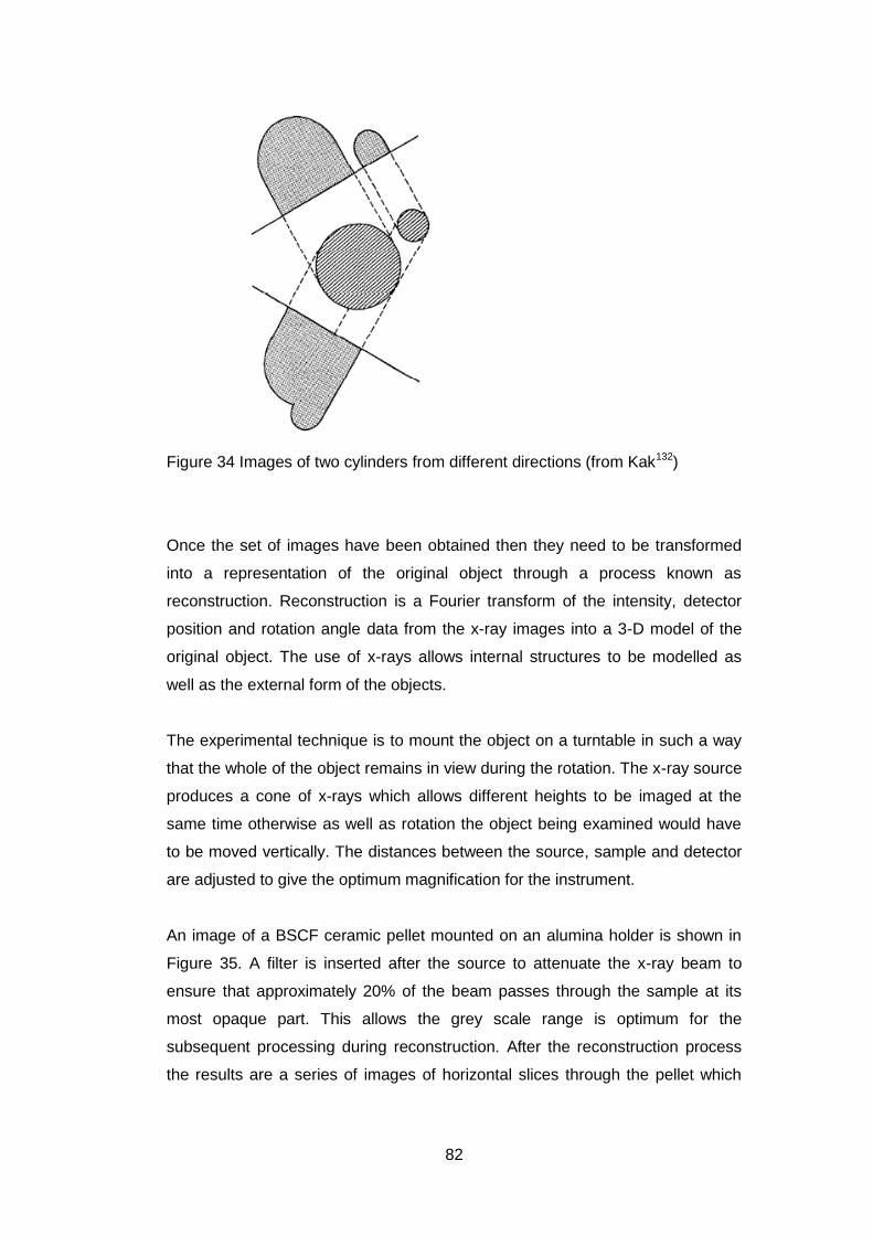
82

Figure 34 Images of two cylinders from different directions (from Kak132)

Once the set of images have been obtained then they need to be transformed

into a representation of the original object through a process known as

reconstruction. Reconstruction is a Fourier transform of the intensity, detector

position and rotation angle data from the x-ray images into a 3-D model of the

original object. The use of x-rays allows internal structures to be modelled as

well as the external form of the objects.

The experimental technique is to mount the object on a turntable in such a way

that the whole of the object remains in view during the rotation. The x-ray source

produces a cone of x-rays which allows different heights to be imaged at the

same time otherwise as well as rotation the object being examined would have

to be moved vertically. The distances between the source, sample and detector

are adjusted to give the optimum magnification for the instrument.

An image of a BSCF ceramic pellet mounted on an alumina holder is shown in

Figure 35. A filter is inserted after the source to attenuate the x-ray beam to

ensure that approximately 20% of the beam passes through the sample at its

most opaque part. This allows the grey scale range is optimum for the

subsequent processing during reconstruction. After the reconstruction process

the results are a series of images of horizontal slices through the pellet which

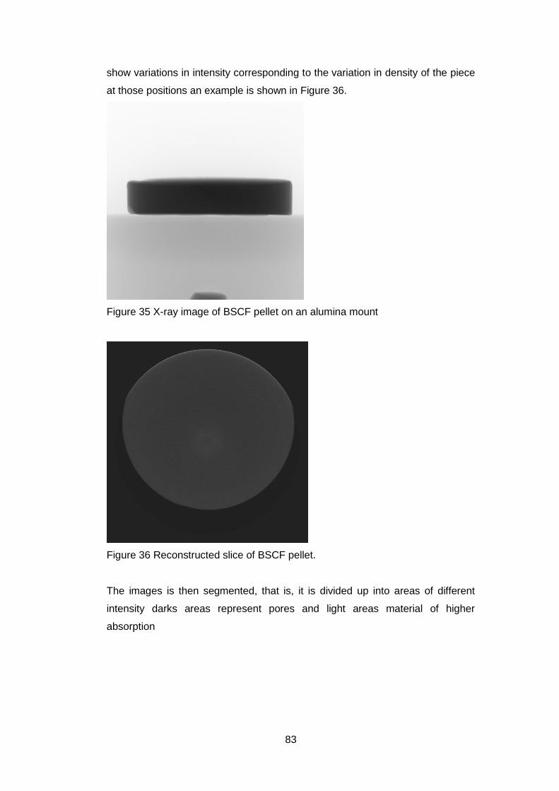
83

show variations in intensity corresponding to the variation in density of the piece

at those positions an example is shown in Figure 36.

Figure 35 X-ray image of BSCF pellet on an alumina mount

Figure 36 Reconstructed slice of BSCF pellet.

The images is then segmented, that is, it is divided up into areas of different

intensity darks areas represent pores and light areas material of higher

absorption

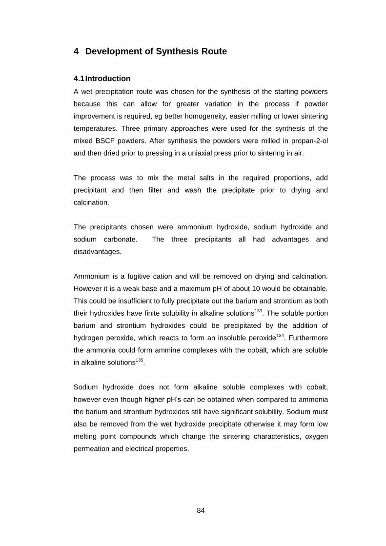
84

4 Development of Synthesis Route

4.1 Introduction

A wet precipitation route was chosen for the synthesis of the starting powders

because this can allow for greater variation in the process if powder

improvement is required, eg better homogeneity, easier milling or lower sintering

temperatures. Three primary approaches were used for the synthesis of the

mixed BSCF powders. After synthesis the powders were milled in propan-2-ol

and then dried prior to pressing in a uniaxial press prior to sintering in air.

The process was to mix the metal salts in the required proportions, add

precipitant and then filter and wash the precipitate prior to drying and

calcination.

The precipitants chosen were ammonium hydroxide, sodium hydroxide and

sodium carbonate. The three precipitants all had advantages and

disadvantages.

Ammonium is a fugitive cation and will be removed on drying and calcination.

However it is a weak base and a maximum pH of about 10 would be obtainable.

This could be insufficient to fully precipitate out the barium and strontium as both

their hydroxides have finite solubility in alkaline solutions133. The soluble portion

barium and strontium hydroxides could be precipitated by the addition of

hydrogen peroxide, which reacts to form an insoluble peroxide134. Furthermore

the ammonia could form ammine complexes with the cobalt, which are soluble

in alkaline solutions135.

Sodium hydroxide does not form alkaline soluble complexes with cobalt,

however even though higher pH’s can be obtained when compared to ammonia

the barium and strontium hydroxides still have significant solubility. Sodium must

also be removed from the wet hydroxide precipitate otherwise it may form low

melting point compounds which change the sintering characteristics, oxygen

permeation and electrical properties.

85

Sodium carbonate precipitates carbonates, hydroxides and basic carbonates.

However some or all of these are insoluble for the metals being used. Sodium

removal is still necessary

4.2 Exploratory Series

In order to avoid problems with removal of chloride ions, which can inhibit

densification even at low levels, the metal nitrates were chosen as starting

materials. Stock solutions in deionised water were made for all the metals

except barium. These solutions were made at 15% weight/weight (w/w) with the

exception of iron, which was at 10% w/w. The concentrations are based on

weight of element in solution. Barium nitrate has a low solubility 8.2%w/w

(4.3%w/w as Ba)133 and was added as a solid. One advantage of using stock

solutions is that it avoids the problems of the hygroscopic nature of many metal

nitrates.

The general method of preparation was as follows:-

1 The metal salt solutions were weighed into a beaker and the solid barium

nitrate added. Further water was added to give a total metal concentration of 8%

w/w. This value was chosen so that the volumes being processed did not

become too large and the final suspension did not become too viscous and thus

unable to be stirred. The mix was heated to 60°C to allow the barium nitrate to

dissolve. It was then generally cooled to less than 30°C, although higher barium

contents gave a precipitate if cooled much below 30°C.

2 The precipitant was diluted to give a 10% w/w solution and this was added

drop wise over approximately an hour to the metal nitrate solution. At the end of

the addition the suspension was left stirring for an hour.

3 The suspension was filtered using a Whatman 541 paper and washed with 3x

the metal nitrate solution starting volume.

4 The precipitate was redispersed in water and filtered.

5 The precipitate was dried overnight at 100°C

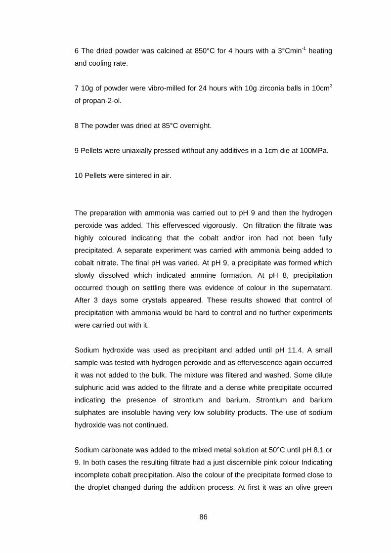
86

6 The dried powder was calcined at 850°C for 4 hours with a 3°Cmin-1 heating

and cooling rate.

7 10g of powder were vibro-milled for 24 hours with 10g zirconia balls in 10cm3

of propan-2-ol.

8 The powder was dried at 85°C overnight.

9 Pellets were uniaxially pressed without any additives in a 1cm die at 100MPa.

10 Pellets were sintered in air.

The preparation with ammonia was carried out to pH 9 and then the hydrogen

peroxide was added. This effervesced vigorously. On filtration the filtrate was

highly coloured indicating that the cobalt and/or iron had not been fully

precipitated. A separate experiment was carried with ammonia being added to

cobalt nitrate. The final pH was varied. At pH 9, a precipitate was formed which

slowly dissolved which indicated ammine formation. At pH 8, precipitation

occurred though on settling there was evidence of colour in the supernatant.

After 3 days some crystals appeared. These results showed that control of

precipitation with ammonia would be hard to control and no further experiments

were carried out with it.

Sodium hydroxide was used as precipitant and added until pH 11.4. A small

sample was tested with hydrogen peroxide and as effervescence again occurred

it was not added to the bulk. The mixture was filtered and washed. Some dilute

sulphuric acid was added to the filtrate and a dense white precipitate occurred

indicating the presence of strontium and barium. Strontium and barium

sulphates are insoluble having very low solubility products. The use of sodium

hydroxide was not continued.

Sodium carbonate was added to the mixed metal solution at 50°C until pH 8.1 or

9. In both cases the resulting filtrate had a just discernible pink colour Indicating

incomplete cobalt precipitation. Also the colour of the precipitate formed close to

the droplet changed during the addition process. At first it was an olive green

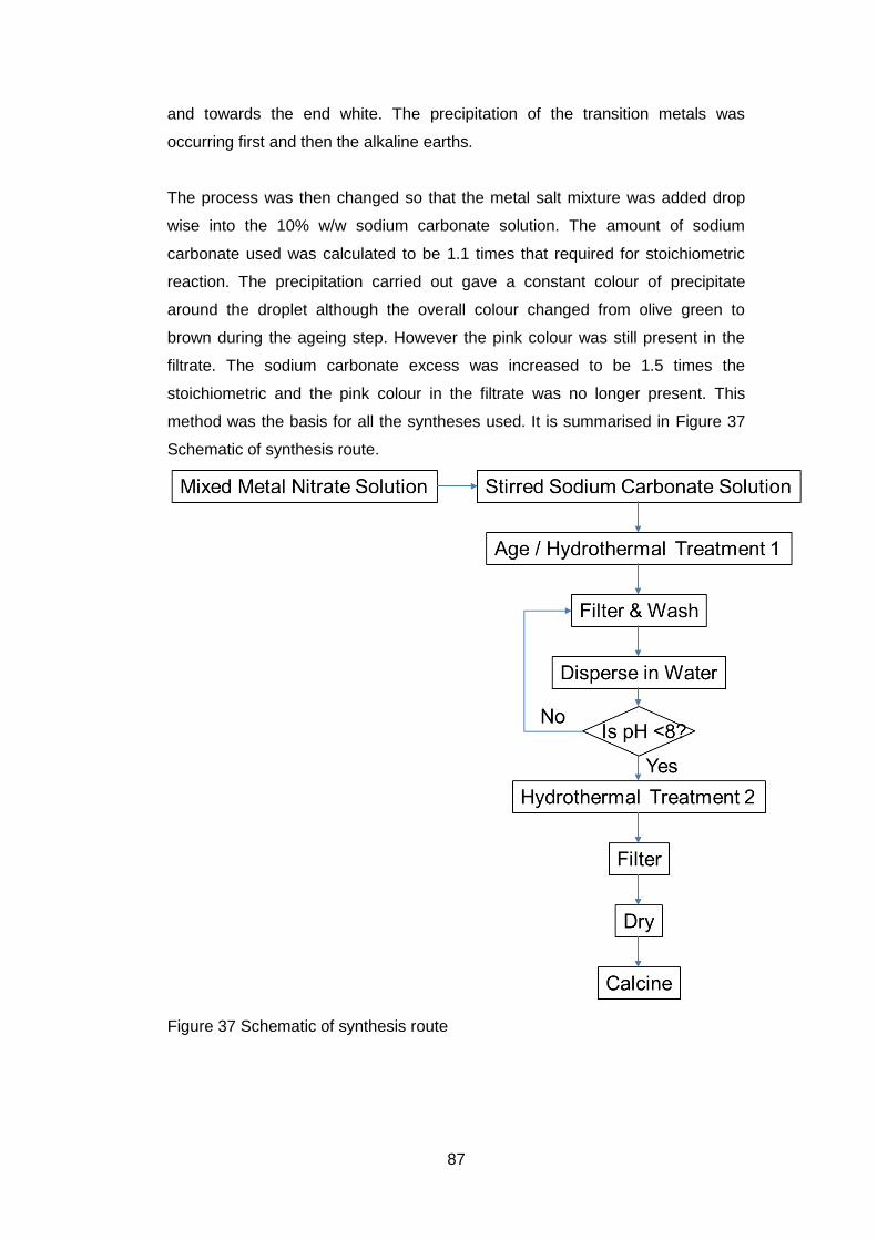
87

and towards the end white. The precipitation of the transition metals was

occurring first and then the alkaline earths.

The process was then changed so that the metal salt mixture was added drop

wise into the 10% w/w sodium carbonate solution. The amount of sodium

carbonate used was calculated to be 1.1 times that required for stoichiometric

reaction. The precipitation carried out gave a constant colour of precipitate

around the droplet although the overall colour changed from olive green to

brown during the ageing step. However the pink colour was still present in the

filtrate. The sodium carbonate excess was increased to be 1.5 times the

stoichiometric and the pink colour in the filtrate was no longer present. This

method was the basis for all the syntheses used. It is summarised in Figure 37

Schematic of synthesis route.

Figure 37 Schematic of synthesis route

88

4.3 Equilibrium Evaluation

MEDUSA chemical equilibrium software was used to verify the experimental

observations of the completeness of precipitation.52 The large number of

potential species in the solution and in the solid phase meant that the diagrams

for the complete Ba-Sr-Fe-Co-Na-H-CO3-NO3 system were extremely

complicated and not suitable for analysis. Therefore one of each of the 4

components (Ba-Sr-Fe-Co) together with the total concentrations of Na CO3 and

NO3, assuming the other components were present, were used in constructing

the diagram. A diagram was also constructed for barium precipitation using

sodium hydroxide. The concentrations used were those that would be present at

the end of the addition stage but ignoring the other components. The diagrams

were constructed over a pH range of 1-12. The diagrams follow, the first one is a

complete diagram, the remaining ones have had many of the lines removed if

they were similar to Na+ that is, invariant or like H+ and OH- the same for all

diagrams.

The diagrams show the log concentration of the species present against pH.

The diagrams are calculated from the starting concentrations given for each

component and the aqueous equilibrium constant data for all possible species

within the system. The equilibrium constant data is contained within the

software.

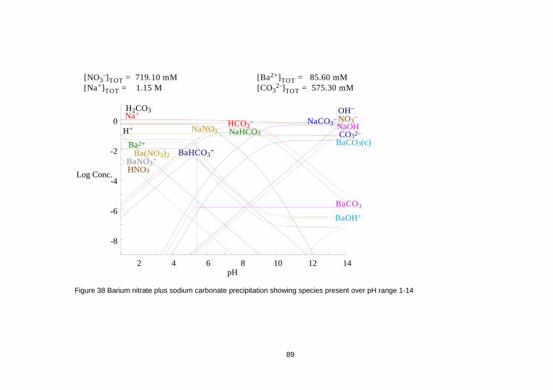
89

Figure 38 Barium nitrate plus sodium carbonate precipitation showing species present over pH range 1-14

2 4 6 8 10 12 14

-8

-6

-4

-2

0

Log Conc.

pH

H +

N a + N O 3

C O 3 2

B a 2 +

B a ( N O 3 ) 2

B a C O 3

B a H C O 3 +

B a N O 3 +

B a O H +

H 2 C O 3

H C O 3

H N O 3

N a C O 3

N a H C O 3 N a N O 3

NaOH

O H

B a C O 3 ( c )

[ N a + ] T O T = 1 . 1 5 M

[ N O 3 ] T O T

= 7 1 9 . 1 0 m M

[ C O 3 2 ] T O T

= 5 7 5 . 3 0 m M

[ B a 2 + ] T O T = 8 5 . 6 0 m M

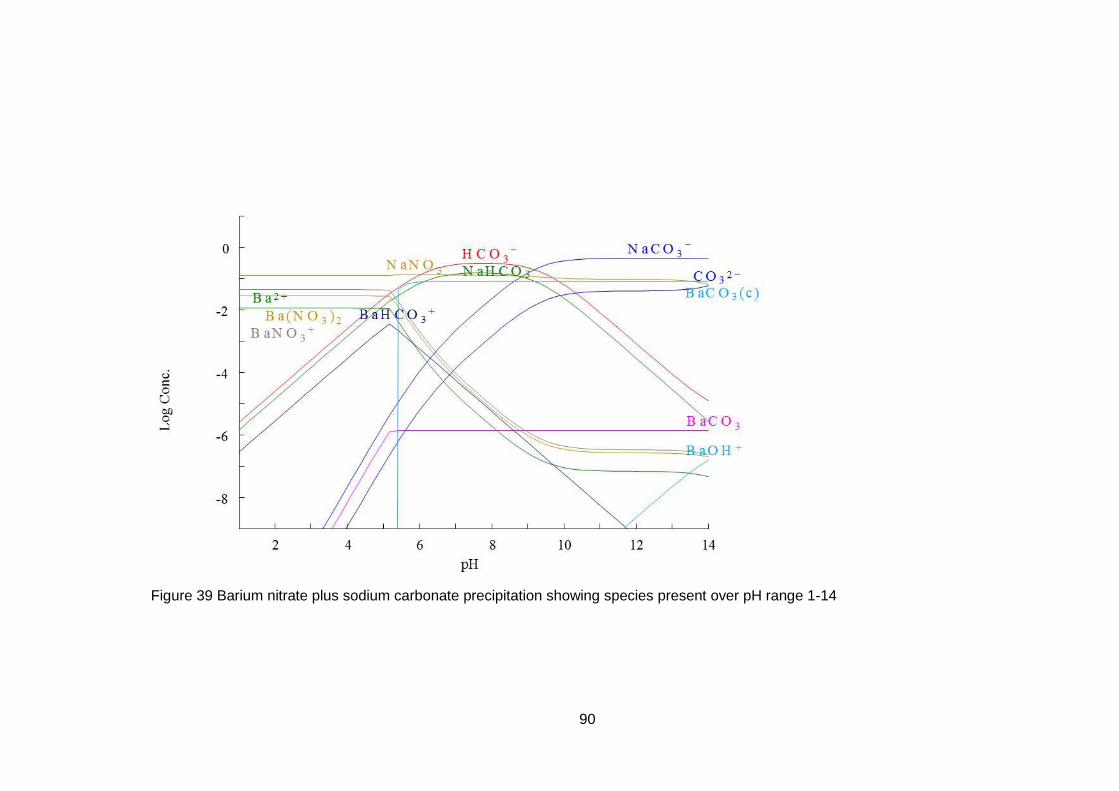
90

Figure 39 Barium nitrate plus sodium carbonate precipitation showing species present over pH range 1-14

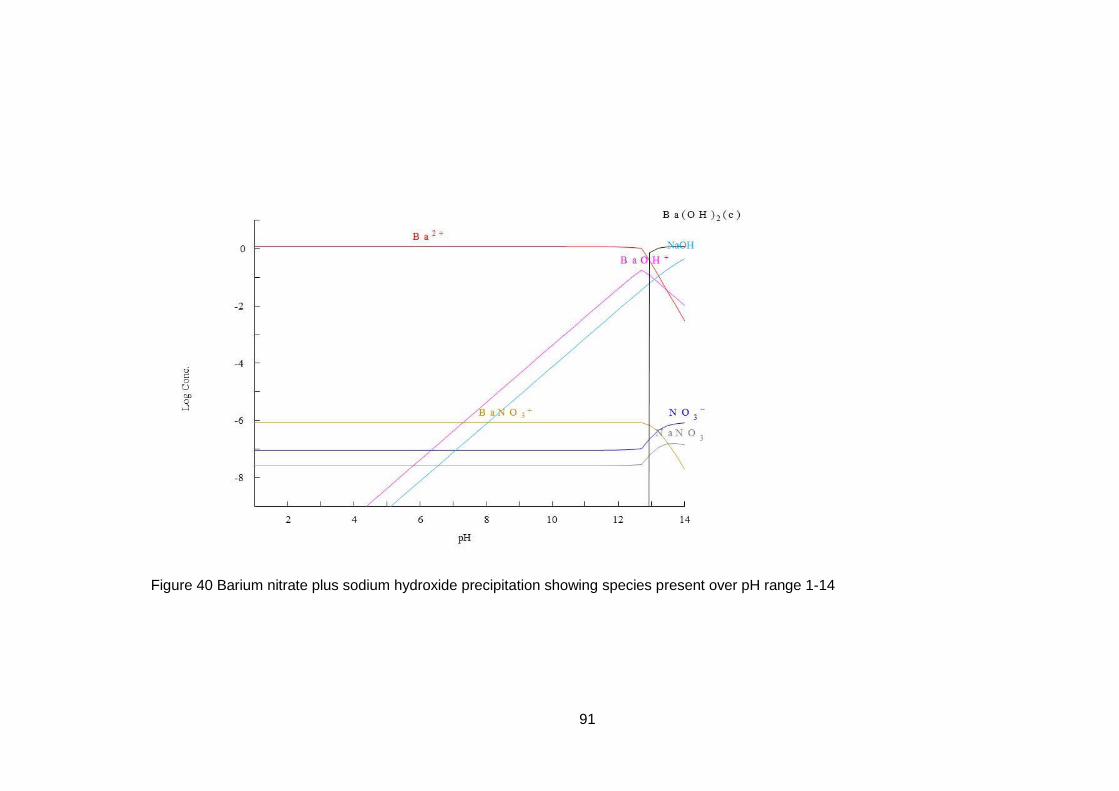
91

Figure 40 Barium nitrate plus sodium hydroxide precipitation showing species present over pH range 1-14

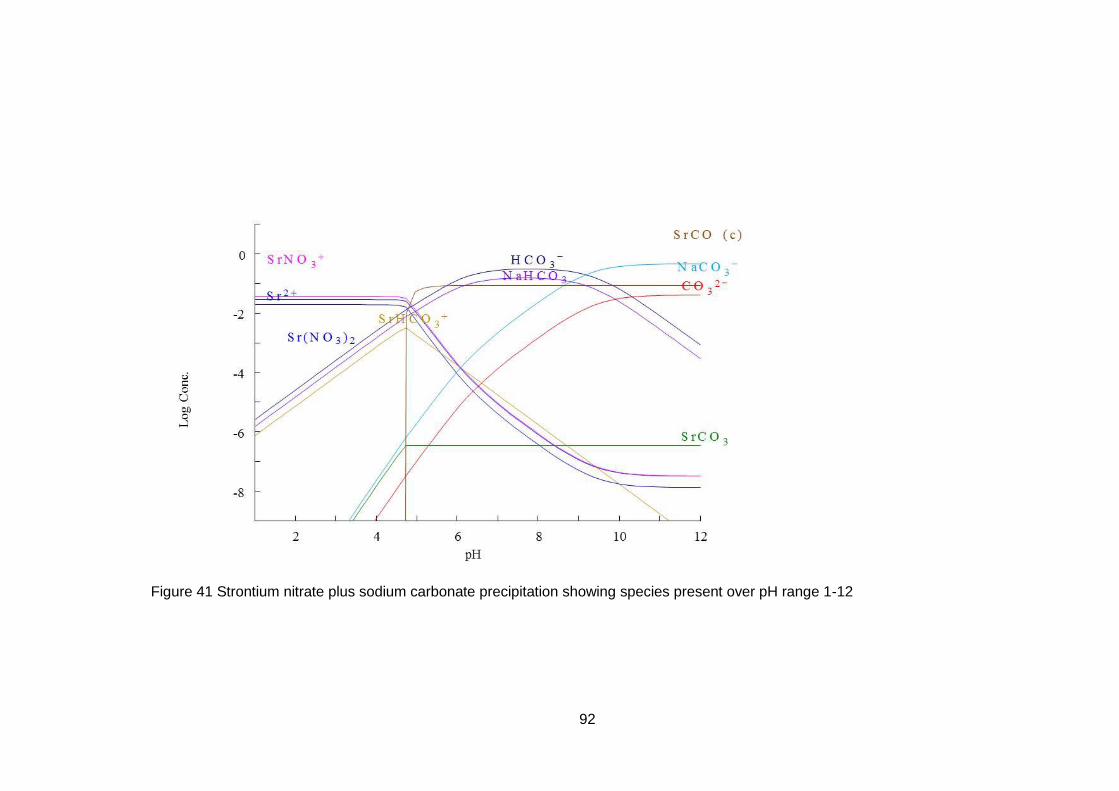
92

Figure 41 Strontium nitrate plus sodium carbonate precipitation showing species present over pH range 1-12

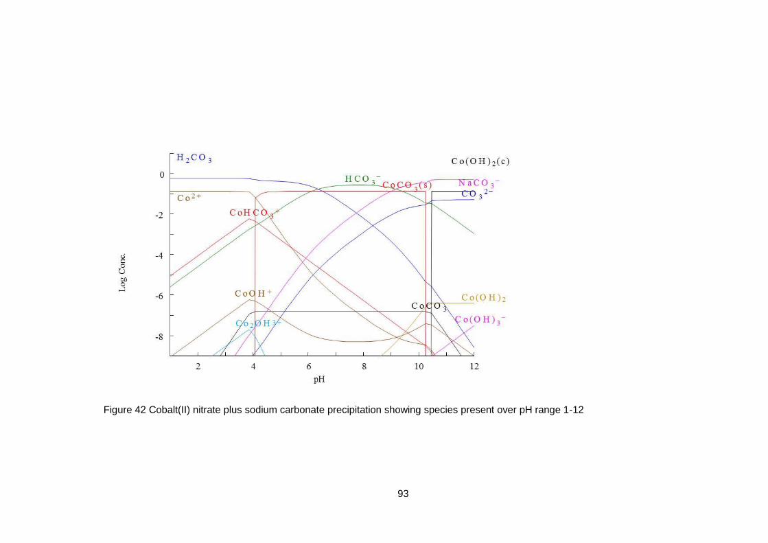
93

Figure 42 Cobalt(II) nitrate plus sodium carbonate precipitation showing species present over pH range 1-12

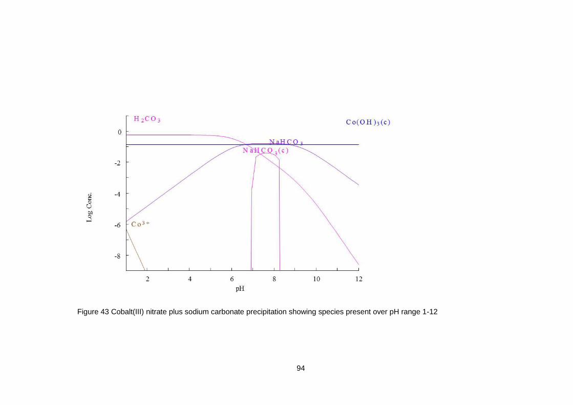
94

Figure 43 Cobalt(III) nitrate plus sodium carbonate precipitation showing species present over pH range 1-12

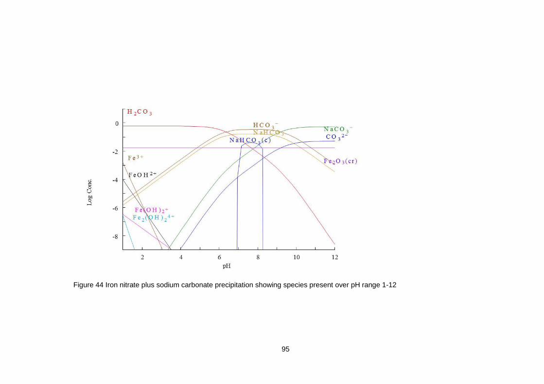
95

Figure 44 Iron nitrate plus sodium carbonate precipitation showing species present over pH range 1-12

96

Comparison of the use of sodium carbonate and hydroxide (Figure 38 and

Figure 40) shows that with the former, there is a very low concentration 10-6 M of

BaCO3 in solution and that precipitation is complete above pH 5 and that at pH

greater than 11.5 there is some reaction of the barium carbonate precipitate to

give some BaOH+ species in solution at very low concentrations. Whereas with

sodium hydroxide as the precipitant there is no solid phase present until

approximately pH 13 as was confirmed by the precipitation of barium sulphate

(white solid) in the exploratory series of preparations. Strontium shows, as is

expected, very similar behaviour to barium (Figure 41).

Cobalt(II) nitrate was used in all the experiments as the source of cobalt.

However during the addition of the mixed salts solution the precipitate changed

from an olive green to a chocolate brown colour, this is ascribed to oxidation of

Co2+ to Co3+ 136.. The equilibrium diagrams were constructed for both Co2+ and

Co3+. The Co2+ diagram (Figure 42) shows that the soluble Co species (CoOH+

and CoHCO3+) drop to concentrations below 10-6M at pH greater than 7 though

they start to rise at pH 10.5 with the formation of Co(OH)3-. At about pH 10.3 the

precipitated CoCO3 is converted to Co(OH)2. The Co3+ diagram (Figure 43)

shows no soluble Co species above pH 2.

The iron diagram (Figure 44) shows no soluble species above pH 3.5. In both

the Co3+ and Fe3+ diagrams sodium bicarbonate is indicated as being present as

a solid phase in the pH range 6.9 to 8.3, to avoid sodium contamination in the

final product careful washing of the precipitates would be needed.

As a result of the exploratory series and the analysis of the equilibrium diagrams

the following series of experiments were performed to determine how robust the

process was and whether it could be further optimised. The main parameters

investigated were:-

1. Final pH

2. Boiling the precipitate

3. pH of boiling.

4.4 Experimental Plan

The object of the precipitation was to make a homogeneous precipitate so that

on calcination it would be easier to prepare a single phase powder that could

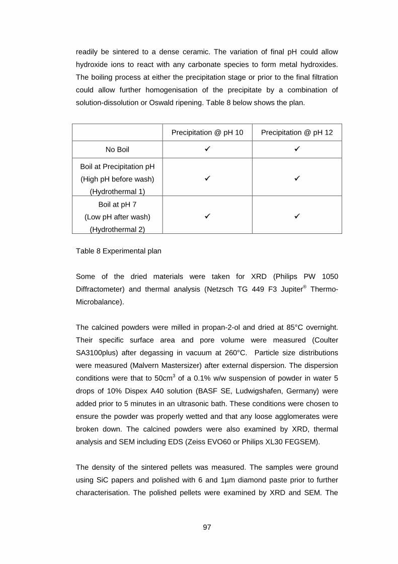
97

readily be sintered to a dense ceramic. The variation of final pH could allow

hydroxide ions to react with any carbonate species to form metal hydroxides.

The boiling process at either the precipitation stage or prior to the final filtration

could allow further homogenisation of the precipitate by a combination of

solution-dissolution or Oswald ripening. Table 8 below shows the plan.

Precipitation @ pH 10 Precipitation @ pH 12

No Boil

Boil at Precipitation pH

(High pH before wash)

(Hydrothermal 1)

Boil at pH 7

(Low pH after wash)

(Hydrothermal 2)

Table 8 Experimental plan

Some of the dried materials were taken for XRD (Philips PW 1050

Diffractometer) and thermal analysis (Netzsch TG 449 F3 Jupiter® Thermo-

Microbalance).

The calcined powders were milled in propan-2-ol and dried at 85°C overnight.

Their specific surface area and pore volume were measured (Coulter

SA3100plus) after degassing in vacuum at 260°C. Particle size distributions

were measured (Malvern Mastersizer) after external dispersion. The dispersion

conditions were that to 50cm3 of a 0.1% w/w suspension of powder in water 5

drops of 10% Dispex A40 solution (BASF SE, Ludwigshafen, Germany) were

added prior to 5 minutes in an ultrasonic bath. These conditions were chosen to

ensure the powder was properly wetted and that any loose agglomerates were

broken down. The calcined powders were also examined by XRD, thermal

analysis and SEM including EDS (Zeiss EVO60 or Philips XL30 FEGSEM).

The density of the sintered pellets was measured. The samples were ground

using SiC papers and polished with 6 and 1µm diamond paste prior to further

characterisation. The polished pellets were examined by XRD and SEM. The

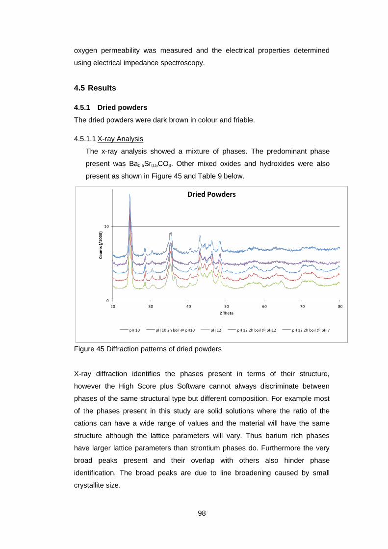
98

oxygen permeability was measured and the electrical properties determined

using electrical impedance spectroscopy.

4.5 Results

4.5.1 Dried powders

The dried powders were dark brown in colour and friable.

4.5.1.1 X-ray Analysis

The x-ray analysis showed a mixture of phases. The predominant phase

present was Ba0.5Sr0.5CO3. Other mixed oxides and hydroxides were also

present as shown in Figure 45 and Table 9 below.

0

10

20 30 40 50 60 70 80

Co

un

ts (

/10

00

)

2 Theta

Dried Powders

pH 10 pH 10 2h boil @ pH10 pH 12 pH 12 2h boil @ pH12 pH 12 2h boil @ pH 7

Figure 45 Diffraction patterns of dried powders

X-ray diffraction identifies the phases present in terms of their structure,

however the High Score plus Software cannot always discriminate between

phases of the same structural type but different composition. For example most

of the phases present in this study are solid solutions where the ratio of the

cations can have a wide range of values and the material will have the same

structure although the lattice parameters will vary. Thus barium rich phases

have larger lattice parameters than strontium phases do. Furthermore the very

broad peaks present and their overlap with others also hinder phase

identification. The broad peaks are due to line broadening caused by small

crystallite size.

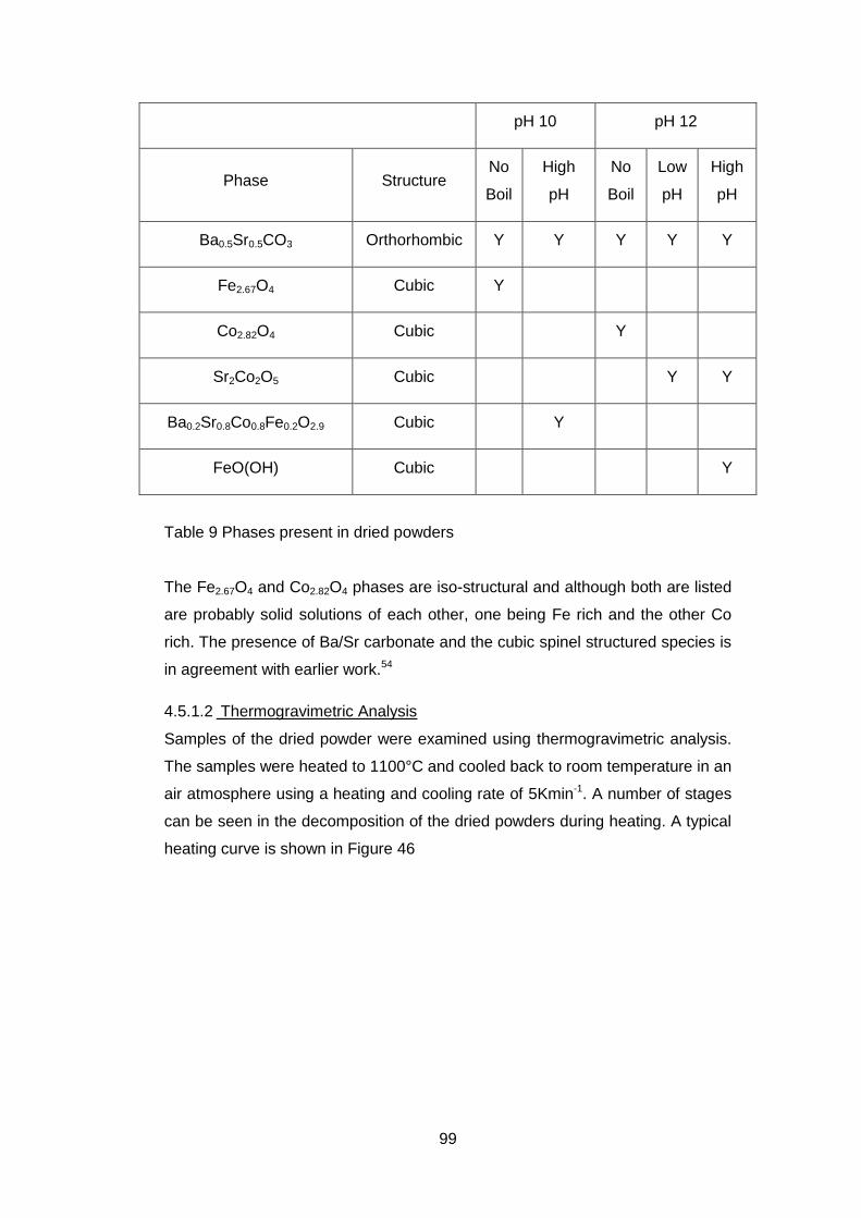
99

pH 10 pH 12

Phase Structure No

Boil

High

pH

No

Boil

Low

pH

High

pH

Ba0.5Sr0.5CO3 Orthorhombic Y Y Y Y Y

Fe2.67O4 Cubic Y

Co2.82O4 Cubic Y

Sr2Co2O5 Cubic Y Y

Ba0.2Sr0.8Co0.8Fe0.2O2.9 Cubic Y

FeO(OH) Cubic Y

Table 9 Phases present in dried powders

The Fe2.67O4 and Co2.82O4 phases are iso-structural and although both are listed

are probably solid solutions of each other, one being Fe rich and the other Co

rich. The presence of Ba/Sr carbonate and the cubic spinel structured species is

in agreement with earlier work.54

4.5.1.2 Thermogravimetric Analysis

Samples of the dried powder were examined using thermogravimetric analysis.

The samples were heated to 1100°C and cooled back to room temperature in an

air atmosphere using a heating and cooling rate of 5Kmin-1. A number of stages

can be seen in the decomposition of the dried powders during heating. A typical

heating curve is shown in Figure 46

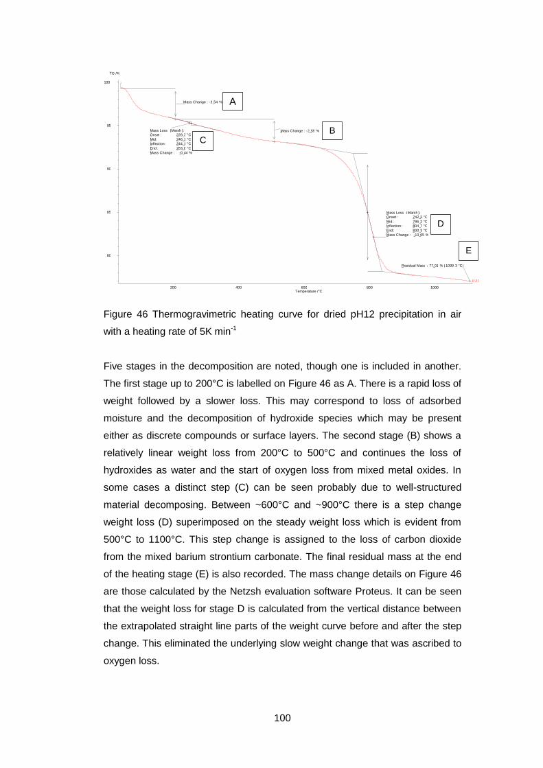
100

Figure 46 Thermogravimetric heating curve for dried pH12 precipitation in air

with a heating rate of 5K min-1

Five stages in the decomposition are noted, though one is included in another.

The first stage up to 200°C is labelled on Figure 46 as A. There is a rapid loss of

weight followed by a slower loss. This may correspond to loss of adsorbed

moisture and the decomposition of hydroxide species which may be present

either as discrete compounds or surface layers. The second stage (B) shows a

relatively linear weight loss from 200°C to 500°C and continues the loss of

hydroxides as water and the start of oxygen loss from mixed metal oxides. In

some cases a distinct step (C) can be seen probably due to well-structured

material decomposing. Between ~600°C and ~900°C there is a step change

weight loss (D) superimposed on the steady weight loss which is evident from

500°C to 1100°C. This step change is assigned to the loss of carbon dioxide

from the mixed barium strontium carbonate. The final residual mass at the end

of the heating stage (E) is also recorded. The mass change details on Figure 46

are those calculated by the Netzsh evaluation software Proteus. It can be seen

that the weight loss for stage D is calculated from the vertical distance between

the extrapolated straight line parts of the weight curve before and after the step

change. This eliminated the underlying slow weight change that was ascribed to

oxygen loss.

200 400 600 800 1000 Temperature /°C

80

85

90

95

100 TG /%

_ Mass Change : - 3 _ . 54 %

_ Mass Loss ( Marsh ): _ Onset : _ Mid : _ Inflection : _ End : _ Mass Change :

_ 228 _ . 3 °C _ 246 _ . 1 °C _ 244 _ . 1 °C _ 263 _ . 8 °C

_ - 0 _ . 44 %

_ Mass Change : - 2 _ . 59 %

_ Mass Loss ( Marsh ): _ Onset : _ Mid : _ Inflection : _ End : _ Mass Change :

_ 742 _ . 2 °C _ 786 _ . 2 °C _ 804 _ . 7 °C _ 830 _ . 3 °C _ - 13 _ . 65 %

_ Residual Mass : 77 _ . 01 % ( 1099 . 3 °C )

_ [ 5 _ . 1 ]

A

B C

D

E

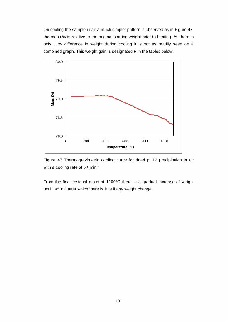
101

On cooling the sample in air a much simpler pattern is observed as in Figure 47,

the mass % is relative to the original starting weight prior to heating. As there is

only ~1% difference in weight during cooling it is not as readily seen on a

combined graph. This weight gain is designated F in the tables below.

78.0

78.5

79.0

79.5

80.0

0 200 400 600 800 1000

Mas

s (%

)

Temperature (°C)

Figure 47 Thermogravimetric cooling curve for dried pH12 precipitation in air

with a cooling rate of 5K min-1

From the final residual mass at 1100°C there is a gradual increase of weight

until ~450°C after which there is little if any weight change.

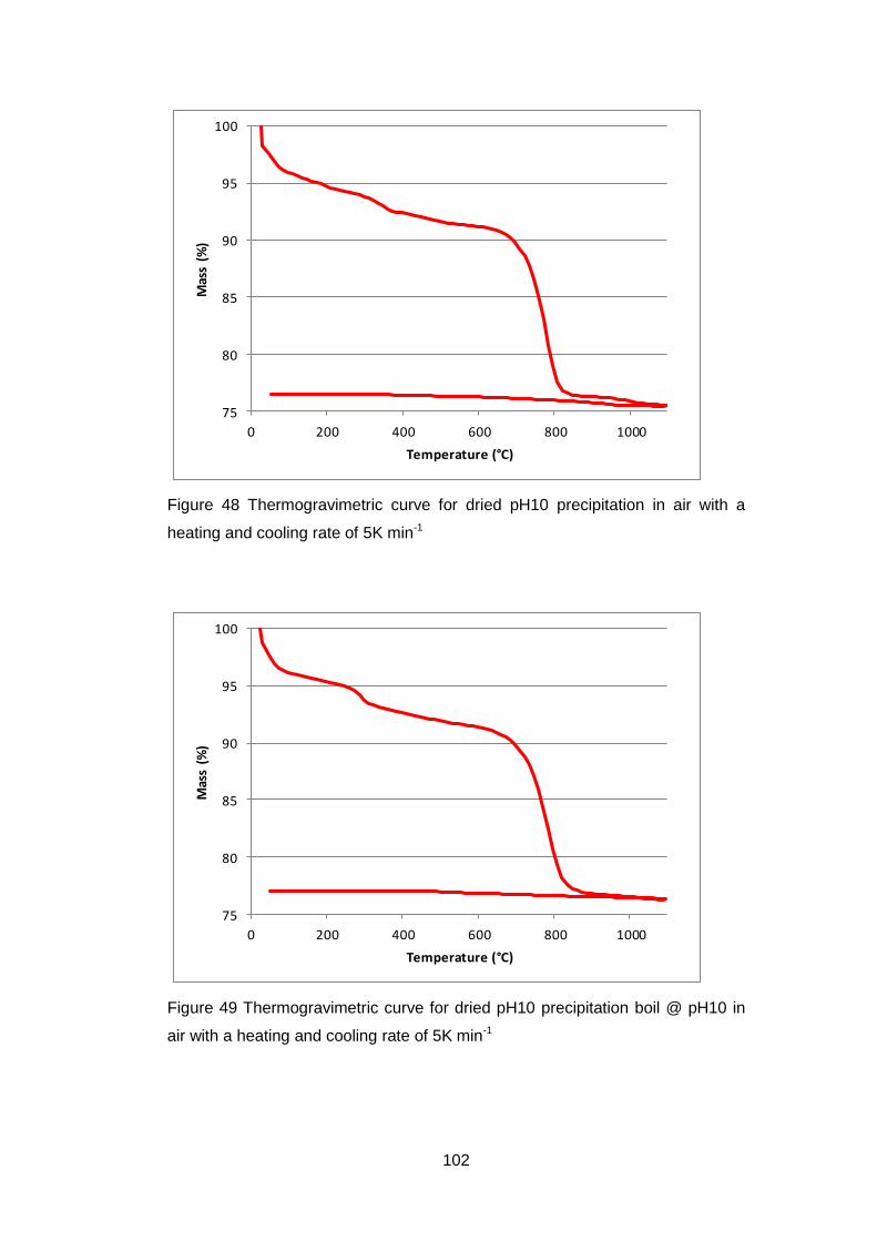
102

75

80

85

90

95

100

0 200 400 600 800 1000

Mas

s (%

)

Temperature (°C)

Figure 48 Thermogravimetric curve for dried pH10 precipitation in air with a

heating and cooling rate of 5K min-1

75

80

85

90

95

100

0 200 400 600 800 1000

Mas

s (%

)

Temperature (°C)

Figure 49 Thermogravimetric curve for dried pH10 precipitation boil @ pH10 in

air with a heating and cooling rate of 5K min-1

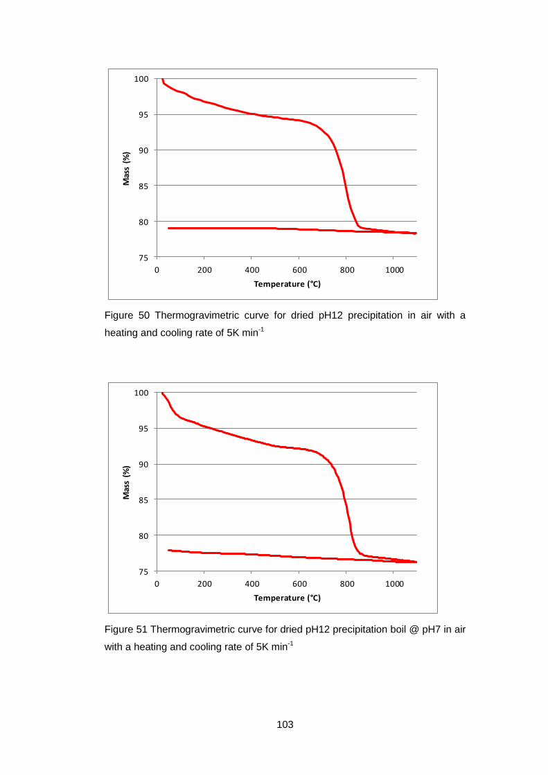
103

75

80

85

90

95

100

0 200 400 600 800 1000

Mas

s (%

)

Temperature (°C)

Figure 50 Thermogravimetric curve for dried pH12 precipitation in air with a


75

80

85

90

95

100

0 200 400 600 800 1000

Mas

s (%

)

Temperature (°C)

Figure 51 Thermogravimetric curve for dried pH12 precipitation boil @ pH7 in air

with a heating and cooling rate of 5K min-1

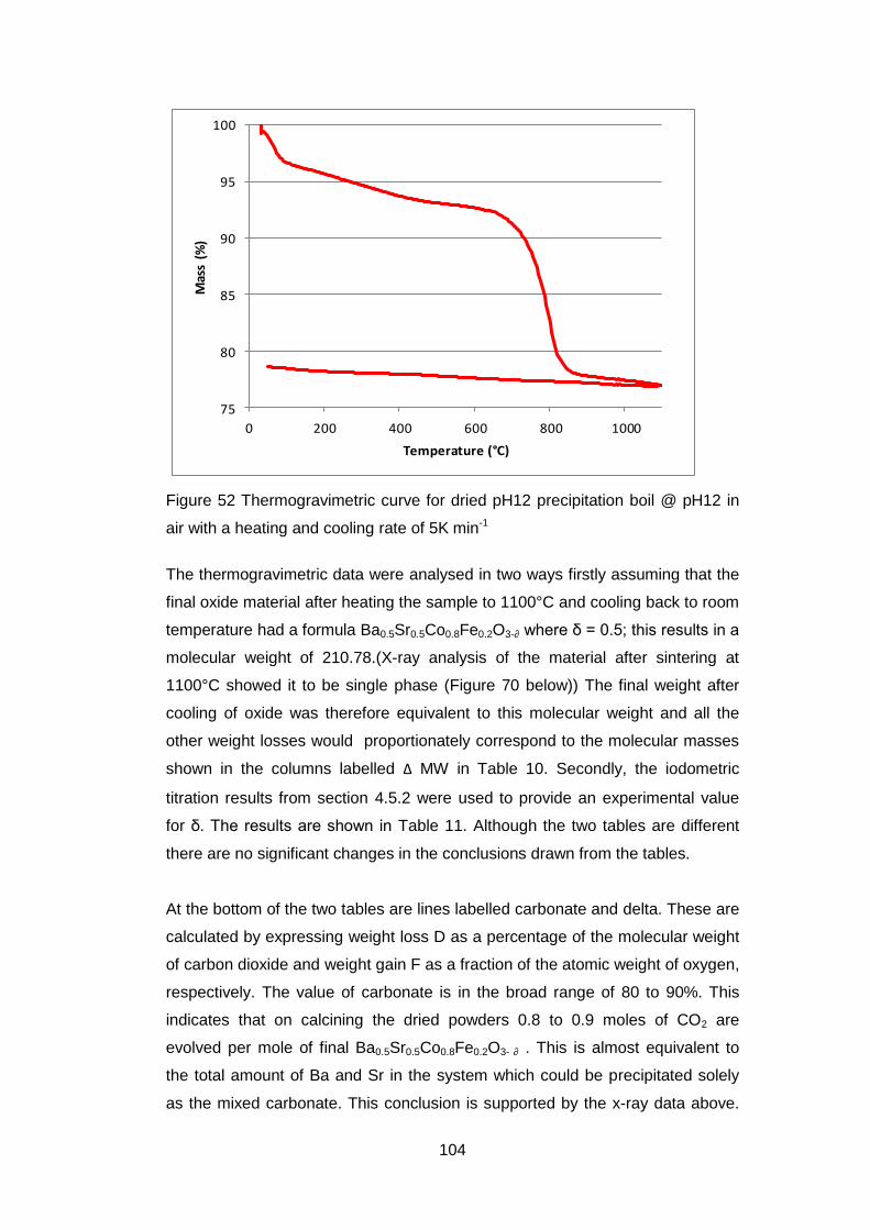
104

75

80

85

90

95

100

0 200 400 600 800 1000

Mas

s (%

)

Temperature (°C)

Figure 52 Thermogravimetric curve for dried pH12 precipitation boil @ pH12 in

air with a heating and cooling rate of 5K min-1

The thermogravimetric data were analysed in two ways firstly assuming that the

final oxide material after heating the sample to 1100°C and cooling back to room

temperature had a formula Ba0.5Sr0.5Co0.8Fe0.2O3-∂ where δ = 0.5; this results in a

molecular weight of 210.78.(X-ray analysis of the material after sintering at

1100°C showed it to be single phase (Figure 70 below)) The final weight after

cooling of oxide was therefore equivalent to this molecular weight and all the

other weight losses would proportionately correspond to the molecular masses

shown in the columns labelled Δ MW in Table 10. Secondly, the iodometric

titration results from section 4.5.2 were used to provide an experimental value

for δ. The results are shown in Table 11. Although the two tables are different

there are no significant changes in the conclusions drawn from the tables.

At the bottom of the two tables are lines labelled carbonate and delta. These are

calculated by expressing weight loss D as a percentage of the molecular weight

of carbon dioxide and weight gain F as a fraction of the atomic weight of oxygen,

respectively. The value of carbonate is in the broad range of 80 to 90%. This

indicates that on calcining the dried powders 0.8 to 0.9 moles of CO2 are

evolved per mole of final Ba0.5Sr0.5Co0.8Fe0.2O3- ∂ . This is almost equivalent to

the total amount of Ba and Sr in the system which could be precipitated solely

as the mixed carbonate. This conclusion is supported by the x-ray data above.

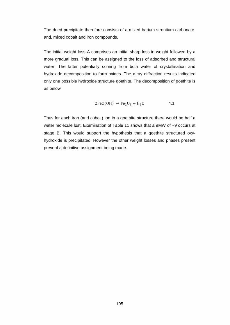
105

The dried precipitate therefore consists of a mixed barium strontium carbonate,

and, mixed cobalt and iron compounds.

The initial weight loss A comprises an initial sharp loss in weight followed by a

more gradual loss. This can be assigned to the loss of adsorbed and structural

water. The latter potentially coming from both water of crystallisation and

hydroxide decomposition to form oxides. The x-ray diffraction results indicated

only one possible hydroxide structure goethite. The decomposition of goethite is

as below

4.1

Thus for each iron (and cobalt) ion in a goethite structure there would be half a

water molecule lost. Examination of Table 11 shows that a ΔMW of ~9 occurs at

stage B. This would support the hypothesis that a goethite structured oxy-

hydroxide is precipitated. However the other weight losses and phases present

prevent a definitive assignment being made.

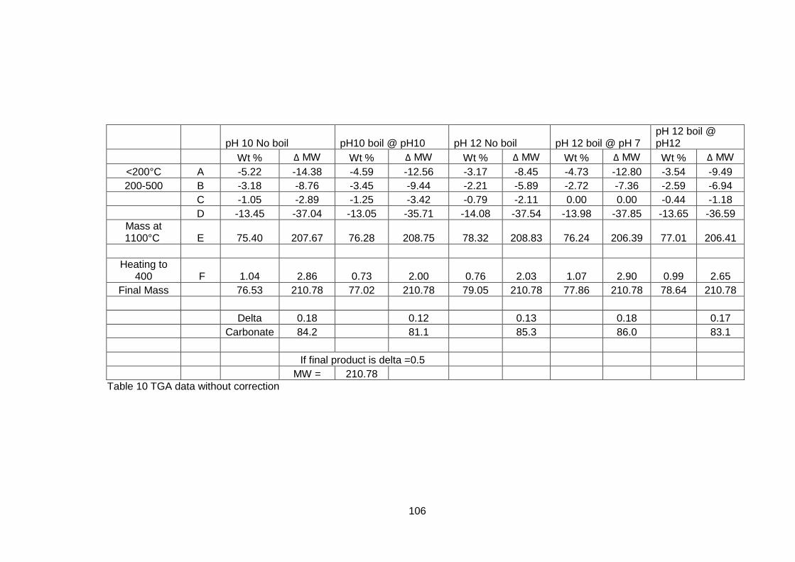
106

pH 10 No boil pH10 boil @ pH10 pH 12 No boil pH 12 boil @ pH 7 pH 12 boil @ pH12

Wt % Δ MW Wt % Δ MW Wt % Δ MW Wt % Δ MW Wt % Δ MW

<200°C A -5.22 -14.38 -4.59 -12.56 -3.17 -8.45 -4.73 -12.80 -3.54 -9.49

200-500 B -3.18 -8.76 -3.45 -9.44 -2.21 -5.89 -2.72 -7.36 -2.59 -6.94

C -1.05 -2.89 -1.25 -3.42 -0.79 -2.11 0.00 0.00 -0.44 -1.18

D -13.45 -37.04 -13.05 -35.71 -14.08 -37.54 -13.98 -37.85 -13.65 -36.59

Mass at 1100°C E 75.40 207.67 76.28 208.75 78.32 208.83 76.24 206.39 77.01 206.41

Heating to 400 F 1.04 2.86 0.73 2.00 0.76 2.03 1.07 2.90 0.99 2.65

Final Mass 76.53 210.78 77.02 210.78 79.05 210.78 77.86 210.78 78.64 210.78

Delta 0.18 0.12 0.13 0.18 0.17

Carbonate 84.2 81.1 85.3 86.0 83.1

If final product is delta =0.5

MW = 210.78

Table 10 TGA data without correction

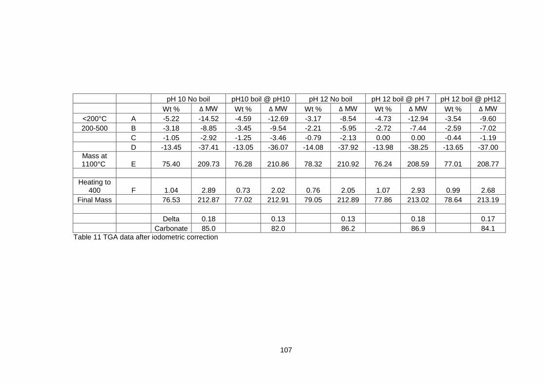
107

pH 10 No boil pH10 boil @ pH10 pH 12 No boil pH 12 boil @ pH 7 pH 12 boil @ pH12

Wt % Δ MW Wt % Δ MW Wt % Δ MW Wt % Δ MW Wt % Δ MW

<200°C A -5.22 -14.52 -4.59 -12.69 -3.17 -8.54 -4.73 -12.94 -3.54 -9.60

200-500 B -3.18 -8.85 -3.45 -9.54 -2.21 -5.95 -2.72 -7.44 -2.59 -7.02

C -1.05 -2.92 -1.25 -3.46 -0.79 -2.13 0.00 0.00 -0.44 -1.19

D -13.45 -37.41 -13.05 -36.07 -14.08 -37.92 -13.98 -38.25 -13.65 -37.00

Mass at 1100°C E 75.40 209.73 76.28 210.86 78.32 210.92 76.24 208.59 77.01 208.77

Heating to 400 F 1.04 2.89 0.73 2.02 0.76 2.05 1.07 2.93 0.99 2.68

Final Mass

76.53 212.87 77.02 212.91 79.05 212.89 77.86 213.02 78.64 213.19

Delta 0.18

0.13

0.13

0.18

0.17

Carbonate 85.0

82.0

86.2

86.9

84.1

Table 11 TGA data after iodometric correction

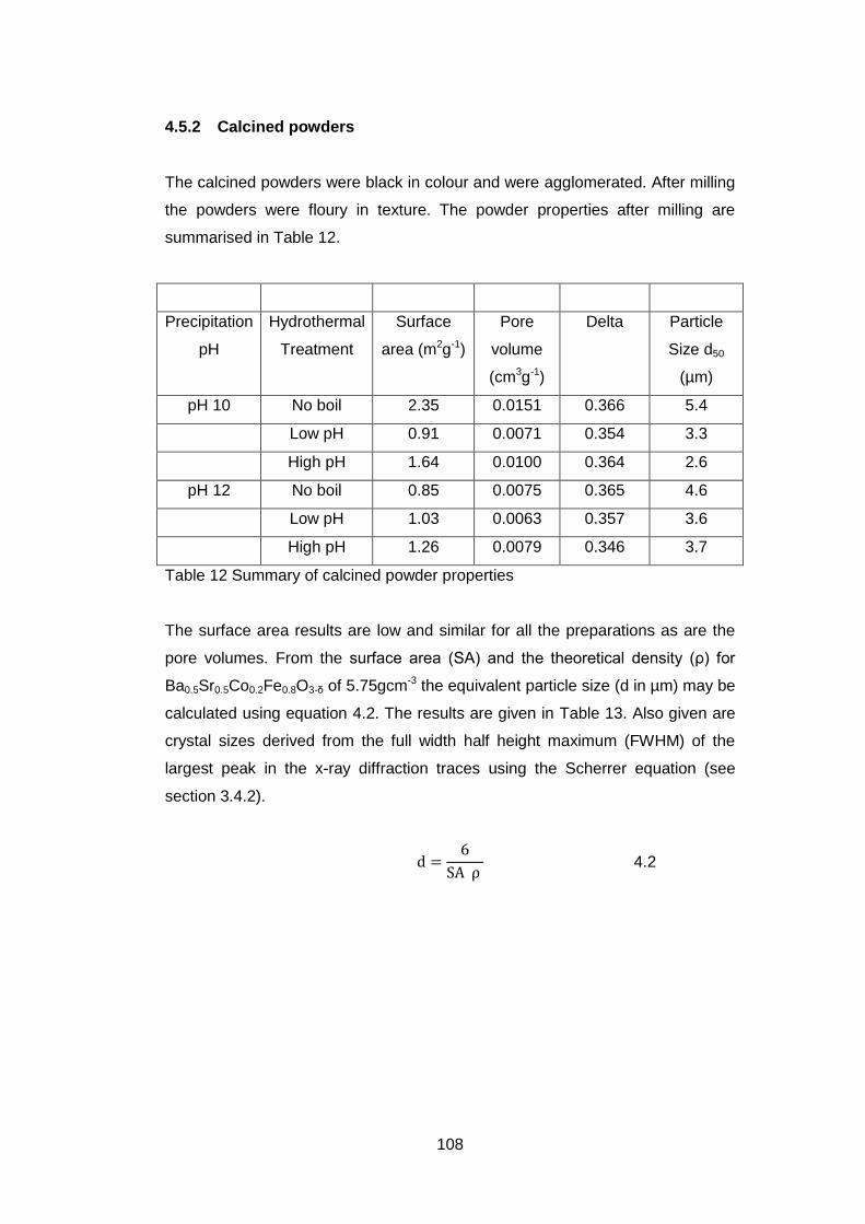
108

4.5.2 Calcined powders

The calcined powders were black in colour and were agglomerated. After milling

the powders were floury in texture. The powder properties after milling are

summarised in Table 12.

Precipitation

pH

Hydrothermal

Treatment

Surface

area (m2g-1)

Pore

volume

(cm3g-1)

Delta Particle

Size d50

(µm)

pH 10 No boil 2.35 0.0151 0.366 5.4

Low pH 0.91 0.0071 0.354 3.3

High pH 1.64 0.0100 0.364 2.6

pH 12 No boil 0.85 0.0075 0.365 4.6

Low pH 1.03 0.0063 0.357 3.6

High pH 1.26 0.0079 0.346 3.7

Table 12 Summary of calcined powder properties

The surface area results are low and similar for all the preparations as are the

pore volumes. From the surface area (SA) and the theoretical density (ρ) for

Ba0.5Sr0.5Co0.2Fe0.8O3-δ of 5.75gcm-3 the equivalent particle size (d in µm) may be

calculated using equation 4.2. The results are given in Table 13. Also given are

crystal sizes derived from the full width half height maximum (FWHM) of the

largest peak in the x-ray diffraction traces using the Scherrer equation (see

section 3.4.2).

4.2

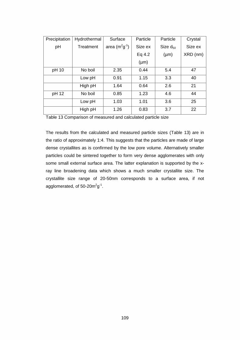
109

Precipitation

pH

Hydrothermal

Treatment

Surface

area (m2g-1)

Particle

Size ex

Eq 4.2

(µm)

Particle

Size d50

(µm)

Crystal

Size ex

XRD (nm)

pH 10 No boil 2.35 0.44 5.4 47

Low pH 0.91 1.15 3.3 40

High pH 1.64 0.64 2.6 21

pH 12 No boil 0.85 1.23 4.6 44

Low pH 1.03 1.01 3.6 25

High pH 1.26 0.83 3.7 22

Table 13 Comparison of measured and calculated particle size

The results from the calculated and measured particle sizes (Table 13) are in

the ratio of approximately 1:4. This suggests that the particles are made of large

dense crystallites as is confirmed by the low pore volume. Alternatively smaller

particles could be sintered together to form very dense agglomerates with only

some small external surface area. The latter explanation is supported by the x-

ray line broadening data which shows a much smaller crystallite size. The

crystallite size range of 20-50nm corresponds to a surface area, if not

agglomerated, of 50-20m2g-1.

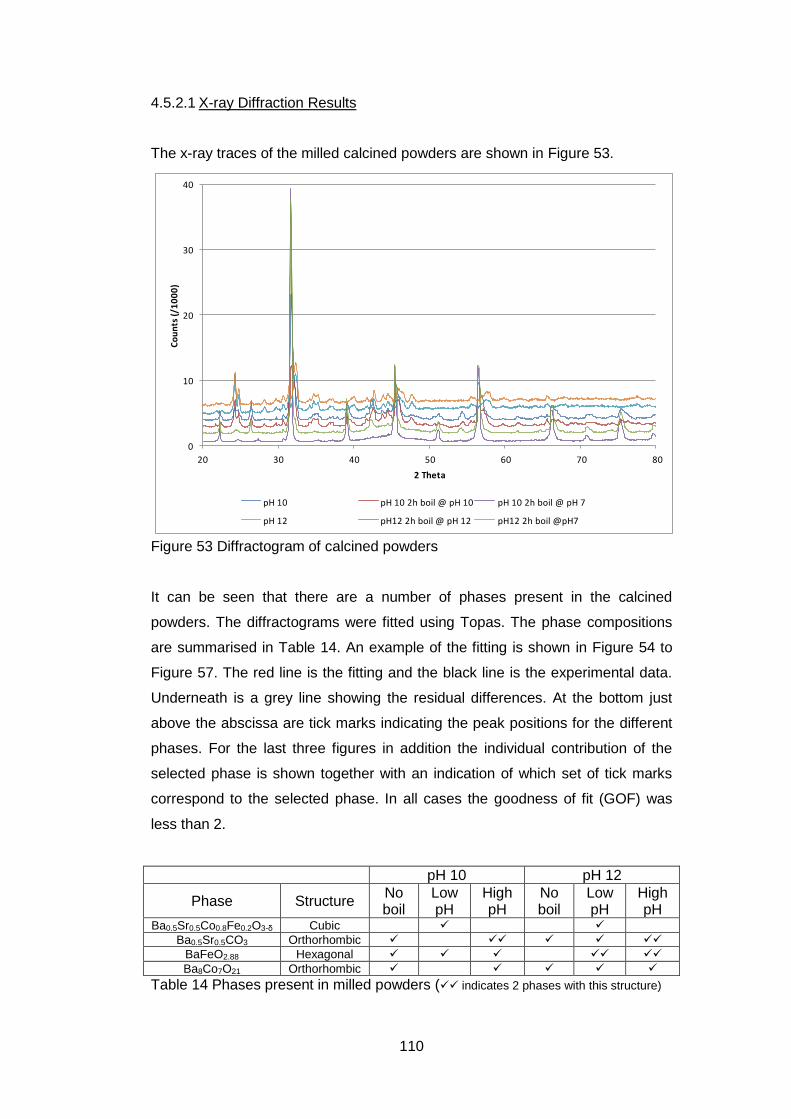
110

4.5.2.1 X-ray Diffraction Results

The x-ray traces of the milled calcined powders are shown in Figure 53.

0

10

20

30

40

20 30 40 50 60 70 80

Co

un

ts (

/10

00

)

2 Theta

pH 10 pH 10 2h boil @ pH 10 pH 10 2h boil @ pH 7

pH 12 pH12 2h boil @ pH 12 pH12 2h boil @pH7

Figure 53 Diffractogram of calcined powders

It can be seen that there are a number of phases present in the calcined

powders. The diffractograms were fitted using Topas. The phase compositions

are summarised in Table 14. An example of the fitting is shown in Figure 54 to

Figure 57. The red line is the fitting and the black line is the experimental data.

Underneath is a grey line showing the residual differences. At the bottom just

above the abscissa are tick marks indicating the peak positions for the different

phases. For the last three figures in addition the individual contribution of the

selected phase is shown together with an indication of which set of tick marks

correspond to the selected phase. In all cases the goodness of fit (GOF) was

less than 2.

pH 10 pH 12

Phase Structure No boil

Low pH

High pH

No boil

Low pH

High pH

Ba0.5Sr0.5Co0.8Fe0.2O3-δ Cubic

Ba0.5Sr0.5CO3 Orthorhombic

BaFeO2.88 Hexagonal

Ba8Co7O21 Orthorhombic

Table 14 Phases present in milled powders ( indicates 2 phases with this structure)

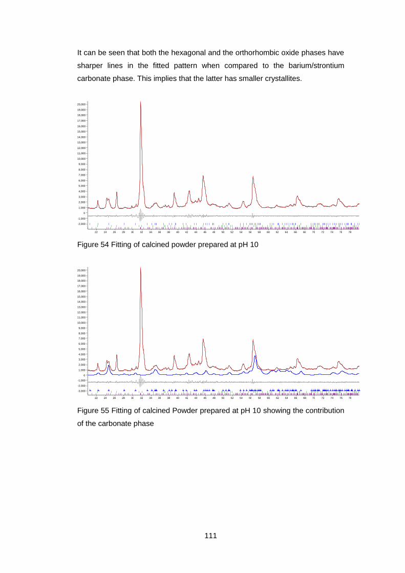
111

It can be seen that both the hexagonal and the orthorhombic oxide phases have

sharper lines in the fitted pattern when compared to the barium/strontium

carbonate phase. This implies that the latter has smaller crystallites.

Figure 54 Fitting of calcined powder prepared at pH 10

Figure 55 Fitting of calcined Powder prepared at pH 10 showing the contribution

of the carbonate phase

78 76 74 72 70 68 66 64 62 60 58 56 54 52 50 48 46 44 42 40 38 36 34 32 30 28 26 24 22

20,000 19,000 18,000 17,000 16,000 15,000 14,000 13,000 12,000 11,000 10,000 9,000 8,000 7,000 6,000 5,000 4,000 3,000 2,000 1,000

0 -1,000 -2,000

78 76 74 72 70 68 66 64 62 60 58 56 54 52 50 48 46 44 42 40 38 36 34 32 30 28 26 24 22

20,000 19,000 18,000 17,000 16,000 15,000 14,000 13,000 12,000 11,000 10,000 9,000 8,000 7,000 6,000 5,000 4,000 3,000 2,000 1,000

0 -1,000 -2,000 -3,000

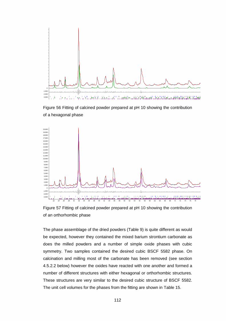
112

Figure 56 Fitting of calcined powder prepared at pH 10 showing the contribution

of a hexagonal phase

Figure 57 Fitting of calcined powder prepared at pH 10 showing the contribution

of an orthorhombic phase

The phase assemblage of the dried powders (Table 9) is quite different as would

be expected, however they contained the mixed barium strontium carbonate as

does the milled powders and a number of simple oxide phases with cubic

symmetry. Two samples contained the desired cubic BSCF 5582 phase. On

calcination and milling most of the carbonate has been removed (see section

4.5.2.2 below) however the oxides have reacted with one another and formed a

number of different structures with either hexagonal or orthorhombic structures.

These structures are very similar to the desired cubic structure of BSCF 5582.

The unit cell volumes for the phases from the fitting are shown in Table 15.

0 -1,000 -2,000 -3,000

78 76 74 72 70 68 66 64 62 60 58 56 54 52 50 48 46 44 42 40 38 36 34 32 30 28 26 24 22

20,000 19,000 18,000 17,000 16,000 15,000 14,000 13,000 12,000 11,000 10,000 9,000 8,000 7,000 6,000 5,000 4,000 3,000 2,000 1,000

0 -1,000 -2,000 -3,000

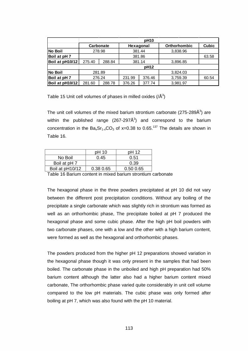
113

Cubic

No Boil

Boil at pH 7 63.58

Boil at pH10/12 275.40 288.84

No Boil

Boil at pH 7 231.99 376.46 60.54

Boil at pH10/12 281.60 288.78 376.26 377.74

276.24

Hexagonal

381.44

3,759.39

3,981.97

pH12

pH10

3,824.03

381.86

381.14

Orthorhombic

3,838.96

3,896.85

Carbonate

278.98

281.89

Table 15 Unit cell volumes of phases in milled oxides (/Å3)

The unit cell volumes of the mixed barium strontium carbonate (275-289Å3) are

within the published range (267-297Å3) and correspond to the barium

concentration in the BaxSr1-xCO3 of x=0.38 to 0.65.137 The details are shown in

Table 16.

pH 10 pH 12

No Boil 0.45 0.51

Boil at pH 7 0.39

Boil at pH10/12 0.38 0.65 0.50 0.65

Table 16 Barium content in mixed barium strontium carbonate

The hexagonal phase in the three powders precipitated at pH 10 did not vary

between the different post precipitation conditions. Without any boiling of the

precipitate a single carbonate which was slightly rich in strontium was formed as

well as an orthorhombic phase, The precipitate boiled at pH 7 produced the

hexagonal phase and some cubic phase. After the high pH boil powders with

two carbonate phases, one with a low and the other with a high barium content,

were formed as well as the hexagonal and orthorhombic phases.

The powders produced from the higher pH 12 preparations showed variation in

the hexagonal phase though it was only present in the samples that had been

boiled. The carbonate phase in the unboiled and high pH preparation had 50%

barium content although the latter also had a higher barium content mixed

carbonate, The orthorhombic phase varied quite considerably in unit cell volume

compared to the low pH materials. The cubic phase was only formed after

boiling at pH 7, which was also found with the pH 10 material.

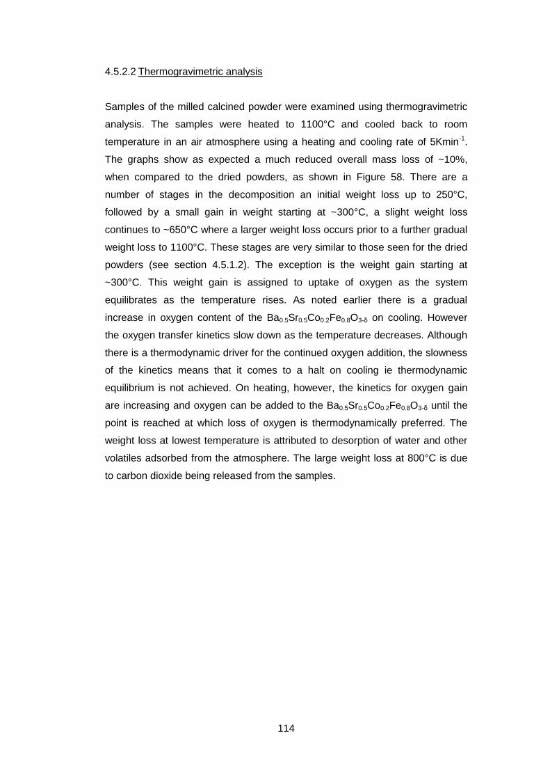
114

4.5.2.2 Thermogravimetric analysis

Samples of the milled calcined powder were examined using thermogravimetric

analysis. The samples were heated to 1100°C and cooled back to room

temperature in an air atmosphere using a heating and cooling rate of 5Kmin-1.

The graphs show as expected a much reduced overall mass loss of ~10%,

when compared to the dried powders, as shown in Figure 58. There are a

number of stages in the decomposition an initial weight loss up to 250°C,

followed by a small gain in weight starting at ~300°C, a slight weight loss

continues to ~650°C where a larger weight loss occurs prior to a further gradual

weight loss to 1100°C. These stages are very similar to those seen for the dried

powders (see section 4.5.1.2). The exception is the weight gain starting at

~300°C. This weight gain is assigned to uptake of oxygen as the system

equilibrates as the temperature rises. As noted earlier there is a gradual

increase in oxygen content of the Ba0.5Sr0.5Co0.2Fe0.8O3-δ on cooling. However

the oxygen transfer kinetics slow down as the temperature decreases. Although

there is a thermodynamic driver for the continued oxygen addition, the slowness

of the kinetics means that it comes to a halt on cooling ie thermodynamic

equilibrium is not achieved. On heating, however, the kinetics for oxygen gain

are increasing and oxygen can be added to the Ba0.5Sr0.5Co0.2Fe0.8O3-δ until the

point is reached at which loss of oxygen is thermodynamically preferred. The

weight loss at lowest temperature is attributed to desorption of water and other

volatiles adsorbed from the atmosphere. The large weight loss at 800°C is due

to carbon dioxide being released from the samples.

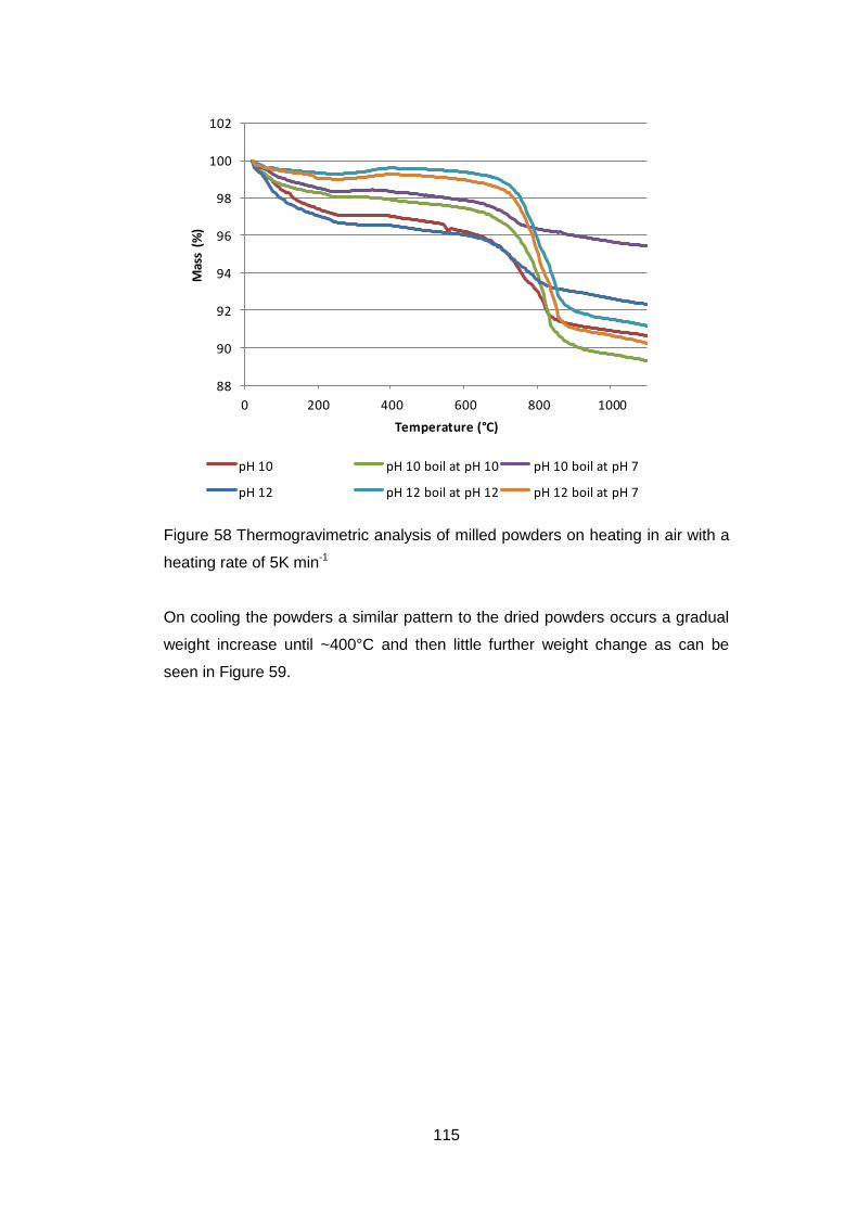
115

88

90

92

94

96

98

100

102

0 200 400 600 800 1000

Mas

s (%

)

Temperature (°C)

pH 10 pH 10 boil at pH 10 pH 10 boil at pH 7


Figure 58 Thermogravimetric analysis of milled powders on heating in air with a

heating rate of 5K min-1

On cooling the powders a similar pattern to the dried powders occurs a gradual

weight increase until ~400°C and then little further weight change as can be

seen in Figure 59.

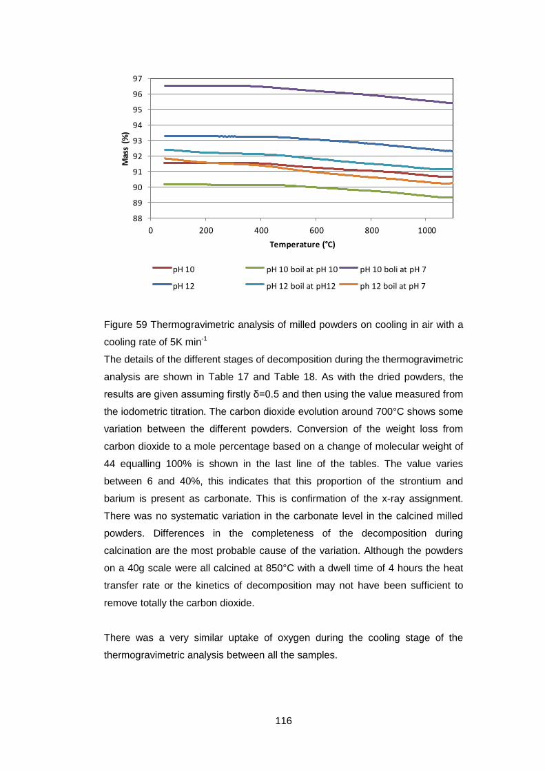
116

88

89

90

91

92

93

94

95

96

97

0 200 400 600 800 1000

Mas

s (%

)

Temperature (°C)

pH 10 pH 10 boil at pH 10 pH 10 boli at pH 7

pH 12 pH 12 boil at pH12 ph 12 boil at pH 7

Figure 59 Thermogravimetric analysis of milled powders on cooling in air with a

cooling rate of 5K min-1

The details of the different stages of decomposition during the thermogravimetric

analysis are shown in Table 17 and Table 18. As with the dried powders, the

results are given assuming firstly δ=0.5 and then using the value measured from

the iodometric titration. The carbon dioxide evolution around 700°C shows some

variation between the different powders. Conversion of the weight loss from

carbon dioxide to a mole percentage based on a change of molecular weight of

44 equalling 100% is shown in the last line of the tables. The value varies

between 6 and 40%, this indicates that this proportion of the strontium and

barium is present as carbonate. This is confirmation of the x-ray assignment.

There was no systematic variation in the carbonate level in the calcined milled

powders. Differences in the completeness of the decomposition during

calcination are the most probable cause of the variation. Although the powders

on a 40g scale were all calcined at 850°C with a dwell time of 4 hours the heat

transfer rate or the kinetics of decomposition may not have been sufficient to

remove totally the carbon dioxide.

There was a very similar uptake of oxygen during the cooling stage of the

thermogravimetric analysis between all the samples.

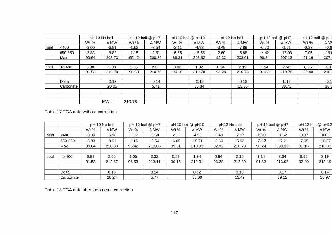
117

Wt % Δ MW Wt % Δ MW Wt % Δ MW Wt % Δ MW Wt % Δ MW Wt % Δ MW

heat <400 -3.00 -6.91 -1.62 -3.54 -2.11 -4.93 -3.49 -7.89 -0.70 -1.61 -0.37 -0.84

650-850 -3.83 -8.82 -1.15 -2.51 -6.65 -15.55 -2.60 -5.88 -7.42 -17.03 -7.05 -16.08

Max 90.64 208.73 95.42 208.36 89.31 208.82 92.32 208.61 90.24 207.13 91.16 207.95

cool to 400 0.88 2.03 1.05 2.29 0.82 1.92 0.94 2.12 1.14 2.62 0.95 2.17

91.53 210.78 96.53 210.78 90.15 210.78 93.28 210.78 91.83 210.78 92.40 210.78

Delta -0.13 -0.14 -0.12 -0.13 -0.16 -0.14

Carbonate 20.05 5.71 35.34 13.35 38.71 36.55

MW = 210.78

pH 10 No boil pH 10 boil @ pH7 pH 10 boil @ pH10 pH12 No boil pH 12 boil @ pH7 pH 12 boil @ pH12

Table 17 TGA data without correction

pH 10 No boil pH 10 boil @ pH7 pH 10 boil @ pH10 pH12 No boil pH 12 boil @ pH7 pH 12 boil @ pH12

Wt % Δ MW Wt % Δ MW Wt % Δ MW Wt % Δ MW Wt % Δ MW Wt % Δ MW

heat <400 -3.00 -6.98 -1.62 -3.58 -2.11 -4.98 -3.49 -7.97 -0.70 -1.62 -0.37 -0.85

650-850 -3.83 -8.91 -1.15 -2.54 -6.65 -15.71 -2.60 -5.93 -7.42 -17.21 -7.05 -16.27

Max 90.64 210.80 95.42 210.66 89.31 210.93 92.32 210.70 90.24 209.33 91.16 210.33

cool to 400 0.88 2.05 1.05 2.32 0.82 1.94 0.94 2.15 1.14 2.64 0.95 2.19

91.53 212.87 96.53 213.11 90.15 212.91 93.28 212.89 91.83 213.02 92.40 213.19

Delta 0.13 0.14 0.12 0.13 0.17 0.14

Carbonate 20.24 5.77 35.69 13.49 39.12 36.97

Table 18 TGA data after iodometric correction

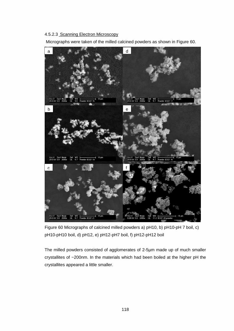
118

4.5.2.3 Scanning Electron Microscopy

Micrographs were taken of the milled calcined powders as shown in Figure 60.

Figure 60 Micrographs of calcined milled powders a) pH10, b) pH10-pH 7 boil, c)

pH10-pH10 boil, d) pH12, e) pH12-pH7 boil, f) pH12-pH12 boil

The milled powders consisted of agglomerates of 2-5µm made up of much smaller

crystallites of ~200nm. In the materials which had been boiled at the higher pH the

crystallites appeared a little smaller.

a

b

c

d

e

f

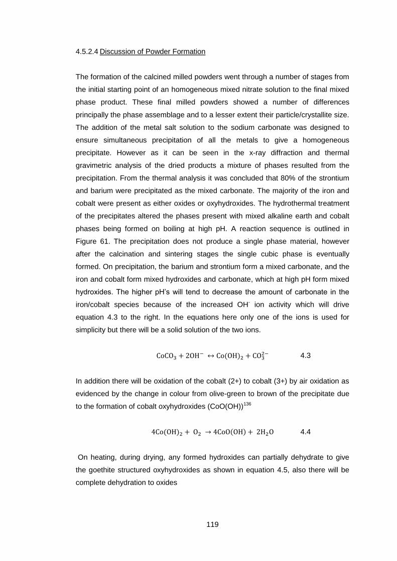
119

4.5.2.4 Discussion of Powder Formation

The formation of the calcined milled powders went through a number of stages from

the initial starting point of an homogeneous mixed nitrate solution to the final mixed

phase product. These final milled powders showed a number of differences

principally the phase assemblage and to a lesser extent their particle/crystallite size.

The addition of the metal salt solution to the sodium carbonate was designed to

ensure simultaneous precipitation of all the metals to give a homogeneous

precipitate. However as it can be seen in the x-ray diffraction and thermal

gravimetric analysis of the dried products a mixture of phases resulted from the

precipitation. From the thermal analysis it was concluded that 80% of the strontium

and barium were precipitated as the mixed carbonate. The majority of the iron and

cobalt were present as either oxides or oxyhydroxides. The hydrothermal treatment

of the precipitates altered the phases present with mixed alkaline earth and cobalt

phases being formed on boiling at high pH. A reaction sequence is outlined in

Figure 61. The precipitation does not produce a single phase material, however

after the calcination and sintering stages the single cubic phase is eventually

formed. On precipitation, the barium and strontium form a mixed carbonate, and the

iron and cobalt form mixed hydroxides and carbonate, which at high pH form mixed

hydroxides. The higher pH’s will tend to decrease the amount of carbonate in the

iron/cobalt species because of the increased OH- ion activity which will drive

equation 4.3 to the right. In the equations here only one of the ions is used for

simplicity but there will be a solid solution of the two ions.

4.3

In addition there will be oxidation of the cobalt (2+) to cobalt (3+) by air oxidation as

evidenced by the change in colour from olive-green to brown of the precipitate due

to the formation of cobalt oxyhydroxides (CoO(OH))136

4.4

On heating, during drying, any formed hydroxides can partially dehydrate to give

the goethite structured oxyhydroxides as shown in equation 4.5, also there will be

complete dehydration to oxides

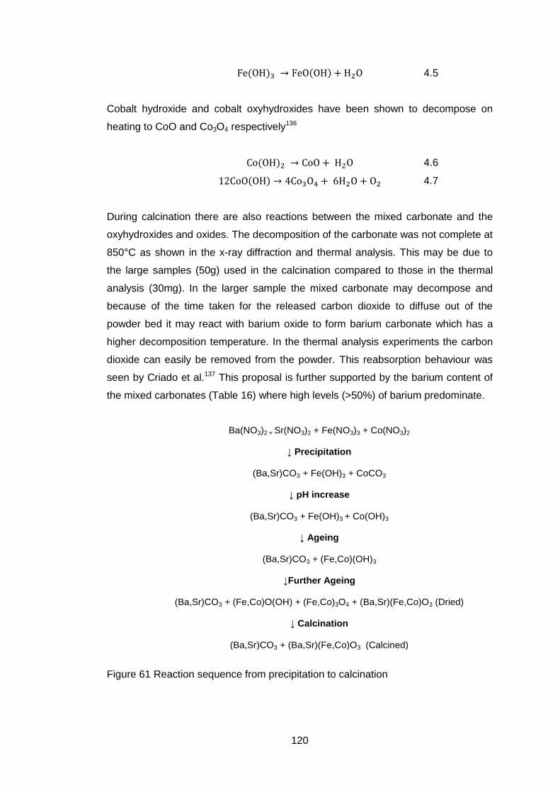
120

4.5

Cobalt hydroxide and cobalt oxyhydroxides have been shown to decompose on

heating to CoO and Co3O4 respectively136

4.6

4.7

During calcination there are also reactions between the mixed carbonate and the

oxyhydroxides and oxides. The decomposition of the carbonate was not complete at

850°C as shown in the x-ray diffraction and thermal analysis. This may be due to

the large samples (50g) used in the calcination compared to those in the thermal

analysis (30mg). In the larger sample the mixed carbonate may decompose and

because of the time taken for the released carbon dioxide to diffuse out of the

powder bed it may react with barium oxide to form barium carbonate which has a

higher decomposition temperature. In the thermal analysis experiments the carbon

dioxide can easily be removed from the powder. This reabsorption behaviour was

seen by Criado et al.137 This proposal is further supported by the barium content of

the mixed carbonates (Table 16) where high levels (>50%) of barium predominate.

Ba(NO3)2 + Sr(NO3)2 + Fe(NO3)3 + Co(NO3)2

↓ Precipitation

(Ba,Sr)CO3 + Fe(OH)3 + CoCO3

↓ pH increase

(Ba,Sr)CO3 + Fe(OH)3 + Co(OH)3

↓ Ageing

(Ba,Sr)CO3 + (Fe,Co)(OH)3

↓Further Ageing

(Ba,Sr)CO3 + (Fe,Co)O(OH) + (Fe,Co)3O4 + (Ba,Sr)(Fe,Co)O3 (Dried)

↓ Calcination

(Ba,Sr)CO3 + (Ba,Sr)(Fe,Co)O3 (Calcined)

Figure 61 Reaction sequence from precipitation to calcination

121

The particle size of the precipitates may also be affected by the pH of the solutions

in which the materials are processed. As the hydroxides may be ion exchange

materials at high and low pH’s138 they can react with the hydroxide ions present and

become charged and form charged species which are mutually repulsive (equation

4.8)

4.8

This repulsion can prevent agglomeration and give rise ultimately to smaller

particles. The agglomeration can also be prevented by the consequent high zeta

potentials present on the particles.

4.5.3 Sintered Ceramics

Pellets were uniaxially pressed from milled calcined powders without any additives

in a 1cm die at 100MPa.

4.5.3.1 Determination of sintering conditions

In addition to sintering at 1100°C for 10 hours a series of experiments were carried

out to determine the sintering temperature for densification and to try to determine

the concurrent pore size changes using computerised x-ray tomography. Evidence

for the presence of continuous porosity would also be sought.

The sintering experiments were carried out by pressing pellets from BSCF 5582

powder and heating them to a maximum of 1125°C. Pellets were removed from the

hot furnace when they reached the temperatures indicated in Figure 62. The last

two pellets 1125-0 and 1125-5 were removed after 0 and 5 hours at temperature

respectively.

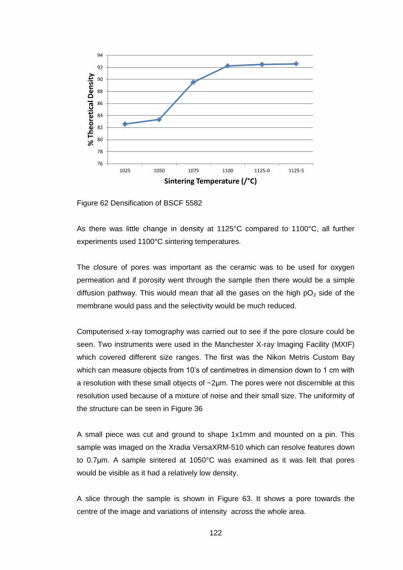
122

Figure 62 Densification of BSCF 5582

As there was little change in density at 1125°C compared to 1100°C, all further

experiments used 1100°C sintering temperatures.

The closure of pores was important as the ceramic was to be used for oxygen

permeation and if porosity went through the sample then there would be a simple

diffusion pathway. This would mean that all the gases on the high pO2 side of the

membrane would pass and the selectivity would be much reduced.

Computerised x-ray tomography was carried out to see if the pore closure could be

seen. Two instruments were used in the Manchester X-ray Imaging Facility (MXIF)

which covered different size ranges. The first was the Nikon Metris Custom Bay

which can measure objects from 10’s of centimetres in dimension down to 1 cm with

a resolution with these small objects of ~2µm. The pores were not discernible at this

resolution used because of a mixture of noise and their small size. The uniformity of

the structure can be seen in Figure 36

A small piece was cut and ground to shape 1x1mm and mounted on a pin. This

sample was imaged on the Xradia VersaXRM-510 which can resolve features down

to 0.7µm. A sample sintered at 1050°C was examined as it was felt that pores

would be visible as it had a relatively low density.

A slice through the sample is shown in Figure 63. It shows a pore towards the

centre of the image and variations of intensity across the whole area.

76

78

80

82

84

86

88

90

92

94

1025 1050 1075 1100 1125-0 1125-5

% T

heo

reti

cal D

ensi

ty

Sintering Temperature (/°C)

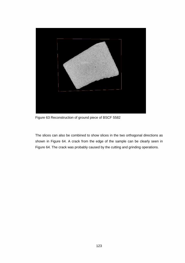
http://www.mxif.manchester.ac.uk/index.php/nikon-custom-bay

123

Figure 63 Reconstruction of ground piece of BSCF 5582

The slices can also be combined to show slices in the two orthogonal directions as

shown in Figure 64. A crack from the edge of the sample can be clearly seen in

Figure 64. The crack was probably caused by the cutting and grinding operations.

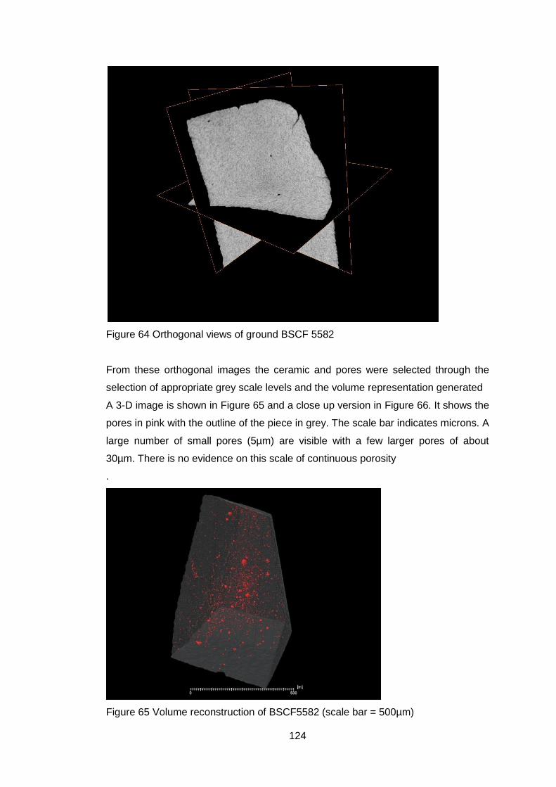
124

Figure 64 Orthogonal views of ground BSCF 5582

From these orthogonal images the ceramic and pores were selected through the

selection of appropriate grey scale levels and the volume representation generated

A 3-D image is shown in Figure 65 and a close up version in Figure 66. It shows the

pores in pink with the outline of the piece in grey. The scale bar indicates microns. A

large number of small pores (5µm) are visible with a few larger pores of about

30µm. There is no evidence on this scale of continuous porosity

.

Figure 65 Volume reconstruction of BSCF5582 (scale bar = 500µm)

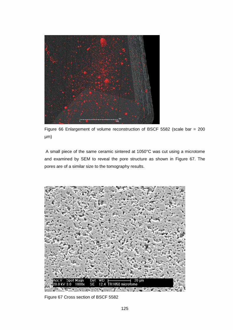
125

Figure 66 Enlargement of volume reconstruction of BSCF 5582 (scale bar = 200

µm)

A small piece of the same ceramic sintered at 1050°C was cut using a microtome

and examined by SEM to reveal the pore structure as shown in Figure 67. The

pores are of a similar size to the tomography results.

Figure 67 Cross section of BSCF 5582

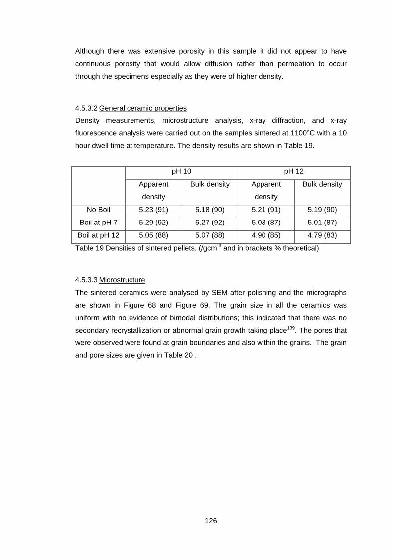
126

Although there was extensive porosity in this sample it did not appear to have

continuous porosity that would allow diffusion rather than permeation to occur

through the specimens especially as they were of higher density.

4.5.3.2 General ceramic properties

Density measurements, microstructure analysis, x-ray diffraction, and x-ray

fluorescence analysis were carried out on the samples sintered at 1100°C with a 10

hour dwell time at temperature. The density results are shown in Table 19.

pH 10 pH 12

Apparent

density

Bulk density Apparent

density

Bulk density

No Boil 5.23 (91) 5.18 (90) 5.21 (91) 5.19 (90)

Boil at pH 7 5.29 (92) 5.27 (92) 5.03 (87) 5.01 (87)

Boil at pH 12 5.05 (88) 5.07 (88) 4.90 (85) 4.79 (83)

Table 19 Densities of sintered pellets. (/gcm-3 and in brackets % theoretical)

4.5.3.3 Microstructure

The sintered ceramics were analysed by SEM after polishing and the micrographs

are shown in Figure 68 and Figure 69. The grain size in all the ceramics was

uniform with no evidence of bimodal distributions; this indicated that there was no

secondary recrystallization or abnormal grain growth taking place139. The pores that

were observed were found at grain boundaries and also within the grains. The grain

and pore sizes are given in Table 20 .

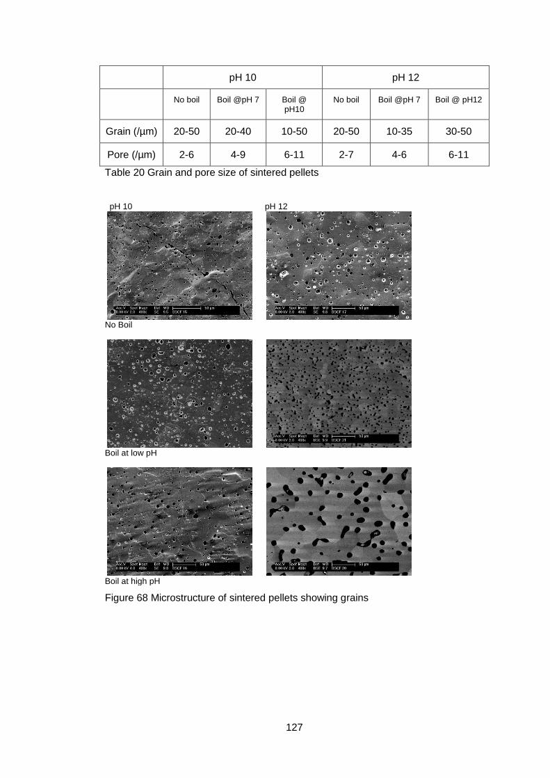
127

pH 10 pH 12

No boil Boil @pH 7 Boil @ pH10


Grain (/µm) 20-50 20-40 10-50 20-50 10-35 30-50

Pore (/µm) 2-6 4-9 6-11 2-7 4-6 6-11

Table 20 Grain and pore size of sintered pellets

Figure 68 Microstructure of sintered pellets showing grains

pH 10 pH 12

No Boil

Boil at low pH

Boil at high pH

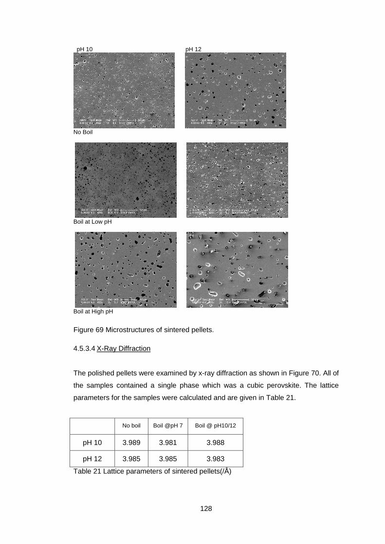
128

Figure 69 Microstructures of sintered pellets.

4.5.3.4 X-Ray Diffraction

The polished pellets were examined by x-ray diffraction as shown in Figure 70. All of

the samples contained a single phase which was a cubic perovskite. The lattice

parameters for the samples were calculated and are given in Table 21.

No boil Boil @pH 7 Boil @ pH10/12

pH 10 3.989 3.981 3.988

pH 12 3.985 3.985 3.983

Table 21 Lattice parameters of sintered pellets(/Å)

pH 10 pH 12

No Boil

Boil at Low pH

Boil at High pH

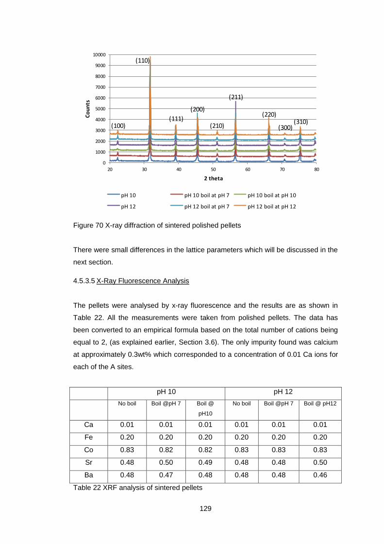
129

0

1000

2000

3000

4000

5000

6000

7000

8000

9000

10000

20 30 40 50 60 70 80

Co

un

ts

2 theta



(100)

(110)

(111)

(200)

(210)

(211)

(220)

(300)(310)

Figure 70 X-ray diffraction of sintered polished pellets

There were small differences in the lattice parameters which will be discussed in the

next section.

4.5.3.5 X-Ray Fluorescence Analysis

The pellets were analysed by x-ray fluorescence and the results are as shown in

Table 22. All the measurements were taken from polished pellets. The data has

been converted to an empirical formula based on the total number of cations being

equal to 2, (as explained earlier, Section 3.6). The only impurity found was calcium

at approximately 0.3wt% which corresponded to a concentration of 0.01 Ca ions for

each of the A sites.

pH 10 pH 12

No boil Boil @pH 7 Boil @

pH10


Ca 0.01 0.01 0.01 0.01 0.01 0.01

Fe 0.20 0.20 0.20 0.20 0.20 0.20

Co 0.83 0.82 0.82 0.83 0.83 0.83

Sr 0.48 0.50 0.49 0.48 0.48 0.50

Ba 0.48 0.47 0.48 0.48 0.48 0.46

Table 22 XRF analysis of sintered pellets

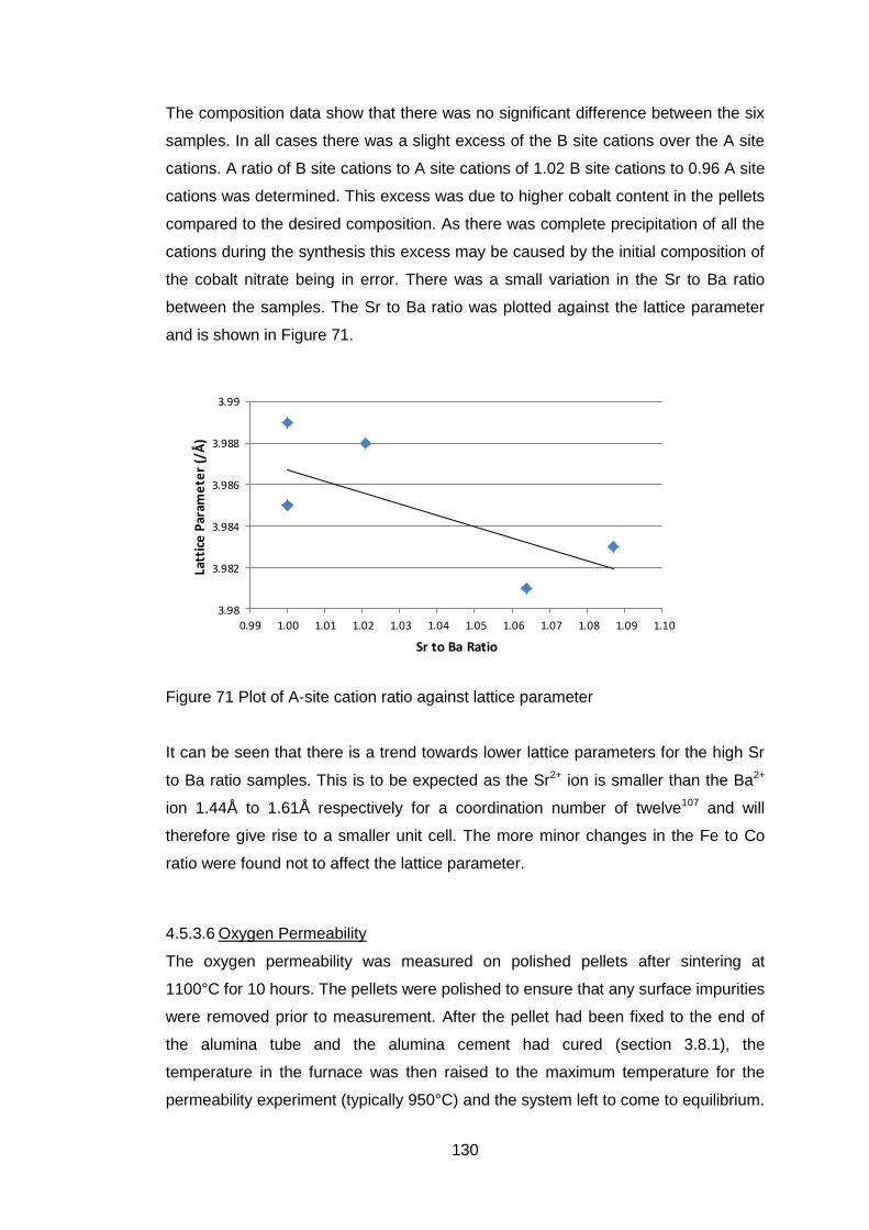
130

The composition data show that there was no significant difference between the six

samples. In all cases there was a slight excess of the B site cations over the A site

cations. A ratio of B site cations to A site cations of 1.02 B site cations to 0.96 A site

cations was determined. This excess was due to higher cobalt content in the pellets

compared to the desired composition. As there was complete precipitation of all the

cations during the synthesis this excess may be caused by the initial composition of

the cobalt nitrate being in error. There was a small variation in the Sr to Ba ratio

between the samples. The Sr to Ba ratio was plotted against the lattice parameter

and is shown in Figure 71.

3.98

3.982

3.984

3.986

3.988

3.99

0.99 1.00 1.01 1.02 1.03 1.04 1.05 1.06 1.07 1.08 1.09 1.10

Latt

ice

Par

ame

ter

(/Å

)

Sr to Ba Ratio

Figure 71 Plot of A-site cation ratio against lattice parameter

It can be seen that there is a trend towards lower lattice parameters for the high Sr

to Ba ratio samples. This is to be expected as the Sr2+ ion is smaller than the Ba2+

ion 1.44Å to 1.61Å respectively for a coordination number of twelve107 and will

therefore give rise to a smaller unit cell. The more minor changes in the Fe to Co

ratio were found not to affect the lattice parameter.

4.5.3.6 Oxygen Permeability

The oxygen permeability was measured on polished pellets after sintering at

1100°C for 10 hours. The pellets were polished to ensure that any surface impurities

were removed prior to measurement. After the pellet had been fixed to the end of

the alumina tube and the alumina cement had cured (section 3.8.1), the

temperature in the furnace was then raised to the maximum temperature for the

permeability experiment (typically 950°C) and the system left to come to equilibrium.

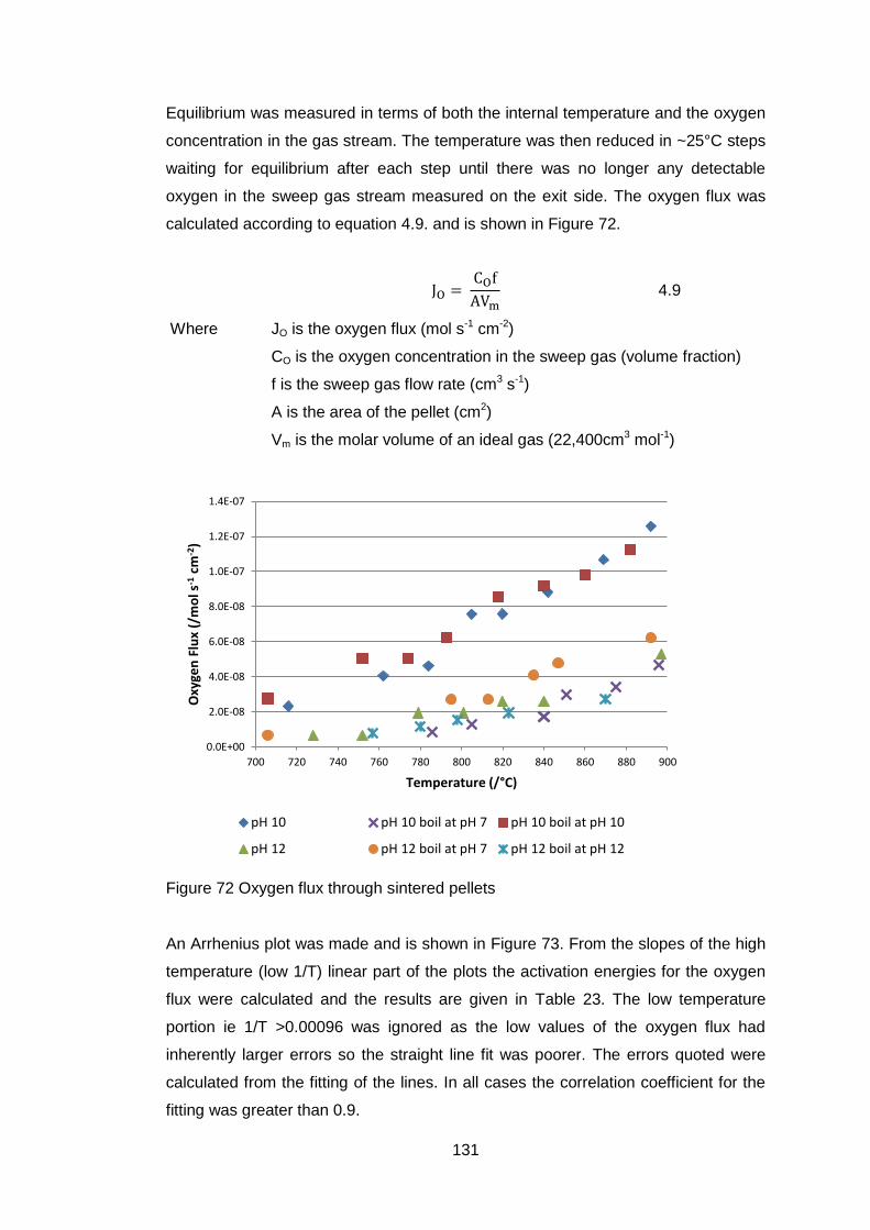
131

Equilibrium was measured in terms of both the internal temperature and the oxygen

concentration in the gas stream. The temperature was then reduced in ~25°C steps

waiting for equilibrium after each step until there was no longer any detectable

oxygen in the sweep gas stream measured on the exit side. The oxygen flux was

calculated according to equation 4.9. and is shown in Figure 72.

4.9

Where JO is the oxygen flux (mol s-1 cm-2)

CO is the oxygen concentration in the sweep gas (volume fraction)

f is the sweep gas flow rate (cm3 s-1)

A is the area of the pellet (cm2)

Vm is the molar volume of an ideal gas (22,400cm3 mol-1)

Figure 72 Oxygen flux through sintered pellets

An Arrhenius plot was made and is shown in Figure 73. From the slopes of the high

temperature (low 1/T) linear part of the plots the activation energies for the oxygen

flux were calculated and the results are given in Table 23. The low temperature

portion ie 1/T >0.00096 was ignored as the low values of the oxygen flux had

inherently larger errors so the straight line fit was poorer. The errors quoted were

calculated from the fitting of the lines. In all cases the correlation coefficient for the

fitting was greater than 0.9.

0.0E+00

2.0E-08

4.0E-08

6.0E-08

8.0E-08

1.0E-07

1.2E-07

1.4E-07

700 720 740 760 780 800 820 840 860 880 900

Oxy

gen

Flu

x (/

mo

l s-1

cm

-2)

Temperature (/°C)



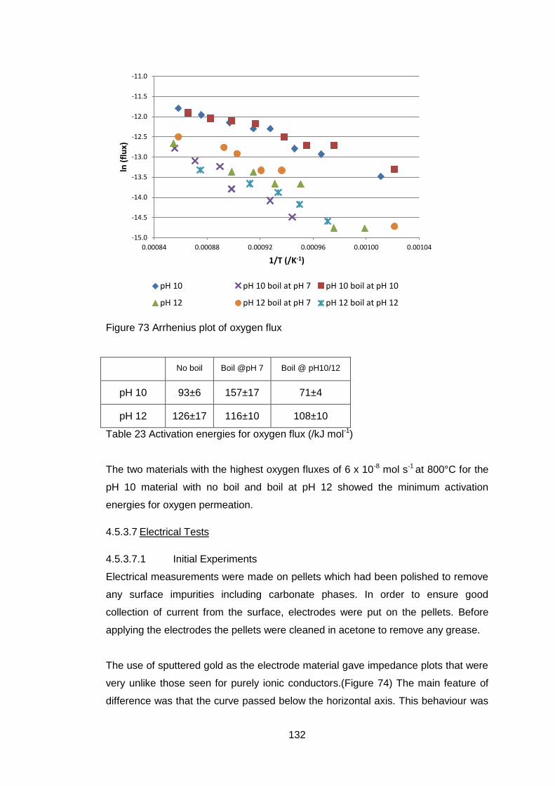
132

Figure 73 Arrhenius plot of oxygen flux

No boil Boil @pH 7 Boil @ pH10/12

pH 10 93±6 157±17 71±4

pH 12 126±17 116±10 108±10

Table 23 Activation energies for oxygen flux (/kJ mol-1)

The two materials with the highest oxygen fluxes of 6 x 10-8 mol s-1 at 800°C for the

pH 10 material with no boil and boil at pH 12 showed the minimum activation

energies for oxygen permeation.

4.5.3.7 Electrical Tests

4.5.3.7.1 Initial Experiments

Electrical measurements were made on pellets which had been polished to remove

any surface impurities including carbonate phases. In order to ensure good

collection of current from the surface, electrodes were put on the pellets. Before

applying the electrodes the pellets were cleaned in acetone to remove any grease.

The use of sputtered gold as the electrode material gave impedance plots that were

very unlike those seen for purely ionic conductors.(Figure 74) The main feature of

difference was that the curve passed below the horizontal axis. This behaviour was

-15.0

-14.5

-14.0

-13.5

-13.0

-12.5

-12.0

-11.5

-11.0

0.00084 0.00088 0.00092 0.00096 0.00100 0.00104

ln (

flu

x)

1/T (/K-1)



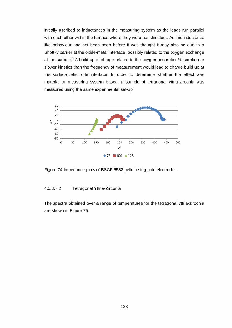
133

initially ascribed to inductances in the measuring system as the leads run parallel

with each other within the furnace where they were not shielded.. As this inductance

like behaviour had not been seen before it was thought it may also be due to a

Shottky barrier at the oxide-metal interface, possibly related to the oxygen exchange

at the surface.6 A build-up of charge related to the oxygen adsorption/desorption or

slower kinetics than the frequency of measurement would lead to charge build up at

the surface /electrode interface. In order to determine whether the effect was

material or measuring system based, a sample of tetragonal yttria-zirconia was

measured using the same experimental set-up.

Figure 74 Impedance plots of BSCF 5582 pellet using gold electrodes

4.5.3.7.2 Tetragonal Yttria-Zirconia

The spectra obtained over a range of temperatures for the tetragonal yttria-zirconia

are shown in Figure 75.

-80

-60

-40

-20

0

20

40

60

0 50 100 150 200 250 300 350 400 450 500

-Z"

Z'

75 100 125

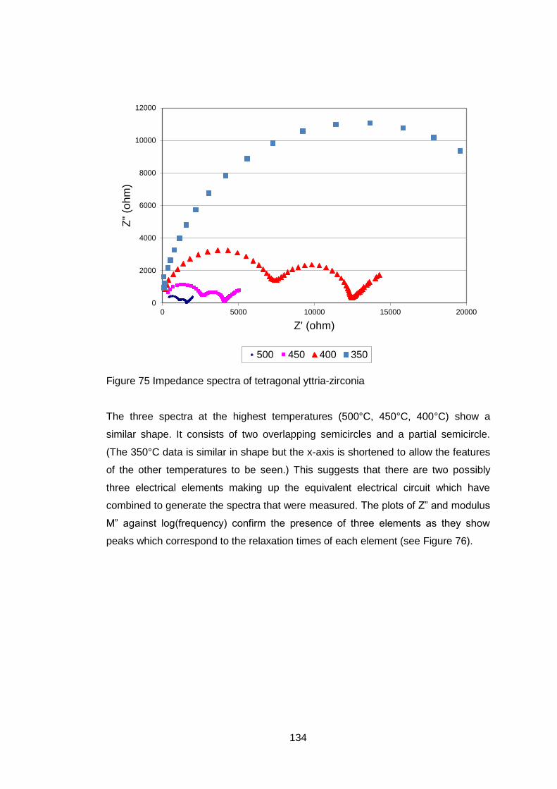
134

Figure 75 Impedance spectra of tetragonal yttria-zirconia

The three spectra at the highest temperatures (500°C, 450°C, 400°C) show a

similar shape. It consists of two overlapping semicircles and a partial semicircle.

(The 350°C data is similar in shape but the x-axis is shortened to allow the features

of the other temperatures to be seen.) This suggests that there are two possibly

three electrical elements making up the equivalent electrical circuit which have

combined to generate the spectra that were measured. The plots of Z” and modulus

M” against log(frequency) confirm the presence of three elements as they show

peaks which correspond to the relaxation times of each element (see Figure 76).

0

2000

4000

6000

8000

10000

12000

0 5000 10000 15000 20000

Z"

(oh

m)

Z' (ohm)

500 450 400 350

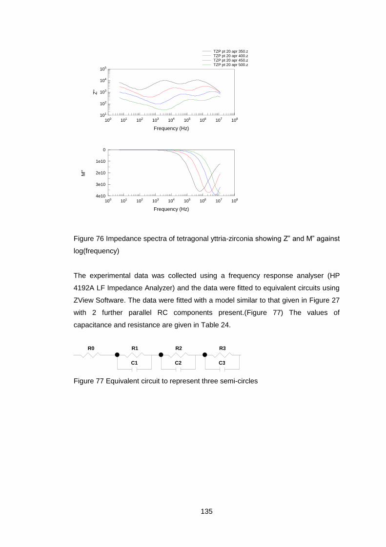
135

Figure 76 Impedance spectra of tetragonal yttria-zirconia showing Z” and M” against

log(frequency)

The experimental data was collected using a frequency response analyser (HP

4192A LF Impedance Analyzer) and the data were fitted to equivalent circuits using

ZView Software. The data were fitted with a model similar to that given in Figure 27

with 2 further parallel RC components present.(Figure 77) The values of

capacitance and resistance are given in Table 24.

Figure 77 Equivalent circuit to represent three semi-circles

100 101 102 103 104 105 106 107 108101

102

103

104

105

Frequency (Hz)

Z''

TZP pt 20 apr 350.zTZP pt 20 apr 400.zTZP pt 20 apr 450.zTZP pt 20 apr 500.z

100 101 102 103 104 105 106 107 108

0

1e10

2e10

3e10

4e10

Frequency (Hz)

M''

R0 R1

C1

R2

C2

R3

C3

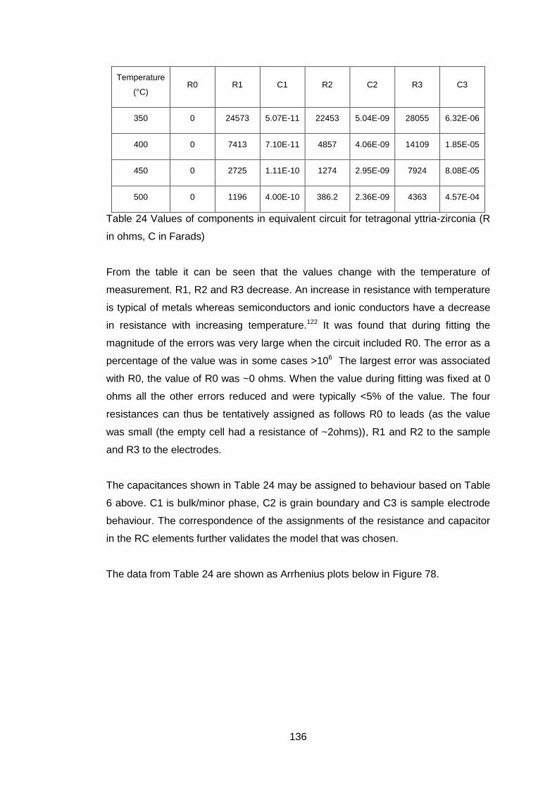
136

Temperature

(°C) R0 R1 C1 R2 C2 R3 C3

350 0 24573 5.07E-11 22453 5.04E-09 28055 6.32E-06

400 0 7413 7.10E-11 4857 4.06E-09 14109 1.85E-05

450 0 2725 1.11E-10 1274 2.95E-09 7924 8.08E-05

500 0 1196 4.00E-10 386.2 2.36E-09 4363 4.57E-04

Table 24 Values of components in equivalent circuit for tetragonal yttria-zirconia (R

in ohms, C in Farads)

From the table it can be seen that the values change with the temperature of

measurement. R1, R2 and R3 decrease. An increase in resistance with temperature

is typical of metals whereas semiconductors and ionic conductors have a decrease

in resistance with increasing temperature.122 It was found that during fitting the

magnitude of the errors was very large when the circuit included R0. The error as a

percentage of the value was in some cases >106 The largest error was associated

with R0, the value of R0 was ~0 ohms. When the value during fitting was fixed at 0

ohms all the other errors reduced and were typically <5% of the value. The four

resistances can thus be tentatively assigned as follows R0 to leads (as the value

was small (the empty cell had a resistance of ~2ohms)), R1 and R2 to the sample

and R3 to the electrodes.

The capacitances shown in Table 24 may be assigned to behaviour based on Table

6 above. C1 is bulk/minor phase, C2 is grain boundary and C3 is sample electrode

behaviour. The correspondence of the assignments of the resistance and capacitor

in the RC elements further validates the model that was chosen.

The data from Table 24 are shown as Arrhenius plots below in Figure 78.

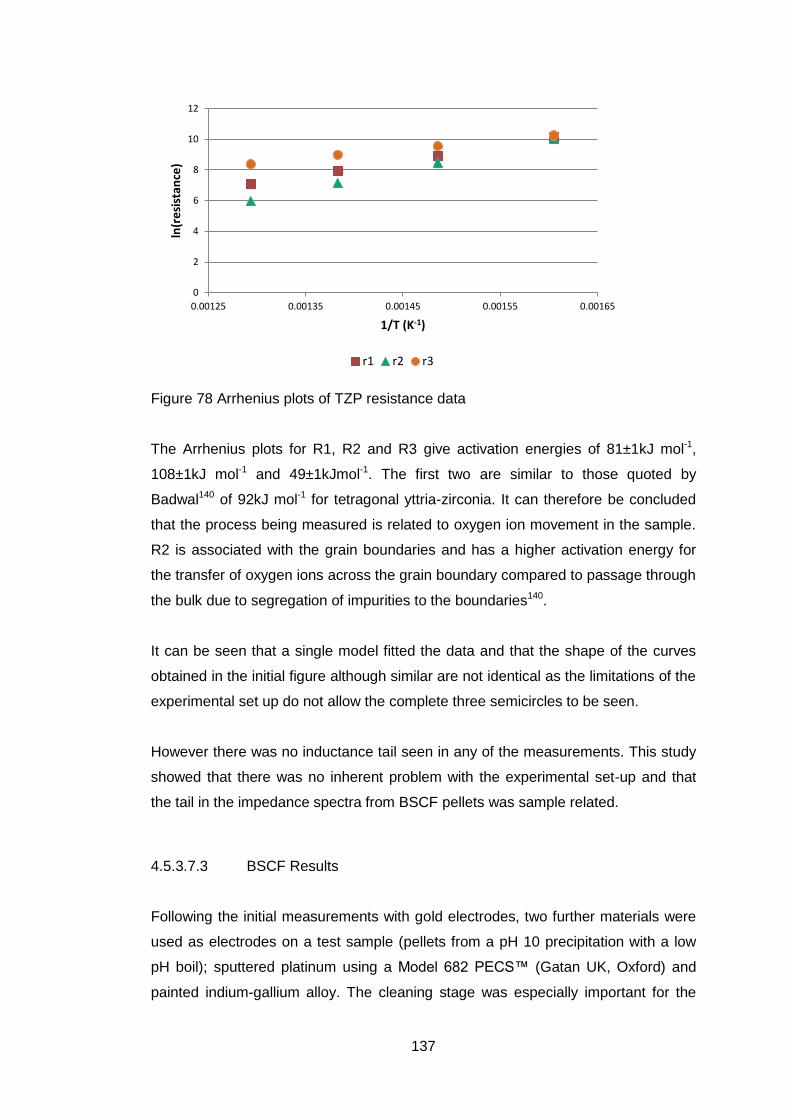
137

Figure 78 Arrhenius plots of TZP resistance data

The Arrhenius plots for R1, R2 and R3 give activation energies of 81±1kJ mol-1,

108±1kJ mol-1 and 49±1kJmol-1. The first two are similar to those quoted by

Badwal140 of 92kJ mol-1 for tetragonal yttria-zirconia. It can therefore be concluded

that the process being measured is related to oxygen ion movement in the sample.

R2 is associated with the grain boundaries and has a higher activation energy for

the transfer of oxygen ions across the grain boundary compared to passage through

the bulk due to segregation of impurities to the boundaries140.

It can be seen that a single model fitted the data and that the shape of the curves

obtained in the initial figure although similar are not identical as the limitations of the

experimental set up do not allow the complete three semicircles to be seen.

However there was no inductance tail seen in any of the measurements. This study

showed that there was no inherent problem with the experimental set-up and that

the tail in the impedance spectra from BSCF pellets was sample related.

4.5.3.7.3 BSCF Results

Following the initial measurements with gold electrodes, two further materials were

used as electrodes on a test sample (pellets from a pH 10 precipitation with a low

pH boil); sputtered platinum using a Model 682 PECS™ (Gatan UK, Oxford) and

painted indium-gallium alloy. The cleaning stage was especially important for the

0

2

4

6

8

10

12

0.00125 0.00135 0.00145 0.00155 0.00165

ln(r

esi

stan

ce)

1/T (K-1)

r1 r2 r3

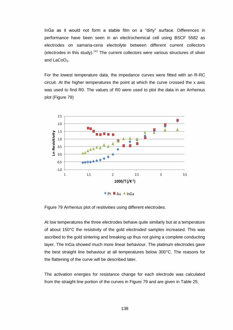
138

InGa as it would not form a stable film on a “dirty” surface. Differences in

performance have been seen in an electrochemical cell using BSCF 5582 as

electrodes on samaria-ceria electrolyte between different current collectors

(electrodes in this study).141 The current collectors were various structures of silver

and LaCoO3.

For the lowest temperature data, the impedance curves were fitted with an R-RC

circuit. At the higher temperatures the point at which the curve crossed the x axis

was used to find R0. The values of R0 were used to plot the data in an Arrhenius

plot (Figure 79)

-1.0

-0.5

0.0

0.5

1.0

1.5

2.0

2.5

1 1.5 2 2.5 3 3.5

Ln

Re

sisi

tiv

ity

1000/T (/K-1)

Pt Au InGa

Figure 79 Arrhenius plot of resitivities using different electrodes.

At low temperatures the three electrodes behave quite similarly but at a temperature

of about 150°C the resistivity of the gold electroded samples increased. This was

ascribed to the gold sintering and breaking up thus not giving a complete conducting

layer. The InGa showed much more linear behaviour. The platinum electrodes gave

the best straight line behaviour at all temperatures below 300°C. The reasons for

the flattening of the curve will be described later.

The activation energies for resistance change for each electrode was calculated

from the straight line portion of the curves in Figure 79 and are given in Table 25.

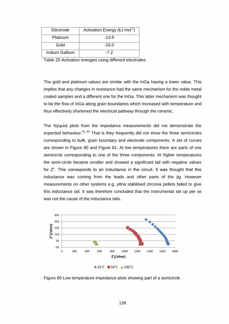
139

Electrode Activation Energy (kJ mol-1)

Platinum -13.9

Gold -15.0

Indium Gallium -7.2

Table 25 Activation energies using different electrodes

The gold and platinum values are similar with the InGa having a lower value. This

implies that any changes in resistance had the same mechanism for the noble metal

coated samples and a different one for the InGa. This latter mechanism was thought

to be the flow of InGa along grain boundaries which increased with temperature and

thus effectively shortened the electrical pathway through the ceramic.

The Nyquist plots from the impedance measurements did not demonstrate the

expected behaviour.81, 82 That is they frequently did not show the three semicircles

corresponding to bulk, grain boundary and electrode components. A set of curves

are shown in Figure 80 and Figure 81. At low temperatures there are parts of one

semicircle corresponding to one of the three components. At higher temperatures

the semi-circle became smaller and showed a significant tail with negative values

for Z”. This corresponds to an inductance in the circuit. It was thought that this

inductance was coming from the leads and other parts of the jig. However

measurements on other systems e.g. yttria stabilised zirconia pellets failed to give

this inductance tail. It was therefore concluded that the instrumental set up per se

was not the cause of the inductance tails.

Figure 80 Low temperature impedance plots showing part of a semicircle

-50

50

150

250

350

450

0 200 400 600 800 1000 1200 1400 1600 1800

Z"(/

oh

m)

Z'(/ohm)

25°C 50°C 100°C

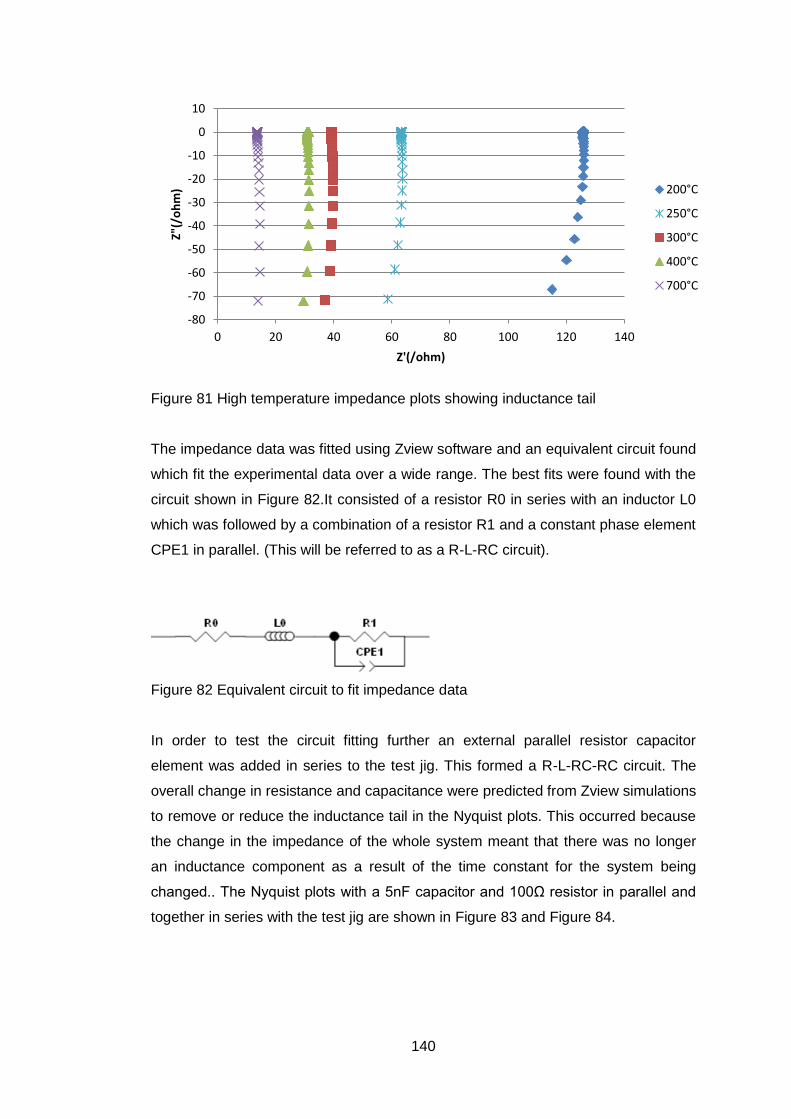
140

Figure 81 High temperature impedance plots showing inductance tail

The impedance data was fitted using Zview software and an equivalent circuit found

which fit the experimental data over a wide range. The best fits were found with the

circuit shown in Figure 82.It consisted of a resistor R0 in series with an inductor L0

which was followed by a combination of a resistor R1 and a constant phase element

CPE1 in parallel. (This will be referred to as a R-L-RC circuit).

Figure 82 Equivalent circuit to fit impedance data

In order to test the circuit fitting further an external parallel resistor capacitor

element was added in series to the test jig. This formed a R-L-RC-RC circuit. The

overall change in resistance and capacitance were predicted from Zview simulations

to remove or reduce the inductance tail in the Nyquist plots. This occurred because

the change in the impedance of the whole system meant that there was no longer

an inductance component as a result of the time constant for the system being

changed.. The Nyquist plots with a 5nF capacitor and 100Ω resistor in parallel and

together in series with the test jig are shown in Figure 83 and Figure 84.

-80

-70

-60

-50

-40

-30

-20

-10

0

10

0 20 40 60 80 100 120 140

Z"(/

oh

m)

Z'(/ohm)

200°C

250°C

300°C

400°C

700°C

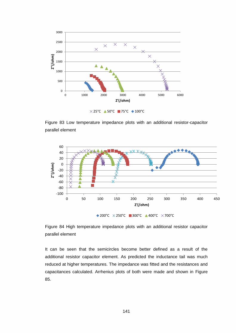
141

Figure 83 Low temperature impedance plots with an additional resistor-capacitor

parallel element

Figure 84 High temperature impedance plots with an additional resistor capacitor

parallel element

It can be seen that the semicircles become better defined as a result of the

additional resistor capacitor element. As predicted the inductance tail was much

reduced at higher temperatures. The impedance was fitted and the resistances and

capacitances calculated. Arrhenius plots of both were made and shown in Figure

85.

0

500

1000

1500

2000

2500

3000

0 1000 2000 3000 4000 5000 6000

Z"(/

oh

m)

Z'(/ohm)

25°C 50°C 75°C 100°C

-100

-80

-60

-40

-20

0

20

40

60

0 50 100 150 200 250 300 350 400 450

Z"(/

oh

m)

Z'(/ohm)

200°C 250°C 300°C 400°C 700°C

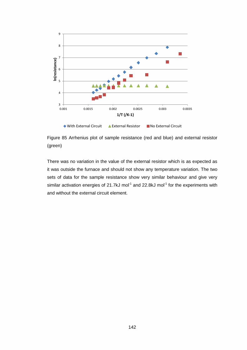
142

Figure 85 Arrhenius plot of sample resistance (red and blue) and external resistor

(green)

There was no variation in the value of the external resistor which is as expected as

it was outside the furnace and should not show any temperature variation. The two

sets of data for the sample resistance show very similar behaviour and give very

similar activation energies of 21.7kJ mol-1 and 22.8kJ mol-1 for the experiments with

and without the external circuit element.

3

4

5

6

7

8

9

0.001 0.0015 0.002 0.0025 0.003 0.0035

ln(r

esi

stan

ce)

1/T (/K-1}

With External Circuit External Resistor No External Circuit

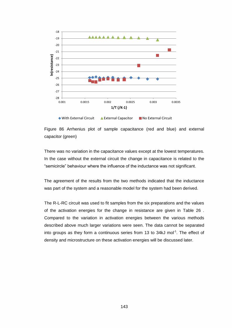
143

Figure 86 Arrhenius plot of sample capacitance (red and blue) and external

capacitor (green)

There was no variation in the capacitance values except at the lowest temperatures.

In the case without the external circuit the change in capacitance is related to the

“semicircle” behaviour where the influence of the inductance was not significant.

The agreement of the results from the two methods indicated that the inductance

was part of the system and a reasonable model for the system had been derived.

The R-L-RC circuit was used to fit samples from the six preparations and the values

of the activation energies for the change in resistance are given in Table 26 .

Compared to the variation in activation energies between the various methods

described above much larger variations were seen. The data cannot be separated

into groups as they form a continuous series from 13 to 34kJ mol-1. The effect of

density and microstructure on these activation energies will be discussed later.

-28

-27

-26

-25

-24

-23

-22

-21

-20

-19

-18

0.001 0.0015 0.002 0.0025 0.003 0.0035

ln(r

esi

stan

ce)

1/T (/K-1}

With External Circuit External Capacitor No External Circuit

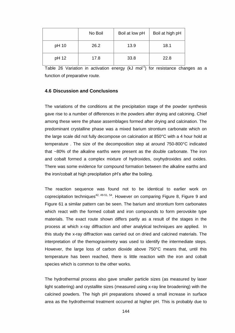
144

No Boil Boil at low pH Boil at high pH

pH 10 26.2 13.9 18.1

pH 12 17.8 33.8 22.8

Table 26 Variation in activation energy (kJ mol-1) for resistance changes as a

function of preparative route.

4.6 Discussion and Conclusions

The variations of the conditions at the precipitation stage of the powder synthesis

gave rise to a number of differences in the powders after drying and calcining. Chief

among these were the phase assemblages formed after drying and calcination. The

predominant crystalline phase was a mixed barium strontium carbonate which on

the large scale did not fully decompose on calcination at 850°C with a 4 hour hold at

temperature . The size of the decomposition step at around 750-800°C indicated

that ~80% of the alkaline earths were present as the double carbonate. The iron

and cobalt formed a complex mixture of hydroxides, oxyhydroxides and oxides.

There was some evidence for compound formation between the alkaline earths and

the iron/cobalt at high precipitation pH’s after the boiling.

The reaction sequence was found not to be identical to earlier work on

coprecipitation techniques42, 49-51, 54. However on comparing Figure 8, Figure 9 and

Figure 61 a similar pattern can be seen. The barium and strontium form carbonates

which react with the formed cobalt and iron compounds to form perovskite type

materials. The exact route shown differs partly as a result of the stages in the

process at which x-ray diffraction and other analytical techniques are applied. In

this study the x-ray diffraction was carried out on dried and calcined materials. The

interpretation of the themogravimetry was used to identify the intermediate steps.

However, the large loss of carbon dioxide above 750°C means that, until this

temperature has been reached, there is little reaction with the iron and cobalt

species which is common to the other works.

The hydrothermal process also gave smaller particle sizes (as measured by laser

light scattering) and crystallite sizes (measured using x-ray line broadening) with the

calcined powders. The high pH preparations showed a small increase in surface

area as the hydrothermal treatment occurred at higher pH. This is probably due to

145

the reactions of excess hydroxide/water with the precipitate to give a

thermodynamically more stable precipitate ie the initial components within the

precipitate reacted with each other and the hydroxide/water. The differences in the

surface area were small and the agglomeration of the crystallites to form dense

particles prevented the adsorbing nitrogen during surface area measurement

accessing the crystallite surface. This is confirmed by the results of the pore volume

measurements of the milled calcined powders, which were very small and indicated

essentially non-porous powders. The particles after milling were agglomerates

(4µm) of small crystallites (40nm). The crystallite sizes from x-ray line broadening

were significantly smaller than that calculated from the surface area (Table 13

Comparison of measured and calculated particle size). A further indication of the

dense nature of the agglomerates The crystallite sizes showed a reduction in size

with hydrothermal treatment. This again indicates some reaction during the

hydrothermal treatment of the type shown below..

4.10

After sintering at 1100°C the densities of the samples were similar at 90% of the

theoretical density. The agreement between the apparent and bulk densities

indicated that there was only a small proportion of open porosity and that the

majority of the pores were closed.

The microstructure of the sintered ceramics showed some differences mainly an

increase in pore size with increasing severity of the hydrothermal treatment (none <

boil at pH 7 < boil at pH 10/12). There was also a greater preponderance of pores at

grain boundaries compared to those within grains. The average grain sizes were

similar for all the ceramics. The change in position of the pores suggests that the

grain growth rate was lower in the ceramics with grain boundary pores as at high

rates of growth, pores break away from the grain boundaries139. The powders with

the lower crystallite size and particle size had fewer pores within the grains the

sintering process probably started at a slightly lower temperature and thus enabled

easier pore removal although overall there was no difference in the final densities.

The composition and the phase analysis of the ceramic pellets showed no

significant differences other than the variation in lattice parameter correlated with

the Ba/Sr ratio in the measured pellets. The effect of compositional changes on

146

lattice parameter has been shown to be more dependent on the barium and

strontium because they are more different in size than the cobalt and iron. 63, 92,142

The activation energy for oxygen permeability for the pH 12 preparations decreased

with the increase in the proportion of pores that were inter-granular. This suggests

that the overall oxygen flux through the ceramic was limited by either the transfer of

oxygen across the grains or by easier grain boundary transfer across the pores. In

the first case the intra-granular pores would act as a barrier to the diffusion of ions

through the lattice with desorption and adsorption steps needed. They also reduce

the cross sectional area of the grains and therefore increase the flux. The correction

of oxygen permeation data by compensating for the porosity did not lead to any

change in the conclusions drawn.143 Desorption and adsorption are also needed at

the grain boundary pores if the oxygen is to pass across them. With neighbouring

grains which are not crystallographically aligned then the anion cannot as easily

move from its site in one crystal to a vacancy in the next grain. Increased grain size

has shown both increased and decreased oxygen flux69, 144, 145. The reason for these

differences is not clear but there was no evidence for grain boundary phases

inhibiting oxygen transfer in a TEM study.69 However this trend with pore size was

not seen for the pH 10 preparations. The no boil and boil at high pH gave the two

lowest activation energies together with the highest oxygen fluxes at 800°C of ~8 x

10-8 mol s-1 cm-2 compared with the other materials giving oxygen fluxes of ~2 x 10-8

mol s-1 cm-2. These differences may be due to the flattening of the curve around the

transition from bulk diffusion to surface control.59 The transition temperatures were

about 800-850°C dependent on thickness from 1.5 to 0.5mm respectively. However

Shao showed variation as a function of composition from 730-820°C but did not

indicate the pellet thickness.11

The differences seen in this study could also be due to variations in the polishing of

the pellets despite all having the same polishing regime. These differences can then

give rise to surface roughening on heating as a result of different depths of sub-

surface damage, (similar to thermal etching) which consequently affects the surface

area available for oxygen adsorption and desorption reactions.

The activation energy was found to be proportional to the lattice parameter as

shown in Figure 87. Although the ceramics were nominally of the same composition,

the minor variations, in their lattice parameters and chemical composition as shown

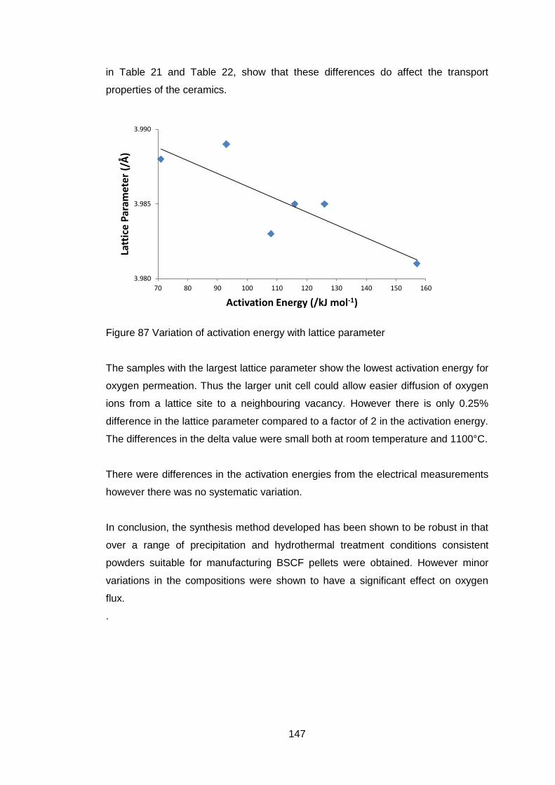
147

in Table 21 and Table 22, show that these differences do affect the transport

properties of the ceramics.

Figure 87 Variation of activation energy with lattice parameter

The samples with the largest lattice parameter show the lowest activation energy for

oxygen permeation. Thus the larger unit cell could allow easier diffusion of oxygen

ions from a lattice site to a neighbouring vacancy. However there is only 0.25%

difference in the lattice parameter compared to a factor of 2 in the activation energy.

The differences in the delta value were small both at room temperature and 1100°C.

There were differences in the activation energies from the electrical measurements

however there was no systematic variation.

In conclusion, the synthesis method developed has been shown to be robust in that

over a range of precipitation and hydrothermal treatment conditions consistent

powders suitable for manufacturing BSCF pellets were obtained. However minor

variations in the compositions were shown to have a significant effect on oxygen

flux.

.

3.980

3.985

3.990

70 80 90 100 110 120 130 140 150 160

Latt

ice

Par

amet

er (

/Å)

Activation Energy (/kJ mol-1)

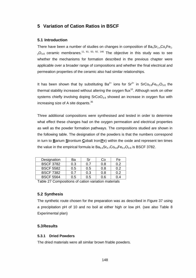
148

5 Variation of Cation Ratios in BSCF

5.1 Introduction

There have been a number of studies on changes in composition of BaxSr1-xCoyFe1-

yO3-δ ceramic membranes.11, 61, 63, 92, 146 The objective in this study was to see

whether the mechanisms for formation described in the previous chapter were

applicable over a broader range of compositions and whether the final electrical and

permeation properties of the ceramic also had similar relationships.

It has been shown that by substituting Ba2+ ions for Sr2+ in SrCo0.8Fe0.2O3-δ the

thermal stability increased without altering the oxygen flux10. Although work on other

systems chiefly involving doping SrCoO3-δ showed an increase in oxygen flux with

increasing size of A site dopants.35

Three additional compositions were synthesised and tested in order to determine

what effect these changes had on the oxygen permeation and electrical properties

as well as the powder formation pathways. The compositions studied are shown in

the following table. The designation of the powders is that the numbers correspond

in turn to Barium Strontium Cobalt Iron(Fe) within the oxide and represent ten times

the value in the empirical formula ie Ba0.3Sr0.7Co0.8Fe0.2O3-δ is BSCF 3782.

Designation Ba Sr Co Fe

BSCF 3782 0.3 0.7 0.8 0.2

BSCF 5582 0.5 0.5 0.8 0.2

BSCF 7382 0.7 0.3 0.8 0.2

BSCF 5564 0.5 0.5 0.6 0.4

Table 27 Compositions of cation variation materials

5.2 Synthesis

The synthetic route chosen for the preparation was as described in Figure 37 using

a precipitation pH of 10 and no boil at either high or low pH. (see also Table 8

Experimental plan)

5.3 Results

5.3.1 Dried Powders

The dried materials were all similar brown friable powders.

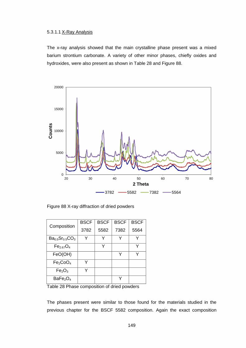
149

5.3.1.1 X-Ray Analysis

The x-ray analysis showed that the main crystalline phase present was a mixed

barium strontium carbonate. A variety of other minor phases, chiefly oxides and

hydroxides, were also present as shown in Table 28 and Figure 88.

Figure 88 X-ray diffraction of dried powders

Composition BSCF

3782

BSCF

5582

BSCF

7382

BSCF

5564

Ba0.5Sr0.5CO3 Y Y Y Y

Fe2.67O4 Y Y

FeO(OH) Y Y

Fe2CoO4 Y

Fe2O3 Y

BaFe2O4 Y

Table 28 Phase composition of dried powders

The phases present were similar to those found for the materials studied in the

previous chapter for the BSCF 5582 composition. Again the exact composition

0

5000

10000

15000

20000

20 30 40 50 60 70 80

Co

un

ts

2 Theta

3782 5582 7382 5564

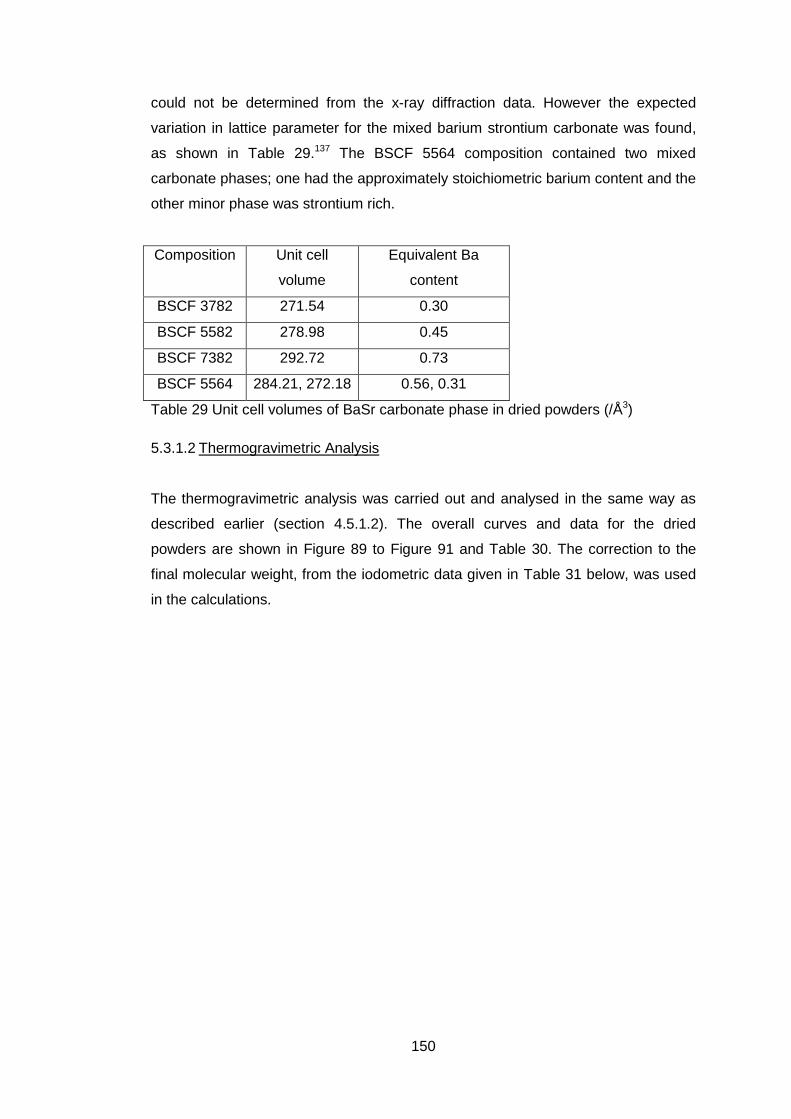
150

could not be determined from the x-ray diffraction data. However the expected

variation in lattice parameter for the mixed barium strontium carbonate was found,

as shown in Table 29.137 The BSCF 5564 composition contained two mixed

carbonate phases; one had the approximately stoichiometric barium content and the

other minor phase was strontium rich.

Composition Unit cell

volume

Equivalent Ba

content

BSCF 3782 271.54 0.30

BSCF 5582 278.98 0.45

BSCF 7382 292.72 0.73

BSCF 5564 284.21, 272.18 0.56, 0.31

Table 29 Unit cell volumes of BaSr carbonate phase in dried powders (/Å3)


The thermogravimetric analysis was carried out and analysed in the same way as

described earlier (section 4.5.1.2). The overall curves and data for the dried

powders are shown in Figure 89 to Figure 91 and Table 30. The correction to the

final molecular weight, from the iodometric data given in Table 31 below, was used

in the calculations.

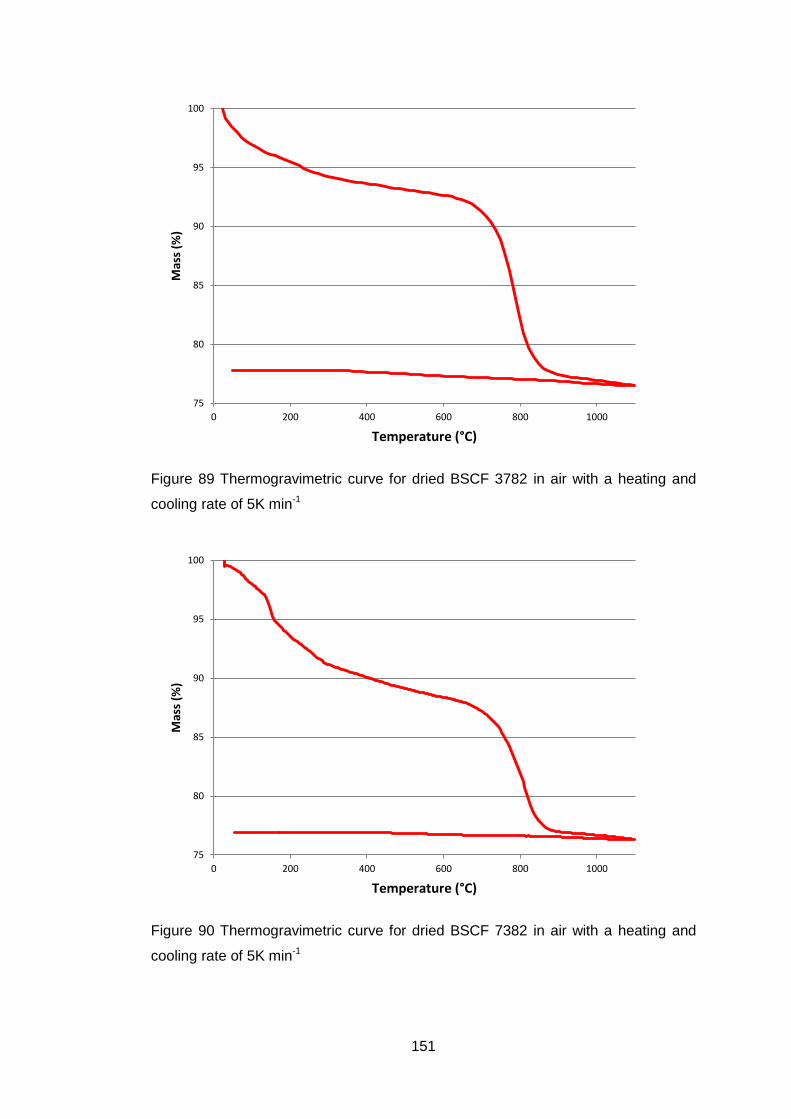
151

Figure 89 Thermogravimetric curve for dried BSCF 3782 in air with a heating and




75

80

85

90

95

100

0 200 400 600 800 1000

Mas

s (%

)

Temperature (°C)

75

80

85

90

95

100

0 200 400 600 800 1000

Mas

s (%

)

Temperature (°C)

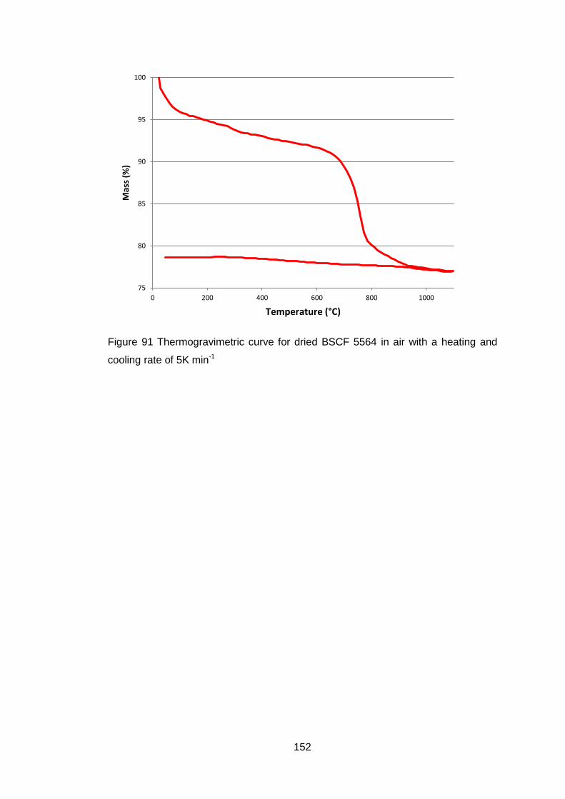
152



75

80

85

90

95

100

0 200 400 600 800 1000

Mas

s (%

)

Temperature (°C)

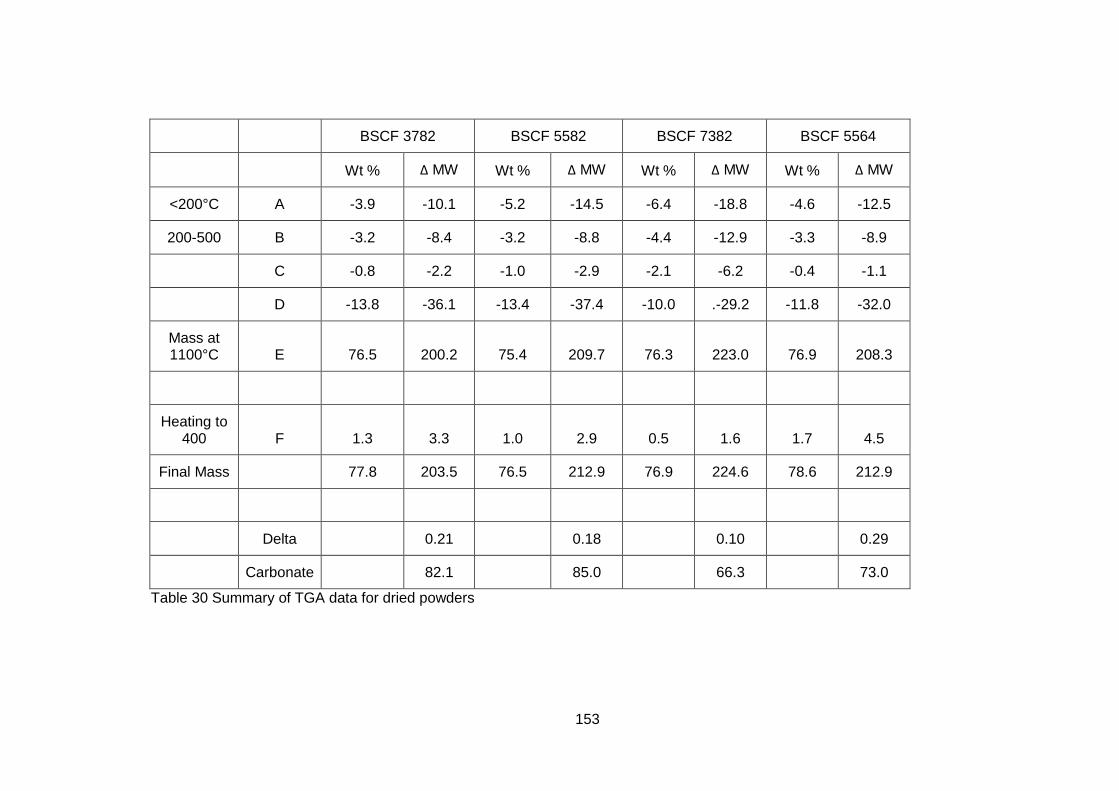
153

BSCF 3782 BSCF 5582 BSCF 7382 BSCF 5564

Wt % Δ MW Wt % Δ MW Wt % Δ MW Wt % Δ MW

<200°C A -3.9 -10.1 -5.2 -14.5 -6.4 -18.8 -4.6 -12.5

200-500 B -3.2 -8.4 -3.2 -8.8 -4.4 -12.9 -3.3 -8.9

C -0.8 -2.2 -1.0 -2.9 -2.1 -6.2 -0.4 -1.1

D -13.8 -36.1 -13.4 -37.4 -10.0 .-29.2 -11.8 -32.0

Mass at 1100°C E 76.5 200.2 75.4 209.7 76.3 223.0 76.9 208.3

Heating to 400 F 1.3 3.3 1.0 2.9 0.5 1.6 1.7 4.5

Final Mass

77.8 203.5 76.5 212.9 76.9 224.6 78.6 212.9

Delta 0.21 0.18 0.10 0.29

Carbonate 82.1 85.0 66.3 73.0

Table 30 Summary of TGA data for dried powders

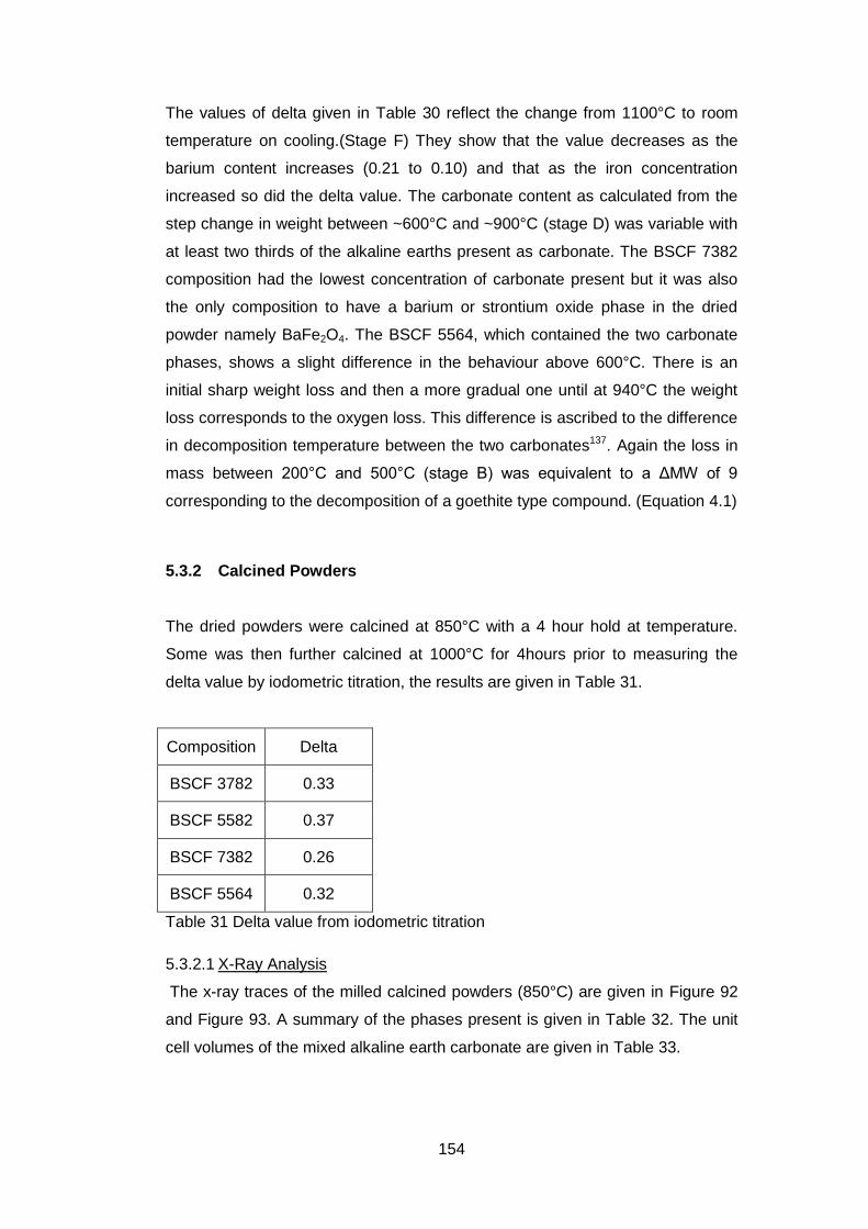
154

The values of delta given in Table 30 reflect the change from 1100°C to room

temperature on cooling.(Stage F) They show that the value decreases as the

barium content increases (0.21 to 0.10) and that as the iron concentration

increased so did the delta value. The carbonate content as calculated from the

step change in weight between ~600°C and ~900°C (stage D) was variable with

at least two thirds of the alkaline earths present as carbonate. The BSCF 7382

composition had the lowest concentration of carbonate present but it was also

the only composition to have a barium or strontium oxide phase in the dried

powder namely BaFe2O4. The BSCF 5564, which contained the two carbonate

phases, shows a slight difference in the behaviour above 600°C. There is an

initial sharp weight loss and then a more gradual one until at 940°C the weight

loss corresponds to the oxygen loss. This difference is ascribed to the difference

in decomposition temperature between the two carbonates137. Again the loss in

mass between 200°C and 500°C (stage B) was equivalent to a ΔMW of 9

corresponding to the decomposition of a goethite type compound. (Equation 4.1)

5.3.2 Calcined Powders

The dried powders were calcined at 850°C with a 4 hour hold at temperature.

Some was then further calcined at 1000°C for 4hours prior to measuring the

delta value by iodometric titration, the results are given in Table 31.

Composition Delta

BSCF 3782 0.33

BSCF 5582 0.37

BSCF 7382 0.26

BSCF 5564 0.32

Table 31 Delta value from iodometric titration


The x-ray traces of the milled calcined powders (850°C) are given in Figure 92

and Figure 93. A summary of the phases present is given in Table 32. The unit

cell volumes of the mixed alkaline earth carbonate are given in Table 33.

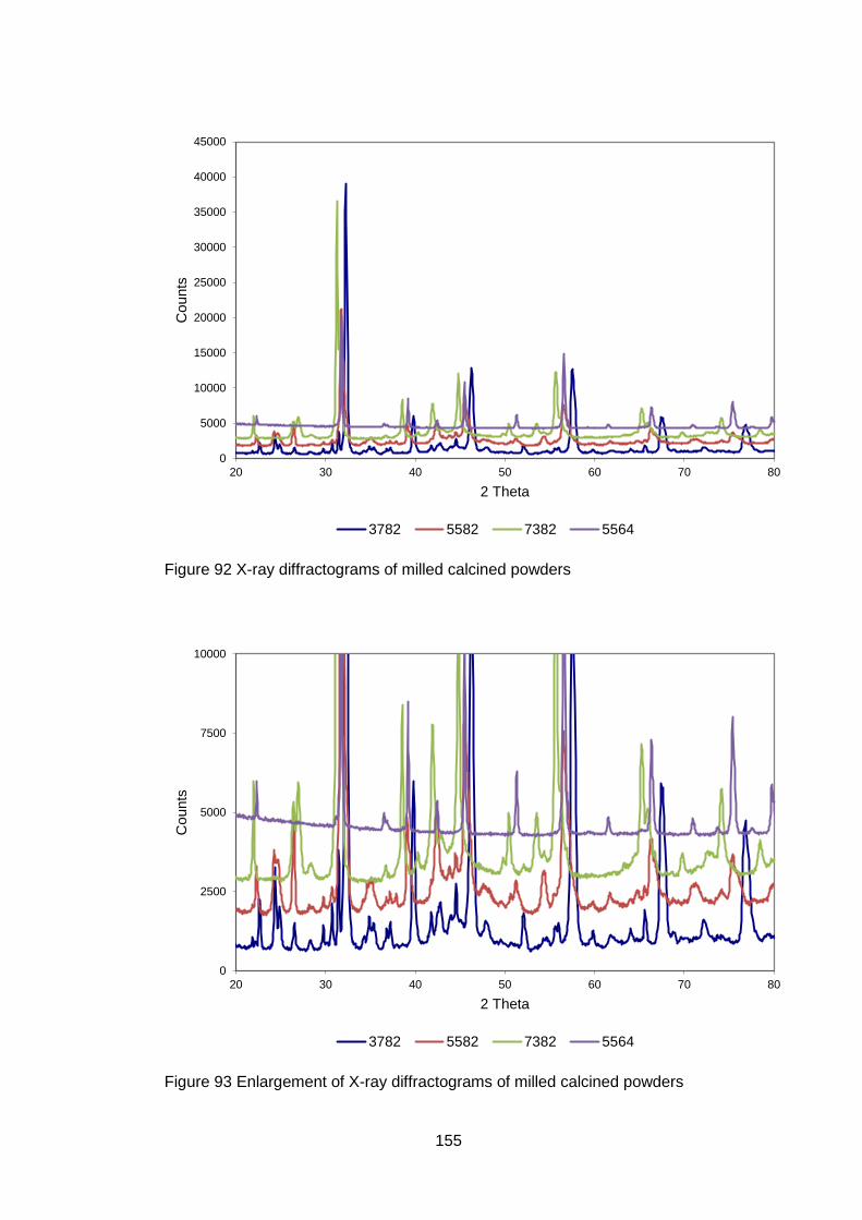
155

Figure 92 X-ray diffractograms of milled calcined powders

Figure 93 Enlargement of X-ray diffractograms of milled calcined powders

0

5000

10000

15000

20000

25000

30000

35000

40000

45000

20 30 40 50 60 70 80

Counts

2 Theta

3782 5582 7382 5564

0

2500

5000

7500

10000

20 30 40 50 60 70 80

Counts

2 Theta

3782 5582 7382 5564

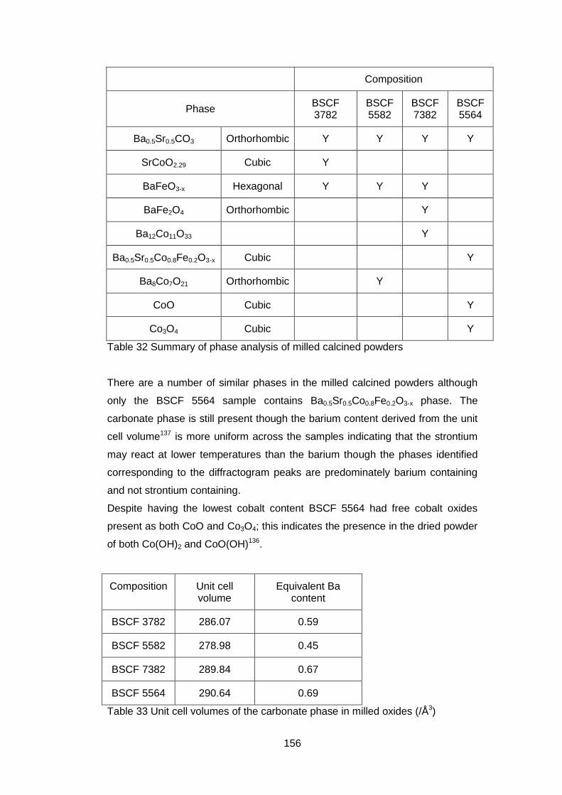
156

Composition

Phase BSCF 3782

BSCF 5582

BSCF 7382

BSCF 5564

Ba0.5Sr0.5CO3 Orthorhombic Y Y Y Y

SrCoO2.29 Cubic Y

BaFeO3-x Hexagonal Y Y Y

BaFe2O4 Orthorhombic

Y

Ba12Co11O33

Y

Ba0.5Sr0.5Co0.8Fe0.2O3-x Cubic Y

Ba8Co7O21 Orthorhombic Y

CoO Cubic Y

Co3O4 Cubic Y

Table 32 Summary of phase analysis of milled calcined powders

There are a number of similar phases in the milled calcined powders although

only the BSCF 5564 sample contains Ba0.5Sr0.5Co0.8Fe0.2O3-x phase. The

carbonate phase is still present though the barium content derived from the unit

cell volume137 is more uniform across the samples indicating that the strontium

may react at lower temperatures than the barium though the phases identified

corresponding to the diffractogram peaks are predominately barium containing

and not strontium containing.

Despite having the lowest cobalt content BSCF 5564 had free cobalt oxides

present as both CoO and Co3O4; this indicates the presence in the dried powder

of both Co(OH)2 and CoO(OH)136.

Composition Unit cell volume

Equivalent Ba content

BSCF 3782 286.07 0.59

BSCF 5582 278.98 0.45

BSCF 7382 289.84 0.67

BSCF 5564 290.64 0.69

Table 33 Unit cell volumes of the carbonate phase in milled oxides (/Å3)

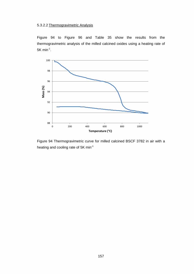
157


Figure 94 to Figure 96 and Table 35 show the results from the

thermogravimetric analysis of the milled calcined oxides using a heating rate of

5K min-1.

Figure 94 Thermogravimetric curve for milled calcined BSCF 3782 in air with a


88

90

92

94

96

98

100

0 200 400 600 800 1000

Mas

s (%

)

Temperature (°C)

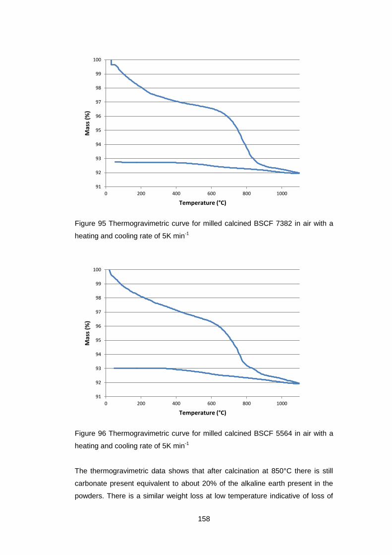
158





The thermogravimetric data shows that after calcination at 850°C there is still

carbonate present equivalent to about 20% of the alkaline earth present in the

powders. There is a similar weight loss at low temperature indicative of loss of

91

92

93

94

95

96

97

98

99

100

0 200 400 600 800 1000

Mas

s (%

)

Temperature (°C)

91

92

93

94

95

96

97

98

99

100

0 200 400 600 800 1000

Mas

s (%

)

Temperature (°C)

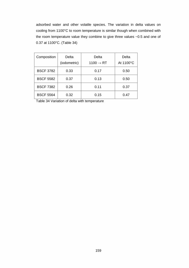
159

adsorbed water and other volatile species. The variation in delta values on

cooling from 1100°C to room temperature is similar though when combined with

the room temperature value they combine to give three values ~0.5 and one of

0.37 at 1100°C. (Table 34)

Composition Delta

(iodometric)

Delta

1100 → RT

Delta

At 1100°C

BSCF 3782 0.33 0.17 0.50

BSCF 5582 0.37 0.13 0.50

BSCF 7382 0.26 0.11 0.37

BSCF 5564 0.32 0.15 0.47

Table 34 Variation of delta with temperature

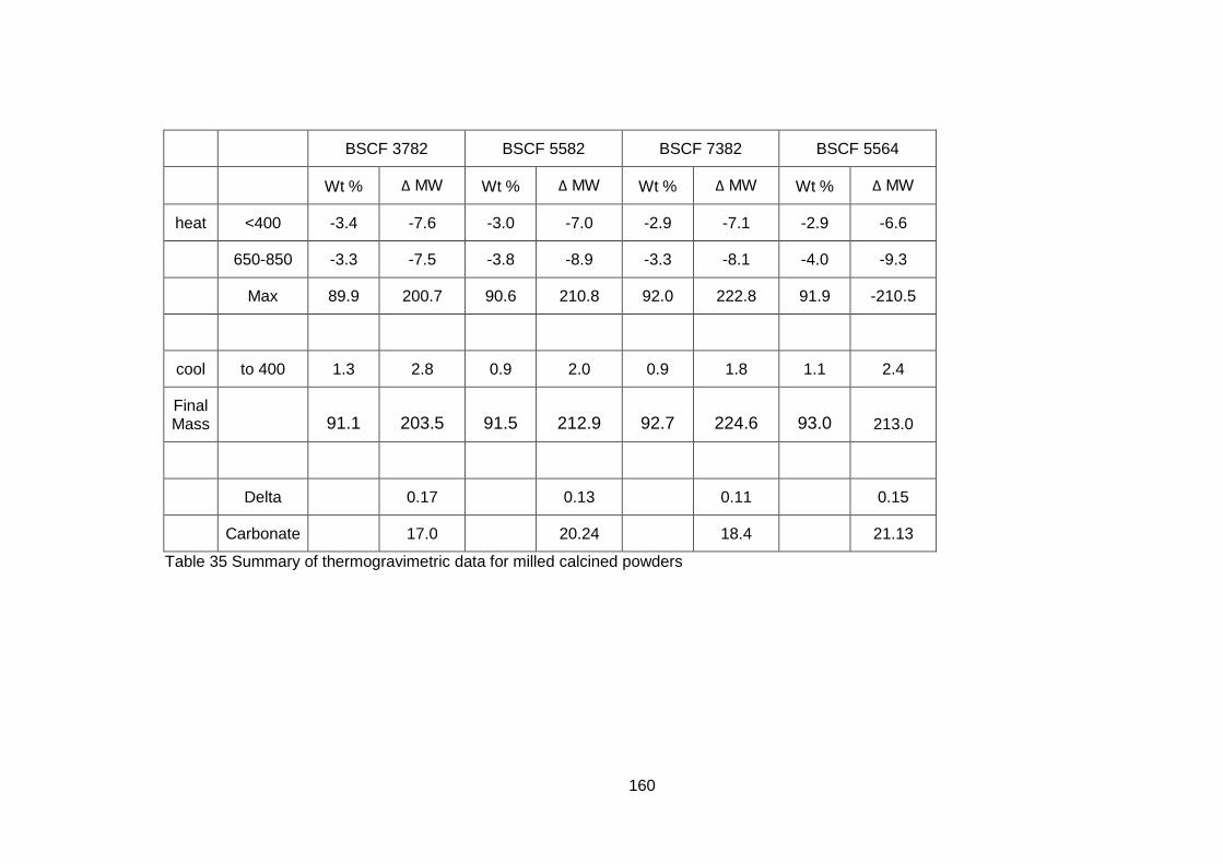
160


Wt % Δ MW Wt % Δ MW Wt % Δ MW Wt % Δ MW

heat <400 -3.4 -7.6 -3.0 -7.0 -2.9 -7.1 -2.9 -6.6

650-850 -3.3 -7.5 -3.8 -8.9 -3.3 -8.1 -4.0 -9.3

Max 89.9 200.7 90.6 210.8 92.0 222.8 91.9 -210.5

cool to 400 1.3 2.8 0.9 2.0 0.9 1.8 1.1 2.4

Final Mass

91.1 203.5 91.5 212.9 92.7 224.6 93.0 213.0

Delta 0.17 0.13 0.11 0.15

Carbonate 17.0 20.24 18.4 21.13

Table 35 Summary of thermogravimetric data for milled calcined powders

161


As was shown in the previous chapter the formation of a large number of

compounds occurs during the initial precipitation, drying and calcination of the

powders. The most well defined compound is the mixed barium-strontium

carbonate which after drying accounts for 66-85% of the barium and strontium in

the powder if all the carbon is present as the mixed carbonate. The unit cell

volume of the mixed carbonate is after drying proportional to the barium content

in the system. However after calcination the unit cell volume is more uniform and

higher. This indicates that the strontium reacts with the other components before

the barium.

The assignments of the phases may seem to contradict this as the identified

phases are mainly barium containing. This is because of the extreme broadness

of the peaks together with their variable composition from the solid solutions

formed. The phases present within HighScore plus may also not include those

present especially the mixed hydroxides and oxyhydroxides. As such the phases

are indicative of the types of compounds formed rather than those present.

On calcination the carbonate was reduced in the powder but was still present in

significant amounts (~20%). Only one material BSCF 5564 was mainly the

desired cubic oxide. The reason for its formation is due to the presence of two

carbonates in the dried sample with barium contents of 0.56 and 0.31 which

after calcination result in a single carbonate with a 0.69 barium content. This

indicates the higher reactivity of the strontium towards the iron and cobalt.

Furthermore the step like character of the CO2 loss has changed with a rapid

loss followed by a more gradual mass loss (compare Figure 91 and Figure 96)

before the slow loss of oxygen. Also at lower temperature (<500°C) the weight

loss is more continuous and less step like indicating more continuous reaction

process.


The milled calcined powders were pressed in a 1cm diameter die at 100MPa

and then sintered at 1100°C with a hold time at temperature of 10 hours. The

heating and cooling rates were both 180K min-1.

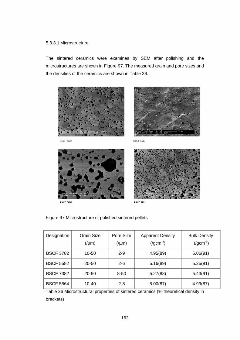
162


The sintered ceramics were examines by SEM after polishing and the

microstructures are shown in Figure 97. The measured grain and pore sizes and

the densities of the ceramics are shown in Table 36.

Figure 97 Microstructure of polished sintered pellets

Designation Grain Size

(/µm)

Pore Size

(/µm)

Apparent Density

(/gcm-3)

Bulk Density

(/gcm-3)

BSCF 3782 10-50 2-9 4.95(89) 5.06(91)

BSCF 5582 20-50 2-6 5.16(89) 5.25(91)

BSCF 7382 20-50 8-50 5.27(88) 5.43(91)

BSCF 5564 10-40 2-8 5.00(87) 4.99(87)

Table 36 Microstructural properties of sintered ceramics (% theoretical density in

brackets)

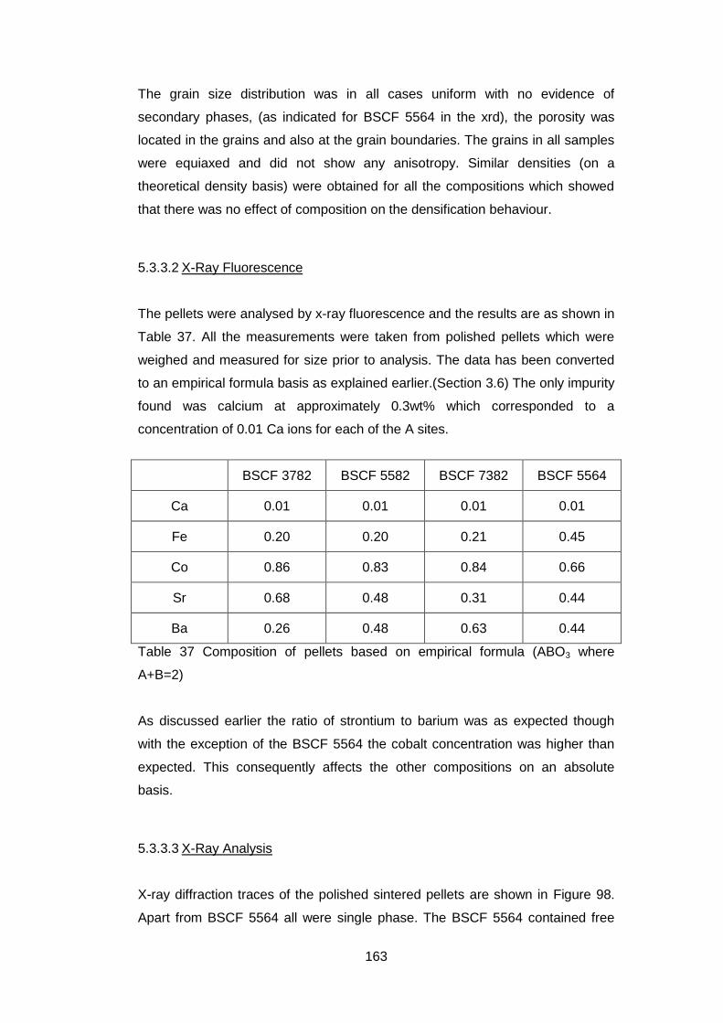
163

The grain size distribution was in all cases uniform with no evidence of

secondary phases, (as indicated for BSCF 5564 in the xrd), the porosity was

located in the grains and also at the grain boundaries. The grains in all samples

were equiaxed and did not show any anisotropy. Similar densities (on a

theoretical density basis) were obtained for all the compositions which showed

that there was no effect of composition on the densification behaviour.

5.3.3.2 X-Ray Fluorescence


Table 37. All the measurements were taken from polished pellets which were

weighed and measured for size prior to analysis. The data has been converted

to an empirical formula basis as explained earlier.(Section 3.6) The only impurity

found was calcium at approximately 0.3wt% which corresponded to a

concentration of 0.01 Ca ions for each of the A sites.


Ca 0.01 0.01 0.01 0.01

Fe 0.20 0.20 0.21 0.45

Co 0.86 0.83 0.84 0.66

Sr 0.68 0.48 0.31 0.44

Ba 0.26 0.48 0.63 0.44

Table 37 Composition of pellets based on empirical formula (ABO3 where

A+B=2)

As discussed earlier the ratio of strontium to barium was as expected though

with the exception of the BSCF 5564 the cobalt concentration was higher than

expected. This consequently affects the other compositions on an absolute

basis.


X-ray diffraction traces of the polished sintered pellets are shown in Figure 98.

Apart from BSCF 5564 all were single phase. The BSCF 5564 contained free

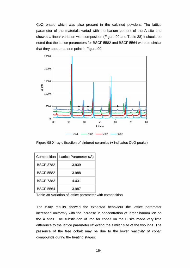
164

CoO phase which was also present in the calcined powders. The lattice

parameter of the materials varied with the barium content of the A site and

showed a linear variation with composition (Figure 99 and Table 38) It should be

noted that the lattice parameters for BSCF 5582 and BSCF 5564 were so similar

that they appear as one point in Figure 99.

Figure 98 X-ray diffraction of sintered ceramics (♦ indicates CoO peaks)

Composition Lattice Parameter (/Å)

BSCF 3782 3.939

BSCF 5582 3.988

BSCF 7382 4.031

BSCF 5564 3.987

Table 38 Variation of lattice parameter with composition

The x-ray results showed the expected behaviour the lattice parameter

increased uniformly with the increase in concentration of larger barium ion on

the A sites. The substitution of iron for cobalt on the B site made very little

difference to the lattice parameter reflecting the similar size of the two ions. The

presence of the free cobalt may be due to the lower reactivity of cobalt

compounds during the heating stages.

0

5000

10000

15000

20000

25000

20 30 40 50 60 70 80

Co

un

ts

2 theta

5564 7382 5582 3782

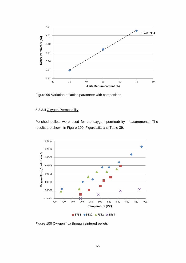
165

Figure 99 Variation of lattice parameter with composition


Polished pellets were used for the oxygen permeability measurements. The

results are shown in Figure 100, Figure 101 and Table 39.

Figure 100 Oxygen flux through sintered pellets

R² = 0.9984

3.92

3.94

3.96

3.98

4.00

4.02

4.04

20 30 40 50 60 70 80

Latt

ice

Par

ame

ter

(/Å

)

A site Barium Content (%)

0.0E+00

2.0E-08

4.0E-08

6.0E-08

8.0E-08

1.0E-07

1.2E-07

1.4E-07

700 720 740 760 780 800 820 840 860 880 900

Oxy

gen

Flu

x (/

mo

l s-1

cm

-2)

Temperature (/°C)

3782 5582 7382 5564

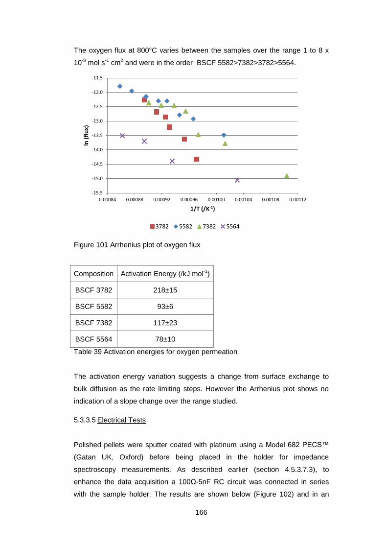
166

The oxygen flux at 800°C varies between the samples over the range 1 to 8 x

10-8 mol s-1 cm2 and were in the order BSCF 5582>7382>3782>5564.

Figure 101 Arrhenius plot of oxygen flux

Composition Activation Energy (/kJ mol-1)

BSCF 3782 218±15

BSCF 5582 93±6

BSCF 7382 117±23

BSCF 5564 78±10

Table 39 Activation energies for oxygen permeation

The activation energy variation suggests a change from surface exchange to

bulk diffusion as the rate limiting steps. However the Arrhenius plot shows no

indication of a slope change over the range studied.


Polished pellets were sputter coated with platinum using a Model 682 PECS™

(Gatan UK, Oxford) before being placed in the holder for impedance

spectroscopy measurements. As described earlier (section 4.5.3.7.3), to

enhance the data acquisition a 100Ω-5nF RC circuit was connected in series

with the sample holder. The results are shown below (Figure 102) and in an

-15.5

-15.0

-14.5

-14.0

-13.5

-13.0

-12.5

-12.0

-11.5

0.00084 0.00088 0.00092 0.00096 0.00100 0.00104 0.00108 0.00112

ln (

flu

x)

1/T (/K-1)

3782 5582 7382 5564

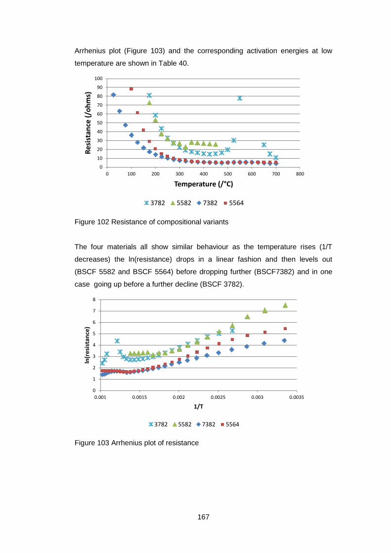
167

Arrhenius plot (Figure 103) and the corresponding activation energies at low

temperature are shown in Table 40.

Figure 102 Resistance of compositional variants

The four materials all show similar behaviour as the temperature rises (1/T

decreases) the ln(resistance) drops in a linear fashion and then levels out

(BSCF 5582 and BSCF 5564) before dropping further (BSCF7382) and in one

case going up before a further decline (BSCF 3782).

Figure 103 Arrhenius plot of resistance

0

10

20

30

40

50

60

70

80

90

100

0 100 200 300 400 500 600 700 800

Res

ista

nce

(/o

hm

s)

Temperature (/°C)

3782 5582 7382 5564

0

1

2

3

4

5

6

7

8

0.001 0.0015 0.002 0.0025 0.003 0.0035

ln(r

esi

stan

ce)

1/T

3782 5582 7382 5564

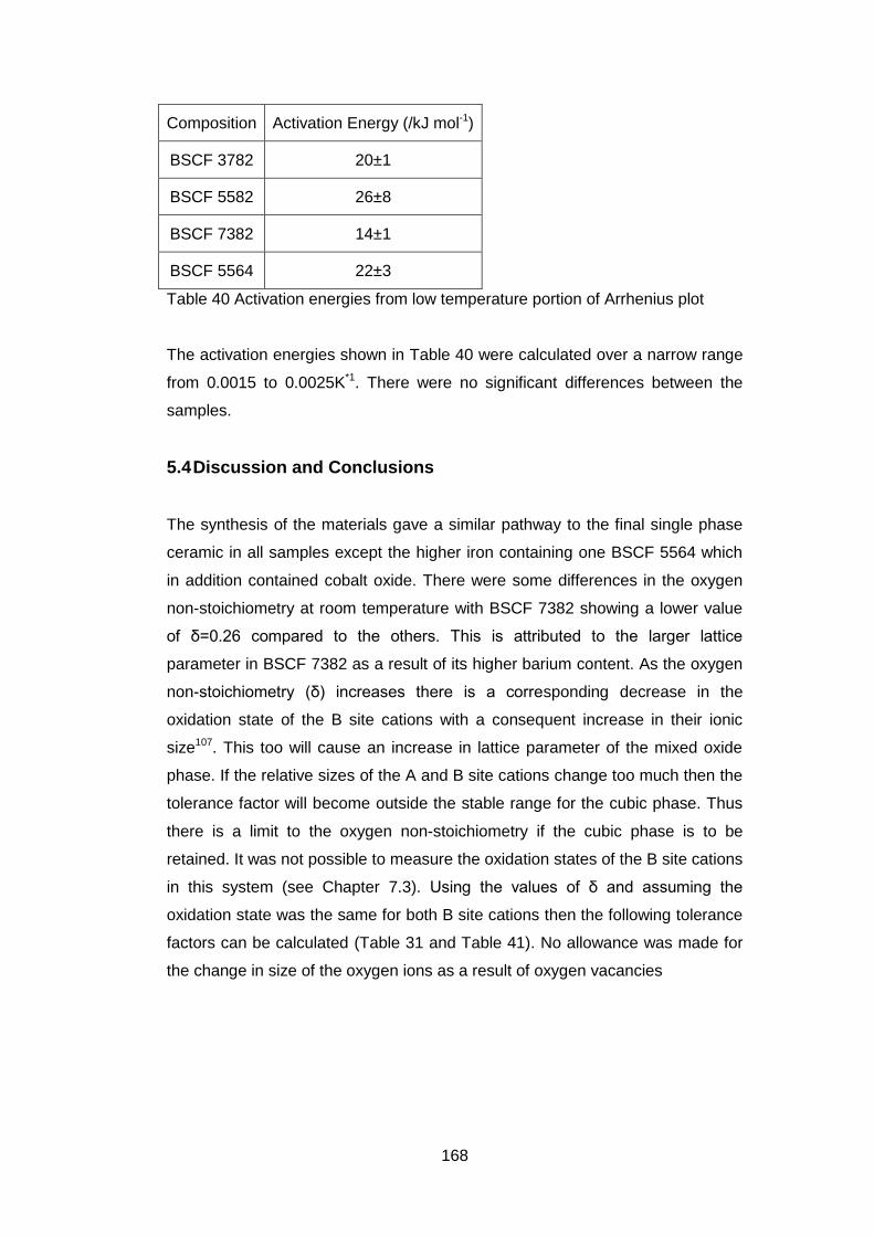
168

Composition Activation Energy (/kJ mol-1)

BSCF 3782 20±1

BSCF 5582 26±8

BSCF 7382 14±1

BSCF 5564 22±3

Table 40 Activation energies from low temperature portion of Arrhenius plot

The activation energies shown in Table 40 were calculated over a narrow range

from 0.0015 to 0.0025K*1. There were no significant differences between the

samples.


The synthesis of the materials gave a similar pathway to the final single phase

ceramic in all samples except the higher iron containing one BSCF 5564 which

in addition contained cobalt oxide. There were some differences in the oxygen

non-stoichiometry at room temperature with BSCF 7382 showing a lower value

of δ=0.26 compared to the others. This is attributed to the larger lattice

parameter in BSCF 7382 as a result of its higher barium content. As the oxygen

non-stoichiometry (δ) increases there is a corresponding decrease in the

oxidation state of the B site cations with a consequent increase in their ionic

size107. This too will cause an increase in lattice parameter of the mixed oxide

phase. If the relative sizes of the A and B site cations change too much then the

tolerance factor will become outside the stable range for the cubic phase. Thus

there is a limit to the oxygen non-stoichiometry if the cubic phase is to be

retained. It was not possible to measure the oxidation states of the B site cations

in this system (see Chapter 7.3). Using the values of δ and assuming the

oxidation state was the same for both B site cations then the following tolerance

factors can be calculated (Table 31 and Table 41). No allowance was made for

the change in size of the oxygen ions as a result of oxygen vacancies

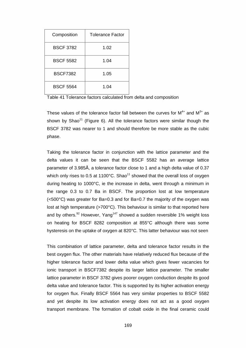
169

Composition Tolerance Factor

BSCF 3782 1.02

BSCF 5582 1.04

BSCF7382 1.05

BSCF 5564 1.04

Table 41 Tolerance factors calculated from delta and composition

These values of the tolerance factor fall between the curves for M4+ and M3+ as

shown by Shao11 (Figure 6). All the tolerance factors were similar though the

BSCF 3782 was nearer to 1 and should therefore be more stable as the cubic

phase.

Taking the tolerance factor in conjunction with the lattice parameter and the

delta values it can be seen that the BSCF 5582 has an average lattice

parameter of 3.985Å, a tolerance factor close to 1 and a high delta value of 0.37

which only rises to 0.5 at 1100°C. Shao11 showed that the overall loss of oxygen

during heating to 1000°C, ie the increase in delta, went through a minimum in

the range 0.3 to 0.7 Ba in BSCF. The proportion lost at low temperature

(<500°C) was greater for Ba=0.3 and for Ba=0.7 the majority of the oxygen was

lost at high temperature (>700°C). This behaviour is similar to that reported here

and by others.92 However, Yang147 showed a sudden reversible 1% weight loss

on heating for BSCF 8282 composition at 855°C although there was some

hysteresis on the uptake of oxygen at 820°C. This latter behaviour was not seen

This combination of lattice parameter, delta and tolerance factor results in the

best oxygen flux. The other materials have relatively reduced flux because of the

higher tolerance factor and lower delta value which gives fewer vacancies for

ionic transport in BSCF7382 despite its larger lattice parameter. The smaller

lattice parameter in BSCF 3782 gives poorer oxygen conduction despite its good

delta value and tolerance factor. This is supported by its higher activation energy

for oxygen flux. Finally BSCF 5564 has very similar properties to BSCF 5582

and yet despite its low activation energy does not act as a good oxygen

transport membrane. The formation of cobalt oxide in the final ceramic could

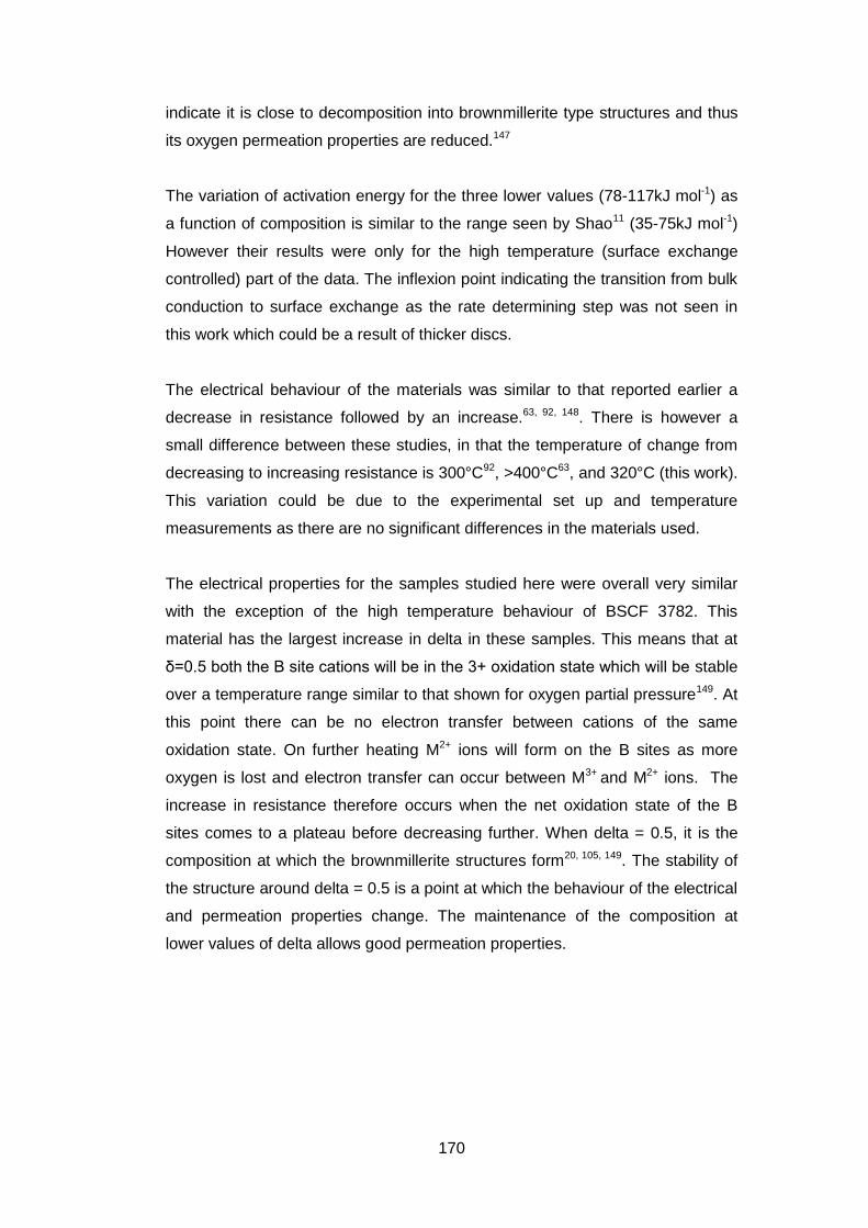
170

indicate it is close to decomposition into brownmillerite type structures and thus

its oxygen permeation properties are reduced.147

The variation of activation energy for the three lower values (78-117kJ mol-1) as

a function of composition is similar to the range seen by Shao11 (35-75kJ mol-1)

However their results were only for the high temperature (surface exchange

controlled) part of the data. The inflexion point indicating the transition from bulk

conduction to surface exchange as the rate determining step was not seen in

this work which could be a result of thicker discs.

The electrical behaviour of the materials was similar to that reported earlier a

decrease in resistance followed by an increase.63, 92, 148. There is however a

small difference between these studies, in that the temperature of change from

decreasing to increasing resistance is 300°C92, >400°C63, and 320°C (this work).

This variation could be due to the experimental set up and temperature

measurements as there are no significant differences in the materials used.

The electrical properties for the samples studied here were overall very similar

with the exception of the high temperature behaviour of BSCF 3782. This

material has the largest increase in delta in these samples. This means that at

δ=0.5 both the B site cations will be in the 3+ oxidation state which will be stable

over a temperature range similar to that shown for oxygen partial pressure149. At

this point there can be no electron transfer between cations of the same

oxidation state. On further heating M2+ ions will form on the B sites as more

oxygen is lost and electron transfer can occur between M3+ and M2+ ions. The

increase in resistance therefore occurs when the net oxidation state of the B

sites comes to a plateau before decreasing further. When delta = 0.5, it is the

composition at which the brownmillerite structures form20, 105, 149. The stability of

the structure around delta = 0.5 is a point at which the behaviour of the electrical

and permeation properties change. The maintenance of the composition at

lower values of delta allows good permeation properties.

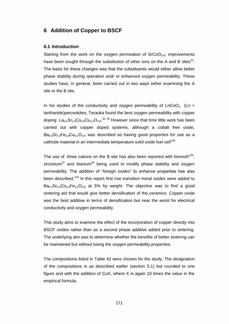
171

6 Addition of Copper to BSCF

6.1 Introduction

Starting from the work on the oxygen permeation of SrCoO3-δ, improvements

have been sought through the substitution of other ions on the A and B sites23.

The basis for these changes was that the substituents would either allow better

phase stability during operation and/ or enhanced oxygen permeability. These

studies have, in general, been carried out in two ways either examining the A

site or the B site.

In his studies of the conductivity and oxygen permeability of LnCoO3 (Ln =

lanthanide)perovskites, Teraoka found the best oxygen permeability with copper

doping La0.6Sr0.4Co0.8Cu0.2O3-δ.32, 33 However since that time little work has been

carried out with copper doped systems, although a cobalt free oxide,

Ba0.5Sr0.5Fe0.8Cu0.2O3-δ was described as having good properties for use as a

cathode material in an intermediate temperature solid oxide fuel cell148

The use of .three cations on the B site has also been reported with bismuth150,

zirconium37 and titanium44 being used to modify phase stability and oxygen

permeability. The addition of “foreign oxides” to enhance properties has also

been described.143 In this report first row transition metal oxides were added to

Ba0.5Sr0.5Co0.8Fe0.2O3-δ at 5% by weight. The objective was to find a good

sintering aid that would give better densification of the ceramics. Copper oxide

was the best additive in terms of densification but near the worst for electrical

conductivity and oxygen permeability.

This study aims to examine the effect of the incorporation of copper directly into

BSCF oxides rather than as a second phase additive added prior to sintering.

The underlying aim was to determine whether the benefits of better sintering can

be maintained but without losing the oxygen permeability properties.

The compositions listed in Table 42 were chosen for the study. The designation

of the compositions is as described earlier (section 5.1) but rounded to one

figure and with the addition of CuX, where X is again 10 times the value in the

empirical formula.

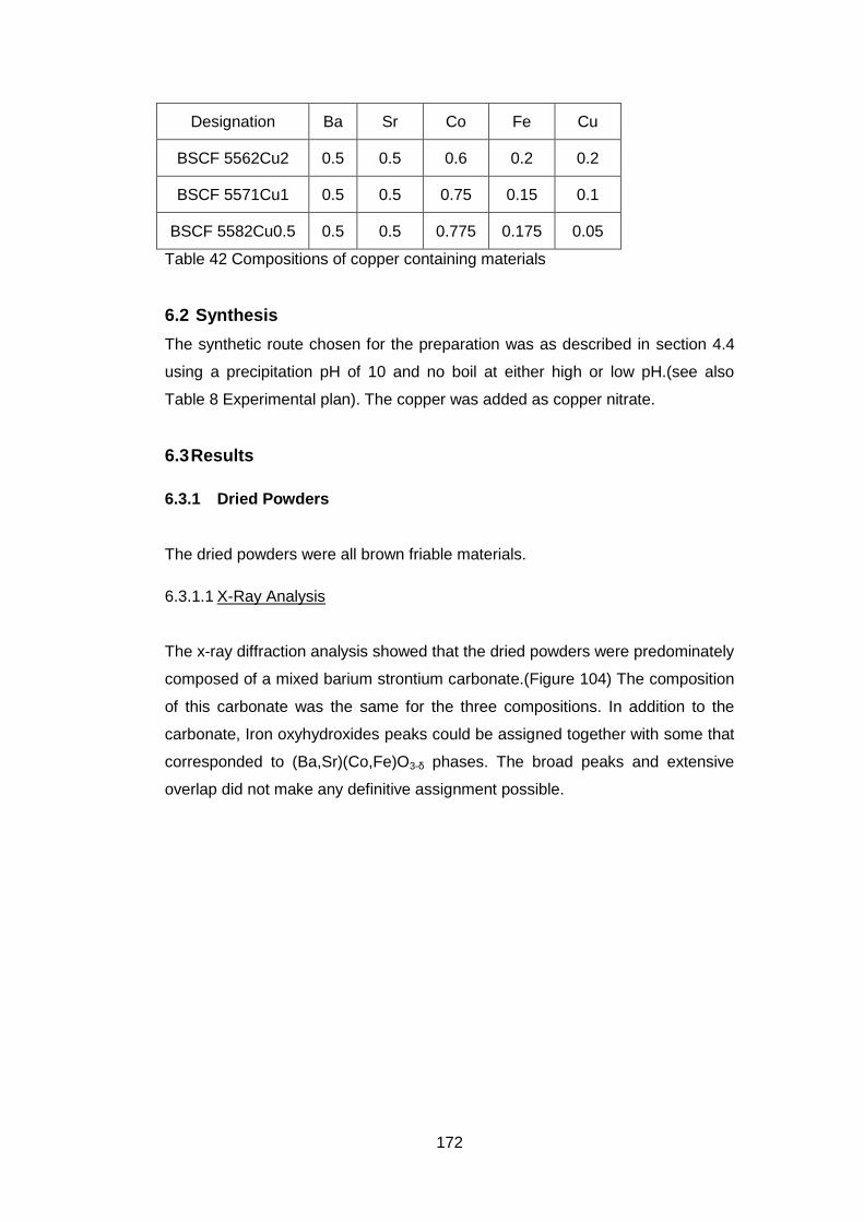
172

Designation Ba Sr Co Fe Cu

BSCF 5562Cu2 0.5 0.5 0.6 0.2 0.2

BSCF 5571Cu1 0.5 0.5 0.75 0.15 0.1

BSCF 5582Cu0.5 0.5 0.5 0.775 0.175 0.05

Table 42 Compositions of copper containing materials

6.2 Synthesis

The synthetic route chosen for the preparation was as described in section 4.4

using a precipitation pH of 10 and no boil at either high or low pH.(see also

Table 8 Experimental plan). The copper was added as copper nitrate.

6.3 Results

6.3.1 Dried Powders

The dried powders were all brown friable materials.


The x-ray diffraction analysis showed that the dried powders were predominately

composed of a mixed barium strontium carbonate.(Figure 104) The composition

of this carbonate was the same for the three compositions. In addition to the

carbonate, Iron oxyhydroxides peaks could be assigned together with some that

corresponded to (Ba,Sr)(Co,Fe)O3-δ phases. The broad peaks and extensive

overlap did not make any definitive assignment possible.

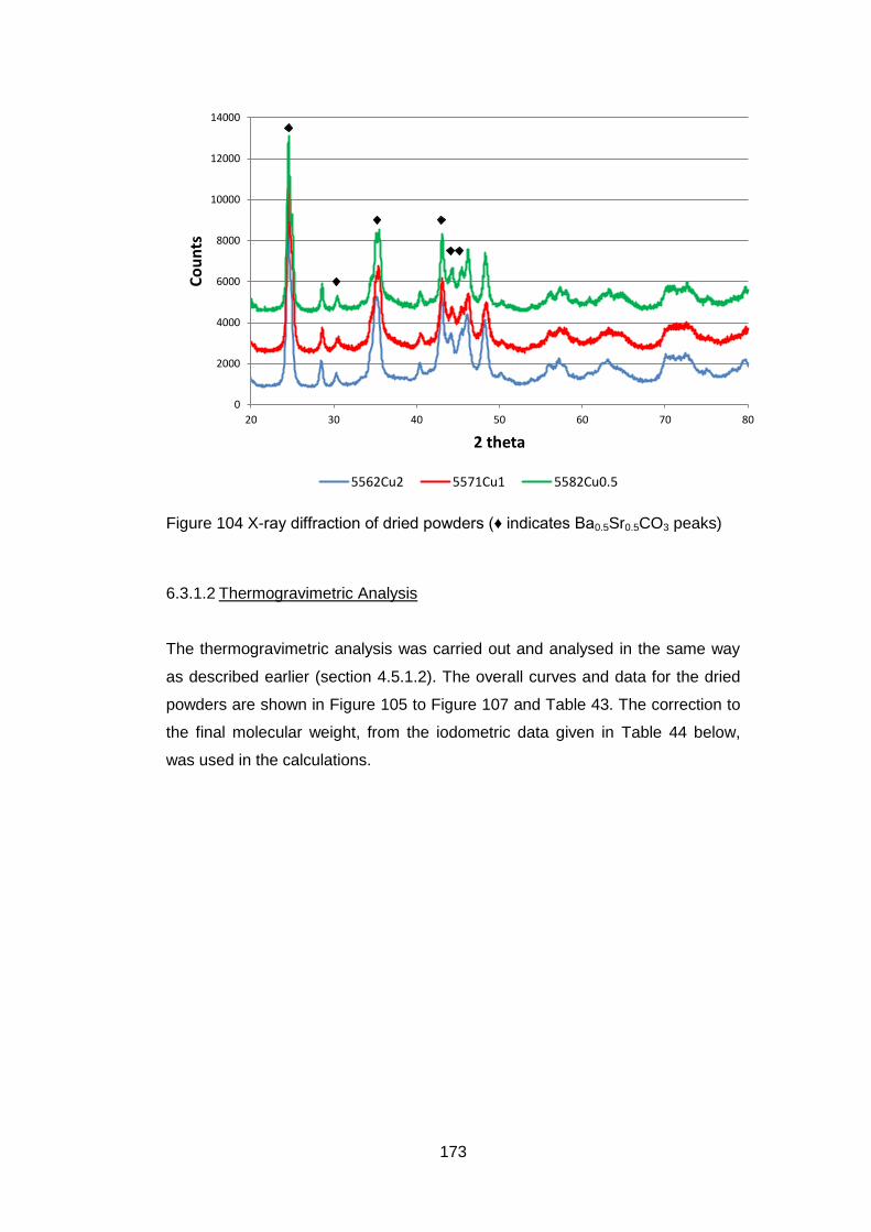
173

Figure 104 X-ray diffraction of dried powders (♦ indicates Ba0.5Sr0.5CO3 peaks)


The thermogravimetric analysis was carried out and analysed in the same way

as described earlier (section 4.5.1.2). The overall curves and data for the dried

powders are shown in Figure 105 to Figure 107 and Table 43. The correction to

the final molecular weight, from the iodometric data given in Table 44 below,

was used in the calculations.

0

2000

4000

6000

8000

10000

12000

14000

20 30 40 50 60 70 80

Co

un

ts

2 theta

5562Cu2 5571Cu1 5582Cu0.5

174

Figure 105 TGA of dried BSCF 5562Cu2 in air with a heating and cooling rate of

5K min-1

Figure 106 TGA of dried BSCF 5571Cu1 in air with a heating and cooling rate of

5K min-1

70

75

80

85

90

95

100

0 200 400 600 800 1000

Mas

s %

Temperature (/°C)

75

80

85

90

95

100

0 200 400 600 800 1000 1200

Mas

s %

Temperature (/°C)

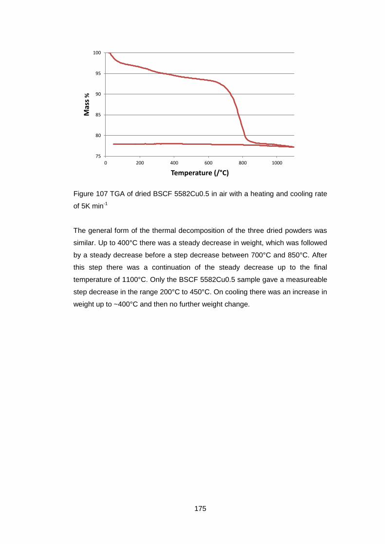
175

Figure 107 TGA of dried BSCF 5582Cu0.5 in air with a heating and cooling rate

of 5K min-1

The general form of the thermal decomposition of the three dried powders was

similar. Up to 400°C there was a steady decrease in weight, which was followed

by a steady decrease before a step decrease between 700°C and 850°C. After

this step there was a continuation of the steady decrease up to the final

temperature of 1100°C. Only the BSCF 5582Cu0.5 sample gave a measureable

step decrease in the range 200°C to 450°C. On cooling there was an increase in

weight up to ~400°C and then no further weight change.

75

80

85

90

95

100

0 200 400 600 800 1000

Mas

s %

Temperature (/°C)

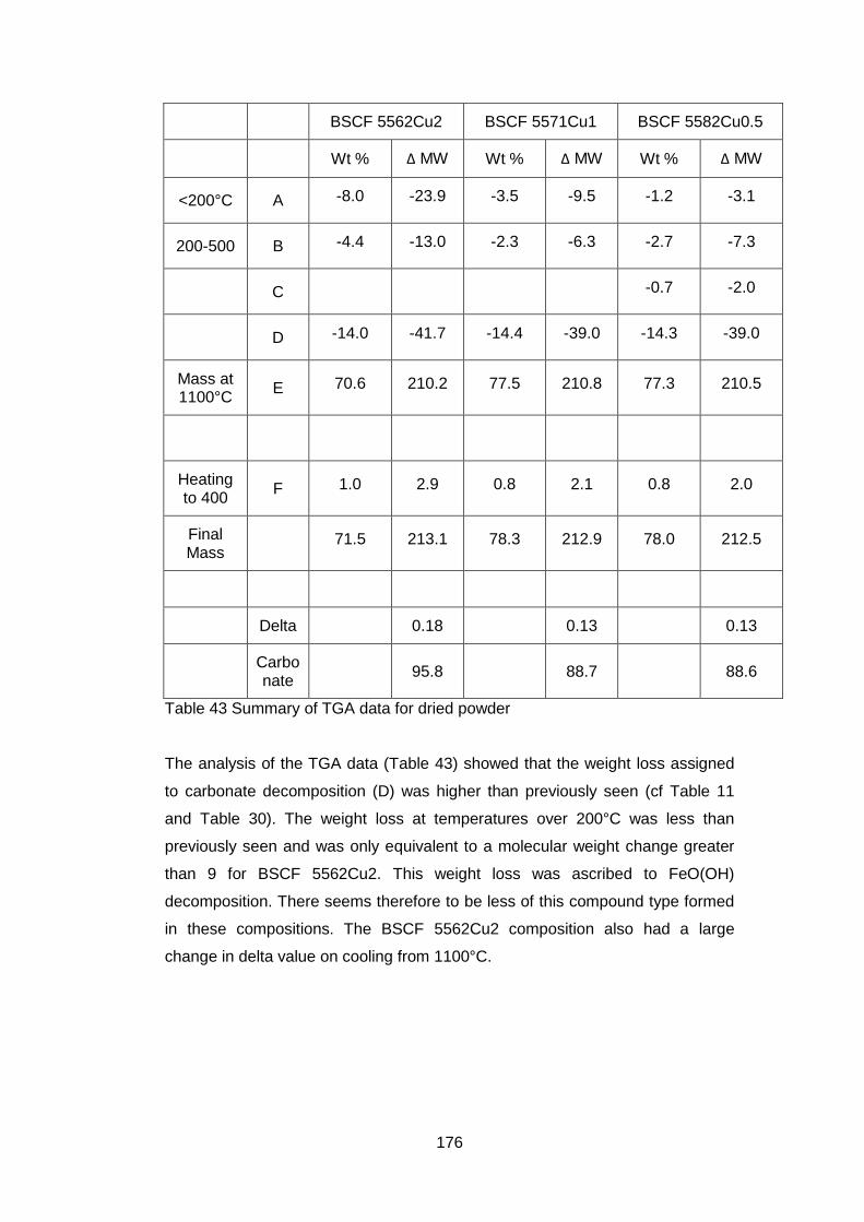
176

BSCF 5562Cu2 BSCF 5571Cu1 BSCF 5582Cu0.5

Wt % Δ MW Wt % Δ MW Wt % Δ MW

<200°C A -8.0 -23.9 -3.5 -9.5 -1.2 -3.1

200-500 B -4.4 -13.0 -2.3 -6.3 -2.7 -7.3

C -0.7 -2.0

D -14.0 -41.7 -14.4 -39.0 -14.3 -39.0

Mass at 1100°C

E 70.6 210.2 77.5 210.8 77.3 210.5

Heating to 400

F 1.0 2.9 0.8 2.1 0.8 2.0

Final Mass

71.5 213.1 78.3 212.9 78.0 212.5

Delta 0.18 0.13 0.13

Carbonate

95.8 88.7 88.6

Table 43 Summary of TGA data for dried powder

The analysis of the TGA data (Table 43) showed that the weight loss assigned

to carbonate decomposition (D) was higher than previously seen (cf Table 11

and Table 30). The weight loss at temperatures over 200°C was less than

previously seen and was only equivalent to a molecular weight change greater

than 9 for BSCF 5562Cu2. This weight loss was ascribed to FeO(OH)

decomposition. There seems therefore to be less of this compound type formed

in these compositions. The BSCF 5562Cu2 composition also had a large

change in delta value on cooling from 1100°C.

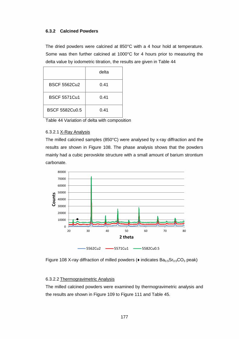
177

6.3.2 Calcined Powders

The dried powders were calcined at 850°C with a 4 hour hold at temperature.

Some was then further calcined at 1000°C for 4 hours prior to measuring the

delta value by iodometric titration, the results are given in Table 44

delta

BSCF 5562Cu2 0.41

BSCF 5571Cu1 0.41

BSCF 5582Cu0.5 0.41

Table 44 Variation of delta with composition


The milled calcined samples (850°C) were analysed by x-ray diffraction and the

results are shown in Figure 108. The phase analysis shows that the powders

mainly had a cubic perovskite structure with a small amount of barium strontium

carbonate.

Figure 108 X-ray diffraction of milled powders (♦ indicates Ba0.5Sr0.5CO3 peak)


The milled calcined powders were examined by thermogravimetric analysis and

the results are shown in Figure 109 to Figure 111 and Table 45.

0

10000

20000

30000

40000

50000

60000

70000

80000

20 30 40 50 60 70 80

Co

un

ts

2 theta

5562Cu2 5571Cu1 5582Cu0.5

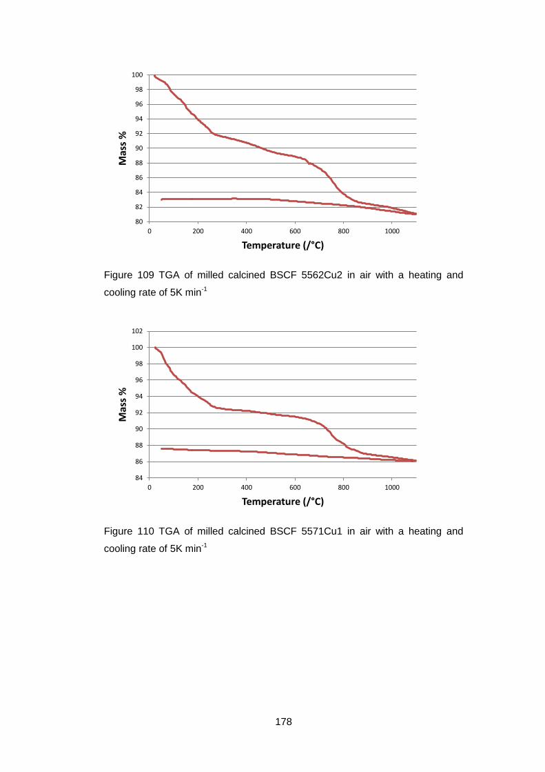
178

Figure 109 TGA of milled calcined BSCF 5562Cu2 in air with a heating and


Figure 110 TGA of milled calcined BSCF 5571Cu1 in air with a heating and


80

82

84

86

88

90

92

94

96

98

100

0 200 400 600 800 1000

Mas

s %

Temperature (/°C)

84

86

88

90

92

94

96

98

100

102

0 200 400 600 800 1000

Mas

s %

Temperature (/°C)

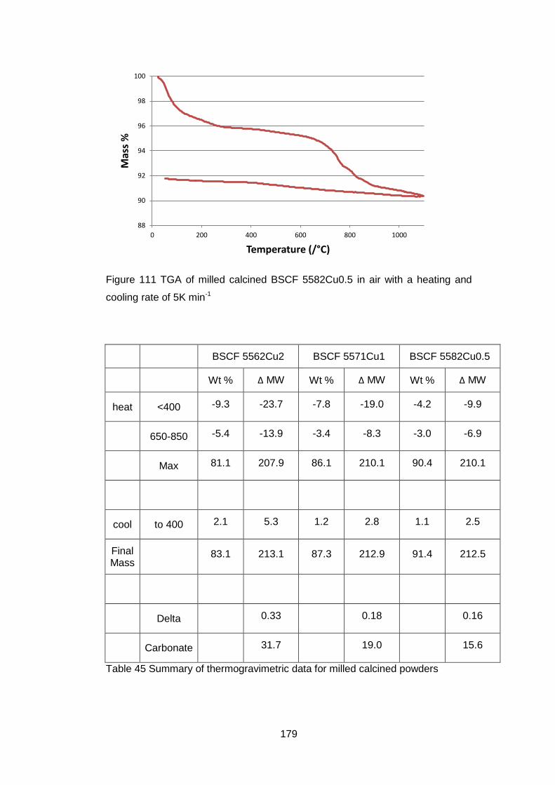
179

Figure 111 TGA of milled calcined BSCF 5582Cu0.5 in air with a heating and


BSCF 5562Cu2 BSCF 5571Cu1 BSCF 5582Cu0.5

Wt % Δ MW Wt % Δ MW Wt % Δ MW

heat <400 -9.3 -23.7 -7.8 -19.0 -4.2 -9.9

650-850 -5.4 -13.9 -3.4 -8.3 -3.0 -6.9

Max 81.1 207.9 86.1 210.1 90.4 210.1

cool to 400 2.1 5.3 1.2 2.8 1.1 2.5

Final Mass

83.1 213.1 87.3 212.9 91.4 212.5

Delta 0.33 0.18 0.16

Carbonate 31.7 19.0 15.6

Table 45 Summary of thermogravimetric data for milled calcined powders

88

90

92

94

96

98

100

0 200 400 600 800 1000

Mas

s %

Temperature (/°C)

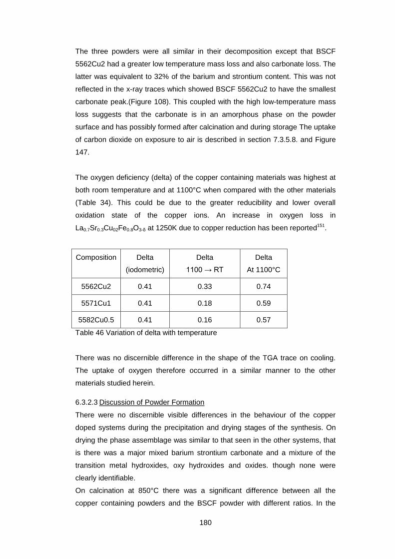
180

The three powders were all similar in their decomposition except that BSCF

5562Cu2 had a greater low temperature mass loss and also carbonate loss. The

latter was equivalent to 32% of the barium and strontium content. This was not

reflected in the x-ray traces which showed BSCF 5562Cu2 to have the smallest

carbonate peak.(Figure 108). This coupled with the high low-temperature mass

loss suggests that the carbonate is in an amorphous phase on the powder

surface and has possibly formed after calcination and during storage The uptake

of carbon dioxide on exposure to air is described in section 7.3.5.8. and Figure

147.

The oxygen deficiency (delta) of the copper containing materials was highest at

both room temperature and at 1100°C when compared with the other materials

(Table 34). This could be due to the greater reducibility and lower overall

oxidation state of the copper ions. An increase in oxygen loss in

La0.7Sr0.3Cu02Fe0.8O3-δ at 1250K due to copper reduction has been reported151.

Composition Delta

(iodometric)

Delta

1100 → RT

Delta

At 1100°C

5562Cu2 0.41 0.33 0.74

5571Cu1 0.41 0.18 0.59

5582Cu0.5 0.41 0.16 0.57

Table 46 Variation of delta with temperature

There was no discernible difference in the shape of the TGA trace on cooling.

The uptake of oxygen therefore occurred in a similar manner to the other

materials studied herein.


There were no discernible visible differences in the behaviour of the copper

doped systems during the precipitation and drying stages of the synthesis. On

drying the phase assemblage was similar to that seen in the other systems, that

is there was a major mixed barium strontium carbonate and a mixture of the

transition metal hydroxides, oxy hydroxides and oxides. though none were

clearly identifiable.

On calcination at 850°C there was a significant difference between all the

copper containing powders and the BSCF powder with different ratios. In the

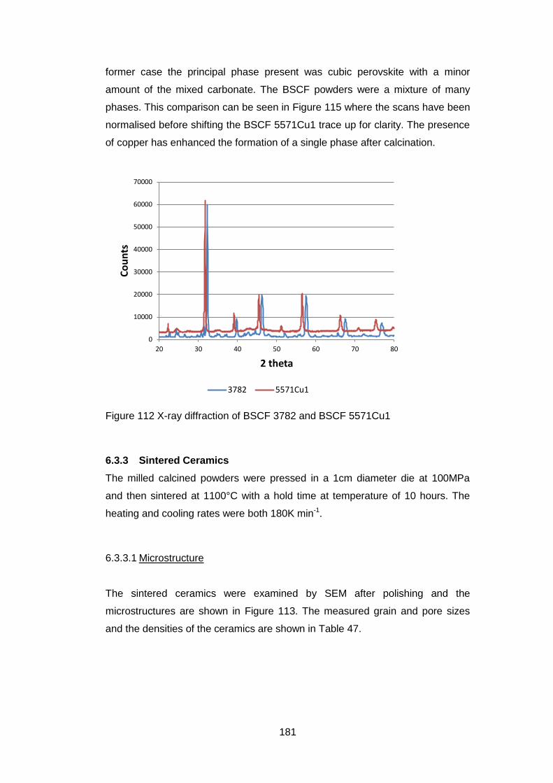
181

former case the principal phase present was cubic perovskite with a minor

amount of the mixed carbonate. The BSCF powders were a mixture of many

phases. This comparison can be seen in Figure 115 where the scans have been

normalised before shifting the BSCF 5571Cu1 trace up for clarity. The presence

of copper has enhanced the formation of a single phase after calcination.

Figure 112 X-ray diffraction of BSCF 3782 and BSCF 5571Cu1


The milled calcined powders were pressed in a 1cm diameter die at 100MPa

and then sintered at 1100°C with a hold time at temperature of 10 hours. The

heating and cooling rates were both 180K min-1.


The sintered ceramics were examined by SEM after polishing and the

microstructures are shown in Figure 113. The measured grain and pore sizes

and the densities of the ceramics are shown in Table 47.

0

10000

20000

30000

40000

50000

60000

70000

20 30 40 50 60 70 80

Co

un

ts

2 theta

3782 5571Cu1

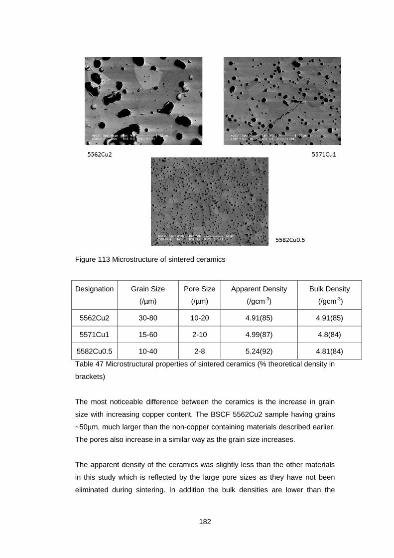
182

Figure 113 Microstructure of sintered ceramics

Designation Grain Size

(/µm)

Pore Size

(/µm)

Apparent Density

(/gcm-3)

Bulk Density

(/gcm-3)

5562Cu2 30-80 10-20 4.91(85) 4.91(85)

5571Cu1 15-60 2-10 4.99(87) 4.8(84)

5582Cu0.5 10-40 2-8 5.24(92) 4.81(84)

Table 47 Microstructural properties of sintered ceramics (% theoretical density in

brackets)

The most noticeable difference between the ceramics is the increase in grain

size with increasing copper content. The BSCF 5562Cu2 sample having grains

~50µm, much larger than the non-copper containing materials described earlier.

The pores also increase in a similar way as the grain size increases.

The apparent density of the ceramics was slightly less than the other materials

in this study which is reflected by the large pore sizes as they have not been

eliminated during sintering. In addition the bulk densities are lower than the

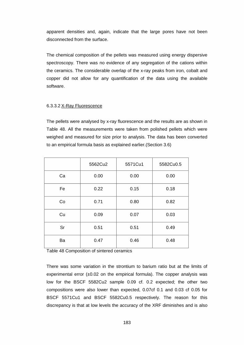
183

apparent densities and, again, indicate that the large pores have not been

disconnected from the surface.

The chemical composition of the pellets was measured using energy dispersive

spectroscopy. There was no evidence of any segregation of the cations within

the ceramics. The considerable overlap of the x-ray peaks from iron, cobalt and

copper did not allow for any quantification of the data using the available

software.

6.3.3.2 X-Ray Fluorescence


Table 48. All the measurements were taken from polished pellets which were

weighed and measured for size prior to analysis. The data has been converted

to an empirical formula basis as explained earlier.(Section 3.6)

5562Cu2 5571Cu1 5582Cu0.5

Ca 0.00 0.00 0.00

Fe 0.22 0.15 0.18

Co 0.71 0.80 0.82

Cu 0.09 0.07 0.03

Sr 0.51 0.51 0.49

Ba 0.47 0.46 0.48

Table 48 Composition of sintered ceramics

There was some variation in the strontium to barium ratio but at the limits of

experimental error (±0.02 on the empirical formula). The copper analysis was

low for the BSCF 5582Cu2 sample 0.09 cf. 0.2 expected; the other two

compositions were also lower than expected, 0.07cf 0.1 and 0.03 cf 0.05 for

BSCF 5571Cu1 and BSCF 5582Cu0.5 respectively. The reason for this

discrepancy is that at low levels the accuracy of the XRF diminishes and is also

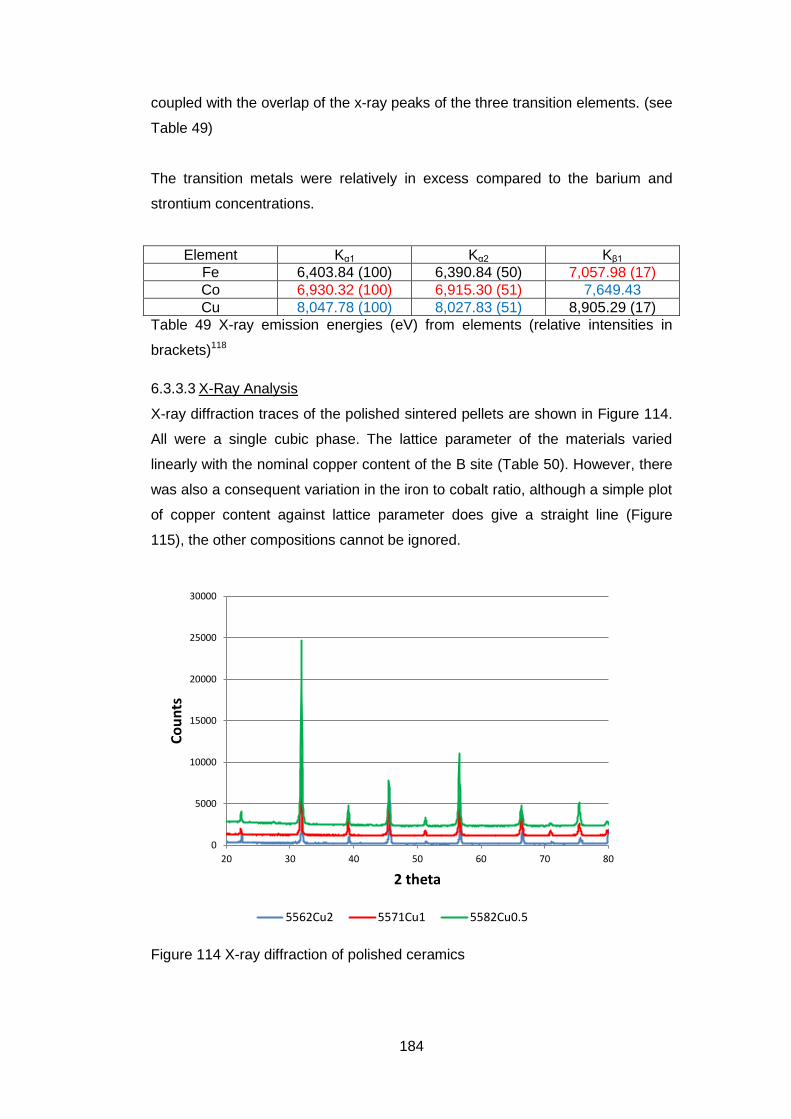
184

coupled with the overlap of the x-ray peaks of the three transition elements. (see

Table 49)

The transition metals were relatively in excess compared to the barium and

strontium concentrations.

Element Kα1 Kα2 Kβ1

Fe 6,403.84 (100) 6,390.84 (50) 7,057.98 (17)

Co 6,930.32 (100) 6,915.30 (51) 7,649.43

Cu 8,047.78 (100) 8,027.83 (51) 8,905.29 (17)

Table 49 X-ray emission energies (eV) from elements (relative intensities in

brackets)118


X-ray diffraction traces of the polished sintered pellets are shown in Figure 114.

All were a single cubic phase. The lattice parameter of the materials varied

linearly with the nominal copper content of the B site (Table 50). However, there

was also a consequent variation in the iron to cobalt ratio, although a simple plot

of copper content against lattice parameter does give a straight line (Figure

115), the other compositions cannot be ignored.

Figure 114 X-ray diffraction of polished ceramics

0

5000

10000

15000

20000

25000

30000

20 30 40 50 60 70 80

Co

un

ts

2 theta

5562Cu2 5571Cu1 5582Cu0.5

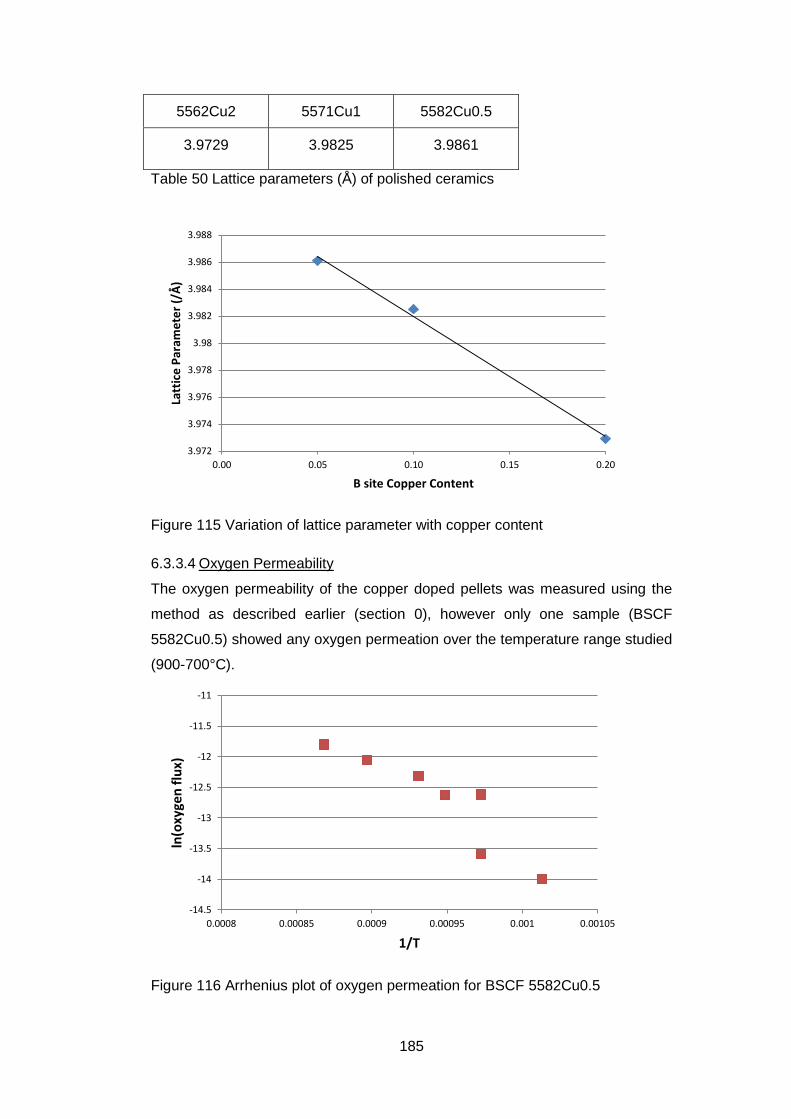
185

5562Cu2 5571Cu1 5582Cu0.5

3.9729 3.9825 3.9861

Table 50 Lattice parameters (Å) of polished ceramics

Figure 115 Variation of lattice parameter with copper content


The oxygen permeability of the copper doped pellets was measured using the

method as described earlier (section 0), however only one sample (BSCF

5582Cu0.5) showed any oxygen permeation over the temperature range studied

(900-700°C).

Figure 116 Arrhenius plot of oxygen permeation for BSCF 5582Cu0.5

3.972

3.974

3.976

3.978

3.98

3.982

3.984

3.986

3.988

0.00 0.05 0.10 0.15 0.20

Latt

ice

Par

ame

ter

(/Å

)

B site Copper Content

-14.5

-14

-13.5

-13

-12.5

-12

-11.5

-11

0.0008 0.00085 0.0009 0.00095 0.001 0.00105

ln(o

xyge

n f

lux)

1/T

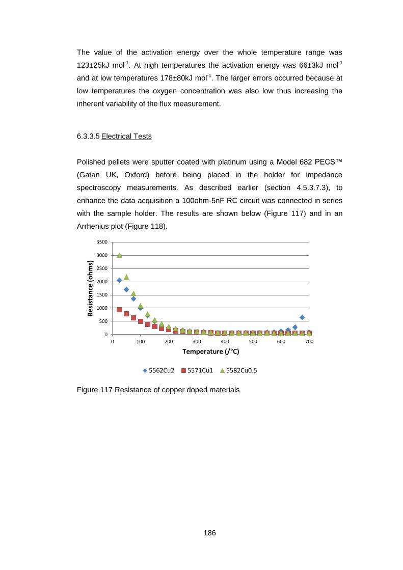
186

The value of the activation energy over the whole temperature range was

123±25kJ mol-1. At high temperatures the activation energy was 66±3kJ mol-1

and at low temperatures 178±80kJ mol-1. The larger errors occurred because at

low temperatures the oxygen concentration was also low thus increasing the

inherent variability of the flux measurement.


Polished pellets were sputter coated with platinum using a Model 682 PECS™

(Gatan UK, Oxford) before being placed in the holder for impedance

spectroscopy measurements. As described earlier (section 4.5.3.7.3), to

enhance the data acquisition a 100ohm-5nF RC circuit was connected in series

with the sample holder. The results are shown below (Figure 117) and in an

Arrhenius plot (Figure 118).

Figure 117 Resistance of copper doped materials

0

500

1000

1500

2000

2500

3000

3500

0 100 200 300 400 500 600 700

Re

sist

ance

(o

hm

s)

Temperature (/°C)

5562Cu2 5571Cu1 5582Cu0.5

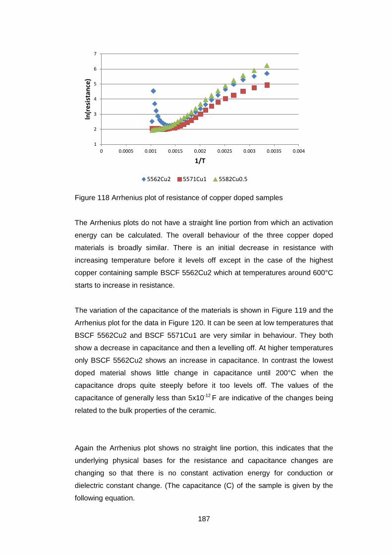
187

Figure 118 Arrhenius plot of resistance of copper doped samples

The Arrhenius plots do not have a straight line portion from which an activation

energy can be calculated. The overall behaviour of the three copper doped

materials is broadly similar. There is an initial decrease in resistance with

increasing temperature before it levels off except in the case of the highest

copper containing sample BSCF 5562Cu2 which at temperatures around 600°C

starts to increase in resistance.

The variation of the capacitance of the materials is shown in Figure 119 and the

Arrhenius plot for the data in Figure 120. It can be seen at low temperatures that

BSCF 5562Cu2 and BSCF 5571Cu1 are very similar in behaviour. They both

show a decrease in capacitance and then a levelling off. At higher temperatures

only BSCF 5562Cu2 shows an increase in capacitance. In contrast the lowest

doped material shows little change in capacitance until 200°C when the

capacitance drops quite steeply before it too levels off. The values of the

capacitance of generally less than 5x10-12 F are indicative of the changes being

related to the bulk properties of the ceramic.

Again the Arrhenius plot shows no straight line portion, this indicates that the

underlying physical bases for the resistance and capacitance changes are

changing so that there is no constant activation energy for conduction or

dielectric constant change. (The capacitance (C) of the sample is given by the

following equation.

1

2

3

4

5

6

7

0 0.0005 0.001 0.0015 0.002 0.0025 0.003 0.0035 0.004

ln(r

esis

tan

ce)

1/T

5562Cu2 5571Cu1 5582Cu0.5

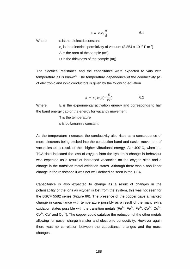
188

6.1

Where εr is the dielectric constant

ε0 is the electrical permittivity of vacuum (8.854 x 10-12 F m-1)

A is the area of the sample (m2)

D is the thickness of the sample (m))

The electrical resistance and the capacitance were expected to vary with

temperature as is known6. The temperature dependence of the conductivity (σ)

of electronic and ionic conductors is given by the following equation

6.2

Where E is the experimental activation energy and corresponds to half

the band energy gap or the energy for vacancy movement

T is the temperature

κ is boltzmann’s constant.

As the temperature increases the conductivity also rises as a consequence of

more electrons being excited into the conduction band and easier movement of

vacancies as a result of their higher vibrational energy. At ~400°C, when the

TGA data indicated the loss of oxygen from the system a change in behaviour

was expected as a result of increased vacancies on the oxygen sites and a

change in the transition metal oxidation states. Although there was a non-linear

change in the resistance it was not well defined as seen in the TGA.

Capacitance is also expected to change as a result of changes in the

polarisability of the ions as oxygen is lost from the system, this was not seen for

the BSCF 5582 series (Figure 86). The presence of the copper gave a marked

change in capacitance with temperature possibly as a result of the many extra

oxidation states possible with the transition metals (Fe2+, Fe3+, Fe4+, Co2+, Co3+,

Co4+, Cu+ and Cu2+). The copper could catalyse the reduction of the other metals

allowing for easier charge transfer and electronic conductivity. However again

there was no correlation between the capacitance changes and the mass

changes.

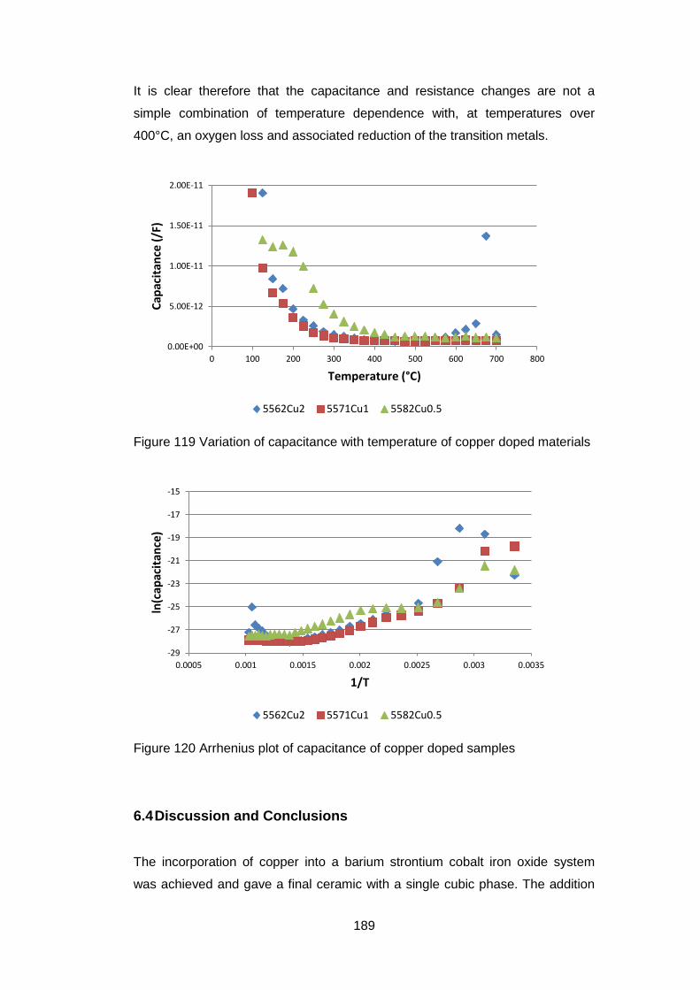
189

It is clear therefore that the capacitance and resistance changes are not a

simple combination of temperature dependence with, at temperatures over

400°C, an oxygen loss and associated reduction of the transition metals.

Figure 119 Variation of capacitance with temperature of copper doped materials

Figure 120 Arrhenius plot of capacitance of copper doped samples


The incorporation of copper into a barium strontium cobalt iron oxide system

was achieved and gave a final ceramic with a single cubic phase. The addition

0.00E+00

5.00E-12

1.00E-11

1.50E-11

2.00E-11

0 100 200 300 400 500 600 700 800

Cap

acit

ance

(/F

)

Temperature (°C)

5562Cu2 5571Cu1 5582Cu0.5

-29

-27

-25

-23

-21

-19

-17

-15

0.0005 0.001 0.0015 0.002 0.0025 0.003 0.0035

ln(c

apac

itan

ce)

1/T

5562Cu2 5571Cu1 5582Cu0.5

190

of the copper allowed much greater grain growth to occur though it was not

accompanied by a comparable increase in densification. In addition the oxide

phase development on calcining was more complete at 850°C than with the

other materials synthesised. The melting at 950°C when CuO was used as a

sintering aid143 was not seen because the reactions of the copper compounds

were complete at 850°C to give a system which did not subsequently melt

incongruously.

The iodometric titrations, coupled with the thermogravimetric analysis on

cooling, indicated that the final oxides were more oxygen deficient than the

previously discussed samples, with delta values of 0.41 for the three samples on

the 1000°C calcined powders. In addition there was an additional high loss of

oxygen at high temperature for BSCF 5562Cu2 which gave a final delta value of

0.74. The assignment of formal oxidation states between the three cations on

the B site could not be made with the available data. (The determination of the

oxidation states in BSCF 5582 was one of the objectives of the high temperature

XPS and is discussed in Chapter 7.3 below).

However if the following assumptions are made, some conclusions can be

drawn.

1. Barium and strontium ions are always 2+

2. Oxygen ions are always 2-

3. The nominal compositions will be used for the analysis.

If the contribution of the copper is not fixed then the net B site cation oxidation

state is as shown in Table 51. Although the same at room temperature there is a

widening difference in the oxidation state as the temperature increases.

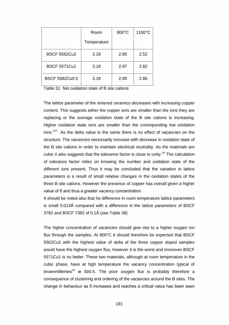
191

Room

Temperature

800°C 1100°C

BSCF 5562Cu2 3.18 2.80 2.52

BSCF 5571Cu1 3.18 2.97 2.82

BSCF 5582Cu0.5 3.18 2.99 2.86

Table 51 Net oxidation state of B site cations

The lattice parameter of the sintered ceramics decreases with increasing copper

content. This suggests either the copper ions are smaller than the ions they are

replacing or the average oxidation state of the B site cations is increasing.

Higher oxidation state ions are smaller than the corresponding low oxidation

ions.107 As the delta value is the same there is no effect of vacancies on the

structure. The vacancies necessarily increase with decrease in oxidation state of

the B site cations in order to maintain electrical neutrality. As the materials are

cubic it also suggests that the tolerance factor is close to unity.24 The calculation

of tolerance factor relies on knowing the number and oxidation state of the

different ions present. Thus it may be concluded that the variation in lattice

parameters is a result of small relative changes in the oxidation states of the

three B site cations. However the presence of copper has overall given a higher

value of δ and thus a greater vacancy concentration.

It should be noted also that he difference in room temperature lattice parameters

is small 0.013Å compared with a difference in the lattice parameters of BSCF

3782 and BSCF 7382 of 0.1Å (see Table 38).

The higher concentration of vacancies should give rise to a higher oxygen ion

flux through the samples. At 800°C it should therefore be expected that BSCF

5562Cu2 with the highest value of delta of the three copper doped samples

would have the highest oxygen flux, however it is the worst and moreover BSCF

5571Cu1 is no better. These two materials, although at room temperature in the

cubic phase, have at high temperature the vacancy concentration typical of

brownmillerites20 ie δ≥0.5. The poor oxygen flux is probably therefore a

consequence of clustering and ordering of the vacancies around the B sites. The

change in behaviour as δ increases and reaches a critical value has been seen

192

as the oxygen partial pressure is varied at constant temperature with changes at

δ=0 and δ=0.5.149

The changes in electrical conductivity with temperature and composition can be

rationalised in terms of the changes in oxygen vacancies and the B site cation

oxidation state. The electronic conduction is due to electron transfer between B

cation sites. In order to have the net oxidation states of 2.52 to 3.18 then there

will be a range of oxidation states from M2+ to M4+. The split of these among the

three B site cations is unknown. However the ratios will be dependent on the

temperature in two ways. Firstly the relative energies of the ionisation reactions

shown below (equation 6.3) will vary and thus the most stable cation will vary

with temperature.( An illustrative example is given in equation 6.4)

6.3

6.4

Thus to begin with there is a gradual drop in resistance as is typical for mixed

conductors and then it plateaus out before stating to rise at high temperatures

for the BSCF5562Cu2 sample. This last behaviour is probably due to the more

extensive reduction of the B site cations which reduces the number of available

sites able to accept an electron during the conduction process.

The capacitance varies in a similar way and reflects the underlying relaxation

times for the process. At first the hopping frequency becomes faster before

slowing down as the potential sites is reduced.

Although the oxygen permeation and electrical properties of the copper doped

materials are qualitatively different their dependence on the structural and

chemical makeup of the materials is similar. The lowest addition level of copper

was beneficial in terms of the desired oxygen flux but at higher levels no flow

occurred. As was shown earlier the presence of copper was beneficial for

sintering behaviour143 but there were only positive effects on permeation at the

lowest level of addition.

193

7 In situ High Temperature Studies

7.1 Introduction In their applications, BSCF ceramics are used at high temperatures >500°C. As

has been described earlier, a number of properties of the material changes on

heating most notably the oxygen content and the electrical properties. In order to

ascertain the nature and possibly the mechanisms of these changes in situ high

temperature examinations of BSCF 5582 were undertaken. Two techniques

were chosen, x-ray diffraction and x-ray photoelectron spectroscopy both using

in situ heating so that the samples could be analysed at temperature as well as

after a heating cycle.

The objectives of the x-ray diffraction were to determine whether there were any

changes in lattice parameter, phase composition and oxygen site occupancy

during heating and cooling of a sample in air. The TGA data presented earlier

showed a weight loss at temperatures over ~400°C ascribed to oxygen loss

during heating, it was hoped that this could be followed by the x-ray diffraction

The objectives of the x-ray photoelectron spectroscopy were to understand the

oxidation states in BSCF 5582 in particular cobalt and iron, to see if in BSCF

5582 the oxygen environment changes with temperature and, if possible, to

determine if a low - high spin transition occurs on heating BSCF 5582. The

iodometric titrations described earlier gave a value for δ, the oxygen non-

stoichiometry. However they could not show whether the reduction of the iron

and cobalt from M4+ to M3+ or M2+ occurred equally with either ions or just one

was preferentially reduced.

7.2 High temperature X-Ray Diffraction

7.2.1 Equipment

The high temperature x-ray diffraction equipment in the Department of

Chemistry was used. This consisted of a Philips diffractometer fitted with an

XRK Reactor chamber (Anton Parr GmbH). This was capable of reaching 900°C

in air. The diffractometer had a position sensitive detector which meant good

spectra could be obtained with a 20 minute scan.

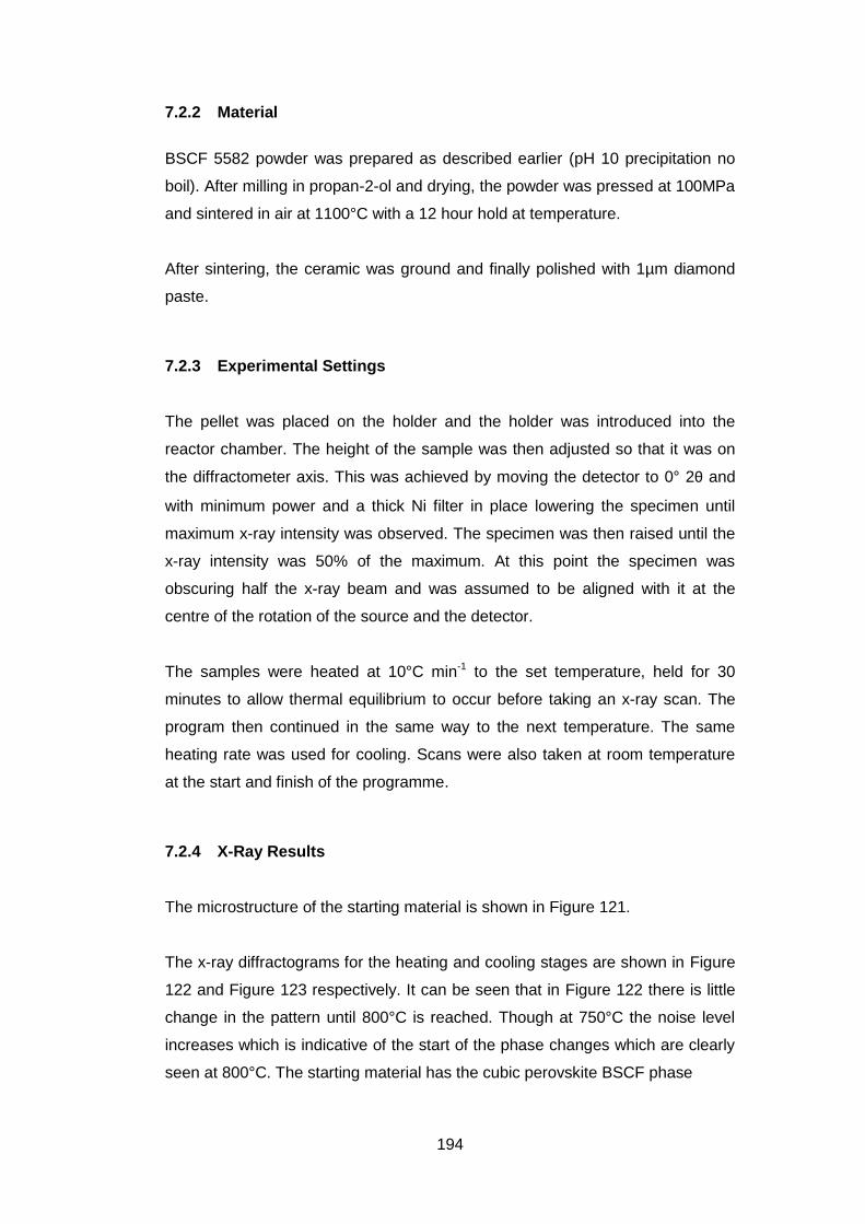
194

7.2.2 Material

BSCF 5582 powder was prepared as described earlier (pH 10 precipitation no

boil). After milling in propan-2-ol and drying, the powder was pressed at 100MPa

and sintered in air at 1100°C with a 12 hour hold at temperature.

After sintering, the ceramic was ground and finally polished with 1µm diamond

paste.

7.2.3 Experimental Settings

The pellet was placed on the holder and the holder was introduced into the

reactor chamber. The height of the sample was then adjusted so that it was on

the diffractometer axis. This was achieved by moving the detector to 0° 2θ and

with minimum power and a thick Ni filter in place lowering the specimen until

maximum x-ray intensity was observed. The specimen was then raised until the

x-ray intensity was 50% of the maximum. At this point the specimen was

obscuring half the x-ray beam and was assumed to be aligned with it at the

centre of the rotation of the source and the detector.

The samples were heated at 10°C min-1 to the set temperature, held for 30

minutes to allow thermal equilibrium to occur before taking an x-ray scan. The

program then continued in the same way to the next temperature. The same

heating rate was used for cooling. Scans were also taken at room temperature

at the start and finish of the programme.

7.2.4 X-Ray Results

The microstructure of the starting material is shown in Figure 121.

The x-ray diffractograms for the heating and cooling stages are shown in Figure

122 and Figure 123 respectively. It can be seen that in Figure 122 there is little

change in the pattern until 800°C is reached. Though at 750°C the noise level

increases which is indicative of the start of the phase changes which are clearly

seen at 800°C. The starting material has the cubic perovskite BSCF phase

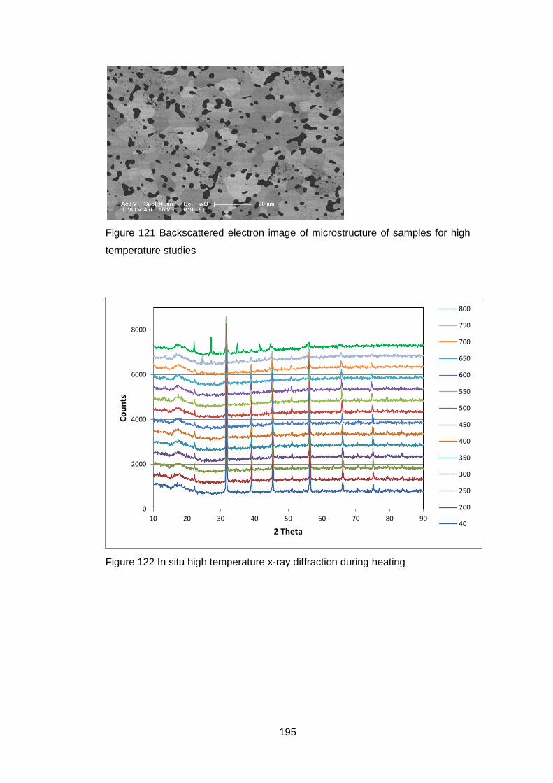
195

Figure 121 Backscattered electron image of microstructure of samples for high

temperature studies

Figure 122 In situ high temperature x-ray diffraction during heating

0

2000

4000

6000

8000

10 20 30 40 50 60 70 80 90

Co

un

ts

2 Theta

800

750

700

650

600

550

500

450

400

350

300

250

200

40

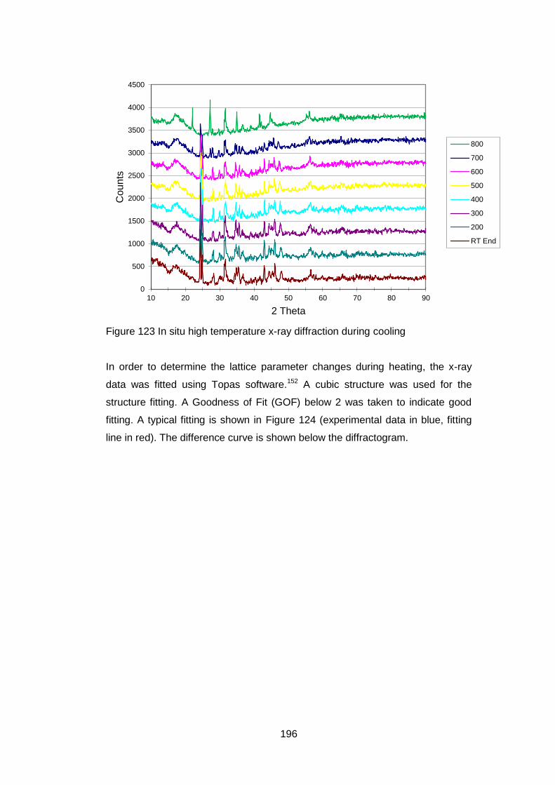
196

Figure 123 In situ high temperature x-ray diffraction during cooling

In order to determine the lattice parameter changes during heating, the x-ray

data was fitted using Topas software.152 A cubic structure was used for the

structure fitting. A Goodness of Fit (GOF) below 2 was taken to indicate good

fitting. A typical fitting is shown in Figure 124 (experimental data in blue, fitting

line in red). The difference curve is shown below the diffractogram.

0

500

1000

1500

2000

2500

3000

3500

4000

4500

10 20 30 40 50 60 70 80 90

Co

un

ts

2 Theta

800

700

600

500

400

300

200

RT End

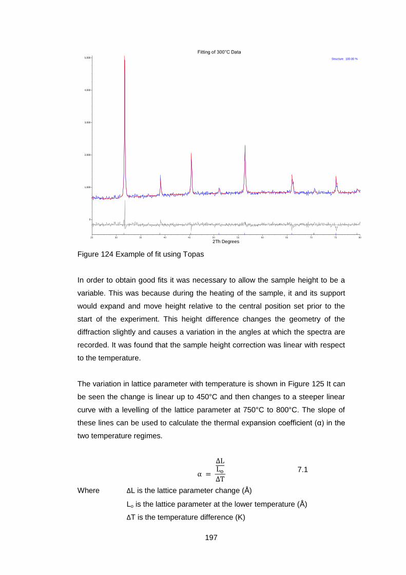
197

Figure 124 Example of fit using Topas

In order to obtain good fits it was necessary to allow the sample height to be a

variable. This was because during the heating of the sample, it and its support

would expand and move height relative to the central position set prior to the

start of the experiment. This height difference changes the geometry of the

diffraction slightly and causes a variation in the angles at which the spectra are

recorded. It was found that the sample height correction was linear with respect

to the temperature.

The variation in lattice parameter with temperature is shown in Figure 125 It can

be seen the change is linear up to 450°C and then changes to a steeper linear

curve with a levelling of the lattice parameter at 750°C to 800°C. The slope of

these lines can be used to calculate the thermal expansion coefficient (α) in the

two temperature regimes.

7.1

Where ΔL is the lattice parameter change (Å)

Lo is the lattice parameter at the lower temperature (Å)

ΔT is the temperature difference (K)

Fitting of 300°C Data

2Th Degrees807570656055504540353025

Co

un

ts

5,000

4,000

3,000

2,000

1,000

0

Structure 100.00 %

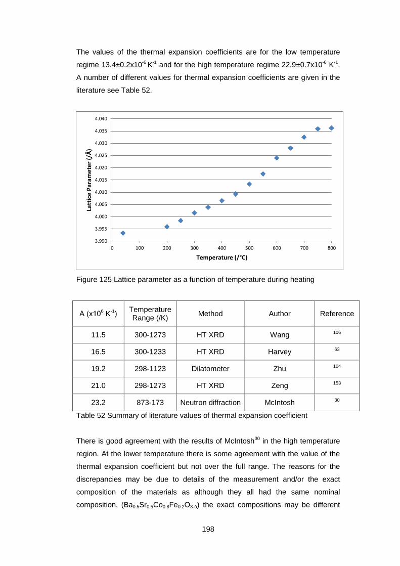
198

The values of the thermal expansion coefficients are for the low temperature

regime 13.4±0.2x10-6 K-1 and for the high temperature regime 22.9±0.7x10-6 K-1.

A number of different values for thermal expansion coefficients are given in the

literature see Table 52.

Figure 125 Lattice parameter as a function of temperature during heating

Α (x106 K-1) Temperature Range (/K)

Method Author Reference

11.5 300-1273 HT XRD Wang 106

16.5 300-1233 HT XRD Harvey 63

19.2 298-1123 Dilatometer Zhu 104

21.0 298-1273 HT XRD Zeng 153

23.2 873-173 Neutron diffraction McIntosh 30

Table 52 Summary of literature values of thermal expansion coefficient

There is good agreement with the results of McIntosh30 in the high temperature

region. At the lower temperature there is some agreement with the value of the

thermal expansion coefficient but not over the full range. The reasons for the

discrepancies may be due to details of the measurement and/or the exact

composition of the materials as although they all had the same nominal

composition, (Ba0.5Sr0.5Co0.8Fe0.2O3-δ) the exact compositions may be different

3.990

3.995

4.000

4.005

4.010

4.015

4.020

4.025

4.030

4.035

4.040

0 100 200 300 400 500 600 700 800

Latt

ice

Par

ame

ter

(/Å

)

Temperature (/°C)

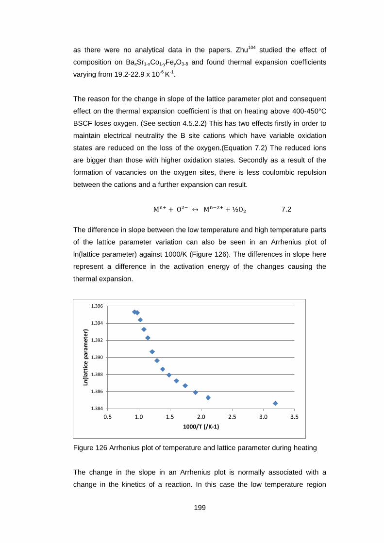
199

as there were no analytical data in the papers. Zhu104 studied the effect of

composition on BaxSr1-xCo1-yFeyO3-δ and found thermal expansion coefficients

varying from 19.2-22.9 x 10-6 K-1.

The reason for the change in slope of the lattice parameter plot and consequent

effect on the thermal expansion coefficient is that on heating above 400-450°C

BSCF loses oxygen. (See section 4.5.2.2) This has two effects firstly in order to

maintain electrical neutrality the B site cations which have variable oxidation

states are reduced on the loss of the oxygen.(Equation 7.2) The reduced ions

are bigger than those with higher oxidation states. Secondly as a result of the

formation of vacancies on the oxygen sites, there is less coulombic repulsion

between the cations and a further expansion can result.

7.2

The difference in slope between the low temperature and high temperature parts

of the lattice parameter variation can also be seen in an Arrhenius plot of

ln(lattice parameter) against 1000/K (Figure 126). The differences in slope here

represent a difference in the activation energy of the changes causing the

thermal expansion.

Figure 126 Arrhenius plot of temperature and lattice parameter during heating

The change in the slope in an Arrhenius plot is normally associated with a

change in the kinetics of a reaction. In this case the low temperature region

1.384

1.386

1.388

1.390

1.392

1.394

1.396

0.5 1.0 1.5 2.0 2.5 3.0 3.5

Ln(l

atti

ce p

aram

ete

r)

1000/T (/K-1)

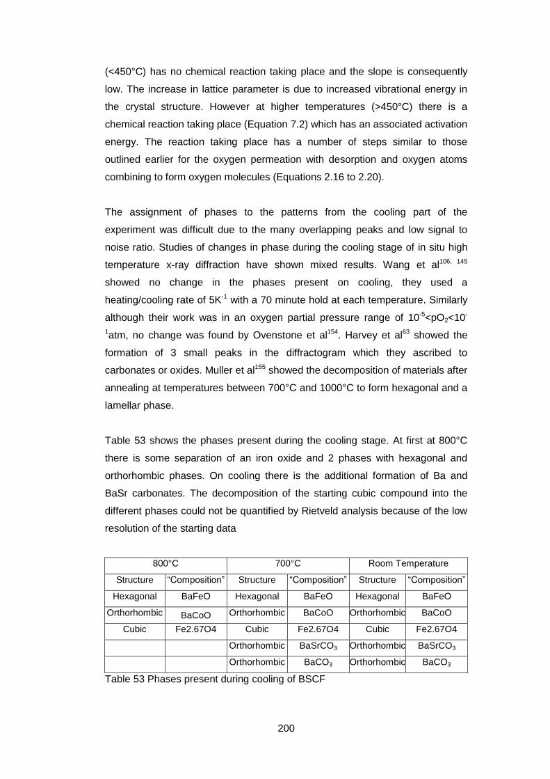
200

(<450°C) has no chemical reaction taking place and the slope is consequently

low. The increase in lattice parameter is due to increased vibrational energy in

the crystal structure. However at higher temperatures (>450°C) there is a

chemical reaction taking place (Equation 7.2) which has an associated activation

energy. The reaction taking place has a number of steps similar to those

outlined earlier for the oxygen permeation with desorption and oxygen atoms

combining to form oxygen molecules (Equations 2.16 to 2.20).

The assignment of phases to the patterns from the cooling part of the

experiment was difficult due to the many overlapping peaks and low signal to

noise ratio. Studies of changes in phase during the cooling stage of in situ high

temperature x-ray diffraction have shown mixed results. Wang et al106, 145

showed no change in the phases present on cooling, they used a

heating/cooling rate of 5K-1 with a 70 minute hold at each temperature. Similarly

although their work was in an oxygen partial pressure range of 10-5<pO2<10-

1atm, no change was found by Ovenstone et al154. Harvey et al63 showed the

formation of 3 small peaks in the diffractogram which they ascribed to

carbonates or oxides. Muller et al155 showed the decomposition of materials after

annealing at temperatures between 700°C and 1000°C to form hexagonal and a

lamellar phase.

Table 53 shows the phases present during the cooling stage. At first at 800°C

there is some separation of an iron oxide and 2 phases with hexagonal and

orthorhombic phases. On cooling there is the additional formation of Ba and

BaSr carbonates. The decomposition of the starting cubic compound into the

different phases could not be quantified by Rietveld analysis because of the low

resolution of the starting data

800°C 700°C Room Temperature

Structure “Composition” Structure “Composition” Structure “Composition”

Hexagonal BaFeO Hexagonal BaFeO Hexagonal BaFeO

Orthorhombic BaCoO Orthorhombic BaCoO Orthorhombic BaCoO

Cubic Fe2.67O4 Cubic Fe2.67O4 Cubic Fe2.67O4

Orthorhombic BaSrCO3 Orthorhombic BaSrCO3

Orthorhombic BaCO3 Orthorhombic BaCO3

Table 53 Phases present during cooling of BSCF

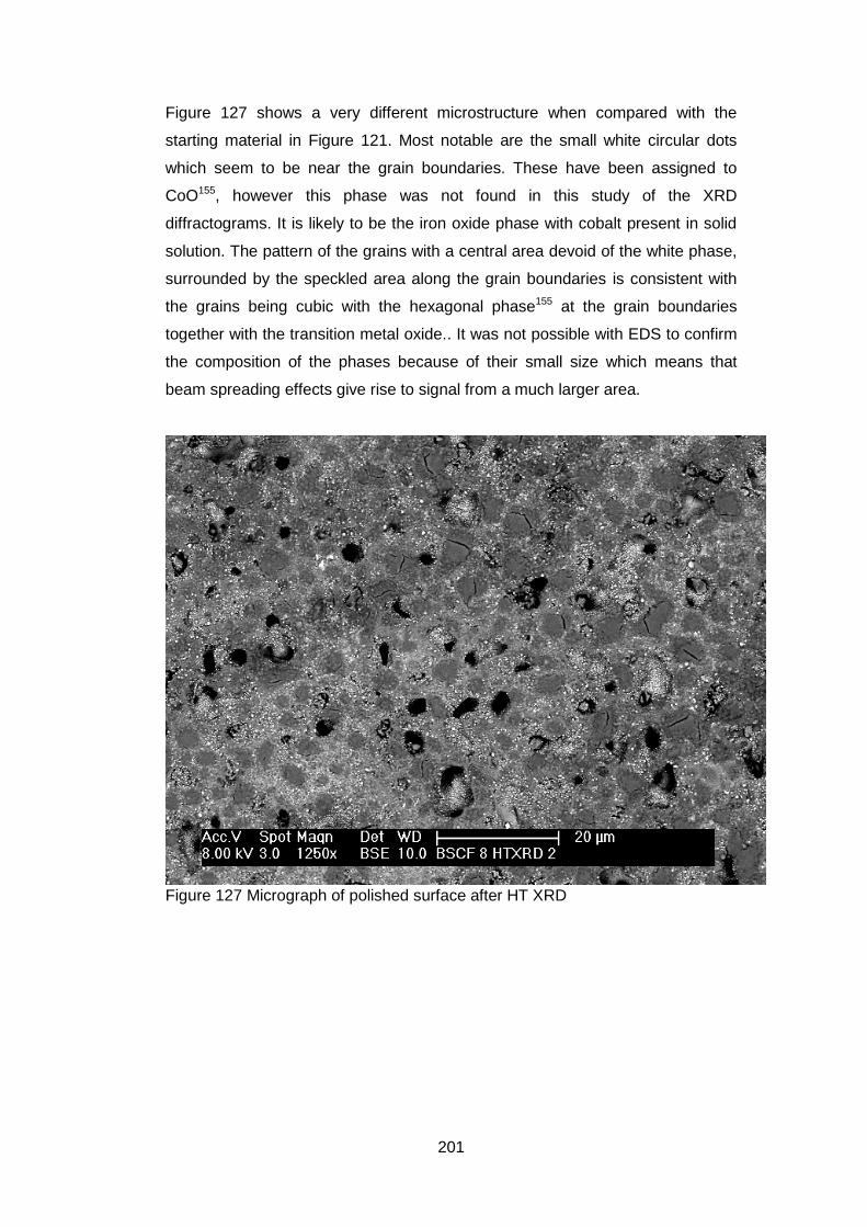
201

Figure 127 shows a very different microstructure when compared with the

starting material in Figure 121. Most notable are the small white circular dots

which seem to be near the grain boundaries. These have been assigned to

CoO155, however this phase was not found in this study of the XRD

diffractograms. It is likely to be the iron oxide phase with cobalt present in solid

solution. The pattern of the grains with a central area devoid of the white phase,

surrounded by the speckled area along the grain boundaries is consistent with

the grains being cubic with the hexagonal phase155 at the grain boundaries

together with the transition metal oxide.. It was not possible with EDS to confirm

the composition of the phases because of their small size which means that

beam spreading effects give rise to signal from a much larger area.

Figure 127 Micrograph of polished surface after HT XRD

202

7.3 In situ High temperature X-Ray Photoelectron Spectroscopy

7.3.1 Equipment

The x-ray photoelectron spectroscopy was carried out at the National Centre for

Electron Spectroscopy and Surface Analysis (NCESS) at Daresbury Laboratory.

The Scienta ESCA300 photoelectron spectrometer was capable of high

intensity, high energy resolution and high spatial resolution. The instrument used

a high power rotating anode, monochromatised Al Kα (hv= 1486.7 eV) x-ray

source.156

The spectrometer had 3 chambers that were kept under vacuum through which

the sample had to pass prior to measurement. The first was the sample

chamber which connected via an air lock to the outside. This had to be

evacuated to a pressure of <5x10-5 torr before the sample could be passed into

the preparation chamber. The preparation chamber was where the ex situ

heating was carried out. On achieving a pressure <2x10-7 torr the sample could

be introduced into the analysis chamber where the pressure was <5x10-10 torr.

There were 2 methods of heat treatment that were employed ex situ and in situ.

The ex situ stage was a metal plate with a hole over which the sample was

placed and held firmly using stainless steel mesh. The stage was placed on the

heating platform which heated the sample using a mixture of radiative and

electron beam heating.

The in situ heating stage allowed studies over the range from ambient to 300°C.

It used resistance heating for temperature control. This operated in the analysis

chamber and allowed measurement at temperature. The sample was held in

place using a collar that fitted over the mount.

Both the stages were thoroughly cleaned with acetone before use to prevent

contamination of the vacuum chambers.

7.3.2 Material

BSCF 5582 powder was prepared as described earlier (section 4.4, pH 10

precipitation no boil). After milling in propan-2-ol and drying, the powder was

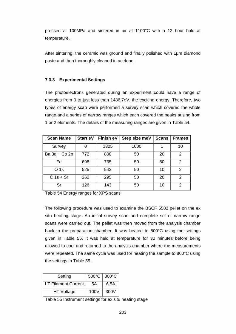
203

pressed at 100MPa and sintered in air at 1100°C with a 12 hour hold at

temperature.

After sintering, the ceramic was ground and finally polished with 1µm diamond

paste and then thoroughly cleaned in acetone.

7.3.3 Experimental Settings

The photoelectrons generated during an experiment could have a range of

energies from 0 to just less than 1486.7eV, the exciting energy. Therefore, two

types of energy scan were performed a survey scan which covered the whole

range and a series of narrow ranges which each covered the peaks arising from

1 or 2 elements. The details of the measuring ranges are given in Table 54.

Scan Name Start eV Finish eV Step size meV Scans Frames

Survey 0 1325 1000 1 10

Ba 3d + Co 2p 772 808 50 20 2

Fe 698 735 50 50 2

O 1s 525 542 50 10 2

C 1s + Sr 262 295 50 20 2

Sr 126 143 50 10 2

Table 54 Energy ranges for XPS scans

The following procedure was used to examine the BSCF 5582 pellet on the ex

situ heating stage. An initial survey scan and complete set of narrow range

scans were carried out. The pellet was then moved from the analysis chamber

back to the preparation chamber. It was heated to 500°C using the settings

given in Table 55. It was held at temperature for 30 minutes before being

allowed to cool and returned to the analysis chamber where the measurements

were repeated. The same cycle was used for heating the sample to 800°C using

the settings in Table 55.

Setting 500°C 800°C

LT Filament Current 5A 6.5A

HT Voltage 100V 300V

Table 55 Instrument settings for ex situ heating stage

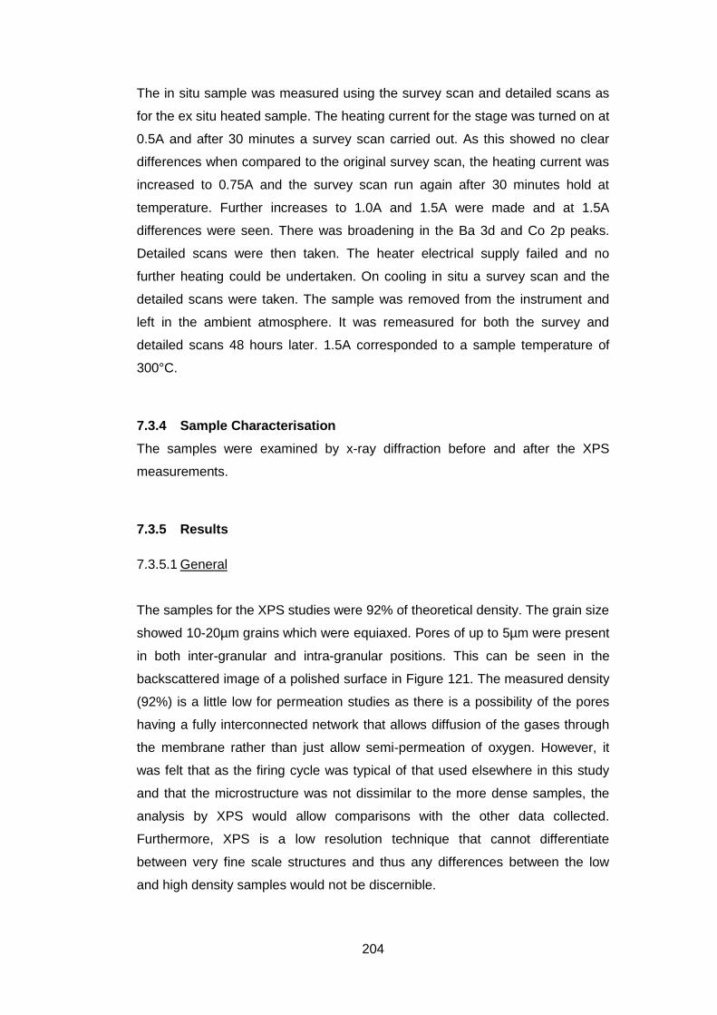
204

The in situ sample was measured using the survey scan and detailed scans as

for the ex situ heated sample. The heating current for the stage was turned on at

0.5A and after 30 minutes a survey scan carried out. As this showed no clear

differences when compared to the original survey scan, the heating current was

increased to 0.75A and the survey scan run again after 30 minutes hold at

temperature. Further increases to 1.0A and 1.5A were made and at 1.5A

differences were seen. There was broadening in the Ba 3d and Co 2p peaks.

Detailed scans were then taken. The heater electrical supply failed and no

further heating could be undertaken. On cooling in situ a survey scan and the

detailed scans were taken. The sample was removed from the instrument and

left in the ambient atmosphere. It was remeasured for both the survey and

detailed scans 48 hours later. 1.5A corresponded to a sample temperature of

300°C.

7.3.4 Sample Characterisation

The samples were examined by x-ray diffraction before and after the XPS

measurements.

7.3.5 Results

7.3.5.1 General

The samples for the XPS studies were 92% of theoretical density. The grain size

showed 10-20µm grains which were equiaxed. Pores of up to 5µm were present

in both inter-granular and intra-granular positions. This can be seen in the

backscattered image of a polished surface in Figure 121. The measured density

(92%) is a little low for permeation studies as there is a possibility of the pores

having a fully interconnected network that allows diffusion of the gases through

the membrane rather than just allow semi-permeation of oxygen. However, it

was felt that as the firing cycle was typical of that used elsewhere in this study

and that the microstructure was not dissimilar to the more dense samples, the

analysis by XPS would allow comparisons with the other data collected.

Furthermore, XPS is a low resolution technique that cannot differentiate

between very fine scale structures and thus any differences between the low

and high density samples would not be discernible.

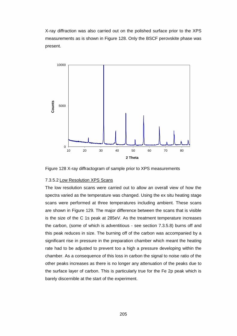
205

X-ray diffraction was also carried out on the polished surface prior to the XPS

measurements as is shown in Figure 128. Only the BSCF perovskite phase was

present.

Figure 128 X-ray diffractogram of sample prior to XPS measurements

7.3.5.2 Low Resolution XPS Scans

The low resolution scans were carried out to allow an overall view of how the

spectra varied as the temperature was changed. Using the ex situ heating stage

scans were performed at three temperatures including ambient. These scans

are shown in Figure 129. The major difference between the scans that is visible

is the size of the C 1s peak at 285eV. As the treatment temperature increases

the carbon, (some of which is adventitious - see section 7.3.5.8) burns off and

this peak reduces in size. The burning off of the carbon was accompanied by a

significant rise in pressure in the preparation chamber which meant the heating

rate had to be adjusted to prevent too a high a pressure developing within the

chamber. As a consequence of this loss in carbon the signal to noise ratio of the

other peaks increases as there is no longer any attenuation of the peaks due to

the surface layer of carbon. This is particularly true for the Fe 2p peak which is

barely discernible at the start of the experiment.

0

5000

10000

10 20 30 40 50 60 70 80

Co

un

ts

2 Theta

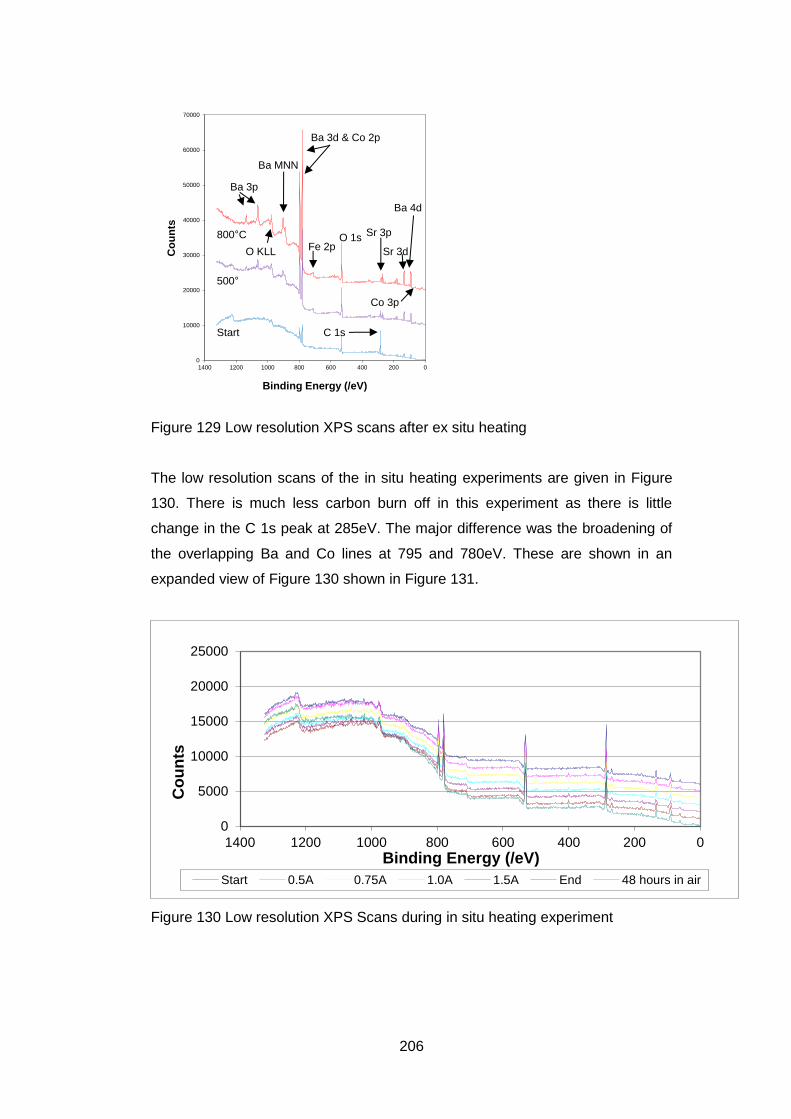
206

Figure 129 Low resolution XPS scans after ex situ heating

The low resolution scans of the in situ heating experiments are given in Figure

130. There is much less carbon burn off in this experiment as there is little

change in the C 1s peak at 285eV. The major difference was the broadening of

the overlapping Ba and Co lines at 795 and 780eV. These are shown in an

expanded view of Figure 130 shown in Figure 131.

Figure 130 Low resolution XPS Scans during in situ heating experiment

0

10000

20000

30000

40000

50000

60000

70000

0200400600800100012001400

Co

un

ts

Binding Energy (/eV)

Start

500°

800°C O 1s

Ba 3d & Co 2p

C 1s

Sr 3p

Sr 3d

Ba 4d

Co 3p

Fe 2p

Ba 3p

Ba MNN

O KLL

0

5000

10000

15000

20000

25000

0200400600800100012001400

Co

un

ts


Start 0.5A 0.75A 1.0A 1.5A End 48 hours in air

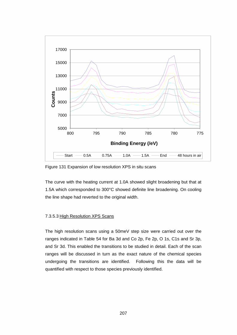
207

Figure 131 Expansion of low resolution XPS in situ scans

The curve with the heating current at 1.0A showed slight broadening but that at

1.5A which corresponded to 300°C showed definite line broadening. On cooling

the line shape had reverted to the original width.

7.3.5.3 High Resolution XPS Scans

The high resolution scans using a 50meV step size were carried out over the

ranges indicated in Table 54 for Ba 3d and Co 2p, Fe 2p, O 1s, C1s and Sr 3p,

and Sr 3d. This enabled the transitions to be studied in detail. Each of the scan

ranges will be discussed in turn as the exact nature of the chemical species

undergoing the transitions are identified. Following this the data will be

quantified with respect to those species previously identified.

5000

7000

9000

11000

13000

15000

17000

775780785790795800

Co

un

ts


Start 0.5A 0.75A 1.0A 1.5A End 48 hours in air

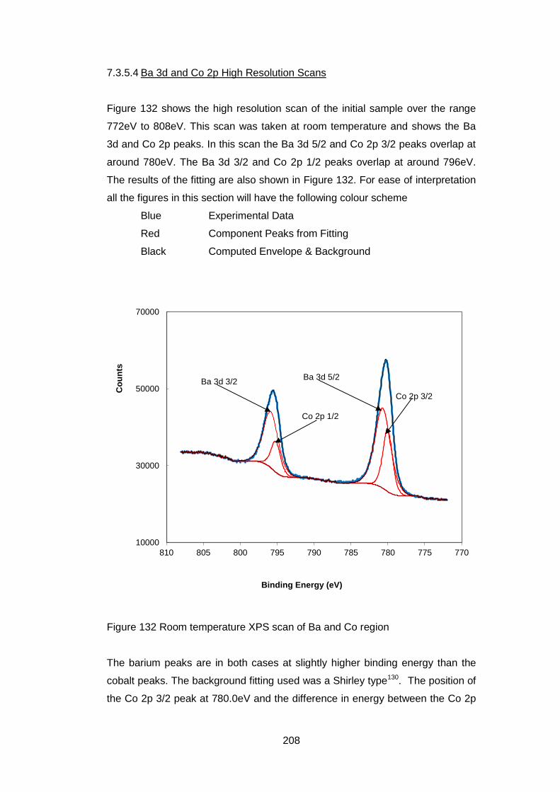
208

7.3.5.4 Ba 3d and Co 2p High Resolution Scans

Figure 132 shows the high resolution scan of the initial sample over the range

772eV to 808eV. This scan was taken at room temperature and shows the Ba

3d and Co 2p peaks. In this scan the Ba 3d 5/2 and Co 2p 3/2 peaks overlap at

around 780eV. The Ba 3d 3/2 and Co 2p 1/2 peaks overlap at around 796eV.

The results of the fitting are also shown in Figure 132. For ease of interpretation

all the figures in this section will have the following colour scheme

Blue Experimental Data

Red Component Peaks from Fitting

Black Computed Envelope & Background

Figure 132 Room temperature XPS scan of Ba and Co region

The barium peaks are in both cases at slightly higher binding energy than the

cobalt peaks. The background fitting used was a Shirley type130. The position of

the Co 2p 3/2 peak at 780.0eV and the difference in energy between the Co 2p

10000

30000

50000

70000

770775780785790795800805810

Co

un

ts

Binding Energy (eV)

Ba 3d 3/2 Ba 3d 5/2

Co 2p 1/2

Co 2p 3/2

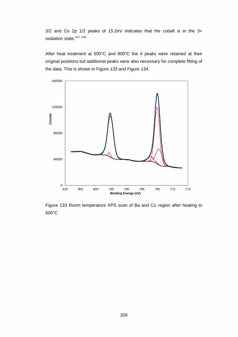
209

3/2 and Co 2p 1/2 peaks of 15.2eV indicates that the cobalt is in the 3+

oxidation state.157, 158

After heat treatment at 500°C and 800°C the 4 peaks were retained at their

original positions but additional peaks were also necessary for complete fitting of

the data. This is shown in Figure 133 and Figure 134.

Figure 133 Room temperature XPS scan of Ba and Co region after heating to

500°C

0

40000

80000

120000

160000

770775780785790795800805810

Co

un

ts

Binding Energy (eV)

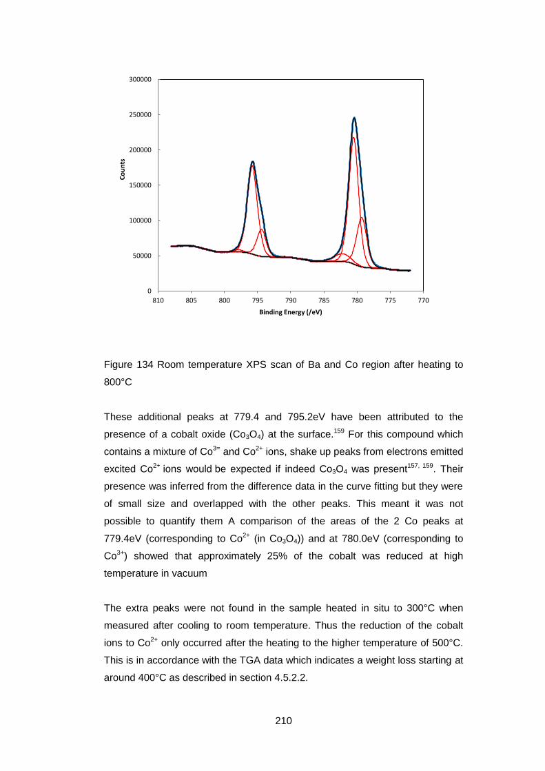
210

Figure 134 Room temperature XPS scan of Ba and Co region after heating to

800°C

These additional peaks at 779.4 and 795.2eV have been attributed to the

presence of a cobalt oxide (Co3O4) at the surface.159 For this compound which

contains a mixture of Co3= and Co2+ ions, shake up peaks from electrons emitted

excited Co2+ ions would be expected if indeed Co3O4 was present157, 159. Their

presence was inferred from the difference data in the curve fitting but they were

of small size and overlapped with the other peaks. This meant it was not

possible to quantify them A comparison of the areas of the 2 Co peaks at

779.4eV (corresponding to Co2+ (in Co3O4)) and at 780.0eV (corresponding to

Co3+) showed that approximately 25% of the cobalt was reduced at high

temperature in vacuum

The extra peaks were not found in the sample heated in situ to 300°C when

measured after cooling to room temperature. Thus the reduction of the cobalt

ions to Co2+ only occurred after the heating to the higher temperature of 500°C.

This is in accordance with the TGA data which indicates a weight loss starting at

around 400°C as described in section 4.5.2.2.

0

50000

100000

150000

200000

250000

300000

770775780785790795800805810

Co

un

ts


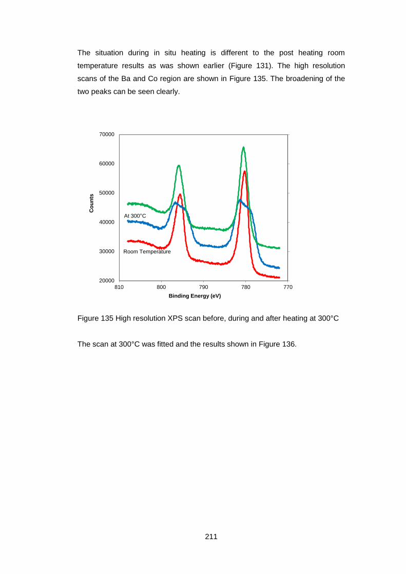
211

The situation during in situ heating is different to the post heating room

temperature results as was shown earlier (Figure 131). The high resolution

scans of the Ba and Co region are shown in Figure 135. The broadening of the

two peaks can be seen clearly.

Figure 135 High resolution XPS scan before, during and after heating at 300°C

The scan at 300°C was fitted and the results shown in Figure 136.

20000

30000

40000

50000

60000

70000

770780790800810

Co

un

ts

Binding Energy (eV)

Room Temperature

At 300°C

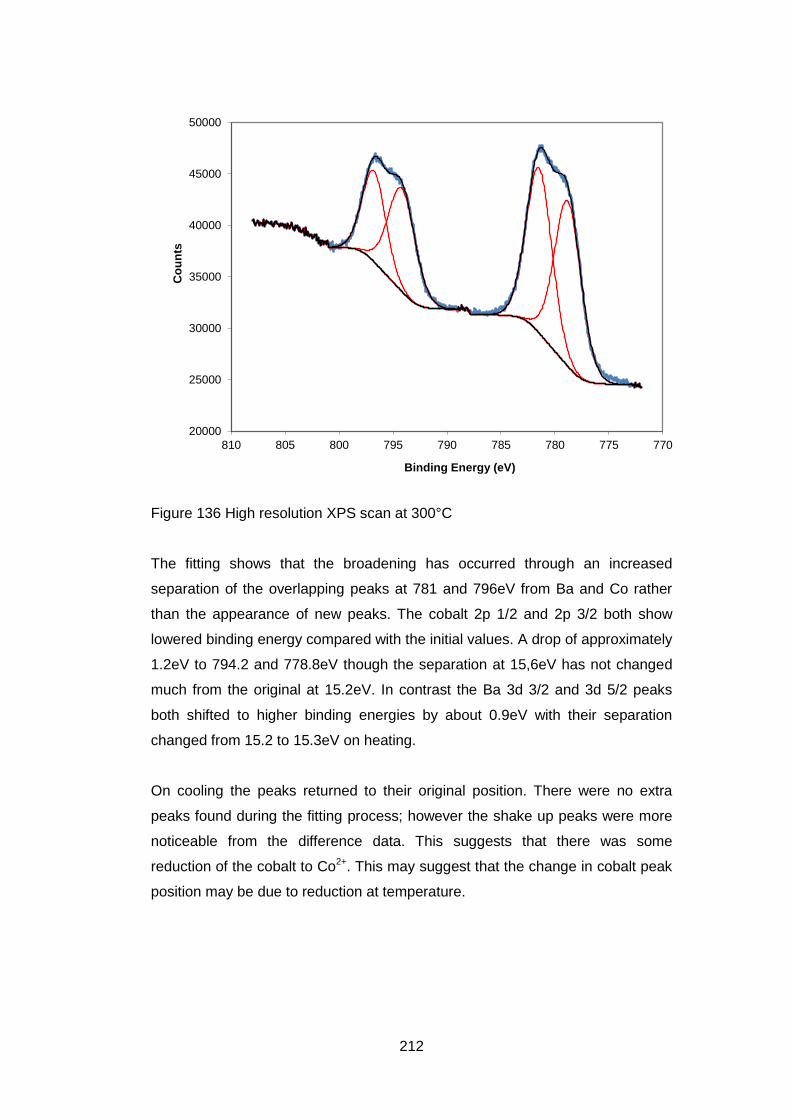
212

Figure 136 High resolution XPS scan at 300°C

The fitting shows that the broadening has occurred through an increased

separation of the overlapping peaks at 781 and 796eV from Ba and Co rather

than the appearance of new peaks. The cobalt 2p 1/2 and 2p 3/2 both show

lowered binding energy compared with the initial values. A drop of approximately

1.2eV to 794.2 and 778.8eV though the separation at 15,6eV has not changed

much from the original at 15.2eV. In contrast the Ba 3d 3/2 and 3d 5/2 peaks

both shifted to higher binding energies by about 0.9eV with their separation

changed from 15.2 to 15.3eV on heating.

On cooling the peaks returned to their original position. There were no extra

peaks found during the fitting process; however the shake up peaks were more

noticeable from the difference data. This suggests that there was some

reduction of the cobalt to Co2+. This may suggest that the change in cobalt peak

position may be due to reduction at temperature.

20000

25000

30000

35000

40000

45000

50000

770775780785790795800805810

Co

un

ts

Binding Energy (eV)

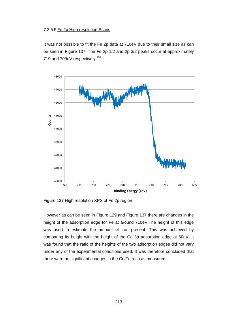
213

7.3.5.5 Fe 2p High resolution Scans

It was not possible to fit the Fe 2p data at 710eV due to their small size as can

be seen in Figure 137. The Fe 2p 1/2 and 2p 3/2 peaks occur at approximately

719 and 709eV respectively.159

Figure 137 High resolution XPS of Fe 2p region

However as can be seen in Figure 129 and Figure 137 there are changes in the

height of the adsorption edge for Fe at around 710eV.The height of this edge

was used to estimate the amount of iron present. This was achieved by

comparing its height with the height of the Co 3p adsorption edge at 60eV. It

was found that the ratio of the heights of the two adsorption edges did not vary

under any of the experimental conditions used. It was therefore concluded that

there were no significant changes in the Co/Fe ratio as measured.

40000

41000

42000

43000

44000

45000

46000

47000

48000

695700705710715720725730735740

Co

un

ts


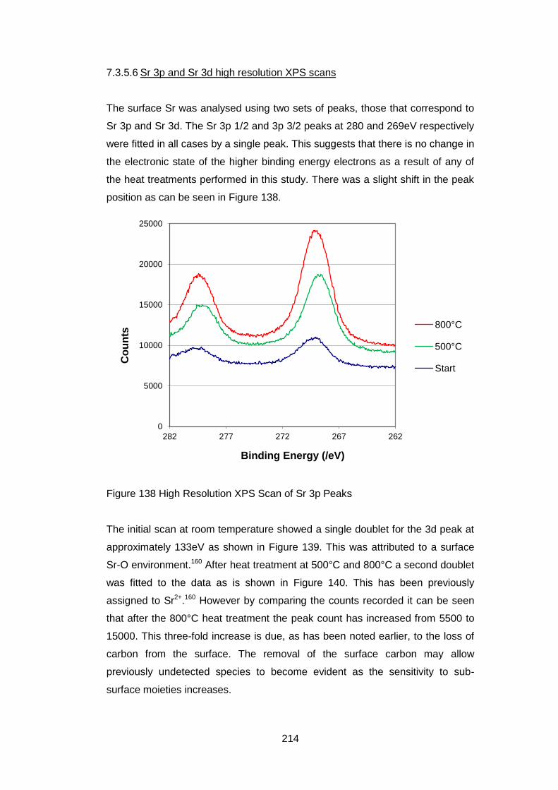
214

7.3.5.6 Sr 3p and Sr 3d high resolution XPS scans

The surface Sr was analysed using two sets of peaks, those that correspond to

Sr 3p and Sr 3d. The Sr 3p 1/2 and 3p 3/2 peaks at 280 and 269eV respectively

were fitted in all cases by a single peak. This suggests that there is no change in

the electronic state of the higher binding energy electrons as a result of any of

the heat treatments performed in this study. There was a slight shift in the peak

position as can be seen in Figure 138.

Figure 138 High Resolution XPS Scan of Sr 3p Peaks

The initial scan at room temperature showed a single doublet for the 3d peak at

approximately 133eV as shown in Figure 139. This was attributed to a surface

Sr-O environment.160 After heat treatment at 500°C and 800°C a second doublet

was fitted to the data as is shown in Figure 140. This has been previously

assigned to Sr2+.160 However by comparing the counts recorded it can be seen

that after the 800°C heat treatment the peak count has increased from 5500 to

15000. This three-fold increase is due, as has been noted earlier, to the loss of

carbon from the surface. The removal of the surface carbon may allow

previously undetected species to become evident as the sensitivity to sub-

surface moieties increases.

0

5000

10000

15000

20000

25000

262267272277282

Co

un

ts


800°C

500°C

Start

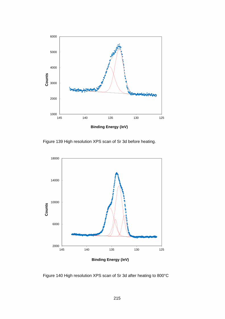
215

Figure 139 High resolution XPS scan of Sr 3d before heating.

Figure 140 High resolution XPS scan of Sr 3d after heating to 800°C

1000

2000

3000

4000

5000

6000

125130135140145

Co

un

ts


2000

6000

10000

14000

18000

125130135140145

Co

un

ts


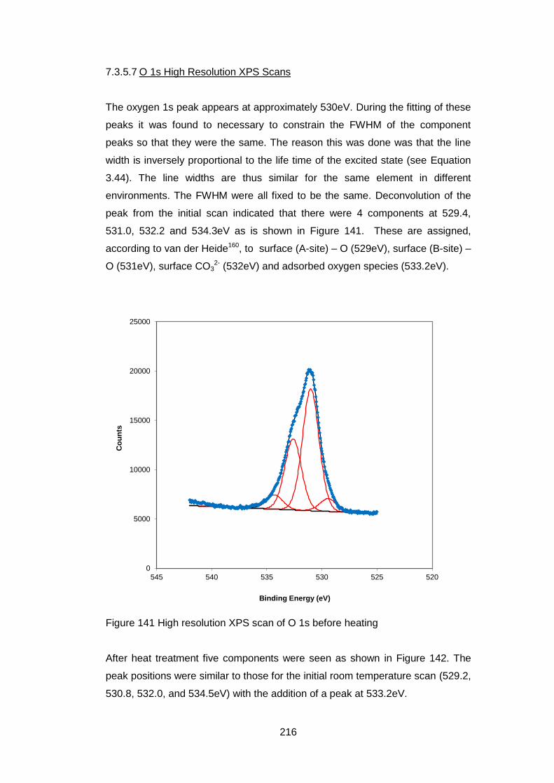
216

7.3.5.7 O 1s High Resolution XPS Scans

The oxygen 1s peak appears at approximately 530eV. During the fitting of these

peaks it was found to necessary to constrain the FWHM of the component

peaks so that they were the same. The reason this was done was that the line

width is inversely proportional to the life time of the excited state (see Equation

3.44). The line widths are thus similar for the same element in different

environments. The FWHM were all fixed to be the same. Deconvolution of the

peak from the initial scan indicated that there were 4 components at 529.4,

531.0, 532.2 and 534.3eV as is shown in Figure 141. These are assigned,

according to van der Heide160, to surface (A-site) – O (529eV), surface (B-site) –

O (531eV), surface CO32- (532eV) and adsorbed oxygen species (533.2eV).

Figure 141 High resolution XPS scan of O 1s before heating

After heat treatment five components were seen as shown in Figure 142. The

peak positions were similar to those for the initial room temperature scan (529.2,

530.8, 532.0, and 534.5eV) with the addition of a peak at 533.2eV.

0

5000

10000

15000

20000

25000

520525530535540545

Co

un

ts

Binding Energy (eV)

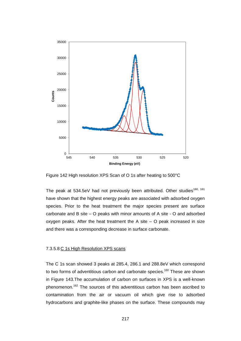
217

Figure 142 High resolution XPS Scan of O 1s after heating to 500°C

The peak at 534.5eV had not previously been attributed. Other studies160, 161

have shown that the highest energy peaks are associated with adsorbed oxygen

species. Prior to the heat treatment the major species present are surface

carbonate and B site – O peaks with minor amounts of A site - O and adsorbed

oxygen peaks. After the heat treatment the A site – O peak increased in size

and there was a corresponding decrease in surface carbonate.

7.3.5.8 C 1s High Resolution XPS scans

The C 1s scan showed 3 peaks at 285.4, 286.1 and 288.8eV which correspond

to two forms of adventitious carbon and carbonate species.160 These are shown

in Figure 143.The accumulation of carbon on surfaces in XPS is a well-known

phenomenon.162 The sources of this adventitious carbon has been ascribed to

contamination from the air or vacuum oil which give rise to adsorbed

hydrocarbons and graphite-like phases on the surface. These compounds may

0

5000

10000

15000

20000

25000

30000

35000

520525530535540545

Co

un

ts

Binding Energy (eV)

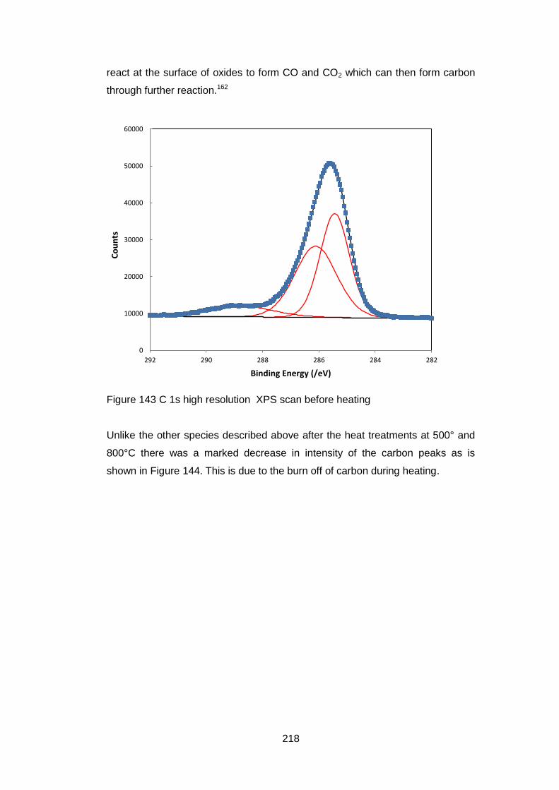
218

react at the surface of oxides to form CO and CO2 which can then form carbon

through further reaction.162

Figure 143 C 1s high resolution XPS scan before heating

Unlike the other species described above after the heat treatments at 500° and

800°C there was a marked decrease in intensity of the carbon peaks as is

shown in Figure 144. This is due to the burn off of carbon during heating.

0

10000

20000

30000

40000

50000

60000

282284286288290292

Co

un

ts


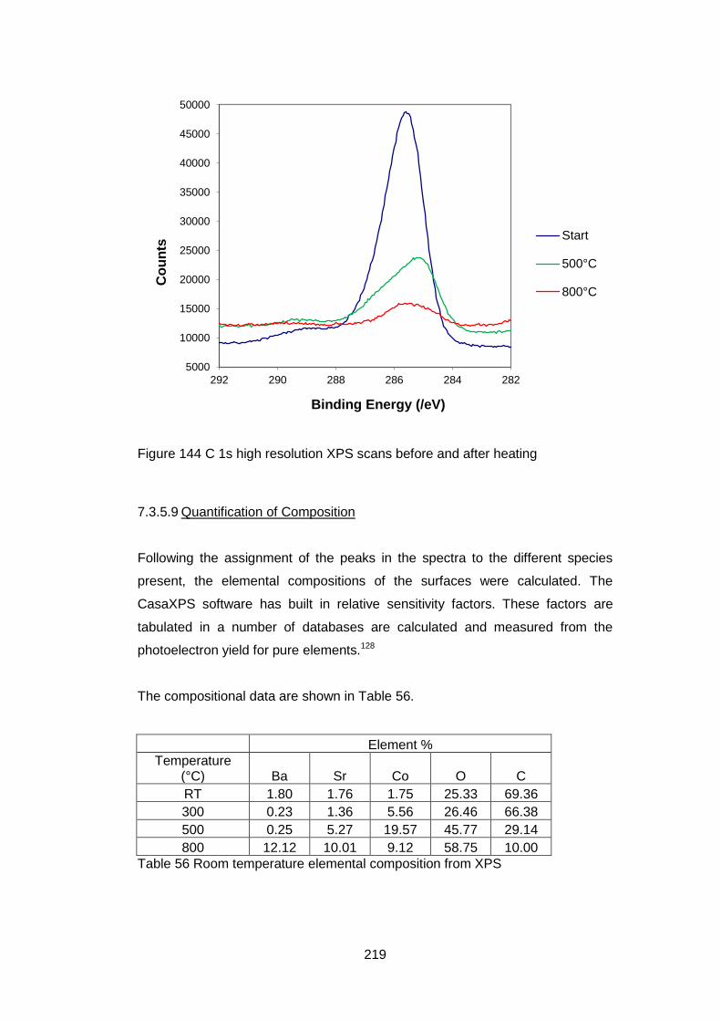
219

Figure 144 C 1s high resolution XPS scans before and after heating

7.3.5.9 Quantification of Composition

Following the assignment of the peaks in the spectra to the different species

present, the elemental compositions of the surfaces were calculated. The

CasaXPS software has built in relative sensitivity factors. These factors are

tabulated in a number of databases are calculated and measured from the

photoelectron yield for pure elements.128

The compositional data are shown in Table 56.

Element %

Temperature (°C) Ba Sr Co O C

RT 1.80 1.76 1.75 25.33 69.36

300 0.23 1.36 5.56 26.46 66.38

500 0.25 5.27 19.57 45.77 29.14

800 12.12 10.01 9.12 58.75 10.00

Table 56 Room temperature elemental composition from XPS

5000

10000

15000

20000

25000

30000

35000

40000

45000

50000

282284286288290292

Co

un

ts


Start

500°C

800°C

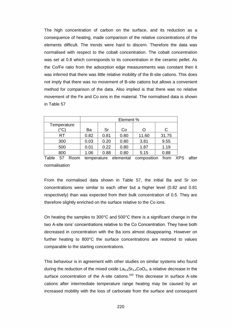
220

The high concentration of carbon on the surface, and its reduction as a

consequence of heating, made comparison of the relative concentrations of the

elements difficult. The trends were hard to discern. Therefore the data was

normalised with respect to the cobalt concentration. The cobalt concentration

was set at 0.8 which corresponds to its concentration in the ceramic pellet. As

the Co/Fe ratio from the adsorption edge measurements was constant then it

was inferred that there was little relative mobility of the B-site cations. This does

not imply that there was no movement of B-site cations but allows a convenient

method for comparison of the data. Also implied is that there was no relative

movement of the Fe and Co ions in the material. The normalised data is shown

in Table 57

Element %

Temperature (°C) Ba Sr Co O C

RT 0.82 0.81 0.80 11.60 31.75

300 0.03 0.20 0.80 3.81 9.55

500 0.01 0.22 0.80 1.87 1.19

800 1.06 0.88 0.80 5.15 0.88

Table 57 Room temperature elemental composition from XPS after

normalisation

From the normalised data shown in Table 57, the initial Ba and Sr ion

concentrations were similar to each other but a higher level (0.82 and 0.81

respectively) than was expected from their bulk concentration of 0.5. They are

therefore slightly enriched on the surface relative to the Co ions.

On heating the samples to 300°C and 500°C there is a significant change in the

two A-site ions’ concentrations relative to the Co Concentration. They have both

decreased in concentration with the Ba ions almost disappearing. However on

further heating to 800°C the surface concentrations are restored to values

comparable to the starting concentrations.

This behaviour is in agreement with other studies on similar systems who found

during the reduction of the mixed oxide La0.6Sr0.4CoO3, a relative decrease in the

surface concentration of the A-site cations.160 This decrease in surface A-site

cations after intermediate temperature range heating may be caused by an

increased mobility with the loss of carbonate from the surface and consequent

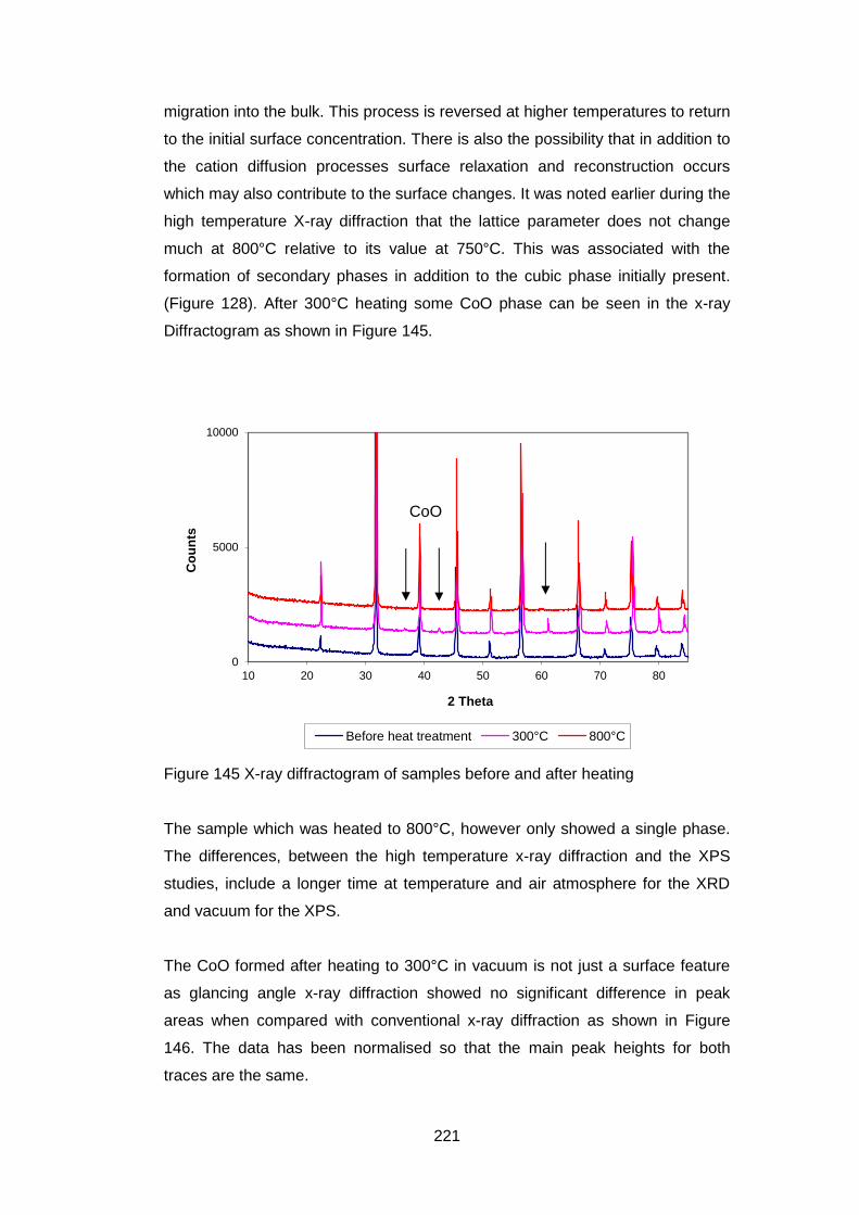
221

migration into the bulk. This process is reversed at higher temperatures to return

to the initial surface concentration. There is also the possibility that in addition to

the cation diffusion processes surface relaxation and reconstruction occurs

which may also contribute to the surface changes. It was noted earlier during the

high temperature X-ray diffraction that the lattice parameter does not change

much at 800°C relative to its value at 750°C. This was associated with the

formation of secondary phases in addition to the cubic phase initially present.

(Figure 128). After 300°C heating some CoO phase can be seen in the x-ray

Diffractogram as shown in Figure 145.

Figure 145 X-ray diffractogram of samples before and after heating

The sample which was heated to 800°C, however only showed a single phase.

The differences, between the high temperature x-ray diffraction and the XPS

studies, include a longer time at temperature and air atmosphere for the XRD

and vacuum for the XPS.

The CoO formed after heating to 300°C in vacuum is not just a surface feature

as glancing angle x-ray diffraction showed no significant difference in peak

areas when compared with conventional x-ray diffraction as shown in Figure

146. The data has been normalised so that the main peak heights for both

traces are the same.

0

5000

10000

10 20 30 40 50 60 70 80

Co

un

ts

2 Theta

Before heat treatment 300°C 800°C

CoO

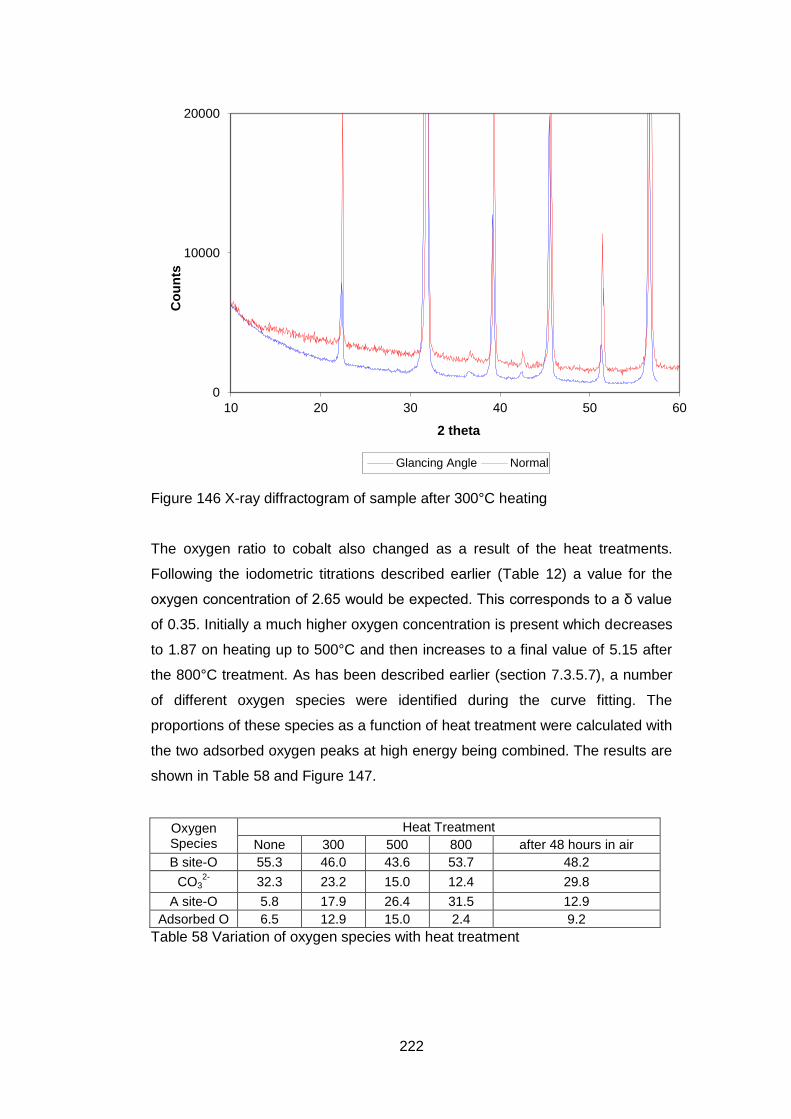
222

Figure 146 X-ray diffractogram of sample after 300°C heating

The oxygen ratio to cobalt also changed as a result of the heat treatments.

Following the iodometric titrations described earlier (Table 12) a value for the

oxygen concentration of 2.65 would be expected. This corresponds to a δ value

of 0.35. Initially a much higher oxygen concentration is present which decreases

to 1.87 on heating up to 500°C and then increases to a final value of 5.15 after

the 800°C treatment. As has been described earlier (section 7.3.5.7), a number

of different oxygen species were identified during the curve fitting. The

proportions of these species as a function of heat treatment were calculated with

the two adsorbed oxygen peaks at high energy being combined. The results are

shown in Table 58 and Figure 147.

Oxygen Species

Heat Treatment

None 300 500 800 after 48 hours in air

B site-O 55.3 46.0 43.6 53.7 48.2

CO32-

32.3 23.2 15.0 12.4 29.8

A site-O 5.8 17.9 26.4 31.5 12.9

Adsorbed O 6.5 12.9 15.0 2.4 9.2

Table 58 Variation of oxygen species with heat treatment

0

10000

20000

10 20 30 40 50 60

Co

un

ts

2 theta

Glancing Angle Normal

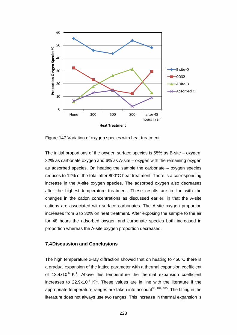
223

Figure 147 Variation of oxygen species with heat treatment

The initial proportions of the oxygen surface species is 55% as B-site – oxygen,

32% as carbonate oxygen and 6% as A-site – oxygen with the remaining oxygen

as adsorbed species. On heating the sample the carbonate – oxygen species

reduces to 12% of the total after 800°C heat treatment. There is a corresponding

increase in the A-site oxygen species. The adsorbed oxygen also decreases

after the highest temperature treatment. These results are in line with the

changes in the cation concentrations as discussed earlier, in that the A-site

cations are associated with surface carbonates. The A-site oxygen proportion

increases from 6 to 32% on heat treatment. After exposing the sample to the air

for 48 hours the adsorbed oxygen and carbonate species both increased in

proportion whereas the A-site oxygen proportion decreased.


The high temperature x-ray diffraction showed that on heating to 450°C there is

a gradual expansion of the lattice parameter with a thermal expansion coefficient

of 13.4x10-6 K-1. Above this temperature the thermal expansion coefficient

increases to 22.9x10-6 K-1. These values are in line with the literature if the

appropriate temperature ranges are taken into account30, 104, 105. The fitting in the

literature does not always use two ranges. This increase in thermal expansion is

0

10

20

30

40

50

60

None 300 500 800 after 48hours in air

Pro

po

rtio

n O

xyge

n S

pe

cie

s %

Heat Treatment

B site-O

CO32-

A site-O

Adsorbed O

224

due to the onset of oxygen loss (chemical expansion30) from the structure

making the value of δ increase. On cooling the cubic phase disproportionates

into a number of different phases and adsorbs carbon dioxide from the air to

form alkaline earth carbonates.

The x-ray photoelectron spectroscopy showed that the surface composition of

BSCF changed during the heating processes. At intermediate temperatures the

cobalt (and iron) was concentrated at the surface relative to the barium and

strontium. At higher temperatures the barium and strontium returned to levels

slightly higher than at the start of the heat treatment. In addition the carbonate

content of the surface decreased during heating with a consequent increase in

the A site – O oxygen.

In contrast to the high temperature x-ray diffraction results there was little

change in the x-ray pattern in the samples after XPS. There was only a small

amount of CoO detected. This phase was identified by Muller et al155 as being

present in their ceramics after heat treatment and cooling although they used

much longer annealing times at temperature 100hrs compared with this works

30mins. The main difference between the HTXRD and XPS heat treatments was

the atmosphere. The former was carried out in ambient air whereas the latter

was at either ~2x10-5 or ~5x10-9 torr. Changes in the value of δ during the

experiments could not be measured, although the results from section 4.5.1.2

show that a change of value approximately equal to 0.1 could be expected on

heating to 800°C. It would be higher in the vacuum present in the XPS.

Increases in δ result in an increase in the oxygen vacancies which allows easier

movement of the oxygen. This can promote the formation of the new phases.

Also the carbon dioxide concentration would be lower which could not react to

form carbonates on cooling.

The decomposition of BSCF at high temperature in air would be enhanced by

the presence of carbon dioxide163, 164. As shown in the XPS at 800°C there is a

surface enrichment of barium and strontium. This leads to the decomposition of

the cubic phase into the hexagonal phase. It has been shown that during oxygen

permeation experiments at 875°C with carbon dioxide in the sweep gas that the

surface layer on the sweep gas side becomes depleted in iron and cobalt67. This

behaviour is reversed when the carbon dioxide is removed from the sweep gas.

Thus in the presence of carbon dioxide the barium and strontium become

225

surface enriched. However in the XPS experiment the surface enrichment of

barium and strontium only occurs when there was a significant carbonate

concentration on the surface. This confirms the necessity of carbon dioxide to

obtain surface enrichment. There was no reaction on the feed side of the

system67. The alkaline earth enriched surface can therefore react with

atmospheric carbon dioxide which is readily adsorbed by the BSCF at room

temperature (see Figure 147). The presence of this surface carbonate can then

further catalyse the decomposition of the single phase into the multi-phase

assemblage. As shown in Figure 46 the loss of carbon dioxide from the dried

powders is not complete until 830°C, thus at the highest temperatures used in

these XRD and XPS studies carbonates are present on the surface, though not

visible using XRD.

During the heat treatment of BSCF ceramic pellets the surface composition

changes in terms of the relative amount of the A site and B site cations present.

During heating there were no noticeable phase changes up to 700°C, thereafter

some decomposition occurred in air though not vacuum. On cooling the air

cooled sample showed decomposition into a number of different phases.

Whereas the vacuum treated sample showed a small amount of CoO formation.

The presence of carbon dioxide can affect the decomposition of the BSCF

material.

226

8 Conclusions

An inorganic synthetic route was developed for the formation of single phase

barium strontium cobalt iron oxide mixed ionic electronic conductors without the

use of organic reagents. This was based on a reverse precipitation route and

used sodium carbonate as the precipitant to ensure complete precipitation of all

components. The use of reverse precipitation in which the acidic mixed salt

solution was added into the excess alkaline precipitant ensured that all the

metals were precipitated immediately and not sequentially.

The precipitation did not give a single phase in the dried and calcined powders

but they were of such small crystallite size that they reacted readily on sintering

to form a single phase on sintering. A common reaction pathway was found with

minor changes as a result of hydrothermal treatment at high and low pH.

The process was thus robust in that the changes in the experimental parameters

(pH and hydrothermal treatment) gave similar ceramic pellets. The incorporation

of copper was also accomplished without any changes to the experimental

process. The addition of copper caused a significant difference in the results in

that after calcination the resulting powder was mainly the desired cubic phase

with a smaller amount of a mixed barium strontium carbonate. The other

difference with the copper doped samples in the formation of the ceramic pellets

was higher grain growth during sintering. Only at the lowest addition level

copper was found to be beneficial in promoting oxygen permeation.

The oxygen permeability of the ceramics was measured and was found to be

dependent on three factors the lattice parameter of the ceramic, the tolerance

factor for the crystal structure and the oxygen non-stoichiometry (δ). Together

they gave a good indicator of the oxygen flux as long as the rate determining

step in the oxygen permeation was the same. The larger lattice parameters were

better as they allowed oxygen ions to pass from one site to another with less

restriction as the interatomic distances were bigger. The tolerance factor was

important as it indicated the stability of the crystal structure. The oxygen non-

stoichiometry indicated an upper limit for good oxygen transfer as when δ≥0.5,

the vacancies could then start to order and additionally there were fewer

variations in the B site oxidation state and thus less electronic transfer.

227

One of the objectives of this study was to relate the electrical properties of the

ceramic to the oxygen permeation. The electrical properties did not match

exactly the oxygen permeation behaviour but varied with a similar dependence

on the three factors. They are both functions of lattice parameter, tolerance

factor and oxygen non-stoichiometry. There was a distinct change in resistance

when the value of δ was close to or greater than 0.5, which corresponded to the

net oxidation state on the B site cations being 3+ and there therefore being no

transfer between cations of different oxidation state.

The lack of correlation between the activation energies of the resistance and

oxygen permeation dependence indicated that the electrical measurements

were not measuring the critical stage of the multi-step oxygen permeation

process. The two critical steps were different for the mainly electronic

conduction and the oxygen permeation. The use of blocking electrodes together

with a better estimation of the transition metal oxidation states would allow

further understanding of the relationship between changes in electrical

properties and oxygen permeation to be made.

The results from BSCF 5582 of the thermogravimetric analysis on cooling

together with the high temperature x-ray diffraction showed that oxygen was

reversibly lost from 400°C continuously up to 1100°C (maximum temperature

used). The onset of oxygen loss was marked in the diffraction experiments by

an increase in the thermal expansion coefficient on heating. On slow cooling

there was decomposition into a mixture of other phases both simple oxides and

mixed perovskite-like orthorhombic and hexagonal structures.

The surface composition was measured using high temperature x-ray

photoelectron spectroscopy and showed that during heating and cooling there

was migration of the alkaline earth ions from the surface at intermediate

temperatures with a return at high temperature. The oxygen spectra showed

behaviour which indicated the loss of surface carbonates from (Ba,Sr)CO3 on

heating which accompanied the initial loss of barium and strontium from the

surface.

The changes seen in surface composition using x-ray photoelectron

spectroscopy have shown that the removal of carbonate from the surface at high

temperatures is necessary to have a “clean” surface. The absorption of carbon

228

dioxide by the sample under ambient conditions showed the facile uptake of

carbon dioxide. Therefore care needs to be taken to ensure that carbonate is

removed from the surface prior to starting any experiment on permeation.

However on heating to high temperature and then cooling (as done in this work)

may allow the BSCF materials to transform from the cubic phase.

229

9 Further Work

1. Compare electrical measurements with and without the use of blocking

electrodes.

2. In order to clarify the phase development during powder formation,

synthesise the end members of the series containing only one A site and

one B site cation.

3. Investigate the use of slower heating rates during sintering to improve

densification by preventing pore breakaway

4. Investigate high temperature XRD with controlled atmospheres at well-

defined oxygen partial pressures with and without carbon dioxide

present.

5. Examine more compositions using XPS to determine the variation of

surface chemistry with composition.

230

10 References

1. Kneer, R. et al. OXYCOAL-AC: Towards an integrated coal-fired power plant process with ion transport membrane-based oxygen supply. Energy Environ Sci 3, 196-207 (2010).

2. Repasky, J.M., Anderson, L.L., Stein, V.E., Armstong, P.A. & Foster, E.P. in International Pittsburgh Coal Conference 2012 (Air Products and Chemicals Inc, Pittsburgh USA, 2012).

3. Smith, A.R. & Klosek, J. A review of air separation technologies and their integration with energy conversion processes. Fuel Processing Technology 70, 115-134 (2001).

4. Hashim, S.S., Mohamed, A.R. & Bhatia, S. Oxygen separation from air using ceramic-based membrane technology for sustainable fuel production and power generation. Renewable and Sustainable Energy Reviews 15, 1284 (2011).

5. Geffroy, P.M., Fouletier, J., Richet, N. & Chartier, T. Rational selection of MIEC materials in energy production processes. Chemical Engineering Science 87, 408-433 (2013).

6. Moulson, A.J. & Herbert, J.M. Electroceramics (Wiley, 2003). 7. Sunarso, J. et al. Mixed ionic-electronic conducting (MIEC)

ceramic-based membranes for oxygen separation. J Membrane Science 320, 13-41 (2008).

8. Faraji, S., Nordheden, K.J. & Stagg-Williams, S.M. A comparative study of Ba0.5Sr0.5Co0.8Fe0.2Ox (BSCF) and SrFeCo0.5Ox (SFC) ceramic membranes used for syngas production. Applied Catalysis B: Environmental 99, 118 (2010).

9. Jiang, H. et al. Hydrogen Production by Water Dissociation in Surface-Modified BaCoxFeyZr1−x−yO3−δ Hollow-Fiber Membrane Reactor with Improved Oxygen Permeation. Chemistry – A European Journal 16, 7898 (2010).

10. Shao, Z. et al. Investigation of the permeation behaviour and stability of a Ba0.5Sr0.5Co0.8Fe0.2O3-δ oxygen membrane. J Membrane Science 172, 177-188 (2000).

11. Shao, Z., Xiong, G., Tong, J., Dong, H. & Yang, W. Ba effect in doped Sr(Co0.8Fe0.2)O3-δ on the phase structure and oxygen permeation properties of the dense ceramic membranes. Sep. Purif. Technol 25, 419-429 (2001).

12. Emsley, J. in Nature's Building Blocks: An A-Z Guide to the Elements (Oxford University Press, 2001).

13. Burdyny, T. & Struchtrup, H. Hybrid membrane/cryogenic separation of oxygen from air for use in the oxy-fuel process. Energy 35, 1884 (2010).

14. Colombo, K.E., Kharton, V.V. & Bolland, O. Simulation of an Oxygen Membrane-Based Gas turbine power Plant: Dynamic Regimes with Operational and Material Constraints. Energy Fuels 24, 590-608 (2010).

15. Dyer, P.N., Richards, R.E., Russek, S.L. & Taylor, D.M. Ion transport membrane technology for oxygen separation and syngas production. Solid State Ionics 134, 21-33 (2000).

231

16. He, Y., Zhu, X., Li, Q. & Yang, W. Perovskite Oxide Absorbents for Oxygen Separation. AIChE Journal 55, 3125-3133 (2009).

17. Zhu, X., Sun, S., He, Y., Cong, Y. & Yang, W. New concept on air separation. J Membrane Science 323, 221.224 (2008).

18. http://www.vattenfall.com/en/ccs/oxyfuel-combustion.htm. (Accessed August 2013).

19. http://www.vattenfall.com/en/ccs/precombustion.htm. (Accessed August 2013).

20. Bouwmeester, H.J.M. Dense ceramic membranes for methane conversion Catalysis Today 82, 141-150 (2003).

21. Park, C.Y., Lee, T.H., Dorris, S.E. & Balachandran, U. Hydrogen production from fossil and renewable sources using an oxygen transport membrane. International Journal of Hydrogen Energy 35, 4103 (2010).

22. Balachandran, U., Lee, T.H., Wang, S. & Dorris, S.E. Use of mixed conducting membranes to produce hydrogen by water dissociation. Int J Hydrogen Energy 29, 291-296 (2004).

23. Zhou, W., Ran, R. & Shao, Z. Progress in understanding and development of Ba0.5Sr0.5Co0.8Fe0.2O3-δ based cathodes for intermediate-temperature solid-oxide fuel cells: A review. Journal of Power Sources 192, 231 (2009).

24. Goldscmidt, V.M. Die Gesetze der Krystallochemie. Die Naturwissenschaften 21, 477-485 (1926).

25. Wells, A.F. in Structural Inorganic Chemistry 584 (Oxford, 1984). 26. Le Toquin, R., Paulus, W., Cousson, A., Prestipino, C. & Lamberti,

C. Time-resolved in Situ Studies of Oxygen Intercalation into SrCoO2.5, Performed by Neutron Diffraction and X-ray Absorption Spectroscopy. J Am Chem Soc 128, 13161-13174 (2006).

27. de la Calle, C., Alonso, J.A., Aguadero, A. & Fernandez-Diaz, M.T. Phase transformations in Sr0.8Ba0.2CoO2.5 brownmillerite: correlation between structure and transport properties. Dalton Transactions, 4104 (2009).

28. Itoh, T. et al. Study of charge density and crystal structure of (La0.75Sr0.25)MnO3.00 and (Ba0.5Sr0.5)(Co0.8Fe0.2)O2.33-δ at 500-900 K by in situ synchrotron X-ray diffraction. Journal Of Alloys And Compounds 491, 527-535 (2010).

29. Ganopadhyay, S. et al. Understanding oxygen vacancy migration and clustering in barium strontium cobalt iron oxide. Solid State Ionics 181, 1067 (2010).

30. McIntosh, S., Vente, J.F., Haije, W.G., Blank, D.H.A. & Bouwmeester, H.J.M. Oxygen stoichiometry and chemical expansion of Ba0.5Sr0.5Co0.8Fe0.2O3-δ measured by in situ neutron diffraction. Chemistry of Materials 18, 2187 (2006).

31. Vashook, V.V. et al. Oxygen non-stoichiometry and electrical conductivity of the binary strontium cobalt oxide SrCoOx. Solid State Ionics 99, 23-32 (1997).

32. Teraoka, Y., Nobunaga, T., Miura, N. & Yamazoe, N. Influence of constituent metal cations in substituted LaCoO3 on mixed conductivity and oxygen permeability. Solid State Ionics 48, 207-212 (1991).

http://www.vattenfall.com/en/ccs/oxyfuel-combustion.htm

http://www.vattenfall.com/en/ccs/precombustion.htm

232

33. Teraoka, Y., Nobunaga, T. & yamazoe, N. Effect of cation substitution on the oxygen semipermeability of perovskite-type oxides. Chem Lett, 503-506 (1988).

34. Svarcova, S., Wiik, K., Tolchard, J., Bouwmeester, H.J.M. & Grande, T. Structural instability of cubic perovskite BaxSrxSr1-xCo1-

yFeyO3-δ. Solid State Ionics 178, 1787-1791 (2008). 35. Kharton, V.V. et al. Perovskite-type oxides for high-temperature

oxygen separation membranes. J Membrane Science 163, 307-317 (1999).

36. Ishihara, T. et al. La ( Sr ) Ga ( Fe ) O 3 Perovskite Oxide as a New Mixed Ionic-Electronic Conductor for Oxygen Permeating Membrane. Journal Of The Electrochemical Society 150, E17-E23 (2003).

37. Chen, W., Zuo, Y.B., Chen, C.S. & Winnubst, A.J.A. Effect of Zr4+ doping on the oxygen stoichiometry and phase stability of SrCo0.8Fe0.2O3-δ oxygen separation membrane. Solid State Ionics 181, 971 (2010).

38. Liang, F. B-site La-doped BaFe0.95-xLaxZr0.05O3-δ perovskite-type membranes for oxygen separation. J Mater Chem A 1, 746-751 (2013).

39. Shao, Z., Zhou, W. & Zhu, Z. Advanced synthesis of materials for intermediate-temperature solid oxide fuel cells. Progress in Materials Science 57, 804-874 (2012).

40. Pechini. (US 3,330,697, 1967). 41. Ring, T.A. Fundamentals of Ceramic Powder Processing and

Synthesis (Academic Press, 1996). 42. Patra, H., Rout, S.K., Pratihar, S.K. & Bhattacharya, S. Effect of

process parameters on combined EDTA-citrate synthesis of Ba0.5Sr0.5Co0.8Fe0.2O3-δ perovskite. Powder Technology 209, 98 (2011).

43. Baumann, F.S., Fleig, J., Habermeier, H.U. & Maier, J. Ba0.5Sr0.5Co0.8Fe0.2O3-δ thin film microelectrodes investigated by impedance spectroscopy. Solid State Ionics 177, 3187-3191 (2006).

44. Bi, L., Fabbri, E. & Traversa, E. Novel Ba0.5Sr0.5(Co0.8Fe0.2)1-xTixO3-

δ(x=0, 0.05, and 0.1) cathode materials for proton-conducting solid oxide fuel cells. Solid State Ionics 214, 1 (2012).

45. Moharil, S.V., Nagrare, B.S. & Shaikh, S.P.S. Nanostructured MIEC Ba0.5Sr0.5Co0.6Fe0.4O3-δ (BSCF5564) cathode for IT-SOFC by nitric acid aided EDTA-citric acid complexing process (NECC). International Journal of Hydrogen Energy 37, 5208 (2012).

46. Zhao, Z. et al. Carbonates formed during BSCF preparation and their effects on performance of SOFCs with BSCF cathode. International Journal Of Hydrogen Energy 37, 19036-19044 (2012).

47. Feldhoff, A., Martynczuk, J. & Wang, H. Advanced Ba0.5Sr0.5Zn0.2Fe0.8O3-δ perovskite-type ceramics as oxygen selective membranes: Evaluation of the synthetic process. Progress In Solid State Chemistry 35, 339-353 (2007).

233

48. Babakhani, E.G., Towfighi, J. & Nazari, K. Synthesis of BSCFO Ceramics Membrane Using a Simple Complexing Method and Experimental Study of Sintering Parameters. Journal of Materials Science & Technology 26, 914-920 (2010).

49. Pelosato, R. et al. Co-precipitation in aqueous medium of La0.8Sr0.2Ga0.8Mg0.2O3−δ via inorganic precursors. Journal Of Power Sources 195, 8116-8123 (2010).

50. Pelosato, R. et al. Co-precipitation synthesis of SOFC electrode materials. International Journal Of Hydrogen Energy 38, 480-491 (2013).

51. Toprak, M.S., Darab, M., Syvertsen, G.E. & Muhammed, M. Synthesis of nanostructured BSCF by oxalate co-precipitation – As potential cathode material for solid oxide fuels cells. International Journal Of Hydrogen Energy 35, 9448-9454 (2010).

52. Puigdomenech, I. Chemical Equilibrium Software MEDUSA and Data Base HYDRA, http://www.kemi.kth.se/medusa/.

53. Lupo, F. et al. Hydrothermal crystallisation of doped zirconia: An in situ X-ray diffraction study Phys Chem. Chem. Phys 6, 1837-1841 (2004).

54. Arnold, M., Gesing, T.M., Martynczuk, J. & Feldhoff, A. Correlation of the formation and the decomposition process of the BSCF perovskite at intermediate temperatures. Chemistry Of Materials 20, 5851-5858 (2008).

55. Martynczuk, J., Arnold, M., Wang, H., Caro, J. & Feldhoff, A. How (Ba0.5Sr0.5)(Fe0.8Zn0.2)O3-δ and (Ba0.5Sr0.5)(Co0.8Fe0.2)O3-δ Perovskites Form via an EDTA/Citric Acid Complexing Method. Adv Mater 19, 2134-2140 (2007).

56. Baumann, S. et al. Influence of sintering conditions on microstructure and oxygen permeation of Ba0.5Sr0.5Co0.8Fe0.2O3-δ (BSCF) oxygen transport membranes. Journal of Membrane Science 359, 102 (2010).

57. Girdauskaite, E. et al. Oxygen transport properties of Ba0.5Sr0.5Co0.8Fe0.2O3-x and Ca0.5Sr0.5Mn0.8Fe0.2O3-x obtained from permeation and conductivity relaxation experiments. Solid State Ionics 179, 385-392 (2008).

58. Leo, A., Liu, S. & Diniz da Costa, J.C. The enhancement of oxygen flux on Ba0.5Sr0.5Co0.8Fe0.2O3-δ (BSCF) hollow fibers using silver surface modification. Journal of Membrane Science 340, 148 (2009).

59. Hong, W.K. & Choi, G.M. Oxygen permeation of BSCF membrane with varying thickness and surface coating. Journal Of Membrane Science 346, 353-360 (2010).

60. Bouwmeester, H.J.M., Kruidhof, H. & Burggraaf, A.J. Importance of the surface exchange kinetics as rate limiting step in oxygen permeation through mixed-conducting oxides. Solid State Ionics 72, 185 (1994).

61. Wang, L., Merkle, R. & Maier, J. Surface kinetics and mechanism of oxygen incorporation into Ba1-xSrxCoyFe1-yO3-δ SOFC microelectrodes. Journal of the Electrochemical Society 157 (2010).

http://www.kemi.kth.se/medusa/

234

62. Guo, Y. Electrochemical contribution of silver current collector to oxygen reduction reaction over Ba0.5Sr0.5Co0.8Fe0.2O3-δ electrode on oxygen-ionic conducting electrolyte. International Journal Of Hydrogen Energy 37, 14492-14500 (2012).

63. Harvey, A.S. et al. Oxidation states of Co and Fe in Ba1-xSrxCo1-

yFeyO3-δ (x, y = 0.2-0.8) and oxygen desorption in the temperature range 300-1273 K. Physical Chemistry Chemical Physics 11, 3090 (2009).

64. Chen, Z., Ran, R., Zhou, W., Shao, Z. & Liu, S. Assessment of Ba0.5Sr0.5Co1-yFeyO3-δ (y = 0.0-1.0) for prospective application as cathode for IT-SOFCs or oxygen permeating membrane. Electrochimica Acta 52, 7343 (2007).

65. Taskin, A.A., Lavrov, A.N. & Ando, Y. Achieving fast oxygen diffusion in perovskites by cation ordering. Appl Phys Lett 86, 091910 (2005).

66. Z H Yang, Y.S.L. Synergetic thermal effects for oxygen sorption and order-disorder transition on perovskite-type oxides. Solid State Ionics 176, 89-96 (2005).

67. Arnold, M., Wang, H. & Feldhoff, A. Influence of CO2 on the oxygen permeation performance and the microstructure of perovskite-type (Ba0.5Sr0.5)(Co0.8Fe0.2)O3-δ membranes. Journal of Membrane Science 293, 44-52 (2007).

68. Shao, Z. & Haile, S.M. A high-performance cathode for the next generation of solid-oxide fuel cells. Nature 431, 170 (2004).

69. Arnold, M., Martynczuk, J., Efimov, K., Wang, H. & Feldhoff, A. Grain boundaries as barrier for oxygen transport in perovskite-type membranes. Journal of Membrane Science 316, 137 (2008).

70. Alaee, M.A. & Mohammadi, T. Preparation and characterisation of BaxSr1–xCo0.8Fe0.2O3–δ perovskite-type membranes: Part II. Membrane Technology 2009, 7-11 (2009).

71. Ali Alaee, M. & Mohammadi, T. Preparation and characterisation of BaxSr1–xCo0.8Fe0.2O3–δ perovskite-type membranes: Part I. Membrane Technology 2009, 6-12 (2009).

72. Alaee, M.A., Movahednia, M.M. & Mohammadi, T. Effect of Ba Content on Oxygen Permeation Performance of BaxSr1-

xCo0.8Fe0.2O3-δ (x=0.2, 0.5, and 0.8) Perovskite-Type Membrane. Journal of Chemical and Engineering Data 54, 3082-3091 (2009).

73. Bo, Y., Wenqiang, Z., Jingming, X. & Jing, C. Microstructural characterization and electrochemical properties of Ba0.5Sr0.5Co0.8Fe0.2O3-δ and its application for anode of SOEC. International Journal of Hydrogen Energy 33, 6873-6877 (2008).

74. Grunbaum, N. et al. Rate limiting steps of the porous La0.6Sr0.4Co0.8Fe0.2O3-δ electrode material. Solid State Ionics 180, 1448-1452 (2009).

75. Darab, M., Toprak, M.S., Syvertsen, G.E. & Muhammed, M. Nanoengineered BSCF Cathode Materials for Intermediate-Temperature Solid-Oxide Fuel Cells. Journal Of The Electrochemical Society 156, K139-K143 (2009).

76. Ge, L., Ran, R., Zhang, K., Liu, S. & Shao, Z. Oxygen selective membranes based on B-site cation-deficient

235

(Ba0.5Sr0.5)(Co0.8Fe0.2)yO3-δ perovskite with improved operational stability. Journal of Membrane Science 318, 182 (2008).

77. Jung, J.I., Misture, S.T. & Edwards, D.D. The electronic conductivity of Ba0.5Sr0.5CoxFe1-xO3-δ (BSCF: x = 0~1.0) under different oxygen partial pressures. Journal of Electroceramics, 1 (2009).

78. Jamnik, J. & Maier, J. Treatment of the Impedance of Mixed Conductors. Equivalent Circuit Model and Explicit Approximate Solutions. J Electrochem Soc 146, 4183-4188 (1999).

79. Jamnik, J. Impedance spectroscopy of mixed conductors with semi-blocking boundaries. Solid State Ionics 157, 19-28 (2003).

80. Riess, I. Mixed ionic-electronic conductors - material properties and applications. Solid State Ionics 157, 1-17 (2003).

81. Baumann, F.S., Fleig, J., Habermeier, H.U. & Maier, J. Impedance spectroscopic study on well-defined (La,Sr)(Co,Fe)O3-δ model electrodes. Solid State Ionics 177, 1071-1081 (2006).

82. Lee, J.S., Jamnik, J. & Maier, J. Generalized equivalent circuits for mixed conductors: silver sulfide as a model system. Monatsh Chem 140, 1113-1119 (2009).

83. Jamnik, J. & Maier, J. Generalised equivalent circuits for mass and charge transport : chemical capacitance and its implications. Phys Chem. Chem. Phys 3, 1668-1678 (2001).

84. Li, S., Lü, Z., Ai, N., Chen, K. & Su, W. Electrochemical performance of (Ba0.5Sr0.5)0.9Sm0.1Co0.8Fe0.2O3-δ as an intermediate temperature solid oxide fuel cell cathode. Journal of Power Sources 165, 97 (2007).

85. Yan, A.Y., Maragou, V., Arico, A., Cheng, M. & Tsiakaras, P. Investigation of a Ba0.5Sr0.5Co0.8Fe0.2O3-δ based cathode SOFC II. The effect of CO2 on the chemical stability. Applied Catalysis B-Environmental 76, 320-327 (2007).

86. Liu, B., Zhang, Y. & Zhang, L. Oxygen reduction mechanism at Ba0.5Sr0.5Co0.8Fe0.2O3-δ cathode for solid oxide fuel cell. International Journal of Hydrogen Energy 34, 1008 (2009).

87. Barsoukov, E. & Macdonald, J.R. Impedance Spectroscopy Theory, Experiment, and Applications (Wiley Interscience, New Jersey, 2005).

88. Salehi, M. et al. A case study of the effect of grain size on the oxygen permeation flux of BSCF disk-shaped membrane fabricated by thermoplastic processing. Journal of Membrane Science 382, 186 (2011).

89. Bucher, E., Egger, A., Ried, P., Sitte, W. & Holtappels, P. Oxygen nonstoichiometry and exchange kinetics of Ba0.5Sr0.5Co0.8Fe0.2O3-δ. Solid State Ionics 179, 1032 (2008).

90. Haas, O., Ludwig, C. & Wokaun, A. Determination of the bulk cobalt valence state of co-perovskites containing surface-adsorbed impurities. Analytical Chemistry 78, 7273-7277 (2006).

91. Karppinen, M., Matvejeff, M., Saloma, K. & Yamauchib, H. Oxygen content analysis of functional perovskite-derived cobalt oxides. J Mater Chem 12, 1761-1764 (2002).

236

92. Jung, J.-I., Misture, S.T. & Edwards, D.D. Oxygen stoichiometry, electrical conductivity, and thermopower measurements of BSCF (Ba0.5Sr0.5CoxFe1 - xO3-δ, 0 ≤ x ≤ 0.8) in air. Solid State Ionics 181, 1287 (2010).

93. McIntosh, S., Vente, J.F., Haije, W.G., Blank, D.H.A. & Bouwmeester, H.J.M. Structure and oxygen stoichiometry of SrCo0.8Fe0.2O3-δ and Ba0.5Sr0.5Co0.8Fe0.2O3-δ. Solid State Ionics 177, 1737 (2006).

94. Liu, B., Zhang, Y. & Tang, L. X-ray photoelectron spectroscopic studies of Ba0.5Sr0.5Co0.8Fe0.2O3-δ cathode for solid oxide fuel cells. International Journal of Hydrogen Energy 34, 435 (2009).

95. Jung, J.-I. & Edwards, D.D. X-ray photoelectron (XPS) and Diffuse Reflectance Infra Fourier Transformation (DRIFT) study of Ba0.5Sr0.5CoxFe1-xO3-δ (BSCF: x=0-0.8) ceramics. Journal of Solid State Chemistry 184, 2238 (2011).

96. Arnold, M., Xu, Q., Tichelaar, F.D. & Feldhoff, A. Local Charge Disproportion in a High-Performance Perovskite. Chemistry Of Materials 21, 635-640 (2009).

97. Leo, A., Liu, S. & Costa, J.C.D.d. Development of mixed conducting membranes for clean coal energy delivery. International Journal of Greenhouse Gas Control 3, 357 (2009).

98. Yi, J.X., Lein, H.L., Grande, T., Yakovlev, S. & Bouwmeester, H.J.M. High-temperature compressive creep behaviour of the perovskite-type oxide Ba0.5Sr0.5Co0.8Fe0.2O3-δ. Solid State Ionics 180, 1564-1568 (2009).

99. Lipinska-Chwalek, M., Malzbender, J., Chanda, A., Baumann, S. & Steinbrech, R.W. Mechanical characterization of porous Ba0.5Sr0.5Co0.8Fe0.2O3-δ. Journal of the European Ceramic Society 31, 2997 (2011).

100. Rutkowski, B., Malzbender, J., Beck, T., Steinbrech, R.W. & Singheiser, L. Creep behaviour of tubular Ba0.5Sr0.5Co0.8Fe0.2O3-δ gas separation membranes. Journal of the European Ceramic Society 31, 493 (2011).

101. Huang, B.X. et al. Anomalies in the thermomechanical behavior of Ba0.5Sr0.5Co0.8Fe0.2O3-δ ceramic oxygen conductive membranes at intermediate temperatures. Applied Physics Letters 95 (2009).

102. Malzbender, J., Huang, B., Monch, J. & Steinbrech, R.W. A comparison of results obtained using different methods to assess the elastic properties of ceramic materials exemplified for Ba0.5Sr0.5Co0.8Fe0.2O3-δ. Journal Of Materials Science 45, 1227-1230 (2010).

103. Huang, B.X., Malzbender, J., Steinbrech, R.W. & Singheiser, L. Discussion of the complex thermo-mechanical behavior of Ba0.5Sr0.5Co0.8Fe0.2O3-δ. Journal of Membrane Science 359, 80 (2010).

104. Zhu, Q.S., Jin, T.A. & Wang, Y. Thermal expansion behavior and chemical compatibility of BaxSr1-xCo1-yFeyO3-δ with 8YSZ and 20GDC. Solid State Ionics 177, 1199-1204 (2006).

237

105. Kriegel, R., Kircheisen, R. & Topfer, J. Oxygen stoichiometry and expansion behavior of Ba0.5Sr0.5Co0.8Fe0.2O3-δ. Solid State Ionics 181, 64-70 (2010).

106. Wang, H., Tablet, C., Yang, W. & Caro, J. In situ high temperature X-ray diffraction studies of mixed ionic and electronic conducting perovskite-type membranes. Materials Letters 59, 3750 (2005).

107. Shannon, R.D. Revised Effective Ionic Radii and Systematic Studies of Interatomic Distances in Halides and Chaleogenides. Acta Cryst A32, 751-767 (1976).

108. BSI. in Part 2: Determination of density and porosity BS EN 623-2:1993.

109. in Vogel's Textbook of Quantitative Chemical Analysis 428-434 (Prentice Hall, 2000).

110. Gregg, S.J. & Sing, K.S.W. Adsorption, Surface Area and Porosity (Academic Press, 1982).

111. Brunauer, S., Emmett, P.H. & Teller, E. Adsorption of Gases in Multimolecular Layers. Journal of the American Chemical Society 60, 309-319 (1938).

112. Rouquerol, J. et al. Recommendations for the characterization of porous solids. Pure and Applied Chemistry 66, 1739-1758 (1994).

113. Klug, H.P. & Alexander, L.E. X-ray Diffraction Procedures for Polycrystalline and Amorphous Materials (John Wiley & Sons, New York, 1974).

114. http://pd.chem.ucl.ac.uk/pdnn/inst1/optics1.htm. (2013). 115. Langford, J.I. & Wilson, A.J.C. Scherrer after sixty years: A survey

and some new results in the determination of crystallite size. Journal of Applied Crystallography 11, 102-113 (1978).

116. Langford, J.I., Louer, D. & Scardi, P. Effect of a crystallite size distribution on X-ray diffraction line profiles and whole-powder-pattern fitting. Journal Of Applied Crystallography 33, 964-974 (2000).

117. Egerton, R.F. Physical Principles of Electron Microscopy: An Introduction to TEM, SEM, and AEM (Springer Science, 2005).

118. Bearden, J.A. X-Ray Wavelengths. Reviews of Modern Physics 39, 78-124 (1967).

119. Brouwer, P. Theory of XRF (PANalytical B.V., Almelo, 2010). 120. Elam, W.T., Shen, R.B., Scruggs, B. & Nicolosi, J. Accuracy of

Standardless FP Analysis of Bulk and Thin Film Samples using a New Atomic Database. Advances in X-ray Analysis 47, 104-109 (2004).

121. Macdonald, J.R. & Johnson, W.B. in Impedance Spectroscopy Theory, Experiment, and Applications

(eds. Barsoukov, E. & Macdonald, J.R.) p6 (Wiley Interscience, New Jersey, 2005).

122. Abram, E.J., Sinclair, D.C. & West, A.R. A Strategy for Analysis and Modelling of Impedance Spectroscopy Data of Electroceramics: Doped Lanthanum Gallate. Journal Of Electroceramics 10, 165-177 (2003).

http://pd.chem.ucl.ac.uk/pdnn/inst1/optics1.htm

238

123. West, A., Sinclair, D. & Hirose, N. Characterization of Electrical Materials, Especially Ferroelectrics, by Impedance Spectroscopy. Journal Of Electroceramics 1, 65-71 (1997).

124. Irvine, J.T.S., Sinclair, D.C. & West, A.R. Electroceramics: Characterization by Impedance Spectroscopy. Advanced Materials 2, 132 (1990).

125. Briggs, D. in Surface Analysis by Auger and X-ray Photoelectron Spectroscopy (eds. Briggs, D. & Grant, J.T.) (IM publications & SurfaceSpectra Limited, Chichester, 2003).

126. Kelly, M.A. in Surface Analysis by Auger and X-ray Photoelectron Spectroscopy (eds. Briggs, D. & Grant, J.T.) (IM Publications & SurfaceSpectra Limited, Chichester, 2003).

127. Grant, J.T. in Surface Analysis by Auger and X-ray Photoelectron Spectroscopy (eds. Briggs, D. & Grant, J.T.) 869-874 (Im Publications & SurfaceSpectra Limited, Chichester, 2003).

128. www.casaxps.com. CasaXPS: Processing Software for XPS, AES, SIMS and More. (Accessed January 2012).

129. Tougaard, S. Background removal in x-ray photoelectron spectroscopy: Relative importance of intrinsic and extrinsic processes. Physical Review B 34, 6779 (1986).

130. Shirley, D.A. High-Resolution X-Ray Photoemission Spectrum of the Valence Bands of Gold. Physical Review B 5, 4709 (1972).

131. Moulder, J.F., Strickle, W.F., Sobol, P.E. & Bomben, K.D. Handbook of X-ray Photoelectron Spectroscopy (Perkin Elmer Corporation, Physical Electronics Division, Eden Prairie, MN, 1992).

132. Kak, A.C. & Slaney, M. Principles of Compurerized Tomographic Imaging (IEEE Press, New York, 1987).

133. Linke, W.F. Solubilities of Inorganic and Metal-Organic Compounds (American Chemical Society, 1958).

134. Mellor, J.W. A Comprehensive Treatise on Inorganic and Theoretical Chemistry (Longman Green & Co, 1923).

135. Mellor, J.W. A Comprehensive Treatise on Inorganic and Theoretical Chemistry (Longman Green & Co, 1923).

136. Yang, J., Liu, H., Martens, W.N. & Frost, R.L. Synthesis and Characterization of Cobalt Hydroxide, Cobalt Oxyhydroxide, and Cobalt Oxide Nanodiscs. The Journal of Physical Chemistry C 114, 111-119 (2009).

137. Criado, J.M., Dianez, M.J., Macias, M. & Paradas, M.C. Crystalline structure and thermal stability of double strontium and barium carbonates. Thermochimica Acta 171, 229-238 (1990).

138. Clearfield, A. Role of Ion Exchange In Solid-State Chemistry. Chem Rev 88, 125-148 (1988).

139. Kingery, W.D., Bowen, H.K. & Uhlmann, D.R. Introduction to Ceramics (Wiley, New York, 1976).

140. Badwal, S.P.S. Zirconia-based solid electrolytes: microstructure, stability and ionic conductivity. Solid State Ionics 52, 23-32 (1992).

141. Guo, Y. et al. Significant impact of the current collection material and method on the performance of Ba0.5Sr0.5Co0.8Fe0.2O3-δ

http://www.casaxps.com/

239

electrodes in solid oxide fuel cells. J Power Sources 196, 5511-5519 (2011).

142. Yang, Z., Harvey, A., Infortuna, A. & Gauckler, L. Phase relations in the Ba–Sr–Co–Fe–O system at 1273 K in air. J Appl Cryst 42, 153-160 (2009).

143. Ran, R., Guo, Y., Gao, D., Liu, S. & Shao, Z. Effect of foreign oxides on the phase structure, sintering and transport properties of Ba0.5Sr0.5Co0.8Fe0.2O3-δ as ceramic membranes for oxygen separation. Separation and Purification Technology 81, 384 (2011).

144. Vente, J.F., McIntosh, S., Haije, W.G. & Bouwmeester, H.J.M. Properties and performance of BaxSr1-xCo0.8Fe0.2O3-δ materials for oxygen transport membranes. Journal Of Solid State Electrochemistry 10, 581-588 (2006).

145. Wang, H., Tablet, C., Feldhoff, A. & Caro, J. Investigation of phase structure, sintering, and permeability of perovskite-type Ba0.5Sr0.5Co0.8Fe0.2O3-δ membranes. Journal of Membrane Science 262, 20 (2005).

146. Ghadimi, A., Alaee, M.A., Behrouzifar, A., Asadi, A.A. & Mohammadi, T. Oxygen permeation of BaxSr1 - xCo0.8Fe0.2O3-δ perovskite-type membrane: Experimental and modeling. Desalination 270, 64 (2011).

147. Yang, Z. et al. Oxygen-Vacancy-Related Structural Phase Transition of Ba0.8Sr0.2Co0.8Fe0.2O3-δ. Chemistry of Materials 23, 3169 (2011).

148. Zhao, L. et al. Electrochemical performance of novel cobalt-free oxide Ba0.5Sr0.5Fe0.8Cu0.2O3-δ J Power Sources 195, 1859-1861 (2010).

149. Girdauskaite, E. et al. Oxygen stoichiometry, unit cell volume, and thermodynamic quantities of perovskite-type oxides. Journal Of Solid State Electrochemistry 11, 469-477 (2007).

150. Yang, J., Zhao, H., Liu, X., Shen, Y. & Xu, L. Bismuth doping effects on the structure, electrical conductivity and oxygen permeability of Ba0.6Sr0.4Co0.7Fe0.3O3-δ ceramic membranes. Int J Hydrogen Energy 37, 12694-12699 (2012).

151. Wackerl, J., Koppitz, T., Peck, D.-H., Woo, S.-K. & Markus, T. Correlation of thermal properties and electrical conductivity of La0.7Sr0.3Cu0.2Fe0.8O3−δ material for solid oxide fuel cells. Journal of Applied Electrochemistry 39, 1243-1249 (2009).

152. http://www.bruker.com/products/x-ray-diffraction-and-elemental-analysis/x-ray-diffraction/xrd-software/applications/xrd-software-applications/topas.html. (Accessed August 2013).

153. Zeng, P. et al. Re-evaluation of Ba0.5Sr0.5Co0.8Fe0.2O3-δ perovskite as oxygen semi-permeable membrane. Journal of Membrane Science 291, 148 (2007).

154. Ovenstone, J., Jung, J.-I., White, J.S., Edwards, D.D. & Misture, S.T. Phase stability of BSCF in low oxygen partial pressures. Journal of Solid State Chemistry 181, 576-586 (2008).

http://www.bruker.com/products/x-ray-diffraction-and-elemental-analysis/x-ray-diffraction/xrd-software/applications/xrd-software-applications/topas.html



240

155. Muller, P. et al. Decomposition pathway of cubic Ba0.5Sr0.5Co0.8Fe0.2O3-δ between 700°C and 1000°C analyzed by electron microscopic techniques. Solid State Ionics 206, 57 (2012).

156. http://www.dl.ac.uk/NCESS/xps/xps.htm. (Accessed August 2013). 157. Li, J.-G., BuÌchel, R., Isobe, M., Mori, T. & Ishigaki, T. Cobalt-

Doped TiO2 Nanocrystallites: Radio-Frequency Thermal Plasma Processing, Phase Structure, and Magnetic Properties. The Journal of Physical Chemistry C 113, 8009 (2009).

158. Batzill, M., Burst, J.M. & Diebold, U. Pure and cobalt-doped SnO2(101) films grown by molecular beam epitaxy on Al2O3. Thin Solid Films 484, 132 (2005).

159. Biesinger, M.C. et al. Resolving surface chemical states in XPS analysis of first row transition metals, oxides and hydroxides: Cr, Mn, Fe, Co and Ni. Applied Surface Science 257, 2717 (2011).

160. Van Der Heide, P.A.W. Systematic x-ray photoelectron spectroscopic study of La1-xSrx-based perovskite-type oxides. Surface and Interface Analysis 33, 414 (2002).

161. Xu, Q., Chen, W. & Yuan, R. XPS Analysis of Ni and oxygen in single-sintered SrTiO3 multifunction ceramic. J Mater Sci Technol 17, 535-537 (2001).

162. Miller, D.J., Biesinger, M.C. & McIntyre, N.S. Interactions of CO2 and CO at fractional atmosphere pressures with iron and iron oxide surfaces: one possible mechanism for surface contamination? Surf Interface Anal 33, 299-305 (2002).

163. Bucher, E., Egger, A., Caraman, G.B. & Sitte, W. Stability of the SOFC Cathode Material (Ba,Sr)(Co,Fe)O3-δ in CO2-Containing Atmospheres. Journal of The Electrochemical Society 155, B1218-B1224 (2008).

164. Yan, A. et al. A temperature programmed desorption investigation on the interaction of Ba0.5Sr0.5Co0.8Fe0.2O3−δ perovskite oxides with CO2 in the absence and presence of H2O and O2. Applied Catalysis B: Environmental 80, 24-31 (2008).

http://www.dl.ac.uk/NCESS/xps/xps.htm

Documents

Synthesis and Characterisation of Barium Strontium Cobalt