Embed Size (px)
Citation preview
SUSTAINABILITY OF PORTUGUESE FISCAL POLICY IN HISTORICAL PERSPECTIVE
CARLOS FONSECA MARINHEIRO
CESIFO WORKING PAPER NO. 1399 CATEGORY 5: FISCAL POLICY, MACROECONOMICS AND GROWTH
FEBRUARY 2005
An electronic version of the paper may be downloaded • from the SSRN website: www.SSRN.com • from the CESifo website: www.CESifo.de
CESifo Working Paper No. 1399
SUSTAINABILITY OF PORTUGUESE FISCAL POLICY IN HISTORICAL PERSPECTIVE
Abstract This paper analyses the sustainability of Portuguese public finances, making use of a long dataset with more than a full century of observations. The use of such a long dataset is appropriate because both unit root and cointegration tests require a long period of data. The sustainability testing procedure is based on unit root and cointegration tests. We find considerable evidence in favour of sustainability for the 1903-2003 period. The overall conclusion of sustainability for the 1903-2003 period is not maintained for the more recent 1975-2003 period, which is characterised by the largest GDP deficit ratios of our sample. This latter period appears to signal a shift to an unsustainable path in Portuguese fiscal policy. Hence, our results suggest that fiscal consolidation efforts must, in fact, be continued in Portugal.
JEL Code: E60, H60.
Keywords: fiscal sustainability, sustainability of public debt, intertemporal budget constraint, government deficits and debt, Portugal.
Carlos Fonseca Marinheiro University of Coimbra Faculty of Economics Av. Dias da Silva 165
3004-512 Coimbra Portugal
Paper presented at the 2004 CESifo-LBI Conference on “Sustainability of Public Debt”, October 22-23 2004, Munich. I am grateful to Henning Bohn and to Paul de Grauwe for very useful comments and suggestions that have much improved this work. All remaining errors or omissions are solely my responsibility.
2
I. Introduction
Fiscal sustainability is a necessary pre‐condition for fiscal policy to be effective at smoothing output fluctuations. In particular, a sustainable fiscal policy is needed to create the room for manoeuvre and enable the automatic fiscal stabilisers to operate. If fiscal policy is not on a sustainable path, it is not possible to use it as a counter‐cyclical tool. Repeated fiscal profligacy resulting into a substantial accumulation of public debt, ultimately leads to the need to reverse such expansionary policy so as to avoid sustainability problems (regardless of the point in the business cycle), ruling out the ability of the budget to stabilise the economy. Consequently, it is desirable that fiscal policy acts symmetrically over the business cycle in order to avoid excessive debt accumulation.
Given this background, it is extremely important to determine whether or not a country has
a sustainable fiscal policy. This paper analyses the case of Portugal in a long‐run perspective. We will make an empirical application using a long time‐span, running from as early as 1852 until 2003. Most of the studies already published regarding Portugal have just used the last thirty or forty years of fiscal data. Bravo and Silvestre (2002) used a similar approach for a sample running from 1960 to 2000 and concluded that Portuguese fiscal policy has not been sustainable. Afonso (2000), using data from 1970 to 1996, also concluded in favour of non‐sustainability.
The organization of the paper is as follows. Section II surveys the theoretical literature on the sustainability tests. Section III analysis the data and provides some historical background to Portuguese fiscal developments. Section IV analyses the 1890‐93 external debt crisis in detail, since this can be viewed as direct evidence against the sustainability of Portuguese public finances in the 19th century. Section V tests for sustainability over the 1903‐2003 period, i.e. excluding the pre‐debt rescheduling (1902) data. We also separate the recent 1975‐2003 subperiod, characterized by the largest deficit ratios of our sample. Section VI concludes.
II. Theoretical analysis The sustainability of public finances is a central issue in recent economic policy debate.
Economic intuition indicates that a sustainable policy must ultimately avoid government bankruptcy. However, as Balassone and Franco (2000) rightly put it, despite such a clear economic intuition there are serious difficulties in both the analytical and operational definition of sustainability. There is no consensus in economic theory regarding the conditions for sustainability. Another problem with analysing sustainability is that it is based on a partial equilibrium framework, which disregards the interactions between the budget and the economy. In practice additional difficulties arise with the statistical definitions of the variables to be used in the assessment of sustainability, namely, the use of gross or net debt and the definition of the deficit.
3
In the literature we can find two groups of sustainability studies: a) those that assess whether past policies have been sustainable; and b) those that assess the sustainability of future budget balances. In this study we will focus on the first class of studies, since the long‐term projections needed for the forward‐looking application tend to be subject to wide margins of error.
The sustainability analysis tries to determine whether there are any limits to the
accumulation of public debt. It basically tries to answer the question of whether a government is able to present a perpetual deficit, rolling over its debt forever, or if it is subject to an intertemporal budget constraint (see Hamilton and Flavin (1986)). If governments, like individuals, are subject to such a constraint, then it is unfeasible to run a permanent primary deficit (i.e., exclusive of interest payments). However, as long as debt does not explode at a rate faster than the growth of the economy, it is possible, under certain circumstances, to run a permanent budget deficit (inclusive of interest payments).
Due to the absence of consensus regarding the effects of the budget variables on the
economy, the sustainability analysis adopts a partial equilibrium framework, assuming that both the interest rate and the economy’s growth rate are exogenous to fiscal policy. Hence, it does not take into account the possible impact of the accumulation of public debt on growth and on interest rates. The analysis departs from the government budget constraint, explaining the dynamics of the public debt as a function of fiscal policy (revenues, primary expenditure and interest payments on public debt). This partial equilibrium framework was first used by Domar (1944).
The empirical analysis of the sustainability issue has favoured two sets of tests. The first set
studies the univariate statistical properties of government debt and is due to the seminal contribution of Hamilton and Flavin (1986). The second set of tests examines the cointegration properties of government revenues and expenditure. The most important contributions to the latter approach are those of Trehan and Walsh (1988), Trehan and Walsh (1991), and Quintos (1995). This second approach departs directly from the intertemporal budget constraint (IBC), and examines the sustainability of the budget process in a cointegration framework. When the government is subject to the IBC the current value of public debt must be equal to the discounted sum of expected future surpluses. If this condition is violated, it indicates that fiscal policy is not sustainable, because the debt would explode at a rate greater than the rate of growth of the economy to become an infinite multiple of GDP.
The analysis departs directly from the intertemporal budget constraint. Abstracting from
monetary financing of the deficit, this constraint could be written as follows: t t t t 1B S (1 i )B −= + + (1) where Bt‐1 is beginning period stock of government debt, St is the government’s primary deficit, and it is the nominal interest rate. Dividing by the price level we obtain:
4
t t t t 1
t t t t 1
B S (1 i ) BP P (1 ) Pπ
−
−
+= +
+ (2)
where Pt is the price level, and πt the inflation rate. Alternatively, the variables could be expressed as ratios to GDP: 3
t t t t 1
t t t t 1
B S (1 i ) BY Y (1 g ) Y
−
−
+= +
+ (3)
Substituting the ratios above by the small caps present in the numerator, and defining rt as
[(1+it)/(1+πt)‐1] for equation (2) or as [(1+it)/(1+gt)‐1] for GDP‐ratios in (3), we can write these two equations more compactly as: t t t t 1b s (1 r )b −= + + (4)
Rewriting and expanding the primary deficit term (st) yields: t t 1 t t t t 1b b g t r b− −− = − + (5)
Where gt is real (or GDP‐ratio) primary government expenditure, tt is real (or GDP‐ratio) government revenues, and rt is the appropriate interest on the debt. By further assuming that the real interest rate is stationary around the mean r, it is possible to write:
ʹ
t t 1 t tb (1 r)b g t−− + = − (6) where ʹ
t t t t 1g g (r r)b −= + − (7) i.e., g’t is real government primary expenditure plus interest payments, with interest rates taken around the r mean.
Since equation (6) holds for every period, solving it by recursive forward substitution yields the usual intertemporal budget constraint:
ʹ
t j t j t j 1t j 1 j 1jj 0
t g bb lim
(1 r) (1 r)
∞+ + + +
+ +→∞=
−= +
+ +∑ (8)
Defining Et (.) as an expectation conditional on information at time t, the intertemporal
budget balance, or deficit sustainability, holds if and only if:
3 According to Hakkio and Rush (1991) the use of ratios is more appropriate for a growing economy.
5
j 1
t t j 1j
1limE b 01 r
+
+ +→∞
⎛ ⎞ =⎜ ⎟+⎝ ⎠ (9)
According to this transversality condition, the IBC implies that the current value of the
outstanding public debt is equal to the present value of the expected future (primary) surpluses. Thus, this condition constrains the public debt to growth no faster than the real interest rate.4 From this condition it is possible to derive various tests based on the concept of cointegration.
The cointegration framework can be motivated in a number of ways. One possibility is to take first differences from equation (8), resulting in:
( ) ( ) ( )( j 1) ( j 1)ʹt t j t j t j 1jj 0
b 1 r t g lim 1 r b∞
− + − ++ + + +→∞
=
∆ = + ∆ − ∆ + + ∆∑ (10)
Using equation (5), the left hand side can be replaced by the total budget deficit inclusive of
interest payments (ggt). Defining ggt as:
t t t t 1gg s r b −= + (11)
equation (10) can then be rewritten as:
( ) ( ) ( )( j 1) ( j 1)ʹt t t j t j t j 1jj 0
gg t 1 r t g lim 1 r b∞
− + − ++ + + +→∞
=
− = + ∆ − ∆ + + ∆∑ (12)
where ggt stands for total government expenditure inclusive of interest payments (evaluated at the adequate interest rate). Further assuming that the variables in levels are integrated of order one, the variables on the right hand side of the equation (12) are by definition stationary, because they are expressed in first differences. For the IBC to hold, the left‐hand side of the equation must also be stationary. As a result, if ggt and tt are also I(1), they must be co‐integrated, with the co‐integrating vector [1 ‐1], in order for the left hand side to be stationary. According to Hakkio and Rush (1991), a possible testing procedure involves two steps:
a) The order of integration of total expenditure and total revenues is analysed, using unit root tests. If both variables are I(1) is possible to go on to the second step.
b) Using adequate tests, the second step analyses whether the variables are cointegrated, and whether the cointegrating vector is [1 ‐1].
It is also possible to find a sufficient condition for sustainability by analysing the order of integration of the first difference of the debt, that is (1‐L)bt. As Trehan and Walsh (1991) show, if that first difference is stationary, than the debt is found to be sustainable. This test could be done
4 If we were using ratios to GDP, and the economy is dynamically efficient, meaning that the real interest rate (r) is greater than the real growth rate of the economy (g), the debt should grow at a rate less than [(1+g)/(1+r)].
6
by using an ADF to test for the presence of a unit root. As the first difference of the debt is mostly explained by the deficit, this test is conceptually equivalent to testing for the stationarity of the overall budget deficit.5 Tests based on a constant expected real interest rate Trehan and Walsh (1991) show that when the conditional expectation of the real interest rate is constant, i.e. E(rt+i | It‐1) = r for all i ≥ 0, and (1‐λL)St a quasi difference of the net‐of‐interest deficit is stationary with 0 ≤ λ ≤ R = 1+r, then the IBC holds if and only if the debt and the primary deficit are cointegrated. Hence, under these conditions sustainability may be tested by a cointegration test between st and bt. If the IBC holds then bt and st are co‐integrated with a co‐integrating vector [1 ‐r]. The intuition behind this result is simple: if fiscal policy is sustainable, an increase in public debt, which implies increased interest payments, must necessarily be matched by a decrease in the primary deficit.
When λ=1, i.e. when the primary deficit is I(1), the test reduces to a test for the stationarity of
the deficit inclusive of interest, as developed by Trehan and Walsh (1988).6 This is a necessary and sufficient condition for sustainability. An equivalent test is a test for a unit root in the first difference of the debt.
Tests based on a variable expected real interest rate
When the assumption of a constant expected rate does not provide a good characterization of the data generating process, the IBC no longer implies cointegration between the stock of debt and the net‐of‐interest (primary) deficit.7 These two variables can even be of different orders of integration. However, the test based on the stationarity of the first difference of the debt (1‐L)bt, or on the stationarity of the inclusive‐of‐interest deficit is still valid. The stationarity of the overall deficit is a sufficient condition for sustainability, as long as the expected real rate of interest is positive.
The stationarity of st + rt.bt‐1 ensures that the outstanding stock of debt grows, at most,
according to a linear trend. If we assume that the real interest rate is stationary and that both the revenues and the inclusive‐of‐interest expenditure are random walks, that is I(1), we reach the Hakkio and Rush (1991) sustainability test. The authors show that the intertemporal budget constraint requires that the inclusive‐of‐interest expenditure is cointegrated with revenues [see also the conclusions derived from equation (12) above]. 5 If actual data is being used in empirical tests, the conclusions of the two tests might differ owing to the deficit‐debt adjustments. Some of such adjustments are due to exchange rate fluctuations which affect the whole stock of foreign debt, but are not reflected in the deficit. In recent years, privatisation revenues have also had a unilateral positive impact on the debt series for some European countries. 6 In empirical tests, Trehan and Walsh (1991) use the deficit inclusive of interest defined as st+ rtbt‐1 instead of st+ rbt‐1. As the authors say in their footnote 7, that use does not invalidate the test because st+ rtbt‐1 only differs from st+ rbt‐1 by (rt ‐r)bt‐1. Under their assumptions (rt ‐r) is a white noise process, which makes its product with bt‐1 stationary. 7 In their derivation Trehan and Walsh (1991) assumed a strictly positive expected real interest rate.
7
Other sustainability tests have been suggested in the literature, such as Quintos (1995) and Bohn (1998). See Chalk and Hemming (2000) for a more exhaustive survey.
III. The data As mentioned before, we will use an extended dataset of historical annual data for the
Portuguese economy since 1851. Since our time period covers almost a century and a half, a graphical analysis of the data is very interesting. This analysis will enable us to put the recent fiscal developments into a historical perspective. We will graph the fiscal variables (total government receipts, government primary expenditure, government interest payments, the budget balance and the primary balance) and data on the government debt. As the economy has been growing over time, we will express the data as a percentage of GDP. Another possibility would be to use real values or real per capita values. However, with very long data, the percent of GDP measures are more relevant, since what counts is the capacity of the economyʹs output to bear the debt burden. When examining the data, the real values measures give the impression of a large increase in the burden of debt in the more recent period, while the percent of GDP measures do not show this at all. Moreover as Bohn (1991: 344) points out, the use of GDP shares also mitigates the heteroskedasticity problems typical of unscaled long‐run series.
The main source of data is Valério (2001), complemented with other sources as explained in
detail the statistical appendix. In order to have a coherent dataset, the budget variables refer only to central government and are expressed on a public accounting basis rather than a national accounting basis.8 Only par values are available for government debt. This is not a problem because the market value of the debt is not the relevant measure for the government. The government only has to pay the market value of the debt if it buys back the debt before it falls due. However, in a long‐run dataset the differences between market and par values should be only temporary.
8 The source of the data is the annual report on budget execution “Conta Geral do Estado” (CGE). As explained in detail in the statistical appendix, a consistent national accounting estimate is only available from 1947 onwards. The reference value for the deficit set in the Treaty on European Union of 3% of GDP is expressed on a national accounting basis (ESA95). Comparing the overlapping period we can say that the fiscal data based on CGE that we use is more demanding for fiscal balance since it excludes some sub‐sectors of the public administration that show surpluses. Moreover, as public accounting mostly follows a cash basis for registering revenues and expenditure, it is theoretically more compatible with the debt series.
8
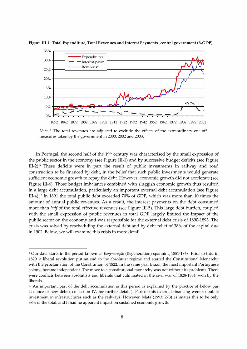
Figure III‐1‐ Total Expenditure, Total Revenues and Interest Payments‐ central government (%GDP)
0%
5%
10%
15%
20%
25%
30%
35%
1852 1862 1872 1882 1892 1902 1912 1922 1932 1942 1952 1962 1972 1982 1992 2002
ExpendituresInterest paymRevenues*
Note: * The total revenues are adjusted to exclude the effects of the extraordinary one‐off measures taken by the government in 2000, 2002 and 2003.
In Portugal, the second half of the 19th century was characterised by the small expression of
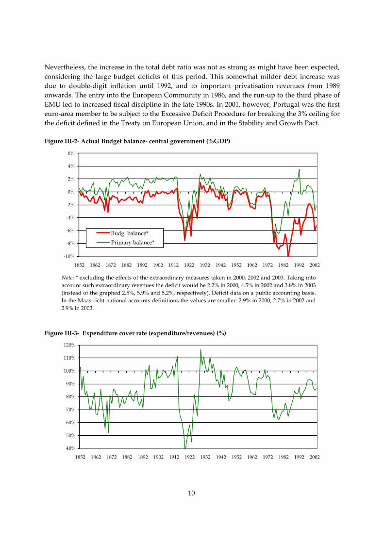
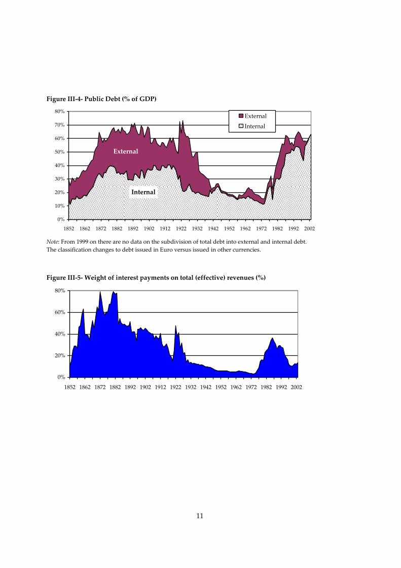
the public sector in the economy (see Figure III‐1) and by successive budget deficits (see Figure III‐2).9 These deficits were in part the result of public investments in railway and road construction to be financed by debt, in the belief that such public investments would generate sufficient economic growth to repay the debt. However, economic growth did not accelerate (see Figure III‐6). Those budget imbalances combined with sluggish economic growth thus resulted in a large debt accumulation, particularly an important external debt accumulation (see Figure III‐4).10 In 1891 the total public debt exceeded 70% of GDP, which was more than 10 times the amount of annual public revenues. As a result, the interest payments on the debt consumed more than half of the total effective revenues (see Figure III‐5). This large debt burden, coupled with the small expression of public revenues in total GDP largely limited the impact of the public sector on the economy and was responsible for the external debt crisis of 1890‐1893. The crisis was solved by rescheduling the external debt and by debt relief of 38% of the capital due in 1902. Below, we will examine this crisis in more detail.
9 Our data starts in the period known as Regeneração (Regeneration) spanning 1851‐1868. Prior to this, in 1820, a liberal revolution put an end to the absolutist regime and started the Constitutional Monarchy with the proclamation of the Constitution of 1822. In the same year Brazil, the most important Portuguese colony, became independent. The move to a constitutional monarchy was not without its problems. There were conflicts between absolutists and liberals that culminated in the civil war of 1828‐1834, won by the liberals. 10 An important part of the debt accumulation is this period is explained by the practice of below par issuance of new debt (see section IV, for further details). Part of this external financing went to public investment in infrastructures such as the railways. However, Mata (1993: 273) estimates this to be only 38% of the total, and it had no apparent impact on sustained economic growth.
9
In the follow‐up to the debt crisis the government was unable to obtain new external loans, and so it was forced to rely instead on the internal capital market and on loans from the Bank of Portugal to finance the deficit. Since funds available from these sources were limited, the government had no choice but to improve the soundness of public finances. As a result, the budget was even in surplus in 1894, 1896, and again in 1901.
In the 20th century, in October 1910 to be precise, the Constitutional Monarchy came to an
end and Portugal became a Republic. The public finances continued to improve gradually until the start of World War I (WWI), in which Portugal participated. The increase in military expenditure and the decline in revenues caused a large fiscal imbalance in this period. Apart from an external loan by the English government, the external capital markets remained closed to the Portuguese government. This meant that the government had to resort to monetary financing by the Bank of Portugal, which led to high inflation. Since most taxes were fixed in monetary terms, the tax revenues were partly eroded by inflation.11 The good news was that the same high inflation, and the suspension of interest payments to enemy countries, helped to reduce the real value of the debt.
The military coup of 28 May 1926, and a few years later the establishment of the “Estado
Novo” (literally New State), a corporatist dictatorial regime lead by Oliveira Salazar, dramatically changed the way fiscal policy was conducted. In the 45 years that followed, the dictatorial regime strictly observed the principle of fiscal balance.12 The public accounts therefore improved considerably, despite the relentless increase of the weight of the public sector on the economy. This made a sharp reduction in the stock of public debt possible (Figure III‐4). The cancellation of the war debt to the UK in 1933 and the conversion of 2/3 of the remaining external debt into internal debt, meant that the external debt was virtually eliminated in 1940. After the Second World War, during which Portugal stayed neutral, strong economic growth and the accumulation of fiscal surpluses enabled the total debt ratio to reach a minimum of 15% of GDP in 1957.
The year of 1974 marked the return of the budget to a substantial deficit position. In April of that year a revolution led by the army brought an end to the “Estado Novo” regime. The predominantly socialist ideology during the first years of the democratic regime that followed the April 25 revolution oversaw a dramatic increase in public intervention in the economy. Heavy industry and banking were nationalized, along with agriculture in the southern part of the country. Those actions plus the 1973 oil crisis led to substantial macroeconomic instability and to successive balance of payments crises. Public expenditure on education, health care, pensions, transfers and subsidies increased massively, as did the budget deficit. As a result, the debt also rose, from 15% in 1973 to a maximum of 64% of GDP in 1996 (63% in 2003).
11 The period of high inflation ended abruptly with the monetary stabilisation programme of Álvaro Castro in 1924. 12 The budget surpluses of this dictatorship period are best viewed on a national accounting basis for the overall government. The data shown here just covers central government accounts, disregarding the other levels of government and public institutes that were generally in surplus.
10
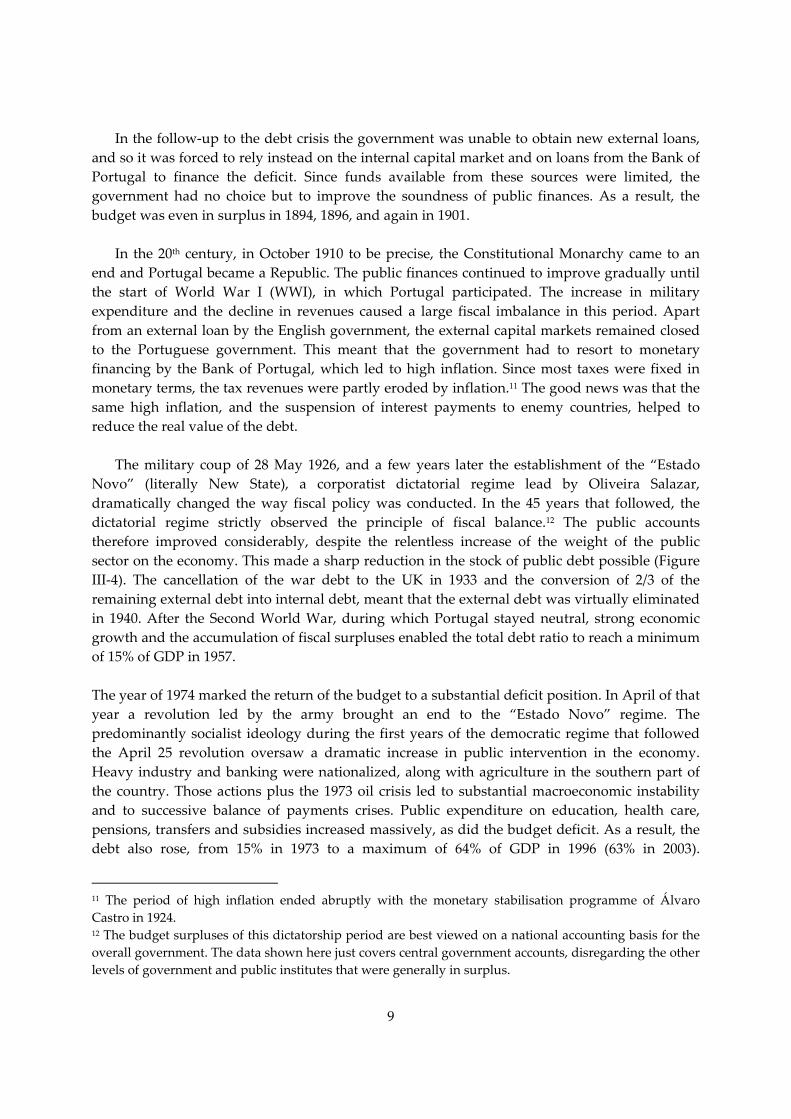
Nevertheless, the increase in the total debt ratio was not as strong as might have been expected, considering the large budget deficits of this period. This somewhat milder debt increase was due to double‐digit inflation until 1992, and to important privatisation revenues from 1989 onwards. The entry into the European Community in 1986, and the run‐up to the third phase of EMU led to increased fiscal discipline in the late 1990s. In 2001, however, Portugal was the first euro‐area member to be subject to the Excessive Deficit Procedure for breaking the 3% ceiling for the deficit defined in the Treaty on European Union, and in the Stability and Growth Pact.
Figure III‐2‐ Actual Budget balance‐ central government (%GDP)
‐10%
‐8%
‐6%
‐4%
‐2%
0%
2%
4%
6%
1852 1862 1872 1882 1892 1902 1912 1922 1932 1942 1952 1962 1972 1982 1992 2002
Budg. balance*Primary balance*
Note: * excluding the effects of the extraordinary measures taken in 2000, 2002 and 2003. Taking into account such extraordinary revenues the deficit would be 2.2% in 2000, 4.5% in 2002 and 3.8% in 2003 (instead of the graphed 2.5%, 5.9% and 5.2%, respectively). Deficit data on a public accounting basis. In the Maastricht national accounts definitions the values are smaller: 2.9% in 2000, 2.7% in 2002 and 2.9% in 2003.
Figure III‐3‐ Expenditure cover rate (expenditure/revenues) (%)
40%
50%
60%
70%
80%
90%
100%
110%
120%
1852 1862 1872 1882 1892 1902 1912 1922 1932 1942 1952 1962 1972 1982 1992 2002
11
Figure III‐4‐ Public Debt (% of GDP)
0%
10%
20%
30%
40%
50%
60%
70%
80%
1852 1862 1872 1882 1892 1902 1912 1922 1932 1942 1952 1962 1972 1982 1992 2002
External
Internal
Internal
External
Note: From 1999 on there are no data on the subdivision of total debt into external and internal debt. The classification changes to debt issued in Euro versus issued in other currencies.
Figure III‐5‐ Weight of interest payments on total (effective) revenues (%)
0%
20%
40%
60%
80%
1852 1862 1872 1882 1892 1902 1912 1922 1932 1942 1952 1962 1972 1982 1992 2002
12
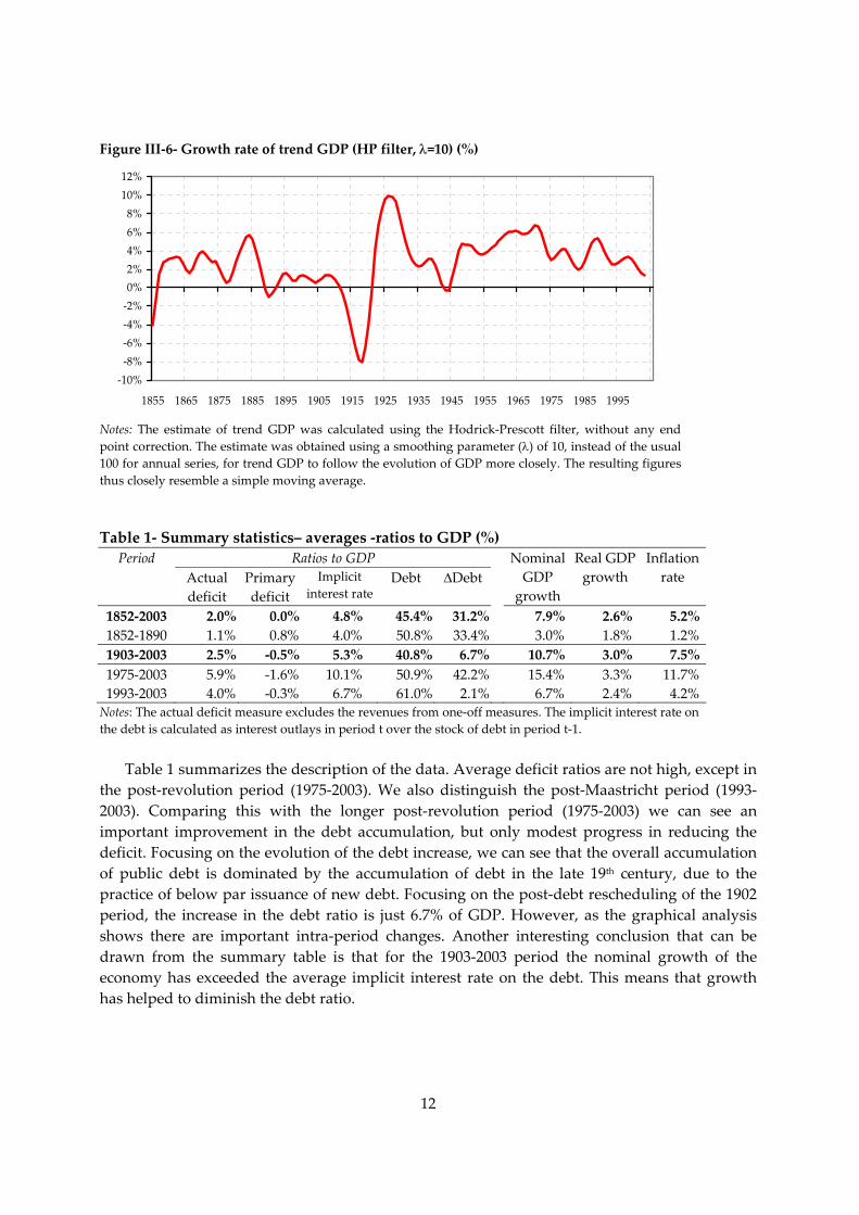
Figure III‐6‐ Growth rate of trend GDP (HP filter, λ=10) (%)
‐10%‐8%‐6%‐4%‐2%0%2%4%6%8%10%12%
1855 1865 1875 1885 1895 1905 1915 1925 1935 1945 1955 1965 1975 1985 1995
Notes: The estimate of trend GDP was calculated using the Hodrick‐Prescott filter, without any end point correction. The estimate was obtained using a smoothing parameter (λ) of 10, instead of the usual 100 for annual series, for trend GDP to follow the evolution of GDP more closely. The resulting figures thus closely resemble a simple moving average. Table 1‐ Summary statistics– averages ‐ratios to GDP (%)
Ratios to GDP Period Actual deficit
Primary deficit
Implicit interest rate
Debt ∆Debt Nominal GDP
growth
Real GDP growth
Inflation rate
1852‐2003 2.0% 0.0% 4.8% 45.4% 31.2% 7.9% 2.6% 5.2% 1852‐1890 1.1% 0.8% 4.0% 50.8% 33.4% 3.0% 1.8% 1.2% 1903‐2003 2.5% ‐0.5% 5.3% 40.8% 6.7% 10.7% 3.0% 7.5% 1975‐2003 5.9% ‐1.6% 10.1% 50.9% 42.2% 15.4% 3.3% 11.7% 1993‐2003 4.0% ‐0.3% 6.7% 61.0% 2.1% 6.7% 2.4% 4.2% Notes: The actual deficit measure excludes the revenues from one‐off measures. The implicit interest rate on the debt is calculated as interest outlays in period t over the stock of debt in period t‐1.
Table 1 summarizes the description of the data. Average deficit ratios are not high, except in
the post‐revolution period (1975‐2003). We also distinguish the post‐Maastricht period (1993‐2003). Comparing this with the longer post‐revolution period (1975‐2003) we can see an important improvement in the debt accumulation, but only modest progress in reducing the deficit. Focusing on the evolution of the debt increase, we can see that the overall accumulation of public debt is dominated by the accumulation of debt in the late 19th century, due to the practice of below par issuance of new debt. Focusing on the post‐debt rescheduling of the 1902 period, the increase in the debt ratio is just 6.7% of GDP. However, as the graphical analysis shows there are important intra‐period changes. Another interesting conclusion that can be drawn from the summary table is that for the 1903‐2003 period the nominal growth of the economy has exceeded the average implicit interest rate on the debt. This means that growth has helped to diminish the debt ratio.
13
IV. The 1890‐1893 debt crisis: direct evidence against sustainability?
In this section we look at the issues related to the external debt crisis of 1890‐1893 in more detail. The purpose is to see whether this crisis is direct evidence against the sustainability of Portuguese public finances in the second half of the 19th century.
A. The causes of the crisis In order to better understand this period, and the statistical data presented earlier, it is
important to look at how was Portuguese public debt issued at the time. Following the external debt conversion of 1852, the Portuguese government wanted to issue debt consolidated (perpetual) debt at the same nominal interest rate of 3% as Great Britain and France. However, external investors were only willing to acquire it at a considerable discount on par value, in order to have an effective rate greater than 3%. Since at the time most debt was perpetual this did not represent any inefficiency for the state: it is the same to issue a perpetual bond at par value with a 6% interest rate, or to issue it 50% below par value and to pay 3% interest.13 Both possibilities imply the same interest payments over time. With regard to the placement markets , London was the dominant market until 1870s, when it was supplanted by Paris (Berlin joined, too, in 1886).
The 1890‐1893 crisis was largely the result of debt accumulation, caused by persistent past
budget deficits, and was detonated by the coincidence of several events. As mentioned above, the Regeneration period was dominated by the idea of “material improvements”.14 Those consisted of large public investment in infrastructure (in transport and communications), financed in large part by public borrowing, especially by external loans. These investments were meant to foster economic growth, repaying themselves (with interest) in increased tax revenues. Given the small weight of the government in the economy, and Portugal’s record of three foreign debt reschedulings, this was a very risky project which, in order to succeed, would have required substantial increases in public revenues.15 However, as Esteves (2004a: 115) points out at the time Portugal’s tax structure was archaic: on average 13% of the revenues were raised by indirect taxes on tobacco, and 39% came from import duties. As a result, the commercial crises of 1867‐69, 1876, and 1889‐90 had a direct negative impact on public accounts. The response to these crises was an increase in direct taxation, which was proportional. But these increases in taxation were achieved by imposing supplements, without reforming the tax code. Nor was there any progress towards reducing tax evasion. Moreover, as economic growth did not
13 As long as the government does not buy it back in the market. The same is not true for amortizable debt. 14 This term was borrowed from the French “améliorations matérielles”. 15 In the aftermath of the civil war there were frequent delays in the payment of interest, usually added to the principal, and three debt reschedulings ‐ in 1840, 1845, and 1852. Before the 1852 conversion the debt service was unsustainable since it absorbed almost 2/3 of the tax revenues. The loans from the civil war period were subject to 9% interest.
14
substantially accelerate in this period, public revenues failed to increase as hoped. Since current expenditure was not curtailed, it was impossible to transform the budget deficit into the surplus required to redeem the debt.
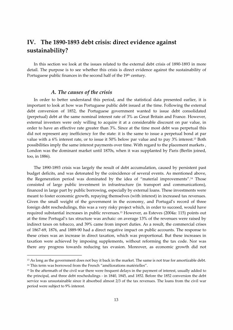
Figure IV‐1‐ Interest outlay (% Revenue), Budget Cover rate (Rev/Exp) and the External debt ratio (%GDP) – 1852‐1910
Interest (% Rev) Budget cover rat Ext debt ratio
1852 1856 1860 1864 1868 1872 1876 1880 1884 1888 1892 1896 1900 1904 19080.0
0.2
0.4
0.6
0.8
1.0
1.2
0.0
0.2
0.4
0.6
0.8
1.0
1.2
Despite this latent non‐sustainability, by today’s Maastricht criteria, there were no
immediate negative fiscal developments around 1890 that could potentially trigger a debt crisis.16 As shown in the previous graphs, in the 1880’s the debt ratio remained relatively stable in the 60‐70% range, the budget deficit was around 1% of GDP, and the cover rate of expenditure by revenues remained fairly constant around 75%. There was even very positive progress in the interest outlay burden over the decade.17 However, we should bear in mind that the weight of the government in the economy was very low, and that the external debt was equivalent to eight years of public revenues. Thus any obstacle to the rollover of the debt could trigger a crisis. In fact, the crisis was sparked off by the conjunction of several political, financial and economic factors:
‐ In 1889 there was a crisis in Brazil’s coffee exports, which led to a substantial reduction in the gold remittances to Portugal from Portuguese emigrants in Brazil (these remittances fell by 82% between 1888 and 1891, from 4355 contos to just 800, i.e. from £965,846 to £165,563).18
16 See also the econometric analysis below, in section IV.C. 17 Interest outlay fell from 76% to 47% of the total effective revenues in the 1880s. 18 Data on Portuguese currency from Esteves (2004a). The conto was a unit of account worth one million réis. The par exchange rate was 4500 réis per pound sterling. Later, with the Republic, the Portuguese currency became the escudo (PTE), worth 1000 réis (a conto being one thousand escudos). Fom 1999, the escudo has been replaced by the euro, worth 200.482 PTE (a conto is equivalent to 4.988 euros).
15
‐ On 11 January 1890 England issued an ultimatum to Portugal to withdraw from some of its possessions in Africa, and sent seven warships to Lisbon to enforce it. The government conceded, which caused great popular outrage and a Republican rebellion on 31‐1‐1891, in Porto.
‐ In April 1890, the crisis was detonated by the inability of the government to place a new loan in Paris. It was the first time this happened in 38 years, and was mainly the result of a boycott campaign led by the holders of the D. Miguel loan.19 Together with the fall in gold remittances, this brought about a lack of liquidity (gold) to service the debt. To make things worse, in the follow‐up to Argentina’s debt crisis, in November 1890, the firm Baring Brothers, which was Portugal’s London agent for floating the short term debt, became insolvent and suspended the payments. The Portuguese government could neither float further debt in external markets, nor pay the interest on the outstanding debt.
‐ With regard to the monetary system, Portugal was in the gold standard. In September 1890 there was a run on the Montepio Geral bank, and several banks in Porto were on the verge of bankruptcy. The Bank of Portugal went to the rescue. Due to the large sums involved, the government granted legal tender status to the notes of Bank of Portugal, abandoning the gold standard in May 1891.20
‐ In 1891 the Portuguese government only managed to issue a new loan in Paris by consigning for 35 years the revenues from the tobacco monopoly. Most of the amount thus obtained, however, was simply to pay in the interest due up to the end of 1891. With this gloomy scenario, negotiation with creditors to reschedule the debt became
inevitable. But no agreement was reached. On 13‐6‐1892, by decree, Portugal unilaterally cut the interest on external debt to 1/3 of its contractual value (to 1%). Alternatively, creditors could opt to convert their securities into internal debt. This partial default caused a long dispute with foreign creditors. In May 1893 a law was passed giving additional compensation to bondholders by sharing some of the import duties between the Portuguese state and the external creditors. Finally, in 1902 a convention was signed. The settlement comprised a debt reduction of 38% (the outstanding capital was reduced from £56,198,000 to £34,734,000), and a reduction in the annual debt service from £1,894,000 in 1892 to £947,000 to be paid over 99 years (3% interest).
19 This was a loan raised by the absolutist government in 1832 (during the civil war, which they lost) and which the liberal government repudiated. The bondholders wanted reimbursement of the loan with interest. 20 As Esteves (2003) puts it, the abandoning of the gold standard helped to ease the transition to sounder public finances, because in the years immediately after 1891 the bulk of the deficit was financed by the Bank of Portugal.
16
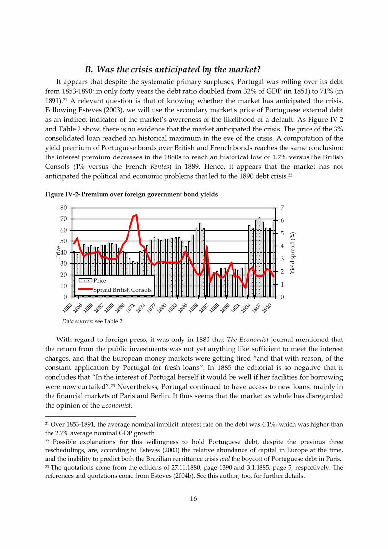
B. Was the crisis anticipated by the market? It appears that despite the systematic primary surpluses, Portugal was rolling over its debt
from 1853‐1890: in only forty years the debt ratio doubled from 32% of GDP (in 1851) to 71% (in 1891).21 A relevant question is that of knowing whether the market has anticipated the crisis. Following Esteves (2003), we will use the secondary market’s price of Portuguese external debt as an indirect indicator of the market’s awareness of the likelihood of a default. As Figure IV‐2 and Table 2 show, there is no evidence that the market anticipated the crisis. The price of the 3% consolidated loan reached an historical maximum in the eve of the crisis. A computation of the yield premium of Portuguese bonds over British and French bonds reaches the same conclusion: the interest premium decreases in the 1880s to reach an historical low of 1.7% versus the British Consols (1% versus the French Rentes) in 1889. Hence, it appears that the market has not anticipated the political and economic problems that led to the 1890 debt crisis.22
Figure IV‐2‐ Premium over foreign government bond yields
0
10
20
30
40
50
60
70
80
1853
1856
1859
1862
1865
1868
1871
1874
1877
1880
1883
1886
1889
1892
1895
1898
1901
1904
1907
1910
Price
0
1
2
3
4
5
6
7
Yield spread (%
)
PriceSpread British Consols
Data sources: see Table 2.
With regard to foreign press, it was only in 1880 that The Economist journal mentioned that
the return from the public investments was not yet anything like sufficient to meet the interest charges, and that the European money markets were getting tired “and that with reason, of the constant application by Portugal for fresh loans”. In 1885 the editorial is so negative that it concludes that “In the interest of Portugal herself it would be well if her facilities for borrowing were now curtailed”.23 Nevertheless, Portugal continued to have access to new loans, mainly in the financial markets of Paris and Berlin. It thus seems that the market as whole has disregarded the opinion of the Economist. 21 Over 1853‐1891, the average nominal implicit interest rate on the debt was 4.1%, which was higher than the 2.7% average nominal GDP growth. 22 Possible explanations for this willingness to hold Portuguese debt, despite the previous three reschedulings, are, according to Esteves (2003) the relative abundance of capital in Europe at the time, and the inability to predict both the Brazilian remittance crisis and the boycott of Portuguese debt in Paris. 23 The quotations come from the editions of 27.11.1880, page 1390 and 3.1.1885, page 5, respectively. The references and quotations come from Esteves (2004b). See this author, too, for further details.
17
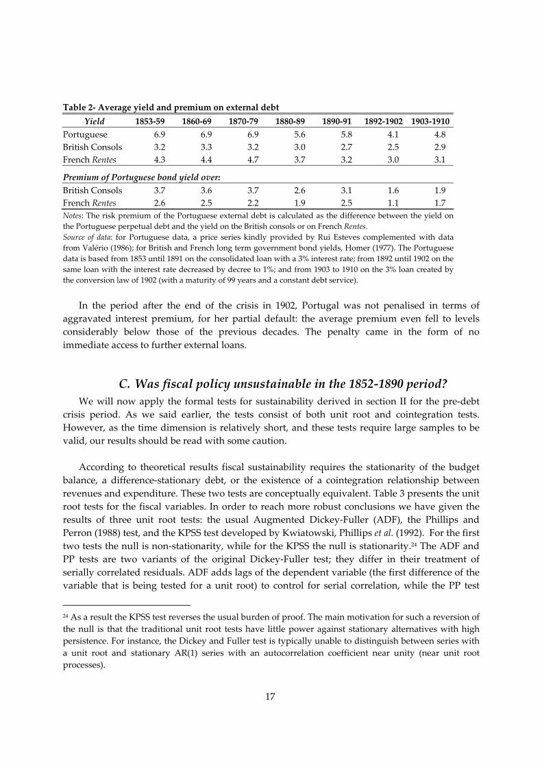
Table 2‐ Average yield and premium on external debt
Yield 1853‐59 1860‐69 1870‐79 1880‐89 1890‐91 1892‐1902 1903‐1910Portuguese 6.9 6.9 6.9 5.6 5.8 4.1 4.8 British Consols 3.2 3.3 3.2 3.0 2.7 2.5 2.9 French Rentes 4.3 4.4 4.7 3.7 3.2 3.0 3.1
Premium of Portuguese bond yield over: British Consols 3.7 3.6 3.7 2.6 3.1 1.6 1.9 French Rentes 2.6 2.5 2.2 1.9 2.5 1.1 1.7 Notes: The risk premium of the Portuguese external debt is calculated as the difference between the yield on the Portuguese perpetual debt and the yield on the British consols or on French Rentes. Source of data: for Portuguese data, a price series kindly provided by Rui Esteves complemented with data from Valério (1986); for British and French long term government bond yields, Homer (1977). The Portuguese data is based from 1853 until 1891 on the consolidated loan with a 3% interest rate; from 1892 until 1902 on the same loan with the interest rate decreased by decree to 1%; and from 1903 to 1910 on the 3% loan created by the conversion law of 1902 (with a maturity of 99 years and a constant debt service).
In the period after the end of the crisis in 1902, Portugal was not penalised in terms of aggravated interest premium, for her partial default: the average premium even fell to levels considerably below those of the previous decades. The penalty came in the form of no immediate access to further external loans.
C. Was fiscal policy unsustainable in the 1852‐1890 period? We will now apply the formal tests for sustainability derived in section II for the pre‐debt
crisis period. As we said earlier, the tests consist of both unit root and cointegration tests. However, as the time dimension is relatively short, and these tests require large samples to be valid, our results should be read with some caution.
According to theoretical results fiscal sustainability requires the stationarity of the budget
balance, a difference‐stationary debt, or the existence of a cointegration relationship between revenues and expenditure. These two tests are conceptually equivalent. Table 3 presents the unit root tests for the fiscal variables. In order to reach more robust conclusions we have given the results of three unit root tests: the usual Augmented Dickey‐Fuller (ADF), the Phillips and Perron (1988) test, and the KPSS test developed by Kwiatowski, Phillips et al. (1992). For the first two tests the null is non‐stationarity, while for the KPSS the null is stationarity.24 The ADF and PP tests are two variants of the original Dickey‐Fuller test; they differ in their treatment of serially correlated residuals. ADF adds lags of the dependent variable (the first difference of the variable that is being tested for a unit root) to control for serial correlation, while the PP test
24 As a result the KPSS test reverses the usual burden of proof. The main motivation for such a reversion of the null is that the traditional unit root tests have little power against stationary alternatives with high persistence. For instance, the Dickey and Fuller test is typically unable to distinguish between series with a unit root and stationary AR(1) series with an autocorrelation coefficient near unity (near unit root processes).
18
applies a nonparametric correction to the test statistic. In fact, the PP correction allows for more general dependence in the residual process, including conditional heteroskedasticity.
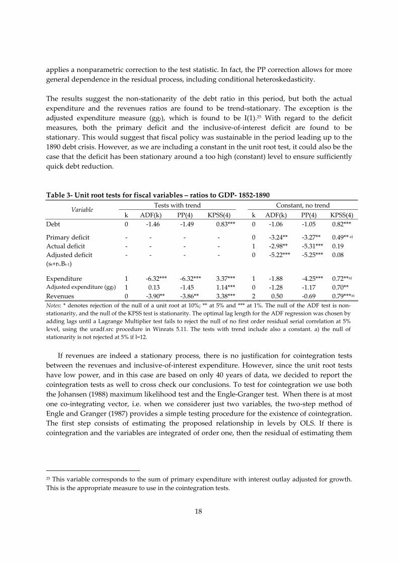
The results suggest the non‐stationarity of the debt ratio in this period, but both the actual expenditure and the revenues ratios are found to be trend‐stationary. The exception is the adjusted expenditure measure (ggt), which is found to be I(1).25 With regard to the deficit measures, both the primary deficit and the inclusive‐of‐interest deficit are found to be stationary. This would suggest that fiscal policy was sustainable in the period leading up to the 1890 debt crisis. However, as we are including a constant in the unit root test, it could also be the case that the deficit has been stationary around a too high (constant) level to ensure sufficiently quick debt reduction.
Table 3‐ Unit root tests for fiscal variables – ratios to GDP‐ 1852‐1890
Tests with trend Constant, no trend Variable k ADF(k) PP(4) KPSS(4) k ADF(k) PP(4) KPSS(4)
Debt
0 ‐1.46 ‐1.49 0.83*** 0 ‐1.06 ‐1.05 0.82***
Primary deficit ‐ ‐ ‐ ‐ 0 ‐3.24** ‐3.27** 0.49** a) Actual deficit ‐ ‐ ‐ ‐ 1 ‐2.98** ‐5.31*** 0.19 Adjusted deficit (st+rt.Bt‐1)
‐ ‐ ‐ ‐ 0 ‐5.22*** ‐5.25*** 0.08
Expenditure 1 ‐6.32*** ‐6.32*** 3.37*** 1 ‐1.88 ‐4.25*** 0.72**a) Adjusted expenditure (ggt) 1 0.13 ‐1.45 1.14*** 0 ‐1.28 ‐1.17 0.70** Revenues 0 ‐3.90** ‐3.86** 3.38*** 2 0.50 ‐0.69 0.79***a) Notes: * denotes rejection of the null of a unit root at 10%; ** at 5% and *** at 1%. The null of the ADF test is non‐stationarity, and the null of the KPSS test is stationarity. The optimal lag length for the ADF regression was chosen by adding lags until a Lagrange Multiplier test fails to reject the null of no first order residual serial correlation at 5% level, using the uradf.src procedure in Winrats 5.11. The tests with trend include also a constant. a) the null of stationarity is not rejected at 5% if l=12.
If revenues are indeed a stationary process, there is no justification for cointegration tests between the revenues and inclusive‐of‐interest expenditure. However, since the unit root tests have low power, and in this case are based on only 40 years of data, we decided to report the cointegration tests as well to cross check our conclusions. To test for cointegration we use both the Johansen (1988) maximum likelihood test and the Engle‐Granger test. When there is at most one co‐integrating vector, i.e. when we considerer just two variables, the two‐step method of Engle and Granger (1987) provides a simple testing procedure for the existence of cointegration. The first step consists of estimating the proposed relationship in levels by OLS. If there is cointegration and the variables are integrated of order one, then the residual of estimating them
25 This variable corresponds to the sum of primary expenditure with interest outlay adjusted for growth. This is the appropriate measure to use in the cointegration tests.
19
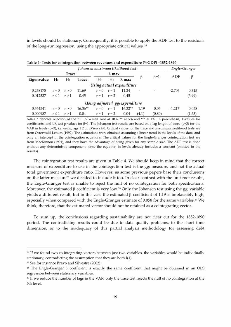
in levels should be stationary. Consequently, it is possible to apply the ADF test to the residuals of the long‐run regression, using the appropriate critical values. 26
Table 4‐ Tests for cointegration between revenues and expenditure (%GDP) –1852‐1890
Johansen maximum likelihood test Engle‐Granger Trace λ max
Eigenvalue H0 H1 Trace H0 H1 λ max β β=1
ADF β
Using actual expenditure 0.268178 r = 0 r > 0 11.69 r = 0 r = 1 11.24 ‐ ‐ ‐2.706 0.315 0.012537 r ≤ 1 r > 1 0.45 r = 1 r = 2 0.45 (3.99)
Using adjusted ggt expenditure 0.364541 r = 0 r > 0 16.36** r = 0 r = 1 16.32** 1.19 0.06 ‐1.217 0.058 0.000987 r ≤ 1 r > 1 0.04 r = 1 r = 2 0.04 (4.1) (0.80) (1.53)
Notes: * denotes rejection of the null of a unit root at 10%; ** at 5% and *** at 1%. In parenthesis, T‐values for coefficients, and LR test p‐values for β=1. The Johansen test results are based on a lag length of three (p=3) for the VAR in levels (p=3), i.e. using lags 1 2 in EViews 4.0. Critical values for the trace and maximum likelihood tests are from Osterwald‐Lenum (1992). The estimations were obtained assuming a linear trend in the levels of the data, and only an intercept in the cointegration equations. The critical values for the Engle‐Granger cointegration test are from MacKinnon (1991), and they have the advantage of being given for any sample size. The ADF test is done without any deterministic component, since the equation in levels already includes a constant (omitted in the results).
The cointegration test results are given in Table 4. We should keep in mind that the correct measure of expenditure to use in the cointegration test is the ggt measure, and not the actual total government expenditure ratio. However, as some previous papers base their conclusions on the latter measure27 we decided to include it too. In clear contrast with the unit root results, the Engle‐Granger test is unable to reject the null of no cointegration for both specifications. Moreover, the estimated β coefficient is very low.28 Only the Johansen test using the ggt variable yields a different result, but in this case the estimated β coefficient of 1.19 is implausibly high, especially when compared with the Engle‐Granger estimate of 0.058 for the same variables.29 We think, therefore, that the estimated vector should not be retained as a cointegrating vector.
To sum up, the conclusions regarding sustainability are not clear cut for the 1852‐1890
period. The contradicting results could be due to data quality problems, to the short time dimension, or to the inadequacy of this partial analysis methodology for assessing debt
26 If we found two co‐integrating vectors between just two variables, the variables would be individually stationary, contradicting the assumption that they are both I(1). 27 See for instance Bravo and Silvestre (2002). 28 The Engle‐Granger β coefficient is exactly the same coefficient that might be obtained in an OLS regression between stationary variables. 29 If we reduce the number of lags in the VAR, only the trace test rejects the null of no cointegration at the 5% level.
20
sustainability in these particular circumstances.30 See Bohn (2004) for an interesting critique of the overall methodology. Using a completely different methodology, based on generational accounting calculations, Esteves (2003) concludes that Portuguese finances were running on an unsustainable path. Moreover, the actual 1892 partial default on the external debt signals a de facto unsustainable debt in this period. The Portuguese economy was unable to generate a sufficient amount of external revenues to service the debt.
V. Empirical evidence for the Portuguese economy Since the 1892 partial debt default may be interpreted as direct evidence of a non‐sustainable
fiscal policy in the 19th century, we decided to exclude the (1902) pre‐debt‐rescheduling period. Hence, we will base our conclusions on the 1903‐2003 period. This is still a long period covering a full century of data, and some of the more important fiscal developments we have analysed. The use of such a long period of data is appropriate for both the unit root and cointegration tests on which we will base our conclusions. As already mentioned, following Hakkio and Rush (1991), our data is expressed in ratios to GDP, which enables us to take into account the growing nature of the economy. We will present the results for both the 1903‐2003 period and for the 1975‐2003 subperiod. The reason for this is to analyse the impact of the 25 April revolution of 1974 on the sustainability of fiscal policy. The 1975‐2003 period comprises the largest budget imbalances of our sample, and so it would naturally be interesting to find out whether 1975 marks a switch into an unsustainable path or is just one step further along the previous (sustainable or unsustainable) path.
We will start the presentation of the empirical evidence by showing the results of the unit
root tests for the fiscal variables. Afterwards we will present the outcome of the cointegration tests. Finally, we will check the robustness of our conclusions to the consideration of structural breaks in the data.
30 This partial equilibrium analysis ignores the interaction between the budget and the economy, the size of the government, its ability to collect taxes, and the composition of the debt. In this period much of the debt was external debt, the debt service was extremely burdensome on the modest public revenues, and there were many exogenous events to fiscal policy in the detonation of the crisis. This is simply not captured by the presented tests.
21
A. Unit root tests As before, in section IV.C, we will present the results of the ADF, PP, and KPSS tests for unit
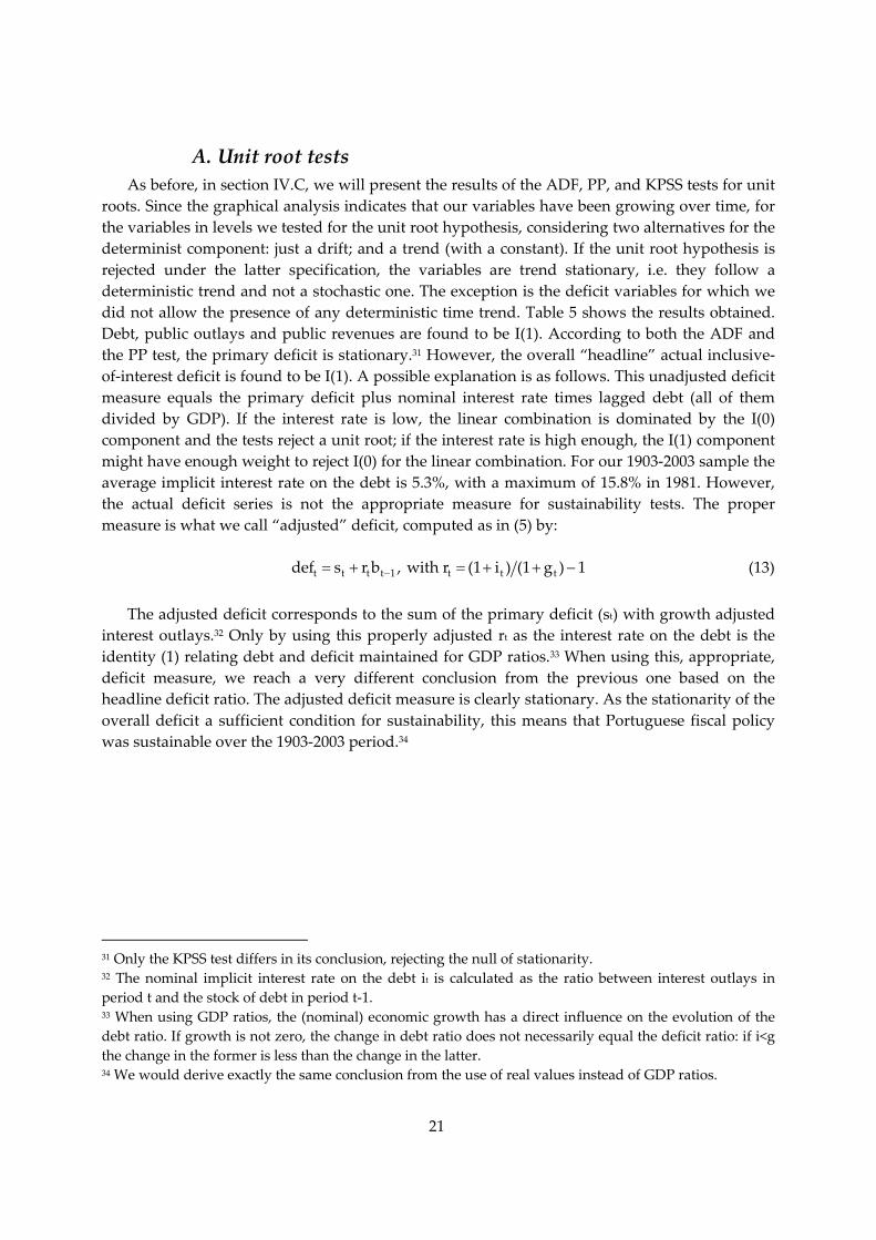
roots. Since the graphical analysis indicates that our variables have been growing over time, for the variables in levels we tested for the unit root hypothesis, considering two alternatives for the determinist component: just a drift; and a trend (with a constant). If the unit root hypothesis is rejected under the latter specification, the variables are trend stationary, i.e. they follow a deterministic trend and not a stochastic one. The exception is the deficit variables for which we did not allow the presence of any deterministic time trend. Table 5 shows the results obtained. Debt, public outlays and public revenues are found to be I(1). According to both the ADF and the PP test, the primary deficit is stationary.31 However, the overall “headline” actual inclusive‐of‐interest deficit is found to be I(1). A possible explanation is as follows. This unadjusted deficit measure equals the primary deficit plus nominal interest rate times lagged debt (all of them divided by GDP). If the interest rate is low, the linear combination is dominated by the I(0) component and the tests reject a unit root; if the interest rate is high enough, the I(1) component might have enough weight to reject I(0) for the linear combination. For our 1903‐2003 sample the average implicit interest rate on the debt is 5.3%, with a maximum of 15.8% in 1981. However, the actual deficit series is not the appropriate measure for sustainability tests. The proper measure is what we call “adjusted” deficit, computed as in (5) by:
−= + = + + −t t t t 1 t t tdef s r b , with r (1 i ) (1 g ) 1 (13)
The adjusted deficit corresponds to the sum of the primary deficit (st) with growth adjusted
interest outlays.32 Only by using this properly adjusted rt as the interest rate on the debt is the identity (1) relating debt and deficit maintained for GDP ratios.33 When using this, appropriate, deficit measure, we reach a very different conclusion from the previous one based on the headline deficit ratio. The adjusted deficit measure is clearly stationary. As the stationarity of the overall deficit a sufficient condition for sustainability, this means that Portuguese fiscal policy was sustainable over the 1903‐2003 period.34
31 Only the KPSS test differs in its conclusion, rejecting the null of stationarity. 32 The nominal implicit interest rate on the debt it is calculated as the ratio between interest outlays in period t and the stock of debt in period t‐1. 33 When using GDP ratios, the (nominal) economic growth has a direct influence on the evolution of the debt ratio. If growth is not zero, the change in debt ratio does not necessarily equal the deficit ratio: if i<g the change in the former is less than the change in the latter. 34 We would derive exactly the same conclusion from the use of real values instead of GDP ratios.
22
Table 5‐ Unit root tests for fiscal variables – ratios to GDP‐ 1903‐2003 Tests with trend Constant, no trend
Variable k ADF(k) PP(4) KPSS(4) k ADF(k) PP(4) KPSS(4) Debt
0 ‐1.04 ‐0.70 0.68*** 0 ‐1.34 ‐1.0 0.51**
Primary deficit ‐ ‐ ‐ ‐ 0 ‐2.95** ‐3.15** 0.24 Actual deficit ‐ ‐ ‐ ‐ 0 ‐2.16 ‐2.29 0.73** Adjusted deficit (st+rt.Bt‐1)
‐ ‐ ‐ ‐ 0 ‐4.75*** ‐4.71*** 0.42*
Expenditure 0 ‐1.75 ‐1.71 2.01*** 0 ‐0.35 ‐1.71 1.77***Adjusted expenditure 0 ‐0.82 ‐0.48 0.50** 0 ‐1.4 ‐1.32 0.72** Revenues 0 ‐2.02 ‐1.95 2.15*** 0 ‐0.34 ‐0.27 1.80***Notes: * denotes rejection of the null of a unit root at 10%; ** at 5% and *** at 1%. The null of the ADF test is non‐stationarity, and the null of the KPSS test is stationarity. The optimal lag length for the ADF regression was chosen by adding lags until a Lagrange Multiplier test fails to reject the null of no first order residual serial correlation at the 5% level, using the uradf.src procedure in Winrats 5.11. The tests with trend also include a constant. Table 6‐ Unit root tests for fiscal variables – ratios to GDP‐ 1975‐2003 Tests with trend Constant, no trend
Variable k ADF(k) PP(4) KPSS(4) k ADF(k) PP(4) KPSS(4) Debt
0 ‐1.74 ‐1.60 0.57** 0 ‐2.5 ‐2.29 0.55**
Primary deficit ‐ ‐ ‐ ‐ 0 ‐1.42 ‐1.52 0.45* Actual deficit ‐ ‐ ‐ ‐ 0 ‐2.15 ‐1.69 0.49* Adjusted deficit (st+rt.Bt‐1)
‐ ‐ ‐ ‐ 0 ‐2.21 ‐2.26 0.21
Expenditure 0 ‐2.86 ‐2.66 1.66*** 0 ‐4.0***a) ‐4.11*** 0.57** Adjusted expenditure 0 ‐2.23 ‐2.21 0.24*** 0 ‐1.0 ‐0.85 0.60** Revenues 0 ‐0.95 ‐0.75 0.64*** 0 ‐1.76 ‐2.14 0.61 Notes: see Table 5. The tests with trend include also a constant. a) The ADF z‐test leads to a different conclusion (non‐rejection of the null of non‐stationarity).
Table 6 repeats the same test for the recent 1975‐2003 subperiod. Now debt, and all the fiscal variables appear to be I(1). Contrary to the previous results, all deficit measures (including the primary deficit) are now non‐stationary. This means that the 1975‐2003 period, marks a shift into an unsustainable fiscal policy in Portugal.
In order to cross check our results, and since the expenditure and public revenues were
found to be I(1), we proceed to the cointegration test between total revenues and total expenditure.35
35 Although the unit root and the cointegration tests are conceptually equivalent, in practice different conclusions might arise. This is because an exact equivalence requires a constant interest rate on the debt, and that all variables are measured consistently. In finite data samples, especially in short ones, the low power of the unit root and cointegration tests might also lead, by itself, to different conclusions.
23
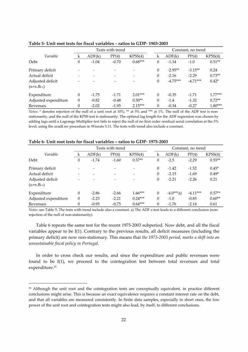
B. Cointegration tests As in section IV.C, we will use the two‐step method of Engle and Granger (1987) and the
Johansen (1988)’s maximum likelihood estimation procedure to test for cointegration. Table 7 summarizes the results. In order to enhance comparison with other studies that include the Portuguese economy, we report the tests using the (incorrect) total expenditure measure and the (correct) ggt defined in equation (11) as the sum of primary expenditure with the growth‐adjusted interest payments on the debt.
Table 7‐ Tests for cointegration between revenues and expenditure (%GDP)
Johansen maximum likelihood test Engle‐Granger Trace λ max
Eigenvalue H0 H1 Trace H0 H1 λ max β β=1
ADF β
Using actual expenditure 1903‐2003 0.119167 r = 0 r > 0 12.85 r = 0 r = 1 12.82 ‐ ‐ ‐2.693 0.753 0.000366 r ≤ 1 r > 1 0.04 r = 1 r = 2 0.04 (30.7)
1975‐2003 0.478347 r = 0 r > 0 24.11** r = 0 r = 1 18.87** 2.39 11.7*** ‐2.601 1.29 0.165299 r ≤ 1 r > 1 5.24* r = 1 r = 2 5.24* (7.2) (0.0) (10.7)
Using adjusted ggt expenditure 1903‐2003 0.153008 r = 0 r > 0 16.79** r = 0 r = 1 16.77** 0.869 2.04 ‐4.43*** 0.711 0.000210 r ≤ 1 r > 1 0.02 r = 1 r = 2 0.02 (10.5) (0.15) 20.0
1975‐2003 0.266533 r = 0 r > 0 11.99 r = 0 r = 1 8.99 ‐ ‐ ‐2.316 0.898 0.098415 r ≤ 1 r > 1 3.0 r = 1 r = 2 3.0 (6.9)
Notes: * denotes rejection of the null of a unit root at 10%; ** at 5% and *** at 1%. In parenthesis, T‐values for coefficients, and LR test p‐values for β=1. The Johansen test results are based on a lag length of three (p=3) for the VAR in levels (p=3), i.e. using lags 1 2 in EViews 4.0. The lag length was chosen using the Akaike information criteria for the 1903‐2003 period. Critical values for the trace and maximum likelihood tests are from Osterwald‐Lenum (1992). The estimations were obtained assuming a linear trend in the levels of the data, and only an intercept in the cointegration equations. The critical values for the Engle‐Granger cointegration test are from MacKinnon (1991), which have the advantage of being given for any sample size. The ADF test is done without any deterministic component, since the equation in levels already includes a constant (omitted from the results).
24
For the 1903‐2003 period the results are in line with those given by the unit root tests. When using the inappropriate headline expenditure measure the null of no cointegration is not rejected by the data. On the other hand, when using the appropriate ggt measure, the null of no cointegration is clearly rejected by both the Engle‐Granger and the Johansen test. Moreover, the null that β equals unity is not rejected by the LR test. This indicates that Portuguese fiscal policy has been sustainable over the 1903‐2003 period. This conclusion is robust to adjusting the revenues for seignorage.36
For the recent 1975‐2003 period, the Engle‐Granger test concludes for the absence of
cointegration, irrespective of the expenditure measures used. In contrast, the Johansen’s test reaches an odd result for the actual unadjusted expenditure: it finds two cointegrating vectors and an implausibly high β estimate.37 This could be the result of low power due to few observations, or to the inadequacy of the headline unadjusted expenditure ratio for the sustainability tests. Using the proper ggt measure, the Johansen test is unable to reject the null of no cointegration at conventional significance levels. As a result, we can safely conclude for the absence of cointegration between revenues and expenditure in the more recent period, meaning that Portuguese fiscal policy appears to have been unsustainable since 1975. This result is in line with the conclusions we derived from the unit root tests.
C. Extension: Cointegration tests allowing for regime shifts A natural extension of this work is to formally test for the presence of structural breaks in
the data. One relevant test has been proposed by Gregory and Hansen (1996) and it could be applied to the Engle‐Granger two‐step procedure. The authors develop a methodology that enables a residual‐based testing of the null of no cointegration against the alternative of cointegration in the presence of a possible regime shift, with the break occurring at an unknown point in time. It is then possible to compute modified ADF statistics (ADF*) allowing for a regime change in the intercept or in the coefficient vector. The independence of this test with regard to the breaking date invalidates data mining from contaminating the choice of the break point. This test is interesting because the power of the usual ADF test decreases sharply in the presence of a structural break. If the model is in fact cointegrated, a standard ADF test may not reject the null, leading to the wrong conclusion that there is no long‐run relationship. The standard cointegration model could be written as follows: 1t 1 2t ty y eµ α= + + (14) where y1r and y2t are I(1) and et is I(0). A structural change would shift the long‐run co‐‐integration relationship to a new level, reflecting changes in the intercept µ and/or in the slope 36 Seignorage revenue was proxied by the (current prices) change in the monetary basis (as a percentage of GDP). Average seignorage gains are 1.1% of GDP, but their distribution over time is not uniform, with the average being dominated by a few large values (the standard deviation is 1.7%). 37 The finding of a cointegration ranking of two, with just two variables in the VAR, is only compatible with the variables being stationary, which is apparently not the case here.
25
α. Hence, the Gregory and Hansen (1996) test allows a regime shift in either the intercept alone or in the entire coefficient vector. More specifically, the authors propose testing the following hypotheses to account for three types of possible structural breaks: 1. Level Shift (C): 1t 1 2 1 2t ty D y eτµ µ α= + + + (15) 2. Level shift with trend (C/T): 1t 1 2 1 2t ty D t y eτµ µ β α= + + + + (16) 3. Regime shift (C/S): 1t 1 2 1 1 2t 2 2t 1 ty D y y D eτ τµ µ α α= + + + + (17) where D1τ = 0 for t ≤ [τT], D1τ = 1 for t > [τT], T is the number of observations, and τ ∈ (0, 1) the unknown parameter that denotes the relative timing of the change point, and [ ] denotes the integer part. The first model allows a change in the intercept at the time of the shift. The second model allows the slope of the vector to shift too. The third possibility is to allow the equilibrium relationship to rotate as well as shift parallel. A cointegration test statistic is calculated for every possible regime shift, retaining the smallest value of the statistics (the largest negative value), across all values of τ. The smallest value is retained because a small value for the statistic constitutes evidence against the null hypothesis of no cointegration.38 In practice the models are recursively estimated by OLS for all possible break points in the trimming interval τ ∈ (0.15, 0.85), and the ADF* statistic is computed as:
(0.15,0.85)ADF* inf ADF( )
ττ
∈= .
Another useful regime change test is proposed by Hansen (2003). This test is applied to the
Johansen method. However, contrary to the previous test, it takes the timing of the change and the number of cointegration relations at any point in time as given, which requires the imposition of a priori information or some resort to the data. We will therefore not use it in our empirical application.
As shown in Table 8, for the 1903‐2003 period, the Gregory‐Hansen ADF* cointegration test
rejects the null hypothesis of no cointegration for all the three possible structural break models (with the exception of the first model for unadjusted data). The rejection of the null hypothesis is
38 With regard to the existence of a structural break, if the standard ADF statistic does not reject, but the ADF* does, this implies that structural change in the cointegrating vector may be important. However, as Gregory and Hansen (1996) note, if both the ADF and the ADF* reject, no inference that structural change has occurred can be drawn from this piece of information alone, since the ADF* statistics is are powerful against conventional cointegration.
26
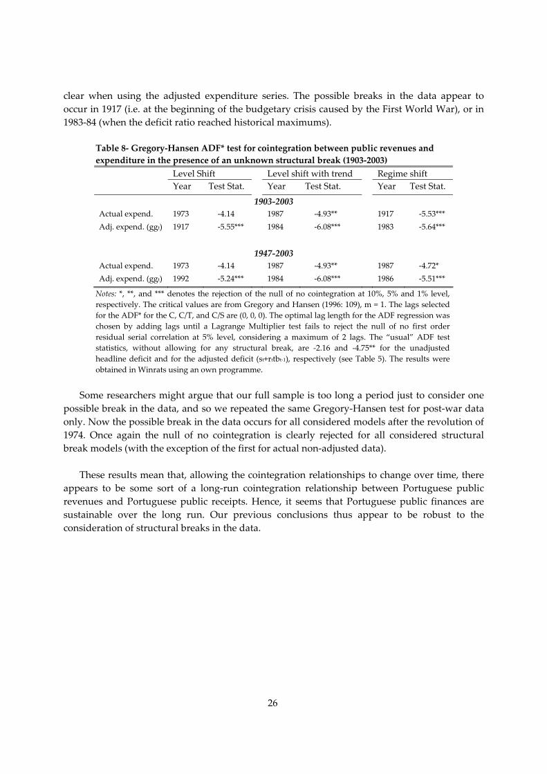
clear when using the adjusted expenditure series. The possible breaks in the data appear to occur in 1917 (i.e. at the beginning of the budgetary crisis caused by the First World War), or in 1983‐84 (when the deficit ratio reached historical maximums).
Table 8‐ Gregory‐Hansen ADF* test for cointegration between public revenues and expenditure in the presence of an unknown structural break (1903‐2003) Level Shift Level shift with trend Regime shift Year Test Stat. Year Test Stat. Year Test Stat.
1903‐2003 Actual expend. 1973 ‐4.14 1987 ‐4.93** 1917 ‐5.53*** Adj. expend. (ggt) 1917 ‐5.55*** 1984 ‐6.08*** 1983 ‐5.64***
1947‐2003 Actual expend. 1973 ‐4.14 1987 ‐4.93** 1987 ‐4.72* Adj. expend. (ggt) 1992 ‐5.24*** 1984 ‐6.08*** 1986 ‐5.51***
Notes: *, **, and *** denotes the rejection of the null of no cointegration at 10%, 5% and 1% level, respectively. The critical values are from Gregory and Hansen (1996: 109), m = 1. The lags selected for the ADF* for the C, C/T, and C/S are (0, 0, 0). The optimal lag length for the ADF regression was chosen by adding lags until a Lagrange Multiplier test fails to reject the null of no first order residual serial correlation at 5% level, considering a maximum of 2 lags. The “usual” ADF test statistics, without allowing for any structural break, are ‐2.16 and ‐4.75** for the unadjusted headline deficit and for the adjusted deficit (st+rttbt‐1), respectively (see Table 5). The results were obtained in Winrats using an own programme.
Some researchers might argue that our full sample is too long a period just to consider one
possible break in the data, and so we repeated the same Gregory‐Hansen test for post‐war data only. Now the possible break in the data occurs for all considered models after the revolution of 1974. Once again the null of no cointegration is clearly rejected for all considered structural break models (with the exception of the first for actual non‐adjusted data).
These results mean that, allowing the cointegration relationships to change over time, there
appears to be some sort of a long‐run cointegration relationship between Portuguese public revenues and Portuguese public receipts. Hence, it seems that Portuguese public finances are sustainable over the long run. Our previous conclusions thus appear to be robust to the consideration of structural breaks in the data.
27
VI. Conclusions This paper tests for the sustainability of Portuguese fiscal policy over a long period of data.
We find considerable evidence in favour of sustainability for the 1903‐2003 period. The use of such a long dataset is appropriate because both unit root and cointegration tests require a long period of data. Our analysis is based on the use of ratios to GDP, which are suitable for a growing economy. Previous results pointing to overall non‐sustainability of Portuguese fiscal policy might be due to a short time dimension and to the use of an improper deficit or expenditure measures, not adjusted for growth.39
The overall conclusion of sustainability for the 1903‐2003 period is not maintained for the
more recent 1975‐2003 period, which is characterised by the largest deficit to GDP ratios of our sample. This period appears to signal a shift to an unsustainable path in Portuguese fiscal policy. Hence, our results suggest that it is in fact necessary to continue to pursue fiscal consolidation efforts in Portugal.
The conclusion of sustainability for the 1903 to 2003 period seems to be robust to the
consideration of structural breaks in the data. Since we found a stationary primary deficit for the 1903‐2003 period, it would be also worthwhile to cross‐check the conclusions of the unit root and cointegration sustainability tests with the method proposed by Bohn (1998). This method tries to find out, using adequate controls, whether the primary surplus responds to changes in the debt to GDP ratio. As that would imply a major expansion of this paper, however, it remains an interesting programme for future research.
Statistical appendix In Portugal, the relevant economic years for fiscal data have not always coincided with
calendar years. The economic years from 1834‐1835 to 1933‐1934 began on 1 July of each civil year and ended on 30 June of the following civil year. The economic years from 1936 on coincided with the civil years. For the purposes of transition, the economic year of 1934‐1935 began on 1 January 1934 and ended on 31 December 1935, under the terms of the same decree‐law. As GDP data is only available on a calendar basis, there is inevitably a timing problem in defining fiscal variables as GDP ratios until 1936. Because fiscal decisions were taken on an annual basis (expressed in economic years), it makes no economic sense to adjust the economic years to calendar years. In order to enable a smooth transition in 1936, we deflate the economic year observation t to t+1 with the GDP of period t+1. For example the data on the fiscal year 1934‐1935 is divided by GDP1935 to calculate the fiscal variable ratios of 1935. An alternative
39 See Bravo and Silvestre (2002) and Afonso (2000). These authors used the actual total inclusive‐of‐interest expenditure (as a percentage of GDP) in their cointegration tests, without correcting the interest payments for growth. As a result their measures are not consistent with the deficit‐debt identity, leading to its clear violation.
28
method would be to calculate, as Mata (1993) did, an average GDP between t and t+1. However, this alternative method would entail having a break in 1936.
We also used official data for the whole period, without making any adjustments to it
(except correcting for the recent one‐off measures). As pointed out by Bohn (1991), the official data is most informative about government behaviour if policy‐makers are primarily influenced by the official data. The main source of data is the publication from the Portuguese Institute of National Statistics (INE) coordinated by Valério (2001). For the period before 1913 the original data was collected by Mata (1993). Since this data is less rounded we have used the original source. Detailed series for the period 1913‐1947 are available in Valério (1994). All variables were converted into euros using the irrevocable conversion rate of 1EUR= 200.482 PTE. The detailed source for each variable is given below.
As discussed in the text, our data refers to the central government accounts, expressed on a
public accounting basis and not on a national accounting basis. This because the main source of the historical data is the “Conta Geral do Estado”, which is a yearly publication from the Ministry of Finance containing the final information on budget execution, in a public accounting perspective. Data on a national accounting basis is only available from 1947 onwards. A coherent dataset, compiled by the Bank of Portugal for the period 1947‐1995, is published in Pinheiro (1999). The main drawback of our dataset is the non‐inclusion of the other sub‐sectors of the public administrations. It is not possible, however, to find historical data for the whole sample period. In contrast, as public accounting mostly follows a cash basis registering, it is theoretically more compatible with the debt series.
Detailed sources GDP
1861‐1994: Valério (2001). The source for this variable for the period 1947‐1994 corresponds to Pinheiro (1999), i.e. the author has linked its historical series with Bank of Portugal’s estimates for the 1947‐1995 period. This series was adjusted to the level of the next period, which is in the ESA95 standard.
1995‐2003: INE estimates, as they appear in Ministério das Finanças (2003).
Primary expenditure The primary expenditure corresponds to the difference between total effective expenditure,
total effective public expenditure and interest payments on the debt. The source of actual data on total effective expenditure was:
1852‐1913: Mata (1993); 1914‐1998: Valério (2001) 1995‐2003: collected by us using the same criteria, from the Conta Geral do Estado (yearly
publication). Public revenues
Corresponds to total effective public revenues of the Portuguese State (Estado) adjusted for the effects of the extraordinary revenues obtained in 2000, 2002 and 2003. Such excluded revenues amounted to 399 million EUR in 2000 (UMTS); 1830 millions in 2002 (CREL revenues,
29
sale of the fixed telecommunication network to Portugal Telecom and an extraordinary regularisation of taxpayers debts); and 1962 millions EUR in 2003 (mainly sale of government credits to Citigroup, and integration of the pension fund of the Portuguese post office, CTT, into the public servants’ pension system, CGA). The effective revenues exclude the revenues from loans.
1852‐1913: Mata (1993); 1914‐1998: Valério (2001) 1999‐2003: collected by us using the same criteria, from the Conta Geral do Estado (yearly
publication). Budget balance
Corresponds to the difference between total public revenues and total public expenditure. Public debt
1861‐1913:Mata (1993); 1914‐1979: Valério (2001) 1980‐2003: Instituto Gestão do Crédito Público (IGCP), Direct State Debt
Interest payments on the debt
1861‐1913: Mata (1993), Table 11. The author distinguishes total public debt servicing costs, which comprises amortization of the debt, interest payments and administrative costs. There are observations on the interest missing for the years 1860, 1866, and 1898‐1907. We assumed that the interest payments in 1860 were an average of its values in 1859 and 1861. Due to lack of data on administrative costs, the interest data for 1866 is calculated by difference, assuming that the administrative costs remain equal to their average weight in the total, during the last three years before 1866 (0.35%). From 1898 to 1913 Mata (1993) is again unable to disaggregate between administrative costs and interest payments. We again found the interest payments by computing the difference between the total servicing costs, excluding the amortization of the debt, and the estimated administrative costs, which were obtained assuming that their weight in the total is equal to the average for the 3 years before and the 3 years after the lack of data (0.3%).
1914‐1947: Valério (1994), table 22 1948‐2003: collected by us, from the Conta Geral do Estado (yearly publication).

30
References AFONSO, A. (2000), ʺFiscal policy sustainability: some unpleasant European evidenceʺ,
Department of Economics, ISEG‐UTL, Working Paper, No. 12/2000/DE/CISEP. BALASSONE, F. and D. FRANCO (2000), ʺAssessing Fiscal Sustainability: a review of methods
with a view to EMUʺ in Banca DʹItalia (ed.), Fiscal Sustainability, Rome: Banca DʹItalia, 21‐60.
BOHN, H. (1991), ʺBudget Balance through revenue or spending adjustments? Some historical evidence for the United Statesʺ, Journal of Monetary Economics, 27, 333‐359.
BOHN, H. (1998), ʺThe Behavior of U. S. Public Debt and Deficitsʺ, The Quarterly Journal of Economics, 113(3), August, 949‐963.
BOHN, H. (2004), ʺThe sustainability of Fiscal Policy in the United Statesʺ, Paper presented at the CESifo‐LBI Conference on ʺThe sustainability of Public Debtʺ, Munich, October.
BRAVO, A. B. and A. L. SILVESTRE (2002), ʺIntertemporal Sustainability of Fiscal Policies: some tests for European countriesʺ, European Journal of Political Economy, 18(3), 517‐528.
CHALK, N. and R. HEMMING (2000), ʺAssessing Fiscal Sustainability in Theory and Practiceʺ in Banca DʹItalia (ed.), Fiscal Sustainability, Rome: Banca DʹItalia, 61‐93.
DOMAR, E. D. (1944), ʺThe ʺBurden of the Debtʺ and the National Incomeʺ, The American Economic Review, 34(4), December, 798‐827.
ENGLE, R. F. and C. W. J. GRANGER (1987), ʺCointegration and Error‐Correction: Representation, Estimation, and Testingʺ, Econometrica, 55, 251‐276.
ESTEVES, R. P. (2003), ʺLooking ahead from the past: the intertemporal sustainability of Portuguese finances, 1854‐1910ʺ, European Review of Economic History, 7, 239‐266.
ESTEVES, R. P. (2004a), ʺAs Pulsações Financeiras: Finanças Públicas, Moeda e Bancosʺ in J. Serrão and A. H. Oliveira Marques (eds.), Nova História de Portugal‐ Portugal e a Regeneração, Lisboa: Editorial Presença, Vol. IX, 108‐148.
ESTEVES, R. P. (2004b), ʺFinanças Públicasʺ in P. Lains and Á. F. d. Silva (eds.), História Económica de Portugal (1700‐2000), forthcoming edition, Lisboa, Vol. II‐ O séc. XIX (1807‐1914).
GREGORY, A. W. and B. E. HANSEN (1996), ʺResidual‐based tests for cointegration in models with regime shiftsʺ, Journal of Econometrics, 70, 99‐126.
HAKKIO, C. S. and M. RUSH (1991), ʺIs the Budget Deficit ʹToo Largeʹ?ʺ Economic Inquiry, 29(3), 429‐445.
HAMILTON, J. and M. A. FLAVIN (1986), ʺOn the Limitations of Government Borrowing: A Framework for Empirical Testingʺ, The American Economic Review, 76V(4), September, 808‐819.
HANSEN, P. R. (2003), ʺStuructural Changes in the Cointegrated Vector Autoregressive Modelʺ, Journal of Econometrics, 114, 261‐295.
HOMER, S. (1977), A history of interest rates: 2000 B.C. to the present, 2nd edition, New Brunswick: Rutgers University Press.
JOHANSEN, S. (1988), ʺStatistical Analysis of Cointegration Vectorsʺ, Journal of Economic Dynamics and Control, 12, 231.254.
31
KWIATOWSKI, D., P. C. B. PHILLIPS, P. SCHMIDT and Y. SHIN (1992), ʺTesting the Null Hypothesis of Stationarity Against the Alternative of a Unit Root: How Sure Are We That Economic Time Series Have a Unit Root?ʺ Journal of Econometrics, 54, 159‐178.
MACKINNON, J. G. (1991), ʺCritical Values for Co‐integration Testsʺ in R. F. Engle and C. W. J. Granger (eds.), Long‐Run Economic Relationships, Oxford: Oxford University Press, 267‐276.
MATA, E. (1993), As finanças públicas portuguesas da Regeneração à primeira Guerra Mundial, Lisboa: Banco de Portugal.
MINISTÉRIO DAS FINANÇAS (2003), A Economia Portuguesa: Reformas e Ajustamento, Lisbon: Ministério das Finanças, December.
OSTERWALD‐LENUM, M. (1992), ʺA Note with Fractiles of the Asymptotic Distribution of the Maximum Likelihood Cointegration Rank Test Statistics: four casesʺ, Oxford Bulletin of Economics and Statistics, 54, 461‐472.
PHILLIPS, P. C. B. and P. PERRON (1988), ʺTesting for a Unit Root in Time Series Regressionʺ, Biometrika, 75, 335‐346.
PINHEIRO, M. (1999), Séries Longas para a Economia Portuguesa Pós II Guerra Mundial: versão revista, e prolongada para 1994 e 1995, Lisboa: Banco de Portugal, Vol. 1.
QUINTOS, C. E. (1995), ʺSustainability of the Deficit Process with Structural Shiftsʺ, Journal of Business and Economic Statistics, 13(4), October, 409‐417.
TREHAN, B. and C. E. WALSH (1988), ʺCommon Trends, Intertemporal Budget Balance, and Revenue Smoothingʺ, Journal of Economic Dynamics and Control, 12, 425‐444.
TREHAN, B. and C. E. WALSH (1991), ʺTesting Intertemporal Budget Constraints: Theory and Applications to U.S. Federal Budget and Current Account Deficitsʺ, Journal of Money, Credit, and Banking, 23(2), 206‐223.
VALÉRIO, N. (1986), ʺExpectativas dos credores externos sobre a solvabilidade do Estado portuguêsʺ, Revista de História Económica e Social, 18, 1‐8.
VALÉRIO, N. (1994), As finanças públicas portuguesas entre as duas guerras mundiais, Lisboa: Ediçoes Cosmos.
VALÉRIO, N. (2001), Estatísticas Históricas Portuguesas/ Portuguese Historical Statistics, Lisboa: INE.
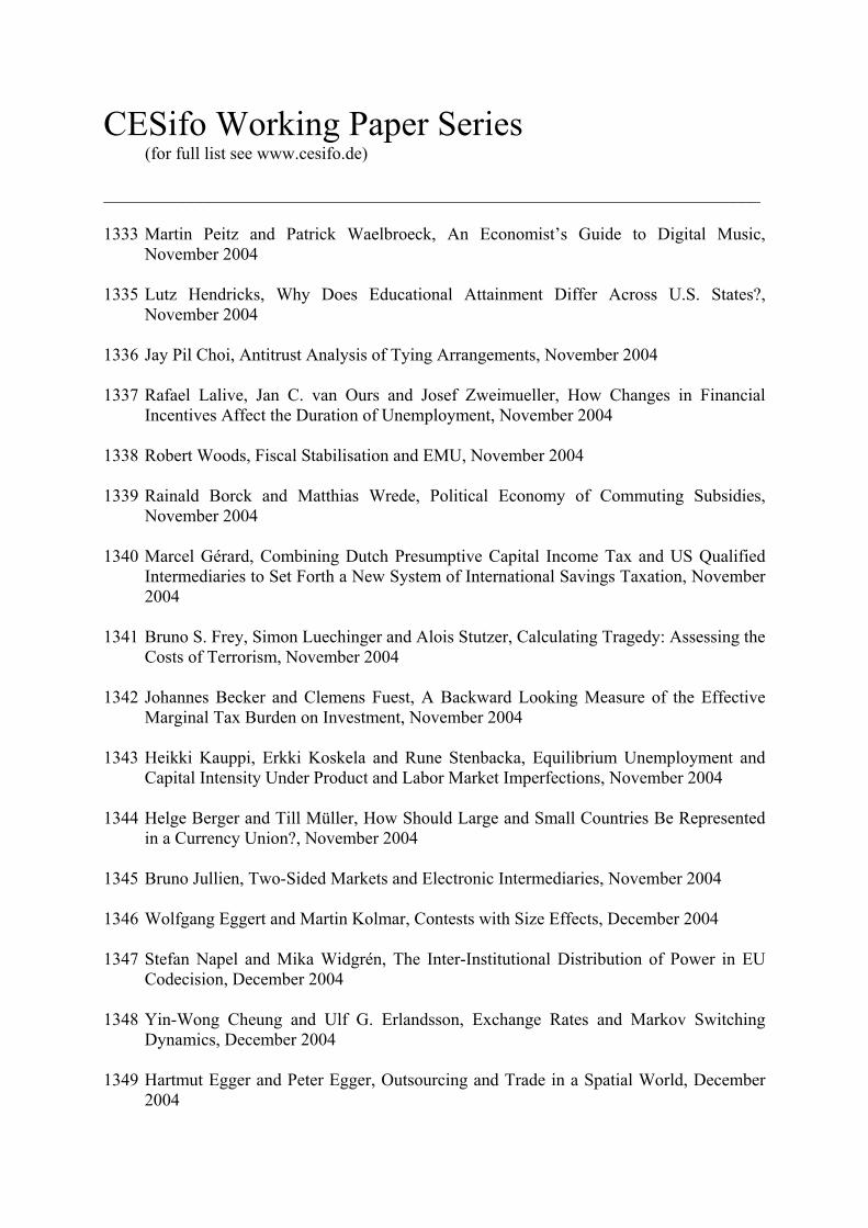
CESifo Working Paper Series (for full list see www.cesifo.de)
___________________________________________________________________________ 1333 Martin Peitz and Patrick Waelbroeck, An Economist’s Guide to Digital Music,
November 2004 1335 Lutz Hendricks, Why Does Educational Attainment Differ Across U.S. States?,
November 2004 1336 Jay Pil Choi, Antitrust Analysis of Tying Arrangements, November 2004 1337 Rafael Lalive, Jan C. van Ours and Josef Zweimueller, How Changes in Financial
Incentives Affect the Duration of Unemployment, November 2004 1338 Robert Woods, Fiscal Stabilisation and EMU, November 2004 1339 Rainald Borck and Matthias Wrede, Political Economy of Commuting Subsidies,
November 2004 1340 Marcel Gérard, Combining Dutch Presumptive Capital Income Tax and US Qualified
Intermediaries to Set Forth a New System of International Savings Taxation, November 2004
1341 Bruno S. Frey, Simon Luechinger and Alois Stutzer, Calculating Tragedy: Assessing the
Costs of Terrorism, November 2004 1342 Johannes Becker and Clemens Fuest, A Backward Looking Measure of the Effective
Marginal Tax Burden on Investment, November 2004 1343 Heikki Kauppi, Erkki Koskela and Rune Stenbacka, Equilibrium Unemployment and
Capital Intensity Under Product and Labor Market Imperfections, November 2004 1344 Helge Berger and Till Müller, How Should Large and Small Countries Be Represented
in a Currency Union?, November 2004 1345 Bruno Jullien, Two-Sided Markets and Electronic Intermediaries, November 2004 1346 Wolfgang Eggert and Martin Kolmar, Contests with Size Effects, December 2004 1347 Stefan Napel and Mika Widgrén, The Inter-Institutional Distribution of Power in EU
Codecision, December 2004 1348 Yin-Wong Cheung and Ulf G. Erlandsson, Exchange Rates and Markov Switching
Dynamics, December 2004 1349 Hartmut Egger and Peter Egger, Outsourcing and Trade in a Spatial World, December
2004
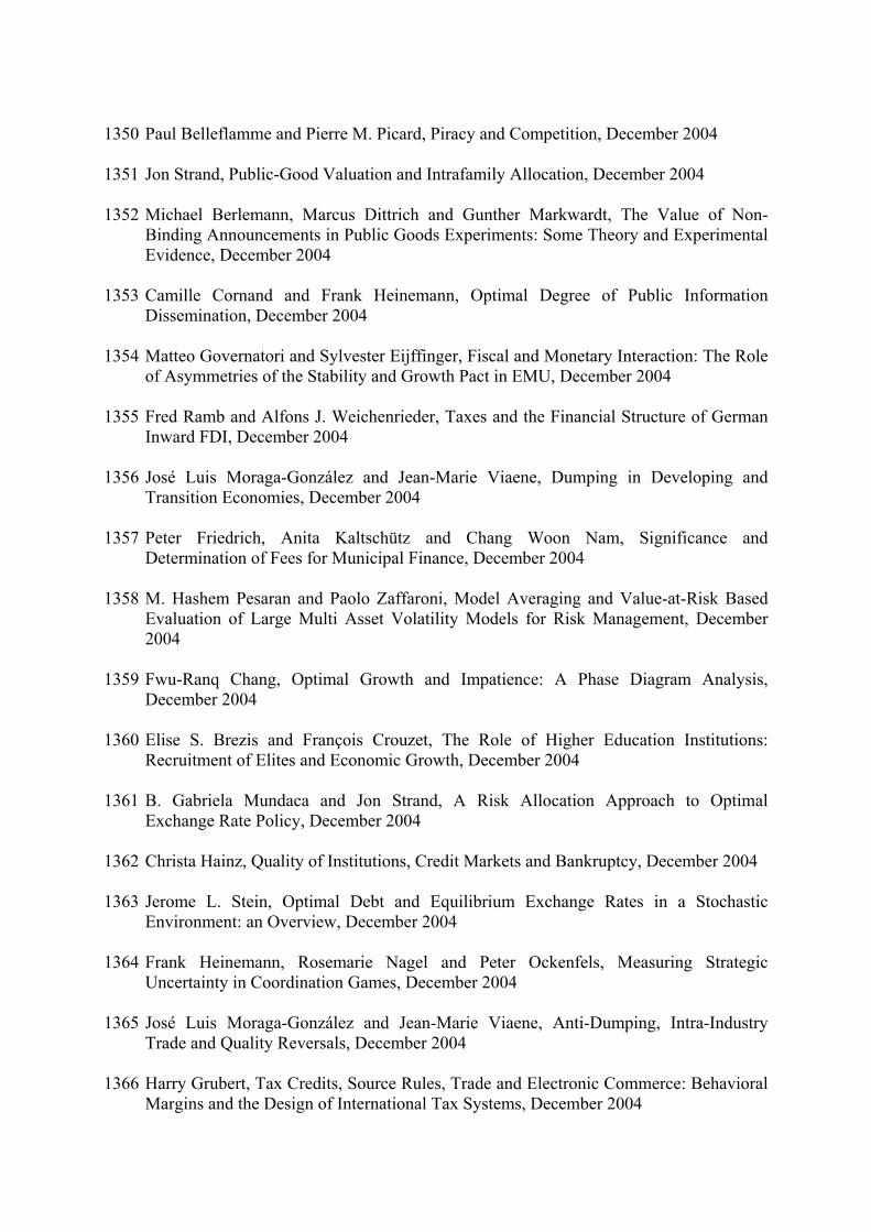
1350 Paul Belleflamme and Pierre M. Picard, Piracy and Competition, December 2004 1351 Jon Strand, Public-Good Valuation and Intrafamily Allocation, December 2004 1352 Michael Berlemann, Marcus Dittrich and Gunther Markwardt, The Value of Non-
Binding Announcements in Public Goods Experiments: Some Theory and Experimental Evidence, December 2004
1353 Camille Cornand and Frank Heinemann, Optimal Degree of Public Information
Dissemination, December 2004 1354 Matteo Governatori and Sylvester Eijffinger, Fiscal and Monetary Interaction: The Role
of Asymmetries of the Stability and Growth Pact in EMU, December 2004 1355 Fred Ramb and Alfons J. Weichenrieder, Taxes and the Financial Structure of German
Inward FDI, December 2004 1356 José Luis Moraga-González and Jean-Marie Viaene, Dumping in Developing and
Transition Economies, December 2004 1357 Peter Friedrich, Anita Kaltschütz and Chang Woon Nam, Significance and
Determination of Fees for Municipal Finance, December 2004 1358 M. Hashem Pesaran and Paolo Zaffaroni, Model Averaging and Value-at-Risk Based
Evaluation of Large Multi Asset Volatility Models for Risk Management, December 2004
1359 Fwu-Ranq Chang, Optimal Growth and Impatience: A Phase Diagram Analysis,
December 2004 1360 Elise S. Brezis and François Crouzet, The Role of Higher Education Institutions:
Recruitment of Elites and Economic Growth, December 2004 1361 B. Gabriela Mundaca and Jon Strand, A Risk Allocation Approach to Optimal
Exchange Rate Policy, December 2004 1362 Christa Hainz, Quality of Institutions, Credit Markets and Bankruptcy, December 2004 1363 Jerome L. Stein, Optimal Debt and Equilibrium Exchange Rates in a Stochastic
Environment: an Overview, December 2004 1364 Frank Heinemann, Rosemarie Nagel and Peter Ockenfels, Measuring Strategic
Uncertainty in Coordination Games, December 2004 1365 José Luis Moraga-González and Jean-Marie Viaene, Anti-Dumping, Intra-Industry
Trade and Quality Reversals, December 2004 1366 Harry Grubert, Tax Credits, Source Rules, Trade and Electronic Commerce: Behavioral
Margins and the Design of International Tax Systems, December 2004
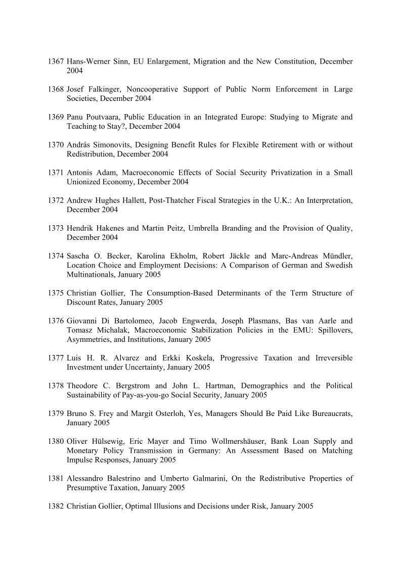
1367 Hans-Werner Sinn, EU Enlargement, Migration and the New Constitution, December
2004 1368 Josef Falkinger, Noncooperative Support of Public Norm Enforcement in Large
Societies, December 2004 1369 Panu Poutvaara, Public Education in an Integrated Europe: Studying to Migrate and
Teaching to Stay?, December 2004 1370 András Simonovits, Designing Benefit Rules for Flexible Retirement with or without
Redistribution, December 2004 1371 Antonis Adam, Macroeconomic Effects of Social Security Privatization in a Small
Unionized Economy, December 2004 1372 Andrew Hughes Hallett, Post-Thatcher Fiscal Strategies in the U.K.: An Interpretation,
December 2004 1373 Hendrik Hakenes and Martin Peitz, Umbrella Branding and the Provision of Quality,
December 2004 1374 Sascha O. Becker, Karolina Ekholm, Robert Jäckle and Marc-Andreas Mündler,
Location Choice and Employment Decisions: A Comparison of German and Swedish Multinationals, January 2005
1375 Christian Gollier, The Consumption-Based Determinants of the Term Structure of
Discount Rates, January 2005 1376 Giovanni Di Bartolomeo, Jacob Engwerda, Joseph Plasmans, Bas van Aarle and
Tomasz Michalak, Macroeconomic Stabilization Policies in the EMU: Spillovers, Asymmetries, and Institutions, January 2005
1377 Luis H. R. Alvarez and Erkki Koskela, Progressive Taxation and Irreversible
Investment under Uncertainty, January 2005 1378 Theodore C. Bergstrom and John L. Hartman, Demographics and the Political
Sustainability of Pay-as-you-go Social Security, January 2005 1379 Bruno S. Frey and Margit Osterloh, Yes, Managers Should Be Paid Like Bureaucrats,
January 2005 1380 Oliver Hülsewig, Eric Mayer and Timo Wollmershäuser, Bank Loan Supply and
Monetary Policy Transmission in Germany: An Assessment Based on Matching Impulse Responses, January 2005
1381 Alessandro Balestrino and Umberto Galmarini, On the Redistributive Properties of
Presumptive Taxation, January 2005 1382 Christian Gollier, Optimal Illusions and Decisions under Risk, January 2005
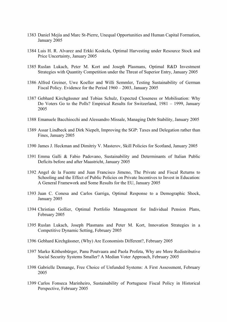
1383 Daniel Mejía and Marc St-Pierre, Unequal Opportunities and Human Capital Formation,
January 2005 1384 Luis H. R. Alvarez and Erkki Koskela, Optimal Harvesting under Resource Stock and
Price Uncertainty, January 2005 1385 Ruslan Lukach, Peter M. Kort and Joseph Plasmans, Optimal R&D Investment
Strategies with Quantity Competition under the Threat of Superior Entry, January 2005 1386 Alfred Greiner, Uwe Koeller and Willi Semmler, Testing Sustainability of German
Fiscal Policy. Evidence for the Period 1960 – 2003, January 2005 1387 Gebhard Kirchgässner and Tobias Schulz, Expected Closeness or Mobilisation: Why
Do Voters Go to the Polls? Empirical Results for Switzerland, 1981 – 1999, January 2005
1388 Emanuele Bacchiocchi and Alessandro Missale, Managing Debt Stability, January 2005 1389 Assar Lindbeck and Dirk Niepelt, Improving the SGP: Taxes and Delegation rather than
Fines, January 2005 1390 James J. Heckman and Dimitriy V. Masterov, Skill Policies for Scotland, January 2005 1391 Emma Galli & Fabio Padovano, Sustainability and Determinants of Italian Public
Deficits before and after Maastricht, January 2005 1392 Angel de la Fuente and Juan Francisco Jimeno, The Private and Fiscal Returns to
Schooling and the Effect of Public Policies on Private Incentives to Invest in Education: A General Framework and Some Results for the EU, January 2005
1393 Juan C. Conesa and Carlos Garriga, Optimal Response to a Demographic Shock,
January 2005 1394 Christian Gollier, Optimal Portfolio Management for Individual Pension Plans,
February 2005 1395 Ruslan Lukach, Joseph Plasmans and Peter M. Kort, Innovation Strategies in a
Competitive Dynamic Setting, February 2005 1396 Gebhard Kirchgässner, (Why) Are Economists Different?, February 2005 1397 Marko Köthenbürger, Panu Poutvaara and Paola Profeta, Why are More Redistributive
Social Security Systems Smaller? A Median Voter Approach, February 2005 1398 Gabrielle Demange, Free Choice of Unfunded Systems: A First Assessment, February
2005 1399 Carlos Fonseca Marinheiro, Sustainability of Portuguese Fiscal Policy in Historical
Perspective, February 2005


