Surface normal overlap: a computer-aided detection algorithm with application to colonic polyps and lung nodules in helical CT

> REPLACE THIS LINE WITH YOUR PAPER IDENTIFICATION NUMBER (DOUBLE-CLICK HERE TO EDIT) <

1

Abstract—We developed a novel computer-aided detection

(CAD) algorithm called the surface normal overlap method that we applied to colonic polyp detection and lung nodule detection in helical CT images. We demonstrate some of the theoretical aspects of this algorithm using a statistical shape model. The algorithm was then optimized on simulated CT data and evaluated using a per-lesion cross-validation on 8 CT colonography datasets and on 8 chest CT datasets. It is able to achieve 100% sensitivity for colonic polyps 10 mm and larger at 7.0 FP/dataset and 90% sensitivity for solid lung nodules 6 mm and larger at 5.6 FP/dataset.

Index Terms—Computer-Aided Detection (CAD), Colonic

Polyp, Lung Nodule, Cross-Validation, Computed Tomography Colonography (CTC), Statistical Shape Model

I. INTRODUCTION In the United States, lung cancer and colon cancer are the

first and second leading cancer killers, respectively. Early detection of colonic polyps and lung nodules, the precursors to these diseases, has been shown to improve survival [1-4]. Clinically significant colonic polyps and lung nodules are resolvable given the spatial resolution of helical computed tomography (CT). However, the accuracy and efficiency of viewing hundreds of source axial images per exam are limited by human factors, such as attention span and eye fatigue. In response to this challenge, a variety of computer-aided diagnosis (CAD) methods have been developed to improve both the accuracy and the efficiency of detecting lesions in this and other difficult 3D diagnostic problems. Among them, many different approaches to CAD for CT lung nodule detection and for CT colonic polyp detection have been developed, several of which are described next.

For detecting lung nodules, Giger et al. [5] developed a 2D multilevel thresholding detection algorithm that creates a tree structure of image components. Rules were applied to shape features in order to identify nodules. 94% per-nodule sensitivity was achieved with 1.25 false positives (FP) per patient. Armato et al. [6, 7] applied multilevel thresholding and a rolling ball algorithm toward detecting lung nodules. Shape and attenuation features were classified using linear discriminant analysis and the algorithm achieved 70% per-nodule sensitivity with 1.5 FP per axial section. Brown et al. [8] have presented an algorithm for both detection and

surveillance of lung nodules in CT. Region-growing and morphological operators were used to create candidate locations. Attenuation, location, volume, and shape features were matched to model objects in a semantic net with fuzzy membership that serves as a generic a priori anatomic model. In the initial detection task, 86% per-nodule sensitivity was achieved with 11 FP per patient. Lee et al. [9] used both genetic algorithm-based and semicircular template matching to identify initial candidates and attenuation, shape, and gradient feature rules to reduce false positives. They achieved 72% per-nodule sensitivity with 31 FP per patient. Erberich et al. [10] applied the Hough transform (HT) for both 2D circles and 3D spheres using a rule-based classifier and achieved 30-40% per-nodule sensitivity with a “large amount of false positive nodules.”

Several approaches to colonic polyp CAD in CT colonography have also been proposed. Vining et al. [11] developed a method that measures abnormal wall thicknesses using heuristics. They report 73% per-polyp sensitivity with a range of 9-90 FP per patient. Other approaches have analyzed the morphology of the mucosal surface. Summers et al. [12, 13] have developed a method that uses size, attenuation, and curvatures calculated with convolution-based partial derivates to find polyps. They achieved 64% per-lesion sensitivity with 3.5 FP per patient. Yoshida et al. [14-16] use shape index and curvedness (computed with partial derivatives), directional gradient concentration, and quadratic discriminant analysis. Using both prone and supine datasets, they achieve 100% per-patient sensitivity with 2.0 FP per patient (per-polyp sensitivity not stated). Kiss et al. [17] combined surface normal and sphere fitting methods to achieve 100% per-polyp sensitivity with 8.2 FP per patient. In addition, secondary CAD algorithms that are designed to reduce the false positive rate of primary CAD algorithms have been proposed. Göktürk et al. [18] applied support vector machines to shape and attenuation features to reduce false positives and reported a 50% increase in specificity at a constant sensitivity level. Acar et al. [19] have applied edge displacement fields to reduce false positives and reported a 23% increase in specificity at a constant sensitivity level. Both of these false positive reduction methods were evaluated using initial versions [20] of the work presented in this paper.

These previously described CAD algorithms for both lung

Surface Normal Overlap: A Computer-Aided Detection Algorithm with Application to

Colonic Polyps and Lung Nodules in Helical CTDavid S. Paik, Christopher F. Beaulieu, Geoffrey D. Rubin, Burak Acar,

R. Brooke Jeffrey, Jr., Judy Yee, Joyoni Dey, and Sandy Napel


2

nodules and colonic polyps have achieved varying levels of accuracy although they all leave room for improvement. Additionally, many of them represent analogous approaches, using similar feature vectors and similar classifiers. The purpose of this work was to create a new and effective approach to CAD by developing new features and by optimizing them toward two clinical applications.

We present in this paper (1) a novel multi-purpose CAD algorithm that we call the Surface Normal Overlap (SNO) method, (2) a theoretical analysis of this algorithm using a statistical model of anatomic shape, (3) an optimization and analysis method for this algorithm using simulated CT data and a per-lesion cross-validation, and (4) preliminary evaluations of the detection performance of the CAD algorithm in lung nodule and colonic polyp detection, using the free-response ROC (FROC) paradigm. We propose to use this algorithm as the first step in a larger overall detection scheme and thus, we strive for high sensitivity at a reasonable false positive rate, thus allowing secondary FP reduction algorithms, such as some of those described above, and/or radiologist visualization to improve specificity.

II. CAD ALGORITHM The following sections describe the processing steps of the

SNO method, of which the end result is a list of the coordinates of the center of each suspicious region, sorted in decreasing prospect of being a lesion.

A. Pre-processing and Segmentation Because both colonic polyps and lung nodules are generally

not much denser than water, high density structures (e.g., bone) are removed by clamping voxel intensities to be no greater than that of water. Next, the CT volume data are made isotropic by tri-linear interpolation to 0.6 mm × 0.6 mm × 0.6 mm voxels to produce I(x,y,z). This is done in order to reduce any bias between lesions at different orientations and also to reduce any bias between datasets with different voxel sizes.

Next, segmentation is performed automatically to identify either the colon lumen or the lung parenchyma. A binary image, S1, is created by thresholding all air intensity voxels (I(x,y,z) < –700 HU) including air outside the body. This is followed by a negative masking of all air intensity voxels morphologically connected to any of the edges of the data volume (air outside the body), thus leaving only voxels with air density within the body. In the case of CT colonography, the inferior portions of the lungs are usually captured and are removed using a negative mask of a 3D region-filling seeded with air intensity regions with a width or depth of greater than 60 mm in the most superior axial slice. Finally, small air pockets (< 15 cc in the colon datasets, < 125 cc in the lung datasets) are also negatively masked from S1.

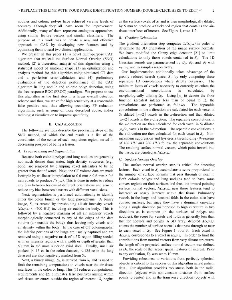
Next, a binary image, S2, is derived from S1 and is used to limit the remaining computations to voxels near the air-tissue interfaces in the colon or lung. This (1) reduces computational requirements and (2) eliminates false positives arising within soft tissue structures outside the region of interest. S2 begins

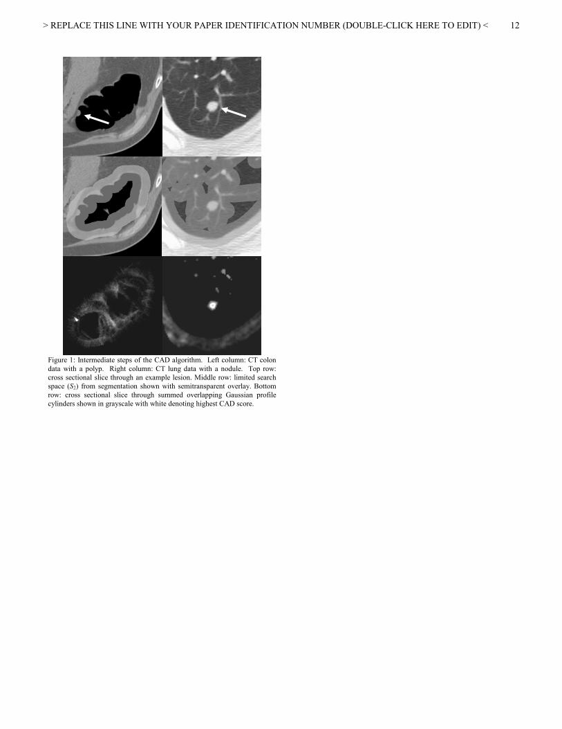
as the surface voxels of S1 and is then morphologically dilated by 5 mm to produce a thickened region that contains the air-tissue interfaces of interest. See Figure 1, rows 1-2.

B. Gradient Orientation The gradient orientation step computes ∇ I(x,y,z) in order to determine the 3D orientation of the image surface normals. We have modified the Canny edge detector [21] to limit calculations to only those voxels contained in S2. The 1D Gaussian kernels are parameterized by σX, σY, and σZ with nX, nY, and nZ samples respectively.

Our implementation additionally takes advantage of the greatly reduced search space, S2, by only computing these separable 1D convolutions where strictly necessary. The minimum locus of voxels necessary to correctly calculate the one-dimensional convolutions is calculated by morphologically dilating S2. Using x to denote the floor function (greatest integer less than or equal to x), the convolutions are performed as follows. The separable convolutions in the x-direction are calculated for each voxel in S2 dilated nZ/2 voxels in the z-direction and then dilated nY/2 voxels in the y-direction. The separable convolutions in the y-direction are then calculated for each voxel in S2 dilated nZ/2 voxels in the z-direction. The separable convolutions in the z-direction are then calculated for each voxel in S2. Non-maximum suppression and hysteresis thresholding (thresholds of 100 HU and 200 HU) follow the separable convolutions The resulting surface normal vectors, which point inward into the tissue, are denoted as N(x,y,z).

C. Surface Normal Overlap The surface normal overlap step is critical for detecting

lesions. Each voxel in S2 accumulates a score proportional to the number of surface normals that pass through or near it. Both colonic polyps and lung nodules tend to have some convex regions on their surfaces and thus, the inward pointing surface normal vectors, N(x,y,z), near these features tend to intersect or nearly intersect within the tissue. Pulmonary vessels in the lungs and haustral folds in the colon also have convex surfaces, but since they have a dominant curvature along a single direction (as opposed to high curvature in two directions as is common on the surfaces of polyps and nodules), the score for vessels and folds is generally less than that for nodules and polyps. A 3D array, denoted A(x,y,z), counts the number of surface normals that pass through or near to each voxel in S2. See Figure 1, row 3. Each voxel in A(x,y,z) corresponds to a voxel in I(x,y,z). In order to limit the contributions from normal vectors from very distant structures, the length of the projected surface normal vectors was defined as DF, the scale of the largest spatial features of interest. Prior to any evaluation, DF was set to 10 mm.

Providing robustness to variations from perfectly spherical objects is critical to the success of this algorithm in real patient data. Our algorithm provides robustness both in the radial direction (objects with non-constant distance from surface points to center) and in the transverse direction (objects with


3

non-uniform magnitude of curvature). Robustness in the radial direction is provided by the fact that normal vectors can intersect at different distances from the surface (up to DF), thus allowing many non-spherical but roughly globular objects to have a significant response.

Robustness in the transverse direction is provided by allowing skewed surface normal vectors (those that do not intersect but nearly intersect) to be additive in A(x,y,z). This is accomplished by projecting cylinders of a finite width in the direction of the surface normal rather than by projecting line segments. Because surface normals that come closer to intersecting are assumed to be more likely generated by the same convex surface patch, the projected cylinders are given a transverse profile that gradually decreases in intensity at greater radial distances, thereby providing robustness in the transverse direction and again, allowing many non-spherical but roughly globular objects to have a significant response. The profile was chosen to be Gaussian with a scale of σcylinder.

For computational efficiency, the entire surface normal overlap step is implemented by first scan converting (i.e., discretizing into voxels) a line segment for each surface normal in N(x,y,z) and summing it into A′(x,y,z). Then, the Gaussian profile of the cylinders is achieved by a sequence of linearly separable 1-D convolutions to produce A(x,y,z). The convolution is given by:

∫∫∫ ′′′′′′′

′−+′−+′−−

⋅= zdydxd)π(σ

e)z,y,x(AA(x,y,z)

σ)z(z)y(y)x(x

3cylinder

2

2

2cylinder

222

(1)

The discrete kernels are chosen so that x′, y′, and z′ include ±2σcylinder sampled at 0.6×0.6×0.6 mm to cover 95% of the Gaussian curve. The computational burden imposed by the convolution calculation is minimized using morphological operators similar to the gradient orientation calculation, as in Section II.B.

D. Candidate Lesion Selection The local maxima of A(x,y,z) are selected as candidate

lesion locations. However, complex anatomic structures with multiple convex surface patches may generate multiple local maxima. DS was defined to be the smallest scale of the features that might generate distinct local maxima and was set to 10 mm prior to any evaluation. Local maxima are considered in descending order, and if a local maximum occurs within DS of an already accepted local maximum, the lesser value is assumed to be part of the same structure and is rejected. After this spatial filtering, the remaining local maxima are sorted in decreasing order and recorded as the potential lesion locations. The score for a potential lesion at location (x,y,z) is given by A(x,y,z), and we refer to this as a “CAD hit”.

III. THEORETICAL ANALYSIS In this section, we present several theoretical analyses of

SNO. To facilitate them, we have created a statistical anatomic shape model that balances the complex variability of human anatomy with sufficient simplicity to allow for analytic insight. We then use this theoretical model to compare the behavior of the SNO method to the 3D Hough Transform for spheres in distinguishing lung nodules from vessels and colonic polyps from haustral folds.

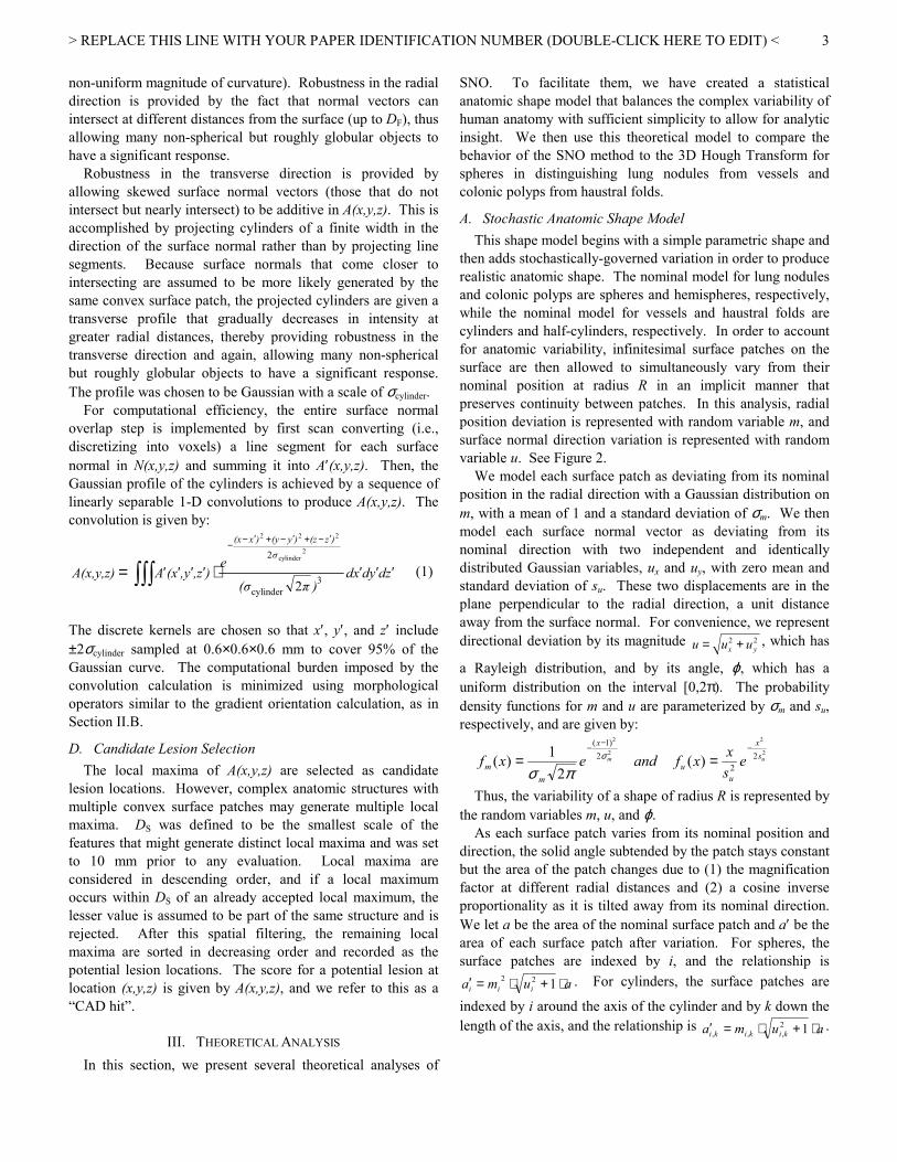
A. Stochastic Anatomic Shape Model This shape model begins with a simple parametric shape and

then adds stochastically-governed variation in order to produce realistic anatomic shape. The nominal model for lung nodules and colonic polyps are spheres and hemispheres, respectively, while the nominal model for vessels and haustral folds are cylinders and half-cylinders, respectively. In order to account for anatomic variability, infinitesimal surface patches on the surface are then allowed to simultaneously vary from their nominal position at radius R in an implicit manner that preserves continuity between patches. In this analysis, radial position deviation is represented with random variable m, and surface normal direction variation is represented with random variable u. See Figure 2.

We model each surface patch as deviating from its nominal position in the radial direction with a Gaussian distribution on m, with a mean of 1 and a standard deviation of σm. We then model each surface normal vector as deviating from its nominal direction with two independent and identically distributed Gaussian variables, ux and uy, with zero mean and standard deviation of su. These two displacements are in the plane perpendicular to the radial direction, a unit distance away from the surface normal. For convenience, we represent directional deviation by its magnitude 22

yx uuu += , which has

a Rayleigh distribution, and by its angle, ϕ, which has a uniform distribution on the interval [0,2π). The probability density functions for m and u are parameterized by σm and su, respectively, and are given by:

2

2

2

2

22

2)1(

)(2

1)( um sx

uu

x

mm e

sxxfandexf

−−−

== σ

πσ

Thus, the variability of a shape of radius R is represented by the random variables m, u, and ϕ.

As each surface patch varies from its nominal position and direction, the solid angle subtended by the patch stays constant but the area of the patch changes due to (1) the magnification factor at different radial distances and (2) a cosine inverse proportionality as it is tilted away from its nominal direction. We let a be the area of the nominal surface patch and a′ be the area of each surface patch after variation. For spheres, the surface patches are indexed by i, and the relationship is

auma iii ⋅+⋅=′ 122 . For cylinders, the surface patches are

indexed by i around the axis of the cylinder and by k down the length of the axis, and the relationship is auma kikiki ⋅+⋅=′ 12

,,,.


4

B. Model Parameter Estimation In order to make quantitative comparisons using this

theoretical model, the parameters controlling the degree of variation from the nominal shapes, σm and su, were estimated directly from the patient datasets. This process involved (1) performing edge detection on the datasets, (2) identifying the surface normal vectors that belong to the nodule, polyp, vessel or fold, (3) finding the nominal sphere or cylinder that fit those surface normal vectors, (4) computing the value of m and u for each surface normal, and (5) estimating σm and su from those sample populations.

All polyps 5 mm and larger and all nodules 3 mm and larger were used for parameter estimation. From each of the 8 colon datasets and each of the 8 lung datasets, eight folds or vessels were selected prospectively and manually and then, selected for parameter estimation. Thus, our analyses included 18 polyps and 64 selected folds in the colon, and 84 nodules and 64 selected vessels in the lung. Section V.C contains full details about these datasets.

Edge detection was performed as described in Section II.B. Isolation of the surface normals belonging to the structure of interest was performed as follows. The center of the structure of interest, C, was chosen manually, and all surface normal vectors whose bases were further than two radii away were eliminated. Next, if a line segment between C and a surface normal intersected an air intensity voxel (< -700 HU), the surface normal was eliminated. Then, surface normals pointing more than 90° away from C were eliminated. Finally, the largest contiguous region of surface normals was kept as belonging to the structure of interest. This algorithm was quite successful in isolating the structures of interest; Figure 3 provides some examples.

The nominal shape was derived using a least squares fit of a sphere or cylinder to the bases of the surface normals (i.e., directional information was not used), which leads to an estimate of R. Using this nominal shape, both m and u were computed directly for each surface normal. Finally, σm was estimated using the maximum likelihood estimate. However, su was estimated differently because a few surface normals were at nearly 90° away from either the center of the sphere or the axis of the cylinder, leading to nearly infinite values of u and thus, giving inaccurate estimates due to MLE sensitivity to outliers. This happened particularly around the “skirt” of polyps and haustral folds where it is difficult to make binary decisions about what belongs to the polyp or fold and what does not. Instead, we estimated su by using the method-of-moments but substituting the more robust median L-estimator for the mean. By setting the empirical median, umedian, equal to the point at which the CDF is 0.5, we get

5.012

2

2 =−−

u

median

su

e , which leads to4ln

medianu

us = .

The results of the parameter estimation are shown in Figure 4.

C. Algorithm Models In order to understand the theoretical performance of the

SNO algorithm and to compare it to the Hough transform for spheres, we applied this anatomic shape model for polyps, folds, nodules, and vessels with differing degrees of variation from the nominal model. Specifically, we compared the expectation of the CAD scores over the random variables m, u, andϕ. See Appendix for the CAD score formulas and their derivations.

D. Theoretical Comparison of SNO and HT In order to compare the theoretical performance of the SNO

and HT algorithms, we varied the shapes from perfect spheres and cylinders to more realistic anatomic shapes. The range of realistic shape variability was estimated as described in Section III.B. Figure 5a-b presents resulting CAD scores as a function of deviation from ideal shape for polyps and folds, and for nodules and blood vessels. These plots demonstrate the robustness of SNO to deviation from ideal shapes whereas HT fails to discriminate between shapes with realistic amounts of shape variability. Figure 5c presents the scores of both polyps and nodules as a function of lesion size, revealing that larger lesions lead to a smoothly increasing response with SNO. However, HT produces a response that varies tremendously for nearly identical lesion sizes.

The estimated values of σm and su were then used to produce a CAD score for each shape. These scores are shown in Figure 6. Wilcoxon rank sum tests were performed to test the difference between TP and FP scores. For SNO, there were significant differences between polyp and fold (p=7×10-5) and between nodule and vessel (p=1×10-14). However, for HT, there were not significant differences between polyp and fold (p=0.77) nor between nodule and vessel (p=0.20).

IV. GRADIENT ORIENTATION OPTIMIZATION Using simulated CT phantoms, we optimized the gradient

orientation kernel scale parameters, σX, σY, and σZ, in order to yield the most accurate gradient orientations. This step was critical because errors in estimating the gradient direction can diminish surface normal overlap in A(x,y,z). The selection of values for σX, σY, and σZ is particularly important because too small a value will lead to errors from noise and very localized perturbations in the surface whereas too large a value will lead to insensitivity to smaller lesions. The optimization of the parameter σcylinder is described later in Section V.

A. Phantom Model and Error Metric A series of hemispherical phantom objects were “scanned”

using software that simulates CT scanning including forward projections, partial volume effects, correlated CT noise, helical interpolation, and filtered backprojection reconstruction [22]. The simulations were performed with a 3 mm slice thickness, pitch of 2 (table travel per rotation = 6 mm), 0.7×0.7 mm pixels in plane, and 1 mm reconstruction interval. For each phantom, a water-equivalent density sphere was embedded


5

halfway into a water-equivalent density, randomly oriented, flat wall to simulate a prototypical colonic polyp or prototypical lung nodule on the chest wall. The diameters of the spheres, dsphere, ranged from 5 to 15 mm at 1 mm increments, chosen to demonstrate the effects of changes in size from the prototypical 10 mm lesion. For each sphere size, there were 10 phantoms, each with a different wall orientation, randomized sub-voxel offset, and randomized CT detector noise, leading to a total of 110 phantoms.

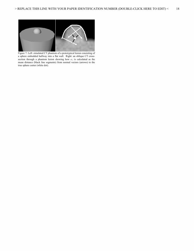
The error metric used to evaluate the accuracy of gradient orientations, e⊥ , was defined to be the mean perpendicular distance from the surface normal vector, N(x,y,z), to the true center of the sphere. In order to include only detected gradient orientations from the hemisphere and not those from the flat wall, only gradients located within 1.05×dsphere/2 of the sphere center entered into the calculation of e⊥ . See Figure 7.

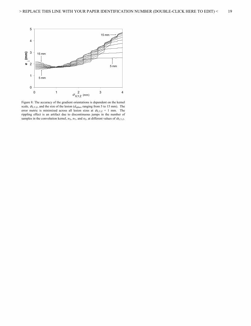
B. Gradient Orientation Kernel Scale We let σX = σY = σZ and executed the CAD algorithm with

all three (σX,Y,Z = σX = σY = σZ) simultaneously varying from 0.05 to 4.0 mm in 0.05 mm increments. The errors, e⊥ from the 10 phantoms at a given dsphere and σX,Y,Z, were then averaged. The results of this optimization are plotted in Figure 8, showing that σX,Y,Z = 1.00 mm led to the least error across all lesion sizes.

C. Gradient Orientation Kernel Anisotropy We also investigated the effects of anisotropic resolution in

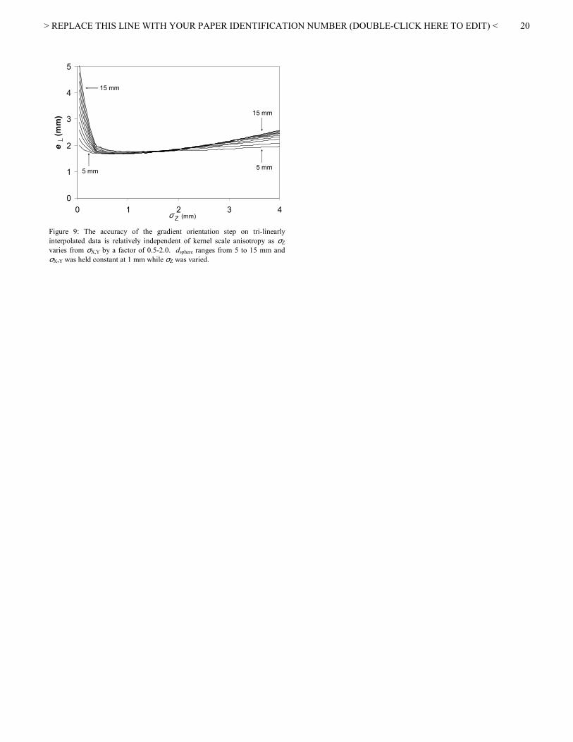
helical CT on gradient orientations. In general, helical CT has lower effective resolution through-plane than in-plane, regardless of reconstruction interval. Thus, one might expect setting σZ < σX,Y would compensate for this effect. To test this, we fixed σX,Y = σX = σY = 1 mm (based on the results of the first optimization) and let σZ vary from 0.05-4.0 mm in 0.05 mm increments. The errors, e⊥ , from the 10 phantoms at a given dsphere and σZ, were then averaged, as in Section III. B.

Figure 9 plots the results of this optimization, showing that the accuracy of the gradient orientations on tri-linearly interpolated anisotropic data is almost independent of the anisotropy of the kernel scale between ratios of 0.5 and 2.0. As a result, all subsequent experiments were carried out with σX = σY = σZ = 1 mm.

V. CAD PERFORMANCE EVALUATION This section describes two experiments that were performed

in order to evaluate the performance of the CAD algorithm in detecting real colonic polyps and in detecting solid lung nodules. In Section III, the goal of the gradient orientation optimization was to produce as accurate gradient orientations as possible using the e⊥ error metric. However, the goal of optimizing the cylinder scale, σcylinder, is to maximally differentiate between lesions and false positives. A wider cylinder scale will increase the robustness to deviations from perfectly spherical shapes but will also decrease the differentiability between lesions and false positive structures.

Since this effect is dependent on the variability of true lesion and false positive shapes, the CT simulations were insufficient. Instead, a cross-validation was performed to evaluate lesion detection performance with prospectively chosen values of σcylinder.

A. Cross-validation When cross-validation is used to evaluate a classifier, the

dataset is split into N sets (sometimes referred to as “folds”). The classifier is trained de novo on N-M sets and then evaluated on the remaining M independent set(s); this is repeated for all possible divisions into N-M sets and M sets and the results are averaged in a reasonable manner [23]. This type of evaluation gives an unbiased estimate of performance and has a lower standard error than traditional holdout methods [24]. In this evaluation, we chose M=1. However, in a detection problem such as this, splitting the dataset (CAD hits) into sets at the granularity of lesions is problematic because the result of training (e.g., selecting σcylinder based on the training sets) changes the dataset (e.g., CAD hit locations) and thus, changes the sets themselves.

In order to retain the independence between training and test sets, the sets were selected on the basis of distinct anatomic features rather than on the basis of CAD hit locations. The locus of all CAD hit locations was computed for each possible value of σcylinder. Two CAD hits were considered to be the same anatomic feature if they were within 10 mm of each other. The sets (7 in the colon dataset, 46 in the lung dataset) were made to be disjoint by having one true positive lesion and equal numbers of randomly selected false positive anatomic features. CAD hits were distributed among the sets according to the anatomic feature to which they belonged. Thus, to within the 10 mm constraint, no two sets contained CAD hits on the same anatomic feature.

For an error metric in training, we selected the value of σcylinder that maximized A′Z, which we define as the normalized partial area under the free-response ROC (FROC) curve from 0-20 FP/dataset and from 90-100% sensitivity. A′Z = 1 indicates perfect detection performance whereas A′Z = 0 indicates that less than 90% of lesions are detected by the time 20 FP/dataset is reached.

B. Automated CAD Scoring Because the results of a CAD evaluation can be especially

numerous, we implemented a method for automatically scoring each CAD hit as either a true positive (TP) or false positive (FP), thus eliminating subjectivity and clerical errors. Because there is some spatial variance in what is declared to be the center of a lesion in the gold standard (Section V.C.2)), the scoring algorithm must allow for some small amount of spatial mis-registration between gold standard lesion locations and true positive CAD hits. Thus, we defined any CAD hit as a TP if it was within half the lesion’s measured diameter from the lesion’s measured center. Lesion diameters were measured manually from the CT images during the setting of the gold standard using a multi-planar digital caliper tool.


6

To determine the overall performance, all of the CAD hits within the test sets were determined to be a TP or a FP and then pooled and sorted in descending order of score. In the event that multiple CAD hits are scored as TP for a given lesion, only the highest scoring hit was considered a TP; lower scoring hits were ignored. TP CAD hits on lesions below the size range of interest were not considered FPs nor did they increase the sensitivity. At a given score threshold, sensitivity was calculated as the percentage of lesions within the size range of interest that had been identified by a TP CAD hit above that score threshold. The false positive rate was calculated as the total number of FP CAD hits divided by the number of datasets.

C. Detection Evaluation 1) Data Collection

Colon: From a database of 116 CT colonography exams performed at either Stanford University or at the San Francisco VA hospital, 8 exams were selected for this study in order to include a reasonably large number of colonic polyps and to balance the number of patients with and without large polyps. Exams with excessive image artifact or retained water were excluded. Case selection was done without regard to polyp conspicuity or shape. These 8 patients were given rectal air contrast and scanned in the supine position with single- or multi-detector helical CT (GE HiSpeed/CTi or LightSpeed, General Electric Medical Systems, Milwaukee, WI) with effective section width of 2.5-3.75 mm and 50% overlapping reconstruction. Immediately following CT scanning, each patient also underwent fiber-optic colonoscopy (FOC). These results were correlated to the CT images with a total of 7 “clinically significant” polyps (≥ 10 mm) found in 4 of 8 patients and a total of 11 small polyps (5-9 mm) found in 3 of 8 patients. A wide range polyp shapes were present in the datasets

Lung: From a database of 21 CT chest exams suspected for nodules and performed at either Stanford or at NYU, 8 exams were selected for this study in order to include a reasonably large number of lung nodules and to balance the number of patients with and without large nodules. The number of nodules was ascertained from the gold standard (see below). Case selection was done without regard to lesion conspicuity, lesion shape, or image quality. In these 8 chest CT scans (GE LightSpeed, General Electric Medical Systems, Milwaukee, WI) there were a total of 46 “clinically significant” solid lung nodules (≥ 6 mm) found in 4 of 8 patients and a total of 38 small solid nodules (3-5 mm) were in 8 of 8 patients. A wide range of nodule shapes were present in the datasets. 2) Gold Standard

Colon: A study coordinator with extensive experience in CTC and blinded to CAD results carefully reviewed the CTC data and recorded the location and diameter of polyps found by FOC into the gold standard database. Only one significant polyp (measured as 15 mm by FOC) was unable to be located in the CT images, most likely due to retained water. A total of 10 small polyps (1 was 8 mm and 9 were 5-6 mm measured by

FOC) were unable to be located in the CT images. Lung: The gold standard in the chest was established by

consensus of two radiologists interpreting the axial CT data. Both the location and diameters of nodules were recorded into the gold standard database.

The CAD algorithm was then executed on the 8 colon and 8 lung datasets using the optimized gradient orientation from Section III and cross-validated as described above. 3) Results

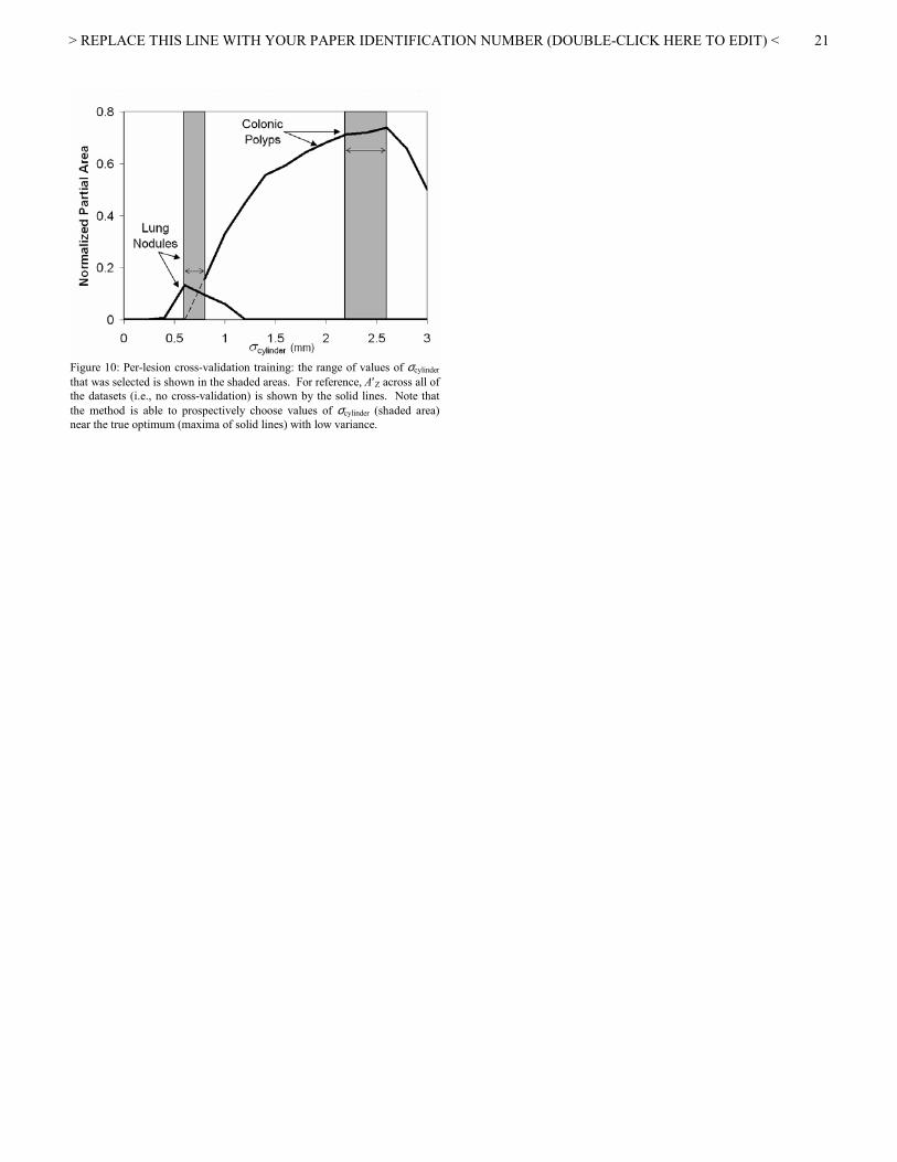
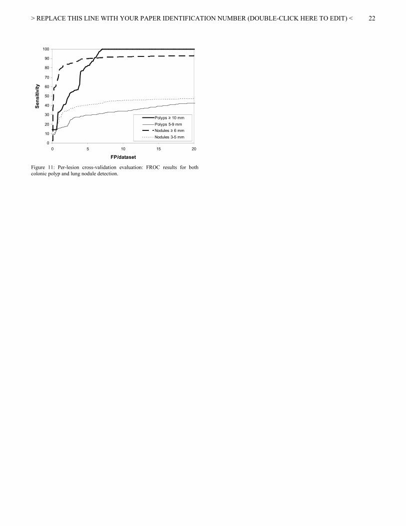
Colon: In the colon datasets, the value of σcylinder based on the cross-validation training sets was in the range 2.2-2.6 mm with a mean of 2.5 mm. Figure 10 shows the range of these values of σcylinder compared to the performance on all of the datasets (A′Z computed on all datasets over all values of σcylinder, not just on training sets). Note that the latter is shown in this figure for reference only and was never used in training or evaluation. The mean performance across the test sets in detecting “clinically significant” colonic polyps was as follows. 80% of polyps ≥ 10 mm in diameter were detected at 4.6 FP/dataset. 90% were detected at 6.0 FP/dataset. 95% were detected at 6.5 FP/dataset. 100% were detected at 7.0 FP/dataset. Figure 11 shows a FROC plot of these results.

A manual analysis of the 50 highest scoring false positives in each colon dataset (400 total) revealed that 86% were due to haustral folds, 5% were due to the colon wall between adjacent loops, 4% were due to a failure in segmentation in one dataset that captured the air trapped in the blanket beneath the patient. Finally, each of the following classes contributed 1% or less: stool, insufflation catheter, small bowel, and the ileocecal valve.

Lung: In the lung datasets, the value of σcylinder based on the cross-validation training sets was in the range 0.6-0.8 mm with a mean of 0.6 mm. See Figure 10. The mean performance across the test sets in detecting “clinically significant” solid lung nodules was as follows. 80% of nodules ≥ 6 mm in diameter were detected at 1.3 FP/dataset. 90% were detected at 5.6 FP/dataset. 95% were detected at 63 FP/dataset. 100% were detected at 165 FP/dataset. See Figure 11.

A manual analysis of the 50 highest scoring false positives in each lung dataset (400 total) revealed that 69% were due to pulmonary vessels, 13% were due to bronchi, 6% were due to vessels or bronchi in the mediastinum, 6% were calcified nodules, 2% were due to bulges on the pleural surface, 2% were small indeterminate opacities, and each of the following classes contributed 1% or less: mass, metal artifact, and a single 2.9 mm non-calcified nodule.

VI. DISCUSSION

A. CAD Algorithm The surface normal overlap algorithm was originally

inspired by the Hough transform for spheres [25] but differs in some important ways. First, the array A(x,y,z) which counts the number of overlapping or nearly overlapping surface


7

normals is similar to the Hough transform accumulator array in that it sums “votes” for objects that could produce those normals, but it does not require all of the votes to correspond to a single parameterized sphere, as does the Hough transform. Second, the Hough transform, in its various forms, is highly specific for one type of shape (e.g., spheres). Even the variant known as the generalized Hough transform, which avoids parametric representations, requires a specific model. This specificity is desirable when the shape to be detected can be precisely defined in advance, but the specificity is problematic when it cannot. In contrast, the SNO algorithm does not use an explicit model of a single type of shape, but instead uses an implicit model to represent an entire gamut of shapes much larger than the set of spheres detected by the Hough transform for spheres. This property is extremely important when the objects to be detected can have significant variability in shape such as with lung nodules or colonic polyps. Rather than specifying the exact shape to be detected, the SNO algorithm defines a fuzzy constraint on surface normal orientation in order to define the varied set of shapes to be detected, both by allowing angular mismatches (transverse robustness) and by allowing edges at different radial distances to sum (radial robustness). For comparison, Erberich et al. have applied the 3D Hough transform for spheres toward lung nodule detection in CT but reported only 30-40% sensitivity at a high false positive rate [10].

The voxel intensity clamping pre-processing step is used to eliminate edges due to bone but will also make calcified lung nodules have a similar response as non-calcified nodules. While the presence of calcification in lung nodules may help distinguish between benign and malignant nodules, the goal of this algorithm is detection, not classification. For classification purposes, the original voxel intensities can easily be restored following the detection of suspicious regions.

While we have presented and evaluated the SNO CAD method as being preceded by a specific segmentation scheme, we emphasize that the only purposes of the segmentation step are (1) to reduce computation by targeting only anatomical regions of interest and (2) to eliminate hits from regions disjoint from the anatomical regions of interest. Unlike some other CAD approaches requiring extremely accurate segmentation (e.g., inclusion of juxtapleural nodules), the goal of our segmentation step is to provide a volumetric region that contains all possible image edges that could be due to the presence of lesions and not to fully delineate their edges. Thus, our relatively simplistic segmentation algorithm is sufficient and is not limiting factor in the overall detection performance. However, it is fair to say that gross errors in segmentation could adversely affect performance. In colon CAD, for example if the most superior axial slice contains a large enough portion of the transverse colon, it could be assumed to be lung and, therefore, erroneously eliminated. Thus far, we have not had any such gross failures in segmentation; however, we note that, ultimately, any robust segmentation method could be substituted for ours.

We also emphasize that, at this stage, this algorithm is not intended to be used independent of visual interpretation by a radiologist. At the present stage of development (and perhaps, well into the foreseeable future), this type of algorithm should be seen as an aid for improving radiologist performance. In this regard, although our algorithm generated more than one FP (on average) per data set in order to achieve high sensitivity, it does not indicate that the majority of patients will have FP detections once reviewed in conjunction with a radiologist. If many of the FP hits are recognized as such and are discarded by the radiologist, overall performance may be acceptable. However, this remains to be shown by future evaluations.

The difference in performance between detecting colonic polyps and detecting lung nodules is of interest. Although neither FROC curve completely dominates the other, the “average” lung nodule (i.e., near 50% sensitivity) was easier to detect (i.e., at fewer FP/dataset) than the “average” colonic polyp, despite the relatively larger size of polyps. The difference is partially accounted for by the difference in lesion morphology the gross shape of the nodules (not at the fine level of spiculations) in these datasets tended to be more globular than that of polyps, which tended to have more complex surfaces due to the gradual rise and fall of the mucosal surface around a polyp. This may be attributable to the relatively isotropic growth pattern of lung nodules in lung parenchyma as compared to the anisotropic growth pattern of colonic polyps, which emerge and protrude from the colon wall. Another factor in the different detection performance is that nodules usually have detectable edges on their entire surface compared to polyps, which have detectable edges only on their outer half and thus, have half the number of overlapping surface normals. The difference in performance is also accounted for by the completely dissimilar sources of false positives (e.g., background anatomy), which are very different in both appearance and quantity between the lung and colon.

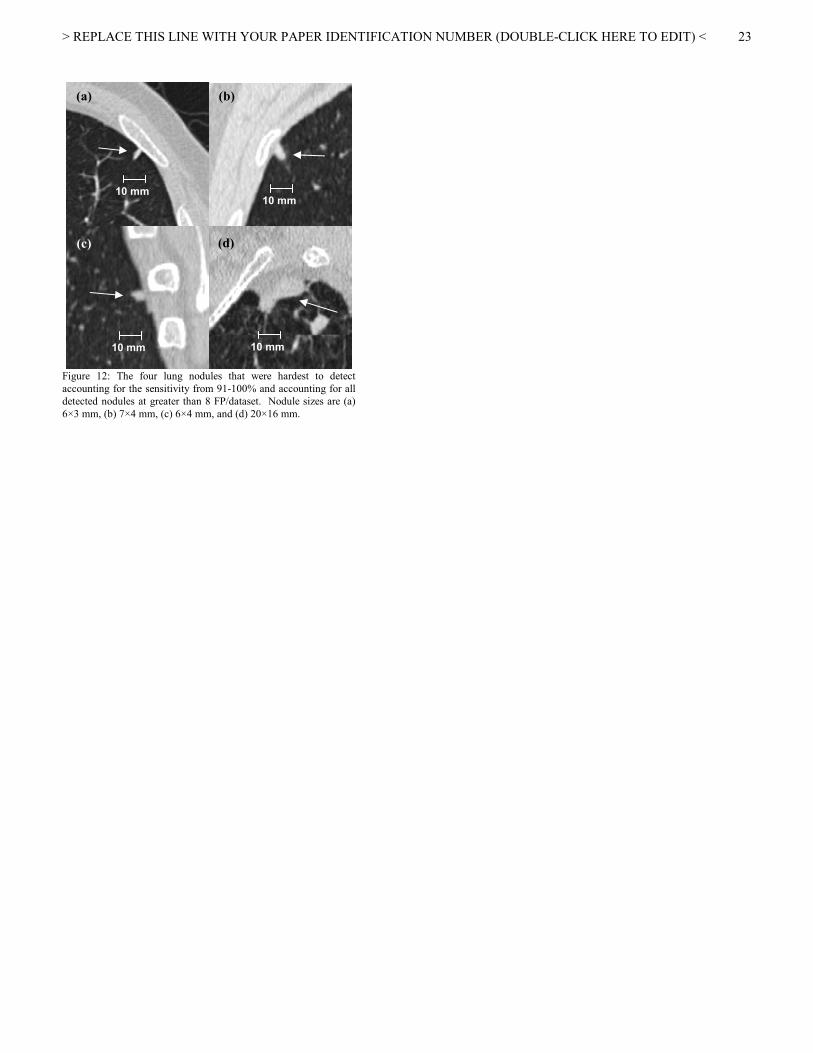
The hardest to find nodules (i.e., near 100% sensitivity) were, however, harder to find than the hardest to find polyps. This was due to several exceptional nodules whose appearance was different than most other nodules. These four nodules accounted for the range of sensitivity from 91-100% and were the only nodules that were detected at greater than 8 FP/dataset. These included three small, elliptical nodules on the chest wall (6×3 mm, 7×4 mm, and 6×4 mm) and one very irregular nodule at the apex of the lung (20×16 mm). See Figure 12.

B. Theoretical Analysis While both SNO and HT perform similarly on perfect

spheres and cylinders, the results shown in Figure 5a-b demonstrate that HT rapidly loses its ability to distinguish between sphere and cylinder as the shape variability approaches realistic levels. On the other hand, SNO retains its shape discrimination under much greater levels of shape variability. Additionally, Figure 5c demonstrates that slight


8

differences in size can lead to very different HT scores due to the interaction of R and B.

The theoretical CAD scores (see Figure 6) suggest that SNO is better able to distinguish between the presented shapes than does HT. While HT is valued for its specificity to the parametric model (e.g., spheres), it is the ability to detect shapes that vary from the nominal shape model that makes SNO particularly suitable for discriminating anatomic shapes.

In the theoretical shape model, note that statistical dependence between neighboring surface patches is not assumed since this would be very unrealistic. However, not assuming independence limits the analysis to the score at the center of the shape instead of the maximum score over the whole shape (expectation of maximum is not maximum of the expectations, see Appendix). Although HT scores may be higher off center, this would require nearly spherical sub-portions of the surface in order to yield higher scores off center.

The theoretical model does assume independence between m and u. The correlation coefficients between m and u for polyps, folds, nodules, and vessels were 0.22, 0.04, 0.06, -0.02, respectively. Although very low correlation does not rule out dependence, it helps to justify this first order approximation.

In our formulation of the SNO method, we have chosen to project Gaussian-profiled cylinders for each surface normal. One limitation of this work is that this choice of projected shape may not be optimal with respect to the theoretical model. This is an area of future work on this algorithm that we plan to investigate further.

C. CAD Algorithm Optimization The design of the simulated phantoms was an important

factor in the optimization of the gradient orientations. The simulated hemisphere on a flat wall model was designed to find the optimal balance between the decreased noise from greater blurring and the increased sensitivity to small objects from lesser blurring. The use of a hemisphere on a flat wall is an obvious first order model for colonic polyps. We had originally tried optimizing gradient orientations for lung nodules on spherical phantoms. However, it was necessary to include other background anatomic structures (e.g., flat wall) in order to realistically model the effect of a large gradient orientation convolution kernel (large σX,Y,Z). With a large kernel, nearby but distinct anatomic structures would contribute to the convolution and cause error in the gradient orientation. This was balanced against the effect of a small kernel, which had a decreased noise reduction benefit due to less blurring (small σX,Y,Z).

The hemisphere on a flat wall also serves as a model for lung nodules in contact with the chest wall, which are not the most common type of lung nodule but are anecdotally more difficult to detect than contact-free nodules by this CAD algorithm. We chose to optimize the gradient orientation step for this type of lung nodule because we wanted the algorithm to perform as well as possible on these difficult to detect

lesions. The results of the gradient orientation kernel anisotropy

optimization were initially unexpected by the authors. The Canny edge detector is designed so that the blurring is performed by the Gaussian and derivative of Gaussian kernels. Because most CT images are inherently blurred more in the longitudinal direction (i.e., z-direction), we originally hypothesized that σZ < σX,Y would compensate and produce more accurate gradient orientations. However, the experiment showed that this effect was nearly non-existent on tri-linearly interpolated data. We have not tested the effect of using an anisotropic kernel on higher order interpolated data, which may yield different results.

There were several other algorithm parameters that were not formally optimized. For instance, the hysteresis thresholds used in edge detection were not optimized. However, in both the colon and lung, image contrast is excellent and edge detection was observed to be very robust. Also note that these thresholds do not affect the direction of detected gradients, which are only dependent on the convolution. Another example is DF, the length of the projected cylinder. We have anecdotally observed both polyp-to-fold and nodule-to-vessel distances to be typically 15-20 mm, greater than DF. Direct visualization of A(x,y,z) has demonstrated that cylinder overlap from neighboring structures is generally not a large problem.

D. CAD Algorithm Evaluation The results of this preliminary evaluation of lung nodule

detection were based on a dataset with a large proportion of the nodules are due to one patient with metastatic disease (37 nodules ≥ 6 mm). Although we cannot distinguish the performance of our algorithm on primary bronchogenic carcinoma from the performance on metastases, we believe that the detection of both primary and metastatic nodules is important. For those patients with pulmonary metastases secondary to colorectal cancer, many gynecological cancers, head and neck cancers, renal cell cancer, malignant melanoma, and sarcomas, pulmonary resection is an important primary therapy with a 5-year survival rate of 21-68% [26, 27]. Also, we note that we did not evaluate the efficacy of our algorithm for detecting ground glass opacities in the lung. Further studies are needed to evaluate the performance characteristics on various types of lesions.

A limitation of the evaluation of colonic polyp detection is that it uses only supine data. Generally, both prone and supine images are used for CT colonography, but we evaluated the algorithm using only supine images because the problem of matching CAD results between prone and supine images is still unsolved. Additionally, treating prone and supine images of the same patient as independent would violate the assumption of independence that allows the cross-validation estimate of performance to be unbiased. Another point regarding the polyp evaluation is that not all FOC determined polyps were found by the gold standard setter in the supine CT images (one ≥ 10 mm), probably due to retained water and/or other factors.


9

Therefore, the CAD algorithm’s failure to identify these polyps is not a failure of the algorithm (since they were not visible in the images) but rather a failure of the CT colonography patient preparation and/or data collection. Thus, they were not counted against the algorithm in this evaluation.

While cross-validation mitigates the problem of over-fitting to the data, it does not remove biases that may be present in the entire dataset. While effort was to avoid bias in the case selection, performance with this algorithm on other datasets may vary with factors such as patient population, image quality, scanner parameters, etc. Although a greater number of cases were available, we did not utilize the entire database for this evaluation because the cross-validation technique required executing the algorithm on each case over a large number of values of σcylinder, which was computationally prohibitive.

For binary classification problems, the area under the ROC curve, AZ, has been widely used as a performance metric. Analogously, the area under the AFROC curve, A1, has been described as a performance metric for multiple detection problems. We experimented with A1 calculated by a binormal FROC curve fitting procedure [28] but found the curve fitting to be unreliable on this data. The false positive image (FPI) model assumes that the operator generally makes less than one FP per image. Data points much beyond one FP per image become nearly indistinguishable due to the Poisson assumption and thus, the fitted curves are most unreliable in this region even though it may be of greatest interest for evaluating a CAD algorithm that will subsequently be reviewed by a human reader. We chose to use partial area under the FROC curve as a cost function for training because it was not prone to curve fitting errors under parametric assumptions. This is analogous to the ROC partial area index [29]. In particular, we found that using a partial area index was important so that the training optimized for the hardest to find polyps and nodules rather than the average polyps and nodules.

E. Comparison to Other CAD Algorithms The SNO method differs from many of the previously

proposed lung nodule CAD algorithms [5-8] in that rather than using a variety of basic shape descriptors such as perimeter, area, volume, sphericity, compactness, elongation, etc., we focus on a single shape measure that is tuned for the specific application(s). Other approaches use some type of idealized shape model [9, 10] but achieve poorer performance, perhaps due to the lack of flexibility in such an explicit model rather than an implicit model that describes an entire gamut of shapes. The approach of McNitt-Gray et al. [30] exemplifies another important aspect of computer-aided diagnosis, the classification between benign and malignant. While our work does not specifically address this problem, we envision our work as part of a larger overall CAD scheme that will at some point also include classification.

The approach of Vining et al. [11] to polyp detection is notable because it attempts to detect polyps based on wall thickness rather than mucosal surface morphology. However, thus far, no other groups have reported success with this type

of approach. The approaches of both Summers et al. [12, 13] and of Yoshida et al. [14-16] share in common the use of partial derivatives to compute principle curvatures. However, the differences in how they are combined and classified vary and may partially account for the differences in performance. Also, Yoshida et al. add gradient concentration (GC) and directional gradient concentration (DGC) in order to improve performance. These two measures also compute the confluence of gradient vectors toward a common point, although they are quite different than the SNO method in actual formulation. However, direct comparison of performance of GC and DGC to this work is difficult because many other features are combined and also, per-polyp sensitivity is not reported. Quantitative comparisons are precluded by differences in study designs and by the relatively small number of datasets used in both this work and other published works.

While most CAD algorithms are described for a single clinical application, the CAD algorithm described in this paper was found to be promising at more than one task. It performed favorably compared to many of the aforementioned CAD schemes although differences in patient populations, CT technology, and analysis methods preclude strict quantitative comparisons.

VII. CONCLUSION We have (1) developed a novel CAD algorithm, the surface

normal overlap method, for both colonic polyp detection and solid lung nodule detection, (2) demonstrated the theoretical traits of this algorithm using a statistical shape model, (3) optimized its performance using a CT simulations and a per-lesion cross-validation method, and (4) provided a preliminary evaluation of its performance in both detection tasks,. The approach we have presented is generalized in that it is able distinguish between focal lesions such as polyps and solid nodules and background anatomy such as blood vessels and haustral folds.

While the CAD algorithm demonstrated in this paper has shown promise for both lung nodule and colonic polyp detection, we ultimately envision it as the first stage of a larger CAD scheme where a set of suspicious locations is passed on to a second stage, possibly comprised of more computationally intensive classifier(s) that would aim to decrease the false positive rate.

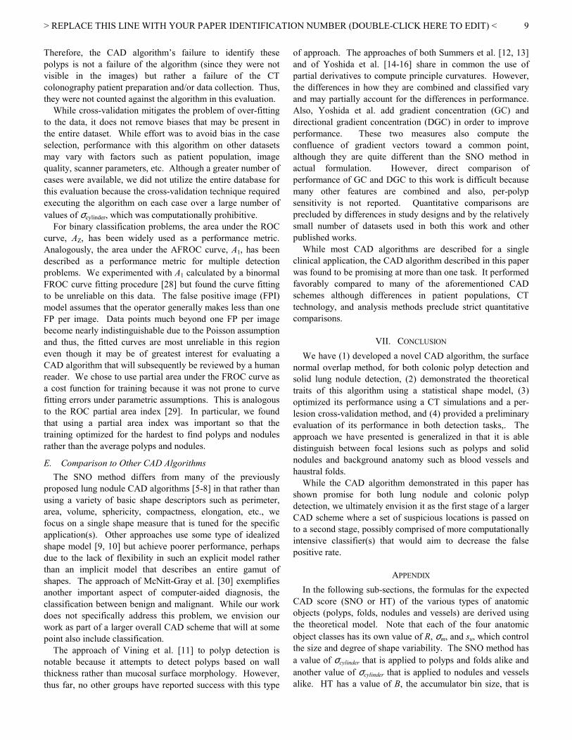
APPENDIX In the following sub-sections, the formulas for the expected

CAD score (SNO or HT) of the various types of anatomic objects (polyps, folds, nodules and vessels) are derived using the theoretical model. Note that each of the four anatomic object classes has its own value of R, σm, and su, which control the size and degree of shape variability. The SNO method has a value of σcylinder that is applied to polyps and folds alike and another value of σcylinder that is applied to nodules and vessels alike. HT has a value of B, the accumulator bin size, that is


10

applied to polyps and folds alike and another value of B that is applied to nodules and vessels alike.

A. SNO: Nodules and Polyps The SNO score can be computed in terms of the weight,

w(⋅), of the surface normals in a given surface patch, the area a′ i of each surface patch, and the density D of surface normals per unit area. The expected SNO score of a polyp or nodule is given by:

⋅′⋅= ∑i

iii DaumwESNO ),(

The weight, w(⋅), of each surface normal due to convolution, has contributions from the entire length in the l direction (along PQ in Figure 2). Using Equation 1 and the relationship

auma iii ⋅+⋅=′ 122 , the expected SNO score for a given

sphere radius R is:

1

1)2(

1

2

1

2223

2

22

+=

⋅

⋅+⋅⋅

= ∑ ∫

=

∞

∞−

+−

i

iii

N

iii

lt

cylinder

u

Rmutwhere

DaumdleESNO cylinder

i

σ

πσ

After factoring, the integral become unity and we get:

⋅⋅+⋅⋅= ∑

=

−N

iii

t

cylinder

DaumeESNO cylinder

i

1

2222 12

1 2

2

σ

πσ

Regardless of dependence, the expectation of a sum of random variables is the sum of the expectations of each random variable, and we obtain:

∑=

−

⋅⋅+⋅⋅=

N

iii

t

cylinder

DaumeESNO cylinder

i

1

2222 12

1 2

2

σ

πσ

Reducing further, substituting for t, and using the relationship NRa /4 2π= , we get:

+⋅⋅= +

−

12 22)1(22

2 22

222

umeERDSNO cylinderuRmu

cylindernodule

σ

σ

Because we model polyps as hemispheres, we use NRa /2 2π= to get:

+⋅⋅= +

−

122)1(22

2 22

222

umeERDSNO cylinderuRmu

cylinderpolyp

σ

σ

B. SNO: Vessels and Folds For the sake of this analysis, a local coordinate system is

chosen with the CAD hit at the origin, the cylinder axis in the z-direction. The index variable k varies along z and the index variable i varies as a function of angle around the axis.

⋅′⋅= ∑∑k i

kikiki DaumwESNO ,,, ),(

A surface patch that whose position varies along the x-direction has a normal vector that is known to pass through:

))sin(),cos(,0(),0,(

,,,,,,,,

,,,

kikikikikikikiki

kikiki

RmuzRmuQzRmP

ϕϕ ⋅+⋅==

Using Equation 1 and di,k, the distance from the line PQ to the CAD hit at the origin, we get:

kiki

kikikiki

N

i kkiki

ld

cylinder

QPPQP

dwhere

DaumdleESNOi

cylinder

ki

,,

,,,,

1 1

2,,

23

)(

1)2(

1 2

22,

××−

=

⋅

⋅+⋅⋅

= ∑∑ ∫

=

∞

=

∞

∞−

+−

σ

πσ

As before, the integral becomes unity after factoring and the expectation of a sum is switched for a sum of expectations:

∑∑=

∞

=

−

⋅⋅+⋅⋅=

icylinder

kiN

i kkiki

d

cylinder

DaumeESNO1 1

2,,

22 12

1 2

2,

σ

πσ

We define zRa ∆⋅∆= θ such that iN/2πθ =∆ and we get:

∑∞

=⋅⋅

−

∆⋅

+⋅⋅⋅⋅=

⋅

1

2,,

22 1

2

2,

kkk

d

cylindervessel zumeERDSNO cylinder

k

σ

σ

We add subscripts to emphasize the dependence of d on m, u, and z, and we get:

∫∞

∞−

−

+⋅⋅⋅⋅= dzumeERDSNO cylinder

zumd

cylindervessel 122

2

2

2,,

σ

σ

Because we model a fold as a half-cylinder, we use iNRa /πθ = to get:

∫∞

∞−

−

+⋅⋅⋅⋅= dzumeERDSNO cylinder

zumd

cylinderfold 1

222

2

2

2,,

σ

σ

C. HT: Nodules and Polyps We model the Hough transform for spheres using a function

h(⋅) that is 1 when a surface normal vector corresponds to a given accumulator bin of width B, and 0 otherwise. This function examines τ, the distance in x-y-z to the true center given R′, the quantized value of R in the accumulator.

( )2

222

25.0

1

02/1

),(

),(

′−−+=

⋅+=′+

=

<

=

⋅′⋅= ∑

RtRmt

BRandu

Rmut

otherwiseBif

umhwhere

DaumhEHT

iiii

BR

i

iii

iii

iiii

τ

τ

This becomes:

⋅⋅+⋅⋅= ∑=

N

iiiii DaumumhEHT

1

22 1),(

The expectation of a sum is switched for a sum of expectations:


11

∑=

⋅⋅+⋅⋅=

N

iiiii DaumumhEHT

1

22 1),(

Reducing further and using the relationship NRa /4 2π= , we get:

]1),([4 222 +⋅⋅⋅⋅= umumhERDHTnodule π Because we model polyps as hemispheres, we use

NRa /2 2π= to get:

]1),([2 222 +⋅⋅⋅⋅= umumhERDHTpolyp π

D. HT: Vessels and Folds Similar to before, we start with:

BRandotherwise

Bifhwhere

DahEHT

BRki

ki

i kkiki

⋅+=′

<

=

⋅′⋅= ∑∑

5.00

2/1)(

)(

,,

,,

ττ

τ

The surface normal passes through P and Q and the point S is the point along the surface normal which corresponds to the quantized value R′.

kiki

kikiki

kikiki

ki

kikikikikikikiki

kikiki

S

QQP

RPQP

RS

RmuzRmuQzRmP

,,

,,,

,,,

,

,,,,,,,,

,,,

1

))sin(),cos(,0(),0,(

=

−′

−+

−′

=

⋅+⋅==

τ

ϕϕ

We get:

⋅⋅+⋅⋅= ∑∑

=

∞

=

iN

i kkikiki DaumhEHT

1 1

2,,, 1)(τ

The expectation of a sum is switched for a sum of expectations:

∑∑=

∞

=

⋅⋅+⋅⋅=

iN

i kkikiki DaumhEHT

1 1

2,,, 1)(τ

We define zRa ∆⋅∆= θ such that iN/2πθ =∆ and we get:

∑∞

=⋅⋅ ∆⋅

+⋅⋅⋅⋅=

1

2,,, 1)(2

kkkkinodule zumhERDHT τπ

In the continuous case, τ is only a function of z and thus:

[ ]∫∞

∞−

+⋅⋅⋅⋅= dzumhERDHT znodule 1)(2 2τπ

Because we model a fold as a half-cylinder, we use iNRa /πθ = to get:

[ ]∫∞

∞−

+⋅⋅⋅⋅= dzumhERDHT zfold 1)( 2τπ

E. Noise limit In order to calculate the response due to noise, we examine

the response due to a single edge element. We assume a surface patch of 1 mm2 and calculate each algorithm’s response. For SNO, the patch will have ti=0 somewhere and thus:

πσ 21

2cylinder

noise DSNO ⋅=

For HT, a single patch will have h(⋅)=1, and thus: DHTnoise =

In order to make scores comparable with in a constant, we present results by normalizing all SNO scores by SNOnoise and all HT scores by HTnoise.

ACKNOWLEDGMENT The authors would like to thank Dr. David Naidich, Dr.

Pamela Schraedley Desmond, Dr. Angel Pineda and the members of the 3D Medical Imaging Laboratory in the Department of Radiology at Stanford University for helpful discussions. This work was supported in part by NIH grants R01-CA72023 and P41-RR09784.


12

Figure 1: Intermediate steps of the CAD algorithm. Left column: CT colon data with a polyp. Right column: CT lung data with a nodule. Top row: cross sectional slice through an example lesion. Middle row: limited search space (S2) from segmentation shown with semitransparent overlay. Bottom row: cross sectional slice through summed overlapping Gaussian profile cylinders shown in grayscale with white denoting highest CAD score.


13

Figure 2: Cross section through the stochastic shape model. Dotted circle is the nominal sphere/cylinder of radius R. Solid contour is the shape after deviation from the nominal model. The deviated surface patch shown as a small oval and the deviated surface normal direction as direction PQ.

u

t

R

m⋅R

1

Q

τ R′

C P


14

0

0.1

0.2

0.3

0.4

0.5

-4 -2 0 2 4m (normalized)

Prob

abili

ty D

ensi

ty

PolypFoldNoduleVesselGaussian

(a) (b) (c)

0

0.1

0.2

0.3

0.4

0.5

0.6

0.7

0.8

0 1 2 3 4 5

u (normalized)

Prob

abili

ty D

ensi

ty

PolypFoldNoduleVesselRayleigh

(d) (e) (f) Figure 3: Examples of theoretical model parameter estimation. The surface normals that belong to the structure are shown as lines on the solid surface and the nominal sphere/cylinder model is shown as partially translucent with perspective. (a) polyp, (b) haustral fold, (d) lung nodule, (e) pulmonary vessel. Histograms of m and u normalized to a unit Gaussian and unit Rayleigh are shown for each shape class and compared to the parametric models in (c) and (f).


15

0

2

4

6

8

10

12

14

16

18

polyps folds nodules vessels

R (

mm

)

0

0.1

0.2

0.3

0.4

0.5


0

0.1

0.2

0.3

0.4

0.5

0.6

0.7


s u

Figure 4: Boxplots showing the minimum, maximum, interquartile range, and median for the theoretical shape model parameters: (a) R, (b) σm, and (c) su.


16

Colon

0

20

40

60

80

100

120

140

160

0 0.5 1 1.5 2

Median Multiplier

CA

D S

core

SNO PolypHT PolypSNO FoldHT Fold

Lung

0

20

40

60

80

100

120

0 0.5 1 1.5 2

Median Multiplier

CAD

Sco

re

SNO NoduleHT NoduleSNO VesselHT Vessel

0

20

40

60

80

100

120

140

160

180

0 1 2 3 4 5 6 7 8 9 10

Lesion Radius (mm)

SN

O S

core

0

1

2

3

4

5

6

7

8

9

HT

Sco

re

SNO PolypSNO NoduleHT PolypHT Nodule

Figure 5: Results from the theoretical model. In (a) and (b), σm and su are simultaneously varied from 0 to twice their median values. (a) Colon CAD scores as a function of σm and su, (b) Lung CAD scores as a function of σm and su, an (c) CAD scores as a function of lesion radius, R, at the median values of σm and su.


17

0

50

100

150

200

SNO

Sco

re

polyps folds0

10

20

30

HT

Scor

e

polyps folds

0

20

40

60

80

SNO

Sco

re

nodules vessels0

2

4

6

8

HT

Sco

re

nodules vessels

Figure 6: (a) Boxplot showing SNO scores using the theorical model in the colon, (b) HT scores in the colon, (c) SNO scores in the lung, and (d) HT scores in the lung.


18

Figure 7: Left: simulated CT phantom of a prototypical lesion consisting of a sphere embedded halfway into a flat wall. Right: an oblique CT cross-section through a phantom lesion showing how e⊥ is calculated as the mean distance (black line segments) from normal vectors (arrows) to the true sphere center (white dot).


19

0

1

2

3

4

5

0 1 2 3 4

e

(mm

)

X,Y,Zσ (mm)

5 mm

5 mm

15 mm

15 mm

Figure 8: The accuracy of the gradient orientations is dependent on the kernel scale, σX,Y,Z, and the size of the lesion (dsphere ranging from 5 to 15 mm). The error metric is minimized across all lesion sizes at σX,Y,Z = 1 mm. The rippling effect is an artifact due to discontinuous jumps in the number of samples in the convolution kernel, nX, nY, and nZ, at different values of σX,Y,Z.


20

0

1

2

3

4

5

0 1 2 3 4

e

(mm

)

Zσ (mm)

5 mm5 mm

15 mm

15 mm

Figure 9: The accuracy of the gradient orientation step on tri-linearly interpolated data is relatively independent of kernel scale anisotropy as σZ varies from σX,Y by a factor of 0.5-2.0. dsphere ranges from 5 to 15 mm and σX,Y was held constant at 1 mm while σZ was varied.


21

Figure 10: Per-lesion cross-validation training: the range of values of σcylinder that was selected is shown in the shaded areas. For reference, A′Z across all of the datasets (i.e., no cross-validation) is shown by the solid lines. Note that the method is able to prospectively choose values of σcylinder (shaded area) near the true optimum (maxima of solid lines) with low variance.


22

0

10

20

30

40

50

60

70

80

90

100

0 5 10 15 20

FP/dataset

Sens

itivi

ty

Polyps ≥ 10 mmPolyps 5-9 mmNodules ≥ 6 mmNodules 3-5 mm

Figure 11: Per-lesion cross-validation evaluation: FROC results for both colonic polyp and lung nodule detection.


23

Figure 12: The four lung nodules that were hardest to detect accounting for the sensitivity from 91-100% and accounting for all detected nodules at greater than 8 FP/dataset. Nodule sizes are (a) 6×3 mm, (b) 7×4 mm, (c) 6×4 mm, and (d) 20×16 mm.

(a) (b)

(d) (c)

10 mm 10 mm

10 mm 10 mm


24

Figure Captions Figure 1: Intermediate steps of the CAD algorithm. Left column: CT colon data with a polyp. Right column: CT lung data with a nodule. Top row: cross sectional slice through an example lesion. Middle row: limited search space (S2) from segmentation shown with semitransparent overlay. Bottom row: cross sectional slice through summed overlapping Gaussian profile cylinders shown in grayscale with white denoting highest CAD score. Figure 2: Cross section through the stochastic shape model. Dotted circle is the nominal sphere/cylinder of radius R. Solid contour is the shape after deviation from the nominal model. The deviated surface patch shown as a small oval and the deviated surface normal direction as direction PQ. Figure 3: Examples of theoretical model parameter estimation. The surface normals that belong to the structure are shown as lines on the solid surface and the nominal sphere/cylinder model is shown as partially translucent with perspective. (a) polyp, (b) haustral fold, (d) lung nodule, (e) pulmonary vessel. Histograms of m and u normalized to a unit Gaussian and unit Rayleigh are shown for each shape class and compared to the parametric models in (c) and (f). Figure 4: Boxplots showing the minimum, maximum, interquartile range, and median for the theoretical shape model parameters: (a) R, (b) σm, and (c) su. Figure 5: Results from the theoretical model. In (a) and (b), σm and su are simultaneously varied from 0 to twice their median values. (a) Colon CAD scores as a function of σm and su, (b) Lung CAD scores as a function of σm and su, an (c) CAD scores as a function of lesion radius, R, at the median values of σm and su. Figure 6: (a) Boxplot showing SNO scores using the theorical model in the colon, (b) HT scores in the colon, (c) SNO scores in the lung, and (d) HT scores in the lung. Figure 7: Left: simulated CT phantom of a prototypical lesion consisting of a sphere embedded halfway into a flat wall. Right: an oblique CT cross-section through a phantom lesion showing how e⊥ is calculated as the mean distance (black line segments) from normal vectors (arrows) to the true sphere center (white dot). Figure 8: The accuracy of the gradient orientations is dependent on the kernel scale, σX,Y,Z, and the size of the lesion (dsphere ranging from 5 to 15 mm). The error metric is minimized across all lesion sizes at σX,Y,Z = 1 mm. The rippling effect is an artifact due to discontinuous jumps in the number of samples in the convolution kernel, nX, nY, and nZ, at different values of σX,Y,Z. Figure 9: The accuracy of the gradient orientation step on tri-linearly interpolated data is relatively independent of kernel

scale anisotropy as σZ varies from σX,Y by a factor of 0.5-2.0. dsphere ranges from 5 to 15 mm and σX,Y was held constant at 1 mm while σZ was varied. Figure 10: Per-lesion cross-validation training: the range of values of σcylinder that was selected is shown in the shaded areas. For reference, A′Z across all of the datasets (i.e., no cross-validation) is shown by the solid lines. Note that the method is able to prospectively choose values of σcylinder (shaded area) near the true optimum (maxima of solid lines) with low variance. Figure 11: Per-lesion cross-validation evaluation: FROC results for both colonic polyp and lung nodule detection. Figure 12: The four lung nodules that were hardest to detect accounting for the sensitivity from 91-100% and accounting for all detected nodules at greater than 8 FP/dataset. Nodule sizes are (a) 6×3 mm, (b) 7×4 mm, (c) 6×4 mm, and (d) 20×16 mm.


25

REFERENCES [1] J. D. Potter, M. L. Slattery, R. M. Bostick, and S. M.

Gapstur, "Colon cancer: a review of the epidemiology," Epidemiologic Reviews, vol. 15, pp. 499-545, 1993.

[2] S. J. Winawer, A. G. Zauber, M. N. Ho, M. J. O'Brien, L. S. Gottlieb, S. S. Sternberg, J. D. Waye, M. Schapiro, J. H. Bond, and J. F. Panish, "Prevention of colorectal cancer by colonoscopic polypectomy. The National Polyp Study Workgroup," New England Journal of Medicine, vol. 329, pp. 1977-81, 1993.

[3] G. M. Strauss and L. Dominioni, "Perception, paradox, paradigm: Alice in the wonderland of lung cancer prevention and early detection," Cancer, vol. 89, pp. 2422-31, 2000.

[4] T. L. Petty, "Screening strategies for early detection of lung cancer: the time is now," JAMA, vol. 284, pp. 1977-80, 2000.

[5] M. L. Giger, K. T. Bae, and H. MacMahon, "Computerized detection of pulmonary nodules in computed tomography images," Investigative Radiology, vol. 29, pp. 459-65, 1994.

[6] S. G. Armato, 3rd, M. L. Giger, C. J. Moran, J. T. Blackburn, K. Doi, and H. MacMahon, "Computerized detection of pulmonary nodules on CT scans," Radiographics, vol. 19, pp. 1303-11, 1999.

[7] S. G. Armato, 3rd, M. L. Giger, and H. MacMahon, "Automated detection of lung nodules in CT scans: preliminary results," Medical Physics, vol. 28, pp. 1552-61, 2001.

[8] M. S. Brown, M. F. McNitt-Gray, J. G. Goldin, R. D. Suh, J. W. Sayre, and D. R. Aberle, "Patient-specific models for lung nodule detection and surveillance in CT images," IEEE Transactions on Medical Imaging, vol. 20, pp. 1242-50, 2001.

[9] Y. Lee, T. Hara, H. Fujita, S. Itoh, and T. Ishigaki, "Automated detection of pulmonary nodules in helical CT images based on an improved template-matching technique," IEEE Transactions on Medical Imaging, vol. 20, pp. 595-604, 2001.

[10] S. G. Erberich, K. Song, H. Arakawa, H. K. Huang, W. Richard, K. S. Hoo, and B. W. Loo, "Knowledge-based Lung Nodule Detection from Helical CT [abstract]," Radiology, vol. 205P, pp. 617, 1997.

[11] D. J. Vining, Y. Ge, D. K. Ahn, and D. R. Stelts, "Virtual colonoscopy with computer-assisted polyp detection," in Computer-Aided Diagnosis in Medical Imaging, K. Doi, H. MacMahon, M. L. Giger, and K. R. Hoffman, Eds. Amsterdam, Netherlands: Elsevier Science B.V., 1999, pp. 445-52.

[12] R. M. Summers, C. F. Beaulieu, L. M. Pusanik, J. D. Malley, R. B. Jeffrey, Jr., D. I. Glazer, and S. Napel, "Automated polyp detector for CT colonography:

feasibility study," Radiology, vol. 216, pp. 284-90, 2000.

[13] R. M. Summers, C. D. Johnson, L. M. Pusanik, J. D. Malley, A. M. Youssef, and J. E. Reed, "Automated polyp detection at CT colonography: feasibility assessment in a human population," Radiology, vol. 219, pp. 51-9, 2001.

[14] H. Yoshida and J. Nappi, "Three-dimensional computer-aided diagnosis scheme for detection of colonic polyps," IEEE Transactions on Medical Imaging, vol. 20, pp. 1261-74, 2001.

[15] H. Yoshida, Y. Masutani, P. MacEneaney, D. T. Rubin, and A. H. Dachman, "Computerized Detection of Colonic Polyps at CT Colonography on the Basis of Volumetric Features: Pilot Study," Radiology, vol. 222, pp. 327-36, 2002.

[16] J. Nappi and H. Yoshida, "Automated detection of polyps with CT colonography: evaluation of volumetric features for reduction of false-positive findings," Academic Radiology, vol. 9, pp. 386-97, 2002.

[17] G. Kiss, J. Van Cleynenbreugel, M. Thomeer, P. Suetens, and G. Marchal, "Computer-aided diagnosis in virtual colonography via combination of surface normal and sphere fitting methods," European Radiology, vol. 12, pp. 77-81, 2002.

[18] S. B. Gokturk, C. Tomasi, B. Acar, C. F. Beaulieu, D. S. Paik, R. B. Jeffrey, Jr., J. Yee, and S. Napel, "A statistical 3-D pattern processing method for computer-aided detection of polyps in CT colonography," IEEE Transactions on Medical Imaging, vol. 20, pp. 1251-60, 2001.

[19] B. Acar, C. F. Beaulieu, S. B. Gokturk, C. Tomasi, D. S. Paik, R. B. Jeffrey, Jr., J. Yee, and S. Napel, "Edge Displacement Field-Based Classification for Improved Detection of Polyps in CT Colonography," IEEE Transactions on Medical Imaging (in press), vol. 21, 2002.

[20] D. S. Paik, C. F. Beaulieu, R. B. Jeffrey, Jr., G. D. Rubin, and S. A. Napel, "Detection of Polyps in CT Colonography: A Comparison of a Computer Aided Detection Algorithm to 3D Visualization Methods [abstract]," Radiology, vol. 213P, pp. 197, 1999.

[21] J. Canny, "A computational approach to edge detection," IEEE Transactions on Pattern Analysis and Machine Intelligence, vol. 8, pp. 679-98, 1986.

[22] C. R. Crawford, "Personal Communications," 1998. [23] R. Kohavi, "A Study of Cross-Validation and

Bootstrap for Accuracy Estimation and Model Selection," Proceedings of the Fourteenth International Joint Conference on Artificial Intelligence, pp. 1137-45, 1995.

[24] C. E. Metz, "Evaluation of CAD methods," in Computer-Aided Diagnosis in Medical Imaging, K. Doi, H. MacMahon, M. L. Giger, and K. R. Hoffman, Eds. Amsterdam, Netherlands: Elsevier Science B.V., 1999, pp. 543-54.

https://www.researchgate.net/publication/11547287_Patient-specific_models_for_lung_nodule_detection_and_surveillance_in_CT_images?el=1_x_8&enrichId=rgreq-8bb5f1dcc71054e0f65f5d0535a4b05c-XXX&enrichSource=Y292ZXJQYWdlOzg1MTY0ODA7QVM6MTA0NTIxNTQ4MTczMzI0QDE0MDE5MzEyODc5NjY=







26

[25] P. V. C. Hough, "Methods and Means for Recognizing Complex Patterns." U.S. Patent 3,069,654, 1962.

[26] "Long-term results of lung metastasectomy: prognostic analyses based on 5206 cases. The International Registry of Lung Metastases," Journal of Thoracic and Cardiovascular Surgery, vol. 113, pp. 37-49, 1997.

[27] V. W. Rusch, "Pulmonary metastasectomy. Current indications," Chest, vol. 107, pp. 322-31, 1995.

[28] D. P. Chakraborty, "Maximum likelihood analysis of free-response receiver operating characteristic (FROC) data," Medical Physics, vol. 16, pp. 561-8, 1989.

[29] Y. Jiang, C. E. Metz, and R. M. Nishikawa, "A receiver operating characteristic partial area index for highly sensitive diagnostic tests," Radiology, vol. 201, pp. 745-50, 1996.

[30] M. F. McNitt-Gray, E. M. Hart, N. Wyckoff, J. W. Sayre, J. G. Goldin, and D. R. Aberle, "A pattern classification approach to characterizing solitary pulmonary nodules imaged on high resolution CT: preliminary results," Medical Physics, vol. 26, pp. 880-8, 1999.

Documents

Surface normal overlap: a computer-aided detection algorithm with application to colonic polyps and lung nodules in helical CT