Surface hopping modeling of two-dimensional spectraRoel Tempelaar, Cornelis P. van der Vegte, Jasper Knoester, and Thomas L. C. Jansen Citation: J. Chem. Phys. 138, 164106 (2013); doi: 10.1063/1.4801519 View online: http://dx.doi.org/10.1063/1.4801519 View Table of Contents: http://jcp.aip.org/resource/1/JCPSA6/v138/i16 Published by the American Institute of Physics. Additional information on J. Chem. Phys.Journal Homepage: http://jcp.aip.org/ Journal Information: http://jcp.aip.org/about/about_the_journal Top downloads: http://jcp.aip.org/features/most_downloaded Information for Authors: http://jcp.aip.org/authors

Downloaded 29 May 2013 to 129.125.210.44. This article is copyrighted as indicated in the abstract. Reuse of AIP content is subject to the terms at: http://jcp.aip.org/about/rights_and_permissions

THE JOURNAL OF CHEMICAL PHYSICS 138, 164106 (2013)

Surface hopping modeling of two-dimensional spectraRoel Tempelaar, Cornelis P. van der Vegte, Jasper Knoester, and Thomas L. C. Jansena)

Zernike Institute for Advanced Materials, University of Groningen, Nijenborgh 4, 9747 AG Groningen,The Netherlands

(Received 30 January 2013; accepted 28 March 2013; published online 23 April 2013)

Recently, two-dimensional (2D) electronic spectroscopy has become an important tool to unravelthe excited state properties of complex molecular assemblies, such as biological light harvestingsystems. In this work, we propose a method for simulating 2D electronic spectra based on a sur-face hopping approach. This approach self-consistently describes the interaction between photoactivechromophores and the environment, which allows us to reproduce a spectrally observable dynamicStokes shift. Through an application to a dimer, the method is shown to also account for correct ther-mal equilibration of quantum populations, something that is of great importance for processes in theelectronic domain. The resulting 2D spectra are found to nicely agree with hierarchy of equations ofmotion calculations. Contrary to the latter, our method is unrestricted in describing the interactionbetween the chromophores and the environment, and we expect it to be applicable to a wide varietyof molecular systems. © 2013 AIP Publishing LLC. [http://dx.doi.org/10.1063/1.4801519]

I. INTRODUCTION

Since its introduction, two-dimensional (2D) infraredspectroscopy has become a well-established techniquefor studying dynamic phenomena such as fast chemicalexchange,1 vibrational energy transport,2, 3 and nonequilib-rium dynamics of proteins.4, 5 More recently, its equivalent inthe ultraviolet and visible optical regime has rapidly gainedpopularity as a powerful probe for electronic processes,6–8

and currently plays a vital role in the research on coherentenergy transport in biological systems such as the Fenna-Matthews-Olson (FMO) complex.6, 9 However, the extensionof 2D spectroscopy to the electronic domain has introducednew challenges for spectral modeling. Notably, 2D electronicspectra are characterized by a clear dynamic Stokes shift10

and signatures of thermal equilibration of quantum popula-tions. To account for these spectral features, the interactionbetween the photoactive chromophores and the environmentshould be described self-consistently, that is, the back actionof the chromophores on the environment should be accountedfor. One way of doing so is by using the Hierarchy of Equa-tions of Motion (HEOM) method.11–14 However, the appli-cability of this method is restricted, e.g., it is exact only forGaussian fluctuations of the environment. The latter is a seri-ous drawback, especially in the light of a recent study on theFMO complex showing that these fluctuations have a markednon-Gaussian nature.15

In this paper, we formulate a method that self-consistently accounts for the chromophore-environment in-teraction by using a surface hopping procedure.16 This pro-cedure is implemented in the Numerical Integration of theSchrödinger Equation (NISE) method18, 26 in which the envi-ronment is represented by classical coordinates. In doing so,no restrictions are posed on the corresponding classical trajec-

a)t.l.c.jansen@rug.nl

tories, or on the interaction with the chromophores, providingthe ability to describe non-Gaussian fluctuations. As such, itis intended as an attractive complement to the HEOM in sim-ulating 2D electronic spectroscopy.

Since the very beginning, numerical models have beencrucial to interpret measured 2D spectra, as these typicallyare complex and congested. The difficulty here is that mostmolecular assemblies under investigation are too complicatedto fully evaluate in terms of quantum mechanics. To over-come this obstacle, several methods have been developed thattreat the environment stochastically, that is, effectively usinga density of states representation, limiting the explicit quan-tum description to the chromophores. Examples are Redfieldtheory,19 cumulant expansions,20 and stochastic Schrödingerand Liouville equations.14, 21 Among the latter is the widelyused HEOM method, which has successfully been employedto simulate 2D electronic spectra.14 Another such method thathas been applied to study nonlinear response is the multi-configurational time-dependent Hartree approach.22 Thisapproach overcomes HEOM’s limitation to Gaussian bathstatistics, but its applicability is restricted to small molec-ular systems. Nevertheless, all of these stochastic methodsshare the downside that they mostly rely on phenomenologi-cal spectral densities, and that they provide little insight in thecorrelation between the chromophores and the environment.In that respect, an appealing alternative is to use quantum-classical dynamics, which allows for an explicit parametriza-tion of the environment through classical coordinates. In anumber of studies, quantum classical schemes have beenadopted to calculate 2D spectra.17, 18, 23, 24, 26 A notable exam-ple is the NISE method,18, 26 for which the classical environ-ment has been modelled as Brownian oscillators,25 or throughmore elaborate molecular dynamics simulations.26 As such,NISE allows to describe correlated dynamics of the classi-cal coordinates and the quantum system. Furthermore, the co-ordinates can perform non-Gaussian fluctuations27 and non-linearity in the quantum-classical interaction can easily be

0021-9606/2013/138(16)/164106/10/$30.00 © 2013 AIP Publishing LLC138, 164106-1

Downloaded 29 May 2013 to 129.125.210.44. This article is copyrighted as indicated in the abstract. Reuse of AIP content is subject to the terms at: http://jcp.aip.org/about/rights_and_permissions

164106-2 Tempelaar et al. J. Chem. Phys. 138, 164106 (2013)

incorporated. At the same time, detailed information on thedissipation of energy is readily available.

NISE has proven to be very effective as a basis for simu-lating 2D infrared spectra,27–29 even for cases in which multi-ple dynamical processes are entangled. In a recent study, thismethod has also been applied to model 2D electronic spec-tra of the FMO complex.15 Nevertheless, implementationsof NISE conventionally treat the quantum-classical interac-tion inconsistently, neglecting the feedback of the quantumsystem on the classical coordinates. Accordingly, these co-ordinates are assumed to always evolve on the potential en-ergy surface corresponding to the quantum ground state. Thisprohibits a description of the dynamic Stokes shift. More-over, it inevitably results into equally distributed quantumpopulations. Such thermalization towards an infinite temper-ature Boltzmann distribution usually works quite well for2D infrared experiments performed at room temperature,but becomes increasingly problematic when probing higherenergies.

The growing interest in 2D electronic spectroscopycalls for models that self-consistently treat the quantum-classical coupling. There are ways to incorporate such cou-pling into NISE, while maintaining the advantages impart tothis method. An incorporation of this kind has successfullybeen carried out by Geva and co-workers for different phys-ical cases involving a quantum monomer.30, 31 When study-ing larger systems, a straightforward approach is to calculatethe quantum feedback according to Ehrenfest’s theorem,32 byusing the weighted average of the quantum energy poten-tial. Such an implementation to the calculation of 2D spectrahas recently been carried out.33 The downside of this mean-field method is its violation of micro-reversibility, which maylead to incorrect thermalization,34 as well as its inability toproperly describe the branching of quantum states. In reac-tion to this shortcoming, several surface hopping approacheshave been introduced, aimed to incorporate the classical re-action to the quantum branching phenomenon. A notableexample is Tully’s fewest-switches surface hopping (FSSH)procedure,16 that has gained popularity in molecular dynam-ics calculations,35–37 and which is shown to bring abouta relaxation of quantum populations towards a Boltzmanndistribution.38, 39

In this work, we complement NISE with FSSH. Throughan application to an electronic dimer system, we demonstratethat this leads to radical changes in the resulting 2D spectrawhen compared with the original NISE method. A dynamicStokes shift is observable, as well as an intense growth ofcross-peaks with increasing waiting time. The latter resultsfrom correct quantum thermalization, which is affirmed byaccompanying population transfer calculations. Furthermore,our results are shown to agree well with the outcome of theHEOM approach, which is employed as a benchmark forspectral calculations.

This paper is organized as follows. Section II A intro-duces the generic model for describing the dynamics of aquantum system and a classical environment, including theself-consistent coupling between the two. In Sec. II B, thismodel is utilized for a brief review of the FSSH algorithm.The implementation of this algorithm in the calculation of 2D

spectra is discussed in Sec. II C. Spectral results for a dimerare demonstrated and analyzed in Sec. III, while a comparisonis made with the HEOM method. Finally, Sec. IV presents adiscussion and summarizes the conclusions.

II. THEORY AND METHODS

A. Mixed quantum-classical dynamics

The distinction between a collection of quantum degreesof freedom and the environment is rooted in the renownedsystem-bath separation. In this paper, the system is assumedto consist of an assembly of interacting two-state quantumunits, where each unit is coupled linearly to a classical co-ordinate, to represent the bath. As such, we follow a methodthat has served as a simplified representation for complex con-densed phase problems in a variety of studies.40 Shown inFig. 1 is a schematic illustration of the setup. Each two-stateunit is attributed a site index n, and a transition energy ωn.Coupling of site n to bath coordinate xn is manifested as achange of the transition energy ωn by the amount of λnxn,where λn is the coupling parameter. Interaction between sitesn and m, denoted Jn, m, results in a delocalization of quantumexcitations. All of this is accounted for by the familiar excitonHamiltonian,

H =∑

n

(ωn + λnxn)B†nBn +

∑n,m

Jn,mB†nBm, (1)

FIG. 1. Schematic illustration of the model used for mixed quantum-classical dynamics. Each site n comprises a quantum two-state unit withtransition energy ωn. Such unit couples to a classical oscillator xn, which inturn interacts with a stochastic environment corresponding to a temperatureT. Arrows indicate couplings, purely quantum mechanical (Jn, m), quantum-classical (λn), and classical-stochastic (γ ).

Downloaded 29 May 2013 to 129.125.210.44. This article is copyrighted as indicated in the abstract. Reuse of AIP content is subject to the terms at: http://jcp.aip.org/about/rights_and_permissions

164106-3 Tempelaar et al. J. Chem. Phys. 138, 164106 (2013)

which describes the quantum system in the absence of anelectro-magnetic field. Here, the operator B

(†)n annihilates

(creates) an excitation at site n. Note that ¯ = 1 is taken,and that the ground state is associated with the zero point ofenergy.

Since the classical coordinates xn are changing in time,the exciton Hamiltonian is parametrically time-dependent,and so are its eigenstates |φk〉. The same holds of course forthe eigenenergies εk, which are considered time-fluctuatingadiabats. At every instant, the state of the quantum system canbe expressed as an expansion of adiabatic eigenfunctions, |�〉= ∑

k ck|φk〉. Its evolution is governed by the time-dependentSchrödinger equation

|�〉 = −iH |�〉. (2)

This directly leads to an equation of motion for the expansioncoefficients,16

ck = −iεkck −∑

l

�x · �dk,l cl, (3)

where in the last term, an inner product is taken of a vectorrepresenting the bath velocities, �x = (x1, x2, . . . , xn, . . .), andone describing the nonadiabatic coupling,

�dk,l ≡ 〈φk|∇�xφl〉. (4)

Equation (3) can be evaluated numerically to obtain thequantum dynamics. However, instead of solving this equation,we follow the NISE approach,18, 26 which is essentially equiv-alent, but practically different. The Hamiltonian H is assumedconstant during a small time interval �t, over which the wave-function is propagated as

|�(t + �t)〉 = e−iH�t |�(t)〉. (5)

This is conveniently solved in the (local) site basis, which in-volves a Hamiltonian diagonalization, but does not require anexplicit calculation of the nonadiabatic coupling vectors.

Generally, the bath coordinates describe classical trajec-tories directed by the total of acting forces. NISE has the ad-vantage of treating such trajectories explicitly without posinglimitations. In this paper, we restrict ourselves to coordinatesevolving in harmonic potentials, but we stress that our methodmay be used equally well for more general potentials. Follow-ing the Brownian oscillator model,20 the situation of dampedharmonic motion is complemented with a random fluctuat-ing force to stochastically represent the effect of tempera-ture. Accordingly, the classical dynamics are governed by theLangevin equation

m �x = −k�x − mγ �x + �F T + �F Q. (6)

Each coordinate xn is associated with a mass m perform-ing a damped oscillation with friction and spring constantsindicated by γ and k, respectively. For simplicity, the pa-rameters m, γ , and k are here assumed to be equal for alloscillators. The Langevin equation is solved numerically us-ing the Euler method with the same time step �t as appliedin the quantum propagation. The thermal contribution �F T isconsidered a white random force and each vector componentis drawn from a normal distribution. In accordance with the

fluctuation-dissipation theorem, the width of this distributionis taken to be (2γmkBT/�t)1/2.20

The final term in Eq. (6), �F Q, accounts for the back re-action of the quantum system on the classical bath. This termwas not incorporated in earlier implementations of NISE, yetit is required to self-consistently describe the system-bathcoupling. A general formulation of the so-called quantumforce reads

�F Q = −∇�x〈ψF|H |ψF〉 = −〈ψF|∇�xH |ψF〉, (7)

where the second equality follows from the Hellmann-Feynman theorem.41 The quantum force derives from thepotential energy associated with the state |ψF〉. There is nounique way in which this “feedback state” can be assigned.This topic was first touched upon by Ehrenfest,32 who statedthat a quantum observable weighted by the probability of itsoccurrence evolves identical to its classical equivalent. Ac-cordingly, the feedback state is set equal to the wavefunction|�〉. Such a mean-field implementation of the quantum forcein the calculation of 2D spectra is the topic of Ref. 33.

However an elegant and numerically inexpensive ap-proach, this Ehrenfest method falls short when significantbranching of quantum states occurs. For such cases, a properaccount of this branching is essential to achieve thermal relax-ation of quantum populations towards a Boltzmann distribu-tion. In Sec. II B, we outline a surface hopping algorithm thatincorporates quantum branching, and so does reproduce thecorrect thermalization. In doing so, we present an alternativeto the Ehrenfest method that is somewhat more numericallydemanding, but still computationally feasible. The questionof which method is best suitable is not unambiguous42 andwill be further addressed in Sec. IV.

B. Surface hopping

Surface hopping, as originally introduced by Tully andPreston,43 employs the intuitive idea that the classical bath co-ordinates always evolve on a single potential energy surface.Accordingly, two wavefunctions appear in the surface hop-ping approach, which are referred to as “primary” and “aux-iliary.” The primary wavefunction provides a quantum me-chanical description of the system, including aspects such asphase and interference. It is nothing but the state |�〉, whoseevolution is described by Eq. (2). The auxiliary wavefunctionis a basis state corresponding to the potential energy surfaceas experienced by the classical bath, hence, the state |ψF〉 ap-pearing in Eq. (7). Surface hopping can be formulated in anyorthogonal basis, yet we assume such basis state to be adia-batic, i.e., an instantaneous eigenstate of the Hamiltonian. Incase the bath coordinates evolve on the adiabat εk, the state|φk〉 is said to act as an auxiliary wavefunction in providingquantum feedback. The quantum force then takes on the form

�F Q = −〈φk|∇�xH |φk〉. (8)

Nonadiabatic coupling affects the classical dynamicsthrough an instantaneous hopping of the auxiliary wavefunc-tion |ψF〉 between adiabats. In 1990, Tully proposed a methodwhich allows such a state transition to happen anywherealong the potential energy trajectories, provided that the

Downloaded 29 May 2013 to 129.125.210.44. This article is copyrighted as indicated in the abstract. Reuse of AIP content is subject to the terms at: http://jcp.aip.org/about/rights_and_permissions

164106-4 Tempelaar et al. J. Chem. Phys. 138, 164106 (2013)

nonadiabatic coupling is nonvanishing.16 According to thisFSSH algorithm, the probability for a transition from state|φk〉 towards state |φl〉 is determined through

Pk→l = −2 �x · �dl,k Re( cl

ck

)�t, (9)

where �t is the integration time step used for the classicaland quantum propagation. At each step, a uniform randomnumber 0 ≤ ξ < 1 is generated, and the proposed surfacehop is performed provided that the calculated probability islarge enough as compared with ξ . More explicitly, all possibleterminal states l are arranged in some (arbitrary) order, and thetransition k → l is executed if

∑l′≤l−1

Pk→l′ < ξ <∑l′≤l

Pk→l′ , (10)

where sums are taken over all states except the initial one |φk〉.Nevertheless, the auxiliary wavefunction usually will remainunaltered as typically

∑l Pk → l 1. Determination of the

hopping probabilities through Eq. (9) does, once again, notrequire an explicit calculation of the nonadiabatic couplingvectors, thanks to the chain rule �x · �dk,l = 〈φk|φl〉. This factorturns out to produce both positive and negative probabilities.Any negative probability is considered unphysical, and is setequal to zero.44

As shown in Ref. 16, Eq. (9) derives directly from theequation of motion of the primary wavefunction |�〉, givenby Eq. (3). As such, the FSSH algorithm assures that anensemble average of the auxiliary wavefunction |ψF〉 statis-tically reproduces the correct quantum populations |ck|2 astaken from |�〉, while the number of hops is minimized.16

However, conservation of energy might prevent a state tran-sition from occurring, thereby disturbing the statistical dis-tribution of the auxiliary wavefunction. In the course of atransition k → l, the total of quantum and classical energy isconserved by changing the component of the velocity �x in thedirection of the nonadiabatic coupling vector �dk,l , so that thechange in classical kinetic energy matches the difference inadiabats εl − εk.16, 45 When there is not enough initial kineticenergy available for this rescaling of �x, the state transition isabandoned, being energy-forbidden. For such forbidden hop,a sign change of the velocity component along the nonadia-batic coupling vector is performed.44 In doing so, we conformto a vast majority of FSSH studies, although recognizing thatsome accounts are made for leaving the velocity unchanged.46

The occurrence of forbidden hops induces a correct thermal-ization of the quantum populations as derived from the aux-iliary wavefunction. In other words, the feedback state |ψF〉does statistically approach the Boltzmann distribution.38, 39

C. Two-dimensional spectroscopy

2D spectra are the result of four light pulses interactingwith the quantum system. Such a sequence of interactions canbe formulated in six different Liouville pathways, describingthe evolution of a part of the quantum density matrix that con-

FIG. 2. Double sided Feynman diagrams illustrating the six Liouville path-ways that contribute to the 2D optical signal. Shown are the diagrams forground state bleach (GB), stimulated emission (SE), and excited state ab-sorption (EA), where |g〉, |e〉, and |f〉 denote the quantum ground state andexcitations in the singly and doubly excited manifold, respectively. Dashedlines represent interactions with a light pulse. The arrows on the left-side in-dicate the time-direction, and serve to specify the interaction times τ 1, τ 2,τ 3, and τ 4, as well as the intervals t1, t2, and t3. The upper row shows therephasing diagrams, whereas the nonrephasing variants are demonstrated inthe bottom row.

tributes to the optical response. These pathways are termedground state bleach (GB), stimulated emission (SE), and ex-cited state absorption (EA), each of which has a rephasingand a nonrephasing variant.47 The corresponding double sidedFeynman diagrams are presented in Fig. 2.

The interaction between light and the quantum system isdescribed by the Hamiltonian

Hint(t) =∑

�μn · �E(t)(B†n + Bn). (11)

For simplicity, the molecular transition dipoles �μn are as-sumed to be time-independent (Condon approximation). Thelight pulses are manifested by four temporal delta peaks inthe electric field E(t). As depicted in Fig. 2, these peaks areassociated with the times t = τ 1, τ 2, τ 3, and τ 4, while theintervals between peaks are denoted t1, t2, and t3. Duringthe coherence time t1, the density matrix describes a coher-ence between the ground state |g〉 and a singly excited state |e〉for all Liouville pathways. This is also the case during t3, ex-cept for EA, where a coherence between |e〉 and a doubly ex-cited state | f 〉 occurs. The latter is the result of two excitationsby light pulses, or in terms of the interaction Hamiltonian(Eq. (11)), by double action of the creation operator. Through-out the waiting time t2, the density matrix corresponds to aground state population for GB, whereas for SE and EA bothpopulations and interstate coherences in the singly excitedmanifold appear.

Downloaded 29 May 2013 to 129.125.210.44. This article is copyrighted as indicated in the abstract. Reuse of AIP content is subject to the terms at: http://jcp.aip.org/about/rights_and_permissions

164106-5 Tempelaar et al. J. Chem. Phys. 138, 164106 (2013)

Calculation of 2D response is commonly performedthrough separate evaluations of the pathways. In the currentsection, this procedure is complemented with the surface hop-ping algorithm, using the theory of Secs. II A and II B. Thefirst thing to note is that a proper reproduction of the dy-namic Stokes shift requires every pathway to be addresseda unique Hamiltonian, and hence a unique classical vector�x to represent the environment. This vector is then propa-gated alongside the density matrix ρ. However, in treatingtheir mutual interaction self-consistently, we uncover the lim-itations inherent to mixed quantum-classical dynamics. Forexample, during t1, the density matrix typically consists of thecoherence

ρ = |e〉〈g|. (12)

The question as to how �x should interact with this form ofρ is not trivial. In the purely quantum picture, the environ-ment takes part in the coherence rather than interacting withit. However, once the environment is considered classically,such coherent behavior is no longer maintainable.

Our approach is based on the simple assumption that aquantum coherence does not provide feedback on the classi-cal vector. Thus, throughout t1, �x is propagated as if interact-ing with the quantum ground state. Moreover, this assumptionis generalized to also apply for coherences between the singlyand doubly excited manifold, as well as interstate coherences.Consequently, only quantum populations that occur during t2deliver a nonvanishing feedback on the classical environment.According to our findings, such an approximation is not toorestrictive, since the effect of coherences is strongly weak-ened by dephasing effects, and populations determine the 2Dresponse to a great extent.

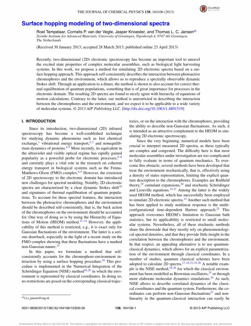
Still, there are several ways in which the above-mentioned approach can be implemented. Our choice of im-plementation is summarized as follows. For a given pathway,the adiabatic populations are separated out, and propagatedusing distinct classical vectors. Such a pathway decomposi-tion leads to the most desirable results, probably because itbest mimics the quantum-branching of the environment. Itessentially comes down to a division into sub-pathways, asis shown schematically for nonrephasing stimulated emission(NR-SE) in Fig. 3. Each sub-pathway (k, l) corresponds tothe density matrix ρk, l interacting with the vector �xk,l . Thedivision is taken so that at time τ 2, right after the secondlight interaction, the density matrix equals ρk, l(τ 2) = |φk〉〈φl|,

FIG. 3. Decomposition of the NR-SE diagram into contributions from pop-ulations |φk〉〈φk| and interstate coherences |φk〉〈φl| (k �= l).

which can be a population (k = l) or an interstate coherence(k �= l) in the adiabatic basis at τ 2. (For ρk, l and �xk,l , the sub-scripts merely indicate the correspondence to a particular sub-pathway.) The contribution of sub-pathway (k, l) to the totalof NR-SE response is determined by the weight factor

Ck,l ≡ 〈φk|Uk,l(τ2, τ1)μ(τ1)ρk,l(−∞)μ(τ2)|φl〉, (13)

which reflects the evolution of ρk, l prior to τ 2. The initial den-sity matrix ρk, l(−∞) ≡ |g〉〈g| is acted upon by the transitiondipole operators μ(τ 1) and μ(τ 2), coupling the ground state tothe singly excited manifold, which derive from the interactionHamiltonian given by Eq. (11). Note that the time argumentsτ 1 and τ 2 purely serve to indicate the interaction times. Thepropagator is given by

Uk,l(τ2, τ1) ≡ e−i

∫ τ2τ1

Hk,l dt ′ (14)

and describes the quantum evolution during the coherencetime t1. In the exponent, a time-integral is taken over theHamiltonian Hk, l as given by Eq. (1), which depends on thevector �xk,l . This vector is in turn integrated through Eq. (6),while the quantum feedback is set to zero.

In the course of the waiting time t2, the adiabatic inter-state coherences are propagated as

ρk,l(t) = Uk,l(t, τ2)|φk〉〈φl|Uk,l(τ2, t) (k �= l), (15)

while the vector �xk,l again is integrated using �F Q = 0. Incontrast, the vector �xk,k does experience a nonzero quantumforce due to the population ρk, k. This is realized throughthe surface hopping algorithm, following the procedure fromSec. II B applied in the singly excited manifold. While doingso, the primary and auxiliary wavefunctions are initialized as|�〉 = |ψF〉 = |φk〉 at time τ 2. Interestingly, the occurrence oftwo wavefunctions provides two ways of calculating the op-tical response. The question as to which variant is the properone will not be addressed at this stage. Rather, we will eval-uate 2D spectra using both wavefunctions, and compare theoutcome. Thus, the population is time-integrated through

ρk,k(t) = USk,k(t, τ2)|φk〉〈φk|US

k,k(τ2, t), (16)

where the surface hopping propagator is given by

USk,k(t, τ2) = e

−i∫ t

τ2Hk,k dt ′

, (17)

when the primary wavefunction |�〉 is employed for the spec-tral calculation, or

USk,k(t, τ2) = |ψF(t)〉〈ψF(τ2)|, (18)

when the auxiliary wavefunction |ψF〉 is used.The above analysis provides all the necessary elements

to formulate the generic expression for the NR-SE optical re-sponse. This response is obtained by taking the trace of thedensity matrix ρk, l at τ 3. Summing over k and l then yields

RNR-SE(t3, t2, t1)

=∑k,l

μ(τ2)Il(τ2)U (S)k,l (τ2, τ3)μ(τ3)μ(τ4)Uk,l(τ4, τ3)

×U(S)k,l (τ3, τ2)Ik(τ2)Uk,l(τ2, τ1)μ(τ1). (19)

Downloaded 29 May 2013 to 129.125.210.44. This article is copyrighted as indicated in the abstract. Reuse of AIP content is subject to the terms at: http://jcp.aip.org/about/rights_and_permissions

164106-6 Tempelaar et al. J. Chem. Phys. 138, 164106 (2013)

In this equation, the adiabatic identity matrix components Ik

≡ |φk〉〈φk| reflect the pathway decomposition. Expressionsfor the other Liouville pathways are derived in an analoguesfashion. The results are formulated in the Appendix. Fouriertransforming these response functions with respect to t1 andt3 yields the 2D spectra for a specific waiting time t2.

III. APPLICATION TO A DIMER SYSTEM

This section presents numerical results obtained throughimplementation of surface hopping in the calculation of 2Dspectra. The parameters are chosen so as to typically representelectronic processes at room temperature, for which a detailedbalance for the quantum populations is of importance. Atthe same time, our choice of parameters matches the regimeof validity of HEOM, which is used as a benchmark forour spectral calculations. Following Ishizaki and Fleming,13

HEOM is applied using a Debye spectral density while ne-glecting the Matsubara frequencies. Hence, when taken in thesemi-classical limit, the bath corresponds to the overdampedBrownian oscillator model. Full details on the correspondingsimulation scheme are given in Refs. 14 and 33.

First, we report that our method is found to successfullydescribe the dynamic Stokes shift for the case of a quantummonomer, something that was not accounted for by conven-tional implementations of NISE. Both the amount of nuclearreorganization and the corresponding time scale are accu-rately reproduced. However, for a detailed account, we re-fer to an implementation of the Ehrenfest approach to 2D

spectroscopy,33 since for a single quantum unit this approachbecomes equivalent to the surface hopping procedure.

Contrary to the monomer case, evaluation of a dimersystem challenges the numerical method to reproduce thecorrect thermal equilibration. In the following, 2D spec-tra are calculated for a dimer of quantum units havingelectronic transition energies of ω1 = 11 500 cm−1 and ω2

= 12 000 cm−1, respectively, and interacting with a strengthof J1,2 = 100 cm−1. Each quantum unit is coupled to a clas-sical coordinate xn (n = 1, 2), with a uniform strength ofλn = 4200 cm−1 nm−1. The coordinates are propagated us-ing Eq. (6), with m = 5 u (atomic units), k = 1117.5 u ps−2,and γ = 50 ps−1. The thermal force is derived from a tem-perature of T = 300 K. These parameters roughly correspondto the overdamped Brownian oscillator model with a corre-lation time of about 0.22 ps, leading to an inhomogeneousspectral broadening of 198 cm−1. Both the quantum systemand the classical coordinates are propagated using a time step�t = 2 fs. For this step size, convergence is assured by sub-tracting the (constant) mean quantum energy (ω1 + ω2)/2 in-side the propagator, which is then corrected for after Fouriertransforming the response functions.

The resulting 2D spectra are shown as contour plots inFig. 4, for zero waiting time (top row), for t2 = 1.5 ps (mid-dle row), and for t2 = 15 ps (bottom row). As outlined inSec. II C, surface hopping provides two ways of calculat-ing the nonlinear response. One way is through using the pri-mary wavefunction, by applying Eq. (17). The outcome of thisapproach is shown in the second left column. Alternatively,the auxiliary wavefunction can be used, see Eq. (18), which

t2 = 0 ps

II

Iω3 (c

m−1

)

Without feedback

1.1

1.15

1.2

1.25

x 104 Primary Auxiliary HEOM

t2 = 1.5 ps

ω3 (c

m−1

)

1.1

1.15

1.2

1.25

−1

−0.5

0

0.5

t2 = 15 ps

ω1 (cm−1)

ω3 (c

m−1

)

1.1 1.15 1.2 1.25

x 104

1.1

1.15

1.2

1.25

ω1 (cm−1)1.1 1.15 1.2 1.25

x 104 ω1 (cm−1)1.1 1.15 1.2 1.25

x 104 ω1 (cm−1)1.1 1.15 1.2 1.25

x 104

FIG. 4. Real part of the calculated 2D spectra for a dimer system at waiting times t2 = 0 ps (top row), 1.5 ps (middle row), and 15 ps (bottom row). Leftcolumn displays results obtained using the conventional NISE method, neglecting quantum feedback. Results for the surface hopping approaches are shownin the second and third columns, where the response is obtained through the primary and auxiliary wavefunctions, respectively. The outcome of HEOM isdemonstrated in the right column. Contours indicate levels for every 10% of the maximum absolute value. This value is used to normalize each spectrum. Thelabels I and II in the top-left plot indicate the two cross-peaks (see text).

Downloaded 29 May 2013 to 129.125.210.44. This article is copyrighted as indicated in the abstract. Reuse of AIP content is subject to the terms at: http://jcp.aip.org/about/rights_and_permissions

164106-7 Tempelaar et al. J. Chem. Phys. 138, 164106 (2013)

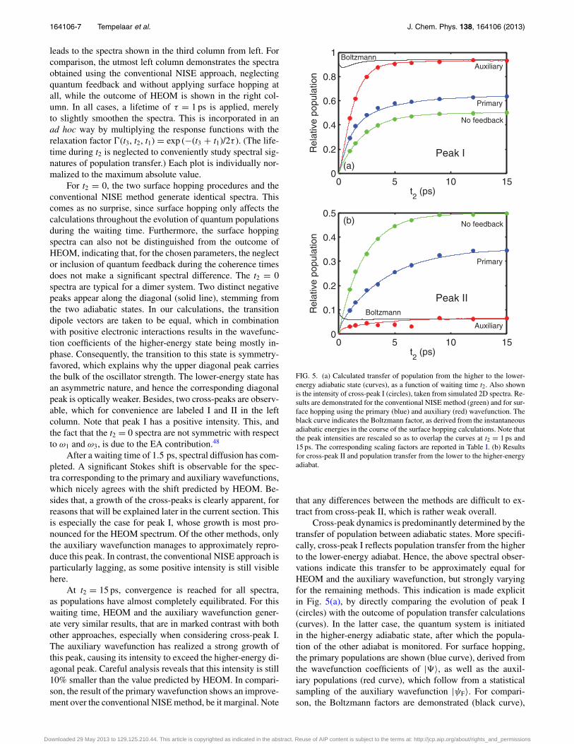
leads to the spectra shown in the third column from left. Forcomparison, the utmost left column demonstrates the spectraobtained using the conventional NISE approach, neglectingquantum feedback and without applying surface hopping atall, while the outcome of HEOM is shown in the right col-umn. In all cases, a lifetime of τ = 1 ps is applied, merelyto slightly smoothen the spectra. This is incorporated in anad hoc way by multiplying the response functions with therelaxation factor (t3, t2, t1) = exp (−(t3 + t1)/2τ ). (The life-time during t2 is neglected to conveniently study spectral sig-natures of population transfer.) Each plot is individually nor-malized to the maximum absolute value.

For t2 = 0, the two surface hopping procedures and theconventional NISE method generate identical spectra. Thiscomes as no surprise, since surface hopping only affects thecalculations throughout the evolution of quantum populationsduring the waiting time. Furthermore, the surface hoppingspectra can also not be distinguished from the outcome ofHEOM, indicating that, for the chosen parameters, the neglector inclusion of quantum feedback during the coherence timesdoes not make a significant spectral difference. The t2 = 0spectra are typical for a dimer system. Two distinct negativepeaks appear along the diagonal (solid line), stemming fromthe two adiabatic states. In our calculations, the transitiondipole vectors are taken to be equal, which in combinationwith positive electronic interactions results in the wavefunc-tion coefficients of the higher-energy state being mostly in-phase. Consequently, the transition to this state is symmetry-favored, which explains why the upper diagonal peak carriesthe bulk of the oscillator strength. The lower-energy state hasan asymmetric nature, and hence the corresponding diagonalpeak is optically weaker. Besides, two cross-peaks are observ-able, which for convenience are labeled I and II in the leftcolumn. Note that peak I has a positive intensity. This, andthe fact that the t2 = 0 spectra are not symmetric with respectto ω1 and ω3, is due to the EA contribution.48

After a waiting time of 1.5 ps, spectral diffusion has com-pleted. A significant Stokes shift is observable for the spec-tra corresponding to the primary and auxiliary wavefunctions,which nicely agrees with the shift predicted by HEOM. Be-sides that, a growth of the cross-peaks is clearly apparent, forreasons that will be explained later in the current section. Thisis especially the case for peak I, whose growth is most pro-nounced for the HEOM spectrum. Of the other methods, onlythe auxiliary wavefunction manages to approximately repro-duce this peak. In contrast, the conventional NISE approach isparticularly lagging, as some positive intensity is still visiblehere.

At t2 = 15 ps, convergence is reached for all spectra,as populations have almost completely equilibrated. For thiswaiting time, HEOM and the auxiliary wavefunction gener-ate very similar results, that are in marked contrast with bothother approaches, especially when considering cross-peak I.The auxiliary wavefunction has realized a strong growth ofthis peak, causing its intensity to exceed the higher-energy di-agonal peak. Careful analysis reveals that this intensity is still10% smaller than the value predicted by HEOM. In compari-son, the result of the primary wavefunction shows an improve-ment over the conventional NISE method, be it marginal. Note

0 5 10 150

0.2

0.4

0.6

0.8

1

t2 (ps)

Rel

ativ

e po

pula

tion

BoltzmannAuxiliary

Primary

No feedback

(a)Peak I

0 5 10 150

0.1

0.2

0.3

0.4

0.5

t2 (ps)

Rel

ativ

e po

pula

tion

Boltzmann

Auxiliary

Primary

Peak II

No feedback(b)

FIG. 5. (a) Calculated transfer of population from the higher to the lower-energy adiabatic state (curves), as a function of waiting time t2. Also shownis the intensity of cross-peak I (circles), taken from simulated 2D spectra. Re-sults are demonstrated for the conventional NISE method (green) and for sur-face hopping using the primary (blue) and auxiliary (red) wavefunction. Theblack curve indicates the Boltzmann factor, as derived from the instantaneousadiabatic energies in the course of the surface hopping calculations. Note thatthe peak intensities are rescaled so as to overlap the curves at t2 = 1 ps and15 ps. The corresponding scaling factors are reported in Table I. (b) Resultsfor cross-peak II and population transfer from the lower to the higher-energyadiabat.

that any differences between the methods are difficult to ex-tract from cross-peak II, which is rather weak overall.

Cross-peak dynamics is predominantly determined by thetransfer of population between adiabatic states. More specifi-cally, cross-peak I reflects population transfer from the higherto the lower-energy adiabat. Hence, the above spectral obser-vations indicate this transfer to be approximately equal forHEOM and the auxiliary wavefunction, but strongly varyingfor the remaining methods. This indication is made explicitin Fig. 5(a), by directly comparing the evolution of peak I(circles) with the outcome of population transfer calculations(curves). In the latter case, the quantum system is initiatedin the higher-energy adiabatic state, after which the popula-tion of the other adiabat is monitored. For surface hopping,the primary populations are shown (blue curve), derived fromthe wavefunction coefficients of |�〉, as well as the auxil-iary populations (red curve), which follow from a statisticalsampling of the auxiliary wavefunction |ψF〉. For compari-son, the Boltzmann factors are demonstrated (black curve),

Downloaded 29 May 2013 to 129.125.210.44. This article is copyrighted as indicated in the abstract. Reuse of AIP content is subject to the terms at: http://jcp.aip.org/about/rights_and_permissions

164106-8 Tempelaar et al. J. Chem. Phys. 138, 164106 (2013)

TABLE I. Time scales, obtained by fitting the data from Fig. 5(a) to theexponential C1 + C2 exp (−t2/tc). Also tabulated are factors used to rescalethe cross-peak intensities in this figure.

Time scale tc (ps) Peak

Peak I Pop. transfer Peak rescaling

No feedback 2.3 2.2 2.3Primary 2.6 1.9 2.0Auxiliary 1.2 1.2 2.2HEOM . . . 1.0 . . .

corresponding to the lower adiabatic energy. Also shownare the primary populations following from the conventionalNISE approach (green curve). Unfortunately, adiabatic pop-ulations cannot be calculated in the HEOM method, since inthat case, information on the quantum system and the envi-ronment are entangled in the hierarchy.

To determine the intensity of peak I, a slice of the cor-responding (unnormalized) 2D spectrum is taken, capturingthe cross-peak extremum, which is then smoothened and fit-ted to a Gaussian. The maximum absolute value of this Gaus-sian is defined as the intensity, assuming the peak width toremain approximately constant in time. This assumption isreasonable after a waiting time of 1 ps, when spectral diffu-sion has fully broadened the spectra. Between 1 ps and 15 ps,9 snapshots are analysed. The results are plotted alongside thecalculated populations, while the peak intensities are rescaledand shifted vertically so as to exactly overlap the populationcurves at t2 = 1 ps and 15 ps. The applied scaling factors arereported in Table I, together with the equilibration time scalestc, obtained by fitting the population transfer curves and cross-peak intensities with the exponential C1 + C2 exp (−t2/tc). Adetermination of the cross-peak time scale is also carried outfor the HEOM spectra.

First, Fig. 5(a) demonstrates that a statistical sampling ofthe auxiliary wavefunction approaches the Boltzmann factor,which agrees with earlier findings.38, 39 In contrast, the pri-mary wavefunction does not obey the correct equilibration, al-though showing an improvement over the infinite temperaturepopulation (= 0.5) predicted by NISE. The Boltzmann factorexhibits a peculiar “dip” around t2 = 0.5 ps. This stems fromrelaxation of the classical coordinates due to quantum feed-back, which (temporarily) diminishes the energy gap betweenadiabats. As follows from Table I, the population equilibrationtimes do nicely agree with the values of tc as derived from thespectral peak fits. The equilibration rates of NISE and the pri-mary wavefunction are comparable, and significantly slowerthan tc = 1.2 ps as obtained for the auxiliary wavefunction.Overall, the peak intensities are rescaled by about the samefactor, which indicates that the transfer of population is ap-propriately reflected in peak I, and hence, that the spectra cor-responding to the auxiliary wavefunction reflect the correctequilibration towards a Boltzmann distribution. As was foundin Fig. 4, the HEOM and auxiliary spectra thermalize towardsapproximately the same equilibrium, although it turns out thatHEOM follows an even somewhat faster time scale of only1.0 ps.

For completeness, the evolution of peak II is shownalongside the outcome of population transfer calculations inFig. 5(b). However, this peak is generally rather weak in inten-sity, leading to poor fitting results. Furthermore, in the light ofthe above analysis, this peak does not contain any additionalinformation.

IV. DISCUSSION AND CONCLUSIONS

Complex molecular assemblies, for which a fullquantum-mechanical description is computationally infeasi-ble, can conveniently be modeled using mixed quantum-classical dynamics. A limited set of degrees of freedom istreated quantum-mechanically, and assumed to be interactingwith a classical environment. Such an approach is the basis ofthe NISE method, which has become a well-established tech-nique for calculating 2D infrared spectra. In this paper, NISEis extended with the FSSH algorithm, which provides a self-consistent description of the quantum-classical interaction.Since FSSH is known for accurately reproducing an equili-bration towards a Boltzmann distribution in the quantum sys-tem, we expect such combination to be particularly suitablefor reproducing higher-energy/lower-temperature processes.As such, we primarily aim at 2D electronic spectroscopy, thathas gained acclaim lately.

The implementation of surface hopping in NISE openstwo ways for calculating the nonlinear response, as it typi-cally involves two different quantum wavefunctions. One wayis by using the “primary” wavefunction, which is the quan-tum state whose evolution is governed by the time-dependentSchrödinger equation. As an alternative, the “auxiliary” wave-function can be used, which at any instant corresponds to asingle adiabatic eigenstate from which the quantum feedbackon the classical environment is derived. In Sec. III, both waysare used to simulate 2D electronic spectra for an electronicquantum dimer system at room temperature, while the envi-ronment is modeled using two overdamped Brownian oscil-lators, each linearly coupled to a single quantum unit. Thespectral outcome is demonstrated alongside results from theconventional NISE approach, without surface hopping. More-over, a comparison is made with HEOM, which accountsfor thermal equilibration on a quantum-mechanical basis. Wehave found that for nonzero waiting time, NISE and the pri-mary wavefunction both generate aberrating spectra, whilethe outcome of the auxiliary wavefunction appears in goodagreement with the results of HEOM. The cross-peaks areshown to accurately indicate population transfer between theadiabatic eigenstates. Our analysis further verifies that thespectrum following the auxiliary wavefunction reflects the ex-pected thermal relaxation of populations towards a Boltzmanndistribution.

In our implementation of NISE/FSSH, nonlinear opti-cal response is evaluated numerically by decomposing thecontributing Liouville pathways in the adiabatic basis, whilebranching the classical coordinates in replicas. Only thereplicas interacting with quantum populations experience afeedback force, and hence, only for these cases a fullyself-consistent treatment of quantum-classical interaction isrealized. This approximation is necessary as a consequence of

Downloaded 29 May 2013 to 129.125.210.44. This article is copyrighted as indicated in the abstract. Reuse of AIP content is subject to the terms at: http://jcp.aip.org/about/rights_and_permissions

164106-9 Tempelaar et al. J. Chem. Phys. 138, 164106 (2013)

the classical nature of the bath coordinates. Another curiosityresulting from mixed quantum-classical dynamics is the ap-pearance of two wavefunctions, as formulated in the surfacehopping algorithm. Our results provide a clear indication thatthe auxiliary wavefunction should be addressed for the opticalresponse, and that the neglect of quantum feedback for quan-tum coherences has a negligible effect on the calculated spec-tra. In the near future, we expect to draw a comparison withexperimental 2D electronic spectroscopy, which might be in-structive as to whether the auxiliary wavefunction is indeedappropriate or not. This in turn would provide deeper insightin the interplay of the environment and the quantum system,and its effect on optical response, and ultimately in how thiscan best be mimicked by quantum-classical simulations.

The combination of NISE and FSSH presented here of-fers the advantages of both methods, at manageable compu-tational costs. Notably, our procedure does not restrict theclassical trajectories in any way, and can easily be extendedto include nonlinear quantum-classical coupling as well asanharmonic classical motion. In that sense, it forms an at-tractive complement to HEOM, which is limited to Gaussianbath fluctuations. Furthermore, we expect it to be applica-ble to larger molecular systems, for which HEOM becomesprohibitively expensive. Another advantage of our procedureis the ease with which the transfer of energy and populationcan be tracked, something that is generally complicated whenthe environment is treated in a stochastic fashion. Finally,it allows non-Condon effects to be incorporated straightfor-wardly. However, the question as to which numerical methodis most appropriate depends strongly on the physical situationat hand. Surface hopping is known to not obey detailed bal-ance per se;38, 39 there might be limits where the method failsreproduce the correct thermalization. Furthermore, the mean-field or Ehrenfest approach is found to outperform FSSHwhen the observables of interest are of diabatic nature, ratherthan adiabatic.42, 46 In a future work, we expect to shed lighton this matter by comparing the performance of Ehrenfest,surface hopping and HEOM in calculating 2D spectra for dif-ferent sets of parameters. Interestingly, various studies haveaimed at combining such methods, leading to hybrid proce-dures that have a broader range of applicability. A notableexample is the fusion of mean-field and FSSH.35, 49

ACKNOWLEDGMENTS

This work is part of the research programme of the Foun-dation for Fundamental Research on Matter (FOM), which ispart of the Netherlands Organization for Scientific Research(NWO).

APPENDIX: 2D RESPONSE FUNCTIONS

This appendix summarizes the response functions for allLiouville pathways that contribute to 2D spectra, followingthe formalism of Sec. II C. First, it should be noted that thecalculation of GB is performed according to the original NISEmethod, since these pathways do not involve any excited statequantum populations. Hence, the response function for the

rephasing variant is given by

RR-GB(t3, t2, t1) = μ(τ1)U (τ1, τ2)μ(τ2)μ(τ4)U (τ4, τ3)μ(τ3),(A1)

whereas the nonrephasing signal follows from

RNR-GB(t3, t2, t1) = μ(τ4)U (τ4, τ3)μ(τ3)μ(τ2)U (τ2, τ1)μ(τ1).(A2)

Rephasing and nonrephasing SE are given by

RR-SE(t3, t2, t1)

=∑k,l

μ(τ1)Uk,l(τ1, τ2)Il(τ2)U (S)k,l (τ2, τ3)μ(τ3)μ(τ4)

×Uk,l(τ4, τ3)U (S)k,l (τ3, τ2)Ik(τ2)μ(τ2) (A3)

and

RNR-SE(t3, t2, t1)

=∑k,l

μ(τ2)Il(τ2)U (S)k,l (τ2, τ3)μ(τ3)μ(τ4)Uk,l(τ4, τ3)

×U(S)k,l (τ3, τ2)Ik(τ2)Uk,l(τ2, τ1)μ(τ1), (A4)

respectively. EA involves the transition dipole operator μef

that couples between the singly and doubly excited manifold.The response functions are formulated as

RR-EA(t3, t2, t1)

=∑k,l

μ(τ1)Uk,l(τ1, τ2)Il(τ2)U (S)k,l (τ2, τ3)Uk,l(τ3, τ4)

×μef (τ4)Uk,l(τ4, τ3)μf e(τ3)U (S)k,l (τ3, τ2)Ik(τ2)μ(τ2)

(A5)

and

RNR-EA(t3, t2, t1) =∑k,l

μ(τ2)Il(τ2)U (S)k,l (τ2, τ3)Uk,l(τ3, τ4)

×μef (τ4)Uk,l(τ4, τ3)μf e(τ3)

×U(S)k,l (τ3, τ2)Ik(τ2)Uk,l(τ2, τ1)μ(τ1).

(A6)

Note that in all cases, including the EA contributions, summa-tions are taken over all adiabatic states k and l in the singly-excited manifold.

1J. Zheng, K. Kwak, J. Ashbury, X. Chen, J. Xie, and M. D. Fayer, Science309, 1338 (2005).

2P. Hamm, M. H. Lim, and R. M. Hochstrasser, J. Phys. Chem. B 102, 6123(1998).

3E. H. G. Backus, P. H. Nguyen, V. Botan, R. Pfister, A. Moretto, M. Crisma,C. Toniolo, G. Stock, and P. Hamm, J. Phys. Chem. B 112, 9091 (2008).

4H. S. Chung, M. Khalil, and A. Tokmakoff, J. Phys. Chem. B 108, 15332(2004).

5C. Kolano, J. Helbing, M. Kozinski, W. Sander, and P. Hamm, Nature (Lon-don) 444, 469 (2006).

6T. Brixner, J. Stenger, H. M. Vaswani, M. Cho, R. E. Blankenship, andG. R. Fleming, Nature (London) 434, 625 (2005).

7J. A. Myers, K. L. M. Lewis, F. D. Fuller, P. F. Tekavec, C. F. Yocum, andJ. P. Ogilvie, J. Phys. Chem. Lett. 1, 2774 (2010).

8M. Aeschlimann, T. Brixner, A. Fischer, C. Kramer, P. Melchior, W.Pfeiffer, C. Schneider, C. Strüber, P. Tuchscherer, and D. V. Voronine, Sci-ence 333, 1723 (2011).

Downloaded 29 May 2013 to 129.125.210.44. This article is copyrighted as indicated in the abstract. Reuse of AIP content is subject to the terms at: http://jcp.aip.org/about/rights_and_permissions

164106-10 Tempelaar et al. J. Chem. Phys. 138, 164106 (2013)

9G. S. Engel, T. R. Calhoun, E. L. Read, T.-K. Ahn, T. Mancal, Y.-C. Cheng,R. E. Blankenship, and G. R. Fleming, Nature (London) 446, 782 (2007).

10T. Gustavsson, G. Baldachino, J.-C. Mialocq, and S. Pommeret, Chem.Phys. Lett. 236, 587 (1995).

11Y. Tanimura and R. Kubo, J. Phys. Soc. Jpn. 58, 101 (1989).12A. Ishizaki and Y. Tanimura, J. Phys. Chem. A 111, 9269 (2007).13A. Ishizaki and G. R. Fleming, J. Chem. Phys. 130, 234111 (2009).14L. Chen, R. Zheng, Q. Shi, and Y. Yan, J. Chem. Phys. 132, 024505

(2010).15C. Olbrich, T. L. C. Jansen, J. Liebers, M. Aghtar, J. Strümpfer, K. Schul-

ten, J. Knoester, and U. Kleinekathöfer, J. Phys. Chem. B 115, 8609 (2011).16J. C. Tully, J. Chem. Phys. 93, 1061 (1990).17T. L. C. Jansen, W. Zhuang, and S. Mukamel, J. Chem. Phys. 121, 10577

(2004).18H. Torii, J. Phys. Chem. A 110, 4822 (2006).19A. G. Redfield, Advances in Magnetic Resonance, edited by J. S. Waugh

(Academic Press, 1965), Vol. 1, pp. 1-30.20S. Mukamel, Principles of Nonlinear Optical Spectroscopy (Oxford Uni-

versity Press, New York, 1995).21J. T. Stockburger and H. Grabert, Phys. Rev. Lett. 88, 170407 (2002).22H. Wang and M. Thoss, Chem. Phys. 347, 139 (2008).23G. Stock and W. H. Miller, J. Chem. Phys. 99, 1545 (1993).24I. Uspenskiy, B. Strodel, and G. Stock, J. Chem. Theory Comput. 2, 1605

(2006).25T. L. C. Jansen and J. Knoester, J. Chem. Phys. 127, 234502 (2007).26T. L. C. Jansen and J. Knoester, J. Phys. Chem. B 110, 22910 (2006).27S. Roy, J. Lessing, G. Meisl, Z. Ganim, A. Tokmakoff, J. Knoester, and

T. L. C. Jansen, J. Chem. Phys. 135, 234507 (2011).28T. L. C. Jansen and J. Knoester, J. Chem. Phys. 124, 044502 (2006).29T. L. C. Jansen, D. Cringus, and M. S. Pshenichnikov, J. Phys. Chem. A

113, 6260 (2009).

30P. L. McRobbie, G. Hanna, Q. Shi, and E. Geva, Acc. Chem. Res. 42, 1299(2009).

31K. Kwac and E. Geva, J. Phys. Chem. B 116, 2856 (2012).32P. Ehrenfest, Z. Phys. 45, 455 (1927).33C. P. van der Vegte, A. Dijkstra, J. Knoester, and T. L. C. Jansen, “Calcu-

lating two-dimensional spectra with the mixed quantum-classical Ehrenfestmethod,” J. Phys. Chem. A (published online).

34P. V. Parandekar and J. C. Tully, J. Chem. Theory Comput. 2, 229 (2006).35O. V. Prezhdo and P. J. Rossky, J. Chem. Phys. 107, 825 (1997).36E. Fabiano, T. W. Keal, and W. Thiel, Chem. Phys. 349, 334 (2008).37T. Nelson, S. Fernandez-Alberti, V. Chernyak, A. E. Roitberg, and S. Tre-

tiak, J. Phys. Chem. B 115, 5402 (2011).38P. V. Parandekar and J. C. Tully, J. Chem. Phys. 122, 094102 (2005).39J. R. Schmidt, P. V. Parandekar, and J. C. Tully, J. Chem. Phys. 129, 044104

(2008).40V. May and O. Kühn, Charge and Energy Transfer Dynamics in Molecular

Systems (John Wiley & Sons, 2004).41D. J. Griffiths, Introduction to Quantum Mechanics (Prentice Hall, 1995).42J. C. Tully, Faraday Discuss. 110, 407 (1998).43J. C. Tully and R. K. Preston, J. Chem. Phys. 55, 562 (1971).44S. Hammes-Schiffer and T. C. Tully, J. Chem. Phys. 101, 4657 (1994).45D. F. Coker and L. Xiao, J. Chem. Phys. 102, 496 (1995).46U. Müller and G. Stock, J. Chem. Phys. 107, 6230 (1997).47P. Hamm and M. Zanni, Concepts and Methods of 2D Infrared Spec-

troscopy (Cambridge University Press, 2011).48This follows from Fig. 1(d) of D. Abramavicius et al., Biophys J. 94, 3613

(2008), considering that excitation to the lowest-energy singly excited stateis only weakly allowed and that the energy of the doubly excited stateamounts to the sum of both singly excited energies.

49S. A. Fischer, C. T. Chapman, and X. Li, J. Chem. Phys. 135, 144102(2011).

Downloaded 29 May 2013 to 129.125.210.44. This article is copyrighted as indicated in the abstract. Reuse of AIP content is subject to the terms at: http://jcp.aip.org/about/rights_and_permissions