Symmetry, Integrability and Geometry: Methods and Applications SIGMA 8 (2012), 070, 12 pages

Superintegrable Extensions

of Superintegrable Systems?

Claudia M. CHANU †, Luca DEGIOVANNI ‡ and Giovanni RASTELLI §

† Dipartimento di Matematica, Universita di Torino,Torino, via Carlo Alberto 10, Italy

E-mail: claudiamaria.chanu@unito.it

‡ Formerly at Dipartimento di Matematica, Universita di Torino,Torino, via Carlo Alberto 10, Italy

E-mail: luca.degiovanni@gmail.com

§ Independent researcher, cna Ortolano 7, Ronsecco, Italy

E-mail: giorast.giorast@alice.it

Received July 30, 2012, in final form September 27, 2012; Published online October 11, 2012

http://dx.doi.org/10.3842/SIGMA.2012.070

Abstract. A procedure to extend a superintegrable system into a new superintegrable oneis systematically tested for the known systems on E2 and S2 and for a family of systemsdefined on constant curvature manifolds. The procedure results effective in many casesincluding Tremblay–Turbiner–Winternitz and three-particle Calogero systems.

Key words: superintegrable Hamiltonian systems; polynomial first integrals

2010 Mathematics Subject Classification: 70H06; 70H33; 53C21

1 Introduction

Given a natural Hamiltonian L with n degrees of freedom, satisfying some additional geometricconditions, it is shown in [1] how to generate a n+ 1 degrees of freedom Hamiltonian H, calledthe extension of L and depending on an integer parameter m ∈ N\{0}, such that H admits twonew independent first integrals: H itself and a polynomial in the momenta of degree m. Thisimplies that, if L is superintegrable with 2n−1 independent first integrals, then all the extendedHamiltonians H also are superintegrable for any m with the maximal number of 2n+ 1 = 2(n+1)−1 first integrals, one of them of arbitrary degree m whose expression is explicitly computed bymeans of a simple iterative process. The extension procedure, summarized in Section 2, is appliedto the superintegrable systems on E2 (Section 3) and S2 (Section 5) as listed in [5]. These areall the superintegrable systems on S2 and E2 admitting two independent first integrals of degreetwo in the momenta other than the Hamiltonian. It is found that a great part of them admitssuperintegrable extensions and for some of them the extensions are explicitly determined. InSection 4 the possible natural Hamiltonians admitting an extension are determined on En and thesuperintegrable systems of Calogero and Wolfes are considered as examples in E3. In Section 6the extension procedure is applied to a class of Hamiltonians on constant curvature manifolds towhich some generalizations of the Tremblay–Turbiner–Winternitz (TTW) system belong [10].These generalizations of the TTW systems are superintegrable for rational values of certainparameters, for which they admit polynomial first integrals of degree greater than two [7, 8].The cases allowing the extensions are determined and the TTW systems are among them,

?This paper is a contribution to the Special Issue “Superintegrability, Exact Solvability, and Special Functions”.The full collection is available at http://www.emis.de/journals/SIGMA/SESSF2012.html

arX

iv:1

210.

3126

v1 [

mat

h-ph

] 1

1 O

ct 2

012

2 C.M. Chanu, L. Degiovanni and G. Rastelli

obtaining in this way their superintegrable extensions. Other superintegrable generalizations inhigher dimensions of the TTW system are obtained in [6].

2 Extensions of superintegrable systems

We resume in the following statement the main results proved in [1].

Theorem 1. Let Q be a n-dimensional (pseudo-)Riemannian manifold with metric tensor g.The natural Hamiltonian L = 1

2gijpipj + V (qi) on M = T ∗Q with canonical coordinates (pi, q

i)admits an extension

H =1

2p2u + α(u)L+ f(u) (1)

with a first integral F = Um(G) where

U = pu + γ(u)XL,

XL is the Hamiltonian vector field of L and G(qi), if and only if the following conditions hold:

i) the functions G and V satisfy

H(G) +mcgG = 0, m ∈ N \ {0}, c ∈ R, (2)

∇V · ∇G− 2m(cV + L0)G = 0, L0 ∈ R, (3)

where H(G)ij = ∇i∇jG is the Hessian tensor of G.

ii) for c = 0 the extended Hamiltonian H is

H =1

2p2u +mA(L+ V0) +mL0A

2(u+ u0)2, (4)

for c 6= 0 the extended Hamiltonian H is

H =1

2p2u +

m(cL+ L0)

S2κ(cu+ u0)

+W0, (5)

with κ, u0, V0, W0, A ∈ R, A 6= 0 and

Sκ(x) =

sin√κx√κ

, κ > 0,

x, κ = 0,

sinh√|κ|x√|κ|

, κ < 0.

Dynamically, extended Hamiltonians (1) can be written as

1

2p2u −

m

S2κ(cu+ u0)

η − h = 0, cL+ L0 + η = 0, if c 6= 0,

and

1

2p2u +mL0A

2u2 − η − h = 0, mA(L+ V0) + η = 0, if c = 0,

Superintegrable Extensions of Superintegrable Systems 3

with H = h, and where constant η can be understood either as a separation constant, betweenthe elements of H depending on (u, pu) and those depending on (qi, pi), or as a coupling constantmerging together the Hamiltonian L on T ∗Q and the Hamiltonian

1

2p2u −

m

S2κ(cu+ u0)

, c 6= 0, or1

2p2u +mL0A

2u2, c = 0,

depending on (u, pu), to build the extended Hamiltonian H. Several examples are given in [1].

Under the hypotheses of Theorem 1, recalling that Cκ(x) = ddxSκ(x), the polynomials in the

momenta

UmG =

(pu +

Cκ(cu+ u0)

Sκ(cu+ u0)XL

)mG, c 6= 0,

(pu −A(u+ u0)XL)mG, c = 0,

are first integrals of H of degree m. For example,

UG = Gpu + γ(u)XL(G) = Gpu + γ(u){L,G},

where { , } are the Poisson brackets. Another way to calculate UmG is to apply the formula [2]

UmG = PmG+DmXLG,

with

Pm =

[m/2]∑k=0

(m2k

)γ2kpm−2ku (−2m(cL+ L0))

k,

Dm =

[m/2]−1∑k=0

(m

2k + 1

)γ2k+1pm−2k−1u (−2m(cL+ L0))

k, m > 1,

where [·] denotes the integer part, D1 = γ and

γ(u) =

Cκ(cu+ u0)

Sκ(cu+ u0), c 6= 0,

−A(u+ u0), c = 0.(6)

Remark 1. For c = 0, if L0 = 0 then pu is a first integral of the extended Hamiltonian andthe extended potential is merely mAV , with m and A constants. Therefore the extension istrivial. Otherwise, a harmonic oscillator term in the variable u, attractive or repulsive, is addedto the potential mAV . In the case c 6= 0, we remark that, in the extended Hamiltonian (5), thepotential V is multiplied by a non-constant factor depending on u.

Remark 2. The expression (6) of γ(u) is determined in [1] as the general solution of thedifferential equation

γ′ + c(γ2 + κ) = 0, (7)

for real values of γ, u, c and κ. However, the general solution of equation (7) in the complexcase can be considered too. Its expression is the same as (6) if we extend functions Sκ and Cκto complex values of x and κ by using the standard exponential expressions of trigonometricfunctions. After this generalization, the extension procedure characterized by Theorem 1 canbe applied also to the complex case.

4 C.M. Chanu, L. Degiovanni and G. Rastelli

In [1] it is proved that, if n > 1, then (2) admits a complete solution G depending ona maximal number of parameters (ai), with i = 0, . . . , n, iff the sectional curvature of Q isconstant and equal to mc. Once such a solution G is known, an extension of L is possible iff thecompatibility condition (3) on V is satisfied. A sharper result on constant curvature manifoldsis the following

Proposition 1. On a manifold with constant curvature K the only eigenvalues mc for theHessian equation (2) are either zero or the curvature K. Moreover, if K 6= 0 and mc = 0 thenthe only solutions of (2) are G = const.

Proof. The equation (2), written in components, becomes

∇i∇jG+mcgijG = ∂ijG− Γkij∂kG+mcgijG = 0.

and the integrability conditions that each solution G(qi) must satisfy are given by (see [1] fordetails)

Rkhijzk = mc(gjhzi − gihzj), ∀h, ∀ i 6= j,

where zk = ∂kG/G and Rkhij = ∂iΓkjl − ∂jΓkil + ΓhjlΓ

kih − ΓhilΓ

kjh is the Riemann tensor of the

metric. For a constant curvature manifold we have Rhlij = K(gjlghi − gilghj) and the aboveconditions become

(K −mc)(gjhzi − gihzj) = 0, ∀h, ∀ i 6= j.

By choosing orthogonal coordinates, we see that, since i 6= j, the equations are identicallysatisfied for h 6= i, j. Otherwise, they reduce to (K −mc)gjjzi = 0. Hence, for mc 6= K, theonly possibility is zi = 0 for all i (that is, G is a constant). For mc 6= K and mc 6= 0, by (2) weget G = 0, thus mc is not an eigenvalue. �

In [1] it is shown that the first integral Um(G) is functionally independent from H, L andall its possible first integrals Li in T ∗Q. It is straightforward to see that L and Li are firstintegrals of H, therefore, if L is a superintegrable Hamiltonian with 2n− 1 first integrals, inclu-ding L, then H is superintegrable too with 2n− 1 + 2 = 2(n+ 1)− 1 first integrals including Hitself. It follows that the extension procedure applied to a superintegrable Hamiltonian L, underthe hypothesis of Theorem 1, always produces a new superintegrable Hamiltonian H. Givena superintegrable system of Hamiltonian L = 1

2gijpipj + V (qi) with a configuration manifold Q

of constant curvature K, its extension to another superintegrable system of Hamiltonian H,when possible, can be obtained by applying the following algorithm (see also [1]):

1. Solve equation (2) on the manifold Q, with c = K/m, to compute the general form of thefunction G(qi, a0, . . . , an).

2. Solve equation (3) with the given V for some of the parameters (ai) in G. This is a crucialstep, because if no solution is found, except for the trivial one G = 0, then the extensionis not possible.

3. Determine the extension via Theorem 1.

4. Compute Um(G) to obtain the additional first integral.

In the following sections we analyze several examples of extensions of superintegrable systems.

Superintegrable Extensions of Superintegrable Systems 5

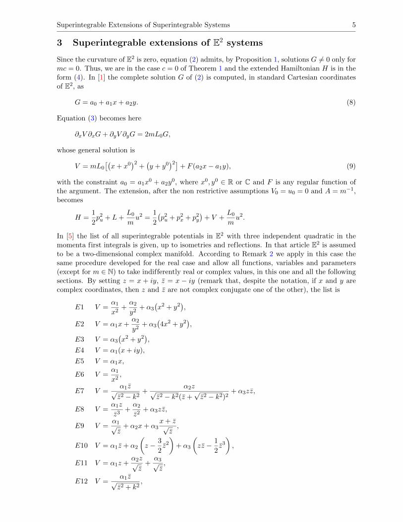
3 Superintegrable extensions of E2 systems

Since the curvature of E2 is zero, equation (2) admits, by Proposition 1, solutions G 6= 0 only formc = 0. Thus, we are in the case c = 0 of Theorem 1 and the extended Hamiltonian H is in theform (4). In [1] the complete solution G of (2) is computed, in standard Cartesian coordinatesof E2, as

G = a0 + a1x+ a2y. (8)

Equation (3) becomes here

∂xV ∂xG+ ∂yV ∂yG = 2mL0G,

whose general solution is

V = mL0

[(x+ x0

)2+(y + y0

)2]+ F (a2x− a1y), (9)

with the constraint a0 = a1x0 + a2y

0, where x0, y0 ∈ R or C and F is any regular function ofthe argument. The extension, after the non restrictive assumptions V0 = u0 = 0 and A = m−1,becomes

H =1

2p2u + L+

L0

mu2 =

1

2

(p2u + p2x + p2y

)+ V +

L0

mu2.

In [5] the list of all superintegrable potentials in E2 with three independent quadratic in themomenta first integrals is given, up to isometries and reflections. In that article E2 is assumedto be a two-dimensional complex manifold. According to Remark 2 we apply in this case thesame procedure developed for the real case and allow all functions, variables and parameters(except for m ∈ N) to take indifferently real or complex values, in this one and all the followingsections. By setting z = x + iy, z = x − iy (remark that, despite the notation, if x and y arecomplex coordinates, then z and z are not complex conjugate one of the other), the list is

E1 V =α1

x2+α2

y2+ α3

(x2 + y2

),

E2 V = α1x+α2

y2+ α3

(4x2 + y2

),

E3 V = α3

(x2 + y2

),

E4 V = α1(x+ iy),

E5 V = α1x,

E6 V =α1

x2,

E7 V =α1z√z2 − k2

+α2z√

z2 − k2(z +√z2 − k2)2

+ α3zz,

E8 V =α1z

z3+α2

z2+ α3zz,

E9 V =α1√z

+ α2x+ α3x+ z√

z,

E10 V = α1z + α2

(z − 3

2z2)

+ α3

(zz − 1

2z3),

E11 V = α1z +α2z√z

+α3√z,

E12 V =α1z√z2 + k2

,

6 C.M. Chanu, L. Degiovanni and G. Rastelli

E13 V =α1√z,

E14 V =α1

z2,

E15 V = h(z), for any function h,

E16 V =1√

x2 + y2

(α1 +

α2

x+√x2 + y2

+α3

x−√x2 + y2

),

E17 V =α1√zz

+α2

z2+

α3

z√zz,

E18 V =α1√x2 + y2

,

E19 V =α1z√z2 − 4

+α2√

z(z + 2)+

α3√z(z − 2)

,

E20 V =1√

x2 + y2

(α1 + α2

√x+

√x2 + y2 + α3

√x−

√x2 + y2

),

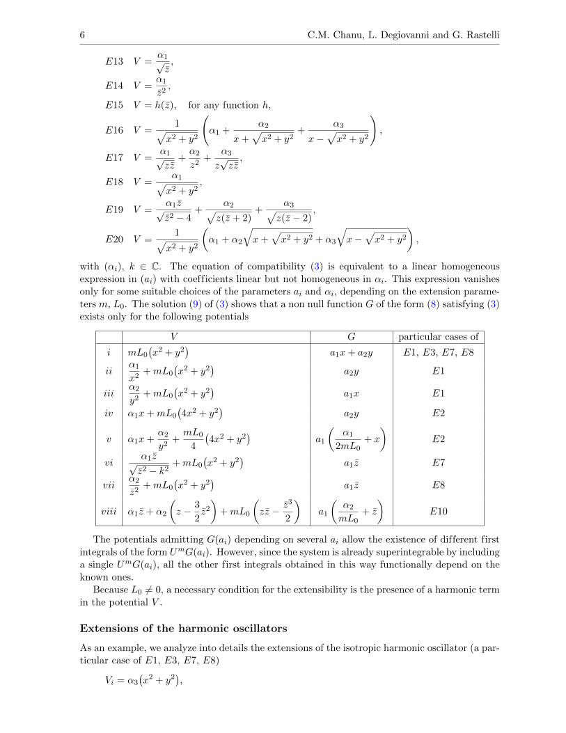
with (αi), k ∈ C. The equation of compatibility (3) is equivalent to a linear homogeneousexpression in (ai) with coefficients linear but not homogeneous in αi. This expression vanishesonly for some suitable choices of the parameters ai and αi, depending on the extension parame-ters m, L0. The solution (9) of (3) shows that a non null function G of the form (8) satisfying (3)exists only for the following potentials

V G particular cases of

i mL0

(x2 + y2

)a1x+ a2y E1, E3, E7, E8

iiα1

x2+mL0

(x2 + y2

)a2y E1

iiiα2

y2+mL0

(x2 + y2

)a1x E1

iv α1x+mL0

(4x2 + y2

)a2y E2

v α1x+α2

y2+mL0

4

(4x2 + y2

)a1

(α1

2mL0+ x

)E2

viα1z√z2 − k2

+mL0

(x2 + y2

)a1z E7

viiα2

z2+mL0

(x2 + y2

)a1z E8

viii α1z + α2

(z − 3

2z2)

+mL0

(zz − z3

2

)a1

(α2

mL0+ z

)E10

The potentials admitting G(ai) depending on several ai allow the existence of different firstintegrals of the form UmG(ai). However, since the system is already superintegrable by includinga single UmG(ai), all the other first integrals obtained in this way functionally depend on theknown ones.

Because L0 6= 0, a necessary condition for the extensibility is the presence of a harmonic termin the potential V .

Extensions of the harmonic oscillators

As an example, we analyze into details the extensions of the isotropic harmonic oscillator (a par-ticular case of E1, E3, E7, E8)

Vi = α3

(x2 + y2

),

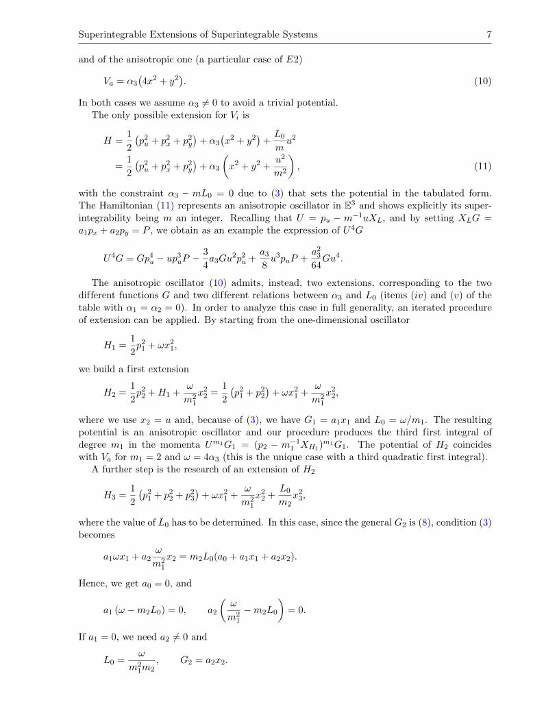
Superintegrable Extensions of Superintegrable Systems 7

and of the anisotropic one (a particular case of E2)

Va = α3

(4x2 + y2

). (10)

In both cases we assume α3 6= 0 to avoid a trivial potential.The only possible extension for Vi is

H =1

2

(p2u + p2x + p2y

)+ α3

(x2 + y2

)+L0

mu2

=1

2

(p2u + p2x + p2y

)+ α3

(x2 + y2 +

u2

m2

), (11)

with the constraint α3 − mL0 = 0 due to (3) that sets the potential in the tabulated form.The Hamiltonian (11) represents an anisotropic oscillator in E3 and shows explicitly its super-integrability being m an integer. Recalling that U = pu − m−1uXL, and by setting XLG =a1px + a2py = P , we obtain as an example the expression of U4G

U4G = Gp4u − up3uP −3

4a3Gu

2p2u +a38u3puP +

a2364Gu4.

The anisotropic oscillator (10) admits, instead, two extensions, corresponding to the twodifferent functions G and two different relations between α3 and L0 (items (iv) and (v) of thetable with α1 = α2 = 0). In order to analyze this case in full generality, an iterated procedureof extension can be applied. By starting from the one-dimensional oscillator

H1 =1

2p21 + ωx21,

we build a first extension

H2 =1

2p22 +H1 +

ω

m21

x22 =1

2

(p21 + p22

)+ ωx21 +

ω

m21

x22,

where we use x2 = u and, because of (3), we have G1 = a1x1 and L0 = ω/m1. The resultingpotential is an anisotropic oscillator and our procedure produces the third first integral ofdegree m1 in the momenta Um1G1 = (p2 − m−11 XH1)m1G1. The potential of H2 coincideswith Va for m1 = 2 and ω = 4α3 (this is the unique case with a third quadratic first integral).

A further step is the research of an extension of H2

H3 =1

2

(p21 + p22 + p23

)+ ωx21 +

ω

m21

x22 +L0

m2x23,

where the value of L0 has to be determined. In this case, since the general G2 is (8), condition (3)becomes

a1ωx1 + a2ω

m21

x2 = m2L0(a0 + a1x1 + a2x2).

Hence, we get a0 = 0, and

a1 (ω −m2L0) = 0, a2

(ω

m21

−m2L0

)= 0.

If a1 = 0, we need a2 6= 0 and

L0 =ω

m21m2

, G2 = a2x2.

8 C.M. Chanu, L. Degiovanni and G. Rastelli

If a1 6= 0 and a2 = 0, then we have

L0 =ω

m2, G2 = a1x1.

Finally, if both a1 6= 0 and a2 6= 0 the two conditions are satisfied iff m21 = 1 (i.e., H2 is the

Hamiltonian of an isotropic oscillator) and

L0 =ω

m2, G2 = a1x1 + a2x2.

In the first two cases, H3 represents an anisotropic harmonic oscillator, which is superintegrablebecause m1, m2 are integers, but they have different functions G2 and consequently differentfirst integrals Um2G2 = (p3 −m−12 XH2)m2G2. If we set m1 = 2, m2 = m and ω = 4α3 in orderto restrict ourselves to the potential (10), we obtain two possible extensions: if a1 = 0 we havethe relation α3 −mL0 = 0 that gives the first form in the table. If, otherwise, a2 = 0 we havethe relation 4α3 −mL0 = 0 that gives the second one.

The extension procedure can be iterated indefinitely obtaining at the n-th step an n-dimen-sional anisotropic oscillator with a complete set of first integrals (Um1G1, U

m2G2, . . . , Umn−1Gn)

of degree (m1,m2, . . . ,mn−1), that, together with the n Hamiltonians (H1, H2, . . . ,Hn) makethe system superintegrable. We remark that the systems obtained in this way are characterizedby the fact that the frequencies are all integer multiples of one of them. See [4, 9] for additionaldetails on superintegrability of anisotropic oscillators.

4 Superintegrable extensions of En

It is straightforward to generalize to En the procedure previously applied to E2. Let us considerin En with Cartesian coordinates the Hamiltonian

L =1

2

(p21 + p22 + · · ·+ p2n

)+ V (x1, x2, . . . , xn).

The general solution of (2) and (3) are

G = a0 + a1x1 + a2x2 + · · ·+ anxn

V = mL0

[(x1 + x01

)2+ · · ·+

(xn + x0n

)2]+ F (a1x2 − a2x1, . . . , a1xn − anx1), (12)

with the constraint a0 =n∑i=1

aix0i , where x0i ∈ R or C, F is any regular function of the arguments

and L0 6= 0. The corresponding extension is

H =1

2p2u +mA(L+ V0) +mL0A

2(u+ u0)2.

We remark that, as well as in dimension 2, the presence of a harmonic term in V is a necessarycondition for the extensibility.

Extensions of the three-body Calogero and Wolfes systems

We consider the particular case of n = 3. If a2 = a3 = a1 and F (X1, X2) in (12) is

F = k(X−21 +X−22 + (X1 −X2)

−2) ,with k ∈ R, then

F = k

(1

(x− y)2+

1

(x− z)2+

1

(y − z)2

)

Superintegrable Extensions of Superintegrable Systems 9

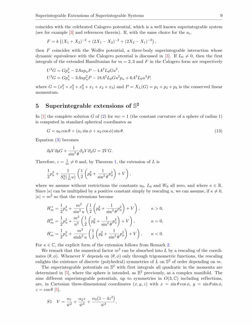
coincides with the celebrated Calogero potential, which is a well known superintegrable system(see for example [3] and references therein). If, with the same choice for the ai,

F = k((X1 +X2)

−2 + (2X1 −X2)−2 + (2X2 −X1)

−2) ,then F coincides with the Wolfes potential, a three-body superintegrable interaction whosedynamic equivalence with the Calogero potential is discussed in [3]. If L0 6= 0, then the firstintegrals of the extended Hamiltonian for m = 2, 3 and F in the Calogero form are respectively

U2G = Gp2u − 2AupuP − 4A2L0Gu2,

U3G = Gp3u − 3Aup2uP − 18A2L0Gu2pu + 6A3L0u

3P,

where G = (x01 + x02 + x03 + x1 + x2 + x3) and P = XL(G) = p1 + p2 + p3 is the conserved linearmomentum.

5 Superintegrable extensions of S2

In [1] the complete solution G of (2) for mc = 1 (the constant curvature of a sphere of radius 1)is computed in standard spherical coordinates as

G = a0 cos θ + (a1 sinφ+ a2 cosφ) sin θ. (13)

Equation (3) becomes

∂θV ∂θG+1

sin2 θ∂φV ∂φG = 2V G.

Therefore, c = 1m 6= 0 and, by Theorem 1, the extension of L is

1

2p2u +

1

S2κ( 1mu)

(1

2

(p2θ +

1

sin2 θp2φ

)+ V

),

where we assume without restrictions the constants u0, L0 and W0 all zero, and where κ ∈ R.Since |κ| can be multiplied by a positive constant simply by rescaling u, we can assume, if κ 6= 0,|κ| = m2 so that the extensions become

H+m =

1

2p2u +

m2

sin2 u

(1

2

(p2θ +

1

sin2 θp2φ

)+ V

), κ > 0,

H0m =

1

2p2u +

m2

u2

(1

2

(p2θ +

1

sin2 θp2φ

)+ V

), κ = 0,

H−m =1

2p2u +

m2

sinh2 u

(1

2

(p2θ +

1

sin2 θp2φ

)+ V

), κ < 0.

For κ ∈ C, the explicit form of the extension follows from Remark 2.We remark that the numerical factor m2 can be absorbed into L by a rescaling of the coordi-

nates (θ, φ). Whenever V depends on (θ, φ) only through trigonometric functions, the rescalingenlights the existence of discrete (polyhedral) symmetries of L on S2 of order depending on m.

The superintegrable potentials on S2 with first integrals all quadratic in the momenta aredetermined in [5], where the sphere is intended, as E2 previously, as a complex manifold. Thenine different superintegrable potentials, up to symmetries in O(3,C) including reflections,are, in Cartesian three-dimensional coordinates (x, y, z) with x = sin θ cosφ, y = sin θ sinφ,z = cos θ [5],

S1 V =α1

w2+α2z

w3+α3

(1− 4z2

)w4

,

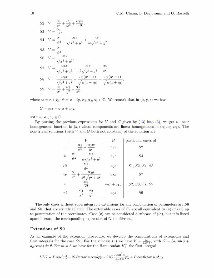
10 C.M. Chanu, L. Degiovanni and G. Rastelli

S2 V =α1

z2+α2

w2+α3w

w3,

S3 V =α1

z2,

S4 V =α1

w2+

α2z√x2 + y2

+α3

w√x2 + y2

,

S5 V =α1

w2,

S6 V =α1z√x2 + y2

,

S7 V =α1x√y2 + z2

+α2y

z2√y2 + z2

+α3

z2,

S8 V =α1x√y2 + z2

+α2(w − z)√w(z − iy)

+α3(w + z)√w(z + iy)

,

S9 V =α1

x2+α2

y2+α3

z2,

where w = x+ iy, w = x− iy, α1, α2, α3 ∈ C. We remark that in (x, y, z) we have

G = a2x+ a1y + a0z,

with a0, a1, a2 ∈ C.By putting the previous expressions for V and G given by (13) into (3), we get a linear

homogeneous function in (ai) whose components are linear homogeneous in (α1, α2, α3). Thenon-trivial solutions (with V and G both not constant) of the equation are

V G particular cases of

iα2

w2+α3w

w3a0z S2

iiα1

w2+

α2

w√x2 + y2

a0z S4

iiiα1

w2a0z S1, S2, S4, S5

ivα1

z2+

α2y

z2√y2 + z2

a2x S7

vα1

z2a2x+ a1y S2, S3, S7, S9

viα1

x2+α2

y2a0z S9

The only cases without superintegrable extensions for any combination of parameters are S6and S8, that are strictly related. The extensible cases of S9 are all equivalent to (v) or (vi) upto permutation of the coordinates. Case (v) can be considered a subcase of (iv), but it is listedapart because the corresponding expression of G is different.

Extensions of S9

As an example of the extension procedure, we develop the computations of extensions andfirst integrals for the case S9. For the subcase (v) we have V = α3

cos2 θ, with G = (a1 sinφ +

a2 cosφ) sin θ. For m = 3 we have for the Hamiltonian H+3 the first integral

U3G = B sin θp3u − 27Bctan3u cos θp3θ − 27Cctan3u

sin3 θp3φ +B cos θctanu p2upθ

Superintegrable Extensions of Superintegrable Systems 11

+ 9Cctanu

sin θp2upφ − 27Bctan2u sin θpup

2θ − 27B

ctan2u

sin θpup

2φ − 27C

ctan3u

sin θp2θpφ

− 27Bctan3u cos θ

sin2 θp2φpθ − 54α3

(B

ctan2u sin θ

cos θpu +B

ctan3u

cos θpθ + C

ctan3u

sin θ cos2 θpφ

),

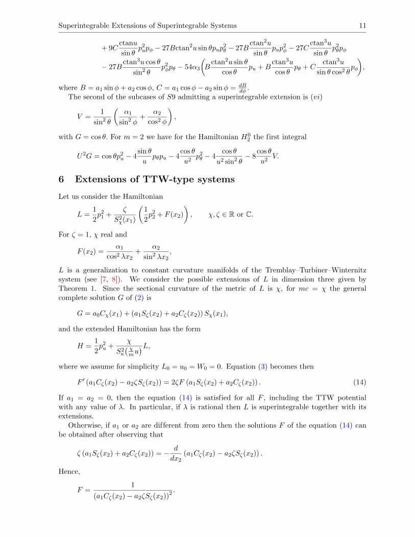
where B = a1 sinφ+ a2 cosφ, C = a1 cosφ− a2 sinφ = dBdφ .

The second of the subcases of S9 admitting a superintegrable extension is (vi)

V =1

sin2 θ

(α1

sin2 φ+

α2

cos2 φ

),

with G = cos θ. For m = 2 we have for the Hamiltonian H02 the first integral

U2G = cos θp2u − 4sin θ

upθpu − 4

cos θ

u2p2θ − 4

cos θ

u2 sin2 θ− 8

cos θ

u2V.

6 Extensions of TTW-type systems

Let us consider the Hamiltonian

L =1

2p21 +

ζ

S2χ(x1)

(1

2p22 + F (x2)

), χ, ζ ∈ R or C.

For ζ = 1, χ real and

F (x2) =α1

cos2 λx2+

α2

sin2 λx2,

L is a generalization to constant curvature manifolds of the Tremblay–Turbiner–Winternitzsystem (see [7, 8]). We consider the possible extensions of L in dimension three given byTheorem 1. Since the sectional curvature of the metric of L is χ, for mc = χ the generalcomplete solution G of (2) is

G = a0Cχ(x1) + (a1Sζ(x2) + a2Cζ(x2))Sχ(x1),

and the extended Hamiltonian has the form

H =1

2p2u +

χ

S2κ

( χmu)L,

where we assume for simplicity L0 = u0 = W0 = 0. Equation (3) becomes then

F ′ (a1Cζ(x2)− a2ζSζ(x2)) = 2ζF (a1Sζ(x2) + a2Cζ(x2)) . (14)

If a1 = a2 = 0, then the equation (14) is satisfied for all F , including the TTW potentialwith any value of λ. In particular, if λ is rational then L is superintegrable together with itsextensions.

Otherwise, if a1 or a2 are different from zero then the solutions F of the equation (14) canbe obtained after observing that

ζ (a1Sζ(x2) + a2Cζ(x2)) = − d

dx2(a1Cζ(x2)− a2ζSζ(x2)) .

Hence,

F =1

(a1Cζ(x2)− a2ζSζ(x2))2.

12 C.M. Chanu, L. Degiovanni and G. Rastelli

By differentiating the relation a1Sζ(x2)+a2Cζ(x2) = ASζ(x2+ξ), valid for suitable constants Aand ξ, we have

F =1

A2C2ζ (x2 + ξ)

,

a result analogous to the one obtained in [1] for the extension of one-dimensional systems.Indeed, when ζ ∈ N \ {0} then L is in the form of an extension of a one-dimensional system.This is another example of iterative extension.

7 Conclusions and future directions

We have shown how the procedure of extension proposed in [1] can be used to produce newsuperintegrable systems starting from the already known ones, together with their first integrals.This procedure allows to extend a number of remarkable systems, including TTW and three-particle Calogero systems. Moreover, in some cases the procedure can be performed iteratively,thus constructing a family of superintegrable systems in higher dimensions.

Unfortunately not all the superintegrable systems can be extended through our method, butthis drawback is balanced by the simplicity and compactness of the algorithm that produces theconstants of motion. Further studies are in progress to find a more general form of extensioncompatible with a larger number of potentials and to analyze iterative extension in other cases.New results about the application to nonconstant curvature manifolds of Theorem 1 have beenobtained. The problem of applying the extension procedure to quantum systems is not yetsolved: the first integrals described by Theorem 1 cannot be straightforwardly associated withsymmetry operators. However, for the quadratic first integrals of type U2(G) a first quantiza-tion procedure has been considered, quite unsuccessfully, in [2] and then a second one has beenstudied, leading in suitable cases to symmetry operators. All these progresses will be presentedin future publications.

References

[1] Chanu C., Degiovanni L., Rastelli G., First integrals of extended Hamiltonians in n+1 dimensions generatedby powers of an operator, SIGMA 7 (2011), 038, 12 pages, arXiv:1101.5975.

[2] Chanu C., Degiovanni L., Rastelli G., Generalizations of a method for constructing first integrals of a classof natural Hamiltonians and some remarks about quantization, J. Phys. Conf. Ser. 343 (2012), 012101,15 pages, arXiv:1111.0030.

[3] Chanu C., Degiovanni L., Rastelli G., Superintegrable three-body systems on the line, J. Math. Phys. 49(2008), 112901, 10 pages, arXiv:0802.1353.

[4] Jauch J.M., Hill E.L., On the problem of degeneracy in quantum mechanics, Phys. Rev. 57 (1940), 641–645.

[5] Kalnins E.G., Kress J.M., Pogosyan G.S., Miller Jr. W., Completeness of superintegrability in two-dimensional constant-curvature spaces, J. Phys. A: Math. Gen. 34 (2001), 4705–4720, math-ph/0102006.

[6] Kalnins E.G., Kress J.M., Miller Jr. W., Talk given by J. Kress during the conference “Superintegrability,Exact Solvability, and Special Functions” (Cuernavaca, February 20–24, 2012).

[7] Kalnins E.G., Kress J.M., Miller Jr. W., Tools for verifying classical and quantum superintegrability, SIGMA6 (2010), 066, 23 pages, arXiv:1006.0864.

[8] Maciejewski A.J., Przybylska M., Yoshida H., Necessary conditions for classical super-integrability of a cer-tain family of potentials in constant curvature spaces, J. Phys. A: Math. Theor. 43 (2010), 382001, 15 pages,arXiv:1004.3854.

[9] Rodrıguez M.A., Tempesta P., Winternitz P., Reduction of superintegrable systems: the anisotropic har-monic oscillator, Phys. Rev. E 78 (2008), 046608, 6 pages, arXiv:0807.1047.

[10] Tremblay F., Turbiner A.V., Winternitz P., An infinite family of solvable and integrable quantum systemson a plane, J. Phys. A: Math. Theor. 42 (2009), 242001, 10 pages, arXiv:0904.0738.