Linear Algebra and its Applications 429 (2008) 1730–1743

Available online at www.sciencedirect.com

www.elsevier.com/locate/laa

Subdirect sums of P(P0)-matrices and totallynonnegative matrices�

Ting-Zhu Huang a,∗, Gu-Fang Mou a, Gui-Xian Tian a, Zhongshan Li b,Di Wang a

a School of Applied Mathematics, University of Electronic Science and Technology of China, Chengdu,Sichuan 610054, PR China

b Department of Mathematics and Statistics, Georgia State University, Atlanta, GA 30302-4110, USA

Received 30 June 2007; accepted 18 May 2008Available online 27 June 2008

Submitted by S.M. Fallat

Abstract

In this paper, the problem of when the subdirect sum of two strictly diagonally dominant P-matricesis a strictly diagonally dominant P-matrix is studied. In particular, it is shown that the subdirect sum ofoverlapping principal submatrices of strictly diagonally dominant P-matrices is a strictly diagonally dom-inant P-matrix. It is also established that the 2-subdirect sum of two totally nonnegative matrices is atotally nonnegative matrix under some conditions. It is obtained that a partial totally nonnegative matrix,whose graph of the specified entries is a monotonically labeled 2-chordal graph, has a totally nonnegativecompletion. Finally, a positive answer to the question (IV) in Fallat and Johnson [S.M. Fallat, C.R. Johnson,Sub-direct sums and positivity classes of matrices, Linear Algebra Appl. 288 (1999) 149–173] is given forP0-matrices.© 2008 Elsevier Inc. All rights reserved.

AMS classification: 15A48

Keywords: k-Subdirect sum; Totally nonnegative matrix; P-Matrix; P0-Matrix

� Supported by Sichuan Province Project for Academic Leader and Group of UESTC.∗ Corresponding author.

E-mail addresses: tzhuang@uestc.edu.cn, tingzhuhuang@126.com (T.-Z. Huang).

0024-3795/$ - see front matter ( 2008 Elsevier Inc. All rights reserved.doi:10.1016/j.laa.2008.05.011

T.-Z. Huang et al. / Linear Algebra and its Applications 429 (2008) 1730–1743 1731

1. Introduction

Subdirect sums of matrices, introduced by Fallat and Johnson [3], are generalizations of the

usual sum of matrices. Suppose that A =[

A11 A12A21 A22

]∈ Mm(C) and B =

[B22 B23B32 B33

]∈ Mn(C),

in which A22, B22 ∈ Mk(C) for some k � min(m, n), then

C =⎡⎣A11 A12 0

A21 A22 + B22 B230 B32 B33

⎤⎦

is called the k-subdirect sum of A and B and is denoted by A ⊕k B. The notion of subdirect sumsarises naturally in a variety of ways, such as in matrix completion [1,2], overlapping subdomainsin domain decomposition methods [7,8], etc.

It is shown [3] that the k-subdirect sum of positive definite matrices or of symmetric M-matrices is positive definite matrix or symmetric M-matrix, respectively. It is also known [3]that the 1-subdirect sum of totally nonnegative matrices, or of P -matrices, or of P0-matrices,is a totally nonnegative matrix or a P -matrix or a P0-matrix, respectively. Subsequently, Bru etal. [5,6] obtained that the k-subdirect sum of nonsingular M-matrices, or of the inverses of M-matrices, or of S-strictly diagonally dominant matrices is a nonsingular M-matrix, or the inverseof an M-matrix or an S-strictly diagonally dominant matrix, respectively.

Fallat and Johnson have shown [3] that the 2-subdirect sum of two P -matrices or totallynonnegative matrices may not be a P -matrix or a totally nonnegative matrix in the general caseand have not resolved question (IV) for the class of P0-matrices (see the discussion precedingSection 5 in Ref. [3]).

In this paper, we show that for a subclass of P -matrices (strictly diagonally dominant P -matrices), the k-subdirect sum of such matrices belongs to the same class, and also obtain thatunder some conditions the 2-subdirect sum of totally nonnegative matrices is a totally nonnegativematrix. Finally, we consider k-subdirect sums of P0-matrices. A positive answer to the question(IV) in Fallat and Johnson [3] is given.

2. Notions

The following introduction can be found, e.g., in [6].Let A and B be two square matrices of orders m and n, respectively, and let k be an integer

such that 1 � k � min(m, n). Let A and B be partitioned into 2 × 2 blocks as follows:

A =[A11 A12A21 A22

], B =

[B22 B23B32 B33

], (2.1)

where A22 and B22 are square matrices of order k. Following [3], we call the following squarematrix of order m + n − k:

C =⎡⎣A11 A12 0

A21 A22 + B22 B230 B32 B33

⎤⎦ ,

the k-subdirect sum of A and B, denoted by A ⊕k B.

1732 T.-Z. Huang et al. / Linear Algebra and its Applications 429 (2008) 1730–1743

It is easy to express each element of C in terms of those A and B. To this end, let us define thefollowing index sets:

S1 = {1, 2, . . . , t},S2 = {t + 1, t + 2, . . . , m},S3 = {m + 1, m + 2, . . . , t + n},

(2.2)

where t = m − k. Clearly, the index set of A is S1 ∪ S2. For simplicity, it is assumed that theindex set of B is S2 ∪ S3.

Write C = (cij ). Then the entries of the subdirect sum are shown

C =

⎡⎢⎢⎢⎢⎢⎢⎢⎢⎢⎢⎢⎣

a11 · · · a1,t+1 · · · a1,m · · · 0... · · · ... · · · ... · · · ...

at+1,1 · · · at+1,t+1 + bt+1,t+1 · · · at+1,m + bt+1,m · · · bt+1,t+n

... · · · ... · · · ... · · · ...

am,1 · · · am,t+1 + bm,t+1 · · · am,m + bm,m · · · bm,t+n

... · · · ... · · · ... · · · ...

0 · · · bt+n,t+1 · · · bt+n,m · · · bt+n,t+n

⎤⎥⎥⎥⎥⎥⎥⎥⎥⎥⎥⎥⎦

.

(2.3)

For A = (aij ) ∈ Mn(C), let

Ri(A) =n∑

j=1j /=i

|aij |, i = 1, . . . , n.

Consider the index sets Si (i = 1, 2, 3) defined in (2.2). Then we have the following relations:

Ri(C) = Ri(A), i ∈ S1,

Ri(C) =t∑

j=1

|aij | +t+n∑

j=m+1

|bij | +m∑

j=t+1j /=i

|aij + bij |, i ∈ S2,

Ri(C) = Ri(B), i ∈ S3.

3. Subdirect sums of strictly diagonally dominant P-matrices

For A ∈ Mn(C), let α, β be subsets of {1, 2, . . . , n}. We denote by A[α|β] (A(α|β)) thesubmatrix of A lying in (deleting) the rows indicated by α and the columns indicated by β. Wealso write A[α|β) for the submatrix of A whose row indices are in α while whose column indicesare in the complement of β. A(α|β] is defined similarly. If α = β, the submatrix A[α|α] (A(α|α))

is abbreviated to A[α](A(α)).A real n × n matrix A is called a P0�matrix (see [4]) if det A[α] � 0, for all nonempty α ⊆

{1, 2, . . . , n}. We say that A is a P�matrix if det A[α] > 0, for all nonempty α ⊆ {1, 2, . . . , n}.Obviously, the main diagonal entries of a P -matrix are positive.

Let A = (aij ) ∈ Mn(C). A is said to be strictly diagonally dominant if |aii | > Ri(A) fori = 1, . . . , n.

T.-Z. Huang et al. / Linear Algebra and its Applications 429 (2008) 1730–1743 1733

Theorem 3.1 [9]. Let A = (aij ) ∈ Mn(C) be strictly diagonally dominant. Then

(1) A is invertible.(2) If all main diagonal entries of A are positive, then all eigenvalues of A have positive real

parts.

Theorem 3.2 [6]. Let A and B be two square matrices of orders m and n, respectively, and letk be an integer such that 1 � k � min(m, n). Let A and B be partitioned as in (2.1). If A andB are strictly diagonally dominant and all diagonal entries of A22 and B22 are positive, then thek-subdirect sum C = A ⊕k B is strictly diagonally dominant, and therefore nonsingular.

Theorem 3.3. Let A and B be strictly diagonally dominant P -matrices of orders m and n,

respectively, and let k be an integer such that 1 � k � min(m, n), and let the sets S1, S2, S3 bedefined as in (2.2). Let A and B be partitioned as in (2.1). Then the k-subdirect sum C = A ⊕k B

is a strictly diagonally dominant P -matrix.

Proof. By Theorem 3.2, C is a strictly diagonally dominant matrix. To prove that C is a P -matrix,it is enough to show det C[α] > 0, for all α ⊆ S1 ∪ S2 ∪ S3. The principal submatrix C[α] isstrictly diagonally dominant matrix with positive diagonal, and by Theorem 3.1 all eigenvaluesof C[α] has positive real part and so det C[α] > 0. Thus C is a strictly diagonally dominantP -matrix. �

Example 3.4 [3]. Let

A =⎡⎣ 2 −1 −1

−1 5 0−1 −9 5

⎤⎦ , B =

⎡⎣ 5 −9 −1

0 5 −1−1 −1 2

⎤⎦ .

Obviously, A and B are not strictly diagonally dominant matrices and are P -matrices, while

C = A ⊕2 B =

⎡⎢⎢⎣

2 −1 −1 0−1 10 −9 −1−1 −9 10 −10 −1 −1 2

⎤⎥⎥⎦

is not a P -matrix.

Example 3.5. The matrix

C =

⎡⎢⎢⎣

4 −2 −1 0−0.5 6 −5 −0.2−1 −4 13 00 −2 −0.5 6

⎤⎥⎥⎦

is a strictly diagonally dominant P -matrix. Note that C = A ⊕2 B where

A =⎡⎣ 4 −2 −1

−0.5 2 −3−1 −1 11

⎤⎦ and B =

⎡⎣ 4 −2 −0.2

−3 2 0−2 0.5 6

⎤⎦

are not strictly diagonally dominant. Thus, the conditions of Theorem 3.3 are not necessary.

1734 T.-Z. Huang et al. / Linear Algebra and its Applications 429 (2008) 1730–1743

Remark 3.6. More generally, if A1, A2, A3, . . . , Ap+1 are strictly diagonally dominant P -matri-ces, then the p-fold subdirect sum C = A1 ⊕k1 A2 ⊕k2 A3 ⊕k3 · · · ⊕kp Ap+1 is also a strictlydiagonally dominant P -matrix.

We now consider the case of square matrices A and B of orders m and n, respectively, whichare principal submatrices of a given strictly diagonally dominant P -matrix, and such that theyhave a common block. This situation, as well as a more general case outlined in Corollary 3.8later in this section, appears in many variants of additive Schwarz preconditioning, e.g. [7,8,10].

Corollary 3.7. Let

M =⎡⎣M11 M12 M13

M21 M22 M23M31 M32 M33

⎤⎦

be a strictly diagonally dominant P -matrix of order m + n − k and with M22 a square matrix oforder k. Let us consider two principal submatrices of M, namely

A =[M11 M12M21 M22

], B =

[M22 M23M32 M33

].

The k-subdirect sum of A and B is a strictly diagonally dominant P -matrix.

This result can be extended to the subdirect sums of overlapping submatrices of a given strictlydiagonally dominant P -matrix M . To this end, we consider principal submatrices of the formM[S] of M , where S = {i, i + 1, i + 2, . . . , j} for some i � j . According to [5], such principalsubmatrices are called principal consecutive submatrices.

Corollary 3.8. Let M be a strictly diagonally dominant P -matrix, let Ai = M[Si], i = 1, . . . , p,

be principal consecutive submatrices of M. Then the subdirect sum C = A1 ⊕k1 A2 ⊕k2 A3 ⊕k3· · · ⊕kp−1 Ap is a strictly diagonally dominant P -matrix.

Example 3.9. Let

M =

⎡⎢⎢⎢⎢⎢⎢⎣

2 0.2 0.16 0.1 0.06 0.0480.8 4 0.8 0.5 0.3 0.240.4 0.5 3 0.5 0.3 0.24

0.32 0.4 0.6 5 0.4 0.320.32 0.4 0.6 0.8 4 0.80.064 0.08 0.12 0.16 0.2 1

⎤⎥⎥⎥⎥⎥⎥⎦

be a strictly diagonally dominant P -matrix. We will consider the following overlapping blocks:

A1 = M[{1, 2, 3, 4}] =

⎡⎢⎢⎣

2 0.2 0.16 0.10.8 4 0.8 0.50.4 0.5 3 0.5

0.32 0.4 0.6 5,

⎤⎥⎥⎦ ,

A2 = M[{2, 3, 4, 5}] =

⎡⎢⎢⎣

4 0.8 0.5 0.30.5 3 0.5 0.30.4 0.6 5 0.40.4 0.6 0.8 4

⎤⎥⎥⎦ ,

T.-Z. Huang et al. / Linear Algebra and its Applications 429 (2008) 1730–1743 1735

A3 = M[{4, 5, 6}] =⎡⎣ 5 0.4 0.32

0.8 4 0.80.16 0.2 1

⎤⎦ .

Then the 3-subdirect sum

A1 ⊕3 A2 =

⎡⎢⎢⎢⎢⎣

2 0.2 0.16 0.1 00.8 8 1.6 1 0.30.4 1 6 1 0.3

0.32 0.8 1.2 10 0.40 0.4 0.6 0.8 4

⎤⎥⎥⎥⎥⎦

is a strictly diagonally dominant P -matrix, and

C = A1 ⊕3 A2 ⊕2 A3 =

⎡⎢⎢⎢⎢⎢⎢⎣

2 0.2 0.16 0.1 0 00.8 8 0.16 1 0.3 00.4 1 6 1 0.3 0

0.32 0.8 1.2 15 0.8 0.320 0.4 0.6 1.6 8 0.80 0 0 0.16 0.2 1

⎤⎥⎥⎥⎥⎥⎥⎦

is also a strictly diagonally dominant P -matrix.

4. 2-Subdirect sum of totally nonnegative matrices

A real n × n matrix A is a totally nonnegative (TN) matrix if det A[α|β] � 0, for all α, β ⊆{1, 2, . . . , n} such that |α| = |β|, where the cardinality of α is denoted by |α|. In particularly, thisimplies that aij � 0, i, j ∈ {1, 2 . . . , n}.

In [3], Fallat and Johnson have obtained that the 1-subdirect sum of two TN matrices is a TNmatrix. In this section, we will show that the 2-subdirect sum of two TN matrices under someconditions is also a TN matrix.

Lemma 4.1 [11]. Suppose that A is an n × n real matrix. If A has a p × q submatrix of zeros,then A is singular whenever p + q � n + 1.

Theorem 4.2. Let A and B be two TN matrices of orders m and n, respectively, and let k = 2,

and A and B be partitioned as in (2.1). Suppose that C = A ⊕2 B, whose entries are as in (2.3)

satisfies the following two conditions:(I) am,j = 0 for j = 1, 2, . . . , m − 2 and bm−1,j = 0 for j = m + 1, m + 2, . . . , n + m −

2; ai,m = 0 for i = 1, 2, . . . , m − 2 and bi,m−1 = 0 for i = m + 1, m + 2, . . . , n + m − 2, and(II) am−1,m−1 � k1am,m−1, k1amm � am−1,m, bm−1,m−1 � k1bm,m−1, k1bmm � bm−1,m

for some k1 � 0.

Then the 2-subdirect sum C = A ⊕2 B is a TN matrix.

Proof. To prove that C is a TN matrix, we shall prove det C[α|β] � 0.Let α, β ⊆ {1, . . . , m + n − 2} be such that |α| = |β|, let α1 = α ∩ {1, . . . , m − 2}, β1 = β ∩

{1, . . . , m − 2}, α2 = α ∩ {m + 1, . . . , n + m − 2}, β2 = β ∩ {m + 1, . . . , n + m − 2}. Firstly,we assume α1, α2, β1 and β2 are all nonempty. Obviously, if |α| = |β| = 1, det C[α|β] � 0.Therefore, we consider α, β such that |α| = |β| > 1.

1736 T.-Z. Huang et al. / Linear Algebra and its Applications 429 (2008) 1730–1743

We will consider the following cases:Case 1. {m − 1, m} � α, {m − 1, m} � β:Case 1.1: α = α1 ∪ α2, β = β1 ∪ β2.

C[α|β] =[A11[α1|β1] 0

0 B33[α2|β2]]

.

Case 1.1.1: |α1| = |β1|.det C[α|β] = det A11[α1|β1] det B33[α2|β2] � 0.

Case 1.1.2: |α1| /= |β1|.Without loss of generality, assume |α1| > |β1| (the case |α1| < |β1| follows by symmetry).

Then A[α|β] has a zero submatrix of size |α1| × |β2|. Furthermore, |α1| + |β2| � |β1| + |β2| +1 = |β| + 1, hence det C[α|β] = 0 according to Lemma 4.1.

Case 1.2: α = α1 ∪ α2 ∪ {m − 1}, β = β1 ∪ β2 ∪ {m − 1}.

C[α|β] =⎡⎣ A11[α1|β1] A12[α1|{m − 1}] 0

A21[{m − 1}|β1] am−1,m−1 + bm−1,m−1 B23[{m − 1}|β2]0 B32[α2|{m − 1}] B33[α2|β2]

⎤⎦ .

Case 1.2.1: |α1| = |β1|.C[α|β] is the 1-subdirect sum of two TN matrices, so C[α|β] is a TN matrix ([3]) and thus

det C[α|β] � 0.Case 1.2.2: |α1| � |β1| + 2.Then A[α|β] has a zero submatrix of size |α1| × |β2|. Furthermore, |α1| + |β2| � |β1| +

|β2| + 1 + 1 = |β| + 1, hence det C[α|β] = 0 by Lemma 4.1.Case 1.2.3: |α1| = |β1| + 1.According to the condition (I), B23[{m − 1}|β2] = 0, then

det C[α|β] = det A[α1|β1 ∪ {m − 1}] det B[α2 ∪ {m − 1}|β2] = 0,

where A[α1|β1 ∪ {m − 1}] and B[α2 ∪ {m − 1}|β2] are square matrices.Case 1.2.4: |β1| � |α1| + 2.This is a symmetric case to Case 1.2.2 and therefore we obtain the result in analogous way.Case 1.2.5: |β1| = |α1| + 1.This case is symmetric to Case 1.2.3 and therefore we obtain the result in analogous way.Case 1.3: α = α1 ∪ α2 ∪ {m − 1}, β = β1 ∪ β2 ∪ {m}.Case 1.4: α = α1 ∪ α2 ∪ {m}, β = β1 ∪ β2 ∪ {m − 1}.Case 1.5: α = α1 ∪ α2 ∪ {m}, β = β1 ∪ β2 ∪ {m}.In analogous way to Case 1.2, we can obtain det C[α|β] � 0 for Cases 1.3, 1.4, 1.5.Case 1.6: α = α1 ∪ α2 ∪ {m − 1}, β = β1 ∪ β2.

C[α|β] =⎡⎣ A11[α1|β1] 0

A21[{m − 1}|β1] B23[{m − 1}|β2]0 B33[α2|β2]

⎤⎦ .

Case 1.6.1: |β1| = |α1|.According to the condition (I), B23[{m − 1}|β2] = 0, then

det C[α|β] = det A11[α1|β1] det B[α2 ∪ {m − 1}|β2] = 0,

where A[α1|β1]and B[α2 ∪ {m − 1}|β2] are square matrices.Case 1.6.2: |β1| = |α1| + 1.

T.-Z. Huang et al. / Linear Algebra and its Applications 429 (2008) 1730–1743 1737

det C[α|β] = det A[α1 ∪ {m − 1}|β1] det B33[α2|β2] � 0,

where A[α1 ∪ {m − 1}|β1] and B[α2|β2] are square matrices.Case 1.6.3: |β1| � |α1| + 2.C[α|β] has a zero submatrix of size |α2| × |β1|. Furthermore, |α2| + |β1| � |α1| + |α2| + 1 +

1 = |α| + 1, and hence, det C[α|β] = 0 according to Lemma 4.1.Case 1.6.4: |α1| � |β1| + 1.C[α|β] has a zero submatrix of size |α1| × |β2|. Furthermore, |α1| + |β2| � |β1| + |β2| + 1 =

|β| + 1, and hence, det C[α|β] = 0 according to Lemma 4.1.Case 1.7: α = α1 ∪ α2, β = β1 ∪ β2 ∪ {m − 1}.This case is symmetric to Case 1.6 and therefore we obtain the result in analogous way.Case 1.8: α = α1 ∪ α2 ∪ {m}, β = β1 ∪ β2.

C[α|β] =⎡⎣ A11[α1|β1] 0

A21[{m}|β1] B23[{m}|β2]0 B33[α2|β2]

⎤⎦ .

Case 1.8.1: |β1| = |α1|.det C[α|β] = det A11[α1|β1] det B[α2 ∪ {m}|β2] � 0,

where A[α1|β1] and B[α2 ∪ {m}|β2] are square matrices.Case 1.8.2: |β1| = |α1| + 1.According to the condition (I), A21[{m}|β1] = 0, then

det C[α|β] = det A[α1 ∪ {m}|β1] det B33[α2|β2] = 0,

where A[α1 ∪ {m}|β1] and B33[α2|β2] are square matrices.Case 1.8.3: |β1| � |α1| + 2.C[α|β] has a zero submatrix of size |α2| × |β1|. Furthermore, |α2| + |β1| � |α1| + |α2| + 1 +

1 = |α| + 1, and hence, det C[α|β] = 0 according to Lemma 4.1.Case 1.8.4: |α1| � |β1| + 1.C[α|β] has a zero submatrix of size |α1| × |β2|. Furthermore, |α1| + |β2| � |β1| + |β2| + 1 =

|β| + 1, and hence, det C[α|β] = 0 according to Lemma 4.1.Case 1.9: α = α1 ∪ α2, β = β1 ∪ β2 ∪ {m − 1}.This case is symmetric to Case 1.8 and therefore we obtain the result in analogous way.Case 2. {m − 1, m} ⊆ α, {m − 1, m}�β:Case 2.1: α = α1 ∪ α2 ∪ {m − 1, m}, β = β1 ∪ β2.

C[α|β] =⎡⎣ A11[α1|β1] 0

A21[{m − 1, m}|β1] B23[{m − 1, m}|β2]0 B33[α2|β2]

⎤⎦ .

Case 2.1.1: |α1| = |β1|.According to the condition (I), B23[{m − 1}|β2] = 0, then

det C[α|β] = det A11[α1|β1] det B[α2 ∪ {m − 1, m}|β2] = 0,

where A[α1|β1] and B[α2 ∪ {m − 1, m}|β2] are square matrices.Case 2.1.2: |α1| > |β1|.C[α|β] has a zero submatrix of size |α1| × |β2|. Furthermore, |α1| + |β2| � |β1| + |β2| + 1 =

|β| + 1. Hence, det C[α|β] = 0 by Lemma 4.1.

1738 T.-Z. Huang et al. / Linear Algebra and its Applications 429 (2008) 1730–1743

Case 2.1.3: |β1| � |α1| + 3.C[α|β] has a zero submatrix of size |α2| × |β1|. Furthermore, |α2| + |β1| � |α1| + |α2| + 2 +

1 = |α| + 1. Hence, det C[α|β] = 0 by Lemma 4.1.Case 2.1.4: |β1| = |α1| + 2.According to the condition (I), A21[{m}|β1] = 0, then

det C[α|β] = det A[α1 ∪ {m − 1, m}|β1] det B[α2|β2] = 0,

where A[α1 ∪ {m − 1, m}|β1] and B[α2|β2] are square matrices.Case 2.1.5: |β1| = |α1| + 1.According to the condition (I), we can obtain

det C[α|β] = det A[α1 ∪ {m − 1}|β1] det B[α2 ∪ {m}|β2] � 0,

where A[α1 ∪ {m − 1}|β1] and B[α2 ∪ {m}|β2] are square matrices.Case 2.2: α = α1 ∪ α2 ∪ {m − 1, m}, β = β1 ∪ β2 ∪ {m − 1}.

C[α|β] =

⎡⎢⎢⎣

A11[α1|β1] A12[α1|{m − 1}] 0A21[{m − 1}|β1] am−1,m−1 + bm−1,m−1 B23[{m − 1}|β2]

A21[{m}|β1] am,m−1 + bm,m−1 B23[{m}|β2]0 B32[α2|{m − 1}] B33[α2|β2]

⎤⎥⎥⎦ .

Case 2.2.1: |α1| � |β1| + 2.C[α|β] has a zero submatrix of size |α1| × |β2|. Furthermore, |α1| + |β2| � |β1| + |β2| + 1 +

1 = |β| + 1. Hence, det C[α|β] = 0 by Lemma 4.1.Case 2.2.2: |α1| = |β1| + 1.According to the condition (I), B23[{m − 1}|β2] = 0, then

det C[α|β] = det A[α1|β1 ∪ {m − 1}] det B[α2 ∪ {m − 1, m}|β2] = 0,

where A[α1|β1 ∪ {m − 1}] and B[α2 ∪ {m − 1, m}|β2] are square matrices.Case 2.2.3: |α1| = |β1|.By applying the conditions (I), we obtain

det C[α|β] = det B[α2 ∪ {m}|β2] det

[A11[α1|β1] A12[α1|{m}]A21[{m − 1}|β1] am−1,m−1 + bm−1,m−1

]� 0,

where A11[α1|β1] and B[α2 ∪ {m}|β2] are square matrices.Case 2.2.4: |β1| � |α1| + 3.C[α|β] has a zero submatrix of size |α2| × |β1|. Furthermore, |α2| + |β1| � |α1| + |α2| + 2 +

1 = |α| + 1, and hence, det C[α|β] = 0 according to Lemma 4.1.Case 2.2.5: |β1| = |α1| + 2.According to the condition (I), A21[{m}|β1] = 0, then

det C[α|β] = det A[α1 ∪ {m − 1, m}|β1] det B[α2|β2 ∪ {m − 1}] = 0,

where A[α1 ∪ {m − 1, m}|β1] and B[α2|β2 ∪ {m − 1}] are square matrices.Case 2.2.6: |β1| = |α1| + 1.By applying the condition (I), we obtain

det C[α|β] = det A[α1 ∪ {m − 1}|β1] det

[am,m−1 + bm,m−1 B23[{m}|β2]B32[α2|{m − 1}] B33[α2|β2]

]� 0,

where A[α1 ∪ {m − 1}|β1] and B33[α2|β2] are square matrices.Case 2.3: α = α1 ∪ α2 ∪ {m − 1, m}, β = β1 ∪ β2 ∪ {m}.

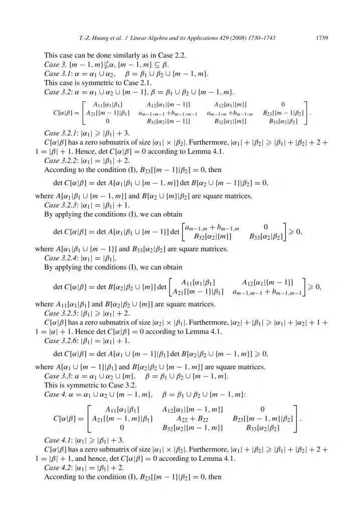
T.-Z. Huang et al. / Linear Algebra and its Applications 429 (2008) 1730–1743 1739

This case can be done similarly as in Case 2.2.Case 3. {m − 1, m}�α, {m − 1, m} ⊆ β.Case 3.1: α = α1 ∪ α2, β = β1 ∪ β2 ∪ {m − 1, m}.This case is symmetric to Case 2.1.Case 3.2: α = α1 ∪ α2 ∪ {m − 1}, β = β1 ∪ β2 ∪ {m − 1, m}.

C[α|β] =⎡⎣ A11[α1|β1] A12[α1|{m − 1}] A12[α1|{m}] 0

A21[{m − 1}|β1] am−1,m−1 +bm−1,m−1 am−1,m +bm−1,m B23[{m − 1|β2]0 B32[α2|{m − 1}] B32[α2|{m}] B33[α2|β2]

⎤⎦ .

Case 3.2.1: |α1| � |β1| + 3.C[α|β] has a zero submatrix of size |α1| × |β2|. Furthermore, |α1| + |β2| � |β1| + |β2| + 2 +

1 = |β| + 1. Hence, det C[α|β] = 0 according to Lemma 4.1.Case 3.2.2: |α1| = |β1| + 2.According to the condition (I), B23[{m − 1}|β2] = 0, then

det C[α|β] = det A[α1|β1 ∪ {m − 1, m}] det B[α2 ∪ {m − 1}|β2] = 0,

where A[α1|β1 ∪ {m − 1, m}] and B[α2 ∪ {m}|β2] are square matrices.Case 3.2.3: |α1| = |β1| + 1.By applying the conditions (I), we can obtain

det C[α|β] = det A[α1|β1 ∪ {m − 1}] det

[am−1,m + bm−1,m 0

B32[α2|{m}] B33[α2|β2]]

� 0,

where A[α1|β1 ∪ {m − 1}] and B33[α2|β2] are square matrices.Case 3.2.4: |α1| = |β1|.By applying the conditions (I), we can obtain

det C[α|β] = det B[α2|β2 ∪ {m}] det

[A11[α1|β1] A12[α1|{m − 1}]

A21[{m − 1}|β1] am−1,m−1 + bm−1,m−1

]� 0,

where A11[α1|β1] and B[α2|β2 ∪ {m}] are square matrices.Case 3.2.5: |β1| � |α1| + 2.C[α|β] has a zero submatrix of size |α2| × |β1|. Furthermore, |α2| + |β1| � |α1| + |α2| + 1 +

1 = |α| + 1. Hence det C[α|β] = 0 according to Lemma 4.1.Case 3.2.6: |β1| = |α1| + 1.

det C[α|β] = det A[α1 ∪ {m − 1}|β1] det B[α2|β2 ∪ {m − 1, m}] � 0,

where A[α1 ∪ {m − 1}|β1] and B[α2|β2 ∪ {m − 1, m}] are square matrices.Case 3.3: α = α1 ∪ α2 ∪ {m}, β = β1 ∪ β2 ∪ {m − 1, m}.This is symmetric to Case 3.2.Case 4. α = α1 ∪ α2 ∪ {m − 1, m}, β = β1 ∪ β2 ∪ {m − 1, m}:

C[α|β] =⎡⎣ A11[α1|β1] A12[α1|{m − 1, m}] 0

A21[{m − 1, m}|β1] A22 + B22 B23[{m − 1, m}|β2]0 B32[α2|{m − 1, m}] B33[α2|β2]

⎤⎦ .

Case 4.1: |α1| � |β1| + 3.C[α|β] has a zero submatrix of size |α1| × |β2|. Furthermore, |α1| + |β2| � |β1| + |β2| + 2 +

1 = |β| + 1, and hence, det C[α|β] = 0 according to Lemma 4.1.Case 4.2: |α1| = |β1| + 2.According to the condition (I), B23[{m − 1}|β2] = 0, then

1740 T.-Z. Huang et al. / Linear Algebra and its Applications 429 (2008) 1730–1743

det C[α|β] = det A[α1|β1 ∪ {m − 1, m}] det B[α2 ∪ {m − 1, m}|β2] = 0,

where A[α1|β1 ∪ {m − 1, m}] and B[α2 ∪ {m − 1, m}|β2] are square matrices.Case 4.3: |α1| = |β1| + 1.By applying the condition (I), we can obtain

det C[α|β] = det A[α1|β1 ∪ {m − 1}] det

[am−1,m + bm−1,m 0B[α2 ∪ {m}|{m}] B[α2 ∪ {m}|β2]

]� 0,

where A[α1|β1 ∪ {m − 1}] and B[α2 ∪ {m}|β2] are square matrices.Case 4.4: |α1| = |β1|.According to the condition (I), we can get

det C[α|β] = det

[A11[α1|β1] A12[α1|{m − 1}]

A21[{m − 1}|β1] am−1,m−1 + bm−1,m−1

]

× det

[am−1,m + bm−1,m 0B[α2 ∪ {m}|{m}] B[α2 ∪ {m}|β2]

]� 0.

In analogous way to Cases 4.1–4.3, respectively, we obtain the result analyzing the subcasesCase 4.5: |β1| � |α1| + 3.Case 4.6: |β1| = |α1| + 2.Case 4.7: |β1| = |α1| + 1.For the above Cases 1, 2, 3 and 4, if any of α1, α2, β1 and β2 is empty, it is easy to verify

det C[α|β] � 0 by applying the conditions (I) and (II).By the above discussion, we have obtained det C[α|β] � 0. �

In [12], the monotonically labeled k-chordal graphs were introduced, and the totally positive(TP) completion problem was solved for monotonically labeled 1-chordal graph. According toTheorem 4.2, we may obtain the TN completion for monotonically labeled 2-chordal graph.

Corollary 4.3. Let

A =⎡⎣A11 A12 X13

A21 A22 A23X31 A32 A33

⎤⎦ .

be an (m + n − 2) × (m + n − 2) partial TN matrix whose specified entries is a monotonicallylabeled 2-chordal graph with two cliques, where A11, A12, A21, A22, A23, A32, A33 denote the

totally specified blocks such that[

A11 A12A21 1/2A22

],[

1/2A22 A23A32 A33

], A22 have sizes m × m, n × n,

and 2 × 2, respectively, and X13, X31 denote the totally unspecified blocks. We assume that[A11 A12A21 1/2A22

]and

[1/2A22 A23

A32 A33

]are TN matrices where the entries of A12, A32, A21 and A23

satisfy the condition (I) of Theorem 4.2, and the entries of A22 satisfy the condition (II) of Theorem4.2. Then the completion of A

Ac =⎡⎣A11 A12 0

A21 A22 A230 A32 A33

⎤⎦

is a totally nonnegative matrix.

T.-Z. Huang et al. / Linear Algebra and its Applications 429 (2008) 1730–1743 1741

5. A remark on subdirect sums of P0-matrices

For P0-matrices, Fallat and Johnson [3] proposed the following question:If

C =⎡⎣C11 C12 0

C21 C22 C230 C32 C33

⎤⎦

is a P0-matrix, may C be written as C = A ⊕k B, such that A and B are both P0-matriceswhen C22 is k-by-k? (see the discussion preceding Section 5 in Ref. [3]). In this section, we givea positive answer to this question.

Lemma 5.1. Let A be a P0-matrix. Then B = A + diag(0, . . . , 0, ti , 0, . . . , 0) is also a P0-matrix, for ti � 0, i ∈ {1, 2, . . . , n}.

Proof. Since A is a P0-matrix and B({i}) = A({i}), then the principal minors of B({i}) arenonnegative. To show that B is a P0-matrix it is enough to show det B[α ∪ {i}] � 0, for eachα ⊆ {1, 2, . . . , n}. By calculation,

det B[α ∪ {i}] = det A[α] + ti det A[α − {i}] � 0.

This completes the proof. �

Lemma 5.1′. Let A be a P0-matrix. Then B = A + diag(t1, t2, . . . , tn) is also a P0-matrix, forti � 0, i ∈ {1, 2, . . . , n}.

Proof. Repeated applications of Lemma 5.1 yield the desired result. �

Note that the following Lemma 5.2 establishes a relationship between P -matrices and P0-matrices.

Lemma 5.2. Let A ∈ Mn(R).A is a P0-matrix if and only if B = A + diag(t1, t2, . . . , tn) is aP -matrix for all sufficiently small ti > 0, i ∈ {1, 2, . . . , n}.

Proof. Suppose A is P0-matrix, to show that B is a P -matrix, it is enough to show det B[α] > 0for all α ⊆ {1, 2, . . . , n}, where α = {j1, j2, . . . , jm}, m � n.

The proof will use induction on |α|. This result holds when α = {j1}. If α = {j1, j2}, we have

det B[α] = det(A[α] + diag(tj1 , tj2))

= det

[aj1j1 aj1j2

aj2j1 aj2j2 + tj2

]+ det

[tj1 aj1j2

0 aj2j2 + tj2

]> 0.

Now assume the result is true for all α = {j1, j2, . . . , jk}, k ∈ {1, 2, . . . , m − 1}. In the following,consider α = {j1, j2, . . . , jm−1, jm}, then

det B[α] = det

[B[α − {jm}] A[α − {jm}|{jm}]

A[{jm}|α − {jm}] ajmjm + tjm

]

= det

[B[α − {jm}] A[α − {jm}|{jm}]

A[{jm}|α − {jm}] ajmjm

]+ tjm det B[α − {jm}] > 0,

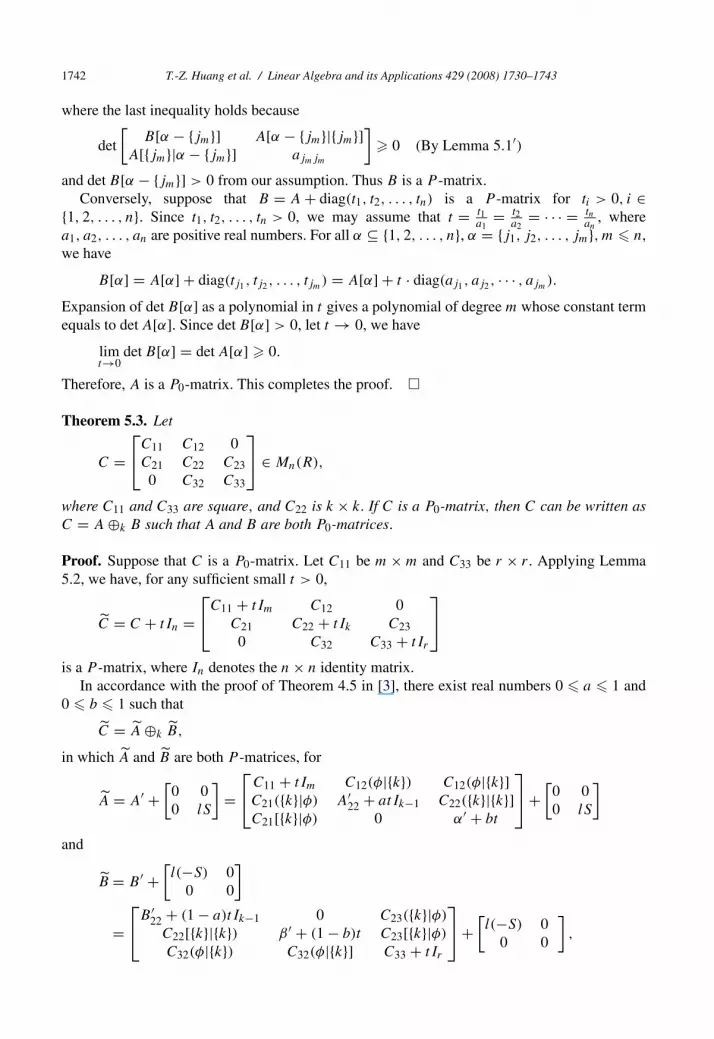
1742 T.-Z. Huang et al. / Linear Algebra and its Applications 429 (2008) 1730–1743

where the last inequality holds because

det

[B[α − {jm}] A[α − {jm}|{jm}]

A[{jm}|α − {jm}] ajmjm

]� 0 (By Lemma 5.1′)

and det B[α − {jm}] > 0 from our assumption. Thus B is a P -matrix.Conversely, suppose that B = A + diag(t1, t2, . . . , tn) is a P -matrix for ti > 0, i ∈

{1, 2, . . . , n}. Since t1, t2, . . . , tn > 0, we may assume that t = t1a1

= t2a2

= · · · = tnan

, wherea1, a2, . . . , an are positive real numbers. For all α ⊆ {1, 2, . . . , n}, α = {j1, j2, . . . , jm}, m � n,we have

B[α] = A[α] + diag(tj1 , tj2 , . . . , tjm) = A[α] + t · diag(aj1 , aj2 , · · · , ajm).

Expansion of det B[α] as a polynomial in t gives a polynomial of degree m whose constant termequals to det A[α]. Since det B[α] > 0, let t → 0, we have

limt→0

det B[α] = det A[α] � 0.

Therefore, A is a P0-matrix. This completes the proof. �

Theorem 5.3. Let

C =⎡⎣C11 C12 0

C21 C22 C230 C32 C33

⎤⎦ ∈ Mn(R),

where C11 and C33 are square, and C22 is k × k. If C is a P0-matrix, then C can be written asC = A ⊕k B such that A and B are both P0-matrices.

Proof. Suppose that C is a P0-matrix. Let C11 be m × m and C33 be r × r . Applying Lemma5.2, we have, for any sufficient small t > 0,

C = C + tIn =⎡⎣C11 + tIm C12 0

C21 C22 + tIk C230 C32 C33 + tIr

⎤⎦

is a P -matrix, where In denotes the n × n identity matrix.In accordance with the proof of Theorem 4.5 in [3], there exist real numbers 0 � a � 1 and

0 � b � 1 such that

C = A ⊕k B,

in which A and B are both P -matrices, for

A = A′ +[

0 00 lS

]=

⎡⎣C11 + tIm C12(φ|{k}) C12(φ|{k}]

C21({k}|φ) A′22 + atIk−1 C22({k}|{k}]

C21[{k}|φ) 0 α′ + bt

⎤⎦ +

[0 00 lS

]

and

B = B ′ +[l(−S) 0

0 0

]

=⎡⎣B ′

22 + (1 − a)tIk−1 0 C23({k}|φ)

C22[{k}|{k}) β ′ + (1 − b)t C23[{k}|φ)

C32(φ|{k}) C32(φ|{k}] C33 + tIr

⎤⎦ +

[l(−S) 0

0 0

],

T.-Z. Huang et al. / Linear Algebra and its Applications 429 (2008) 1730–1743 1743

where S is a fixed nonzero k × k skew-symmetric matrix with all off-diagonal entries nonzero inthe last row and column and all other off-diagonal entries zero, l is a sufficiently large positivereal number, and

C22({k}) = A′22 + B ′

22, C22[{k}] = α′ + β ′.

Also by Lemma 5.2, we have

A ={A′ +

[0 00 lS

]}t=0

and B ={B ′ +

[l(−S) 0

0 0

]}t=0

are both P0-matrices. Furthermore, C = A ⊕k B. This completes the proof. �

Acknowledgements

The authors would like to express their great gratitude to the referees and editor Dr. ShaunFallat for their constructive comments and suggestions that lead to enhancement of this paper.

References

[1] Shaun M. Fallat, C.R. Johnson, J.R. Torregrosa, A.M. Urbano, P-matrix completions under weak symmetry assump-tions, Linear Algebra Appl., 312 (2000) 73–91.

[2] C.R. Johnson, Matrix completion problems: a survey, Proc. Symp. Appl. Math. 40 (1990) 171–198.[3] S.M. Fallat, C.R. Johnson, Sub-direct sums and positivity classes of matrices, Linear Algebra Appl. 288 (1999)

149–173.[4] R.A. Horn, C.R. Johnson, Topics in Matrix Analysis, Cambridge University Press, New York, 1991.[5] R. Bru, F. Pedroche, D.B. Szyld, Sub-direct sums of nonsingular M-matrices and of their inverses, Electron. J. Linear

Algebra 13 (2005) 162–174.[6] R. Bru, F. Pedroche, D.B. Szyld, Sub-direct sums of S-strictly diagonal dominant matrices, Electron. J. Linear

Algebra 15 (2006) 201–209.[7] B.F. Smith, P.E. Bjorstad, W.D. Groop, Domain Decomposition: Parallel Multilevel Methods for Elliptic Partial

Equations, Cambridge University Press, Cambridge, 1996.[8] A. Toselli, O.B. Widlund, Domain decomposition: Algorithms and theory, Spring Series in Computational Mathe-

matics, Springer, Berlin, Heidelberg, 2005.[9] R.A. Horn, C.R. Johnson, Matrix Analysis, Cambridge University Press, New York, 1985.

[10] R. Bru, F. Pedroche, D.B. Szyld, Additive Schwarz iterations for Markov Chains, SIAM J. Matrix Anal. Appl. 27(2005) 445–458.

[11] H.J. Ryser, Combinatorial Mathematics, The Mathematical Association of America, Rahway, 1963.[12] Cristina Jordan, Juan R. Torregrosa, The totally positive completion problem, Linear Algebra Appl. 393 (2004)

259–274.