Embed Size (px)
Citation preview

Student’s Manual to Accompany
Introduction toProbability Models
Tenth Edition
Sheldon M. RossUniversity of Southern California
Los Angeles, CA
AMSTERDAM • BOSTON • HEIDELBERG • LONDONNEW YORK • OXFORD • PARIS • SAN DIEGO
SAN FRANCISCO • SINGAPORE • SYDNEY • TOKYOAcademic Press is an imprint of Elsevier

Academic Press is an imprint of Elsevier30 Corporate Drive, Suite 400, Burlington, MA 01803, USA525 B Street, Suite 1900, San Diego, California 92101-4495, USAElsevier, The Boulevard, Langford Lane, Kidlington, Oxford, OX5 1GB, UK
Copyright c© 2010 Elsevier Inc. All rights reserved.
No part of this publication may be reproduced or transmitted in any form or by any means, electronic ormechanical, including photocopying, recording, or any information storage and retrieval system, withoutpermission in writing from the publisher. Details on how to seek permission, further information about thePublisher’s permissions policies and our arrangements with organizations such as the Copyright ClearanceCenter and the Copyright Licensing Agency, can be found at our website: www.elsevier.com/permissions.
This book and the individual contributions contained in it are protected under copyright by the Publisher(other than as may be noted herein).
NoticesKnowledge and best practice in this field are constantly changing. As new research and experience broaden ourunderstanding, changes in research methods, professional practices, or medical treatment may become necessary.
Practitioners and researchers must always rely on their own experience and knowledge in evaluating andusing any information, methods, compounds, or experiments described herein. In using such information ormethods they should be mindful of their own safety and the safety of others, including parties for whom theyhave a professional responsibility.
To the fullest extent of the law, neither the Publisher nor the authors, contributors, or editors, assume any liabilityfor any injury and/or damage to persons or property as a matter of products liability, negligence or otherwise, orfrom any use or operation of any methods, products, instructions, or ideas contained in the material herein.
ISBN: 978-0-12-381446-3
For information on all Academic Press publicationsvisit our Web site at www.elsevierdirect.com
Typeset by: diacriTech, India
09 10 9 8 7 6 5 4 3 2 1

Contents
Chapter 1 . . . . . . . . . . . . . . . . . . . . . . . . . . . . . . . . . . . . . . . . . . . . . . . . . . . . . . . . . . . . . . . . . . . . 4
Chapter 2 . . . . . . . . . . . . . . . . . . . . . . . . . . . . . . . . . . . . . . . . . . . . . . . . . . . . . . . . . . . . . . . . . . . . 7
Chapter 3 . . . . . . . . . . . . . . . . . . . . . . . . . . . . . . . . . . . . . . . . . . . . . . . . . . . . . . . . . . . . . . . . . . . 12
Chapter 4 . . . . . . . . . . . . . . . . . . . . . . . . . . . . . . . . . . . . . . . . . . . . . . . . . . . . . . . . . . . . . . . . . . . 20
Chapter 5 . . . . . . . . . . . . . . . . . . . . . . . . . . . . . . . . . . . . . . . . . . . . . . . . . . . . . . . . . . . . . . . . . . . 26
Chapter 6 . . . . . . . . . . . . . . . . . . . . . . . . . . . . . . . . . . . . . . . . . . . . . . . . . . . . . . . . . . . . . . . . . . . 34
Chapter 7 . . . . . . . . . . . . . . . . . . . . . . . . . . . . . . . . . . . . . . . . . . . . . . . . . . . . . . . . . . . . . . . . . . . 39
Chapter 8 . . . . . . . . . . . . . . . . . . . . . . . . . . . . . . . . . . . . . . . . . . . . . . . . . . . . . . . . . . . . . . . . . . . 44
Chapter 9 . . . . . . . . . . . . . . . . . . . . . . . . . . . . . . . . . . . . . . . . . . . . . . . . . . . . . . . . . . . . . . . . . . . 51
Chapter 10 . . . . . . . . . . . . . . . . . . . . . . . . . . . . . . . . . . . . . . . . . . . . . . . . . . . . . . . . . . . . . . . . . . 54
Chapter 11 . . . . . . . . . . . . . . . . . . . . . . . . . . . . . . . . . . . . . . . . . . . . . . . . . . . . . . . . . . . . . . . . . . 57
Chapter 1
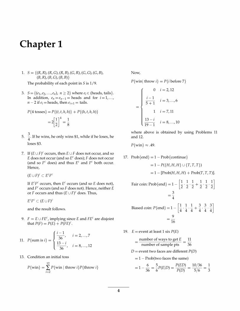
1. S = {(R, R), (R, G), (R, B), (G, R), (G, G), (G, B),(B, R), (B, G), (B, B)}
The probability of each point in S is 1/9.
3. S = {(e1, e2, …, en), n ≥ 2} where ei ∈ (heads, tails}.In addition, en = en−1 = heads and for i = 1, …,n − 2 if ei = heads, then ei+1 = tails.
P{4 tosses} = P{(t, t, h, h)} + P{(h, t, h, h)}
= 2[
12
]4= 1
8
5.34
. If he wins, he only wins $1, while if he loses, he
loses $3.
7. If (E ∪ F)c occurs, then E ∪ F does not occur, and soE does not occur (and so Ec does); F does not occur(and so Fc does) and thus Ec and Fc both occur.Hence,
(E ∪ F)c ⊂ EcFc
If EcFc occurs, then Ec occurs (and so E does not),and Fc occurs (and so F does not). Hence, neither Eor F occurs and thus (E ∪ F)c does. Thus,
EcFc ⊂ (E ∪ F)c
and the result follows.
9. F = E ∪ FEc, implying since E and FEc are disjointthat P(F) = P(E) + P(FE)c.
11. P{sum is i} =
⎧⎪⎪⎨⎪⎪⎩
i − 136
, i = 2, …, 7
13 − i36
, i = 8, …, 12
13. Condition an initial toss
P{win} =12
∑i=2
P{win | throw i}P{throw i}
Now,
P{win| throw i} = P{i before 7}
=
⎧⎪⎪⎪⎪⎪⎪⎪⎪⎪⎪⎨⎪⎪⎪⎪⎪⎪⎪⎪⎪⎪⎩
0 i = 2, 12
i − 15 + 1
i = 3, …, 6
1 i = 7, 11
13 − i19 − 1
i = 8, …, 10
where above is obtained by using Problems 11and 12.
P{win} ≈ .49.
17. Prob{end} = 1 − Prob{continue}= 1 − P({H, H, H} ∪ {T, T, T})
= 1 − [Prob(H, H, H) + Prob(T, T, T)].
Fair coin: Prob{end} = 1 −[
12
· 12
· 12
+ 12
· 12
· 12
]
= 34
Biased coin: P{end} = 1 −[
14
· 14
· 14
+ 34
· 34
· 34
]
= 916
19. E = event at least 1 six P(E)
= number of ways to get Enumber of sample pts
= 1136
D = event two faces are different P(D)
= 1 − Prob(two faces the same)
= 1 − 636
= 56
P(E|D) = P(ED)P(D)
= 10/365/6
= 13
4
Answers and Solutions 5
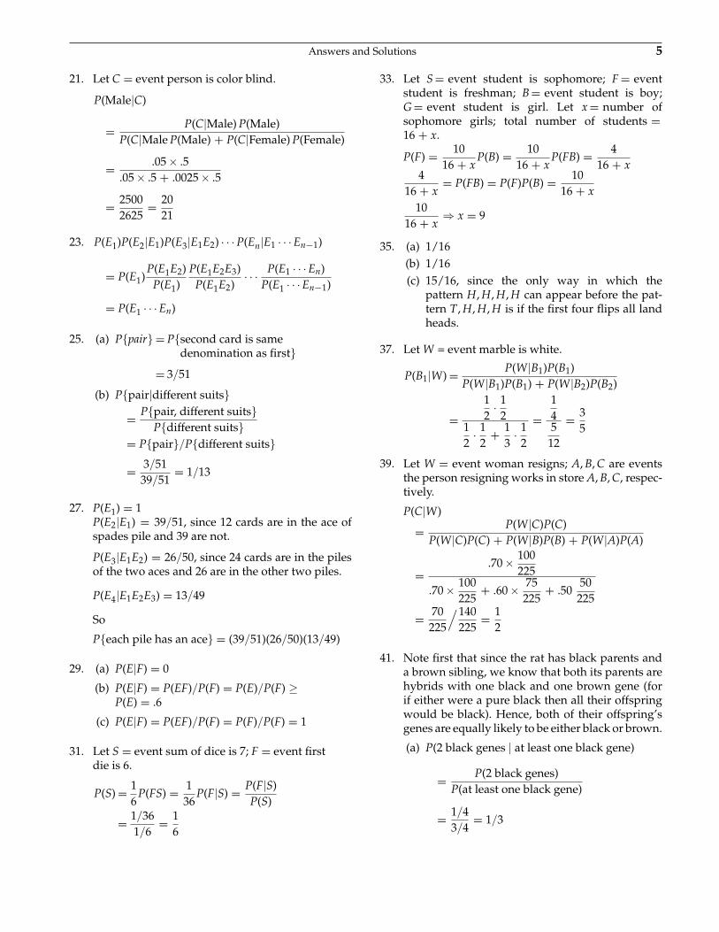
21. Let C = event person is color blind.
P(Male|C)
= P(C|Male) P(Male)P(C|Male P(Male) + P(C|Female) P(Female)
= .05 × .5.05 × .5 + .0025 × .5
= 25002625
= 2021
23. P(E1)P(E2|E1)P(E3|E1E2) · · · P(En|E1 · · · En−1)
= P(E1)P(E1E2)
P(E1)P(E1E2E3)
P(E1E2)· · · P(E1 · · · En)
P(E1 · · · En−1)
= P(E1 · · · En)
25. (a) P{pair} = P{second card is samedenomination as first}
= 3/51
(b) P{pair|different suits}= P{pair, different suits}
P{different suits}= P{pair}/P{different suits}
= 3/5139/51
= 1/13
27. P(E1) = 1P(E2|E1) = 39/51, since 12 cards are in the ace ofspades pile and 39 are not.
P(E3|E1E2) = 26/50, since 24 cards are in the pilesof the two aces and 26 are in the other two piles.
P(E4|E1E2E3) = 13/49
So
P{each pile has an ace} = (39/51)(26/50)(13/49)
29. (a) P(E|F) = 0
(b) P(E|F) = P(EF)/P(F) = P(E)/P(F) ≥P(E) = .6
(c) P(E|F) = P(EF)/P(F) = P(F)/P(F) = 1
31. Let S = event sum of dice is 7; F = event firstdie is 6.
P(S) = 16
P(FS) = 136
P(F|S) = P(F|S)P(S)
= 1/361/6
= 16
33. Let S = event student is sophomore; F = eventstudent is freshman; B = event student is boy;G = event student is girl. Let x = number ofsophomore girls; total number of students =16 + x.
P(F) = 1016 + x
P(B) = 1016 + x
P(FB) = 416 + x
416 + x
= P(FB) = P(F)P(B) = 1016 + x
1016 + x
⇒ x = 9
35. (a) 1/16(b) 1/16(c) 15/16, since the only way in which the
pattern H, H, H, H can appear before the pat-tern T, H, H, H is if the first four flips all landheads.
37. Let W = event marble is white.
P(B1|W) = P(W|B1)P(B1)P(W|B1)P(B1) + P(W|B2)P(B2)
=12
· 12
12
· 12
+ 13
· 12
=145
12
= 35
39. Let W = event woman resigns; A, B, C are eventsthe person resigning works in store A, B, C, respec-tively.
P(C|W)
= P(W|C)P(C)P(W|C)P(C) + P(W|B)P(B) + P(W|A)P(A)
=.70 × 100
225
.70 × 100225
+ .60 × 75225
+ .5050
225
= 70225
/140225
= 12
41. Note first that since the rat has black parents anda brown sibling, we know that both its parents arehybrids with one black and one brown gene (forif either were a pure black then all their offspringwould be black). Hence, both of their offspring’sgenes are equally likely to be either black or brown.
(a) P(2 black genes | at least one black gene)
= P(2 black genes)P(at least one black gene)
= 1/43/4
= 1/3
6 Answers and Solutions
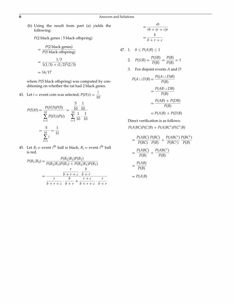
(b) Using the result from part (a) yields thefollowing:
P(2 black genes | 5 black offspring)
= P(2 black genes)P(5 black offspring)
= 1/31(1/3) + (1/2)5(2/3)
= 16/17
where P(5 black offspring) was computed by con-ditioning on whether the rat had 2 black genes.
43. Let i = event coin was selected; P(H|i) = i10
.
P(5|H) = P(H|5)P(5)10
∑i=1
P(H|i)P(i)
=5
10· 1
1010
∑i=1
110
· 110
= 510
∑i=1
i
= 111
45. Let Bi = event ith ball is black; Ri = event ith ballis red.
P(B1|R2) = P(R2|B1)P(B1)P(R2|B1)P(B1) + P(R2|R1)P(R1)
=r
b + r + c· b
b + rr
b + r + c· b
b + r+ r + c
b + r + c· r
b + r
= rbrb + (r + c)r
= bb + r + c
47. 1. 0 ≤ P(A|B) ≤ 1
2. P(S|B) = P(SB)P(B)
= P(B)P(B)
= 1
3. For disjoint events A and D
P(A ∪ D|B) = P((A ∪ D)B)P(B)
= P(AB ∪ DB)P(B)
= P(AB) + P(DB)P(B)
= P(A|B) + P(D|B)
Direct verification is as follows:
P(A|BC)P(C|B) + P(A|BCc)P(Cc|B)
= P(ABC)P(BC)
P(BC)P(B)
+ P(ABCc)P(BCc)
P(BCc)P(B)
= P(ABC)P(B)
+ P(ABCc)P(B)
= P(AB)P(B)
= P(A|B)
Chapter 2
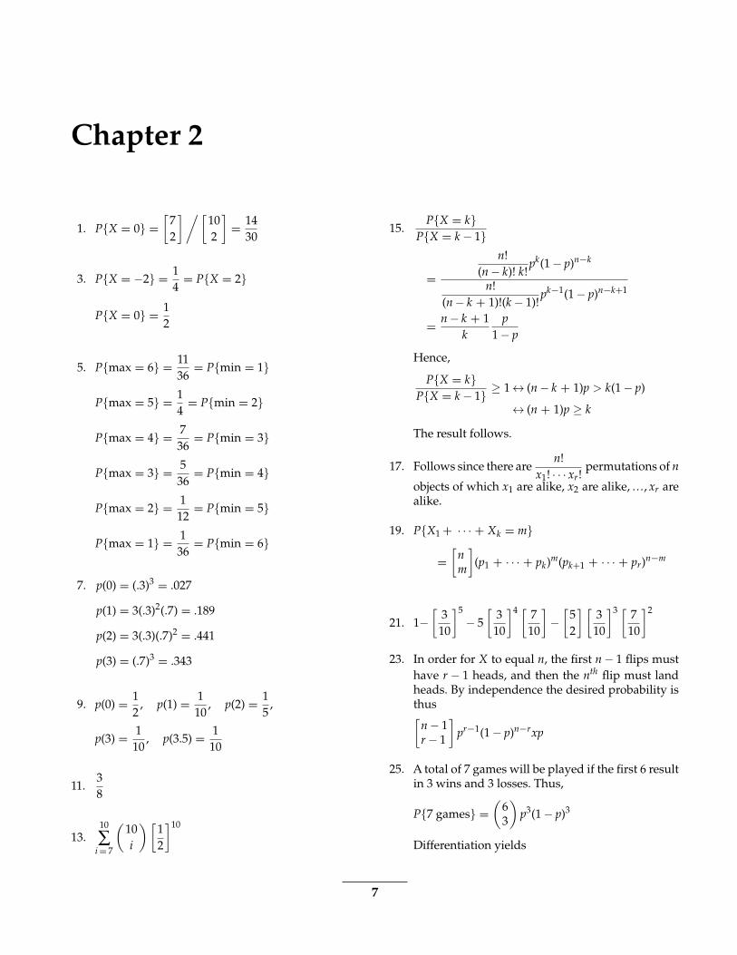
1. P{X = 0} =[
72
]/[102
]= 14
30
3. P{X = −2} = 14
= P{X = 2}
P{X = 0} = 12
5. P{max = 6} = 1136
= P{min = 1}
P{max = 5} = 14
= P{min = 2}
P{max = 4} = 736
= P{min = 3}
P{max = 3} = 536
= P{min = 4}
P{max = 2} = 112
= P{min = 5}
P{max = 1} = 136
= P{min = 6}
7. p(0) = (.3)3 = .027
p(1) = 3(.3)2(.7) = .189
p(2) = 3(.3)(.7)2 = .441
p(3) = (.7)3 = .343
9. p(0) = 12
, p(1) = 110
, p(2) = 15
,
p(3) = 110
, p(3.5) = 110
11.38
13.10
∑i = 7
(10i
)[12
]10
15.P{X = k}
P{X = k − 1}
=n!
(n − k)! k!pk(1 − p)n−k
n!(n − k + 1)!(k − 1)!
pk−1(1 − p)n−k+1
= n − k + 1k
p1 − p
Hence,
P{X = k}P{X = k − 1} ≥ 1 ↔ (n − k + 1)p > k(1 − p)
↔ (n + 1)p ≥ k
The result follows.
17. Follows since there aren!
x1! · · · xr!permutations of n
objects of which x1 are alike, x2 are alike, …, xr arealike.
19. P{X1 + · · · + Xk = m}
=[
nm
](p1 + · · · + pk)m(pk+1 + · · · + pr)n−m
21. 1−[
310
]5− 5
[3
10
]4 [ 710
]−[
52
] [310
]3 [ 710
]2
23. In order for X to equal n, the first n − 1 flips musthave r − 1 heads, and then the nth flip must landheads. By independence the desired probability isthus[
n − 1r − 1
]pr−1(1 − p)n−rxp
25. A total of 7 games will be played if the first 6 resultin 3 wins and 3 losses. Thus,
P{7 games} =(
63
)p3(1 − p)3
Differentiation yields
7
8 Answers and Solutions
ddp
P{7} = 20[3p2(1 − p)3 − p33(1 − p)2
]= 60p2(1 − p)2 [1 − 2p
]Thus, the derivative is zero when p = 1/2. Takingthe second derivative shows that the maximum isattained at this value.
27. P{same number of heads} = ∑i
P{A = i, B = i}
= ∑i
(ki
)(1/2)k
(n − k
i
)(1/2)n−k
= ∑i
(ki
)(n − k
i
)(1/2)n
= ∑i
(k
k − i
)(n − k
i
)(1/2)n
=(
nk
)(1/2)n
Another argument is as follows:
P{# heads of A = # heads of B}= P{# tails of A = # heads of B}
since coin is fair
= P{k − # heads of A = # heads of B}= P{k = total # heads}
29. Each flip after the first will, independently, resultin a changeover with probability 1/2. Therefore,
P{k changeovers}=(
n − 1k
)(1/2)n−1
33. c∫ 1
−1
(1 − x2
)dx = 1
c
[x − x3
3
]∣∣∣∣∣1
−1
= 1
c = 34
F(y) = 34
∫ 1
−1(1 − x2)dx
= 34
[y − y3
3+ 2
3
], −1 < y < 1
35. P{X > 20}=∫ ∞
20
10x2 dx = 1
2
37. P{M ≤ x} = P{max(X1, …, Xn) ≤ x}= P{X1 ≤ x, …, Xn ≤ x}
=n∏
i=1
P{Xi ≤ x}
= xn
fM(x) = ddx
P{M ≤ x} = nxn−1
39. E [X] = 316
41. Let Xi equal 1 if a changeover results from the ith
flip and let it be 0 otherwise. Then
number of changeovers =n
∑i=2
Xi
As,
E [Xi] = P{Xi = 1} = P{flip i − 1 = flip i}= 2p(1 − p)
we see that
E[number of changeovers] =n
∑i=2
E [Xi]
= 2(n − 1)p(1 − p)
43. (a) X =n
∑i=1
Xi
(b) E [Xi] = P{Xi = 1}= P{red ball i is chosen before all n
black balls}= 1/(n + 1) since each of these n + 1
balls is equally likely to be theone chosen earliest
Therefore,
E [X] =n
∑i=1
E [Xi] = n/(n + 1)
45. Let Ni denote the number of keys in box i,i = 1, …, k. Then, with X equal to the number
of collisions we have that X =k
∑i=1
(Ni − 1)+ =k
∑i=1
(Ni − 1 + I{Ni = 0}) where I{Ni = 0} is equal
to 1 if Ni = 0 and is equal to 0 otherwise. Hence,
Answers and Solutions 9
E[X] =k
∑i=1
(rpi − 1 + (1 − pi)r) = r − k
+k
∑i=1
(1 − pi)r
Another way to solve this problem is to let Y denotethe number of boxes having at least one key, andthen use the identity X = r − Y, which is true sinceonly the first key put in each box does not result in
a collision. Writing Y =k
∑i=1
I{Ni > 0} and taking
expectations yields
E[X] = r − E[Y] = r −k
∑i=1
[1 − (1 − pi)r]
= r − k +k
∑i=1
(1 − pi)r
47. Let Xi be 1 if trial i is a success and 0 otherwise.
(a) The largest value is .6. If X1 = X2 = X3, then
1.8 = E[X] = 3E[X1] = 3P{X1 = 1}
and so
P{X = 3} = P{X1 = 1} = .6
That this is the largest value is seen by Markov’sinequality, which yields
P{X ≥ 3} ≤ E[X]/3 = .6
(b) The smallest value is 0. To construct a probabil-ity scenario for which P{X = 3} = 0 let U be auniform random variable on (0, 1), and define
X1 = 1 if U ≤ .60 otherwise
X2 = 1 if U ≥ .40 otherwise
X3 = 1 if either U ≤ .3 or U ≥ .70 otherwise
It is easy to see that
P{X1 = X2 = X3 = 1} = 0
49. E[X2] − (E[X])2 = Var(X) = E(X − E[X])2 ≥ 0.Equality when Var(X) = 0, that is, when X isconstant.
51. N =r
∑i=1
Xj where Xi is the number of flips between
the (i − 1)st and ith head. Hence, Xi is geometricwith mean 1/p. Thus,
E[N] =r
∑i=1
E[Xi] = rp
53.1
n + 1,
12n + 1
−[
1n + 1
]2.
55. (a) P(Y = j) =j
∑i=0
(ji
)e−2λλj/j!
= e−2λ λj
j!
j
∑i=0
(ji
)1i1j−i
= e−2λ (2λ) j
j!
(b) P(X = i) =∞∑j=i
(ji
)e−2λλj/j!
= 1i!
e−2λ∞∑j=i
1( j − i)!
λj
= λi
i!e−2λ
∞∑k=0
λk/k!
= e−λ λi
i!
(c) P(X = i, Y − X = k) = P(X = i, Y = k + i)
=(
k + ii
)e−2λ λk+i
(k + i)!
= e−λ λi
i!e−λ λk
k!
showing that X and Y − X are independentPoisson random variables with mean λ. Hence,
P(Y − X = k) = e−λ λk
k!
57. It is the number of successes in n + m independentp-trials.
59. (a) Use the fact that F(Xi) is a uniform (0, 1) ran-dom variable to obtain
p = P{F(X1) < F(X2) > F(X3) < F(X4)}= P{U1 < U2 > U3 < U4}
where the Ui, i = 1, 2, 3, 4, are independentuniform (0, 1) random variables.
10 Answers and Solutions
(b) p =∫ 1
0
∫ 1
x1
∫ x2
0
∫ 1
x3
dx4dx3dx2dx1
=∫ 1
0
∫ 1
x1
∫ x2
0(1 − x3)dx3dx2dx1
=∫ 1
0
∫ 1
x1
(x2 − x22/2)dx2dx1
=∫ 1
0(1/3 − x2
1/2 + x31/6)dx1
= 1/3 − 1/6 + 1/24 = 5/24
(c) There are 5 (of the 24 possible) orderings suchthat X1 < X2 > X3 < X4. They are as follows:
X2 > X4 > X3 > X1
X2 > X4 > X1 > X3
X2 > X1 > X4 > X3
X4 > X2 > X3 > X1
X4 > X2 > X1 > X3
61. (a) fX(x) =∫ ∞
xλ2e−λydy
= λe−λx
(b) fY(y) =∫ y
0λ2e−λydx
= λ2ye−λy
(c) Because the Jacobian of the transformationx = x, w = y − x is 1, we have
fX,W (x, w) = fX,Y(x, x + w) = λ2e−λ(x+w)
= λe−λx λe−λw
(d) It follows from the preceding that X andW are independent exponential random vari-ables with rate λ.
63. φ(t) =∞∑n=1
etn(1 − p)n−1p
= pet∞∑n=1
((1 − p)et)n−1
= pet
1 − (1 − p)et
65. Cov(Xi, Xj) = Cov(μi +n
∑k=1
aikZk , μj +n
∑t=1
ajtZt)
=n
∑t=1
n
∑k=1
Cov(ajkZk , ajtZt)
=n
∑t=1
n
∑k=1
aikajtCov(Zk , Zt)
=n
∑k=1
aikajk
where the last equality follows since
Cov(Zk , Zt) = 1 if k = t0 if k = t
67. P{5 < X < 15} ≥ 25
69. Φ(1) − Φ
[12
]= .1498
71. (a) P {X = i} =[
ni
] [m
k − i
]/[n + m
k
]
i = 0, 1,…, min(k, n)
(b) X =k
∑i=1
Xi
E[X] =K
∑i=1
E[Xi] = knn + m
since the ith ball is equally likely to beeither of the n + m balls, and soE[Xi] = P{Xi = 1} = n
n + m
X =n
∑i=1
Yi
E[X] =n
∑i=1
E[Yi]
=n
∑i=1
P{ith white ball is selected}
=n
∑i=1
kn + m
= nkn + m
73. As Ni is a binomial random variable with para-meters (n, Pi), we have (a) E[Ni] = nPji (b) Var(Xi) =nPi = (1 − Pi); (c) for i = j, the covariance of Ni andNj can be computed as
Cov (Ni, Nj) = Cov
[∑k
Xk , ∑k
Yk
]
Answers and Solutions 11
where Xk(Yk) is 1 or 0, depending upon whether ornot outcome k is type i( j). Hence,
Cov(Ni, Nj) = ∑k
∑�
Cov(Xk , Y�)
Now for k = �, Cov(Xk , Y�) = 0 by independence oftrials and so
Cov (Ni, Nj) = ∑k
Cov(Xk , Yk)
= ∑k
(E[XkYk] − E[Xk]E[Yk])
= −∑k
E[Xk]E[Yk] (since XkYk = 0)
= −∑k
PiPj
= −nPiPj
(d) Letting
Yi ={
1, if no type i’s occur0, otherwise
we have that the number of outcomes that never
occur is equal tor
∑1
Yi and thus,
E
[r
∑1
Yi
]=
r
∑1
E[Yi]
=r
∑1
P{outcomes i does not occur}
=r
∑1
(1 − Pi)n
75. (a) Knowing the values of N1, …, Nj is equivalentto knowing the relative ordering of the ele-ments a1, …, aj. For instance, if N1 = 0, N2 = 1,N3 = 1 then in the random permutation a2is before a3, which is before a1. The indepen-dence result follows for clearly the numberof a1,…, ai that follow ai+1 does not proba-bilistically depend on the relative ordering ofa1, …, ai.
(b) P{Ni = k} = 1i
, k = 0, 1,…, i − 1
which follows since of the elements a1, …, ai+1the element ai+1 is equally likely to be first orsecond or … or (i + 1)st.
(c) E[Ni] = 1i
i−1
∑k=0
k = i − 12
E[N2i ] = 1
i
i−1
∑k=0
k2 = (i − 1)(2i − 1)6
and so
Var(Ni) = (i − 1)(2i − 1)6
− (i − 1)2
4
= i2 − 112
77. If g1(x, y) = x + y, g2(x, y) = x − y, then
J =
∣∣∣∣∣∣∣∂g1∂x
∂g1∂y
∂g2∂x
∂g2∂y
∣∣∣∣∣∣∣ = 2
Hence, if U = X + Y, V = X − Y, then
fU, V(u, v) = 12
fX, Y
[u + v
2,
u − v2
]
= 24τσ2 exp
[− 1
2σ2
[[u + v
2− μ
]2
+[
u − v2
− μ
]2]]
= e−μ2/σ2
4τσ2 exp[
uμ
σ2 − u2
4σ2
]
exp{
− v2
4σ2
}
79. K′(t) = E[XetX]
E[etX]
K′′(t) = E[etX]E[X2etX]− E2[XetX]
E2[etX]
Hence,
K′(0) = E[X]
K′′(0) = E[X2] − E2[X] = Var(X)
Chapter 3
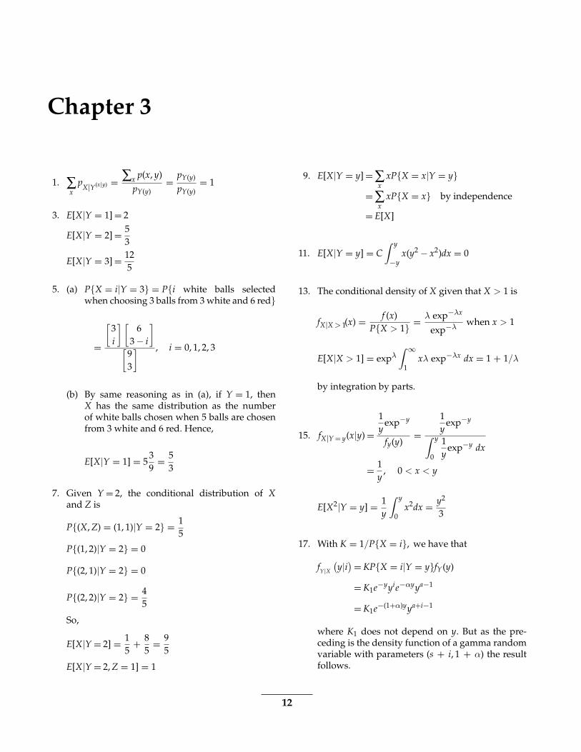
1. ∑x
pX|Y(x|y) = ∑x p(x, y)
pY(y)= pY(y)
pY(y)= 1
3. E[X|Y = 1] = 2
E[X|Y = 2] = 53
E[X|Y = 3] = 125
5. (a) P{X = i|Y = 3} = P{i white balls selectedwhen choosing 3 balls from 3 white and 6 red}
=
[3i
] [6
3 − i
][
93
] , i = 0, 1, 2, 3
(b) By same reasoning as in (a), if Y = 1, thenX has the same distribution as the numberof white balls chosen when 5 balls are chosenfrom 3 white and 6 red. Hence,
E[X|Y = 1] = 539
= 53
7. Given Y = 2, the conditional distribution of Xand Z is
P{(X, Z) = (1, 1)|Y = 2} = 15
P{(1, 2)|Y = 2} = 0
P{(2, 1)|Y = 2} = 0
P{(2, 2)|Y = 2} = 45
So,
E[X|Y = 2] = 15
+ 85
= 95
E[X|Y = 2, Z = 1] = 1
9. E[X|Y = y] = ∑x
xP{X = x|Y = y}= ∑
xxP{X = x} by independence
= E[X]
11. E[X|Y = y] = C∫ y
−yx(y2 − x2)dx = 0
13. The conditional density of X given that X > 1 is
fX|X > 1(x) = f (x)P{X > 1} = λ exp−λx
exp−λwhen x > 1
E[X|X > 1] = expλ∫ ∞
1xλ exp−λx dx = 1 + 1/λ
by integration by parts.
15. fX|Y = y(x|y) =1y
exp−y
fy(y)=
1y
exp−y
∫ y
0
1y
exp−y dx
= 1y
, 0 < x < y
E[X2|Y = y] = 1y
∫ y
0x2dx = y2
3
17. With K = 1/P{X = i}, we have that
fY|X(y|i)= KP{X = i|Y = y}fY(y)
= K1e−yyie−αyya−1
= K1e−(1+α)yya+i−1
where K1 does not depend on y. But as the pre-ceding is the density function of a gamma randomvariable with parameters (s + i, 1 + α) the resultfollows.
12
Answers and Solutions 13
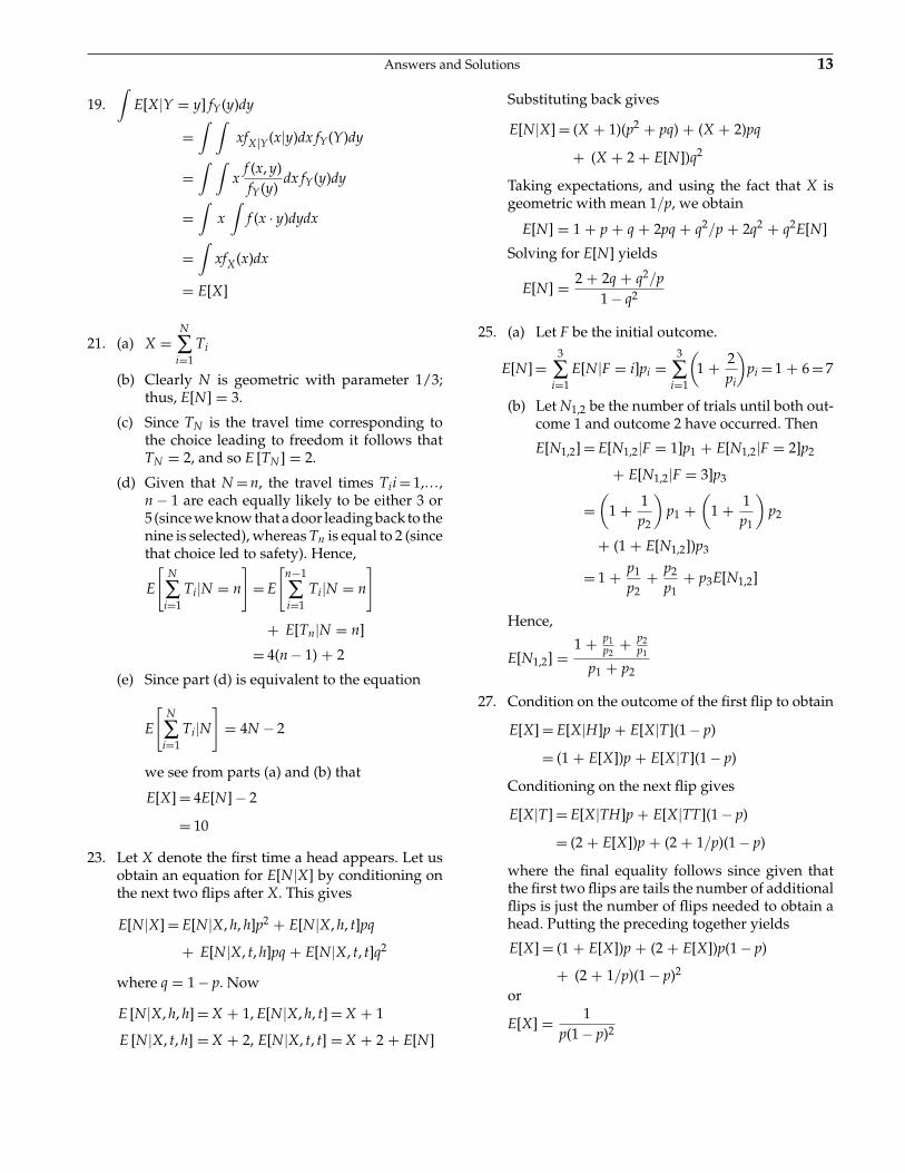
19.∫
E[X|Y = y] fY(y)dy
=∫ ∫
xfX|Y(x|y)dx fY(Y)dy
=∫ ∫
xf (x, y)fY(y)
dx fY(y)dy
=∫
x∫
f (x · y)dydx
=∫
xfX(x)dx
= E[X]
21. (a) X =N
∑i=1
Ti
(b) Clearly N is geometric with parameter 1/3;thus, E[N] = 3.
(c) Since TN is the travel time corresponding tothe choice leading to freedom it follows thatTN = 2, and so E [TN] = 2.
(d) Given that N = n, the travel times Tii = 1,…,n − 1 are each equally likely to be either 3 or5 (since we know that a door leading back to thenine is selected), whereas Tn is equal to 2 (sincethat choice led to safety). Hence,
E
[N
∑i=1
Ti|N = n
]= E
[n−1
∑i=1
Ti|N = n
]
+ E[Tn|N = n]
= 4(n − 1) + 2
(e) Since part (d) is equivalent to the equation
E
[N
∑i=1
Ti|N]
= 4N − 2
we see from parts (a) and (b) that
E[X] = 4E[N] − 2
= 10
23. Let X denote the first time a head appears. Let usobtain an equation for E[N|X] by conditioning onthe next two flips after X. This gives
E[N|X] = E[N|X, h, h]p2 + E[N|X, h, t]pq
+ E[N|X, t, h]pq + E[N|X, t, t]q2
where q = 1 − p. Now
E [N|X, h, h] = X + 1, E[N|X, h, t] = X + 1
E [N|X, t, h] = X + 2, E[N|X, t, t] = X + 2 + E[N]
Substituting back gives
E[N|X] = (X + 1)(p2 + pq) + (X + 2)pq
+ (X + 2 + E[N])q2
Taking expectations, and using the fact that X isgeometric with mean 1/p, we obtain
E[N] = 1 + p + q + 2pq + q2/p + 2q2 + q2E[N]
Solving for E[N] yields
E[N] = 2 + 2q + q2/p1 − q2
25. (a) Let F be the initial outcome.
E[N] =3
∑i=1
E[N|F = i]pi =3
∑i=1
(1 + 2
pi
)pi = 1 + 6 = 7
(b) Let N1,2 be the number of trials until both out-come 1 and outcome 2 have occurred. Then
E[N1,2] = E[N1,2|F = 1]p1 + E[N1,2|F = 2]p2
+ E[N1,2|F = 3]p3
=(
1 + 1p2
)p1 +
(1 + 1
p1
)p2
+ (1 + E[N1,2])p3
= 1 + p1
p2+ p2
p1+ p3E[N1,2]
Hence,
E[N1,2] =1 + p1
p2+ p2
p1
p1 + p2
27. Condition on the outcome of the first flip to obtain
E[X] = E[X|H]p + E[X|T](1 − p)
= (1 + E[X])p + E[X|T](1 − p)
Conditioning on the next flip gives
E[X|T] = E[X|TH]p + E[X|TT](1 − p)
= (2 + E[X])p + (2 + 1/p)(1 − p)
where the final equality follows since given thatthe first two flips are tails the number of additionalflips is just the number of flips needed to obtain ahead. Putting the preceding together yields
E[X] = (1 + E[X])p + (2 + E[X])p(1 − p)
+ (2 + 1/p)(1 − p)2
or
E[X] = 1p(1 − p)2
14 Answers and Solutions
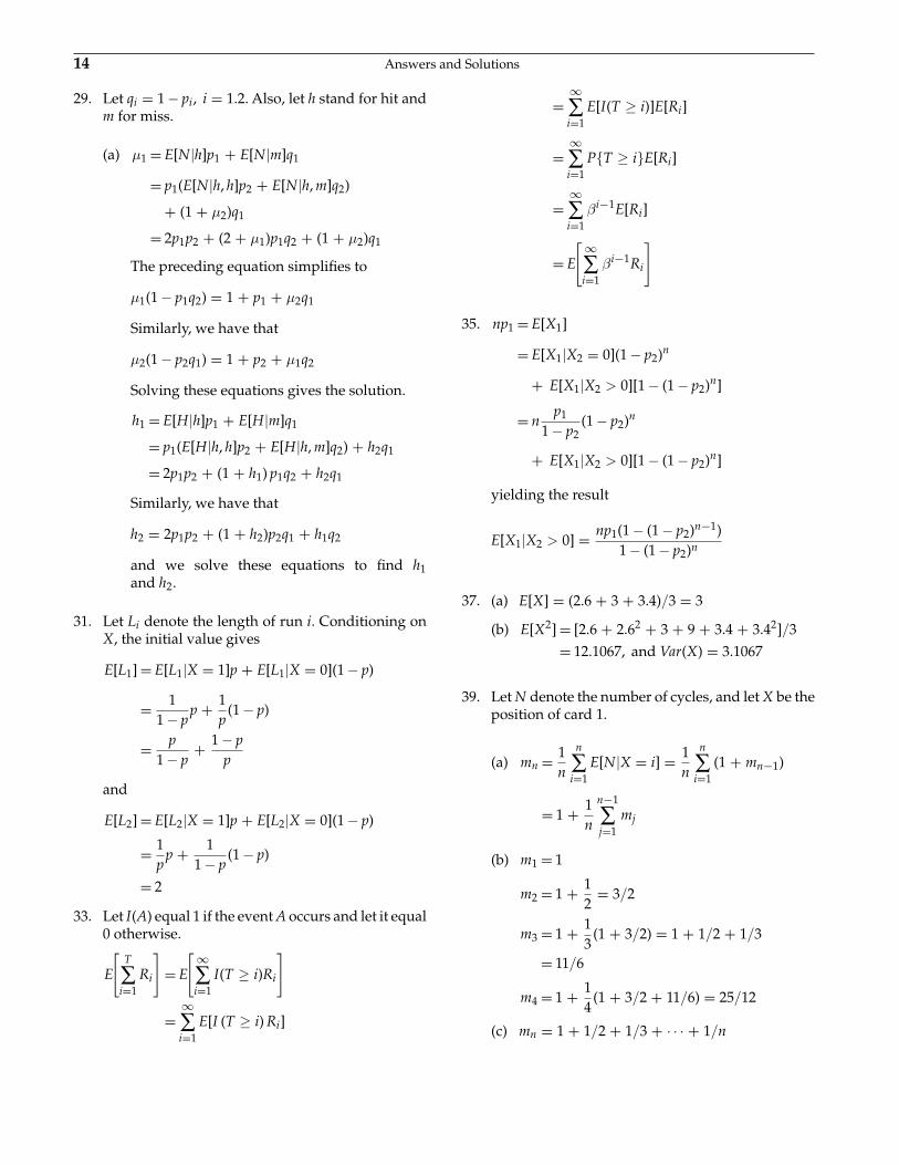
29. Let qi = 1 − pi, i = 1.2. Also, let h stand for hit andm for miss.
(a) μ1 = E[N|h]p1 + E[N|m]q1
= p1(E[N|h, h]p2 + E[N|h, m]q2)
+ (1 + μ2)q1
= 2p1p2 + (2 + μ1)p1q2 + (1 + μ2)q1
The preceding equation simplifies to
μ1(1 − p1q2) = 1 + p1 + μ2q1
Similarly, we have that
μ2(1 − p2q1) = 1 + p2 + μ1q2
Solving these equations gives the solution.
h1 = E[H|h]p1 + E[H|m]q1
= p1(E[H|h, h]p2 + E[H|h, m]q2) + h2q1
= 2p1p2 + (1 + h1) p1q2 + h2q1
Similarly, we have that
h2 = 2p1p2 + (1 + h2)p2q1 + h1q2
and we solve these equations to find h1and h2.
31. Let Li denote the length of run i. Conditioning onX, the initial value gives
E[L1] = E[L1|X = 1]p + E[L1|X = 0](1 − p)
= 11 − p
p + 1p
(1 − p)
= p1 − p
+ 1 − pp
and
E[L2] = E[L2|X = 1]p + E[L2|X = 0](1 − p)
= 1p
p + 11 − p
(1 − p)
= 2
33. Let I(A) equal 1 if the event A occurs and let it equal0 otherwise.
E
[T
∑i=1
Ri
]= E
[∞∑i=1
I(T ≥ i)Ri
]
=∞∑i=1
E[I (T ≥ i) Ri]
=∞∑i=1
E[I(T ≥ i)]E[Ri]
=∞∑i=1
P{T ≥ i}E[Ri]
=∞∑i=1
βi−1E[Ri]
= E
[∞∑i=1
βi−1Ri
]
35. np1 = E[X1]
= E[X1|X2 = 0](1 − p2)n
+ E[X1|X2 > 0][1 − (1 − p2)n]
= np1
1 − p2(1 − p2)n
+ E[X1|X2 > 0][1 − (1 − p2)n]
yielding the result
E[X1|X2 > 0] = np1(1 − (1 − p2)n−1)1 − (1 − p2)n
37. (a) E[X] = (2.6 + 3 + 3.4)/3 = 3
(b) E[X2] = [2.6 + 2.62 + 3 + 9 + 3.4 + 3.42]/3= 12.1067, and Var(X) = 3.1067
39. Let N denote the number of cycles, and let X be theposition of card 1.
(a) mn = 1n
n
∑i=1
E[N|X = i] = 1n
n
∑i=1
(1 + mn−1)
= 1 + 1n
n−1
∑j=1
mj
(b) m1 = 1
m2 = 1 + 12
= 3/2
m3 = 1 + 13
(1 + 3/2) = 1 + 1/2 + 1/3
= 11/6
m4 = 1 + 14
(1 + 3/2 + 11/6) = 25/12
(c) mn = 1 + 1/2 + 1/3 + · · · + 1/n
Answers and Solutions 15
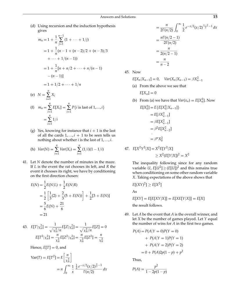
(d) Using recursion and the induction hypothesisgives
mn = 1 + 1n
n−1
∑j=1
(1 + · · · + 1/j)
= 1 + 1n
(n − 1 + (n − 2)/2 + (n − 3)/3
+ · · · + 1/(n − 1))
= 1 + 1n
[n + n/2 + · · · + n/(n − 1)
− (n − 1)]
= 1 + 1/2 + · · · + 1/n
(e) N =n
∑i=1
Xi
(f) mn =n
∑i=1
E[Xi] =n
∑i=1
P{i is last of 1,…, i}
=n
∑i=1
1/i
(g) Yes, knowing for instance that i + 1 is the lastof all the cards 1, …, i + 1 to be seen tells usnothing about whether i is the last of 1, …, i.
(h) Var(N) =n
∑i=1
Var(Xi) =n
∑i=1
(1/i)(1 − 1/i)
41. Let N denote the number of minutes in the maze.If L is the event the rat chooses its left, and R theevent it chooses its right, we have by conditioningon the first direction chosen:
E(N) = 12
E(N|L) + 12
E(N|R)
= 12
[13
(2) + 23
(5 + E(N))]
+ 12
[3 + E(N)]
= 56
E(N) + 216
= 21
43. E[T|χ2n] = 1√
χ2n/n
E[Z|χ2n] = 1√
χ2n/n
E[Z] = 0
E[T2|χ2n] = n
χ2n
E[Z2|χ2n] = n
χ2n
E[Z2] = nχ2
n
Hence, E[T] = 0, and
Var(T) = E[T2] = E[
nχ2
n
]
= n∫ ∞
0
1x
12 e−x/2(x/2)
n2 −1
Γ (n/2)dx
= n2Γ (n/2)
∫ ∞
0
12
e−x/2(x/2)n−2
2 −1 dx
= nΓ (n/2 − 1)2Γ (n/2)
= n2(n/2 − 1)
= nn − 2
45. Now
E[Xn|Xn−1] = 0, Var(Xn|Xn−1) = βX2n−1
(a) From the above we see that
E[Xn] = 0
(b) From (a) we have that Var(xn) = E[X2n]. Now
E[X2n] = E{E[X2
n|Xn−1]}= E[βX2
n−1]
= βE[X2n−1]
= β2E[X2n−2]
·= βnX2
0
47. E[X2Y2|X] = X2E[Y2|X]
≥ X2(E[Y|X])2 = X2
The inequality following since for any randomvariable U, E[U2] ≥ (E[U])2 and this remains truewhen conditioning on some other random variableX. Taking expectations of the above shows that
E[(XY)2] ≥ E[X2]
As
E[XY] = E[E[XY|X]] = E[XE[Y|X]] = E[X]
the result follows.
49. Let A be the event that A is the overall winner, andlet X be the number of games played. Let Y equalthe number of wins for A in the first two games.
P(A) = P(A|Y = 0)P(Y = 0)
+ P(A|Y = 1)P(Y = 1)
+ P(A|Y = 2)P(Y = 2)
= 0 + P(A)2p(1 − p) + p2
Thus,
P(A) = p2
1 − 2p(1 − p)
16 Answers and Solutions
E[X] = E[X|Y = 0]P(Y = 0)
+ E[X|Y = 1]P(Y = 1)
+ E[X|Y = 2]P(Y = 2)
= 2(1 − p)2 + (2 + E[X])2p(1 − p) + 2p2
= 2 + E[X]2p(1 − p)
Thus,
E[X] = 21 − 2p(1 − p)
51. Let α be the probability that X is even. Condition-ing on the first trial gives
α = P(even|X = 1)p + P(even|X > 1)(1 − p)= (1 − α)(1 − p)
Thus,
α = 1 − p2 − p
More computationally
α =∞∑n=1
P(X = 2n) = p1 − p
∞∑n=1
(1 − p)2n
= p1 − p
(1 − p)2
1 − (1 − p)2 = 1 − p2 − p
53. P{X = n} =∫ ∞
0P{X = n|λ}e−λdλ
=∫ ∞
0
e−λλn
n!e−λdλ
=∫ ∞
0e−2λλn dλ
n!
=∫ ∞
0e−ttn dt
n!
[12
]n+1
The result follows since∫ ∞
0e−ttndt = Γ (n + 1) = n!
57. Let X be the number of storms.
P{X ≥ 3} = 1 − P{X ≤ 2}
= 1 −∫ 5
0P{X ≤ 2|Λ = x}1
5dx
= 1 −∫ 5
0[e−x + xe−x + e−xx2/2]
15
dx
59. (a) P(AiAj) =n
∑k=0
P(AiAj|Ni = k)(
nk
)pk
i (1 − pi)n−k
=n
∑k=1
P(Aj|Ni = k)(
nk
)pk
i (1 − pi)n−k
=n−1
∑k=1
[1 −
(1 − pj
1 − pi
)n−k](
nk
)
× pki (1 − pi)n−k
=n−1
∑k=1
(nk
)pk
i (1 − pi)n−k −n−1
∑k=1
×(
1 − pj
1 − pi
)n−k (nk
)× pk
i (1 − pi)n−k
= 1 − (1 − pi)n − pni −
n−1
∑k=1
(nk
)× pk
i (1 − pi − pj)n−k
= 1 − (1 − pi)n − pni − [(1 − pj)n
−(1 − pi − pj)n − pni ]
= 1 + (1 − pi − pj)n − (1 − pi)n
−(1 − pj)n
where the preceding used that conditional onNi = k, each of the other n − k trials indepen-dently results in outcome j with probability
pj
1 − pi.
(b) P(AiAj) =n
∑k=1
P(AiAj|Fi = k) pi(1 − pi)k−1
+ P(AiAj|Fi > n) (1 − pi)n
=n
∑k=1
P(Aj|Fi = k) pi(1 − pi)k−1
=n
∑k=1
[1 −
(1 − pj
1 − pi
)k−1(1 − pj)n−k
]× pi(1 − pi)k−1
(c) P(AiAj) = P(Ai) + P(Aj) − P(Ai ∪ Aj)
= 1 − (1 − pi)n + 1 − (1 − pj)n
−[1 − (1 − pi − pj)n]
= 1 + (1 − pi − pj)n − (1 − pi)n
−(1 − pj)n
61. (a) m1 = E[X|h]p1 + E[H|m]q1 = p1 + (1 + m2)
q1 = 1 + m2q1.
Answers and Solutions 17
Similarly, m2 = 1 + m1q2. Solving these equa-tions gives
m1 = 1 + q1
1 − q1q2, m2 = 1 + q2
1 − q1q2
(b) P1 = p1 + q1P2
P2 = q2P1
implying that
P1 = p1
1 − q1q2, P2 = p1q2
1 − q1q2
(c) Let fi denote the probability that the final hitwas by 1 when i shoots first. Conditioning onthe outcome of the first shot gives
f1 = p1P2 + q1 f2 and f2 = p2P1 + q2 f1
Solving these equations gives
f1 = p1P2 + q1p2P1
1 − q1q2
(d) and (e) Let Bi denote the event that both hitswere by i. Condition on the outcome of the firsttwo shots to obtain
P(B1) = p1q2P1 + q1q2P(B1) → P(B1)
= p1q2P11 − q1q2
Also,
P(B2) = q1p2(1 − P1) + q1q2P(B2) → P(B2)
= q1p2(1 − P1)1 − q1q2
(f) E[N] = 2p1p2 + p1q2(2 + m1)
+ q1p2(2 + m1) + q1q2(2 + E[N])
implying that
E[N] = 2 + m1p1q2 + m1q1p2
1 − q1q2
63. Let Si be the event there is only one type i in thefinal set.
P{Si = 1} =n−1
∑j=0
P{Si = 1|T = j}P{T = j}
= 1n
n−1
∑j=0
P{Si = 1|T = j}
= 1n
n−1
∑j=0
1n − j
The final equality follows because given that thereare still n − j − 1 uncollected types when the firsttype i is obtained, the probability starting at thatpoint that it will be the last of the set of n − j typesconsisting of type i along with the n − j − 1 yetuncollected types to be obtained is, by symmetry,1/(n − j). Hence,
E
[n
∑i=1
Si
]= nE[Si] =
n
∑k=1
1k
65. (a) P{Yn = j} = 1/(n + 1), j = 0, …, n
(b) For j = 0, …, n − 1
P{Yn−1 = j} =n
∑i=0
1n + 1
P{Yn−1 = j|Yn = i}
= 1n + 1
(P{Yn−1 = j|Yn = j}
+ P{Yn−1 = j|Yn = j + 1})
= 1n + 1
(P(last is nonred| j red)
+ P(last is red| j + 1 red)
= 1n + 1
(n − j
n+ j + 1
n
)= 1/n
(c) P{Yk = j} = 1/(k + 1), j = 0, …, k
(d) For j = 0, …, k − 1
P{Yk−1 = j} =k
∑i=0
P{Yk−1 = j|Yk = i}
P{Yk = i}
= 1k + 1
(P{Yk−1 = j|Yk = j}
+ P{Yk−1 = j|Yk = j + 1})
= 1k + 1
(k − j
k+ j + 1
k
)= 1/k
where the second equality follows from theinduction hypothesis.
67. A run of j successive heads can occur in the fol-lowing mutually exclusive ways: (i) either there isa run of j in the first n − 1 flips, or (ii) there is noj-run in the first n − j − 1 flips, flip n − j is a tail,and the next j flips are all heads. Consequently, (a)follows. Condition on the time of the first tail:
Pj(n) =j
∑k=1
Pj(n − k)pk−1(.1 − p) + p j, j ≤ n
18 Answers and Solutions
69. (a) Let I(i, j) equal 1 if i and j are a pair and 0otherwise. Then
E
[∑i<j
I(i, j)
]=⎛⎝n
2
⎞⎠1
n1
n − 1= 1/2
Let X be the size of the cycle containing person1. Then
Qn =n
∑i=1
P{no pairs|X = i}1/n = 1n ∑
i �=2Qn−i
73. Condition on the value of the sum prior to goingover 100. In all cases the most likely value is 101.(For instance, if this sum is 98 then the final sumis equally likely to be either 101, 102, 103, or 104. Ifthe sum prior to going over is 95 then the final sumis 101 with certainty.)
75. (a) Since A receives more votes than B (since a > a)it follows that if A is not always leading thenthey will be tied at some point.
(b) Consider any outcome in which A receivesthe first vote and they are eventually tied,say a, a, b, a, b, a, b, b…. We can correspond thissequence to one that takes the part of thesequence until they are tied in the reverseorder. That is, we correspond the above to thesequence b, b, a, b, a, b, a, a… where the remain-der of the sequence is exactly as in the original.Note that this latter sequence is one in whichB is initially ahead and then they are tied. Asit is easy to see that this correspondence is oneto one, part (b) follows.
(c) Now,P{B receives first vote and they areeventually tied}= P{B receives first vote}= n/(n + m)Therefore, by part (b) we see thatP{eventually tied}= 2n/(n + m)and the result follows from part (a).
77. We will prove it when X and Y are discrete.
(a) This part follows from (b) by takingg(x, y) = xy.
(b) E[g(X, Y)|Y = y] = ∑y
∑x
g(x, y)
P{X = x, Y = y|Y = y}Now,
P{X = x, Y = y|Y = y}
=⎧⎨⎩
0, if y = y
P{X = x, Y = y}, if y = y
So,
E[g(X, Y)|Y = y
]= ∑k
g(x, y)P{X = x|Y = y}
= E[g(x, y)|Y = y
(c) E[XY] = E[E[XY|Y]]
= E[YE[X|Y]] by (a)
79. Let us suppose we take a picture of the urn beforeeach removal of a ball. If at the end of the exper-iment we look at these pictures in reverse order(i.e., look at the last taken picture first), we willsee a set of balls increasing at each picture. Theset of balls seen in this fashion always will havemore white balls than black balls if and only if inthe original experiment there were always morewhite than black balls left in the urn. Therefore,these two events must have same probability, i.e.,n − m/n + m by the ballot problem.
81. (a) f (x) = E[N] =∫ 1
0E[N|X1 = y]dy
E[N|X1 = y] ={
1 if y < x
1 + f (y) if y > x
Hence,
f (x) = 1 +∫ 1
xf (y)dy
(b) f ′(x) = −f (x)
(c) f (x) = ce−x. Since f (1) = 1, we obtain thatc = e, and so f (x) = e1−x.
(d) P{N > n} = P{x < X1 < X2 < · · · < Xn} =(1 − x)n/n! since in order for the above event tooccur all of the n random variables must exceedx (and the probability of this is (1 − x)n), andthen among all of the n! equally likely order-ings of this variables the one in which they areincreasing must occur.
(e) E[N] =∞∑n=0
P{N > n}
= ∑n
(1 − x)n/n! = e1−x
83. Let Ij equal 1 if ball j is drawn before ball i andlet it equal 0 otherwise. Then the random variableof interest is ∑
j �= iIj. Now, by considering the first
Answers and Solutions 19
time that either i or j is withdrawn we see thatP{ j before i} = wj/(wi + wj). Hence,
E
[∑j �=i
Ij
]= ∑
j �=i
wj
wi + wj
85. Consider the following ordering:e1, e2, …, el−1, i, j, el+1, …, en where Pi < Pj
We will show that we can do better by inter-changing the order of i and j, i.e., by takinge1, e2, …, el−1, j, i, el+2, …, en. For the first ordering,the expected position of the element requested is
Ei,j = Pe1 + 2Pe2 + · · · + (l − 1)Pel−1
+ lpi + (l + 1)Pj + (l + 2)Pel+2 + · · ·Therefore,
Ei,j − Ej,i = l(Pi − Pj) + (l + 1)(Pj − Pi)
= Pj − Pi > 0
and so the second ordering is better. This showsthat every ordering for which the probabilities arenot in decreasing order is not optimal in the sensethat we can do better. Since there are only a finitenumber of possible orderings, the ordering forwhich p1 ≥ p2 ≥ p3 ≥ · · · ≥ pn is optimum.
87. (a) This can be proved by induction on m. It isobvious when m = 1 and then by fixing thevalue of x1 and using the induction hypothe-
sis, we see that there aren
∑i=0
[n − i + m − 2
m − 2
]
such solutions. As[
n − i + m − 2m − 2
]equals the
number of ways of choosing m − 1 items froma set of size n + m − 1 under the constraintthat the lowest numbered item selected isnumber i + 1 (that is, none of 1, …, i areselected where i + 1 is), we see that
n
∑i=0
[n − i + m − 2
m − 2
]=[
n + m − 1m − 1
]It also can be proven by noting that each solu-tion corresponds in a one-to-one fashion witha permutation of n ones and (m − 1) zeros.The correspondence being that x1 equals thenumber of ones to the left of the first zero, x2
the number of ones between the first and sec-ond zeros, and so on. As there are (n + m −1)!/n!(m − 1)! such permutations, the resultfollows.
(b) The number of positive solutions of x1 + · · · +xm = n is equal to the number of nonnegativesolutions of y1 + · · · + ym = n − m, and thus
there are[
n − 1m − 1
]such solutions.
(c) If we fix a set of k of the xi and require themto be the only zeros, then there are by (b)
(with m replaced by m − k)
⎡⎣ n − 1
m − k − 1
⎤⎦ such
solutions. Hence, there are
⎡⎣m
k
⎤⎦⎡⎣ n − 1
m − k − 1
⎤⎦
outcomes such that exactly k of the Xi areequal to zero, and so the desired probability
is
⎡⎣m
k
⎤⎦⎡⎣ n − 1
m − k − 1
⎤⎦/
⎡⎣n + m − 1
m − 1
⎤⎦.
89. Condition on the value of In. This gives
Pn(K) = P
{n
∑j=1
jIj ≤ K|In = 1
}1/2
+ P
{n
∑j=1
jIj ≤ K|In = 0
}1/2
= P
{n−1
∑j=1
jIj + n ≤ K
}1/2
+ P
{n−1
∑j=1
jIj ≤ K
}1/2
= [Pn−1(k − n) + Pn−1(K)]/2
91.1
p5(1 − p)3 + 1p2(1 − p)
+ 1p
95. With α = P(Sn < 0 for all n > 0), we have
−E[X] = α = p−1β
Chapter 4
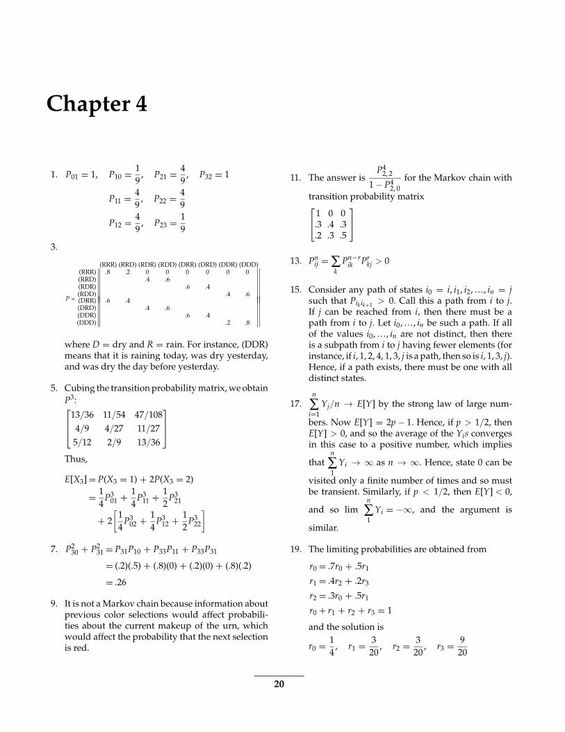
1. P01 = 1, P10 = 19
, P21 = 49
, P32 = 1
P11 = 49
, P22 = 49
P12 = 49
, P23 = 19
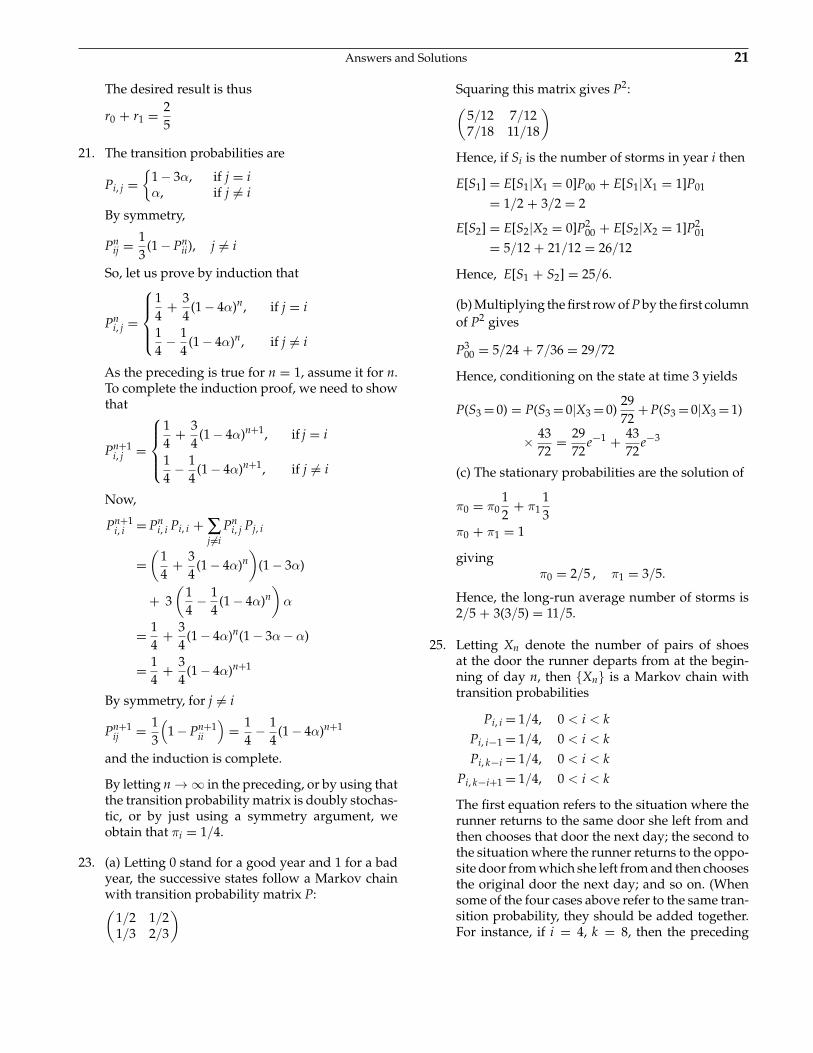
3.
(RRR) (RRD) (RDR) (RDD) (DRR) (DRD) (DDR) (DDD)(RRR) .8 .2 0 0 0 0 0 0(RRD) .4 .6(RDR) .6 .4(RDD) .4 .6
P = (DRR) .6 .4(DRD) .4 .6(DDR) .6 .4(DDD) .2 .8
where D = dry and R = rain. For instance, (DDR)means that it is raining today, was dry yesterday,and was dry the day before yesterday.
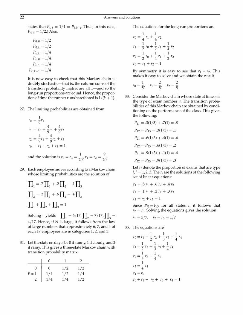
5. Cubing the transition probability matrix, we obtainP3:⎡⎢⎣13/36 11/54 47/108
4/9 4/27 11/275/12 2/9 13/36
⎤⎥⎦
Thus,
E[X3] = P(X3 = 1) + 2P(X3 = 2)
= 14
P301 + 1
4P3
11 + 12
P321
+ 2[
14
P302 + 1
4P3
12 + 12
P322
]
7. P230 + P2
31 = P31P10 + P33P11 + P33P31
= (.2)(.5) + (.8)(0) + (.2)(0) + (.8)(.2)
= .26
9. It is not a Markov chain because information aboutprevious color selections would affect probabili-ties about the current makeup of the urn, whichwould affect the probability that the next selectionis red.
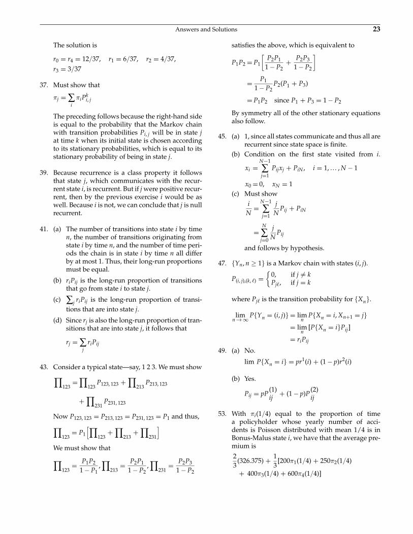
11. The answer isP4
2, 2
1 − P42, 0
for the Markov chain with
transition probability matrix⎡⎣1 0 0
.3 .4 .3
.2 .3 .5
⎤⎦
13. Pnij = ∑
kPn−r
ik Prkj > 0
15. Consider any path of states i0 = i, i1, i2, …, in = jsuch that Pikik+1 > 0. Call this a path from i to j.If j can be reached from i, then there must be apath from i to j. Let i0, …, in be such a path. If allof the values i0, …, in are not distinct, then thereis a subpath from i to j having fewer elements (forinstance, if i, 1, 2, 4, 1, 3, j is a path, then so is i, 1, 3, j).Hence, if a path exists, there must be one with alldistinct states.
17.n
∑i=1
Yj/n → E[Y] by the strong law of large num-
bers. Now E[Y] = 2p − 1. Hence, if p > 1/2, thenE[Y] > 0, and so the average of the Yis convergesin this case to a positive number, which implies
thatn
∑1
Yi → ∞ as n → ∞. Hence, state 0 can be
visited only a finite number of times and so mustbe transient. Similarly, if p < 1/2, then E[Y] < 0,
and so limn
∑1
Yi = −∞, and the argument is
similar.
19. The limiting probabilities are obtained from
r0 = .7r0 + .5r1
r1 = .4r2 + .2r3
r2 = .3r0 + .5r1
r0 + r1 + r2 + r3 = 1
and the solution is
r0 = 14
, r1 = 320
, r2 = 320
, r3 = 920
20
Answers and Solutions 21
The desired result is thus
r0 + r1 = 25
21. The transition probabilities are
Pi, j ={
1 − 3α, if j = iα, if j = i
By symmetry,
Pnij = 1
3(1 − Pn
ii), j = i
So, let us prove by induction that
Pni, j =
⎧⎪⎪⎨⎪⎪⎩
14
+ 34
(1 − 4α)n, if j = i
14
− 14
(1 − 4α)n, if j = i
As the preceding is true for n = 1, assume it for n.To complete the induction proof, we need to showthat
Pn+1i, j =
⎧⎪⎪⎨⎪⎪⎩
14
+ 34
(1 − 4α)n+1, if j = i
14
− 14
(1 − 4α)n+1, if j = i
Now,
Pn+1i, i = Pn
i, i Pi, i + ∑j �=i
Pni, j Pj, i
=(
14
+ 34
(1 − 4α)n)
(1 − 3α)
+ 3(
14
− 14
(1 − 4α)n)
α
= 14
+ 34
(1 − 4α)n(1 − 3α − α)
= 14
+ 34
(1 − 4α)n+1
By symmetry, for j = i
Pn+1ij = 1
3
(1 − Pn+1
ii
)= 1
4− 1
4(1 − 4α)n+1
and the induction is complete.
By letting n → ∞ in the preceding, or by using thatthe transition probability matrix is doubly stochas-tic, or by just using a symmetry argument, weobtain that πi = 1/4.
23. (a) Letting 0 stand for a good year and 1 for a badyear, the successive states follow a Markov chainwith transition probability matrix P:(
1/2 1/21/3 2/3
)
Squaring this matrix gives P2:(5/12 7/127/18 11/18
)Hence, if Si is the number of storms in year i then
E[S1] = E[S1|X1 = 0]P00 + E[S1|X1 = 1]P01
= 1/2 + 3/2 = 2
E[S2] = E[S2|X2 = 0]P200 + E[S2|X2 = 1]P2
01
= 5/12 + 21/12 = 26/12
Hence, E[S1 + S2] = 25/6.
(b) Multiplying the first row of P by the first columnof P2 gives
P300 = 5/24 + 7/36 = 29/72
Hence, conditioning on the state at time 3 yields
P(S3 = 0) = P(S3 = 0|X3 = 0)2972
+ P(S3 = 0|X3 = 1)
× 4372
= 2972
e−1 + 4372
e−3
(c) The stationary probabilities are the solution of
π0 = π012
+ π113
π0 + π1 = 1
givingπ0 = 2/5 , π1 = 3/5.
Hence, the long-run average number of storms is2/5 + 3(3/5) = 11/5.
25. Letting Xn denote the number of pairs of shoesat the door the runner departs from at the begin-ning of day n, then {Xn} is a Markov chain withtransition probabilities
Pi, i = 1/4, 0 < i < k
Pi, i−1 = 1/4, 0 < i < k
Pi, k−i = 1/4, 0 < i < k
Pi, k−i+1 = 1/4, 0 < i < k
The first equation refers to the situation where therunner returns to the same door she left from andthen chooses that door the next day; the second tothe situation where the runner returns to the oppo-site door from which she left from and then choosesthe original door the next day; and so on. (Whensome of the four cases above refer to the same tran-sition probability, they should be added together.For instance, if i = 4, k = 8, then the preceding
22 Answers and Solutions
states that Pi, i = 1/4 = Pi, k−i. Thus, in this case,P4, 4 = 1/2.) Also,
P0, 0 = 1/2P0, k = 1/2Pk, k = 1/4Pk, 0 = 1/4Pk, 1 = 1/4
Pk, k−1 = 1/4
It is now easy to check that this Markov chain isdoubly stochastic—that is, the column sums of thetransition probability matrix are all 1—and so thelong-run proportions are equal. Hence, the propor-tion of time the runner runs barefooted is 1/(k + 1).
27. The limiting probabilities are obtained from
r0 = 19
r1
r1 = r0 + 49
r1 + 49
r2
r2 = 49
r1 + 49
r2 + r3
r0 + r1 + r2 + r3 = 1
and the solution is r0 = r3 = 120
, r1 = r2 = 920
.
29. Each employee moves according to a Markov chainwhose limiting probabilities are the solution of∏
1= .7
∏1
+ .2∏
2+ .1
∏3∏
2= .2
∏1
+ .6∏
2+ .4
∏3∏
1+∏
2+∏
3= 1
Solving yields∏
1= 6/17,
∏2
= 7/17,∏
3=
4/17. Hence, if N is large, it follows from the lawof large numbers that approximately 6, 7, and 4 ofeach 17 employees are in categories 1, 2, and 3.
31. Let the state on day n be 0 if sunny, 1 if cloudy, and 2if rainy. This gives a three-state Markov chain withtransition probability matrix
0 1 2
0 0 1/2 1/2P = 1 1/4 1/2 1/4
2 1/4 1/4 1/2
The equations for the long-run proportions are
r0 = 14
r1 + 14
r2
r1 = 12
r0 + 12
r1 + 14
r2
r2 = 12
r0 + 14
r1 + 12
r2
r0 + r1 + r2 = 1
By symmetry it is easy to see that r1 = r2. Thismakes it easy to solve and we obtain the result
r0 = 15
, r1 = 25
, r2 = 25
33. Consider the Markov chain whose state at time n isthe type of exam number n. The transition proba-bilities of this Markov chain are obtained by condi-tioning on the performance of the class. This givesthe following:
P11 = .3(1/3) + .7(1) = .8
P12 = P13 = .3(1/3) = .1
P21 = .6(1/3) + .4(1) = .6
P22 = P23 = .6(1/3) = .2
P31 = .9(1/3) + .1(1) = .4
P32 = P33 = .9(1/3) = .3
Let ri denote the proportion of exams that are typei, i = 1, 2, 3. The ri are the solutions of the followingset of linear equations:
r1 = .8 r1 + .6 r2 + .4 r3
r2 = .1 r1 + .2 r2 + .3 r3
r1 + r2 + r3 = 1
Since Pi2 = Pi3 for all states i, it follows thatr2 = r3. Solving the equations gives the solution
r1 = 5/7, r2 = r3 = 1/7
35. The equations are
r0 = r1 + 12
r2 + 13
r3 + 14
r4
r1 = 12
r2 + 13
r3 + 14
r4
r2 = 13
r3 + 14
r4
r3 = 14
r4
r4 = r0
r0 + r1 + r2 + r3 + r4 = 1
Answers and Solutions 23
The solution is
r0 = r4 = 12/37, r1 = 6/37, r2 = 4/37,r3 = 3/37
37. Must show that
πj = ∑i
πiPki, j
The preceding follows because the right-hand sideis equal to the probability that the Markov chainwith transition probabilities Pi, j will be in state jat time k when its initial state is chosen accordingto its stationary probabilities, which is equal to itsstationary probability of being in state j.
39. Because recurrence is a class property it followsthat state j, which communicates with the recur-rent state i, is recurrent. But if j were positive recur-rent, then by the previous exercise i would be aswell. Because i is not, we can conclude that j is nullrecurrent.
41. (a) The number of transitions into state i by timen, the number of transitions originating fromstate i by time n, and the number of time peri-ods the chain is in state i by time n all differby at most 1. Thus, their long-run proportionsmust be equal.
(b) riPij is the long-run proportion of transitionsthat go from state i to state j.
(c) ∑j riPij is the long-run proportion of transi-tions that are into state j.
(d) Since rj is also the long-run proportion of tran-sitions that are into state j, it follows that
rj = ∑j
riPij
43. Consider a typical state—say, 1 2 3. We must show∏123
=∏
123P123, 123 +
∏213
P213, 123
+∏
231P231, 123
Now P123, 123 = P213, 123 = P231, 123 = P1 and thus,∏123
= P1
[∏123
+∏
213+∏
231
]We must show that
∏123
= P1P2
1 − P1,∏
213= P2P1
1 − P2,∏
231= P2P3
1 − P2
satisfies the above, which is equivalent to
P1P2 = P1
[P2P1
1 − P2+ P2P3
1 − P2
]
= P1
1 − P2P2(P1 + P3)
= P1P2 since P1 + P3 = 1 − P2
By symmetry all of the other stationary equationsalso follow.
45. (a) 1, since all states communicate and thus all arerecurrent since state space is finite.
(b) Condition on the first state visited from i.
xi =N−1
∑j=1
Pijxj + PiN , i = 1, … , N − 1
x0 = 0, xN = 1(c) Must show
iN
=N−1
∑j=1
jN
Pij + PiN
=N
∑j=0
jN
Pij
and follows by hypothesis.
47. {Yn, n ≥ 1} is a Markov chain with states (i, j).
P(i, j),(k, �) ={
0, if j = kPj�, if j = k
where Pj� is the transition probability for {Xn}.
limn → ∞ P{Yn = (i, j)} = lim
nP{Xn = i, Xn+1 = j}
= limn
[P{Xn = i}Pij]
= riPij
49. (a) No.
lim P{Xn = i} = pr1(i) + (1 − p)r2(i)
(b) Yes.
Pij = pP(1)ij + (1 − p)P
(2)ij
53. With πi(1/4) equal to the proportion of timea policyholder whose yearly number of acci-dents is Poisson distributed with mean 1/4 is inBonus-Malus state i, we have that the average pre-mium is
23
(326.375) + 13
[200π1(1/4) + 250π2(1/4)
+ 400π3(1/4) + 600π4(1/4)]
24 Answers and Solutions
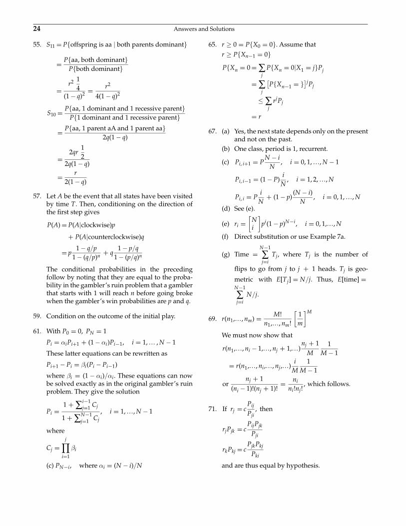
55. S11 = P{offspring is aa | both parents dominant}
= P{aa, both dominant}P{both dominant}
=r2 1
4(1 − q)2 = r2
4(1 − q)2
S10 = P{aa, 1 dominant and 1 recessive parent}P{1 dominant and 1 recessive parent}
= P{aa, 1 parent aA and 1 parent aa}2q(1 − q)
=2qr
12
2q(1 − q)
= r2(1 − q)
57. Let A be the event that all states have been visitedby time T. Then, conditioning on the direction ofthe first step gives
P(A) = P(A|clockwise)p
+ P(A|counterclockwise)q
= p1 − q/p
1 − (q/p)n + q1 − p/q
1 − (p/q)n
The conditional probabilities in the precedingfollow by noting that they are equal to the proba-bility in the gambler’s ruin problem that a gamblerthat starts with 1 will reach n before going brokewhen the gambler’s win probabilities are p and q.
59. Condition on the outcome of the initial play.
61. With P0 = 0, PN = 1
Pi = αiPi+1 + (1 − αi)Pi−1, i = 1, … , N − 1
These latter equations can be rewritten as
Pi+1 − Pi = βi(Pi − Pi−1)
where βi = (1 − αi)/αi. These equations can nowbe solved exactly as in the original gambler’s ruinproblem. They give the solution
Pi =1 + ∑i−1
j=1 Cj
1 + ∑N−1j=1 Cj
, i = 1, …, N − 1
where
Cj =j∏
i=1
βi
(c) PN−i, where αi = (N − i)/N
65. r ≥ 0 = P{X0 = 0}. Assume thatr ≥ P{Xn−1 = 0}P{Xn = 0 = ∑
jP{Xn = 0|X1 = j}Pj
= ∑j
[P{Xn−1 = }]jPj
≤ ∑j
rjPj
= r
67. (a) Yes, the next state depends only on the presentand not on the past.
(b) One class, period is 1, recurrent.
(c) Pi, i+1 = PN − i
N, i = 0, 1, …, N − 1
Pi, i−1 = (1 − P)i
N, i = 1, 2, …, N
Pi, i = Pi
N+ (1 − p)
(N − i)N
, i = 0, 1, …, N
(d) See (e).
(e) ri =[
Ni
]pi(1 − p)N−i, i = 0, 1,…, N
(f) Direct substitution or use Example 7a.
(g) Time =N−1
∑j=i
Tj, where Tj is the number of
flips to go from j to j + 1 heads. Tj is geo-
metric with E[Tj] = N/j. Thus, E[time] =N−1
∑j=i
N/j.
69. r(n1,…, nm) = M!n1,…, nm!
[1m
]M
We must now show that
r(n1,…, ni − 1,…, nj + 1,…)nj + 1
M1
M − 1
= r(n1,…, ni,…, nj,…)i
M1
M − 1
ornj + 1
(ni − 1)!(nj + 1)!= ni
ni!nj!, which follows.
71. If rj = cPij
Pji, then
rjPjk = cPijPjk
Pji
rkPkj = cPjkPkj
Pki
and are thus equal by hypothesis.
Answers and Solutions 25
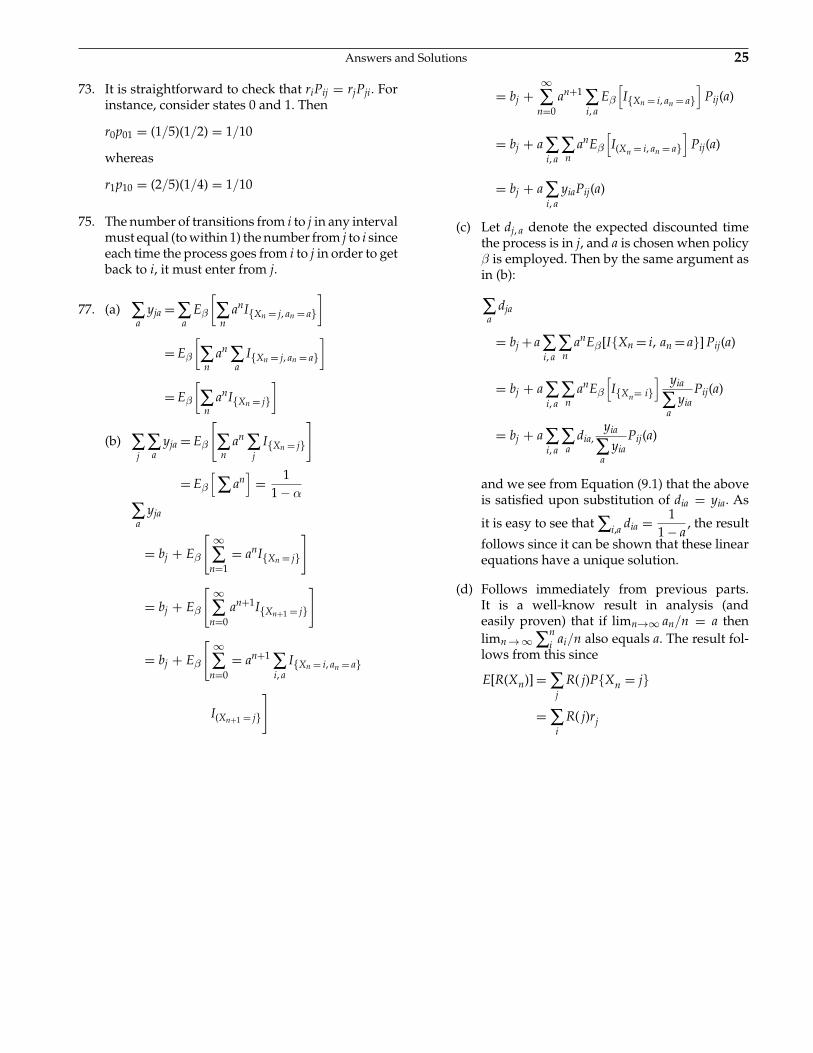
73. It is straightforward to check that riPij = rjPji. Forinstance, consider states 0 and 1. Then
r0p01 = (1/5)(1/2) = 1/10
whereas
r1p10 = (2/5)(1/4) = 1/10
75. The number of transitions from i to j in any intervalmust equal (to within 1) the number from j to i sinceeach time the process goes from i to j in order to getback to i, it must enter from j.
77. (a) ∑a
yja = ∑a
Eβ
[∑n
anI{Xn = j, an = a}]
= Eβ
[∑n
an ∑a
I{Xn = j, an = a}]
= Eβ
[∑n
anI{Xn = j}]
(b) ∑j
∑a
yja = Eβ
[∑n
an ∑j
I{Xn = j}
]
= Eβ
[∑ an
]= 1
1 − α
∑a
yja
= bj + Eβ
[ ∞∑n=1
= anI{Xn = j}
]
= bj + Eβ
[ ∞∑n=0
an+1I{Xn+1 = j}
]
= bj + Eβ
[ ∞∑n=0
= an+1 ∑i, a
I{Xn = i, an = a}
I(Xn+1 = j}
]
= bj +∞∑n=0
an+1 ∑i, a
Eβ
[I{Xn = i, an = a}
]Pij(a)
= bj + a ∑i, a
∑n
anEβ
[I(Xn = i, an = a}
]Pij(a)
= bj + a ∑i, a
yiaPij(a)
(c) Let dj, a denote the expected discounted timethe process is in j, and a is chosen when policyβ is employed. Then by the same argument asin (b):
∑a
dja
= bj + a ∑i, a
∑n
anEβ[I{Xn = i, an = a}] Pij(a)
= bj + a ∑i, a
∑n
anEβ
[I{Xn= i}
] yia
∑a
yiaPij(a)
= bj + a ∑i, a
∑a
dia,yia
∑a
yiaPij(a)
and we see from Equation (9.1) that the aboveis satisfied upon substitution of dia = yia. As
it is easy to see that ∑i,a dia = 11 − a
, the result
follows since it can be shown that these linearequations have a unique solution.
(d) Follows immediately from previous parts.It is a well-know result in analysis (andeasily proven) that if limn→∞ an/n = a thenlimn → ∞ ∑n
i ai/n also equals a. The result fol-lows from this since
E[R(Xn)] = ∑j
R( j)P{Xn = j}
= ∑i
R( j)rj
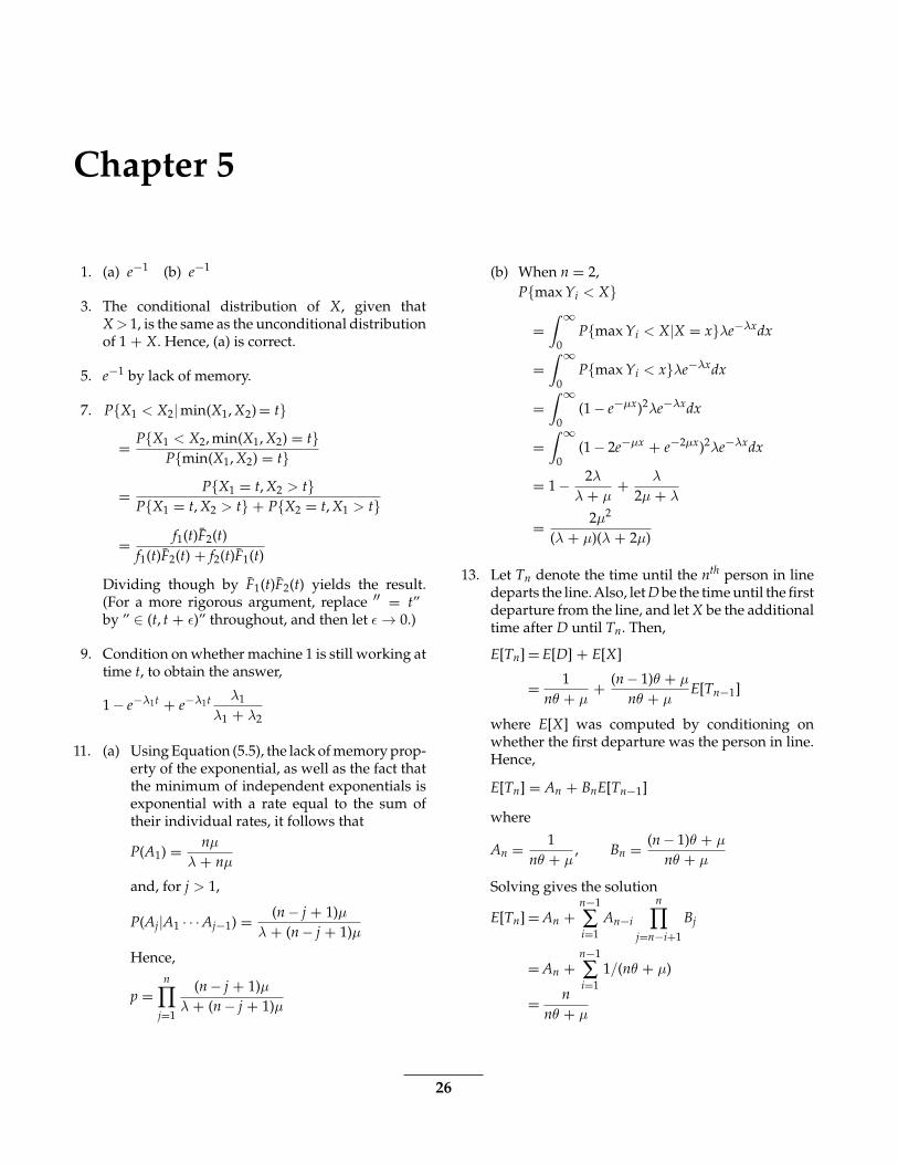
Chapter 5
1. (a) e−1 (b) e−1
3. The conditional distribution of X, given thatX > 1, is the same as the unconditional distributionof 1 + X. Hence, (a) is correct.
5. e−1 by lack of memory.
7. P{X1 < X2| min(X1, X2) = t}
= P{X1 < X2, min(X1, X2) = t}P{min(X1, X2) = t}
= P{X1 = t, X2 > t}P{X1 = t, X2 > t} + P{X2 = t, X1 > t}
= f1(t)F2(t)f1(t)F2(t) + f2(t)F1(t)
Dividing though by F1(t)F2(t) yields the result.(For a more rigorous argument, replace ′′ = t”by ” ∈ (t, t + ε)” throughout, and then let ε → 0.)
9. Condition on whether machine 1 is still working attime t, to obtain the answer,
1 − e−λ1t + e−λ1t λ1
λ1 + λ2
11. (a) Using Equation (5.5), the lack of memory prop-erty of the exponential, as well as the fact thatthe minimum of independent exponentials isexponential with a rate equal to the sum oftheir individual rates, it follows that
P(A1) = nμ
λ + nμ
and, for j > 1,
P(Aj|A1 · · · Aj−1) = (n − j + 1)μλ + (n − j + 1)μ
Hence,
p =n∏
j=1
(n − j + 1)μλ + (n − j + 1)μ
(b) When n = 2,P{max Yi < X}
=∫ ∞
0P{max Yi < X|X = x}λe−λxdx
=∫ ∞
0P{max Yi < x}λe−λxdx
=∫ ∞
0(1 − e−μx)2λe−λxdx
=∫ ∞
0(1 − 2e−μx + e−2μx)2λe−λxdx
= 1 − 2λ
λ + μ+ λ
2μ + λ
= 2μ2
(λ + μ)(λ + 2μ)
13. Let Tn denote the time until the nth person in linedeparts the line.Also, let D be the time until the firstdeparture from the line, and let X be the additionaltime after D until Tn. Then,
E[Tn] = E[D] + E[X]
= 1nθ + μ
+ (n − 1)θ + μ
nθ + μE[Tn−1]
where E[X] was computed by conditioning onwhether the first departure was the person in line.Hence,
E[Tn] = An + BnE[Tn−1]
where
An = 1nθ + μ
, Bn = (n − 1)θ + μ
nθ + μ
Solving gives the solution
E[Tn] = An +n−1
∑i=1
An−i
n∏j=n−i+1
Bj
= An +n−1
∑i=1
1/(nθ + μ)
= nnθ + μ
26
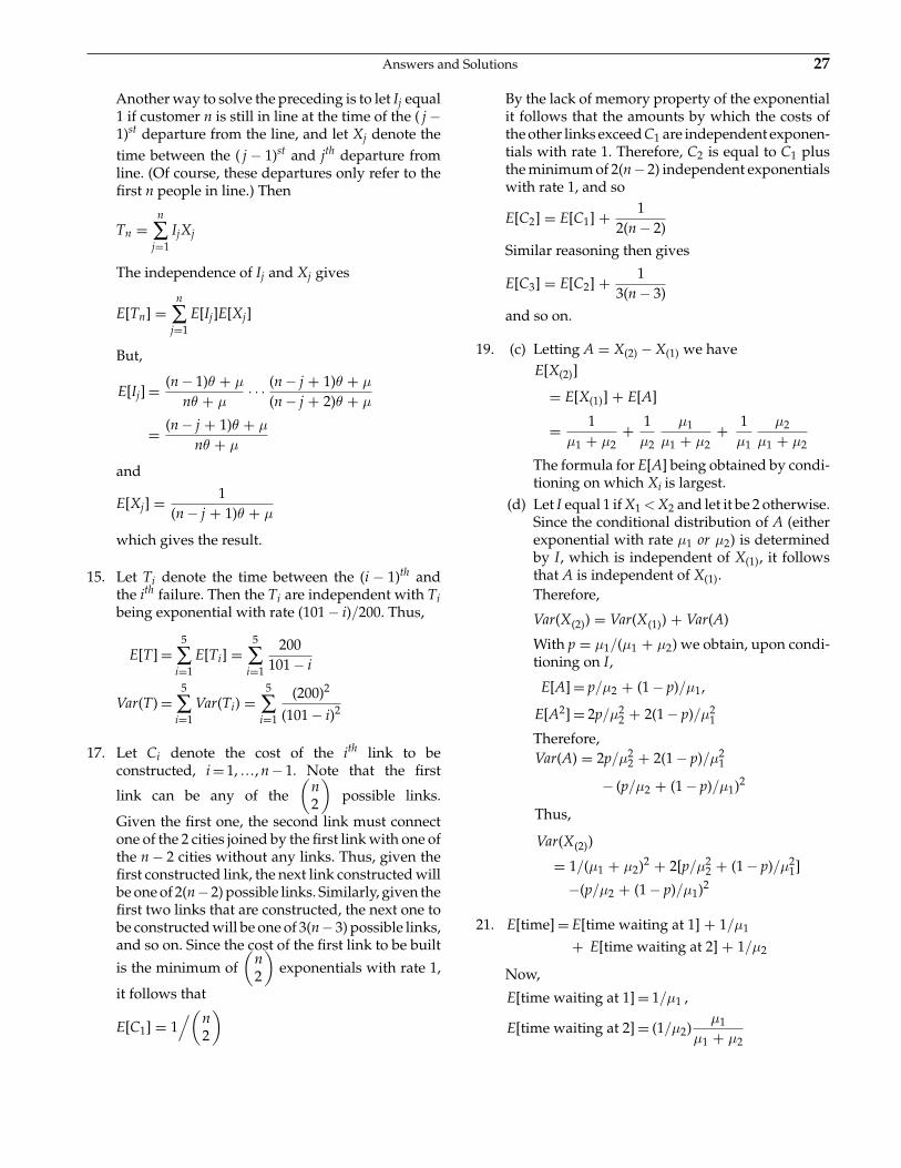
Answers and Solutions 27
Another way to solve the preceding is to let Ij equal1 if customer n is still in line at the time of the ( j −1)st departure from the line, and let Xj denote thetime between the ( j − 1)st and jth departure fromline. (Of course, these departures only refer to thefirst n people in line.) Then
Tn =n
∑j=1
IjXj
The independence of Ij and Xj gives
E[Tn] =n
∑j=1
E[Ij]E[Xj]
But,
E[Ij] = (n − 1)θ + μ
nθ + μ· · · (n − j + 1)θ + μ
(n − j + 2)θ + μ
= (n − j + 1)θ + μ
nθ + μ
and
E[Xj] = 1(n − j + 1)θ + μ
which gives the result.
15. Let Ti denote the time between the (i − 1)th andthe ith failure. Then the Ti are independent with Tibeing exponential with rate (101 − i)/200. Thus,
E[T] =5
∑i=1
E[Ti] =5
∑i=1
200101 − i
Var(T) =5
∑i=1
Var(Ti) =5
∑i=1
(200)2
(101 − i)2
17. Let Ci denote the cost of the ith link to beconstructed, i = 1, …, n − 1. Note that the first
link can be any of the(
n2
)possible links.
Given the first one, the second link must connectone of the 2 cities joined by the first link with one ofthe n − 2 cities without any links. Thus, given thefirst constructed link, the next link constructed willbe one of 2(n − 2) possible links. Similarly, given thefirst two links that are constructed, the next one tobe constructed will be one of 3(n − 3) possible links,and so on. Since the cost of the first link to be built
is the minimum of(
n2
)exponentials with rate 1,
it follows that
E[C1] = 1/(n
2
)
By the lack of memory property of the exponentialit follows that the amounts by which the costs ofthe other links exceed C1 are independent exponen-tials with rate 1. Therefore, C2 is equal to C1 plusthe minimum of 2(n − 2) independent exponentialswith rate 1, and so
E[C2] = E[C1] + 12(n − 2)
Similar reasoning then gives
E[C3] = E[C2] + 13(n − 3)
and so on.
19. (c) Letting A = X(2) − X(1) we haveE[X(2)]
= E[X(1)] + E[A]
= 1μ1 + μ2
+ 1μ2
μ1
μ1 + μ2+ 1
μ1
μ2
μ1 + μ2
The formula for E[A] being obtained by condi-tioning on which Xi is largest.
(d) Let I equal 1 if X1 < X2 and let it be 2 otherwise.Since the conditional distribution of A (eitherexponential with rate μ1 or μ2) is determinedby I, which is independent of X(1), it followsthat A is independent of X(1).Therefore,
Var(X(2)) = Var(X(1)) + Var(A)
With p = μ1/(μ1 + μ2) we obtain, upon condi-tioning on I,
E[A] = p/μ2 + (1 − p)/μ1,
E[A2] = 2p/μ22 + 2(1 − p)/μ2
1
Therefore,Var(A) = 2p/μ2
2 + 2(1 − p)/μ21
− (p/μ2 + (1 − p)/μ1)2
Thus,
Var(X(2))
= 1/(μ1 + μ2)2 + 2[p/μ22 + (1 − p)/μ2
1]
−(p/μ2 + (1 − p)/μ1)2
21. E[time] = E[time waiting at 1] + 1/μ1
+ E[time waiting at 2] + 1/μ2
Now,
E[time waiting at 1] = 1/μ1 ,
E[time waiting at 2] = (1/μ2)μ1
μ1 + μ2
28 Answers and Solutions
The last equation follows by conditioning onwhether or not the customer waits for server 2.Therefore,
E[time] = 2/μ1 + (1/μ2)[1 + μ1/(μ1 + μ2)]
23. (a) 1/2.(b) (1/2)n−1: whenever battery 1 is in use and a
failure occurs the probability is 1/2 that it isnot battery 1 that has failed.
(c) (1/2)n−i+1, i > 1.(d) T is the sum of n − 1 independent exponentials
with rate 2μ (since each time a failure occursthe time until the next failure is exponentialwith rate 2μ).
(e) Gamma with parameters n − 1 and 2μ.
25. Parts (a) and (b) follow upon integration. For part(c), condition on which of X or Y is larger and usethe lack of memory property to conclude that theamount by which it is larger is exponential rate λ.For instance, for x < 0,
fx − y(x)dx
= P{X < Y}P{−x < Y − X < −x + dx|Y > X}
= 12λeλxdx
For (d) and (e), condition on I.
27. (a)μ1
μ1 + μ3
(b)μ1
μ1 + μ3
μ2
μ2 + μ3
(c) ∑i
1μi
+ μ1
μ1 + μ3
μ2
μ2 + μ3
1μ3
(d) ∑i
1μi
+ μ1
μ1 + μ2
[1μ2
+ μ2
μ2 + μ3
1μ3
]
+ μ2
μ1 + μ2
μ1
μ1 + μ3
μ2
μ2 + μ3
1μ3
29. (a) fX|X + Y(x|c) = CfX. X+Y(x, c)
= C1 fXY(x, c−x)
= fX(x) fY(c − x)
= C2e−λxe−μ(c−x), 0 < x < c
= C3e−(λ−μ)x, 0 < x < c
where none of the Ci depend on x. Hence, wecan conclude that the conditional distributionis that of an exponential random variable con-ditioned to be less than c.
(b) E[X|X + Y = c] = 1 − e−(λ−μ)c(1 + (λ − μ)c)
λ(1 − e−(λ−μ)c)(c) c = E [X + Y|X + Y = c] = E [X|X + Y = c]
+ E [Y|X + Y = c]implying that
E[Y|X + Y = c]
= c − 1 − e−(λ−μ)c(1 + (λ − μ)c)
λ(1 − e−(λ−μ)c)
31. Condition on whether the 1 PM appointment is stillwith the doctor at 1:30, and use the fact that if she orhe is then the remaining time spent is exponentialwith mean 30. This gives
E[time spent in office]
= 30(1 − e−30/30) + (30 + 30)e−30/30
= 30 + 30e−1
33. (a) By the lack of memory property, no matterwhen Y fails the remaining life of X is expo-nential with rate λ.
(b) E [min (X, Y) |X > Y + c]
= E [min (X, Y) |X > Y, X − Y > c]
= E [min (X, Y) |X > Y]
where the final equality follows from (a).
37.1μ
+ 1λ
39. (a) 196/2.5 = 78.4
(b) 196/(2.5)2 = 31.36
We use the central limit theorem to justify approx-imating the life distribution by a normal distri-bution with mean 78.4 and standard deviation√
31.36 = 5.6. In the following, Z is a standard nor-mal random variable.
(c) P{L < 67.2} ≈ P{
Z <67.2 − 78.4
5.6
}= P{Z < −2} = .0227
(d) P{L > 90} ≈ P{
Z >90 − 78.4
5.6
}= P{Z > 2.07} = .0192
(e) P{L > 100} ≈ P{
Z >100 − 78.4
5.6
}= P{Z > 3.857} = .00006
Answers and Solutions 29
41. λ1/(λ1 + λ2)
43. Let Si denote the service time at server i, i = 1, 2 andlet X denote the time until the next arrival. Then,with p denoting the proportion of customers thatare served by both servers, we have
p = P{X > S1 + S2}= P{X > S1}PX > S1 + S2|X > S1}= μ1
μ1 + λ
μ2
μ2 + λ
45. E[N(T)] = E[E[N(T)|T]] = E[λT] = λE[T]
E[TN(T)] = E[E[TN(T)|T]] = E[TλT] = λE[T2]
E[N2(T)] = E[E[N2(T)|T]
]= E[λT + (λT)2]
= λE[T] + λ2E[T2]
Hence,
Cov(T, N(T)) = λE[T2] − E[T]λE[T] = λσ2
and
Var(N(T)) = λE[T] + λ2E[T2] − (λE[T])2
= λμ + λ2σ2
47. (a) 1/
(2μ) + 1/λ
(b) Let Ti denote the time until both servers arebusy when you start with i busy servers i =0, 1. Then,
E[T0] = 1/λ + E[T1]
Now, starting with 1 server busy, let T be thetime until the first event (arrival or departure);let X = 1 if the first event is an arrival and let itbe 0 if it is a departure; let Y be the additionaltime after the first event until both servers arebusy.
E[T1] = E[T] + E[Y]
= 1λ + μ
+ E[Y|X = 1]λ
λ + μ
+ E[Y|X = 0]μ
λ + μ
= 1λ + μ
+ E[T0]μ
λ + μ
Thus,
E[T0] − 1λ
= 1λ + μ
+ E[T0]μ
λ + μ
or
E[T0] = 2λ + μ
λ2
Also,
E[T1] = λ + μ
λ2
(c) Let Li denote the time until a customer is lostwhen you start with i busy servers. Then,reasoning as in part (b) gives that
E[L2] = 1λ + μ
+ E[L1]μ
λ + μ
= 1λ + μ
+ (E[T1] + E[L2])μ
λ + μ
= 1λ + μ
+ μ
λ2 + E[L2]μ
λ + μThus,
E[L2] = 1λ
+ μ(λ + μ)λ3
49. (a) P{N(T) − N(s) = 1} = λ(T − s)e−λ(T−s)
(b) Differentiating the expression in part (a) andthen setting it equal to 0 gives
e−λ(T−s) = λ(T − s)e−λ(T−s)
implying that the maximizing value is
s = T − 1/λ
(c) For s = T − 1/λ, we have that λ(T − s) = 1 andthus,
P{N(T) − N(s) = 1} = e−1
51. Condition on X, the time of the first accident, toobtain
E[N(t] =∫ ∞
0E[N(t)|X = s]βe−βsds
=∫ t
0(1 + α(t − s))βe−βsds
53. (a) e−1
(b) e−1 + e−1(.8)e−1
55. As long as customers are present to be served,every event (arrival or departure) will, inde-pendently of other events, be a departure withprobability p = μ/(λ + μ). Thus P{X = m} is theprobability that there have been a total of m tails atthemomentthat thenth headoccurs,whenindepen-dent flips of a coin having probability p of comingup heads are made: that is, it is the probability thatthe nth head occurs on trial number n + m. Hence,
p{X = m} =(
n + m − 1n − 1
)pn(1 − p)m
30 Answers and Solutions
57. (a) e−2
(b) 2 p.m.
59. The unconditional probability that the claim is type1 is 10/11. Therefore,
P(1|4000) = P(4000|1)P(1)P(4000|1)P(1) + P(4000|2)P(2)
= e−410/11e−410/11 + .2e−.81/11
61. (a) Poisson with mean cG(t).
(b) Poisson with mean c[1 − G(t)].
(c) Independent.
63. Let X and Y be respectively the number of cus-tomers in the system at time t + s that were presentat time s, and the number in the system at t + sthat were not in the system at time s. Since thereare an infinite number of servers, it follows thatX and Y are independent (even if given the num-ber is the system at time s). Since the service dis-tribution is exponential with rate μ, it follows thatgiven that X(s) = n, X will be binomial with param-eters n and p = e−μt. Also Y, which is indepen-dent of X(s), will have the same distribution as X(t).
Therefore, Y is Poisson with mean λ
t∫0
e−μydy
= λ(1 − e−μt)/μ
(a) E[X(t + s)|X(s) = n]
= E[X|X(s) = n] + E[Y|X(s) = n].
= ne−μt + λ(1 − e−μt)/μ
(b) Var(X(t + s)|X(s) = n)
= Var(X + Y|X(s) = n)
= Var(X|X(s) = n) + Var(Y)
= ne−μt(1 − e−μt) + λ(1 − e−μt)/μ
The above equation uses the formulas for thevariances of a binomial and a Poisson randomvariable.
(c) Consider an infinite server queuing system inwhich customers arrive according to a Poissonprocess with rate λ, and where the servicetimes are all exponential random variableswith rate μ. If there is currently a single cus-tomer in the system, find the probability that
the system becomes empty when that cus-tomer departs.Condition on R, the remaining service time:P{empty}
=∫ ∞
0P{empty|R = t}μe−μtdt
=∫ ∞
0exp{−λ
∫ t
0e−μydy
}μe−μtdt
=∫ ∞
0exp{−λ
μ(1 − e−μt)
}μe−μtdt
=∫ 1
0e−λx/μdx
= μ
λ(1 − e−λ/μ)
where the preceding used that P{empty|R = t} is equal to the probability that anM/M/∞ queue is empty at time t.
65. This is an application of the infinite server Pois-son queue model. An arrival corresponds to a newlawyer passing the bar exam, the service time isthe time the lawyer practices law. The number inthe system at time t is, for large t, approximately aPoisson random variable with mean λμ where λ isthe arrival rate and μ the mean service time. Thislatter statement follows from∫ n
0[1 − G(y)]dy = μ
where μ is the mean of the distribution G. Thus, wewould expect 500 · 30 = 15, 000 lawyers.
67. If we count a satellite if it is launched before times but remains in operation at time t, then the num-ber of items counted is Poisson with mean m(t) =∫ s
0G(t − y)dy. The answer is e−m(t).
69. (a) 1 − e−λ(t−s)
(b) e−λse−λ(t−s)[λ(t − s)]3/3!
(c) 4 + λ(t − s)
(d) 4s/t
71. Let U1, … be independent uniform (0, t) randomvariables that are independent of N(t), and let U(i, n)
be the ith smallest of the first n of them.
Answers and Solutions 31
P
{N(t)
∑i=1
g(Si) < x
}
= ∑n
P
{N(t)
∑i=1
g(Si) < x|N(t) = n
}P{N(t) = n}
= ∑n
P
{n
∑i=1
g(Si) < x|N(t) = n
}P{N(t) = n}
= ∑n
P
{n
∑i=1
g(U(i,n)) < x
}P{N(t) = n}
(Theorem 5.2)
= ∑n
P
{n
∑i=1
g(Ui) < x
}P{N(t) = n}
(n
∑i=1
g(U(i, n)) =n
∑i=1
g(Ui)
)
= ∑n
P
{n
∑i=1
g(Ui) < x|N(t) = n
}P{N(t) = n}
= ∑n
P
{N(t)
∑i=1
g(Ui) < x|N(t) = n
}P{N(t) = n}
= P
{N(t)
∑i=1
g(Ui) < x
}
73. (a) It is the gamma distribution with parametersn and λ.
(b) For n ≥ 1,P{N = n|T = t}
= P{T = t|N = n}p(1 − p)n−1
fT(t)
= C (λt)n−1
(n − 1)! (1 − p)n−1
= C (λ(1 − p)t)n−1
(n − 1)!
= e−λ(1−p)t (λ(1 − p)t)n−1
(n − 1)!
where the last equality follows since theprobabilities must sum to 1.
(c) The Poisson events are broken into two classes,those that cause failure and those that do not.By Proposition 5.2, this results in two indepen-dent Poisson processes with respective ratesλp and λ(1 − p). By independence it follows
that given that the first event of the first pro-cess occurred at time t the number of events ofthe second process by this time is Poisson withmean λ(1 − p)t.
75. (a) {Yn} is a Markov chain with transition proba-bilities given by
P0j = aj, Pi, i−1+j = aj, j ≥ 0
where
aj =∫
e−λt(λt)j
j!dG(t)
(b) {Xn} is a Markov chain with transition proba-bilities
Pi, i+1−j = βj, j = 0, 1, …, i, Pi, 0 =∞∑
k=i+1βj
where
βj =∫
e−μt(μt)j
j!dF(t)
77. (a)μ
λ + μ
(b)λ
λ + μ
2μ
λ + 2μ
(c)j−1∏i=1
λ
λ + iμjμ
λ + jμ, j > 1
(d) Conditioning on N yields the solution; namely∞∑j=1
1j
P(N = j)
(e)∞∑j=1
P(N = j)j
∑i=0
1λ + iμ
79. Consider a Poisson process with rate λ in which anevent at time t is counted with probability λ(t)/λindependently of the past. Clearly such a processwill have independent increments. In addition,
P{2 or more counted events in(t, t + h)}≤ P{2 or more events in(t, t + h)}= o(h)
and
P{1 counted event in (t, t + h)}= P{1 counted | 1 event}P(1 event)
32 Answers and Solutions
+ P{1 counted | ≥ 2 events}P{≥ 2}
=∫ t+h
t
λ(s)λ
dsh
(λh + o(h)) + o(h)
= λ(t)λ
λh + o(h)
= λ(t)h + o(h)
81. (a) Let Si denote the time of the ith event, i ≥ 1.Let ti + hi < ti+1, tn + hn ≤ t.P{ti < Si < ti + hi, i = 1, …, n|N(t) = n}P{1 event in (ti, ti + hi), i = 1, …, n,
= no events elsewhere in (0, t)P{N(t) = n}
=
[n∏
i=1
e−(m(ti+hi)−m(ti))[m(ti + hi) − m(ti)]
]
e−[m(t)−∑im(ti+hi)−m(ti)]
e−m(t)[m(t)]n/n!
=n
n∏i
[m(ti + hi) − m(ti)]
[m(t)]n
Dividing both sides by h1 · · · hn and using the
fact that m(ti + hi) − m(ti) =∫ ti+h
ti
λ(s) ds =λ(ti)h + o(h) yields upon letting the hi → 0:fS1 ··· S2 (t1, …, tn|N(t) = n)
= n!n∏
i=1
[λ(ti)/m(t)]
and the right-hand side is seen to be the jointdensity function of the order statistics from aset of n independent random variables fromthe distribution with density function f (x) =m(x)/m(t), x ≤ t.
(b) Let N(t) denote the number of injuries by timet. Now given N(t) = n, it follows from part (b)that the n injury instances are independent andidentically distributed. The probability (den-sity) that an arbitrary one of those injuries wasat s is λ(s)/m(t), and so the probability thatthe injured party will still be out of work attime t is
p =∫ t
0P{out of work at t|injured at s} λ(s)
m(t)dζ
=∫ t
0[1 − F(t − s)]
λ(s)m(t)
dζ
Hence, as each of the N(t) injured parties havethe same probability p of being out of work att, we see that
E[X(t)]|N(t)] = N(t)p
and thus,E[X(t)] = pE[N(t)]
= pm(t)
=∫ t
0[1 − F(t − s)]λ(s) ds
83. Since m(t) is increasing it follows that nonover-lapping time intervals of the {N(t)} process willcorrespond to nonoverlapping intervals of the{No(t)} process. As a result, the independentincrement property will also hold for the {N(t)}process. For the remainder we will use the identity
m(t + h) = m(t) + λ(t)h + o(h)
P{N(t + h) − N(t) ≥ 2}= P{No[m(t + h)] − No[m(t)] ≥ 2}= P{No[m(t) + λ(t)h + o(h)] − No[m(t)] ≥ 2}= o[λ(t)h + o(h)] = o(h)
P{N(t + h) − N(t) = 1}= P{No[m(t) + λ(t)h + o(h)] − No[m(t)] = 1}= P{1 event of Poisson process in interval
of length λ(t)h + o(h)]}= λ(t)h + o(h)
85. $ 40,000 and $1.6 × 10⁸.
87. Cov[X(t), X(t + s)]
= Cov[X(t), X(t) + X(t + s) − X(t)]
= Cov[X(t), X(t)] + Cov[X(t), X(t + s) − X(t)]
= Cov[X(t), X(t)] by independent increments
= Var[X(t)] = λtE[Y2]
89. Let Ti denote the arrival time of the first type ishock, i = 1, 2, 3.
P{X1 > s, X2 > t}= P{T1 > s, T3 > s, T2 > t, T3 > t}= P{T1 > s, T2 > t, T3 > max(s, t)}
= e−λ1s e−λ2t e−λ3max(s, t)
Answers and Solutions 33
91. To begin, note that
P
[X1 >
n
∑2
Xi
]
= P{X1 > X2}P{X1 − X2 > X3|X1 > X2}= P{X1 − X2 − X3 > X4|X1 > X2 + X3}…
= P{X1 − X2 · · · − Xn−1 > Xn|X1 > X2
+ · · · + Xn−1}= (1/2)n−1
Hence,
P
{M >
n
∑i=1
Xi − M
}=
n
∑i−1
P
{X1>
n
∑j �=i
Xi
}
= n/2n−1
93. (a) max(X1, X2) + min(X1, X2) = X1 + X2.
(b) This can be done by induction:
max{(X1, …, Xn)
= max(X1, max(X2, …, Xn))
= X1+ max(X2, …, Xn)
− min(X1, max(X2, …, Xn))
= X1+ max(X2, …, Xn)
− max(min(X1, X2), …, min (X1, Xn)).
Now use the induction hypothesis.A second method is as follows:Suppose X1 ≤ X2 ≤ · · · ≤ Xn. Then the coeffi-cient of Xi on the right side is
1 −[
n − i1
]+[
n − i2
]−[
n − i3
]+ · · ·
= (1 − 1)n−i
={
0, i = n1, i = n
and so both sides equal Xn. By symmetry theresult follows for all other possible orderingsof the X′s.
(c) Taking expectations of (b) where Xi is the timeof the first event of the ith process yields
∑i
λ−1i − ∑
i∑<j
(λi + λj)−1
+ ∑i
∑<j
∑<k
(λi + λj + λk)−1 − · · ·
+ (−1)n+1
[n
∑1
λi
]−1
95. E[L|N(t) = n] =
∫xg(x)e−xt(xt)ndx∫g(x)e−xt(xt)ndx
Conditioning on L yields
E[N(s)|N(t) = n]
= E[E[N(s)|N(t) = n, L]|N(t) = n]
= E[n + L(s − t)|N(t) = n]
= n + (s − t)E[L|N(t) = n]
For (c), use that for any value of L, given that therehave been n events by time t, the set of n event timesare distributed as the set of n independent uniform(0, t) random variables. Thus, for s < t
E[N(s)|N(t) = n] = ns/t
97. With C = 1/P(N(t) = n), we have
fL|N(t)(λ|n) = Ce−λt (λt)n
n!pe−pλ (pλ)m−1
(m − 1)!
= Ke−(p+t)λλn+m−1
where K does not depend on λ. But we recognizethe preceding as the gamma density with param-eters n + m, p + t, which is thus the conditionaldensity.
Chapter 6
1. Let us assume that the state is (n, m). Male i matesat a rate λ with female j, and therefore it mates at arate λm. Since there are n males, matings occur ata rate λnm. Therefore,
v(n, m) = λnm
Since any mating is equally likely to result in afemale as in a male, we have
P(n, m); (n+1, m) = P(n, m)(n, m+1) = 12
3. This is not a birth and death process since we needmore information than just the number working.We also must know which machine is working. Wecan analyze it by letting the states be
b : both machines are working
1 : 1 is working, 2 is down
2 : 2 is working, 1 is down
01: both are down, 1 is being serviced
02: both are down, 2 is being serviced
vb = μ1 + μ2, v1 = μ1 + μ, v2 = μ2 + μ,
v01 = v02 = μ
Pb, 1 = μ2μ2 + μ1
= 1 − Pb, 2, P1, b = μμ + μ1
= 1 − P1,02
P2, b = μμ + μ2
= 1 − P2, 01 , P01, 1 = P02, 2 = 1
5. (a) Yes.
(b) It is a pure birth process.
(c) If there are i infected individuals thensince a contact will involve an infected andan uninfected individual with probabilityi (n − i) /(n
2), it follows that the birth rates areλi = λi(n − i)/(n
2), i = 1, …, n. Hence,
E[time all infected] = n(n − 1)2λ
n
∑i=1
1/[i(n−i)]
7. (a) Yes!
(b) For n = (n1, … , ni, ni+1, …, nk−1) let
Si(n) = (n1, …, ni−1, ni+1 + 1, …, nk−1),
i = 1, …, k − 2
Sk−1(n) = (n1, …, ni, ni+1, …nk−1 − 1),
S0(n) = (n1 + 1, …, ni, ni+1, …, nk−1)Then
qn, S1(n) = niμ, i = 1, …, k − 1
qn, S0(n) = λ
9. Since the death rate is constant, it follows that aslong as the system is nonempty, the number ofdeaths in any interval of length t will be a Poissonrandom variable with mean μt. Hence,
Pij(t) = e−μt(μt)i − j/(i − j)!, 0 < j ≤ i
Pi, 0(t) =∞∑k=i
e−μt(μt)k/k!
11. (b) Follows from the hint upon using the lack ofmemory property and the fact that εi, the min-imum of j − (i − 1) independent exponentialswith rateλ, is exponential with rate (j − i + 1)λ.
(c) From (a) and (b)
P{T1 + · · · + Tj ≤ t} = P{
max1 ≤ i ≤ j
Xi ≤ t}
= (1 − e−λt) j
(d) With all probabilities conditional on X(0) = 1
P1j(t) = P{X(t) = j}= P{X(t) ≥ j} − P{X(t) ≥ j + 1}= P{T1 + · · · + Tj ≤ t}
−P{T1 + · · · + Tj+1 ≤ t}
(e) The sum of independent geometrics, eachhaving parameter p = e−λt, is negative bino-mial with parameters i, p. The result follows
34
Answers and Solutions 35
since starting with an initial population of i isequivalent to having i independent Yule pro-cesses, each starting with a single individual.
13. With the number of customers in the shop as thestate, we get a birth and death process with
λ0 = λ1 = 3, μ1 = μ2 = 4
Therefore
P1 = 34
P0, P2 = 34
, P1 =[
34
]2P0
And since2
∑0
Pi = 1, we get
P0 =[
1 + 34
+[
34
]2]−1
= 1637
(a) The average number of customers in theshop is
P1 + 2P2 =[
34
+ 2[
34
]2]
P0
= 3016
[1 + 3
4+[
34
]2]−1
= 3037
(b) The proportion of customers that enter theshop is
λ(1 − P2)λ
= 1 − P2 = 1 − 916
· 1637
= 2837
(c) Now μ = 8, and so
P0 =[
1 + 38
+[
38
]2]−1
= 6497
So the proportion of customers who now enterthe shop is
1 − P2 = 1 −[
38
]2 26497
= 1 − 997
= 8897
The rate of added customers is therefore
λ
[8897
]− λ
[2837
]= 3
[8897
− 2837
]= 0.45
The business he does would improve by 0.45customers per hour.
15. With the number of customers in the system as thestate, we get a birth and death process with
λ0 = λ1 = λ2 = 3, λi = 0, i ≥ 4
μ1 = 2, μ2 = μ3 = 4
Therefore, the balance equations reduce to
P1 = 32
P0, P2 = 34
P1 = 98
P0, P3 = 34
P2 = 2732
P0
And therefore,
P0 =[
1 + 32
+ 98
+ 2732
]−1= 32
143
(a) The fraction of potential customers that enterthe system is
λ(1 − P3)λ
= 1 − P3 = 1 − 2732
× 32143
= 116143
(b) With a server working twice as fast we wouldget
P1 = 34
P0 P2 = 34
P1 =[
34
]2P0 P3 =
[34
]3P0
and P0 =[
1 + 34
+[
34
]2+[
34
]3]−1
= 64175
So that now
1 − P3 = 1 − 2764
= 1 − 64175
= 148175
17. Say the state is 0 if the machine is up, say it is iwhen it is down due to a type i failure, i = 1, 2. Thebalance equations for the limiting probabilities areas follows.λP0 = μ1P1 + μ2P2
μ1P1 = λpP0
μ2P2 = λ(1 − p)P0
P0 + P1 + P2 = 1
These equations are easily solved to give the results
P0 = (1 + λp/μ1 + λ(1 − p)/μ2)−1
P1 = λpP0/μ1, P2 = λ(1 − p)P0/μ2
19. There are 4 states. Let state 0 mean that nomachines are down, state 1 that machine 1 is downand 2 is up, state 2 that machine 1 is up and 2 isdown, and 3 that both machines are down. The bal-ance equations are as follows:
(λ1 + λ2)P0 = μ1P1 + μ2P2
(μ1 + λ2)P1 = λ1P0 + μ1P3
(λ1 + μ2)P2 = λ2P0
μ1P3 = μ2P1 + μ1P2
P0 + P1 + P2 + P3 = 1
These equations are easily solved and theproportion of time machine 2 is down is P2 + P3.
36 Answers and Solutions
21. How we have a birth and death process withparameters
λi = λ, i = 1, 2μi = iμ, i = 1, 2
Therefore,
P0 + P1 = 1 + λ/μ
1 + λ/μ + (λ/μ)2/2
and so the probability that at least one machine isup is higher in this case.
23. Let the state denote the number of machines thatare down. This yields a birth and death processwith
λ0 = 310
, λ1 = 210
, λ2 = 110
, λi = 0, i ≥ 3
μ1 = 18
, μ2 = 28
, μ3 = 28
The balance equations reduce to
P1 = 3/101/8
P0 = 125
P0
P2 = 2/102/8
P1 = 45
P1 = 4825
P0
P3 = 1/102/8
P2 = 410
P3 = 192250
P0
Hence, using3
∑0
Pi = 1 yields
P0 =[
1 + 125
+ 4825
+ 192250
]−1= 250
1522
(a) Average number not in use
= P1 + 2P2 + 3P3 = 21361522
= 1068761
(b) Proportion of time both repairmen are busy
= P2 + P3 = 6721522
= 336761
25. If Ni(t) is the number of customers in the ithsystem (i = 1, 2), then let us take {N1(t), N2(t)}as the state. The balance equation are withn ≥ 1, m ≥ 1.
(a) λP0, 0 = μ2P0, 1
(b) Pn, 0(λ + μ1) = λPn−1, 0 + μ2Pn, 1
(c) P0, m(λ + μ2) = μ1P1, m−1 + μ2P0, m+1
(d) Pn, m(λ + μ1 + μ2) = λPn−1, m + μ1Pn+1, m−1
+ μ2Pn, m+1
We will try a solution of the form Cαnβm = Pn, m.From (a), we get
λC = μ2Cβ = β = λ
μ2
From (b),
(λ + μ1) Cαn = λCαn−1 + μ2Cαnβ
or
(λ + μ1) α = λ + μ2αβ = λ + μ2αλ
μ= λ + λα
and μ1α = λ ⇒ α = λ
μ1
To get C, we observe that ∑n, m
Pn, m = 1
but
∑n, m
Pn, m = C ∑n
αn ∑m
βm = C[
11 − α
] [1
1 − β
]
and C =[
1 − λ
μ1
] [1 − λ
μ2
]
Therefore a solution of the form Cαnβn must begiven by
Pn, m =[
1 − λ
μ1
] [λ
μ1
]n [1 − λ
μ2
] [λ
μ2
]m
It is easy to verify that this also satisfies (c) and(d) and is therefore the solution of the balanceequations.
27. It is a Poisson process by time reversibility. Ifλ > δμ, the departure process will (in the limit) bea Poisson process with rate δμ since the servers willalways be busy and thus the time between depar-tures will be independent random variables eachwith rate δμ.
29. (a) Let the state be S, the set of failed machines.
(b) For i ∈ S, j ∈ Sc,
qS, S − i = μi/|S|, qS, S+j = λj
where S − i is the set S with i deleted and S + jis similarly S with j added. In addition, |S|denotes the number of elements in S.
(c) PSqS, S−i = PS−iqS − i, S
Answers and Solutions 37
(d) The equation in (c) is equivalent to
PSμi/|S| = PS − iλi
or
PS = PS−i|S|λi/μi
Iterating this recursion gives
PS = P0(|S|)!∏i∈S
(λi/μi)
where 0 is the empty set. Summing over all Sgives
1 = P0 ∑S
(|S|)!∏i∈S
(λi/μi)
and so
PS =(|S|)!
∏i∈S
(λi/μi)
∑S
(|S|)!∏i∈S
(λi/μi)
As this solution satisfies the time reversibilityequations, it follows that, in the steady state,the chain is time reversible with these limitingprobabilities.
31. (a) This follows because of the fact that all of theservice times are exponentially distributed andthus memoryless.
(b) Let n = (n1, …, ni, …, nj, …, nr), whereni > 0 and let n′ = (n1, …, ni − 1, …,nj − 1, …, nr). Then qn, n′ = μi/(r − 1).
(c) The process is time reversible if we can findprobabilities P(n) that satisfy the equations
P(n)μi/(r − 1) = P(n′)μj/(r − 1)
where n and n′ are as given in part (b). Theabove equations are equivalent to
μiP(n) = μj/P(n′)
Since ni = n′i + 1 and n′
j = nj + 1 (where nk
refers to the kth component of the vector n), theabove equation suggests the solution
P(n) = Cr∏
k=1
(1/μk)nk
where C is chosen to make the probabili-ties sum to 1. As P(n) satisfies all the timereversibility equations it follows that the chainis time reversible and the P(n) given above arethe limiting probabilities.
33. Suppose first that the waiting room is ofinfinite size. Let Xi(t) denote the number of cus-tomers at server i, i = 1, 2. Then since each ofthe M/M/1 processes {Xi(t)} is time-reversible,it follows by Problem 28 that the vector process{(X1(t), X2(t)), t ≥ 0} is a time-reversible Markovchain. Now the process of interest is just the trun-cation of this vector process to the set of states Awhere
A = {(0, m) : m ≤ 4} ∪ {(n, 0) : n ≤ 4}∪ {(n, m) : nm > 0, n + m ≤ 5}
Hence, the probability that there are n with server 1and n with server 2 is
Pn, m = k(λ1/μ1)n(1 − λ1/μ1)(λ2/μ2)m(1 − λ2/μ2),
= C(λ1/μ1)n(λ2/μ2)m, (n, m) ∈ A
The constant C is determined from
∑ Pn, n = 1
where the sum is over all (n, m) in A.
35. We must find probabilities Pni such that
Pni qn
ij = Pnj qn
ji
or
cPni qij = Pn
j qji, if i ∈ A, j /∈ APiqij = cPn
j qji, if i /∈ A, j ∈ APiqij = Pjqji, otherwise
Now, Piqij = Pjqji and so if we let
Pni = kPi/c if i ∈ A
kPi if i /∈ A
then we have a solution to the above equations. Bychoosing k to make the sum of the Pn
j equal to 1, wehave the desired result. That is,
k =(
∑i∈A
Pi/c − ∑i/∈A
Pi
)−1
37. The state of any time is the set of downcomponents at that time. For S ⊂ {1, 2, …, n},i /∈ S, j ∈ S
q(S, S + i) = λi
q(S, S − j) = μjα|S|
where S + i = S ∪ {i}, S − j = S ∩ {j}c, |S| = numberof elements in S.
38 Answers and Solutions
The time reversible equations are
P(S)μiα|S| = P(S − i)λi, i ∈ S
The above is satisfied when, for S = {i1, i2, …, ik}
P(S) = λi1λi2 · · ·λik
μi1μi2 · · ·μik αk(k+1)/2
P(φ)
where P(φ) is determined so that
∑ P(S) = 1
where the sum is over all the 2n subsets of{1, 2, …, n}.
39. E[0(t)|x(0) = 1] = t − E[time in 1|X(0) = 1]
= t − λtλ + μ
− μ
(λ + μ)2 [1 − e−(λ+μ)t]
The final equality is obtained from Example 7b (orProblem 38) by interchanging λ and μ.
41. (a) Letting Ti denote the time until a transition outof i occurs, we have
Pij = P{X(Y) = j} = P{X(Y) = j | Ti < Y}
× vivi + λ
+ P{X(Y) = j|Y ≤ Ti} λλ + vi
= ∑k
PikPkjvi
vi + λ+ δijλ
λ + vi
The first term on the right follows upon con-ditioning on the state visited from i (which is kwith probability Pik) and then using the lack ofmemory property of the exponential to assertthat given a transition into k occurs before timeY then the state at Y is probabilistically thesame as if the process had started in state kand we were interested in the state after an
exponential time with rate λ. As qik = viPik ,the result follows.
(b) From (a)
(λ + vi)Pij = ∑k
qikPkj + λδij
or
−λδij = ∑k
rikPkj − λPij
or, in matrix terminology,
−λI = RP − λIP
= (R − λI)P
implying that
P = −λI(R − λI)−1 = −(R/λ − I)−1
= (I − R/λ)−1
(c) Consider, for instance,
P{X(Y1 + Y2) = j|X(0) = i}
= ∑k
P{X(Y1 + Y2) = j|X(Y1) = k, X(0) = i)
P{X(Y1) = k|X(0) = i}
= ∑k
P{X(Y1 + Y2) = j|X(Y1) = k}Pik
= ∑k
P{X(Y2) = j|X(0) = k}Pik
= ∑k
PkjPik
and thus the state at time Y1 + Y2 is just the2-stage transition probabilities of Pij. The gen-eral case can be established by induction.
(d) The above results in exactly the same approx-imation as Approximation 2 in Section 6.8.
Chapter 7
1. (a) Yes, (b) no, (c) no.
3. By the one-to-one correspondence of m(t) and F, itfollows that {N(t), t ≥ 0} is a Poisson process withrate 1/2. Hence,
P{N(5) = 0) = e−5/2
5. The random variable N is equal to N(I) + 1 where{N(t)} is the renewal process whose interarrivaldistribution is uniform on (0, 1). By the results ofExample 2c,
E[N] = a (1) + 1 = e
7. Once every five months.
9. Ajob completion constitutes a reneval. Let T denotethe time between renewals. To compute E[T] startby conditioning on W, the time it takes to finish thenext job:
E[T] = E[E[T|W]]
Now, to determine E[T|W = w] condition on S, thetime of the next shock. This gives
E[T|W = w] =∞∫
0
E[T|W = w, S = x]λe−λxdx
Now, if the time to finish is less than the time of theshock then the job is completed at the finish time;otherwise everything starts over when the shockoccurs. This gives
E[T|W = w, S = x] ={
x + E[T], if x < ww, if x ≥ w
Hence,
E[T|W = w]
=w∫
0
(x + E[T])λe−λxdx + w
∞∫w
λe−λxdx
= E[T][1−e−λw]+1/λ − we−λw− 1λ
e−λw−we−λw
Thus,
E[T|W] = (E[T] + 1/λ)(1 − e−λW )
Taking expectations gives
E[T] = (E[T] + 1/λ)(1 − E[e−λW ])
and so
E[T] = 1 − E[e−λW ]
λE[e−λW ]
In the above, W is a random variable having distri-bution F and so
E[e−λW ] =∞∫
0
e−λwf (w)dw
11.N(t)
t= 1
t+ number of renewals in (X1, t)
t
Since X1 < ∞, Proposition 3.1 implies that
number of renewals in (X1, t)t
− 1μ
as t − ∞.
13. (a) N1 and N2 are stopping times. N3 is not.
(b) Follows immediately from the definition of Ii.
(c) The value of Ii is completely determinedfrom X1, …, Xi−1 (e.g., Ii = 0 or 1 depend-ing upon whether or not we have stoppedafter observing X1, …, Xi−1). Hence, Ii is inde-pendent of Xi.
(d)∞∑i=1
E[Ii] =∞∑i=1
P{N ≥ i} = E[N]
(e) E[X1 + · · · + XN1
] = E[N1]E[X]
But X1 + · · · + XN1 = 5, E[X] = p and so
E[N1] = 5/p
E[X1 + · · · + XN2
] = E[N2]E[X]
E[X] = p, E[N2] = 5p + 3(1 − p) = 3 + 2p
E[X1 + · · · + XN2
] = (3 + 2p)p
39
40 Answers and Solutions
15. (a) Xi =amount of time he has to travel after his ithchoice (we will assume that he keeps on mak-ing choices even after becoming free). N is thenumber of choices he makes until becomingfree.
(b) E[T] = E
[N
∑1
Xi
]= E[N]E [X]
N is a geometric random variable withP = 1/3, so
E[N] = 3, E[X] = 13
(2 + 4 + 6) = 4
Hence, E[T] = 12.
(c) E
[N
∑1
Xi|N = n
]= (n − 1)
12
(4 + 6) + 2 = 5n −3, since given N = n, X1, …, Xn−1 are equally
likely to be either 4 or 6, Xn = 2, E(∑n
1 Xi
)=
4n.
(d) From (c),
E
[N
∑1
Xi
]= E [5N − 3] = 15 − 3 = 12
17. (i) Yes. (ii) No—Yes, if F exponential.
19. Since, from Example 2c, m(t) = et − 1, 0 < t ≤ 1,we obtain upon using the identity t + E[Y(t)] =μ[m(t) + 1] that E[Y(1)] = e/2 − 1.
21.μG
μ + 1/λ, where μG is the mean of G.
23. Using that E[X] = 2p − 1, we obtain from Wald’sequation when p = 1/2 that
E[T](2p − 1) = E
[T
∑j=1
Xj
]
= (N − i)1 − (q/p)i
1 − (q/p)N − i[
1 − 1 − (q/p)i
1 − (q/p)N
]
= N1 − (q/p)i
1 − (q/p)N − i
yielding the result:
E[T] =N
1 − (q/p)i
1 − (q/p)N − i
2p − 1, p = 1/2
When p = 1/2, we can easily show by a condition-ing argument that E[T] = i(N − i)
25. Say that a new cycle begins each time a train isdispatched. Then, with C being the cost of a cycle,we obtain, upon conditioning on N(t), the numberof arrivals during a cycle, that
E[C] = E[E|C|N(t)]] = E[K + N(t)ct/2]
= k + λct2/2
Hence,
average cost per unit time = E[C]t
= Kt
+ λct/2
Calculus shows that the preceding is minimizedwhen t =
√2K/(λc), with the average cost equal to√
2λKc.
On the other hand, the average cost for the Npolicy of Example 7.12 is c(N − 1)/2 + λK/N. Treat-ing N as a continuous variable yields that itsminimum occurs at N =
√2λK/c, with a resulting
minimal average cost of√
2λKc − c/2.
27. Say that a new cycle begins when a machine fails;let C be the cost per cycle; let T be the time of acycle.
E[C] = K + c2
λ1 + λ2+ λ1
λ1 + λ2
c1
λ2+ λ2
λ1 + λ2
c1
λ1
E[T] = 1λ1 + λ2
+ λ1
λ1 + λ2
1λ2
+ λ2
λ1 + λ2
1λ1
T the long-run average cost per unit time isE[C]/E[T].
29. (a) Imagine that you are paid a reward equal toWi on day i. Since everything starts over whena busy period ends, it follows that the rewardprocess constitutes a renewal reward processwith cycle time equal to N and with the rewardduring a cycle equal to W1 + · · · + WN . ThusE[W], the average reward per unit time, isE[W1 + · · · + WN]/E[N].
(b) The sum of the times in the system of allcustomers and the total amount of work thathas been processed both start equal to 0 andboth increase at the same rate. Hence, they arealways equal.
(c) This follows from (b) by looking at the valueof the two totals at the end of the first busyperiod.
(d) It is easy to see that N is a stopping timefor the Li, i ≥ 1, and so, by Wald’s Equation,
E
[N
∑i=1
Li
]= E[L]E[N]. Thus, from (a) and (c),
we obtain that E[W] = E[L].
Answers and Solutions 41
31. P{E(t) > x|A(t) = s}= P{0 renewals in (t, t + x]|A(t) = s}= P{interarrival > x + s|A(t) = s}= P{interarrival > x + s|interarrival > s}= 1 − F(x + s)
1 − F(s)
33. Let B be the amount of time the server is busy ina cycle; let X be the remaining service time of theperson in service at the beginning of a cycle.
E[B] = E[B|X < t](1 − e−λt) + E[B|X > t]e−λt
= E[X|X < t](1 − e−λt) +(
t + 1λ + μ
)e−λt
= E[X] − E[X|X > t]e−λt +(
t + 1λ + μ
)e−λt
= 1μ −
(t + 1
μ
)e−λt +
(t + 1
λ + μ
)e−λt
= 1μ
[1 − λ
λ + μe−λt
]More intuitively, writing X = B + (X − B), and not-ing that X − B is the additional amount of servicetime remaining when the cycle ends, gives
E[B] = E[X] − E[X − B]
= 1μ
− 1μ
P(X > B)
= 1μ
− 1μ
e−λt λ
λ + μ
The long-run proportion of time that the server is
busy isE[B]
t + 1/λ.
35. (a) We can view this as an M/G/∞ system wherea satellite launching corresponds to an arrivaland F is the service distribution. Hence,
P{X(t) = k} = e−λ(t)[λ(t)]k/k!
where λ(t) = λ
∫ t
0(1 − F(s))ds.
(b) By viewing the system as an alternatingrenewal process that is on when there is at leastone satellite orbiting, we obtain
lim P{X(t) = 0} = 1/λ
1/λ+ E[T]
where T, the on time in a cycle, is the quantityof interest. From part (a)
lim P{X(t) = 0} = e−λμ
where μ =∫ ∞
0(1 − F(s))ds is the mean time
that a satellite orbits. Hence,
e−λμ = 1/λ
1/λ + E[T]
and so
E[T] = 1 − e−λμ
λe−λμ
37. (a) This is an alternating renewal process, withthe mean off time obtained by conditioning onwhich machine fails to cause the off period.
E[off] =3
∑i=1
E[off|i fails]P{i fails}
= (1/5)λ1
λ1 + λ2 + λ3+ (2)
λ2
λ1 + λ2 + λ3
+ (3/2)λ3
λ1 + λ2 + λ3
As the on time in a cycle is exponential withrate equal to λ1 + λ2 + λ3, we obtain that p,the proportion of time that the system isworking is
p = 1/(λ1 + λ2 + λ3)E[C]
where
E[C] = E[cycle time]= 1/(λ1 + λ2 + λ3) + E[off]
(b) Think of the system as a renewal reward pro-cess by supposing that we earn 1 per unit timethat machine 1 is being repaired. Then, r1, theproportion of time that machine 1 is beingrepaired is
r1 =(1/5)
λ1
λ1 + λ2 + λ3E[C]
(c) By assuming that we earn 1 per unit time whenmachine 2 is in a state of suspended anima-tion, shows that, with s2 being the propor-tion of time that 2 is in a state of suspendedanimation,
s2 =(1/5)
λ1
λ1 + λ2 + λ3+ (3/2)
λ3
λ1 + λ2 + λ3E[C]
39. Let B be the length of a busy period. With S equalto the service time of the machine whose failure
42 Answers and Solutions
initiated the busy period, and T equal to theremaining life of the other machine at that moment,we obtain
E[B] =∫
E[B|S = s]g(s)ds
Now,
E[B|S = s] = E[B|S = s, T ≤ s](1 − e−λs)
+ E[B|S = s, T > s]e−λs
= (s + E[B])(1 − e−λs) + se−λs
= s + E[B](1 − e−λs)
Substituting back gives
E[B] = E[S] + E[B]E[1 − e−λs]
or
E[B] = E[S]E[e−λs]
Hence,
E[idle] = 1/(2λ)1/(2λ) + E[B]
41.∫ 1
0
(1 − F(x)dxμ
=
⎧⎪⎪⎪⎪⎨⎪⎪⎪⎪⎩
∫ 1
0
2 − x2
dx = 34
in part (i)
∫ 1
0e−x dx = 1 − e−1 in part (ii)
43. Since half the interarrival times will be exponentialwith mean 1 and half will be exponential with mean2, it would seem that because the exponentials withmean 2 will last, on average, twice as long, that
Fe(x) = 23
e−x/2 + 13
e−x
With μ= (1)1/2 + (2)1/2 = 3/2 equal to the meaninterarrival time
Fe(x) =∫ ∞
x
F(y)μ
dy
and the earlier formula is seen to be valid.
45. The limiting probabilities for the Markov chain aregiven as the solution of
r1 = r212
+ r3
r2 = r1
r1 + r2 + r3 = 1
or
r1 = r2 = 25
, r3 = 15
(a) r1 = 25
(b) Pi = riμi
∑i riμiand so,
P1 = 29
, P2 = 49
, P3 = 39
.
47. (a) By conditioning on the next state, we obtainthe following:
μj = E[time in i]
= ∑ E[time in i|next state is j]Pij
= ∑i
tijPij
(b) Use the hint. Then,
E[reward per cycle]= E[reward per cycle|next state is j]Pij
= tijPij
Also,
E[time of cycle] = E[time between visits to i]Now, if we had supposed a reward of 1 per unittime whenever the process was in state i and0 otherwise then using the same cycle times asabove we have that
Pi = E[reward is cycle]E[time of cycle]
= μi
E[time of cycle]
Hence,
E[time of cycle] = μi/Pi
and so
average reward per unit time = tijPijPi/μi
The above establishes the result since the aver-age reward per unit time is equal to the pro-portion of time the process is in i and will nextenter j.
49. Think of each interarrival time as consisting of nindependent phases—each of which is exponen-tially distributed with rate λ—and consider thesemi–Markov process whose state at any time isthe phase of the present interarrival time. Hence,this semi-Markov process goes from state 1 to 2 to3 … to n to 1, and so on. Also the time spent in eachstate has the same distribution. Thus, clearly the
Answers and Solutions 43
limiting probabilities of this semi-Markov chain arePi = 1/n, i = 1, …, n. To compute lim P{Y(t) < x},we condition on the phase at time t and note that ifit is n – i + 1, which will be the case with probability1/n, then the time until a renewal occurs will be thesum of i exponential phases, which will thus havea gamma distribution with parameters i and λ.
51. It is an example of the inspection paradox. Becauseevery tourist spends the same time in departingthe country, those questioned at departure consti-tute a random sample of all visiting tourists. Onthe other hand, if the questioning is of randomlychosen hotel guests then, because longer stayingguests are more likely to be selected, it follows thatthe average time of the ones selected will be largerthan the average of all tourists. The data that theaverage of those selected from hotels was approx-imately twice as large as from those selected atdeparture are consistent with the possibility thatthe time spent in the country by a tourist is expo-nential with a mean approximately equal to 9.
55. E[T(1)] = (.24)−2 + (.4)−1 = 19.8611,
E[T(2)] = 24.375, E[T12] = 21.875,
E[T2, 1] = 17.3611. The solution of the equations
19.861 = E[M] + 17.361P(2)
24.375 = E[M] + 21.875P(1)
1 = P(1) + P(2)
gives the results
P(2) ≈ .4425, E[M] ≈ 12.18
57. P{T
∑i=1
Xi > x} = P{T
∑i=1
Xi > x|T = 0}(1 − ρ)
+ P{T
∑i=1
Xi > x|T > 0}ρ
= P{T
∑i=1
Xi > x|T > 0}ρ
= ρ
∫ ∞
0P{
T
∑i=1
Xi > x|T > 0, X1 = y} F(y)μ
dy
= ρ
μ
∫ x
0P{
T
∑i=1
Xi > x|T > 0, X1 = y}F(y)dy
+ ρ
μ
∫ ∞
xF(y)dy
= ρ
μ
∫ x
0h(x − y)F(y)dy + ρ
μ
∫ ∞
xF(y)dy
= h(0) + ρ
μ
∫ x
0h(x − y)F(y)dy − ρ
μ
∫ x
0F(y)dy
where the final equality used that
h(0) = ρ = ρ
μ
∫ ∞
0F(y)dy
Chapter 8
1. (a) E[number of arrivals]
= E[E{number of arrivals|serviceperiod is S}]
= E[λS]
= λ/μ
(b) P{0 arrivals}= E[P{0 arrivals|service period is S}]
= E[P{N(S) = 0}]
= E[e−λS]
=∫ x
0e−λsμe−μsds
= μ
λ + μ
3. Let CM = Mary’s average cost/hour and CA =Alice’s average cost/hour.
Then, CM = $3 + $1× (Average number of cus-tomers in queue when Mary works),
and CA = $C + $1 × (Average number of cus-tomers in queue when Alice works).
The arrival stream has parameter λ = 10, and thereare two service parameters—one for Mary and onefor Alice:
μM = 20, μA = 30.
Set LM = average number of customers inqueue when Mary works and
LA = average number of customers inqueue when Alice works.
Then using Equation (3.2), LM = 10(20 − 10)
= 1
LA = 10(20 − 10)
= 12
So CM = $3 + $1/customer × LM customers= $3 + $1= $4/hour
Also, CA = $C + $1/customer × LA customers
= $C + $1 × 12
= $C + 12
/ hour
(b) We can restate the problem this way: If CA =CM, solve for C.
4 = C + 12
⇒ C = $3.50/hour
i.e., $3.50/hour is the most the employershould be willing to pay Alice to work. At ahigher wage his average cost is lower withMary working.
5. Let I equal 0 if W∗Q = 0 and let it equal 1 otherwise.
Then,
E[W∗Q|I = 0] = 0
E[W∗Q|I = 1] = (μ − λ)−1
Var(W∗Q|I = 0) = 0
Var(W∗Q|I = 1) = (μ − λ)−2
Hence,
E[Var(W∗Q|I] = (μ − λ)−2λ/μ
Var(E[W∗Q|I]) = (μ − λ)−2λ/μ(1 − λ/μ)
Consequently, by the conditional variance formula,
Var(W∗Q) = λ
μ(μ − λ)2 + λ
μ2(μ − λ)
7. To compute W for the M/M/2, set up balance equa-tions as
λp0 = μp1 (each server has rate μ)
(λ + μ)p1 = λp0 + 2μp2
(λ + 2μ)pn = λpn−1 + 2μpn+1, n ≥ 2
These have solutions Pn = ρn/2n−1p0 whereρ = λ/μ.
44
Answers and Solutions 45
The boundary condition∞∑n=0
Pn = 1 implies
P0 = 1 − ρ/21 + ρ/2
= (2 − ρ)(2 + ρ)
Now we have Pn, so we can compute L, and henceW from L = λW :
L =∞∑n=0
npn = ρp0
∞∑n=0
n[ρ2
]n−1
= 2p0
∞∑n=0
n[ρ2
]n
= 2 (2 − ρ)(2 + ρ)
(ρ/2)(1 − ρ/2)2
= 4ρ(2 + ρ)(2 − ρ)
= 4μλ(2μ + λ)(2μ − λ)
From L = λW we have
W = Wm/m/2 = 4μ
(2μ + λ)(2μ − λ)
The M/M/1 queue with service rate 2μ has
Wm/m/1 = 12μ − λ
from Equation (3.3). We assume that in theM/M/1 queue, 2μ > λ so that the queue is stable.
But then 4μ > 2μ + λ, or4μ
2μ + λ> 1, which
implies Wm/m/2 > Wm/m/1.
The intuitive explanation is that if one finds thequeue empty in the M/M/2 case, it would do nogood to have two servers. One would be better offwith one faster server.
Now let W1Q = WQ(M/M/1)
W2Q = WQ(M/M/2)
Then,
W1Q = Wm/m/1 − 1/2μ
W2Q = Wm/m/2 − 1/μ
So,
W1Q = λ
2μ(2μ − λ)(3.3)
and
W2Q = λ2
μ(2μ − λ)(2μ + λ)
Then,
W1Q > W2
Q ⇔ 12 > λ
(2μ + λ)λ < 2μ
Since we assume λ < 2μ for stability in theM/M/1, W2
Q < W1Q whenever this comparison is
possible, i.e., whenever λ < 2μ.
9. Take the state to be the number of customers atserver 1. The balance equations are
μP0 = μP1
2μPj = μPj+1 + μPj−1, 1 ≤ j < n
μPn = μPn−1
1 =n
∑j=0
Pj
It is easy to check that the solution to these equa-tions is that all the Pjs are equal, so Pj = 1/(n + 1),j = 0, …, n.
11. (a) λP0 = αμP1
(λ + αμ)Pn = λPn−1 + αμPn+1, n ≥ 1
These are exactly the same equations as in theM/M/1 with αμ replacing μ. Hence,
Pn =[
λ
αμ
]n [1 − λ
αμ
], n ≥ 0
and we need the condition λ < αμ.
(b) If T is the waiting time until the customer firstenters service, then conditioning on the num-ber present when he arrives yieldsE[T] = ∑
nE[T|n present]Pn
= ∑n
nμ
Pn
= Lμ
Since L = ∑ nPn, and the Pn are the same asin the M/M/1 with λ and αμ, we have thatL = λ/(αμ − λ) and so
E[T] = λ
μ(αμ − λ)
(c) P{enters service exactly n times}= (1 − α)n−1α
(d) This is expected number of services × meanservices time = 1/αμ
46 Answers and Solutions
(e) The distribution is easily seen to be memory-less. Hence, it is exponential with rate αμ.
13. Let the state be the idle server. The balance equa-tions are
Rate Leave = Rate Enter,
(μ2 + μ3)P1 = μ1μ1 + μ2
P3 + μ1μ1 + μ3
P2,
(μ1 + μ3)P2 = μ2μ2 + μ3
P1 + μ2μ2 + μ1
P3,
μ1 + μ2 + μ3 = 1.
These are to be solved and the quantity Pi repre-sents the proportion of time that server i is idle.
15. There are four states = 0, 1A, 1B, 2. Balance equa-tions are
2P0 = 2P1B
4P1A = 2P0 + 2P2
4P1B = 4P1A + 4P2
6P2 = 2P1B
P0 + P1A + P1B + P2 = 1 ⇒ P0 = 39
P1A = 29
, P1B = 39
, P2 = 19
(a) P0 + P1B = 23
(b) By conditioning upon whether the state was 0or 1B when he entered we get that the desiredprobability is given by
12
+ 12
26
= 46
(c) P1A + P1B + 2P2 = 79
(d) Again, condition on the state when he entersto obtain
12
[14
+ 12
]+ 1
2
[14
+ 26
12
]= 7
12
This could also have been obtained from (a)
and (c) by the formula W = Lλa
.
That is, W =79
2[
23
] = 712
.
17. The state space can be taken to consist of states(0, 0), (0, 1), (1, 0), (1, 1), where the ith component of
the state refers to the number of customers at serveri, i = 1, 2. The balance equations are
2P0, 0 = 6P0, 1
8P0, 1 = 4P1, 0 + 4P1, 1
6P1, 0 = 2P0, 0 + 6P1, 1
10P1, 1 = 2P0, 1 + 2P1, 0
1 = P0, 0 + P0, 1 + P1, 0 + P1, 1
Solving these equations gives P0, 0 = 1/2,P0, 1 = 1/6, P1, 0 = 1/4, P1, 1 = 1/12.
(a) P1, 1 = 1/12
(b) W = Lλa
= P0, 1 + P1, 0 + 2P1, 1
2(1 − P1, 1)= 7
22
(c)P0, 0 + P0, 1
1 − P1, 1= 8
11
19. (a) Say that the state is (n, 1) whenever it is a goodperiod and there are n in the system, and saythat it is (n, 2) whenever it is a bad period andthere are n in the system, n = 0, 1.
(b) (λ1 + α1)P0, 1 = μP1, 1 + α2P0, 2
(λ2 + α2)P0, 2 = μP1, 2 + α1P0, 1
(μ + α1)P1, 1 = λ1P0, 1 + α2P1, 2
(μ + α2)P1, 2 = λ2P0, 2 + α1P1, 1
P0, 1 + P0, 2 + P1, 1 + P1, 2 = 1
(c) P0, 1 + P0, 2
(d) λ1P0, 1 + λ2P0, 2
21. (a) λ1P10
(b) λ2(P0 + P10)
(c) λ1P10/[λ1P10 + λ2(P0 + P10)]
(d) This is equal to the fraction of server 2’s cus-tomers that are type 1 multiplied by the pro-portion of time server 2 is busy. (This is truesince the amount of time server 2 spends witha customer does not depend on which type ofcustomer it is.) By (c) the answer is thus
(P01 + P11)λ1P10/[λ1P10 + λ2(P0 + P10)]
23. (a) The states are n, n ≥ 0, and b. State n meansthere are n in the system and state b meansthat a breakdown is in progress.
Answers and Solutions 47
(b) βPb = a(1 − P0)
λP0 = μP1 + βPb
(λ + μ + a)Pn = λPn−1 + μPn+1, n ≥ 1
(c) W = L/λn =∞∑n=1
nPa/[λ(1 − Pb)]
(d) Since rate at which services are completed =μ(1 − P0 − Pb) it follows that the proportion ofcustomers that complete service isμ(1 − P0 − Pb)/λa
= μ(1 − P0 − Pb)/[λ(1 − Pb)]An equivalent answer is obtained by condi-tioning on the state as seen by an arrival. Thisgives the solution
∞∑n=0
Pn[μ/(μ + a)]n+1
where the above uses that the probability thatn + 1 services of present customers occurbefore a breakdown is [μ/(μ + a)]n+1.
(e) Pb
25. (a) λP0 = μAPA + μBPB
(λ + μA)PA = aλP0 + μBP2
(λ + μB)PB = (1 − a)λP0 + μAP2
(λ + μA+μB)Pn = λPn−1 + (μA + μB)Pn+1′
n ≥ 2 where P1 = PA + PB.
(b) L = PA + PB +∞∑n=2
nPn
Average number of idle servers = 2P0 +PA + PB.
(c) P0 + PB + μA
μA + μB
∞∑n=2
Pn
27. (a) The special customer’s arrival rate is act θbecause we must take into account his ser-vice time. In fact, the mean time between hisarrivals will be 1/θ + 1/μ1. Hence, the arrivalrate is (1/θ + 1/μ1)−1.
(b) Clearly we need to keep track of whether thespecial customer is in service. For n ≥ 1,setPn = Pr{n customers in system regular cus-
tomer in service},
PSn = Pr{n customers in system, special cus-
tomer in service}, andP0 = Pr{0 customers in system}.
(λ + θ)P0 = μP1 + μ1PS1
(λ + θ + μ)Pn = λPn−1 + μPn+1 + μ1PSn+1
(λ + μ)PSn = θPn−1 + λPS
n−1,
n ≥ 1[PS
0 = P0]
(c) Since service is memoryless, once a customerresumes service it is as if his service hasstarted anew. Once he begins a particular ser-vice, he will complete it if and only if the nextarrival of the special customer is after his ser-vice. The probability of this is Pr {Service <Arrival of special customer}= μ/(μ + θ), sinceservice and special arrivals are independentexponential random variables. So,
Pr{bumped exactly n times}= (1 − μ/(μ + θ))n(μ/(μ + θ))
= (θ/(μ + θ))n(μ/(μ + θ))
In essence, the number of times a customer isbumped in service is a geometric random vari-able with parameter μ/(μ + θ).
29. (a) Let state 0 mean that the server is free; let state1 mean that a type 1 customer is having a wash;let state 2 mean that the server is cutting hair;and let state 3 mean that a type 3 is getting awash.
(b) λP0 = μ1P1 + μ2P2
μ1P1 = λp1P0
μ2P2 = λp2P0 + μ1P3
μ1P3 = λp3P0
P0 + P1 + P2 + P3 = 1
(c) P2
(d) λP0Direct substitution now verifies the equation.
31. The total arrival rates satisfy
λ1 = 5
λ2 = 10 + 13
5 + 12
λ3
λ3 = 15 + 13
5 + λ2
48 Answers and Solutions
Solving yields that λ1 = 5, λ2 = 40, λ3 = 170/3.Hence,
L =3
∑i=1
λi
μi − λi= 82
13
W = Lr1 + r2 + r3
= 41195
33. (a) Use the Gibbs sampler to simulate a Markovchain whose stationary distribution is that ofthe queuing network system with m − 1 cus-tomers. Use this simulated chain to estimatePi, m−1, the steady state probability that thereare i customers at server j for this system.Since, by the arrival theorem, the distribu-tion function of the time spent at server j inthe m customer system is ∑m−1
i=0 Pi, m−1Gi+1(x) ,where Gk(x) is the probability that a gamma(k, μ) random variable is less than or equal tox, this enables us to estimate the distributionfunction.
(b) This quantity is equal to the average numberof customers at server j divided by m.
35. Let S and U denote, respectively, the service timeand value of a customer. Then U is uniform on(0, 1) and
E[S|U] = 3 + 4U, Var(S|U) = 5
Hence,
E[S] = E{E[S|U]} = 3 + 4E[U] = 5
Var(S) = E[Var(S|U)] + Var(E[S|U])
= 5 + 16Var(U) = 19/3
Therefore,
E[S2] = 19/3 + 25 = 94/3
(a) W = WQ + E[S] = 94λ/31 − δλ
+ 5
(b) WQ + E[S|U = x] = 94λ/31 − δλ
+ 3 + 4x
37. (a) The proportion of departures leaving behind0 work
= proportion of departures leaving anempty system
= proportion of arrivals finding an emptysystem
= proportion of time the system is empty(by Poisson arrivals)
= P0
(b) The average amount of work as seen by adeparture is equal to the average number itsees multiplied by the mean service time (sinceno customers seen by a departure have yetstarted service). Hence,Average work as seen by a departure
= average number it sees × E[S]= average number an arrival sees × E[S]= LE[S] by Poisson arrivals
= λ(WQ + E[S])E[S]
= λ2E[S]E[S2]λ − λE[S] + λ(E[S])2
39. (a) a0 = P0 due to Poisson arrivals. Assumingthat each customer pays 1 per unit timewhile in service the cost identity (2.1) statesthatAverage number in service = λE[S]or
1 − P0 = λE[S]
(b) Since a0 is the proportion of arrivals that haveservice distribution G1 and 1 − a0 the propor-tion having service distribution G2, the resultfollows.
(c) We have
P0 = E[I]E[I] + E[B]
and E[I] = 1/λ and thus,
E[B] = 1 − P0λP0
= E[S]1 − λE[S]
Now from (a) and (b) we have
E[S] = (1 − λE[S])E[S1] + λE[S]E[S2]
or
E[S] = E[S1]1 + λE[S1] + λE[S2]
Substitution into E[B] = E[S]/(1 − λE[S]) nowyields the result.
41. E[N] = 2, E[N2] = 9/2, E[S2] = 2E2[S] = 1/200
W =1
2052/4 + 4 · 2/400
1 − 8/20= 41
480
WQ = 41480
− 120
= 17480
Answers and Solutions 49
43. Problem 42 shows that if μ1 > μ2, then serving 1’sfirst minimizes average wait. But the same argu-ment works if c1μ1 > c2μ2, i.e.,
E(S1)c1
<E(S2)μ1
45. By regarding any breakdowns that occur during aservice as being part of that service, we see thatthis is an M/G/1 model. We need to calculate thefirst two moments of a service time. Now the timeof a service is the time T until something happens(either a service completion or a breakdown) plusany additional time A. Thus,
E[S] = E[T + A]
= E[T] + E[A]
To compute E[A] we condition upon whether thehappening is a service or a breakdown. This gives
E[A] = E[A|service]μ
μ + α
+ E[A|breakdown]α
μ + α
= E[A|breakdown]α
μ + α
= (1/β + E[S])α
μ + α
Since, E[T] = 1/(α + μ) we obtain
E[S] = 1α + μ
+ (1/β + E[S])α
μ + α
or
E[S] = 1/μ + α/(μβ)
We also need E[S2], which is obtained as follows.
E[S2] = E[(T + A)2]
= E[T2] + 2E[AT] + E[A2]
= E[T2] + 2E[A]E[T] + E[A2]
The independence of A and T follows becausethe time of the first happening is independent ofwhether the happening was a service or a break-down. Now,
E[A2] = E[A2|breakdown] αμ + α
= α
μ + αE[(down time + Sα)2]
= α
μ + α
{E[down2] + 2E[down]E[S] + E[S2]
}
= α
μ + α
{2β2 + 2
β
[1μ
+ α
μβ
]+ E[S2]
}
Hence,
E[S2] = 2(μ + β)2 + 2
[α
β(μ + α)
+ α
μ + α
(1μ
+ α
μβ
)]
+ α
μ + α
{2β2 + 2
β
[1μ
+ α
μβ
]+ E[S2]
}
Now solve for E[S2]. The desired answer is
WQ = λE[S2]2(1 − λE[S])
In the above, Sα is the additional service neededafter the breakdown is over. Sα has the same dis-tribution as S. The above also uses the fact thatthe expected square of an exponential is twice thesquare of its mean.
Another way of calculating the moments of S is touse the representation
S =N
∑i=1
(Ti + Bi) + TN+1
where N is the number of breakdowns while a cus-tomer is in service, Ti is the time starting when ser-vice commences for the ith time until a happeningoccurs, and Bi is the length of the ith breakdown.We now use the fact that, given N, all of the ran-dom variables in the representation are indepen-dent exponentials with the Ti having rate μ + αand the Bi having rate β. This yields
E[S|N] = (N + 1)/(μ + α) + N/β
Var(S|N) = (N + 1)/(μ + α)2 + N/β2
Therefore, since 1 + N is geometric with mean(μ + α)/μ (and variance α(α + μ)/μ2) we obtain
E[S] = 1/μ + α/(μβ)
and, using the conditional variance formula,
Var(S) = [1/(μ + α) + 1/β]2α(α + μ)/μ2
+ 1/[μ(μ + α)] + α/μβ2)
47. For k = 1, Equation (8.1) gives
P0 = 11 + λE(S) = (λ)
(λ) + E(S) P1 = λ(ES)1 + λE(S)
= E(S)λ + E(S)
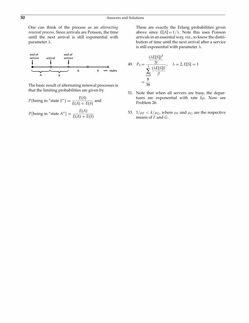
50 Answers and Solutions
One can think of the process as an alteractingrenewal process. Since arrivals are Poisson, the timeuntil the next arrival is still exponential withparameter λ.
end of service arrival
end of service
AA S
S states
The basic result of alternating renewal processes isthat the limiting probabilities are given by
P{being in “state S”} = E(S)E(A) + E(S)
and
P{being in “state A”} = E(A)E(A) + E(S)
These are exactly the Erlang probabilities givenabove since E[A] = 1/λ. Note this uses Poissonarrivals in an essential way, viz., to know the distri-bution of time until the next arrival after a serviceis still exponential with parameter λ.
49. P3 =(λE[S])3
3!3
∑j=0
(λE[S])j
j!
, λ = 2, E[S] = 1
= 838
51. Note that when all servers are busy, the depar-tures are exponential with rate kμ. Now seeProblem 26.
53. 1/μF < k/μG, where μF and μG are the respectivemeans of F and G.
Chapter 9
1. If xi = 0, φ(x) = φ(0i, x).
If xi = 1, φ(x) = φ(1i, x).
3. (a) If φ is series, then φ(x) = minixi and so φD(x) =1 − mini (1 − xi) = max xi, and vice versa.
(b) φD,D(x) = 1 − φD(1 − x)
= 1 − [1 − φ(1 − (1 − x))]
= φ(x)
(c) An n − k + 1 of n.
(d) Say {1, 2, …, r} is a minimal path set. Thenφ(1, 1, …,︸ ︷︷ ︸
r
1, 0, 0, …0) = 1, and so
φD(0, 0, …,︸ ︷︷ ︸r
0, 1, 1, …, 1) = 1 − φ(1, 1, …,
1, 0, 0, …, 0) = 0, implying that {1, 2, …, r} is acut set. We can easily show it to be minimal.For instance,
φD(0, 0, …,︸ ︷︷ ︸r−1
0, 1, 1, …, 1)
= 1 − φ(1, 1, …,︸ ︷︷ ︸r−1
1, 0, 0, …, 0) = 1,
since φ(1, 1, …,︸ ︷︷ ︸r−1
1, 0, 0, …, 0) = 0 since
{1, 2, …, r − 1} is not a path set.
5. (a) Minimal path sets are
{1, 8}, {1, 7, 9}, {1, 3, 4, 7, 8}, {1, 3, 4, 9},
{1, 3, 5, 6, 9}, {1, 3, 5, 6, 7, 8}, {2, 5, 6, 9},
{2, 5, 6, 7, 8}, {2, 4, 9}, {2, 4, 7, 8},
{2, 3, 7, 9}, {2, 3, 8}.
Minimal cut sets are
{1, 2}, {2, 3, 7, 8}, {1, 3, 4, 5}, {1, 3, 4, 6},
{1, 3, 7, 9}, {4, 5, 7, 8}, {4, 6, 7, 8}, {8, 9}.
7. {1, 4, 5}, {3}, {2, 5}.
9. (a) A component is irrelevant if its functioning ornot functioning can never make a difference asto whether or not the system functions.
(b) Use the representation (2.1.1).
(c) Use the representation (2.1.2).
11. r(p) = P{either x1x3 = 1 or x2x4 = 1}P{either of 5 or 6 work}
= (p1p3 + p2p4 − p1p3p2p4)
(p5 + p6 − p5p5)
13. Taking expectations of the identity
φ(X) = Xiφ(1i, X) + (1 − Xi)φ(0i, X)
noting the independence of Xi and φ(1i, X) and ofφ(0i, X).
15. (a) 732 ≤ r
[12
]≤ 1 −
[78
]3 = 169512
The exact value is r(1/2) = 7/32, whichagrees with the minimal cut lower bound sincethe minimal cut sets {1}, {5}, {2, 3, 4} do notoverlap.
17. E[N2] = E[N2|N > 0]P{N > 0}≥ (E[N|N > 0])2P{N > 0}
since E[X2] ≥ (E[X])2.
Thus,
E[N2]P{N > 0} ≥ (E[N|N > 0]P{N > 0})2
= (E[N])2
Let N denote the number of minimal path setshaving all of its components functioning. Thenr(p) = P{N > 0}.
Similarly, if we define N as the number of minimalcut sets having all of its components failed, then1 − r(p) = P{N > 0}.
51
52 Answers and Solutions
In both cases we can compute expressions for E[N]and E[N2] by writing N as the sum of indicator (i.e.,Bernoulli) random variables. Then we can use theinequality to derive bounds on r(p).
19. X(i) is the system life of an n − i + 1 of n systemeach having the life distribution F. Hence, the resultfollows from Example 5e.
21. (a) (i), (ii), (iv) − (iv) because it is two-of-three.
(b) (i) because it is series, (ii) because it can bethought of as being a series arrangement of 1and the parallel system of 2 and 3, which asF2 = F3 is IFR.
(c) (i) because it is series.
23. (a) F(t) =n∏
i=1Fi(t)
λF(t) =ddt
F(t)
F(t)=
n
∑j=1
F′j (t)∏i �=j
Fj(t)
n∏i=1
Fi(t)
=
n
∑j=1
F′j (t)
Fj(t)
=n
∑j=1
λj(t)
(b) Ft(a) = P{additional life of t-year-old > a}
=
n∏1
Fi(t + a)
Fi(t)
where Fi is the life distribution for componenti. The point being that as the system is series,it follows that knowing that it is alive at time tis equivalent to knowing that all componentsare alive at t.
25. For x ≥ ξ,
1 − p = 1 − F(ξ) = 1 − F(x(ξ/x)) ≥ [1 − F(x)]ξ/x
since IFRA.
Hence,
1 − F(x) ≤ (1 − p)x/ξ = e−θx
For x ≤ ξ,
1 − F(x) = 1 − F(ξ(x/ξ)) ≥ [1 − F(ξ)]x/ξ
since IFRA.
Hence,
1 − F(x) ≥ (1 − p)x/ξ = e−θx
27. If p > p0, then p = p0α for some a ∈ (0, 1). Hence,
r(p) = r(p0α) ≥ [r(p0)]α = p0
α = p
If p < p0, then p0 = pα for some a ∈ (0, 1). Hence,
pα = p0 = r(p0) = r(pα) ≥ [r(p)]α
29. Let X denote the time until the first failure and letY denote the time between the first and second fail-ure. Hence, the desired result is
EX + EY = 1μ1 + μ2
+ EY
Now,
E[Y] = E[Y|μ1 component fails first] μ1μ1 + μ2
+ E[Y|μ2 component fails first] μ2μ1 + μ2
= 1μ2
μ1μ1 + μ2
+ 1μ1
μ2μ1 + μ2
31. Use the remark following Equation (6.3).
33. The exact value can be obtained by conditioningon the ordering of the random variables. Let Mdenote the maximum, then with Ai,j,k being theeven that Xi < Xj < Xk , we have that
E[M] = ∑ E[M|Ai, j, k]P(Ai, j, k)
where the preceding sum is over all 6 possible per-mutations of 1, 2, 3. This can now be evaluated byusing
P(Ai, j, k) = λiλi + λj + λk
λjλj + λk
E[M|Ai, j, k] = 1λi + λj + λk
+ 1λj + λk
+ 1λk
35. (a) It follows when i = 1 since 0 = (1 − 1)n
= 1 − [n1] + [n2] · · · ± [n
n]. So assume it true fori and consider i + 1. We must show that[
n − 1i
]=[
ni + 1
]−[
ni + 2
]+ · · · ±
[nn
]which, using the induction hypothesis, isequivalent to[
n − 1i
]=[n
i
]−[
n − 1i − 1
]which is easily seen to be true.
Answers and Solutions 53
(b) It is clearly true when i = n, so assume it for i.We must show that
[n − 1i − 2
]=[
ni − 1
]−[
n − 1i − 1
]+ · · · ±
[nn
]which, using the induction hypothesis,reduces to[
n − 1i − 2
]=[
ni − 1
]−[
n − 1i − 1
]which is true.
Chapter 10
1. X(s) + X(t) = 2X(s) + X(t) − X(s).
Now 2X(s) is normal with mean 0 and variance 4sand X(t) − X(s) is normal with mean 0 and variancet − s. As X(s) and X(t) − X(s) are independent, itfollows that X(s) + X(t) is normal with mean 0 andvariance 4s + t − s = 3s + t.
3. E[X(t1)X(t2)X(t3)]
= E[E[X(t1)X(t2)X(t3) | X(t1), X(t2)]]
= E[X(t1)X(t2)E[X(t3) | X(t1), X(t2)]]
= E[X(t1)X(t2)X(t2)]
= E[E[X(t1)E[X2(t2) | X(t1)]]
= E[X(t1)E[X2(t2) | X(t1)]] (∗)
= E[X(t1){(t2 − t1) + X2(t1)}]
= E[X3(t1)] + (t2 − t1)E[X(t1)]
= 0
where the equality (∗) follows since given X(t1),X(t2) is normal with mean X(t1) and variancet2 − t1. Also, E[X3(t)] = 0 since X(t) is normal withmean 0.
5. P{T1 < T−1 < T2} = P{hit 1 before − 1 before 2}= P{hit 1 before −1}
× P{hit −1 before 2 | hit 1 before −1}
= 12
P{down 2 before up 1}
= 12
13
= 16
The next to last equality follows by looking at theBrownian motion when it first hits 1.
7. Let M = {maxt1≤s≤t2 X(s) > x}. Condition on X(t1)to obtain
P(M) =∫ ∞
−∞P(M|X(t1) = y)
1√2πt1
e−y2/2t1dy
Now, use that
P(M|X(t1) = y) = 1, y ≥ x
and, for y < x
P(M|X(t1) = y
)= P{ max0<s<t2−t1
X(s) > x − y}
= 2P{X(t2 − t1) > x − y}
11. Let X(t) denote the value of the process at timet = nh. Let Xi = 1 if the ith change results in thestate value becoming larger, and let Xi = 0 other-
wise. Then, with u = eσ√
h, d = e−σ√
h
X(t) = X(0)u∑ni=1 Xi dn−∑n
i=1 Xi
= X(0)dn(u
d
)∑ni=1 Xi
Therefore,
log(
X(t)X(0)
)= n log(d) +
n
∑i=1
Xi log(u/d)
= − thσ√
h + 2σ√
ht/h
∑i=1
Xi
By the central limit theorem, the precedingbecomes a normal random variable as h → 0. More-over, because the Xi are independent, it is easy tosee that the process has independent increments.Also,
E[
log(
X(t)X(0)
)]
= − th
σ√
h + 2σ√
hth
12
(1 + μ
σ
√h)
= μt
and
Var[
log(
X(t)X(0)
)]= 4σ2h
th
p(1 − p)
→ σ2t
where the preceding used that p → 1/2 as h → 0.
54
Answers and Solutions 55
13. If the outcome is i then our total winnings are
xioi − ∑j �=i
xj =oi(1 + oi)−1 − ∑
j �=i(1 + oj)−1
1 − ∑k
(1 + ok)−1
=(1 + oi)(1 + oi)−1 − ∑
j(1 + oj)−1
1 − ∑k
(1 + ok)−1
= 1
15. The parameters of this problem are
σ = .05, σ = 1, xo = 100, t = 10.
(a) If K = 100 then from Equation (4.4)
b = [.5 − 5 − log(100/100)]/√
10
= −4.5√
10 = −1.423
and
c = 100φ(√
10 − 1.423) − 100e−.5φ(−1.423)
= 100φ(1.739) − 100e−.5[1 − φ(1.423)]
= 91.2
The other parts follow similarly.
17. E [B(t)|B(u), 0 ≤ u ≤ s]
= E[B(s) + B(t) − B(s)|B(u), 0 ≤ u ≤ s]
= E[B(s)|B(u), 0 ≤ u ≤ s]
+ E[B(t) − B(s)|B(u), 0 ≤ u ≤ s]
= B(s) + E[B(t) − B(s)] by independent
increments
= B(s)
19. Since knowing the value of Y(t) is equivalent toknowing B(t) we have
E[Y(t)|Y(u), 0 ≤ u ≤ s]
= e−c2t/2E[ecB(t)|B(u), 0 ≤ u ≤ s]
= e−c2t/2E[ecB(t)|B(s)]
Now, given B(s), the conditional distribution ofB(t) is normal with mean B(s) and variance t − s.
Using the formula for the moment generating func-tion of a normal random variable we see that
e−c2t/2E[ecB(t)|B(s)]
= e−c2t/2ecB(s)+(t−s)c2/2
= e−c2s/2ecB(s)
= Y(s)
Thus, {Y(t)} is a Martingale.
E[Y(t)] = E[Y(0)] = 1
21. By the Martingale stopping theorem
E[B(T)] = E[B(0)] = 0
But, B(T) = (x − μT)/σ and so
E[(x − μT)/σ] = 0
or
E[T] = x/μ
23. By the Martingale stopping theorem we have
E[B(T)] = E[B(0)] = 0
Since B(T) = [X(T) − μT]/σ this gives the equality
E[X(T) − μT] = 0
or
E[X(T)] = μE[T]
Now
E[X(T)] = pA − (1 − p)B
where, from part (c) of Problem 22,
p = 1 − e2μB/σ2
e−2μA/σ2 − e2μB/σ2
Hence,
E[T] = A(1 − e2μB/σ2) − B(e−2μA/σ2 − 1)
μ(e−2μA/σ2 − e2μB/σ2 )
25. The means equal 0.
Var[∫ 1
0tdX(t)
]=∫ 1
0t2dt = 1
3
Var[∫ 1
0t2dX(t)
]=∫ 1
0t4dt = 1
5
56 Answers and Solutions
27. E[X(a2t)/a] = 1a
E[X(a2t)] = 0
For s < t,
Cov(Y(s), Y(t)) = 1a2 Cov(X(a2s), X(a2t))
= 1a2 a2s = s
As {Y(t)} is clearly Gaussian, the result follows.
29. {Y(t)} is Gaussian with
E[Y(t)] = (t + 1)E(Z[t/(t + 1)]) = 0
and for s ≤ t
Cov(Y(s), Y(t))
= (s + 1)(t + 1) Cov[
Z[
ss + 1
], Z
[t
t + 1
]]
= (s + 1)(t + 1)s
s + 1
[1 − t
t + 1
](∗)
= s
where (∗) follows since Cov(Z(s), Z(t)) = s(1 − t).Hence, {Y(t)} is Brownian motion since it is alsoGaussian and has the same mean and covariancefunction (which uniquely determines the distribu-tion of a Gaussian process).
31. (a) Starting at any time t the continuation of thePoisson process remains a Poisson processwith rate λ.
(b) E[Y(t)Y(t + s)]
=∫ ∞
0E[Y(t)Y(t + s) | Y(t) = y]λe−λydy
=∫ ∞
0yE[Y(t + s) | Y(t) = y]λe−λydy
+∫ ∞
sy(y − s)λe−λydy
=∫ s
0y
1λ
λe−λydy +∫ ∞
sy(y − s)λe−λydy
where the above used that
E[Y(t)Y(t + s)|Y(t) = y]
=⎧⎨⎩yE(Y(t + s)) = y
λ, if y < s
y(y − s), if y > s
Hence,Cov(Y(t), Y(t + s))
=∫ s
0ye−yλdy +
∫ ∞
sy(y − s)λe−λydy − 1
λ2
33. Cov(X(t), X(t + s))
= Cov(Y1 cos wt + Y2 sin wt,
Y1 cos w(t + s) + Y2 sin w(t + s))
= cos wt cos w(t + s) + sin wt sin w(t + s)
= cos(w(t + s) − wt)
= cos ws
Chapter 11
1. (a) Let u be a random number. Ifi−1
∑j=1
Pj < u ≤i
∑j=1
Pj
then simulate from Fi.(In the above
i−1
∑j=1
Pj ≡ 0 when i = 1.
)
(b) Note that
F(x) = 13
F1(X) + 23
F2(x)
where
F1(x) = 1 − e−2x, 0 < x < ∞
F2(x) ={
x, 0 < x < 1
1, 1 < x
Hence, using (a), let U1, U2, U3 be randomnumbers and set
X =⎧⎨⎩
−log U2
2, if U1 < 1/3
U3, if U1 > 1/3
The above uses the fact that−log U2
2is expo-
nential with rate 2.
3. If a random sample of size n is chosen from a set ofN + M items of which N are acceptable then X, thenumber of acceptable items in the sample, is suchthat
P{X = k} =[
Nk
] [M
n − k
]/[N + M
k
]
To simulate X note that if
Ij ={
1, if the jth section is acceptable
0, otherwise
then
P{Ij =1| I1, …, Ij−1} =N −
j−1
∑1
Ii
N + M − (j − 1). Hence, we
can simulate I1, …, In by generating random num-bers U1, …, Un and then setting
Ij =
⎧⎪⎪⎪⎨⎪⎪⎪⎩1, if Uj <
N −j−1
∑1
Ii
N + M − (j − 1)0, otherwise
X =n
∑j=1
Ij has the desired distribution.
Another way is to let
Xj =⎧⎨⎩
1, the jth acceptable item is in the sample
0, otherwise
and then simulate X1, …, XN by generating randomnumbers U1, …, UN and then setting
Xj =
⎧⎪⎪⎪⎪⎨⎪⎪⎪⎪⎩
1, if Uj <
N −j−1
∑i=1
Ii
N + M − (j − 1)
0, otherwise
X =N
∑j=1
Xj then has the desired distribution.
The former method is preferable when n ≤ N andthe latter when N ≤ n.
7. Use the rejection method with g(x) = 1. Differen-tiating f (x)/g(x) and equating to 0 gives the tworoots 1/2 and 1. As f (.5) = 30/16 > f (1) = 0, wesee that c = 30/16, and so the algorithm is
Step 1: Generate random numbers U1 and U2.
Step 2: If U2 ≤ 16(U21 − 2U3
1 + U41), set X = U1.
Otherwise return to step 1.
57
58 Answers and Solutions
13. P{X = i} = P{Y = i|U ≤ PY/CQY}
= P{Y = i, U ≤ PY/CQY}K
= QiP{U ≤ PY/CQY|Y = i}K
= QiPi/CQiK
= Pi
CK
where K = P{U ≤ PY/CQY}. Since the above is aprobability mass function it follows that KC = 1.
15. Use 2μ = X.
17. (a) Generate the X(i) sequentially using that givenX(1), …, X(i−1) the conditional distribution ofX(i) will have failure rate function λi(t) givenby
λi(t) =
⎧⎪⎨⎪⎩
0, t < X(i−1),X(0) ≡ 0.
(n − i + 1)λ(t), t > X(i−1)
(b) This follows since as F is an increasing functionthe density of U(i) is
f(i)(t) = n!(i − 1)!(n − i) (F(t))i−1
× (F(t))n−if (t)
= n!(i − 1)!(n − i) ti−1(1 − t)n−i,
0 < t < 1
which shows that U(i) is beta.
(c) Interpret Yi as the ith interarrival time of a Pois-son process. Now given Y1 + · · · + Yn+1 =t, the time of the (n + 1)st event, it fol-lows that the first n event times are distri-buted as the ordered values of n uniform (0, t)random variables. Hence,
Y1 + · · · + Yi
Y1 + · · · + Yn+i, i = 1, …, n
will have the same distribution as U(1), …,U(n).
(d) fU(1), …|U(n)(y1, …, yn−1|yn)
= f (y1, …, yn)fU(n) (yn)
= n!nyn−1
= (n − 1)!yn−1 , 0 < y1 < · · · < yn−1 < y
where the above used that
FU(n) (y) = P{max Ui ≤ y} = yn
and so
FU(n) (y) = nyn−1
(e) Follows from (d) and the fact that ifF(y) = yn then F−1(U) = U1/n.
21. Pm+1{i1, …, ik−1, m + 1}
= ∑j≤m
j �=i1,…,ik−1
Pm{i1, …, ik−1, j} km + 1
1k
= (m − (k − 1))1[mk
] 1m + 1
1[m + 1
k
]
25. See Problem 4.
27. First suppose n = 2.
Var(λX1 + (1 − λ)X2) = λ2σ21 + (1 − λ)2σ2
2.
The derivative of the above is 2λσ21 −2(1−λ)σ2
2 andequating to 0 yields
λ = σ22
σ21 + σ2
2= 1/σ2
1
1/σ21 + 1/σ2
2
Now suppose the result is true for n − 1. Then
Var
[n
∑i=1
λiXi
]= Var
[n−1
∑i=1
λiXi
]+ Var(λnXn)
= (1 − λn)2 Var
[n−1
∑i=1
λi1 − λn
Xi
]
+ λ2n Var Xn
Now by the inductive hypothesis for fixed λn theabove is minimized when
(∗)λi
1 − λn= 1/σ2
in−1
∑j=1
1/σ2j
, i = 1, …, n − 1
Answers and Solutions 59
Hence, we now need choose λn so as to minimize
(1 − λn)2 1n−1
∑j=1
1/σ2j
+ λ2n σ2
n
Calculus yields that this occurs when
λn = 1
1 + σ2n
n−1
∑j=1
1/σ2j
= 1/σ2n
n
∑j=1
1/σ2j
Substitution into (*) now gives the result.
29. Use Hint.
31. Since E[Wn|Dn] = Dn + μ, it follows that toestimate E[Wn] we should use Dn + μ. SinceE[Dn|Wn] = Wn − μ, the reverse is not true and
so we should use the simulated data to determineDn and then use this as an estimate of E[Dn].
33. (a) E[X2] ≤ E[aX] = aE[X]
(b) Var(X) = E[X2] − E2[X] ≤ aE[X] − E2[X]
(c) From (b) we have that
Var(X) ≤ a2(
E[X]a
)(
1 − E[X]a
)≤ a2 max
0<p<1p(1 − p) = a2/4
35. Use the estimatork
∑i=1
Ni/k2 where Ni = number
of j = 1, …, k : Xi < Yj.


